Universitat Politècnica de València

Departamento de Máquinas y Motores

Térmicos

Online Control of Automotive

systems for improved Real-World

Performance

PhD Dissertation

Presented by

Varun Pandey

Advised by

Dr. Benjamín Pla Moreno

Valencia, July 2021

3

Dedication

This thesis is dedicated to all my respected teachers and my darling youngZüri.

5

Acknowledgments

This thesis is possible due to many people to whom I would eternally remaingrateful. Foremost, it is di�cult to overstate my gratitude to my thesis super-visor, Dr.Benjamin Pla Moreno. His continuous enthusiasm, optimism andencouragement kept me on my toes during the development of this thesis andis really appreciated. I owe him for introducing me to the research world andguiding me all the way to work on the critical scienti�c problems. Apart fromhelping me to solve the complex control problems, he also instilled in me aculture of detail-orientation. On a personal front, his unfailing kindness, ad-vises and support helped me sail through many turbulent moments and forwhich I am grateful.

My work at CMT would have been far less enjoyable, without the friend-ship and moral support of my lab colleagues. While I remain indebted to PauBares, Alvin Barbier, Andre Aronis, Irina Jimenez, Alexandra, Chaitanya andAditya. I remain ever-grateful for making my life in Valencia feel like home.I will always cherish those never-ending conversations that we have had overcerveza and bravas.

I remain eternally grateful to the Spanish Ministry of Economy and Com-petitiveness and the direction of CMT motores for fully �nancing my research.A special note of thanks is due to Amparo Cutillas, and the other adminis-trative o�cials, for hand-holding during all the bureaucratic tasks.

I would like to show my sincere gratitude to Professors Christopher On-der for giving me an opportunity to be part of his research team at Zurichfor an internship. I thoroughly enjoyed the research stay, all thanks to, Raf-fae Hedingerl, Stijn van Dooren, Ritzmann Johannes and David Machacek.With the incredible team it was possible to perform required simulations andexperiments in an incredibly short span of time.

None of this would have been possible without the love, support and in-spiration of my parents Sulekha and Ravindra. I remain grateful to themfor being a source of reliable calm and developing in me a basic trust in myown capacities and chances of ful�llment. To my brother Rahul too, I re-main grateful for helping me recognize the importance of being persistentand resilient. Finally, this thesis would never have converged in the way itdid without the mature love and unwavering support of my friend and wife,Ananya. Her unreserved intellectual and emotional support has been the fuelfor this journey.

Contents

List of Acronyms 11

I Introduction 1

1 Thesis Overview 3

1.1 Background . . . . . . . . . . . . . . . . . . . . . . . . . . . . 31.2 Problem description . . . . . . . . . . . . . . . . . . . . . . . . 71.3 Objective . . . . . . . . . . . . . . . . . . . . . . . . . . . . . 81.4 Thesis Organisation . . . . . . . . . . . . . . . . . . . . . . . . 10

2 State-of-the-Art 13

2.1 Drivetrain Unit Control - Internal Combustion Engine . . . . 142.1.1 Engine Calibration . . . . . . . . . . . . . . . . . . . . 152.1.2 Engine Control in real driving perspective . . . . . . . 21

2.2 Powertrain Control - Hybrid Electric Vehicle (HEV) . . . . . . 232.2.1 Heuristic Supervisory Controller . . . . . . . . . . . . . 242.2.2 Optimal Supervisory controller . . . . . . . . . . . . . 24

2.3 Advanced Driving Assistance System (ADAS) . . . . . . . . . 282.3.1 Cruise Control and Eco-Driving . . . . . . . . . . . . . 31

II Theoretical Tools 35

3 Vehicle Model 37

3.1 Longitudinal Vehicle Dynamics . . . . . . . . . . . . . . . . . 393.2 Gear Box . . . . . . . . . . . . . . . . . . . . . . . . . . . . . 423.3 Internal Combustion Engine . . . . . . . . . . . . . . . . . . . 433.4 HEV architecture . . . . . . . . . . . . . . . . . . . . . . . . . 463.5 Electric Motor . . . . . . . . . . . . . . . . . . . . . . . . . . . 483.6 Power- coupling device in pHEV . . . . . . . . . . . . . . . . . 493.7 Battery . . . . . . . . . . . . . . . . . . . . . . . . . . . . . . 50

8

4 Optimisation tool 53

4.1 Dynamic Programming and its Application . . . . . . . . . . . 534.2 Pontryagin's minimum Principle, application and extension to

ECMS . . . . . . . . . . . . . . . . . . . . . . . . . . . . . . . 57

5 Driving cycle prediction 63

5.1 Markov Chain Principle . . . . . . . . . . . . . . . . . . . . . 645.2 Implementation of MC principle in Driving cycle prediction . . 65

III Experimental Setup 71

6 Experimental Test Setup 73

6.1 Experimental Setup - A . . . . . . . . . . . . . . . . . . . . . 746.2 Experimental Setup - B . . . . . . . . . . . . . . . . . . . . . 776.3 Experimental Setup - C . . . . . . . . . . . . . . . . . . . . . 796.4 Experimental Setup - D . . . . . . . . . . . . . . . . . . . . . 81

IV Applications to powertrain control, Design andAssessment 85

7 Powertrain Control in Real Driving Mission 87

7.1 Adaptive control of Diesel Engine . . . . . . . . . . . . . . . . 887.1.1 Introduction . . . . . . . . . . . . . . . . . . . . . . . . 887.1.2 Method description . . . . . . . . . . . . . . . . . . . . 897.1.3 Designed use cases for method validation . . . . . . . . 937.1.4 Results . . . . . . . . . . . . . . . . . . . . . . . . . . . 957.1.5 Summary and conclusions . . . . . . . . . . . . . . . . 99

7.2 Variable Smoothing of Diesel Engine Calibration . . . . . . . . 1047.2.1 Introduction . . . . . . . . . . . . . . . . . . . . . . . . 1047.2.2 Method Description . . . . . . . . . . . . . . . . . . . . 1057.2.3 Results . . . . . . . . . . . . . . . . . . . . . . . . . . . 1077.2.4 Summary and Conclusions . . . . . . . . . . . . . . . . 118

7.3 Online optimal Energy Management strategy for Parallel HEV 1197.3.1 Introduction and problem description . . . . . . . . . . 1197.3.2 Method Description . . . . . . . . . . . . . . . . . . . . 1217.3.3 Design of case study for method veri�cation and validation1237.3.4 Results . . . . . . . . . . . . . . . . . . . . . . . . . . . 1247.3.5 Summary and conclusion . . . . . . . . . . . . . . . . . 127

9

8 Vehicle Speed Advisory Based Optimisation 131

8.1 Optimisation based on Tra�c Light information . . . . . . . . 1318.1.1 Introduction and problem description . . . . . . . . . . 1318.1.2 Design of case study for method veri�cation and validation1338.1.3 Method description . . . . . . . . . . . . . . . . . . . . 1348.1.4 Results . . . . . . . . . . . . . . . . . . . . . . . . . . . 1388.1.5 Summary and conclusions . . . . . . . . . . . . . . . . 143

8.2 Online vehicle speed advisor . . . . . . . . . . . . . . . . . . . 1468.2.1 Introduction and problem description . . . . . . . . . . 1468.2.2 Method description . . . . . . . . . . . . . . . . . . . . 1478.2.3 Results . . . . . . . . . . . . . . . . . . . . . . . . . . . 1538.2.4 Summary and conclusions . . . . . . . . . . . . . . . . 155

9 Assessment of driving dynamics in RDE test on NOx emission

dispersion 157

9.1 Introduction and problem description . . . . . . . . . . . . . . 1579.2 Method description . . . . . . . . . . . . . . . . . . . . . . . . 1609.3 Results . . . . . . . . . . . . . . . . . . . . . . . . . . . . . . . 1649.4 Summary and conclusion . . . . . . . . . . . . . . . . . . . . . 167

V Conclusion and Outlook 171

10 Conclusions and Outlook 173

10.1 Summary of the presented results . . . . . . . . . . . . . . . . 17310.2 Future directions . . . . . . . . . . . . . . . . . . . . . . . . . 175

Appendices 179

A Appendix Example 181

A.1 Algorithm for Bisection method . . . . . . . . . . . . . . . . . 181

Bibliography 183

List of Acronyms

ADAS Advanced Driving Assistance System . . . . . . . . . . . . . . 9

A-ECMS Adaptive Equivalent Consumption Minimisation Strategy . 27

ACP Average Cycle Prediction . . . . . . . . . . . . . . . . . . . . . . 123

BSFC Brake Speci�c Fuel Consumption . . . . . . . . . . . . . . . . . 117

CAN Controller Area Network . . . . . . . . . . . . . . . . . . . . . . 82

CAD Crank Angle Degree . . . . . . . . . . . . . . . . . . . . . . . . . 99

CD Charge Depleting . . . . . . . . . . . . . . . . . . . . . . . . . . . 23

COM Control Oriented Model . . . . . . . . . . . . . . . . . . . . . . 17

CS Charge Sustaining . . . . . . . . . . . . . . . . . . . . . . . . . . . 23

CPF Cumulative Probabilty Function . . . . . . . . . . . . . . . . . . 67

CHW Control Horizon Window . . . . . . . . . . . . . . . . . . . . . 120

DOE Design-of-Experiment . . . . . . . . . . . . . . . . . . . . . . . . 43

DUC Drivetrain Unit Control . . . . . . . . . . . . . . . . . . . . . . . 13

DEM Discrete Event Modelling . . . . . . . . . . . . . . . . . . . . . . 18

DP Dynamic Programming . . . . . . . . . . . . . . . . . . . . . . . . 25

ED Eco-Driving . . . . . . . . . . . . . . . . . . . . . . . . . . . . . . 30

EV Electric Vehicles . . . . . . . . . . . . . . . . . . . . . . . . . . . . 6

ECU Electronic Control Unit . . . . . . . . . . . . . . . . . . . . . . . 13

EGR Exhaust Gas Recirculation . . . . . . . . . . . . . . . . . . . . . 6

EM Electric Motor . . . . . . . . . . . . . . . . . . . . . . . . . . . . . 46

12

EF Equivalent Factor . . . . . . . . . . . . . . . . . . . . . . . . . . . 120

ECMS Equivalent Consumption Minimisation Strategy . . . . . . . . 22

EMS Energy Management Strategy . . . . . . . . . . . . . . . . . . . 7

EU European Union . . . . . . . . . . . . . . . . . . . . . . . . . . . . 3

GHG Green House Gases . . . . . . . . . . . . . . . . . . . . . . . . . 3

GPS Global Positioning System . . . . . . . . . . . . . . . . . . . . . 30

HCCI Homogeneous Charge Compression Ignition . . . . . . . . . . . 6

HEV Hybrid Electric Vehicles . . . . . . . . . . . . . . . . . . . . . . 6

HIL Hardware-In-Loop . . . . . . . . . . . . . . . . . . . . . . . . . . 124

ICE Internal Combustion Engine . . . . . . . . . . . . . . . . . . . . . 6

I2V Infrastructure to Vehicle . . . . . . . . . . . . . . . . . . . . . . . 8

MC Markov Chain . . . . . . . . . . . . . . . . . . . . . . . . . . . . . 28

MCP Markov Chain Process . . . . . . . . . . . . . . . . . . . . . . . 124

MVM Mean Value Modelling . . . . . . . . . . . . . . . . . . . . . . . 18

MPC Model Predictive Control . . . . . . . . . . . . . . . . . . . . . . 22

NEDC New European Driving Cycle

NN Neural Network . . . . . . . . . . . . . . . . . . . . . . . . . . . . 28

NRTC Non-Road Transient Cycle . . . . . . . . . . . . . . . . . . . . 107

OC Optimal Control . . . . . . . . . . . . . . . . . . . . . . . . . . . . 25

OBD On-board Diagnostics . . . . . . . . . . . . . . . . . . . . . . . . 82

PM Particulate Matter . . . . . . . . . . . . . . . . . . . . . . . . . . 17

pHEV Parallel Hybrid Electric Vehicle . . . . . . . . . . . . . . . . . 23

PMP Pontryagins Minimum Principle . . . . . . . . . . . . . . . . . . 27

PHW Prediction Horizon Window . . . . . . . . . . . . . . . . . . . . 90

RPA Relative Positive Acceleration . . . . . . . . . . . . . . . . . . . 158

13

RCCI Reactivity Controlled Compression Ignition . . . . . . . . . . . 6

RDE Real Driving Emission . . . . . . . . . . . . . . . . . . . . . . . 10

SOA State-of-the-Art . . . . . . . . . . . . . . . . . . . . . . . . . . . 9

SoC State-of-Charge . . . . . . . . . . . . . . . . . . . . . . . . . . . . 9

SMPC Stochastic Model Predictive Control . . . . . . . . . . . . . . . 28

SCR Selective Catalytic Reduction . . . . . . . . . . . . . . . . . . . . 6

TA Type Approval . . . . . . . . . . . . . . . . . . . . . . . . . . . . . 4

VGT Variable Geometry Turbocharger . . . . . . . . . . . . . . . . . 6

V2V Vehicle to Vehicle . . . . . . . . . . . . . . . . . . . . . . . . . . 8

WLTC World Harmonised Light-duty Transient Cycle

Part I

Introduction

Chapter 1

Thesis Overview

Contents

1.1 Background . . . . . . . . . . . . . . . . . . . . . . . . . 3

1.2 Problem description . . . . . . . . . . . . . . . . . . . . 7

1.3 Objective . . . . . . . . . . . . . . . . . . . . . . . . . . 8

1.4 Thesis Organisation . . . . . . . . . . . . . . . . . . . . 10

1.1 Background

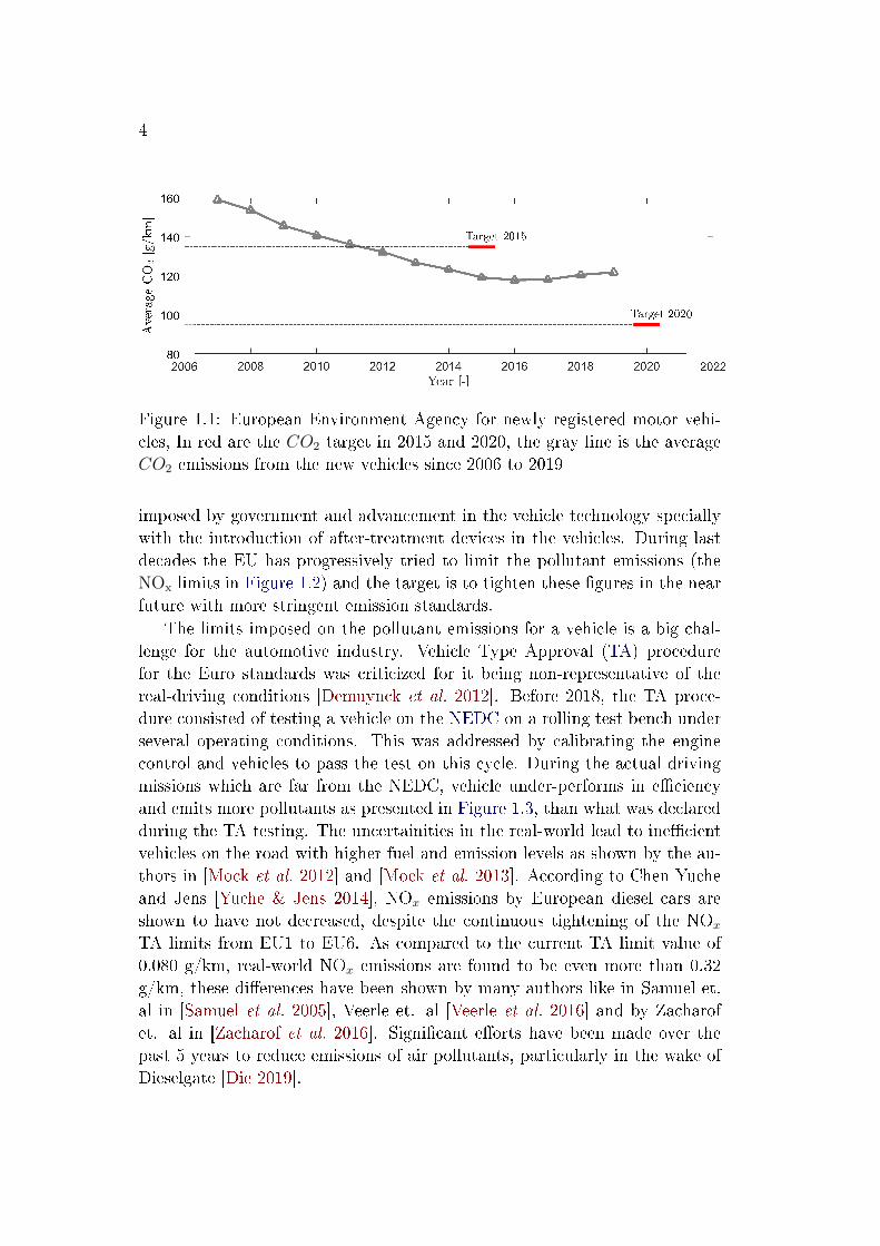
The new sustainable growth strategy proposed by European Commission in2019 [EGD 2019], essentially requires the development of sustainable trans-portation that is climate neutral, cost and energy e�cient and non-polluting.According to the authors in [Sims et al. 2014], the on-road vehicles contributeto 22% of the Green House Gases (GHG) emission which is responsible forglobal warming. As per the report by European Energy Agency [EEA 2019],from 2010 to 2016, CO2 per kilometre (g CO2/km) declined steadily by 22g. The average emissions from new passenger cars increased in 2018 by 2.8 gCO2/km. According to the data in 2019, CO2/km increased further resultingin 122.4 g of CO2 per kilometre. This is well above the European Union (EU)target of 95 g CO2/km in 2020 as shown in Figure 1.1.

The nitrogen oxides (NOx) are identi�ed as another prominent pollutantcoming from the road transportation. It not only has adversarial impacton ozone concentration but also e�ects the human health [Sims et al. 2014].However, according to the data in [AQR 2019] the NOx emissions due to roadtransportation in the EU-28 countries have been reduced by 40% since the year2000. This reduction in NOx is majorly due to the stricter emission standards

4

Figure 1.1: European Environment Agency for newly registered motor vehi-cles, In red are the CO2 target in 2015 and 2020, the gray line is the averageCO2 emissions from the new vehicles since 2006 to 2019

imposed by government and advancement in the vehicle technology speciallywith the introduction of after-treatment devices in the vehicles. During lastdecades the EU has progressively tried to limit the pollutant emissions (theNOx limits in Figure 1.2) and the target is to tighten these �gures in the nearfuture with more stringent emission standards.

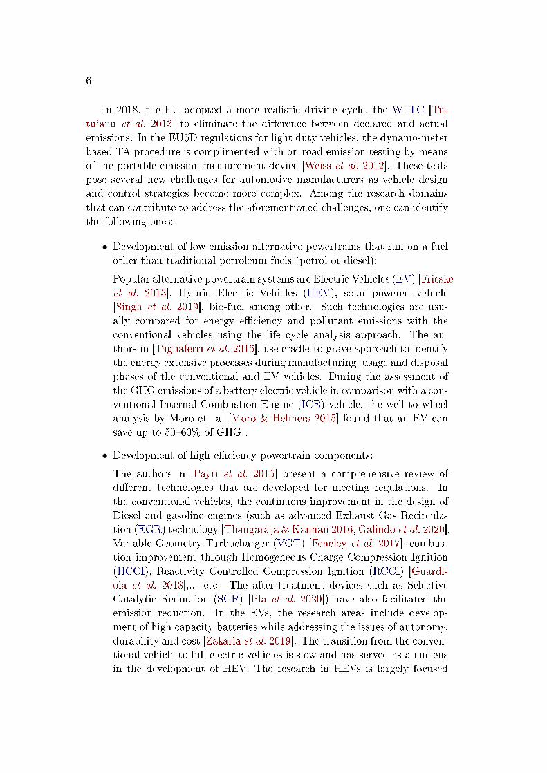
The limits imposed on the pollutant emissions for a vehicle is a big chal-lenge for the automotive industry. Vehicle Type Approval (TA) procedurefor the Euro standards was criticized for it being non-representative of thereal-driving conditions [Demuynck et al. 2012]. Before 2018, the TA proce-dure consisted of testing a vehicle on the NEDC on a rolling test bench underseveral operating conditions. This was addressed by calibrating the enginecontrol and vehicles to pass the test on this cycle. During the actual drivingmissions which are far from the NEDC, vehicle under-performs in e�ciencyand emits more pollutants as presented in Figure 1.3, than what was declaredduring the TA testing. The uncertainities in the real-world lead to ine�cientvehicles on the road with higher fuel and emission levels as shown by the au-thors in [Mock et al. 2012] and [Mock et al. 2013]. According to Chen Yucheand Jens [Yuche & Jens 2014], NOx emissions by European diesel cars areshown to have not decreased, despite the continuous tightening of the NOx

TA limits from EU1 to EU6. As compared to the current TA limit value of0.080 g/km, real-world NOx emissions are found to be even more than 0.32g/km, these di�erences have been shown by many authors like in Samuel et.al in [Samuel et al. 2005], Veerle et. al [Veerle et al. 2016] and by Zacharofet. al in [Zacharof et al. 2016]. Signi�cant e�orts have been made over thepast 5 years to reduce emissions of air pollutants, particularly in the wake ofDieselgate [Die 2019].

5

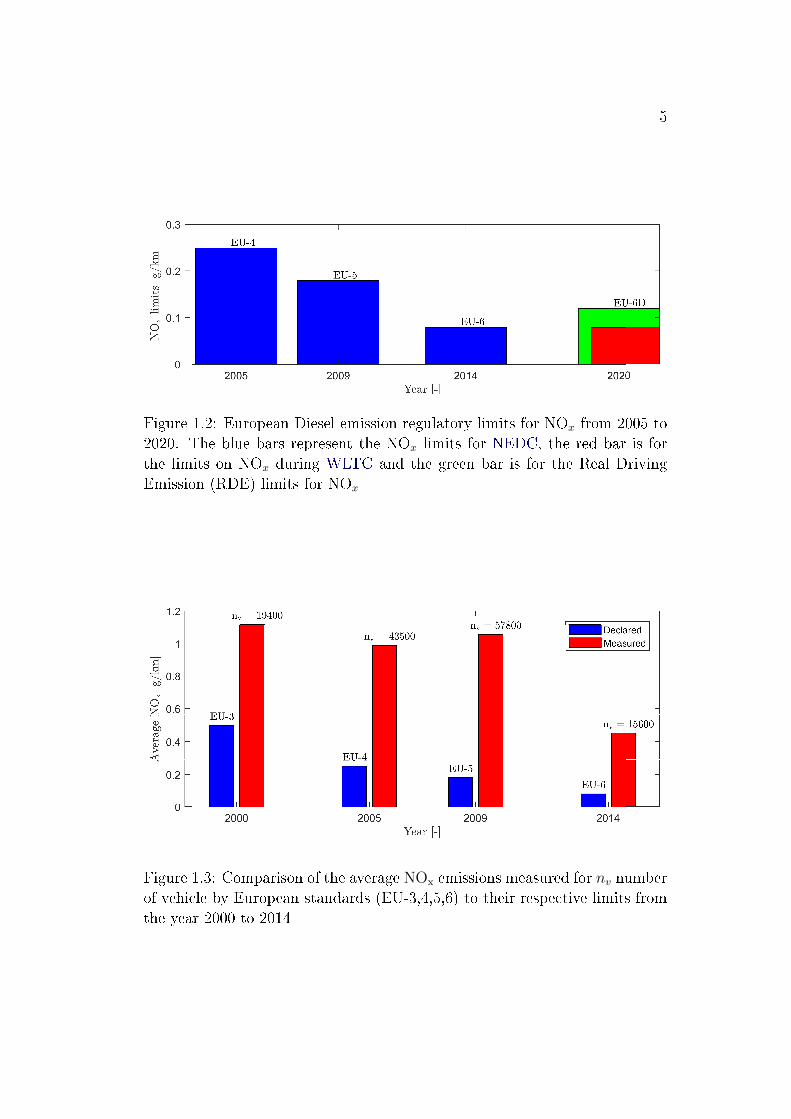
Figure 1.2: European Diesel emission regulatory limits for NOx from 2005 to2020. The blue bars represent the NOx limits for NEDC, the red bar is forthe limits on NOx during WLTC and the green bar is for the Real DrivingEmission (RDE) limits for NOx

Figure 1.3: Comparison of the average NOx emissions measured for nv numberof vehicle by European standards (EU-3,4,5,6) to their respective limits fromthe year 2000 to 2014

6

In 2018, the EU adopted a more realistic driving cycle, the WLTC [Tu-tuianu et al. 2013] to eliminate the di�erence between declared and actualemissions. In the EU6D regulations for light duty vehicles, the dynamo-meterbased TA procedure is complimented with on-road emission testing by meansof the portable emission measurement device [Weiss et al. 2012]. These testspose several new challenges for automotive manufacturers as vehicle designand control strategies become more complex. Among the research domainsthat can contribute to address the aforementioned challenges, one can identifythe following ones:

• Development of low emission alternative powertrains that run on a fuelother than traditional petroleum fuels (petrol or diesel):

Popular alternative powertrain systems are Electric Vehicles (EV) [Frieskeet al. 2013], Hybrid Electric Vehicles (HEV), solar powered vehicle[Singh et al. 2019], bio-fuel among other. Such technologies are usu-ally compared for energy e�ciency and pollutant emissions with theconventional vehicles using the life cycle analysis approach. The au-thors in [Tagliaferri et al. 2016], use cradle-to-grave approach to identifythe energy extensive processes during manufacturing, usage and disposalphases of the conventional and EV vehicles. During the assessment ofthe GHG emissions of a battery electric vehicle in comparison with a con-ventional Internal Combustion Engine (ICE) vehicle, the well to wheelanalysis by Moro et. al [Moro & Helmers 2015] found that an EV cansave up to 50�60% of GHG .

• Development of high e�ciency powertrain components:

The authors in [Payri et al. 2015] present a comprehensive review ofdi�erent technologies that are developed for meeting regulations. Inthe conventional vehicles, the continuous improvement in the design ofDiesel and gasoline engines (such as advanced Exhaust Gas Recircula-tion (EGR) technology [Thangaraja & Kannan 2016, Galindo et al. 2020],Variable Geometry Turbocharger (VGT) [Feneley et al. 2017], combus-tion improvement through Homogeneous Charge Compression Ignition(HCCI), Reactivity Controlled Compression Ignition (RCCI) [Guardi-ola et al. 2018],.. etc. The after-treatment devices such as SelectiveCatalytic Reduction (SCR) [Pla et al. 2020]) have also facilitated theemission reduction. In the EVs, the research areas include develop-ment of high capacity batteries while addressing the issues of autonomy,durability and cost [Zakaria et al. 2019]. The transition from the conven-tional vehicle to full electric vehicles is slow and has served as a nucleusin the development of HEV. The research in HEVs is largely focused

7

on the topological, optimal component sizing and Energy ManagementStrategy (EMS).

• Development of advanced vehicular control system:

The optimal engine control, EMS in HEVs, development of autonomousvehicles and connected vehicle have gained huge momentum in the lastdecades. Broadly speaking, the objective of the automotive controlsis to operate the vehicle or any of its subsystems in the most e�cientway while ful�lling several constraints at the system and surroundinglevels. As the complexity of engine and vehicle kept growing with thenew technological developments, the demand for more complex con-trol system also grew. The opportunities arising due to the improvedcomputational capabilities, connected vehicles and more sophisticatedmodelling and control techniques are paving the way for adoption ofoptimal control theory in the automotive industry. For instance, thetypical approach in conventional engines was based on the calibratedmaps that contain control set-points as a function of several variables.These set-points are interpolated according to the current sensor read-ings, estimations and then corrected for dynamic transients. It requiresa lot of experimental and heuristic knowledge for obtaining a single cali-bration. Automated frameworks are proposed by the authors in [Stuhleret al. 2002, Jiang et al. 2012, Hellström et al. 2013] to address this costlyand time demanding solution. The optimal control theory is found rele-vant in not just engine controls but also in transmission control, EMS forHEV among others. The e�cient driving is also shown to have signi�-cant impact on fuel saving and emission by Sciarretta et.al [Sciarretta &Vahidi 2020a]. Autonomous driving eliminates any human interventionin vehicle speed control and drives the vehicle in the most energy e�-cient way for a given powertrain system. An optimal control perspectivefor e�cient driving is presented in [Han et al. 2019].

This thesis is focused on the third topic, i.e. the optimisation of control formodern powertrain systems. The control is important in itself, but also servesas a technology enabler for the �rst two topics of the above list. Followingsection describes the problem that has been addressed in this work.

1.2 Problem description

The problem addressed in the current thesis is to optimise the vehicle con-trol such that the fuel consumption and constraints regarding the powertrainbehaviour, for instance pollutant emissions or battery state of the charge for

8

HEVs is respected in actual driving missions. The thesis proposes model-based control that approximates the minimum energy consumption of thevehicle subject to constraints (emissions, electric range, ...) in real drivingconditions by applying optimal control techniques. To do that, three maintopics are covered:

• Models that are capable of estimating (in real-time) the general be-haviour and performance of the powertrain based on its requirements(vehicle speed, acceleration, torque demand, environmental conditions)and control settings (engine management , power-split).

• Statistical models capable of estimating future operating conditions fromthe vehicle's history, in addition to other information provided by theinfrastructure (Infrastructure to Vehicle (I2V)) or other vehicles (Vehicleto Vehicle (V2V)) that is available.

• Optimization algorithms that combined with the above elements canprovide optimal powertrain controls that minimize energy while satisfy-ing emissions or other forms of constraints.

1.3 Objective

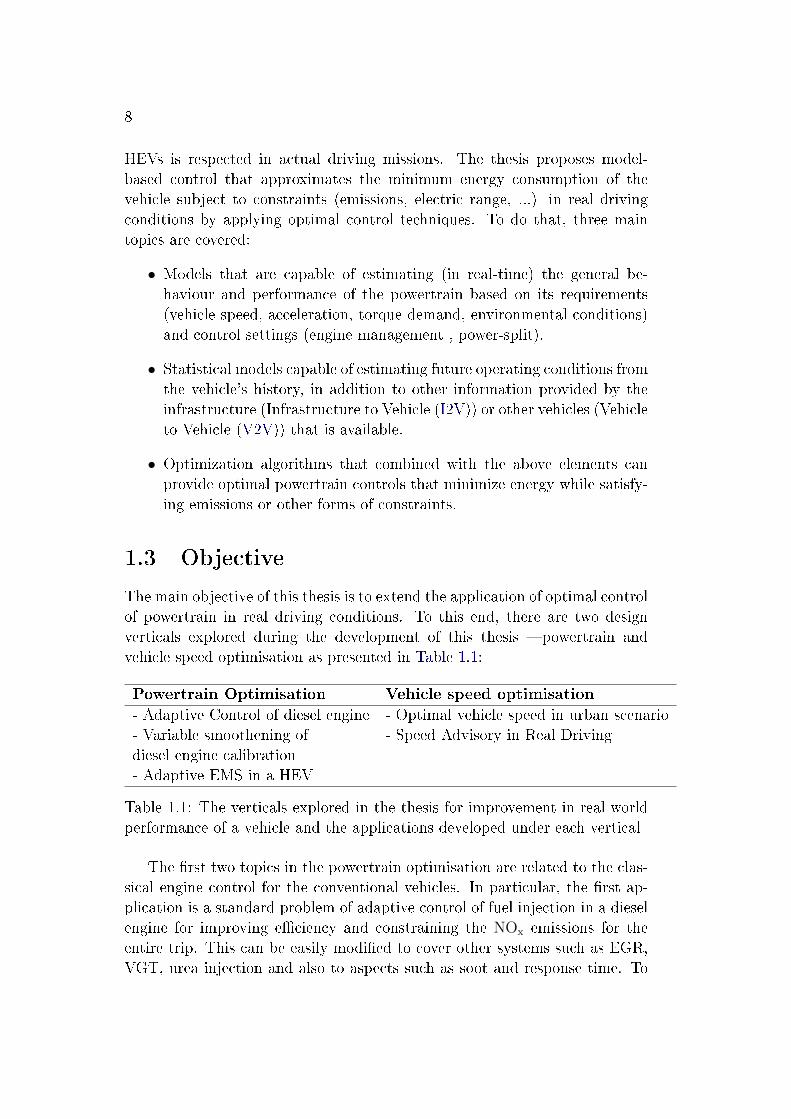
The main objective of this thesis is to extend the application of optimal controlof powertrain in real driving conditions. To this end, there are two designverticals explored during the development of this thesis � powertrain andvehicle speed optimisation as presented in Table 1.1:

Powertrain Optimisation Vehicle speed optimisation

- Adaptive Control of diesel engine - Optimal vehicle speed in urban scenario- Variable smoothening of - Speed Advisory in Real Drivingdiesel engine calibration- Adaptive EMS in a HEV

Table 1.1: The verticals explored in the thesis for improvement in real-worldperformance of a vehicle and the applications developed under each vertical

The �rst two topics in the powertrain optimisation are related to the clas-sical engine control for the conventional vehicles. In particular, the �rst ap-plication is a standard problem of adaptive control of fuel injection in a dieselengine for improving e�ciency and constraining the NOx emissions for theentire trip. This can be easily modi�ed to cover other systems such as EGR,VGT, urea injection and also to aspects such as soot and response time. To

9

do that two main problems are required to be addressed: At �rst the curse ofdimensionality arising due to the number of extra variables and then develop-ment of models to estimate outputs such as soot and dynamics. The secondproblem arises from the optimisation procedure itself. The second applicationis regarding the auto-smoothening of the calibration maps of a diesel engine inreal driving conditions. For which a single tuning parameter is used to obtaina trade-o� between fuel consumption, NOx emissions and the engine torquereference following capability.

The modern powertrain systems are rapidly progressing towards hybridisa-tion and electri�cation. Therefore, the scope of powertrain optimisation is notlimited to the engine control but also covers the control of HEVs. The thirdproblem is regarding the online EMS of a HEV. The State-of-the-Art (SOA)o�ine EMS is extended with a cycle prediction strategy for making it anonline application. In particular, the performance of developed method iscompared with SOA EMSs in terms of fuel e�ciency and capability to trackthe reference State-of-Charge (SoC).

Even though the controllability of the powertrain system is high, the com-plexity of the control problem increases multi-fold with the increasing numberof control parameters. During its implementation in powertrain systems withseveral control inputs and constraints, the optimal powertrain control prob-lem becomes extremely complex and eventually over-weighs the performancerelated bene�ts. For this reason, another research vertical is also investigatedin this thesis: Control of vehicle speed in real-driving conditions. Such con-trol problems have less number of actuators (acceleration pedal, braking pedaletc..) but the number of states and disturbances is much higher since it in-cludes all the powertrain related states plus the ones related to the driver andthe environment. Therefore, the observability (in passive or active control)is very limited in real-time. The observabilty is related to the ability of theset of sensors and sources of information to estimate the state of the system.The limitation is due to the amount of information (I2V or V2V) that is re-quired to be processed to obtain an optimal control solution. On the otherside, even if the optimal actuations provided with a good estimation of thesystem state could be calculated, those actuations arrive to the powertrainthrough the driver whose controllability is questionable (at least in the caseof being a human being). In any case, due to the high impact of the vehiclespeed pro�le on its performance in terms of fuel consumption and emissions,this second veritcal is related to Advanced Driving Assistance System (ADAS)which has three major sub-domains: the vehicle safety, the e�ciency and thedriving comfort. As this thesis is focused on the development of methods forimproving the vehicle e�ciency in real driving conditions, only the e�ciencysub-domain is investigated. Specially, two applications are developed � the

10

�rst application is regarding the speed optimisation of a vehicle in the urbanscenario with the information of the tra�c light phasing. The objective is toassess the impact of optimisation on the fuel consumption and NOx emissionswith the tra�c light information. The second application is a speed advisoryin real driving mission for improved fuel economy and travel time.

Other than designing the above control applications for real driving sce-nario, the thesis also present the �ndings of an assessment regarding the NOx

emission dispersion due to the driving dynamics within the Real Driving Emis-sion (RDE) regulation (EU6D) limits. The following section describes thethesis organisation with brie�ng about the contents.

1.4 Thesis Organisation

This thesis has ten chapters (divided into sections and subsections) which areorganised in �ve parts. The �rst part is about the introduction and containstwo chapters: The chapter 1 introduced the background of the sustainabletransportation strategy adopted by the government in recent time with anemphasis on the real driving emissions. The control role for automotive power-train management was presented with focus on the requirement of new controlmethods to deal with the latest emission regulation. Finally, a general outlineof the problem is described with a clear de�nition of the thesis objective. Thechapter 2 is focused on analysing the current SOA advances in the control ofautomotive systems with emphases on SOA of the applications developed inthis work. The �rst section is about the advancement of the diesel engine con-trol methods in real driving emission perspective. The second section is aboutthe energy management of the hybrid electric vehicles in recent years. Finally,the work available in literature related to the vehicle speed optimisation withthe objective of e�ciency improvement are presented within a framework ofadvanced driving assistance system.

The following part is about the theoretical tools developed in the thesisand it contains 3 chapters: The chapter 3 is regarding the vehicle model usedin this work. These models were used at several instances in the developmentof this thesis. The vehicle dynamics are addressed with a longitudinal model.Gear-box, ICE, electric motor, power-coupling device and battery models aredescribed in di�erent sections. The chapter 4 introduces optimisation toolswith their mathematical formulations and supported by suitable examples.The �rst section elaborates the dynamic programming as a tool for �ndinga global optimal solution. The second section is regarding the PontryaginsMinimum Principle and its extension to the Equivalent Consumption Minimi-sation Strategy. The chapter 5 introduces a tool developed for driving cycle

11

prediction in real world conditions. The tool is �rst described in its mathe-matical form and then, the method of prediction is described with the help ofa simple example.

Then, there is a part describing the experimental setups being used inthe development of the applications. This part has chapter 6 which presentdescriptive layout of the relevant engine/vehicle components and instrumen-tations. The speci�cation of the engine/vehicle are also tabulated. The fourtest setups are marked in alphabetical order from A to D and are referedduring the description of the application in the following parts.

The fourth part is about the applications developed during this work andhas three chapters: The chapter 7 present the three design applications underthe vertical of powertrain optimisation as discussed previously in Table 1.1.Each application is described using a standard format that covers �ve top-ics: Beginning with the application speci�c introduction and followed by themethod description, case studies used for their validation, results and sum-mary/conclusions. The chapter 8 present two design applications under thevertical of vehicle speed optimisation (refer Table 1.1). A similar structure asin chapter 7 is used to describe the developed methods and important �ndings.Finally, chapter 9 present an assessment of the impact of driving dynamics onreal driving NOx emissions. Presenting the summary of experimental resultsand the conclusions that can be derived from the study.

Finally, the last part is about the overall conclusions and the outlook of thisthesis described in chapter 10. In this chapter the summary of the researchand future scope of the work is presented.

Chapter 2

State-of-the-Art

Contents

2.1 Drivetrain Unit Control - Internal Combustion Engine 14

2.1.1 Engine Calibration . . . . . . . . . . . . . . . . . . . . 15

2.1.2 Engine Control in real driving perspective . . . . . . . 21

2.2 Powertrain Control - Hybrid Electric Vehicle (HEV) 23

2.2.1 Heuristic Supervisory Controller . . . . . . . . . . . . 24

2.2.2 Optimal Supervisory controller . . . . . . . . . . . . . 24

2.3 Advanced Driving Assistance System (ADAS) . . . . 28

2.3.1 Cruise Control and Eco-Driving . . . . . . . . . . . . . 31

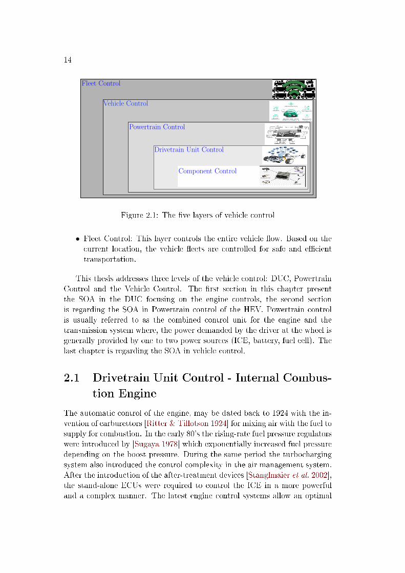
In conventional vehicles, �ve layers of intelligent vehicle control can beidenti�ed as presented in Figure 2.1:

• Component Control: This includes electronic hardware components suchas sensors, actuators and Electronic Control Unit (ECU)s.

• Drivetrain Unit Control (DUC): They are the controllable vehicle driv-etrain units, for example the engine, motor, transmission, suspension,brake and the steering system.

• Powertrain Control: This is a overall control of the drivetrain units ona vehicle level in�uencing the whole vehicle motion.

• Vehicle Control: At this level, direct V2V communications and directV2I communications are controlled such that driving is safe and eco-nomical.

14

Figure 2.1: The �ve layers of vehicle control

• Fleet Control: This layer controls the entire vehicle �ow. Based on thecurrent location, the vehicle �eets are controlled for safe and e�cienttransportation.

This thesis addresses three levels of the vehicle control: DUC, PowertrainControl and the Vehicle Control. The �rst section in this chapter presentthe SOA in the DUC focusing on the engine controls, the second sectionis regarding the SOA in Powertrain control of the HEV. Powertrain controlis usually referred to as the combined control unit for the engine and thetransmission system where, the power demanded by the driver at the wheel isgenerally provided by one to two power sources (ICE, battery, fuel cell). Thelast chapter is regarding the SOA in vehicle control.

2.1 Drivetrain Unit Control - Internal Combus-

tion Engine

The automatic control of the engine, may be dated back to 1924 with the in-vention of carburettors [Ritter & Tillotson 1924] for mixing air with the fuel tosupply for combustion. In the early 80's the rising-rate fuel pressure regulatorswere introduced by [Sugaya 1978] which exponentially increased fuel pressuredepending on the boost pressure. During the same period the turbochargingsystem also introduced the control complexity in the air management system.After the introduction of the after-treatment devices [Stanglmaier et al. 2002],the stand-alone ECUs were required to control the ICE in a more powerfuland a complex manner. The latest engine control systems allow an optimal

15

coordination of fuel-injection, turbocharging, EGR, Exhaust After-Treatment(EAT) in stationary and transient conditions. Generally, the main objectivesof the engine control can be summarized as:

• The torque demanded by the driver through acceleration pedal must bemet resulting in good drivability.

• The engine must operate at high thermal e�ciencies resulting in lowfuel consumption while emissions must be within the regulatory limits.

• The system must function in a safe operating region derived from theindividual limits (such as mechanical) of all the elements.

With many mutually dependent subsystems, the engine control is a verycomplex problem and the control theory plays an important role in enabling itsoptimisation. SOA engine optimisation method is usually based on feedbackand feed-forward controllers. Fixed look-up tables generate the set-points forfeed-forward controller. The look-up tables also referred in the literature asthe maps are obtained using the calibration process as shown by the authorsin [Isermann 2014] with a goal of minimising fuel consumption while ful�llingthe regulatory and customer constraints regarding the emissions and drivingcomfort. The SOA engine calibration process is described in the followingsubsection.

2.1.1 Engine Calibration

The engine calibration is a process of feeding the engine ECU with a set ofinformation that de�ne the actions of the actuators during its operation. Thegoal of engine calibration process is to obtain optimal and drivable actuationmaps. The SOA engine calibration begins with identifying the set of operatingpoints (engine speed and engine torque) which are representative of the engineoperation zone (largely dependent on the vehicle application). During theengine calibration process the actuator settings are identi�ed which, optimisethe engine e�ciency at the identi�ed operating points while, simultaneouslylimiting the emission and other requirements on a pre-de�ned driving cycle.The control structure of the modern diesel engines consists of feed-forward andfeedback controllers. The article by Castagne et al. [Castagné et al. 2008] givesan overview of several calibration methods. The authors explain traditionallocal approaches, characterised by a phase of smoothing after local optimalsettings are found, as well as global approaches, which directly include enginespeed and load parameters in the model.

16

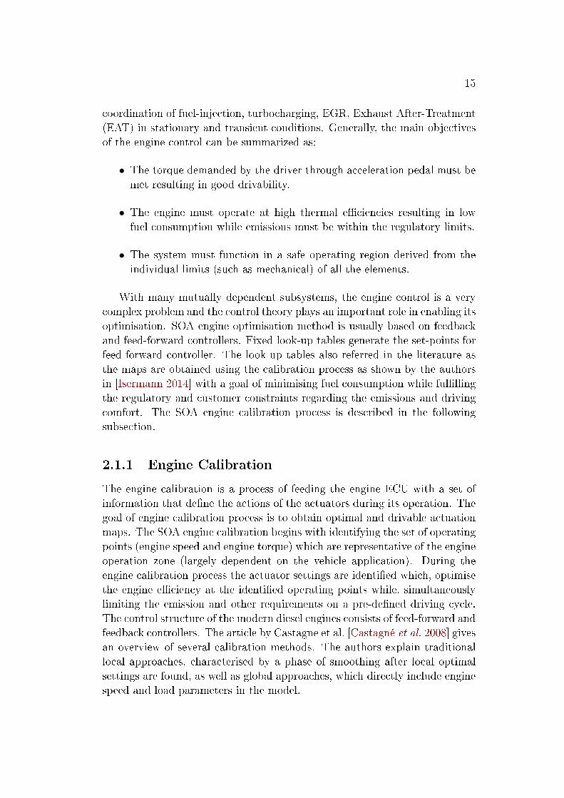
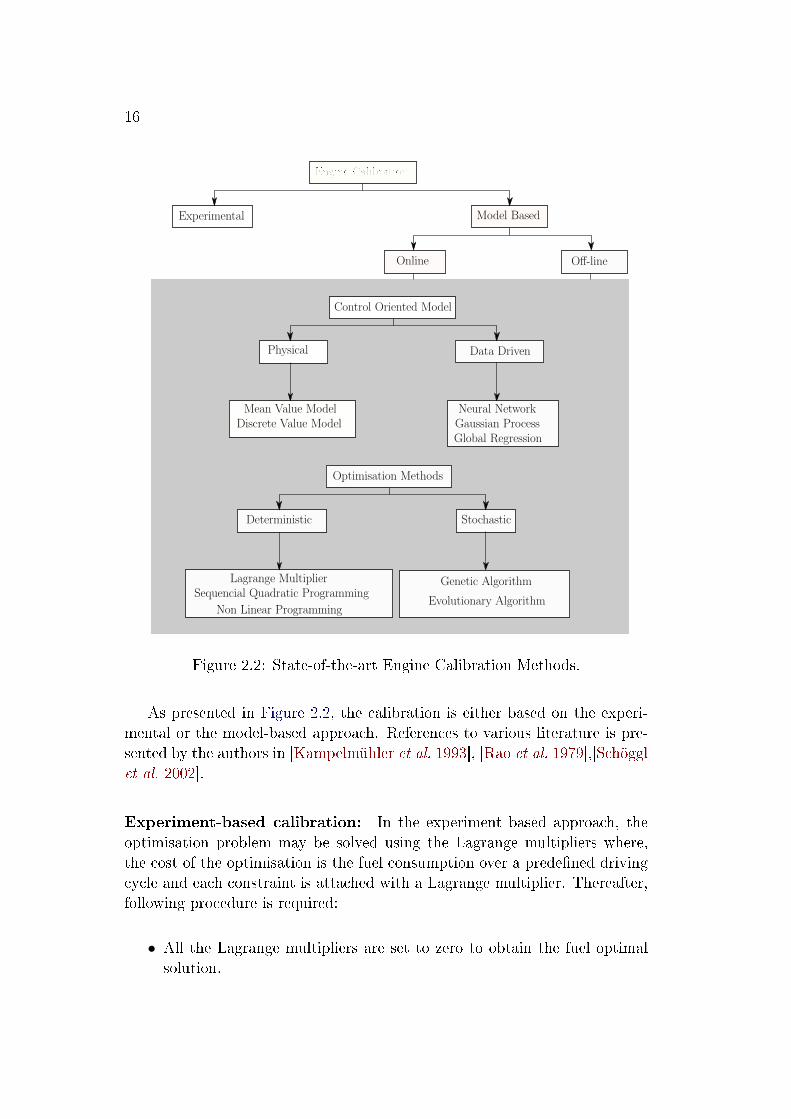
Figure 2.2: State-of-the-art Engine Calibration Methods.

As presented in Figure 2.2, the calibration is either based on the experi-mental or the model-based approach. References to various literature is pre-sented by the authors in [Kampelmühler et al. 1993], [Rao et al. 1979],[Schögglet al. 2002].

Experiment-based calibration: In the experiment based approach, theoptimisation problem may be solved using the Lagrange multipliers where,the cost of the optimisation is the fuel consumption over a prede�ned drivingcycle and each constraint is attached with a Lagrange multiplier. Thereafter,following procedure is required:

• All the Lagrange multipliers are set to zero to obtain the fuel optimalsolution.

17

• If all the constraints are ful�lled, the actuators settings recorded as afunction of the operating point and used as feed-forward maps in thecalibration

• If any of the constraint is not ful�lled, the corresponding multiplier istuned until the solution is reached.

The experiment based calibration method require calibration experts and eventhen does not guarantee an optimal solution. With the advent of powerfulcomputational tools such as MBC tool by MATLAB, the modern calibra-tion process includes model-based phases in addition to the experiment-basedphases.

Model-based calibration: To reduce the complexity arising due to thehigh number of control inputs and mutually contradicting objectives severalresearchers have explored model-based calibration approach (a combinationof Control Oriented Model (COM)s and optimisation techniques). In recenttime, the model based approach is gaining ever more popularity due to theavailability of high computational power. These methods are capable of cali-brating the engine in an online [Tan et al. 2017, Bachler et al. 2003, Asprionet al. 2014] or an o�ine [Hiroyasu et al. 2002, Luján et al. 2018, Alonsoet al. 2007] setting. Many of the commercially available calibration tools[Sampson 2009] are purely designed for model-based o�ine optimisation anddo not have a connection to the engine test bench. The AVL CAMEO 4consists of a test bed and o�ce version with an additional toolbox called asiPROCEDURE ADAPTIVE DOE and is capable of performing online opti-misation. The BMW also has its own tool MBMINIMIZE tool to performonline calibration [Sung et al. 2007] among others.

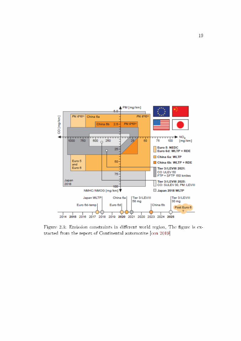
The process of model-based engine calibration has been broadly dividedinto three steps by the authors in [Langouët et al. 2011, Park et al. 2017]. The�rst step is to select steady-state operating points which are representative ofthe engine operation. Then, a global engine model is developed and validatedusing measurement data from steady-state experiments. Finally, optimisationand smoothing are carried out for a representative driving cycle, with the goalof minimizing fuel consumption, while meeting constraints on pollutant emis-sion and ensuring good drivability. The constraint over pollutant emissionssuch as NOx, Particulate Matter (PM), CO and HC are well de�ned by thegovernment agencies as presented in the Figure 2.3. The EU has enforcedthe type-approval process based on the representative cycles like NEDC andmore recently WLTC. The other constraint is regarding the drivability andis often de�ned only qualitatively. Assis et al. [Assis et al. 2003] de�ne driv-ability as the capability of the engine to deliver the torque requested by the

18

driver in a way which is pleasant to the driver. From a vehicle perspective, thedriver subjectively provides feedback regarding drivability during the vehicledevelopment phase. Pedal tip-in and tip-out are the typical drivability testingscenarios. The authors show that, even though the torque produced by theengine is desired to be equal to that demanded by the driver, it may resultin undesirable behaviour due to powertrain excitation's during large torquesteps. The authors propose a rail pressure control strategy to dampen the im-pact of sudden jumps in the engine torque. Nessler et al. [Nessler et al. 2006]de�ne drivability as the transition felt by the driver between engine speed andload points during real vehicle driving, which means that a constant powersupply is necessary during acceleration phases while avoiding sudden reduc-tion of torque in order to have a good drivability. The authors propose toreduce the Gaussian curvature of the optimal calibration maps in order toobtain smoother maps. In the articles by Nishio et al. [Nishio et al. 2018]and Niedernolte et al. [Niedernolte et al. 2006], a constraint in the step sizefor each parameter is applied to generate drivable calibration maps. However,some loss of optimality has been shown by the authors in terms of engine per-formance due to the manual elimination of the peaks in the map. This methodrequires all other parameters to be adjusted consistently in order to achievethe target torque. However, no relationship has been shown between mapsmoothing on the torque reference following capability and the engine perfor-mance. From an engine perspective, other than calibration map smoothing,some transient compensation strategies are also applied in order to obtainsmooth transients, which in fact is another method of improving drivability.Adaptation of exhaust-gas recirculation (EGR) and fuel injection has an im-pact on transient emissions and drivability, as shown in the article by Zentneret al.[Zentner et al. 2013]. The authors propose an EGR and injection limiterto reduce NOx emissions and to improve drivability and the drivability wascharacterised by the transient response of the engine during load steps.

The model based technique is fundamentally based on a control orientedmodel and an optimisation method (as described in the following paragraphs)for performing the engine calibration (online or o�ine).

Control Oriented Model: The control-oriented models with reasonableprecision but low computational cost are ideal for testing the complex controlstrategies on the engine system. These models are either based on the physicalequations and experiments necessary to identify some key parameters, or theyare based on the experimental data. The control oriented physical modellingin the ICE is classi�ed by the authors in [Guzzella & Onder 2010] as MeanValue Modelling (MVM) and Discrete Event Modelling (DEM). The MVMapproach neglects the discrete cycles of the engine and assume that all pro-

19

Figure 2.3: Emission constraints in di�erent world region, The �gure is ex-tracted from the report of Continental automotive [con 2019]

20

cesses and e�ects are spread out over the engine cycle. Whereas, in the DEMapproach the reciprocating behaviour of the engine is also modelled. Thereis a lot of literature available which describe the methods and their imple-mentation in the control perspective [Jung 2003, Baldi et al. 2015, Pinamontiet al. 2017, Guardiola et al. 2012, Guardiola et al. 2014, Jiang et al. 2009, Mar-tin et al. 2018, Torregrosa et al. 2011, Payri et al. 2005].

The empirical models use the experimental data from an engine of certainspeci�cation where the interesting control actuators are varied as much aspossible within their boundary conditions. The desired model output variablesare stored as a function of the control actions. Such models are data drivensince the predicted outputs are based on simple functions of the measureddata. There are several data driven models described in the literature, wherevery popular are based on the Neural network [Atkinson et al. 2008], Gaussianprocess [Berger et al. 2011], global regression [Grahn et al. 2012], etc.

Optimisation Methods: The multi-objective optimisation for online oro�ine calibration is classi�ed in two categories by the authors in [Cavaz-zuti 2013]: The deterministic and stochastic optimisation. The deterministicalgorithms are commonly based on the computation of the gradient and insome cases also on the hessian of the objective function. The determinis-tic optimisation approach is further subdivided into constrained and uncon-strained optimisation methods. The constrained optimisation methods havebeen widely used in the literature for Diesel engine calibration where, thevery popular are Lagrangian method [Hochschwarzer et al. 1992], Sequentialquadratic programming [Hafner & Isermann 2003], Non-linear programming[Rao et al. 1979]. On the other hand the Stochastic optimisation methodsare based on randomness with slower convergence as compared to the de-terministic algorithms. In the literature, stochastic methods are found inthe diesel engine calibration as particle swarm optimisation algorithm [Zhanget al. 2018], genetic algorithm [Millo et al. 2018], evolutionary alogrithms [Maet al. 2015] etc. In the thesis [Schmied 2004], the author proposed a newmethod called Multistoch which is based on designing dynamic experimentsusing constrained functional quanti�cation.

As discussed, the existing engine control is based on the �xed calibrationmaps which are optimal for a driving cycle known in advance. With newregulations the vehicle emissions should be constrained in the real drivingconditions. The following section is regarding the SOA of engine control inreal-driving perspective.

21

2.1.2 Engine Control in real driving perspective

Despite a substantial e�ort during the last decades in order to reduce thefuel consumption and emissions in light duty vehicles by means of improvedpowertrain design and controls [Payri et al. 2015], noticeable discrepancies arestill observed between declared and real driving consumption and pollutant�gures [Pelkmans & Debal 2006, Weiss et al. 2011]. One of the main reasonsfor such a deviation is that the driving cycles considered by regulations onlyrepresent to some extent the set of conditions that a vehicle may face duringtheir entire life. To make-up for such a limitation, the current regulations haveintroduced RDE testing procedures as a method to reduce the gap betweendeclared performance and that perceived by users. In any case, those factspoint out the impact that driving conditions, including tra�c but also drivingstyle, have on fuel-consumption and emissions. To this aim, the traditionalcontrol scheme based on �xed calibration can be upgraded by including somedegree adaptation introducing the following three features to address the issueof real-driving uncertainty:

• Vehicle speed prediction model: The prediction model can be based onthe available information about vehicle speed on a given route by includ-ing information from a database of real-world driving and to generatethe driving cycle using a stochastic process. SOA for construction ofsynthetic driving cycles is to randomly append driving segments, wherea segment is a driving sequence between two stops as demonstrated byMichel in [Michel 1996]. An issue with such a method as mentioned byJie and Debbie in [Jie & Debbie N 2002], is that it gives no consider-ation for di�erentiation in modal events (e.g. cruise, idle, accelerationand deceleration) and also there is no way to set the length of the cycle.In [Jie & Debbie N 2002], Jie and Debbie proposes to use a stochasticprocess for binning of data until certain statistical criteria are met. Thebins are based on which modal event they belong to and are extractedfrom the measured driving cycles. However, due to the size of thesesnippets, it is still di�cult to achieve the desired driving distance andat the same time obtain driving cycles that are representative of realworld. Another way would be to generate single velocity and acceler-ation states at any instant, instead of the entire bin. One option is togenerate driving cycles by using Markov chains, as described in [TK &ZS 2011]. This includes extracting information from a database of real-world tra�c and then analysing the data to generate driving cycles usinga stochastic process. In the article by Gong et. al [Gong et al. 2011],the Markov chain approach is shown to be the most popular method forgenerating representative driving cycles.

22

In the article by Francois et. al [François 2017], a considerable disper-sion has been reported in the driving dynamics of average drivers andvehicles. In the article [Josh & Vicente 2016] by Josh et. al it hasbeen shown that the driving conditions (including freezing or hot am-bient temperatures, driving dynamics, driving at high speeds, drivingat higher altitude and diesel particulate �lter regeneration events) notcovered by the RDE test are to have a relatively high contribution tooverall NOx emissions. As a matter of fact, driver monitoring and driverstyle correction can improve fuel economy. According to Rajan et. alin [Rajan et al. 2012], driver style and driving events like city and high-way driving both a�ects vehicle energy demand. Hence, both have tobe considered in developing a vehicle. A lot of work is focused towardsimproving driver style by providing driver assist both in conventionalvehicles as shown by the Guenter et. al in [Günter Reichart et al. 1998]and for HEVs as shown by the authors in [Fazal et al. 2010].

• Vehicle model: For estimating the engine performance in real-time asimpli�ed vehicle model is required. Although, some works have appliedOptimal Control to vehicle powertrains without the so called quasi-staticengine simpli�cations [Asprion et al. 2014, Luján et al. 2018, Maroteaux& Saad 2015], very simplistic 0D models as followed by the authors in[Ozatay et al. 2014b, Ozatay et al. 2014c, Sciarretta et al. 2015a]. In thearticle by Yang et al. [Zhijia et al. 2013] should be applied for onlinepurpose.

• A supervisory controller is also required to control the engine for min-imised fuel consumption with constrained emissions. Optimal controltheory has been widely used in literature as consolidated by the authorsin [Jonas et al. 2014] to address complex control problem. However,application of these methods in engine management system is still abig challenge due to their computational cost. Some other methodshave been focused on lower level engine control for Spark-Ignition en-gine. Extremum seeking method has been widely used in [Hellströmet al. 2013, Corti et al. 2013, Popovic et al. 2006], most of the workis related to online optimal calibration but does not include real driv-ing emission constraint. The authors in [Andreas et al. 2010], presenta theoretical basis and algorithmic implementation for allowing the en-gine to learn the optimal actuator settings in real-time. Even thoughshort transients have been presented for online optimisation, the ap-plicability of this method in real driving condition still remains an un-solved issue. Other methods, like Equivalent Consumption Minimisa-tion Strategy (ECMS) and Model Predictive Control (MPC) as in [Petri

23

et al. 2018, Nishio & Shen 2019], seem to be more promising in real-timeengine control. Stephan et. al [Stephan et al. 2014] proposed an ECMSmethod to provide a solution for online optimal control of Diesel en-gine with constraint in NOx emission. The authors assume a constantemission reference target which leads unrealistic emission in real-worlddriving. In the article by Gokul et.al [Gokul et al. 2019], MPC is formu-lated to maximise the fuel e�ciency while tracking boost pressure andexhaust gas recirculation rate references, in the face of uncertainties, ad-hering to the input, safety constraints and limits on emissions averagedover some �nite time period. Authors in [Guardiola et al. 2016], presenta model based approach to adapt the engine calibration depending onthe driver behaviour and the target pollutant emissions: they considera �xed probability matrix for expected engine operating points, whichdoes not represent a real world scenario.

2.2 Powertrain Control - Hybrid Electric Vehi-

cle (HEV)

With two energy sources the HEVs present a system with higher degree offreedom with improved possibilities of reducing the fuel consumption and theemissions than traditional powertrains exclusively based on ICEs. This po-tential can be realised through optimisation in any of the three HEV systemlevels : the powertrain topology (series HEV, Parallel Hybrid Electric Vehi-cle (pHEV), series-parallel HEV), the technology and sizing of the compo-nents and the EMS. Extensive literature is explored by the authors in [Tranet al. 2020] and [Bradley & Frank 2009] regarding the topology of HEVs.However, this section is focused on describing the various types of EMS inthe literature for HEVs. In contrast to the conventional vehicle, in HEVs,the power demand by the driver can be ful�lled by combining the powersfrom an ICE and EM. The number of possible combinations depends on thepowertrain topology. For instance, in pHEV con�guration the power can bedelivered by the ICE and EM exclusively or in a combination, the battery canbe also recharged using the regenerative braking system. The main objectiveof the EMS in a HEV is to minimise the fuel consumption of the vehicle whileful�lling the energy demand of the driver and restraining the battery SoCwithin a certain range. The EMS must also ensure to operate the system toful�l the constraints regarding ICE, EM and battery.

In general, the pHEVs operating modes are classi�ed by the author in[Markel 2006] as Charge Depleting (CD), Charge Sustaining (CS). In CD,the SoC may �uctuate but on-average decreases while driving. However, in

24

CS mode the SoC is maintained at a certain level. The EMS for pHEVs aredesigned to ful�l the conditions of desired operating mode and are broadlyclassi�ed by the authors in [Tran et al. 2020] as : Heuristic, Optimisation-based and learning-based.

2.2.1 Heuristic Supervisory Controller

The early control strategy for the HEVs was based on heuristic consider-ations which results in Boolean rules [Guzzella & Sciarretta 2005, Mouraet al. 2011, Gong et al. 2008, Peng et al. 2015]. These methods require ex-haustive experiments and experience to set up a rule based control system.According to the authors in [Guzzella & Sciarretta 2005], there are two guid-ing principles of the heuristic supervisory controller in hybrid vehicles: The�rst principle is to use the engine only if it can run at high e�ciency, while inthe conditions where the engine e�ciency can not be high the electric modeshould be preferred. The engine is used during the warm-ups to activate thecatalyst. In [Peng et al. 2017], the authors propose a method to calibrate theheuristic control strategy with the global optimisation result. The dynamicprogramming is applied to obtain the optimal powertrain energy managementstrategy for a series-parallel HEV over a driving cycle and the calibration isbuilt based on the optimisation results. The second principle is that the bat-tery SoC must be observed and regulated in such a way that the SoC mustremain within a certain prede�ned limit. The main advantage of these meth-ods is that they are robust, intuitive and made to directly translate controlspeci�cations. The rule-based controllers require experimental database andthe behaviour of heuristic controller strongly depends upon the driving condi-tions. If the vehicle operates far from the conditions for which the controllerwas calibrated, the performance deteriorates [Hofman et al. 2006]. The opti-mal supervisory controllers aim at eliminating the disadvantages of the rulebased controls by introducing a well-de�ned mathematical approach for opti-misation.

2.2.2 Optimal Supervisory controller

In the optimisation based methods, the performance index J is either simplythe mass of fuel or a combination of other performance indexes based overa mission of duration tf . The other performance indexes may include theemission rates of a regulated pollutant, drivability of the vehicle in termsof acceleration and jerk-free vehicle operation, frequency of mode switches,battery life, etc... depending on the vehicle application. In Equation 2.1, a

25

simpli�ed cost J is de�ned for a performance index L.

J =

∫ tf

0

L(ω(t), u(t), x(t)) dt (2.1)

ω(t) is the disturbance, in the case at hand the main disturbance is the drivingcycle that has to be followed, u(t) are the control signals and x(t) are the statevariables related to the system dynamics. For studying the energy manage-ment strategy of the HEVs, the models are usually designed using quasi-staticapproach where most of the mechanical, electrical and thermal dynamics ofthe subsystems are eliminated. However, there are some states which areincluded such as the battery SoC dynamics, temperature dynamics of theafter-treatment devices ([Kum et al. 2013]), battery ageing etc. The mostcommon is the battery SoC which is not only required to be constrained in-stantaneously but also the terminal SoC(tf ) must be close to a pre-determinedvalue. This value is dependent on the type of HEV considered and its oper-ating mode such as charge depleting, charge sustaining etc. The constraintson these state variables are handled using the soft (penalising the deviationfrom the desired level) or a hard integral constraint (must reach the desiredSoC level). The hard constraint is feasible only if the driving cycle is perfectlyknown in advance. However, the soft constraint can be applied in the onlineoptimisation. Other than the integral constraints on the battery energy con-sumption there are local constraints that are supposed to be handled by theoptimal controller. Such as, the mechanical limits of the ICE, EM, charg-ing and discharging rates, torque response, etc. The Optimal Control (OC)methods are either solved o�ine or online. In the o�ine method optimisationproblem is solved on a desktop without any link to the experimental setupand therefore real time calculations are not required. However, in the onlinemethods optimisation problem is solved on a real time control platform witha link to the experimental setup. The classical methods used in the o�ineapproach are Dynamic Programming (DP) [Gong et al. 2007], Pontryagin'sMinimisation Principle [Kim et al. 2014], and meta-heuristic search meth-ods i.e. the Genetic Algorithm, Particle Swarm Optimisation and SimulatedAnnealing. The online methods are Equivalent Consumption MinimisationStrategy (ECMS originally developed by [Paganelli et al. 2000]) and Deter-ministic or Stochastic Model Predictive Control [Johannesson et al. 2007].

O�ine Methods An o�ine Optimal Control (OC) strategy is a non-causalsince it relies on future information. It requires a priori knowledge of thedriving cycle and therefore they are often used to obtain a standard optimalsolution for comparing the results obtained with the online methods. Oneof the very popular method to solve the non-causal optimisation is the DP

26

[Bryson & Ho 2018]. In the DP, computation burden is directly dependent onthe number of states and therefore simpli�ed models can be used to solve theoptimsation problem. The DP requires to grid the states and time variables.It uses the performance index in Equation 2.1 with an extension to any pointin the time-state space by de�ning it as a cost-to-go function of time andthe state. In [Vinot et al. 2007, Scordia et al. 2005, Debert et al. 2012],authors have shown the application of the DP in optimisation of EMS ofHEV. As mentioned, the computation burden of the DP has a drawback inthe implementation of complex problems, several improved algorithms [Yanget al. 2019, Lee et al. 2020, Li & Gorges 2019] have been developed.

Other optimisation method that permits a reduction of the computatione�ort is the PMP which, minimises the following Hamiltonian (H) function ateach time step.

u∗(t) = argminv{H(t, x(t), v, µ(t))} (2.2)

H(t, x, v, µ) = L(ω(t), u) + µ.f(ω(t), u, x) (2.3)

where t is a continuous variable, µ(t) is the co-state which is described by theEuler-Lagrange equation as:

µ(t) = − ∂

∂xH (2.4)

the function f(.) depends on the SoC, which is dependent on the open-circuitvoltage and internal resistance of the battery. However, this dependency canbe neglected in the case of electric hybrid systems where only large deviationof the SoC can cause substantial variations of the internal battery parame-ters. Consequently, the co-state is assumed to be constant along an optimaltrajectory. Therefore, the problem reduces to �nding a constant value of theco-state (µo) for a given vehicle mission. The relationship between the µoand SoC(tf ) is monotonous and µo is usually determined using iterations bycorrecting the previous estimation and the di�erence between the target SoCand actual SoC in each iteration. In the case with constant µ, a new meaningis acquired by the Hamiltonian function. Since the battery open-circuit volt-age is constant under this assumption, both terms on the right-hand side ofEquation 2.4 can be reduced to power terms:

PH(t, u(t)) = Pf (ω(t), u(t)) + µs.Pe(ω(t), u(t)) (2.5)

27

In this equation, Pf (ω(t), u(t)) is the power of the fuel and Pe(ω(t), u(t)) isthe battery electro-chemical power. The dimensionless scaling of the co-stateis termed as equivalence factor µs and is de�ned as:

µs = −µo.HLHV

UOC .Qo

(2.6)

The formulation in Equation 2.4 is called the Pontryagin's Minimum Prin-ciple and has been explored in the literature [Hou et al. 2014, Buie et al. 2004].This method requires a priori knowledge of the driving cycle which is not thecase in real driving missions. The workaround to this drawback are the causalmethods represented by the equation in and are called the ECMS which aredescribed in the following section.

Causal Methods In contrast to the o�ine methods, the online methodsmust be causal as they should not require a priori knowlegde of the drivingcycle and resulting in suboptimal (hopefully near optimal) solutions. The on-line methods are real-time implementable with a limited computation time andmemory. Three categories were identi�ed by the authors in [Zhang et al. 2020]namely, instantaneous optimization-based EMSs (ioEMS), predictive EMSs(pEMS) and learning based EMSs (lEMS).

In the ioEMSs the power split is optimised by minimizing the instanta-neous cost (fuel consumption and other performances) at each instant. In re-cent times ECMS and Adaptive Equivalent Consumption Minimisation Strat-egy (A-ECMS) are explored by many researchers. The ECMS shows promisingbut slightly sub-optimal results with a challenge of properly determining theequivalent factor (µs) [Tulpule et al. 2011]. The ECMS combined with thecycle prediction methods is the realisation of the Pontryagins Minimum Prin-ciple (PMP) in real time. The co-state in the PMP was estimated o�ine andwas constant for a known driving mission. In contrast, the co-state in theECMS is estimated online usually leading to a variable co-state. The uncer-tainty in the future driving conditions is curbed by correcting the value ofthe co-state in real time. The real-time control performance of an ECMS isheavily related to the equivalent factor. Therefore, a well tuned equivalentfactor is essential to improve the performance of ECMS. The future powerrequirement and the current SoC are used to determine the equivalent factor.To determine a proper value of equivalent factor, A-ECMS is proposed whichrefreshes the control parameters according to the current and future powerdemand. There are several methods available in the literature regarding theonline estimation of the co-state. The non-causality is addressed in the liter-ature by taking advantage of the driving information [Payri et al. 2014]. To

28

recognise and predict future driving conditions, researchers propose di�erentprdictive techniques, the authors in [Guardiola et al. 2013, Payri et al. 2012]use statistic and clustering techniques to classify the driving characteristicsand Markov chain-based method are used to develop driving cycles based onpreviously recorded velocity pro�les on a given route. Out of several methodsavailable in literature Neural Network (NN)and Markov Chain (MC) basedmethods are most popular. In the article by the authors in [Xie et al. 2018],a comparison of the two approaches is shown in terms of prediction accuracyand computation speed.

The MPC is another option in predictive EMSs for an unknown drivingmission. Compared with other EMSs, MPC is based on the system predic-tion information to obtain a rolling horizon optimization. The MPC is areceding horizon control strategy with a predictive scheme using three mainsteps. Firstly, over a prediction horizon the optimal inputs are calculatedwhich minimise the objective function subject to the constraints. Then, fromthe calculated optimal inputs, the �rst element is implemented to the phys-ical plant and �nally, the entire prediction horizon is moved forward. Thisprocess is iterated from the �rst step. The MPCs are formalised in the lit-erature in several ways to optimize the power split, such as hybrid MPC [Li& Goerges 2017], distributed MPC [Josevski & Abel 2016], variable horizonMPC [Cao et al. 2017]. In [Marx & So�ker 2012], the authors propose non-linear MPC for energy management with an adaptive prediction time horizon.Another form of MPC is Stochastic Model Predictive Control (SMPC) andis proposed in [Li et al. 2016]. In this method, the distribution of driver'sfuture power demand can be obtained and the MPC is adopted to obtain theoptimal power split for a HEV bus commuting on a particular route.

2.3 Advanced Driving Assistance System (ADAS)

The research community has been traditionally more focused on the enginedesign including realistic driving conditions [Ortiz-Soto et al. 2012] or evenclose loop emissions control [Tschanz et al. 2013] than on the optimisation ofvehicle operating conditions due to the intrinsically complex nature of thisoptimisation problem. The important research e�orts have been focused onthe development and integration of engine technologies aimed to improve fuele�ciency and emissions of light duty vehicles. Those e�orts have materialisedin important reductions in emissions and fuel consumption according to reg-ulation cycles, however, their impact on real driving is limited [Pelkmans &Debal 2006, Weiss et al. 2011]. Amongst other reasons, the vehicle operat-ing conditions play a major role in global e�ciency and emissions, therefore,

29

di�erences between real driving and regulation cycles give rise to the usualfact that the actual consumption exceeds that from the vehicle speci�cations.Note the lack of controllability of the system since the driver manipulability is,at least, arguable, and it is evident that there are other factors a�ecting driv-ing that are completely out of control (reactions of other drivers, weather,...).According to the US Environmental Protection Agency (EPA) and NaturalResources Canada (NRCan), there is up to 35% fuel economy di�erence be-tween drivers in the same �eet of vehicles. Similar results are reported froma �eld experiment by Eaton Corporation, which reported 30% fuel economydi�erence amongst pick-up drivers. The di�erence in fuel consumption, pollu-tant emissions and trip duration of the vehicles commuting on the same routeis majorly due to two reasons:

• Di�erence in the driver behaviour: On a given road condition (i.e. twohypothetical vehicles on a route at the same time and position but withdi�erent drivers), the two drivers are likely to act di�erently. The re-lated line of research is focused on how the driver should behave to min-imise fuel consumption and emissions. In [Ulleberg & Rundmo 2003],the authors conclude that the driver personality primarily in�uencesthe driving behaviour. The assessment of the impact of di�erent driv-ing styles on safety is based on the statistical analysis of the behaviourof several drivers while driving. The literature about the impact ofdriving behaviours on safety is available from past four decades [Cram-ton 1969], [Canale & Malan 2002], [BLOCKEY & HARTLEY 1995].However, the impact of driving style on fuel consumption and emissionsis a more recent topic and is addressed by the authors in [Ross 1994],[Tong et al. 2000], [Ping et al. 2019]. An aggressive driver is morelikely to accelerate/decelerate the vehicle faster than an average driver.Such behaviour when cumulated for a driving mission results in di�er-ence in fuel consumption and emissions in the order of 30-35% [Vermaet al. 2013]. Several publications address how to monitor the driverbehaviour and promote Eco-Driving. An example of such a tool is pre-sented by [Vagg et al. 2013] where, they propose to encourage economi-cal driving behaviour by giving feedback to the driver with a light codeshowing his driving aggressiveness (product of velocity and accelera-tion), since an aggressive driving style will naturally lead to higher fuelconsumption. A similar approach is presented and evaluated in [Larsson& Ericsson 2009].

• Di�erence in the speed pro�les due to randomness in tra�c situation: Avehicle on the same route at di�erent times consume di�erent amount offuel, emits di�erent amount of pollutant emissions and covers the same

30

distance in di�erent time. A vehicle commuting on the same route willhave di�erent velocity pro�les due on the tra�c situation. The tra�csituation is largely dependent on two factors: Static environmental fac-tors and dynamics conditions of the tra�c. In static environment thereare lanes, intersection, position and timings of the tra�c light signals.The dynamic tra�c conditions are largely due to the intensity of thetra�c and randomness arising due to the real time tra�c situation.

The improvement of computation capabilities, the introduction of OptimalControl in powertrain management and the increase of cost-e�ective sensorsand information sources (Global Positioning System (GPS), V2V, V2I, ...)have lead to an intensive research activity in the assisted driving techniques.The rapid progress in intelligent transportation systems has signi�cantly in-creased availability of tra�c information that can be integrated to the vehiclecontrol system for reducing the impact of randomness in driving on fuel con-sumption, pollutant emissions and travel time.

Traditionally, an Advanced Driving Assistance System (ADAS) tracks andutilizes information (such as vehicle location, distance of the objects to thedriver, lane detection, etc.) so as to allow a vehicle to drive more safely.The research on ADAS can be broadly classi�ed into two categories: Thepassive assistance systems that act as a feedback advisory to the driver. Theactive assistance systems where, driving is automated to some extent suchas adaptive cruise control and vehicle collision avoidance where the driveris operating exclusively without any dependence to these systems. The newdevelopments are into using ADAS as a tool for promoting Eco-Driving (ED)either passively or actively. ED is a way to optimise the velocity pro�le,with the aim of reducing the fuel consumption [Ozatay et al. 2014b, Ozatayet al. 2014c, Sciarretta et al. 2015a] in actual driving. The driving advisorysystems provide velocity and acceleration recommendations that take traveltime, fuel consumption and emissions into account using the route and thetra�c light schedule information. The integration of the route and tra�cinformation such as the position of nearby vehicles, timing and positioning ofthe tra�c signal at the intersections [Rakha & Kamalanathsharma 2011, Yanget al. 2020], road grade[Bakibillah et al. 2018], route maps [Minett et al. 2011],etc. into the cruise control systems to reduce the overall energy consumptionare the popular research topics. A study on freeway-based eco-driving systemsshowed fuel savings of the order of 10-20 % when real-time signals were used[Barth & Boriboonsomsin 2009]. For this reason ED is a hot topic in theautomotive control sector that has been approached during the last decadeswith di�erent methods, e.g. in [Li et al. 2011] with MPC, in [Stanger &del Re 2013] by using look-ahead information or [Naranjo et al. 2003] with

31

fuzzy-logic controllers.Other than ED, Vehicle Platooning is another application of cruise control

which allows vehicle platoons with optimal inter vehicle distances. This highlyincreases the roadway capacity, while the energy consumption is reduced dueto the reduction of aerodynamic drags and unnecessary speed �uctuations.On several occasions, research work has proven the approach in simulations[Milanes et al. 2014, van Arem et al. 2006, Fernandes & Nunes 2012], rela-tively few of them have conducted experiments to prove their strategy [Kianfaret al. 2012, Ploeg et al. 2014, Englund et al. 2016]. In [Tsugawa et al. 2011],the authors show that Platooning of 10m gap at 80km/h can reduce energy byabout 15% (measurement) by the aerodynamic drag reduction, and CO2 by2.1% along an expressway (simulation) when the 40 % penetration in heavytrucks by the roadway capacity increase. In the present thesis, the applica-tions developed were related to the ED and the following subsection describesthe SOA of cruise control and ED.

2.3.1 Cruise Control and Eco-Driving

The automatic speed control for vehicles was introduced by Wolfe et al. in[George F Wolfe 1938]. The objective of the invention was to indicate thedriver through a resistance to the movement of the acceleration pedal that apre-determined speed of the vehicle has been reached. In 1950, Teetor [Tee-tor 1950] invented the modern speed control device for resisting the operationof the accelerator. The �rst car Imperial, that implemented Teetor's systemwas in 1958. In 1965, American Motors corporation introduced a an auto-matic speed control system. Soon in 1968, Radio Corporation of Americaintroduced the automotive cruise control system. Since then, the automotivecar industry has been developing advanced Cruise Control Systems in orderto improve the performance measured in terms of driving comfort, drivingsafety and fuel e�ciency. Modern cruise control is not limited to maintaininga desired vehicle driving speed, but it also incorporates the communication ofthe vehicle with the infrastructure and the other vehicles in order to improvethe degree-of-freedom. All the information is used to improve the performanceand such systems are termed as cooperative adaptive cruise control systemsin the literature. [Li et al. 2011, Bu et al. 2010, Ploeg et al. 2011]. This line ofstudy is aimed to obtain a vehicle speed pro�le to minimise fuel consumptionon a given route. This is a problem that matches the �eld of OC. In fact, OChas been applied to the speed pro�le optimization since 1977 in the work of[Schwarzkopf & Leipnik 1977], who calculated the optimal speed pro�le on ahill. From then on, and specially during the last decade, several OC techniqueshave been applied to the vehicle speed trajectory optimization at di�erent

32

scenarios. Some of these approaches are PMP in [Fröberg et al. 2006, Petitet al. 2011, Sciarretta et al. 2015b], DP in [Hellström et al. 2009, Hellströmet al. 2010b, Ozatay et al. 2014a] and Direct Methods (DM) in [Saboohi &Farzaneh 2009, Reig 2017]. Due to the complexity of reproducing real driv-ing conditions, most of them focus on particular driving conditions (highway,tra�c lights, ...) and address this topic from a modelling perspective. A com-prehensive review of them can be found in [Sciarretta & Vahidi 2020b]. Inaddition, few of the previous studies include the report of the optimal vehiclespeed pro�le to the driver and the assessment of their impact on the fuel con-sumption. An example of such study is [Ozatay et al. 2014a] where, authorspropose a cloud-based optimization of the vehicle speed pro�le by DP that isdownloaded in the vehicle for a given route.

In this work the ED techniques are explored in line with the research in[Hooker 1988]. Hooker et. al show, how the vehicle speed pro�le can beresponsible for up to 30% of the fuel consumption. Other studies [Passenberget al. 2009] point out that ED can reduce fuel consumption by about 5%compared to standard driving . OC theory is explored in the literature toaddress the problem of �nding the optimal velocity pro�le on several occasions.The cost involved in such a problem formulation is generally in the form ofminimising a function from intial to �nal time:

Qf =

∫ tf

ti

qf (v(t), a(t)) dt (2.7)

where, qf is the fuelling rate, v(t) is the vehicle velocity, a(t) is the vehicleacceleration. The goal of the optimisation is to �nd the speed trajectory v(t)

that minimises the cost index in Equation 2.7. In the literature, there are sev-eral advanced methods like Model Predictive Control [Li et al. 2011, Stanger &del Re 2013, Bageshwar et al. 2004], Stochastic Dynamic Programming [Weiÿ-mann et al. 2018, Johannesson et al. 2007], etc to solve the above problem.Apart from the main objective there are other constraints that are requiredto be taken into account while solving the OCP:

• The ego vehicle must not crash with any vehicle and therefore a mini-mum inter vehicle distance is required to be maintained.

• The ego vehicle must also adhere the tra�c rules i.e. stoping at redtra�c lights, safe lane change, maximum permissible speed etc.

• The powertrain related limitations must also be taken into account.

• The driving comfort which is acceptable by a human driver must alsobe ensured at all time.

33

Combining all these essential requirements turns the OCP into a non-linearoptimisation problem within prediction horizon subject to the dynamic andnon-linear constraints.

Part II

Theoretical Tools

Chapter 3

Vehicle Model

Contents

3.1 Longitudinal Vehicle Dynamics . . . . . . . . . . . . . 39

3.2 Gear Box . . . . . . . . . . . . . . . . . . . . . . . . . . 42

3.3 Internal Combustion Engine . . . . . . . . . . . . . . . 43

3.4 HEV architecture . . . . . . . . . . . . . . . . . . . . . 46

3.5 Electric Motor . . . . . . . . . . . . . . . . . . . . . . . 48

3.6 Power- coupling device in pHEV . . . . . . . . . . . . 49

3.7 Battery . . . . . . . . . . . . . . . . . . . . . . . . . . . 50

The vehicle velocity and acceleration of vehicle motion in the plane can becalculated by applying Newton's equations by balancing forces and momen-tum. The main external forces on the vehicle are balanced with the vehicleinertial forces in the longitudinal, lateral and the vertical axis. However, in-cluding the lateral vehicle dynamics largely increase the model complexitywith limited e�ect on the vehicle performance in terms of fuel economy andemissions. As the scope of this thesis is limited to the evaluation of the fuelconsumption and emissions, the lateral forces are not included in the devel-oped vehicle dynamic model. A straight road was considered and regardedas a smooth surface with no vibrations from the road generating vertical dis-placement in the cabin. Usually, there are two main philosophies used tomodel the vehicle powertrain: the backward modelling approach (or vehicledriven or non-causal) and the forward modelling approach (or driver drivenor causal) as shown in Figure 3.1.

In a forward-looking model, in order to follow the desired vehicle speedtrace, the accelerator or brake pedal signals are sent from the driver model

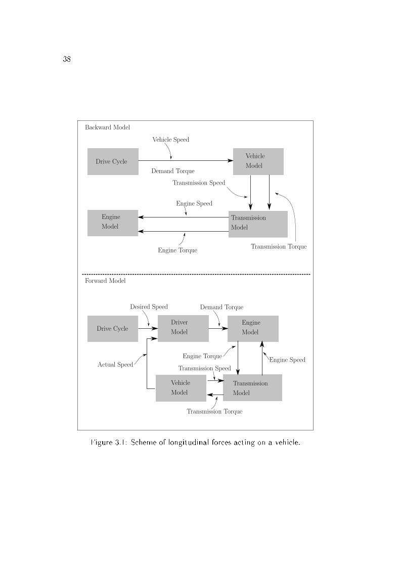
38

Figure 3.1: Scheme of longitudinal forces acting on a vehicle.

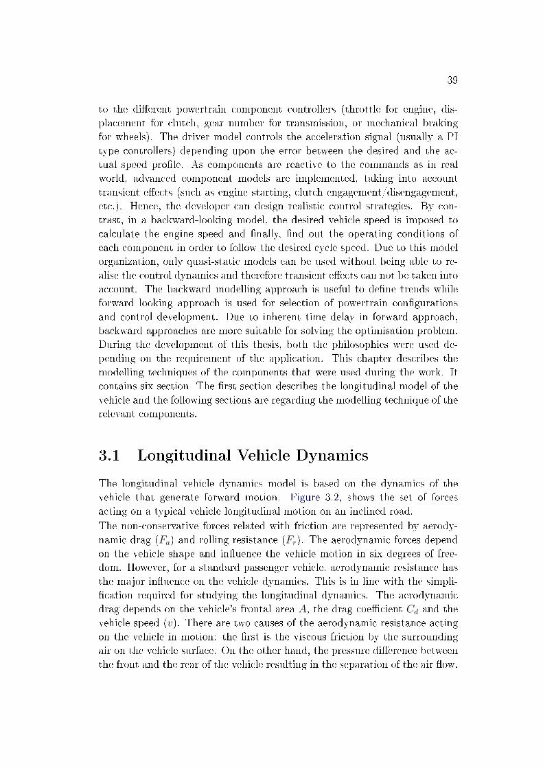
39

to the di�erent powertrain component controllers (throttle for engine, dis-placement for clutch, gear number for transmission, or mechanical brakingfor wheels). The driver model controls the acceleration signal (usually a PItype controllers) depending upon the error between the desired and the ac-tual speed pro�le. As components are reactive to the commands as in realworld, advanced component models are implemented, taking into accounttransient e�ects (such as engine starting, clutch engagement/disengagement,etc.). Hence, the developer can design realistic control strategies. By con-trast, in a backward-looking model, the desired vehicle speed is imposed tocalculate the engine speed and �nally, �nd out the operating conditions ofeach component in order to follow the desired cycle speed. Due to this modelorganization, only quasi-static models can be used without being able to re-alise the control dynamics and therefore transient e�ects can not be taken intoaccount. The backward modelling approach is useful to de�ne trends whileforward looking approach is used for selection of powertrain con�gurationsand control development. Due to inherent time delay in forward approach,backward approaches are more suitable for solving the optimisation problem.During the development of this thesis, both the philosophies were used de-pending on the requirement of the application. This chapter describes themodelling techniques of the components that were used during the work. Itcontains six section- The �rst section describes the longitudinal model of thevehicle and the following sections are regarding the modelling technique of therelevant components.

3.1 Longitudinal Vehicle Dynamics

The longitudinal vehicle dynamics model is based on the dynamics of thevehicle that generate forward motion. Figure 3.2, shows the set of forcesacting on a typical vehicle longitudinal motion on an inclined road.The non-conservative forces related with friction are represented by aerody-namic drag (Fa) and rolling resistance (Fr). The aerodynamic forces dependon the vehicle shape and in�uence the vehicle motion in six degrees of free-dom. However, for a standard passenger vehicle, aerodynamic resistance hasthe major in�uence on the vehicle dynamics. This is in line with the simpli-�cation required for studying the longitudinal dynamics. The aerodynamicdrag depends on the vehicle's frontal area A, the drag coe�cient Cd and thevehicle speed (v). There are two causes of the aerodynamic resistance actingon the vehicle in motion: the �rst is the viscous friction by the surroundingair on the vehicle surface. On the other hand, the pressure di�erence betweenthe front and the rear of the vehicle resulting in the separation of the air �ow.

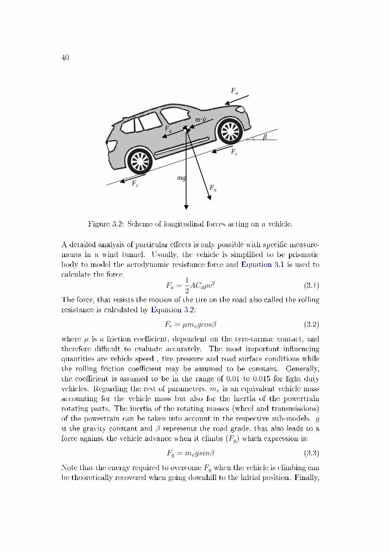
40

mgFn

Fg

m·��𝑣

Fa

Fr

Ft

𝛽𝛽

Figure 3.2: Scheme of longitudinal forces acting on a vehicle.

A detailed analysis of particular e�ects is only possible with speci�c measure-ments in a wind tunnel. Usually, the vehicle is simpli�ed to be prismaticbody to model the aerodynamic resistance force and Equation 3.1 is used tocalculate the force.

Fa =1

2ACdρv

2 (3.1)

The force, that resists the motion of the tire on the road also called the rollingresistance is calculated by Equation 3.2:

Fr = µmvgcosβ (3.2)

where µ is a friction coe�cient, dependent on the tyre-tarmac contact, andtherefore di�cult to evaluate accurately. The most important in�uencingquantities are vehicle speed , tire pressure and road surface conditions whilethe rolling friction coe�cient may be assumed to be constant. Generally,the coe�cient is assumed to be in the range of 0.01 to 0.015 for light dutyvehicles. Regarding the rest of parameters, mv is an equivalent vehicle massaccounting for the vehicle mass but also for the inertia of the powertrainrotating parts. The inertia of the rotating masses (wheel and transmissions)of the powertrain can be taken into account in the respective sub-models. gis the gravity constant and β represents the road grade, that also leads to aforce against the vehicle advance when it climbs (Fg) which expression is:

Fg = mvgsinβ (3.3)

Note that the energy required to overcome Fg when the vehicle is climbing canbe theoretically recovered when going downhill to the initial position. Finally,

41

the traction force comes ultimately from the engine torque or from the brakes,then:

Ft =

{ηt(ugb)Meng(neng ,upedal)

rwRt(ugb)if upedal > 0

upedalFb otherwise(3.4)

where Meng is a non-linear function depending on the engine speed (neng) andpedal (upedal) representing engine torque, in the case at hand a map based onexperimental data. This torque is transferred to the wheels by means of thetransmission, which e�ciency (ηt) and ratio (Rt) depend on the selected gear(ugb). Particularly, in the current model, both ηt and Rt are a�ne functions ofugb. The wheel radius necessary to pass from torque to force is represented byrw. Finally, a simple force balance leads to the following ordinary di�erentialequation:

v =1

mv

.(Ft(t)− (Fa(t) + Fr(t) + Fg(t))) (3.5)

which is the main equation of the vehicle longitudinal dynamics. The integra-tion provides the instanteneous vehicle speed making it a forward modellingapproach. While the parameters in Equation 3.1 to Equation 3.4 can be ob-tained experimentally or estimated from literature, Equation 3.5 allows track-ing the velocity evolution as a function of an initial state, the driver actuation(upedal, ugb) and problem perturbations such as the road grade. It must alsobe noticed that all the forces do not act at the centre of mass of the vehiclewhich, produce moment and a variation on the pitch. However,these momentsare assumed to be cancelled by the reaction to the normal force on the pointof contact between the tires and the road.

When braking, the force applied to the wheels is proportional to a maxi-mum braking force (Fb) through variable upedal. For the sake of model simplic-ity, both throttle and braking pedals (upedal and ub) are modelled with a singlevariable (upedal) ranging from -1 to 1. This assumption involves that situationswhere both pedals are actuated at the same time cannot be modelled. Theclutch is not modelled, so the potential losses in this element during normaloperation should be included in ηt while slipping during gear change is ne-glected. In order to reduce the number of actuators of the model, the brakingand throttle actions (ub and upedal) have been lumped in a single actuator (u)such that:

upedal =

{u if upedal ≥ 0

0 if upedal < 0(3.6)

ub =

{0 if upedal ≥ 0

u if upedal < 0(3.7)

42

In this sense, analysing Equation 3.6 to Equation 3.7 one can observe thatthe model has single state (v) and actuator (u) since the gear shift followsa prede�ned policy depending on the engine speed, and accordingly on thevehicle speed. In the following section the powertrain models developed duringthis thesis are presented.

3.2 Gear Box

In a conventional vehicle, the internal combustion engine is used to meet thepower demanded by the driver. The transmission of power from the engineto the wheels passes through gearbox and clutch. Assuming zero losses atthe clutch, gearbox is modelled as a discrete set of gear ratios with a �xede�ciency. The torque and the angular speed required at the gearbox outputare calculated based on the following equations:

ωW =v

rW(3.8)

ωW =v

rW(3.9)

(3.10)

TW =

{rW .Ft, if v > 0

0, if v = 0

The parameter rW is the wheel radius, TW the torque at the wheel. The wheelinertia and constant torque loss is neglected. The gearbox is modelled as thetransmission ratios with constant e�ciencies. The speed and torque requiredat the gearbox input to satisfy the demanded speed and torque at the wheelare calculated by

ωg = νg(gb).ωW (3.11)

ωg = νg(gb).ωW (3.12)

(3.13)

Tg =

{TW

ηg .νg(gb), if TW ≥ 0

TW .ηgνg(gb)

, if TW < 0

Where ωg is the angular speed input to the gear box, ωW is the angularspeed of the wheels, ωg is the angular acceleration input to the gearbox, ωWis the angular acceleration of the wheels, gb is the selected gear number and

43

νg(gb) the corresponding transmission ratio. Tg is the torque input to thegearbox. The ICE torque include inertial terms which is a product of theangular acceleration and the required torque.

3.3 Internal Combustion Engine

The design of an ICE model is usually driven from the application require-ments. In the present work, there are two type of applications that are beingstudied: the �rst type of applications are regarding the control of an internalcombustion engine for maximum fuel e�ciency and emission reduction in realdriving missions. These applications require an engine model that is capa-ble of predicting the trends in fuel consumption and emissions responding tothe variations in engine operating points (ωe, Te) and a few engine actuators(such as uvgt, uegr, usoi etc..). The second kind of applications, obtain an op-timal speed trajectory of a vehicle on a real driving mission. Wherein theengine calibration is �xed and does not require access. The only actuator,controller has an access to is the throttle position upedal and therefore an evenmore simplistic engine model is applicable. The two aforementioned enginemodel types are described in the following paragraphs:

Type 1 In this type of engine models, the fuel consumption and engine outemissions are modelled at each operating point using static response models.The following three steps are carried out to obtain the engine response models.

• At �rst, the steady-state measurements are carried out at the enginetest-bench. The desired control inputs are varied at each operatingpoint and the desired torque is obtained by controlling the fuel injectionquantity. The feasible range of control inputs is explored at each op-erating point. Usually Design-of-Experiment (DOE) technique is usedto reduce the number of tests required for the purpose of building theengine response models. In this thesis a full factorial DOE techniquewas used. One of such measurement campaign was conducted for theoperating points shown in Figure 3.3, the black dot represent the pointstested during the campaign and black line is the limiting torque.

• After completing the measurement, point-by-point models (which is alsoreferred to as steady-state model) are created, and they are interpolatedusing appropriate method. These models are capable of predicting thee�ect of the input variables on the output variables.

• The prediction capability of the model is validated experimentally atthe operating points which were not included during the model creation.

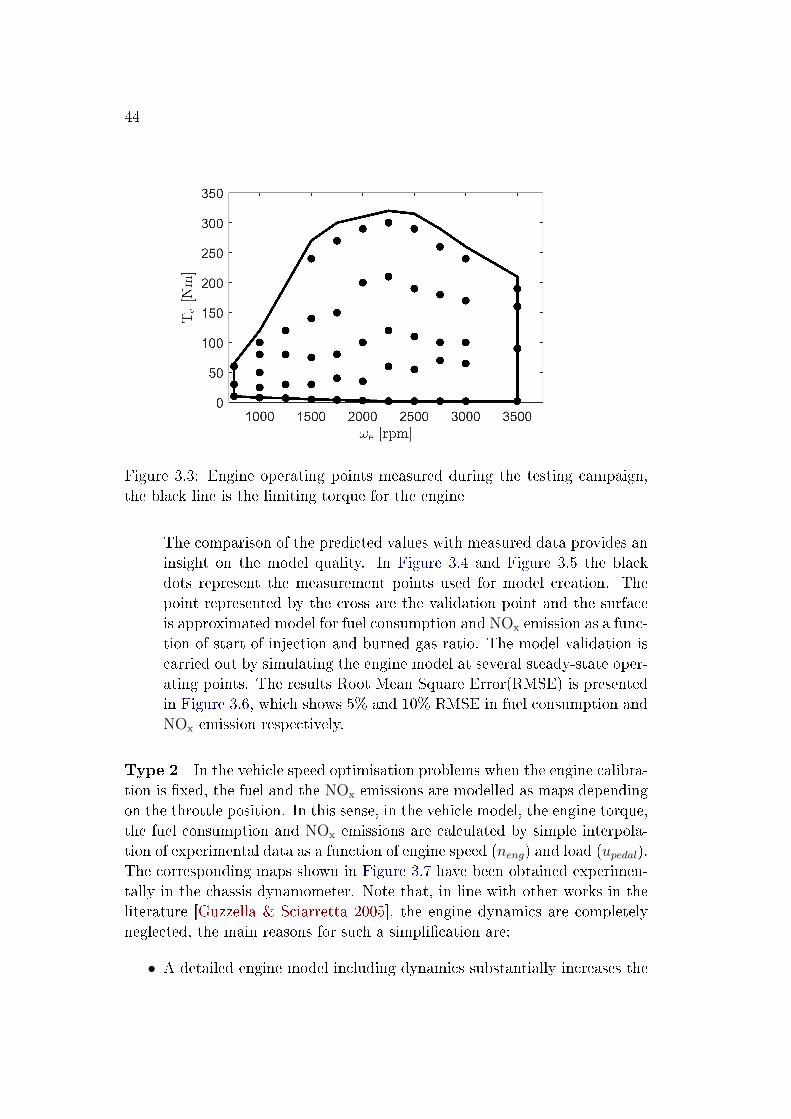
44

Figure 3.3: Engine operating points measured during the testing campaign,the black line is the limiting torque for the engine

The comparison of the predicted values with measured data provides aninsight on the model quality. In Figure 3.4 and Figure 3.5 the blackdots represent the measurement points used for model creation. Thepoint represented by the cross are the validation point and the surfaceis approximated model for fuel consumption and NOx emission as a func-tion of start-of-injection and burned gas ratio. The model validation iscarried out by simulating the engine model at several steady-state oper-ating points. The results Root Mean Square Error(RMSE) is presentedin Figure 3.6, which shows 5% and 10% RMSE in fuel consumption andNOx emission respectively.

Type 2 In the vehicle speed optimisation problems when the engine calibra-tion is �xed, the fuel and the NOx emissions are modelled as maps dependingon the throttle position. In this sense, in the vehicle model, the engine torque,the fuel consumption and NOx emissions are calculated by simple interpola-tion of experimental data as a function of engine speed (neng) and load (upedal).The corresponding maps shown in Figure 3.7 have been obtained experimen-tally in the chassis dynamometer. Note that, in line with other works in theliterature [Guzzella & Sciarretta 2005], the engine dynamics are completelyneglected, the main reasons for such a simpli�cation are:

• A detailed engine model including dynamics substantially increases the

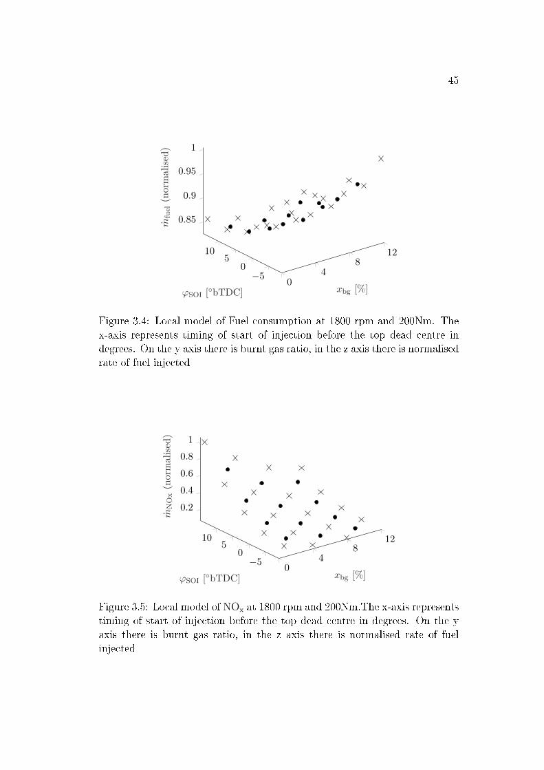
45

04

812

−50

510

0.85

0.9

0.95

1

xbg [%]ϕSOI [◦bTDC]

mfuel

(nor

mal

ised)

Figure 3.4: Local model of Fuel consumption at 1800 rpm and 200Nm. Thex-axis represents timing of start of injection before the top dead centre indegrees. On the y axis there is burnt gas ratio, in the z axis there is normalisedrate of fuel injected

04

812

−50

510

0.2

0.4

0.6

0.8

1

xbg [%]ϕSOI [◦bTDC]

mNOx

(nor

mal

ised)

Figure 3.5: Local model of NOx at 1800 rpm and 200Nm.The x-axis representstiming of start of injection before the top dead centre in degrees. On the yaxis there is burnt gas ratio, in the z axis there is normalised rate of fuelinjected

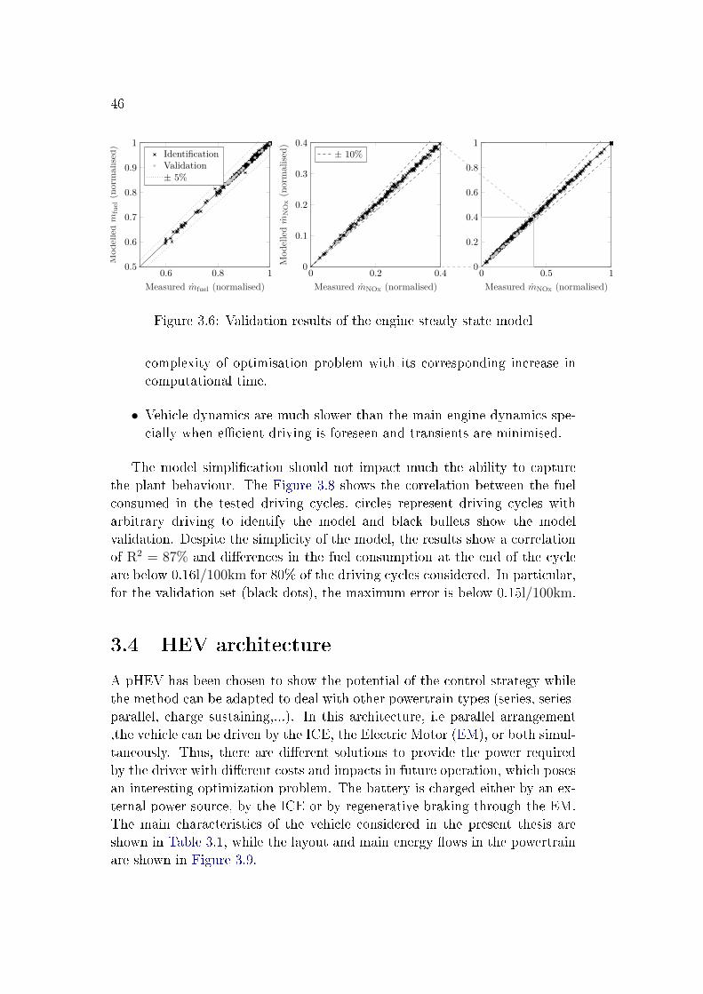
46

0.6 0.8 10.5

0.6

0.7

0.8

0.9

1

Measured mfuel (normalised)

Mod

elle

dm

fuel

(nor

mal

ised) Identification

Validation± 5%

0 0.2 0.40

0.1

0.2

0.3

0.4

Measured mNOx (normalised)M

odel

ledm

NOx

(nor

mal

ised) ± 10%

0 0.5 10

0.2

0.4

0.6

0.8

1

Measured mNOx (normalised)

Figure 3.6: Validation results of the engine steady state model

complexity of optimisation problem with its corresponding increase incomputational time.

• Vehicle dynamics are much slower than the main engine dynamics spe-cially when e�cient driving is foreseen and transients are minimised.

The model simpli�cation should not impact much the ability to capturethe plant behaviour. The Figure 3.8 shows the correlation between the fuelconsumed in the tested driving cycles, circles represent driving cycles witharbitrary driving to identify the model and black bullets show the modelvalidation. Despite the simplicity of the model, the results show a correlationof R2 = 87% and di�erences in the fuel consumption at the end of the cycleare below 0.16l/100km for 80% of the driving cycles considered. In particular,for the validation set (black dots), the maximum error is below 0.15l/100km.

3.4 HEV architecture

A pHEV has been chosen to show the potential of the control strategy whilethe method can be adapted to deal with other powertrain types (series, series-parallel, charge sustaining,...). In this architecture, i.e parallel arrangement,the vehicle can be driven by the ICE, the Electric Motor (EM), or both simul-taneously. Thus, there are di�erent solutions to provide the power requiredby the driver with di�erent costs and impacts in future operation, which posesan interesting optimization problem. The battery is charged either by an ex-ternal power source, by the ICE or by regenerative braking through the EM.The main characteristics of the vehicle considered in the present thesis areshown in Table 3.1, while the layout and main energy �ows in the powertrainare shown in Figure 3.9.

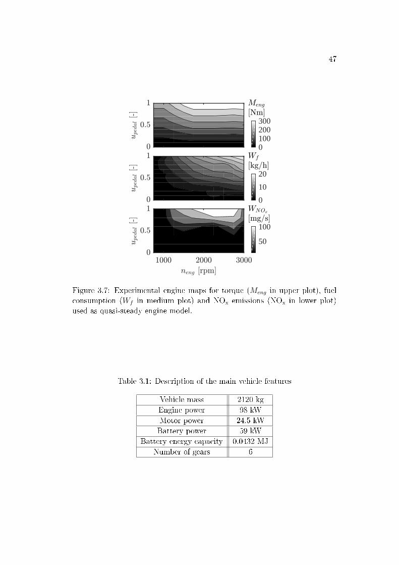
47

50

100

0

10

20

0100200300

Figure 3.7: Experimental engine maps for torque (Meng in upper plot), fuelconsumption (Wf in medium plot) and NOx emissions (NOx in lower plot)used as quasi-steady engine model.

Table 3.1: Description of the main vehicle features

Vehicle mass 2120 kgEngine power 98 kWMotor power 24.5 kWBattery power 59 kW

Battery energy capacity 0.0432 MJNumber of gears 6

48

R2=0.87

[L/1

00 k

m]

[L/100 km] [L/100 km]

Figure 3.8: Vehicle model performance. Left: comparison between measuredand modelled fuel consumption during the set of driving cycles tested. Right:Percentage of cycles with modelling error (εVf ) below certain limit νVf .

The aim of developing HEV model in this thesis is to support the devel-opment of control algorithm which manages its power �ow. The engine ismodelled as a quasi-static subsystem whose inputs are the desired torque andengine speed with fuel �ow as the output. The torque generation dynamicsare fast and hence negligible. The energy management is performed at a muchslower rate than the torque control. Accordingly, the engine is also modelledas quasi-steady maps with limits over the torque. The maps are presented inFigure 3.10. The �rst plot represents the engine e�ciency map with respectto the engine speed and the torque and the second plot presents the ICE op-erating region with minimum and maximum power with respect to the enginespeed.

3.5 Electric Motor

In Figure 3.9, the parallel architecture of the HEV is presented. The powersources are the battery and the internal combustion engine. They can togetheror individually propel the vehicle through the driveline that constitutes atorque coupler and a gearbox(GB). The energy can be recuperated in thebattery during vehicle deceleration.

The power split device manage the supply of energy to the wheels bysplitting the power demand between the electric motor and the internal com-bustion engine. The design of power splitter is not in the scope of this thesishowever, the study is focused on how the power is been split. In particular, the

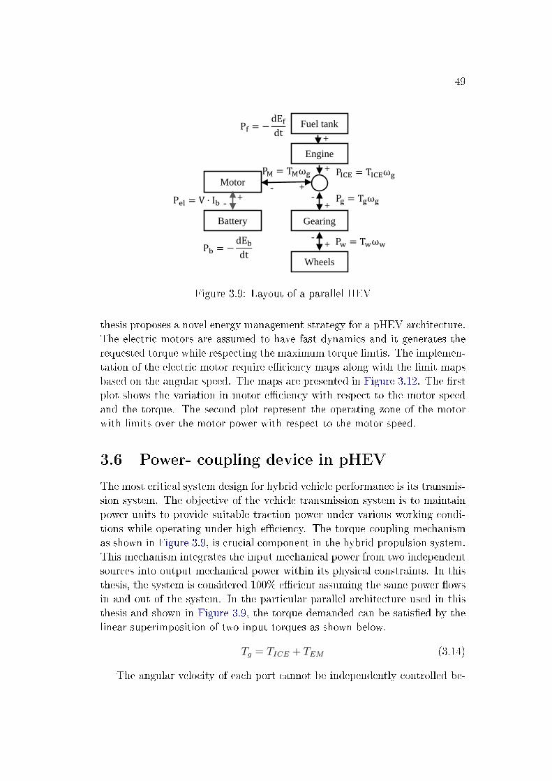
49

+--

Engine

Battery

Motor

Wheels

Gearing

+

++

+-

-

Fuel tank+

PICE = TICEωgPM = TMωg

Pg = Tgωg

Pf = −dEfdt

Pb = −dEbdt

Pel = V · Ib

Pw = Twωw

Figure 3.9: Layout of a parallel HEV

thesis proposes a novel energy management strategy for a pHEV architecture.The electric motors are assumed to have fast dynamics and it generates therequested torque while respecting the maximum torque limtis. The implemen-tation of the electric motor require e�ciency maps along with the limit mapsbased on the angular speed. The maps are presented in Figure 3.12. The �rstplot shows the variation in motor e�ciency with respect to the motor speedand the torque. The second plot represent the operating zone of the motorwith limits over the motor power with respect to the motor speed.

3.6 Power- coupling device in pHEV

The most critical system design for hybrid vehicle performance is its transmis-sion system. The objective of the vehicle transmission system is to maintainpower units to provide suitable traction power under various working condi-tions while operating under high e�ciency. The torque coupling mechanismas shown in Figure 3.9, is crucial component in the hybrid propulsion system.This mechanism integrates the input mechanical power from two independentsources into output mechanical power within its physical constraints. In thisthesis, the system is considered 100% e�cient assuming the same power �owsin and out of the system. In the particular parallel architecture used in thisthesis and shown in Figure 3.9, the torque demanded can be satis�ed by thelinear superimposition of two input torques as shown below.

Tg = TICE + TEM (3.14)

The angular velocity of each port cannot be independently controlled be-

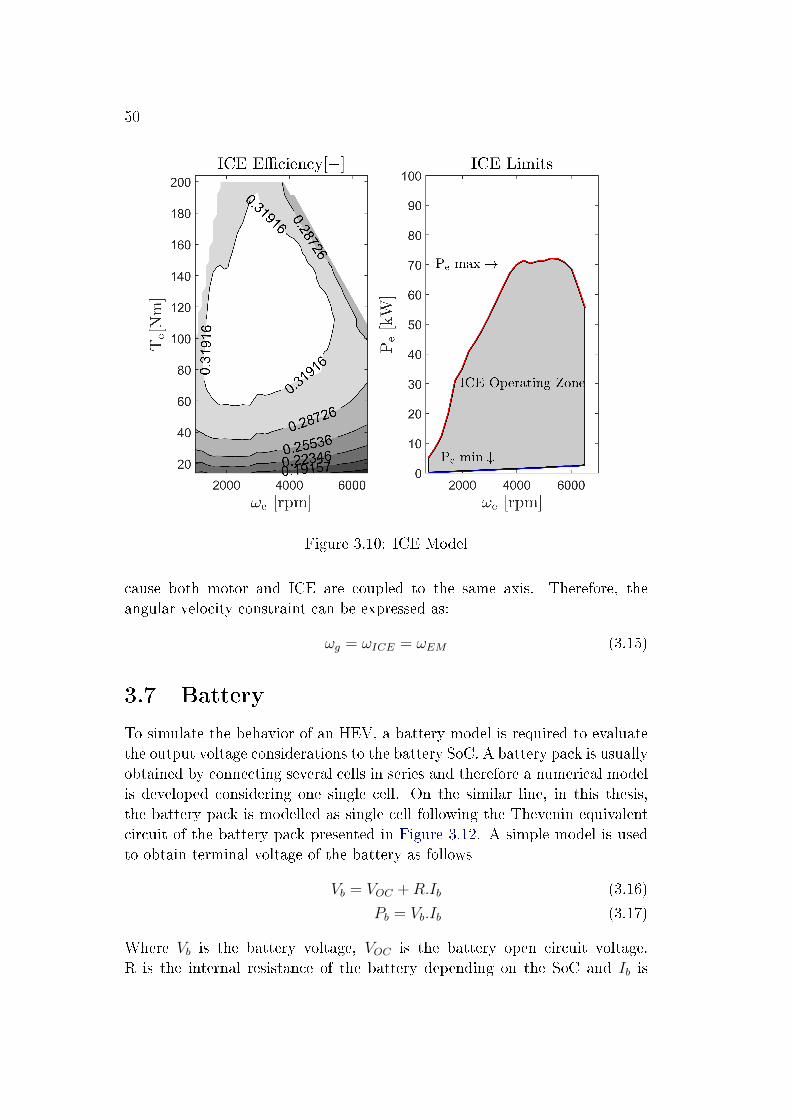
50

Figure 3.10: ICE Model

cause both motor and ICE are coupled to the same axis. Therefore, theangular velocity constraint can be expressed as:

ωg = ωICE = ωEM (3.15)

3.7 Battery

To simulate the behavior of an HEV, a battery model is required to evaluatethe output voltage considerations to the battery SoC. A battery pack is usuallyobtained by connecting several cells in series and therefore a numerical modelis developed considering one single cell. On the similar line, in this thesis,the battery pack is modelled as single cell following the Thevenin equivalentcircuit of the battery pack presented in Figure 3.12. A simple model is usedto obtain terminal voltage of the battery as follows

Vb = VOC +R.Ib (3.16)

Pb = Vb.Ib (3.17)

Where Vb is the battery voltage, VOC is the battery open circuit voltage.R is the internal resistance of the battery depending on the SoC and Ib is

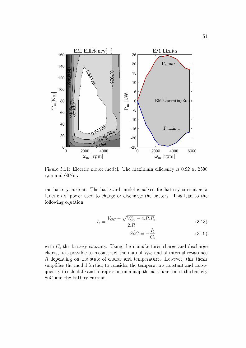
51

Figure 3.11: Electric motor model. The maximum e�ciency is 0.92 at 2300rpm and 60Nm.

the battery current. The backward model is solved for battery current as afunction of power used to charge or discharge the battery. This lead to thefollowing equation:

Ib =VOC −

√V 2OC − 4.R.Pb

2.R(3.18)

˙SoC = − IbCb

(3.19)

with Cb the battery capacity. Using the manufacturer charge and dischargecharts, it is possible to reconstruct the map of VOC and of internal resistanceR depending on the state of charge and temperature. However, this thesissimpli�es the model further to consider the temperature constant and conse-quently to calculate and to represent on a map the as a function of the batterySoC and the battery current.

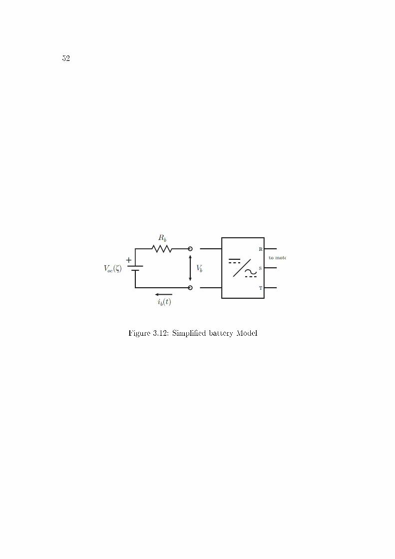
52

Figure 3.12: Simpli�ed battery Model

Chapter 4

Optimisation tool

Contents

4.1 Dynamic Programming and its Application . . . . . . 53

4.2 Pontryagin's minimum Principle, application and ex-

tension to ECMS . . . . . . . . . . . . . . . . . . . . . . 57

In an optimal control problem, the trajectories of the control variables u ofa dynamic system f are calculated for minising a cost index. The cost index isquanti�able, such as energy consumption, time, etc. The state of the dynamicsystem is driven by the di�erential equation given by:

x = f(x, u, t) (4.1)

where, x represent the state and t is the time dependence.There are two optimisation techniques that were the basis of the online

control methods explored during the development of this thesis: Dynamic pro-gramming and Pontryagins Minimum Principle. The intention of this sectionis not to describe them in detail, but to provide insight in some ideas that areused in the thesis.

4.1 Dynamic Programming and its Application

The DP was originally developed by Richard Bellman [Bellman 1970], whostated that an optimal policy has the property that, whatever the initial stateand initial decision are, the remaining decisions must constitute an optimalpolicy with regard to the state resulting from the �rst decision. This meansthat the problem can be broken into sub-problems of lower size which are to

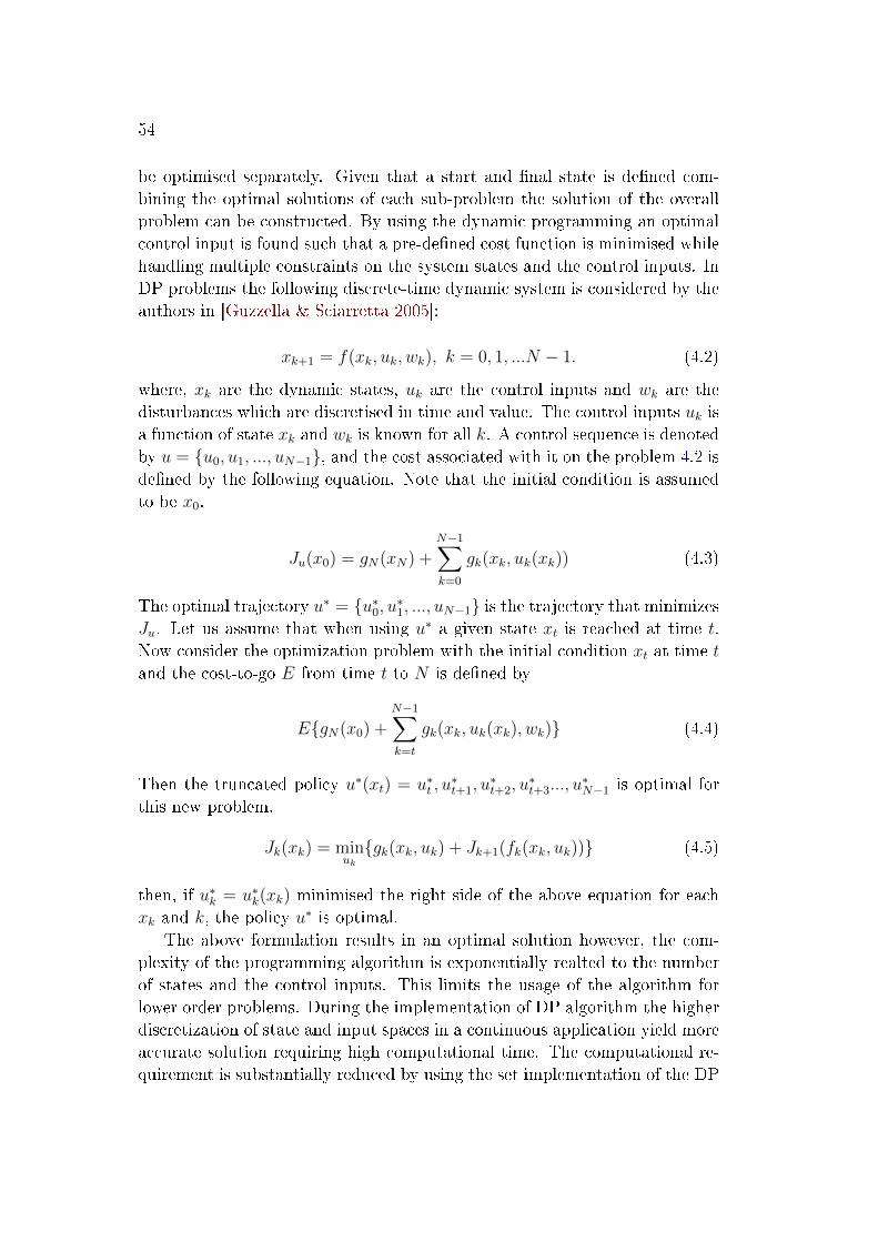
54

be optimised separately. Given that a start and �nal state is de�ned com-bining the optimal solutions of each sub-problem the solution of the overallproblem can be constructed. By using the dynamic programming an optimalcontrol input is found such that a pre-de�ned cost function is minimised whilehandling multiple constraints on the system states and the control inputs. InDP problems the following discrete-time dynamic system is considered by theauthors in [Guzzella & Sciarretta 2005]:

xk+1 = f(xk, uk, wk), k = 0, 1, ...N − 1. (4.2)

where, xk are the dynamic states, uk are the control inputs and wk are thedisturbances which are discretised in time and value. The control inputs uk isa function of state xk and wk is known for all k. A control sequence is denotedby u = {u0, u1, ..., uN−1}, and the cost associated with it on the problem 4.2 isde�ned by the following equation. Note that the initial condition is assumedto be x0.

Ju(x0) = gN(xN) +N−1∑k=0

gk(xk, uk(xk)) (4.3)

The optimal trajectory u∗ = {u∗0, u∗1, ..., uN−1} is the trajectory that minimizesJu. Let us assume that when using u∗ a given state xt is reached at time t.Now consider the optimization problem with the initial condition xt at time tand the cost-to-go E from time t to N is de�ned by

E{gN(x0) +N−1∑k=t

gk(xk, uk(xk), wk)} (4.4)

Then the truncated policy u∗(xt) = u∗t , u∗t+1, u

∗t+2, u

∗t+3..., u

∗N−1 is optimal for

this new problem.

Jk(xk) = minuk{gk(xk, uk) + Jk+1(fk(xk, uk))} (4.5)

then, if u∗k = u∗k(xk) minimised the right side of the above equation for eachxk and k, the policy u∗ is optimal.

The above formulation results in an optimal solution however, the com-plexity of the programming algorithm is exponentially realted to the numberof states and the control inputs. This limits the usage of the algorithm forlower order problems. During the implementation of DP algorithm the higherdiscretization of state and input spaces in a continuous application yield moreaccurate solution requiring high computational time. The computational re-quirement is substantially reduced by using the set implementation of the DP

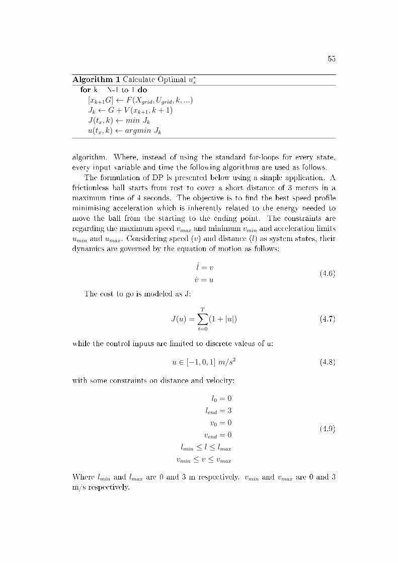
55

Algorithm 1 Calculate Optimal u∗sfor k =N-1 to 1 do

[xk+1G]← F (Xgrid, Ugrid, k, ...)

Jk ← G+ V (xk+1, k + 1)

J(tx, k)← min Jku(tx, k)← argmin Jk

algorithm. Where, instead of using the standard for-loops for every state,every input variable and time the following algorithms are used as follows.

The formulation of DP is presented below using a simple application. Africtionless ball starts from rest to cover a short distance of 3 meters in amaximum time of 4 seconds. The objective is to �nd the best speed pro�leminimising acceleration which is inherently related to the energy needed tomove the ball from the starting to the ending point. The constraints areregarding the maximum speed vmax and minimum vmin and acceleration limitsumin and umax. Considering speed (v) and distance (l) as system states, theirdynamics are governed by the equation of motion as follows:

l = v

v = u(4.6)

The cost to go is modeled as J:

J(u) =T∑t=0

(1 + |u|) (4.7)

while the control inputs are limited to discrete valeus of u:

u ∈ [−1, 0, 1] m/s2 (4.8)

with some constraints on distance and velocity:

l0 = 0

lend = 3

v0 = 0

vend = 0

lmin ≤ l ≤ lmax

vmin ≤ v ≤ vmax

(4.9)

Where lmin and lmax are 0 and 3 m respectively. vmin and vmax are 0 and 3m/s respectively.

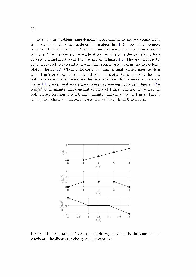
56

To solve this problem using dynamic programming we move systematicallyfrom one side to the other as described in algorithm 1. Suppose that we movebackward from right to left. At the last intersection at 4 s there is no decisionto make. The �rst decision is made at 3 s. At this time the ball should havecovered 2m and must be at 1m/s as shown in �gure 4.1. The optimal cost-to-go with respect to two states at each time step is presented in the �rst columnplots of �gure 4.2. Clearly, the corresponding optimal control input at 4s isu = -1 m/s as shown in the second columns plots. Which implies that theoptimal strategy is to decelerate the vehicle to rest. As we move leftwards at2 s in 4.1, the optimal acceleration presented moving upwards in �gure 4.2 is0 m/s2 while maintaining constant velocity of 1 m/s. Further left at 1 s, theoptimal acceleration is still 0 while maintaining the speed at 1 m/s. Finallyat 0 s, the vehicle should acclerate at 1 m/s2 to go from 0 to 1 m/s.

0 1 2 3 40

2

4

0 1 2 3 40

1

2

3

1 1.5 2 2.5 3 3.5 4-1

0

1

Figure 4.1: Realisation of the DP algorithm, on x-axis is the time and ony-axis are the distance, velocity and acceeration.

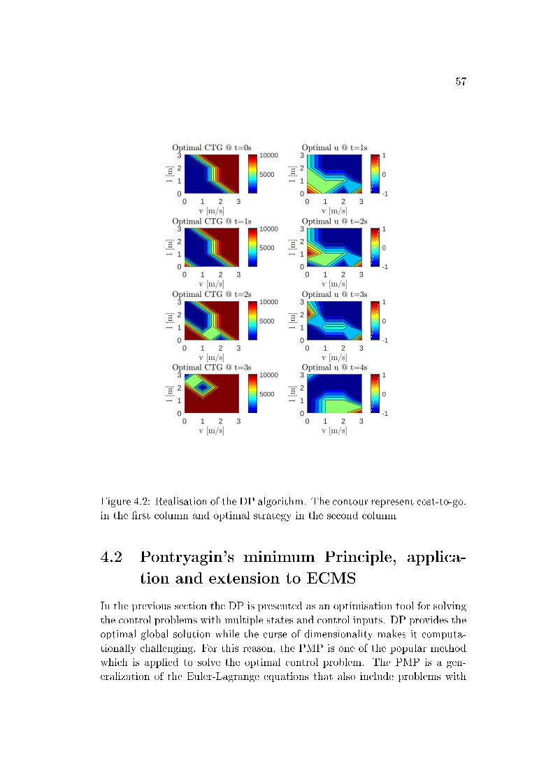
57

0 1 2 30

1

2

3

5000

10000

0 1 2 30

1

2

3

5000

10000

0 1 2 30

1

2

3

5000

10000

0 1 2 30

1

2

3

5000

10000

0 1 2 30

1

2

3

-1

0

1

0 1 2 30

1

2

3

-1

0

1

0 1 2 30

1

2

3

-1

0

1

0 1 2 30

1

2

3

-1

0

1

Figure 4.2: Realisation of the DP algorithm. The contour represent cost-to-go.in the �rst column and optimal strategy in the second column

4.2 Pontryagin's minimum Principle, applica-

tion and extension to ECMS

In the previous section the DP is presented as an optimisation tool for solvingthe control problems with multiple states and control inputs. DP provides theoptimal global solution while the curse of dimensionality makes it computa-tionally challenging. For this reason, the PMP is one of the popular methodwhich is applied to solve the optimal control problem. The PMP is a gen-eralization of the Euler-Lagrange equations that also include problems with

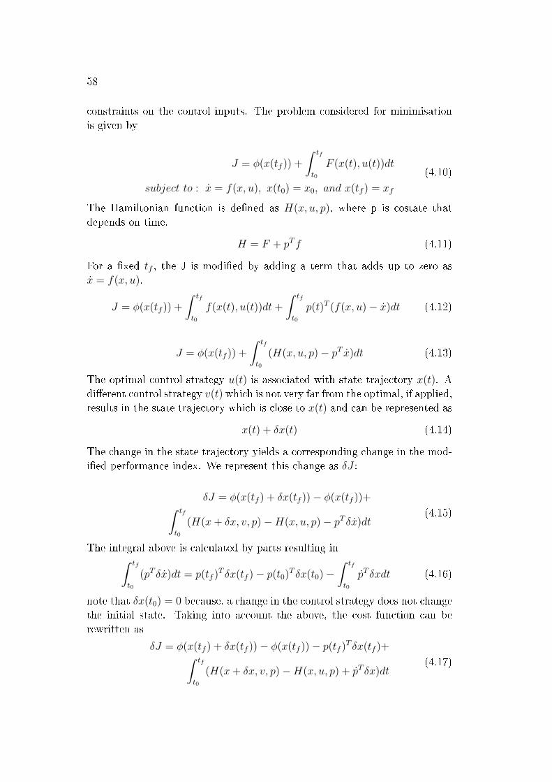
58

constraints on the control inputs. The problem considered for minimisationis given by

J = φ(x(tf )) +

∫ tf

t0

F (x(t), u(t))dt

subject to : x = f(x, u), x(t0) = x0, and x(tf ) = xf

(4.10)

The Hamiltonian function is de�ned as H(x, u, p), where p is costate thatdepends on time.

H = F + pTf (4.11)

For a �xed tf , the J is modi�ed by adding a term that adds up to zero asx = f(x, u).

J = φ(x(tf )) +

∫ tf

t0

f(x(t), u(t))dt+

∫ tf

t0

p(t)T (f(x, u)− x)dt (4.12)

J = φ(x(tf )) +

∫ tf

t0

(H(x, u, p)− pT x)dt (4.13)

The optimal control strategy u(t) is associated with state trajectory x(t). Adi�erent control strategy v(t) which is not very far from the optimal, if applied,results in the state trajectory which is close to x(t) and can be represented as

x(t) + δx(t) (4.14)

The change in the state trajectory yields a corresponding change in the mod-i�ed performance index. We represent this change as δJ :

δJ = φ(x(tf ) + δx(tf ))− φ(x(tf ))+∫ tf

t0

(H(x+ δx, v, p)−H(x, u, p)− pT δx)dt(4.15)

The integral above is calculated by parts resulting in∫ tf

t0

(pT δx)dt = p(tf )T δx(tf )− p(t0)T δx(t0)−

∫ tf

t0

pT δxdt (4.16)

note that δx(t0) = 0 because, a change in the control strategy does not changethe initial state. Taking into account the above, the cost function can berewritten as

δJ = φ(x(tf ) + δx(tf ))− φ(x(tf ))− p(tf )T δx(tf )+∫ tf

t0

(H(x+ δx, v, p)−H(x, u, p) + pT δx)dt(4.17)

59

the term φ(x(tf ) + δx(tf ))− φ(x(tf )) is replaced with its �rst order approxi-mation while H(x, v, p) is added and subtracted under the integral to obtain.

δJ = (∇xφt=tf − p(tf ))T δx(tf )+∫ tf

t0

(H(x+ δx, v, p)−H(x, v, p) +H(x, v, p)−H(x, u, p) + pT δx)dt(4.18)

The (H(x+ δx, v, p)¯H(x, v, p) is replaced with its �rst order approximation,

δJ = (∇xφt=tf − p(tf ))T δx(tf )+∫ tf

t0

(∂H

∂xδx+H(x, v, p)−H(x, u, p) + pT δx)dt

(4.19)

If p is the solution to the di�erential equation

∂H

∂x+ pT δx = 0 (4.20)

with the �nal condition

p(tf ) = ∇xφt=tf (4.21)

reduces the deviation in the cost to

δJ =

∫ tf

t0

(H(x, v, p)−H(x, u, p))dt (4.22)

If the u is optimal then (H(x, v, p) − H(x, u, p)) must be greater than zero.The necessary conditions for u to minimise J subject to the constraints in theEquation 4.11 are:

p = −(∂H

∂x)T (4.23)

where H = H(x, u, p) = F (x, u) + pTf(x, u)

H(x∗, u∗, p∗) = minu{H(x, u, p)} (4.24)

The PMP can be used to solve the minimum fuel problem described in 4.7-4.9. The goal was to derive the state to the origin with minimum cost. Thestates in the problem are distance(x1) and velocity(x2) while the dynamicsare governed by:

x1 = x2

x2 = u(4.25)

60

If we apply u=±1, the system response can be represented by the followingequations:

if u = 1,

x2(t) = t+ c1

x1(t) =1

2t2 + c1t+ c2

x1(t) =1

2(t+ c1)

2 + c3x1(t) =1

2x2(t)

2 + c3

(4.26)

the hamiltonian for the system can be formulated as:

H = 1 + |u|+ [p1 p2][0 1; 0 0][x1;x2] + [0; 1]u

H = 1 + |u|+ p1.x2 + p2.u(4.27)

the equation of the co-state can be derived as:

p = −HxT

p1 = −Hx1

p1 = 0

p1 = cp2 = −Hx2

p2 = −p1p2 = −c1t+ c2

(4.28)

the above equation shows that p2 is linear in time.To �nd the optimal control, the value of u making 0 the derivative of the

Hamiltonian respect to u should be found:

Hu =u

|u| + p2 (4.29)

then :

Hu =

{p2 + 1, if u ≥ 0

p2 − 1, if u < 0

Note that provided the value of p2, Hu is constant, leading to a linear depen-dence of H with u.

Therefore the control law can be described using the three conditions basedon the sign of H which depends size of p2 .

u(t) =

−um, if 1 < p2(t)

0, if − 1 < p2(t) < 1

um, if p2(t) < −1

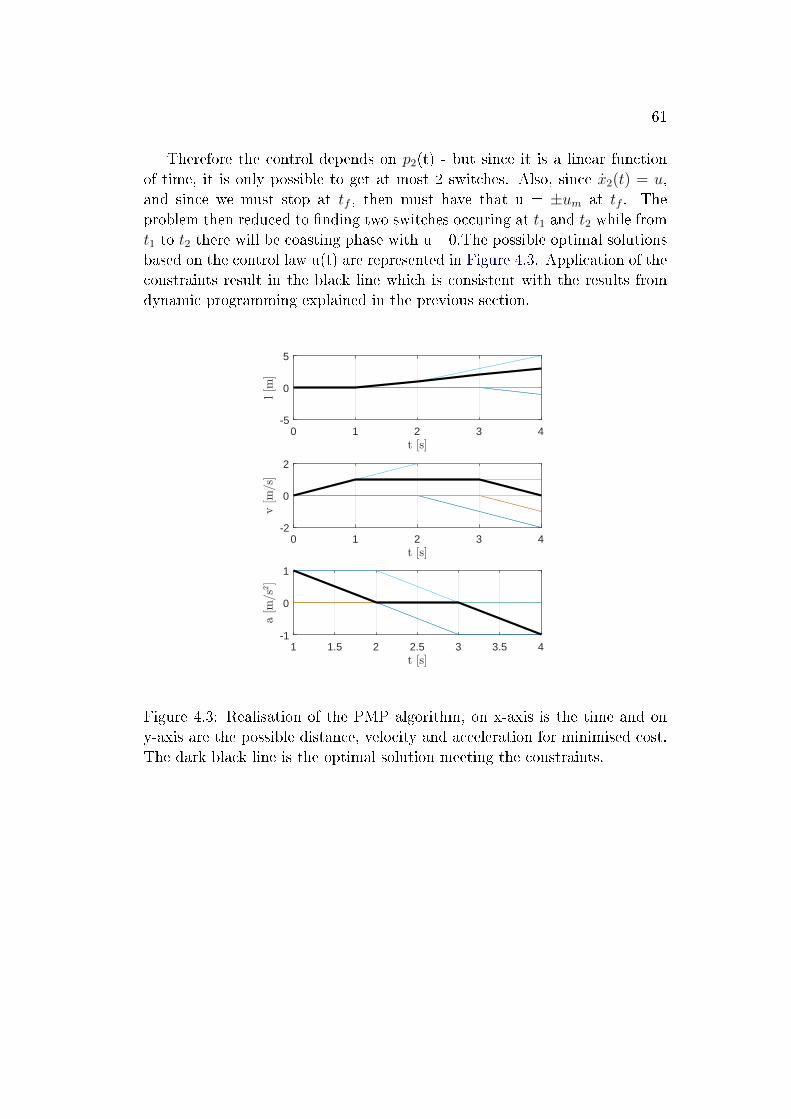
61

Therefore the control depends on p2(t) - but since it is a linear functionof time, it is only possible to get at most 2 switches. Also, since x2(t) = u,and since we must stop at tf , then must have that u = ±um at tf . Theproblem then reduced to �nding two switches occuring at t1 and t2 while fromt1 to t2 there will be coasting phase with u =0.The possible optimal solutionsbased on the control law u(t) are represented in Figure 4.3. Application of theconstraints result in the black line which is consistent with the results fromdynamic programming explained in the previous section.

0 1 2 3 4-5

0

5

0 1 2 3 4-2

0

2

1 1.5 2 2.5 3 3.5 4-1

0

1

Figure 4.3: Realisation of the PMP algorithm, on x-axis is the time and ony-axis are the possible distance, velocity and acceleration for minimised cost.The dark black line is the optimal solution meeting the constraints.

Chapter 5

Driving cycle prediction

Contents

5.1 Markov Chain Principle . . . . . . . . . . . . . . . . . 64

5.2 Implementation of MC principle in Driving cycle pre-

diction . . . . . . . . . . . . . . . . . . . . . . . . . . . . 65

An online energy management strategy that is optimal and can be im-plemented in real time has been a topic of interest by researchers and theindustry. Optimal control methods guarantee an optimal solution if the driv-ing cycle is perfectly known in advance. However, perfect knowledge of thedriving cycle is not possible and ECMS allows to �nd a suboptimal solutionwith some estimation of the driving conditions. To this end, online calculationof the co-state is required to deal with the changing driving scenarios. Thus,any estimation of future information to feed the ECMS control module withappropriate values of the equivalence factor is required. Usually, driving cycleprediction techniques are used to forecast the distribution of various futuredriving conditions like velocity, acceleration, driver behaviour etc. The fore-cast is primarily used in the predictive energy management strategies of thevehicle. On one hand, in the conventional vehicles, the forecast can be used tooptimise the engine control while on the other hand, the energy managementstrategy is optimised for the hybrid electric vehicles. In this chapter a popularmethod based on MC is described for the purpose of driving cycle prediction.The �rst section describes the MC principle followed by a section regardingits application in the cycle prediction.

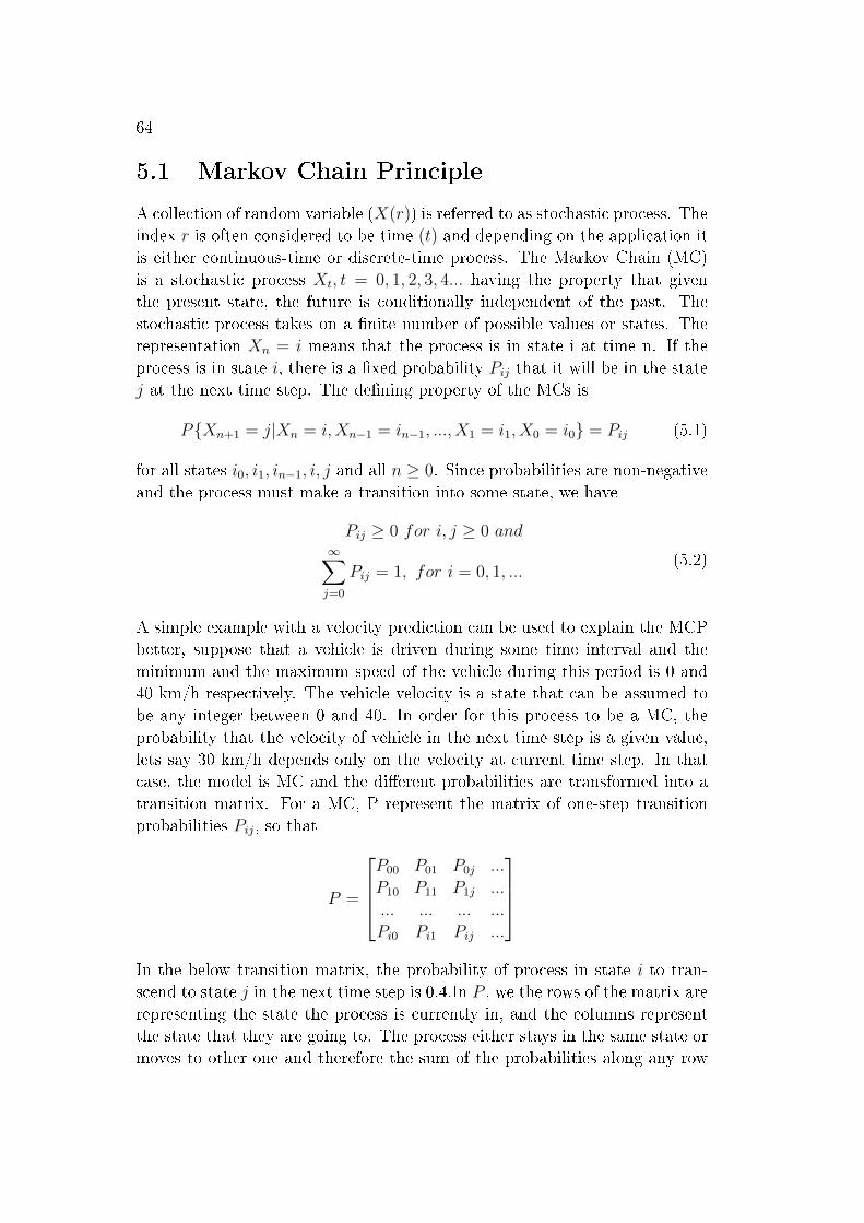
64

5.1 Markov Chain Principle

A collection of random variable (X(r)) is referred to as stochastic process. Theindex r is often considered to be time (t) and depending on the application itis either continuous-time or discrete-time process. The Markov Chain (MC)is a stochastic process Xt, t = 0, 1, 2, 3, 4... having the property that giventhe present state, the future is conditionally independent of the past. Thestochastic process takes on a �nite number of possible values or states. Therepresentation Xn = i means that the process is in state i at time n. If theprocess is in state i, there is a �xed probability Pij that it will be in the statej at the next time step. The de�ning property of the MCs is

P{Xn+1 = j|Xn = i,Xn−1 = in−1, ..., X1 = i1, X0 = i0} = Pij (5.1)

for all states i0, i1, in−1, i, j and all n ≥ 0. Since probabilities are non-negativeand the process must make a transition into some state, we have

Pij ≥ 0 for i, j ≥ 0 and∞∑j=0

Pij = 1, for i = 0, 1, ...(5.2)

A simple example with a velocity prediction can be used to explain the MCPbetter, suppose that a vehicle is driven during some time interval and theminimum and the maximum speed of the vehicle during this period is 0 and40 km/h respectively. The vehicle velocity is a state that can be assumed tobe any integer between 0 and 40. In order for this process to be a MC, theprobability that the velocity of vehicle in the next time step is a given value,lets say 30 km/h depends only on the velocity at current time step. In thatcase, the model is MC and the di�erent probabilities are transformed into atransition matrix. For a MC, P represent the matrix of one-step transitionprobabilities Pij, so that

P =

P00 P01 P0j ...

P10 P11 P1j ...

... ... ... ...

Pi0 Pi1 Pij ...

In the below transition matrix, the probability of process in state i to tran-scend to state j in the next time step is 0.4.In P , we the rows of the matrix arerepresenting the state the process is currently in, and the columns representthe state that they are going to. The process either stays in the same state ormoves to other one and therefore the sum of the probabilities along any row

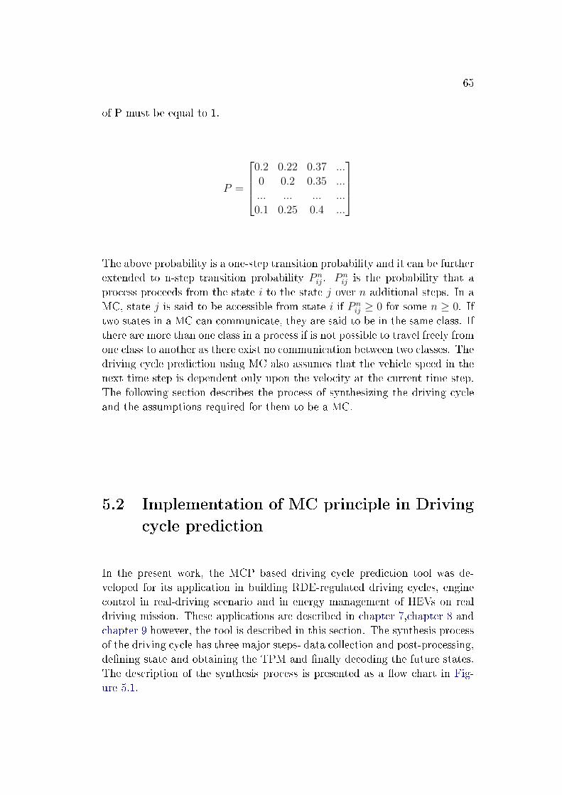
65

of P must be equal to 1.

P =

0.2 0.22 0.37 ...

0 0.2 0.35 ...

... ... ... ...

0.1 0.25 0.4 ...

The above probability is a one-step transition probability and it can be furtherextended to n-step transition probability P n

ij. P nij is the probability that a

process proceeds from the state i to the state j over n additional steps. In aMC, state j is said to be accessible from state i if P n

ij ≥ 0 for some n ≥ 0. Iftwo states in a MC can communicate, they are said to be in the same class. Ifthere are more than one class in a process if is not possible to travel freely fromone class to another as there exist no communication between two classes. Thedriving cycle prediction using MC also assumes that the vehicle speed in thenext time step is dependent only upon the velocity at the current time step.The following section describes the process of synthesizing the driving cycleand the assumptions required for them to be a MC.

5.2 Implementation of MC principle in Driving

cycle prediction

In the present work, the MCP based driving cycle prediction tool was de-veloped for its application in building RDE-regulated driving cycles, enginecontrol in real-driving scenario and in energy management of HEVs on realdriving mission. These applications are described in chapter 7,chapter 8 andchapter 9 however, the tool is described in this section. The synthesis processof the driving cycle has three major steps- data collection and post-processing,de�ning state and obtaining the TPM and �nally decoding the future states.The description of the synthesis process is presented as a �ow chart in Fig-ure 5.1.

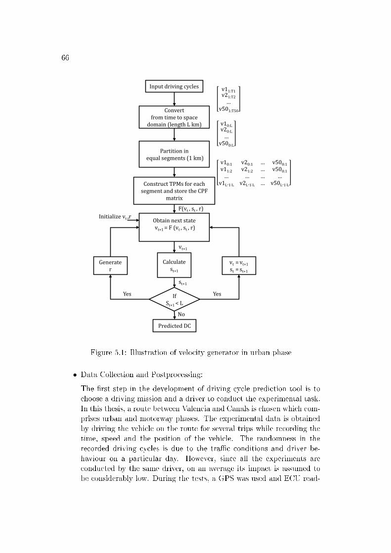
66

Input driving cycles

Obtain next statevt+1 = F (vt , st , r)

Convert from time to space

domain (length L km)

Partition inequal segments (1 km)

Construct TPMs for each segment and store the CPF

matrix

Calculate st+1

If St+1 < L

Predicted DC

Generater

Initialize vt ,r

vt = vt+1st = st+1

F(vt , st , r)

vt+1

st+1

Yes

No

Yes

v10:1 v20:1 … v500:1v11:2 v21:2 … v500:1

… … … …v1L-1:L v2L-1:L … v50L-1:L

v10:Lv20:L

…v500:L

v11:T1v21:T2

…v501:T50

Figure 5.1: Illustration of velocity generator in urban phase

• Data Collection and Postprocessing:

The �rst step in the development of driving cycle prediction tool is tochoose a driving mission and a driver to conduct the experimental task.In this thesis, a route between Valencia and Canals is chosen which com-prises urban and motorway phases. The experimental data is obtainedby driving the vehicle on the route for several trips while recording thetime, speed and the position of the vehicle. The randomness in therecorded driving cycles is due to the tra�c conditions and driver be-haviour on a particular day. However, since all the experiments areconducted by the same driver, on an average its impact is assumed tobe considerably low. During the tests, a GPS was used and ECU read-

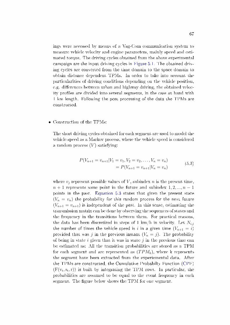
67

ings were accessed by means of a Vag-Com communication system tomeasure vehicle velocity and engine parameters, mainly speed and esti-mated torque. The driving cycles obtained from the above experimentalcampaign are the input driving cycles in Figure 5.1. The obtained driv-ing cycles are converted from the time domain to the space domain toobtain distance dependent TPMs. In order to take into account theparticularities of driving conditions depending on the vehicle position,e.g. di�erences between urban and highway driving, the obtained veloc-ity pro�les are divided into several segments, in the case at hand with1 km length. Following the post processing of the data the TPMs areconstructed.

• Construction of the TPMs:

The short driving cycles obtained for each segment are used to model thevehicle speed as a Markov process, where the vehicle speed is considereda random process (V ) satisfying:

P (Vn+1 = vn+1|V1 = v1, V2 = v2, . . . , Vn = vn)

= P (Vn+1 = vn+1|Vn = vn)(5.3)

where vj represent possible values of V , subindex n is the present time,n + 1 represents some point in the future and subindex 1, 2, ..., n − 1

points in the past. Equation 5.3 states that given the present state(Vn = vn) the probability for this random process for the next future(Vn+1 = vn+1) is independent of the past. In this sense, estimating thetransmission matrix can be done by observing the sequences of states andthe frequency in the transitions between them. For practical reasons,the data has been discretized in steps of 1 km/h in velocity. Let Ni,j

the number of times the vehicle speed is i in a given time (Vn+1 = i)provided that was j in the previous instant (Vn = j). The probabilityof being in state i given that it was in state j in the previous time canbe estimated as: All the transition probabilities are stored as a TPMfor each segment and are represented as (TPMk), where k representsthe segment have been extracted from the experiemental data. Afterthe TPMs are constructed, the Cumulative Probabilty Function (CPF)(F(vt, st, r)) is built by integrating the TPM rows. In particular, theprobabilities are assumed to be equal to the event frequency in eachsegment. The �gure below shows the TPM for one segment.

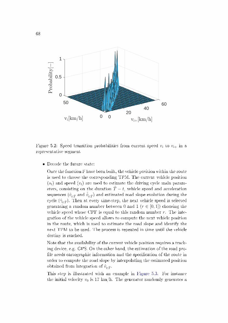
68

0

50

0.5

6040

1

200 0

Figure 5.2: Speed transition probabilities from current speed vi to vi+ in arepresentative segment

• Decode the future state:

Once the function F have been built, the vehicle position within the routeis used to choose the corresponding TPM. The current vehicle position(st) and speed (vt) are used to estimate the driving cycle main param-eters, consisting on the duration T − t, vehicle speed and accelerationsequences (vt:T and ˆvt:T ) and estimated road slope evolution during thecycle (γt:T ). Then at every time-step, the next vehicle speed is selectedgenerating a random number between 0 and 1 (r ∈ [0, 1]) choosing thevehicle speed whose CPF is equal to this random number r. The inte-gration of the vehicle speed allows to compute the next vehicle positionin the route, which is used to estimate the road slope and identify thenext TPM to be used. The process is repeated in time until the vehicledestiny is reached.

Note that the availability of the current vehicle position requires a track-ing device, e.g. GPS. On the other hand, the estimation of the road pro-�le needs cartographic information and the speci�cation of the route inorder to compute the road slope by interpolating the estimated positionobtained from integration of vt:T .

This step is illustrated with an example in Figure 5.3. For instancethe initial velocity v0 is 17 km/h. The generator randomly generates a

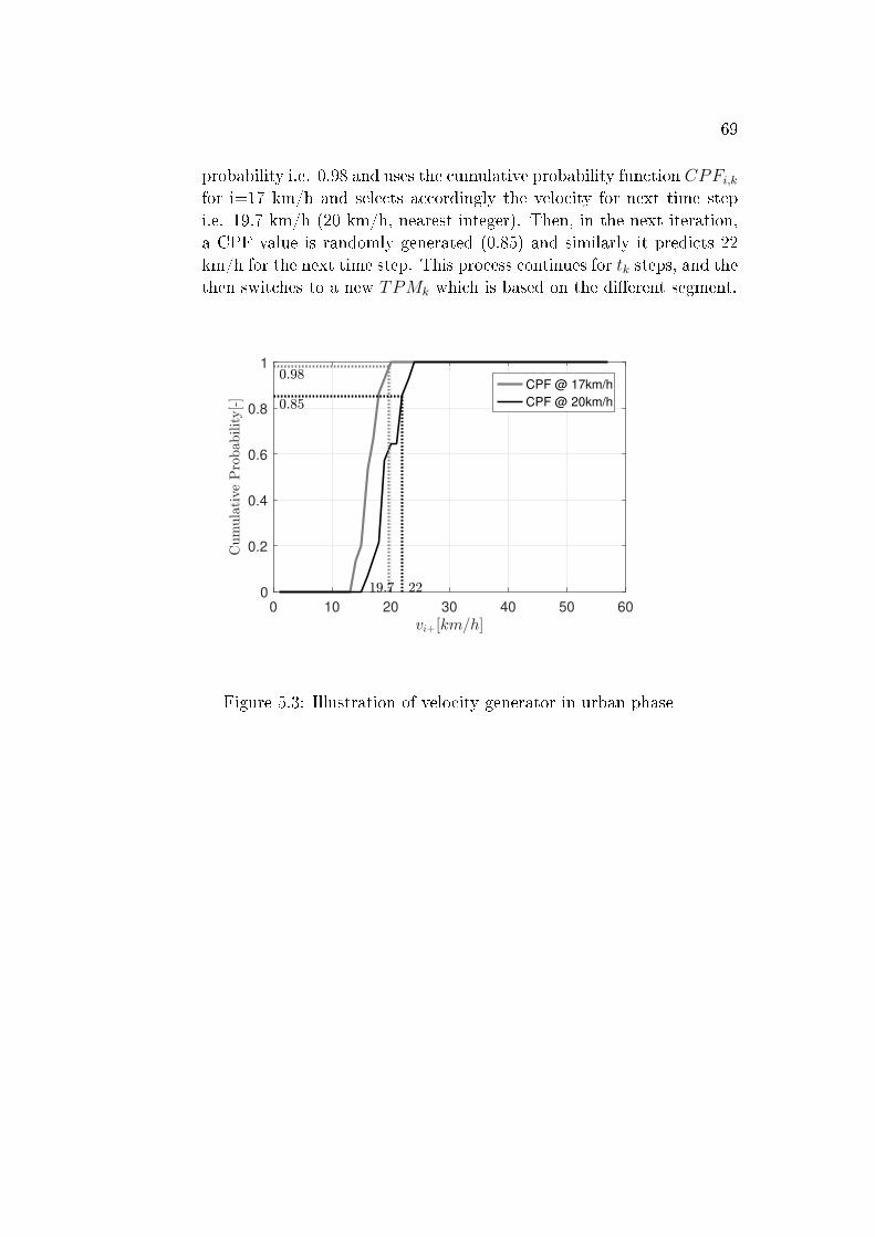
69

probability i.e. 0.98 and uses the cumulative probability function CPFi,kfor i=17 km/h and selects accordingly the velocity for next time stepi.e. 19.7 km/h (20 km/h, nearest integer). Then, in the next iteration,a CPF value is randomly generated (0.85) and similarly it predicts 22km/h for the next time step. This process continues for tk steps, and thethen switches to a new TPMk which is based on the di�erent segment.

0 10 20 30 40 50 600

0.2

0.4

0.6

0.8

1

CPF @ 17km/h

CPF @ 20km/h

Figure 5.3: Illustration of velocity generator in urban phase

Part III

Experimental Setup

Chapter 6

Experimental Test Setup

Contents

6.1 Experimental Setup - A . . . . . . . . . . . . . . . . . . 74

6.2 Experimental Setup - B . . . . . . . . . . . . . . . . . . 77

6.3 Experimental Setup - C . . . . . . . . . . . . . . . . . . 79

6.4 Experimental Setup - D . . . . . . . . . . . . . . . . . . 81

During the development of a control application for a vehicle or an enginethere are several instances when a real system is required to be tested eitherduring the design process itself or in the veri�cation and validation stage. Thetesting is performed in a controlled environment, which allow experimental re-producibility and validation over a wide range of conditions by designing theapplication speci�c case studies. There are several experimental campaignsrun during this work, each campaign is detailed in the third part of the thesis.This chapter is focused on describing the testing setups with a brief introduc-tion about the objective of each application. In speci�c, there are 6 di�erentapplications tested on four experimental setups. The �rst three applications(A.1, A.2, A.3) were tested on the same diesel engine test setup (Setup � A),with only slight di�erences. The fourth application (B.1) is tested on a four-cylinder diesel engine test bench (Setup � B). The experiments related to the�fth application (C.1) were conducted on a chassis dynamometer (Setup �C) and the last application (D.1) was tested on a real vehicle (Setup � D)which was driven between two locations in Spain.

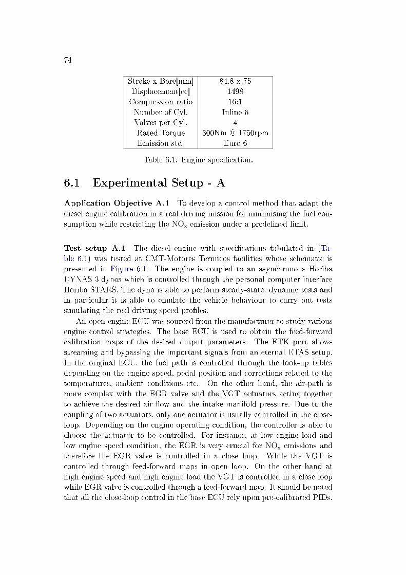
74

Stroke x Bore[mm] 84.8 x 75Displacement[cc] 1498Compression ratio 16:1Number of Cyl. Inline 6Valves per Cyl. 4Rated Torque 300Nm @ 1750rpmEmission std. Euro 6

Table 6.1: Engine speci�cation.

6.1 Experimental Setup - A

Application Objective A.1 To develop a control method that adapt thediesel engine calibration in a real driving mission for minimising the fuel con-sumption while restricting the NOx emission under a prede�ned limit.

Test setup A.1 The diesel engine with speci�cations tabulated in (Ta-ble 6.1) was tested at CMT-Motores Termicos facilities whose schematic ispresented in Figure 6.1. The engine is coupled to an asynchronous HoribaDYNAS 3 dynos which is controlled through the personal computer interfaceHoriba STARS. The dyno is able to perform steady-state, dynamic tests andin particular it is able to emulate the vehicle behaviour to carry out testssimulating the real driving speed pro�les.

An open engine ECU was sourced from the manufacturer to study variousengine control strategies. The base ECU is used to obtain the feed-forwardcalibration maps of the desired output parameters. The ETK port allowsstreaming and bypassing the important signals from an eternal ETAS setup.In the original ECU, the fuel path is controlled through the look-up tablesdepending on the engine speed, pedal position and corrections related to thetemperatures, ambient conditions etc.. On the other hand, the air-path ismore complex with the EGR valve and the VGT actuators acting togetherto achieve the desired air �ow and the intake manifold pressure. Due to thecoupling of two actuators, only one actuator is usually controlled in the close-loop. Depending on the engine operating condition, the controller is able tochoose the actuator to be controlled. For instance, at low engine load andlow engine speed condition, the EGR is very crucial for NOx emissions andtherefore the EGR valve is controlled in a close loop. While the VGT iscontrolled through feed-forward maps in open loop. On the other hand athigh engine speed and high engine load the VGT is controlled in a close loopwhile EGR valve is controlled through a feed-forward map. It should be notedthat all the close-loop control in the base ECU rely upon pre-calibrated PIDs.

75

Figure 6.1: Experimental setup-A.1. At the node m1, the start of injectionwas bypassed and controlled through dSpace. At m2, the NOx emission andthe exhaust gas concentration is measured.

The design of experiment approach was used to model the engine torqueand mNOx emissions as a function of the input parameters. To do that, theengine torque and mNOx emissions were measured while varying the param-eters such as vgt position xvgt, egr valve position xegr, start of injection θsoiand fuelling rate mfuel. For which, a rapid prototyping system (RPS) wasconnected via ECU ETK port allowing for sending and receiving the enginesignals. This by-pass con�guration is created using INTERCRIO and gener-ated in the dSpace system.The important measurement nodes for this application are represented by thered dots in the Figure 6.1. For the concentration's measurement in the testbench, the Horiba MEXA 7100 DEGR GA is used to measure the concen-tration of NOx at one point of the exhaust line. This apparatus employstechniques like the non-dispersive infrared (NDIR) for the NOx measurement.Regarding the data recording, the use of di�erent systems to record data im-plies that three �les are obtained for each experiment in this setup i.e. fromdSpace, STARS and ETAS. In order to be able to phase the di�erent �les

76

afterwards, the RPS dSpace triggers a square signal, which allows phasingthem in post-processing.

The real-time simulation of the developed controller interfaces with theengine test bench using actuators and sensors; these actuators and sensorshave their own characteristics which detract from the realism of completesystem response. The vehicle is emulated by a numerical model interactingwith a physical engine system. A similar approach is also applied to validatethe hybrid electric vehicle model in the following application A.2.

Application Objective A.2 To develop an online energy managementstrategy for a parallel hybrid electric vehicle on a real driving mission.

Test setup A.2 The application was tested in the same experimental setupdescribed in A.1 except for the parameters that were bypassed and an ad-ditional input to the dSpace Microautobox. The need for real-time com-munication is satis�ed by means of a Controller Area Network (CAN) bus.The experimental test platform uses CANopen protocol to integrate all theelements and assure synchronous distribution of reference speed and torquecommands, as well as to read back the actual speed and torque. The torque re-quired from the diesel engine is calculated using the vehicle backward model inthe Simulink and is translated into the throttle position through a calibrationmap. To test a realistic hybrid electric vehicle on this engine testing setup, thetorque sensor system provides the torque feedback signals from the test-benchback into the dSpace. Inside the dSpace, the reference and feedback torquesignals generate error signals and the excess energy is absorbed by the electricmotor in the vehicle dynamic model where the instantaneous battery state-of-charge is calculated. The HiL system allows the online assessment of thedeveloped EMS controller. The total energy consumed in di�erent measure-ments on a same driving cycle of length 20km produced a standard deviationof 43.5 kJ . This energy was later used for correcting the total fuel consump-tion during di�erent experiments on the same driving cycle. The engine speedand the throttle position are calculated in advance using a vehicle backwardmodel and are imposed in the Horiba - STARS. The engine speed which is anoutput of the real-time simulation on the dSpace must be synchronised withthe engine speed that is an input from the Horiba STAR dyno control. Thissynchronisation was achieved manually in the present case by triggerng thebypassed signal and the driving cycle in STARs at the same moment. Thefuel consumption is not a direct measurement, but rather a calibrated valuewithin the ECU. The ECU usually contain signals giving an indication of theamount of fuel being injected into the cylinder. The remaining connectionmeasurements are similar to the �rst application.

77

Application Objective A.3 To study the impact of driving dynamics inreal driving emission test on NOx emissions dispersion.

Test setup A.3 The diesel engine described in applications A.1 and A.2with speci�cations as in Table 6.1 was used for the experiments. In addition,the engine was also equiped with a state-of-the art after-treatment systemcomprising Diesel oxidation Catalyst, Diesel Particulate Filter and Selectivecatalytic reduction system. No parameters were required to be bypassed forthis application and therefore the dSpace and ControlDesk were redundant.Several driving cycles were imposed through Horiba-Stars while measuringthe fuel consumption and NOx emissions before and after the after-treatmentsystem. The nodes m1,m2 and m3 represent the approximation of the fuel in-take, NOx emissions before and after the after-treatment system respectively.The NOx concentration was measured using the Horiba MEXA 7100 DEGRGA as in previous applications.

6.2 Experimental Setup - B

Application Objective - B.1 To develop a control method that varies thediesel engine calibration smoothing for minimising the fuel consumption whilerestricting the torque error and NOx emissions under a prede�ned limit.

Test setup - B.1 The measurements presented in this study were obtainedfrom a dynamic engine test-bench at ETH Zurich. The engine under consid-eration is a commercial heavy-duty Diesel engine.

The schematic of the application is presented in Figure 6.2. The workwas carried out in a test bench mainly composed by an engine coupled to adynamometric brake. The engine was a four-stroke, heavy-duty Diesel enginewith four cylinders, turbocharged, intercooled EGR and with a common-railinjection system. This engine (see main speci�cations in Table 6.2) is repre-sentative of those typical used in Diesel construction equipment in Europe.The engine was instrumented to measure several key temperatures and pres-sures (intake air, fuel, exhaust gases, lube oil, etc.). A piezoelectric pressuretransducer coupled to a charge ampli�er was used for recording instantaneousin-cylinder pressure. Crankshaft rotational speed and instantaneous pistonposition were determined by means of an angle encoder. For the rapid proto-typing of the software developed and tested in this study, a dSpace MicroAuto-Box system was applied in combination with MATLAB/Simulink from Math-Works, Inc. This device is also used for the data acquisition of the various sen-sor signals. The engine speed is controlled by a highly dynamic dynamometer.

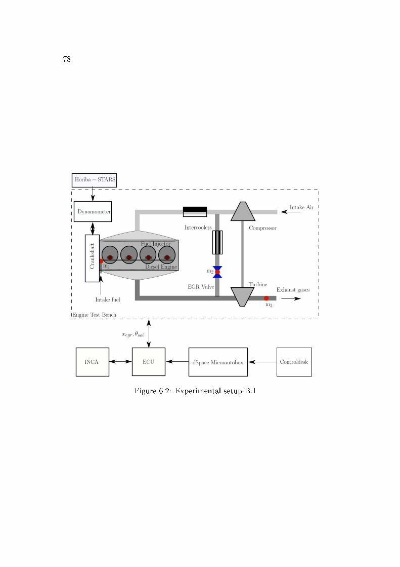
78

Figure 6.2: Experimental setup-B.1

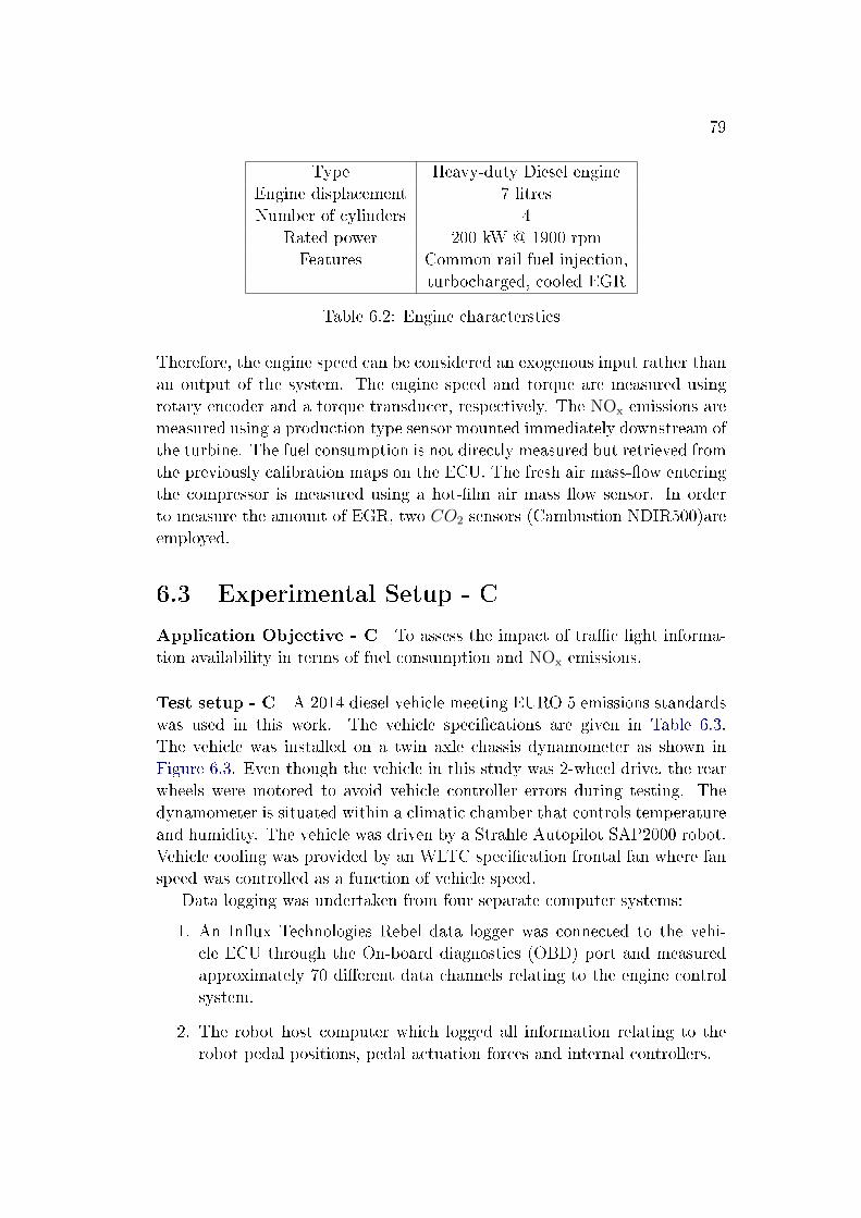
79

Type Heavy-duty Diesel engineEngine displacement 7 litresNumber of cylinders 4

Rated power 200 kW @ 1900 rpmFeatures Common rail fuel injection,

turbocharged, cooled EGR

Table 6.2: Engine characterstics

Therefore, the engine speed can be considered an exogenous input rather thanan output of the system. The engine speed and torque are measured usingrotary encoder and a torque transducer, respectively. The NOx emissions aremeasured using a production type sensor mounted immediately downstream ofthe turbine. The fuel consumption is not directly measured but retrieved fromthe previously calibration maps on the ECU. The fresh air mass-�ow enteringthe compressor is measured using a hot-�lm air mass �ow sensor. In orderto measure the amount of EGR, two CO2 sensors (Cambustion NDIR500)areemployed.

6.3 Experimental Setup - C

Application Objective - C To assess the impact of tra�c light informa-tion availability in terms of fuel consumption and NOx emissions.

Test setup - C A 2014 diesel vehicle meeting EURO 5 emissions standardswas used in this work. The vehicle speci�cations are given in Table 6.3.The vehicle was installed on a twin axle chassis dynamometer as shown inFigure 6.3. Even though the vehicle in this study was 2-wheel drive, the rearwheels were motored to avoid vehicle controller errors during testing. Thedynamometer is situated within a climatic chamber that controls temperatureand humidity. The vehicle was driven by a Strahle Autopilot SAP2000 robot.Vehicle cooling was provided by an WLTC speci�cation frontal fan where fanspeed was controlled as a function of vehicle speed.

Data logging was undertaken from four separate computer systems:

1. An In�ux Technologies Rebel data logger was connected to the vehi-cle ECU through the On-board diagnostics (OBD) port and measuredapproximately 70 di�erent data channels relating to the engine controlsystem.

2. The robot host computer which logged all information relating to therobot pedal positions, pedal actuation forces and internal controllers.

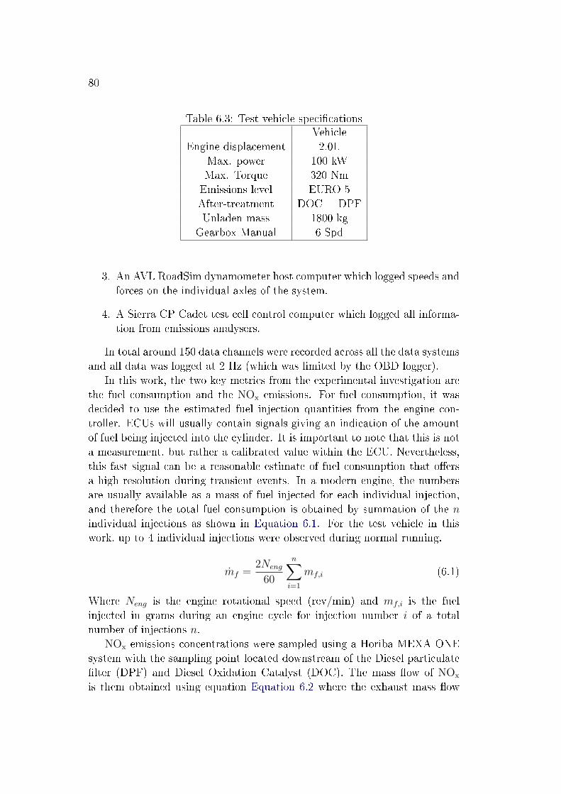
80

Table 6.3: Test vehicle speci�cationsVehicle

Engine displacement 2.0LMax. power 100 kWMax. Torque 320 NmEmissions level EURO 5After-treatment DOC + DPFUnladen mass 1800 kg

Gearbox Manual 6 Spd

3. An AVL RoadSim dynamometer host computer which logged speeds andforces on the individual axles of the system.

4. A Sierra CP Cadet test cell control computer which logged all informa-tion from emissions analysers.

In total around 150 data channels were recorded across all the data systemsand all data was logged at 2 Hz (which was limited by the OBD logger).

In this work, the two key metrics from the experimental investigation arethe fuel consumption and the NOx emissions. For fuel consumption, it wasdecided to use the estimated fuel injection quantities from the engine con-troller. ECUs will usually contain signals giving an indication of the amountof fuel being injected into the cylinder. It is important to note that this is nota measurement, but rather a calibrated value within the ECU. Nevertheless,this fast signal can be a reasonable estimate of fuel consumption that o�ersa high resolution during transient events. In a modern engine, the numbersare usually available as a mass of fuel injected for each individual injection,and therefore the total fuel consumption is obtained by summation of the nindividual injections as shown in Equation 6.1. For the test vehicle in thiswork, up to 4 individual injections were observed during normal running.

mf =2Neng

60

n∑i=1

mf,i (6.1)

Where Neng is the engine rotational speed (rev/min) and mf,i is the fuelinjected in grams during an engine cycle for injection number i of a totalnumber of injections n.

NOx emissions concentrations were sampled using a Horiba MEXA ONEsystem with the sampling point located downstream of the Diesel particulate�lter (DPF) and Diesel Oxidation Catalyst (DOC). The mass �ow of NOx

is them obtained using equation Equation 6.2 where the exhaust mass �ow

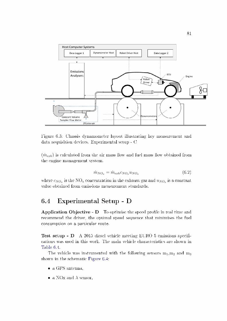
81

Figure 6.3: Chassis dynamometer layout illustrating key measurement anddata acquisition devices. Experimental setup - C

(mexh) is calculated from the air mass �ow and fuel mass �ow obtained fromthe engine management system.

mNOx = mexhcNOxuNOx (6.2)

where cNOx is the NOx concentration in the exhaust gas and uNOx is a constantvalue obtained from emissions measurement standards.

6.4 Experimental Setup - D

Application Objective - D To optimise the speed pro�le in real time andrecommend the driver, the optimal speed sequence that minimises the fuelconsumption on a particular route.

Test setup - D A 2015 diesel vehicle meeting EURO 5 emissions speci�-cations was used in this work. The main vehicle characteristics are shown inTable 6.4.

The vehicle was instrumented with the following sensors m1,m2 and m3

shown in the schematic Figure 6.4:

• a GPS antenna,

• a NOx and λ sensor,

82

Table 6.4: Test vehicle speci�cationsVehicle

Engine displacement 1.4 LMax. power 50 kWMax. Torque 160 NmEmissions level EURO 5After-treatment DOC + DPFUnladen mass 1125 kg

Manual Gearbox 6 Spd

• a pressure transducer and an inductive sensor to measure in-cylinderpressure and phase it with the crank angle.

Also, OBD-II SAE J1979 mode 01 information is read by means of aController Area Network (CAN) interface. This information is captured andprocessed with a National Instruments PXI system equipped with analog in-puts (board model), high speed CAN interface (board model) and a USB se-rial interface. A scheme of the instrumentation system is shown in Figure 6.4.This system allows to capture in-cylinder pressure with an angular resolutionof one sample per degree at 5100 rpm, mNOx values ten times per second andOn-board Diagnostics (OBD)-II relevant values �ve times per second. Geo-graphical position of the vehicle is acquired with a temporal resolution of onesample per second, which is the GPRMC message period. Optimal speed ref-erences are also managed by the PXI system. This information is presented tothe user in a screen and updated every two seconds. In Figure 6.4, the nodesm1 is to acquire the crank angle θcyl, the node m2 is for cylinder pressure Pcyl

and m3 is for exhaust emissions mexh and mNOx emission.

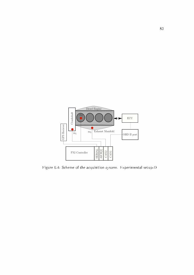
83

Figure 6.4: Scheme of the acquisition system. Experimental setup-D

Part IV

Applications to powertrain

control, Design and Assessment

Chapter 7

Powertrain Control in Real

Driving Mission

Contents

7.1 Adaptive control of Diesel Engine . . . . . . . . . . . . 88

7.1.1 Introduction . . . . . . . . . . . . . . . . . . . . . . . . 88

7.1.2 Method description . . . . . . . . . . . . . . . . . . . . 89

7.1.3 Designed use cases for method validation . . . . . . . . 93

7.1.4 Results . . . . . . . . . . . . . . . . . . . . . . . . . . 95

7.1.5 Summary and conclusions . . . . . . . . . . . . . . . . 99

7.2 Variable Smoothing of Diesel Engine Calibration . . 104

7.2.1 Introduction . . . . . . . . . . . . . . . . . . . . . . . . 104

7.2.2 Method Description . . . . . . . . . . . . . . . . . . . 105

7.2.3 Results . . . . . . . . . . . . . . . . . . . . . . . . . . 107

7.2.4 Summary and Conclusions . . . . . . . . . . . . . . . . 118

7.3 Online optimal Energy Management strategy for Par-

allel HEV . . . . . . . . . . . . . . . . . . . . . . . . . . 119

7.3.1 Introduction and problem description . . . . . . . . . . 119

7.3.2 Method Description . . . . . . . . . . . . . . . . . . . 121

7.3.3 Design of case study for method veri�cation and validation123

7.3.4 Results . . . . . . . . . . . . . . . . . . . . . . . . . . 124

7.3.5 Summary and conclusion . . . . . . . . . . . . . . . . 127

88

The objective of this chapter is to describe the applications developed forthis thesis. The applications are either developed for control of diesel engine orhybrid electric vehicle. There are three sections in this chapter; each section isdedicated for an application in a structured way. The section 7.1 describes themodelling and validation of an adaptive diesel engine controller for a vehicleon real driving mission. The section 7.2 is regarding a new calibration methodthat enables variable-smoothing of a diesel engine for improved performanceof a vehicle on real driving missions. Finally, section 7.3 is regarding anonline controller for optimal energy management of a parallel hybrid electricvehicle for minimised fuel consumption and constrained state-of-charge on anunknown driving mission.

7.1 Adaptive control of Diesel Engine

7.1.1 Introduction

Motivated by the requirement of improvement in fuel-e�ciency with minimalemissions, the control of diesel-engine is being investigated in this section. De-spite the continuous tightening of the NOx emission type approval limits, thedi�erence between the type approval NOx and the real world NOx emissionshas grown over the years ([Chen & Borken-Kleefeld 2014]). The reason forthis discrepancy is the uncertainty due to driving dynamics, ambient temper-ature and road slope during real driving conditions which are not consideredin the engine calibration process. SOA engine calibration method is based onfeedback and feed-forward controllers. Fixed look-up tables are employed asthe set-point generator and the feed-forward controller. The standard enginecalibration approach consists on taking a limited set of driving cycle to makean optimisation and then use the obtained results to �ll the calibration maps.However, in this case, the optimality of the calibration for a given driver willdepend on the similarity between the considered driving set for calibrationand his driving patterns. Moreover, this approach neglects other boundariessuch as the tra�c, pollution levels in the area or other environmental condi-tions. The presented approach poses the calibration problem as an optimalcontrol problem by �nding a set of optimal calibration maps in real time. Thecalibration maps contain the set points that minimise the instantaneous fuelconsumption (mf) over a sequence of engine speed (ωe) and torque (Te), whileful�lling the integral constraint on (NOx) emission on an unknown drivingcycle. To solve the problem, a look-ahead strategy is proposed to periodicallyadapt the engine calibration such that the cumulative fuel consumption is

89

minimised while ful�lling the integral NOx emission constraint. The strategyis to estimate the driving cycle and then calculate the vehicle performance(fuel consumption and the NOx emission) on the estimated cycle using a 0-Dvehicle model. The performance is calculated in parallel with di�erent start-of-injection (SOI) calibration maps resulting in a set of SOI maps associatedwith di�erent levels of cumulative fuel consumption and emissions. A super-visory controller updates the calibration from the available set of maps suchthat, the cost function is minimised while integral constraint is also ful�lled.The constraint on NOx emission is time dependent and is calculated as thedi�erence between the actual NOx emission (measured by the sensor) and theNOx limit for entire trip.

Speci�cally, this method involve three developments: The �rst is a drivingcycle prediction tool (elaborated in chapter 5) which is based on the space-variant transition probability matrix obtained from an actual vehicle speeddataset. Then, a vehicle and an engine model described in chapter 3, to pre-dict the fuel consumption and NOx emissions on a driving cycle. Finally, anadaptive controller is proposed which calibrates the engine online, to ful�l theNOx emission constraint at the end of the driving mission while minimisingthe fuel consumption. The developed control strategy was implemented andassessed on an engine test bench described in section 6.1. The engine perfor-mance using the proposed method is compared with the SOA static calibrationtechnique for di�erent NOx emission limits on real world cycles.

7.1.2 Method description

As mentioned before, the online engine control require the following:

• A vehicle speed prediction model.

• A simple but accurate vehicle model to estimate the engine performanceonline.

• A controller to calculate and implement the optimal actuations in thereal-time.

In this sense, the proposed control algorithm has three layers: The �rstlayer is to predict the power demand of the vehicle, the second layer computesthe expected fuel consumption and NOx emissions depending on the SOI cali-bration map(from a limited set of possible calibrations). The last layer appliesand holds the optimal calibration with minimum expected fuel consumptionfrom those whose expected NOx emissions are below a prede�ned limit.

In Figure 7.1, schematic of the high level control system of the developedmethod is presented. Where vestim and vreal are the estimated and real vehicle

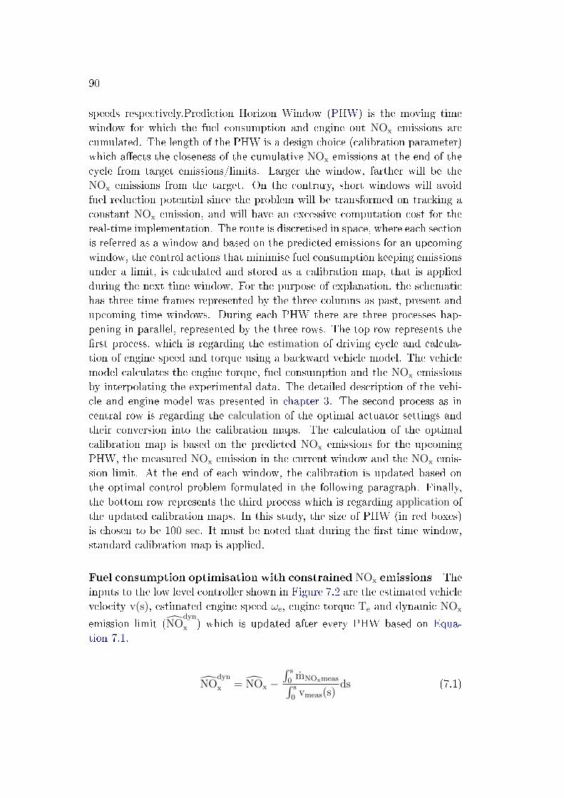
90

speeds respectively.Prediction Horizon Window (PHW) is the moving timewindow for which the fuel consumption and engine out NOx emissions arecumulated. The length of the PHW is a design choice (calibration parameter)which a�ects the closeness of the cumulative NOx emissions at the end of thecycle from target emissions/limits. Larger the window, farther will be theNOx emissions from the target. On the contrary, short windows will avoidfuel reduction potential since the problem will be transformed on tracking aconstant NOx emission, and will have an excessive computation cost for thereal-time implementation. The route is discretised in space, where each sectionis referred as a window and based on the predicted emissions for an upcomingwindow, the control actions that minimise fuel consumption keeping emissionsunder a limit, is calculated and stored as a calibration map, that is appliedduring the next time window. For the purpose of explanation, the schematichas three time frames represented by the three columns as past, present andupcoming time windows. During each PHW there are three processes hap-pening in parallel, represented by the three rows. The top row represents the�rst process, which is regarding the estimation of driving cycle and calcula-tion of engine speed and torque using a backward vehicle model. The vehiclemodel calculates the engine torque, fuel consumption and the NOx emissionsby interpolating the experimental data. The detailed description of the vehi-cle and engine model was presented in chapter 3. The second process as incentral row is regarding the calculation of the optimal actuator settings andtheir conversion into the calibration maps. The calculation of the optimalcalibration map is based on the predicted NOx emissions for the upcomingPHW, the measured NOx emission in the current window and the NOx emis-sion limit. At the end of each window, the calibration is updated based onthe optimal control problem formulated in the following paragraph. Finally,the bottom row represents the third process which is regarding application ofthe updated calibration maps. In this study, the size of PHW (in red boxes)is chosen to be 100 sec. It must be noted that during the �rst time window,standard calibration map is applied.

Fuel consumption optimisation with constrained NOx emissions Theinputs to the low level controller shown in Figure 7.2 are the estimated vehiclevelocity v(s), estimated engine speed ωe, engine torque Te and dynamic NOx

emission limit (NOdyn

x ) which is updated after every PHW based on Equa-tion 7.1.

NOdyn

x = NOx −∫ s

0mNOxmeas∫ s

0vmeas(s)

ds (7.1)

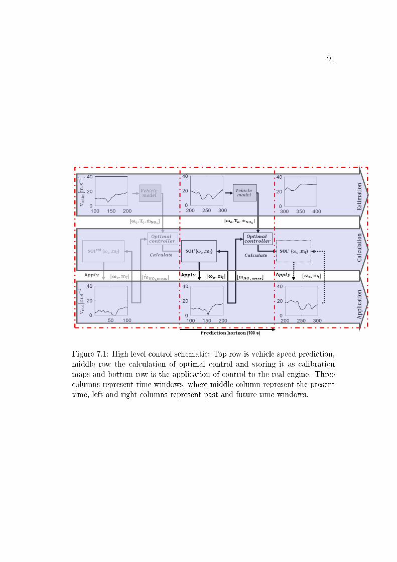
91

Figure 7.1: High level control schematic: Top row is vehicle speed prediction,middle row the calculation of optimal control and storing it as calibrationmaps and bottom row is the application of control to the real engine. Threecolumns represent time windows, where middle column represent the presenttime, left and right columns represent past and future time windows.

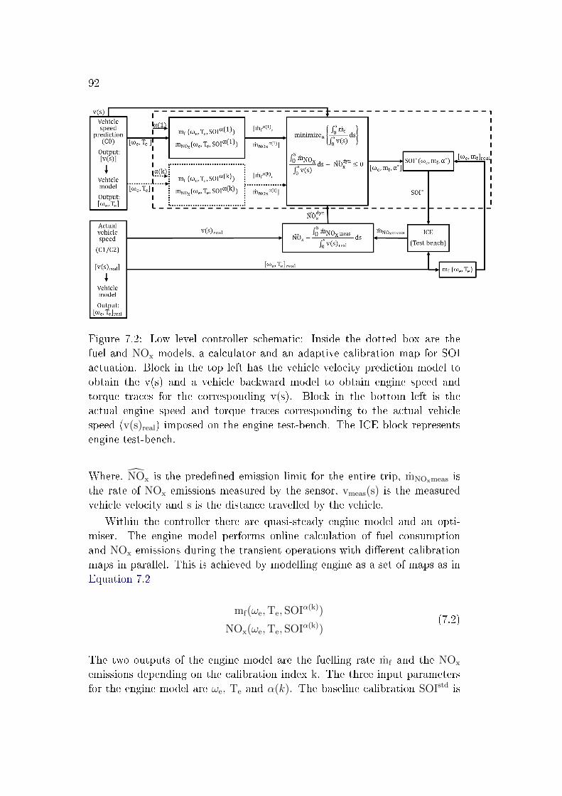
92

Figure 7.2: Low level controller schematic: Inside the dotted box are thefuel and NOx models, a calculator and an adaptive calibration map for SOIactuation. Block in the top left has the vehicle velocity prediction model toobtain the v(s) and a vehicle backward model to obtain engine speed andtorque traces for the corresponding v(s). Block in the bottom left is theactual engine speed and torque traces corresponding to the actual vehiclespeed (v(s)real) imposed on the engine test-bench. The ICE block representsengine test-bench.

Where, NOx is the prede�ned emission limit for the entire trip, mNOxmeas isthe rate of NOx emissions measured by the sensor, vmeas(s) is the measuredvehicle velocity and s is the distance travelled by the vehicle.

Within the controller there are quasi-steady engine model and an opti-miser. The engine model performs online calculation of fuel consumptionand NOx emissions during the transient operations with di�erent calibrationmaps in parallel. This is achieved by modelling engine as a set of maps as inEquation 7.2

mf(ωe,Te, SOIα(k))

NOx(ωe,Te, SOIα(k))(7.2)

The two outputs of the engine model are the fuelling rate mf and the NOx

emissions depending on the calibration index k. The three input parametersfor the engine model are ωe, Te and α(k). The baseline calibration SOIstd is

93

perturbed using α(k) as shown in Equation 7.3.

SOIα(k) = SOIstd + α0(k) + α1(k) ∗ ωnorme

+α2(k) ∗ Tnorme

(7.3)

where, α0, α1, α2 ∈ [−1, 1], ωnorme , Tnorm

e are normalised engine speed andtorque in euclidean space. Then, obtained calibrations are stored as vectorsinto a matrix A as in Equation 7.4, where α(k) is a vector of the three coe�-cients of the kth calibration.

The lookup set must ful�l the following conditions:

• They must lie within the feasible actuator boundary. In the currentstudy, SOI was explored within [SOIstd-3,SOIstd+3] CAD, which is inthe feasible boundary shown in Figure 7.3 for the engine under study.The engine must have sensitivity to the changing calibrations within thelook-up set.

• Calibration maps must be smooth enough in order to ful�l conditions ofdrivability. For ensuring map smoothness following strategy is used.

A =

α(1)

α(2)

α(3)

.

.

α(k)

;α =[α0 α1 α2

](7.4)

Finally, the controller selects an optimal calibration α(k) by solving theproblem in Equation 7.5, where fuel consumption is minimised for a givendistance s while being within the dynamic NOx limits .

minα(k)∈A

∫ s

0

mf

v(s)ds

subject to :

∫ s

0

mNOx

v(s)ds− NO

dyn

x ≤ 0

(7.5)

The components of α are discretised in 3 elements leading to 27 combinationswhich is the size of the lookup set. Figure 7.4, presents sequence of optimalcalibration map adapting with time for the �rst 600 s of a real driving cycle.

7.1.3 Designed use cases for method validation

In the current study three driving cycles are considered: The �rst cycle C0

is an estimated cycle, synthesized using the tool described previously. The

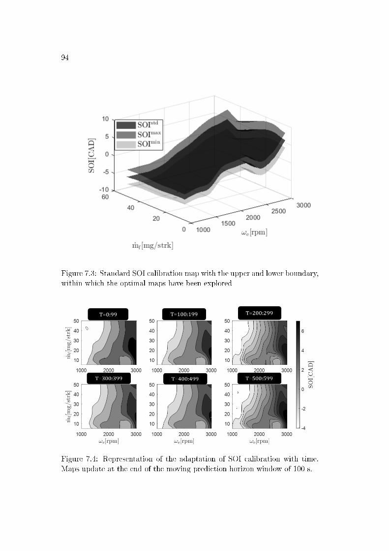
94

Figure 7.3: Standard SOI calibration map with the upper and lower boundary,within which the optimal maps have been explored

Figure 7.4: Representation of the adaptation of SOI calibration with time.Maps update at the end of the moving prediction horizon window of 100 s.

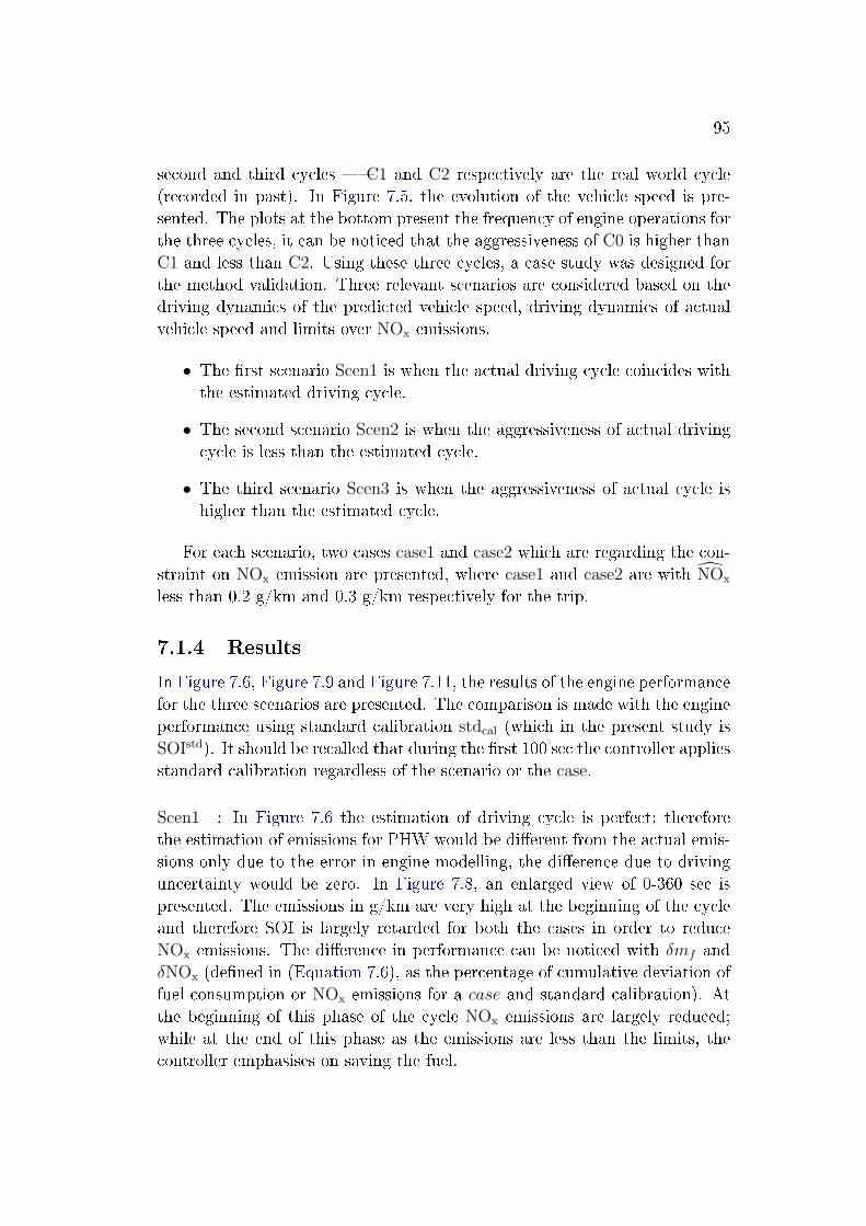
95

second and third cycles � C1 and C2 respectively are the real world cycle(recorded in past). In Figure 7.5, the evolution of the vehicle speed is pre-sented. The plots at the bottom present the frequency of engine operations forthe three cycles, it can be noticed that the aggressiveness of C0 is higher thanC1 and less than C2. Using these three cycles, a case study was designed forthe method validation. Three relevant scenarios are considered based on thedriving dynamics of the predicted vehicle speed, driving dynamics of actualvehicle speed and limits over NOx emissions.

• The �rst scenario Scen1 is when the actual driving cycle coincides withthe estimated driving cycle.

• The second scenario Scen2 is when the aggressiveness of actual drivingcycle is less than the estimated cycle.

• The third scenario Scen3 is when the aggressiveness of actual cycle ishigher than the estimated cycle.

For each scenario, two cases case1 and case2 which are regarding the con-straint on NOx emission are presented, where case1 and case2 are with NOx

less than 0.2 g/km and 0.3 g/km respectively for the trip.

7.1.4 Results

In Figure 7.6, Figure 7.9 and Figure 7.11, the results of the engine performancefor the three scenarios are presented. The comparison is made with the engineperformance using standard calibration stdcal (which in the present study isSOIstd). It should be recalled that during the �rst 100 sec the controller appliesstandard calibration regardless of the scenario or the case.

Scen1 : In Figure 7.6 the estimation of driving cycle is perfect; thereforethe estimation of emissions for PHW would be di�erent from the actual emis-sions only due to the error in engine modelling, the di�erence due to drivinguncertainty would be zero. In Figure 7.8, an enlarged view of 0-360 sec ispresented. The emissions in g/km are very high at the beginning of the cycleand therefore SOI is largely retarded for both the cases in order to reduceNOx emissions. The di�erence in performance can be noticed with δmf andδNOx (de�ned in (Equation 7.6), as the percentage of cumulative deviation offuel consumption or NOx emissions for a case and standard calibration). Atthe beginning of this phase of the cycle NOx emissions are largely reduced;while at the end of this phase as the emissions are less than the limits, thecontroller emphasises on saving the fuel.

96

0 200 400 600 800 1000 1200 1400 1600 1800 20000

50

100

150

1000 2000 3000

0

50

100

150

200

250

1000 2000 3000

0

50

100

150

200

250 [%]

1000 2000 3000

0

50

100

150

200

250

Figure 7.5: Predicted and measured vehicle speed on the route under con-sideration; frequency of engine operating points for the three cases velocitypro�les

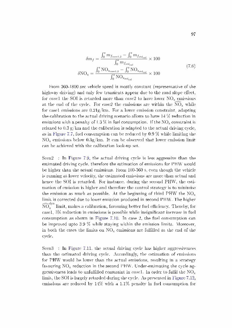
97

δmf =

∫ s0mfcase1,2 −

∫ s0mfstdcal∫ s

0mfstdcal

× 100

δNOx =

∫ s0

NOxcase1,2 −∫ s0

NOxstdcal∫ s0

NOxstdcal

× 100

(7.6)

From 360-1800 sec vehicle speed is mostly constant (representative of thehighway driving) and only few transients appear due to the road slope e�ect,for case1 the SOI is retarded more than case2 to have lower NOx emissionsat the end of the cycle. For case2 the emissions are within the NOx whilefor case1 emissions are 0.21g/km. For a lower emission constraint, adaptingthe calibration to the actual driving scenario allows to have 14 % reduction inemissions with a penalty of 1.3 % in fuel consumption. If the NOx constraint isrelaxed to 0.3 g/km and the calibration is adapted to the actual driving cycle,as in Figure 7.7, fuel consumption can be reduced by 0.9 % while limiting theNOx emissions below 0.3g/km. It can be observed that lower emission limitcan be achieved with the calibration look-up set.

Scen2 : In Figure 7.9, the actual driving cycle is less aggressive than theestimated driving cycle, therefore the estimation of emissions for PHW wouldbe higher than the actual emissions. From 100-360 s, even though the vehicleis running at lower velocity, the estimated emissions are more than actual andhence the SOI is retarded. For instance, during the second PHW, the esti-mation of emission is higher and therefore the control strategy is to minimisethe emission as much as possible. At the beginning of third PHW the NOx

limit is corrected due to lower emission produced in second PHW. The higher

NOdyn

x limit, makes a calibration, favouring better fuel e�ciency. Thereby, forcase1, 5% reduction in emissions is possible while insigni�cant increase in fuelconsumption as shown in Figure 7.10. In case 2, the fuel consumption canbe improved upto 3.9 % while staying within the emission limits. Moreover,in both the cases the limits on NOx emissions are ful�lled at the end of thecycle.

Scen3 : In Figure 7.11, the actual driving cycle has higher aggressivenessthan the estimated driving cycle. Accordingly, the estimation of emissionsfor PHW would be lower than the actual emissions, resulting in a strategyfavouring NOx reduction in the second PHW. Under-estimating the cycle ag-gressiveness leads to unful�lled constraint in case1. In order to ful�l the NOx

limit, the SOI is largely retarded during the cycle. As presented in Figure 7.12,emissions are reduced by 14% with a 1.1% penalty in fuel consumption for

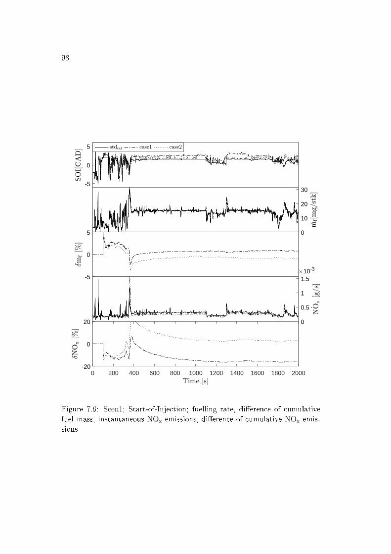
98

-5

0

5

0

10

20

30

-5

0

5

0

0.5

1

1.510-3

0 200 400 600 800 1000 1200 1400 1600 1800 2000-20

0

20

Figure 7.6: Scen1; Start-of-Injection; fuelling rate, di�erence of cumulativefuel mass, instantaneous NOx emissions, di�erence of cumulative NOx emis-sions

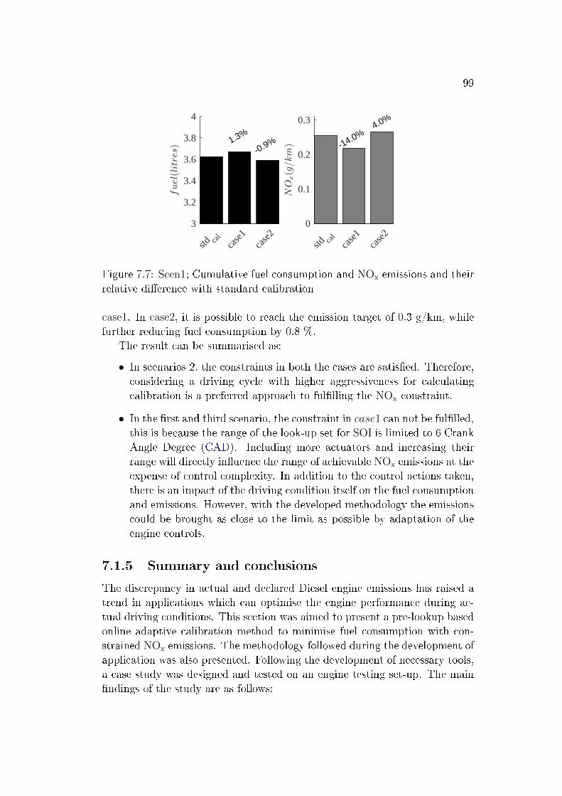
99

std cal

case

1ca

se2

3

3.2

3.4

3.6

3.8

4

1.3%

-0.9%

std cal

case

1ca

se2

0

0.1

0.2

0.3

-14.0% 4.0%

Figure 7.7: Scen1; Cumulative fuel consumption and NOx emissions and theirrelative di�erence with standard calibration

case1. In case2, it is possible to reach the emission target of 0.3 g/km, whilefurther reducing fuel consumption by 0.8 %.

The result can be summarised as:

• In scenarios 2, the constraints in both the cases are satis�ed. Therefore,considering a driving cycle with higher aggressiveness for calculatingcalibration is a preferred approach to ful�lling the NOx constraint.

• In the �rst and third scenario, the constraint in case1 can not be ful�lled,this is because the range of the look-up set for SOI is limited to 6 CrankAngle Degree (CAD). Including more actuators and increasing theirrange will directly in�uence the range of achievable NOx emissions at theexpense of control complexity. In addition to the control actions taken,there is an impact of the driving condition itself on the fuel consumptionand emissions. However, with the developed methodology the emissionscould be brought as close to the limit as possible by adaptation of theengine controls.

7.1.5 Summary and conclusions

The discrepancy in actual and declared Diesel engine emissions has raised atrend in applications which can optimise the engine performance during ac-tual driving conditions. This section was aimed to present a pre-lookup basedonline adaptive calibration method to minimise fuel consumption with con-strained NOx emissions. The methodology followed during the development ofapplication was also presented. Following the development of necessary tools,a case study was designed and tested on an engine testing set-up. The main�ndings of the study are as follows:

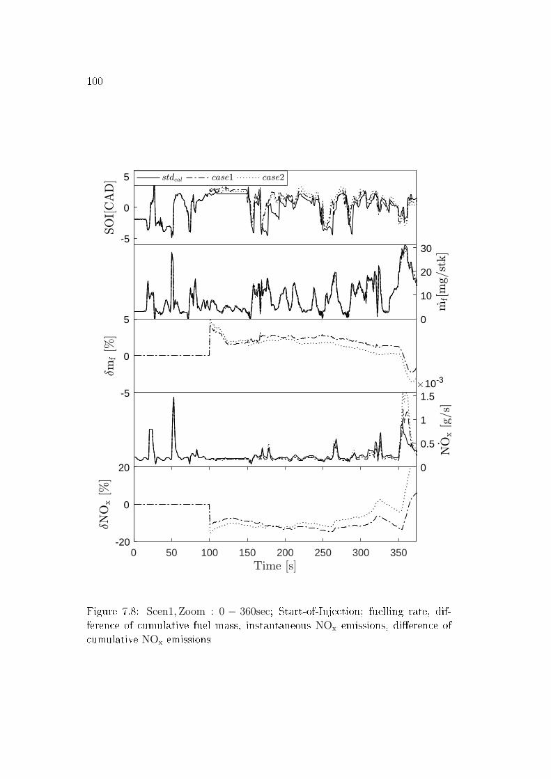
100

-5

0

5

0

10

20

30

-5

0

5

0

0.5

1

1.510-3

0 50 100 150 200 250 300 350-20

0

20

Figure 7.8: Scen1,Zoom : 0 − 360sec; Start-of-Injection; fuelling rate, dif-ference of cumulative fuel mass, instantaneous NOx emissions, di�erence ofcumulative NOx emissions

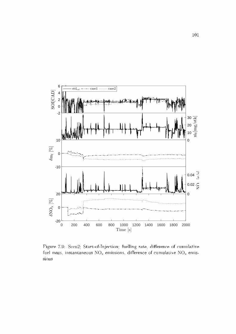
101

-2

0

2

4

6

0

10

20

30

-10

0

10

0

0.02

0.04

0 200 400 600 800 1000 1200 1400 1600 1800 2000-20

0

20

Figure 7.9: Scen2; Start-of-Injection; fuelling rate, di�erence of cumulativefuel mass, instantaneous NOx emissions, di�erence of cumulative NOx emis-sions

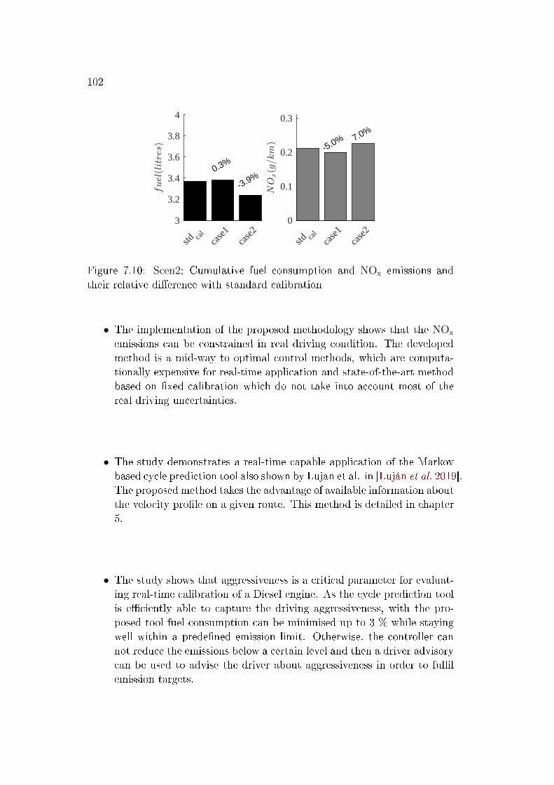
102

std cal

case

1ca

se2

3

3.2

3.4

3.6

3.8

4

0.3%

-3.9%

std cal

case

1ca

se2

0

0.1

0.2

0.3

-5.0% 7.0%

Figure 7.10: Scen2; Cumulative fuel consumption and NOx emissions andtheir relative di�erence with standard calibration

• The implementation of the proposed methodology shows that the NOx

emissions can be constrained in real driving condition. The developedmethod is a mid-way to optimal control methods, which are computa-tionally expensive for real-time application and state-of-the-art methodbased on �xed calibration which do not take into account most of thereal driving uncertainties.

• The study demonstrates a real-time capable application of the Markovbased cycle prediction tool also shown by Lujan et al. in [Luján et al. 2019].The proposed method takes the advantage of available information aboutthe velocity pro�le on a given route. This method is detailed in chapter5.

• The study shows that aggressiveness is a critical parameter for evaluat-ing real-time calibration of a Diesel engine. As the cycle prediction toolis e�ciently able to capture the driving aggressiveness, with the pro-posed tool fuel consumption can be minimised up to 3 % while stayingwell within a prede�ned emission limit. Otherwise, the controller cannot reduce the emissions below a certain level and then a driver advisorycan be used to advise the driver about aggressiveness in order to ful�lemission targets.

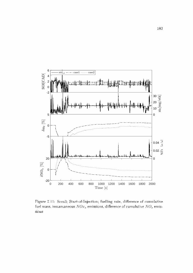
103

-2

0

2

4

6

0

10

20

30

-5

0

5

0

0.02

0.04

0 200 400 600 800 1000 1200 1400 1600 1800 2000-20

0

20

Figure 7.11: Scen3; Start-of-Injection; fuelling rate, di�erence of cumulativefuel mass, instantaneous NOxx emissions, di�erence of cumulative NOx emis-sions

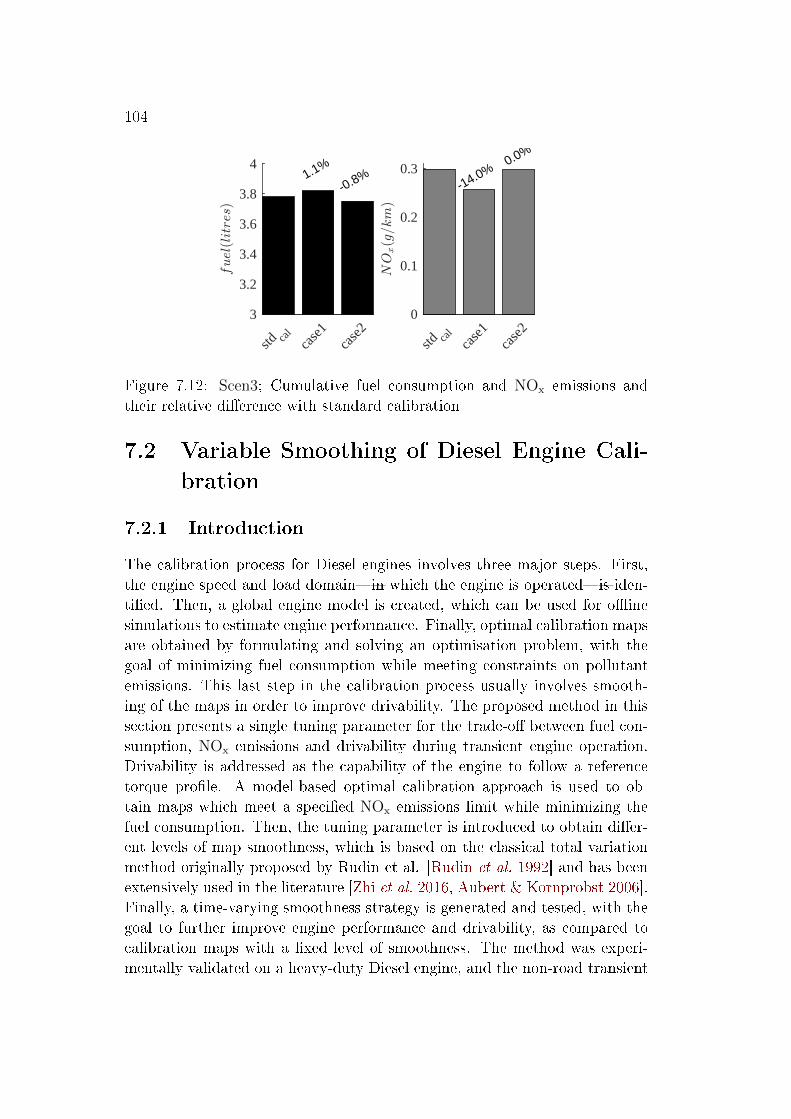
104

std cal

case

1ca

se2

3

3.2

3.4

3.6

3.8

4 1.1%

-0.8%

std cal

case

1ca

se2

0

0.1

0.2

0.3-14.0% 0.0%

Figure 7.12: Scen3; Cumulative fuel consumption and NOx emissions andtheir relative di�erence with standard calibration

7.2 Variable Smoothing of Diesel Engine Cali-

bration

7.2.1 Introduction

The calibration process for Diesel engines involves three major steps. First,the engine speed and load domain�in which the engine is operated�is iden-ti�ed. Then, a global engine model is created, which can be used for o�inesimulations to estimate engine performance. Finally, optimal calibration mapsare obtained by formulating and solving an optimisation problem, with thegoal of minimizing fuel consumption while meeting constraints on pollutantemissions. This last step in the calibration process usually involves smooth-ing of the maps in order to improve drivability. The proposed method in thissection presents a single tuning parameter for the trade-o� between fuel con-sumption, NOx emissions and drivability during transient engine operation.Drivability is addressed as the capability of the engine to follow a referencetorque pro�le. A model-based optimal calibration approach is used to ob-tain maps which meet a speci�ed NOx emissions limit while minimizing thefuel consumption. Then, the tuning parameter is introduced to obtain di�er-ent levels of map smoothness, which is based on the classical total variationmethod originally proposed by Rudin et al. [Rudin et al. 1992] and has beenextensively used in the literature [Zhi et al. 2016, Aubert & Kornprobst 2006].Finally, a time-varying smoothness strategy is generated and tested, with thegoal to further improve engine performance and drivability, as compared tocalibration maps with a �xed level of smoothness. The method was experi-mentally validated on a heavy-duty Diesel engine, and the non-road transient

105

cycle (NRTC) was used as a case study. The error between the reference andactual engine torque was used as a metric for drivability, and the error wasfound to decrease with increasing map smoothness.

7.2.2 Method Description

For the calibration of Diesel engines, it is common practice to model theinput-output relationships statically [Berger 2012, Schüler 2001]. Various soft-ware tools are available to support the calibration engineer with the steady-state measurements and subsequent modelling [Gschweitl et al. 2001, Gutjahret al. 2017, Mat 2017]. After that, model-based optimisation techniques areoften used to �nd an engine calibration that yields the lowest possible fuelconsumption while adhering to the limits on pollutant emissions [Hafner &Isermann 2003, Sequenz 2013].

For the engine in this study, the static engine model and model-basedcalibration were obtained as described in [van Dooren et al. 2019]. The controlinputs u consist of the amount of fuel injected per cylinder and per cycle minj,the start-of-injection usoi in degrees before top dead centre, and the desiredburned gas ratio xbg in the intake manifold. Whilst the amount of injectedfuel is controlled to reach the requested torque T ref

e , the two remaining controlinputs usoi and xbg are the degrees of freedom to trade o� fuel consumption mf

against engine-out NOx emissions mNOx . This is done as in [Elbert et al. 2017]by formulating and solving the following optimisation problem:

u∗(ωe, Te, µNOx) = arg minu{(1− µNOx) · mf +

µNOx · mNOx}(7.7)

The optimal control inputs u∗ for each engine operating point dependon the weighting or �strategy parameter� µNOx ∈ [0, 1]. Choosing a highervalue for µNOx results in lower engine-out NOx emissions, but at the cost of ahigher fuel consumption. While the engine strategy can�and usually is��xedduring the calibration process, the authors of [Elbert et al. 2017, Guardiolaet al. 2016] have shown that an adaptive operating strategy can be used toadapt the raw emissions in a situation-speci�c manner.

The optimal values from (Equation 7.7) are stored on the engine controlunit (ECU) as static maps that serve as a feed-forward controller. An EGRcontroller controls the intake valve and EGR valve position to reach the desiredburned gas ratio.

Variable Map Smoothing The optimal calibration maps obtained fromthe previous section are usually non-smooth. The calibration engineer may

106

chose to smooth them manually or using available tools as in [Gschweitlet al. 2001, Gutjahr et al. 2017, Mat 2017]. The methods are usually basedon �ltering techniques, where the value of �ltered data point is the average oforiginal data point and its adjacent points. A group of adjacent points in theoriginal data are multiplied point-by-point by a set of coe�cients that de�nesthe smooth shape, the products are added up and divided by the sum of thecoe�cients, which becomes one point of smoothed data. Subsequently, theset of coe�cients is shifted one point down the original data and the processis repeated. Mean �ltering methods are not well suited for speci�cally elim-inating peaks from the maps. Another method used for smoothing is basedon computing the second derivative (local curvature) at each point and thencalculating the average of the squared values of the local curvature for theentire map.

The methods described above do not explicitly take into account the costof smoothing in terms of closeness to the original map or the loss of optimality.In this work, a variational method is applied to obtain the smooth maps. Themethod is based on a classical variation model for image de-noising, originallyproposed by Rudin et al. in [Rudin et al. 1992]. The problem is formulatedas the following convex optimisation problem and solved by the primal-dualmethod as demonstrated by Zhi et al. in [Zhi et al. 2016]:

minu

∫{ (1− µsm) · (u− u∗)2 + µsm · ∇ux,y } dx dy (7.8)

where u are the control inputs of the smoothed two-dimensional (x,y) cali-bration map and u∗ denotes the optimal but non-smooth map, obtained fromthe model-based calibration method described in the previous section. Forall the investigations presented in this application, a �xed engine strategyµNOx = 0.11 was used.

The �rst term in Equation 7.8 accounts for the closeness of the obtainedsmoothed map to the original optimal but generally non-smooth map, andthe second term contributes to the total variation of the obtained map. Thecloseness to the original map has been considered rather than the cost interms of fuel consumption and NOx emissions in (Equation 9.1). This is doneto separate the optimisation and smoothing phases in the calibration process.The normalised total variation in the direction of engine speed and torque is∇ux,y. The regularisation weight µsm ∈ [0, 1] is used to tune the smoothnesslevel of the maps. When µsm = 1, only the second term in Equation 9.1 isminimised, producing the smoothest possible map. For µsm = 0, no smoothingis applied, and the resulting map is the original non-smooth map.

The continuous problem in Equation 7.8 can be discretised and solvednumerically as in Equation 7.9, where n = 5 is the grid size of the map under

107

consideration:

minu

n∑i=1

n∑j=1

{ (1− µsm) · (ui,j − u∗i,j)2 + µsm · ∇ui,j } (7.9)

in which ∇ui,j denotes the �rst order forward di�erence operation, de�ned as:

∇ui,j =

[ui+1,j − ui,jui,j+1 − ui,j

](7.10)

Five calibration maps with di�erent values of µsm ∈ {0, 0.2, 0.4, 0.6, 0.9}were calculated. Figure 7.13 and Figure 7.14 show the impact of varyingµsm on the calibration maps for start-of-injection (usoi) and burned gas ratioxbg, respectively. The original maps u∗ are shown in grey, and they are non-smooth. With increasing value of µsm, the smoothness of the maps visiblyincreases. As µsm is increased from zero, the maps initially get smootherwhere a maximum reduction of the total variation can be achieved. When µsmis further increased, also the remaining regions of the map become smoother.

In Figure 7.15, the impact of µsm on the primary and secondary termsof Equation 9.2 is shown. As expected, with increasing µsm, the normalisedtotal variation of the map decreases at the cost of its distance from the originalmap.

7.2.3 Results

In this study the following two sets of experiment were conducted:

• The �ve calibration maps obtained from the method described in subsec-tion 7.2.2 were tested on the engine test bench described in section 6.2.The Non-Road Transient Cycle (NRTC) cycle was run to obtain thetrade-o� between fuel consumption, NOx emission and torque error.

• The optimal problem was solved to obtain a µsm pro�le for minimisingthe NOx emission while constraining the fuel consumption and torqueerror within prede�ned limits. The obtained variable µsm strategy wastested on the engine.

Trade-o� between Performance and Drivability The calibration mapsin Figure 7.13 and Figure 7.14 show that with an increasing µsm, the SOI isadvanced at lower engine speeds and torque, whereas SOI is retarded at higherengine speed and torque. On the other hand, the burned gas ratio is reducedat high engine torque and increased for µsm = 0.6 and 0.8, regardless of the

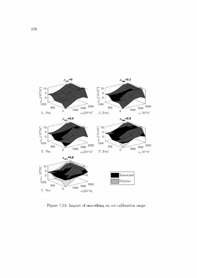
108

Figure 7.13: Impact of smoothing on soi calibration maps

109

Figure 7.14: Impact of smoothing on egr calibration maps.

110

Figure 7.15: Impact of weighting factor on the total variation ∇ui,j and dis-tance from the original map

∑(ui,j − u∗i,j)2

engine speed. The obtained calibration maps are stored in the engine ECU asstatic maps to serve as a feed-forward controller. Taking the NRTC as a casestudy, the various maps are implemented and tested on the engine test-bench.The results are presented and discussed in this section.

Figure 7.16 shows the instantaneous engine torque, start-of-injection, burnedgas ratio, fuel consumption, and NOx emissions during the NRTC. The cumu-lative impact of the control actions can be clearly seen in the instantaneousNOx emissions in the bottom plot.

In order to compare the torque response of each calibration map, the errorbetween reference and actual engine torque is calculated for the cycle as:

T errore =

∑NRTC

(T refe − Te) (7.11)

The top plot in Figure 7.17 shows the reference torque pro�le T refe . In

the bottom plot, normalised T errore is shown for the cycle. It is normalised by

dividing T errore obtained with a speci�c calibration by the error obtained with

µsm = 0. As expected, with increasing smoothness of the calibration maps,the torque error is reduced consistently.

In Figure 7.18, the trade-o� between fuel consumption, NOx emissions,and torque error is shown. For µsm = 0.9, the NOx emissions increase by 9%,fuel consumption increases by 1%, and an improvement in torque responseis observed. Table 7.1 consolidates the parameters related to the engine per-formance with di�erent values of µsm. Based on this data, the calibration

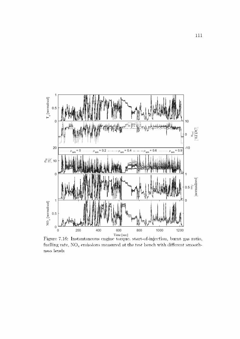
111

Figure 7.16: Instantaneous engine torque, start-of-injection, burnt gas ratio,fuelling rate, NOx emissions measured at the test bench with di�erent smooth-ness levels

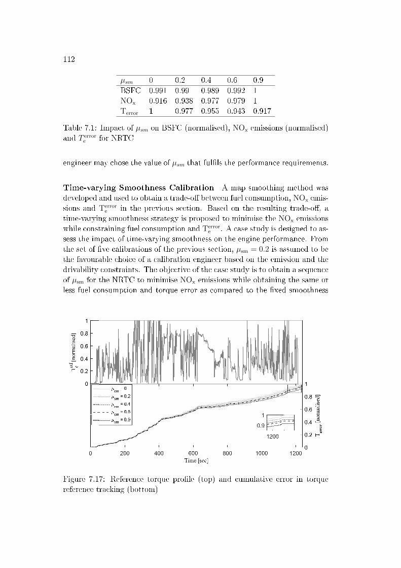
112

µsm 0 0.2 0.4 0.6 0.9BSFC 0.991 0.99 0.989 0.992 1NOx 0.916 0.938 0.977 0.979 1Terror 1 0.977 0.955 0.943 0.917

Table 7.1: Impact of µsm on BSFC (normalised), NOx emissions (normalised)and T error

e for NRTC

engineer may chose the value of µsm that ful�ls the performance requirements.

Time-varying Smoothness Calibration A map smoothing method wasdeveloped and used to obtain a trade-o� between fuel consumption, NOx emis-sions and Terror

e in the previous section. Based on the resulting trade-o�, atime-varying smoothness strategy is proposed to minimise the NOx emissionswhile constraining fuel consumption and Terror

e . A case study is designed to as-sess the impact of time-varying smoothness on the engine performance. Fromthe set of �ve calibrations of the previous section, µsm = 0.2 is assumed to bethe favourable choice of a calibration engineer based on the emission and thedrivability constraints. The objective of the case study is to obtain a sequenceof µsm for the NRTC to minimise NOx emissions while obtaining the same orless fuel consumption and torque error as compared to the �xed smoothness

Figure 7.17: Reference torque pro�le (top) and cumulative error in torquereference tracking (bottom)

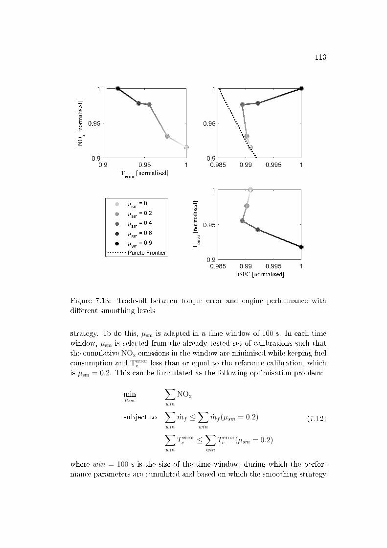
113

Figure 7.18: Trade-o� between torque error and engine performance withdi�erent smoothing levels

strategy. To do this, µsm is adapted in a time window of 100 s. In each timewindow, µsm is selected from the already tested set of calibrations such thatthe cumulative NOx emissions in the window are minimised while keeping fuelconsumption and Terror

e less than or equal to the reference calibration, whichis µsm = 0.2. This can be formulated as the following optimisation problem:

minµsm

∑win

NOx

subject to∑win

mf ≤∑win

mf (µsm = 0.2)

∑win

T errore ≤

∑win

T errore (µsm = 0.2)

(7.12)

where win = 100 s is the size of the time window, during which the perfor-mance parameters are cumulated and based on which the smoothing strategy

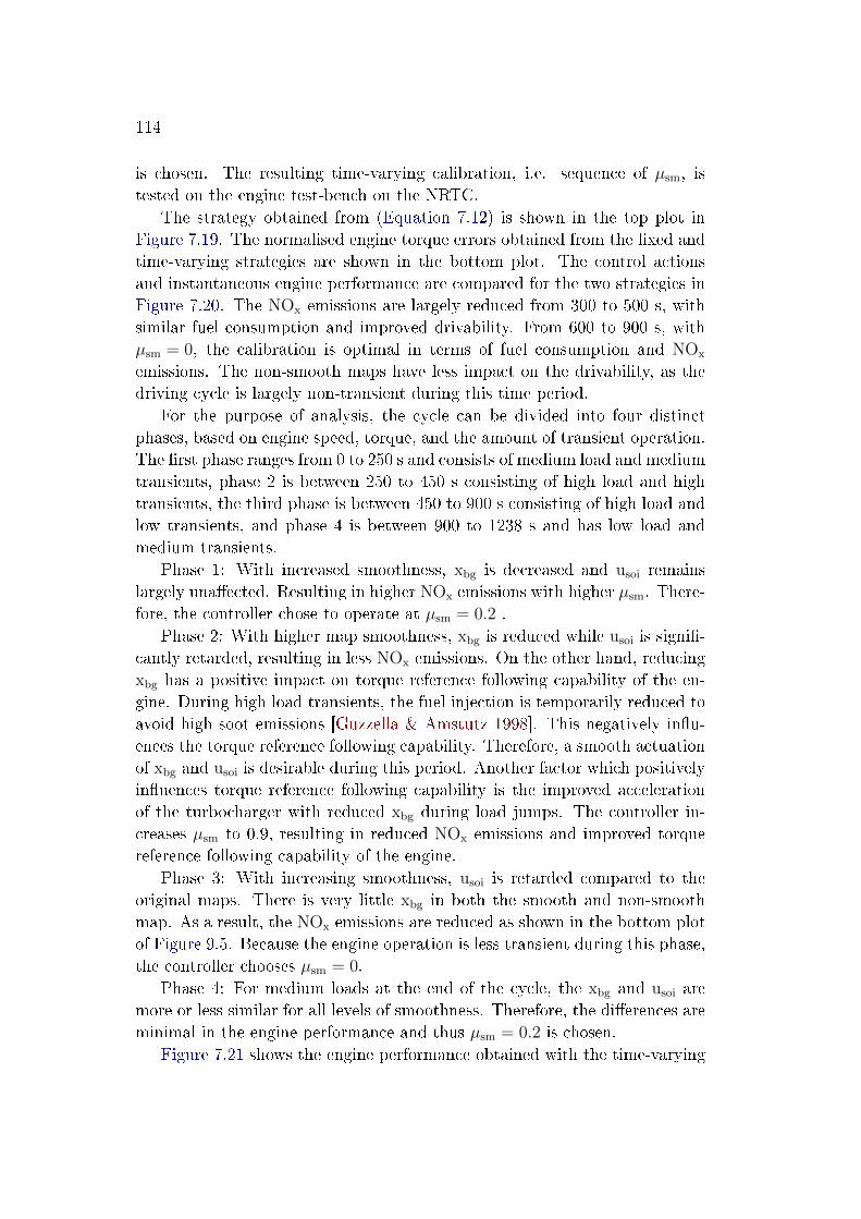
114

is chosen. The resulting time-varying calibration, i.e. sequence of µsm, istested on the engine test-bench on the NRTC.

The strategy obtained from (Equation 7.12) is shown in the top plot inFigure 7.19. The normalised engine torque errors obtained from the �xed andtime-varying strategies are shown in the bottom plot. The control actionsand instantaneous engine performance are compared for the two strategies inFigure 7.20. The NOx emissions are largely reduced from 300 to 500 s, withsimilar fuel consumption and improved drivability. From 600 to 900 s, withµsm = 0, the calibration is optimal in terms of fuel consumption and NOx

emissions. The non-smooth maps have less impact on the drivability, as thedriving cycle is largely non-transient during this time period.

For the purpose of analysis, the cycle can be divided into four distinctphases, based on engine speed, torque, and the amount of transient operation.The �rst phase ranges from 0 to 250 s and consists of medium load and mediumtransients, phase 2 is between 250 to 450 s consisting of high load and hightransients, the third phase is between 450 to 900 s consisting of high load andlow transients, and phase 4 is between 900 to 1238 s and has low load andmedium transients.

Phase 1: With increased smoothness, xbg is decreased and usoi remainslargely una�ected. Resulting in higher NOx emissions with higher µsm. There-fore, the controller chose to operate at µsm = 0.2 .

Phase 2: With higher map smoothness, xbg is reduced while usoi is signi�-cantly retarded, resulting in less NOx emissions. On the other hand, reducingxbg has a positive impact on torque reference following capability of the en-gine. During high load transients, the fuel injection is temporarily reduced toavoid high soot emissions [Guzzella & Amstutz 1998]. This negatively in�u-ences the torque reference following capability. Therefore, a smooth actuationof xbg and usoi is desirable during this period. Another factor which positivelyin�uences torque reference following capability is the improved accelerationof the turbocharger with reduced xbg during load jumps. The controller in-creases µsm to 0.9, resulting in reduced NOx emissions and improved torquereference following capability of the engine.

Phase 3: With increasing smoothness, usoi is retarded compared to theoriginal maps. There is very little xbg in both the smooth and non-smoothmap. As a result, the NOx emissions are reduced as shown in the bottom plotof Figure 9.5. Because the engine operation is less transient during this phase,the controller chooses µsm = 0.

Phase 4: For medium loads at the end of the cycle, the xbg and usoi aremore or less similar for all levels of smoothness. Therefore, the di�erences areminimal in the engine performance and thus µsm = 0.2 is chosen.

Figure 7.21 shows the engine performance obtained with the time-varying

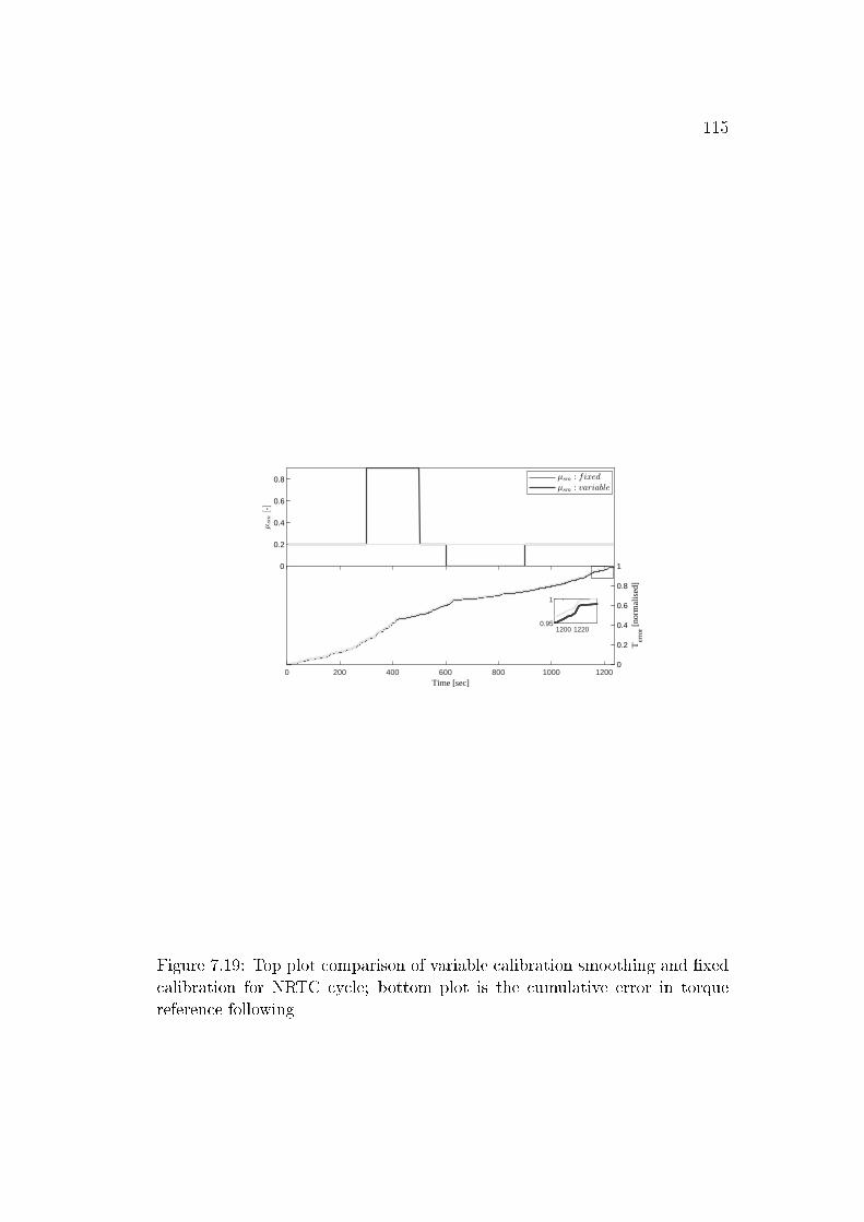
115

0

0.2

0.4

0.6

0.8

0 200 400 600 800 1000 1200Time [sec]

0

0.2

0.4

0.6

0.8

1

Ter

ror [

norm

alis

ed]

1200 12200.95

1

Figure 7.19: Top plot comparison of variable calibration smoothing and �xedcalibration for NRTC cycle; bottom plot is the cumulative error in torquereference following

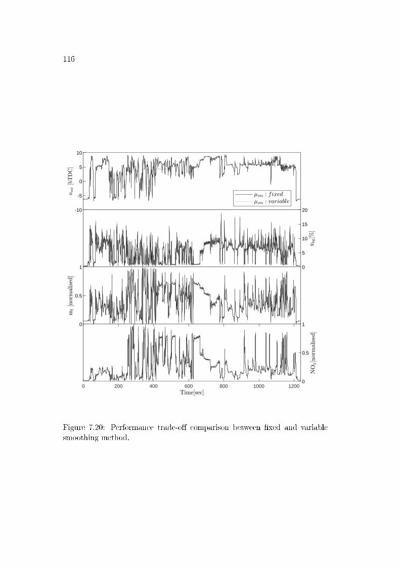
116

-10

-5

0

5

10

0

5

10

15

20

0

0.5

1

0 200 400 600 800 1000 12000

0.5

1

Figure 7.20: Performance trade-o� comparison between �xed and variablesmoothing method.

117

smoothness strategy, as compared to the �xed calibration strategy. With thetime-varying smoothness, NOx emissions can be reduced by 3-4% comparedto the �xed calibration, while maintaining the same fuel consumption andtorque reference following capability.

Figure 7.21: Comparison of engine performance for �xed and time-varyingsmoothness calibration.

The result highlights the potential of variable smoothing on a driving cycle.Although, this demonstration is made for the NRTC it can be extended to thereal world scenario by online estimation of the error in torque,Brake Speci�cFuel Consumption (BSFC) and NOx emission. These estimations require adriving cycle prediction tool, an engine model and a supervisory controllerto choose the optimal value of the proposed tuning parameter in real drivingcondition.

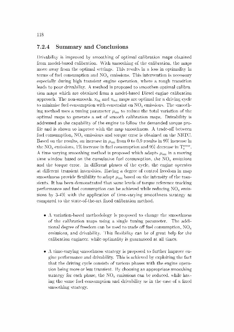
118

7.2.4 Summary and Conclusions

Drivability is improved by smoothing of optimal calibration maps obtainedfrom model-based calibration. With smoothing of the calibration, the mapsmove away from the optimal settings. This results in a loss in optimality interms of fuel consumption and NOx emissions. This intervention is necessaryespecially during high transient engine operation, where a rough transitionleads to poor drivability. A method is proposed to smoothen optimal calibra-tion maps which are obtained from a model-based Diesel engine calibrationapproach. The non-smooth, xbg and usoi maps are optimal for a driving cycleto minimise fuel consumption with constraint on NOx emissions. The smooth-ing method uses a tuning parameter µsm to reduce the total variation of theoptimal maps to generate a set of smooth calibration maps. Drivability isaddressed as the capability of the engine to follow the demanded torque pro-�le and is shown to improve with the map smoothness. A trade-o� betweenfuel consumption, NOx emissions and torque error is obtained on the NRTC.Based on the results, an increase in µsm from 0 to 0.9 results in 9% increase inthe NOx emissions, 1% increase in fuel consumption and 9% decrease in Terror

e .A time varying smoothing method is proposed which adapts µsm in a movingtime window based on the cumulative fuel consumption, the NOx emissionsand the torque error. In di�erent phases of the cycle, the engine operatesat di�erent transient intensities. Having a degree of control freedom in mapsmoothness provide �exibility to adapt µsm based on the intensity of the tran-sients. It has been demonstrated that same levels of torque reference trackingperformance and fuel consumption can be achieved while reducing NOx emis-sions by 3-4% with the application of time-varying smoothness strategy ascompared to the state-of-the-art �xed calibration method.

• A variation-based methodology is proposed to change the smoothnessof the calibration maps using a single tuning parameter. The addi-tional degree of freedom can be used to trade o� fuel consumption, NOx

emissions, and drivability. This �exibility can be of great help for thecalibration engineer, while optimality is guaranteed at all times.

• A time-varying smoothness strategy is proposed to further improve en-gine performance and drivability. This is achieved by exploiting the factthat the driving cycle consists of various phases with the engine opera-tion being more or less transient. By choosing an appropriate smoothingstrategy for each phase, the NOx emissions can be reduced, while hav-ing the same fuel consumption and drivability as in the case of a �xedsmoothing strategy.

119

An additional degree-of-freedom has provided more �exibility to controlthe engine with the time-varying smoothness strategy. The proposed methodcan be extended to the real world scenario by including a driving cycle pre-diction model, an engine model and a controller that can optimally chose theproposed smoothness tuning parameter such that the fuel-e�ciency is max-imised while limiting the reference torque error and the NOx emission.

7.3 Online optimal Energy Management strat-

egy for Parallel HEV

7.3.1 Introduction and problem description

This chapter proposes an online Energy Management Strategy (EMS) for aplug-in Hybrid Electric Vehicle (pHEV) with the goal of minimising the fuelconsumption while ful�lling the constraint on the terminal battery State-of-Charge (SoC) on a driving mission. In order to cope with limitations ofboth heuristic and Optimal Control (OC)approaches, several model based ap-proaches have been proposed in past, most of them are based to some extent onOC, but sacri�cing optimality for the sake of applicability. Amongst them, onecan �nd Equivalent Consumption Minimization Strategy (ECMS) proposed by[Paganelli et al. 2000] and Deterministic or Stochastic Model Predictive Con-trol as in [Johannesson et al. 2007]. The ECMS is probably the most widelyexplored approach with several versions, all of them showing near-optimalresults with a challenge of properly determining the equivalent factor (EF)[Tulpule et al. 2011]. The values of EF are cycle-dependent and hence pose theissue of non-causality. The task of updating the co-state online as driving sce-narios vary is referred to as co-state adaptation and the supervisory controlleris referred to as adaptive optimal supervisory controller. Method falling in thiscategory are referred in the literature as Adaptive-ECMS(A-ECMS) strategy[Onori et al. 2015, Lei et al. 2020]. The non-causality is addressed in the lit-erature by taking advantage of the driving information [Payri et al. 2015, Yuet al. 2020] to estimate the suitable values of the weighting factor betweenfuel and battery energy sources. The adaptation techniques in the literatureare classi�ed in two categories: The �rst category is adaptation base on thedriving cycle prediction. The equivalence factor is estimated online based ona look ahead horizon de�ned in terms of energy at the wheels, to determineat each instant the most likely behaviour. [Sciarretta et al. 2004, Ambuhl& Guzzella 2009]. In literature, the task of driving cycle prediction is usu-ally performed using Neural-Network (NN) and Markov-Chain (MC) basedmethods. In the article by the authors in [Xie et al. 2018], a comparison of

120

the two approaches is shown in terms of prediction accuracy and computa-tion speed. The MC based method is shown to outperform the NN basedmethod. In the article [Sun et al. 2017], authors proposed a RBF-NN speedprediction method integrated to the A-ECMS. This method used open-loopspeed prediction derived from the current vehicle state. The second cate-gory of the adaptation methods is by exploiting the fact that the equivalencefactors are similar for cycles with similar statistical properties. To recognisethe driving cycle characteristics, the authors in [Guardiola et al. 2013, Payriet al. 2012, Gu & Rizzoni 2006, il Jeon et al. 2000] use statistic and clusteringtechniques to classify the driving type. Most of the pattern recognition algo-rithms in the literature �rst identify the kind of driving conditions the vehicleis undergoing, and then select the most appropriate equivalence factors froma prede�ned set.

This application addresses the adaptation by using the �rst method men-tioned above. In the original A-ECMS, introduced by the authors in [Musardoet al. 2005], the algorithm predicts mission that the vehicle is following anddetermines the optimal Equivalent Factor (EF) for the current mission by thedirect optimization method. The cycle prediction is based on a �xed transitionprobability matrix for the entire route and it does not account for the devia-tion in the predicted and the actual vehicle velocity. To this end, a close-loopdriving cycle prediction method based on the MC approach is introduced inthe A-ECMS. The driving prediction uses the historical information to obtainspace dependent transition probability matrices and then uses Markov prin-ciple to recursively predict the driving cycle and update the EF based on theonline ECMS results. In this way, the predicted speed and the EF adapt them-selves periodically during the Control Horizon Window (CHW) such that, atany instance the power split is optimal and the expected terminal SoC is closeto the desired level.

The main objective of the study is to develop an online applicable EMS fora pHEV that exploits the information obtained when the vehicle recurrentlycovers a given route. For application purposes, a route of 21km includingrural, highway and urban areas has been chosen. The route was covered bythe same driver 50 times during consecutive working days.

Regarding the vehicle, a pHEV has been chosen to show the strategy po-tential while the method can be adapted to deal with other powertrain types(series, series-parallel, charge sustaining,...). In this architecture, i.e parallelarrangement ,the vehicle can be driven by the ICE, the EM, or both simulta-neously. Thus, there are di�erent solutions to provide the power required bythe driver with di�erent costs and impacts in future operation, which poses aninteresting optimization problem. The battery is charged either by an exter-nal power source, by the ICE or by regenerative braking through the electric

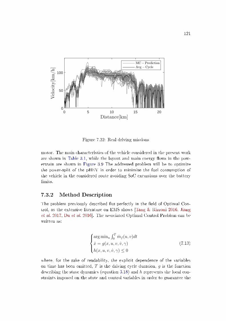
121

0 5 10 15 200

50

100

Figure 7.22: Real driving missions

motor. The main characteristics of the vehicle considered in the present workare shown in Table 3.1, while the layout and main energy �ows in the pow-ertrain are shown in Figure 3.9 The addressed problem will be to optimizethe power-split of the pHEV in order to minimise the fuel consumption ofthe vehicle in the considered route avoiding SoC excursions over the batterylimits.

7.3.2 Method Description

The problem previously described �ts perfectly in the �eld of Optimal Con-trol, as the extensive literature on EMS shows [Tang & Rizzoni 2016, Jianget al. 2017, Du et al. 2016]. The associated Optimal Control Problem can bewritten as:

arg minu

∫ T0mf (u, v)dt

x = g(x, u, v, v, γ)

h(x, u, v, v, γ) ≤ 0

(7.13)

where, for the sake of readability, the explicit dependence of the variableson time has been omitted, T is the driving cycle duration, g is the functiondescribing the state dynamics (equation 3.18) and h represents the local con-straints imposed on the state and control variables in order to guarantee the

122

physical operation limits (maximum and minimum limits on battery state ofcharge and power, speed and torque of powertrain elements).

Regarding the solution of system Equation 7.13 one can observe that pro-vided the dependence on T, v, v and γ a proper estimation of such parametersis needed. In fact, the optimal solution of the problem can only be obtainedif perfect knowledge of the driving cycle is available. Assuming a suitableapproximation of those variables, there is a wide set of solutions in literatureconsolidated by the authors in [Zhang et al. 2020]. Amongst them, those de-rived from the Equivalent Consumption Minimization Strategy (ECMS) arewidespread since provide a feasible on-board application. The ECMS is aimedto replace the integral problem presented in Equation 7.13 with a set of equiv-alent problems to be solved at every time step:

J = Pf + µPb (7.14)

where the parameter µ, is a weighting factor between fuel and battery energysources. An analytical derivation of the ECMS can be obtained from thePMP [Serrao et al. 2009], in any case, intuition shows that a penalty on thebattery use should be included in the cost function to avoid its depletion. Theselection of the proper value of µ depending on the driving conditions is thekey aspect of the ECMS. Provided a driving cycle (T, v, v and γ) the value ofµ that ful�ls with constraints in problem Equation 7.13, and particularly thelimitations in the SoC.

According to the suitability of the ECMS method and requirement of anestimation of driving cycle, the proposed controller is presented in Figure 7.23.

The prediction block uses the current vehicle position (st) and speed (vt) toestimate the driving cycle main parameters, consisting on the duration T − t,vehicle speed and acceleration sequences (vt:T and ˆvt:T ) and estimated roadslope evolution during the cycle (γt:T ). The prediction block is based on thetool described in chapter 5.

Once the driving cycle is estimated, the power demand block calculates thedesired torque and speed based on the vehicle model described in section 3.1and using T , vt:T , ˆvt:T and γt:T .

The inputs to the µ calculation block are the estimated torque and speedvectors (Tgt:T and ωgt:T ) and the current SoC (SoCt). The optimal µ in thesense of that leading to minimum SoC at the end of the estimated drivingcycle is calculated by an iterative method, in the case at hand the bisectionmethod. Note that the condition of minimum SoC at the end of the cyclehas been chosen due to the plug in nature of the powertrain and taking intoaccount that the vehicle can be fully recharged at the end of the route. In anycase, the target SoC can be modi�ed adding a new calibration parameter tothe control strategy. The calculated µ is applied during a prede�ned CHW,

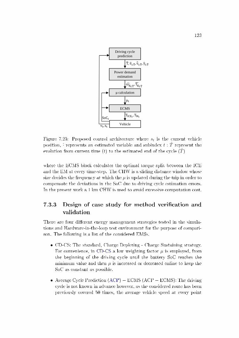
123

Driving cycle prediction

Power demand estimation

μ calculation

ECMS

Vehicle

�T, �vt:�T, �vt:�T, �γt:�T

�ωgt:�T,�Tgt:�T

μt

TICEt , TMt

vt, st

SoCt

Figure 7.23: Proposed control architecture where st is the current vehicleposition, · represents an estimated variable and subindex t : T represent theevolution from current time (t) to the estimated end of the cycle (T )

where the ECMS block calculates the optimal torque split between the ICEand the EM at every time-step. The CHW is a sliding distance window whosesize decides the frequency at which the µ is updated during the trip in order tocompensate the deviations in the SoC due to driving cycle estimation errors.In the present work a 1 km CHW is used to avoid excessive computation cost.

7.3.3 Design of case study for method veri�cation and

validation

There are four di�erent energy management strategies tested in the simula-tions and Hardware-in-the-loop test environment for the purpose of compari-son. The following is a list of the considered EMSs.

• CD-CS: The standard, Charge Depleting - Charge Sustaining strategy.For convenience, in CD-CS a low weighting factor µ is employed, fromthe beginning of the driving cycle until the battery SoC reaches theminimum value and then µ is increased or decreased online to keep theSoC as constant as possible.

• Average Cycle Prediction (ACP) + ECMS (ACP + ECMS): The drivingcycle is not known in advance however, as the considered route has beenpreviously covered 50 times, the average vehicle speed at every point

124

of the route (represented by black line in Figure 7.22) is used as anestimation of the driving cycle to feed the power demand estimationblock in Figure 7.23, then calculate µ and apply the ECMS. The valueof µ is updated after a given space window (1 km) to make up fordeviations in the SoC.

• Markov Chain Process (MCP) + ECMS (MCP + ECMS): The drivingcycle is not known in advance and the method proposed in section 5.2is used following all the steps in Figure 5.1. Several predicted vehiclespeed pro�les are presented by the gray lines in Figure 7.22.

• Optimal (Equivalent Consumption Minimisation Strategy): The drivingcycle is known in advance and an optimal weighting factor (µ) is appliedduring the complete driving cycle to minimise fuel consumption with aconstraint in the minimum SoC.

In order to assess the performance of the proposed control strategy in a wideset of scenarios, a simulation campaign using forward versions of the pow-ertrain model presented in section chapter 3 was done. Then, a veri�cationof the method suitability is done experimentally on the test cell described insection section 6.1. A single driving cycle has been chosen to con�rm themodelling results previously discussed. The simulation campaign consisted ofrunning the vehicle model with 4 EMSs on 50 di�erent driving cycles. On theother hand the experimental study comprised of running 4 EMSs on a singledriving cycle.

7.3.4 Results

The scatter of the results with 4 EMSs (presented in the previous section) onseveral driving cycles is presented in Figure 7.24. Even though the objectiveof the control problem is to keep the SoC at 15% at the end of the mission, atolerance is ±5 was allowed during the study.

The dispersion of the fuel consumption for the similar value of the terminalSoC for each strategy is presented in Figure 7.25. It can be noticed that theMCP+ECMS strategy is nearest and CD-CS is farthest from the optimal;hence proving the potential of the current intervention. The performance ofthe CD-CS which does not take into account any prediction is inferior to theother two prediction based methods (MCP and ACP).

The implementation of the above four strategies in Hardware-In-Loop(HIL) setup was to further validate the results obtained from the simula-tion study. Figure 7.26 shows the driving cycle (vehicle speed) in the topplot, the evolution of µ and SoC with the tested strategies in the central

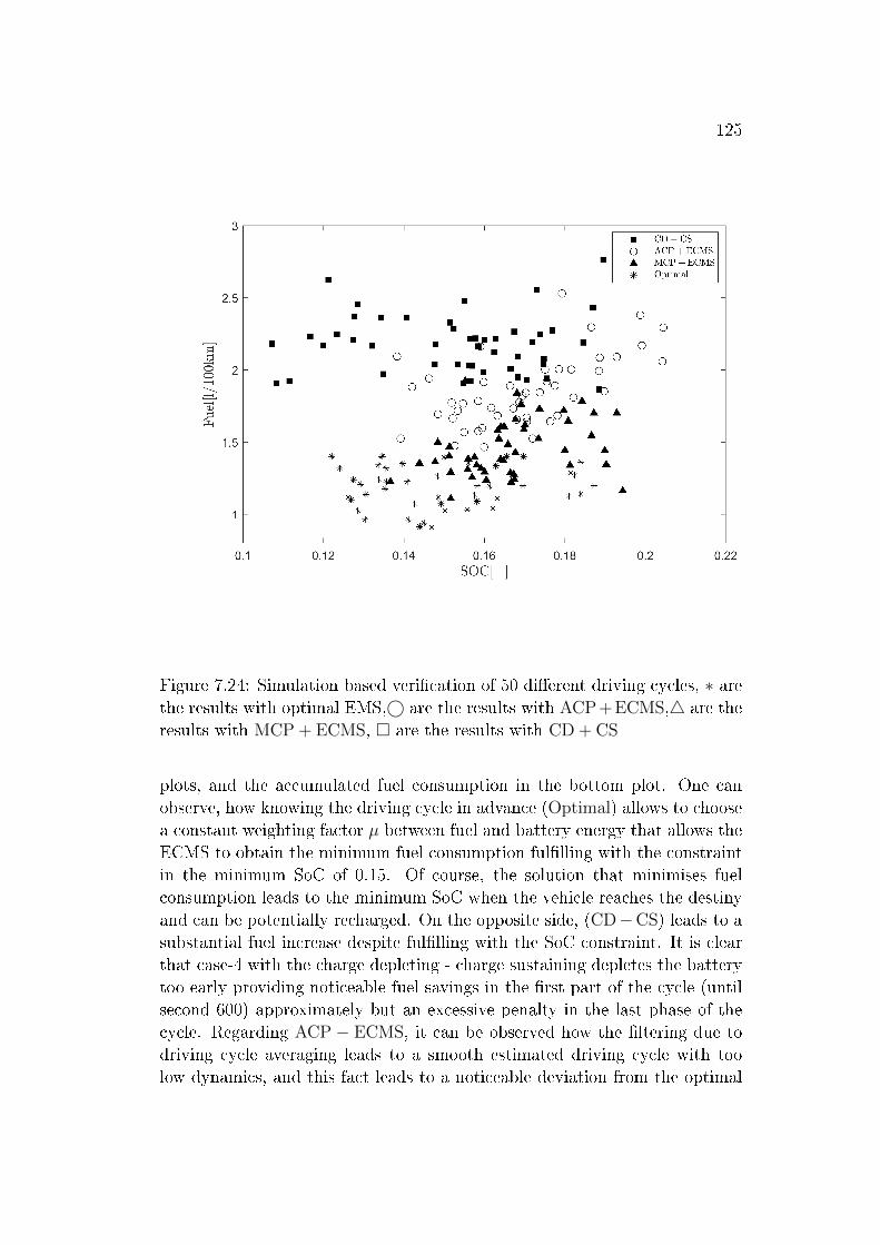
125

Figure 7.24: Simulation based veri�cation of 50 di�erent driving cycles, ∗ arethe results with optimal EMS,© are the results with ACP + ECMS,4 are theresults with MCP + ECMS, � are the results with CD + CS

plots, and the accumulated fuel consumption in the bottom plot. One canobserve, how knowing the driving cycle in advance (Optimal) allows to choosea constant weighting factor µ between fuel and battery energy that allows theECMS to obtain the minimum fuel consumption ful�lling with the constraintin the minimum SoC of 0.15. Of course, the solution that minimises fuelconsumption leads to the minimum SoC when the vehicle reaches the destinyand can be potentially recharged. On the opposite side, (CD−CS) leads to asubstantial fuel increase despite ful�lling with the SoC constraint. It is clearthat case-4 with the charge depleting - charge sustaining depletes the batterytoo early providing noticeable fuel savings in the �rst part of the cycle (untilsecond 600) approximately but an excessive penalty in the last phase of thecycle. Regarding ACP − ECMS, it can be observed how the �ltering due todriving cycle averaging leads to a smooth estimated driving cycle with toolow dynamics, and this fact leads to a noticeable deviation from the optimal

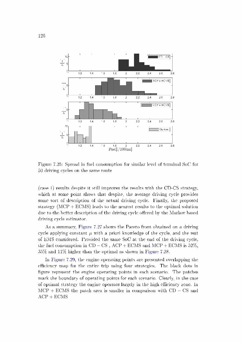
126

Figure 7.25: Spread in fuel consumption for similar level of terminal SoC for50 driving cycles on the same route

(case 1) results despite it still improves the results with the CD-CS strategy,which at some point shows that despite, the average driving cycle providessome sort of description of the actual driving cycle. Finally, the proposedstrategy (MCP + ECMS) leads to the nearest results to the optimal solutiondue to the better description of the driving cycle o�ered by the Markov baseddriving cycle estimator.

As a summary, Figure 7.27 shows the Pareto front obtained on a drivingcycle applying constant µ with a priori knowledge of the cycle, and the restof EMS considered. Provided the same SoC at the end of the driving cycle,the fuel consumption in CD−CS , ACP + ECMS and MCP + ECMS is 52%,35% and 11% higher than the optimal as shown in Figure 7.28.

In Figure 7.29, the engine operating points are presented overlapping thee�ciency map for the entire trip using four strategies. The black dots in�gure represent the engine operating points in each scenario. The patchesmark the boundary of operating points for each scenario. Clearly, in the caseof optimal strategy the engine operates largely in the high e�ciency zone. InMCP + ECMS the patch area is smaller in comparison with CD − CS andACP + ECMS

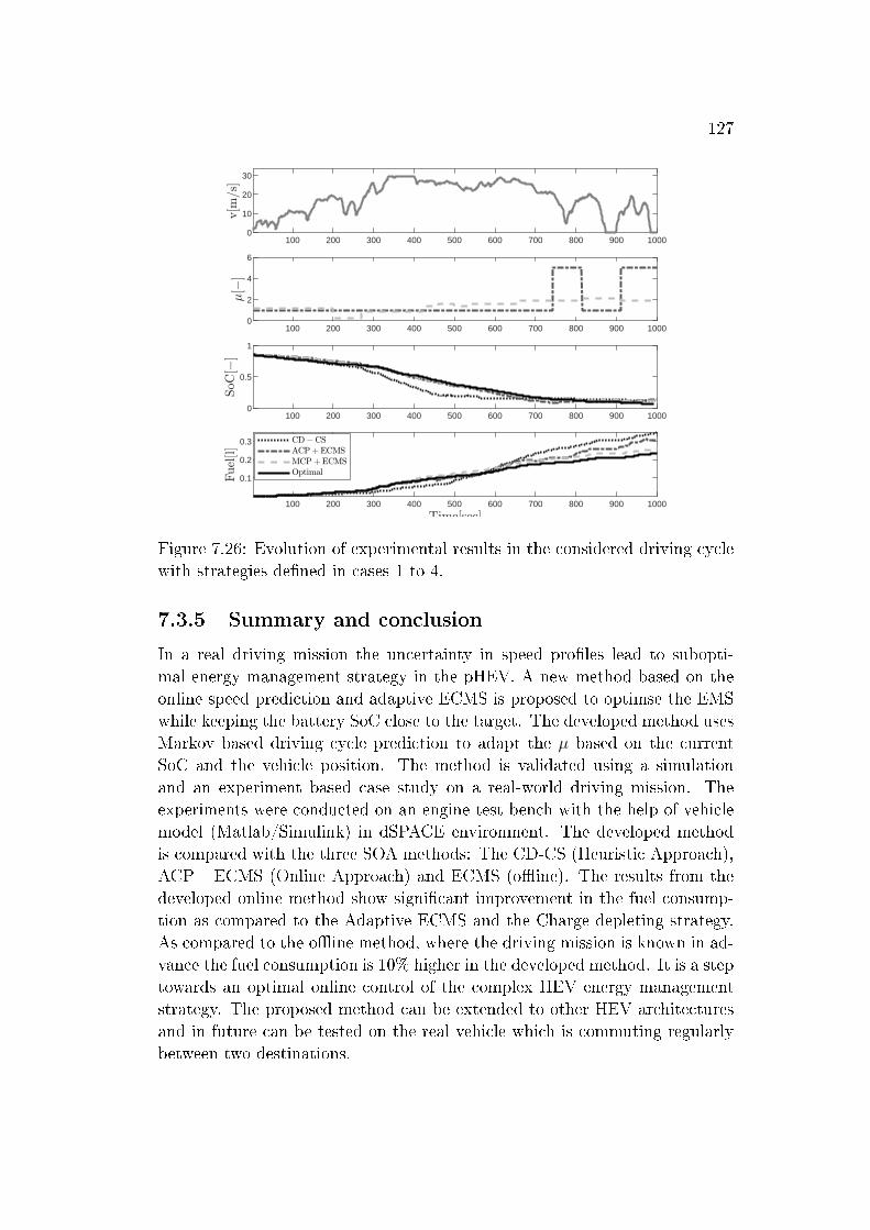
127

100 200 300 400 500 600 700 800 900 10000

10

20

30

100 200 300 400 500 600 700 800 900 10000

2

4

6

100 200 300 400 500 600 700 800 900 10000

0.5

1

100 200 300 400 500 600 700 800 900 1000

0.1

0.2

0.3

Figure 7.26: Evolution of experimental results in the considered driving cyclewith strategies de�ned in cases 1 to 4.

7.3.5 Summary and conclusion

In a real driving mission the uncertainty in speed pro�les lead to subopti-mal energy management strategy in the pHEV. A new method based on theonline speed prediction and adaptive ECMS is proposed to optimse the EMSwhile keeping the battery SoC close to the target. The developed method usesMarkov based driving cycle prediction to adapt the µ based on the currentSoC and the vehicle position. The method is validated using a simulationand an experiment based case study on a real-world driving mission. Theexperiments were conducted on an engine test bench with the help of vehiclemodel (Matlab/Simulink) in dSPACE environment. The developed methodis compared with the three SOA methods: The CD-CS (Heuristic Approach),ACP+ ECMS (Online Approach) and ECMS (o�ine). The results from thedeveloped online method show signi�cant improvement in the fuel consump-tion as compared to the Adaptive ECMS and the Charge depleting strategy.As compared to the o�ine method, where the driving mission is known in ad-vance the fuel consumption is 10% higher in the developed method. It is a steptowards an optimal online control of the complex HEV energy managementstrategy. The proposed method can be extended to other HEV architecturesand in future can be tested on the real vehicle which is commuting regularlybetween two destinations.

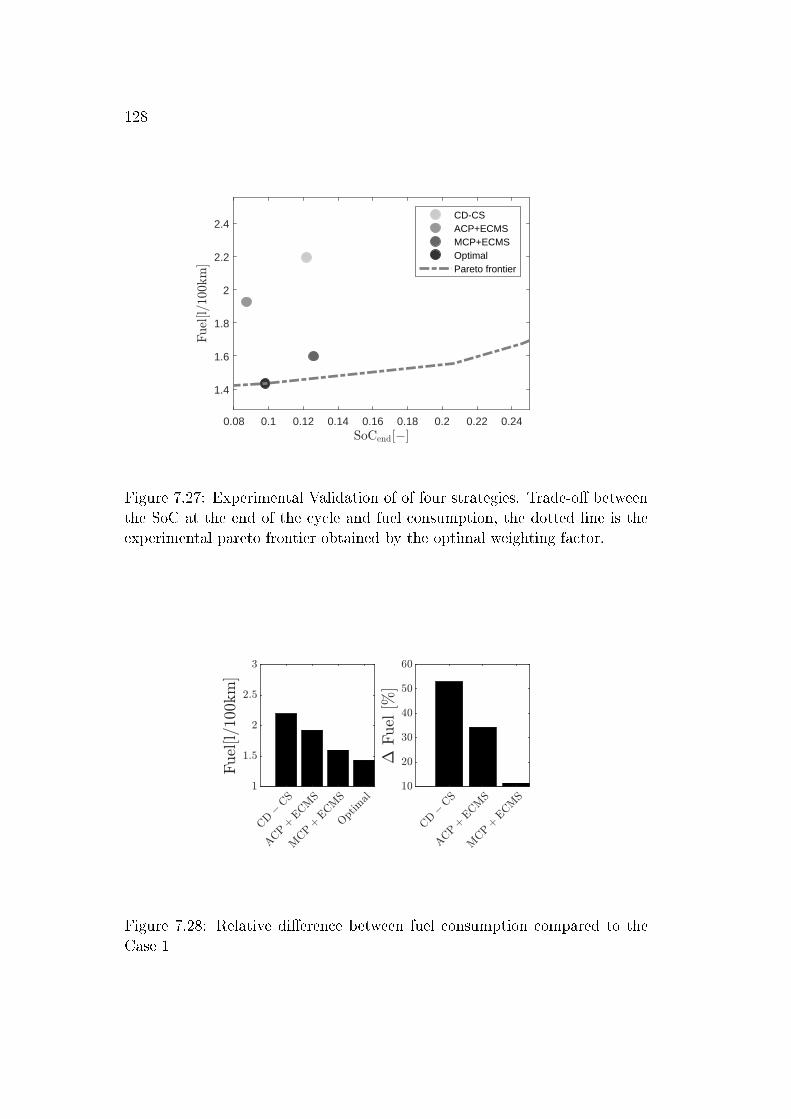
128

0.08 0.1 0.12 0.14 0.16 0.18 0.2 0.22 0.24

1.4

1.6

1.8

2

2.2

2.4CD-CSACP+ECMSMCP+ECMSOptimalPareto frontier

Figure 7.27: Experimental Validation of of four strategies. Trade-o� betweenthe SoC at the end of the cycle and fuel consumption, the dotted line is theexperimental pareto frontier obtained by the optimal weighting factor.

Figure 7.28: Relative di�erence between fuel consumption compared to theCase 1

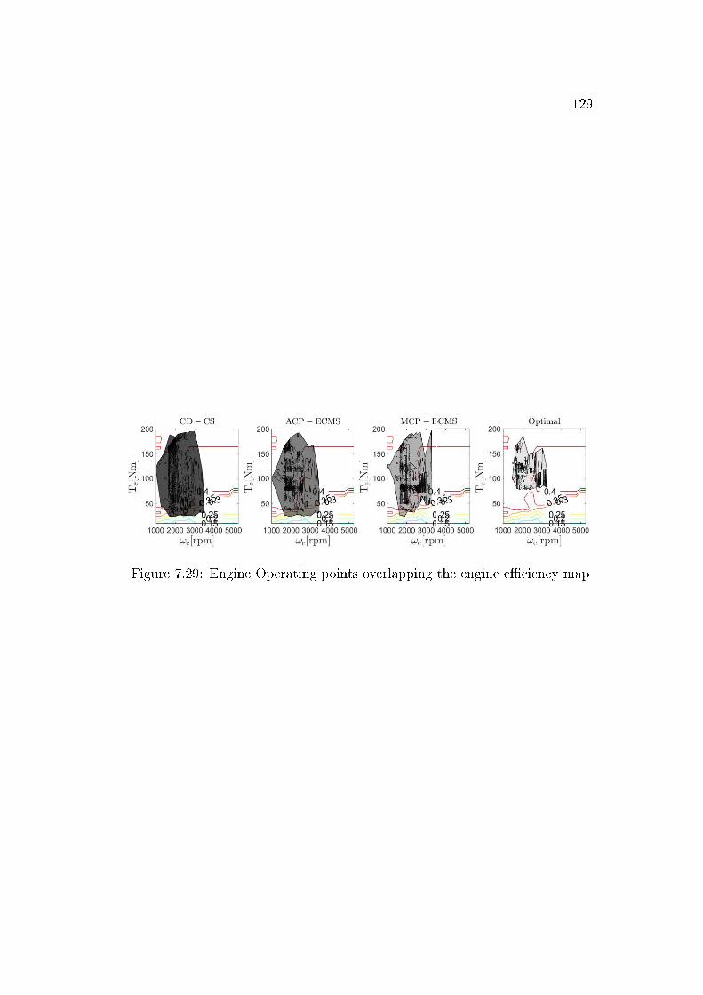
129

Figure 7.29: Engine Operating points overlapping the engine e�ciency map

Chapter 8

Vehicle Speed Advisory Based

Optimisation

Contents

8.1 Optimisation based on Tra�c Light information . . . 131

8.1.1 Introduction and problem description . . . . . . . . . . 131

8.1.2 Design of case study for method veri�cation and validation133

8.1.3 Method description . . . . . . . . . . . . . . . . . . . . 134

8.1.4 Results . . . . . . . . . . . . . . . . . . . . . . . . . . 138

8.1.5 Summary and conclusions . . . . . . . . . . . . . . . . 143

8.2 Online vehicle speed advisor . . . . . . . . . . . . . . . 146

8.2.1 Introduction and problem description . . . . . . . . . . 146

8.2.2 Method description . . . . . . . . . . . . . . . . . . . . 147

8.2.3 Results . . . . . . . . . . . . . . . . . . . . . . . . . . 153

8.2.4 Summary and conclusions . . . . . . . . . . . . . . . . 155

8.1 Optimisation based on Tra�c Light infor-

mation

8.1.1 Introduction and problem description

The intrinsic complexity of optimising the speed pro�le of a vehicle driven ona route kept the researchers sceptical about the subject. Only until recently

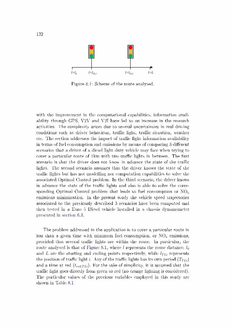
132

l=l0 l=Ll=lTL1 l=lTL2

Figure 8.1: Scheme of the route analysed.

with the improvement in the computational capabilities, information avail-ability through GPS, V2V and V2I have led to an increase in the researchactivities. The complexity arises due to several uncertainties in real drivingconditions such as driver behaviour, tra�c light, tra�c situation, weatheretc. The section addresses the impact of tra�c light information availabilityin terms of fuel consumption and emissions by means of comparing 3 di�erentscenarios that a driver of a diesel light duty vehicle may face when trying tocover a particular route of 1km with two tra�c lights in between. The �rstscenario is that the driver does not know in advance the state of the tra�clights. The second scenario assumes that the driver knows the state of thetra�c lights but has not modelling nor computation capabilities to solve theassociated Optimal Control problem. In the third scenario, the driver knowsin advance the state of the tra�c lights and also is able to solve the corre-sponding Optimal Control problem that leads to fuel consumption or NOx

emissions minimisation. In the present study the vehicle speed trajectoriesassociated to the previously described 3 scenarios have been computed andthen tested in a Euro 5 Diesel vehicle installed in a chassis dynamometerpresented in section 6.3.

The problem addressed in the application is to cover a particular route inless than a given time with minimum fuel consumption, or NOx emissions,provided that several tra�c lights are within the route. In particular, theroute analysed is that of Figure 8.1, where l represents the route distance, l0and L are the starting and ending points respectively, while lTLi representsthe position of tra�c light i. Any of the tra�c lights has its own period (TTLi)and a time at red (tred,TLi). For the sake of simplicity, it is assumed that thetra�c light goes directly from green to red (no orange lighting is considered).The particular values of the previous variables employed in this study areshown in Table 8.1

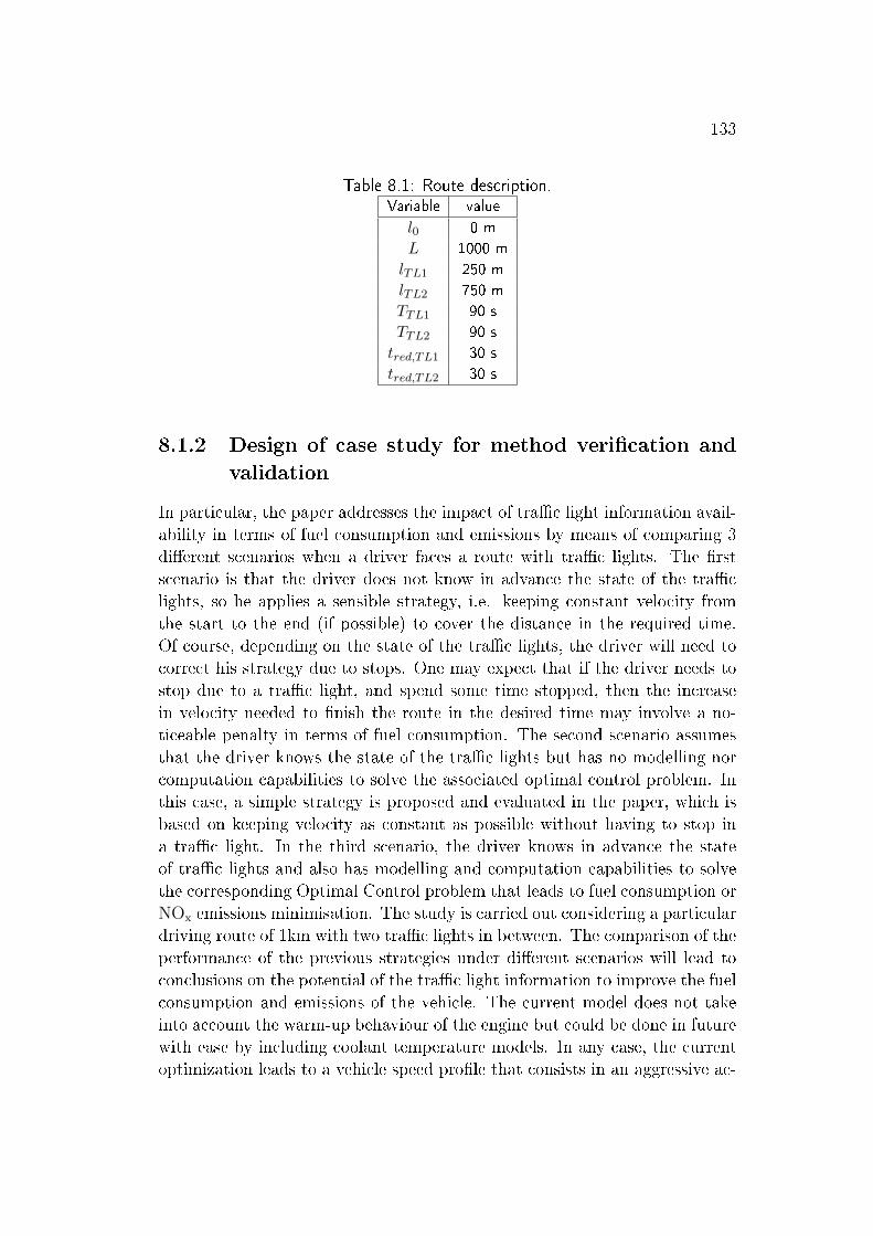
133

Table 8.1: Route description.Variable value

l0 0 m

L 1000 m

lTL1 250 m

lTL2 750 m

TTL1 90 s

TTL2 90 s

tred,TL1 30 s

tred,TL2 30 s

8.1.2 Design of case study for method veri�cation and

validation

In particular, the paper addresses the impact of tra�c light information avail-ability in terms of fuel consumption and emissions by means of comparing 3di�erent scenarios when a driver faces a route with tra�c lights. The �rstscenario is that the driver does not know in advance the state of the tra�clights, so he applies a sensible strategy, i.e. keeping constant velocity fromthe start to the end (if possible) to cover the distance in the required time.Of course, depending on the state of the tra�c lights, the driver will need tocorrect his strategy due to stops. One may expect that if the driver needs tostop due to a tra�c light, and spend some time stopped, then the increasein velocity needed to �nish the route in the desired time may involve a no-ticeable penalty in terms of fuel consumption. The second scenario assumesthat the driver knows the state of the tra�c lights but has no modelling norcomputation capabilities to solve the associated optimal control problem. Inthis case, a simple strategy is proposed and evaluated in the paper, which isbased on keeping velocity as constant as possible without having to stop ina tra�c light. In the third scenario, the driver knows in advance the stateof tra�c lights and also has modelling and computation capabilities to solvethe corresponding Optimal Control problem that leads to fuel consumption orNOx emissions minimisation. The study is carried out considering a particulardriving route of 1km with two tra�c lights in between. The comparison of theperformance of the previous strategies under di�erent scenarios will lead toconclusions on the potential of the tra�c light information to improve the fuelconsumption and emissions of the vehicle. The current model does not takeinto account the warm-up behaviour of the engine but could be done in futurewith ease by including coolant temperature models. In any case, the currentoptimization leads to a vehicle speed pro�le that consists in an aggressive ac-

134

celeration, then almost steady velocity and �nally coasting, in this sense, thecurrent optimized pro�le will contribute to the warm-up during the �rst phaseof the cycle. If warm-up phase is included we expect that the optimizationstrategy will be to accelerate even faster in order to warm the engine as fastas possible.

8.1.3 Method description

Amongst the variables a�ecting the solution to a given optimisation problem,one may �nd three that are specially relevant:

• The optimisation objective. In the case at hand, two di�erent objectivesare to be considered. First, the minimisation of the fuel consumption.Then, the minimisation of the NOx emissions since it is the most criticalemission in Diesel powered vehicles and there is an increasing concernabout Diesel vehicle NOx emissions in urban areas. Note that a multi-objective optimisation can be carried out considering a cost functionweighting both fuel and NOx emissions like in works addressing theenergy management of Diesel Hybrid Electric Vehicles [Simon et al. 2018,Huo et al. 2018].

• The information availability. In this case, two opposite situations areconsidered: the case where there is no information about the state ofthe tra�c lights and the situation where the state of the tra�c lights isa priori known.

• The computation burden. An online application of the strategy willrequire an estimator for fuel consumption and emissions (model) anda real time optimisation tool while generally, both have high computa-tion. In this sense, two di�erent situations are considered: the situationwhere there are no computation restrictions that allow the applicationof Optimal Control techniques, in the case at hand Dynamic Program-ming, and a sub-optimal solution with real time application. Note thatif tra�c disturbances are neglected, the vehicle speed trajectories canbe precomputed and applied according to the tra�c lights state.

Taking into account the previous aspects, 4 strategies are evaluated in thepresent paper:

(i) Driver without tra�c light information (woTLI): In this situation, thedriver does not have information on the current and future state of thetra�c lights. Taking into account that his objective is to cover the

135

distance L within a time frame [0, T ], a sensible strategy is to try to seta target velocity (vsp) such that:

vsp(t) =L− l(t)T − t (8.1)

Of course, depending on the state of the tra�c lights, the driver mayhave to stop. According to item 8.1, from this point the objective ve-locity vsp(t) will be increased to compensate for the stopped time.

(ii) Driver with tra�c light information (wTLI): It is rather intuitive thatkeeping the velocity as constant as possible has a positive impact onengine e�ciency, since the inertial term in the energy balance is min-imised. It is also intuitive that stopping the vehicle in a tra�c lightshould be avoided to minimise fuel consumption and emissions since onone hand it involves a kinetic energy dissipation during breaking fol-lowed by an energy expenditure to accelerate the vehicle again, and onthe other hand it will force a higher velocity after the tra�c light tocompensate for the time stopped. According to the above arguments,a solution close to the optimum in the case without tra�c lights wouldbe to maintain a constant average speed that would take the vehicle tothe end of the trip at the desired time. For sure, the existence of tra�clights will often make this solution infeasible, but knowing when thestate of the tra�c lights changes can be used to consider a limited num-ber of cases in which the vehicle speed is as constant as possible. In thissense, the proposed strategy consists of considering a set of segmentswith constant velocity, and then choose the combination with lower ve-locity variations that does not incur in passing through a tra�c light inred. The case at hand, with 2 tra�c lights, leads to the 9 trajectoriesof constant velocity segments without crossing the tra�c lights in redrepresented in Figure 8.2.

From an implementation point of view, the three following aspects shouldbe considered:

• This strategy is not optimal in terms of fuel consumption, nor NOx

emissions since the quantity to minimise is how the velocity is de-viated from the constant velocity, provided some restrictions onthe vehicle position at di�erent times (i.e. the vehicle should passthrough the position of every tra�c light when its state is green).The optimisation problem can be stated as:

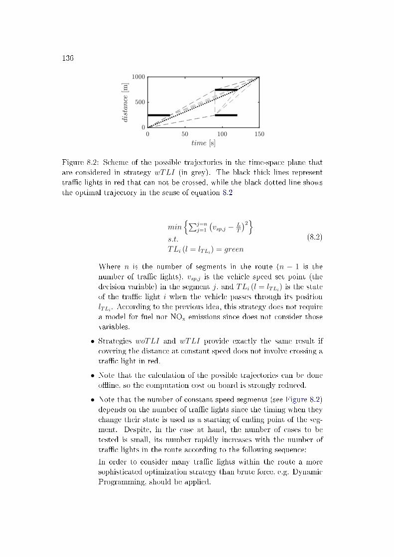
136

Figure 8.2: Scheme of the possible trajectories in the time-space plane thatare considered in strategy wTLI (in grey). The black thick lines representtra�c lights in red that can not be crossed, while the black dotted line showsthe optimal trajectory in the sense of equation 8.2

min{∑j=n

j=1

(vsp,j − L

T

)2}s.t.

TLi (l = lTLi) = green

(8.2)

Where n is the number of segments in the route (n − 1 is thenumber of tra�c lights), vsp,j is the vehicle speed set point (thedecision variable) in the segment j, and TLi (l = lTLi

) is the stateof the tra�c light i when the vehicle passes through its positionlTLi

. According to the previous idea, this strategy does not requirea model for fuel nor NOx emissions since does not consider thosevariables.

• Strategies woTLI and wTLI provide exactly the same result ifcovering the distance at constant speed does not involve crossing atra�c light in red.

• Note that the calculation of the possible trajectories can be doneo�ine, so the computation cost on board is strongly reduced.

• Note that the number of constant speed segments (see Figure 8.2)depends on the number of tra�c lights since the timing when theychange their state is used as a starting of ending point of the seg-ment. Despite, in the case at hand, the number of cases to betested is small, its number rapidly increases with the number oftra�c lights in the route according to the following sequence:

In order to consider many tra�c lights within the route a moresophisticated optimization strategy than brute force, e.g. DynamicProgramming, should be applied.

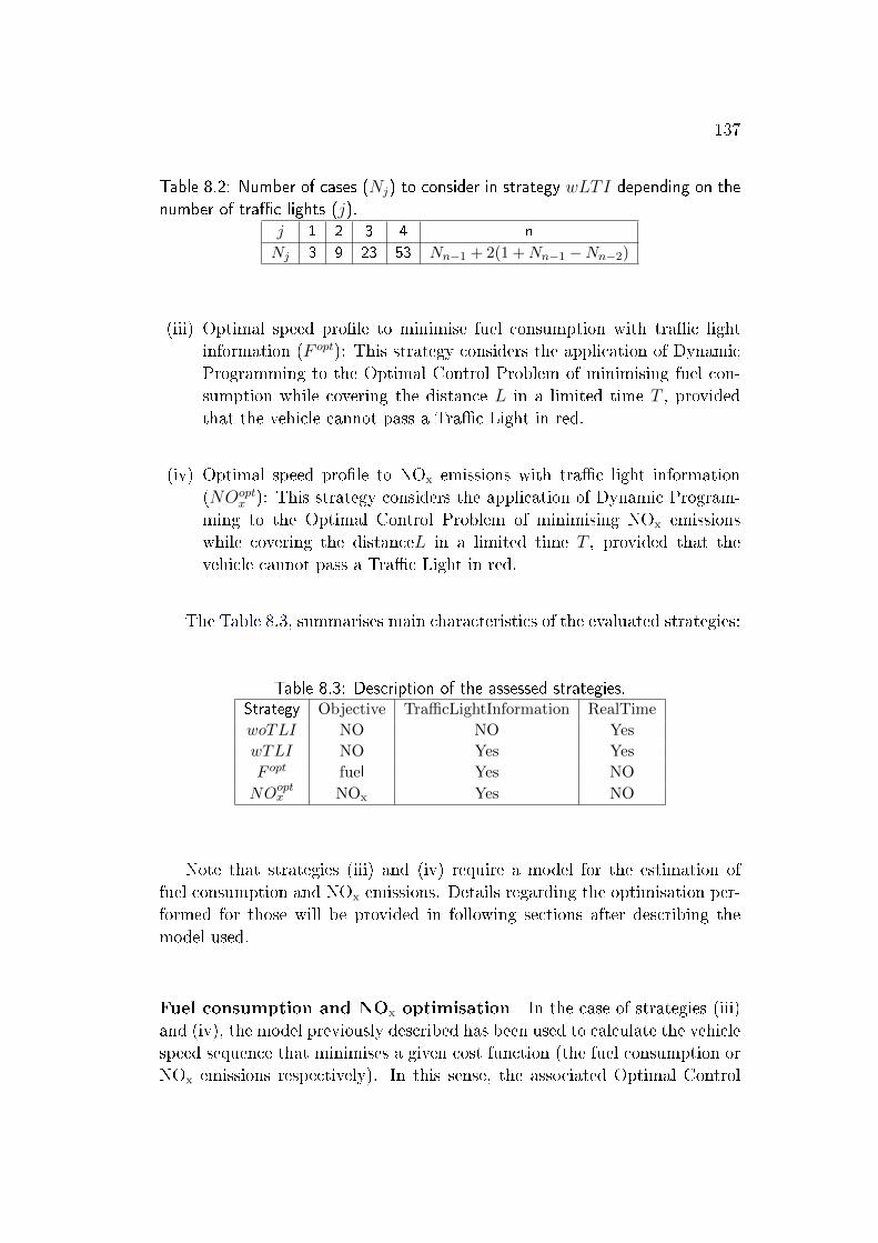
137

Table 8.2: Number of cases (Nj) to consider in strategy wLTI depending on the

number of tra�c lights (j).j 1 2 3 4 n

Nj 3 9 23 53 Nn−1 + 2(1 + Nn−1 −Nn−2)

(iii) Optimal speed pro�le to minimise fuel consumption with tra�c lightinformation (F opt): This strategy considers the application of DynamicProgramming to the Optimal Control Problem of minimising fuel con-sumption while covering the distance L in a limited time T , providedthat the vehicle cannot pass a Tra�c Light in red.

(iv) Optimal speed pro�le to NOx emissions with tra�c light information(NOopt

x ): This strategy considers the application of Dynamic Program-ming to the Optimal Control Problem of minimising NOx emissionswhile covering the distanceL in a limited time T , provided that thevehicle cannot pass a Tra�c Light in red.

The Table 8.3, summarises main characteristics of the evaluated strategies:

Table 8.3: Description of the assessed strategies.Strategy Objective TrafficLightInformation RealTime

woTLI NO NO Yes

wTLI NO Yes Yes

F opt fuel Yes NO

NOoptx NOx Yes NO

Note that strategies (iii) and (iv) require a model for the estimation offuel consumption and NOx emissions. Details regarding the optimisation per-formed for those will be provided in following sections after describing themodel used.

Fuel consumption and NOx optimisation In the case of strategies (iii)and (iv), the model previously described has been used to calculate the vehiclespeed sequence that minimises a given cost function (the fuel consumption orNOx emissions respectively). In this sense, the associated Optimal Control

138

Problem (OCP) can be expressed as:

min{∫ L

0hvdl}

s.t.dvdl

= fv

dtdl

= 1v

v(0) = 0

v(L) = 0

t(0) = 0

t(lTL1) = tgreen,TL1t(lTL2) = tgreen,TL2t(L) ≤ T

(8.3)

Where the function h represents the fuel consumption (Wf ) in the case ofstrategy (iii) or the NOx emissions (WNOx) in case of strategy (iv). Functionf represents equation of vehicle dynamics and tgreen,TLj represents the timerange when the tra�c light j is green. From the OCP presented in Equa-tion 8.3 one can observe that:

• While the typical domain for OCPs is time, in this case, space (l) hasbeen selected since it presents a more natural domain to include con-straints related to tra�c lights whose position is constant. The sameapproach is usually followed when constraints on the road gradient orvehicle speed limits are to be considered [Hellström et al. 2010a]

• The problem de�ned inEquation 8.3 has 2 states (v and t) and onlyone decision variable (upedal). In this sense, as the number of statesand control variables is small, the problem is specially well suited forthe application of Dynamic Programming (DP). In particular, the DPsolver used in this work is a Matlab based code presented in [Sundstrom& Guzzella 2009].

8.1.4 Results

Independently on the availability of information concerning the state of thetra�c lights, the starting time of the route with respect to the tra�c lightperiod, is a variable that is outside of control, at least this is the hypothesisfollowed in this work. In addition, it is obvious that the performance of anygiven strategy will strongly depend on the tra�c light timing, and thereforeon the instant of the tra�c light period in which the travel starts. Accordingto that, in the present work the timing of tra�c lights when the trip startsis considered as a stochastic variable uniformly distributed between 0 and

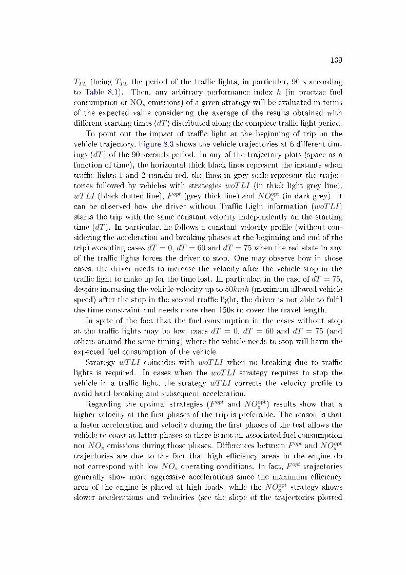
139

TTL (being TTL the period of the tra�c lights, in particular, 90 s accordingto Table 8.1). Then, any arbitrary performance index h (in practise fuelconsumption or NOx emissions) of a given strategy will be evaluated in termsof the expected value considering the average of the results obtained withdi�erent starting times (dT ) distributed along the complete tra�c light period.

To point out the impact of tra�c light at the beginning of trip on thevehicle trajectory, Figure 8.3 shows the vehicle trajectories at 6 di�erent tim-ings (dT ) of the 90 seconds period. In any of the trajectory plots (space as afunction of time), the horizontal thick black lines represent the instants whentra�c lights 1 and 2 remain red, the lines in grey scale represent the trajec-tories followed by vehicles with strategies woTLI (in thick light grey line),wTLI (black dotted line), F opt (grey thick line) and NOopt

x (in dark grey). Itcan be observed how the driver without Tra�c Light information (woTLI)starts the trip with the same constant velocity independently on the startingtime (dT ). In particular, he follows a constant velocity pro�le (without con-sidering the acceleration and breaking phases at the beginning and end of thetrip) excepting cases dT = 0, dT = 60 and dT = 75 when the red state in anyof the tra�c lights forces the driver to stop. One may observe how in thosecases, the driver needs to increase the velocity after the vehicle stop in thetra�c light to make up for the time lost. In particular, in the case of dT = 75,despite increasing the vehicle velocity up to 50kmh (maximum allowed vehiclespeed) after the stop in the second tra�c light, the driver is not able to ful�lthe time constraint and needs more then 150s to cover the travel length.

In spite of the fact that the fuel consumption in the cases without stopat the tra�c lights may be low, cases dT = 0, dT = 60 and dT = 75 (andothers around the same timing) where the vehicle needs to stop will harm theexpected fuel consumption of the vehicle.

Strategy wTLI coincides with woTLI when no breaking due to tra�clights is required. In cases when the woTLI strategy requires to stop thevehicle in a tra�c light, the strategy wTLI corrects the velocity pro�le toavoid hard breaking and subsequent acceleration.

Regarding the optimal strategies (F opt and NOoptx ) results show that a

higher velocity at the �rst phases of the trip is preferable. The reason is thata faster acceleration and velocity during the �rst phases of the test allows thevehicle to coast at latter phases so there is not an associated fuel consumptionnor NOx emissions during those phases. Di�erences between F opt and NOopt

x

trajectories are due to the fact that high e�ciency areas in the engine donot correspond with low NOx operating conditions. In fact, F opt trajectoriesgenerally show more aggressive accelerations since the maximum e�ciencyarea of the engine is placed at high loads, while the NOopt

x strategy showsslower accelerations and velocities (see the slope of the trajectories plotted

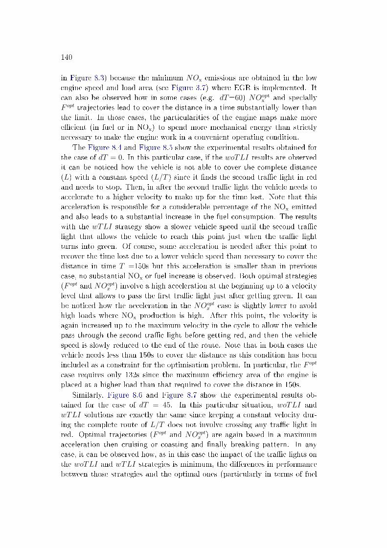
140

in Figure 8.3) because the minimum NOx emissions are obtained in the lowengine speed and load area (see Figure 3.7) where EGR is implemented. Itcan also be observed how in some cases (e.g. dT=60) NOopt

x and speciallyF opt trajectories lead to cover the distance in a time substantially lower thanthe limit. In those cases, the particularities of the engine maps make moree�cient (in fuel or in NOx) to spend more mechanical energy than strictlynecessary to make the engine work in a convenient operating condition.

The Figure 8.4 and Figure 8.5 show the experimental results obtained forthe case of dT = 0. In this particular case, if the woTLI results are observedit can be noticed how the vehicle is not able to cover the complete distance(L) with a constant speed (L/T ) since it �nds the second tra�c light in redand needs to stop. Then, in after the second tra�c light the vehicle needs toaccelerate to a higher velocity to make up for the time lost. Note that thisacceleration is responsible for a considerable percentage of the NOx emittedand also leads to a substantial increase in the fuel consumption. The resultswith the wTLI strategy show a slower vehicle speed until the second tra�clight that allows the vehicle to reach this point just when the tra�c lightturns into green. Of course, some acceleration is needed after this point torecover the time lost due to a lower vehicle speed than necessary to cover thedistance in time T =150s but this acceleration is smaller than in previouscase, no substantial NOx or fuel increase is observed. Both optimal strategies(F opt and NOopt

x ) involve a high acceleration at the beginning up to a velocitylevel that allows to pass the �rst tra�c light just after getting green. It canbe noticed how the acceleration in the NOopt

x case is slightly lower to avoidhigh loads where NOx production is high. After this point, the velocity isagain increased up to the maximum velocity in the cycle to allow the vehiclepass through the second tra�c light before getting red, and then the vehiclespeed is slowly reduced to the end of the route. Note that in both cases thevehicle needs less than 150s to cover the distance as this condition has beenincluded as a constraint for the optimisation problem. In particular, the F opt

case requires only 132s since the maximum e�ciency area of the engine isplaced at a higher load than that required to cover the distance in 150s.

Similarly, Figure 8.6 and Figure 8.7 show the experimental results ob-tained for the case of dT = 45. In this particular situation, woTLI andwTLI solutions are exactly the same since keeping a constant velocity dur-ing the complete route of L/T does not involve crossing any tra�c light inred. Optimal trajectories (F opt and NOopt

x ) are again based in a maximumacceleration then cruising or coasting and �nally breaking pattern. In anycase, it can be observed how, as in this case the impact of the tra�c lights onthe woTLI and wTLI strategies is minimum, the di�erences in performancebetween those strategies and the optimal ones (particularly in terms of fuel

141

0 50 100 1500

250

500

750

10000

250

500

750

10000

250

500

750

10000

250

500

750

10000

250

500

750

10000

250

500

750

1000

Figure 8.3: Vehicle trajectories at 6 di�erent tra�c light timings (dT ). Lightgrey line: trajectory without tra�c light information (woTLI). Black dottedline: trajectory with real time strategy and tra�c light information (wTLI).Thick grey line: trajectory with Dynamic Programming optimisation for min-imum fuel consumption (F opt). Dark grey line: trajectory with DynamicProgramming optimisation for NOx emissions (NOopt

x )

142

Figure 8.4: Experimental results (trajectories in upper plot, velocity pro�lesin second plot, fuel consumption in third plot and NOx emissions in bottomplot) obtained for the case with dT =0s. Light grey line: trajectory withouttra�c light information (woTLI). Black dotted line: trajectory with real timestrategy and tra�c light information (wTLI). Thick grey line: trajectory withDynamic Programming optimisation for minimum fuel consumption (F opt).Dark grey line: trajectory with Dynamic Programming optimisation for NOx

emissions (NOoptx ).

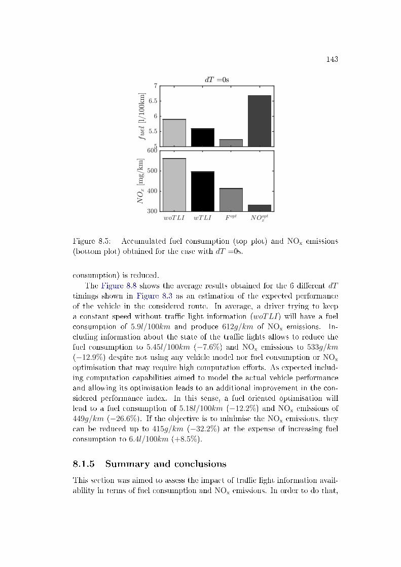
143

Figure 8.5: Accumulated fuel consumption (top plot) and NOx emissions(bottom plot) obtained for the case with dT =0s.

consumption) is reduced.The Figure 8.8 shows the average results obtained for the 6 di�erent dT

timings shown in Figure 8.3 as an estimation of the expected performanceof the vehicle in the considered route. In average, a driver trying to keepa constant speed without tra�c light information (woTLI) will have a fuelconsumption of 5.9l/100km and produce 612g/km of NOx emissions. In-cluding information about the state of the tra�c lights allows to reduce thefuel consumption to 5.45l/100km (−7.6%) and NOx emissions to 533g/km

(−12.9%) despite not using any vehicle model nor fuel consumption or NOx

optimisation that may require high computation e�orts. As expected includ-ing computation capabilities aimed to model the actual vehicle performanceand allowing its optimisation leads to an additional improvement in the con-sidered performance index. In this sense, a fuel oriented optimisation willlead to a fuel consumption of 5.18l/100km (−12.2%) and NOx emissions of449g/km (−26.6%). If the objective is to minimise the NOx emissions, theycan be reduced up to 415g/km (−32.2%) at the expense of increasing fuelconsumption to 6.4l/100km (+8.5%).

8.1.5 Summary and conclusions

This section was aimed to assess the impact of tra�c light information avail-ability in terms of fuel consumption and NOx emissions. In order to do that,

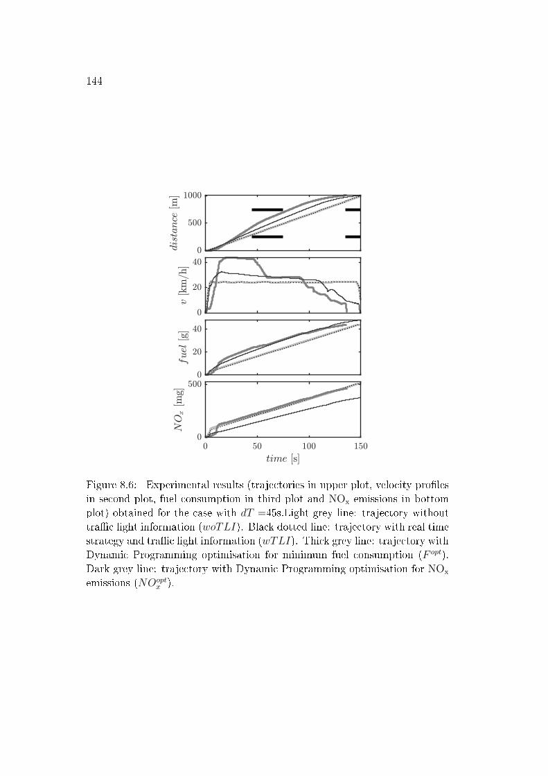
144

Figure 8.6: Experimental results (trajectories in upper plot, velocity pro�lesin second plot, fuel consumption in third plot and NOx emissions in bottomplot) obtained for the case with dT =45s.Light grey line: trajectory withouttra�c light information (woTLI). Black dotted line: trajectory with real timestrategy and tra�c light information (wTLI). Thick grey line: trajectory withDynamic Programming optimisation for minimum fuel consumption (F opt).Dark grey line: trajectory with Dynamic Programming optimisation for NOx

emissions (NOoptx ).

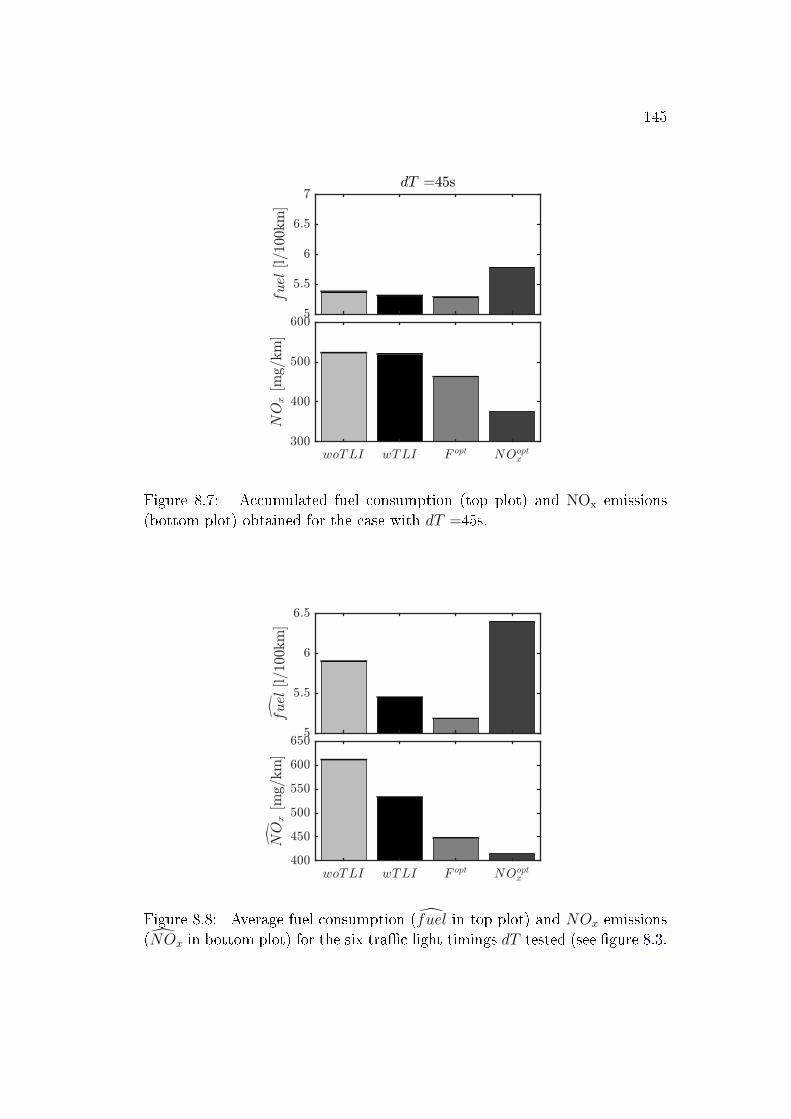
145

Figure 8.7: Accumulated fuel consumption (top plot) and NOx emissions(bottom plot) obtained for the case with dT =45s.

Figure 8.8: Average fuel consumption (fuel in top plot) and NOx emissions(NOx in bottom plot) for the six tra�c light timings dT tested (see �gure 8.3.

146

a non-linear dynamic vehicle model is developed to evaluate the performanceof a vehicle in terms of fuel consumption and NOx emissions in a route withdi�erent scenarios of information about the state of the tra�c lights. In par-ticular, three cases are studied: the case without information about the stateof the tra�c lights, a case where the state of the tra�c lights is known butsuboptimal strategies have to be used due to computation capabilities lim-itations and �nally the case where the state of tra�c lights is known andthere are not computation limitations, so optimal control (DP) can be used.Previous strategies have been used with fuel consumption and with NOx asoptimisation objectives to check the impact of the solution on both parame-ters. The obtained trajectories have been evaluated experimentally in a chassisdynamometer with a Euro5 Diesel light duty vehicle.

8.2 Online vehicle speed advisor

8.2.1 Introduction and problem description

In the same line that the last work, the target of the present study is toexplore the potential of speed pro�le optimisation in real driving conditions,by assessing the suitability of an application which recommends the driverthe optimal vehicle speed sequence that minimises the fuel consumption for aparticular route. To this aim, there are three main aspects to consider:

• The route: The optimal vehicle speed pro�le is route-dependent. In a�nal application, information about the route should be a priori availableto allow the optimal trajectory computation.

• Model and optimisation tool: In order to provide any advice to thedriver about the vehicle speed pro�le that minimises fuel consumption,a model able to estimate in advance the impact of driver decisions andparticularly of the vehicle speed on fuel consumption is required. Thismodel in combination with an optimisation tool allows to compute theoptimal speed pro�le to be followed.

• Driver advisor: The computed optimal speed trajectory should be trans-mitted to the driver that will follow it in the best way possible. In thesame way, the optimal speed trajectory should be continuously updatedto make up for the deviations of the actual driving speed from the op-timal pro�le.

This application deals with minimisation of fuel consumption under real driv-ing conditions using a vehicle speed advisor. The aim is to explore the po-tential of speed pro�le optimisation in real driving conditions while assessing

147

the suitability of an application which recommends the driver the optimalvehicle speed sequence that minimises the fuel consumption on a particularroute. The speed advisor is based on solving the Optimal Control problemof covering a particular route with minimum fuel consumption with a de�nedtime constraint. The approach presented was applied to and implemented ona real passenger vehicle to obtain a trade-o� between fuel consumption andtravel time for several trips on the route. Experimental results are presentedwith and without advisory, demonstrating that with speed advisor the resultsapproach the pareto front with lesser dispersion on the other hand withoutadvisory the dispersion is higher and largely above the Pareto front. In thepresented work, a particular route between two cities has been selected for theoptimisation. The route consists mainly on highway driving with presence ofspeed limits and altitude variations but limited tra�c and no vehicle stops.The route has been covered several times in order to identify an energy modelof the vehicle and characterize the route. Then, the optimal control problemof covering the route with minimum fuel consumption in a given time has beensolved by DP for di�erent time constraints in order to assess the compromisebetween fuel consumption and trip time. The optimal vehicle speed is passedwith a display to the driver as a reference to minimise fuel consumption. De-spite the high computation cost and curse of dimensionality of DP, it allowsstoring not only the optimal control between initial and �nal states, but theoptimal control sequence between any state contained in the feasible set andthe �nal one. This property is used in the present work to correct any devi-ation from the optimal speed pro�le, due to non-considered disturbances orlack of accuracy of the driver.

8.2.2 Method description

The aim of this work is to explore the potential of speed pro�le optimisationin real driving conditions by means of a driving advisor application. In orderto provide advice to the driver, a sensible possibility is to compute what isthe velocity pro�le to minimize a given cost function and then provide thisinformation to the driver. Regarding the speed pro�le computation, the fuelconsumption is an intuitive cost function while the time spent during thetrip seems a sensible constraint. Other restrictions that should be taken intoaccount are the speed limits during the route or the limits of the vehicle andthe powertrain. In any case, a generic control problem consisting in �nding thecontrol policy to drive a dynamic system from a given initial state to a de�ned�nal state with minimum cost and ful�lling a set of constraints �ts in the �eldof Optimal Control. The formulation of an Optimal Control Problem (OCP)considers a cost index and constraints expressed in terms of system states

148

(x), system actuators (u), problem disturbances (w) and domain. Taking intoaccount that, in the case at hand, the route is a priori known, the slope andspeed limits (which are the problem disturbances) are space (s) dependent, itseems more convenient to consider s as the problem domain. In this case, thecost index can be de�ned as:

J =

∫ L

0

mf

vds (8.4)

where L is the route length and for the sake of readability, the dependenceof the fuel consumption on the actuator (up) has been omitted. The system,i.e the vehicle model described in chapter 3 can be condensed in the genericdynamic system:

x = f(x, u, w, t) (8.5)

Where the dependence of the state (velocity) evolution on the state itself, thecontrol actions (in the case at hand u), disturbance (road slope) and time isdescribed. Therefore, the state evolution with the problem domain (space)becomes:

dx

ds=f

v(8.6)

Where the dependence of f on the system state, actions and disturbances hasbeen omitted for the sake of clarity.

The vehicle should cover the de�ned distance (L) within a given time (T ),which leads to the following integral constraint:∫ L

0

1

vds ≤ T (8.7)

Road speed limits have to be respected which leads to the following pathconstraint:

v(s) ≤ v(s) (8.8)

Limits on the engine (speed range and maximum power output) and brakes(maximum braking force) are also considered. Finally, the initial speed is alsoimposed. Despite the vehicle starts from rest a minimum vehicle speed isimposed to avoid divisions by 0 in the model (boundary constraint):

v(0) = v (8.9)

Regarding �nal speed, no restrictions are imposed beyond the maximum speedof the road.

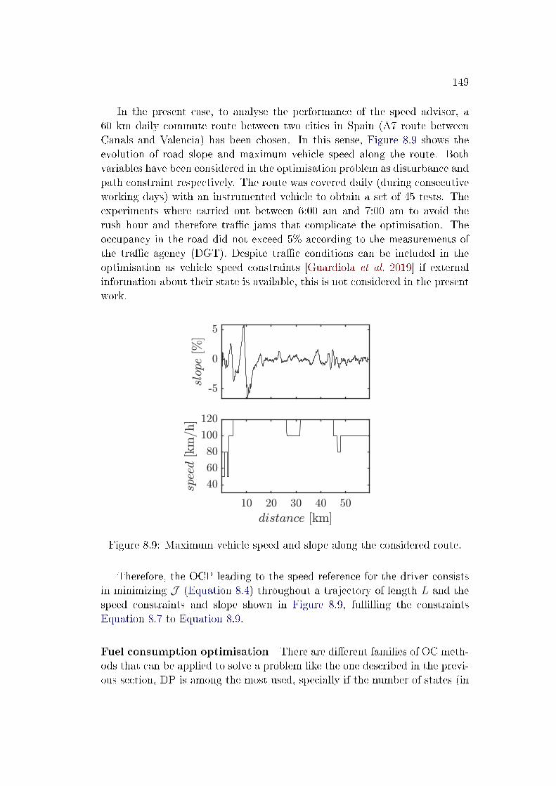
149

In the present case, to analyse the performance of the speed advisor, a60 km daily commute route between two cities in Spain (A7 route betweenCanals and Valencia) has been chosen. In this sense, Figure 8.9 shows theevolution of road slope and maximum vehicle speed along the route. Bothvariables have been considered in the optimisation problem as disturbance andpath constraint respectively. The route was covered daily (during consecutiveworking days) with an instrumented vehicle to obtain a set of 45 tests. Theexperiments where carried out between 6:00 am and 7:00 am to avoid therush hour and therefore tra�c jams that complicate the optimisation. Theoccupancy in the road did not exceed 5% according to the measurements ofthe tra�c agency (DGT). Despite tra�c conditions can be included in theoptimisation as vehicle speed constraints [Guardiola et al. 2019] if externalinformation about their state is available, this is not considered in the presentwork.

Figure 8.9: Maximum vehicle speed and slope along the considered route.

Therefore, the OCP leading to the speed reference for the driver consistsin minimizing J (Equation 8.4) throughout a trajectory of length L and thespeed constraints and slope shown in Figure 8.9, ful�lling the constraintsEquation 8.7 to Equation 8.9.

Fuel consumption optimisation There are di�erent families of OC meth-ods that can be applied to solve a problem like the one described in the previ-ous section, DP is among the most used, specially if the number of states (in

150

the case at hand 1) and actuators (also 1) remains low. The DP algorithmis the numerical implementation of the Hamilton-Jacobi-Bellman equationwhich is a su�cient condition for a global optimum in an OCP. The methodis based on the discretization of the domain (S) in N steps, and also the statespace (X) and control space (U) to build a set of possible trajectories betweenthe de�ned boundary conditions. Then, a cost to go function J such that:

J(xk, sk) = minu{L(X,U, sk) + J(xk+1, sk+1)} (8.10)

Where k = 0, ..., N − 1 and L is the cost in a given step (term inside theintegral in Equation 8.4), is calculated backwards in order to represent theminimal cost to reach a suitable terminal state from any feasible state attime-step k.

The model used in the present work has only one state (v) and one ac-tuator (u), nevertheless, the time constraint represented by Equation 8.7 hasto be handled. Since the problem does not explicitly depend on time, thetime restriction can be addressed adding it to the cost function and using aweighting factor (α) that balances between fuel consumption and time:

L′ = mf

v+ α∆t (8.11)

where ∆t is the time needed to cover a step in the space discretization. Then,the DP can be applied with only one state, but a shooting method should beapplied to �nd the proper value of α that allows to ful�l the integral constraintin Equation 8.7. The alternative used in this work is to consider time as asecond state, in order to compute its evolution and assure that constraint inEquation 8.7 is hold. In this last case, the number of states of the problemincreases to 2. Note that despite issues such as the curse of dimensionality, therecursive nature of DP allows it to compute not only the optimal trajectorybut a set of optimal trajectories from any state in the feasible state space Xat any instant k. This feature is specially interesting to implement a closeloop advise on the driver that allows him to make up for any deviation fromthe optimal trajectory due to disturbances not considered in the optimizationor due to the lack of accuracy in his driving when trying to follow the advisedtrajectory. Of course, this is only possible if constraint in Equation 8.7 isaddressed by considering time as a state of the problem.

The Table 8.4 shows the settings used in the DP algorithm, and as an in-dicative number of the computation burden, the simulation of one route takes1 hour in a standard laptop (Intel(R) Core(TM) i7-8550U CPU @ 1.8GHzand 8GB RAM).

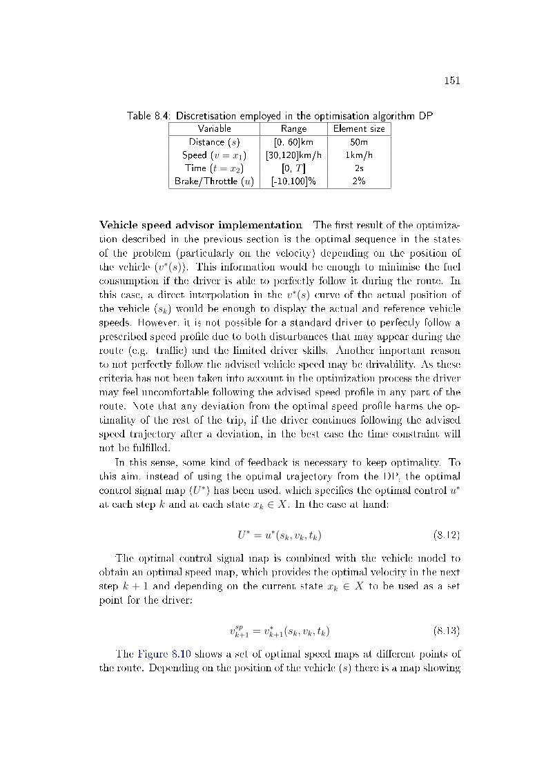
151

Table 8.4: Discretisation employed in the optimisation algorithm DPVariable Range Element size

Distance (s) [0, 60]km 50m

Speed (v = x1) [30,120]km/h 1km/h

Time (t = x2) [0, T ] 2s

Brake/Throttle (u) [-10,100]% 2%

Vehicle speed advisor implementation The �rst result of the optimiza-tion described in the previous section is the optimal sequence in the statesof the problem (particularly on the velocity) depending on the position ofthe vehicle (v∗(s)). This information would be enough to minimise the fuelconsumption if the driver is able to perfectly follow it during the route. Inthis case, a direct interpolation in the v∗(s) curve of the actual position ofthe vehicle (sk) would be enough to display the actual and reference vehiclespeeds. However, it is not possible for a standard driver to perfectly follow aprescribed speed pro�le due to both disturbances that may appear during theroute (e.g. tra�c) and the limited driver skills. Another important reasonto not perfectly follow the advised vehicle speed may be drivability. As thesecriteria has not been taken into account in the optimization process the drivermay feel uncomfortable following the advised speed pro�le in any part of theroute. Note that any deviation from the optimal speed pro�le harms the op-timality of the rest of the trip, if the driver continues following the advisedspeed trajectory after a deviation, in the best case the time constraint willnot be ful�lled.

In this sense, some kind of feedback is necessary to keep optimality. Tothis aim, instead of using the optimal trajectory from the DP, the optimalcontrol signal map (U∗) has been used, which speci�es the optimal control u∗

at each step k and at each state xk ∈ X. In the case at hand:

U∗ = u∗(sk, vk, tk) (8.12)

The optimal control signal map is combined with the vehicle model toobtain an optimal speed map, which provides the optimal velocity in the nextstep k + 1 and depending on the current state xk ∈ X to be used as a setpoint for the driver:

vspk+1 = v∗k+1(sk, vk, tk) (8.13)

The Figure 8.10 shows a set of optimal speed maps at di�erent points ofthe route. Depending on the position of the vehicle (s) there is a map showing

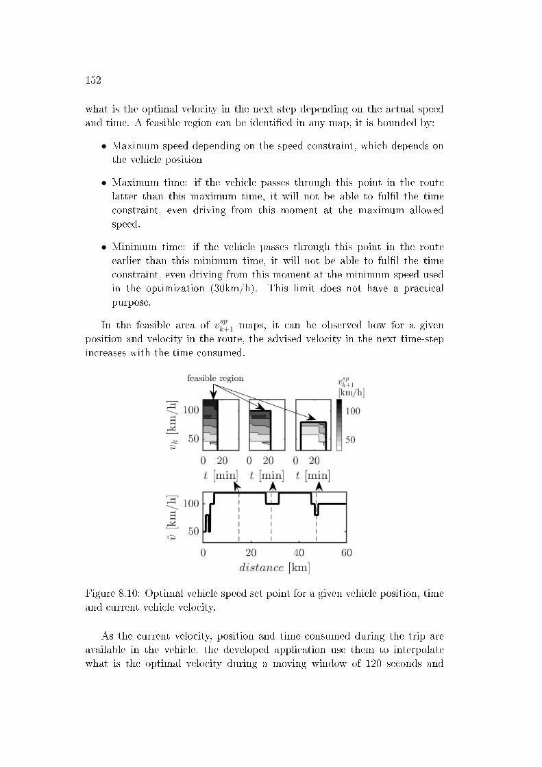
152

what is the optimal velocity in the next step depending on the actual speedand time. A feasible region can be identi�ed in any map, it is bounded by:

• Maximum speed depending on the speed constraint, which depends onthe vehicle position

• Maximum time: if the vehicle passes through this point in the routelatter than this maximum time, it will not be able to ful�l the timeconstraint, even driving from this moment at the maximum allowedspeed.

• Minimum time: if the vehicle passes through this point in the routeearlier than this minimum time, it will not be able to ful�l the timeconstraint, even driving from this moment at the minimum speed usedin the optimization (30km/h). This limit does not have a practicalpurpose.

In the feasible area of vspk+1 maps, it can be observed how for a givenposition and velocity in the route, the advised velocity in the next time-stepincreases with the time consumed.

Figure 8.10: Optimal vehicle speed set point for a given vehicle position, timeand current vehicle velocity.

As the current velocity, position and time consumed during the trip areavailable in the vehicle, the developed application use them to interpolatewhat is the optimal velocity during a moving window of 120 seconds and

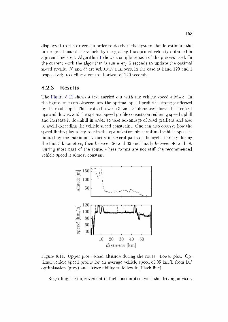
153

displays it to the driver. In order to do that, the system should estimate thefuture positions of the vehicle by integrating the optimal velocity obtained ina given time step. Algorithm 1 shows a simple version of the process used. Inthe current work the algorithm is run every 5 seconds to update the optimalspeed pro�le. N and δt are arbitrary numbers, in the case at hand 120 and 1respectively to de�ne a control horizon of 120 seconds.

8.2.3 Results

The Figure 8.11 shows a test carried out with the vehicle speed advisor. Inthe �gure, one can observe how the optimal speed pro�le is strongly a�ectedby the road slope. The stretch between 3 and 15 kilometres shows the steepestups and downs, and the optimal speed pro�le consists on reducing speed uphilland increase it downhill in order to take advantage of road gradient and alsoto avoid exceeding the vehicle speed constraint. One can also observe how thespeed limits play a key role in the optimization since optimal vehicle speed islimited by the maximum velocity in several parts of the cycle, namely duringthe �rst 3 kilometres, then between 26 and 32 and �nally between 46 and 48.During most part of the route, where ramps are not sti� the recommendedvehicle speed is almost constant.

Altitude

Figure 8.11: Upper plot: Road altitude during the route. Lower plot: Op-timal vehicle speed pro�le for an average vehicle speed of 95 km/h from DPoptimisation (grey) and driver ability to follow it (black line).

Regarding the improvement in fuel consumption with the driving advisor,

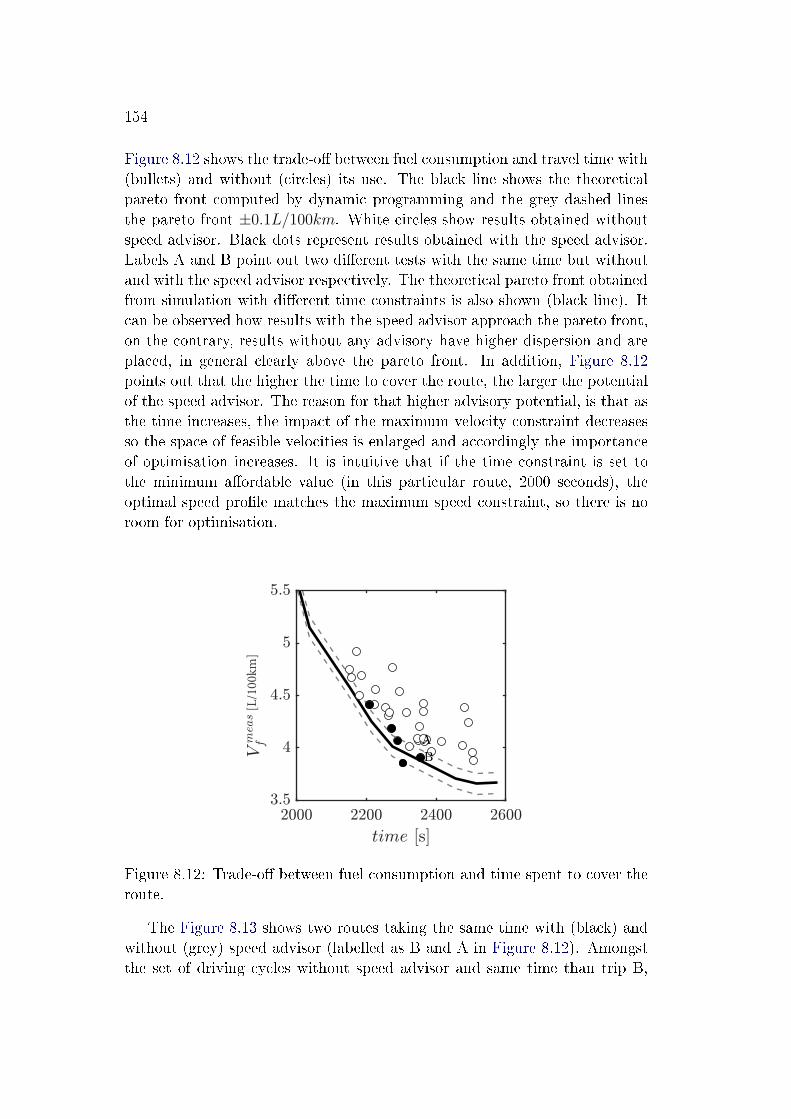
154

Figure 8.12 shows the trade-o� between fuel consumption and travel time with(bullets) and without (circles) its use. The black line shows the theoreticalpareto front computed by dynamic programming and the grey dashed linesthe pareto front ±0.1L/100km. White circles show results obtained withoutspeed advisor. Black dots represent results obtained with the speed advisor.Labels A and B point out two di�erent tests with the same time but withoutand with the speed advisor respectively. The theoretical pareto front obtainedfrom simulation with di�erent time constraints is also shown (black line). Itcan be observed how results with the speed advisor approach the pareto front,on the contrary, results without any advisory have higher dispersion and areplaced, in general clearly above the pareto front. In addition, Figure 8.12points out that the higher the time to cover the route, the larger the potentialof the speed advisor. The reason for that higher advisory potential, is that asthe time increases, the impact of the maximum velocity constraint decreasesso the space of feasible velocities is enlarged and accordingly the importanceof optimisation increases. It is intuitive that if the time constraint is set tothe minimum a�ordable value (in this particular route, 2000 seconds), theoptimal speed pro�le matches the maximum speed constraint, so there is noroom for optimisation.

[L/100km

]

Figure 8.12: Trade-o� between fuel consumption and time spent to cover theroute.

The Figure 8.13 shows two routes taking the same time with (black) andwithout (grey) speed advisor (labelled as B and A in Figure 8.12). Amongstthe set of driving cycles without speed advisor and same time than trip B,

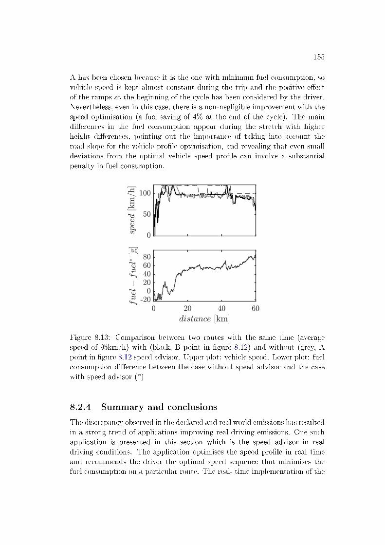
155

A has been chosen because it is the one with minimum fuel consumption, sovehicle speed is kept almost constant during the trip and the positive e�ectof the ramps at the beginning of the cycle has been considered by the driver.Nevertheless, even in this case, there is a non-negligible improvement with thespeed optimisation (a fuel saving of 4% at the end of the cycle). The maindi�erences in the fuel consumption appear during the stretch with higherheight di�erences, pointing out the importance of taking into account theroad slope for the vehicle pro�le optimisation, and revealing that even smalldeviations from the optimal vehicle speed pro�le can involve a substantialpenalty in fuel consumption.

Figure 8.13: Comparison between two routes with the same time (averagespeed of 95km/h) with (black, B point in �gure 8.12) and without (grey, Apoint in �gure 8.12 speed advisor. Upper plot: vehicle speed. Lower plot: fuelconsumption di�erence between the case without speed advisor and the casewith speed advisor (*)

8.2.4 Summary and conclusions

The discrepancy observed in the declared and real world emissions has resultedin a strong trend of applications improving real driving emissions. One suchapplication is presented in this section which is the speed advisor in realdriving conditions. The application optimises the speed pro�le in real timeand recommends the driver the optimal speed sequence that minimises thefuel consumption on a particular route. The real- time implementation of the

156

application shows the possibility to stay very close to the Pareto front. This ismajorly possible because the developed application allows storing not only theoptimal control between the initial and the �nal states, but also the optimalcontrol sequence between any state contained in the feasible set and the �nalone. This property is used as a feedback to correct any deviation from theoptimal speed pro�le, due to non-considered disturbances or lack of accuracyof the driver. The study also points out a strong dependence of optimal speedpro�le on road slope and vehicle speed constraint.

In particular, with the proposed application fuel consumption can be im-proved up to 4% without any penalty in travel time. Given the increasing useof information systems, which can lead to some degree of a priori knowledgeof the vehicle speed trajectory, the results presented a step forward in under-standing the potential of online optimization methods in advising the driverto save fuel in real driving conditions.

Chapter 9

Assessment of driving dynamics in

RDE test on NOx emission

dispersion

Contents

9.1 Introduction and problem description . . . . . . . . . 157

9.2 Method description . . . . . . . . . . . . . . . . . . . . 160

9.3 Results . . . . . . . . . . . . . . . . . . . . . . . . . . . . 164

9.4 Summary and conclusion . . . . . . . . . . . . . . . . . 167

9.1 Introduction and problem description

The EU6D emission regulation intends to bridge the gap between laboratorytests and the real driving conditions by the introduction of RDE testing. Itrequires the measurement of RDE as an additional type approval test in orderto take into account the in�uence of the road pro�le, ambient conditions andtra�c situations. An important amendment was included in Commission reg-ulation (EU) 2016/646, limiting the driving dynamics and hence avoiding thebiased testing of the vehicle. The emission measurement under real drivingconditions pose a major challenge for OEMs since the situational environmen-tal conditions such as temperature, tra�c and the behaviour of the driver arenot reproducible. As to investigate in�uences of hardware and software on theemission performance, constant or at least, reproducible conditions are neces-sary. The challenges in meeting RDE requirements are most pressing in early

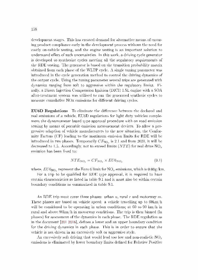
158

development stages. This has created demand for alternative means of ensur-ing product compliance early in the development process without the need forcostly on-vehicle testing, and the engine testing is an important solution tounderstand e�ect of such uncertainties. In this work, a driving cycle generatoris developed to synthesize cycles meeting all the regulatory requirements ofthe RDE testing. The generator is based on the transition probability matrixobtained from each phase of the WLTP cycle. A single tuning parameter wasintroduced in the cycle generation method to control the driving dynamics ofthe output cycle. Using the tuning parameter several trips are generated withdynamics ranging from soft to aggressive within the regulatory limits. Fi-nally, a Direct Injection Compression Ignition (DICI) 1.5L engine with a SOAafter-treatment system was utilised to run the generated synthetic cycles tomeasure cumulative NOx emissions for di�erent driving cycles.

EU6D Regulations To eliminate the di�erence between the declared andreal emissions of a vehicle, EU6D regulations for light duty vehicles comple-ment the dynamometer based type approval procedure with on road emissiontesting by means of portable emission measurement devices. To allow a pro-gressive adaption of vehicle manufacturers to the new situation, the Confor-mity Factors (CF) leading to the maximum emission limits for RDE will beintroduced in two phases. Temporarily CFNOx is 2.1 and from 2020, it will bedecreased to 1.5. Accordingly, not to exceed limits (NTE) for real drive NOx

emission has been �xed to:

NTENOx = CFNOx × EU6NOx (9.1)

where, EU6NOx represent the Euro 6 limit for NOx emissions, which is 0.08g/km.For a trip to be quali�ed for RDE type approval, it is required to have

certain characteristics as listed in table 9.1 and it must also be within certainboundary conditions as summarized in table 9.1.

An RDE trip must cover three phases: urban u, rural r and motorway m.These phases are based on vehicle speed: a vehicle travelling up to 60km/hwill be considered to be operating in urban conditions; at 60 to 90 km/h inrural and above 90km/h in motorway conditions. The trip is then binned (inphases) for assessment of the dynamics in each phase. The RDE regulation asin the document [201 2016], de�nes a lower and an upper boundary conditionfor the driving dynamics in each phase. This is in order to ensure that thevehicle is not driven in an excessively soft or aggressive style.

An excessively soft driving that would lead too low and non-realistic NOx

emissions is eliminated by lower boundary limits de�ned for Relative Positive

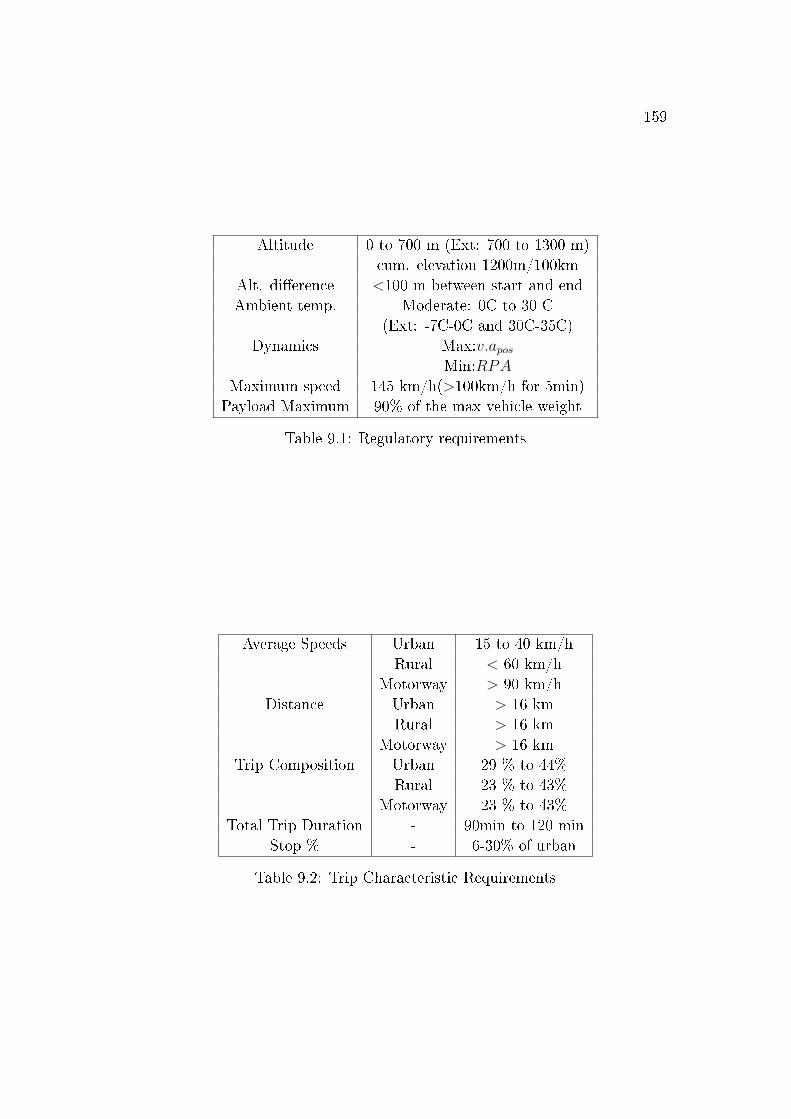
159

Altitude 0 to 700 m (Ext: 700 to 1300 m)cum. elevation 1200m/100km

Alt. di�erence <100 m between start and endAmbient temp. Moderate: 0C to 30 C

(Ext: -7C-0C and 30C-35C)Dynamics Max:v.apos

Min:RPAMaximum speed 145 km/h(>100km/h for 5min)Payload Maximum 90% of the max vehicle weight

Table 9.1: Regulatory requirements

Average Speeds Urban 15 to 40 km/hRural < 60 km/h

Motorway > 90 km/hDistance Urban > 16 km

Rural > 16 kmMotorway > 16 km

Trip Composition Urban 29 % to 44%Rural 23 % to 43%

Motorway 23 % to 43%Total Trip Duration - 90min to 120 min

Stop % - 6-30% of urban

Table 9.2: Trip Characteristic Requirements

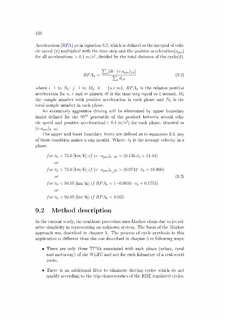
160

Acceleration (RPA) as in equation 9.2, which is de�ned as the integral of vehi-cle speed (v) multiplied with the time step and the positive acceleration(apos)for all accelerations > 0.1m/s2, divided by the total distance of the cycle(d).

RPAk =

∑j[dt · (v.apos)j,k]∑

i di,k(9.2)

where i=1 to Nk; j=1 to Mk; k = {u,r,m}, RPAk is the relative positiveacceleration for u, r and m phases, dt is the time step equal to 1 second, Mk

the sample number with positive acceleration in each phase and Nk is thetotal sample number in each phase.

An excessively aggressive driving will be eliminated by upper boundarylimits de�ned for the 95th percentile of the product between actual vehi-cle speed and positive acceleration(> 0.1 m/s2) for each phase, denoted as(v.apos)k_95.

The upper and lower boundary limits are de�ned as in equations 9.3, anyof these condition makes a trip invalid. Where, vk is the average velocity in aphase.

for vk < 74.6 [km/h]; if (v · apos)k_95 > (0.136.vk + 14.44)

or

for vk > 74.6 [km/h]; if (v · apos)k_95 > (0.0742 · vk + 18.966)

or

for vk < 94.05 [km/h]; if RPAk < (−0.0016 · vk + 0.1755)

or

for vk > 94.05 [km/h]; if RPAk < 0.025

(9.3)

9.2 Method description

In the current study, the synthesis procedure uses Markov chain due to its rel-ative simplicity in representing an unknown system. The basis of the Markovapproach was described in chapter 5. The process of cycle synthesis in thisapplication is di�erent than the one described in chapter 5 in following ways:

• There are only three TPMs associated with each phase (urban, ruraland motorway) of the WLTC and not for each kilometre of a real-worldroute.

• There is an additional �lter to eliminate driving cycles which do notqualify according to the trip characterstics of the RDE regulated cycles.

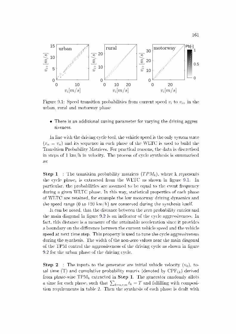
161

0 100

5

10

15

0 10 200

10

20

0 200

10

20

30

0

0.5

1Pb[-]

Figure 9.1: Speed transition probabilities from current speed vi to vi+ in theurban, rural and motorway phase

• There is an additional tuning parameter for varying the driving aggres-siveness.

In line with the driving cycle tool, the vehicle speed is the only system state(xn = vn) and its sequence in each phase of the WLTC is used to build theTransition Probability Matrices. For practical reasons, the data is discretisedin steps of 1 km/h in velocity. The process of cycle synthesis is summarisedas:

Step 1 : The transition probability matrices (TPMk), where k representsthe cycle phase, is extracted from the WLTC as shown in �gure 9.1. Inparticular, the probabilities are assumed to be equal to the event frequencyduring a given WLTC phase. In this way, statistical properties of each phaseof WLTC are retained, for example the low motorway driving dynamics andthe speed range (0 to 120 km/h) are conserved during the synthesis itself.

It can be noted, that the distance between the zero probability entries andthe main diagonal in �gure 9.2 is an indicator of the cycle aggressiveness. Infact, this distance is a measure of the attainable acceleration since it providesa boundary on the di�erence between the current vehicle speed and the vehiclespeed at next time step. This property is used to tune the cycle aggressivenessduring the synthesis. The width of the non-zero values near the main diagonalof the TPM control the aggressiveness of the driving cycle as shown in �gure9.2 for the urban phase of the driving cycle.

Step 2 : The inputs to the generator are initial vehicle velocity (v0), to-tal time (T) and cumulative probability matrix (denoted by CPFi,k) derivedfrom phase-wise TPMk extracted in Step 1. The generator randomly allotsa time for each phase, such that

∑k=u,r,m tk = T and ful�lling with composi-

tion requirements in table 2. Then the synthesis of each phase is dealt with

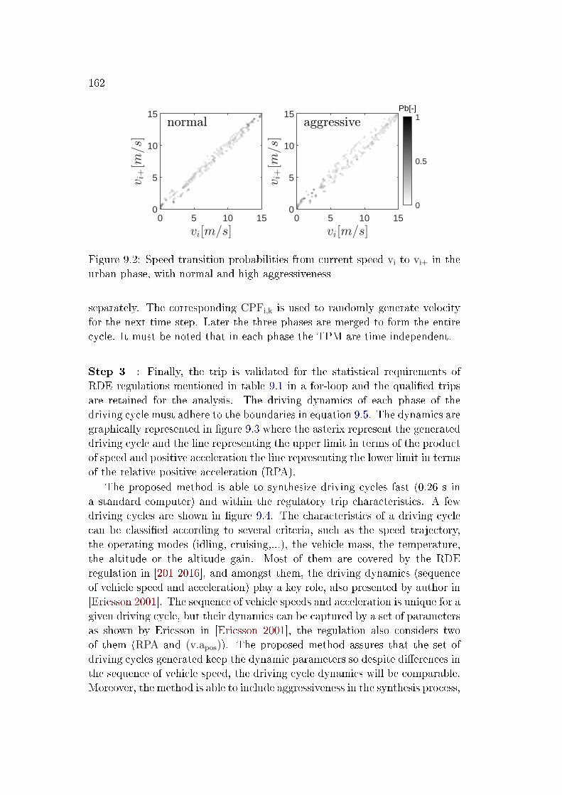
162

0 5 10 150

5

10

15

0 5 10 150

5

10

15

0

0.5

1Pb[-]

Figure 9.2: Speed transition probabilities from current speed vi to vi+ in theurban phase, with normal and high aggressiveness

separately. The corresponding CPFi,k is used to randomly generate velocityfor the next time step. Later the three phases are merged to form the entirecycle. It must be noted that in each phase the TPM are time independent.

Step 3 : Finally, the trip is validated for the statistical requirements ofRDE regulations mentioned in table 9.1 in a for-loop and the quali�ed tripsare retained for the analysis. The driving dynamics of each phase of thedriving cycle must adhere to the boundaries in equation 9.5. The dynamics aregraphically represented in �gure 9.3 where the asterix represent the generateddriving cycle and the line representing the upper limit in terms of the productof speed and positive acceleration the line representing the lower limit in termsof the relative positive acceleration (RPA).

The proposed method is able to synthesize driving cycles fast (0.26 s ina standard computer) and within the regulatory trip characteristics. A fewdriving cycles are shown in �gure 9.4. The characteristics of a driving cyclecan be classi�ed according to several criteria, such as the speed trajectory,the operating modes (idling, cruising,...), the vehicle mass, the temperature,the altitude or the altitude gain. Most of them are covered by the RDEregulation in [201 2016], and amongst them, the driving dynamics (sequenceof vehicle speed and acceleration) play a key role, also presented by author in[Ericsson 2001]. The sequence of vehicle speeds and acceleration is unique for agiven driving cycle, but their dynamics can be captured by a set of parametersas shown by Ericsson in [Ericsson 2001], the regulation also considers twoof them (RPA and (v.apos)). The proposed method assures that the set ofdriving cycles generated keep the dynamic parameters so despite di�erences inthe sequence of vehicle speed, the driving cycle dynamics will be comparable.Moreover, the method is able to include aggressiveness in the synthesis process,

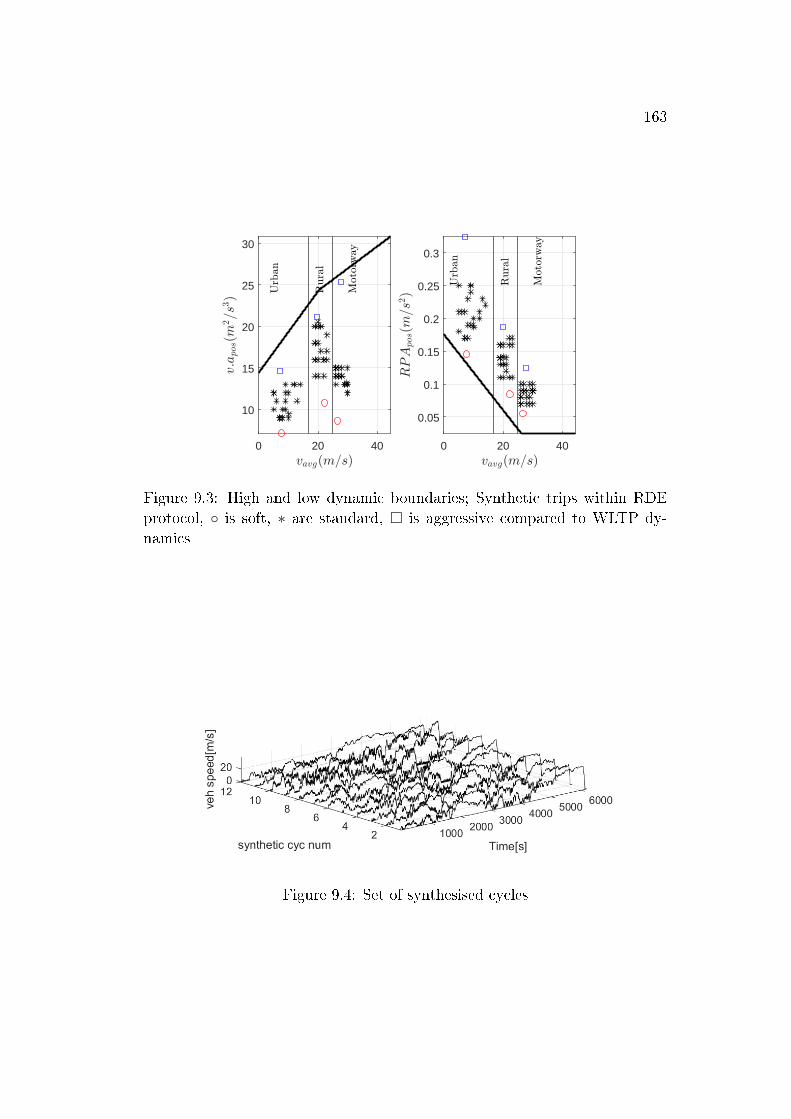
163

0 20 40

10

15

20

25

30

0 20 40

0.05

0.1

0.15

0.2

0.25

0.3

Figure 9.3: High and low dynamic boundaries; Synthetic trips within RDEprotocol, ◦ is soft, ∗ are standard, � is aggressive compared to WLTP dy-namics

Figure 9.4: Set of synthesised cycles

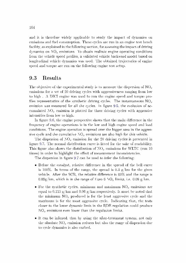
164

and it is therefore widely applicable to study the impact of dynamics onemissions and fuel consumption. These cycles are run in an engine test benchfacility, as explained in the following section, for assessing the impact of drivingdynamics on NOx emissions. To obtain realistic engine operating conditionsfrom the vehicle speed pro�les, a validated vehicle backward model based onlongitudinal vehicle dynamics was used. The obtained trajectories of enginespeed and torque are run on the following engine test setup.

9.3 Results

The objective of the experimental study is to measure the dispersion of NOx

emissions for a set of 20 driving cycles with aggressiveness ranging from lowto high . A DICI engine was used to run the engine speed and torque pro-�les representative of the synthetic driving cycles. The instantaneous NOx

emission was measured for all the cycles. In �gure 9.5, the evolution of ac-cumulated NOx emission is plotted for three driving cycles with aggressiveintensities from low to high.

In �gure 9.6, the engine perspective shows that the main di�erence in thefrequency of engine operations is in the low and high engine speed and loadconditions. The engine operation is spread over the bigger area in the aggres-sive cycle and the cumulative NOx emissions are also high for this vehicle.

The dispersion of NOx emission for the 20 driving cycles is presented in�gure 9.7. The normal distribution curve is �tted for the sake of readability.This �gure also shows the distribution of NOx emissions for WLTC (run 10times) in order to highlight the e�ect of measurement inconsistencies.

The dispersion in �gure 9.7 can be used to infer the following:

• Before the catalyst, relative di�erence in the spread of the bell curveis 100%. In terms of the range, the spread is 0.3 g/km for the givenvehicle. After the SCR, the relative di�erence is 60% and the range is0.09g/km, which is in the range of Euro 6 NOx limits, i.e. 0.08 g/km.

• For the synthetic cycles, minimum and maximum NOx emissions areequal to 0.115 g/km and 0.06 g/km respectively. It must be noted thatthe minimum NOx produced is for the least aggressive cycle and themaximum is for the most aggressive cycle. Indicating that, the testscloser to the lower dynamic limit in the RDE regulation could produceNOx emissions even lower than the regulation limits.

• It can be inferred, that by using the after-treatment system, not onlythe absolute NOx emission reduces but also the range of dispersion dueto cycle dynamics is also curbed.

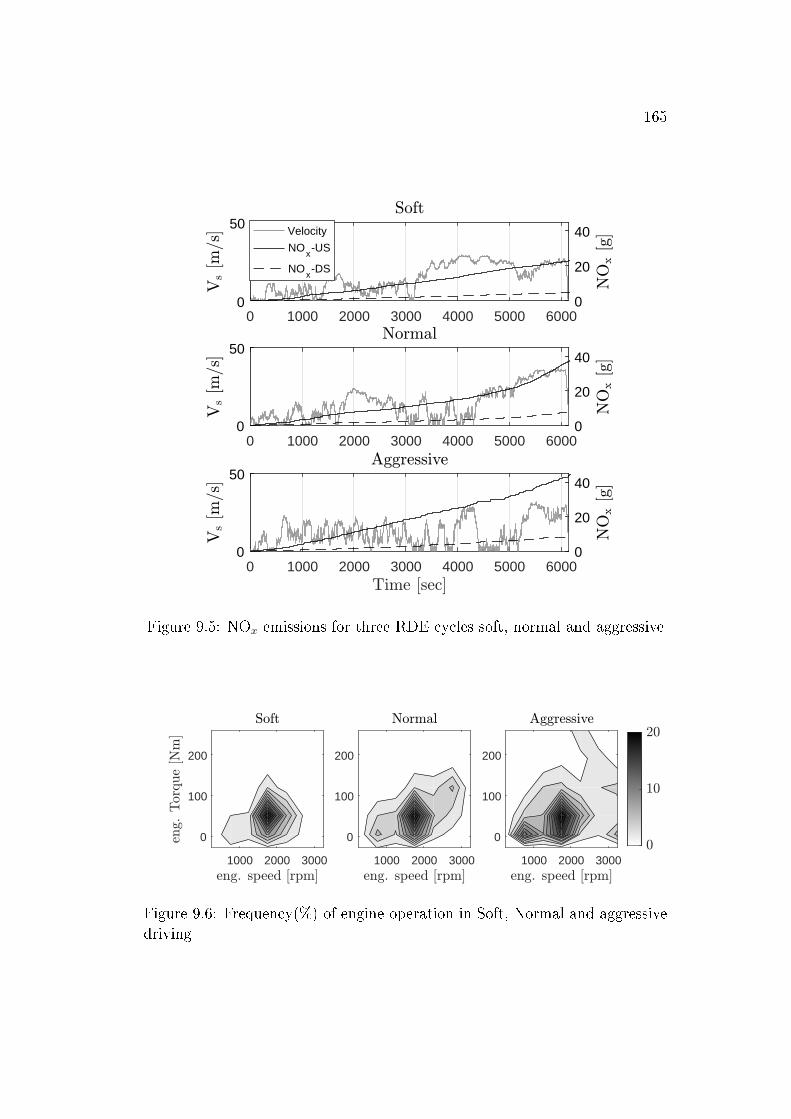
165

0 1000 2000 3000 4000 5000 60000

50

0

20

40Velocity

NOx-US

NOx-DS

0 1000 2000 3000 4000 5000 60000

50

0

20

40

0 1000 2000 3000 4000 5000 60000

50

0

20

40

Figure 9.5: NOx emissions for three RDE cycles soft, normal and aggressive

1000 2000 3000

0

100

200

1000 2000 3000

0

100

200

1000 2000 3000

0

100

200

Figure 9.6: Frequency(%) of engine operation in Soft, Normal and aggressivedriving

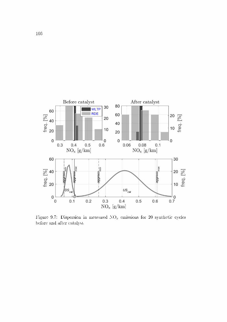
166

Figure 9.7: Dispersion in measured NOx emissions for 20 synthetic cyclesbefore and after catalyst

167

• For the WLTC, relative dispersion and the range in NOx emission is lessthan 5% and 0.02g/km respectively before the catalyst and the relativedispersion and range is less than 2% and 0.002g/km after the catalyst.It can be inferred that the dispersion plotted in the �gure are relativelyless in�uenced by the measurement inconsistencies.

In present the trend of emissions due to dynamics, two variables- (v · apos_95)avgand (RPAk)avg are de�ned as an average of trip dynamics in equations 9.4 and9.5.

(v · apos_95)avg =

∑3k=1[(v · apos)k_95.tk]∑3

k=1[tk](9.4)

(RPAk)avg =

∑3k=1[(RPA)k.tk]∑3

k=1[tk](9.5)

For all the drive cycles the average trip driving dynamics and NOx emissionshave been clustered in �gure 9.8. The results show that the driving dynamicsplay a key role on NOx emissions; the aggressive cycles tend to have higherNOx emissions. However, there are other parameters that also a�ect NOx andare outside the scope of the present study, i.e. one may think that two driv-ing cycles, despite completely equal in the velocity sequence will go throughdi�erent areas in the engine map if there are di�erences in the gear selected,so there will be di�erences on NOx emissions.

Finally, the phase wise NOx emissions are plotted in �gure.9.9, the urbandriving is seen to have maximum contribution in the overall NOx emissions.In the urban phase, the relative di�erence obtained after catalyst is about30% and the range is approximately 0.13 g/km, which is considerably high,considering exclusive limits on NOx emissions in urban phase in EU6D norms.The regulation already demands 50% driving to be done by Type ApprovalAuthority, which reduces the risk of biased driving style. this can be improvedby demanding 50% driving by TAA in each phase of the trip especially inurban phase.

9.4 Summary and conclusion

A real driving cycle generator based on the velocity transition probabilitymatrix obtained from the WLTC is developed. The method is found to beconsistent and fast in producing the synthetic driving cycles. The drivingdynamics are varied using a single tuning parameter within the regulatorylimits. A vehicle model was used to obtain the engine speed and torquepro�le which were used to run on the engine test bench. The instantaneous

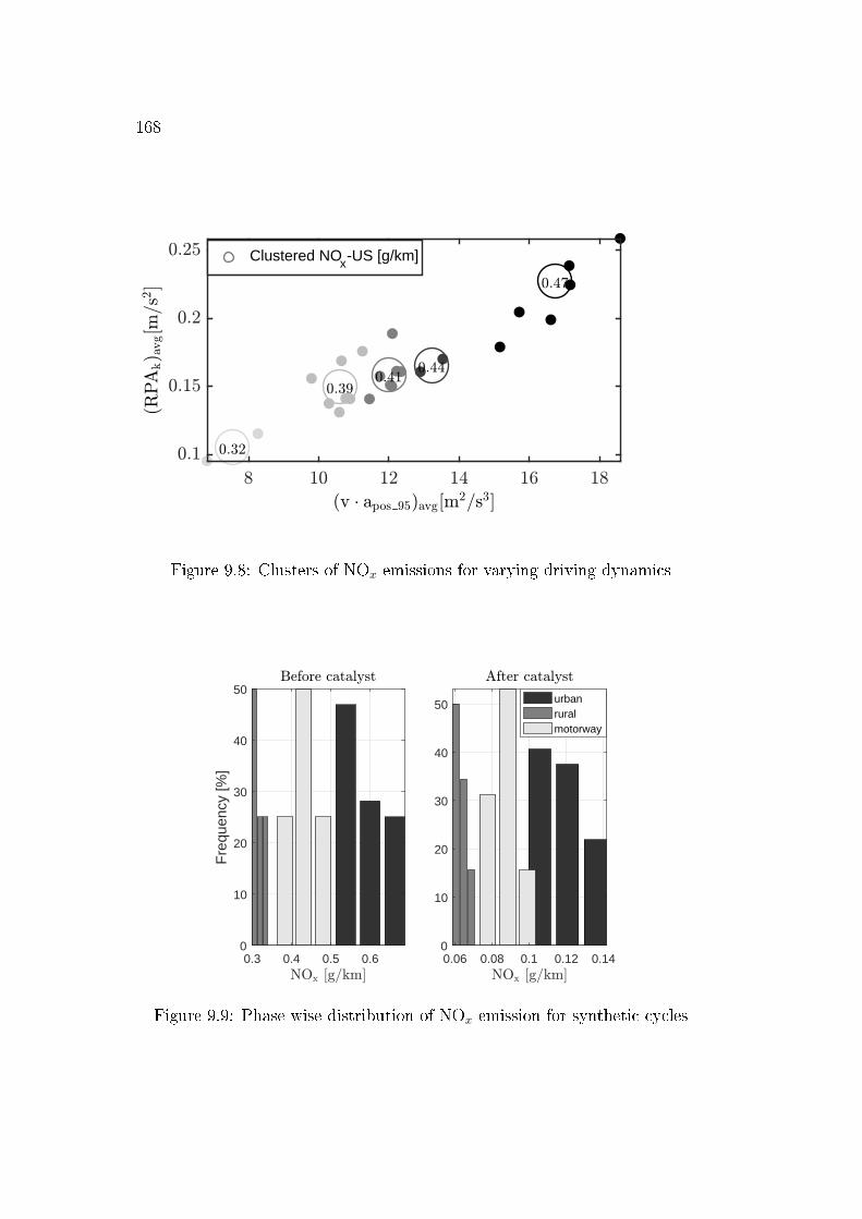
168

Clustered NOx-US [g/km]

Figure 9.8: Clusters of NOx emissions for varying driving dynamics

0.3 0.4 0.5 0.60

10

20

30

40

50

Fre

quen

cy [%

]

0.06 0.08 0.1 0.12 0.140

10

20

30

40

50 urbanruralmotorway

Figure 9.9: Phase wise distribution of NOx emission for synthetic cycles

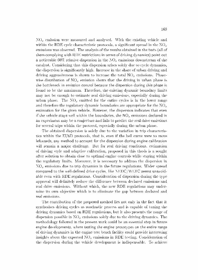
169

NOx emission were measured and analysed. With the existing vehicle andwithin the RDE cycle characteristic protocols, a signi�cant spread in the NOx

emissions was observed. The analysis of the results obtained in the tests (all ofthem complying with RDE restrictions in terms of driving dynamics) point outa noticeable 60% relative dispersion in the NOx emissions downstream of thecatalyst. Considering that this dispersion arises solely due to cycle dynamics,the dispersion is signi�cantly high. Increase in the share of urban driving anddriving aggressiveness is shown to increase the total NOx emissions. Phase-wise distribution of NOx emission shows that the driving in urban phase isthe bottleneck in emission control because the dispersion during this phase isfound to be the maximum. Therefore, the existing dynamic boundary limitsmay not be enough to estimate real driving emissions, especially during theurban phase. The NOx emitted for the entire cycles is in the lower rangeand therefore the regulatory dynamic boundaries are appropriate for the NOx

estimation for the given vehicle. However, the dispersion indicates that evenif the vehicle stays well within the boundaries, the NOx emissions declared inan experiment may be a conjecture and fails to predict the real drive emissionsfor several trips within the protocol, especially during the urban phase.

The obtained dispersion is solely due to the variation in trip characteris-tics within the EU6D protocols, that is, even if the bell curve were to moveleftwards, any method to account for the dispersion during engine calibrationwill remain a major challenge. But for real driving conditions, estimationof driving style and adaptive calibration, proposed in this thesis is a soughtafter solution to obtain close to optimal engine controls while staying withinthe regulatory limits. Moreover, it is necessary to address the dispersion inNOx emissions due to trip dynamics in the future regulations. Wider spreadcompared to the well-de�ned drive cycles, like NEDC/WLTC seems unavoid-able even with RDE regulations. Consideration of dispersion during the typeapproval will de�nitely reduce the di�erence between declared emissions andreal drive emissions. Without which, the new RDE regulations may under-mine its own objective which is to eliminate the gap between declared andreal emissions.

The contribution of the proposed method lies not only in the fact that itsynthesises driving cycles as stochastic process and is capable of tuning thedriving dynamics based on RDE regulations, but it also presents the range ofdispersion possible in NOx emissions solely due to the driving dynamics. Themethodology followed in the present work could be an essential step in futureengine developments, where testing the engine prototypes on the entire rangeof driving dynamics in the engine test bench facility could provide interestinginsights about the expected NOx emissions in RDE testing. Consideration ofthe dispersion during the vehicle development is indispensable. To achieve

170

the RDE objective, on one hand, the manufacturer must develop their vehiclecalibration for the worse case scenario while on the other hand the regulatorsmust include it during type approval testing. Therefore, during the devel-opment phase of any vehicle the presented cycle synthesis tool accompaniedby an engine test bench facility would be very useful tool to have a sense ofrequired engine calibration in order to reduce the risk of failure during theType approval.

The EU6D regulation which mandates the vehicle to pass emission normsindividually in urban phase is an appropriate control and an additional controlover urban driving style will de�nitely improve the con�dence in the estimationof real driving emissions. The regulation already demands 50% driving to bedone by TAA to reduce the risk of biased driving style, can be improved bydemanding 50% driving by TAA in each phase of the trip.

Part V

Conclusion and Outlook

Chapter 10

Conclusions and Outlook

Contents

10.1 Summary of the presented results . . . . . . . . . . . 173

10.2 Future directions . . . . . . . . . . . . . . . . . . . . . . 175

In this chapter, there are two sections: the �rst section summarises im-portant conclusion that can be drawn from the thesis. In the second section,potential future directions in this line of research are outlined, along with thepotential challenges that would need to be tackled in each of them.

10.1 Summary of the presented results

In this thesis, the automotive control methods are investigated for reducingthe vehicle emissions in real driving condition. In general, the automotivecontrol problem was tackled using the optimal control theory by de�ning anobjective function (to be minimised) and a set of constraints related to thesystem and the environment. The three tools that were often used to per-form the speci�c task of larger applications are developed using state-of theart techniques. In chapter 3, the backward vehicle modelling technique basedon the quasi steady approach was described. This chapter introduced themodelling of vehicle longitudinal dynamics and then the most relevant pow-ertrain components of a conventional vehicle and a hybrid electric vehicle.The engine and the motor models were data driven and therefore their util-ity was limited to the speci�c goal or application. In chapter 4, the state-ofthe-art optimal control methods which were used in the thesis were presented.The dynamic programming was derived from the Bellmans principle and anexample was presented to calculate the optimal vehicle speed pro�le in real

174

driving condition. The limitation of the dynamic programming in real timedue its exponential complexity to the number of states lead to the utilisationof the PMP in the control applications. As an implication of the Pontrya-gin's principle, the optimal solution to the problem of minimizing the totalfuel consumption over a driving cycle must also minimize the instantaneousequivalent fuel consumption, was de�ned using the opportune equivalence fac-tors in ECMS. The chapter 5, presented a driving cycle prediction tool usingthe Markov chain principle. Design of driving cycle generator was illustratedwith the help of an example. Later in chapter 6, all the experimental setupswhich were used during the thesis were presented. The rapid prototyping us-ing the dSpace microautobox or the PXI allowed to test the control strategieson test benches and on a vehicle. Using the tools described in chapter 3,chapter 4 and chapter 5, few applications were developed and presented inthe following chapters.

In general two approaches were investigated in this thesis. The �rst ap-proach was to optimise the powertrain control in real driving condition. Forwhich, chapter 7present a novel adaptive control of diesel engine to minimisefuel consumption with constrained NOx emissions on a real driving mission.MC based driving cycle prediction method is able to capture important driv-ing characteristics in real-time. The experimental campaign shows that, if thedriving aggressiveness of the predicted cycle is greater than or equal to theactual cycle the controller is able to meet the target NOx emissions. However,underestimating the aggressiveness leads to excessive emissions. In anotherapplication in chapter 7, a calibration method was presented, which includeda single tuning parameter to trade-o� between, fuel consumption, NOx emis-sions and drivability of the engine. The additional degree of freedom give�exibility to the calibration engineer, while optimality is guaranteed at alltimes. This tuning parameter was used to obtain a time-varying calibrationof the diesel engine for NRTC to improve the engine performance and driv-ability. The comparison of the �xed and variable calibration strategies showedthat, with variable strategy the NOx emissions can be reduced upto 3% whilemaintaining similar levels of fuel consumption and drivability. The last sec-tion in chapter 7 was regarding the optimal control of the HEV powertrain.It presented a new method based on the online speed prediction and adaptiveECMS to optimse the EMS while tracking the battery SoC close to the target.The method was validated using a simulation and an experiment based casestudy on a real driving mission. The developed method was compared withthree SOA methods: The ECMS (optimal and o�ine approach), ACP+ECMS(online approach) and the CD-CS (online approach). The results from the de-veloped online method show signi�cant improvement in the fuel consumptioncompared to the other online methods. in comparison to the o�ine method,

175

where the driving mission is known in advance the fuel consumption is 10%higher in the developed method.

The second approach was to optimise the speed pro�les of the vehiclebased on the available data from the infrastructure. The controllability (eitherpassive or active control) is limited in real-time for such an application. Thelimitation is due to the amount of information (I2V or V2V) that is requiredto be processed in real time. For this in chapter 8, an application was aimedto assess the impact of tra�c light information availability in terms of fuelconsumption and NOx emissions. An e�cient management of vehicle speedis a key factor for fuel and NOx minimisation. Tra�c light information isessential for vehicle speed management, even if suboptimal strategies are used,substantial reductions in terms of both fuel consumption (7%) and emissions(12%) may be obtained. One may note that this level of reduction is, byfar, higher to what can be attained with online optimisation of the enginecontrol itself. Another application in chapter 8 was regarding optimal speedadvisory in real driving mission. The application optimises the speed pro�le inreal-time and recommends the driver optimal speed sequence that minimisesthe fuel consumption on a particular route. The real-time implementation ofthe application shows the possibility to stay very close to the Pareto frontobtained by trading o� travel time and fuel consumption. In particular 4%reduction in fuel consumption was recorded for the same travel time using thedeveloped application.

Finally, in chapter 9, a real driving cycle generator based on the velocityTPM obtained from the WLTC was presented. A single tuning parameter wasused to vary the cycle dynamics within the EU6D regulatory limits. A vehiclemodel was used to obtain the engine speed and torque pro�le which were thenrun on the engine installed in a SOA engine test bench. The instantaneousNOx emission were measured and analysed. With the existing vehicle andwithin the RDE cycle characteristic protocols, a noticeable 60% relative dis-persion in the NOx emissions downstream of the catalyst was recorded. Theassessments highlight the importance of considering this dispersion during theengine calibration to succeed in TA process.

10.2 Future directions

Include more states to the quasi-steady engine model The power-train control performance rely heavily upon the engine model. In the work,quasi steady engine model was used as described in chapter 3. These mod-els were based on interpolated maps depending on only a few states. Withcomplexity of these models increasing linearly with the number of states, this

176

thesis limited them to two for focusing on the controller development. How-ever, more states can be easily integrated in the current engine models at thecost of implementation complexity in the rapid prototyping controller (due tolimited memory). A straightforward research direction would be to explorenew methods for engine modelling such as neural network.

Include more states in the driving cycle predictor for improved accu-

racy The global objective of this investigation was to minimise the drivinguncertainties in real driving conditions for calculating the optimal actuations.The driving cycle prediction tool developed in this thesis was based on theMC principle. The states included in the TPM were vehicle velocity andposition. Even though the cycle predictions were able to capture the maincharacteristics of driving such as aggressiveness, the model can be enhancedwith 'time' as an additional state in the TPM. This would further improvethe capability of the model to capture the tra�c intensities in urban drivingconditions. This can be realised by modelling the tra�c �ow on an urbanstreet using experimental data and tools such as SUMO. Such a model is ca-pable of providing velocity speed pro�les as a function of time and positionand with this information three dimensional (current velocity, time, position)TPMs can be easily formulated. Finally, the speed prediction process can alsoinclude the current information of other vehicles in the route.

Include ATS temperature as an additional state in the control prob-

lem to capture cold state problems in HEV During the developmentof online EMS of HEV, the only state considered was battery SoC however,there are other parameters that in�uence the performance of the HEV con-troller in real driving conditions. For instance, by including the thermal modelof the after-treatment system, the temperature of the ATS can be included asan additional state. The new cost function will also include another co-staterelated to the vehicle emissions addressing the cold start problem of dieselengine based HEV.

Explore combined powertrain and ADAS optimisation In this the-sis, online optimal control methods for powertrain and ADAS were exploredseparately. Applications and case studies were used to demonstrate the capa-bilities of both the approaches. In future, application can be developed withcombined optimisation of powertrain and ADAS with the same objective. Forexample, the driver is advised of speed based on tra�c situation to minimisethe fuel consumption and maintain the terminal SoC while the EMS adap-tively controls the torque-split torwards the same objective. As the basis for

177

online control of HEV was speed prediction, a speed advisory would furtherreduce the uncertainty arising due to the driver.

Appendices

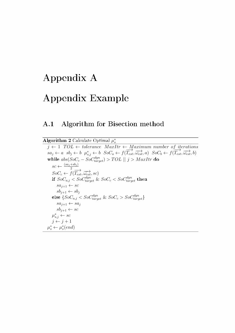
Appendix A

Appendix Example

A.1 Algorithm for Bisection method

Algorithm 2 Calculate Optimal µ∗sj ← 1 TOL ← tolerance MaxItr ← Maximum number of iterations

saj ← a sbj ← b µ∗s,j ← b SoCa ← f(−→Test,−−→ωest, a) SoCb ← f(

−→Test,−−→ωest, b)

while abs(SoCc − SoCdyntarget) > TOL || j > MaxItr do

sc← (saj+sbj)

2

SoCc ← f(−→Test,−−→ωest, sc)

if SoCa,j < SoCdyntarget & SoCc < SoCdyn

target then

saj+1 ← sc

sbj+1 ← sbjelse {SoCa,j < SoCdyn

target & SoCc > SoCdyntarget}

saj+1 ← sajsbj+1 ← sc

µ∗s,j ← sc

j ← j + 1

µ∗s ← µ∗s(end)

Bibliography

[201 2016] Commission regulation EU 2016/646 of 20th april 2016 amending

Regulation EC No 692/2008 as regards emissions from light passenger

and commercial vehicles (Euro6), 2016. (Cited on pages 158 and 162.)

[Alonso et al. 2007] Jos M. Alonso, Fernando Alvarruiz, Jos M. Desantes,Leonor Hernndez, Vicente Hernndez and Germn Molt. Combining

Neural Networks and Genetic Algorithms to Predict and Reduce Diesel

Engine Emissions. IEEE Transactions on Evolutionary Computation,vol. 11, no. 1, pages 46�55, feb 2007. (Cited on page 17.)

[Ambuhl & Guzzella 2009] D. Ambuhl and L. Guzzella. Predictive ReferenceSignal Generator for Hybrid Electric Vehicles. IEEE Transactions onVehicular Technology, vol. 58, no. 9, pages 4730�4740, nov 2009. (Citedon page 119.)

[Andreas et al. 2010] A. Malikopoulos Andreas, Y.Papalambros Panos andN. Assanis Dennis. Online Identi�cation and Stochastic Control for

Autonomous Internal Combusiton Engines. Journal of Dynamic Sys-tems, Measurement, and Control, 2010. (Cited on page 22.)

[AQR 2019] Air quality in Europe � 2019 report, 2019. (Cited on page 3.)

[Asprion et al. 2014] Jonas Asprion, Oscar Chinellato and Lino Guzzella.Optimal control of diesel engines: Numerical methods, applications,

and experimental validation. Mathematical Problems in Engineering,vol. 2014, 2014. (Cited on pages 17 and 22.)

[Assis et al. 2003] Edgard Marcelo De Assis, Ricardo Kurauchi,Marcelo Conti Carloti, J. Celso Ribeiro, Liao Dai Lon and Adri-ano Cardon Castro. Drivability Improvements on Electronic Diesel

Engines. In SAE Technical Paper Series. SAE International, nov2003. (Cited on page 17.)

184

[Atkinson et al. 2008] Chris Atkinson, Marc Allain and Houshun Zhang. Us-ing Model-Based Rapid Transient Calibration to Reduce Fuel Consump-

tion and Emissions in Diesel Engines. In SAE Technical Paper Series.SAE International, apr 2008. (Cited on page 20.)

[Aubert & Kornprobst 2006] Gilles Aubert and Pierre Kornprobst. Mathe-matical problems in image processing. Springer New York, 2006. (Citedon page 104.)

[Authors 2006] V Authors. Reciprocating internal combustion engines. Ex-

haust emission measurement. Test-bed measurement of gaseous and

particulate exhaust emissions. BS ISO 8178-1: 2006, 2006. (Not cited.)

[Bachler et al. 2003] Johann Bachler, Peter Mathis and Martin Rzehorska.Calibration Methodologies for Online Optimisation of Diesel Engines

with Regard to Emissions, NVH and Performance. In SAE TechnicalPaper Series. SAE International, jan 2003. (Cited on page 17.)

[Bageshwar et al. 2004] V.L. Bageshwar, W.L. Garrard and R. Rajamani.Model Predictive Control of Transitional Maneuvers for Adaptive

Cruise Control Vehicles. IEEE Transactions on Vehicular Technology,vol. 53, no. 5, pages 1573�1585, sep 2004. (Cited on page 32.)

[Bakibillah et al. 2018] A.S.M. Bakibillah, M.A.S. Kamal, C.P. Tan,T. Hayakawa and J. Imura. Eco-driving on Hilly Roads Using Model

Predictive Control. In 2018 Joint 7th International Conference on Infor-matics, Electronics & Vision (ICIEV) and 2018 2nd International Con-ference on Imaging, Vision & Pattern Recognition (icIVPR). IEEE, jun2018. (Cited on page 30.)

[Baldi et al. 2015] Francesco Baldi, Gerasimos Theotokatos and Karin Ander-sson. Development of a combined mean value�zero dimensional model

and application for a large marine four-stroke Diesel engine simula-

tion. Applied Energy, vol. 154, pages 402�415, sep 2015. (Cited onpage 20.)

[Barth & Boriboonsomsin 2009] Matthew Barth and Kanok Boriboonsomsin.Energy and emissions impacts of a freeway-based dynamic eco-driving

system. Transportation Research Part D: Transport and Environment,vol. 14, no. 6, pages 400�410, aug 2009. (Cited on page 30.)

[Bellman 1970] Richard Bellman. Dynamic programming and inverse optimal

problems in mathematical economics. Journal of Mathematical Anal-

185

ysis and Applications, vol. 29, no. 2, pages 424�428, feb 1970. (Citedon page 53.)

[Berger et al. 2011] Benjamin Berger, Florian Rauscher and Boris Lohmann.Analysing Gaussian Processes for Stationary Black-Box Combustion

Engine Modelling. IFAC Proceedings Volumes, vol. 44, no. 1, pages10633�10640, jan 2011. (Cited on page 20.)

[Berger 2012] Benjamin Berger. Modeling and Optimization for Stationary

Base Engine Calibration. PhD thesis, TECHNISCHE UNIVERSITATMUNCHEN, 2012. (Cited on page 105.)

[BLOCKEY & HARTLEY 1995] P. N. BLOCKEY and L. R. HARTLEY.Aberrant driving behaviour: errors and violations. Ergonomics, vol. 38,no. 9, pages 1759�1771, sep 1995. (Cited on page 29.)

[Bradley & Frank 2009] Thomas H. Bradley and Andrew A. Frank. Design,

demonstrations and sustainability impact assessments for plug-in hy-

brid electric vehicles. Renewable and Sustainable Energy Reviews,vol. 13, no. 1, pages 115�128, jan 2009. (Cited on page 23.)

[Bryson & Ho 2018] Arthur E. Bryson and Yu-Chi Ho. Applied optimal con-trol. Routledge, may 2018. (Cited on page 26.)

[Bu et al. 2010] Fanping Bu, Han-Shue Tan and Jihua Huang. Design and

�eld testing of a Cooperative Adaptive Cruise Control system. In Pro-ceedings of the 2010 American Control Conference. IEEE, jun 2010.(Cited on page 31.)

[Buie et al. 2004] Lawrence Buie, Malcolm Fry, Peter Fussey and Chad Mitts.An Application of Cost Based Power Management Control Strategies

to Hybrid Fuel Cell Vehicles. In SAE Technical Paper Series. SAEInternational, mar 2004. (Cited on page 27.)

[Canale & Malan 2002] M. Canale and S. Malan. Analysis and Classi�cation

of Human Driving Behaviour in an Urban Environment. Cognition,Technology Work, vol. 4, no. 3, pages 197�206, sep 2002. (Cited onpage 29.)

[Cao et al. 2017] Jianfei Cao, Jiankun Peng and Hongwen He. Research on

Model Prediction Energy Management Strategy with Variable Horizon.Energy Procedia, vol. 105, pages 3565�3570, may 2017. (Cited onpage 28.)

186

[Guardiola et al. 2016] Guardiola Carlos, Pla Benjamin, Bares Pau andWaschl Harald. Adaptive calibration for reduced fuel consumption

and emissions. Journal of Automotive Engineering, 2016. (Cited onpage 23.)

[Castagné et al. 2008] M. Castagné, Y. Bentolila, F. Chaudoye, A. Hallé,F. Nicolas and D. Sinoquet. Comparison of Engine Calibration Meth-

ods Based on Design of Experiments (DoE). Oil & Gas Science andTechnology - Revue de IFP, vol. 63, no. 4, pages 563�582, jul 2008.(Cited on page 15.)

[Cavazzuti 2013] Marco Cavazzuti. Optimization methods. Springer BerlinHeidelberg, 2013. (Cited on page 20.)

[Chen & Borken-Kleefeld 2014] Yuche Chen and Jens Borken-Kleefeld. Real-driving emissions from cars and light commercial vehicles�Results from

13 years remote sensing at Zurich/CH. Atmospheric Environment,vol. 88, pages 157�164, 2014. (Cited on page 88.)

[con 2019] Worldwide Emission Standards and Related Regulations, 2019.(Cited on page 19.)

[Corti et al. 2013] Enrico Corti, Giorgio Mancini, Claudio Forte and DavideMoro. Automatic Combustion Phase Calibration With Extremum Seek-

ing Approach. In Volume 1: Large Bore Engines; Advanced Combus-tion; Emissions Control Systems ; Instrumentation, Controls, and Hy-brids. American Society of Mechanical Engineers, oct 2013. (Cited onpage 22.)

[Cramton 1969] Roger C. Cramton. Driver Behavior and Legal Sanctions:

A Study of Deterrence. Michigan Law Review, vol. 67, no. 3, pages421�454, 1969. (Cited on page 29.)

[Debert et al. 2012] Maxime Debert, Thomas Miro Padovani, GuillaumeColin, Yann Chamaillard and Lino Guzzella. Implementation of

comfort constraints in dynamic programming for hybrid vehicle en-

ergy management. International Journal of Vehicle Design, vol. 58,no. 2/3/4, page 367, 2012. (Cited on page 26.)

[Demuynck et al. 2012] Joachim Demuynck, Dirk Bosteels, Michel De Paepe,Cécile Favre, John May and Sebastian Verhelst. Recommendations for

the new WLTP cycle based on an analysis of vehicle emission measure-

ments on NEDC and CADC. Energy Policy, vol. 49, pages 234�242,2012. (Cited on page 4.)

187

[Die 2019] Brochure: EU actions since Dieselgate - An overview from 2015

until today, 2019. (Cited on page 4.)

[Du et al. 2016] Yongchang Du, Yue Zhao, Qinpu Wang, Yuanbo Zhang andHuaicheng Xia. Trip-oriented stochastic optimal energy management

strategy for plug-in hybrid electric bus. Energy, vol. 115, pages 1259�1271, nov 2016. (Cited on page 121.)

[EEA 2019] Monitoring of CO2 emissions from passenger cars � Regulation

(EU) 2019/631, 2019. (Cited on page 3.)

[EGD 2019] COMMUNICATION FROM THE COMMISSION TO THE

EUROPEAN PARLIAMENT, THE EUROPEAN COUNCIL, THE

COUNCIL, THE EUROPEAN ECONOMIC AND SOCIAL COM-

MITTEE AND THE COMMITTEE OF THE REGIONS The Euro-

pean Green Deal COM/2019/640 �nal, 2019. (Cited on page 3.)

[Elbert et al. 2017] Philipp Elbert, Alois Amstutz and Christopher Onder.Adaptive Control for the Real Driving Emissions of Diesel Engines.MTZ worldwide, vol. 78, no. 12, pages 68�74, nov 2017. (Cited onpage 105.)

[Englund et al. 2016] Cristofer Englund, Lei Chen, Jeroen Ploeg, ElhamSemsar-Kazerooni, Alexey Voronov, Hoai Hoang Bengtsson and JonasDido�. The Grand Cooperative Driving Challenge 2016: boosting the

introduction of cooperative automated vehicles. IEEEWireless Commu-nications, vol. 23, no. 4, pages 146�152, aug 2016. (Cited on page 31.)

[Ericsson 2001] Eva Ericsson. Independent driving pattern factors and their

in�uence on fuel-use and exhaust emission factors. TRANSPORT RE-SEARCH PART D, 2001. (Cited on page 162.)

[Fazal et al. 2010] Syed Fazal, Allen Dobryden S.N., Grand Carrie, McGeeRyan and Filev Dimitar. Design and Analysis of an Adaptive RealTime

Advisory System for Improving Real World Fuel Economy in a Hybrid

Electric Vehicle. SAE Journal, 2010. (Cited on page 22.)

[Feneley et al. 2017] Adam J. Feneley, Apostolos Pesiridis and Amin Mah-moudzadeh Andwari. Variable Geometry Turbocharger Technologies

for Exhaust Energy Recovery and Boosting-A Review. Renewable andSustainable Energy Reviews, vol. 71, pages 959�975, may 2017. (Citedon page 6.)

188

[Fernandes & Nunes 2012] Pedro Fernandes and Urbano Nunes. Platooning

With IVC-Enabled Autonomous Vehicles: Strategies to Mitigate Com-

munication Delays, Improve Safety and Tra�c Flow. IEEE Trans-actions on Intelligent Transportation Systems, vol. 13, no. 1, pages91�106, mar 2012. (Cited on page 31.)

[François 2017] Cuenot François. Real world fuel economy measurements.Technical report, groupe PSA, transport and environment, Francenature environnement (FnE) and Bureau Veritas, 2017. (Cited onpage 22.)

[Frieske et al. 2013] Benjamin Frieske, Matthias Kloetzke and FlorianMauser. Trends in vehicle concept and key technology development

for hybrid and battery electric vehicles. In 2013 World Electric Vehi-cle Symposium and Exhibition (EVS27). IEEE, nov 2013. (Cited onpage 6.)

[Fröberg et al. 2006] Anders Fröberg, Erik Hellström and Lars Nielsen. Ex-

plicit Fuel Optimal Speed Pro�les for Heavy Trucks on a Set of To-

pographic Road Pro�les. In SAE Technical Paper, 2006. (Cited onpage 32.)

[Galindo et al. 2020] Jose Galindo, Hector Climent, Benjamin Pla and Chai-tanya Patil. EGR Transient Operations in Highly Dynamic Driving

Cycles. International Journal of Automotive Technology, vol. 21, no. 4,pages 865�879, jul 2020. (Cited on page 6.)

[George F Wolfe 1938] John I Spencer George F Wolfe. Automatic speed con-

trol for vehicles, 1938. (Cited on page 31.)

[Günter Reichart et al. 1998] S.F Günter Reichart, Dorrer Claus, RiekerHeinrich, Drechsel Eberhard and Wermuth Gisbert. Potentials of

BMW Driver Assistance to Improve Fuel Economy. FISITA 1998World Automotive Congress, 1998. (Cited on page 22.)

[Gokul et al. 2019] S. Sankar Gokul, C. Shekhar Rohan, Manzie Chris, SanoTakeshi and Nakada Hayato. Model Predictive Controller with Aver-

age Emissions Constraints for Diesel Airpath. Control EngineeringPractice, 2019. (Cited on page 23.)

[Gong et al. 2007] Qiuming Gong, Yaoyu Li and Zhong-Ren Peng. Trip BasedPower Management of Plug-in Hybrid Electric Vehicle with Two-Scale

Dynamic Programming. In 2007 IEEE Vehicle Power and PropulsionConference. IEEE, sep 2007. (Cited on page 25.)

189

[Gong et al. 2008] Qiuming Gong, Yaoyu Li and Zhong-Ren Peng. Trip-BasedOptimal Power Management of Plug-in Hybrid Electric Vehicles. IEEETransactions on Vehicular Technology, vol. 57, no. 6, pages 3393�3401,nov 2008. (Cited on page 24.)

[Gong et al. 2011] Q. Gong, Mohler S. Midlam, V. Marano and Rizzoni G. Aniterative markov chain approach for generating vehicle driving cycles.SAE International Journal of Engines, 2011. (Cited on page 21.)

[Grahn et al. 2012] Markus Grahn, Krister Johansson, Christian Vartia andTomas McKelvey. A Structure and Calibration Method for Data-

Driven Modeling of NOX and Soot Emissions from a Diesel Engine.In SAE Technical Paper Series. SAE International, apr 2012. (Citedon page 20.)

[Gschweitl et al. 2001] Kurt Gschweitl, Horst P�uegl, Tiziana Fortuna andRainer Leithgoeb. Increasing the e�ciency of model-based engine ap-

plications through the use of CAMEO online DoE toolbox. ATZ world-wide, vol. 103, no. 7-8, pages 17�20, jul 2001. (Cited on pages 105and 106.)

[Gu & Rizzoni 2006] Bo Gu and Giorgio Rizzoni. An Adaptive Algorithm for

Hybrid Electric Vehicle Energy Management Based on Driving Pat-

tern Recognition. In Dynamic Systems and Control, Parts A and B.ASMEDC, jan 2006. (Cited on page 120.)

[Guardiola et al. 2012] Carlos Guardiola, Antonio Gil, Benjamín Pla and Pe-dro Piqueras. Representation Limits of Mean Value Engine Models. InIdenti�cation for Automotive Systems, pages 185�206. Springer Lon-don, 2012. (Cited on page 20.)

[Guardiola et al. 2013] C. Guardiola, B. Pla, D. Blanco-Rodríguez andA. Reig. Modelling driving behaviour and its impact on the energy

management problem in hybrid electric vehicles. International Journalof Computer Mathematics, vol. 91, no. 1, pages 147�156, sep 2013.(Cited on pages 28 and 120.)

[Guardiola et al. 2014] Carlos Guardiola, Benjamin Pla, David Blanco-Rodriguez and Pierre Olivier Calendini. ECU-oriented models for NOx

prediction. Part 1: a mean value engine model for NOx prediction. Pro-ceedings of the Institution of Mechanical Engineers, Part D: Journalof Automobile Engineering, vol. 229, no. 8, pages 992�1015, nov 2014.(Cited on page 20.)

190

[Guardiola et al. 2016] Carlos Guardiola, Benjamín Pla, Pau Bares and Har-ald Waschl. Adaptive calibration for reduced fuel consumption and

emissions. Proceedings of the Institution of Mechanical Engineers,Part D: Journal of Automobile Engineering, vol. 230, no. 14, pages2002�2014, aug 2016. (Cited on page 105.)

[Guardiola et al. 2018] C. Guardiola, B. Pla, P. Bares and A. Barbier. A

combustion phasing control-oriented model applied to an RCCI engine.IFAC-PapersOnLine, vol. 51, no. 31, pages 119�124, 2018. (Cited onpage 6.)

[Guardiola et al. 2019] Carlos Guardiola, Benjamín Pla, Varun Pandey andRichard Burke. On the potential of tra�c light information availability

for reducing fuel consumption and NOx emissions of a diesel light-duty

vehicle. Proceedings of the Institution of Mechanical Engineers, PartD: Journal of Automobile Engineering, page 0954407019867167, 2019.(Cited on page 149.)

[Gutjahr et al. 2017] Tobias Gutjahr, Thomas Kruse and Thorsten Huber.ADVANCED MODELING AND OPTIMIZATION FOR VIRTUAL

CALIBRATION OF INTERNAL COMBUSTION ENGINES. 2017.(Cited on pages 105 and 106.)

[Guzzella & Amstutz 1998] L. Guzzella and A. Amstutz. Control of diesel

engines. IEEE Control Systems, vol. 18, no. 5, pages 53�71, oct 1998.(Cited on page 114.)

[Guzzella & Onder 2010] Lino Guzzella and Christopher H. Onder. Introduc-tion to modeling and control of internal combustion engine systems.Springer Berlin Heidelberg, 2010. (Cited on page 18.)

[Guzzella & Sciarretta 005] L. Guzzella and A. Sciarretta. Vehicle propulsionsystems. introduction to modeling and optimization,. Berlin:Springer-Verlag, pp. 190, 2005. (Not cited.)

[Guzzella & Sciarretta 2005] L Guzzella and A Sciarretta. Vehicle propulsionsystems. Introduction to modeling and optimization. Springer-Verlag,2005. (Cited on pages 24, 44 and 54.)

[Hafner & Isermann 2003] Michael Hafner and Rolf Isermann. Multiobjective

optimization of feedforward control maps in engine management sys-

tems towards low consumption and low emissions. Transactions of theInstitute of Measurement and Control, vol. 25, no. 1, pages 57�74, mar2003. (Cited on pages 20 and 105.)

191

[Han et al. 2019] Jihun Han, Ardalan Vahidi and Antonio Sciarretta. Funda-mentals of energy e�cient driving for combustion engine and electric

vehicles: An optimal control perspective. Automatica, vol. 103, pages558�572, may 2019. (Cited on page 7.)

[Hellström et al. 2009] Erik Hellström, Maria Ivarsson, Jan Åslund and LarsNielsen. Look-ahead control for heavy trucks to minimize trip time and

fuel consumption. Control Engineering Practice, vol. 17, no. 2, pages245�254, 2009. (Cited on page 32.)

[Hellström et al. 2010a] Erik Hellström, Jan Åslund and Lars Nielsen. Designof an e�cient algorithm for fuel-optimal look-ahead control. ControlEngineering Practice, vol. 18, no. 11, pages 1318�1327, 2010. (Citedon page 138.)

[Hellström et al. 2010b] Erik Hellström, Jan Åslund and Lars Nielsen. Designof an e�cient algorithm for fuel-optimal look-ahead control. ControlEngineering Practice, vol. 18, no. 11, pages 1318�1327, 2010. (Citedon page 32.)

[Hellström et al. 2013] E. Hellström, D. Lee, L. Jiang, A. G. Stefanopoulouand H. Yilmaz. On-Board Calibration of Spark Timing by Extremum

Seeking for Flex-Fuel Engines. IEEE Transactions on Control SystemsTechnology, vol. 21, no. 6, pages 2273�2279, 2013. (Cited on pages 7and 22.)

[Hiroyasu et al. 2002] T. Hiroyasu, M. Miki, J. Kamiura, S. Watanabe andH. Hiroyasu. Multi-Objective Optimization of Diesel Engine Emissions

and Fuel Economy using Genetic Algorithms and Phenomenological

Model. In SAE Technical Paper Series. SAE International, oct 2002.(Cited on page 17.)

[Hochschwarzer et al. 1992] Helmuth Hochschwarzer, Wolfgang Kriegler andManfred Schon. Fully Automatic Determination and Optimization of

Engine Control Characteristics. SAE Transactions, vol. 101, pages380�391, 1992. (Cited on page 20.)

[Hofman et al. 2006] T. Hofman, M. Steinbuch, R.M. van Druten and A.F.A.Serrarens. RULE-BASED ENERGY MANAGEMENT STRATEGIES

FOR HYBRID VEHICLE DRIVETRAINS: A FUNDAMENTAL AP-

PROACH IN REDUCING COMPUTATION TIME. IFAC Proceed-ings Volumes, vol. 39, no. 16, pages 740�745, 2006. (Cited on page 24.)

192

[Hooker 1988] J N Hooker. Optimal driving for single-vehicle fuel economy.Transportation Research Part A: General, vol. 22, no. 3, pages 183�201, 1988. (Cited on page 32.)

[Hou et al. 2014] Cong Hou, Minggao Ouyang, Liangfei Xu and Hewu Wang.Approximate Pontryagin's minimum principle applied to the energy

management of plug-in hybrid electric vehicles. Applied Energy,vol. 115, pages 174�189, feb 2014. (Cited on page 27.)

[Huo et al. 2018] Yi Huo, Fengjun Yan and Daiwei Feng. A hybrid electric

vehicle energy optimization strategy by using fueling control in diesel

engines. Proceedings of the Institution of Mechanical Engineers, PartD: Journal of Automobile Engineering, page 0954407017747372, 2018.(Cited on page 134.)

[il Jeon et al. 2000] Soon il Jeon, Sung tae Jo, Yeong il Park and Jang mooLee. Multi-Mode Driving Control of a Parallel Hybrid Electric Vehi-

cle Using Driving Pattern Recognition. Journal of Dynamic Systems,Measurement, and Control, vol. 124, no. 1, pages 141�149, aug 2000.(Cited on page 120.)

[Isermann 2014] Rolf Isermann. Engine modeling and control: Modelingand electronic management of internal combustion engines. Berlin,Germnay: Springer, 2014. (Cited on page 15.)

[Jiang et al. 2009] Li Jiang, Julien Vanier, Hakan Yilmaz and Anna Ste-fanopoulou. Parameterization and Simulation for a Turbocharged

Spark Ignition Direct Injection Engine with Variable Valve Timing.In SAE Technical Paper Series. SAE International, apr 2009. (Citedon page 20.)

[Jiang et al. 2012] Shugang Jiang, Donald Nutter and Anthony Gullitti. Im-

plementation of Model-Based Calibration for a Gasoline Engine. InSAE Technical Paper, 2012. (Cited on page 7.)

[Jiang et al. 2017] Qi Jiang, Florence Ossart and Claude Marchand. Compar-

ative Study of Real-Time HEV Energy Management Strategies. IEEETransactions on Vehicular Technology, vol. 66, no. 12, pages 10875�10888, dec 2017. (Cited on page 121.)

[Jie & Debbie N 2002] Lin Jie and Niemer Debbie N. An exploratory analysis

comparing a stochastic driving cycle to California's regulatory cycle.Atmospheric Environment, 2002. (Cited on page 21.)

193

[Johannesson et al. 2007] Lars Johannesson, Mattias Asbogard andBo Egardt. Assessing the Potential of Predictive Control for

Hybrid Vehicle Powertrains Using Stochastic Dynamic Programming.IEEE Transactions on Intelligent Transportation Systems, vol. 8,no. 1, pages 71�83, mar 2007. (Cited on pages 25, 32 and 119.)

[Jonas et al. 2014] Aspiron Jonas, Chinellato Oscar and Guzzella Lino. Opti-mal Contorl of Diesel Engines: Numerical methods, Application, and

Experimental Validation. Hindawi Publishing corporation, Mathemat-ical Problems in Engineering, 2014. (Cited on page 22.)

[Josevski & Abel 2016] Martina Josevski and Dirk Abel. Distributed predic-

tive control approach for fuel e�cient gear shifting in hybrid electric

vehicles. In 2016 European Control Conference (ECC). IEEE, jun2016. (Cited on page 28.)

[Josh & Vicente 2016] Miller Josh and Franco Vicente. IMPACT OF IM-

PROVED REGULATION OF REAL-WORLD NOx EMISSIONS

FROM DIESEL PASSENGER CARS IN THE EU 2015 2030. Tech-nical report, International Council on Clean Transportation, 2016.(Cited on page 22.)

[Jung 2003] Merten Jung. Mean-value modelling and robust control of the

airpath of a turbocharged diesel engine. 2003. (Cited on page 20.)

[Kampelmühler et al. 1993] F. T. Kampelmühler, R. Paulitsch andK. Gschweitl. Automatic ECU-Calibration - An Alternative to

Conventional Methods. In SAE Technical Paper Series. SAEInternational, mar 1993. (Cited on page 16.)

[Kianfar et al. 2012] Roozbeh Kianfar, Bruno Augusto, Alireza Ebadighajari,Usman Hakeem, Josef Nilsson, Ali Raza, Reza S. Tabar, Naga Vish-nuKanth Irukulapati, Cristofer Englund, Paolo Falcone, Stylianos Pa-panastasiou, Lennart Svensson and Henk Wymeersch. Design and Ex-

perimental Validation of a Cooperative Driving System in the Grand

Cooperative Driving Challenge. IEEE Transactions on IntelligentTransportation Systems, vol. 13, no. 3, pages 994�1007, sep 2012.(Cited on page 31.)

[Kim et al. 2014] N. W. Kim, D. H. Lee, C. Zheng, C. Shin, H. Seo andS. W. Cha. Realization of pmp-based control for hybrid electric vehi-

cles in a backward-looking simulation. International Journal of Auto-motive Technology, vol. 15, no. 4, pages 625�635, may 2014. (Cited onpage 25.)

194

[Kum et al. 2013] Dongsuk Kum, Huei Peng and Norman K. Bucknor. Op-

timal Energy and Catalyst Temperature Management of Plug-in Hy-

brid Electric Vehicles for Minimum Fuel Consumption and Tail-Pipe

Emissions. IEEE Transactions on Control Systems Technology, vol. 21,no. 1, pages 14�26, jan 2013. (Cited on page 25.)

[Langouët et al. 2011] Hoël Langouët, Ludovic Métivier, Delphine Sinoquetand Quang-Huy Tran. Engine calibration: multi-objective constrained

optimization of engine maps. Optimization and Engineering, vol. 12,no. 3, pages 407�424, Sep 2011. (Cited on page 17.)

[Larsson & Ericsson 2009] Hanna Larsson and Eva Ericsson. The e�ects of

an acceleration advisory tool in vehicles for reduced fuel consumption

and emissions. Transportation Research Part D: Transport and Envi-ronment, vol. 14, no. 2, pages 141�146, 2009. (Cited on page 29.)

[Lee et al. 2020] Heeyun Lee, Changhee Song, Namwook Kim and Suk WonCha. Comparative Analysis of Energy Management Strategies for HEV:

Dynamic Programming and Reinforcement Learning. IEEE Access,vol. 8, pages 67112�67123, 2020. (Cited on page 26.)

[Lei et al. 2020] Zhenzhen Lei, Datong Qin, Liliang Hou, Jingyu Peng, Yong-gang Liu and Zheng Chen. An adaptive equivalent consumption min-

imization strategy for plug-in hybrid electric vehicles based on traf-

�c information. Energy, vol. 190, page 116409, jan 2020. (Cited onpage 119.)

[Li & Goerges 2017] Guoqiang Li and Daniel Goerges. Hybrid Modeling and

Predictive Control of the Power Split and Gear Shift in Hybrid Elec-

tric Vehicles. In 2017 IEEE Vehicle Power and Propulsion Conference(VPPC). IEEE, dec 2017. (Cited on page 28.)

[Li & Gorges 2019] Guoqiang Li and Daniel Gorges. Fuel-E�cient Gear Shift

and Power Split Strategy for Parallel HEVs Based on Heuristic Dy-

namic Programming and Neural Networks. IEEE Transactions on Ve-hicular Technology, vol. 68, no. 10, pages 9519�9528, oct 2019. (Citedon page 26.)

[Li et al. 2011] Shengbo Li, Keqiang Li, Rajesh Rajamani and JianqiangWang. Model Predictive Multi-Objective Vehicular Adaptive Cruise

Control. IEEE Transactions on Control Systems Technology, vol. 19,no. 3, pages 556�566, may 2011. (Cited on pages 30, 31 and 32.)

195

[Li et al. 2016] Liang Li, Sixiong You, Chao Yang, Bingjie Yan, Jian Songand Zheng Chen. Driving-behavior-aware stochastic model predictive

control for plug-in hybrid electric buses. Applied Energy, vol. 162,pages 868�879, jan 2016. (Cited on page 28.)

[Luján et al. 2018] Jose Manuel Luján, Carlos Guardiola, Benjamín Pla andAlberto Reig. Optimal control of a turbocharged direct injection diesel

engine by direct method optimization. International Journal of EngineResearch, vol. 20, no. 6, pages 640�652, may 2018. (Cited on pages 17and 22.)

[Luján et al. 2019] José Manuel Luján, Carlos Guardiola, Benjamín Pla andVarun Pandey. Impact of driving dynamics in RDE test on NOx

emissions dispersion. Proceedings of the Institution of Mechani-cal Engineers, Part D: Journal of Automobile Engineering, page095440701988158, nov 2019. (Cited on page 102.)

[Ma et al. 2015] He Ma, Hongming Xu, Jihong Wang, Thorsten Schnier, BenNeaves, Cheng Tan and Zhi Wang. Model-Based Multiobjective Evo-

lutionary Algorithm Optimization for HCCI Engines. IEEE Transac-tions on Vehicular Technology, vol. 64, no. 9, pages 4326�4331, sep2015. (Cited on page 20.)

[Markel 2006] Tony Markel. Plug-in Hybrid Electric VehiclesCurrent Status,

Long-Term Prospects and Key Challenges. Technical report, NationalRenewable Energy Laboratory, 8 May 2006. (Cited on page 23.)

[Maroteaux & Saad 2015] Fadila Maroteaux and Charbel Saad. Combined

mean value engine model and crank angle resolved in-cylinder modeling

with NOx emissions model for real-time Diesel engine simulations at

high engine speed. Energy, vol. 88, pages 515�527, aug 2015. (Citedon page 22.)

[Martin et al. 2018] Jaime Martin, Francisco Arnau, Pedro Piqueras and An-gel Auñon. Development of an Integrated Virtual Engine Model to

Simulate New Standard Testing Cycles. In SAE Technical Paper Se-ries. SAE International, apr 2018. (Cited on page 20.)

[Marx & So�ker 2012] Matthias Marx and Dirk So�ker. Optimization of the

power�ow control of a hybrid electric powertrain including load pro�le

prediction. In 2012 IEEE Vehicle Power and Propulsion Conference.IEEE, oct 2012. (Cited on page 28.)

196

[Mat 2017] The MathWorks, Inc. MathWorks Model-Based Calibration Tool-

box - CAGE User's Guide. ., 2017, September 2017. (Cited onpages 105 and 106.)

[Michel 1996] Andre Michel. Driving Cycles Development: Characterization

of the Methods. SAE Technical Papers, 1996. (Cited on page 21.)

[Milanes et al. 2014] Vicente Milanes, Steven E. Shladover, John Spring,Christopher Nowakowski, Hiroshi Kawazoe and Masahide Nakamura.Cooperative Adaptive Cruise Control in Real Tra�c Situations. IEEETransactions on Intelligent Transportation Systems, vol. 15, no. 1,pages 296�305, feb 2014. (Cited on page 31.)

[Millo et al. 2018] Federico Millo, Pranav Arya and Fabio Mallamo. Opti-

mization of automotive diesel engine calibration using genetic algo-

rithm techniques. Energy, vol. 158, pages 807�819, sep 2018. (Citedon page 20.)

[Minett et al. 2011] Claire F. Minett, A. Maria Salomons, Winnie Daamen,Bart van Arem and Sjon Kuijpers. Eco-routing: Comparing the fuel

consumption of di�erent routes between an origin and destination us-

ing �eld test speed pro�les and synthetic speed pro�les. In 2011 IEEEForum on Integrated and Sustainable Transportation Systems. IEEE,jun 2011. (Cited on page 30.)

[Mock et al. 2012] Peter Mock, John German, Anup Bandivadekar and IddoRiemersma. Discrepancies between type-approval and �real-world� fuel-

consumption and CO. Technical report, International Council on CleanTransportation, 2012. (Cited on page 4.)

[Mock et al. 2013] Peter Mock, Uwe Tietge, Vicente Franco, John Ger-man, Anup Bandivadekar, Udo Lambrecht, Jörg Kühlwein and IddoRiemersma. From laboratory to road. Technical report 30, Interna-tional Council on Clean Transportation, 2013. (Cited on page 4.)

[Moro & Helmers 2015] Alberto Moro and Eckard Helmers. A new hybrid

method for reducing the gap between WTW and LCA in the carbon

footprint assessment of electric vehicles. The International Journal ofLife Cycle Assessment, vol. 22, no. 1, pages 4�14, sep 2015. (Cited onpage 6.)

[Moura et al. 2011] Scott Jason Moura, Hosam K. Fathy, Duncan S. Callawayand Je�rey L. Stein. A Stochastic Optimal Control Approach for Power

Management in Plug-In Hybrid Electric Vehicles. IEEE Transactions

197

on Control Systems Technology, vol. 19, no. 3, pages 545�555, may2011. (Cited on page 24.)

[Musardo et al. 2005] Cristian Musardo, Giorgio Rizzoni, Yann Guezennecand Benedetto Staccia. A-ECMS: An Adaptive Algorithm for Hybrid

Electric Vehicle Energy Management. European Journal of Control,vol. 11, no. 4-5, pages 509�524, jan 2005. (Cited on page 120.)

[Naranjo et al. 2003] J. E. Naranjo, C. González, J. Reviejo, R. García andT. de Pedro. Adaptive fuzzy control for inter-vehicle gap keeping. IEEETransactions on Intelligent Transportation Systems, vol. 4, no. 3, pages132�142, 2003. (Cited on page 30.)

[Nessler et al. 2006] Adrian Nessler, Carsten Haukap and Karsten Roepke.Global evaluation of the drivability of calibrated diesel engine maps. In2006 IEEE Conference on Computer Aided Control System Design,2006 IEEE International Conference on Control Applications, 2006IEEE International Symposium on Intelligent Control. IEEE, oct 2006.(Cited on page 18.)

[Niedernolte et al. 2006] H. Niedernolte, F. Klopper, A. Mitterer andF. Schwarzer. Work�ow for data evaluation during basic calibration

of combustion engines. In 2006 IEEE Conference on Computer AidedControl System Design, 2006 IEEE International Conference on Con-trol Applications, 2006 IEEE International Symposium on IntelligentControl. IEEE, oct 2006. (Cited on page 18.)

[Nishio & Shen 2019] Yui Nishio and Tielong Shen. Model predictive con-

trol with tra�c information-based driver's torque demand prediction

for diesel engines. International Journal of Engine Research, page146808741985167, may 2019. (Cited on page 23.)

[Nishio et al. 2018] Yui Nishio, Yutaka Murata, Yukihisa Yamaya and MasatoKikuchi. Optimal calibration scheme for map-based control of diesel

engines. Science China Information Sciences, vol. 61, no. 7, page 70205,Jun 2018. (Cited on page 18.)

[Onori et al. 2015] Simona Onori, Lorenzo Serrao and Giorgio Rizzoni. Adap-tive Optimal Supervisory Control Methods. In SpringerBriefs in Elec-trical and Computer Engineering, pages 79�87. Springer London, dec2015. (Cited on page 119.)

[Ortiz-Soto et al. 2012] Elliot Ortiz-Soto, Dennis Assanis and AristotelisBabajimopoulos. A comprehensive engine to drive-cycle modelling

198

framework for the fuel economy assessment of advanced engine and

combustion technologies. International Journal of Engine Research,vol. 13, no. 3, pages 287�304, 2012. (Cited on page 28.)

[Ozatay et al. 2014a] E. Ozatay, S. Onori, J. Wollaeger, U. Ozguner, G. Riz-zoni, D. Filev, J. Michelini and S. Di Cairano. Cloud-Based Velocity

Pro�le Optimization for Everyday Driving: A Dynamic-Programming-

Based Solution. IEEE Transactions on Intelligent Transportation Sys-tems, vol. 15, no. 6, pages 2491�2505, 2014. (Cited on page 32.)

[Ozatay et al. 2014b] Engin Ozatay, Simona Onori, James Wollaeger, UmitOzguner, Giorgio Rizzoni, Dimitar Filev, John Michelini and StefanoDi Cairano. Cloud-based velocity pro�le optimization for everyday driv-

ing: A dynamic-programming-based solution. IEEE Transactions onIntelligent Transportation Systems, vol. 15, no. 6, pages 2491�2505,2014. (Cited on pages 22 and 30.)

[Ozatay et al. 2014c] Engin Ozatay, Umit Ozguner, John Michelini and Dim-itar Filev. Analytical solution to the minimum energy consumption

based velocity pro�le optimization problem with variable road grade.IFAC Proceedings Volumes, vol. 47, no. 3, pages 7541�7546, 2014.(Cited on pages 22 and 30.)

[Paganelli et al. 2000] G Paganelli, T. M. Guerra, S Delprat, J-J Santin,M Delhom and E Combes. Simulation and assessment of power con-

trol strategies for a parallel hybrid car. Proceedings of the Institutionof Mechanical Engineers, Part D: Journal of Automobile Engineering,vol. 214, no. 7, pages 705�717, jul 2000. (Cited on pages 25 and 119.)

[Park et al. 2017] Sangki Park, Youngkun Kim, Seungchul Woo and KihyungLee. Optimization and calibration strategy using design of experiment

for a diesel engine. Applied Thermal Engineering, vol. 123, pages917�928, aug 2017. (Cited on page 17.)

[Passenberg et al. 2009] B. Passenberg, P. Kock and O. Stursberg. Combined

time and fuel optimal driving of trucks based on a hybrid model. In Eu-ropean Control Conference, pages 4955�4960, 2009. (Cited on page 32.)

[Payri et al. 2005] F. Payri, X. Margot, A. Gil and J. Martin. Computa-

tional Study of Heat Transfer to the Walls of a DI Diesel Engine. InSAE Technical Paper Series. SAE International, apr 2005. (Cited onpage 20.)

199

[Payri et al. 2012] F. Payri, C. Guardiola, B. Pla and D. Blanco-Rodriguez.On a Stochastic Approach of the (ECMS) Method for Energy Manage-

ment in Hybrid Electric Vehicles. IFAC Proceedings Volumes, vol. 45,no. 30, pages 341�348, 2012. (Cited on pages 28 and 120.)

[Payri et al. 2014] F. Payri, C. Guardiola, B. Pla and D. Blanco-Rodriguez.A stochastic method for the energy management in hybrid electric ve-

hicles. Control Engineering Practice, vol. 29, pages 257�265, aug 2014.(Cited on page 27.)

[Payri et al. 2015] F Payri, José M Luján, Carlos Guardiola and B Pla. A

challenging future for the ic engine: new technologies and the control

role. Oil & Gas Science and Technology�Revue IFP Energies nouvelles,vol. 70, no. 1, pages 15�30, 2015. (Cited on pages 6, 21 and 119.)

[Pelkmans & Debal 2006] Luc Pelkmans and Patrick Debal. Comparison of

on-road emissions with emissions measured on chassis dynamometer

test cycles. Transportation Research Part D: Transport and Environ-ment, vol. 11, no. 4, pages 233�241, 2006. (Cited on pages 21 and 28.)

[Peng et al. 2015] Jiankun Peng, Hao Fan, Hongwen He and Deng Pan. A

Rule-Based Energy Management Strategy for a Plug-in Hybrid School

Bus Based on a Controller Area Network Bus. Energies, vol. 8, no. 6,pages 5122�5142, jun 2015. (Cited on page 24.)

[Peng et al. 2017] Jiankun Peng, Hongwen He and Rui Xiong. Rule based

energy management strategy for a series�parallel plug-in hybrid electric

bus optimized by dynamic programming. Applied Energy, vol. 185,pages 1633�1643, jan 2017. (Cited on page 24.)

[Petit et al. 2011] Nicolas Petit, Antonio Sciarrettaet al. Optimal drive of

electric vehicles using an inversion-based trajectory generation ap-

proach. In Proceedings of the 18th IFACWorld Congress, pages 14519�14526, 2011. (Cited on page 32.)

[Petri et al. 2018] Sebastian Petri, Giovanni Vagnoni, Ferenc Aubeck, Jo-han Lindberg, Esteban R. Gelso, Nikolce Murgovski, Mohammed R.Karim, Joschka Schaub and Andrea Pantaleo. Predictive engine and

aftertreatment control concepts for a heavy-duty long-haul truck. In27th Aachen Colloquium Automobile and Engine Technology 2018,2018. (Cited on page 23.)

[Pinamonti et al. 2017] Silvio A. Pinamonti, Domenico Brancale, GerhardMeister and Pablo Mendoza. A Correlation Methodology between AVL

200

Mean Value Engine Model and Measurements with Concept Analysis of

Mean Value Representation for Engine Transient Tests. In SAE Tech-nical Paper Series. SAE International, sep 2017. (Cited on page 20.)

[Ping et al. 2019] Peng Ping, Wenhu Qin, Yang Xu, Chiyomi Miyajima andKazuya Takeda. Impact of Driver Behavior on Fuel Consumption:

Classi�cation, Evaluation and Prediction Using Machine Learning.IEEE Access, vol. 7, pages 78515�78532, 2019. (Cited on page 29.)

[Pla et al. 2020] Benjamin Pla, Pau Bares, Enrique Sanchis and André Aro-nis. Ammonia injection optimization for selective catalytic reduction

aftertreatment systems. International Journal of Engine Research, page146808742093312, jul 2020. (Cited on page 6.)

[Ploeg et al. 2011] Jeroen Ploeg, Bart T. M. Scheepers, Ellen van Nunen,Nathan van de Wouw and Henk Nijmeijer. Design and experimental

evaluation of cooperative adaptive cruise control. In 2011 14th Interna-tional IEEE Conference on Intelligent Transportation Systems (ITSC).IEEE, oct 2011. (Cited on page 31.)

[Ploeg et al. 2014] Jeroen Ploeg, Dipan P. Shukla, Nathan van de Wouw andHenk Nijmeijer. Controller Synthesis for String Stability of Vehicle

Platoons. IEEE Transactions on Intelligent Transportation Systems,vol. 15, no. 2, pages 854�865, apr 2014. (Cited on page 31.)

[Popovic et al. 2006] D. Popovic, M. Jankovic, S. Magner and A.R. Teel. Ex-tremum seeking methods for optimization of variable cam timing engine

operation. IEEE Transactions on Control Systems Technology, vol. 14,no. 3, pages 398�407, may 2006. (Cited on page 22.)

[Rajan et al. 2012] Brahmadevan V Padma Rajan, Andrew McGordon andPaul A Jennings. An investigation on the e�ect of driver style and

driving events on energy demand of a PHEV. World Electric VehicleJournal Vol. 5, 2012. (Cited on page 22.)

[Rakha & Kamalanathsharma 2011] Hesham Rakha and Raj Kishore Ka-malanathsharma. Eco-driving at signalized intersections using V2I

communication. In 2011 14th International IEEE Conference on In-telligent Transportation Systems (ITSC). IEEE, oct 2011. (Cited onpage 30.)

[Rao et al. 1979] Harish S Rao, A I Cohen, J A Tennant and K L VanVoorhies. Engine Control Optimization Via Nonlinear Programming.

201

SAE Transactions, vol. 88, 1979, pp. 667�676., 1979. (Cited on pages 16and 20.)

[Reig 2017] Alberto Reig. Optimal Control for Automotive Powertrain Appli-

cations. PhD thesis, 2017. (Cited on page 32.)

[Ritter & Tillotson 1924] George F Ritter and Harry C Tillotson. Carburetor,1924. (Cited on page 14.)

[Ross 1994] M Ross. Automobile Fuel Consumption and Emissions: E�ects

of Vehicle and Driving Characteristics. Annual Review of Energy andthe Environment, vol. 19, no. 1, pages 75�112, nov 1994. (Cited onpage 29.)

[Rudin et al. 1992] Leonid I. Rudin, Stanley Osher and Emad Fatemi. Non-linear total variation based noise removal algorithms. Physica D: Non-linear Phenomena, vol. 60, no. 1-4, pages 259�268, nov 1992. (Citedon pages 104 and 106.)

[Saboohi & Farzaneh 2009] Y. Saboohi and H. Farzaneh. Model for develop-

ing an eco-driving strategy of a passenger vehicle based on the least fuel

consumption. Applied Energy, vol. 86, no. 10, pages 1925�1932, 2009.(Cited on page 32.)

[Sampson 2009] D Sampson. Use of Model-Based Calibration in the Test Cell.In In Proceedings of the 5th conference Design of Experiments (DOE)in Engine DEvelopment, 2009. (Cited on page 17.)

[Samuel et al. 2005] S Samuel, D Morrey, M Fowkes, C D H Taylor, L Austin,T Felstead and S Latham. Real-world fuel economy and emission levels

of a typical EURO-IV passenger vehicle. Proceedings of the Institution

of Mechanical Engineers. Part D: Journal of Automobile Engineering,2005. (Cited on page 4.)

[Schöggl et al. 2002] P. Schöggl, H. M. Koegeler, K. Gschweitl, H. Kokal,P. Williams and K. Hulak. Automated EMS Calibration using Objective

Driveability Assessment and Computer Aided Optimization Methods.In SAE Technical Paper Series. SAE International, mar 2002. (Citedon page 16.)

[Schüler 2001] M. Schüler. Stationäre Optimierung der Motorsteuerung von

PKW-Dieselmotoren mit Abgasturbolader durch Einsatz schneller neu-

ronaler Netze. PhD thesis, TU Darmstadt, 2001. (Cited on page 105.)

202

[Schmied 2004] A Schmied. Stochastic optimisation methods for engine cali-

bration; Methodes stochastiques d'optimisation appliquees a la mise au

point moteur, 2004. (Cited on page 20.)

[Schwarzkopf & Leipnik 1977] A. B. Schwarzkopf and R. B. Leipnik. Controlof highway vehicles for minimum fuel consumption over varying ter-

rain. Transportation Research, vol. 11, no. 4, pages 279�286, 1977.(Cited on page 31.)

[Sciarretta & Vahidi 2020a] Antonio Sciarretta and Ardalan Vahidi. Energy-e�cient driving of road vehicles. Springer International Publishing,2020. (Cited on page 7.)

[Sciarretta & Vahidi 2020b] Antonio Sciarretta and Ardalan Vahidi. Energy-e�cient driving of road vehicles. Springer, 2020. (Cited on page 32.)

[Sciarretta et al. 2004] A. Sciarretta, M. Back and L. Guzzella. Optimal Con-

trol of Parallel Hybrid Electric Vehicles. IEEE Transactions on ControlSystems Technology, vol. 12, no. 3, pages 352�363, may 2004. (Citedon page 119.)

[Sciarretta et al. 2015a] Antonio Sciarretta, Giovanni De Nunzio andLuis Leon Ojeda. Optimal ecodriving control: Energy-e�cient driving

of road vehicles as an optimal control problem. IEEE Control Systems,vol. 35, no. 5, pages 71�90, 2015. (Cited on pages 22 and 30.)

[Sciarretta et al. 2015b] Antonio Sciarretta, Giovanni De Nunzio andLuis Leon Ojeda. Optimal Ecodriving Control: Energy-E�cient Driv-

ing of Road Vehicles as an Optimal Control Problem. IEEE ControlSystems, vol. 35, no. 5, pages 71�90, 2015. (Cited on page 32.)

[Scordia et al. 2005] J. Scordia, M. Desbois Renaudin, R. Trigui, B. Jean-neret, F. Badin and C. Plasse. Global optimisation of energy manage-

ment laws in hybrid vehicles using dynamic programming. InternationalJournal of Vehicle Design, vol. 39, no. 4, page 349, 2005. (Cited onpage 26.)

[Sequenz 2013] H. Sequenz. Emission Modelling and Model-Based Optimi-

sation of the Engine Control. PhD thesis, Technischen UniversitatDarmstadt, 2013. (Cited on page 105.)

[Serrao et al. 2009] Lorenzo Serrao, Simona Onori and Giorgio Rizzoni.ECMS as a realization of Pontryagins minimum principle for HEV

control. In 2009 American Control Conference. IEEE, 2009. (Cited onpage 122.)

203

[Simon et al. 2018] A Simon, D Nelson-Gruel, A Charlet, T Jaine, C Nouillantand Y Chamaillard. Optimal supervisory control of a Diesel HEV tak-

ing into account both DOC and SCR e�ciencies. IFAC-PapersOnLine,vol. 51, no. 9, pages 323�328, 2018. (Cited on page 134.)

[Sims et al. 2014] R Sims, Schae�er R, Creutzig F, Cruz-Núñez X, D'AgostoM, Dimitriu D, Figueroa Meza M.J, Fulton L, Kobayashi S, Lah O,McKinnona A, Newman P, Ouyang M, Schauer J.J, Sperling D andTiwari G. Transport. In: Climate Change 2014: Mitigation of Climate

Change. Contribution of Working Group III to the Fifth Assessment

Report of the Intergovernmental Panel on Climate Change [Edenhofer,

O., R. Pichs-Madruga, Y. Sokona, E. Farahani, S. Kadner, K. Sey-

both, A. Adler, I. Baum, S. Brunner, P. Eickemeier, B. Kriemann, J.

Savolainen, S. Schlömer, C. von Stechow, T. Zwickel and J.C. Minx

(eds.)]. Technical report, Cambridge University Press, Cambridge,United Kingdom and New York, NY, USA, 2014. (Cited on page 3.)

[Singh et al. 2019] Krishna Veer Singh, Hari Om Bansal and DheerendraSingh. A comprehensive review on hybrid electric vehicles: architec-

tures and components. Journal of Modern Transportation, vol. 27,no. 2, pages 77�107, mar 2019. (Cited on page 6.)

[Stanger & del Re 2013] T. Stanger and L. del Re. A model predictive Coop-

erative Adaptive Cruise Control approach. In American Control Con-ference, pages 1374�1379, 2013. (Cited on pages 30 and 32.)

[Stanglmaier et al. 2002] Rudolf H. Stanglmaier, Ryan C. Roecker, Charles E.Roberts and Jr.Daniel W. Stewart. NOx aftertreatment system and

method for internal combustion engines, 2002. (Cited on page 14.)

[Stephan et al. 2014] Zentner Stephan, Asprion Jonas, Onder Christopherand Guzzella Lin. An Equivalent Emission Minimization Strategy for

Causal Optimal Control of Diesel Engines. Energies, 2014. (Cited onpage 23.)

[Stuhler et al. 2002] Harald Stuhler, Thomas Kruse, Axel Stuber, KurtGschweitl, Walter Piock, Horst P�uegl and Peter Lick. Automated

Model-Based GDI Engine Calibration Adaptive Online DoE Approach.In SAE Technical Paper, 2002. (Cited on page 7.)

[Sugaya 1978] Kazuyoshi Sugaya. Fuel pressure regulator, 1978. (Cited onpage 14.)

204

[Sun et al. 2017] Chao Sun, Fengchun Sun and Hongwen He. Investigating

adaptive-ECMS with velocity forecast ability for hybrid electric vehi-

cles. Applied Energy, vol. 185, pages 1644�1653, jan 2017. (Cited onpage 120.)

[Sundstrom & Guzzella 2009] O. Sundstrom and L. Guzzella. A generic dy-

namic programming Matlab function. In 2009 IEEE Control Applica-tions, (CCA) Intelligent Control, (ISIC), pages 1625�1630, July 2009.(Cited on page 138.)

[Sung et al. 2007] Alexander Sung, Florian Klöpper, Alexander Mitterer,Georg Wachtmeister and Andreas Zell. Modellbasierte Online-

Optimierung in der Simulation und am Motorenprüfstand. MTZ - Mo-tortechnische Zeitschrift, vol. 68, no. 1, pages 42�48, jan 2007. (Citedon page 17.)

[Tagliaferri et al. 2016] Carla Tagliaferri, Sara Evangelisti, Federica Acconcia,Teresa Domenech, Paul Ekins, Diego Barletta and Paola Lettieri. Lifecycle assessment of future electric and hybrid vehicles: A cradle-to-

grave systems engineering approach. Chemical Engineering Researchand Design, vol. 112, pages 298�309, aug 2016. (Cited on page 6.)

[Tan et al. 2017] Qingyuan Tan, Prasad Divekar, Ying Tan, Xiang Chen andMing Zheng. Online calibration of combustion phase in a diesel engine.Control Theory and Technology, vol. 15, no. 2, pages 129�137, may2017. (Cited on page 17.)

[Tang & Rizzoni 2016] Li Tang and Giorgio Rizzoni. Energy management

strategy including battery life optimization for a HEV with a CVT. In2016 IEEE Transportation Electri�cation Conference and Expo, Asia-Paci�c (ITEC Asia-Paci�c). IEEE, jun 2016. (Cited on page 121.)

[Teetor 1950] Ralph R Teetor. Speed control device for resisting operation of

the accelerator, 1950. (Cited on page 31.)

[Thangaraja & Kannan 2016] J. Thangaraja and C. Kannan. E�ect of ex-

haust gas recirculation on advanced diesel combustion and alternate

fuels - A review. Applied Energy, vol. 180, pages 169�184, oct 2016.(Cited on page 6.)

[TK & ZS 2011] Lee TK and Filipi ZS. Synthesis of real-world driving cy-

cles using stochastic process and statistical methodology. InternationalJournal of Vehicle Design, 2011. (Cited on page 21.)

205

[Tong et al. 2000] H.Y. Tong, W.T. Hung and C.S. Cheung. On-Road Motor

Vehicle Emissions and Fuel Consumption in Urban Driving Condi-

tions. Journal of the Air & Waste Management Association, vol. 50,no. 4, pages 543�554, apr 2000. (Cited on page 29.)

[Torregrosa et al. 2011] Antonio J. Torregrosa, Pablo Olmeda, Jaime Martínand Carlos Romero. A Tool for Predicting the Thermal Performance

of a Diesel Engine. Heat Transfer Engineering, vol. 32, no. 10, pages891�904, sep 2011. (Cited on page 20.)

[Tran et al. 2020] Dai-Duong Tran, Majid Vafaeipour, Mohamed El Bagh-dadi, Ricardo Barrero, Joeri Van Mierlo and Omar Hegazy. Thor-

ough state-of-the-art analysis of electric and hybrid vehicle powertrains:

Topologies and integrated energy management strategies. Renewableand Sustainable Energy Reviews, vol. 119, page 109596, mar 2020.(Cited on pages 23 and 24.)

[Tschanz et al. 2013] Frédéric Tschanz, Alois Amstutz, Christopher H Onderand Lino Guzzella. Control of diesel engines using NOx-emission feed-

back. International Journal of Engine Research, vol. 14, no. 1, pages45�56, 2013. (Cited on page 28.)

[Tsugawa et al. 2011] S. Tsugawa, S. Kato and K. Aoki. An automated truck

platoon for energy saving. In 2011 IEEE/RSJ International Conferenceon Intelligent Robots and Systems. IEEE, sep 2011. (Cited on page 31.)

[Tulpule et al. 2011] Pinak Tulpule, Vincenzo Marano and Giorgio Rizzoni.E�ect of Tra�c, Road and Weather Information on PHEV Energy

Management. In SAE Technical Paper Series. SAE International, sep2011. (Cited on pages 27 and 119.)

[Tutuianu et al. 2013] Monica Tutuianu, Alessandro Marotta, Heinz Steven,Eva Ericsson, Takahiro Haniu, Noriyuki Ichikawa and Hajime Ishii.Development of a World-wide Worldwide harmonized Light duty driv-

ing Test Cycle (WLTC). Technical report, WLTP DHC Chair, 2013.(Cited on page 6.)

[Ulleberg & Rundmo 2003] Pål Ulleberg and Torbjørn Rundmo. Personality,attitudes and risk perception as predictors of risky driving behaviour

among young drivers. Safety Science, vol. 41, no. 5, pages 427�443,jun 2003. (Cited on page 29.)

206

[Vagg et al. 2013] Chris Vagg, Chris Brace, Deepak Hari, Sam Akehurst andLloyd Ash. A driver advisory tool to reduce fuel consumption. Technicalreport, SAE Technical Paper, 2013. (Cited on page 29.)

[van Arem et al. 2006] Bart van Arem, Cornelie J. G. van Driel and RubenVisser. The Impact of Cooperative Adaptive Cruise Control on Tra�c-

Flow Characteristics. IEEE Transactions on Intelligent TransportationSystems, vol. 7, no. 4, pages 429�436, dec 2006. (Cited on page 31.)

[van Dooren et al. 2019] Stijn van Dooren, Camillo Balerna, Mauro Salazar,Alois Amstutz and Christopher H. Onder. Optimal Diesel Engine Cal-

ibration using Convex Modelling of Pareto Frontiers. Control Engi-neering Practice, 2019. ,Revision submitted in October 2019. (Citedon page 105.)

[Veerle et al. 2016] Heijne Veerle, Kadijk Gerrit, Ligterink Norbert, derMarkPetervan, Spreen Jordy and Stelwagen Uilke. NOx emissions of �fteen

Euro 6 diesel cars: Results of the Dutch LD road vehicle emission

testing programme 2016. Technical report, TNO, 2016. (Cited onpage 4.)

[Verma et al. 2013] Rajeev Verma, Nikhil Nahar, Zhijun Tang and BenjaminSaltsman. A Driver Assistance System for Improving Commercial Ve-

hicle Fuel Economy. In SAE Technical Paper Series. SAE International,jan 2013. (Cited on page 29.)

[Vinot et al. 2007] Emmanuel Vinot, Rochdi Trigui, Bruno Jeanneret, JulienScordia and Frangois Badin. HEVs Comparison and Components Siz-

ing Using Dynamic Programming. In 2007 IEEE Vehicle Power andPropulsion Conference. IEEE, sep 2007. (Cited on page 26.)

[Weiss et al. 2011] Martin Weiss, Pierre Bonnel, Rudolf Hummel, UrbanoManfredi, Rinaldo Colombo, Gaston Lanappe, Philippe Le Lijour,Mirco Sculatiet al. Analyzing on-road emissions of light-duty vehicles

with Portable Emission Measurement Systems (PEMS). JRC Scienti�cand Technical Reports, EUR, vol. 24697, 2011. (Cited on pages 21and 28.)

[Weiss et al. 2012] Martin Weiss, Pierre Bonnel, Jörg Kühlwein, AlessioProvenza, Udo Lambrecht, Stefano Alessandrini, Massimo Carriero,Rinaldo Colombo, Fausto Forni, Gaston Lanappeet al. Will Euro 6 re-

duce the NOx emissions of new diesel cars?�Insights from on-road tests

with Portable Emissions Measurement Systems (PEMS). AtmosphericEnvironment, vol. 62, pages 657�665, 2012. (Cited on page 6.)

207

[Weiÿmann et al. 2018] Andreas Weiÿmann, Daniel Görges and Xiaohai Lin.Energy-optimal adaptive cruise control combining model predictive con-

trol and dynamic programming. Control Engineering Practice, vol. 72,pages 125�137, mar 2018. (Cited on page 32.)

[Xie et al. 2018] Shaobo Xie, Xiaosong Hu, Zongke Xin and Liang Li. Time-

E�cient Stochastic Model Predictive Energy Management for a Plug-

In Hybrid Electric Bus With an Adaptive Reference State-of-Charge

Advisory. IEEE Transactions on Vehicular Technology, vol. 67, no. 7,pages 5671�5682, jul 2018. (Cited on pages 28 and 119.)

[Yang et al. 2019] Yalian Yang, Huanxin Pei, Xiaosong Hu, Yonggang Liu,Cong Hou and Dongpu Cao. Fuel economy optimization of power

split hybrid vehicles: A rapid dynamic programming approach. Energy,vol. 166, pages 929�938, jan 2019. (Cited on page 26.)

[Yang et al. 2020] Hao Yang, Fawaz Almutairi and Hesham Rakha. Eco-

Driving at Signalized Intersections: A Multiple Signal Optimization

Approach. IEEE Transactions on Intelligent Transportation Systems,pages 1�13, 2020. (Cited on page 30.)

[Yu et al. 2020] Yuanbin Yu, , Junyu Jiang, Pengyu Wang and Jinke Li. A-EMCS for PHEV based on real-time driving cycle prediction and per-

sonalized travel characteristics. Mathematical Biosciences and Engi-neering, vol. 17, no. 6, pages 6310�6341, 2020. (Cited on page 119.)

[Yuche & Jens 2014] Chen Yuche and Broken-Kleefeld Jens. Real-driving

emissions from cars and light commercial vehicles � Results from 13

years remote sensing at Zurich/CH. Atmospheric Environment, 2014.(Cited on page 4.)

[Zacharof et al. 2016] N Zacharof, U Tietge, V Franco and P Mock. Type ap-proval and real-world CO2 and NOx emissions from EU light commer-

cial vehicles. International Council on Clean Transportation, Germany,2016. (Cited on page 4.)

[Zakaria et al. 2019] HAJI Zakaria, MOUNIR Hamid, EL MARJANI Abdel-latif and AMARIR Imane. Recent Advancements and Developments

for Electric Vehicle Technology. In 2019 International Conference ofComputer Science and Renewable Energies (ICCSRE). IEEE, jul 2019.(Cited on page 6.)

[Zentner et al. 2013] Stephan Zentner, Erika Schäfer, Christopher Onder andLino Guzzella. Model-Based Injection and EGR Adaptation and its

208

Impact on Transient Emissions and Drivability of a Diesel Engine.IFAC Proceedings Volumes, vol. 46, no. 21, pages 89�94, 2013. (Citedon page 18.)

[Zhang et al. 2018] Yunfan Zhang, Quan Zhou, Ziyang Li, Ji Li and Hong-ming Xu. Intelligent transient calibration of a dual-loop EGR diesel

engine using chaos-enhanced accelerated particle swarm optimization

algorithm. Proceedings of the Institution of Mechanical Engineers,Part D: Journal of Automobile Engineering, vol. 233, no. 7, pages1698�1711, may 2018. (Cited on page 20.)

[Zhang et al. 2020] Fengqi Zhang, Lihua Wang, Serdar Coskun, Hui Pang,Yahui Cui and Junqiang Xi. Energy Management Strategies for Hybrid

Electric Vehicles: Review, Classi�cation, Comparison, and Outlook.Energies, vol. 13, no. 13, page 3352, jun 2020. (Cited on pages 27and 122.)

[Zhi et al. 2016] Zhanjiang Zhi, Baoli Shi and Yi Sun. Primal-dual method to

smoothing TV-based model for image denoising. Journal of Algorithms& Computational Technology, vol. 10, no. 4, pages 235�243, jul 2016.(Cited on pages 104 and 106.)

[Zhijia et al. 2013] Yang Zhijia, Stobart Richard and Winward Edward. On-line adjustment of start of injection and fuel rail pressure based on

combustion process parameters of diesel engine. SAE International,2013. (Cited on page 22.)

Online Control of Automotive Systems for Improved

Real-World Performance

Abstract: The need of improving the real-world fuel consumption and emis-sion of automotive applications is the basis of this thesis. To this end, twoverticals are explored: First is the online control of the powertrain systems. Instate-of-the-art Optimal Control techniques (such as Dyanmic Programming,Pontryagins Minimum Principle, etc...) are extensively used to formulate theoptimal control laws. These laws are stored in the production ECUs in theform of feedforward calibration maps. The unaccounted uncertainities re-lated to the real-world during the powertrain calibration result in suboptimaloperations of the powertrain in actual driving. Therefore, adaptive controlmethods are proposed in this work which, optimise the energy managementof the conventional and the HEV powertrain control on real driving mission.The second vertical is regarding the vehicle speed control (popularly known asEco-Driving in the literature) methods in real driving condition. In particular,speed advisory systems are proposed for real time application on a vehicle.The control methods developed for each application are described in detailswith their veri�cation and validation on the designed case studies. Apart fromthe developed control methods, there are three tools that were developed andused at various stages of this thesis: A vehicle model, A driving cycle pre-diction tool and optimal control methods (dynamic programming, PMP andECMS). Depending on the application, the developed methods were imple-mented on the Hardware-In-Loop Internal Combustion Engine testing setupor on a real vehicle. The results show signi�cant improvements in the perfor-mance of the powertrain in terms of fuel economy and emissions in comparisonto the state-of-the-art methods.

Keywords: Optimal Control, Model based control, Hybrid Electric Ve-hicle, Energy Management Strategy, Adaptive control, Calibration Smooth-ing, Real Driving Emissions, Eco-Driving, Vehicle speed Optimisation

210

Control de sistemas propulsivos de automoción para la

mejorara del rendimiento en condiciones reales de

conducción

Resumen: La necesidad de mejorar el consumo de combustible y las emi-siones de los sistemas propulsivos de automoción en condiciones reales deconducción es la base de esta tesis. Para ello, se exploran dos ejes: En primerlugar, el control de los sistemas de propulsión. El estado del arte de control enlos sistemas propulsivos de automoción se basa en gran medida en el uso detécnicas de optimización que buscan las leyes de control que minimizan unafunción de coste en un conjunto de condiciones de operación de�nidas a priori.Estas leyes se almacenan en las ECUs de producción en forma de mapas decalibración de los diferentes actuadores del motor. Las incertidumbres asoci-adas al conjunto limitado de condiciones en el proceso de calibración dan lugara un funcionamiento subóptimo del sistema de propulsión en condiciones deconducción real. Por lo tanto, en este trabajo se proponen métodos de controladaptativo que optimicen la gestión de la planta propulsiva a las condicionesesperadas de funcionamiento para un usuario y un caso determinado en lu-gar de a un conjunto genérico de condiciones. El segundo eje se re�ere aoptimizar, en lugar de los parámetros de control del sistema propulsivo, lademanda de potencia de este, introduciendo al propio conductor en el buclede control, sugiriéndole las acciones a tomar. En particular, este segundoeje se re�ere al control de la velocidad del vehículo (conocido popularmentecomo Eco-Driving en la literatura) en condiciones reales de conducción. Seproponen sistemas de aviso en tiempo real al conductor acerca de la veloci-dad óptima para minimizar el consumo del vehículo. Los métodos de controldesarrollados para cada aplicación se describen en detalle en la tesis y se mues-tran ensayos experimentales de validación en los casos de estudio diseñados.Ambos ejes representan un problema de control óptimo, de�nido por un sis-tema dinámico, unas restricciones a cumplir y un coste a minimizar, en estesentido las herramientas desarrolladas en la tesis son comunes a los dos ejes:Un modelo de vehículo, una herramienta de predicción del ciclo de conduccióny métodos de control óptimo (Programación Dinámica, Principio Mínimo dePontryagin y Estrategia de Consumo Equivalente Mínimo). Dependiendo dela aplicación, los métodos desarrollados se implementaron en varios entornosexperimentales: un motor térmico en sala de ensayos simulando el resto delvehículo, incluyendo el resto del sistema de propulsión híbrido y en un ve-hículo real. Los resultados muestran mejoras signi�cativas en el rendimientodel sistema de propulsión en términos de ahorro de combustible y emisionesen comparación con los métodos empleados en el estado del arte actual.

211

Control de sistemes propulsius d'automoció per a la

millorara del rendiment en condicions reals de conducció

Resum: La necessitat de millorar el consum de combustible i les emissionsdels sistemes propulsius d'automoció en condicions reals de conducció és labase d'aquesta tesi. Per a això, s'exploren dos eixos: En primer lloc, el controldels sistemes de propulsió. L'estat de l'art de control en els sistemes propulsiusd'automoció es basa en gran manera en l'ús de tècniques d'optimització quebusquen les lleis de control que minimitzen una funció de cost en un conjuntde condicions d'operació de�nides a priori. Aquestes lleis s'emmagatzemenen les Ecus de producció en forma de mapes de calibratge dels diferents ac-tuadors del motor. Les incerteses associades al conjunt limitat de condicionsen el procés de calibratge donen lloc a un funcionament subòptim del sistemade propulsió en condicions de conducció real. Per tant, en aquest treball esproposen mètodes de control adaptatiu que optimitzen la gestió de la plantapropulsiva a les condicions esperades de funcionament per a un usuari i uncas determinat en lloc d'un conjunt genèric de condicions. El segon eix esrefereix a optimitzar, en lloc dels paràmetres de control del sistema propulsiu,la demanda de potència d'aquest, introduint al propi conductor en el buclede control, suggerint-li les accions a prendre. En particular, aquest segon eixes refereix al control de la velocitat del vehicle (conegut popularment comEco-*Driving en la literatura) en condicions reals de conducció. Es proposensistemes d'avís en temps real al conductor sobre la velocitat òptima per aminimitzar el consum del vehicle. Els mètodes de control desenvolupats pera cada aplicació es descriuen detalladament en la tesi i es mostren assajosexperimentals de validació en els casos d'estudi dissenyats. Tots dos eixosrepresenten un problema de control òptim, de�nit per un sistema dinàmic,unes restriccions a complir i un cost a minimitzar, en aquest sentit les einesdesenvolupades en la tesi són comunes als dos eixos: Un model de vehicle,una eina de predicció del cicle de conducció i mètodes de control òptim (Pro-gramació Dinàmica, Principi Mínim de *Pontryagin i Estratègia de ConsumEquivalent Mínim). Depenent de l'aplicació, els mètodes desenvolupats esvan implementar en diversos entorns experimentals: un motor tèrmic en salad'assajos simulant la resta del vehicle, incloent la resta del sistema de propul-sió híbrid i en un vehicle real. Els resultats mostren millores signi�cativesen el rendiment del sistema de propulsió en termes d'estalvi de combustible iemissions en comparació amb els mètodes emprats en l'estat de l'art actual.