LiveMap: Real-Time Dynamic Map in Automotive EdgeComputing

Qiang Liu, Tao Han, Jiang (Linda) XieThe University of North Carolina at Charlotte{qliu12, tao.han, linda.xie}@uncc.edu

BaekGyu KimToyota Motor North America R&D InfoTech Labs

baekgyu.kim@toyota.com

Abstract—Autonomous driving needs various line-of-sight sen-sors to perceive surroundings that could be impaired underdiverse environment uncertainties such as visual occlusion andextreme weather. To improve driving safety, we explore towirelessly share perception information among connected vehicleswithin automotive edge computing networks. Sharing massiveperception data in real time, however, is challenging underdynamic networking conditions and varying computation work-loads. In this paper, we propose LiveMap, a real-time dynamicmap, that detects, matches, and tracks objects on the road withcrowdsourcing data from connected vehicles in sub-second. Wedevelop the data plane of LiveMap that efficiently processesindividual vehicle data with object detection, projection, featureextraction, object matching, and effectively integrates objectsfrom multiple vehicles with object combination. We design thecontrol plane of LiveMap that allows adaptive offloading of vehiclecomputations, and develop an intelligent vehicle scheduling andoffloading algorithm to reduce the offloading latency of vehiclesbased on deep reinforcement learning (DRL) techniques. Weimplement LiveMap on a small-scale testbed and develop alarge-scale network simulator. We evaluate the performance ofLiveMap with both experiments and simulations, and the resultsshow LiveMap reduces 34.1% average latency than the baselinesolution.

Index Terms—Dynamic Map, CrowdSourcing, ComputationOffloading, Automotive Edge Computing

I. INTRODUCTION

As the development of contemporary artificial intelligenceand parallel computing hardware, autonomous driving andadvanced driving assistance system (ADAS) are becominga reality more than ever [1]. Vehicles rely on sensors suchas stereo camera, LiDAR and radar, to perceive surroundingenvironments, and depend on advanced onboard processorsto process the massive volume perception data in real time.By understanding the environment, e.g., high-accurate local-ization, lane detection and pedestrian recognition, alongsidethe accurate high-definition (HD) map, intelligent controlalgorithms can correctly react to most of the environmentalsituations by controlling the vehicle, e.g., lane changing andpassing vehicles.

It is, however, very difficult to realize high reliable and safedriving under extremely diverse environmental uncertaintiessuch as extreme weather, lighting conditions, visual occlusion,and sensor failures [2]. For example, vehicle sensors are pri-marily range-limited and line-of-sight, which means they areincapable of perceiving information from occluded areas [3].Consider a single-lane road, a car is following a big truck thatoccludes the car’s sensor perception, passing the truck withoutsufficient information about the opposite lane is absolutelyunsafe. Besides, the perception range and fidelity of sensors

Edge Server

Base

Station

LiveMap

Fig. 1: An illustration of automotive edge computing.

might be further impaired by extreme weather, e.g., rain, snow,and dust. Thus, relying on sensors in a single vehicle alonemay not be sufficient to fulfill high-safety driving.

Connected vehicle is the key building block of the Internetof Vehicles (IoV) [4], which connects vehicles with wirelesstechnologies, e.g., cellular networks and dedicated short-rangecommunications (DSRC). It allows the communication ofvehicle-to-vehicle (V2V), vehicle-to-infrastructure (V2I), andvehicle-to-network (V2N), and could substantially improvedriving safety by effectively sharing information among ve-hicles. For example, if the truck shares its perception data tothe car, e.g., a detected vehicle on the opposite lane, the car candecide not to pass the truck even if the vehicle is unobservedby the car’s sensors.

However, sharing perception data among connected vehiclesin automotive edge computing networks is challenging. Forexample, in a dense urban scenario, allowing all vehiclesto share could lead to redundant information exchangingsince their sensing coverages are heavily overlapped. Besides,letting vehicles to share their raw data, e.g., point clouds orRGB-D images, requires tremendous wireless bandwidth andmight result in network congestion [5]. Furthermore, edgeservers need to support hundreds or thousands of vehiclessimultaneously, thus its workloads vary from time to time.Optimizing the time to share for vehicles needs intelligenceunder the complex networking and computation in automotiveedge computing networks.

In this paper, we propose LiveMap, a real-time dynamicmap in automotive edge computing illustrated in Fig. 1, thatdetects, matches and tracks objects on the road in sub-secondbased on the crowdsourcing data from connected vehicles.We design the data plane of LiveMap that consists of objectdetection, projection, feature extraction and object matchingfor processing individual vehicle data efficiently, and objectcombination for combining objects from multiple vehicleseffectively. Specifically, we reduce the detection time withneural network pruning techniques in the object detection,

arX

iv:2

012.

1025

2v1

[cs

.NI]

16

Dec

202

0

Object Detection Feature ExtractionCombination & Tracking

Object Matching

detections

objects:{id, loc, features}

Global Data Base

features

RGB-D imageData Acquisition

Service Request

Projection

configs

object images

historical objects

Vehicle Server

vehicle state service decisionD

ata

Pla

ne

Co

ntr

ol

Pla

ne

DRL Agent

Scheduler

objects

Local Data Base

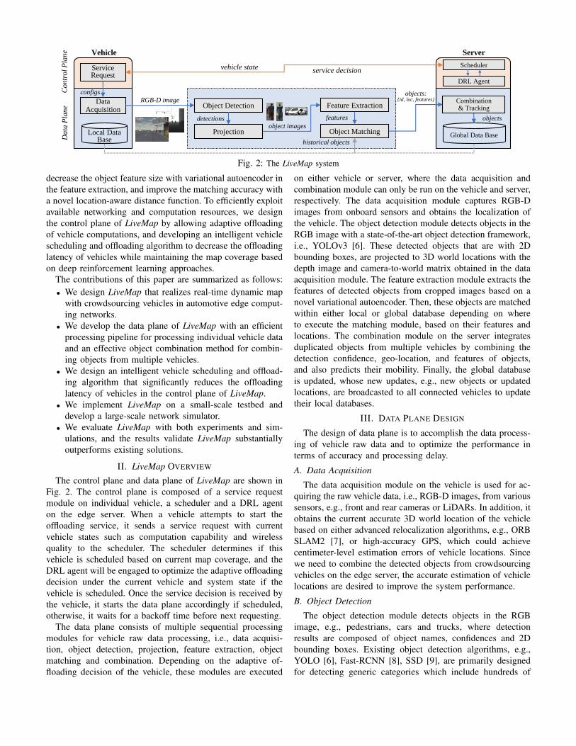
Fig. 2: The LiveMap system

decrease the object feature size with variational autoencoder inthe feature extraction, and improve the matching accuracy witha novel location-aware distance function. To efficiently exploitavailable networking and computation resources, we designthe control plane of LiveMap by allowing adaptive offloadingof vehicle computations, and developing an intelligent vehiclescheduling and offloading algorithm to decrease the offloadinglatency of vehicles while maintaining the map coverage basedon deep reinforcement learning approaches.

The contributions of this paper are summarized as follows:• We design LiveMap that realizes real-time dynamic map

with crowdsourcing vehicles in automotive edge comput-ing networks.

• We develop the data plane of LiveMap with an efficientprocessing pipeline for processing individual vehicle dataand an effective object combination method for combin-ing objects from multiple vehicles.

• We design an intelligent vehicle scheduling and offload-ing algorithm that significantly reduces the offloadinglatency of vehicles in the control plane of LiveMap.

• We implement LiveMap on a small-scale testbed anddevelop a large-scale network simulator.

• We evaluate LiveMap with both experiments and sim-ulations, and the results validate LiveMap substantiallyoutperforms existing solutions.

II. LiveMap OVERVIEW

The control plane and data plane of LiveMap are shown inFig. 2. The control plane is composed of a service requestmodule on individual vehicle, a scheduler and a DRL agenton the edge server. When a vehicle attempts to start theoffloading service, it sends a service request with currentvehicle states such as computation capability and wirelessquality to the scheduler. The scheduler determines if thisvehicle is scheduled based on current map coverage, and theDRL agent will be engaged to optimize the adaptive offloadingdecision under the current vehicle and system state if thevehicle is scheduled. Once the service decision is received bythe vehicle, it starts the data plane accordingly if scheduled,otherwise, it waits for a backoff time before next requesting.

The data plane consists of multiple sequential processingmodules for vehicle raw data processing, i.e., data acquisi-tion, object detection, projection, feature extraction, objectmatching and combination. Depending on the adaptive of-floading decision of the vehicle, these modules are executed

on either vehicle or server, where the data acquisition andcombination module can only be run on the vehicle and server,respectively. The data acquisition module captures RGB-Dimages from onboard sensors and obtains the localization ofthe vehicle. The object detection module detects objects in theRGB image with a state-of-the-art object detection framework,i.e., YOLOv3 [6]. These detected objects that are with 2Dbounding boxes, are projected to 3D world locations with thedepth image and camera-to-world matrix obtained in the dataacquisition module. The feature extraction module extracts thefeatures of detected objects from cropped images based on anovel variational autoencoder. Then, these objects are matchedwithin either local or global database depending on whereto execute the matching module, based on their features andlocations. The combination module on the server integratesduplicated objects from multiple vehicles by combining thedetection confidence, geo-location, and features of objects,and also predicts their mobility. Finally, the global databaseis updated, whose new updates, e.g., new objects or updatedlocations, are broadcasted to all connected vehicles to updatetheir local databases.

III. DATA PLANE DESIGN

The design of data plane is to accomplish the data process-ing of vehicle raw data and to optimize the performance interms of accuracy and processing delay.

A. Data Acquisition

The data acquisition module on the vehicle is used for ac-quiring the raw vehicle data, i.e., RGB-D images, from varioussensors, e.g., front and rear cameras or LiDARs. In addition, itobtains the current accurate 3D world location of the vehiclebased on either advanced relocalization algorithms, e.g., ORBSLAM2 [7], or high-accuracy GPS, which could achievecentimeter-level estimation errors of vehicle locations. Sincewe need to combine the detected objects from crowdsourcingvehicles on the edge server, the accurate estimation of vehiclelocations are desired to improve the system performance.

B. Object Detection

The object detection module detects objects in the RGBimage, e.g., pedestrians, cars and trucks, where detectionresults are composed of object names, confidences and 2Dbounding boxes. Existing object detection algorithms, e.g.,YOLO [6], Fast-RCNN [8], SSD [9], are primarily designedfor detecting generic categories which include hundreds of

Initial Network

Sparsity Training Channel Pruning Fine Tuning

Pruned Network

Fig. 3: The flow-chat of neural network pruning.

object classes, e.g., person, book, boat, table and kite. As aresult, applying these algorithms directly to embedded plat-forms such as electronic control unit (ECU) in vehicles, leadsto long detection time. In general, a larger neural networkis required to achieve similar detection accuracy, e.g., meanaverage precision (mAP), for a larger number of classes.

To address this issue, we propose a slim object detector withreduced categories specifically for automotive transportationsystem, by using neural network pruning techniques. Theneural network pruning is to reduce the neural network size byremoving unnecessary neurons without dramatically scarifyingdetection accuracy. As shown in Fig. 3, we adopt a similarnetwork pruning workflow in [10], which mainly consists ofsparsity training, channel pruning, fine-tuning. Specifically, theinitial network is re-trained by minimizing the loss functionwith a weighted L1 regulation on the scaling factors in batchnormalization (BN) layers during the sparsity training phase.By decreasing these BN scaling factors, insignificant convolu-tional channels that are with nearly zeros scaling factors canbe pruned during the channel pruning phase. Then, the neuralnetwork is fine tuned during the fine-tuning phase. Such train-prune-tune sequential processes can be repeated to seek theoptimal trade-off between detection accuracy and network size.

As a result, we show the performance of detection networkpruning in Table I. We apply the network pruning on theYOLOv3 tiny framework, where we decrease 80 classes to 10classes that includes person, bicycle, car, motorcycle, airplane,bus, train, truck, boat, and traffic light. We reduce the networksize by 93.7% with the cost of 0.01 mAP degradation. Mean-while, the detection time on Nvidia Jetson Nano is decreasedby 19.4% or 18.7% if using TensorRT acceleration.C. Projection

The projection module calculates the 3D world location ofdetected objects in the world coordinate system based on thedetection results, i.e., 2D bounding boxes of objects, depthimage, and camera specifications.

As shown in Fig. 4, the objects in real world are projectedonto the image plane by the camera sensor. The calculationof the world location of an object is completed by two steps,i.e., from pixel coordinates to camera coordinates, and fromcamera coordinates to world coordinates. Denote (u0, v0) asthe center of an object in pixel coordinates, the focal length ofthe camera as f , and the image resolution as (RW , RH). The3D location of the object (X,Y, Z) in the camera coordinatesystem can be written as

X = −(d ∗ (v0 − 0.5 ∗RH))/f,

Y = (d ∗ (u0 − 0.5 ∗RW ))/f, (1)Z = d,

Detection mAP@0.5 Num. of time(Nano)Networks 640x parameters w/o TensorRT

YOLOv3 tiny 0.534 8.69e+06 191.9/37.4 msPruned Network 0.524 0.54e+06 154.7/30.4 ms

TABLE I: Pruning results of detection network on our dataset

𝑋𝑐

𝑌𝑐

𝑍𝑐

camera

𝑍𝑤𝑌𝑤

𝑋𝑤

world

𝑓 𝑥

𝑦

𝑢

𝑣

pixel

𝑑𝑢0

𝑣0

Fig. 4: The illustration of coordinate systems.

where d is the Z-axis depth of the object w.r.t. the camera.However, estimating the depth of an object is not easy sincethe object usually occupies an irregular 2D area in the depthimage while its bounding box only gives the rectangle area.Given the bounding box of the object and depth image, wesample multiple small 5x5 squares in close proximity to theobject center and calculate the average depth after removingthe largest and smallest values.

Next, we convert the object location in camera coordinateto the world location (Wx,Wy,Wz) in world coordinate as

[Wx, Wy, Wz, 1]T=Mc2w × [X, Y, Z, 1]

T, (2)

where Mc2w is the 4x4 camera-to-world conversion matrixobtained from the data acquisition module, and [·]T is theoperation of matrix transpose.

In addition, the projection module estimates the coverageof a vehicle by obtaining the default coverage of its camerasand calculating the visual occlusion incurred by objects. InLiveMap, we consider the area is occluded by an object if theobject height is higher than that of the camera in the cameracoordinate system, i.e., X >= 0.D. Feature Extraction

Although we obtain the world location of all detectedobjects by the detection and projection modules, we need toidentify and match them within the database to track their mo-bility. The feature extraction module is used to extract featuresfrom cropped object images based on variational autoencoderframework. The conventional feature extraction algorithms,e.g., SIFT, SURF [11], and ORB [12], could generate keypointfeatures with similar data size as compared to that of the objectimage [13]. Consequently, the computation complexity offeature matching raises and the transmission delay of featuresoffloading if applicable is increased accordingly. Besides, thedetected objects are usually small, e.g., pedestrian imagescould be 50x50 out of 540p camera images, because they aretens of meters away from vehicles. In practice, we found thatthese algorithms either generate no features or trivial featuresfrom small objects, which results in low matching accuracy.

To solve this issue, we propose to use variational autoen-coder [14], an unsupervised machine learning framework, to

Object

Image

Encoder

Loss Function

Latents / Features

Rebuild

Image𝜇

𝜎

sampled 𝑧

Fig. 5: The design of autoencoder as feature extraction.

extract lightweight features from object images, as shown inFig. 5. The autoencoder primarily consists of an encoder thatencodes the input image into condensed latent vectors anda decoder that rebuilds the image from the latents. Unlikeconventional autoencoders, which are prone to generate irreg-ular latent space [14], e.g., similar images may be encodedto distinct latent vectors, the variational autoencoder uses aunique neural network architecture and introduces a regular-ization in the loss function. Denote x, z as the object imageand the sampled latent vector from the distribution N (µ, σ2),respectively. The training loss of variational autoencoder canbe written asLoss = −Ez∼q(z|x) [log p(x|z)] +DKL [q(z|x)|p(z)] , (3)

where q(z|x) and p(x|z) denote the encoder and decoder,respectively. And DKL is the Kullback-Leibler divergence toevaluate the difference between two probability distributions,where p(z) ∼ N (0, 1) is selected as a normal distribution.After the training of the variational autoencoder, the encoder isused to extract features from object images and the generatedlatent vectors are recognized as the features of objects.E. Object Matching

The object matching module is designed to match thedetected objects within the database based on their features andlocations. Since the database in LiveMap could have hundredsor thousands of items such as pedestrians and cars, matchingan object with all these items is compute-intensive and time-consuming. Meanwhile, matching objects merely based on thedistance of features, i.e., latent vectors, could fail in a dynamicautomotive environment [5].

To solve this issue, we propose a novel location-awaredistance function for matching based on our estimated worldlocations of vehicles and objects. Specifically, we only matchthe database items in close proximity to the detected object,e.g., 100 meters for vehicles and 10 meters for pedestrians,which decreases the size of matching set and reduces thematching time accordingly. In LiveMap, we construct a mobil-ity model for each object in the database based on its historicallocations. The location of objects in the database are predictedwhen matching objects at the current time. Then, we introducea novel location-aware distance function by considering notonly the features distance but also the geographic distancebetween two objects. Denote g as the geo-location of an objectin the world coordinate system, the distance between the ithand jth object is defined asDi,j = min(

[||zi,m − zj,m||2,∀m ∈M

])+w||gi−gj ||2, (4)

object id class geo-location confidencespeed direction update time multi-view latents

TABLE II: Attributes of an object in the database

where w is a weighted factor, z are the latent features ofobjects, ||·||2 is the L2-norm operation, andM denotes the setof latent features associated with an item in the database. Sincean object may be observed by multiple vehicles from differentangles, these multi-view generated features are associated withthe object in the database. Here, we use the minimum featuredistance among these multi-view features to calculate the finaldistance between two objects.

F. Object Combination

The object combination module on the server integratesthe detected objects from different vehicles and updates theirinformation in the global database, e.g., locations and latentfeatures. The global database is a collection of historicaldetected objects, where each object is represented by severalattributes as shown in Table II. In LiveMap, we remove objectsfrom the global database if their information is outdated, e.g.,a pedestrian is deleted if not observed for more than 1 hour.

Due to the high diversity of vehicles, e.g., camera specs,view angles and lighting, an object captured and processedby different vehicles may generate slightly different resultsin terms of confidence, location and latents features. Toeffectively integrate these results together, we first considerthe objects with the same object id as a unique object, andthen propose a confidence weighted combination method thatcalculates the geo-location of the unique object as

g =∑m∈M

Pm ∗ gm∑m∈M

Pm, (5)

where Pm is the confidence generated by the object detectionmodule, and gm is the geo-location estimated by the projectionmodule. Here, we assign more weights to the results withhigher confidence. Meanwhile, we consider each latent featureof a unique object is valid and associate it with the object intothe database for better matching accuracy as shown in Eq. 4.

Finally, these unique objects are updated and stored in theglobal database. The new updates at the current time in theglobal database, e.g., newly detected objects, new location andlatents of existing objects, are broadcasted to all connectedvehicles in LiveMap.

IV. CONTROL PLANE DESIGN

In this section, we describe the system model, formulate thevehicle scheduling and offloading problem in LiveMap, anddevelop a novel algorithm to solve the problem efficiently.

A. System Model

We consider an automotive edge computing network withmultiple vehicles denoted as I, a cellular base stations (BS)and an edge computing server, where vehicles are wirelesslyconnected to the BS. Connected vehicles offload vehicle com-putations to the edge server asynchronously to build LiveMap.We consider vehicle computations, e.g., the data plane in

LiveMap, can be separated between computation modules1,denoted yi ∈ {0, 1, ..., N},∀i ∈ I, where N is the maximumseparation scheme. For example, if the separation scheme is 1in LiveMap, it means the object detection module is executedon the vehicle and the remaining modules, i.e., projection,feature extraction and object matching, are processed on theserver. Meanwhile, the intermediate data generated by theobject detection module, i.e., detection results and croppedobject RGB-D images, are offloaded to the edge server forremaining processing.

Before the computation offloading, a connected vehiclesends an offloading request to the scheduler in the edgeserver with some vehicle information, e.g., wireless quality andcomputation capacity. Denote xi ∈ {0, 1},∀i ∈ I as the binaryschedule indicator of the ith vehicle, where xi = 1 meansthe current request of the vehicle is scheduled, otherwise,the request is not scheduled. Denote C(t)

i as the geographiccoverage area of the ith vehicle at the t time slot. Denote X ,Yas the set of vehicle scheduling and offloading decision for allvehicles, respectively. Define the latency L(t)

i of the ith vehicleat the t time slot as the time between the vehicle gets the rawdata by the data acquisition module and the vehicle receivesthe broadcasted database updates from the edge server.

B. Problem Formulation

On maintaining LiveMap, our objective is to provide infor-mation about the environment to all connected vehicles as fastas possible. Due to the high mobility of vehicles, the outdatedinformation is less meaningful, e.g., a recorded location ofa truck 10 seconds ago does not help on making controllingdecisions in a highway scenario. Meanwhile, LiveMap shouldmaintain sufficient coverage areas by scheduling more crowd-sourcing vehicles where each vehicle covers a certain area onits current location. Here, we define the overall map coverageat the current time as

⋃i∈I

C(t)i .

Therefore, we formulate the vehicle scheduling and offload-ing problem as

min{X ,Y}

∑t∈T

∑i∈I

L(t)i (6)

s.t.⋃

i∈I,xi 6=0

C(t)i ≥ β

⋃i∈I

C(t)i ,∀t ∈ T , (7)

x(t)i ∈ {0, 1},∀i ∈ I, t ∈ T , (8)

y(t)i ∈ {0, 1, ..., N},∀i ∈ I, t ∈ T , (9)

where T is a given time period such as 1 hour, constraintsin Eq. 7 guarantee the minimum requirement of overall mapcoverage, and β ∈ [0, 1] is a factor.

The key difficulties in solving the above problem are high-lighted. First, due to the heterogeneity of vehicles in terms ofcomputation capability and varying wireless quality, alongsidethe complicated of networking and computation in LiveMap,the accurate modeling of vehicle latencies are impractical tobe obtained in real systems. Second, with the asynchronous

1The discrete separation model can be easily extended for different systems,such as partial neural network offloading in AR/VR system [15].

offloading of crowdsourcing vehicles, their wireless trans-missions and server computations are probably overlappedin time. As a result, the vehicle scheduling and offloadingin LiveMap exhibits Markovian property on serving theseconnected vehicles, which further complicates the problem.

C. Algorithm Design

To effectively solve the problem, we develop a novelalgorithm based on deep reinforcement learning. The DRLtechniques have shown promising improvement in networkmanagement and control [16], [17] in terms of system perfor-mance, however, it is challenging to apply DRL in solving theaforementioned problem directly. On one hand, the number ofconnected vehicles in LiveMap is varying from time to timebecause the high-speed vehicles might come and leave thecoverage of the BS. Most DRL solutions are designed to solveproblems with fixed action space, and thus they are unable tohandle the dynamic vehicle scheduling in LiveMap. On theother hand, existing DRL solutions are inefficient to optimizeproblems with multiple constraints2, i.e., the requirement ofmap coverage in Eq. 7.

We address the problem by optimizing the vehicle schedul-ing and offloading decision in different time scales. Thisis based on the observation that the offloading of vehiclesrun in sub-second time scale, such as vehicle latencies arehundreds of milliseconds, whereas the scheduling of vehiclescan operate at second time scale. Therefore, we design a two-layer veHicle schEduling and offloAding Decision (HEAD)algorithm (see Alg. 1) in LiveMap. In the upper layer, weschedule the minimum number of vehicles while maintain-ing the requirement of map coverage. Here, minimizing thenumber of scheduled vehicles corresponds to decreasing thenumber of offloading vehicles that share the common network-ing and computation resources in LiveMap. In the lower layer,we optimize the offloading decision for every single incomingvehicle with DRL techniques, where the action space becomesfixed.

1) Vehicle Scheduling: We build a complete graph (V,E)where V is the set of vertices that correspond to all vehicles,and E is the set of edges between vertices. Then, we define theoverlapping ratio between the coverage of ith and jth vehicleas

oi,j =Ci⋂Cj

Ci⋃Cj, (10)

and assign oi,j to the edge value between the ith and jthvehicle, where oi,j = oj,i. Denote the average overlappingratio of the ith vehicle as

Oi =1

|I|∑

j∈I,j 6=i

oi,j . (11)

Then, we greedily prune the graph (V,E) by removing theith vehicle if it has the largest average overlapping ratio, i.e.,i = argmax

k∈IOk. The basic idea behind this pruning is that we

2Although there are some works [18], [19] target to solve constrained re-inforcement learning problems, they are unable to guarantee these constraintsare met at any time slots.

continuously remove a vehicle with the minimum decrease inthe overall map coverage. The pruning processes stop until wereach the required map coverage by evaluating Eq. 7.

2) Offloading Decision: To determine the offloading deci-sion of a vehicle, we resort to the deep reinforcement learning,e.g., deep Q network [20], that is capable of handling the com-plex offloading in LiveMap. Consider a generic reinforcementlearning setting where an agent interacts with an environmentin discrete decision epochs. At each decision epoch t, theagent observes a state st, takes an action at, i.e., offloadingdecision, based on its policy πθ that parameterized by neuralnetworks with parameters θ. Then, the agent receives a rewardr(st,at), and the environment transits to the next state st+1

according to the action taken by the agent. The objective isto seek a optimal policy π∗θ that maximizes the discountedcumulative reward R0 =

∑∞t=0 γ

tr(st,at). Here, γ ∈ [0, 1) isa discounting factor and the transition τ = (st,at, rt, st+1).

Then, we define the state space, action space and reward.State Space: The state space determines what information

can be observed from the system by the DRL agent. Thedesign of state space is to represent the status of LiveMapcompletely and informatively. Thus, we build the state spacest , [svt , sst , swt ], where svt is vehicle status, sst is serverstatus, and swt is system workload. The vehicle status providesuseful information about the vehicle, including wireless quality(measured by received signal strength) and computation capa-bility (represented by the number of CPUs, CPU frequency,memory size, GPU cores and GPU frequency). The serverstatus includes the computation capability of the edge serverand the wireless bandwidth. The system workload includesthe number of total connected vehicles in LiveMap and thenumber of queuing vehicles on the edge server.

Action Space: Based on the observed state space, the DRLagent decides which offloading decision is applied to thecurrent vehicle, which is at , [y].

Reward: When applying the offloading decision at to thevehicle under the current state space st, the DRL agent willreceive a reward from LiveMap, which is defined as thenegative latency of this vehicle, i.e., r(st,at) , −L(t). In thereal system, the reward is delayed because the latency can onlybe obtained after the vehicle offloading is completed. Duringthis time interval, requests from other vehicles may arrivefor offloading decisions. We resolve the issue by allowingLiveMap to temporally store state-action pairs and report thestate-action-reward pairs once available to the DRL agent.

Policy Training: We use Deep Q network (DQN) [21] withprioritized experience replay (PER) [20] to train the policy ofDRL agent in LiveMap. Denote the value function Qπ(st,at)as the expected discounted cumulative reward if the agentstarts with the state-action pair (st,at) at decision epoch tand then acts according to the policy π. Thus, the valuefunction can be expressed as Qπ(st,at) = Eτ∼π [Rt|st,at],where Rt =

∑Tk=t γ

(k−t)r(sk,ak). Based on the Bellmanequation [22], the optimal value function Q∗(st,at) is

Q∗(st,at) = r(st,at) + γmaxat+1

Q∗(st+1,at+1). (12)

Algorithm 1: The HEAD AlgorithmInput: β, θ∗, sst , s

wt

Output: x, y1 svt , i← vehicle, / ∗ accept vehicle ∗ /;2 st ← [svt , s

st , s

wt ], / ∗ build state ∗ /;

3 if time to schedule then4 xk ← 1, ∀k ∈ I;5 while True do6 k ← arg max

k∈I,xk 6=0Ok;

7 xk ← 0;8 if

⋃i∈I,xi 6=0

C(t)i ≤ β

⋃i∈I

C(t)i then

9 xk ← 1;10 break;

11 if xi == 1 (scheduled) then12 y ← argmax

at

Q∗(st,at|θ∗), / ∗ get action ∗ /;

13 else14 y ← −1, / ∗ not scheduled ∗ /;

15 return x, y;

To obtain the optimal policy, DQN is trained by minimizingthe mean-squared Bellman error (MSBE) as follow

Loss(θQ) = Eτ∈D

[(ht −Q(st,at|θQ)

)2], (13)

where θQ are weights of the Q-network and D is a replaybuffer. ht is the target value estimated by a target networkht = r(st,at) + γmaxat+1 Q(st+1, π(st+1|θπ

′)|θQ

′), (14)

where θQ′

are weights of the target network. The targetnetwork has the same architecture with the Q-network andits weights θQ

′are slowly updated to track that of Q-network.

In the DQN, experience transitions in replay buffer areuniformly sampled, regardless of the significance of expe-riences. Prioritized experience replay (PER) [20] improvesthe efficiency of DQN sampling by prioritizing experiencetransitions in the replay buffer. The importance of experiencetransitions are measured by the absolute TD error, that is

p ∝ |ht −Q(st,at|θQ)|α, (15)where α is a hyper-parameter.

V. SYSTEM IMPLEMENTATION

In this section, we implement LiveMap on a small-scaletestbed and develop a large-scale network simulator for auto-motive edge computing networks.

A. System Prototype

We prototype LiveMap system on a small-scale automotiveedge computing testbed as shown in Fig 6, which is com-posed of four JetRacers, an 802.11ac 5GHz WiFi router with20MHz wireless bandwidth and an Intel i7 edge server withNvidia GTX 1070 GPU and CUDA 10.1 [23]. The JetRaceris a racecar equipped with an onboard Nvidia Jetson Nanoembedded GPU. The dynamic wireless channel of vehiclesare emulated by randomly configuring the transmit power ofboth the JetRacers and the WiFi router with Linux ”iw” CLI

Vehicle #2

Vehicle #4Vehicle #3

Vehicle #1

Edge Server & WiFi Router

loc. i

mg

.lo

c. i

mg

. loc. im

g.

loc. im

g.

Fig. 6: The implementation of LiveMap.

configuration utility, i.e., from 1dBm to 22dBm. On the edgeserver, we develop a single queue to process all incomingoffloading of vehicles. To reduce the transmission delay, weuse LZ4 compression algorithm before socket communication.

We implement the DRL agent by using Python 3.7 andPyTorch 1.40. Specifically, we use a 2-layer fully-connectedneural network, i.e., [256, 256], with Leaky Recifier activiationfunction [24]. The learning rate of DQN is 5e-4 with 512 batchsize, and the discounted factor γ = 0.9. We add a decayingε-greedy starts from probability 0.5 to 0.1 during the trainingphase for balancing the exploitation and exploration.

Due to the Markovian property of the vehicle schedulingand offloading problem in LiveMap, i.e., the current vehicleoffloading decision could immediately affect the offloading ofthe next vehicle, it is ineffective to collect dataset and trainthe DRL agent offline, and apply the trained policy online.Hence, we online train the DRL agent by directly interactingwith JetRacers in the real LiveMap system with 100k trainingsteps. To accomplish the functionalities of control and dataplane in LiveMap, e.g., object detector, autoencoder, scheduler,the DRL agent and network simulator, we finish more than6000 line codes.

B. Traces DataSet

We build a Unity3d environment to generate traces forboth testbed experiments and network simulations. The tracesare composed of more than 1000 frames, where each frameincludes the world location, RGB-D images, and camera-to-world matrix of vehicles, and the world location of pedes-trians for calculating estimation errors. We create multipletransportation scenarios, e.g., intersection, highway and circle,based on the modern city package in Unity3d, where eachscenario includes hundreds of pedestrians and vehicles. Themovement of pedestrians and vehicles follow their predefinedpaths. Each vehicle is mounted a front RGB-D camera withfocal length 50mm, field of view 54.04

◦, maximum sensing

range 50m, which generates 741x540 images.

C. Network Simulator

We build a time-driven network simulator, which is com-posed of multiple onboard computation modules, a wirelesstransmission module, and a server computation module asdepicted in Fig. 7. When the offloading decision of a vehicleis determined, a task is created on this vehicle’s onboardcomputation module. The task describes the remaining on-board computation time, data size of uplink and broadcasttransmission, and server computation time, where these data

Server

Computation

Wireless

Transmission

Onboard

Computation

Server 1Server 2

uplink

broadcastnetwork

Network Simulator

12

⋯

FIF

O Q

ueu

e

⋯

Fig. 7: The design of network simulator.

are sampled from experimental measurements (see Fig. 10).The onboard computation of a task is simulated by decreasingits remaining computation time for every simulation intervalsuch as 1 ms. The simulation of server computation is similar,but based on a single FIFO (First-In-First-Out) queue andmultiple parallel servers architecture.

The wireless transmission module is developed based onan open-source 5G simulator [25], where we use the urbanmicro (UMi - Street Canyon) channel model recommended inETSI TR 138.901 [26], and consider all vehicles equally sharethe total bandwidth for the sake of simplicity. We use both1MHz wireless bandwidth for uplink and downlink channels,and place the base station at the center of the Unity3denvironment. Thus, the transmission of tasks are simulatedby calculating their wireless data rates and decreasing theirremaining uplink/downlink data sizes. A task is sent to the nextsimulation module only if it is completed in the last module,e.g., zero remaining computation time or transmission datasize.

D. Comparison Algorithms

In the experiments, we compare LiveMap with the followingalgorithms: 1) Edge offloading (EO): EO offloads RGB-Dimages of vehicles and allows all the processing modules tobe executed on the edge server. 2) Local process (LP): LPexecutes all the processing modules onboard, and sends thematched objects to the edge server. 3) Random offloading(RO): RO randomly selects the offloading decision for everyvehicle. 4) Regression model (RM): We propose RM thatidentifies wireless data rate and the number of vehicles astwo important factors when making the offloading decision.Thus, RM fits a multivariate polynomial regression modelwith scikit-learn tool based on an experimental dataset thatincludes different combinations of wireless data rate, numberof vehicles, offloading decision and the resulted latency. Tomake the offloading decision, RM predicts the latency ofdifferent actions under the current network state, and takesthe action with the minimum predicted latency. 5) LiveMap-Lite: LiveMap-Lite determines offloading decision as same asthat of LiveMap, but it schedules all vehicle requests. Besides,these comparison algorithms schedule all vehicle requests.

VI. PERFORMANCE EVALUATION

In this section, we evaluate the performance of LiveMap onboth small-scale testbed and large-scale simulator. We aim tostudy: 1) what’s the performance of LiveMap as compared toexisting solutions; 2) how does LiveMap optimize offloadingdecision in complex automotive edge computing networks; 3)

0 0.2 0.4 0.6 0.8 1Latency (s)

0

0.2

0.4

0.6

0.8

1

Cu

mu

lati

ve

Pro

bab

ilit

y

0 0.2 0.4 0.6 0.8 1Latency (s)

0

0.2

0.4

0.6

0.8

1

Cu

mu

lati

ve

Pro

bab

ilit

y

0 0.2 0.4 0.6 0.8 1Latency (s)

0

0.2

0.4

0.6

0.8

1

Cu

mu

lati

ve

Pro

bab

ilit

y

LiveMapLiveMap-LiteRORMEOLP

(a) intersection (b) highway (c) circle

LiveMapLiveMap-LiteRORMEOLP

LiveMapLiveMap-LiteRORMEOLP

Fig. 8: The cumulative probability of latency by different algorithms under various scenarios.

1 2 3 40

1

2

3

Number of Vehicles

Off

load

ing D

ecis

ion

-80 -75 -70 -65 -60 -55Receive Signal Strength

0

1

2

3O

fflo

adin

g D

ecis

ion

(a) (b)

Fig. 9: The intelligent offloading decision in LiveMap.

how does the data plane of LiveMap perform over a baselinesystem; 4) whether LiveMap can effectively scale under thedifferent number of vehicles. In the experiments, we considerthe minimum requirement of overall map coverage is 80%,i.e., β = 0.8. The potential offloading decisions in LiveMapare [0, 1, 2, 3, 4], which correspond to offloading after the dataacquisition, object detection, projection, feature extraction, andobject matching module, respectively.

A. Impact of Various Scenarios

Fig. 8 shows the latency performance of different algorithmsunder various scenarios. We observe that LiveMap achievesthe lowest latency as compared to other algorithms. In theintersection scenario, LiveMap reduces 20.3% average latencyas compared to RM, which validates that LiveMap can effec-tively schedule vehicles and intelligently determine offloadingdecisions, whereas model-based approach (RM) is ineffec-tive in handling complex network system. Meanwhile, wesee LiveMap outperforms LiveMap-Lite with 16.4% averagelatency reduction, which indicates that selectively schedulingvehicles could decrease the offloading traffic in the system andthus improve the latency performance. Furthermore, LiveMapobtains less significant performance improvement over theother algorithms under the highway scenario, as comparedto that of other scenarios. This can be attributed to the lesscoverage overlap among vehicles in the highway scenario.

B. Intelligent Offloading Decision

We illustrate how LiveMap makes the offloading decisionintelligently under varying system workloads and dynamicwireless qualities. In Fig. 9 (a), we show the statistics of of-floading decisions when there are different number of vehiclesin the system. We can see that LiveMap is prone to make largeroffloading decisions, i.e., executing more modules onboardbefore offloading, when more vehicles are observed by the

DRL agent. In Fig. 9 (b), we show the correlations betweenoffloading decisions and received signal strength of vehicles.LiveMap is likely to lower the offloading decision of a vehiclewhen better wireless quality, e.g., -60dBm, is observed. Underthe worst wireless quality, e.g., -80dBm, LiveMap does notkeep increasing the offloading decision, because the offloadingdata size after the feature extraction is similar to that of objectmatching. As a result, increasing the offloading decision atsuch conditions will only cost more onboard execution timewithout reducing significant transmission delay. These resultsindicate that the DRL agent can intelligently optimize theoffloading decision of vehicles in LiveMap.

C. Design of Data Plane

We show the performance of LiveMap data plane as com-pared to a baseline system in terms of processing latency,offloading data size, and the number of successfully detectedobjects in Fig. 10. The baseline system is implemented withtiny YOLOv3 model [6], ORB feature extraction [12], andbrutal-force feature matching algorithm, and the other modulesare implemented as same as LiveMap. In Fig. 10 (a), Wesee that LiveMap has lower onboard execution latency thanthe baseline system on different processing modules. This isachieved by optimizing various modules in LiveMap, e.g.,lower detection time with neural network pruning in objectdetection, lower extraction time with autoencoder for featureextraction, and lower matching time since total object fea-tures are smaller. Here, the object detection, including imagepreparation, detection network inference, and post-processing,consumes an average 72.4ms in LiveMap and 80.2ms in thebaseline system. This is because the preparation, e.g., imagereading and formatting, and the post-processing, e.g., non-maximal suppression (nms) in YOLOv3 and memory copyingfrom GPU to CPU, account for considerable latency in theJetson Nano embedded GPU platform. Besides, we observethe offloading data size of LiveMap is substantially smallerthan that of the baseline system after feature extraction inFig. 10 (b). This is attributed to the high compression ratioof autoencoder during the feature extraction, where the outputlatent features of an object image have only 25 values. Here,the large variations in projection and feature extraction, i.e.,offloading decision 1 and 2, come from the varying numberof objects detected from RGB images.

In Fig. 10 (c), we show the cumulative probability of latencyobtained by LiveMap, the HEAD algorithm and LP algorithm

(b)

0 5 10 15 20 25 300

0.2

0.4

0.6

0.8

1

Cum

ula

tive

Pro

bab

ilit

y

Number of Detected Objects(d)(c)

0 1 2 3 40

20

40

60

80

100

1200

1400

Offloading Decision

Off

load

ing D

ata

Siz

e (K

B)

LiveMap

Baseline

0.23 0.19

0

0.1

0.2

0.3

0 1 2 3 4Offloading Decision

On-b

oar

d L

aten

cy (

s)

LiveMap

Baseline

(a)

detection

extraction

projection

matching

Latency(s)

Cu

mu

lati

ve

Pro

bab

ilit

y

0 0.2 0.4 0.6 0.8 10

0.2

0.4

0.6

0.8

1

LiveMap

BaselineHEAD + Baseline

LP + Baseline

LiveMap

Fig. 10: The system comparison between LiveMap and baseline.

(a) (b)

20% 40% 60% 80% 100%0

0.05

0.1

0.15

0.2

0.25

0.3

0

0.2

0.4

0.6

0.8

1

Av

g. L

aten

cy (

s)

Sch

edu

led V

ehic

le R

atio

Coverage Requirement

Latency

Ratio

10 50 1000.1

0.15

0.2

0.25

Number of Vehicles

Av

g. L

aten

cy (

s)

0.431.76 8.68

1.65 2.9817.3

LiveMap

LiveMap-Lite

RM

EORO LP

Fig. 11: The simulated results under different number of vehiclesand coverage requirements.

in the baseline system, where LiveMap obtains 20.1% and34.1% the average latency reduction than the HEAD andLP algorithm in the baseline system, respectively. This resultvalidates the performance of data plane in LiveMap is consid-erably better than that of the baseline system. Furthermore,we evaluate the system performance of LiveMap and thebaseline system in Fig. 10 (d), in terms of the number ofsuccessfully detected objects. In the experiments, we considerthe object is successfully detected only if its object ID ismatched correctly and the estimated geo-location error is lessthan 1 meter. We can see LiveMap substantially outperformsthe baseline system with 74.9% improvement on the averagenumber of detected objects. This is because the ORB featureextraction is ineffective in extracting meaningful features fromsmall images. As a result, the baseline system produces morematching errors, either matching to incorrect objects in thedatabase or identifying existing objects as newly detected. Inaddition, the location-aware distance function in the objectmatching module also contributes to the better performanceof LiveMap. Therefore, we can conclude that the optimizationof data plane in LiveMap significantly improves the systemperformances.

D. Scalability in Trace-driven Simulation

We further evaluate the performance of LiveMap in thelarge scale network simulator. In Fig. 11 (a), we show theaverage latency under various algorithms with the differentnumber of vehicles. We observe that LiveMap outperformsother algorithms, e.g., it reduces 10.4% and 12.7% latency thanLiveMap-Lite and RM respectively, when there are 50 vehiclesin the system. Besides, we show the average latency and ratioof scheduled vehicles obtained by LiveMap under differentcoverage requirements in Fig. 11 (b). We can see that LiveMapschedules fewer vehicles with the decreasing of coveragerequirement. By sacrificing more coverage performance, e.g.,

from 100% to 60%, the scheduled vehicle ratio is decreasedfrom 100% to 15.6%, and thus the average latency is reducedfrom 231.7ms to 159.1ms. These results validate that LiveMapis scalable under the different number of vehicles.

VII. RELATED WORK

This work relates to ML-based resource management andvehicle sensing in automotive edge computing networks.

ML in Networking: Harmony [27] exploits deep learningbased scheduler to optimize the average completion time ofconcurrent ML tasks in cloud computing clusters. EdgeS-lice [16] uses a decentralized DRL based approach to managemultiple network resources while meeting the service levelagreement (SLA) of network slices. DeepCast [17] utilizesDRL techniques to learn the personalized quality of experience(QoE) of viewers and optimize edge servers assignment incrowdsourcing livecast. However, these works focus on un-constrained RL problems with fixed action space, e.g., fixednumber of users, while LiveMap handles the varying numberof vehicles under the requirement of map coverage.

Vehicle Sensing: Augmented vehicular reality (AVR) [3]extends vehicular vision with V2V visual sensor data shar-ing to improve driving safety, where only point clouds ofdynamic objects are exchanged for efficient transmission. F-Cooper [28] fuses visual features from multiple vehicles tocooperatively perceive objects on the road, which allows thetradeoff between detection accuracy and wireless bandwidthrequirements. CarMap [5] realizes near real-time updates onthe feature-represented map by excluding transient informa-tion, e.g., parked cars and pedestrians, from map processing.However, these works focus on static information sharing,e.g., point clouds or features, where LiveMap allows dynamicadaptive offloading, e.g., images, features or labels, for crowd-sourcing vehicles in automotive edge computing networks.

VIII. CONCLUSION

In this paper, we have presented LiveMap, a real-timedynamic map that allows efficient information sharing amongconnected vehicles in automotive edge computing networks.We have developed the data plane of LiveMap to detect, match,and track objects on the road based on the crowdsourcing datafrom connected vehicles in sub-second. We have designed thecontrol plane of LiveMap to intelligently schedule vehicles anddetermine offloading decision according to the availability ofnetworking and computation resources. We have demonstratedLiveMap has better performance than existing solutions withboth experimental and simulation results.

REFERENCES

[1] S. Liu, L. Liu, J. Tang, B. Yu, Y. Wang, and W. Shi, “Edge computingfor autonomous driving: Opportunities and challenges,” Proceedings ofthe IEEE, vol. 107, no. 8, pp. 1697–1716, 2019.

[2] I. Yaqoob, L. U. Khan, S. A. Kazmi, M. Imran, N. Guizani, andC. S. Hong, “Autonomous driving cars in smart cities: Recent advances,requirements, and challenges,” IEEE Network, vol. 34, no. 1, pp. 174–181, 2019.

[3] H. Qiu, F. Ahmad, F. Bai, M. Gruteser, and R. Govindan, “AVR:Augmented vehicular reality,” in Proceedings of the 16th Annual In-ternational Conference on Mobile Systems, Applications, and Services,2018, pp. 81–95.

[4] J. Contreras-Castillo, S. Zeadally, and J. A. Guerrero-Ibanez, “Internetof vehicles: architecture, protocols, and security,” IEEE internet of thingsJournal, vol. 5, no. 5, pp. 3701–3709, 2017.

[5] F. Ahmad, H. Qiu, R. Eells, F. Bai, and R. Govindan, “CarMap: Fast 3dfeature map updates for automobiles,” in 17th {USENIX} Symposiumon Networked Systems Design and Implementation ({NSDI} 20), 2020,pp. 1063–1081.

[6] J. Redmon and A. Farhadi, “Yolov3: An incremental improvement,”arXiv preprint arXiv:1804.02767, 2018.

[7] R. Mur-Artal and J. D. Tardos, “ORB-SLAM2: an open-source SLAMsystem for monocular, stereo and RGB-D cameras,” IEEE Transactionson Robotics, vol. 33, no. 5, pp. 1255–1262, 2017.

[8] R. Girshick, “Fast R-CNN,” in Proceedings of the IEEE internationalconference on computer vision, 2015, pp. 1440–1448.

[9] W. Liu, D. Anguelov, D. Erhan, C. Szegedy, S. Reed, C.-Y. Fu, and A. C.Berg, “SSD: Single shot multibox detector,” in European conference oncomputer vision. Springer, 2016, pp. 21–37.

[10] Z. Liu, J. Li, Z. Shen, G. Huang, S. Yan, and C. Zhang, “Learningefficient convolutional networks through network slimming,” in TheIEEE International Conference on Computer Vision (ICCV), Oct 2017.

[11] H. Bay, A. Ess, T. Tuytelaars, and L. Van Gool, “Speeded-up robustfeatures (SURF),” Computer vision and image understanding, vol. 110,no. 3, pp. 346–359, 2008.

[12] E. Rublee, V. Rabaud, K. Konolige, and G. Bradski, “ORB: An efficientalternative to SIFT or SURF,” in 2011 International conference oncomputer vision. Ieee, 2011, pp. 2564–2571.

[13] W. Zhang, B. Han, and P. Hui, “Jaguar: Low latency mobile augmentedreality with flexible tracking,” in Proceedings of the 26th ACM interna-tional conference on Multimedia, 2018, pp. 355–363.

[14] D. P. Kingma and M. Welling, “Auto-encoding variational bayes,” arXivpreprint arXiv:1312.6114, 2013.

[15] X. Ran, H. Chen, Z. Liu, and J. Chen, “Delivering deep learning tomobile devices via offloading,” in Proceedings of the Workshop onVirtual Reality and Augmented Reality Network, 2017, pp. 42–47.

[16] Q. Liu, T. Han, and E. Moges, “EdgeSlice: Slicing Wireless EdgeComputing Network with Decentralized Deep Reinforcement Learning,”arXiv preprint arXiv:2003.12911, 2020.

[17] F. Wang, C. Zhang, J. Liu, Y. Zhu, H. Pang, L. Sun et al., “Intelligentedge-assisted crowdcast with deep reinforcement learning for person-alized qoe,” in IEEE INFOCOM 2019-IEEE Conference on ComputerCommunications. IEEE, 2019, pp. 910–918.

[18] J. Achiam, D. Held et al., “Constrained policy optimization,” in Proceed-ings of the 34th International Conference on Machine Learning-Volume70. JMLR. org, 2017, pp. 22–31.

[19] C. Tessler, D. J. Mankowitz, and S. Mannor, “Reward constrained policyoptimization,” arXiv preprint arXiv:1805.11074, 2018.

[20] T. Schaul, J. Quan, I. Antonoglou, and D. Silver, “Prioritized experiencereplay,” arXiv preprint arXiv:1511.05952, 2015.

[21] V. Mnih, K. Kavukcuoglu et al., “Human-level control through deepreinforcement learning,” Nature, vol. 518, no. 7540, p. 529, 2015.

[22] R. Bellman, “Dynamic programming,” Science, vol. 153, no. 3731, pp.34–37, 1966.

[23] C. Nvidia, “Nvidia CUDA C programming guide,” Nvidia Corporation,vol. 120, no. 18, p. 8, 2011.

[24] I. Goodfellow, Y. Bengio, and A. Courville, Deep learning. MIT press,2016.

[25] E. J. Oughton, K. Katsaros, F. Entezami, D. Kaleshi, and J. Crowcroft,“An open-source techno-economic assessment framework for 5G de-ployment,” IEEE Access, vol. 7, pp. 155 930–155 940, 2019.

[26] G. T. . R. 14, Study on channel model for frequencies from 0.5 to 100GHz. 3GPP, 2018.

[27] Y. Bao, Y. Peng, and C. Wu, “Deep learning-based job placement indistributed machine learning clusters,” in IEEE INFOCOM 2019-IEEEConference on Computer Communications. IEEE, 2019, pp. 505–513.

[28] Q. Chen, X. Ma, S. Tang, J. Guo, Q. Yang, and S. Fu, “F-Cooper: featurebased cooperative perception for autonomous vehicle edge computingsystem using 3D point clouds,” in Proceedings of the 4th ACM/IEEESymposium on Edge Computing, 2019, pp. 88–100.