Design and Implementation of an Automated Irrigation Control ...

Design and Implementation of an Automated Irrigation Control System for Optimal Water Usage and Enhanced

Agricultural Productivity

by

Innocent Ncube (201406116)

A Research Project submitted to the University of Botswana in partial fulfillment of requirements for the Degree of

MASTER OF SCIENCE

Electrical & Electronic Engineering

Supervisor: Dr E.D. Maje

Co-Supervisor Dr A. Jeffrey

2018

i

APPROVAL PAGE

This research has been examined and is approved as meeting the required standards of scholarship for

partial fulfillment of the requirements of the degree of Master of Science in Electrical and Electronic

Engineering.

Supervisor: …………………………………………………………………………

Co-Supervisor: ……………………………………………………………...

Internal Examiner: …………………………………………………………………

External Examiner: ………………………………………………………………...

Dean, School of Graduate Studies: ……………………………………...................

ii

STATEMENT OF ORIGINALITY

The work contained in this Dissertation was carried out by the author while a student at the University

of Botswana between 2015 and 2018. It is original work except where due reference is made. The work

has never been submitted, nor will it ever be submitted to another University for the award of a Degree.

Student: ………………………………………………………….

Signature: ……………………Date: ……………………………

iii

ACKNOWLEDGEMENTS

The author of this Dissertation would like to extend his profound gratitude to his Supervisor,

Dr E.D. Maje and Co-Supervisor, Dr A. Jeffrey of the Department of Electrical Engineering at the

University of Botswana for their guidance and wise counsel during the processes of design, development,

and implementation of the Prototype.

iv

COPYRIGHT

All rights reserved. No part of this dissertation may be reproduced, stored in any retrieval system, or

transmitted in any form or by any means, electronic, mechanical, photocopying, recording or otherwise

for scholarly purposes, without the prior written permission of the author or of University of Botswana

on behalf of the author.

v

DEDICATION

This research dissertation is dedicated to my family who endured long hours of my absence from home

during the research and compilation phases.

vi

ABSTRACT

Irrigation of crops is essential for profitable crop production in most arid regions. The “million dollar”

question is: when to water, and how much water is needed? The answer to this question lies in the

development of innovative ways of irrigation control. In most irrigation installations in developing

countries, the trend is to irrigate or to water the crop at the farmer’s hunch without relying on scientific

data. They do not use accurate data logging systems that gather data about the condition of the crop.

This traditional approach of irrigation results in too much or too little water being delivered to the

crop resulting in crop stress and reduced yield. This document outlines the design, development and

implementation of a ‘smart’ and innovative automatic irrigation control system with Internet

capability. The system makes use of accurate scientific methods of finding out if plants need water.

If plants are found to be in need of water, the controller automatically triggers the system to deliver

the right amounts of water to the crop. The design employs the Internet of Things (IoT) applications

to automatically connect and download weather data and weather-forecast information from the

OpenWeatherMap Internet server. The OpenWeatherMap is a Meteorological services provider

company which is situated in London in the United Kingdom. OpenWeatherMap collects, stores and

automatically disseminates on request, weather data about any geographical location in the world

over the Internet. Through the automatic irrigation control system, the farmer is able to receive

weather updates and weather forecast information covering the next thirteen days. The received

weather data comprises ambient temperature, barometric pressure, ambient humidity, wind speed,

sunrise and sunset times. The automatic irrigation control system’s ability to combine data from

agricultural sensors and weather forecast information available on the Internet allows for optimisation

of irrigation activities, thereby saving water and improving crop yield. To cater for situations where

there are internet outages, the system has an in-built mini-weather station which measures local

vii

ambient temperature, ambient humidity and barometric pressure. The Internet capability of the system

also enables the manufacturer to easily render remote technical assistance to the farmer. The system

allows the farmer to use a smartphone or a personal computer to remotely monitor system parameters

and crop performance from anywhere in the world through the Internet. The prototype was subjected

to several validation tests and the results suggest that the system may reduce irrigation water

consumption by 26%. It was concluded that the smart automatic irrigation control system results in

optimised water usage and increased crop yield.

viii

TABLE OF CONTENTS

CONTENTS PAGE

Approval page i

Statement of Originality ii

Acknowledgement iii

Copyright iv

Dedication v

Abstract vi

Table of Contents viii

List of Figures xiii

List of Tables xv

List of Abbreviations xvi

CHAPTER 1: INTRODUCTION AND BACKGROUND 1

1.1 Introduction 1

1.2 Background of the Study 1

1.3 Problem Statement and Justification 1

1.4 The Project Scope 2

1.5 Limitations of the Study 3

CHAPTER 2: LITERATURE REVIEW 4

2.1.0 Introduction 4

2.2.0 An overview of existing Irrigation Controllers 4

2.2.1 Hunter Eco-logic Irrigation Controller 5

2.3.0 Weather forecasting 6

2.4.0 Statistical Analysis of data 7

ix

2.4.1 The Split-Sample test 8

2.4.2 Mann-Kendall Tau test 8

2.4.3 The test for accuracy 8

2.5.0 The Internet of Things (IoT) Technology 9

2.5.1 The Internet of Things Architecture 9

2.6.0 Water requirements of crops 10

2.6.1 Optimum utilization of Irrigation water 11

2.6.2 Soil Moisture monitoring for optimal crop growth 12

2.6.3 Water holding capacity 13

2.6.4 Water content, Tension and Field Capacity 15

2.6.5 Water logging 16

2.6.6 Irrigation Efficiencies 17

2.6.7 Techniques of water distribution on farms 18

2.6.8 The Sprinkler Irrigation method 18

2.6.9 Crop period or Base period 19

2.6.10 Duty and Delta of a crop 19

2.6.11 Relationship between Duty and Delta 20

2.6.12 Factors on which duty depends 21

2.7 Chapter Summary 21

CHAPTER 3: PROJECT DESIGN AND METHODOLOGY 22


3.2.0 Design Methodology 22

3.3.0 Hardware Design 22

x

3.3.1 The Automated Irrigation Control System as connected to the Internet platform 23

3.3.2 The Automated Irrigation Control System Wiring diagram 25

3.3.3 The Automated Control System Schematic diagram 26

3.4.0 Design components description 27

3.4.1 The Arduino Microcontroller board 27

3.4.2 The ESP8266 WiFi module 30

3.4.3 Arduino Ethernet Shield [optional] 33

3.4.4 YL-69 Soil Moisture sensor and YL-69 amplifier/comparator PCB 35

3.4.5 HMZ-435 CHS1 Air Humidity sensor module 36

3.4.6 Light Dependent Resistor (LDR) 37

3.3.7 LM35 Temperature sensor 39

3.4.8 2 X 16 Liquid Crystal Display (LCD) 39

3.4.9 Inter-Integrated Circuit (I2C) interface bus 42

3.4.10 The Data Logger 44

3.4.11 WH360-WH3000 Waterhouse pump 45

3.4.12 4N35 Opto-coupler 45

3.4.13 A 2 channel, 5V, 10A Relay module 46

3.4.14 Light Emitting Diode (LED) 47

3.4.15 The Power supply 50

3.5.0 The Design Software 52


3.5.2 The Integrated Development Environment (IDE) 52

3.5.3 The Code for the automated irrigation control System 52

xi

3.5.4 The process of operation and the program flowchart of the Automated Irrigation

System 53

CHAPTER 4: THE PROTOTYPE 55


4.1.1 The working Prototype 55

CHAPTER 5: DATA PRESENTATION, RESULTS ANALYSIS AND DISCUSSION 58


5.2.0 Data presentation 58

5.2.0.1 Web-Page Results with the Controller working as a Web-Server 60

5.2.0.2 Weather data automatically acquired from the OpenWeatherMap Meteorological

website using the Automatic Irrigation Control System 61

5.2.0.3 Calculation of the percentage water saved through night irrigation using the

Automatic irrigation Control System 64

5.2.0.4 The Ubiquiti Radio Parameters 66

5.3.0 Statistical Analysis of Results and Discussion 68


5.3.2 Recorded data: February and March 2018 68

5.3.3 Statistical Analysis of results 72

5.3.3.1 Use of Mann-Kendall Tau Statistics to determine the Trend in the data on

percentages of Soil-Moisture content levels from 15/03/18 to 21/03/18 72

5.3.3.2 Checking for Intervention on Soil Moisture content percentage levels 74

5.3.3.3 Testing for Accuracy of Soil-Moisture data recorded by the controller 75

5.3.3.4 Split-Sample test for Self-Stationarity of Soil-Moisture data 76

xii


percentages of Ambient Humidity levels from 15/03/18 to 21/03/18 77

5.3.3.6 Checking for Intervention on Humidity percentage levels 79

5.3.3.7 Testing for Accuracy of Humidity data recorded by the controller 80

5.3.3.8 Split-Sample test for Self-Stationarity the ambient Humidity 81


percentages of Ambient Temperature from 15/03/18 to 21/03/18 82

5.3.3.10 Checking for Intervention on Temperature data 84

5.3.3.11 Testing for Accuracy of Temperature data recorded by the controller 85

5.3.3.12 Split-Sample test for Self-Stationarity of Temperature data 86

CHAPTER 6: SUMMARY, CONCLUSION AND RECOMMENDATIONS 88

6.1 Summary 88

6.2 Conclusion 89

6.3 Recommendations for further Improvements 89

6.4 List of References 90

List of Appendices 91

Appendix 1: The Code for the Automatic Irrigation Control System 91

Appendix 2: Sample results from the SD Memory card 109

xiii

LIST OF FIGURES PAGE

Figure 2.2.1: Hunter Eco-logic Irrigation Controller 5

Figure 2.2.2: Irrigation Control System measuring nutrients in plants 6

Figure 2.5.1: Internet of Things architecture 9

Figure 2.6.1: Yield versus water depth 11

Figure 2.6.2 Soil texture triangle 14

Figure 2.6.3 Management Line diagram 15

Figure 3.1: A complete block diagram of an Automatic Irrigation Control System 24

Figure 3.2: Automatic Irrigation Controller wiring diagram 25

Figure 3.3: Automatic Irrigation Controller Schematic diagram 26

Figure 3.4: The Arduino Mega prototyping board 27

Figure 3.5: ESP8266 Wi-Fi board pinout 30

Figure 3.6: ESP8266 Wi-Fi module operating in the soft Access Point mode 31

Figure 3.7: ESP8266 Wi-Fi board operating in the station mode 32

Figure 3.8: Station pus Access Point 32

Figure 3.9: Arduino Ethernet 2 shield 33

Figure 3.10: Wiznet W5500 Ethernet shield pin layout 34

Figure 3.11: YL-69 Soil Moisture sensor 36

Figure 3.12: The light dependent resistor (LDR) 38

Figure 3.13: The HD44780 liquid crystal display 40

Figure 3.14: I2C interface bus 43

Figure 3.15: SD Memory card pinout 44

Figure 3.16: WH300-WH3000 Waterhouse pump 45

xiv

Figure 3.17: The 4N35 Opto-coupler 46

Figure 3.18: Two channel relay module 47

Figure 3.19: The Super bright light emitting diode 47

Figure 3.20: Light emitting diode circuit connection 48

Figure 3.21: The 5V Power Supply 51

Figure 3.22: Automatic Irrigation Controller Signal Flowchart 54

Figure 4.1: The Prototype undergoing laboratory tests 56

Figure 5.1: Sample results retrieved from the computer serial monitor 59

Figure 5.2: Results remotely displayed on the web-browser 60

Figure 5.3: The automatically acquired weather data from the OpenWeatherMap Internet

Server 62

Figure 5.4: Weather data and forecast information acquired from OpenweatherMap server 63

Figure 5.5: Monthly water usage for a period of one year 65

Figure 5.6: Ubiquity Nano radio parameters 67

Figure 5.7: Automatic Irrigation Controller operational parameter graphs 70

Figure 5.8: Soil Moisture trend curve 75

Figure 5.9: Humidity trend curve 80

Figure 5.10: Temperature trend curve 85

xv

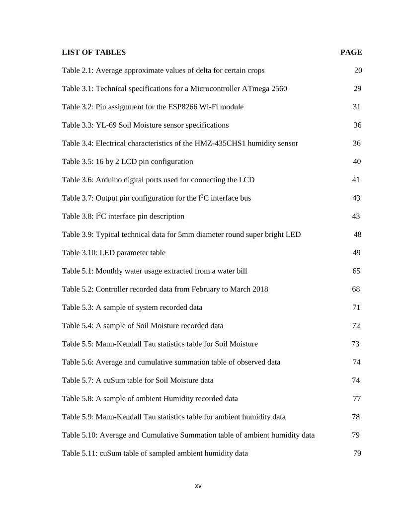
LIST OF TABLES PAGE

Table 2.1: Average approximate values of delta for certain crops 20

Table 3.1: Technical specifications for a Microcontroller ATmega 2560 29

Table 3.2: Pin assignment for the ESP8266 Wi-Fi module 31

Table 3.3: YL-69 Soil Moisture sensor specifications 36

Table 3.4: Electrical characteristics of the HMZ-435CHS1 humidity sensor 36

Table 3.5: 16 by 2 LCD pin configuration 40

Table 3.6: Arduino digital ports used for connecting the LCD 41

Table 3.7: Output pin configuration for the I2C interface bus 43

Table 3.8: I2C interface pin description 43

Table 3.9: Typical technical data for 5mm diameter round super bright LED 48

Table 3.10: LED parameter table 49

Table 5.1: Monthly water usage extracted from a water bill 65

Table 5.2: Controller recorded data from February to March 2018 68

Table 5.3: A sample of system recorded data 71

Table 5.4: A sample of Soil Moisture recorded data 72

Table 5.5: Mann-Kendall Tau statistics table for Soil Moisture 73

Table 5.6: Average and cumulative summation table of observed data 74

Table 5.7: A cuSum table for Soil Moisture data 74

Table 5.8: A sample of ambient Humidity recorded data 77

Table 5.9: Mann-Kendall Tau statistics table for ambient humidity data 78

Table 5.10: Average and Cumulative Summation table of ambient humidity data 79

Table 5.11: cuSum table of sampled ambient humidity data 79

xvi

Table 5.12: A sample of Temperature data 82

Table 5.13: Mann-Kendall Tau statistics table for temperature data 83

Table 5.14: average and Cumulative Summation table for Temperature observed data 84

Table 5.15: cuSum table of sampled Temperature data 84

List of Abbreviations

1. GSM-----Global System for Mobile Communication

2. GPS------Global Positioning System

3. IoT-------Internet of Things

4. SSD------Service Set Identifier

5. HTTP----Hyper Text Transfer Protocol

6. API------Application Programming Interface

7. PWM----Pulse Width Modulation

8. SoC------System-on Chip

9. WPA-----Wi-Fi Protected Access

10. Wi-Fi----Wireless Fidelity

11. I2C-------Inter-Integrated Circuit

12. GPIO----General Purpose Input Output

13. SPI-------Serial Peripheral Interface

14. DMA----Direct Multiple Access

15. UART---Universal Asynchronous Receiver Transmitter

16. TCP/IP--Transmission Control Protocol/Internet Protocol

17. IDE------Integrated Development Environment

xvii

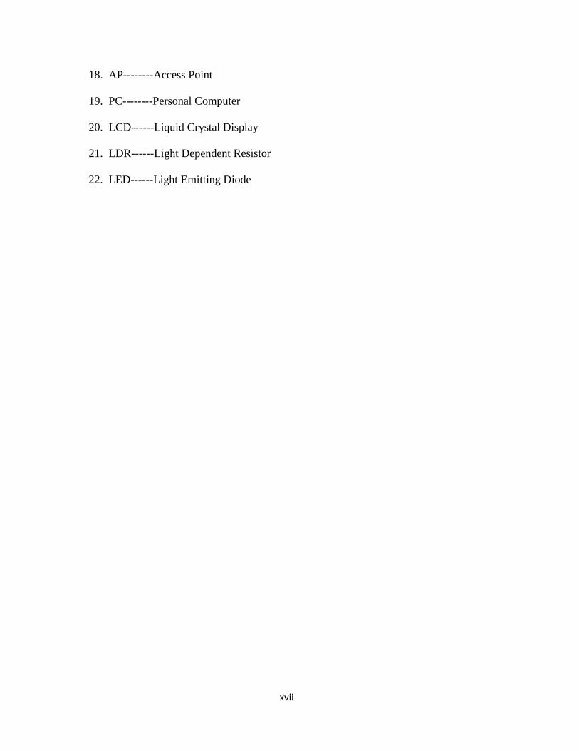
18. AP--------Access Point

19. PC--------Personal Computer

20. LCD------Liquid Crystal Display

21. LDR------Light Dependent Resistor

22. LED------Light Emitting Diode

1

CHAPTER 1: INTRODUCTION AND BACKGROUND

1.1 Introduction

The ever-growing need for food security requires that we continually improve on food production technologies

so as to increase the harvest per hectare in our farms. Experience gained from the recent series of droughts in

Southern Africa suggests that seasonal farming practices where farmers patiently wait for the rainy season may

contribute towards continuous food insecurity [1]. Part of the solution therefore is to resort to latest technologies

and innovations in a much larger scale. Irrigated agriculture is dependent on water bodies such as dams and

boreholes. Suffice it to say that this water is not enough and hence must be used sparingly. To conserve water,

there is therefore need for intelligent systems that can be used to water the crops as and when they need water

(optimal water usage). Besides saving water and cutting down on cost of labour, crops will also be better

nourished. This results in improved crop quality, higher yields and higher profits.

1.2 Background of the Study

This research design project is motivated by the need to address the incessant problem of food insecurity in

developing nations which is mainly due to erratic rainfall patterns [1] and a shortage of robust irrigation

solutions that are backed by state of the art technologies. The design of “smart” agricultural equipment that are

tailor-made to solve the specific problems faced by developing nations, has the potential to increase food

productivity and save on scarce water resources [2 ].

1.3 Problem Statement and Justification

Due to climate change and the occurrence of El Nino-induced droughts in Southern Africa, seasonal agriculture

is no longer a dependable way of ensuring food security [2, pp. 10]. Irrigated agriculture relies on water bodies

whose water levels keep diminishing as a result of droughts. Therefore optimal and effective use of the scarce

water resource becomes paramount. The farmers need to water their crops when the time and conditions are

2

right. The solution therefore lies in the deployment of technological pieces of equipment such as the smart

irrigation systems that use scientific methods to gather data, make informed decisions as to what the crop

requirements are. Crops must be watered exactly at the right time with the right amounts of water in order to

prevent over-watering or under-watering. Without use of smart systems and other modern technologies, the

developing world will continue to find it difficult to produce enough food to feed its people.

1.4 The Project Scope

The design build project incorporates a Wi-Fi module and an algorithm which enables it to work as an Internet

of Things (IoT) object [12] in the process of acquiring, intelligently manipulating, and displaying current

weather data and thirteen days weather-forecast information from the OpenWeatherMap Internet Server [3] for

free. In the field of weather monitoring, there are global platforms which keep track of weather conditions

around the world. These platforms are IoT ecosystems which can be accessed online. It is possible to design

custom electronic devices that can connect with such platforms and fetch weather related data from the cloud

platform. One such global platform is OpenWeatherMap. The OpenWeatherMap is an online service that

provides weather data to web services and mobile applications. It provides more than 1 billion forecasts [3]

every day from around the world. There are more than a million users of this platform and thousands of new

subscribers are adding each day [3]. The platform provides more than twenty application programming

interfaces (APIs) to render weather related data. In this project, the ESP8266 Wi-Fi module is programmed to

connect to one of the APIs provided by OpenWeatherMap so as to facilitate automatic download and display

of weather data and weather forecast information on the computer display or on a smartphone. The system also

employs scientific and very accurate methods of finding out if plants are in need of water or not. If plants are

found to be in need of water, that is if soil moisture level reduces to the plant’s management allowable depletion

level (the lowest moisture level which can be sustained by plants without adverse stress effects) [13], the

controller automatically triggers the system to water the crops. The other aim of this project is to save water. If

plants are watered during the day, a large percentage of water is lost through evapotranspiration due to the sun’s

heat. To mitigate the problem of evapotranspiration, the controller will automatically cause watering of the

3

plants, (i) only if they are about to be “thirsty”, and (ii) when it gets dark, without user intervention. The system

is “smart” enough to tell if soil moisture level is still above, or if it has gone below Management Allowable

Depletion level and reducing towards the Permanent Wilting Point for a particular crop in a particular soil type

[13]. If moisture is still above the Management Allowable Depletion level and there is need for irrigation, the

system will only irrigate when it gets dark since the plant is still not yet at risk of stressing. If by any chance, it

happens that soil moisture drops to levels between Management Depletion level and the Permanent Wilting

Point, then the system must irrigate the crops right away and also activate the alarm since this is a stressful

range for the crop. Crop watering and the alarm signal will stop once soil moisture level in the crop’s root zone

has risen to a safe percentage. This system also incorporates an in-built mini weather station which measures

the ambient temperature, barometric pressure, and the ambient humidity at the farm site. The in-built weather

station comes handy when the OpenWeatherMap server is unavailable during periods of Internet outages. The

system can also be made to operate in manual mode when the need arises. Besides making it possible to

remotely operate the system, the Internet of Things (IoT) application also enables the manufacturer of the

product to easily render remote technical assistance to the farmer through monitoring and updating of the system

software. The farmer does not need to visit the fields in order to see how the system is operating and to get

system parameters, but can access all the data from the comfort of their home. Most of the features discussed

here are not available in the products that are currently visible on the market.

1.5 Limitations of the Study

This research project involves construction of a physical, working prototype. The designer of this project faced

challenges in terms of acquiring the necessary components required for the construction of the prototype. Local

retailers hardly have the required components in stock. Therefore, most components for the prototype

construction were imported. This had an effect of increasing the duration and costs of prototype development.

4

CHAPTER 2: LITERATURE REVIEW

2.1.0 Introduction

This section consists of a review of relevant literature, including a review of automatic irrigation systems

available on the market and a review of the water requirements of different crops. Since this automatic irrigation

control system incorporates an algorithm for remotely acquiring weather data and weather-forecast information

from the OpenWeatherMap internet server [3], a discussion of weather prediction methods and the Internet of

Things (IoT) is also going to be conducted. Statistical methods for data analysis are employed for the analysis

of prototype test results. Therefore, statistical methods such as the Mann-Kendal Tau statistics, the Split-Sample

test, and the t-test for accuracy are also discussed.

2.2.0 An overview of existing Irrigation Controllers

After a market search for irrigation controllers that can be found on the market, it was discovered that: (a) The

products that are currently visible on the market are semi-automatic, open-loop and unintelligent, which means

that there is need for user intervention in their operation since most of them use a timer that is set by the user [4].

This is a draw back since it becomes difficult to gauge if enough water has been delivered to the crop or not.

Too much or too little water causes stress, diseases and crop failure. Besides the inclusion of an IoT application

which enhances its smartness, the design at hand is completely automatic and closed-loop to ensure that the

system works very well without user intervention. All that the user does is just to check the system status and

parameters remotely or locally at their own convenience. (b) Most automatic irrigation controllers that currently

exist in the market do not incorporate IoT applications. This means that they do not have Internet communication

capabilities. Internet of Things Technology is a game changer since it easily facilitates remote customer service

technical support and product autonomy. Products in the market lack this vital technology. Internet connectivity

enables the user to monitor and to control the system from any location in the world.

5

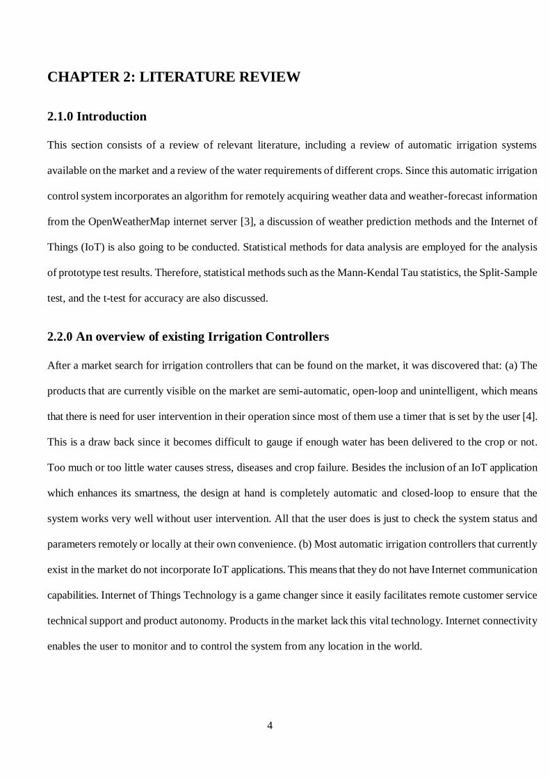
2.2.1 Hunter Eco-Logic Irrigation Controller

The most visible Irrigation Controller on the market currently is the Hunter Eco-Logic [4], which is shown in

Figure 2.2.1. The Hunter Eco-Logic irrigation controller has the same short comings as described on points (a)

and (b) in page 4.

Figure 2.2.1: Hunter Eco-Logic Irrigation Controller [4].

The semi-automatic Hunter Eco-Logic irrigation controller uses several timers in order to achieve its open loop

control of water pumps. It comes with a voluminous manual which is not very user friendly. This irrigation

controller and other such machines that are currently found in the market are not very user friendly in the sense

that it is difficult to learn how to use them and also that too much time is wasted while the user is manually

programming the system. This has an effect of disadvantaging most farmers since they may find it so difficult

to read through it. This shows that these systems were not designed with the semi-literate customer in mind.

The X-core irrigation controller does not connect to the Internet. This means there is no remote technical support

for the customer and it does not provide weather data. Also the user has to read data directly on the instrument’s

panel [4], meaning that the user has to travel to the site where the system is deployed in order to collect data

about the system parameters and the state of the irrigation equipment. These are some of the challenges that are

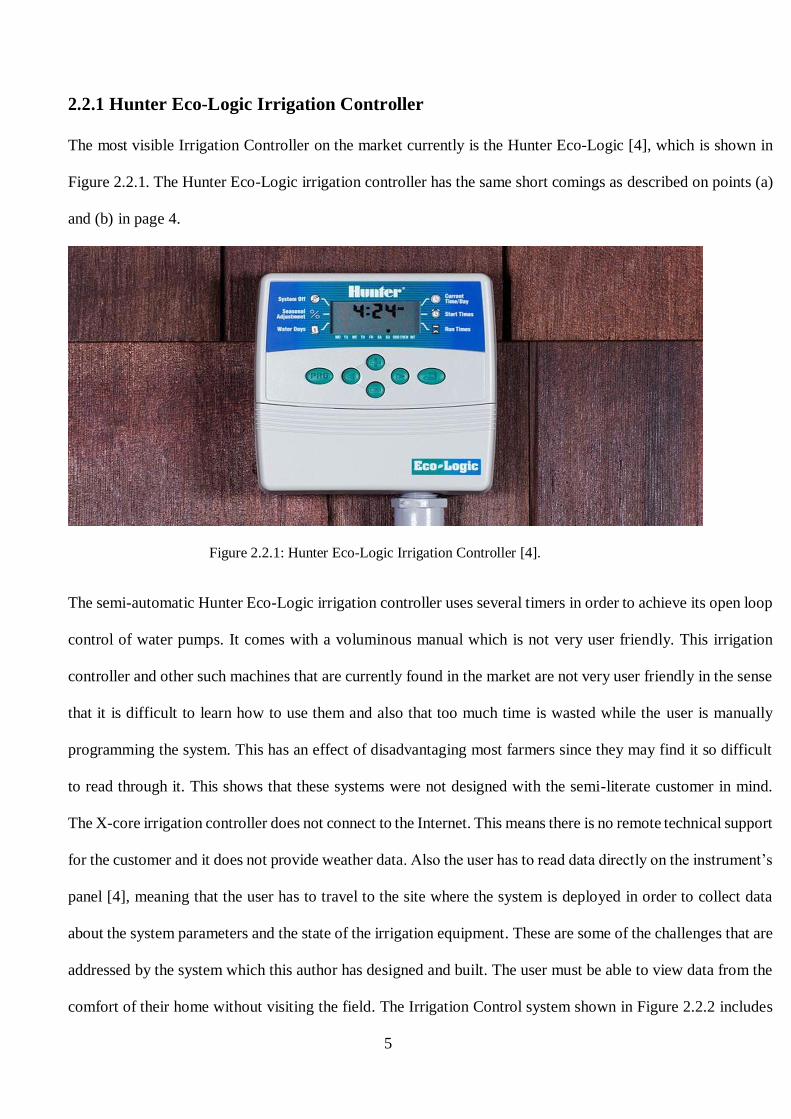
addressed by the system which this author has designed and built. The user must be able to view data from the

comfort of their home without visiting the field. The Irrigation Control system shown in Figure 2.2.2 includes

6

more functionalities when compared with Hunter Eco-Logic since it also measures plant nutrients. Its short

comings are that it does not address the issues of soil-moisture monitoring and does not provide weather data

[5]. It also does not address the vital remote communication requirements between the field devices (sensors,

actuators, and the controller) and the farmer’s control and monitoring console at home. The aim of the design–

build project at hand is to correct all these shortcomings.

Figure 2.2.2: Irrigation Control System measuring nutrients in plants [5].

2.3.0 Weather forecasting

The automatic irrigation control system at hand automatically downloads weather data and weather forecast information

from an Internet server and it also accommodates a standby in-built mini-weather station which can be relied upon during

Internet outages since it gives less weather parameters than those obtained from the Internet. Therefore this document

also discusses the topic of weather and weather forecasting. Weather is the state of the atmosphere at a particular place

during a short period of time [6]. Weather involves such atmospheric phenomena as temperature, humidity, precipitation,

air pressure, wind, and cloud cover. Weather is largely confined to the troposphere, the lowest region of the atmosphere

that extends from the earth’s surface to about 6km to 8 km at the poles and to about 17 km at the equator [6]. The

phenomena occurring in upper regions of the troposphere and above, such as jet streams and upper air waves, significantly

affect sea-level atmospheric pressure patterns and hence, the weather conditions at the terrestrial surface. Geographic

features, most notably mountains and large water bodies such as lakes and oceans, also affect weather patterns. Ocean-

surface temperature anomalies are a potential cause of atmospheric temperature anomalies in successive seasons and at

distant locations. One result of such weather interactions between the ocean and the atmosphere is the ElNino Oscillation

7

(ENSO) [6], which is responsible for draughts in Southern Africa and elsewhere around the world. Weather has a huge

influence in food production. Thunderstorms, tornadoes, hail, and sleet storms may damage or destroy crops. The long

absence of rainfall may cause droughts and severe dust storms when winds blow over parched farmland as with the

“dustbowl” conditions of the United States plains in the 1930s [7]. Weather forecasting is a prediction of what the state

of the atmosphere will be like at a particular future time and place through use of technology and scientific knowledge to

make weather observations [7]. Weather forecasting involves predicting weather phenomena such as cloud cover, rain,

snow, wind speed, air-pressure, humidity, precipitation, and temperature [7]. Farmers need weather information to help

them plan for the planting and harvesting of their crops in line with the weather predictions. A farmer can decide not to

irrigate if the weather forecast says that it is going to rain in the next few hours or in the next few days. A farmer can also

decide to harvest the crop before an approaching bad weather destroys the crops. The tools used for weather forecasting

are instruments such as air-pressure barometers, radar for measuring the location and speed of clouds, thermometers for

measuring ambient temperature, hygrometers for measuring soil-moisture content, anemometers for measuring wind

speed, and computer models for processing data accumulated from the instruments. Weather forecasts are derived from

a collection of as much data as possible about the current state of the atmosphere and then using techniques of metrology

to determine how the atmosphere will evolve in future. There are three major types of weather predictions, which are: the

short-range, medium-range, and the long-range weather-forecasts. Short-range forecasts are predictions made between

one day and seven days before they happen. Medium-range forecasts usually fall between one week and four weeks in

advance. Long-range forecasts are given between one month and a year in advance. The longer the period of forecast, the

less the accuracy [7]. Therefore, short-range forecasts are far more accurate than the medium-range and the long-range

forecasts.

2.4.0 Statistical analysis of data

For the analysis of results recorded during prototype testing, statistical tools are used to check for accuracy and

trend of the data. The employed statistical tools are going to be introduced in this chapter. The primary

parameters used are the variance, the mean, the standard deviation, and the range. The main tools used are the

Split-sample test (t-test) for self-stationarity, the Mann-kendal tau statistic, and the test for data accuracy.

8

2.4.1 The Split- sample test

The split-sample test (t-test) is being used to test for self-stationarity of data to check whether there is significant or no

significant difference amongst the observed sample averages. This is done so as to establish if there was intervention or

no intervention in the processes, and to find out the cause of the intervention in order to assess its impact. The t-test

analysis is mostly applied to small sets of data (n1, n2 < 30) [8], where s1 and s2 are dissimilar. It compares the

means of the sets of data for accuracy and for bias. The T-test formula [8, 9] is given by:

𝑡 =|1−2|

√𝑠1

2

𝑛1+

𝑠22

𝑛2

(1)

where: s1 is the standard deviation of sample 1, s2 is the standard deviation of sample 2, n1 is number of elements

in sample 1, n2 is the number of elements in sample 2, x1 is the mean value of sample 1, and x2 is the mean

value of sample 2.

2.4.2 The Mann-kendall test

The common purpose of the Mann-Kendall [9, 10, 11] test is to detect monotonic trends in a series of

environmental data, climate data or hydrological data. The null hypothesis (when there is no trend), H0, is that

the data comes from a population of independent and identically distributed data. The alternative hypothesis

(when there is a trend), HA, is that the data follow a monotonic trend. The Mann-Kendall test statistic is

calculated according to the following formula:

S = ∑ ∑ 𝑆𝑔𝑛(𝑋𝑗 − 𝑋𝑘)𝑛𝑗=𝑘+1

𝑛−1𝑘=1 (2)

With 𝑠𝑔𝑛(𝑥) =

1 𝑖𝑓 𝑥 > 00 𝑖𝑓 𝑥 = 0−1 𝑖𝑓 𝑥 < 0

(3)

2.4.3 The test for accuracy

The collected data is also tested for percentage accuracy. This is done in order to establish the reliability of the

system under test. The system accuracy is calculated according to the following formula.

𝐀𝐜𝐜𝐮𝐫𝐚𝐜𝐲 = 𝟏 − |−𝝁

𝑹| Where is the sample mean, 𝜇 is the population mean, and 𝑅 is the range (4)

9

2.5.0 The Internet of Things (IoT) technology

The Internet of Things (IoT) is the extension of the current internet to designate a technological concept in

which everyday objects are connected to the Internet, perceive or capture information from the environment,

communicate and act intelligently [12]. With the Internet of Things, objects can be remotely activated and

controlled through an existing network infrastructure, creating opportunities for integration between the

physical world and computer systems. In the case of ‘smart’ Agriculture, scattered sensors can provide

information on temperature, soil moisture, wind speed, and when combined with weather forecast information

available on the Internet can allow optimization of irrigation systems, saving water and improving farm yield.

Sensors connected to animals can help control livestock. For example, a microchip attached to an ox ear can

track the animal and inform on its vaccination record, among other information [12].

2.5.1 The Internet of Things architecture

The Internet of Things architecture consists of three main sections namely, Perception/Performance, Network,

and Application as shown in Figure 2.5.1. The Perception / Performance component refers to the parts of the

IoT system that interact with the physical world. Normally the "things" of IoT, which are the intelligent

objects, belong to this section. This section is called perception because it collects information from the real

world and allows the Internet of Things platform to respond to real events. The Network component is

responsible for making connections amongst IoT systems. These connections can be with other intelligent

objects or computers. In Internet of Things, as the name says, the Internet is mostly used to connect smart

objects. The technologies and strategies for making this connection to the Internet are defined in the Network

section. The Application component is the part of the Internet of Things platform that delivers services to the

people. It uses the other two components (perception and network) to do something useful.

Figure 2.5.1: Internet of Things Architecture [12].

10

The main communication technologies used in IoT are: (i) Ethernet (IEEE 802.3): It is widely used to connect

desktop computers to the Internet. Ethernet uses a cable medium, and it has high data transmission rates and a

wide range. It has data transmission rates of up to 1Gbps for a maximum range of 100 meters. Using the optical

fibre, it can transmit at a rate of 10Gbps for a distance of up to 2 kilometers. As it uses cables, this technology

would not be applicable to most intelligent objects such as an intelligent umbrella for example, since it makes

mobility difficult. But on the other hand, it could be used for smart refrigerator. (ii) WiFi (IEEE 802.11): This

standard refers to a wireless communication technology with a radius of about 50 m which

is suitable for local area networks. It has data transmission rates that are fast enough

to enable watching and downloading of videos. This wireless technology is mostly used

in such places as offices, industry, and public spaces. (iii) ZigBee: This is a wireless

communication technology standard with a radius of about 30 m at a lower data

transmission rate than the Wi-Fi standard (around 250Kbps). Nevertheless, ZigBee

consumes less battery energy than Wi-Fi, hence it has been adopted for use in several

IoT products. (iv) Bluetooth Low Energy: Bluetooth is a wireless communication technology standard that

has been developed to be the intermediate between ZigBee and Wi-Fi in terms of data transmission rate, range,

and battery consumption. Its latest version, the Bluetooth Low Energy is capable of transmitting 1Mbps with a

range of up to 80m at a low battery power consumption. This technology has been adopted in many smartphones

and tablets. (v) Third generation (3G) and Fourth Generation (4G) networks: This technology is for wireless

communication over cellular networks. Its power consumption is high when compared to other technologies.

3G/4G are used for communication with remote locations and when high mobility is a requirement. The

throughput achieved in the 3G standard is about 1Mbps and the standard 4G is up to 10Mbps [12].

2.6.0 Water requirements of crops

Every type of crop requires a certain quantity of water after a certain interval of time which varies due to soil

11

retention, ambient temperature, and ambient humidity, throughout its period of growth. If the natural rain is

sufficient and timely, no irrigation water is required for raising the crop. In England, for example, the natural

rain falling regularly throughout the year, satisfies requirements of practically all the crops, and, therefore,

irrigation is not significantly needed in England [13]. In Sub-Saharan Africa, the natural rainfall is no longer

sufficient and does not fall regularly due to climate change [13, 14]. Since the quantity as well as the frequency

of the rainfall varies throughout Sub-Saharan Africa, certain crops may require irrigation in certain parts of a

country. The area where irrigation is a must for agriculture is called the arid region, while the area in which

inferior crops can be grown without irrigation is called semi-arid region [13, pp. 22]. The title ‘Water

requirements of a crop’ means the total quantity required and the way in which a crop requires water, from the

time it is sown to the time it is harvested. It is very clear from the above discussion that the water requirement,

will vary with the crop as well as with the place. i.e. different crops will have different water requirements, and

the same crop may have different water requirements at different places of the same country; depending upon

the variations in climates, type of soils, methods of cultivation, and useful rainfalls.

2.6.1 Optimum utilization of Irrigation Water

If a crop is sown and produced under absolutely identical conditions, using different amounts of water, the yield

is found to vary [13, pp. 31]. The yield increases with water, reaches a certain maximum value and then

decreases, as shown in Figure 2.6.1.

Figure 2.6.1: Yield versus Water depth [13].

The quantity of water at which the yield is maximum, is called the optimum water depth. Therefore, optimum

utilization of irrigation generally means, getting maximum yield with any amount of water. The supply of water

12

to various crops should be adjusted in such a way as to get optimum benefit ratio, not only for the efficient use

of available water and maximum yield, but also to prevent water-logging of the land in question. In order to use

water sparingly, it is necessary that the farmers be made aware of the fact that only a certain fixed amount of

water gives best results. Anything more than the required quantity, and anything less than the required quantity

reduces the yield. Many farmers feel that they can increase the crop yield by using a lot of water. Hence, they

try to supply lots of water to their fields by undue tapping at the outlets [13, pp. 31]. This does not increase

yield. Farmers should be encouraged to line their water courses, thereby saving a significant amount of the

costly irrigation water.

2.6.2 Soil Moisture Monitoring for Optimal Crop growth

Methods of irrigation monitoring and scheduling assume that the soil moisture content largely determines the

level of moisture in the plant. At any depth, if the soil is dry, water and nutrients become less available to the

roots and, this results in reduced yields [13, 14]. If excess water is administered, this water will go deeper than

the root zone, carrying valuable nutrients with it. This results in wasted water, as well as the risk of underground

water pollution and reduced yields [13, 14]. Keeping the soil too wet also causes the water-root hairs to die due

to lack of oxygen [12, 13]. Higher levels of humidity also increase the risk of diseases [13, 14].

Understanding the dynamics of soil-moisture fluctuations in the root zone will enhance the efforts for

maximizing yield and curbing waste of resources. The following points are key to soil and water relationship.

Water is held in a soil mixture by action of surface tension attracting water molecules to soil particles. The

amount of water that can be stored by a soil and its availability to plants both depend on soil type. Volumetric

Water Content (VWC) is a measure of the amount of water held in a soil expressed as a percentage of the total

mixture. Tension is a measure of the amount of water held in a soil expressed as the amount of work required

for plants to remove water from the soil. The relationship between VWC and Tension depends on soil type.

Field capacity is a soil water content that results in a state of balance between the force of gravity and surface

tension force [13, 14]. At field capacity soils have a balance of air and water that result in good growing

conditions.

13

2.6.3 Water Holding Capacity

Among other things, soil is a storage medium for farm water until it is used by plants. Water resides in the

spaces between soil particles [13, 14, 15]. The force of gravity constantly acts on water in the soil to move it

downwards and out of reach of the roots of the plants. The counterbalancing force which keeps it from moving

downward is surface tension, which causes the water to stick to soil particles. The smaller the soil particles, the

more combined the surface area they have, and the more they are able to hold onto water through the surface

tension [13, 14, 15]. Hence, the ability of water to move through soil and be stored in soil depends heavily on

soil type. When water enters a soil with large sandy particles, only a small amount stays attached to the particles

and the remainder quickly drains downwards. Sand has low ‘water holding capacity’. Conversely, a volume of

clay soil has very small particles. When water enters a clay soil, surface tension holds it tightly to the soil

particles and only a small remainder drains downwards. Therefore, clay has a high ‘water holding capacity’. A

soil with a high water holding capacity can store large amounts of water relative to its own volume after a rain

event and, under the right conditions; this stored water can remain available for plants to use. In a soil with very

small particles, the surface tension forces that allow for a large water holding capacity also make it difficult for

plants to extract and use the water. Water does not move easily through a fine-particle soil and it takes a large

amount of energy for plants to extract and use it. The force that a plant exerts on water so as to separate it from

soil particles and move it into the root system is referred to as tension force (measured in centibars as a negative

pressure or vacuum since plants suck the water out of the soil) [13, 14, 15]. Even if a soil contains water, if the

tension required to extract the water is greater than what the plants can overcome, they will wilt and die [13,

14, 15]. Sandy soils have low water holding capacity due to their large particles, therefore both water and

nutrients can easily drain away out of reach of plant roots. However, even though a sandy soil does not hold

much water, whatever it can hold is easily available to plants. Clay soils have large water holding capacity, but

because they hold onto water tightly, tension is relatively high for a given amount of water. A certain amount

of water in clay soil is not easily available to plants. Just as clay soil tightly binds to water, it can also keep

14

nutrients out of reach of plants. The ideal soil for most growing conditions is a loamy soil with a variety of

particle sizes and ample structure which can hold a large amount of water that is easy for plants to extract. The

relationship amongst soil type, water holding capacity and water availability is illustrated in the Soil Texture

Triangle shown in Figure 2.6.2. The soil texture triangle gives names associated with various combinations of

sand, silt and clay. A course-textured or sandy soil is one comprised primarily of sand-sized particles. A fine-

textured or clayey soil is one dominated by tiny clay particles. Due to the strong physical properties of clay, a

soil with only 20% clay particles behaves as sticky, gummy clayey soil. The term loam refers to a soil with a

combination of sand, silt, and clay-sized particles. For example, a soil with 30% clay, 50% sand, and 20% silt

is called a sandy clay loam [14]. It is important to know what soil types are present in one’s field. Since any

point in the field can contain different soil types at different depths, it may be useful to use core samples to

determine soil type versus depth profiles at key locations.

Figure 2.6.2: Soil Texture Triangle [15]

15

2.6.4 Water Content, Tension and Field Capacity

The management line diagram in Figure 2.6.3 shows ranges for permanent wilting point, management allowable

depletion, field capacity and saturation. Saturation, Field Capacity, management allowable depletion, and

permanent wilt points shown in Figure 2.6.3 are the three important water content (or tension) levels used for

planning irrigation. These can be understood better through examination of how water moves through the soil

after a watering event.

Figure 2.6.3: Management Line diagram [15].

(i) Saturation: this is a phenomenon that comes as a result of water entering the soil volume at a faster rate than

when it is moved down by the force of gravity. Saturation is formally defined as the condition where all soil

pores/voids are filled with water. Saturated soil becomes heavy, contains little air, and can be thought of as mud. Conditions

in a saturated soil are anaerobic and are not conducive to healthy plant growth. Tension in saturated soil is very low,

generally less than -10 centibar. Volumetric Water Content at saturation can range between 15% and 60% depending on

soil type [13, 14, 15].

(ii) Field Capacity: After some time, substantially all of the water that will drain due to gravity has drained.

The soil solution is now in balance, containing all of the water that can be held by surface tension. This condition

16

is referred to as field capacity. At field capacity, water is easily available to plants, and the soil solution contains

ample oxygen. Optimal growing conditions for most plants occur at field capacity or slightly drier than field

capacity. Tension at field capacity is between -10 and -20 centibar. Volumetric Water Content can range from

10% to 50% depending on soil type [13, 14, 15].

(iii) Management Allowable Depletion: Management Allowable Depletion (MAD) is the lowest moisture

level which can be sustained by plants without adverse stress effects [13, 14, 15]. This is the moisture point at

which irrigation should be initiated to avoid having stress affect plant growth. Tension at MAD is typically -50

to -70 centibar. Volumetric Water Content at this point can range from 5% to 40%. Any moisture content below

this level is in the “stress” zones.

(iv) Permanent Wilting Point: As soil is subject to evaporation and withdrawals from plants, water content

deceases and tension increases to a point where plants can no longer extract water. Maintaining soil at this level

for any length of time can cause permanent damage to plants. Tension at PWP can be as great as -15 bar (-1500

centibar). The volumetric water content ranges from 2% for sandy soils to 30% for high clay-content soils [13,

14, 15].

2.6.5 Water Logging

An agricultural land is said to be water-logged, when its productivity gets affected by a high water table [13,

14, 15]. The productivity of the land in fact, gets reduced when the root of the plant gets flooded with water,

and thus become ill-aerated. Ill-aeration reduces crop yield, as explained below:

The life of a plant depends upon the nutrients such as nitrates. The foliage which produces the nitrates consumed

by the plants is produced by the bacteria, under the process called nitrification. These bacteria need oxygen for

their survival. The supply of oxygen gets cutoff when the land becomes ill aerated, resulting in the death of the

bacteria, and fall in the production of plants’ food (nitrates) and consequently reduction in the plant growth,

which reduces the crop yield. Apart from ill-aeration of the plants, many other problems are created by water-

logging, as discussed below [13, 14, 15].

2.6.5.1: The normal cultivation operations, such as tilling, ploughing, etc. cannot be easily carried out in very

17

wet soils. In extreme cases, the free water may rise above the surface of the land, making the cultivation

operations impossible. In ordinary language, such land is called a swampy land.

2.6.5.2: Certain water loving plants like grasses, weeds, etc. grow profusely and luxuriantly in water-logged

lands, thus affecting and interfering with the growth of the crops.

2.6.5.3: Water logging also leads to salinity, as explained in the following paragraph:

If the water table has risen up, or if the plant roots happen to come within the capillary fringe, water is

continuously evaporated by capillarity. Thus, a continuous upward flow of water from the water table to the

land surface gets established. With this upward flow, the salts which are present in the water also rise towards

the surface resulting in the deposition of salts in the root zone of the crops. The concentration of these alkali

salts present in the root zone of the crops has a corroding effect on the roots, which reduces the osmotic activity

of the plants and checks the plant growth, and the plant ultimately fades away. Such soils are called saline soils.

From this discussion, it becomes evident that water-logging ultimately leads to salinity, the result of which is,

the reduced crop yield for most crops. For this reason, salinity and water logging are treated as a twin problem;

under the heading “salinity and water-logging”. Whenever there is water logging, salinity also occurs [13, 14].

2.6.6 Irrigation Efficiencies

Efficiency is the ratio of the water output to the water input, and usually expressed as a percentage [13, pp. 31].

Higher input than output results in losses, and hence, if losses are high, efficiency is low. Efficiency is inversely

proportional to the losses. Water is lost in irrigation during various processes and, therefore, there are different

kinds of irrigation efficiencies, as given below:

(i) Efficiency of water-conveyance: it is the ratio of the water delivered into the fields from the outlet point of

the channel, to the water entering into the channel at its starting point. It may be represented by ηc. It takes the

conveyance or transit losses into consideration.

(ii) Efficiency of water-application: it is the ratio of the quantity of water stored into the root zone of the crops

to the quantity of water actually delivered into the field. It may be represented by ηa. It may also be called

on-farm efficiency, as it takes into consideration the water lost in the farm.

18

(iii) Efficiency of water storage: It is the ratio of water stored in the root zone during irrigation to the water

needed in the root zone prior to irrigation. It may be represented by ηs.

(iv) Efficiency of water use: it is the ratio of the water beneficially used, including leaching water, to the quantity

of water delivered. It may be represented by ηu.

2.6.7 Techniques of Water distribution on Farms

There are various ways in which the irrigation water can be applied to the fields [13, 14].

1. Sprinkler irrigation

2. Free flooding

3. Check flooding

4. Furrow irrigation method

5. Drip irrigation method

6. Border flooding

7. Basin flooding

Out of the above mentioned irrigation techniques, the author of this project will only elaborate on Sprinkler

irrigation since it is the most commonly used method in Southern Africa.

2.6.8 The Sprinkler Irrigation method

In this farm-water application method, water is applied to the soil in the form of a spray through a network of

pipes, pumps and sprinklers. It is some kind of an artificial rain and, therefore gives very good results. It can be

used for all types of soils and for widely different topographies and slopes. It can advantageously be used for

many crops, because it fulfills the normal requirement of uniform distribution of water. This method possesses

great potentialities for irrigating areas where other types of surface or sub-surface irrigation are very difficult.

The correct design and efficient operation are very important for the success of this method. Special steps have

to be taken to prevent entry of silt and debris, which are very harmful for the sprinkler equipment. Debris choked

nozzles interfere with the application of water on the land; while the abrasive action of silt causes excessive

wear on pump impellers, sprinkler nozzles, and bearings. The system is to be designed in such a way that the

19

entire sprayed water seeps into the soil, and there is no run off from the irrigated area [13, 14].

The conditions favoring the adoption of this method are: [13].

(i) When the land topography is irregular, and hence unsuitable for surface irrigation

(ii) When the land gradient is steeper, and soil is easily erodible

(iii) When the land soil is excessively permeable, so as not to permit good water distribution by surface

irrigation; or when the soil is highly impermeable

(iv) When the water-table is high

(v) When the area is such that the seasonal water requirement is low, such as near the coasts

(vi) When the crops to be grown are to require humidity control, as in tobacco; crops having shallow roots; or

crops requiring high and frequent irrigation; or when the water is scarce

2.6.9 Crop period or Base period

The time period that elapses from the instant of its sowing to the instant of its harvesting is called the crop-

period [13, 14]. The time between the first watering of a crop at the time of its sowing to its last watering before

harvesting is called the Base period or the Base of the crop. Crop period is slightly more than the Base period,

but for all practical purposes, they are taken as one and the same thing, and generally expressed in days. Hence,

the terms such as growth period, crop period, and base period, are used as synonyms, each representing crop

period, and will be represented by B (in days).

2.6.10 Duty and Delta of a Crop

Each crop requires a certain amount of water after a certain fixed interval of time, throughout its period of

growth. The depth of water required every time, generally varies from 5 to 10 cm depending upon the type of

the crop, climate and soil [13, 14]. The time interval between two consecutive watering is called the frequency

of irrigation, or rotation period. The rotation period may vary between 6-15 days for different crops [13, 14].

The summation of the total water depth supplied during the base period of a crop, for its full growth, will

evidently represent the total quantity of water required by the crop for its full-fledged nourishment. This total

20

quantity of water required by the crop for its full growth (maturity) may be expressed in hectare-metre (Acre-

ft) or in million cubic metres (million cubic-ft) or simply as depth to which water would stand on the irrigated

area, if the total quantity supplied were to stand above the surface without percolation or evaporation. This total

depth of water (in cm) required by a crop to come to maturity is called its delta (Δ). The average values of delta

for certain crops are shown in Table 2.1. These values represent the total water requirement of the crops. The

actual requirement of irrigation may be less, depending upon the useful rainfall. Moreover, these values

represent the values on field, i.e. ‘delta on field’ which includes the evaporation and percolation losses.

Table 2.1: Average approximate values of Δ for certain important crops [13].

S.No Crop Delta on field

1. Sugarcane 120 cm (48″)

2. Rice 120 cm (48″)

3. Tobacco 75 cm (30″)

4. Garden Fruits 60 cm (24″)

5. Cotton 50 cm (22″)

6. Vegetables 45 cm (18″)

7. Wheat 40 cm (16″)

8. Barley 30 cm (12″)

9. Maize 25 cm (10″)

10. Fodder 22.5 cm (9″)

11. Peas 15 cm (6″)

2.6.11 Relationship between Duty and Delta

Let there be crop of base period B days. Now, the volume of water applied to this crop during B days is

V = (1 x 60 x 60 x 24 x B) m3 = 86 400 B (cubic meter) (5)

By definition of duty (D), one cubic meter supplied for B days matures D hectares [13] of land. Therefore: This

quantity of water (V) matures D hectares of land or 104 D sq.m of area.

Total depth of water applied on this land = Volume

Area=

86400B

104D=

8.64B

D m (6)

21

By definition, this total depth of water is called delta (Δ).

Therefore: ∆ =8.64B

Dm or ∆ =

8.64

Dcm (7)

Where Δ is in cm, B is in days, and D is duty in hectares/cumec.

2.6.12 Factors on which duty depends

Duty of irrigation water depends upon the following:

Type of crop: Different crops require different amount of water, and hence, the duties for them are different. A

crop requiring more water will have less flourishing acreage for the same supply of water as compared to that

requiring less water. Hence, duty will be less for a crop requiring more water and vice versa [13].

2.7 Chapter Summary

For the review of related literature, typical automatic irrigation controllers that are available on the market were

discussed. It was observed that these controllers are mainly semi-automatic, unintelligent, and sometimes too

expensive for the small holder farmer. They do not exploit the benefits brought about by the Internet of Things

(IoT) platform (one of the latest technologies available) and its user-friendly application software. This

document therefore tries to address most of the shortcomings of the irrigation controllers that are available on

the market. It tries to achieve this by coming up with a “smart” system which can make intelligent decisions to

the benefit of the farmer. The importance of weather forecast was also discussed as this should be one of the

very important tools used by the farmer to plan ahead. Therefore, designing a control system which is part of

the IoT platform makes it possible for the system to automatically acquire weather data and weather forecast

information from the Internet and present it to the farmer in whatever location in the world. Discussion on the

water requirements of the crop was also carried-out. It was observed that since the management allowable

depletion, saturation point, and the wilting points are different for different types of soil, the system under

design should have different modes of operation in order to cater for different soil types. This is mainly

implementable in the code section of the system. Statistical tools that are going to be used for analyzing the

prototype results were also discussed. This is done in order to ensure accuracy of the results.

22

CHAPTER 3: PROJECT DESIGN AND METHODOLOGY

3.1.0 Introduction

In order to come up with a working prototype, a step by step systematic design procedure is followed since one

procedure feeds into the next. This involves coming up with block diagrams, wiring diagrams, circuit diagrams,

the code, physical wiring of hardware components and finally, prototype integration and testing.

3.2.0 Design Methodology

The design part of the automated irrigation control system consists of three main sections, which are: the

controller hardware, the software, and the communications section. The integration of the three sections resulted

in the construction of a prototype, which was subjected to tests, and its results validated using statistical tools.

The automatic irrigation control system communication module involves Internet connectivity through Wi-Fi,

so as to enhance system capability. The intelligent controller block can be viewed as an Internet of Things (IoT)

object. IoT is a technological concept in which everyday objects are connected to the Internet, perceive

information from the environment and act intelligently [16]. With the Internet of Things, objects can be

remotely activated and controlled through an existing network infrastructure, creating opportunities for

integration between the physical world and computer systems [17].

3.3.0 Hardware Design

The hardware design aspect of the project starts with the block diagram, followed by the wiring diagram, which

is then followed by the circuit diagram. The block diagram will show how the different individual modules are

interconnected. These interconnected modules include the Arduino microcontroller module, the soil moisture

sensor module, the air humidity detection module, the temperature sensor module, the water-pump module, the

data logger module, the irrigation sprinkler module, the borehole pump module, the status Light-Emitting-

Diode module, and the power supply module. The block diagram is used as the guiding tool for compiling

schematic and wiring diagrams. The Arduino-Mega microcontroller board is the central controlling device for

23

the irrigation system. In this design, only one watering pump channel is shown, but ten or more such channels

can be added to the system. In this project, the YL69 soil moisture level sensors, can be replaced by homemade

soil moisture sensors in the field since the YL69 sensor has a problem of gathering rust resulting in changed

parameters and inaccurate output values. Soil moisture percentage levels and the borehole pump status are

displayed on the local liquid crystal display (LCD). All the other system parameters which include the weather

data from the Internet and from the standby in-built mini- weather station, are displayed remotely on the

personal computer screen and on the smartphone. LEDs show the present state of the pumps. The ESP8266

Wi-Fi module and the home access point plus router equipment enable the system to connect to the internet.

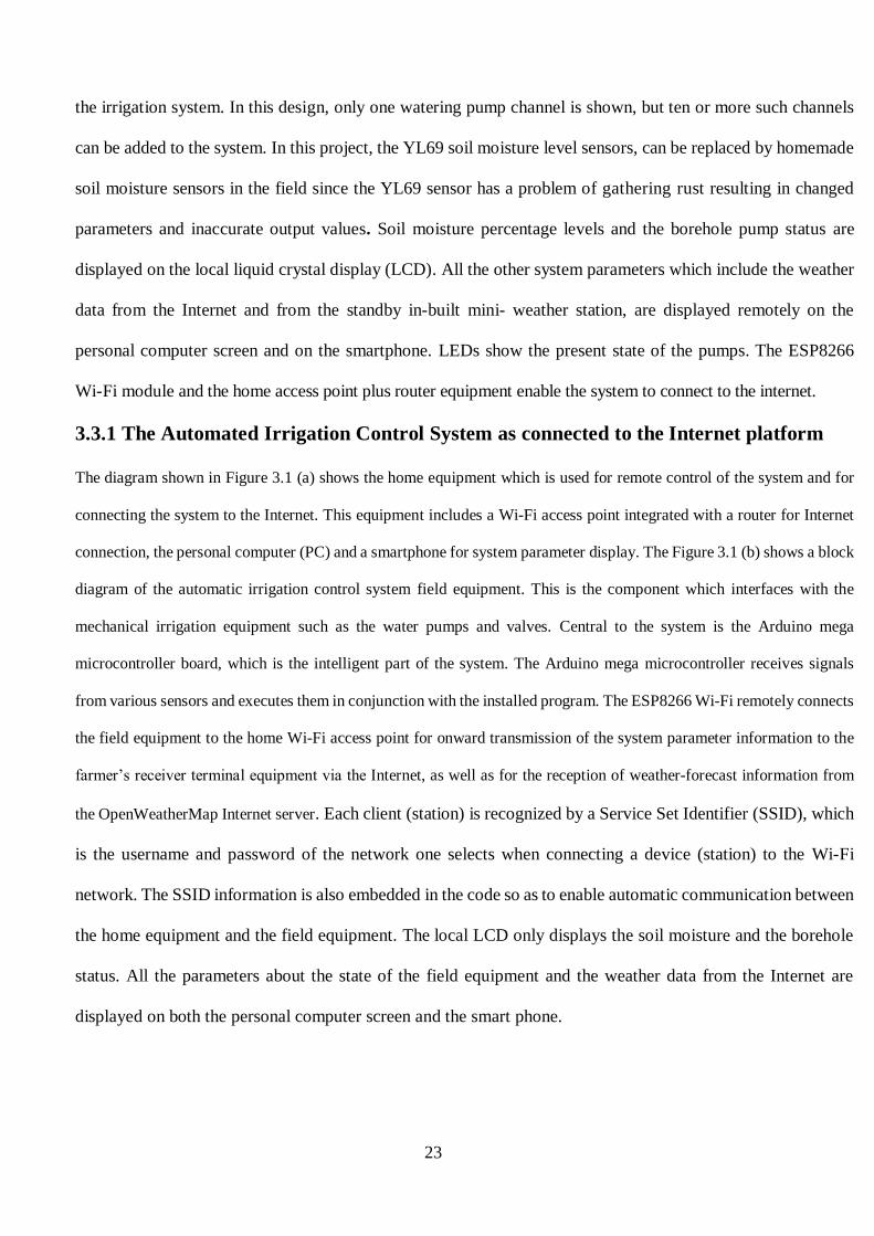
3.3.1 The Automated Irrigation Control System as connected to the Internet platform

The diagram shown in Figure 3.1 (a) shows the home equipment which is used for remote control of the system and for

connecting the system to the Internet. This equipment includes a Wi-Fi access point integrated with a router for Internet

connection, the personal computer (PC) and a smartphone for system parameter display. The Figure 3.1 (b) shows a block

diagram of the automatic irrigation control system field equipment. This is the component which interfaces with the

mechanical irrigation equipment such as the water pumps and valves. Central to the system is the Arduino mega

microcontroller board, which is the intelligent part of the system. The Arduino mega microcontroller receives signals

from various sensors and executes them in conjunction with the installed program. The ESP8266 Wi-Fi remotely connects

the field equipment to the home Wi-Fi access point for onward transmission of the system parameter information to the

farmer’s receiver terminal equipment via the Internet, as well as for the reception of weather-forecast information from

the OpenWeatherMap Internet server. Each client (station) is recognized by a Service Set Identifier (SSID), which

is the username and password of the network one selects when connecting a device (station) to the Wi-Fi

network. The SSID information is also embedded in the code so as to enable automatic communication between

the home equipment and the field equipment. The local LCD only displays the soil moisture and the borehole

status. All the parameters about the state of the field equipment and the weather data from the Internet are

displayed on both the personal computer screen and the smart phone.

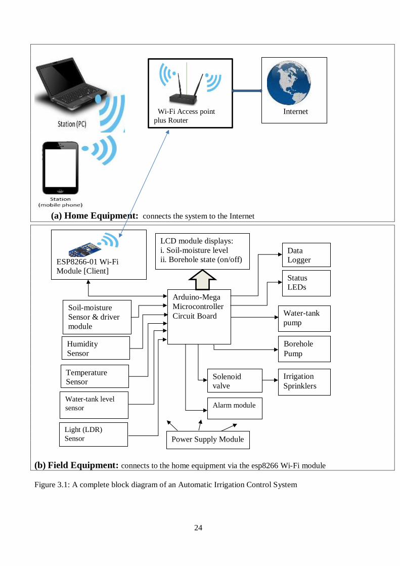
24

(a) Home Equipment: connects the system to the Internet

(b) Field Equipment: connects to the home equipment via the esp8266 Wi-Fi module

Figure 3.1: A complete block diagram of an Automatic Irrigation Control System

Wi-Fi Access point

plus Router

Internet

Arduino-Mega

Microcontroller

Circuit Board Water-tank

pump

LCD module displays:

i. Soil-moisture level

ii. Borehole state (on/off)

Irrigation

Sprinklers

Soil-moisture

Sensor & driver

module

Humidity

Sensor

Data

Logger

Status

LEDs

Power Supply Module

ESP8266-01 Wi-Fi

Module [Client]

Water-tank level

sensor Alarm module

Borehole

Pump

Light (LDR)

Sensor

Temperature

Sensor Solenoid

valve

25

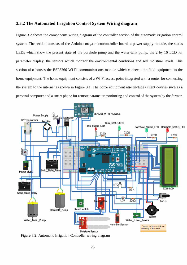
3.3.2 The Automated Irrigation Control System Wiring diagram

Figure 3.2 shows the components wiring diagram of the controller section of the automatic irrigation control

system. The section consists of the Arduino-mega microcontroller board, a power supply module, the status

LEDs which show the present state of the borehole pump and the water-tank pump, the 2 by 16 LCD for

parameter display, the sensors which monitor the environmental conditions and soil moisture levels. This

section also houses the ESP8266 Wi-Fi communications module which connects the field equipment to the

home equipment. The home equipment consists of a Wi-Fi access point integrated with a router for connecting

the system to the internet as shown in Figure 3.1. The home equipment also includes client devices such as a

personal computer and a smart phone for remote parameter monitoring and control of the system by the farmer.

Figure 3.2: Automatic Irrigation Controller wiring diagram

26

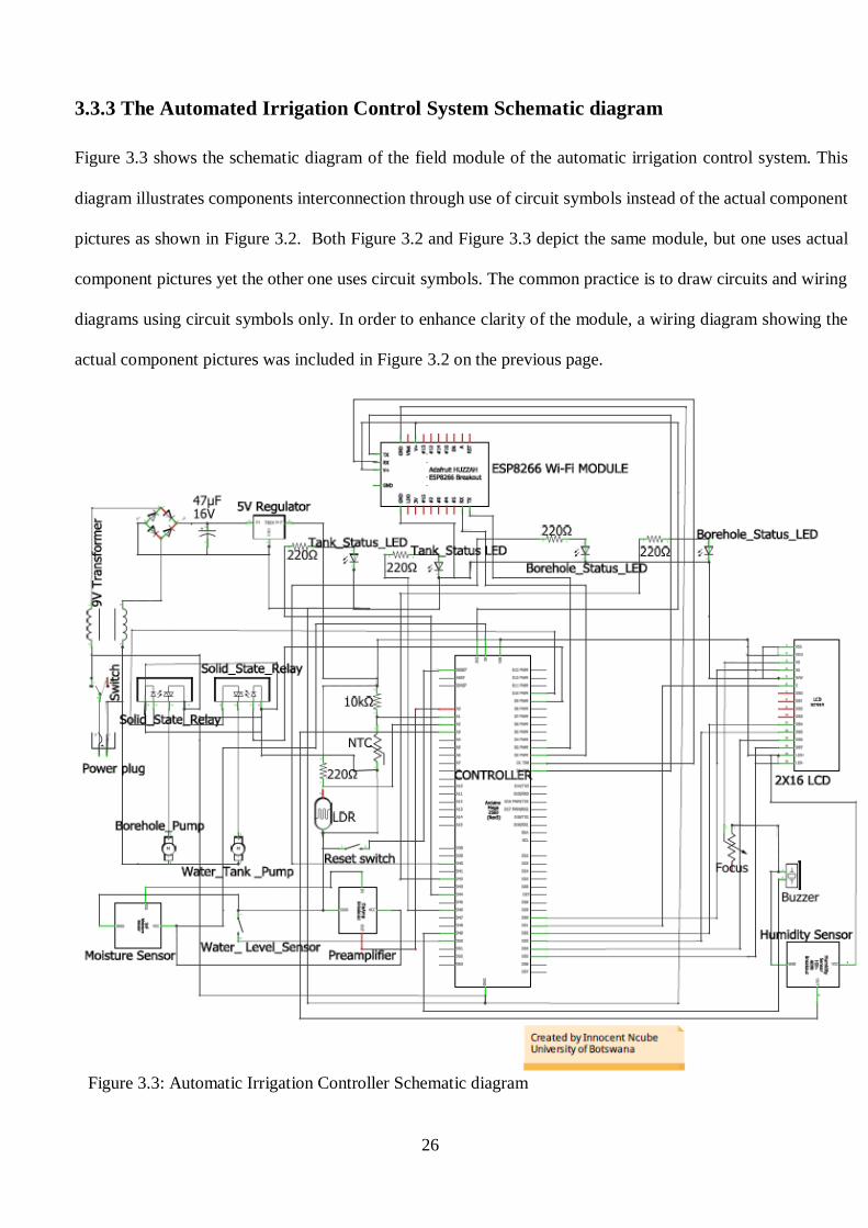
3.3.3 The Automated Irrigation Control System Schematic diagram

Figure 3.3 shows the schematic diagram of the field module of the automatic irrigation control system. This

diagram illustrates components interconnection through use of circuit symbols instead of the actual component

pictures as shown in Figure 3.2. Both Figure 3.2 and Figure 3.3 depict the same module, but one uses actual

component pictures yet the other one uses circuit symbols. The common practice is to draw circuits and wiring

diagrams using circuit symbols only. In order to enhance clarity of the module, a wiring diagram showing the

actual component pictures was included in Figure 3.2 on the previous page.

Figure 3.3: Automatic Irrigation Controller Schematic diagram

27

3.4.0 Design Components description

The hardware components used for this design consist of the Arduino Mega microcontroller board, the ESP8266

Wi-Fi communication module, the Arduino Ethernet shield (optional), the 16 by 2 liquid crystal display (LCD),

the light dependent resistor (LDR) sensor, the LM35 temperature sensor, the red, and green status light emitting

diodes (LEDs), 2 by 5V relay modules, Humidity sensor module, the I2C interface module, the alarm buzzer,

the data-logger memory module, and the Ubiquity microwave radios(optional).

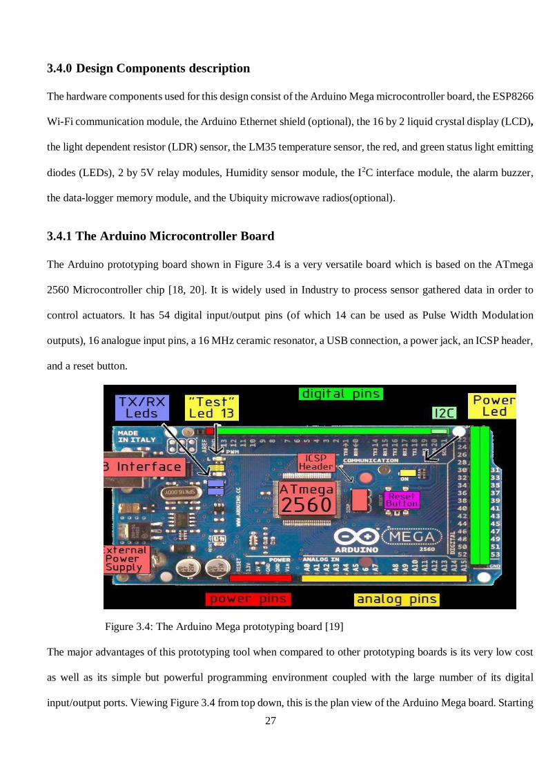
3.4.1 The Arduino Microcontroller Board

The Arduino prototyping board shown in Figure 3.4 is a very versatile board which is based on the ATmega

2560 Microcontroller chip [18, 20]. It is widely used in Industry to process sensor gathered data in order to

control actuators. It has 54 digital input/output pins (of which 14 can be used as Pulse Width Modulation

outputs), 16 analogue input pins, a 16 MHz ceramic resonator, a USB connection, a power jack, an ICSP header,

and a reset button.

Figure 3.4: The Arduino Mega prototyping board [19]

The major advantages of this prototyping tool when compared to other prototyping boards is its very low cost

as well as its simple but powerful programming environment coupled with the large number of its digital

input/output ports. Viewing Figure 3.4 from top down, this is the plan view of the Arduino Mega board. Starting

28

clockwise from the top center [19, pp. 275-277]: 1. Analogue reference pin, 2. Digital ground 3. Digital pins

2-21, 4. Digital pins 0-1/Serial in/Out – Transmit/Receive: these two pins cannot be used for digital input/output

(digitalRead and digitalWrite) if one is also using serial communication e.g. (serial.begin) at the same time,

5. Reset button and the In-circuit Serial programmer, 6. Digital pins 22 – 54, 7. Analogue input pins

8. Power and ground pins, 9. External power supply is (9- 12 VDC), 10. USB port: for uploading sketches onto

the board and for serial communication between the board and the computer. It can also be used to power the

board.

The Atmega 2560 has the following modules which are described in detail:

The Digital I/O Pins: It has 54 of which 14 provide Pulse Width Modulated (PWM) output)

Analogue Input Pins: 16 analogue input

Flash Memory: 256 KB of which 8 KB are used for the bootloader

EEPROM: 4 KB

1. Digital Pins: In addition to the specific functions listed below, the digital pins on an Arduino Mega board

can be used for general purpose input and output when configured in pinMode(), digitalRead(), and

digitalWrite() commands. Each pin has an internal pull-up resistor (disconnected by default) of 20-50kΩ which

can be turned on and off using digitalWrite() HIGH or LOW respectively when the pin is configured as an input.

The maximum current per pin is 40mA.

(a) Serial: Pin 0 (RX) and Pin 1 (TX); Serial 1: Pin 19 (RX) and Pin 18 (TX); Serial 2: Pin 17 (RX) and Pin

16 (TX); Serial 3: Pin 15 (RX) and Pin 14 (TX), used to receive (RX) and transmit (TX) TTL serial data. Pins

0 and 1 are also connected to the corresponding pins of the ATmega8U2 USB-to- TTL serial chip. These lines

are intended for use with an external TTL serial module (e.g. the mini-USB Adapter).

(b) External Interrupts: Pin 2 (interrupt 0), Pin 3 (interrupt 1), Pin 18 (interrupt 5), Pin 19 (interrupt 4), Pin

20 (interrupt 3), and Pin 21 (interrupt 2). These pins can be configured to trigger an interrupt on a low value, a

rising or falling edge, or a change in value. The function is attachInterrupt()

(c) Pulse Width Modulation (PWM): Pin 0 to Pin 13. Provide 8-bit PWM output with the analogWrite()

function.

29

(d) SPI: Pin 50 (MISO), Pin 51 (MOSI), Pin 52 (SCK), Pin53 (SS). These pins support SPI communication,

which although provided by the underlying hardware, is not currently included in the Arduino language. The

SPI pins are also broken out on the ICSP header.

(e) LED: Pin 13. There is a built-in LED connected to digital pin 13. When the pin is HIGH value, the LED is

on, when the pin is LOW, it is off.

2. Analogue Pins:

(a) I2C: Pin 20 (SDA) and Pin 21 (SCL) support I2C (TWI) communication using the Wire library.

(b) AREF: Reference voltage for the analogue inputs. Used with analogReference().

(c) Reset: It brings this line LOW to reset the microcontroller. Typically used to add a reset button to shields

which block the one on the board.

3. Power Pins: The power pins are arranged as follows:

(a) VIN: The input voltage to the Arduino board when it is using an external power source (as opposed to 5

volts from the USB connection or other regulated power source). Voltage can be supplied through this pin, or,

if supplying the voltage via the power jack, it can be accessed through this pin.

(b) 5V: The regulated power supply used to power the microcontroller and other components on the board. This

can come either from VIN via an on-board regulator, or be supplied by USB or another regulated 5V supply.

(c) 3V3: is generated by the on-board regulator. Maximum current drawn is 50 mA.

(d) GRD: This is for grounding the pins

Table 3.1: Technical Specifications for a Microcontroller ATmega 2560 [19].

Operating voltages: Input Voltage (recommended)

Input Voltage (limits)

7-12V

6-20V

Digital I/O Pins 54 (of which 14 provide PWM output)

Analog Input Pins 16

DC Current per I/O Pin 40mA

DC Current for 3.3V Pin 50 mA

Flash Memory 256 KB of which 8 KB are used by the bootloader

Static RAM 8KB

EEPROM 4KB

Clock Speed 16 MHz

30

3.4.2 The ESP8266 Wi-Fi Module:

The ESP8266 Wi-Fi board is a system-on-chip (SoC) which integrates a 32-bit Tensilica microcontroller,

standard digital peripheral interfaces, antenna switches, RF balun, power amplifier, a low noise receive

amplifier, filters and power management modules into a small package. It provides capabilities for 2.4 GHz

Wi-Fi (802.11 b/g/n, supporting WPA), general-purpose input/output (2 GPIO), Inter-Integrated Circuit (I²C),

analog-to-digital conversion (10-bit ADC), Serial Peripheral Interface (SPI), I²S interfaces with DMA (sharing

pins with GPIO), UART (on dedicated pins, plus a transmit-only UART can be enabled on GPIO2), and pulse-

width modulation (PWM).

The ESP8266 board can also be described as a Wi-Fi modem which can connect to a Wi-Fi hotspot or router

through use of the SSID and Password. Using the API key, the ESP8266 module can access data from the IoT

service. The ESP8266 is an Arduino compatible module. It needs to be loaded with a firmware that could fetch

data received over the internet and display that data to any designated screen. The Arduino board is used to

flash the firmware code on the ESP8266 module. The ESP module can also be flashed using an FTDI converter

such as the CP2102 board. The firmware itself is written in the Arduino IDE [21].

Figure 3.5: ESP8266 Wi-Fi board pinout [21].

Table 3.2 shows the pin assignment and description for the ESP8266 Wi-Fi module.

31

Table 3.2: Pin assignment for the ESP8266 Wi-Fi module [21]

Pin No.

Pin Name Alternative Name Normally used for Alternative purpose

1 Ground - connected to the ground of

the circuit

-

2 Transmit (Tx) GPIO-1 Connected to Rx pin of

programmer

microcontroller to upload

program

can act as a general purpose

input/output pin when not

used as Tx

3 GPIO-2 - General purpose

input/output pin

-

4 CH_EN - Chip Enable- Active high -

5 GPIO-0 Flash General purpose

input/output pin

takes module into serial

programming when held low

during start up

6 Reset - Resets the module -

7 Receive (Rx) GPIO-3 General purpose

input/output pin

Can act as a general purpose

input/output pin when not

used as Rx

8 Vcc - Connect to +3.3V only

ESP8266 Wi-Fi module operational modes:

The ESP8266 Wi-Fi module has three modes of operation, which are:

Access Point (AP) mode:

In AP mode, the ESP8266 module acts as a hub for one or more stations, allowing other devices to connect to

the Internet through itself. It establishes a two way communication between itself and the device that is

connected to it via Wi-Fi. Figure 3.6 shows the ESP8266 Wi-Fi module operating in the access point mode.

Figure 3.6: ESP8266 Wi-Fi module operating in the soft Access Point mode [22]

32

Station mode:

In the station mode, the ESP8266 Wi-Fi module can connect to the access point such as the Wi-Fi network from

a house or office. This enables any other device connected to the network to communicate with the ESP8266

module.

Figure 3.7 shows the ESP8266 Wi-Fi board operating in the station mode.

Figure 3.7: ESP8266 Wi-Fi board operating in the Station mode [22]

Station plus Access Point mode:

In the station plus access point mode, the ESP8266 Wi-Fi module acts as both an access point and a station.

Figure 3.8 shows the ESP8266 Wi-Fi board connected in the station and access point mode.

Figure 3.8: Station plus Access Point mode [22].

33

3.4.3 Arduino Ethernet Shield [optional]

The Arduino Ethernet shield makes it possible to connect and configure the Arduino board over the Internet

using an Ethernet cable connection medium [23, pp. 43-47]. An Ethernet shield is a printed circuit board

designed to mount on top of an Arduino board by connecting the headers on the Arduino. Shields are used to

extend the hardware features of the Arduino [23, pp. 45]. The Ethernet Arduino shield gives the Automatic

Irrigation controller some Internet capability through use of an Ethernet cable connection. The Arduino Ethernet

shield shown in Figure 3.9 and Figure 3.10 is a microcontroller communications board that works together with

the Arduino microcontroller board. Ethernet shield uses a Wiznet W5500 hardwired TCP/IP embedded Ethernet

controller interface to enable connection to the Internet. The Ethernet shield has 14 digital input/output pins, 6

analog input pins, a 16 MHz crystal oscillator, and an RJ45 Ethernet connection port. The Ethernet shield also

accommodates a micro-SD card memory chip for data logging.

Figure 3.9: Arduino Ethernet-2 Shield [24].

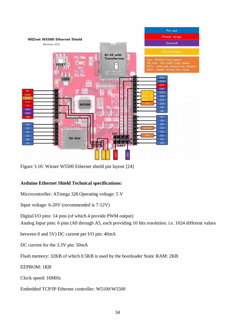
34

Figure 3.10: Wiznet W5500 Ethernet shield pin layout [24]

Arduino Ethernet Shield Technical specifications:

Microcontroller: ATmega 328 Operating voltage: 5 V

Input voltage: 6-20V (recommended is 7-12V)

Digital I/O pins: 14 pins (of which 4 provide PWM output)

Analog Input pins: 6 pins (A0 through A5, each providing 10 bits resolution. i.e. 1024 different values

between 0 and 5V) DC current per I/O pin: 40mA

DC current for the 3.3V pin: 50mA

Flash memory: 32KB of which 0.5KB is used by the bootloader Static RAM: 2KB

EEPROM: 1KB

Clock speed: 16MHz

Embedded TCP/IP Ethernet controller: W5100/W5500

35

Special Function Pins:

Serial pin 0 (RX) and pin 1 (TX): Used to receive and transmit TTL serial data

External Interrupts pins 2 and 3: can be configured to trigger an interrupt

Pulse Width Modulation (PWM) pins 3, 5, 6, 9 and 10: provide 8-bit PWM output with the analogWrite()

function

Serial Peripheral Interface (SPI) pins: pin10 Slave Select (SS), pin11 (MOSI),

pin12 (MISO), pin 13(SCK): These pins support SPI communication using the SPI library

Inter-Integrated Circuit/Two Wire Interface (I2C/TWI) pins A4 Serial data line (SDA) and pin 5 Serial

Clock Line(SCL): These support TWI communications using the wire library.

AREF: Reference voltage for the analogue inputs used with analogReference() function

Reset: Brings this line LOW to reset the microcontroller

The Arduino communicates with both W5500 and SD card using the Serial Peripheral Interface (SPI) bus

(through the ICSP header). That is, digital pins 11, 12, 13 on Uno and pins 50, 51 and 52 on the Mega.

On both Boards, pin 10 is used to select the W5500 and pin 4 for the SD card. These pins cannot be used for

general input/output. On Mega, the hardware SS pin 53 is not used for either W5500 or SD card, but it must be

kept as an output or the SPI interface won’t work. Because both the W500 and the SD card share the SPI bus,

only one can be active at a time. To deselect the SD card, set pin4 as an output and write a HIGH to it. For the

W5500, set digital pin 10 as a HIGH output.

3.4.4 YL-69 Soil Moisture Sensor and YL-69 Amplifier/Comparator PCB

The YL-69 soil moisture sensor shown in Figure 3.11 is an electrical variable resistance sensor which is made

up of two electrodes. It reads the soil moisture content of the soil surrounding it. Current passes across the

electrodes via the soil. The resistance to current in the soil depends on the soil moisture content. If the soil has

more water, resistance will be low and hence more current flows. On the other hand when the soil moisture is

low, the probe will give out a higher resistance. The YL-69 sensor module provides both digital and analogue

outputs. The analogue output pin is used in this case since the YL-69 sensor is connected to an analogue port

of the Arduino microcontroller board.

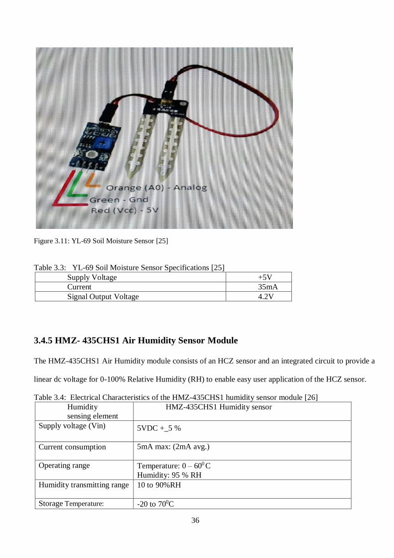
36

Figure 3.11: YL-69 Soil Moisture Sensor [25]

Table 3.3: YL-69 Soil Moisture Sensor Specifications [25]

Supply Voltage +5V

Current 35mA

Signal Output Voltage 4.2V

3.4.5 HMZ- 435CHS1 Air Humidity Sensor Module

The HMZ-435CHS1 Air Humidity module consists of an HCZ sensor and an integrated circuit to provide a

linear dc voltage for 0-100% Relative Humidity (RH) to enable easy user application of the HCZ sensor.

Table 3.4: Electrical Characteristics of the HMZ-435CHS1 humidity sensor module [26]

Humidity

sensing element

HMZ-435CHS1 Humidity sensor

Supply voltage (Vin) 5VDC +_5 %

Current consumption 5mA max: (2mA avg.)

Operating range Temperature: 0 – 600 C

Humidity: 95 % RH

Humidity transmitting range 10 to 90%RH

Storage Temperature: -20 to 700C

37

Storage Humidity 95%RH or less

Accuracy

Temperature: Resistance(1%): 50+-0.5KΩ(at 25+-0.20C)

Humidity: +_5%RH (at 250C, 60%RH, Vin = 5VDC)

Humidity output 0-3.3V at 250C, Vin = 5VDC

Signal reference Output impedance approx.: 5KΩ

Humidity(%RH) 10 20 30 40 50 60 70 80 90

Output

Voltage(V)

0.88 1.13 1.42 1.74 2.06 2.37 2.66 2.90 3.07

Temperature Output: Using thermistor 503 R (250C) = 50KΩ+_1% Signal

(Reference): B (25/85) = 3950K+_1%

Temperature(0C) 0 10 20 25 30 40 50 60

Resistance(KΩ) 160.56 98.714 62.328 50.0 40.356 26.756 18.138 12.554

3.4.6 Light Dependent Resistor (LDR)

A light dependent resistor (LDR) is also called a photo resistor or a cadmium sulfide (CdS) cell. It is also called

a photoconductor. It is basically a photocell that works on the principle of photoconductivity. It is a passive

component which is basically a resistor whose resistance value decreases when the intensity of light increases.

This optoelectronic device is mostly used in light varying sensor circuits, and light and dark activated switching

circuits as in this project. Some of its applications include camera light meters, street lights, clock radios, light

beam alarms, reflective smoke alarms, and outdoor clocks.

LDR Structure and its process of operation

The snake-like track shown in Figure 3.12(a) is the Cadmium Sulphide (CdS) film which also passes through the sides.

On the top and bottom are metal films which are connected to the terminal leads. It is designed in such a way as to provide

maximum possible contact area with the two metal films. The structure is housed in a clear plastic or resin case, to provide

free access to external light. As explained above, the main component for the construction of LDR is the cadmium

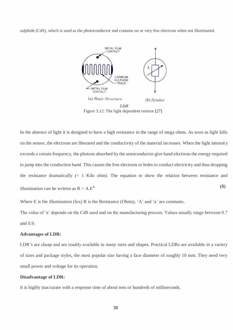
http://www.circuitstoday.com/optoelectronic-devices

38

sulphide (CdS), which is used as the photoconductor and contains no or very few electrons when not illuminated.

Figure 3.12: The light dependent resistor [27]

In the absence of light it is designed to have a high resistance in the range of mega ohms. As soon as light falls

on the sensor, the electrons are liberated and the conductivity of the material increases. When the light intensity

exceeds a certain frequency, the photons absorbed by the semiconductor give band electrons the energy required

to jump into the conduction band. This causes the free electrons or holes to conduct electricity and thus dropping

the resistance dramatically (< 1 Kilo ohm). The equation to show the relation between resistance and

illumination can be written as R = A.Ea (8)

Where E is the illumination (lux) R is the Resistance (Ohms), ‘A’ and ‘a’ are constants.

The value of ‘a’ depends on the CdS used and on the manufacturing process. Values usually range between 0.7

and 0.9.

Advantages of LDR:

LDR’s are cheap and are readily available in many sizes and shapes. Practical LDRs are available in a variety

of sizes and package styles, the most popular size having a face diameter of roughly 10 mm. They need very

small power and voltage for its operation.

Disadvantage of LDR:

It is highly inaccurate with a response time of about tens or hundreds of milliseconds.

39

3.4.7 LM35 Temperature Sensor

Is an integrated temperature sensor that can be used to measure temperature with an electrical output

proportional to temperature in degrees Celsius (0C).

It has a sensitivity of 10mV/0C. Use of a conversion factor that is a reciprocal of the sensitivity, i.e. 100V/ 0C

is made. The LM35 temperature sensor does not require any external calibration and it maintains an accuracy

of +/- 0.4 0C at room temperature and +/- 0.8 0C over a range of 0 0C to +100 0C.

It draws only 60𝜇A from its power supply and it possesses a low self-heating capability. The general equation used to convert the output voltage to temperature is:

Temperature in (0C) = Vout* (1000C/V) (9)

For example, if Vout is 1V, the Temperature = 1000C.

Output voltage varies linearly with temperature. Parameters:

Vcc ......................................................................... 4V to 30V; 5V or 12V typical

Current ..................................... 60𝜇A Power .................................................. 80KW to 600KW

3.4.8 2 by16 Liquid Crystal Display (LCD)

A liquid crystal display (LCD) screen is an electronic display module. It is one of the most versatile ways to

display information. LCD can display text, custom characters, numeric data, and graphics. It energizes a series

of crystals contained within a sealed enclosure to appear either opaque or transparent against a lit background.

The crystals are arranged in a pattern so that they can produce letters, numbers, and symbols based on which

crystals are opaque and which ones a transparent. The 16 by 2 LCD shown in Figure 3.13 displays two lines of

16 characters. The HD44780 controller chip can operate in two modes: i.e. 8-bit mode or 4-bit mode. In 4-bit

mode, four data lines are used to send the character data, which actually reduces the number of wires needed to

interface from the arduino to the chip. Only six wires will be required, i.e. 4 data lines (i.e. 4 through 7) as

shown in Table 3.5, the Enable line, and the Register select line. For the 8-bit mode, 8 data lines are used. Any

40

LCD with an HD44780 or KS0066 compatible interface is usually compatible with the Arduino Board.

Figure 3.13: The HD44780 Liquid Crystal Display [28]

Table 3.5: 16 x 2 LCD pin configuration [28]

Pin Number Symbol Function

1 VSS Ground

2 VDD +5V

3 V0 Contrast Adjustment

4 RS Register Select

5 R/W Read/Write

6 E Enable

7-14 DB0-DB7 Data Bus Lines

15 A +4.2V for LED(backlight anode)

16 K Backlight Cathode (0V)

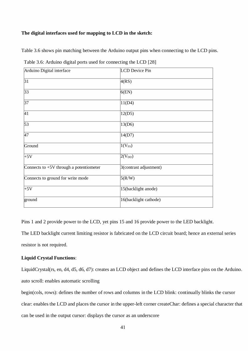
41

The digital interfaces used for mapping to LCD in the sketch:

Table 3.6 shows pin matching between the Arduino output pins when connecting to the LCD pins.

Table 3.6: Arduino digital ports used for connecting the LCD [28]

Arduino Digital interface LCD Device Pin

31 4(RS)

33 6(EN)

37 11(D4)

41 12(D5)

53 13(D6)

47 14(D7)

Ground 1(VSS)

+5V 2(VDD)

Connects to +5V through a potentiometer 3(contrast adjustment)

Connects to ground for write mode 5(R/W)

+5V 15(backlight anode)

ground 16(backlight cathode)

Pins 1 and 2 provide power to the LCD, yet pins 15 and 16 provide power to the LED backlight.

The LED backlight current limiting resistor is fabricated on the LCD circuit board; hence an external series

resistor is not required.

Liquid Crystal Functions:

LiquidCrystal(rs, en, d4, d5, d6, d7): creates an LCD object and defines the LCD interface pins on the Arduino.

auto scroll: enables automatic scrolling

begin(cols, rows): defines the number of rows and columns in the LCD blink: continually blinks the cursor

clear: enables the LCD and places the cursor in the upper-left corner createChar: defines a special character that

can be used in the output cursor: displays the cursor as an underscore

42

display: turns on the LCD, displaying any data currently in the output buffer home: places the cursor in the

upper-left corner, without erasing the output

leftToRight: sets the direction new characters display starting at the left and going toward the right.

setCursor(col, row): places the cursor at a specific row and column location write(char): sends a single character

to the LCD device

noAutoscroll: disables automatic scrolling noBlink: disables the blinking cursor noCursor: disables the cursor

display

noDisplay: blanks the display output, but retains the output data

print(data, BASE): prints text to the LCD device. For numeric values, BASE can be specified rightToLeft: sets

the direction new characters display starting at the left

scrollDisplayLeft: scrolls the display contents one position to the left scrollDisplayRight: scrolls the display

contents one position to the right

3.4.9 Inter-Integrated Circuit (I2C) Interface Bus

The Inter-Integrated Circuit (I2C) Communications bus shown in Figure 3.14 is a serial data bus used for 2-

way, 2-wire communications between different integrated circuits or modules. The bus allows data and

instructions to be exchanged between devices by means of just two wires. This results in a considerable

simplification of circuits. In this project, the I2C bus is used as an interface bus between the 1602 liquid crystal

display (LCD) and the Arduino development board. If the LCD directly connects to the Arduino board, it uses

six digital ports i.e. Enable, chip select, D0-D3. When the LCD connects to the Arduino board through the I2C

interface bus, all the six digital pins are spared since only two Arduino analogue pins are used to connect the

LCD. The six digital pins that could have been occupied by the LCD can then be used to add more peripherals

for the board, hence increasing the capacity of the Arduino board. I2C bus pin connection to both the LCD and

the Arduino board are shown in Table 3.7 and Table 3.8 respectively.

43

Figure 3.14: I2C interface bus to the 1602 LCD [29]

Table 3.7: Output pin configuration for the I2C interface bus [29] 1602 I2C module Arduino

VCC 5V

GND GND

SDA A4

SCL A5

Table 3.8: I2C interface pin description [29]

Symbol Pin Description

A0 1 Address input 0



P0 4 Quasi-bidirectional I/O 0




VSS 8 Supply ground


44




INT/ 13 Interrupt output (active LOW)

SCL 14 Serial clock line

SDA 15 Serial data line

VDD 16 Supply voltage

3.4.10 The Data Logger

Figure 3.15 shows the pin layout of an SD memory card which is being used as the data logger. The purpose of

the data-logger is to store parameter data so that data about the performance of the system is available when

required.

Fig 3.15: SD memory card pinout [30]

Pin 1: Ground, Pin 2: + 3.3V, Pin 3: + 5V, Pin 4: Chip Select (CS), Pin 5: Master Out Slave In (MOSI)

Pin 6: Clock (SClK), Pin 7: Master In Slave Out (MISO), Pin 8: Ground, Pin 9: Not connected

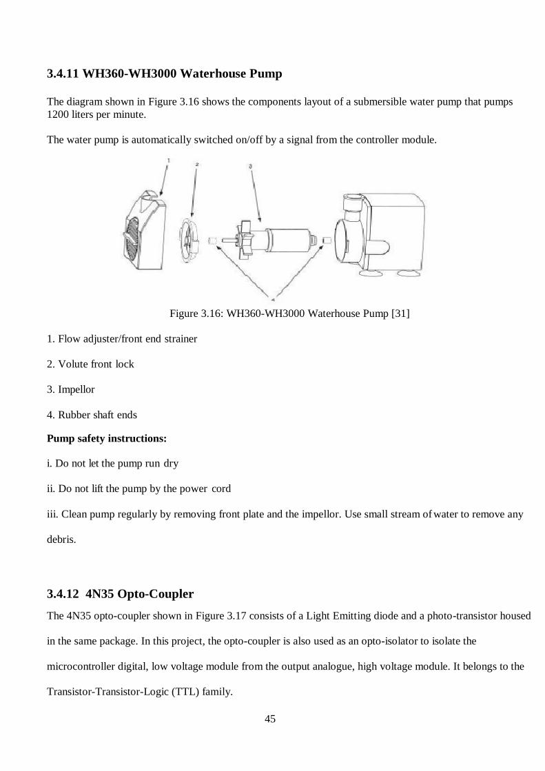
45

3.4.11 WH360-WH3000 Waterhouse Pump

The diagram shown in Figure 3.16 shows the components layout of a submersible water pump that pumps

1200 liters per minute.

The water pump is automatically switched on/off by a signal from the controller module.

Figure 3.16: WH360-WH3000 Waterhouse Pump [31]

1. Flow adjuster/front end strainer

2. Volute front lock

3. Impellor

4. Rubber shaft ends

Pump safety instructions:

i. Do not let the pump run dry

ii. Do not lift the pump by the power cord

iii. Clean pump regularly by removing front plate and the impellor. Use small stream of water to remove any

debris.

3.4.12 4N35 Opto-Coupler

The 4N35 opto-coupler shown in Figure 3.17 consists of a Light Emitting diode and a photo-transistor housed

in the same package. In this project, the opto-coupler is also used as an opto-isolator to isolate the

microcontroller digital, low voltage module from the output analogue, high voltage module. It belongs to the

Transistor-Transistor-Logic (TTL) family.

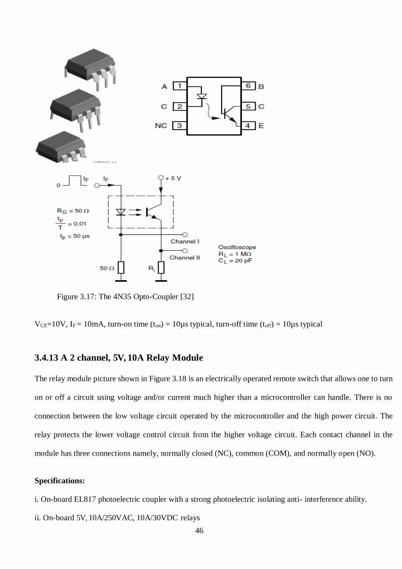
46

Figure 3.17: The 4N35 Opto-Coupler [32]

VCE=10V, IF = 10mA, turn-on time (ton) = 10µs typical, turn-off time (toff) = 10µs typical

3.4.13 A 2 channel, 5V, 10A Relay Module

The relay module picture shown in Figure 3.18 is an electrically operated remote switch that allows one to turn

on or off a circuit using voltage and/or current much higher than a microcontroller can handle. There is no

connection between the low voltage circuit operated by the microcontroller and the high power circuit. The

relay protects the lower voltage control circuit from the higher voltage circuit. Each contact channel in the

module has three connections namely, normally closed (NC), common (COM), and normally open (NO).

Specifications:

i. On-board EL817 photoelectric coupler with a strong photoelectric isolating anti- interference ability.

ii. On-board 5V, 10A/250VAC, 10A/30VDC relays

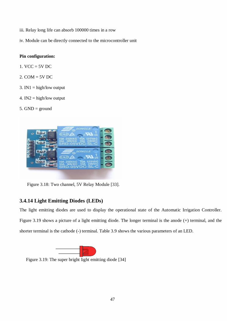
47

iii. Relay long life can absorb 100000 times in a row

iv. Module can be directly connected to the microcontroller unit

Pin configuration:

1. VCC = 5V DC

2. COM = 5V DC

3. IN1 = high/low output

4. IN2 = high/low output

5. GND = ground

Figure 3.18: Two channel, 5V Relay Module [33].

3.4.14 Light Emitting Diodes (LEDs)

The light emitting diodes are used to display the operational state of the Automatic Irrigation Controller.

Figure 3.19 shows a picture of a light emitting diode. The longer terminal is the anode (+) terminal, and the

shorter terminal is the cathode (-) terminal. Table 3.9 shows the various parameters of an LED.

Figure 3.19: The super bright light emitting diode [34]

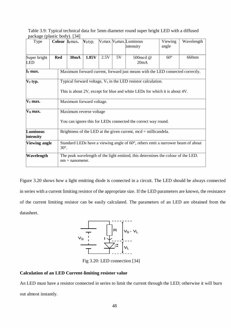
48

Table 3.9: Typical technical data for 5mm diameter round super bright LED with a diffused

package (plastic body). [34] Type Colour IFmax. VFtyp. VFmax. VRmax. Luminous

intensity Viewingangle

Wavelength

Super bright

LED

Red 30mA 1.85V 2.5V 5V 500mcd @

20mA

60° 660nm

IF max. Maximum forward current, forward just means with the LED connected correctly.

VF typ. Typical forward voltage, VL in the LED resistor calculation.

This is about 2V, except for blue and white LEDs for which it is about 4V.

VF max. Maximum forward voltage.

VR max. Maximum reverse voltage

You can ignore this for LEDs connected the correct way round.

Luminous

intensity

Brightness of the LED at the given current, mcd = millicandela.

Viewing angle Standard LEDs have a viewing angle of 60°, others emit a narrower beam of about 30°.

Wavelength The peak wavelength of the light emitted, this determines the colour of the LED. nm = nanometer.

Figure 3.20 shows how a light emitting diode is connected in a circuit. The LED should be always connected

in series with a current limiting resistor of the appropriate size. If the LED parameters are known, the resistance

of the current limiting resistor can be easily calculated. The parameters of an LED are obtained from the

datasheet.

Fig 3.20: LED connection [34]

Calculation of an LED Current-limiting resistor value

An LED must have a resistor connected in series to limit the current through the LED; otherwise it will burn

out almost instantly.

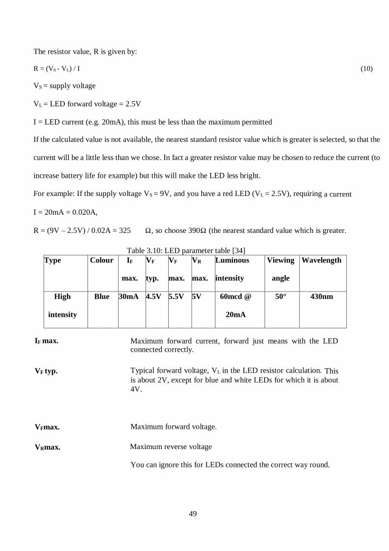
49

The resistor value, R is given by:

R = (VS - VL) / I (10)

VS = supply voltage

VL = LED forward voltage = 2.5V

I = LED current (e.g. 20mA), this must be less than the maximum permitted

If the calculated value is not available, the nearest standard resistor value which is greater is selected, so that the

current will be a little less than we chose. In fact a greater resistor value may be chosen to reduce the current (to

increase battery life for example) but this will make the LED less bright.

For example: If the supply voltage VS = 9V, and you have a red LED (VL = 2.5V), requiring a current

I = 20mA = 0.020A,

R = (9V – 2.5V) / 0.02A = 325 , so choose 390 (the nearest standard value which is greater.

Table 3.10: LED parameter table [34]

Type Colour IF

max.

VF

typ.

VF

max.

VR

max.

Luminous

intensity

Viewing

angle

Wavelength

High

intensity

Blue 30mA 4.5V 5.5V 5V 60mcd @

20mA

50° 430nm

IF max.

Maximum forward current, forward just means with the LED connected correctly.

VF typ. Typical forward voltage, VL in the LED resistor calculation. This

is about 2V, except for blue and white LEDs for which it is about

4V.

VFmax. Maximum forward voltage.

VRmax. Maximum reverse voltage

You can ignore this for LEDs connected the correct way round.

50

Luminous

intensity

Brightness of the LED at the given current, mcd = millicandela.

Viewing angle Standard LEDs have a viewing angle of 60°, others emit a narrower

beam of about 30°.

Wavelength The peak wavelength of the light emitted, this determines the

colour of the LED. nm = nanometer.

3.4.15 The Power Supply

The microcontroller board gets its energy from a 5V external power supply. Therefore in this section, a

regulated voltage power supply is constructed since it is cheaper to convert an alternating current voltage to a

direct current voltage when compared with the use of a battery power source. Figure 3.21 shows a 5V dc

regulated voltage power supply. A higher ac voltage is stepped-down to a lower ac voltage, the lower ac voltage

is then rectified and changed from ac to a pulsating dc voltage. The pulsating dc voltage is smoothened out to

remove the ripples, the smoothened dc voltage is then regulated. An LED is used to indicate the presence of

voltage in the circuit. The main load for this power supply is also shown connected at the output terminal of the

5V regulator.

Theory of Operation

230Vac is applied into the power supply from the mains through a 9V step-down transformer. The 9V from the

step-down transformer is fed into the bridge rectifier where it is converted from ac to a pulsating dc voltage.

The pulsating dc voltage is fed into the smoothing circuit for ripple reduction whereas part of the current is

channeled to the voltage indicating circuit, which is composed of the light- emitting diode and a current limiting

resistor. The LED shows the availability of power in the circuit. It shows whether the power supply is on or off.

A 1kΩ resistor is connected in series with the LED so as to limit the amount of current that flows through the

LED and hence protecting it. The value for the resistor is derived using the formula R= (VS-VF)/IF (11).

51

Fig 3.21: +5Vdc dual power supply

where VS is the supply voltage; VF is the LED forward voltage and IF is the LED forward current. The

smoothened dc current is passed into the LA7805 integrated circuit voltage regulator where the actual regulation

takes place. The regulator gives out a stable +5Vdc voltage. Apart from stepping down voltage, the transformer

also electrically isolates the rectifier from the high voltage ac power source, hence preventing a shock hazard

in the secondary circuit. The block LA7805 does the actual regulation. The average or dc value of the load

current is given by:

IAV = Idc =1

πId(wt) (12)

=1

πImsinwtd(wt)

=2𝐼𝑚

𝜋=

2𝑉𝑚

𝜋(𝑅𝐹+𝑅𝐿)

Therefore: 𝐼𝑚 =𝑉𝑚

(𝑅𝐹+𝑅𝐿) (13)

Where RF is dynamic resistance of the diode and RL is the load resistance.

52

The average or dc value of the output voltage is given by: 𝑉𝑎 = 𝑉𝑑𝑐 = 𝐼𝑑𝑐𝑅𝐿 =2𝐼𝑚𝑅𝐿

𝜋=

2𝑉𝑚

𝜋 (14)

3.5.0 The Design Software

3.5.1 Introduction:

The software part of the system involves the development of a code/program using the Arduino Integrated

Development Environment (IDE) platform. The Arduino programming language is derived from the C and C++

programming languages. The code is written on a Personal Computer (PC) and then uploaded to the

microcontroller chip using a Universal Serial Bus (USB) cable. This developed program constitutes a set of

instructions which tell the microcontroller what to do.

3.5.2 The Integrated Development Environment

The Integrated Development Environment (IDE) is a Software platform that is used to develop the control

program for the Arduino prototyping board. It is an open-source development software which can be

downloaded from the Arduino website for free. The IDE software plays a vital role in the development of the

control system since it makes programming, debugging, compiling, simulation and also uploading the code to

the Arduino prototyping Board a possibility. The IDE is a very user- friendly software. The software is a major

component of the design. It is the one that gives the decision intelligence to the system by way of directing how

the microcontroller and hence the entire system should behave. Software is basically a set of instructions that

give commands to the system. These instructions are executed by a microcontroller.

3.5.3 The Code for the Automated Irrigation Control System

See Appendix 1 for the code

53

3.5.4 The process of operation and the program flow chart of the Automated Irrigation

control system

The Figure 3.22 shows the operation of the Automatic irrigation control system. The microcontroller reads the

code in sequence from top to bottom. As soon as electrical power is supplied to the system, the code in the

microcontroller starts to run. The microcontroller on the Arduino mega board reads the declared library

functions or header files, global constants and variables. The global variables and functions are those that can

be used in any part of the code. The system defined functions are predefined functions, which perform general

and often very useful tasks [35, pp. 159]. After the reading of library functions and variables, the microcontroller

shifts to the user defined setup function. User defined functions are those functions that are created by the

programmer [35, pp. 159]. The user defined setup function is where configuration of digital ports to either work

as inputs or outputs is carried out. This is also where the communication speed of the Arduino board [36, pp.

271-277] is configured. Setup is only scanned once by the microcontroller. After scanning the setup function,

the microcontroller enters another user defined function called the loop function. The loop function stores the

main program which scans the inputs (sensors) and updates the outputs (actuators such as the pumps and the

display). The microcontroller repeatedly scans the loop function until a reset button is pressed or until power is

switched off. If a reset button is pressed, the program will exit the loop and start all over again. If soil moisture

is greater than 50%, the system switches off the water pumps, the buzzer alarm and the red status light emitting

diode. At the same time it switches on the green status LED to show that soil moisture level is in the acceptable

range. If soil moisture is less than 50% and greater than 40% and it is daytime, the system keeps the water pump

off in order to save water which could be wasted due to evaporation since the crops are not yet in danger of

wilting. If soil moisture is less than 50% and greater than 40%, and its dark, then the irrigating water pump is

switched on, the buzzer alarm is kept off, the red LED is switched on, and the green LED is switched off. If

moisture level is less than 40% at any time of day, the system switches on the water pump, the buzzer alarm,

and the red status LED. It keeps the green status LED off. It also displays all system parameters on both the

local and the remote displays. The program also senses the water tank float switch signal. If the float switch

indicates that water level in the tank is below a preset limit, it switches on, the borehole pump so that the water

54

tank fills up again. The system is connected to the internet and the farmer can remotely switch it on and off.

The farmer can also receive remote technical support such as software updates from the manufacturer via

Internet. The farmer also receives weather forecast information from the Internet. All this becomes possible due

to the adoption of the Internet of Things technology in the design and development of the system.

Figure 3.22: Automated Irrigation Controller Signal flowchart

55

CHAPTER 4: THE PROTOTYPE

4.1.0 Introduction

This chapter presents a completed working prototype of the automatic irrigation control system. The labeled

photograph of the system undergoing tests is presented and discussed. The prototype was tested both in the

laboratory and in a field environment. The results obtained from the tests are presented and discussed in the

next chapter.

4.1.1 The working Prototype

Figure 4.1 shows the automatic irrigation controller under test. This particular test was conducted in the

laboratory. The irrigation controller receives signals from sensors and then controls the borehole pump and the

water-tank pump. In the absence of a pump for the water-tank, the water-tank is mounted at an elevated place

so that watering can be done under force of gravity. The irrigation controller also incorporates the ESP8266

Wi-Fi module which enables it to connect to the internet. This allows for automatic downloading of weather

data and weather forecasts for the city where the system is located. The on state or off sate of the water-tank

level sensor enables the controller to automatically switch the borehole pump on and off in order to keep the

water level in the water tank constant. The soil-moisture sensor enables the controller to give signal to the water-

tank pump either to start irrigating or to stop irrigating. The system’s in-built mini-weather station is there to

ensure that the user continues to receive vital weather information even during times of Internet outages when

the OpenWeatherMap server is not available and cannot supply the system with weather data and weather

forecast information. Figure 4.2 shows a working prototype of the irrigation control system clearly showing

the system parameters. The modules shown are the controller module and the weather station module. The

irrigation controller displays the soil moisture content and the status of the borehole pump. The weather module

displays ambient temperature, ambient humidity, barometric pressure and the altitude above sea-level in meters.

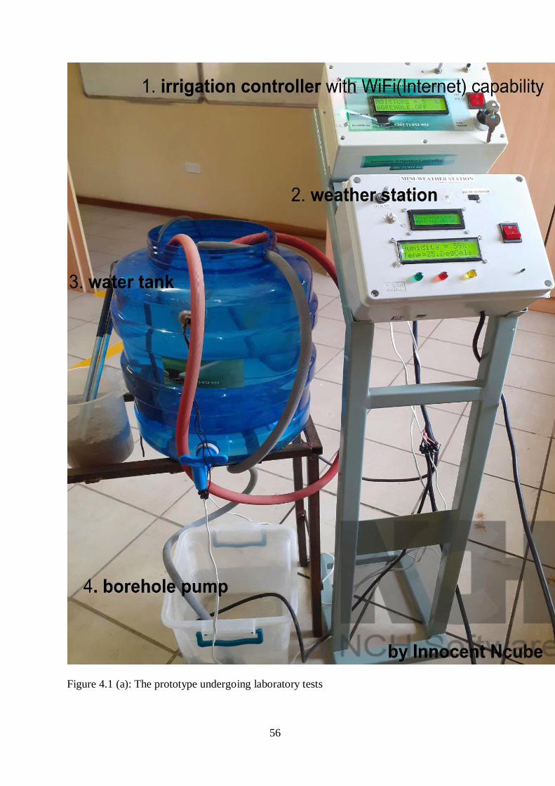
56

Figure 4.1 (a): The prototype undergoing laboratory tests

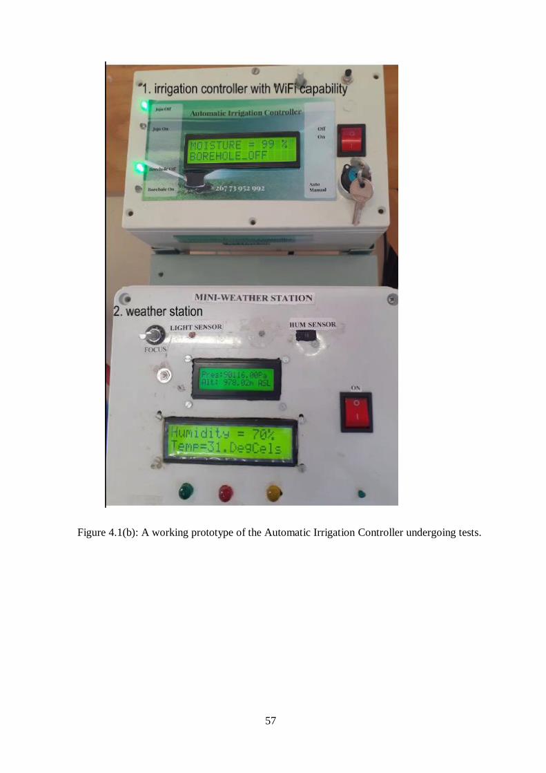
57

Figure 4.1(b): A working prototype of the Automatic Irrigation Controller undergoing tests.

58

CHAPTER 5: DATA PRESENTATION, RESULTS ANALYSIS AND

DISCUSSION

5.1.0 Introduction

The main purpose of this project is to design, implement and test a ‘smart’ irrigation controller in order to

optimize water usage and to enhance agricultural productivity. Having successfully designed, built and tested

a prototype, it is therefore imperative to validate the prototype test results through use of statistical tools for

data analysis. In that regard, this section of the document is dedicated to the test results presentation, statistical

analysis and validation of test results using tools and methods which were briefly discussed in chapter 2. The

results are tested for accuracy, trend, self- stationarity and intervention.

5.2.0 Data presentation

The prototype test results were collected remotely and displayed on a personal computer monitor using an

Internet web browser. The results include soil-moisture status, ambient temperature, ambient humidity,

borehole pump status, water tank pump status as shown in Figure 5.1, and the weather and forecast information

from the OpenWeatherMap Internet server which include temperature, barometric pressure, cloudiness,

humidity, sun-set and sun-rise times as shown in Figure 5.3.

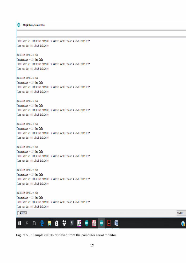
59

Figure 5.1: Sample results retrieved from the computer serial monitor

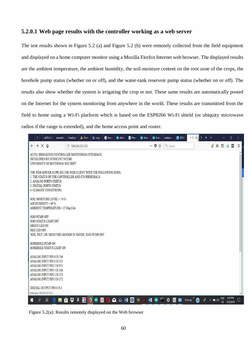
60

5.2.0.1 Web page results with the controller working as a web server

The test results shown in Figure 5.2 (a) and Figure 5.2 (b) were remotely collected from the field equipment

and displayed on a home computer monitor using a Mozilla Firefox Internet web browser. The displayed results

are the ambient temperature, the ambient humidity, the soil-moisture content on the root zone of the crops, the

borehole pump status (whether on or off), and the water-tank reservoir pump status (whether on or off). The

results also show whether the system is irrigating the crop or not. These same results are automatically posted

on the Internet for the system monitoring from anywhere in the world. These results are transmitted from the

field to home using a Wi-Fi platform which is based on the ESP8266 Wi-Fi shield (or ubiquity microwave

radios if the range is extended), and the home access point and router.

Figure 5.2(a): Results remotely displayed on the Web browser

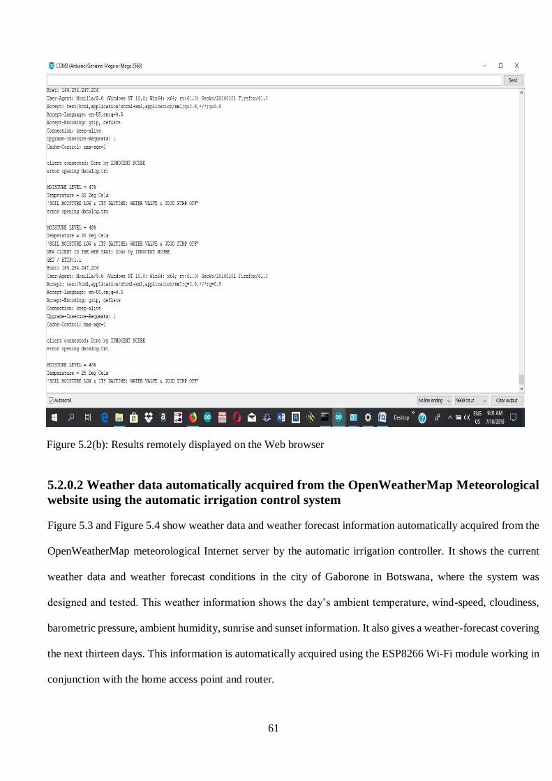
61

Figure 5.2(b): Results remotely displayed on the Web browser

5.2.0.2 Weather data automatically acquired from the OpenWeatherMap Meteorological

website using the automatic irrigation control system

Figure 5.3 and Figure 5.4 show weather data and weather forecast information automatically acquired from the

OpenWeatherMap meteorological Internet server by the automatic irrigation controller. It shows the current

weather data and weather forecast conditions in the city of Gaborone in Botswana, where the system was

designed and tested. This weather information shows the day’s ambient temperature, wind-speed, cloudiness,

barometric pressure, ambient humidity, sunrise and sunset information. It also gives a weather-forecast covering

the next thirteen days. This information is automatically acquired using the ESP8266 Wi-Fi module working in

conjunction with the home access point and router.

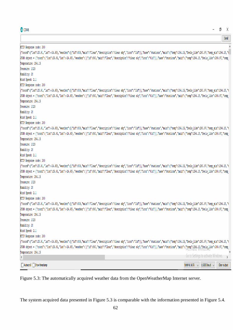
62

Figure 5.3: The automatically acquired weather data from the OpenWeatherMap Internet server.

The system acquired data presented in Figure 5.3 is comparable with the information presented in Figure 5.4.

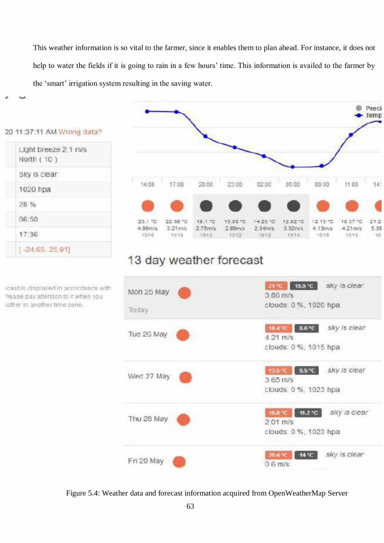
63

This weather information is so vital to the farmer, since it enables them to plan ahead. For instance, it does not

help to water the fields if it is going to rain in a few hours’ time. This information is availed to the farmer by

the ‘smart’ irrigation system resulting in the saving water.

Figure 5.4: Weather data and forecast information acquired from OpenWeatherMap Server

64

5.2.0.3 Calculation (percentage) of the water saved through irrigating at night using the

automatic irrigation control system

The combined loss of water from soil and crop by vaporisation is identified as evapotranspiration (13). Crops

need water for transpiration and evaporation. During the growing period of a crop, there is a continuous

movement of water from soil into the roots, up the stems and leaves, and out of the leaves to the atmosphere.

This movement of water is essential for carrying plant food from the soil to various parts of the plant. Only a

very small portion (less than 2 per cent) of water absorbed by the roots is retained in the plant and the rest of

the absorbed water, after performing its tasks, gets evaporated to the atmosphere mainly through the leaves and

stem. This process is called transpiration. In addition, some water gets evaporated to the atmosphere directly

from the adjacent soil and water surfaces and from the surfaces of the plant leaves (i.e., the intercepted

precipitation on the plant foliage). The water needs of a crop thus consists of transpiration and evaporation and

is called evapotranspiration or consumptive use. Evapotranspiration is dependent on climatic conditions like

temperature, daylight hours, humidity, wind movement, type of crop, stage of growth of crop, soil moisture

depletion, and other physical and chemical properties of soil. For example, in a sunny and hot climate, crops

need more water per day than in a cloudy and cool climate [13]. Table 5.1 presents empirical evidence of water

usage data, pulled from monthly water utility bills. The same information is also illustrated in a graphical format

in Figure 5.5. In this analysis, a vegetable garden is irrigated at night from January to June using the automatic

irrigation control system during tests. The minimum water consumption in January and February points to wet

soils due to rainfall and prolonged cloud cover, when evapotranspiration was at its lowest. Night irrigation was

carried out from January to June. Day time watering was then started from July until December. Water

consumption rose significantly during this period as a result of evapotranspiration. This shows that when plants

are irrigated in a hot day, evaporation contributes a lot to loss of consumptive water.

65

Table 5.1: Monthly water usage extracted from a water bill

Figure 5.5: Monthly water usage for a period of one year

To estimate irrigation water usage when automatically irrigating at night, we take an average monthly water

usage from the months when watering was done at night (January to June) as follows:

Average water usage = ∑(25.126+30.368+35.182+40.424+41.64+40.098)

6=

212.838

6= 35.473 m3 per month

Therefore, estimated annual water usage when automatically watering at night is:

Average monthly water usage x 12 months. That is 35.473 x 12 = 425.676 m3 per year

To estimate average monthly automatic irrigation water usage when irrigating during the day, we subtract the

0

10

20

30

40

50

60

70

wat

er v

olu

me

(m

3)

Time (months)

Month Water usage (m3)

January 25.126

February 30.368

March 35.182

April 40.424

May 41.64

June 40.098

July 56.78

August 61.764

September 64.794

October 63.28

November 64.794

December 50.494

Total 574.744

66

average monthly water usage when watering at night from the metered total presented in Table: 5.1 as follows:

Average monthly water usage when watering during the day is:

Average water usage = 574.744−212.838

6=

361.906

6= 60.32m3 per month

Therefore: Estimated annual water usage when watering during the day is:

Estimated annual water usage = 60.32m3 x 12 months = 723.84 m3 per year

The average amount of water saved per month by watering at night is:

Average water saved per month = 60.32 m3 – 35.473 m3 = 24.847 m3

Therefore: Water saved when watering at night per year is:

24.847 m3 per month x 12 months = 298.164 m3

or 723.84 m3 per year – 425.676 m3/year = 298.164 m3

The Percentage water saving is:

Water saving per month (%) = 24.847

95.793x100% = 25.938%

or Water saving per month (%) = 298.164

1149.516x100% = 25.938%

5.2.0.4 The Ubiquiti Radio Parameters

The ubiquity radios are required if the range between the home equipment and the field equipment (where the

controller is deployed) is too large to be adequately covered by the Wi-Fi modem which is located at the

farmhouse. These ubiquity radios work like a very long “wireless Ethernet cable” and their signal is

unidirectional. Therefore their main purpose is to extend the Wi-Fi coverage range by about 5km in a particular

direction. These ubiquity radios were tested on a range of 5km between them and they worked successfully

with very minimal signal attenuation. Figure 5.6(a) shows the transmit and receive signal parameters for a

ubiquity radio which is being used as a unidirectional transmitter, and Figure 5.6 (b) shows the signal transmit

and receive parameters for a ubiquity radio which is configured to work as the receiver station. The transmit

radio is located at the field where the irrigation controller system is located, and the receive radio is connected

together with the home equipment which connects the system to the internet.

67

Figure 5.6(a): Ubiquity transmit Nano radio parameters

Figure 5.6(b): Ubiquity Nano-station (receiver) parameters

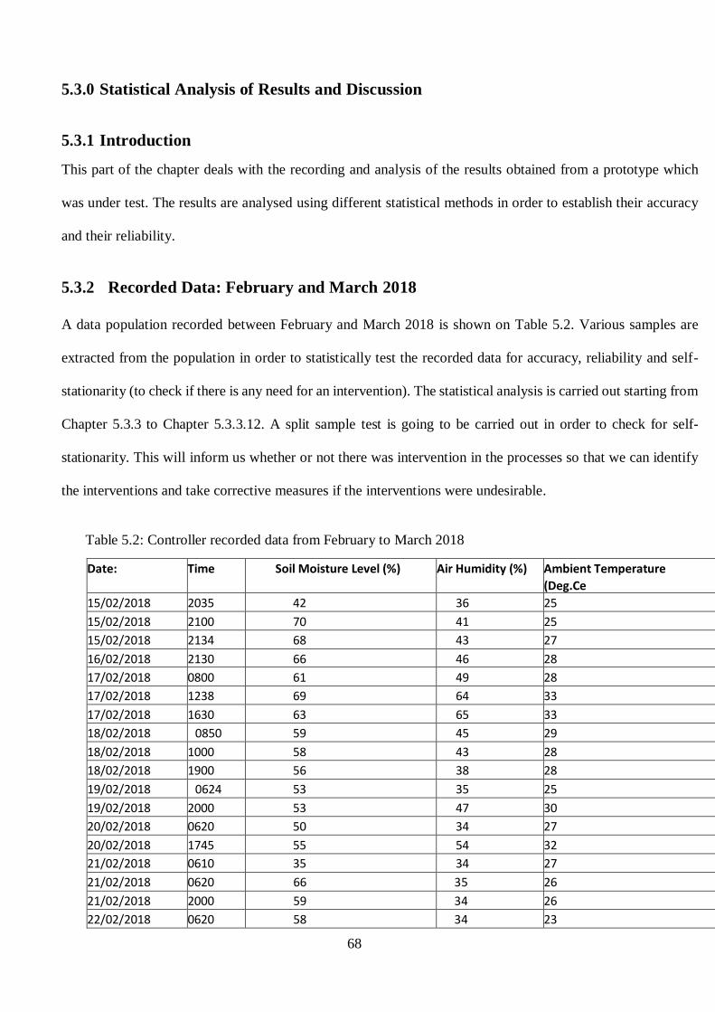
68

5.3.0 Statistical Analysis of Results and Discussion

5.3.1 Introduction

This part of the chapter deals with the recording and analysis of the results obtained from a prototype which

was under test. The results are analysed using different statistical methods in order to establish their accuracy

and their reliability.

5.3.2 Recorded Data: February and March 2018

A data population recorded between February and March 2018 is shown on Table 5.2. Various samples are

extracted from the population in order to statistically test the recorded data for accuracy, reliability and self-

stationarity (to check if there is any need for an intervention). The statistical analysis is carried out starting from

Chapter 5.3.3 to Chapter 5.3.3.12. A split sample test is going to be carried out in order to check for self-

stationarity. This will inform us whether or not there was intervention in the processes so that we can identify

the interventions and take corrective measures if the interventions were undesirable.

Table 5.2: Controller recorded data from February to March 2018

Date: Time Soil Moisture Level (%) Air Humidity (%) Ambient Temperature

(Deg.Ce

15/02/2018 2035 42 36 25

15/02/2018 2100 70 41 25

15/02/2018 2134 68 43 27

16/02/2018 2130 66 46 28

17/02/2018 0800 61 49 28

17/02/2018 1238 69 64 33

17/02/2018 1630 63 65 33

18/02/2018 0850 59 45 29

18/02/2018 1000 58 43 28

18/02/2018 1900 56 38 28

19/02/2018 0624 53 35 25

19/02/2018 2000 53 47 30

20/02/2018 0620 50 34 27

20/02/2018 1745 55 54 32

21/02/2018 0610 35 34 27

21/02/2018 0620 66 35 26

21/02/2018 2000 59 34 26

22/02/2018 0620 58 34 23

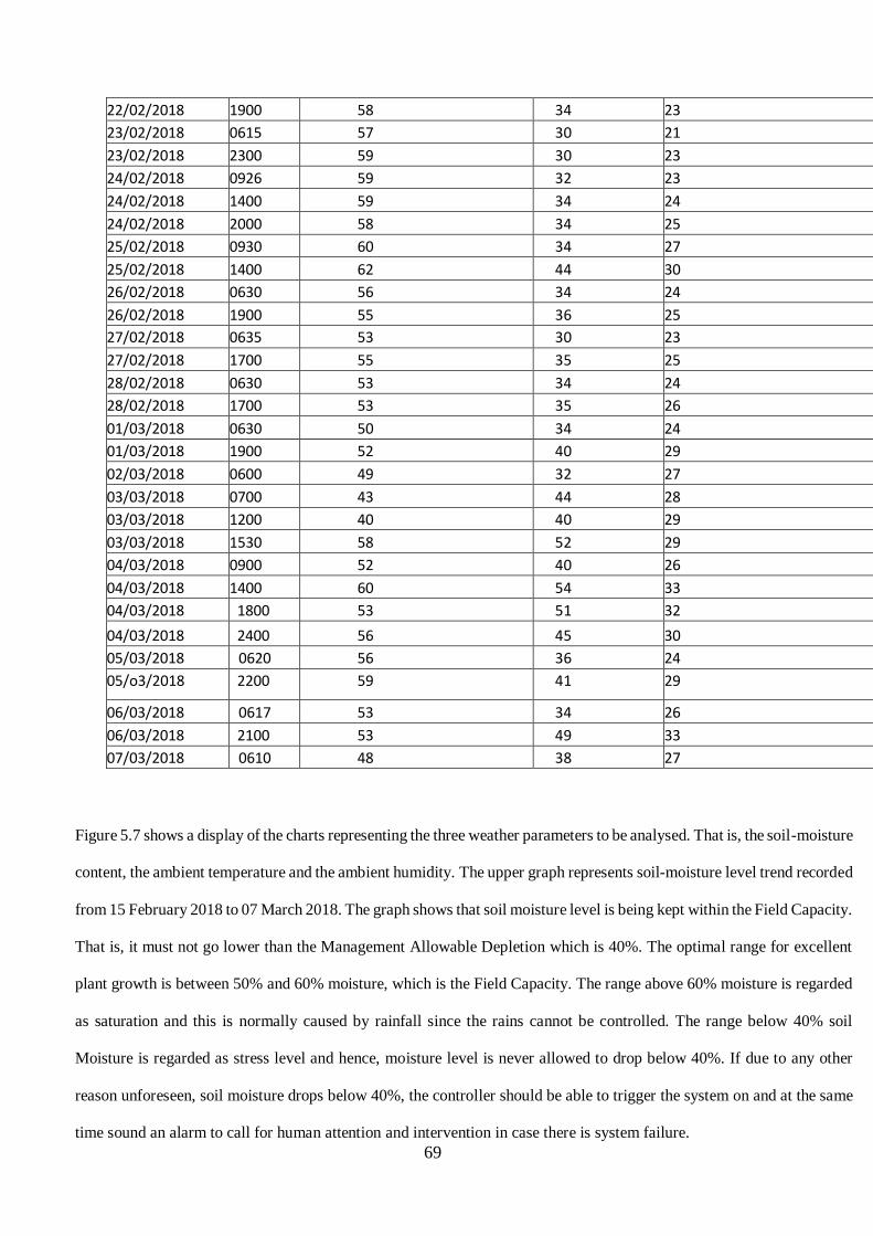
69

Figure 5.7 shows a display of the charts representing the three weather parameters to be analysed. That is, the soil-moisture

content, the ambient temperature and the ambient humidity. The upper graph represents soil-moisture level trend recorded

from 15 February 2018 to 07 March 2018. The graph shows that soil moisture level is being kept within the Field Capacity.

That is, it must not go lower than the Management Allowable Depletion which is 40%. The optimal range for excellent

plant growth is between 50% and 60% moisture, which is the Field Capacity. The range above 60% moisture is regarded

as saturation and this is normally caused by rainfall since the rains cannot be controlled. The range below 40% soil

Moisture is regarded as stress level and hence, moisture level is never allowed to drop below 40%. If due to any other

reason unforeseen, soil moisture drops below 40%, the controller should be able to trigger the system on and at the same

time sound an alarm to call for human attention and intervention in case there is system failure.

22/02/2018 1900 58 34 23

23/02/2018 0615 57 30 21

23/02/2018 2300 59 30 23

24/02/2018 0926 59 32 23

24/02/2018 1400 59 34 24

24/02/2018 2000 58 34 25

25/02/2018 0930 60 34 27

25/02/2018 1400 62 44 30

26/02/2018 0630 56 34 24

26/02/2018 1900 55 36 25

27/02/2018 0635 53 30 23

27/02/2018 1700 55 35 25

28/02/2018 0630 53 34 24

28/02/2018 1700 53 35 26

01/03/2018 0630 50 34 24

01/03/2018 1900 52 40 29

02/03/2018 0600 49 32 27

03/03/2018 0700 43 44 28

03/03/2018 1200 40 40 29

03/03/2018 1530 58 52 29

04/03/2018 0900 52 40 26

04/03/2018 1400 60 54 33

04/03/2018 1800 53 51 32

04/03/2018 2400 56 45 30

05/03/2018 0620 56 36 24

05/o3/2018 2200 59 41 29

06/03/2018 0617 53 34 26

06/03/2018 2100 53 49 33

07/03/2018 0610 48 38 27

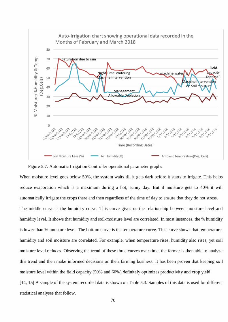
70

Figure 5.7: Automatic Irrigation Controller operational parameter graphs

When moisture level goes below 50%, the system waits till it gets dark before it starts to irrigate. This helps

reduce evaporation which is a maximum during a hot, sunny day. But if moisture gets to 40% it will

automatically irrigate the crops there and then regardless of the time of day to ensure that they do not stress.

The middle curve is the humidity curve. This curve gives us the relationship between moisture level and

humidity level. It shows that humidity and soil-moisture level are correlated. In most instances, the % humidity

is lower than % moisture level. The bottom curve is the temperature curve. This curve shows that temperature,

humidity and soil moisture are correlated. For example, when temperature rises, humidity also rises, yet soil

moisture level reduces. Observing the trend of these three curves over time, the farmer is then able to analyze

this trend and then make informed decisions on their farming business. It has been proven that keeping soil

moisture level within the field capacity (50% and 60%) definitely optimizes productivity and crop yield.

[14, 15] A sample of the system recorded data is shown on Table 5.3. Samples of this data is used for different

statistical analyses that follow.

Ambient Tempreature(Deg. Cels) Air Humidity(%) Soil Moisture Level(%)

Time (Recording Dates)

20

10

Management Allowable Depletion 30

Machine Intervention on Soil moisture 40

Field capacity (optimal)

machine watering Night Time Watering Machine intervention

60

50

Saturation due to rain

80

70

Auto-Irrigation chart showing operational data recorded in the Months of February and March 2018

% M

ois

ture

/ %

Hu

mid

ity

& T

emp

(D

eg.

Cel

s)

71

Table 5.3: A sample of system recorded data

Date Time Soil Moisture level

Air Humidity level

Ambient Temperature(Deg.Cels)

15/02/18 2035 42 36 25

15/02/18 2100 70 41 25

15/02/18 2134 68 43 27

16/02/18 2130 66 46 28

17/02/18 0800 61 49 28

17/02/18 1238 69 64 33

17/02/18 1630 63 65 33

18/02/18 0850 59 45 29

18/02/18 1000 58 43 28

18/02/18 1900 56 38 28

19/02/18 0624 53 35 25

19/02/18 2000 53 47 30

20/02/18 0620 50 34 27

20/02/18 1745 55 54 32

21/02/18 0610 40 34 27

21/02/18 0620 66 35 26

21/02/18 2000 59 34 26

22/02/18 0620 58 34 23

22/02/18 1900 58 34 23

23/02/18 0615 57 30 21

23/02/18 2300 59 30 23

24/02/18 0926 59 32 23

24/02/18 1400 59 34 24

24/02/18 2000 58 34 25

25/02/18 0930 60 34 27

25/02/18 1400 62 44 30

26/02/18 0630 56 34 24

26/02/18 1900 55 36 25

27/02/18 0635 53 30 23

28/02/18 0630 53 34 24

28/02/18 1700 53 35 26

01/03/18 0630 50 34 24

01/03/18 1900 52 40 29

02/03/18 0600 49 32 27

03/03/18 0700 43 44 28

03/03/18 1200 40 40 29

03/03/18 1530 58 52 29

04/03/18 0900 52 40 26

04/03/18 1400 60 54 33

04/03/18 1800 53 51 32

04/03/18 2400 56 45 30

05/03/18 0620 56 36 24

05/03/18 2200 59 41 29

06/03/18 0617 53 34 26

06/03/18 2100 53 49 33

07/03/18 0610 48 38 27

72

5.3.3 Statistical Analysis of Results

The reasons for analyzing the results obtained from testing of the prototype are to verify the accuracy and the

reliability of the system. The analysed results are also useful for the establishment of a weather prediction

algorithm. Statistical tests are therefore carried out to establish the accuracy of the results, to establish the trend

of the results using Mann-Kendall Tau statistics, checking for intervention using the cumulative sum (CuSum)

formula, as well as using a Split-sample t-test formula to check for self-stationarity of data.


percentages of Soil Moisture content levels from 15/03/18 to 21/03/18

Table 5.4: A sample of Soil-Moisture recorded data Sample Observed Data Xi

0.42 1

0.70 2

0.68 3

0.66 4

0.61 5

0.69 6

0.63 7

0.59 8

0.58 9

0.56 10

0.53 11

0.50 12

0.55 13

0.40 14

0.66 15

𝑆 = ∑ ∑ 𝑆𝑔𝑛(𝑋𝑗 − 𝑋𝑖)𝑛𝑗=𝑖+1

𝑛−1𝑖=1 (15)

n = 16

i = n-1 = 1, 2, 3, 4, 5, 6, 7, 8, 9, 10, 11, 12, 13, 14, 15

j = i + 1 = 2, 3, 4, 5, 6, 7, 8, 9, 10, 11, 12, 13, 14, 15, 16

𝜏 =𝑠

0.5(𝑛−1) (16)

(𝑋𝑗 − 𝑋𝑖) = 1 if computed value >0 (𝑋𝑗 − 𝑋𝑖) = 0 if computed value =0 (𝑋𝑗 − 𝑋𝑖) = −1 if computed value <0

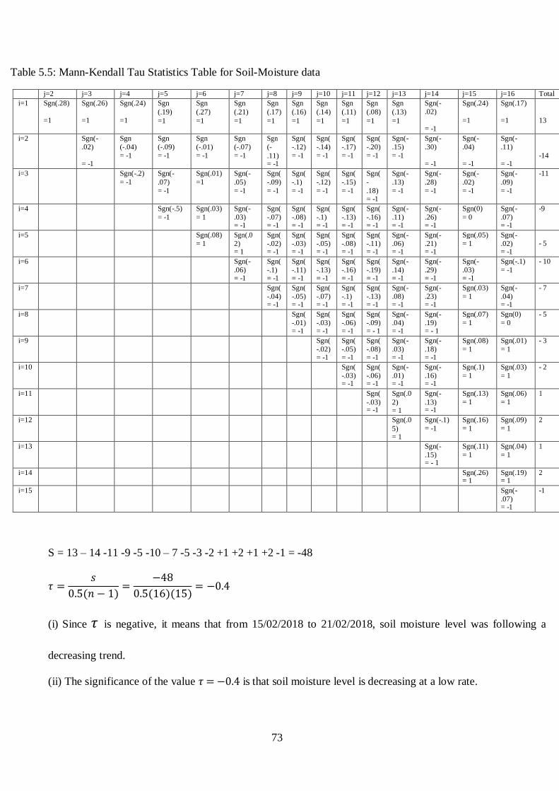
73

Table 5.5: Mann-Kendall Tau Statistics Table for Soil-Moisture data

S = 13 – 14 -11 -9 -5 -10 – 7 -5 -3 -2 +1 +2 +1 +2 -1 = -48

𝜏 =𝑠

0.5(𝑛 − 1)=

−48

0.5(16)(15)= −0.4

(i) Since 𝜏 is negative, it means that from 15/02/2018 to 21/02/2018, soil moisture level was following a

decreasing trend.

(ii) The significance of the value 𝜏 = −0.4 is that soil moisture level is decreasing at a low rate.

j=2 j=3 j=4 j=5 j=6 j=7 j=8 j=9 j=10 j=11 j=12 j=13 j=14 j=15 j=16 Total

i=1 Sgn(.28)

=1

Sgn(.26)

=1

Sgn(.24)

=1

Sgn

(.19)

=1

Sgn

(.27)

=1

Sgn

(.21)

=1

Sgn

(.17)

=1

Sgn

(.16)

=1

Sgn

(.14)

=1

Sgn

(.11)

=1

Sgn

(.08)

=1

Sgn

(.13)

=1

Sgn(-

.02)

= -1

Sgn(.24)

=1

Sgn(.17)

=1

13

i=2 Sgn(-

.02)

= -1

Sgn

(-.04)

= -1

Sgn

(-.09)

= -1

Sgn

(-.01)

= -1

Sgn

(-.07)

= -1

Sgn

(-

.11) = -1

Sgn(

-.12)

= -1

Sgn(

-.14)

= -1

Sgn(

-.17)

= -1

Sgn(

-.20)

= -1

Sgn(-

.15)

= -1

Sgn(-

.30)

= -1

Sgn(-

.04)

= -1

Sgn(-

.11)

= -1

-14

i=3 Sgn(-.2)

= -1

Sgn(-

.07)

= -1

Sgn(.01)

=1

Sgn(-

.05)

= -1

Sgn(

-.09)

= -1

Sgn(

-.1)

= -1

Sgn(

-.12)

= -1

Sgn(

-.15)

= -1

Sgn(

-

.18) = -1

Sgn(-

.13)

= -1

Sgn(-

.28)

= -1

Sgn(-

.02)

= -1

Sgn(-

.09)

= -1

-11

i=4 Sgn(-.5)

= -1

Sgn(.03)

= 1

Sgn(-

.03) = -1

Sgn(

-.07) = -1

Sgn(

-.08) = -1

Sgn(

-.1) = -1

Sgn(

-.13) = -1

Sgn(

-.16) = -1

Sgn(-

.11) = -1

Sgn(-

.26) = -1

Sgn(0)

= 0

Sgn(-

.07) = -1

-9

i=5 Sgn(.08)

= 1

Sgn(.0

2) = 1

Sgn(

-.02) = -1

Sgn(

-.03) = -1

Sgn(

-.05) = -1

Sgn(

-.08) = -1

Sgn(

-.11) = -1

Sgn(-

.06) = -1

Sgn(-

.21) = -1

Sgn(.05)

= 1

Sgn(-

.02) = -1

- 5

i=6 Sgn(-

.06) = -1

Sgn(

-.1) = -1

Sgn(

-.11) = -1

Sgn(

-.13) = -1

Sgn(

-.16) = -1

Sgn(

-.19) = -1

Sgn(-

.14) = -1

Sgn(-

.29) = -1

Sgn(-

.03) = -1

Sgn(-.1)

= -1

- 10

i=7 Sgn(

-.04) = -1

Sgn(

-.05) = -1

Sgn(

-.07) = -1

Sgn(

-.1) = -1

Sgn(

-.13) = -1

Sgn(-

.08) = -1

Sgn(-

.23) = -1

Sgn(.03)

= 1

Sgn(-

.04) = -1

- 7

i=8 Sgn(

-.01) = -1

Sgn(

-.03) = -1

Sgn(

-.06) = -1

Sgn(

-.09) = - 1

Sgn(-

.04) = -1

Sgn(-

.19) = - 1

Sgn(.07)

= 1

Sgn(0)

= 0

- 5

i=9 Sgn(

-.02) = -1

Sgn(

-.05) = -1

Sgn(

-.08) = -1

Sgn(-

.03) = -1

Sgn(-

.18) = -1

Sgn(.08)

= 1

Sgn(.01)

= 1

- 3

i=10 Sgn(

-.03) = -1

Sgn(

-.06) = -1

Sgn(-

.01) = -1

Sgn(-

.16) = -1

Sgn(.1)

= 1

Sgn(.03)

= 1

- 2

i=11 Sgn(

-.03) = -1

Sgn(.0

2) = 1

Sgn(-

.13) = -1

Sgn(.13)

= 1

Sgn(.06)

= 1

1

i=12 Sgn(.0

5) = 1

Sgn(-.1)

= -1

Sgn(.16)

= 1

Sgn(.09)

= 1

2

i=13 Sgn(-

.15) = - 1

Sgn(.11)

= 1

Sgn(.04)

= 1

1

i=14 Sgn(.26) = 1

Sgn(.19) = 1

2

i=15 Sgn(-

.07) = -1

-1

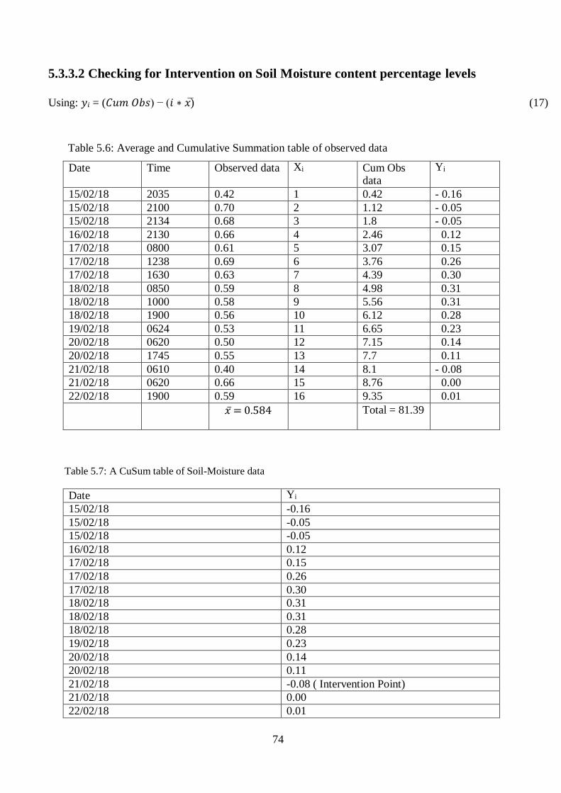
74

5.3.3.2 Checking for Intervention on Soil Moisture content percentage levels

Using: 𝑦𝑖 = (𝐶𝑢𝑚 𝑂𝑏𝑠) − (𝑖 ∗ ) (17)

Table 5.6: Average and Cumulative Summation table of observed data

Date Time Observed data Xi Cum Obs data

Yi

15/02/18 2035 0.42 1 0.42 - 0.16

15/02/18 2100 0.70 2 1.12 - 0.05

15/02/18 2134 0.68 3 1.8 - 0.05

16/02/18 2130 0.66 4 2.46 0.12

17/02/18 0800 0.61 5 3.07 0.15

17/02/18 1238 0.69 6 3.76 0.26

17/02/18 1630 0.63 7 4.39 0.30

18/02/18 0850 0.59 8 4.98 0.31

18/02/18 1000 0.58 9 5.56 0.31

18/02/18 1900 0.56 10 6.12 0.28

19/02/18 0624 0.53 11 6.65 0.23

20/02/18 0620 0.50 12 7.15 0.14

20/02/18 1745 0.55 13 7.7 0.11

21/02/18 0610 0.40 14 8.1 - 0.08

21/02/18 0620 0.66 15 8.76 0.00

22/02/18 1900 0.59 16 9.35 0.01

𝑥 = 0.584 Total = 81.39

Table 5.7: A CuSum table of Soil-Moisture data

Date Yi

15/02/18 -0.16

15/02/18 -0.05

15/02/18 -0.05

16/02/18 0.12

17/02/18 0.15

17/02/18 0.26

17/02/18 0.30

18/02/18 0.31

18/02/18 0.31

18/02/18 0.28

19/02/18 0.23

20/02/18 0.14

20/02/18 0.11

21/02/18 -0.08 ( Intervention Point)

21/02/18 0.00

22/02/18 0.01

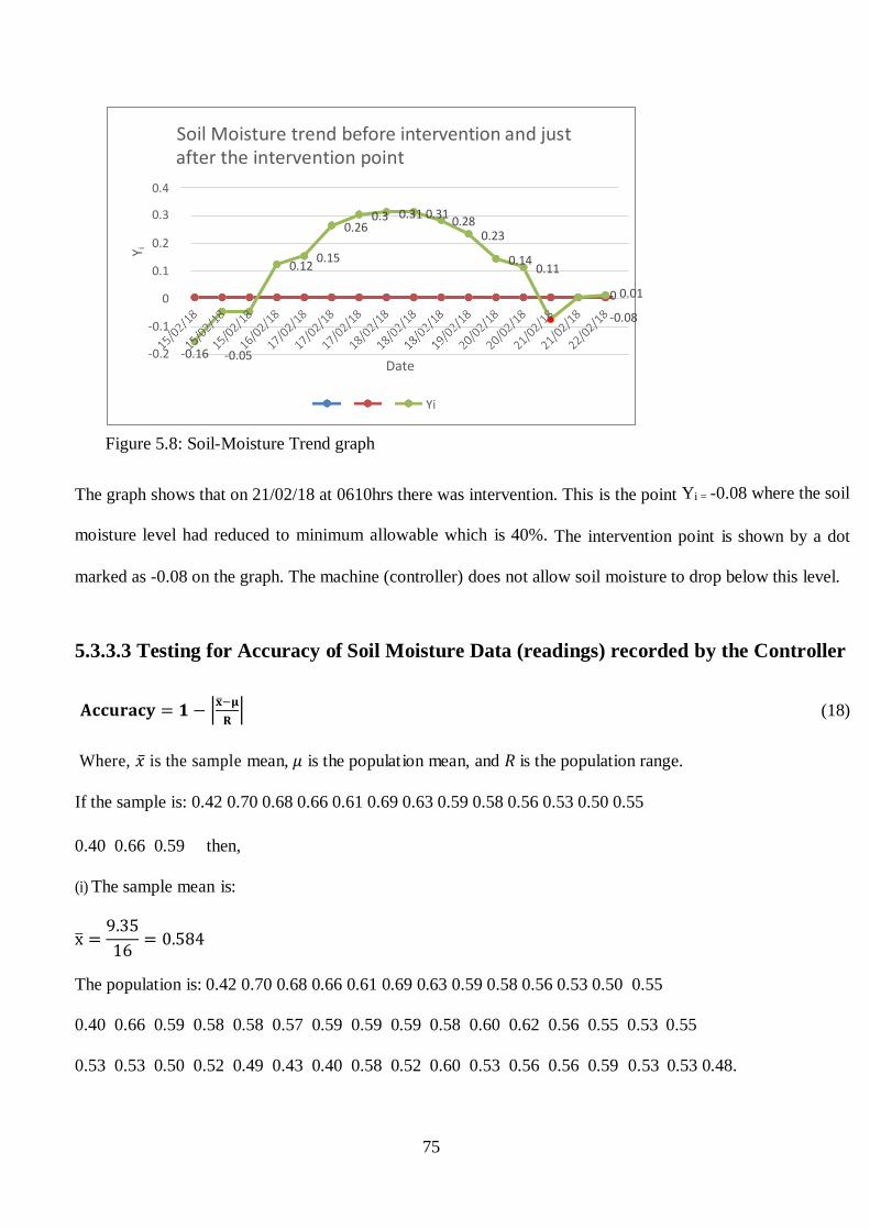
75

Figure 5.8: Soil-Moisture Trend graph

The graph shows that on 21/02/18 at 0610hrs there was intervention. This is the point Yi = -0.08 where the soil

moisture level had reduced to minimum allowable which is 40%. The intervention point is shown by a dot

marked as -0.08 on the graph. The machine (controller) does not allow soil moisture to drop below this level.

5.3.3.3 Testing for Accuracy of Soil Moisture Data (readings) recorded by the Controller

𝐀𝐜𝐜𝐮𝐫𝐚𝐜𝐲 = 𝟏 − |−𝛍

𝐑| (18)

Where, is the sample mean, 𝜇 is the population mean, and 𝑅 is the population range.

If the sample is: 0.42 0.70 0.68 0.66 0.61 0.69 0.63 0.59 0.58 0.56 0.53 0.50 0.55

0.40 0.66 0.59 then,

(i) The sample mean is:

x =9.35

16= 0.584

The population is: 0.42 0.70 0.68 0.66 0.61 0.69 0.63 0.59 0.58 0.56 0.53 0.50 0.55

0.40 0.66 0.59 0.58 0.58 0.57 0.59 0.59 0.59 0.58 0.60 0.62 0.56 0.55 0.53 0.55

0.53 0.53 0.50 0.52 0.49 0.43 0.40 0.58 0.52 0.60 0.53 0.56 0.56 0.59 0.53 0.53 0.48.

Soil Moisture trend before intervention and just after the intervention point

0.4

0.3 0.3 0.26

0.31 0.31 0.28

0.2 0.23

0.1 0.12 0.15 0.14

0.11

-0.05

-0.1

0 0.01

-0.08

-0.2 -0.16 Date

Yi

Y i

76

Therefore:

(i) The population range is: 0.7 – 0.4 = 03

(ii) The population mean is:

𝜇 =25.72

46 = 0.559 Where 25.72 is the sum of the population, and 46 is the number of elements in the

population.

Therefore: Accuracy = 1 − |0.584 −0.559

0.3 |

The sampling efficiency for soil moisture level is 0.92, and this indicates that very accurate sampling is being

carried out by the irrigation controller.

5.3.3.4 Split-Sample test for Self-Stationarity of Soil Moisture data

The t-test is being used to test for self-stationarity of data to check whether there is significant or no significant

difference amongst the observed sample averages. This is done so as to establish if there was intervention or

not, and to find out what the intervention was all about.

Sample 1:

0.42 0.70 0.68 0.66 0.61 0.69 0.63 0.59 0.58 0.56 0.53 0.50 0.55 0.40 0.66 0.59 0.58

0.58 0.57 0.59 0.59 0.59

n1 = 23

𝑥1=0.582

S1 = 0.075

Sample 2:

0.58 0.60 0.62 0.56 0.55 0.53 0.55 0.53 0.53 0.50 0.52 0.49 0.43 0.40 0.58 0.52

0.60 0.53 0.56 0.56 0.59 0.53 0.53

n2 =24

𝑥2 =0.536

S2=0.052

77

𝑡 =1−2

√𝑠1

2

𝑛1+

𝑠22

𝑛2

(19)

Where 1 and 2 are mean values of sample 1 and sample 2. S1 and S2 are standard deviations for sample 1

and sample 2.

𝑛1 and 𝑛2 are number of values or observations for sample 1 and sample 2 respectively.

Therefore: 𝑡 =0.582−0.536

√0.0752

23+

0.0522

24

= 2.43

Since the split sample test is greater than 1.96, this means that there is a significant difference between the two

sample averages. Hence intervention took place.

This intervention was through watering of the plants when moisture level reduced to the lowest tolerable level

of 40% which is the Management Allowable Depletion level.


percentages of ambient Humidity levels from 15/03/18 to 21/03/18

Table 5.8: A sample of Air Humidity recorded data

Sample Observed Data Xi

0.36 1

0.41 2

0.43 3

0.46 4

0.49 5

0.64 6

0.65 7

0.45 8

0.43 9

0.38 10

0.35 11

0.47 12

0.34 13

0.54 14

0.34 15

0.35 16


𝑛−1𝑖=1 (20)

n = 16

i = n-1 = 1, 2, 3, 4, 5, 6, 7, 8, 9, 10, 11, 12, 13, 14, 15

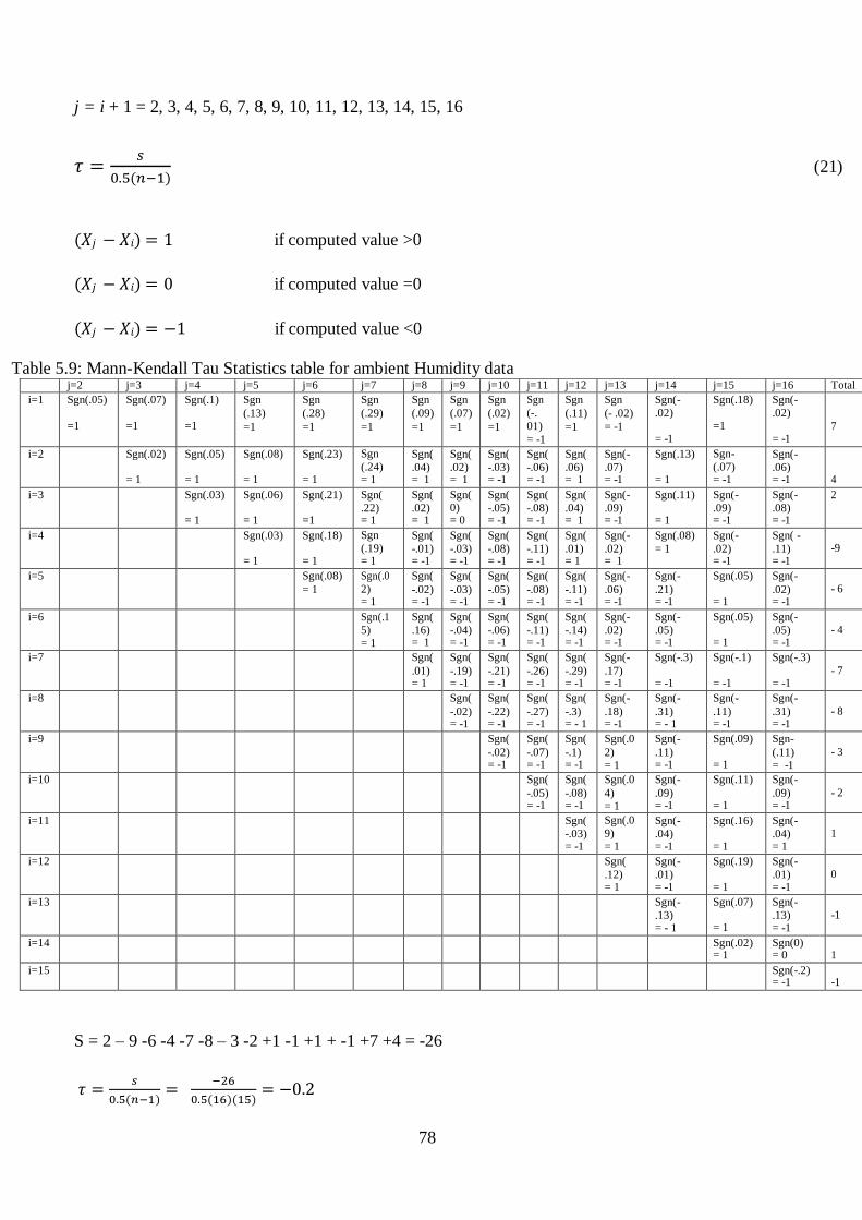
78

j = i + 1 = 2, 3, 4, 5, 6, 7, 8, 9, 10, 11, 12, 13, 14, 15, 16

𝜏 =𝑠

0.5(𝑛−1) (21)

(𝑋𝑗 − 𝑋𝑖) = 1 if computed value >0

(𝑋𝑗 − 𝑋𝑖) = 0 if computed value =0

(𝑋𝑗 − 𝑋𝑖) = −1 if computed value <0

Table 5.9: Mann-Kendall Tau Statistics table for ambient Humidity data

S = 2 – 9 -6 -4 -7 -8 – 3 -2 +1 -1 +1 + -1 +7 +4 = -26

𝜏 =𝑠

0.5(𝑛−1)=

−26

0.5(16)(15)= −0.2


i=1 Sgn(.05)

=1

Sgn(.07)

=1

Sgn(.1)

=1

Sgn

(.13)

=1

Sgn

(.28)

=1

Sgn

(.29)

=1

Sgn

(.09)

=1

Sgn

(.07)

=1

Sgn

(.02)

=1

Sgn

(-.

01)

= -1

Sgn

(.11)

=1

Sgn

(- .02)

= -1

Sgn(-

.02)

= -1

Sgn(.18)

=1

Sgn(-

.02)

= -1

7

i=2 Sgn(.02)

= 1

Sgn(.05)

= 1

Sgn(.08)

= 1

Sgn(.23)

= 1

Sgn

(.24) = 1

Sgn(

.04) = 1

Sgn(

.02) = 1

Sgn(

-.03) = -1

Sgn(

-.06) = -1

Sgn(

.06) = 1

Sgn(-

.07) = -1

Sgn(.13)

= 1

Sgn-

(.07) = -1

Sgn(-

.06) = -1

4

i=3 Sgn(.03)

= 1

Sgn(.06)

= 1

Sgn(.21)

=1

Sgn(

.22) = 1

Sgn(

.02) = 1

Sgn( 0) = 0

Sgn(

-.05) = -1

Sgn(

-.08) = -1

Sgn(

.04) = 1

Sgn(-

.09) = -1

Sgn(.11)

= 1

Sgn(-

.09) = -1

Sgn(-

.08) = -1

2

i=4 Sgn(.03)

= 1

Sgn(.18)

= 1

Sgn

(.19) = 1

Sgn(

-.01) = -1

Sgn(

-.03) = -1

Sgn(

-.08) = -1

Sgn(

-.11) = -1

Sgn(

.01) = 1

Sgn(-

.02) = 1

Sgn(.08)

= 1

Sgn(-

.02) = -1

Sgn( -

.11) = -1

-9

i=5 Sgn(.08)

= 1

Sgn(.0

2) = 1

Sgn(

-.02) = -1

Sgn(

-.03) = -1

Sgn(

-.05) = -1

Sgn(

-.08) = -1

Sgn(

-.11) = -1

Sgn(-

.06) = -1

Sgn(-

.21) = -1

Sgn(.05)

= 1

Sgn(-

.02) = -1

- 6

i=6 Sgn(.1

5) = 1

Sgn(

.16) = 1

Sgn(

-.04) = -1

Sgn(

-.06) = -1

Sgn(

-.11) = -1

Sgn(

-.14) = -1

Sgn(-

.02) = -1

Sgn(-

.05) = -1

Sgn(.05)

= 1

Sgn(-

.05) = -1

- 4

i=7 Sgn(

.01) = 1

Sgn(

-.19) = -1

Sgn(

-.21) = -1

Sgn(

-.26) = -1

Sgn(

-.29) = -1

Sgn(-

.17) = -1

Sgn(-.3)

= -1

Sgn(-.1)

= -1

Sgn(-.3)

= -1

- 7

i=8 Sgn(

-.02) = -1

Sgn(

-.22) = -1

Sgn(

-.27) = -1

Sgn(

-.3) = - 1

Sgn(-

.18) = -1

Sgn(-

.31) = - 1

Sgn(-

.11) = -1

Sgn(-

.31) = -1

- 8

i=9 Sgn(

-.02) = -1

Sgn(

-.07) = -1

Sgn(

-.1) = -1

Sgn(.0

2) = 1

Sgn(-

.11) = -1

Sgn(.09)

= 1

Sgn-

(.11) = -1

- 3

i=10 Sgn(

-.05) = -1

Sgn(

-.08) = -1

Sgn(.0

4) = 1

Sgn(-

.09) = -1

Sgn(.11)

= 1

Sgn(-

.09) = -1

- 2

i=11 Sgn(

-.03) = -1

Sgn(.0

9) = 1

Sgn(-

.04) = -1

Sgn(.16)

= 1

Sgn(-

.04) = 1

1

i=12 Sgn(

.12) = 1

Sgn(-

.01) = -1

Sgn(.19)

= 1

Sgn(-

.01) = -1

0

i=13 Sgn(-

.13) = - 1

Sgn(.07)

= 1

Sgn(-

.13) = -1

-1

i=14 Sgn(.02) = 1

Sgn(0) = 0

1

i=15 Sgn(-.2) = -1

-1

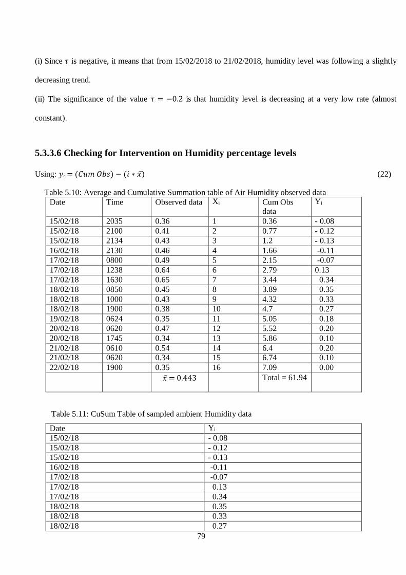
79

(i) Since 𝜏 is negative, it means that from 15/02/2018 to 21/02/2018, humidity level was following a slightly

decreasing trend.

(ii) The significance of the value 𝜏 = −0.2 is that humidity level is decreasing at a very low rate (almost

constant).

5.3.3.6 Checking for Intervention on Humidity percentage levels

Using: 𝑦𝑖 = (𝐶𝑢𝑚 𝑂𝑏𝑠) − (𝑖 ∗ 𝑥) (22)

Table 5.10: Average and Cumulative Summation table of Air Humidity observed data


Yi

15/02/18 2035 0.36 1 0.36 - 0.08

15/02/18 2100 0.41 2 0.77 - 0.12

15/02/18 2134 0.43 3 1.2 - 0.13

16/02/18 2130 0.46 4 1.66 -0.11

17/02/18 0800 0.49 5 2.15 -0.07

17/02/18 1238 0.64 6 2.79 0.13

17/02/18 1630 0.65 7 3.44 0.34

18/02/18 0850 0.45 8 3.89 0.35

18/02/18 1000 0.43 9 4.32 0.33

18/02/18 1900 0.38 10 4.7 0.27

19/02/18 0624 0.35 11 5.05 0.18

20/02/18 0620 0.47 12 5.52 0.20

20/02/18 1745 0.34 13 5.86 0.10

21/02/18 0610 0.54 14 6.4 0.20

21/02/18 0620 0.34 15 6.74 0.10

22/02/18 1900 0.35 16 7.09 0.00

𝑥 = 0.443 Total = 61.94

Table 5.11: CuSum Table of sampled ambient Humidity data

Date Yi

15/02/18 - 0.08

15/02/18 - 0.12

15/02/18 - 0.13

16/02/18 -0.11

17/02/18 -0.07

17/02/18 0.13

17/02/18 0.34

18/02/18 0.35

18/02/18 0.33

18/02/18 0.27

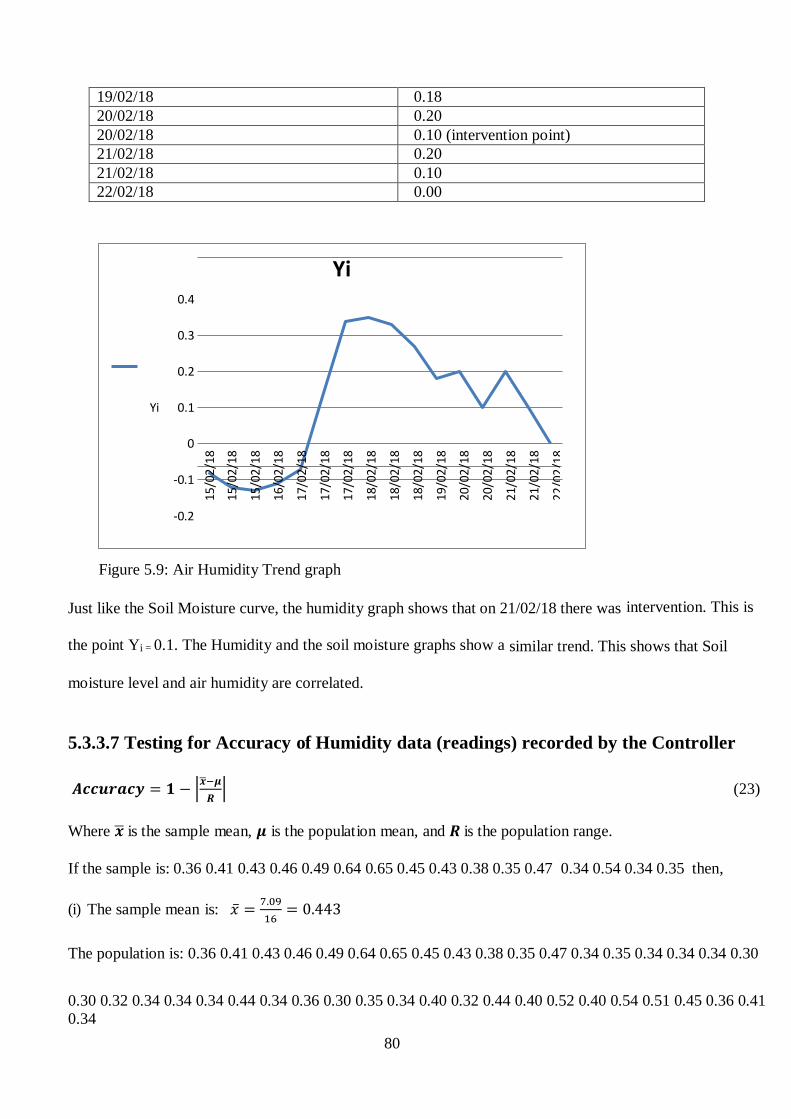
80

Yi 0.4

0.3

0.2

Yi 0.1

-0.1

-0.2

19/02/18 0.18

20/02/18 0.20

20/02/18 0.10 (intervention point)

21/02/18 0.20

21/02/18 0.10

22/02/18 0.00

Figure 5.9: Air Humidity Trend graph

Just like the Soil Moisture curve, the humidity graph shows that on 21/02/18 there was intervention. This is

the point Yi = 0.1. The Humidity and the soil moisture graphs show a similar trend. This shows that Soil

moisture level and air humidity are correlated.

5.3.3.7 Testing for Accuracy of Humidity data (readings) recorded by the Controller

𝑨𝒄𝒄𝒖𝒓𝒂𝒄𝒚 = 𝟏 − |−𝝁

𝑹| (23)

Where is the sample mean, 𝝁 is the population mean, and 𝑹 is the population range.

If the sample is: 0.36 0.41 0.43 0.46 0.49 0.64 0.65 0.45 0.43 0.38 0.35 0.47 0.34 0.54 0.34 0.35 then,

(i) The sample mean is: =7.09

16= 0.443

The population is: 0.36 0.41 0.43 0.46 0.49 0.64 0.65 0.45 0.43 0.38 0.35 0.47 0.34 0.35 0.34 0.34 0.34 0.30

0.30 0.32 0.34 0.34 0.34 0.44 0.34 0.36 0.30 0.35 0.34 0.40 0.32 0.44 0.40 0.52 0.40 0.54 0.51 0.45 0.36 0.41

0.34

15/0

2/18

15/0

2/18

15/0

2/18

16/0

2/18

17/0

2/18

17/0

2/18

17/0

2/18

18/0

2/18

18/0

2/18

18/0

2/18

19/0

2/18

20/0

2/18

20/0

2/18

21/0

2/18

21/0

2/18

22/0

2/18

81

Therefore:

(ii) The population range is: 0.65 – 0.30 = 0.35

(iii) The population mean is:

𝜇 =18.83

47= 0.401 Where 18.83 is the sum of the population, and 47 is the number of elements in the population.

Therefore: 𝐴𝑐𝑐𝑢𝑟𝑎𝑐𝑦 = 1 − |0.443−0.401

0.35| = 0.88

The sampling efficiency for humidity level is 0.88, and this indicates that 88% accuracy is being achieved for

humidity data logging by the irrigation controller.

5.3.3.8 Split-Sample test for Self-Stationarity of the ambient Humidity




Sample 1:

0.36 0.41 0.43 0.46 0.49 0.64 0.65 0.45 0.43 0.38 0.35 0.47 0.34 0.54 0.34 0.35

0.34 0.34 0.34 0.30 0.30 0.32 0.34 0.34

n1 = 24

𝑥1=0.405

S1 = 0.098

Sample 2:

0.34 0.44 0.34 0.36 0.30 0.35 0.34 0.35 0.34 0.40 0.32 0.44 0.40 0.52 0.40 0.54

0.51 0.45 0.36 0.41 0.34 0.49 0.38

n2=23

2 =0.397

S2=0.068

𝑡 =1−2

√𝑠1

2

𝑛1+

𝑠22

𝑛2

(24)

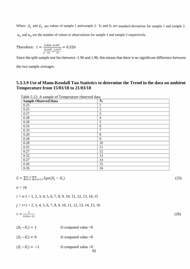
82

Where 1 and 2 are values of sample 1 and sample 2. S1 and S2 are standard deviations for sample 1 and sample 2.

𝑛1 and 𝑛2 are the number of values or observations for sample 1 and sample 2 respectively.

Therefore: 𝑡 =0.404−0.397

√0.0982

24+

0.3972

23

= 0.326

Since the split sample test lies between -1.96 and 1.96, this means that there is no significant difference between

the two sample averages.

5.3.3.9 Use of Mann-Kendall Tau Statistics to determine the Trend in the data on ambient

Temperature from 15/03/18 to 21/03/18

Table 5.12: A sample of Temperature observed data Sample Observed Data Xi

0.25 1

0.25 2

0.27 3

0.28 4

0.28 5

0.33 6

0.33 7

0.29 8

0.28 9

0.28 10

0.25 11

0.27 12

0.32 13

0.27 14

0.26 15

0.26 16


𝑛−1𝑖=1 (25)

n = 16

i = n-1 = 1, 2, 3, 4, 5, 6, 7, 8, 9, 10, 11, 12, 13, 14, 15

j = i+1 = 2, 3, 4, 5, 6, 7, 8, 9, 10, 11, 12, 13, 14, 15, 16

𝜏 =𝑠

0.5(𝑛−1) (26)

(𝑋𝑗 −𝑋𝑖) = 1 if computed value >0

(𝑋𝑗 −𝑋𝑖) = 0 if computed value =0

(𝑋𝑗 −𝑋𝑖) = −1 if computed value <0

83

Table 5.13: Mann-Kendall Tau Statistics Table for Temperature data

S = 13 + 13 + 5 – 1 – 1 - 9 - 9 - 6 - 2 - 2 + 5 + 0 – 3 – 2 + 0 = 1

𝜏 =𝑠

0.5(𝑛−1)=

1

0.5(16)(15)= 0.01

Since 𝜏 is very close to zero, it means that from 15/02/2018 to 21/02/2018, temperature was not changing

much and it had a very small (almost insignificant) upward trend.


i=1 Sgn(0)

= 0

Sgn(.02)

=1

Sgn(.03)

=1

Sgn(.03)

=1

Sgn(.08)

=1

Sgn

(.08) =1

Sgn

(.04) =1

Sgn

(.03) =1

Sgn

(.03) =1

Sgn

(0) = 0

Sgn

(.02) =1

Sgn

(.07) = 1

Sgn(.02)

= 1

Sgn(.01)

= 1

Sgn(.01)

= 1

13

i=2 Sgn(.02)

= 1

Sgn(.03)

= 1

Sgn(.03)

= 1

Sgn(.08)

= 1

Sgn

(.08) = 1

Sgn(

.04) = 1

Sgn(

.03) = 1

Sgn

(.03) = 1

Sgn

(0) = 0

Sgn(

.02) = 1

Sgn

(.07) = 1

Sgn(.02)

= 1

Sgn(.01)

= 1

Sgn(.01)

= 1

13

i=3 Sgn(.01)

= 1

Sgn(.01)

= 1

Sgn(.06)

=1

Sgn

( .06) = 1

Sgn(

.02) = 1

Sgn(

.01) = 1

Sgn(

.01) = 1

Sgn(

-.02) = -1

Sgn

(0) = 0

Sgn

(.05) = 1

Sgn(0)

= 0

Sgn

(-.01) = -1

Sgn

(-.01) = -1

5

i=4 Sgn(0)

= 0

Sgn(.05)

= 1

Sgn

(.05) = 1

Sgn

(.01) = 1

Sgn(

0) = 0

Sgn(

0) = 0

Sgn(

-.03) = -1

Sgn(

-.01) = -1

Sgn

(.04) = 1

Sgn

(-.01) = - 1

Sgn(-

.02) = - 1

Sgn( -

.02) = -1

-1

i=5 Sgn(.05)

= 1

Sgn

(.05) = 1

Sgn(

.01) = 1

Sgn(

0) = 0

Sgn(

0) = 0

Sgn(

-.03) = -1

Sgn(

-.01) = -1

Sgn(.0

4) = 1

Sgn(-

.01) = -1

Sgn(-

.02) = -1

Sgn(-

.02) = -1

- 1

i=6 Sgn(0)

= 0

Sgn(

-.04) = -1

Sgn(

-.05) = -1

Sgn(

-.05) = -1

Sgn(

-.08) = -1

Sgn(

-.06) = -1

Sgn(-

.01) = -1

Sgn(-

.06) = -1

Sgn(-

.07) = -1

Sgn(-

.07) = -1

- 9

i=7 Sgn(

-.04) = -1

Sgn(

-.05) = -1

Sgn(

-.05) = -1

Sgn(

-.08) = -1

Sgn(

-.06) = -1

Sgn(-

.01) = -1

Sgn(-

.06) = -1

Sgn(-

.07) = -1

Sgn(-

.07) = -1

- 9

i=8 Sgn(

-.01) = -1

Sgn(

-.01) = -1

Sgn(

-.04) = -1

Sgn(

-.02) = - 1

Sgn(.0 3) = 1

Sgn(-

.02) = - 1

Sgn(-

.03) = -1

Sgn(-

.03) = -1

- 6

i=9 Sgn( 0) = 0

Sgn(

-.03) = -1

Sgn(

-.01) = -1

Sgn(.0 4) = 1

Sgn(-

.01) = -1

Sgn(-

.02) = 1

Sgn(-

.02) = -1

- 2

i=10 Sgn(

-.03) = -1

Sgn(

-.01) = -1

Sgn(.0

4) = 1

Sgn(-

.01) = -1

Sgn(-

.02) = 1

Sgn(-

.02) = -1

- 2

i=11 Sgn(

.02) = 1

Sgn(.0

7) = 1

Sgn(.02)

= 1

Sgn(.01)

= 1

Sgn(.01)

= 1

5

i=12 Sgn(

.05) = 1

Sgn(0)

= 0

Sgn(-

.01) = -1

Sgn(-

.01) = -1

0

i=13 Sgn(-

.05) = - 1

Sgn(-

.06) = -1

Sgn(-

.06) = -1

-3

i=14 Sgn(-

.01) = -1

Sgn(-

.01) = -1

-2

i=15 Sgn(0) = 0

0

84

5.3.3.10 Checking for Intervention on Temperature data

Using: 𝑦𝑖 = (𝐶𝑢𝑚 𝑂𝑏𝑠) − (𝑖 ∗ 𝑥) (27)

Table 5.14: Average and Cumulative Summation table of Temperature observed data


Yi

15/02/18 2035 0.25 1 0.25 - 0.03

15/02/18 2100 0.25 2 0.50 - 0.06

15/02/18 2134 0.27 3 0.77 - 0.07

16/02/18 2130 0.28 4 1.05 -0.07

17/02/18 0800 0.28 5 1.33 -0.07

17/02/18 1238 0.33 6 1.66 -0.01

17/02/18 1630 0.33 7 1.99 0.04

18/02/18 0850 0.29 8 2.28 0.05

18/02/18 1000 0.28 9 2.56 0.05

18/02/18 1900 0.28 10 2.84 0.05

19/02/18 0624 0.25 11 3.09 0.02

20/02/18 0620 0.27 12 3.36 0.01

20/02/18 1745 0.32 13 3.68 0.05

21/02/18 0610 0.27 14 3.95 0.04

21/02/18 0620 0.26 15 4.21 0.03

22/02/18 1900 0.26 16 4.47 0.01

𝑥 = 0.279 Total = 37.99

Table 5.15: CuSum table of sampled Temperature data

Date Yi

15/02/18 - 0.03

15/02/18 - 0.06

15/02/18 - 0.07

16/02/18 -0.07

17/02/18 -0.07

17/02/18 -0.01

17/02/18 0.04

18/02/18 0.05

18/02/18 0.05

18/02/18 0.05

19/02/18 0.02

20/02/18 0.01

20/02/18 0.05

21/02/18 0.04

21/02/18 0.03

22/02/18 0.01

85

Yi 0.06

0.04

0.02

0 Yi

-0.02

-0.04

-0.06

-0.08

Figure 5.10: Temperature Trend graph

The temperature curve shows a similar trend to the humidity curve. This shows that air humidity and

temperature are correlated.

5.3.3.11 Testing for accuracy of Temperature data (readings) recorded by the Controller

𝐴𝑐𝑐𝑢𝑟𝑎𝑐𝑦 = 1 − |−𝜇

𝑅| (28)

Where is the sample mean, µ is the population mean, and R is the population range.

If the sample is: 0.25 0.25 0.27 0.28 0.28 0.33 0.33 0.29 0.28 0.28 0.25 0.27 0.32 0.27 0.26 0.26

then,

(i) The sample mean is:

=4.47

16= 0.279

The population is: 0.25 0.25 0.27 0.28 0.28 0.33 0.33 0.29 0.28 0.28 0.25 0.30 0.27 0.26 0.26 0.23 0.23 0.21

0.23 0.23 0.24 0.25 0.27 0.30 0.24 0.25 0.23 0.26 0.24 0.29 0.27 0.28 0.29 0.29 0.26 0.33 0.32 0.30 0.24 0.29

0.26

Therefore:

(i) The population range is: 0.33 – 0.21 = 0.12

15/0

2/18

15/0

2/18

15/0

2/18

16/0

2/18

17/0

2/18

17/0

2/18

17/0

2/18

18/0

2/18

18/0

2/18

18/0

2/18

19/0

2/18

20/0

2/18

20/0

2/18

21/0

2/18

21/0

2/18

22/0

2/18

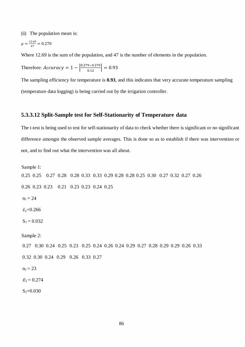
86

(ii) The population mean is:

𝜇 =12.69

47= 0.270

Where 12.69 is the sum of the population, and 47 is the number of elements in the population.

Therefore: 𝐴𝑐𝑐𝑢𝑟𝑎𝑐𝑦 = 1 − |0.279−0.270

0.12| = 0.93

The sampling efficiency for temperature is 0.93, and this indicates that very accurate temperature sampling

(temperature data logging) is being carried out by the irrigation controller.

5.3.3.12 Split-Sample test for Self-Stationarity of Temperature data




Sample 1:

0.25 0.25 0.27 0.28 0.28 0.33 0.33 0.29 0.28 0.28 0.25 0.30 0.27 0.32 0.27 0.26

0.26 0.23 0.23 0.21 0.23 0.23 0.24 0.25

n1 = 24

1=0.266

S1 = 0.032

Sample 2:

0.27 0.30 0.24 0.25 0.23 0.25 0.24 0.26 0.24 0.29 0.27 0.28 0.29 0.29 0.26 0.33

0.32 0.30 0.24 0.29 0.26 0.33 0.27

n2 = 23

𝑥2 = 0.274

S2=0.030

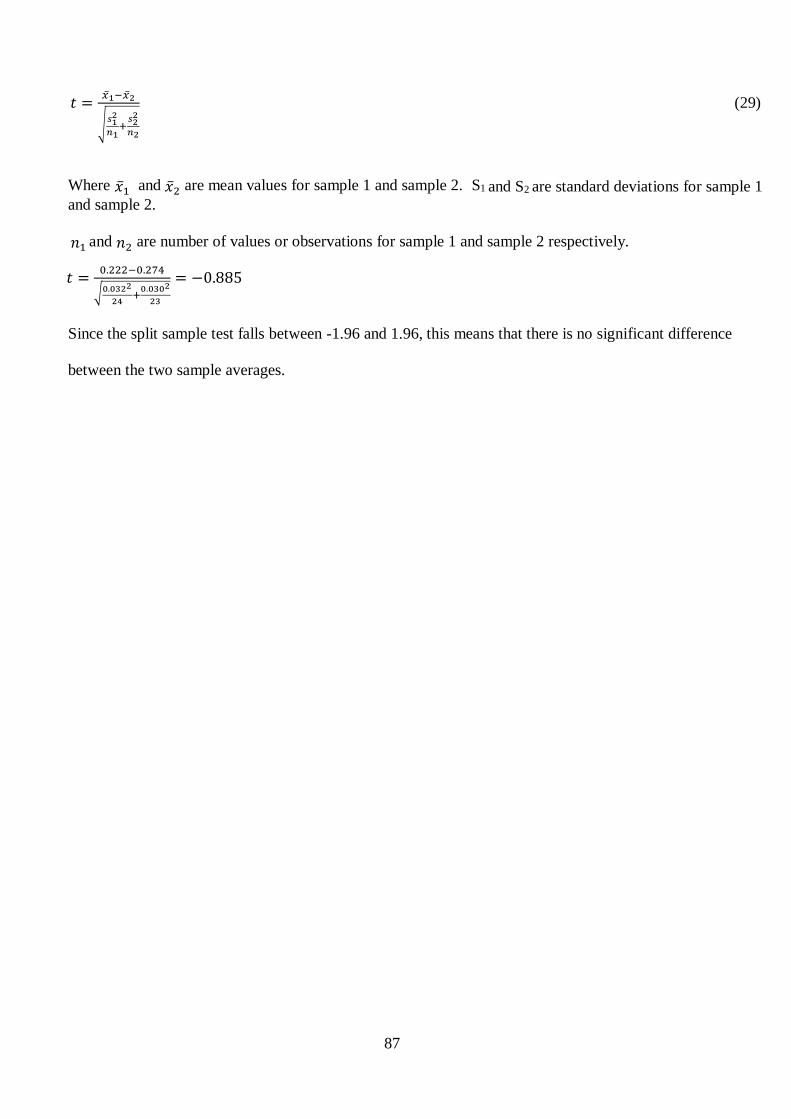
87

𝑡 =1−2

√𝑠1

2

𝑛1+

𝑠22

𝑛2

(29)

Where 1 and 2 are mean values for sample 1 and sample 2. S1 and S2 are standard deviations for sample 1

and sample 2.

𝑛1 and 𝑛2 are number of values or observations for sample 1 and sample 2 respectively.

𝑡 =0.222−0.274

√0.0322

24+

0.0302

23

= −0.885

Since the split sample test falls between -1.96 and 1.96, this means that there is no significant difference

between the two sample averages.

88

CHAPTER 6: SUMMARY, CONCLUSION AND RECOMMENDATIONS

6.1 Summary

The persistent droughts that continue to bedevil the Southern Africa region and the other parts of the world are

a cause for concern. These El Nino induced droughts are a real threat to food security in the affected countries.

There is therefore need to find means and ways of conserving the little amounts of water stored in our water

bodies. Development of ‘smart’ irrigation control systems using modern technologies can help optimize water

usage and increase agricultural productivity. This design-build project was therefore undertaken with the aim

to help improve the way how farmers irrigate their crops and also to help save water. A survey of irrigation

controllers that are currently available on the market was undertaken and it was discovered that these systems

are mainly semi-automatic and they require the farmer’s presence for them to operate. These systems do no

optimize on water usage and they are also not ‘smart’ since they cannot determine crop water requirements and

they cannot make decisions as to when to start and to stop watering. The system relies on the farmer’s

experience which may be inaccurate and unreliable. The importance of the acquisition of reliable weather

forecasting information was also highlighted. This resulted in the design incorporating an Internet weather data

acquisition algorithm. This algorithm enables the system to automatically download weather data and thirteen

days weather forecast information from the OpenWeatherMap Internet server in order to enable the farmer to

plan in ahead. “It is not a good idea to water the crops when it’s going to rain in a couple of hours.” Therefore

the farmer needs to know how the weather is going to be like in a couple of days to come. The system relies

more on the Internet of Things (IoT) technology for its architecture and for its ‘smart’ decision-making

processes. The IoT applications enable the system to send and receive data to the farmer’s smartphone and to a

personal computer through the Internet. Therefore the farmer is able to communicate with the system from any

geographical location in the world. The prototype was tested and the results were subjected to statistical

analysis to verify their accuracy and validity using statistical tools such as the Mann-kendal tau statistic, the

split-sample t-test for self-stationarity, and t-test for data accuracy. The prototype test results suggest that this

‘smart’ automatic irrigation control system can optimize water usage as well as enhance productivity.

89

6.2 Conclusion

In conclusion, a “smart” automatic irrigation control system with Internet capability was successfully designed

and implemented. The system receives and processes data about soil moisture levels and local weather

conditions. It then uses the information to automatically control the water pumps for timeous irrigation of crops.

It also automatically acquires weather and weather-forecast information covering the next thirteen days from

an international meteorological service provider called OpenWeatherMap, through the internet. To cater for

periods of internet outages, the system also incorporates a mini-weather station which measures local ambient

temperature, ambient humidity and barometric pressure. A working prototype was successfully tested and the

results suggest that 26% of irrigation water may be saved through use of the ‘smart’ automatic irrigation control

system.

6.3 Recommendations for further Improvements

The system may be improved by incorporating an algorithm which would analyse the soil fertility levels and

automatically suggest a suitable crop to grow on that particular type of soil. This algorithm can also take into

account the variations in the soil water retention properties at different locations within a single farm and hence

implement selective watering for different regions of the farm. This can be implemented using the Global

Positioning System (GPS) to map and analyse the soil properties and then recommend the different soil water

requirements.

90

List of References

[1] R. M. Jury, Economic Impacts of Climate Variability in South Africa and Development of Resource

Prediction Models. [online]. Available: https://journals.ametsoc.org/doi/full/. [Accessed May. 28. 2018]

[2] D. Rojas, et al., “Understanding the Draught Impact of El Nino on the Global Agricultural Areas,” An

Assessment using FAO’s Agricultural Stress Index, Rome: 2014, pp. 10-15.

[3] OpenWeatherMap. (2019, Jun. 20). Current Weather and Forecasts [Online]. Available:

https://OpenWeatherMap.org. [Accessed: April 13. 2019].

[4] IrrigationOnline, “Hortech Systems for Irrigation Systems and Watering needs: Hunter Eco- Logic

Controller”. [online]. Available: [Accessed: May. 12. 2018].

[5] S.W.R. Cox, Microelectronics in Agriculture and Horticulture, 2nd ed. London:

Granada Publishers, 1982.

[6] J.R. Starr, Forecaster’s Reference Book, Berkshire: the Met. Office, Feb. 1997.

[7] A.J. Iser and T.Y. Woma, “Weather Forecasting Models, Methods and Applications,” vol.2 Issue 12, Dec

2013.

[8] L. Pincus, “T-Test Review,” Agriculture Innovation Programme, University of Califonia, UVDAVIS,

USA, 2014

[9] R.O. Gilbert, Statistical Methods for Environmental Pollution Monitoring, New York: Wiley, 1987.

[10] M.G. Kendall, Rank Correlation Methods, 4th ed. London: Charles Griffin, 1975.

[11] K.W. Hipel and A.I. McLoed, Time series modelling of water resources and environ-mental systems,”

Amsterdam: Elsevier Publishers, 1994.

[12] CodeIoT. (2019, Aug. 2019). Intelligent Connected Ojects[Online]. Available:

https://codeiot.org.br/courses/course-v1:LSi-TEC+IOTIO6EN. [Accesed: May20. 2020].

[13] S. K. Garg, Irrigation Engineering and Hydraulic Structures, 19th ed. Delhi:

Khanna Publishers, 2005.

[14] G. L. Asawa, Irrigation and water Resources Engineering, New Delhi: New Age International Publishers,

2008.

[15] L. Pitts. (2016, May). “Monitoring Soil Moisture for Crop Growth.” [online]. Available:

https://observant.zendesk.com/hc/en-us/articles/208067926-Monitoring-Soil-Moisture-for-Optimal-Crop-

Growth [Accessed: June 12. 1018].

“

[16] M. Schwartz, Internet of Things with Arduino, Birmingham: Packt Publishing Ltd, 2016

[17] C. pfister, Getting Started with the Internet of Things, USA: O’Reilly Media, 2011.

https://openweathermap.org/

https://codeiot.org.br/courses/course-v1:LSi-TEC+IOTIO6EN

https://observant.zendesk.com/hc/en-us/articles/208067926-Monitoring-Soil-Moisture-for-Optimal-Crop-Growth

https://observant.zendesk.com/hc/en-us/articles/208067926-Monitoring-Soil-Moisture-for-Optimal-Crop-Growth

91

[18] C. Bell, Beginning Sensor Networks with Arduino and Raspberry Pi, New York: Apress, 2013, pp 45.

[19] J. Boxall, Arduino Workshop: A hands-on Introduction, San Francisco: No Starch Press, 2013.

[20] J. R. Castro, Home Security System with Arduino, Birmingham: Packt Publishing, Aug 2005.

[21] M. Schwartz, Internet of Things with ESP8266, Birmingham: Packt Publishing, 2016.

[22] R. Santos, ESP8266 Web Server with Arduino IDE, Porto: Random Nerd Tutorials, 2018.

[23] B. Hammell, “Connecting Arduino: Programming and Networking with the Ethernet Shield”, 2014,

U.S.A.

[24] E. Gertz and P.D. Justo, “Environmental Monitoring with Arduino”, Building simple

Devices to collect data about the world around us, USA: O’Reilly Media, 2012, pp. 43-47.

[25] Mantech Products. (2018, April.20). Soil Moisture Monitor [Online]. Available:

www.mantech.co.za/datasheets/products/A000047.pdf [Accessed: July 26. 2018].

“

[26] Mantech Products. (2018, April.20). Humidity Sensor [Online]. Available:

www.mantech.co.za/datasheets/products/A000047.pdf [Accessed: Aug 12. 2018].

“

[27] Mantech Products. (2018, April.20). Light Dependent resistor [Online]. Available:

www.mantech.co.za/datasheets/products/A000047.pdf [Accessed: Sept 12. 2018].

“

[28] R. Blum, Teach yourself Arduino Programming in 24 hours, Indianapolis: Pearson Education, Sept 2014,

pp. 319-329.

[29] M. R. Roberts, A complete Beginner’s Guide to Arduino, Earthshine Electronics Publishers, 5 th ed.

August 2010.

[30] J. Baichtal, Arduino for Beginners: Essential Skills every Maker needs, USA: Pearson Education

Publishers, 2014.

[31] WH360-WH3000 Waterhouse Pumps (2018, March. 20). [Online] Available:

https://www.builders.co.bw/Garden-Decor/Water-Feature-Pumps/Waterhouse-WH360-Permaflo-3-Core-

Pump/p/. [Accessed: Sept 18. 2018].

[32] C. Amariei, Arduino Development Cookbook, Birmingham: Packt Publishing, April 2015.

[33] Mantech Products. (2018, April.20). Two channel 5V Relay [Online]. Available:

www.mantech.co.za/datasheets/products/A000047.pdf [Accessed: June 10. 2018].

“

[34] LED Datasheet(2018, Feb.20). [Online] Available:

https://category.alldatasheet.com/index.jsp?sSearchword=5mmleddatasheet&gclid. [Accessed: May 20.

2018].

[ [35] R. Beri, “Programming and Problem Solving through ‘C’ Language”, 2nd ed. New Delhi: Macmillan

Publishers, 2003.

http://www.mantech.co.za/datasheets/products/A000047.pdf



https://www.builders.co.bw/Garden-Decor/Water-Feature-Pumps/Waterhouse-WH360-Permaflo-3-Core-Pump/p/

https://www.builders.co.bw/Garden-Decor/Water-Feature-Pumps/Waterhouse-WH360-Permaflo-3-Core-Pump/p/


https://category.alldatasheet.com/index.jsp?sSearchword=5mm

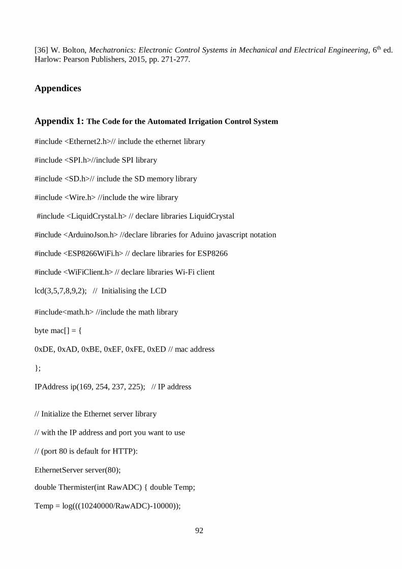
92

[36] W. Bolton, Mechatronics: Electronic Control Systems in Mechanical and Electrical Engineering, 6th ed.

Harlow: Pearson Publishers, 2015, pp. 271-277.

Appendices

Appendix 1: The Code for the Automated Irrigation Control System

#include <Ethernet2.h>// include the ethernet library

#include <SPI.h>//include SPI library

#include <SD.h>// include the SD memory library

#include <Wire.h> //include the wire library

#include <LiquidCrystal.h> // declare libraries LiquidCrystal

#include <ArduinoJson.h> //declare libraries for Aduino javascript notation

#include <ESP8266WiFi.h> // declare libraries for ESP8266

#include <WiFiClient.h> // declare libraries Wi-Fi client

lcd(3,5,7,8,9,2); // Initialising the LCD

#include<math.h> //include the math library

byte mac[] =

0xDE, 0xAD, 0xBE, 0xEF, 0xFE, 0xED // mac address

;

IPAddress ip(169, 254, 237, 225); // IP address

// Initialize the Ethernet server library

// with the IP address and port you want to use

// (port 80 is default for HTTP):

EthernetServer server(80);

double Thermister(int RawADC) double Temp;

Temp = log(((10240000/RawADC)-10000));

93

Temp = 1/(0.001129148+(0.000234125*Temp)+(0.0000000876741*Temp*Temp*Temp));

Temp = Temp-273.15; //convert kelvin to celsius return

Temp;

//configure the thermistor sensor

const int chipSelect = 4;// chip select control pin for the LCD

int sensorPin=A0;// analogue pin 0 as moisture sensor pin

int sensorValue=0;// memory location for moisture sensor data

int ldr = A2; // ldr sensor connected to analogue pin 2

int ldrValue = 0;// memory location for ldr sensor value or data

int ledgreen=11; //connect green LED to digital port 11

int ledred=12;// connect red LED to digital port 12

int water_tankStatus=28;

int boreholeStatus=29;

int water_tankPump=31;// connect the water_tank pump to digital port 31

int boreholePump=32;// connect the borehole pump to digital port 32

int limitSwitch=34;// connect limit switch to digital port 34

int val=0;//temporary storage file for the limit switch value

int RH=A3;

int humidity=0;

int speakerPin=35;

char c;

int Pin = 53;

void setup()

void OpenWeathrMap();

// Open serial communications and wait for port to open:

Serial.begin(9600);

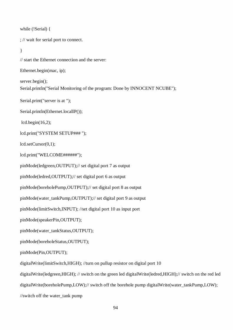
94

while (!Serial)

; // wait for serial port to connect.

// start the Ethernet connection and the server:

Ethernet.begin(mac, ip);

server.begin();

Serial.println("Serial Monitoring of the program: Done by INNOCENT NCUBE");

Serial.print("server is at ");

Serial.println(Ethernet.localIP());

lcd.begin(16,2);

lcd.print("SYSTEM SETUP### ");

lcd.setCursor(0,1);

lcd.print("WELCOME######");

pinMode(ledgreen,OUTPUT);// set digital port 7 as output

pinMode(ledred,OUTPUT);// set digital port 6 as output

pinMode(boreholePump,OUTPUT);// set digital port 8 as output

pinMode(water_tankPump,OUTPUT);// set digital port 9 as output

pinMode(limitSwitch,INPUT); //set digital port 10 as input port

pinMode(speakerPin,OUTPUT);

pinMode(water_tankStatus,OUTPUT);

pinMode(boreholeStatus,OUTPUT);

pinMode(Pin,OUTPUT);

digitalWrite(limitSwitch,HIGH); //turn on pullup resistor on digital port 10

digitalWrite(ledgreen,HIGH); // switch on the green led digitalWrite(ledred,HIGH);// switch on the red led

digitalWrite(boreholePump,LOW);// switch off the borehole pump digitalWrite(water_tankPump,LOW);

//switch off the water_tank pump

95

digitalWrite(speakerPin,HIGH);

digitalWrite(jojoStatus,HIGH);

digitalWrite(boreholeStatus,HIGH);

delay(100);

digitalWrite(speakerPin,LOW);

delay(100);


delay(100);


delay(100);


delay(100);

digitalWrite(speakerPin,LOW),

delay(100);


delay(100); digitalWrite(speakerPin,LOW);

while (!Serial) //wait for serial port to connect. Needed for native USB port only

Serial.println("Initialising SD card. ............... "); // initializing sd card

//see if the card is present and can be initialised:

if (!SD.begin(chipSelect))

Serial.println("Card failed, or not present");

//don't do anything more

else Serial.println("card initialised.");

96

void loop()

OpenWeatherMap(); // call the function OpenWeathrMap

// listen for incoming clients

EthernetClient client = server.available();

if (client)

Serial.println("NEW CLIENT IS THE WEB PAGE: Done by INNOCENT NCUBE");

// an http request ends with a blank line

boolean currentLineIsBlank = true;

while (client.connected())

if (client.available())

char c = client.read();

Serial.write(c);

// if we’ve gotten to the end of the line (received a newline

// character) and the line is blank, the http request has ended,

// so we can send a reply

if (c == '\n' && currentLineIsBlank)

// send a standard http response header

client.println("HTTP/1.1 200 OK");

client.println("Content-Type: text/html");

client.println("Connection: close"); // the connection will be closed after completion of the response

client.println("Refresh: 5"); // refresh the page automatically every 5 sec

client.println();

client.println("<!DOCTYPE HTML>");

client.println("<html>");

// output the value of each analog input pin

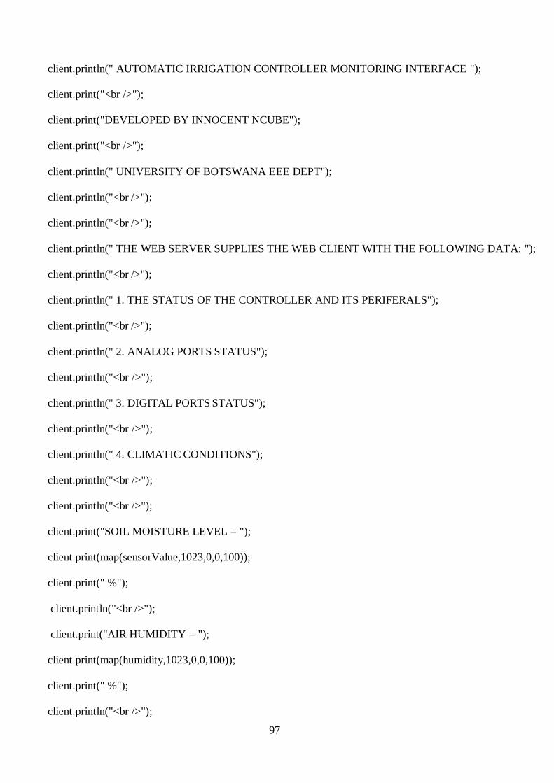
97

client.println(" AUTOMATIC IRRIGATION CONTROLLER MONITORING INTERFACE ");

client.print(" ");

client.print("DEVELOPED BY INNOCENT NCUBE");

client.print(" ");

client.println(" UNIVERSITY OF BOTSWANA EEE DEPT");

client.println(" ");


client.println(" THE WEB SERVER SUPPLIES THE WEB CLIENT WITH THE FOLLOWING DATA: ");


client.println(" 1. THE STATUS OF THE CONTROLLER AND ITS PERIFERALS");


client.println(" 2. ANALOG PORTS STATUS");


client.println(" 3. DIGITAL PORTS STATUS");


client.println(" 4. CLIMATIC CONDITIONS");



client.print("SOIL MOISTURE LEVEL = ");

client.print(map(sensorValue,1023,0,0,100));

client.print(" %");


client.print("AIR HUMIDITY = ");

client.print(map(humidity,1023,0,0,100));

client.print(" %");

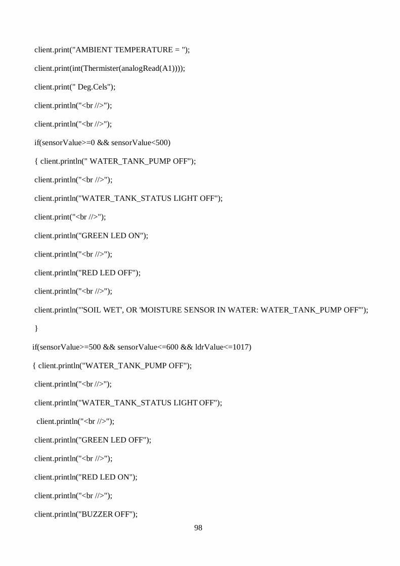
98

client.print("AMBIENT TEMPERATURE = ");

client.print(int(Thermister(analogRead(A1))));

client.print(" Deg.Cels");

client.println(" ");


if(sensorValue>=0 && sensorValue<500)

client.println(" WATER_TANK_PUMP OFF");


client.println("WATER_TANK_STATUS LIGHT OFF");

client.print(" ");

client.println("GREEN LED ON");


client.println("RED LED OFF");


client.println("'SOIL WET', OR 'MOISTURE SENSOR IN WATER: WATER_TANK_PUMP OFF'");

if(sensorValue>=500 && sensorValue<=600 && ldrValue<=1017)

client.println("WATER_TANK_PUMP OFF");


client.println("WATER_TANK_STATUS LIGHT OFF");


client.println("GREEN LED OFF");


client.println("RED LED ON");


client.println("BUZZER OFF");

99


client.println("'SOIL MOISTURE LOW & ITS DAYTIME: WATER_TANK_PUMP OFF'");


client.println("WILL WATER WHEN IT GETS DARK");

if(sensorValue>=500 && sensorValue<=600 && ldrValue>1017)

client.println("WATER_TANK_Pump ON");


client.println("WATER_TANK_STATUS LIGHT ON");






client.println("BUZZER OFF");


client.println("'ITS DARK & SOIL MOISTURE LOW: WATER_TANK_PUMP ON'");

if(sensorValue>600)

client.println("WATER_TANK_PUMP ON");


client.println("WATER_TANK_ STATUS LIGHT ON");

100



client.println("BUZZER ON");


client.println("SOIL IS DRY <'WATER_TANK_PUMP ON'>");



if(val==HIGH)

client.print("BOREHOLE PUMP OFF"); //switch on borehole pump


client.print("BOREHOLE STATUS LIGHT OFF");//switch on status light

else

client.print("BOREHOLE PUMP ON");//switch off borehole pump


client.print("BOREHOLE STATUS LIGHT ON");//switch off borehole status



for (int analogChannel = 0; analogChannel < 6; analogChannel++)

int sensorReading = analogRead(analogChannel);

client.println("ANALOG INPUT PIN ");

client.print(analogChannel);

client.print(" IS ");

client.print(sensorReading); client.println(" ");

101


for (int digitalChannel =0; digitalChannel < 14; digitalChannel++)

int actuatorReading = digitalRead(digitalChannel); client.println("");

client.print("DIGITAL OUTPUT PIN ");

client.print(digitalChannel);

client.print(" IS ");

client.print(actuatorReading); client.println(" ");

client.println("</html>");

break;

if (c == '\n')

// you're starting a new line

currentLineIsBlank = true;

else if (c != '\r')

// you've gotten a character on the current line

currentLineIsBlank = false;

// give the web browser time to receive the data delay(1);

// close the connection:

client.stop();

Serial.println("client connected: Done by INNOCENT NCUBE");

102

analogRead (RH);

sensorValue=analogRead(sensorPin);// read the soil moisture sensor value

int humidityReal =map(sensorValue,1023,0,0,100);// display soil moisture as a %

humidity=analogRead(RH);

int humiditypercentage = map(humidity,1023,0,0,100);

val=digitalRead(limitSwitch); //check state of water_tank limit switch

if(val==HIGH)

digitalWrite(boreholePump,LOW); //switch on borehole pump

digitalWrite(boreholeStatus,LOW);//switch on status light

else

digitalWrite(boreholePump,HIGH);//switch off borehole pump

digitalWrite(boreholeStatus,HIGH);//switch off borehole status

ldrValue=analogRead(ldr); // read the ldr sensor value

File dataFile = SD.open("datalog.txt", FILE_WRITE);//open the file

//if the file is available,write to it

if (dataFile )

dataFile.print("");// write data on memory card

dataFile.print("");

dataFile.print("Moisture Level = ");

dataFile.print( humidityReal); dataFile.println("%");

dataFile.print("Temperature = ");

dataFile.print( int(Thermister(analogRead(A1))));

dataFile.println(" Deg.Cels"); dataFile.println("");

103

dataFile.println("");

dataFile.close();

else

Serial.println("error opening datalog.txt");// write this on serial monitor

Serial.println("");// space cursor one step down on serial monitor

lcd.clear();// clear the lcd

lcd.setCursor(11,0);// set the cursor on column 6 and row 0

lcd.print(humidityReal);// write the percentage moisture level on lcd


lcd.print("%");// write the percentage moisture content

lcd.print("Humidity =");

lcd.setCursor(11,0);

lcd.print(humiditypercentage);


lcd.print("%");

lcd.setCursor(0,1);

lcd.print("Temp =");


lcd.print(int(Thermister(analogRead(A1)))); // write temperature value on lcd


lcd.print("Deg.C");

if(sensorValue>=0 && sensorValue<500)

digitalWrite(ledgreen,HIGH);// switch on the green

led digitalWrite(ledred,LOW);// switch off the red led

104

digitalWrite(water_tankPump,LOW);// switch off the water_tank pump

digitalWrite(water_tankStatus,LOW);//switch off the status light

digitalWrite(speakerPin,LOW);//switch off alarm

lcd.setCursor(0,1);// set the cursor on column 0 and row1

lcd.print("Soil Wet PumpOff");// write on lcd

Serial.print("MOISTURE LEVEL = ");//write on serial monitor

Serial.print(humidityReal); //write on serial monitor

Serial.println("%");//write on serial monitor

Serial.print("Temperature = ");//write on serial monitor

Serial.print(int(Thermister(analogRead(A1))));

Serial.println(" Deg Cels");// write on serial monitor

Serial.println("'SOIL WET' or 'MOISTURE SENSOR IN WATER: WATER VALVE &

WATER_TANK_PUMP OFF'");// write on serial monitor

if(sensorValue>=500 && sensorValue<=600 && ldrValue<=1017)

digitalWrite(ledgreen,LOW);// switch off green

led digitalWrite(ledred,HIGH);// switch off red

led digitalWrite(water_tankPump,LOW);// switch off water_tank pump

digitalWrite(water_tankStatus,LOW);//switch off status light


lcd.setCursor(0,1);// set cursor on column 0 and row 1

lcd.print("Daytime:Pump Off");//write on lcd

Serial.print("MOISTURE LEVEL = ");// write on serial monitor

Serial.print(humidityReal);// write on serial monitor

Serial.println("%");// write on serial monitor

Serial.print("Temperature = ");// write on serial monitor

105

Serial.print(int(Thermister(analogRead(A1))));// write temperature value


Serial.println("'SOIL MOISTURE LOW & ITS DAYTIME: WATER VALVE & WATER_TANK

PUMP OFF'");// write on serial monitor

if(sensorValue>=500 && sensorValue<=600 && ldrValue>1017)

digitalWrite(ledred,HIGH); // switch off red led

digitalWrite(ledgreen,LOW);//switch off green led

digitalWrite(jojoPump,HIGH);// switch on jojo pump

digitalWrite(jojoStatus,HIGH);//switch on status light


lcd.setCursor(0,1);// set cursor to column 0 and row 1

lcd.print("Its Dark:Pump On");//write on lcd Serial.print("MOISTURE LEVEL = ");// write on serial monitor

Serial.print(humidityReal);// write on serial monitor


Serial.print("Temperature = ");//write on serial monitor

Serial.print(int(Thermister(analogRead(A1))));// write the temperature value


Serial.println("'ITS DARK & SOIL MOISTURE LOW: WATER VALVE & WATER_TANK PUMP

ON'"); // write on serial monitor

if(sensorValue>600) digitalWrite(ledred,HIGH);// switch on red led

digitalWrite(ledgreen,LOW);// switch off green

led digitalWrite(water_tankPump,HIGH);// switch on water_tank pump

digitalWrite(water_tankStatus,HIGH);//switch on status light

106

lcd.setCursor(0,1);// set cursor to column 0 and row 1

lcd.print("I am Irrigating");// write on lcd

Serial.print("MOISTURE LEVEL = ");//write on serial monitor

Serial.print(humidityReal);// write moisture content on serial monitor


Serial.print("Temperature = ");// write on serial monitor

Serial.print(int(Thermister(analogRead(A1))));// write on serial monitor

Serial.println(" Deg Cels");//write on serial monitor

Serial.println("SOIL IS DRY & ITS DARK: <'WATER VALVE & WATER_TANK PUMP ON'>");//

wrte on serial monitor

delay(3000);//delay by 3 seconds

/*code for downloading the Internet weather data from OpenWeatherMap Internet server. This code is a

module code (function) to be called into the main code when weather data is required*/

void OpenWeatherMap()

#include <ESP8266WiFi.h> // library files

#include <ESP8266HTTPClient.h>

#include <WiFiClient.h>

#include <Arduino_JSON.h>

const char* ssid = "TNCAP37789B"; // the Wi-Fi name

const char* password = "33FE4B5AE6";// the Wi-Fi password

String city = "Gaborone"; // name of city where the system is located

String countryCode = "BW"; // the Botswana country code

unsigned long lastTime = 0;

unsigned long timerDelay = 10000; // connection time

107

String jsonBuffer;

void setup()

Serial.begin(115200); // configuring and setting up the serial monitor data rate

WiFi.begin(ssid, password); // Enter Wi-Fi network details

Serial.println("Connecting"); // send signal to serial monitor

while(WiFi.status() != WL_CONNECTED)

delay(500);

Serial.print("."); // print to serial monitor

Serial.println("");

Serial.print("Connected to WiFi network with IP Address: "); // print to serial monitor

Serial.println(WiFi.localIP());

Serial.println("Timer set to 10 seconds (timerDelay variable), it will take 10 seconds before publishing the first

reading.");

void loop()

// Send an HTTP GET request

if ((millis() - lastTime) > timerDelay)

// Check WiFi connection status

if(WiFi.status()== WL_CONNECTED)

String serverPath = "http://api.openweathermap.org/data/2.5/weather?q=" + city + "," + countryCode

+"&APPID=" + openWeatherMapApiKey;

jsonBuffer = httpGETRequest(serverPath.c_str());

Serial.println(jsonBuffer);

JSONVar myObject = JSON.parse(jsonBuffer);

// JSON.typeof(jsonVar) can be used to get the type of the var

108

if (JSON.typeof(myObject) == "undefined")

Serial.println("Parsing input failed!");

return;

/* Print weather data*/

Serial.print("JSON object = ");

Serial.println(myObject);

Serial.print("Temperature: ");

Serial.println(myObject["main"]["temp"]);

Serial.print("Pressure: ");

Serial.println(myObject["main"]["pressure"]);

Serial.print("Humidity: ");

Serial.println(myObject["main"]["humidity"]);

Serial.print("Wind Speed: ");

Serial.println(myObject["wind"]["speed"]);

else

Serial.println("WiFi Disconnected");

lastTime = millis();

String httpGETRequest(const char* serverName)

HTTPClient http;

// Your IP address with path or Domain name with URL path

109

http.begin(serverName);

// Send HTTP POST request

int httpResponseCode = http.GET();

String payload = "";

if (httpResponseCode>0)

Serial.print("HTTP Response code: ");

Serial.println(httpResponseCode);

payload = http.getString();

else

Serial.print("Error code: ");

Serial.println(httpResponseCode);

http.end();

return payload;

Appendix 2: Sample results retrieved from the SD Memory card

Initialising SD card.........

cardinitialised.

Time now is: 20:35:22 15/02/2018 SOIL MOISTURE LEVEL = 42% AIR HUMIDITY = 36%

TEMPERATURE = 25DegCels

SOIL IS DRY & ITS DARK: <'WATER_TANK &BOREHOLE PUMPS ON'>

Time now is: 21:00:27 15/02/2018

SOIL MOISTURE LEVEL = 70% AIR HUMIDITY = 41% TEMPERATURE = 25DegCels

110

SOIL IS WET: <'WATER_TANK&BOREHOLE PUMPS OFF'>

Time now is: 21:30:32 16/02/2018



Time now is: 12:38:37 17/02/2018

SOIL MOISTURE LEVEL = 69% AIR HUMIDITY = 64% TEMPERATURE = 33 DegCels


Time now is: 08:50:22 18/02/2018



Time now is: 06:24:42 19/02/2018

SOIL MOISTURE LEVEL = 53%

AIR HUMIDITY = 35% TEMPERATURE = 25DegCels

SOIL IS DRY& ITS DAYTIME<'WATERING AFTER DARK'>

Time now is: 06:20:47 20/02/2018


SOIL IS DRY & ITS DAYTIME: <'WATERING AFTER DARK'>

Time now is: 06:10:52 21/02/2018


SOIL IS DRY: <'WATER_TANK &BOREHOLE PUMPS ON'>

Time now is: 06:20:57 22/02/2018

111



Time now is: 06:15:02 23/02/2018

SOIL MOISTURE LEVEL = 57% AIR HUMIDITY = 30%

TEMPERATURE = 21 DegCels

SOIL IS WET: <'WATER_TANK &BOREHOLE PUMPS OFF'>

Time now is: 09:26:07 24/03/2018



Time now is: 09:30:12 25/02/2018



Time now is: 06:30:17 26/02/2018


SOIL IS WET: <’WATER_TANK&BOREHOLE PUMPS OFF'>

Time now is: 06:35:22 27/02/2018


SOIL IS DRY &ITS DAYTIME: <'WATERING AFTER DARK'>

Time now is: 06:30:27 28/02/2018

112


Time now is: 06:30:32 01/03/2018



Time now is: 06:00:22 02/03/2018



Time now is: 06:00:37 03/03/2018


SOIL IS DRY: <'WATER_TANK&BOREHOLE PUMPS ON'>

Time now is: 06:20:42 04/03/2018


SOIL IS DRY: <'WATERING AFTER DARK'>

Time now is: 06:20:47 05/03/2018



Time now is: 06:17:52 06/03/2018



Time now is: 06:20:57 07/03/2018

Design and Implementation of an Automated Irrigation Control ...

Documents

Transcript of Design and Implementation of an Automated Irrigation Control ...