Design and Characterization for Regenerative Shock Absorbers

30 July 2022

POLITECNICO DI TORINORepository ISTITUZIONALE

Design and Characterization for Regenerative Shock Absorbers / Xu, Yijun. - (2018 Nov 20), pp. 1-168.[10.6092/polito/porto/2724280]

Original

Design and Characterization for Regenerative Shock Absorbers

Publisher:

PublishedDOI:10.6092/polito/porto/2724280

Terms of use:Altro tipo di accesso

Publisher copyright

(Article begins on next page)

This article is made available under terms and conditions as specified in the corresponding bibliographic description inthe repository

Availability:This version is available at: 11583/2724280 since: 2019-01-31T17:09:39Z

Politecnico di Torino

Doctoral Dissertation

Doctoral Program in Mechanical Engineering (30thcycle)

Design and Characterization ofRegenerative Shock Absorbers

based on ElectrohydrostaticActuation

By

Yijun Xu******

Supervisor(s):Prof. Nicola Amati

Doctoral Examination Committee:Prof. Lei Zuo, Reviewer, Virginia Polytechnic Institute and State UniversityProf. Subhash Rakheja, Reviewer, Concordia University MontrealProf. Andrea Tonoli, Committee, Politecnico di Torino

Politecnico di Torino

2018

Declaration

I hereby declare that, the contents and organization of this dissertation constitute myown original work and does not compromise in any way the rights of third parties,including those relating to the security of personal data.

Yijun Xu2018

* This dissertation is presented in partial fulfillment of the requirements for Ph.D.degree in the Graduate School of Politecnico di Torino (ScuDo).

"A man has free choice to the extent that he is rational."-St. Thomas Aquinas

Acknowledgements

I am grateful to the whole staff of the Mechatronics Laboratory of Politecnico diTorino (LIM) for their constant support and help through my three years of work asa Ph.D. student. Their friendship and professional collaboration allowed for a greatdeal of personal and professional improvements.

I would like to express my most grateful acknowledgments to my supervisorProf. Nicola Amati for his professional advice based on his extensive experience. Igratefully acknowledge the director of LIM, Prof. Andrea Tonoli for his generousand creative comments and observations that broadened the limits of our knowledge.

This dissertation was developed within the research contract 236/2016 whichwas funded by Magneti Marelli Shock Absorbers and coordinated by Politecnicodi Torino. During the development of this project, I found invaluable help in mycolleague and also a dear friend Ph.D. Eng. Renato Galluzzi, who volunteered tohelp me during the development of this project. His talent and untiring attitudetowards our objectives in the research contributed a lot to this work.

Furthermore, I am grateful to my dear friends Joaquim Girardello Detoni, Mariadi Napoli and Qingwen Cui, with whom I have shared all the good moments duringmy Ph.D. period and these valuable memories in Italy will never be forgotten.

Most of all, I would like to dedicate this work to my family, I am grateful to myfather and mother who have always been my stronghold after I left my country tofollow this journey in Italy.

Abstract

The trend of reducing the emissions in automotive sector leads to the developmentof electrification of vehicle powertrain and chassis. Those vehicles equipped withregenerative shock absorbers can transfer the vibrational energy coming through theroad irregularities into electricity which can be further used for other purpose, i.e. tocharge the battery. To realize the regeneration target, the developed device should beable to vary their damping behaviors while converting part of the dissipated powerinto electricity. Therefore, an electric machine together with a suitable transmissionsystem need to be integrated to the vehicle. Several types of solutions have beeninvestigated during the last two decades. In the present thesis, one prototype ofregenerative damper with controllable damping and energy harvesting featuresis developed. The regenerative shock absorber employs the electro-hydrostaticactuation principle, uses a hydraulic actuator directly interfaced with a motor-pumpgroup by means of hydraulic circuit to convert the linear motion of the piston intorotation. To maximize the energy regeneration as well as to guarantee the dampingfeatures, the hydraulic, mechanical and electric subsystems must be integratedand optimized as an entire system. The thesis establishes a system-level approachduring the design phase while complying with important constraints such as envelopvolume and supply voltage limitation. Different aspects that will affect the finalconversion efficiency are analyzed individually, a prototype is also produced and fullycharacterized with experimental tests. Furthermore, this approach can be extendedto any motor-pump unit for hydraulic regenerative dampers. The significance ofthe present work can be seen also from its integration with the electric powertrain.Since the shock absorber is electrical, it can easily transfer the power to the vehiclebattery which is also electrical, in this case, a single system can be used to handle theenergy. Another important aspect is about the autonomous driving technology, sincesystems and devices nowadays are getting towards having more controlled dampingproperties to enhance the driving comfort experience.

Contents

List of Figures ix

List of Tables xvi

Nomenclature xvii

1 Introduction 1

1.1 Motivation . . . . . . . . . . . . . . . . . . . . . . . . . . . . . . . 1

1.2 Aim of the Work . . . . . . . . . . . . . . . . . . . . . . . . . . . 5

1.3 State of the Art . . . . . . . . . . . . . . . . . . . . . . . . . . . . 5

1.3.1 Linear Regenerative Shock Absorber . . . . . . . . . . . . 6

1.3.2 Rotary Regenerative Shock Absorber . . . . . . . . . . . . 10

1.3.3 Comparison of different energy conversion mechanisms . . 19

1.4 Thesis Outline . . . . . . . . . . . . . . . . . . . . . . . . . . . . . 23

2 Working Principle 24

2.1 Kinetic Energy to Electric Energy Conversion . . . . . . . . . . . . 24

2.1.1 Road Profile Excitation . . . . . . . . . . . . . . . . . . . . 25

2.1.2 Regenerated Energy Storage . . . . . . . . . . . . . . . . . 26

2.2 System Overview . . . . . . . . . . . . . . . . . . . . . . . . . . . 28

2.2.1 Hydraulic RSA modeling . . . . . . . . . . . . . . . . . . . 28

Contents vii

2.2.2 System Layout . . . . . . . . . . . . . . . . . . . . . . . . 33

2.2.3 Controlled Damping Theory . . . . . . . . . . . . . . . . . 35

2.3 Preliminary Analysis . . . . . . . . . . . . . . . . . . . . . . . . . 40

2.3.1 Quarter Car Model . . . . . . . . . . . . . . . . . . . . . . 40

2.3.2 Suspension Assessment . . . . . . . . . . . . . . . . . . . 41

3 Hydraulic Pump Design 49

3.1 Gear Geometry . . . . . . . . . . . . . . . . . . . . . . . . . . . . 56

3.2 Hydraulic Ports . . . . . . . . . . . . . . . . . . . . . . . . . . . . 59

3.3 Clearances Design . . . . . . . . . . . . . . . . . . . . . . . . . . 60

3.4 Design verification and preliminary assessment . . . . . . . . . . . 63

4 Electric Machine Design 74

4.1 Electromagnetic Design . . . . . . . . . . . . . . . . . . . . . . . . 75

4.2 Winding Design . . . . . . . . . . . . . . . . . . . . . . . . . . . . 80

4.3 Thermal Analysis . . . . . . . . . . . . . . . . . . . . . . . . . . . 82

4.4 Mechanical Packaging . . . . . . . . . . . . . . . . . . . . . . . . 84

5 Control strategy 89

5.1 Field Oriented Control for PMSM . . . . . . . . . . . . . . . . . . 89

5.1.1 Introduction to FOC algorithm . . . . . . . . . . . . . . . . 89

5.1.2 Phase transformation in PMSM model . . . . . . . . . . . . 91

5.2 Control strategy implementation . . . . . . . . . . . . . . . . . . . 98

5.2.1 Control algorithm . . . . . . . . . . . . . . . . . . . . . . . 98

5.2.2 Control unit management . . . . . . . . . . . . . . . . . . . 101

5.2.3 Power stage hardware . . . . . . . . . . . . . . . . . . . . 102

6 Experimental Validation 104

viii Contents

6.1 Experiments based on static test bench . . . . . . . . . . . . . . . . 104

6.1.1 Test rig Setup and Testing Procedure . . . . . . . . . . . . . 104

6.1.2 Static Test Results . . . . . . . . . . . . . . . . . . . . . . 108

6.2 Experiments based on dynamic test bench . . . . . . . . . . . . . . 114

6.2.1 Test rig Setup and testing procedure . . . . . . . . . . . . . 118

6.2.2 Dynamic Test Results . . . . . . . . . . . . . . . . . . . . 119

6.3 Experiments based on real road testing . . . . . . . . . . . . . . . . 120

6.3.1 Test rig Setup and Testing Procedure . . . . . . . . . . . . . 122

6.3.2 Road Test Results . . . . . . . . . . . . . . . . . . . . . . . 124

7 Conclusions 129

References 131

Appendix A Permanent-Magnet Synchronous Motor Modelling 141

A.1 Three-phase model . . . . . . . . . . . . . . . . . . . . . . . . . . 141

A.2 Two-phase model . . . . . . . . . . . . . . . . . . . . . . . . . . . 143

List of Figures

1.1 IEA, WEO 2010, 450 Scenario [1] . . . . . . . . . . . . . . . . . . 1

1.2 Energy related NOx emissions around the world in 2015 [2] . . . . 3

1.3 EU NO.443/2009 for reducing CO2 emissions for passenger vehicles[3] . . . . . . . . . . . . . . . . . . . . . . . . . . . . . . . . . . . 4

1.4 Scheme of voice coil linear actuator. . . . . . . . . . . . . . . . . . 7

1.5 Magnetic Circuit and Armature with Conducting Grids as RadialFins shown in [4]. . . . . . . . . . . . . . . . . . . . . . . . . . . . 8

1.6 Direct-drive electromagnetic active suspension system developed in [5] 9

1.7 Linear electromagnetic based energy harvesting shock absorber pro-posed in [6] . . . . . . . . . . . . . . . . . . . . . . . . . . . . . . 10

1.8 Section view for two linear motor constructions proposed in [7]; (a)Structure with two neodymium-boron magnets and three ferromag-netic spacers assembly; (b) Structure with three neodymium-boronmagnet systems and four ferromagnetic spacers assembly. . . . . . . 11

1.9 Rack pinion mechanism layout in [8]. . . . . . . . . . . . . . . . . 12

1.10 Regenerative shock absorber based on rack-pinion mechanism withMMR proposed in [9]. Rack (1), Roller (2), Pinion (3), Ball bearings(4), Planetary gears and motor (5), Thrust bearing (6), Roller clutches(7), Bevel gears (8). . . . . . . . . . . . . . . . . . . . . . . . . . . 13

1.11 Ball screw mechanism layout: rotating screw (left) in [10] androtating nut (right) in [11]. . . . . . . . . . . . . . . . . . . . . . . 14

1.12 Ball-screw energy regeneration mechanism proposed in [12]. . . . . 14

x List of Figures

1.13 3D model of the ball-screw transmission-based energy harvestingdamper in suspension proposed in [13]. . . . . . . . . . . . . . . . 15

1.14 Regenerative shock absorber based on the two-leg mechanism pro-posed in [14]; (a) prototype of the two-leg mechanism-based damper;(b) CAD assembly of the proposed prototype. . . . . . . . . . . . . 16

1.15 The innovative eROT based on a horizontally arranged electrome-chanical rotary damper proposed by Audi in [15]. . . . . . . . . . . 17

1.16 EHA concept scheme: battery (1), power stage (2), electric motor(3), hydraulic pump (4), pressure-relief valves (5), check valves (6),piston (7), gas accumulator (8), base (9) . . . . . . . . . . . . . . . 18

1.17 Hydraulic harvesting absorber (HESA prototype) with HMR in [16] 19

1.18 Prototype of a hydraulic regenerative based shock absorber withoutHMR proposed in [17]. . . . . . . . . . . . . . . . . . . . . . . . . 20

1.19 Expectations of the energy harvesting with respect to the HESAprototype in [18]. . . . . . . . . . . . . . . . . . . . . . . . . . . . 21

1.20 Old version (above) and latest version (below) of Genshock devel-oped by ClearMotion Corp. . . . . . . . . . . . . . . . . . . . . . . 22

2.1 Quarter car model for conventional vehicle suspension(left) andregenerative damper(right). . . . . . . . . . . . . . . . . . . . . . 25

2.2 Integration of the current from shock absorbers in the electric gridof the vehicle. . . . . . . . . . . . . . . . . . . . . . . . . . . . . . 28

2.3 Hydraulic regenerative shock absorber model scheme. . . . . . . . . 29

2.4 Check valve aperture behavior. The valve cross section Av dependson its pressure drop ∆Pv . . . . . . . . . . . . . . . . . . . . . . . . 32

2.5 Layout of a hydraulic regenerative shock absorber. Concept scheme(a): battery (1), power stage (2), electric motor (3), hydraulic pump(4), pressure-relief valves (5), check valves (6), piston (7), gas ac-cumulator (8), base (9). Prototype side view (b): manifold (10),regenerative device (11), spring holder (12), rod (13), external tube(14), anti-roll bar bracket (15), wheel hub bracket (16). . . . . . . . 34

List of Figures xi

2.6 Simplified motor model . . . . . . . . . . . . . . . . . . . . . . . . 35

2.7 Torque speed map . . . . . . . . . . . . . . . . . . . . . . . . . . . 37

2.8 Torque speed map for power recovery . . . . . . . . . . . . . . . . 38

2.9 Torque speed map working regions . . . . . . . . . . . . . . . . . . 39

2.10 An example scheme of quarter car model. . . . . . . . . . . . . . . 40

2.11 Power Spectral Densities of different road profiles according to [19]. 42

2.12 Road Profile Class C . . . . . . . . . . . . . . . . . . . . . . . . . 44

2.13 Modified quarter car model . . . . . . . . . . . . . . . . . . . . . . 45

2.14 Sensitivity analysis of evaluation parameters to shunt resistance forregenerative shock absorbers . . . . . . . . . . . . . . . . . . . . . 47

3.1 Design method for the motor-pump unit . . . . . . . . . . . . . . . 50

3.2 Ideal Force-speed maps of the regenerative shock absorber limitedby damping, force and speed values. . . . . . . . . . . . . . . . . . 51

3.3 Expected Force-speed maps of the regenerative shock absorber lim-ited by damping, force and speed values . . . . . . . . . . . . . . . 52

3.4 Layout of a generic gerotor pump . . . . . . . . . . . . . . . . . . 53

3.5 Working principle of a generic gerotor pump in [20]. . . . . . . . . 54

3.6 Gear profile of the gerotor pump . . . . . . . . . . . . . . . . . . . 56

3.7 Hydraulic port geometry. . . . . . . . . . . . . . . . . . . . . . . . 60

3.8 Fluid geometry extraction and imported into Pumplinx . . . . . . . 62

3.9 CFD analysis of Viscous loss in Pumplinx . . . . . . . . . . . . . . 62

3.10 Disassembled components of Parker Hydraulic Motor MGG20030 . 64

3.11 Characterization curve of Parker Hydraulic Motor MGG20030 [21] 66

3.12 Result comparison between CFD simulation and Parker datasheet.CFDsimulations(dots) and their interpolations(solid), datasheet(dash) . . 67

3.13 Experimental test rig setup for Parker pump MGG20030 . . . . . . 67

xii List of Figures

3.14 Hydraulic efficiency comparison between experimental tests andCFD simulations . . . . . . . . . . . . . . . . . . . . . . . . . . . 68

3.15 Mechanical efficiency comparison between experimental tests andCFD simulations . . . . . . . . . . . . . . . . . . . . . . . . . . . 69

3.16 Experimental test rig setup for Parker pump MGG20030 . . . . . . 70

3.17 Volumetric features of the designed pump. The volume and emptyingfunction are plotted for chamber 0 (solid) and the remaining cham-bers (dash-dot). The volumetric displacement (solid) is compared toits average value (dash-dot). . . . . . . . . . . . . . . . . . . . . . 71

3.18 Hydraulic pump efficiency map in the force-speed plane. Maximumdamping behavior cp,max (dashed) and damping behavior due tohydro-mechanical losses cp,min (dash-dot) linearized for low speeds. 72

3.19 Hydraulic pump efficiency with different total axial clearance values.Minimum angular speed, minimum (square), mild (triangle) andmaximum (circle) damping coefficients. Results are interpolatedwith a piecewise-cubic function (solid). . . . . . . . . . . . . . . . 73

3.20 Hydraulic pump efficiency with different total axial clearance values.Maximum angular speed, minimum (square) and mild (triangle)damping coefficients. Results are interpolated with a piecewise-cubic function (solid). . . . . . . . . . . . . . . . . . . . . . . . . . 73

4.1 Electric machine design work-flow . . . . . . . . . . . . . . . . . . 75

4.2 2D geometry of the electric machine . . . . . . . . . . . . . . . . . 76

4.3 Electric machine magnetostatic FEA results. The color map denotesthe magnetic flux density norm, whereas the contours belong to themagnetic vector potential. The letters and signs indicate the windingphase and direction. . . . . . . . . . . . . . . . . . . . . . . . . . . 78

4.4 Winding distribution layout(left) and stator winding prototype(right). 80

4.5 Efficiency map of the electric machine working as a generator. . . . 83

4.6 Stationary thermal analysis result of the electric motor. . . . . . . . 84

List of Figures xiii

4.7 Isometric cut view of the motor-pump unit. Pump port plugs (1),pump cover manifold (2), casing (3), gerotor gears (4), ball bearings[×2] (5), stator (6), motor spacer (7), wave spring (8), positionsensor (9), drain cap (10), cable gland [×4] (11), motor cover (12),permanent magnet [×10] (13), winding coil [×6] (14), key (15),rotor shaft (16). . . . . . . . . . . . . . . . . . . . . . . . . . . . . 85

4.8 Prototype assembly with main components in the proposed design. . 86

4.9 Analysis for the prototype casing wall thickness. . . . . . . . . . . 86

4.10 Integrated shock absorber with motor-pump unit using manifold. . . 87

4.11 Packaging check for the regenerative shock absorbers on the vehicle. 88

5.1 Layout of PMSM with one pole pair illustrated in [22] . . . . . . . 90

5.2 Basic scheme of FOC illustrated in [22] . . . . . . . . . . . . . . . 91

5.3 Three-phase model of SPM motor and its inductance behavior . . . 92

5.4 Clarke transformation . . . . . . . . . . . . . . . . . . . . . . . . . 93

5.5 Park transformation . . . . . . . . . . . . . . . . . . . . . . . . . . 94

5.6 abc−dq0 transformation . . . . . . . . . . . . . . . . . . . . . . . 96

5.7 Block diagram of the control strategy for the motor-pump unit. . . . 98

5.8 Angle estimation plot from hall sensor . . . . . . . . . . . . . . . . 100

5.9 Screen-shot of the User Interface for control unit . . . . . . . . . . 102

5.10 Multipurpose power module (MPPM). Courtesy of MechatronicsLaboratory, Politecnico di Torino. . . . . . . . . . . . . . . . . . . 103

6.1 Test rig layout. Inverter (1), driving motor (2), driving pump (3),hydraulic lines (4), prototype pump (5), prototype motor (6), gas-loaded accumulator (7), prototype power stage (8), battery array(9). . . . . . . . . . . . . . . . . . . . . . . . . . . . . . . . . . . . 105

xiv List of Figures

6.2 Test rig setup. Motor-pump prototype (1), power stage (2), drivingmotor-pump unit (3), current probe (4), hydraulic lines (5), handpump to fill the circuit (6), battery array (7), data logging PC (8), driv-ing motor switchboard (9), control PC (10), gas-loaded accumulator(11). . . . . . . . . . . . . . . . . . . . . . . . . . . . . . . . . . . 106

6.3 Experimental volumetric, hydro-mechanical, electrical and totalconversion efficiency maps obtained from the prototype (front rightcorner). . . . . . . . . . . . . . . . . . . . . . . . . . . . . . . . . 109

6.4 Internal leakage flow characterization. . . . . . . . . . . . . . . . . 110

6.5 Torque loss characterization. . . . . . . . . . . . . . . . . . . . . . 111

6.6 Comparison between leakage and torque losses. . . . . . . . . . . . 112

6.7 Experimental total conversion efficiency map. . . . . . . . . . . . . 113

6.8 Theoretical total conversion efficiency map of the motor-pump pro-totype. . . . . . . . . . . . . . . . . . . . . . . . . . . . . . . . . . 114

6.9 Dynamic test rig for damper characterization used in [23]. . . . . . 115

6.10 An example of force-displacement graph for shock absorber charac-terization shown in [23]. . . . . . . . . . . . . . . . . . . . . . . . 116

6.11 An example of force-velocity graph for shock absorber characteriza-tion shown in [23]. . . . . . . . . . . . . . . . . . . . . . . . . . . 117

6.12 Proposed regenerative damper prototypes and dynamic test benchfor characterization. . . . . . . . . . . . . . . . . . . . . . . . . . . 118

6.13 Triangular displacement profile imposed to the test bench. . . . . . 119

6.14 Result of force-displacement curve and total conversion efficiencyfor the front right corner from dynamic test bench. . . . . . . . . . . 120

6.15 Simulink model for road test. . . . . . . . . . . . . . . . . . . . . . 122

6.16 Electric wiring layout for road testing. . . . . . . . . . . . . . . . . 123

6.17 Testing arrangement on the vehicle. . . . . . . . . . . . . . . . . . 124

6.18 Testing road profiles. . . . . . . . . . . . . . . . . . . . . . . . . . 125

6.19 User interface used in the test. . . . . . . . . . . . . . . . . . . . . 126

List of Figures xv

6.20 Road testing results. . . . . . . . . . . . . . . . . . . . . . . . . . . 127

6.21 Road testing results. . . . . . . . . . . . . . . . . . . . . . . . . . . 128

A.1 Three-phase model for PMSM. . . . . . . . . . . . . . . . . . . . . 142

A.2 Two-phase model for PMSM. . . . . . . . . . . . . . . . . . . . . . 143

A.3 Two-phase and three-phase model of PMSM. . . . . . . . . . . . . 145

A.4 Two-phase and three-phase model of PMSM. . . . . . . . . . . . . 147

List of Tables

2.1 ISO Road Profiles . . . . . . . . . . . . . . . . . . . . . . . . . . . 43

2.2 Quarter car model parameters . . . . . . . . . . . . . . . . . . . . . 45

2.3 Estimated CO2 emission reduction with different road profiles . . . 48

3.1 Geometric parameters for gerotor pump design . . . . . . . . . . . 57

3.2 Oil properties . . . . . . . . . . . . . . . . . . . . . . . . . . . . . 63

3.3 Design parameters of Parker Hydraulic Motor MGG20030 . . . . . 65

4.1 Parameters for electric machine design . . . . . . . . . . . . . . . . 77

4.2 Thermal simulation data. . . . . . . . . . . . . . . . . . . . . . . . 84

4.3 Wall thickness calculation og the casing body . . . . . . . . . . . . 85

5.1 Legend table of system states and transient conditions for the statemachine . . . . . . . . . . . . . . . . . . . . . . . . . . . . . . . . 101

6.1 Equipments used in the test rig. . . . . . . . . . . . . . . . . . . . . 107

6.2 Statistic features of the experimental efficiency map. The optimalvalues are obtained in the point where ηt = maxηt. . . . . . . . . . 113

6.3 Phase wire resistance assessment . . . . . . . . . . . . . . . . . . . 123

Nomenclature

Roman Symbols

Ap piston cross section

Vg volumetric displacement

Qg input flow rate

∆Pg input pressure drop

Tm electromagnetic torque

Tro radial viscous drag torque

Ta axial viscous drag torque

Vdc DC bus voltage

Idc DC bus current

cp linear damping coefficient

Fp piston/damping force

vp piston/damping speed

Kt torque constant

Ke back-EMF constant

R phase resistance

Rext external impedance

R1o outer gear outside radius

R1l outer gear lobe radius

R1r outer gear root radius

R2o inner gear outside radius

R2i inner gear inside radius

lg gear axial length

eg gear eccentricity

gt inter-teeth clearance

Ng number of inner gear teeth

Vj volume of the jth chamber

fv chamber volume function

θg pump shaft angular position

fa axial viscous drag function

Jcyl cylinder moment of inertia

lcyl cylinder length

Rcyl,o cylinder outside radius

Rcyl,i cylinder inside radius

Rp,o port outside radius

xviii List of Tables

Rp,i port inside radius

Rcyl,o cylinder outside radius

dp minimum distance between ports

gi inside diameter clearance

go outside diameter clearance

ga axial clearance

Ds shaft diameter

Dp pocket diameter

lp pocket depth

csc maximum rotary damping coeffi-cient

p number of pole pairs

Nc number of coils

Nt number of turns per coil

As slot cross section

Kλ PM flux per unit length

lm active length

let end-turn length

Aw wire cross section

Kcp coil packing factor

Pm,avg average power loss

cref linear damping reference

Pg harvested power

d direct axis

q quadrature axis

Greek Symbols

ηe electrical efficiency

ηhm hydro-mechanical efficiency

ηt total conversion efficiency

ηv volumetric efficiency

ηg pump total efficiency

Ωg angular speed

τ electrohydrostatic transmission ra-tio

αt teeth aspect ratio

αg1 outer gear aspect ratio

αg2 inner gear aspect ratio

δg pulsation index

γp port opening angle

ρcyl cylinder mass density

µf dynamic viscosity

λp PM flux linkage amplitude

ρCu copper resistivity

Θ0 initial temperature

Θc winding temperature

Θp PM temperature

Other Symbols

List of Tables xix

Az magnetic vector potential z com-ponent

F j emptying rate function of the jthchamber

Acronyms / Abbreviations

ICE Internal Combustion Engine

HEV Hybrid Electric Vehicle

PLDV Passenger Light Duty Vehicle

RDE Real Driving Emission

RSA Regenerative Shock Absorber

EHA Electro-Hydrostatic Actuation

MMR Mechanical Motion Rectifier

HMR Hydraulic Motion Rectifier

GA Genetic Algorithm

AC Alternating Current

DC Direct Current

BLDC Brushless DC electric

EMF Electromotive Force

BEMF Back Electromotive Force

PSD Power Spectral Density

NEDC New European Driving Cycle

SOC State of Charge

CFD Computational Fluid Dynamics

FEA Finite Element Analysis

RMS Root Mean Square

PM Permanent Magnet

LPT N Lumped Parameter Thermal Net-work

PI Proportional Integral

ECU Electronic Control Unit

DOF Degree of Freedom

MPPM Multi-purpose Power Module

Chapter 1

Introduction

1.1 Motivation

By considering an energy outlook scenario which is in line with Kyoto and Copen-hagen (450 Scenario) as shown in Fig.1.1 [1], IEA estimates for 2035 shows that:

• More than 80% of PLDV sales will have on-board ICEs (Internal CombustionEngines).

• Most of these ICEs will be high-efficient and flex fuels (capable of runningwith alternative fuels, biofules, synthesis fuels,etc).

• More than 2/3 of these ICEs will be integrated in hybrid powertrain of thethermal-electric type (HEVs).

Fig. 1.1 IEA, WEO 2010, 450 Scenario [1]

2 Introduction

Air pollution is the effect caused by concentrations of solids, liquids or gases inthe air that have a negative impact on the surrounding environment and people.

Primary pollutants are those emitted directly as a result of human activity ornatural processes, while secondary pollutants are created from primary pollutants,sunlight and components in the atmosphere reacting with one another.

Examples of primary air pollutants from combustion systems are:

• Generated by incomplete and non-ideal combustion process: CO, HC, NOx,PM

• Derived by additives or other chemical species present in the fuel: SOx, metalcompounds (such as salt of Pb in old gasoline fuel)

• Derived from lubricant oil (aerosol of lubricant oil) or material coming fromwear of machine components

Non-combustion emissions are also relevant. They consist of process emissions inindustry and non-exhaust emissions in transport. Process emissions in industry relateto the formation of emitted compounds from non-combustion chemical syntheses ordust production, and stem from activities such as iron and steel, aluminum paper andbrick production, mining and chemical and petrochemical production. Non-exhaustemissions are very significant in transport, relating to emissions from the abrasionand corrosion of vehicle parts (e.g. tyres, brakes) and road surfaces, and are (in manycases) still relevant for those vehicles that have no exhaust emissions.

Main secondary air pollutants includes ground-level ozone, photochemical smog,and acid rains (acid deposition). Manmade industrial chemicals (CFC) and pollutants(NOx) can also deplete the ozone layer in the stratospheric ozone (so called "ozonehole").

Fig.1.2 shows the statistical data about NOx emissions all around the world [2],from which it is clear to see that China and U.S are the most polluted regions andnearly 40% of the NOx emissions are coming from the transport system.

The air pollution mentioned above can significantly affect the human health (e.g.heart and lung diseases), it also can cause the acidification and eutrophication ofwater and soil, crop damage, climate change (both warming and cooling effects),damage to cultural sites and biodiversity and reduced visibility.

1.1 Motivation 3

Fig. 1.2 Energy related NOx emissions around the world in 2015 [2]

However, the European Union (EU) has also established some regulatory frame-works regarding the emissions for road vehicles. According to document NO.443/2009[3], for reducing CO2 emissions for passenger vehicles as shown in Fig.1.3, the fleetaverage to be achieved by all cars registered in the EU is 130g CO2/km. Fromthe year 2020, this value should be reduced to 95 g/km, and from 2025, CO2 fleetaverage should be further reduced to 68-78g CO2/km. Furthermore, starting from2019 there is also an excess emissions premium which is 95 Euro per each exceedingg CO2/km for each sold vehicle.

Document NO.715/2007 established the pollutant emission limits for passengercars (CO, HC, NOx, PM, PN). It sets emission standards for vehicle type-approvaland different emission targets for vehicle running on SI/CI ICEs, Real DrivingEmissions (RDE) testing requirements are being phased-in between 2017 and 2021to control vehicle emissions in real operation, outside of the laboratory emission test.

However, this critical environment issue together with the strict regulations onvehicle emissions motivate the research to improve the energy efficiency in all thevehicle subsystems. Among these, the vehicle suspension is no exception. It is wellknown that this subsystem plays a key role in filtering the road irregularities in orderto guarantee the comfort and safety features of driving. The conventional shockabsorber systems dissipate the kinetic energy coming from the road unevenness intowasted heat. Nevertheless, recent research efforts have addressed the possibility of

4 Introduction

Fig. 1.3 EU NO.443/2009 for reducing CO2 emissions for passenger vehicles [3]

implementing regenerative shock absorber (RSA) devices This kind of suspension isable to vary its damping behavior while converting part of the otherwise-dissipatedpower into electricity. This technology exploits the intrinsic reversibility of electricmachines and a suitable transmission system for the integration into vehicles.

Among the available solutions to address the problem of regenerating energy,shock absorbers equipped with electro-hydrostatic actuation (EHA) systems seem tobe a promising method compared with other alternatives in terms of power density,reliability and flexibility. By adopting this solution, the regenerating capabilityis heavily influenced by the motor-pump unit which is the core element of thesystem. To maximize the energy regeneration, hydraulic, mechanical and electricsubsystems must be integrated and optimized together while preserving the dampingfunctionality. Nevertheless, the state of the art does not offer clear guidelines on thedesign of this motor-pump group as a whole.

1.2 Aim of the Work 5

1.2 Aim of the Work

The aim of the present dissertation is to design and characterize a regenerativeshock absorber implementing the electro-hydrostatic solution in automotive field.In order to achieve this objective and maximize the energy harvesting capability,the design process follows a system-level approach that investigates the role ofdifferent design aspects in order to understand which is the most critical requirementthrough the design, production and testing phase. Prototypes will be assembled andinstalled on the four corners of a testing vehicle. Furthermore, in order to providefull-active functionality, a power stage with a three-phase bridge is also adopted. Afully characterization process will be provided including static, dynamic and realroad testing. The aim is to validate the design from energy recovery point of view.Although the design and characterization are based on the development of particularprototypes, the followed approach can be extended to any motor-pump unit forhydraulic regenerative dampers.

The significance of this project is that integration with the electric powertrain.since the shock absorber is electrical, it can easily transfer the power to the batteryof the car which is also electric, so there is a single system can handle the energy.

1.3 State of the Art

As mentioned earlier in the motivation part, the environmental problem due to CO2

emissions is getting more severe over the past decades. And it is already known thata large portion of the pollutant is coming from the transportation system. To solvethis critical issue, in recent years, one of the main targets in automotive field is toincrease the vehicle efficiency.

In these efforts, research and development has been focusing not only on theICE, but also on other vehicle subsystems. In many cases, the goal is to recoverenergy from inevitable energy sinks [24]. For example the recuperation of thedissipated kinetic energy through friction brakes is well investigated by researchers.In addition to recover the energy from friction brakes, another approach whichis getting more popular is recuperation from the vehicle shock absorbers becauseof its high-energy conversion efficiency, design simplicity, quick response, strongcontrollability and capability in energy recovery [25, 26], for example, the GenShock

6 Introduction

made by ClearMotion. These regenerative dampers can convert the linear movementof the suspension into electricity through an electromagnetic circuit.

In recent years, many researchers have made their efforts in the field of re-generative shock absorbers. Studies and researches regarding active [27–41] andsemi-active [42–52] suspensions are well investigated from different aspects such asdesign methodology [31, 38, 50, 52–54], control strategy [33, 36, 37, 42, 43, 46, 47,49, 51, 55], and simulation techniques [34, 44, 45]. While there are also some otherworks focused other aspects for example the damper dynamic behavior [56], designoptimization process [57–59] and experimental validation [60].

Furthermore, the potential energy that can be recovered from vehicle shockabsorbers are investigated in [24, 61], while the main performance of the vehicleconsidering its ride comfort and harshness are also addressed in the works [58, 62].

Regenerative shock absorber system can be realized in different ways and basedon how the linear vibrations are translated into electricity, usually it can be cate-gorized into linear electromagnetic harvesters (direct energy harvesters) and rotaryelectromagnetic harvesters (indirect energy harvesters). Both the linear and rotaryelectromagnetic based regenerative suspensions with their configurations and work-ing principles will be investigated in the following parts. At the end of this section, acomparison of different studies conducted on energy harvesting shock absorbers isalso addressed.

1.3.1 Linear Regenerative Shock Absorber

Karnopp’s research [4] was the first to examine the feasibility of using a permanent-magnet linear motor with variable resistors to substitute the conventional dampers.

Different from the rotary based solution which depends on a transmission systemto provide the rotary generator with a unidirectional motion, the linear regenerativeshock absorber transforms the kinetic energy of the suspension directly into elec-tricity by electromagnetic induction. In this regard, the linear solution can offera high capacity of the regenerated power due to the lack of power losses by thetransmissions.

Figure1.4 shows the scheme of a generic voice coil which can be consideredas a typical type of linear motion actuator. We assume that the magnets generate a

1.3 State of the Art 7

Fig. 1.4 Scheme of voice coil linear actuator.

uniform field with a flux density B in space. The coil has a cylindrical geometry withradius rc, it carries a current flow i and consists of N turns of wires or conductors witha total resistance R. When the coil moves in the field with a speed vc perpendicularto the field. By applying Faraday’s law and Biot-Savart’s Law, the induced voltageE and the magnetic force F on the conductors can be expressed by:

E = Blvc (1.1)

F = Bli (1.2)

where l indicates the total length of the wire and can be expressed as:

l = 2πrcN (1.3)

If an external resistance Rext is connected to the coil, it becomes a linear mechan-ical damper. The damping coefficient is varied when Rext varies. Furthermore, thecurrent is related to the induced voltage, thus:

E = (R+Rext)i (1.4)

by combining Eq.1.1, Eq.1.2 and Eq.1.4, the force F can be rewritten as:

8 Introduction

Fig. 1.5 Magnetic Circuit and Armature with Conducting Grids as Radial Fins shown in [4].

F =B2l2

R+Rextvc (1.5)

from Eq.1.5 we can obtain the relationship between force and speed which iscoherent with the definition of damping, and the equivalent damping coefficient ceq

can be defined as:

ceq =B2l2

R+Rext(1.6)

if the external resistance varies, the damping coefficient will also vary accordingly,and the coefficient reaches its maximum value when the coil is in short circuit(Rext = 0).

Based on the this principle, Karnopp did the improvements to the conventionallinear motion actuator as shown in Fig.1.5. This configuration consists only ofmagnets and air gaps, a toroidal path is used for the magnetic circuit rather than theelectrical one, the current flows radially through the grids which are placed in the airgaps.

Compared with previous design, this configuration eliminates completely theiron core part which usually has a larger weight and therefore reduces the total mass.

There are many other research groups that continue to study this topic and duringthe first decade of this century, Gysen et al. [5] developed an active electromagneticsuspension that employs a brushless tubular permanent-magnet actuator to controlthe roll and pitch of the vehicle.


Fig. 1.6 Direct-drive electromagnetic active suspension system developed in [5]

The prototype they built can be seen in Fig.1.6, which is based on a conventionalMcPherson suspension, it consists of a passive coil spring that is used to supportthe sprung mass and a passive oil-filled damper which can still provide the dampingfeatures when needed. A direct-drive brushless tubular permanent-magnet actuatoris placed in parallel with the damper to deliver active forces.

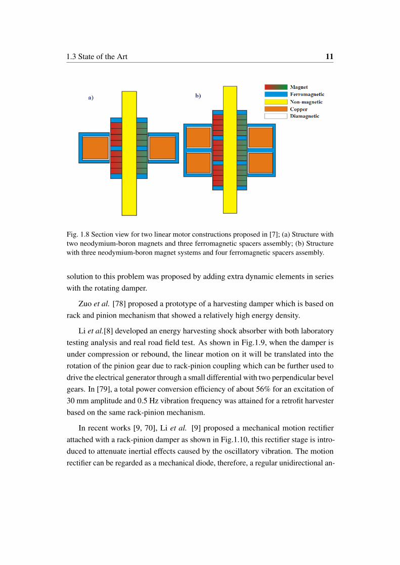
Suda et al. [63] developed an energy harvesting system with a linear DC motorbased on an active suspension to achieve a good compromise between riding comfortperformance and energy consumption. Zuo et al. [6] prototyped a linear motor basedregenerative damper to convert the vibrational kinetic energy of the vehicle intoelectricity. Fig.1.7 shows the main structure of the proposed linear electromagneticharvester with magnet assembly and the coil assembly separately. In the studyconducted by Sapinski and Krupa [7], two linear motor structures were proposed asshown in Fig.1.8. Both structures were constructed with neodymium-boron magnetassemblies, ferromagnetic spacers and suitable coil windings.

Linear electromagnetic regenerative dampers are commonly used for active andsemi-active suspensions due to their good controllability properties. Furthermore,the simple and reliable integration into most existing suspension layouts and lackof a transmission system makes the linear motors seem to be a straightforwardchoice for automotive industry. However, their limited force density make themwork inefficiently and a substantial weight cannot be avoided and need to be addedto the vehicle chassis, high production cost, and due to the relatively low vibrationvelocity, their size is still large. These shortcomings lead the research towards othersolutions.

10 Introduction

Fig. 1.7 Linear electromagnetic based energy harvesting shock absorber proposed in [6]

1.3.2 Rotary Regenerative Shock Absorber

In the work [64], the authors demonstrate that the power density of linear actua-tors, referred in literature as the damping-to-weight ratio, is limited and definitelyoutperformed by rotary electric motors.

When a rotary electric machine is going to be integrated into a conventionalsuspension, transmission systems are required in order to convert the linear motioncoming from the ground into an angular displacement. There are mainly two commonlinear-to-rotary motion transmissions which are the electro-mechanical transmissionbased solution and the electro-hydraulic transmission based solution. and hydraulicmethod [16, 65, 17, 66, 67]. Different efforts have been devoted in order to find anoptimal solution.

Electro-mechanical Solution

Because of its simple structure and high conversion efficiency, the electro-mechanicalbased rotary regenerative damper becomes one of the most common solutions amongdifferent energy harvesting structures. Furthermore,it can be categorized as rack-pinion [8, 9, 68–70], ball-screw [10, 11, 71–75], algebraic screw mechanism [76],pullies-cables assembly and other mechanical based systems [77]. Whereas, therotating inertia of the transmission mechanism affected the suspension system, a


Fig. 1.8 Section view for two linear motor constructions proposed in [7]; (a) Structure withtwo neodymium-boron magnets and three ferromagnetic spacers assembly; (b) Structurewith three neodymium-boron magnet systems and four ferromagnetic spacers assembly.

solution to this problem was proposed by adding extra dynamic elements in serieswith the rotating damper.

Zuo et al. [78] proposed a prototype of a harvesting damper which is based onrack and pinion mechanism that showed a relatively high energy density.

Li et al.[8] developed an energy harvesting shock absorber with both laboratorytesting analysis and real road field test. As shown in Fig.1.9, when the damper isunder compression or rebound, the linear motion on it will be translated into therotation of the pinion gear due to rack-pinion coupling which can be further used todrive the electrical generator through a small differential with two perpendicular bevelgears. In [79], a total power conversion efficiency of about 56% for an excitation of30 mm amplitude and 0.5 Hz vibration frequency was attained for a retrofit harvesterbased on the same rack-pinion mechanism.

In recent works [9, 70], Li et al. [9] proposed a mechanical motion rectifierattached with a rack-pinion damper as shown in Fig.1.10, this rectifier stage is intro-duced to attenuate inertial effects caused by the oscillatory vibration. The motionrectifier can be regarded as a mechanical diode, therefore, a regular unidirectional an-

12 Introduction

Fig. 1.9 Rack pinion mechanism layout in [8].

gular motion is guaranteed to enhance the system reliability and harvesting efficiencyby decreasing the friction effectiveness.

Furthermore, this type of harvester is not only limited in automotive sector butalso can be extended to other industry field. For example, based on the mechanicaltransmission of rack-pinion converter, Zhang et al. [80] developed a portable trackvibration-based energy harvesting unit which can be considered as an alternativepower source of a railway. Specifically, the motion is rectified using one-waybearings and an efficiency of about 55.5% was obtained.

Another common solution for this motion conversion is to implement ball-screwmechanism. Based on the rotating part which is attached to the rotor of the electricmachine, this system can have different configurations: rotating screw [10] or rotatingnut [11] as shown in Fig. 1.11. Compared with rack-pinion coupling, this alternativesolution is able to reduce backlash [11]. Similarly, the motion rectifier has been alsoimplemented in some works [74, 75] to allow the unidirectional rotary motion.

Fig.1.12 shows the structure of the harvester prototype developed in [12], theinput torque for the motor is created through a ball-screw assembled with a smallball nut and coupler.

Fig.1.13 shows an ball-screw based energy harvesting absorber which was pro-posed by Xie et al. [13, 81] to recover the kinetic energy dissipated and adjust thedamping coefficient according to road conditions continuously.

Zhang et al. [82] proposed and validated experimentally a regenerative damperusing a ball-screw transmission system. Due to the effect of high inertia moment ofthe ball-screw parts, the ride performance of the vehicle is related with the frequencyexcitations. A high frequencies excitation gave a poor ride behavior, while a good


Fig. 1.10 Regenerative shock absorber based on rack-pinion mechanism with MMR proposedin [9]. Rack (1), Roller (2), Pinion (3), Ball bearings (4), Planetary gears and motor (5),Thrust bearing (6), Roller clutches (7), Bevel gears (8).

ride performance was achieved for low frequencies excitation. Similarly, in thework [83, 84], the authors patented a regenerative shock absorber with ball-screwmechanisms. However, bad ride comfort was found at high frequencies bandwidth.

To realize the linear-to-rotary transmission, apart from the common rack-pinionand ball-screw mechanism mentioned above, there are other possible alternatives.Fig.1.14 shows another regenerative damper which was based on a two-leg mecha-nism concept proposed by Maravandi and Moallem [14]. Although this prototype iscapable of recovering energy with an average mechanical efficiency of 78%. How-ever, from practical point of view, it is difficult to apply such solution in vehiclesuspension to achieve the damping properties.

In [15], engineers from Audi AG. prototyped an electromechanical rotary dampercalled “eROT” based on a high-output 48-volt electrical system to replace theconventional hydraulic dampers in order to achieve a more comfortable ride. Asshown in Fig. 1.15, the geometry of this new damper system is also well designed.

14 Introduction

Fig. 1.11 Ball screw mechanism layout: rotating screw (left) in [10] and rotating nut (right)in [11].

Fig. 1.12 Ball-screw energy regeneration mechanism proposed in [12].

The upright telescopic shock absorbers are replaced by the horizontally arrangedelectric motors in the rear axle area to save more space in the luggage compartment.As an actively suspension, eROT adapts ideally to irregularities in the road surfaceand eliminates the mutual dependence of the rebound and compression strokes thatlimits conventional hydraulic dampers. Besides the freely programmable dampingcharacteristic, eROT can convert the kinetic energy during compression and reboundinto electricity by using a lever arm. The force coming from the motion of the wheelcarrier is transmitted by this lever arm to an electric motor through a series of gears.

Although the mechanical based harvesting system is promising, in a high-cycletask like vehicle damping, component wear and fatigue are more critical aspectscompared to hydraulic based system. Another drawback is the poor controllabilityof the mechanical parts in the case of active or semi-active systems. In the further


Fig. 1.13 3D model of the ball-screw transmission-based energy harvesting damper insuspension proposed in [13].

progress, possible solutions should be developed to overcome these drawbacks toachieve good durability, compactness and enhanced dynamics behavior.

Electro-hydrostatic Solution

Energy harvester based on hydraulic transmission or electro-hydrostatic actuation(EHA) system can be considered as one of the promising energy harvesting sus-pension systems. This type of damper depends mainly on the hydraulic fluid totransfer the linear displacement inside the cylinder to a rotational motion of anelectric machine through a hydraulic pump/motor. Some other components such asgas accumulators and hydraulic check valves as motion rectifiers [85–87] are alsopresent to achieve stability in the system.

Fig.1.16 shows the structure of a hydraulic based regenerative shock absorberwith EHA system which is able to transform the motion from linear to rotary domain.Specifically, the system is directly interfaced with a motor-pump unit by means of ahydrostatic circuit. When there is a linear displacement, it produces a mechanical

16 Introduction

Fig. 1.14 Regenerative shock absorber based on the two-leg mechanism proposed in [14];(a) prototype of the two-leg mechanism-based damper; (b) CAD assembly of the proposedprototype.

power which will be transformed by fluid into hydraulic power, and if the generatedflow passes through a hydraulic pump, the power will be converted to mechanicaldomain in the form of rotary motion and then drives the electric machine.

Many recent works have addressed the design and implementation of this kind ofdampers. Fang et al. [16] prototyped a hydraulic electromagnetic shock absorberwith rectifier and internal accumulator in which the regeneration efficiency of theproposed system was 16% as shown in Fig.1.17. Li et al. [17] developed a hydraulic-based regenerative damper (Fig.1.18) and assessed its damping and regenerativecapabilities with a hydraulic motion rectifier (HMR) depending on four sets ofcheck valves to rectify the hydraulic motor direction of rotation. According to theexperimental investigation in [17], the hydraulic regenerative suspension based onHMR offered a maximum conversion efficiency of 39% approximately for a definedharmonic excitation.

Zhang et al. [66] exploited the intrinsic fluid rectification of twin-tube shockabsorbers to yield and validate a prototype and used the genetic algorithm (GA)optimization method to detect optimal regeneration power trends of a hydraulicpumping regenerative suspension with HMR, as a result, the obtained theoreticalhydraulic efficiency was between 70 and 73%.


Fig. 1.15 The innovative eROT based on a horizontally arranged electromechanical rotarydamper proposed by Audi in [15].

In the study [88], Demetgul et al. proposed a hybrid energy harvesting solutioncontaining hydraulic and electromagnetic damper mechanisms to produce electricityfrom the linear motion. The concept of developing a hybrid energy harvestingsuspension, combination of both direct and indirect drive energy harvesters, is apromising direction that can achieve the balance among all the energy harvestingmechanisms [89, 90].

According to [91], it has been conclusively shown that the hydraulic transmissionbased rotary electromagnetic harvesting damper could practically harvest a power of310 W out of an input power of 840 W with a conversion ratio of 37% approximately.In [92], the authors prototyped a hydraulic electromagnetic shock absorber (HESA)combined with a horizontal linear generator which operated by a mechanical linkagemechanism. At last, the proposed system achieved a conversion ratio of about 20%.As the authors provided in [18], Fig.1.19 shows the expectations of the harvestedenergy based on a specific HESA prototype. It is obvious that such a harvestingfunction-based damper provides a high capacity of the regenerative power per damper

18 Introduction

Fig. 1.16 EHA concept scheme: battery (1), power stage (2), electric motor (3), hydraulicpump (4), pressure-relief valves (5), check valves (6), piston (7), gas accumulator (8), base(9)

in the case of overloaded trucks and military vehicles owing to their bad drivingcircumstances.

However, ClearMotion Corp. (former Levant Power Corp.) has lead the develop-ment in this field with their fully controllable active energy-harvesting suspensioncalled GenShock as shown in Fig.1.20. It is a commercial active suspension withvibration energy harvesting function considering a hydraulic-based transmission[93, 94]. The heart of the GenShock device is called Activalve which consists of ahydraulic pump and an electrical generator driven by an integrated electronic controlunit. The Activalve is utilized to route and regulate the fluid inside a standard hy-draulic absorber. Besides the energy harvesting purpose, the GenShock was proposedas a fully active suspension where an active force can be applied to push and pullthe wheels leading to significantly enhanced ride comfort, handling and drivingexperience [95]. From the scientific point of view, they have also provided usefulguidelines to optimize the hydraulic pump for constructing a regenerative damper[65].

Noticed that among the literature reviews, the research works usually focused ona single or few aspects, for instance, the improvement of efficiency from a specificpoint of view (either mechanical, hydraulic, or electrical), the implementation ofcontrol strategies, or the integration of components such as motion rectifiers.

As demonstrated in the following chapters for the hydraulic regenerative shockabsorbers, the performance of the motor-pump unit directly influences the kinetic to


Fig. 1.17 Hydraulic harvesting absorber (HESA prototype) with HMR in [16]

electric energy conversion while there is very few works available in the previousliteratures focused on the overall conversion efficiency and thus, this is the maintarget and topic of this dissertation.

Considering the advantages of hydraulic based regenerative dampers, since thefluid is used for the purpose of power transmission, the intrinsic lubrication of fluid-based solutions overcomes the main tribology concerns of electromechanical systemsand offers better flexibility within the suspension. Furthermore, the studies [96, 97]have demonstrated that EHA systems are able to yield elevated actuation powerwithout penalizing compactness and robustness. All these advantages motivate thechoice of adopting EHA system for designing the regenerative shock absorber in thepresent thesis work. A complete comparison among different types of regenerativeshock absorbers including their advantages and limitations will be summarized innext section.

1.3.3 Comparison of different energy conversion mechanisms

Comparison of the most popular energy harvesting systems in automotive suspensionwith their advantages and limitations are summarized below.

20 Introduction

Fig. 1.18 Prototype of a hydraulic regenerative based shock absorber without HMR proposedin [17].

• Linear regenerative shock absorberLinear regenerative damper is used as a self-power controllable system whichshows a simple structure and good reliability. It is easy to be fabricated, andmore applicable to a real vehicle (easily integrated into most existing auto-motive suspensions) without any transmission mechanism, and it can get thepower even for the small velocities. Therefore, this kind of harvesting damperis considered as the suitable choice for achieving good vehicle dynamicsbehavior as a semi-active or active suspension.

However, because of the relatively low vibration velocity, the size of this typeof damper is still large, and suffers from its low power density by using a linearmotor. Moreover, to produce this harvesting damper, accurate system designand high production cost are also required. Furthermore, due to the continuouschanging direction of the motor,a high inertia power loss is unavoidable andleading to a low conversion efficiency.

• Rotary regenerative shock absorber based on rack-pinion mechanismRack-pinion transmission based rotary harvesting damper can achieve a highassembly accuracy with the ability of motion and force magnification. Thestroke depends on the rack length. This type of damper has a considerablepotential energy and power density, the energy conversion efficiency is high.

However, by using rack-pinion transmission mechanism, the input and outputaxis are perpendicular to each other and this will lead to a large space designs


Fig. 1.19 Expectations of the energy harvesting with respect to the HESA prototype in [18].

and the torque transmission capability is limited by the gear module. Further-more, due to the lubrication issue for the mechanical parts which could be alsodamaged easily, this kind of damper has a shorter operation life cycle whileaccurate system design is still required.

• Rotary regenerative shock absorber based on ball-screw mechanismBall-screw transmission based rotary harvesting damper has a simple construc-tion, it can operate smoothly with high positional accuracy and good durabilitycomparing to rack-pinion solution. Moreover, it has a high mechanical effi-ciency with lower power consumption and losses, it could be also used forlarge-scale systems.

Compared to the rack-pinion mechanism, ball-screw gives a relatively lowerconversion efficiency but higher cost, there is also the risk of buckling in theregion between supports and requires more parts for ball recirculating system.

22 Introduction

Fig. 1.20 Old version (above) and latest version (below) of Genshock developed by Clear-Motion Corp.

• Rotary regenerative shock absorber based on hydraulic transmissionHydraulic transmission based rotary harvesting damper adopts fluid as the me-dia to achieve torque transmission purpose and leads to a high potential powerand high-power density with high sensitivity for even small stroke changes, thesystem can be implemented for all the four suspensions of the vehicle with onlyone common power generation modulator, good controllability and durabilityproperties makes it very effective in motion and force control. Comparing toother systems, due to the intrinsic lubrication properties of the fluid, this typeof damper has the longest operation life cycle without any mechanical damage.Moreover, hydraulic based system can hold a large force and absorb impactseffectively, therefore, it can be used for large-scale energy harvesting systems,such as heavy duty vehicles.

However, due to the presence of hydraulic loop, this system has a relativelyhigher power losses, oil leakage issues and usually the production cost ishigher and the manufacturing process is complex.

1.4 Thesis Outline 23

From the comparison, it can be observed that the hydraulic-based system cansatisfactorily provide an acceptable energy conversion performance for a full vehicledespite its high-power losses especially in case of heavy duty vehicles. The totalpower losses for an implemented hydraulic based harvesting system for a full vehicle(4-sets of suspension) can be suppressed in which one common power generationcircuit could be recognized for all vehicle suspensions. In addition, using a controlledhydraulic suspension can improve significantly the vehicle dynamics due to its goodcontrollability which facilitates the control of the displacement and the force using thehydraulic suspension. Therefore, the hydraulic transmission based electromagneticrotary energy-harvesting suspension should be more investigated as a promisingdirection in terms of vibration energy-harvesting and vehicle dynamic behavior.

1.4 Thesis Outline

This thesis is divided into six chapters:

• Chapter 1 briefly motivates and delimits the present work, includes a state-of-the-art research that covers available technology for regenerative shockabsorbers.

• Chapter 2 formally introduces the working principle of the system and pro-vides the preliminary assessment of the suspension.

• Chapter 3 describes the hydraulic pump design of prototypes.

• Chapter 4 describes the electric motor design of prototypes.

• Chapter 5 describes the integration of prototypes and explains the imple-mented control strategies.

• Chapter 6 contains the experimental results of different tests that assess theperformance of the prototypes.

• Chapter 7 discusses the obtained results, states the conclusions and indicatespossible future developments.

Chapter 2

Working Principle

2.1 Kinetic Energy to Electric Energy Conversion

In this Chapter, the conversion of kinetic energy to electricity by using shock ab-sorbers is explained. As shown in Fig.2.1, the conventional damper of the suspensionsystem is replaced by an energy harvester through which the electricity is producedand used for charging the battery.

In the last Chapter, we have already seen several types of regenerative shockabsorbers by which the kinetic energy can be transferred into electricity. Here wecan make a short and brief review:

• Linear regenerative shock absorbers

This electromagnetic solution allows to produce Alternating Current (AC).The prototypes exhibited in [5] and [98] are made based on this concept.

• Rotary regenerative shock absorbers based on mechanical transmissionmechanism

The electromechanical solution usually adopts rack-pinion or ball-screw mech-anism to transfer the kinetic energy to a bidirectional rotation and powersa generator to produces AC. In recent studies[9], a motion rectifier is alsointegrated to reach unidirectional movement. Furthermore, if a Direct Current(DC) generator is employed the output will be DC as well.

2.1 Kinetic Energy to Electric Energy Conversion 25

Fig. 2.1 Quarter car model for conventional vehicle suspension(left) and regenerativedamper(right).

• Rotary regenerative shock absorbers based on hydraulic transmissionmechanism

For this type of solution, an hydraulic motion rectifier is used to convert theoscillatory vibration of the shock absorber into a unidirectional rotation andpowers an electrical generator, which produces DC directly. For example,ClearMotion Corp. exploited this concept and developed their GenShock.

2.1.1 Road Profile Excitation

When a vehicle is running, there are several excitations which will be introducedto its suspension system. For example, the road irregularities, load transfers inlongitudinal and lateral directions due to different maneuvers. Among which theroad irregularities are considered to be the most critical disturbance for the drivingcomfort and handling because they continuously excite the vehicle suspension evenif the car is moving straightly with a constant speed.

The purpose of vehicle shock absorber system is to filter the road irregularitiesand perform a good balance between ride comfort and road holding properties. Todo this, the conventional dampers usually dissipate the kinetic energy coming fromthe uneven road as wasted heat.

26 Working Principle

Since our target is to harvest energy from the dissipation, it is important to figureout the amount of kinetic energy that can be dissipated or in other words regeneratedby the shock absorber. It is straight forward that the vehicle suspension will dissipatemore energy if passing through a rougher surface. Vehicle speed is considered asanother factor which will affect the amount of dissipated energy, a higher vehiclespeed makes the shock absorber dissipate more energy. Therefore, the unevenness ofthe road together with the speed represent the source of the excitation for the vehicle.

As the only interface between the road and vehicle, the behavior of tires can alsoaffect the kinetic energy dissipation, they determine the entity of dynamic verticalforces which are transmitted by the road to the vehicle body, the stiffer the tires, themore the energy dissipated by the shock absorbers.

Other parameters like masses (both sprung mass and unsprung mass) and suspen-sion characteristics (spring stiffness and damping coefficient) can be neglected indetermining the energy dissipated by the shock absorbers. However, this assumptionwill be used in the following sections to calculate the CO2 saving.

2.1.2 Regenerated Energy Storage

Once the harvested energy is obtained, one possible usage of the produced electricityis to charge the car battery. In this way, in theory the alternator does not have toproduce that amount of electricity as it does for conventional vehicles equipped withInternal Combustion Engines (ICEs). For hybrid and pure electrical vehicles, thisproduced electricity could be used either to charge the low voltage battery (12V) orthe high voltage traction batteries, the former condition is more common while thehigh voltage usage is quite rare.

For conventional ICE application, the harvested electricity will be used mainlyfor accessories and engine control unit, while in the case of hybrid or pure electricvehicles, it could be used for both accessories (usually through a DC/DC converter)and powertrain system. Furthermore, the current produced can be either alternate(AC) or direct (DC) depending on the particular conversion strategy adopted.

In the content of State of the Art (Section 1.3), it is shown that the linear har-vesting dampers will generate less power and lower damping curves with respect tothe other solutions, therefore, the linear type will not be further investigated in thefollowing parts.

2.1 Kinetic Energy to Electric Energy Conversion 27

Whereas, for the rotary harvesting dampers, a further distinction can be made:

• Directly coupled with the electric machine (usually a reverse operated DCmotor or an AC rectified generator).

• Connected with the electric machine (again a reverse operated DC motor or anAC rectified generator) through motion rectification (mechanical or hydraulic).

In the first condition, the regenerated electricity is AC type and therefore, theoutput current needs to be rectified, a relevant rectification efficiency must be takeninto account considering the associated power losses, while in the second condition,by means of the mechanical or hydraulic motion rectifier, the electric machine isforced to perform unidirectional rotation and thus, the electrical rectification can beavoided. Furthermore, in [9], the authors also pointed out that this configuration ismore efficient due to the unidirectional rotation can lead to a higher efficiency of theelectric machine. For this reason, configuration with motion rectification is chosento construct the prototype in present dissertation.

In any case, even if the output current is DC, a dedicated DC/DC converter isstill needed to adapt the voltage level between the harvester output and the batteryinput. For example, a 92% efficiency is considered for this electrical-to-electricalconversion in [99].

Since the regenerative shock absorber is an electromechanical system, its damp-ing effect can be obtained by setting the equivalent load resistance. As the systeminput, the mechanical power which can be regenerated by the shock absorber doesnot depend on its particular damping characteristic. Therefore, the mechanical powerand the damping curve can be decoupled from each other. On the other hand, theoverall conversion efficiency is needed in order to obtain the output electrical powerrecovered from the mechanical power, and the overall conversion efficiency gener-ally depends on the equivalent load resistance, as a result, the choice of a particulardamping characteristic of the shock absorber determines the value of the overallconversion efficiency and, thus, influences the amount of electrical power that can beproduced.

Being the equivalent load resistance determined by the desired damping charac-teristic of the shock absorber, it is not possible to rely on it to maximize the overallconversion efficiency. This equivalent resistance is modulated in order to obtain


Power Electronics

- Equivalent load

resistances modulation

- Switch to dissipative

loads for over-charged

battery

DC/DC

Converter

Voltage level

adaptation

Battery

Alternator

Shock

Absorber

Shock

Absorber

Shock

Absorber

Shock

Absorber

(Front Left)

(Front Right)

(Rear Left)

(Rear Right)

Fig. 2.2 Integration of the current from shock absorbers in the electric grid of the vehicle.

the required damping characteristic and the overall conversion efficiency must becalculated for each possible operating point.

The integration of the current from the shock absorbers to the electric grid of thevehicle is represented in Fig.2.2. During the charging phase of the battery, priorityis always given to the power coming from the shock absorbers. This is possibledue to the fact that when the charge level of the battery exceeds a certain threshold,the alternator which has a voltage regulator stops charging the battery and only thepower coming from the shock absorbers remains.

In case of the battery is over-charged, a resistive load (dissipative) which is drivenby the power electronics will perform the damping action when there is still an extraamount of energy from the shock absorbers. Obviously this is a very particularcondition and no energy will be harvested in this rare situation.

2.2 System Overview

2.2.1 Hydraulic RSA modeling

Figure 2.3 represents a complete model of the hydraulic regenerative shock absorbersystem. It exploits an electro-hydrostatic transmission to transfer the mechanicalpower between the linear and rotary domains. As shown in the figure, the system

2.2 System Overview 29

Fig. 2.3 Hydraulic regenerative shock absorber model scheme.

consists of three parts: an electric machine, a hydraulic pump, and a linear hydraulicactuator. The electric machine is rigidly coupled with the fixed displacement hy-draulic pump, the pump and the linear hydraulic actuator are connected by means oftwo pipelines. Hence, when the piston makes a linear movement, it will generatea fluid flow inside the hydraulic circuit and subsequently, it will be converted to arotation on the shaft of the electric machine to generate electricity that stored in thebattery.

Specifically, the electric machine is a three-phase brushless permanent-magnetmotor, since its elevated power-to-weight ratio favors design compactness. Assuminga perfectly balanced winding layout, the phase impedance is characterized by thewinding resistance R, shunt or load resistance Rext, and winding inductance L.Mutual inductance contributions between phases are also present. The motor backelectromotive force (EMF) constant Km is given by

Km =|Ea,b,c|

Ωm(2.1)

where Ea,b,c represents any of the phase back EMF waveform, and Ωm indicatesthe mechanical angular speed of the rotor.


The dynamic behavior of the motor can be represented in a two-phase rotatingreference frame. This transformation simplifies mutual inductance terms and reducesthe order of the resulting differential equation system.

(R+Rext)iq +Lqdiqdt

+ pΩmLdid +KmΩm = 0 (2.2)

(R+Rext)id +Lddiddt

− pΩmLqiq = 0 (2.3)

Tm =32[Kmiq + p(Ld −Lq)idiq] (2.4)

Here, d and q subscripts denote direct and quadrature axis variables. Currentsare indicated with the letter i, Tm represents the motor torque and p is the number ofpole pairs of the electric machine. If the rotor is ideally isotropic, the inductances inboth axes are equivalent:

Ld = Lq =32

L (2.5)

By substituting Ld and Lq in Eq.2.4, the reluctance torque term vanishes, thus,yielding a torque that depends only on the quadrature component of the current (iq).

The implementation of Eq.2.2 to 2.4 is necessary to introduce the nonlineardynamic behavior of the machine, which is highly dependent on its impedance terms[100]. From the mechanical point of view, the electric machine is rigidly coupledto the hydraulic pump gears, yielding a total moment of inertia Jm. Dissipativephenomena of both devices are represented as:

Tf = cmΩm +Tstsign(Ωm) (2.6)

where cm is a rotary viscous damping coefficient and Tst is the startup torque dueto Coulomb friction.

The hydraulic pump is assumed as an ideal transformer between the mechanicaland hydraulic domains:


Tm = Dm∆Pm (2.7)

Qm = DmΩm (2.8)

where ∆Pm is the pressure differential across the pump with a fixed displacementDm, and Qm indicates the flow rate that is produced.

The hydraulic actuator is a two-chamber asymmetric cylinder with a gas-loadedaccumulator for compensation. The evolution of the pressure in a generic hydraulicchamber is governed by a first-order differential equation:

ddt

Pch =βf

Vch(xp)∑

jQ j (2.9)

where βf is the fluid bulk modulus, Vch is the volume of the chamber and Q j isthe generic flow rate entering the chamber. Note that the volume Vch and a flow ratecomponent depend on the position of the piston xp and its cross sections: Ap1 duringrebound and Ap2 during compression.

The accumulator pressure can be found by solving:

PaccVγacc = P0V γ

0 (2.10)

being Pacc and Vacc the pressure and volume of the accumulator at a given time,and P0 and V0 its preload pressure and the initial volume, respectively. The adiabaticconstant γ is a property of the accumulator gas.

In the layout shown in Fig.2.3, the pressure P1 can be approximated using Eq.2.10.Pressures P2 and P3 can be assumed equal and governed by the behavior of the accu-mulator (Eq.2.10), as its compliance dominates that of the oil. The stiffness of thehydraulic lines can be lumped into the stiffness of the hydraulic chambers. Further-more, fluid inertial contributions are negligible due to the geometric dimensions ofthe hydraulic circuit.

The piston body is equipped with two check valves and two hydraulic orificesthat limit pressure shocks during rebound and compression. The flow rate throughthe orifice element is defined as:


Fig. 2.4 Check valve aperture behavior. The valve cross section Av depends on its pressuredrop ∆Pv

Qor =CdAor

√2ρf

∆Por

(∆P2or +∆P2

cr)14

(2.11)

where Cd is the orifice discharge coefficient, Aor its cross section, ∆Por its pressuredrop and ρf the fluid density. Assuming circular orifices, the critical pressure drop∆Pcr is given by

∆Pcr =ρf

2(Recrνf

Cddh)2 (2.12)

being Recr the critical Reynolds number that establishes the transition betweenlaminar and turbulent flows, νf the fluid kinematic viscosity, and dh the hydraulicdiameter:

dh =

√4Aπ

(2.13)

In a similar fashion, check valves present an orifice-like behavior with a variablecross section Av that depends on the pressure drop across the valve ∆Pv (Fig.2.4).In particular, low pressure values lead to a negligible (leakage) cross section Av0.A transition between the cracking pressure ∆Pv0 and the maximum pressure ∆Pv1

yields a linear growth of the valve cross section up to its maximum aperture area Av1.

Finally, in the linear mechanical domain, the piston and rod are lumped into amass mp. Dissipative phenomena are described in a similar way to those in the rotarydomain:

Ff = cpvp +Fstsign(vp) (2.14)


where cp is the linear viscous damping coefficient, Fst is the startup force due toCoulomb friction, and vp represents the piston speed.

vp =dxp

dt(2.15)

2.2.2 System Layout

Fig. 2.5 shows the configuration of the regenerated shock absorber proposed inpresent dissertation, the system exploits a conventional twin-tube shock absorberarchitecture connected to the hydraulic ports of a pump. During vehicle cruise, thepiston of the shock absorber oscillates inside the tube at a speed vp due to the groundirregularities. This motion leads to an oil flow rate Qg that drives the hydraulicpump and therefore, the linear movement is transformed into a rotary motion Ωg.Since the pump is mechanically coupled to an electric machine, a suitable controlstrategy of the latter device allows to modify the damping characteristic of the shockabsorber. Furthermore, the electric motor acts as a generator in a portion of thedamping quadrants. Hence, the system is also able to convert the kinetic energy ofthe suspension into electricity which can be stored in the battery.

In addition, the twin-tube architecture provides unidirectional motion of themotor-pump group. The fluid flow is rectified with the aperture of the base checkvalve during rebound and the piston check valve during compression. This workingprinciple is already covered by previous research works [101, 102].

Considering its application, first of all, the designed regenerative device must actas a fully functional shock absorber, which means it must exhibit the required force-velocity characteristic to perform the desired damping action in order to achieveoptimum comfort and vehicle dynamics. Moreover, the system must be easilyadaptable to the activity of tuning on the road.

As shown in Fig. 2.5 (b), the prototype is fixed onto the shock absorber tube witha manifold. This approach yields a compact system and minimizes the introductionof losses due to hydraulic lines. Furthermore, it provides modularity because themotor-pump group unit can be installed on any shock absorber tube. For this reason,the optimization process of this single unit will be investigated in the followingchapters disregarding the selected shock absorber architecture.


Fig. 2.5 Layout of a hydraulic regenerative shock absorber. Concept scheme (a): battery(1), power stage (2), electric motor (3), hydraulic pump (4), pressure-relief valves (5), checkvalves (6), piston (7), gas accumulator (8), base (9). Prototype side view (b): manifold (10),regenerative device (11), spring holder (12), rod (13), external tube (14), anti-roll bar bracket(15), wheel hub bracket (16).

In general, the power conversion from the hydraulic domain of the pump to theelectrical domain of the battery is inevitably affected by a number of loss terms.

The hydraulic power applied to the pump is initially reduced by a volumetricloss due to internal leakages. The volumetric efficiency is given by

ηv =VgΩg

Qg, (2.16)

where Qg is the flow rate across the pump, Ωg its angular speed and Vg its fixedvolumetric displacement.

Subsequently, a hydro-mechanical loss term considers the pressure/torque dropdue to hydraulic minor losses and mechanical friction affecting the rotating elements.The hydro-mechanical efficiency associated to these phenomena is

ηhm =Tm

Vg∆Pg. (2.17)

Here, Tm is the electromagnetic torque of the motor and ∆Pg the pump pressure drop.


Fig. 2.6 Simplified motor model

Finally, a third loss term considers the conversion from the mechanical domainof the motor to the electrical domain of the battery, i.e.

ηe =VdcIdc

TmΩg, (2.18)

in which Vdc and Idc define the voltage and current of the power stage DC bus,respectively. This electrical efficiency can be attributed to motor and power-stagelosses.

The product of the three aforementioned terms yields the total conversion effi-ciency of the motor-pump unit:

ηt = ηvηhmηe =VdcIdc

∆PgQg. (2.19)

2.2.3 Controlled Damping Theory

In this section, the working principle of the electromagnetic damping control isdemonstrated through a simplified motor model.

Fig.2.6 shows a simplified motor model, the sign convention of the model indi-cates that a positive current i rises when V > E, and this positive current will lead toa positive torque T , while the speed Ω is imposed externally.

Before going to detail, several assumptions are made:

• The motor is a DC motor.

• The system is in static conditions which means no inductances, and rotate withconstant speed.


• Only the motor model is considered disregarding other mechanical parameters.

• An ideal power supply that can vary from −Vdc to Vdc is considered.

It is known that the DC motor can be represented in Bond Graph as a gyrator,therefore, the back electromotive force (BEMF) E can be written as:

E = KmΩ (2.20)

and the torque T is represented as:

T = Kmi (2.21)

where Km is the motor constant.

According to Kirchhoff’s voltage law (KVL), we can obtain that:

V = Ri+E (2.22)

Eq.2.21 and Eq.2.22 yields:

T =Km

R(V −E) (2.23)

furthermore, E can be substituted by Eq.2.20, thus we can obtain the torque-speedcharacteristic:

T =−K2m

RΩ+

KmVR

(2.24)

noticed here, by giving a command V , we can obtain the torque T as an output,while speed Ω is imposed externally as a disturbance.

Once we obtain the torque-speed characteristic, it can be represented in the fourquadrants as shown in Fig.2.7.

When the speed and torque have the same sign, we consider it as a Motor, asshown in Fig.2.7 the light gray regions; while when the speed and torque have theopposite sign, we consider it as a Damper, as shown in Fig.2.7 the dark gray regions.


Fig. 2.7 Torque speed map

The maximum stall torque Tst is obtained at null speed when the motor is fed atmaximum voltage Vdc:

Tst =KmVdc

R(2.25)

and the no-load speed Ωnl is calculated at null torque:

Ωnl =Vdc

Km(2.26)

therefore, the working envelope is constrained by the area limited by the stalltorque and no-load speed, as shown in Fig.2.7 the red lines.

Considering one special case, when the motor phases are in short circuit, whichmeans V = 0, we obtain the short-circuit damping as indicated by the black line inFig.2.7. In this case, the torque is represented by:

T =−K2m

RΩ (2.27)


Fig. 2.8 Torque speed map for power recovery

As we mentioned before in the assumptions, the supply voltage can vary from−Vdc to Vdc, varying the supply voltage will yield a group of parallel lines with thesame slope but different offsets as shown in Fig.2.7 the gray lines.

After defining our working envelope, next step is to define the power recoveryregion.

According to the sign convention, power is regenerated only if Vi < 0. In otherwords, the torque and the supply voltage must have the opposite signs. This is shownin the gray regions in Fig.2.8.

The recovery region is bounded between the open-circuit response which meansT = 0 and the short-circuit response. Every other torque speed combination outlyingfrom this region will require a certain amount of power.

Alternatively, the same behavior can be obtained by shunting the stator with anexternal resistance. In this case, the damping slope changes as shown in Fig.2.8, Rext

can vary from 0 to infinity:

T =− K2m

R+RextΩ (2.28)


Fig. 2.9 Torque speed map working regions

Fig.2.9 summaries what we have discussed before, the working envelope can bedivided into 3 different regions:

• Regenerative damping (dark gray) The torque (hence current) and the voltagepresent opposite signs, power flows into the battery. The machine behaves as adamper because torque and speed are opposite;

• Active motor (light gray) The torque (hence current) and voltage have the samesign: the device behaves as a motor because the speed and the torque have thesame sign;

• Active damper (white) The torque (hence current) and supply voltage havethe same signs. However, the torque and speed oppose each other. Thisconfiguration is a damper helped by an external supply to fulfill the requiredbehavior.


Fig. 2.10 An example scheme of quarter car model.

2.3 Preliminary Analysis

2.3.1 Quarter Car Model

Quarter car model is the most employed and common model that used for studyingthe vehicle suspension system [103], as shown in Fig.2.10.

The model is basically made of two masses, sprung mass ms and unsprung massmu. The sprung mass represents one quarter of the vehicle body weight, and theunsprung mass represents one wheel of the vehicle. The sprung mass is supportedby a spring with stiffness ks, and a shock absorber with viscous damping coefficientcs, while the unsprung mass is in contact with the ground through the tire, which canbe represented with a stiffness ku, noticed here, the damping of the tire is ignoreddue to its small value compared with cs to simplify the model. Variables xs, xu, andxr represent the vertical displacements at different levels.

The differential equations of the motion for quarter car model can be written as:

msxs + cs(xs − xu)+ ks(xs − xu) = 0 (2.29)

2.3 Preliminary Analysis 41

muxu + cs(xu − xs)+(ku + ks)xu − ksxs = kuxr (2.30)

which is commonly expressed with the state space form:

x = Ax+Buy = Cx+Du

(2.31)

in which, the state vector x and the control input u are given below as an example:

x =

xs

xu

xs

xu

, u =

[xr

xr

]. (2.32)

However, depends on the requirement, the output vector y can be defined freely bythe user, and in this way, the matrix A, B, C, and D (usually contains the informationabout system mass, stiffness and damping properties) will be calculated accordingly.

This simple linear quarter-vehicle model has several advantages: due to its simplestructure and low dynamic order it offers an intuitive understanding of the verticaldynamic behavior of the vehicle.

Furthermore, after making suitable modifications on the original quarter carmodel, it can be also used to assess the behavior of the suspension which equippedwith regenerative shock absorber.The modified model will be fed with a certainroad profile, based on the simulation results, several performance indicators (forexample, the potential harvested power, conversion efficiency, vehicle comfort androad holding properties) are evaluated and this will be discussed in the followingsections.

2.3.2 Suspension Assessment

To assess the performance of vehicle suspension and study the behavior of the systemexcited by the road irregularities, a quarter car model is commonly adopted. To feedthis model, a particular road profile will be first generated and used later as an input.


Fig. 2.11 Power Spectral Densities of different road profiles according to [19].

It is known that a random profile can be indicated by superimposing a number ofsine waves. For a certain road, if the Power Spectral Density (PSD) of the profileis known, it is possible to reconstruct the road condition by using the relationshipbetween the road height and the position.

Furthermore, the road roughness is usually represented as a stationary Gaussianstochastic process and thus, the road profile PSD can be expressed by:

SPSD(n) = Grnβ (2.33)

where n is the spatial frequency, Gr is the road roughness coefficient, and theexponent β is commonly approximated as -2.

According to International Organization for Standardization (ISO), the roadprofiles can be divided into eight classes, indicated by letters from A to H [19].Their relative PSDs can be found in Fig.2.11. Class A refers to very good roads forexample, the newly paved highways; class B indicates good road condition, class Crefers to an average road, class D a poor road and so on. However, in general, mostof the roads in our daily lives can be considered in the range from class A to D.

The road profile used in our application was generated based on ISO 8608standard [19]. Specifically, these road profiles with different PSDs S(n) and roadroughness coefficients Gr are listed in Tab.2.1, where the spatial frequency n0 =

0.1cycle/m.


Table 2.1 ISO Road Profiles

Road class Description S(n0)[m3/cycle] Gr[m/cycle]

A Very good 1.60e-5 1.60e-7

B Good 6.40e-5 6.40e-7

C Average 2.56e-4 2.56e-6

D Poor 1.02e-3 1.02e-5

E Very poor 4.10e-3 4.10e-5

Eq.2.33 shows the relationship between S(n) and Gr in space frequency domain.By taking into account the vehicle velocity vcar, now it can be converted in the timedomain.

f = vcarnS( f ) = S(n)/vcar

(2.34)

by substituting Eq.2.33, S( f ) can be expressed as:

S( f ) =Grvcar

f 2 (2.35)

Note that the road profile generation can be done by using white noise, and S( f )is expressed in the unit of m2/Hz, thus, S( f ) can be rewritten as:

S( f ) = |H( f )|2Sin( f ) (2.36)

By setting Sin = 1, |H( f )| is expressed as:

|H( f )|= 2π√

Grvcar

2π f(2.37)

and knowing that s = j2π f , therefore, we can obtain:

H(s) =2π

√Grvcar

s(2.38)


Fig. 2.12 Road Profile Class C

Furthermore, by adding a cutoff pole at low frequency to avoid drifts, the PSDwhite noise signal can be expressed as:

Hr(s) =2π

√Grvcar

s+2π f0(2.39)

the filter cutoff frequency is indicated by f0 and can be represented as :

f0 =vcar

λ0(2.40)

where λ0 = 100 m

If a class C (average) road with Gr = 2.56 ·10−6m/cycle and vcar = 35km/h isconsidered. In particular, this value is the average vehicle speed of the New EuropeanDriving Cycle (NEDC). The simulation result can be seen in Fig.2.12.

Once the road profile is obtained, it is time to feed the quarter car model as shownin Fig.2.13. In this modified version, the original damper cs is replaced by a genericdissipative device that can impose a damping force Fdamp as a function of pistonspeed vp. Particularly, an off-road passenger vehicle (Jeep Renegade) is taken as areference. All the parameters which are considered in the model are listed in Table2.2.


Fig. 2.13 Modified quarter car model

Table 2.2 Quarter car model parameters

Parameters Symbol Front Rear

Sprung mass ms 416.5 kg 256 kg

Unsprung mass mu 40 kg 30 kg

Suspension stiffness ks 23.26 kN/m 21.74 kN/m

Tire stiffness ku 226 kN/m 206 kN/m

To evaluate correctly the performance of the shock absorber within the quartercar model, the useful metrics presented by Zuo and Zhang[104] are employed.

Since the shock absorber is assumed to use a brushless permanent-magnet electricmachine, its regenerated power can be calculated through the formula below , :

Pg =32

Rext(i2d + i2q) (2.41)

where Rext is the external resistance of the electric machine, id and iq representthe current of direct and quadrature axis respectively.

Instead, the damping power can be represented by the product of damping forceand piston speed:


Pd = Fdampvp = Fdamp(xs − xu) (2.42)

as suggested in literature [104], the damping power in the suspension is heavilyinfluenced by the road profile, the vehicle speed and the tire stiffness. Its dependenceon the other quarter car model parameters is negligible, thus, it can be approximatedby:

Pd = π2Grvcarku (2.43)

therefore, the conversion efficiency can be determined by the ratio betweenregenerated and dissipated power:

ηg =Pg

Pd(2.44)

Comfort property can be assessed by filtering the sprung mass acceleration with

H2631(s) =80.03s2 +989s+0.02108

s3 +78.92s2 +2412s+5614(2.45)

which yields a weighted acceleration aw that takes into account the humansensitivity indicated by the ISO 2631 standard [105]

Whereas, road holding behavior can be evaluated through index ηrh which isdefined as:

ηrh =ku(xu − xr)

(ms +mu)g(2.46)

this index represents the ratio between dynamic forces due to tire deflection andstatic forces due to the vehicle weight. Indexes larger than unity indicate the loss ofground contact.

To yield characteristic numbers for these four indicators, the mean values ofharvested power and conversion efficiency were calculated. Instead, for weightedacceleration and road holding index, their RMS values were obtained. These param-eters were assessed in a sensitivity analysis with respect to the shunt resistance, asillustrated in Fig.2.14

From the sensitivity analysis results, it is shown that when the shunt resistanceRext equals to 0.14 Ω will lead to a maximum harvested power and conversion


Fig. 2.14 Sensitivity analysis of evaluation parameters to shunt resistance for regenerativeshock absorbers

efficiency for the target regenerated shock absorber with specific pump and electricmotor characteristics. Meanwhile, from the results of weighted acceleration aw

and road holding index ηrh, when the shunt resistance is chosen, a relative goodcompromise between the ride comfort and vehicle road holding capabilities is alsoguaranteed.

It is also possible to obtain a rough estimation of the emission savings in termsof grams of CO2 per kilometer according to the European technical guidelines foreco-innovation [99].

SCO2 =ηconvPgVpeCf

ηavcar(2.47)


Table 2.3 Estimated CO2 emission reduction with different road profiles

Road class Description Gr[m/cycle] SCO2 [gCO2/km]

A Very good 1.60e-7 0.16

B Good 6.40e-7 0.64

C Average 2.56e-6 2.6

D Poor 1.02e-5 10

E Very poor 4.10e-5 41

where ηconv is the total conversion efficiency of the power stage and its value isassumed as 0.9, Vpe is the fuel consumption of effective power for a reference dieselengine with a value of 0.22 l/kWh, Cf = 2640g/l is a factor that considers the fuelconversion into CO2 and ηa = 0.67 is the alternator efficiency.

Quick estimation can be done by substituting the regenerated power for all thefour dampers, and as a result, Eq. 2.47 can be rewritten as:

SCO2 =ηconvηg

ηaltπ

2Gr ·4

∑i=1

ku,i ·VpeCf (2.48)

From Eq.2.48, it is observed that the emission reduction is directly proportionalto the road roughness coefficient Gr, while showing no dependence on the vehiclevelocity vcar. Furthermore, if a class C (average) road profile is considered, togetherwith a conversion efficiency ηg of 0.54 is assumed, Eq.2.48 can yield a 2.6 g/km ofCO2 savings for all the four regenerated shock absorbers. More simulation resultsconsidering different road roughness coefficients can be seen in Tab.2.3 and theseapproximations proved that the regenerative device could be advantageous for vehicleemission reduction.

Chapter 3

Hydraulic Pump Design

From this chapter, a detailed design and optimization process of the proposedregenerative shock absorber will be explained. To do this, a system level designapproach as shown in Fig. 3.1 is adopted to comply with different requirements in allthe domains of interest. Particularly, three different specification sets are consideredhere:

1. Damping requirements.The proposed device must act as a fully functional shock absorber to exhibitthe required force-speed characteristic to perform desired damping actions.

2. Target envelope requirements.Since the proposed device will be integrated to the vehicle suspension, anyinterference with other components in that region must be avoided eitherunder static or dynamic conditions (such as suspension deflection and vehiclesteering maneuvers).

3. Power supply requirements.Assuming the power stage of the proposed device is connected with the vehiclebattery which is shared among different accessories. Therefore, some intrinsiclimitations like DC voltage, State of Charge (SOC) and charge-discharge ratesneed to be taken into account during the design phase to guarantee the systemreliability.

The first requirement about damping can be used to establish the design specifi-cations for the hydraulic part of the proposed device (pump), for example, defining

50 Hydraulic Pump Design

Fig. 3.1 Design method for the motor-pump unit

the gear geometry and clearance. Once the characteristics of hydraulic pump is fullydefined, the electromagnetic design of the electric machine can be carried out suchas stator and rotor configurations (slotted or slotless), pole pair numbers, and activelength, while the winding layout, size and number of turns, instead, are selectedto meet the limitation of DC supply voltage. After the whole design process ofpump and electric machine, the proposed motor-pump group will be validated with athermal analysis in the worst-case working condition.

To meet the second requirement about the envelope space, it would be helpful tominimize the bulk and mass of the final prototype to comply with the establishedgeometry constraints. Therefore, the proposed device can be easily integrated to thevehicle suspension system without any interference, to achieve this target, multipleiteration processes are needed.

51

Fig. 3.2 Ideal Force-speed maps of the regenerative shock absorber limited by damping,force and speed values.

Considering the third requirement about the power stage and control, both hard-ware and software components used to construct the power stage system are selectedbased on the electric machine characteristics and power supply constraints. A suitablecontrol strategy is also implemented taking into account the damping requirementsand other physical limitations of the system.

Fig.3.2 shows the first quadrant of the force-speed map, the x axis representsthe piston speed vp while the y axis represents the damping force Fdamp. It isknown that the damping coefficient cp can be defined by the ratio between force andspeed (shown as the slope in the figure), therefore, one feasible choice to define theworking region is to constrain this working area as purely regenerative which meansthe battery can only absorb power from the system. Specifically, this working regionis bounded by maximum damping cp,max, maximum force Fdamp,max and speed vp,max

that the suspension can achieve.

Due to the linear-to-rotary conversion is not perfectly efficient, this workingenvelope will be inevitably reshaped, as shown in Fig. 3.3, mainly the following twophenomena are taken into account:

1. Pump leakages

Pump leakage paths will speed up the effective damping inside the system, inthis way, for any attainable damping behavior, a lower damping coefficient ora smaller slope of the damping curve is expected, and this correspond to thevolumetric efficiency ηv defined in Eq.2.16.


Fig. 3.3 Expected Force-speed maps of the regenerative shock absorber limited by damping,force and speed values

2. Hydro-mechanical losses

Since the hydraulic pump and the electric machine are both mechanical com-ponents, in reality the hydro-mechanical losses (for example the pressure dropand mechanical friction) for the pump and electric machine are not avoidable,as a result, this will increase the output force and hence the output dampingbehavior which is equivalent to increase the slop of the damping curve andthese losses correspond to the hydro-mechanical efficiency ηhm defined inEq.2.17.

It is worth to note that at low speed region, the pump leakage phenomenonhas more influence, therefore, due to volumetric efficiency the actual maximumdamping value will be lower than that in the ideal case. As the speed increases, thehydro-mechanical loss becomes dominant, and due to the inherent efficiency ηhm,the real minimum damping will be greater than zero. Although this non-null valueof cp,min will penalize the final conversion efficiency of the device, it also provides apassive damping action to the vehicle in case of system failure.

Specifically, the proposed hydraulic pump is going to adopt a gerotor layout asshown in Fig.3.4. This fixed displacement device consists of only two elements:one inner gear and one outer gear. Both gears have conjugate tooth profiles, theouter gear presents one additional tooth with respect to the inner gear and generate anumber of chambers in between. The inner gear is usually fixed on a rotating shaft

53

Fig. 3.4 Layout of a generic gerotor pump

while the outer gear is positioned at a fixed eccentricity from the center of inner gearand shaft.

As mentioned in the design guidelines [20], despite of a variety of geometriesand materials, all the gerotor sets share the same basic working principle as shown inthe Fig.3.5, when the pump is working, the inner gear is driven by the shaft, the fluidwill be drawn into one chamber and starts to enlarge its volume until reaching themaximum value, as the rotation continuous, the volume of the chamber will decreaseand therefore, the inside fluid will be forced to flow out of the original chamber andstart to fill in the next chamber. This process will take place continuously and as aresult, a smooth pumping action is provided.

Furthermore, in the gerotor pump, the movement between inner and outer gearsis a pure relative rolling, and compared to other systems with sliding elements, thispure rolling motion effectively reduces the wear and shows a larger mechanicalefficiency. If the shaft moves with a speed of Ωg, while this relative rolling motiontakes place at rather low speed as shown below:

Ωg,rel = Ωg

(1−

Ng

Ng +1

)=

Ωg

Ng +1(3.1)

where Ng is the number of teeth on the inner gear.

In summary, compared with other pump types, the advantages of such gerotorpump can be seen from:


Fig. 3.5 Working principle of a generic gerotor pump in [20].

• The simplicity of the gerotor pump requires the least amount of components tomachine, for example, compared with spur gears, gerotor can eliminate a shaftand two bearings.

• The versatility of the gerotor pump gives the greatest advantages, it can bemounted directly on the shaft or driven by the outer gear, it is suitable for alarge variety of fluids from air to hot melt liquid.

• The size and geometry of the gerotor pump can be adjusted accordingly to meetspecific requirements. In general, the inner gear diameter, outer gear diameterand the active length can be optimized to be coherent with the designed overallsize and weight.

• Since the relative velocity between the inner and outer gears is very low andthis leads to a reduced tooth wear compared with other types, therefore gerotorpumps usually can have a longer service life.

55

• The gerotor pumps are suitable for the low-mid pressure range (up to 150 bar)which is coherent with our applications for shock absorbers in automotivefield.

In general, the gerotor pump can be characterized by its volumetric displacementVg. Based on the analysis made in the EHA modeling part, it is known that when theideal transmission ratio τ is given, the electromechanical torque Tm as well as therotational speed Ωg can be defined as:

Tm = τFp

Ωg = vp/τ(3.2)

Therefore, the maximum angular speed Ωg,max under low pressure condition(when the pump internal leakages are small) can be approximated as

Ωg,max ∼=vp,max

τ. (3.3)

From Eq.3.3, the ideal transmission ratio can be computed as the ratio betweenmaximum angular and linear speeds. For example, in the proposed design condition,a 12 krpm rotating speed versus a linear speed of 1.5m/s is considered.

Once τ is defined, the volumetric displacement can be represented as:

Vg = τAp =vp,max

Ωg,maxAp (3.4)

In this case, the average piston cross section Ap is calculated through:

Ap =π

4 [(d2p −d2

r )+d2r ]

2(3.5)

where dp and dr represent the diameter of piston and rod inside the cylinderrespectively.

Noticed that Vg is limited by the maximum angular speed that the system canachieve, and this maximum speed constraint has to be pushed as high as possible inorder to lower the required damping torque and hence, minimize the envelope of the


Fig. 3.6 Gear profile of the gerotor pump

electric motor. Nevertheless, the design must also account for the limitations in thefilling capability of the gerotor pump at high speed [106].

3.1 Gear Geometry

Fig.3.6 shows the section and side view of a gerotor gear set with its geometricfeatures, the main parameters for the pump design are listed in Tab.3.1. The innergear has a number of teeth equals to Ng (in this case Ng is equal to 6) while the outergear has Ng +1 teeth, and thus, the pump preserves Ng + 1 fluid chambers sealedby the teeth tips of both gears. Angle θg is used to represent the angular position ofthe shaft, furthermore, the volume of a generic chamber Vj can be described with ageneralized periodic function with appropriate angular offset:

Vj = fv

(θg +

2π jNg +1

)∀ j ∈

[0,Ng

]. (3.6)

Noticed that the function fv depends on the geometric features of both gears. Inturn, the kinematic flow rate of the pump is expressed as

Qg(θg) = Ωg

Ng

∑j=0

F j(θg), (3.7)

3.1 Gear Geometry 57

Table 3.1 Geometric parameters for gerotor pump design

Design parameter Description

Ng Number of inner gear teeth

R1o Outer gear outside radius

R1l Outer gear lobe radius

R1r Outer gear root radius

R2o Inner gear outside radius

R2i Inner gear inside radius

eg Eccentricity

gt Inter-teeth clearance

lg Gear length

Vj Volume of the jth chamber

where

F j(θg) =−min(

dVj

dθg,0)

(3.8)

is a nonlinear function that denotes the volumetric emptying rate of each chamber.The volumetric displacement is calculated as the ratio between the flow rate and theangular speed:

Vg(θg) =Qg(θg)

Ωg, (3.9)

in formal terms, the design target should be the average value per revolution:

Vg =1

2π

∫ 2π

0Vg(θg)dθg. (3.10)

The pulsation index δg gives an indication of the flow ripple. However, theminimization of this phenomenon is desirable in shock absorbers because it could


introduce unwanted vibrations into the suspension. Here, δg can be defined as:

δg =max

(Vg(θg)

)−min

(Vg(θg)

)Vg

. (3.11)

Noticed that the pulsation index is greatly influenced by another parameter whichis the tooth profile. In [65], the authors have demonstrated that the inter-teethclearance gt and the teeth aspect ratio

αt =R1l

R1r(3.12)

are relevant for the volumetric efficiency. The minimization of gt shrinks the inter-teeth passage cross section, while the reduction of αt increases the passage length.The final outcome is the diminution of leakage in the tooth tip area.

The gear aspect ratio αg is considered as another relevant design parameter andit can be defined as:

αg1 = R1o/lgαg2 = R2o/lg

. (3.13)

Their selection is driven by considerations on mechanical losses and inertialcontributions. Later in the design verification part about the drag analysis, we willsee that the viscous drag can be split in two main torque losses: radial and axialcomponents. The radial drag only affects the outer gear and originates from the thinfluid film between the pocket and the gear outside diameter. Its contribution reportedto the output shaft of the pump can be approximated as

Tro ∼=(

Ng

Ng +1

)2 4πµflgR31o

goΩg, (3.14)

where µf is the fluid dynamic viscosity and go is the outside diameter clearance(defined later in the clearance design section). Equation 3.14 assumes a homoge-neous distribution of the gap between the outer gear and the pocket along theircircumference. However, this simplification does not affect the dependence with lgand R3

1o.

3.2 Hydraulic Ports 59

Similarly, the axial drag acts on the cross sections of both gears due to the filmbetween gears and the casing. It yields a cumbersome analytic expression because itis predominantly influenced by the geometries of the gears and the casing (such ashydraulic ports and grooves). Nevertheless, it can be stated that the axial viscousdrag is a function of R4

1o and R42o, since their cross section depends on the squared

radius and the transformation of linear variables into the rotary domain requiresanother squared radius term.

To analyze the inertial contribution, both gerotor gears can be simplified ashollow cylinders and the moment of inertia for a generic hollow cylinder is describedas:

Jcyl =πρcyllcyl

2

(R4

cyl,o −R4cyl,i

), (3.15)

where ρcyl is its mass density, lcyl its length, and Rcyl,o and Rcyl,i its outside andinside radii, respectively. Hence, it can be deduced that both gear moments of inertiadepend on R4

1o.

As a result, during the pump design process, it is favored to minimize αg1 andαg2 within the established envelope limits.

3.2 Hydraulic Ports

According to the guideline [20], hydraulic porting is also an important aspect for thedesign. Depending on the application and manufacturing considerations, there exista number of choices.

In the proposed design, the twin-tube damper will provide an intrinsic fluid flowrectification. Therefore, a symmetric port architecture which will yield the samehydraulic behavior in both directions is adopted to simplify the applicability forbidirectional operation. Fig.3.7 shows the geometry features on the section viewof a symmetric port with inside radius Rpi, outside radius Rpo, opening angle γp,minimum distance dp and gear eccentricity eg.

Compared with other types, the chosen port structure exhibits a better fillingand sealing feature, while the disadvantages mainly come from the complexity ofmachining. Furthermore, it is also recommended to have the so-called shadow groove


Fig. 3.7 Hydraulic port geometry.

features by replicating the same porting geometry on the bottom of the gear pocket(sometimes lubrication channels can be also found on the side wall of the casing).This operation will help (pressure) balance the pump axially and further reduce theviscous drag.

The port depth is another crucial aspect need to be considered, a proper designshould not restrict the pump flow and guarantee a correct fluid fill especially on theinlet side. And it is mentioned in some design handbook that this depth must be atleast equal to the length of the rotors. Just to complete our design, once the portinghas been chosen, further considerations for example, the size, length and design ofinlet lines also need to be taken into account in order to optimize the inlet flow.

3.3 Clearances Design

To define the clearances between the gears and the casing is considered as a challeng-ing step in the pump design process. Furthermore, the most important clearanceswhich will influence the pump performance are defined and listed below:

• Inside diameter clearance gi

It is defined as the difference between inner gear and shaft diameters:

gi = 2R2i −Ds (3.16)

where Ds is the shaft diameter.

3.3 Clearances Design 61

• Outside diameter clearance go

It is defined as the difference between pocket and outer gear diameters:

go = Dp −2R1o (3.17)

where Dp is the pocket diameter.

• Axial clearance ga

It is defined as the difference between pocket depth and gear axial length:

ga = lp − lg (3.18)

where lp is the pocket depth.

This task was accomplished with the aid of Simerics Pumplinx, which is a3D Computational Fluid Dynamics (CFD) tool that can provide accurate virtualtesting for the analysis and performance prediction of fluid devices such as pumps,turbines, compressors, and valves, or complete fluid systems with rotating or slidingcomponents.

Using such software enables to obtain reliable simulation results, yet keeping arelatively low computing effort with respect to other software alternatives.

To set up the simulation, first the 3D geometry of the fluid is required and thiscan be done by importing the model directly from CAD files as shown in Fig.3.8,and next step is to create mesh for each fluid domain including ports, shadow ports,gerotor chambers and clearance gaps.

Here we need to pay attention on the number of cell layers within these gaps,according to [106] and [107], in order to reproduce the leakage flow accurately, atleast three cell layers are needed and the generated meshes must present a gradualcell density transition as shown in Fig.3.9.

The fluid domains are interfaced with mismatched grids, which are useful tocouple static and moving domains. Pumplinx implements an efficient method thatfirst identifies the common areas between mismatched grids and then treats themlike generic interfaces. Therefore, the problem solution is fully conservative, fullyimplicit and fast [108].


Fig. 3.8 Fluid geometry extraction and imported into Pumplinx

Another key factor for the efficiency characteristics of the pump is oil properties.It is obvious that oil with low viscosity will lead to more leakages and less viscousdrag, while with high-viscosity fluids the opposite phenomenon is expected. Infact, the properties of employed fluid will be inserted to the program as an input.Furthermore, it should be noticed that viscosity is heavily affected by the temperature.Tab.3.2 shows the oil properties which are used in the proposed design.

Fig. 3.9 CFD analysis of Viscous loss in Pumplinx

3.4 Design verification and preliminary assessment 63

Table 3.2 Oil properties

Oil parameter Values

Density 836 kg/m3

Bulk modulus 2.15 GPa

Gas mass fraction 9e-5

Operating temperature 300 K

Kinematic viscosity 22.7 cSt

To understand the effectiveness of clearances, different models will be simulatedwith laminar flow and cavitation modules. The models are initialized with constantpressure drop between the pump ports (∆Pg) and constant inner gear angular speeds(Ωg). After the initial transient is vanished, the average values of the gerotor torque(Tm) and the flow rate across the ports (Qg) are extracted.

The clearances, instead, are inserted in the geometry using the gerotor templatemesher in Pumplinx. Since the software does not consider fluid-body interactions,the clearances will remain constant as initial value at every time step. Diameterclearances (for example gi and go) are set assuming the bodies perfectly centeredwith respect to their rotation axes while the axial clearance (ga) is defined as equallydistributed among front and back sides of the gears.

In reality, this assumption is not always true because pressure unbalance inboth axial and radial directions will displace the gears from their nominal position.Limitations in the representation of this phenomenon will affect the final results,especially those concerning the mechanical viscous losses.

3.4 Design verification and preliminary assessment

In the design phase of the hydraulic pump, it is useful and helpful to obtain someindications in advance from other similar products. For this purpose, a commercialParker MGG20030 Hydraulic Motor with a displacement of 11.471 cm3/rev ischosen and its hydro-mechanical properties are investigated.


The chosen pump together with its disassembled components are shown inFig.3.10, from which it is clear to see that the chosen pump adopts a gerotor layoutand the inner gear has 6 teeth while the outer one has 7. Other relevant parametersare measured precisely and reported in Tab.3.3. These parameters will be used torebuild the CAD model of the hydraulic pump and used for the CFD simulations.

Fig. 3.10 Disassembled components of Parker Hydraulic Motor MGG20030

Fig.3.11 shows the Parker pump characterization curve from their datasheet[21], and this characterization curve will be used to compare with the simulationresults from the CFD analysis. Particularly, the simulations are carried out with twokinematic viscosities indicated in the datasheet as nominal (32cSt) and minimum(13 cSt) values. The fluid density is assumed as 836 kg/m3, while the bulk modulusis set to be 2.15 GPa.

It is worth to point out that to account for viscous losses, the outer gear ring andthe gear faces were set to rotate. Since the gear faces are knitted into a single surface,the surface was set to rotate with the speed and center of rotation of the outer gear.This will lead to a small error in the estimation since the inner gear is rotating 7/6faster and its center of rotation is eccentric. However, it is expected that the drag


Table 3.3 Design parameters of Parker Hydraulic Motor MGG20030

Design parameter Description Value [mm]

Ng Number of inner gear teeth 6

R1o Outer gear outside radius 28.552

R1l Outer gear lobe radius 9.7

R1r Outer gear root radius 0.7

R1b Outer gear base radius 23.54

R2o Inner gear outside radius 20.252

R2i Inner gear inside radius 7.945

eg Eccentricity 2.8

gt Inter-teeth clearance 0.04

lg Gear length 19.132

Rc Case pocket radius 28.592

lc Case pocket depth 19.15

Rs Shaft radius 7.935

in the inner gear is much lower than the one in the outer gear. Hence, the initialassumption is still valid.

The comparison between the results from CFD simulation and the datasheet canbe found in Fig.3.12. From the result, it is observed that within a certain range ofspeed (for example from 1.7 krpm to 3.2 krpm), the CFD simulation results can beassumed as accurate when compared with the datasheet value while at some otherregions, the error may become more evident.

However, there are many reasons to explain this observation, for instance, thedatasheet does not indicate the exact viscosity value during their characterizationprocess. Furthermore, since viscosity may change its value with a temperaturegradient, it is possible that the test starts at a viscosity higher than the nominal valueand during the test, the increment of speed leads to a drop on the viscosity.


Fig. 3.11 Characterization curve of Parker Hydraulic Motor MGG20030 [21]

To solve this issue and further validate the CFD model to achieve a higheraccuracy, an experimental test for characterizing the pump is designed and carriedout in the lab. Fig.3.13 shows the test rig setup. Basically, the whole test rigcan be separated in two functional regions which are known as driving stage anddriven stage. The driving stage consists of a Kollmorgen Electric Motor which iscontrolled by the inverter to set different input speeds, and the motor is coupled witha MGG20030 Parker pump, while the driven stage has another identical Parker pumpcoupled with an PM electric machine which has its own power stage and differentcurrent commands (iq) are given during the test. These two stages are connectedwith each other by means of hydraulic pipelines and since the two pumps are the


Fig. 3.12 Result comparison between CFD simulation and Parker datasheet.CFD simula-tions(dots) and their interpolations(solid), datasheet(dash)

Fig. 3.13 Experimental test rig setup for Parker pump MGG20030

same, this system is assumed to present an unitary transmission ratio. Regardingthe measurements, two pressure sensors are used to register the inlet and outlet portpressure, one flow meter is connected properly to read the oil flow rate and all thesemeasurements are monitored and registered by the data acquisition system.

Unfortunately, due to some hardware issue, the measurements of the flow meterused in the test are not reliable for speeds above 2000 rpm, in this case the speedrange was reduced (for example 500 rpm, 1000 rpm, 1500 rpm, 2000 rpm). Andconsidering the power stage limitation at driven stage side, the chosen quadraturecurrents (iq) are 0 A, 10 A, 20 A, 30 A, and 37 A. Then, the hydraulic (volumetric)and mechanical (hydro-mechanical) efficiencies can be calculated accordingly foreach testing point and in the end, the results can be fitted afterwards to obtain acomplete efficiency map.


Fig. 3.14 Hydraulic efficiency comparison between experimental tests and CFD simulations

The results can be found in Fig.3.14 and Fig.3.15, from which it is observed thatthe error of mechanical efficiency is relatively large (with the absolute error 0.06 inhydraulic efficiency and 0.51 in mechanical efficiency) and this difference betweenthe CFD and experiment must be related to those elements which are not modelledin the Finite Element (FE) simulator. One possible assumption could be related tothe seal between the shaft and body of the pump.

To characterize this seal friction loss, first the external gear of the gerotor pumpwas removed and the pump was driven with the driving motor (Kollmorgen) atdifferent speeds and pressures preloaded. The torque was estimated from the currentyielded by the motor. To this torque, a (minimum) part due to the inner gear viscousdrag was also subtracted. In this way, the friction loss due to the seal can be modelledby a second degree polynomial and this loss can be recovered from the mechanicallosses to match the CFD simulations. The updated results are shown in Fig.3.16and now the absolute error of mechanical efficiency has decreased from 0.51 to 0.11which means a better coherency between the test and the model.

Noticed that when the set of quadrature currents (iq) are applied to the electricmotor, the estimated pressure drop lies in a range which is completely out of theworking range of the Parker MGG20030 hydraulic motor that is claimed in thedatasheet (Fig.3.11), which means this commercial system is not able to yield theefficiency we need. However, this pressure drop value fits more with the pumps which


Fig. 3.15 Mechanical efficiency comparison between experimental tests and CFD simulations

have lower displacements, in this case, instead of using the commercial product,we modified the original Parker pump and developed a new system to integrate themotor and pump together inside a single case.

Based on the previous analysis, the target hydraulic pump yields a volumetricdisplacement of 3.6 cm3/rev. Figure 3.17 shows the kinematic features of thedesigned pump. In this case, the selected profile yields a pulsation index of 4.36%.

To verify the design, the identified pump configuration was simulated at differentworking points and the results were interpolated to generate an efficiency map.Furthermore, if Ap is considered as the piston cross section, the map can be convertedin the force-speed plane as shown in Fig. 3.18 through the equation below:

Fp = Ap∆Pg

vp = Qg/Ap. (3.19)

Noticed that the units in numerical and experimental plots have been normalizedto protect proprietary data. However, force and speed values can be associated to thetypical damping characteristics in the automotive field. The maximum force usuallyranges from 1 to 4 kN, depending on the size of the vehicle, while the piston speedcan reach up to 2 m/s.


Fig. 3.16 Experimental test rig setup for Parker pump MGG20030

The behavior spans a relevant portion of the force-speed plane. Furthermore,the maximum damping coefficient specification cp,max lies inside the obtained map,while the damping behavior due to hydro-mechanical losses can be linearized at lowspeed to obtain cp,min.

This result defines the design objective of the electric motor. The maximumrotary damping provided by the motor must counteract leakages and account forhydro-mechanical loss:

csc =τ2

ηv

(cp,max − cp,min

). (3.20)

The selected design constraint yields a motor able to accomplish the dampingtask with the minimum footprint. Alternatively, it is possible to optimize the machineto match the maximum efficiency point of the pump map. However, this choicewould potentially lead to a motor with larger geometric envelope.

A first set of simulations is devoted to assess the diameter clearances gi and go.From the results, it is observed that the inside diameter clearance has no effect onboth the volumetric and hydro-mechanical efficiency terms. Thus, gi is selectedto provide a tight fit without interference to minimize inner gear radial play, yetallowing its axial motion on the shaft for pressure balancing. The outside diameter


Fig. 3.17 Volumetric features of the designed pump. The volume and emptying functionare plotted for chamber 0 (solid) and the remaining chambers (dash-dot). The volumetricdisplacement (solid) is compared to its average value (dash-dot).

clearance, instead, has a heavy influence on the hydro-mechanical losses, whilevolumetric ones are negligibly affected. This is expected, as the radial viscous dragtorque on the outer gear is inversely proportional to go (Eq. 3.14). More importantly,the selection of go must consider the creation of a thin fluid film to lubricate andsupport the outer gear under pressure load.

Subsequently, a sensitivity analysis was carried out to understand the optimalaxial clearance of the gerotor unit. Models with different axial clearances weresimulated with two angular speeds. For each speed, three damping coefficientsspanning a portion of the damping envelope were selected. Accordingly, the pressuredrops were calculated following the ideal expression


Fig. 3.18 Hydraulic pump efficiency map in the force-speed plane. Maximum dampingbehavior cp,max (dashed) and damping behavior due to hydro-mechanical losses cp,min (dash-dot) linearized for low speeds.

∆Pg =τcpΩp

Ap(3.21)

Noticed that at high speed, the test with the highest damping yields a pres-sure drop that goes well beyond the design limit ∆Pg,max. Hence, this dataset wasdiscarded.

The results are reported in Fig. 3.19 and Fig. 3.20. It is observed that theefficiency is a convex function of the axial clearance. Lower values favor volumetricover hydro-mechanical efficiency. On the contrary, large gaps reduce viscous drag atthe cost of increasing internal leakages. The obtained results are helpful to definean axial clearance value in simultaneous agreement with all the selected workingpoints.


Fig. 3.19 Hydraulic pump efficiency with different total axial clearance values. Minimumangular speed, minimum (square), mild (triangle) and maximum (circle) damping coefficients.Results are interpolated with a piecewise-cubic function (solid).

Fig. 3.20 Hydraulic pump efficiency with different total axial clearance values. Maximumangular speed, minimum (square) and mild (triangle) damping coefficients. Results areinterpolated with a piecewise-cubic function (solid).

Chapter 4

Electric Machine Design

As mentioned in the end of last chapter, the electric machine should be designed tocomply with the damping specification when the system is in short circuit as shownin Eq.3.20, under this condition, it means that there will be no additional activepower for the electric machine to perform the damping specifications.

Fig.4.1 shows the electric machine design work-flow, basically, the process canbe divided into three parts: magnetic design, winding design and design assessment.The magnetic design aims to maximize the torque delivered by the electric motor ata maximum slot current density (RMS value). The winding design aims to selecta suitable coil arrangement to match the limitations of the inverter (i.e.maximumvoltage). At last, the proposed design will be assessed and validated by thermal andlumped-parameter models.

Considering the layout of the electric machine, both slotted and slotless configu-rations are able to yield the damping requirement. However, through a preliminaryanalysis, the slotted configuration can exhibit a higher efficiency, which, in turn,leads to a larger power harvesting and better thermal performance than the slotlessone. As a result, the slotted configuration is chosen and investigated in the followingdesign.

Furthermore, a brushless permanent-magnet (PM) topology is advantageousto maximize the torque-to-mass ratio. Specifically, the design targets an innerrotor, radial flux, surface-mounted PM motor due to its construction simplicity. Afractional-slot profile is also adopted to reduce the Joule losses and cogging torque[109].

4.1 Electromagnetic Design 75

Fig. 4.1 Electric machine design work-flow

4.1 Electromagnetic Design

As shown in Fig.4.2, the electric machine adopts a slotted inner rotor configuration.Specifically, the stator is laminated and devised with M270-35A steel, it shows anoutside radius Rso, a back iron radius Rsi, and the width of each tooth is indicatedby wt. While the inner rotor can be seen as a hollow cylinder which is made of softiron with its outer radius Rro and inner radius Rri. A number of permanent magnets(PM) made in NdFeB of grade N45SH are equally spaced on the circumferences ofthe soft iron part by means of gluing. Rm represents the overall radius of the rotorincluding magnets, the air gap g describes the distance between the tooth tip and thesurface of the magnets.

Since the electric machine and hydraulic pump will be integrated together as aunit group, from the geometry point of view, the outside diameter of the stator shouldbe constrained in order to match the cross section of the pump. Therefore, a numberof design parameters which listed in Tab.4.1 which can be considered as fixed whenthe pump is fully designed, while other parameters that can vary their values will bedefined through an optimization process afterwards.

76 Electric Machine Design

Fig. 4.2 2D geometry of the electric machine

These parameters which can vary their values can be called as independentvariables such as the rotor outside radius Rro, the magnet outside radius Rm, statorinside radius Rsi and the magnet pitch αm, which is defined as:

αm =Nmθm

2π(4.1)

where θm corresponds to the central angle of one single magnet as shown inFig.4.2.

To achieve a feasible design, several constraints must be set to bound thesevariables, i.e.

• Geometric consistency:

Rri < Rro < Rm < Rsi < Rso, (4.2)

• Magnet pitch bounds:0 < αm < 1, (4.3)

• Back iron linearity:Bbi < Bsat, (4.4)

where Bbi represents the magnetic flux density inside the stator back iron.


Table 4.1 Parameters for electric machine design

Symbol Description Value

Br Magnet remanent flux density 1.3 T

Bsat Iron saturation flux density 1.2-1.8 T

d Tooth tip to winding gap 1 mm

g Air gap 0.5 mm

JRMSw Maximum wire current density (RMS) 6 A/mm2

kcp Coil packing factor 0.3

lm Active length 22 mm

Nm Number of magnets 10

Ns Number of slots 12

Rri Rotor inside radius 4 mm

Rso Stator outer radius 35 mm

• Tooth overlap constraint:

2π

Ns> 2arcsin

wt

2(Rm +g), (4.5)

where wt indicates the tooth width and it is defined as:

wt = 2Nm

Ns(Rso −Rsi). (4.6)

To find the optimum values for these variables, the process may need a numberof iterations. According to [110], for electric motor design procedure, the authorprovides a starting point in the definition of the machine’s 2D geometry by optimizingthe PM flux paths and the torque per unit length. To do this, the embedded AC/DCmodule in the software COMSOL Multiphysics is applied, and the 2D design can berefined through magnetostatic finite-element analysis (FEA) models. The obtainedFEA results for the designed motor are shown in Fig.4.3.


Fig. 4.3 Electric machine magnetostatic FEA results. The color map denotes the magneticflux density norm, whereas the contours belong to the magnetic vector potential. The lettersand signs indicate the winding phase and direction.

Once the motor cross section layout is obtained, the active length can be deter-mined accordingly to match the target damping requirement. The damping coefficientimposed by the electric machine [11] is ideally expressed as:

c =KtKe

τ2(R+Rext)(4.7)

where Kt is the torque constant of the electric motor, Ke is the back electromotiveforce (EMF) constant, R is the phase resistance and Rext indicates the impedanceimposed by the power stage output. Furthermore, the maximum attainable dampingor the short-circuit rotary damping coefficient of the machine is a particular case ofEq.4.7 (Rext = 0 and τ = 1). For a brushless PM motor, its short-circuit dampingcoefficient can be expressed as:

csc =3p2λ 2

p

2R. (4.8)

where p is the number of pole pair and λp is the PM flux linkage amplitude.

Assuming that each motor phase consists of Nc coils in series, each coil has Nt

turns with an active length lm, located inside slots with a cross section area As. The


PM flux linkage is calculated from the magnetic vector potential component Az

ortogonal to As:

λp =NcNt plm

As

(∫A+

s

AzdA−∫

A−s

AzdA). (4.9)

The superscript signs are used to denote the winding direction. Since the magneticvector potential Az does not depend on the number of turns per coil or active length,Eq. 4.9 can be rewritten as:

λp = Kλ Ntlm, (4.10)

where the PM flux per unit length constant Kλ depends on the established 2Dgeometry layout.

The phase resistance R can be calculated by:

R =2NcNtρCu

Aw(lm + let) , (4.11)

where ρCu is the copper resistivity with a value of 1.6e-4 Ωm and let representsthe end-turn length of the coil which remains outside of the slots. The wire crosssection area Aw can be expressed in terms of the slot area and the coil packing factorkcp:

Aw =kcpAs

Nt(4.12)

Substituting Eq. 4.10 and Eq.4.11 into Eq.4.8 yields

csc =3p2NckcpK2

λAs

4ρCu

(l2m

lm + let

), (4.13)


Fig. 4.4 Winding distribution layout(left) and stator winding prototype(right).

in which, it is observed that the active length of the machine lm can be determinedby using the constraint of csc.

4.2 Winding Design

Winding construction is another important aspect in the electric machine design, inparticular, a fractional-slot winding layout is used as shown in Fig.4.4. Comparedwith other types of winding configurations, a fractional-slot winding can provideseveral advantages such as reduced mutual coupling among the phases, reducedend–turn winding lengths, lower torque ripple, and lower manufacturing cost.

Some of the winding design parameters can be extracted directly from the FEAresults, for example, the coil cross section area As, and the end-turn length let. Whileothers such as the phase flux φ can be described as a function of the magnetic vectorpotential Az to estimate the coil inductance.

φ =lmAs

(∫

A+s

AzdA−∫

A−s

AzdA) (4.14)

Furthermore, KJ is used to represent the motor torque to current density (RMSvalue) ratio which can be defined as:

KJ =Tmot√2JRMS

w(4.15)

4.2 Winding Design 81

subsequently, the common used parameter (motor torque constant) Kt can beexpressed by KJ and the wire cross section area Aw through:

Kt =KJ

Aw(4.16)

whereas, the other parameter (back EMF constant) Ke is defined as:

Ke =23

Kt (4.17)

Considering the Phase-to-Phase voltage amplitude constraint:

√3KeΩmax ≤Vdc (4.18)

specifically, considering the limit condition and substituting Eq. 4.16 and Eq.4.17 in Eq. 4.18, Aw can be expressed as:

Aw =2KJΩmax√

3Vdc(4.19)

Furthermore, noticed that the number of turns per coil Nt should be an integernumber to give a physical meaning and therefore, it can be computed by:

Nt = int(kcpAs

Aw) (4.20)

To be more realistic and accurate, the value of Aw should be updated by the newinteger number Nt using Eq.4.12, and similarly, the phase resistance R need to berecalculated accordingly in Eq.4.11.

From the power supply limitation point of view, the value of Nt should alsosatisfy the constraint for the battery on board, particularly, in the proposed design,the DC bus voltage is limited to 48 V which is intended to coherent with the mildhybrid standard and the electric machine EMF should not exceed this value for safetyreasons. Hence, the DC bus voltage Vdc can be expressed by:

Vdc =√

3pλpΩmax, (4.21)


where λp is a function of Nt as shown in Eq. 4.10.

4.3 Thermal Analysis

To guarantee the proposed electric machine can work properly even in some strictworking conditions, a stationary analysis was carried out to further assess the obtaineddesign.

To accomplish this task, a worst-case-scenario was simulated with the aid of thesoftware Motor-CAD, which is used by major motor manufacturers and universitiesworldwide. This software is based on lumped-parameter thermal network (LPTN)models, it provides the ability to perform electromagnetic and thermal analysis onelectric machine designs. Accurate calculation results regarding the electromagneticand thermal analysis can be obtained quickly with low-computation effort. There-fore, it is a very powerful and efficient tool in designing electromagnetic product.Moreover, the problem formulation requires the machine and winding geometry, thepower losses and a working duty cycle.

The power losses are calculated when the electric machine works as a generator.Joule losses are computed through phase resistance. Iron and PM losses are obtainedby implementing the discretized Berttotti equations [111] in a dedicated FEA model.Different combinations of current and speed are applied to the electric motor as input.The resulting efficiency map of the electric machine is plotted in Fig. 4.5. From theresult, it is observed that Joule losses are dominative at low angular speed and highcurrent region, whilst, iron and PM losses take place predominantly at high speedand low current area.

Considering the simulation setup, the thermal test is carried out within a quartercar model running on an ISO C road profile with a speed of 120 km/h, the system isset with the maximum damping under an initial temperature of 60 C. The motor isrotating at a predefined speed and air is taken as the only outside fluid with naturalconvection and the inside fluid is the engine oil which is circulated by the rotor, itsflow rate can be calculated by the volumetric displacement of the hydraulic pumpand the average motor speed. Furthermore, the fluid flows exclusively through theair gap, the copper losses are calculated by the winding currents while other types oflosses are neglected in this simulation.

4.3 Thermal Analysis 83

Fig. 4.5 Efficiency map of the electric machine working as a generator.

The stationary simulation result from Motor-CAD can be seen in Fig.4.6 showsthe transient result of the hot spots inside the winding.

To assess the duty cycle performance of the motor-pump unit, a quarter carmodel is built using the parameters from the proposed design [101] in Simulink. Themotor is assumed in short circuit to have maximum dissipation in the stator winding.Furthermore, suitable vehicle speed and road roughness are selected to reproduce aworst-case-scenario.

In the end, the average power dissipation and angular speed of the electricmachine are extracted from Simulink. Motor-CAD is initialized with these dataand the initial system temperature. The simulation result shows that the testedconfiguration is able to withstand the described working conditions because thetwo most critical points, i.e. the winding hotspot and the PM stay well below theirtemperature thresholds (see Table 4.2).


Fig. 4.6 Stationary thermal analysis result of the electric motor.

Table 4.2 Thermal simulation data.

Description Symbol Value Unit

Initial system temperature Θ0 50 CFinal winding hotspot temperature Θc 137.7 CWinding temperature limit Θc,max 180 CFinal PM temperature Θp 123.5 CPM temperature limit Θp,max 150 C

4.4 Mechanical Packaging

Fig.4.7 shows the structure layout of the motor-pump group, the casing separateshydraulic part (pump gears) and electric machine, the inner rotor of the gerotor isfixed on the same shaft of the electric machine and the torque can be transmittedfrom the pump gears to the latter component through a rectangular key. As we havediscussed before, ten permanent magnets (thus five pole pairs) are glued onto thesurface of the shaft which is supported by two ball bearings and one of them isaxially preloaded by a wave spring and the stator of the electric machine is lockedby a spacer between the casing and motor cover. A position sensor array is fixed onthis cover and the sensor and phase wirings are brought outside through four sealingcable glands. The whole motor-pump group is oil-filled and the friction losses areminimized due to in this case the seal element between shaft and case is omitted and

4.4 Mechanical Packaging 85

Fig. 4.7 Isometric cut view of the motor-pump unit. Pump port plugs (1), pump covermanifold (2), casing (3), gerotor gears (4), ball bearings [×2] (5), stator (6), motor spacer(7), wave spring (8), position sensor (9), drain cap (10), cable gland [×4] (11), motor cover(12), permanent magnet [×10] (13), winding coil [×6] (14), key (15), rotor shaft (16).

the final design of the prototype yielded a compact unit with a total length of 90 mm,maximum diameter of 88 mm and total mass of 3.5 kg. The main components of theprototype are shown in the Fig.4.8.

Table 4.3 Wall thickness calculation og the casing body

Parameters Values (100 bar) Values (50 bar)

Outside diameter Do 76 mm 76 mm

Allowable stress S 51.7 MPa 51.7 MPa

Wall thickness t 7.3 mm 3.6 mm

The geometry of the design is affected by several constraints. On one hand, acompact designed with smaller size and less mass is always favored, on the otherhand, the proposed design should provide desired performance and functionalitieseven under some critical working conditions. For example, the oil-filled device


Fig. 4.8 Prototype assembly with main components in the proposed design.

Fig. 4.9 Analysis for the prototype casing wall thickness.

should always be able to resist the internal pressure to guarantee a proper work,therefore, a wall thickness analysis is performed at this stage.

The wall thickness of a tube or pipe structure can be calculated by using Barlow’sformula:

t =PiDo

2S(4.22)

where Pi is the internal pressure, Do indicates the tube outside diameter, and Srepresents the allowable stress. Tab.4.3 shows the results of thickness which arecalculated based on the pressure rating values of 100 bars and 50 bars.

4.4 Mechanical Packaging 87

Fig. 4.10 Integrated shock absorber with motor-pump unit using manifold.

Specifically, in our proposed design, the casing body is made of 7075-T6 alu-minum alloy which shows a yielding stress of 503 MPa. However, inside themotor-pump unit, the pressure will increase and reach a maximum value about 60bars at the gerotor region. Then the pressure drops along the casing body and finallyyields around 6 bars at the drain. In the end, the casing body shows a minimum wallthickness of 3.1 mm (corresponding to a pressure of 43 bar) which is sufficient tohold the pressure in that region. A FEM analysis is also performed to verify thedesign as shown in Fig.4.9.(No critical thickness values were found in the pumpcover, hence, here only shows the FEM results of the casing part.)

To install the motor-pump unit on the shock absorber, a special designed manifoldas shown in Fig.4.10 is used. Such manifold also has the function to close the systemas a pump cover, therefore, the designed hydraulic ports are directly "duplicated"to the manifold (on the surface which contacted with the gears). And then, theclosed device will be fixed to the damper body through welding. Furthermore, themotor-pump unit is placed in such a position that the axis of the unit is parallel withthe axis of the shock absorber body. Axial and radial o-rings on the pump and motorside are also present to guarantee the fluid seal towards the exterior.


Fig. 4.11 Packaging check for the regenerative shock absorbers on the vehicle.

Depend on different states of the vehicle (in standstill or perform maneuveringsuch as steering), the position of the vehicle body is also different. Thus, it isnecessary to have a packaging check before installing the complete regenerativeshock absorber assembly on the vehicle. To do this, a Jeep Renegade SUV vehicleis taken as a reference. Specifically, the car is equipped with a R17 tire plus thesnow chain (in worst-case scenario) as shown in Fig.4.11. The result from CADanalysis shows that with such arrangement, under each condition (front, rear, nominal,steering) there is no interference between the prototype and any other mechanicalcomponent in that region.

Chapter 5

Control strategy

To provide full-active functionality to the proposed design, a power stage with athree-phase bridge is adopted, the deigned electric machine will be controlled bythe Field Oriented Control (FOC) algorithm, which can be considered as the mostefficient and common control strategy for AC machines. Basicaly, FOC is based onthree major points: the machine current and voltage space vectors, the transformationof a three phase speed and time dependent system into a two co-ordinate (dq co-ordinates) time invariant system and effective Pulse Width Modulation (PWM)pattern generation. Furthermore, two input references are needed for field orientatedcontrolled machines: the torque component (aligned with the q co-ordinate) and theflux component (aligned with d co-ordinate).

5.1 Field Oriented Control for PMSM

5.1.1 Introduction to FOC algorithm

Fig.5.1 shows the conceptual layout of our control target, a brushless PMSM. Ingeneral, this type of motor has a wound stator, a permanent magnet rotor assemblytogether with some sensing devices (sensors) to detect the rotor position. Sincethe rotor excitation is given by the permanent magnets mounted onto the shaft, theproduced flux and torque will depend on each other and stator current will be theonly source that can be controlled.

90 Control strategy

Fig. 5.1 Layout of PMSM with one pole pair illustrated in [22]

One of the common methods to control this type of machine is the so-called FieldOriented Control (FOC), a digital implementation which demonstrates the capabilityof performing direct torque control. Basically, by implementing such algorithm,microcontrollers will engage several mathematical transformations (Clarke, Park) todecouple the torque generation and the magnetization functions in PM motors.

According to the electromagnetic laws, the torque produced in the synchronousmachine is equal to the vector cross product of the two existing magnetic fields:

Tem=Bstator×Brotor (5.1)

From the equation, it is obvious that the maximum torque is obtained when thestator and rotor magnetic fields are orthogonal. Therefore, the control target is tomaintain the rotor and stator flux in quadrature.

Fig.5.2 summarizes the basic scheme of torque control with FOC algorithm.In particular, two motor phase currents are measured. These measurements feedthe Clarke transformation module. The outputs of this projection are designatediSα and iSβ which are also the inputs of the Park transformation that provide thecurrent in dq rotating reference frame. The iSd and iSq components are comparedto the references iSdref (the flux reference) and iSqref (the torque reference). As insynchronous permanent magnet a motor, the rotor flux is fixed determined by themagnets; there is no need to create one. Hence, when controlling a PMSM, iSdref

should be set to zero. The torque command iSqref could be the output of the speedregulator when using a speed FOC. The outputs of the current regulators are VSdref

and VSqref; they are applied to the inverse Park transformation. The outputs of this

5.1 Field Oriented Control for PMSM 91

Fig. 5.2 Basic scheme of FOC illustrated in [22]

projection are VSαref and VSβ ref, which are the components of the stator vectorvoltage in the (α , β ) stationary orthogonal reference frame. These are the inputsof the space vector PWM. The outputs of this block are the signals that drive theinverter.

Since FOC is simply based on projections, the control structure handles instan-taneous electrical quantities. This makes the control accurate in every workingoperation (steady state and transient), leads to high dynamic performance in termsof response times and power conversion. While the mathematical transformations(Clarke, Park) will be described in detail in the next section.

5.1.2 Phase transformation in PMSM model

Fig.5.3 shows the layout of a single pole pair surface-mounted permanent-magnetic(SPM) motor with three phases a, b and c, and θe represents the electric angle of therotating machine. Such motor yields the following dynamic equation:

vabc =ddt

λabc +Rabciabc (5.2)

92 Control strategy

Fig. 5.3 Three-phase model of SPM motor and its inductance behavior

where vabc and iabc represent the voltage and current vectors. Rabc is the resis-tance matrix, λabc indicates the flux linkage vectors and it can be further definedas:

λabc = Labciabc +λp,abc (5.3)

in which, Labc indicate the inductance matrix which contains the information ofboth auto inductance and mutual inductance (indicated by M, noticed that due tomachine symmetry, the two mutual inductances between two phases should be equalMi j = M ji). while λp,abc is the permanent-magnetic (PM) flux linkage vector.

In general, the auto inductance (i.e. La) of each phase shows a relationship withthe angle θe as shown in Fig.5.3, the shape of the waveform is mainly due to thevariable reluctance of the rotor along the circumferential direction. For example,when the angle is zero, the inductance path will go in the same direction whichmeans the flux will go across the PM, since the permeability of PM is very low, thereluctance of the magnetic circuit is larger (inductance will be lower) and therefore,minimum inductance is obtained at zero degree. When the angle reaches 90 degrees,the inductance will go into a direction which the circuit shows minimum reluctanceand maximum inductance. At 180 degrees, from the magnetic point of view, themachine is in the same condition as for zero degree and as a result, a repetition


Fig. 5.4 Clarke transformation

pattern will be obtained, and the auto inductance can be expressed into a constantterm L1 plus a sinusoidal term L2 that varies with two times the electric angle:

La = L1 −L2 cos(2θe) (5.4)

In the case of SPM motors, the rotor can be considered as a perfectly cylindricalobject. Since there is no anisotropy of the machine, the motor always shows the samereluctance and therefore, L2 term will be vanished and yield a constant inductancevalue.

Clarke transformation

As mentioned before, the FOC is the control strategy that based on several mathemat-ical transformations (Clarke and Park). These transforms will simplify the solutionof the model equations and the control task.

The first transformation can convert any variables in the original three-phasesystem (abc) to the two-phase representation (αβ0) which is fixed on the stator byimplementing the Clarke transformation matrix Tc.

vαβ0 = Tcvabc (5.5)

94 Control strategy

Fig. 5.5 Park transformation

Tc =23

1 −1/2 −1/20

√3/2 −

√3/2

1/2 1/2 1/2

(5.6)

As shown in Fig.5.4, the obtained phase α is in line with phase a, while there isa phase lag of π/2 between the phase α and β , and the third phase 0 will be null.

vabc =

V cosθe

V cos(θe −2π/3)V cos(θe +2π/3)

↔ vαβ0 =

V cosθe

V sinθe

0

(5.7)

Furthermore, the resulting system shows that this transformation can preservethe magnitude of the signals (i.e.voltage,current,flux linkage), while to match thepower terms, an additional factor 3/2 is needed.

Pabc =32

Pαβ0 (5.8)

Park transformation

As shown in Fig.5.5, the obtained two-phase system (αβ0) can be further trans-formed to another reference frame system (dq0) which is fixed on the rotor and rotate


at the speed of the motor. This can be done by applying a simple rotation matrix orPark transformation matrix Tp.

vdq0 = Tpvαβ0 (5.9)

Tp =

cosθe sinθe 0−sinθe cosθe 0

0 0 1

(5.10)

The resulting system will be easier to understand. Compared with the two-phasesystem fixed on the stator, after applying the Park transformation, the sinusoidalfunction of the angle becomes a constant meanwhile preserves the signal ampli-tude.(Eq.5.12 takes into account when there is a lag ϕ between the phases.)

vαβ0 =

V cosθe

V sinθe

0

↔ vdq0 =

V00

(5.11)

vαβ0 =

V cos(θe +ϕ)

V sin(θe +ϕ)

0

↔ vdq0 =

V cosϕ

V sinϕ

0

(5.12)

abc-dq0 transformation

As shown in Fig.5.6, at this stage, a complete transformation matrix Tpc can becreated by multiplying those two matrices Tc and Tp to transform from three-phasesystem (abc) to two-phase system (dq0).

vdq0 = Tpcvabc

Tpc = TpTc(5.13)

Tpc =23

cosθe cos(θe −2π/3) cos(θe +2π/3)−sinθe −sin(θe −2π/3) −sin(θe +2π/3)

1/2 1/2 1/2

(5.14)

96 Control strategy

Fig. 5.6 abc−dq0 transformation

If apply this transformation matrix to the machine dynamic equations (Eq.5.2and Eq.5.3) in three-phase domain, the two-phase representation of equations will beobtained accordingly.

vdq0 = Tpcddt(LabcT−1

pc idq0 +λp,abc)+TpcRabcT−1pc idq0 (5.15)

vd

vq

=

[32(L1 −L2) 0

0 32(L1 −L2)

]ddt

idiq

+

[0 −3

2(L1 +L2)32(L1 −L2) 0

]Ωe

idiq

+

0

λp

Ωe +R

idiq

(5.16)

As shown in the model, the final voltage terms can be expressed by using twoinductance terms which affect the derivative and value of currents together with thespeed, the PM flux linkage term (back-EMF of the motor) and finally, the Joulelosses.

Ld = 3

2(L1 −L2)

Lq =32(L1 +L2)

(5.17)

Furthermore, Eq.5.17 defines the inductances in the d and q axes respectively.Ld depends on the minimum inductance (the difference between the constant term


L1 and the amplitude of the sinusoidal term L2) while Lq depends on the maximuminductance (or the sum of L1 and L2).

By substituting Ld and Lq, the representation can be simplified as:

vd = Ld

diddt −LqΩeiq +Rid

vq = Lqdiqdt +LdΩeid +λpΩe +Riq

(5.18)

So far, the analysis is made for a single pole machine model, for a p pole pairsmachine, the equation can be rewritten by just substituting θe with pΩ:

vd = Ld

diddt − pLqΩiq +Rid

vq = Lqdiqdt + pLdΩid + pλpΩ+Riq

(5.19)

Remember that for SPM motors, the sinusoidal term L2 vanishes due to theisotropic property of the rotor and thus, the inductance Ld and Lq are equal.

Power balance analysis

Next step is to make the power balance of the machine by performing the sumof products of the voltages and currents in both d and q axes with the introducedmatching factor 3/2, and yield the result:

P=32(vdid+vqiq)=

32

[Ldid

diddt

+Lqiqdiqdt

+ p(Ld −Lq)Ωidiq + pλpΩiq +R(i2d + i2q)]

(5.20)

It is worth to note that the first part of the equation ([Ldiddiddt +Lqiq

diqdt ]) is related

to the variation of the magnetic energy, then there is the term ([R(i2d + i2q)]) related tothe Joule losses and finally, the remaining part which is proportional to the speed isrelated to the mechanical power Pm (or the air gap power). The torque therefore canbe obtained by diving this mechanical power by the speed.

T =Pm

Ω=

32

pλpiq +32

p(Ld −Lq)idiq (5.21)

98 Control strategy

Fig. 5.7 Block diagram of the control strategy for the motor-pump unit.

It is observed that the first term (32 pλpiq) which is exclusively dependent on iq

and it is defined as the PM alignment torque, while the other term which depends onboth currents and the inductance is called the reluctance torque. When a machineis generating torque, these two terms interact with each other and in particular, forSPM motors, since Ld and Lq have the same value, the reluctance torque will be zeroand only the PM alignment torque remains.

5.2 Control strategy implementation

5.2.1 Control algorithm

Fig.5.7 shows the block diagram of the control strategy for the designed motor-pumpprototype, basically, there are two tasks, an internal loop task (also known as the

5.2 Control strategy implementation 99

current loop) and an external loop task to give the current references Id and Iq.Furthermore, the corresponding algorithm related to the internal and external looptask are given below:

Algorithm 1 Internal Loop TaskInput: Measured current on phase a, Ia; Measured current on phase b, Ib;Output: Switching pattern to the inverter;1: Filter the signals Ia and Ib;2: Execute task to obtain rotor speed Ω and position θ ;3: Filter the signals Ω and θ ;4: Apply Clarke transformation Tc;5: Apply Park transformation Tp;6: Compare with reference signals in PI and obtain signal error;7: Compute PI output (voltage command);8: Apply inverse Park transformation T−1

p ;9: Apply inverse Clarke transformation T−1

c ;10: Obtain switching pattern from three-phase voltage command through Space

Vector Modulation (SVM);11: return

Algorithm 2 External Loop TaskInput: Rotor speed, Ω; Damping coefficient gain (in [mA/rpm]), ceq;Output: Reference current on d-axis, Id,ref; Reference current on q-axis, Iq,ref;1: Set Id,ref = 0;2: Multiply the filtered signal Ω by ceq to obtain Iq,ref;3: Saturate the obtained signal Iq,ref at 40A;4: return

Since the rotor flux position is the core of FOC (noticed that both Park andinverse Park transformations need this information). In synchronous machines, therotor speed is equal to the rotor flux speed. Then the rotor flux position can bedirectly measured by position sensors or by integration of rotor speed.

To compute the rotor speed, the angle sensors were placed to yield an electricalangle accuracy of 2π/6, which means a 60-degree resolution in the electrical frame(electrical angles are needed for the commutation). To achieve a larger resolution,the angles were interpolated based on the previous measurements. In particular, theapproach is to adapt the slope of these angles according to the previous measurements,and the mistake (if any) will be corrected right away at each Hall sensor edge. Finally,the speed can be estimated as the slope of the interpolation while the angle or position

100 Control strategy

Fig. 5.8 Angle estimation plot from hall sensor

is just the integration of the speed as shown in Fig.5.8. Noticed that a noisy speedestimation may lead to a poor angle feedback for FOC (Park transformations) anda poor current reference, therefore, a 50 Hz low pass filter (LPF) has been alsoimplemented to obtain a cleaner signal.

The Hall sensors are sampled at the switching frequency fsw (40 kHz), and thespeed is calculated with a ’capture’ approach, as:

Ω =θ

∆T=

θ fsw

count(5.22)

where θ is a fixed angular displacement, while ∆T is the time that takes to movesuch a displacement. At first, the rising edge of one Hall sensor(i.e.H1) was taken asa reference with a θ = 360/5 = 72.

Noticed that the minimum value of ∆T will be 25µs (1 · f−1sw ), which will yield a

maximum measurable speed of 480 krpm. Whereas, the maximum ∆T is limited to200 ms and leads to a minimum speed of 60 rpm.

It is worth to note that, for a time-varying speed signal, the speed measurementwithin an arc of θ = 360/5 might not be enough and thus, may lead to some wrongestimations. To solve this issue, it is possible to use all the Hall sensors to enhance thealgorithm and reduce θ to a value of 60/5. In this case, the maximum measurablespeed is limited to a more reasonable value (compared with 480 krpm):

Ωmax =60

5· 60rpm

360· 1

25µs= 80krpm (5.23)


5.2.2 Control unit management

Regarding the control unit management, since during the control process, there willbe several system exceptions and errors that need to be handled, a discrete statemachine is implemented here to describe this process. As shown below, basically, thestate machine used in the control consists of three system states (i.e.S1, S2, and S3),for each state, if a specific transient condition (i.e.a,b,c,d) is achieved, the systemwill pass from current state to another (i.e.transients are indicated by arrowhead linesor curves). All the related parameters are described in Tab.5.1.

S1start

S2 S3

a

cb

c

d

Symbol Description

Stat

e S1 CONTROL READYS2 CONTROL EXECUTINGS3 FAULT PRESENT

Con

ditio

n

a Control_enable=1

b Force_idle=1

c Overcurrent=1 OROvertemperature=1

d Fault_reset=1 ANDOvercurrent=0 ANDOvertemperature=0

Table 5.1 Legend table of system states and transient conditions for the state machine

At the beginning, the system is in ’CONTROL READY’ state, to start, the userjust need to give one command (i.e.insert 1 in ’FR.ON’ cell), then the control will beenabled, and system will enter to ’CONTROL EXECUTING’ state, if the user wantsto go back to the initial state (’CONTROL READY’), similarly, another command

102 Control strategy

Fig. 5.9 Screen-shot of the User Interface for control unit

should be given (i.e.insert 1 in ’FR.OFF’ cell). Noticed that in the control unit,usually there will be a threshold (limit) for the current and temperature consideringthe safety reasons, whenever an over current OR over temperature event occurs willbring the system to ’FAULT PRESENT’ state immediately. However, to recoverfrom the fault state, the user need to give the command to clear the fault (i.e.insert 1in ’FR.FaultReset’ cell) at the same time make sure that there is no critical issueslead to over-current or over temperature failure.

While Fig.5.9 shows the screen-shot from the user interface (UI) for commu-nicating which is connected via CAN by a PCAN-USB adapter. Furthermore, allthe above mentioned bidirectional communication variables can be found in suchscreen-shot.

5.2.3 Power stage hardware

The control strategies were executed by using the multipurpose power module(MPPM) shown in Fig.5.10. The control algorithms were directly implemented ina 32-bit floating-point Digital Signal Processing (DSP) unit (TI TMS320F28335).While the position feedback is obtained with an array of three Hall-effect latches(Allegro A1210) and a PM array fixed to the end of the rotor. The DC bus andphase currents are measured using Hall-effect current probes (AMPLOC AMP25).


Fig. 5.10 Multipurpose power module (MPPM). Courtesy of Mechatronics Laboratory,Politecnico di Torino.

Furthermore, the internal (current)loop task runs at a frequency of 40 kHz while theexternal loop task runs at one tenth of the inner one, i.e. 4 kHz.

To provide full-active functionality, a power stage with a three-phase bridge isadopted, the employed power unit presents an inverter constructed by three MOSFETphase legs (IXYS FMM150-0075X2F). These switches were carefully selected tocomply with the motor ratings and provide a low conduction resistance.

Chapter 6

Experimental Validation

Several experimental tests are carried out in this chapter. First, a static test benchis used to validate the proposed design and evaluate its performance. Then, theprototype will be mounted on a single vehicle shock absorber and tested on thedamper test rig. In the end, all the four prototypes will be installed on a vehiclewhich is running on the real road and experimental data will be collected directlyfrom the test. The testing process will be discussed and the results will be comparedand analyzed.

6.1 Experiments based on static test bench

6.1.1 Test rig Setup and Testing Procedure

The static test should be carried out on the proposed design to replicate its behavioron a real shock absorber. Fig.6.1 shows the conceptual layout of such test rig, inwhich, on the left side of the layout, a motor-pump unit is used to drive the designedprototype by means of two hydraulic pipelines, a gas-loaded accumulator is alsoconnected to stabilize the low-pressure side and avoid pump cavitation phenomenon.The speed of this driving motor-pump unit can be controlled through a dedicatedinverter and the prototype is connected with its own power stage which is fed by a48V battery array.

During the test, a hydraulic flow rate will be generated by the driving motor-pumpunit in the circuit, and through the pipelines, the flow will be transformed as an

6.1 Experiments based on static test bench 105

Fig. 6.1 Test rig layout. Inverter (1), driving motor (2), driving pump (3), hydraulic lines (4),prototype pump (5), prototype motor (6), gas-loaded accumulator (7), prototype power stage(8), battery array (9).

angular speed on the rotor of the prototype. If the power stage can simultaneouslyset constant damping coefficients to the tested electric machine, it is possible toattain different points in the working force-speed plane and thus, to characterize theefficiency.

As shown in Fig.6.2, the complete test rig consists of an inverter-controlledbrushless PM motor which is coupled with an external gear pump, the hydrostaticcircuit is made of two flexible pipelines together with an accumulator, the length,cross section and profile of the pipelines are chosen specifically in order to minimizethe unwanted pressure losses.

A dedicated power stage is used to control the prototype and it is fed by four12V lead acid batteries in series (48V in total), both the driving unit inverter andthe power stage are connected to a PC to monitor and control the testing process bymeans of RS232 and CAN connection. Different type of sensors are also installed onthe test rig to characterize the prototype (i.e. two pressure sensors used to measurethe high-pressure and low-pressure sides of the hydraulic circuit, one turbine flowmeter used to measure the circuit flow rate). Battery voltage and current can beobtained with dedicated probes. The angular speed of the prototype is monitoredfrom one of the Hall latches with a voltage probe. All these signals are recorded intime using a dedicated data acquisition system. The detailed information of eachequipment or device appeared in the test rig are listed in Tab.6.1.

To obtain more reliable and accurate results, during the test, a sequence of stepsshould be followed strictly as shown below:

106 Experimental Validation

Fig. 6.2 Test rig setup. Motor-pump prototype (1), power stage (2), driving motor-pump unit(3), current probe (4), hydraulic lines (5), hand pump to fill the circuit (6), battery array (7),data logging PC (8), driving motor switchboard (9), control PC (10), gas-loaded accumulator(11).

1. Give a command to the driving motor to rotate with a constant speed, therefore,the external gear pump which is hydraulically connected to the prototype isalso driven by a constant speed value.

2. A set of reference damping coefficients starting from zero is imposed fromthe power stage to the prototype, and these damping values will help to coverdifferent working points on the damper force-speed plane.

3. Under each imposed damping coefficient, a set of measurements from thesensor signals (i.e. the pressure drop, input flow rate, gerotor angular speed,DC bus voltage and current) are acquired by the data acquisition system.

4. After acquiring the desired set of measurements, change the speed of thedriving motor to another constant value and the same acquisition procedurefrom step 1 to 3 is repeated.

Noticed that since there will be four prototypes in total (one for each corner ofthe vehicle), the same testing procedure and post-processing of the measurementdata will be performed for each single prototype.


Table 6.1 Equipments used in the test rig.

Device used in the test rig Detailed information

Driving motor Kollmorgen AKM42GExternal gear pump Casappa PLP10Pipeline connector G3/8Accumulator FOX GR2Pressure sensor GEFRAN TKFlow meter KEM HM11Data acquisition hardware LMS SCADAS

Regarding the data post-processing, different power contributions which will becalculated are summarized below:

• Hydraulic power:Ph = ∆PQ (6.1)

• Mechanical power:Pm = Dg∆PΩ (6.2)

• Electromagnetic power:

Pem =32

KeIq,refΩ (6.3)

• Supply power:Pdc =VdcIdc (6.4)

Furthermore, the pump displacement Dg and the electric machine constant Ke

can be directly extracted from pump and motor design results, in particular, Dg = 3.6cc/rev and Ke = 21.12 mVs/rad are taken into account. All these power terms,together with the input flow rate will be interpolated with respect to the pressuredrop by using different orders of polynomials.

The obtained polynomials will help to create a map of the different power termswith respect to ∆P and Q. Additional combinations of ∆P and Q can be evaluatedthrough interpolation methods (i.e. scatteredInterpolant function in MATLAB).

Once the power functions have been evaluated for a set of ∆P and Q points, thecorresponding efficiencies can be calculated as:


• Hydraulic efficiency:

ηh =Pm

Ph(6.5)

• Mechanical efficiency:

ηm =Pem

Pm(6.6)

• Electrical efficiency:

ηe =Pdc

Pem(6.7)

• Total conversion efficiency:

ηtot =Pdc

Ph= ηhηmηe (6.8)

To be more realistic, the obtained efficiency map can be expressed in the force-speed plane through the transform in Eq. 3.19, it helps to convert the hydraulicvariables into linear mechanical domain when an unitary efficiency of the damperand a cross section area Ap are considered.

6.1.2 Static Test Results

Since the proposed design intrinsically yields the same hydraulic behavior in bothdirections, the characterization result of such device can be represented only in asingle quadrant on the force-speed plane.

Fig.6.3 exhibits the experimental results of the prototype which will be installedon the front right corner of the vehicle. Each efficiency contribution (includingvolumetric, hydro-mechanical and electrical) is plotted separately while the totalconversion efficiency is also given as the product of each individual efficiency term.

As shown in the result, the minimum speed of the characterized area starts fromabout 0.3 m/s which is bounded by the minimum measurable flow rate. By converse,the maximum speed is around 0.8 m/s which is limited by the angular speed of thedriving motor-pump unit. The characterized area covers force values between 400N and 1400 N, which confirms the ability of the proposed design to span differentdamping characteristics. Furthermore, the maximum force of the prototype is keptbelow 1500 N to limit the pressure drop and the motor current.


Fig. 6.3 Experimental volumetric, hydro-mechanical, electrical and total conversion efficiencymaps obtained from the prototype (front right corner).

The experimental result shows that the hydraulic or volumetric efficiency tendsto decrease as the damping value increases, this happens mainly due to the internalleakages inside the pump. While the hydro-mechanical efficiency tends to null inthe lower bound of the map, this is because the viscous drag is dominant in thesmall damping region, as the damping increases, the drag will play a less-substantialrole in the total power and change the purely-dissipative behavior. Regarding theelectrical efficiency, when the damping increases, the electric machine works closeto the short-circuit damping condition and in this case, the Joule loss will increaseas well and therefore, lead to a less electrical efficiency value. In contrast, whenthe reference damping is null, the power stage imposes null current, i.e. infiniteimpedance, and the electrical efficiency tends to unit.

The total conversion efficiency map can be seen as the superposition of all thecontributions. Noticed that at low damping region, the efficiency is lower because inthis condition the viscous drag plays an important role and the hydro-mechanicalloss is dominant. Then as the damping increases, the total efficiency will increaseuntil reaching its maximum value and then drops again due to the increasing internalleakages and the Joule loss effect.


Fig. 6.4 Internal leakage flow characterization.

The results shown in Fig.6.3 can be also used to further characterize the volumet-ric losses and torque losses.

Eq.2.16 gives the expression of the volumetric efficiency considering the inter-nal leakage phenomenon, therefore, the leakage flow Qleak can be written as thedifference between the inlet and outlet flow of the pump:

Qleak = Qg −VgΩg, (6.9)

Instead of plotting the volumetric efficiency, the leakage flow can be characterizedfor different pressure drops and flow rates as shown in Fig.6.4 (The result should bein 3D, but since the dependence of leakages on the flow rate is very low, the internalleakage is considered to be depend on the pressure drop only). Suitable polynomialscan be found to express this relationship between the leakage and pressure.

Similarly, the hydro-mechanical efficiency map can be used to characterizethe torque losses which is mainly caused by hydraulic minor loss and mechanicalfriction affecting the rotating elements. As shown in Eq.2.17, the hydro-mechanicalefficiency can be expressed as the ratio between the electromagnetic torque of themotor and the input torque produced by the rotating pump. Therefore, torque lossesTloss can be written as the difference of those two terms:


Fig. 6.5 Torque loss characterization.

Tloss =Vg∆Pg −Tm. (6.10)

where Tm can be calculated by using Eq.2.4.

Different from the leakage flow, here, the dependence of the torque losses on thepressure drop is very low, instead, it is more related to the speed, as shown is Fig.6.5(again the result should be in 3D, due to the weak dependence on pressure drop, thetorque loss is considered to be depend on the speed only).

It is observed that it seems strange in Fig.6.4, the leakage flow is not continuousbut shows a piecewise behavior, to investigate this phenomenon, the leakage andtorque losses are compared at the same time as shown in Fig.6.6 where both plotsshare the same y-axis which indicates the pressure drop. From the plot, it is clearto see that when the pressure drop reaches about 19 bars, there is a jump on theangular speed, and one possible explanation could be that at the beginning, the pumpgears are pushed against the casing, as the pressure increases, at a certain moment,pressure balance is achieved and the friction is therefore, reduced evidently and thiscauses a speedup on the gears and thus, reduces the internal leakage.

From the system modelling point of view, the pump behaves like a non-linearrestrictor and the volumetric feature of the pump can be also represented as a non-


Fig. 6.6 Comparison between leakage and torque losses.

linear restrictor which is in parallel with the pump. While The behavior of thetorque loss is more like a damping phenomenon and its damping coefficient canbe calculated and this is useful to determine the damping of the moving part of thepump.

Tab.6.2 shows the results from statistical point of view including the averagevalue, standard deviation, minimum, maximum and optimal values of differentefficiency contributions and total conversion efficiency. It is observed that thestandard deviation of both volumetric and electrical terms are kept below 8% whilethis value for hydro-mechanical efficiency becomes 17.4%. Considering their rangeof variety (the difference between maximum and minimum values), similarly thehydro-mechanical term has a larger value than the others. This less-variant behaviorfor volumetric and electrical terms is somehow expected because the characterizedregion in the test does not cover very large damping coefficients. As shown in Fig.6.7,the test was carried out in a region with a relative higher piston speed and lowerdamping force in the force-speed plane. Therefore, larger leakage phenomenonand electrical losses are expected when the damping values continue to increase.However, in the test, a maximum total conversion efficiency of 41.7% is assumedas an optimal value. Therein, the corresponding volumetric efficiency equals to85%, and a 78% electrical efficiency is obtained. While the larger portion of hydro-


Table 6.2 Statistic features of the experimental efficiency map. The optimal values areobtained in the point where ηt = maxηt.

Feature Volumetric Hydro-mechanical Electrical Total

Average value [%] 85.6 44 78.3 28Standard deviation [%] 6 17.4 7.5 8.4Minimum value [%] 69.7 0 50.1 0Maximum value [%] 98.5 80 100 41.7Optimal value [%] 85.5 62.4 78.2 41.7

Fig. 6.7 Experimental total conversion efficiency map.

mechanical losses also indicates that the most critical aspect of the design is thehydro-mechanical efficiency.

The experimental results can be compared with the total efficiency map obtainedfrom numerical analysis as shown in Fig. 6.8. The maximum conversion efficiencyin this case is 48.7%, against 41.7% obtained in the experiments. The differencecan be mainly attributed to larger hydro-mechanical losses. This phenomenon isexpected because the pump gears can move axially and radially within the clearancegaps, thus increasing viscous drag, however, these phenomena are not reproduced bythe used simulation tools. Furthermore, it is worth to note that when the piston speedis around 0.5 m/s, the minimum force, which is dictated by these losses, reachesabout 200 N while in experiments, with the same speed, this force is larger (about


0 0.2 0.4 0.6 0.8speed [m/s]

0

200

400

600

800

1000fo

rce

[N]

5 10 15 20 25 30 35 40 45efficiency [%]

Fig. 6.8 Theoretical total conversion efficiency map of the motor-pump prototype.

500 N). Which means the damping span of the device is shifted to higher forcevalues, as observed in Fig. 6.7, and thus, the total conversion efficiency is penalized.

The obtained results highlight the importance of the experimental characterizationof the prototype: hydro-mechanical efficiency is identified as the main responsible ofperformance reduction. This phenomenon is more evident in the real prototype dueto the limitations of the design tools. Hydro-mechanical efficiency can be furtherenhanced by introducing roller bearing elements on the perimeter of the pump outergear, reducing the contact surface between the gears and the case and improvingradial and axial pressure balance on both pump gears.

6.2 Experiments based on dynamic test bench

Fig.6.9 shows the test bench which is commonly used for characterizing shockabsorbers. Before starting the test, the rod of the shock absorber is fixed to the testbench while its body can still move linearly. A certain motion profile can be imposedto the bench according to the need of the user (the most common ones are sinusoidaland triangular movements, sometimes other motion laws are also adopted to replicate

6.2 Experiments based on dynamic test bench 115

Fig. 6.9 Dynamic test rig for damper characterization used in [23].

specific movement profiles). The reaction force of the shock absorber is measuredand acquired through a load cell which is connected with the rod. By convention,the measured forces from the bench are considered positive in extension (rebound)and negative in compression (bump). With this test bench, it is possible to fullycharacterize the shock absorber by plotting its force-displacement behavior or theforce-velocity properties.

To simplify the case, if a sinusoidal movement profile is imposed to the testbench, the displacement d can be expressed by:

d = Asin(2π f t) (6.11)


Fig. 6.10 An example of force-displacement graph for shock absorber characterization shownin [23].

where A is the amplitude and f indicates the frequency of the motion.

By definition, the moving velocity v should be the first derivative of the displace-ment d:

v = d = 2π f Acos(2π f t) (6.12)

After assigning different values for the amplitude and frequency, a group offorce–displacement curves can be obtained as shown in Fig.6.10. Each curve refersto a peak velocity vpk, which can be defined as:

vpk = 2π f A (6.13)

From the graph it is observed that for each curve, when the displacement isequal to zero, there will be two points (forces) corresponding to the current peakvelocity, one appears during extension (rebound) region and the other one happensin compression (bump) part. Furthermore, the area enclosed within each curverepresents the mechanical work that is considered as an input to the shock absorber,


Fig. 6.11 An example of force-velocity graph for shock absorber characterization shown in[23].

which also equals to the energy dissipated during one cycle by the shock absorberunder each test.

In some cases, besides using the force-displacement curve, the behavior of shockabsorber can be also characterized by the force-velocity graph as shown in Fig.6.11.At each peak velocity, a set of two points (forces) corresponding to zero displacementare reported on the plot, changing force-displacement curves will generate differentsets of points and in the end, two curves of forces as a function of the peak velocityis obtained (one for rebound and one for bump).

In the present work, similar dynamic test bench and testing procedures will beadopted for the proposed design. Once the force-displacement (or force-velocity)curve for the regenerative damper is obtained, the overall conversion efficiency canbe further characterized accordingly.

In general, the overall conversion efficiency of the regenerative damper dependson its force–velocity characteristics. Furthermore, by definition, the overall conver-sion efficiency can be defined as the ratio between the electrical work recovered bythe shock absorber and the required mechanical work during one cycle of each test.


Fig. 6.12 Proposed regenerative damper prototypes and dynamic test bench for characteriza-tion.

As mentioned before, the mechanical work can be obtained by calculating the areaenclosed within the force–displacement curve. While the recovered electrical workcan be computed simply by integrating the output electric power (in this case, theelectric power is calculated by the product of directly measured DC-bus voltage andcurrent) delivered during each cycle.

It is worth to note that even for the same shock absorber, with different calibra-tions, the value of overall conversion efficiency may be changed and therefore, thetesting procedure need to be repeated several times and the final overall conversionefficiency will be obtained as the mean value of all the individual efficiency in eachsingle test.

6.2.1 Test rig Setup and testing procedure

Fig.6.12 shows all the four proposed regenerative dampers together with the dynamictest bench which is going to be used for the characterization. Before the test, eachdamper is filled with 340 cc of a specific suspension oil (with the properties listedin Tab.3.2) as its nominal volume and plus additional 115 cc taking into accountthe volume of valve and manifold, all the dampers are preloaded to a pressure


Fig. 6.13 Triangular displacement profile imposed to the test bench.

level between 6 to 8 bars aims to attenuate the cavitation problem during the tests.Furthermore, the regenerative shock absorber is electrically connected with the powerstage and supplied by the same 48V battery array from which the DC bus voltageand current can be obtained directly. During the test, a predefined movement profilewith triangular waveform is imposed to the bench, experiments are carried out underdifferent frequencies to obtain the force-speed behaviors. At last, the force appliedto the damper is measured and subsequently, the total conversion efficiency can becalculated.

6.2.2 Dynamic Test Results

In particular, the triangular waveform imposed to the bench has an amplitude of 45mm (both for bump and rebound) with a certain frequency, as the velocity is definedby the first derivative of displacement, therefore, such triangular profile is equivalentto a square wave velocity as shown in Fig.6.13. After assigning different frequencyvalues, the damper is able to cover a range of speed (i.e. from 25 mm/s to 1000mm/s). At the same time, different damping coefficients are imposed to the shockabsorber. Fig.6.14 shows the final result including the force-displacement curve and


Fig. 6.14 Result of force-displacement curve and total conversion efficiency for the frontright corner from dynamic test bench.

the total conversion efficiency (here, only five tests are selected and plotted to have aclear presentation).

It is observed from the result that the total conversion efficiency of the prototypeis slightly above 30%. Considering that the measured efficiency in the static test isaround 40%, which means the shock absorber itself leads to an efficiency of 75%.

Another observation is that all the prototypes provided a cavitation-free behaviorwhen the input speed is limited to 600 mm/s. While when the speed further increases(i.e. above 800 and 1000 mm/s), the cavitation phenomenon starts to become moreevident as shown in the plot (see the lower right corner of the curve). Nevertheless,it is also discovered that this cavitation phenomenon can dramatically reduced witha proper fluid filling condition.

6.3 Experiments based on real road testing

Once the assessments of both static and dynamic tests are done, next challenge willbe to mount all the four regenerative dampers on the vehicle and start the real roadtesting.

6.3 Experiments based on real road testing 121

During the test, the vehicle is equipped with two electronic control units (ECUs)on board, one is used to control the front axle (front-right and front-left corner) whilethe other one is in charge of the rear part (rear-right and rear-left corner). Each ECUhas two independent output channels corresponding to the two wheels, therefore, itis possible to control the behavior and vary the damping coefficients of the damperseparately. Both ECUs are supplied by a 48V battery array from which the DCbus voltage and current will be measured directly to obtain the recovered power.There are several other type of sensors (i.e. the displacement stroke sensor andaccelerometers) installed on the vehicle to collect signals for computing the inputmechanical power of the suspension. All these measurements are monitored andrecorded by a data acquisition system and the final conversion efficiency will beassessed by just making the ratio of the two powers.

Furthermore, a one-degree-of-freedom (1-DOF) model in time domain is used toanalyze the obtained signals from the sensors, specifically, this 1-DOF model can berepresented as:

mszs + ks(zs − zu)+Fd = 0 (6.14)

Fd = f (zs − zu) (6.15)

where the body acceleration zs and hub acceleration zu are the measured signalsfrom the sensors during the test.

Fig.6.15 shows the model which is used for simulating the road test, the hubacceleration is used as an input to the model while the body acceleration is extractedas an output. Numeric and measured data for zs are compared. The damper isrepresented with its nonlinear model comprising mechanical and volumetric losses.This 1-DOF model presents a single resonance due to the sprung mass at lowfrequency (close to 1 Hz). Hence, during pre-processing, the acceleration signalswere filtered with a 20 Hz low-pass filter. The bias was also removed to avoid signaldrift after integration.

During the test, the vehicle is supposed to run straightly along a specific roadprofile (i.e.ISO-C road) with a constant speed (through the cruise control functionof the vehicle). To obtain more reliable and meaningful measurements, it is recom-


Fig. 6.15 Simulink model for road test.

mended to proceed with the test always on the same road with the same velocityunder each damping condition, the duration time of each test can vary from someseconds up to some minutes.

6.3.1 Test rig Setup and Testing Procedure

A FIAT 500X vehicle is chosen to perform the real road testing. Fig.6.16 shows thestatus of electric wiring on board. Specifically, the front ECU is placed under theglove compartment while the rear ECU together with the 48 V battery array are fixedon the flat surface of a wooden support which is located in the luggage compartment,special protective actions (i.e. by putting some foam to work as a buffer) are madeto avoid possible oscillations and therefore, potential damages during the test. Toavoid direct connection to the battery, a fused 12 V output is available coming fromthe car lighter. On one hand, it can be used to connect the control side of the twopower modules directly with 12 V and on the other hand, to supply the monitoringsensors (5 V output) through a step-down DC/DC converter. Fig.6.17 shows the realsituation of some components on board.

To guarantee a proper work of the prototypes, before the test, the wire resistanceof each phase and each corner is measured and the result will be compared with thewinding resistance of electric machine. Tab.6.3 shows the average phase resistance


Fig. 6.16 Electric wiring layout for road testing.

of each corner and it turns out that these values are acceptable and the vehicle isready to perform the following tests.

Fig.6.19 shows the user interface which is used during the test, it is possible tohave the monitoring and control of the regenerative dampers at the same time foreach corner. By looking at this interface, it can be divided into four different areascorresponding to the four corners of the vehicle. Within each area, the dampingcoefficient can be changed manually and the control action can be enabled or stoppedat any time by the user, other informations for example, the system running status,gerotor rotating speed and reference control current are also indicated for monitoring

Table 6.3 Phase wire resistance assessment

Vehicle corner Average phase resistance Relative to motor winding

Front right 2.3 mΩ 0.12

Front left 3.2 mΩ 0.16

Rear right 2.6 mΩ 0.13

Rear left 2.8 mΩ 0.14


Fig. 6.17 Testing arrangement on the vehicle.

purpose. Furthermore, the regenerated power of front-right and front-left damperare added together as the indicator for front axle, similarly the rear axle regeneratedpower is also indicated.

6.3.2 Road Test Results

In particular, the road test is carried out focusing on the vehicle’s rear right corner,besides the regenerative damper, that corner has also equipped with accelerometersfor vehicle body and hub, plus a damper stroke sensor. The suspension power canbe obtained directly from the sensor signals and independent from the suspensionproperties (i.e. stiffness or damping characteristics). Since the stiffness ideally yieldsa zero-mean contribution, the average value of the power can be considered as thedissipation of suspension. This value is also useful to identify the ISO road roughnessindex with the formula described in Eq.2.42. Furthermore, this dissipated powercan be compared with the value calculated in the model to evaluate the dampingperformance of the suspension.

As shown in Fig.6.18, to complete the experiment, three road profiles withdifferent speeds are tested. Based on the difference of the power stage and load, twotesting setups are used for the vehicle rear right corner:


Fig. 6.18 Testing road profiles.

• Use the multi-purpose power module (MPPM) as power stage, and 48V batteryarray works as load.

• Use the three phase diode rectifier (bridge) as power stage, and differentresistor configurations work as load (with external resistance equals to 55mΩ,135mΩ and 465mΩ).

The test results are shown in Fig.6.20 and Fig.6.21. From the result, it is observedthat at low damping region, in the region of maximum recovery, it is seen that thepoor power recovery cannot be attributed to the MPPM control strategy. Volumetricand mechanical efficiency components might be lower than expected due to a non-proper fluid filling. While at high damping region, the active control struggles toimpose the current because of possible position/speed feedback inaccuracy. Theinitially estimated speeds are impulsive and thus, the current references are high andproduce a large power draw.


Fig. 6.19 User interface used in the test.


Fig. 6.20 Road testing results.


Fig. 6.21 Road testing results.

Chapter 7

Conclusions

The present dissertation discussed the design and implementation of an automotiveregenerative shock absorber based on the electro-hydrostatic actuation system. Themain contributions of this work consists in:

• Based on the quarter car model, a modified model is established taking intoaccount different road profiles which will give us the indication on the potentialregenerative energy.

• A system level approach is followed in the design phase to maximize theoverall conversion efficiency.

• The volumetric, hydro-mechanical and electric efficiencies are analyzed indi-vidually to understand their influences and contributions.

• The whole system is controlled by a dedicated power stage and connectedwith load (a 48V battery) instead of using diode bridge rectifier and externalresistances.

• A fully characterization of the prototype including static, dynamic and realroad tests are carried out to assess the performance of the proposed design.

In the literature review part about the regenerative shock absorbers, it is com-mon to see different works that focused on one or two aspects that influences theconversion efficiency, but very rare to see a fully analysis that covers all the as-pects (volumetric, hydro-mechanical and electrical) which is also the novelty of thispresent work.

130 Conclusions

From the analysis, it is observed that among different efficiencies that affect thefinal overall conversion efficiency, the hydro-mechanical part is the most critical oneespecially at low speed working region. During the experimental test, it shows thatsometimes due to the large portion of hydro-mechanical losses, the gerotor will bestuck and cannot rotate normally.

The static experimental results shows a maximum conversion efficiency of 41.7%while this value decreases in the dynamic test (considering the shock absorberefficiency and cavitation phenomenon) and gets further reduced in the real roadtesting, this is mainly because during the test, the road condition is not strictly thesame as ISO standard and the road profile gives a very low excitation on the systemand therefore, less energy will be recovered.

References

[1] iea, weo 2010, 450 scenario. http://www.iea.org/.

[2] Energy related nox emissions around the world in 2015. http://www.iea.org/.

[3] CO2 emissions reducing for passenger vehicles. No.443/2009. Technicalreport, EU.

[4] Dean Karnopp. Permanent magnet linear motors used as variable mechanicaldampers for vehicle suspensions. Vehicle System Dynamics, 18(4):187–200,1989.

[5] Bart LJ Gysen, Tom PJ van der Sande, Johannes JH Paulides, and Elena ALomonova. Efficiency of a regenerative direct-drive electromagnetic activesuspension. IEEE transactions on vehicular technology, 60(4):1384–1393,2011.

[6] Brian Scully, Lei Zuo, Jurgen Shestani, and Yu Zhou. Design and character-ization of an electromagnetic energy harvester for vehicle suspensions. InASME 2009 International Mechanical Engineering Congress and Exposition,pages 1007–1016. American Society of Mechanical Engineers, 2009.

[7] Bogdan Sapinski and Stanisław Krupa. Efficiency improvement in a vibrationpower generator for a linear mr damper: numerical study. Smart Materialsand Structures, 22(4):045011, 2013.

[8] Zhongjie Li, Lei Zuo, George Luhrs, Liangjun Lin, and Yi-xian Qin. Elec-tromagnetic energy-harvesting shock absorbers: design, modeling, and roadtests. IEEE Transactions on Vehicular Technology, 62(3):1065–1074, 2013.

[9] Zhongjie Li, Lei Zuo, Jian Kuang, and George Luhrs. Energy-harvestingshock absorber with a mechanical motion rectifier. Smart Materials andStructures, 22(2):025008, 2012.

[10] Y Kawamoto, Y Suda, H Inoue, and T Kondo. Electro-mechanical suspensionsystem considering energy consumption and vehicle manoeuvre. VehicleSystem Dynamics, 46(S1):1053–1063, 2008.

[11] Andrea Tonoli, Nicola Amati, Joaquim Girardello Detoni, Renato Galluzzi,and Enrico Gasparin. Modelling and validation of electromechanical shockabsorbers. Vehicle System Dynamics, 51(8):1186–1199, 2013.

132 References

[12] Xu Wang. Frequency analysis of vibration energy harvesting systems. Aca-demic Press, 2016.

[13] Longhan Xie, Jiehong Li, Xiaodong Li, Ledeng Huang, and Siqi Cai.Damping-tunable energy-harvesting vehicle damper with multiple controlledgenerators: Design, modeling and experiments. Mechanical Systems andSignal Processing, 99:859–872, 2018.

[14] Amir Maravandi and Mehrdad Moallem. Regenerative shock absorber us-ing a two-leg motion conversion mechanism. IEEE/ASME Transactions onMechatronics, 20(6):2853–2861, 2015.

[15] Audi’s latest chassis suspension system innovation: erot (electrome-chanical rotary damper). https://www.audi-mediacenter.com/en/press-releases/theinnovative-shock-absorber-system-from-audi-new-technology-saves-fuel-andenhances-comfort-6551.

[16] Zhigang Fang, Xuexun Guo, Lin Xu, and Han Zhang. Experimental studyof damping and energy regeneration characteristics of a hydraulic electro-magnetic shock absorber. Advances in Mechanical Engineering, 5:943528,2013.

[17] Chuan Li, Rongrong Zhu, Ming Liang, and Shuai Yang. Integration of shockabsorption and energy harvesting using a hydraulic rectifier. Journal of Soundand Vibration, 333(17):3904–3916, 2014.

[18] Mohamed AA Abdelkareem, Lin Xu, Xuexun Guo, Mohamed Kamal AhmedAli, Ahmed Elagouz, Mohamed A Hassan, FA Essa, and Junyi Zou. Energyharvesting sensitivity analysis and assessment of the potential power andfull car dynamics for different road modes. Mechanical Systems and SignalProcessing, 110:307–332, 2018.

[19] International Organization for Standardization. Mechanical vibration - RoadSurfaces Profiles - Reporting of measured data. The Organization, 1995.

[20] Nichols Portland. Gerotor selection and pump design. Technical report, USA.

[21] Catalog HY09-PGG/MGG/US. Gerotor pump and motor. Technical report,Parker Hannifin Corporation.

[22] M Bhardwaj. Sensored field oriented control of 3-phase permanent mag-net synchronous motors. Texas Instruments, Dallas, TX, USA, Appl. Rep.SPRABQ2, 2013.

[23] Giordano Greco, Luigi Ippolito, Andrea Nepote, Geert van Grootveld, andGiorgio Martini. Kinetic energy to electric energy conversion using shockabsorber. Material from Magneti Marelli, pages 1–22, 2013.

[24] Christian Riese, Oliver Stump, and Frank Gauterin. Investigation of the energyrecuperation potential of the damper system for a compact class passenger car.International Journal of Vehicle Design, 74(4):281, 2017.

References 133

[25] Harish Kumar Gangwar, Ankur Sharma, SB Pathak, VIvek Dwivedi, and AmitNigam. Performance optimization of electronically controlled hydraulic fandrive (hfd) used in commercial application. Technical report, SAE TechnicalPaper, 2016.

[26] M Montazeri-Gh and O Kavianipour. Investigation of the passive electromag-netic damper. Acta Mechanica, 223(12):2633–2646, 2012.

[27] SagivBarDavid and BenZionBobrovsky. Actively controlled vehicle sus-pension with energy regeneration capabilities. Vehicle System Dynamics,49(6):833–854, 2011.

[28] Zhaoxiang Deng and Fei Lai. Electromagnetic active vehicle suspensionsystem. In Third International Conference on Measuring Technology andMechatronics Automation, pages 15–18, 2011.

[29] BabakEbrahimi, HamidrezaBolandhemmat, MirBehradKhamesee, and Farid-Golnaraghi. A hybrid electromagnetic shock absorber for active vehiclesuspension systems. Vehicle System Dynamics, 49(1-2):311–332, 2011.

[30] Daniel Fischer and Rolf Isermann. Mechatronic semi-active and active vehiclesuspensions. Control Engineering Practice, 12(11):1353–1367, 2004.

[31] Bart L. J. Gysen, Jeroen L. G. Janssen, Johannes J. H. Paulides, and Elena A.Lomonova. Design aspects of an active electromagnetic suspension systemfor automotive applications. IEEE Transactions on Industry Applications,45(5):1589–1597, 2008.

[32] Bart L. J. Gysen, Johannes J. H. Paulides, Jeroen L. G. Janssen, and Elena A.Lomonova. Active electromagnetic suspension system for improved vehicledynamics. IEEE Transactions on Vehicular Technology, 59(3):1156–1163,2010.

[33] Seungho Lee and Won Jong Kim. Active suspension control with direct-drivetubular linear brushless permanent-magnet motor. IEEE Transactions onControl Systems Technology, 18(4):859–870, 2010.

[34] Xu Lin, Yang Bo, Xuexun Guo, and Jun Yan. Simulation and performanceevaluation of hydraulic transmission electromagnetic energy-regenerativeactive suspension. In Second Wri Global Congress on Intelligent Systems,pages 58–61, 2010.

[35] I. Martins, J. Esteves, G. D. Marques, and F. Pina Da Silva. Permanent-magnets linear actuators applicability in automobile active suspensions. IEEETransactions on Vehicular Technology, 55(1):86–94, 2006.

[36] M. Montazeri-Gh and O. Kavianipour. Investigation of the active electro-magnetic suspension system considering hybrid control strategy. ARCHIVEProceedings of the Institution of Mechanical Engineers Part C Journal of Me-chanical Engineering Science 1989-1996 (vols 203-210), 228(10):1658–1669,2014.

134 References

[37] Hideyuki Harada, Yohji Okada, and Kohei Suzuki. Active and regenerativecontrol of an electrodynamic-type suspension. Transactions of the JapanSociety of Mechanical Engineers, 62(2):272–278, 2008.

[38] J Paulides, E Lomonova, and A Vandenput. Design considerations for anactive electro-magnetic suspension system. In Magnetics Conference, 2006.INTERMAG 2006. IEEE International, pages 774–774, 2006.

[39] J. Wang, W. Wang, K. Atallah, and D. Howe. Comparative studies of linearpermanent magnet motor topologies for active vehicle suspension. In VehiclePower and Propulsion Conference, 2008. VPPC ’08. IEEE, pages 1–6, 2008.

[40] Jiabin Wang, Weiya Wang, and Kais Atallah. A linear permanent-magnet mo-tor for active vehicle suspension. IEEE Transactions on Vehicular Technology,60(1):55–63, 2011.

[41] Jiabin Wang, Weiya Wang, Simon Tuplin, and Matthew Best. Design andcontrol of a linear electromagnetic actuator for active vehicle suspension.pages 311–323, 2010.

[42] M Canale, M Milanese, C Novara, and Z Ahmad. Semi-active suspensioncontrol using "fast" model predictive control. In American Control Conference,2005. Proceedings of the, pages 274–281, 2005.

[43] M. Canale, M. Milanese, and C. Novara. Semi-active suspension control using“fast” model-predictive techniques. IEEE Transactions on Control SystemsTechnology, 14(6):1034–1046, 2006.

[44] N. Docquier, A. Poncelet, M. Delannoy, and P. Fisette. Multiphysics modellingof multibody systems: application to car semi-active suspensions. VehicleSystem Dynamics, 48(12):1439–1460, 2010.

[45] Renato Galluzzi, Andrea Tonoli, and Nicola Amati. Modeling, control, andvalidation of electrohydrostatic shock absorbers. Journal of Vibration &Acoustics, 137(1), 2015.

[46] N Giorgetti, A Bemporad, H. E Tsengz, and D Hrovat. Hybrid model predic-tive control application towards optimal semi-active suspension. InternationalJournal of Control, 79(5):521–533, 2006.

[47] Guoliang Hu, Qianjie Liu, Ruqi Ding, and Gang Li. Vibration con-trol of semi-active suspension system with magnetorheological damperbased on hyperbolic tangent model. Advances in Mechanical Engineering,9(5):168781401769458, 2017.

[48] DEANKARNOPP. Force generation in semi-active suspensions using modu-lated dissipative elements. Vehicle System Dynamics, 16(5-6):333–343, 1987.

[49] Olof Lindgärde. Kalman filtering in semi-active suspension control. IFACProceedings Volumes, 35(1):439–444, 2002.

References 135

[50] J. J. H. Paulides, L. Encica, E. A. Lomonova, and A. J. A. Vandenput. Designconsiderations for a semi-active electromagnetic suspension system. IEEETransactions on Magnetics, 42(10):3446–3448, 2006.

[51] Sankaranarayanan Velupillai. Vehicle chassis control using adaptive semi-active suspension. IFAC Proceedings Volumes, 41(2):4677–4682, 2008.

[52] S. M. Savaresi, E. Silani, S. Bittanti, and N. Porciani. On performanceevaluation methods and control strategies for semi-active suspension systems.In Decision and Control, 2003. Proceedings. IEEE Conference on, pages2264–2269 Vol.3, 2003.

[53] Renato Galluzzi, Francesco Fornari, Enrico Gasparin, and Nicola Amati.Design methodology of electro-hydrostatic shock absorbers for automotivesuspensions. In Congresso Dell’associazione Italiana Di Meccanica TeoricaE Applicata, 2013.

[54] B. L. J Gysen. Generalized harmonic modeling technique for 2d electromag-netic problems : applied to the design of a direct-drive active suspensionsystem. Technische Universiteitndhoven, 2011.

[55] K. Huang, F. Yu, and Y. Zhang. Active controller design for an electromag-netic energy-regenerative suspension. International Journal of AutomotiveTechnology, 12(6):877–885, 2011.

[56] N. Amati, A. Tonoli, A. Canova, F. Cavalli, and M. Padovani. Dynamic behav-ior of torsional eddy-current dampers: Sensitivity of the design parameters.IEEE Transactions on Magnetics, 43(7):3266–3277, 2007.

[57] Renato Galluzzi, Yijun Xu, Nicola Amati, and Andrea Tonoli. Optimizeddesign and characterization of motor-pump unit for energy-regenerative shockabsorbers. Applied Energy, 210:16–27, 2018.

[58] Mina M. S. Kaldas, Kemal ?al??kan, Roman Henze, and Ferit Kü?ükay.Optimization of damper top mount characteristics to improve vehicle ridecomfort and harshness. Shock and Vibration,2014,(2014-3-13), 20(6):179–184, 2014.

[59] R. Sonnenburg. Optimized parameter combinations of hydraulic dampermodules. Journal of Transportation Technologies, 4(3):277–288, 2014.

[60] Sijing Guo, Lin Xu, Yilun Liu, Xuexun Guo, and Lei Zuo. Modeling andexperiments of a hydraulic electromagnetic energy harvesting shock absorber.IEEE/ASME Transactions on Mechatronics, PP(99):1–1, 2017.

[61] G. J. Stein, P. Múcka, T. P. Gunston, and S. Badura. Modelling and simulationof locomotive driver’s seat vertical suspension vibration isolation system.International Journal of Industrial Ergonomics, 38(5–6):384–395, 2008.

136 References

[62] Mina M. S. Kaldas, Kemal Çalıskan, Roman Henze, and Ferit Küçükay. Theinfluence of damper top mount characteristics on vehicle ride comfort andharshness: Parametric study. SAE International Journal of Passenger Cars -Mechanical Systems, 5(1):01–21, 2012.

[63] Yoshihiro Suda and Taichi Shiiba. A new hybrid suspension system with activecontrol and energy regeneration. Vehicle System Dynamics, 25(S1):641–654,1996.

[64] Nicola Amati, Andrea Festini, and Andrea Tonoli. Design of electromag-netic shock absorbers for automotive suspensions. Vehicle system dynamics,49(12):1913–1928, 2011.

[65] Colin O’Shea, Yanjun Xia, and Sam Lowry. Analysis and optimizationof an electrohydraulic power pack for use in a fully-active vehicle suspen-sion through the use of computational fluid dynamics. In ASME/BATH2013 Symposium on Fluid Power and Motion Control, pages V001T01A002–V001T01A002. American Society of Mechanical Engineers, 2013.

[66] Yuxin Zhang, Xinjie Zhang, Min Zhan, Konghui Guo, Fuquan Zhao, andZongwei Liu. Study on a novel hydraulic pumping regenerative suspensionfor vehicles. Journal of the Franklin Institute, 352(2):485–499, 2015.

[67] Ruichen Wang, Fengshou Gu, Robert Cattley, and Andrew D Ball. Mod-elling, testing and analysis of a regenerative hydraulic shock absorber system.Energies, 9(5):386, 2016.

[68] Peng Li and Lei Zuo. Influences of the electromagnetic regenerative damperson the vehicle suspension performance. Proceedings of the Institution of Me-chanical Engineers, Part D: Journal of Automobile Engineering, 231(3):383–394, 2017.

[69] Chongxiao Zhang, Peng Li, Shaoxu Xing, Junyoung Kim, Liangyao Yu, andLei Zuo. Integration of regenerative shock absorber into vehicle electricsystem. In Active and Passive Smart Structures and Integrated Systems 2014,volume 9057, page 90570V. International Society for Optics and Photonics,2014.

[70] Zutao Zhang, Xingtian Zhang, Weiwu Chen, Yagubov Rasim, Waleed Salman,Hongye Pan, Yanping Yuan, and Chunbai Wang. A high-efficiency energyregenerative shock absorber using supercapacitors for renewable energy ap-plications in range extended electric vehicle. Applied Energy, 178:177–188,2016.

[71] Damon Andrews Weeks, Joseph H Beno, Andreas M Guenin, and Don A Bre-sie. Electromechanical active suspension demonstration for off-road vehicles.Technical report, SAE Technical Paper, 2000.

References 137

[72] Yasuhiro Kawamoto, Yoshihiro Suda, Hirofumi Inoue, and Takuhiro Kondo.Modeling of electromagnetic damper for automobile suspension. Journal ofSystem Design and Dynamics, 1(3):524–535, 2007.

[73] Guoguang Zhang, Jianyong Cao, and Fan Yu. Design of active andenergy-regenerative controllers for dc-motor-based suspension. Mechatronics,22(8):1124–1134, 2012.

[74] Changmiao Yu, Subhash Rakheja, Weihua Wang, and Qingnian Wang. Analy-sis of an ‘on–off’regenerative electromechanical damper. Proceedings of theInstitution of Mechanical Engineers, Part D: Journal of Automobile Engineer-ing, 227(5):704–722, 2013.

[75] Yilun Liu, Lin Xu, and Lei Zuo. Design, modeling, lab and field testsof a mechanical-motion-rectifier-based energy harvester using a ball-screwmechanism. IEEE/ASME Transactions on Mechatronics, 2017.

[76] Reza Sabzehgar, Amir Maravandi, and Mehrdad Moallem. Energy regenera-tive suspension using an algebraic screw linkage mechanism. IEEE/ASMETransactions on Mechatronics, 19(4):1251–1259, 2014.

[77] Waleed Salman, Lingfei Qi, Xin Zhu, Hongye Pan, Xingtian Zhang, SheharBano, Zutao Zhang, and Yanping Yuan. A high-efficiency energy regenerativeshock absorber using helical gears for powering low-wattage electrical deviceof electric vehicles. Energy, 159:361–372, 2018.

[78] L Zuo, X Tang, and P Zhang. Regenerative shock absorbers with high energydensity. US Patent application, 61(368.846), 2010.

[79] Zhongjie Li, Lei Zuo, George Luhrs, Liangjun Lin, and Yi-Xian Qin. De-sign, modeling, and road tests of electromagnetic energy-harvesting shockabsorbers. In ASME 2012 5th Annual Dynamic Systems and Control Confer-ence joint with the JSME 2012 11th Motion and Vibration Conference, pages675–684. American Society of Mechanical Engineers, 2012.

[80] Xingtian Zhang, Zutao Zhang, Hongye Pan, Waleed Salman, Yanping Yuan,and Yujie Liu. A portable high-efficiency electromagnetic energy harvestingsystem using supercapacitors for renewable energy applications in railroads.Energy Conversion and Management, 118:287–294, 2016.

[81] Longhan Xie, Jiehong Li, Siqi Cai, and Xiaodong Li. Electromagnetic energy-harvesting damper with multiple independently controlled transducers: On-demand damping and optimal energy regeneration. IEEE/ASME Transactionson Mechatronics, 22(6):2705–2713, 2017.

[82] Yongchao Zhang, Kun Huang, Fan Yu, Yonghui Gu, and Daofei Li. Ex-perimental verification of energy-regenerative feasibility for an automotiveelectrical suspension system. In Vehicular Electronics and Safety, 2007.ICVES. IEEE International Conference on, pages 1–5. IEEE, 2007.

138 References

[83] Xubin Song and Zhesheng Li. Regenerative damping method and apparatus,July 26 2005. US Patent 6,920,951.

[84] Xubin Song, Zhesheng Li, and Jeremy Richard Edmondson. Regenerativepassive and semi-active suspension, August 8 2006. US Patent 7,087,342.

[85] Khushal Ahmad and Monis Alam. Design and simulated analysis of regenera-tive suspension system with hydraulic cylinder, motor and dynamo. Technicalreport, SAE Technical Paper, 2017.

[86] Mahmoud Omar, MM El-Kassaby, and Walid Abdelghaffar. A universal sus-pension test rig for electrohydraulic active and passive automotive suspensionsystem. Alexandria Engineering Journal, 56(4):359–370, 2017.

[87] Jia Mi, Lin Xu, Sijing Guo, Lingshuai Meng, and Mohamed AA Abdelkareem.Energy harvesting potential comparison study of a novel railway vehicle bogiesystem with the hydraulic-electromagnetic energy-regenerative shock ab-sorber. In 2017 Joint Rail Conference, pages V001T07A004–V001T07A004.American Society of Mechanical Engineers, 2017.

[88] Mustafa Demetgul and Ismail Guney. Design of the hybrid regenerative shockabsorber and energy harvesting from linear movement. Journal of CleanEnergy Technologies, 5(1), 2017.

[89] Babak Ebrahimi, Hamidreza Bolandhemmat, Mir Behrad Khamesee, andFarid Golnaraghi. A hybrid electromagnetic shock absorber for active vehiclesuspension systems. Vehicle System Dynamics, 49(1-2):311–332, 2011.

[90] Han Zhang, Xuexun Guo, Sanbao Hu, Zhigang Fang, Lin Xu, and Jie Zhang.Simulation analysis on hydraulic-electrical energy regenerative semi-activesuspension control characteristic and energy recovery validation test. Trans-actions of the Chinese Society of Agricultural Engineering, 33(16):64–71,2017.

[91] Ruichen Wang, Fengshou Gu, Robert Cattley, and Andrew D Ball. Mod-elling, testing and analysis of a regenerative hydraulic shock absorber system.Energies, 9(5):386, 2016.

[92] Nitin V Satpute, Shankar Singh, and SM Sawant. Energy harvesting shockabsorber with electromagnetic and fluid damping. Advances in MechanicalEngineering (Hindawi Publishing Corporation), 2014.

[93] Levant power‘s new activalve integrated valve technology. genshock energy-recovery suspension. https://www.speedgoat.com/user-stories/speedgoat-userstories/clearmotion.

[94] Zackary Martin Anderson, Shakeel Avadhany, Matthew D Cole, RobertDriscoll, John Giarratana, Marco Giovanardi, Vladimir Gorelik, Jonathan RLeehey, William G Near, Patrick W Neil, et al. Active vehicle suspensionsystem, July 11 2017. US Patent 9,702,349.

References 139

[95] Marco Giovanardi, Clive Tucker, Ross J Wendell, Zackary Martin Anderson,Colin Patrick O’shea, Vladimir Gorelik, Tyson David Sawyer, Jonathan RLeehey, Johannes Schneider, Robert Driscoll, et al. Active suspension withon-demand energy flow, January 24 2017. US Patent 9,550,404.

[96] G Romeo. Electro Hydrostatic Actuation: Comparison with Electro Mechani-cal Power Actuation System. PhD thesis, Politecnico di Torino, 2011.

[97] C Prister‘a. Electro Hydrostatic Actuation: Industrial Applications. PhDthesis, Politecnico di Torino, 2011.

[98] Lei Zuo, Brian Scully, Jurgen Shestani, and Yu Zhou. Design and characteri-zation of an electromagnetic energy harvester for vehicle suspensions. SmartMaterials and Structures, 19(4):045003, 2010.

[99] CLIMATE ACTION. Technical guidelines for the preparation of applicationsfor the approval of innovative technologies pursuant to regulation (ec) no443/2009 of the european parliament and of the. February2013, 2013.

[100] Andrea Tonoli. Dynamic characteristics of eddy current dampers and couplers.Journal of Sound & Vibration, 301(3–5):576–591, 2007.

[101] Renato Galluzzi, Andrea Tonoli, Nicola Amati, Gabriele Curcuruto, PieroConti, Giordano Greco, and Andrea Nepote. Regenerative shock absorbersand the role of the motion rectifier. Technical report, SAE Technical Paper,2016.

[102] Yuxin Zhang, Hong Chen, Konghui Guo, Xinjie Zhang, and Shengbo EbenLi. Electro-hydraulic damper for energy harvesting suspension: Modeling,prototyping and experimental validation. Applied Energy, 199:1–12, 2017.

[103] N Jasar Reza. Vehicle dynamics: theory and applications. New York, StateleUnite ale Americii, EdituraSpringersScience+ Business Media, LLC, 2008.

[104] Lei Zuo and Pei-Sheng Zhang. Energy harvesting, ride comfort, and road han-dling of regenerative vehicle suspensions. Journal of Vibration and Acoustics,135(1):011002, 2013.

[105] International Organization for Standardization. Mechanical vibration andshock-Evaluation of human exposure to whole-body vibration-Part 1: Generalrequirements. The Organization, 1997.

[106] Giorgio Altare and Massimo Rundo. Cfd analysis of gerotor lubricatingpumps at high speed: Geometric features influencing the filling capability. InASME/BATH 2015 Symposium on Fluid Power and Motion Control, pagesV001T01A024–V001T01A024. American Society of Mechanical Engineers,2015.

[107] Simerics Inc. Predicting pump leakage with computational fluid dynamics.White paper, USA, 2014.

140 References

[108] Hb Ding, FC Visser, Y Jiang, and M Furmanczyk. Demonstration and valida-tion of a 3d cfd simulation tool predicting pump performance and cavitationfor industrial applications. Journal of fluids engineering, 133(1):011101,2011.

[109] Nicola Bianchi, Michele Dai Pre, Luigi Alberti, and Emanuele Fornasiero.Theory and design of fractional-slot pm machines. In Conf. Rec. IEEE IASAnnu. Meeting, page 196, 2007.

[110] Duane C Hanselman. Brushless permanent magnet motor design. The Writers’Collective, 2003.

[111] Philip A Hargreaves, Barrie C Mecrow, and Ross Hall. Calculation of ironloss in electrical generators using finite-element analysis. IEEE Transactionson Industry Applications, 48(5):1460–1466, 2012.

Appendix A

Permanent-Magnet SynchronousMotor Modelling

A.1 Three-phase model

Fig.A.1 shows the single-pole pair Permanent-Magnet Synchronous Motor (PMSM),the stator has three phases a, b, and c with their corresponding voltages vi andcurrents ii. The rotor is constituted by two phases d and q, with a permanent magnetflux linkage vector of amplitude Λr which is aligned to the d axis. The statorequations are:

va = λa

′+Raiavb = λb

′+Rbibvc = λc

′+Rcic

(A.1)

where λi represents the flux linkage of the ith winding and R is the resistance.Furthermore, the flux linkages for each phase can be defined as:

λa = Laia +Mabib +Macic +Λr cosθ

λb = Mbaia +Lbib +Mbcic +Λr cos(θ −2π/3)λc = Mcaia +Mcbib +Lcic +Λr cos(θ +2π/3)

(A.2)

Here, L represents the (auto) inductance which is the flux generated by eachphase seeing by the coil itself. This inductance will have a waveform with the angle

142 Permanent-Magnet Synchronous Motor Modelling

Fig. A.1 Three-phase model for PMSM.

as well. Because the reluctance of the rotor is variable along the circumferentialdirection in each case and M denotes the mutual inductance between two phases.

Combine Eq.A.1 and A.2 can yield the result in matrix form:

vabc = Labciabc′+Rabciabc + e (A.3)

va

vb

vc

=

La Mab Mac

Mba Lb Mbc

Mca Mcb Lc

iaibic

′

+

Ra 0 00 Rb 00 0 Rc

iaibic

−Λrθ′

sinθ

sin(θ −2π/3)sin(θ +2π/3)

(A.4)

In particular, the vector e represents the back EMF in each phase.

Assuming periodicity and symmetry machine conditions and an isotropic rotorrotating at constant speed Ω, it yields:

A.2 Two-phase model 143

Fig. A.2 Two-phase model for PMSM.

va

vb

vc

= Ls

1 −1/2 −1/2−1/2 1 −1/2−1/2 −1/2 1

iaibic

′

+Rs

iaibic

−ΛrΩ

sin(Ωt)

sin(Ωt −2π/3)sin(Ωt +2π/3)

(A.5)

A.2 Two-phase model

Any poly-phase PMSM can be modelled as a two phase motor if an adequatereference frame transformation is applied. For three-to-two phase conversion asshown in Fig.A.2, in this case, the reference frame is fixed to the stator and this isalso known as the Clarke transformation, considering:

k1(va + vb cos(2π/3)+ vc cos(−2π/3)) = vα

k1(vb sin(2π/3)+ vc sin(−2π/3)) = vβ

k1k2(va + vb + vc) = 0(A.6)

Similarly, it can be written in matrix form:


vαβ0 = Tαβ0vabc (A.7)

vα

vβ

0

= k1

1 −1/2 −1/20

√3/2 −

√3/2

k2 k2 k2

va

vb

vc

(A.8)

Noticed that here the introduction of two constants k1 and k2. These coefficientsallow matching either the instantaneous power or the signal amplitude betweentwo and three-phase representations. The condition for instantaneous power isorthonormality,since

P = vTabciabc = vT

αβ0iαβ0 (A.9)

vTabciabc = (Tαβ0vabc)

TTαβ0iαβ0 (A.10)

vTabciabc = vT

abcTTαβ0Tαβ0iαβ0 (A.11)

Solving for k1 and k2 and substituting into the matrix yields:

Tαβ0 =

√

2/3 −1/√

6 −1/√

60 1/

√2 −1/

√2

1/√

3 1/√

3 1/√

3

(A.12)

This matrix constitutes the Clarke transformation for three-phase systems. it isworth noting that, when applied to three-phase quantities, the peak values of theirtwo-phase representations will be scaled by a factor of

√3/2. This property clearly

shows that the conversion of instantaneous power does not preserve the amplitude ofthe signals.

When apply this transformation to the three-phase model, it yields:

vαβ0 = Tαβ0LabcTTαβ0iαβ0

′+Tαβ0RabcTTαβ0iαβ0 +Tαβ0e (A.13)


Fig. A.3 Two-phase and three-phase model of PMSM.

vα

vβ

= L

iαiβ

′

+R

iαiβ

+ΛΩ

−sin(Ωt)cos(Ωt)

(A.14)

where R = Rs, L =√

3/2Ls and Λ =√

3/2Λr. The third equation was neglectedin the matrix form for simplicity.

The same set of equations can be represented in complex notation. Let:vαβ = vα + jvβ

iαβ = iα + jiβejΩt = cos(Ωt)+ j cos(Ωt)

(A.15)

Hence,

vαβ = Liαβ′+Riαβ + jΩΛejΩt (A.16)

Moreover, consider the following system as shown in Fig.A.3, the same rotor ispositioned inside two-phase (αβ ) and three-phase (abc) winding layouts. Derivedfrom the Lorentz force term, the magnitude of the torque is calculated as:

Tαβ = IαΛr sinθ + Iβ Λr cosθ

Tabc = IaΛr sinθ + IbΛr sin(θ −2π/3)+ IcΛr sin(θ +2π/3)(A.17)


Suppose that the rotor spins at constant speed ω . To have maximum and constantoutput torque, the current imposed in the windings should try to keep orthogonalitywith respect to the PM flux linkage.

To do this, currents must be sinusoids with opportune phase lags and an angularfrequency that matches the angular speed of the rotor.

T2 = I2Λrsin2(ωt)+ I2Λrcos2(ωt)Tabc = I3Λrsin2

ω + I3Λrsin2(ωt −2π/3)+ I3Λrsin2(ωt +2π/3)(A.18)

The indexes 2 and 3 denotes the amplitude of both torque and current for the twoand three-phase system. Applying trigonometric identities:

sin2θ + cos2

θ = 1 (A.19)

sin2θ =

1+ cos2θ

2(A.20)

the final expression for torque are:

T2 = I2Λr

T3 =32 I3Λr

(A.21)

Since the mechanical power produced in one system must equate the other andthe speed is the same in both cases T2 = T3 = T . Thus:

I2Λr =32

I3Λr (A.22)

There is another commonly used two-phase model which is called the Parktransformation, different from the previous Clarke transformation, in this case asshown in Fig.A.4, the two-phase reference fixed to the stator is transformed intoa two-phase reference which is fixed to the rotor. Considering a rotor angulardisplacement θ , a rotation of the same magnitude but with opposite sign should beapplied to the stator quantities. In other words, if the rotor presents a displacementθ , a frame fixed to the rotor sees that the stator presents a displacement −θ .


Fig. A.4 Two-phase and three-phase model of PMSM.

vdq0 = Tdq0vαβ0 (A.23)

Tdq0 = R(−θ) =

cosθ sinθ 0−sinθ cosθ 0

0 0 1

(A.24)

The matrix above is known as the Park transformation. If constant speed Ω isassumed and the third column and row are omitted for simplicity.

Tdq =

[cos(Ωt) sin(Ωt)−sin(Ωt) cos(Ωt)

](A.25)

Since rotation matrices are intrinsically orthonormal, the resulting set of equationspreserves the instantaneous power of the original system as well. The advantageof applying this transformation resides in the fact that alternating currents becomeconstant values.

Following the same approach as for the three-phase transformation results in:


vd

vq

= L

idiq

′

+

[R −LΩ

LΩ R

]idiq

+ΛΩ

01

(A.26)

similarly, it can be represented in the complex notation form:

vdq = vd + jvq

idq = id + jiq(A.27)

vdq = Lidq′+(R+ jΩL)idq + jΩΛ (A.28)

Suppose the system is fed by a three-phase input voltage:

va =−Vx sin(ωt)vb =−Vx sin(ωt −2π/3)vc =−Vx sin(ωt +2π/3)

(A.29)

In dq axes, this three-phase voltage set becomes:

vd =√

32Vx sin(θ −ωt)

vq =√

32Vx cos(θ −ωt)

(A.30)

If the peak voltage in the three-phase representation is limited by the DC busvoltage Vdc, it can be stated that:

∣∣vdq∣∣=√

v2d + v2

q ≤√

32

Vdc (A.31)

Considering steady-state operation:

vdq = (R+ jΩL)(id + jiq)+ jΩΛ (A.32)

vdq = Rid −ΩLiq + j(Riq+ΩLid+ΩΛ) (A.33)


∣∣vdq∣∣=√

(Rid −ΩLiq)2 +(Riq +ΩLid +ΩΛ)2 (A.34)

Introducing the constraint on the peak voltage produces:

(Rid −ΩLiq)2 +(Riq +ΩLid +ΩΛ)2 ≤ 3

2V 2

dc (A.35)

If the resistance term is neglected, the currents are limited by the circle

(iq)2 +(id +

Λ

L)

2≤ 3

2V 2

dcΩ2L2 (A.36)

Substituting the actual three-phase parameters, it yields:

(iq)2 +(id +

√3/2Λr

L)

2

≤V 2

dcΩ2L2

s(A.37)

Design and Characterization for Regenerative Shock Absorbers

Documents

Transcript of Design and Characterization for Regenerative Shock Absorbers