Da

Ka

b

c

a

ARRA

KABCDR

1

clviaapumu

SmHNNS

(

1h

International Journal of Greenhouse Gas Control 17 (2013) 127–139

Contents lists available at SciVerse ScienceDirect

International Journal of Greenhouse Gas Control

j ourna l h o mepage: www.elsev ier .com/ locate / i jggc

ense gas dispersion modeling of CO2 released from carbon capturend storage infrastructure into a complex environment

un-Jung Hsieha, Fue-Sang Lienb, Eugene Yeec,∗

Waterloo CFD Engineering Consulting Inc., Waterloo, ON, N2T 2N7, CanadaUniversity of Waterloo, Waterloo, ON, N2L 3G1, CanadaDefence Research and Development Canada Suffield, P.O. Box 4000, Medicine Hat, AB, T1A 8K6, Canada

r t i c l e i n f o

rticle history:eceived 22 December 2012eceived in revised form 11 April 2013ccepted 9 May 2013

eywords:tmospheric dispersion modelingoussinesq approximationarbon capture and storage

a b s t r a c t

Two scenarios for atmospheric dispersion relevant for consequence assessment associated with the loss ofcontainment from carbon capture and storage related infrastructure were investigated using a physics-based mathematical model: namely, the leakage of carbon dioxide (CO2), which is a heavier-than-air(or, dense) gas, from storage tanks and transportation pipelines. Simulations of these two scenarios(viz., a storage tank release in the vicinity of a cubical obstacle and a pipeline rupture in a complextopography involving two axisymmetric hills) were performed using computational fluid dynamics, inwhich the density variations of the fluid (containing the dense gas) were simplified using the Boussinesqapproximation. It is shown that the presence of an obstacle and/or complex terrain has a significant

ense gas dispersionisk assessment

influence on the dispersion of the dense gas. Owing to the ‘slumping’ of the dense gas under the actionof gravity, regions well upwind of the source of the gas release can also lie within the hazard zone.The research reported herein provides an improved model for analyzing hazards associated with thedispersion of dense gas clouds and their interaction with local building wakes and/or topographic (terrain)features and contributes to providing a sophisticated method for the assessment of safety and securityrelated to the transportation and geological storage of CO2.

. Introduction

Carbon capture and storage (CCS) is a process that involves theapture and storage of carbon dioxide (CO2) emissions in deep geo-ogical formations. This technology is now widely accepted as aiable method for reducing significantly greenhouse gas emissionsnto the atmosphere and is being pursued and implemented glob-lly. Carbon dioxide emitted from sources such as power plantsnd other industrial processes is compressed and transported byipelines and/or tankers to storage sites, and then injected deep

nderground into various types of geological structures and for-ations (e.g., depleted oil and gas reservoirs, deep saline aquifers,

nmineable coal seams) for long-term storage.

Abbreviations: CCS, Carbon Capture and Storage; CDS, Central Differencingcheme; CFD, Computational Fluid Dynamics; ERCOFTAC, European Research Com-unity on Flow, Turbulence and Combustion; IAHR, International Association forydro-Environment Engineering and Research; LES, Large Eddy Simulation; NIOSH,ational Institute for Occupational Safety and Health; RANS, Reynolds-Averagedavier–Stokes; SIMPLE, Semi-Implicit Method for Pressure-Linked Equations; SGS,ubgrid Stress; UMIST, Upstream Monotonic Interpolation for Scalar Transport.∗ Corresponding author. Tel.: +1 403 544 4605; fax: +1 403 544 3388.

E-mail addresses: kjhsieh@gmail.com (K.-J. Hsieh), fue-sang.lien@uwaterloo.caF.-S. Lien), eugene.yee@drdc-rddc.gc.ca, eyee0309@gmail.com (E. Yee).

750-5836/$ – see front matter © 2013 Elsevier Ltd. All rights reserved.ttp://dx.doi.org/10.1016/j.ijggc.2013.05.003

© 2013 Elsevier Ltd. All rights reserved.

A significant amount of research has been conducted on the geo-logical storage of CO2. Hosa et al. (2011) and Michael et al. (2010)reviewed various existing and completed CCS projects world-wide that involved the injection of CO2 into saline formations(e.g., Sleipner project in Norway). The operational and reservoircharacteristics of injection sites, such as the rate and depth ofinjection, and the permeability and porosity of the aquifer, werealso summarized in these studies. These projects are useful fordemonstrating the feasibility of safe CO2 storage, for verifying themonitoring techniques required for CO2 leakage detection, and forproviding the detailed experimental data needed for the calibrationand validation of mathematical models for prediction of the var-ious complex physico-chemical phenomena associated with CO2sequestration.

Schnaar and Digiulio (2009) provided a comprehensive reviewof a number of numerical studies of CCS, including characteriza-tion and monitoring of the sequestration site, and assessment ofthe potential leakage of CO2 through caprock, faults, and aban-doned wells to the vadose zone and the overlying atmosphere.Class et al. (2009) and Pruess et al. (2004) compared the predic-

tive performance of various reservoir simulators (e.g., TOUGH2,ECLIPSE, etc.) on several benchmark (albeit hypothetical) prob-lems related to the geological storage of CO2. The benchmarkproblems considered by Pruess et al. (2004) were mainly focused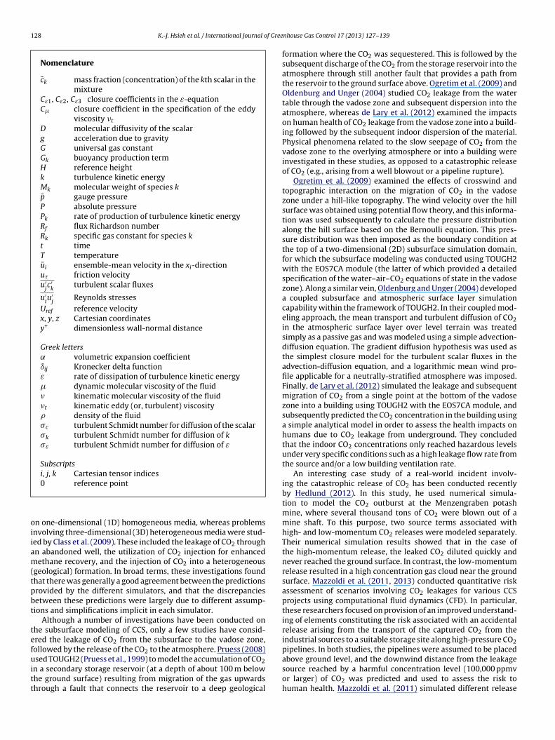

128 K.-J. Hsieh et al. / International Journal of Gree

Nomenclature

ck mass fraction (concentration) of the kth scalar in themixture

Cε1, Cε2, Cε3 closure coefficients in the ε-equationC� closure coefficient in the specification of the eddy

viscosity �t

D molecular diffusivity of the scalarg acceleration due to gravityG universal gas constantGk buoyancy production termH reference heightk turbulence kinetic energyMk molecular weight of species kp gauge pressureP absolute pressurePk rate of production of turbulence kinetic energyRf flux Richardson numberRk specific gas constant for species kt timeT temperatureui ensemble-mean velocity in the xi-directionu� friction velocityu′

jc′

kturbulent scalar fluxes

u′iu′

jReynolds stresses

Uref reference velocityx, y, z Cartesian coordinatesy+ dimensionless wall-normal distance

Greek letters˛ volumetric expansion coefficientıij Kronecker delta functionε rate of dissipation of turbulence kinetic energy� dynamic molecular viscosity of the fluid� kinematic molecular viscosity of the fluid�t kinematic eddy (or, turbulent) viscosity� density of the fluid�c turbulent Schmidt number for diffusion of the scalar�k turbulent Schmidt number for diffusion of k�ε turbulent Schmidt number for diffusion of ε

Subscriptsi, j, k Cartesian tensor indices

oiiam(tpbt

tefuitt

above ground level, and the downwind distance from the leakage

0 reference point

n one-dimensional (1D) homogeneous media, whereas problemsnvolving three-dimensional (3D) heterogeneous media were stud-ed by Class et al. (2009). These included the leakage of CO2 throughn abandoned well, the utilization of CO2 injection for enhancedethane recovery, and the injection of CO2 into a heterogeneous

geological) formation. In broad terms, these investigations foundhat there was generally a good agreement between the predictionsrovided by the different simulators, and that the discrepanciesetween these predictions were largely due to different assump-ions and simplifications implicit in each simulator.

Although a number of investigations have been conducted onhe subsurface modeling of CCS, only a few studies have consid-red the leakage of CO2 from the subsurface to the vadose zone,ollowed by the release of the CO2 to the atmosphere. Pruess (2008)sed TOUGH2 (Pruess et al., 1999) to model the accumulation of CO2

n a secondary storage reservoir (at a depth of about 100 m belowhe ground surface) resulting from migration of the gas upwardshrough a fault that connects the reservoir to a deep geological

nhouse Gas Control 17 (2013) 127–139

formation where the CO2 was sequestered. This is followed by thesubsequent discharge of the CO2 from the storage reservoir into theatmosphere through still another fault that provides a path fromthe reservoir to the ground surface above. Ogretim et al. (2009) andOldenburg and Unger (2004) studied CO2 leakage from the watertable through the vadose zone and subsequent dispersion into theatmosphere, whereas de Lary et al. (2012) examined the impactson human health of CO2 leakage from the vadose zone into a build-ing followed by the subsequent indoor dispersion of the material.Physical phenomena related to the slow seepage of CO2 from thevadose zone to the overlying atmosphere or into a building wereinvestigated in these studies, as opposed to a catastrophic releaseof CO2 (e.g., arising from a well blowout or a pipeline rupture).

Ogretim et al. (2009) examined the effects of crosswind andtopographic interaction on the migration of CO2 in the vadosezone under a hill-like topography. The wind velocity over the hillsurface was obtained using potential flow theory, and this informa-tion was used subsequently to calculate the pressure distributionalong the hill surface based on the Bernoulli equation. This pres-sure distribution was then imposed as the boundary condition atthe top of a two-dimensional (2D) subsurface simulation domain,for which the subsurface modeling was conducted using TOUGH2with the EOS7CA module (the latter of which provided a detailedspecification of the water–air–CO2 equations of state in the vadosezone). Along a similar vein, Oldenburg and Unger (2004) developeda coupled subsurface and atmospheric surface layer simulationcapability within the framework of TOUGH2. In their coupled mod-eling approach, the mean transport and turbulent diffusion of CO2in the atmospheric surface layer over level terrain was treatedsimply as a passive gas and was modeled using a simple advection-diffusion equation. The gradient diffusion hypothesis was used asthe simplest closure model for the turbulent scalar fluxes in theadvection-diffusion equation, and a logarithmic mean wind pro-file applicable for a neutrally-stratified atmosphere was imposed.Finally, de Lary et al. (2012) simulated the leakage and subsequentmigration of CO2 from a single point at the bottom of the vadosezone into a building using TOUGH2 with the EOS7CA module, andsubsequently predicted the CO2 concentration in the building usinga simple analytical model in order to assess the health impacts onhumans due to CO2 leakage from underground. They concludedthat the indoor CO2 concentrations only reached hazardous levelsunder very specific conditions such as a high leakage flow rate fromthe source and/or a low building ventilation rate.

An interesting case study of a real-world incident involv-ing the catastrophic release of CO2 has been conducted recentlyby Hedlund (2012). In this study, he used numerical simula-tion to model the CO2 outburst at the Menzengraben potashmine, where several thousand tons of CO2 were blown out of amine shaft. To this purpose, two source terms associated withhigh- and low-momentum CO2 releases were modeled separately.Their numerical simulation results showed that in the case ofthe high-momentum release, the leaked CO2 diluted quickly andnever reached the ground surface. In contrast, the low-momentumrelease resulted in a high concentration gas cloud near the groundsurface. Mazzoldi et al. (2011, 2013) conducted quantitative riskassessment of scenarios involving CO2 leakages for various CCSprojects using computational fluid dynamics (CFD). In particular,these researchers focused on provision of an improved understand-ing of elements constituting the risk associated with an accidentalrelease arising from the transport of the captured CO2 from theindustrial sources to a suitable storage site along high-pressure CO2pipelines. In both studies, the pipelines were assumed to be placed

source reached by a harmful concentration level (100,000 ppmvor larger) of CO2 was predicted and used to assess the risk tohuman health. Mazzoldi et al. (2011) simulated different release

K.-J. Hsieh et al. / International Journal of Gree

Table 1Test cases pertinent to the leakage of CO2 from storage and transportation facilities.

Test cases Release scenario

Thorney Island (Davies and Singh, 1985) Storage tank leakage near abuilding

sNat(ac

dilwvarprsnhajceqactewdo

rolCtesotirabego(EtEMeop

acceleration in the x -direction; � is the density of the fluid; and,

Axisymmetric hill (Simpson et al., 2002) Pipeline rupture in thevicinity of hilly terrain

cenarios for CO2 using both CFD (based on the Reynolds-averagedavier–Stokes approach) and Gaussian plume models, and evalu-ted the predictive performance of these two approaches againstwo field experiments (Mazzoldi et al., 2008). They concludedperhaps not surprisingly) that CFD models offered improved riskssessments for hazards associated with the dispersion of CO2louds compared to the simpler Gaussian plume models.

It is important to understand the risks associated with theeployment of CCS, and a principal component of this understand-

ng involves the prediction and quantification of the effects of CO2eakage from the subsurface where it is stored to the atmosphere

here it is dispersed by natural turbulent mixing processes on aariety of scales. The objective of this paper is to investigate thetmospheric dispersion of CO2 arising from its leakage from CCSelated infrastructure such as pipelines and CO2 storage tanks. Thisaper focuses on the physics-based modeling of large and rapid CO2eleases (e.g., from a pipeline rupture or loss of containment in atorage facility) using CFD. These large releases of CO2 will resultecessarily in the formation of dense gas clouds (viz., clouds thatave greater density than the ambient environment) which have

tendency to disperse at ground level (where people will be sub-ected to their effects). Indeed, negatively buoyant clouds/plumes ofontaminants tend to cover large surface areas with limited verticalxtent, leading potentially to more serious environmental conse-uences because the gas will remain near the ground and populatedreas. The dispersion behavior of negatively buoyant releases isomplicated even for the simplest conditions (unobstructed and flaterrain), but in reality the complexity of the phenomena is furtherxacerbated by the interaction of the dense gas cloud with buildingakes and/or topographic features. Consequently, the modeling ofense gas dispersion needs to incorporate properly the influencesf real terrain and local obstacles on the dispersion.

A numerical three-dimensional dense gas dispersion modelepresenting the interaction between the dense gas cloud andbstacles or complex terrain is developed, and applied to the simu-ation of two scenarios that are similar to (or mimic) the leakages ofO2 from storage and transportation facilities (cf. Table 1). The firstest case involves simulation of the Thorney Island Phase II fieldxperiments (Davies and Singh, 1985). This test case can perhapserve as a prototype for a catastrophic and instantaneous releasef a dense gas from a storage tank located near a building, andests the accuracy of predictions of dense gas dispersion under thenfluence of a ruptured container and a local building (where theeleased volume is comparable to the building scale). Alternatively,s pointed out by an anonymous reviewer, this test case can alsoe a surrogate for a scenario involving the rapid release of a mod-rate quantity of CO2 gas from a near-surface (perhaps temporary)eological storage site. The second test case involves a simulationf the complex flow over an axisymmetric three-dimensional hillSimpson et al., 2002), and is one of the test cases used in the 11thuropean Research Community on Flow Turbulence and Combus-ion (ERCOFTAC)/International Association for Hydro-Environmentngineering and Research (IAHR) Workshop on Refined Turbulenceodeling. Although there is no dispersion data available for this

xperiment, the detailed measurements of flow are used to validateur predictions of the mean flow and turbulence fields for the com-lex topography, and then this information is used subsequently

nhouse Gas Control 17 (2013) 127–139 129

to develop a scenario involving the continuous release of a denseCO2 gas plume (from an accidental or malicious pipeline rupturein a transportation facility) over complex terrain and to investigatenumerically the influence of the topographic features on the densegas dispersion. In both the Thorney Island Phase II field experimentsand the axisymmetric three-dimensional hill test case, the Boussi-nesq approximation for the representation of the buoyancy termin the momentum equation is used to simplify the modeling of thedense gas dispersion.

It should be noted that in the case of CO2 storage or trans-portation facilities (e.g., storage tanks, pipelines), the materialis normally stored or transported in a liquefied form afterundergoing pressurization. In consequence, it is expected that ahigh-pressure CO2 release will first experience a significant pres-sure drop, followed by a substantial temperature drop due to theJoule–Thompson effect. As a result, the CO2 will undergo a phasechange from liquid to solid or gas, and potentially result in the for-mation of dry ice and/or of a sonic jet flow during the process ofpressure decompression. Currently, many of the physical processesassociated with the rapid release of CO2 have not been explic-itly modeled in dense gas dispersion models [see Koornneef et al.(2010) for a discussion of these issues]. Nevertheless, Mazzoldi et al.(2011) argued that most rapid releases of a liquid/vapor mixture ofCO2 would transform rapidly into the gas phase due to the frictionalheating and mixing provided by the ambient air (following rapidentrainment of air into the initial dense gas cloud). Although sourceterm modeling is an important problem, it is beyond the scope ofthe current study. Accordingly, we will simply assume [followingthe arguments by Mazzoldi et al., 2011] that the CO2 liquid/gas mix-ture has been converted entirely into the gas phase immediatelyafter its release from the source. This is the implicit assumptionmade in our proposed scenarios described later in Section 3.2.

2. Mathematical formulation and numerical framework

The dispersion of a heavier-than-air (dense) gas cloud is pre-dicted by solving the three-dimensional conservation equations formean (ensemble-averaged) quantities in a turbulent flow field. Thisinvolves solving the conservation equations of mass, momentum,and species concentration for an isothermal (constant tempera-ture) fluid flow based on the Reynolds-averaged Navier–Stokes(RANS) approach:

∂�

∂t+ ∂

∂xj(�uj) = 0, (1)

∂

∂t(�ui) + ∂

∂xj(�ujui) = − ∂p

∂xi+ ∂

∂xj

(�

∂ui

∂xj

)− ∂

∂xj(�u′

iu′

j)

+ (� − �0)gi, (2)

∂

∂t(�ck) + ∂

∂xj(�ujck) = ∂

∂xj

(�D

∂ck

∂xj

)− ∂

∂xj(�u′

jc′

k),

k = 1, 2, . . . , N, (3)

where ui is the ensemble-mean (or, Reynolds-averaged) velocityin the xi-direction with i = 1, 2, 3 representing the x, y, and z direc-tions, respectively; t is the time; p is the mean (gauge) pressure; �is the dynamic molecular viscosity of the fluid; ck is the mass frac-tion (concentration) of the kth scalar (or species) in the mixture;D is the molecular diffusivity of the scalar; gi is the gravitational

i�0 is a reference density (chosen herein as the density of air at sealevel with a representative value of �0 = 1.25 kg m−3). Summation isimplied by repeated indices. Reynolds-averaging of the momentum

1 f Gree

tga

aed

�

apca(aRspetips

BtffcmiBfitpUswt

teobp(omcotsts

�

wsi(E

30 K.-J. Hsieh et al. / International Journal o

ransport equation (2) and the advection-diffusion equation (3)ives rise, respectively, to the Reynolds stresses which are defineds the tensor u′

iu′

jand the turbulent scalar fluxes which are defined

s the vector u′jc′

k(k = 1, 2, . . ., N). These equations, along with an

quation of state that uses the ideal gas law approximation for theensity, namely

= P

T∑N

k=1Rkck

= P

R∗T, (4)

re the main governing equations. Here, P is the absoluteressure, T is the absolute temperature (assumed to be aonstant for the isothermal atmosphere considered herein),nd Rk ≡ G/Mk is the specific gas constant for species kG = 8.314472 × 103 J K−1 kg mol−1 is the universal gas constantnd Mk is the molecular weight of species k). Also, in Eq. (4),∗ is the specific gas constant for the mixture consisting of Npecies. It is noted that the gauge pressure p in Eq. (2) is theressure deviation from an adiabatic atmosphere in hydrostaticquilibrium with corresponding density�0, with the result thathe absolute pressure in Eq. (4) is related to the gauge pressuren Eq. (2) as P = p + P0, where P0 is some nominal atmosphericressure level in the adiabatic atmosphere (e.g., at the groundurface).

If the density variations are not too large, we can apply theoussinesq approximation to Eqs. (1)–(3). Indeed, it is expectedhat the numerical solution of Eqs. (1)–(4) that incorporates theull effect of the density variations on the fluid flow and the massraction of the various species is a very challenging problem. Inonsequence, we consider application of the Boussinesq approxi-ation in order to ensure a more tractable problem. Nevertheless,

t is important to stress that the exact limits of validity of theoussinesq approximation and the precise effects of this simpli-cation on the model predictions are not known quantitatively. Tohe authors’ best knowledge, this issue has not been addressed byrevious investigators and is beyond the scope of the present study.ndoubtedly, a useful future research endeavor would be to con-

ider a detailed comparison of model predictions obtained with andithout using the Boussinesq approximation in order to quantify

he errors in the predictions arising from use of this approximation.The main step in developing the Boussinesq approximation is

o treat the density as a constant (which can be taken as the ref-rence density�0) in the unsteady, convective and diffusive termsf Eqs. (1)–(3), while retaining the density variations only in theuoyancy (gravity) term (� − �0)gi in the mean momentum trans-ort equation. This approach was used by Perdikaris and Mayinger1993) and Scargiali et al. (2005) to simulate dense gas dispersionver a topographically complex terrain. However, the approxi-ation for the buoyancy term given in these two papers is not

orrectly stated. In consequence, we provide a simple derivationf the Boussinesq approximation of (� − �0)gi in the context ofhe dispersion of a heavier-than-air gas released into the atmo-phere. Toward this purpose, consider a Taylor series expansion ofhe density � = �(P, T, c1, . . . , cN) to first order about a referencetate (denoted using a subscript 0) given by

= �0 + ∂�

∂P

∣∣∣∣0

(P − P0) + ∂�

∂T

∣∣∣∣0

(T − T0) +N∑

k=1

∂�

∂ck

∣∣∣∣0

(ck − ck,0), (5)

ith the partial derivatives in Eq. (5) evaluated at the reference

tate (P0, T0, c1,0, . . . , cN,0) and �0 = �(P0, T0, c1,0, . . . , cN,0). For ansothermal atmosphere, the third term on the right-hand side of Eq.5) vanishes identically. Inserting the ideal gas law of Eq. (4) intoq. (5), the density perturbations (from the reference state) can be

nhouse Gas Control 17 (2013) 127–139

expressed as follows:

� − �0

�0≡ ı�

�0= (P − P0)

P0−

N∑k=1

˛k(ck − ck,0)≡ıP

P0−

N∑k=1

˛k(ck − ck,0),

(6)

where ı� ≡ (� − �0) and ıP ≡ (P − P0) = p are used to denote thedensity and pressure perturbations, respectively; and,

˛k ≡ − 1�0

∂�

∂ck

∣∣∣∣0

= Rk∑Ni=1Rici,0

, (7)

is the volumetric expansion coefficient arising from perturbationsin the concentration of species k.

To simplify the approximation in Eq. (6), we consider order-of-magnitude estimates for ıP/P0 in comparison to ı�/�0. To proceed,it is assumed that the pressure gradient term in the mean momen-tum transport equation (2) is of the same order of magnitude as thebuoyancy term and, with the buoyancy force acting in the y (i = 2)direction, this implies within the Boussinesq approximation that∣∣∣∣ 1

�0

∂p

∂y

∣∣∣∣ ≡∣∣∣∣ 1

�0

∂ıP

∂y

∣∣∣∣ ≈∣∣∣� − �0

�0g∣∣∣ ≡

∣∣∣∣ı�

�0g

∣∣∣∣ . (8)

An estimate of the magnitude of the term on the left-hand-sideof Eq. (8) [obtained by using the ideal gas law of Eq. (4) for thereference state] gives∣∣∣∣ 1

�0

∂ıP

∂y

∣∣∣∣ ≈ R∗T0

P0

∣∣ıP∣∣

ly, (9)

where ly is a representative or characteristic spatial scale of the cir-culations in the atmospheric surface layer (and typically, ly ∼ 100 min an adiabatic atmosphere). Insertion of the order-of-magnitudeestimate of Eq. (9) into Eq. (8) leads to∣∣ıP

∣∣P0

≈ lyg

R∗T0

∣∣ı�∣∣

�0= lyg

P0/�0

∣∣ı�∣∣

�0= lyg�0

P0

∣∣ı�∣∣

�0. (10)

To proceed further, we need an estimate for P0 which can beobtained as follows. The reference pressure P0 at the Earth’s sur-face is determined for an atmosphere in hydrostatic equilibrium,so P0 ≈ �0gH0 where H0 is the effective height in the atmospherewhere the pressure is equal to zero (approximately). H0 is estimatedto be about H0 ∼ 8000 m (Pielke, 2002). Now, using this estimate forP0 in Eq. (10), it follows that∣∣ıP

∣∣P0

≈ lyg�0

P0

∣∣ı�∣∣

�0= lyg�0

�0gH0

∣∣ı�∣∣

�0= ly

H0

∣∣ı�∣∣

�0, (11)

from which it is seen that (|ıP|/P0) � (|ı�|/�0) because ly/H0 � 1.From this observation, it is now evident that the density perturba-tions in Eq. (6) are well approximated as

� − �0

�0≡ ı�

�0≈ −

N∑k=1

˛k(ck − ck,0). (12)

Finally, for the special case of a two-component mixture consistingof air (a, or species k = 1) and a contaminant species (g, or speciesk = 2) [CO2 or some other contaminant in the cases consideredherein], the density perturbation of Eq. (12) reduces to

� − �0 = ˛c, (13)

�0

on noting ca = 1 − cg ≡ 1 − c, ≡ (�g − �a)/�g , and assuming thatthe concentrations of air and contaminant gas in the refer-ence state are ca,0 = 1 and cg,0 = 1 − ca,0 = 0. Using the density

f Greenhouse Gas Control 17 (2013) 127–139 131

pm

(

FEmaaticabf

k

flma(th

u

u

wCndmwo

wt(p

G

fttczwoi

dfi(w

x/H

z/H

-10 -5 0 5 10

-6

-4

-2

0

2

4

6

x/H

y/H

-10 -5 0 5 100

2

4

6

8

Fig. 1. A two-dimensional view of the computational mesh for trial number 26 in avertical x–y plane at z = 0 (top panel) and in a horizontal x–z plane at y = 0 (bottom

on the Thorney Island airfield in southern England from July 1982to July 1983. In these trials, isothermal gas clouds of fixed vol-ume and of varying density were instantaneously released into the

Table 2Parameters used for the power-law specification of the vertical profile of the stream-wise mean wind velocity for Thorney Island trial numbers 26 and 29 (Phase II).

K.-J. Hsieh et al. / International Journal o

erturbation given by Eq. (13), the buoyancy term can be approxi-ated as follows:

� − �0)gi = �0˛cgi. (14)

or the simulation of both test case scenarios studied in this paper,q. (14) will be used to model the buoyancy term in the meanomentum equation within the framework of the Boussinesq

pproximation. It is noted that this approximation for the buoy-ncy term differs from that used in Scargiali et al. (2005) in thathe quantity involves normalization by �a rather than �g (as usedn the current formulation). Finally, for a two-component mixtureonsisting of air and a contaminant gas, we need only consider

transport equation for the contaminant species concentration cecause the concentration of the air in the mixture is determinedrom (1 − c).

Within the framework of the standard high-Reynolds-number–ε model, the Reynolds stresses u′

iu′

jand the turbulent scalar

uxes u′jc′, required to close the transport equations for the mean

omentum and mean concentration of the contaminant species,re modeled using the Boussinesq eddy-viscosity approximationwhich should not be confused with the Boussinesq approxima-ion for buoyant-driven flows) and the simple gradient diffusionypothesis, respectively, as follows:

′iu′

j= 2

3kıij − �t

(∂ui

∂xj+ ∂uj

∂xi

), (15)

′jc′ = − �t

�c

∂c

∂xj, (16)

here �t = C�k2/ε is the kinematic (turbulent) eddy viscosity,� = 0.09 is a model constant, �c = 0.63 is the turbulent Schmidtumber for the scalar, k is the turbulence kinetic energy, ε is theissipation rate of k, and ıij is the Kronecker delta function. Theodeled transport equations for k and ε in the standard k–ε modelith buoyancy terms assume the following form within the context

f the Boussinesq approximation:

∂

∂t(�0k) + ∂

∂xj(�0ujk) = ∂

∂xj

(�0

�t

�k

∂k

∂xj

)+ �0(Pk + Gk) − �0ε, (17)

∂

∂t(�0ε) + ∂

∂xj(�0ujε) = ∂

∂xj

(�0

�t

�ε

∂ε

∂xj

)

+ Cε1�0ε

k(Pk + Gk)(1 + Cε3Rf ) − Cε2�0

ε2

k, (18)

here Pk ≡ −u′iu′

j∂ui/∂xj is the turbulence kinetic energy produc-

ion term, �k = 1.0, �ε = 1.3, Cε1 = 1.44, and Cε2 = 1.92 are modelclosure) constants. Furthermore, in Eqs. (17) and (18), Gk is theroduction term relating to buoyancy and is given by

k = −˛gi�t

�c

∂c

∂xi, (19)

or the case of a two-component mixture (where c is the con-aminant species concentration). In Eq. (18), Rf = −Gk/(Pk + Gk) ishe flux Richardson number and Cε3 = 0.8 is an additional modelonstant (Rodi, 1978) that is applicable both for vertical and hori-ontal buoyant shear layers. In particular, for a vertical shear layerhere the lateral velocity component is normal to the direction

f gravity, we note that Rf = 0. This is the case of relevance for ournvestigation.

The system of partial differential equations for atmospheric

ispersion modeling was solved numerically using a collocated,nite-volume method and implemented in the urbanSTREAM codeYee et al., 2007; Lien et al., 2010). Diffusive volume-face fluxesere discretized using a second-order accurate central differencing

panel). The mesh consists of 189 × 60 × 83 nodes in the streamwise (x), vertical (y),and spanwise (z) directions, respectively.

scheme (CDS). Advective volume-face fluxes were approximatedusing a second-order accurate Upstream Monotonic Interpolationfor Scalar Transport (UMIST) scheme (Lien and Leschziner, 1994).The transient term was discretized using a fully implicit, second-order accurate three-time-level method described in Ferziger andPeric (2002). The Semi-Implicit Method for Pressure-Linked Equa-tions (SIMPLE) algorithm (Patankar and Spalding, 1972) was used todetermine the (gauge) pressure p. A nonlinear interpolation scheme(Rhie and Chow, 1983) was used to interpolate the cell face veloci-ties from the adjacent nodal velocities at the cell centers in order toprevent checkerboard oscillations from developing in the pressurefield.

3. Results and discussion

3.1. Storage tank release with obstacle (Thorney Island)

Extensive field trials on the dispersion of dense gas clouds atground level in the atmosphere were performed by the Healthand Safety Executive in Great Britain. The trials were conducted

Trial number Wind speed u0 (m s−1) Exponent n

26 1.9 0.0729 5.6 0.15

132 K.-J. Hsieh et al. / International Journal of Greenhouse Gas Control 17 (2013) 127–139

x/H

y/H

-10 -8 -6 -4 -2 0 2 4 6 8

2

4

6C

100.00

46.42

21.54

10.00

4.64

2.15

1.00

0.46

0.22

0.10

Trial 26: t = 0 s

x/H

y/H

-10 -8 -6 -4 -2 0 2 4 6 8

2

4

6C

100.00

46.42

21.54

10.00

4.64

2.15

1.00

0.46

0.22

0.10

Trial 26: t = 2.84 s

x/H

y/H

-10 -8 -6 -4 -2 0 2 4 6 8

2

4

6C

100.00

46.42

21.54

10.00

4.64

2.15

1.00

0.46

0.22

0.10

Trial 26: t = 14.68 s

x/H

y/H

-10 -8 -6 -4 -2 0 2 4 6 8

2

4

6C

100.00

46.42

21.54

10.00

4.64

2.15

1.00

0.46

0.22

0.10

Trial 26: t = 57.32 s

entrat

aFvwItaaat(t3tqteidtr

Fig. 2. Time evolution of mean flow streamlines and contours of mean conc

tmosphere. The gas concentrations in the cloud, consisting ofreon-12 and air mixtures, were measured using sensors placed atarious downwind fetches from the release location. In this paper,e consider the trials conducted in the second phase of the Thorney

sland test series (Davies and Singh, 1985). In these experiments,he dense gas cloud dispersion was conducted in the presence ofn obstacle. The obstacle used was a sharp-edged solid cube with

dimension of 9 m on each side. In the instantaneous releases, cylindrical gas tent of 14 m diameter and 13 m height with aotal volume of 2000 m3 was filled with a mixture of Freon-12dichlorodifluoromethane, CCl2F2) and nitrogen. More specifically,he released gas consisted of a mixture of 68.4% nitrogen and1.6% Freon-12 (w/w) to give a mixture density that is roughlywice that of air. The top and sides of the cylindrical tent wereuickly removed, leaving an upright cylinder of dense gas exposedo the ambient conditions. The mixture immediately began toxpand outwards isotropically in all horizontal directions by grav-

tational slumping. The gravitational slumping and atmosphericispersion of this dense gas cloud is affected by its interaction withhe cubical obstacle, located either downwind or upwind of theelease.

ion (% v/v) of the gas cloud in a vertical plane at z/H = 0 for trial number 26.

In trial number 26, the windward face of the cubical obstacle waslocated 50 m downwind from the center of the cylindrical gas tent.The measured wind speed at 10 m above the ground was 1.9 m s−1,and the concentration of the gas cloud was measured on the wind-ward and leeward faces of the obstacle at heights of 6.4 m and 0.4 mabove ground level, respectively. In trial number 29, the leewardface of the cubical obstacle was located 27 m upwind from the cen-ter of the cylindrical gas tent. The measured wind speed at 10 mabove the ground was 5.6 m s−1, and the concentration was mea-sured on the leeward face of the obstacle at the height of 0.4 mabove ground level.

Simulations of the flow and dense gas dispersion for trial num-ber 26 were conducted on a computational mesh of 189 × 60 × 83control volumes (nodes) in a spatial domain (shown in Fig. 1) withan extent of 16.4H × 4.4H × 14.0H in the streamwise, vertical andspanwise directions, respectively, where H = 9 m is the height ofthe cubical obstacle. The simulations for trial number 29 were per-

formed on a computational mesh of 139 × 60 × 83 nodes in a spatialdomain that spanned 15.9H × 4.4H × 14.0H in the streamwise, ver-tical and spanwise directions, respectively. The mesh used for thecomputational domain of trial number 29 (not shown) was very

K.-J. Hsieh et al. / International Journal of Greenhouse Gas Control 17 (2013) 127–139 133

x/Hy/H

0 5 10

1

2

3

4

5 C

100.00

46.42

21.54

10.00

4.64

2.15

1.00

0.46

0.22

0.10

Trial 29: t = 0 s

x/H

y/H

0 5 10

1

2

3

4

5 C

100.00

46.42

21.54

10.00

4.64

2.15

1.00

0.46

0.22

0.10

Trial 29: t = 20.52 s

x/H

y/H

0 5 10

1

2

3

4

5 C

100.00

46.42

21.54

10.00

4.64

2.15

1.00

0.46

0.22

0.10

Trial 29: t = 3.09 s

x/H

y/H

0 5 10

1

2

3

4

5 C

100.00

46.42

21.54

10.00

4.64

2.15

1.00

0.46

0.22

0.10

Trial 29: t = 8.47 s

entrat

spc

uawTtutbaaafato

d

Fig. 3. Time evolution of mean flow streamlines and contours of mean conc

imilar to that used in trial number 26, where the grid lines werereferentially concentrated near the solid surfaces in order to betterapture the expected sharp gradients of the flow properties here.

At the inlet boundary of the spatial domain used for the sim-lations, the vertical profile of the mean streamwise velocity waspproximated using a power-law functional form u(y) = u0(y/y0)n,here u0 is the reference velocity at the reference height y0 = 10 m.

able 2 summarizes the values of u0 and n used in the simula-ions for trial numbers 26 and 29. This power-law profile was alsosed by Qin et al. (2007) and Sklavounos and Rigas (2004) forheir simulations of the Thorney Island experiments. At the outletoundary, zero Neumann boundary conditions were imposed onll flow variables. At the spanwise and top boundaries, symmetrynd free-slip boundary conditions were applied to the flow vari-bles, respectively. At all the solid boundaries (ground and obstacleaces), standard wall functions were used for the mean velocitiesnd turbulence quantities, and the zero Neumann boundary condi-

ion was applied for the concentration of the gas (implying no fluxf material across the solid boundary).

In the simulations, computations were conducted firstly to pre-ict the steady-state flow field, including as such the complex

ion (% v/v) of the gas cloud in a vertical plane at z/H = 0 for trial number 29.

influence of both the cylindrical gas tent and the cubical obstacle onthe flow. This disturbed flow field was then used as the initial con-dition for the subsequent predictions of the dense gas dispersion,which occurred immediately after the collapse of the cylindricalgas tent. The gas mixture inside the cylindrical tent was releasedinstantaneously to the atmosphere at time t = 0 s. Figs. 2 and 3 showthe mean flow streamlines and contours of concentration at differ-ent times after the dense gas cloud was released and documentsthe time evolution of the dense gas cloud. The gravity slumpingeffect on the dispersion can be seen clearly in both figures, partic-ularly at the earlier times where the streamlines within the highlyconcentrated gas cloud exhibit a strong downward bulk motion.Note that initially the buoyancy generated forces and pressure gra-dients arising from density differences between the gas cloud andits environment lead to a bulk motion that causes the dense cloudto spread in all directions near the release location (including alateral spreading, as well as an upwind spreading against the pre-

vailing wind direction). Further downstream from the release, thebulk flow resulting from the gravitational slumping weakens as dif-fusion, mixing, and entrainment between the gas cloud and theambient air reduces the negative buoyancy effects of the cloud

134 K.-J. Hsieh et al. / International Journal of Gree

t (s)

c(%v/v)

0 50 100 150 200 250 3000

1

2

3

4

5

t (s)

c(%v/v)

0 50 100 150 200 250 3000

1

2

3

Fig. 4. Time history of gas concentration on the windward face of the obstacle ata height of 6.4 m (top panel) and on the leeward face of the obstacle at a height of0S

afittcodadaotqi

p2o

Fh(

.4 m (bottom panel) for trial number 26: (–©–) experimental data from Davies andingh (1985); (—) simulation.

nd strengthens the influence of the externally imposed velocityeld on the transport and dispersion of the cloud. It is noted inrial number 26 that the dense gas cloud flows around and overhe cubical obstacle located downwind of the release (cf. Fig. 2). Inontrast, for trial number 29, the cubical obstacle located upwindf the release is seen to block the further upwind spread of theense gas cloud arising from the gravitational slumping. Also, inddition to the blocking effect, the gas cloud undergoes increasedilution in the wake of the upstream cubical obstacle (cf. Fig. 3),s well as retention or “hold-up” of the material within the wakef the obstacle followed by a slow detrainment of material fromhe wake. This retention of material in the wake followed subse-uently by the detrainment of the material converts the putative

nstantaneous release into a time-varying one.Figs. 4 and 5 display a comparison between the measured and

redicted gas concentration time histories for trial numbers 26 and9, respectively. In particular, Fig. 4 shows that the time historiesf concentration observed at the windward and leeward faces of

t (s)

c(%v/v)

0 20 40 60 80 1000

5

10

15

20

25

ig. 5. Time history of gas concentration on the leeward face of the obstacle at aeight of 0.4 m for trial number 29: (–©–) experimental data from Davies and Singh1985); (—) simulation.

nhouse Gas Control 17 (2013) 127–139

the cubical obstacle are quite different. Note that the persistence ofthe gas cloud (as measured by the difference between the arrivaland departure times of the cloud) observed at the leeward face ofthe cubical obstacle is significantly greater than that observed atthe windward face. This demonstrates the effect of the obstacle ondispersion, where the recirculation bubble in the wake region of theobstacle entrains and “holds-up” (traps) the contaminant materialof the gas cloud. The hold-up mechanism within the wake of theobstacle is correctly predicted by the model.

Generally, numerical predictions of concentration are seen tobe in quite good agreement with the experimental data. It is notedthat in interpreting the level of agreement between predictionsand measurements, one needs to recognize that the measure-ments of the short time-averaged concentration obtained in trialnumbers 26 and 29 correspond to one realization of the instan-taneous dispersion, whereas the model predictions correspond toan ensemble-averaged concentration (and, as such, is associatedwith an average over an ensemble of realizations of the instanta-neous dispersion). Because the model prediction is compared toone realization out of the ensemble of all possible realizations, thediscrepancy between the model predictions and the experimentalmeasurements cannot be smaller than the expected fluctuationsof the individual realizations about the ensemble mean. In con-sequence, it is impossible for even a perfect model to give agreater precision in its predictions of the concentration than theexpected concentration variability from realization to realizationin the atmospheric dispersion. Keeping this caveat in mind, anyremaining discrepancies between the predictions and the measure-ments could be probably attributed to the use of the standard k–εturbulence model. It is well known that the standard k–ε modeltends to over-predict levels of the turbulence kinetic energy for aflow impinging on a solid obstacle [the so-called the “stagnationpoint anomaly”, Durbin, 1996], resulting in prediction of a largerrecirculation bubble in the wake region of a three-dimensionalobstacle than is actually observed.

For trial number 26, the more pronounced impingement of theapproaching flow on the front face of the cylindrical gas tent result-ing in a predicted larger recirculation bubble in the wake regionof the tent will have the tendency to dilute the gas concentrationfaster after the tent collapses. In consequence, this will lead to alower predicted concentration downstream of the cylindrical gastent when compared to the associated measured concentration, ascan be seen in Fig. 4. For trial number 29, a larger recirculation bub-ble behind the upwind cubical obstacle will entrain material fromthe dense gas cloud (that has spread upwind owing to the gravityslumping) into the wake earlier. This effect will result in an ear-lier predicted arrival time for the cloud (at the leeward face of theupwind obstacle) in comparison to the measurements, as can beseen in Fig. 5.

The effect of the buoyancy production term Gk in the k–ε model[cf. Eqs. (17) and (18)] on the prediction of dense gas dispersionis investigated and demonstrated in Fig. 6. It was found that theinclusion of the Gk term in the k–ε model suppresses the turbu-lence kinetic energy, particularly in the wake region of the obstacle,which is not too surprising owing to the negative buoyancy effectof the dense gas cloud. In contrast, the effect of the Gk term on theprediction of the concentration levels in the cloud appears to beinsignificant (at least for the example considered here). This obser-vation is similar to the findings of Worthy et al. (2001), where itwas reported that the Gk term made very little difference to themodeling of buoyant (hot) thermal plumes.

3.2. Pipeline rupture with axisymmetric hill(s)

The experiment of Simpson et al. (2002) consists of measure-ments of the flow over a three-dimensional axisymmetric hill

K.-J. Hsieh et al. / International Journal of Greenhouse Gas Control 17 (2013) 127–139 135

x/Hy/H

0 5 10

1

2

3

4

5 K

0.10

0.09

0.08

0.07

0.06

0.05

0.04

0.03

0.02

0.01

Trial 29: t = 8.47 s

x/H

y/H

0 5 10

1

2

3

4

5 K

0.10

0.09

0.08

0.07

0.06

0.05

0.04

0.03

0.02

0.01

Trial 29: t = 8.47 s, Gk= 0

x/H

y/H

0 5 10

1

2

3

4

5 C

100.00

46.42

21.54

10.00

4.64

2.15

1.00

0.46

0.22

0.10

Trial 29: t = 8.47 s

x/H

y/H

0 5 10

1

2

3

4

5 C

100.00

46.42

21.54

10.00

4.64

2.15

1.00

0.46

0.22

0.10

Trial 29: t = 8.47 s, Gk= 0

F ic enep of the

mis

wffsaistvdd1M7b

ig. 6. Buoyancy production term sensitivity analysis: contours of turbulence kinetanels) in a vertical plane at z/H = 0 for trial number 29, with and without inclusion

ounted on the floor of a wind tunnel. The wind tunnel has a work-ng section that is 7.62 m long, 0.91 m wide, and 0.25 m high. Thehape of the three-dimensional hill is defined as follows:

y(r)H

= − 16.04844

[J0()I0

(

r

2H

)− I0()J0

(

r

2H

)], (20)

here H = 0.078 m is the hill height, = 3.1926, J0(x) is the Besselunction of the first kind of order 0, and I0(x) is the modified Besselunction of the first kind of order 0. The nominal inlet velocity for thepatial domain containing the axisymmetric hill is Uref = 27.5 m s−1

t the hill height H, and the Reynolds number based on H and Urefs 130,000. Measurements of the flow were conducted at variouspanwise locations at 3.63H downstream of the hill crest. Detailedhree-component laser Doppler anemometer measurements ofelocity are available for this test case, providing a comprehensiveocumentation of a complex flow field with a challenging three-imensional separation. This experiment was used as “Test Case

1.2” in the 11th ERCOFTAC/IAHR Workshop on Refined Turbulenceodeling held at Chalmers University of Technology in Sweden on

th and 8th April, 2005. The experimental data for this test case cane found at http://www.tfd.chalmers.se/∼gujo/WS11 2005/.

rgy (top two panels) and mean concentration (% v/v) in the gas cloud (bottom two Gk term in the turbulence transport equations.

Simulations for flow over the axisymmetric hill were con-ducted on a computational mesh of 151 × 35 × 102 control volumes(nodes) in a spatial domain (shown in Fig. 7) with an extent of19.8H × 3.205H × 11.67H in the streamwise, vertical and spanwisedirections, respectively. Predicted results of the flow were com-pared with the associated experimental data at four spanwiselocations (namely, at z/H = 0.00, 0.33, 0.65 and 0.81) at a down-stream fetch of x/H = 3.63.

At the inlet boundary of the spatial domain, the vertical profile ofthe mean streamwise velocity was approximated by a power-law

function of the form u(y) = Uref

(y/H

)1/7. At the outlet boundary,

zero Neumann boundary conditions were imposed on all flow vari-ables. At the spanwise boundaries, a symmetry boundary conditionwas used. Finally, at the top and bottom boundaries of the domain,standard wall functions were applied for mean velocities and tur-bulence quantities, and the zero Neumann boundary condition was

applied for the mean concentration field.

Fig. 8 shows the velocity vector field in the vicinity of the hill.In the experiment, there was a thin recirculation region observedon the leeward side of the hill. Simulations using RANS, large-eddy

136 K.-J. Hsieh et al. / International Journal of Greenhouse Gas Control 17 (2013) 127–139

x/H

y/H

-4 0 4 8 12 160

2

4

6

z/H

-6

-4

-2

0

2

4

6

x/H

-4

0

4

8

12

X

Y

Z

F at z =g reamw

s2hcatotmftdkakr

Ft

ig. 7. A two-dimensional view of the computational mesh in a vertical x–y planeround surface (bottom panel). The mesh consists of 151 × 35 × 102 nodes in the st

imulation (LES), or hybrid RANS-LES (e.g., Garcia-Villalba et al.,009; Krajnovic, 2008; Persson et al., 2006; Tessicini et al., 2007)ave shown that it is difficult to predict this recirculation regionorrectly. In the RANS calculation of Persson et al. (2006) in which

non-linear cubic eddy viscosity model was employed, these inves-igators predicted a recirculation region that was too large. In onef the LES studies conducted by Tessicini et al. (2007), no recircula-ion was captured when they used a dynamic subgrid stress (SGS)

odel on a computational grid of 192 × 64 × 128 control volumesor a spatial domain with an extent of 16H × 3.205H × 11.67H, withhe near-wall nodes having values of the normalized wall-normalistance y+ ( yu� /�, where u� is the friction velocity and � is theinematic molecular viscosity of the fluid) in the range between 40

nd 60. In conformance with these previous studies, the standard–ε model with wall functions used herein also failed to predict theecirculation region in the lee of the hill.

x/H

y/H

-3 -2 -1 0 1 2 30

1

2

3

ig. 8. Mean velocity vector field in a vertical x–y plane at z/H = 0 in the vicinity ofhe hill, where H is the height of the hill.

0 (top panel) and a three-dimensional view of the computational mesh along theise (x), vertical (y), and spanwise (z) directions, respectively.

Figs. 9 and 10 show the predictions of mean streamwise veloc-ity and turbulence kinetic energy, respectively, at various spanwisez-locations at a fixed downwind fetch of x/H = 3.63. In general, thepredicted mean velocity profiles are in good conformance with themeasurements. However, the predicted turbulence kinetic energyprofiles in Fig. 10 show a poorer agreement with the measure-ments. For example, the measured turbulence kinetic energy atz/H = 0.0 decreases rapidly for y/H > 0.9, but the numerical predic-tion in this region is quite high. This is likely due to the standardk–ε model predicting excessive turbulence kinetic energy levelswhen the approaching flow impinges on the windward side of thehill. This high turbulence energy is advected downstream, affectingpredictions of the levels turbulence kinetic energy at all locationsdownwind of the impingement zone.

Although there is no concentration data available from Simpsonet al. (2002) to compare with our predictions of dense gas disper-sion on complex topography, the three-dimensional axisymmetrichill is used to study the effect of the terrain on the dispersionof a dense gas cloud. A scenario is proposed here to investigatethe potential safety concern involving a pipeline rupture (througheither an accidental or malicious release) in the vicinity of hilly ter-rain. It is assumed that CO2 is released continuously from a sectionof pipeline (on the ground surface) located at x/H = −3 upstreamof the center (summit) of the hill. The area of the source release is0.118H2 m2 and the gas jet velocity from the release is 0.1Uref m s−1.Atmospheric dispersion of the resulting dense gas plume over oneand two hills is considered in our simulations. Fig. 11 shows thecomputational mesh for the case of the two hills, where the dis-tribution of grid nodes and domain size is identical to that for the

one hill case. Fig. 12 shows the mean flow streamlines and iso-surfaces of the concentration field resulting from the CO2 release.Here, two iso-surfaces of the concentration field with values of 0.5%and 4% (v/v) are selected to exhibit various features of the resulting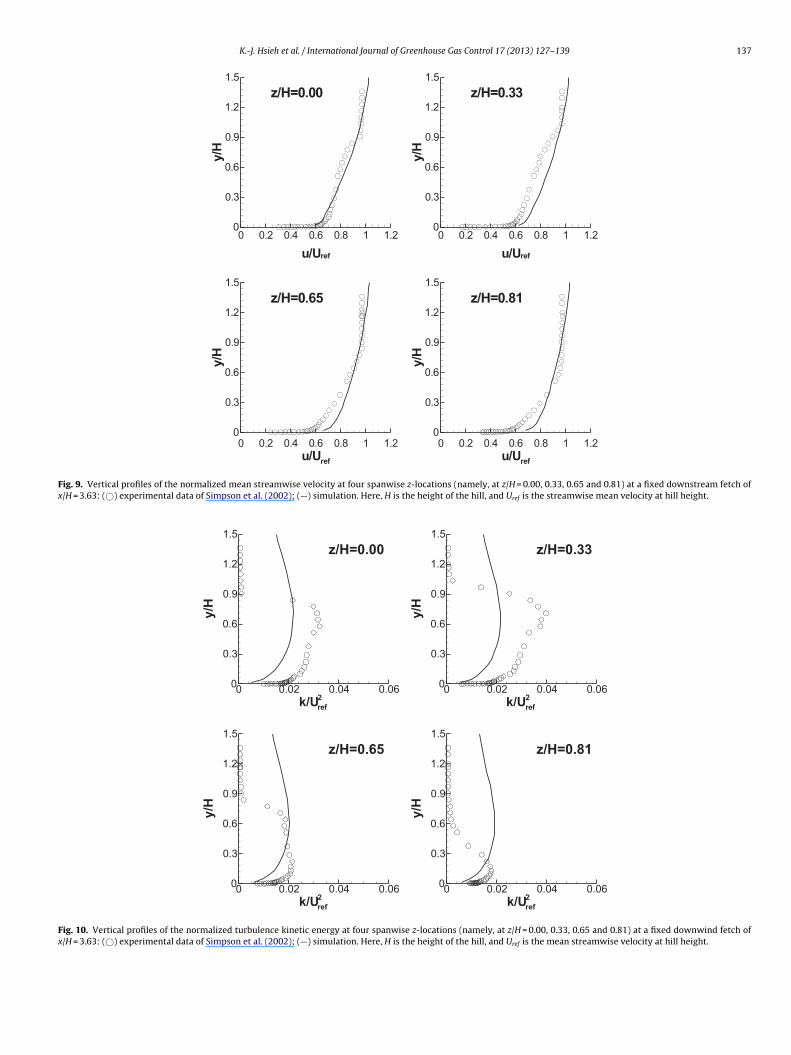

K.-J. Hsieh et al. / International Journal of Greenhouse Gas Control 17 (2013) 127–139 137

u/Uref

y/H

0 0.2 0.4 0.6 0.8 1 1.20

0.3

0.6

0.9

1.2

1.5

z/H=0.00

u/Uref

y/H

0 0.2 0.4 0.6 0.8 1 1.20

0.3

0.6

0.9

1.2

1.5

z/H=0.33

u/Uref

y/H

0 0.2 0.4 0.6 0.8 1 1.2

0

0.3

0.6

0.9

1.2

1.5

z/H=0.65

u/Uref

y/H

0 0.2 0.4 0.6 0.8 1 1.2

0

0.3

0.6

0.9

1.2

1.5

z/H=0.81

Fig. 9. Vertical profiles of the normalized mean streamwise velocity at four spanwise z-locations (namely, at z/H = 0.00, 0.33, 0.65 and 0.81) at a fixed downstream fetch ofx/H = 3.63: (©) experimental data of Simpson et al. (2002); (—) simulation. Here, H is the height of the hill, and Uref is the streamwise mean velocity at hill height.

k/U2

ref

y/H

0 0.02 0.04 0.060

0.3

0.6

0.9

1.2

1.5

z/H=0.00

k/U2

ref

y/H

0 0.02 0.04 0.060

0.3

0.6

0.9

1.2

1.5

z/H=0.33

k/U2

ref

y/H

0 0.02 0.04 0.060

0.3

0.6

0.9

1.2

1.5

z/H=0.81

k/U2

ref

y/H

0 0.02 0.04 0.060

0.3

0.6

0.9

1.2

1.5

z/H=0.65

Fig. 10. Vertical profiles of the normalized turbulence kinetic energy at four spanwise z-locations (namely, at z/H = 0.00, 0.33, 0.65 and 0.81) at a fixed downwind fetch ofx/H = 3.63: (©) experimental data of Simpson et al. (2002); (—) simulation. Here, H is the height of the hill, and Uref is the mean streamwise velocity at hill height.

138 K.-J. Hsieh et al. / International Journal of Greenhouse Gas Control 17 (2013) 127–139

z/H

-6

-4

-2

0

2

4

6

x/H

-4

0

4

8

X

Y

Z

nal me

ctrtai

c

Fccttv

Fig. 11. A three-dimensional view of the computatio

oncentration distribution. As a point of reference, we note thathe National Institute for Occupational Safety and Health (NIOSH)ecommends chronic exposure limits for CO2 for a 40-h work weeko not exceed 0.5% (5000 ppmv). Furthermore, NIOSH suggests thatn acute exposure to CO2 concentration levels at 4% (40,000 ppmv)

s immediately dangerous to life or health (NIOSH, 2005).

The effect of terrain (viz., one hill compared to two hills) on theoncentration field is displayed in Fig. 12 for concentration levels

ig. 12. Mean flow streamlines along the ground surface and two iso-surfaces ofoncentration in the dense gas plume at concentration levels of 4% (bright greenontour) and 0.5% (dark green contour) for dispersion over one hill (top panel) andwo hills (bottom panel). The concentration is expressed in (% v/v). (For interpreta-ion of the references to color in this figure legend, the reader is referred to the webersion of the article.)

sh along the ground surface for the case of two hills.

of 0.5% and 4% (v/v). It can be seen that significant concentrationsat a level of 4% (bright green contour) exist at or near the groundsurface in the range of downwind locations lying between the loca-tions of the pipeline rupture and the first hill (owing to the fact thatthe plume of dense gas is “pancake-shaped” and does not rise veryfar from the ground). For the case of one hill, it is seen that the con-centration iso-surface of 0.5% (dark green contour) extends aroundand over the single hill topography to regions that are well down-stream of the lee of the hill. In contrast, for the case of dispersionover two hills, the distribution of the concentration iso-surface at avalue of 0.5% is more limited in its downwind extent. In particular,the presence of the second hill appears to “trap” the contaminantin the region (valley) between the two hills, resulting in an accu-mulation of CO2 here. Furthermore, there exists also a recirculationregion on the leeward side of the second hill, and this region willfacilitate further entrainment and holdup of the CO2 in the leewardregion of the second hill.

4. Conclusions

Most of the numerical studies on CCS have been focused onthe subsurface modeling, with the consequence that only very fewstudies have investigated the leakage of CO2 from the subsurfaceinto the atmosphere and subsequent dispersion of the dense gascloud. In this paper, a dense gas dispersion model based on the RANSapproach has been developed and applied to simulate two scenar-ios that serve as surrogates for potential CO2 leakage events fromCCS related infrastructure, such as pipelines and CO2 storage tanksin complex terrain and/or in the vicinity of buildings and otherobstacles and obstructions. A simple and rigorous derivation for themodeling of the buoyancy term within the framework of the Boussi-nesq approximation is provided. The effects of buildings and/orcomplex topography on the dispersion of dense gas clouds/plumesare studied. It is shown that the model is able to provide fair togood predictions for either the flow or species concentration forthe two scenarios studied herein. The prediction of the distribu-tion of the dense gas cloud concentration when expressed in termsof iso-contours or iso-surfaces of critical concentration levels pro-vides useful information for the delineation of hazard zones (or,toxic corridors) resulting from the release of a dense gas cloud nearground level. It is anticipated that the model can be used to provide

information required for undertaking quantified risk assessmentsfor the potential risks to the public posed by the accidental or mali-cious release of carbon dioxide from existing or future CCS relatedinfrastructure.

f Gree

A

R

R

C

D

d

D

F

G

H

H

K

K

L

L

M

M

M

K.-J. Hsieh et al. / International Journal o

cknowledgements

This work was supported by CanmetENERGY – Ottawa, Naturalesources Canada.

eferences

lass, H., Ebigbo, A., Helmig, R., Dahle, H.K., Nordbotten, J.M., Celia, M.A., Audigane,P., Darcis, M., Ennis-King, J., Fan, Y., Flemisch, B., Gasda, S.E., Jin, M., Krug, S.,Labregere, D., Beni, A.N., Pawar, R.J., Sbai, A., Thomas, S.G., Trenty, L., Wei, L.,2009. A benchmark study on problems related to CO2 storage in geologicalformations: summary and discussion of the results. Computational Geosciences13, 409–434.

avies, M.E., Singh, S., 1985. The phase II trials: a data set on the effect of obstruc-tions. Journal of Hazardous Materials 11, 301–323.

e Lary, L., Loschetter, A., Bouc, O., Rohmer, J., Oldenburg, C.M., 2012. Assessinghealth impacts of CO2 leakage from a geological storage site into buildings: roleof attenuation in the unsaturated zone and building foundation. InternationalJournal of Greenhouse Gas Control 9, 322–333.

urbin, P.A., 1996. On the k-3 stagnation point anomaly. International Journal ofHeat and Fluid Flow 17, 89–90.

erziger, J.H., Peric, M., 2002. Computational Methods for Fluid Dynamics. Springer-Verlag.

arcia-Villalba, M., Li, N., Rodi, W., Leschziner, M.A., 2009. Large-eddy simulationof separated flow over a three-dimensional axisymmetric hill. Journal of FluidMechanics 627, 55–96.

edlund, F.H., 2012. The extreme carbon dioxide outburst at the Menzengrabenpotash mine 7 July 1953. Safety Science 50, 537–553.

osa, A., Esentia, M., Stewart, J., Haszeldine, S., 2011. Injection of CO2 into salineformations: benchmarking worldwide projects. Chemical Engineering Researchand Design 89, 1855–1864.

oornneef, J., Spruijt, M., Molag, M., Ramirez, A., Turkenburg, W., Faaij, A., 2010.Quantitative risk assessment of CO2 transport by pipelines – a review of uncer-tainties and their impacts. Journal of Hazardous Materials 177, 12–27.

rajnovic, S., 2008. Large-eddy simulation of the flow over a three-dimensional hill.Flow, Turbulence and Combustion 81, 189–204.

ien, F.S., Leschziner, M.A., 1994. Upstream monotonic interpolation for scalartransport with application in complex turbulent flows. International Journal forNumerical Methods in Fluids 19, 527–548.

ien, F.S., Yee, E., Wang, B.C., Ji, H., 2010. Grand computational challenges for pre-diction of the turbulent wind flow and contaminant transport and dispersionin the complex urban environment. In: Lang, P.R., Lombargo, F.S. (Eds.), Atmo-spheric Turbulence, Meteorological Modeling and Aerodynamics. Nova SciencePublishers.

azzoldi, A., Hill, T., Colls, J.J., 2011. Assessing the risk for CO2 transportation withinCCS projects, CFD modeling. International Journal of Greenhouse Gas Control 5,816–825.

azzoldi, A., Hill, T., Colls, J.J., 2008. CFD and Gaussian atmospheric dispersion mod-

els: a comparison for leakages within carbon dioxide transportation and storagefacilities. Atmospheric Environment 42, 8046–8054.

azzoldi, A., Picard, D., Sriram, P.G., Oldenburg, C.M., 2013. Simulation-basedestimates of safety distances for pipeline transportation of carbon dioxide.Greenhouse Gases: Science and Technology 3, 66–83.

nhouse Gas Control 17 (2013) 127–139 139

Michael, K., Golab, A., Shulakova, V., Ennis-King, J., Allinson, G., Sharma, S., Aiken,T., 2010. Geological storage of CO2 in saline aquifers – a review of the experi-ence from existing storage operations. International Journal of Greenhouse GasControl 4, 659–667.

NIOSH, 2005. NIOSH Pocket Guide to Chemical Hazards, DHHS (NIOSH) PublicationNo. 2005-149. U.S. Government Printing Office.

Ogretim, E., Gray, D.D., Bromhal, G.S., 2009. Effects of crosswind-topography inter-action on the near-surface migration of a potential CO2 leak. Energy Procedia 1,2341–2348.

Oldenburg, C.M., Unger, A.J.A., 2004. Coupled vadose zone and atmospheric surface-layer transport of carbon dioxide from geologic carbon sequestration sites.Vadose Zone Journal 3, 848–857.

Patankar, S.V., Spalding, D.B., 1972. A calculation procedure for heat, mass andmomentum transfer in three-dimensional parabolic flows. International Journalof Heat and Mass Transfer 15, 1787–1806.

Perdikaris, G.A., Mayinger, F., 1993. Numerical simulation of heavy gas cloud dis-persion within topographically complex terrain. Journal of Loss Prevention inthe Process Industries 7, 391–396.

Persson, T., Liefvendahl, M., Bensow, R.E., Fureby, C., 2006. Numerical investiga-tion of the flow over an axisymmetric hill using LES, DES and RANS. Journal ofTurbulence 7, 1–17.

Pielke Sr., R.A., 2002. Mesoscale Meteorological Modeling, second edition. AcademicPress.

Pruess, K., Oldenburg, C., Moridis, G., 1999. TOUGH2 User’s Guide. Version 2.0, ReportLBNL-43134. Lawrence Berkeley National Laboratory, Berkeley, CA.

Pruess, K., Garcia, J., Kovscek, T., Oldenburg, C., Rutqvist, J., Steefel, C., Xu, T., 2004.Code intercomparison builds confidence in numerical simulation models for

geologic disposal of CO2. Energy 29, 1431–1444.Pruess, K., 2008. Leakage of CO2 from geological storage: role of secondary accu-

mulation at shallow depth. International Journal of Greenhouse Gas Control 2,37–46.

Qin, T.X., Guo, Y.C., Lin, W.Y., 2007. Large eddy simulation of heavy gas dispersionaround an obstacle. In: Proceedings of the Fifth International Conference on FluidMechanics, Shanghai, China.

Rhie, C.M., Chow, W.L., 1983. Numerical study of the turbulent flow past an airfoilwith trailing edge separation. AIAA Journal 21, 1525–1532.

Rodi, W., 1978. Turbulence Models and Their Applications in Hydraulics – A Stateof the Art Review. University of Karlsruhe, SFB 80/T/127.

Scargiali, F., Di Rienzo, E., Ciofalo, M., Grisafi, F., Brucato, A., 2005. Heavy gas disper-sion modeling over a topographically complex mesoscale: a CFD based approach.Process Safety and Environmental Protection 83, 242–256.

Schnaar, G., Digiulio, D.C., 2009. Computational modeling of the geologic seques-tration of carbon dioxide. Vadose Zone Journal 8, 389–403.

Simpson, R.L., Long, C.H., Byun, G., 2002. Study of vortical separation froman axisymmetric hill. International Journal of Heat and Fluid Flow 23,582–591.

Sklavounos, S., Rigas, F., 2004. Validation of turbulence models in heavy gas disper-sion over obstacles. Journal of Hazardous Materials 108, 9–20.

Tessicini, F., Li, N., Leschziner, M.A., 2007. Large-eddy simulation of three-dimensional flow around a hill-shaped obstruction with a zonal near-wall

approximation. International Journal of Heat and Fluid Flow 28, 894–908.

Worthy, J., Sanderson, V., Rubini, P., 2001. Comparison of modified k-ε turbulencemodels for buoyant plumes. Numerical Heat Transfer, Part B 39, 151–165.

Yee, E., Lien, F.S., Ji, H., 2007. Technical description of urban microscale modelingsystem: component 1 of CRTI Project 02-0093RD. DRDC, Suffield, TR 2007-067.