DEMOGRAPHIC DIFFERENTIALS IN EDUCATIONAL ATTAINMENT USING A

MEASURE INCORPORATING HORIZONTAL ASPECTS OF STRATIFICATION*

Arthur Sakamoto

Department of Sociology

Texas A&M University

4351 TAMU

College Station, Texas 77843-4351

email: asakamoto@tamu.edu

telephone/voice mail: (979) 845-5133

fax: (979) 862-4057

ChangHwan Kim

Department of Sociology

University of Kansas

1415 Jayhawk Blvd., Room 716

Lawrence, KS 66045

Tel: (785) 864-9430

Fax: (785) 864-5280

Email: chkim@ku.edu

October 7, 2013

word count: 7194 (including text, footnotes, and references)

*Direct correspondence to Arthur Sakamoto at the above address.

DEMOGRAPHIC DIFFERENTIALS IN EDUCATIONAL ATTAINMENT USING A

MEASURE INCORPORATING HORIZONTAL ASPECTS OF STRATIFICATION

ABSTRACT

Dimensions of educational attainment other than highest level completed may be increasing in

their significance. Field of study and college type affect labor market earnings net of the highest

level. In order to improve our understanding of the link between schooling and ascriptive

inequalities, we propose a market based measure of educational attainment that incorporates

information on not only the highest level completed, but also on field of study and college type

for persons with a bachelor’s degree. Results indicate that women are disadvantaged when using

the market based measure. The latter approach yields more disadvantaged estimates of the

educational attainments of African Americans while conversely indicating more advantaged

estimates of the educational attainments of Asian Americans.

2

Much research to date has focused on educational attainment as represented by a

hierarchy of ordinal levels. This research has been highly insightful. It has revealed the great

importance of educational attainment for understanding social stratification. Education

measured as an ordinal scale indicating the highest level completed has been shown to be

implicated in many processes relating to a variety socioeconomic phenomena such as

intergenerational mobility, income inequality, occupational attainment, and poverty status.

Given the continuing if not increasing significance of education for inequality and

stratification (Fischer and Hout 2006; Autor, Katz and Kearney 2008; Goldin and Katz 2008;

Kim and Sakamoto 2008), we suggest that other measures of educational attainment may also be

explored. In order to promote further insight on this important phenomenon, enriched or more

complex measures of educational attainment may be useful for some research purposes. In the

following, we develop and illustrate a measure that incorporates not only the ordinal dimension

but also horizontal elements of educational attainment. Our general concern for developing this

approach is to provide an additional tool that may prove useful for researchers who wish to study

educational attainment as a dependent variable.

The broader context for our analysis is the apparent “puzzle” that arises in the findings of

Bloome and Western (2011:392). Their study of American men in recent decades finds a decline

in the level of intergenerational income mobility but no change (or an increase in the case of

African American men) in the level of educational mobility. That is, compared to an older

cohort, the educational attainment of a more recent cohort of men did not become more

dependent on parental education or income, but the income attainment of that more recent cohort

did become more positively associated with parental income. While not logically contradictory

or statistically impossible, one would have expected (based on prior research on social

3

stratification) to instead observe positively associated changes in the level of educational

mobility and the level of income mobility.

In their discussion of this unexpected finding, Bloome and Western (2011:392) state that

“it is likely that higher parental incomes are associated with higher quality schooling in the form

of better schools, superior academic achievement or greater cognitive ability at a given grade

level.” In other words, the empirical results as well as the substantive discussion in Bloome and

Western (2011) suggest that that horizontal sources of educational stratification may be

becoming important for income attainment. Their “puzzle” might derive from a reduction in

educational mobility if education attainment were investigated using a measure that accounts for

both ordinal and horizontal dimensions.

THEORETICAL ISSUES AND PRIOR RESEARCH

In research on educational attainment as the dependent variable, the most common

approach has been to study the highest educational level completed as an ordinal outcome (Mare

1995). That is, educational attainment is often measured as an ordinal set of categorical levels

such as: less than high school; high school graduate; some college (or associate’s degree);

bachelor’s degree; master’s degree; Ph’D or professional degree (Farley 1996). Collapsed

versions of this hierarchy are also frequently studied (Mare and Maralani 2006) including simply

the dichotomous distinction of obtaining at least a bachelor’s degree (Buchmann and DiPrete

2006; Brand and Xie 2010). Although an older literature often measured education by an

interval-level indicator represented by the years of schooling that are usually associated with

each level (Sewell and Hauser 1975), this interval-level approach is now more commonly used in

studies with primarily descriptive concerns (Everett et al. 2007) because in various demographic

4

statistical models, the effects of the educational levels are frequently non-linear relative to their

years-of-schooling scaling (Farley 1996; Mirowsky and Ross 2003).

In detailed studies of educational attainment, the focus on the transition from one

educational level to the next higher level has come to be known as the “Mare Model” (Mare

1980). This model has been studied for different age cohorts in the U.S. as well as in several

other developed countries (Shavit and Bossfeld 1993). The effect of socioeconomic origins

(such as parental education) on making a particular educational transition may be obtained using

Mare’s logistic specification so that the estimated coefficient is independent of the degree of

dispersion in the distribution of educational attainment overall (Mare 1980). In the context of

this model, inequality in educational opportunity refers to large effects of socioeconomic origins

on making the major educational transitions. Studies for the U.S. and several European nations

generally find some decline in inequality in educational opportunity during the period following

the World War II era but some reemergence of inequality in more recent cohorts (Breen and

Goldthorpe 1997). This pattern is often summarized as “persistent inequality” (Shavit and

Bossfeld 1993; Shavit, Yaish and Ban-Haim 2007).

The “Mare Model” was proposed over three decades ago when the supply of college-

educated workers was much lower. While studies using that approach have been highly

informative, they have been based entirely on educational attainment measured as an ordinal

outcome referring to the highest completed level. However, given the more recent trends of

rising rates of college completion and continued increases in wage inequality (Autor et al. 2006;

Lemieux 2006), other dimensions of educational attainment may now be becoming increasingly

useful to investigate. That is, among persons with the same highest level completed, other

aspects of educational attainment such as college prestige might become significant in affecting

5

labor market opportunities (e.g., a Ph.D. in sociology from a Research University I institution is

generally more competitive than a Ph.D. in sociology from a Doctoral Granting II institution). In

other cases, field of study might be more important than educational level for access to certain

types of jobs (e.g., an M.A. or Ph.D. in English is likely to be less competitive than a B.A. in

biochemistry for a job in biochemical research).

Although not considered in the “Mare Model,” field of study has significant implications

for the job prospects of college graduates in the contemporary labor market. Field of study

affects earnings and labor market opportunities (Thomas and Zhang 2005). Using data from the

Baccalaureate and Beyond survey, for example, the results of Thomas and Zhang (2005:447)

indicate that engineering majors earn 94% more than history majors net of gender, race/ethnicity,

college type and quality, parental income, whether a first-generation college graduate, SAT/ACT

quartile ranking, age, years employed with current firm, and number of hours worked. This

sizeable net advantage was observed about five years after obtaining the B.A. degree.

Some other studies that find notable net effects of field of study include Berger (1998),

Rumberger and Thomas (1993), Thomas (2000), Card and DiNardo (2002) and Song and Glick

(2004). Black et al. (2006) find that controlling for field of study (using the 1993 National

Survey of College Graduates) significantly reduces the black-white gap among college-educated

men whereas Kim and Sakamoto (2010) find that controlling for field of study increases the

earnings gap for Asian American men (relative to white men) because Asian American men are

concentrated in science, technology, engineering and medical (i.e., STEM) fields of study that

tend to have higher earnings. Morgan (2008) has shown that factoring in field of study has

important implications for understanding gender differentials in earnings.

An additional dimension of educational attainment that is not included in the “Mare

6

Model” is college quality which has been shown to have an independent effect on earnings

(Rumberger and Thomas 1993; Loury and Garman 1995; Brewer et al. 1999; Thomas 2003;

Thomas and Zhang 2005). As argued by the careful review and analysis of Zhang (2005), part of

the advantage of attending a high quality undergraduate institution is its indirect effect of

increasing one’s chances of attending a high quality graduate program. That is, institutional

quality tends to be correlated across one’s educational career. Although the “Mare Model” is

focused on transitions between levels as separated processes, “students are not randomly

rearranged after graduating from each educational level. The quality of institutions at the

previous level helps determine the quality of institutions chosen at the following levels and also

influences the educational outcomes of the following levels” (Zhang 2005:334). Given the

increasingly exorbitant costs that many people seem willing to pay to attend a high quality

college, we should consider not only whether such elite institutions do in fact eventually provide

significant economic returns, but also whether the level of social mobility is impeded by such

institutions (Kane 2004).

Cameron and Heckman (1998) critique the “Mare Model.” They argue that its focus on

transitions to the next higher level is “myopic” and unrealistic. In keeping with the economics

perspective, Cameron and Heckman assume that human behavior has a foresightedness that

facilitates broader “rational choice” behavior than that implied by a series of schooling

continuation decisions.

We believe that hyper-rationality is an exaggeration and that unanticipated exogenous

events often affect educational careers. Nonetheless, we also believe that students do not choose

fields of study and college types independently of their aspirations for obtaining a particular

educational level and eventual occupational career. As noted above, various STEM related jobs

7

do not necessarily require a graduate degree but they often pay higher salaries than those

typically associated with persons with graduate degrees in the humanities. Zhang (2005:334-335)

argues that graduates from elite colleges majoring in lower paying fields are more likely to

attend graduate school because of the limited labor market opportunities associated with their

field of study at the B.A. level as well as their improved chances of being accepted by a lucrative

graduate program due to the prestige of their undergraduate institution. The transition to

graduate school, rather than being a separated process, is thus affected by field of study and

college quality at the undergraduate level.

In sum, the contemporary labor market is increasingly characterized by a highly unequal

distribution of earnings. Opportunities for employment in higher paying jobs are undoubtedly

highly competitive, and given the substantial portion of the labor force that is college educated,

field of study and college quality have become important determinants of earnings. In terms of

understanding the level of educational opportunity in relation to the chances for labor market

success, the dependence of educational attainment on socioeconomic origins may be

significantly understated if field of study and college quality are absent from the analysis. To the

extent that the latter variables have independent effects on earnings net of educational level, and

to the extent that persons from higher socioeconomic origins are more likely to obtain

combinations of field of study and college quality that are the most lucrative for their highest

completed educational level, then the actual degree of socioeconomic mobility will typically be

less than that indicated by analyses which implicitly assume that each educational level is

homogenous with respect to labor market opportunities.

RESEARCH METHODS

8

To our knowledge, no prior research has systematically analyzed a measure of

educational attainment that simultaneously incorporates multiple dimensions to investigate

educational opportunity. We therefore propose an alternative approach that we refer to as a

market based measure (MBM). It measures educational attainment in terms of a scale that refers

to the expected earnings increase associated with a particular combination of educational level,

field of study and college quality (LFC) net of individual characteristics that are known to affect

earnings. That is, each LFC combination is assigned a score that refers to the expected increase

in earnings that is associated with that composite set of educational indicators after controlling

for the individual’s other demographic characteristics. This MBM approach thereby measures

educational attainment to reflect its value in terms of labor market opportunities. The degree of

inequality in educational opportunity can then be assessed as the extent to which MBM is

dependent upon and explained by socioeconomic origins, race/ethnicity, and gender.

Prior research has argued that the link between earnings and education may reflect labor

market processes relating to human capital, screening, and credentialism that are not necessarily

mutually exclusive (Sakamoto and Powers 1995). Our approach is consistent with that

assumption. Because each MBM score reflects multiple dimensions of educational attainment

(i.e., some LFC combination), some aspects of human capital, screening, and credentialism may

perhaps be relevant to the causal processes underlying the MBM scores. Our approach is not

dependent on any particular theory about the specific causal links between education and income.

Data

We use the 2003 National Survey of College Graduates (NSCG). The sampling frame

for the NSCG consists of all non-institutionalized persons who answered in the 2000 U.S.

Census that they had a bachelor’s or some higher degree. The NSCG includes information on

9

field of study as well as college type. The latter information is provided in terms of the Carnegie

classification for the schools awarding the respondent’s highest degree. Although the Carnegie

classification does not directly measure college prestige, there is some correlation between them.

Prior research with these data finds that the Carnegie classification categories differ substantially

in terms of the mean earnings of their graduates (Kim and Sakamoto 2010).

Because the NSCG does not include persons without a college degree, we supplement our

data file with data from the General Social Survey (GSS) from 2000 through 2008. We merged

the 2003 NSCG data with respondents from the 2000-2008 GSS whose educational level is less

than a B.A. degree. Although our general approach may be applied to only the college-educated

population, we prefer to include those who did not attend college in order to have a broader study

of inequality in educational opportunity. Due to its smaller sample size, however, several years

of the GSS needed to be utilized in order to obtain an adequate sample size.

In concatenating the data sets, we selected all cases from the 2003 NSCG who

participated in the labor force and then merged them with all cases from the 2000-2008 GSS who

participated in the labor force but did not have a B.A. degree. The cases were then weighted to

reflect the distribution of educational levels as reported in the 2003 Current Population Survey

(CPS), but the original total sample size was not altered. The final weighting factor incorporates

both the internal weights provided by the GSS and the NSCG as well as an additional adjustment

that yields a final distribution of educational level that corresponds to the 2003 CPS.

Construction of the Market Based Measure of Educational Attainment

To compute the MBM scores, we first used our combined weighted data set (obtained

from the 2003 NSCG and the 2000-2008 GSS as described above) to estimate the following

10

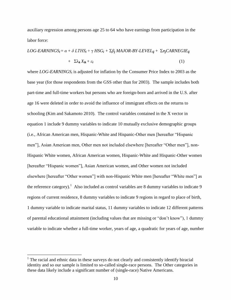
auxiliary regression among persons age 25 to 64 who have earnings from participation in the

labor force:

LOG-EARNINGSi = α + δ LTHSi + γ HSGi + Σβj MAJOR-BY-LEVELij + ΣπjCARNEGIEij

+ Σλk Xik + εi (1)

where LOG-EARNINGSi is adjusted for inflation by the Consumer Price Index to 2003 as the

base year (for those respondents from the GSS other than for 2003). The sample includes both

part-time and full-time workers but persons who are foreign-born and arrived in the U.S. after

age 16 were deleted in order to avoid the influence of immigrant effects on the returns to

schooling (Kim and Sakamoto 2010). The control variables contained in the X vector in

equation 1 include 9 dummy variables to indicate 10 mutually exclusive demographic groups

(i.e., African American men, Hispanic-White and Hispanic-Other men [hereafter “Hispanic

men”], Asian American men, Other men not included elsewhere [hereafter “Other men”], non-

Hispanic White women, African American women, Hispanic-White and Hispanic-Other women

[hereafter “Hispanic women”], Asian American women, and Other women not included

elsewhere [hereafter “Other women”] with non-Hispanic White men [hereafter “White men”] as

the reference category).1 Also included as control variables are 8 dummy variables to indicate 9

regions of current residence, 8 dummy variables to indicate 9 regions in regard to place of birth,

1 dummy variable to indicate marital status, 11 dummy variables to indicate 12 different patterns

of parental educational attainment (including values that are missing or “don’t know”), 1 dummy

variable to indicate whether a full-time worker, years of age, a quadratic for years of age, number

1 The racial and ethnic data in these surveys do not clearly and consistently identify biracial

identity and so our sample is limited to so-called single-race persons. The Other categories in

these data likely include a significant number of (single-race) Native Americans.

11

of children, and two interaction terms between being female with marital status, and being

female with number of children.

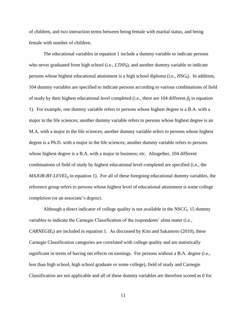
The educational variables in equation 1 include a dummy variable to indicate persons

who never graduated from high school (i.e., LTHSi), and another dummy variable to indicate

persons whose highest educational attainment is a high school diploma (i.e., HSGi). In addition,

104 dummy variables are specified to indicate persons according to various combinations of field

of study by their highest educational level completed (i.e., there are 104 different βj in equation

1). For example, one dummy variable refers to persons whose highest degree is a B.A. with a

major in the life sciences; another dummy variable refers to persons whose highest degree is an

M.A. with a major in the life sciences; another dummy variable refers to persons whose highest

degree is a Ph.D. with a major in the life sciences; another dummy variable refers to persons

whose highest degree is a B.A. with a major in business; etc. Altogether, 104 different

combinations of field of study by highest educational level completed are specified (i.e., the

MAJOR-BY-LEVELj in equation 1). For all of these foregoing educational dummy variables, the

reference group refers to persons whose highest level of educational attainment is some college

completion (or an associate’s degree).

Although a direct indicator of college quality is not available in the NSCG, 15 dummy

variables to indicate the Carnegie Classification of the respondents’ alma mater (i.e.,

CARNEGIEi) are included in equation 1. As discussed by Kim and Sakamoto (2010), these

Carnegie Classification categories are correlated with college quality and are statistically

significant in terms of having net effects on earnings. For persons without a B.A. degree (i.e.,

less than high school, high school graduate or some college), field of study and Carnegie

Classification are not applicable and all of these dummy variables are therefore scored as 0 for

12

these groups in equation 1.

Based on the results for equation 1, the MBM score for less than high school is the

estimated δ while the MBM score for high school graduate is the estimated γ. Because some

college is used as the reference category, its MBM score is defined to be zero. For persons who

have higher educational attainment, their MBM score is obtained as the sum of their respective

estimated βj (based on their particular combination of educational level and field of study) and

their respective estimated πj (based on the Carnegie classification for the college of their highest

degree). Thus, an individual’s MBM score refers to the coefficients from equation 1 that are

associated with his or her educational attainment.

Regression Models of MBM

Having constructed MBM using the above procedure, we then can use it as the dependent

variable in another separate regression to investigate demographic differentials in educational

attainment. Because MBM is a continuous variable, a linear regression model may be estimated.

In this part of the analysis, the models are estimated across all individuals with valid data on their

educational attainment (i.e., is not restricted to persons in the labor force). We estimate these

OLS regressions models for the cohort of ages 25 to 34. The same 10 demographic groups

differentiated by race, ethnicity and gender (as described above) are again used with White men

as the reference category. In order to simplify the analysis, foreign-born persons are excluded in

order to avoid the confluence of immigration effects with these demographic groups. The other

independent variables include age, age-squared, 8 dummy variables to indicate region of

residence at age 16, 4 dummy variables to mother’s educational level, and 4 dummy variables to

father’s educational level. An additional dummy variable to indicate whether father’s

13

educational level is unknown since it may be correlated with having grown up in a female-

headed household which likely reduces educational attainment (McLanahan and Sandefur 1997).

EMPIRICAL RESULTS

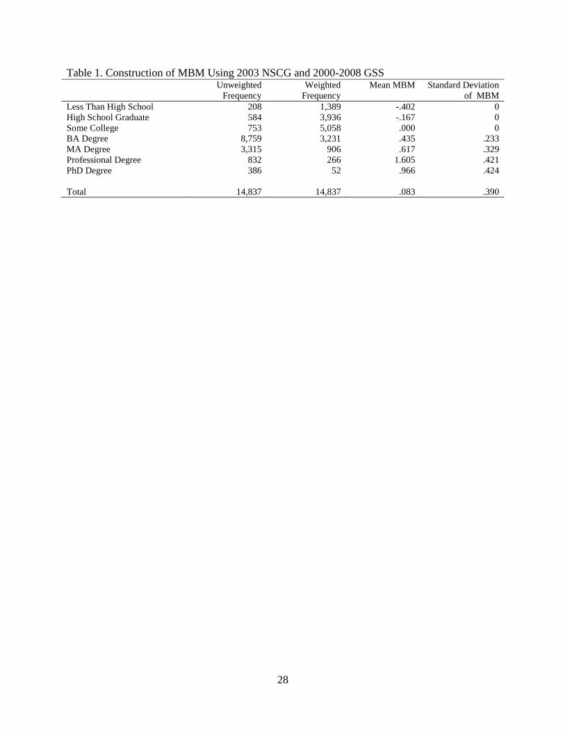
The results for the construction of the MBM are shown in Table 1. The cases from the

2000-2008 GSS are those respondents who are shown in Table 1 as having an educational level

that is less than high school, high school graduate, or some college. The cases from the 2003

NSCG are those respondents who are shown in Table 1 as having an educational level that is B.A.

degree, M.A. degree, professional degree, or Ph.D. degree.

TABLE 1 ABOUT HERE

As shown in Table 1, the mean MBM across the entire sample is .083 which is relatively

low due to the fact that most people do not have a college degree. Table 1 further shows that, for

persons without a high school degree, their MBM is -.402. This figure may also be interpreted as

indicating that the net effect of being a high school dropout is about 33 percent lower earnings

relative to workers with some college (because exp(-.402) – 1 = -.33). For high school graduates,

their MBM is -.167 which may also be interpreted as indicating that the net effect of being a high

school graduate is approximately15 percent lower earnings relative to workers with some college

(because exp(-.167) – 1 = -.15).

For persons with a B.A. degree, MBM varies depending upon the respondent’s particular

combination of field of study and Carnegie Classification. Table 1 shows that the standard

deviation in MBM among persons at the B.A. educational level is .233. The scores do not vary

(i.e., have a standard deviation of 0) for less than high school, high school graduate, and some

college because at those educational levels, field of study and Carnegie classification type are not

14

applicable in our construction of the MBM.

The mean MBM, as also shown in Table 1, is .435 at the B.A. level. The result implies

that workers with a B.A. degree earn, on average, about percent more than workers with some

college net of measured individual characteristics (because exp(.435) – 1 = .54). Furthermore,

the implied earnings differential relative to high school graduates is about 69 percent (i.e., 54 – (-

15)). For workers with an M.A. degree, the results in Table 1 imply that the net earnings

advantage (relative to some college) is about 85 percent on average. For workers with a Ph.D.

degree the net earnings advantage is 163 percent while it is 398 percent for workers with a

professional degree. The standard deviation for the MBM scores for each of these graduate

degrees shows that there is significant variation in these net effects depending upon the specific

field of study and the Carnegie classification type.

TABLES 2 AND 3 ABOUT HERE

Other descriptive statistics are shown in Table 2. Mean age is relatively young (i.e.,

about 30) because the sample is limited to persons aged 25 to 34. Slightly over one-fifth of the

sample has a B.A. degree as their highest completed educational level, and about that same

figure has a father or a mother with at least a B.A. degree.

The multiple regression results for educational attainment are shown in Table 3. MBM is

the dependent variable for Models 1 and 2.2 For comparative purposes, Models 3 and 4 show the

results for the corresponding specifications except that a logistic regression is used with the

2 The residuals from these OLS regressions have a slight degree of skew and heteroscedasticity

but adjusting for these features did not substantially improve or alter the estimates and so we

simply report the OLS results which are statistically consistent as well as easier to interpret.

Throughout these tables we report robust standard errors which are used in our assessments of

statistical significance.

15

dependent variables being whether or not the respondent has a B.A. degree regardless of field of

study and college type (i.e., the traditional approach as discussed earlier).

Models 1 and 3 in Table 3 are the bivariate specification that includes only the 9 dummy

variables to indicate the 10 different demographic groups. The estimates in Model 3 for college

completion that are statistically significant (relative to White men) include highly negative

effects for African American men, African American women, Hispanic men, Hispanic women,

Other men, and Other women. Such negative effects for African Americans and Hispanics in

Model 3 are consistent with prior research (Kao and Thompson 2003). The negative effects for

Other men and Other women probably derive from the high proportion of Native Americans in

these categories, and especially single-race Native Americans have lower levels of college

completion (Huyser, Sakamoto and Takei 2010). A large and statistically significant coefficient

for Asian American women is also consistent with prior research (Sakamoto, Goyette and Kim

2009). A positive coefficient for Asian American men is also reported in Model 3 although it is

not statistically significant at the .05 level.

After controlling for the social background variables in Model 4, many of the

aforementioned effects are statistically explained away. That is, the coefficients for African

American men, African American women, Hispanic men, Hispanic women, and Asian women

are no longer statistically significant in Model 4. Only the negative coefficients for Other men

and Other women remain significant in Model 4 after controlling for the social background

variables.

These results using the traditional approach may be contrasted with those using MBM as

the dependent variable in Models 1 and 2. The estimates for the demographic groups in Model 1

using MBM are mostly consistent with the estimates using the traditional approach in Model 3.

16

However, in Model 2 which controls for the social background variables, many of the

coefficients for the demographic groups remain statistically significant. When measured in

terms of MBM, the net effect for African American men is -.0683 which is significant at the .01

level. This result may also be interpreted as indicating that after controlling for the social

background variables, African American men have educational attainment that is associated with

6.8 percent lower earnings. Also in contrast to the results in Model 4, the coefficient for African

American women in Model 2 is significant and is indicative of having educational attainment

that is associated with 6.0 percent lower earnings.

Other estimates that differ from the results based on the traditional approach include the

statistically significant coefficient for Asian men in Model 2. This coefficient is .2109 and is the

largest (in absolute value) for any of the demographic groups in Model 2. By contrast, using the

traditional approach, the largest net effect (in absolute value) is for Other men in Model 4.

Another difference is that the coefficient for White women in Model 2 is -.0296 and it is

statistically significant at the .05 level. Net of social background variables, White women have

(on average) an MBM score than is about .03 lower than that for White men (or, in other words,

average educational attainment among White women is associated with 3 percent lower earnings

compared to the educational attainment of White men). This slight disadvantage contrasts with

the positive point estimate for White women in Model 4 using the traditional approach.

In terms of the net effects of parental education, the largest coefficients in Model 4 using

the traditional approach are for mothers with a B.A. degree and mothers with a graduate degree.

By contrast, using MBM as the dependent variable in Model 2, the largest coefficients are for

fathers with a B.A. degree and fathers with a graduate degree. Using MBM rather than the

17

traditional approach enlarges the effects of having a college-educated father relative to having a

college-educated mother.

TABLE 4 ABOUT HERE

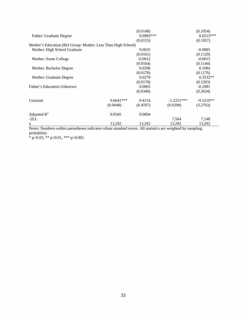
For exploratory purposes we re-estimated the models in Table 3 after restricting the

sample to persons who have a least a B.A. degree. These results for the college-educated sample

are shown in Table 4. The long specifications including all of the social background variables

are given by Models 6 and 8 in Table 4. Model 8 in Table 4 is based on the traditional approach

but in this case the dependent variable refers to the completion of any graduate degree (i.e., a

master’s degree or higher) since the sample if restricted to persons with at least a B.A. degree.

The results for Models 6 and 8 in Table 4 generally indicate fewer or smaller net effects

of the social background variables (especially in regard to parental education) in comparison to

the estimates in Table 3 for the overall sample. For example, none of the effects of mother’s

education is statistically significant when using MBM in Model 6 in Table 4. These reduced net

effects of the social background variables generally seem consistent with the assumption of

greater selectivity among more highly educated individuals and hence their greater deviation

from average social background effects (Mare 1980; Lucas 2001).

However, some notable differences are evident between Tables 3 and 4 in regard to the

net effects of demographic groups especially for women. The disadvantages for the female

demographic groups are greater in terms of MBM when the sample is restricted to college-

educated persons (i.e., in Table 4). For the overall sample in Model 2 using MBM in Table 3,

the net effect for White women is -.0296 but it is -.1639 in Model 6 in Table 4 for the college-

educated sample. This same comparison for African American women is -.0603 versus -.1226

while for Hispanic women it is -.0259 versus -.1005. When using the traditional approach in

18

Model 8 in Table 4, the coefficient for African American women is actually positive and

statistically significant (i.e., .2007) in contrast to the negative point estimate (i.e., -.3220) for this

group in Model 4 in Table 3.

DISCUSSION AND CONCLUSIONS

Our foregoing results may be interpreted as being broadly consistent with prior research.

In general, women are much less likely than men to major in STEM fields (Eide 1994; Morgan

2008). African Americans and Hispanics are less likely than Whites to major in STEM fields or

to graduate from Research I universities (Eide 1997; Black et al. 2006). Conversely, Asian

Americans tend to be overrepresented in both STEM fields and Research I universities (Xie and

Goyette 2003; Kim and Sakamoto 2010). Because MBM incorporates the earnings effects of

field of study and college type, demographic differentials associated with MBM may be expected

to vary from those based on the traditional approach which only depends upon educational level.

Using the traditional approach, recent research has emphasized the growing advantage

that women (especially White women) have over men in regard to the probability of obtaining a

B.A. degree (Buchmann and DiPrete 2006). While we agree that this pattern is undoubtedly

important, our results help to further enrich our understanding of gender differentials by

revealing that White women continue to be disadvantaged relative to White men when MBM is

used to calibrate educational attainment in a way that incorporates other dimensions besides the

highest level completed. Because White women are substantially less likely than White men to

complete STEM fields of study, White women remain slightly disadvantaged in terms of MBM

after controlling for social background variables (i.e., Model 2 in Table 3). This disadvantage is

especially pronounced when restricting the analysis to the college-educated sample (i.e., Model 6

19

in Table 4) because by conditioning on already having reached that stage, educational level is

thereby reduced in significance and field of study becomes more differentiating. In sum, our

findings indicate that when educational attainment is measured in terms of its potential for

greater earnings in the labor market, White women still lag behind and have yet to have achieved

parity with White men.

In a similar vein, the disadvantages for African Americans relative to White men are

more obvious when educational attainment is measured in terms of MBM rather than focusing

exclusively on educational level. After controlling for the social background variables using the

traditional approach, none of our estimates indicate a statistically significant negative effect for

either African American men or African American women. By contrast, after controlling for the

social background variables using MBM, all of our estimates indicate a statistically significant

negative effect for both African American men and African American women.

The extraordinary educational attainment of Asian men becomes more readily apparent

when using MBM due to the higher rates at which they major in STEM fields and attend more

prestigious universities. After controlling for the social background variables using MBM (i.e.,

Model 2 in Table 3), the coefficient for Asian men is the largest (in absolute value) across all of

the demographic groups. Contrarily, the coefficient for Asian men based on the traditional

approach (i.e., in Model 4 in Table 3), is smaller (in absolute value) than for several other groups,

and it is not even statistically significant at any conventional level.

Relative to the traditional approach, our findings for MBM increase the significance of

father’s education and decrease the significance of mother’s education in terms of their impact

on respondents’ educational attainment. This result may reflect that fact that fathers are more

likely than mothers to have degrees in STEM, and field of study factors into the construction of

20

MBM. Consistent with this interpretation, the results in Table 3 indicate that the relative

significance of father’s versus mother’s educational attainment in terms of MBM versus the

traditional approach do not differ for respondents whose parents do not have a B.A. or graduate

degree (among whom field of study is not defined in our approach).

In regard to future research, a topic that we would suggest is the investigation of the

possibly increasing role of parental income on educational attainment (Reardon 2011) when the

latter is measured in terms of MBM. As college costs continue to increase, the direct effect of

parental income on educational attainment may be rising. If the economic return to attending an

elite university is rising (Brewer, Eide and Ehrenberg 1999) while the tuition costs at such

institutions are reaching extraordinarily high levels, then parental income could possibly be

becoming more important in social stratification which could lead to a reduction in

intergenerational income mobility (Blanden, Gregg and Macmillan 2011). Although the

traditional approach to studying educational attainment focuses on educational level and thereby

omits elite institutional achievement, MBM is well equipped to be fruitfully deployed in the

study of this topic.

In this regard, obtaining data that provide more information on specific colleges would be

helpful in order to more carefully delineate the role of elite institutions in the social reproduction

of the higher social classes. Although useful, the categories provided by the Carnegie

classification are nonetheless fairly heterogeneous (West Virginia University and Harvard are

both classified as Research I Universities, for example). More precise data on alma maters

would facilitate greater precision in estimating the impact of parental income on educational

attainment as measured by MBM. The general issue of parental income may be particularly

21

relevant for the most recent cohorts who have encountered continued cost increases in tuition

fees especially at prestigious universities.3

Our MBM approach might also prove fruitful for international studies.4 In comparing

academic achievement across nations, the multidimensionality of different educational systems is

often difficult to collapse into the traditional approach because it assumes a single ordered

hierarchy of educational levels. By contrast, the construction of MBM readily handles multiple

dimensions (and does away with any reliance on a clearly defined ordered hierarchy) by

calibrating educational attainment in terms of its potential for labor market rewards. Indeed,

given suitable data and an appropriate rationale for a given society, equation 1 could be extended

to include additional dimensions of educational outcomes (e.g., GPA or test scores) if they are

significant in terms of the how employers reward workers.

3 Given more precise information on alma maters, future research might also explore three-way

interactions between college prestige, field of study, and educational level. An M.B.A. from

Harvard or a master’s degree in computer science from University of Illinois at Urbana might

differ notably from other degrees from those universities in terms of economic opportunities. 4 In fact, our MBM approach is inspired by a comparative study of the effect of educational

attainment on occupational achievement in the U.S. and the U.K. (Treiman and Terrell 1975).

22

REFERENCES

Autor, David H., Lawrence F. Katz and Melissa S. Kearney. 2006. “The Polarization of the U.S.

Labor Market.” American Economic Review 96:189-194.

Autor, David H., Lawrence F. Katz and Melissa S. Kearney. 2008. “Trends in U.S. Wage

Inequality: Revising the Revisionists.” Review of Economics and Statistics Review

90:300-323.

Becker, Gary S. and Kevin M. Murphy. 2007. “Education and Consumption: The Effects of

Education in the Household Compared to the Marketplace.” Journal of Human Capital

1:9-35.

Berger, Mark C. 1988. “Predicted Future Earnings and Choice of College Major.” Industrial and

Labor Relations Review 41:375–83.

Black, Dan, Amelia Haviland, Seth Sanders and Lowell Taylor. 2006. “Why Do Minority Men

Earn Less? A Study of Wage Differentials among the Highly Educated.” Review of

Economics and Statistics 82:300-313.

Blanden, Jo, Paul Gregg and Lindsey Macmillan. 2011. “Intergenerational Persistence in Income

and Social Class: The Impact of Within-Group Inequality.” IZA Discussion paper

No.6202. Institute for the Study of Labor. Bonn, Germany.

ftp://ftp.iza.org/RePEc/Discussionpaper/dp6202.pdf

Brand, Jennie E. and Yu Xie. 2010. “Who Benefits Most from College? Evidence for Negative

Selection in Heterogeneous Economic Returns to Higher Education.” American

Sociological Review 75:273-302.

Breen, Richard and John H. Goldthorpe. 1997. “Explaining Educational Differentials: Towards a

Formal Rational Action Theory.” Rationality and Society 9:275-305.

23

Brewer, Dominic J., Eric R. Eide, and Ronald G. Ehrenberg. 1999. “Does It Pay to Attend and

Elite Private College? Cross-Cohort Evidence on the Effects of College Type on

Earnings.” Journal of Human Resources 34:104–23.

Buchmann, Claudia and Thomas A. DiPrete. 2006. “The Growing Female Advantage in College

Completion: The Role of Family Background and Academic Achievement.” American

Sociological Review 71:515-541.

Cameron, Stephen V. and James J. Heckman. 2001. “The Dynamics of Educational Attainment

for Black, Hispanic, and White Males.” Journal of Political Economy 109:455-499.

Card, David and John E. DiNardo. 2002. “Skill-Biased Technological Change and Rising Wage

Inequality: Some Problems and Puzzles.” Journal of Labor Economics 20:733–83.

Eide, Eric. 1994. “College Major Choice and Changes in the Gender Wage Gap.” Contemporary

Economic Policy 12:55-64.

Eide, Eric. 1997. “Accounting for Race and Gender Differences in College Wage Premium

Changes.” Southern Economic Journal 63:1039–50.

Everett, Bethany G., Richard G. Rodgers, Patrick M. Krueger and Robert A. Hummer. 2007.

“Trends in Educational Attainment by Sex, Race/Ethnicity, and Nativity in the United

States, 1989-2005.” Working Paper #POP2007-07, Institute of Behavioral Science,

University of Colorado at Boulder, Boulder, Colorado.

Farley, Reynolds. 1996. The New American Reality. New York: Russell Sage Foundation.

Fischer, Claude S. and Michael Hout. 2006. Century of Difference: How America Changed in the

Last One Hundred Years. New York: Russell Sage Foundation.

Goldin, Claudia and Lawrence Katz. 2008. The Race between Education and Technology.

Cambridge, MA: Belknap Press of Harvard University Press.

24

Goyette, Kimberly A. and Ann L. Mullen. 2006. “Who Studies the Arts and Sciences? Social

Background and the Choice and Consequences of Undergraduate Field of Study.”

Journal of Higher Education 77:497-538.

Huyser, Kimberly R., Arthur Sakamoto and Isao Takei. 2010. “The Persistence of Racial

Disadvantage: The Socioeconomic Attainments of Single-Race and Multi-Race Native

Americans.” Population Research and Policy Review 29:541-568.

Kane, Thomas J. 2004. “College-Going and Inequality.” Pp. 319-353 in Social Inequality edited

by K. M. Neckerman. New York: Russell Sage Foundation.

Kao, Grace and Jennifer S. Thompson. 2003. “Racial and Ethnic Stratification in Educational

Achievement and Attainment.” Annual Review of Sociology 29:417-442.

Kim, ChangHwan and Arthur Sakamoto. 2008. “The Rise of Intra-Occupational Inequality in the

United States, 1983 to 2002.” American Sociological Review 73:129-157.

Kim, ChangHwan and Arthur Sakamoto. 2010. “Have Asian American Men Achieved Labor

Market Parity with White Men?” American Sociological Review 75:934-957.

Lemieux, Thomas. 2006. “Postsecondary Education and Increasing Wage Inequality.” American

Economic Review 96:195-199.

Loury, Linda Datcher and David Garman. 1995. “College Selectivity and Earnings.” Journal of

Labor Economics 13:289–308.

Lucas, Samuel. 2001. “Effectively Maintained Inequality: Education Transitions, Track

Mobility, and Social Background Effects.” American Journal of Sociology 106:1642-

1690.

Mare, Robert D. 1980. “Social Background and School Continuation Decisions.” Journal of

American Statistical Association 75:295–305.

25

Mare, Robert D. 1995. “Changes in Educational Attainment and School Enrollment.” Pp. 155-

213 in State of the Union: America in the 1990s. Volume I: Economic Trends edited by R.

Farley. New York: Russell Sage Foundation.

Mare, Robert D. and Vida Maralani. 2006. “The Intergenerational Effects of Changes in

Women’s Educational Attainments.” American Sociological Review 71:542-564.

McLanahan, Sara and Gary D. Sandefur. 1997. Growing Up with a Single Parent: What Hurts,

What Helps. Cambridge, MA: Harvard University Press.

Mirowsky, John and Catherine E. Ross. 2003. Education, Social Status, and Health. New York:

Aldine de Gruyter.

Morgan, Laurie A. 2008. “Major Matters: A Comparison of the Within-Major Pay Gap across

College Majors for Early-Career Graduates.” Industrial Relations 47:625-650.

Reardon, F. Sean. 2011. “The Widening Academic Achievement Gap between the Rich and the

Poor: New Evidence and Possible Explanations.” Pp. 91-116 in Whither Opportunity:

Rising Inequality and the Uncertain Life Chances of Low-Income Children edited by R.

Murname and G. Duncan. New York: Russell Sage Foundation.

Rumberger, Russell and Scott L. Thomas. 1993. “The Economic Returns to College Major,

Quality and Performance: A Multilevel Analysis of Recent Graduates.” Economics of

Education Review 12:1–19.

Sakamoto, Arthur and Daniel A. Powers. 1995. “Education and the Dual Labor Market for

Japanese Men.” American Sociological Review 60:222-246.

Sakamoto, Arthur, Kimberly A. Goyette and ChangHwan Kim. 2009. “The Socioeconomic

Attainments of Asian Americans.” Annual Review of Sociology 35:255-276.

26

Sewell, William H. and Robert M. Hauser. 1975. Education, Occupation, and Earnings. New

York: Academic Press.

Shavit, Yossi and Hans-Peter Blossfeld (eds). 1993. Persistent Inequality: Changing Educational

Attainment in Thirteen Countries. Boulder, CO: Westview Press.

Shavit, Yossi, Meir Yaish and Eyal Bar-Haim. 2007. “The Persistence of Persistent Inequality.”

Pp.37-57 in From Origin to Destination: Trends and Mechanisms in Social Stratification

Research edited by S. Scherer, R. Pollack, G. Otte and M. Gangl. Chicago, IL: University

of Chicago Press.

Song, Chunyan and Jennifer E. Glick. 2004. “College Attendance and Choice of College Majors

Among Asian-American Students.” Social Science Quarterly 85:1401–21.

Thomas, Scott. 2000. “Deferred Costs and Economic Returns to College Quality, Major and

Academic Performance: An Analysis of Recent Graduates in Baccalaureate and Beyond.”

Research in Higher Education 41:281-313.

Thomas, Scott. 2003. “Longer-Term Economic Effects of College Selectivity and Control.”

Research in Higher Education 44:263-299.

Thomas, Scott and Liang Zhang. 2005. “Post-Baccalaureate Wage Growth within Four Years of

Graduation: The Effects of College Quality and College Major.” Research in Higher

Education 46:437-459.

Treiman, Donald J. and Kermit Terrell. 1975. “The Process of Status Attainment in the United

States and Great Britain.” American Journal of Sociology 81:563–583.

U.S. Census Bureau. 2012. Statistical Abstract of the United States (131st edition). Washington,

D.C., 2011. http://www.census.gov/compendia/statab/.

Weber, Max. [1904]/1949. The Methodology of the Social Sciences. New York: Free Press.

27

Xie, Yu and Kimberly A. Goyette. 2003. “Social Mobility and the Educational Choices of Asian

Americans.” Social Science Research 32:467–98.

Zhang, Liang. 2005. “Advance to Graduate Education: The Effect of College Quality and

Undergraduate Majors.” Review of Higher Education 28:313-338.

28

Table 1. Construction of MBM Using 2003 NSCG and 2000-2008 GSS Unweighted

Frequency

Weighted

Frequency

Mean MBM Standard Deviation

of MBM

Less Than High School 208 1,389 -.402 0

High School Graduate 584 3,936 -.167 0

Some College 753 5,058 .000 0

BA Degree 8,759 3,231 .435 .233

MA Degree 3,315 906 .617 .329

Professional Degree 832 266 1.605 .421

PhD Degree 386 52 .966 .424

Total 14,837 14,837 .083 .390

29

Table 2. Descriptive Statistics Total Men Women

Level of Education (%)

Less Than High School 9.36 9.45 9.29

High School Graduate 26.53 28.29 25.13

Some College 34.09 32.53 35.33

Bachelor Degree 21.78 22.12 21.51

Master Degree 6.10 4.98 7.00

Professional Degree 1.79 2.20 1.46

PhD 0.35 0.43 0.28

Age (Mean) 29.82 29.79 29.85

Father’s education BA+ (%) 21.1 22.1 20.3

Mother’s education BA+ (%) 19.4 20.3 18.2

Weighted Sample Size 14,837 6,568 8,269

Notes: All statistics are weighted by sampling probabilities.

30

Table 3. OLS and Logistic Regression Models of Educational Attainment Using the Merged

2003 NSCG and the 2000-2008 GSS OLS of MBM Logit of Having Bachelor

or Higher Degree

Model 1 Model 2 Model 3 Model 4

Coeffi. Sig. Coeffi. Sig. Coeffi. Sig. Coeffi. Sig.

Group: (Ref Group: Non-Hispanic White Men)

Non-Hispanic Black Men -0.1782 *** -0.0683 ** -1.1912 *** -0.3840

(0.0205) (0.0217) (0.1555) (0.2342)

Hispanic Men -0.2077 *** -0.0291 -1.3946 *** -0.4097

(0.0258) (0.0284) (0.1668) (0.3041)

Asian Men 0.2542 * 0.2109 * 0.5880 0.6624

(0.1220) (0.0873) (0.4388) (0.4354)

Other Race Men -0.2452 *** -0.1506 *** -2.6093 *** -2.4178 ***

(0.0164) (0.0170) (0.1504) (0.2352)

Non-Hispanic White Women -0.0272 -0.0296 * 0.0925 0.1050

(0.0146) (0.0118) (0.0802) (0.1036)

Non-Hispanic Black Women -0.1866 *** -0.0603 *** -1.1457 *** -0.3220

(0.0173) (0.0164) (0.1127) (0.1745)

Hispanic Women -0.1951 *** -0.0259 -1.2611 *** -0.3189

(0.0199) (0.0235) (0.1478) (0.2856)

Asian Women 0.3135 0.1721 1.5332 * 1.2448

(0.1649) (0.1259) (0.7554) (0.7280)

Other Race Women -0.2593 *** -0.1518 *** -2.4946 *** -2.3527 ***

(0.0163) (0.0164) (0.1379) (0.1940)

Age 0.1182 *** 2.6232 ***

(0.0359) (0.3961)

Age-squared -0.0017 ** -0.0409 ***

(0.0006) (0.0066)

Region at age 16: (Ref Group: New

England)

Middle Atlantic 0.0200 -0.0066

(0.0297) (0.2721)

East North Central -0.0131 -0.3867

(0.0289) (0.2596)

West North Central -0.0041 -0.1536

(0.0313) (0.2870)

South Atlantic -0.0304 -0.5956 *

(0.0288) (0.2600)

East South Central -0.0184 -0.3997

(0.0314) (0.2999)

West South Central -0.0269 -0.4037

(0.0302) (0.2796)

Mountain -0.0915 ** -1.0776 ***

(0.0325) (0.2957)

Pacific -0.0809 ** -0.9182 ***

(0.0298) (0.2739)

Father’s Education: (Ref Group: Father: Less Than High School)

Father: High School Graduate 0.0449 ** 0.4311 **

(0.0154) (0.1412)

Father: Some College 0.1550 *** 1.1119 ***

(0.0177) (0.1597)

31

Father: Bachelor Degree 0.2549 *** 1.8042 ***

(0.0210) (0.1811)

Father: Graduate Degree 0.3389 *** 2.0219 ***

(0.0251) (0.2113)

Mother’s Education (Ref Group: Mother: Less Than High School)

Mother: High School Graduate 0.1017 *** 1.0623 ***

(0.0123) (0.1433)

Mother: Some College 0.1699 *** 1.5556 ***

(0.0137) (0.1581)

Mother: Bachelor Degree 0.2429 *** 2.0330 ***

(0.0196) (0.1918)

Mother: Graduate Degree 0.2932 *** 2.4357 ***

(0.0236) (0.2310)

Father’s Education Unknown -0.0939 *** -2.9973 ***

(0.0143) (0.2048)

Constant 0.1636 *** -2.0291 *** -0.4715 *** -43.7548 ***

(0.0115) (0.5271) (0.0593) (5.8737)

Adjusted R2 0.0725 0.3221

-2LL 10,994 9,082

n 14,837 14,837 14,837 14,837

Notes: Numbers within parentheses indicates robust standard errors. All statistics are weighted by sampling

probability.

* p<0.05, ** p<0.01, *** p<0.001

32

Table 4. OLS and Logistic Regression Models of Educational Attainment Among Workers with

Bachelor Degree or Higher Using the Merged 2003 NSCG and the 2000-2008 GSS OLS of MBM Logit of Having Graduate Degree

Model 5 Model 6 Model 7 Model 8

Coeffi. Sig. Coeffi. Sig. Coeffi. Sig. Coeffi. Sig.

Group: (Ref Group: Non-Hispanic White Men)

Non-Hispanic Black Men -0.0565 *** -0.0412 * -0.1966 -0.1158

(0.0165) (0.0167) (0.1128) (0.1169)

Hispanic Men -0.0390 * -0.0027 -0.0889 0.1039

(0.0179) (0.0183) (0.1197) (0.1257)

Asian Men 0.1788 *** 0.1789 *** 1.1288 *** 1.0677 ***

(0.0215) (0.0213) (0.1247) (0.1297)

Other Race Men -0.0750 ** -0.0615 * 0.1597 0.2115

(0.0239) (0.0240) (0.1749) (0.1818)

Non-Hispanic White Women -0.1662 *** -0.1639 *** 0.0360 0.0573

(0.0065) (0.0065) (0.0418) (0.0428)

Non-Hispanic Black Women -0.1443 *** -0.1226 *** 0.0508 0.2007 *

(0.0133) (0.0136) (0.0840) (0.0885)

Hispanic Women -0.1391 *** -0.1005 *** -0.1314 0.0908

(0.0200) (0.0199) (0.1126) (0.1189)

Asian Women -0.0167 -0.0134 0.7646 *** 0.6926 ***

(0.0198) (0.0199) (0.1291) (0.1336)

Other Race Women -0.1397 *** -0.1204 *** -0.1729 -0.1002

(0.0210) (0.0209) (0.1369) (0.1419)

Age 0.0049 0.4326 *

(0.0306) (0.2162)

Age-squared 0.0000 -0.0056

(0.0005) (0.0036)

Region at age 16: (Ref Group: New

England)

Middle Atlantic 0.0058 0.1034

(0.0127) (0.0871)

East North Central 0.0310 * 0.0412

(0.0124) (0.0860)

West North Central 0.0047 -0.0791

(0.0143) (0.0990)

South Atlantic 0.0075 0.0193

(0.0130) (0.0896)

East South Central 0.0077 -0.0318

(0.0164) (0.1115)

West South Central -0.0150 -0.2049 *

(0.0142) (0.0978)

Mountain 0.0097 -0.1952

(0.0164) (0.1122)

Pacific -0.0412 ** -0.1016

(0.0141) (0.0950)

Father’s Education: (Ref Group: Father: Less Than High School)

Father: High School Graduate 0.0147 0.0195

(0.0143) (0.1026)

Father: Some College 0.0269 0.0429

(0.0147) (0.1048)

Father: Bachelor Degree 0.0513 *** 0.1323

33

(0.0148) (0.1054)

Father: Graduate Degree 0.0983 *** 0.6513 ***

(0.0155) (0.1057)

Mother’s Education (Ref Group: Mother: Less Than High School)

Mother: High School Graduate 0.0032 -0.0885

(0.0161) (0.1129)

Mother: Some College -0.0012 -0.0015

(0.0164) (0.1144)

Mother: Bachelor Degree 0.0296 0.1084

(0.0170) (0.1176)

Mother: Graduate Degree 0.0279 0.3532 **

(0.0178) (0.1203)

Father’s Education Unknown 0.0065 -0.2081

(0.0346) (0.2624)

Constant 0.6641 *** 0.4154 -1.2251 *** -9.5210 **

(0.0048) (0.4597) (0.0298) (3.2763)

Adjusted R2 0.0545 0.0694

-2LL 7,564 7,148

n 13,292 13,292 13,292 13,292

Notes: Numbers within parentheses indicates robust standard errors. All statistics are weighted by sampling

probability.

* p<0.05, ** p<0.01, *** p<0.001