Demand System Estimations and Welfare Comparisons : Application to

Indian Household Data

Jaya Krishnakumar, Gabriela Flores and Sudip Ranjan Basu

No 2004.13

Cahiers du département d’économétrie

Faculté des sciences économiques et sociales Université de Genève

Mai 2004

Département d’économétrie Université de Genève, 40 Boulevard du Pont-d’Arve, CH -1211 Genève 4

http://www.unige.ch/ses/metri/

Demand System Estimations and Welfare Comparisons: Application to Indian Household Data

Gabriela Flores Jaya Krishnakumar1 Department of Econometrics Department of Econometrics

University of Geneva University of Geneva

and

Sudip Ranjan Basu Graduate Institute of International Studies

University of Geneva

May 2004

Abstract In this study, we explore the relationship between the rank of a demand system and the estimation results both in terms of consumption behaviour and more importantly in terms of welfare analysis. Money-metric utility levels given by equivalent expenditures are taken as welfare indicators for calculating poverty and inequality measures as they incorporate substitution effects due to relative price changes. Estimations are carried out using relevant data concerning Indian households (rural and urban) collected from nation-wide surveys conducted by the National Sample Survey Organisation (NSSO). We find that although the specification does play an important role in the economic explanation of consumer behaviour with some models being more suited than others depending on the pattern of consumption, welfare comparisons do not change significantly from one model specification to the other. On the other hand, there are notable differences between results based on estimated equivalent expenditures and those based on observed real expenditures.

Keywords: Demand system estimation, household surveys, poverty, inequality, India

JEL Classification Codes: C3, D1, D6, O53

1 Corresponding author: Department of Econometrics, University of Geneva, 40 Bd. du Pont d’Arve, CH-1211 Geneva 4, Switzerland. Tel. +41 22 379 8220. Fax. +41 22 379 8299. Email: jaya.krishnakumar@metri.unige.ch The authors wish to thank the Swiss National Fund for Scientific Research for providing financial support for this study.

1. Introduction Poverty and inequality comparisons are in general based on income or total

consumption expenditure deflated using the conventional Consumer Price Index as the

deflator. The problem with this practice is that substitution effects in consumption due to

changes in relative prices are ignored and therefore utility-compensated effects are not

considered. Depending on the structure of preferences and the extent of relative price changes,

the above method could seriously bias welfare comparisons. One way to solve this problem is

to use equivalent expenditures calculated at some references prices.

What kind of consequences do we run into by ignoring substitution effects in the

evaluation of total expenditures? Do demand systems of different ranks give different

conclusions? How do distortions in the estimation of equivalent expenditures affect the

welfare measures which are based on the distribution of these expenditures? Our study is an

attempt to answer all these questions using appropriate econometric models and methods, and

large-scale micro-level data for a developing country. It is mainly focused on taking

substitution effects into account in calculating welfare measures, exploring different

preference structures leading to demand systems of different ranks, and investigating the

relationship between rank and welfare comparisons based on equivalent expenditures. As our

data set refers to a developing country with a relatively low per capita expenditure, we give

special attention to the substitution effects for the poor as it is often assumed that these effects

are negligible for them.

The above research is carried out using household budget data from the 55th round of

India’s National Sample Survey (1999-2000) and price data for different categories of goods

across different States published by the Labour Bureau of the Government of India. The next

section gives a summary of the theoretical models used to estimated equivalent expenditures

and goes over the poverty and inequality measures calculated in our analysis. A description of

the data set is given in the Section 3. Section 4 analyses the estimation results both in terms of

coefficients and elasticities. Here we also include a brief discussion on the quality of fit.

Section 5 examines the distribution of equivalent expenditure estimates according to different

models and ranks. This section also contains our main results on welfare measures based on

our estimations comparing them among different models and with those based on observed

real expenditures. Finally we end the paper with the main conclusions.

2

2. Theoretical Background

Poverty measures are often derived from income or total expenditure as a welfare

indicator. However using any indicator in nominal terms can introduce apparent welfare

improvements over time when it is not true. A practical and simple solution consists in

deflating period 1 data by an aggregate price index given by a weighted average of elementary

price indices with fixed weights ( ) : jω

P(1/0) = 0j

1j

jj p

p ∑ ω

with period 0 as the reference period. However, this approach rules out substitution effects

between various categories or groups due to changes in relative prices.

A more suitable choice is the indirect utility function u(p1, xh, ah) which gives the

utility achieved in period 1, given prices p1, income xh and other relevant characteristics ah. A

money measure of this utility at constant prices is given by the equivalent expenditure: x e,h = c(u(p1, xh, ah), a0, p0)

where p0 and p1 denote prices at periods 0 and 1 respectively, a0 denotes the reference

household characteristics, u(...) the indirect utility function, and c(..) denotes the cost function.

Household composition can be accounted for either by demographic scaling or demographic

translating, we decided to adopt the latter approach as a first attempt.

In demand analysis, Gorman (1981) investigated the class of polynomial demand

systems which can be written in the form

q j (p, x) = )x(G)p(a sSs

js∑∈

and showed that the maximum column rank of the n × S matrix A= {a js} is three in the class

of demand systems which are linear in functions of expenditure and aggregate over

consumers. Full rank systems, i.e. systems with maximum column rank, maximise the degree

of income flexibility of demands with the fewest number of parameters. Our analysis of the

sensitivity of welfare measures to rank is based on three models of different ranks: Linear

expenditure system of rank 1 (cf. Stone (1954)), Almost Ideal Demand System (AIDS) of rank

2 (cf. Deaton and Muellbauer (1980) ) and Quadratic AIDS of rank 3 (cf. Banks, Blundell and

3

Lewbel (1997) and Ravallion and Subramanian (1996) ). As these models are well-known in

the economic literature, we only give below the expressions of the various quantities used in

our further calculations without additional explanations.

Demand systems

Linear Expenditure System, LES

The simplest unit rank demand system we may consider is the linear demand system

proposed by Stone (1954). Introducing the household characteristics with the translating

method the demand function is given by

−−++= ∑ ∑∑∑

==

n

1ks

S

sisk

n

kik

i

isS

1sisii Dδp * p r

p Dδ* x αβα , i = 1,...,M (1)

where Ds, s = 1,…,S denote the household’s demographic characteristics. The indirect utility

function is: ( ) ( )∏

∑∑∑=

k

k

kβα

α

kp

Dδp - *p -r rp,

0

k ssksk

kk

u

and the equivalent expenditure is given by

x e,h(p0, u) = ( ) ( ) ∑∑∑∏ ++k s

sks0k

kk

0k

k

k0k

11 Dδp * p p r ,pu αβ

The additivity restriction ∑ implies that =i

ii r qp .1 ∑ =i

iα

Almost Ideal Demand System, AIDS

This model proposed by Deaton and Muellbauer (1980) is of a flexible functional form

which derives the budget share equation starting from the specification of a cost function

belonging to the PIGLOG family. The budget share is of the form:

∑∑ +

++=

jjiji

sii plog γ

Prlog β D α w

sisδ (2)

The indirect utility function incorporates the demographic conditions is given by:

( )∏

∑ ∑∑=

k

β 1k

i j

1j

1i

1k

ss

1k

1

k

k0

p

plog plog 21 -plog D - plog - -r log

r),u(pksδαα ∑

4

with log P = ∑ ∑∑∑ +

++

kj

k jk

sk plog plog γ

21 plog D α α

kjsks0 kδ

Because of the additivity restriction given by , parameters are constrained as

follows:

1 wM

1ii =∑

=

iαα ∑−

=

−=.1M

1i 1

n, , , ∑

=

=1-M

1iis

- δδ ns ∑−

=

=1M

1in i

β - β ∑=

=1-M

1iijnj γ - γ

The equivalent expenditure function for this model is:

Log x e,h = ( ) ( )0110 p r ,pu Plog b+

where b(p) defines a price aggregator. ( )∏=i

iβ ip

Quadratic Almost Ideal Demand System

Bank, Blundell, and Lewbel (1997) proposed a QUAIDS model2 which in fact adds a

quadratic income term to the Deaton and Muellbauer AIDS model as we can see below:

Prlog

b(p)λ

plog γ Pr log β D w

2

jss

i

jijiii

++

++= ∑∑ isδα (3)

where the price index is given by

log P = ∑ ∑∑∑ +

++

k k jk

sk plog log γ

21 plog D α

kjsks0 kjpδα

and a price aggregator is defined as . A new function λ is introduced: ( )∏=i

iβ ip b(p)

( )ii

i plog λ λ(p) ∑= , and all the constraints of AIDS hold. λ λ1n

0iin ∑

−

==

The equivalent expenditure3 would be written as:

logx e,h = ( )

( )( ) ( )0111

00

p r ,pulog

p Plog

λ−+ −

bL

2 denoted as BBLQ in our empirical results 3 it is straightforward from this formula that if ( ) 0 =0pλ , the equivalent expenditure corresponds to the AIDS

equivalent expenditure.

5

We also consider an alternative QUAIDS model4 proposed by Ravallion and

Subramanian (1996). The principal difference between BBLQ and RSQ resides in the

specification of the parameter for the quadratic term whereas the price index and the

constraints remain the same. The model is:

( ) ( ) ( ) ( )( ) Prlog plog plog γ P

r log β D w2

jj

jjiji

ssisi i

+++++= ∑∑∑ jii θβθδα (4)

and the equivalent expenditure function is:

log x e,h = ( ) ( )1

0j

i

0110 log r ,pu Plog−

−

+− ∑∏

jji pp i θβ

In all the three models AIDS, QUAIDS-BBLQ and QUAIDS-RSQ, we impose the

symmetry condition jiij γγ = .

Estimation method

The equations directly estimated using our data are (1), (2), (3) and (4). An error term

εi is added to all these equations for estimation purposes. In addition, we assume that εvec ~

( )( )NIN ⊗ΣM ,0 where [ ]Mεεε ... 1' ≡ , M is the number of equations (categories) and N the

number of households. However the additivity restriction implies that Σ is singular. Therefore,

one of the M demand equations is dropped from the system, the remaining (M-1) equations

are estimated by maximum likelihood, and then the parameters of the last equation are

recovered using the parameters constraints of each model. The likelihood function for the (M-

1) equations is written as:

( ) ( ) [ ] *1*'*N

* vec 21 - IΣ log

21 - 2π log

21-MN - Llog εε vecI N

−⊗Σ⊗= (5)

denoting [ ]11*' ... −≡ Mεεε *. Substituting the expressions of Σ* in terms ε (derived from the

first order conditions) into the above likelihood, one obtains the following concentrated

likelihood function to be maximised with respect to θ, the vector of parameters:

( ) [ ]{ } *Σ log 2π log 1 1K 2N Llog ++−−= with ( ) ( )θθθ 'εε

N1 )(* *

h

N

1h

*h∑

=

≡Σ (6)

4 denoted as RSQ in our empirical results

6

where h represents a household index. This gives a nonlinear SUR model and as the

estimation program of such a model is not readily available, it was written in Stata. Here we

should gratefully acknowledge the help of Brian P. Poi who kindly gave us a code5 for

estimating the QUAIDS model of Bundell et al. (cf. Poi (2002) ). We wrote the estimation

programs of all the four different models taking Poi’s code as a base and modifying it

appropriately.

Once the unknown parameters are estimated, the equivalent expenditures are

calculated using the corresponding xe functions given above. Using xe as a welfare indicator, a

LES specification will amount to assuming that an additional 100 monetary units will

increment well-being by the same amount for poor and wealthy families alike. Rank 2

demand systems allowing for nonlinearities in the real expenditure response go some way in

alleviating this deficiency, while rank 3 systems further add flexibility in the expenditure

response.

Elasticities

An important element of the understanding of consumer behaviour is provided by

income and price elasticities of demand. These depend on the model considered and the

parameters therein. Income elasticity (or we should rather talk about total expenditure

elasticity) captures the percentage variation of the demand for the ith good for a 1% variation

of total expenditure. Let ηi denote this income elasticity . Demand of a “normal” good should

increase when the total expenditure increases (ηi > 0). If the variation is proportionally greater

than the income growth (ηi > 1), the good is qualified as a “luxurious” item. On the other

hand, if despite the income increase the demand of a good decreases (ηi < 0) , it is “inferior”.

5 Poi’s estimation code in STATA is available in www.stata-journal.com .

7

TABLE 1

Income elasticity formulas

Model ( ) rlogw i

∂∂ iiη

LES

iwiβ

AIDS

1 φ 1 iiwiβ +=+

BBLQ ( )Pr log b(p)

2λ β µ iii += 1

iwi +

µ

QRS

+

+= ∑

jjplog θ

Prlog 2β ψ

iii jiθβ

1 iwi+

ψ

Price elasticities give the “apparent” percentage variation of demand for the ith good

for a 1% variation of either its own price (own price elasticity єii ) or the price of the jth good

(cross price elasticity єij). This is an “apparent” change because it is a mixture of the income

effect and the substitution effect, namely a decrease of the price of the jth good for the same

quantity purchased increases the amount available to consumption of other items and

decreases demand of all substitutable goods. The price elasticities for our four models are

given below:

LES cross price elasticity with demographic variables:

єij =

+− ∑s

sjsjji

ji D q pp

δαβ

and єii = ( ) 1 - D q p

- 1 s

sisiii

i

+∑δαβ−

AIDS cross price elasticity with demographic variables:

єij = ( ) ijk

jkks

sjsjii

ij - plog D φ - w

δγδαγ

++ ∑∑ , with 0 1, ijii == δδ

BBLQ cross price elasticity with demographic variables:

єij = ( )( ) ( ) ijk

jkks

sjsji

i 2

i

ij

i

ij - plog D α wµ - P

r log wb(p)λ β

- w

δγδγ

++ ∑∑

8

QRS cross price elasticity with demographic variables:

єij = ( )( ) ( ) ijk

jkks

sjsji

i 2

i

ij

i

ij - plog D α w

- Pr log

w β

w

δγδψθγ

+++ ∑∑

The additivity restriction of the budget constraint ∑ =i

rqpii

or ∑ =i

w 1 i leads to the

following restrictions on elasticities:

- Engel’s aggregation restrictions in terms of elasticities given by: ∑i

wi ηi = 1

- Cournot’s aggregation restrictions : ∑i

wi єij + ηj = 0

The homogeneity of degree 0 of demand functions with respect to income (or total

expenditure) and prices also leads to a restriction in terms of elasticities: ∑j

єij + ηi = 0.

Compensated cross and own price elasticities ζij identify the “pure” price effect once

income has been compensated for the price increase. They are given by the Slustky equation:

ζij = єij + ηi wj

If ζij < 0 goods i and j are complementary.

If ζij < 0 goods i and j are independent.

If ζij > 0 goods i and j are substitutable.

Our estimates of elasticities are calculated at the mean values of budget shares because

median values are not very different from the mean ones in our sample.

Welfare measures

Sensitivity of welfare measurement to the rank of demand systems is analysed using

poverty and inequality measures based on equivalent expenditure as a household welfare

metric. This approach is adopted to incorporate utility-compensated substitution effects in

response to relative price changes which are simply ignored if one deflates nominal

expenditure by a fixed-weighted price index.

9

A first direct use of the equivalent expenditure, xe, is the well known cost of living

index (CLI) which measures the impact of relative price change in terms of percentage

variation of the cost function in order to keep the utility at a certain reference level :

( )( )1

0

11

u,pc

u,pc =CLI

Poverty measures

We have chosen six poverty measures and three inequality measures for our study.

The first three poverty measures belong to the class of decomposable poverty measures in the

sense that total poverty is a weighted average of the subgroup poverty levels and not in the

sense of decomposability applied to inequality that involves a “between-group” term. The first

two of them belong to the general class of Foster, Greer and Thorbecke (1984) measures:

FGT = α

∑=

−q

1i

izyz n

1 , 0 ≥α

where z is any given poverty line, yi the income of the ith household and q the number of poor,

i.e. person with an income less than or equal to z. The parameter α is a measure of poverty

aversion therefore a larger α gives more importance to the poorest of the poor and implies

greater severity of poverty.

When α = 0, the Foster et al. measure becomes the well known head count ratio H and

gives the proportion of the population living in households with per capita consumption below

the poverty line.

When α = 1, FGT is the poverty gap ratio PG and all the poor are given the same

weight. This index is also the product of the head count ratio and the income gap I, which is

the gap between the poverty line and the average income of the poor:

I = zz zµ− where is the mean consumption of the poor. zµ

These first two measures are distribution insensitive in the sense that they do not

consider the income distribution of the poor. Therefore two samples with the same mean

income of the poor but different income distributions would have the same head count and

poverty gap ratio.

10

All measures with α > 1 are distribution sensitive with weights being equal to the

income shortfalls of the poor. Thus they give importance to the extent of poverty among the

poor and not just to the number of poor. When α = 2 we have the squared gap ratio.

Our next measure, the Watts measure, is the first proposed distribution sensitive

poverty measure (cf. Watts (1968) ) and it gives the average of the income shortfall in

logarithmic terms. This is also a decomposable poverty measure.

W = ∑=

q

i iyz

n 1log 1

Next, we take the poverty measure proposed by Clark et al. (1981 ) (CHU), which is

distribution sensitive, subgroup consistent but not decomposable. It is obtained as the

deviation of an aggregate of individual poverty measures:

where ≤

=otherwise

y if , i*

zzy

y ii

( )

( )

=

≥≠

−

=

∑

∑

=

−−

1 if ,ln

exp-z

0 and 1 if ,

n

1i

*

11

1*

ε

εε

εε

n

y

n

yz

CHU

i

n

ii

Finally Sen’s poverty measure uses a poor person’s rank within the poor (or the whole

population) as an indicator of relative deprivation, Sen (1976). This aggregate measure

combines income gap and Gini index, along with headcount ratio:

S = [ ]pGIKIH )1( −+ , where K = 1+q

q and is the Gini index of the poor. pG

If there is no inequality among the poor ( G = 0), then S = Poverty Gap = I H p

Inequality measures

The first of the three inequality measures considered is the well-known Gini index

which gives the extent to which the actual distribution of income and/or consumption

expenditure differs from a hypothetical distribution in which each person receives an identical

11

share. This index is scaled from a minimum of zero (no inequality) to a maximum of one

(maximum inequality in the distribution).

For the linear expenditure system (LES), Kakwani (1980) establishes a direct link in

between the Gini index and the expenditure elasticity:

*G G ii η=

where i η is the expenditure elasticity of the ith commodity calculated at the mean prices and

is the Gini index of total expenditure. According to this relation, the expenditure elasticity

of the i

*Gth commodity at the mean expenditure is equal to the ratio of the Gini index of the

distribution of the ith commodity expenditure and the total expenditure, respectively. If i η

>(<) 1, expenditure on the ith good is more (less) unequally distributed than the total

expenditure. Using both definitions together mean that all luxurious item are also more

unequally distributed.

The second inequality measure proposed by Atkinson (1970) incorporates a normative

judgement of social welfare and is given by the Atkinson index:

µµ ey A −= , incomemean actual =µ

ey is the equity sensitive average income, defined as that level of per capita income which, if

enjoyed by everybody, would make total welfare exactly equal to the total welfare generated

by the actual income distribution:

( )ξξ −

=

−

= ∑

11

?

1

1.G

iiie

yyfy ,

where proportion of total income earned by the i=)y(f ith group, i = 1,…G. Here ξ6 is the

inequality aversion parameter, with higher values of ξ implying that society has greater

aversion towards inequality. We have 0 ≤ A ≤ 1 with inequality increasing as A approaches 1.

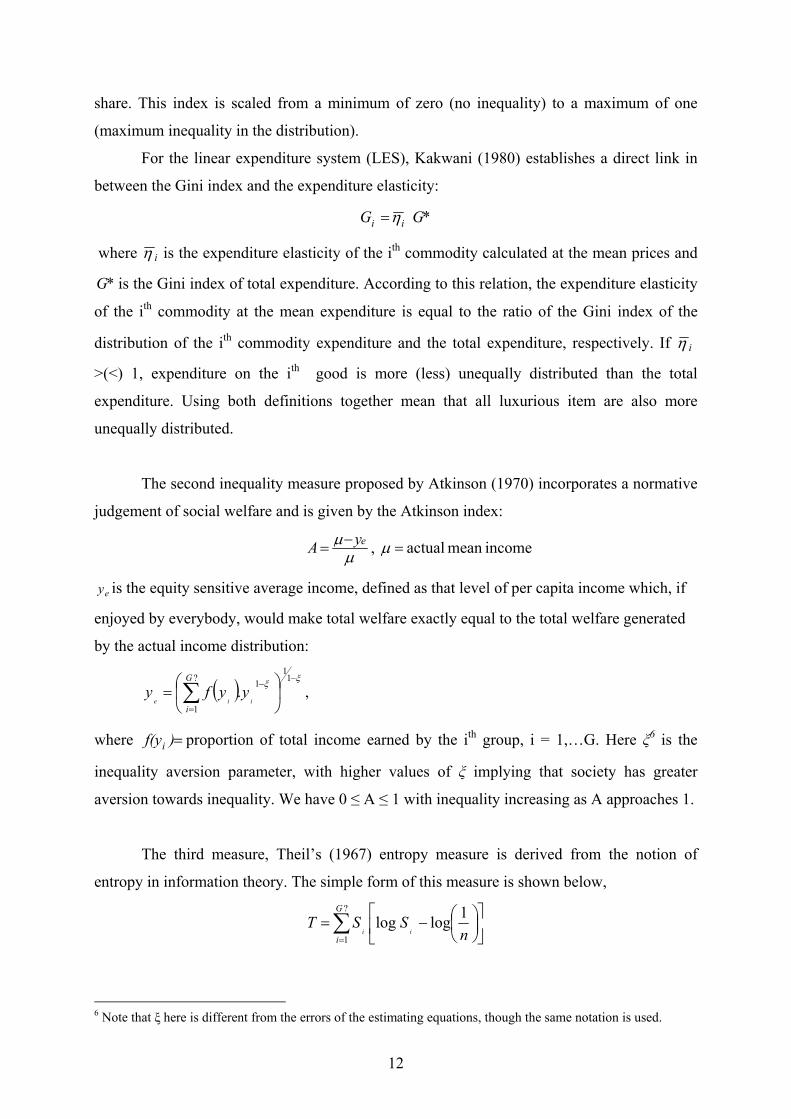
The third measure, Theil’s (1967) entropy measure is derived from the notion of

entropy in information theory. The simple form of this measure is shown below,

∑=

−=

?

1

1loglogG

i nSST

ii

6 Note that ξ here is different from the errors of the estimating equations, though the same notation is used.

12

where share of the i =iS th group in total income, G = total number of income groups. Higher

values of T imply more inequality.

3. Data

Consumer Price Index for Rural Labourers and Industrial workers are obtained from

the Labour Bureau (Government of India) on a monthly basis and Statewise with a 1986-

87=100 base for Rural Labourers and a 1982=100 base for Industrial workers. A simple

average is used to get a single value for each State in the sample, assuming that all the

households in a same State and a same area (rural or urban) face the same price level for each

item. Data on price index allows a five way split of consumption categories, namely Food

(FD); Fuel and light (FL); Pan, tobacco and intoxicants (PTI); Clothing, bedding and footwear

(CBF) and Miscellaneous7 (MISC).

Expenditures are based on unit record data from the 55th Round of India’s National

Sample Survey (1999-2000), from which total expenditure for the five major categories are

calculated. The sample is composed of 71’385 rural households and 48’924 urban ones. In

order to constitute the sample for our analysis, we consider the number of households

consuming food as the maximum possible size for each State (which should also be the total

size of the survey). However not all the households consuming food, consume all the five

categories. Thus we consider only the households consuming all the items groups which

correspond in fact to the total number consuming pan, tobacco and intoxicants. PTI being

typically an item where zero expenditures may indicate a deliberate choice not to consume

rather than due to lack of resources, we are well aware that ignoring this decision making

process may induce a bias in the estimation (though the number of households retained in the

final sample is still large). It is our intention in the future to carry out estimations that take

into account the null values in an appropriate way.

To get an idea of the extent of bias that may be introduced in our results, we make a

few comparisons between the full distribution and the distribution used in the estimations.

This was done for each category by calculating the percentage variation between the mean,

7 In urban areas miscellaneous and housing price indices are considered separately whereas in rural areas they belong to same price index. In order to have the same definition in both areas we have included housing in the miscellaneous price index using a weighted average.

13

median, first and third quartile of the whole sample and the final one used in our estimations.

Figure 1 illustrates these variations for food, fuel, clothing and miscellaneous whereas pan-

tobacco is ignored as it has determined the number of households included in the final sample.

FIGURE 1

Percentage variation of mean, median,

first (Q1) and third quartile (Q3) of total expenditure by commodity

rural areas

-20

-15

-10

-5

0

5

0 1 2 3 4

categories

varia

tion

in %

Mean Q1 Median Q3

1: Food / 2: Fuel / 3: Clothing / 4:Miscellaneous

urban areas

-20

-15

-10

-5

0

5

0 1 2 3 4

categories

varia

tion

in %

Mean Q1 Median Q3

1: Food / 2: Fuel / 3: Clothing / 4:Miscellaneous

It clearly appears that in urban areas all measures are systematically underestimated

for all items. Miscellaneous percentage decrease is the most important with all measures

having a variation greater than 10% in absolute value. Mean of fuel is also considerably

underestimated whereas consumption of food is subject to the least decrease. In rural areas the

bias is less important and never exceeds 10% in absolute terms. Moreover, some items are

underestimated and some others overestimated. This result could mean that in rural areas

consuming pan-tobacco leads to a trade-off in consumption among different commodities

because of a more restrictive budget constraint than in urban areas where the money that is

not used in the consumption of PTI is simply allocated to all other items. For the rural sector,

the expenditure on miscellaneous items is always underestimated whereas that of food is

always overestimated.

In terms of budget shares (Figure 2) we see that the key values of PTI distribution are

also underestimated. In fact the summary statistics of the distributions of all budget shares are

subject to an under-evaluation, with the most important bias in miscellaneous and the least

important one in food. Our final sample consist of 51’355 households in rural areas and

20’226 in urban ones.

14

FIGURE 2

Percentage variation of the budget share in rural areas

-10

-5

0

5

0 1 2 3 4 5

categories

varia

tion

in %

Mean Q1 Median Q3

1: Food / 2: Fuel / 3: Clothing / 4: Pan-tobacco / 5:Miscellaneous

Let us continue with a brief descriptive analysis of the households’ consumption

behaviour starting with the budget shares allocated per item. As shown in Table 2 below,

more than 50% of budget shares in both regions are allocated to consumption of food, with a

median in rural areas at 0.625 against 0.544 in urban areas. Miscellaneous items represent

more than 15% of the budget share for more than 50% of the households with a higher median

in urban areas. In both areas fuel and clothing median represent around 7% whereas the pan-

tobacco median consumption is down at 3%. The matrix of correlations among the different

budget shares is given in Table A.1. In rural areas budget the share of food, fuel and clothing

are positively correlated with one another whereas in urban regions food is positively

correlated only with fuel. This means that an increase in the budget share for food leads to a

decrease in the proportion of total expenditure allocated to all goods except fuel.

Among the various socio-demographic characteristics household demand is likely to

depend on, such as household size, household type, religion, the amount of land possessed

and many others, we retained four major ones that turned out to be significant in our

preliminary trials. These variables, described in Table A.2, capture the impact of the

following important characteristics: the economic situation of the household, its level of

education, its demographic composition and the region of location of the household.

The NSS surveys introduced the concept of a second stage stratum in the 46th round.

According to this, all rural and urban households are divided into two categories, namely

‘affluent households’ forming the second stage stratum 1, and the ‘rest’ forming the second

stage stratum 2. However, the criterion for identifying a household as ‘affluent’ is different in

15

rural and urban samples. In rural areas, households owning land or livestock in excess of

certain limits or having items like motor car or jeep, colour TV, telephone are in the ‘affluent’

category. In the urban regions, households having a monthly per capita expenditure (MPCE)

greater than a certain limit for the given town/city, are considered as ‘affluent’ households.

Non-affluent household constitute the majority of the sample with 88% in rural areas and

90.2% in urban ones. Thus by taking into account the stratum to which a household belongs,

one can capture the effect of wealth possessed by the household on consumption ( a stock

variable in addition to that of income which is a flow variable).

TABLE 2

Descriptive statistics of budget shares and total household expenditure (Rs.)

Rural areas W1 W2 W3 W4 W5 Total expenditure

Mean 0.614 0.079 0.079 0.044 0.184 2866.220

SD 0.107 0.039 0.034 0.043 0.107 2248.454

CV(%) 17.496 48.665 43.389 98.265 57.882 78.447

Minimum 0.010 0.000 0.000 0.000 0.000 170

Maximum 0.990 0.640 0.990 0.940 0.970 92325 Percentiles 25% 0.551 0.053 0.055 0.017 0.110 1604

50% 0.625 0.073 0.075 0.031 0.160 2324 75% 0.689 0.098 0.097 0.056 0.231 3440

Urban areas W1 W2 W3 W4 W5

Mean 0.536 0.079 0.073 0.045 0.267 3783.3

SD 0.120 0.038 0.033 0.047 0.132 3119.4

CV (%) 22.458 47.939 45.697 103.814 49.269 82.5

Minimum 0.010 0.000 0.000 0.000 0.000 87.4

Maximum 0.990 0.890 0.500 0.570 0.990 168849.5 Percentiles 25% 0.458 0.053 0.051 0.016 0.167 2079.1

50% 0.544 0.074 0.069 0.031 0.248 3090.3

75% 0.622 0.098 0.091 0.057 0.346 4759.5

Education level of the head of a household is used to see what influence education has

on consumer pattern. In rural regions there are almost as many illiterate heads as literate ones

(48.83% and 51.17% respectively) whereas the cleavage is drastically more important in

urban areas with only 22.46% with an illiterate head.

Table 3 below, gives the mean per capita expenditure per type of households. As

expected affluent households have a higher mean consumption in both areas but two

16

important features have to be pointed out: not only affluent households in urban areas

consume in average three times more than rural ones but rural affluent households and urban

non-affluent ones have almost the same mean! Using the mean as an indicator of the spending

capacity of a particular group (median being not very different), it appears that head illiterate

households have the least mean consumption, followed by non-affluent, literate and affluent.

If literate households have the second best mean in both regions, difference between their

mean and that of affluent ones is much more important in urban areas than in rural ones. In

general, urban values have a higher variation than rural ones.

Rural Urban Affluent 736.00 2236.86 Non-affluent 455.85 740.32 Head Illiterate 417.44 548.40 Head Literate 522.44 888.73

TABLE 3 Mean per capita expenditure

by type of household

Regional dummies were added to determine how consumption patterns change across

different regions of India and how different levels of economic development may affect

spending habits as Northern states are mainly agricultural based whereas West is more

industrial and South is rather mixed. States were divided into different regions according to

the official classification retaining only those for which CPI were either available or easily

attributable (cf. Table A.3). Frequency of the number of households in rural and urban

samples per region are given in the following figure. The highest percentage of households

come from the East and the Center in rural areas and the South in urban ones whereas North

West has the least frequency in our sample.

FIGURE 3

Frequency of the number of households by region

0

30

N NW NE E C W S

regions

frequ

ence

in %

rural regions urban regions

17

Figure 4 shows that urban means of monthly per capita expenditure (MMPCE) are

systematically greater than Rs. 600 whereas rural ones never exceed Rs. 600 except in the

North (Rs. 721.1). Further North has the highest mean in both areas, followed by the North

West in rural and West in urban.

FIGURE 4

Mean of per capita expenditure by region

0

200

400

600

800

1000

1200

N NW NE E C W S

regions

MM

PCE

in ru

pees

rural regions urban regions

Household size was disaggregated into three variables: number of children, number of

adult males and number of adult females.

4. Estimation results

We fitted four different models with three different ranks in order to evaluate how

rank affects welfare comparisons based on equivalent expenditure. Equivalent expenditures

are calculated with 1997 as the reference period. We chose 1997 as the reference period as

this is as far as one can go back without changing the base for rural price index calculations.

In order to construct the relevant welfare measures, the first step is to convert the

nominal monthly per capita expenditure (MPCE) to real terms using the 2000 CPI for

Industrials Workers for urban and Rural Labourers for rural. As 2000 CPI rural is in 86-87

base and 2000 CPI urban is in 82 base, deflating, using these indices, gives the real MPCE at

18

86-87, and 82 prices respectively. So in order to compare with equivalent expenditures, we

still have to multiply these deflated expenditures by the corresponding 1997 Consumer Price

Index to bring them up to 1997 base. Poverty lines are those of India’s Planning Commission.

Tables A.4 to A.11 give the maximum likelihood estimates of LES, AIDS, BBLQ8 and RSQ9

models for rural and urban areas estimated separately. The same socio-demographic

variables10 are included in all the four models: household size decomposed into number of

children, number of adult males and number of adult females, regional dummies, dummy for

affluent/non-affluent and dummy for head illiterate/literate.

Parameter estimates

Linear expenditure system, LES

LES urban and rural parameters are all significant at 1% level; only some

demographic ones are not significant even at 5% level. There are however important

difference in the signs and values of coefficients between the two areas.11.

Minimum required quantities given by αi in Tables A.4 and A.5 show some basic

difference in the adjustment of the rural and urban models. If both models estimate a negative

sign for minimum quantities of miscellaneous, in rural clothing-bedding-footwear parameter

is also negative and in urban it is the food parameter that is negative. Usually a negative sign

denotes a non-essential good, namely an item that is only consumed if income (or total

expenditure in our case) exceeds a certain amount. So having a negative sign for the minimum

consumption of food is, in that sense, very inconvenient as this commodity is always

considered as a necessary good but this problem is eliminated with higher rank models which

may be better suited for urban data, as we argue later.

Marginal effects of supernumerary income12 denoted by βi are all positive in both

models with almost the same parameter value for food and fuel whose confidence intervals

intersect. This last result suggests that an increase of supernumerary income has the same 8 Bundell et al. quadratic almost ideal demand system (1997) 9 Ravallion and Subramaniam’s quadratic almost ideal demand system (1996) 10 see Table A.2 11 Whenever there is no mention about the statistical significance of the parameters it means they are significant at 1% level. 12 income available once all essential quantities have been bought

19

effect in terms of expenditure on food and fuel in rural and urban areas. The biggest values

are in both cases found for food and miscellaneous.

Demographic parameters included in our model (Tables A.4, A.5) capture sensitivity

of demand for ith good with respect to household’s economic status, its composition and its

location as well as head’s education level. As mentioned earlier, we use second stage stratum

variable as a base for classifying a household into the affluent or the non-affluent category. In

theory, non-affluent households should have a smaller expenditure in all items (because they

consume lower quality goods) but a bigger budget share for necessary goods, leading to a

smaller income elasticity of primary items. We find two major differences between urban

non-affluent households and rural ones:

- Rural poor households consume less food (δ11 < 0) and less fuel than the affluent

whereas urban ones have a higher demand for food (δ11 > 0) than affluent ones.

- In rural areas non-affluent households, with respect to affluent ones, spend less on

food and fuel but more on clothing and miscellaneous. However their expenditure

on pan-tobacco is not statistically different from that of affluent ones. In urban

areas the non-affluent spend less on PTI and CBF whereas they have the same

consumption of miscellaneous as the affluent.

The problem with the above rural results is that it is hard to explain why poor

households should consume more of miscellaneous and clothing especially in this area as

these are luxurious goods. One plausible explanation could be that the affluent ones have a

reasonable stock of these goods (being durable) and hence do not necessarily buy more of

them whereas the non-affluent buy as need arises and thus may show a higher consumption.

This problem is however sorted out with models in terms of budget share.

In rural areas head illiterate households spend less on food and fuel but more on pan-

tobacco compared to literate ones but their consumptions of clothing and miscellaneous are

not different from those of literate ones. In urban areas, head illiterate and non-affluent

households spend more on food and miscellaneous and less on all other items except for pan

tobacco for which there is no significant difference.

20

Household demographic composition also influences demand for all goods: in theory

one extra person should definitely increase expenditure on food and fuel; impact on PTI and

MISC is less certain whereas consumption of clothing-bedding-footwear may not increase as

this category contains goods that can be shared13. These demographic effects are given by δ3

to δ5 in our model:

In rural areas, a household with one more child or one more adult (male or female)

consumes more food, more fuel and less of all other items, all other characteristic being equal.

The same household in an urban area, consumes less miscellaneous and more of everything

else. There are only two exceptions: an extra woman has no significant influence on

consumption of PTI in rural regions whereas in urban areas she decreases its consumption and

it is an extra child that has no influence on its expenditure.

Let us finish this discussion with what we have called the “regional” influence,

namely, how sensitive is a household demand to the region where it is located, with North

being taken as the reference. Let us remind the reader that the regional classification is given

in Table A.3. These effects are captured by δ6 to δ11 in Tables A.4 and A.5. In rural areas

households’ demand for fuel is less than its demand in the North for all regions. Demand for

food is also less than the North for East, Centre, West and South. All regions, except North

West, have a positive impact on demand for miscellaneous. In urban areas, fuel demand is

higher in the North East and the North West whereas it remains smaller in the other regions;

clothing demand in all other regions is always less than in the North and miscellaneous

expenditure is higher than the North for Centre, West and South. In addition to significant

differences in consumption behaviour between the North, the South, the East and the West, it

is interesting to notice important variations within the same region e.g. households living in

the North West and the North East have a different behaviour than those living in the North.

AIDS, BBLQ and RSQ

Looking at the results for AIDS, BBLQ and RSQ (Tables A.6 to A.11), a first remark

has to be made: in general the performances of both the QUAIDS models are very similar, the

difference in parameters never exceed 1% and both models have the same significant

parameters. We should also point out that AIDS always overestimates the budget share 13 Because of a budget constraint households cannot increase all their expenditures: if they want to consume more on one item they have to spend less on another one.

21

allocated to food and underestimates the one given to miscellaneous whereas both QUAIDS

models give a higher budget share to miscellaneous.

A second important remark concerns the interpretation of the alpha parameter in these

models. LES models have a concept of subsistence expenditure, namely what is consumed in

the absence of income (which may be financed by savings or borrowings) and this effect is

given by the intercept. AIDS and QUAIDS models estimate budget shares linear in logarithm

of prices and logarithm of deflated income (which is also introduced in square terms in

QUAIDS). Therefore a concept of subsistence budget share in the sense of commodities

share in the absence of income is impossible! As a result, the intercept denoted by alpha,

gives the budget share for the reference point at which the logarithm of prices are equal to the

logarithm of deflated income, namely when the general index price denoted by P is equal to

one (see equation (2)) and total expenditure (or income) is equal to the general index price

giving a ratio also equal to one. Estimations of the three models in both areas always give

positive and statistically significant intercepts, greater than 55% for food, 10% for fuel and

the rest is divided into clothing, pan-tobacco and miscellaneous (2%-6% in rural areas, and

7%-16% in urban). Like in LES, in QUAIDS, confidence intervals of alpha for food in urban

and rural areas overlap, which means that both areas may have the same budget share for food

around the value of alpha.

In terms of budget share we can distinguish between two types of behaviour in

general: an increase in real income should lead to a decrease in the budget share for all

necessary goods whereas it increases the budget share of luxurious items. In all the models,

the marginal effect of “deflated income” is given by the beta parameter. In urban and rural

AIDS, this parameter is always significant at the 1% level. According to these models the

only luxurious good in both areas is miscellaneous but LES classifies clothing as a luxurious

good in rural areas. All the other goods have a negative coefficient implying their essential

nature. Both the QUAIDS models gives the same sign to beta coefficient but RSQ values are

always slightly smaller for food and hardly bigger for all other commodities. In rural areas,

these models do not seem appropriate to capture household’s consumption behaviour because

marginal effect of income is positive for food and clothing and negative for all other items.

This is a problem that we already mentioned when trying to estimate urban expenditure with

LES: food cannot be a luxurious item though the above result leads to that interpretation. On

the other hand in urban areas they seem more appropriate because food, fuel and pan-tobacco

22

coefficients are negative, the miscellaneous one is positive whereas the clothing coefficient is

not statistically significant meaning that a variation of the real income has no impact on its

budget share.

Effects of changes in prices are captured through γij but we would discuss their effects

more in detail with compensated elasticities further on. Here we would just emphasize that in

rural areas all coefficients are significant at 1% level in all models (except for price effect of

food on food and on pan tobacco in AIDS). In urban areas (and all models) on the other hand

budget share for fuel is not significantly influenced by a variation of the logarithm of the price

for food, miscellaneous and even by a variation of its own logarithm of price suggesting that

this commodity could be very inelastic with respect to prices but it has to be confirmed with

compensated elasticities. Combining this last result with QUAIDS income elasticity of fuel

implies that fuel’s budget share is not influenced by price variation but only by income

fluctuations.

Social and economic effects defined by δ ( dummy for a non-affluent household

compared to an affluent one) and δ (dummy for a head illiterate household compared to a

head literate ) show that a non-affluent household or a head illiterate one has always a higher

budget share of food in both regions and according to all models. According to AIDS, non-

affluent ones do not have a significantly different budget share for miscellaneous in rural and

in urban, they also assign the same part of their total expenditure to pan-tobacco. In all other

cases their spend proportionately less of all other items. Head illiterate households in rural

areas have a smaller budget share for pan-tobacco and miscellaneous than head literate ones

in all models with the same share for fuel in both QUAIDS. In urban regions they also give a

smaller part of their income to miscellaneous but consumption of pan-tobacco is not

significantly different in both QUAIDS whereas it is superior in urban AIDS.

1i

2i

Household composition also influences the budget shares of different commodities. In

rural areas and for all models, a household with one more child or one more adult ( male or

female), assigns a bigger part of its income to clothing and a smaller proportion to

miscellaneous consumption with all other characteristics remaining constant. For AIDS it also

implies a higher share for food whereas the QUAIDS models indicate a higher budget share

only in the case of one extra child and one extra man. In urban regions and for AIDS any

23

supplementary person in a household decreases the budget share of pan-tobacco and increases

all others. Both the QUAIDS models give higher proportions to consumption of fuel for any

extra individual, behaviour with respect to food remains the same as in rural regions whereas

an extra woman does not influence the share of clothing statistically speaking.

The regional effect is very important in terms of budget share allocated to

commodities. Recalling the rural LES results, namely that a household living in any region

different from the North consumes less fuel, more miscellaneous (except for those living in

the North West) and less food in the East, Center, West and South, AIDS and both QUAIDS

models results point out almost the same behaviour. AIDS also assigns a smaller budget share

for fuel in all regions compared to the reference household living in the North. BBLQ and

RSQ corroborate this except for a household living in the South that does not have a

statistically different behaviour according to BBLQ and the difference is significant and

positive according to RSQ.

Like in LES but in terms of budget share, both the QUAIDS models give a higher

consumption of miscellaneous in all States except in the North West where households

consume less. Another general trend is pointed out by all the three models: Households living

in North West, North East, Center, West or South have a smaller budget share for clothing

than those living in the North; on the other hand those living in the East spend more on

clothing. In urban areas this is also true except for southern households in QUAIDS models

that do not have a significantly different consumption to those living in the North. A further

general trend can be noted regarding the budget share of pan-tobacco: in AIDS, southern

households consume proportionally more than households living in the north whereas they do

not have a statistically different consumption in both QUAIDS which also do not identify any

different behaviour for households living in the west. All other households have a higher

budget share of pan-tobacco.

This section will end with a discussion about the quadratic term in both the QUAIDS

models considering the significance of the related parameters and using the Wald test. In rural

areas, results with Bundell et al. quadratic model gives parameter estimates significant at the

1% level for all commodities with negative signs for fuel and clothing and positive for all

others. Wald test corroborates these results. However Ravallion and Subramanian model gives

non-significant parameters for food and miscellaneous (with positive estimated values in both

24

cases), indicating that a quadratic term does not provide any further information in their

consumption. In urban areas results for both quadratic models are coherent: miscellaneous is

the only non-significant parameter at 1% level with negative signs for clothing and pan-

tobacco. Even though almost all parameters are significant, coefficient values are almost

negligible in both areas and for both models.

Elasticities

Income elasticities At all India level

Now, let us look at another measure that considers income effect on demand for each

good in terms of percentage variation, namely income elasticity. We have calculated this

elasticity for all the models at all India level, by household type and by region. Table A.12

gives expenditure elasticities at all India level and for all models calculated at the mean

expenditures. In the case of LES, income elasticity values allow us to make use of Kakwani’s

relation14 between commodity Gini index and the overall Gini index. For these models, there

are two main similarities between rural and urban areas:

- food (η1 ≈ 0.6), fuel (η2 ≈ 0.3) and pan-tobacco (η4,rural = 0.57 and η4,urban = 0.83)

are normal commodities implying less inequality in expenditure on these items

than in total purchase.

- miscellaneous is a luxurious item (η5,rural = 2.495 and η5,urban = 2.022) and therefore

its consumption (or expenditure) is more unequally distributed than the total

expenditure.

It is also important to emphasize that for the same percentage variation of the total

expenditure15 the percentage variation of demand for the ith good is always superior in rural

areas compared to urban ones. Considering miscellaneous in particular, an increase of 1% of

the total expenditure leads to an increase of its demand of 2.022% in urban areas and of

2.495% in rural so the demand but also the inequality increases more in rural regions for the

same income growth. CBF expenditure is also a luxurious item in rural and consequently

more unequally distributed, whereas it is a normal good with less inequality in the urban

sector.

14 This relation is given on page 187, Kakwani (1980) and recalled on p.11 of this paper. 15 We are using ‘expenditure’ and ‘income’ in an indifferent manner.

25

AIDS income elasticities at all India level give similar results to LES income

elasticities: miscellaneous remains a luxurious item in both sectors with a value less than 1.7

(η5,rural = 1.632 and η5,urban = 1.577), which confirms the higher inequality level in terms of

consumption of this item than in terms of total expenditure. On the other hand CBF becomes a

normal good in both areas. In urban areas QUAIDS income elasticities corroborate AIDS

results: miscellaneous is again identified as a luxurious good but fuel appears to be one too

(η2, urban ~ 1.028). If clothing remains a normal item in rural QUAIDS (like in AIDS), food is

the only luxurious good (η1,rural ~ 1.09)! Even if this result suggests that consumption of food

is more unequally distributed than total expenditure, which can be reasonably accepted, not

considering food as a necessary item is more difficult to explain. This problem has already

been discussed when analysing parameters and it strengthens our belief that QUAIDS models

are not appropriate in rural areas with our data set.

Going into the different characteristics of a household, we selected two of them to see

the difference they made in the magnitude of the elasticity : first an indicator of the wealth

possessed by the households given by the classification affluent or non-affluent and second

the level of education of the head. From Table A.13 for LES, it clearly appears that

miscellaneous is a luxurious good for all types of households in both sectors (urban and rural).

In both areas head illiterate and ‘non-affluent’ households are the poorest and have the biggest

income elasticity which means that they also suffer the most inequality in expenditure on this

item. Between the other two types - affluent and head literate - affluent types have a higher

mean per capita total expenditure as they are richer and their miscellaneous income elasticity

is also greater than that of head-literate. In both areas fuel’s income elasticity is less than one

for all types and hence less unequally distributed. In rural areas clothing is also a luxurious

good which implies more inequality in its purchase.

AIDS income elasticities by type of household (Table A.14) do not change the results

obtained either with AIDS at all India level or with LES by type of household, namely

miscellaneous is a luxurious item for all types and in both sectors. However one can note

some distinctions with LES results: elasticity of miscellaneous for affluent is less than the one

for literate headed households and clothing is a normal good in rural areas. On the other hand

fuel remains the most inelastic item in terms of income in both areas. Differences are more

26

important between income elasticities of commodities and not really so between households

types.

QUAIDS rural income elasticities (Table A.15) remain unsuitable from an economic

point of view, classifying food as a luxurious good for all types of households as well as

miscellaneous but only for affluent and literate ones that are richer than non-affluent and head

illiterate! In urban areas we find the same conclusions as urban all India and again the main

differences are among commodities.

At the regional level

At the regional level for the LES model (see Figure 5.) the classification of

commodities in terms of income elasticities remains the same as at the all India level:

miscellaneous is a luxurious good in all regions of both areas. In rural North East and East,

income elasticity reaches its highest values in all India (η5 north-east = 3.498, η5

east = 3.165 !)

and recalling that these States are the poorest rural States in terms of mean per capita

expenditure, having such high elasticities implies that expenditure on this item is also the

most unequally distributed compared to total expenditure. In urban areas, the North West,

North East and East share the biggest income elasticities in miscellaneous (around 2.25) but

only North West and East belong to the three poorest urban States whereas East is the third

richest one. On the other hand Centre has the smallest mean per capita expenditure but not the

highest income elasticity. Clothing-bedding-footwear is also a luxurious good in all rural

regions as well as pan-tobacco in rural East and as at all India level, fuel has the smallest

income elasticity in all rural and urban regions with values around 0.3 in both areas.

Fluctuations among LES income elasticities are also more important in rural regions than in

urban ones.

AIDS income elasticities by region again show that elasticities are more sensitive to

the commodity type than across regions. LES and AIDS income elasticities have the same

structure across regions even though variations are more important with LES. Miscellaneous

is always a luxurious good in all regions and for both models, with the highest values in the

rural North East and urban East. On the other hand clothing is a luxurious item only in rural

LES but in AIDS its income elasticity is really close to 1. Now if we consider income

27

elasticities for food, clothing and pan-tobacco we can see that they are almost constant within

urban and within rural regions. This stability is also observed in BBLQ where there is

practically no difference among elasticities of different regions leading to a constant

difference among goods for all regions alike. Consumption of pan-tobacco is the least elastic

but the most sensitive to regions in urban BBLQ with its smallest value in the West.

Miscellaneous remains a luxurious good in QUAIDS urban model and in rural North and

North West. However, food which was inelastic in LES and AIDS becomes elastic in the

QUAIDS model for rural areas with a value greater than 1. In urban areas its elasticity stays

less than 1.

28

FIGURE 5

Income elasticities by region

LES

Rural Urban

0

1

2

3

4

N NW NE E C W Scommodity

inco

me

elas

ticity

FD FL CBF PTI MISC

0

1

2

3

4

0 2 4 6commodity

inco

me

elas

ticity

8FD FL CBF PTI MISC

AIDS

Rural Urban

0

1

2

3

4

0 2 4 6commodity

inco

me

elas

ticity

8FD FL CBF PTI MISC

0

1

2

3

4

0 2 4 6commodity

inco

me

elas

ticity

8FD FL CBF PTI MISC

BBLQ

Rural Urban

0

1

2

3

4

0 2 4 6commodity

inco

me

elas

ticity

8

FD FL CBF PTI MISC

0

1

2

3

4

0 2 4 6commodity

inco

me

elas

ticity

8FD FL CBF PTI MISC

29

Compensated price elasticities

Compensated price elasticities give the percentage variation of the demand for the ith

good with respect to a one percent variation of the price of the jth good after compensating for

the loss in purchasing power. As they depend on the socio-demographic characteristics, we

present the results for a reference household which is non-affluent, has an illiterate head and

lives in the Centre16. We have chosen such characteristics because the Centre is the most

populated region, around 90% of the population is non-affluent in both areas and in rural

sector almost 50% of the households have an illiterate head whereas this ratio becomes 20%

in the urban sector.

Own compensated elasticities describe the variation of the demand of a good when its

own price changes. Figure 6 (and Table A.16) illustrate these elasticities for all models. So far

we have seen that the differences in income elasticities are not very important between LES

and AIDS; even though values are different they lead to the same conclusions in terms of

luxurious and necessary items and the most elastic goods in a given region are the same one in

both models. On the other hand LES and QUAIDS results are drastically different and can

even be contradictory. In terms of own compensated elasticities concordance between LES

and AIDS results is no longer there whereas a general common trend exists between AIDS

and QUAIDS own price elasticities (See Figure 6, as the results of BBLQ and RSQ are very

close we have presented only one of the two.).

In rural areas pan-tobacco is the most elastic item in both AIDS and QUAIDS. The

least sensitive good to its own price variation is food which confirms the essential nature of

this commodity. LES results corroborate the trend given by AIDS and QUAIDS except for the

own price elasticity of pan-tobacco that is much smaller. For LES the most elastic item is

miscellaneous (-1.25) and it is followed by clothing with a value of –1.014. For AIDS and

QUAIDS the most elastic good is PTI (-1.8) followed by CBF/MISC (very close to each other

with a value around -1.1). The main difference in these elasticities between LES on one hand

and AIDS/QUAIDS on the other is that of PTI.

16 We calculated these elasticities all types of households in all regions but do not reproduce them here as they will add even more tables to an already lengthy text.

30

In urban areas food remains the most inelastic item for all models (Figure 6).

According to LES, miscellaneous is the only elastic item whereas all goods are inelastic for

both AIDS and QUAIDS. Here the differences between LES and AIDS/QUAIDS are more

important than in rural especially for fuel, pan-tobacco and miscellaneous.

Figure 6

Own compensated price elasticities Rural Urban

-2.0

-1.0

0.00.000 1.000 2.000 3.000 4.000 5.000 6.000

commodities

own

elas

ticiti

es

LES AIDS BBLQ

-2.0

-1.0

0.00.000 1.000 2.000 3.000 4.000 5.000 6.000

commodities

own

elas

ticiti

es

LES AIDS BBLQ

In terms of cross compensated elasticity, all the models have, in general, inelastic and

substitutable relations. Although standard LES does not allow for complementarity, the

presence of socio-demographic variables makes it possible to have positive and negative

compensated price elasticities in our results. In rural areas we find some complementary

effects for fuel with respect to a relative change of the price of clothing and pan-tobacco and

for food with respect to pan-tobacco price variation. However the percentage decrease of

both demands is so small ( it hardly reaches 0.015%) that it is almost insignificant in

economic terms. In urban areas all elasticities are positive meaning that all items are also

substitutable but again the percentage variations do not exceed 0.2% except for miscellaneous

whose elasticities are slightly bigger but remain less than 1. AIDS and QUAIDS results lead

to the same conclusions: complementary effects are only found in demand for fuel and

clothing. All other items are substitutes and the only strong variation is given in rural areas by

the elasticity of demand for clothing with respect to a variation of the price for food which is

equal to one. All elasticities satisfy restrictions of additivity and homogeneity.

31

Quality of fit

Of the four models that we estimated, LES and AIDS seem to be the better ones to

estimate households’ consumption behaviour in our context. Measures such as R-squared and

correlation between estimated expenditure and actual expenditure favour LES (Tables A.17

and A.18) but AIDS has better standardised residual plots and qq-plots. As we are using the

maximum likelihood estimation method, which assumes normality of residuals, AIDS would

thus be the best model. Regarding QUAIDS results, let us recall that households’

consumption basket is composed of food for more than 50%, followed by miscellaneous with

not even 20 % of the total budget. It is well known that a linear Working-Leser form is often

adequate for the necessary commodity groups like food. This may explain why both the

QUAIDS models give very poor results for food with a negative correlation and a decreasing

structure in the standardised residual plot (which is not present in AIDS) whereas QUAIDS

results for other items are relatively better though still less performing than those obtained

with the LES and AIDS models.

5 .Welfare analysis and rank

At this point we once again recall that the main aim of our study is twofold: (i) take

substitution effects into account for calculating welfare indicators based on equivalent

expenditure and exploring different preference structures leading to demand systems of

different ranks; (ii) investigate the relationship between rank and welfare comparisons. In this

framework, one has to ask oneself more questions than just the ones relating to standard

measures of quality of fit. What kind of consequences do we run into ignoring substitution

effects in expenditures of commodities and total expenditure? How do distortions in the

estimation of equivalent expenditures affect the welfare measures which are based on the

distribution of these expenditures? Finally do different ranks give different conclusions?

Equivalent expenditures and real total expenditures

In order to answer the first question, we first compared distributions of deflated

expenditures by item and the estimated expenditures. To evaluate the sensitivity of welfare

measures we compared distributions of deflated total expenditure (which ignore substitution

effects) and the estimated equivalent expenditure at reference prices (which take into account

32

the substitution effects) both among themselves and among the different models (for rank

effects) and using different measures like the mean, median, first and third quartile.

The comparison by commodity is made in terms of percentage rate variation and is

given in Figure 7. Ignoring substitution effect leads to an overestimation of the mean of food

with respect to LES model (rank 1) in urban and rural areas whereas it is underestimated

compared to all other demand specifications; the underestimation increasing with the rank of

the model. In both areas the mean of the total expenditure on miscellaneous is overestimated

compared to the equivalent expenditure of the same item estimated with LES and both

QUAIDS and again the bias rises with the rank. For the AIDS mean of miscellaneous, the

mean of the given distribution is underestimated. In rural areas mean of fuel is always

overestimated if price effects are not considered. Now analysing results by model leads to the

following observations: According to LES ignoring substitution effect overestimates all

means in urban areas whereas in rural regions means of clothing and pan-tobacco are

underestimated. AIDS on the other hand indicates that means of clothing and pan-tobacco are

over-evaluated in both sectors as well as the mean of fuel in rural areas. According to both the

QUAIDS models clothing and pan-tobacco are overestimated in urban regions as well as the

mean of miscellaneous whereas in rural areas only the mean of miscellaneous and fuel are

overestimated. In general the impact on rural means is less than that on urban ones.

Differences between rural and urban areas are less important with LES and AIDS than with

both QUAIDS except for miscellaneous for which the rural mean of the deflated total

expenditure is more than two times greater than the mean of the estimated expenditure!!!!! In

urban areas this ratio falls to 1.26!

A first remark can be made here. When behaviour on consumption of an item is

similar in urban and rural areas, results in both areas lead to the same conclusions within the

same model. However not all the results are coherent across models in the kind of distortions

introduced when ignoring substitution effects. In other words, comparing the mean of the total

expenditure (or budget share) of a given item to the means of the estimated distribution of the

same item does not produce the same consequences: for example, mean of food is

overestimated according to LES but underestimated according to AIDS. What happens in

cases when different demand systems detect the same distortion? If rank two and three models

are coherent we see the bias increasing with the rank, however when all models lead to the

same conclusions AIDS demand system (rank 2) gives the smallest impact, followed by LES

33

(rank 1) and both QUAIDS (rank 3). When both QUAIDS give an important bias, RSQ model

has the bigger variation between the two.

It is often assumed that substitution effects are negligible for the poor. In order to

analyse this statement we consider the first quartile of the total expenditure or budget share

and the equivalent expenditure per commodity. Percentage differences are also shown in

Figure 7. In both areas, all models indicate that not considering the price effect is far from

being negligible for food which is underestimated. In rural regions the percentage variation

vary from –6.89% to –20.6% and in urban ones from –2.01% to –6.48%. Once again, a higher

variation is given by the demand system with a higher rank. In urban regions ignoring

substitution effects uniformly leads to an underestimation of the consumption of fuel and pan-

tobacco of the poorest since all the models give the same result (here the difference is greater

than 19%). In rural areas they are also underestimated except for fuel with RSQ and PTI with

LES. In general the first quartile of the total expenditure for all commodities is

underestimated according to LES in urban areas whereas only the consumption of the poor on

clothing and pan-tobacco is underestimated in rural areas. According to AIDS all

consumptions are underestimated in both sectors. Consumption of miscellaneous goods leads

to different conclusions depending on the model considered: for LES and AIDS consumption

or budget share of the poor is underestimated. According to both the QUAIDS it is

overestimated and in rural areas this overestimation rises to +137% (BBLQ) and +139%

(RSQ) whereas it falls to +26% and +27% respectively in urban areas. Therefore ignoring

substitution effect clearly implies some distortion whether it is overestimation or

underestimation of the consumption of the poor and even though all models do not agree on

the direction of the impact, they all give variations greater than 2% in absolute terms!

The same kind of observations can be made with the median and the third quartile.

The median shows that consumption of fuel and pan-tobacco is again underestimated in urban

areas whereas in rural areas the direction of the effect depends on the rank of the demand

system and the item considered. The median of miscellaneous is overestimated except for

AIDS; clothing and pan-tobacco medians on the other hand are underestimated except for

LES. Considering the consumption (or budget shares) of 75% of the total number of

households, results in rural areas become clearer: fuel, pan-tobacco and miscellaneous are

definitely overestimated when price effects are ignored. In urban areas pan-tobacco is also

overestimated as well as clothing.

34

Figure 7

Rate of variation of the mean, median, first and third quartiles of the expenditure

Rural Urban Food

-30%

-20%

-10%

0%

10%

20%

30%

LES AIDS BBLQ QRS

models

varia

tion

in %

mean

p25

p50

p75

-30%

-20%

-10%

0%

10%

20%

30%

LES AIDS BBLQ QRS

modelsvaria

tion

in %mean

p25

p50

p75

Fuel

-50%

-30%

-10%

10%

30%

50%

LES AIDS BBLQ QRS

modelsvaria

tion

in %

mean

p25

p50

p75

-50%

-30%

-10%

10%

30%

50%

LES AIDS BBLQ QRS

models

varia

tion

in %

mean

p25

p50

p75

Clothing, bedding and footwear

-50%

-30%

-10%

10%

30%

50%

LES AIDS BBLQ QRS

modelsvaria

tion

in %

mean

p25

p50

p75

-50%

-30%

-10%

10%

30%

50%

LES AIDS BBLQ QRS

modelsvaria

tion

in %

mean

p25

p50

p75

Pan-tobacco

-100%

-50%

0%

50%

100%

LES AIDS BBLQ QRS

modelsvaria

tion

in %

mean

p25

p50

p75

-100%

-50%

0%

50%

100%

LES AIDS BBLQ QRS

models

varia

tion

in %

mean

p25

p50

p75

Miscellaneous

-100%

-50%

0%

50%

100%

150%

200%

LES AIDS BBLQ QRS

models

varia

tion

in %

mean

p25

p50

p75

-100%

-50%

0%

50%

100%

150%

200%

LES AIDS BBLQ QRS

models

varia

tion

in %

mean

p25

p50

p75

35

Equivalent expenditure and rank

So far we have seen that commodity share estimations are very sensitive to the rank:

Ignoring substitution effect has an impact but that impact can be different according to the

demand system and item considered. However when the item represents an important

expenditure, all the models tend to indicate the same distortion. In general the main bias is

given by rank 3 models. In order to analyse the sensitivity of the welfare measures to the rank,

we have to first investigate the effect on equivalent expenditure or per capita equivalent

expenditure (pcee) which is a metric of the utility achieved. To do so, we have again

considered the mean, median, first and third quartiles of the per capita CPI deflated

expenditure and our estimations of equivalent expenditures for each model. The difference (in

percentage) between the deflated total per capita expenditure and the estimated per capita

expenditure is illustrated in Figure 8. It appears that ignoring substitution effects has a major

effect in urban areas than in rural ones. Whereas the percentage variation is greater than 3 in

absolute value in urban areas, it does not even reach two percent in rural ones. In urban

areas, all models indicate the same impact: consumption is underestimated and the under-

evaluation increases with the rank. In rural areas, LES, AIDS and BBLQ also indicate an

underestimation of the distribution but the underestimation decreases with the rank turning

into an overestimation for RSQ where we find an overestimation of all measures except for

the first quartile. In this case, the main impact is given by AIDS. Substitution effects cannot

reasonably be ignored for the poorest (represented by the first quartile), especially in the

urban sector, even though distortion is in general the smallest one. In terms of correlations

between per capita equivalent expenditure and real per capita expenditure or, correlation

between equivalent expenditure and real expenditure, they are very similar and high for all the

models in both sectors.

If we now consider differences among the models and we take rank one model (LES)

as the reference17, Figure 9, it appears that AIDS results are the closest results to LES in both

areas with a percentage variation for all measures of at most 0.16% in rural areas!!!! Here

both the QUAIDS underestimate all measures of pcee compared to LES and again a bigger

variation is found in RSQ model which is at most of 2.3% in absolute value. In urban areas

17 LES being the simplest formulation (of rank 1) has been taken as the base model for making comparisons as rank increases.

36

not only the percentages are more important than for rural, but the percentage variation

increases with the rank and again RSQ gives the most distortion. In these areas, all measures

are overestimated compared to LES results, AIDS differences remain below 1% whereas RSQ

go up to the +7.8%. We can point out here that in all cases, differences among the models are

the smallest for the poorest (given by Q1) but the ratio increases with the rank (Figure 9).

Figure 8

Statistics of per capita equivalent expenditure Rural Urban

200300400500600700800900

100011001200

MPC LES AIDS BBLQ QRS

models

stat

s in

rupe

es

mean p25 p50 p75

200300400500600700800900

100011001200

MPC LES AIDS BBLQ QRS

models

stat

s in

rupe

es

mean p25 p50 p75 Rate of variation of the mean, median, first and third quartiles of per capita total expenditure

Rural Urban

-14%

-12%

-10%

-8%

-6%

-4%

-2%

0%

2%

LES AIDS BBLQ QRS

modelsmean p25 p50 p75

-14%

-12%

-10%

-8%

-6%

-4%

-2%

0%

2%

LES AIDS BBLQ QRS

models

varia

tion

in %

mean p25 p50 p75

37

Figure 9

Percentage variation of the per capita equivalent expenditure among models LES model is the reference

Rural Urban

-5%

-3%

-1%

2%

4%

6%

8%

10%

AIDS BBLQ QRS

models

varia

tion

in %

mean p25 p50 p75

-5%

-3%

-1%

2%

4%

6%

8%

10%

AIDS BBLQ QRS

models

varia

tion

in %

mean p25 p50 p75

One of our main motivations for estimating different demand systems is to capture

utility compensated substitution effects in the calculation of our welfare indicator. Estimating

different rank demand systems allows for better adjustment to non-linear behaviour of some

commodities shares. Using the estimated parameters we calculate indirect utilities at current

prices, and then the cost functions and per capita equivalent expenditure at reference period

prices for all models. We chose 1997 was chosen as the reference period it was the first year

for which prices are available in the new base (base 1986-1987).

So how does welfare compare across the different models? Before looking into

welfare measures, we first look at another aspect relevant to consumption analysis namely the

cost of living index. In consumer demand theory, this index is constructed as the ratio of the

cost functions of two different periods, keeping utility constant. Here we examine how the

cost of living has evolved between 1997 and 2000 according to the different models:

(1) at all India level and by type of household

(2) by regions in urban and rural for all households

38

In order to evaluate how households have been affected in terms of cost of living, we

decide to calculate the index for four types of households: a head illiterate household (which

is among the poorest), a non-affluent one, a rich household which is affluent with a literate

head and finally the poorest household which is head illiterate and non-affluent. Figure 10

shows that according to all models the cost of living index has increased in both areas

between 8% and 20% for all types of households and all models. Urban results have more

variance. LES and AIDS cost of living differences are negligible (not even 0.05%!) in both

areas. On the other hand both the QUAIDS estimate a higher increase of the cost of living in

rural than in urban. In rural head illiterate households suffer the maximum increase for all

models and non-affluent the smallest one. In urban areas head illiterate as well as poor

households are the most affected ones whereas the rich households are the least affected.

Figure 10

Cost of living index by type of household

Rural Urban

1.00

1.05

1.10

1.15

1.20

1.25

0 1 2 3 4

modelsinde

x ba

se=1

5

LES AIDS BBLQ AFF + LIT

1.00

1.05

1.10

1.15

1.20

1.25

0 1 2 3 4

modelsinde

x ba

se=1

5LES AIDS BBLQ QRS

Across regions (Figure 11) the cost of living index has also increased according to all

models in both areas except in urban West whose index has decreased for all models. The

increase in rural regions vary from 10% to 20% whereas in urban ones it reaches almost

30% and even decreases for the West as we have already mentioned. The North suffers

the most increase in urban areas whereas in rural ones the rise is rather homogenous.

39

Figure 11

Cost of living index across regions

Rural Urban

0.80

0.90

1.00

1.10

1.20

1.30

1.40

0 2 4 6

modelsinde

x ba

se=1

8

LES AIDS BBLQ QRS

0.80

0.90

1.00

1.10

1.20

1.30

1.40

0 2 4 6

modelsinde

x ba

se=1

8

LES AIDS BBLQ QRS

Effects of rank on poverty and inequality measures are analysed through head illiterate

and head literate types of households. We have seen that households with an illiterate head are

among the poorest (when they are not actually the poorest) whereas literate ones are rather

rich. Considering these two types of household has the advantage of not only capturing the

bias introduced in welfare measures when using a CPI deflated expenditure but also to point

out sensitivity of the poorest to substitution effects.

Poverty measures18 According to poverty measures (Table 4), at the rural all India level about 30% of the

population is below the poverty line; however the average shortfall of the poor households is

6% from the poverty line. Foster et al. and Watts poverty measures also confirm that poor

households are close to the poverty line. However Sen’s measure, which takes into account

inequality among poor, indicates that there is some inequality in their distribution as the value

of the index is closer to the poverty gap than to the head count ratio. In urban areas at all India

level, poverty is less important with about 20% of the population below the poverty line. Only

5% increase (on average) would be necessary for the poor to reach the poverty line and FGT

18 All poverty and inequality indices have been computed with the help of DAD software (see Duclos et al. (2004a, 2004b) and Duclos and Araar (2004)).

40

confirms they are close to the poverty line with almost the same value as in rural areas. Sen’s

measure indicates that there is some inequality among the poor, however the value is even

closer to the poverty gap than in rural areas.

In general head illiterate households suffer from more poverty than literate ones. In

rural areas around 38% of the former are below the poverty line against 20% for the second

type (Table 4). The aggregated value of the percentage difference between the incomes of the

poor illiterate headed households and the poverty line is about 7.5% whereas it is about 4%

for the poor households with a literate head. In other words if the income of the poor head

illiterates households was 7.5% higher on average they would reach the poverty line which in

turn means that poor households are not that far from the minimum required to live in a

“decent” way (defined by the poverty line). If we give more importance to the distribution of

the poor considering Foster et al. measure it appears that distribution is close to the poverty

line for both types as FGT219hill ~ 0.02 and FGT2hlit ~ 0.01 and difference between head

illiterate and literate is only of 1%. Watts measure confirms that poor households are rather

close to the poverty line for both types of households. Sen’s poverty measure is closer to the

poverty gap than to the head count ratio for both types of households (Senhill ~ 0.1 and Senhlit

~0.05) meaning there is inequality among the poor, even though they are close to the poverty

line, and inequality is more important among illiterates than within the literate group as their

index is twice that of the literates ones.

In urban areas there is also more poverty among illiterate households than within

literates and moreover the difference in the severity of the poverty suffered by both types is

much more important than in rural areas. Here the first group is composed of more or less

40% of poor whereas the second one has “only” around 15%. Head illiterate households need

10% rise in income on average to reach the poverty line whereas literate ones would do it with

3% more on average. Even though illiterate households in urban areas need more than rural

ones to reach the poverty line they remain close to it. Literate households are even closer in

urban areas than in rural one. FGT and Watts measure corroborate this last result meaning that

income levels among the poor are close to the threshold.

19 FGT2 is Foster et al. measure with alpha = 2.

41

Rank and Poverty Now that we have given a general view of poverty among illiterate and literate

households we can analyse the sensitivity of the poverty measures to the rank by looking at

the different model results. First we examine the well known Foster et al. family type, namely

the head count ratio, the poverty gap (both being insensitive to distribution of the poor) and

the squared gap ratio (which is sensitive to the distribution) taking official all India poverty

lines. In both areas, for all models and with CPI per capita deflated expenditure (Table 4)

there are more poor among head illiterate than among literate households (HCRhill > HCRhlit),

the gap between the poverty line and the average income of the poor is more important for

illiterate (PGRhill > PGRhlit) and they suffer greater poverty (FGT220hill > FGT2hlit).

In general measures based on real MPCE overestimated all Foster et al. measures

considered (distribution sensitive and insensitive), however the bias is more important in

urban areas than in rural ones. We have emphasized that distribution of total expenditure is

underestimated when ignoring substitution effect in both areas and the distortion decreases

with the rank of the demand system in rural areas whereas it increases according to the rank

in urban ones. In rural areas the maximum effect is given by AIDS.

If distributions are underestimated it means that poverty measures based on CPI

deflated expenditure will tend to give greater poverty. Comparing real expenditure with

estimated distributions of equivalent expenditures confirms this intuition: ignoring

substitution effect results in an overestimation of all FGT measures but the overestimation

decreases according to the rank of the demand system considered in rural areas and increases

in urban ones. In rural areas the main overestimation of the MPCE is found in AIDS whereas

it is given by RSQ in urban areas.

Head illiterate households are always poorer than literate ones in both areas; moreover

their expenditure distribution has less variance than literate ones. Also dispersion among rural

illiterate households is less than that of urban illiterate ones. This has mainly two effects:

- real MPCE overestimates poverty in both areas and according to all models; the

overestimation is more important for literate heads than for illiterate ones.

- overestimation is more important in urban areas for both household types. 20 FGT2 is Foster et al. measure with alpha = 2.

42

Considering the question: are substitution effects less important for poor households?

According to our results (Table A.19) and for all FGT measures: if the overestimation with

real MPCE is relatively small in rural areas and is of the same order for all measures (with a

percentage difference below 7%), in urban ones the percentage ratio is always greater than 8%

and increases when the poverty aversion parameter increases. In other words, in urban areas

the head count ratio of illiterate heads based on deflated per capita expenditure is

overestimated by 8% with respect to results obtained with per capita equivalent expenditure

based on LES; PGR is over-evaluated by 17% and FGT by 23%. Thus when substitution

effects are taken into account, poverty among head illiterate household is more stable in urban

areas.

So far we have seen that poverty measures are sensitive to substitution effect and all

models lead to this conclusion. However how sensitive are they to rank of the demand

system? We pointed out earlier that the bias increases or decreases with rank, RSQ always

giving always the most extreme values. Now all these assertions are made comparing results

with CPI deflated expenditure and estimated equivalent expenditure. Thus what happens

when comparing results among demand systems? If LES is taken as the reference model to

calculate the percentage variation of FGT measures for higher rank models (Table 5), it

appears that in rural areas AIDS results give a lower value of severity of poverty of both types

of households whereas RSQ gives a higher one. In urban areas, the opposite is observed:

AIDS is higher and QUAIDS lower. In rural areas Bundell et al. equivalent expenditures lead

to smaller poverty gap and FGT whereas they imply higher head count ratios for both types of

households. In the urban sector, models of rank 2 and 3 give smaller measures than LES

except in the case of FGT for illiterate head households which is bigger. Now, we have to be

careful with these statements because the degree of sensitivity within rural is very different

from within urban. In rural areas the difference between results obtained with AIDS or BBLQ

compared to LES poverty measures is at most of 1.17% in absolute terms for head illiterate

and literate ones. RSQ ratio is higher but remains below 5%. In urban areas percentage

variation of poverty measures of head illiterate between LES and AIDS/BBLQ remains

moderate (at most 6%) but is more important between LES and RSQ (13.3%). For head

literate households the variations exceed 10%. In general in urban areas, AIDS and LES

results are the closest whereas BBLQ/RSQ are higher.

43

All the above statements are confirmed with Watts and Clark et al. poverty measures.

Sen’s measures in rural and urban areas and for all models are higher for head illiterate than

for literate households. Once again, illiterate suffer from greater poverty. Ignoring substitution

effect leads to overestimating poverty in both regions and once again the main overestimation

is pointed out by AIDS in rural areas and by RSQ in urban. Compared to LES Sen’s

measures, AIDS ones are higher in urban and lower in rural, RSQ measures are on the other

hand greater in rural and smaller in urban whereas BBLQ head illiterate measure is lower in

both areas.

Figure 12

Poverty measures by model

Rural Urban

Head count ratio

0.10

0.20

0.30

0.40

0.50

0 1 2 3 4 5 6

models

HCR bas

e 1

HILL HLIT

0.10

0.20

0.30

0.40

0.50

0 1 2 3 4 5

models

HCR b

ase

1

HILL HLIT

Foster et al. index with alpha = 2

0.00

0.01

0.02

0.03

0.04

0 1 2 3 4 5

models

FGT

base

1

HILL HLIT

0.00

0.01

0.02

0.03

0.04

0 1 2 3 4 5 6

models

FGT

base

1

HILL HLIT

Sen index

0.01

0.03

0.05

0.07

0.09

0.11

0.13

0.15

0 1 2 3 4 5

models

SEN in

dex ba

se 1

HILL HLIT

0.01

0.03

0.05

0.07

0.09

0.11

0.13

0.15

0 1 2 3 4 5

models

SEN

inde

x ba

se 1

HILL HLIT

44

Table 4

Welfare measures

Rural Urban

MPCE30 LES AIDS BBLQ RSQ

MPCE30 LES AIDS BBLQ RSQ POVERTY

HCR At all India level 0.307 0.291 0.290 0.291 0.302 0.247 0.217 0.218 0.214 0.186

hill 0.384 0.366 0.365 0.367 0.378 0.450 0.414 0.416 0.406 0.359 hlit 0.223 0.208 0.207 0.208 0.219 0.172 0.144 0.146 0.122 0.122

PGR At all India level 0.060 0.057 0.057 0.057 0.059 0.051 0.043 0.044 0.043 0.038

hill 0.079 0.075 0.075 0.075 0.078 0.104 0.089 0.091 0.088 0.079 hlit 0.040 0.037 0.037 0.037 0.039 0.032 0.026 0.027 0.022 0.022

FGT At all India level 0.018 0.017 0.017 0.017 0.017 0.016 0.013 0.014 0.013 0.012

hill 0.024 0.023 0.022 0.023 0.023 0.035 0.028 0.030 0.029 0.026 hlit 0.011 0.010 0.010 0.010 0.011 0.009 0.007 0.008 0.006 0.006

WATTS At all India level 0.072 0.068 0.068 0.068 0.071 0.062 0.051 0.053 0.052 0.045

hill 0.096 0.091 0.090 0.091 0.094 0.129 0.108 0.112 0.108 0.096 hlit 0.047 0.044 0.043 0.044 0.046 0.038 0.050 0.032 0.027 0.027

CHU At all India level 9.830 9.305 9.276 9.326 9.663 9.030 7.934 7.994 7.830 6.808

hill 12.306 11.727 11.705 13.871 14.392 16.502 15.144 15.231 14.874 16.662 hlit 7.125 6.658 6.622 6.667 6.997 6.285 5.283 5.334 5.239 4.476

SEN At all India level 0.084 0.079 0.079 0.079 0.082 0.072 0.060 0.062 0.061 0.053

hill 0.109 0.104 0.103 0.104 0.107 0.144 0.124 0.127 0.124 0.110 hlit 0.056 0.052 0.052 0.052 0.055 0.045 0.036 0.038 0.037 0.032

INEQUALITY

GINI At all India level 0.252 0.254 0.254 0.253 0.252 0.321 0.327 0.328 0.338 0.340

hill 0.231 0.233 0.232 0.232 0.230 0.252 0.259 0.263 0.271 0.272 hlit 0.258 0.260 0.259 0.259 0.258 0.316 0.320 0.320 0.331 0.333

ATKINSON At all India level 0.053 0.054 0.054 0.054 0.053 0.084 0.087 0.087 0.093 0.094

hill 0.045 0.046 0.046 0.045 0.045 0.056 0.058 0.060 0.064 0.064 hlit 0.055 0.056 0.056 0.056 0.055 0.081 0.083 0.083 0.089 0.089

THEIL At all India level 0.164 0.120 0.119 0.119 0.119 0.189 0.195 0.194 0.208 0.211

hill 0.100 0.102 0.101 0.101 0.101 0.131 0.139 0.142 0.152 0.154 hlit 0.123 0.124 0.123 0.123 0.123 0.179 0.183 0.181 0.197 0.197

45

Inequality Inequality in rural areas at all India level is less important than in urban areas but in

both cases it is closer to 0 than to 1 meaning that distributions of income among poor in both

areas is not so unequally distributed. Atkinson measure indicates that if income was equally

distributed only 95% and 92% of the income would be necessary to reach the same level of

welfare in rural and urban areas respectively.

Interesting remarks can be made with Sen’s measure to introduce inequality: Sen

showed in his article of 1976, that when all poor have the same income, the Gini index of the

poor is zero and Sen’s measure is equivalent to the Poverty Gap Ratio. On the other hand, the

lower the income of the poor, the closer will his measure be to head count ratio whereas the

larger the proportion of the poor, the closer will S be to the income gap ratio.

In both sectors, Sen’s poverty measure of the literate headed households is very close

to their poverty gap ratio and both measures are close to 0.05 and 0.04 (Table 4). This has two

interpretations: poor households with literate head have expenditure close to the poverty line

and income distribution among poor literate household is rather equitable. Gini index shows

on the other hand that there is more equality among head illiterate households than among

literate ones in both areas as the Gini index of illiterates is closer to zero. In rural areas

inequality of both types of households is less important than in urban ones. Atkinson and

Theil inequality measures corroborate these statements. Atkison index value implies that, in

rural areas about 95% and 94% of the current mean per capita expenditure, distributed equally

among the households, should be enough to achieve the same level of welfare of head literate

and illiterate households respectively. In urban areas the corresponding figures are 94% for

head illiterate and around 91% for literates.

46

Inequality and Rank

Looking at Figure 12 it is straightforward that in urban areas all inequality indices

increase with the rank. This can be seen in Table 5 which gives, as we have already seen, the

percentage bias introduced in measures based on CPI deflated per capita expenditure ignoring

substitution effects. In urban areas, all inequality measures are underestimated and the

distortion increases with the rank. Measures of head illiterate suffer the most underestimation

which is always greater than 4% for Atkinson and Theil indices. In rural areas, according to

LES, AIDS and BBLQ inequality measures are underestimated when ignoring price effect but

they are overestimated according to RSQ. Again the main bias is for head illiterate households

but it does not even reach –2% for illiterate and is at most 1% for literates, so it could be

neglected. Sensitivity of inequality measures to the rank is also analysed comparing rank 2

and rank 3 derived indices with rank 1 measures. Once again, the difference is more important

for head illiterate than for literate ones and increases with the rank. However it can be

neglected in rural areas where it is below 0.2% in absolute terms where AIDS and both

QUAIDS equivalent expenditure distribution give a lower inequality compared to LES! In

urban areas on the other hand rank 2 and rank 3 demand systems indicate higher inequality

among both types of households with the difference being negligible (-1.3%) for AIDS.

47

Figure 12

Inequality measures by model Rural Urban

Gini

0.20

0.25

0.30

0.35

0.40

0 1 2 3 4 5 6

models

gini

inde

x ba

se 1 HILL HLIT

0.20

0.25

0.30

0.35

0.40

0 1 2 3 4 5 6

models

gini

inde

x ba

se 1

HILL HLIT

Atkinson

0.04

0.05

0.06

0.07

0.08

0.09

0.10

0 1 2 3 4 5 6

models

atki

nson

inde

x ba

se 1 HILL HLIT

0.04

0.05

0.06

0.07

0.08

0.09

0.10

0 1 2 3 4 5 6

models

atki

nson

inde

x ba

se 1 HILL HLIT

Theil

0.08

0.10

0.12

0.14

0.16

0.18

0.20

0 1 2 3 4 5 6

models

Thei

l ind

ex b

ase

1 HILL HLIT

0.08

0.10

0.12

0.14

0.16

0.18

0.20

0 1 2 3 4 5 6

models

Thei

l ind

ex b

ase

1

HILL HLIT

48

Table 5 Percentage rate variation of poverty and inequality measures

with respect to rank one model Rural Urban POVERTY AIDS BBLQ RSQ AIDS BBLQ RSQHCR hill -0.183% 0.285% 3.194% 0.518% -1.827% -13.245%hlit -0.544% 0.143% 5.100% 0.946% -15.342% -15.298%PGR hill -0.718% -0.249% 3.461% 2.579% -0.581% -11.404%hlit -0.915% -0.257% 4.743% 4.495% -12.222% -12.177%FGT hill -1.171% -0.840% 3.288% 5.084% 1.824% -9.841%hlit -1.380% -0.861% 4.416% 7.724% -9.180% -9.133%WATTS hill -0.832% -0.399% 3.380% 3.237% 0.052% -11.032%hlit -1.016% -0.389% 4.655% -36.274% -46.423% -46.449%CHU hill -0.187% 18.280% 22.724% 0.569% -1.783% 10.020%hlit -0.546% 0.140% 5.097% 0.966% -0.823% -15.280%SEN hill -0.682% -0.274% 3.321% 2.764% -0.093% -11.478%hlit -0.950% 0.621% 5.153% 4.313% 2.200% -12.173% INEQUALITY GINI hill -0.327% -0.674% -1.170% 1.745% 4.770% 5.302%hlit -0.180% -0.311% -0.685% -0.099% 3.329% 3.813%ATKINSON hill -0.659% -1.231% -1.704% 2.755% 9.255% 10.429%hlit -0.339% -0.566% -1.160% -0.600% 6.581% 7.636%THEIL hill -0.724% -1.187% -1.047% 2.079% 9.253% 10.746%hlit -0.320% -0.521% -0.953% -1.241% 7.813% 7.769%

49

6. Conclusions The issue of taking substitution effect into account when analysing poverty and

inequality has led us to consider different preference structures in order to estimate equivalent

expenditure. Of course adjusting different models to the same data is bound to give different

estimation results and different quality of fit but we have seen that differences are more

important in estimation of expenditure at the commodity level than in the estimation of

equivalent expenditure. Moreover adjusting the same model to different sectors (like rural

and urban) also gives different quality of fit. In rural areas a rank three model which allows

more flexibility to the effect of the real income is found to be inappropriate, giving parameter

estimates which are not justifiable in an economic sense. In urban areas on the other hand

these types of models are not so inconvenient though not as good as rank two. This difference

could be explained by the fact that in a developing country rural regions are really poorer than

urban ones and the consumption basket is basically composed of only essential goods. Such

goods are well represented by a linear Working-Leser form; therefore the rank one model

gives a good adjustment in rural areas. In urban, the level of the development being greater in

general, a more flexible form such as AIDS works better though even more flexibility given

by QUAIDS is not warranted. AIDS model (which is rank two) is the only model that gives a

good estimation in both areas. Ignoring substitution effects has an impact but that impact can

be different according to the demand system and item considered. However when the item

represents an important expenditure, all the models tend to indicate the same distortion. In

general the main bias is given by rank 3 models.

We also considered two different rank three models in order to see if the specification

of the quadratic term in the budget share had an influence in the adjustment. While BBLQ

introduces a new parameter to identify the effect of the squared deflated expenditure21, RSQ

model also combines the effect of the price with that of a quadratic real expenditure. Despite

this difference it appears in our results that the performance of both the QUAIDS was very

similar with the same significant socio-economic parameters. If the quadratic term is

significant for the same goods in urban regions, in rural ones it is not: Bundell et al. model’s

squared term is significant for all commodities while Ravallion and Subramanian coefficients

21 See equation 3 and 4.

50

for food and miscellaneous are not, indicating that in this case the substitution effect is more

important than the income effect. Even when the “quadratic term” parameters are relevant,

coefficient values are so small that they are almost negligible in both sectors. Knowing that

the major difference between AIDS and QUAIDS model is the quadratic term and that the

effect on total expenditure is not so “important”, this explains why estimated total expenditure

are not so different with both models.

Our welfare measures are based on distributions of equivalent expenditures and

therefore any difference between deflated and equivalent expenditure distribution will be

translated into poverty measures. In both rural and urban, ignoring substitution effects leads to

an underestimation of total consumption and the under-evaluation increases with the rank in

urban areas whereas it decreases with the rank in rural ones. As a consequence, poverty

measures based on deflated expenditure distributions which ignore substitution effects are

overestimated and the over-evaluation does also increase with the rank in urban areas and

decrease with the rank in rural ones. The more the measure is sensitive to distribution among

poor the higher is the bias introduced. On the other hand inequality measures are

underestimated when changes in relative prices are not considered and again the bias

increases with the rank in urban areas and decreases in rural ones. It clearly appears that when

trying to take into account substitution effects the quality of the adjustment directly interferes

with the welfare analysis. Another indication is that the variance of the bias in urban areas is

much more important than in rural ones therefore the variance of the distortion is also much

more important in urban. However all models indicate the same direction of the bias; so if we

are only interested in knowing whether measures based on deflated expenditures are under or

over evaluated any model will answer this question.

If we compare the effect of the rank only among the estimated equivalent expenditure

it also appears that it is directly linked to the quality of adjustment. As we go from rank one

model to higher rank models, we see that in urban areas per capita equivalent expenditures

tend to be higher with a bigger variance. Once again this leads to decreasing poverty measures

and increasing differences as rank increases. Inequality measures also become higher as rank

increases. In rural areas estimated equivalent expenditure is very similar for all models.

Therefore difference in poverty measures is at most of 5% for all poverty measures except for

Clark et al. index whereas it can be higher than 10% in urban ones. In rural areas difference in

inequality measures among models never exceeds 1.5%!

51

In order to determine if substitution effect matters for poor households, welfare

measures are calculated for head illiterate households (which are among the poorest ones) and

head literate ones which belong to the wealthier type of households. It clearly appears that

substitution effect does influence the welfare for “poor” households especially in the

evaluation of the degree of poverty whereas the bias in inequality measures is less important

than for poverty. The distortion in poverty measures is also more important than that in

inequality for “richer” households. However, between the rich and the poor, the poorer the

household is, the higher the underestimation of inequality.

This work also allows us to calculate income and price elasticities of the

different commodities at all India level, by type of household and by region. In general the

differences between income elasticities implied by LES and AIDS models are not important;

even though the values are different they lead to the same conclusions in terms of luxurious

and necessary items and the most elastic good in a given sector is the same one in both

models. On the other hand LES and QUAIDS results are drastically different and can even be

contradictory. In general one can say that all food, fuel and pan-tobacco are essential in rural

and clothing and miscellaneous are “luxury” goods. In urban clothing becomes essential and

only miscellaneous is “luxury”. In terms of own compensated price elasticities concordance

between LES and AIDS results less obvious though not completely dissimilar and AIDS and

QUAIDS own price elasticities are more or less the same. Food is the least elastic to its own

price in both sectors whereas miscellaneous is the most elastic in both sectors according to

LES. AIDS/QUAIDS give the maximum elasticity to pan-tobacco in rural and fuel in urban.

All goods are basically substitutes according to all models for both rural and urban.

Greater differences arise when analysing income elasticities between commodities

than between household type or between regions for a given model. However different

models give different results for the same type of household and the same region. LES and

AIDS income elasticities have the same structure across regions even though variations are

more important for LES. Fluctuations among LES income elasticities are also more important

in rural regions than in urban ones. Income elasticities with BBLQ are almost constant within

urban and within rural regions leading to a constant difference among goods for all regions

alike.

52

Now some directions for future work. The present research was carried out using only

those households that consumed all the items and a further step could be to integrate all

households independently of whether they consume a commodity or not. Due to the technical

complexities involved in the programming of systems of demand equation in which some

expenditure are continuous and others are censored at 0, we have left this issue to a later

stage. Next, the substitution effect has only been considered through regional price changes

for the same period. Another way to incorporate them is to capture the effects over time when

prices change. This will be done in another paper. Finally, discussion on poverty and

inequality was mainly concentrated on the effect of ignoring substitution effect and the effect

of the model specification as per the stated purpose of the paper. No doubt welfare

distributions across various States of India and different socio-economic and religious groups

are also interesting aspects of welfare analysis to be considered. We did not go into these

points in this paper to keep our analysis focused on the aim of the study without

overwhelming the reader with numerous additional comparisons. We plan to do it in a

separate paper devoted to the spatial distribution of welfare across India.

References ATKINSON, A. B. (1970): “On the Measurement of Inequality”, Journal of Economic

Theory, 2, 244-263.

ATKINSON, A. B. (1987): “On the Measurement of Poverty”, Econometrica, 55,749-764.

BANKS, J., R. BLUNDELL AND A. LEWBEL (1997): “Quadratic Engel Curves and

Consumer Demand”, The Review of Economics and Statistics, 79, 527-539.

BISHOP, J. A., K. VICTOR CHOW AND BUHONG ZHENG (1995): “Statistical Inference

and decomposable poverty measures”, Bulletin of Economic Research, 47:4, 329-340.

BISHOP, J. A., J. P. FORMBY AND BUHONG ZHENG (1997): “Statistical Inference and

the Sen Index of Poverty”, International Economic Review, 38, 381-387.

BLUNDELL, R., P. PASHARDES AND G. WEBER (1993): “What do we Learn About

Consumer Demand Patterns from Micro Data”, The American Economic Review, 83, 570-597.

53

CLARK, S., R. HEMMING AND D. ULPH (1981): “On Indices for the Measurement of

Poverty”, The Economic Journal, 91, 515-526.

DEATON, A. S. (1974): “The Analysis of Consumer Demand in the United Kingdom, 1900-

1970”, Econometrica, 42, 341-368.

DEATON, A. S. (1997): The Analysis of Household Surveys, World Bank Publications,

Johns Hopkins University Press.

DEATON, A. S. AND J. MUELLBAUER (1980): “An Almost Ideal Demand System”, The

American Economic Review, 70, 312-326.

DEATON, A. S. AND A. TAROZZI (2000): “Prices and poverty in India”, Princeton

University Working Paper.

DUCLOS, Jean-Yves, A. ARAAR and C. FORTIN (2004a): "DAD: a software for

Distributive Analysis / Analyse Distributive", MIMAP programme, International

Development Research Centre, Government of Canada, and CIRPÉE, Université Laval,

Quebec, Canada.

DUCLOS, Jean-Yves, A. ARAAR and C. FORTIN (2004b): "DAD: Distributive Analysis,

User’s Manual", Université Laval, Quebec, Canada.

DUCLOS, Jean-Yves and A. ARRAR (2004): "Poverty and Equity Measurement, Policy and

Estimation with DAD”, CIRPÉE, Université Laval, Quebec, Canada.

FOSTER, J., J. GREER AND E. THORBECKE (1984): “A Class of Decomposable Poverty

Measures”, Econometrica, 52,761-766.

FOSTER, J. AND A. F. SHORROCKS (1991): “Subgroup Consistent Poverty Indices”,

Econometrica, 59,687-709.

54

GORMAN, W. (1981), “Some Engel Curves”, reprinted in Blackorby, C.. and A. Shorrocks

(eds., 1995): Separability and Aggregation: The Collected Works of W.M. Gorman, Vol.I,

Oxford, Clarendon Press.

KAKWANI, N. C. (1980): “Methods of Estimation and Policy Applications”, World Bank

Research Publication, Oxford University Press.

KAKWANI, N. C (1993): “Statistical Inference in the Measurement of Poverty”, The Review

of Economics and Statistics, 75,632-639.

LEWBEL, A. (1990): “Full Rank Demand Systems”, International Economic Review, 31,

289-300.

LEWBEL, A. (1987): “Characterizing Some Gorman Engel Curves”, Econometrica, 55,1451-

1459.

NSSO Expert Group, Government of India (1993): Report of the Expert Group on Estimation

of Proportion of Poor and Number of Poor, Perspective Planning Division, Planning

Commission, July, New Delhi.

POI, B. P.(2002) : “From the help Desk: Demand system estimation”, Stata Journal, 2(4),

403-410.

RAVALLION, M. and S. SUBRAMANIAN (1996), “ Welfare measurement with and

without substitution”, Working paper.

SEN, A. (1976): “Poverty: An Ordinal Approach to Measurement”, Econometrica, 44, 219-

231.

STONE, R. (1954): “Linear Expenditure Systems and Demand Analysis: An Application to

the Pattern of British Demand”, The Economic Journal, 64, 511-527.

THEIL, H. (1965). ‘The Information Approach to Demand Analysis,’ Econometrica 33: 67-

87.

55

WATTS, H.W (1968): “An Economic Definition of Poverty”, in D.P. Moynihan (ed.), On

Understanding Poverty, New York: Basic Books.

ZHENG BUHONG (1997): “Aggregate Poverty Measures”, Journal of Economic Surveys,

11, 123-162.

56

Annex

TABLE A.1

Correlation matrix of budget shares

In rural areas

W1 W2 W3 W4 W5

W1 1

W2 0.9169 1

W3 0.4172 0.4423 1

W4 -0.595 -0.2667 -0.2486 1

W5 -0.992 -0.952 -0.4853 0.5148 1

In urban areas

W1 1

W2 0.098 1

W3 -0.113 -0.021 1

W4 -0.114 -0.081 -0.092 1

W5 -0.874 -0.342 -0.113 -0.205 1

TABLE A.2

Description of demographic variables used in our models

Label Unit variable coefficient

Household’s “economic” situation:

Non-affluent

Affluent

dummy

1=Yes; 0= No or no answer

reference modality

NA

δ1

Head’s education level:

Illiterate

Literate

dummy

1=Yes; 0= No or no answer

reference modality

HILL

δ2

Household’s demographic composition:

Number of children

Number of adult male

Number of adult female

Integer

Integer

Integer

NCHLD

NAMAL

NAFEM

δ3

δ4

δ5

Household’s living region:

North

North west

North east

East

Center

West

South

Dummy

reference modality

1=Yes; 0= No

1=Yes; 0= No

1=Yes; 0= No

1=Yes; 0= No

1=Yes; 0= No

1=Yes; 0= No

NW

NE

E

C

W

S

δ6

δ7

δ8

δ9

δ10

δ11

57

TABLE A.3

Regional Classification of States

N Punjab, Jammu and Kashmir, Himachal Pradesh, Chandigarh, Haryana and Delhi

NW Rajasthan NE Assam, Manipur and Meghalaya

E West Bengal, Bihar and Orissa

C Uttar Pradesh and Madhya Pradesh

W Gujarat, Maharastra, Daman & Diu, Dadra Nagar and Haveli

S Tamil Nadu, Pondicherry, Kerala, Karnataka, Andra Pradesh and Goa

TABLE A.4 LES rural estimates

log likelihood = -1311208.4

Coefficient Std.err FD FL CBF PTI MISC

0.571 0.705 -0.183 0.128 -1.222 α 0.047 0.011 0.031 0.014 0.051

0.382 0.0289 0.0993 0.0319 0.458 β 0.002 0.000 0.001 0.001 0.002

0.177 -0.094 0.104 0.012* 0.155 δ1 0.027 0.006 0.018 0.008 0.030

-0.066 -0.039 0.025** 0.037 0.043** δ2 0.016 0.004 0.0107 0.005 0.018

0.260 0.018 -0.016 -0.007 -0.255 δ3 0.005 0.001 0.003 0.001 0.005

0.385 0.035 -0.021 -0.007 -0.393 δ4 0.008 0.002 0.006 0.003 0.009

0.333 0.045 -0.005* 0.019 -0.353 δ5 0.010 0.002 0.006 0.003 0.010

0.073* -0.184 0.060** 0.032** 0.019* δ6 0.047 0.010 0.031 0.015 0.052

0.179 -0.404 -0.030* 0.066 0.189 δ7 0.037 -0.009 0.025 0.011 0.041

-0.153 -0.400 -0.020* -0.128 0.702 δ8 0.034 0.008 0.022 0.010 0.037

-0.675 -0.291 0.048* -0.076 0.994 δ9 0.034 0.008 0.023 0.010 0.037

-0.453 -0.285 0.016* -0.067 0.790 δ10 0.039 0.009 0.027 0.011 0.043

-0.419 -0.454 -0.111 0.062 0.921 δ11 0.035 0.008 0.024 0.010 0.038

* not significant at 5% level ** not significant at 1% level but significant at 5% level

58

TABLE A.5 LES urban estimates log likelihood = -538820.26

Coefficient FD FL CBF PTI MISC Std.err

-0.488 0.329 0.503 0.282 -0.626 α 0.086 0.016 0.019 0.012 0.086

0.374 0.028 0.039 0.023 0.535 β 0.003 0.495 0.0005 0.001 0.003

0.500 -0.100 -0.373 -0.109 0.081* δ 10.065 0.012 0.015 0.009 0.066

0.048* -0.065 -0.136 0.004* 0.149 δ 20.042 0.008 0.010 0.006 0.042

0.199 0.016 0.035δ 3 0.002* -0.251 0.013 0.002 0.003 0.002 0.013

0.273 0.045 0.093 0.006** -0.418 δ4 0.020 0.004 0.004 0.003 0.019

0.149 0.074 0.116 -0.321 δ5 0.021 0.004 0.005 0.003 0.021

0.121* 0.068 -0.095 -0.018* -0.076* δ6 0.106 0.022 0.023 0.016 0.107

0.807 0.042** -0.228 -0.050 -0.572 δ7 0.080 0.018 0.016 0.011 0.082

0.389 -0.071 -0.153 -0.114 -0.051* δ8 0.064 0.012 0.014 0.009 0.064

-0.109* -0.078 -0.075 -0.098 0.359 δ9 0.062 0.012 0.015 0.010 0.062

0.060* -0.037 -0.141 -0.120 0.238 δ10 0.066 0.012 0.015 0.009 0.065

0.051 -0.121 -0.194 -0.009* 0.273 δ11 0.061 0.012 0.015 0.009 0.061

-0.018

* not significant at 5% level ** not significant at 1% level but significant at 5% level

59

* not significant at 5% level

TABLE A.6 AIDS rural estimates

log likelihood = 326820.59 Coefficient

Std.err FD FL CBF PTI MISC 0.674 0.153 0.084 0.063 0.026 α

0.004 0.001 0.001 0.002 0.003

-0.081 -0.025 -0.005 -0.004 0.116 β 0.001 0.000 0.000 0.000 0.001

-0.044* -0.034 0.043 -0.014 0.050** γ1 0.007 0.002 0.003 0.003 0.006

0.018 -0.010 0.009 0.017 γ2 0.001 0.001 0.001 0.002

-0.015 0.011 -0.029 γ3 0.004 0.003 0.003

-0.030 0.025 γ4 0.004 0.006

γ5 -0.063

0.018 -0.003 -0.004 0.001* -0.012 δ1

0.001 0.001 0.001 0.001 0.001

0.005* 0.000 -0.003 0.006 -0.008 δ2 0.001 0.0003 0.0003 0.0004 0.001

0.015 0.000 0.000 -0.001 -0.013 δ3 0.000 0.0001 0.0001 0.0001 0.000

0.015 0.000* 0.002 -0.001 -0.016 δ4 0.000 0.0002 0.0002 0.0002 0.000

0.012 0.001 0.003 -0.002 -0.014 δ5 0.001 0.0002 0.0002 0.0002 0.000

0.004 0.000* 0.005 0.001* -0.010 δ6 0.003 0.001 0.001 0.001 0.002

0.056 -0.022 -0.014 0.008 -0.028 δ7 0.002 0.001 0.001 0.001 0.002

0.035 -0.021 -0.005 -0.018 0.009 δ8 0.002 0.001 0.001 0.001 0.002

-0.029 -0.011 0.004 -0.006 0.042 δ9 0.002 0.001 0.001 0.001 0.002

-0.011 -0.016 -0.003 -0.002* 0.032 δ10 0.002 0.001 0.001 0.001 0.002

-0.004* -0.032 -0.013 0.016 0.033 δ11 0.002 0.001 0.001 0.001 0.002

** not significant at 1% level but significant at 5% level

60

TABLE A.7

AIDS urban estimates log likelihood = 126237.71

Coefficient Std.err FD FL CBF PTI MISC

0.649 0.119 0.096 0.065 0.072 α 0.005 0.002 0.002 0.003 0.005

-0.124 -0.021 -0.003 -0.005 0.153 β 0.002 0.001 0.001 0.001 0.002

-0.037 -0.002* -0.017 0.012 0.043 γ1 0.004 0.002 0.002 0.002 0.004

0.002* 0.024 -0.019 -0.004* γ2 0.002 0.002 0.002 0.003

0.043 -0.013 -0.037 γ3 0.004 0.003 0.003

0.024 -0.004* γ4 0.005 0.006

γ5 0.002

0.011 0.003 -0.005 -0.004 -0.005* δ1

0.003 0.001 0.001 0.001 0.003

0.010 0.002** -0.004 0.006 -0.013 δ2 0.002 0.001 0.001 0.001 0.002

0.022 0.001 0.001 -0.002 -0.022 δ3 0.001 0.0002 0.0002 0.0003 0.001

0.027 0.001 0.003 -0.001 -0.029 δ4 0.001 0.0003 0.0003 0.0004 0.001

0.023 0.005 0.004 -0.007 -0.025 δ5 0.001 0.0003 0.0003 0.0004 0.001

-0.004* 0.002* 0.001* 0.001* 0.001* δ6 0.004 0.002 0.001 0.002 0.004

0.058 -0.007 -0.020 -0.013 -0.018 δ7 0.003 0.002 0.002 0.003 0.004

0.038 0.005 -0.009 -0.013 -0.020 δ8 0.003 0.001 0.001 0.001 0.003

-0.023 0.004 0.004 -0.006 0.022 δ9 0.003 0.001 0.001 0.001 0.003

0.010 0.005 -0.005 -0.007 -0.003* δ10 0.003 0.001 0.001 0.001 0.003

-0.013 -0.006 -0.010 0.002* 0.027 δ11 0.003 0.001 0.001 0.001 0.003

* not significant at 5% level ** not significant at 1% level but significant at 5% level

61

TABLE A.8

BBLQ rural estimates log likelihood = 328071.65

CoefficientStd.err FD FL CBF PTI MISC

0.569 0.157 0.074 0.071 0.129 α 0.004 0.002 0.002 0.002 0.004

0.048 -0.031 0.007 -0.014 -0.011 β 0.003 0.001 0.001 0.001 0.003

-0.048 -0.030 0.042 -0.012 0.048 γ1 0.007 0.002 0.003 0.003 0.006

0.017 -0.009 0.008 0.013 γ2 0.001 0.001 0.001 0.002

-0.015 0.012 -0.030 γ3 0.004 0.003 0.003

-0.030 0.023 γ4 0.004 0.006

γ5 -0.054

0.002 -0.002 -0.005 0.002 0.003 λ

0.001 0.0003 0.0003 0.0003 0.001

0.007 -0.001* -0.003 0.006 -0.010 δ1 0.001 0.001 0.001 0.001 0.001

0.015 0.000* 0.000* -0.001 -0.013 δ2 0.001 0.0003 0.0003 0.0004 0.001

0.016 0.000 0.002 -0.001 -0.018 δ3 0.0003 0.0001 0.0001 0.0001 0.0002

0.015 0.001 0.003 -0.003 -0.016 δ4 0.0005 0.0002 0.0002 0.0002 0.0004

-0.001 0.001 0.004 0.001 -0.005 δ5 0.001 0.0002 0.0002 0.0002 0.0005

0.049 -0.022 -0.015 0.009 -0.021 δ6 0.003 0.001 0.001 0.001 0.002

0.030 -0.020 -0.006 -0.018 0.013 δ7 0.002 0.001 0.001 0.001 0.002

-0.033 -0.011 0.003 -0.006 0.046 δ8 0.002 0.001 0.001 0.001 0.002

-0.017 -0.016 -0.004 -0.001* 0.038 δ9 0.002 0.001 0.001 0.001 0.002

-0.009 -0.032 -0.014 0.017 0.037 δ10 0.002 0.001 0.001 0.001 0.002

-0.033 0.001* -0.003 0.003 0.032 δ11 0.002 0.001 0.001 0.001 0.002

* not significant at 5% level ** not significant at 1% level but significant at 5% level

62

TABLE A.9

BBLQ urban estimates log likelihood = .126522.71

CoefficientStd.err FD FL CBF PTI MISC

0.580 0.109 0.090 0.069 0.151 α 0.006 0.002 0.003 0.003 0.006

-0.038 -0.008 0.003** -0.011 0.054 β 0.004 0.002 0.002 0.002 0.005

-0.028 -0.001* -0.017 0.013 0.033 γ1 0.004 0.002 0.002 0.002 0.004

0.002* 0.024 -0.019 -0.006** γ2 0.002 0.002 0.002 0.003

0.043 -0.013 -0.037 γ3 0.004 0.003 0.003

0.024 -0.005* γ4 0.005 0.006

γ5 0.014

0.004 0.003 -0.006 -0.004 0.003** λ

0.001 0.0004 0.0004 0.001 0.001

0.012 0.002* -0.004 0.006 -0.016 δ1 0.003 0.001 0.001 0.001 0.003

0.021 0.000* 0.001* -0.002** -0.021 δ2 0.002 0.001 0.001 0.001 0.002

0.027 0.001 0.003 -0.001 -0.029 δ3 0.001 0.0002 0.0002 0.0003 0.001

0.022 0.005 0.004 -0.007 -0.025 δ4 0.001 0.0003 0.0003 0.0004 0.001

-0.008 0.002 0.000* 0.001 0.005 δ5 0.001 0.0003 0.0003 0.0004 0.001

0.056 -0.007 -0.020 -0.013 -0.016 δ6 0.004 0.002 0.001 0.002 0.004

0.037 0.005 -0.009 -0.013 -0.019 δ7 0.003 0.002 0.002 0.003 0.004

-0.025 0.004 0.004 -0.006 0.024 δ8 0.003 0.001 0.001 0.001 0.003

0.007 0.005 -0.005 -0.007 *0.000 δ9 0.003 0.001 0.001 0.001 0.003

-0.015 -0.006 -0.010 0.002* 0.029 δ10 0.003 0.001 0.001 0.001 0.003

-0.021 -0.003 -0.002* 0.001* 0.024 δ11 0.003 0.001 0.001 0.001 0.003

* not significant at 5% level ** not significant at 1% level but significant at 5% level

63

* not significant at 5% level

TABLE A.10 RSQ rural estimates log likelihood = 328069.04

Coefficient

Std.err FD FL CBF PTI MISC 0.569 0.157 0.074 0.070 0.130 α

0.004 0.002 0.002 0.002 0.004

0.048 -0.031 0.008 -0.013 -0.012 β 0.003 0.001 0.001 0.001 0.003

-0.035 -0.034 0.044 -0.014 0.040 γ1 0.007 0.002 0.003 0.003 0.006

0.017 -0.009 0.008 0.018 γ2 0.001 0.001 0.001 0.002

-0.015 0.011 -0.031 γ3 0.004 0.003 0.003

-0.030 0.025 γ4 0.004 0.006

γ5 -0.051

0.002* -0.002 -0.005 0.002 0.003* θ 0.002 0.001 0.0005 0.001 0.001

0.007 -0.001* -0.003 0.006 -0.010 δ1 0.001 0.001 0.001 0.001 0.001

0.015 0.000* 0.000* -0.001 -0.013 δ2 0.001 0.0003 0.0003 0.0004 0.001

0.016 0.000 0.002 -0.001 -0.018 δ3 0.0003 0.0001 0.0001 0.0001 0.0002

0.015 0.001 0.003 -0.003 -0.016 δ4 0.0005 0.0002 0.0002 0.0002 0.0004

-0.002 0.000 0.004 0.001 -0.004 δ5 0.001 0.0002 0.0002 0.0002 0.0005

0.049 -0.022 -0.015 0.009 -0.021 δ6 0.003 0.001 0.001 0.001 0.002

0.030 -0.020 -0.006 -0.018 0.014 δ7 0.002 0.001 0.001 0.001 0.002

-0.033 -0.011 0.003 -0.006 0.046 δ8 0.002 0.001 0.001 0.001 0.002

-0.017 -0.016 -0.004 -0.001* 0.038 δ9 0.002 0.001 0.001 0.001 0.002

-0.010 -0.031 -0.014 0.017 0.038 δ10 0.002 0.001 0.001 0.001 0.002

-0.042 0.007 -0.005 0.005 0.035 δ11 0.002 0.001 0.001 0.001 0.002

** not significant at 1% level but significant at 5% level

64

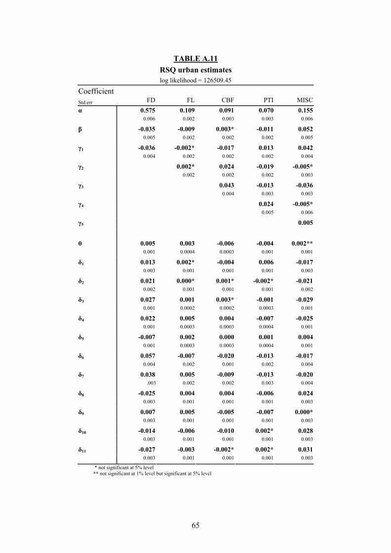
TABLE A.11

RSQ urban estimates log likelihood = 126509.45

Coefficient Std.err FD FL CBF PTI MISC

0.575 0.109 0.091 0.070 0.155 α 0.006 0.002 0.003 0.003 0.006

-0.035 -0.009 0.003* -0.011 0.052 β 0.005 0.002 0.002 0.002 0.005

-0.036 -0.002* -0.017 0.013 0.042 γ1 0.004 0.002 0.002 0.002 0.004

0.002* 0.024 -0.019 -0.005* γ2 0.002 0.002 0.002 0.003

0.043 -0.013 -0.036 γ3 0.004 0.003 0.003

0.024 -0.005* γ4 0.005 0.006

γ5 0.005

0.005 0.003 -0.006 -0.004 0.002** θ

0.001 0.0004 0.0003 0.001 0.001

0.013 0.002* -0.004 0.006 -0.017 δ1 0.003 0.001 0.001 0.001 0.003

0.021 0.000* 0.001* -0.002* -0.021 δ2 0.002 0.001 0.001 0.001 0.002

0.027 0.001 0.003* -0.001 -0.029 δ3 0.001 0.0002 0.0002 0.0003 0.001

0.022 0.005 0.004 -0.007 -0.025 δ4 0.001 0.0003 0.0003 0.0004 0.001

-0.007 0.002 0.000 0.001 0.004 δ5 0.001 0.0003 0.0003 0.0004 0.001

0.057 -0.007 -0.020 -0.013 -0.017 δ6 0.004 0.002 0.001 0.002 0.004

0.038 0.005 -0.009 -0.013 -0.020 δ7 .003 0.002 0.002 0.003 0.004

-0.025 0.004 0.004 -0.006 0.024 δ8 0.003 0.001 0.001 0.001 0.003

0.007 0.005 -0.005 -0.007 0.000* δ9 0.003 0.001 0.001 0.001 0.003

-0.014 -0.006 -0.010 0.002* 0.028 δ10 0.003 0.001 0.001 0.001 0.003

-0.027 -0.003 -0.002* 0.002* 0.031 δ11 0.003 0.001 0.001 0.001 0.003

* not significant at 5% level ** not significant at 1% level but significant at 5% level

65

TABLE A.12

Income elasticity at all India level

Rural Urbanitem FD FL CBF PTI MISC FD FL CBF PTI MISC

model LES 0.617 0.375 1.234 0.826 2.495 0.691 0.353 0.533 0.570 2.022AIDS 0.868 0.673 0.933 0.896 1.632 0.772 0.743 0.953 0.874 1.577RSQ 1.092 0.505 0.828 0.897 0.995 0.976 1.028 0.711 0.327 1.223BBLQ 1.093 0.503 0.824 0.882 0.998 0.963 1.028 0.713 0.342 1.248

TABLE A.13

LES income elasticity by type of household

Rural Urban type of hhd AFF NA HILL LIT AFF NA HILL LIT

item FD 0.629 0.615 0.608 0.678 0.715 0.684 0.634 0.943FL 0.387 0.371 0.364 0.456 0.364 0.351 0.327 0.438CBF 1.227 1.239 1.239 1.142 0.530 0.534 0.542 0.518PTI 0.916 0.819 0.758 1.000 0.608 0.570 0.486 0.559MISC 2.277 2.543 2.733 1.797 1.866 2.071 2.622 1.269

TABLE A.14

AIDS income elasticity by type of household

Rural Urban

type of hhd AFF NA HILL LIT AFF NA HILL LIT

item FD 0.855 0.869 0.870 0.866 0.688 0.774 0.790 0.764 FL 0.602 0.676 0.683 0.662 0.681 0.745 0.762 0.735

CBF 0.938 0.932 0.932 0.933 0.955 0.953 0.953 0.954 PTI 0.874 0.897 0.905 0.885 0.876 0.874 0.892 0.865

MISC 1.456 1.645 1.693 1.577 1.362 1.591 1.748 1.532

TABLE A.15

BBLQ income elasticity by type of household

Rural Urban type of hhd AFF NA HILL LIT AFF NA HILL LIT

item FD 1.108 1.092 1.094 1.096 0.967 0.963 0.957 0.963FL 0.352 0.509 0.491 0.480 1.100 1.026 1.012 1.036CBF 0.745 0.828 0.835 0.806 0.595 0.717 0.756 0.699PTI 0.968 0.879 0.859 0.889 0.204 0.348 0.352 0.279MISC 1.014 0.997 0.996 1.002 1.166 1.253 1.224 1.231

66

Table A.16

Compensated price elasticities by model for a reference household Rural Urban

item FD FL CBF PTI MISC FD FL CBF PTI MISC LES LES FD -0.406 0.038 0.009 -0.012 0.156 FD -0.454 0.114 0.095 0.122 0.354FL 0.111 -0.451 -0.004 -0.014 0.073 FL 0.080 -0.433 0.017 0.009 0.122CBF 0.551 0.147 -1.014 0.088 0.372 CBF 0.138 0.011 -0.516 0.000 0.190PTI 0.320 0.078 0.045 -0.862 0.235 PTI 0.097 0.018 0.026 -0.692 0.198MISC 1.368 0.539 0.516 0.513 -1.251 MISC 0.741 0.458 0.376 0.543 -1.152 AIDS AIDS FD -0.447 0.047 0.172 0.028 0.263 FD -0.435 0.121 0.079 0.097 0.277FL 0.216 -0.691 -0.025 0.147 0.353 FL 0.578 -0.881 0.340 -0.153 0.129CBF 1.094 -0.019 -1.076 0.159 -0.153 CBF 0.383 0.382 -0.400 -0.112 -0.251PTI 0.211 0.332 0.383 -1.794 0.862 PTI 0.886 -0.353 -0.227 -0.400 MISC 0.891 0.206 -0.009 0.217 -1.009 MISC 0.851 0.161 0.014 0.107 -0.595 BBLQ BBLQ FD -0.479 0.030 0.158 0.014 0.277 FD -0.459 0.092 0.054 0.066 0.248FL 0.274 -0.691 -0.014 0.145 0.286 FL 0.576 -0.883 0.342 -0.163 0.128CBF 1.098 -0.016 -1.076 0.167 -0.174 CBF 0.399 0.386 -0.403 -0.114 -0.268PTI 0.258 0.327 0.408 -1.800 0.807 PTI 0.957 -0.346 -0.230 -0.390 0.010MISC 0.859 0.158 -0.073 0.161 -1.105 MISC 0.710 0.053 -0.100 0.013 -0.677

0.083

TABLE A.17 R-squared by model

Rural Urban item FD FL CBF PTI MISC FD FL CBF PTI MISCmodel LES 0.808 0.551 0.277 0.399 0.743 0.617 0.298 0.539 0.240 0.719AIDS 0.312 0.305 0.179 0.217 0.377 0.425 0.175 0.166 0.128 0.485BBLQ -1.579 0.064 0.069 0.105 -1.313 -0.188 -0.433 -0.238 -0.024 0.056RSQ -1.620 -0.004 0.073 0.109 -1.326 -0.264 -0.412 -0.244 -0.041 0.018

67

Table A.18 Correlation matrix of estimated and deflated expenditure/budget share

Rural Urban

LES tc1 tc2 tc3 tc4 tc5 tc1 tc2 tc3 tc4 tc5 tchat_LES1 0.890 tchat_LES1 0.771 tchat_LES2 0.675 tchat_LES2 0.513 tchat_LES3 0.509 tchat_LES3 0.686 tchat_LES4 0.380 tchat_LES4 0.380 tchat_LES5 0.838 tchat_LES5 0.841 AIDS w1 w2 w3 w4 w5 w1 w2 w3 w4 w5 what_aS1 0.509 whataS1 0.628 what_aS2 0.419 whataS2 0.361 what_aS3 0.284 whataS3 0.263 what_aS4 0.308 whataS4 0.272 what_aS5 0.575 whataS5 0.677 BBLQ w1 w2 w3 w4 w5 w1 w2 w3 w4 w5 what_BBLQ1 0.073 what_BBLQ1 0.298 what_BBLQ2 0.290 what_BBLQ2 0.017 what_BBLQ3 0.083 what_BBLQ3 0.020 what_BBLQ4 0.058 what_BBLQ4 0.184 what_BBLQ5 0.028 what_BBLQ5 0.544 RSQ w1 w2 w3 w4 w5 w1 w2 w3 w4 w5 what_ RSQ1 -0.075 what_ RSQ1 0.253 what_ RSQ2 0.273 what_ RSQ2 0.025 what_ RSQ3 0.095 what_ RSQ3 0.020 what_RSQ4 0.074 what_RSQ4 0.185 what_RSQ5 0.023 what_RSQ5 0.527

1:FOOD/ 2: FUEL/ 3:CBF/ 4:PTI/ 5:MISC tc ≡ deflated per capita total expenditure and tchat ≡ estimated per capita total expenditure w ≡ deflated per capita budget share and what ≡ estimated per capita budget share

68

TABLE A.19 Difference in welfare measures between different rank model estimates and estimates

obtained from observed values Rural Urban LES AIDS BBLQ RSQ LES AIDS BBLQ RSQ POVERTY HCR hill 4.933% 5.125% 4.635% 1.686% 8.868% 8.307% 10.894% 25.490% hlit 7.013% 7.597% 6.860% 1.820% 18.933% 17.819% 40.486% 40.414% PGR hill 5.271% 6.032% 5.533% 1.749% 17.108% 14.163% 17.793% 32.182% hlit 7.202% 8.192% 7.478% 2.347% 24.459% 19.105% 41.789% 41.716% FGT hill 5.292% 6.540% 6.184% 1.940% 23.118% -14.648% -20.913% -26.770% hlit 7.541% 9.046% 8.475% 2.993% 32.408% -18.642% -45.792% -31.374% WATTS hill 5.239% 6.122% 5.660% 1.798% 18.602% 14.883% 18.541% 33.309% hlit 7.236% 8.337% 7.655% 2.466% -23.546% 19.974% 42.699% 42.768% CHU hill 4.935% 5.132% -11.282% -14.495% 8.964% 8.348% 10.942% -0.960% hlit 7.014% 7.601% 6.864% 1.824% 18.967% 17.828% 19.954% 40.424% SEN hill 5.194% 5.917% 5.483% 1.813% 16.025% 12.904% 16.133% 31.070% hlit 7.344% 8.373% 7.705% 2.427% 25.272% 20.092% 22.575% 42.635% INEQUALITY GINI hill -1.021% -0.696% -0.350% 0.151% -2.562% -4.233% -6.998% -7.468% hlit -0.574% -0.395% -0.264% 0.112% -1.463% -1.365% -4.637% -5.082% ATKINSON hill -1.827% -1.175% -0.603% -0.125% -4.898% -7.448% -12.954% -13.879% hlit -1.036% -0.699% -0.472% 0.126% -2.599% -2.011% -8.613% -9.509% THEIL hill -1.688% -0.971% -0.507% -0.648% -5.348% -7.275% -13.365% -14.532% hlit -0.951% -0.633% -0.432% 0.002% -2.506% -1.281% -9.571% -9.534% This table gives the percentage variation between the poverty and inequality measures based on deflated per capita expenditure and per capita equivalent expenditure based on LES, AIDS, BBLQ and QRS respectively.

69

70

Publications récentes du Département d’économétrie pouvant être obtenues à l’adresse suivante :

Université de Genève UNI MAIL

A l'att. de Mme Caroline Schneeberger Département d'économétrie

40, Bd du Pont-d'Arve CH - 1211 Genève 4

ou sur INTERNET : http//www.unige.ch/ses/metri/cahiers

2004.12 KRISHNAKUMAR Jaya, Going beyond functionings to capabilities: an

econometric model to explain and estimate capabilities, Août 2004, 29 pages. 2004.11 MÜLLER Tobias, RAMSES Abul Naga, KOLODZIEJCZYK Christophe, The

Redistributive Impact of Altrnative Income Maintenance Schemes : A Microsimulation Study using Swiss Data, Août 2004, 40 pages.

2004.10 GHIGLINO Christian, DUC François, Expectations in an OG Economy, Août

2004, 21 pages. 2004.09 GHIGLINO Christian, OLSZAK-DUQUENNE Marielle, On the Impact of

Heterogeneity on Indeterminacy, Août 2004, 29 pages. 2004.08 FIELD Chris, ROBINSON John, RONCHETTI Elvezio, Saddlepoint

Approximations for Multivariate M-Estimates with Applications to Bootstrap Accuracy, Août 2004, 26 pages.

2004.07 VICTORIA-FESER Maria-Pia, CONNE David, A Latent Variable Approach for

the Construction of Continuous Health Indicators, Août 2004, 8 pages. 2004.06 DELL'AQUILA Rosario, RONCHETTI Elvezio, Resistant Nonparametric

Analysis of the Short Term Rate, Juillet 2004, 26 pages. 2004.05 DELL'AQUILA Rosario, RONCHETTI Elvezio, Stock and Bond Return

Predictability : The Discrimination Power of Model Selection Criteria, Juin 2004, 25 pages.

2004.04 MANCINI Loriano, RONCHETTI Elvezio, TROJANI Fabio, Optimal

Conditionally Unbiased Bounded-Influence Inference in Dynamic Location and Scale Models, Juin 2004 (révision), 35 pages.

2004.03 CANTONI Eva, RONCHETTI Elvezio, A robust approach for skewed and

Heavy-tailed outcomes in the analysis of health care expenditures, Mai 2004, 18 pages.

2004.02 MOUSTAKI Irini, VICTORIA-FESER Maria-Pia, Bounded-Bias Robust

Estimation in Generalized Linear Latent Variable Models, Avril 2004, 45 pages.