
Delft University of Technology On early-stage design of vital ...
205
Delft University of Technology On early-stage design of vital distribution systems on board ships de Vos, Peter DOI 10.4233/uuid:eb604971-30b7-4668-ace0-4c4b60cd61bd Publication date 2018 Document Version Final published version Citation (APA) de Vos, P. (2018). On early-stage design of vital distribution systems on board ships. https://doi.org/10.4233/uuid:eb604971-30b7-4668-ace0-4c4b60cd61bd Important note To cite this publication, please use the final published version (if applicable). Please check the document version above. Copyright Other than for strictly personal use, it is not permitted to download, forward or distribute the text or part of it, without the consent of the author(s) and/or copyright holder(s), unless the work is under an open content license such as Creative Commons. Takedown policy Please contact us and provide details if you believe this document breaches copyrights. We will remove access to the work immediately and investigate your claim. This work is downloaded from Delft University of Technology. For technical reasons the number of authors shown on this cover page is limited to a maximum of 10.
-
Upload
khangminh22 -
Category
Documents
-
view
0 -
download
0
Transcript of Delft University of Technology On early-stage design of vital ...

Delft University of Technology
On early-stage design of vital distribution systems on board ships
de Vos, Peter
DOI10.4233/uuid:eb604971-30b7-4668-ace0-4c4b60cd61bdPublication date2018Document VersionFinal published versionCitation (APA)de Vos, P. (2018). On early-stage design of vital distribution systems on board ships.https://doi.org/10.4233/uuid:eb604971-30b7-4668-ace0-4c4b60cd61bd
Important noteTo cite this publication, please use the final published version (if applicable).Please check the document version above.
CopyrightOther than for strictly personal use, it is not permitted to download, forward or distribute the text or part of it, without the consentof the author(s) and/or copyright holder(s), unless the work is under an open content license such as Creative Commons.
Takedown policyPlease contact us and provide details if you believe this document breaches copyrights.We will remove access to the work immediately and investigate your claim.
This work is downloaded from Delft University of Technology.For technical reasons the number of authors shown on this cover page is limited to a maximum of 10.
On early-stage design of vital
distribution systems on board
ships
20
1 1 1 1 1 1 1
1
1
1
1
1
1
2
3
4
6
5
3 4 5 6
6
10
15
10 15
20
1 1 1 1 1 1 1
1
1
1
1
1
1
2
3
4
6
5
3 4 5 6
6
10
15
10 15
20
1111111
1
1
1
1
1
1
2
3
4
6
5
3456
6
10
15
1015
20
1111111
1
1
1
1
1
1
2
3
4
6
5
3456
6
10
15
1015
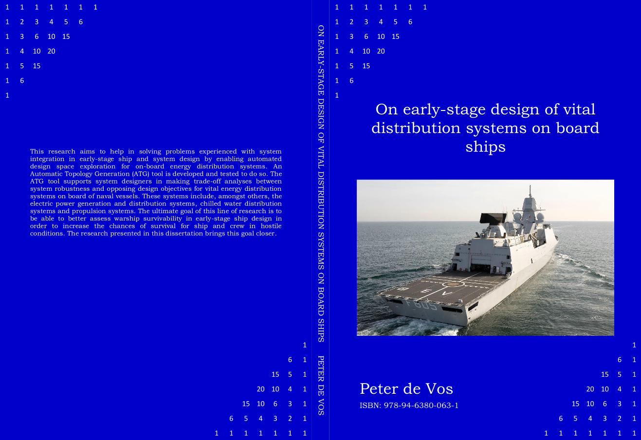
This research aims to help in solving problems experienced with system integration in early-stage ship and system design by enabling automated design space exploration for on-board energy distribution systems. An Automatic Topology Generation (ATG) tool is developed and tested to do so. The ATG tool supports system designers in making trade-off analyses between system robustness and opposing design objectives for vital energy distribution systems on board of naval vessels. These systems include, amongst others, the electric power generation and distribution systems, chilled water distribution systems and propulsion systems. The ultimate goal of this line of research is to be able to better assess warship survivability in early-stage ship design in order to increase the chances of survival for ship and crew in hostile conditions. The research presented in this dissertation brings this goal closer.
Peter de Vos
ON
EA
RLY
-STA
GE
DE
SIG
N O
F V
ITA
L D
ISTR
IBU
TIO
N S
YS
TE
MS
ON
BO
AR
D S
HIP
S
PE
TE
R D
E V
OS ISBN: 978-94-6380-063-1
Propositions accompanying the thesis
On early-stage design of distribution systems on board ships
by P. de Vos
29 November 2018
Delft University of Technology
1. Current early-stage ship design approaches produce sub-optimal, vulnerable and
hardly innovative ships. Mainly because of implicit choices being made with
respect to on-board systems. [This proposition pertains to this dissertation]
2. The limited applicability of network theory to on-board distribution systems is
unveiled when hubs are positioned in a ship. [This proposition pertains to this
dissertation]
3. The decision to perform an elaborate design space exploration is a clear indication
that the designers have no idea what to design; the latter is also true when it is
decided not to perform an elaborate design space exploration. The only difference
is awareness. [This proposition pertains to this dissertation]
4. The maritime industry is promoting the “revolutionary and promising concepts”
of Digital Twins, large-scale unmanned vessels and Big Data solutions. Believing
these concepts are either “revolutionary” or “promising” will turn out to be a
foolish mistake.
5. What first principles, like mass and energy conservation, are to physics, the
equality principle is to society.
6. Doubt and a need for confirmation do not reconcile well with the main objective
of a PhD research. Still, they are indispensable.
7. In their work, scientific staff of Delft University of Technology should act more
in the spirit of the Royal Decision of 8 January 1842 that founded this great
institute. It had an applied nature.
8. Scientific research led to the second law of Thermodynamics. Yet, science itself
undermines this first principle as research closely approaches perpetual motion.
9. If the devil is in the details, the divine may be found in universality.
10. Those who can do, those who won’t teach (after a quote of George Bernard
Shaw)
These propositions are regarded as opposable and defendable, and have been
approved as such by the promotor and copromotor:
prof.ir. D. Stapersma and dr.ir. B.J. van Oers

On early-stage design of vital distribution systems on
board ships
Dissertation
for the purpose of obtaining the degree of doctor at Delft University of Technology
by the authority of the Rector Magnificus prof.dr.ir. T.H.J.J. van der Hagen
chair of the Board for Doctorates to be defended publicly on
Thursday 29 November 2018 at 12:30 o’clock
by
Peter DE VOS
Master of Science in Maritime Technology, Delft University of Technology, the Netherlands
born in Dordrecht, the Netherlands

This dissertation has been approved by the promotors.
Composition of the doctoral committee:
Rector Magnificus Chairperson
Prof.ir. D. Stapersma Delft University of Technology, promotor
Dr.ir. B.J. van Oers Delft University of Technology, copromotor
Independent members:
Prof.dr. A. Brown Virginia Tech, United States of America
Prof.dr. R. Bucknall University College London, United Kingdom
Prof.dr. C. Witteveen Delft University of Technology
Prof.dr. F.M. Brazier Delft University of Technology
Prof.ir. J.J. Hopman Delft University of Technology
Copyright © 2018 by P. de Vos
This work is licensed under the Creative Commons Attribution-NonCommercial-ShareAlike
4.0 International License. To view a copy of this license, visit
http://creativecommons.org/licenses/by-nc-sa/4.0/ or send a letter to Creative Commons, PO
Box 1866, Mountain View, CA 94042, USA.
For permission requests, contact the author at [email protected].
ISBN: 978-94-6380-063-1
Source front cover picture: Netherlands Ministry of Defence

To my parents
For being there
To my wife Anne
For being home
To my children Niels and Lise
For being purpose

Summary
V
Summary This research aims to help in solving problems experienced with system integration in early-
stage ship and system design by enabling automated design space exploration for on-board
energy distribution systems. An Automatic Topology Generation (ATG) tool is developed and
tested to do so. The ATG tool supports system designers in making trade-off analyses between
system robustness and opposing design objectives for vital energy distribution systems on
board of naval vessels. These systems include, amongst others, the electric power generation
and distribution systems, chilled water distribution systems and propulsion systems. The
ultimate goal of this line of research is to be able to better assess warship survivability in early-
stage ship design in order to increase the chances of survival for ship and crew in hostile
conditions. The research presented in this dissertation brings this goal closer.
The ATG tool is based on a topological model of on-board energy distribution systems that is
combined with the fundamental concepts of network theory. Nodes are differentiated as being
either suppliers, hubs or users in different distribution systems. Edges are differentiated
according to the prevailing effort or flow variable of specific energy domains, e.g. 6600 V,
440 V, 5 °C, 750 rpm, etc. This node and edge differentiation framework enables a
mathematical definition of network topologies of different, integrated on-board energy
distribution systems in an adjacency matrix. In networks connecting distribution systems of
different domains, suppliers and users of specific distribution systems combine into a single
converter (user in one, supplier in another specific distribution system), while hubs become
“super nodes” that represent common distribution lines within specific distribution systems.
The topological model is combined with a genetic algorithm to enable the generation of a large
number of varying system topologies. The system topologies represent system concept designs
that are used to populate the design space. The genetic algorithm automatically assesses
generated system topologies on two opposing objective functions: system claim and system
robustness. The system claim objective function crudely captures the weight and space
requirements, procurement and installation costs and even operability of the system concept
designs. Two system robustness objective functions have been developed. The first focuses on
system re-configurability as a robustness measure and aims to improve system re-
configurability by maximising the flow in hub layers. In doing so, the function increases the
number of disjoint paths between hubs, which also increases the number of paths between
suppliers and users. The second system robustness objective function focuses on vulnerability
by assessing the chance that pre-defined vital users are still supplied with the required flow
type after randomly removing nodes and edges (i.e. system components and connections). This
assessment may be done for different hit scenarios.
Summary
VI
The ATG tool is tested in two case studies. The first case study contains the electric power and
chilled water distribution systems of a notional frigate. The applicability and performance of
the ATG tool as a design space exploration tool is assessed with this first case study. In terms
of speed: the generation of 40000 networks (i.e. system topologies) required 20 minutes on a
modern PC with moderate computing capabilities. In terms of populating the design space with
system concept designs and optimising these according to the two opposing objective
functions (with system re-configurability as system robustness measure): initially sufficient
unique designs were generated, however an unsatisfactory populated design space was found
in the sense that the Pareto front was not complete. It appears that the genetic algorithm is
greatly supported by applying a steering rule that focuses the search effort on the relevant part
of the design space. Applying such a rule increases the performance and a satisfactory
populated design space is found with the entire Pareto front of non-dominated system concept
designs visible. The effect of defining “elite individuals” for the first case study is also
investigated and resulted in a significant reduction of the computational time required. Similar
non-dominated system concept designs are found with the generation of only 3600 networks
in only two minutes of computational time.
The second case study concerns similar systems of a notional Ocean-going Patrol Vessel
(OPV) but now with the inclusion of the propulsion system. Again, the ATG tool performs
well as a design space exploration tool. Besides demonstrating the applicability of the ATG
tool with a new case study, the second case study also served to compare the two objective
functions for system robustness. The two functions are fundamentally different. The first is an
a-priori function designed to capture what is considered to be the most important and suitable
robustness measure to capture given the focus on topologies: system re-configurability. The
second is an a-posteriori simulation of hit cases to assess system vulnerability. Despite this
fundamental difference, the two functions are shown to converge towards the same Pareto
front of non-dominated design solutions when choices concerning the input of the ATG tool
are coherent. As such, the second system robustness objective function verifies the validity of
the first.
The ATG tool enables design space exploration of distribution systems in a very early stage.
A revised design procedure for integrated ship and system design was set-up to incorporate
the ATG tool in the design process and demonstrate which steps follow in the procedure after
using the ATG tool. The purpose of design space exploration is providing insight in how design
requirements, constraints, technical design solutions and performance characteristics relate. It
is concluded that the ATG tool succeeds in obtaining this goal as insight was gained in
important design choices concerning system robustness. This is particularly true in the second
case study which uncovered a practical implication when the ATG tool was applied to the
OPV case study network: current system designs often have a hierarchy of hubs in the
distribution network; this practice can be questioned from a robustness perspective as it
inhibits an improvement of system re-configurability. This result can be related to a classical

Summary
VII
discussion in marine engineering: radial distribution vs zonal, ring distribution. The latter is
often regarded as more robust because of increased re-configurability. The results of this
research seem to confirm this point of view.
At the same time there is room for criticism, and thus improvement: the generated system
topologies, although considered relatively realistic from a technical feasibility perspective,
lack a level-of-detail that is required for truly assessing technical feasibility of system concept
designs. Furthermore, verification of the first system robustness objective function uncovers a
dilemma with respect to the normalisation that was applied in the function. Normalisation
ensures attention is given first to distribution systems with a low number of hubs, for which
re-configurability is arguably more important, during automated design space exploration. The
choice to apply normalisation backfires however when the number of hubs within a specific
distribution system increases while the number of hub-hub connections does not. This brings
us to the last critical note: the number of system components, including hubs, is fixed in the
present ATG tool. This is for the moment considered a drawback of the method as in practical
design space exploration the number of system components should be variable as well, like
system topology is.
Therefore, the research is far from finished. The ATG tool itself for instance can still be
improved tremendously by increasing the appropriateness of the objective functions. Improved
objective functions as well as an improved design space exploration algorithm should enable
a varying number of system components, as implied previously. From that perspective this
research has resulted in a proof-of-principle only and much needs to be done before the tool
can be used as a practical designer support tool. To achieve the latter, future research should
focus on finding a method to include load balancing and matching of suppliers and users of
the different distribution systems using a fundamentally sound approach (for different
operational modes). Doing so would enable (first-principle) dimension prediction of system
components as well. Finally, to achieve the ultimate goal of better assessing warship
survivability, (automatic) integration of the generated or selected system concept designs into
ship concept designs still needs to be performed. First steps in this direction have already been
taken in follow-on research. As such, the outcome of this research has already inspired new
research results.

Summary
VIII
Table of Contents
IX
Table of Contents Summary ................................................................................................................................. V
Table of Contents ................................................................................................................... IX
List of Figures ..................................................................................................................... XIII
List of Tables ..................................................................................................................... XVII
Publications ..................................................................................................................... XVIII
Chapter 1 Introduction ........................................................................................................ 1
1.1 Distribution systems on board ships ................................................................... 1
1.2 Early-stage naval ship and on-board system design ........................................... 5
1.2.1 Process ................................................................................................................ 5
1.2.2 Design space exploration .................................................................................... 8
1.3 Problem definition .............................................................................................. 9
1.4 Research goal ................................................................................................... 11
1.5 Principle of methodology ................................................................................. 12
1.6 Dissertation outline ........................................................................................... 14
Chapter 2 Elaboration of ship and on-board distribution system design ........................... 17
2.1 Early-stage ship design ..................................................................................... 17
2.1.1 Process and methodology ................................................................................. 17
2.1.2 Design requirements ......................................................................................... 20
2.1.3 Problems ........................................................................................................... 22
2.2 Early-stage system design ................................................................................ 24
2.2.1 Process and methodology ................................................................................. 24
2.2.2 Design requirements ......................................................................................... 27
2.2.3 Problems ........................................................................................................... 29
2.3 System robustness ............................................................................................ 30
2.4 Design procedure for on-board systems ........................................................... 33
2.5 Summary and conclusion ................................................................................. 40
Chapter 3 Topological modelling of on-board distribution systems ................................. 43
3.1 Applying network theory to on-board distribution systems ............................. 44
3.1.1 Fundamentals of network theory ...................................................................... 44
3.1.2 Nodes and edges in on-board distribution systems ........................................... 45
3.2 Common features of on-board distribution systems: node and edge
differentiation ................................................................................................... 46

Table of Contents
X
3.2.1 Considerations of system architecture .............................................................. 46
3.2.2 Node and edge differentiation – step 1 ............................................................. 47
3.2.3 Hubs (node differentiation – step 2) ................................................................. 50
3.2.4 Closure.............................................................................................................. 54
3.3 Overview of systems and their components ..................................................... 54
3.3.1 Systems on board of ships ................................................................................ 54
3.3.2 System components categorised ....................................................................... 56
3.4 Introduction of first case study and benchmark system .................................... 56
3.5 A-priori constraints to limit the size of the design space .................................. 63
3.5.1 Constraint 1: Technical feasibility of connections............................................ 64
3.5.2 Constraint 2: No converter-converter connections ........................................... 64
3.5.3 Constraint 3: Connected networks .................................................................... 66
3.6 Directed vs. undirected connections ................................................................. 67
3.7 Further treatment of network theory ................................................................. 68
3.8 Summary and conclusion ................................................................................. 71
Chapter 4 Automatic Topology Generation ...................................................................... 73
4.1 Topology generation in general ........................................................................ 74
4.2 ATG for on-board energy distribution systems ................................................ 76
4.2.1 Required input .................................................................................................. 78
4.2.2 Calculation procedure ....................................................................................... 81
4.2.3 (Initial) vector x ................................................................................................ 82
4.2.4 Repair function ................................................................................................. 82
4.2.5 Objective functions ........................................................................................... 83
4.2.6 Steering ............................................................................................................. 84
4.2.7 NSGA-II ........................................................................................................... 85
4.3 Summary and conclusion ................................................................................. 86
Chapter 5 Objective functions ........................................................................................... 87
5.1 Objective function 1: Design for minimum system claim ................................ 88
5.1.1 Design for minimum space and weight requirements ....................................... 88
5.1.2 Design for minimum procurement and installation costs ................................. 89
5.1.3 Design for maximum operability ...................................................................... 89
5.1.4 Synthesis of treated design objectives in one “system claim” objective function:
n_connections ................................................................................................... 90
Table of Contents
XI
5.2 Objective function 2: Design for maximum system robustness ....................... 93
5.2.1 Design for maximum robustness ...................................................................... 94
5.2.2 Design for maximum re-configurability ........................................................... 95
5.2.3 Design for minimum vulnerability ................................................................... 96
5.2.4 Other robustness objective functions ................................................................ 97
5.2.5 Re-configurability objective function: max-flow-between-hubs .................... 100
5.2.6 Vulnerability objective function: hurt-state-percolation ................................. 107
5.3 Summary and conclusion ............................................................................... 108
Chapter 6 Results of Automatic Topology Generation tool ............................................ 109
6.1 Results for frigate case study .......................................................................... 110
6.1.1 Output of ATG tool without / with steering rule ............................................ 111
6.1.2 Setting the starting point of the design space exploration .............................. 114
6.1.3 Reflection on first case study .......................................................................... 120
6.2 Results for OPV case study systems ............................................................... 121
6.2.1 23-node case study system on board of OPV ................................................. 122
6.2.2 Necessity for scaling up the 23-node system to a 35-node system ................. 123
6.2.3 Automatic Topology Generation for OPV case study systems ....................... 125
6.2.4 Reflection on second case study ..................................................................... 141
6.3 Verification of and reflection on objective functions n_connections and max-
flow-between-hubs ......................................................................................... 141
6.4 Summary and conclusion ............................................................................... 150
Chapter 7 Conclusions & Recommendations .................................................................. 153
Bibliography ........................................................................................................................ 161
Symbol list ........................................................................................................................... 167
Acronyms ............................................................................................................................. 169
Glossary ............................................................................................................................... 171
Acknowledgements .............................................................................................................. 173
Curriculum Vitae ................................................................................................................. 175
Appendix A .......................................................................................................................... 177
Appendix B .......................................................................................................................... 179

Table of Contents
XII
List of Figures
XIII
List of Figures Figure 1.1 A number of ships with different missions, i.e. different ship types. ............... 1 Figure 1.2 Block diagram of conventional diesel geared-drive propulsion system (left) and
seawater cooling system (right) – copied from Klein Woud et al. [36] and [37]
with permission. ............................................................................................... 2 Figure 1.3 Principle of one-line diagram for electric power generation and distribution
system – copied from Klein Woud et al. [36] with permission. ....................... 3 Figure 1.4 V-diagram of integrated early-stage ship and system design including the role
of requirements – repeated from de Vos et al. [68]. ......................................... 6 Figure 1.5 Example of 3D ship configuration (or ship concept design) – copied from
Duchateau et al. [20] with permission.............................................................. 7 Figure 1.6 Principle of design space exploration with the ATG tool – repeated from de
Vos et al. [68]................................................................................................. 12 Figure 1.7 Flow diagram of this dissertation. .................................................................. 15 Figure 2.1 Energy Flow Diagram of hybrid drive, copied from Klein Woud et al. [36] with
permission. ..................................................................................................... 25 Figure 2.2 General system response curve to a disruption. ............................................. 32 Figure 3.1 Example of a small undirected network (nn = 4) incl. adjacency matrix A. .. 44 Figure 3.2 Radial distribution (“star network”) – reproduced from Klein Woud et al. [37]
with permission. ............................................................................................. 48 Figure 3.3 Single distribution (“tree network”) – reproduced from Klein Woud et al. [37]
with permission. ............................................................................................. 50 Figure 3.4 Single, zonal distribution – reproduced from Klein Woud et al. [37] with
permission. ..................................................................................................... 51 Figure 3.5 Double distribution – reproduced from Klein Woud et al. [37] with permission.
....................................................................................................................... 51 Figure 3.6 Graph of tree network of Figure 3.3 – repeated from de Vos [66]. ................ 52 Figure 3.7 Distribution systems on board of ships and their interdependencies – repeated
from de Vos et al. [67]. .................................................................................. 55 Figure 3.8 Benchmark system: multi-disciplinary network with four different energy
distribution systems and one data distribution system for a notional frigate –
repeated from de Vos et al. [67]. The topology of this system is defined by the
author; i.e. it is not automatically generated. ................................................. 58 Figure 3.9 Adjacency matrix of benchmark system topology. ........................................ 61 Figure 3.10 Possible non-zero elements in upper triangle of the adjacency matrix for the
benchmark study system (consisting of 36 nodes) before (left) and after (right)
inclusion of a-priori constraints. .................................................................... 63 Figure 3.11 Independent paths. There are two edge-independent paths between A and B,
but only one node-independent path. Figure based on Figure 6.15 of Newman
[41]. ................................................................................................................ 69
List of Figures
XIV
Figure 4.1 Principle of design space exploration with the ATG tool – repeated from de
Vos et al. [68]................................................................................................. 76 Figure 4.2 Schematic representation of process for reducing the size of the design space
and identifying interesting design solutions with the ATG tool – process steps
above dashed line are within the scope of this dissertation. ........................... 77 Figure 4.3 Calculation procedure ATG tool. ................................................................... 81 Figure 6.1 Results of ATG tool for frigate case study network without steering rule. .. 111 Figure 6.2 Results of ATG tool for frigate case study network with steering rule. ....... 112 Figure 6.3 Minimally connected network for case study: f1 = 80, f2 = -41.67. ............ 116 Figure 6.4 Maximally connected network for frigate case study: f1 = 210, f2 = 0. ...... 116 Figure 6.5 Minimally connected network with maximum hub connectivity for frigate case
study: f1 = 102, f2 = -441.67. ...................................................................... 117 Figure 6.6 Results of ATG tool for frigate case study network when extremes of the Pareto
front are used as elite individuals at the start of the design space exploration.
..................................................................................................................... 117 Figure 6.7 Graph of 23-node case study system. ........................................................... 122 Figure 6.8 Graph of 35-node OPV case study system. Note the added propulsion system
components, shaft connections (green), rudders and bow thruster. ............. 125 Figure 6.9 Design spaces for 23-node OPV case study system with n_connections as
system claim objective function and max-flow-between-hubs (left) or hurt-
state-percolation (right) as robustness objective functions. ......................... 127 Figure 6.10 Generated system topologies of 23-node OPV case study system: A1 (left) and
A2 (right), ref. Figure 6.9. ............................................................................ 129 Figure 6.11 Generated system topologies of 23-node OPV case study system: B1 (left) and
B2 (right), ref. Figure 6.9. ............................................................................ 129 Figure 6.12 Generated system topologies of 23-node OPV case study system: C1 (left) and
C2 (right), ref. Figure 6.9. ............................................................................ 129 Figure 6.13 Design spaces for 35-node OPV case study system with n_connections as
system claim objective function and max-flow-between-hubs (left) or hurt-
state-percolation (right) as robustness objective functions. Compare with
Figure 6.9. .................................................................................................... 131 Figure 6.14 Generated system topology of 35-node OPV system: D1, ref. Figure 6.13. 132 Figure 6.15 Generated system topology of 35-node OPV system: D2, ref. Figure 6.13. 132 Figure 6.16 Generated system topology of 35-node OPV system: E1, ref. Figure 6.13. 133 Figure 6.17 Generated system topology of 35-node OPV system: E2, ref. Figure 6.13. 133 Figure 6.18 Single Line Diagram of 440 V distribution system of Figure 6.17. ............. 135 Figure 6.19 Design space (top) and generated system topology F (bottom) for 35-node case
study system: Load Centres act as 440 V hubs as well, together with
switchboards. ............................................................................................... 137

List of Figures
XV
Figure 6.20 Generated and by-hand improved system topologies for OPV case study
network. ....................................................................................................... 138 Figure 6.21 Design space (top) and generated system topology G (bottom) for 35-node case
study system: Load Centres act as 440 V hubs as well, together with
switchboards. ............................................................................................... 140 Figure 6.22 Radial distribution (star network) – Network 1. .......................................... 143 Figure 6.23 Single distribution (tree network) – Network 2. .......................................... 144 Figure 6.24 Single, zonal distribution – Network 3. ....................................................... 144 Figure 6.25 Double distribution with communication between the two supply lines and
separation valves – Network 4. .................................................................... 144 Figure 6.26 Double distribution with vital and non-vital consumers and separate and
combined suppliers – Network 5. ................................................................ 145 Figure 6.27 Ring distribution – Network 6. .................................................................... 145 Figure 6.28 Zonal distribution – Network 7. ................................................................... 145 Figure 6.29 Scores of different networks shown in this section on system claim objective
function n_connections. ............................................................................... 146 Figure 6.30 Scores of different networks shown in this section on system robustness
objective function max-flow-between-hubs. ................................................ 147 Figure 6.31 Scores of different networks shown in this section on the actual max-flow-
between-hubs part of objective function f2 when this term is normalised. .. 148 Figure 6.32 Scores of different networks shown in this section on the actual max-flow-
between-hubs part of objective function f2 when this term is not normalised.
..................................................................................................................... 148 Figure 6.33 Scores of different networks shown in this section on the hub density part of
objective function f2. ................................................................................... 149

List of Figures
XVI

List of Tables
XVII
List of Tables Table 2.1 Some Effort and Flow quantities; based on Table 2.1 of Karnopp et al. [34]. 40 Table 3.1 Overview of on-board distribution systems and main components categorised
according to the developed node and edge differentiation framework. ......... 57 Table 3.2 Overview of system components in first case study system of Figure 3.8. .... 60 Table 3.3 Overview of possible types of connections according to the node and edge
differentiation framework, including which are allowed before and after the
application of the no converter-converter connections constraint. ................. 65 Table 5.1 Max flow values if [A1] equals [A]. ............................................................ 103 Table 5.2 Max flow values if [A1] equals [A] only with regards to hub layer sub-matrices.
..................................................................................................................... 103 Table 5.3 Element values if HL2 is fully connected. ................................................... 105 Table 5.4 Element values if HL2 has 2 / 3 connections. .............................................. 105 Table 5.5 Element values if HL1 has four connections which make a “full” ring (all four
hubs part of the ring structure). .................................................................... 106 Table 5.6 Element values if HL1 has four connections which make a “partial” ring (only
three out of four hubs part of the ring structure). ......................................... 106 Table 6.1 List of OPV system components and associated distribution systems. ........ 123 Table 6.2 List of additional OPV system components and associated distribution systems.
..................................................................................................................... 124

Publications
XVIII
Publications Publications related to the research documented in this dissertation:
de Vos, P. (2014); On the application of network theory in naval engineering, Proc. of
International Naval Engineering Conference (INEC 2014), Amsterdam, IMarEST, UK.
Stapersma, D., de Vos, P. (2015); Dimension prediction models of ship system components
based on first principles, Proc. of 12th Int. Marine Design Conference (IMDC), Tokyo, Japan,
ISBN 978-4-930966-04-9.
de Vos, P., Stapersma, D. (2018); Automatic Topology Generation for early design of on-
board energy distribution systems, Ocean Engineering, volume 170: p. 55–73, UK.
de Vos, P., Stapersma, D., Duchateau, E.A.E., van Oers, B.J. (2018); Design Space
Exploration for on-board Energy Distribution Systems - A New Case Study, Proc. of 17th
Conference on Computer and IT Applications in the Maritime Industries (COMPIT), TUHH,
Pavone, Italy, ISBN 978-3-89220-707-8.
Duchateau, E.A.E., de Vos, P., van Leeuwen, S. (2018); Early stage routing of distributed ship
service systems for vulnerability reduction, Proc. of 13th Int. Marine Design Conference
(IMDC), Helsinki, Finland.
Other publications by the author:
Ten Hacken, M., de Vos, P., Boogaart, R., Visser, K. (2018); Submarine Propulsion Plant
Design using Mean Value First Principle models, Proc. of Undersea Defence Technology
Conference (UDT), Glasgow, UK.
de Vos, P. (2015); Design of a New Ship Propulsion System Fundamentals course, Proc. of
12th Int. Marine Design Conference (IMDC), Tokyo, Japan, ISBN 978-4-930966-04-9.
van Es, G.F., de Vos, P. (2012); System design as a decisive step in engineering naval
capability, Proc. of 11th Int. Naval Engineering Conference (INEC), Edinburgh, United
Kingdom, IMarEST. Also published in Proc. of 4th World Maritime Technology Conference
(WMTC), Saint Petersburg, Russia.
Vrijdag, A., de Vos, P. (2012); Uncertainties and Margins in the Ship Propulsion System
Design Process, Proc. of 11th Int. Naval Engineering Conference (INEC), Edinburgh, United
Kingdom, IMarEST. Also published in Proc. of 4th World Maritime Technology Conference
(WMTC), Saint Petersburg, Russia.

Publications
XIX
Moredo, E., de Vos, P., Krikke, E.M. (2011); A new System Structure to improve
Documentation Processes Tender Phase, Proc. of Int. Conference on Computer Applications
in Shipbuilding (ICCAS), RINA, Trieste, Italy.
Grimmelius, H.T., de Vos, P., Krijgsman, M., van Deursen, E. (2011); Control of Hybrid Ship
Drive Systems, Proc. of 10th Conference on Computer and IT Applications in the Maritime
Industries (COMPIT), TUHH, Berlin, Germany, ISBN 978-3-89220-649-1.
Stapersma, D., Grimmelius, H.T., de Vos, P. (2010); The use of simulation models in
education: the affordable engineer, Proc. of 10th Int. Naval Engineering Conference (INEC),
Portsmouth, IMarEST, UK.
de Vos, P., Versluijs, E., Stapersma, D., Barendregt, I. (2010); Application of dynamic models
during design of a hybrid diesel-fuelled PEMFC system with fuel reformer, Proc. of Practical
Design of Ships conference (PRADS), Rio de Janeiro, Brazil.
de Vos, P., Grimmelius, H.T. (2009); Environment-Friendly Inland Shipping: Dynamic
modelling of propulsion systems for inland ships using different fuels and fuel cells, Proc. of
Int. Symposium on Marine Engineering (ISME), Busan, Korea.

Publications
XX
Introduction
1
“The only true wisdom is in knowing you know nothing.”
― Socrates
Chapter 1 Introduction
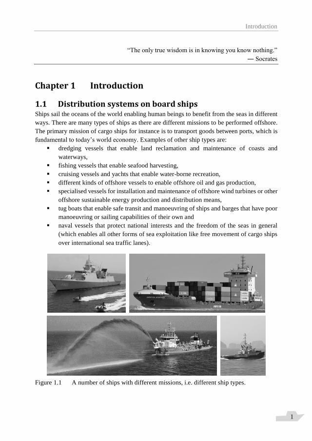
1.1 Distribution systems on board ships Ships sail the oceans of the world enabling human beings to benefit from the seas in different
ways. There are many types of ships as there are different missions to be performed offshore.
The primary mission of cargo ships for instance is to transport goods between ports, which is
fundamental to today’s world economy. Examples of other ship types are:
dredging vessels that enable land reclamation and maintenance of coasts and
waterways,
fishing vessels that enable seafood harvesting,
cruising vessels and yachts that enable water-borne recreation,
different kinds of offshore vessels to enable offshore oil and gas production,
specialised vessels for installation and maintenance of offshore wind turbines or other
offshore sustainable energy production and distribution means,
tug boats that enable safe transit and manoeuvring of ships and barges that have poor
manoeuvring or sailing capabilities of their own and
naval vessels that protect national interests and the freedom of the seas in general
(which enables all other forms of sea exploitation like free movement of cargo ships
over international sea traffic lanes).
Figure 1.1 A number of ships with different missions, i.e. different ship types.
Introduction
2
Figure 1.1 shows a number of ships with different missions. All ships are equipped with
systems that ensure proper functioning of the ship while fulfilling its mission; among them are
vital energy distribution systems. For example, typically ships are equipped with an electric
power generation and distribution system that supplies the right amount of electric power (at
suitable voltage levels) to electric power users on board. Similarly, a propulsion system is
installed which enables sailing and manoeuvring of the ship. In this system rotating mechanical
power is distributed from engines, or other driving machines, to propellers, or other propulsors,
via shafts, gears and/or other forms of mechanical transmission. As a final example, there are
a number of heating or cooling systems in any ship in which heat (thermal power) is distributed
to control temperature levels of spaces and equipment at various locations inside the ship. Note
that in such flow systems a fluid (typically a liquid) is distributed through pipe lines as a carrier
of heat. There are also a number of pipe flow systems in which a fluid is distributed for a
different reason than heat carrying capacity, like chemically stored energy (fuel), oxygen
content (air) and lubrication properties (lubrication oil). All systems mentioned above, and a
few more, are captured in this dissertation under the overarching term distribution systems.
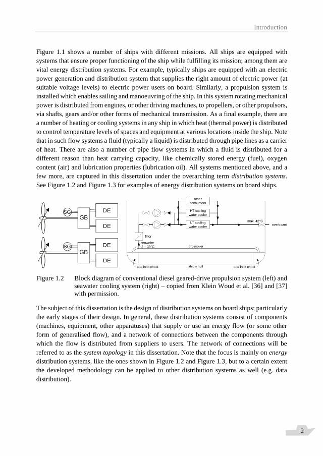
See Figure 1.2 and Figure 1.3 for examples of energy distribution systems on board ships.
Figure 1.2 Block diagram of conventional diesel geared-drive propulsion system (left) and
seawater cooling system (right) – copied from Klein Woud et al. [36] and [37]
with permission.
The subject of this dissertation is the design of distribution systems on board ships; particularly
the early stages of their design. In general, these distribution systems consist of components
(machines, equipment, other apparatuses) that supply or use an energy flow (or some other
form of generalised flow), and a network of connections between the components through
which the flow is distributed from suppliers to users. The network of connections will be
referred to as the system topology in this dissertation. Note that the focus is mainly on energy
distribution systems, like the ones shown in Figure 1.2 and Figure 1.3, but to a certain extent
the developed methodology can be applied to other distribution systems as well (e.g. data
distribution).

Introduction
3
Figure 1.3 Principle of one-line diagram for electric power generation and distribution
system – copied from Klein Woud et al. [36] with permission.
The design of on-board distribution systems (which components?, which system topology?,
etc.) is driven by operational feasibility and performance, costs, weight and space
requirements, safety considerations and operability. A trade-off between these different design
objectives, of which some are opposing each other, needs to be made during the design of
these systems. With regards to operational performance, a good overall system efficiency or
low energy consumption may for instance be an important requirement1 (i.e. a design driver).
That is, provided that a system can perform operationally, meaning that the system is
technically feasible and thus able to fulfil its function. The latter of course is the primary
operational performance requirement, which may be considered to be non-negotiable; thus
transforming the requirement into a constraint. Complying with regulations concerning
harmful emissions may nowadays be another design driver in the context of operational
performance. With regards to costs, procurement and installation costs (or capital expenditure)
of distribution systems typically is a design driver, but operational expenditure may be
important as well (which amongst others is a function of energy consumption again). A trade-
off between capital and operational expenditure typically exists, i.e. operational expenditure
can be lowered by increasing overall system efficiency but only at the expense of higher
procurement costs because more expensive or additional system components are required.
1 A glossary is provided at the end of this dissertation to shed some light on closely related
terms like design considerations, design objectives, design requirements and design drivers.

Introduction
4
In terms of safety considerations, requirements concerning system robustness may be
important. This certainly is the case for distribution systems that fulfil or support a vital
function. System robustness is particularly important for ship types that require continuity of
service during high-risk operations, like naval and offshore vessels. Naval vessels require vital
distribution systems to be highly robust to increase the chances for survival of crew and ship
in hostile conditions. Offshore vessels require vital distribution systems to be robust to
decrease the risk for adverse environmental (and economic) impact. Finally, operability may
drive the design of on-board distribution systems as the crew on board of the ship needs to
“work with the systems”. Operability here means to capture system characteristics like
comprehensibility and controllability. A system with centralised flow control is for instance
deemed to be more comprehensible and better controllable by the crew of the ship. Operability
thus is related to Human-Machine Interaction and ease of operation, which is typically strived
for during system design.
Of the different design objectives described above, system robustness will prove to be
important in this research. How to assess system robustness, together with other, opposing
design objectives, automatically for a large number of system concept designs is one of the
main questions addressed. Being able to do so is essential for the development of a useful
designer support tool that enables design space exploration for on-board distribution systems
during early-stage ship and system design. The methodology underlying the so-called
Automatic Topology Generation (ATG) tool constitutes the main contribution of this
dissertation. The ATG tool, as a novel design methodology, enhances the possibilities for
early-stage on-board distribution system design when compared to current design methods.
The ATG tool adds a new design phase, ahead of the current early stages of system design, as
automated design space exploration is currently not (or hardly) performed for on-board
distribution systems.
Early-stage on-board distribution system design, as a parallel process in early-stage naval ship
design, will further be discussed in the next section. A problem definition will subsequently
be given in section 1.3 on basis of the text in this section and section 1.2. The problem
definition leads to the definition of the research goal addressed in this dissertation in section
1.4. With the research goal introduced, the principle of the employed methodology can be
discussed in section 1.5 as a general introduction of how the research documented here tries
to achieve the research goal. This then naturally leads to the outline of this dissertation as given
in section 1.6.

Introduction
5
1.2 Early-stage naval ship and on-board system design The context of this dissertation is early-stage naval ship design2 as for these ships system
robustness is very important. Many features and processes in early-stage naval ship design are
however also applicable to the design of other ship types. This section is therefore written as
generic as possible but will at times be specifically applicable to naval ships or comparable
ship types (most notably offshore vessels).
1.2.1 Process Ship and on-board system design are integrated, iterative processes in which the level-of-detail
and fidelity of the design is increased with every iteration. In this section the two processes
(ship and system design) and the interaction between them during early-stage ship design is
discussed, amongst others to introduce when and why design space exploration techniques
may be beneficial.
Many visualisations of the ship design process, with its many different aspects included, have
been developed since the design spiral of Evans [22]. Hopman [31] used a V-diagram to
represent the ship design and building process based on the Systems Engineering V-diagram
for large, complex systems; INCOSE [33]. Both van Oers [43] and Duchateau [21] adapted
Hopman’s figure to make it applicable to early stage ship design. Figure 1.4 below is based on
their V-diagrams, but it has been extended to show distribution system design as a parallel
process in early stage ship design.
The design process starts with a definition of the mission of the ship and the definition of main
functions (functional decomposition). This helps in defining qualitative requirements but does
not yet require the development of one or more technical design solutions. The generation of
design solutions is in the bottom part of the figure and asserts a list of required mission-related
systems and spaces can be set up from the mission of the ship. Having the mission-related
systems and corresponding spaces, other, supporting spaces which are required for the ship to
function can be defined (arrow A1). At this point the list of spaces is assumed to be complete,
or at least defined with sufficient level-of-detail, to start arranging the spaces into a ship
configuration (arrow A2). Route A (A1-A2) leads to one or more ship concept designs, see
Figure 1.5 for an example. Route A is the focus of the research of van Oers [43] and Duchateau
[21].
2 Early-stage ship design is here meant to encompass both the conceptual (feasibility study)
and preliminary design stages of the ship design process. For a more complete text on the
different stages of the ship design process refer to Lamb et al. [38].

Introduction
6
Figure 1.4 V-diagram of integrated early-stage ship and system design including the role
of requirements – repeated from de Vos et al. [68].
Route B (B1-B2) is the extension of the V-diagram and shows distribution system design as a
similar, parallel process in early stage ship design. The focus of this research will be on this
part of design process. Route B leads to one or more system concept designs. As with ship
design, the mission-related systems are the starting point to define a list of other, supporting
distribution systems and their components (arrow B1). Assuming the list of required systems
and components is then sufficiently defined, the components in the different distribution
systems need to be connected to each other, i.e. a system topology needs to be defined, in order
to arrive at a system concept design (arrow B2). Examples of high-level system diagrams,
which are produced during early-stage system design, were already shown in Figure 1.2 and
Figure 1.3.
Introduction
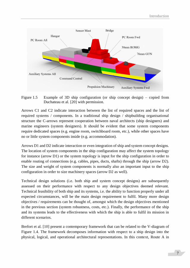
7
Figure 1.5 Example of 3D ship configuration (or ship concept design) – copied from
Duchateau et al. [20] with permission.
Arrows C1 and C2 indicate interaction between the list of required spaces and the list of
required systems / components. In a traditional ship design / shipbuilding organisational
structure the C-arrows represent cooperation between naval architects (ship designers) and
marine engineers (system designers). It should be evident that some system components
require dedicated spaces (e.g. engine room, switchboard room, etc.), while other spaces have
no or little system components inside (e.g. accommodation).
Arrows D1 and D2 indicate interaction or even integration of ship and system concept designs.
The location of system components in the ship configuration may affect the system topology
for instance (arrow D1) or the system topology is input for the ship configuration in order to
enable routing of connections (e.g. cables, pipes, ducts, shafts) through the ship (arrow D2).
The size and weight of system components is normally also an important input to the ship
configuration in order to size machinery spaces (arrow D2 as well).
Technical design solutions (i.e. both ship and system concept designs) are subsequently
assessed on their performance with respect to any design objectives deemed relevant.
Technical feasibility of both ship and its systems, i.e. the ability to function properly under all
expected circumstances, will be the main design requirement to fulfil. Many more design
objectives / requirements can be thought of, amongst which the design objectives mentioned
in the previous section (system robustness, costs, etc.). Finally, the performance of the ship
and its systems leads to the effectiveness with which the ship is able to fulfil its mission in
different scenarios.
Brefort et al. [10] present a contemporary framework that can be related to the V-diagram of
Figure 1.4. The framework decomposes information with respect to a ship design into the
physical, logical, and operational architectural representations. In this context, Route A in

Introduction
8
Figure 1.4 is associated with the physical architecture, Route B is associated with the logical
architecture and routes C and D are associated with the overlapping area of physical and logical
architectures. In the context of this framework the ATG tool developed in this research may
be interpreted as an essential first step to find initial logical architectures.
1.2.2 Design space exploration From a theoretical perspective early stages of ship and system design contain a number of
combinatorial problems that can be addressed using an automated design space exploration
approach; i.e. multi-objective optimisation by generation and comparison of a large number of
design solutions to enable trade-off analysis. The purpose of design space exploration is
providing insight in how design requirements, constraints, technical design solutions and
performance characteristics relate, i.e. to support a designer in different trade-off analyses that
are typically present in early-stage design. Note that in (marine / naval engineering) practice
elaborate design space exploration is often avoided on basis of experience, previous designs
and/or design rules, i.e. heuristic knowledge, to speed up the process of finding a satisfactory
design solution.
Below is a list of a few of the combinatorial problems encountered in early-stage ship and
system design for which design space exploration techniques could be adopted if deemed
appropriate:
1. The number of possible ship configurations, i.e. the number of ways in which spaces
and components can be arranged inside the ship’s envelope, is extremely large (arrow
A2 in Figure 1.4). The optimal solution depends on a number of constraints for
different spaces, non-negotiable requirements like “the ship must float upright” and
negotiable design objectives like costs, sensor and weapon suit, speed, range, days-
at-sea and survivability.
2. The number of possible system topologies in different distribution systems containing
n components is extremely large (arrow B2 in Figure 1.4). The optimal solution
depends on a number of constraints for different components, non-negotiable
requirements like “the system must work (i.e. be technically feasible)” and negotiable
design objectives like fuel consumption, costs, operability and system robustness
(incl. related terms like re-configurability and vulnerability).
3. The number of possibilities in routing the connections of distribution systems through
the ship is extremely large (arrow D2 in Figure 1.4). The optimal solution depends
on a number of constraints per connection and/or compartment, non-negotiable
requirements like “connections between components must exist as dictated by the
system topology” and negotiable design objectives like costs, network length and
susceptibility.
Introduction
9
4. The number of possibilities of dividing total power demand over n different power
supplying components of m different types within a certain energy domain is
extremely large. The optimal solution depends on a number of constraints per
component, non-negotiable requirements like “the combined capacity of all power
supplying components must be equal to the maximum power demand” and negotiable
requirements like efficiency, flexibility in arrangement and operation, weight and
space requirements and operability.
The first combinatorial problem was addressed by van Oers [43]. He combined a packing
methodology with a genetic algorithm, which enabled multi-objective optimisation of ship
configurations. As such, his tool searches and populates the design space by automatically
generating multiple, and varying, ship concept designs with the intent of giving ship designers
better insight into the design freedom that exists and the driving design requirements. The
packing tool was made semi-automatic by Duchateau [21], who enabled interaction between
the packing tool and ship designers to help concentrate the search effort on basis of user input.
The second combinatorial problem, i.e. finding “optimal” system topologies, will be addressed
in this dissertation using a similar approach. The other two combinatorial problems are left
outside the scope of this research but could be addressed with an automated design space
exploration approach as well.
Note that all combinatorial problems introduced above are related to the (difficult) concept of
warship survivability, which, according to Said [56], is defined as: “The capability of a ship
and its shipboard systems to avoid and withstand a weapons effects environment without
sustaining impairment of their ability to accomplish designated missions”. The fact that the
different combinatorial problems listed above need to be solved is indeed one of the reasons
that ship survivability is a difficult negotiable design objective to assess, especially in early-
stage ship design.
1.3 Problem definition From the previous sections it is clear that early-stage ship and system design are complicated,
integrated and mutually interacting processes with many variables, options and opportunities.
At the same time constraints need to be respected and different, opposing design objectives
need to be assessed. Faced with the complexity of early-stage ship and system design,
designers have different ways to quickly find a technically feasible solution in a limited amount
of time. With respect to distribution system design this will often involve copying (parts of)
previously realised system designs that have proven A) to be feasible and B) to satisfy design
requirements that are comparable to the design requirements for the new system. Furthermore,
designers may rely on application of “design rules”, templates or “educated guesses” by
experienced designers. Although the current design practice relies on such heuristic
knowledge, it undeniably leads to technically feasible system design solutions.

Introduction
10
Still, a number of shortcomings can be identified:
No information is gathered on the size of the design space or the optimality of a design
solution that is found with heuristic techniques.
Heuristic knowledge may contain cognitive biases. Consequently, it is difficult to
differentiate between objective rules and subjective opinions, both for beginning and
experienced designers. This is particularly true for design objectives that are difficult
to measure, like system robustness.
Extensive training is needed to transfer heuristic knowledge.
The usefulness of heuristic knowledge decreases when uncertainty about the design
requirements and the number of possible design solutions increase, as is now the case
in the traditional field of marine / naval engineering.
Next to these problems that generically exist for heuristic design approaches, the current ship
and system design methods are generally lacking when it comes to system integration - both
between different distribution systems and of systems into the ship - in early-stage design.
Typically, different specialised organisational units are responsible for the design of different
distribution systems, leading to different design approaches for different systems and poor
system integration between the different systems. This in turn may lead to vulnerable systems
and naval ships with sub-optimal survivability.
With respect to the integration of systems into the ship, it is known that major re-design efforts
are sometimes needed in later ship design stages as it becomes clear only then that system
components or connections did not fit or were simply wrongly chosen in early-stage ship
design. Such re-design (or even re-building) efforts are associated with high costs. Why such
problems are experienced with integration of distribution systems into ship concept designs is
more elaborately explained in section 2.1. Here it is simply stated that more detailed system
design is often left for later design stages in many practical ship design methods. The potential
necessity of expensive re-design efforts is not the only disadvantage of this practice. It also
means that the assessment of design objectives that highly depend on vital on-board
distribution system design (including their topology), i.e. warship vulnerability, cannot be
performed accurately in early-stage naval ship design.
Introduction
11
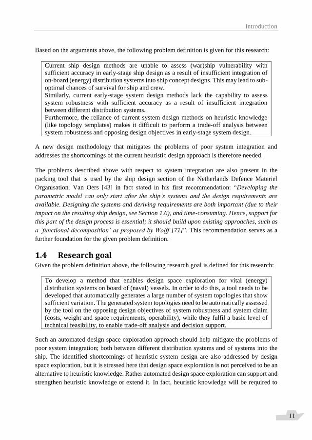
Based on the arguments above, the following problem definition is given for this research:
Current ship design methods are unable to assess (war)ship vulnerability with
sufficient accuracy in early-stage ship design as a result of insufficient integration of
on-board (energy) distribution systems into ship concept designs. This may lead to sub-
optimal chances of survival for ship and crew.
Similarly, current early-stage system design methods lack the capability to assess
system robustness with sufficient accuracy as a result of insufficient integration
between different distribution systems.
Furthermore, the reliance of current system design methods on heuristic knowledge
(like topology templates) makes it difficult to perform a trade-off analysis between
system robustness and opposing design objectives in early-stage system design.
A new design methodology that mitigates the problems of poor system integration and
addresses the shortcomings of the current heuristic design approach is therefore needed.
The problems described above with respect to system integration are also present in the
packing tool that is used by the ship design section of the Netherlands Defence Materiel
Organisation. Van Oers [43] in fact stated in his first recommendation: “Developing the
parametric model can only start after the ship’s systems and the design requirements are
available. Designing the systems and deriving requirements are both important (due to their
impact on the resulting ship design, see Section 1.6), and time-consuming. Hence, support for
this part of the design process is essential; it should build upon existing approaches, such as
a ‘functional decomposition’ as proposed by Wolff [71]”. This recommendation serves as a
further foundation for the given problem definition.
1.4 Research goal Given the problem definition above, the following research goal is defined for this research:
To develop a method that enables design space exploration for vital (energy)
distribution systems on board of (naval) vessels. In order to do this, a tool needs to be
developed that automatically generates a large number of system topologies that show
sufficient variation. The generated system topologies need to be automatically assessed
by the tool on the opposing design objectives of system robustness and system claim
(costs, weight and space requirements, operability), while they fulfil a basic level of
technical feasibility, to enable trade-off analysis and decision support.
Such an automated design space exploration approach should help mitigate the problems of
poor system integration; both between different distribution systems and of systems into the
ship. The identified shortcomings of heuristic system design are also addressed by design
space exploration, but it is stressed here that design space exploration is not perceived to be an
alternative to heuristic knowledge. Rather automated design space exploration can support and
strengthen heuristic knowledge or extend it. In fact, heuristic knowledge will be required to

Introduction
12
some extent in automated design space exploration as well, as objective functions that assess
different design objectives become more realistic when they are based on heuristic knowledge.
This introduces a difficult dilemma though; defining objective functions based on heuristic
knowledge can increase the appropriateness of the objective function but may also introduce
cognitive biases into the function. After reading the dissertation it will be clear to the reader
that this dilemma is encountered in this research as well. A reflection will be given that may
be useful to readers that deal with a similar dilemma.
The next section introduces the principle of the methodology that is developed in this
dissertation to achieve the research goal as defined above.
1.5 Principle of methodology3 Design space exploration using evolutionary algorithms is a well-known approach to map
design solution spaces; Deb [14]. The purpose of design space exploration is providing insight
in how requirements, constraints, technical design solutions and performance characteristics
relate. This is achieved by automatically generating many alternative design solutions, order
of magnitude is 103 – 105 (or even above) and comparing these with respect to their scores on
objective functions, see Figure 1.6. In case of opposing objective functions this leads to a set
of Pareto-optimal design solutions. Exploring the design space and evaluating the (Pareto-
optimal) design solutions helps illustrate the existing design freedom and provides insight into
what is driving design requirements. This insight is vital to arrive at (ultimately) a single,
balanced, well-founded concept design that can serve as input for later design stages in which
the selected concept design is worked out in more detail.
Figure 1.6 Principle of design space exploration with the ATG tool – repeated from de Vos
et al. [68].
3 The first part of the text in this section is repeated directly from de Vos et al. [68].

Introduction
13
The left-hand side of Figure 1.6 is generically applicable to all early-stage design processes
and is further explained in section 2.2. The right-hand side of Figure 1.6 shows the principle
of the Automatic Topology Generation (ATG) tool that is developed in this research and
explained in this dissertation. The ATG tool enables design space exploration for on-board
distribution systems. As indicated, the tool should be able to vary system topology of these
systems. As an example of a possible design solution, a (very) simplistic system topology is
shown at the right-hand side of Figure 1.6 to provide the reader with an idea of the generated
design solutions in the ATG tool. In this example, a diesel-generator set (DG) supplies electric
power to a switchboard (SWB), which distributes the power to an electric motor (EM) that
drives a propeller (Prop) through a gearbox (GB) and a chilled water plant (CWP) that provides
chilled water to a heat exchanger (HE) through a main pipe line (Pipe). The system topologies
generated by the ATG tool are larger and more difficult but can be principally understood with
this simple example. It is expected that achievement of the research goal by realisation of the
ATG tool will support system designers of vital distribution systems on board naval vessels
better than current decision support tools for early-stage system design. The developed
methodology may benefit other system designers (of other systems on board of other ships) as
well.
The ATG tool resembles the packing tool of van Oers [43] in the sense that concept designs
are automatically generated and evaluated by a genetic algorithm. However, where the packing
tool generates ship concept designs, the ATG tool generates system concept designs. The
approach to design space exploration is for both tools characterised by the following specific
features:
- The high computing power of current-day computers is exploited to populate the design
space with a very large number of design solutions (>104) concurrently.
- Populating the design space is performed by the NSGA-II genetic algorithm, ref. Deb
[15], which searches the design space for optimal design solutions. The search is directed
by the objective functions that serve as an indication for design drivers.
- From analysis of the generated design solutions designers can learn a number of things:
o More detailed, quantified design requirements.
o Features of design solutions that are desirable / undesirable.
o Quality of the objective functions used.
- After analysis a designer may select a number of generated design solutions that require
further development in a next iteration of the design process (i.e. concept designs).

Introduction
14
1.6 Dissertation outline The first step in realisation of the ATG tool is to establish a topological model of on-board
distribution systems. This model will be introduced in Chapter 3. The topological model is
combined with the fundamental concepts of network (or graph) theory to arrive at a “node and
edge differentiation framework”. This framework can be used to define networks (or system
topologies) of all relevant, interdependent on-board distribution systems. This is demonstrated
by applying the topological model and resulting node and edge differentiation framework to a
number of vital distribution systems on board of a notional frigate and in doing so the
benchmark system is introduced. The electric power and chilled water distribution systems on
board of the notional frigate also represent the first of two case studies in this research for
which design space exploration is performed. Using the benchmark system as an example, a
first result of this research is already obtained in Chapter 3 in the determination of the size of
the design space as a function of the number of components (nodes), both before and after the
inclusion of a-priori constraints.
The sheer size of the design space leads to the requirement for design space exploration, which
is enabled by the ATG tool that automatically generates system topologies to “search and
populate” the design space. In the ATG tool the node and edge differentiation framework of
Chapter 3 is combined with a genetic algorithm. This is described in Chapter 4. All
automatically generated design solutions (system topologies of vital, interdependent on-board
distribution systems) are assessed on their performance with respect to different design
objectives. This is done by the objective functions of the genetic algorithm. They direct the
search of the design space and as such deserve to be treated in their own chapter: Chapter 5.
This chapter discusses how to assess system robustness and other, opposing design objectives
captured under the term system claim in early-stage distribution system design.
The results of the ATG tool, for both the systems on board of the notional frigate and for a
second case study, systems on board of a notional Ocean-going Patrol Vessel, are presented in
Chapter 6. Both case studies demonstrate that the ATG tool enables design space exploration
for vital on-board distribution systems. However, they also solicit a critical reflection on the
presented methodology, the developed objective functions and the usefulness of the ATG tool.
The last (sub-)sections of Chapter 6 provide this critical reflection, after which Chapter 7
concludes this dissertation and provides recommendation for future research.
Some of the recommendations are related to a theoretical design procedure introduced in the
last section of the next chapter. Chapter 2 is not directly concerned with the development and
presentation of the ATG tool. It provides more background information on early-stage ship
and system design and helps to position the research. Chapter 2 discusses the current approach
to the ship and system design process and elaborates shortcomings in the assessment of
technical feasibility of design solutions. Other difficult-to-assess design objectives are
discussed in more detail as well; robustness in particular. Thus, Chapter 2 will provide a more
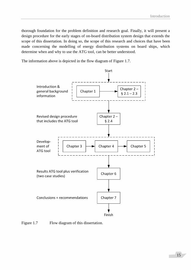
Introduction
15
thorough foundation for the problem definition and research goal. Finally, it will present a
design procedure for the early stages of on-board distribution system design that extends the
scope of this dissertation. In doing so, the scope of this research and choices that have been
made concerning the modelling of energy distribution systems on board ships, which
determine when and why to use the ATG tool, can be better understood.
The information above is depicted in the flow diagram of Figure 1.7.
Figure 1.7 Flow diagram of this dissertation.

Introduction
16
Elaboration of ship and on-board distribution system design
17
“Nous proposon en traitant de la construction des Vaisseaux, & de la Mécanique de leurs
mouvemens, de substituer, s’il se peut, des regles exactes & précises, aux pratiques obscures
& tatonneuses qui font en usage dans la Marine”
(first sentence of: Traité du Navire, de sa construction, et de se mouvemens)
― Pierre Bouguer (1746)
Chapter 2 Elaboration of ship and on-board
distribution system design The previous chapter contained the core background information necessary to introduce the
research goal and methodology of this dissertation. This chapter has a larger scope and aims
to embed the research presented here in its “wider surroundings”. It elaborates the earlier
statement that more detailed system design is often left for later ship design stages, which leads
to poor integration of vital distribution systems into naval ship concept designs; see section
1.3. Thus, the question addressed here is: “Why is more detailed system design left for later
design stages?”
Furthermore, the assessment of different design objectives or design requirements is discussed
in more detail, most notably technical feasibility (of both ships and on-board distribution
systems) and system robustness, as these are key to this research. The final section of this
chapter introduces a design procedure that advances beyond the scope of the present Automatic
Topology Generation tool. This provides insight into the modelling choices that have been
made with respect to the topological model of on-board distribution systems that is introduced
in Chapter 3.
Another reason to describe this larger scope is that the original ambition of the research was
too large. The topics that were, in the end, not or not fully addressed are described in this
chapter as well. These topics may provide ways forward for future, related research.
2.1 Early-stage ship design
2.1.1 Process and methodology The goal of naval architects during early-stage ship design is to find one or more feasible
concept designs given a set of functional requirements following from the mission of the ship
and budget constraints. An abstract idea or functional description of the ship is transformed
into concrete ship configurations defining the ship’s overall dimensions and the number, size
and weight of spaces (building blocks) inside the ship. In this process, many different
alternative design solutions may be considered and compared, refer to Figure 1.4. Ship
configurations can be depicted as General Arrangement Plans (2D) or 3D concept designs;
Figure 1.5 showed an example of the latter.

Elaboration of ship and on-board distribution system design
18
Ship configurations are a first visualisation of the ship that is to be designed and built. They
are the basis for stability and performance calculations, cost estimations and assessment of
other design objectives. They enable the translation from qualitative, functional requirements
to quantitative requirements, i.e. criteria for design objectives. In the early stages of ship design
naval architects therefore concurrently and/or iteratively draw a number of different design
solutions to establish more detailed, quantitative requirements and to enable the selection of
one or more concept designs that strike the right balance between these requirements. The
nature of early-stage ship design has therefore also been described as requirements elucidation,
ref. Andrews [3].
Note that the text above is closely related to the left-hand side of Figure 1.6, which shows a
generic input-process-output representation of early-stage design processes; applicable to both
ship and system design. The process depicted shows that the output of an early-stage design
process is not only y feasible (ship) concept designs, but also n more detailed, quantified
requirements. Both outputs are input to the next design stage (or iteration step). This was
particularly clear in the traditional ship design spiral as introduced by Evans [22], but to a large
extent still is the case in modern concurrent engineering approaches, ref. Nowacki [42]. It
should be noted that the number of “output” requirements n will be larger than the number of
input requirements m (n > m). Furthermore, the number of generated design solutions x may
be larger than the number of concept designs y that are selected for further development in the
next design stage (x > y). The latter particularly is the case when an automated design space
exploration approach is employed that generates and evaluates a very large number of design
solutions (order of magnitude 104 and above). This approach is taken here.
Automated design space exploration becomes an essential first step in early-stage design when
the set of functional requirements m (input) are not sufficiently restrictive and can still be met
by many different concept designs. In the context of ship design, this is the case when the
mission of the ship, or future operations, are unclear. This currently is the case for many navies
and naval ships. Many practical early-stage ship design tools are however based on
(empirically found) design rules, experience with previous, similar ships or even “parent
ships” (i.e. heuristic knowledge). Such tools implicitly set up a relatively large set of m
restrictive design requirements that very effectively limits the size of the design space and thus
the number of considered design solutions x. This is a valid approach when the mission and
functions of the ship is clear. Acknowledging the uncertain future of naval warfare however
necessitates a shift in the adhered-to philosophy concerning early-stage ship design. A shift in
the applied methodology for design solution generation towards the evaluation of a very large
number of design solutions x. In other words, a shift towards automated design space
exploration. Note that the larger design freedom offered by automated design space
exploration may also be embraced for its potential to find new, unexpected design solutions.

Elaboration of ship and on-board distribution system design
19
The earlier mentioned packing tool that is in use by the Netherlands Defence Material
Organisation (DMO), ref. van Oers [43] and Duchateau [21], is an example of an automated
design space exploration tool. It enables (semi-)automatic generation of multiple, and varying,
ship concept designs with the intent of giving designers better insight into the design freedom
that exists and the driving design requirements. Through interactive design space exploration,
the designer is supported in finding more detailed requirements and in striking the right balance
between these requirements, i.e. selecting one or more concept designs which need further
development in the next design stage. The idea behind the packing tool is that a number of
measurable rules can be set up that are applicable to all generated design solutions, like
everything that needs to be on board needs to fit and the ship needs to float upright. These
rules can be translated into constraints for all generated design solutions to ensure the design
solutions are “not wrong”, i.e. technically feasible. Therefore, the packing tool saves time that
can be spent on more complex trade-off analyses, i.e. the decision whether design solutions
are better or worse and why. Other modern, (semi-) automatic approaches to early-stage
(naval) ship design are described by Pawling [49], Singer et al. [59], Andrews et al. [4],
Gillespie [24] and Brown et al. [11].
When automated design space exploration is undertaken another difficulty arises: assessing
design objectives. The tools available for assessing design objectives normally lack accuracy
or applicability, even without automated design space exploration and a lower number of
considered design solutions. A lack of accuracy is caused by the inherent low level of detail
of the design solutions in early design stages. This means the assessment tools that are used
have to produce results (stability calculations, performance prediction, cost estimation,
survivability assessment, etc.) on input that still suffers from a high degree of uncertainty.
Therefore, the goal of many early-stage designer support tools is not to find a single, right
concept design, but rather to give insight into design drivers, relative characteristics of design
solutions and consequences of certain design choices, while ensuring technical feasibility of
the design solutions.
The packing tool is no exception: the generated design solutions have a relatively low level of
detail and (energy) distribution systems are only crudely integrated in the design solutions. As
a consequence, the assessment of technical feasibility lacks accuracy. Problems are
experienced with the assessment of other design objectives as well, warship survivability for
instance is even harder to assess. This of course is the background for the first recommendation
of van Oers [43], as repeated in section 1.3, stating that support with respect to system design
is needed. To understand the problems experienced with assessing design objectives /
requirements and integrating systems, a further treatment of design requirements for ships will
follow in the next section.

Elaboration of ship and on-board distribution system design
20
2.1.2 Design requirements To understand why it is difficult to better integrate distribution systems in early-stage ship
design it is necessary to first better understand the assessment of feasibility of ship concept
designs. The task to come up with feasible concept designs can be subdivided into assessing
economic and technical feasibility of generated design solutions. It is next to impossible to
accurately predict economic feasibility during early-stage ship design; not only because of the
inherent low level of detail of considered design solutions, but also because of the uncertainty
in required cost data (market situations change every day). The often-used term cost estimation
is therefore adequately chosen. Costs, and in particular the purchase costs of a ship (also known
as the budget), are an important design driver though. Cost estimation only makes sense once
technical feasibility of design solutions has been established though.
Assessing technical feasibility is somewhat less uncertain than cost estimation because laws
of nature governing the ship’s stability and behaviour are well known and invariable. Naval
architects assessing technical feasibility of concept designs focus on at least two design
requirements, which are non-negotiable until a certain threshold value is reached:
Ship stability: The ship must, under normal circumstances, but also in extreme
weather conditions and up to a certain damage level, be able to float upright. If this
non-negotiable requirement is met, ship stability may still be improved from a ship
motions perspective; the latter being the negotiable part of ship stability.
Ship configuration (arrangement of spaces): All spaces (building blocks) must fit
inside the ship’s envelope and they cannot overlap. Furthermore, any constraints
different spaces may have concerning their location must be respected (e.g. the bridge
is not to be located under the waterline). If this non-negotiable requirement is met,
ship configuration may still be improved in such a way that logistics of people and
goods within the ship are well organised (negotiable).
A design solution may be considered technically feasible if the non-negotiable parts of ship
stability and ship configuration are met. To assess this, the weight and space balances of a
design solution need to be set up. There can be discussion on the accurateness with which these
balances are set up in early-stage ship design. To ascertain that a ship floats for instance, it
suffices to check whether the governing principle of Archimedes (the weight of a floating
object equals the weight of the displaced water) is obeyed by concept designs. The weight
distribution within the ship is however needed to assess whether a ship floats upright. In order
to do this, the weight of spaces in the design solutions need to be estimated, or rather the weight
of components within them and the construction surrounding them. But to what extent shall
the components in the spaces be taken into account? And how to assess construction weight?
These are choices that have to be made; it should be clear that in early-stage ship design the
chosen level of detail is often limited, particularly if a very large number of highly varying
design solutions is evaluated.

Elaboration of ship and on-board distribution system design
21
Having the weights of the building blocks is still not sufficient though, no matter the accuracy
of the weight estimation. A weight distribution is only known when the spaces (building
blocks) have also been arranged into a ship configuration, which brings us to the space balance.
Assessing whether all spaces fit inside a ship’s envelope means solving the space balance for
a design solution; i.e. arranging spaces and corridors into a ship configuration and wrapping a
hull and superstructure around them. In order to be able to do this, the dimensions of spaces
(and components within them) need to be estimated. The same dilemma as for weight
estimation exists: to what extent are components inside the spaces taken into account and with
what accuracy are the dimensions estimated?
It is clear that solving the weight and space balances for a (large) number of design solutions
is a difficult job. Given the dilemma with respect to the accurateness with which the weight
and space balances are solved to assess technical feasibility, it is also understandable that the
number of considered design solutions are traditionally limited and built as much as possible
on heuristic knowledge. When an automated design space exploration approach is adopted,
like with the packing tool, the number of generated design solutions is large and sacrifices with
respect to accuracy of technical feasibility assessment need to be made by e.g. limiting the
integration of distribution systems to choosing and placing the larger system components and
leaving out system connections.
Finally, consider that technical feasibility is not the only design requirement. Other design
requirements may be design drivers as well, like speed, range, maximum days-at-sea, manning,
ship motions, internal logistics and survivability. Thus, these objectives need to be assessed as
well for each design solution (whether automatically generated or not), preferably after
confirmation of technical feasibility. This further adds to the complexity of early-stage ship
design, not only because there evidently are more design requirements to be considered than
just technical feasibility, but also because some of these design objectives are difficult to
quantify. An example of the latter is whether a ship configuration is “good” from an internal
logistics point-of-view for instance; a design objective that is considered important by many
ship designers.
Expressed differently, some of these design objectives lack a clear metric, survivability being
an important example. Ship survivability represents the ship’s ability to remain functional
during and after a disruptive disturbance occurs. There can be a lot of discussion (negotiation)
as to which disturbances the ship should be able to resist and to what extent. The result of such
discussions will highly depend on the context. For example, the natural (or unintentionally
man-made) disturbances an offshore vessel should be able to cope with (e.g. fire, flooding) are
different from the intentional hostile disruption that a naval vessel is designed to withstand
(e.g. missile hit). Consequently, there is no clear way to measure ship survivability. The choice
of metric will highly depend on the context and even when a metric is chosen there can be
discussion whether that particular metric accurately reflects ship survivability.
Elaboration of ship and on-board distribution system design
22
In the specific case of the packing tool the considerations above led to an approach in which
only truly unfeasible designs, i.e. “wrong” designs that do not meet constraints like floating
upright, were removed from the design space, while all other generated design solutions are
retained. Van Oers [43] did so in order to maximise the chance of finding surprising, novel
design solutions. As a consequence, the design space is enormous and computational effort
may be wasted on uninteresting parts of the design space from the perspective of negotiable
design requirements. This was the reason for Duchateau [21] to enable interactive steering of
the packing tool by the user, who can then, with negotiable design requirements in mind, direct
the design space exploration.
2.1.3 Problems The assessment of technical feasibility of ship concept designs thus depends on the ability to
solve the weight and space balances. In an automated design space exploration approach this
needs to be done for a large number of automatically generated design solutions. It is now also
clear that the weight and space balance can only be solved when a ship configuration is
available. Now distinguish between mission-related spaces, crew spaces (accommodation) and
machinery spaces inside a ship.
The weight and space of mission-related spaces or equipment (e.g. sensor and weapon suit)
are typically known or defined before the design starts as they follow directly from the mission
of the ship. Predicting the weight and space required by crew spaces is more difficult, but a
typical room lay-out is available for the different crew members on board and to a certain
extent crew size and composition can be estimated. At the same time, crew size and
composition depend on the systems on board and the chosen level of automation. This
dependency was elaborately researched by Wolff [71].
Normally, the greatest difficulty is experienced with predicting the weight and space required
by machinery spaces (e.g. engine room(s), switchboard rooms, HVAC rooms, etc.), because
the number and type of distribution system components within these spaces are still unknown
during early-stage ship design. This at least is the consequence when a choice is made to leave
early-stage system design for later ship design stages, which often is the case as is argued in
the previous section. The lay-out of machinery spaces is then also unknown. As a consequence,
it is difficult to incorporate machinery spaces accurately on the weight and space balances,
even though such spaces are among the largest and heaviest spaces on a ship. Note that this
problem of “not yet knowing details of the design of distribution systems” also causes
uncertainty in the crew size and composition prediction and therefore the required size and
weight of crew spaces. Dealing with this latter uncertainty is outside the scope of this research
and the reader is referred to Wolff [71]; dealing with early-stage distribution system design is
not outside the scope of this research.
Elaboration of ship and on-board distribution system design
23
There are methods, currently used in industry, that by-pass the problem of the number, type,
size and weight of distribution system components being unknown in early-stage ship design.
These methods for instance assume a certain floor area and volume of the engine room based
on the power rating of the (main) engine(s) installed. The quantification for such design
parameters follows from a database of already existing ships. Such a method is considered
crude as it does not consider the dimensions of the actual engines but extrapolates the main
engine power rating directly to space dimensions. The idea is that the entire engine room,
including the propulsion support systems needed for operating the engines, which are also in
the engine room, scale with the main engine power. Many effects, some of them non-linear,
like varying power density of engines, alternative technologies for auxiliary systems, etcetera
are not taken into account with such methods. Furthermore, while one can to a certain extent
assume that propulsion support systems correlate with main engine power rating, this cannot
be assumed for other (energy) distribution systems like electric power and chilled water
distribution systems, Fire-Fighting and HVAC systems, potable water distribution systems,
etc. These systems scale mainly with mission-related systems, other distribution systems than
propulsion, ship size and/or crew size.
The topology of the network of connections between the distribution system components is
normally not considered in early-stage ship design either. Determining the topology of the
network and the routing of the connections through the ship (i.e. the number, type and routes
of cables, pipes, ducts and shafts) is normally left for later design stages as the connections of
distribution systems hardly affect the ship’s weight and space balances. The topology, the
routing and the number and type of components of distribution systems do however have a
large influence on other design objectives like ship survivability.
Two problems encountered in current early-stage ship design become clear from the text above
(also when advanced tools, like the packing tool, are applied):
Solving the two main balances (i.e. weight and space) in early-stage ship design to
assess technical feasibility of design solutions, remains inaccurate as long as
distribution system design is not, or only crudely, considered. This is particularly the
case for ships where a large part of the total weight and space is taken up by such
systems, like naval and offshore vessels. Because of this inaccuracy there is a
significant risk for re-design work being necessary in later, more detailed design
stages. This re-design work is associated with high development costs.
Assessing other design objectives, like survivability, in early-stage ship design is
impossible with current design methodologies, since the design of distribution
systems has a large influence on these objectives.
These two problems are the foundation for the paragraph in section 1.3 in which it is stated
that the integration of systems in ship concept designs is insufficient. Overcoming these two

Elaboration of ship and on-board distribution system design
24
problems can only be achieved by including early-stage distribution system design more
elaborately in early-stage ship design. The original ambition of this research was to enable this
to such an extent that both problems would be addressed. The method developed in this
dissertation addresses only the second problem though. The first problem was addressed by
Stapersma et al. [61] in the context of this research, but that part of the research has not
advanced sufficiently to be part of this dissertation, the main reason being that addressing the
second problem proved to be sufficiently difficult on its own. The precise nature of the first
problem will be explained when in section 2.4 the design procedure of on-board distribution
systems will be analysed in detail.
Either way, early-stage distribution system design needs to be included more elaborately in
early-stage ship design. Section 1.3 introduced problems with early-stage system design as
well though, particularly when it comes to system integration between different distribution
systems. Therefore, the next section introduces early-stage system design according to a
similar structure as presented in this section for early-stage ship design: i.e. the process, design
requirements and problems encountered in current early-stage system design are elucidated.
2.2 Early-stage system design
2.2.1 Process and methodology The goal of marine engineers during early-stage system design is to find one or more feasible
concept designs for the distribution system or systems under consideration given a set of
functional requirements following from the mission of the ship and budget constraints. An
abstract idea or functional description of the systems under consideration is transformed into
a first, more concrete principle system diagram defining the number, type and capacity of
system components and the topology of the distribution network connecting the components.
Examples of such system diagrams include so-called single-line or key one-line diagrams for
electric power generation and distribution systems, block diagrams or energy flow diagrams,
ref. Klein Woud et al. [36], for propulsion systems or integrated power plants (see Figure 2.1)
and principle piping system diagrams for pipe flow systems needed for transporting fluids or
heat throughout the ship.
Principle system diagrams are a first visualisation of the system in a similar manner as first
drawings of ship configurations are first visualisations of the ship that is to be designed. They
are the basis for system performance calculations, cost estimations and quantification of other
requirements the systems have to meet. They enable the translation from m qualitative,
functional requirements of the systems to n quantitative system requirements (see Figure 1.6),
i.e. criteria for design objectives. Here, as well, the term requirement elucidation is
appropriate; ref. section 2.1.1.
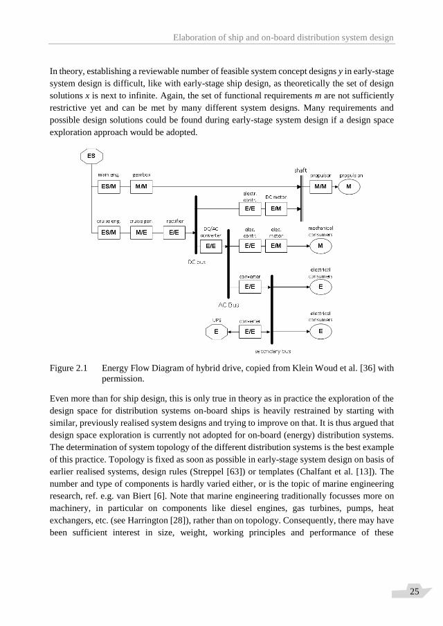
Elaboration of ship and on-board distribution system design
25
In theory, establishing a reviewable number of feasible system concept designs y in early-stage
system design is difficult, like with early-stage ship design, as theoretically the set of design
solutions x is next to infinite. Again, the set of functional requirements m are not sufficiently
restrictive yet and can be met by many different system designs. Many requirements and
possible design solutions could be found during early-stage system design if a design space
exploration approach would be adopted.
Figure 2.1 Energy Flow Diagram of hybrid drive, copied from Klein Woud et al. [36] with
permission.
Even more than for ship design, this is only true in theory as in practice the exploration of the
design space for distribution systems on-board ships is heavily restrained by starting with
similar, previously realised system designs and trying to improve on that. It is thus argued that
design space exploration is currently not adopted for on-board (energy) distribution systems.
The determination of system topology of the different distribution systems is the best example
of this practice. Topology is fixed as soon as possible in early-stage system design on basis of
earlier realised systems, design rules (Streppel [63]) or templates (Chalfant et al. [13]). The
number and type of components is hardly varied either, or is the topic of marine engineering
research, ref. e.g. van Biert [6]. Note that marine engineering traditionally focusses more on
machinery, in particular on components like diesel engines, gas turbines, pumps, heat
exchangers, etc. (see Harrington [28]), rather than on topology. Consequently, there may have
been sufficient interest in size, weight, working principles and performance of these

Elaboration of ship and on-board distribution system design
26
components, but much less in survivability aspects of marine engineering, which are heavily
influenced by system topology.
Many practical early-stage system design tools are thus based on experience with previous,
similar systems, (empirically found) design rules, or even “parent systems” (i.e. heuristic
knowledge). Such tools implicitly set up a relatively large set of restrictive design requirements
that very effectively limits the size of the design space and thus the number of considered
design solutions. If a number of different design solutions is considered, the variation is limited
to a fixed, low number (< 10) of preliminary designs and/or alternative components.
A number of reasons can be given for the low number of system design solutions that are
generated and evaluated in current design practices, even though the design space theoretically
is much larger:
More detailed design of distribution systems is started too late in the ship design
process. The space, weight and budget reserved for systems is then already set and
innovative designs (with more, other and/or newer components or alternative
topologies) can no longer be accommodated, see section 2.1. In fact, choices about
the design of different distribution systems have then already been made (often
implicitly) earlier on in the design process on basis of previous systems / ships (by
ship designers).
Variation in system topology is considered a waste of effort as already existing
topologies work well (primary design requirement) and allowing more design
freedom for system topology creates too much “room” for the generation of infeasible
system concept designs. If system robustness (which heavily depends on system
topology) is an important design objective, there are design rules that are considered
reliable and can guide system designers to more robust systems.
Specific distribution systems are designed by different departments or companies
specialised in their own system. Each of these organisations may have their own
preference or method with respect to applied system components and topology.
Furthermore, these organisations may become involved too late in the overall ship
design project, in different advanced design stages.
Interaction between different distribution systems adds to complexity of integrated
systems design, which makes the job already sufficiently difficult and time-
consuming without more elaborate design space exploration.
Re-using system designs is effective; especially from the perspective that crew
needed for operating the systems have had certain training and need additional
training if the system designs vary more often.
Proper designer support tools to aid system designers with design space exploration
are not available.
Elaboration of ship and on-board distribution system design
27
As a result of the arguments above, it is stated here that automated design space exploration
for on-board distribution systems is currently not performed, neither in practice, nor in naval
engineering research, at least not in a similar manner as is done for ship design with e.g. the
packing tool. This statement leads to a number of (rather philosophical) questions that started
this research: What if on-board (energy) distribution system design is started with automated
design space exploration? Would alternative concept designs be found for distribution systems
(that perhaps even outperform current system designs)? What can system designers learn from
the design space exploration approach in ship design? Can integration of concept systems in
concept ships be improved by such an approach and if so, what would be the impact on the
assessment of different design objectives, like ship and system technical feasibility and warship
survivability?
This research aims to find some initial answers to the questions raised above and introduce
more elaborate design space exploration in early-stage distribution system design, see section
1.4. To have an idea of which system design objectives should be included in such a novel,
automated design space exploration approach the next section focusses on which design
requirements are taken into account by current system design methodologies.
2.2.2 Design requirements Based on Klein Woud et al. [36] and Klein Woud et al. [37], the following design requirements
are identified for all distribution systems on board ships. Note that most were already
mentioned in section 1.1 and are clarified here.
Technical feasibility: System operation is in all conditions and all operational modes
governed by physical principles like mass and energy conservation. The primary goal
of any system design effort is to design a system that works (under normal and other
to-be-expected circumstances). Technical feasibility is thus the primary, non-
negotiable requirement for distribution systems (as it is for ships as well). During
design technical feasibility of different energy distribution systems is ensured by
solving at least the energy balance for each distribution system (with different levels
of detail).
Operational performance: System operation may be optimised with respect to energy
consumption, emissions etc. Operational performance typically is a negotiable design
requirement for distribution systems.
Economic feasibility: both the capital expenditure and operational expenditure
associated with system realisation and operation need to acceptable. Economic
feasibility is more of a negotiable requirement than technical feasibility, but often
“the budget” is regarded as a non-negotiable requirement / constraint.
Legal compliance: ship and system designs, of non-military vessels especially, but
nowadays more often those for military vessels as well, have to comply with the law
and classification societies’ rules and regulations.

Elaboration of ship and on-board distribution system design
28
Weight and space requirements: distribution systems “claim” precious weight and
space on ships (see section 2.1); especially their components. Weight and space
requirements for distribution systems are negotiable, but typically need to be
minimised since non-mission-related systems are often considered a “necessary
nuisance”.
System reliability and safety: firstly, the crew on-board ships, but in fact society as a
whole, require the distributions systems on-board ships to operate reliably and safe
in all operational modes and circumstances. Associated terms with this design
requirement are: system vulnerability, robustness, resilience, redundancy, re-
configurability, availability and maintainability.
Monitoring and control: sensors and actuators need to be fitted within the system to
enable monitoring and control of system operation. A related design requirement is:
Operability: system operators, control engineers as well as software designers of the
Monitoring and Control system benefit from a clear, comprehensible system lay-out
that can be controlled in a straightforward manner in normal and in emergency and
damage conditions. For the latter conditions manual control may be required, as was
also the philosophy of Admiral H.G. Rickover; see Hill [30].
Quantifying the design requirements above can be difficult and time-consuming; especially in
early stages of system design. Like with ship design this may be due to a low level-of-detail
of the design solutions being evaluated, but limited applicability of metrics for the different
design requirements contribute to this problem as well. What exactly is meant with system
vulnerability for instance is difficult to define (like with ship survivability); especially if it
must be a mathematical definition that can be evaluated by a computer programme. Such a
metric quantifying system vulnerability accurately is difficult to find and depends in fact on
the context and level-of-detail of a design solution. This is one of the reasons why system
vulnerability is typically not assessed in early-stage system design and system designers rely
on templates for system topology or design rules, ref. Spruit et al. [60] and Chalfant et al. [13],
which fixates the system vulnerability early on in the design process to a large extent. Only in
later design stages, like contract design when much more detail of the ship and systems are
available do engineers in practice discuss system vulnerability, but by then radical design
changes may no longer be possible or at least are costly.
How the other design requirements above are assessed in early-stage system design is
described in marine engineering handbooks like Klein Woud et al. [36] and [37], which
typically focus on the assessment of technical feasibility of specific energy distribution
systems. A qualitative discussion on design requirements for systems on board warships
specifically is given by Bradbeer et al. [9]. Note however that these assessment methods
presume the topology of the system is already known or can quickly be fixed based on heuristic
knowledge. For the methodology employed here, where system topology is still variable, all
objective functions representing design requirements need to be defined anew. Given the

Elaboration of ship and on-board distribution system design
29
above discussion on metrics for system vulnerability it is expected that finding a definition for
this design requirement in early-stage system design is challenging. At the same time, since
vulnerability depends highly on topology, the method may also be the most rewarding for this
system design requirement and thus indeed help in better assessing warship survivability
(ultimately). Therefore section 2.3 discusses system robustness in more detail. Assessing
technical feasibility when topology is highly variable will also be difficult, since current
methodologies are too detailed. This statement will be further elaborated in section 2.4.
Noteworthy is also the current assessment method for weight and space requirements of
distribution system components in early-stage ship and system design. Dimension prediction
tools (estimating the dimensions and weight of system components) that are currently often
used suffer from fundamental flaws. Many of them establish mathematical relationships (fit
functions) between main performance characteristics of system components (e.g. power
output) and dimensions that are not based on first principles. This typically renders the
relationships invalid at or beyond the limits of the databases they are based upon. This may go
as far as predicting nonsense like negative dimensions and weight for distribution system
components if a system designer is not careful. A subtler risk of such methods is the application
of linear interpolation where non-linearities are present. It was found in Stapersma et al. [61]
that by using first principles an analogy between preliminary design of different components
(engines, gearboxes, electric machines, heat exchangers, etc.) can be established which
improves the applicability of dimension prediction tools with relative ease and mitigates risks
for erroneous dimension prediction. The methodology explained there has already been
expanded upon, ref. Hu [32], and has found its way into graduation projects with a focus on
early-stage design of specific on-board power plants, ref. Rietveld [54], ten Hacken [29] and
van Dijk [18].
2.2.3 Problems A number of problems for early-stage on-board distribution system design become clear from
the text of the previous sections:
Conceptual system design is absent in current ship design practice in the sense that
elaborate design space exploration using modern techniques for topology variation is
not yet undertaken for distribution systems: i.e. the number of design solutions
generated and analysed in early-stage system design is typically below 10, while the
design space is orders of magnitude larger when topology is variable. This is a
consequence of the choice to focus on system components and leave distribution
system design for later ship design stages, as described in section 2.1. System
designers are then forced to re-use earlier established system designs (both
topologically and component-wise).

Elaboration of ship and on-board distribution system design
30
The low number of design solutions is mainly established by fixing the system
topology at the start of the system design process by relying on heuristic knowledge.
The implication of this design practice is that the actual size of the design space is
unknown and as a consequence the dominance or optimality of the small number of
design solutions that are analysed is uncertain: are we evaluating the “best” concept
designs? This problem becomes more urgent when system robustness needs to be
assessed in early-stage system design as well, since robustness heavily depends on
system topology.
System integration, i.e. integration of different energy distribution systems, receives
too little attention in early-stage system design because different organisational units
are responsible for different systems. This has adverse effects on system performance
and system robustness.
Dimension prediction of system components is currently often done by fitting an
equation onto database information of existing system components without inclusion
of first principles. This leads to models that may produce invalid dimension
prediction (e.g. negative dimensions) and are prone to overlook non-linearities.
The first three problems provide a more thorough foundation for the problem definition stated
in section 1.3. The last problem needs to be addressed as well, and to certain extent this has
been done in the context of this research, but the developed methodology requires more input
information than the present ATG tool and is therefore considered to be applicable only after
automated design space exploration has been performed. This is elaborated in section 2.4.
First, system robustness is explained in more detail as this design objective is of prime
importance to this dissertation (as explained).
2.3 System robustness4 Systems on board of special ships like naval and offshore vessels are designed to withstand
failure of components or parts of the system in adverse conditions, i.e. these systems have a
certain degree of robustness and are thus able to maintain operation even if failures occur; see
Klein Woud and Stapersma [36] and Doerry [19]. In particular for spatially extensive on-board
energy distribution systems that provide vital functions (e.g. electric power supply), the
requirements on system robustness are of prime importance during the design of these ships
and their systems. Improvement in system robustness is in practice often achieved by:
A. Increasing redundancy by duplicating functionally similar components, either as full
back-up or with performance degradation, or by different type of components (similar
function, different working principle) such as accumulators,
4 The text in this section is repeated directly from de Vos et al. [67].

Elaboration of ship and on-board distribution system design
31
B. Introducing separate “islands” in the system topology. The islands are able to operate
as stand-alone systems in critical operations (islands should then also be physically
separated; i.e. located in different zones in the ship separated by fire-resistant and
watertight bulkheads),
C. Increasing re-configurability of the distribution systems by increasing the number of
paths between suppliers and users. This is achieved by additional supply lines to vital
users and by interconnecting the afore-mentioned islands by so-called cross-overs.
A primary example of this design practice are the rules with respect to system configurations
for vessels with Dynamic Positioning (DP) capability: for higher DP classes, classification
societies require increased (functional and spatial) redundancy and re-configurability in
components and connections to achieve higher availability of thrusters;, see amongst others
the (online) rules of ABS [1] and DNV-GL [16], [17] . In the context of naval ship design
similar design “rules” exist (although not enforced by classification societies); see e.g. Streppel
[63] and Spruit et al. [60]. It is also possible to make use of templates, like Chalfant et al. [13]
have done.
Despite these practical design rules, system robustness is an ambiguous term that has many
definitions and embodies a number of related concepts like resilience and vulnerability. There
are also a number of different aspects of robustness, like susceptibility and recoverability.
Finally, there are different ways to improve robustness during system design, like redundancy
and re-configurability (see bullet list above). Thus, robustness as a concept needs to be studied
first, before an objective function for this design objective can be developed for the ATG tool.
Therefore, this section discusses robustness and its related terms; first from a broad
perspective, then from a marine engineering perspective.
Resilience of land-based energy distribution systems has received a lot of attention with
different sources giving different definitions. Willis et al. [70] quote three sources that define
resilience from different perspectives, including the more technological definition given by
Haimes [27]: “Resilience is the ability of the system to withstand a major disruption within
acceptable degradation parameters and to recover within an acceptable time and composite
costs and risks”. Haimes [27] concludes his article stating that resilience cannot be captured
in a simple metric. Nor does vulnerability according to him. Nonetheless Willis et al. [70]
identified 154 resilience metrics in 58 papers.
Within the marine engineering community multiple vulnerability metrics exist as well. The
impression of the author is that offshore engineers are more accustomed to the term robustness
in this case, while naval engineers typically use survivability and vulnerability, amongst other
terms. Resilience is a term that is not so often encountered in a maritime context, but marine
engineers will recognise and accept the definition of resilience as given by Haimes [27]: the
design objective is to increase the system’s ability to withstand major disruptions.
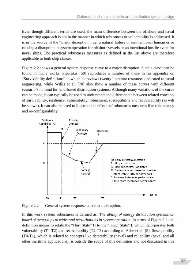
Elaboration of ship and on-board distribution system design
32
Even though different terms are used, the main difference between the offshore and naval
engineering approach is not in the manner in which robustness or vulnerability is addressed. It
is in the source of the “major disruption”; i.e. a natural failure or unintentional human error
causing a disruption in system operation for offshore vessels or an intentional hostile event for
naval ships. The practical robustness measures as defined in the list above are therefore
applicable to both ship classes.
Figure 2.2 shows a general system response curve to a major disruption. Such a curve can be
found in many works. Piperakis [50] reproduces a number of these in his appendix on
“Survivability definitions” in which he reviews twenty literature resources dedicated to naval
engineering, while Willis et al. [70] also show a number of these curves with different
scenario’s in mind for land-based distribution systems. Although many variations of the curve
can be made, it can typically be used to understand and differentiate between related concepts
of survivability, resilience, vulnerability, robustness, susceptibility and recoverability (as will
be shown). It can also be used to illustrate the effects of robustness measures like redundancy
and re-configurability.
Figure 2.2 General system response curve to a disruption.
In this work system robustness is defined as: The ability of energy distribution systems on
board of (war)ships to withstand perturbations in system operation. In terms of Figure 2.2 this
definition means to relate the “Hurt State” H to the “Intact State” I, which incorporates both
vulnerability (T1-T2) and recoverability (T2-T3) according to Ashe et al. [5]. Susceptibility
(T0-T1), which is related to concepts like detectability (naval) and reliability (naval and all
other maritime applications), is outside the scope of this definition and not discussed in this

Elaboration of ship and on-board distribution system design
33
dissertation. Furthermore note that, compared to the definition of resilience according to
Haimes [27], the time aspect (x-axis) is not considered in the above robustness definition. This
is a result of the focus on early-stage system design in this work; it is assumed that at these
design stages insufficient information about the systems is available to perform proper time
domain analysis (this will be elaborated in the next section).
Focussing specifically on electric power distribution systems on board of naval vessels, Doerry
[19] has contributed significantly to the design of survivable distribution systems, as well as
Trapp [65] and Rigterink [55]. More robustness studies, within and outside a naval engineering
context exist, most of which apply more complicated methods like time-domain analysis of
system operations. In fact, the rather general observation of Sydney et al. [64] that “To date,
robustness metrics are deficient and unfortunately the following dilemmas exist: accurate
models necessitate complex analysis while conversely, simple models lack applicability to our
definition of robustness”, can be observed in robustness assessment studies for on-board
energy distribution systems as well. This is the reason this study focuses specifically on the
application of cross-overs (see list above) in order to maximise system re-configurability,
which is better captured in a simple metric. The robustness definition introduced above will
therefore be transformed into a re-configurability objective function in section 5.2. The
function is based on a framework for node and edge differentiation that will be introduced in
Chapter 3.
2.4 Design procedure for on-board systems Before Chapter 3 can introduce the topological model of on-board distribution systems and
resulting node and edge differentiation framework, another design objective, which in fact is
a constraint, needs to be analysed: technical feasibility of systems. This section will start with
introducing four different levels of technical feasibility assessment of which the first is
relatively unknown in a marine engineering context. Subsequently this section will introduce
a (theoretical) design procedure for early stages of integrated ship and system design when
automated design space exploration is adopted as a starting point for system design. It will be
argued why automated design space exploration, and thus this research, should be limited to
the first level of technical feasibility assessment. Nonetheless, the presented design procedure
will continue until the second level of technical feasibility assessment is reached. As such, the
scope of the presented design procedure is larger than the scope of this dissertation. This is
important because early-stage ship and system design are not finished when the present ATG
tool has produced its results. Consequently, it can be better understood from this section where
the ATG tool fits in the overall design process.
The design procedure has been set up with technical feasibility of distribution systems as a
non-negotiable design requirement in mind, which means that technical feasibility will be used
later in this dissertation to set up a-priori constraints that limit the size of the design space. In
the context of this dissertation technical feasibility means that an (automatically) generated
Elaboration of ship and on-board distribution system design
34
design solution can reasonably be expected to be able to “work” (i.e. fulfil its function) once
the design has advanced sufficiently, in other words a design is “not wrong”. In general, a
system design can be considered technically feasible when the supply and demand of an
(energy) flow match (in the broadest sense of that word); i.e. the energy balance can be
confirmed in all different operational modes and conditions. It was stated in section 2.2.2 that
current assessment methods for technical feasibility, i.e. current matching procedures, are too
detailed. Indeed, the procedures and associated calculations in Klein Woud et al. [36] for
matching supply and demand in propulsion systems or Klein Woud et al. [37] for matching
supply and demand in pipe flow systems are too detailed when system topology is highly
variable and / or when the number of users and suppliers is large, as is the case in the ATG
tool.
Therefore, the following levels for technical feasibility assessment are identified:
I. Flow type pairing (excluding different operational modes or conditions): assessment
whether the required type of input (flow type) of certain system components (users)
correspond to the provided output of other system components (suppliers). Example:
a sensor that requires 440 V AC power supply must be connected to (i.e. paired with)
a 440 V AC power supplier.
II. Power balancing (including frequently occurring and emergency operational modes
or conditions): assessment whether power supply and demand in different distribution
systems are balanced for typical, stationary operations (design condition) and / or
operation in extreme conditions. The aim of power balancing is to determine the
maximum combined power that is required from suppliers in a specific distribution
system. This is typically done by setting up a load balance that specifies the power
requirement per (major) user in frequently occurring operational modes or conditions.
Note that Power = effort ∙ flow – effort and flow as used by e.g. Karnopp et al. [34];
the terms effort and flow will be specified for different energy domains at the end of
this section. Examples of power balancing: electric load balances for e.g. 690 V AC
power distribution system (incl. electrically-driven high-power users that are part of
the propulsion and/or manoeuvring system) – see appendix A for a simple example
of an electric load balance, heat load balances for different spaces, etc. Often effort
and flow balancing is separated from power balancing (at least in the mechanical
energy domain). For many components proper dimensioning, i.e. based on first
principles, is only possible when two out of three (power, effort and flow) are known.
Elaboration of ship and on-board distribution system design
35
III. Effort & Flow matching (including all stationary operational modes or conditions):
assessment whether supply and demand in different distribution systems match for
both effort and flow for all expected stationary operations and extreme conditions by
evaluating how individual suppliers are loaded (in terms of effort and flow) in a
detailed performance characteristic (or envelope) of the supplier. The aim of effort
and flow matching is to prove that the different combinations of effort and flow (in
different operational modes) lie within safe margins of the envelopes of the supplying
components: this is the crux of matching as intended by Klein Woud et al. [36] and
[37]. Examples: evaluation of propeller load line in torque – rotational speed diagram
of internal combustion engine, evaluation of pipe flow system characteristic in pump
characteristic and evaluation of combined electric load as experienced by an electric
power generator in its P/Q diagram (also known as capability curve). For many on-
board systems (that are normally operating at stationary loads, i.e. no transients) this
level of technical feasibility assessment will be sufficient to initiate procurement of
system components.
IV. Dynamic operations matching: time-domain assessment of technical feasibility by
simulation, experimenting, prototyping, etc. in order to verify that operating points
(effort - flow combinations) remain within machinery envelopes also during transient
situations.
The first level of supply and demand matching, from here on called flow type pairing to avoid
confusion with the third and fourth level of technical feasibility assessment, can be performed
without taking different operational modes or conditions into account as this basic level of
technical feasibility is required in all operational modes or conditions (even in a “hurt state”,
i.e. when the system is (partly) damaged, which forms the link with system robustness). Flow
type pairing ensures the right connections (i.e. feasible connections) exist between suppliers
and users in different distribution systems (e.g. an electric motor is supplied with the right kind
of electric power and not with e.g. fuel or seawater).
Flow type pairing is often implicitly performed in design practice as the topological variations
are normally limited, i.e. a system designer ensures the right connections exist by fixating the
system topology early on in the design process. As a consequence, practical system designers
can immediately go to the second level of technical feasibility assessment: power balancing,
and sometimes even the third level: effort and flow matching (e.g. propulsion systems). Note
that this observation is closely related to the statement in section 2.2 that automated design
space exploration is absent in current early-stage system design and to the observation that
system integration between systems is lacking. The first level of technical feasibility
assessment should be applied when topology is undefined, like in the approach to early-stage
system design taken here, and sets (most welcome) limits (i.e. constraints) on the design
freedom in network topologies for different, interdependent on-board distribution systems.
The latter will be elaborated in section 3.5 where the non-negotiable design requirement
Elaboration of ship and on-board distribution system design
36
technical feasibility will be transformed into an a-priori constraint that limits the size of the
design space (note that this also means technical feasibility is guaranteed and does not need to
be assessed after automatic topology generation).
Choosing to limit technical feasibility assessment to flow type pairing (the first level) means
automatic topology generation for interdependent on-board distribution systems becomes
possible which leads to the requirement of a new (theoretical) design procedure that includes
automatic topology generation. The design procedure will be introduced below. Note that a
consequence of this choice also is that all functions and calculation procedures to assess other
(negotiable) design objectives need to be redefined as well (like technical feasibility
assessment was redefined here to flow type pairing) when system topology is variable (as was
already stated in section 2.2.2).
The design procedure for the early stages of on-board distribution system design, when an
automated design space exploration is the start of the design process, is:
1. Determine the mission related systems the ship is equipped with to execute her
mission(s).
2. Determine the type of flows (energy or other commodity – e.g. data for monitoring
& control) the mission related systems require from supporting distribution systems
in order to be able to fulfil their function.
3. Determine the type of flows (energy or other commodity – e.g. data for monitoring
& control) the suppliers of the supporting distribution systems require from other
supporting distribution systems in order to be able to fulfil their function. [Continue
until the list of components of different, interdependent on-board distribution systems
is complete].
These questions lead to a list of different distribution systems (and their components) the ship
will need to be equipped with in order to function properly. The type of flow that is distributed
within these systems is specified on this list (e.g. 440 V AC electric power, 5 °C chilled water,
rotational mechanical power, ventilation / conditioned air, etc.). Principally the sequence can
continue to a fourth, fifth or nth question until one arrives at the ultimate sources a ship needs
for a successful mission. These sources are mainly fuel, air and sea water, but also lubrication
oil, provisions and other consumables. Note that choosing types of (energy) flow that are to be
distributed in dedicated systems may also (implicitly) involve a choice for a certain control
strategy: e.g. choosing to have users of electric power that are designed for 440 V AC electric
power also means choosing to have a dedicated 440 V AC electric power distribution system
including associated voltage control for that type of distribution system. Such a choice is not
essential from a first-principle perspective, standards rarely are, but they are practical.
Elaboration of ship and on-board distribution system design
37
Note that the first steps of the design procedure as described above correspond to arrow B1 in
Figure 1.4 and the blocks this arrow connects. The design procedure continues with arrow B2
for each particular (energy) distribution system with the following steps:
4. Determine the number and type of suppliers (users are known from step 1-3).
5. Determine the topology of the network that connects the suppliers and users
(suppliers and users for each particular distribution system are known from steps 1-
4). This step, connecting the suppliers and users in different distribution systems, is
really flow type pairing.
At this point in the design procedure, system diagrams (i.e. system concept designs or system
topologies) can be produced; regardless of whether that is done by an automated design space
exploration tool, as will be done in this research, or whether this is done differently. Further
note that the number and type of suppliers for each distribution system have been chosen; but
not their capacity. This is a consequence of choosing for the first level of technical feasibility:
flow type pairing. This means that it can be ensured that users are provided with the right kind
of flow, but not yet whether there is sufficient flow for typical operational conditions / modes.
This will be done at a later stage in this design procedure.
As one can conclude from questions 1-3 suppliers in one particular distribution system can be
users in another. It is therefore more correct to interpret suppliers and users as converters which
form the interaction links between different distribution systems. Interestingly, the latter step
in the design procedure (step 5) typically also leads to the introduction of one or more common
distribution line(s). Large distribution systems, i.e. systems with a large number of users and
(usually fewer) suppliers, are typically designed such that they bring together the flow from
the suppliers in a small number of common distribution lines from where the flow is distributed
to the users. Such common distribution lines enable centralised flow control and significantly
decrease the total length of connections when compared to distribution systems where
suppliers and users are directly connected according to Klein Woud et al. [37]. A more
elaborate discussion on suppliers users and common distribution lines will follow in Chapter
3.
After the first five steps, (automatically generated) design solutions for different,
interdependent distribution systems are available and their performance (in the broadest sense)
can and should be assessed. Therefore, step six is:
6. Assess and compare the generated design solutions for vital on-board distribution
systems on different design objectives, like costs, weight and space requirements
(collectively system claim) and system robustness as far as that is possible with the
available “information” in the generated design solutions.
Elaboration of ship and on-board distribution system design
38
For the ATG tool, developed and explained in this dissertation, this is the last step, i.e. the
ATG tool is meant to support the design process up to this point in the design procedure. The
design procedure does not stop here though. At the ship level, system robustness depends not
only on the number and type of components and the generated system topology, but also on
aspects like network length and location of system components and connections (susceptibility
of the systems). The design procedure then continues with:
7. Determine the location of system components in the ship.
8. Determine the routing of connections between suppliers and users for each
distribution system through the ship compartments, possibly via common distribution
lines.
9. Assess and compare the generated design solutions for ships (now fitted with routed
distribution systems) on design objectives like system claim and (war)ship
vulnerability.
With these steps conceptual system design is integrated with conceptual ship design (arrow
D2 in Figure 1.4. Performing these steps using a similar design space exploration approach as
the one taken in this dissertation has already been tested by Duchateau et al. [20].
While the procedure until now does lead to technically feasible system designs by flow type
pairing, it does not yet provide sufficient level-of-detail with respect to system design to assess
the technical feasibility of a conceptual ship design with more accuracy than current methods
(first problem mentioned in section 2.1.3). For this to be possible, assessment of the
dimensions and weight per system component is required as well. Unfortunately, assessing
weight and space requirements for different system components more accurately, requires the
second level of technical feasibility assessment for systems, i.e. power balancing, as the
dimensions of system components depend on required power output. In fact, the dimensions
of system components depend on required effort and flow output, so possibly even the third
level of technical feasibility assessment, i.e. effort and flow matching, is required. Unless
either effort or flow is fixed beforehand according to certain standards or availability (e.g. 440
V AC is standard in low-voltage electric power distribution systems and engines are available
at nominal speeds of e.g. 600 and 750 rpm but nothing in between). If such standards or other
means of fixing two out of three (power, effort or flow) are not available, matching, i.e. the
third level of technical feasibility assessment, really is required before dimensions of system
components can be predicted. Therefore, the design procedure for early-stage ship and system
design advances to a next stage in which the level-of-detail of both ship and system design is
increased (e.g. preliminary system design, after conceptual system design):
10. For each particular distribution system: determine the amount of power (= effort ∙
flow) the users of each particular distribution system need in the operational
conditions of interest, i.e. set up a load balance for each distribution system. Where
Elaboration of ship and on-board distribution system design
39
necessary differentiate between effort and flow or determine effort-flow
combinations required from suppliers.
11. For each particular distribution system: determine the individual capacity (i.e. power
rating) of the supplying components in order to balance the total power demand of
users in the operational conditions of interest. If power capacity is known, from this
step, but effort and flow are unknown, the load should be analysed further and a load
line (specifying required effort – flow combinations) as will be experienced by
individual suppliers should be determined. This load line is plotted in performance
characteristics (envelopes defining operational limits) of individual suppliers to
assess whether effort-flow combinations as required by the load can be supplied, i.e.
are within the supplier’s envelope.
The latter step requires at least a strategy for power division, i.e. which part of the total power
demand is delivered by which individual supplier (this in fact is one of the other combinatorial
problems specified in section 1.2.2). A sensible power division can only be decided upon once
load balances have been set up for design conditions and other frequently occurring operational
modes (like harbour mode) or less frequently occurring but important emergency modes (step
10). Setting up a load balance for a single distribution system can already be challenging and
requires detailed knowledge of the ship’s and system’s operational profile. A (rather simple)
example of a load balance for a low-voltage electric power distribution system can be found
in appendix A as a foundation for the latter statement.
Once the power rating in terms of effort and flow for supplying system components has been
determined, proper (i.e. first-principle based) dimension prediction for these components can
be performed; i.e. they can be sized and placed. The methodology of first-principle dimension
prediction has been explained in Stapersma et al. [61]; some core figures are repeated in
appendix B. Dimension prediction and the resulting possibilities result in the subsequent steps
in the design procedure:
12. Determine the dimensions (L∙B∙H) and weight of system components.
13. Assess whether the previously chosen locations of system components (step 7) are
still valid, i.e. whether the components still fit.
14. Assess ship and distribution systems preliminary designs again on different
negotiable design objectives now that the level-of-detail of the design solutions has
increased.
The latter five steps increased the level-of-detail of technical feasibility assessment from the
first level (flow type pairing) to the second level (power balancing) or even the third level
(effort and flow matching). Note that for both levels system topology also needs to be defined;
at least to such an extent that it is clear which users can receive power from which suppliers
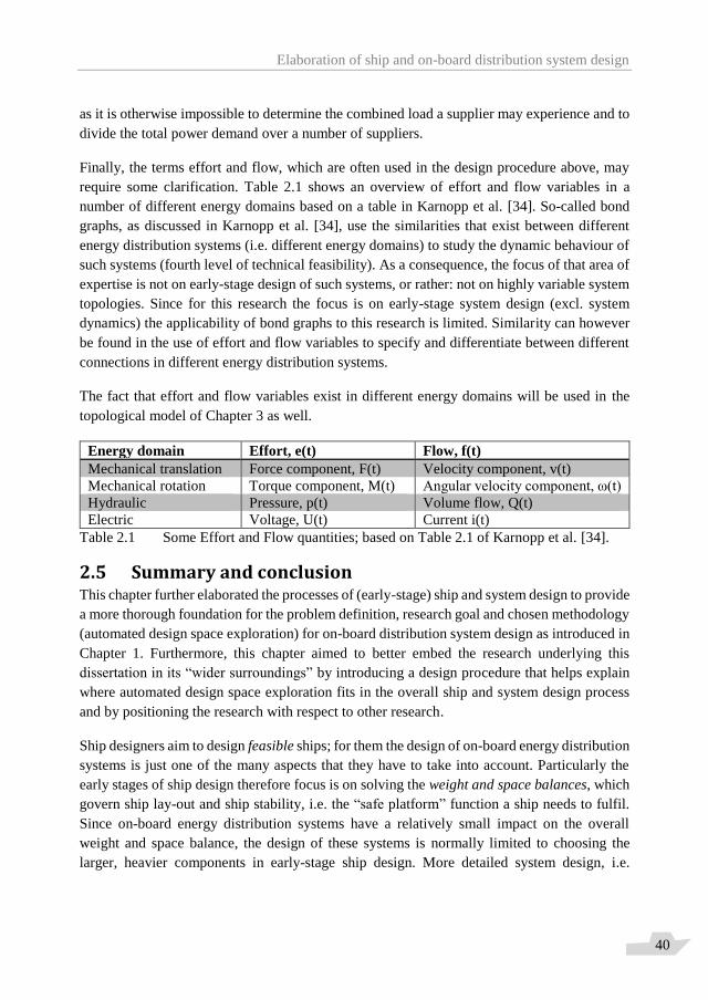
Elaboration of ship and on-board distribution system design
40
as it is otherwise impossible to determine the combined load a supplier may experience and to
divide the total power demand over a number of suppliers.
Finally, the terms effort and flow, which are often used in the design procedure above, may
require some clarification. Table 2.1 shows an overview of effort and flow variables in a
number of different energy domains based on a table in Karnopp et al. [34]. So-called bond
graphs, as discussed in Karnopp et al. [34], use the similarities that exist between different
energy distribution systems (i.e. different energy domains) to study the dynamic behaviour of
such systems (fourth level of technical feasibility). As a consequence, the focus of that area of
expertise is not on early-stage design of such systems, or rather: not on highly variable system
topologies. Since for this research the focus is on early-stage system design (excl. system
dynamics) the applicability of bond graphs to this research is limited. Similarity can however
be found in the use of effort and flow variables to specify and differentiate between different
connections in different energy distribution systems.
The fact that effort and flow variables exist in different energy domains will be used in the
topological model of Chapter 3 as well.
Energy domain Effort, e(t) Flow, f(t)
Mechanical translation Force component, F(t) Velocity component, v(t)
Mechanical rotation Torque component, M(t) Angular velocity component, ω(t)
Hydraulic Pressure, p(t) Volume flow, Q(t)
Electric Voltage, U(t) Current i(t)
Table 2.1 Some Effort and Flow quantities; based on Table 2.1 of Karnopp et al. [34].
2.5 Summary and conclusion This chapter further elaborated the processes of (early-stage) ship and system design to provide
a more thorough foundation for the problem definition, research goal and chosen methodology
(automated design space exploration) for on-board distribution system design as introduced in
Chapter 1. Furthermore, this chapter aimed to better embed the research underlying this
dissertation in its “wider surroundings” by introducing a design procedure that helps explain
where automated design space exploration fits in the overall ship and system design process
and by positioning the research with respect to other research.
Ship designers aim to design feasible ships; for them the design of on-board energy distribution
systems is just one of the many aspects that they have to take into account. Particularly the
early stages of ship design therefore focus is on solving the weight and space balances, which
govern ship lay-out and ship stability, i.e. the “safe platform” function a ship needs to fulfil.
Since on-board energy distribution systems have a relatively small impact on the overall
weight and space balance, the design of these systems is normally limited to choosing the
larger, heavier components in early-stage ship design. More detailed system design, i.e.

Elaboration of ship and on-board distribution system design
41
selecting the number and type of (smaller) system components and the adopted system
topology, is left for later design stages.
However, for naval vessels, ship survivability is important. This design driver is difficult to
assess in early-stage ship design when designing on-board distribution systems is limited to
only choosing the larger, heavier components. The topology of the systems (i.e. how the
components are connected) and design choices concerning centralised vs. distributed power
generation (i.e. the number of power generating components and their location) have a
significant influence on ship survivability. Therefore, a design methodology is sought for
early-stage on-board distribution system design in which the topology and number of
generating components is still variable, as stated in the research goal (section 1.4).
This brings us to the topic of early-stage system design. System designers aim to design
feasible on-board (energy) distribution systems. Particularly the early stages of system design
therefore focus on solving the energy balance for different energy distribution systems, which
governs system operation. Solving the energy balance for different energy distribution system
aims to match power generation with power consumption. Four different levels of such a
system analysis were introduced for assessing technical feasibility of distribution systems. It
was argued that the first level (flow type pairing) is in practice guaranteed as practical system
design methods immediately focus on the second level of system analysis (power balancing),
see section 2.4. Power balancing can however only be done when system topology is simply
chosen on basis of previous system designs, design rules, system topology templates and other
marine engineering heuristic knowledge.
As a consequence, the influence of system topology on system robustness (which underlies
ship survivability – see section 2.3) is hardly known. As far as the relation between system
topology and system robustness is taken into account it is also based on heuristic knowledge.
The relationship between system robustness and other design objectives is then unknown and
trade-off analyses cannot be performed. To address this important issue, this research will take
a different approach and develop the ATG tool.

Elaboration of ship and on-board distribution system design
42
Topological modelling of on-board distribution systems
43
“If the doors of perception were cleansed,
everything would appear to man as it is - infinite.”
― William Blake
Chapter 3 Topological modelling of on-board
distribution systems The research goal implies the development of an Automatic Topology Generation (ATG) tool
for vital on-board (energy) distribution systems. The first implication is that a suitable method
should be found to have a “computer definition” of system concept designs (or system
diagrams – see e.g. Figure 2.1). Once such a method is available a genetic algorithm may be
used to vary “computer definitions” of system concept designs and thus generate and evaluate
many of them (see section 1.5).
Such a computer definition of system concept designs is in theory already available if on-board
distribution systems are regarded as networks of different kinds of flow. Flows that are
distributed in the different networks are electric power, chilled water, mechanical power, heat,
data, etc. Recognising and modelling on-board distribution systems as networks means that
the mathematical field known as network theory (or graph theory) provides the required
method for computer definitions of on-board distribution systems. This chapter therefore first
introduces the fundamental concepts of network theory (nodes and edges) in section 3.1 and
discusses their application to on-board distribution systems. Section 3.2combines the concepts
of nodes and edges with a topological model of on-board distribution systems. This will result
in a framework for node and edge differentiation which will be used throughout this research
for automatic topology generation.
The topological model and resulting node and edge differentiation framework are subsequently
applied to on-board distribution systems to demonstrate their applicability and validity in
section 3.3. The framework is then also applied to a number of vital, interdependent on-board
distribution systems on board of a notional frigate in section 3.4. This section introduces both
the first case study of this research (vital systems on board of a frigate) and the benchmark
system, which is a system topology made by hand.
With the first case study known, the theoretical size of the design space can be determined. A-
priori constraints, aiming to ensure technical feasibility of generated system concept designs,
can then be applied to limit the size of the design space. This will be done in section 3.5.
Sections 3.6 and 3.7 further treat the application of network theory to on-board distribution
systems and introduce a number of concepts and metrics from this mathematical field that may
help in later chapters to develop the ATG tool (most notably with respect to system
robustness). Section 3.8 concludes this chapter with a small summary.
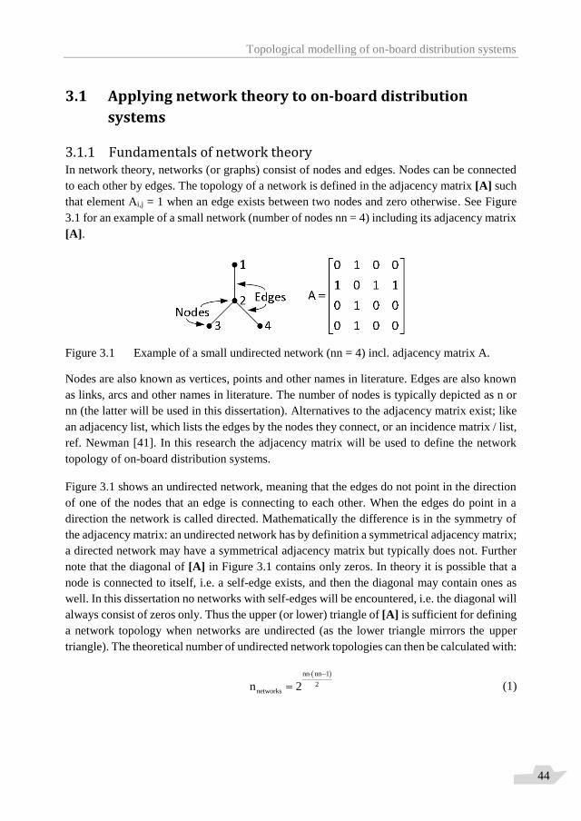
Topological modelling of on-board distribution systems
44
3.1 Applying network theory to on-board distribution
systems
3.1.1 Fundamentals of network theory In network theory, networks (or graphs) consist of nodes and edges. Nodes can be connected
to each other by edges. The topology of a network is defined in the adjacency matrix [A] such
that element Ai,j = 1 when an edge exists between two nodes and zero otherwise. See Figure
3.1 for an example of a small network (number of nodes nn = 4) including its adjacency matrix
[A].
Figure 3.1 Example of a small undirected network (nn = 4) incl. adjacency matrix A.
Nodes are also known as vertices, points and other names in literature. Edges are also known
as links, arcs and other names in literature. The number of nodes is typically depicted as n or
nn (the latter will be used in this dissertation). Alternatives to the adjacency matrix exist; like
an adjacency list, which lists the edges by the nodes they connect, or an incidence matrix / list,
ref. Newman [41]. In this research the adjacency matrix will be used to define the network
topology of on-board distribution systems.
Figure 3.1 shows an undirected network, meaning that the edges do not point in the direction
of one of the nodes that an edge is connecting to each other. When the edges do point in a
direction the network is called directed. Mathematically the difference is in the symmetry of
the adjacency matrix: an undirected network has by definition a symmetrical adjacency matrix;
a directed network may have a symmetrical adjacency matrix but typically does not. Further
note that the diagonal of [A] in Figure 3.1 contains only zeros. In theory it is possible that a
node is connected to itself, i.e. a self-edge exists, and then the diagonal may contain ones as
well. In this dissertation no networks with self-edges will be encountered, i.e. the diagonal will
always consist of zeros only. Thus the upper (or lower) triangle of [A] is sufficient for defining
a network topology when networks are undirected (as the lower triangle mirrors the upper
triangle). The theoretical number of undirected network topologies can then be calculated with:
nn nn 1
2networksn 2
(1)

Topological modelling of on-board distribution systems
45
Note that the power term in the equation above is simply the number of elements in the upper
or lower triangle of the adjacency matrix. When a network is directed the lower triangle can
be different from the upper triangle making the power term in the above equation twice as
large as in the equation above; i.e. nn∙(nn-1).
3.1.2 Nodes and edges in on-board distribution systems Applying the fundamental concepts “nodes” and “edges” to on-board distribution systems,
system components like engines, gearboxes, transformers, heat exchangers etc. are modelled
as nodes in this dissertation and connections between the system components are modelled as
edges. Doing so provides a “computer definition” of system concept designs; i.e. the adjacency
matrix, which mathematically defines system topologies of interdependent on-board
distribution systems.
However, when on-board distribution systems are “simply” modelled as directed or undirected
networks the number of possible system topologies become seemingly endless. The latter
statement can be quantified when estimating that the number of nodes (system components)
in early-stage system design will be between 10 – 100. This results in a theoretical number of
system topologies of 245 – 24950 according to equation (1). Note that these unimaginably large
numbers represent the theoretical size of the design space.
For at least two reasons it is then clear that this number of possible system topologies needs to
be reduced:
1. From a computational perspective it is clear that the number of possible system
topologies is too large to reach acceptable computational times, even for non-
exhaustive optimisation algorithms and modern computers. To underline this, note
that the theoretical size of the design space quickly and significantly exceeds the
estimated number of hydrogen atoms in the observable universe, which according to
(Wikipedia, 05-2018) is approximately 1080 (≈ 2265).
2. More importantly, from an engineering perspective it is clear that a very large part of
the theoretical design space contains technically infeasible design solutions. Imagine
for instance an electric motor (EM) supplying mechanical power to a heat exchanger
(HE). Although such a “connection” is infeasible from an engineering and physics
perspective, it would be considered valid if the two components (EM and HE) are
modelled as mere nodes connected by an edge.
In order to reduce the size of the design space and ensure a basic level of technical feasibility
of system designs, a node and edge differentiation framework needs to be developed. This
framework will be based on a topological model of on-board distribution systems and enable
the application of constraints that “filter” technically infeasible design solutions from the
design space. These constraints will be based on physical principles and practical engineering

Topological modelling of on-board distribution systems
46
judgement. Care must be taken with setting up such a-priori constraints though, as a design
space exploration approach requires sufficient freedom and is most successful when it avoids
biases. The constraints that ensure technical feasibility are introduced and applied in section
3.5. First, on-board distribution systems have to be studied more elaborately and common
features have to be found in order to arrive at the required node and edge differentiation
framework.
3.2 Common features of on-board distribution systems:
node and edge differentiation In chapter 3 of Klein Woud et al. [37] some common features of on-board distribution systems
are identified. This text inspired the author to focus the present research on distribution systems
and therefore the section below is copied from this source with permission.
3.2.1 Considerations of system architecture5 The principles outlined hereafter are applicable to all systems that have a distribution function
and a network structure, be it mechanical fluid systems or electrical systems. In fact the only
features that the system must have are:
There must be some sort of "supply" components such as generators, pumps, air
compressors etc. These are the "suppliers". Sometimes the supply is a connection to
another hierarchically higher system.
The suppliers provide something, i.e. electrical current, hydraulic oil, air etc. These
are all a form of generalised "flow". Associated with this flow is an "effort", i.e. an
electrical voltage, hydraulic pressure etc.
The "supply" must be distributed. The distribution system really is the "network" and
may be an electrical network with switchboards and cables or a pipe system, with
pipes and valves.
The distribution system may embody "conversions" for instance voltage or frequency
converters in electrical systems, pressure transformers in hydraulic systems and
pressure reducing stations in air systems.
The distribution system may be connected to "storage" systems i.e. batteries in an
electrical system, accumulators in hydraulic systems and air bottles in air systems.
The distribution system is connected to "users" or "consumers" often all over the ship
but sometimes concentrated in a particular area. In most cases the users are
connected in parallel since the purpose of most systems is to distribute "flow" at
maximum available "effort". In case of putting users in series they share the same
"flow" but at a reduced "effort". This is sometimes done in case of heat exchangers
5 The text in this section is copied directly from Klein Woud and Stapersma [37] with
permission.
Topological modelling of on-board distribution systems
47
in pipe flow systems where the "effort" is temperature and heat sometimes is required
at different temperatures.
After the consumers the "flow" is either dumped in the environment (e.g. seawater
going overboard directly after a cooler) or saved and returned to the supply source
(e.g. electrical three-phase cable, hydraulic return line, closed circuit fresh cooling
water system). Sometimes only the architecture of the supply side is given in a one-
line diagram since the return normally is symmetrical.
The considerations above are the basis for the topological model for on-board distribution
systems used in this dissertation. Many of the considerations and concepts above are re-used,
most notably the idea that there are different on-board distribution systems distributing specific
types of flow from suppliers to users via their own network of connections. The specific
distribution systems are interconnected through the different system components specified
above. These ideas will be revisited in the next sections and combined with the concepts of
nodes and edges from network theory.
3.2.2 Node and edge differentiation – step 1 Indeed the “system architecture considerations” in the list above are applicable to all on-board
distribution systems and the idea of “suppliers” and “users” in different distribution systems
are already used in the previous chapters. This idea of suppliers and users can also be aligned
with the concept of nodes in network theory. The first step in developing a node and edge
differentiation framework applicable to on-board distribution systems is then taken by
declaration 1 for node differentiation:
Declaration 1: A node can be either a supplier or a user in a specific distribution system.
Note that the above declaration implies that a node may have a dual functionality. For example,
an electric motor is a user in an electric power distribution system and a supplier in a
mechanical power distribution system. Further note that a supplier typically has only one type
of flow as output, while users often require different types of flow as input (especially end-
users like sensors and weapons).
The second declaration then concerns edge differentiation, while the first concerned node
differentiation:
Declaration 2: Edges are connections of specific distribution systems, i.e. an edge that
belongs to a specific distribution system can “carry” only the specific (pre-
defined) flow type that comes from its suppliers; it cannot distribute any
other flow types.
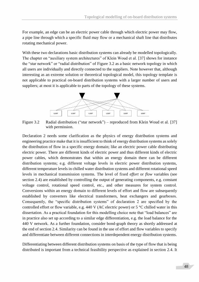
Topological modelling of on-board distribution systems
48
For example, an edge can be an electric power cable through which electric power may flow,
a pipe line through which a specific fluid may flow or a mechanical shaft line that distributes
rotating mechanical power.
With these two declarations basic distribution systems can already be modelled topologically.
The chapter on “auxiliary system architectures” of Klein Woud et al. [37] shows for instance
the “star network” or “radial distribution” of Figure 3.2 as a basic network topology in which
all users are individually and directly connected to the suppliers. Note however that, although
interesting as an extreme solution or theoretical topological model, this topology template is
not applicable to practical on-board distribution systems with a larger number of users and
suppliers; at most it is applicable to parts of the topology of these systems.
Figure 3.2 Radial distribution (“star network”) – reproduced from Klein Woud et al. [37]
with permission.
Declaration 2 needs some clarification as the physics of energy distribution systems and
engineering practice make that it is insufficient to think of energy distribution systems as solely
the distribution of flow in a specific energy domain; like an electric power cable distributing
electric power. There are different kinds of electric power and thus different kinds of electric
power cables, which demonstrates that within an energy domain there can be different
distribution systems; e.g. different voltage levels in electric power distribution systems,
different temperature levels in chilled water distribution systems and different rotational speed
levels in mechanical transmission systems. The level of fixed effort or flow variables (see
section 2.4) are established by controlling the output of generating components, e.g. constant
voltage control, rotational speed control, etc., and other measures for system control.
Conversions within an energy domain to different levels of effort and flow are subsequently
established by converters like electrical transformers, heat exchangers and gearboxes.
Consequently, the “specific distribution systems” of declaration 2 are specified by the
controlled effort or flow variable, e.g. 440 V (AC electric power) or 5 °C chilled water in this
dissertation. As a practical foundation for this modelling choice note that “load balances” are
in practice also set up according to a similar edge differentiation, e.g. the load balance for the
440 V network. As a further foundation, consider bond-graph theory as shortly addressed at
the end of section 2.4. Similarity can be found in the use of effort and flow variables to specify
and differentiate between different connections in interdependent energy distribution systems.
Differentiating between different distribution systems on basis of the type of flow that is being
distributed is important from a technical feasibility perspective as explained in section 2.4. It
Topological modelling of on-board distribution systems
49
is stated there that “flow type pairing” is the most basic level of technical feasibility
assessment; i.e. making sure that the right connections are made when a system topology is
generated (whether by hand or automatically). Therefore, declaration 2 is very important: the
fact that there are different types of edges (because there are different types of flow) means
that connections between certain node pairs (two system components) are feasible, while
others are not. The feasibility / infeasibility of connections between different node pairs will
be used in section 3.5 to limit the size of the design space.
Specifying different distribution systems according to the controlled effort and flow variable
also means that converters (transformers, heat exchangers, etc.) are modelled as suppliers (of
one distribution system) or users (of another distribution system) as well. Thus the difference
between converters within an energy domain and converters between energy domains
disappears and all nodes (up till now) are converters, i.e. supplier and user at the same time.
Unless nodes are at the boundary of interest (a choice!), then nodes really are supplier or user
only; e.g. mission-related components are typically the final (end-)users. Following this line
of thought the other way around, i.e. “upstream”, the ultimate suppliers (sources) of a ship at
sea are the fuel tanks (and the surrounding sea and air), but in this research the boundary of
interest for vital distribution systems will typically lie with the suppliers of electric power
(presuming that e.g. diesel-generator sets will always have fuel supply).
Another type of node may be distinguished in the list of section 3.2.1; the accumulator.
Depending on the mode of operation, the accumulator acts as a supplier or user, like the other
nodes. However, different modes of operation are not considered in this research as explained
in section 2.4. Thus, it is for this study necessary to choose whether an accumulator is modelled
as a supplier or as a user. Here it is chosen to model accumulators like Uninterruptable Power
Suppliers (UPS), other battery types, flywheels and other energy storage options, as suppliers.
The reason for this choice is that typically, accumulators are part of a system to provide back-
up supply in case other, regular suppliers fail or to dampen (high-frequency) transients. In the
first case it is obvious that the accumulator may be modelled as a supplier; the fact that it is
used as supplier at different times than other (main) suppliers does not make for a topological
difference. In the second case the accumulator may still be modelled as a supplier, but will in
fact regularly switch between supplier and user mode, depending on the transients and applied
energy management system. Transient behaviour of distribution systems is however outside
the scope of early-stage system design and thus also outside the scope of this research.
The latter paragraph does however raise a question concerning the topological modelling of
distribution systems: should the network be modelled directed or undirected? The terms
supplier and user imply a directed network, but accumulators show that the flow in some
connections may be bidirectional (i.e. changing in direction from time to time). These
accumulator connections are not the only bidirectional (i.e. undirected) edges that may occur
in on-board distribution systems as will be shown in section 3.2.3. Finally, even though
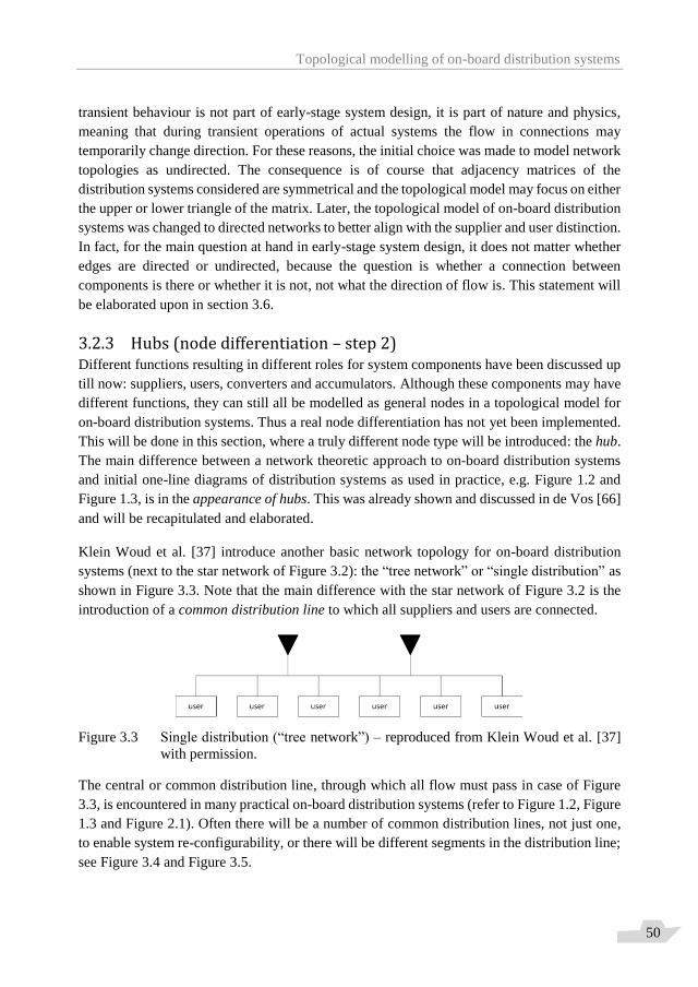
Topological modelling of on-board distribution systems
50
transient behaviour is not part of early-stage system design, it is part of nature and physics,
meaning that during transient operations of actual systems the flow in connections may
temporarily change direction. For these reasons, the initial choice was made to model network
topologies as undirected. The consequence is of course that adjacency matrices of the
distribution systems considered are symmetrical and the topological model may focus on either
the upper or lower triangle of the matrix. Later, the topological model of on-board distribution
systems was changed to directed networks to better align with the supplier and user distinction.
In fact, for the main question at hand in early-stage system design, it does not matter whether
edges are directed or undirected, because the question is whether a connection between
components is there or whether it is not, not what the direction of flow is. This statement will
be elaborated upon in section 3.6.
3.2.3 Hubs (node differentiation – step 2) Different functions resulting in different roles for system components have been discussed up
till now: suppliers, users, converters and accumulators. Although these components may have
different functions, they can still all be modelled as general nodes in a topological model for
on-board distribution systems. Thus a real node differentiation has not yet been implemented.
This will be done in this section, where a truly different node type will be introduced: the hub.
The main difference between a network theoretic approach to on-board distribution systems
and initial one-line diagrams of distribution systems as used in practice, e.g. Figure 1.2 and
Figure 1.3, is in the appearance of hubs. This was already shown and discussed in de Vos [66]
and will be recapitulated and elaborated.
Klein Woud et al. [37] introduce another basic network topology for on-board distribution
systems (next to the star network of Figure 3.2): the “tree network” or “single distribution” as
shown in Figure 3.3. Note that the main difference with the star network of Figure 3.2 is the
introduction of a common distribution line to which all suppliers and users are connected.
Figure 3.3 Single distribution (“tree network”) – reproduced from Klein Woud et al. [37]
with permission.
The central or common distribution line, through which all flow must pass in case of Figure
3.3, is encountered in many practical on-board distribution systems (refer to Figure 1.2, Figure
1.3 and Figure 2.1). Often there will be a number of common distribution lines, not just one,
to enable system re-configurability, or there will be different segments in the distribution line;
see Figure 3.4 and Figure 3.5.
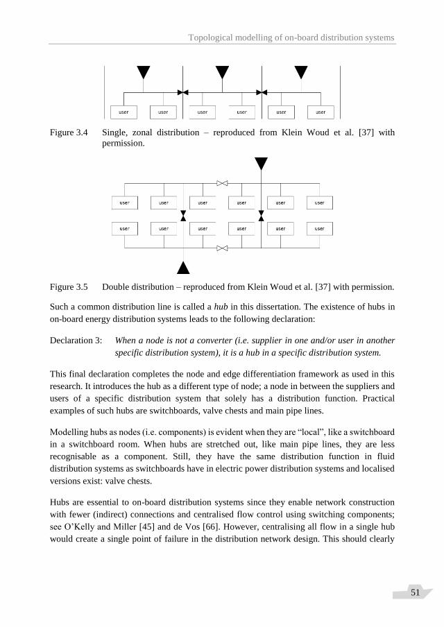
Topological modelling of on-board distribution systems
51
Figure 3.4 Single, zonal distribution – reproduced from Klein Woud et al. [37] with
permission.
Figure 3.5 Double distribution – reproduced from Klein Woud et al. [37] with permission.
Such a common distribution line is called a hub in this dissertation. The existence of hubs in
on-board energy distribution systems leads to the following declaration:
Declaration 3: When a node is not a converter (i.e. supplier in one and/or user in another
specific distribution system), it is a hub in a specific distribution system.
This final declaration completes the node and edge differentiation framework as used in this
research. It introduces the hub as a different type of node; a node in between the suppliers and
users of a specific distribution system that solely has a distribution function. Practical
examples of such hubs are switchboards, valve chests and main pipe lines.
Modelling hubs as nodes (i.e. components) is evident when they are “local”, like a switchboard
in a switchboard room. When hubs are stretched out, like main pipe lines, they are less
recognisable as a component. Still, they have the same distribution function in fluid
distribution systems as switchboards have in electric power distribution systems and localised
versions exist: valve chests.
Hubs are essential to on-board distribution systems since they enable network construction
with fewer (indirect) connections and centralised flow control using switching components;
see O’Kelly and Miller [45] and de Vos [66]. However, centralising all flow in a single hub
would create a single point of failure in the distribution network design. This should clearly
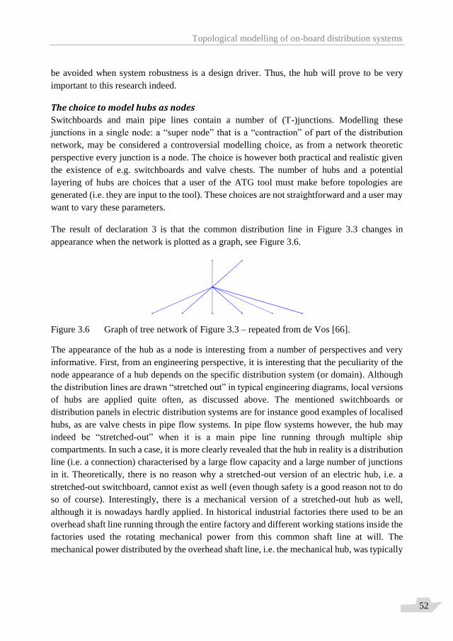
Topological modelling of on-board distribution systems
52
be avoided when system robustness is a design driver. Thus, the hub will prove to be very
important to this research indeed.
The choice to model hubs as nodes
Switchboards and main pipe lines contain a number of (T-)junctions. Modelling these
junctions in a single node: a “super node” that is a “contraction” of part of the distribution
network, may be considered a controversial modelling choice, as from a network theoretic
perspective every junction is a node. The choice is however both practical and realistic given
the existence of e.g. switchboards and valve chests. The number of hubs and a potential
layering of hubs are choices that a user of the ATG tool must make before topologies are
generated (i.e. they are input to the tool). These choices are not straightforward and a user may
want to vary these parameters.
The result of declaration 3 is that the common distribution line in Figure 3.3 changes in
appearance when the network is plotted as a graph, see Figure 3.6.
Figure 3.6 Graph of tree network of Figure 3.3 – repeated from de Vos [66].
The appearance of the hub as a node is interesting from a number of perspectives and very
informative. First, from an engineering perspective, it is interesting that the peculiarity of the
node appearance of a hub depends on the specific distribution system (or domain). Although
the distribution lines are drawn “stretched out” in typical engineering diagrams, local versions
of hubs are applied quite often, as discussed above. The mentioned switchboards or
distribution panels in electric distribution systems are for instance good examples of localised
hubs, as are valve chests in pipe flow systems. In pipe flow systems however, the hub may
indeed be “stretched-out” when it is a main pipe line running through multiple ship
compartments. In such a case, it is more clearly revealed that the hub in reality is a distribution
line (i.e. a connection) characterised by a large flow capacity and a large number of junctions
in it. Theoretically, there is no reason why a stretched-out version of an electric hub, i.e. a
stretched-out switchboard, cannot exist as well (even though safety is a good reason not to do
so of course). Interestingly, there is a mechanical version of a stretched-out hub as well,
although it is nowadays hardly applied. In historical industrial factories there used to be an
overhead shaft line running through the entire factory and different working stations inside the
factories used the rotating mechanical power from this common shaft line at will. The
mechanical power distributed by the overhead shaft line, i.e. the mechanical hub, was typically

Topological modelling of on-board distribution systems
53
supplied by a steam engine. More specific examples of hubs (whether stretched-out or local)
for different on-board distribution systems will follow in section 3.3.
From a ship design perspective, the considerations above may serve as an additional
explanation of why it is difficult to include the design of energy distribution systems more
thoroughly in early design stages. It is now clear that early-stage system design involves not
only design choices with respect to the number and type of suppliers and users, but also design
choices concerning the number of hubs and the “stretched-outness” of hubs, i.e. physical size.
On top of that there is a design choice concerning the “layering” of hubs, i.e. whether there is
a certain hierarchy in the hubs that are connected to each other. There has been no hierarchy
of hubs in the diagrams that were shown up till now, but there can be a hierarchy in hub layers
of practical systems, also in on-board distribution systems. Such layering of hubs will be
discussed more thoroughly in the second case study of this research – in section 6.2.
From a topological perspective it can be concluded that practical distribution system
topologies are always a combination of the two basic topologies “tree” and “star”. Especially
from Figure 3.6, where the common distribution line is indeed reduced to a point, i.e. a node,
it is clear that the star network distribution will typically be found from and to the hubs of
specific distribution systems. Naturally this is the case because each user will need at least one
individual supply line from a “higher” supply node (unless users are put in series, but this
rarely is the case as stated in section 3.2.1). Similarly, each supplier will have at least one
discharge line to a “lower” node. This could be a direct connection to a user, but more often is
a connection to a common distribution line, i.e. a hub. The latter typically is the case when the
number of users (far) exceeds the number of suppliers. From this perspective hubs can be seen
as a way to “postpone” the individual connections of users that are characteristic to the star
network and it becomes clear that the user-supplier ratio of a specific distribution system is a
key variable with respect to the existence and the number of hubs within that specific
distribution system.
Short discussion on advantages and disadvantages of hubs
Hubs are not specific to on-board distribution systems, they are found in many networks. In
their review and synthesis paper on the hub network design problem O’Kelly et al. [45] state
that hubs “allow the construction of a network where direct connections between all origin
and destination pairs can be replaced with fewer, indirect connections”. This of course is
exactly the difference between a star network in Figure 3.2 and a tree network in Figure 3.3.
Such hub network topologies “reduce and simplify network construction costs, centralize
commodity handling and sorting and allow carriers to take advantage of scale economies
through consolidation of flows”. Although the paper of O’Kelly et al. [45] focusses on
transportation networks, the mentioned arguments to introduce hubs in network topologies are
just as valid for on-board energy distribution systems.

Topological modelling of on-board distribution systems
54
The mentioned advantages of networks with hubs can be related to the design objectives
introduced in Chapter 1 and Chapter 2. Costs were mentioned there as a design driver, but also
operability (centralising flow handling) and weight and space requirements, which, as
economies, typically scale with the inverse of flow consolidation. What is hardly discussed by
O’Kelly and Miller, but is brought forward in amongst others Klein Woud et al. [37] is the
main disadvantage of hubs in networks: the relation between hubs in networks and network
vulnerability. Although it will later be shown that it is difficult to accurately assess and
compare network vulnerability when hubs are, or are not, present in the network, it should be
clear at this point that hubs are important nodes that, when unavailable, affect a large part of
the network. For example, in Figure 3.3 and Figure 3.6 the hub is even a single point of failure
for the entire network, as stated previously.
3.2.4 Closure Notwithstanding the disadvantages of hubs, they are present in actual systems on board of
ships. This will be shown in the next section (3.3) as well, in which the applicability of the
complete node and edge differentiation framework, as introduced in this section (3.2), is
discussed. The section thereafter (3.4), applies the framework to a number of interdependent,
vital distribution systems of a notional frigate, thus introducing the benchmark system of this
study.
3.3 Overview of systems and their components To appreciate the usefulness of the node and edge differentiation framework as introduced in
the previous section, this section applies the framework to commonly found (energy)
distribution systems on board ships. First an overview of these common systems and their
interdependencies is given, then the components in these systems are categorised according to
the supplier / hub / user node differentiation per specific (energy) distribution system (edge
differentiation).
3.3.1 Systems on board of ships6 On the ship level, there are a number of energy distribution systems (often categorised into
main and auxiliary systems) that are needed for the ship to function properly. Some of these
systems are localised in specific parts of the ship, while others extend the entire ship envelope.
A number of these systems are depicted in Figure 3.7, including typical system
interdependencies. Note that the distinction between main and auxiliary is different from vital
and non-vital. Some auxiliary systems are absolutely vital for the ship to be able to perform its
mission, while some parts of the main systems may be considered to be non-vital.
6 The text of this section is repeated from de Vos et al. [67] and adjusted to fit here.
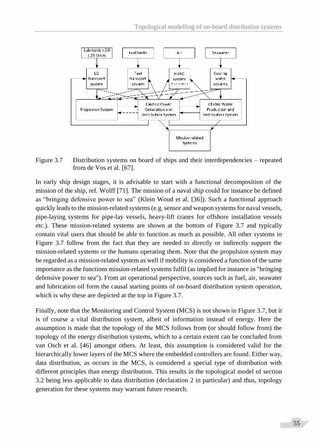
Topological modelling of on-board distribution systems
55
Figure 3.7 Distribution systems on board of ships and their interdependencies – repeated
from de Vos et al. [67].
In early ship design stages, it is advisable to start with a functional decomposition of the
mission of the ship, ref. Wolff [71]. The mission of a naval ship could for instance be defined
as “bringing defensive power to sea” (Klein Woud et al. [36]). Such a functional approach
quickly leads to the mission-related systems (e.g. sensor and weapon systems for naval vessels,
pipe-laying systems for pipe-lay vessels, heavy-lift cranes for offshore installation vessels
etc.). These mission-related systems are shown at the bottom of Figure 3.7 and typically
contain vital users that should be able to function as much as possible. All other systems in
Figure 3.7 follow from the fact that they are needed to directly or indirectly support the
mission-related systems or the humans operating them. Note that the propulsion system may
be regarded as a mission-related system as well if mobility is considered a function of the same
importance as the functions mission-related systems fulfil (as implied for instance in "bringing
defensive power to sea"). From an operational perspective, sources such as fuel, air, seawater
and lubrication oil form the causal starting points of on-board distribution system operation,
which is why these are depicted at the top in Figure 3.7.
Finally, note that the Monitoring and Control System (MCS) is not shown in Figure 3.7, but it
is of course a vital distribution system, albeit of information instead of energy. Here the
assumption is made that the topology of the MCS follows from (or should follow from) the
topology of the energy distribution systems, which to a certain extent can be concluded from
van Osch et al. [46] amongst others. At least, this assumption is considered valid for the
hierarchically lower layers of the MCS where the embedded controllers are found. Either way,
data distribution, as occurs in the MCS, is considered a special type of distribution with
different principles than energy distribution. This results in the topological model of section
3.2 being less applicable to data distribution (declaration 2 in particular) and thus, topology
generation for these systems may warrant future research.
Topological modelling of on-board distribution systems
56
3.3.2 System components categorised Table 3.1 lists a number of distribution systems, including the ones shown in Figure 3.7, with
their components categorised according to the supplier / hub / user node differentiation. Note
that the first column relates to the edge differentiation, but here still at the more generic level
of (energy) domains and not yet specified according to prevailing effort or flow variable, which
is why “converters” within an energy domain are listed as a separate category.
3.4 Introduction of first case study and benchmark system7 In the first case study, for which automatically generated topologies are presented in section
6.1, the focus is on the network topology of the electric power distribution system (EPDS) and
the chilled water distribution system (CWDS) of a notional frigate. These systems typically
extend the entire ship envelope, making them susceptible to hits. They provide vital functions
for the mission-related systems and for platform and hotel functions and they typically have a
high user-to-supplier ratio, which is a characteristic for systems that are or should be
reconfigurable (the relationship between system robustness and system re-configurability will
be discussed in section 5.2). These systems can therefore be considered the most vital energy
distribution systems on board of naval vessels, i.e. robustness is of prime importance for these
systems. Therefore, they serve as excellent case study material for the Automatic Topology
Generation (ATG) tool presented in this dissertation. Trapp [65] focuses his work on similar
on-board energy distribution systems for the same reasons.
This section will introduce the benchmark system topology, which is a hand-made topology
for the systems in the first case study, i.e. the EPDS and CWDS of a notional frigate. Energy
distribution systems like the EPDS and CWDS on board of ships are characterized by
centralized power generation, which leads to the earlier mentioned high user-to-supplier ratio.
Operability of the systems is improved by centralisation: this makes it easier to oversee and
control the systems (both for human operators and control systems) in comparison to
distributed power generation. Furthermore, a centralised power generation system with an
extensive network for energy distribution may be cheaper, lighter and smaller than many small,
separate generation systems, since one can benefit from economies of scale for the power
supplying components, as already argued in section 3.2.3.
7 The text of this section is repeated from de Vos et al. [67] and adjusted to fit here.

Topological modelling of on-board distribution systems
57
Type of
(Power) Flow
Suppliers
(source)
Hubs Converters Users (sinks)
Electric power
distribution
system
Generator /
Fuel cell (e.g.
PEMFC)
Switchboard /
distribution
panel
Transformer /
converter /
inverter
Electric Motor /
Lighting / Heater /
Navigation / etc.
Heat - Chilled
water
Chilled water
plant
Main pipeline Heat
exchanger
Cooled equipment
/ Heat exchanger
Heat – Heated
water
Boiler Main pipeline Heat
exchanger
Radiator / Heat
exchanger
Heat – air
e.g. HVAC
system
HVAC unit Main channel
/ duct
Recirculation /
Enthalpy
wheel
Spaces (rooms) /
equipment / people
(crew)
Firefighting
water
Pump Main pipeline - Sprinkler / water
mist sprayer
Mechanical
power
(rotational)
e.g. propulsion
system
IC engine (e.g.
diesel engine) /
Turbine (e.g.
gas turbine) /
Motor (e.g.
electric motor)
Gearbox /
main shaft
line
Gearbox Propulsor (e.g.
propeller) / Pump
(e.g. centrifugal
pump) / Fans /
Compressors /
Winches / Tools
Mechanical
power
(translational)
Propeller /
Crane
- Lever Ship
Heat – Cooling
water
Pump Main pipeline Heat
exchanger
Heat exchanger /
IC engine jacket &
coolers
Fuel Tank / Pump Valve chest /
Main pipeline
- IC engines /
Boilers
Lubrication oil Tank / Pump Valve chest - IC engine /
gearbox
Hydraulic
system
Pump /
Hydraulic
Power Pack
Main pipeline Reducer Hydraulic motor /
CPP
Fresh (potable)
water
Fresh water
plant (e.g. RO
unit)
Main pipeline - Taps, showers,
galley, toilets, etc.
Sensor Data Sensor Router - Computer
Control Data Computer Router - Actuator
Table 3.1 Overview of on-board distribution systems and main components categorised
according to the developed node and edge differentiation framework.
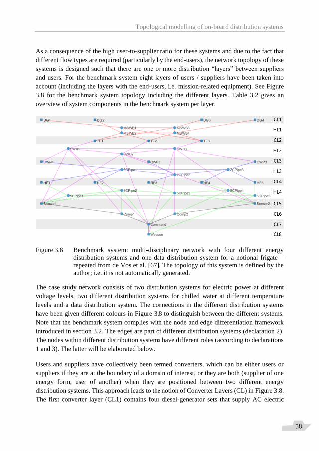
Topological modelling of on-board distribution systems
58
As a consequence of the high user-to-supplier ratio for these systems and due to the fact that
different flow types are required (particularly by the end-users), the network topology of these
systems is designed such that there are one or more distribution “layers” between suppliers
and users. For the benchmark system eight layers of users / suppliers have been taken into
account (including the layers with the end-users, i.e. mission-related equipment). See Figure
3.8 for the benchmark system topology including the different layers. Table 3.2 gives an
overview of system components in the benchmark system per layer.
Figure 3.8 Benchmark system: multi-disciplinary network with four different energy
distribution systems and one data distribution system for a notional frigate –
repeated from de Vos et al. [67]. The topology of this system is defined by the
author; i.e. it is not automatically generated.
The case study network consists of two distribution systems for electric power at different
voltage levels, two different distribution systems for chilled water at different temperature
levels and a data distribution system. The connections in the different distribution systems
have been given different colours in Figure 3.8 to distinguish between the different systems.
Note that the benchmark system complies with the node and edge differentiation framework
introduced in section 3.2. The edges are part of different distribution systems (declaration 2).
The nodes within different distribution systems have different roles (according to declarations
1 and 3). The latter will be elaborated below.
Users and suppliers have collectively been termed converters, which can be either users or
suppliers if they are at the boundary of a domain of interest, or they are both (supplier of one
energy form, user of another) when they are positioned between two different energy
distribution systems. This approach leads to the notion of Converter Layers (CL) in Figure 3.8.
The first converter layer (CL1) contains four diesel-generator sets that supply AC electric
Topological modelling of on-board distribution systems
59
power at 6600 V. The 6600 V connections are red-coloured; these connections, together with
the nodes they interconnect, constitute the first energy distribution system of the case study
system. Converter layer 2 (CL2) can contain all 6600 V electric power users, but their number
has been limited for this case study to three transformers that convert 6600 V AC electric
power to 440 V AC power. Other users of 6600 V AC power could for instance be main
propulsion motors in an all-electric propulsion system configuration or “high energy
weapons”. The 440 V AC distribution system (magenta-coloured connections) is the second
energy distribution system in the case study network (and in the EPDS).
Converter layer 3 contains three Chilled Water Plants (CWP’s) that use 440 V AC power in
order to supply chilled water with a temperature of 2 °C to the CWDS. The transformation
from the EPDS to the CWDS occurs at these Chilled Water Plants. Similar to CL2, CL3 as
well could contain other users (of 440 V AC electric power in this case), but the number of
components taken into consideration has for sake of clarity been limited to the relevant
components for this study. The blue and green energy distribution systems in Figure 3.8 are
part of the CWDS; the blue connections (pipes) contain chilled water with a temperature of 2
°C and the green connections contain chilled water with temperature 5 °C (after having been
cooled down by the 2 °C chilled water in the Heat Exchangers of CL4).
The black connections represent the Data Distribution System (DDS), i.e. the connections are
LAN cables. This distribution system is not part of this study in the sense that topologies for
this distribution system will not be automatically generated. There is no practical reason for
not generating topologies for the DDS; the ATG tool is able to do so for these systems as well.
However, the author is not convinced that topologies generated for data distribution systems
would be as realistic as they are for energy distribution systems. The main difference is that
multiple forms of data can be distributed over a single LAN cable (edge in DDS), while only
one type of energy can be distributed in connections of energy distribution systems; i.e.
declaration 2 of the node and edge differentiation framework is not valid for data distribution
systems.
Note that between the converter layers (containing suppliers and/or users of the different
distribution systems) there are other components that have solely a distribution function; i.e.
hubs. In the first case study system four hub layers (HL) exist, that belong to the two
distribution systems of the EPDS and the two distribution systems of the CWDS. When system
robustness is a design driver the number of hubs and the way in which they are interconnected,
i.e. the topology of hub layers, require special attention, as discussed in section 3.2.3. This is
also reflected in the practical robustness measures specified in section 2.3. A system designer
should be careful not to create single points of failure. Centralising flow control in a single
hub would establish just that. The topologies of the hub layers in Figure 3.8 are considered to
be realistic topologies that could be observed in actual systems on board frigates. They are so-
called ring distributions; rings are known in graph theory as cycles or loops. Zonal, ring
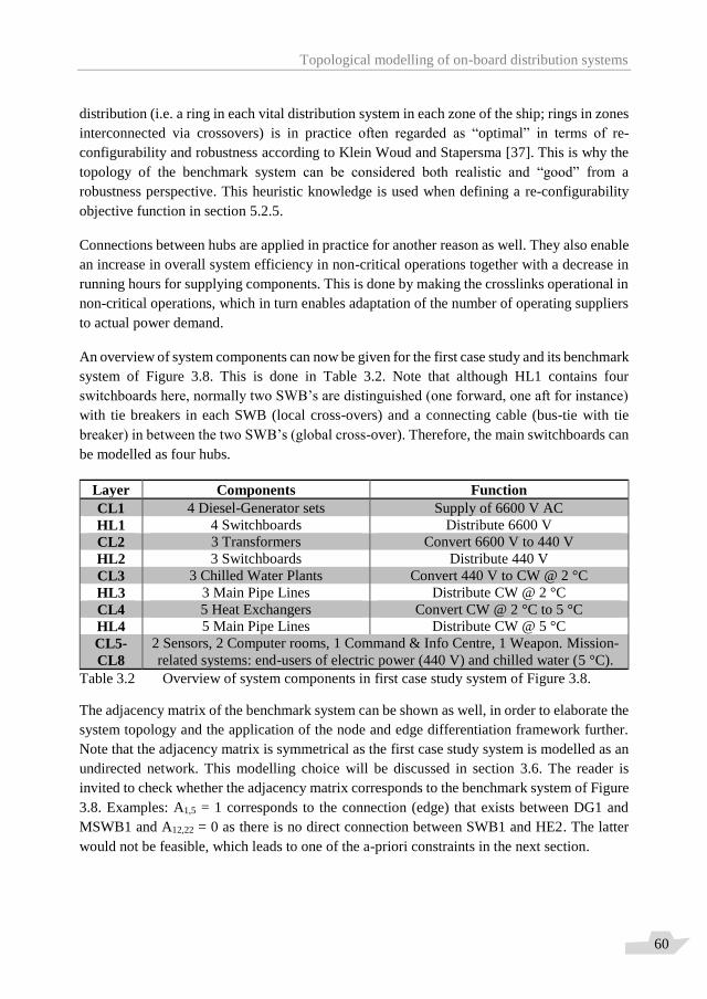
Topological modelling of on-board distribution systems
60
distribution (i.e. a ring in each vital distribution system in each zone of the ship; rings in zones
interconnected via crossovers) is in practice often regarded as “optimal” in terms of re-
configurability and robustness according to Klein Woud and Stapersma [37]. This is why the
topology of the benchmark system can be considered both realistic and “good” from a
robustness perspective. This heuristic knowledge is used when defining a re-configurability
objective function in section 5.2.5.
Connections between hubs are applied in practice for another reason as well. They also enable
an increase in overall system efficiency in non-critical operations together with a decrease in
running hours for supplying components. This is done by making the crosslinks operational in
non-critical operations, which in turn enables adaptation of the number of operating suppliers
to actual power demand.
An overview of system components can now be given for the first case study and its benchmark
system of Figure 3.8. This is done in Table 3.2. Note that although HL1 contains four
switchboards here, normally two SWB’s are distinguished (one forward, one aft for instance)
with tie breakers in each SWB (local cross-overs) and a connecting cable (bus-tie with tie
breaker) in between the two SWB’s (global cross-over). Therefore, the main switchboards can
be modelled as four hubs.
Layer Components Function
CL1 4 Diesel-Generator sets Supply of 6600 V AC
HL1 4 Switchboards Distribute 6600 V
CL2 3 Transformers Convert 6600 V to 440 V
HL2 3 Switchboards Distribute 440 V
CL3 3 Chilled Water Plants Convert 440 V to CW @ 2 °C
HL3 3 Main Pipe Lines Distribute CW @ 2 °C
CL4 5 Heat Exchangers Convert CW @ 2 °C to 5 °C
HL4 5 Main Pipe Lines Distribute CW @ 5 °C
CL5-
CL8
2 Sensors, 2 Computer rooms, 1 Command & Info Centre, 1 Weapon. Mission-
related systems: end-users of electric power (440 V) and chilled water (5 °C).
Table 3.2 Overview of system components in first case study system of Figure 3.8.
The adjacency matrix of the benchmark system can be shown as well, in order to elaborate the
system topology and the application of the node and edge differentiation framework further.
Note that the adjacency matrix is symmetrical as the first case study system is modelled as an
undirected network. This modelling choice will be discussed in section 3.6. The reader is
invited to check whether the adjacency matrix corresponds to the benchmark system of Figure
3.8. Examples: A1,5 = 1 corresponds to the connection (edge) that exists between DG1 and
MSWB1 and A12,22 = 0 as there is no direct connection between SWB1 and HE2. The latter
would not be feasible, which leads to one of the a-priori constraints in the next section.
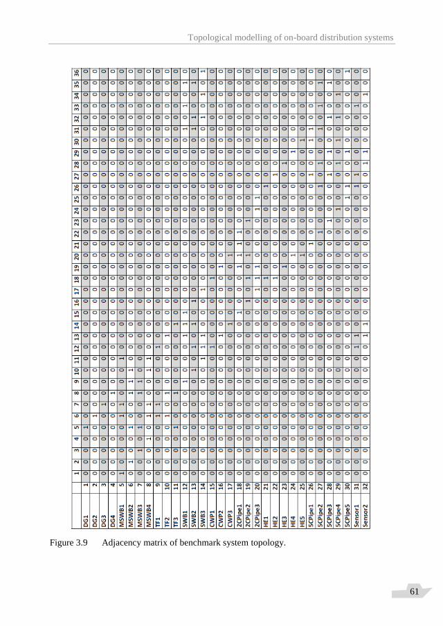
Topological modelling of on-board distribution systems
61
Figure 3.9 Adjacency matrix of benchmark system topology.

Topological modelling of on-board distribution systems
62
The benchmark and first case study systems contain 36 system components, i.e. 36 nodes, of
which 21 are converters and 15 are hubs. These numbers are considered realistic for early
stages of integrated on-board distribution system design (when design space exploration can
be useful). An actual system would however contain many more converters, or rather many
more end-users. The end-users have here been limited to the most important systems /
components from a mission perspective, but in real systems particularly CL3 (users of 440 V)
and CL5 (users of 5 °C Chilled Water) would contain many more users than the current
network. Furthermore, other domains (e.g. mechanical power) and “lower” distribution
systems (e.g. at lower voltage levels), have been omitted because it is expected that in early-
stage design the focus will not be on these less extensive or less vital distribution systems.
Note that this choice will be revisited in the second case study.
Having many more end-users, actual (i.e. complete) energy distribution systems like the EPDS
and CWDS on board of naval vessels are characterised by centralised power generation, which
indeed indicates a large number of users, a modest number of suppliers and an extensive
distribution system in between; i.e. a high user-to-supplier ratio as earlier mentioned. The large
number of users in actual on-board distribution systems means there are many components
with only one supply line and some vital users with two supply lines. Users may require
multiple inputs, which increases the total number of supply lines, but they will still typically
have a relatively low number of connections when compared to hubs. Similarly, suppliers
normally have only one (or in rare cases two) outputs to nearby hubs. Since the number of
hubs will be in the order of magnitude of the number of suppliers, there will be a small number
of hubs with a high number of connections (one or two from suppliers and many to the many
users). In mathematical terms, this means there will be a large number of nodes with a low
degree (suppliers and users) and a small number of nodes with a high degree (hubs) in real on-
board distribution systems. This is a characteristic of networks with a power law degree
distribution and it will therefore be stated in section 4.1 that actual on-board energy distribution
systems exhibit scale-free properties. This knowledge could serve a purpose when concept
designs are developed further in more detailed design stages.
The “hub-and-spoke” nature of on-board energy distribution systems was also recognised by
Rigterink [55] who, like this work, used it to introduce his own robustness assessment
technique based on network theory. However, unlike the present work, he did not integrate his
robustness metrics with a genetic algorithm to enable automatic topology generation, but rather
developed the topologies by hand, based on earlier realised designs.
This section showed that the node and edge differentiation framework as introduced in section
3.2 can successfully be applied to vital, interdependent on-board distribution systems. The
framework bridges the gap between (the fundamental concepts of) network theory and marine
engineering practice.

Topological modelling of on-board distribution systems
63
3.5 A-priori constraints to limit the size of the design space8 With the first case study and benchmark system introduced it is possible to analyse the size of
the design space as a function of the number of nodes. Equation (1) in section 3.1 was shown
to provide the theoretical size of the design space when on-board distribution systems are
modelled as undirected networks. For the systems in the first case study network on board a
frigate, consisting of 36 nodes, that equation evaluates to 2630 possible network topologies.
Note that the number 630 corresponds to the number of elements in the upper triangle of the
adjacency matrix; see the left-hand side of Figure 3.10 below. Since each element in the
adjacency matrix corresponds to a potential connection between a node pair (the element has
a value of one if the connection exists and a value of zero if it does not – see section 3.1), this
means the frigate case study network has 630 potential connections when it is modelled as an
undirected network.
Figure 3.10 Possible non-zero elements in upper triangle of the adjacency matrix for the
benchmark study system (consisting of 36 nodes) before (left) and after (right)
inclusion of a-priori constraints.
This is only true of course if all system components are modelled as generic nodes and all
connections are modelled as generic edges, i.e. if there is no node and edge differentiation
framework. At the end of section 3.1 it was argued that the node and edge differentiation
framework as introduced in section 3.2 provides a means to introduce constraints that limit the
size of the design space, i.e. constraints that limit the number of potential connections. This
section introduces a small set of such a-priori constraints that indeed drastically decreases the
number of possible system topologies. For the first case study network, the constraints used
decrease the size of the design space from 2630 to 2172. This is graphically shown in Figure
3.10, which shows for two cases the potential non-zero elements in the adjacency matrix
8 The text of this section is partly repeated from de Vos et al. [67] and adjusted to fit here.

Topological modelling of on-board distribution systems
64
specifying the network topology, i.e. the potential connections that are allowed before and
after the inclusion of a-priori constraints. The reader may check that the non-zero elements in
the adjacency matrix of the benchmark system (Figure 3.9) correspond to connections that are
allowed according to the adjacency matrix on the right-hand side of Figure 3.10, i.e. after
inclusion of a-priori constraints.
3.5.1 Constraint 1: Technical feasibility of connections Following from the fact that there are different distribution systems on board of ships
(distributing different kinds of flow), declaration 2 in section 3.2 introduced edge
differentiation. Because of this, a large part of the 630 potential connections in the adjacency
matrix of the frigate case study network are infeasible. Take for instance the first eleven nodes
of the network, i.e. the system components in CL1, HL1 and CL2 in Figure 3.8. These are all
components of the 6600 V distribution system; the first four are suppliers (Diesel-Generator
sets), the next four are hubs (Main Switchboards) and the last three are users of 6600 V
(Transformers). None of the other nodes (nodes 12 – 36) of the frigate case study network
supply, distribute or use 6600 V. Therefore, any connection between the first eleven nodes and
all other nodes are infeasible. So the fact that edges are differentiated makes that a large
number of elements in the adjacency matrix are zero by default. That is, technical feasibility
as discussed in section 2.4 can be used as an a-priori constraint to limit the number of potential
connections, thereby limiting the size of the design space.
3.5.2 Constraint 2: No converter-converter connections The “technical feasibility of connections” constraint, whose application is made possible by
edge differentiation, is not the only constraint to limit the size of the design space. Node
differentiation within specific distribution systems (i.e. declaration 1 and 3 of section 3.2)
makes a further limitation of the design space size possible. The “no converter-converter
connections” constraint as explained here reduces the number of potential connections even
further. To some extent it may however be debated whether the constraint is valid, i.e. whether
it is non-negotiable. The “no converter-converter connections” constraint forbids any direct
connections to exist between converters, as the name implies. This means that user-user
connections, supplier-supplier connections and direct supplier-user connections are not
allowed to exist in the networks generated by the ATG tool. The consequence is that all
suppliers and all users can only be connected directly to hubs and any flow between suppliers
and users has to pass at least one hub. To elaborate Table 3.3 shows which connections are
allowed to exist in energy distribution systems before and after the application of the “no
converter-converter connections” constraint.
For many suppliers and users in actual on-board distribution systems it is true that they have
only one output or input connection. Such connections are indeed to / from a hub, which also
means that converters are normally connected in parallel. Series connections of converters do
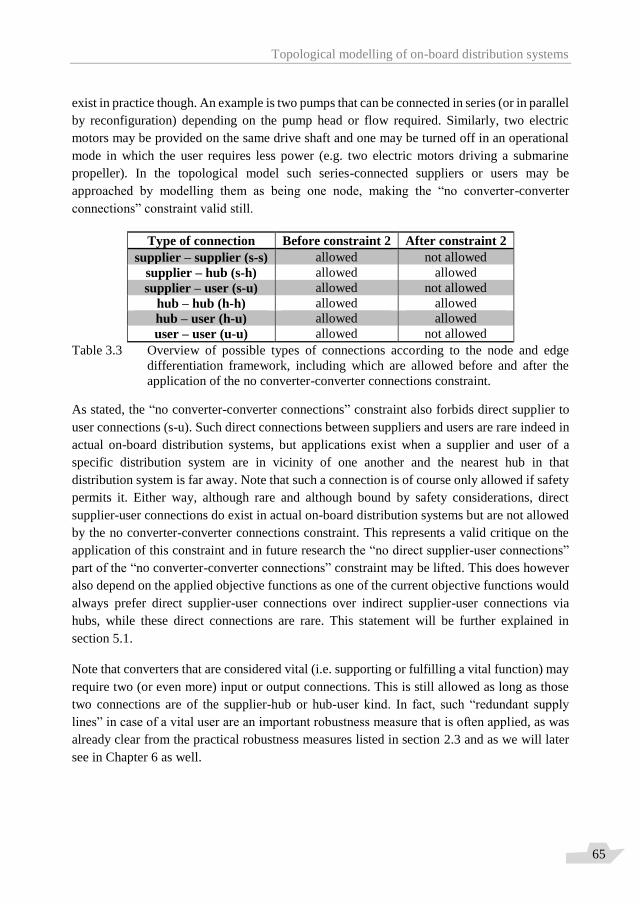
Topological modelling of on-board distribution systems
65
exist in practice though. An example is two pumps that can be connected in series (or in parallel
by reconfiguration) depending on the pump head or flow required. Similarly, two electric
motors may be provided on the same drive shaft and one may be turned off in an operational
mode in which the user requires less power (e.g. two electric motors driving a submarine
propeller). In the topological model such series-connected suppliers or users may be
approached by modelling them as being one node, making the “no converter-converter
connections” constraint valid still.
Type of connection Before constraint 2 After constraint 2
supplier – supplier (s-s) allowed not allowed
supplier – hub (s-h) allowed allowed
supplier – user (s-u) allowed not allowed
hub – hub (h-h) allowed allowed
hub – user (h-u) allowed allowed
user – user (u-u) allowed not allowed
Table 3.3 Overview of possible types of connections according to the node and edge
differentiation framework, including which are allowed before and after the
application of the no converter-converter connections constraint.
As stated, the “no converter-converter connections” constraint also forbids direct supplier to
user connections (s-u). Such direct connections between suppliers and users are rare indeed in
actual on-board distribution systems, but applications exist when a supplier and user of a
specific distribution system are in vicinity of one another and the nearest hub in that
distribution system is far away. Note that such a connection is of course only allowed if safety
permits it. Either way, although rare and although bound by safety considerations, direct
supplier-user connections do exist in actual on-board distribution systems but are not allowed
by the no converter-converter connections constraint. This represents a valid critique on the
application of this constraint and in future research the “no direct supplier-user connections”
part of the “no converter-converter connections” constraint may be lifted. This does however
also depend on the applied objective functions as one of the current objective functions would
always prefer direct supplier-user connections over indirect supplier-user connections via
hubs, while these direct connections are rare. This statement will be further explained in
section 5.1.
Note that converters that are considered vital (i.e. supporting or fulfilling a vital function) may
require two (or even more) input or output connections. This is still allowed as long as those
two connections are of the supplier-hub or hub-user kind. In fact, such “redundant supply
lines” in case of a vital user are an important robustness measure that is often applied, as was
already clear from the practical robustness measures listed in section 2.3 and as we will later
see in Chapter 6 as well.
Topological modelling of on-board distribution systems
66
Since on-board energy distribution systems typically have a far larger number of converters
(suppliers and users) than hubs, the “no converter-converter connections” constraint indeed
reduces the design space significantly as well, as large parts of the adjacency matrix become
zero by default. This constraint, together with the “technical feasibility of connections”
constraint, is the reason that the number of possible non-zero elements was so significantly
reduced in the adjacency matrices of the frigate case study network in Figure 3.10. Together,
the two constraints reduced the number of potential connections from 630 to 172, resulting in
the earlier mentioned reduction of the size of the design space from 2630 to 2172.
3.5.3 Constraint 3: Connected networks Where the first two constraints set a higher bound on the number of potential connections, the
third constraint effectively reduces the size of the design space by setting a lower bound on
the number of allowed connections. The “connected networks” constraint requires that there
is a finite distance between all nodes (system components), i.e. there is a path between all node
pairs. Here, distance is not meant literally (in meters), but rather the mathematical concept of
distance measured in number of edges between node pairs (also known as number of hops).
This constraint is similar to stating that all generated system topologies should be connected,
i.e. no unconnected components or disjoint sub-networks (known in network theory as
components) consist within it. The “connected networks” constraint follows from the
observation that all components in actual on-board energy distribution systems have a
connection with other components in the network. The only unconnected system component
that could be present on board of a ship is a spare system component, but even for spare system
components it is rare that they are physically unconnected. Such spare system components
may be operationally unconnected, by means of open switches or closed valves in the supply
or discharge lines, but that still means a connection exists; the system component is merely
unused in a certain operational mode and becomes operational in case of an emergency. Note
that system components are here meant to be entire machines or pieces of equipment, not
components of those machines, for which actual unconnected spares may be on board and that
may need to be installed in case of emergencies while at sea.
It is possible though that different networks, i.e. physically unconnected systems, exist in the
ship. Two separate mechanical propulsion trains for instance, or an electric power plant
separated from the (mechanical) propulsion system. For such separated systems it is possible
to run the ATG tool separately, making the constraint of connected networks still valid.
The “connected networks” constraint sets a theoretical lower bound on the number of
connections in the network: nn – 1. For the frigate case study network this means that at least
35 connections are needed to ensure a connected network. This minimum is however truly
theoretical as the components in the lower converter layers (end-users like sensor and weapon
systems) require more than one input to function (in the frigate case study network at least

Topological modelling of on-board distribution systems
67
both a 440 V electric supply and a 5 °C chilled water supply), which increases the actual
minimum number of connections beyond 35 of course.
Note that, although the “connected networks” constraint is an a-priori constraint, it is not
implemented as such in the ATG tool. Rather the constraint is implemented as a repair
function. This will be further explained in Chapter 4 and Chapter 5, which together discuss
how the ATG tool searches the remaining design space by automatically generating system
topologies.
As a final remark: although some characteristics of the three constraints above may be
considered unacceptable by some, like not allowing direct supplier – user connections, it is
here still chosen to apply the constraints as introduced. This choice avoids computational effort
being wasted on infeasible or improbable system topologies irrespective of the calculation
method used for searching the design space. This is considered a major advantage.
3.6 Directed vs. undirected connections Section 3.1 also introduced the concept of directed vs. undirected networks. What about the
network topologies developed in this research? Do they contain directed or undirected
connections? The benchmark system, as shown and introduced in section 3.4, clearly depicts
undirected connections (otherwise the connections would have had arrow heads) and indeed
the topological model was originally set up to have only undirected connections. There are
two reasons why undirected connections can be chosen all over.
1. For early-stage system design the direction of flow through the connections is not
important. Only the existence of a connection between two components is needed to
define a network topology and make assessment of design drivers possible.
2. From a physical perspective all connections are undirected, i.e. in principle flow can
go each way through the connections unless devices are implemented that obstruct
the flow in one direction, like diodes or non-return valves.
Then again, each distribution system contains both suppliers and users, clearly indicating a
predominant direction of flow. Indeed, even in the absence of obstruction devices the flow in
normal operation of energy distribution systems is from suppliers to users, indicating that
directed connections may be chosen just as well in the topological model. Only in transient
conditions a reversal of flow direction may occur and such conditions are not modelled or
investigated in early-stage system design.
When the different types of connections are studied, it is clear that s-h and h-u connections
may indeed be directed. However, h-h connections cannot be directed. Unless a certain
hierarchy between hubs exists, but that will be discussed later. Hub – hub connections between
equally important hubs cannot be directed as they are used to reconfigure systems, meaning
Topological modelling of on-board distribution systems
68
that sometimes the flow will be from hub A to B and at other times the other way around.
Reconfiguration of systems (in fact the operational topology) is in practice often done for a
number of reasons. First of all, it can be a way to improve system robustness as it allows a
system to be reconfigured such that, after a hit has occurred, the flow between suppliers and
users is redirected (to have as many users operational as possible). Another reason may be of
an operational nature; the number of operational suppliers can be adapted to the power
demand. This can for instance increase fuel efficiency.
To show that both options, i.e. all connections undirected (1) or (2) s-h and h-u connections
directed and h-h connections undirected, are viable, both options will be used in this
dissertation. All connections of the notional frigate distribution systems, of which the
benchmark system has been shown in section 3.4, will remain undirected throughout the
dissertation. In section 6.2 the ATG tool will however also be applied to the systems on board
of another naval ship type using the second option.
Note that the size of the design space is not affected by the choice between the two options for
modelling connections. This might perhaps be expected as theoretically there is a difference
between the number of possible system topologies when a network is modelled as directed or
undirected. The number of edges in directed networks is indeed twice as high as in undirected
networks, from a theoretic perspective. For the second option though, with directed s-h and h-
u connections, connections are only allowed to go from suppliers towards users (with hubs in
between). Hub – hub connections are in this case made undirected by a repair function.
Consequently, the focus is for both options on the upper triangle of the adjacency matrix only
(see Figure 3.10) and thus the number of possible connections is unaffected.
3.7 Further treatment of network theory After the introduction of the node and edge differentiation framework and its application to
the benchmark system, some further concepts of network theory can be introduced that can be
related to the framework and will prove of interest for system robustness. The concepts
discussed are described on basis of the descriptions given in the handbook on network theory
of [Newman, 2012].
Degree (centrality)
In an undirected network, the degree of a node in a graph or network is the number of edges
connected to it. In a directed network there is a difference between “inbound” and “outbound”
edges captured in the in- and out-degree respectively. From the previous sections it should be
clear that suppliers and users in on-board distribution systems typically have a low degree,
while hubs can be specified as nodes with an unusual high degree compared to other nodes
inside the same network. This can be related to the concept of degree centrality. Centrality
metrics in network theory aim to answer the question: “which nodes are the most important?”
What is considered important is subjective, but when degree centrality is indeed regarded as a
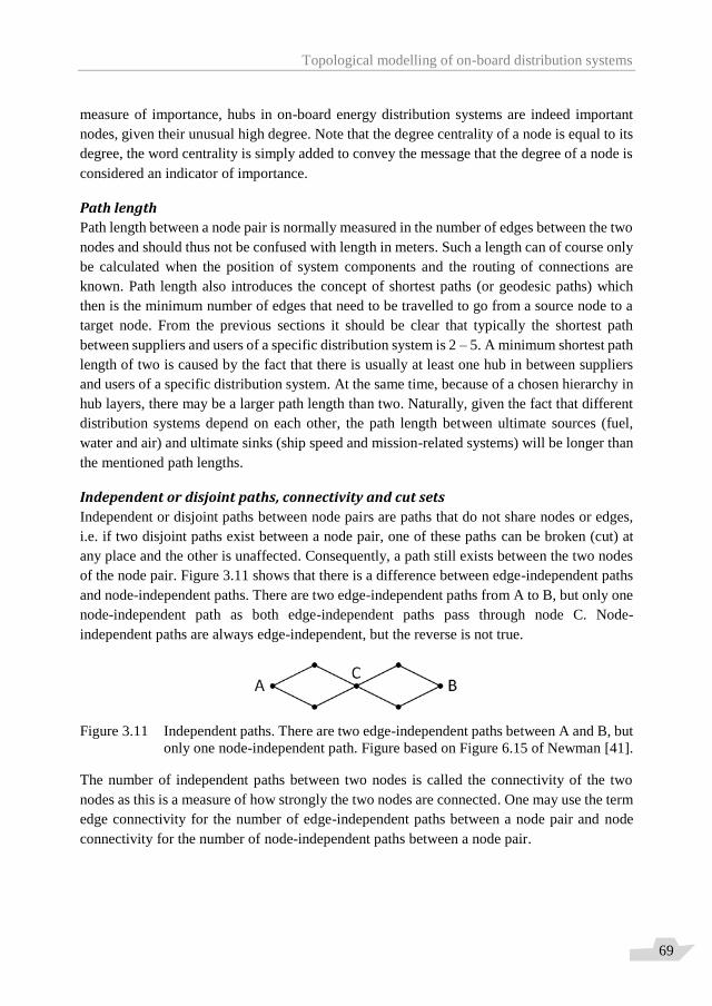
Topological modelling of on-board distribution systems
69
measure of importance, hubs in on-board energy distribution systems are indeed important
nodes, given their unusual high degree. Note that the degree centrality of a node is equal to its
degree, the word centrality is simply added to convey the message that the degree of a node is
considered an indicator of importance.
Path length
Path length between a node pair is normally measured in the number of edges between the two
nodes and should thus not be confused with length in meters. Such a length can of course only
be calculated when the position of system components and the routing of connections are
known. Path length also introduces the concept of shortest paths (or geodesic paths) which
then is the minimum number of edges that need to be travelled to go from a source node to a
target node. From the previous sections it should be clear that typically the shortest path
between suppliers and users of a specific distribution system is 2 – 5. A minimum shortest path
length of two is caused by the fact that there is usually at least one hub in between suppliers
and users of a specific distribution system. At the same time, because of a chosen hierarchy in
hub layers, there may be a larger path length than two. Naturally, given the fact that different
distribution systems depend on each other, the path length between ultimate sources (fuel,
water and air) and ultimate sinks (ship speed and mission-related systems) will be longer than
the mentioned path lengths.
Independent or disjoint paths, connectivity and cut sets
Independent or disjoint paths between node pairs are paths that do not share nodes or edges,
i.e. if two disjoint paths exist between a node pair, one of these paths can be broken (cut) at
any place and the other is unaffected. Consequently, a path still exists between the two nodes
of the node pair. Figure 3.11 shows that there is a difference between edge-independent paths
and node-independent paths. There are two edge-independent paths from A to B, but only one
node-independent path as both edge-independent paths pass through node C. Node-
independent paths are always edge-independent, but the reverse is not true.
Figure 3.11 Independent paths. There are two edge-independent paths between A and B, but
only one node-independent path. Figure based on Figure 6.15 of Newman [41].
The number of independent paths between two nodes is called the connectivity of the two
nodes as this is a measure of how strongly the two nodes are connected. One may use the term
edge connectivity for the number of edge-independent paths between a node pair and node
connectivity for the number of node-independent paths between a node pair.
Topological modelling of on-board distribution systems
70
Cut sets are sets of nodes or edges that, when removed from the network, disconnects a
specified node pair. For example, the minimum node cut set for node pair A, B in Figure 3.11
has a size of 1 and concerns node C. Its removal will ensure that no path exists between A and
B. Similarly, the minimum edge cut set has a size of 2 and is a set of two edges whose removal
would cut the two edge-independent paths. Note that the size of cut sets for specified node
pairs are equal to the connectivity of those node pairs and thus equal to the number of
independent paths between those node pairs. This is exactly what Menger’s theorem teaches
us.
Maximum flow
The edge version of Menger’s theorem generalises to the max-flow min-cut theorem which in
its most general form states that (Newman [41]):
The maximum flow between a given pair of vertices in a network is equal to the sum of the
weights on the edges of the minimum edge cut set that separates the same two vertices.
Weights of edges were not discussed up till now as all networks up till now have been
unweighted and in fact will remain so throughout this research. However, in a flow network
one can imagine assigning weights to edges which represent e.g. the capacity of edges. In such
a case, the maximum flow between two nodes (source and sink) can be calculated by summing
the capacities of the lowest-capacity edges in edge-independent paths between the two nodes.
After all, the lowest-capacity edges in a path determine the maximum flow that can flow
through that path and if there are edge-independent paths between two nodes it is clear from
the previous section that the only way to separate two nodes is by cutting each independent
path.
In unweighted networks the weight of each edge is one and consequently the maximum flow
through each path is also one. This means that for unweighted networks the maximum flow is
equal to minimum edge cut set size, which is equal to the connectivity of a node pair, which is
equal to the number of edge-independent paths (or edge-disjoint paths) between a source and
a sink (or target). This is an important conclusion as maximum flow algorithms are readily
available and can thus be used to count the number of disjoint paths between node pairs. It
may already be clear to the reader that this will prove to be important when trying to assess
the robustness of on-board energy distribution systems.
Betweenness centrality
Finally, betweenness centrality or simply betweenness may prove useful as it measures to what
extent a node or an edge (distinguish node betweenness and edge betweenness) lies on paths
between source and target nodes. Furthermore, according to Newman [41], one must
distinguish betweenness centrality and flow betweenness, where betweenness centrality of
node i represents the number of shortest paths between a source and target node that pass
Topological modelling of on-board distribution systems
71
through node i and flow betweenness of node i represents the flow through that node when
there is maximum flow between a source and a target node. In the section on betweenness
Newman [41] also discusses normalisation of betweenness (the concept of normalisation will
later be used in this research as well) and the fact that the betweenness of the central node in a
star graph is the maximum possible value for betweenness. This will prove to be important
later as well.
3.8 Summary and conclusion A topological model of on-board distribution systems has been introduced in this chapter. It
can be summarised as follows: There are different (i.e. distinguishable) (energy) distribution
systems on board of (naval) vessels that distribute different types of (energy) flow from
suppliers to users. Each specific distribution system distributes a specific flow type and
consists of suppliers, hubs and users. Hubs are common distribution lines in which all flow
from suppliers is gathered and distributed to the users. A user in one specific distribution
system may be a supplier in another, i.e. the different distribution systems are connected to
each other via their system components, which makes the systems interdependent. This
topological model leads to a node and edge differentiation framework when combined with
the fundamental concepts nodes and edges from network theory. Doing so enables the set-up
of an adjacency matrix defining a network topology of interdependent on-board distribution
systems. This is the first step to enable automated design space exploration in early-stage
system design. The applicability of the node and edge differentiation framework may be wider
than just on-board systems; i.e. land-based systems may perhaps also be captured with the
same framework. Then again, only on-board systems are designed completely anew when a
ship (class) is designed. Land-based systems need to be integrated in already existing systems
and their design freedom may for this reason be less large.
Representing suppliers and users as nodes is considered a first logical choice in the topological
modelling of on-board distribution systems. The choice to model hubs as nodes as well is less
obvious (and more controversial) but is deemed necessary to make the topological model
work. Hubs can sometimes be recognised as “local, discrete objects” in practical systems; then
the choice to model hubs as nodes is relatively obvious. The choice becomes less obvious
when hubs are in practice extensive (i.e. stretched out), high-capacity common distribution
lines, like a long pipe line extending over the length of the ship. In that case hubs are perhaps
better regarded as a “super node” consisting of different junctions and “overlapping edges”.
The usefulness and applicability of the topological model were discussed in sections 3.3 and
3.4. The latter introduced the first case study of this research and the hand-made benchmark
system consisting of the electric power and chilled water distribution systems on board a
notional frigate; see Figure 3.8.

Topological modelling of on-board distribution systems
72
The topological model also allows for the calculation of the size of the design space as a
function of the number of nodes. With the benchmark system consisting of 36 nodes,
theoretically the design space is 2630. After inclusion of a-priori constraints, based on first
principles and engineering practice, the size of the design space was limited to 2172, as
described in section 3.5. The constraints put a lower and higher bound on the number of
connections allowed in a network topology. This number is however still unacceptably high
from a practical decision support perspective. This is the reason the next chapter incorporates
the topological model in a genetic algorithm which enables population of the design space and
optimisation of the generated design solutions within acceptable computational times.
Section 3.6 discussed whether connections should be directed or undirected in the topological
model. It was argued that all connections may be modelled as undirected, as is done in the
frigate case study. Or that s-h and h-u connections may be modelled as directed and h-h
connections as undirected. This will be done in a case study that will be introduced in section
6.2. Section 3.7 revisited network theory and introduced a number of measures and metrics
from this mathematical field that will become useful when objective functions are discussed
in Chapter 5. Objective functions are needed by the genetic algorithm that varies system
topologies. Therefore, incorporation of the topological model of this chapter is first described
in the next chapter; Chapter 4.
Automatic Topology Generation
73
“Natural selection is not the wind which propels the vessel, but the rudder which,
by friction, now on this side and now on that, shapes the course.”
― Asa Gray
Chapter 4 Automatic Topology Generation The previous chapter showed that the developed node and edge differentiation framework
enables topological modelling of on-board energy distribution systems. However, automated
design space exploration becomes possible only after the topological model is combined with
an algorithm that uses the model to generate varying system topologies. For practical reasons
mainly, the choice is made here to use the genetic algorithm that is also used by the packing
tool, ref. van Oers [43], for generating varying ship configurations. This is deemed an
appropriate choice as the specific genetic algorithm is designed to support trade-off analyses
between opposing design objectives, which here clearly is the case (an increase in system
robustness opposes other design objectives like weight and space requirement and costs).
Combining the topological model of the previous section with this genetic algorithm results in
the Automatic Topology Generation tool (ATG tool) that is able to generate many different
design solutions for on-board energy distribution systems.
This chapter first shortly introduces the principle of design space exploration using
evolutionary algorithms, of which genetic algorithms are a subset. The ATG tool as a specific
application of such a design space exploration tool is subsequently introduced in section 4.2.
First the input that is required by the ATG tool is elaborated, then the calculation procedure as
followed is explained. This leads to an understanding of the function of different elements of
the ATG tool and how these are related. These elements are: repair function, objective
functions, steering mechanism and NSGA-II as the genetic algorithm. Most of these elements
will be further elaborated in the remaining sections of this chapter. Initial, possibly elite,
“individuals” as a starting point of the calculation are introduced as well.
The objective functions as element of the ATG tool will be discussed in the next chapter as
these are key to the usefulness of the design space exploration approach and validity of
generated design solutions. The latter statement is true for any optimisation procedure and a
genetic algorithm is just that, an optimisation procedure. Here the genetic algorithm is however
mainly used as a search algorithm, not necessarily an optimisation algorithm. The difference
being that not only the design solutions on the non-dominated Pareto front are interesting, the
other generated design solutions may be of interest as well.
Automatic Topology Generation
74
4.1 Topology generation in general Network theory, as introduced in the previous chapter, typically focusses on assessing and
understanding the topology of already existing real-world networks. Real-world networks that
are studied are for instance the internet, social networks, metabolic networks, logistical
networks and electrical engineering networks. The topology of many of these (large and/or
invisible) networks are unknown and much can be learned from discovering their underlying
structure, i.e. topology. Generating network topologies of not yet existing networks as done in
this research is therefore not necessarily the primary aim of network theory.
Still, the idea of topology generation, even when applied to technical systems, is not new and
there are a number of ways in which it can be done. Although automatic topology generation
will here be enabled by incorporating the topological model of Chapter 3 with a Genetic
Algorithm, this is not the only way to enable topology generation. Neither is topology
generation using GA techniques a novel approach; it is at most a novel approach in the context
of energy distribution systems on board ships. Therefore, this section first shortly discusses
the application of topology generation in other technology sectors and a small number of
different ways in which it may be done.
Application in other technology sectors9
For different applications and for different types of networks, topology generators have been
developed. Arguably the most famous and generic topology generation model is the one of
Albert and Barabasi [2]. The BA model generates networks with a power law degree
distribution, also called scale-free networks, which can be found in many real-world
applications. Indeed, on-board energy distribution systems exhibit scale-free properties as well
(see section 3.4), as there are many users and suppliers with only one or two connections and
a small number of hubs with a high degree. The BA model incorporates growth and preferential
attachment, of which especially the latter might be of interest to topology generation for on-
board energy distribution systems, since components that supply a specific energy flow are
typically connected to nearby users or hubs and vice versa. The concept of growth is less
applicable as on-board systems are designed and built in a relatively short period of time. After
the ship has been built it is unlikely that (many) new components (nodes) and connections
(edges) are added, at least not frequently (although there are midlife conversions). In
information technology research the generation of similar topologies as the network topology
of the internet has received a lot of attention; ref. Sterbenz et al. [62], Medina et al. [40] and
Calvert et al. [12].
9 The text of this section is repeated from de Vos et al. [67] and adjusted to fit here.
Automatic Topology Generation
75
Although aimed specifically at the design of control network topologies Fencl et al. [23] try to
obtain similar goals in a comparable manner as this study. In their research as well, network
topologies are generated using a genetic algorithm to optimise between the opposing design
objectives fault-tolerance and acquisition costs. The main difference with the methodology
that is presented in this dissertation (besides the application) is that Fencl et al. assume a matrix
[M] specifying the number of independent paths between each node pair to be known
beforehand. For early-stage design of on-board energy distribution systems this information is
not known and thus the methodology of Fencl et al. cannot be applied here. Furthermore, it
was found that node pairs in actual on-board energy distribution systems rarely have more than
one completely independent path; rather there are parts of the paths between node pairs that
are common to all paths, while other parts of the paths between suppliers and users are
independent. This again is related to the existence of hubs in the systems and will be utilised
later in this dissertation.
Related more closely to the on-board energy distribution systems that are central to this
research is the topology generator of Silvas et al. [58] for the electric / mechanical power
distribution systems of hybrid electric vehicles. Similarly, the optimisation of topology and
pipe size for water distribution systems in Saleh et al. [57] is comparable to this research.
However, both of these studies contain detailed system topological models that have been
tailored to the specific characteristics of the studied systems. In a multi-disciplinary approach,
such as the one taken in this research, one cannot utilise too much specific system knowledge
and is limited to the common features of different energy distribution systems. This
consideration is the foundation of the node and edge differentiation framework that was
introduced in section 3.2.
From this section, it can be concluded that topology generation can be considered a viable
method to explore design spaces for networked systems like energy distribution systems on
board of ships. The application of topology generation to different energy distribution systems
on board of ships asks for a high-level, integrated approach combined with marine engineering
heuristics to make the results as realistic as possible.

Automatic Topology Generation
76
4.2 ATG for on-board energy distribution systems10 The working principle of the ATG tool was already shown in Figure 1.6. The figure is repeated
below for convenience. The ATG tool is implemented in Matlab®.
Figure 4.1 Principle of design space exploration with the ATG tool – repeated from de Vos
et al. [68].
A-priori constraints, as introduced in section 3.5, limit the size of the design space. Although
effective, inclusion of the a-priori constraints will not be sufficient to bring down the number
of possible topologies to a number that can be overseen by a system designer. Therefore,
optimisation will be applied in order to enable exploration of the remaining design space and
find the most interesting system topologies. A genetic algorithm will be used to find the Pareto
front of non-dominated solutions for the opposing design objectives of system robustness and
system claim; note that these objective functions will be explained in Chapter 5. Optimisation
brings down the number of topologies to a more manageable amount. For the frigate case
study, it is possible to generate 40000 (≈ 215) network topologies with the ATG tool in
approximately 20 minutes on an ordinary, modern PC with average computational capacity.
The actual number of network topologies generated depends on the settings of the genetic
algorithm concerning population size. A relatively small part of this still rather high number
of topologies is on the Pareto front of non-dominated design solutions, as will be shown later.
Still a final selection strategy would be required to support a system designer in selecting the
right topology or topologies to pursue in later design stages, but this selection phase is outside
the scope of this research as it is the part where more negotiable (or fuzzy) constraints are
applied by a designer given the specific system(s) and/or ship he/she is designing. Further,
remember that the main purpose of design space exploration may not necessarily be to generate
a small number of feasible, highly optimised design solutions, but rather to gain insight in the
10 The text of this section is partly repeated from de Vos et al. [67] and adjusted to fit here.
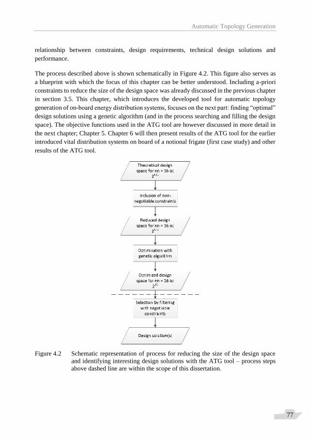
Automatic Topology Generation
77
relationship between constraints, design requirements, technical design solutions and
performance.
The process described above is shown schematically in Figure 4.2. This figure also serves as
a blueprint with which the focus of this chapter can be better understood. Including a-priori
constraints to reduce the size of the design space was already discussed in the previous chapter
in section 3.5. This chapter, which introduces the developed tool for automatic topology
generation of on-board energy distribution systems, focuses on the next part: finding “optimal”
design solutions using a genetic algorithm (and in the process searching and filling the design
space). The objective functions used in the ATG tool are however discussed in more detail in
the next chapter; Chapter 5. Chapter 6 will then present results of the ATG tool for the earlier
introduced vital distribution systems on board of a notional frigate (first case study) and other
results of the ATG tool.
Figure 4.2 Schematic representation of process for reducing the size of the design space
and identifying interesting design solutions with the ATG tool – process steps
above dashed line are within the scope of this dissertation.
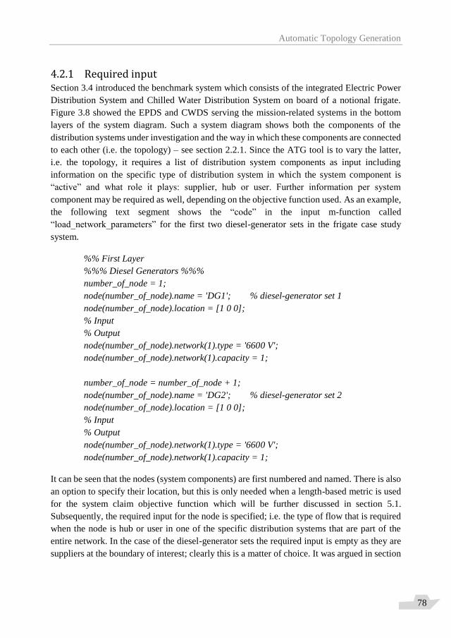
Automatic Topology Generation
78
4.2.1 Required input Section 3.4 introduced the benchmark system which consists of the integrated Electric Power
Distribution System and Chilled Water Distribution System on board of a notional frigate.
Figure 3.8 showed the EPDS and CWDS serving the mission-related systems in the bottom
layers of the system diagram. Such a system diagram shows both the components of the
distribution systems under investigation and the way in which these components are connected
to each other (i.e. the topology) – see section 2.2.1. Since the ATG tool is to vary the latter,
i.e. the topology, it requires a list of distribution system components as input including
information on the specific type of distribution system in which the system component is
“active” and what role it plays: supplier, hub or user. Further information per system
component may be required as well, depending on the objective function used. As an example,
the following text segment shows the “code” in the input m-function called
“load_network_parameters” for the first two diesel-generator sets in the frigate case study
system.
%% First Layer
%%% Diesel Generators %%%
number_of_node = 1;
node(number_of_node).name = 'DG1'; % diesel-generator set 1
node(number_of_node).location = [1 0 0];
% Input
% Output
node(number_of_node).network(1).type = '6600 V';
node(number_of_node).network(1).capacity = 1;
number_of_node = number_of_node + 1;
node(number_of_node).name = 'DG2'; % diesel-generator set 2
node(number_of_node).location = [1 0 0];
% Input
% Output
node(number_of_node).network(1).type = '6600 V';
node(number_of_node).network(1).capacity = 1;
It can be seen that the nodes (system components) are first numbered and named. There is also
an option to specify their location, but this is only needed when a length-based metric is used
for the system claim objective function which will be further discussed in section 5.1.
Subsequently, the required input for the node is specified; i.e. the type of flow that is required
when the node is hub or user in one of the specific distribution systems that are part of the
entire network. In the case of the diesel-generator sets the required input is empty as they are
suppliers at the boundary of interest; clearly this is a matter of choice. It was argued in section
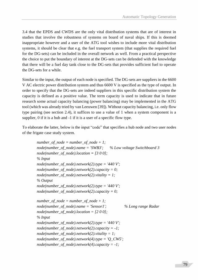
Automatic Topology Generation
79
3.4 that the EPDS and CWDS are the only vital distribution systems that are of interest in
studies that involve the robustness of systems on board of naval ships. If this is deemed
inappropriate however and a user of the ATG tool wishes to include more vital distribution
systems, it should be clear that e.g. the fuel transport system (that supplies the required fuel
for the DG-sets) can be included in the overall network as well. From a practical perspective
the choice to put the boundary of interest at the DG-sets can be defended with the knowledge
that there will be a fuel day tank close to the DG-sets that provides sufficient fuel to operate
the DG-sets for a while.
Similar to the input, the output of each node is specified. The DG-sets are suppliers in the 6600
V AC electric power distribution system and thus 6600 V is specified as the type of output. In
order to specify that the DG-sets are indeed suppliers in this specific distribution system the
capacity is defined as a positive value. The term capacity is used to indicate that in future
research some actual capacity balancing (power balancing) may be implemented in the ATG
tool (which was already tried by van Leeuwen [39]). Without capacity balancing, i.e. only flow
type pairing (see section 2.4), it suffices to use a value of 1 when a system component is a
supplier, 0 if it is a hub and -1 if it is a user of a specific flow type.
To elaborate the latter, below is the input “code” that specifies a hub node and two user nodes
of the frigate case study system.
number_of_node = number_of_node + 1;
node(number_of_node).name = 'SWB3'; % Low voltage Switchboard 3
node(number_of_node).location = [3 0 0];
% Input
node(number_of_node).network(2).type = '440 V';
node(number_of_node).network(2).capacity = 0;
node(number_of_node).network(2).vitality = 1;
% Output
node(number_of_node).network(2).type = '440 V';
node(number_of_node).network(2).capacity = 0;
number_of_node = number_of_node + 1;
node(number_of_node).name = 'Sensor1'; % Long range Radar
node(number_of_node).location = [2 0 0];
% Input
node(number_of_node).network(2).type = '440 V';
node(number_of_node).network(2).capacity = -1;
node(number_of_node).network(2).vitality = 1;
node(number_of_node).network(4).type = 'Q_CW5';
node(number_of_node).network(4).capacity = -1;

Automatic Topology Generation
80
node(number_of_node).network(4).vitality = 1;
% Output
node(number_of_node).network(5).type = 'Data from Sensor 1';
node(number_of_node).network(5).capacity = 1;
number_of_node = number_of_node + 1;
node(number_of_node).name = 'Weapon'; Missile launcher
node(number_of_node).location = [3 0 0];
% Input
node(number_of_node).network(2).type = '440 V';
node(number_of_node).network(2).capacity = -1;
node(number_of_node).network(2).vitality = 1;
node(number_of_node).network(4).type = 'Q_CW5';
node(number_of_node).network(4).capacity = -1;
node(number_of_node).network(4).vitality = 1;
node(number_of_node).network(7).type = 'Data to Shooter';
node(number_of_node).network(7).capacity = -1;
node(number_of_node).network(7).vitality = 1;
% Output
The first node mentioned above is one of the low voltage switchboards in Hub Layer 2 of
Figure 3.8; these components gather and distribute all 440 V AC electric power. The second
node mentioned above is one of the sensors in CL5 and the third node is the weapon in CL8.
The types of flow required by these users is 440 V AC electric power and 5 °C chilled water.
These nodes also show the supply and usage of another flow type: different types of
information data. As explained in section 3.4 topologies are not generated for these kind of
distribution systems in the frigate case study network as the node and edge differentiation
framework is considered less applicable to these distribution systems. The main difference is
that connections in energy distribution systems can carry only the specific flow it is intended
for (declaration 2 in section 3.2), while connections in data distribution systems can carry
different kinds of data; i.e. the same LAN-cable can carry all sorts of information.
Finally, the vitality of each required input flow can be specified. Like the location of the node
this input is only required when a specific objective function (for system robustness in this
case) is used. This will be further elaborated in section 5.2.
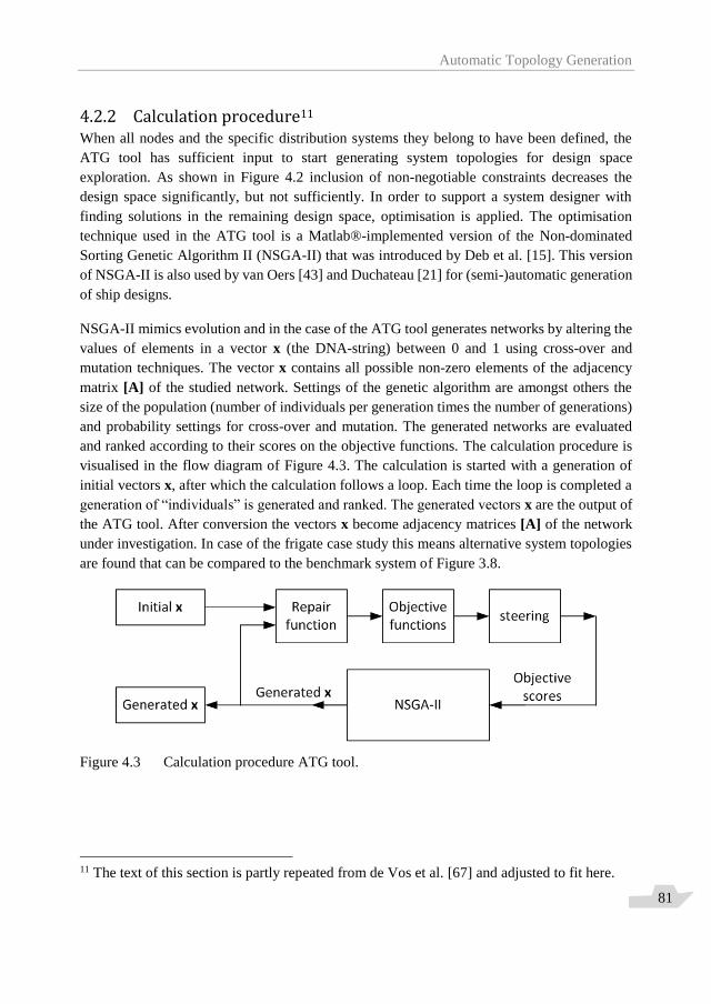
Automatic Topology Generation
81
4.2.2 Calculation procedure11 When all nodes and the specific distribution systems they belong to have been defined, the
ATG tool has sufficient input to start generating system topologies for design space
exploration. As shown in Figure 4.2 inclusion of non-negotiable constraints decreases the
design space significantly, but not sufficiently. In order to support a system designer with
finding solutions in the remaining design space, optimisation is applied. The optimisation
technique used in the ATG tool is a Matlab®-implemented version of the Non-dominated
Sorting Genetic Algorithm II (NSGA-II) that was introduced by Deb et al. [15]. This version
of NSGA-II is also used by van Oers [43] and Duchateau [21] for (semi-)automatic generation
of ship designs.
NSGA-II mimics evolution and in the case of the ATG tool generates networks by altering the
values of elements in a vector x (the DNA-string) between 0 and 1 using cross-over and
mutation techniques. The vector x contains all possible non-zero elements of the adjacency
matrix [A] of the studied network. Settings of the genetic algorithm are amongst others the
size of the population (number of individuals per generation times the number of generations)
and probability settings for cross-over and mutation. The generated networks are evaluated
and ranked according to their scores on the objective functions. The calculation procedure is
visualised in the flow diagram of Figure 4.3. The calculation is started with a generation of
initial vectors x, after which the calculation follows a loop. Each time the loop is completed a
generation of “individuals” is generated and ranked. The generated vectors x are the output of
the ATG tool. After conversion the vectors x become adjacency matrices [A] of the network
under investigation. In case of the frigate case study this means alternative system topologies
are found that can be compared to the benchmark system of Figure 3.8.
Figure 4.3 Calculation procedure ATG tool.
11 The text of this section is partly repeated from de Vos et al. [67] and adjusted to fit here.
Automatic Topology Generation
82
The functionality of each block in Figure 4.3 will be discussed in the subsequent sections,
except for the objective functions. The definition of the objective functions is crucial to the
credibility of the results, which is why these are treated in their own chapter; Chapter 5. The
latter remark is true for any optimisation algorithm, not just genetic algorithms.
4.2.3 (Initial) vector x The calculation starts with an initial generation of “individuals”, i.e. a number of initial vectors
x. The vector x contains all possible non-zero elements of the adjacency matrix [A] of the
network under investigation, i.e. the potential connections between system components of
different on-board distribution systems. For the vital distribution systems on board of the
notional frigate these potential connections are the 172 elements indicated on the right-hand
side of Figure 3.10. Conversion functions were written to convert [A] to x and x to [A].
Note that these conversion functions enforce the first two a-priori constraints of section 3.5 as
vector x contains only the connections that are allowed after the inclusion of these constraints.
If the constraints would not be applied, vector x would contain all elements of the upper
triangle of adjacency matrix [A] (630 for the frigate case study network). It was argued in
section 3.5 that many of these elements represent infeasible or unlikely connections, which is
why that section described the first two a-priori constraints to limit the number of potential
connections (to 172 for the frigate case study network).
The length of vector x in general depends on the number of different distribution systems in
the overall network and the number of nodes and the roles these nodes have in the specific
distribution systems. This information is available in the input data defined in the
“load_network_parameters” file. With that information the constraints can be applied, the
number of potential connections calculated and thus the length of vector x determined.
The number of vectors x in the initial generation depends on the number of individuals per
generation as specified in the settings for NSGA-II. The initial generation is as large as the
subsequent generations. The initial generation normally contains randomly generated
individuals, i.e. each of the 172 elements of initial vectors x are randomly assigned a value of
1 or 0 (a connection exists, or it does not). Alternatively, the initial generation may contain
(some) “elite” individuals; i.e. vectors x of which it is already known that they score well on
the objective functions (known for instance from previous runs with the ATG tool or from
experience).
4.2.4 Repair function The ATG tool also contains a repair function to repair generated networks that are considered
infeasible, before objective functions are called upon to evaluate a generated network. The
main part of the repair function follows from the “connected networks” constraint, see section
3.5.3. This part ensures that a generated network does not contain unconnected components or
Automatic Topology Generation
83
sub-networks. It does so by checking for each node whether at least one connection exists with
the layer above and below it. If this is not the case a connection is made to a random node in
the layer above or below it.
Another part of the repair function checks whether a node is considered vital and if so, how
many supply lines a node should have; this number is pre-defined by the user. If the amount
of supply lines has not yet been reached more supply lines are made by connecting randomly
to other hubs with similar functionality. It depends on which system robustness objective
function is used whether this vitality repair function is needed as will become clear in section
5.2.
Finally, in case the networks are directed, hub – hub connections are made bi-directional by
the repair function as explained in section 3.6.
4.2.5 Objective functions The objective functions direct the search or optimisation of NSGA-II. They are the
mathematical expressions of what are considered design drivers, i.e. important design
requirements. Their validity to the design problem at hand determine the usefulness of the
automated design space exploration approach using genetic algorithms. Their importance
cannot be underestimated and they are therefore treated in a separate chapter hereafter. For
now, it is sufficient to introduce the two groups of objectives that are opposing each other in
on-board energy distribution system design:
weight & space requirements
procurement & installation costs
operability of the system
versus
vulnerability
recoverability
or briefly: the "claim" of the systems on the ship (objective function 1) versus system
robustness (objective function 2). Chapter 5 will introduce and discuss the mathematical
formulations of the objective functions as used in the ATG tool.
Automatic Topology Generation
84
4.2.6 Steering12 First results of the ATG tool showed that NSGA-II wasted computational effort on networks
that could be considered feasible within the context of this study but would still be considered
impractical. To avoid this, steering the search effort of the genetic algorithm is applied. The
search effort of the genetic algorithm is steered by two mechanisms: overwriting the score on
objective function 2 (robustness) for systems with too many connections and by setting smart
starting points of the search effort during initialisation of the genetic algorithm. The latter was
already introduced in section 4.2.3 on initial vectors x as the possibility to include so-called
“elite” individuals in the initial generation. The first steering mechanism is explained below.
As already indicated in section 3.5, the frigate case study network needs theoretically at least
35 connections to be fully connected (nn-1) and has a maximum of 172 potential connections
after inclusion of the constraints. Thus NSGA-II has the freedom to explore the design space
by “producing” any number of connections within these bounds.
The NSGA-II algorithm at first explored large parts of the entire design space and many
networks that were generated had more than 100 connections, especially in the first
generations. This is easily possible in the frigate case study network with many potential direct
connections between a single converter and multiple hubs in the previous or next layer. For
example, CWP1 supplying 2 °C water to all three main pipe lines in hub layer 3 or Sensor2
receiving 5 °C water for cooling from four out of the five main pipe lines in hub layer 4 and
440 V electric power from three out of three switchboards in hub layer 2, i.e. in total seven
inputs to Sensor2.
While it can surely be the case that some converters and end-users in practical systems have
more than one supply line; particularly for vital users, it is rare to have more than two supply
lines of the same kind. It is therefore to be expected that the network topologies that are of
interest to a practical system designer will be at the “few connections side” of the design space.
Therefore, the search of NSGA-II is steered by overwriting the value of the system robustness
objective function if a network contains more than two times the theoretical minimum amount
of connections. In the case study network this means setting f2 to zero if the system claim
objective function f1 (n_connections) is larger than 70 (= 2∙(nn-1) ) plus the number of nodes
nn, i.e. when f1 >= 70 + 36 = 106 than f2 = 0.
It will be shown in Chapter 6 that application of this steering rule is an effective steering
method that causes NSGA-II to focus much faster on the interesting part of the design space.
The rule has an even more important advantage, which will be explained below. First a
warning must be given though to be cautious with application of the specific steering rule
introduced above. Especially the factor 2 in the rule should be critically evaluated; it depends
12 The text of this section is partly repeated from de Vos et al. [67] and adjusted to fit here.
Automatic Topology Generation
85
on the number of hubs and number of converters whether this factor two is sufficiently high.
NSGA-II must retain the freedom to make all possible hub-hub connections and if necessary
also double supply lines to vital users. NSGA-II retains this freedom for the frigate case study
network and thus the factor 2 is maintained in the steering rule, but when the number of hubs
or vital users increases, the factor 2 may need to be increased as well.
The steering rule has another, more important, advantage. It was found that the diversity of the
solutions at the Pareto front was greatly increased with the steering rule. Without it, only a
small part of the complete Pareto front was found by the ATG tool, irrespective of the settings
for population size and/or crossover and mutation probability. NSGA-II seems to develop a
preference for one of the two objective functions, in this case the system re-configurability
objective function max-flow-between-hubs. In the context of early stage ship design this
phenomenon was also observed and attributed to the discontinuities in both input and output
of the design problem; see Duchateau [21]. The difference between results of the ATG tool
with and without the described steering rule for the frigate case study network will be shown
in section 6.1.
4.2.7 NSGA-II NSGA-II is the genetic algorithm that makes design space exploration for on-board
distribution systems possible with the ATG tool. The algorithm was introduced by Deb [14].
An implementation of this algorithm for maritime applications was first developed in Matlab®
by Pouw [51]. Significant contributions to the further development of this implementation of
NSGA-II were delivered by van Oers [43], Duchateau [21] and Rose [53]. The author
thankfully acknowledges the fact that he was provided with the code in order to focus his
research on making design space exploration for on-board distribution systems possible.
Note that in the earliest stages of this research a method was sought in which hubs would
“appear” while system topologies were generated. This idea was abandoned when it was
concluded to be irreconcilable with the application of a genetic algorithm; which cannot deal
with a “growing DNA-string” (crossover and mutation processes would no longer be possible).
If hubs would appear during topology generation, the adjacency matrix of the network would
increase in size whenever a hub is generated. Since the genetic algorithm uses a vector x in
which the elements correspond to the allowed connections from the adjacency matrix, this
vector x would grow as well, hence a “growing DNA-string”. The available NSGA-II code
cannot deal with such a situation and thus it was decided to let the hubs be defined in the input
as well, like the suppliers and users.
Automatic Topology Generation
86
4.3 Summary and conclusion This chapter discussed automatic topology generation; first from a broad perspective, then
from the perspective of the specific ATG tool developed in this research. All elements of the
calculation procedure of the ATG tool were introduced and discussed. The input to the tool
was elaborated in section 4.2.1, while the different functions in the calculation procedure were
elaborated in the subsequent sections. The discussion of the objective functions was however
referred to the next chapter. The objective functions of the ATG tool were developed for this
research specifically and some important choices were made while doing so.
Furthermore, as already stated, the applicability of the generated design solutions during
automated design space exploration with the ATG tool depends fully on the validity of the
used objective functions. Thus, the importance of the objective functions cannot be
underestimated and they require a chapter of their own: Chapter 5.
Objective functions
87
“Auch ist das Suchen und Irren gut, denn durch Suchen und Irren lernt man.”
― Johann Wolfgang von Goethe
Chapter 5 Objective functions As discussed13, at least two groups of objectives are opposing each other in on-board energy
distribution system design: the "claim" of the system on the ship versus system robustness. In
this chapter, the mathematical formulations of the objective functions as used in the ATG tool,
which try to capture system claim respectively system robustness in metrics, are presented and
discussed.
System claim aims to capture weight and space requirements of the distribution systems, their
procurement and installation costs, and system operability. The first two are important aspects
of the impact systems have on the overall ship design and total investment costs. The latter,
system operability, is related to Human-Machine Interaction and asserts that systems with less
components and connections are easier to understand and operate for human operators. Two
versions of the system claim objective function, differing in the way system claim is measured,
have been developed and implemented in the ATG tool. These are discussed in section 5.1.4.
System robustness is the second, opposing design objective which will require more system
components and connections. System robustness is an ambiguous term with many definitions.
De Vos et al. [67] defined system robustness in the context of naval ship design as “The ability
of energy distribution systems on board of (war)ships to withstand perturbations in system
operation to a certain extent”. Seven different versions of the system robustness objective
function have been developed and implemented in the ATG tool. They differ in the way system
robustness is measured / assessed. These metrics (or indicators) for system robustness are
discussed in different sub-sections of section 5.2. Two of the seven investigated objective
functions for system robustness are for now considered best, i.e. they are more or less in line
with the given definition of system robustness. These two system robustness objective
functions are used and compared in the second case study that is presented in Chapter 6.
A thorough discussion in this chapter of the system claim and system robustness objective
functions is necessary as the fidelity of the generated system topologies highly depends on the
quality of these functions. Then again it is difficult, if not impossible, to have high-quality
functions, i.e. accurate assessment, of system claim and robustness in (very) early design
stages. Drastic simplifications of the design objectives are necessary to be useful in inherently
low-detailed early stage design tools like the ATG tool. This is also the reason for having
13 The text of this section is repeated from de Vos et al. [68] and adjusted to fit here.

Objective functions
88
multiple options and metrics for the two opposing objective functions; i.e. to investigate their
applicability.
In addition to a list of systems components and their functions (converter / hub), the ATG tool
might require further input depending on the chosen objective functions. For example, the
(approximate) location of the components in the ship or the vitality of components (i.e. whether
or not a component fulfils a vital function). The different objective functions, their workings,
and their required inputs are discussed further below.
5.1 Objective function 1: Design for minimum system claim
5.1.1 Design for minimum space and weight requirements Section 2.1 discussed how the assessment of the technical feasibility of ships depends on the
ability to solve the weight and space balances for ship concept designs. Chapter 2 also argued
that it is difficult to accurately predict the dimensions and weight of system components as
long as their capacity (power capacity / demand) are unknown. In fact, an alternative to current
dimension prediction tools based on power capacity was developed and presented in
Stapersma et al. [61] as current dimension prediction tools based on power capacity often
suffer from fundamental flaws.
However, for the ATG tool it was chosen to ensure technical feasibility of systems on the first
system analysis level (flow type pairing – see section 2.4) which means power capacity of
system components is not needed / known. What is known in the ATG tool is the number and
type of system components (user input) and the number of connections in each specific energy
distribution system (generated by ATG tool). When this is the only available information only
a crude approximation can be made with regards to weight and space requirements of systems.
It is assumed here that weight and space requirements scale with the number of components
and connections. After all, each component and connection will take up space and have a
certain weight. It could be argued that dividing power over more system components will
require less space and weight; it is however assumed this is only true on a per component basis;
i.e. the components themselves are smaller but the total of all components will still require
more space and weight than a smaller number of components. Especially for the space
requirements this may be defended with the consideration that each component will also
require space around it to enable access to the component (for maintenance tasks for example).
Based on the above assumption it can be stated that, in order to minimise weight and space
requirements of on-board energy distribution systems, the number of components and
connections need to be minimised. This assumption will be turned into an objective function
for system claim in section 5.1.4.
Objective functions
89
5.1.2 Design for minimum procurement and installation costs Section 2.1 discussed how the assessment of the economic feasibility of ships is even more
difficult to achieve accurately in early-stage ship design than the technical feasibility of ships
due to the ever-changing market situations. Again, given the very low level-of-detail of
information available on systems in the ATG tool (lower even than typically available for
current cost estimation tools), only a crude approximation can be made with regards
procurement and installation costs of on-board energy distribution systems. Thus, a similar
assumption has to be made: procurement and installation costs of systems scale with the
number of components and connections.
Since installations costs of connections in particular scale with the number and length of
connections, it must be noted that the estimation of installation costs can be improved when
the length of connections is (approximately) known. Therefore, a length-based metric for
system claim would be considered more valuable especially from this perspective (installation
costs).
Based on the above assumption it can be stated that, in order to minimise procurement and
installation costs of on-board energy distribution systems, the number of components and
connections need to be minimised. This assumption will be turned into an objective function
for system claim in section 5.1.4. A second version of this objective function will be presented
as well that indeed takes the (approximate) length of connections into account. The
disadvantage of this metric is however that the location of system components inside the ship
needs to be known (approximately).
5.1.3 Design for maximum operability Operability of on-board energy distribution systems was already related to concepts like
comprehensibility, controllability, maintainability, etc. in section 1.1. Particularly from the
perspective of comprehensibility it may be assumed that systems with a lower number of
components and connections are better overseen and therefore better and quicker understood
by operators. Thus it can be stated that, in order to maximise operability of on-board energy
distribution systems, the number of components and connections need to be minimised. This
assumption will be turned into an objective function for system claim in section 5.1.4.
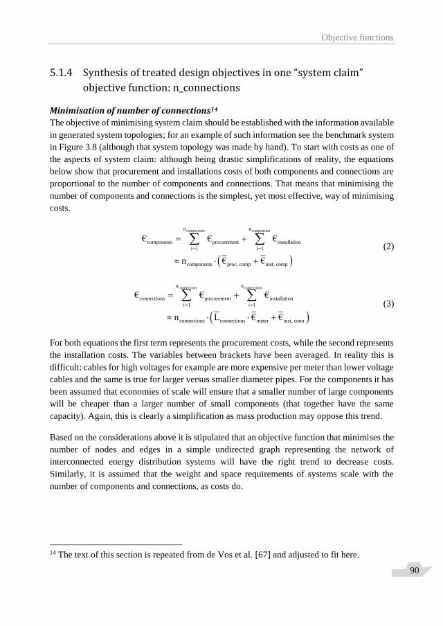
Objective functions
90
5.1.4 Synthesis of treated design objectives in one “system claim”
objective function: n_connections
Minimisation of number of connections14
The objective of minimising system claim should be established with the information available
in generated system topologies; for an example of such information see the benchmark system
in Figure 3.8 (although that system topology was made by hand). To start with costs as one of
the aspects of system claim: although being drastic simplifications of reality, the equations
below show that procurement and installations costs of both components and connections are
proportional to the number of components and connections. That means that minimising the
number of components and connections is the simplest, yet most effective, way of minimising
costs.
components componentsn n
components procurement installation
i 1 i 1
components proc, comp inst, comp
€ € €
n € €
(2)
connections connectionsn n
connections procurement installation
i 1 i 1
connections connections meter inst, conn
€ € €
n L € €
(3)
For both equations the first term represents the procurement costs, while the second represents
the installation costs. The variables between brackets have been averaged. In reality this is
difficult: cables for high voltages for example are more expensive per meter than lower voltage
cables and the same is true for larger versus smaller diameter pipes. For the components it has
been assumed that economies of scale will ensure that a smaller number of large components
will be cheaper than a larger number of small components (that together have the same
capacity). Again, this is clearly a simplification as mass production may oppose this trend.
Based on the considerations above it is stipulated that an objective function that minimises the
number of nodes and edges in a simple undirected graph representing the network of
interconnected energy distribution systems will have the right trend to decrease costs.
Similarly, it is assumed that the weight and space requirements of systems scale with the
number of components and connections, as costs do.
14 The text of this section is repeated from de Vos et al. [67] and adjusted to fit here.
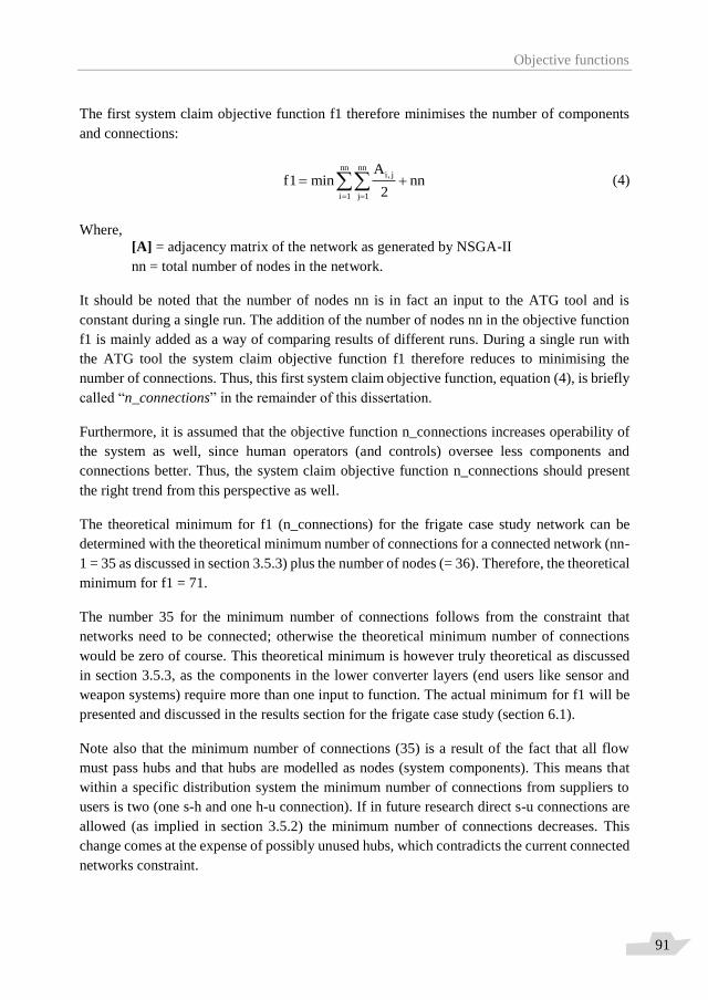
Objective functions
91
The first system claim objective function f1 therefore minimises the number of components
and connections:
nn nn
i, j
i 1 j 1
Af1 min nn
2
(4)
Where,
[A] = adjacency matrix of the network as generated by NSGA-II
nn = total number of nodes in the network.
It should be noted that the number of nodes nn is in fact an input to the ATG tool and is
constant during a single run. The addition of the number of nodes nn in the objective function
f1 is mainly added as a way of comparing results of different runs. During a single run with
the ATG tool the system claim objective function f1 therefore reduces to minimising the
number of connections. Thus, this first system claim objective function, equation (4), is briefly
called “n_connections” in the remainder of this dissertation.
Furthermore, it is assumed that the objective function n_connections increases operability of
the system as well, since human operators (and controls) oversee less components and
connections better. Thus, the system claim objective function n_connections should present
the right trend from this perspective as well.
The theoretical minimum for f1 (n_connections) for the frigate case study network can be
determined with the theoretical minimum number of connections for a connected network (nn-
1 = 35 as discussed in section 3.5.3) plus the number of nodes (= 36). Therefore, the theoretical
minimum for f1 = 71.
The number 35 for the minimum number of connections follows from the constraint that
networks need to be connected; otherwise the theoretical minimum number of connections
would be zero of course. This theoretical minimum is however truly theoretical as discussed
in section 3.5.3, as the components in the lower converter layers (end users like sensor and
weapon systems) require more than one input to function. The actual minimum for f1 will be
presented and discussed in the results section for the frigate case study (section 6.1).
Note also that the minimum number of connections (35) is a result of the fact that all flow
must pass hubs and that hubs are modelled as nodes (system components). This means that
within a specific distribution system the minimum number of connections from suppliers to
users is two (one s-h and one h-u connection). If in future research direct s-u connections are
allowed (as implied in section 3.5.2) the minimum number of connections decreases. This
change comes at the expense of possibly unused hubs, which contradicts the current connected
networks constraint.
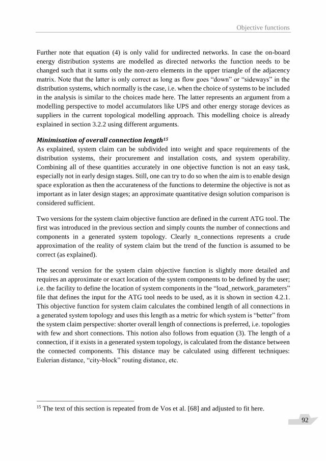
Objective functions
92
Further note that equation (4) is only valid for undirected networks. In case the on-board
energy distribution systems are modelled as directed networks the function needs to be
changed such that it sums only the non-zero elements in the upper triangle of the adjacency
matrix. Note that the latter is only correct as long as flow goes “down” or “sideways” in the
distribution systems, which normally is the case, i.e. when the choice of systems to be included
in the analysis is similar to the choices made here. The latter represents an argument from a
modelling perspective to model accumulators like UPS and other energy storage devices as
suppliers in the current topological modelling approach. This modelling choice is already
explained in section 3.2.2 using different arguments.
Minimisation of overall connection length15
As explained, system claim can be subdivided into weight and space requirements of the
distribution systems, their procurement and installation costs, and system operability.
Combining all of these quantities accurately in one objective function is not an easy task,
especially not in early design stages. Still, one can try to do so when the aim is to enable design
space exploration as then the accurateness of the functions to determine the objective is not as
important as in later design stages; an approximate quantitative design solution comparison is
considered sufficient.
Two versions for the system claim objective function are defined in the current ATG tool. The
first was introduced in the previous section and simply counts the number of connections and
components in a generated system topology. Clearly n_connections represents a crude
approximation of the reality of system claim but the trend of the function is assumed to be
correct (as explained).
The second version for the system claim objective function is slightly more detailed and
requires an approximate or exact location of the system components to be defined by the user;
i.e. the facility to define the location of system components in the “load_network_parameters”
file that defines the input for the ATG tool needs to be used, as it is shown in section 4.2.1.
This objective function for system claim calculates the combined length of all connections in
a generated system topology and uses this length as a metric for which system is “better” from
the system claim perspective: shorter overall length of connections is preferred, i.e. topologies
with few and short connections. This notion also follows from equation (3). The length of a
connection, if it exists in a generated system topology, is calculated from the distance between
the connected components. This distance may be calculated using different techniques:
Eulerian distance, “city-block” routing distance, etc.
15 The text of this section is repeated from de Vos et al. [68] and adjusted to fit here.
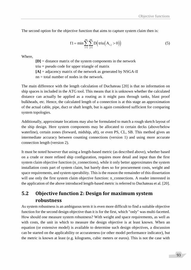
Objective functions
93
The second option for the objective function that aims to capture system claim then is:
nn nn
i, j
i 1 j 1
f1 min D triu A 0
(5)
Where,
[D] = distance matrix of the system components in the network
triu = pseudo code for upper triangle of matrix
[A] = adjacency matrix of the network as generated by NSGA-II
nn = total number of nodes in the network.
The main difference with the length calculation of Duchateau [20] is that no information on
ship spaces is included in the ATG tool. This means that it is unknown whether the calculated
distance can actually be applied as a routing as it might pass through tanks, blast proof
bulkheads, etc. Hence, the calculated length of a connection is at this stage an approximation
of the actual cable, pipe, duct or shaft length, but is again considered sufficient for comparing
system topologies.
Additionally, approximate locations may also be formulated to match a rough sketch layout of
the ship design. Here system components may be allocated to certain decks (above/below
waterline), certain zones (forward, midship, aft), or even PS, CL, SB. This method gives an
intermediate accuracy between counting connections (version 1) and using more accurate
connection length (version 2).
It must be noted however that using a length-based metric (as described above), whether based
on a crude or more refined ship configuration, requires more detail and input than the first
system claim objective function (n_connections), while it only better approximates the system
installation costs part of system claim, but barely does so for procurement costs, weight and
space requirements, and system operability. This is the reason the remainder of this dissertation
will use only the first system claim objective function: n_connections. A reader interested in
the application of the above introduced length-based metric is referred to Duchateau et al. [20].
5.2 Objective function 2: Design for maximum system
robustness As system robustness is an ambiguous term it is even more difficult to find a suitable objective
function for the second design objective than it is for the first, which "only" was multi-facetted.
How should one measure system robustness? With weight and space requirements, as well as
with costs, the unit in which to measure the design objective is at least known. When an
equation (or extensive model) is available to determine such design objectives, a discussion
can be started on the applicability or accurateness (or other model performance indicator), but
the metric is known at least (e.g. kilograms, cubic meters or euros). This is not the case with

Objective functions
94
system robustness as a clear definition and measurement unit is not available. Koç [35] even
states that different forms of robustness exist and that some of these forms may sometimes be
competing as well. Still, for the ATG tool a mathematical formulation of robustness is
required. A number of these formulations will be discussed in the following sections after
which a founded choice will be made for two final objective functions that best capture the
difficult concept of robustness within the context of this research.
5.2.1 Design for maximum robustness16 Both some practical measures to improve system robustness and a more theoretical
background of system robustness and related terms were discussed in section 2.3. It was shown
that system robustness is here considered to consist of both vulnerability and recoverability.
Vulnerability is related to the immediate damage that results from a disruption or hit (see
Figure 2.2). This is related to both the system topology and the power division over (possibly
segregated) suppliers. Recoverability covers the actions undertaken to mitigate the final
damage resulting from the hit. Such actions may be undertaken by an autonomous control
system that is designed to mitigate damage as fast as possible after a hit occurs, like DINCS:
see van Bodegraven et al. [7]. Alternatively, such actions are undertaken by the crew of the
ship by, for instance, (remotely) closing valves or opening switches. Either way it is clear that
re-configurability of systems, which is done by such actions, is a major part of system
robustness.
Most early system design studies that take robustness into account apply a rule-based
approach; ref. e.g. Streppel [63]. It is also possible to make use of templates, like Chalfant et
al. [13] have done. A different approach, very similar to the one taken here, was discussed by
van Oers et al. [44]. Indeed, this work includes both topological generation and routing of
connections through the ship (which makes application of length-based metrics possible).
However, the number and type of components used by van Oers et al. [44] are not
representative to on-board energy distribution systems, as they did not systematically
differentiate between nodes that solely have a distribution function (hubs) and those that do
not (converters). The omission of hubs in distribution systems occurs frequently in early-stage
ship design research that addresses vulnerability assessment. Omission of hubs in (some of
the) on-board distribution systems renders the results of such research less realistic and
applicable.
16 Part of the text in this section is repeated from de Vos et al. [67] and adjusted to fit here.
Objective functions
95
5.2.2 Design for maximum re-configurability17 It was argued in de Vos [67] that an attempt to increase system robustness in early system
design stages should focus on improving system re-configurability by increasing the number
of disjoint paths between hubs. The system robustness objective function presented in that
paper does so by maximising the flow in hub-hub sub-matrices of the generated adjacency
matrix, i.e. system topologies with more connections between hubs are preferred (remember
that for unweighted networks the maximum flow equals the number of edge-independent paths
– see section 3.7). Moreover, not only are more connections (in fact disjoint paths) between
hubs preferred, max-flow-between-hubs even prefers ring distributions (if sufficient hubs are
available to make rings) over other distribution patterns. In a practical setting such hub-hub
connections are bus-ties between switchboards, cross-connect gear transmissions, and
undirected “communication” pipe lines between main pipe lines in a fluid distribution system,
allowing reconfiguration of the system in case of system damage.
This “max-flow-between-hubs” objective function, which is defined and explained in section
5.2.5, is based on the observation that in design practice system robustness of on-board energy
distribution systems is increased by the practical measures mentioned in section 2.3. These
measures are repeated here for convenience:
A. Increasing redundancy by duplicating functionally similar components, either as full
back-up or with performance degradation, or by different type of components (similar
function, different working principle) such as accumulators,
B. Introducing separate “islands” in the system topology. The islands are able to operate
as stand-alone systems in critical operations (islands should then also be physically
separated; i.e. located in different zones in the ship separated by fire-resistant and
watertight bulkheads),
C. Increasing re-configurability of the distribution systems by increasing the number of
paths between suppliers and users. This is achieved by additional supply lines to vital
users and by interconnecting the afore-mentioned islands by so-called cross-overs.
The latter measure is the main reason for measuring system robustness by the potential flow
between hubs in the max-flow-between-hubs objective function. A consequence of choosing
this metric is that the other robustness measures that are mentioned above are not part of the
objective function and need to be introduced in the ATG tool in a different way. The number
and type of system components are input (as described in section 4.2.1), so the measures of
redundant components and (potential for) separate islands, i.e. sub-systems of suppliers, hubs
and users, are captured in the input of the ATG tool. The main (topological) measure that is
missed is increasing the number of direct supply lines to vital users. This is solved in the ATG
tool by specifying the required number of supply lines of a certain type of energy for a (vital)
17 The text of this section is repeated from de Vos et al. [68] and adjusted to fit here.
Objective functions
96
component in the input for the tool. Section 4.2.1 showed for instance that the vitality of each
required input flow for Sensor1 of the frigate case study system can be defined. Thus, if a vital
user requires 440 V the number of required 440 V supply lines for that user may be specified
as two in the vitality input value to ensure that two 440 V supply lines are provided. The
number of supply lines is, in other words, a “non-negotiable requirement” defined by the
system designer when max-flow-between-hubs is the applied system robustness objective
function (like the connectedness of the system, which also is in the repair function – see section
4.2.4). With the other “candidate” objective function for system robustness, as described in the
next section, the number of supply lines is not a “non-negotiable requirement” and the vitality
repair function should be “switched off”.
5.2.3 Design for minimum vulnerability18 An alternative robustness objective function, developed by van Leeuwen [39] and used by
Duchateau et al. [20], does not require the number of supply lines as input to the ATG tool.
This objective function is based on percolation theory; it employs a depth-first search of the
remaining system topology after one or more random hits take out nodes or edges to determine
whether “end users” are still connected to the required suppliers; i.e. whether a path exists
(then percolation is possible) between vital end users and components that generate their
required energy. As such the method is fundamentally different from the max-flow-between-
hubs objective function in that it is not a deterministic a-priori objective function but the a-
posteriori outcome of a (random) hit-based vulnerability analysis on the topological level. The
latter will be explained in section 5.2.6.
The method is called “vulnerability connectivity” by van Leeuwen [39], but mathematically
connectivity implies the number of disjoint paths between nodes, see section 3.7, while fully
disjoint paths may not be necessary to have flow between suppliers and vital users – this will
be elaborated in the next section. Furthermore, vulnerability is again an ambiguous term. One
could define vulnerability as the inverse of robustness, but that does not help much if
robustness is not well defined. More importantly vulnerability is here clearly not considered
to be exactly the inverse of robustness as robustness was stated to consist of both vulnerability
and recoverability (section 2.3). Therefore, the robustness objective function of van Leeuwen
[39] will here be called “hurt-state-percolation”. This function does require end users to be
defined that are considered to be vital and as such must remain operational even after damage
impairment to enable the ship to perform its mission. Note that, with regards to the required
input to the tool, the difference with the max-flow-between-hubs objective function is that one
or more components are declared vital and not the consequence of this declaration: an
increased number of supply lines. As a result, the ATG tool will determine itself which
topological robustness measure is preferred: adding redundancy in supply lines to vital users
18 The text of this section is repeated from de Vos et al. [68] and adjusted to fit here.

Objective functions
97
(A) or increasing overall system re-configurability by interconnecting hubs (C), when
generating system topologies with hurt-state-percolation as applied robustness objective
function (and n_connections as system claim objective function).
Arguably, the hurt-state-percolation objective function is more in line with the earlier specified
definition of system robustness and the given practical robustness measures than the max-
flow-between-hubs objective function. Furthermore, the function may fit better with the
explorative nature of early-stage system design and the evolutionary nature of the genetic
algorithm. Finally, the hurt-state-percolation function, being a topological vulnerability
analysis, can also be employed to establish the validity of earlier design choices or simpler
design tools like the max-flow-between-hubs function. A disadvantage is however the
increased computational time for assessing the robustness of a system topology as a
consequence of performing a random hit vulnerability analysis for each system topology
generated. This is further explained in section 5.2.6.
Regardless of one’s perception of the different robustness objective functions, it is interesting
to note that it was observed in van Leeuwen [39], that the ATG tool preferred system
topologies with redundant supply lines to vital users when hurt-state-percolation and
n_connections were the applied opposing objective functions. Increasing overall system re-
configurability with hub-hub connections was not used as a robustness measure. This begs the
question whether the max-flow-between-hubs robustness objective function “misses the point
completely” with its focus on hub-hub connections.
However, the number of specified vital end users was limited in van Leeuwen [39], which is
believed to be the reason that hurt-state-percolation (in combination with n_connections)
prefers redundancy in supply lines over hub-hub connections. It is hypothesised here that the
two robustness objective functions converge; i.e. show similar system topologies on the Pareto
front, when the number of vital end users is increased. To test this hypothesis both the max-
flow-between-hubs and the hurt-state-percolation robustness objective functions are used and
compared in a different case study than the frigate, namely an Ocean-going Patrol Vessel or
OPV. Results for this case study are presented in section 6.2.
5.2.4 Other robustness objective functions Several other robustness objective functions were developed and implemented in the ATG
tool:
1. Maximising the number of disjoint paths between suppliers and users
2. Maximising the number of connections between hubs (which does not
necessarily lead to disjoint paths between hubs, max-flow-between-hubs does)
3. Maximising the number of paths between suppliers and users by counting the
number of paths of a pre-defined range of lengths (length measured in number of
edges travelled; also known as number of hops)
Objective functions
98
4. Maximising edge betweenness (see section 3.7)
5. A more detailed metric based on hurt-state percolation but including capacity
calculations.
These five options will not be used as robustness objective functions in the case studies of
Chapter 6 though. This is for different reasons that will now be shortly discussed.
The first two options were discussed in de Vos et al. [67] and will be explained in more detail
in the next section as well, as their definition helps with understanding the max-flow-between-
hubs robustness objective function. They are however considered less applicable for
maximising the robustness of on-board distribution systems on basis of the preferred system
topologies. The first because it preferred “star-like” networks with many s-h and h-u
connections, but no h-h connections. The second did prefer h-h connections, but it did not
distinguish disjoint paths between hubs.
The third option was implemented in the ATG tool as well and is for the same reason
abandoned as for the first option, i.e. preferring “star-like” networks without hub-hub
connections. This is also the case for the fourth option, which was tried by van Leeuwen [39]
as an alternative to the already existing max-flow-between-hubs objective function. He
calculated and summed the betweenness centrality (not flow betweenness) of all node pairs
however in his objective function. A focus on hubs or hub layers may have been a better
approach. Therefore, edge betweenness as defined by van Leeuwen [39] is abandoned as a
system robustness objective function for now as well.
The last option is an interesting approach for future research; but has for now been placed
outside the scope of this research. The main difficulties one experiences if capacity
calculations become part of the problem are:
A load balance (see Appendix A for an example) is required for each specific
distribution system to determine the capacities of components in a nominal, intact
condition and other frequently occurring conditions before topology variation can be
executed.
A decision on total power division over the number and type of suppliers that are
chosen needs to be made – these choices may require detailed component
characteristics.
A rudimentary power management system needs to be defined and implemented in
the code in order to be able to calculate the remaining capacity after one or more
random hits occur.
The first issue is considered hard to automate as it requires detailed knowledge of the future
operations of the ship. The second issue is possibly better suited for an automated approach
(for instance with a similar design space exploration tool as the ATG tool), but represents a
Objective functions
99
different combinatorial problem as already indicated in section 1.2.2. This combinatorial
problem definitely requires the load balance to be solved beforehand, while the combinatorial
problem addressed in this research does not have that requirement. The third issue opens up
new questions about level and method of automation.
As a consequence of the considerations above, solving load balances is considered to be too
time-consuming and too detailed for early stage system design or design space exploration.
This is the reason also the fifth option of the list above is not applied as robustness objective
function in this dissertation. Note that the difficulties listed above provide a further foundation
for the choice to perform system analysis only on the first level, i.e. flow-type pairing, and not
on the second level, i.e. power balancing: see section 2.4.
Interesting research is being performed though with regards to the synthesis of network flow
(power) quantification and vulnerability assessment. The work of Robinson [52] for instance
does include power balancing as he performs “Architecture Flow Optimisation”, based on the
work of Trapp [65], to find optimal topologies in different operational and damaged modes.
Some of the robustness metrics proposed by Koç [35] includes quantification of network flow
as well. His work focusses on targeted attacks on land-based electric power transmission and
distribution systems – such targeted attacks are unlikely for distribution systems on board
ships.
Now return to the first four options for robustness objective functions, which were
implemented in the ATG tool but were not used in this research for the reasons mentioned
above. These functions can be characterised as connectivity-based robustness metrics. Other
research projects are currently being conducted to find more applicable connectivity-based
robustness metrics. Habben Jansen et al. [26] and Paparistodimou et al. [48] present interesting
new approaches to connectivity-based robustness assessment of on-board distribution systems
in early-stage design. Furthermore, Paparistodimou et al. [47] studied other, more theoretic
approaches to robustness assessment in a maritime context. They conclude however that “The
limitations in the network theory approach include the high level of abstraction and the
general assumption of equality among components, such as nodes, of a system network”. This
limitation was found in this research as well and led to the introduction of the node and edge
differentiation framework of section 3.2. The robustness objective functions introduced in the
next two sections are therefore based upon this framework.

Objective functions
100
5.2.5 Re-configurability objective function: max-flow-between-hubs19
Definition of max-flow-between-hubs objective function
The second objective function is harder to define as this objective function means to increase
system robustness. As discussed in the previous sections and section 2.3, many definitions and
mathematical formulations of system robustness are possible; these are either tailor-made to a
specific application and therefore not applicable to on-board energy distribution systems or
too general. Therefore, a tailor-made mathematical formulation of system robustness that is
based on the introduced node differentiation is used in this study, in spite of the warning of
Haimes [27] that robustness cannot be captured in a simple metric and the observation of
Sydney [64] that a dilemma exists concerning the level-of-detail of system robustness
assessment.
System robustness is in marine engineering practice often increased by increasing redundancy
and system re-configurability, as discussed in sections 2.3 and 5.2.2. An increase in
redundancy is typically established by duplicating similar components or installing different
types of machines/equipment with similar functionality. This method for system robustness
increase is outside the scope of the max-flow-between-hubs objective function as it will be
defined shortly. Our objective function f2 (f2 because it opposes the f1 objective function:
system claim) aims to increase system re-configurability.
Increasing re-configurability in energy distribution systems in essence means creating
different paths from suppliers to users. Doing so increases the chance that a path remains
available between suppliers and users that can be followed by an energy flow after a major
disruption has occurred. A first logical attempt for a system re-configurability objective
function then establishes disjoint paths between suppliers and users. Disjoint paths from
supplier i to user j means that whenever one path is unavailable, because a connection or in-
between component has failed or is damaged, a completely other path can be taken by the flow
from supplier i to user j. This new path avoids all edges that were on the previous path. One
of the first functions that was tried in this research did exactly that: it utilised the max flow
function in Matlab® between suppliers and users for each energy distribution system in the
network. Maximising flow in case of simple, undirected (and unweighted) graphs equals
increasing the number of edge-disjoint paths, since only completely edge-disjoint paths would
increase the maximum flow between suppliers and users (see section 3.7). This first approach
to system re-configurability worked well in the sense that it opposed the system claim objective
function n_connections (that minimises the number of connections) and indeed more robust
systems with more connections were found. The solutions were however not realistic, since
the ATG tool created mainly “star-like” distribution systems with e.g. every generator having
two or more connections to the main switchboards for the more robust systems. Although such
19 The text of this section is repeated from de Vos et al. [67] and adjusted to fit here.
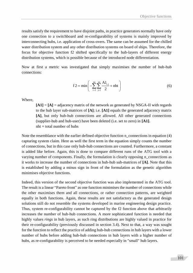
Objective functions
101
results satisfy the requirement to have disjoint paths, in practice generators normally have only
one connection to a switchboard and re-configurability of systems is mainly improved by
interconnecting hubs, i.e. application of cross-overs. The same can be assumed for the chilled
water distribution system and any other distribution systems on board of ships. Therefore, the
focus for objective function f2 shifted specifically to the hub-layers of different energy
distribution systems, which is possible because of the introduced node differentiation.
Now at first a metric was investigated that simply maximises the number of hub-hub
connections:
nn nn
i, j
i 1 j 1
A1f 2 min nht
2
(6)
Where,
[A1] = [A] = adjacency matrix of the network as generated by NSGA-II with regards
to the hub layer sub-matrices of [A]; i.e. [A1] equals the generated adjacency matrix
[A], but only hub-hub connections are allowed. All other generated connections
(supplier-hub and hub-user) have been deleted (i.e. set to zero) in [A1].
nht = total number of hubs
Note the resemblance with the earlier defined objective function n_connections in equation (4)
capturing system claim. Here as well the first term in the equation simply counts the number
of connections, but in this case only hub-hub connections are counted. Furthermore, a constant
is added like before. Again, this is done to compare different runs of the ATG tool with a
varying number of components. Finally, the formulation is clearly opposing n_connections as
it works to increase the number of connections in hub-hub sub-matrices of [A]. Note that this
is established by adding a minus sign in front of the formulation as the genetic algorithm
minimises objective functions.
Indeed, this version of the second objective function was also implemented in the ATG tool.
The result is a linear “Pareto front” as one function minimises the number of connections while
the other maximises them and all connections, or rather connection patterns, are weighted
equally in both functions. Again, these results are not satisfactory as the generated design
solutions still do not resemble the systems developed in marine engineering design practice.
Thus, system re-configurability cannot be captured by the f2 function above that arbitrarily
increases the number of hub-hub connections. A more sophisticated function is needed that
highly values rings in hub layers, as such ring distributions are highly valued in practice for
their re-configurability (previously discussed in section 3.4). Next to that, a way was sought
for the function to reflect the practice of adding hub-hub connections in hub layers with a lower
number of hubs before adding hub-hub connections in hub layers with a higher number of
hubs, as re-configurability is perceived to be needed especially in "small" hub layers.

Objective functions
102
Both conditions are met by the following function, which is the system re-configurability
objective function f2 that is developed and mainly used in this study:
i, j
nh nh
i, j
i 1 j 1
max flow A1 i, jA2
nh 1
A2
p hlnh nh 1
f 2 min p 100 nht nn 100
(7)
Where,
[A2] = max flow matrix
max flow = pseudo code for an algorithm that determines the max flow between node
pairs.
[A1] = [A] = adjacency matrix of the network as generated by NSGA-II with regards
to the hub layer sub-matrices of [A] (like in equation (6))
nh = number of hubs in a specific hub layer (3, 4 or 5 for the frigate case study system)
p = max flow vector
hl = hub layer index (1-4 for the frigate case study system)
f2 = system re-configurability objective function
nht = total number of hubs (15 for the frigate case study system)
nn = total number of nodes (36 for the frigate case study system)
This objective function maximises the flow between hubs and satisfies the conditions set
previously. It will be called max-flow-between-hubs from here onwards. Using the built-in
max flow function of Matlab® the number of disjoint paths between hubs is increased, which
means ring distributions indeed score better than any other distribution pattern between hubs
that has the same number of hubs and connections. An elaboration of the variables and
functionality of the equations in equation (7) will be given below.
Explanation of max-flow-between-hubs objective function
[A2] is a matrix with the same size as the adjacency matrix [A] of the network generated by
the genetic algorithm, but only elements that represent hub-hub connections may be non-zero
in [A2]. This is a result of [A1], in the top equation, being equal to the generated network [A],
but only with respect to hub layer sub-matrices. Other connections, i.e. supplier-hub and hub-
user connections, are set to zero in [A1]. This is necessary to avoid that disjoint paths between
hubs via suppliers or users, which may be present in [A], are also counted by the max flow
function. As an example, the tables below show why connections between hub layer 2 and
converter layer 2 of the frigate case study network are set to zero in [A1].

Objective functions
103
Connection [A]i,j [A1]i,j Max flow i-j
TF1–SWB1 1 1 2
TF1–SWB2 1 1 2
SWB1–SWB2 1 1 2
Table 5.1 Max flow values if [A1] equals [A].
Connection [A]i,j [A1]i,j Max flow i-j
TF1–SWB1 1 0 0
TF1–SWB2 1 0 0
SWB1–SWB2 1 1 1
Table 5.2 Max flow values if [A1] equals [A] only with regards to hub layer sub-matrices.
If transformer 1 (TF1) is connected to both SWB1 and SWB2 and these are connected to each
other as well, the connections make a ring and there are two disjoint paths from any node to
any other node. Note that the necessity of setting supplier-hub and hub-user connections to
zero is a consequence of the choice to model the networks as undirected graphs, with directed
graphs this would not have been the case.
Thus, only elements in hub layer sub-matrices can be non-zero in [A2]. They are non-zero if
the genetic algorithm generated one or more disjoint paths between different hub pairs in the
specific hub layers, since the max flow function applied to unweighted graphs counts disjoint
paths (again see section 3.7). Note that the potential non-zero elements in [A2] can have a
value between zero and one. This is a result of normalising the maximum flow between hub i
and j in the top equation with the maximum amount of connections a hub can have in a fully
connected hub layer (nh-1). As an example, consider a hub layer consisting of three hubs. Max
flow between hub i and j is two when there are two completely disjoint paths between hub i
and j. If the total number of hubs is indeed three, the maximum amount of connections for a
hub has been reached and [A2]i,j = 2/2 = 1. However, if there are four hubs [A2]i,j = 2/3. When
there are five hubs [A2]i,j = 2/4 and so on. The maximum flow between hubs is determined
using the built-in maxflow function in Matlab®. It uses the Boykov-Kolmogorov [8] algorithm
for determining the maximum flow between connected (hub) nodes in [A1].
Variable p in the second equation is a vector with a length of the number of hub layers (four
in the frigate case study network).
Element hl (hub layer) of vector p is the normalised double sum of hub layer sub-matrices in
the maximum flow matrix [A2]. The elements of p have a value between 0 and 1 because of

Objective functions
104
normalisation with the total number of hub-hub connections that can exist in a specific hub
layer (nh∙(nh-1)).
The total maximum flow in a hub layer is normalised in this way as the ATG tool would
otherwise prefer to add connections (in fact disjoint paths) in hub layers with a larger number
of hubs, since creating connections in a layer where many connections can be made results in
a larger maximum flow. The condition from engineering practice is however that hub layers
with less hubs are preferred, i.e. connections between hubs in smaller hub layers are more
important (or at least equally important) and should be made first. Once sufficient disjoint
paths in these layers are made it is also wise to add disjoint paths in hub layers with a larger
number of hubs in order to maximise overall system re-configurability. This trend is
established with the two normalisations in the top and middle equation and can be observed in
section 6.1, where generated design solutions on the Pareto front are presented. The Pareto
front itself will naturally also be shown and discussed in that section.
Finally, the last equation in equation (7) minimises the negative sum of vector p (in fact the
minimisation is done by the genetic algorithm) and together with the first two equations thus
maximises the maximum flow, i.e. the number of disjoint paths, in each hub layer. Again, a
constant is added to the objective function, like with the system claim objective function
n_connections and the previously introduced simple version of f2 (equation (6)). The constant
in this case is the hub density of the network as defined in de Vos [66], being the total number
of hubs (nht) divided by the total number of nodes (nn). The idea is that with a larger hub
density, re-configurability possibilities increase. Of course, there is a limit to this idea as a
network with a hub density of 1 consists of only hubs and has no practical meaning (there are
no suppliers or users of any kind). Here, like with n_connections, adding a constant is meant
for comparing results of different runs with the ATG tool (with a different number of nodes /
hubs). During a single run with the ATG tool the objective function max-flow-between-hubs
reduces to minimising the negative sum of p, capturing the design objective to maximise
system re-configurability.
This approach, i.e. max-flow-between-hubs, which increases the number of disjoint paths
between hubs, is considered a good indicator for maximising re-configurability of a network
with a fixed number of converters and hubs. The factor 100 in the bottom equation is there for
creating more “distance” between design solutions. This enhances the effectiveness of NSGA-
II but is not essential for the function to work. Furthermore, a percentage is mimicked with the
factor 100, with 100% representing fully connected hub layers. From the sum sign it should
be clear that f2 is not to be interpreted literally as a percentage. Note that the factor 100 is also
applied to the hub density in order to make it of the same order of magnitude as the first term
in the bottom equation.
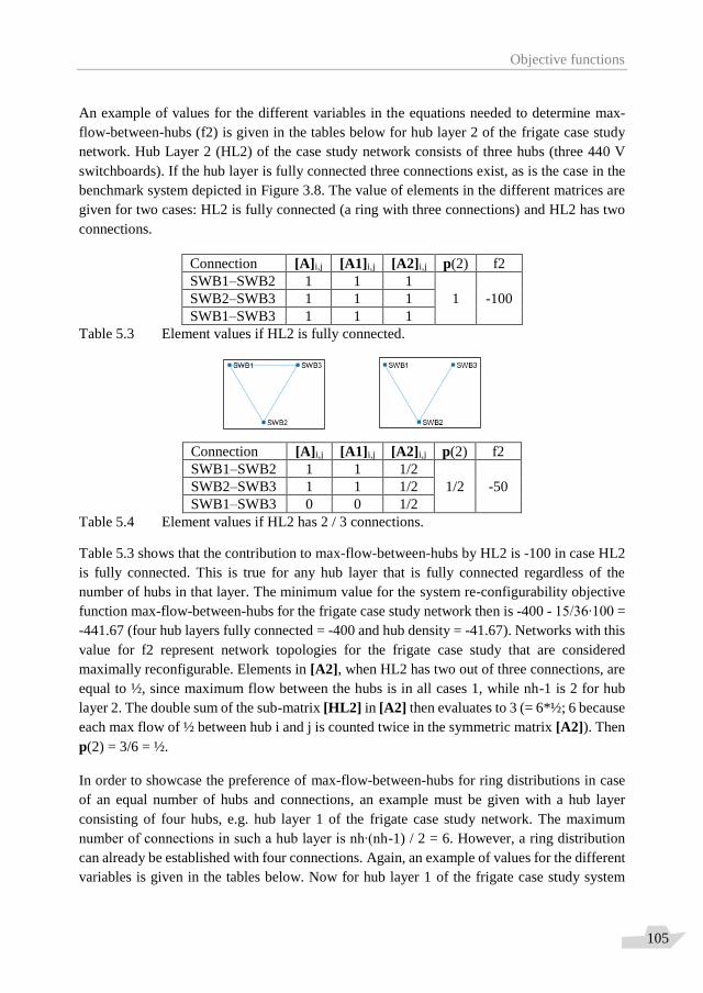
Objective functions
105
An example of values for the different variables in the equations needed to determine max-
flow-between-hubs (f2) is given in the tables below for hub layer 2 of the frigate case study
network. Hub Layer 2 (HL2) of the case study network consists of three hubs (three 440 V
switchboards). If the hub layer is fully connected three connections exist, as is the case in the
benchmark system depicted in Figure 3.8. The value of elements in the different matrices are
given for two cases: HL2 is fully connected (a ring with three connections) and HL2 has two
connections.
Connection [A]i,j [A1]i,j [A2]i,j p(2) f2
SWB1–SWB2 1 1 1
1 -100 SWB2–SWB3 1 1 1
SWB1–SWB3 1 1 1
Table 5.3 Element values if HL2 is fully connected.
Connection [A]i,j [A1]i,j [A2]i,j p(2) f2
SWB1–SWB2 1 1 1/2
1/2 -50 SWB2–SWB3 1 1 1/2
SWB1–SWB3 0 0 1/2
Table 5.4 Element values if HL2 has 2 / 3 connections.
Table 5.3 shows that the contribution to max-flow-between-hubs by HL2 is -100 in case HL2
is fully connected. This is true for any hub layer that is fully connected regardless of the
number of hubs in that layer. The minimum value for the system re-configurability objective
function max-flow-between-hubs for the frigate case study network then is -400 - 15/36∙100 =
-441.67 (four hub layers fully connected = -400 and hub density = -41.67). Networks with this
value for f2 represent network topologies for the frigate case study that are considered
maximally reconfigurable. Elements in [A2], when HL2 has two out of three connections, are
equal to ½, since maximum flow between the hubs is in all cases 1, while nh-1 is 2 for hub
layer 2. The double sum of the sub-matrix [HL2] in [A2] then evaluates to 3 (= 6*½; 6 because
each max flow of ½ between hub i and j is counted twice in the symmetric matrix [A2]). Then
p(2) = 3/6 = ½.
In order to showcase the preference of max-flow-between-hubs for ring distributions in case
of an equal number of hubs and connections, an example must be given with a hub layer
consisting of four hubs, e.g. hub layer 1 of the frigate case study network. The maximum
number of connections in such a hub layer is nh∙(nh-1) / 2 = 6. However, a ring distribution
can already be established with four connections. Again, an example of values for the different
variables is given in the tables below. Now for hub layer 1 of the frigate case study system
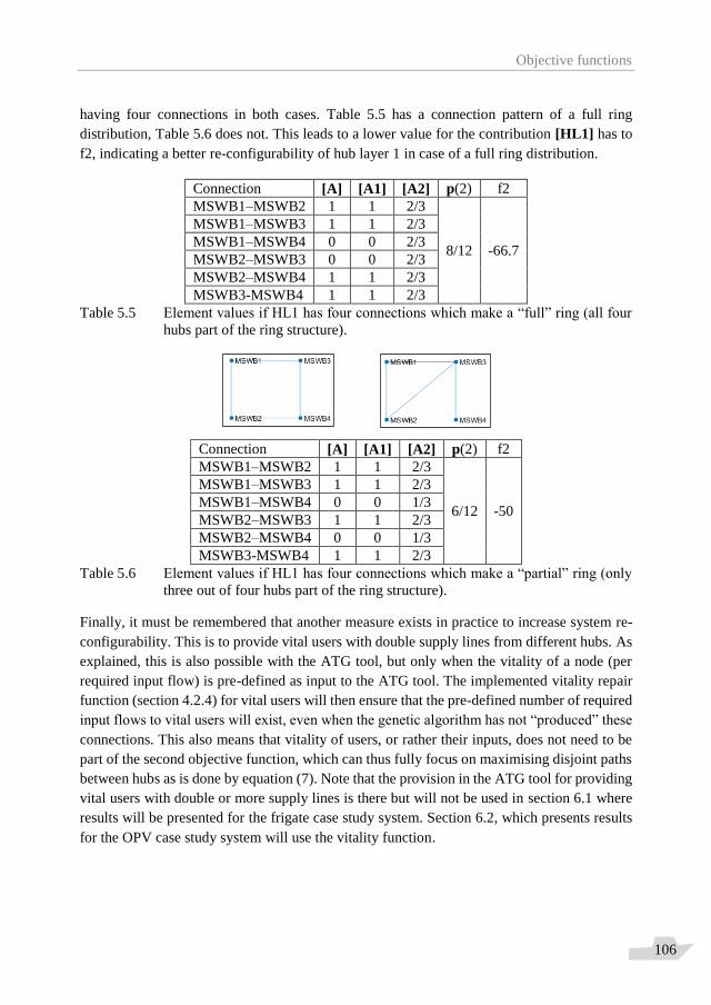
Objective functions
106
having four connections in both cases. Table 5.5 has a connection pattern of a full ring
distribution, Table 5.6 does not. This leads to a lower value for the contribution [HL1] has to
f2, indicating a better re-configurability of hub layer 1 in case of a full ring distribution.
Connection [A] [A1] [A2] p(2) f2
MSWB1–MSWB2 1 1 2/3
8/12 -66.7
MSWB1–MSWB3 1 1 2/3
MSWB1–MSWB4 0 0 2/3
MSWB2–MSWB3 0 0 2/3
MSWB2–MSWB4 1 1 2/3
MSWB3-MSWB4 1 1 2/3
Table 5.5 Element values if HL1 has four connections which make a “full” ring (all four
hubs part of the ring structure).
Connection [A] [A1] [A2] p(2) f2
MSWB1–MSWB2 1 1 2/3
6/12 -50
MSWB1–MSWB3 1 1 2/3
MSWB1–MSWB4 0 0 1/3
MSWB2–MSWB3 1 1 2/3
MSWB2–MSWB4 0 0 1/3
MSWB3-MSWB4 1 1 2/3
Table 5.6 Element values if HL1 has four connections which make a “partial” ring (only
three out of four hubs part of the ring structure).
Finally, it must be remembered that another measure exists in practice to increase system re-
configurability. This is to provide vital users with double supply lines from different hubs. As
explained, this is also possible with the ATG tool, but only when the vitality of a node (per
required input flow) is pre-defined as input to the ATG tool. The implemented vitality repair
function (section 4.2.4) for vital users will then ensure that the pre-defined number of required
input flows to vital users will exist, even when the genetic algorithm has not “produced” these
connections. This also means that vitality of users, or rather their inputs, does not need to be
part of the second objective function, which can thus fully focus on maximising disjoint paths
between hubs as is done by equation (7). Note that the provision in the ATG tool for providing
vital users with double or more supply lines is there but will not be used in section 6.1 where
results will be presented for the frigate case study system. Section 6.2, which presents results
for the OPV case study system will use the vitality function.

Objective functions
107
Verification of max-flow-between-hubs objective function
A verification of the max-flow-between-hubs objective function has been carried out for the
case of varying number of nodes; especially hubs. This verification can be better understood
after the presentation of results with a non-varying number of nodes and is therefore located
in section 6.3.
5.2.6 Vulnerability objective function: hurt-state-percolation For an elaborate explanation of the working principle of the hurt-state-percolation
vulnerability objective function reference is made to section 4.4 of van Leeuwen [39]. Here, a
short summary will be given.
After a topology is generated by NSGA-II, the hurt-state-percolation method first takes out
one or more nodes or edges to simulate a hit. When a hit has occurred a depth-first search is
undertaken that starts at the pre-defined vital end users and ends (if possible) with the required
suppliers for those users. For example, if Sensor1 in the frigate case study system is pre-
defined by the user of the ATG tool as being vital, hurt-state-percolation will assess whether
this vital user is connected to a supplier of 440 V and a supplier of 5 °C CW when a hit has
occurred, since these are the flow types that are required by Sensor1 in order to be able to fulfil
its function. Hurt-state-percolation for each and every topology that is generated by NSGA-II
and for every vital end user that is pre-defined to establish the probability that all pre-defined
vital end users receive the required supply. If one of the vital end users is not receiving one or
more of the required flow type(s) the system is considered to fail in the ability to fulfil its
function and thus considered infeasible and vulnerable. If all pre-defined vital users receive all
the flow types they require, the system is considered feasible and robust. The number of nodes
or edges that are hit is pre-defined by the user as well. Depending on this number either all
nodes and edges are hit one time and the hurt-state simulation is complete (when the number
of hits is low, e.g. 1 or 2), or a sample is taken of sufficient size to ensure a 95% accuracy of
the hurt-state simulation (when the number of hits is high, e.g. 3 or higher). It is probably clear
to the reader that if the pre-defined number of hits is high, the number of pre-defined vital
users is high and the number of generated system topologies is high, the ATG tool will require
some computational time to finish automated design space exploration.

Objective functions
108
5.3 Summary and conclusion This chapter discussed the objective functions of the ATG tool. Different options for the
opposing design objectives of system claim and system robustness were investigated and
discussed. Choices with regards to the level-of-detail of the objective functions and on which
concepts the objective functions should focus were introduced and the mathematical definition
of the functions were presented.
The combination of this chapter and the previous two chapters describes all relevant
information and elements of the ATG tool. Thus, it is now appropriate to start using the ATG
tool for exploring design spaces. The next chapter therefore presents the results of the ATG
tool and the lessons that can be learned from using it.
Results of Automatic Topology Generation tool
109
“The TV scientist who mutters sadly, "The experiment is a failure; we have failed to achieve
what we had hoped for," is suffering mainly from a bad script writer.”
― Robert M. Pirsig
Chapter 6 Results of Automatic Topology Generation
tool The ATG tool has been tested on its ability to explore design spaces using two case studies.
The first concerns the electric power and chilled water distribution systems on board a notional
frigate. The benchmark system, shown in Figure 3.8, is an example of a system topology that
could be generated in the first case study, meaning that the shown system components in Figure
3.8 are the same for all generated topologies; the connections may differ of course. Note that
the benchmark system itself was pre-defined by the author; its scores on the two objective
functions will also be presented in order to see “how well it does” and “where it is located in
the design space”. The intention of the first case study is mainly to find out how well the ATG
tool performs. Not necessarily as design space exploration tool, but rather what goes well and
what should the user keep in mind when using the tool. As such, the focus is more on the
relationship between its inner workings and the generated output and less on the output itself.
This is different for the second case study. In the second case study the ATG tool is truly used
as a design space exploration tool and the focus is more on what the user can learn from the
generated output. Does the tool indeed provide insight in how requirements, constraints,
technical design solutions and performance characteristics are related (which was mentioned
as the purpose of design space exploration in section 1.5)? Furthermore, the second case study
was used to compare the two different system robustness objective functions (max-flow-
between-hubs and hurt-state-percolation) when they are used in combination with the opposing
n_connections system claim objective function. It was hypothesised at the end of section 5.2.3
that the two robustness objective functions would converge; i.e. show similar system
topologies on the Pareto front, when the number of vital end users is increased. This hypothesis
is tested in second case study.
The second case study contains similar systems as the first, but the propulsion system will be
added as a vital distribution system as well. More importantly, the systems are on board of a
different kind of naval vessel, namely an Ocean-going Patrol Vessel. Typically, the
requirements with respect to system robustness (and thus ship survivability) are lower for such
an OPV than for a frigate. De Vos et al. [68] noted the following on the matter:
“An Ocean-going Patrol Vessel is a relatively large Patrol Vessel, or a relatively small warship,
that is typically designed for hostile environments that are considered to be “low in the
violence spectrum”. As such they are typically well equipped for anti-drugs and anti-piracy
Results of Automatic Topology Generation tool
110
missions and/or (sea) border control, but unfit for enemy engagement in an actual war. Still,
the lifetime of these vessels is such that one cannot assume that these ships will never see an
actual war environment. As a result, a fictional scenario in which the ship and its systems are
extensively re-designed and engineered for a more violent environment can be thought of. This
fictional scenario is the background of the present case study.”
Thus, the second case study focuses on vital distribution systems on board of an OPV and the
usefulness of the ATG tool as a design space exploration tool, while the first case study focuses
on vital distribution systems on board of a frigate and the performance of the ATG tool. The
results of the first case study were presented in de Vos et al. [67]. The results of the second
case study were presented in de Vos et al. [68]. The text and figures in sections 6.1 and 6.2 are
thus largely repeated from these papers.
The two case studies are considered relevant and contemporary; meaning they explore design
spaces that could be explored in current marine engineering practice using modern
technologies. The ATG tool allows for exploring design spaces with new, emerging
technologies as well, for instance alternative electric power distribution system topologies
using more extensive DC distribution to allow for large-scale electric energy storage or future
power sources, like fuel cells. The case studies were chosen to focus on contemporary
technologies in order to build confidence in the ATG tool by verifying it generates realistic
topologies. In future research the focus may turn to new, emerging technologies.
The final section of this chapter discusses verification of the two main objective functions in
this research: n_connections for system claim and max-flow-between-hubs for system
robustness. The verification can be better understood after the results of the two case studies
have been discussed, which is the reason for describing the verification in section 6.3.
6.1 Results for frigate case study20 In this section the results of the ATG tool will be limited to the frigate case study network for
which the benchmark system was presented in section 3.4. The present section consists of two
sub-sections: the first showing initial results of the ATG tool without and with the steering rule
as described in section 4.2.6. The main output of the ATG tool will be explained in this first
sub-section including details on computational time and a discussion on whether the results
are sufficiently satisfying. The second sub-section shows results when the starting point of the
ATG tool is set using “elite” design solutions. It will be shown that this way of steering can
effectively decrease computational time. However, doing so contradicts the underlying idea of
an evolutionary approach.
20 The text of this section is repeated from de Vos et al. [67] and adjusted to fit here.

Results of Automatic Topology Generation tool
111
6.1.1 Output of ATG tool without / with steering rule Figure 6.1 shows the results of a run of the ATG tool for the case study system with randomly
assigned connections as starting point, i.e. a random number generator fills in zeros or ones in
the “DNA”-vector x, containing the 172 potential connections of the frigate case study
network. The steering rule as described in section 4.2.6 is not yet applied during the run with
the ATG tool that resulted in Figure 6.1. This is only done for the run that resulted in Figure
6.2.
Settings for the NSGA-II genetic algorithm were for both runs such that 200 generations of
200 individuals (network topologies) were generated. For the first run, without the steering
rule, 79.23% of the generated 40000 networks is unique, i.e. 31692 networks are unique while
8308 network topologies are generated at least two times. For the second run, with the steering
rule, 89.05% is unique (i.e. 35620 networks). Note that these uniqueness values are here
presented for sake of completeness of information only. The uniqueness values differ per run
with the ATG tool as “production of individuals” in NSGA-II contains random events, like in
nature. One should be careful to interpret the uniqueness values as a performance parameter.
How well NSGA-II, or any other optimisation or evolutionary algorithm, is performing for a
specific problem statement is difficult issue that will not be addressed here.
Figure 6.1 Results of ATG tool for frigate case study network without steering rule.
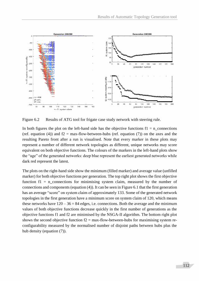
Results of Automatic Topology Generation tool
112
Figure 6.2 Results of ATG tool for frigate case study network with steering rule.
In both figures the plot on the left-hand side has the objective functions f1 = n_connections
(ref. equation (4)) and f2 = max-flow-between-hubs (ref. equation (7)) on the axes and the
resulting Pareto front after a run is visualised. Note that every marker in these plots may
represent a number of different network topologies as different, unique networks may score
equivalent on both objective functions. The colours of the markers in the left-hand plots show
the “age” of the generated networks: deep blue represent the earliest generated networks while
dark red represent the latest.
The plots on the right-hand side show the minimum (filled marker) and average value (unfilled
marker) for both objective functions per generation. The top right plot shows the first objective
function f1 = n_connections for minimising system claim, measured by the number of
connections and components (equation (4)). It can be seen in Figure 6.1 that the first generation
has an average “score” on system claim of approximately 133. Some of the generated network
topologies in the first generation have a minimum score on system claim of 120, which means
these networks have 120 – 36 = 84 edges, i.e. connections. Both the average and the minimum
values of both objective functions decrease quickly in the first number of generations as the
objective functions f1 and f2 are minimised by the NSGA-II algorithm. The bottom right plot
shows the second objective function f2 = max-flow-between-hubs for maximising system re-
configurability measured by the normalised number of disjoint paths between hubs plus the
hub density (equation (7)).
Results of Automatic Topology Generation tool
113
Clearly the system re-configurability objective function f2 decreases more quickly than the
system claim objective function f1 in Figure 6.1. The minimum value for f2, as introduced in
section 5.2.5, is -441.67 for the frigate case study network. This minimum value is found
quickly; already in generation 12. As the search proceeds, the average value for f2 lowers
towards this minimum value, indicating less and less variety in the generated solutions.
At the same time both the minimum and average value for f1 are decreasing as well, but
whether the true minimum is found is not yet clear. In fact, from the left-hand plot one can
already expect this is not the case: Is the found Pareto front complete? Or should the Pareto
front protrude further in to the upper left corner of the plot? One is left with the impression
that even fewer connections are possible, i.e. “cheaper, less bulky” network topologies with
less system claim, but the ATG tool apparently is unable to find these design solutions. For
that to happen, the genetic algorithm should increase the average of f2 again, i.e. delete hub-
hub connections, but it does not. Even when the settings for cross-over and mutation
probability are set to 100%, this does not occur. This problem with NSGA-II “preferring” one
of the objective functions was already discussed in section 4.2.6 and has now been clearly
shown.
Section 4.2.6 also stated that the steering rule, as introduced there, would increase the diversity
of solutions at the Pareto front. The validity of that statement can be concluded from the Pareto
front in Figure 6.2, which is “richer” than the Pareto front in Figure 6.1. Since the first
generations during the run with the ATG tool that resulted in Figure 6.2 contain only topologies
with more than 70 (= 2∙(nn-1)) connections (like before), the system re-configurability
objective function f2 evaluates to zero for these topologies according to the now applied
steering rule. This can be observed in both the left-hand plot and bottom right plot of Figure
6.2. Overwriting f2 values to zero in this way, in combination with the minimisation of f1,
steers NSGA-II quickly into the left-hand side of the design space, where the Pareto front is.
After eleven generations, the first topologies with less than 70 connections are found, as can
be seen in the top right plot (remember: 70 connections mean f1 = 70 + 36 = 106). This also
means the maximum system re-configurability (f2) that is found for this generation is less than
0, as can be seen in the bottom right plot. The average value for f2 then still is almost zero as
only very few topologies in the eleventh generation have less than 70 connections. This is
quickly solved in the next generations and NSGA-II really starts to explore the left-hand side
of the design space.
After 50 generations the minimum number of connections that is found is 45; see the top right
plot: f1 = 45 + 36 = 81. This clearly is a significantly lower number of connections than was
found to be the minimum during the first run that resulted in Figure 6.1. On top of that, this
minimum is found much sooner. This however still is not the absolute minimum for f1, as will
become clear in the next section.
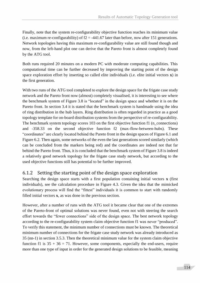
Results of Automatic Topology Generation tool
114
Finally, note that the system re-configurability objective function reaches its minimum value
(i.e. maximum re-configurability) of f2 = -441.67 later than before, now after 151 generations.
Network topologies having this maximum re-configurability value are still found though and
now, from the left-hand plot one can derive that the Pareto front is almost completely found
by the ATG tool.
Both runs required 20 minutes on a modern PC with moderate computing capabilities. This
computational time can be further decreased by improving the starting point of the design
space exploration effort by inserting so called elite individuals (i.e. elite initial vectors x) in
the first generation.
With two runs of the ATG tool completed to explore the design space for the frigate case study
network and the Pareto front now (almost) completely visualised, it is interesting to see where
the benchmark system of Figure 3.8 is “located” in the design space and whether it is on the
Pareto front. In section 3.4 it is stated that the benchmark system is handmade using the idea
of ring distribution in the hub layers. Ring distribution is often regarded in practice as a good
topology template for on-board distribution systems from the perspective of re-configurability.
The benchmark system topology scores 103 on the first objective function f1 (n_connections)
and -358.33 on the second objective function f2 (max-flow-between-hubs). These
“coordinates” are clearly located behind the Pareto front in the design spaces of Figure 6.1 and
Figure 6.2. Then again, some networks of the even the last generations scored similarly (which
can be concluded from the markers being red) and the coordinates are indeed not that far
behind the Pareto front. Thus, it is concluded that the benchmark system of Figure 3.8 is indeed
a relatively good network topology for the frigate case study network, but according to the
used objective functions still has potential to be further improved.
6.1.2 Setting the starting point of the design space exploration Searching the design space starts with a first population containing initial vectors x (first
individuals), see the calculation procedure in Figure 4.3. Given the idea that the mimicked
evolutionary process will find the “fittest” individuals it is common to start with randomly
filled initial vectors x, as was done in the previous section.
However, after a number of runs with the ATG tool it became clear that one of the extremes
of the Pareto-front of optimal solutions was never found, even not with steering the search
effort towards the “fewer connections” side of the design space. The best network topology
according to the re-configurability system claim objective function f1 was never “produced”.
To verify this statement, the minimum number of connections must be known. The theoretical
minimum number of connections for the frigate case study network was already introduced as
35 (nn-1) in section 3.5.3. Then the theoretical minimum value for the system claim objective
function f1 is 35 + 36 = 71. However, some components, especially the end-users, require
more than one type of input in order for the generated design solutions to be feasible, meaning
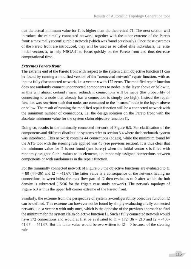
Results of Automatic Topology Generation tool
115
that the actual minimum value for f1 is higher than the theoretical 71. The next section will
introduce the minimally connected network, together with the other extreme of the Pareto
front: a maximally reconfigurable network (which was found previously). Once these extremes
of the Pareto front are introduced, they will be used as so called elite individuals, i.e. elite
initial vectors x, to help NSGA-II to focus quickly on the Pareto front and thus decrease
computational time.
Extremes Pareto front
The extreme end of the Pareto front with respect to the system claim objective function f1 can
be found by running a modified version of the “connected network” repair function, with as
input a fully disconnected network, i.e. a vector x with 172 zeros. The modified repair function
does not randomly connect unconnected components to nodes in the layer above or below it,
as this will almost certainly mean redundant connections will be made (the probability of
connecting to a node that already has a connection is simply too high). Instead the repair
function was rewritten such that nodes are connected to the “nearest” node in the layers above
or below. The result of running the modified repair function will be a connected network with
the minimum number of connections, i.e. the design solution on the Pareto front with the
absolute minimum value for the system claim objective function f1.
Doing so, results in the minimally connected network of Figure 6.3. For clarification of the
components and different distribution systems refer to section 3.4 where the benchmark system
was introduced. This network contains 44 connections (edges), while the minimum found by
the ATG tool with the steering rule applied was 45 (see previous section). It is thus clear that
the minimum value for f1 is not found (just barely) when the initial vector x is filled with
randomly assigned 0 or 1 values to its elements, i.e. randomly assigned connections between
components or with randomness in the repair function.
For the minimally connected network of Figure 6.3 the objective functions are evaluated to f1
= 80 (44+36) and f2 = -41.67. The latter value is a consequence of the network having no
connections between hubs; the max flow part of f2 then evaluates to 0 after which the hub
density is subtracted (15/36 for the frigate case study network). The network topology of
Figure 6.3 is thus the upper left corner extreme of the Pareto front.
Similarly, the extreme from the perspective of system re-configurability objective function f2
can be defined. This extreme can however not be found by simply evaluating a fully connected
network, i.e. a vector x with only ones, which is the opposite of the previous approach to find
the minimum for the system claim objective function f1. Such a fully connected network would
have 172 connections and would at first be evaluated to f1 = 172+36 = 210 and f2 = -400-
41.67 = -441.67. But the latter value would be overwritten to f2 = 0 because of the steering
rule.
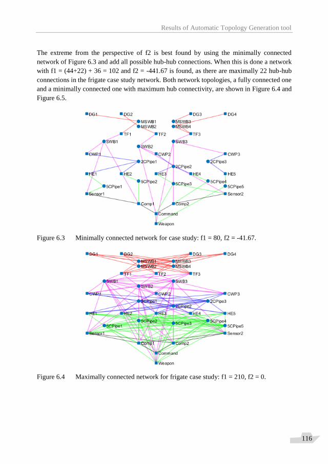
Results of Automatic Topology Generation tool
116
The extreme from the perspective of f2 is best found by using the minimally connected
network of Figure 6.3 and add all possible hub-hub connections. When this is done a network
with f1 = (44+22) + 36 = 102 and f2 = -441.67 is found, as there are maximally 22 hub-hub
connections in the frigate case study network. Both network topologies, a fully connected one
and a minimally connected one with maximum hub connectivity, are shown in Figure 6.4 and
Figure 6.5.
Figure 6.3 Minimally connected network for case study: f1 = 80, f2 = -41.67.
Figure 6.4 Maximally connected network for frigate case study: f1 = 210, f2 = 0.
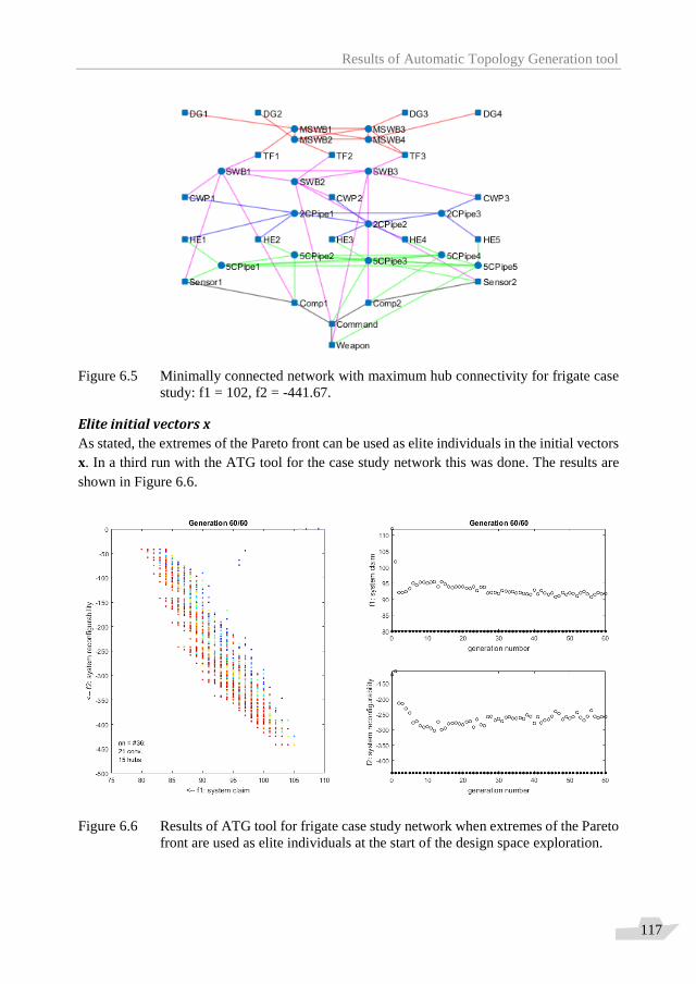
Results of Automatic Topology Generation tool
117
Figure 6.5 Minimally connected network with maximum hub connectivity for frigate case
study: f1 = 102, f2 = -441.67.
Elite initial vectors x
As stated, the extremes of the Pareto front can be used as elite individuals in the initial vectors
x. In a third run with the ATG tool for the case study network this was done. The results are
shown in Figure 6.6.
Figure 6.6 Results of ATG tool for frigate case study network when extremes of the Pareto
front are used as elite individuals at the start of the design space exploration.
Results of Automatic Topology Generation tool
118
It can be observed from the right-hand side plots that the ATG tool starts the design space
exploration with the minimum values for f1 and f2 already present in generation 1. With this
starting point NSGA-II can focus immediately on filling the Pareto front between these two
extremes. From the average values (unfilled markers) in the right-hand plots it is in fact clear
that after approximately ten generations the complete Pareto front is already found, as the
average values of scores on the two objective functions hardly varies after that.
Now only 3600 networks are generated (60∙60) in slightly more than two minutes time on the
same computer that was used for the generation of 40000 networks in Figure 6.1 and Figure
6.2. Of the 3600 networks 87.334% is unique (3144 networks); again this is only reported for
sake of completeness of information. It can be concluded, from comparing Figure 6.6 to Figure
6.2, that even though the scales of the plots are different, the shape and coordinates of the
Pareto front is equivalent for both runs, meaning that in both cases the ATG tool has succeeded
in finding all optimal design solutions according to the used objective functions:
n_connections representing system claim and max-flow-between-hubs representing system re-
configurability.
Finally, a number of different networks on the Pareto front, generated by the ATG tool, are
depicted below including information on their coordinates in Figure 6.6. Note that the Pareto
front is followed from top left corner to bottom right corner, i.e. from lowest number of
connections and least reconfigurable systems towards systems with maximum re-
configurability in the hub layers. It is clear the ATG tool is capable of automatically generating
interesting network topologies, i.e. system concept designs, for vital and interdependent on-
board energy distribution systems. Note that the interesting system concept designs do not
necessarily lie on the Pareto front; a system designer may find generated topologies behind the
front more interesting when having more (subjective) design requirements. That of course is
the essence of design space exploration.
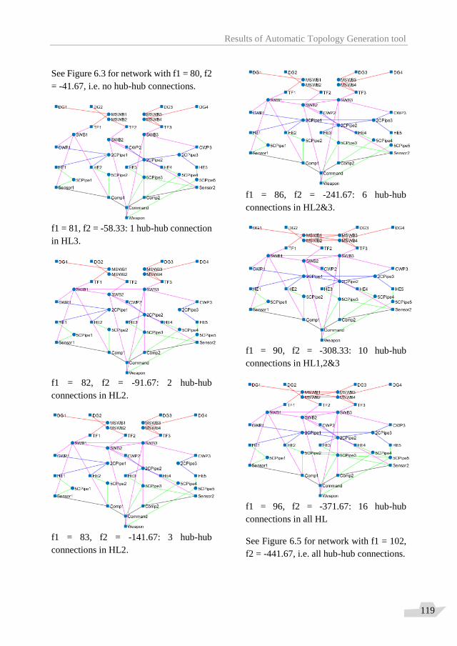
Results of Automatic Topology Generation tool
119
See Figure 6.3 for network with f1 = 80, f2
= -41.67, i.e. no hub-hub connections.
f1 = 81, f2 = -58.33: 1 hub-hub connection
in HL3.
f1 = 82, f2 = -91.67: 2 hub-hub
connections in HL2.
f1 = 83, f2 = -141.67: 3 hub-hub
connections in HL2.
f1 = 86, f2 = -241.67: 6 hub-hub
connections in HL2&3.
f1 = 90, f2 = -308.33: 10 hub-hub
connections in HL1,2&3
f1 = 96, f2 = -371.67: 16 hub-hub
connections in all HL
See Figure 6.5 for network with f1 = 102,
f2 = -441.67, i.e. all hub-hub connections.
Results of Automatic Topology Generation tool
120
6.1.3 Reflection on first case study21 The first case study presented in this section demonstrated that the ATG tool is able to
automatically generate a large number of network topologies for vital distribution systems on
board of a notional frigate. It also showed that the used Genetic Algorithm, NSGA-II, needed
help with finding the complete Pareto front. One way of doing so was by using a steering rule
that helped focussing on the more interesting part of the design space: the fewer connections
side. The other was by application of “elite individuals” in the initial generation.
The robustness objective function used in this first case study, max-flow-between-hubs, is
elaborately discussed in section 5.2.5. That section elaborated that the developed function
focusses on system reconfiguration possibilities and stated that the function is considered to
be relatively successful in doing so. Indeed, the author is convinced that the function follows
the right trend as long as the number of hubs (or nodes in general) is kept constant, like was
done for the frigate case study network. The applicability of the function is a consequence of
the efforts to make max-flow-between-hubs mimic practical design approaches.
However, it is also stressed that the max-flow-between-hubs objective function is not yet fully
successful in comparing systems completely in correspondence to how systems would be
valued in practice, when the number of nodes vary (in an early stage of system design). For
instance, Klein Woud and Stapersma [37] consider a zonal, ring distribution to be more robust
and reconfigurable than a ring distribution without zones. The presented max-flow-between-
hubs function is not capable to make this distinction.
Furthermore, verification attempts raise questions about the value of normalisation in the
equation for max-flow-between-hubs. As was discussed normalisation was implemented to
make sure that the ATG tool focusses on increasing reconfiguration in smaller hub layers first.
The verification attempts have however shown that this approach may backfire when systems
with different numbers of hubs are compared using max-flow-between-hubs. This issue is
addressed in section 6.3. A comparison between max-flow-between-hubs as robustness
objective function and hurt-state-percolation as introduced in section 5.2.6 would also help in
understanding the value of max-flow-between-hubs. This issue is addressed in section 6.2.
The first case study has shown that automatic topology generation is a valid approach to early
stage system design for on-board energy distribution systems, provided a certain amount of
practical engineering knowledge is brought into the picture. It enables analysis of a vast
amount of network topologies and provides a system designer with a way of comparing
different design solutions. This design space exploration approach is considered, at least
during very early stages of design, a better approach for selecting one or more concept designs
than many current rule-based approaches that narrow down the design space immediately to a
21 The text of this section is repeated from de Vos et al. [67] and adjusted to fit here.
Results of Automatic Topology Generation tool
121
very small number of concept designs. With such approaches a system designer is unaware of
and does not benefit from the design freedom that exists. For a more experienced system
designer the ATG tool can serve as an addition to current design methodologies to acquire,
perhaps unexpected, insights in the variety of different options and interaction between
requirements and design solutions.
One of the contributions of this case study is that it shows the difference between the
theoretical number of possible design solutions and the design freedom a system designer in
practice has concerning the topology of on-board energy distribution systems. This design
freedom is, even with the application of constraints, still very large, as has been shown. This
should be acknowledged by system designers and may serve as a reason to apply the here
presented methodology more often in practice, even if it is only done to realise how many
options are not considered with a rule-based approach.
6.2 Results for OPV case study systems22 This section will present the results for the OPV case study. System topologies will be
automatically generated for a number of vital distribution systems on board of an OPV, which
will help test the hypothesis (formulated in section 5.2.3) concerning the two system
robustness objective functions max-flow-between-hubs and hurt-state-percolation. Note that
the first system topologies that are shown in this section, i.e. Figure 6.7 and Figure 6.8, are
handmade and not generated by the ATG tool.
In Duchateau et al. [20] the OPV lay-out and a single network topology for a small number of
its “distributed ship service systems” is presented. This single network topology is
subsequently automatically routed many times over through spaces inside the ship’s envelope
using a k-shortest path algorithm. While doing so constraints coming from e.g. the type of
space and / or bulkhead location are taken into account. For each routing the hurt-state-
percolation objective function is used to determine the vulnerability of that routing to one or
more random hits. Repeating the process of routing and vulnerability assessment is achieved
by integrating the algorithms with NSGA-II “in an attempt to find a Pareto-set of solutions
minimising both overall routing configuration length and the distributed system vulnerability”
(Duchateau et al. [20]). The paper as such demonstrates the possibility to better incorporate
early-stage system design in early-stage ship design. However, automatic routing was done for
a single system concept design (a single network topology) in a single ship concept design (a
single lay-out of spaces). This may lead to sub-optimal solutions as a good routing will hardly
mitigate the flaws of sub-optimal system or ship concept designs.
22 The text of this section is repeated from de Vos et al. [68] and adjusted to fit here.
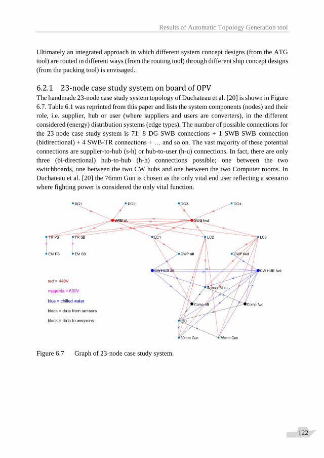
Results of Automatic Topology Generation tool
122
Ultimately an integrated approach in which different system concept designs (from the ATG
tool) are routed in different ways (from the routing tool) through different ship concept designs
(from the packing tool) is envisaged.
6.2.1 23-node case study system on board of OPV The handmade 23-node case study system topology of Duchateau et al. [20] is shown in Figure
6.7. Table 6.1 was reprinted from this paper and lists the system components (nodes) and their
role, i.e. supplier, hub or user (where suppliers and users are converters), in the different
considered (energy) distribution systems (edge types). The number of possible connections for
the 23-node case study system is 71: 8 DG-SWB connections + 1 SWB-SWB connection
(bidirectional) + 4 SWB-TR connections + … and so on. The vast majority of these potential
connections are supplier-to-hub (s-h) or hub-to-user (h-u) connections. In fact, there are only
three (bi-directional) hub-to-hub (h-h) connections possible; one between the two
switchboards, one between the two CW hubs and one between the two Computer rooms. In
Duchateau et al. [20] the 76mm Gun is chosen as the only vital end user reflecting a scenario
where fighting power is considered the only vital function.
Figure 6.7 Graph of 23-node case study system.
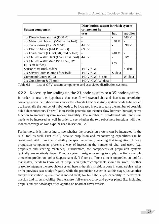
Results of Automatic Topology Generation tool
123
System component
Distribution system in which system
component is:
user hub supplier
4 x Diesel-Generator set (DG1-4) - - 440 V
2 x Main Switchboard (SWB aft & fwd) - 440 V -
2 x Transformer (TR PS & SB) 440 V - 690 V
2 x Electric Motor (EM PS & SB) 690 V
3 x Load Centre (LC1-3; aft, mid & fwd) - 440 V -
2 x Chilled Water Plant (CWP aft & fwd) 440 V - CW
2 x Chilled Water Main Pipe line (CW
HUB aft & fwd) - CW -
Sensor Mast (incl. radar) 440 V; CW - S_data
2 x Server Room (Comp aft & fwd) 440 V; CW S_data -
Command Centre (CIC) 440 V; CW; S_data - W_data
2 x Gun (30mm & 76mm) 440 V; CW; W_data - -
Table 6.1 List of OPV system components and associated distribution systems.
6.2.2 Necessity for scaling up the 23-node system to a 35-node system In order to test the hypothesis that max-flow-between-hubs and hurt-state-percolation
converge given the right circumstances the 23-node OPV case study system needs to be scaled
up. Especially the number of hubs needs to be increased in order to raise the number of possible
hub-hub connections. This will increase the potential for the max-flow-between-hubs objective
function to improve system re-configurability. The number of pre-defined vital end-users
needs to be increased as well in order to see whether the two robustness functions will then
indeed converge as was hypothesised in section 5.2.3.
Furthermore, it is interesting to see whether the propulsion system can be integrated in the
ATG tool as well. First of all, because propulsion and manoeuvring capabilities can be
considered vital from a survivability perspective as well, meaning that integration of more
propulsion components presents a way of increasing the number of vital end users (e.g.
propellers and steering machines). Furthermore, the components of propulsion systems
typically are relatively large. Thus, a system designer wanting to apply the first-principle
dimension prediction tool of Stapersma et al. [61] (or a different dimension prediction tool for
that matter) needs to know which propulsion system components should be sized. Another
reason to integrate the propulsion system here is that this is seldom done in comparable studies
or the previous case study (frigate), while the propulsion system is, at this stage, just another
energy distribution system that is indeed vital; for both the ship’s capability to perform its
mission and its survivability. Furthermore, full-electric or hybrid power plants (i.e. including
propulsion) are nowadays often applied on board of naval vessels.
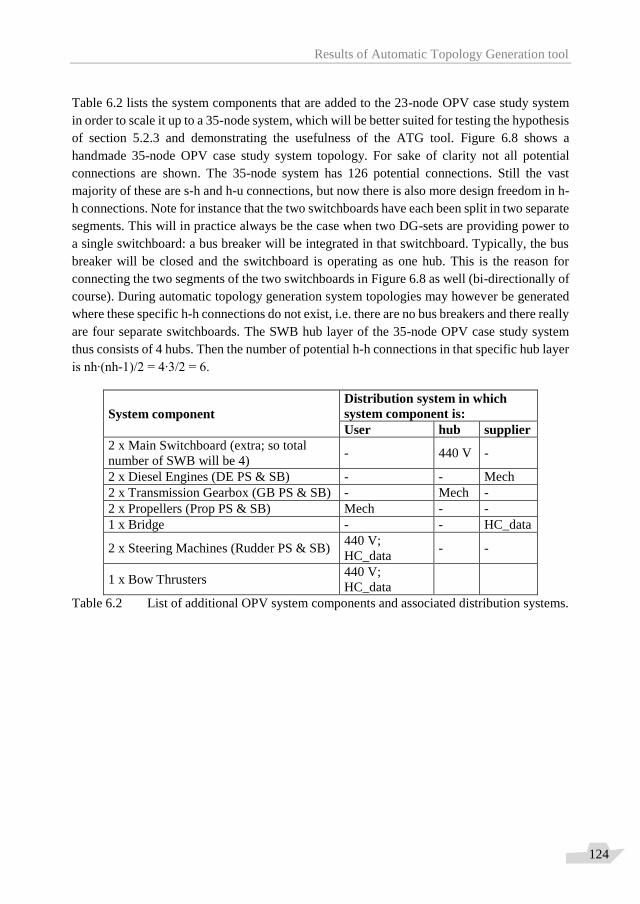
Results of Automatic Topology Generation tool
124
Table 6.2 lists the system components that are added to the 23-node OPV case study system
in order to scale it up to a 35-node system, which will be better suited for testing the hypothesis
of section 5.2.3 and demonstrating the usefulness of the ATG tool. Figure 6.8 shows a
handmade 35-node OPV case study system topology. For sake of clarity not all potential
connections are shown. The 35-node system has 126 potential connections. Still the vast
majority of these are s-h and h-u connections, but now there is also more design freedom in h-
h connections. Note for instance that the two switchboards have each been split in two separate
segments. This will in practice always be the case when two DG-sets are providing power to
a single switchboard: a bus breaker will be integrated in that switchboard. Typically, the bus
breaker will be closed and the switchboard is operating as one hub. This is the reason for
connecting the two segments of the two switchboards in Figure 6.8 as well (bi-directionally of
course). During automatic topology generation system topologies may however be generated
where these specific h-h connections do not exist, i.e. there are no bus breakers and there really
are four separate switchboards. The SWB hub layer of the 35-node OPV case study system
thus consists of 4 hubs. Then the number of potential h-h connections in that specific hub layer
is nh∙(nh-1)/2 = 4∙3/2 = 6.
System component
Distribution system in which
system component is:
User hub supplier
2 x Main Switchboard (extra; so total
number of SWB will be 4) - 440 V -
2 x Diesel Engines (DE PS & SB) - - Mech
2 x Transmission Gearbox (GB PS & SB) - Mech -
2 x Propellers (Prop PS & SB) Mech - -
1 x Bridge - - HC_data
2 x Steering Machines (Rudder PS & SB) 440 V;
HC_data - -
1 x Bow Thrusters 440 V;
HC_data
Table 6.2 List of additional OPV system components and associated distribution systems.

Results of Automatic Topology Generation tool
125
Figure 6.8 Graph of 35-node OPV case study system. Note the added propulsion system
components, shaft connections (green), rudders and bow thruster.
It can be seen that the propulsion system is indeed added more elaborately in the 35-node OPV
case study system (hybrid or CODELAD concept), including the steering machines (rudders).
Both the rudders and the propellers will be defined as vital users, but redundant supply lines
for the propellers implies each propeller being driven by two shafts, which is impractical to
say the least. The redundant supply with the propulsion diesel engines as driving machines
next to the electric motors of course is the crux of hybrid propulsion. Note that the propulsion
diesel engines (same as the diesel generators) are “stand-alone” in the sense that their fuel
supply and cooling water & lube oil systems are omitted here. Further, the ATG tool will
confront a system designer with an important question concerning the mechanical power
distribution system, as it may generate system topologies where the gearboxes are connected
by a cross-connect transmission. After all, to the tool these are just hubs (in a mechanical
power distribution system). This will be shown in the next section, where system topologies
are automatically generated for both the 23-node and 35-node OPV case study systems.
6.2.3 Automatic Topology Generation for OPV case study systems Based on the previous sections and recommendations of the other, related publications; van
Leeuwen [39], Duchateau [20] and de Vos [67], the following questions are raised with respect
to automatic topology generation for the OPV case study systems:
1. How do the two robustness objective functions (max-flow-between-hubs and hurt-
state-percolation) perform in terms of finding realistic system concept designs, i.e.
which is most suited to the design problem at hand? Do the metrics indeed converge
when the number of end users is increased?

Results of Automatic Topology Generation tool
126
2. Does the ATG tool succeed in supporting a system designer who aims to find system
design requirements and promising system concept designs?
These questions are the main focus of this section in which the results of the ATG tool for the
OPV case study are presented and analysed.
ATG for 23-node OPV case study system
The plots in Figure 6.9 show two generated design spaces and Pareto fronts for two runs with
the ATG tool for the 23-node case study system: one with max-flow-between-hubs (left) and
one with hurt-state-percolation (right) as robustness objective function (on the y-axis). The
system claim objective function is in both cases n_connections (on the x-axis), to which a
constant number of components (23 in this case) is added.
Max-flow-between-hubs is a normalised function with respect to the maximum flow that could
occur per hub layer (multiplied by 100 per hub layer to mimic a percentage). A constant “hub
density” multiplied by 100 is added. The mathematical function and algorithm itself is not very
difficult, but the explanation and interpretation of the values is. A reader wishing to understand
the function and its output is referred to section 5.2.5. The output of the function is made
negative as NSGA-II minimises objective functions, while the idea behind the max-flow-
between-hubs objective function is that flow between hubs is maximised.
Hurt-state-percolation calculates the chance that a number of vital end users do not receive the
energy (or other supply) they require for operation, given a generated system topology and a
pre-defined number of random hits. Note that the values on the y-axis can then best be
interpreted as: the chance that energy cannot flow (percolate) towards pre-defined vital end
users when the system is hit. An elaborate explanation of this function can be found in van
Leeuwen [39].
Focussing on the “Pareto front” of the left-hand plot it is clear that there are only four “optimal”
system topologies when max-flow-between-hubs is the applied system robustness objective
function. All other generated system topologies score equal on max-flow-between-hubs but
have more connections as can be seen from the “design space”. Note that every marker may
represent multiple unique system topologies as different topologies may score equal on both
objective functions. The difference in such a case is then in the supplier-hub (s-h) or hub-user
(h-u) connections.
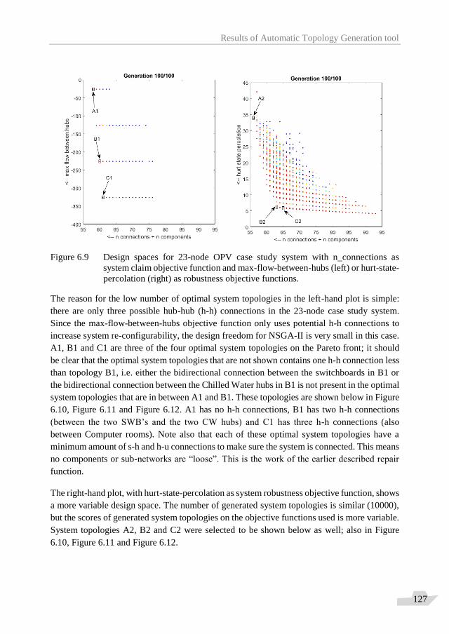
Results of Automatic Topology Generation tool
127
Figure 6.9 Design spaces for 23-node OPV case study system with n_connections as
system claim objective function and max-flow-between-hubs (left) or hurt-state-
percolation (right) as robustness objective functions.
The reason for the low number of optimal system topologies in the left-hand plot is simple:
there are only three possible hub-hub (h-h) connections in the 23-node case study system.
Since the max-flow-between-hubs objective function only uses potential h-h connections to
increase system re-configurability, the design freedom for NSGA-II is very small in this case.
A1, B1 and C1 are three of the four optimal system topologies on the Pareto front; it should
be clear that the optimal system topologies that are not shown contains one h-h connection less
than topology B1, i.e. either the bidirectional connection between the switchboards in B1 or
the bidirectional connection between the Chilled Water hubs in B1 is not present in the optimal
system topologies that are in between A1 and B1. These topologies are shown below in Figure
6.10, Figure 6.11 and Figure 6.12. A1 has no h-h connections, B1 has two h-h connections
(between the two SWB’s and the two CW hubs) and C1 has three h-h connections (also
between Computer rooms). Note also that each of these optimal system topologies have a
minimum amount of s-h and h-u connections to make sure the system is connected. This means
no components or sub-networks are “loose”. This is the work of the earlier described repair
function.
The right-hand plot, with hurt-state-percolation as system robustness objective function, shows
a more variable design space. The number of generated system topologies is similar (10000),
but the scores of generated system topologies on the objective functions used is more variable.
System topologies A2, B2 and C2 were selected to be shown below as well; also in Figure
6.10, Figure 6.11 and Figure 6.12.
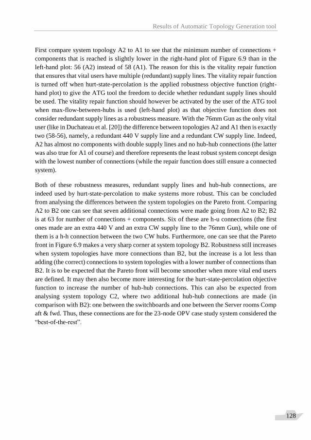
Results of Automatic Topology Generation tool
128
First compare system topology A2 to A1 to see that the minimum number of connections +
components that is reached is slightly lower in the right-hand plot of Figure 6.9 than in the
left-hand plot: 56 (A2) instead of 58 (A1). The reason for this is the vitality repair function
that ensures that vital users have multiple (redundant) supply lines. The vitality repair function
is turned off when hurt-state-percolation is the applied robustness objective function (right-
hand plot) to give the ATG tool the freedom to decide whether redundant supply lines should
be used. The vitality repair function should however be activated by the user of the ATG tool
when max-flow-between-hubs is used (left-hand plot) as that objective function does not
consider redundant supply lines as a robustness measure. With the 76mm Gun as the only vital
user (like in Duchateau et al. [20]) the difference between topologies A2 and A1 then is exactly
two (58-56), namely, a redundant 440 V supply line and a redundant CW supply line. Indeed,
A2 has almost no components with double supply lines and no hub-hub connections (the latter
was also true for A1 of course) and therefore represents the least robust system concept design
with the lowest number of connections (while the repair function does still ensure a connected
system).
Both of these robustness measures, redundant supply lines and hub-hub connections, are
indeed used by hurt-state-percolation to make systems more robust. This can be concluded
from analysing the differences between the system topologies on the Pareto front. Comparing
A2 to B2 one can see that seven additional connections were made going from A2 to B2; B2
is at 63 for number of connections + components. Six of these are h-u connections (the first
ones made are an extra 440 V and an extra CW supply line to the 76mm Gun), while one of
them is a h-h connection between the two CW hubs. Furthermore, one can see that the Pareto
front in Figure 6.9 makes a very sharp corner at system topology B2. Robustness still increases
when system topologies have more connections than B2, but the increase is a lot less than
adding (the correct) connections to system topologies with a lower number of connections than
B2. It is to be expected that the Pareto front will become smoother when more vital end users
are defined. It may then also become more interesting for the hurt-state-percolation objective
function to increase the number of hub-hub connections. This can also be expected from
analysing system topology C2, where two additional hub-hub connections are made (in
comparison with B2): one between the switchboards and one between the Server rooms Comp
aft & fwd. Thus, these connections are for the 23-node OPV case study system considered the
“best-of-the-rest”.
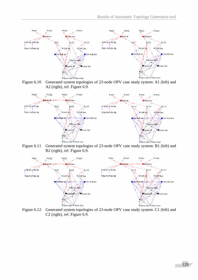
Results of Automatic Topology Generation tool
129
Figure 6.10 Generated system topologies of 23-node OPV case study system: A1 (left) and
A2 (right), ref. Figure 6.9.
Figure 6.11 Generated system topologies of 23-node OPV case study system: B1 (left) and
B2 (right), ref. Figure 6.9.
Figure 6.12 Generated system topologies of 23-node OPV case study system: C1 (left) and
C2 (right), ref. Figure 6.9.
Results of Automatic Topology Generation tool
130
ATG for 35-node OPV case study system
For the 35-node OPV case study system the variety in system topologies increases compared
to the 23-node case study system; see Figure 6.13. The left-hand plot shows that with the 35-
node case study system the design freedom has now also increased for the max-flow-between-
hubs robustness objective function. The freedom and resulting variety in developed system
topologies remains however inherently lower than for the hurt-state-percolation robustness
function as more constraints are applied and the focus remains limited to hub-hub connections
(remember the explanation of the vitality repair function in section 4.2.4). Note that the
maximum value of the y-axis has increased with 100; this is a consequence of a new hub layer
being part of the system: the mechanical hubs (better known as gearboxes). Their contribution
to the increased design freedom is limited however, since there are only two gearboxes and
the only option for max-flow-between-hubs is to add a bi-directional connection between the
gearboxes or not. Nevertheless, confronting a system designer with the option of having such
a “cross-connect” transmission to increase system re-configurability fits well with the intention
of the ATG tool.
The real increase in design freedom is caused by the increase in number of hubs in the 440 V
hub layer. There are now four hubs, which means there is now a possibility that generated
system topologies have ring distributions in that hub layer. The max-flow-between-hubs
objective function is designed to value such topologies and indeed system topology D1 (see
below) has a full ring in the 440 V hub layer. The only topologies that outperform D1 according
to max-flow-between-hubs have the same full ring + additional connections between the hubs
in the ring. Note that this in fact just increases the number of rings present in the 440 V hub
layer as can be seen from topology E1.
The Pareto front in the right-hand plot in Figure 6.13 is much smoother than in Figure 6.9, as
was expected. Note that for this run with hurt-state-percolation as robustness objective
function nine vital end users were specified: the 76mm Gun, 30mm Gun, CIC, Sensor Mast,
Bridge, both propellers and both steering machines (rudders). System topologies with hub-hub
connections start to appear more frequently in the left (steep) end of the Pareto front in this
case. One should however be careful to conclude that this is because hub-hub connections are
now in general valued by hurt-state-percolation. It is also possible that the ATG tool is
unsuccessful in finding approximately equally robust topologies with less (hub-hub)
connections as the optimisation with NSGA-II may not be perfect.
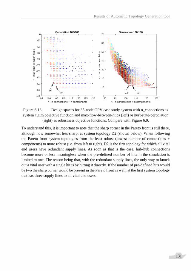
Results of Automatic Topology Generation tool
131
Figure 6.13 Design spaces for 35-node OPV case study system with n_connections as
system claim objective function and max-flow-between-hubs (left) or hurt-state-percolation
(right) as robustness objective functions. Compare with Figure 6.9.
To understand this, it is important to note that the sharp corner in the Pareto front is still there,
although now somewhat less sharp, at system topology D2 (shown below). When following
the Pareto front system topologies from the least robust (lowest number of connections +
components) to more robust (i.e. from left to right), D2 is the first topology for which all vital
end users have redundant supply lines. As soon as that is the case, hub-hub connections
become more or less meaningless when the pre-defined number of hits in the simulation is
limited to one. The reason being that, with the redundant supply lines, the only way to knock
out a vital user with a single hit is by hitting it directly. If the number of pre-defined hits would
be two the sharp corner would be present in the Pareto front as well: at the first system topology
that has three supply lines to all vital end users.

Results of Automatic Topology Generation tool
132
Figure 6.14 Generated system topology of 35-node OPV system: D1, ref. Figure 6.13.
Figure 6.15 Generated system topology of 35-node OPV system: D2, ref. Figure 6.13.
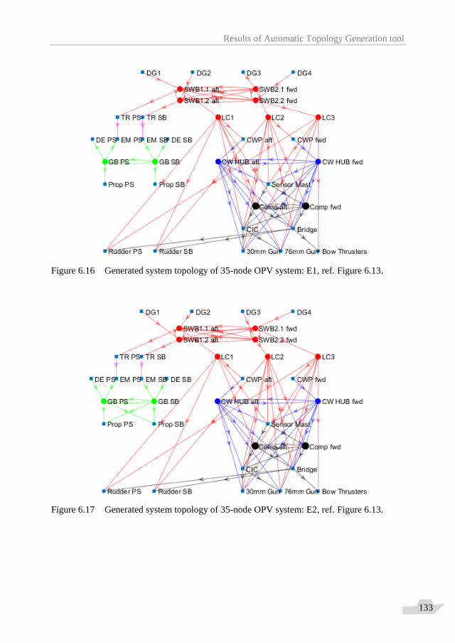
Results of Automatic Topology Generation tool
133
Figure 6.16 Generated system topology of 35-node OPV system: E1, ref. Figure 6.13.
Figure 6.17 Generated system topology of 35-node OPV system: E2, ref. Figure 6.13.
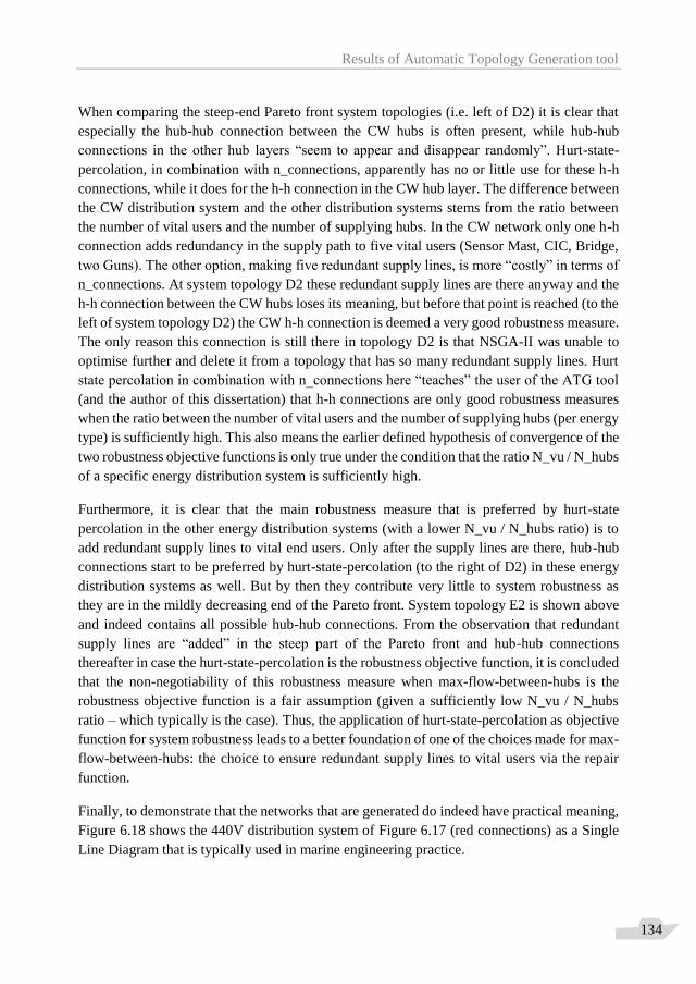
Results of Automatic Topology Generation tool
134
When comparing the steep-end Pareto front system topologies (i.e. left of D2) it is clear that
especially the hub-hub connection between the CW hubs is often present, while hub-hub
connections in the other hub layers “seem to appear and disappear randomly”. Hurt-state-
percolation, in combination with n_connections, apparently has no or little use for these h-h
connections, while it does for the h-h connection in the CW hub layer. The difference between
the CW distribution system and the other distribution systems stems from the ratio between
the number of vital users and the number of supplying hubs. In the CW network only one h-h
connection adds redundancy in the supply path to five vital users (Sensor Mast, CIC, Bridge,
two Guns). The other option, making five redundant supply lines, is more “costly” in terms of
n_connections. At system topology D2 these redundant supply lines are there anyway and the
h-h connection between the CW hubs loses its meaning, but before that point is reached (to the
left of system topology D2) the CW h-h connection is deemed a very good robustness measure.
The only reason this connection is still there in topology D2 is that NSGA-II was unable to
optimise further and delete it from a topology that has so many redundant supply lines. Hurt
state percolation in combination with n_connections here “teaches” the user of the ATG tool
(and the author of this dissertation) that h-h connections are only good robustness measures
when the ratio between the number of vital users and the number of supplying hubs (per energy
type) is sufficiently high. This also means the earlier defined hypothesis of convergence of the
two robustness objective functions is only true under the condition that the ratio N_vu / N_hubs
of a specific energy distribution system is sufficiently high.
Furthermore, it is clear that the main robustness measure that is preferred by hurt-state
percolation in the other energy distribution systems (with a lower N_vu / N_hubs ratio) is to
add redundant supply lines to vital end users. Only after the supply lines are there, hub-hub
connections start to be preferred by hurt-state-percolation (to the right of D2) in these energy
distribution systems as well. But by then they contribute very little to system robustness as
they are in the mildly decreasing end of the Pareto front. System topology E2 is shown above
and indeed contains all possible hub-hub connections. From the observation that redundant
supply lines are “added” in the steep part of the Pareto front and hub-hub connections
thereafter in case the hurt-state-percolation is the robustness objective function, it is concluded
that the non-negotiability of this robustness measure when max-flow-between-hubs is the
robustness objective function is a fair assumption (given a sufficiently low N_vu / N_hubs
ratio – which typically is the case). Thus, the application of hurt-state-percolation as objective
function for system robustness leads to a better foundation of one of the choices made for max-
flow-between-hubs: the choice to ensure redundant supply lines to vital users via the repair
function.
Finally, to demonstrate that the networks that are generated do indeed have practical meaning,
Figure 6.18 shows the 440V distribution system of Figure 6.17 (red connections) as a Single
Line Diagram that is typically used in marine engineering practice.
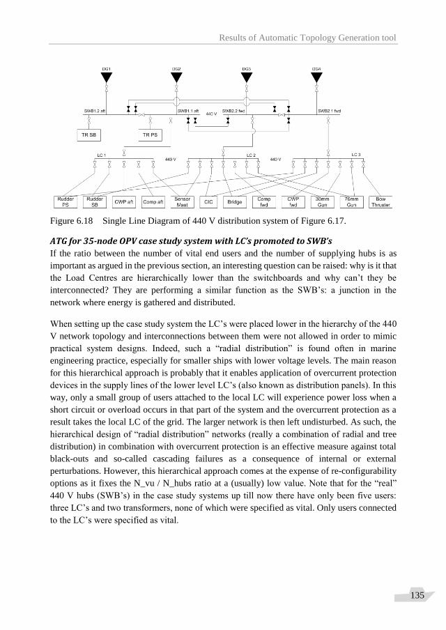
Results of Automatic Topology Generation tool
135
Figure 6.18 Single Line Diagram of 440 V distribution system of Figure 6.17.
ATG for 35-node OPV case study system with LC’s promoted to SWB’s
If the ratio between the number of vital end users and the number of supplying hubs is as
important as argued in the previous section, an interesting question can be raised: why is it that
the Load Centres are hierarchically lower than the switchboards and why can’t they be
interconnected? They are performing a similar function as the SWB’s: a junction in the
network where energy is gathered and distributed.
When setting up the case study system the LC’s were placed lower in the hierarchy of the 440
V network topology and interconnections between them were not allowed in order to mimic
practical system designs. Indeed, such a “radial distribution” is found often in marine
engineering practice, especially for smaller ships with lower voltage levels. The main reason
for this hierarchical approach is probably that it enables application of overcurrent protection
devices in the supply lines of the lower level LC’s (also known as distribution panels). In this
way, only a small group of users attached to the local LC will experience power loss when a
short circuit or overload occurs in that part of the system and the overcurrent protection as a
result takes the local LC of the grid. The larger network is then left undisturbed. As such, the
hierarchical design of “radial distribution” networks (really a combination of radial and tree
distribution) in combination with overcurrent protection is an effective measure against total
black-outs and so-called cascading failures as a consequence of internal or external
perturbations. However, this hierarchical approach comes at the expense of re-configurability
options as it fixes the N_vu / N_hubs ratio at a (usually) low value. Note that for the “real”
440 V hubs (SWB’s) in the case study systems up till now there have only been five users:
three LC’s and two transformers, none of which were specified as vital. Only users connected
to the LC’s were specified as vital.
Results of Automatic Topology Generation tool
136
Completely connected hub layers with many rings, as would surely be preferred by the max-
flow-between-hubs objective function may be preferred by the hurt-state-percolation function
as well when the LC’s are “promoted” to the level of the SWB’s. The ATG tool can cope with
such a “wild idea”: all that needs to be done is allowing bi-directional interconnections
between the LC’s themselves and between the LC’s and SWB’s. This promotes the LC’s to
440 V SWB’s, of which there are suddenly seven (4 former SWB’s + 3 former LC’s). This
increases the N_vu / N_hubs ratio for the 440 V network from 0/4 to 7/7. Note however that
the ratio still does not become as high as it is for the CW network (5/2) as the number of vital
users is approximately equal while the number of 440 V hubs is much higher (7) than the
number of CW hubs (still 2).
Figure 6.19 shows the design space when the run of Figure 6.13 is re-done with the Load
Centres at the same level as the 440 V switchboards. Note that the sharp corner is again present
in the Pareto front; this time at n_connections + n_components = 113. Again, these topologies,
and the topologies to the right of the corner, are the topologies where all vital users have
redundant supply lines. The increased availability of hub-hub connections in the 440 V
network is now used by hurt-state-percolation to improve robustness in the steep end of the
Pareto front (to the left of the corner). System topology F, at the right-hand side of Figure 6.19,
even shows a ring (SWB2.1 – SWB2.2 – LC1 – LC2 – SWB2.1) to which almost all vital end
users are connected. This was observed in other topologies in the steep end of the Pareto front
as well. This is considered sufficient proof that the two robustness functions indeed converge
as long as the N_vu / N_hubs ratio is sufficiently high. It is also clear that the CW hub-hub
connection is present in system topology F. Again, it is stressed that especially for this energy
distribution system the N_vu / N_hubs ratio is favourable for hub-hub connections (cross-
over) as robustness measure.
Note that also for the OPV case study discussed in this section it is found that NSGA-II is not
fully able to find the most optimal design solutions. This may have been expected already from
the fact that NSGA-II needed help with finding the complete Pareto front for the frigate case
study network by use of a steering rule and elite individuals. In the case of the OPV the Pareto
fronts resulting from runs with the ATG tool are quite complete though; without steering or
elite individuals. That the most optimal design solutions are not found however can be shown
by creating a design solution by hand that scores better than the shown Pareto front in Figure
6.19. This is done below.
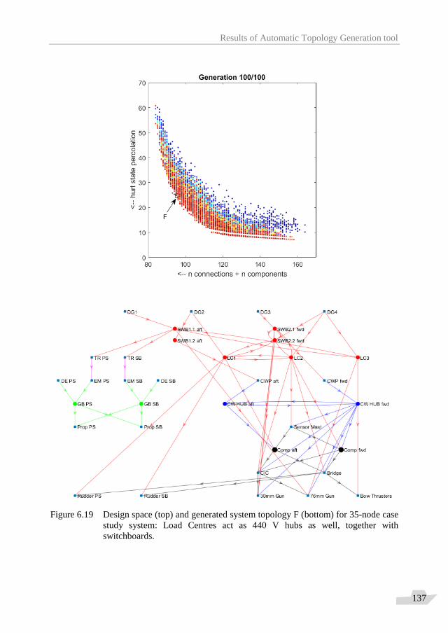
Results of Automatic Topology Generation tool
137
Figure 6.19 Design space (top) and generated system topology F (bottom) for 35-node case
study system: Load Centres act as 440 V hubs as well, together with
switchboards.
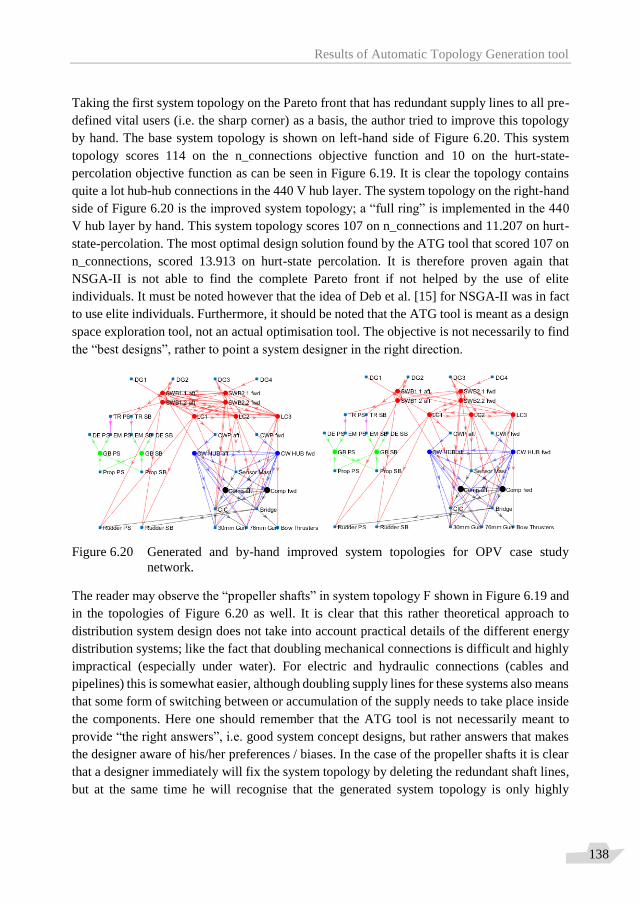
Results of Automatic Topology Generation tool
138
Taking the first system topology on the Pareto front that has redundant supply lines to all pre-
defined vital users (i.e. the sharp corner) as a basis, the author tried to improve this topology
by hand. The base system topology is shown on left-hand side of Figure 6.20. This system
topology scores 114 on the n_connections objective function and 10 on the hurt-state-
percolation objective function as can be seen in Figure 6.19. It is clear the topology contains
quite a lot hub-hub connections in the 440 V hub layer. The system topology on the right-hand
side of Figure 6.20 is the improved system topology; a “full ring” is implemented in the 440
V hub layer by hand. This system topology scores 107 on n_connections and 11.207 on hurt-
state-percolation. The most optimal design solution found by the ATG tool that scored 107 on
n_connections, scored 13.913 on hurt-state percolation. It is therefore proven again that
NSGA-II is not able to find the complete Pareto front if not helped by the use of elite
individuals. It must be noted however that the idea of Deb et al. [15] for NSGA-II was in fact
to use elite individuals. Furthermore, it should be noted that the ATG tool is meant as a design
space exploration tool, not an actual optimisation tool. The objective is not necessarily to find
the “best designs”, rather to point a system designer in the right direction.
Figure 6.20 Generated and by-hand improved system topologies for OPV case study
network.
The reader may observe the “propeller shafts” in system topology F shown in Figure 6.19 and
in the topologies of Figure 6.20 as well. It is clear that this rather theoretical approach to
distribution system design does not take into account practical details of the different energy
distribution systems; like the fact that doubling mechanical connections is difficult and highly
impractical (especially under water). For electric and hydraulic connections (cables and
pipelines) this is somewhat easier, although doubling supply lines for these systems also means
that some form of switching between or accumulation of the supply needs to take place inside
the components. Here one should remember that the ATG tool is not necessarily meant to
provide “the right answers”, i.e. good system concept designs, but rather answers that makes
the designer aware of his/her preferences / biases. In the case of the propeller shafts it is clear
that a designer immediately will fix the system topology by deleting the redundant shaft lines,
but at the same time he will recognise that the generated system topology is only highly
Results of Automatic Topology Generation tool
139
impractical, not entirely impossible! It can be deduced that with max-flow-between-hubs this
strange design solution for the propulsion system would not have been generated. That
function is more an “engineering tool”, leaving somewhat more room for such practical
considerations. In the case of the double propeller shafts for one propeller for instance; these
would only be generated if a user of the ATG tool was to define a vitality of 2 for shaft lines
towards the propellers when max-flow-between-hubs is the system robustness objective
function. It is unlikely an experienced (marine) engineer would do so.
A fundamental (i.e. first-principle) lesson can be learned from the strange design solution with
two propeller shafts driving a single propeller. Hubs exist in all energy distribution systems
according to the topological model for different on-board distribution systems. They exist
either as local nodes or as long, stretched-out common distribution lines. They are encountered
in electric power distribution systems, in mechanical power distribution systems and in fluid
flow distribution systems. However, unlike in the other distribution systems, in mechanical
power distribution systems flows cannot be “mixed”, only combined. This means that
mechanical flows (rotational speeds) cannot be added in a local junction and Kirchoff’s law
for currents does not apply to mechanical systems (while it does for both electric and fluid
flow systems). To clarify, consider a junction of three connections. Two of the connection
supply flow to the junction, i.e. inward flow, while the other has an outward flow. If the
connections are electric power cables the flow of charge (current) in the outward flow cable is
the sum of the two inward flows. The same is true for fluid flow connections where the flow
in the outward pipe line is also the sum of the inward flows. In both cases this can be seen as
a result of the two inward flows mixing in the junction and Kirchoff’s law for currents is
applicable. Now consider three rotating shafts coming together in a junction. The rotational
speed of the outgoing shaft will not be the sum of the rotational speeds of the two ingoing
shafts. Depending on the form of the mechanical link the rotational speed of the outgoing shaft
may be lower (e.g. a propeller shaft from a gearbox with twin input shaft lines from similar
internal combustion engines), the same or higher. The conclusion is that Kirchoff’s law for
currents can only be applied in case the flow consists of many discrete objects that are able to
“mix”, whether those discrete objects are electrons or molecules. Despite this fundamental
difference it is interesting to note that the concept hub can still be applied in mechanical power
distribution systems as well as in electric power and fluid flow distribution systems.
Finally, to demonstrate that the Pareto front indeed contains topologies with ring distributions
in the 440 V hub layer when the run of Figure 6.13 is re-done with the Load Centres at the
same level as the 440 V switchboards and with max-flow-between-hubs as the objective
function, Figure 6.21 shows both the design space and a system topology G that was generated
during design space exploration.
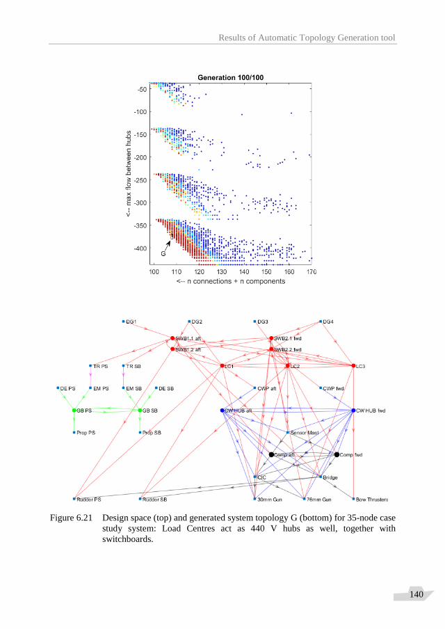
Results of Automatic Topology Generation tool
140
Figure 6.21 Design space (top) and generated system topology G (bottom) for 35-node case
study system: Load Centres act as 440 V hubs as well, together with
switchboards.
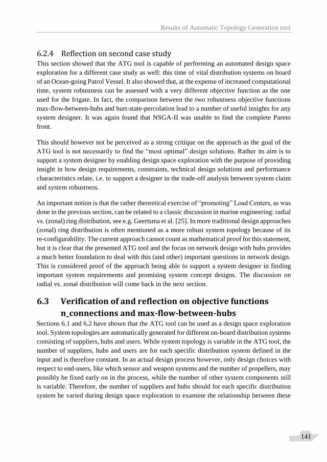
Results of Automatic Topology Generation tool
141
6.2.4 Reflection on second case study This section showed that the ATG tool is capable of performing an automated design space
exploration for a different case study as well: this time of vital distribution systems on board
of an Ocean-going Patrol Vessel. It also showed that, at the expense of increased computational
time, system robustness can be assessed with a very different objective function as the one
used for the frigate. In fact, the comparison between the two robustness objective functions
max-flow-between-hubs and hurt-state-percolation lead to a number of useful insights for any
system designer. It was again found that NSGA-II was unable to find the complete Pareto
front.
This should however not be perceived as a strong critique on the approach as the goal of the
ATG tool is not necessarily to find the “most optimal” design solutions. Rather its aim is to
support a system designer by enabling design space exploration with the purpose of providing
insight in how design requirements, constraints, technical design solutions and performance
characteristics relate, i.e. to support a designer in the trade-off analysis between system claim
and system robustness.
An important notion is that the rather theoretical exercise of “promoting” Load Centers, as was
done in the previous section, can be related to a classic discussion in marine engineering: radial
vs. (zonal) ring distribution, see e.g. Geertsma et al. [25]. In more traditional design approaches
(zonal) ring distribution is often mentioned as a more robust system topology because of its
re-configurability. The current approach cannot count as mathematical proof for this statement,
but it is clear that the presented ATG tool and the focus on network design with hubs provides
a much better foundation to deal with this (and other) important questions in network design.
This is considered proof of the approach being able to support a system designer in finding
important system requirements and promising system concept designs. The discussion on
radial vs. zonal distribution will come back in the next section.
6.3 Verification of and reflection on objective functions
n_connections and max-flow-between-hubs Sections 6.1 and 6.2 have shown that the ATG tool can be used as a design space exploration
tool. System topologies are automatically generated for different on-board distribution systems
consisting of suppliers, hubs and users. While system topology is variable in the ATG tool, the
number of suppliers, hubs and users are for each specific distribution system defined in the
input and is therefore constant. In an actual design process however, only design choices with
respect to end-users, like which sensor and weapon systems and the number of propellers, may
possibly be fixed early on in the process, while the number of other system components still
is variable. Therefore, the number of suppliers and hubs should for each specific distribution
system be varied during design space exploration to examine the relationship between these
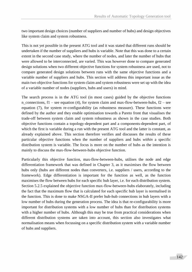
Results of Automatic Topology Generation tool
142
two important design choices (number of suppliers and number of hubs) and design objectives
like system claim and system robustness.
This is not yet possible in the present ATG tool and it was stated that different runs should be
undertaken if the number of suppliers and hubs is variable. Note that this was done to a certain
extent in the second case study, where the number of nodes, and later the number of hubs that
were allowed to be interconnected, are varied. This was however done to compare generated
design solutions when two different objective functions for system robustness are used, not to
compare generated design solutions between runs with the same objective functions and a
variable number of suppliers and hubs. This section will address this important issue as the
main two objective functions for system claim and system robustness were set up with the idea
of a variable number of nodes (suppliers, hubs and users) in mind.
The search process is in the ATG tool (in most cases) guided by the objective functions
n_connections, f1 – see equation (4), for system claim and max-flow-between-hubs, f2 – see
equation (7), for system re-configurability (as robustness measure). These functions were
defined by the author and they enable optimisation towards a Pareto front that visualises the
trade-off between system claim and system robustness as shown in the case studies. Both
objective functions contain a topology-dependent part and a components-dependent part, of
which the first is variable during a run with the present ATG tool and the latter is constant, as
already explained above. This section therefore verifies and discusses the results of these
particular objective functions when the number of suppliers and hubs within a specific
distribution system is variable. The focus is more on the number of hubs as the intention is
mainly to discuss the max-flow-between-hubs objective function.
Particularly this objective function, max-flow-between-hubs, utilises the node and edge
differentiation framework that was defined in Chapter 3, as it maximises the flow between
hubs only (hubs are different nodes than converters, i.e. suppliers / users, according to the
framework). Edge differentiation is important for the function as well, as the function
maximises the flow between hubs for each specific hub layer, i.e. for each distribution system.
Section 5.2.5 explained the objective function max-flow-between-hubs elaborately, including
the fact that the maximum flow that is calculated for each specific hub layer is normalised in
the function. This is done to make NSGA-II prefer hub-hub connections in hub layers with a
low number of hubs during the generation process. The idea is that re-configurability is more
important for distribution systems with a low number of hubs than for distribution systems
with a higher number of hubs. Although this may be true from practical considerations when
different distribution systems are taken into account, this section also investigates what
normalisation means when focussing on a specific distribution system with a variable number
of hubs and suppliers.
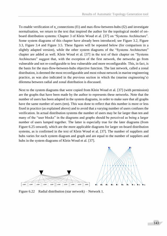
Results of Automatic Topology Generation tool
143
To enable verification of n_connections (f1) and max-flow-between-hubs (f2) and investigate
normalisation, we return to the text that inspired the author for the topological model of on-
board distribution systems: Chapter 3 of Klein Woud et al. [37] on “Systems Architecture”.
Some system diagrams of this chapter have already been introduced; see Figure 3.2, Figure
3.3, Figure 3.4 and Figure 3.5. These figures will be repeated below (for comparison in a
slightly adapted version), while the other system diagrams of the “Systems Architecture”
chapter are added as well. Klein Woud et al. [37] in the text of their chapter on “Systems
Architecture” suggest that, with the exception of the first network, the networks go from
vulnerable and not re-configurable to less vulnerable and more reconfigurable. This, in fact, is
the basis for the max-flow-between-hubs objective function. The last network, called a zonal
distribution, is deemed the most reconfigurable and most robust network in marine engineering
practice, as was also indicated in the previous section in which the (marine engineering’s)
dilemma between radial and zonal distribution is discussed.
Next to the system diagrams that were copied from Klein Woud et al. [37] (with permission)
are the graphs that have been made by the author to represents these networks. Note that the
number of users has been adapted in the system diagrams, in order to make sure that all graphs
have the same number of users (ten). This was done to reflect that this number is more or less
fixed in practice (as explained above) and to avoid that a varying number of users confuses the
verification. In actual distribution systems the number of users may be far larger than ten and
many of the “user blocks” in the diagrams and graphs should be perceived as being a larger
number of users lumped together. The latter is especially true for the later diagrams (from
Figure 6.25 onward), which are the more applicable diagrams for larger on-board distribution
systems, as is confirmed in the text of Klein Woud et al. [37]. The number of suppliers and
hubs varies for each system diagram and graph and are equal to the number of suppliers and
hubs in the system diagrams of Klein Woud et al. [37].
Figure 6.22 Radial distribution (star network) – Network 1.
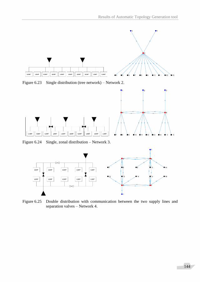
Results of Automatic Topology Generation tool
144
Figure 6.23 Single distribution (tree network) – Network 2.
Figure 6.24 Single, zonal distribution – Network 3.
Figure 6.25 Double distribution with communication between the two supply lines and
separation valves – Network 4.
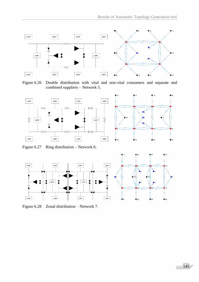
Results of Automatic Topology Generation tool
145
Figure 6.26 Double distribution with vital and non-vital consumers and separate and
combined suppliers – Network 5.
Figure 6.27 Ring distribution – Network 6.
Figure 6.28 Zonal distribution – Network 7.
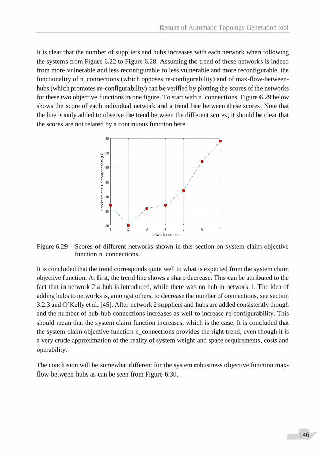
Results of Automatic Topology Generation tool
146
It is clear that the number of suppliers and hubs increases with each network when following
the systems from Figure 6.22 to Figure 6.28. Assuming the trend of these networks is indeed
from more vulnerable and less reconfigurable to less vulnerable and more reconfigurable, the
functionality of n_connections (which opposes re-configurability) and of max-flow-between-
hubs (which promotes re-configurability) can be verified by plotting the scores of the networks
for these two objective functions in one figure. To start with n_connections, Figure 6.29 below
shows the score of each individual network and a trend line between these scores. Note that
the line is only added to observe the trend between the different scores; it should be clear that
the scores are not related by a continuous function here.
Figure 6.29 Scores of different networks shown in this section on system claim objective
function n_connections.
It is concluded that the trend corresponds quite well to what is expected from the system claim
objective function. At first, the trend line shows a sharp decrease. This can be attributed to the
fact that in network 2 a hub is introduced, while there was no hub in network 1. The idea of
adding hubs to networks is, amongst others, to decrease the number of connections, see section
3.2.3 and O’Kelly et al. [45]. After network 2 suppliers and hubs are added consistently though
and the number of hub-hub connections increases as well to increase re-configurability. This
should mean that the system claim function increases, which is the case. It is concluded that
the system claim objective function n_connections provides the right trend, even though it is
a very crude approximation of the reality of system weight and space requirements, costs and
operability.
The conclusion will be somewhat different for the system robustness objective function max-
flow-between-hubs as can be seen from Figure 6.30.
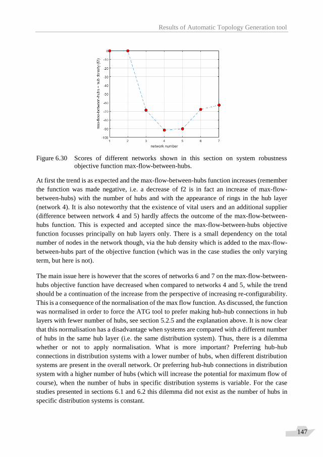
Results of Automatic Topology Generation tool
147
Figure 6.30 Scores of different networks shown in this section on system robustness
objective function max-flow-between-hubs.
At first the trend is as expected and the max-flow-between-hubs function increases (remember
the function was made negative, i.e. a decrease of f2 is in fact an increase of max-flow-
between-hubs) with the number of hubs and with the appearance of rings in the hub layer
(network 4). It is also noteworthy that the existence of vital users and an additional supplier
(difference between network 4 and 5) hardly affects the outcome of the max-flow-between-
hubs function. This is expected and accepted since the max-flow-between-hubs objective
function focusses principally on hub layers only. There is a small dependency on the total
number of nodes in the network though, via the hub density which is added to the max-flow-
between-hubs part of the objective function (which was in the case studies the only varying
term, but here is not).
The main issue here is however that the scores of networks 6 and 7 on the max-flow-between-
hubs objective function have decreased when compared to networks 4 and 5, while the trend
should be a continuation of the increase from the perspective of increasing re-configurability.
This is a consequence of the normalisation of the max flow function. As discussed, the function
was normalised in order to force the ATG tool to prefer making hub-hub connections in hub
layers with fewer number of hubs, see section 5.2.5 and the explanation above. It is now clear
that this normalisation has a disadvantage when systems are compared with a different number
of hubs in the same hub layer (i.e. the same distribution system). Thus, there is a dilemma
whether or not to apply normalisation. What is more important? Preferring hub-hub
connections in distribution systems with a lower number of hubs, when different distribution
systems are present in the overall network. Or preferring hub-hub connections in distribution
system with a higher number of hubs (which will increase the potential for maximum flow of
course), when the number of hubs in specific distribution systems is variable. For the case
studies presented in sections 6.1 and 6.2 this dilemma did not exist as the number of hubs in
specific distribution systems is constant.

Results of Automatic Topology Generation tool
148
To show that the normalisation is the cause of the lower scores for networks 6 and 7, Figure
6.31 shows the actual max-flow-between-hubs part (first part) of the objective function f2 with
normalisation and Figure 6.32 without normalisation.
Figure 6.31 Scores of different networks shown in this section on the actual max-flow-
between-hubs part of objective function f2 when this term is normalised.
Figure 6.32 Scores of different networks shown in this section on the actual max-flow-
between-hubs part of objective function f2 when this term is not normalised.
First of all, note that the scores for max-flow-between-hubs do not change between networks
4 and 5 and networks 6 and 7. This is caused by now fully focussing on the hub layers and
excluding hub density. This will be elaborated below. The max flow trend without
normalisation (Figure 6.32) is now overall increasing until network 6 (ring distribution) and
network 7 (zonal ring distribution). Not normalising the max flow function should thus be
considered as a real option, when the number of hubs within specific distribution systems is
varying.
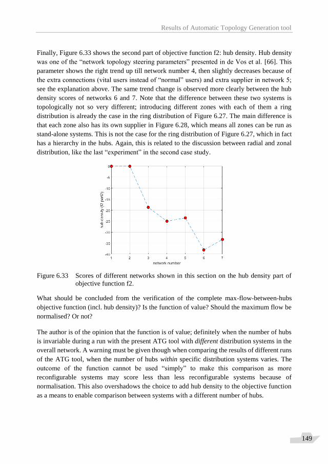
Results of Automatic Topology Generation tool
149
Finally, Figure 6.33 shows the second part of objective function f2: hub density. Hub density
was one of the “network topology steering parameters” presented in de Vos et al. [66]. This
parameter shows the right trend up till network number 4, then slightly decreases because of
the extra connections (vital users instead of “normal” users) and extra supplier in network 5;
see the explanation above. The same trend change is observed more clearly between the hub
density scores of networks 6 and 7. Note that the difference between these two systems is
topologically not so very different; introducing different zones with each of them a ring
distribution is already the case in the ring distribution of Figure 6.27. The main difference is
that each zone also has its own supplier in Figure 6.28, which means all zones can be run as
stand-alone systems. This is not the case for the ring distribution of Figure 6.27, which in fact
has a hierarchy in the hubs. Again, this is related to the discussion between radial and zonal
distribution, like the last “experiment” in the second case study.
Figure 6.33 Scores of different networks shown in this section on the hub density part of
objective function f2.
What should be concluded from the verification of the complete max-flow-between-hubs
objective function (incl. hub density)? Is the function of value? Should the maximum flow be
normalised? Or not?
The author is of the opinion that the function is of value; definitely when the number of hubs
is invariable during a run with the present ATG tool with different distribution systems in the
overall network. A warning must be given though when comparing the results of different runs
of the ATG tool, when the number of hubs within specific distribution systems varies. The
outcome of the function cannot be used “simply” to make this comparison as more
reconfigurable systems may score less than less reconfigurable systems because of
normalisation. This also overshadows the choice to add hub density to the objective function
as a means to enable comparison between systems with a different number of hubs.

Results of Automatic Topology Generation tool
150
The fundamental cause for the experienced problems is in the end the choice to determine the
maximum flow between hubs, whether normalised or not. This function will “steer” the
generated system topologies to complete graphs (a network with all possible connections) in
the hub layers. Although this would certainly represent the most reconfigurable system, in
practice a true “zonal distribution system” as in Figure 6.28 would already be considered a
major step forwards to the system topologies that are now found on board of (naval) vessels.
A different objective function; one that steers towards “long rings” or (more mathematically)
“cycles of large length” would perhaps be more fitting for networks of different,
interdependent, vital on-board distribution systems. This task is left for later research.
6.4 Summary and conclusion This chapter has demonstrated that the ATG tool is able to explore design spaces for (energy)
distribution systems on board ships by automatically generating design solutions for these
systems. The first case study explored design spaces for the Electric Power Distribution
System (EPDS) and the Chilled Water Distribution System (CWDS) on board a notional
frigate and demonstrated the usefulness of the ATG tool as a design space exploration tool.
The first case study also unveiled a number of issues that can be encountered when using the
ATG tool and demonstrated possible fixes. The second case study explored design spaces for
other systems than the first; this time the focus was on the EPDS and CWDS, but also the
propulsion system, on board a notional Ocean-going Patrol Vessel. The second case study
demonstrated the usefulness of the ATG tool even better, as the results could be related to
classic marine engineering discussions with respect to system topologies. Furthermore, a
comparison was made between two very different system robustness objective functions which
turned out to be in good agreement with one another. Section 6.3 verified the max-flow-
between-hubs objective function in case the number of nodes, and hubs specifically, vary.
Routing of the systems inside a ship has however not been shown and only one system diagram
was shown in this chapter that contains information on how the generated networks can be
laid-out spatially: the Single Line Diagram of Figure 6.18. Routing and more appropriate
network visualisation are in fact the subsequent steps, as discussed in section 2.4. First, a better
visualisation method of the generated networks should be found that better resembles the
Single Line Diagrams, principle piping diagrams or block diagrams that are used in practice.
Second, with the generated network topologies it is now possible to start routing the systems
through a ship, assuming its envelope is available. A first step in this direction was already
taken by Duchateau et al. [20]. Note that a difficult issue arises when routing the networks
through a ship, as the location and size of hubs is not known from the networks that are
generated by the ATG tool; i.e. is a hub located in a single compartment, in a single zone, or
is it extended throughout the ship. Another activity that can now be undertaken is setting up
load balances that include different operational modes of the systems which subsequently
enables dimension prediction of the system components. Given that different possibilities for

Results of Automatic Topology Generation tool
151
connecting those components are available from the generated network topologies in the ATG
tool, it should also be possible to start predicting the dimensions needed by connections in the
systems as well.

Results of Automatic Topology Generation tool
152
Conclusions & Recommendations
153
“It does not matter how slowly you go as long as you do not stop.”
― Confucius
Chapter 7 Conclusions & Recommendations
Conclusion
This dissertation described the development and application of the so-called Automatic
Topology Generation (ATG) tool. The ATG tool enables design space exploration for vital on-
board (energy) distribution systems. The theoretical design procedure of section 2.4 embedded
the ATG tool in its “wider surroundings”. It was stated there that the first six steps (1-6) of the
procedure are addressed in this research. Therefore, these steps are revisited in this chapter
first, before a main conclusion to this research is reached. After drawing the main conclusion,
a number of recommendations will be given for future research that are related to the next
steps in the design procedure (7-14). An outlook to future possibilities, when future research
has been performed, will be given as well.
The first three steps of the design procedure in section 2.4 require the establishment of a list
of specific (energy) distribution systems on board of (naval) vessels and their components:
1. Determine the mission related systems the ship is equipped with to execute her
mission(s).
2. Determine the type of flows the mission related systems require from supporting
distribution systems in order to be able to fulfil their function.
3. Determine the type of flows the suppliers of the supporting distribution systems
require from yet other supporting distribution systems in order to be able to fulfil their
function. [Continue until the list of components of different, interdependent on-board
distribution systems is complete].
The list starts with the mission-related systems, like sensors, weapons and propulsion systems,
which follow from the mission of the ship. These systems in all probability will require the
ship to be equipped with supporting on-board distribution systems like an electric power
generation and distribution system and a chilled water distribution system. The list of different
distribution systems is completed either when the ultimate sources of a ship at sea (fuel, air
and seawater) are reached or when a user of the ATG tool decides that the list contains the
vital distribution systems for which he/she wants to perform design space exploration. Thus,
the first three steps of the design procedure mainly define the input that is required by the ATG
tool from the user before it can be used. Note that the first three steps focus on listing what
type of flow (distributed in specific distribution systems) are needed (i.e. used) by different
systems or system components.
Conclusions & Recommendations
154
The required input for the ATG tool is however not complete with a specification of different
distribution systems and users therein, as is also clear from the fourth step in the design
procedure, which requires the number and type of “suppliers” to be defined for each specific
distribution system:
4. Determine the number and type of suppliers (users are known from step 1-3).
In fact, the different system components that need to be defined for each distribution system
are the suppliers, hubs and users of these systems. Suppliers, hubs and users are present in
every vital on-board distribution system according to a topological model that was introduced
and explained in Chapter 3. The topological model of on-board distribution systems is
combined in that chapter with the fundamental concepts “nodes” and “edges” of network
theory to establish a node and edge differentiation framework.
Differentiating between different nodes and edges with the developed framework has several
advantages:
The generated system topologies are more realistic in comparison to using general
nodes and edges as one can relate to practical system components and connections
found on board ships.
In practice components may have different roles in different distribution systems, i.e.
be a supplier in one distribution system and a user in another. The developed node
and edge differentiation framework is able to deal with this dual (or multiple)
functionality of system components.
The amount of possible system topologies (i.e. the size of the design space) is
drastically reduced as differentiation between different nodes and edges makes the
assessment of infeasibility or unlikeliness of different connections possible. Based on
this assessment a-priori constraints are set up and applied. The constraints were
discussed in section 3.5.
The second advantage may be the most important from a practical perspective, as this
advantage of the node and edge differentiation framework makes system integration between
distribution systems possible in early-stage system design. This novel ability of the ATG tool
is considered one of the main contributions of the research presented in this dissertation as
proper system integration is deemed to be lacking in current early stages of ship and system
design.
What input the ATG tool exactly requires on basis of the node and edge differentiation
framework, applied constraints and applied objective functions is explained in section 4.2.1.
The incorporation of the node and edge differentiation framework with the available NSGA-
II code (a specific Genetic Algorithm) in Chapter 4, including the definition of objective
Conclusions & Recommendations
155
functions for system claim and system robustness in Chapter 5, leads to the realisation of the
ATG tool. This achievement enables fulfilment of step 5 and 6 in the design procedure:
5. Determine the topology of the network that connects the suppliers, hubs and users.
6. Assess and compare the generated design solutions for vital on-board distribution
systems on different design objectives: system claim and system robustness.
The ATG tool can perform step 5 and 6 automatically for a (very) large number of system
topologies (> 104). In doing so, the tool enables design space exploration for vital on-board
distribution systems. This was demonstrated in Chapter 6, which presented the results of the
ATG tool for two different case studies: a notional frigate and a notional Ocean-going Patrol
Vessel. The same chapter reflected critically on the used optimisation algorithm and defined
objective functions.
This brings us to the main conclusion of this dissertation, for which it is necessary to repeat
the research goal of section 1.4:
To develop a method that enables design space exploration for vital (energy)
distribution systems on board of (naval) vessels. In order to do this, a tool needs to be
developed that automatically generates a large number of varying system topologies.
The generated system topologies need to be automatically assessed by the tool on the
opposing design objectives of system robustness and system claim (costs, weight and
space requirements, operability), while they fulfil the most basic level of technical
feasibility, to enable trade-off analysis and decision support.
This goal has been achieved with the realisation of the Automatic Topology Generation tool
that enables design space exploration for on-board energy distribution systems. The ATG tool
generates varying system topologies that are assessed on their performance with regards to
system robustness and the opposing design objective of system claim (representing weight and
space requirements, costs and operability). A basic level of technical feasibility of generated
system concept designs is ensured by the ATG tool by “flow type pairing”, which is a first
level of system analysis to connect supply and demand in different distribution systems (see
section 2.4). Flow type pairing makes the distinction between feasible and infeasible
connections. Flow type pairing is used to set up a priori constraints that leave infeasible
connections outside the scope of the ATG tool, i.e. outside the explored design space. As such,
the ATG tool succeeds in its goal as a design space exploration tool: to provide insight in how
design requirements, constraints, technical design solutions and performance characteristics
relate. Therefore, the ATG tool is considered to be a good first step in the direction of enabling
useful design space exploration for on-board energy distribution systems.
The number and type of components in a system concept design are input to the ATG tool
though and are therefore invariable (unless multiple runs are made with the ATG tool to
Conclusions & Recommendations
156
explore alternative design spaces). This is considered a drawback of the method. Especially
because it means also the number of hubs need to be pre-defined for each specific distribution
system under consideration. In a practical design space exploration the number of hubs in
particular and the number of system components in general, should be variable. This will be
further discussed in the recommendations.
Finally, the main contributions of this research can be listed:
Network theory and mathematical optimisation techniques are applied in a marine
engineering context, thus bridging the gap between fundamental mathematical
disciplines and the applied science of marine engineering.
Early-stage design of vital on-board (energy) distribution systems is improved by
enabling design space exploration. In fact, the early-stage design process for on-board
distribution systems has been extended by placing design space exploration at the
start of the process, which was not done before this research (to the knowledge of the
author).
A mathematical formulation for the ambiguous concept of system robustness has
been defined. From verification it is clear that the function can still be improved, but
it is a good first step to enable quantitative analysis of system designs with respect to
system re-configurability (one of the main robustness improvement measures).
Recommendations
The first recommendations for future research follow from proceeding with the design
procedure of section 2.4, as early-stage stage ship and system design are not finished when the
present ATG tool has produced its results. Step 7 – 9 of the design procedure aim to integrate
system concept designs into ship concept designs. A valid critique on this research may be that
the integration of system design into ship design is hardly undertaken. In fact, many of the
(modelling) choices that were made, made it possible to perform design space exploration for
vital on-board distribution systems without requiring any ship design information. This was
already clear in section 1.2.1 where it was stated that this research focussed on route B in
Figure 1.4, which runs parallel to early-stage ship design (route A). The C- and D-arrows
(interaction between system and ship design) are hardly covered in this research. Duchateau
et al. [20] already tried to explore further integration of the ATG tool and ship concept design
by automatically routing the connections of a single system topology in many different ways
through a single ship concept design. This still is a limited form of integration, but clearly is
already a next step following this research. Ultimately an integrated approach in which
different system concept designs (from the ATG tool) are routed in different ways (from the
routing tool) through different ship concept designs (from the packing tool) is envisaged.
Imagine that it is possible in early-stage ship design to compare distributed generation (i.e.
many suppliers for different energy distribution systems dispersed over the ship) versus
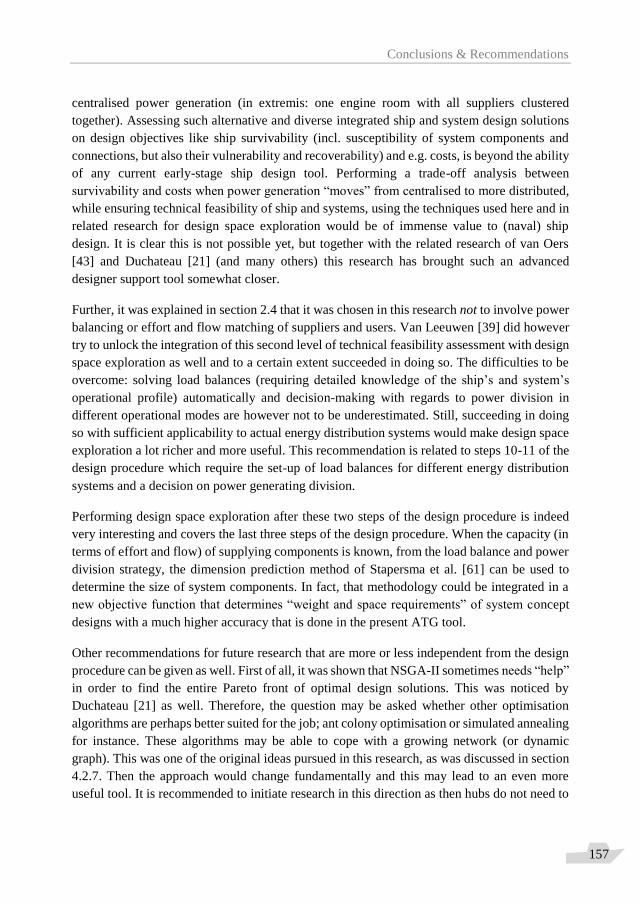
Conclusions & Recommendations
157
centralised power generation (in extremis: one engine room with all suppliers clustered
together). Assessing such alternative and diverse integrated ship and system design solutions
on design objectives like ship survivability (incl. susceptibility of system components and
connections, but also their vulnerability and recoverability) and e.g. costs, is beyond the ability
of any current early-stage ship design tool. Performing a trade-off analysis between
survivability and costs when power generation “moves” from centralised to more distributed,
while ensuring technical feasibility of ship and systems, using the techniques used here and in
related research for design space exploration would be of immense value to (naval) ship
design. It is clear this is not possible yet, but together with the related research of van Oers
[43] and Duchateau [21] (and many others) this research has brought such an advanced
designer support tool somewhat closer.
Further, it was explained in section 2.4 that it was chosen in this research not to involve power
balancing or effort and flow matching of suppliers and users. Van Leeuwen [39] did however
try to unlock the integration of this second level of technical feasibility assessment with design
space exploration as well and to a certain extent succeeded in doing so. The difficulties to be
overcome: solving load balances (requiring detailed knowledge of the ship’s and system’s
operational profile) automatically and decision-making with regards to power division in
different operational modes are however not to be underestimated. Still, succeeding in doing
so with sufficient applicability to actual energy distribution systems would make design space
exploration a lot richer and more useful. This recommendation is related to steps 10-11 of the
design procedure which require the set-up of load balances for different energy distribution
systems and a decision on power generating division.
Performing design space exploration after these two steps of the design procedure is indeed
very interesting and covers the last three steps of the design procedure. When the capacity (in
terms of effort and flow) of supplying components is known, from the load balance and power
division strategy, the dimension prediction method of Stapersma et al. [61] can be used to
determine the size of system components. In fact, that methodology could be integrated in a
new objective function that determines “weight and space requirements” of system concept
designs with a much higher accuracy that is done in the present ATG tool.
Other recommendations for future research that are more or less independent from the design
procedure can be given as well. First of all, it was shown that NSGA-II sometimes needs “help”
in order to find the entire Pareto front of optimal design solutions. This was noticed by
Duchateau [21] as well. Therefore, the question may be asked whether other optimisation
algorithms are perhaps better suited for the job; ant colony optimisation or simulated annealing
for instance. These algorithms may be able to cope with a growing network (or dynamic
graph). This was one of the original ideas pursued in this research, as was discussed in section
4.2.7. Then the approach would change fundamentally and this may lead to an even more
useful tool. It is recommended to initiate research in this direction as then hubs do not need to
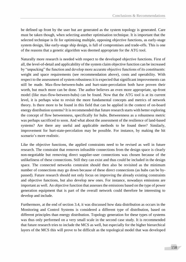
Conclusions & Recommendations
158
be defined up front by the user but are generated as the system topology is generated. Care
must be taken though, when selecting another optimisation technique. It is important that the
selected technique is fit for optimising multiple, opposing objective functions, as early-stage
system design, like early-stage ship design, is full of compromises and trade-offs. This is one
of the reasons that a genetic algorithm was deemed appropriate for the ATG tool.
Naturally more research is needed with respect to the developed objective functions. First of
all, the level-of-detail and applicability of the system claim objective function can be increased
by “unpacking” the function and develop more accurate objective functions of its constituents:
weight and space requirements (see recommendation above), costs and operability. With
respect to the assessment of system robustness it is expected that significant improvements can
still be made. Max-flow-between-hubs and hurt-state-percolation both have proven their
worth, but much more can be done. The author believes an even more appropriate, up-front
model (like max-flow-between-hubs) can be found. Now that the ATG tool is at its current
level, it is perhaps wise to revisit the more fundamental concepts and metrics of network
theory. Is there more to be found in this field that can be applied in the context of on-board
energy distribution systems? It is recommended that future research starts with better exploring
the concept of flow betweenness, specifically for hubs. Betweenness as a robustness metric
was perhaps sacrificed to soon. And what about the assessment of the resilience of land-based
systems? Are there any useful and applicable methods to be found there? Similarly,
improvement for hurt-state-percolation may be possible. For instance, by making the hit
scenario’s more realistic.
Like the objective functions, the applied constraints need to be revised as well in future
research. The constraint that removes infeasible connections from the design space is clearly
non-negotiable but removing direct supplier-user connections was chosen because of the
unlikeliness of these connections. Still they can exist and thus could be included in the design
space. The connected networks constraint should then also be revisited as the minimum
number of connections may go down because of these direct connections (as hubs can be by-
passed). Future research should not only focus on improving the already existing constraints
and objective functions, but also develop new ones. For instance, nowadays emissions are
important as well. An objective function that assesses the emissions based on the type of power
generation equipment that is part of the overall network could therefore be interesting to
develop and include.
Furthermore, at the end of section 3.4, it was discussed how data distribution as occurs in the
Monitoring and Control Systems is considered a different type of distribution, based on
different principles than energy distribution. Topology generation for these types of systems
was thus only performed on a very small scale in the second case study. It is recommended
that future research tries to include the MCS as well, but especially for the higher hierarchical
layers of the MCS this will prove to be difficult as the topological model that was developed

Conclusions & Recommendations
159
and applied here is less applicable to data distribution systems; particularly declaration 2 with
respect to edge differentiation.
Then it is acknowledged that the time path of this research was such that the main result of
Duchateau [21]: the possibility for the user to interact with the design space exploration tool
for conceptual ship design (packing), was not implemented here. Conceptual system design,
using the ATG tool for design space exploration, may benefit as well from such interaction.
This may have several benefits:
To overcome the disadvantage of the current ATG tool of having a fixed number of
system components (suppliers and hubs mainly, see above),
To overcome the characteristic of NSGA-II to prefer one the objective functions.
Together with the previous recommendation of developing more (and more advanced)
objective functions and / or constraints, the interactivity between ATG tool and user would be
a major step forwards as the user can then “play” with a multitude of functions and constraints
that drive the search process.
Such “playing” with the tool is also the final recommendation of this dissertation. The case
studies in Chapter 6 were explorations of design spaces using known, contemporary
technologies. It was chosen to do this in order to build confidence in the ATG tool; by showing
that the generated system concept designs are realistic. The automated design space
exploration methodology is so different from current design practice that building confidence
in the ATG tool is considered necessary before unknown design spaces can be explored. But
now that step can be made: i.e. start playing and investigate what kind of topologies are
possible if new technologies, like more extensive DC distribution or decentralised power
generation with fuel cells, batteries and even solar panels are used.
Closure
Finally, a recommendation is given to practicing ship and system designers: embrace design
space exploration approaches (with a healthy critical attitude of course)!
Over are the days that the power plants of ships are driven by diesel engines only. New (dual
fuel engines) and newer (fuel cells) technologies will become part of the solutions in the 21st
century. Emission abatement systems will become more common as well. When to use which
type of equipment, which fuel to use, which combinations of equipment are the most suited
for the different applications (ship types / operational profiles) and how they should be
connected together and cooperate will become a challenging issue. The selection of system
components and system topology is more a combinatorial problem now, than it ever was.
Design space exploration is essential for dealing with this new reality.

Conclusions & Recommendations
160
Our field of expertise is rich in heuristic knowledge. People have been building ships for
thousands of years! We excel in making beautiful, brilliantly balanced (naval) vessels. BUT,
we have no idea of the sheer magnitude of possibilities that have still been unexplored. Our
educational programmes, whether that is at university or applied university level, succeed well
in transferring modern maritime technology heuristic knowledge, and on-going research
extends this heuristic knowledge even further. But only design space exploration techniques
will show us where heuristic knowledge turns to cognitive bias and what is possible if we free
ourselves of “altijd zoo geweescht”23.
23 Dutch for: the way it has always been

Bibliography
161
Bibliography [1] ABS online publication (visited 10-2017):
https://ww2.eagle.org/content/dam/eagle/rules-and-
guides/current/other/191_dpsguide/DPS_Guide_e-Feb16-New%20Logo.pdf.
[2] Albert, R., Barabási, A. L. (2002); Statistical mechanics of complex networks, Reviews of
modern physics 74(1): p. 47-98.
[3] Andrews, D.J. (2011); Marine requirements elucidation and the nature of preliminary
ship design, Int. Journal of Maritime Engineering 153: p. A23-A39.
[4] Andrews, D., Duchateau, E.A.E., Gillespie, J., Hopman, J.J., Pawling, R.J. and Singer, D.
(2012); State of the art report: Design for layout, Proc. of 11th Int. Marine Design
Conference (IMDC), volume 1: p. 111-137, UK.
[5] Ashe, G., Bosman, T., Cheng, F., Dow, R., Ferraris, S., Ferreiro, L., Kaeding, P., Kaneko,
H., McGeorge, D., Norwood, M., Park, J. (2006); Naval Ship Design, Proc. of the 16th
International Ship and Offshore Structures Congress, volume 2, UK. Accessed online
(October 2017): https://www.scribd.com/document/42621845/Naval-Ship-Design.
[6] van Biert, L., Godjevac, M., Visser, K., Aravind, P.V. (2016); A review of fuel cell systems
for maritime applications, Journal of Power Sources 327: p. 345-364.
[7] van Bodegraven, K.S., Logtmeijer, R.A. (2009); Sailing with an unmanned Ship Control
Centre, Proc. of 14th International Ship Control Systems Symposium (ISCSS), Ottawa,
IMarEST, UK.
[8] Boykov, Y., Kolmogorov, V. (2004); An Experimental Comparison of Min-Cut/Max-
Flow Algorithms for Energy Minimization in Vision, IEEE Transactions on PAMI, Vol.
26, No. 9, p. 1124-1137.
[9] Bradbeer, N., Greig, A. (2017); Warship Machinery Constraints, Encyclopedia of
Maritime and Offshore Engineering, online John Wiley & Sons, Ltd.
DOI: https://onlinelibrary.wiley.com/doi/10.1002/9781118476406.emoe306
[10] Brefort, D.C., Shields, C.P.F., Habben Jansen, A.C., Duchateau, E.A.E., Pawling, R.J.,
Droste, K., Jaspers, T., Sypniewski, M., Goodrum, C., Parsons, M., Yasin Kara, M., Roth,
M., Singer, D.J., Andrews, D.J., Hopman, J.J., Brown, A., Kana, A.A. (2018); An
architectural framework for distributed naval ship systems, Ocean Engineering 147, pp.
375–385.
[11] Brown, A.J., Salcedo, J. (2003); Multiple Objective Genetic Optimization in Naval Ship
Design, Naval Engineers Journal, volume 115 (4), p. 49-61, USA.
[12] Calvert, K. L., Doar, M. B., Zegura, E. W. (1997); Modeling Internet topology, IEEE
Communications Magazine, Volume 35, Issue 6, p. 160-163.
[13] Chalfant, J., Chryssostomidis, C. (2017); Application of Templates to Early-Stage Ship
Design, IEEE Electric Ship Technologies Symposium, USA.
[14] Deb, K. (2001); Multi-Objective Optimization Using Evolutionary Algorithms, Wiley-
Interscience Series in Systems and Optimization, Wiley, Chichester, UK.

Bibliography
162
[15] Deb, K.; Pratap, A.; Agarwal, S.; Meyarivan, T. (2002); A fast and elitist multiobjective
genetic algorithm: NSGA-II, IEEE Trans. On Evolutionary Computation 6(2): p. 182–
197.
[16] DNV-GL online publication (visited 10-2017):
https://rules.dnvgl.com/docs/pdf/DNV/rulesship/2012-01/ts607.pdf.
[17] DNV-GL online publication (visited 10-2017):
http://rules.dnvgl.com/docs/pdf/gl/maritimerules/gl_i-1-15_e.pdf.
[18] van Dijk, J. (2018); Automatic Selection of an Optimal Power Plant Configuration, MSc
thesis Delft University of Technology (will be available in TU Delft repository – currently
under embargo), NL.
[19] Doerry, N. (2007); Designing Electrical Power Systems for Survivability and Quality of
Service, ASNE Naval Engineers Journal, Vol. 119, No 2, p. 25-34.
[20] Duchateau, E.A.E., de Vos, P., van Leeuwen, S. (2018); Early stage routing of distributed
ship service systems for vulnerability reduction, Proc. of 13th Int. Marine Design
Conference (IMDC), Helsinki, Finland.
[21] Duchateau, E.A.E. (2016); Interactive evolutionary concept exploration in preliminary
ship design, Dissertation Technical University of Delft (available in TU Delft repository),
Gildeprint, NL.
[22] Evans, J.H. (1959); Basic Design Concepts, Journal American Society of Naval
Engineers.
[23] Fencl, T., Burget, P., Bilek, J. (2011); Network topology design, Control Engineering
Practice, volume 19 (11): p. 1287–1296.
[24] Gillespie, J. (2012); A network science approach to understanding and generating ship
arrangements in early-stage design, Dissertation University of Michigan, USA.
[25] Geertsma, R.D., Weston, A.V., Devlin, J., Wright, W. (2009); Power system survivability
– how can we deliver?, Proc. of 3rd Engine as a Weapon Conference (EAAWIII), London,
IMarEST, UK.
[26] Habben Jansen, A.C., Duchateau, E.A.E., Kana, A.A. (2018); Towards a novel design
perspective for system vulnerability using a Markov chain, Proc. of International Naval
Engineering Conference (INEC 2018), Glasgow, IMarEST, UK.
[27] Haimes, Y. Y. (2009); On the definition of resilience in systems, Risk Analysis, volume
29(4): p. 498–501.
[28] Harrington, R.L. (1992); Marine Engineering, The Society of Naval Architects and
Marine Engineers, USA.
[29] ten Hacken, M. (2017); Optimization of a submarine propulsion system by implementing
a PEM fuel cell and a PMSM in a first principle model, MSc thesis Delft University of
Technology (will be available in TU Delft repository – currently under embargo), NL.
[30] Hill, R. (2005); Admiral Hyman G Rickover USN and the UK Nuclear Submarine
Propulsion Programme, The Thomas Lowe Gray Memorial Lecture, IMechE, UK.

Bibliography
163
[31] Hopman, J.J. (2007); Ontwerpen van schepen: Tussen kunst en topsport (in Dutch),
Intreerede Delft University of Technology (available in TU Delft repository), NL,
uuid:dfb91b55-23b8-4678-89b5-48ca2f22a09d.
[32] Hu, Y. (2016); Dimension Prediction of Marine System Equipment Based on First
Principles, MSc thesis Delft University of Technology (available in TU Delft repository),
NL.
[33] INCOSE (2015); Systems Engineering Handbook, John Wiley & Sons Inc., ISBN10:
1118999401, 4th Edition.
[34] Karnopp, D.C., Margolis, D.L., Rosenberg, R.C. (2012); System Dynamics: Modeling,
Simulation and Control of Mechatronic Systems, John Wiley & Sons Inc., 5th Edition.
[35] Koç, Y. (2015); On Robustness of Power Grids, Dissertation Technical University of
Delft (available in TU Delft repository), CPI – Koninklijke Wöhrmann, NL.
[36] Klein Woud, J. and Stapersma, D. (2008); Marine Engineering: Design of Propulsion and
Electric Power Generation Systems, The Institute of Marine Engineering, Science and
Technology (IMarEST), UK.
[37] Klein Woud, J. and Stapersma, D. (2016); Selected chapters of Marine Engineering:
Design of Auxiliary Systems, Shafting and Flexible Mounting, Lecture Notes Delft
University of Technology (to be published as book).
[38] Lamb, T. (editor) et al. (2003); Ship Design and Construction, The Society of Naval
Architects and Marine Engineers, USA.
[39] van Leeuwen, S.P. (2017); Estimating the vulnerability of ship distributed system
topologies, MSc thesis Delft University of Technology (available in TU Delft repository),
NL.
[40] Medina, A., Matta, I., Byers, J. (2000); On the Origin of Power Laws in Internet
Topologies, ACM SIGCOMM Computer Communication Review.
[41] Newman, M. E. J. (2012); Networks; An Introduction, Oxford University Press.
[42] Nowacki, H. (2016); A Farewell to the Design Spiral, Invited Note presented at the Mini-
Symposium on Ship Design, Ship Hydrodynamics & Maritime Safety, Athens, Greece.
[43] van Oers, B.J. (2011); A packing approach for the early stage design of service vessels,
Dissertation Technical University of Delft (available in TU Delft repository), VSSD, NL.
[44] van Oers, B.J., van Ingen, G., Stapersma, D. (2012); An integrated approach for the design
of resilient ship services systems, Proc. of International Naval Engineering Conference
(INEC 2012), Edinborough, IMarEST, UK.
[45] O’Kelly, M.E., Miller, H.J. (1994); The Hub Network Design Problem: a review and
synthesis, Journal of Transport Geography, volume 2 (1): p. 31-40.
[46] van Osch, S. J. M., Worthington, J. P. W., Galloway, W. D., Geertsma, R. D., Janssen, J.
A. A. J., Smit, C. S. (2014); Distributed Intelligent Networked Control Systems (DINCS)
applied to a whole ship integrated Platform Management System, Proc. of International
Naval Engineering Conference (INEC 2014), Amsterdam, IMarEST, UK.
Bibliography
164
[47] Paparistodimou, G., Duffy, A., Voong, C., Robb, M. (2017); System architectures
assessment based on network metrics, Proc. of 17th Int. Dependency and Structure
Modeling Conference (DSM2107), Espoo, Finland.
[48] Paparistodimou, G., Duffy, A., Knight, P., Whitfield, I., Robb, M., Voong, C. (2018);
Network-based metrics for assessment of naval distributed system architectures, Proc. of
International Naval Engineering Conference (INEC 2018), Glasgow, IMarEST, UK.
[49] Pawling, R.J. (2007); The application of the design building block approach to innovative
ship design, Dissertation University College London, UK.
[50] Piperakis, A.S. (2013); An Integrated Approach to Naval Ship Survivability in
Preliminary Ship Design, Dissertation University College London, UK.
[51] Pouw, C.P. (2007); Development of a Multiobjective Design Optimization Procedure for
Marine Propellers, MSc thesis Delft University of Technology (available in TU Delft
repository), NL.
[52] Robinson, K.M. (2018); Modeling Distributed Naval Ship Systems Using Architecture
Flow Optimization, MSc thesis Virginia Tech (available in Virginia Tech repository),
USA.
[53] Rose, C.D. (2017); Automatic production planning for the construction of complex ships,
Dissertation Technical University of Delft (available in TU Delft repository), NL.
[54] Rietveld, L.P.W. (2017); Optimization of a propulsion plant for a submarine based on
first principles, MSc thesis Delft University of Technology (will be available in TU Delft
repository – currently under embargo), NL.
[55] Rigterink, D.T. (2014); Methods for Analyzing Early Stage Naval Distributed Systems
Designs, Employing Simplex, Multislice, and Multiplex Networks”, Dissertation
University of Michigan, USA.
[56] Said, M.O. (1995); Theory and Practice of Total Ship Survivability for Ship Design, Naval
Engineers Journal, volume 107 (4): p. 191-203.
[57] Saleh, S. H. A., Tanyimboh, T. T. (2013); Coupled Topology and Pipe Size Optimization
of Water Distribution Systems, Water Resources Management, volume 27 (14): p. 4795–
4814.
[58] Silvas, E., Hofman, T., Serebrenik, A., Steinbuch, M. (2014); Functional and Cost-Based
Automatic Generator for Hybrid Vehicles Topologies, IEEE/ASME Transactions on
Mechatronics 20 (4): p. 1561–1572.
[59] Singer, D.J., Doerry, N. and Buckley, M.E. (2009); What Is Set-Based Design?, Naval
Engineers Journal, volume 121: p. 31–43, USA.
[60] Spruit, J.P., Bodegraven, K.S. van, Logtmeijer, R.A. and Parent, J.M. (2009); Survivable
naval platform distribution systems and their automation, Proc. of Engine as a Weapon
III, IMarEST, UK.
[61] Stapersma, D., de Vos, P. (2015); Dimension prediction models of ship system
components based on first principles, Proc. of 12th Int. Marine Design Conference
(IMDC), Tokyo, Japan, ISBN 978-4-930966-04-9.

Bibliography
165
[62] Sterbenz, J. P. G., Cetinkaya, E. K., Hameed, M. A., Jabbar, A., Qian, S., Rohrer, J. P.
(2013); Evaluation of network vulnerability, survivability, and disruption tolerance:
analysis, topology generation, simulation, and experimentation, Telecommunication
Systems, volume 52 (2): p. 705–736.
[63] Streppel, G. (2004); Optimalisatie Restcapaciteit: ontwikkeling van een
kwantificeringsmethode en ontwerpregels (in Dutch), MSc thesis Delft University of
Technology, NL.
[64] Sydney, A., Scoglio, C., Schumm, P., Kooij, R.E. (2008); ELASTICITY: Topological
Characterization of Robustness in Complex Networks, Proc. of 3rd International
Conference on Bio-Inspired Models of Network, Information and Computing Systems
(BIONETICS).
[65] Trapp, T. A. (2015); Shipboard Integrated Engineering Plant Survivable Network
Optimization, Dissertation Massachusetts Institute of Technology (MIT), USA.
[66] de Vos, P. (2014); On the application of network theory in naval engineering, Proc. of
International Naval Engineering Conference (INEC 2014), Amsterdam, IMarEST, UK.
[67] de Vos, P., Stapersma, D. (2018); Automatic Topology Generation for early design of on-
board energy distribution systems, Ocean Engineering, volume 170: p. 55–73, UK.
[68] de Vos, P., Stapersma, D., Duchateau, E.A.E., van Oers, B.J. (2018); Design Space
Exploration for on-board Energy Distribution Systems - A New Case Study, Proc. of 17th
Conference on Computer and IT Applications in the Maritime Industries (COMPIT),
TUHH, Pavone, Italy, ISBN 978-3-89220-707-8.
[69] Wikipedia: https://en.wikipedia.org/wiki/Observable_universe#Matter_content, visited
May 2018.
[70] Willis, H. H., Loa, K. (2015); Measuring the Vulnerability of Energy Distribution
Systems, RAND Corporation, USA,
http://www.rand.org/pubs/research_reports/RR883.html.
[71] Wolff, P.A. (2000); Conceptual design of Warships, Dissertation TU Twente, NL.

Bibliography
166

Symbol list
167
Symbol list [A] adjacency matrix [-]
[A2] max flow matrix [-]
Ai,j element i,j of adjacency matrix [A] [-]
[D] distance matrix [m]
€ costs [€]
f1 first objective function [-]
f2 second objective function [-]
h-h hub – hub connection [-]
h-u hub – user connection [-]
hl hub layer index [-]
L length [m]
max flow maximum flow between node pairs [-]
min minimum of (objective) function [-]
ncomponents number of components [-]
nconnections number of connections [-]
nnetworks number of networks [-]
nh number of hubs [-]
nht total number of hubs [-]
nn number of nodes [-]
ns number of suppliers [-]
nu number of users [-]
p max flow vector used in re-configurability
objective function
[-]
s-h supplier – hub connection [-]
s-s supplier – supplier connection [-]
s-u supplier – user connection [-]
triu upper triangle of matrix [-]
u-u user – user connection [-]
x vector used in NSGA-II as “chromosome” [-]

Symbol list
168

Acronyms
169
Acronyms ATG Automatic Topology Generation
CIC Command and Information Centre
CL Converter Layer (suppliers / users)
Comp Computer (room)
CW Chilled Water
CWDS Chilled Water Distribution System
CWP Chilled Water Plant
DE Diesel Engine
DG-set Diesel – Generator set
DSE Design Space Exploration
EM Electric Machine
EPDS Electric Power Distribution System
fwd Forward (side of a ship, as opposed to the aft of a ship)
GA Genetic Algorithm
GB Gearbox
HC_data Heading Control data signal
HE Heat exchanger
HL Hub Layer
LC Load Center
Mech Mechanical
MSWB Main Switchboard
NSGA-II Non-dominated Sorting Genetic Algorithm II
Prop Propeller
PS Portside (left side of a ship)
S_data Sensor data signal
SB Starboard (right side of a ship)
SWB Switchboard
TF Transformer
TR Transformer
W_data Weapon data signal

Acronyms
170

Glossary
171
Glossary Concept design A particular design solution that is selected to be further developed
in later design stages.
Design consideration A qualitative characteristic of a design that is considered when the
“value” of a design is assessed or compared (e.g. good / bad, cheap
/ expensive, etc.).
Design driver Important (negotiable) design requirements that are decisive for
design solution selection.
Design objective A quantitative characteristic of a design that is to be considered
when a design is assessed or compared. An objective gives direction
to a design consideration; e.g. high efficiency is good.
Design requirement A threshold value for a design objective; a design is considered to
perform well when the threshold value is reached.
Design solution A potential (concept) design as a solution to a given design problem
(ship / system / other). A design solution may be automatically
generated (and in this dissertation typically is), but can be man-
made as well. The decision to select a particular design solution as
a concept design is always made by a human designer.
Design space
exploration Approach to early-stage design problems in which design spaces
are “populated” with a very large number of design solutions with
the intent to compare design solutions and in doing so develop
design requirements. Design solutions are typically generated by a
computer (e.g. with genetic algorithm).
Feasible Complying with a set of selected design requirements.
Functional requirement More or less synonymous to “design consideration”: a qualitative
design requirement.
Negotiable requirement The term negotiable indicates that the threshold value for a design
requirement is still uncertain and may still depend on its interaction
with other design requirements; e.g. efficiency is low, but may be
acceptable if the design is low-cost.

Glossary
172
Non-negotiable req. The term non-negotiable indicates that a threshold value for a
design requirement must be achieved. Examples include
requirements following from physical principles; e.g. positive GM
for positive ship stability and energy is always conserved. Non-
negotiable design requirements lead to a-priori constraints that can
be applied to limit the size of the design space or to characterise a
design solution as infeasible.
Vital The term vital refers to a system or user or other component that is
absolutely required for the ship to be able to perform its mission.

Acknowledgements
173
Acknowledgements Here it is: my dissertation! I have often questioned whether I would get to this point.
Approximately eight years ago I started working on my PhD research. In part-time, as I had
already other responsibilities; both educational and (other) research-related. Striking the right
balance between my PhD research and other responsibilities at the University was never easy.
But I hate giving up, and I am a lucky man; Delft University of Technology (DUT) supported
me all the way. The Dutch Materiel Organisation was there to fund the start of my PhD
research and to support me in-kind by providing me with a co-promotor.
I will get the credit for this dissertation, but I would like to acknowledge that there were a lot
of people that supported me to get this far. I will thank a number of those people here.
I will start with Hugo Grimmelius: the one person that can no longer read these words. Hugo,
you were an inspiring lecturer and supervisor when I was a student, a great boss when I started
working at DUT, but above all you were a friend and mentor to me. I deeply regret not being
able to share these final moments of my PhD research with you.
My direct colleagues: Klaas, Roelf, Milinko, Arthur, Jeroen, Robert, Erik, Koos, Jenny and
Hans, and my fellow PhD researchers: Rinze, Etienne, Ding, Ioana, Chris, Harsh, Wei, Zheng,
Lindert, Lode, Agnieta, Erik, Jialun, Koen, Arjen, Marc and others at MT-DPO: I could not
have finished this research without you taking over or otherwise supporting me with my
teaching responsibilities and all the interesting and informative discussions we had. During
my research I could also count on the support of many colleagues at other research groups and
departments within the faculty of 3ME; it goes without saying that I am grateful to them as
well. People outside the university have also helped me tremendously; most notably people I
know from the Dutch Defence Materiel Organisation, people in the Dutch maritime industry,
people from the NICOP research projects and people I have met through IMarEST BeNeLux
or during my sabbatical at NTNU (thank you, Eilif and Kevin!). I will not be able to list all the
brilliant people that I got to know through my PhD research, but please know I have enjoyed
the opportunity to present my research and receive feedback every time.
My doctoral committee members; this work would not have reached the quality it attained
without your critical and helpful comments. Thank you for taking the time to scrutinise this
dissertation and also for the good discussions we will have during my defence ceremony. My
promotor Douwe Stapersma and co-promotor Bart van Oers; I have thoroughly enjoyed the
many fundamental and philosophical discussions we had about e.g. design freedom and how
to deal with that freedom in a meaningful manner. You have taught me many things about
doing scientific research, and about myself. It is difficult to express how much I appreciate
your supervision and guidance over the past years. Also, or especially, when my own
confidence waivered. Thank you!

Acknowledgements
174
My students. I have been teaching at the undergraduate, graduate and postgraduate levels for
a number of years now and consequently have met many interesting students and professionals
looking to expand their knowledge. I look forward to giving many more lectures and please
note that supervising you during graduation and other projects is an honour always. Regard
the university as an environment that will constantly challenge you to become a better
professional and person, and I ensure you your time spent at university will be both satisfying
and valuable (although I understand this is sometimes not so obvious).
My dear friends: Thijs, Brian, Frank, Arjan, Rogier. It was during my sabbatical in Norway
that I initiated our “mannenavonden”. Without all the laughter and friendship you have brought
me during those nights, during skiing holidays and during all other “events” over the past 18
years, life wouldn’t have been as good. I hope we will continue to play many card games (in
which I will have many “pitjes”), enjoy dinners and movies together and in general be the best
of friends until we are old and grey (or bald). David, when can I enjoy your company again?
And another one of your delicious meals? Elena, it is always a pleasure to drink a cup of coffee
with you and share views. My paranymphs; Frank and Etienne, I feel honoured you will stand
by my side during my defence, and beyond. Thank you.
Last but not least: my family. My parents and parents-in-law: Arie, Yvonne, Adrie, Elly, Corrie
(deceased), Gerard and Nicole. I have deeply felt your love and support in different periods of
my life and will always love and respect you for it. My brother, Jelle: “Tik ‘m aan, ouwe”.
Suzanne and “crew”, thank you for your help with Niels on countless Friday afternoons, which
helped me focus on my research when I needed it most. Bart, Emiele, Rik, Chantal: I could
not have wished for better siblings-in-law. I am proud to be the uncle of your children.
Niels and Lise, you mean everything to me! A father could not feel more blessed. May you
grow up healthy and strong and may you learn from my mistakes. Anne, no other person knows
me as well as you. You were there for me all the way and know what difficulties I have faced,
both professionally and personally. Almost ten years ago I asked you to marry me. I have never
made a better decision in my life and feel the luckiest man in the world to find you by my side
every day. May we continue to share laughter, tears and everything else!
What more? It is almost inevitable I forgot some people. If that’s you, please forgive me. What
can I say, I am blessed to have so many wonderful people in my life.
Finally, to the reader: I hope you have enjoyed, or will enjoy - if you started reading here, this
dissertation. I have tried to report my research as clear as possible, but English is not my first
language and writing not my strongest skill. Thank you for bearing with me. I hope you will
be inspired by my research, as I was inspired by so many researchers before me.
Peter de Vos, Delft, October 2018.

Curriculum Vitae
175
Curriculum Vitae Peter de Vos was born on 21 March 1982 in Dordrecht, the Netherlands. He finished secondary
school in 2000. In September 2000 he entered to the Maritime Technology BSc-programme
of Delft University of Technology. Later he was admitted to the MSc-programme Maritime
Technology at the same university. He graduated cum laude on 27 August 2008 on a MSc
thesis titled “Dynamic modelling of a diesel-fuelled PEMFC system for electric power
generation”.
In September 2008 Peter started working at the Maritime Technology department of Delft
University of Technology as researcher. His first assignments consisted of two nationally-
funded research projects in cooperation with partners from the Dutch maritime industry.
During this time he also started a number of teaching activities at the university. In recognition
of his performance on both the research projects and with regards to lecturing Peter was offered
a continuation of his contract, the opportunity to earn a UTQ-certificate (University Teaching
Qualification) and a PhD position.
At the end of 2010 Peter wrote first draft proposals for his PhD research, which marked the
start of his PhD project. He continued with teaching activities as well and completed the UTQ
programme in 2012. After the tragic death of his university mentor in the fall of 2012, he took
over a large number of teaching activities related to marine engineering for a while. In the fall
of 2013 he took a sabbatical leave to NTNU in Trondheim, Norway to revitalize his PhD
research. For the last five years Peter continued to balance numerous teaching responsibilities
with part-time PhD research.
Peter lives with his wife Anne, their six-year old son and their three-year old daughter in
Dordrecht, the Netherlands.

Curriculum Vitae
176

Appendix A
177
Appendix A An example of a load balance for a low-voltage electric power distribution system on board of
an Offshore Support Vessel is given on the next page. The source of this load balance is an
assignment in the “Fundamentals of Marine Engineering” course in the MT-MSc programme
of Delft University of Technology.
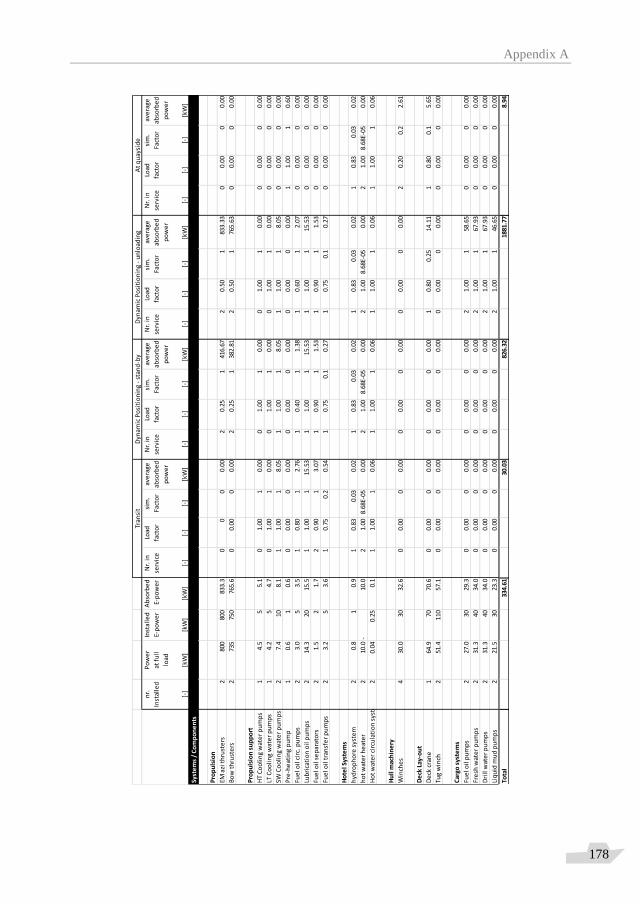
Appendix A
178
nr.
Inst
alle
d
[-]
Po
we
r
at f
ull
load
[kW
]
Inst
alle
d
E-p
ow
er
[kW
]
Ab
sorb
ed
E-p
ow
er
[kW
]
Nr.
in
serv
ice
[-]
Load
fact
or
[-]
sim
.
Fact
or
[-]
ave
rage
abso
rbe
d
po
we
r
[kW
]
Nr.
in
serv
ice
[-]
Load
fact
or
[-]
sim
.
Fact
or
[-]
ave
rage
abso
rbe
d
po
we
r
[kW
]
Nr.
in
serv
ice
[-]
Load
fact
or
[-]
sim
.
Fact
or
[-]
ave
rage
abso
rbe
d
po
we
r
[kW
]
Nr.
in
serv
ice
[-]
Load
fact
or
[-]
sim
.
Fact
or
[-]
ave
rage
abso
rbe
d
po
we
r
[kW
]
Syst
em
s /
Co
mp
on
en
ts
Pro
pu
lsio
n
EM a
zi t
hru
ste
rs2
800
800
833.
30
00
0.00
20.
251
416.
672
0.50
183
3.33
00.
000
0.00
Bo
w t
hru
ste
rs2
735
750
765.
60
0.00
00.
002
0.25
138
2.81
20.
501
765.
630
0.00
00.
00
Pro
pu
lsio
n s
up
po
rt
HT
Co
oli
ng
wat
er
pu
mp
s1
4.5
55.
10
1.00
10.
000
1.00
10.
000
1.00
10.
000
0.00
00.
00
LT C
oo
lin
g w
ate
r p
um
ps
14.
25
4.7
01.
001
0.00
01.
001
0.00
01.
001
0.00
00.
000
0.00
SW C
oo
lin
g w
ate
r p
um
ps
27.
410
8.1
11.
001
8.05
11.
001
8.05
11.
001
8.05
00.
000
0.00
Pre
-he
atin
g p
um
p1
0.6
10.
60
0.00
00.
000
0.00
00.
000
0.00
00.
001
1.00
10.
60
Fue
l oil
cir
c. p
um
ps
23.
05
3.5
10.
801
2.76
10.
401
1.38
10.
601
2.07
00.
000
0.00
Lub
rica
tio
n o
il p
um
ps
214
.320
15.5
11.
001
15.5
31
1.00
115
.53
11.
001
15.5
30
0.00
00.
00
Fue
l oil
se
par
ato
rs2
1.5
21.
72
0.90
13.
071
0.90
11.
531
0.90
11.
530
0.00
00.
00
Fue
l oil
tra
nsf
er
pu
mp
s2
3.2
53.
61
0.75
0.2
0.54
10.
750.
10.
271
0.75
0.1
0.27
00.
000
0.00
Ho
tel S
yste
ms
hyd
rop
ho
re s
yste
m2
0.8
10.
91
0.83
0.03
0.02
10.
830.
030.
021
0.83
0.03
0.02
10.
830.
030.
02
ho
t w
ate
r h
eat
er
210
.0-
10.0
21.
008.
68E-
050.
002
1.00
8.68
E-05
0.00
21.
008.
68E-
050.
002
1.00
8.68
E-05
0.00
Ho
t w
ate
r ci
rcu
lati
on
sys
tem
20.
040.
250.
11
1.00
10.
061
1.00
10.
061
1.00
10.
061
1.00
10.
06
Hu
ll m
ach
ine
ry
Win
che
s4
30.0
3032
.60
0.00
00.
000
0.00
00.
000
0.00
00.
002
0.20
0.2
2.61
De
ck L
ay-o
ut
De
ck c
ran
e1
64.9
7070
.60
0.00
00.
000
0.00
00.
001
0.80
0.25
14.1
11
0.80
0.1
5.65
Tug
win
ch2
51.4
110
57.1
00.
000
0.00
00.
000
0.00
00.
000
0.00
00.
000
0.00
Car
go s
yste
ms
Fue
l oil
pu
mp
s2
27.0
3029
.30
0.00
00.
000
0.00
00.
002
1.00
158
.65
00.
000
0.00
Fre
sh w
ate
r p
um
ps
231
.340
34.0
00.
000
0.00
00.
000
0.00
21.
001
67.9
30
0.00
00.
00
Dri
ll w
ate
r p
um
ps
231
.340
34.0
00.
000
0.00
00.
000
0.00
21.
001
67.9
30
0.00
00.
00
Liq
uid
mu
d p
um
ps
221
.530
23.3
00.
000
0.00
00.
000
0.00
21.
001
46.6
50
0.00
00.
00
Tota
l33
4.61
30.0
382
6.32
1881
.77
8.94
Tran
sit
Dyn
amic
Po
siti
on
ing
- st
and
-by
Dyn
amic
Po
siti
on
ing
- u
nlo
adin
gA
t q
uay
sid
e
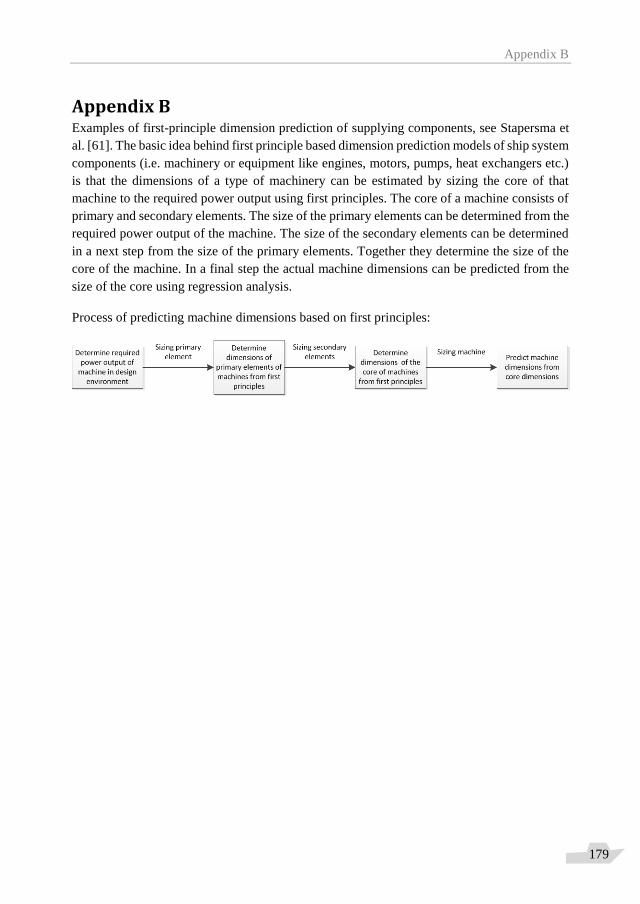
Appendix B
179
Appendix B Examples of first-principle dimension prediction of supplying components, see Stapersma et
al. [61]. The basic idea behind first principle based dimension prediction models of ship system
components (i.e. machinery or equipment like engines, motors, pumps, heat exchangers etc.)
is that the dimensions of a type of machinery can be estimated by sizing the core of that
machine to the required power output using first principles. The core of a machine consists of
primary and secondary elements. The size of the primary elements can be determined from the
required power output of the machine. The size of the secondary elements can be determined
in a next step from the size of the primary elements. Together they determine the size of the
core of the machine. In a final step the actual machine dimensions can be predicted from the
size of the core using regression analysis.
Process of predicting machine dimensions based on first principles:
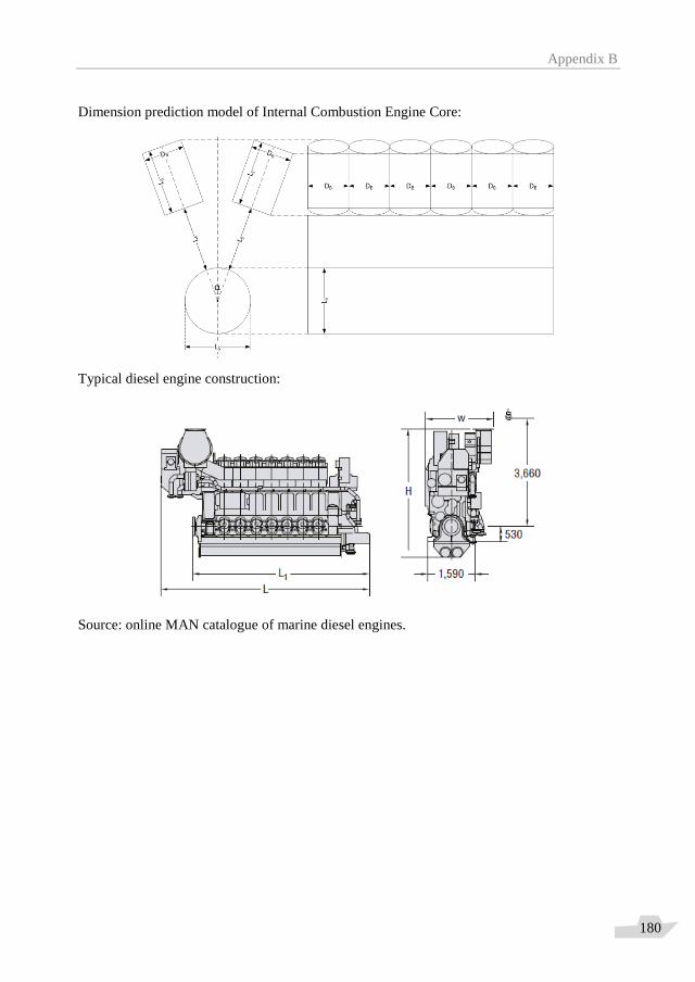
Appendix B
180
Dimension prediction model of Internal Combustion Engine Core:
Typical diesel engine construction:
Source: online MAN catalogue of marine diesel engines.
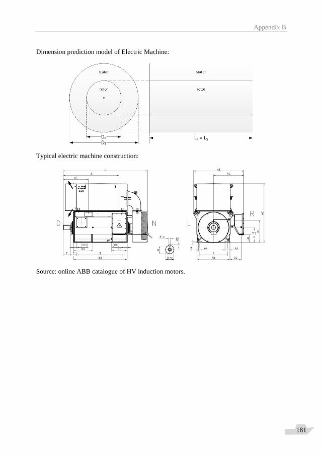
Appendix B
181
Dimension prediction model of Electric Machine:
Typical electric machine construction:
Source: online ABB catalogue of HV induction motors.
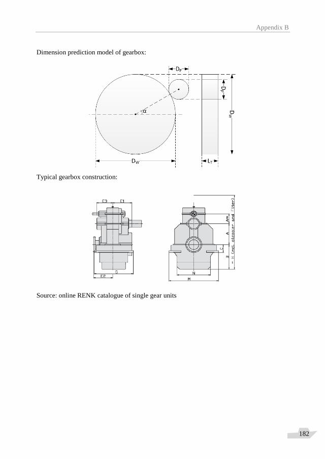
Appendix B
182
Dimension prediction model of gearbox:
Typical gearbox construction:
Source: online RENK catalogue of single gear units