Delay and Capacity Trade-off in Wireless Ad Hoc Networks withRandom Mobility

Gaurav Sharma and Ravi R. MazumdarSchool of Electrical & Computer Engineering

Purdue University, West-Lafayette, IN 47907-1285email: gsharma, mazum@purdue.edu

AbstractIn this paper, we study the delay and capacity trade-off in mobile ad hoc networks. We consider

an ad hoc network with n nodes distributed uniformly on a sphere. The nodes are mobile, andmove in accordance with the random way-point mobility model, used widely in the ad hoc networksliterature. We show that the 2-hop relaying algorithm proposed by Grossglauser and Tse (2001),incurs an expected packet delay of Θ(nTp(n)), where Tp(n) is the packet duration. We show thatany protocol that allows only nearest neighbor transmissions, incurs an expected packet delay ofΩ(Tp(n)

√n). We show that the trade-off: delay/capacity ≥ Θ(Tp(n)n), is both necessary as well as

sufficient in mobile ad hoc networks. A protocol which introduces redundancy into the 2-hop relayingalgorithm, and offers a throughput of Θ(1/k(n)) and an expected packet delay of Θ(nTp(n)/k(n)),for any k(n) = O(

√n), is developed.

Keywords: Ad Hoc Networks, Random Mobility, Delay, Throughput Capacity, Scaling Laws.

1 Introduction

Ad hoc networks are autonomous systems of nodes (routers) which communicate with each other

without a fixed infrastructure usually via wireless links. The nodes in an ad hoc network can be either

static or mobile. In their seminal work, Gupta and Kumar [1], have shown that for a random wireless

network with n static nodes, the per node capacity is Θ( 1√n log n

)1. Thus each node gets a vanishingly

small throughput as the node density grows. This is a negative result as it implies that ad hoc networks

are not scalable. Grossglauser and Tse [2], have shown that a constant per node throughput can be

achieved in the case of mobile ad hoc networks. However, no bounds on the packet delay are provided

in [2].1We use the following asymptotic notation throughout:

f(n) = O(g(n)) ↔ lim supn→∞

f(n)

g(n)< ∞, f(n) = o(g(n)) ↔ lim

n→∞f(n)

g(n)= 0,

f(n) = O(g(n)) ↔ g(n) = Ω(f(n)), f(n) = o(g(n)) ↔ g(n) = ω(f(n))

f(n) = Θ(g(n)) ↔ f(n) = O(g(n)) and f(n) = Ω(g(n))

1

Clearly, the usefullness of the throughput result is limited since both quantities, the delay and

throughput, are important. A little amount of reflection also shows that there is a trade-off between

the two quantities in that one can only be improved at the expense of the other. Characterization of

this trade-off would not only provide useful insights about the fundamental limits of mobile ad hoc

networks, but would also help in the design of novel and superior scheduling and relaying algorithms.

The delay and capacity trade-off in mobile ad hoc networks has attracted a lot of attention recently.

Delay limited capacity of ad hoc networks has been addressed in [15]. Their work is motivated by the

diversity coding approach given in [12]. Geographical routing with maximum delay guarantees is

considered in [13]. In [11], the authors derive the delay and capacity trade-off for a cell partitioned

network with a so-called instantaneous or infinite mobility model, where each node’s location in a

future time-slot is independent of its present and past locations. This independence assumption greatly

simplifies the analysis but at the same time makes the model quite unrealistic. Our work complements

their work in the sense that we consider more realistic mobility model.

Toumpis and Goldsmith [5] present a scheme that can achieve a per-node capacity of Θ(nd−12 / log

52 n)

under a bound of O(nd) on the packet delay. Ignoring the logarithmic term, we see that the trade-off,

λ2 ≤ O(

dn

), is achievable in [5], where λ is the average throughput and d the average delay. Lin and

Shroff [10] improved their results and showed that the trade-off, λ3 ≤ O(

dn

), is achievable under the

same settings. Both these works assume a mobility model similar to the infinite mobility model in [11].

El Gamal et al [6] consider the delay and capacity trade-off in wireless networks using a random walk

mobility model on a torus. They consider a cellular network and use a cellular TDMA transmission

scheme in which each cell becomes active at regularly scheduled cell time-slots. Their scheme achieves

the trade-off given by λ = Θ(1/√

na(n) log n) and d = O(log4 (1/a(n))/√

a(n)v(n)), where a(n) is

the area of each cell and v(n) is the speed of the nodes. It is interesting to note that all these above

mentioned trade-offs are between the packet delay and the throughput per node, and different packet

size scalings have been assumed in each of these works. It is intuitively clear that the packet delay

would be dependent on the size of the packet. How does one compare these trade-offs? Is there any

fundamental trade-off for mobile ad hoc networks which holds irrespective of the packet size scaling?

These questions along with others are answered in this paper.

The main contributions of this paper are the following. We derive the delay and capacity trade-off

2

with the random way-point mobility model, which is used widely in the ad hoc networks literature,

and is much more realistic than the mobility models considered in [11, 6, 5, 10]. Also, the protocols

that we consider in this paper are totally distributed, and very simple to implement, unlike the ones

in [5, 10, 6], which require co-ordination between large number of nodes.

The remaining paper is organized as follows. In Section 2, we introduce our model and discuss some

previous results. In section 3, we analyze our mobility model in detail. The delay performance of the

distributed 2-hop relaying protocol is analyzed in section 4. In Section 5, we develop an alternative

relaying protocol for delay improvement, and analyze its performance. Delay and capacity trade-offs

are considered in Section 6. We end this paper with some concluding remarks in section 7.

2 Model and Prior Results

We consider an ad hoc network formed by n mobile nodes distributed uniformly and independently

on the surface of a sphere of radius R at the start. The nodes move in accordance with the random

way-point mobility model, which is described in the next subsection. Since we are interested in the

asymptotic throughput capacity and delay, we consider n to be large in the sequel.

We consider a typical interference based transmission model as in [3, 2, 15, 1]. Node i is capable of

transmitting W bits/sec to node j, at time t, if

Pi(t)γij(t)No + 1

L

∑k 6=i Pk(t)γkj(t)

> β,

where Pi is the transmit power of node i, γij(t) is the channel gain from node i to node j at time t, No

is the background noise power, L is the processing gain of the system, and β is the SINR requirement

for successful communication. The channel gain is assumed to be of the form

γij(t) =1

dij(t)α

where dij(t) is the distance between the nodes i and j, at time t, and typically, α ∈ (2, 4].

All nodes generate traffic at the same rate and each node sends packet to a unique destination.

This makes sure that no node can become the bottleneck in the network, resulting in a decrease of the

3

per node throughput, like in the multi-access channels.

The two most widely used mobility models in ad hoc networks literature are the random way-point

mobility model, and the random walk (Brownian) mobility model (see [14]). In this paper, we focus

mainly on the random way-point mobility model. Brownian mobility model has been considered in [3].

We now describe the random way-point mobility model in detail.

2.1 Random Way-point Mobility Model (RWMM)

In this model, at each time-step the mobile node chooses a random destination on the sphere and

moves toward it with a random speed. The speed is chosen uniformly from the interval [vmin, vmax],

where vmin(n) and vmax(n) are strictly positive. The movement is along the great circle that passes

through the initial position and the final destination. On reaching the destination, the node pauses for

a random amount of time and the process repeats itself. In this paper, we consider the RWMM with

no pause times. The pause times can easily be accounted for with only a minor set of changes in the

analysis.

We now describe the distributed 2-hop relaying protocol, which is analyzed in detail in the next

section.

2.2 Distributed 2-Hop Relaying Protocol

In this protocol, the packets are either transmitted directly from the source to the destination, or via

a single relay node. Let Mi(t) be the number of source node i packets that destination d(i) receives,

up to time t. Then we say that a long term throughput of λ(n) is feasible, if for every S − D pair i,

we have,

lim infT→∞

Mi(T )T

≥ λ(n) (2.1)

We assume a slotted system. In every time-slot, each node randomly and independently decides

to be a sender or a potential receiver. In particular, each node flips a biased coin and decides to be a

sender with probability p, and otherwise decides to be a potential receiver. The sender density (p) is

a global parameter known to all the nodes in the network. The optimal value of p depends on the size

4

of the neighborhood of a typical node. Larger the size of the neighborhood, the smaller p should be.

After deciding to be a sender, each sender node transmits to its nearest neighbor with a unit

transmit power. It is however possible that the nearest neighbor decided to be a sender as well. In that

case, it certainly cannot receive the packet. Even when the nearest neighbor decided to be a potential

receiver, the packet transmission might fail due to the interference generated by other simultaneous

transmissions in the network.

The following strategy is used by each sender node to choose which packet to send to its nearest

neighbor:

1. If there is a packet generated locally for the nearest neighbor, then, send it. (S-D transmission)

2. If no such packet is found, then randomly choose one of the following two options with equal

probability:

• If there is a packet destined for some other node in the network, then, send it. Else remain

idle. (S-R transmission)

• If there is packet destined for the nearest neighbor, then, send it. Else remain idle. (R-D

transmission)

Let Nt be the number of successful sender-receiver pairs per slot, in [2] it is shown that

limn→∞

E[Nt]n

= φ > 0 (2.2)

The main reason why we can have Θ(n) concurrent nearest neighbor transmissions is that the

received power at the nearest neighbor is of the same order as the total interference generated by Θ(n)

number of interferers (see [8], for a similar proof).

For simplicity, we assume that all nodes have the same radius of communication, say, r(n). Thus,

two nodes can communicate if and only if they are within distance r(n) of each other. It is clear that

r(n) should scale down with n to prevent the interference from becoming excessive as n grows. In

[4], we show that this simplified model of communication is equivalent to the interference based model

(in terms of the throughput and delay), provided r(n) is Θ(1/√

n). In the sequel, we consider this

simplified model of communication.

5

3 Random Way-Point Mobility Model: Contact Time And Inter-

Meeting Time

In this section, we define several new concepts, which are required for the analysis of the delay in the

following sections. We start by defining the notion of the contact time, Tc(n), which characterizes the

duration of a typical wireless link in the network.

Definition 3.1 (Contact time) Consider any two arbitrary nodes, say i and j, with positions Xi(t)

and Xj(t), respectively, at time t. We define,

Tc(n) = inft : dS(Xi(t),Xj(t)) ≥ r(n) | dS(Xi(0),Xj(0)) = r(n)/2, dS(Xi(0−),Xj(0−)) > r(n)/2

The use of r(n)/22 instead of r(n) in the above definition is to ensure that all contacts be at least

as long as the packet duration. The following Lemma shows how Tc(n) is related to r(n) and v(n).

Lemma 3.1 The expected contact time, ETc(n), is Θ(

r(n)v(n)

).

Proof: The nodes must at least travel a relative distance of r(n)/2 in order to move out of contact, and

the time for this is at least Θ(r(n)/v(n)). Further, if the nodes travel a relative distance of 3r(n)/2

then they are guaranteed to be out of contact, and the time for this is at most Θ(r(n)/v(n)).

Let Tp(n) denote the transmission time or the duration of a packet. Then, in order for a packet

transmission to be successful, the communicating nodes must remain in contact for a length of time

longer than the packet duration. Hence, Tp(n) must be O(Tc(n)). Without much loss of generality, we

assume Tp(n) to be Θ(Tc(n)). This is in some sense the best case, as making Tp(n) = o(Tc(n)) does

not reduces the packet delay, but increases the overhead per packet.

The packet delay under the D2HRP, and other mobility dependent relaying protocols, is related

to how frequently any two arbitrary nodes in the network come in contact with each other or their

inter-meeting time, I(n).

Definition 3.2 (Inter-meeting time) Consider any two arbitrary nodes, say i and j, with positions2The factor of half is not really important here, εr(n), such that 0 < ε < 1, would also be fine.

6

Xi(t) and Xj(t), respectively, at time t. We define,

I(n) = inft : dS(Xi(t),Xj(t)) ≤ r(n)/2 | dS(Xi(0),Xj(0)) = r(n), dS(Xi(0−),Xj(0−)) < r(n)

It turns out that in order to estimate the delay under the D2HRP, we need to estimate the first

two moments of the inter-meeting time. Our approach is to bound the complementary distribution of

the inter-meeting time, and hence obtain a bound on all higher order moments of the inter-meeting

time. Without any loss of generality, consider the nodes to be placed on a unit sphere (unit area), and

define:

• S2 = The surface of the unit sphere centred at the origin

• dS(x, y) = The distance between the two points x and y on S2.

• ℵ = The north pole.

• < = x ∈ S2: dS(x,ℵ) ≤ r(n)/2.

We start with the following Lemma which shows that the probability that a line connecting two

random points on S2 intersects with < is Θ(r(n)).

Lemma 3.2 Let L be a line connecting two uniformly and independently chosen points on S 2. Then,

there exists strictly positive constants c1 and c2 such that c1r(n) ≥ P(L intersects <) ≥ c2r(n), for

large enough n.

Proof: Let the two points be X and Y. We first establish the upper bound. If X lies at a distance

x, > r(n)/2, from the north pole then the angle β subtended at X by < is no more than c3r(n)/x. The

area of the sector so formed is no more than c4r(n)/x. If Y does not lie in this sector then L cannot

intersect <. Since, Y is uniformly distributed on S2, the probability of this is no more than c4r(n)/x.

Since, X is uniformly distributed on S2, the probability density that it is at a distance x from the

north pole is√

π sin (2√

πx). Integrating over all possible values of x, we get:

7

P (L intersects <) ≤ c5r2(n) +

∫ √π

2

r(n)2

c4r(n)x

√π sin (2

√πx)dx

≤ c5r2(n) + c4π

32 r(n) (Using sinx ≤ x, for x ≥ 0)

≤ c1r(n) (For n large enough) (3.1)

provided c1 is chosen to be large enough.

S

x

1/4

T1

T2

ℜ

A

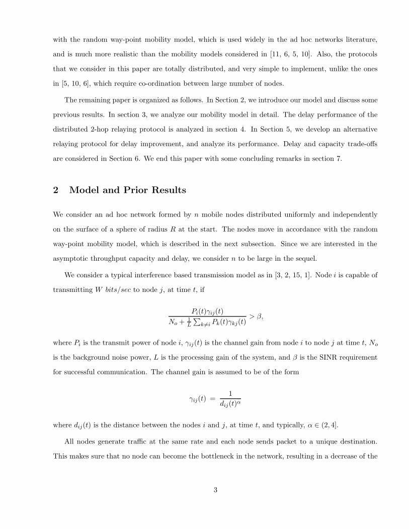
Figure 1: The figure shows the top view of the regions A and <. For convenience sake, the distances shown are theactual distances and not the ones which one would observe in a top view.

To prove the lower bound, suppose that X is at a distance x, ≤ √π/4, from the north pole. Draw

the tangent lines from X to <. Let T1 and T2 be their points of intersection with <. Consider the

rectangular region A with T1 and T2 as two of its vertices as shown in the Figure 3. If Y lies in A then

L interse cts <. The area of the region A, and hence the probability that Y lies in A, is at least c5r(n).

Noting that the probability that x≤ √π/4 is 1/2, and taking c2 = c5/2, the result follows.

The following Lemma establishes the monotonicity property of the conditional intersection proba-

bility. This is a key result for establishing the lower bound on the complementary distribution of the

inter-meeting time.

Lemma 3.3 Let X1 and X2 be two arbitrary points on S2, with 0 ≤ dS(X1,ℵ) ≤ dS(X2,ℵ) ≤ √π/2.

Consider the lines L1 and L2 joining X1 to Y1 and X2 to Y2, respectively, with Y1 and Y2 distributed

uniformly on S2. Then, P (L1 intersects <) ≥ P (L2 intersects <).

Proof: The proof is constructive. Join X2 with ℵ, along the great circle on which they lie. Denote

by T2, the line segment joining X2 with ℵ. Without any loss of generality, we assume that X1 lies on

8

this line segment. Let A1 (respectively A2) denote the region on S2 in which Y1 (respectively Y2) must

belong in order for L1 (respectively L2) to intersect with <. Then, it is easily seen that A1 ⊃ A2.

Since, Y1 and Y2 are uniformly distributed on S2, the result follows.

Consider a node, say i, distributed uniformly on S2 at time t = 0, and let Xi(t) be its position at time

t. Define F (n) = inft : Xi(t) ∈ <. Also, define If (n) = inft : dS(Xi(t),ℵ) ≤ r(n)/2 | dS(Xi(0),ℵ) =

r(n). Then, it is clear that I(n) = Θ(If (n))3. In what follows, we first bound the complementary

distribution of F (n), and then by proving that If (n) = Θ(F (n)), we extend those bounds to I(n).

The following Lemma gives an upper bound on the complementary distribution of F (n).

Lemma 3.4 With F(n) as defined above, we have

1. P(F (n) > m

√π

vmin(n)

)≤ (1 − c2r(n))m

2. EF (n) ≤√

πc2r(n)vmin(n)

3. EF 2(n) ≤ π(c2r(n)vmin(n))2

Proof: Let N denote the random variable indicating the number of trips that node i makes (including

any incomplete one) before entering into <. Define Γj = jth trip does not intersect <. Since the

duration of each trip is bounded above by√

π/2vmin(n), we have P (F (n) > m√

π/vmin(n)|N ≤ 2m) =

0, and hence

P

(F (n) >

m√

π

vmin(n)

)= P

(F (n) >

m√

π

vmin(n)|N > 2m

)P (N > 2m)

≤ P (N > 2m)

≤ P (Γ1 ∩ Γ3 ∩ ... ∩ Γ2m−1)

≤ (1 − c2r(n))m (3.2)

where the last equation follows by noting that Γi for odd i are independent, and from Lemma 3.2, we

have P (Γi) ≥ (1 − c2r(n)). This proves I.

3This is to be interpreted as EIk(n) = Θ(EIkf (n)), ∀k.

9

Using the non-negativity of F (n) along with (3.2), we have

EF (n) =∫ ∞

0P (F (n) > x)dx

≤√

π

vmin(n)

∞∑m=0

(1 − c2(r(n))m

=√

π

c2r(n)vmin(n)(3.3)

This proves II. Similarly, we have

EF 2(n) =∫ ∞

0xP (F (n) > x)dx

≤ π

v2min(n)

∞∑m=0

(m + 1)(1 − c2(r(n))m

=π

(c2r(n)vmin(n))2(3.4)

And III is proved.

To establish a lower bound on the complementary distribution of F (n), we need some more results.

The following Lemma shows that the kind of dependency that exists between successive trips (end

point of the current trip is the starting point of the next trip) in the RWMM, makes it more likely that

the number of trips that a node makes before it enters into < would be larger, as compared to the case

where the successive trips are independent.

Lemma 3.5 Let N be defined as before, then P (N > m) ≥ (1 − c1r(n))m.

Proof: With Γi defined as before, we have

P (N > m) = P (Γ1 ∩ Γ2 ∩ ... ∩ Γm)

= P (Γ1)m∏

i=2

P (Γi|Γ1 ∩ Γ2 ∩ ... ∩ Γi−1)

≥m∏

i=1

P (Γi)

≥ (1 − c1r(n))m (From Lemma 3.2) (3.5)

10

The only step which requires an explanation is the third step. Consider a point X, distributed uniformly

on S2, and define U(x) = P (dS(X,ℵ) > x). We say that F G if F (x) ≥ G(x), ∀x ∈ [0,∞). Given

that the first i trips do not intersect <, the distribution of the starting point of the (i + 1)th trip, Si+1,

is skewed. Let C(x) = P (dS(Si+1,ℵ) > x), then a simple Bayesian argument, using Lemma 3.3, implies

that C U . This implies that P (Γi|Γ1 ∩ Γ2 ∩ ... ∩ Γi−1) ≥ P (Γi).

Consider an i.i.d sequence of lines, (Li)∞i=1, connecting two uniformly and independently chosen

points on S2, and define (li)∞i=1 to be the corresponding sequence of lengths. The following Lemma is

a simple application of the Tchebychev’s inequality under the i.i.d case.

Lemma 3.6 P(∑m

i=1 li < ml2

)≤ σ2

l

4ml2 , where l and σ2

l are the common mean and variance, respec-

tively, of li.

Proof: By Tchebychev’s inequality, we obtain

P

(m∑

i=1

(li − l) >ml

2

)≤ σ2

l

4ml2

Since, P(∑m

i=1(li − l) > ml2

)≥ P

(∑mi=1 li < ml

2

), the result follows.

Define ζm = ∩mi=1Li does not intersect <. Given that ζm has occurred, it is more likely that the

first m trips were short in length, rather than long. However, the following Lemma shows that the

conditional lengths of the trips are not too different from the unconditional lengths.

Lemma 3.7 P (∑m

i=1 li > x|ζm) ≥ P (∑m

i=1 li > x)(1 − c1r(n))m.

Proof: Let us look at the probability that Li would intersect <, given that li = l. It is easy to

see that the upper bound on the intersection probability of c1r(n), as derived in Lemma 3.2, is valid

in this case irrespective of l. This implies that P (ζi|li = l) ≥ (1 − c1r(n)) for all possible values of l.

Using this, together with the independence of Li’s, we obtain

P

(m∑

i=1

li > x | ζm

)≥ P

(m∑

i=1

li > x ∩ ζm

)(3.6)

≥ (1 − c1r(n))mP (m∑

i=1

li > x) (3.7)

11

We are now ready to give a lower bound on the complementary distribution of F (n).

Lemma 3.8 1. P(F (n) > lm

2vmax(n)

)≥ 1

2(1 − c1r(n))m.

2. EF (n) ≥ l16c1r(n)vmax(n) .

3. EF 2(n) ≥ l2

64(c1r(n)vmax(n))2.

Proof: Let (di)∞1=1 denote the lengths of the trips that a node makes under the RWMM. We have,

P

(F (n) >

ml

2vmax(n)

)≥ P

(F (n) >

ml

2vmax(n)| N > m

)P (N > m)

≥ P

(m∑

i=1

di >ml

2| N > m

)(1 − c1r(n))m (From Lemma 3.5)

≥ P

(m∑

i=1

li >ml

2| ζm

)(1 − c1r(n))m (3.8)

≥ P

(m∑

i=1

li >ml

2

)(1 − c1r(n))2m (From Lemma 3.7)

≥(

1 − σ2l

4ml2

)(1 − c1r(n))2m (From Lemma 3.6)

≥ 12(1 − c1r(n))m (For all m ≥ mo, where mo is chosen to be large enough)

(3.9)

where (3.8) follows from the fact that the dependence between the trips in the RWMM makes it more

likely for a node to spend long times before entering into <. This proves I.

Non-negativity of F (n) implies:

EF (n) =∫ ∞

0P (F (n) > x)dx

≥ l

4vmax(n)

∞∑m=mo

(1 − c1r(n))2m

≥ l

4vmax(n)(1 − c1r(n))2mo

2c1r(n)

≥ l

16c1vmax(n)r(n)(For large enough n) (3.10)

12

This proves II. To prove III, we use the non-negativity of F(n) once more, to obtain

EF 2(n) =∫ ∞

0xP (F (n) > x)dx ≥ l

2

8v2max(n)

∞∑m=mo

m(1 − c1r(n))2m

≥ l2

8v2max(n)

(1 − c1r(n))2mo

∞∑m=0

m(1 − c1r(n))2m

≥ l2

64(c1r(n)vmax(n))2(For large enough n) (3.11)

Now, we are ready to prove that If (n) = Θ(F (n)).

Lemma 3.9 If (n) = Θ(F (n)).

Proof: Let us consider a node moving under the RWMM. As required in the inter-meeting time

definition, assume that the node is at a distance of r(n) from ℵ at time t = 0. Let us denote by

To the time remaining in current trip of the node, and by T1 the time duration of the next trip, which

we denote by T1. At time To +T1 the node will be at a uniformly distributed point on S2, and it would

require F (n) amount of time for the node to come inside <. Now, since the duration of all trips is

upper bounded by√

π/2vmin(n), we obtain

P (If (n) > x +√

π/2vmin(n)) ≤ P (F (n) > x) (3.12)

This establishes the upper bound. To derive the lower bound, we note that given T1 does not intersect

with <, the distribution of the end point of the trip T1 is skewed in such a way that it is less likely that

the next trip would intersect with <. Therefore, the time taken by the node to come within < would

be at least F (n). Since the probability that T1 would intersect with < is less than c1r(n), we obtain

P (If (n) > x) ≥ P (F (n) > x)(1 − c1r(n)) (3.13)

From (3.12) and (3.13) it follows that all the moments of If (n) and F (n) are of the same order, i.e.,

If (n) = Θ(F (n)).

Using Lemmas 3.4, 3.8, and 3.9, together with the fact that I(n) = Θ(If (n)), we arrive at the main

result of this section.

13

Proposition 3.1 Let I(n) denote the inter-meeting time of an arbitrary pair of nodes under the

RWMM. Then there exist positive constants c1, c2, c6, and c7, such that:

1. P(I(n) > c6m

v(n)

)≥ 1

2(1 − c1r(n))m.

2. P(I(n) > c7m

v(n)

)≤ (1 − c2r(n))m.

3. EI(n) = Θ(

1r(n)v(n)

), and EI2(n) = Θ

(1

r2(n)v2(n)

). Assuming, Tp(n) = Θ(Tc(n)), we note

that: EI(n) = Θ (nTp(n)), and EI2(n) = Θ(n2T 2

p (n)).

Here v(n) is the average velocity of the nodes.

So far we have not discussed how the velocity of the nodes should scale with n. In this paper, we

consider the following two, perhaps extreme, possibilities:

I. vmin(n) = vmax(n) = Θ(1)4: In this case, Lemma 3.1 implies that the Tc(n) is Θ(1/√

n), and

hence Tp(n) must be Θ(1/√

n) as well. We refer to this as the variable packet size strategy

(VPSS).

II. vmin(n) = vmax(n) = Θ(1/√

n): In this case, Lemma 3.1 implies that the Tc(n) is Θ(1), and

hence Tp(n) is Θ(1) as well. We refer to this as the fixed packet size strategy (FPSS).

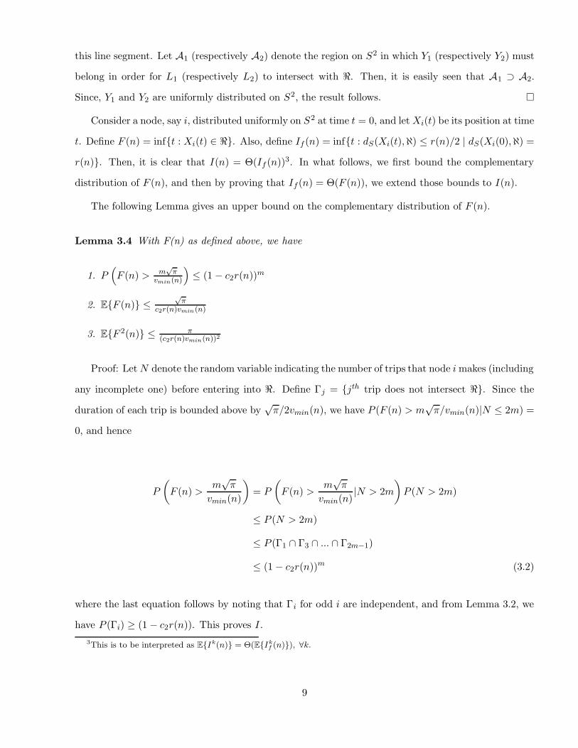
0 20 40 60 80 100 120 140 160 180 2000

0.5

1

1.5

2

2.5

x 108

Number of Nodes

Exp

ecte

d F

irst−

Mee

ting

Tim

e

Expected First−Meeting Time vs Number of Nodes (RWMM)Linear Fit

Figure 2: Expected inter-meeting time vs n, for R =100, Tp(n) = 1ms, and v(n) = r(n) = 1√

n.

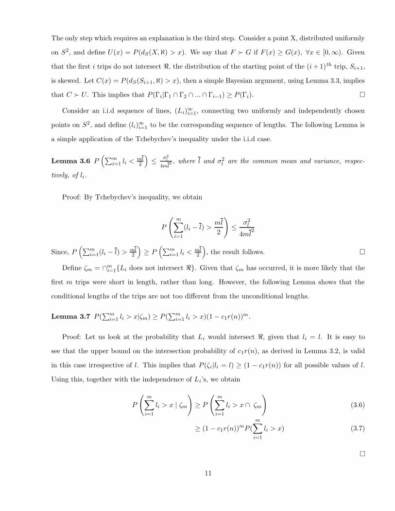
0 2 4 6 8 10 12 14 1610

−7

10−6

10−5

10−4

10−3

10−2

10−1

100

Normalized Inter−Meeting Time

Com

plem

enta

ry D

istr

ibut

ion

Complementary Distribution of the Normalized Inter−Meeting Time (RWMM)Complementary Distribution of an exponential random variable

Figure 3: Complementary distribution of the inter-meeting time, for R = 100, n = 50, Tp(n) = 1ms, andv(n) = r(n) = 1√

n.

Our simulation results (see Figure 2) are in complete agreement with these analytical results.

The simulation results seem to suggest that the distribution of the inter-meeting is exponential. The

exponential distribution assumption is used in [3] to simplify the analysis, and the results obtained are

quite similar to this paper.4This is to be interpreted as: ∃ positive constants c1 and c2, independent of n, such that, c1 < vmin(n) ≤ vmax(n) < c2.

14

4 Delay And The D2HRP

Consider a network with n nodes and n S-D pairs, with all nodes following the D2HRP. In most cases,

the packet delay has two components, the queuing delay at the source node and the queuing delay at

the relay node. Sometimes the packet might be directly transmitted from the source to the destination,

eliminating the queuing delay at the relay node. It is easily seen that the S-D transmissions contribute

only Θ(1/n) to the throughput, and hence can be ignored during the analysis. Henceforth, we assume

that every packet travels exactly two hops, i.e., from the source to the relay, and then from the relay

to the destination.

Consider the source queue at some arbitrary node, say, node i. To account for the queuing delay

at the source, we assume that the input to this source queue is a Bernoulli stream of rate λi. The

following Lemma gives the queuing delay at such a queue.

Lemma 4.1 If the exogenous packet stream at node i is Bernoulli with rate λi, where λi < φ2 , then

a) the expected queuing delay (EDsi ) at the source node i, is given by

EDsi = Tp(n)

1 − λi

φ2 − λi

(4.1)

b) and the output process from the queue is Bernoulli stream of rate λi.

Proof: We know that in the case of the distributed 2-hop relaying protocol, for large enough n, the

total number of successful sender-receiver pairs per slot are roughly nφ. Since the R-D transmissions

and the S-R transmissions are given equal priority, the service time at any source is Bernoulli with rate

φ2 . Now, (a) follows by noting that the source is a Bernoulli(λi)/Bernoulli(φ

2 ) queue. And (b) follows

from the reversibility of the Bernoulli/Bernoulli queues.

Consider any arbitrary S-D pair in the network. The packets from the source can reach the desti-

nation via any of the n− 2 relay nodes. As in [2], we assume that the relay nodes maintain a separate

queue for each of the S-D pairs (see Figure 4). Since Tp(n) = Θ(Tc(n)), Θ(1) packets are exchanged

during a contact between any two nodes. Hence, the packet stream from the source is distributed

evenly between the relay nodes. Consider one such relay queue, the arrival to the queue occurs when

the source sends a packet to the relay node, and the departure from the queue takes place when the

relay node delivers a packet to the destination node. It is clear that the inter-arrival time and the

15

2

1

n−2

S−R Transmission

S−R Transmission

S−R TransmissionS−R T

rans

miss

ion

R−D Transmission

R−D Transmission

R−D Transmission

R−D Transmission

: : :

:

DS

R

R

R

R

Direct S−D Transmission

Figure 4: Network model for a particular S-D pair. The source queue is a simple Bernoulli(λ)/Bernoulli( φ2). Each packet

either goes directly to the destination or through one of the n − 2 relay nodes. The relay queues are GI/GI/1-FCFS.

inter-departure time for this queue are of the same order as the inter-meeting time of any two arbitrary

nodes in the network. We are now ready to estimate the overall queuing delay.

Proposition 4.1 If all the nodes move in accordance with the RWMM, and if the exogenous packet

stream at node i is Bernoulli with rate λi, where λi < φ2 , then the expected packet delay for the source

node i is Θ(Tp(n)n).

Proof: Since the inter-meeting time scales as Θ(nTp(n)), the queuing delay at the relay queue must

at least be Θ(nTp(n)). Hence, the queuing delay at the source node can simply be ignored. Using the

first and the second moment of I(n), as given in Proposition 3.1 (part III), along with the Kingman’s

([9]) upper bound on delay given for a GI/G/1-FCFS queue (see [7]), the result follows.

The following corollary is a direct consequence of proposition 4.1.

Corollary 4.1 If all the nodes move in accordance with the RWMM, then the expected packet delay

scales as Θ(n) under the FPSS, and Θ(√

n) under the VPSS.

Our simulation results are in complete agreement with these theoretical results. Due to space

constraints, we do not include them here.

5 Distributed 2-Hop Relaying With Redundancy

The D2HRP provides Θ(1) throughput per node, but incurs a large packet delay of the order of

Θ(nTp(n)). For most of the applications, such large packet delay would be impossible to tolerate. In

16

this section, we consider a simple distributed protocol that gives a much better delay performance than

the D2HRP by introducing redundancy into the system. Before discussing the protocol any further, let

us first look at how much the delay can possibly be improved. It turns out that there is a fundamental

lower bound on the packet delay which is valid under all protocols which allow only nearest neighbors

to communicate with each other.

Proposition 5.1 For a network with n nodes, moving in accordance with the RWMM, no scheduling

or relaying protocol which allows only nearest neighbor to communicate can guarantee an expected delay

better than Θ(Tp(n)√

n).

Proof: Note that since the S-D pairs are chosen randomly, each packet travels an expected distance of

Θ(1) before reaching the destination. Further, since Tc(n) = Ω(Tp(n)), the packet travels a distance of

O(1/√

n) per time-slot due to mobility. Since, only nearest neighbor communications are allowed the

distance travelled due to relaying is also O(1/√

n) per time-slot. Hence, in any time-slot the packet

travels an aggregate distance of O(1/√

n) towards the destination, and the result follows.

We now describe the distributed 2-hop relaying protocol with redundancy (D2HRP-WR), which

can achieve the above mentioned lower bound on the delay.

In the D2HRP-WR, each source node sends duplicate copies of the packet to new relay nodes,

whenever possible. The packet is delivered to the destination either by the source node or one of the

relay nodes. Clearly, once the packet is delivered to the destination, there is no need for any node to

hold the packet in its queue. But, notifying all the nodes which currently hold the packet in their queue

would result in too much of overhead. To avoid this overhead we follow the same approach as in [11].

All source nodes maintain a send number (SN). The source node increments the SN before sending a

new packet, and all subsequent copies of the packet are sent with same SN. Each destination maintains

a request number (RN), which is delivered to the transmitter before any R-D or S-D transmission.

The source node sends at most k(n) duplicate copies of the packet. This k(n) can be varied depending

upon the requirements of the application.

The detailed implementation of the protocol is as follows.

In each time-slot each node independently decides to be a sender or a potential receiver, just like

in the case of the D2HRP. Then, one of the following three actions is performed by each successful

sender-receiver pair:

17

I. S-D Mode: If the sender node has packets generated locally for the receiver then it asks the

receiver for the current RN. All packets with SN < RN are deleted from the source. If a packet

with SN=RN is found, then it is transmitted to the receiver, and the sender and the receiver

increment their corresponding numbers, i.e., SN=SN+1 and RN=RN+1.

II. If no such packet exists then the sender chooses one of the following two options with equal

probability:

• S-R Mode: The sender transmits the packet with current SN, and does so upon every

transmission opportunity until k(n) replicas have been delivered to distinct nodes. After

such a time, SN is incremented to SN+1. If the sender node does not have any such packet

to send, then it remains idle for that slot.

• R-D mode: As in the case of the S-D Mode, the sender asks the receiver for the current RN,

and deletes all the packets with SN < RN. If any packet with SN=RN is found then it is

sent to the receiver, and the receiver increments RN to RN+1. If no such packet is found

then the sender remains idle for that slot.

Note that the above protocol guarantees an in-order delivery of the packets to the destination. The

performance of the protocol can be improved slightly by allowing out of order packet delivery. We do

not consider such a possibility in this paper.

The following Proposition states the main result of this section.

Proposition 5.2 Consider a network with n nodes, moving in accordance with the RWMM, and fol-

lowing the D2HRP-WR. Let ED(n) be the expected packet delay, and λ(n) be throughput per node.

Then, for any k(n) = O(√

n), we have ED(n) = Θ(

nTp(n)k(n)

)and λ(n) = Θ

(1

k(n)

). In particular,

when k(n) = Θ(√

n), then, ED(n) = Θ(Tp(n)√

n) and λ(n) = Θ(

1√n

).

Proof: Consider a packet generated at an arbitrary source node at time t = 0. For the time being,

assume that it is the only packet generated at the source, i.e., there is no delay due to queuing at

the relay nodes. Once the packet reaches the head of the line at the source queue, the time required

to reach the destination is at most T (n) = T1(n) + T2(n), where T1(n) is the time required by the

source node to send the packet to k(n) other nodes, and T2(n) is the time required by one of those

18

k(n) nodes to deliver the packet to the destination node. It is easy to show that T1(n) = Θ(k(n)Tp(n))

and T 21 (n) = Θ(k2(n)T 2

p (n)). Clearly, the position of these k(n) nodes, having received a packet from

the same source node, are correlated, and thus the time taken to reach the destination node are also

correlated. However, at time T1 +√

πvmin

5 these k(n) nodes are guaranteed to be uniformly distributed on

S2. Let A(n) denote the additional amount of time required by one of these nodes to come into contact

with the destination node. Clearly, A(n) is the minimum of k(n) i.i.d random variables, each of which

is Θ(F (n)) (see the definition of F (n), given in section 3). Using Lemma 3.4 and 3.1, it is easily seen

that EA(n) = Θ(nTp(n)/k(n)) and EA2(n) = Θ(n2T 2p (n)/k2(n)). Noting that

√π

vmin= Θ(

√nTp(n))

and k(n) = O(√

n), we have E(T (n)) = O(nTp(n)/k(n)) and E(T 2(n)) = O(n2T 2p (n)/k2(n)).

The SN/RN handshake ensures that newer packets do not interfere with the older packets, but

that the replication of the next packet waiting at the source queue begins at or before time T (n) after

the current packet. The packets thus view the network as a single queue to which they arrive and are

served sequentially. Using the Kingman’s [9] upper bound, it follows that the expected packet delay is

O(nTp(n)/k(n)).

The lower bound on the expected packet delay follows easily by noting that the expected packet

delay is at least as large as EA(n), which is Θ(nTp(n)/k(n)). Hence, the delay is Θ(nTp(n)/k(n)).

Further, since each packet gets relayed to Θ(k(n)) nodes, the throughput per node is Θ(1/k(n)).

Note that, making k(n) = ω(√

n) cannot reduce the delay beyond Θ(Tp(n)√

n). This follows

from the fact the D2HRP-WR allows only nearest neighbor communications, and hence according to

Proposition 5.1, must incur an expected packet delay of Ω(Tp(n)√

n).

6 Delay and Capacity Trade-offs

Note that the packet delay and throughput capacity under the D2HRP and the D2HRP-WR satisfy

delay/capacity = Θ(nTp(n)). In this section, we show that delay/capacity ≥ Θ(nTp(n)) is indeed a

necessary trade-off. The fact that the D2HRP and the D2HRP-WR achieve this trade-off with equality

establishes the sufficiency of the trade-off.

Proposition 6.1 Consider a network with n mobile nodes, moving in accordance with the RWMM,5This is twice the maximum trip duration

19

and n S-D pairs, each generating traffic at an expected rate of λ(n) packets per time-slot. Consider

any arbitrary control protocol, which is used to stabilize the network, and guarantee an expected packet

delay of ED(n). Then,ED(n)

λ(n)≥ Θ(Tp(n)n)

Proof: The proof requires a lot of algebraic manipulations, and is forwarded to the Appendix.

It is interesting to note that the above trade-off is not entirely limited to our settings. In fact, it

holds under some remarkably different settings as well, like for example the static wireless networks.

7 Concluding Remarks

In this paper, we studied the delay and capacity trade-offs in mobile ad hoc networks with the random

way-point mobility model. While there are some results available for random walk models, the RWMM

has not been considered in any of the previous works. From a practical standpoint, the random way-

point mobility model is perhaps more realistic than the random walk models.

We showed that the distributed 2-hop relaying protocol incurs a delay of Θ(nTp(n)), and that the

delay performance can be significantly improved by introducing some redundancy into the system. This

is similar in some sense to the multi-hop in static networks, where the redundancy can be thought of

as the number of hops that the packet takes to reach the destination. Although, we considered only

the random way-point mobility model in this paper, similar results can be derived under the Brownian

mobility model as well (see [3]).

We showed that trade-off, delay/capacity ≥ Θ(Tp(n)n), is both necessary as well sufficient under

the RWMM. Using similar arguments, as to those in [1, 6], it is easy to show that the same trade-off

holds for static networks as well.

Our results inspire a rich set of questions concerning the fundamental limits of mobile ad hoc

networks. It would be nice to characterize the class of mobility models for which this trade-off holds.

We believe that the trade-off would hold for all possible mobility models under which the distribution

of the nodes remains uniform at all times. Such a result can perhaps be proved using similar techniques

as in this paper.

20

References

[1] P. Gupta and P.R. Kumar. The capacity of wireless networks. IEEE Transactions on Information

Theory, vol. IT-46(2):388–404, March 2000.

[2] M. Grossglauser and D. N. C. Tse. Mobility increases the capacity of ad-hoc wireless networks.

In IEEE INFOCOM, pages 1360–1369, 2001.

[3] G. Sharma and R. Mazumdar. On Achievable Delay/Capacity Trade-offs in Mobile Ad Hoc

Networks. Workshop on Modeling and Optimization in Mobile, Ad Hoc and Wireless Networks

(WIOPT), Cambridge, UK, Mar 2004.

[4] G. Sharma and R. Mazumdar. Scaling Laws for Capacity and Delay in Wireless Ad Hoc Networks

with Random Mobility. In IEEE International Conference on Communications, Paris, June 2004.

[5] S. Toumpis and A. Goldsmith. Large wireless networks under fading, mobility, and delay con-

straints. In IEEE INFOCOM, Mar 2004.

[6] A. El Gamal, J. Mammen, B. Prabhakar, and D. Shah. Throughput-delay trade-off in wireless

networks. In IEEE INFOCOM, Mar 2004.

[7] E. Gelenbe and G. Pujolle. Introduction to Queuing Networks. Wiley, New York, 1987.

[8] B. Hajek, A. Krishna, and R.O. LaMaire. On the capture probability of large number of stations.

IEEE Trans. Commun., vol. 45, pp.254-260, Feb. 1997.

[9] J. F. C. Kingman. Inequalities in the theory of queues. J. Roy. Statist. Soc. Ser. B, 32:102–110,

1970.

[10] X. Lin and N. B. shroff. Improved delay-capacity trade-off in large mobile ad hoc networks.

Preprint, Purdue University, November 2003.

[11] M.J. Neely and E. Modiano. Capacity and delay tradeoffs for ad-hoc mobile networks. Preprint,

Dept. of EECS, MIT, 2003.

[12] A.Tsirigos and Z.J.Haas. Multipath routing in presence of frequent topological changes. IEEE

Commun. Mag., pp. 132-138, Nov 2001.

21

[13] N. Bansal and Z. Liu. Capacity, delay and mobility in wireless ad-hoc networks. In IEEE INFO-

COM, April 2003.

[14] T. Camp, J. Boleng, and V. Davies. A survey of mobility models for ad hoc network research.

In Wireless Communications and Mobile Computing (WCMC): Special issue on Mobile Ad Hoc

Networking: Research,Trends and Applications, 2002.

[15] E.Perevalov and R.Blum. Delay limited capacity of ad hoc networks: Asymptotically optimal

transmission and relaying strategy. In IEEE INFOCOM, April 2003.

8 Appendix

Proof of Proposition 6.1

Let EDi(n) be the expected packet delay for the S-D pair i. Then, we have

ED(n) =∑

i EDi(n)n

Let ERi(n) be the expected redundancy of the packets generated by the S-D pair i. Note that

the redundancy of the packet is the number of nodes who receive a copy of the packet, including

the destination node. The S-D pair i generates an expected traffic of λ(n)ERi(n) per time-slot.

Summing over all i, we obtain that the aggregate traffic generated by all the S-D pairs in the network

is λ(n)∑

i ERi(n). Since there can be at most n/2 successful transmissions per time-slot, we have:

λ(n)∑

i

ERi(n) ≤ n

2(8.1)

Now suppose that the expected redundancy, ERi(n), of the packets generated by the S-D pair i is

Ω(√

n). Since, the Proposition 5.1 implies that EDi(n) must at least be Θ(Tp(n)√

n), we obtain

EDi(n)ERi(n) ≥ Θ(nTp(n)) (8.2)

Now suppose that ERi(n) = o(√

n). Consider a packet generated at the S-D pair i. The packet has

an expected delay of EDi(n), and an expected redundancy of ERi(n). Let the random variables

22

Ri(n) and Di(n) represent the actual redundancy and delay for the packet. Then we have:

EDi(n) ≥ EDi(n)|Ri(n) ≤ 2aERi(n)PrRi(n) ≤ 2a

ERi(n)

≥ EDi(n)|Ri(n) ≤ 2aERi(n)

(1 − 1

2a

)(8.3)

where (8.3) follows from Markov Inequality, and a is a positive integer to be fixed later.

Consider a virtual system in which there are 2aERi(n) uniformly distributed nodes holding the

packet at the start. Let T (n) be the time required for one of these nodes to deliver the packet to

the destination node. Then, T (n) = Θ(Z(n)), where Z(n) is the mininum of 2aERi(n) i.i.d random

variables with the same distribution as F (n) (see the definition of F (n) in section 3). Using Lemma 3.4,

it follows that ET (n) = Θ(nTp(n)/2aERi(n)). Although, there are more nodes holding the packet

in this virtual system, the mean of T (n) does not necessarily bound EDi(n)|Ri(n) ≤ 2aERi(n).

This is because conditioning on the event Ri(n) ≤ 2aERi(n) might skew the probabilities associated

with the node mobility process. To understand this, consider an extreme case: if the redundancy of a

packet is given to be less than or equal to 1, then it would imply that the packet is sent directly from

the source to the destination. The expected delay in such a case is much smaller than the expected

delay in the case where there is only one node holding the packet at the start.

However, since the event Ri(n) ≤ 2aERi(n) occurs with a probability at least 1 − 1/2a, we

obtain the following bound:

EDi(n)|Ri(n) ≤ 2aERi(n) ≥ inf

F :P (F)≥(1− 12a )

ET (n)|F

Since T (n) = Θ(Z(n)), there exists a constant c8 > 0, such that

EDi(n)|Ri(n) ≤ 2aERi(n) ≥ c8 inf

F :P (F)≥(1− 12a )

ET (n)|F

It is clear that the event F which achieves the infimum must be F = Z(n) ≤ x : P (Z(n) ≤ x) =

1 − 1/2a, and we get

EDi(n)|Ri(n) ≤ 2aERi(n) ≥ c8EZ(n)|Z(n) ≤ x (8.4)

23

Now since Z(n) is the minimum of 2aERi(n) i.i.d random variables with the same distribution as

F (n), it follows from Lemma 3.4 and 3.8, that

P

(Z(n) >

m√

π

vmin(n)

)≤ (1 − c2r(n))2

amERi(n)

P

(Z(n) >

lm

2vmax(n)

)≥ 1

2(1 − c1r(n))2

amERi(n) (For m ≥ mo )

In order to simplify the exposition, assume that vmax(n) = vmin(n) = 1 (this corresponds to the VPSS).

A little more careful analysis along the lines of Lemma 3.2 shows that c1 and c2 can be taken to be 4

and 1/4, respectively. Since√

π < 2 and l > 1/4, we obtain

P (Z(n) > 2m) ≤ (1 − 4r(n))2amERi(n)

≤ e−2a+2mr(n)ERi(n) (Using e−x ≥ (1 − x), for 0 ≤ x ≤ 1) (8.5)

P(Z(n) >

m

8

)≥ 1

2(1 − 1

4r(n))2

amERi(n) (For m ≥ mo)

≥ 12e−2a−1mr(n)ERi(n) (For m ≥ mo , using e−2x ≤ (1 − x), for 0 ≤ x ≤ 1/2)

(8.6)

Now since P (Z(n) ≤ x) = 1 − 1/2a, from (8.6), we obtain

x ≥ (a − 1) log 22a+2r(n)ERi(n) = x1 (8.7)

Since r(n) = Θ(1/√

n) and ERi(n) = o(√

n), x1 goes to ∞ with n. This implies that for any positive

integer b (to be fixed later) there exists an integer, say x2, such that x1/2 < x2 < x1 and x2 is an

integer multiple of 2b. Since x2 is an integer multiple of 2b, x2/b is an even integer, and equation (8.6)

implies that

P(Z(n) >

x2

b

)≥ 1

2e−

2a+2x2r(n)ERi(n)b

≥ 12e−

(a−1) log 2b (Using x2 < x1)

=(

12

) a+b−1b

(8.8)

24

Using (8.5), we obtain

P (Z(n) > x2) ≤ e−2a+1x2r(n)ERi(n)

≤ e−(a−1) log 2

4 (Using x2 > x1/2)

=(

12

)a−14

(8.9)

Setting a = 13 and b = 12, we obtain P (Z(n) > x2) ≤ 1/8 and P (Z(n) > x2/b) ≥ 1/4. Now, we have

EZ(n)|Z(n) ≤ x ≥ EZ(n)|Z(n) ≤ x2 (Using x > x2)

≥ x2

b

P (x2b ≤ Z(n) ≤ x2)P (Z(n) ≤ x2)

≥ x1

2b

(P(Z(n) >

x2

b

)− P (Z(n) > x2)

)=

(a − 1) log 22a+6r(n)ERi(n)b

=log 2

219r(n)ERi(n) (8.10)

Since vmax(n) = vmin(n) = 1, we have Tp(n) = Θ(r(n)) = Θ(1/√

n). Using (8.3), (8.4), and (8.10), we

obtain

EDi(n)ERi(n) ≥ Θ(nTp(n))

Hence, EDi(n)ERi(n) ≥ Θ(nTp(n)) for all possible values of ERi(n). Taking the sum over all i,

and multiplying with λ(n), we obtain

λ(n)Θ(nTp(n))n∑

i=1

1EDi(n) ≤ λ(n)

n∑i=1

ERi(n)

≤ n

2(Using (8.1)) (8.11)

Now using the convexity of 1/x, for x ≥ 0, it follows that

1n

n∑i=1

1EDi(n) ≥ 1

1n

∑ni=1 EDi(n)

=1

ED(n) (8.12)

Using (8.11) and (8.12), the result follows.

25