AgriEngineering

Article

Definition and Application of a Computational Parameter forthe Quantitative Production of Hydroponic Tomatoes Based onArtificial Neural Networks and Digital Image Processing

Diego Palacios , Mario Arzamendia , Derlis Gregor , Kevin Cikel, Regina León and Marcos Villagra *

�����������������

Citation: Palacios, D.; Arzamendia,

M.; Gregor, D.; Cikel, K.; León, R.;

and Villagra, M. Definition and

Application of a Computational

Parameter for the Quantitative

Production of Hydroponic Tomatoes

Based on Artificial Neural Networks

and Digital Image Processing.

AgriEngineering 2021, 3, 1–18.

https://doi.org/10.3390/

agriengineering3010001

Received: 5 November 2020

Accepted: 15 December 2020

Published: 4 January 2021

Publisher’s Note: MDPI stays neu-

tral with regard to jurisdictional clai-

ms in published maps and institutio-

nal affiliations.

Copyright: c© 2021 by the authors.

Licensee MDPI, Basel, Switzerland.

This article is an open access article

distributed under the terms and con-

ditions of the Creative Commons At-

tribution (CC BY) license (https://

creativecommons.org/licenses/by/

4.0/).

Facultad de Ingeniería, Universidad Nacional de Asunción, Campus Universitario, San Lorenzo C.P. 111421,Paraguay; ingdfpr@gmail.com (D.P.); marzamendia@ing.una.py (M.A.); dgregor@ing.una.py (D.G.);kcikel@ing.una.py (K.C.); rleon@ing.una.py (R.L.)* Correspondence: mdvillagra@fiuna.edu.py

Abstract: This work presents an alternative method, referred to as Productivity Index or PI, to quan-tify the production of hydroponic tomatoes using computer vision and neural networks, in contrastto other well-known metrics, such as weight and count. This new method also allows the automationof processes, such as tracking of tomato growth and quality control. To compute the PI, a series ofcomputational processes are conducted to calculate the total pixel area of the displayed tomatoesand obtain a quantitative indicator of hydroponic crop production. Using the PI, it was possibleto identify objects belonging to hydroponic tomatoes with an error rate of 1.07%. After the neuralnetworks were trained, the PI was applied to a full crop season of hydroponic tomatoes to showthe potential of the PI to monitor the growth and maturation of tomatoes using different dosages ofnutrients. With the help of the PI, it was observed that a nutrient dosage diluted with 50% watershows no difference in yield when compared with the use of the same nutrient with no dilution.

Keywords: artificial neural networks; digital image processing; precision agriculture

1. Introduction

Precision agriculture introduces efficiency to food production, achieving effectivenessthat increases along with the technological advances applied to it. With a growing worldpopulation, the challenges in food production are increasingly demanding, and manysolutions lie in optimizations applied to production techniques. To optimize production, itis necessary to make use of a parameter or indicator value showing the differences betweenalternative ways of growing an agricultural product and that can determine the mostefficient agricultural methods. For example, weight is a widely used production indicator;however, weight does not have discriminatory properties by itself; that is, product qualitycan be measured by weight but only after carrying out some other filtering methods,such as human observation. To achieve classification capabilities in conjunction with anindicator or quantitative production parameter, it is necessary to resort to computationaltechniques [1]. In this work, a new general production indicator is introduced, calledProductivity Index(PI), which is defined through the digital processing of images takenfrom cultivation plots and the application of techniques based on neural networks. PIprovides a quantitative measure of production and facilitates quality control at the sametime. This is done by processing images at the pixel level where discrimination of objectsthat do not meet certain restrictions takes place. Restrictions are established during thetraining of a neural network that classifies valid pixels, which are counted to obtain a valuethat represents the quantitative production of an agricultural plot. In this work, the PItechnique is applied to a complete season of a tomato cultivation, and it showed greatpotential for optimizing crop production.

The application of technology in food production ranges from the use of IoT (Internetof Things) [2] through automatic control based on wireless sensors [3] to cutting-edge arti-

AgriEngineering 2021, 3, 1–18. https://doi.org/10.3390/agriengineering3010001 https://www.mdpi.com/journal/agriengineering

AgriEngineering 2021, 3 2

ficial intelligence techniques [4]. Currently, among the most popular artificial intelligencetechniques is deep learning [5], where a perceptron [6] allows the creation of neural networksthat facilitate the classification and identification of patterns. Techniques, such as computervision [7] and “electronic noses”, have been implemented for the quality control of tomatocrops to determine a maturity index for tomatoes [8]. Lin et al. [9] presented a review oncomputational vision technologies applied to the detection of stress in greenhouse crops.Lin [9] observed that the segmentation or identification of the target continues to be aproblem, which is an issue they addressed. The authors of Reference [9] also discussedproblems regarding the dosage of water and nutrients in crops, as well as the presenceof diseases and pests. Lin et al. [9] then concluded that, to tackle all these problems atthe same time, many different algorithms are needed for each crop in order to identify allpossible states of the objects of interest.

In this work, a novel algorithm based on neural networks is introduced to addressall those problems at the same time. The proposed neural network identifies, at the pixellevel, a target and then classifies it according to the training process the network receivedbased on its desired functionality. In this training process, the network learns to effectivelyidentify a target; detect diseases or lack of nutrients and water; and establish a parameterthat determines how productive the plot is. Most works in the literature only take considera certain aspect in food production. The authors of Reference [10] only carried out thepreparation and creation of a data set for the training of a neural network. The authorsof Reference [11] focused on the complete implementation of the automated acquisitionsystem. The authors of Reference [12] only performed disease detection. Computationalvision techniques have been applied to the identification of targets, for example, locatingapples in trees using stereoscopic vision [13], detecting tomatoes using the AdaBoostclassifier [14], and recognizing groups of tomatoes based on binocular stereo vision [15].

Precision technology and agriculture go together, as is evidenced by the research workcarried out in recent years where digital image processing has a high impact. Rezende Silvaet al. [16] proposed the use of aerial images of plantations, captured from unmanned aerialvehicles, to monitor the health of crops through methods, such as NDVI (Normalized Dif-ference Vegetation Index), in conjunction with a classification algorithm as a managementmechanism for cultivable areas. Image processing was also the main technique used byTreboux and Genoud [17,18], who applied machine learning methods, such as the decisiontree ensemble. Kala et al. [19] implemented a SVM (Support Vector Machine) for the detec-tion of plant diseases and optimal application of insecticides. Akila et al. [20] implementedCRFT (Conditional Random Field Temporal Search) to detect plants and monitor theirgrowth. Sudhesh et al. [21] carried out a review on recognition, categorization, and quantifi-cation of diseases in various agricultural plants through different computational methods.Yalcin [22] used a deep learning approach to recognize and classify the phenological stagesof agricultural plants from their digital images.

In precision agriculture, Convolutional Neural Networks (CNN) are recurring implemen-tations in digital image processing, as can be seen in the works of Umamaheswari et al. [23]and Li et al. [24], where CNNs are used to identify and differentiate weeds from thetarget crop using a GPU (Graphics Processing Unit) to speed up the process. Furthermore,Yang et al. [25] implemented CNNs to diagnose cold damage to crops through hyperspec-tral images. Nardari et al. [26] presented a comparison of methods based on CNNs,evaluating the complexity of the model and the performance based on multiple metricsfor the task of binary classification of tree segmentation in the environment. In addition,Andrea et al. [27] and Abdullahi et al. [28] used CNNs to identify and classify maize andtarget plants. The use of other types of neural networks can also be seen in the work byBarrero et al. [29], who implemented weed detection in rice fields with perceptron-basednetworks. Purwar et al. [30] applied Recurrent Neural Networks (RNN) in satellite imagesto classify crop plots.

Most of the works in the literature aim to identify an objective and then classify it. Thiswork proposes to go a little further and quantify more precisely what is identified, which is

AgriEngineering 2021, 3 3

achieved by discriminating pixels by their characteristics. The main idea is that pixels canbe discriminated through their RGB (Red, Green, Blue) values with a neural network asa classification instrument. In a technologically advanced hydroponic greenhouse with acontrolled environment, it is possible to implement an automatic imaging system for plotsand apply digital image processing and artificial intelligence techniques. Furthermore, aproduction indicator is also proposed in this work, which keeps an automatic record ofgrowth and development of crops and can make comparisons between plots to optimizeproductive resources and make efficient application and dosing of nutrients.

Koirala et al. [31] presented a survey of deep learning techniques for the detection andcounting of objects through digital image processing. They also discussed the weight of theobject as a parameter, but they mentioned that only an approximate estimation can be donefrom the image. The lack of precision for counting objects is especially troublesome whenthe objects can vary in size, for example, in tomatoes. Five small tomatoes give the sameproductivity as five large tomatoes if only the count is considered. Clearly, simply countingobjects is not a good metric of productivity. On the other hand, if weight is consideredinstead, there is a control automation problem, i.e., weight does not discriminate by itselfthe quality of the product. For example, 5 kg of rotten tomatoes would be the same as 5 kgof healthy tomatoes.

Reis et al. [32] presented an identification system for grapes using images. Their mainidea is to use the RGB values of pixels to classify objects, which is achieved by definingfour main RGB coordinates for a given type of grape and a set of boundaries around thosecoordinates in order to discriminate if a pixel belongs to the target object or not.

Inspired by the works of Koirala et al. [31] and Reis et al. [32], the main contribution ofthis work is the definition of a metric called Productivity Index (PI) that uses the images takenfrom agricultural plots of tomatoes grown with different nutrient dosages to record andmonitor their growth. PI is arguably more precise in terms of productivity than a simplecounting of objects, and, additionally, it can be used to automate quality control. In contrastto other works in the literature, in this work, a neural network is used for classification andidentification of tomatoes. In addition, this work also presents a comparison of productiontechniques using the PI with data obtained from perceptron-based neural networks.

The rest of this paper is organized as follows. Section 2 presents the techniquesused in this work, particularly the architecture of the neural network used, the stagesof data processing for the entire proposed system, and the definition of the productivityindex. Section 3 presents the results obtained by detailing the numerical values used inthe experiments and the experimental environment. Section 4 presents a discussion of theobtained results and compares them against other works in the literature. Finally, Section 5gives the conclusions of this work.

2. Materials and Methods

To achieve the goal of determining an effective computational indicator of quantitativeproductivity (the Productivity Index (PI) proposed in this work), it is necessary at somepoint in the process to discriminate or classify pixels within an image. The focus of thiswork is on identifying a target fruit or vegetable product by examining the correspondingpixels in an image, which is achieved with a perceptron-based neural network specificallytrained for classification. The identification of the objective is done through a binaryclassification on the image. A complete tour of the image is made, and each pixel of theimage is classified accordingly, that is, a pixel belongs to the target product or not.

The complete process of determining the PI consists of two fundamental parts: (1)the identification of valid pixels using a neural network for binary classification and (2) apost-processing stage for confirmation or rectification of predictions of pixels. Once theobjects have been identified, a valid pixel calculation is made to obtain a number that isproportional to the quantitative production of the hydroponic yield. A pre-processing stepcan be included to have a better control of the environment captured in the image. Figure 1shows the complete process proposed in this work.

AgriEngineering 2021, 3 4

Neural

Network

Post

Processing

Quantitative

Production Parameter

Calculation

Pre

Processing

Figure 1. Productivity Index (PI) calculation process.

The entire process is based on the idea that pixels can be discriminated using a neuralnetwork as belonging to a target object or not. The neural network is trained with labeleddata with valid pixels corresponding to the target and invalid pixels that do not belongto the target. The training is supervised and the discrimination pattern is based on a 3 ×1 array of integers, where the positions in the array correspond to the RGB (Red, Green,Blue) value of a pixel of the image. Once the pixel identification process is over, there willbe some false positives and false negatives as predictions are not infallible. To overcomethese drawbacks, a post-processing step is performed where the environment of each pixel,referred to as kernel in this work, is evaluated. A scope of a kernel that surrounds eachpixel and a siege percentage in the environment are computed to confirm the objective asvalid or make the corresponding correction. A siege percentage is defined as the relativenumber of non-target pixels within a kernel. The general rule of thumb for discriminatingpixels is that the probability for a pixel to be valid is determined by the number of validpixels that surrounds it, that is, a low siege percentage. The values of the evaluation kernelscope and siege levels that determine the validity of a pixel are determined with tests withreal data during the implementation of the algorithm. With a count of valid pixels, the PIcan then be computed.

In the following subsections, each functional block of Figure 1 is explained. Section 2.1describes the neural network architecture used in this work and how it was constructed.Section 2.2 describes the post-processing stage of images. Section 2.3 defines the produc-tivity index. Finally, Section 2.4 describes the pre-processing stage of images, which ispresented last because it is considered as an optional stage in the entire system.

2.1. Neural Network

For identification and classification purposes, this work uses a specially designedand trained neural network. The virtues of this computational technique are well knownin applications of machine learning [33,34]. In Figure 2, the general outline of the neuralnetwork model for a pixel classification process is presented. The pattern to identify isformed by a vector of three components that represent the intensity levels of the red (R),green (G), and blue (B) colors that make up a pixel. The output is binary, that is, it can takeonly two values or states: “Belongs to the Target” or “Does not belong to the Target,” whichmakes reference to whether a pixel is part or not of the fruit or vegetable product to beidentified in the image. The neural network is a Fully Connected Multilayer Perceptron (MLP),that is, a perceptron-based artificial neural network fully connected between neuronsin different layers [6]. No assumptions are made regarding the characteristics of thedata; therefore, a fully connected network is used to let the network learn by itself thosecharacteristics through all possible combinations between layers.

AgriEngineering 2021, 3 5

R

G

B

Belongs to the

Target

Does not belong

to the Target

1

2

…

N

S

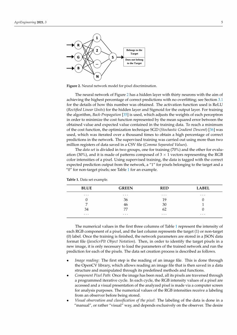
Figure 2. Neural network model for pixel discrimination.

The neural network of Figure 2 has a hidden layer with thirty neurons with the aim ofachieving the highest percentage of correct predictions with no overfitting; see Section 3.1for the details of how this number was obtained. The activation function used is ReLU(Rectified Linear Units) for the hidden layer and Sigmoid for the output layer. For trainingthe algorithm, Back-Propagation [35] is used, which adjusts the weights of each perceptronin order to minimize the cost function represented by the mean squared error between theobtained value and expected value contained in the training data. To reach a minimumof the cost function, the optimization technique SGD (Stochastic Gradient Descent) [36] wasused, which was iterated over a thousand times to obtain a high percentage of correctpredictions in the network. The supervised training was carried out using more than twomillion registers of data saved in a CSV file (Comma Separated Values).

The data set is divided in two groups, one for training (70%) and the other for evalu-ation (30%), and it is made of patterns composed of 3 × 1 vectors representing the RGBcolor intensities of a pixel. Using supervised training, the data is tagged with the correctexpected prediction output from the network, a “1” for pixels belonging to the target and a“0” for non-target pixels; see Table 1 for an example.

Table 1. Data set example.

BLUE GREEN RED LABEL

· · · · · · · · · · · ·0 36 19 07 46 30 1

34 77 62 0· · · · · · · · · · · ·

The numerical values in the first three columns of Table 1 represent the intensity ofeach RGB component of a pixel, and the last column represents the target (1) or non-target(0) label. Once the training is finished, the network parameters are stored in a JSON dataformat file (JavaScrPIt Object Notation). Then, in order to identify the target pixels in anew image, it is only necessary to load the parameters of the trained network and run theprediction for each of the pixels. The data set creation process is described as follows.

• Image reading: The first step is the reading of an image file. This is done throughthe OpenCV library, which allows reading an image file that is then saved in a datastructure and manipulated through its predefined methods and functions.

• Component Pixel Path: Once the image has been read, all its pixels are traversed througha programmed iterative cycle. In each cycle, the RGB intensity values of a pixel areaccessed and a visual presentation of the analyzed pixel is made via a computer screenfor analysis purposes. The numerical values of the RGB intensities receive a labelingfrom an observer before being stored.

• Visual observation and classification of the pixel: The labeling of the data is done in a“manual”, or rather “visual” way, and depends exclusively on the observer. The desire

AgriEngineering 2021, 3 6

to implement human characteristics in artificial machines, and for the particular caseof computer vision, supervised training requires that the data be pre-classified bya human observer before it is used for training in a neural network. Observing theevaluated pixel of an image, an input is intered by an observer who labels the RGBdata trio as belonging to a pixel that corresponds to the target, or not belonging to thetarget. Figure 3 shows an example of pixel tagging.

• Storage of training vector: Once the RGB data trio is tagged, it is stored in a file inside anon-volatile device. The data thus obtained and stored are then used for training theneural network. It is important to always store data with relevant, diverse, and largeamounts of information to improve training and increase the probability of correctpredictions by the network.

Figure 3. Pixel tagging example.

For the training to be successful, numerous relevant and varied data are needed, i.e., alarge quantity of quality data sets of images taken from scenarios of real operations of thesystem, and with a wide diversification in the nuances of the information to be identified.Once the neural network has been trained with a data set that meets the aforementionedcharacteristics, it will be ready to make predictions on unknown data and categorize thepixels of new images.

2.2. Post Processing

After making a prediction in the classification of pixels with the neural network inoperation after training, inevitably there will be some false positives and false negatives.This problem can be corrected by applying a post-processing step with a verification algo-rithm proposed in this work. The verification algorithm is based on the idea that a pixel isalso surrounded by pixels belonging to the target, and hence, these pixels also belong tothe target with high probability. To carry out the verification step, the environment of eachpixel of an image is analyzed and a siege percentage is calculated. Siege percentage is anidea that represents the number of pixels different from a given evaluated reference pixelwithin the analyzed environment of that pixel. If the siege percentage is high, then there isa high probability that the reference pixel is incorrectly labeled after prediction.

The verification algorithm reads an image pixel by pixel, and each pixel is taken as areference pixel. The kernel defines the surroundings of a reference pixel evaluated in thatiteration of the algorithm. Given a positive integer k, a kernel with respect to a referencepixel is defined as the set of pixels that are contained in a rectangular window of size(2k + 1)× (2k + 1) that is centered at the reference pixel. The number k is called the sizeof the kernel; see Figure 4 for an example. As each pixel in the kernel is examined, thenumber of pixels different from the reference pixel is counted. This count is interpreted asa percentage, which, if it is equal to or greater than an established siege percentage threshold,then the predicted tag value of the reference pixel is updated. The kernel and siegepercentage threshold are established experimentally in this work and will be discussed inlater sections.

AgriEngineering 2021, 3 7

Figure 4. Reference pixel path during an iteration with a kernel size of 2, one painted in blue andanother painted in orange.

The verification algorithm is shown in Figure 5. There are two main loops, one thatgoes through all the pixels in the image, and another nested loop that goes through thekernel for each reference pixel. The “Travel” variable keeps track of each pixel in the kerneluntil the entire kernel is traversed, while the “Error” variable keeps track of the differentpixels compared to the reference pixel.

No

No

Yes

Yes

Yes

Yes

Were all

Reference Pixels

traversed?

Travel =

Kernel?

Has the Siege

rate been

exceded? Is it different

from the

Reference Pixel?

ANN output image

Paint invalid

pixels black

Save the image

Take

Reference

Pixel

Error = 0

Travel= 0

Take pixel from

environment to

compare

Error = Error +1

Toggle

Reference

Pixel

Travel = Travel +1

No

No

Figure 5. Verification algorithm.

The verification algorithm of Figure 5 validates the pixels identified as belonging tothe target and rectifies the false negatives. With a similar argument, false positives can berectified, that is, correctly labeling a pixel as not belonging to the target when the networkwrongly identified it as belonging to the target. Figure 6 shows an example of the neuralnetwork prediction and a corresponding post-processed image.

AgriEngineering 2021, 3 8

Figure 6. Neural network prediction and its corresponding post-processing step.

2.3. Productivity Index

To quantify the production of the plots or cultivation tables automatically, a compu-tational production index is defined referred to as a Productivity Index or PI. The PI isdefined as a quotient between the number of valid pixels in the image that correspond to atarget and the total number of pixels, that is,

PI =number of valid pixelstotal number of pixels

. (1)

The process of computing the PI involves traversing all pixels in the post-processedimage and counting those labeled as valid pixels, that is, pixels corresponding to tomatoesin this work. The PI is then calculated by dividing the number of valid pixels by the totalnumber of pixels in the image to obtain as a result the proportion of pixels in the imagethat correspond to the target, which in this work corresponds to tomatoes.

In this way, the PI represents a quantity of tomatoes produced on the plot, that is, aquantitative productivity.

2.4. Pre-Processing

The pre-processing step is explained last because it is an optional functional block ofthe entire system, and it is only used when there is no physical control of the environment.The environment control refers to the manipulation of everything that appears in theimages during the process of taking photographic samples of the crops. The control of theenvironment can be done manually in the same cultivation site, taking care that everythingthat appears in the image does not interfere in a correct calculation of the PI. This situationis done by avoiding any foreign object with the same range of RGB intensities as tomatoes,for example, a red tube for irrigation. Some further control of the environment can also bedone computationally with a pre-processing step where targets are first identified beforeperforming a classification at the pixel level. The identification of tomatoes can be donewith a Convolutional Neural Network (CNN) trained to identify tomatoes [4,37]. A pre-selection of targets with Faster R-CNN focuses the PI calculation only on tomatoes, thusavoiding any foreign object that may introduce errors in the calculation of the PI. Table 2shows the hyperparameters for the Faster R-CNN with a ResNet architecture [38]. Figure 7shows some examples for the valid targets training data set and Figure 8 for the invalidtargets training data set.

AgriEngineering 2021, 3 9

Table 2. Faster R-CNN hyperparameters.

Hyperparameter Value

Anchor box scale [0.25, 0.5, 1.0, 2.0]Anchor box aspect ratio [0.5, 1.0, 2.0]

Anchor box height stride 16Anchor box width stride 16

Iterations 200,000Learning rate 0.0003

Momentum for SGD 0.9

Figure 7. Valid targets.

Figure 8. Invalid targets.

3. Results

The essence of this work lies on identifying whether objects in an image are tomatoesor not. The main goal is to quantify valid pixels in the image, thus obtaining an indicatoror index of production quantity. The computational implementation is done with theprogramming language Python version 3.6, along with its libraries for scientific computingapplications: Keras in its version 2.2.4 for neural networks, and OpenCV in its version 4.1for digital image management.

Figure 9 shows results of the behavior of the trained neural network. Invalid pixelsare painted in black and valid target pixels are displayed. As can be seen in Figure 9,the prediction is not perfect and false positives and false negatives appear, that is, pixelsidentified as valid targets when in fact they are not, and pixels identified as invalid whenin fact they are. The post-processing verification algorithm can check these predictions andrectifies them.

Figure 9. Results of the prediction of the trained neural network with no post-processing.

AgriEngineering 2021, 3 10

3.1. Siege Percentage Threshold, Kernel Size, and System Error Rate

To calculate the precision and accuracy of the models and obtain a fair estimation ofthe siege percentage threshold and kernel size, it is necessary to find the deviation betweenthe observed values and the real values. For this purpose, an image is “manually painted”,simulating the ideal detection of the pixels corresponding to “tomatoes.” This way, themanually painted image can be used as a reference to measure different pixels when thepost-processed image and the ideal image are compared against each other. Thus, a patternfor calculating the system’s error can be established. Figure 10 shows an example of anoriginal image and its respective ideal detection pattern.

Figure 10. Original image and reference pattern, painted ideally.

Several tests have been carried out to choose the best combination of post-processingparameters and the neural network model with the least prediction errors. The kernel size,the siege percentage threshold value, the number of hidden layers of the neural network,and the number of neurons per layer have been varied. Figure 11 shows the test results forthe calculation of the average error of the processing of 200 samples with a neural networkmodel with a single hidden layer of 30 neurons. The error rate is calculated as the numberof pixels different from the ideal pattern in relation to the total number of pixels of a image.

2,332,48

2,622,75

1,25 1,28 1,33 1,37

1,1 1,08 1,08 1,071,22 1,21 1,19 1,18

0

0,5

1

1,5

2

2,5

3

7 8 9 10

Ave

rage

Err

or

Rat

e

(%)

20 40 60 80Siege Percentage (%) =

Figure 11. Average system error rate with kernel values between 7 and 10, and Siege PercentageThresholds equal to 20%, 40%, 60%, and 80%.

The kernel size and siege percentage threshold values with the minimum system errorrate that are used in this work are a kernel size of 10 pixels and a siege percentage thresholdof 60%. Figures 12 and 13 show each step of image processing. Figures 14 and 15 also showtwo examples of a final result after all processing stages.

AgriEngineering 2021, 3 11

Figure 12. Original image (left) and Neural Network output (right).

Figure 13. Post-processing output (left) and final processed image (right) with errors marked in blue.

Figure 14. Original image (left) and final processed image (right).

Figure 15. Original image (left) and final processed image (right).

3.2. Application of PI on a Complete Tomato Growing Season

Once the PI is computed for each image of the crop plot sampled over time, a timecurve is obtained that describes the growth of cultivated products and allows objectivecomparisons between agricultural plots.

For this work, tomatoes were grown in a hydroponic greenhouse in three differentplots, each with a different nutrient dosage. The concentration of the final nutrient solutionwas modified from a commercial solution based on the Hoagland solution [39]. Plot 1received the commercial nutrient dosage of 100%, plot 2 with a diluted dosage of 75%, andplot 3 received a diluted dosage of 50%. Using the PI, it is possible to determine whether adiluted nutrient solution affects the quantitative production of the plots. Then, it is anothergoal of this work to establish an optimal dosage for greater effective production.

Since the sowing of tomatoes, photographs were taken of the plots with a samplingperiod of one day, and images were always taken from the same distance as recommendedby the proposed method, which was 1 meter in this case. Additionally, each plot wasdivided into 8 subplots to cover the entire extension of the crops. The length of the plotis 16 meters approximately, and photos were taken along the plot from both sides. ThePI resulting from a complete parcel in a single temporal sample event is the result of theaverage PI for each sub-parcel and the average PI of both sides. The temporal registration

AgriEngineering 2021, 3 12

of the PI is represented through curves that will be shown later as results and that willserve to analyze and compare the different production techniques.

In summary, the PI is calculated each day for each of the three plots, and for each day16 photographs are taken, since there are 8 subplots and one photograph is taken fromeach side. This gives us a total of 48 photographs; thus, the PI for a day is computed byaveraging the PI of each individual photograph.

Digital images are in JPEG format with a dimension of 5120 × 3840 pixels encodedin 8-bit RGB per channel. The digital camera used was an AKASO Brave 4 4K 20MP. Asan example, Figure 16 shows the original image of one sample, the pre-processing withCNNs, and its processing with the proposed method identifying objective pixels.

Figure 16. Original image, Convolutional Neural Networks (CNN) pre-processing, and pixel-level processing of sample 38with 75% diluted nutrient dosage.

Figures 17 and 18 show the photographic samples and the digital processing of the firstsampling event and an intermediate event, respectively. The processing of the first samplein Figure 17 presents a totally black screen, indicating that the target is not perceived withthe algorithm. Over time, tomatoes begin to ripen, and the target is identified by computingthe PI, as shown in Figure 18, thus achieving a record of growth and productivity throughthe PI curves. Daily photographic samples were taken from sowing to harvest, and theresulting PI processing gave rise to a time curve that determines the growth of tomatoesand describes the evolution of quantitative productivity.

Figure 17. First photographic sample of the first sub plot with 50% of commercial nutritional solution and its digitalProductivity Index (PI) processing with the date and time of the sampling.

AgriEngineering 2021, 3 13

Figure 18. Photographic sample of the first sub plot with 50% of commercial nutritional solution and its digital PI processingwith the date and time of the sampling.

A drawback that occurs when calculating the PI over time is what is called, in thecontext of this work, as the Harvesting problem, which influences the accuracy of the PIcalculation as time passes. An early harvest can cause the PI measurement at that momentto drop when, in reality, the productivity is the same or increases, that is, productivitymeasurement errors are introduced due to the extraction or fall of very mature targets. Inorder to overcome the harvesting problem, a method of accumulating the PI is proposedaccording to

PI(accumulated)i =n=i

∑n=1

∆PIn where ∆PIn = PIn − PIn−1 > 0, (2)

and PIn is defined as the instantaneous PI at time step n. The time curve of PI actuallyshows the accumulation of PI over time, which translates into cumulative productivityregardless of whether the instantaneous calculations record a PI reduction due to earlyharvest. The accumulated PI at a given instant i is calculated with the sum of ∆PIn, fromthe first sample to that of instant i, as long as ∆PIn is positive. Thus ∆PIn represents thedifference of instantaneous PIs between consecutive samples. The value of PIi − PIi−1must necessarily be positive in order to be included in the summation, since a negativevalue represents an early harvest, and, after it is identified in this way, it must be ignoredin the calculation to avoid incurring productivity measurement errors.

The calculation explained in the previous paragraph was performed with the threeplots, and the resulting curve is presented in Figure 19.

Looking at the time curves of the three plots, relevant information regarding theirproductivity can be obtained. In the first stage of growth, it is observed that a nutritionalsolution at 50% shows higher productivity, even reaching 23.5 times more production thanthe plot with 100% nutritional solution on day 19, and it is also 11.2 times more productivethan the 75% plot on the same day. In the middle time stages, the productive superiority ofthe solution is maintained at 50% with respect to the others until day 33, in which the 75%solution begins to look more productive; meanwhile, the 100% solution stays very inferior.In the final stages, the 75% and 50% solutions show higher productivity than the 100%solution, these being 1.5 and 1.4 times more productive, respectively. The 75% solutionpresented the highest final productivity, being 1.1 times more productive than the 50%solution.

Table 3 shows three types of productivity magnitudes for the three plots in their finalstages, two of which are commonly used, like weight and count, and the third whichis the PI proposed in this work. As can be seen, there is a certain correlation betweenthe three magnitudes, where all of them reflect the superiority of the solution with 75%concentration, followed by the solution at 50%, and the solution at 100% with the slightlyworst productivity.

AgriEngineering 2021, 3 14

Figure 19. Cumulative PI time curves of the three plots. The curves are the PIs with 50% diluted dosage (blue), 75% diluteddosage (green), and non-diluted dosage (orange).

Table 3. Count, weight, and PI comparison table.

Solution Count [units] Weight [g] PI [%]

Concentration 50% 73 4299 1.26Concentration 75% 89 5867 1.38Concentration 100% 60 3997 0.93

It is interesting to note that the 75% solution is 1.5 times more productive than the100% solution, taking into account the three specified magnitudes. However, if we compareit against the 50% solution, it is 1.2 times more productive considering the count, 1.4times more productive considering the weight, and 1.1 times more productive consideringthe PI. This difference, even between two well-known measures of productivity, is dueto the precision with which all these magnitudes measure the produced quantity (twolarge tomatoes are heavier than two small tomatoes). The PI approach aims to be moreprecise than the most common approach in computational vision where objects countsare implemented. The PI aims to improve even measurement by weight, automatingquality control through pixel-level identification of healthy targets (one kilogram of healthytomatoes and one kilogram of rotten tomatoes have the same weight) and making it easierto track the growth of tomatoes instead of doing it through weighing before harvest.

4. Discussion

The productivity index or PI was implemented using digital image processing with aperceptron-based artificial neural network. It should be noted that the calculation of thePI is made based on photographs taken automatically by a robotic system or by a human

AgriEngineering 2021, 3 15

that acquires digital samples always from the same distance and pointing to the sameobjective. This way, the automatic system creates the necessary context for the PI to makesense and be able to provide necessary information regarding the growth of agriculturalproducts in the different plots. The PI also provides a computational numerical parameterfor comparisons between different crops and their agro-production techniques, such ascomposition and dosage of nutrients, thus obtaining a reference for optimizing production.

Regarding the precision in the identification of objects in digital images, Reis et al. [32]achieves a precision of 97% in the identification of red grapes using a pixel identificationmethod similar to this work. Villacrés and Auat [4] were able to identify cherries with aprecision of 85% using faster R-CNN. Si et al. [13] identified apples using stereoscopicvision with a precision of 89.5%. Xiang et al. [15] achieved a precision of 87.9% in theidentification of groups of tomatoes using binocular stereo vision. Zhao et al. [14] showedthat, combining the AdaBoost classifier and color analysis, tomatoes can be detected with aprecision of 96%. With the Single Shot Detector, (SSD) the authors of Reference [40] showed aprecision of 95.99% in the detection of tomatoes. Other works, like Mu et al. [41], achieveda precision of 87.83% using faster R-CNN, also in tomatoes. In this work, a specific neuralnetwork was trained for the identification of pixels belonging to tomatoes and a verificationalgorithm was programmed to optimize target detection achieving a success rate of 98.93%.The nature of the computational technique used to calculate the PI allows to be adaptedfor other scenarios and contexts. With the versatility of neural networks, the same conceptdeveloped in the present work can be applied to detect other fruit and vegetable speciessimply by retraining the network with another specific data set for the desired target crop.

Other works in the literature, besides identification, use the count of objects as pro-ductivity parameter [4,14,40–43]. As explained before, counting of objects is not a preciseindicator for productivity, and that is one reason this works introduces the PI. Most ofthe works in the literature focus on detecting objects and not on monitoring of objects,which is what this current paper is emphasizing. For monitoring, there are works that keepa register of the size of plants [20], controlling diseases [44], environmental control [11],tracking the count of flowers and tomatoes [40,45], and keeping a registry of the volume oftomatoes [46]. This last work of Fukui et al. [46] is the closest to the current paper, and oneimportant point to notice is that the authors of Reference [46] achieved good results in acontrolled environment inside a laboratory, whereas, in outside environments, the resultswere not as expected. On the other hand, the results obtained in this work were performedcompletely in a typical working environment of hydroponic tomatoes.

The PI was computationally applied over time through digital image processing witha fully connected multilayer perceptron in three tomato crop plots and three differentnutrient dosages of a Hoagland solution. The control of the environment of the samplingplace was analyzed, and a computational method based on convolutional neural networkswas proposed to avoid erroneous measurements. In addition, an adequate mathematicalcalculation was established to correct the Harvesting Problem caused by early harvestsduring the processing of the curves. Through the innovative computational method ofPI calculation, three time curves of three different production techniques were obtained:dosing of nutrients with commercial chemical compounds at 100%, diluted at 75%, anddiluted at 50%. With these time curves, the production of the plots was recorded andanalyzed. As a conclusion, it was observed that the plots with a nutrient dosage diluted to75% showed higher productivity compared to the other two plots with different dosingtechniques, this being 1.1 times more productive than the plots with a dosage of 50% and1.5 times more productive than those with a dosage of nutritional chemical compounds at100%. The PI was compared with two well-known magnitudes of productivity, weight andcount, highlighting the advantages of this approach in precision and automation of qualitycontrol.

In agronomic terms, it can be concluded through the PI that there is no significantdifference in productivity between the three solutions studied. Therefore, the results

AgriEngineering 2021, 3 16

suggest that it is recommended to use a 75% solution to have a slight improvement inproductivity, as well as to potentially use a 50% solution to minimize production costs.

5. Conclusions

This work introduced a new computational parameter, a so-called Productivity Indexor PI, to quantify productivity of hydroponic tomatoes using neural networks and digitalimage processing. The neural network presented an error rate of 1.07% in the identificationof pixels belonging to tomatoes. This neural network together with the PI was then used ina full season of hydroponic tomatoes in order to test the entire system in a real workingenvironment. From the application of the PI in real scenarios, it is possible to concludethat there is no difference in terms of productivity of a plot of tomatoes when a Hoaglandsolution is diluted 50% with water or is not diluted at all.

One limitation of the approach is the poor detection of very green tomatoes, whichrequires specializing the system for the detection of tomatoes before their middle ripeningstage. The neural network of this work is trained to detect tomatoes when they start itsred coloration process; when tomatoes are green they are not perceived by the network,which will required a new training stage to detect green tomatoes and can potentially beconfused with invalid objects like leaves. This, however, can be considered as positive,since the system can detect which exact moment in time a tomato plot enters its ripeningstage by observing the change in PI.

Regarding occlusions, two types can be noted: occlusions by invalid targets (branches,leaves), and occlusions by valid targets (tomatoes obstructing other tomatoes). Invalidtarget occlusions can be improved with good environmental control, periodic pruning,or human intervention. Payne et al. [43] takes images from four different points of viewpointing to the same objective in order to obtain robust results even with occlusions. In thispaper, the photographs were taken only from two points of view considering that plots areorganized in lines. The proposed method of this work, however, offers improved solutionsof up to 50% in invalid target occlusions. This is due to the way samples are taken andthe process of computing the PI, that is, the samples are taken from both sides of the cropline and the resulting PI from that subplot is calculated by averaging the instantaneousPI of the image from each side of that subplot. Having two points of view facing eachother improves the field of vision when taking samples. Occlusions for valid objectives aremore complicated to solve, and they are beyond the scope of this work, which is why it isproposed to study them in future works. The solution in general is to identify tomatoes thatare occluded, define their contours, and reconstruct them with an elliptical approximation.Small occlusions in general are accepted and tolerated since they do not affect the PI whenusing it as a means of comparison. This is because small occlusions can be considered as“white noise” that affect all measurements equally.

The execution time of the entire process is approximately 3 minutes for each image.A dedicated server was used in this work that stores the images and processes themper day. Execution time can be reduced by implementing GPU (Graphics ProcessingUnit) processing, thus parallelizing calculations. To achieve this, the program code mustbe adapted to implement the same algorithm presented in this approach. One of theadvantages of using a neural network as a classification method is its ease of parallelizingcalculations with GPU programming. This implementation will be done in future works inorder to improve the system.

For future work, this study with image processing is intended to be validated withother agronomical studies of the productivity and the physicochemical properties of crops.Even though this work used Faster R-CNN, which is considered as a deep neural network,further studies using other network architectures can improve our understanding of theapplications of deep learning for the detection and classification of fruits and vegetables.Furthermore, it is expected to use optimization algorithms, like genetic algorithms, in orderto improve the model of the neural network.

AgriEngineering 2021, 3 17

Author Contributions: Conceptualization, D.G. and D.P.; Methodology, D.P.; Software, D.P. andK.C.; Validation, R.L., D.G., and M.A.; Formal Analysis, D.G. and D.P.; Investigation, M.A. and D.P.;Resources, D.G., K.C., and M.A.; Data Curation, K.C. and R.L.; Writing—original draft preparation,D.P. and R.L.; Writing—review and editing, D.G., M.A., and M.V.; Visualization, D.G. and D.P.;Supervision, D.G. and M.A.; Project administration, D.G.; and Funding acquisition, D.G. All authorshave read and agreed to the published version of the manuscript.

Funding: This research was funded by CONACYT (National Council of Science and Technology) ofParaguay, providing the necessary funds to finance the project PINV15-068 “Image Processing ofFruits and Vegetable Products in a Hydroponic Greenhouse”.

Acknowledgments: The authors thank the Faculty of Engineering of the National University ofAsunción for the support provided for the development of this project.

Conflicts of Interest: The authors declare no conflict of interest. The funders had no role in the designof the study; in the collection, analyses, or interpretation of data; in the writing of the manuscript, orin the decision to publish the results.

References1. Szeliski, R. What is computer vision? In Computer Vision: Algorithms and Applications; Springer: London, UK, 2011 ; pp. 3–10.2. Charumathi, S.; Kaviya, R.M.; Kumariyarasi, J.; Manisha, R.; Dhivya, P. Optimization and control of hydroponics agriculture

using IOT. Asian J. Appl. Sci. Technol. 2017, 1, 96–98.3. Dae-Heon, P.; Beom-Jin, K.; Kyung-Ryong, C.; Chang-Sun, S.; Sung-Eon, C.; Jang-Woo, P.; Won-Mo, Y. A study on greenhouse

automatic control system based on wireless sensor network. Wirel. Pers. Commun. 2011, 56, 117–130.4. Villacrés, J.F.; Auat Cheein, F. Detection and Characterization of Cherries: A Deep Learning Usability Case Study in Chile.

Agronomy 2020, 10, 835. [CrossRef]5. LeCun, Y.; Bengio, Y.; Hinton, G. Deep Learning. Nat. Int. J. Sci. 2015, 521, 436–444. [CrossRef] [PubMed]6. Rosenblatt, F. The perceptron: A probabilistic model for information storage and organization in the brain. Psychol. Rev. 1958, 65,

386–408. [CrossRef] [PubMed]7. García, J.; Navalón, A.; Jordi, A.; Juárez, D. Visión artificial aplicada al control de la calidad. 3C Tecnol. 2014, 3, 297–308.8. Durán, C.; Gualdron, O.; Hernández, M. Nariz electrónica para determinar el índice de madurez del tomate de árbol (Cyphoman-

dra Betacea Sendt). Ing. Investig. Y Tecnol. 2014, 15, 351–362.9. Lin, K.; Chen, J.; Si, H.; Wu, J. A Review on Computer Vision Technologies Applied in Greenhouse Plant Stress Detection. In

Chinese Conference on Image and Graphics Technologies; Springer: Berlin/Heidelberg, Germany, 2013; Volume 363.10. Zaborowicz, M.; Przybyl, J.; Koszela, K.; Boniecki, P.; Mueller, W.; Raba, B.; Lewicki, A.; Przybyl, K. Computer image analysis in

obtaining characteristics of images: Greenhouse tomatoes in the process of generating learning sets of artificial neural networks.In Proceedings of the SPIE 9159, Sixth International Conference on Digital Image Processing (ICDPI 2014), Athens, Greece, 16April 2014.

11. Story, D.; Kacira, M. Design and implementation of a computer vision-guided greenhouse crop diagnostics system. Mach. Vis.Appl. 2015, 26, 495–506. [CrossRef]

12. Wspanialy, P.; Moussa, M. Early powdery mildew detection system for application in greenhouse automation. Comput. Electron.Agric. 2016, 127, 487–494. [CrossRef]

13. Si, Y.; Liu, G.; Feng, J. Location of apples in trees using stereoscopic vision. Comput. Electron. Agric. 2015, 112, 68–74. [CrossRef]14. Zhao, Y.; Gong, L.; Zhou, B.; Huang, Y.; Liu, C. Detecting tomatoes in greenhouse scenes by combining AdaBoost classifier and

colour analysis. Biosyst. Eng. 2016, 148, 127–137. [CrossRef]15. Xiang, R.; Jiang, H.; Ying, Y. Recognition of clustered tomatoes based on binocular stereo vision. Comput. Electron. Agric. 2014,

106, 75–90. [CrossRef]16. Silva, G.R.; Escarpinati, M.C.; Abdala, D.D.; Souza, I.R. Definition of Management Zones Through Image Processing for Precision

Agriculture. In Proceedings of the 2017 Workshop of Computer Vision (WVC), Natal, Brazil, 30 October–1 November 2017; pp.150–154.

17. Treboux, J.; Genoud, D. High Precision Agriculture: An Application Of Improved Machine-Learning Algorithms. In Proceedingsof the 2019 6th Swiss Conference on Data Science (SDS), Bern, Switzerland, 14 June 2019; pp. 103–108.

18. Treboux, J.; Genoud, D. Improved Machine Learning Methodology for High Precision Agriculture. In Proceedings of the 2018Global Internet of Things Summit (GIoTS), Bilbao, Spain, 4–7 June 2018; pp. 1–6.

19. Kala, H.S.; Hebbar, R.; Singh, A.; Amrutha, R.; Patil, A.R.; Kamble, D.; Vinod, P.V. AgRobots (A Combination of Image Processingand Data Analytics for Precision Pesticide Use). In Proceedings of the 2018 International Conference on Design Innovations for3Cs Compute Communicate Control (ICDI3C), Bangalore, India, 25–28 April 2018; pp. 56–58.

20. Akila, S.; Sivakumar, A.; Swaminathan, S. Automation in plant growth monitoring using high-precision image classificationand virtual height measurement techniques. In Proceedings of the 2017 International Conference on Innovations in Information,Embedded and Communication Systems (ICIIECS), Coimbatore, India, 17–18 March 2017; pp. 1–4.

AgriEngineering 2021, 3 18

21. Sudhesh, R.; Nagalakshmi, V.; Amirthasaravanan, A. A Systematic Study on Disease Recognition, Categorization, and Quan-tification in Agricultural Plants using Image Processing. In Proceedings of the 2019 IEEE International Conference on System,Computation, Automation and Networking (ICSCAN), Pondicherry, India, 29–30 March 2019; pp. 1–5.

22. Yalcin, H. Phenology recognition using deep learning. In Proceedings of the 2018 Electric Electronics, Computer Science,Biomedical Engineerings’ Meeting (EBBT), Istanbul, Turkey, 18–19 April 2018; pp. 1–5.

23. Umamaheswari, S.; Arjun, R.; Meganathan, D. Weed Detection in Farm Crops using Parallel Image Processing. In Proceedings ofthe 2018 Conference on Information and Communication Technology (CICT), Jabalpur, India, 26–28 October 2018; pp. 1–4.

24. Li, N.; Zhang, X.; Zhang, C.; Guo, H.; Sun, Z.; Wu, X. Real-Time Crop Recognition in Transplanted Fields With Prominent WeedGrowth: A Visual-Attention-Based Approach. IEEE Access 2019, 7, 185310–185321. [CrossRef]

25. Yang, W.; Xie, C.; Hao, Z.; Yang, C. Diagnosis of Plant Cold Damage Based on Hyperspectral Imaging and Convolutional NeuralNetwork. IEEE Access 2019, 7, 118239–118248. [CrossRef]

26. Nardari, G.V.; Romero, R.A.F.; Guizilini, V.C.; Mareco, W.E.C.; Milori, D.M.B.P.; Villas-Boas, P.R.; Santos, I.A.D. Crop AnomalyIdentification with Color Filters and Convolutional Neural Networks. In Proceedings of the 2018 Latin American RoboticSymposium, 2018 Brazilian Symposium on Robotics (SBR) and 2018 Workshop on Robotics in Education (WRE), Joao Pessoa,Brazil, 6–10 November 2018; pp. 363–369.

27. Andrea, C.; Daniel, B.; Misael, J. Precise weed and maize classification through convolutional neuronal networks. In Proceedingsof the 2017 IEEE Second Ecuador Technical Chapters Meeting (ETCM), Salinas, Ecuador, 16–20 October 2017; pp. 1–6.

28. Abdullahi, H.; Sheriff, R.; Mahieddine, F. Convolution neural network in precision agriculture for plant image recognition andclassification. In Proceedings of the 2017 Seventh International Conference on Innovative Computing Technology (INTECH),Luton, UK, 16–18 August 2017; pp. 1–3.

29. Barrero, O.; Rojas, D.; Gonzalez, C.; Perdomo, S. Weed detection in rice fields using aerial images and neural networks. InProceedings of the 2016 XXI Symposium on Signal Processing, Images and Artificial Vision (STSIVA), Bucaramanga, Colombia,31 August–2 September 2016; pp. 1–4.

30. Purwar, P.; Rogotis, S.; ChatzPIapadopoulus, F.; Kastanis, I. A Reliable Approach for Pixel-Level Classification of Land usagefrom Spatio-Temporal Images. In Proceedings of the 2019 6th Swiss Conference on Data Science (SDS), Bern, Switzerland, 14 June2019; pp. 93–94.

31. Koirala, A.; Walsh, K.B.; Wang, Z.; McCarthy, C. Deep learning–Method overview and review of use for fruit detection and yieldestimation. Comput. Electron. Agric. 2019, 162, 219–234. [CrossRef]

32. Reis, M.J.C.S.; Morais, R.; Peres, E.; Pereira, C.; Contente, O.; Soares, S.; Valente, A.; Baptista, J.; Ferreira, P.J.S.G.; Bulas Cruz, J.Automatic detection of bunches of grapes in natural environment from color images. J. Appl. Log. 2012, 10, 285–290. [CrossRef]

33. Boniecki, P.; Koszela, K.; Swierczynski, K.; Skwarcz, J.; Zaborowicz, M.; Przybył, J. Neural Visual Detection of Grain Weevil(Sitophilus granarius L.). Agriculture 2020, 10, 25. [CrossRef]

34. Niedbała, G.; Kurasiak-Popowska, D.; Stuper-Szablewska, K.; Nawracała, J. Application of Artificial Neural Networks to Analyzethe Concentration of Ferulic Acid, Deoxynivalenol, and Nivalenol in Winter Wheat Grain. Agriculture 2020, 10, 127. [CrossRef]

35. LeCun, Y. A theoretical framework for back-propagation. In Proceedings of the 1988 Connectionist Models Summer School; MorganKaufmann: Pittsburg, PA, USA, 1988; pp. 21–28.

36. Robbins, H. A stochastic approximation method. Ann. Math. Stat. 1951, 22, 400–407. [CrossRef]37. Li, Y.; Chao, X. ANN-Based Continual Classification in Agriculture. Agriculture 2020, 10, 178. [CrossRef]38. He, K.; Zhang, X.; Ren, S.; Sun, J. Deep Residual Learning for Image Recognition. In Proceedings of the 2016 IEEE Conference on

Computer Vision and Pattern Recognition (CVPR) 2016, Las Vegas, NV, USA, 1 July 2016; pp. 770–778.39. Harmanpreet, K.; Rakesh, S.; Pankaj, S. Effect of Hoagland solution for growing tomato hydroponically in greenhouse. HortFlora

Res. Spectr. 2016, 5, 310–315.40. de Luna, R.G.; Dadios, E.P.; Bandala, A.A.; Vicerr, R.R.P. Tomato Growth Stage Monitoring for Smart Farm Using Deep Transfer

Learning with Machine Learning-based Maturity Grading. AGRIVITA J. Agric. 2020, 42. [CrossRef]41. Mu, Y.; Chen, T.-S.; Ninomiya, S.; Guo, W. Intact Detection of Highly Occluded Immature Tomatoes on Plants Using Deep

Learning Techniques. Sensors 2020, 20, 2984. [CrossRef]42. Liu, G.; Mao, S.; Kim, J.H. A Mature-Tomato Detection Algorithm Using Machine Learning and Color Analysis. Sensors 2019, 19,

2023. [CrossRef]43. Payne, A.B.; Walsh, K.B.; Subedi, P.P.; Jarvis, D. Estimation of mango crop yield using image analysis – Segmentation method.

Comput. Electron. Agric. 2013, 91, 57–64. [CrossRef]44. Ma, J.; Li, X.; Wen, H.; Fu, Z.; Zhang, L. A key frame extraction method for processing greenhouse vegetables production

monitoring video. Comput. Electron. Agric. 2015, 111, 92–102. [CrossRef]45. Sun, J.; He, X.; Wu, M.; Wu, X.; Shen, J.; Lu, B. Detection of tomato organs based on convolutional neural network under the

overlap and occlusion backgrounds. Mach. Vis. Appl. 2020, 31, 31. [CrossRef]46. Fukui, R.; Schneider, J.; Nishioka, T.; Warisawa, S.; Yamada, I. Growth measurement of Tomato fruit based on whole image

processing. In Proceedings of the 2017 IEEE International Conference on Robotics and Automation (ICRA), Singapore, 29 May–3June 2017; pp. 153–158.