arX

iv:1

107.

2282

v2 [

mat

h.PR

] 6

Mar

201

2

On the existence of a time inhomogeneous skew Brownian motion

and some related laws

Pierre Etore∗ Miguel Martinez†

March 7, 2012

Abstract:

This article is devoted to the construction of a solution for the ”skewinhomogeneous Brownian motion” equation:

Bβt = x+Wt +

∫ t

0β(s)dL0

s(Bβ), t ≥ 0.

Here β : R+ → [−1, 1] is a Borel function, W is a standard Brownian mo-tion, and L0

. (Bβ) stands for the symmetric local time at 0 of the unknown

process Bβ.Using the description of the straddling excursion above a deterministic

time t, we also compute the joint law of(Bβ

t , L0t (B

β), Gβt

)where Gβ

t is

the last passage time at 0 before t of Bβ.

Keywords:

Skew Brownian motion ; Local time ; Straddling excursion.

1 Introduction

1.1 Presentation

Consider (Wt)t≥0 a standard Brownian motion on some filtered probability space (Ω,F , (Ft)t≥0,P)where the filtration satisfies the usual right continuity and completeness conditions.

Let us introduce Bβ the solution of

Bβt = x+Wt +

∫ t

0β(s)dL0

s(Bβ), t ≥ 0 (1)

where β : R+ → [−1, 1] is a Borel function and L0. (B

β) stands for the symmetric local time at 0of the unknown process Bβ. The process Bβ will be called ”time inhomogeneous skew Brownianmotion” for reasons explained below.

Of course, the equation (1) is an extension of the now well-known skew Brownian motion withconstant parameter, namely the solution of (1) when the function β is a constant in (−1, 1).

∗Corresponding author, Laboratoire Jean Kuntzmann- Tour IRMA 51, rue des Mathematiques 38041 GrenobleCedex 9, France. Phone: + 33 (0)4 76 63 56 93; E-mail: pierre.etore@imag.fr

†Universite Paris-Est Marne-la-Vallee, Laboratoire d’Analyse et de Mathematiques Appliquees, UMR 8050, 5Bld Descartes, Champs-sur-marne, 77454 Marne-la-Vallee Cedex 2, France. Phone: +33 (0)1 60 95 75 25; E-mail:miguel.martinez@univ-mlv.fr

1

The reader may find many references concerning the homogeneous skew Brownian motion andvarious extensions in the literature : starting with the seminal paper by Harrisson and Shepp [10],let us cite [3], [18], [20], [5], [7], [17], [22], [31], and the recent article [1]. To complete the referenceson the subject, we mention the interesting survey by Lejay [15] and the cited articles therein.

On the contrary, concerning extensions of the skew Brownian motion in an inhomogeneoussetting, we only found very few references : apart from the seminal paper by Weinryb [27], wemention [4], where a variably skewed Brownian motion is constructed as the solution of a differentequation than (1).

Up to our knowledge, concerning an existence result for possible solutions of equation (1) thesituation reduces to only two references : we have already mentioned [27] where it is said that”partial existence results were obtained by Watanabe [25, 24]” (to be precise, see however a detailexplained in Remark 1). Unfortunately, we have not been able to exploit these results fully in orderto give a satisfactory response to the existence problem for the solutions of (1). So that, contraryto what is said in the introduction of [4], the paper [27] does not show that strong existence holdsfor equation (1) unless β(s) ≡ β is a constant function.

Our second reference concerning the possible solutions of (1) is the fundamental book (posteriorto [27]) of Revuz and Yor [23] , Chapter VI Exercise 2.24 p. 246, which starts with : ”Let Bβ be acontinuous semimartingale, if it exists, such that (1) holds” (in this quote, we adapted the notationto our setting ; we underlined what seems to be a crucial point).

In this article, we give the expected positive answer to the existence of weak solutions forequation (1) in the general case where the parameter function is a Borel function β with valuesin [−1, 1]. Our results may be completed with the result of Weinryb [27], where it is shown thatpathwise uniqueness holds for equation (1). Then, the combination of both results ensures theexistence of a unique strong solution to (1).

We will present essentially two ways of constructing a weak solution to (1).

The first one is based on the description of the excursion that straddles some fixed deterministictime. Up to our knowledge, though the idea seems quite natural in our context, the recovery of thetransition probability density of a skew Brownian motion (be it inhomogeneous or homogeneous)from the description of the excursion that straddles some fixed deterministic time seems to be newand is not mentioned in the survey paper [15]. As a by product, we also compute the trivariate

density of the vector (L01

(Bβ), Gβ

1 , Bβ1 ) where Gβ

1 := sups < 1 : |Bβs | = 0 is the last passage at

0 before time 1 of the constructed process.

Let us now explain briefly the second construction.The main idea is to approximate the function β by a monotone sequence of piecewise constant

functions (βn)n≥0. Still we have to face some difficulties and the construction, even in the simpler

case of a given (fixed) piecewise constant coefficient β, does not seem so trivial.In order to treat the simpler case of a given piecewise constant coefficient β, we are inspired by

a construction for the classical skew Brownian motion with constant parameter which is explainedin an exercise of the reference book [23]. This construction uses a kind of random flipping forexcursions that come from an independent standard reflected Brownian motion |B|. The difficultyto adapt this construction in our inhomogeneous setting lies in the fact that it does not seempossible, at least directly and in order to construct Bβ, to combine it with ”pasting trajectory”arguments at each point where β changes its value. This difficulty arises because the flow of aclassical skew Brownian motion is not defined for all starting points x simultaneously (see theremark in the introduction of [7] p.1694, just before Theorem 1.1). Still, we manage to adapt the”excursion flipping” arguments in our inhomogeneous setting and to identify our construction witha weak solution of equation (1) : instead of trying to paste trajectories together, we show that ourconstruction preserves the Markovian character of the reflected Brownian motion |B|. Then, theideas developed in the previous sections allow us to show that the constructed process satisfies an

2

equation of type (1), yielding a weak solution. The existence in the general case is then deducedby proving a strong convergence result.

1.2 Organisation of the paper

The paper is organised as follows :

• In Section 2 we first present results given in [27] concerning the possible solutions of (1). Wealso recall some facts concerning the standard Brownian motion and its excursion straddlingone. We expose in a separate subsection the result obtained in this paper.

• In Section 3 we assume that we have a solution of (1) and we compute a one-dimensionalmarginal law of this solution using the inversion of the Fourier transform. Comparing theseresults with well-known results concerning the standard Brownian motion gives a hint onwhat should be the bivariate density of (Gβ

1 , Bβ1 ).

• These hinted links are explained in Section 4 : following the lines of [2] for a more complicatedbut time-homogeneous process (namely Walsh’s Brownian motion), we manage to give aprecise description of what happens after the last exit from 0 before time 1 for the solutionsof (1). This permits to compute the Azema projection of Bβ on the filtration (F

Gβt). In

turn, this description enables us to retrieve the results of the previous section and to give aproof of the Markov property for Bβ in full generality. We finish this section by proving aKolmogorov’s continuity criterion, which is uniform w.r.t. the parameter function β.

• Using the results of the previous sections, we show the existence of solutions for the inho-mogeneous skew Brownian equation (1) in Section 5. We give a first result of existence forthe solutions of (1) in the case where β is sufficiently smooth. In this case, the constructedsolution is strong. The methods used in this part rely on stochastic calculus and an extensionof the Ito-Tanaka formula in a time dependent setting due to [19].

The general case is deduced by convergence and the Chapman-Kolmogorov equations.

• As a by product of the study made in the preceding sections, we derive the joint distributionof (L0

1

(Bβ), Gβ

1 , Bβ1 ) using well-known facts concerning the standard Brownian motion.

• Finally, in the last section, we give a proof for the existence of the solution of (1), using aflipping of excursions argument and a convergence result.

2 Notations, preliminaries and main results

2.1 Notations

Throughout this note, e denotes the exponential law of parameter 1 ; Arcsin is the standard arcsinlaw with density (π

√y(1− y))−1 on [0, 1]; R(p) denotes the Rademacher law with p parameter

i.e. the law of random variable Y taking values −1,+1 with P(Y = 1) = p = 1− P(Y = −1).We denote for all t ≥ 0,

Gt := sups < t : |Ws| = 0 and Gβt := sups < t : |Bβ

s | = 0.

It is well known that G1L∼ Arcsin (see [23] Chap. III, Exercise 3.20). We will also denote for

all 0 ≤ u ≤ 1,

Mu :=∣∣WG1+u(1−G1)

∣∣/√

1−G1 and Mβu :=

∣∣Bβ

Gβ1+u(1−Gβ

1 )

∣∣/√

1−Gβ1 .

3

The process M is called the Brownian Meander of length 1. It is well known that M1L∼√2e (see

See [23], Chap. XII, Exercise 3.8).

Acronyms : throughout the paper the acronym BM denotes a standard Brownian motion.The acronym SBM denotes a constant parameter skew Brownian motion solution of (1) for someconstant function β(s) ≡ β. The acronym ISBM for Inhomogeneous Skew Brownian Motion denotesthe solution of (1) in the case where β is not a constant function. Unless there is no ambiguity, thecharacter weak or strong of the considered solutions of (1) will be made precise.

For a given semimartingale X, we denote by L0. (X) its symmetric local time at level 0.

The expectation Ex (resp. Es,x) refers to the probability measure Px := P( · |Bβ0 = x) (resp.

Ps,x := P( · |Bβs = x)).

2.2 Preliminaries

Let β : R+ → [−1, 1] a Borel function. The following fundamental facts are the key of many

considerations of this paper.

Proposition 2.1 (see [27] or [23] Chap. VI Exercise 2.24 p. 246) Assume (1) has a weak solutionBβ. Then under P0,

(|Bβt |)t≥0

L∼ (|Wt|)t≥0 .

We give the short proof for the sake of completeness.

Proof. Applying Ito’s formula we get on one side

(Wt)2 = 2

∫ t

0WsdWs + t = 2

∫ t

0|Ws|sgn(Ws)dWs + t = 2

∫ t

0

√W 2

s dZs + t,

where we have set Zt :=∫ t0 sgn(Ws)dWs. Notice that Z is a Brownian motion, thanks to Levy’s

theorem. On the other side we get

(Bβt )

2 = 2

∫ t

0Bβ

s dBβs + t = 2

∫ t

0Bβ

s dWβs + t = 2

∫ t

0

√(Bβ

s )2 dZβs + t,

where we have used 1

Bβs =0

dL0s(B

β) = dL0s(B

β), and where Zβt :=

∫ t0 sgn(B

βs )dW

βs , with W β the

BM associated to the weak solution Bβ. Notice that Zβ is a Brownian motion, thus (W )2 and(Bβ)2 are solutions of the same SDE, that enjoys uniqueness in law. This proves the result (see[28, 26]).

Theorem 2.2 (see [27] or [23] Chap. VI Exercise 2.24 p. 246)Pathwise uniqueness holds for the weak solutions of equation (1).

Remark 1 In the introductory article [27], it is shown that there is pathwise uniqueness for equation(1) but with a slight modification : in [27] the local time appearing in the equation is the standardright sided local time, so that the function β is supposed to take values in (−∞, 1/2]. Still, all theresults of [27] may be easily adapted for the case where L0

. (Bβ) stands for the symmetric local time

at 0. We leave these technical aspects to the reader.

As L01(B

β), Mβ1 and Gβ

1 (resp. L01(W ), M1 and G1) are measurable functions of the trajectories

of |Bβ| (resp. |W |), we get immediately the following corollary.

4

Corollary 2.3 We have

(|Bβ1 |, L0

1(Bβ), Gβ

1 ,Mβ1 )

L∼ (|W1|, L01(W ), G1,M1).

The following known trivariate density will play a crucial role.

Proposition 2.4 i) We have

(|W1|, L01(W ), G1) = (

√1−G1M1,

√G1l

0, G1), (2)

where l0L∼√2e, and with G1,M1, l

0 independent.ii) As a consequence, for all t, s > 0, and all ℓ, x ≥ 0, the image measure P0[|Wt| ∈ dx,L0

t (W ) ∈dℓ,Gt ∈ ds] is given by

1s≤t

√2

πs3ℓ exp

(− ℓ2

2s

) x√2π(t− s)3

exp

(− x2

2(t− s)

)ds dℓ dx. (3)

Proof. See [23], Chap. XII, Exercise 3.8.

Remark 2 Note that, by integrating (3) with respect to ℓ, and using a symmetry argument we getthat

p(t, 0, y) =|y|2π

∫ t

0

1√s(t− s)3/2

exp

(− y2

2(t− s)

)ds, (4)

where p(t, x, y) := 1√2πt

exp(− (y−x)2

2t

)is the transition density of a Brownian motion.

2.3 Transition probability density

All through the paper the transition probability density of Bβ will be denoted pβ(s, t;x, y) (weshow that it exists).

Let us now give the analytical expression of the function pβ(s, t;x, y). It will be shown later (Sec-tion 5) that pβ(s, t;x, y) is a transition probability function (in particular it satisfies the Chapman-Kolmogorov equations), and that the existing strong solution Bβ of (1) is indeed an inhomogeneousMarkov process with transition function pβ(s, t;x, y).

Definition 2.5 For all t > 0, y ∈ R, we set

pβ(0, t; 0, y) :=|y|π

∫ t

0

1 + sgn(y)β(s)

2

1√s(t− s)3/2

exp

(− y2

2(t− s)

)ds. (5)

Remark 3 Note that, when β(s) ≡ β is constant, using (4) we have

pβ(0, t; 0, y) = (1 + β)p(t, 0, y)1y>0 + (1− β)p(t, 0, y)1y<0.

This is the density of the SBM starting from zero with skewness parameter α := (β + 1)/2, givenfor example in [23] Chap. III Exercise 1.16 p.87.

5

Let us now introduce the shift operator (σt) acting on time dependent functions as follows:

β σt(s) = β(t+ s).

Assume for a moment that (1) has a solution Bβ which enjoys the strong Markov property andsatisfies

P0(Bβt ∈ dy) = pβ(0, t; 0, y)dy.

Let x 6= 0 be the starting point of Bβ at time s. Let

T0 := inf(t ≥ s : Bβt = 0).

Since the local time L0. (B

β) does not increase until Bβ reaches 0, the process Bβ, heuristicallyspeaking, behaves like a Brownian motion on time interval (s, T0), implying that Ps,x(T0 ∈ du) =|x| exp(−x2/2(u− s))/

√2π(u− s)3. Then it starts afresh from zero, behaving like an ISBM. Thus,

for t > s,

Ps,x(Bβt ∈ dy) = Ps,x(Bβ

t ∈ dy ; s ≤ T0 ≤ t) + Ps,x(Bβt ∈ dy ; T0 > t)

= dy

∫ t−s

0

|x|e−x2/2u

√2πu3

pβσsσu(0, t − s− u; 0, y)du

+1√

2π(t− s)

[exp

(−(y − x)2

2(t− s)

)− exp

(−(y + x)2

2(t− s)

)]1xy>0.

(6)

The second line is a consequence of the assumed strong Markov property, while the third line is aconsequence of the reflection principle due to the fact that on the event T0 > t the process Bβ

behaves like a Brownian motion.But using (5), a Fubini-Tonelli argument, a change of variable, and (4), we get :

∫ t−s

0

|x|e−x2/u

√2πu3

pβσsσu(0, t− s− u; 0, y)du

=

∫ t−s

u=0

∫ u

r=0

1 + sgn(y)β σs(u)2

√2

π

|y|(t− (s+ u))3/2

e− y2

2(t−(s+u))|x|

2π√r(u− r)3/2

e− x2

2(u−r)dr du

=

∫ t−s

0

1 + sgn(y)β σs(u)2

|y|π

e− y2

2(t−(s+u))

√u(t− s− u)3/2

e−x2/2udu.

(7)This leads us to the following definition.

Definition 2.6 For t > s, x, y ∈ R, we set

pβ(s, t;x, y) :=

∫ t−s

0

1 + sgn(y)β σs(u)2

|y|π

e− y2

2(t−(s+u))

√u(t− s− u)3/2

e−x2/2udu

+1√

2π(t− s)

[exp

(−(y − x)2

2(t− s)

)− exp

(−(y + x)2

2(t− s)

)]1xy>0.

(8)

6

Remark 4 Note that in the case of Brownian motion (β ≡ 0) we have :

p(t, x, y) =

∫ t

0

|y|2π

e− y2

2(t−u) e−x2

2u

√u(t− u)3/2

du+1√2πt

[exp

(−(y − x)2

2t

)− exp

(−(y + x)2

2t

)]1xy>0. (9)

Thus, considering (8),

pβ(s, t;x, y) = p(t− s, x, y) +

∫ t−s

0

β σs(u)2

y

π

e− y2

2(t−(s+u))

√u(t− s− u)3/2

e−x2/2udu. (10)

This will be useful in forthcoming computations.

Remark 5 When β(s) ≡ β is constant, pβ(s, t;x, y) is just the transition density of the SBM givenfor example in [23].

2.4 Main results

We now state the main results obtained in this paper.

Proposition 2.7 Let Bβ a weak solution of (1).For all t > 0, y ∈ R, we have

P0(Bβt ∈ dy) = pβ(0, t; 0, y)dy,

where the function pβ(0, t; 0, y) is explicit in Definition 2.5.

The most important results of the paper may be summarized in the following theorem :

Theorem 2.8 Let β : R+ → [−1, 1] a Borel function and W a standard Brownian motion. Forany fixed x ∈ R, there exists a unique (strong) solution to (1). It is a (strong) Markov process withtransition function pβ(s, t;x, y) given by Definition 2.6.

Still, a (very) little more work allows to retrieve the law of (Bβt , L

0t (B

β), Gβt ) under P

0.

Theorem 2.9 For all t, s > 0, all ℓ ≥ 0 and all x ∈ R, the image measure P0[Bβt ∈ dx,L0

t (Bβ) ∈

dℓ,Gβt ∈ ds] is given by

1s≤t1 + sgn(x)β(s)

2

√2

πs3ℓ exp

(− ℓ2

2s

) |x|√2π(t− s)3

exp

(− x2

2(t− s)

)ds dℓ dx. (11)

3 Law of the ISBM at a fixed time : proof of Proposition 2.7

Let β : R+ → [−1, 1] a Borel function. In this section the stochastic differential equation (1) isassumed to have a weak solution Bβ. It will be shown later on that this is indeed the case (seeTheorem 5.6, Section 5).

3.1 Proof of Proposition 2.7 from the Fourier transform

In this part, we note gt,x(λ) := Ex exp(iλBβ

t

)the Fourier transform of Bβ

t starting from x and

hx(t) := Ex

∫ t

0β(s)dL0

s(Bβ).

First, let us collect different results that will be used in the sequel to prove Proposition 2.7.

7

Lemma 3.1 We have

h0(t) =1√2π

∫ t

0

β(s)√sds.

Proof. Using the symmetric Tanaka formula and Proposition 2.1 we get E0(L0t (B

β)) = E0|Bβt | =

E0|Wt| =√

2π

√t.

Consequently, we may apply Fubini’s theorem and we get that,

h0(t) = E0

∫ t

0β(s)dL0

s(Bβ) =

∫ t

0β(s)d

(E0L0

s(Bβ))=

1√2π

∫ t

0

β(s)√sds.

Lemma 3.2 We have for all λ > 0 and t > 0,

gt,0(λ) = e−λ2t/2

(1 +

i λ√2π

∫ t

0

β(s)√seλ

2s/2ds

).

Proof. Applying Ito’s formula ensures that for any fixed λ ∈ R the process (gt,x(λ))t≥0 is solutionof the first order differential equation :

gt,x(λ) = eiλx − λ2

2

∫ t

0gs(λ)ds + iλhx(t),

(see [27] or [23] Chap. VI Exercise 2.24 p. 246). Solving formally this equation, we find that forany fixed λ > 0 :

gt,x(λ) = e−λ2t/2

(eiλx + iλhx(t)e

λ2t/2 − iλ3

2

∫ t

0hx(s)e

λ2s/2ds

). (12)

Integrating by part, taking x = 0 and using Lemma 3.1 we get the announced result.

Proof of Proposition 2.7. In the following computations we note F−1(g)(z) := 2π∫Rg(λ)e−izλdλ

the inverse Fourier transform of a function g. We will sometimes write F−1(g(λ))(z) to make thedependence of g with respect to λ explicit.

We have for y ∈ R,

pβ(0, t; 0, y) = F−1(gt,0)(y)

= F−1(e−λ2t/2)(y) + 2π

∫

R

iλ√2π

( ∫ t

0

β(s)e−λ2(t−s)/2

√s

ds)e−iyλdλ

= p(t, 0, y) +1√2π

∫ t

0β(s)2π

( ∫

R

iλe(iλ)

2(t−s)/2

√s

e−iyλdλ)ds

= p(t, 0, y) +1√2π

∫ t

0β(s)F−1

(iλ(t− s)

e(iλ)2(t−s)/2

√s(t− s)

)(y)ds

= p(t, 0, y) +1√2π

∫ t

0β(s)F−1

( d

dλ

(e(iλ)2(t−s)/2

√s(t− s)

))(y)ds

= p(t, 0, y) +1√2π

∫ t

0yβ(s)F−1

(e(iλ)2(t−s)/2

√s(t− s)

)(y)ds

= p(t, 0, y) +y√2π

∫ t

0

β(s)√s(t− s)

F−1(e−λ2(t−s)/2)(y)ds

8

so that

pβ(0, t; 0, y) = p(t, 0, y) +y√2π

∫ t

0

β(s)√s(t− s)

1√2π(t− s)

exp(− y2

2(t− s)

)ds

= p(t, 0, y) +y

2π

∫ t

0

β(s)√s(t− s)3/2

exp(− y2

2(t− s)

)ds.

Using (4), we get the announced result.

3.2 Consequences of Proposition 2.7

Corollary 3.3 We have, under P0,

Bβ1

L∼ Y√

1−G1 M1, (13)

where G1L∼ Arcsin, M1

L∼√2e, G1 and M1 are independent, and where Y denotes some r.v.

independent of M1 satisfying

L (Y |G1 = s)L∼ R

(1 + β(s)

2

).

Proof. First form the result of Corollary 2.3, we have that(√

1−Gβ1 , M

β1

)L∼(√

1−G1,M1

)

from which we retrieve that Gβ1 and Mβ

1 are necessarily independent (see Proposition 2.4 for theindependence between G1 and M1). Furthermore, using Proposition 2.7 and easy computations ofconditional expectations, we can see that under P0,

Bβ1

L∼ Y√

1−G1 M1, (14)

where Y is a random variable independent of M1 satisfying

L (Y |G1 = s)L∼ R

(1 + β(s)

2

).

Remark 6 We have

Bβ1 = sgn(Bβ

1 )

√1−Gβ

1 Mβ1

L∼ Y√

1−G1 M1

with Gβ1

L∼ G1 and Mβ1

L∼ M1 and Y constructed as above. Unfortunately, this is not enough to

deduce the conditional law of sgn(Bβ1 ) w.r.t (Gβ

1 ,Mβ1 ). The result is completed in Proposition 4.1

below.

4 Last exit from 0 before time 1 and Markov property

Let us recall that in equation (1), we work with the symmetric sgn(.) function, satisfying sgn(0) = 0.We now assume that Bβ is a strong solution of (1) and that (Ft) denotes the Brownian filtration

of the Brownian motion W .Recall also the definitions of

9

• FGβ

1, the σ-algebra generated by the variables H

Gβ1, where H ranges through all the (Ft)

optional (and thus predictable) processes (see [23], Chap. XII p.488).

• FGβ

1+, the σ-algebra generated by the variables H

Gβ1, where H ranges through all the (Ft)

progressively measurable processes (see [2]).

Throughout the section, all equalities involving conditional expectations have to be understoodwith the restriction that they hold only P-almost surely. We will not precise it in our statements.

4.1 Azema’s projection of the ISBM

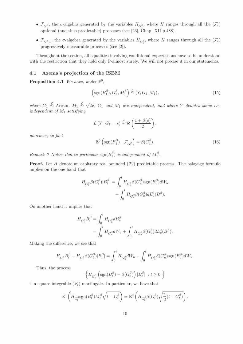
Proposition 4.1 We have, under P0,

(sgn(Bβ

1 ), Gβ1 ,M

β1

) L∼ (Y,G1,M1) , (15)

where G1L∼ Arcsin, M1

L∼√2e, G1 and M1 are independent, and where Y denotes some r.v.

independent of M1 satisfying

L (Y |G1 = s)L∼ R

(1 + β(s)

2

).

moreover, in fact

E0(sgn(Bβ

1 ) | FGβ1

)= β(Gβ

1 ). (16)

Remark 7 Notice that in particular sgn(Bβ1 ) is independent of Mβ

1 .

Proof. Let H denote an arbitrary real bounded (Fs) predictable process. The balayage formulaimplies on the one hand that

HGβ

tβ(Gβ

t )|Bβt | =

∫ t

0H

Gβuβ(Gβ

u)sgn(Bβu )dWu

+

∫ t

0H

Gβuβ(Gβ

u)dL0u(B

β).

On another hand it implies that

HGβ

tBβ

t =

∫ t

0H

GβudBβ

u

=

∫ t

0H

GβudWu +

∫ t

0H

Gβuβ(Gβ

u)dL0u(B

β).

Making the difference, we see that

HGβ

tBβ

t −HGβ

tβ(Gβ

t )|Bβt | =

∫ t

0H

GβudWu −

∫ t

0H

Gβuβ(Gβ

u)sgn(Bβu )dWu.

Thus, the process H

Gβt

(sgn(Bβ

t )− β(Gβt ))|Bβ

t | : t ≥ 0

is a square integrable (Ft) martingale. In particular, we have that

E0

(H

Gβtsgn(Bβ

t )Mβt

√t−Gβ

t

)= E0

(H

Gβtβ(Gβ

t )

√π

2(t−Gβ

t )

).

10

And since this equality is satisfied for all predictable process H,

E0(sgn(Bβ

t )Mβt | F

Gβt

)=

√π

2β(Gβ

t ). (17)

This proves that sgn(Bβt ) and Mβ

t are conditionally uncorrelated. However, even though sgn(Bβt )

takes only values in −1, 1 P0-a.s., this equality is not enough to deduce the conditional law

L(sgn(Bβ

t ) | σ(Gβt ))and we have to work a little more. In the following, we follow the lines of the

article [2] p.290.

Let (Ht) the smallest right-continuous enlargement of (Ft) such that Gβ1 becomes a stopping

time. Then, according to Jeulin [11] p.77 and the exchange formula, we have

HGβ

1= F

Gβ1+

= σ(FGβ

1

)∨⋂

n≥N∗

σ

(W

Gβ1+u

: 0 ≤ u ≤ 1

n

). (18)

Define for ε ∈ (0, 1), Gβ,ε1 = Gβ

1 + ε(1 − Gβ1 ) ; this is a family of (Ht) stopping times, such

that : HGβ,ε

1= F

Gβ,ε1

(see again [11]). Moreover, since (Ht) is right-continuous, we have :

FGβ

1+= H

Gβ1=

⋂

ε∈(0,1)FGβ,ε

1.

We now proceed to show that Mβ1 is independent from H

Gβ1. We first remark that the (Ft)

submartingale P

(Gβ

1 < t | Ft

)(for t < 1) can be computed explicitly using the Theorem 2.1. We

easily find that

P

(Gβ

1 < t | Ft

)= Φ

(|Bβ

t |√1− t

)

where Φ(y) :=

√2

π

∫ y

0exp

(−x2

2

)dx. We deduce from this, using the explicit enlargement for-

mulae that :(|Bβ

Gβ1+u

| − L0Gβ

1+u(Bβ)

)−(|Bβ

Gβ1

| − L0Gβ

1

(Bβ)

)

= ϑu +

∫ u

0

ds√1− (Gβ

1 + s)

(Φ′

Φ

)

|Bβ

Gβ1+s

|√

1− (Gβ1 + s)

, for u < 1−Gβ

1 ,

(19)

where ϑu : u ≥ 0 is a(H

Gβ1+u

, u ≥ 0)Brownian motion, so that ϑu : u ≥ 0 is independent

from HGβ

1.

Note that Bβ

Gβ1

= 0 and L0Gβ

1+u(Bβ) = L0

Gβ1

(Bβ) for 0 ≤ u < 1−Gβ1 .

Using Brownian scaling, we deduce that

mβv = γv +

∫ v

0

dh√1− h

(Φ′

Φ

)(mβ

h√1− h

)for v < 1, (20)

where γv := 1√

1−Gβ1

ϑ(1−Gβ

1 )vis again a Brownian motion which is independent from H

Gβ1and

mβv :=

|Bβ

Gβ1+v(1−G

β1)|

√

1−Gβ1

.

11

From this, we deduce that mβv : v < 1 is the unique strong solution of a SDE driven

(γv). Consequently, mβv : v < 1 is independent of H

Gβ1and by continuity of (mβ

v )0≤v≤1 so is

mβ1 := Mβ

1 .From the fact that Bβ is a (Ft) predictable process and (18) (19), we deduce that

⋂

n≥N∗

σ

(Bβ

Gβ1+u

: 0 ≤ u ≤ 1

n

)⊆ F

Gβ1+

and thus, since sgn(Bβ1 ) = sgn(Bβ

Gβ1+1/n

) for all n > 0, the random variable sgn(Bβ1 ) is F

Gβ1+

measurable. So that,

E0(sgn(Bβ

1 )Mβ1 | F

Gβ1

)= E0

(E0(sgn(Bβ

1 )Mβ1 | F

Gβ1+

)| F

Gβ1

)

= E0(Mβ

1

)E0(sgn(Bβ

1 ) | FGβ1

)

=

√π

2E0(sgn(Bβ

1 ) | FGβ1

),

and identifying with (17) ensures that

E0(sgn(Bβ

1 ) | FGβ1

)= β(Gβ

1 )(= E0

(sgn(Bβ

1 ) | σ(Gβ1 )))

.

Remark 8 The time t = 1 plays no role in the above reasoning so the relation E0(sgn(Bβ

t ) | FGβt

)=

β(Gβt ) holds also for any time t. This proves that, up to a modification, the dual predictable

projection of the process (sgn(Bβt ))t≥0 on the filtration (F

Gβt) is given by the process (β(Gβ

t ))t≥0.

This means that the fundamental equation of the Inhomogeneous Skew Brownian motion maybe re-interpreted like forcing with β a prescribed (F

Gβt)-predictable projection for (sgn(Bβ

t ))t≥0 in

the following equation

Bβt = Wt +

∫ t0p(sgn(Bβ

s ))dL0

s(Bβ)

p(sgn(Bβ

t ))= β(Gβ

t ),(21)

where p (Y.) is a notation for the (FGβ

t) predictable projection of the measurable process Y .

4.2 Markov property

Using the results of the previous section, we may show that the inhomogeneous skew Brownianmotion Bβ is a Markov process. Indeed, even in the homogeneous case, the Markov property forthe existing solution Bβ, is up to our knowledge a non trivial question (see [29, 30, 13, 9, 8, 6]).

Proposition 4.2 Let f be a positive Borel function, then

Ex(f(Bβ

t )|Fs

)=

∫ ∞

−∞dyf(y)pβ(s, t;Bβ

s , y).

Proof. In the following computations, we will use various times the Fubini-Tonelli theorem, whichis justified since we are dealing with positive integrable integrands.

Ex(f(Bβ

t )|Fs

)= Ex

(f(Bβ

t )1Gβt ≤s

|Fs

)+ Ex

(f(Bβ

t )1Gβt >s

|Fs

).

12

Let Hs denote some Fs measurable random variable. We have :

Ex(Hs f(B

βt )1Gβ

t >s

)= Ex

Hs f

sgn

(Bβ

t

) |Bβt |√

t−Gβt

√t−Gβ

t

1

Gβt >s

= Ex

Ex

Hs f

sgn

(Bβ

t

) |Bβt |√

t−Gβt

√t−Gβ

t

1

Gβt >s

|FGβ

t

.

Since the process (Hs 1u>s)u≥0 is (Fu) predictable for any fixed time s, the random variableHs1Gβ

t >sis F

Gβtmeasurable by definition of F

Gβt. So that

Ex(Hs f(B

βt )1Gβ

t >s

)= Ex

Hs1Gβ

t >sEx

f

sgn

(Bβ

t

) |Bβt |√

t−Gβt

√t−Gβ

t

|F

Gβt

= Ex

Hs1Gβ

t >s

∑

δ∈−1,1

1 + δβ(Gβt )

2

∫ ∞

−∞f

(δ

√t−Gβ

t y

)µ0(dy)

where we have used the fact that|Bβ

t |√

t−Gβt

is independent of FGβ

tand sgn(Bβ

t ), and µ0(dy) stands

for the law of√2e (see Proposition 4.1).

Note that the processHsK

su(f) := Hs1u>s

∑δ∈−1,1

1+δβ(u)2 f

(δ√t− uy

): u ≥ 0

is (Fu)

predictable. Since Gβt is the last exist time before time t of some reflected Brownian motion, well-

known results concerning the dual predictable projection of last exit times for BM (and hence forreflected BM as well) ensure that :

Ex(HsK

sGβ

t

(f))= Ex

(∫ t

0HsK

su(f)

(π2(t− u)

)−1/2dL0

u(|Bβ |)).

In particular, using Theorem 2.1, we have

Ex(Hs f(B

βt )1Gβ

t >s

)=

∫ ∞

0µ0(dy)Ex

[∫ t

0HsK

su(f)

(π2(t− u)

)−1/2dL0

u(|Bβ|)]

=

∫ ∞

0µ0(dy)Ex

[Hs

∫ t

0Ks

u(f)(π2(t− u)

)−1/2dL0

u(|Bβ|)].

So that using the Markov property for the absolute value of Brownian motion, and denoting Wsome standard Brownian motion independent of Fs, we obtain :

Ex(Hs f(B

βt )1Gβ

t >s

)

=

∫ ∞

0µ0(dy)Ex

[HsE

|Bβs |∫ t−s

0Ks

u+s(f)(π2(t− (s+ u))

)−1/2dL0

u(|W |)]

=

∫ ∞

0µ0(dy)Ex

[Hs

∫ t−s

0Ks

u+s(f)(π2(t− (s+ u))

)−1/2p(u, |Bβ

s |, 0)du

],

where we have used Exercise 1.12, Chap. X of [23] (whose result remains true for symmetric localtime). Performing the change of variable ξ = δ

√t− (s+ u)y finally yields

Ex(Hs f(B

βt )1Gβ

t >s

)=

∫ ∞

−∞Ex

Hs

∑

δ∈−1,1

∫ t−s

0f(ξ)

1 + δ(β σs)(u)2

√2

π

|ξ|e−ξ2

2(t−(s+u))

(t− (s+ u))3/2e−

|Bβs |2

2u

√2πu

du

1δξ>0dξ

13

On another hand, for a fixed time s > 0 we may set

Dβs := infu ≥ 0 : Bβ

s+u = 0 = infu ≥ 0 : Bβs + (Ws+u −Ws) = 0.

So that using the equation solved by the inhomogeneous skew Brownian motion (1) and the usualMarkov property for the standard Brownian motion :

Ex(Hsf(B

βt )1Gβ

t ≤s

)= Ex

[Hs f

(Bβ

s + (Ws+(t−s) −Ws))1

Dβs≥(t−s)

]

= Ex[Ex[Hs f

(Bβ

s + (Ws+(t−s) −Ws))1

Dβs≥(t−s)

| Fs

]]

= Ex[HsE

Bβs

[f(Wt−s

)1T0≥(t−s)

]]

=

∫ ∞

−∞dyf(y)Ex

[Hs

1√2π(t− s)

[exp

(−(y −Bβ

s )2

2(t− s)

)− exp

(−(y +Bβ

s )2

2(t− s)

)]1

Bβs y>0

].

Adding these terms and using the characterization of conditional expectation finally yields that

Ex(f(Bβ

t )|Fs

)=

∫ ∞

−∞dyf(y)pβ(s, t;Bβ

s , y),

where we used the Definition 2.6.

Let us notice that, as∫∞−∞ dyf(y)pβ(s, t;Bβ

s , y) is a σ(Bβs )-measurable random variable, we get

from Proposition 4.2 ,

Ex(f(Bβ

t )|Fs

)= Ex

(f(Bβ

t )|Bβs

)=

∫ ∞

−∞dyf(y)pβ(s, t;Bβ

s , y). (22)

This leads naturally to the following important consequence.

Proposition 4.3 We havei) The process Bβ is a Markov process, in the sense of Definition 2.5.10 in [12].ii) For all x, y ∈ R we have

Ps,x(Bβt ∈ dy) = pβ(s, t;x, y)dy. (23)

Remark 9 The proposition 4.3 will imply in turn that the family pβ(s, t;x, y) may be considered asa transition family (t.f.). See the forthcoming Proposition 5.3.

Notice that since the considerations of Proposition 4.2 may be repeated if the fixed time s isreplaced by T a (Ft)-stopping time, we may also state the following :

Corollary 4.4 The process Bβ is a strong Markov process in the sense given by Theorem 3.1 in[23] Chap. III sect.3, p.102.

4.3 Kolmogorov’s continuity criterion

The next result shows a Kolmogorov’s continuity criterion for Bβ uniform w.r.t. the parameterfunction β(.).

Proposition 4.5 There exists a universal constant C > 0 (independent of the function β(.)) suchthat for all ε ≥ 0 and t ≥ 0,

Ex|Bβt+ε −Bβ

t |4 ≤ C ε2. (24)

14

Proof. Conditioning with respect to Ft and using the Markov property and (23) we get,

Ex|Bβt+ε −Bβ

t |4 = Ex[ ∫ ∞

−∞(y −Bβ

t )4 pβ(t, t+ ε;Bβ

t , y)dy]

= Ex[ ∫ ∞

−∞(y −Bβ

t )4 p(ε,Bβ

t , y)dy

+

∫ ∞

−∞dy (y −Bβ

t )4

∫ ε

0

β σs(u)2

y

π

e− y2

2(ε−u)

√u(ε− u)3/2

e−|B

βt|2

2u du]

≤ Ex[ ∫ ∞

−∞(y −Bβ

t )4 p(ε,Bβ

t , y)dy

+

∫ ∞

−∞dy (y −Bβ

t )4

∫ ε

0

|y|2π

e− y2

2(ε−u)

√u(ε− u)3/2

e−|B

βt|2

2u du]

≤ 2Ex[ ∫ ∞

−∞(y −Bβ

t )4 p(ε,Bβ

t , y)dy]

where we have successively used (10) and (9). As for the brownian density we have∫∞−∞(y −Bβ

t )4 p(ε,Bβ

t , y)dy ≤ Cε2, we get the desired result.

5 Existence result for the inhomogeneous skew Brownian motion

5.1 Part I : the case of a smooth coefficient β

Proposition 5.1 Assume there exist −1 < m < M < 1 s.t. m ≤ β(t) ≤ M , for all t ≥ 0. Assumemoreover that β ∈ C1

b (R+). Then there exists a unique strong solution Bβ to (1).

Let us introduce some notations. We introduce the C1,2(R+ × R∗) function r(t, y) defined by

r(t, y) :=

β(t) + 1

2y if y ≥ 0

1− β(t)

2y if y < 0.

(25)

The proof of Proposition 5.1 relies on the following lemma.

Lemma 5.2 Under the assumptions of Proposition 5.1 the SDE

dYt =dWt

r′y(t, Yt)− r′t(t, Yt)

r′y(t, Yt)dt, (26)

has a unique strong solution.

Proof. The coefficient (r′y(t, y)) is piecewise C1 with respect to y, measurable with respect to(t, y), uniformly positive, and bounded. The coefficient r′t(t, y)/r

′y(t, y) is measurable and bounded.

Thus, according to Theorem 1.3 in [14], and the remark following it, the SDE (26) enjoys pathwiseuniqueness and has a weak solution. Therefore the result, using [28, 26].

Proof of Proposition 5.1. We set Xt := r(t, Yt) with Y the unique strong solution of (26) (cor-responding to the given Brownian motion W ). We will show that X solves (1) (with W ). Therefore

15

the result, as X is (Ft) adapted. Using the change of variable formula proposed by Peskir in [19],we get

Xt = r(0, Y0) +

∫ t

0r′t(s, Ys)ds +

∫ t

0r′y(s, Ys)dYs +

1

2

∫ t

0β(s)dL0

s(Y )

= r(0, Y0) +

∫ t

0r′t(s, Ys)ds +Wt

−∫ t

0r′t(s, Ys)ds +

1

2

∫ t

0β(s)dL0

s(Y )

= r(0, Y0) +Wt +1

2

∫ t

0β(s)dL0

s(Y ).

It remains to show that 12L

0t (Y ) = L0

t (X). To this end we adapt the methodology proposed inSubsection 5.2 of [16]. On one hand the symmetric Tanaka formula gives,

d|Xt| = sgn(Xt)dXt + L0t (X) = sgn(Yt)dWt + L0

t (X),

where we have used sgn(Xt) = sgn(Yt) and sgn(0) = 0 (for the sign function involved in thesymmetric Tanaka formula is the symmetric sign function). On the other hand, using again theformula by Peskir, with the function (t, y) 7→ |r(t, y)|, we get

|Xt| = |r(t, Yt)| = |r(0, Y0)|+∫ t

0sgn(Ys)r

′t(s, Ys)ds+

∫ t

0sgn(Ys)dWs

−∫ t

0sgn(Ys)r

′t(s, Ys)ds+

1

2L0t (Y )

= |r(0, Y0)|+∫ t

0sgn(Ys)dWs +

1

2L0t (Y ).

By unicity of the decomposition of a semi-martingale we get 12L

0t (Y ) = L0

t (X), and we are done.

5.2 Part II: the general case (proof of Theorem 2.8)

Till the end of the section we are given a Borel function β : R+ → [−1, 1].

Firstly, combining Propositions 5.1 and 4.3 we get the following crucial result.

Proposition 5.3 The family of measures pβ(s, t;x, y)dy of Definition 2.6 is a (inhomogeneous)family of transition probabilities satisfying the Chapman-Kolmogorov equation

∫ ∞

−∞pβ(s, t;x, y)pβ(t, v; y, z)dy = pβ(s, v;x, z), 0 < s < t < v, x, z ∈ R. (27)

Proof. For a smooth function β(.) satisfying the assumptions of Proposition 5.1, there exists asolution to (1), which is a Markov process satisfying (23). Thus, the family pβ(s, t;x, y)dy satisfies(27) (see Chap. III, sect. 1, p. 80 of [23]).

For the Borel function β(.) we may approximate β by a sequence of smooth functions βn(.).As the family pβn(s, t;x, y)dy satisfies (27) we recover the same result for pβ(s, t;x, y)dy thanks toLebesgue’s domination theorem.

16

Let us discuss briefly the point that we have reached till now. For any Borel function β the familypβ(s, t;x, y)dy, is a transition family (t.f.). If a strong solution Bβ to (1) exists, it is necessarily aMarkov process with transition family pβ(s, t;x, y)dy.

We will now construct a Markov process with t.f. pβ(s, t;x, y)dy and show that it provides aweak solution of (1).

Thanks to the result of Proposition 5.3, we can construct a probability Q0 on (R[0,∞),R[0,∞))such that the coordinate process (ω(t))t≥0 is a Markov process with t.f. pβ(s, t;x, y)dy (startingfrom zero) on (R[0,∞),R[0,∞), Q0) (Theorem 1.5 Chap. III in [23]).

Using the same computations than in the proof of Proposition 4.5, it possible to show that aKolmogorov’s continuity criterion holds for (ω(t))t≥0 under Q0. This implies that we can constructa modification of (ω(t))t≥0 with Q0-a.s. continuous paths. Transporting the measure Q0 on the setof continuous functions C (see [23] p.35 for details) we get the following:

Proposition 5.4 There exists a probability measure Q0 on (C,B(C)) under which the coordinateprocess is a Markov process with t.f. pβ(s, t;x, y)dy.

Proposition 5.4 implies that there exists a Markov process Xβ with continuous paths and t.f.pβ(s, t, x, y), defined on a probability space (C,B(C),Q0).

We will denote by (Fβt )t≥0 the complete right continuous filtration endowed byXβ on (C,B(C),Q0).

Having in mind the results of the previous sections, we begin to prove the following proposition :

Proposition 5.5 We have

(|Xβt |)t≥0

L∼ (|Wt|)t≥0 .

Proof. Let y, x > 0 and 0 < s < t. We compute

Q0(|Xβt | ∈ dy

∣∣ |Xβs | = x) = Q0(|Xβ

t | ∈ dy∣∣ Xβ

s = x)Q0(Xβs > 0

∣∣ |Xβs | = x)

+Q0(|Xβt | ∈ dy

∣∣ Xβs = −x)Q0(Xβ

s < 0∣∣ |Xβ

s | = x)

= dyQ0(Xβ

s > 0∣∣ |Xβ

s | = x)(pβ(s, t;x, y) + pβ(s, t;x,−y)

)

+Q0(Xβs < 0

∣∣ |Xβs | = x)

(pβ(s, t;−x, y) + pβ(s, t;−x,−y)

)

= dyQ0(Xβ

s > 0∣∣ |Xβ

s | = x)(p(t− s, x, y) + p(t− s, x,−y)

)

+Q0(Xβs < 0

∣∣ |Xβs | = x)

(p(t− s,−x, y) + p(t− s,−x,−y)

)

= dy [p(t− s, x, y) + p(t− s, x,−y)],

where we have used Equation (10), and the symmetry of (x, y) 7→ p(t, x, y) in the computations. Thefinal right hand side expression is the well-known (homogeneous) density of a reflected Brownianmotion |W | starting from x > 0.

As |Xβ | is Markov as well as |W |, and since both processes have continuous sample paths, weget the desired result (see for example Theorem 1.5 Chap. III in [23]).

Consequently, we have the following theorem :

Theorem 5.6 There exists a weak solution to (1).

17

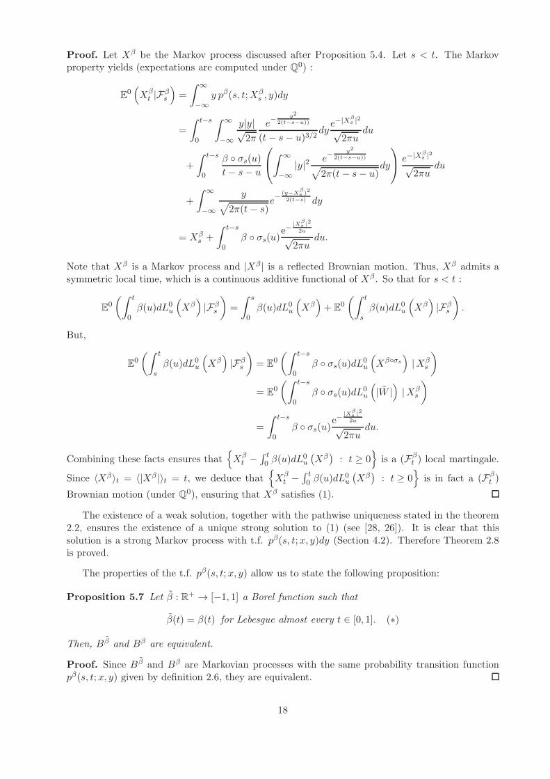
Proof. Let Xβ be the Markov process discussed after Proposition 5.4. Let s < t. The Markovproperty yields (expectations are computed under Q0) :

E0(Xβ

t |Fβs

)=

∫ ∞

−∞y pβ(s, t;Xβ

s , y)dy

=

∫ t−s

0

∫ ∞

−∞

y|y|√2π

e− y2

2(t−s−u))

(t− s− u)3/2dy

e−|Xβs |2

√2πu

du

+

∫ t−s

0

β σs(u)t− s− u

∫ ∞

−∞|y|2 e

− y2

2(t−s−u))

√2π(t− s− u)

dy

e−|Xβ

s |2√2πu

du

+

∫ ∞

−∞

y√2π(t− s)

e− (y−X

βs )2

2(t−s) dy

= Xβs +

∫ t−s

0β σs(u)

e−|X

βs |2

2u

√2πu

du.

Note that Xβ is a Markov process and |Xβ | is a reflected Brownian motion. Thus, Xβ admits asymmetric local time, which is a continuous additive functional of Xβ. So that for s < t :

E0

(∫ t

0β(u)dL0

u

(Xβ)|Fβ

s

)=

∫ s

0β(u)dL0

u

(Xβ)+ E0

(∫ t

sβ(u)dL0

u

(Xβ)|Fβ

s

).

But,

E0

(∫ t

sβ(u)dL0

u

(Xβ)|Fβ

s

)= E0

(∫ t−s

0β σs(u)dL0

u

(Xβσs

)|Xβ

s

)

= E0

(∫ t−s

0β σs(u)dL0

u

(|W |

)|Xβ

s

)

=

∫ t−s

0β σs(u)

e−|X

βs |2

2u√2πu

du.

Combining these facts ensures thatXβ

t −∫ t0 β(u)dL

0u

(Xβ)

: t ≥ 0

is a (Fβt ) local martingale.

Since 〈Xβ〉t = 〈|Xβ |〉t = t, we deduce thatXβ

t −∫ t0 β(u)dL

0u

(Xβ)

: t ≥ 0

is in fact a (Fβt )

Brownian motion (under Q0), ensuring that Xβ satisfies (1).

The existence of a weak solution, together with the pathwise uniqueness stated in the theorem2.2, ensures the existence of a unique strong solution to (1) (see [28, 26]). It is clear that thissolution is a strong Markov process with t.f. pβ(s, t;x, y)dy (Section 4.2). Therefore Theorem 2.8is proved.

The properties of the t.f. pβ(s, t;x, y) allow us to state the following proposition:

Proposition 5.7 Let β : R+ → [−1, 1] a Borel function such that

β(t) = β(t) for Lebesgue almost every t ∈ [0, 1]. (∗)

Then, Bβ and Bβ are equivalent.

Proof. Since Bβ and Bβ are Markovian processes with the same probability transition functionpβ(s, t;x, y) given by definition 2.6, they are equivalent.

18

6 Proof of Theorem 2.9

The result of Theorem 2.9 will appear as a consequence of the previous Proposition 4.1 and thefollowing lemma which appears again as a consequence of Proposition 2.1 and known results con-cerning the standard Brownian motion :

Lemma 6.1 Under P0, the process |Bβt | := 1

√

Gβ1

|Bβ

tGβ1

| : t ≤ 1 is the reflection (above 0) of a

Brownian Bridge independent of G := σ

Gβ

1 , Bβ

Gβ1+u

; u ≥ 0

.

Proof. By the result of Theorem 2.1 and time inversion, |Bβt | := t |Bβ

1t

| is a reflected Brownian

motion. Note that

dβ1 := inf(u > 1 : |Bβ

u | = 0)=

1

Gβ1

.

So that, since Bβ1

Gβ1

= Bβ

dβ1= 0,

1√Gβ

1

|Bβ

tGβ1

| = t

√Gβ

1 |Bβ

1

t Gβ1

| = t√dβ1

|Bβ1

Gβ1

+ 1

Gβ1

( 1t−1)

− Bβ1

Gβ1

|

=t√dβ1

|Bβ

dβ1+dβ1 (1t−1)

− Bβ

dβ1|.

Since

|Bβ

dβ1+u− Bβ

dβ1| : u ≥ 0

is a reflected Brownian motion independent of F

dβ1and Bβ

dβ1= 0,

the process |Bβu | := 1

√

dβ1

|Bβ

dβ1+dβ1u| is also a reflected Brownian motion independent of F

dβ1; hence,

(t|Bβ

1t−1

|)

t≥0

is a reflected Brownian Bridge independent of Fdβ1. This implies the result.

Corollary 6.2 We have that under P0,

L01

(Bβ)=

√Gβ

1 ℓ01 (28)

where ℓ01 is the symmetric local time at time 1 of a standard Brownian Bridge independent of G.

Proof. Under P0, we have that

L01

(Bβ)= L0

1

(|Bβ|

)= L0

Gβ1

(|Bβ|

)

= L0Gβ

1

(√Gβ

1 |Bβ

./Gβ1

|).

Recall that the symmetric local time a semimartingale (Yt) is given by

L0t (Y ) = lim

ε→0

1

2ε

∫ t

01(−ε,ε)(Ys)d〈Y 〉s.

So we find, using an obvious change of variable, that

L01

(Bβ)=

√Gβ

1L01

(|Bβ|

)=

√Gβ

1 ℓ01,

where the last equality comes from the result of Lemma 6.1.

19

Combining this result and the result of Proposition 4.1 gives that

(Gβ

1 , L01

(Bβ), Bβ

1

)L∼(G1,

√G1ℓ

01, Y

√1−G1M1

)

where G1L∼ Arcsin, ℓ01

L∼√2e, M1

L∼√2e are independent and where Y denotes a r.v. independent

of M1 and ℓ01 and satisfying

L (Y |G1 = s)L∼ R

(1 + β(s)

2

).

This construction gives the result announced in Theorem 2.9.

Remark 10 We proved the result of Theorem 2.9 using only probabilistic tools and not the compu-tations of Section 3. Since we used only that Bβ is solution of (1), the arguments developed in thissection yield another proof of Proposition 2.7 as a by product.

7 Another construction of the inhomogeneous skew Brownian mo-

tion

7.1 Construction of the Inhomogeneous SBM with piecewise constant coeffi-cient β from a reflected Brownian motion

Let Π : 0 = t0 < t1 < · · · < ti < · · · < tn = 1 be a partition of the interval [0, 1].We define a function i : [0, 1] → J0 : n− 1K by

i(t) = sup0 ≤ k ≤ n− 1 : tk ≤ t, ∀t ∈ [0, 1) and i(1) = n− 1.

Let β : R+ → [0, 1] be a r.c.l.l. function with constant value in [−1, 1] on each interval [ti, ti+1).In particular β is a Borel function. In this section, we give a construction of a weak solution of(1) on the interval [0, 1], obtained by changing the sign of the excursion of a reflecting Brownianmotion. We are inspired by [23], Chap. XII, Exercise 2.16 p. 487.

Let us follow the notations of [23] concerning the excursions of a Brownian motion B: theexcursion process is denoted by (es)s≥0, where the index s is in the local time scale. Each excursiones(ω) has support [τs−(ω), τs(ω)), where τs(ω) =

∑u≤sR(eu(ω)), and τs−(ω) =

∑u<sR(eu(ω)),

with R(es(ω)) the length of the excursion es(ω). We recall that L0t (B) can be recovered as the

inverse of τt.

The construction is the following : for each 0 ≤ i ≤ n−1 let (Y ik )k be a sequence of independent

r.v.’s, identically distributed with lawR(1+βn

i

2

)(with βn

i := β(ti)), and defined on some probability

space (Ω,F ,P). Let B be a standard Brownian motion independent of the Y ik ’s, constructed on

(Ω,F ,P). The set of its excursions es(ω) is countable and may be given the ordering of N.We define a process X β on [0, 1] by putting

∀t ∈ [0, 1], X βt (ω) = Y

i(τs−(ω))ks(ω)

(ω)|es(t− τs−(ω), ω)|,

if τs−(ω) ≤ t ≤ τs(ω) and es(ω) is the ks(ω)-th excursion in the above ordering.For τs−(ω) ≤ t ≤ τs(ω) we have τs−(ω) = gt(ω) where gt := supu < t : |Bu| = 0, and

|es(t− τs−(ω), ω)| = |Bt(ω)|.Note also that for a fixed ω ∈ Ω, the construction does not make a use of the entire double

indexed sequence (Y ik (ω))i∈0,...,n−1,k∈N.

Proposition 7.1 The process X β is a weak solution of equation (1) with parameter β and startingfrom zero.

20

Proof. We only detail the main arguments of the proof and leave some of the details to the reader.1st step : preliminary factsNote that X β is constructed such that

(|X βt |)t≥0

L∼ (|Wt|)t≥0 .

Moreover, defining Gβ1 := sup

(0 ≤ s ≤ 1 : X β

s = 0)and M β

1 := |X β1 |/√

1−Gβ1 , we see from the

construction of X β that (sgn(X β

1 ), Gβ1 ,M

β1

)L∼ (Y,G1,M1) , (29)

where G1L∼ Arcsin, M1

L∼√2e, G1 and M1 are independent, and where Y denotes some r.v.

independent of M1 satisfying

L (Y |G1 = s)L∼ R

(1 + β(s)

2

).

Let(Ft

)the natural filtration of X β that has been completed and augmented in order to satisfy

the usual conditions. From the construction of X β, we see that

E

(sgn(X β

t ) | FGβt

)= E

(Y

i(Gβt )

kL0t(|B|)

| FGβ

t

)= β(Gβ

t ). (30)

2nd step : X β is a(Ft

)Markov process

Because of these preliminary facts, we may repeat the arguments of the first part in the proofof Proposition 4.2 : we see that for s < t and any measurable function f :

E

(f(X β

t )1Gβt >s

|Fs

)

=

∫ ∞

−∞dξf(ξ)E0

∑

δ∈−1,1

∫ t−s

0

1 + δ(β σs)(u)2

√2

π

|ξ|e−ξ2

2(t−(s+u))

(t− (s+ u))3/2e−

|Xβs |2

2u√2πu

du

1δξ>0.

The part E(f(X β

t )1Gβt ≤s

|Fs

)is more complicated since we cannot refer to Equation (1).

Still, for a fixed time s > 0 we may set

Dβs := infu ≥ 0 : X β

s+u = 0.

We have :

Dβs = infu ≥ 0 : X β

s+u = 0= infu ≥ 0 : X β

s +X βs+u −X β

s = 0= infu ≥ 0 : X β

s + sgn(X βs ) (|Bs+u| − |Bs|) = 0

= infu ≥ 0 : (|Bs+u| − |Bs|) = −|X βs |.

But on the set Gβt ≤ s = Dβ

s ≥ (t − s) and for r < Dβs , the random variables Bs+r and Bs

share the same sign. We deduce that on the set Gβt ≤ s,

Dβs =

infu ≥ 0 : (Bs+u −Bs) = −|X β

s | := T+s if Bs ≥ 0 ;

infu ≥ 0 : (Bs+u −Bs) = |X βs | := T−

s if Bs < 0.

21

Let us introduce Ks := Fs ∨ σ (Bs).We have

E

(f(X β

t )1Gβt ≤s

|Ks

)= E

(f(X β

s + sgn(X βs )(|Bs+(t−s)| − |Bs|

))1

Dβs≥(t−s)

|Ks

)

= 1Bs≥0E

(f(X β

s + sgn(X βs )(Bs+(t−s) −Bs

))1T+

s ≥(t−s)|Ks

)

+ 1Bs<0E

(f(X β

s − sgn(X βs )(Bs+(t−s) −Bs

))1T−

s ≥(t−s)|Ks

).

Since (Bs+u −Bs : u ≥ 0) is a Brownian motion independent of Bs and of Fs (and thus ofKs), we may integrate this expression using the known laws of the Brownian motion killed whenhitting 0 :

1Bs≥0E

(f(X β

s + sgn(X βs )(Bs+(t−s) −Bs

))1T+

s ≥(t−s)|Ks

)

= 1Bs≥0

∫ ∞

−∞dθf

(X β

s + sgn(X βs )(θ − |X β

s |))

× 1√2π(t− s)

[exp

(−(θ − |X β

s |)22(t− s)

)− exp

(−(θ + |X β

s |)22(t− s)

)]1|Xβ

s | θ>0

= 1Bs≥0

∫ ∞

−∞dyf (y)

1√2π(t− s)

[exp

(−(y −X β

s )2

2(t− s)

)− exp

(−(y +X β

s )2

2(t− s)

)]1

Xβs y>0

where for the last line, we performed the change of variable y = sgn(X βs )θ. We have a similar term

on the side Bs < 0, so that

E

(f(X β

t )1Gβt ≤s

|Ks

)

=

∫ ∞

−∞dyf (y)

1√2π(t− s)

[exp

(−(y −X β

s )2

2(t− s)

)− exp

(−(y +X β

s )2

2(t− s)

)]1

Xβs y>0

= E

(f(X β

t )1Gβt ≤s

|Fs

).

Finally, adding both parts gives that

E

(f(X β

t )|Fs

)=

∫ ∞

−∞dyf(y)pβ(s, t;X β

s , y).

This is enough to conclude thatX β is a Markov process with pβ(s, t;x, y)dy as its family of transitionprobability (satisfying (27)).

3rd step : the process X β is a weak solution of equation (1)It suffices to perform the same computations as in the proof of Theorem 5.6. Indeed X β is

Markov and, by construction, |X β| is a reflected Brownian motion.

7.2 The convergence result

In this section, we show another way of constructing a weak solution of (1) on the time interval[0, 1].

22

7.2.1 The technical assumption H

In this subsection we state the assumptions of Theorem 7.3.Let Πn : 0 = tn0 < tn1 < · · · < tni < . . . tnn = 1, n ≥ 0 a sequence of partitions over [0, 1].

Assume thatsup

0≤i≤n−1|tni+1 − tni | −−−−−→n→+∞

0.

We now state a technical assumption H that will be used in force in all our considerations.It is possible to construct a decreasing (resp. increasing) sequence (βn) (resp. (βn)) of r.c.l.l.

step functions that are constant on each of the intervals [tni , tni+1) in such a way that

βn(t) ≥ β(t) ≥ βn(t) and limn→+∞

βn(t) = limn→+∞

βn(t) = β(t), ∀t ∈ [0, 1].

7.2.2 A convergence result

Corresponding to such sequences (βn) and (βn), we introduce the corresponding sequences (Bβn)n≥0

and (Bβn)n≥0 of ISBM which are strong solutions to equation (1) and driven by the same Brownianmotion W .

Then, we have the following comparison principle :

Proposition 7.2 For any n ≥ 0,

P

[Bβn

t ≥ Bβn+1t , ∀t ∈ [0, 1]

]= 1,

andP

[Bβn

t ≤ Bβn+1

t , ∀t ∈ [0, 1]]= 1.

Proof. Since βn (resp. βn) is a step function, the process Bβn can be viewed as a concatenationof (homogeneous) skew Brownian motions on each interval [tni , t

ni+1[. Thus the result is a direct

consequence of the comparison principle for the SBM (see [14], p.73).

Remark 11 In the above proof it is convenient to see the existing process Bβn as a concatenationof SBM’s. Conversely we may wish to take the concatenation of SBM’s as the starting point of theconstruction of an ISBM with piecewise constant coefficient. However we did not manage to exploitthis idea, because the flow of a classical skew Brownian motion is not defined for all starting pointsx simultaneously (see the remark in the introduction of [7], previously cited).

Let us now state the main result of this section,

Theorem 7.3 Assume that H is satisfied.Then,

P

[lim

n→+∞supt∈[0,1]

|Bβn

t −Bβt | = lim

n→+∞supt∈[0,1]

|Bβn

t −Bβt | = 0

]= 1.

Proof. 1st step : convergence UCP

Let t ∈ [0, 1] fixed. The result of Proposition 7.2 implies that (Bβn

t )n≥0 (resp. (Bβn

t )n≥0) isan a.s. decreasing (resp. increasing) sequence of random variables bounded from below (resp.

bounded from above). Thus, the sequence (Bβn

t )n≥0 (resp. (Bβn

t )n≥0) converges a.s. to somerandom variable Yt (resp. Yt). For simplicity, we concentrate in the rest of the proof to the familyof random variables Yt : 0 ≤ t ≤ 1.

23

From Lebesgue’s theorem and the result of Proposition 4.5, we have for t ∈ [0, 1] :

E|Yt+ε − Yt|4 = E limn→+∞

|Bβn

t+ε −Bβn

t |4 ≤ Cε2. (31)

Kolmogorov’s continuity criterion implies that there is a continuous modification of the process Y(that we still denote abusively Y ). Moreover, Proposition 7.2 implies that the sequence (Bβn

. )n≥0

is an a.s decreasing sequence of continuous functions on the compact space [0, 1] converging simplyto a continuous function Y. : from Dini’s theorem this convergence is uniform almost surely. Conse-quently, (Bβn

. )n≥0 is a.s. a Cauchy sequence for the uniform norm over [0, 1]. Moreover, Lebesgue’sdominated convergence theorem ensures that

E

[supt∈[0,1]

|Bβp

t −Bβq

t |]−−−−−→p,q→+∞

0. (32)

From (32), we see that (Bβn. )n≥0 is a Cauchy sequence in the complete space Ducp (see for example

[21] Chap. II, p. 57). Combining these facts ensures that the family (Yt) agregates as a processwith a.s. continuous trajectories and we have proved that :

supt∈[0,1]

|Bβn

t − Yt| P−a.s.−−−−−→n→+∞

0. (33)

2nd step : identification of the limit

Let us proceed to identify(Yt

)t∈[0,1] with the unique strong solution of (1) (relative to the

Brownian motion W ).

On one hand, from the fact that (|Bβn

t |)t≥0L∼ (|Wt|)t≥0 and from (33), we deduce that

(|Yt|)t∈[0,1]L∼ (|Wt|)t∈[0,1]. In particular,

(|Yt|)t∈[0,1] is a semimartingale and admits a symmet-

ric local time process L0. (|Y |).

A consequence of the (symmetric) Tanaka formula is that

|Bβn

t | = |x|+∫ t

0sgn(Bβn

s )dWs + L0t (B

βn) (with sgn(0) = 0). (34)

As |Y | is a reflected brownian motion we have

|Yt| = |x|+ Wt + L0t

(|Y |), (35)

for some brownian motion W . But from the a.s. uniform convergence of (Bβn

t )t∈[0,1] towards

(Yt)t∈[0,1] and the dominated convergence theorem for stochastic integrals (see for example Theorem2.12 p.142 in [23]), we can see that there is a finite variation process A s.t.

sups∈[0,1]

|L0s(B

βn)−As| P−−−−−→n→+∞

0,

and that

sups∈[0,1]

∣∣ |Bβns | − (|x|+

∫ s

0sgn(Yu)dWu +As)

∣∣ P−−−−−→n→+∞

0.

Thus,

|Yt| = |x|+∫ t

0sgn(Yu)dWu +At. (36)

24

Using (35) and (36), and the unicity of the Doob decomposition of a semimartingale yields that

|Yt| = |x|+∫ t

0sgn(Ys)dWs + L0

t

(|Y |). (37)

Note that we have proven that,

[supt∈[0,1]

∣∣∣L0t (B

βn)− L0t (|Y |)

∣∣∣ > ε

]P−−−−−→

n→+∞0.

On another hand, proceeding as in Section 5, it is not difficult to see from the a.s. uniform

convergence of (Bβn

t )t∈[0,1] towards (Yt)t∈[0,1] that (Yt)t∈[0,1] is a Markov process with pβ(s, t;x, y)dyas its t.f. Hence, we may proceed just as in Step 3 of Proposition 7.1 and we see that there existsa Brownian motion W such that

Yt = x+ Wt +

∫ t

0β(s)dL0

s(|Y |) = x+ Wt +

∫ t

0β(s)dL0

s(Y ). (38)

It remains to identify W with W .From (37) and (38), we see that necessarily

|Yt| = |x|+∫ t

0sgn(Ys)dWs + L0

t (|Y |) = |x|+∫ t

0sgn(Ys)dWs + L0

t (|Y |), (39)

so that ∫ t

0sgn(Ys)dWs =

∫ t

0sgn(Ys)dWs,

and

Wt =

∫ t

0sgn(Ys)sgn(Ys)dWs =

∫ t

0sgn(Ys)sgn(Ys)dWs = Wt.

This ends the proof.

Remark 12 Theorem 7.3 gives a construction of a solution of (1) when the technical assumptionH is satisfied. When this is not the case, we may conclude that there exists a weak solution to (1),with the help of Proposition 5.7.

Remark 13 We have not been able to prove directly that

limn→+∞

P

[∣∣∣∣∫ 1

0βn(s)dL

0s(B

βn)−∫ 1

0β(s)dL0

s(Y )

∣∣∣∣ > ε

]= 0.

This convergence is strongly related to the convergence of the sequence (Gβn

t )n≥0 towards Gt :=sup0 ≤ s ≤ t : Ys = 0, which cannot be guaranteed neither by the uniform convergence of

(Bβn)n≥0 towards Y , nor by the monotonicity of (Bβn)n≥0.

Acknowledgements

Both authors would like to thank Pr. A. Gloter for helpful discussion.

25

References

[1] Thilanka Appuhamillage, Vrushali Bokil, Enrique Thomann, Edward Waymire, and BrianWood, Occupation and local times for skew Brownian motion with applications to dispersionacross an interface, Ann. Appl. Probab. 21 (2011), no. 1, 183–214. MR 2759199

[2] M. Barlow, J. Pitman, and M. Yor, On Walsh’s Brownian motions, Seminaire de Probabilites,XXIII, Lecture Notes in Math., vol. 1372, Springer, Berlin, 1989, pp. 275–293. MR 1022917(91a:60204)

[3] M. T. Barlow, Skew Brownian motion and a one-dimensional stochastic differential equation,Stochastics 25 (1988), no. 1, 1–2. MR 1008231 (91e:60165)

[4] Martin Barlow, Krzysztof Burdzy, Haya Kaspi, and Avi Mandelbaum, Variably skewed Brown-ian motion, Electron. Comm. Probab. 5 (2000), 57–66 (electronic). MR 1752008 (2001j:60146)

[5] , Coalescence of skew Brownian motions, Seminaire de Probabilites, XXXV, LectureNotes in Math., vol. 1755, Springer, Berlin, 2001, pp. 202–205. MR 1837288 (2002h:60166)

[6] M. Bossy, N. Champagnat, S. Maire, and D. Talay, Probabilistic interpretation and randomwalk on spheres algorithms for the Poisson–Boltzmann equation in molecular dynamics, Math.Model. Numer. Anal. 44 (2010), no. 5, 997–1048.

[7] Krzysztof Burdzy and Zhen-Qing Chen, Local time flow related to skew Brownian motion,Ann. Probab. 29 (2001), no. 4, 1693–1715. MR 1880238 (2003f:60098)

[8] Krzysztof Burdzy and Haya Kaspi, Lenses in skew Brownian flow, Ann. Probab. 32 (2004),no. 4, 3085–3115. MR 2094439 (2005j:60153)

[9] H. Hajri, Stochastic flows related to walsh brownian motion, Preprint (2011).

[10] J. M. Harrison and L. A. Shepp, On skew Brownian motion, Ann. Probab. 9 (1981), no. 2,309–313. MR 606993 (82j:60144)

[11] T. Jeulin, Semi-martingales et grossissement d’une filtration, Lecture Notes in Mathematics,vol. 833, Springer, Berlin, 1980. MR 604176 (82h:60106)

[12] I. Karatzas and S.E. Shreve, Brownian motion and stochastic calculus. 2nd ed., Graduate Textsin Mathematics, 113. New York etc.: Springer-Verlag. xxiii, 470 p. , 1991.

[13] A. M. Kulik, On the solution of a one-dimensional stochastic differential equation with singulardrift coefficient, Ukrainian Mathematical Journal 56 (2004), 774–789, 10.1007/s11253-005-0088-8.

[14] J.-F. Le Gall, One-dimensional stochastic differential equations involving the local times ofthe unknown process, Stochastic analysis and applications (Swansea, 1983), Lecture Notes inMath., vol. 1095, Springer, Berlin, 1984, pp. 51–82. MR 777514 (86g:60071)

[15] Antoine Lejay, On the constructions of the skew Brownian motion, Probab. Surv. 3 (2006),413–466 (electronic). MR 2280299 (2008h:60333)

[16] , On the constructions of the skew Brownian motion, Probab. Surv. 3 (2006), 413–466(electronic). MR 2280299 (2008h:60333)

[17] , A probabilistic interpretation of the transmission conditions using the skew Brownianmotion, Multi scale problems and asymptotic analysis, GAKUTO Internat. Ser. Math. Sci.Appl., vol. 24, Gakkotosho, Tokyo, 2006, pp. 195–206. MR 2233179

26

[18] Y. Ouknine, Le “Skew-Brownian motion” et les processus qui en derivent, Teor. Veroyatnost.i Primenen. 35 (1990), no. 1, 173–179. MR 1050069 (91e:60242)

[19] Goran Peskir, A change-of-variable formula with local time on curves, J. Theoret. Probab. 18(2005), no. 3, 499–535. MR 2167640 (2006k:60096)

[20] Nikolai I. Portenko, On multidimensional skew Brownian motion and the Feynman-Kac for-mula, Proceedings of the Donetsk Colloquium on Probability Theory and Mathematical Statis-tics (1998), vol. 4, 1998, pp. 60–70. MR 2026613 (2004k:60220)

[21] P. E. Protter, Stochastic integration and differential equations, Stochastic Modelling and Ap-plied Probability, vol. 21, Springer-Verlag, Berlin, 2005, Second edition. Version 2.1, Correctedthird printing. MR 2273672 (2008e:60001)

[22] Jorge M. Ramirez, Skew Brownian motion and branching processes applied to diffusion-advection in heterogeneous media and fluid flow, ProQuest LLC, Ann Arbor, MI, 2007, Thesis(Ph.D.)–Oregon State University. MR 2710544

[23] D. Revuz and M. Yor, Continuous martingales and Brownian motion, 3rd ed, Springer-Verlag,1999.

[24] Shinzo Watanabe, Applications of poisson point processes to markov processes, Intern. Conf.Prob. Math. Stat. Vilnius, Vol. I, 1973.

[25] , Construction of diffusion processes by means of Poisson point process of Brownian ex-cursions, Proceedings of the Third Japan-USSR Symposium on Probability Theory (Tashkent,1975) (Berlin), Springer, 1976, pp. 650–654. Lecture Notes in Math., Vol. 550. MR 0451428(56 #9714)

[26] Shinzo Watanabe and Toshio Yamada, On the uniqueness of solutions of stochastic differentialequations. II, J. Math. Kyoto Univ. 11 (1971), 553–563. MR 0288876 (44 #6071)

[27] Sophie Weinryb, Etude d’une equation differentielle stochastique avec temps local, C. R. Acad.Sci. Paris Ser. I Math. 296 (1983), no. 6, 319–321. MR 695387 (84d:60093)

[28] Toshio Yamada and Shinzo Watanabe, On the uniqueness of solutions of stochastic differentialequations., J. Math. Kyoto Univ. 11 (1971), 155–167. MR 0278420 (43 #4150)

[29] Ludmila L. Zaitseva, On stochastic continuity of generalized diffusion processes constructedas the strong solution to an SDE, Theory Stoch. Process. 11 (2005), no. 1-2, 125–135. MR2327454 (2008e:60105)

[30] , On the Markov property of strong solutions to SDE with generalized coefficients, The-ory Stoch. Process. 11 (2005), no. 3-4, 140–146. MR 2330011 (2008e:60247)

[31] Mikhail Zhitlukhin, A maximal inequality for skew Brownian motion, Statist. Decisions 27

(2009), no. 3, 261–280. MR 2732522

27