Deep Just-In-Time Defect Localization - Xin Xia

IEEE TRANSACTIONS ON SOFTWARE ENGINEERING, VOL. , NO. , 1

Deep Just-In-Time Defect LocalizationFangcheng Qiu, Zhipeng Gao, Xin Xia, David Lo, John Grundy and Xinyu Wang

Abstract—During software development and maintenance, defect localization is an essential part of software quality assurance. Eventhough different techniques have been proposed for defect localization, i.e., information retrieval (IR)-based techniques andspectrum-based techniques, they can only work after the defect has been exposed, which can be too late and costly to adapt to thenewly introduced bugs in the daily development. There are also many JIT defect prediction tools that have been proposed to predict thebuggy commit. But these tools do not locate the suspicious buggy positions in the buggy commit. To assist developers to detect bugs intime and avoid introducing them, just-in-time (JIT) bug localization techniques have been proposed, which is targeting to locatesuspicious buggy code after a change commit has been submitted. In this paper, we propose a novel JIT defect localization approach,named DEEPDL (Deep Learning-based defect localization), to locate defect code lines within a defect introducing change. DEEPDLemploys a neural language model to capture the semantics of the code lines, in this way, the naturalness of each code line can belearned and converted to a suspiciousness score. The core of our DEEPDL is a deep learning-based neural language model. We trainthe neural language model with previous snapshots (history versions) of a project so that it can calculate the naturalness of a piece ofcode. In its application, for a given new code change, DEEPDL automatically assigns a suspiciousness score to each code line andsorts these code lines in descending order of this score. The code lines at the top of the list are considered as potential defectlocations. Our tool can assist developers efficiently check buggy lines at an early stage, which is able to reduce the risk of introducingbugs in time and improve the developers’ confidence in the reliability of their software. We conducted an extensive experiment on 14open source Java projects with a total of 11,615 buggy changes. We evaluate the experimental results considering four evaluationmetrics. The experimental results show that our method outperforms the state-of-the-art by a substantial margin.

F

1 INTRODUCTION

In software development and maintenance, developers of-ten spend much effort and resources for program debug-ging. For example, software debugging can cost 80% of thetotal software cost for some software projects [1]. Neverthe-less, identifying the locations of bugs has historically beena manual task, which is considered to be time-consumingand labor-intensive [2]. In this study, our research aims tohelp developers to reduce the manual efforts regarding thesoftware debugging process. Two types of software engi-neering tasks are relevant to our work: Just-In-Time (JIT) de-fect prediction and fault localization. (i) Fault localization:this task aims to help developers localize potential faultycode elements (e.g., statements or methods) by analyzingvarious dynamic execution information (e.g., failed/passedtests, bug reports). Previous work investigated the faultlocalization task by using information retrieval (IR) basedtechniques [3], spectrum-based techniques [4], or learningbased techniques [5], [6]. However, one of the crucial dis-advantages of these fault localization techniques is thatthey heavily depend on the dynamic execution informationand only work after the defect has been exposed, which

• Fangcheng Qiu and Xinyu Wang are with the College of ComputerScience and Technology, Zhejiang University, China.E-mail: {fangchengq, wangxinyu}@zju.edu.cn

• Zhipeng Gao and John Grundy are with the Faculty of InformationTechnology, Monash University, Melbourne, Australia.E-mail: {zhipeng.gao, john.grundy}@monash.edu

• Xin xia is with Software Engineering Application Technology Lab,Huawei, China.E-mail: [email protected]

• David Lo is with the School of Information Systems, Singapore Manage-ment University, Singapore.E-mail: [email protected]

• Xin Xia is the corresponding author.

can be too late and costly for the newly introducing bugs.Besides, spectra-based techniques require test cases that areoften unavailable [7]–[9]. IR-based does not work until linelevel (usually only until file/method level). (ii) JIT defectprediction task: for a given commit, the JIT defect predictiontool aims to help developers to check if the commit is abuggy commit. Although different techniques have beenproposed to predict the buggy commit just-in-time [10], [11],these prior works do not locate the suspicious positions.Considering a submitted commit usually involves dozens ofchanged files with hundreds of added lines (e.g., accordingto our empirical study, the average number of added linesof a commit is 98), finding the buggy line from a set ofirrelevant lines is still tedious and time-consuming.

To address the above challenges regarding the faultlocalization and JIT defect prediction task, Yan et al. [12]first proposed the task of “Just-in-time (JIT) defect local-ization”, which aims to locate buggy code elements be-fore the defect symptoms have cased any negative effects.Compared with the task of JIT defect prediction and faultlocalization, JIT defect localization can yield the followingbenefits: (i) Fine-granularity detection. Compared with JITdefect prediction which detects the buggy changes at file-level or module level, JIT defect localization can locate thebuggy code elements at a fine-granularity (i.e., line-level).Such fine-granularity detection can save the developer’stime and effort to locate and address the defects. (ii) Earlystage detection. Compared with fault localization, whichheavily relies on defect symptoms and can only work afterthe defects have been exposed, JIT defect localization isperformed when code change happens, in other words, JITdefect localization locates the buggy code lines whenever acommit is submitted. The early stage detection can preventthe buggy code at an early stage and give developers


immediate feedback.Yan et al. [12] developed their JIT defect localization

framework based on the basic idea of “software natural-ness”. Hindle et al. [13] have investigated the possibility ofusing “naturalness” for the defect prediction task, becausebuggy code tends to be more “unnatural” compared withcorrect code [14]. They built a traditional language modelusing n-gram techniques to estimate the “naturalness” ofa submitted change, However, their approach still suffersfrom several inherent disadvantages.

• Contextual Features. Their approach employed n-gramtechniques for calculating naturalness scores, consider-ing that n-gram technique is based on bag-of-words(BOW) models, which can only capture the lexicallevel features. When developers write code, the codeline is not written as an isolated element, developersconsider the connection of each code line with respectto its context. Capturing the semantic level features andcontextual relations between the code lines can boostthe model.

• Out-of-Vocabulary (OOV) Problem. If a word appears inthe testing set but not in the training set, a traditionalmodel treats this word as an unknown word and fails topredict it in the testing phase. The OOV problem occursvery frequently in practice because different developerstend to define variables according to their own habits.Previous studies [15] suggest that such OOV problemsmay greatly hinder the learning performance of themodel. Their approach can hardly handle the tokensout of vocabulary.

To address the above challenges, in this paper, we pro-pose a novel approach, named DEEPDL (Deep Learning-based Just-in-Time Defect Localization), that can help de-velopers to locate the buggy code lines at check-in time(the inspection phase that after developers change sourcecode, before running the program) efficiently and accu-rately. DEEPDL consists of three stages: data processing,model training and model application. Particularly, in thedata processing stage, we collect code lines from the latestsnapshot of a software project as training samples to train aneural language model. To alleviate the OOV problems, weleverage a Byte-Pair Encoding (BPE) algorithm [16] to tok-enize source code, which can greatly reduce the size of thesource code vocabulary and successfully solve the unseenword in the testing set. DEEPDL can then be trained withthese training samples. During the model training stage, toeffectively capture the contextual features of the code linesand their relations, we leverage a neural language model tolearn the naturalness of the code lines. Our neural languagemodel takes a sequence of code line blocks as input andoutputs a code line sequence, which can be formulated as asequence-to-sequence learning problem.

When it comes to the model application stage, when adeveloper submits a new code change, after going throughthe same data processing procedures, the newly changedcode is analysed by DEEPDL to estimate its “suspicious-ness” score. The code line with the highest suspiciousnessscore is considered to be a possible defect location. DEEPDLcan be used to assist developers in identifying the locationof the potential buggy code lines during code changes, and

can consequently reduce or even avoid the introduction ofbugs in daily development.

To demonstrate the effectiveness of our approach, wetrain and evaluate DEEPDL on a Java dataset which con-tains 14 open source Java projects from GitHub. We usethe source code from previous snapshots of the project totrain the model and use the buggy changes introducedafter this snapshot to evaluate the model. We measure theperformance of DEEPDL using Top-k accuracy, MRR andMAP. The experimental results demonstrate that DEEPDLachieves a Top-1 accuracy 0.32, Top-5 accuracy 0.59, MRR0.44, and MAP 0.40 on average, outperforming the state-of-the-art approachs by Yan et al.’s approach [12] andCC2Vec [17].

We make the following key contributions with this work:• We propose the first neural language model, DEEPDL,

for just-in-time line-level defect localization task. Ourmodel can help developers locate the suspicious bugcode lines in a bug introducing change.

• We perform extensive experiments on DEEPDL and ourresults demonstrate the effectiveness and superiority ofour solution wrt. the existing work.

• We confirm that a large training corpus makes a cross-project model achieve comparable performance to awithin-project model.

The organization of this paper is as follows. Section2 describes the background of the language model andsequence-to-sequence model. Section 3 describes the de-tailed design of our approach. Section 4 describes our ex-perimental design. Section 5 presents the evaluation results.Section 6 discusses our work and gives the threats to va-lidity. Section 7 presents the related work. We conclude thepaper in Section 8.

Fig. 1: An Example Commit in Flink

2 MOTIVATION

Figure 1 shows a commit example from the Flink project,where the developer has submitted a commit for the pur-pose of “Dynamically load Hadoop security module when avail-able”, this single commit involves 21 changed files with 474additions and 144 deletions. Even the state-of-the-art JITdefect prediction tool can successfully identify whether thiscommit is buggy or not, manually checking the changedfiles one by one within this commit is still time-consumingand labor-intensive. Therefore it is preferable to have a toolthat can check the potential defective lines within these


Developer New Commit

Submit

JIT Defect Prediction Tool

Clean Change

Buggy Change DeepDLSuspicious Buggy Lines

in This Change

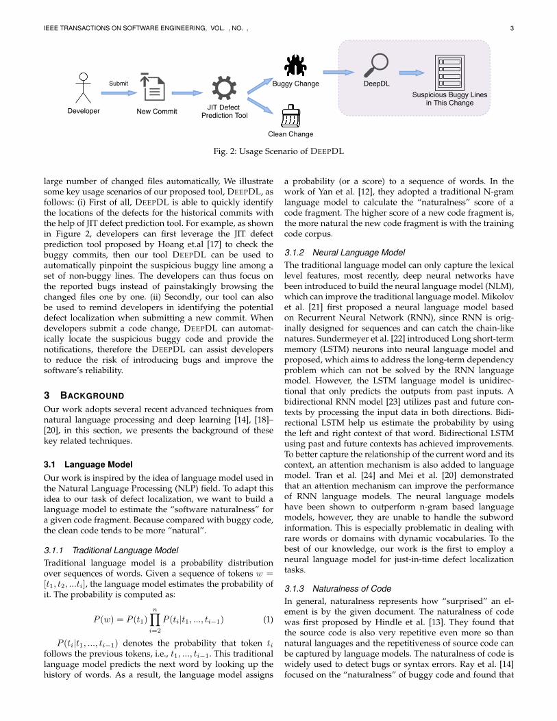
Fig. 2: Usage Scenario of DEEPDL

large number of changed files automatically, We illustratesome key usage scenarios of our proposed tool, DEEPDL, asfollows: (i) First of all, DEEPDL is able to quickly identifythe locations of the defects for the historical commits withthe help of JIT defect prediction tool. For example, as shownin Figure 2, developers can first leverage the JIT defectprediction tool proposed by Hoang et.al [17] to check thebuggy commits, then our tool DEEPDL can be used toautomatically pinpoint the suspicious buggy line among aset of non-buggy lines. The developers can thus focus onthe reported bugs instead of painstakingly browsing thechanged files one by one. (ii) Secondly, our tool can alsobe used to remind developers in identifying the potentialdefect localization when submitting a new commit. Whendevelopers submit a code change, DEEPDL can automat-ically locate the suspicious buggy code and provide thenotifications, therefore the DEEPDL can assist developersto reduce the risk of introducing bugs and improve thesoftware’s reliability.

3 BACKGROUND

Our work adopts several recent advanced techniques fromnatural language processing and deep learning [14], [18]–[20], in this section, we presents the background of thesekey related techniques.

3.1 Language ModelOur work is inspired by the idea of language model used inthe Natural Language Processing (NLP) field. To adapt thisidea to our task of defect localization, we want to build alanguage model to estimate the “software naturalness” fora given code fragment. Because compared with buggy code,the clean code tends to be more “natural”.

3.1.1 Traditional Language ModelTraditional language model is a probability distributionover sequences of words. Given a sequence of tokens w =[t1, t2, ...ti], the language model estimates the probability ofit. The probability is computed as:

P (w) = P (t1)n∏i=2

P (ti|t1, ..., ti−1) (1)

P (ti|t1, ..., ti−1) denotes the probability that token tifollows the previous tokens, i.e., t1, ..., ti−1. This traditionallanguage model predicts the next word by looking up thehistory of words. As a result, the language model assigns

a probability (or a score) to a sequence of words. In thework of Yan et al. [12], they adopted a traditional N-gramlanguage model to calculate the “naturalness” score of acode fragment. The higher score of a new code fragment is,the more natural the new code fragment is with the trainingcode corpus.

3.1.2 Neural Language ModelThe traditional language model can only capture the lexicallevel features, most recently, deep neural networks havebeen introduced to build the neural language model (NLM),which can improve the traditional language model. Mikolovet al. [21] first proposed a neural language model basedon Recurrent Neural Network (RNN), since RNN is orig-inally designed for sequences and can catch the chain-likenatures. Sundermeyer et al. [22] introduced Long short-termmemory (LSTM) neurons into neural language model andproposed, which aims to address the long-term dependencyproblem which can not be solved by the RNN languagemodel. However, the LSTM language model is unidirec-tional that only predicts the outputs from past inputs. Abidirectional RNN model [23] utilizes past and future con-texts by processing the input data in both directions. Bidi-rectional LSTM help us estimate the probability by usingthe left and right context of that word. Bidirectional LSTMusing past and future contexts has achieved improvements.To better capture the relationship of the current word and itscontext, an attention mechanism is also added to languagemodel. Tran et al. [24] and Mei et al. [20] demonstratedthat an attention mechanism can improve the performanceof RNN language models. The neural language modelshave been shown to outperform n-gram based languagemodels, however, they are unable to handle the subwordinformation. This is especially problematic in dealing withrare words or domains with dynamic vocabularies. To thebest of our knowledge, our work is the first to employ aneural language model for just-in-time defect localizationtasks.

3.1.3 Naturalness of CodeIn general, naturalness represents how “surprised” an el-ement is by the given document. The naturalness of codewas first proposed by Hindle et al. [13]. They found thatthe source code is also very repetitive even more so thannatural languages and the repetitiveness of source code canbe captured by language models. The naturalness of code iswidely used to detect bugs or syntax errors. Ray et al. [14]focused on the “naturalness” of buggy code and found that


buggy code tends to be more unnatural than the clean code.And Santos et al. [25] proposed a tool to detect and correctthe syntax errors based on naturalness of code. Based onthe code naturalness, Yan et al. [12] proposed a two-phaseframework to detect buggy commits and localize buggycode lines in buggy commits. Based on their findings, wealso leverage naturalness in our approach.

3.2 Seq2Seq ModelThe language model is a fundamental task in natural lan-guage processing, which is formalized as a probability dis-tribution over a sequence of target words. The languagemodel has various applications (e.g., speech recognition,text generation and machine translation), all these appli-cations can be viewed as generating a variable-length se-quence of tokens from a variable-length sequence of inputdata. Intuitively, the sequence-to-sequence (Seq2Seq) mod-els can model these mappings well and achieve state-of-the-art results with respect to the aforementioned applica-tions [26]–[28]. Besides, both the encoder and decoder ofSeq2Seq model can be trained with paired text to obtainas language model [29], [30]. Similarly, for our task of JITdefect localization, we aim to learn the naturalness betweenthe newly added line with respect to its surrounding lines,we thus adopt the Seq2Seq model to train a neural languagemodel (i.e., the input sequence is a code block and the out-put sequence is the code line). Ideally, our neural languagemodel will take a code block as input and generate a “clean”code line as output with respect to the code block. Then a“naturalness” score can be calculated (measured by entropy)between the added line and the generated “clean” code line.

3.2.1 Encoders & Decoders.In general, a Seq2Seq model uses an encoder-decoder ar-chitecture. It first employs an encoder to map the inputsequence into a fixed dimensional vector, then this vector isused by the decoder to decode the target sequence. Encoderis responsible for embedding the input sequence into acontextualized hidden state vector. Particularly, given theinput sequence X = (x1, x2, ..., xn) comprising a numberof n tokens. These tokens are fed sequentially into thethe encoder, which generates a sequence of hidden statesH = (h1, h2, ..., hn). The final hidden state hn can be usedas the embedding vector v of the whole input sequence.Decoder is responsible for generating the target sequencebased on the embedding vector. Specifically, at time stept, the decoder takes the embedding vector of the previousword yt−1 and the previous hidden state st−1 to producethe output yt and hidden state st for time step t.

3.2.2 Attention MechanismThe attention mechanism [31] has been recently proposedfor selecting the important parts from the input sequencefor each target word. In practice, we compute the attentionfunction on a set of queries simultaneously, packed togetherinto a matrix. The attention mechanism has been widelyused in NLP tasks. Different types of attention mecha-nisms have also been proposed, i.e., self-attention, multi-dimensional attention, multi-headed attention. The atten-tion mechanism amplify the signal from the relevant part

of the input sequence and provide a better representationfor the input sequence.

3.3 Transformer

Ashish et al. introduced a novel architecture called Trans-former [19]. Its encoder and decoder use attention mecha-nisms to replace the RNN. Our work applies this techniqueand its core part is introduced below:• Self-Attention The input of Self-Attention consists of

queries and keys of dimension dk , and values ofdimension dv . We compute the attention function on aset of queries simultaneously, packed together keys(K)and values(V) into a matrix Q. We compute the matrixof outputs as:

Attention(Q,K, V ) = softmax(QKT

√dk

)V (2)

• Multi-Head Attention Multi-Head Attention is a com-bination of multiple Self-Attention structures, eachhead learns features in different representation spaces,which makes the model have more capacity. Multi-Head Attention linearly projects the queries, keys andvalues h times with different, learned linear projectionsto dk , dk and dv dimensions, respectively. It is com-puted as below:

MultiHead(Q,K, V ) = Concat(head1, ..., headn)WO

where headi = Attention(QWQi ,KW

Ki , V W

Vi )(3)

• Positional Encoding After embedding, we have a ma-trix representation of our tokens sequence. But theserepresentations are not encoding the fact that tokensappear in different positions. In order for the modelto make use of the order of the sequence, we need tomodify the meaning represented by a specific tokendepending on its position. Without changing the com-plete representation of the token, we slightly modifyit to encode its position, which is positional encoding.There are many kinds of positional encodings, learnedand fixed [32]. We use sinusoidal functions described asfollows – i is the position of the token in the sequenceand j is the position of the embedding feature.

Pi,2j = sin(i/100002j/dmodel)

Pi,2j+1 = cos(i/100002j/dmodel)(4)

• Transformer Encoder. The transformer encoder is com-posed of a stack of N = 6 identical layers. Each layerhas a multi-head self-attention mechanism sub-layerand a position-wise fully connected feed-forward net-work sub-layer. There is a residual connection aroundeach of the two sub-layers, followed by layer normal-ization.

• Transformer Decoder. The transformer decoder is alsocomposed of a stack of N = 6 identical layers. Eachlayer has the two sub-layers that are same as encoderand a multi-head attention sub-layer. There is also aresidual connection around each of the two sub-layers,followed by layer normalization.


Project Java Files

Pre-process Data

Tokenize + BPE

SourceSequence

TargetSequence

Embedding

Embedding

Extract ExtractLine Encoder

Decoder

Linear Softmax

Loss

Added Lines

Added Line

ContextBlocks Added Line

Buggy Score Sorted List

Extract Descending

New Commit

Trained Model

Data ProcessingSeq2Seq Model

Multi-Head Attention

Multi-Head AttentionMasked Multi-Head Attention

Pre-process Data

TargetSequenceContext

Blocks

Model Training

Model Application

Context Encoder

Multi-Head Attention

Attention Layer

Fig. 3: Overall Framework of DEEPDL

4 APPROACH

We propose a novel deep learning based model,named DEEPDL (Deep Learning-based Just-in-Time DefectLocalization), for just-in-time suspicious buggy code linelocation. Figure 3 outlines the details of our DEEPDL withrespect to its three stages – data processing, model trainingand model application respectively.

4.1 Data PreparationWe use the same dataset setting by Yan et al. [12] fora fair comparison. These projects have a varying numberof contributors. Besides, all the projects have over 5,000changes to ensure sufficient samples and over 2,000 starsto ensure that the studied projects are non-trivial ones. Andthey have a good issue tracking system making it easy forus to label commits and source code lines. To make ourpaper self explanatory, we describe the details of our datapreparation process as follows.

4.1.1 Collecting Training and Testing SetIn the data collecting process, we identify the clean codelines and buggy code lines respectively. Clean code linesare used as the training set for building a “Clean” neurallanguage model. Buggy code lines are used as the testingset for evaluating the bug localization performance.

For a fair comparison, we use the same projects collectedby Yan et al. [12] and choose the same settings for the startdate and end date of each project. That is, for each project, wecollect the changes from the start of the project to October 1,2017. Following their experimental settings, we then identifythe splitting commit according to the total number of changesin chronological order (60% of the commits for training and40% of the commits for testing). The splitting commit isused to split the training and testing set. Table 1 presentsthe summary of the selected projects, e.g., the project name,the time period (i.e., start date and end date) we choose foreach project, the total number of commits of each projectduring the time period.

For example, as shown in Figure 4, for the Flink project,we first count all the commits from the start date (2010/12/15)until end date (2017/10/1), which comprises 11,982 commitsin total. After that, we can easily identify the splitting com-mit (happened in 2015/03/08) for dividing the training andtesting set. The data before the splitting commit are used fortraining and the data after the splitting commit are used fortesting.

After identifying the splitting commit, we downloadedthe snapshot of each project before the splitting commit fortraining. A snapshot represents the project’s state at thatpoint of time. To build a “Clean” neural language model,we need to make a “Clean” snapshot. In other words, weneed to ensure that the downloaded snapshot only containsclean code lines. We thus need to remove all the buggylines from the downloaded snapshot. To do this, we leverageRA-SZZ [33] to identify the clean and buggy lines both inthe training set and the testing set. The detailed process isconducted as follows:

1) Bug-fix commit identification. For each commit after thesplitting point, we first identify whether this commitis a bug-fix commit. For a given commit, if the corre-sponding commit message contains the defect relatedmessage (e.g., “Fixed #233”), we then check the corre-sponding issue report from the issue tracking system(ITS) to determine whether the report is defined as adefect. If the report is defined as a defect and it isresolved, we mark this commit as a bug-fix commit.If the report is defined as a defect and it is resolved, wethen mark this commit as a bug-fix commit.

2) Bug-introducing commit identification. After identi-fying the bug-fix commits, for each bug-fix commit,we further leverage RA-SZZ [33] to identify the bug-introducing commits. RA-SZZ first compares the bug-fix commit with its previous version to identify thechanged lines. Then RA-SZZ filters out the changedlines that are irrelevant to the defect changes (e.g.,blank/comment lines, format modification). After that,


RA-SZZ traces back the remaining lines through thechange history to identify the commits that introducethese lines, which are identified as bug-introducing com-mits.

3) Removing buggy lines from the downloaded snapshot.After identifying the bug-introducing commits, for eachbug-introducing commit, if it happened before the split-ting point, then this commit has introduced buggy linesto our training set. Therefore, we need to remove thebuggy lines introduced by the bug-introducing commitand only retain the clean lines. Following the previouswork’s settings, we define the lines that were added bythe bug-introducing commit and were later fixed by thebug-fix commit as buggy lines. These identified buggylines are further mapped to the downloaded snapshotversion of the project. We remove these buggy linesfrom the downloaded snapshot, the remaining linescan be viewed as clean code lines, which are added tothe “Clean” snapshot for training a “Clean” languagemodel.

4) Identifying the buggy lines within the testing set. Foreach bug-introducing commit, if it is happened after thesplitting point, we add it to our testing set. Differentfrom removing buggy code lines from our training set,we need to identify the buggy code lines in the test-ing set as ground truth for evaluating the localizationperformance. Our testing set starts from the splittingpoint and ends on October 1, 2017. To ensure all thebuggy lines in the testing set can be correctly identified,following Yan et al’s work [12], we further use a fivemonths window (from October 1, 2017 to March 1,2018) to cover the bug-fix and bug-introducing commitsas much as possible. This is reasonable because 80% ofthe buggy commits are fixed within 5 months on aver-age [12]. Then we pinpointed the buggy lines within thetesting set introduced by the bug-introducing commits.

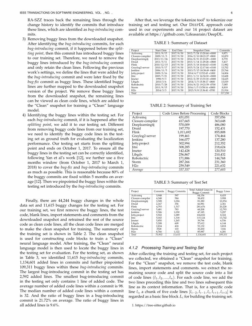
Finally, there are 44,244 buggy changes in the wholedata set and 11,615 buggy changes for the testing set. Forour training set, we first remove the buggy lines, the testcode, blank lines, import statements and comments from thedownloaded snapshot and retrained the rest of the sourcecode as clean code lines, all the clean code lines are mergedto make the clean snapshot for training. The summary ofthe training set is shown in Table 2. The clean snapshotis used for constructing code blocks to train a “Clean”neural language model. After training, the “Clean” neurallanguage model is then used to locate the buggy lines inthe testing set for evaluation. For the testing set, as shownin Table 3, we identified 11,615 bug-introducing commits,1,134,601 added lines in commits and further pinpointed109,311 buggy lines within these bug-introducing commits.The largest bug-introducing commit in the testing set has2,592 added lines. The smallest bug-introducing commitin the testing set only contains 1 line of added code. Theaverage number of added code lines within a commit is 98.The median number of added code lines within a commitis 32. And the ratio of buggy lines in a bug-introducingcommit is 21.72% on average. The ratio of buggy lines inall added lines is 9.6%.

After that, we leverage the tokenize tool1 to tokenize ourtraining set and testing set. Our DEEPDL approach codeused in our experiments and our 14 project dataset areavailable at https://github.com/Lifeasarain/DeepDL.

TABLE 1: Summary of Dataset

Project Start Date End Date Snapshot Date CommitsActivemq 2011/9/15 2017/9/30 2012/7/24 13:20:44 +0000 9,871Closure-compiler 2009/11/3 2017/9/30 2016/2/10 08:21:27 -0800 10,870Deeplearning4j 2013/11/26 2017/9/30 2016/8/31 23:12:09 +1000 8,770Druid 2011/5/11 2017/9/30 2013/1/14 11:29:28 +0800 5,417Flink 2010/12/15 2017/9/30 2015/3/18 10:44:43 +0100 11,982Graylog2-server 2010/5/17 2017/9/30 2015/5/24 12:17:44 +0100 13,702Jenkins 2006/11/5 2017/9/30 2013/5/15 18:38:49 -0400 23,764Jetty.project 2009/3/16 2017/9/30 2014/4/7 12:52:43 +1000 14,804Jitsi 2005/7/21 2017/9/30 2011/1/11 14:34:18 +0000 12,608Jmeter 1998/9/3 2017/9/30 2012/2/29 13:33:18 +0000 14,625Libgdx 2010/3/6 2017/9/30 2014/1/5 15:38:17 -0800 13,019Robolectric 2010/7/28 2017/9/30 2014/8/21 19:21:59 -0700 7,085Storm 2011/9/15 2017/9/30 2016/1/5 13:58:16 +0800 8,819H2o 2014/3/3 2017/9/30 2015/9/8 13:36:41 -0700 21,914Total 117,250

TABLE 2: Summary of Training Set

Project Code Lines Before Processing Code BlocksActivemq 431,051 357,056Closure-compiler 417,665 363,648Deeplearning4j 570,009 486,080Druid 197,770 152,431Flink 1,011,692 855,808Graylog2-server 199,461 174,464Jenkins 166,077 137,280Jetty.project 302,994 212,352Jitsi 308,285 218,624Jmeter 142,428 120,510Libgdx 256,867 210,432Robolectric 171,886 144,768Storm 287,266 231,360H2o 259,549 221,632Average 337,357 277,603

TABLE 3: Summary of Test Set

Project Commits Buggy Commits Total Added Lines inBuggy Commit Buggy Lines

Activemq 3,948 597 64,156 8,433Closure-compiler 4,348 584 38,432 3,998Deeplearning4j 3,508 1,024 81,280 10,254Druid 2,167 356 66,981 2,361Flink 4,793 1,317 281,676 20,228Graylog2-server 5,481 783 68,208 12,793Jenkins 9,506 1,030 47,185 5,297Jetty.project 5,922 1,089 104,832 8,322Jitsi 5,043 1,318 115,124 13,742Jmeter 5,850 1,265 39,796 6,536Libgdx 5,208 609 57,612 6,144Robolectric 2,834 418 53,132 3,818Storm 3528 103 30,200 1104H2o 8,766 1,122 85,987 6,281Total 70,902 11,615 1,134,601 109,311

4.1.2 Processing Training and Testing SetAfter collecting the training and testing set, for each projectwe collected, we obtained a “Clean” snapshot for training.For the “Clean” snapshot, we remove the test code, blanklines, import statements and comments. we extract the re-maining source code and split the source code into a listof code lines (l1, l2, ..., ln). For each code line, we add thetwo lines preceding this line and two lines subsequent thisline as its context information. That is, for a specific codeline li, a chunk of five code lines [li−2, li−1, li, li+1, li+2] isregarded as a basic line block Li for building the training set.

1. https://tree-sitter.github.io


Finally, our final training set is built by stacking all the lineblocks together. In summary, our training set contains a listof line blocks [L1, L2, ..., Ln]. Each line block Li include 5associated code lines, i.e., Li = [li−2, li−1, li, li+1, li+2], andeach code line li contains a sequence of tokens.

Regarding the testing set, for each project we collected,the testing set contains a set of bug-introducing commits andthe associated pinpointed buggy lines. Each bug-introducingcommits contains a set of added lines (i.e., regular addedlines and buggy added lines). The buggy added lines arethe lines that are pinpointed as buggy for introducing bugslater. When it comes to the evaluation, since we aim to locatethe buggy added lines among the added line candidates.Therefore, for each added line within the bug-introducingcommit, we add its surrounding two lines to make a basicline block, we then feed each basic line block into ourneural language model to calculate the naturalness score, orin other words suspiciousness score. The top ranked addedlines are considered to be potential buggy code lines, whichare used to calculate the localization performance of ourmodel. In summary, we collected 3,886,445 code line blocksfor training and 1,134,601 code line blocks for testing.

Flink

Time Line

. . .Commit 1

Snapshot

Commit b Commit M

2010/12/15

Commit a . . .. . .

Start Date2017/10/1End Date

2015/3/18 2018/3/1Extened Date

Commit N. . . . . .

FixBug Introducing

CommitBug Introducing

CommitBug FixCommit

Fig. 4: Project Time Line

4.1.3 Tokenization and Building Vocabulary

In this step, for each line block Li in the training set andtesting set, we tokenize the code line into a list of tokensand then build our single vocabulary. However, due toreasons that the identifier names in the code corpus are quitearbitrary and vary greatly according to different developers,simply leveraging traditional tokenization methods on thecode corpus will lead to serious Out-of-Vocabulary (OOV)problem.

Because our model is based on neural language models,which are sensitive to the unknown tokens, too many un-known words in the testing corpus will significantly hinderthe learning performance of our approach [15]. To addressthis challenge, Sennrich et al. [34] proposed a subwordunits-level model to reduce OOV problems. Following thiswork, Karampatsis et al. [35] applied this technique inmodeling source code, which has been demonstrated to beeffective in reducing OOV tokens. Inspired by their work,we first tokenize the source code line into word-level units

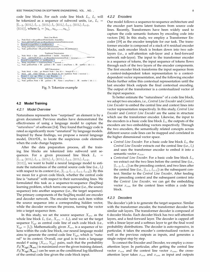
and then we employ a Byte Pair Encoding (BPE) method [16]for subword segmentation. BPE is a data compression tech-nique that iteratively collects the most frequent pair ofbytes in a sequence and replaces it with a single unusedbyte. Sennrich et.al [34] first apply this technique to theword segmentation field. They merge characters or char-acter sequences instead of bytes. They find it can actuallyimprove performance in neural machine translation models.BPE builds up the vocabulary iteratively. For each iteration,the training corpus (in our case: a code line) is segmentedinto a sequence of subwords (symbols) based on the currentvocabulary (a suffix symbol ’@’ is added to reorganize theoriginal sequence of tokens). Following that, we count allthe symbol pairs, the most frequent symbol pair (W1, W2)is merged and replaced with a new symbol ’W1W2’ andadded to the vocabulary. BPE algorithm takes all charactersin the data set as initial vocabulary and stops after the givennumber of merge operations. An example of a Java codesnippet tokenized into BPE subwords is shown in Figure 5.

The reasons why we adopt BPE algorithm for tokeniza-tion are as follows: (i) The OOV problem can be allevi-ated. Because our vocabulary contains more words, moreunknown words in the testing set now can be representedproperly. Common sequences can be represented by a singleword, while the rare or unseen word will be segmented intomore common subwords. (ii) The size of the vocabularycan be significantly reduced. Even the new identifier namesproliferate as code corpus increases, we can maintain a codevocabulary with relatively small vocabulary size.

As a result, given a basic code line blockLi = [li−2, li−1, li, li+1, li+2] from training set, for eachcode line lk(i − 2 ≤ k ≤ i + 2), lk is tokenized into asequence of subword units, i.e., lk = [uk1 , uk2 , ..., ukn ],where [uk1 , uk2 , ..., ukn ] represents the subword unit tokensafter tokenization. For example, as shown in Figure 5,the second code line “block.addChildToFront(newBranchInstrumentationNode(traversal); ” istokenized to a sequence of subword units [‘block’, ‘.’,‘add’, ‘Child’, ‘ToFront’, ‘new’, ‘Branch’, ‘In’, ‘stru’,‘mentation’, ‘Node’, ‘(’, ‘traversal’, ‘)’, ‘;’] by applyingthe BPE tokenization method described above. When tok-enizing this source code line, the BPE algorithm encounterstwo out of vocabulary tokens, e.g., ‘addChildToFront‘and ‘newBranchInstrumentationNode‘. Take‘newBranchInstrumentationNode‘ as an example,BPE splits ‘newBranchInstrumentationNode‘ into asequence of characters and apply the learned operationsto merge the characters into larger, known word in thevocabulary. Since the words ‘new’, ‘Branch’, ‘In’, ‘stru’,‘mentation’, ‘Node’ already exist in the vocabulary, so thisOOV word ‘newBranchInstrumentationNode’ is splitinto a chunk of subword unit tokens [ ‘new’, ‘Branch’, ‘In’,‘stru’, ‘mentation’, ‘Node’ ].

Traditional tokenizers can only split the source codeinto tokens according to grammar, BPE can split the tokenstokenized by traditional tokenizer into finer granularity sub-word units. In this way, we can reduce the size of vocabularyand alleviate OOV problems.

After that, we add a special token ‘〈EOL〉’ to sepa-rate each line and a special token ‘〈EOS〉’ to the endof each basic line block. Finally, we obtained 5,021,046


code line blocks. For each code line block Li, Li willbe tokenized as a sequence of subword units, i.e., Li =[li−2, 〈EOL〉, li−1, 〈EOL〉, li, 〈EOL〉, li+1, 〈EOL〉, li+2,〈EOS〉], where lk = [uk1 , uk2 , ..., ukn ].

Basic Line Block:Node block = data.getBranchNode(lineIdx, branchIdx);block.addChildToFront( newBranchInstrumentationNode(traversal);branchCoverageOffset += numBranches;String arrayName = createArrayName(traversal);Node getElemNode = IR.getelem(IR.name(arrayName), IR.number(idx));

Traditional Tokenization:Node block = data . getBranchNode ( lineIdx , branchIdx ) ;block . addChildToFront ( newBranchInstrumentationNode ( traversal ) ;branchCoverageOffset += numBranches ;String arrayName = createArrayName ( traversal ) ;Node getElemNode = IR . getelem ( IR . name ( arrayName ) , IR . number ( idx ) ) ;

BPE Tokenization :Node block = data . get Branch Node ( line. Id. x , branch. Id x ) ;block . add . Child ToFront ( new Branch In stru mentation Node ( traversal ) ;branch C over age Offset += num Branches ;String arrayName = create ArrayName ( traversal ) ;Node getElem. Node = IR . getelem ( IR . Name ( arrayName ) , IR . number ( idx ) ) ;

Li-2Li-1LiLi+1Li+2

Li-2Li-1LiLi+1Li+2

Li-2Li-1LiLi+1Li+2

Added Line

Fig. 5: Tokenize example

4.2 Model Training

4.2.1 Model Overview

Naturalness represents how “surprised” an element is by agiven document. Previous studies have demonstrated theeffectiveness of using a language model to capture the“naturalness” of software [14]. They found that buggy code israted as significantly more “unnatural” by language models.Inspired by these findings, we propose a neural languagemodel, DEEPDL, to locate the suspicious code elementswhen the code change happens.

After the data preparation process, all the train-ing line blocks are tokenized into subword unit se-quences. For a given processed line block Li =[li−2, 〈EOL〉, li−1, 〈EOL〉, li, 〈EOL〉, li+1, 〈EOL〉, li+2,〈EOS〉], we want to build a neural language model to esti-mate the naturalness of the central source code line (i.e., li)with respect to its context (i.e., [li−2, li−1, li+1, li+2]). By thiswe mean for a given code block, whether the central codeline is “natural” with respect to their surrounding lines. Weformulated this task as a sequence-to-sequence (Seq2Seq)learning problem, which turns one sequence (i.e., the sourcesequence) into another sequence (i.e., the target sequence).The primary components of the Seq2Seq model are encoderand decoder network. The encoder turns each item withinthe source sequence into a corresponding hidden vector,while the decoder reverses the process, turning the vectorinto a target sequence item.

In this study, we set the source sequence Xsrc as thewhole line block Li (i.e., Xsrc = Li), and we set the targetsequence Ytgt as central code line of each code block (i.e.,Ytgt = [li]). Mathematically, given Xsrc is a sequence of to-kens within the code line block, our neural language modelaims to generate the central code line Ytgt, which is “natu-ral” to its context. Overall, our goal is to train a languagemodel θ using 〈Xsrc, Ytgt〉 pairs, such that the probabilityPθ(Ytgt|Xsrc) is maximized over the given training dataset,Pθ(Ytgt|Xsrc) can be seen as the conditional log-likelihoodof the central code line given the code block input.

4.2.2 Encoders

Our model follows a sequence-to-sequence architecture andthe encoder part learns latent features from source codelines. Recently, Transformers have been widely used tocapture the code semantic features by encoding code intovectors [36]. In this study, we employ a Transformer En-coder [19] as the encoder template for our task. The trans-former encoder is composed of a stack of 6 residual encoderblocks, each encoder block is broken down into two sub-layers (i.e., a self-attention sub-layer and a feed-forwardnetwork sub-layer). The input to the transformer encoderis a sequence of tokens, the input sequence of tokens flowsthrough each of the two layers of the encoder components.The first encoder block transforms the input sequence froma context-independent token representation to a context-dependent vector representation, and the following encoderblocks further refine this contextual representation until thelast encoder block outputs the final contextual encoding.The output of the transformer is a contextualized vector ofthe input sequence.

To better estimate the “naturalness” of a code line block,we adopt two encoders, i.e., Central Line Encoder and ContextLine Encoder to embed the central line and context lines intovector representation respectively. In this study, Central LineEncoder and Context Line Encoder are the same in structurewhich use the transformer encoder. Likewise, the input tothe encoders is a basic code line block Li, the outputs of theencoders are two embedding vectors respectively. Throughthe two encoders, the semantically related concepts acrossdifferent source code lines can be mapped and correlated inthe higher dimensional vector space.• Central Line Encoder. For a basic code line block Li, the

Central Line Encoder extracts out the central line (i.e., li)and uses the transformer encoder to embed it into asemantic vector xcen.

• Contextual Line Encoder. For a basic code line block Li,we extract out the two lines before the central line (i.e.,[li−2, li−1]) as the preceding context, and two lines afterthe central line (i.e., [li+1, li+1]) as the subsequent con-text. Similar to the Central Line Encoder, After feedingthe preceding context and the subsequent context intothe Context Line Encoder, we can get the embeddingvector xcon for the context lines within a code lineblock.

4.2.3 Decoders

The decoder’s job is to generate the target sequence. Similarwith the transformer encoder, the transformer decoder hassimilar sub layers. The transformer decoder is composed of6 decoder blocks. Each decoder block has two self-attentionlayers, and a feed-forward layer. The decoder is capped offwith a linear layer and a softmax layer to get the final wordprobability distributions. The decoder is auto-regressive, inparticular, it takes the encoder’s contextualized vectors aswell as the previous outputs as inputs, and generates asingle output step by step.

To connect the Encoder and Decoder, we employ a cross-attention layer. In particular, after getting the central linevector xcen and the context line vector xcon, the cross-attention layer takes xcen and xcon as input and outputs


a hidden state vector xh. We then send xh into our trans-former decoder, the transformer decoder will turn the hid-den vector into a target sequence. Mathematically, giventhe hidden states xh, the transformer decoder calculates theconditional probability distribution of the target sequenceYtgt, i.e., Pθ(Ytgt|xh), as follows:

Pθ(Ytgt|xh) =L∏i=1

Pθ(yi|Y0:i−1;xh) (5)

where L is the length of the target sequence Ytgt. Thetransformer decoder first maps the encoded hidden states(i.e., xh) and all the previous target states Y0:i−1, to logitvector li. The logit vector li is then processed by thesoftmax operation to estimate the conditional distributionPθ(yi|Y0:i−1;xh). After calculating the above conditionaldistribution, we can auto-regressively generate the outputsequence and thus define a mapping of an input sequenceXsrc to an output sequence Ytgt.

4.2.4 Data FlowWe summarize the data-flow of our model as follows: asshown in Figure 6, the input to our model is a basic code lineblock Li, which is broken into two parts (the central codeline [li] and the context code lines [li−2, li−1, li+1, li+2]).Each code line is represented as a sequencee of subwordunit tokens. Then the central code line is passed throughthe Central Line Encoder to generate the central line encodedvector xcen, while the context code lines are passed throughthe Context Line Encoder to generate the context lines en-coded vector xcon. After that, a cross attention layer takesthe xcen and xcon as input and outputs a hidden state vectorxh, which can capture the relationship between the centralcode line and the context code lines. The hidden state vectorxh is then passed through the Decoder part to generatethe target sequence. The Decoder part takes in the encodedhidden states (i.e., xh) and step by step generates a singleoutput yi while also being fed the previous output Y0:i−1.To be more specifically, the transformer decoder first mapsthe hidden state vector (i.e., xh) as well as the previousoutput Y0:i−1 to a logit vector li, the logit vector li thengoes through a final softmax layer to model the conditionalprobability distribution of the target sequence. The softmaxlayer will produce a probability distribution vector overall vocabulary tokens, and we choose the token with thehighest probability as the predicted token.

4.2.5 Loss FunctionWe leverage a cross entropy loss function to calculate theloss of the model. The cross entropy (entropy in short) is awidely-adopted metric used in statistical language models,a sentence with higher entropy score is considered to bemore natural. Ray et al. [14] investigated the possibility ofusing entropy to estimate the “naturalness of buggy code”.The core research question of their work is “can entropyprovide a useful indication of the likely bugginess of aline of code?”. According to their experimental results, theyfound that buggy code lines have higher entropy scoresthan non-buggy lines, which means the entropy can be anindicator to measure the naturalness (or suspiciousness) ofa code snippet. The higher entropy of a code snippet, the

Self-Attention

Add & Normalize

Feed Forward

Add & Normalize

Attention Layer

Self-Attention

Add & Normalize

Feed Forward

Add & Normalize

Self-Attention

Add & Normalize

Linear

Softmax

Central Line Encoder

x 6 x 6

Central LineAbove Context

Below Context

Self-Attention

Add & Normalize

Feed Forward

Add & Normalize

Central Line Output Sequence

Cross EntropyLoss

Contextual Line Encoder

Decoder

x 6

Fig. 6: Architecture of Proposed Approach

more unnatural (or suspicious) the code snippet is withthe training corpus. In particular, regarding the decodingprocess, the probability of generating a token yi is P (yi).During the training process, for each token at each times-tamp, the loss associated with the generated central codeline is− 1

l

∑li=1 log2 p(yi), where l is the length of the central

code line. The final goal of our model is to minimize thecross entropy, i.e., minimize the following objective functionover all the training dataset:

H(y) = − 1

N

N∑j=1

l∑i=1

log2 p(y(j)i ) (6)

where N is the number of training instances, y(j)i rep-resents the ith token in the jth training sample. The crossentropy describes how much the predicted probability di-verges from the ground truth. Through optimizing theabove objective loss function using optimization algorithms(e.g., gradient descendant), the parameters θ of our modelcan be estimated. Finally, after the training process, we canobtain a neural language model (i.e., DEEPDL). The neurallanguage model maximizes the probability of the targetsequence given the input sequence (i.e., Pθ(Ytgt|Xsrc))over our training dataset.

4.3 Model ApplicationFor practical application, the input of DEEPDL is a buggycommit (identified by the JIT defect prediction tools) or


a newly submitted commit. Given a buggy code commit,DEEPDL first extracts all the added code lines within thiscommit. For each added line, we make a code line blockby adding its surrounding two lines, we process the codeline block as described in Section 4.1.1 and Section 4.1.2.For each code line block, we fed the code line block intoour trained neural language model, DEEPDL, to generatean output sequence. The generated sequence can be consid-ered as a “clean” code line since it is generated from ourtrained “clean” neural language model. After that, we cancalculate the entropy between the generated sequence andthe added line, and the entropy of the added code line canbe computed as the average of the entropy of each subwordtoken within this code line, as follows:

Hp(s) =1

|s|

|s|∑n=1

Hp(ti) (7)

Finally, we get the entropy of all the added lines in thebuggy commits and treat the entropy as its suspiciousnessscore. The code line with the highest suspiciousness score isconsidered to be a possible defect location in the code. Sim-ilar to the buggy commit, if we are handling the newly sub-mitted commits, by following the same application pipeline,DEEPDL can identify the suspicious added lines within thenewly submitted commits, which can reduce the risk ofintroducing bugs and improve the software’s reliability.

5 EXPERIMENT SETUP

We first introduce our data preparation process, thenpresent the detailed parameter settings for training ourDEEPDL approach. We then introduce our chosen evalu-ation metrics used in this study for evaluating the perfor-mance of our approach.

5.1 Training Details

We set the initial learning rate to 0.1 with a momentumof 0.5 and clip the gradients norm by 5. The learning ratedecay of 0.99. The size of mini-batches is 16. Our modelis trained using the Stochastic Gradient Descent (SGD)algorithm. We use the cross-entropy as the loss function.It is worth mentioning that for each project, we reserve 10%of the training set as the validation set. We further tunedthe hyperparameters according to the performance of themodel on the validation set. Specifically, for each project, thetraining runs for 50 epochs and we save the model after eachepoch, we then select the model with the best performance(the lower of the entropy score, the better performance of theneural language model) on validation set as our final neurallanguage model. We build our model based on Pytorch 2

using four NVIDIA RTX 2080Ti GPU.

5.2 Evaluation Measure

To evaluate the performance of our approach, we use thewidely accepted metrics MRR (Mean Reciprocal Rank),MAP (Mean Average Precision) [37] and Top-k Accuracy asthe evaluation metrics. In addition, these evaluation metrics

2. https://pytorch.org

are also adopted in Yan et al’s work. Thus they can be usedfor fair comparison purposes We introduce the details ofthese three evaluation metrics as follows.

5.2.1 MRR

MRR is a popular metric used to evaluate an informationretrieval technique [37]. For a given query, its reciprocal rankis the multiplicative inverse of the rank of the first correctanswer. For our study, MRR measures how far we need tocheck down a sorted list of added lines of a buggy changeto locate the first buggy line. It can be computed as follows:

MRR =1

|Q|

|Q|∑i=1

1

ranki(8)

where Q is the number of queries. MRR is the average of thereciprocal ranks for queries Q.

5.2.2 MAP

MAP provides the mean of the average precision scores fora set of queries. The average precision (AP) of a query isthe average of the precision values for this query. MAPconsiders the ranks of all buggy lines in that sorted list. Itcan be computed as:

AP =M∑i=1

P (i) ∗ rel(i)numberofrelevantdocuments

(9)

where i is then rank in the sequence of retrieved item, P (i)isthe precision at cut-off i in the list. rel(k) is a indicatorfunction equaling 1if the item at rank i is a relevant item

MAP =1

N

N∑i=1

APi (10)

Our evaluation is performed at the change-level. Eachbuggy change in our test set has a MRR and a MAPperformance value. The higher MRR and MAP value meansthat the model has a better bug localization performance.

5.2.3 Top-K Accuracy

Top-k Accuracy measures whether the Top-k most likelybuggy lines returned by our approach are actually the buggycode location. For example, given one defect change c, if atleast one of the Top-k most likely buggy lines returned byour approach is actually the buggy location, we regard thelocalization as successful, and set the Top-k value of thischange Topk(c) to 1; otherwise, we regard the localizationas unsuccessful and set the Top-k value Topk(c) to 0.Consider a set of N defect changes in a project P, its Top-k accuracy is computed as:

Topk(P ) =1

N

N∑c=1

Topk(c). (11)

Following the experimental settings in previous studies [12],in this paper, we set k = 1 and 5.


TABLE 4: The performance DEEPDL vs. Baselines

Project Top-1 accuracy Top-5 accuracy MRR MAPYan’s CC2Vec Ours Yan’s CC2Vec Ours Yan’s CC2Vec Ours Yan’s CC2Vec Ours

Activemq 0.3936 0.3417 0.4070 0.5628 0.5142 0.6348 0.4785 0.4317 0.5117 0.4505 0.4217 0.4749Closure-compiler 0.2432 0.2226 0.2774 0.4966 0.4452 0.4983 0.3650 0.3404 0.3933 0.3504 0.3289 0.3718Deeplearning4j 0.2451 0.1963 0.3184 0.4971 0.4189 0.5908 0.3702 0.3150 0.4464 0.3264 0.2847 0.3746Druid 0.2107 0.1517 0.1966 0.4157 0.2949 0.4663 0.3149 0.2330 0.3297 0.2720 0.2043 0.2975Flink 0.2065 0.1716 0.2445 0.4146 0.3470 0.4761 0.3125 0.2625 0.3584 0.2608 0.2307 0.2894Graylog2-server 0.3384 0.3207 0.3742 0.5951 0.5249 0.6731 0.4637 0.4207 0.5077 0.4222 0.3961 0.4503Jenkins 0.3602 0.2951 0.3748 0.6184 0.5436 0.6699 0.4834 0.4149 0.5149 0.4536 0.4026 0.4792Jetty 0.2452 0.1928 0.2773 0.4702 0.4279 0.5427 0.3550 0.3104 0.4022 0.3210 0.2838 0.3537Jitsi 0.3475 0.3126 0.3634 0.6297 0.5849 0.6798 0.4798 0.4373 0.5043 0.4325 0.4007 0.4425Jmeter 0.4545 0.4103 0.4980 0.7462 0.6743 0.7968 0.5838 0.5336 0.6285 0.5615 0.5188 0.6048Libgdx 0.3448 0.2808 0.3711 0.6010 0.5107 0.6568 0.4668 0.3945 0.4981 0.4258 0.3740 0.4582Robolectric 0.2368 0.1699 0.2536 0.4928 0.4115 0.5383 0.3654 0.2920 0.3851 0.3145 0.2662 0.3301Storm 0.0971 0.0874 0.1748 0.3495 0.2524 0.3689 0.2062 0.1840 0.2789 0.1810 0.2338 0.2338H2o 0.2584 0.2299 0.3057 0.5258 0.4483 0.5954 0.3854 0.3427 0.4427 0.3542 0.3197 0.3996average 0.2844 0.2416 0.3169 0.5297 0.4571 0.5849 0.4022 0.3509 0.4430 0.3662 0.3197 0.3972p-value <0.001 <0.001 <0.001 <0.001 <0.001 <0.001 <0.001 <0.001

TABLE 5: The performance Cross-Project model vs. Within-Project model

Project Top-1 accuracy Top-5 accuracy MRR MAPCP WP Improve CP WP Improve CP WP Improve CP WP Improve

Activemq 0.4154 0.4070 -2.01% 0.6181 0.6348 2.71% 0.5146 0.5117 -0.57% 0.4779 0.4749 -0.63%Closure-compiler 0.2759 0.2774 0.54% 0.5017 0.4983 -0.68% 0.3962 0.3933 -0.73% 0.3743 0.3718 -0.66%Deeplearning4j 0.3174 0.3184 0.30% 0.5879 0.5908 0.50% 0.4442 0.4464 0.50% 0.3720 0.3746 0.71%Druid 0.2022 0.1966 -2.76% 0.4579 0.4663 1.83% 0.3249 0.3297 1.48% 0.2896 0.2975 2.74%Flink 0.2498 0.2445 -2.12% 0.4951 0.4761 -3.84% 0.3640 0.3584 -1.54% 0.2900 0.2894 -0.21%Graylog2-server 0.3908 0.3742 -4.25% 0.6731 0.6731 -0.01% 0.5169 0.5077 -1.78% 0.4536 0.4503 -0.73%Jenkins 0.3592 0.3748 4.33% 0.6573 0.6699 1.92% 0.5002 0.5149 2.94% 0.4670 0.4792 2.62%Jetty 0.2617 0.2773 5.97% 0.5298 0.5427 2.43% 0.3870 0.4022 3.93% 0.3434 0.3537 3.00%Jitsi 0.3695 0.3634 -1.64% 0.6737 0.6798 0.91% 0.5068 0.5043 -0.50% 0.4428 0.4425 -0.08%Jmeter 0.4830 0.4980 3.11% 0.7794 0.7968 2.24% 0.6146 0.6285 2.26% 0.5946 0.6048 1.71%Libgdx 0.3744 0.3711 -0.88% 0.6355 0.6568 3.35% 0.4982 0.4981 -0.02% 0.4565 0.4582 0.38%Robolectric 0.2512 0.2536 0.95% 0.5526 0.5383 -2.59% 0.3856 0.3851 -0.13% 0.3361 0.3301 -1.77%Storm 0.1650 0.1748 5.91% 0.4078 0.3689 -9.53% 0.2758 0.2789 1.11% 0.2341 0.2338 -0.13%H2o 0.3128 0.3057 -2.27% 0.5865 0.5954 1.52% 0.4453 0.4427 -0.58% 0.3975 0.3996 0.53%average 0.3163 0.3169 0.19% 0.5826 0.5849 0.39% 0.4410 0.4430 0.45% 0.3950 0.3972 0.56%p-value >0.05 <0.05 <0.001 <0.001

6 EMPIRICAL EVALUATION

We evaluate the performance of our new DEEPDL approachon 14 open source projects. We attempt to answer thefollowing key research questions:• RQ1: How effective is our approach compared with the

state-of-the-art baselines?• RQ2: How effective is our approach when using cross-

project modeling?• RQ3: How effective is our approach for using of context

information and BPE tokenization methods?

6.1 RQ1: Effectiveness Evaluation

6.1.1 Experimental Setup.

To evaluate the effectiveness of our model, we conductedextensive experiments on the selected 14 projects. We useour trained neural language model, DEEPDL, to predict thelocations of buggy lines within the test set. We compareDEEPDL with the following state-of-the-art models for com-parison purposes:• Yan’s approach. Yan’s approach is currently the state-

of-the-art JIT defect localization approach. It estimatessoftware naturalness with the N-gram language model,which can locate suspicious defective lines in a defectchange at check-in time. Different from building the n-gram language model, in this study, we employ the

transformer based encoder and decoder to make anneural language model.

• CC2Vec. CC2Vec is the state-of-the-art defect predictiontool. CC2Vec is an embedding-based approach pro-posed by Hoang et al. [17]. Different from the JIT defectlocalization task, CC2Vec is designed for the JIT defectprediction task. For a given commit, CC2Vec learnstwo embedding vectors from the log message and codechange and outputs a probability to judge if this commitis buggy or not. To adapt this JIT defect prediction toolto our task of JIT defect localization, for a given commit,we regard each added line of this commit as a singlecommit, then the added line is passed through CC2Vecto produce a probability indicating that this addedline is buggy. The added lines with highest probabilityscores will be considered as potential buggy lines forthis commit. It is worth to mention that for a faircomparison, we drop the log message related featuresand only keep the code change part for CC2Vec, thisis reasonable because DEEPDL only model the sourcecode without considering additional information.

6.1.2 Experimental Results.

Table 4 illustrates the Top-1 and Top-5 accuracy, MRR, MAPof our approach and the baselines. We can observe thefollowing points from the table:


1) The CC2Vec model achieves the worst performanceregarding different evaluation measurements. TheCC2Vec model is originally designed for the task of JITdefect prediction. It formulates the JIT defect predictiontask as a binary classification problem, that is given acommit, CC2Vec outputs a probability score to judgethis commit is buggy or not. We transfer their approachfrom predicting a buggy commit to predicting a buggyline (treating each separate line as a commit). Thesuboptimal performance of CC2Vec indicates that thebinary classification strategy is not suitable for the taskof JIT defect localization. This is because CC2Vec treatsa single added line as input, it is thus unable to considerthe preference relationship among different code lines.By contrast, the language model based approaches (in-cluding Yan’s approach and ours) models the historicalclean code lines, which can estimate the naturalness ofthe source code.

2) Our approach outperforms Yan’s approach in terms ofall measures on average. From the table 4, we can seethat our approach can achieve a higher accuracy thanYan’s approach with the defect localization task. Forexample, the improvement of our approach over Yan’sapproach is 11.42% for Top-1 accuracy and 9.69% forTop-5 accuracy, while 11.35% for MAP and 9.55% forMRR scores. We attribute this to the following reasons:First, both DEEPDL and Yan’s approach adopt thelanguage model, however, Yan’s approach builds thelanguage model with n-grams, which can only capturethe lexical level features. In this study, we use thetransformer based encoder and decoder to construct aneural language model, which not only considers thelexical level features but also semantic level features.Second, we adopt the BPE algorithm for tokenization,which can solve the OOV problem when dealing withthe testing set.

3) Regarding all the 14 projects, the improvements ofour proposed model over baseline are significant. Totest the statistical significance, we employ the Wilcoxonsigned-rank test [38] with a Bonferroni correction [39] at95% confidence level. The Wilcoxon signed-rank test isa non-parametric hypothesis test that used to comparetwo matched samples to assess whether their popula-tion mean ranks differ, while Bonferroni correction isused to counteract the problem of multiple compar-isons. From the table, we can see that on average allthe p-values are substantially smaller than 0.05, whichshows that the improvements of our proposed modelare statistically significant.

4) Only for the project ”Druid” is the Top-1 accuracy ofour approach is lower than the baseline. This is becausethe number of bug introducing changes in this project issmall and the bug introducing lines are relatively lowin the added lines in most bug introducing changes.Both our approach and the baseline do not performwell on the top-1 accuracy. Except for this indicator,Our approach outperforms the baseline in terms of allthe measures, we argue that the improvement of ourapproach is significant.

Answer to RQ1: How effective is our approach comparedwith the state-of-the-art baseline? – we conclude thatour approach significantly outperforms the baseline andachieves a new state-of-the-art performance for just-in-time defect localization.

6.2 RQ2: Cross-Project Evaluation6.2.1 Experimental SetupA cross-project defect localization technique trains the local-ization model by using data from other source projects anduses the trained model to perform defect localization for thetarget project. To measure the performance of our approachin cross-project defect localization, we build our DEEPDLmodel by learning from all other projects. To identify defectsin the target project, it follows a two-step process, modelbuilding step and model application step. In the modelbuilding step, we first combine all the training data of otherprojects except the target one as a multi-project training set.A specific localization model is then built based on thiscorpus using the same setting in RQ1. During the modelapplication step, we choose the target project as testing setand run the model on this set. Finally, we compare theperformance of the cross-project model with the within-project model.

6.2.2 Experimental ResultsTable 5 shows the performance of the cross-project modeland corresponding within-project model. From the table, wecan see that the cross-project model achieves a comparableperformance to the within-project model. In all projects,the within-project model achieves a slightly better perfor-mance on average compared with the cross-project model.For example, the average Top-1, Top-5, MRR and MAP scoreof cross-project model are 0.3163, 0.5826, 0.441, 0.395, whilethe within-project model achieves very close performance of0.3169, 0.5849, 0.4430 and 0.3972 respectively.

We can conclude that a cross-project defect predictionmodel is feasible. This is because the training corpus inthe cross-project is much larger than the corpus used forthe within-project. For example, in our cross-project setting,the size of training corpus is about 236MB on average. Inour within-project setting, the size of training corpus isabout 18MB on average. The cross-project training corpusis 13 times larger than the within-project training corpus.When our DEEPDL model is trained with the larger cross-project data, it successfully capture the program semanticsand automatically learns the naturalness of the code fromdifferent types of projects, this also justifies the robustnessand generalize ability of our model. This enlightens us thatwe can train a defect localization model with a large trainingcorpus, and then apply it to new projects in future applica-tions. While the model has achieved good performance, wehave saved a lot of training time and the model is moreversatile.

Answer to RQ2: How effective is our approach when us-ing cross-project modeling? – we conclude that trainingour approach with cross-project data is feasible and canachieve comparable performance as the within-projectsetting.


TABLE 6: The performance without BPE model vs. enhanced model

Project Top-1 accuracy Top-5 accuracy MRR MAPWB Original Improve WB Original Improve WB Original Improve WB Original Improve

Activemq 0.3735 0.4070 8.97% 0.5796 0.6348 9.54% 0.4762 0.5117 7.44% 0.4580 0.4749 3.68%Closure-compiler 0.2894 0.2774 -4.14% 0.5086 0.4983 -2.02% 0.3960 0.3933 -0.67% 0.3701 0.3718 0.47%Deeplearning4j 0.2988 0.3184 6.54% 0.5518 0.5908 7.08% 0.4215 0.4464 5.91% 0.3546 0.3746 5.65%Druid 0.2360 0.1966 -16.67% 0.4522 0.4663 3.11% 0.3449 0.3297 -4.42% 0.2968 0.2975 0.26%Flink 0.2103 0.2445 16.25% 0.4366 0.4761 9.04% 0.3250 0.3584 10.28% 0.2668 0.2894 8.47%Graylog2-server 0.3729 0.3742 0.34% 0.6054 0.6731 11.18% 0.4843 0.5077 4.84% 0.4314 0.4503 4.38%Jenkins 0.3670 0.3748 2.12% 0.6379 0.6699 5.02% 0.4950 0.5149 4.02% 0.4517 0.4792 6.09%Jetty 0.2525 0.2773 9.82% 0.4995 0.5427 8.64% 0.3756 0.4022 7.09% 0.3272 0.3537 8.10%Jitsi 0.3422 0.3634 6.21% 0.6351 0.6798 7.05% 0.4798 0.5043 5.09% 0.4211 0.4425 5.07%Jmeter 0.4957 0.4980 0.48% 0.7897 0.7968 0.90% 0.6285 0.6285 0.00% 0.5992 0.6048 0.93%Libgdx 0.3415 0.3711 8.65% 0.6190 0.6568 6.10% 0.4647 0.4981 7.19% 0.4238 0.4582 8.13%Robolectric 0.2297 0.2536 10.42% 0.4785 0.5383 12.50% 0.3529 0.3851 9.13% 0.3089 0.3301 6.87%Storm 0.1650 0.1748 5.88% 0.3883 0.3689 -5.00% 0.2726 0.2789 2.30% 0.2137 0.2338 9.42%H2o 0.2941 0.3057 3.94% 0.5793 0.5954 2.78% 0.4306 0.4427 2.81% 0.3814 0.3996 4.77%average 0.3049 0.3169 3.94% 0.5544 0.5849 5.50% 0.4248 0.4430 4.27% 0.3789 0.3972 4.82%p-value <0.001 <0.001 <0.001 <0.001

TABLE 7: The performance Without context learning model vs. enhanced model

Top-1 accuracy Top-5 accuracy MRR MAPProject WC Original Improve WC Original Improve WC Original Improve WC Original ImproveActivemq 0.3819 0.4070 6.58% 0.6147 0.6348 3.27% 0.4930 0.5117 3.79% 0.4612 0.4749 2.96%Closure-compiler 0.2723 0.2774 1.89% 0.5188 0.4983 -3.96% 0.3932 0.3933 0.04% 0.3687 0.3718 0.85%Deeplearning4j 0.2734 0.3184 16.43% 0.5566 0.5908 6.14% 0.4100 0.4464 8.88% 0.3588 0.3746 4.41%Druid 0.1798 0.1966 9.38% 0.4466 0.4663 4.40% 0.3101 0.3297 6.32% 0.2837 0.2975 4.89%Flink 0.2422 0.2445 0.94% 0.4655 0.4761 2.28% 0.3515 0.3584 1.95% 0.2866 0.2894 0.98%Graylog2-server 0.3678 0.3742 1.74% 0.6807 0.6731 -1.13% 0.5058 0.5077 0.37% 0.4541 0.4503 -0.84%Jenkins 0.3699 0.3748 1.31% 0.6563 0.6699 2.07% 0.5064 0.5149 1.67% 0.4714 0.4792 1.66%Jetty 0.2498 0.2773 11.03% 0.5271 0.5427 2.96% 0.3797 0.4022 5.94% 0.3364 0.3537 5.12%Jitsi 0.3680 0.3634 -1.24% 0.6715 0.6798 1.24% 0.5073 0.5043 -0.60% 0.4451 0.4425 -0.60%Jmeter 0.4964 0.4980 0.32% 0.7834 0.7968 1.72% 0.6241 0.6285 0.71% 0.5986 0.6048 1.03%Libgdx 0.3662 0.3711 1.35% 0.6289 0.6568 4.44% 0.4898 0.4981 1.70% 0.4487 0.4582 2.12%Robolectric 0.2368 0.2536 7.07% 0.5144 0.5383 4.65% 0.3693 0.3851 4.27% 0.3247 0.3301 1.66%Storm 0.1845 0.1748 -5.26% 0.4466 0.3689 -17.39% 0.2988 0.2789 -6.68% 0.2382 0.2338 -1.84%H2o 0.2825 0.3057 8.20% 0.5517 0.5954 7.92% 0.4143 0.4427 6.86% 0.3770 0.3996 5.99%average 0.3068 0.3169 3.28% 0.5778 0.5849 1.23% 0.4338 0.4430 2.13% 0.3905 0.3972 1.71%p-value <0.001 <0.001 <0.001 <0.001

6.3 RQ3: Ablation Evaluation

6.3.1 Experimental Setup

Our approach adds two enhancements to the originalSeq2Seq model: using BPE method in the tokenization stepfor solving the OOV problems, and using the code line’scontext for better representing the program semantics. Toevaluate the performance of our approach of incorporatingthese two techniques, we also perform an ablation analysisto investigate if such enhancements significantly improvethe performance of our approach. To do this we compare theperformance of DEEPDL with its two variants as follows:

• WB (Without BP) Model: WB model drops the BPEtokenization technique in data processing stage, andreplaces it with the traditional tokenization method.

• WC (Without Context) Model: WC model drops thecontext information we added to the code lines, andtrains the DEEPDL with a single line instead.

6.3.2 Experimental Results

Table 6 and Table 7 demonstrates the performance of ourapproach compared with WB and WC respectively. Fromthe tables, we can see that the DEEPDL outperforms theWB model and the WC model by a large margin onaverage. Regarding the Top-1 accuracy, The improvement ofour approach over WB is 3.94% and the improvement overWC is 3.28% on average. The evaluation result verifies theimportance and necessity of these two techniques incorpo-

rated within DEEPDL, and further confirms their usefulnessfor enhancing the performance of defect localization.

By dropping the BPE tokenization method from dataprocessing, the average number of unknown words sharplyincreases from 68 to 6215 (about 100 times larger). Whenthere are too many OOV tokens in the testing set, thenaturalness score estimated by DEEPDL will be greatly af-fected by these unknown words. It can no longer effectivelycalculate the likelihood of a buggy code line. Under suchconditions, the bug probability score we calculated is alsoinaccurate and unreliable.

By dropping the context of the code line and treatingeach single code line as input, the model loses much valu-able information of this code line. However, the adjacentcode lines are often closely connected with each other andshould be considered as an united block. The performancedrop between our approach and WC further justifies ourassumption, that the context information do have contribu-tions on the overall performance of our approach.

Answer to RQ3: How effective is our approach for usingof context information and BPE tokenization methods?– we conclude that both the context information andBPE method are effective and helpful to enhance theperformance of our approach.

6.4 Threats to ValidityThreats to internal validity refer to errors in our experi-ments. For each task, we carefully reuse existing imple-


mentations of the baseline approach [12]. We have doublechecked our code and implementation, but errors may re-main.

Threats to external validity concern the generalizabil-ity of our approach. In our experiment, we only considerJava software projects. Although the results on Java haveproved the effectiveness of our approach, we do not verifythe generality of our approach to projects written in otherprogramming languages, which may be a threat to externalvalidity. When doing further research in other programminglanguages, some steps should be carefully adapted. For ex-ample, removing testing files, removing comments and codetokenization should follow different programming languagerules. In the future, we will extend our approach to otherprogramming languages to mitigate this threat.

Threats to the quality of collected dataset. We collectedthe bug introducing changes and bug introducing codelines from the open source projects as other work does.Although the mining method RA-SZZ [33] can deal withnoise including blank/comment lines, format modificationsand refactoring modifications, there is some noise in ourdataset. In the future, we will investigate a better techniqueto build a better dataset.

Threats to the model validity relates to model structurethat could affect the learning performance of our approach.In this study, we choose the transformer-based encoder anddecoder to build a neural language model for capturingthe naturalness of the source code. Recent research hasproposed new models, such as BERT [40], ALBERT [41],GPT [42], that can achieve better performance than trans-former. However, our results do not shed light on the effec-tiveness of employing other advanced models with respectto different structures and new features. We will try to useother deep learning models for our tasks in future work.

7 DISCUSSION

7.1 Impact of Different Methods for Using Entropy

When submitting code changes, in order to detect the local-ization of the possible buggy line, our tool DEEPDL sorts allof the added lines according to their line entropy. Therefore,the way we calculate the line entropy is an importantfactor to affect the performance of our approach. For agiven line, it is intuitive to represent the line entropy byaveraging the entropy of all tokens within this line, In ourpreliminary study, we employed this calculation method forDEEPDL. However, there are some other ways to estimatethe line entropy. For example, a common way is to usethe max entropy as the representation. Yan et al. proposethat sum average with max entropy is useful for describingthe entire naturalness of the line, especially when the maxentropy of different lines might be equal. To investigate theperformance of our approach under different line entropycalculation methods, we combine the average entropy andmax entropy as follows:

Hp(s) =1

|s|

|s|∑n=1

Hp(ti) +max(Hp(t1), . . . Hp(ts)) (12)

Table 8 presents the performance of our approach withrespect to the three different line entropy calculating meth-ods. From the table, we can see that the average entropymethod can achieve a better performance in most of thecases, and average entropy method outperforms the othermethod by a large margin in average. This is the reason whywe choose average entropy as the line entropy calculatingmethod for our approach.

7.2 Time EfficiencyTo analyze the complexity of our proposed model, DEEPDL,we further measure the time complexity of DEEPDL interms of training and application process. Considering Yan’sapproach is highly efficient for JIT defect localization, wecompare DEEPDL with Yan’s approach for time efficiencyanalysis. In particular, regarding the model training process,we record the time cost for training our DEEPDL modeland Yan’s approach on each selected project respectively.Regarding the model application process, we sequentiallyinput the commits in the test set to the model and record thetime it takes to obtain the results. To reduce the bias of theexperimental results, we repeat the testing process 5 timeson each project and calculate the average time for processinga buggy commit. Both models are trained and tested on thesame machine, which contains an Intel i9-9900k CPU andfour RTX 2080Ti GPU.

Table 9 shows the results of our time cost experiment.From the table, we can observe the following points: (i)Yan’s approach is highly efficient for training and testing.For example, it costs only 25s for training a project and5ms for checking a buggy commit, this is reasonable becauseYan’s approach uses the n-gram language model to estimatethe naturalness of the source code, which requires littlecomputing resources and calculation time. (ii) The time costof DEEPDL is mostly for training process. DEEPDL takes1,660s on average for training a project, which is muchslower than Yan’s approach. This is because DEEPDL isbased on the neural language model, which is heavily de-pendent on the sizes of the source code database. However,we argue that since training DEEPDL is a one-time cost,after the training process is completed, the trained DEEPDLmodel can be easily loaded and reused. (iii) The averageapplication time of DEEPDL only costs 8ms, which meansDEEPDL takes 8ms on average to check a given commit.The gap between our model and Yan’s approach is 3ms forapplication, which is difficult to notice the time differencebetween the two models in actual applications. Consideringthat checking a buggy commit using DEEPDL is highlyefficient, we argue that DEEPDL is efficient enough forpractical use.

7.3 Impact of Different TokenizerOne of the key challenges in JIT defect localization is theout-of-vocabulary (OOV) problem. To alleviate the OOVproblem, we adopt the BPE algorithm for tokenizing thesource code. Two advantages can be obtained by employingthe BPE algorithm as the tokenizer: (i) The BPE tokenizercan alleviate the OOV problem in the testing set, (ii) The BPEtokenizer can greatly reduce the source code vocabularysize. To quantitatively investigate the effectiveness of using


TABLE 8: The performance of different methods for calculating the line entropy

Project Top-1 accuracy Top-5 accuracy MRR MAPAvg+Max Max Avg Avg+Max Max Avg Avg+Max Max Avg Avg+Max Max Avg

Activemq 0.3836 0.3769 0.4070 0.6131 0.5829 0.6348 0.4939 0.4757 0.5117 0.4628 0.4452 0.4749Closure-compiler 0.2723 0.2654 0.2774 0.5257 0.5240 0.4983 0.3979 0.3909 0.3933 0.3762 0.3677 0.3718Deeplearning4j 0.2861 0.2539 0.3184 0.5771 0.5273 0.5908 0.4199 0.3848 0.4464 0.3565 0.3280 0.3746Druid 0.1910 0.1573 0.1966 0.4466 0.4017 0.4663 0.3162 0.2782 0.3297 0.2819 0.2563 0.2975Flink 0.2187 0.1913 0.2445 0.4351 0.3933 0.4761 0.3314 0.2965 0.3584 0.2710 0.2500 0.2894Graylog2-server 0.3436 0.3333 0.3742 0.6450 0.6143 0.6731 0.4860 0.4644 0.5077 0.4415 0.4221 0.4503Jenkins 0.3835 0.3485 0.3748 0.6650 0.6447 0.6699 0.5139 0.4861 0.5149 0.4776 0.4548 0.4792Jetty 0.2626 0.2323 0.2773 0.5124 0.4830 0.5427 0.3840 0.3586 0.4022 0.3366 0.3186 0.3537Jitsi 0.3627 0.3323 0.3634 0.6707 0.6396 0.6798 0.4983 0.4727 0.5043 0.4362 0.4186 0.4425Jmeter 0.4949 0.4648 0.4980 0.7794 0.7502 0.7968 0.6219 0.5944 0.6285 0.5938 0.5679 0.6048Libgdx 0.3432 0.3350 0.3711 0.6371 0.6141 0.6568 0.4748 0.4625 0.4981 0.4444 0.4265 0.4582Robolectric 0.2464 0.2273 0.2536 0.5144 0.4665 0.5383 0.3762 0.3458 0.3851 0.3183 0.2946 0.3301Storm 0.1650 0.1456 0.1748 0.4078 0.3883 0.3689 0.2872 0.2612 0.2789 0.2397 0.2200 0.2338H2o 0.2977 0.2549 0.3057 0.5927 0.5294 0.5954 0.4345 0.3847 0.4427 0.3900 0.3474 0.3996average 0.3037 0.2799 0.3169 0.5730 0.5400 0.5849 0.4311 0.4040 0.4430 0.3876 0.3655 0.3972p-value <0.001 <0.001 <0.001 <0.001 <0.001 <0.001 <0.001 <0.001

TABLE 9: Time Cost Analysis

ProjectYan’sTrainingTime /s

Yan’sApplicationTime /s

DeepDLTrainingTime /s

DeepDLApplicationTime /s

Activemq 23 0.004 2437 0.009Closure-compiler 26 0.005 1873 0.007Deeplearning4j 30 0.005 2621 0.008Druid 23 0.004 972 0.007Flink 25 0.005 5312 0.008Graylog2-server 23 0.005 1135 0.007Jenkins 25 0.004 887 0.007Jetty.project 26 0.006 1175 0.007Jitsi 23 0.006 1378 0.007Jmeter 24 0.007 687 0.008Libgdx 27 0.005 1206 0.007Robolectric 23 0.005 762 0.008Storm 23 0.005 1456 0.007H2o 26 0.008 1351 0.008Average 25 0.005 1660 0.008

BPE tokenizer for solving the OOV problem, we counted thenumber of OOV words and the vocabulary size by usingBPE tokenizer and the traditional tokenizer.

Table 10 shows the results of adopting different tokeniz-ers for tokenizing source code. From the table, several pointsstand out: (i) By applying the BPE tokenizer instead of thetraditional tokenizer in data processing step, the vocabularysize of the source code sharply decreases from 43,410 to5,809 on average, which shows the ability of our approachfor reducing the vocabulary size. (ii) The vocabulary sizeof the traditional tokenizer heavily depends on the specificproject, while the BPE tokenizer can keep a relatively smallvocabulary size. For example, the maximum and minimumvocabulary size of using traditional tokenizer are 84,875 and25,253 respectively, while by using BPE tokenizer, the max-imum and minimum vocabulary size are 6,367 and 5,427respectively. This shows the robustness of BPE tokenizer formaintaining a stable code vocabulary. (iii) The advantage ofusing BPE tokenizer for solving the OOV problem is moreobvious. For example, the average number OOV tokens inthe test set is 556 by applying the BPE tokenizer, this numberrockets up to 242,195 by using the traditional tokenizer.This further confirms the power of the BPE tokenizer foralleviating the OOV problem.

TABLE 10: The performance of different Tokenizer

Vocabulary Size OOV in Test SetProject Traditional BPE Traditional BPEActivemq 38,900 5,581 148,879 109Closure-compiler 42,979 5,493 127,066 265Deeplearning4j 44,841 6,367 349,601 144Druid 27,650 5,758 289,007 575Flink 84,875 6,192 416,437 203Graylog2-server 28,253 5,646 157,463 1271Jenkins 32,296 5,855 260,513 234Jetty.project 63,688 5,474 320,502 677Jitsi 53,360 6,192 154,862 604Jmeter 30,861 5,999 68,134 231Libgdx 49,825 5,726 208,954 1435Robolectric 32,864 6,082 211,605 537Storm 30,086 5,427 226,368 966H2o 47,268 5,533 451,340 538Average 43,410 5,809 242,195 556

8 RELATED WORK

We divide our related work into three parts: defect localiza-tion, Just-in-Time defect localization and deep learning indefect prediction.

8.1 Defect Localization

8.1.1 Program Spectrum-based Techniques

A program spectrum describes the execution information ofa program from certain perspectives, which can be used totrack program behavior [43], [44]. Collofello and Cousinssuggested that the program spectrum can be used for soft-ware fault localization [45]. Jones and Harrold [46] proposedthe ESHS-based similarity coefficient-based Tarantula tech-nique that uses a suspiciousness score which is provided bythe information of successful and failed test cases to locatebuggy elements. Abreu proposed the Ochiai a similaritycoefficient-based technique [47]. It is generally consideredmore effective than Tarantula. W. Eric Wong proposed atechnique using both single-fault and multi-fault programsnamed DStar, which outperforms Tarantula and Ochiaitechniques in most cases [48]. However, spectrum-basedtechniques require test cases that are often unavailable [7]–[9].


8.1.2 Machine Learning-based TechniquesLi et al. proposed that it can be quite challenging for thetraditional Learning-to-Rank algorithms to automaticallyidentify effective existing/latent features. They introducea deep learning-based approach named DeepFL to auto-matically learn the most effective existing/latent featuresfor precise fault localization. The experimental results showDeepFL can significantly outperform the state-of-the-artTraPT/FLUCCS [5], [6]. Chaleshtari et al. proposed a newmutation-based fault localization approach called SMBFLto reduce the execution cost by reducing the number ofstatements to be mutated [49]. In the SMBFL method, thesuspiciousness score of program statements is measuredbased on the entropy of their mutants. Recently, Lou etal. proposed a coverage-based fault localization technique,Grace, which fully utilizes detailed coverage informationwith graph-based representation learning [50]. But thesemachine learning-based techniques are employed after thedefect is discovered. Our defect localization approach isapplied at code check-in time.

8.2 Just-in-Time Defect LocalizationYan et al. propose a two-phase framework, i.e., Just-in-Timedefect identification and Just-in-Time defect localization[12]. Especially the Just-in-Time defect localization phaseis the first Just-in-Time defect localization approach. Theyleverage software naturalness with the N-gram model. Theirmodel will rank the source code lines introduced by thenew change according to their suspiciousness scores. Thesource code lines ranked at the top of the list are estimatedas the defect location. They conduct an empirical study on14 open source Java projects. Their model outperforms thePMD [51] (PMD is a commonly used static bug-finder tooland has been used in prior related studies, such as “Softwaredefect prediction via convolutional neural network”. PMDproduces line-level warnings and assigns a priority for eachwarning.) in terms of Top-1 accuracy, Top-5 accuracy, MAPand MRR measures.

Our work is inspired by their work that locates buggyprograms prior to the appearance of the defect symptoms.Yan’s method use N-gram as the language model. Al-though they have fine-tuned the model, there are still manyshortcomings of their model (e.g. containing many OOVproblems, localness of the source code are not considered).Therefore, we can make more improvements in the Just-in-Time defect localization field. So we proposed a new modeland the experimental results also prove that our approachoutperforms Yan’s.

8.3 Deep Learning in Source Code8.3.1 Deep Learning in Defect PredictionDeep learning algorithms have been adopted to improveresearch tasks in software engineering. Yang et al. proposea defect prediction model that leverages deep learning togenerate new features from existing ones and then use thesenew features [10]. They used a Deep Belief Network (DBN)to generate features from 14 traditional change level fea-tures. Li et al. propose a framework called Defect Predictionvia Convolutional Neural Network (DP-CNN) [11]. They ex-tract token vectors based on the programs’ Abstract Syntax

Trees (ASTs) and feed the numerical vectors into DP-CNNto automatically learn semantic and structural features ofprograms. Finally, They combine the learned features withtraditional hand-crafted features to predict defect. Wanget. alleverage Deep Belief Network (DBN) to automaticallylearn semantic features from token vectors extracted fromprograms’ Abstract Syntax Trees (ASTs) [52].

Despite the above techniques being successfully used indefect prediction, there is no attempt yet at applying deeplearning methods to Just-in-Time defect localization. Thus,in this paper, we leverage the deep learning based Seq2Seqmodel to Just-in-Time defect localization.

8.3.2 Deep Learning in Automatic Program RepairSEQUENCER proposed by Chen et al. [53], CoCoNuT pro-posed by Lutellier et al. [54] and CURE proposed by Jiang etal. [55], have been developed to automatically repair sourcecode. They all apply sequence-to-sequence model to fixbugs. However, our usage of sequence-to-sequence modelis different. DEEPDL analyzes the rationality (naturalness)of the specific code line based on this line and its contextand gives a risk score of suspicious buggy code lines.

8.3.3 Deep Learning in Code RepresentationThere are many papers on the representation of sourcecode [17], [56]–[59]. Code2vec [56] is an example of learningdistributed representations of source code. It representssnippets of code as continuous distributed vectors. Besides,Alon et al. proposed code2seq [57], which leverages the syn-tactic structure of programming languages to encode sourcecode. Hoang et al. proposed CC2Vec [17], which produces adistributed representation of code changes. Although thesestudies completed the code representation task, they cannotcomplete the JIT defect location task well. DEEPDL learnsthe associations between clean code and its context to calcu-late the risk of code that contains bugs.

9 CONCLUSIONS AND FUTURE WORK

We propose a novel approach, DEEPDL, to locate buggysource code lines in a defect change at check-in time.DEEPDL takes added code lines in the defect change asinput. Then DEEPDL will assign a suspiciousness score toeach code line and sort these code lines in descending orderof this score. The source code lines at the top of the listare considered to be a possible defect location. Our exper-imental results show that DEEPDL outperforms the state-of-the-art approach and achieves better results in terms offour ranking measures. In future work, we plan to improvethe effectiveness of our proposed approach by adding moreinformation (e.g. source code history) to the model. We alsoplan to apply our proposed approach to other programminglanguages (e.g. C#, Python, etc). We want to evaluate ourapproach with developers to see if it helps them addressjust-in-time detected defects.

ACKNOWLEDGEMENTS

This research is supported by National Key R&D Programof China under Grant No.2019YFB1600700, ARC Laureate


Fellowship FL190100035 and the National Research Foun-dation, Singapore under its Industry Alignment Fund –Pre-positioning (IAF-PP) Funding Initiative. Any opinions,findings and conclusions or recommendations expressed inthis material are those of the author(s) and do not reflect theviews of National Research Foundation, Singapore.

REFERENCES

[1] Xia Li, Wei Li, Yuqun Zhang, and Lingming Zhang. Deepfl:Integrating multiple fault diagnosis dimensions for deep faultlocalization. In Proceedings of the 28th ACM SIGSOFT InternationalSymposium on Software Testing and Analysis, pages 169–180.

[2] Iris Vessey. Expertise in debugging computer programs: A processanalysis. International Journal of Man-Machine Studies, 23(5):459–494, 1985.

[3] Stacy K Lukins, Nicholas A Kraft, and Letha H Etzkorn. Bug lo-calization using latent dirichlet allocation. Information and SoftwareTechnology, 52(9):972–990, 2010.

[4] Klaus Changsun Youm, June Ahn, and Eunseok Lee. Improvedbug localization based on code change histories and bug reports.Information and Software Technology, 82:177–192, 2017.

[5] Xia Li and Lingming Zhang. Transforming programs and tests intandem for fault localization. Proceedings of the ACM on Program-ming Languages, 1(OOPSLA):1–30, 2017.

[6] Jeongju Sohn and Shin Yoo. Fluccs: Using code and change metricsto improve fault localization. In Proceedings of the 26th ACMSIGSOFT International Symposium on Software Testing and Analysis,pages 273–283.

[7] Pavneet Singh Kochhar, Ferdian Thung, David Lo, and JuliaLawall. An empirical study on the adequacy of testing in opensource projects. In 2014 21st Asia-Pacific Software EngineeringConference, volume 1, pages 215–222. IEEE.

[8] Pavneet Singh Kochhar, Tegawende F Bissyande, David Lo, andLingxiao Jiang. An empirical study of adoption of software testingin open source projects. In 2013 13th International Conference onQuality Software, pages 103–112. IEEE.

[9] Pavneet Singh Kochhar, Ferdian Thung, Nachiappan Nagappan,Thomas Zimmermann, and David Lo. Understanding the testautomation culture of app developers. In 2015 IEEE 8th Inter-national Conference on Software Testing, Verification and Validation(ICST), pages 1–10. IEEE.

[10] Xinli Yang, David Lo, Xin Xia, Yun Zhang, and Jianling Sun.Deep learning for just-in-time defect prediction. In 2015 IEEEInternational Conference on Software Quality, Reliability and Security,pages 17–26. IEEE.

[11] Jian Li, Pinjia He, Jieming Zhu, and Michael R Lyu. Softwaredefect prediction via convolutional neural network. In 2017 IEEEInternational Conference on Software Quality, Reliability and Security(QRS), pages 318–328. IEEE.

[12] Meng Yan, Xin Xia, Yuanrui Fan, Ahmed E. Hassan, David Lo, andShanping Li. Just-in-time defect identification and localization: Atwo-phase framework. IEEE Transactions on Software Engineering,pages 1–1, 2020.

[13] Abram Hindle, Earl T Barr, Zhendong Su, Mark Gabel, andPremkumar Devanbu. On the naturalness of software. In 201234th International Conference on Software Engineering (ICSE), pages837–847. IEEE.

[14] Baishakhi Ray, Vincent Hellendoorn, Saheel Godhane, ZhaopengTu, Alberto Bacchelli, and Premkumar Devanbu. On the” nat-uralness” of buggy code. In 2016 IEEE/ACM 38th InternationalConference on Software Engineering (ICSE), pages 428–439. IEEE.

[15] Vincent J Hellendoorn and Premkumar Devanbu. Are deep neuralnetworks the best choice for modeling source code? In Proceedingsof the 2017 11th Joint Meeting on Foundations of Software Engineering,pages 763–773, 2017.

[16] Philip Gage. A new algorithm for data compression. C UsersJournal, 12(2):23–38, 1994.

[17] Thong Hoang, Hong Jin Kang, Julia Lawall, and David Lo.Cc2vec: Distributed representations of code changes. arXiv preprintarXiv:2003.05620, 2020.

[18] Ilya Sutskever, Oriol Vinyals, and Quoc V Le. Sequence tosequence learning with neural networks. In Advances in neuralinformation processing systems, pages 3104–3112.

[19] Ashish Vaswani, Noam Shazeer, Niki Parmar, Jakob Uszkoreit,Llion Jones, Aidan N Gomez, Łukasz Kaiser, and Illia Polosukhin.Attention is all you need. In Advances in neural informationprocessing systems, pages 5998–6008.

[20] Hongyuan Mei, Mohit Bansal, and Matthew Walter. Coherentdialogue with attention-based language models. In Proceedingsof the AAAI Conference on Artificial Intelligence, volume 31.

[21] Stefan Kombrink, Tomas Mikolov, Martin Karafiat, and LukasBurget. Recurrent neural network based language modeling inmeeting recognition. In Twelfth annual conference of the internationalspeech communication association.

[22] Martin Sundermeyer, Ralf Schluter, and Hermann Ney. Lstmneural networks for language modeling. In Thirteenth annualconference of the international speech communication association.

[23] Mike Schuster and Kuldip K Paliwal. Bidirectional recurrent neu-ral networks. IEEE transactions on Signal Processing, 45(11):2673–2681, 1997.

[24] Hoa Khanh Dam, Truyen Tran, and Trang Pham. A deep languagemodel for software code. arXiv preprint arXiv:1608.02715, 2016.

[25] Eddie Antonio Santos, Joshua Charles Campbell, Dhvani Patel,Abram Hindle, and Jose Nelson Amaral. Syntax and sensibility:Using language models to detect and correct syntax errors. In 2018IEEE 25th International Conference on Software Analysis, Evolutionand Reengineering (SANER), pages 311–322. IEEE.

[26] Dzmitry Bahdanau, Jan Chorowski, Dmitriy Serdyuk, PhilemonBrakel, and Yoshua Bengio. End-to-end attention-based large vo-cabulary speech recognition. In 2016 IEEE international conferenceon acoustics, speech and signal processing (ICASSP), pages 4945–4949.IEEE.

[27] Xing Hu, Ge Li, Xin Xia, David Lo, and Zhi Jin. Deep code com-ment generation. In 2018 IEEE/ACM 26th International Conferenceon Program Comprehension (ICPC), pages 200–20010. IEEE.

[28] Yonghui Wu, Mike Schuster, Zhifeng Chen, Quoc V Le, Moham-mad Norouzi, Wolfgang Macherey, Maxim Krikun, Yuan Cao, QinGao, and Klaus Macherey. Google’s neural machine translationsystem: Bridging the gap between human and machine transla-tion. arXiv preprint arXiv:1609.08144, 2016.

[29] Xin Li, Piji Li, Wei Bi, Xiaojiang Liu, and Wai Lam. Relevance-promoting language model for short-text conversation. In Pro-ceedings of the AAAI Conference on Artificial Intelligence, volume 34,pages 8253–8260.

[30] Chung-Cheng Chiu, Tara N Sainath, Yonghui Wu, Rohit Prab-havalkar, Patrick Nguyen, Zhifeng Chen, Anjuli Kannan, Ron JWeiss, Kanishka Rao, and Ekaterina Gonina. State-of-the-artspeech recognition with sequence-to-sequence models. In 2018IEEE International Conference on Acoustics, Speech and Signal Pro-cessing (ICASSP), pages 4774–4778. IEEE.

[31] Volodymyr Mnih, Nicolas Heess, and Alex Graves. Recurrentmodels of visual attention. pages 2204–2212.

[32] Jonas Gehring, Michael Auli, David Grangier, Denis Yarats, andYann N Dauphin. Convolutional sequence to sequence learning.In International Conference on Machine Learning, pages 1243–1252.PMLR.

[33] Edmilson Campos Neto, Daniel Alencar Da Costa, and UiraKulesza. The impact of refactoring changes on the szz algorithm:An empirical study. In 2018 IEEE 25th International Conference onSoftware Analysis, Evolution and Reengineering (SANER), pages 380–390. IEEE.

[34] Rico Sennrich, Barry Haddow, and Alexandra Birch. Neuralmachine translation of rare words with subword units. pages1715–1725.

[35] Rafael-Michael Karampatsis, Hlib Babii, Romain Robbes, CharlesSutton, and Andrea Janes. Big code!= big vocabulary: Open-vocabulary models for source code. pages 1073–1085.

[36] Wasi Uddin Ahmad, Saikat Chakraborty, Baishakhi Ray, and Kai-Wei Chang. A transformer-based approach for source code sum-marization. arXiv preprint arXiv:2005.00653, 2020.

[37] Hinrich Schutze, Christopher D Manning, and Prabhakar Ragha-van. Introduction to information retrieval, volume 39. CambridgeUniversity Press Cambridge, 2008.

[38] Frank Wilcoxon. Individual comparisons by ranking methods, pages196–202. Springer, 1992.

[39] Herve Abdi. Bonferroni and Sidak corrections for multiple com-parisons. Encyclopedia of measurement and statistics, 3:103–107, 2007.

[40] Jacob Devlin, Ming-Wei Chang, Kenton Lee, and KristinaToutanova. Bert: Pre-training of deep bidirectional transformersfor language understanding. arXiv preprint arXiv:1810.04805, 2018.


[41] Zhenzhong Lan, Mingda Chen, Sebastian Goodman, Kevin Gim-pel, Piyush Sharma, and Radu Soricut. Albert: A lite bert for self-supervised learning of language representations. arXiv preprintarXiv:1909.11942, 2019.

[42] Alec Radford, Karthik Narasimhan, Tim Salimans, and IlyaSutskever. Improving language understanding by generative pre-training.

[43] Mary Jean Harrold, Gregg Rothermel, Kent Sayre, Rui Wu, and LiuYi. An empirical investigation of the relationship between spectradifferences and regression faults. Software Testing, Verification andReliability, 10(3):171–194, 2000.

[44] Nicholas Kidd, Thomas Reps, Julian Dolby, and Mandana Vaziri.Finding concurrency-related bugs using random isolation. InInternational Workshop on Verification, Model Checking, and AbstractInterpretation, pages 198–213. Springer.

[45] James S Collofello and Larry Cousins. Towards automatic soft-ware fault location through decision-to-decision path analysis. InManaging Requirements Knowledge, International Workshop on, pages539–539. IEEE Computer Society.

[46] James A Jones and Mary Jean Harrold. Empirical evaluation ofthe tarantula automatic fault-localization technique. In Proceedingsof the 20th IEEE/ACM international Conference on Automated softwareengineering, pages 273–282.

[47] Rui Abreu, Peter Zoeteweij, and Arjan JC Van Gemund. Anevaluation of similarity coefficients for software fault localization.In 2006 12th Pacific Rim International Symposium on DependableComputing (PRDC’06), pages 39–46. IEEE.

[48] W Eric Wong, Vidroha Debroy, Ruizhi Gao, and Yihao Li. The dstarmethod for effective software fault localization. IEEE Transactionson Reliability, 63(1):290–308, 2013.

[49] Xia Li, Wei Li, Yuqun Zhang, and Lingming Zhang. Deepfl:Integrating multiple fault diagnosis dimensions for deep faultlocalization. In Proceedings of the 28th ACM SIGSOFT InternationalSymposium on Software Testing and Analysis, pages 169–180.

[50] Yiling Lou, Qihao Zhu, Jinhao Dong, Xia Li, Zeyu Sun, Dan Hao,Lu Zhang, and Lingming Zhang. Boosting coverage-based faultlocalization via graph-based representation learning. In Proceed-

ings of the 29th ACM Joint Meeting on European Software EngineeringConference and Symposium on the Foundations of Software Engineering,pages 664–676.

[51] Tom Copeland. PMD applied, volume 10. Centennial BooksArexandria, Va, USA, 2005.

[52] Song Wang, Taiyue Liu, and Lin Tan. Automatically learningsemantic features for defect prediction. In 2016 IEEE/ACM 38thInternational Conference on Software Engineering (ICSE), pages 297–308. IEEE.

[53] Zimin Chen, Steve James Kommrusch, Michele Tufano, Louis-Noel Pouchet, Denys Poshyvanyk, and Martin Monperrus. Se-quencer: Sequence-to-sequence learning for end-to-end programrepair. IEEE Transactions on Software Engineering, 2019.

[54] Thibaud Lutellier, Hung Viet Pham, Lawrence Pang, Yitong Li,Moshi Wei, and Lin Tan. Coconut: combining context-awareneural translation models using ensemble for program repair. InProceedings of the 29th ACM SIGSOFT international symposium onsoftware testing and analysis, pages 101–114.

[55] Nan Jiang, Thibaud Lutellier, and Lin Tan. Cure: Code-awareneural machine translation for automatic program repair. In 2021IEEE/ACM 43rd International Conference on Software Engineering(ICSE), pages 1161–1173. IEEE.

[56] Uri Alon, Meital Zilberstein, Omer Levy, and Eran Yahav.code2vec: Learning distributed representations of code. Proceed-ings of the ACM on Programming Languages, 3(POPL):1–29, 2019.

[57] Uri Alon, Shaked Brody, Omer Levy, and Eran Yahav. code2seq:Generating sequences from structured representations of code.arXiv preprint arXiv:1808.01400, 2018.

[58] Zhipeng Gao, Lingxiao Jiang, Xin Xia, David Lo, and John Grundy.Checking smart contracts with structural code embedding. IEEETransactions on Software Engineering, 2020.

[59] Zhipeng Gao, Xin Xia, David Lo, John Grundy, and Thomas Zim-mermann. Automating the removal of obsolete todo comments.In Proceedings of the 29th ACM Joint Meeting on European SoftwareEngineering Conference and Symposium on the Foundations of SoftwareEngineering, pages 218–229, 2021.

Deep Just-In-Time Defect Localization - Xin Xia

Documents

Transcript of Deep Just-In-Time Defect Localization - Xin Xia