DECISION SUPPORT AND RISK MANAGEMENT SYSTEM FOR

COMPETITIVE BIDDING IN REFURBISHMENT WORK

By

HO PIN TEO, B.Sc.(Hons), M.Sc.(Distinction)

Submitted in fulfillment

of the requirement for the

Degree of Doctor of Philosophy

at

Heriot-Watt University

Department of Building

June 1990

This copy of the thesis has been supplied on condition that anyone who consults it is understood to recognise that thecopyright rests with its author and that no quotation from the thesis and no information derived from it may be publishedwithout the prior written consent of the author or the University (as may be appropriate).

To

My wife, Pauline Goh, who has given me tremendous

encouragement and support throughout the study

and my parents who have waited patiently

in Singapore whilst I pursued this study.

Table of Contents

Page No.

List of tables viii

List of figures xiii

Acknowledgements xv

Abstract xvii

Chapter One : Introduction

1.1 Introduction 1

1.2 Background of the study 1

1.3 Objectives of the study 3

1.4 Research methodology 5

1.5 Findings of research 6

1.6 Structure of the thesis 8

Chapter Two : Literature review - Characteristics of refurbishment work

2.1 Introduction 11

2.2 Growth of refurbishment work in the construction industry 11

2.3 Factors influencing the growth of refurbishment work 13

2.4 Definitions of terms in refurbishment work 18

2.5 Characteristics of refurbishment work 20

2.6 Estimating and tendering procedures in refurbishment work 26

1

Page No.

Chapter Three : Risk and decision-making in competitive bidding

3.1 Introduction 29

3.2 Definition of risk and uncertainty 29

3.3 Distinction between risk and uncertainty 31

3.4 Sources of risks in competitive bidding 33

3.5 Risk management strategies 40

3.5.1 Risk identification 40

3.5.2 Risk analysis 40

3.5.3 Risk response 41

3.6 Risk management tools and techniques 46

3.6.1 Sensitivity analysis 46

3.6.2 Probability analysis 47

3.6.3 Decision tree analysis 48

3.6.4 Utility theory 49

3.7 Normative process of decision-making 51

3.7.1 Definition of decision making 51

3.7.2 Decision making process 52

3.7.3 Decision making model 52

3.7.4 Elements of a decision 53

Chapter Four : Perception of risk (Personal Construct Theory)

4.1 Introduction 56

4.2 Personal Construct Theory 56

4.3 Repertory Grid technique 58

4.4 Repertory Grid interview procedure 61

4.4.1 Defining the purpose of the grid 61

4.4.2 Selection of elements 62

ii

Page No.

4.4.3 Elicitation of constructs 63

4.4.4 Rating of elements of each construct 66

4.4.5 Analysis of grid 66

4.4.6 Feedback to respondent 69

Chapter Five : Review of current bidding models

5.1 Introduction 70

5.2 Background of bidding theory 70

5.3 Current bidding models 72

5.3.1 Expected Monetary Value bidding models 72

5.3.1.1 Friedman's model 73

5.3.1.2 Other Expected Monetary Value bidding models 76

5.3.1.3 Differences in bidding models 76

5.3.2 Expected Utility Value bidding models 83

5.3.3 Other approaches to competitive bidding 83

5.4 Limitations of current bidding models 84

Chapter Six : Decision support and risk management system

6.1 Introduction 88

6.2 Conceptualisation of Decision Support and

Risk Management System (DSRMS) 88

6.3 Definition of terms in Decision Support System (DSS) 90

6.4 Characteristics of Design Support System 91

6.5 Development of the proposed Decision Support and

Risk Management System (DSRMS) 92

6.6 Description of Decision Support and Risk Management System 96

iii

Page No.

6.6.1 Module One - Databases of tender bid records and

Repertory grid data 96

6.6.2 Module Two - General information of bidding characteristics 96

6.6.3 Module Three - Contractor's analysis 102

6.6.4 Module Four - Competitors' analysis 106

6.6.5 Module Five - Bidding models 108

6.6.6 Module Six - Risk management system 109

Chapter Seven : Research methodology

7.1 Introduction 110

7.2 Selection of research methodology and strategy 110

7.2.1 Choice of research methodology 118

7.2.2 Research strategy adopted 119

7.3 Justification of research instrument and sample size adopted 121

7.3.1 Selection of research instrument and sample size 121

7.3.2 Design and structure of survey questionnaire 125

7.3.3 Research strategy and design of Repertory Grid interview 130

Chapter Eight : Description of research data and quantitative

measures adopted

8.1 Introduction 135

8.2 Description of tender bid data 135

8.3 Description of survey questionnaire information and

Repertory Grid data 136

8.4 Organisation and classification of data 139

iv

Page No.

8.5 Description of statistical techniques and quantitative

measures adopted 140

8.5.1 Measures of central location 140

8.5.2 Measures of dispersion 140

8.5.3 Measures of shape of distribution 141

8.5.4 Measure of level of competitiveness 142

8.5.5 Statistical analysis and tests adopted 142

Chapter Nine : Analysis of research results

9.1 Introduction 145

9.2 Module 1 - Databases of tender bids records and

Repertory Grid data 145

9.3 Module 2 - General information of bidding characteristics 147

9.3.1 Descriptive statistics of tender bids (Population analysis) 147

9.3.1.1 General information about refurbishment contracts 147

9.3.1.2 Measures of bid dispersion 152

9.3.1.3 Measure of level of competitiveness 155

9.3.2 Descriptive statistics of tender bids (Sub-population analysis) 160

9.3.3 Competitive pattern of tender bids 176

9.3.4 Correlation analysis of bidding variables 189

9.4 Module 3 - Contractor's analysis 197

9.4.1 Bidding performance of contractor A 197

9.4.2 Win margin distribution of contractor A 199

9.4.3 Lose margin distribution of contractor A 199

9.4.4 Contractor's bid to mean bid ratio 201

9.4.5 Identification of strengths and weaknesses of contractor A 201

V

Page No.

9.5 Module 4 - Competitors' analysis 208

9.5.1 Bidding performance of contractor A against his

key competitors 208

9.5.2 Identification of strengths and weaknesses of competitors 209

9.5.3 Identification of specialities of competitors in

refurbishment work 211

9.6 Module 5 - Bidding models 214

9.6.1 Description of bidding models 214

9.6.2 Research methodology adopted for bidding models 214

9.6.3 Assumptions of bidding models 216

9.6.4 Parameters required for bidding models 216

9.6.5 Development and testing of bidding models 217

9.6.5.1 Step 1: Determinatin of tender bid distribution 218

9.6.5.2 Step 2: Fitting of Edgeworth or

Normal distribution 228

9.6.5.3 Step 3: Testing of bidding models 238

9.6.6 Conclusion 241

9.7 Module 6 - Risk management system 255

9.7.1 Questionnaire survey of risk management of contractors 255

9.7.1.1 Tender adjudication factors 256

9.7.1.2 Risk management of contractors 279

9.7.1.3 General information of firm 282

9.7.2 Analysis of Repertory Grid data 285

9.7.2.1 Frequency analysis of grid 285

9.7.2.2 Content analysis of grid 291

9.7.2.3 Principal Component analysis (PCA) 307

9.7.2.4 Cluster analysis of grid 323

vi

Page No.

Chapter Ten : Summary of findings and conclusions

10.1 Introduction 330

10.2 Main findings of research

330

10.3 Conclusions and discussions 342

10.4 Recommendations for future work

344

References 346

Bibliography 356S

Appendices

Appendix A:

Appendix B

Appendix C:

Appendix D:

Appendix E:

Appendix F:

Appendix G:

Appendix H:

Appendix I:

Appendix J:

Appendix K:

Survey Questionnaire and Repertory Grid form. 365

BCIS tender indices. 372

Derivation of interquartile range and relative dispersion. 373(Athol Korabinski)

One-way analysis of variance and Scheffe test of biddingvariables. 376

Scatterplot of bidding variables. 394

Statistical tables. 397

Fortran program for computation of k values for Normaland Edgeworth distribution (Dr W. F. Scott). 406

Derivation of an unbiased estimator (R) for reciprocalof true coefficient of variation (Dr W. F. Scott). 407

Scatterplots of R, number of bidders and bid mean fordifferent job types. 408

Stepwise regression for Log R for different job types. 424

Table of k values for Normal and Edgeworth distribution. 427

vii

List of Tables

Page No.

3.1 Bankruptcies and Company Liquidations: Analysis byindustry 1988. 30

3.2 Detailed list of risk factors in construction projects. 37

3.3 Risk factors in competitive tendering for refurbishmentwork. 39

5.1 Distribution parameters for true cost/cost estimate. 78

5.2 Distribution parameters for tender bids. 79

6.1 Classification of bid RD. 101

6.2 Classification of bid spread. 102

8.1 Example of a fully rated grid of one contractor. 138

8.2 Classification and coding of tender bid data. 139

9.1 Database of tender bid data in SPSS-X format. 146

9.2 Comparison of mean number of bidders amongresearchers. 148

9.3 Comparison of bid range of tender bids betweennew-build and refurbishment work. 154

9.4 Comparison of percentage of jobs with bid spreadgreater than or equal to any given amount betweennew-build and refurbishment work. 157

9.5 Descriptive statistics of tender bids by year oftender. 160

9.6 One-way analysis of variance of biddingcharacteristics by year of tender. 161

9.7 Descriptive statistics of tender bids by job type. 164

9.8 One-way analysis of variance of biddingcharacteristics by job type. 164

9.9 Descriptive statistics of tender bids by job size. 168

9.10 One-way analysis of variance of biddingcharacteristics by job size. 168

9.11 Comparison of mean number of bidders betweennew-build and refurbishment work. 170

9.12 Descriptive statistics of tender bids by client type. 171

9.13 One-way analysis of variance of biddingcharacteristics by client type. 172

Page No.

9.14 Descriptive statistics of tender bids by joblocation. 172

9.15 One-way analysis of variance of biddingcharacteristics by job location. 173

9.16 Descriptive statistics of tender bids by numberof bidders. 175

9.17 One-way analysis of variance of biddingcharacteristics by number of bidders. 175

9.18 Comparison of mean bid spread for different number ofbidders between new-build and refurbishment work. 176

9.19 Cross-tabulation of tender bids by number of biddersand job size. 178

9.20 Cross-tabulation of tender bids by number of biddersand job type. 180

9.21 Cross-tabulation of tender bids by number of biddersand year of tender. 181

9.22 Cross-tabulation of tender bids by bid spread and job size. 183

9.23 Cross-tabulation of tender bids by bid spread and job type. 184

9.24 Cross-tabulation of tender bids by bid spread and yearof tender. 185

9.25 Cross-tabulation of tender bids by bid RD and job size. 187

9.26 Cross-tabulation of tender bids by bid RD and job type. 188

9.27 Cross-tabulation of tender bids by bid RD and year oftender. 190

9.28 Bidding performance of contractor A. 198

9.29 Tender success value of contractor A. 198

9.30 Computer output of past contracts of contractor A. 203

9.31 Computer output of past contracts of contractor Afor different job type. 204

9.32 Bidding performance of contractor A againsthis key competitors. 209

9.33 Computer output of past contracts of contractor Aagainst his key competitor (K4). 210

9.34 Identification of speciality of contractors (job size). 212

9.35 Identification of speciality of contractors (jobtype, client type and job location). 213

ix

Page No.

9.36 Skewness and adjusted kurtosis of tender bids. 218

9.37 Method 1 - Test of skewness of tender bids. 221

9.38 Method 2 - Test of skewness of tender bids. 221

9.39 Method 1 - Test of adjusted kurtosis of tender bids. 222

9.40 Method 2 - Test of adjusted kurtosis of tender bids. 223

9.41 One-way analysis of variance of skewness by numberof bidders. 224

9.42 One-way analysis of variance of skewness by job type. 225

9.43 One-way analysis of variance of adjusted kurtosisby number of bidders. 225

9.44 One-way analysis of variance of adjusted kurtosisby job type. 226

9.45 Constants for R calculations. 228

9.46 Mean values of R for different numbers of bidders. 229

9.47 Mean values of R for different job types. 229

9.48 Classification of bid mean. 230

9.49 One-way analysis of variance of R by number of bidders. 231

9.50 One-way analysis of variance of R by job type. 231

9.51 One-way analysis of variance of R by bid mean. 232

9.52 Two-way analysis of variance of R by bid meanand job type. 233

9.53 Two-way analysis of variance of R by number ofbidders and bid mean. 234

9.54 Two-way analysis of variance of R by number of biddersand job type. 234

9.55 Pearson Correlation Coefficient of R and number ofbidders for different job types. 235

9.56 Pearson Correlation Coefficient of R and bid meanfor different job types. 236

9.57 Regression equations for Log R for different job types. 237

9.58 Tender bid data of contractor A in spreadsheet format. 242

9.59 Testing of bidding model on contractor A. 243

9.60 Testing of bidding model on contractor B. 245

x

Page No.

9.61 Testing of bidding model on contractor C. 247

9.62 Testing of bidding model on contactor D. 249

9.63 Testing of bidding model on contractor E. 251

9.64 Testing of bid predictions (Edgeworth distribution model). 253

9.65 Testing of bid predictions (Normal distribution model). 254

9.66 Classification of size of firm. 255

9.67 Ranking of tender adjudication factors. 257

9.68 Classification of tender adjudication factors. 259

9.69 Frequency analysis of rating scores of tenderadjudication factors. 260

9.70 Distributional characteristics of ratings of tenderadjudication factors. 261

9.71 Comparison of mean scores of tender adjudicationfactors by size of firm. 267

9.72 Comparison of mean scores of tender adjudication factorsby specialism of firm. 270

9.73 Comparison of mean scores of tender adjudication factorsby position of respondent. 273

9.74 Decision-making strategy for different sizes of firm. 275

9.75 Kendall's Coefficient of Concordance test. 276

9.76 Ranking of job types in order of pricing difficulties. 277

9.77 Ranking of construction risk factors. 280

9.78 Risk management strategies of contractors. 281

9.79 Information sources for monitoring bidding performance. 284

9.80 Frequency analysis of free-response risk perceptionconstructs of contractors. 286

9.81 Frequency analysis of pre-determined risk perceptionconstructs of contactors. 290

9.82 Frequency analysis of preferences for most frequent constructs. 291

9.83 Comparison of risk perception constructs by size of firm. 294

9.84 Comparison of risk perception constructs by specialismof firm. 295

9.85 Comparison of risk perception constructs by positionof respondent. 297

xi

Page No.

9.86 Characteristics of elements (bidding situations). 298

9.87 Chi-square test of elements by client type. 299

9.88 Chi-square test of elements by job location. 300

9.89 Contingency table test of elements by job type. 301

9.90 Contingency table test of elements by job size. 302

9.91 Content analysis of risk perception constructs ofcontractors. 304

9.92 Contingency table test of constructs by firm size. 305

9.93 Contingency table test of constructs byspecialism of firm. 306

9.94 Contingency table test of constructs byposition of respondent. 307

9.95 Table of construct statistics (PCA). 309

9.96 Correlation matrix of constructs (PCA). 309

9.97 Table of principal components and factor scores (PCA). 310

9.98 Table of varimax rotated components (PCA). 310

9.99 Graphical representation of constructs and elementson key dimensions (PCA). 311

9.100 Most variable constructs for individual contractors (PCA). 314

9.101 Cumulative percentage of total variation explained bydifferent key dimensions (PCA). 315

9.102 Constructs related to key dimensions of individualcontractors (PCA). 316

9.103 Frequency analysis of constructs associated with riskconstruct. 318

9.104 Construct poles related to the worst bidding situation ofindividual contractors. 320

9.105 Characteristics of ideal bidding situations as describedby contractors. 322

9.106 Matching scores of construct matrix. 324

9.107 Matching scores of element matrix. 325

9.108 Cluster analysis of constructs of individual contactors. 327

10.1 One-way analysis of variance of bidding characteristics 333

10.2 Correlation analysis of bidding variables 335

xii

List of Figures

Page No.

2.1 Construction output in the United Kingdom (NEDO). 12

2.2 Procedure for estimating and tendering. 28

3.1 An example of a spider diagram for sensitivity analysis. 47

3.2 A decision tree. 49

3.3 Utility functions of individuals. 50

3.4 A typical decision making model. 53

4.1 Flow diagram for grid elicitation. 60

5.1 Probability density function of a known competitor's bidto contractor's cost ratio. 74

6.1 Decison Support and Risk Management System for competitivebidding in refurbishment work. 97

7.1 flowchart for the selection of research methodology. 112

7.2 Procedure for designing survey questionnaire. 126

9.1 Histogram of tender bids by number of biddersper contract. 148

9.2 Histogram of tender bids by job size. 149

9.3 Histogram of tender bids by job type. 150

9.4 Histogram of tender bids by job location. 151

9.5 Histogram of tender bids by client type. 152

9.6 Distribution of bid range of tender bids. 153

9.7 Distribution of bid RD of tender bids. 155

9.8 Distribution of bid spread of tender bids. 156

9.9 Percentage of jobs with bid spread greater than orequal to any given amount between new-build andrefurbishment work. 157

9.10 Distribution of skewness of tender bids. 158

9.11 Distribution of kurtosis of tender bids. 159

9.12 Scatterplot of log bid range and log job size. 191

9.13 Scatterplot of log bid range and log number of bidders. 192

9.14 Scatterplot of log bid RD and log job size. 193

Page No.

9.15 Scatterplot of log bid RD and log number of bidders. 194

9.16 Scatterplot of log bid spread and log job size. 195

9.17 Scatterplot of log bid spread and log number of bidders. 196

9.18 Win margin distribution of contractor A. 200

9.19 Lose margin distribution of contractor A. 201

9.20 Contractor's bid to mean bid ratio distribution. 202

9.21 Distribution of skewness of tender bids (1984-1987). 227

9.22 Distribution of adjusted kurtosis of tender bids(1984-1987). 227

9.23 Significantly negatively skewed factor(accuracy of cost estimate). 262

9.24 Slightly negatively skewed factor (size of job). 262

9.25 Normally distributed factor (proportion of priceable builder's work). 263

9.26 Significantly positively skewed factor (political conditions). 263

9.27 Uniformly distributed factor (identity of bidders). 264

9.28 Bi-modally distributed factor (financial availability ofcontractor). 264

9.29 Minitab LPLOT and TWO-WAY ANOVA of mean rating scoresof tender adjudication factors by size of firm. 268

9.30 Minitab LPLOT and TWO-WAY ANOVA of mean rating scoresfor tender adjudication factors by specialism of firm. 271

9.31 Minitab LPLOT and TWO-WAY ANOVA of mean rating scoresfor tender adjudication factors by position of respondent. 274

9.32 Decision-making strategy of contractors. 275

9.33 Turnover of firms (refurbishment work). 283

9.34 Tender success rate of firms (refurbishment work). 283

9.35 Response rate of contactors who perform tender analysis. 284

9.36 Plot of elements and constructs on key dimensions (PCA). 312

9.37 Element tree. 325

9.38 Construct tree. 326

xiv

Acknowledgements

I would like to express my sincere gratitude and thanks to many people who have most

generously given many hours of their time and energy in assisting and guiding me

throughout this study. Special thanks must be addressed to the following people who have

given me much assistance, encouragement and support during the entire period of the

study.

Professor Victor B. Torrance, my supervisor, for his invaluable guidance and

encouragement during the study.

Dr W. F. Scott, my co-supervisor, for his advice and assistance in developing the

competitive bidding model.

Dr Peter Aspinall, lecturer at Heriot-Watt University, who has given me much assistance

and guidance on the use of the Repertory grid technique.

Mr Athol Korabinski, lecturer at Heriot-Watt University, for his advice and guidance on

the statistical analysis of this study.

Dr Quah Lee Kiang, for establishing the initial contact with the Builders' Conference in

London and the contractors and also for her assistance in the collection of tender bid data.

Mr Noel Unsworth, Chief Executive of Builders' Conference in London, for allowing me

access to his tender bid data files.

Mr Dave Morriss, Systems and Communications Manager at Heriot-Watt University

Computer Centre, who has spent much time and effort in proof-reading the thesis.

XV

I would like to express my gratitude and thanks to the twenty-two refurbishment

contractors who have participated in this study and also to those contractors who have

supplied me with additional tender bid data for testing the bidding model.

My gratitude also goes to all staff members of the Heriot-Watt University Computer

Centre (Riccarton campus) for their assistance in the use of the computer facilities and

also the Library staff for their kind support and assistance.

Special thanks must also be addressed to the staff members of the Department of Building

at Heriot-Watt University for their support and assistance.

Finally, I would like to thank all those who have in one way or another helped me to

make this study possible.

xvi

Abstract

This study is concerned with the management of risks in competitive bidding for

refurbishment work (lump sum contracts). It investigates the main difficulties and risks

faced by contractors when they are making decisions in competitive bidding as a result of

the general lack of information both inside and outside a contractor's organisation.

A decision support and risk management system model is developed which provides a

systematic and objective approach to risk management in competitive bidding for

refurbishment work. The model provides a framework whereby both quantitative (tender

bid records) and qualitative (risk perception of contractors) information may be obtained

to support the decisions of contractors during tendering.

The research adopts a combination of both Archival and Opinion research methodologies

to build up two main databases consisting of tender bid records and information on the

risk perception of contractors during tendering.

From the analysis, a decision support and risk management system is developed consisting

of six modules namely: (i) Module 1 - Databases of tender bid records and Repertory grid

data, (ii) Module 2 - General information of bidding characteristics, (iii) Module 3 -

Contractor's analysis, (iv) Module 4 - Competitor's analysis, (v) Module 5 - Bidding

models, and (vi) Module 6 - Risk management system.

This study has demonstrated that past tender bid records of contractors may be organised

in a systematic way to provide invaluable strategic information to enhance the

understanding of contractors with respect to their competitive bidding environments, their

own bidding performance and the bidding behaviour of their competitors, thereby enabling

contractors to manage risks more effectively and efficiently.

xvii

CHAPTER ONE

INTRODUCTION

CHAPTER ONE

INTRODUCTION

1.1 Introduction

This chapter provides the background to the research, identifying the common risks and

uncertainties faced by contractors in competitive bidding. It highlights the general lack

of information both inside and outside a contractor's organisation to support the

decisions of management during competitive tendering. Particular emphasis was placed

on the comparatively high risks involved when tendering for refurbishment contracts. It

also provides a brief review of past work undertaken by various researchers aimed at

helping contractors to manage risks in tendering. Against this background, the chapter

sets out the main objectives of this research together with a discussion of various

research strategies and methods and the selection of the research approach. The main

contributions of this research are summarised and the structure of the thesis is outlined

in the last section of this chapter.

1.2 Background of the study

Bidding for contracts is one of the most important activities for all contractors in the

construction industry. Currently, competitive bidding is still a common method of

awarding contracts to contractors in the industry. This method of work procurement has

been widely accepted by many clients, particularly government organisations, as one of

the most efficient and fair means of distributing work among contractors. Besides this,

it also provides the most acceptable price (usually the lowest price) for a project in the

prevailing market conditions.

1

Although competitive bidding is commonly practiced in the industry, it has a number

of drawbacks. Tendering is a costly and time-consuming process. Very often,

contractors must invest considerable effort and expense in preparing a bid and yet do

not know the chance of success of their bids. As such, this expense is incurred through

the submission of unsuccessful bids, which may cause contractors to suffer financial

losses. In recent years, the cost of abortive tendering has been a major concern to

many contractors, especially in the present competitive market. Many contractors

understand that there is an urgent need to develop an appropriate bidding strategy to

increase the effectiveness and efficiency of their bids.

In practice, contractors often encounter many difficulties when making a decision to

submit a bid (tender adjudication). This is mainly attributed to the general lack of

information both inside and outside the contractor's organisation to support the

decisions of contractors during tendering. Often the information provided by consultants

is inadequate or insufficient to enable contractors to assess the risks involved and price

the tender accurately. Furthermore, not much information is available to enhance the

understanding of contractors with respect to the bidding environment. This problem is

further aggravated when tendering for refurbishment contracts which usually involve

much higher risks in comparison to new build work due to its inherently uncertain and

unpredictable nature. This difficulty is further compounded when clients impose

stringent time constraint on contractors in the preparation of tender bids.

As a result, most contractors make decisions by relying on their intuition and

experience. These decisions are often based upon subjective judgements of the

decision-makers and could sometimes lead to undesirable consequences, such as

incurring heavy financial loss or even bankruptcy. Although most contractors possess

abundant competitive data based upon their own tender records, most of them fail to

make full use of this information to support or improve their decision-making process.

This is because most of the data are not being organised to make meaningful valuable

strategic information available to contractors.

2

The subject of competitive bidding has attracted much interest among researchers and

academics since 1956. Many researchers have made various attempts to improve

contractors' understanding of the competitive market and of their competitors. Various

prediction models were developed to aid contractors to determine the probability of

winning a contract or to decide the optimum bid for different bidding situations. Many

of these efforts have been concentrated on the development of mathematical

probabilistic models which are aimed at predicting the probability of a contractor

winning a particular contract. Unfortunately, most of these models have received very

few practical applications in the industry. This is mainly attributed to the lack of

consensus among bidding experts and the highly theoretical nature of most models.

Another reason for their limited applications is that most contractors feel that it is

unnecessary to adopt a statistical approach to bidding, and that their existing intuitive

practices are adequate.

This research aims to provide a systematic and objective approach to risk assessment

and management in competitive bidding for refurbishment work. It attempts to

develop a framework whereby tender bid information may be organised to provide

strategic information to support the decision-making processes of contractors during

tender adjudication. Thus, this study adopts an Information Search approach to risk

management in competitive bidding. The use of Information Search approach has been

widely acknowledged and supported by many researchers such as Halcannson and

Wootz (1) as being one of the most effective risk management strategies.

1.3 Objectives of the study

This study aims to provide an integrated and systematic approach to risk management

in competitive bidding for refurbishment work. It proposes to develop a decision

support and risk management system which will provide quantitative and qualitative

information to support the decisions of contractors during tendering.

3

The main purpose of the decision support system is to determine strategic information

which will enhance the understanding of contractors with respect to the competitive

bidding environment in refurbishment work. This system adopts a structured framework

to analyse the past tender bids of contractors so as to produce strategic information

describing the bidding characteristics of various competitive environments. Besides this,

the system also provides a mechanism for contractors to monitor their bidding

performance and the relative performance of their firms against their competitors. Two

bid prediction models are also incorporated into the system to enable contractors to

predict the probability of success when submitting a tender bid.

The risk management system aims to identify major and pertinent risk factors involved

in competitive bidding for refurbishment work under different types of bidding

situations. Its main objective is to highlight significant characteristics of bidding

situations which have undue influence on the risk assessment of contractors. Using a

well established psychological technique called the Repertory Grid Interview, this

system is able to identify the major risk perception constructs of contractors and

establish relationships between various risk factors in competitive bidding for

refurbishment work.

The main objectives of the study may be outlined as follows:-

a) To develop a decision support and risk management system which will increase

awareness and enhance the understanding of contractors in competitive bidding

for refurbishment work.

b) To provide a systematic and consistent risk management approach which will

enable contractors to manage the risks involved in competitive bidding more

effectively and efficiently.

The secondary objectives of the decision support and risk management system are as

follows:-

4

a) To set up a database containing tender bid information of contractors in a

computer system.

b) To identify and measure major bidding variables such as job type, job size,

number of bidders, client type and job location so as to provide descriptive

information about the bidding characteristics of refurbishment contracts.

c) To develop a suitable mechanism for contractors to monitor their bidding

performance and that of their competitors.

d) To develop a bidding model for predicting the probability of success when

submitting a tender bid under various bidding situations.

e) To highlight significant risk factors influencing the risk assessment of contractors

during tendering.

f) To recommend appropriate risk management strategies for contractors in

competitive bidding.

1.4 Research methodology

In order to determine the most appropriate research methodology, it is necessary to

identify the main requirements of the proposed decision support and risk management

system. As this study is mainly concerned with the setting up of an information search

system (decision support system), the research methodology must be able to obtain

adequate facts (tender bid records) in order to provide accurate information to

contractors. This requirement demands the collection of a substantial number of tender

bid records from contractors to obtain a statistically representative sample to describe

the bidding characteristics of refurbishment work. As such, an Archival Research

approach (2) is adopted whereby large quantities of data or factual information may be

obtained and manipulated to analyse various bidding situations. This research method is

a well established technique commonly employed to analyse accounting records such as

serialised checks, receipts or purchase orders or salary records of employees. The main

advantage of this method lies in its ability to access and manage a vast quantity of

hard and very often factual information. Using this approach, a total of 2261 tender bid

5

records for refurbishment contracts (lump sum contracts) were made available through

the Builders' Conference in London for the study.

As for the risk management system, an Opinion Research methodology is used because

this approach permits the collection of information describing the risk perception of

contractors. The salient advantage of this technique is its ability to capture people's

impressions about themselves, their environment and their responses to changing

conditions. Thus, this method is most suitable for measuring the risk perception of

contractors under different competitive bidding situations. Besides this, Opinion

Research has numerous secondary advantages such as simplicity of administration,

ability to sample a large population and considerable opportunities to analyse the data

through various statistical procedures.

Thus, the main research methods adopted for this study consist of a combination of

Archival and Opinion research. A detailed description of each of these research

methodologies is provided in chapter seven. Major advantages and limitations of the

adopted research methods were also highlighted including an explanation of various

precautions taken by the researcher to improve the accuracy and reliability of the

proposed decision support and risk management system.

1.5 Findings of research

As will be discussed in chapter ten, this research has provided an integrated and

systematic approach to risk management in competitive bidding for refurbishment work.

It has identified the common problems faced by contractors due to the lack of

information when they are deciding to submit a tender. The proposed decision support

and risk management system has proved to be an effective risk management tool by

increasing the awareness and understanding of contractors during tendering. It has

enabled contractors to obtain strategic information about their competitive environment

and the bidding behaviour of their own firms and their competitors.

6

Besides this, the system has also highlighted significant risk factors affecting the risk

assessment of contactors during tendering in various bidding situations. This has

increased the knowledge and understanding of contractors and at the same time, has

provided guidance to enable contactors to focus their efforts on managing risks more

effectively and efficiently. The risk management system also shows how the risk

perception of contractors differs under different bidding situations or circumstances.

Significant relationships between the risk perception of individual contractors and

various risk factors are also determined. The results of this analysis have significantly

enhanced the understanding of contractors.

This research has shown that it is possible to use bidding and risk management theories

to develop a framework for contractors to manage risks more effectively and efficiently

in competitive bidding. Records of the bidding performance of contractors may be

organised in a meaningful way to facilitate the decision-making process of contactors

during tendering. This method also provides a more consistent and objective approach

to managing risks in competitive tendering.

Thus, the main benefits and contributions of this research may be summarised as

follows:-

a) It has increased the understanding of contractors with respect to the unique

characteristics of refurbishment work and its competitive tendering system (lump

sum contracts).

b) It has identified the main risk factors commonly encountered by contractors under

different bidding environments and has recommended suitable risk management

strategies for handling these risks effectively and efficiently.

c) It has demonstrated how risk perception of contractors varies under different

competitive conditions and has determined the underlying reasons for such

variations.

7

d) The study has provided an objective approach whereby past tender records may

be utilised through proper organisation to improve the decisions of contactors in

competitive bidding.

In conclusion, this study has provided a new insight into the management of risks in

competitive tendering for refurbishment work and has contributed towards reducing the

risks faced by contractors in competitive tendering.

1.6 Structure of the thesis

This thesis has been organised in a logical and readable manner so as to enable readers

to appreciate the thoughts of the researcher in the development of the proposed

decision support and risk management system. The thesis is organised into ten chapters.

The first five chapters provide a comprehensive review of literature relating to the

characteristics of refurbishment work, decision and risk management theories and past

bidding models. The next three chapters describe the design and development of the

proposed decision support and risk management model including the description of

research data and methodology. The last two chapters concentrate on the analysis of

the results of the research and provide a summary of the main findings of the study. A

brief description of each chapter is given below:-

Chapter one addresses the common risks and uncertainties faced by contractors

when tendering for refurbishment work. It also states the main objectives of this

research and provides a discussion on the available research strategies and

methods.

In chapter two, a comprehensive review of the nature and characteristics of

refurbishment work is presented. This review focuses on the unique problems and

risks commonly encountered by contractors in the execution of refurbishment

work. Besides this, it also highlights the estimating and tendering procedures

8

commonly practiced by refurbishment contractors in the United Kingdom

construction industry.

Chapter three identifies the main sources of risks involved in competitive bidding

for refurbishment contracts (lump sum contracts). Various risk management

strategies, tools and techniques are discussed in relation to their potential

application in the management of risk in competitive bidding for refurbishment

work. A brief review of decision-making theory is presented, with particular

emphasis on the decision-making process of contractors in competitive bidding.

The theoretical concept of Personal Construct Theory is described in chapter four

together with the use of the Repertory Grid interview technique for measuring the

risk perception of people. This chapter also discusses the logical procedure

commonly adopted for the elicitation of personal constructs of people.

Chapter five provides a literature review of the past bidding models of various

researchers. It discusses the assumptions made by various bidding experts and

summarises the main findings of all these researchers. The main limitations of

these models are also highlighted, explaining the underlying reasons for the

scarcity of applications of bidding theory in the construction industry.

Chapter six outlines the basic concepts of the decision support and risk

management system. It describes the conceptualisation process, design approach

and construction of the proposed system. It also highlights the main information

requirements of contractors in competitive bidding and explains how the proposed

system is able to fulfill the needs of contractors in managing risks more

effectively and efficiently.

The main research methodology is discussed in chapter seven including the

selection and justification of the research approach adopted. The reasons for

9

selecting various research instruments are highlighted together with the

justification of the sample size adopted.

Chapter eight provides a detailed description of the tender bid data used in the

proposed system. It describes the collection, collation and coding methods adopted

to facilitate the development of the information system. Besides this, it also

explains the quantitative and statistical measures used to describe the bidding

characteristics of refurbishment work.

In chapter nine, the main analysis of the results is described and the findings of

various modules of the decision support and risk management are displayed in

their respective sections.

Finally, chapter ten summarises the main findings of this research and its

contribution to risk management in competitive bidding. It also provides

recommendations for further research into this area.

10

CHAPTER TWO

LITERATURE REVIEW - CHARACTERISTICS OF

REFURBISHMENT WORK

CHAPTER TWO

CHARACTERISTICS OF REFURBISHMENT WORK

2.1 Introduction

This chapter describes the growing market of refurbishment work in the United Kingdom

construction industry. It highlights the main contributory factors influencing the

unprecedented growth in the refurbishment, rehabilitation, modernisation and improvement

of various types of buildings during the last fifteen years. The unique characteristics of

refurbishment work are also described with particular emphasis on their influence on the

estimating, tendering and construction processes. The last section of this chapter provides

an overview of the estimating and tendering procedures adopted by contractors for

refurbishment work.

2.2 Growth of refurbishment work in the construction industry

In the last fifteen years, the value of refurbishment and modernisation work has increased

significantly in the United Kingdom construction industry. Dramatic changes have

occurred in the refurbishment market, particularly in the period between 1977 and 1980

when the workload of repair and maintenance work rose rapidly accounting for about 37%

to 40% of the total construction output as illustrated in figure 2.1. Since then, the

proportion of maintenance and repair work has remained around 40% and thus has been

contributing significantly to the total output of the construction industry.

Although, there are no official statistics available to indicate the exact size of the

refurbishment market, the Department of Environment (DOE) publishes statistics

indicating the value of repair and maintenance work in the construction industry.

According to the Department of the Environment, repair and maintenance work includes

11

Rapcirs and laintancnce

••n• Public mon—housing

Private compilercl

•••n ••••••—• Pivta housinc

• Proecte induimricl

—••• Public housing

t %• 0 n

% .... , %%

.."' %,•

..... ..••

.....

••

••

%., ....

• s

n/ .m•I•

• n w •

.• r

•,„

•*.n

..• ,

....7/,

..

coln •nn

.

all improvement work carried out on existing housing but excludes improvement work to

non-housing sectors which is classified as new-build work. It also excludes the conversion

of industrial and commercial buildings through refurbishment to housing units which is

also considered as new-build work.

Figure 2.1 : Construction output in the United Kingdom

(Source: Construction forecasts 1988-1989-1990, NEDO)

Actual

Foreccst

10. 800 -10. 400

10. 000

9600 -

9200

8800

8400

8000

7600

7200 -

6800 -

6400

6000

5600

5200

4800 -

4400

4000

3600

3200 -

2800 -

2400 -

2000

1600

1200

800

400

1972

•••n•

73 74 75 76 77 78 79 80 81 82 83 8 4 65 86 87 S8 G o 30

12

There is a distinct difference between repair and maintenance work and refurbishment

work. Repair and maintenance work usually refers to "work undertaken in order to keep

or restore every facility, i.e. every part of a site, building and contents to an acceptable

standard." (BS 3811, 1964). On the other hand, refurbishment work encompasses a wider

range of work which includes the repair, conversion, alteration, modernisation,

improvement and extension of a building or area which is previously unusable or

unsuitable to a state where it becomes usable at a standard acceptable to the community.

Thus, there is effectively no accurate measure to determine the actual value of

refurbishment work in the industry. However, the DOE'S statistics on repair and

maintenance work are generally used by practitioners as a yardstick for monitoring trends

in the refurbishment market. Although this provides a satisfactory yardstick for the

housing market, it is a poor indicator for the industrial and commercial sectors.

Furthermore, this figure does not take into account the value of "DIY" work carried out

by many house owners in the so called "black economy". As such, the actual value of

refurbishment work is probably much larger due to the unrecorded statistics from the

"black economy".

2.3 Factors influencing the growth of refurbishment work

The growth of the refurbishment market has been motivated by a number of factors which

are related to the political, economic, social and technological forces of the environment.

Demand for refurbishment work has increased significantly as a result of these market

forces which are explained in the following sections.

2.3.1 Sociological changes

In the last 40 to 50 years, the United Kingdom construction industry has undergone many

changes and much restructuring. As a result of the Second World War, there were severe

shortages of housing. Most maintenance work was postponed while much effort was

13

concentrated on the provision of new buildings. By the mid 1970's, the demand for new

buildings was met and more emphasis was placed on the repair, maintenance,

refurbishment and improvement of the existing stock of buildings. This has greatly

increased the refurbishment activities of the construction industry thus increasing the

overall contribution of the refurbishment sector to the total construction output.

Increasing pressure from social groups to maintain and upkeep communities together as

against slum clearance have also contributed much to the increased workload of the

refurbishment industry. For instance, the strong conservation and preservation movement

towards "conservation" by the English Heritage (formerly known as Historic and

Monument Commission) has provided much impetus to the rapid growth of refurbishment

and rehabilitation activities. Many buildings have been listed to be of historical value and

are only permitted to be refurbished instead of being re-built, thus contributing to the

demand for refurbishment work.

Another factor which has contributed significantly to the growth of refurbishment work,

particularly in the modernisation of shopping and retail centres, is the changing taste and

preferences of consumers. There is a growing tendency for consumers to drift from the

traditional corner shop towards town centre or major superstores. This change of shopping

habits has sparked off a major boost in the refurbishment of many retail and shopping

developments which were originally built for a different style of shopping activities. Many

developers are compelled to upgrade and modernise their shopping premises in order to

attract shoppers.

The gradual decline in average household size together with the rapid rise in house prices,

especially in London, has also created considerable demand for the refurbishment of

residential properties particularly the conversion of large flats into smaller units.

Thus, the above social developments and changes have created a sizeable market for the

refurbishment of residential, industrial, commercial and retail buildings in both the piivate

14

and public sectors over the years.

2.3.2 Political changes

The refurbishment industry has also been greatly influenced by changes in the political

conditions of the United Kingdom. Under the Conservative government, the economy has

been re-structured quite drastically over the last ten years. Various old forms of

manufacturing and sea port activities have declined drastically. Consequently, this has

created a stock of redundant industrial buildings which now require refurbishment work

either to reinstate them or convert them for other uses such as residential or commercial

purposes.

In recent years, increasing importance has also been placed on renewing and regenerating

existing assets (building stocks) of the country. As observed by Hillebrandt (1), many

buildings especially those located in the inner cities have been under-utilised, wrongly

utilised or have become dilapidated. These run-down geographical areas and buildings

tend to generate or exacerbate social problems such as vandalism. A number of new

initiatives have been undertaken both by the government and the private sector to

regenerate these areas.

As part of their continuing effort to regenerate existing building assets, the government

had also launched an "Urban Programme" in July 1981. Under this scheme, all local

authorities were requested to develop schemes for improving the physical environment and

ensuring that all local services and amenities were upgraded to fulfill the social needs of

the local communities in the urban areas. Private sector involvement was also encouraged

and partnerships were formed between the government and the private sector to undertake

major refurbishment projects. Development grants were also introduced to encourage the

refurbishment of industrial and commercial properties particularly in regions of high

unemployment.

15

In the housing sector, the need for improvement and rehabilitation is well documented in

the English House Condition Survey 1981 (2) which states that "there are 1.1 million

dwellings unfit to live in; 0.9 million dwellings which lack of one of the five basic

amenities and 2 million dwellings requiring repairs in excess of £7000". Improvement,

repair and maintenance grants were provided by the government through local authorities

to provide incentives for house owners to rehabilitate their dwellings. Thus, the

government has been one of the main motivating forces behind the increasing demand for

refurbishment work.

2.3.3 Technological changes

Technological advances such as office automation and computerisation together with the

increased image consciousness of many enterprises have put many developers under

considerable pressure to update their offices in order to achieve a satisfactory occupancy

rate and secure a reasonable return on rental rates. Many office buildings which were built

in the 1960's and 1970's are not suitable for incorporating these modern communication

systems. Consequently, extensive upgrading work is required to improve the conditions of

these offices so as to meet the new requirements of tenants.

2.3.4 Economic changes 1,

As emphasised by Hillebrandt (1), the demand for the construction industry is highly

sensitive to the general economic conditions. In a buoyant market with growing gross

domestic product, high employment rate and a satisfactory balance of payments position,

the standard of living will tend to rise and government will be able to increase its public

expenditure to improve the services of the community thus boosting demand for

construction work. On the other hand, in times of a depressed market and soaring interest

rates, demand for construction work, particularly refurbishment and improvement work

will be drastically reduced. Public expenditure will be severely cut and many property

owners will also tend to postpone any refurbishment or improvement work to their

16

properties thus dampening demand for refurbishment work.

2.3.5 Health and safety standards

In recent years, various stringent restrictions and regulations have been imposed by the

government to ensure the health and safety of occupants in buildings. The introduction of

these regulations has resulted in many buildings failing to comply with these new

requirements. This applies particularly to buildings which were constructed in the early

1960's and 1970's. Most of them fail to meet the minimum required standards in terms of

fire safety, energy conservation, heating and ventilation. Thus, the imposition of new

regulations has also prompted the refurbishment of many existing buildings.

2.3.6 Ageing stock of buildings

The ageing of the existing stock of buildings is another contributory factor to the growth

of the refurbishment market. There are many buildings built in the early 1900's which

either lack basic amenities (to the present standard of living) or have run into disrepair.

The number of dwellings which were considered unfit for habitation, as surveyed by the

English House Condition Survey 1981 (2) and discussed earlier, exceeds a million. The

declining condition of these buildings has exerted considerable pressure on both the

government and house-owners to carry out rehabilitation work. Various incentive schemes

such as improvement grants were provided by the government to encourage house owners

to upgrade and improve their dwellings.

Besides residential properties, there are also many existing industrial buildings which are

either in a dilapidated condition or have been designed for purposes for which they are no

longer required. These buildings also need substantial refurbishment and improvement

work to upgrade them to acceptable standards. As discussed earlier, the government has

also introduced various schemes to regenerate these properties.

17

2.3.7 Benefits of refurbishing

There are many benefits of refurbishing an existing building as compared to the

construction of a new building. Refurbishment provides a cheaper alternative and usually

requires a shorter completion period which is of paramount importance to many clients,

particularly those in the commercial sector. Besides this, it also enables clients to continue

their business operations during the entire refurbishment period. Another advantage of

refurbishing is that it avoids the lengthy process of obtaining planning approval.

Furthermore, the refurbishment of an existing building is not constrained by stringent plot

ratio restrictions (which are imposed on new-build work) especially in inner city areas.

Thus, the enormous benefits of refurbishment work have also provided much impetus to

the growing trend towards it.

2.3.8 Others

There are many other factors which have contributed to the rapid growth of the

refurbishment market in the construction industry. The increasing requirements and

awareness of tenants of their choices for premises have placed considerable pressures on

developers and property owners to upgrade and improve their properties, especially in

offices. Developers are also more aware of the cost-in-use of their buildings and thus

hope to improve their premises to achieve low maintenance and running costs, a

satisfactory working environment, flexibility and adaptability of internal space and

attractiveness to tenants.

2.4 Definition of terms in refurbishment work

The term "refurbishment" has been commonly adopted by many practitioners, researchers

and institutions to include various forms of construction work carried out on existing

buildings or areas. Norman Douglas (3), director of Costain Construction Limited

(refurbishment division), defined refurbishment as:-

18

"a process of changing a building, or indeed an area previously unusable or unsuitable,

to a condition where it becomes usable at a standard acceptable to the community. It may

involve substantial change of use. This also includes improvement which is less dramatic

and does not usually involve change of use. Repair and maintenance also enters into this

section of the building industry, which implies the continuing up-keep of building stock to

existing standards."

The Chartered Institute of Building in its code of estimating practice supplement number

one (4) defines "Refurbishment and Modernisation" as:-

"The alteration of an existing building designed to improve the facilities, re-arrange

internal areas, and/or increase the structural lifespan without changing its original

function."

Another definition as put forward by George Hall (5) is as follows:-

"Refurbishment refers to the process of repair, conversion and alterations of existing

buildings to permit their re-use for various specified purposes."

According to George Hall, refurbishment work may be generally categorised into the

following main types:-

a) Alteration - This is work which is carried out to change the structure of a building

to meet new requirements. For instance, changing the internal layout of a building.

b) Adaptation - This is work which is carried out to accommodate a change in use of

a building.

c) Extension - This is work which is carried out to increase the floor area of a

building and includes both horizontal and vertical extensions.

19

d) Improvement - This is work which is carried out to bring a building and its

facilities up to an acceptable standard.

For the purpose of this study, refurbishment work is considered to encompass a wide

range of work such as rehabilitation, alteration, adaptation, extension, improvement,

conversion, modernisation, fitting out and repair, which is undertaken on an existing

building to permit its re-use for various specified purposes. This defmition does not

include repair and maintenance, which is normally carried out on a continuing routine

basis to up-keep a building to an acceptable standard and consists of work such as daily

cleaning, periodic painting or other emergency maintenance work.

2.5 Characteristics of refurbishment work

Every building has its own unique problems and difficulties. However, these problems are

more acute when carrying out refurbishment work in existing buildings or adjacent to

other buildings especially when tenants are in occupation. Unlike new-build, refurbishment

work possesses certain unique characteristics which have caused much difficulty and

uncertainty to contractors particularly during the estimating, tendering and construction

processes. These characteristics may be broadly classified into five main categories as

discussed below.

2.5.1 Labour

a) Small work packages - Refurbishment work often consists of small work

packages. It usually includes "cut and carve" work on different parts of a building

such as forming openings for doors and windows, providing ducts or trunlcing for

services or replacing defective parts of a building. These work packages are often

uneconomical and also pose much difficulty to contractors in allocating their labour

resource to achieve maximum productivity.

20

b) Restriction of site access - Site access is often restricted especially when carrying

out refurbishment work in urban areas. As a result, the working conditions on site

are severely constrained, thus increasing the labour hours needed and also lowering

labour productivity. For instance, travelling time of workers may be increased and

more difficulty will be also encountered in the movement of labour forces from one

work position to another.

c) Restriction of working hours - In refurbishment work, clients may impose certain

working hours on the contractor especially when work is being carried out in

premises where tenants are in occupation. The extent of restrictions usually depends

on the type of occupants and their sensitivities to noise, dust and working

operations disturbances. Sometimes, contractors are only permitted to work during

specified hours of a day or at certain time period intervals. For example, in

refurbishing school buildings, contractors may be restricted to work on weekends or

school holidays for reasons of safety and health to the occupants. Such restrictions

may cause much disruption to the continuity of work and also increase the cost of

work as overtime working is required.

d) Labour intensive - Due to the nature of work (small work lots) and restricted

access, it is often difficult and uneconomical to utilise many mechanical plant and

power tools. The selection of plant is also limited thus making refurbishment work

more labour intensive as compared to new-build work.

e) More dangerous - Refurbishment work is also more dangerous due to its

inherently uncertain nature. This characteristic is more apparent in the refurbishment

of historic buildings with a high content of demolition work or when the work

involves the removal or stripping of asbestos, lead or other toxic products. Very

often, it is difficult to determine the exact condition of a building until work begins

and thus there is a higher probability of encountering unexpected conditions which

may sometimes be dangerous.

21

f) Matching of traditional skills - The matching of refurbished work with existing

work is a unique feature of refurbishment work and involves special skills and

attention. This is particularly so when refurbishing expensive or priceless

ornamental fittings or finishing in buildings of high historical value. In the present

tight labour market, contractors often encounter much difficulty in employing

skilled labour especially in traditional skills such as masonry, glazing and joinery

work. The problem of matching refurbished work with the existing building

components is well emphasised by a refurbishment specialist (6) as follows:-

"It' s no secret that the business of blending new construction with old holds a

unique stock of technical booby-traps"

2.5.2 Materials

a) Storage and handling of materials - Site constraints also cause many problems in

the storage and handling of materials. Inadequate site storage space usually restricts

the amount of material which can be delivered to site thus increasing the frequency

of deliveries. This problem is further compounded when working in inner city areas

due to strict traffic regulations which only permit loading and unloading of

materials at specified times and places. As a result, materials have to be transported

to the site in small quantities (subject to site storage space) at specified times. This

not only increases the cost of transportation but also requires more management

effort to plan and co-ordinate the flow of materials on site. The handling and

distribution of materials to various work positions (different parts of a building)

may also cause much difficulty especially in confined sites, and may entail

considerable amounts of double handling.

b) Matching of materials - Problems may also arise in matching new materials with

existing materials in the refurbished building. This problem is more acute in the

refurbishment of listed buildings which often possess features of historic importance

22

and may be built with materials which are no longer in production. Another

common difficulty encountered by contactors is the replacement of brickwork in

old buildings which were constructed of bricks in imperial sizes while new bricks

are manufactured using metric measurements.

c) Economies of scale - Due to the characteristic of small work packages comprising

different trades, materials are usually purchased in small quantities and thus no

benefit of bulk purchase could be achieved by contractors.

2.5.3 Plant

a) Limited selection of plant - As discussed before, the problem of limited site

access imposes many constraints on the selection of mechanical plant. However, in

recent years many plant manufacturers have produced a variety of "small sized"

machines which are specially designed to work in confined site conditions.

b) Productivity of plant - It is also difficult for plant to achieve their optimum

productivity levels in such working conditions. Movement and manoeuvrability of

plant is severely restrained thus reducing productivity.

c) Standing time of plant - There is a higher proportion of standing and idling time

of machines such as hoists or scaffolding especially when there are restrictions on

working hours. Plant may have to be left on site (non-productive) when the

proposed work has to be carried out in stages or at certain time intervals.

2.5.4 General facilities

a) Protection - Generally, refurbishment work requires more protective measures and

precautions to be taken as compared to new-build work. This is because it is

performed in existing buildings or in proximity to other buildings and sometimes

23

may have to be undertaken with tenants in occupation. Provisions must be made to

protect existing buildings, the general public, occupants of buildings and the

refurbished work. Temporary work may be necessary to strengthen existing or

neighbouring structures. Noise and dust protective screens may be required to

ensure the safety and comfort of the general public and occupants of the buildings.

In certain circumstances, special precautions must be taken to protect sensitive

office equipment and installations such as computers. In addition, the contractors

must also protect the newly refurbished work to avoid damage or pilferage.

b) Provision of temporary services - When refurbishing buildings which are in

operation, existing services must be maintained either through relocation or the

provision of temporary services. This may present difficulties especially when there

is limited space on site.

c) Security - This is an increasing problem particularly when working in highly

sensitive premises such as the premises of High Commissions, Embassies or

government offices. Added precautions must be taken to ensure that these premises

are properly locked and secured at the end of each working day. The pilferage of

building materials is also widespread especially in remote areas such as council

estates.

d) Safety and welfare - The stringent regulations concerning safety and welfare of

both the public and construction workers also cause grave concern to refurbishment

contractors. Strict compliance to the Health and Safety Act 1974 must be adhered

to particularly in the handling of hazardous and toxic products such as asbestos and

lead. This point is further emphasised by Claude Brown, past president of the

National Federation of Demolition Contractors (NFDC) (7) as follows:-

"Nobody used to worry unduly about the removal of asbestos and lead paint, but

things have changed. Now you have got to take special precautions when you're

24

removing lead products, and you need a licence to handle asbestos."

2.5.5 Management

a) Planning, co-ordination and supervision - Refurbishment requires a more flexible

approach in its planning and co-ordination as it is less predictable (higher element

of uncertainty) unlike new-build. The sequence of work is less uniform and

sequential as in new-build work and often involves the simultaneous working of

multiple trades at different parts of a building. Thus, it is more difficult to plan the

flow of work to attain high productivity due to the nature of the work, problems of

site constraints, restrictions on work hours and additional necessary precautions.

The co-ordination and supervision of work is also more problematic as workmen

are scattered throughout the building or in isolated areas.

b) Crisis management - Due to its inherent uncertain nature, refurbishment work

invariably involves certain elements of "crisis management" and thus demands

higher management and supervisory skills. More management resources inputs are

required to ensure the smooth running of the project. Besides this, additional

communication and public relation skills are needed to maintain good working

relationships with clients and consultants to avoid unnecessary disputes.

c) Contractual obligations - Refurbishment work is renowned for exceeding project

duration due to its high degree of uncertainty. Very often, a "time is of the

essence" clause is included in the contract thus making the contractor liable if there

is any delay in the project. Consequently, management must plan the work

programme more carefully and accurately, allowing sufficient contingency

provisions for unexpected circumstances. There is also a higher proportion of

remeasurement work in refurbishment as many items of work are usually not

possible to ascertain until work begins. As a result, there are always many

provisional items which may lead to contractual dispute.

25

2.6 Estimating and tendering procedures in refurbishment work

The Code of Estimating (8) as published by the Chartered Institute of Building provides

an authoritative guide to good practice in estimating for building work. In 1986, the

institute published a supplementary guide to the code of estimating practice for

refurbishment and modernisation work (4) taking into considerations the unique

characteristics of such work. As defined by the Chartered Institute of Building,

"Estimating is the technical process of predicting cost of construction" while "Tendering

is a separate and subsequent commercial function based upon the net cost estimate."

The detailed procedure for the estimating of and bidding for building work is described in

the code of estimating practice. Figure 2.2 provides a flow chart displaying the process of

preparing a tender. Basically, the preparation of a tender in refurbishment work is similar

to new-build work and involves the following main steps which are outlined as follows:-

a) Invitation to tender

- Receipt of invitation to tender from client.

b) Decision to tender

- Receipt of tender documents.

- Completion of preliminary / tender enquiry form.

- Inspection of tender documents.

- Checking information required for estimating.

- Checking conditions of contract.

- Considering work load (estimating department) and time-table.

- Considering type of work and resources needed.

- Management decision to tender.

c) Project appreciation

- Management of estimate.

- Ensuring all tender documents are received.

- Time-table for the production of cost estimate and tender.

26

- Thorough examination of tender documents.

- Prime cost, provisional sums, daywork and contingency.

- Production of tender programme and method statement.

- Site visit.

- Visit to consultants.

d) Enquiries and quotations

- Preparation of documents for inquiring purposes.

- Enquiries.

- Quotation analysis.

e) 'All-in-rates' and unit rates

- Establishment of 'all-in-rates'.

- Receipt, analysis and selection of quotations.

- Establishment of net unit rates.

f) Completion of cost estimate

- Considering nominated suppliers and sub-contractors.

- Considering preliminaries and project overheads.

- Considering firm price allowance or increased cost allowance.

- Review and finalise cost estimate.

g) Estimator's report and adjudication

- Estimator's summary, analysis and report.

- Adjudication.

- Submission of the tender.

The tender preparation process begins with the decision to tender. Once the management

decides to submit a tender, an estimate programme will be prepared for monitoring the

estimating process. This is followed by the project appreciation process whereby tender

documents are examined and enquiries are made to consultants in order to derive a

method for carrying out the proposed work. Thereafter, the cost of work is determined.

The cost estimating process includes the establishment of all-in-rates of labour, material

and plant, build-up of unit rates, calculation of preliminaries and overheads and obtaining

27

I Price Sub-ContractWork in Sill

rTenderAdjudication

quotations from sub-contractors and suppliers. A site visit will be carried out to determine

the working conditions and thereafter the cost estimate will be prepared together with the

estimator's report for tender adjudication. During tender adjudication, the management will

add in the profit, general overheads and the necessary risk allowance to arrive at the

tender bid. The amount to be added will normally depend on considerations such as the

workload of the firm, the assessment of risks involved, the likely level of competition and

the desirable profit margin of the firm.

Figure 2.2 : Procedure for estimating and tendering

(Source; Bennett et. al., Construction cost data base, 1st report,)

(Property Services Agency, Dept. of Environment, 1979).

Invitation ToTender

DirectorsDecision To

Tinder

Sao Visa byEstimator

Discussion WithEnquiriesTo Suppliers Planner Concerning

CceistructionMethod.

Price Bill Items ConstructionTimetable and

Calculation ofPlant Regimental!:

Engulf. as Te Labour and PlantSub—Contractors Output Rates

Calculation ofLabour and Plant

Costs

Calculation al

Material Costs

Submit Tender

28

CHAPTER THREE

RISK AND DECISION-MAKING IN COMPETITIVE BIDDING

CHAPTER THREE

RISK AND DECISION-MAKING IN COMPETITIVE BIDDING,

3.1 Introduction

This chapter provides a brief review of the concept of risk and defines it within the

context of the construction industry. It discusses the debate among researchers with regard

to the distinction between risk and uncertainty and adopts the view that both risk and

uncertainty are synonymous when making decisions in the turbulent and unpredictable

construction industry. Major sources of risk in estimating and tendering are identified with

particular reference to competitive tendering for refurbishment work. Finally, this chapter

describes the main risk management strategies and techniques which are applicable to the

construction industry.

3.2 Definition of risk and uncertainty

The construction industry is renowned for being a high risk industry. This is clearly

reflected in the relatively high proportion of construction firms which went into

liquidation in 1988 in comparison with other industries, as reported by the Department of

Trade and Industry (1) (illustrated in table 3.1). Risk has been a major problem

confronting the industry. Cost and time overruns are commonly encountered by

contractors in projects due to unforeseen circumstances. As a result, in recent years many

contractors are becoming increasing aware of the problem of risk and realise that their

survival depends very much on how they manage these risks effectively and efficiently.

As pointed out by Orsaah (2), the term "risk" possesses a variety of meanings and means

different things to different people in different situations. Opinion varies among

researchers regarding the precise definition of risk. This is mainly attributed to the

29

England and Wales

Scotland

Industry Classification Company liquidations

Bank- Total Corn- Credi-ruptoes pulsory torsand Liqui- Volun-deeds dations taryof liqui-arrange- clarionsment

Company liquidations

Total Corn- Credi-pulsory torsLiqui- Volun-clarions tary

liqui-dations

Agnculture and horticulture 162 73 31 42 5 3 2Manufacturing

Food, drink and tobacco 25 88 14 74 1 1 0Chemicals 3 75 9 66 5 2 3Metals and engineering 158 708 226 482 58 31 27Textiles and clothing 73 811 92 719 9 6 3Timber, furniture etc 94 242 47 195 8 3 5Paper, printing and

publishing 60 326 109 217 5 2 3Other manufacturing 30 480 96 384 6 5 I

Construction 1,590 1,471 868 603 67 47 20

Transport andcommunication 527 548 277 271 11 4 7

WholesalingFood, drink and tobacco 53 125 46 79 7 4 3Motor vehicles 6 91 11 80 0 0 oOther wholesaling 69 487 198 289 s 5 o

RetailingFood 447 170 78 92 18 13 5Motor vehicles (including

filling stations) 163 121 58 63 10 4 6Other retailing 459 795 339 456 50 22 28

Financial institutions 86 159 34 125 4 2 2Business services 325 843 519 324 46 23 23Hotels and catering 625 359 210 149 15 8All other industries and

businesses 646 1,455 405 1,050 66 43 23Employees 686 — — — — —No occupation and

unemployed 652 — — — — —Directors and promotors of

COT panics 345 — — — — —Occupation unknown 444 — — — — —

Total 7,728 9,427 3,667 5,760 396 228 168

30

different context or discipline in which the concept of risk is being applied. A general

definition of risk as suggested by the Association of Insurance and Risk Managers in

Industry and Commerce (3) is as follows:-

"Risk has been defined as any situation arising out of an organisation's activities which

can give rise to loss, injury, damage, liability or impairment of growth in social, moral

and financial terms."

Table 3.1 : Bankruptcies and Company Liquidations: Analysis by industry 1988

(Source: Insolvency : General annual report for the year 1988,

Department of Trade and Industry, 1989)

Pollatsek and Tversky (4) found that in the fields of economics and business, risk is often

defined "in terms of the distribution of returns or in terms of the properties of the utility

function". According to Pollatsek and Tversky, although the definition of risk differs

among researchers, there are three basic assumptions which are made:-

a) risk is a property of options that affect choice among them;

b) options can be meaningfully ordered with respect to their level of risk; and

c) the risk of an option is related in some way to the dispersion or the variance of the

outcomes.

Another definition as put forward by Cooley (5) is that risk "is associated with

uncertainty about future events, and more risk implies more uncertainty."

In the construction context, Chapman and Cooper (6) defines risk as "exposure to the

possibility of economic or financial loss or gain, physical damage or injury or delay, as a

consequence of the uncertainty associated with pursuing a course of action."

In this study, we are mainly concerned with the financial risks faced by contractors in

competitive tendering. Thus, risk may be defined as "exposure to the possibility of

financial loss or gain as a consequence of the uncertainty associated with pursuing a

course of action (submission of a tender)."

3.3 Distinction between risk and uncertainty

Many researchers have attempted to distinguish between risk and uncertainty. Van Horne

(7) acknowledged that risk is distinct from uncertainty and argued that "the distinction

between risk and uncertainty is that risk involves situations in which the probabilities of a

particular event occurring are known; whereas with uncertainty, these probabilities are

not known." This view is also shared by other researchers such as Sharpe (8), Knight (9)

and Duncan (10).

31

Fellows and Langford (11) in their investigation on decision theory and tendering in the

construction industry also distinguish between risk and uncertainty. According to them,

risk may be defined "as an unknown, the probability of occurrence of which can be

assessed by statistical means. Uncertainty, on the other hand, is an unknown, the

probability of the occurrence of which cannot be assessed."

However, there are some researchers who argued that risk and uncertainty are

synonymous. For instance, Green (12) made no distinction between risk and uncertainty

and defined risk as "the uncertainty surrounding the occurrence of an event which may

cause a loss." Nicosia (13) also acknowledged that "handling of risk means handling of

uncertainty." Other researchers who adopt similar opinions include Cooley (5), Hertz

(14), Bauer (15) and Taylor (16).

Although there is much debate concerning the distinction between risk and uncertainty, in

practice such a distinction does not provide much importance to the decision makers. As

remarked by Perry and Haynes (17), the distinction between risk and uncertainty is

unnecessary and may even be unhelpful in construction risk management.

This view on the synonymity of risk and uncertainty is also shared by Hill and Hillier

(18) who acknowledged that:-

"In a business environment, decisions are usually made under conditions of uncertainty

rather than risk because it is difficult to anticipate future market and environmental

developments and to relate them to events in the past in an objective manner."

Thus, accepting the fact that the construction industry is a highly turbulent and

unpredictable industry where it is often difficult to foresee any future changes, many

business decisions are made by contractors on the basis of subjective judgements

(subjective probability estimates). Therefore, it is appropriate to treat risk and uncertainty

as synonymous when considering risk management applications in the industry.

32

3.4 Sources of risk in competitive bidding

The review of existing literature on risk in the construction industry shows that many

researchers hold different opinions with respect to the categorisation of risks in the

construction process. A brief outline of various categorisation schemes which have been

developed by various researchers follows:-

3.4.1 S.L. Shaffer

Shaffer (19) investigated the application of risk analysis for cost estimating and provided

a classification of risk elements as follows:-

a) Design elements.

- Engineering changes.

- Field changes.

b) Contingency elements.

- Labour.

- Other job conditions.

- Pricing.

3.4.2 Otto Mendel

Otto Mendel (20) analysed the risks commonly encountered by contractors during their

operations. He divided the list of risk factors into two major categories as follows:-

a) Manageable risks.

- Internal organisation.

- Undercapitalisation.

- Competence of personnel.

- Delegation of authority.

33

- Contractual arrangements.

- Contract administration.

- Documentation of proceedings.

- Lines of communications.

- Cost control system.

- Labour relations.

- Sub-contract management.

b) Risks outside of contractor's control.

- Labour problems and availability.

- Results of inflationary pressures.

- In-house problems of suppliers or sub-contractors.

- Materials and equipment availability.

- Transportation difficulties.

- Acts of God or Government.

3.4.3 Langford and Wong

In a study involving the assessment of risks in competitive tendering for construction

work, Langford and Wong (21) identified a list of major risk factors faced by contractors.

These risks may be classified into six categories as follows:-

a) Risks in errors in estimating.

b) Risks due to bad weather.

c) Risks of delay caused by the client, architect, sub-contractors or

suppliers.

d) Risks of client's financial failure.

e) Risks associated with cash flow problems.

Risks associated with industrial actions.

34

3.4.4 John Mckirdy

John Mcicirdy's (22) analysis of risks in contracting also identifies four main categories of

risks in the construction process as follows:-

a) Portfolio risks.

b) Project risks.

c) Catastrophic risks.

d) Risks due to bias in the building system.

3.4.5 J.C. Pim

Pim (23) acknowledged that tender bids vary as a result of bidding "errors" which are

classified as follows:-

a) Errors in calculation.

b) Errors in quantity in:-

- Bill items

- Rates and standards

- Magnitude of overheads

c) Errors in judgement in:-

- Planning and method

- Assessing learning factor

- Estimating non-productive costs

- Evaluating economic environment

- Guessing number of competitors

- Guessing attitude of competitors

- Assessing penalty of failure (or success)

d) Errors in policy in:-

- Method of application of overheads

35

- Choice of market

To date, perhaps the most comprehensive study of risk analysis in the construction

industry was performed by Perry and Haynes (17). They investigated the risks involved in

a construction project at different stages of the project's life and compiled a detailed list

of risk factors in construction projects as shown in table 3.2. These risk factors may be

grouped into seven main categories as follows:-

a) Physical.

b) Construction.

c) Design.

d) Political.

e) Financial.

f) Legal.

g) Environmental.

Thus, the above discussion shows how opinions differ among researchers in the

categorisation of risks in the construction industry. In this study, only the major sources

of risks in estimating and tendering of refurbishment work are considered. As described in

chapter two, refurbishment work is inherently uncertain in nature and these characteristics

pose additional problems to contractors in competitive tendering.

36

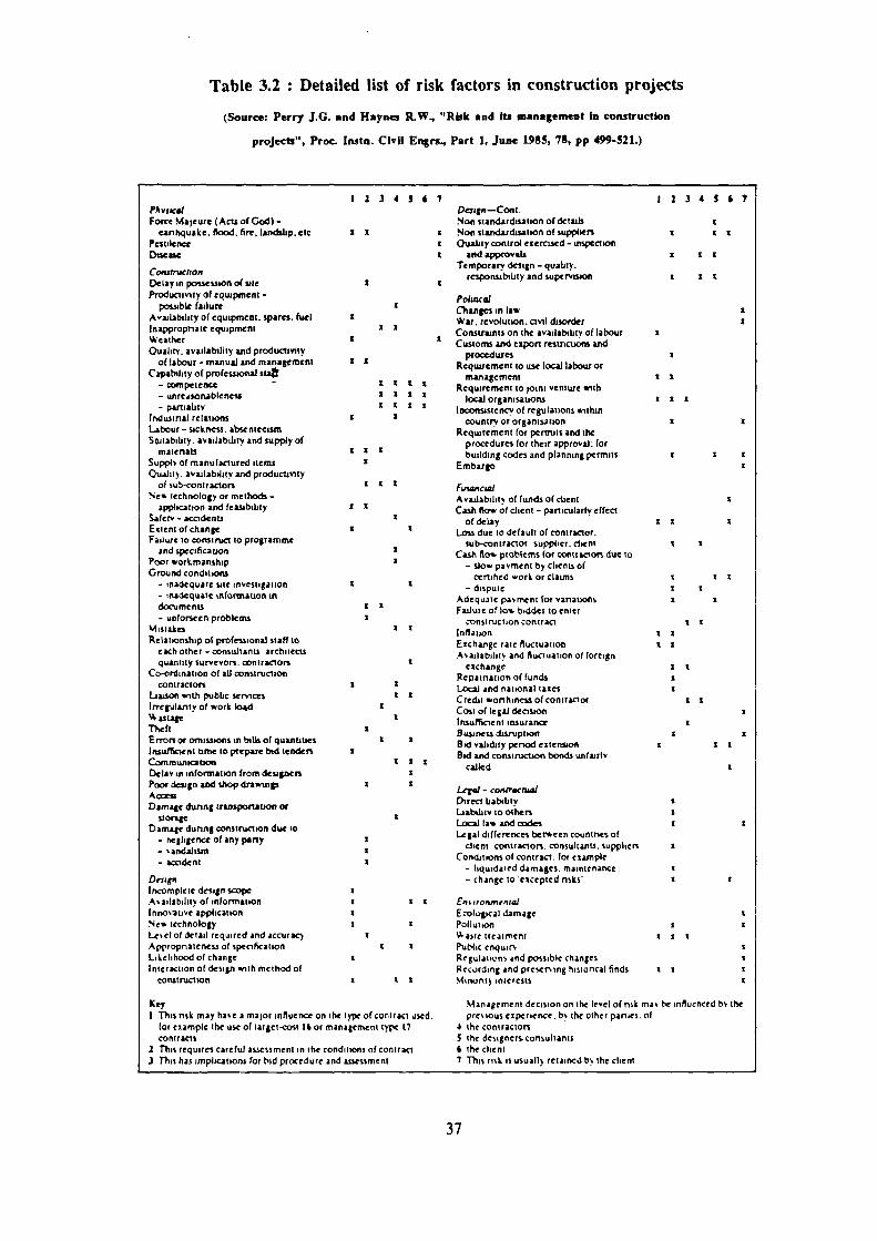
1 2 3 4 5 6 7

S II

x

111

II

I

11

51

X I

z

Table 3.2 : Detailed list of risk factors in construction projects

(Source: Perry J.G. and Haynes R.W., "Risk and its management in construction

projects", Proc. Instn. Civil Engrs., Part 1, June 1985, 78, pp 499-521.)

1 2 3 4 5 6 7PhysicalForce MaKure (Acts o1 G) -

earthquake. flood, fire. landshp. etc 8 ItPestilence()nesse

CommacnonDelay in possession of siteProductivity of equipment -

possible failureAvailability of equipment. spares. fuelInappropriate equipment 2 xWeatherQuality . availability and productivity

of labour - manual and managementCapability of professional starf

competence- unreasonableness- partiality

Industrial relationsLabour - sickness. absenteeismSeutabihty. availability and supply of

maienalsSupply of manufactured itemsQuality. availability and productivity

of sub-contractorsNew technology or methods -

application and feasibilitySalem - accidentsExtent of changeFailure to construct to programme

and specificationPoor workmanshipGround conditions

- inadequate site investigation- inadequate information indocuments a x- unforseen problems

MistakesRelationship of professional staff to

each other - consultants architectsgummy surveyors. contractors

Co-ordination of all constructioncontractors

Liaison with public servicesIrregulanty of work load%LuneTheftErrors Of omissions in bills of quantitiesInsufficient time to prepare bid tendersCommunicanonDela y in information from designersPoor design and shop drawuipACCeiiDamage dunng transportation or

storageDamage dunng construction due to

- negligence of any party- sandalam- accident

DevgnIncomplete design scopeAs allability of informationInnovative applicationNew technologyLeset of detail required and accurst-)Appropriateness of specificationLikelihood of changeInteraction of design with method of

construction

KeyI This risk may hue a major influence on the type of contract used.

for example the use of target-cost 16 or management type 1/contracts

2 This requires careful assessment in the conditions of contract.3 This has implications for bid procedure and assessment

Daign—Cont.Non standardisation of details

• Non standardisation of suppliers• Quality control exerctsed - inspection

and approvalsTemporary design - quality.

responsibility and supervision

PoliticalChanges in lawWar, revolution, civil disorderConstraints on the availability of labour

• Customs and export restrictions andprocedures

Requirement to use local labour ormanagement

Requirement to loam venture withlocal organisauons

Inconsistency of regulations withincountry or organisation

Requirement for permits and theprocedures for their approval: forbuilding codes and planning permits

Embargo

FinancialAvailability of funds of clientCash flow of client - particularly effect

of delayLoss due to default of contractor.

sub-contractor supplier. clientCash flow problems for contractors due to

- slow pa yment by clients ofcertihed work or claims

- disputeAdequate pas ment for vanauonsFailure of low bidder to enter

construction contractInflationExchange rate fluctuationAs ailability and fluctuation of foreign

exchangeRepatriation of fundsLocal and national taxesCredit worthiness of contractorCost of legal decisionInsufficient insuranceBusiness disruptionBid validity period extensionBid and construction bonds unfairly

called

Legs/ - contractualDirect liabilityLiability to othersLocal law and codesLegal differences between countries of

client contractors. consultants. suppliersConditions of contract, for example

- liquidated damages. maintenance- change to 'excepted nsks'

En n tronmentalEcological damagePollution

Ailf treatment I I xPublic engulfsRegulations and possible changesRecording and presersing histoncal finds xMinority interests

Management decision on the level of risk mas he influenced bv thepresious experience, by the other parties. of

4 the contractors5 the designers. consultants6 the client7 This nsk is usually retained by the Client

37

From the literature review and discussion with refurbishment contractors, the major risks

commonly encountered by contractors when tendering for refurbishment work are listed in

table 3.3 and may be broadly classified as follows:-

a) Contract related risks:- This refers to risks which arise as a result of the

contractual arrangements between the client and

contractor.

b) Information related risks:- This relates to risks caused by "information gap" in

the tendering process both inside and outside a

contractor's organisation.

c) Protection related risks:- These risks are mainly concerned with the

uncertainty which is inherent in the provision of

protective measures required for the proposed

refurbishment work.

d) Personnel related risks:- This category of risks relates to the nature of the

relationship between the client, consultants and

contractor.

e) Work content related risks:- These are risk factors which are inherent in the work

content of the proposed contract such as the intensity

of work, the proportion of sub-contractor's work or

the size of job.

f) Work nature related risks:- These are risk factors attributed to the unique

characteristics of the proposed work and include the

complexity of the job, site restrictions or degree of

structural work.

38

Table 3.3 : Risk factors in competitive tendering for refurbishment work

CATEGORY CONSTRUCTS

1) Contract related constructs a) Contract formb) Liquidated damagesc) Contract periodd) Restrictions on working hourse) Quality requirementsf) Collateral warrantyg) Specification of work hoursh) Percentage of retention

2) Information related constructs a) Documentation (Bills of quantities)b) Design informationc) Cost estimate .d) Number of bidderse) Riskf) Identify of bidders

3) Protection related constructs a) Noise and dust protectionb) Public protectionc) Protection of listed buildings and expensive itemsd) Securitye) Protection new of workf) Protection of existing building

4) Personnel related constructs a) Consultant relationshipb) Competence of consultantsc) Commercial clientd) Familiar cliente) Client relationshipf) Client credit

5) Work content related constructs a) Intensity of workb) Phase workc) Timely start of projectd) Buildabilitye) Complexity of contractor's own workf) Proportion of contractor's own workg) Proportion of new workh) Complexity of sub-contract worki) Proportion of specialist workj) Size of jobk) Work load of contractor1) Familiarity of work

6) Work nature related constructs

_.

a) Occupation of buildingb) Degree of temporary workc) Degree of structural workd) Degree of demolition worke) Occupation of domestic buildingf) Degree of ground workg) Internal or External refurbishmenth) Complexity of jobi) Restriction of access

39

3.5 Risk management strategies

Perry and Haynes (17) have suggested a simple and systematic approach to risk

management in the construction industry. This approach consists of three distinct stages

namely: (i) risk identification; (ii) risk analysis, and (ii) risk response. The first stage

involves the identification of major sources of risks pertaining to the decision problem. In

the second stage, the effects of these risks are assessed and evaluated. Thereafter,

appropriate risk policies and responses are developed to reduce and control the risks

involved. Thus, it can be seen from the mechanism of the above process that risk

management does not actually remove all risks from a project. It merely provides an

organised framework for assisting decision makers to manage risks more effectively and

efficiently. The following describes the main activities involved in the risk management

process of competitive bidding in the construction industry.

3.5.1 Risk identification

In a bidding situation, the risk management process begins with the initial identification of

the relevant and pertinent risks associated with the proposed contract. The contractor must

be able to identify both the risks allocated to him through the contractual arrangement

(type of contract and contract form) and also the risks which are inherent in the nature of

the project. This process entails a thorough understanding of both the contractual and

construction procedures involved in the project. Very often, contractors rely upon their

experience and intuition to identify and assess such risks. However, this task may be very

complicated when dealing with complex projects. The major sources of risk in competitive

tendering for refurbishment work have been discussed earlier.

3.5.2 Risk analysis

Once the major risk factors are identified, various measures must be taken to quantify

them so that it is possible to determine their effects on the outcome states of the decision.

40

Various decision criteria (for example, profitability) must be developed so as to facilitate

the selection of alternative courses of action by the decision maker. Various risk analysis

techniques such as decision tree, probability and simulation, sensitivity analysis and utility

theory may be utilised to analyse the effects of these risk factors on the outcomes. Very

often, these techniques involve assigning a range of values for each risk factor together

with its associated probability of occurrence and analysing the impact on the decision

outcome in terms of monetary or utility values. Sometimes, subjective judgement is

required to quantify some of the risk factors. This is partly due to the fact that many

contractors find it difficult to obtain adequate data to determine the probability distribution

of these risk factors. Hence, risk analysis suffers severe limitations (as contractors are

sceptical of its reliability and accuracy) especially when subjective judgement is required.

3.5.3 Risk response

Risk may be treated in a number of different ways. There are four common methods in

which decision makers can respond to risk which are described as follows:-

a) Risk avoidance - As its name implies, this simply involves taking actions to avoid

the risk in the decision problem. In competitive tendering, this response may be

taken by a contractor when he finds that his risk exposure for the proposed contract

is too high or beyond his risk absorption capacity. Risk avoidance may be adopted

by a contractor after he has received an invitation to tender. If he is of the opinion

that the project involves high risk, he may reject the invitation and return the tender

documents to the client thus avoiding any risk in tendering. However, in some

cases a contractor may only decide not to submit a bid after detailed appreciation

of the project or after the preparation of a cost estimate. Under such circumstances,

the contractor may either return the tender documents as before (this is not

commonly practiced as it may offend the client) or the contractor may resort to

submiting a non-serious bid (cover bid) which is considerably higher, thus

deliberately reducing his chance of being awarded the contract. The use of cover

41

bids is one means whereby a contractor can avoid the risks of tendering and at the

same time avoid offending his prospective clients. However, caution must be

exercised in the submission of cover bids as sometimes a cover bid may turn out to

be the lowest bid.

b) Risk reduction - Risk reduction strategy is one of the strategies most commonly

practiced by contractors in the industry. A common approach is through the use of

an information search whereby information is obtained from a variety of sources so

as to enable contractors to appreciate and price the contract more accurately. The

use of an information search has been recognised by researchers such as Hakannson

and Wootz (24), and Covello (25) as one of the most effective strategies for the

management of perceived risk. There are two main types of information required by

contractors in competitive bidding:-

i) Information which will help the contractor to price his cost estimate

accurately (micro level).

ii) Information which will enhance the understanding of contractors with

respect to the competitive envirorunent (macro level).

There are a number of information sources which are commonly utilised by

contractors for the preparation of cost estimates. This includes tender

documentation, enquiries from clients and consultants, site visits, published cost

data and historical cost records of contractors. The influence of information on the

estimating accuracy has been investigated by various researchers such as Whittaker

(26), Bennett and Barnes (27), and Flanagan and Norman (28). Whittaker

acknowledged that "estimating uncertainty" is mainly attributed to an "information

gap". Bennett and Barnes found that by varying the amount of information

available to estimators, the shape of the distribution of the population of cost

estimates became flatter indicating higher variability in the cost estimates. Similarly,

Flanagan and Norman managed to establish that a negative correlation exists

42

between tender bid variability and the quality of information (as measured by the

proportion of prime cost and provisional sum in a tender).

On the other hand, information on the competitive environment is often difficult to

obtain due to the sensitivity of such information and the unwillingness of

contractors to share tender bid information. Despite these barriers, in practice

contractors are able to obtain indicative information concerning the bidding

environment through sources such as grape-vine information, contacts with clients,

consultants or competitors, sub-contractors, suppliers or through independent

organisations such as the Builders' Conference.

Although there is an abundant amount of information available, this information has

often not been put to effective use in helping contractors to manage tendering risks.

This is mainly attributed to the severe time constraint which is commonly imposed

by clients on contractors in the preparation of a tender (two to three weeks).

Furthermore, the vast amount of information available both inside and outside a

contractor's organisation has not been organised in any comprehensible form. This

observation was also made by Cussack (29) who commented that there is an

abundance of information but not in the 'right form' to support the decision making

process of contractors. As a result, many contractors encounter difficulty in

adopting an information search as a risk reduction strategy. Consequently, decisions

are frequently based upon intuitive judgement and experience.

Another risk reduction strategy which is commonly practiced by contractors is

tender qualification. Contractors may qualify their tender bid or alter certain

conditions of the contract, thus reducing their liabilities. This strategy is normally

adopted when the contractor finds the contract conditions ambiguous or unfair. But,

this practice is normally not favoured by clients and consultants. However, the

rationale for taking such action is explained by one contractor (30) as follows:

43

"One must realise that clients can write any conditions into the documents that they

desire. There are circumstances where the client's interests conflict radically with

the contractor's interests. There are circumstances where conditions have been

written into documents which are so grossly unfair that the contractor has either to

qualify or to send the documents back. The difficulties in doing the latter have been

touched on (if a contractor does not submit the tender documents, he is liable to be

crossed off the architect's list for future invitation to selective tendering), therefore

there is no alternative but to qualify. If all documents when sent out were

masterpieces of fairness and clarity there would be no need to qualify, but this is

an Utopian situation which has certainly not been reached."

c) Risk transfer - There are two main routes whereby risk may be transferred by A

contractor to another party in competitive tendering as follows:-

i) Contractor to insurer.

ii) Contractor to sub-contractors.

The transfer of risk to an insurer is usually carried out by means of the contractor

taking up insurance policies. For instance, the contractor's all risks policy (CAR

policy) provides an useful instrument which indemnifies the contractor against "loss

or damage from whatsoever cause to contract works or materials whilst on

contract site(s) and in use in connection with the contract specified or type of work

described in the schedule and where such loss or damage arises out of

performance of the contract and/or during the period of maintenance". Similarly, a

contractor can also transfer risk of legal liabilities through the employer's liability

and the public liability policies. The employer's policy covers the "liability of the

contractor to his employees (those persons under a contract of service or

apprenticeship with the employer) for bodily injury or disease arising out of and in

the course of employment". While the public liability policy indemnifies a

contractor against "personal injury claims by the public and property damage

44

claims". Thus, the adoption of insurance provides an effective way to transfer risks

in a contract.

Another means by which main contractors may transfer risks is through the sub-

contracting of certain portions of the proposed work to sub-contractors or

specialists. This is commonly practiced, especially in refurbishment work which

often contains a high proportion of complex and specialised work. But, contractors

must be cautious and selective to ensure that such risks are transferred properly to

the appropriate sub-contractors (in terms of their competence and risk absorbing

capacities). Otherwise, if the amount of risk being transferred is beyond the

capacity of the sub-contractor, the risks may be transferred back to the main

contractor if the sub-contractor goes into liquidation or when the sub-contractor is

unable to complete the sub-contracted work, thus causing much disruption to the

overall progress of the construction work. Therefore, most contractors usually

maintain a group of sub-contractors with whom they have established a good

working relationship or adopt a stringent vetting system in the selection of domestic

sub-contractors and suppliers.

d) Risk retention - Whatever risk is remaining after adopting the above three risk

management strategies has to be borne by the contractor. As suggested by Perry

and Haynes (17), these risks may be grouped into two main categories: (i)

controllable risks and (ii) uncontrollable risks. Controllable risks are usually

managed by either reducing their likelihood of occurrence or reducing their impact

if they occur. In competitive bidding, contractors normally allow a contingency sum

to cater for any unforeseen circumstances so as to reduce the impact of such risks

on the profitability of the project. Contingency allowance is usually provided in the

tender bid either as a percentage of the cost of work or as a lump sum. In certain

cases, the quantum of risk exposure may be small relative to the risk absorbing

capacity of the contractor, especially for large sized firms. Under such

circumstances, contractors may instead utilise risk retention strategy as a bidding

45

strategy by not providing any risk allowance, thus increasing their chance of

winning the contract.

3.6 Risk management tools and techniques

Over the years, numerous risk analysis techniques have been developed to facilitate the

decision making and risk management processes of managers. However, many of these

techniques have received limited application in the construction industry. This is mainly

due to the sophisticated and theoretical nature of these methods. The following provides a

brief review of some of the more common risk analysis techniques which are relevant to

the construction industry.

3.6.1 Sensitivity analysis

Sensitivity analysis is normally used to study the impact of change in a single risky

element or uncertain parameter on the outcome of a decision problem. This technique is

frequently used in financial and investment analysis where uncertain factors such as

interest rate may be varied so as to determine their impact on the financial returns of

investment decisions. The main purpose of sensitivity analysis is to determine the

influence of each uncertain element on the outcome and thus identify the major risk

factors. Very often, this analysis is performed by assigning a likely range of variation for

each uncertain element. The effect of change of the uncertain element on the final

outcome is then assessed by varying the value of the uncertain element (within the

prescribed range). This process may be reiterated by varying the values of other uncertain

elements. When the analysis involves a single uncertain variable, the results may be

presented in a simple table to enable a decision maker to choose among the alternatives.

But, when there are several variables involved, the results of the analysis may be

displayed in a spider diagram (an example is shown in figure 3.1) which provides a clear

representation identifying the critical variables (risk factors). The main advantage of

sensitivity analysis is that it enables a decision maker to identify critical risk factors so

46

that appropriate actions may be taken to reduce the risks involved. However, this

technique has certain limitations:-

i) the variables are treated individually and this leads to severe limitations in the

extent to which combinations of variables can be assessed directly from the data.

ii) it provides no indication of the anticipated probability of occurrence of any event.

Figure 3.1 : An example of a spider diagram for sensitivity analysis

(Source: Perry and Haynes, Proc. Inatn. CIT. Engrs., Part 1, 78, June 1978)

3.6.2 Probability analysis

The use of probability theory provides a powerful and sophisticated form of risk analysis.

Probability analysis overcomes the limitations of sensitivity analysis by specifying a

probability distribution for each uncertain variable and thus provides the mechanism which

allows all variables to change their values at the same time. However, in practice it is

often difficult to quantify all risk factors, particularly in the construction industry where

47

projects are unique in nature and their operating environment highly dynamic. Thus,

inadequate data prevents the quantitative derivation of the probability distribution of many

uncertain elements. As such, subjective judgements are often required to estimate the

probability of occurrence of uncertain events. Sometimes, this problem of specifying

probability distribution is overcome by utilising a sampling approach such as the Monte

Carlo simulation technique. Therefore, although probability risk analysis provides a more

quantitative approach to risk management, it is not commonly used by contractors. This is

partly due to its complex nature and the scepticism which contractors possess regarding

the use of subjective judgement to estimate the probability distributions of various

uncertain elements.

3.6.3 Decision tree analysis

In this analysis, the anatomy of a decision is displayed diagrammatically using a decision

tree as shown in figure 3.2. The decision tree clearly shows the possible courses of action

together with the outcomes and associated probabilities of various outcome states. As

illustrated in figure 3.2, the branches of the tree represent either decision alternatives or

chance events. Decision alternatives originate from decision nodes as indicated by the

squares while chance events emanate from chance nodes (represented by circles). The

decision tree branches from the left to the right displaying various decision points and

chance events of the decision problem over a specified time period (planning period).

Thus, the structuring of a decision problem in this manner facilitates the decision making

process of managers. This technique has an obvious advantage as it forces the decision

maker to assign probabilities to various outcomes and to quantify these outcomes, thus

allowing the decision maker to evaluate the decision alternatives. Various researchers such

as Chapman and Cooper (6), Ashley (31) and Shaifer (32) have applied this technique in

the construction industry.

48

Planning period ,i0utcornes

Event'

Event

Event

Event

Event

Event

Decision node

0 Chance node

Figure 3.2 : A decision tree

(Source: L. Shaifer, Construction Management and Engineering, John Wiley & Sons, 19112)

3.6.4 Utility theory

Utility theory basically originates from the work of Von Neuman and Morgenstern (33). It

is a psychological concept which is used to measure the desire of individuals to possess

units of a given commodity. It provides the basic foundation for modelling the value

system of an individual decision maker. In the past, most work on risk analysis focussed

on the use of Maximum Expected Value (MEV) criteria (usually expressed in monetary

units) as a basis to assist decision makers evaluate and choose among decision

alternatives. However, this approach has been criticised for failing to appreciate the non-

linearity of the value system of individuals. As acknowledged by Von Neuman and

Morgenstern:-

i) There exists an interval scale for measuring the preferences (utility scale) of

individual decision maker.

49

R,sh

1•••Se

ii) This utility scale is defined in such a manner that if the decision maker chooses the

alternative with the highest expected utility, his "choice will be consistent with the

expressed preferences that were used in defining the scale."

Using a method called Standard Gamble technique, Von Neuman and Morgenstern

developed a procedure for determining the utility function of individuals. As shown in

figure 3.3, there are three common characteristic forms of utility functions (curves): (i)

risk averse. (ii) risk neutral, and (iii) risk seeking.

Figure 3.3 : Utility functions of individuals

UlahlieS

/ Seek',ig

•1

• 2

Once the utility function of the decision maker is determined, it is then possible to

transform expected monetary values into expected utilities by multiplying the utility value

of each outcome and its associated probability. In cases where there are several possible

outcomes, the expected utility value for each alternative course of action is determined by

summing the weighted expected utility values of all possible outcomes for that course of

50

action. This is expressed as follows:-

EUVA = P, u(0 1) + P2 u(02) + P. u(on)

where u(0 1 ) + u(02) + u(0„) are utility values as a consequence of

action A and P„ P29 P. are the associated probabilities of each outcome

respectively.

Once the expected utility value of each decision alternative is determined, the decision

maker will then be able to select the course of action which yields the Maximum

Expected Utility (MEU). Thus, the Utility theory approach provides a better representation

of the value system of the decision maker. Furthermore, it also measures the risk attitude

of the decision maker. In spite of this, Utility theory is seldom applied in the construction

industry. This is because contractors tend to regard this approach as theoretical.

Furthermore, it is often difficult to accurately determine the utility functions of decision

makers.

3.7 Normative process of decision making

The process of decision making usually involves the selection of an act or course of

action from among alternative acts or courses of action. Generally, a rational decision

maker is one who would desire to select the course of action or act that will produce the

optimum results under certain criteria of optimisation. This section attempts to explain

some of the basic concepts of decision making and their potential applications in the

construction industry.

3.7.1 Definition of decision making

Various writers have defined decision making in a variety of ways. The essential

ingredients of a decision making process may be summarised in a simple definition as

51

follows:-

"Decision making simply consists of a choice between two or more options after an

evaluation of these options and in the light of progress towards fulfilling an objective or

objectives."

3.7.2 Decision making process

There is a vast amount of literature on the study of decision making processes. But,

perhaps one of most distinguished and respected writers is Herbert A. Simon (34).

According to Simon, the central issue of any decision making process is that of rational

behaviour. As illustrated by Simon, a decision making process basically consists of three

distinct stages as follows:-

a) Intelligence stage - This involves the surveying of the economic, technical,

political and social environment in order to identify conditions or circumstances

calling for new actions. It is basically finding occasions for making a decision.

b) Design stage - In this stage, the decision makers invent, develop and analyse

possible courses of action. Thus, this stage consists of finding all possible courses

of action to a decision problem.

c) Choice stage - This simply consists of choosing one of the alternative courses of

action.

3.7.3 Decision making model

Numerous attempts have been made to develop decision making models to facilitate the

decision making process of management in various industries. Most of these models

attempt to provide a "systematic framework" for structuring the decision-making process

so that quantitative analysis or evaluation models may be utilised to enable management

to select the optimum course of action under various circumstances. A typical decision

52

3 Oeveitopreliminary

system medal

Syntheers

'41

_L_ .1.EreitatonAnalyps

Sefertinelystsmodels

S S neheeizeeiternetreee

8

Anolyzesibmatres

Endueselionweees

Developsvalushen

model

Define the dechan utushon

Domes

Communicate

making model as proposed by Shaifer (32) is illustrated in figure 3.4.

Figure 3.4 : A typical decision making model

(Source: L. Shaifer, Construction Management and Engineering,

John Wiley & Sons, 1982)

The main objective of this model is to present a sequence of activities aimed at providing

guidance to management in order to perform the synthesis, analysis and evaluation of data

for the purpose of generating the necessary information on which the decision is based.

Thus, this model provides an effective management tool facilitating the decision making

process of managers.

3.7.4 Elements of a decision

There are five main elements of a decision which are described briefly as follows:-

53

a) Decision maker - This is the primary element of any decision situation and may

comprise of individuals or groups who have been designated the relevant authority

to select a course of action in the decision problem. In competitive bidding,

decisions with respect to the cost estimating and tender adjudicating processes are

often made by estimators and directors of the firms respectively. The decision

process may be performed individually or in a group depending on the policy and

size of the company. Generally, tender decisions in smaller firms (especially sole

proprietorships) are made by individuals while large construction firms tend to

adopt group decision making.

b) Candidate alternatives - This refers to the alternative courses of action

surrounding a decision problem. In a bidding situation, two main decisions are

usually made as follows:-

i) Which of the jobs to bid on ?

ii) How much to bid ?

Alternative courses of action for the first decision include whether to bid for job X

or job Y or job Z or other jobs. While in the second decision situation, the

candidate alternatives consist of submitting different amounts for a tender bid.

c) States - Very often, the consequences of a decision depend upon conditions which

are external to the decision making process. Although such conditions affect the

results of the decision, they are not themselves being influenced by the decision.

These external conditions are termed "states of nature". The set of states is often

exhaustive (that is, some members within the set must occur) and mutually

exclusive (that is, only one state can occur at a time). Examples of states of nature

which may affect the results of a tendering decision include weather conditions,

inflationary fluctuations or industrial action.

54

d) Outcomes and decision criteria - The consequences estimated for each alternative

course of action under each state are termed outcomes. In a bidding situation, there

are usually several outcomes arising from a number of consequences of a decision.

These outcomes are usually measured by several characteristics or dimensions

(economic or physical). In practice, the decision maker normally only considers the

most significant dimensions of the outcomes and these are termed his decision

criteria.

e) Value systems - In selecting an alternative from a set of candidate alternatives, the

decision maker uses his "value system" to evaluate the alternatives so as to enable

him to select the optimum course of action which best satisfies his goals. There are

two common approaches which have been developed to represent the value system

of a decision maker namely: (i) Maximum Expected Value criteria and (ii)

Maximum Utility Value criteria. In the Maximum Expected Value approach,

outcomes of each alternative course of action are usually transformed into monetary

units in order to allow decision makers to make meaningful comparisons among

alternatives. Similarly, the Maximum Expected Utility Value method adopts an

utility scale to represent the value system of decision makers. In this case,

outcomes of candidate alternatives are expressed in utility values to facilitate

decision making.

55

CHAPTER FOUR

PERCEPTION OF RISK (PERSONAL CONSTRUCT THEORY)

CHAPTER FOUR

PERCEPTION OF RISK (PERSONAL CONSTRUCT THEORY),

4.1 Introduction

This chapter describes the theoretical background of Personal Construct Theory as

developed by Kelly (1). Particular emphasis is placed on the use of Repertory Grid

Interview technique as a means to measure people's perception. The logical procedure of

the Repertory Grid Interview is also discussed together with various techniques commonly

adopted to elicit personal constructs of people.

4.2 Personal Construct Theory

Personal Construct Theory was first established in 1955 by a psychologist named

George Kelly (1). According to George Kelly, each person builds for himself a

representational model of the world which enables him to plan a course of behaviour.

This model changes over time as constructions of reality are tested and modified so as to

allow better predictions. As pointed out by Kelly,

II .... a person's processes are psychologically channelised by the ways in which he

anticipates events"

Throughout a person's life, he questions, explores, revises and replaces constructions in

attempts to anticipate events in the light of predictive failure. People make sense of

situations by imposing certain structures on them. This proposition is well explained by

Kelly as follows :-

"We impose the structure - events do not carry their meaning engraved on their backs."

56

From birth, we build up a set of expectancies ("hypotheses") which clearly reflect our

past experiences. However, the crucial point is that these hypotheses influence and

condition our present experience and our anticipation of the future. They are like a pair

of spectacles through which we get information but which also affect what we see and

how we see it. Kelly called the "spectacles" a construct system, and termed the

individual hypotheses constructs. There are certain unique properties of constructs which

must be understood in order to facilitate communication and shared understanding as

described below.

a) The medium through which perception occurs is the construct system.

b) Construct systems are unique to individuals and develop throughout life.

c) A construct is an aspect, feature or quality which distinguishes some objects from

others. It is an axis of discrimination to all thinking operations - a reference axis

upon which one may project events in an effort to make sense of what is going on.

According to Kelly, a construct always involves a basic contrast of similarity and

difference.

d) Kelly (1) grouped constructs into three types.

i) Pre-emptive constructs group objects exclusively in their own realm (for

example, species name). This is an X and nothing but an X.

ii) Propositional constructs are not exclusive and do not prevent objects being

construed by other constructs. This is an X, but it can also be a Y.

iii) Constellatory constructs fix membership not only to one, but on several

constructs. If it is an X, then it must also be a Y.

e) Constructs are linked together in a hierarchical manner to form a construct system.

0 The psychological processes of two persons are similar to the degree in which both

of them construe certain sets of similar experience.

g) Similarly, to the extent that one person construes the construction processes of

another, he or she may play a role in a social process involving the other.

h) The constructs most useful to us are those which discriminate best between events.

i) Constructs have a limited range over which they operate.

57

4.3 Repertory Grid technique

The Repertory grid technique originates from Kelly's (1) Personal Construct Theory.

Originally, this technique had been adopted to investigate the relationships between

patients and their families, friends or colleagues and to assess the relationships between a

patient's constructs about people. Its procedure is closely linked to the theoretical roots of

Kelly's definition of a construct. As put forward by Kelly, a construct is " in its minimum

context, a way in which two elements are similar and contrast with the third."

This distinction has been emphasised by Fransella and Bannister (2) who state that :-

"When we say that Bill Boggs is honest, we are not saying that Bill Boggs is honest,

he is not a chrysanthemum or a battle-ship or the square root of minus one. We are

saying that Bill Boggs is honest, he is not a crook.

Thus a construct is basically a dimension which may evolve when considering a particular

set of elements but can usually be applied to a further range of elements. The

dimensionality of a construct allows one to extract matrices of inter-relationships between

constructs and between elements.

Kelly also observed that constructs do not exist in isolation but in fact they are closely

linked to one another in more or less coherent and hierarchical manner. A person's

constructs may be grouped into two categories namely:- "core" constructs and "peripheral"

constructs. "Core" constructs are of central importance to the individual and often remain

very stable and more resistant to changes. On the contrary, "peripheral" constructs are

subject to changes and occur at different levels of an individual's construct system.

Laddering is a technique commonly adopted to move between construct levels. Given a

construct, one can either ladder "upwards" towards the central construct by asking which

pole of that construct is more important to the individual and why. For example, in

investigating the constructs of an individual about efficiency at work and the construct

58

"keeps good time/always late" is elicited. It is possible to obtain further constructs (for

instance, construct such as "shows commitment/no commitment" may be elicited by

laddering from the "keeps good time/always late" construct) by asking the "why" question.

This process may repeated until the central construct of the respondent is revealed.

Similarly, constructs could also be laddered "downwards" by using the "how" or "what"

questions instead to obtain more specific constructs.

There are some definitions of terms commonly adopted in the Repertory Grid Interview as

follows:-

a) Element - This is the subject of the investigation and may consist of objects,

people, situations or even other abstract descriptions. There are two main points

which should be noted in the selection of elements:-

i) Elements should be homogeneous - They should be chosen from the same

category.

ii) The selected elements should provide representative coverage of the area of

investigation.

b) Constructs - These are bi-polar distinctions of the elements and represent the

dimensions which the respondent uses to discriminate the elements.

c) Construct elicitation - This is the process of obtaining constructs from the

respondents based upon triadic method, dyadic method, free response method or a

combination of these methods.

4.4 Repertory Grid Interview procedure

There are many well established methods used in practice to elicit the construct system

of individuals. The most typical approach as illustrated by Pope and Keen (3) is shown in

figure 4.1 and involves the following steps.

59

NO

Figure 4.1 : Flow diagram for grid elicitation

(Source: Pope and Keen, Personal construct psychology and education,

1981, Academic Press)

Negotiation of purpose

Elicitation of a representative setof elements

Revise set

Check IIs the setrepresentative, NO

YES

Consider first 3 element,elicitation of construct Iname ooles

Check 2Do pole namesreflect whet NOPerson means'

YES

Assign ratings 1 - 5 to eachelement in tutn lot Construct I

Revisepolenames

-411—•

Pirate

Check 3Does Personwant to change YESratIngi

NO

Check 4Does Personwant to change YESpole names,

NO

Consider next 3 elements•fic.tat on of construct 2

IAssign ratings for construct 2

I

Repeatchecks 2. 3 & 4 I

Continueelicitation

Continue taking elements in groups of 3elicitation of further constructs

Assign ratings and tepee checks 2. 3 & 4for each construct

When several constructs have been eIrc.tedusing triadic method switch to lull contextform

Check 5Has Peison °fired allthe constructs he/she!eels are relevant

YES

FINISH I

60

4.4.1 Defining the purpose of the grid

This is the most important preliminary consideration before beginning the process of

eliciting elements and constructs. Two issues must be clearly addressed and answered at

this stage.

a) What is the topic to be investigated ?

b) What is the intended use of the grid information ?

It is essential that adequate time and consideration should be given to define the purpose

of the investigation. With a clear objective defined, it is then possible to select

representative elements and elicit constructs which are appropriate to the purpose of the

exploration.

The second issue on the intended use of the grid information has an influence on the

format and procedure of grid elicitation. There are various ways in which the grid

information could be used. The following list provides some examples of its potential

usage:-

a) a conversation with one's self;

b) gathering of information about an individual's views on a particular topic;

c) a comparison of the viewpoints of two people in terms of either:-

i ) degree of agreement between, or

ii) the degree to which either can gauge the other's point of view;

d) an exploration of the nature and sharing of construing within a group;

e) monitoring of changes in perspectives.

61

4.4.2 Selection of elements

This involves the selection of a set of elements representative of the area of investigation.

Elements may consist of objects, events, situations, pictures, buildings or people. They

could be provided by the researcher or elicited personally from the respondents. The

choice between elicited and provided elements depends on the researcher and also the

purpose of the investigation. However, it is important that adequate groundwork should be

done to ensure that the selected elements are representative of the nature of the problem

to be investigated. Normally, this would entail discussion or conversation with the

potential subjects so that a common understanding could be achieved between the

researcher and the subjects.

Thus, in order to determine the risk perception of contractors during tendering, it is

necessary to elicit various representative bidding situations which will reflect the

experience and risk attitude of the contractors. Generally, there are four distinct ways in

generating elements as follows:-

a) Supply elements (Provided elements) - The elements are provided by the

researcher.

b) Provide role or situation description - The researcher provides description on

certain role, object or situation and the respondent is requested to provide

examples to fit the description.

c) Defining a "pool" - The respondent is asked to "name five effective managers" or

"list seven types of perfumes she likes" or "to list five leisure activities he or she

indulges in".

d) Elicit through discussion - The researcher discusses the topic of investigation with

the respondent providing guidelines and prompts to elicit the appropriate elements.

In the past, there has been some debate among researchers comparing the usefulness

between provided and elicited constructs. For instance, Bonarius (4) in his study suggested

62

that:-

" .... subjects consistently use the more extreme poles of rating scales when using

personal constructs rather than provided constructs in rating themselves and others."

However, the controversy between provided and elicited elements in Repertory Grid

technique was well summarised by Adams-Webber (5) who commented:-

"Although normal subjects prefer to use their own elicited constructs to describe

themselves and others, both kinds of dimensions seem to be functionally similar when the

grid technique is employed to assess the structural features of their cognitive systems."

Another question commonly asked is "how many elements should a Repertory Grid

contain 7". Ideally, it would be very informative to have a large number of elements. But,

the task of construing a large number of elements can be very tedious and

time-consuming. On the other extreme, a small number of elements may provide

insufficient details or a devoid grid. In practice, between 6 to 10 elements would provide

a useful basis for the elicitation of a reasonable grid.

4.4.3 Elicitation of constructs

Normally, the elicitation of constructs is carried out by presenting a random set of three

elements at a time to the respondent and inviting him or her to think of similarities and

differences between the elements. The standard question is:-

"In what ways are two of these alike and different from the third in terms of

(purpose of study) ?"

As described by Kelly (1), there are six principal approaches to the elicitation of

constructs as follows:-

63

a) Triadic construct elicitation - In this method, the respondent is presented with

three elements at a time from a list of representative elements and asked to

distinguish in what ways are two of the elements are alike and different from the

third. The respondent is then requested to name the emergent pole and the

implicit or contrast pole which discriminate the elements. The two contrasting poles

of the construct are then recorded.

b) Dyadic construct elicitation - As suggested by Keen and Bell (6), this method is

used when the respondent finds it difficult to supply any constructs. Each time,

two elements are presented to the respondent to enable him to discriminate the

differences or likeness between them.

c) Free response construct elicitation - Through conversation, respondents provide

their personal constructs instinctively.

d) Supply constructs - This is the fastest way to generate constructs whereby the

researcher provides pre-determined constructs for the respondent to assign the

necessary ratings.

e) Laddering - This technique is normally used in conjunction with one of the above

methods after some constructs have been elicited. It involves asking the respondent

a series of "Why" or "How" questions so as to elicit more specific constructs.

0 A combination of the above methods.

One point which should be emphasised is that the researcher should ensure that the

elicited constructs are appropriate to the purpose of the investigation. There are four

different types of constructs which may arise from the elicitation process:-

i) Sensory-perceptual - These constructs are normally elicited when investigating the

perceived attributes of objects or situations. For example, the elicitation of personal

constructs of quality controllers who are working on a production line.

ii) Behavioural/Inferential - These constructs reflect upon the behaviour of the

subjects on certain persons or situations. For example, it would be appropriate to

elicit behavioural constructs of shoppers or consumers.

64

Feelings/attitudinal - These constructs describe the feelings or attitude of

individuals towards certain persons, objects or situations such as the constructs of

workers when working on production line.

There is also the question as to how many constructs should be included in the repertory

grid. As suggested by Kelly (1), it is vital to elicit several constructs in order to explore

an individual's world of meaning. Thus, it is necessary to achieve a balance between

eliciting sufficient numbers of constructs and the practical constraints present. This

consideration is well put forward by Maureen L. Pope and Terence R. Keen (3).

"one is not aiming to encapsulate the whole of an individual construct system but only

that part of it which is relevant to the defined purpose."

However, there are some criteria and limitations to consider when eliciting constructs:-

a) The constructs elicited must cover the range of constructs which the individual

feels are important to the area under consideration. Construct elicitation should

continue until the individual indicates that his repertoire of constructs for that

particular range of events is exhausted.

b) The elicitation of constructs can be exhausting both for the person completing the

grid and the person carrying out the grid interview. Thus, the researcher should be

careful not to stretch beyond the limits of exhaustion. Otherwise, the constructs

obtained may be unreliable and inaccurate.

c) In many circumstances there may be time limit constraints on behalf of either the

individual or the person conducting the grid interview which may well impose a

limitation on the number of constructs which are elicited at any one session.

d) It is necessary to consider the limitations of computer software used for the

analysis, such as the number of constructs and elements.

65

4.4.4 Rating of elements of each construct

Kelly's (1) original approach adopted a dichotomous form of grid whereby respondents

were asked to place ticks or crosses across elements for each construct. But, this method

does not permit finer discrimination between elements or constructs. Furthermore, as noted

by Bannister (7), the dichotomous grid may produce spurious relationships possibility

caused by lopsidedness (too many ticks and few crosses or vice versa) on a particular

construct.

As such, in recent years two popular forms of the grid have emerged namely:-

rating (Bannister and Fransella) (2) and ranking (Bannister and Mair) (8) grids.

Generally, in practice it is less tedious for the respondents to rate elements than ranking

them, especially when there is a large number of elements. Thus, rating of elements is

commonly used whereby the respondent is free to assign rating along a linear scale from

the emergent pole to the implicit pole of each construct. A 5-point or 7-point scale is

usually employed which provides much fmer discriminations between elements and

constructs.

4.4.5 Analysis of grid

Once the grid is fully completed, the element by construct matrix is then analysed for its

underlying structure. There are five principal methods of analysing the full grid data as

follows:-

a) Frequency counts analysis - This analysis simply counts the number of times a

particular construct or element occurs from all the respondents. It is commonly

used to identify general trends among groups of people. This analysis is frequently

employed when the elements are discrete and well defined and have consistent

meanings to the subjects.

66

b) Content analysis - In content analysis, all elements or constructs are grouped into

different categories with respect to their similarity in content. A frequency analysis

is then performed to determine the distribution of various elements or constructs in

these categories. A simple Chi-square test may be conducted to compare the

relative distributions of categories across two or more groups of respondents.

c) Visual focusing - This technique is normally used on a raw grid with ticks and

crosses rather than on a rated grid. In a ticks and crosses grid, it compares the

degree of agreement of each construct across the elements and produces a matrix

of agreement scores for all possible pairs of elements. Similarly, it is also possible

to compare the degree of agreement of various elements over different constructs.

d) Cluster analysis - The clustering technique developed by Shaw and Thomas

(1976) (9) attempts to group or cluster similar elements or constructs so as to

exhibit certain patterns of the original grid data. There are several computer

packages such as Pegasus and Focus developed by Shaw and Thomas (9) available

for performing cluster analysis. These programs usually produce a linear re-ordering

of elements or constructs to highlight similarities in the way in which they are

construed. A typical computer printout may consist of the following information:-

i) The original raw grid.

A matching score matrix of the relationships between all pairs of elements.

A matching score matrix of the relationships between all pairs of constructs

(with ratings reversed as well as originally rated).

iv) A statement as to which constructs (if any) should be reversed.

v) A re-ordered grid with tree diagrams attached showing the patterns of

relationships in the data.

e) Principal Component analysis (Factor analysis) - This method of grid analysis

was developed by Slater (10) in 1964. It is based upon two matrices of similarity

measures - an element matrix which includes the measure of similarity of every

element with every other element, and the construct matrix which shows the

67

measure of similarity of all pairs of constructs. These measures of similarity are

viewed as distances in space or dimensions. This analysis extracts the major

dimensions which then describes each of the elements or constructs to these

dimensions.

The Principal Component analysis is a statistical technique commonly used to

identify a relatively small number of factors that can be used to represent the

relationships among sets of many interrelated variables. It is a data reduction

technique for identifying a set of independent factors in data. The basic assumption

of this technique is that there exist underlying dimensions or factors that can be

used to explain the complex relationships of certain variables such as the

intelligence, creativity or risk perception of people. Factor analysis is usually

performed in four logical steps as follows:-

i) The computation of a correlation matrix of all variables to determine the

association among various variables.

ii) The second step involves factor extraction where a number of factors

(dimensions) necessary to represent the data is determined.

iii) The third step, rotation, focuses on transforming the factors to make them

more interpretable.

iv) Lastly, a score for each factor is computed for each case.

There are also computer programs such as Griddle (Keen and Bell) (6) and Ingrid (Slater)

(10) for analysing the intraclass relationships between elements and constructs of the

Repertory Grid. The main output of these programs provides the following information

(which is described in chapters eight and nine):-

i) Listing of raw grid data.

ii) Table of construct statistics and construct correlation matrix.

iii) Table of element statistics and element correlation matrix.

68

iv) Table of principal components

v) Graphical output of elements and constructs on major dimensions.

One aspect of computer analysis which is worthwhile mentioning is that the use of

computer packages simply reduces the amount of work required to analyse and interpret

the full grid data. The computer analysis does not add any new information to the grid

and also does not provide indications of the meaning of the grid. It merely summarises

the data in a more understandable form. This point is well emphasised by Kelly (1):-

"Neither abstraction nor generalisation has ever been computerised... .What can be

computerised ...is the elimination of redundancy in a construction matrix. The resultant

shrinkage in the matrix is sometimes mistaken for abstraction, or it appears to result in

the expression of a great deal in relatively few terms. But the contribution the computer

makes is to economy of the language employed, not to conceptualisation II

4.4.6 Feedback to respondent

When the full grid is completely analysed and certain patterns or relationships between

elements and constructs are established, this information can be fed back to the

respondents. This feedback may serve as a confirmation process for these relationships or

any associations found. Further constructs or elements may also be elicited using

laddering to investigate more specific constructs of the respondents.

Thus, this chapter provides an insight into the theoretical background of Personal

Construct Theory and the use of Repertory Grid Interview technique as a research

instrument for measuring the risk perception of people. The main research strategy when

adopting the Repertory Grid Interview to elicit risk perception constructs of contractors

(directors and estimators) when they are assessing risks in competitive bidding is

discussed in chapter 7.

69

CHAPTER FIVE

REVIEW OF CURRENT BIDDING MODELS

CHAPTER FIVE

REVIEW OF CURRENT BIDDING MODELS

5.1 Introduction

This chapter provides a review of past bidding models which have been developed both in

the Construction and Operations Research industries. A background of bidding theories is

provided describing the developments of various bidding models since the first

competitive bidding model developed by Friedman (1) in 1956. Discussions are made with

respect to the different distinctive approaches which various researchers have taken to

develop models for assisting contractors to manage risks in competitive bidding. A brief

review of the more prominent bidding models is provided highlighting the main benefits

and limitations of these models. Besides this, criticisms are made regarding the limited

practical applications of many bidding models in the construction industry. Suggestions to

improve risk management in competitive bidding are also proposed.

5.2 Background of bidding theory

Competitive bidding is one of the most critical activities of contractors in the construction

industry. To date, this form of contract procurement is still a common method adopted by

both the public and private sectors for awarding contracts to contractors in the industry.

But, bidding is a tricky process which demands considerable judgement on the part of the

contractor. Normally, in a bidding situation, a contractor must first estimate the cost of the

proposed work (after assessing all the uncertainties involved in pricing the materials, plant

and labour), and thereafter add a markup to cover for his overhead, profit and any risk

allowance if necessary to form a tender bid. In order to make a profit on the job, he must

submit a bid which is lower than his competitors, and at the same time the bid must

enable him to make a profit or at least cover his costs. If he bids too high, he may fail to

70

win the contract and thus lose time and money spent on the preparation of the tender. On

the other hand, if his bid is too low, he also loses as he may have undertaken the job at a

lower price than necessary. This phenomenon is commonly termed as "having left too

much money on the table". Thus, if he adds too high a markup to his bid, he may not

win enough contracts to stay in business. Conversely, if his markup is too low, he may

win many contracts but may not make enough money to stay in business. This dilemma

which is commonly faced by contractors in competitive bidding is well expressed by Park

(2) as follows:-

"In competitive bidding, the contractor is faced with two seemingly incompatible and

contradictory objectives: he must bid high enough to make a profit, yet low enough to get

a job - both at the same time!"

The severity and prominence of risk in competitive tendering has motivated the

development of numerous bidding models over the years. Most of these models have

attempted to provide guidance to bidders in the selection of an "optimum bid" under

various bidding situations. Much effort has been concentrated in the development of a

probabilistic model which will enable a contractor to predict his chance of winning a

contract under various competitive situations by producing statement such as "if you bid

at a markup of x%, you will have y% chance of winning a contract"

However, many of these models have received limited practical applications in the

construction industry. This is mainly attributed to the fact that there is an apparent lack of

consensus among bidding experts with respect to the basic concepts of bidding theory.

Furthermore, the results of all these models are not conclusive and many models have

been criticised for being too theoretical in nature, involving mathematical expressions

which are too complex.

71

5.3 Current competitive bidding models

From the literature review of current bidding models, it is observed that although many

models have been developed, most of these efforts have adopted a number of distinct

approaches to the competitive problem. This may be broadly classified into the following

categories:-

a) Expected Monetary Value bidding models;

b) Expected Utility Value bidding models;

c) Other approaches which include cash flow analysis, portfolio theory, game theory,

tender bid pattern analysis and simulation methods.

5.3.1 Expected Monetary Value bidding models

This is the principal approach adopted by many researchers such as Friedman (1), Park

(2), Gates (3), Casey and Shaffer (4), Whittaker (5), Benjamin (6), Broemser (7), Howard

(8), Flanagan and Norman (9), Shaffer and Micheau (10), Oren and Rothkopf (11), Wade

and Harris (12), Sugrue (13) and Skitmore (14). Essentially, this method attempts to

identify an "optimum markup" which will enable a bidder to maximise his expected profit

when submitting a tender bid.

The basic premise underlying this approach is that there exists a relationship between the

probability of winning and the tender bid. It is assumed that in a bidding situation, a

contractor will normally estimate the cost of work and then add a markup to form the

tender bid. If he is desperate for jobs, he will lower his markup so as to achieve a higher

chance of winning. On the other hand, if he is not keen on the job, he will increase his

markup thus reducing his chance of success. Therefore, between these two extremes there

exists a continuum of bids (with various markups) with associated probabilities indicating

their chances of successes. Thus, the competitive bidding problem is to formulate this

relationship mathematically.

72

5.3.1.1 Friedman's model

Friedman (1) was the first to attempt to establish this relationship by introducing the

concept of expected profit to competitive bidding. He assumed that the main objective of

a contractor is to maximise his expected profit, that is, his expected monetary value, in

every bidding situation. In deriving the profit function of a bid, he also assumed that the

actual cost of fulfilling a contract is a random variable and the ratio of the contractor's

true cost (actual cost) to his estimated cost (termed the "s" ratio) is also a random

variable. As such, his model may be expressed as follows:-

Profit function:-

p = bo - s co

where P = profit which will be realised if 130 is less than all other competitors.

bo = bid submitted by contractor.

co = cost estimate of contractor.

The expected profit of a given bid is then determined by multiplying the probability of

beating all other competitors with that particular bid and the amount of profit that will be

realised if the bid wins. This is determined as follows:-

E(p) =f .' PP. < bj) n (b0 < b3) n . . . n 00 < benr 0

xi(b, - s cd h(s) ds

= P[(b0 < hi ) n 00 < 1,0 n . . . n (bo < b i )] (bo -

where b1 , i=1,2,3, n, are bids of n competitors and h(s) = the density function of the

ratio of the true cost to the estimated cost. If pg represents the mean of the ratio of the

true cost to the estimated cost, then

c, = c. f . s h(s) ds = II, co

c')

73

ii

Once the profit function is determined, it is then necessary to compute the probability of

beating a particular competitor with a given bid amount. This is determined by analysing

the distribution of ratios, r,=1,2,3, n of competitors' bids to the contractor's cost

estimate based upon past bidding patterns. The distribution of r, of a known competitor (i)

is shown in figure 5.1. Thus, the probability that b 0 is less than that of the competitor is

indicated by the area under the curve to the right of bdc. (shaded portion of curve). The

probability that b0 is less than the bid of competitor i is determined as follows:-

PO, < b i ) = f fe (re) drb lcel o

b lcof o

= 1 - f fe(re) dr•

= 1 - Fi (2g)c,

where Fi(bdco) = Cumulative distribution function of r, evaluated at bico.

Figure 5.1 : Probability density function of a known competitor's

bid to contractor's cost ratio

I b. IC.

SIO - COST PATIO n r

74

Thus, the probability of beating any given competitor may be determined as described

above by simply analysing the past tender bids of the competitors.

However, in a bidding situation, there is usually more than one bidder. As such, it is not

only necessary to determine the probability of beating each individual competitor but also

the combined probability of beating all the competitors at the same time. In this case,

Friedman assumed stochastic independence of the bidding process and thus adopted the

multiplication rule of probability theory to determine the probability that b o is less than all

the bidders as follows:-11(b, < b) 11 (b, < bd 11 . . . 11 (b, < b,)1

n

- n [1 - F i (24)]

The competitive bidding problem is thus to find out the bid, b:, over all possible bid

amounts, which maximises the expected profit.

x

max E(p) . max (bo - Ile co) 11 [1 - F i Gool

all be i•a

•

= (b: - As Co) n [1 - Fi (Y.)]i•I

For cases where the identities of the bidders are not known, Friedman suggested a

distribution of the ratio of an average bidder's bid (typical bidder) to the contractor's cost

estimate. This distribution is obtained by combining the bid/cost estimate (s) ratios of all

bidders into a single distribution. The probability of beating an average bidder is thus

derived as follows:-

, .PO, < b cd = J f a (r a) dr

6 Ita a

= 1 - Fa (-

12)co

where I a(•) = density function of the average bidder; and

Fa( • ) = cumulative function of the average bidder.

ba = bid of an average bidder.

75

Therefore, the competitive bidding problem for beating against n unknown bidders is

expressed as follows:-

max E(p) • max ( bo - As CO) [I Fa GIS'all b,

. (b: - ps co) [1 - Fa Cf

5.3.1.2 Other Expected Monetary Value bidding models

Since the development of Friedman's model in 1956, numerous attempts have also been

made by many other researchers to develop various models to guide the decision making

processes of bidders. However, most of these models have in one way or another adopted

the same approach as Friedman but with various modifications. A comprehensive review

comparing the differences of principal bidding models is provided by Benjamin (6) and

more recently by Sundaram (15). Most of these efforts have been focussed on resolving

the controversy involved in the development mechanism (probability derivation and

assumptions) of past bidding models. Some have managed to refine Friedman's model

while others have adopted new approaches to the bidding problem.

5.3.1.3 Differences in bidding models

Although many bidding models have been developed, they differ from each other

principally in one or more of the following aspects:-

a) Derivation of profit function.

b) Derivation of probability of beating a specific competitor.

c) Combination of probabilities of beating individual competitors to determine

the probability of beating all the competitors at the same time.

d) Assumptions of model.

i) Relationship between number of bidders and job cost.

76

Influence of factors such market conditions, job type, client type,

job location and identity of competitor on the competitive

environment.

(a) Derivation of profit function

The difference in profit function arises due to variations in methods adopted by various

researchers in measuring the cost of work. Basically, the profit of a contract is the margin

between the bid and the actual cost which is often not known until the job is completed.

Thus, the key issue lies in whether the estimated cost is close to the actual cost of the

job. Friedman (1) acknowledged the presence of systematic errors in engineering estimate

and thus suggested a procedure (adoption of the "s" ratio as described before) for

correcting this bias. However, Park (2), Gates (3), Casey and Shaffer (4), Weverbergh

(16), and Capen et. al. (17) take the view that cost estimate is often correct on average,

and therefore the population mean of "s" is unity with a dispersion of zero. As a result,

they assumed that the true cost of the job is equal to its estimated cost. There are many

other researchers who have taken different views regarding the distribution of the true cost

and cost estimate. Skitmore (14) has summarised the main distribution parameters of the

true cost / estimated cost distribution as presented by various modellers as shown in table

5.1.

(b) Derivation of probability of beating a specific competitor

All bidding models concede that the derivation of the probability of beating a competitor

must be obtained by analysing past tender bids of the competitor. Friedman (1), Park (2),

Gates (3), and Casey and Shaffer (4) have suggested fitting the data (competitor's bid /

contractor's cost estimate) into a continuous function so as to determine the probability of

beating a particular competitor. Morin and Clough (18) have instead utilised a discrete

probability function in their OPBID model. They argued that this method eliminates any

smoothing errors which may result when fitting observations into a continuous function.

77

± 5%

less than 1006

1.0 (median)

close to 1

1.0 (exp. val)

+ 3%

The main controversy in the derivation of probability of beating a given competitor is

centered on the fitting of the data into various types of distributions. A summary of the

distribution parameters of various distributions as adopted by various researchers is

provided by Skitmore (14) as shown in table 5.2.

Table 5.1 : Distribution parameters for true cost / cost estimate

(Source: Skitmore M., Contract bidding in constructios, Longman, 19119)

Modeller

Shape Spread

Location

Barnes (1971)bBarnes & Lau (1974)ABeckmann (1974)ABeeston (1974)gCapen et al. (1971)3Case (1972)cCauwelaert & Heynig (1978)AFine (1974)bFine & Hackemar (1970)bFriedman (1956)cGates (1967)dGnesmer et al. (1967)AHackcmar (1970)bHarris & McCatTer (1983)ALeech & Earthrowl (1972)cLiddle (1979)AMitchell (1977)AMorin & Clough (1969)cMorrison & Stevens (1980)a

Moyles (1973)1.Naert & Weverbergh (1978)1Oren & Rothkopf (1975) AWeibullPark (1966)ARickwood (1972)bRothkopf (1969)ARothkopf (1980)ARubey & Milner (1966)ASmith & Case (1975)cSmith & Case (1975)cVickrey (1961)AWhittaker (1970)cWillenbrock (1972)i

cv 5.8%cv 4-15%

Normalcv 4%

Lognormalcv 5.5°/0

Uniform ± A%Uniform ± 10%Uniform ± 8-10%GammaNormal cv 7.5%Uniform

± 5-15%Uniform ± A%Lognormal

± 5%NormalSymmetrical cv 2%

± 5-71/2%(mean)

+ 5%

NormalWeibullWeibull

LognormalLoglogisticUniformUniform

assumed for theoretical purposesassumed for simulation purposessource of data unknownanalysis of 110 USA road projectsanalysis of 153 UK construction projectsopinion survey of UK contractorsanalysis of extent of agreement between UK construction esnmatorsanalysis of 160 British construction projectsdiscussion with Dutch construction companiesanalysis of 20 USA road projects

78

Table 5.2 : Distribution parameters for tender bids

(Source: Skitmore M., Contract bidding in construction, Loagman, 1989)

Modeller

Shape Spread Location

AICBOR (1967)0cv 6.8%Alexander (1970) dNormalArps (1965)dLognormalBarnes (1971)incv 6.5%Beeston (1971) 1Pos. skewed cv 5.2-6%Brown (1966) dLognormalCapen et al. (1971) dLognormalCauwelaert & Heynig (1978) a UniformCauwelaert & Heynig (1978)s NormalCrawford (1970)dLognormalDougherty & Nozaki (1975) d GammaEmond (1971) dNormalFine & Hackemar (1970) hUniform cv 5%Friedman (1956) .GammaGnnyer & Whittaker (1973) c Uniform cv 6.04%Hossein (1977) kGammaKlein (1976) aLognormalMcCaffer (1976a) fNormal cv 6.5%McCaffer (1976a) .Normal cv 7.5%McCaffer (1976a)1 Normal cv 8.4%McCaffer & Pettin (1976)) Pos. skewed cv 8.4%Mitchell ( 19Th. NormalMorrison & Stevens (1980) a Normal 19.1%av.rangeOren & Rothkopf (1975) 1WeibullPark (1966) hPos. skewedPelt() (1971) dLognormalShaffer & Micheau (1971)P cv 7.65%Skitmore (1981a) 1ev 7.65%Skitmore (1986) qNormal cv 6.8%Skitmore (1986) r3 param cv 13.5%

lognormalSkitmore (1986) s3 param cv 7.8%

lognormalWeverbergh (1982) 4LognormalWhittaker (1970) 1Uniform 1.068

Assumed for theoretical purposesAnalysis of an 'adequate' sample of UK construction contractsAnalysis of 153 UK government consmiction contractsUSA oil and mineral tracts — source of data unknownAssumed for simulation studiesAnalysis of 183 Belgian building contracts'consistent with work of ocher researchers'USA construction projects — source of data unknownLarge sample of PSA building contractsAnalysis of 384 Belgian road contractsAnalysts of 545 US an] engineering and 63 mechanical engineering contractsAnalysis of 269 UK budding contractsAnalysis of 159 Uk construction contractsAnalysis of 16 Belgian bridge contractsAnalysis of 213 UK motorway contractsAnalysts o(50 USA construction contractsAnalysis of 51 UK construction contractsAnalysts of 218 UK local authority construction contractsAnalysis.of 373 UK construction contracts

79

(c) Combination of probabilities of beating individual competitors to determine

the probability of beating all competitors at the same time

Probably the most controversial issue among all bidding models is that of determining the

combined probability of beating all competitors. If bidding may be regarded as a random

process and stochastic independence assumed, it is then possible to compute the

probability of beating all competitors by simply multiplying the probability of beating

each competitor (multiplication rule of probability theory). However, severe criticisms

were made by various researchers with respect to this assumption of stochastic

independence. Benjamin (6) argued that "a sequence of bidding situations is not really a

sequence of performances of the same experiment and each job is unique" and thus

bidding events are not truly random in the classical statistical sense. Despite this, many

researchers have adopted a more pragmatic view of this assumption and argued that the

data "reasonably" resemble the statistical premises.

The assumption of stochastic independence was adopted by researchers such as Friedman

(1), Park (2), Morin and Clough (18) and many others. Gates (3), on the other hand,

disagreed with Friedman's model and provided his own unique probability of beating all

bidders. Rickwood (19), in an attempt to resolve the controversy between Friedman and

Gates, developed a probability function which is basically a weighted average of Friedman

and Gates based upon the extent of the variability of the cost estimate and markup.

Alternatively, there are other researchers who avoided this controversy by simply

developing a "lowest bidder" model. For instance, Fine (20) argued that the only

competitor a contractor is interested in beating is the lowest bidder. As such, he modelled

the behaviour of a contractor against the lowest bidder to obtain a single distribution.

Thereafter, the probability of beating the lowest bidder may be determined directly from

the lowest bidder's distribution. This approach has obvious advantage of avoiding the use

of complex mathematical expressions to combine probabilities. However, it has a severe

limitation as the model requires a substantial amount of data to form a "stable"

distribution. The collection of such data will usually take a long time during which the

80

bidding strategies of competitors may change dramatically, thus rendering the distribution

invalid. A similar approach was also adopted by Beeston (21) in his D-curve model which

monitors the winning bids of contracts. Conversely, there are also some researchers such

as Broemser (7), and Wade and Harris (12) who have not assumed stochastic

independence in their bidding models. Thus, it can also be observed that no definite

conclusion has been reached on this aspect of bidding theory.

(d) Assumptions of current bidding models

Various assumptions were also made in the development of bidding models. Many

researchers have attempted to establish relationships between bidding variables such as

number of bidders, job size, client type, job type, job location and market conditions. The

principal differences between the models are discussed as follows:-

i) Relationship between number of bidders and job cost

Both Friedman (1) and Park (2) have acknowledged that the number of bidders competing

on any specific job is related to its job cost. They argued that larger jobs offer higher

potential profit and thus should logically attract more bidders and vice versa. Park (2) has

further investigated the relationship between optimum markup, cost estimate and job size

as follows:-

(C1/C2) = (11-12/m)

(n1/n2Y = (1112/m1)

where

C, and C, = estimated direct cost of jobs.

m, and m, = markups.

n, and n2= number of bidders on jobs.

x = an appropriate exponent.

81

On the other hand, Gates (3) has analysed a sample of 30 highway projects and concluded

that "there is no evidence that the number of bidders for a construction project is in any

way related to the magnitude of the cost of the job." There are also numerous attempts

made by other researchers such as Wade and Harris (12), Sugrue (13), and many others to

establish the relationship between number of bidders and job size but without any

conclusive evidence. In a recent work by Skitmore (14), he suggested that a logarithmic

linear model provides the most appropriate means of expressing the relationship between

number of bidders and contact value.

Influence of factors such market conditions, job type, client type, job location

and identity of competitor on the competitive environment.

The influence of market conditions (economic conditions) on the competitive environment

is investigated by researchers such as Flanagan and Norman (9), Skiunore (14), Beeston

(21), McCaffer (22), deNeufville, Ham and Lesage (23) and others. Generally, most

researchers tend to agree that a negative correlation exists between market conditions and

the intensity of competition (usually measured by the number of bidders, bid spread or bid

dispersion). That is, in a buoyant market competition is less intense, while in a depressed

market bidding is more competitive among bidders.

With regard to the influence of identities of competitors, Benjamin (6), Morin and Clough

(18), Wade and Harris (12) have suggested that the combination of bidders is dependent

upon factors such as type of work, job size, type of client and job location. Other

researchers such as Shaffer and Micheau (10), and Skitmore (14) have attempted to

develop prediction models (such as logarithmic linear model) to determine the

combination of bidders under various bidding conditions or the LOMARK model by

Wade and Harris (12) which attempts to represent the local construction market

environment in bidding.

82

5.3.2 Expected Utility Value bidding models

Basically, this approach was utilised by some researchers as a result of limitations in

existing bidding models. The use of the Expected Monetary Value approach has been

severely criticised for making simplistic assumptions about what people want and how

they make decisions. All these models presume that bidders will try to maximise their

profit function (which is often expressed in monetary units) and the value system of an

individual is linearly related to the profit function. The validity of this assumption was

first questioned by Bernoulli (24) who expressed that:-

"The determination of the value of an item must not be based on its price, but rather on

the utility it yields. The price of the item is dependent only on the thing itself and is equal

for everyone; the utility, however, is dependent on the particular circumstances of the

person making the estimate. Thus, there is no doubt that a gain of one thousand ducats is

more significant to a pauper than to a rich man though both gain the same amount."

As a result, modifications to existing models were made by researchers such as Benjamin

(6), deNeufville, Ham and Lesage (23), Willenbrook (25), Carr (26), and Ibbs and

Crandall (27) incorporating the concept of Utility theory in bidding models to represent

the attitude of bidders. The development of Expected Utility Value bidding models is

similar to the Expected Monetary Value approach except that the competitive bidding

problem is being expressed in terms of maximising the expected utility of the bidder.

5.3.3 Other approaches to competitive bidding

Besides the two main approaches described above, there are many other researchers who

have employed a variety of other methods and techniques to enable bidders to manage

risks in bidding more effectively and efficiently. The main alternatives include cash flow

analysis (15, 28), portfolio theory (29), game theory (30, 31, 32, 33), tender bid pattern

analysis (2, 9, 14, 20, 21, 22, 35, 36, 37, 38, 39, 40) and simulation methods (19, 20).

83

5.4 Limitations of current bidding models

From the review of bidding literature, it is noticed that extensive research has been carried

out both in the Construction and Operations Research industries on competitive bidding

strategy. Disappointingly, there is still no clear and conclusive evidence showing their

practical applications in the industry. Furthermore, there is a lack of guidelines given to

contractors to enable them to apply such knowledge in practice. As such, many

contractors are still relying on their intuitive judgement and experience to make decisions

in competitive bidding. The main reasons for the apparent lack of application of the

current bidding models are described as follows:-

a) Lack of consensus among bidding experts

The most obvious reason for the limited application of bidding models is the general lack

of consensus among various bidding experts with regard to the basic concept of bidding

theory. As discussed earlier, many criticisms were made of many different approaches and

models developed by various researchers. There is very little evidence of agreement

among researchers on the fundamental issues (such as derivation of profit function and

probability of beating competitors) involved in the development of bidding models. As a

result, numerous bidding models were developed thus causing much confusion to

contractors in selecting the appropriate model. This general lack of agreement among

researchers has also made contractors sceptical about the reliability of the existing

prediction models.

b) Data limitations

Most bidding models involve statistical and mathematical analyses requiring a reasonably

large sample size of tender bid data in order to produce reliable and accurate predictions.

However, in practice most contractors only tender for a limited number of jobs and,

furthermore, they meet different competitors in different bidding situations. Thus, it is

84

difficult to obtain adequate data to measure the relative bidding performance of the

contractor and his competitors so as to fit into probability density function. Furthermore,

in certain bidding situations, it is difficult to ascertain the identities of competitors, thus

making it more difficult to provide accurate analysis and predictions. This problem of data

limitations was recognised by a number of researchers such as Friedman (1), Whittaker

(5), Benjamin (6) and Weverbergh (16). Friedman introduced the concept of the/an

"average or typical" bidder by aggregating the tender bids of all competitors into a single

probability density function so as to model the collective behaviour of competitors.

Whittaker adopted a similar approach by standardising all bids in a contract by their bid

means, and then combining these standardised bids into one distribution. However, this

method has been criticised by Curtis and Maines (41) as being statistically invalid. There

are some researchers (19, 20) who have attempted to resolve this deficiency by means of

computer simulation.

c) Insensitivity of models to market conditions

Many existing bidding models have been criticised for making over simplistic assumptions

about bidding situations. Most researchers considered bidding in isolation and failed to

appreciate the influence of changing market conditions on the competitive environment

and the impact of such changes on the behaviour of bidders. Some researchers (12, 23)

have managed to incorporate the influence of market factors in their models but without

much success. Flanagan and Norman (9) have also suggested that tendering should be

modelled as a sequential process whereby the success or failure of a bid submission will

affect the bidding level of future contract opportunities.

d) Assumptions on the modelling of competitors' behaviour

Perhaps the most controversial issue in bidding models is that of the modelling of

competitors' bidding behaviour. Most models assume that competitors will follow the

same bidding patterns in the future as in the past. Obviously, this assumption does not

85

hold in practice as competitors are known to change their bidding strategies according to

different bidding situations. As pointed out by Beeston (21), if a competitor changes his

strategy, all past data about his bidding behaviour will be rendered invalid or misleading,

thus defying any accurate predictions of his future behaviour. This notion is further

confirmed by McCaffer (22) who found that some contractors do not behave consistently

as indicated by his CUSUM analysis of individual contractors. Thus, if competitors do not

behave consistently enough to allow any reasonable prediction of their behaviour, this

would render many current bidding models invalid. However, Park (2) and Beeston (21)

argued that in the absence of other information, past data still provides the best possible

guide to monitoring bidding performance of competitors.

e) Theoretical nature of models

Another reason for the limited application of most bidding models is the highly theoretical

nature of these models. Very often, complex mathematical expressions or statistical

analyses are used in the development of these models. These techniques are usually not

familiar to contractors thus reducing their potential practical applications.

Thus, it can be seen that despite the presence of numerous bidding models, they are

seldom utilised by contractors in the industry. Investigations by Stark (42), Wong (43) and

Lansley (44) have found that most contractors do not favour the use of bidding models

and are still relying upon their intuitive judgement and experience to make decisions in

competitive tendering. The apparent failure of most bidding models is mainly attributed to

the high complexity and difficulty involved in modelling the competitive problem. This

observation is made by several researchers such as Flanagan and Norman (9), Sldtmore

(14) and Woodward (45). As described by Woodward, the whole subject of bidding and

tendering "appears to defy analysis and is cloaked in a certain amount of mystery."

According to Woodward, there are two principal reasons contributing to this phenomenon.

Firstly, there are too many variables involved in a competitive bidding situation and these

variables interact in a highly complex manner thus making it difficult to establish any

86

meaningful relationships among the factors. Secondly, this is a highly sensitive area of

investigation as it concerns the survival of the firms. Many contractors are thus unwilling

to provide or share information (tender bid information and strategy) thus making data

collection a tedious and difficult process.

From the review of bidding literature, it is observed that many quantitative (mathematical)

models have failed to model the bidding process accurately. The main reason for such

failures is well summarised by Flanagan and Norman (9) as follows:-

"Price prediction is not a precise science, but an art which involves intuition and expert

judgement"

This view is also shared by Whittaker (5) who acknowledged that "mathematics is

unlikely to supersede judgement entirely." Thus, from the above review, it can be

concluded that "tendering is not a precise science and the process of risk management in

competitive bidding should include the application of both scientific and intuitive

approaches in order to attain a satisfactory solution to the problem." This view is also

supported by Sldtmore (14) who commented that "what is needed is a model that reflects

the truly pivotal factors in the environment being modelled, especially with regard to the

types and amounts of available data and the ability to process this information rapidly

enough to be useful to the decision maker."_

Thus, this study aims to provide an integrated approach to risk management in

competitive bidding. It proposes to develop a decision support and risk management

system which will provide both quantitative (tender bid analysis and bidding model) and

qualitative (identify major risk factors and risk perception of bidders) information to

enable contractors to make decisions more effectively and efficiently in competitive

tendering.

87

CHAPTER SIX

DECISION SUPPORT AND RISK MANAGEMENT SYSTEM

CHAPTER SIX

DECISION SUPPORT AND RISK MANAGEMENT SYSTEM

6.1 Introduction

This chapter describes the concepts of Decision Support Systems (DSS) and discusses

their potential applications in competitive tendering to support the decision making

processes of contractors. Various definitions of the Decision Support System are reviewed,

highlighting the essential ingredients of the system. Besides this, the main development

process of the proposed decision support and risk management system is described,

identifying the principal tools and techniques adopted for the system. Finally, the main

modules of the system are described, highlighting the key features of each module.

6.2 Conceptualisation of Decision Support and Risk Management System (DSRMS)

The concept of the Decision Support System (DSS) was first introduced by Scott Morton

(1) in the early '70s when he was investigating management decision systems. Since then,

much research effort has been concentrated in this area, especially in the fields of decision

making and information technology, with attempts to develop interactive computer based

systems, aimed at helping decision makers to solve unstructured problems. As

acknowledged by Keen and Scott Morton (2), managers generally face two main types of

decision tasks in an organisation namely: (i) structured tasks, and (ii) unstructured tasks.

They defined unstructured decision tasks or problems as "those tasks that require a

manager to make situational value judgements from a personal frame of reference" while

structured tasks refer to activities which can be automated to a certain extent in order to

achieve the "best way" of doing them. Therefore, this implies that any decision support

system must be capable of identifying the structured and unstructured tasks of a manager.

Consequently, computer automation may then be utilised to perform the structured tasks

88

while allowing the manager to exercise his judgement to resolve the unstructured

problems, thus improving his decisions.

Besides resolving unstructured problems, Decision Support Systems are also commonly

applied in certain decision situations. Mittra (3) has identified various characteristics of a

situation where Decision Support Systems are needed or useful, as described below:-

a) In situations where there exists a large database which is so large that

managers find it difficult to access and make conceptual use of it.

b) The decision situation necessitates the manipulation and computation of the

data to arrive at a solution.

c) There is considerable time pressure imposed on the decision maker to

provide a solution to the problem.

d) It requires judgement to decide upon available alternatives by asking many

"what if' questions.

From the discussion in chapters three and five, it is observed that the nature of the

problem in competitive bidding fits into the situational characteristics which require a

decision support system. First of all, the task of tendering (pricing of a tender bid) is a

highly complex and unstructured problem which requires considerable judgement from

contractors. Secondly, there is an abundance of information available both inside and

outside a contractor's organisation where contractors either encounter difficulties in gaining

access to the data or fail to understand the data in their existing form (often not organised

in any understandable form as observed by Cussack (4) ). Furthermore, there is often

considerable time pressure imposed (by the client) on the contractors to make decisions in

competitive bidding. Thus, it can be seen that contractors are often faced with bidding

situations where they need information rapidly to support their decisions, and at the same

time require critical judgements to arrive at a solution. The viability of applying the

concept of DSS to competitive bidding was also acknowledged by Slcitmore (5) who

commented as follows:-

89

"A decision support system is a management information system that has some processing

capacity to help the decision maker use other information The nature

of the contract bidding problem suggests that a decision support system may well provide

a viable approach."

Thus, from the above discussion, it can be concluded that competitive bidding is a

complex and unstructured task requiring both information support and judgement from

contractors in order to arrive at a satisfactory solution. As such, this study aims to

develop a decision support and risk management system (DSRMS) which will provide a

systematic framework supplying both quantitative and qualitative information to support

and improve the decision making processes of contractors in competitive tendering.

6.3 Definition of terms in Decision Support System (DSS)

There are several definitions of DSS as put forward by various researchers. For instance,

Scott Morton (1) defined DSS as:-

"an interactive computer based system which helps the decision maker to utilise data and

models to solve unstructured problems."

A similar definition of DSS as suggested by Mittra (3) is that:-

"A decision support system is a computer based information system that helps a manager

make decisions by providing him or her all the relevant data in an easily understandable

form."

Another definition of DSS is provided by Sprague and Watson (6) as follows:-

"DSS is defined as :-

- a computer based system

- that helps decision makers

90

- confront ill-structured problems

- through direct interaction

- with data and analysis models."

As observed by Sprague and Watson (6), the main objective of a DSS "must be viewed in

terms of the ability of the information systems to support the improved performance of

people in organisations." This view is also shared by Keen and Scott Morton (7) who

emphasised that DSS "supports, rather than replaces managerial judgement."

Thus, from the above definitions, it can be identified that a DSS is basically a

computerised information system that supports the decisions of managers in resolving

unstructured problems.

As discussed in chapter five, one of the principal causes of failure of current bidding

models is that most of these models fail to understand that tendering is not a precise

science and that it involves considerable judgement from contractors. It is basically an

unstructured decision task of contractors and thus cannot possibly be formulated in a

"structured manner" as suggested by many researchers to obtain an "optimum solution".

As such, this study adopts the view that the problems of competitive bidding should be

treated as unstructured tasks which require information support and judgement from

contractors in order to achieve a satisfactory solution. It is also a task that demands

considerable entrepreneurial judgements (business acumen) on the part of the decision-

makers.

6.4 Characteristics of Decision Support System

There are several unique characteristics which are inherent to a DSS that must be

understood prior to the development of the system. The main features as identified by

Alter and Keen (8) are listed as follows:-

91

a) They are usually aimed at less structured, underspecified problems that upper

managers typically face.

b) They utilise a combination of models or analytic techniques with traditional data

access and retrieval functions.

c) They focus on features which make them easy to use by means of an interactive

manner.

d) They have high flexibility and adaptability to accommodate changes in the

environment and the decision making approach of the decision maker.

6.5 Development of the proposed Decision Support and Risk Management System

(DSRMS)

There are basically five main stages involved in the development process of the proposed

decision support and risk management system for competitive bidding in refurbishment

work. The principal activities involved in each stage are described below highlighting the

main considerations and criteria adopted in designing the system.

a) Problem definition and feasibility study

The first task in developing any DSS system usually involves the searching, identifying

and defining of the problem to be solved by the system. This process entails the gathering

of facts by reviewing documents, reports, manuals or by interviewing the people involved

in the decision process. In this study, this process of problem searching and definition was

carried out by reviewing past bidding literature, criticisms of various modellers and

interviewing of directors and estimators (decision makers of bidding problem) of

refurbishment firms.

With regard to feasibility analysis, three main aspects of the system are considered

namely: (i) economic feasibility, (ii) technical feasibility, and (iii) operational feasibility.

In order to be practically functional and operational, the proposed system must achieve a

92

delicate balance of the above three criteria in terms of cost of implementing, operating

and maintaining the system.

Thus, the main objective of the proposed DSRMS as discussed in chapter one is as

follows:-

"To provide a decision support and risk management system that will supply both

quantitative (tender bid analysis) and qualitative information (risk perception of

contractors) to support and improve tendering decisions of contractors."

The main information requirements of contractors in competitive bidding in refurbishment

work have been identified as follows:-

a) Information on tender bid patterns (population analysis).

b) Information on tender bid patterns (sub-population analysis).

c) Competitive pattern of tender bids.

d) Relationship between bidding variables.

e) Information on bidding performance of contractor.

0 Information on bidding performance of competitors.

g) Bid prediction model.

h) Identification of major risk factors.

i) Information on risk perception of contractors.

b) System analysis

In this phase, in-depth investigations were conducted to determine the capabilities required

for the proposed DSRMS. The overall objective of the system is analysed so as to enable

the main system to be sub-divided into sub-systems which are linked together in a logical

way. Detailed investigations were also performed to determine the main deficiencies of the

existing system (tendering decision processes of contractors). Thus, essentially this phase

93

involves analysing and understanding the competitive problems (information gap) faced by

contractors in practice and determining the capabilities which must be built in the

proposed system in order to produce the required information to support decisions. In this

study, the main requisite capabilities of the system are identified as follows:-

i) Capacity to store large databases.

ii) Statistical and mathematical analyses.

iii) Data retrieval functions.

iv) Graphics and report facilities.

c) Preliminary system design

Once the main objectives of the system are determined and the required capabilities

identified, the next step is to determine how to achieve the proposed system capabilities.

Essentially, this stage involves the specification of input data, processing ability and

output data of the system. Very often, the details of output information are provided by

the users (contractors in this instance) while the input requirements are specified by both

the system designer and users. The link between the input and output component is

provided by the processing component of the system. This process usually entails the use

of flow diagrams to develop the logic of the system in terms of data processing and

output requirements. Thus, the input, output and processing requirements of the proposed

DSRMS as specified as follows:-

a) Input component

- Tender bid records of contractors.

- Information of risk perception of contractors.

b) Processing component

- Statistical analyses.

- Mathematical modelling.

- Risk perception analysis.

94

- Data management capabilities.

c) Output component

- Information as described in the problem definition phase.

d) Detailed design

This consists of the detailed design of the system and involves specifying the system level

design and the program level design. The main activities in this phase are listed as

follows:-

i) Selection of both hardware and software.

- Heriot-Watt University, DEC VAX 8700.

- Micro-computer for Flexigrid analysis.

- SPSS-X and Minitab statistical packages.

- FORTRAN programming.

- SPSS-X data management procedures.

ii) Organisation and classification of data.

iii) Design of data input mechanism.

iv) Development of computer programs.

v) Specification and description of the proposed DSRMS.

e) Implementation, maintenance and evaluation

This last phase of the development process consists of implementing the system and

testing its reliability and accuracy. The main activities include testing and debugging

programs, provision of user documentation, user training, implementation schedule and

program. Once a system is implemented, maintenance operations must be carried out for

the upkeep of the system.

95

6.6 Description of Decision Support and Risk Management System

The proposed decision support and risk management system consists of six modules as

shown in figure 6.1. The first five modules (as set up in the DEC VAX 8700) provide

quantitative information which describes the bidding characteristics of tender bids in

refurbishment contracts (lump sum contracts) and information on the bidding performance

of contractors. All statistical and mathematical analyses were performed using the SPSS-X

and Minitab statistical packages, and FORTRAN programs. The last module of the system

provides information which measures the risk perception of contractors (directors and

estimators) in competitive tendering. Information in this module is provided by means of

a specially developed program called Flexigrid as described in chapter nine.

The main features and capabilities of each module are described as follows:-

6.6.1 Module One - Databases of tender bid records and Repertory grid data

This module contains the databases of the system. There are two primary databases

namely: tender bid database and Repertory grid database in the system. The tender bid

database contains information such as year of tender, client type, job type, job size, job

location, number of bidders, identities of bidders and their respective tender bids. This

information is input into a fixed data format database (using SPSS-X on the DEC VAX

8700) which is described in chapter nine. On the other hand, the Repertory grid database

is set up on a micro-computer system. It contains information on the personal risk

constructs of directors and estimators in competitive bidding for refurbishment contracts.

6.6.2 Module Two - General information of bidding characteristics

This module provides general information on the bidding characteristics of refurbishment

contracts (lump sum contracts). Descriptive statistics of major bidding variables such as

number of bidders, job size, job type, job location and client type are computed. Besides

96

15.13

MIN

2

.sg 0

8

tu.s'it' Ic

11'w.-a

E

ei.

i

1 E: S

3

if 12 if>,.c i I--li F---igi111 ac! i 51

1.-6

1 0!(..)

.13

U

1

97

this, various measures of tender bid dispersion and level of competitiveness of bids are

also determined. The main purpose of this module is to provide information which will

enhance the understanding of contractors in competitive bidding. For example, information

on the number of bidders and bid dispersion for specific job types will enable contractors

to understand the general level of competitiveness of these markets. Such information

provides vital feedback to contractors and also assists them to formulate appropriate

bidding strategies for future contracts.

In this module, various SPSS-X statistical procedures were adopted in order to provide the

necessary information describing the bidding characteristics of different bidding situations.

The main SPSS-X procedures utilised are listed below:-

a) Descriptive statistics.

b) Breakdown analysis and one-way analysis of variance.

c) Cross-tabulation.

d) Scatterplot and correlation analysis.

Descriptive statistics such as mean, standard deviation, minimum, maximum, skewness

and kurtosis are used to describe the characteristics of tender bids in refurbishment work.

The SPSS-X BREAKDOWN command provides facilities for analysing bidding

characteristics of tender bids under different bidding situations such as job type or job

size. The CROSS-TABS procedure identifies competitive patterns of tender bids by

plotting the frequency of bids on any two specified bidding variables. For example, the

frequency of bids may be plotted on a table defined by job size and bid RD thus

displaying how tender bids are distributed for different job sizes and bid RD. The

scatterplot and correlation analysis basically measures the degree of association between

different bidding variables. Based upon the information as contained in the tender bid

database, the main information outputs of this module are listed as follows:-

a) Descriptive statistics of tender bids (population analysis).

98

b) Descriptive statistics of tender bids (sub-population analysis).

c) One-way analysis of variance of bidding variables.

d) Competitive pattern of tender bids.

e) Correlation analysis of bidding variables.

6.6.2.1 Descriptive statistics of tender bids (population analysis)

The following provides a list of measures which are adopted to describe the bidding

characteristics of tender bids in refurbishment contracts.

a) General information about bidding characteristics

i) Distribution of number of bidders per contract.

ii) Distribution of job size.

iii) Distribution of job type.

iv) Distribution of job location.

v) Distribution of client type.

b) Measures of tender bid dispersion

i) Bid range.

ii) Bid RD.

c) Measures of level of competitiveness

i) Bid spread ("Money left on table").

ii) Skewness of bid.

iii) Kurtosis of bid.

6.6.2.2 Descriptive statistics of tender bids (sub-population analysis)

The sub-population analysis involves the sorting of tender bids into specific bidding

variables such as job type or job size and then determining the bidding characteristics of

the bids for each category. For example, the tender bid records may be grouped into

different job types so that the mean number of bidders, bid range, bid RD and skewness

99

may be determined for each category of job type. Such information provides useful

feedback to contractors and also enhances the understanding of the contractors with

respect to their bidding environment. Descriptive statistics of tender bids were determined

for the following sub-population analyses:-

i) Analysis of tender bids by year of tender.

ii) Analysis of tender bids by job type.

iii) Analysis of tender bids by job size.

iv) Analysis of tender bids by client type.

v) Analysis of tender bids by job location.

vi) Analysis of tender bids by number of bidders.

Besides this, statistical analyses were also performed to determine the variability of

bidding variables among different job characteristics. One-way analysis of variance tests

were conducted to test whether the population means of bidding variables such as bid RD,

bid range, bid spread and number of bidders are equal for different categories of job type,

job size, year of tender, job location and client type. The main objective of this analysis is

to determine whether bidding characteristics of refurbishment contracts are different in

various bidding situations. For instance, the dispersion of bids as measured by the bid RD

or bid range may differ for different job types or job sizes. Such feedback provides useful

specific market information to contractors particularly for those who either specialise in

and/or only operate in specific refurbishment markets (for instance, specific job type,

client type or job size). Thus, the above analysis provides invaluable information which

will enable contractors to have a better understanding both of their existing competitive

environment as well as their potential market sectors.

6.6.2.3 Competitive pattern of tender bids

The competitive bidding pattern of the tendering process is identified by using the

CROSSTABS procedure in the SPSS-X system. This procedure enables the frequency of

100

tender bids to be tabulated according to any two bidding variables. For instance, it is

possible to display the distribution of tender bids (frequency of bids) for different numbers

of bidders in different job sizes. This provides a visual representation of tender bid

distribution as defined by different bidding characteristics, thereby displaying specific

patterns of tender bids.

In this analysis, the bid RD (measure of dispersion) and bid spread (measure of level of

competitiveness) were selected to determine the competitive patterns of tender bids under

different bidding situations. The main rationale for choosing the bid RD instead of the bid

range is that bid RD provides a better and more robust measure of bid dispersion and is

not adversely affected by extreme values of observations (tender bids). Similarly, the bid

spread is also a better measure for indicating the level of competition and has been

commonly adopted by many other researchers.

In order to perform the cross-tabulation of tender bids, it is necessary to classify the bid

RD and bid spread into discrete categories as illustrated in tables 6.1 and 6.2 respectively.

Table 6.1 : Classification of bid RD

BID RD (%) CATEGORY

0 to 3 1

3 to 6 2

6 to 9 3

9 to 12 4

12 to 15 5

15 to 18 6

Over 18 7

101

Table 6.2 : Classification of bid spread

BID SPREAD (%) CATEGORY

0 to 2 1

2 to 4 2

4 to 6 3

6 to 8 4

8 to 10 5

10 to 12 6

12 to 14 7

Over 14 8

6.6.2.4 Correlation analysis of bidding variables

The main purpose of this analysis is to measure the strength of linear relationship (if any)

of various bidding variables so as to develop prediction models. The SPSS-X PLOT

procedure was adopted to determine the degree of association between various bidding

variables (quantifiable variables only) such as number of bidders, job size, bid range, bid

RD, skewness and kurtosis. The strength of linear association was measured using the

Pearson Product Moment Correlation Coefficient.

6.6.3 Module Three - Contractor's analysis

This module provides a framework which enables a contractor to monitor and measure his

bidding performance. It determines the tender success rate of a firm and provides a

mechanism for monitoring the bidding performance of a contractor against his respective

competitors. Besides this, an information retrieval system was also incorporated whereby

102

past tender bid records of a contractor could be retrieved rapidly, displaying information

about the bidding performance of the contractor under various bidding situations. For

example, it is possible to find out the tender success rate, win/lose margin and

competitiveness of a contractor's bids for specific job types such as office or residential

buildings.

The main criteria for measuring and monitoring the bidding performance of a contractor

are listed below:-

6.6.3.1 Bidding performance of contractor

a) Tender success rate

The tender success rate measures the number of contracts won by the firm out of the total

number of bids submitted by the firm over a specified period. It is determined by

expressing the number of successful bids as a percentage of the total number of contracts

submitted by the firm as illustrated below:-

Tender success rate = (Total no. of successful bids) 100 / (Total no. of bids submitted)

b) Tender success value

The tender success value measures the total value of jobs won by the firm over a

specified period. It is determined by expressing the total value of contracts won by the

firm as a fraction of the total value of all contracts tendered by the firm. By measuring

the total value of contracts secured by the firm at a certain point of time, contractors are

able to monitor the progress of their firm in achieving their targeted turnover. The

tender success value is computed as follows:-

103

Tender success value = (Total value of successful bids) 100 /

(Total value of bids submitted)

c) Win margin distribution

The win margin distribution provides a measure of the contractor's bidding efficiency. It

determines the extent to which a contractor has succeeded in a contract. Ideally, contracts

should be won with a minimum win margin so as to achieve higher profitability.

However, in practice most contracts are secured with a win margin ranging from 0% to

58% (see figure 9.8). If contracts are consistently secured with high win margins, this

would indicate poor bidding efficiency of the contractor as he has "left too much money

on the table" (a term commonly used to describe win margin). On the contrary,

contractors who manage to secure contracts with consistently low win margin may be

considered to have attained high bidding efficiency. The win margin of a bid is calculated

by expressing the difference between the second lowest bid and the winning bid of the

contractor as a percentage over the contractor's bid as shown below:-

Win margin = (Second lowest bid - Contractor's bid) 100 / (Contractor's bid)

6.6.3.2 Level of competitiveness

a) Lose margin distribution

The lose margin basically determines the margin by which a contractor has lost a contract.

It is computed by expressing the difference between the contractor's bid and the lowest

bid as a percentage of the contractor's bid in that contract. This margin enables a

contractor to measure the competitiveness of his bids. Murray (9) in his study of

competitive bidding in 1980 also adopted this measure. As acknowledged by Murray, the

percentage of a bid above the lowest bid provides an indication of the competitiveness of

a bidder. An increase in percentage being equated with a lack of desire to win the

104

contact and vice versa. Thus, by analysing the lose margin distribution of past contracts,

a contractor will be able to monitor the competitiveness of his tender bids. The lose

margin is computed as follows:-

Lose margin = (Lowest bid - contractor's bid) 100 / (Contractor's bid)

b) Contractor's bid to mean bid ratio

This ratio measures the variation of a contractor's bids to the mean of all bids submitted

for each contact. Generally, a high ratio would indicate that the contractor's bid is above

the bid mean (mean of all bids in that contract) and thus would have a lower probability

of success. While a low ratio would mean that the contractor's bid has a higher chance of

success. This ratio is expressed as follows:-

Contractor's bid to mean bid = (Contractor's bid) 100) / (Mean bid)

6.6.3.3 Identification of strengths and weaknesses of a contractor

This section provides a framework which enables a contractor to conduct a tender

performance audit so as to monitor and improve his bidding performance. It identifies the

strengths and weaknesses of the firm in competitive bidding by analysing the bidding

characteristics of both successful and unsuccessful bids of the firm. From the tender bid

database in the DSRMS, it is possible to determine the bidding performance of a

contractor under various bidding situations such as different job type or job location.

The identification of the competitive strengths and weaknesses of a contractor is

performed by relating the job characteristics of past contracts to the bidding performance

of the contractor, and monitoring the performance of the contractor under various bidding

situations. The first stage is performed by simply listing out the job characteristics such as

job number, date of tender, number of bidders, job size, client type, job type, job location

105

and win/lose margin of the contractor. Similarly, the bidding performance of a contractor

under various bidding situations may be listed.

6.6.4 Module Four - Competitors' analysis

Module 4 provides information describing the bidding behaviour of competitors of a

contractor. This module enables a contractor to identify his key competitors (frequently

encountered competitors) and provides a framework for monitoring the bidding

performance of these key competitors. Through the review of past bidding literature and

interviewing of refurbishment contractors, the main information requirements for

monitoring competitors' behaviour are as follows:-

i) Identification of key competitors.

ii) Relative performance of contractor and his key competitors.

iii) Identification of competitive strengths and weaknesses of key competitors.

6.6.4.1 Identification of key competitors

The first step in the competitors' analysis involves the identification of the key

competitors of a contractor. The main criterion adopted to distinguish key competitors

from other bidders is by means of tender bid encounter. By analysing the frequency of

encounters between a contractor and his respective competitors, it is possible to identify a

number of competitors with which a contractor often competes. Once the key competitors

are identified, a contractor can then measure the bidding performance of his firm against

these competitors. The tender success rate and win/lose margin may be computed to

determine the competition power of the contractor against his key competitors.

The main performance indicators for measuring the relative performance of a contractor

and his key competitors is the win/lose margin. The win margin of a contractor against

his key competition measures the margin of difference between the contractor's bid and

106

his competitor, irrespective of whether the contractor has won the contract or not. As

such, this measure determines the relative competitiveness of bids between a contractor

and his competitors. A consistently large win margin would indicate that a contractor's

bids are more competitive than his competitors and vice versa. Similarly, the lose margin

measures the margin by which he has lost to his competitors. The computation of both the

win and lose margin of a contractor is illustrated as follows:-

Win / lose margin = (Competitor's bid - Contractor's bid) 100 / (Contractor's bid)

Thus, by monitoring the performance of key competitors, a contractor will have a better

understanding of the bidding behaviour of his competitors. Furthermore, this information

provides additional competitive advantage to a contractor as he is able to formulate an

appropriate bidding strategy to increase his chance of success.

6.6.4.2 Identification of strengths and weaknesses of key competitors

Besides monitoring the relative bidding performance of a contractor and his key

competitors, this module also identifies the strengths and weaknesses of key competitors.

This is performed by analysing the characteristics of past contracts won by each

respective competitor. From the tender bid database, it is possible to retrieve past

contracts in which a contractor and his key competitors were in competition. In doing so,

a contractor will be able to monitor the performance of his firm against his key

competitors under different job characteristics, such as different job types or job sizes.

Thus, by simply analysing the past contracts of key competitors, useful information may

be obtained to increase the efficiency of bidding strategies of contractors.

6.6.4.3 Identification of speciality of competitors

As we are aware, most contractors have different capabilities and capacities. Furthermore,

many contractors tend to specialise or focus their business activities in different market

107

sectors of the refurbishment market such as different job types or job sizes. This

observation is also acknowledged by Murray (9) who mentioned that most contractors

tend to specialise in certain types of construction or buildings and would not compete in

other types of construction. Thus, it would be useful if it is possible to identify the

specialties or interests of contractors in the refurbishment market. One way of achieving

this is to determine the identities of contractors who are frequent lowest bidders for

contacts with various job characteristics situations. From the tender bid database, it is

possible to group the tender bids into various bidding situations such as different job

types (for instance, industrial or residential) or job sizes so that the identities of

contractors with the highest number of lowest bids can be determined.

Thus, the identification of contractors with frequent lowest bids for various bidding

situations also provides vital market information to contractors in understanding the

keenness or desire of other contractors when tendering for specific jobs.

6.6.5 Module Five - Bidding models

This module contains two bid prediction models namely: the Normal distribution model

and the Edgeworth distribution model. From the analysis of 1350 tender bids from the

database, tender bids are fitted into either a Normal or Edgeworth distribution for the

purpose of predicting the probability of success when submitting a tender bid. The main

parameters required for the application of the models are (i) the contractor's cost estimate

of the proposed contract, and (ii) the ratio of the contractor's cost estimate and bid mean

of past contracts. Using a total of 1350 tender bids, this module determines the

distribution characteristics of tender bids in refurbishment contracts. From the analysis,

two bidding models were developed which enable a contractor to predict the probability

of success of a tender bid.

108

6.6.6 Module Six - Risk management system

This module provides a systematic framework for identifying and evaluating pertinent risk

factors in competitive bidding. Significant risk factors which affect the pricing decisions

of contractors are identified by means of a survey questionnaire. A well established

psychological technique (Repertory Grid) is adopted for identifying the major risk

constructs (risk perception) of directors and estimators when they are assessing risks in

competitive tendering. Thus, this module provides qualitative information which enables

contractors to understand the important risk factors involved in tendering for

refurbishment contracts, thereby assisting them to manage risks more effectively and

efficiently.

In conclusion, the proposed decision support and risk management system provides an

integrated approach to risk management in competitive bidding. This objective is achieved

by combining various items of information required by contractors during tendering into a

computerised information system capable of utilising a variety of statistical and

mathematical tools so as to produce invaluable information to support the decision making

processes of contractors.

109

CHAPTER SEVEN

RESEARCH METHODOLOGY

CHAPTER SEVEN

RESEARCH METHODOLOGY

7.1 Introduction

This chapter describes the main research methodology adopted for this study. It sets

out the main criteria and considerations made when selecting the most suitable research

approach to develop the decision support and risk management system. Various

methodological issues and alternative research methods are discussed highlighting the

advantages and limitations of various research approaches. This is followed by an

explanation of the main reasons for choosing the selected research approach. The

research strategy is also described together with the justification for employing various

types of data collection techniques and sample size selected.

7.2 Selection of research methodology and strategy

From the literature review of past work relating to competitive bidding, it is observed

that many researchers have adopted different research approaches to develop various

bidding models to aid contractors to manage the risks involved in competitive bidding.

The most popular research method is that of Archival Research approach whereby past

tender bid records of contractors are collected and analysed to determine the bidding

behaviour of contractors. This is a well established technique which has been employed

by researchers such as Friedman (1), Gates (2), Park (3), McCaffer (4), Skitmore (5)

and many others.

Thus, in deciding on the most appropriate research methodology, this researcher has

adopted the guidelines of past research work and the systematic research methodology

framework (figure 7.1) as suggested by John W. Buckley, Marlene H. Buckley and

110

Hung Fu Chiang (6).

As illustrated in figure 7.1, this procedure provides a systematic and logical approach

which enables a researcher to examine the options available in selecting a research

methodology. It maps out the available alternative strategies and guides the researcher

by asking the appropriate questions. In addition to the above guidelines, this researcher

has also considered the following selection criteria when choosing the research

methodology for this study.

a) The research approach must be capable of collecting adequate tender bid data so

as to provide accurate information describing the bidding characteristics of

refurbishment work (lump sum contracts). The data collected should span over

several years so that bidding trends of contractors may be determined.

b) The data must be collected randomly from a statistically representative sample of

refurbishment contractors. Furthermore, the selected data collection techniques

must be free from bias arising from sources such as sampling using a non-random

method, sampling frame bias or lack of response from sampling units in the

sample.

c) It must also provide a means for measuring the risk perception of contractors

under different bidding situations.

d) Due to the high sensitivity of the data (tender bid records and risk perception of

contractors), the adopted approach must provide accurate and reliable research

instruments for the collection of the required information.

111

,•••

F.°

•-•••

h7

112

Ca%

4

4.4

an

a)ecom

4.0

•et.e

o

• •

0.0

c

A

c.)•

I

•

CA

0

o

..-ft

n1.10

nI1N

2

^

- 4

7c

o

g g

7-2

1178

ga?007.

uE

E

ET

E

.L6

o

2.

n—•dF.

.2;72L.20

77.

=

a f.:

;

There are four main types of research methodologies which may be applied to

problem-solving in different situations as described by John W. Buckley, Marlene H.

Buckley and Hung Fu Chiang (6) as follows:-

a) Opinion Research.

b) Empirical Research.

c) Archival Research.

d) Analytical Research.

A) Opinion Research

In this method, the researcher seeks to obtain information relating to the views,

judgements or opinions of other people with respect to a research problem. This

approach is commonly used in opinion polls associated with government election. The

main data collection techniques for this method include survey research, personal

interview, the Delphi method and brainstorming.

The main advantages of this research methodology are as follows:-

a) It is most appropriate for research on attitudes, impressions, opinion, beliefs and

judgements of people.

b) Large samples can be surveyed thereby providing more representation of the

population.

c) It is simple to devise and administer and often consists of questionnaires and

interviews.

d) The data collected is capable of being analysed by a variety of standard statistical

procedures thus facilitating analysis.

113

Its main limitations are as follows:-

a) It may suffer from methodological deficiencies such as (i) biases inherent in the

design of survey instruments, for example prior selection of questions and

response sets, (ii) systematic biases in the way in which the respondents answer

the questions, for instance biases between favourable or unfavourable, or familiar

and unfamiliar questions, and (iii) systematic biases in the administration of the

survey instruments such as sampling errors, role of the interviewer and the

reactions of the respondents.

b) Opinions are subjective and may be unstable over time and thus this retards the

development of a general theory.

c) It is difficult to capture the opinions of a group of respondents or analyse the

dynamics in consensual processes.

B) Empirical Research

As defined in the dictionary, empirical refers to "something which originates in or is

based on observation or experience". Thus, this approach requires the researcher to

observe and/or experience things for himself rather than through the mediation of

others. In this method, the researcher must enter the arena of action and either

experience the phenomena himself or be an eye-witness to the events that take place.

Empirical research methods are usually found in domains such as case studies, field

studies and laboratory work.

The main advantages of empirical research are as follows:-

a) It is best suited for analysing actual behaviour, for fact-finding or for seeking

reality.

b) With respect to case and field studies, it provides the richest context in which

research can take place. As for laboratory investigation, it permits stringent

114

controls to be imposed upon the subject of the study.

c) Sophisticated monitoring equipment or instrument may be employed to obtain

accurate and reliable information for analysis.

However, it has a number of drawbacks as follows:-

a) The analysis is limited to the present and it is not possible to analyse events in

the past or future.

b) It is time consuming and most of the time, only a few situations may be

investigated.

c) In case studies, it is usually difficult to determine the parameters surrounding the

problems. As for laboratory investigation, crucial variables may be excluded in an

attempt to achieve a clean experiment or the test may suffer from biases due to

inherent bias in the design and the conduct of the experiment. Furthermore, the

respondents which are subject to the investigation may by influenced by overt or

covert hostility toward the researcher or the experiment, thus resulting in

unreliable or inaccurate results.

C) Archival Research

This approach is mainly concerned with the examination of recorded facts. As

identified by John W. Buckley, Marlene H. Buckley and Hung Fu Chiang (6), there are

basically three main domains (data sources) in this method namely: (i) primary, (ii)

secondary, and (iii) physical. The differentiation between primary and secondary data is

well explained by Murdick (7) who defines a primary archive as one consisting of

original documents or official files and records while the secondary sources include

publications of data gathered by other researchers. The physical domain consists mainly

of ad hoc physical evidence which is often investigated or collected when solving

investigative problems.

115

The main advantages of this method are as follows:-

a) It is able to access and manipulate a vast quantity of data and is suitable for the

analysis of data in documents, official files and records, data banks and also

information as recorded in the physical environment.

b) It is suitable for historical analysis and the extrapolation of past trends into the

future.

c) It is possible to obtain relatively large samples of data to facilitate statistical

analysis. Furthermore, more accurate results and generalisations may be made

based upon the vast amount of information.

The main limitations of this approach are listed below:-

a) The collection of data suffers from the following deficiencies :-

i) Selective depositing - This occurs when the information presented

exhibits systematic bias towards certain matters such as events of

historical significance, political or economic systems, or military

achievements.

ii) Selective suicidal - This results when the information is incomplete due

to the failure to gain access to determine the rationale of those who failed

to communicate. For instance, unpublished manuscripts or out of print

books may contribute to biases in the collection of information.

iii) Selective retrieval - In this case, the information collected suffers from

systematic bias and sampling errors. For example, an investment analyst

may place greater emphasis on certain performance indices to persuade his

client to invest in particular investment portfolio.

iv) "Filling in the gap" - This occurs when the researcher adds his own

suppositions in an attempt to "complete the record".

v) Biases inherent in the researcher - This refers to the personal prejudices

(consciously or unconsciously) of the researcher.

116

b) The problem of communication is more acute as compared to other methods such

as Opinion or Empirical research.

D) Analytical Research

This method involves solving problems analytically, that is, by breaking down the

problem into its component parts so that its true nature and the causal relationships of

its variables may be determined. It depends on the logical power and abilities of the

researcher to determine the solutions to the problems and no reference to explicit

external data sources is necessary. Analytic research is basically an intellectual research

which demands exhaustive study into a problem by the researcher. It requires deep

thinking and logically reasoning to determine the cause and effect of a problem.

The main benefits of this approach are as follows:-

a) It is best suited for cerebral activity and provides the most scope for imagination

and creativity.

b) It can propose theories which are beyond impressions or reality and does not

require additional data. The solution to the problem lies within the researcher.

c) It is most suitable when using (i) logic, (ii) philosophy and (iii) operations

research techniques such as mathematical modelling, flowcharting, network

analysis, decision strategies, algorithms and heuristic methods.

The main limitations of this method are as follows:-

a) It can be easily abused and may be employed by some researchers to obscure the

truth or mislead the unwary.

b) Researchers undertaking this approach often have an unwillingness or inability to

adopt or apply scientific methods to the research problem thus making analytic

research sloppy.

117

c) It suffers from methodological pitfalls such as logical errors, problems of

semantics, failure to meet epistemological criteria, failure to meet methodological

criteria and failure to meet metaphysical criteria.

7.2.1 Choice of research methodology

By comparing the above research methodologies with reference to the requirements of

the proposed decision support and risk management system, this researcher has decided

to adopt a combination of Archival and Opinion Research approaches for the study.

The Archival Research method provides the most accurate and reliable means of

collecting, collating and analysing large quantities of tender bid data. As this study is

the second phase of a research program currently undertaken by the Building

Department of Heriot-Watt University, initial contact had already been established with

the Builders' Conference in London for the collection of tender bid data of

refurbishment work. A total of 1350 tender bid records (lump sum refurbishment

contracts) was collected by Quah (8) during the first phase of the study. These data

were collected from a total of 670 refurbishment contractors who are operating in

London and span between 1984 and 1987.

In order to set up a decision support system, it is essential that an adequate number of

tender bid records (quantitative information) are collected to build up a reliable and

stable database so as to facilitate accurate processing of information. As such, it would

be most logical to expand the existing database (1350 cases) by collecting more

information through the Builders' Conference. Thus, the Archival Research method is

the most flexible and versatile approach as it enables the collection of a relatively large

sample of data and provides the means by which to access and manipulate the data.

Furthermore, since the data is obtained from an independent source, it is generally free

from methodological deficiencies such as selective deficiencies, selective suicidal,

selective retrieval, "filling in the gap", and biases from the researcher. The Builders'

118

Conference in London is a trade association which was established in 1935 by 60

London builders with the aim of reducing the intensity of competition. It achieves this

objective by providing a tender reporting service to over 200 of it members through the

exchange of tender bid information among contractors. Thus, this organisation provides

an invaluable source of information which does not suffer from data limitations

(inadequate tender records) and bias (only records of one contractor) commonly

encountered and criticised by various researchers such as McCaffer (4) and Fine (9).

As for the risk management system, the Opinion Research approach provides a suitable

means for obtaining qualitative information on the subjective risk perception of

contractors under various bidding environments. This method is considered to be the

most appropriate since the required information is highly subjective and sensitive. To

overcome the main deficiencies of this approach, various precautionary actions were

taken with respect to data collection and sampling techniques which will be discussed

in section 7.3.

7.2.2 Research strategy adopted

In order to facilitate data collection and to ensure that appropriate information is

collected, this researcher has adopted a progressive research strategy approach to the

study. The research was conducted in various stages as follows:-

a) Preliminary investigation and analysis of tender bid data collected in the first

phase of the study (existing database of 1350 tender bids).

b) Presentation of research proposal to those contractors who have participated in the

first phase of the study and piloting of survey questionnaire on risk perception of

contractors.

c) Interviewing of selected contractors using the Repertory Grid technique and

collection of tender bid data through the Builders' Conference.

d) Feedback of findings to contractors.

119

At the outset of this research, this researcher performed a number of preliminary

investigations to determine the feasibility of the proposed decision support and risk

management system. Consultations were made with fellow colleagues and researchers

within the department of building at Heriot-Watt University so as to formulate the

appropriate research strategy for the study. Prior to the research, the bidding

performance of 12 refurbishment contractors was investigated using data collected in

the first phase of the research program in 1986 (10). This pilot study has provided the

initial background and impetus to the development of the proposed decision support

and risk management system.

Upon completion of the preliminary investigations, the researcher then proceeded to

present a short seminar to a group of 15 refurbishment contractors (mainly directors

and estimators) during a conference meeting in London. A brief introduction to the

objectives and strategy of the research was made and at the same time, a pilot

questionnaire survey was conducted on the 15 contractors. The main purpose of the

presentation and the pilot survey was two-fold namely: (i) to obtain further support and

co-operation from the contractors and (ii) to test the appropriateness, design and format

of the survey questionnaire.

The next stage of data collection consists of soliciting detailed information on the risk

perception of the contractors when they are tendering under various bidding situations.

Based upon the feedback obtained from the pilot survey, appropriate modifications

were made to develop the main survey questionnaire. A total of 100 sets of

questionnaires was then sent to a sample of 100 refurbishment contactors who were

randomly selected from the population of all refurbishment contractors who are

operating in London.

The survey questionnaire was then immediately followed by personal interviews of

twenty-two refurbishment contractors conducted by the researcher. These interviews

were conducted using the well established Repertory Grid Interview technique which is

120

commonly employed in psychological studies to measure people's perception, as

discussed in chapter four. At the same time, tender bid data were also collected from

the Builders' Conference in London. Details of an additional 911 refurbishment

contracts were obtained to form a total of 2261 cases of tender bid records for the

database of the decision support system. Finally, the last stage of the research involved

analysing the data in the decision support and risk management system and providing

feedback information to the contractors.

7.3 Justification of research instrument and sample size adopted

7.3.1 Selection of research instrument and sample size

As for the 2261 cases of tender bid data, the main research instrument employed was

that of direct collection by the researcher from the archive tender bid records of the

Builders' Conference. A longitudinal research approach was adopted to collect tender

bid data spanning over several years so that accurate and reliable information

(statistically representative information) may be produced to describe the bidding

characteristics of refurbishment work. Furthermore, the collection of data over a period

of time also enables the identification of bidding behaviour (trends) of contractors.

Initial contact was established by the researcher through established working

relationship between the building department and the Builders' Conference requesting

for support and access to the tender bid data (tender bid records of refurbishment

work). This was followed by an informal discussion by the researcher, his supervisor

and the chief executive of the Builders' Conference regarding the research objectives

and strategy. Upon approval by the chief executive, the researcher then proceeded to

make arrangements to collect the tender bid data from the conference office.

All the tender bid information (primary archive) are recorded in standardised tender

reporting sheets designed by the Conference. A random sampling method was adopted

121

to collect tender bid data from each year (1984 to 1989). Photocopies of these records

were then made so as to facilitate the coding process of these information prior to their

input into the computer system.

The main benefits of using the direct data collection approach are as follows:-

a) It provides an expedient way of obtaining large quantities of tender bid

information.

b) A unique and reliable source of data had been developed through the Builders'

Conference in London.

c) Personal direct data collection ensures that all appropriate information were

collected thus increasing the effectiveness and efficiency of the data collection

process. However, special care has been taken to avoid bias through selective

information retrieval.

As for the collection of qualitative information on risk perception of the contractors

(directors and estimators), the survey questionnaire and personal interview techniques

were adopted. The main purpose of the survey questionnaire is to obtain general

opinions from a large pool of contractors with respect to risk management in

competitive bidding for refurbishment work. While the personal interview aims to

measure quantitatively the risk attitude of a selected pool of refurbishment contractors

during competitive tendering.

The use of a survey questionnaire offers numerous advantages as given below:-

a) It is an effective, efficient and consistent technique for exploring and soliciting

information on attitudes, beliefs, values, motives and experience of the selected

contractors. This technique also enables the researcher to identify general trends

of risk perception, attitudes and strategies of contractors in competitive bidding.

122

b) It is one of the simplest and most direct ways to obtain qualitative information

from a wide population of contractors and also a description of the contractors'

behaviour.

c) It is relatively less expensive than other research approaches in collecting

information. Furthermore, more specific information may be obtained through well

structured questionnaires.

d) The information obtained is standardised and consistent due to the structuring of

the survey questions.

e) It allows the contractors adequate time to response to the questions thereby

increasing the reliability and accuracy of the responses.

The survey questionnaire was carried out in two main stages as described below:-

a) A pilot survey was conducted using the guidelines as suggested by Sinclair (11).

Individual criticisms were invited from fellow research associates, academics and

statisticians (Heriot-Watt University) with regard to the design and format of the

pilot questionnaire. Appropriate amendments were then made to increase the

accuracy and reliability of the questionnaire. After which, the pilot questionnaire

was given to a sample of 15 contractors (directors and estimators) during a

seminar presentation given by the researcher. Any queries with regard to the

questionnaires were answered and clarified by the researcher during the seminar

session. This procedure ensures that the respondents understood the exact meaning

of the questions in the survey questionnaire. The pilot questionnaires were then

fed back to the researchers for further modifications and re-examination. The pilot

survey has provided much benefits to the researcher in understanding the

suitability of the design and format of the questionnaire, its accuracy and

reliability and the likely response rate.

123

b) The second phase of the research survey consists of the main survey of 100

refurbishment contractors in London. This sample of contractors includes a list of

42 refurbishment contractors who have participated in the first phase of the study

undertaken by Quah (8) together with 58 contractors who were randomly selected

from the Kelly's business directory (12). As such, this group of contractors may

be considered to be a statistically representative sample of all refurbishment

contractors in London. A set of questionnaires was then sent to each of the

selected contractors with a covering letter stating the purpose of the study. The

details of the design and structure of the main survey questionnaire will be

discussed later in section 7.3.2.

In determining the risk perception of contactors, a cross-sectional approach has been

adopted by the researcher. From the response of the main research survey, twenty-two

contractors (7 small, 7 medium and 8 large sized firms) agreed to be interviewed. This

group of contractors provides a representative cross-section of all refurbishment

contractors in London. As such, the personal interview provides a normative survey to

obtain information on the risk attitudes of refurbishment contractors.

In order to measure the risk attitude of contractors and determine the relationships

among different risk factors, this researcher has utilised the Repertory Grid Interview

technique as discussed earlier in chapter four. The main benefits for adopting this

technique in this study may be summarised as follows:-

a) It allows the contractors to increase their awareness of their own risk perception

constructs. This serves as useful feedback information which will improve their

management of risks in competitive bidding. It also allows contractors to make

explicit what is implicit in their thinking processes thereby potentially enhancing

the quality of their decisions and judgements.

b) It enables both the researcher and the respondents not only to identify the major

dimensions commonly adopted by all contractors in assessing risks, but also to

124

identify the way these constructs are related to one another.

c) The identification of key constructs for assessing risks in competitive bidding may

increase the efficiency of the risk management of contactors.

d) This technique also facilitates the comparison of risk perception constructs among

different groups of contractors. It explores the degree of agreement or

disagreement among contactors in their respective approaches to risk management

in competitive tendering.

e) It provides a flexible approach and accurate measurement of subtle perceptions

and is easily adaptable.

7.3.2 Design and structure of survey questionnaire

In designing the survey questionnaire, this researcher has followed closely the

procedures illustrated by Sinclair (11) as shown in figure 7.2. According to Sinclair,

there are five main issues to be considered when designing a survey questionnaire

which are described as follows:-

a) Definition of objectives and resources.

b) Coverage.

c) Sampling method.

d) Problems of non-response.

e) Question wording.

The most important step involves the definition of clear and precise objectives of the

questionnaire survey. Three important questions were considered at this stage as

follows:-

i) What sort of information should be collected ?

What is the level of accuracy required ?

What additional data will be needed to link this survey with other work ?

125

VQuestionnaire

lithe Respondent sayingwhat he actually means?

Does the Respondent have theright knowiedge?

Can he retrievi the informationyou require?

Figure 7.2 : Procedure for designing survey questionnaire

(Source : M.A. Sinclair, Questionnaire design, Applied Ergonomka, 1975)

Initiating body

Is the brief properlyspecified?

Survey brief

Do you understand thebrief?

Can the s ponsors understand your report?

Final report

Does the data mean whatYOU think it means'

[You (questionnaire designer)

I Computer Will your questions elicit theinformation required by the brief,

Manual analysis

Computer analysis

Is the coding 'forcing'sense into the data?

\ Interviewer survey Postal survey Is the recorded information

—42 accurate, and intertxstable,

Interviewer

DOes the internewer understandwhat is wonted. and can sheask the Questions correctly,

Can the Respondent understandthe Question?

Respondent

Respondent's memory

rt— Me

-1 —1I I

1-*

r_ILMy environment'

Communication problems in survey work, from

initial conce p tion to final report.

The arrows may be considered to be processes ofcommunication The questions ind n cate some of the

problems that might occur The questionnaire itselfaffects most of these, and the art of questionnairedesign is to minimise the probability of these errorsoccurr Iry

126

From the above considerations, the main objectives of the questionnaire were

determined as given below:-

a) To identify pertinent risk factors considered by contractors during tender

adjudication.

b) To determine common construction risks encountered by contractors in

refurbishment work.

c) To investigate how frequently different risk management strategies are being

employed by contractors.

d) To find out whether contractors monitor their bidding performance and identify

the main sources of information that are used.

e) To serve as a preliminary investigation prior to the personal interview of the

selected contractors.

Since the main data source (tender bid data) is from London (Builders' Conference), it

would be most logical and appropriate to survey contractors who are operating in

London so that inter-comparison of results is possible between the quantitative data

(tender bid records) and the qualitative information (risk perception). As a result, a

sample of 100 contractors who are operating in London was selected.

However, the use of mail survey has been severely criticised by many researchers such

as Kerlinger (13), Adams and Stacey (14) and Dillman (15). It suffers from major

disadvantages such as poor response rate and response bias. There are a variety of

techniques suggested by many researchers to overcome these deficiencies. But, from

the literature review conducted by Leslie Konuk and Conrad Berenson (16), there is no

conclusive evidence supporting the effectiveness of any specific technique in increasing

the response rate of mail surveys. However, the use of preliminary notification

(17,18,19,20) and followup techniques (19,21) have been widely accepted by many

researchers as having significant effects in improving the response rate. Besides this,

there are also various techniques which have produced less consistent results in

127

improving response rate such as (a) Questionnaire length, (b) Survey sponsorship, (c)

Return envelopes, (d) Postage-Outgoing and return, (e) Personalisation, (f) Covering

letter, (g) Anonymity, and (h) Size, production and colour of questionnaire.

Therefore, to ensure a good response rate from the contractors, this researcher has

adopted the following techniques as described below:-

a) Preliminary notification was conducted through a seminar presentation (Builders'

Conference seminar) by the researcher and also by telephone calls to those

selected contractors who did not attend the seminar.

b) The survey questionnaire is divided into three main sections: (i) Section A

Tender adjudication, (ii) Section B : Risk management, and (ill) Section C

General information of firnz, and consists of four pages as shown in appendix A.

Section A primarily seeks to investigate the decision-making processes of

contractors during tender adjudication. It aims to identify significant risk factors

which affect the pricing decisions of contractors when tendering. From the

literature review, a list of risk factors was compiled and each contractor was

requested to assign suitable ratings to these factors based upon their respective

judgement and experience. The rating of these factors highlights the relative

importance of each factor. Besides this, it also enables the comparison of risk

perception between individual contractors or between groups of contractors.

Furthermore, questions in this section also endeavour to identify the difficulties

encountered by refurbishment contractors when pricing for different types of jobs

such as industrial, residential and office buildings.

Section B elicits information on the risk perception of contractors in competitive

bidding. It focuses upon the financial risks involved in the pricing of specific

items of work in refurbishment projects. This section also attempts to identify the

128

common risk management strategies adopted by contractors.

Section C provides general information on both the respondent and the firm, such

as position of respondent, turnover of firm, specialism and experience of firm. It

also investigates the main sources of information used by contractors in

monitoring their bidding performance and the performance of their respective

competitors.

c) A simple tabular design (as shown in appendix A) is adopted so as to facilitate

the completion of the questionnaire by the contractors. Each question is tabulated

to achieve clarity and simplicity. In order to allow easy coding of the data for

computer analysis, an one inch margin is provided on the right hand side of each

page of the questionnaire. A 7-point rating scale was adopted for questions

involving the rating of factors by the contractors. The main reason for using a 7-

point scale is that it allows finer discrimination between the measured factors.

This is important especially when the list of variables to be rated is closely

associated and the measurement of risk perception is very subtle.

d) A covering letter was enclosed stating the purpose of the research, the researcher

and his supervisor and the research strategy. Personalisation of the letter was

made by addressing the questionnaire to the director or chief estimator of each

firm. The cover letter was signed personally by the researcher's supervisor. A

stamped, addressed envelope was also enclosed for the return of the questionnaire.

e) A single followup procedure was performed using telephone calls after launching

the main questionnaire survey.

129

7.3.3 Research strategy and design of Repertory Grid interview.

In an attempt to enhance the understanding of contractors with respect to the risks

involved in competitive bidding for refurbishment work, the Repertory Grid Interview

technique was adopted to achieve the following objectives as given below:-

a) To elicit personal constructs of key personnel (directors and estimators) of the

selected construction firms when they are assessing and evaluating risks in

competitive bidding.

b) To identify major constructs adopted by contractors in discriminating between

high and low risk bidding situations.

c) To determine key constructs associated with the risk construct of key personnel

(directors and estimators) of the selected construction firms.

d) To compare the risk perception constructs of different directors and estimators of

the selected construction firms.

e) To provide feedback information to individual contractors (directors and

estimators) about their own risk perception.

Prior to interviewing the contractors, this researcher conducted a pilot study on some of

his colleagues and associates in order to gain some experience on the "mechanics" of

the Repertory Grid Interview technique. This initial test was essential as it enabled the

researcher to determine the precise scope of the investigation (interview) and the

necessary information required.

Based upon the feedback from the main questionnaire survey, forty-seven contractors

responded and twenty-two of them agreed to be interviewed by the researcher. This

consists of directors and chief estimators from seven small, seven medium and eight

large sized firms. Fifteen of these firms are refurbishment specialists while the

remaining seven are general contractors.

130

A flexible and conversational approach was adopted during the personal interviews.

Each interview lasted approximately two hours and a relaxed atmosphere was

maintained throughout the interview so as to enable the respondents to express their

views and opinions freely. It is vital to employ this approach as the area of

investigation is highly sensitive, and normally contractors are unwilling or cautious

about sharing knowledge with their respective competitors.

In designing the Repertory Grid Interview, a combination of both provided and free-

response elements and constructs was adopted (refer to chapter four). From the

response of the survey research, the ten most important adjudication factors (in terms

of risk assessment) which are commonly considered by directors and estimators were

selected to provide a list of pre-determined constructs for the grid interview. These

constructs are printed on standard formatted response forms as shown in appendix A.

As for the selection of elements, tender job sheets (if available) of recently tendered

contracts by the selected contractors were obtained through the Builders' Conference.

Thus, the list of contracts for each contractor serves as the pre-determined elements

(bidding situations) for that contactor during the grid interview. The main rationale

for providing the pre-determined elements is two-fold: firstly, to reduce the burden of

the respondent trying to recall too many past bidding situations and secondly, the

provision of selected elements allows the researcher to choose common bidding

situations encountered by different contractors. This provides a common basis for the

comparison of risk perception among contractors.

All interviews started with the researcher explaining the overall objectives of the

research and the purpose of the repertory grid interview. Thereafter, based upon the

availability of job sheets through the Builders' Conference, the respondent (director or

estimator) was presented with a list of past contracts (pre-determined elements) for

which he has recently tendered. The respondent was then asked to group the provided

elements into high or low risk bidding situations. Alternatively, the respondent may

131

have been requested to provide examples of high and low risk bidding situations which

he had recently encountered. Using both of these methods (pre-determined and free-

response methods), a total of six elements (bidding situations) were elicited comprising

three high and three low risk bidding situations.

The elicitation of risk perception constructs from the contractors (directors and

estimators) was performed using a mixture of triadic, dyadic and free-response

techniques (as explained in chapter four). The choice of method depends on the ease in

which the respondent reacts to the construct elicitation process.

In the triadic elicitation procedure, random sets of three elements were displayed and

the respondent was asked the following question:-

"Can you tell me something that two of these bidding situations have in common that

they do not share with the third bidding situation, in terms of whether you thought they

were high or low risk."

Similarly, the dyadic method simply provides two bidding situations at a time to allow

the respondents to discriminate the bidding situations in terms of risk. Most of the

time, through conversation between the researcher and the respondents, contractors

(directors and estimators) tended to respond spontaneously describing why they

perceived certain bidding situations as high or low risk. This kind of response is rather

instinctive especially when the elements are provided by the respondent himself. Using

a combination of the above construct elicitation methods, the process is repeated until

adequate constructs have been elicited. Once adequate constructs were obtained, the

respondent was then requested to rate the respective elements for each construct. There

are basically two approaches to obtain ratings for the grid: namely, a down- method

whereby the respondent is asked to assign ratings to various elements after all the

constructs have been elicited, and the across-method in which ratings are assigned to

all elements immediately after the elicitation of each construct.

132

In this study, the down-method approach was employed as it enables the respondent to

concentrate on each bidding situation at a time. This is necessary as the respondent

needed some time to recall details or characteristics of each bidding situation. From the

experience of this researcher, the down-method provides a more efficient and expedient

way to complete a fully rated grid. Furthermore, this method enables the respondent to

concentrate on one bidding situation at a time thereby increasing the reliability of the

elicited information (recollection of respondent's memory).

During the process of eliciting constructs, a number of checks were conducted as

shown in figure 4.1. This is to ensure that both the labelling of the bi-polar dimensions

of each construct reflected the actual meaning intended by the respondent and also that

the respondent was satisfied with the assignment of rating to various respective

elements.

When the full grid was completed, a simple laddering process was conducted to

determine other construct levels of the pre-determined risk construct. This process was

performed by asking the following questions:-

a) "Do you prefer to tender in high risk or low risk bidding situations ?"

b) "Why do you prefer high risk bidding situations to low risk situations ?" (if the

answer to question (a) was that the respondent prefers high risk situations).

"Why do you prefer low risk bidding situations to high risk situations ?" (if the

answer to question (a) was that the respondent prefers low risk situations).

Besides laddering, the respondent was also asked to state his preferences for the

contrasting poles of each construct. For example, the respondent was asked:

"Do you prefer to tender for complex or simple jobs ?"

133

The interviewing of each director or estimator was completed by asking the respondent

to name the most preferred, typical and worst bidding situations out of the six selected

elements. The main purpose of this process is to enable the computer program to

identify the main constructs which discriminate between the ideal and worst bidding

situations.

Thus, in conclusion, this chapter has provided a comprehensive review of various

alternative research approaches available and the choice of the most suitable research

methodology adopted for this study. The research strategy was formulated logically and

progressively to achieve maximum effectiveness and efficiency in accomplishing the

objectives of the decision support and risk management system. This has resulted in the

use of a combination of various research methods (Opinion and Archival Research) and

data collection techniques (Questionnaire survey and Interview). Various precautions

and measures were also adopted with respect to sampling techniques in order to

increase the reliability and accuracy of the results.

134

CHAPTER EIGHT

DESCRIPTION OF RESEARCH DATA AND

QUANTITATIVE MEASURES ADOPTED

CHAPTER EIGHT

DESCRIPTION OF RESEARCH DATA AND QUANTITATIVE

MEASURES ADOPTED

8.1 Introduction

This chapter describes the nature of the research data and its classification and

organisation. It explains how the research data were collated and coded to facilitate the

development of the decision support and risk management system. Besides this, a brief

description of all statistical techniques and quantitative measures which were adopted to

analyse the bidding characteristics of refurbishment contracts is provided.

8.2 Description of tender bid data

In order to set up the decision support and risk management system, it is necessary to

build two databases namely: (i) tender bid records of contractors and (ii) information on

the risk perception of contractors in competitive tendering. The main requisite of the

tender bid database is that it should contain adequate information (details of tender bid

records and number of cases) to permit accurate processing of the information. The tender

bid data should be comprehensive enough so that thorough statistical analysis could be

performed to produce reliable and accurate information describing the characteristics of

tender bids in refurbishment work. Besides this, the data source should be independent

and free from any bias, which is a common criticism made by many researchers.

As discussed in chapter seven, the Builders' Conference in London has been identified as

an organisation capable of providing access to the essential data. This organisation which

comprises a confederation of contractors mainly operating in the South East of London

provides a tender reporting service to a large number of contractors and thus serves as an

135

ideal independent data source.

A total of 2261 refurbishment contract documents were obtained through the Builders'

Conference in London. These consist of lump sum contracts with bills of quantities. The

data were collected in two stages. The first stage involved the collection of 1350 cases of

refurbishment contracts spanning between 1984 and 1987. This set of data was collated

and complied by Quah (1) during the first phase of this research program. The second set

of data which consists of 911 cases of tender bids (1987 to 1989) was collected by the

researcher. Both these sets of data were combined to form the database of tender bid

records for the decision support system. This database comprises tender bid records of

refurbishment contractors who are mainly operating in London. The tender bid data were

recorded on job sheets of the Builders' Conference and contained the following

information:-

a) Date of tender.

b) Type of client.

c) Type of project.

d) Project location.

e) Number of bidders.

f) Identity of bidders.

g) Tender bids of bidders.

8.3 Description of survey questionnaire information and Repertory Grid data

The information on risk perception of contractors (directors and estimators) during

competitive tendering were obtained by means of survey questionnaire and personal

interviews of the contractors. Due to the sensitivity and subjectivity of the data, a well

established psychological technique (Repertory Grid interview) was adopted to obtain

information on how contractors perceive and assess risks under different bidding

situations. The collection of qualitative information on the risk perception of contractors

136

was carried out in two phases. Firstly, a set of survey questionnaires (as shown in

appendix A) was mailed to each of the 100 participating contractors. This was then

followed by conducting personal interviews on selected contractors (twenty-two in total).

The main information obtained through the questionnaire response of forty-seven

contractors includes the following :-

a) Tender adjudication factors - This contains the rating of various tender

adjudication factors in order of their importance in influencing the pricing decisions

of management during tendering.

b) Risk management strategies of contractors - This consists of information

identifying the main sources of risks encountered by contractors when competing

for refurbishment contracts. It also highlights the common risk management

strategies adopted by contractors. Besides this, it also identifies the common

sources of information which contractors used in order to reduce the risks involved

in competitive tendering.

c) General information of company - This comprises information on the company

such as firm size, specialism, experience, turnover, tender success rate, decision-

making strategy and designation of respondent.

With respect to the risk perception of contractors, information on the personal risk

constructs of individual contractors (directors and estimators) were contained in the

repertory grid as shown in table 8.1. The fully rated grid provides information on the

types of constructs which enable each individual contractor to discriminate between high

or low risk bidding situations. In addition, the rating of each construct also enables the

determination of the association between different constructs and the identification of key

constructs representing the risk perception of contractors.

137

Table 8.1 : Example of fully rated grid of one contractor

(a) Pre-determined constructs

Construct Elements Construct

A BCDEHigh accuracy incost estimate

- 2 6 3 3 2 2 + Low Accuracy incost estimate

Good relationshipwith client

- 7 4 2 2 3 1 + Poor relationshipwith client

Good relationshipwith consultants

- 3 2 2 3 2 1 + Poor relationshipwith consultants

Low workloadof contractor

NA NA NA NA NA NA High workloadof contractor

High credit worthinessof client

- 2 2 1 1 2 1 + Low credit worthinessof client

Few bidders(3 or 4 bidders)

NA NA NA NA NA NA Many bidders( more than 5 bidders)

Small job size - 3 6 3 3 2 1 + Large job size

Low risk + 4 6 3 2 3 1 - High risk

Easy locationof work

- 2 6 3 4 2 3 + Difficult locationof work

Low complexity + 2 6 3 1 1 1 - High complexity

Know identityof bidders

NA NA NA NA NA NA Do not knowidentity of bidders

(b) Free response constructs

Construct Elements Construct

CDEFLow intensityof work

+ 3 5 1 2 6 2 - High intensityof work

Standard form + 7 4 2 3 2 2 - Modified form

Low degree oftemporary work

- 6 7 5 4 5 2 + High degree oftemporary work

Little noiseprotection

- 6 7 4 6 6 6 + Lots of noiseprotection

Low LD - 5 2 4 2 3 3 + High LD

Vacant building + 3 2 3 6 7 6 - Occupied building.

No protection oflisted building

- 5 6 4 4 5 6 + Protection oflisted building

(Note: Elements A to F = different projects, rating I = low risk , rating 7 = high risk, +/- indicates the positive/negative

preferences of contractor, NA = risk constructs which are not adopted by contractor when discriminating between high or

low risk bidding situation.)

138

8.4 Organisation and classification of data

To facilitate computer analysis and the development of the proposed decision support

system, it was necessary to code all this tender bid information systematically. The

guidelines as laid down in the Cl/SfB classification (2) were adopted to classify the

information into various categories as shown in table 8.2. The names of firms were also

coded so as to maintain anonymity and confidentiality. All tender bid prices were also

indexed to 1988 using the BCIS tender indices as shown in appendix B. The coded data

were then input into a database (SPSS-X format) in the mainframe computer (DEC VAX

8700) at Heriot-Watt University. For simplicity and easy data editing purpose, the tender

bid information was organised and keyed into the database using a fixed data format as

displayed in table 9.1.

Table 8.2 : Classification and coding of tender bid data

VARIABLES CATEGORIES CODES

Date of tender 1984 21985 31986 41987 51988 61989 r

Job me Lest than £100000 1/100,000 to /250,000 21250.000 to /500,000 3.1500.000 to 1750,000 4/750,000 to /1 00 in 6L1 00 m to L1.26 m 6f I 25 m to El 50 m 711.50 ra to fl 75 In 611 75 m to 12.00 m 912 00 at to 12.2S m 10L2 25 m to 12.50 m 11/2.50 in to 12.M m 12/2.75 in to /3.00 in 13

Over f 3 00 m 14Job type Transport and Utility 1

Industrial 2Administrative, Public and OfRce 3

Health and Welfare 4Refreihment, Recreation and Entertainment 6

Religions 6Education, information and 'dentine T

Residential 8Client type Public 1

Private 2Job location London and outer London 4

Outside London 5Number of bidders Three 3

Fouz 4Five 5Six 6

S y s en 7Eight $Nine 9Ten 10

139

As for the repertory grid data, information from the fully rated grid was coded and input

into a specially developed computer program (Flexigrid, which will be described in

chapter nine) in a micro-computer.

8.5 Description of statistical techniques and quantitative measures adopted

In this study, various statistical tests and quantitative measures were utilised so as to

describe the bidding characteristics of refurbishment contracts. These are described briefly

as follows:-

8.5.1 Measures of central location

a) Mean - The mean (or the "arithmetic mean") provides a measure of central

location. It is commonly used for measuring the central tendency of symmetrical

distribution and is usually referred to as "the average".

b) Median - This is the value of the middle observation of a distribution. It is a more

robust measure of central location particularly for non-symmetrical distributions

since it is not affected by extreme values.

8.5.2 Measures of dispersion

a) Range - This is simply the difference between the highest and the lowest values. In

this study, it is used to measure the dispersion of tender bids within a contract. In

order to allow comparison of bid dispersion over a wide range of projects (different

job sizes), it is necessary to standardise the bid range. The standardised bid range is

determined as follows:-

Bid range = (Highest bid - Lowest bid) 100 / Lowest bid

140

The bid range is highly sensitive to extreme values or outliers (non-genuine or

erroneous bids) and thus does not provide a consistent and reliable measure of bid

dispersion. However, it has been adopted in this study for the purpose of comparing

the results with other researchers.

b) Interquartile range and bid RD - The interquartile range is used to measure the

difference between the upper and lower quartiles of a tender bid distribution (the

bids being arranged in ascending order). It is a relatively more robust measure of

bid dispersion and is not affected by extreme values or outliers. The derivation of

the interquartile range for different number of bidders in a contract was computed

by Korabinski (the researcher's adviser on statistical matters) as shown in appendix

C. In order to compare the bid dispersion for different projects (varying job sizes),

it is necessary to standardise the interquartile range. This standardised measure is

termed "bid RD" and is determined as follows:-

Bid RD = (Q3-Q1) 100 / Q2

where Q1 = Lower quartile

Q2 = Median quartile

Q3 = Upper quartile

8.5.3 Measures of shape of distribution

a) Skewness - This measures describes the shape of a distribution. In this study, it is

used to determine the symmetry of tender bid distribution in a contract. A positive

skewness indicates that more bids are clustered towards the lowest bid while a

negative skewness shows that more bids are located near the highest bid. While a

skewness of zero would indicate that tender bids are distributed symmetrically.

b) Kurtosis - The kurtosis measures the peakedness of a distribution and also

determines how much is in the tails of a distribution. It provides an indication as to

how tender bids in a contract are clustered together. A high positive kurtosis

141

indicates that bids are clustered very closely, together while a negative kurtosis

would mean that bids are more evenly or uniformly distributed in a contract. While

a kurtosis of zero would mean that the peakedness of bids is close to a normal

distribution.

8.5.4 Measure of level of competitiveness

a) Bid spread - The bid spread measures the margin between the lowest and second

lowest bids of each contract. The extent of this margin provides a yardstick for

measuring the level of desire (keenness) and bidding efficiency of contractors.

According to Park (3), the bid spread is significant for the following reasons:-

i) The bid spread indicates, to some extent, the intensity of competition for a

job.

ii) It measures the amount of money left "on the table" and tells how much

higher the lowest bidder could have been and still taken the job.

iii) An unusually wide bid spread is probably indicative of an estimating error

on the lowest bid especially if the second and higher bids are grouped

closely together. However, it may also refer to an extremely keen bid of a

contractor.

The bid spread is also standardised as follows:-

Bid spread = (Second lowest bid-Lowest bid) 100 / Lowest bid

8.5.5 Statistical analysis and tests adopted

Various statistical measures and tests were adopted in analysing the data so as to describe

the bidding characteristics of refurbishment contracts (lump sum contracts) and the risk

perception of contractors. All statistical analyses were performed using two statistical

142

packages namely: SPSS-X (4) and Minitab (5) on the mainframe computer at Heriot-Watt

University. A significance level of 5% has been adopted throughout the testing of

hypotheses for various statistical tests such as one-way analysis of variance and

contingency tables except for the development of bidding model (chapter nine). In module

5, a 1% significance level is used so as to achieve higher precision in the hypothesis

testing and also to reduce the mathematical complexities of the model.

a) One-way analysis of variance - This test is performed to determine whether

several population means are equal. For instance, it is possible to determine

whether the population means of bid RD are equal for different numbers of bidders

b) Scheffe test - This is basically a range test which is conducted to permit pairwise

comparison of means between different pairs of groups. It is commonly adopted as

a follow-up procedure when significant difference has been detected among

different groups. For example, if the one-way analysis of variance indicates that

there is a significant difference between the population means of bid spread for

different job types, a Scheffe test will determine the pair(s) of job types which have

a significant difference in bid spread at the 5% significance level.

c) Scatterplot and correlation - This procedure is used to determine the nature and

strength of association between any two bidding variables such as bid RD and job

size. The scatterplot provides a visual representation of the relationship between the

variables while the strength of linear association is measured using the Pearson

Product Moment Correlation Coefficient (r). When a correlation coefficient of 1

or -1 is obtained, it indicates strong positive or negative linear association between

the variables respectively. However, if the value of r is close to 0, it shows poor or

no linear association between the variables.

143

d) Regression analysis - When significant linear association is detected between two

or more variables, it is possible to use regression analysis to quantify this

relationship by means of a linear regression equation. In a simple regression

analysis, the regression equation consists of one dependent variable (Y) and one

independent variable (X). Hence, the dependent variable can be used to explain the

variation of the independent variable using the equation. A coefficient of

determination (122) is computed to determine the goodness-of-fit of the line.

Similarly, a multiple regression analysis adopts a number of independent variables

to explain the variation of one dependent variable.

e) Contingency table test - This is used to test whether the proportions of several

populations are equal. For example, it is possible to determine whether high risk

and low risk bidding situations are distributed in similar proportions for different

job types (office, residential or industrial buildings) at the 5% significance level.

144

CHAPTER NINE

ANALYSIS OF RESEARCH RESULTS

CHAPTER NINE

ANALYSIS OF RESEARCH RESULTS,

9.1 Introduction

This chapter presents the results of the research showing the output of the decision

support and risk management system for competitive bidding in refurbishment work. The

main findings of the study are presented according to the respective modules of the

decision support and risk management system: (i) Module 1 - Databases of tender bid

records and Repertory Grid data, (ii) Module 2 - General information of bidding

characteristics , (iii) Module 3 - Contractor's analysis, (iv) Module 4 - Competitors'

analysis, (v) Module 5 - Bidding models and (iv) Module 6 - Risk management system.

The results of the analysis are also compared with past research work on competitive

bidding so as to validate and confirm the findings.

9.2 Module 1 - Databases of tender bid records and Repertory Grid data.

The decision support and risk management system has two main databases namely: (i)

tender bid records and (ii) Repertory Grid data. The tender bid database comprises 2261

records of lump sum refurbishment contracts in London. Details of each tender bid record

is described earlier in chapter eight. The data were input into a database (SPSS-X fixed

data format as shown in table 9.1) in the mainframe computer (DEC VAX 8700) at

Heriot-Watt University.

The Repertory Grid database consists of the fully rated grid obtained through the

interview of twenty-two refurbishment contractors. It contains information on the risk

perception constructs of key personnel (directors and estimators) of the seleted

construction firms. These information are stored in a microcomputer which uses a

145

+ +

specially developed software program called Flexigrid (which will be discussed in

section 9.7) to analyse the repertory grid data.

Table 9.1 : Database of tender bid data in SPSS-X format

+

I

112888 5 03 02 2 8 4 256 120 131 000 000 000 000 000 000 000 00112247

1 00120952 00126335 00000000 00000000 00000000 00000000 00000000

1 00000000 00000000 07/08/1987

112874 5 03 06 2 8 4 288 241 533 000 000 000 000 000 000 000 01189556

1 01339953 01363899 00000000 00000000 00000000 00000000 00000000

1 00000000 00000000 03/08/1987

112875 5 04 02 2 1 5 606 605 607 310 000 000 000 000 000 000 00219973

1 00257233 00300641 00320000 00000000 00000000 00000000 00000000

1 00000000 00000000 07/08/1987

112899 5 06 14 2 8 4 017 030 608 073 021 131 000 000 000 000 05974000

1 06295400 06328111 06341782 06350000 07382879 00000000 00000000

1 00000000 00000000 11/08/1987

112928 5 09 03 1 4 5 020 152 178 196 021 193 410 024 028 000 00346096

1 00354469 00366721 00379188 00407200 00415349 00424884 00429148

1 00430819 00000000 11/08/1987

112945 5 06 06 1 4 4 578 237 061 154 028 310 000 000 000 000 01052491

1 01081003 01093243 01303494 01425192 01441089 00000000 00000000

1 00000000 00000000 05/08/1987

112954 5 03 03 2 8 4 192 021 023 000 000 000 000 000 000 000 00346000

1 00388199 00467256 00000000 00000000 00000000 00000000 00000000

1 00000000 00000000 03/08/1987

112962 5 07 03 2 8 4 609 569 610 175 328 391 240 000 000 000 00452611

1 00474375 00493289 00501233 00542196 00612331 00629111 00000000

1 00000000 00000000 14/08/1987

112975 5 06 03 2 8 4 021 269 158 256 611 015 000 000 000 000 00275076

1 00317200 00357837 00373606 00386067 00439368 00000000 00000000

1 00000000 00000000 03/08/1987

112984 5 04 05 1 3 4 241 350 007 215 000 000 000 000 000 000 00805589

1 00883457 00899917 00905668 00000000 00000000 00000000 00000000

1 00000000 00000000 05/08/1987

1

146

9.3 Module 2 - General information of bidding characteristics

9.3.1 Descriptive statistics of tender bids (Population analysis)

9.3.1.1 General information about refurbishment contracts

a) Number of bidders

Figure 9.1 provides a histogram of tender bids (2261 cases) plotted according to the

number of bidders per contract. The number of bidders per contract for refurbishment

work ranges between three to ten bidders. The mean number of bidders is 4.80 and has a

standard deviation of 1.42. The distribution of contracts for different numbers of bidders

is positively skewed, with more contracts having four to five bidders (534 and 580 cases

respectively) as shown in figure 9.1.

The mean number of bidders in refurbishment contracts (lump sum contracts) is compared

to the results of other researchers such as Quah (1), Park (2), Skitmore (3). As illustrated

in table 9.2, the mean number of bidders for refurbishment work is comparatively lower

than new-build work. This simply indicates that refurbishment contracts are less

competitive in nature and thus prima facie, refurbishment contractors should achieve a

higher rate of success in competitive tendering.

b) Job size

The histogram of tender bids by job size in figure 9.2 shows that a large proportion of

refurbishment contracts are within the £100,000 to £500,000 value range (52.6% of all

contracts). The distribution of bids by job size also reveals that there are not many large

refurbishment contracts (over £3 millions) available in the refurbishment market. This is

clearly reflected in the small number of jobs (50 out of 2261 cases) as recorded by this

relatively large sample of refurbishment contracts over the last 6 years (1984 to 1989).

147

700

600 —14761---1

777 \

4.1 4000

1n••n0

30004

Fa]

100

3 4 5 6 7 6

Number of Bidders

LLJr-rrio

10

Figure 9.1 : Histogram of tender bids by number of bidders per contract

Table 9.2 : Comparison of mean number of bidders among researchers

RESEARCHERS SAMPLE SIZE TYPE OF WORK MEAN NUMBEROF BIDDERS

Park 100 New build 7.00

Skitmore 269 New build 6.10

Quah 1350 Refurbishment 4.80

Teo 2261 Refurbishment 4.80

(Note: There is an overlap between Teo's and Quah's data )

148

200

800

676700

800

500

0

INN 400

a300

fa.

90

IIN100

11-1R7--,

r-11 I

IEI

Figure 9.2 : Histogram of tender bids by job size

oa 000 006 000 _A + _ + + + + + •n%IP yoll ' %:v. sr Of' s-4° s.r+••

0,•faa,',,o',p- yip ,* ,4 ts Vs° %0° j-e01/ 7-ta0(3F- 44). ‘7. •!j11 'OP ReSa let° S-16

Size of job (pounde)

c) Job type

The refurbishment of office and residential buildings constitutes a large proportion (65.6%

of all contracts) of all refurbishment work in the sample as shown in figure 9.3. This is

probably attributed to the property boom experienced in London during the last few years

(especially in 1987). The increase in construction activities (both new-build and

maintenance work) as recorded by the National Economic Development Office (NEDO) is

shown in figure 2.1.

149

BOO

700

..54 600

o 500

0400

41) 900

200

100

Figure 9.3 : Histogram of tender bids by job type

• 900

Al 46" 4" 1>e° 4,4_, ce"et,

oteO'S

9

ce 4°94546Vce

Type of job

The upsurge in office refurbishment is also partly caused by the impact of technology

especially in computer and office automation. The advancements of these technologies

have rendered many existing office buildings particularly those built in the '60s and '70s

unsuitable for incorporating such new technologies. Coupled with increasing demands of

tenants, many owners of commercial properties are compelled to embark on intensive

refurbishment programs to enhance the rental value of their properties. As shown in figure

9.3, there is generally less refurbishment work on religious buildings (27 cases). This is

probably due to the fact that there are relatively fewer religious buildings as compared to

other types of buildings in London.

150

400

200

11642]

d) Job location

Figure 9.4 provides a histogram of tender bids arranged according to job location. There

are relatively more contracts (72.6% of all contracts) located in London and Greater

London as compared to those outside London. This is mainly due to the fact that the

sample of tender bids is collected through the Builders' Conference which mainly keeps

records for contractors operating in London.

e) Client type

As illustrated by the histogram of tender bids by client type in figure 9.5, there appears to

be an equal distribution of jobs between public and private clients. There is a total of

1053 (46.6%) public jobs as compared to 1208 (53.4%) projects from the private sector.

The workload from the public sector mainly came from housing associations and public

statutory boards while the private sector was the prime motivator of commercial

refurbishment in London.

Figure 9.4 : Histogram of tender bids by job location

tondos I Crania.. loalas OotaUs Lamb=

Location of Job

151

1400

1200

1000

4...o.....

BOOo

INu0I;o SOOo•

Z400

200

Figure 9.5 : Histogram of tender bids by client type

PubIle Prtrata

Type of client

9.3.1.2 Measures of bid dispersion

a) Bid range

The distribution of the bid range of tender bids is displayed in figure 9.6. The bid range

of refurbishment work ranges from a minimum of 1.0% to a maximum of 88.8%. The

mean bid range of tender bids is 20.6%. This indicates that the average margin difference

between the highest and lowest bid is about 20.6% of the lowest bid. As illustrated in

figure 9.6, the distribution of bid range is also positively skewed (skewness = 1.43). The

results show that tender bids in refurbishment work vary considerably. This could be

attributed to the inherently precarious nature of refurbishment work which generally

involves higher uncertainty than new-build work.

Flanagan (4) investigated a total of 129 building projects over 1971 to 1978 and found

that the bidding range of tender bids is very wide. The mean bidding range of each year

152

DID RINGS

COUNT MIDPOINT On SYMBOL LOULLS APPROIIMATIL7 10.00 OCCULLESCIS

0 -6

is 0 es234

479 10

42$ 16

361 20

220 26

147 30

127 31

72 40

IS 44

63 60

21 46 se

14 40 ee

19 46 ee

11 70 •

2 76

4 $0

2 46

1 SO

0 96

0 100 200 300 400MISTOCRAM ISOMER

NIA' 20.113 STD OA .267NODE 1.466 STD DO 13.440KURTOSIS 2.141 S I KUST .103S I SKIN .061 LUCE 47.843NAIINVIA 64.036 SUN 46604.960

VALID CASES 2241 lassnic CASES 0

MEDIAE 17.104

TAAIAJCI 144.044SIEWISS 1.424NIMINUN .912

153

varies between 19% and 26%. A comparison was made between the results obtained by

Flanagan and this study as shown in table 9.3. From the table, it is observed that the

weighted mean bidding range of refurbishment and new-build work are 20.6% and 21.8%

respectively. As suggested by Flanagan (4), the bidding range provides a good guide to

assessing the risk perception of contractors. Thus, from the above results it could be

inferred that the risk perception of contractors varies considerably for both new-build and

refurbishment work.

Figure 9.6 : Distribution of bid range of tender bids

Table 9.3 : Comparison of bid range of tender bids between

new-build and refurbishment work

NEW BUILD WORK REFURBISHMENT WORK

YEAR NO. OFCASES

MEANBID RANGE%

WEIGHTEDMEAN

YEAR NO. OFCASES

MEANBID RANGE%

WEIGHTEDMEAN

1971 18 26 468 1984 421 19 7999

1972 20 19 380 1985 524 22 11528

1973 13 20 260 1986 250 19 4750

1974 16 22 352 1987 595 22 13090

1975 15 22 330 1988 359 20 7180

1976 17 24 408 1989 112 23 2576

1977 18 19 342

1978 12 23 276

Mean weighted bid range for new build work -7 . 21.8%

Mean weighted bid range for refurbishment work IiiiN = 20.6%

b) Bid RD

The distribution of Bid RD as exhibited in figure 9.7 is also positively skewed. The mean

bid RD of tender bids is 11.0% and has a standard deviation of 7.4. As observed in figure

9.7, the value of Bid RD varies from a minimum of 0.4% to a maximum of 62.2%. Thus,

the measurement of bid RD provides supporting evidence that tender bids of

refurbishment contracts are widely dispersed.

154

BID RD

COUNT MIDPOINT ONE SYMBOL EQUALS APPROXIMATELY 12.00 OCCURRENCES

91 1

424 4

636 7

377 10

293 13

172 18

131 19

90 22

49 26 0.0028 28

29 31 0.20 34

6 37

7 40 •4 43

2 46

1 49

1 62

O 66

O 68

1 81

0 120 240 360 440 800

IISTOGRAM FREQUENCY

MEAN 10.968 STD ERR .166 MEDIAN 8.968MODE 6.269 STD DEV 7.377 VARIANCE 64.422KURTOSIS 3.831 S E KURT .103 SKEWNESS 1.682S E SKEW .051 RANGE 81.746 MINIMUM .437MAXIMUM 82.182 SUM 24797.646

VALID CASES 2261 MISSING CASES 0

Figure 9.7 : Distribution of bid RD of tender bids

9.3.1.3 Measure of level of competitiveness

a) Bid spread

As illustrated in figure 9.8, the distribution of bid spread is significantly positively skewed

with a mean of 6.2% and standard deviation of 6.8. The value of bid spread varies quite

considerably between 0% to 58.1%. The median bid spread is about 4.1%. Thus, the

median indicates that 50% of all refurbishment contracts were secured by contractors with

4% of contract value "left on the table".

155

BID SPREAD

COUNT MIDPOINT ONE SYMBOL EQUALS APPROXIMATELY 16.00 OCCURRENCES

173 1

796 2

587 5

284 8

160 11

103 14

49 17 •oo

37 20 041

30 23 4.•

19 26 •

10 29 •

10 32 •

6 35

6 38

4 41

1 44

0 47

1 50

1 53

3 56

1 69

160 320 480 640 800HISTOGRAM FREQUENCY

MEIN 6.203 STD ERR .144 MEDIAN 4.109MODE .000 STD DEV 6.833 VARIANCE 46.684KURTOSIS 10.872 S E KURT .103 SKEWNESS 2.716S E SKEW .061 RANGE 58.072 MINIMUM .000MAXIMUM 58.072 SUM 14026.004

VALID CASES 2261 MISSING CASES

Figure 9.8 : Distribution of bid spread of tender bids

The results were compared to the findings of Park (2) as illustrated in table 9.4. Park

investigated 60 building projects in the United States and found that 50% of the projects

have a bid spread greater than or equal to 4%. He also determined the percentage of jobs

with a bid spread greater than or equal to any given amount of bid spread as shown in

table 9.4. The percentage of jobs with varying bid spread of both Park and this study

were plotted as displayed in figure 9.9. It is observed that both the percentage of jobs

with bid spread greater than or equal to any given amount are similar between Park's

building projects and refurbishment work. This suggests that the proportions of jobs with

various bid spread are similar for both refurbishment and new-build work.

156

uu

20

NO

TO

20

N

10

SO

w

10

— Teo

— Poric

\

\\\....\6.

n

'...‘120Nitt.‘,4144.421

I,....

1

Table 9.4 : Comparison of percentage of jobs with bid spread greater

than or equal to any given amount between new-build and

refurbishment work

PERCENTAGE OFBID SPREAD

PERCENTAGE OFNEW-BUILD WORK

(PARK)

PERCENTAGE OFREFURBISHMENT WORK

(TEO)

1 91 862 78 733 61 634 51 515 42 436 37 357 36 308 25 249 21 2110 18 1811 17 1612 13 1313 10 1114 9 1015 8 8

Figure 9.9 : Percentage of jobs with bid spread greater than or

equal to any given amount between new-build and

refurbishment work

2 4 I 2 10 12 14

Bid spread (%)

157

b) Skewness of tender bids

The distribution of the skewness of tender bids in each contract is displayed in figure

9.10. The skewness of tender bids for refurbishment contracts ranges from a minimum

of -1.8 to a maximum of 2.2. The mean skewness is 0.1 and thus indicates that tender

bids of refurbishment work are approximately symmetrically distributed. Thus, the above

result suggests that refurbishment contracts are not very competitive in nature.

Figure 9.10 : Distribution of skewness of tender bids

SKEWNESS

COUNT MIDPOINT ONE SYMBOL EQUALS APPROXIMATELY 8.00 OCCURRENCES

1 -1.8

6 -1.6 •

20 -1.4 4.4.•

24 -1.2 •41*

76 -1.0

116 -.8

216 -.6

231 -.4

218 -.2

306 .o

260 .2

238 .4

247 .6

134 .8

TT 1.0

68 1.2

21 1.4 .6**

10 1.6 •

4 1.8 •

0 2.0

1 2.2

0 80 160 240 320 400

HISTOGRAM FREQUENCY

MEAN .051 STD ERR .013 MEDIAN .050

MODE -.381 STD DEV .608 VARIANCE .370

KURTOSIS -.346 S E KURT .103 SKEWNESS .017

S E SKEW .061 HINGE 3.966 MINIMUM -1.762

MAXIMUM 2.203 SUM 114.360

VALID CASES 2261 MISSING CASES

158

c) Kurtosis of tender bids

The distribution of the kurtosis of tender bids is shown in figure 9.11. The mean kurtosis

of tender bids is -1.1 and has a standard deviation of 0.6. As illustrated in figure 9.11, the

kurtosis of tender bids in refurbishment work ranges from a minimum of -2.9 to a

maximum of 3.0. This result shows that the peakedness of tender bids in each contract

varies quite considerably in refurbishment work but tender bids are generally more

uniformly distributed.

Figure 9.11 : Distribution of kurtosis of tender bids

KURTOSIS

COUNT MIDPOINT ONE SYMBOL EQUALS APPROXIMATELY 20.00 OCCURRENCES

1 -2.9

O -2.6

3 -2.3

41 -2.0 ee

220 -1.7

836 -1.4

422 -1.1

335 -.8

164 -.5

113 -.2

63 .1

31 .4 es

15 .7 •

1.0

1 1.3

4 1.6

2 1.9

1 2.2

O 2.5

O 2.8

3.1

0 200 400 600 800 1000HISTOGRAM FREQUENCY

MEIN -1.087 STD ERR .012 MEDIAN -1.224MODE -1.500 STD DEV .566 VARIANCE .320KURTOSIS 3.647 S E KURT .103 SKEWNESS 1.450S E SKEW .051 RANGE 5.840 MINIMUM -2.866

MAXIMUM 2.984 SUM -2458.286

VALID CASES 2261 MISSING CASES 0

159

9.3.2 Descriptive statistics of tender bids (Sub-population analysis)

a) Analysis of tender bids by year of tender

The tender bids collected span between 1984 and 1989. In this analysis, the bids were

sorted according to their respective year of tender so that various bidding characteristics

of the tender bids such as number of bidders, bid RD, bid range and bid spread could be

determined for each respective year. The main purpose of this analysis is to determine

whether the bidding characteristics of tender bids are affected by the year of tender.

As illustrated in table 9.5, the bidding characteristics of tender bids vary quite

considerably between the different years of tender. A One-way analysis of variance test

was performed to determine whether the population means of the above bidding

characteristics are significantly different for different year of tender. The SPSS-X

computer output is shown in appendix D and a summary of the results is compiled in

table 9.6.

Table 9.5 : Descriptive statistics of tender bids by year of tender

YEAROF

TENDER

NUMBEROF

CASES

MEANNUMBER

OF BIDDERS

MEANBID

RANGE

MEANBID RD

MEANBID

SPREAD

MEANSKEWNESS

MEANKURTOSIS

,1984 421 4.57 19.20 10.64 5.83 0.07 -1.11

1985 524 4.83 21.51 11.48 6.06 0.10 -1.07

1986 250 5.15 18.83 9.58 5.41 0.07 -1.02

1987 595 4.73 21.67 11.57 6.56 0.07 -1.10

1988 359 4.81 19.73 10.49 6.57 -0.06 -1.13

1989 112 5.17 22.87 11.25 6.98 -0.01 -1.01

(Note: Bid range, bid RD and bid spread are expressed in percentages.)

160

Table 9.6 : One-way analysis of variance of bidding

characteristics by year of tender

BIDDING CHARACTERISTICS F-RATIO F-PROB ACCEPT OR REJECTNULL HYPOTHESIS

Number of bidders 7.242 0.000 Reject

Bid range 3.860 0.002 Reject

Bid RD 3.571 0.003 Reject

Bid spread 1.801 0.109 Accept

Skewness 3.409 0.005 Reject

Kurtosis 1.900 0.091 Accept

(Note: Null hypothesis is rejected at the 5% significance level)

Table 9.6 shows that the values of F-prob for number of bidders, bid range, bid RD and

skewness are extremely small. Thus, we have strong statistical evidence that the

population means of number of bidders, bid range, bid RD and skewness are not equal for

different year of tender.

The variation in the number of bidders per contract between different years may be

attributed to changing market conditions in different * years of tender. Generally, the

conditions of a market determine the job opportunities available to contractors and thus

have undue influence on the level of competition. When there are not many jobs available

in the market, more contractors will be competing for the limited number of contracts

thereby increasing the number of bidders per contract and vice versa.

In order to determine any significant difference between any two groups of bidding

characteristics, a Scheffe test was incorporated into the one-way analysis of variance test.

As shown in appendix D, the Scheffe test indicates that the mean number of bidders in

161

1984 is significantly different from the mean number of bidders in 1986 and 1989 at the

5% significance level. There is also significant difference in the mean number of bidders

between 1986 and 1987. Thus, the one-way analysis of variance test provides strong

statistical evidence that the mean numbers of bidders varies in different years of tender. In

this case, the mean number of bidders are significantly different (at 5% significance level)

between 1986 and 1987.

The dispersion of bids (bid range and bid RD) and skewness are also affected by

changing level of competition for different years. In a tight market, contractors are more

keen to tender for jobs to maintain the workload of their existing resources. As such, bids

are more competitive resulting in closer bids (low bid dispersion). On the other hand,

when there are many job opportunities in the market, contractors tend to be more selective

in tendering and also have wide differences in their expected profit margin. Thus, tender

bids are more dispersed in this bidding situation. Furthermore, in a buoyant market,

contractors may also receive many invitations to tender at times when they have high

workload. Under such circumstances, they may submit non-genuine bids (cover bids) or

uncompetitive bids thereby causing tender bids to vary considerably.

Although the Scheffe test shows no significant difference between any two pairs of bid

range for different years (appendix D), the bid RD of 1986 is significantly different from

that of 1985 and 1987 at the 5% significance level. The Scheffe test also indicates that

bid skewness of 1985 (0.10) is significantly different from that of 1988 (-0.06).

The relationship between skewness and year of tender is also acknowledged by Skitmore

(3) in his study of 269 new-build projects. Skitmore observed that the skewness of tender

bids varies between different year of tender and acknowledged that skewness of bid

appears to be correlated to the economic conditions of each respective year. From the

above results, we confirm that bid skewness for both new-build and refurbishment work is

influenced by the year of tender.

162

As illustrated in table 9.6, the one-way analysis of variance test shows that bid kurtosis

and bid spread are approximately equal for different year of tender. This implies that the

mean bid spread and kurtosis of tender bids in refurbishment work are approximately 6%

(figure 9.8) and -1.1 (figure 9.11) respectively.

b) Analysis of tender bids by job type

The main purpose of this analysis is to determine the bidding characteristics of bids for

different job types in refurbishment work. Tender bids are grouped into various categories

of job types and descriptive statistics of the tender bids are determined as shown in table

9.7. The results of the one-way analysis of variance tests as displayed in table 9.8 show

that the population means of number of bidders, bid range, bid RD, bid spread and

kurtosis are significantly different for various categories of job types (as indicated by the

small F-prob values). Thus, we have strong statistical evidence that the above bidding

characteristics of tender bids are different for various types of jobs such as office,

residential or industrial buildings.

As illustrated in column 3 of table 9.7, the mean number of bidders varies between 4.67

(religious buildings) to 5.12 (education, scientific and information buildings). One

plausible reason for this variation could be due to the influence of job characteristics,

speciality of contractors or client requirements. Generally, more complex jobs such as

religious, health and some residential buildings attract less bidders as not many

refurbishment contractors possess the necessary specialist skills and resources to undertake

such work. Hence, there are relatively fewer contractors competing in such contracts.

Conversely, simple refurbishment contracts such as industrial, educational and office

buildings are often competed for by more contractors.

Table 9.7 shows that the mean number of bidders for education, scientific and information

buildings is relatively high (5.12) as compared to other types of buildings. This is

probably due to the tendering policies of government organisations which often require a

163

Table 9.7 : Descriptive statistics of tender bids by job type

TYPEOF

JOB

NUMBEROF

CASES

MEANNUMBER

OF BIDDERS

MEANBID

RANGE

MEANBID RD

MEANBID

SPREAD

MEANSKEWNESS

MEANKURTOSIS

Transport and 122 4.82 21.11 10.71 6.15 0.13 -1.16Utility

Indaetrial 66 4.85 17.12 9.29 5.64 0.07 -1.13

Office aad 640 4.73 18.16 9.71 6.50 0.07 -1.10

Adminiettation

Health and 175 4.95 20.00 11.01 6.04 0.00 •1.13

Wellnie

Recitation and 112 4.75 18.77 9.96 5.62 0.18 4.09

Entertainment

R eligions 27 4.67 21.34 10.98 6.35 0.21 -0.95

Education and 276 5.12 18.31 9.38 5.45 0.24 -0.98

Information

Residential 843 4.73 23.78 12.74 7.14 0.24 -1.10

(Note: Bid range, bid RD and bid spread are rip d in percentages.)

Table 9.8 : One-way analysis of variance of bidding

characteristics by job type

BIDDING CHARACTERISTICS F-RATIO F-PROB ACCEPT OR REJECTNULL HYPOTHESIS

Number of bidders 2.865 0.006 Reject

Bid range 11.947 0.000 Reject

Bid RD 12.678 0.000 Reject

Bid spread 3.969 0.000 Reject

Skewness 1.881 0.069 Accept

Kurtosis 2.148 0.009 Reject

(Note: Null hypothesis is rejected at the 5% significance level)

164

minimum number of bidders to tender for their contracts. This observation is further

confirmed by the Scheffe test as illustrated in appendix D. The test shows that the mean

number of bidders for education, scientific and information buildings are significantly

different from office and residential buildings at the 5% significance level. Thus, the

above results clearly show that the mean number of bidders (level of competition) varies

between different types of jobs in refurbishment work.

The dispersion of bids (bid range and bid RI)) also varies quite considerably between

different job types as shown in table 9.7. The difference in bid dispersion between job

types may be attributed to the nature and complexity of various types of jobs. For

instance, refurbishment contracts for industrial buildings are often quite simple and do not

pose many construction problems such as access restrictions to contractors. As such,

contractors are able to estimate the cost of construction more accurately thereby resulting

in less disparity of bids. This is clearly reflected in the low bid dispersion of tender bids

for industrial buildings (bid range = 17.1% and bid RD = 9.3%) as shown in table 9.7.

On the contrary, tender bids are more widely dispersed in residential buildings as

indicated by the high mean bid range of 23.8% and bid RD of 12.7%. This could be

attributed to the high level of risks involved in the refurbishment of such buildings. This

is particularly so if the work involves high quality residential buildings located in highly

sensitive city areas with tenants in occupation. Under such circumstances, contractors

often encounter many difficulties in pricing. Furthermore, the assessment of risk also

differs considerably among contractors thus causing wide variations in bids.

Another possible reason for the high dispersion of bids in residential buildings could be

due to the mix of competition among contractors. The nature and complexity of

residential buildings vary quite considerably, ranging from very simple and straightforward

kitchen renovation to highly complex re-roofing or restoration work. As explained earlier,

the complexity of a project affects bid dispersion due to different risk assessment and

pricing approaches of contractors. Thus, tender bids are more widely dispersed in high

165

complexity jobs. Although it would seem logically that simple residential buildings should

have lower dispersion of bids due to more accurate pricing by contractors, this is not the

case in refurbishment work. The main reason is that such contracts often attract many

contractors with varying capabilities and capacities. These contractors have different costs

of production (particularly between large and small sized firms) and tendering policies

thereby resulting in high dispersion of bids.

The difference in bid dispersion between specific pairs of job types as determined by the

Scheffe test indicates that bid range and bid RD of residential buildings are significantly

different from those in industrial, office, education, scientific and information buildings at

the 5% significance level (appendix D). Thus, the results indicate that dispersion of tender

bids is relatively higher in residential buildings than other types of buildings.

Table 9.7 also shows that transport and utility, health and welfare, religious and residential

buildings have comparatively higher bid dispersion than other types of buildings. This

indicates that such buildings are either more complex in nature or they attract a more

heterogeneous mix of contractors in competition. The job characteristics and mix of

competition may also affect the variation of bid spread between different job types. As

illustrated in table 9.7, residential buildings have much higher bid RD (23.8%) than other

types of buildings. This result confirms that the refurbishment of residential buildings

involves either more uncertainties or usually tend to attract a more heterogeneous mix of

contractors.

As shown in table 9.8, the F-prob value for the one-way analysis of variance test of

skewness for different job types is approximately 0.069. This indicates that the population

means of skewness for different categories of job types cannot be considered as different

at the 5% significance level. Thus, we have no statistical evidence that bid skewness is

affected by the type of job in refurbishment work. On the other hand, the kurtosis of bids

shows significant difference between various job types as indicated by its small F-prob

value (0.036). Therefore, we conclude that the kurtosis of bids (peakedness) is different

166

for various types of jobs at the 5% significance level.

c) Analysis of tender bids by job size

As shown in table 9.9, there are generally more bidders tendering for larger projects (over

£3m) than smaller contracts in refurbishment work. The one-way analysis of variance test

also shows that the population means of number of bidders for different job sizes are not

equal as illustrated in table 9.10. The above results clearly show that the level of

competition (number of bidders in competition) is different for various job sizes in

refurbishment work. The increasing trend of bidders for larger refurbishment contracts

may be attributed to the fact that most refurbishment contracts are small (as shown in

figure 9.2) as compared to new-build projects. Therefore, more contractors are eligible to

undertake a wider range of contracts (different job sizes). Furthermore, most large sized

firms are relatively more keen to tender for large refurbishment projects to achieve their

targeted turnover. As illustrated in figure 9.2, there are not many large job opportunities

in the refurbishment market. Thus, with limited large contract opportunities in the market,

contractors are even more keen to tender for large contracts thereby increasing the number

of bidders in competition.

The influence of job size on the number of bidders in competition is also acknowledged

by Park (2). He argued that the mean number of bidders in a job will depend upon both

the job characteristics and the general competitive situation within the industry. According

to Park, logically larger jobs offer greater profit opportunity and should therefore attract

more bidders than small jobs. However, as the size of job increases, the number of

contractors qualified for the work is likely to decrease (larger commitment of resources).

He investigated a total of 100 jobs ranging from US$10,000 to US$70 millions and found

that the average mean number of bidders varied with job size as shown in table 9.11. The

comparison of the results obtained by Park and this study (as shown in table 9.11) shows

that both new-build and refurbishment work exhibit very similar trend. In Park's case, the

mean number of bidders increases for jobs over US$100,000 up to US$10tn and

167

Table 9.9 : Descriptive statistics of tender bids by job size

SIZEOF

JOB

NUMBEROF

CASES

MEANNUMBER

OF BIDDERS

MEAN

BIDRANGE

MEANBID RD

MEANBID

SPREAD

MEANSKEWNESS

MEAN

KURTOSIS

1 100 4.03 30.36 17.07 9.46 0.09 -1.242 513 4.22 24.83 13.69 8.52 0.48 -1.233 676 4.64 20.38 11.07 6.30 0.02 -1.134 338 5.07 18.81 9.55 5.19 0.04 -1.035 180 5.09 17.61 9.22 4.36 0.11 -1.036 144 5.32 18.07 9.27 4.02 0.13 -0.967 78 5.67 18.94 8.37 5.63 0.06 -0.738 54 5.57 15.73 7.91 4.46 -0.01 -1.049 40 5.55 13.24 5.93 3.91 -0.07 -0.7810 36 5.19 16.46 9.12 3.46 0.13 -1.0511 22 5.95 17.64 8.69 5.18 -0.26 -0.8412 11 6.18 14.44 6.38 3.29 0.22 -0.5713 19 5.53 14.47 7.84 3.55 0.05 -1.1414 50 6.04 13.04 6.09 3.16 0.13 -0.83

(Note: Bid range, bid RD and bid spread are expressed in percentages.)

(Please refer to table 8.2, page 139, for classification of job size)

Table 9.10 : One-way analysis of variance of bidding

characteristics by job size

BIDDING CHARACTERISTICS F-RATIO F-PROB ACCEPT OR REJECTNULL HYPOTHESIS

Number of bidders 25.521 0.000 Reject

Bid range 13.678 0.000 Reject

Bid RD 20.551 0.000 Reject

Bid spread 12.005 0.000 Reject

Skewness 0.830 0.629 Accept

Kurtosis 9.888 0.000 Reject

(Note: Null hypothesis is rejected at the 5% significance level)

168

thereafter the number of bidders decreases. Similarly, the mean number of bidders also

increases for refurbishment contracts up to £1.50m. After which, the mean number of

bidders fluctuates randomly between 5 and 6 bidders.

The importance of such analysis is also emphasised by Park. He acknowledged that by

relating the number of bidders to job size, useful information may be obtained to assist

contractors in formulating more efficient and appropriate bidding strategies. This is

particularly so in situations in which the exact number and identity of competitors is not

known. Thus, by anticipating the approximate contract value and the likely type of

competition to be encountered, contractors may reject invitations to tender without

incurring any tendering costs. Indirectly, great savings could be made through the

reduction of abortive tendering costs. That is, the above analysis enables contractors to be

more selective in tendering and thus increases their chance of success and efficiency in

competitive bidding.

From the results of the one-way analysis of variance tests as shown in table 9.10, the

population means of bid range, bid RD, bid spread, and kurtosis are also significantly

different for various categories of job sizes. Thus, we have strong statistical evidence that

the above bidding characteristics of tender bids are influenced by the size of project in

refurbishment work.

As observed in table 9.9, there is a general decrease in bid range, bid RD and bid spread

as job size increases. This is probably due to the comparability of mix of competition in

large job sizes. As the job size increases, the number of contractors who are qualified to

undertake such work decreases. Furthermore, competition among these contractors is more

comparable thus resulting in lower bid dispersion and bid spread.

169

Table 9.11 : Comparison of mean number of bidders between new-build

and refurbishment work

NEW-BUILD WORK(PARK)

REFURBISHMENT WORK(TEO)

SIZE OF JOB MEAN NUMBER SIZE OF JOB MEAN NUMBER(US DOLLARS) OF BIDDERS (POUNDS) OF BIDDERS

Less than 50,000 4.8 Less than 100,000 4.03

50,000 - 100,000 7.1 100,000 - 250,000 4.22

100,000 - 500,000 5.5 250,000 - 500,000 4.64

500,000 - 1.00 M 7.3 500,000 - 750,000 5.07

1.00 M - 5.00 M 8.3 750,000 - 1.00 M 5.09

5.00 M - 10.00 M 9.2 1.00 M - 1.25 M 5.32

Over 10.00 M 7.9 1.25 M - 1.50 M 5.67

1.50 M - 1.75 M 5.57

1.75 M - 2.00 M 5.55

2.00 M - 2.25 M 5.19

2.25 M - 2.50 M 5.95

2.50 M - 2.75 M 6.18

2.75 M - 3.00 M 5.53

Over 3.00 M 6.04

d) Analysis of tender bids by client type

The descriptive statistics of tender bids between public and private clients is displayed in

table 9.12. As illustrated in table 9.13, the F-prob values of bid range, bid RD, skewness

and kurtosis are substantially greater than 0.05 (5% significance level). Thus, we have no

statistical evidence that the population means of bid range, bid RD, skewness and kurtosis

of bids are affected by the type of client in refurbishment work. On the other hand, the

170

one-way analysis of variance test shows that the population means of number of bidders

and bid spread are not the same for different client type. The F-prob values for number of

bidders and bid spread obtained are 0 and 0.01 respectively. Thus, we have strong

statistical evidence that the population means of number of bidders and bid spread are not

equal for public and private jobs.

Table 9.12 : Descriptive statistics of tender bids by client type

CLIENTTYPE

NUMBEROF

CASES

MEANNUMBER

OF BIDDERS

MEANBID

RANGE

MEANBID RD

MEANBID

SPREAD

MEANSKEWNESS

MEANKURTOSIS

Public

Private

1053

1208

5.01

4.62

20.46

20.75

10.85

11.07

5.77

6.58

0.07

0.04

-1.07

-1.10

(Note: Bid range, bid RD and bid spread are expressed in percentages.)

There are generally more bidders in competition for public jobs (mean number of bidders

= 5.0) as compared to private contracts (mean = 4.6) as shown in table 9.12. This is

probably due to the tendering policies of public clients (statutory boards and district

councils). Very often , a minimum number of bidders must be invited to tender for public

jobs due to reason of public accountability (obtaining the most competitive quote).

e) Analysis of tender bids by Job location

From the descriptive statistics as shown in table 9.14, there are large variations in the

bidding characteristics of bids between contracts in London and those outside London.

These variations are confirmed by the results of the one-way analysis of variance as

displayed in table 9.15. The population means of number of bidders, bid range, bid RD,

bid spread and kurtosis are significantly different between London and outside London.

171

Table 9.13 : One-way analysis of variance of bidding

characteristics by client type

BIDDING CHARACTERISTICS F-RATIO F-PROB ACCEPT OR REJECTNULL HYPOTHESIS

Number of bidders 43.582 0.000 Reject

Bid range 0.246 0.620 Accept

Bid RD 0.493 0.483 Accept

Bid spread 8.043 0.005 Reject

Skewness 1.359 0.244 Accept

Kurtosis 0.978 0.323 Accept

(Note: Null hypothesis is rejected at the 5% significance level)

Table 9.14 : Descriptive statistics of tender bids by job location

JOB

LOCATION

NUMBER

OFCASES

MEAN

NUMBEROF BIDDERS

MEAN

BIDRANGE

MEAN

BID RD

MEANBID

SPREAD

MEAN

SKEWNESSMEAN

KURTOSIS

London andGreater London

Outside London

1642

619

4.70

5.07

21.17

19.14

11.41

9.81

6.41

5.65

0.05

0.55

-1.11

-1.04

(Note: Bid range, bid RD and bid spread are expressed in percentages.)

172

Table 9.15 : One-way analysis of variance of bidding

characteristics by job location

BIDDING CHARACTERISTICS F-RATIO F-PROB ACCEPT OR REJECTNULL HYPOTHESIS

Number of bidders 30.373 0.000 Reject

Bid range 10.026 0.002 Reject

Bid RD 21.346 0.000 Reject

Bid spread 5.646 0.018 Reject

Skewness 0.054 0.816 Accept

Kurtosis 6.821 0.009 Reject

(Note: Null hypothesis is rejected at the 5% significance level)

One possible reason for this variation could be attributed to the relatively large pool of

contractors with varying capabilities and capacities operating in London. As explained

before, the mix of competition has undue influence on the characteristics of tender bids.

Conversely, there is normally a smaller group of local builders with more comparable

abilities competing for contracts outside London, particularly in smaller towns. These

contractors have comparatively fewer differences in their methods and costs of production.

Thus, their tender bids tend to be much closer.

The one-way analysis of variance test also indicates there is no statistical evidence of

difference in the skewness of bids between London and outside London as shown in table

9.15. But, the kurtosis of bids is different for different job location as indicated by the

small F-prob value (0.01).

173

f) Analysis of tender bids by number of bidders

As shown in table 9.16, the bidding characteristics of tender bids differ quite considerably

between different numbers of bidders. The one-way analysis of variance tests confirm that

the population means of bid range, bid RD, bid spread and kurtosis are significantly

different for various bidding sets (number of bidders). Table 9.17 shows that except for

bid skewness, the one-way analysis of variance for bid range, bid RD, bid spread and

kurtosis have extremely small F-prob values. This provides very strong statistical evidence

that the population means of bid range, bid RD, bid spread and kurtosis are significantly

different for different number of bidders.

It is observed from table 9.9, that the dispersion of tender bids (bid range and bid RD)

and bid spread are generally smaller for larger contracts. It also shows that there are more

contractors in competition in the larger job range. Similar trends are also observed in the

characteristics of tender bids as the number of bidders increases (table 9.16). As explained

earlier, only large contractors have the necessary resources to undertake large

refurbishment contracts. Thus, the above results imply that there are more large

contractors in competition for larger contracts in the refurbishment industry. Therefore,

there is a more comparable mix of contractors (of similar capacities and capabilities) in

competition. These contractors are often more systematic and efficient in their pricing and

have quite similar overheads. As a result, their tender bids are usually much closer

thereby resulting in lower bid dispersion. The comparability of competition among

contractors for larger job sizes is also reflected in the low bid spread for higher bidding

sets (more bidders) as shown in table 9.16. Thus, the above results show that bid range,

bid RD and bid spread decrease with increasing number of bidders in refurbishment work.

The relationship between bid spread and number of bidders is also investigated by Park

(2). Using a sample of 60 projects ranging from US$23,000 to US$123m, he observed

that the average bid spread decreases as the number of bidders per contract increases. A

comparison between Park's results and this research is tabulated in table 9.18.

174

Table 9.16 : Descriptive statistics of tender bids by number of bidders

NUMBEROF

BIDDERS

NUMBEROF

CASES

MEANBID

RANGE

MEANBID RD

MEANBID

SPREAD

MEANSKEWNESS

MEANKURTOSIS

3 476 18.46 12.21 8.91 0.02 -1.50

4 534 20.21 11.81 6.39 0.03 -1.23

5 580 21.99 10.83 5.76 0.08 -0.94

6 450 21.21 9.73 4.86 0.05 -0.86

7 122 20.61 9.43 3.78 0.10 -0.77

s 62 23.54 9.42 4.35 0.06 -0.64

9 24 19.68 8.64 3.10 0.03 -0.73

10 13 17.77 5.76 3.30 0.09 -0.13

_

(Note: Bid range, bid RD and bid spread are expressed in percentages.)

Table 9.17 : One-way analysis of variance of bidding

characteristics by number of bidders

BIDDING CHARACTERISTICS F-RATIO F-PROB ACCEPT OR REJECTNULL HYPOTHESIS

Bid range 3.217 0.002 Reject

Bid RD 7.329 0.000 Reject

Bid spread 18.385 0.000 Reject

Skewness 0.523 0.818 Accept

Kurtosis 97.190 0.000 Reject

(Note: Null hypothesis is rejected at the 5% significance level)

175

From table 9.18, it is observed that bid spread in refurbishment work is relatively lower

as compared to those projects investigated by Park. However, both results indicate that bid

spread decreases as the number of bidders increases. This clearly shows that when there

are more bidders in competition, jobs tend to be secured with lower bid spread. Using bid

spread as a yardstick for measuring bidding efficiency, this finding suggests that contracts

are more efficiently secured with more bidders.

Table 9.18 : Comparison of mean bid spread for different number of

bidders between new-build and refurbishment work

NUMBER OF

BIDDERS

MEAN BID SPREAD (%)

PARK(New-build work)

TEO(Refurbishment work)

4 to 6

7 to 9

10 to 12

13 to 15

8.00

5.80

3.80

2.00

5.70

3.87

3.30

•

( Note : • denotes that no information is available as there are norefurbishment contracts with more than 10 bidders in the sample.)

9.3.3 Competitive pattern of tender bids

In this analysis, tender bids are cross-tabulated as defined by selected bidding variables

such as bid RD, bid spread and job characteristics (year of tender, number of bidders, job

size, job type, client type and job location) so that general trends of bids could be

identified. The cross-tabulation of tender bids provides a clear visual representation of

bidding patterns for various defined bidding situations as described below:-

176

a) Number of bidders by job size

As discussed earlier, tables 9.9 and 9.10 analyse the mean number of bidders for different

job sizes and determine whether the population means of number of bidders per contract

varies with the size of job or not respectively. In this cross-tabulation analysis, we are

analysing the distribution of bids for different bidding sets (number of bidders per

contract) under various job size categories. As shown in table 9.19, there are 4 main

clusters of bids observed in three distinct ranges of job sizes. Jobs of less than £250,000

tend to attract three to four bidders as indicated by the large proportion of bids in this

category. A large proportion of contacts (between 60% to 70%) which are less than

£250,000 have three to four bidders in competition. This clearly indicates that

refurbishment contracts in job size categories 1 and 2 (as shown in table 9.19) are less

competitive in nature.

As project size increases, there is a gradual increase in the number of bidders in

competition. This is illustrated by the large concentration of contracts (between £250,000

to £750,000) with four to six bidders.

Contracts ranging from £250,000 to £1.75m tend to attract more bidders. This is probably

due to the large number of contractors who are eligible and keen to tender for contracts in

this value range. Furthermore, a large proportion of refurbishment contracts falls within

these job size categories as shown in figure 9.2. Small refurbishment contracts (less than

£250,000) normally do not interest larger contractors particularly large firms and

refurbishment specialists. As such, these jobs are usually undertaken by small jobbing

builders or small sized firms. On the other extreme, large refurbishment contracts are

often very complex and require the heavy commitment of resources. Only a limited

number of refurbishment contractors are competent to undertake such contracts. Thus,

there are relatively fewer bidders (usually five to six bidders) in competition as compared

to medium sized contracts. This pattern is clearly reflected in the high percentage of

medium sized contracts with more than 6 bidders as shown in table 9.19.

177

Table 9.19 : Cross-tabulation of tender bids by number of bidders

and job size

JOBSIZE size of job by NOBID number of bidders

NOBID Page 1 of 2

Count IRow Pct Ithree bi four bid five bid six bidd seven bi eight bi nine bid ten bidd

Col Pct Idd•rs dors ders ers dders dders dens ors Row

Tot Pct I 3 I 4 I 5 I 6 I 7 I a I 9 I 10 hotelJOBS17E + + -+ 4 + +- -+ +1 I 38 I 29 I 25 I 8 I I I I I 100

f £0.10 M I 38.0 I 29.0 I 25.0 1 8.0 I I I I I 4.4I 8.0 I 5.4 I 4.3 I 1.8 I I I I II 1.7 I 1.3 I 1.1 I .4 I I I I I+ + 4-- + + + + +

2 I 168 I 158 I 111 I 64 I 8 I 4 I I I 513

/0.10 M - /0.25 I 32.7 I 30.8 I 21.6 I 12.5 I 1.6 I .8 I I I 22.7I 35.3 I 29.6 I 19.1 I 14.2 I 6.6 I 6.5 I I II 7.4 I 7.0 I 4.9 I 2.8 I .4 I .2 I I I+ + +- -+ +- + + + +

3 I 149 I 180 I 181 I 116 I 31 I 17 I 2 I I 676

/0.25 M - £0.50 I 22.0 I 26.6 I 26.8 I 17.2 I 4.6 I 2.5 I .3 I I 29.9I 31.3 I 33.7 I 31.2 I 25.8 I 25.4 I 27.4 I 8.3 I II 6.6 I 8.0 I 8.0 I 5.1 I 1.4 I .8 I .1 I I

+ • +- +- -+ + + • +4 I 52 I 60 I 97 I 86 I 27 I 15 I 1 I I 338

£0.50 M - /0.75 I 15.4 I 17.8 I 28.7 I 25.4 I 8.0 I 4.4 I .3 I I 14.9I 10.9 I 11.2 I 16.7 I 19.1 I 22.1 I 24.2 I 4.2 I II 2.3 I 2.7 I 4.3 I 3.8 I 1.2 I .7 I .0 I I+ + + + + + + + +

5 I 29 I 36 I 40 I 54 I 11 I 7 I 2 I 1 I 180

[0.75 M - £1.00 I 16.1 I 20.0 I 22.2 I 30.0 I 6.1 I 3.9 I 1.1 I .6 I 8.0I 6.1 I 6.7 I 6.9 I 12.0 I 9.0 I 11.3 I 8.3 I 7.7 II 1.3 I 1.6 I 1.8 I 2.4 I .5 I .3 I .1 I .0 I+ + +- +- -+ + + + r

6 1 12 1 26 I 42 I 44 I 12 1 5 4 2 I 1 I 144£1.00 M - E1.25 I 8.3 I 18.1 I 29.2 I 30.6 I 8.3 I 3.5 I 1.4 I .7 I 6.4

I 2.5 I 4.9 I 7.2 I 9.8 I 9.8 I 8.1 I 8.3 I 7.7 II .5 I 1.1 I 1.9 I 1.9 I .5 I .2 I .1 I .0 I• +- -+ -+ + + +

71 91 91 231 19 I 61 41 41 41 78

11.25 M - £1.50 I 11.5 I 11.5 I 29.5 I 24.4 I 7.7 I 5.1 I 5.1 I 5.1 I 3.4I 1.9 I 1.7 I 4.0 I 4.2 I 4.9 I 6.5 I 16.7 I 30.8 II .4 I .4 I 1.0 I .8 I .3 I .2 I .2 I .2 I+ + -+ + +- + + + +

81 51 121 8 I 141 101 21 21 1 I 54

11.50 M - [1.75 I 9.3 I 2:.2 I 14.8 I 25.9 I 18.5 I 3.7 I 3.7 I 1.9 I 2.4I 1.1 I 2.2 I 1.4 I 3.1 I 8.2 I 3.2 I 8.3 I 7.7 II .2 I .5 I .4 I .6 I .4 I .1 I .1 I .0 I• r- + +- -+ + r • +

Column 476 534 580 450 122 62 24 13 2261(Continued) Total 21.1 23.6 25.7 19.9 5.4 2.7 1.1 .6 100.0

JOBSIZE size or job by NOBID number of bidders

NOB1D Page 2 of 2Count IRow Pcl. ILhree bi four bid five bid si. btdd seven bi eight bi nine bid ten bidd

Col Pct Udders dorsders res dders dders ders ers Row

Tot Pct. I 3 I 4 I 5 I 6 I 7 I a I 9 I 10 I TotalJOB912E • • - -• +- -• • • •

91 II 4 1 181 9 I 21 I II11.25 M - 12.00 I 10.0 I 30.0 I 40.0 I 22.5 I 5.0 I I 10.0 I 21

1 40.5 I 1.8

1 .8 I .7 I 2.8 I 2.0 I 1.6 I I 16.7 1 7.7 I

I .2 I .2 I .7 I .4 I .1 I 1 .2 I .0 I• o- . • •

10 I 2 I 9 I 12 I 10 I 1 I 1 I I 1 ; 36[2.00 M - 12.25 I 5.6 I 25.0 I 33.3 I 27.8 I 2.8 I 2.8 I I 2.81.6

1 .4 I 1.7 I 2.1 I 2.: I .8 I 1.6 I I 7.7 1

I .1 I .4 I .51 .41 .01 .01 1 .01• +- -• 4- .... • • • •

11 I 2 I 1 I 51 73 41 1 I 21 I 2212.25 M - [ 2.50 I 9.1 I 4.5 I 22.7 I 31.8 I 18.2 I 4.5 I 9.1 I I 1.0

I .4 I .2 I .9 I 1.6 I 3.3 I 1.6 1 8.3 I I

1 .1 I .01 .21 .31 .21 .01 .11 I• 4 • • • •

;

121 1 1 I 21 51 II 1 I II 11£2.50 M - 12.75 I i 9.1 ; 18.2 I 45.5 I 9.1 I 9.1 1 9.1 I I .5

I I .2 I .3 I 1.1 I .8 I 1.6 I 4.2 I I

I I .0 I .1 I .2 I .0 1 .0 1 .0 1

• • .- -. .- • • • !

131 21 21 61 41 31 21 I I 19£2.75 M - (3.00 I 10.5 I 10.5 I 31.6 I 21.1 I 15.8 I 10.5 I I 1 .8

I .4 I .4 i 1.0 I .9 I 2.5 I 3.2 I 1 1

1 .1 I .1 I .31 .23 .1 I .1 I I I• ... 4- • 4. •

14 I 41 7 I 121 101 61 31 4 ;I 4 50) 13.00 M I 8.0 I 14.0 I 24.0 I 20.0 I 12.0 1 6.0 1 8.0 1 8.0 1 2.2

I .8 I 1.3 I 2.1 I 2.2 I 4.9 I 4.8 I 16.7 I 30.8 I

I .2 I .3 I .5 I .4 I .3 I .1 I .2 I .2 I• • • • 4.- • • • •

476 534 580 450 122 62 24 13 2261ColumnTotal 21.1 23.6 25.7 19.9 5.4 2.7 1.1 .6 100.0

Number of Missing Ob lions* 0

178

As illustrated in table 9.19, there are generally more bidders competing for large value

contracts (over £750,000) in refurbishment work. This is clearly indicated by the relatively

high proportion of contracts having more than seven bidders in competition for jobs over

£750,000. While there are much fewer contracts with more than seven bidders competing

in smaller refurbishment jobs (less than £750,000). Thus, the distributional pattern of

tender bids for different job sizes and number of bidders shows that refurbishment

contracts which are over £750,000 have higher intensity of competition as compared to

those below £750,000.

b) Number of bidders by job type

As depicted in table 9.20, there are not many contracts in industrial, recreation and

religious buildings with more than seven bidders in competition. This implies that such

contracts are comparatively less competitive in nature (fewer bidders). This result is

supported by the interview of twenty-two refurbishment contractors in London by this

researcher. Generally, most contractors are not keen to tender for the above three types of

buildings. Industrial buildings are relatively simple jobs which normally do provide

enough scope for making clear profit. Most of these contracts are also located outside

London which are sometimes outside the operating zone of many contractors.

On the other hand, the refurbishment of religious and recreation buildings is more

complex. Such work usually involves a high proportion of specialist work (religious

buildings) or extensive protective measures such as noise and dust protection (recreation

and refreshment buildings) which are often required due to the presence of occupants and

passers-by. These additional provisions often involve more risks and added complexity

thus deterring some contractors from tendering.

From table 9.20, it can be observed that there are generally more contracts with more than

seven bidders in office and administration, education, scientific and information. and

residential buildings. This simply implies that these three types of buildings are relatively

179

more competitive in nature.

Table 9.20 : Cross-tabulation of tender bids by number of bidders

and job type

JOIITYPE type or job by NOB10 nueber of bidders

mom Page 1 of I

Count I

Row Pct I 1 four bid five bid al. bidd seven bi eight bi nine bid ten bldd

Col Pct Idd•rs dere d•rS ire dders Odors dors ars Row

Tot Pct 1 3 I 4 I 5 i 6 I 7 I 8 I 9 I 10 I Total

JOBTYPE • • • • • • • • •

1 I 31 I 24 I 27 I 24 I 11 I 3 I I I 1 I 122

Transport 1 25.4 1 19.7 I 22.1 I 19.7 I 9.0 I 2.5 I .8 I .4 1 5.4

1 6.5 1 4.5 1 4.7 I 5.3 I 9.0 I 4.8 1 4.2 I 7.7 I

I 1.4 I 1.1 I 1.2 I 1.1 I .5 1 .1 I .0 I .0 I

• .- -• -. .-. • • • •

2 I 141 14 I 171 151 1 I 5 I I I 66

Industrial I 21.2 I 21.2 I 25.8 I 22.7 I 1.5 I 7.6 I I I 2.9

I 2.9 I 2.6 I 2.9 I 3.3 I .4 I 4.1 I I I

1 .61 .61 .81 .7 I .01 .21 I I

• - • • C 4-1. • • •

3 I 145 I 165 I 145 I 120 I 44 I 14 I 3 1 4 I eeo

orrice 1 22.7 I 25.8 I 22.7 I 14.8 I 6.9 I 2.2 I .5 I .6 I 24.3

I 30.5 I 30.9 I 25.0 I 26.7 I 36.1 I 22.6 I 12.5 I 30.4 I

I 6.4 I 7.3 I 6.4 I 5.3 I 1.9 I .6 I .1 I .2 I

• C C • • 0 • . •

4 I 361 331 421 46 I 9 1 4 I 5 I I 175

Health I 20.6 I 18.9 I 24.0 I 26.3 I 5.1 I 2.3 I 2.9 I I 7.7

I 7.6 I 6.2 I 7.2 I 10.2 I 7.4 I 6.5 I 20.8 I I

I 1.6 I 1.5 I 1.9 I 2.0 I .4 I .2 I .2 I I

• • - • • • • • • •

5 I IS I 33 I 24 I 27 I 4 I 2 I I i 112

RecreatIon 1 16.1 1 29.5 1 25.0 1 24.1 1 3.6 1 1.1 1 1 I 5.0

I 3.4 I 6.2 i 4.4 I 6.0 I 3.3 I 3.2 I i I

I .4 I 1.5 I 1.2 I 1.2 I .2 I .1 1 1 I• .- • • 0- 0 • - • •

6 1 6 1 5 I 10 1 4 I 2 I I I I 27

Religious I 22.2 I 14.5 I 37.0 I 14.8 I 7.4 I I I I 1.2

I 1.3 I .9 i 1.7 I .9 I 1.6 1 I I I

I .3 I .2 I .4 i .71 .1 I I a i

• - • 4,- -0 • • • •

7 i 32 1 61 I $2 I 57 I 151 13 I 6 I I 276

Education I 13.4 I 22.1 I 29.7 I 20.7 i 5.4 I 4.7 I 2.2 I 1.: I 12.2

I 6.0 I 11.4 1 141.1 ; 12.7 I 12.3 I 21.0 I 25.0 I 30.4 I

I 1.7 I 2.7 I 3.6 I 2.5 I .7 i .6 1 .3 I .2 i

• • 0- .-• • • •

4 I 144 I IV, I 229 1 157 I 36 I 21 I 9 I 4 i 443

ResIdential 1 22.3 I 23.6 1 27.2 i 10.6 I 4.3 I 2.5 I 1.11 .5 I 37.3

I 39.5 I 37.3 I 39.5 I 34.9 I 21.5 I 33.9 I 37.5 I ao.s 1

I 8.3 I 11.4 I 10.1 I 6.9 I 1.6 I .9 I .4 I .2 I

• - 0 • • • • • • •

Column 476 •

534 580 450 122 62 •

24 •

13 2261

Total 21.1 23.6 25.7 19.9 5.4 2.7 1.1 .6 100.0

Number of NIssing Observations, 0

c) Number of bidders by year of tender

Although the one-way analysis of variance test (as shown in table 9.6) indicates that the

population means of the number of bidders differ for different years, the distribution of

contracts with various bidders for each year (1984 to 1989) appears to be quite similar as

exhibited in table 9.21. Generally, most refurbishment contracts have three to six bidders

in competition in all years. However, in some years there are more jobs with fewer or

more bidders as compared to other years. For instance, as illustrated in table 9.21, there

180

are relatively more contracts with five and six bidders for 1986 and 1989. This simply

implies that competition was relatively more intense for these two years.

Table 9.21 : Cross-tabulation of tender bids by number of bidders

and year of tender

YEAR Y•or which bid is suboiltod by ROP1D number or bidders

M0810 Page 1 of 1

Count. IRow Pcl. !throe bl four bid five 010 s1x bidd sowon bl eight bl nine Old ton blddCol Rcl. Iddersders dlers ors Oder* ddersdlers ors Row

Tot. PcS3 I 4

II

5 I O 1 7 Ia I

9 i 10 I 'Total • . • -• • . - . • •YEAR

2 1 106 I 114 I 100 i 72 I 20 I 5 1 3 1 1 1 4211984 I 25.2 1 27.1 I 23.6 I 17.1 I 4.8 I 1.2 1 .7 I .2 1 18.4

I 22.3 I 21.3 1 17.2 I 16.0 I 16.4 1 8.1 1 12.5 I 7.7 11 4.7 I 5.0 1 4.4 I 3.2 I .9 I .2 1 .1 1 .0 1• • ..4 4 • • .- •

3 I 110 1 124 1 120 I 118 I 27 1 17 1 6 1 2 I 5241 21.0 1 23.7 I 22.9 I 22.5 5.2 I 3.2 1 1.1 I .4 I 23.219851 23.1 I 23.2 I 20.7 I 26.2 I 22.1 i 27.4 1 25.0 I 15.4 II 4.9 1 5.5 1 5.3 I 5.2 I 1.2 1 .8 1 .3 1 .1 I• • _ _ • • • •

6 I 38 1 47 1 68 1 59 I 20 1 13 i 3 I 2 I 2501986 I 15.2 I 18.8 I 27.2 I 23.6 I 8.0 I 5.2 I 1.2 I .8 I 11.1

I 8.0 I 8.8I 11.7 I 13.1 I 16.4 I 21.0 I 12.5 I 15.4 II ' 1.7 1 2.1 1 3.0 I 2.6 I .9 I .6 1 .1 I .1 I• • • .- .4 • • • •

5 I 135 I 156 1 144 I 101 I 31 I 17 I

5.2 I 2.9 I5 I

1987 I 22.7 I 26.2 I 24.2 I 17.01 28.4 I 29.2 I 24.8 I 22.4 25.4 I 27.4 I 20:: : 4;.7 n 5

326.59

I 4.0 I 6.9 1 4.6 1 4.5 I .4 I .8 I .2 1 .3 I• • • -. . • • . •

6 1 72 I 73 I lie I 68 I 14 1 7 1 51 2 I 3591 20.1 1 20.3 1 32.9 i 18.9 I 3.9 I 1.9 I 1.4 i .9 I 15.91988I 15.1 I 13.7 I 20.3 I 15 . 1 I 1 1 .5 I 11.3 I 20.6 1 15.4 11 3.2 1 3.2 I 5.2 I 3.0 I .6 1 .3 1 ,2 1

'1 1.- • • • -. • .

7 I 15$ 20 I 30 1 32 $0 1 3' 2 I 1 1121,89 1 13.4 i 17.9 I 28.8 I 28.6

'.; 1 ..j : 71:118

8.9 I 2.7 I 1.8 I

.2 I 4.8 I 8.3 II 5.0

1 32 1 31 .7 1 .4 I .1 I .1 I 1

• • • .- _ .- . - • •

Co'wo n 476 534 580 450 122 62 24 13 2261

Tol,•1 21.1 23.6 25.7 19.9 5.4 2.7 1.1 .6 100.0Nwolsor of Missing Ob - tionol 0

d) Bid spread by job size

Table 9.22 shows that bid spread of tender bids varies considerably in refurbishment work

especially for contracts which are less than £750,000. The bid spread of these contracts

ranges from 0% to over 14%. There is also a high proportion of small contracts (less than

£500,000) with bid spread over 14% as displayed in table 9.22. One plausible reason for

this pattern could be attributed to the mix of competition in small refurbishment contracts.

Very often, these contracts are tendered by small builders of varying abilities. These

contractors vary considerably in their pricing and tendering policies. As a result, contracts

181

are sometimes secured with large win margin (bid spread).

Another possible reason for the high bid spread in smaller contracts could be due to new

contractors entering the refurbishment market. This is commonly practiced by large

contractors who set up refurbishment subsidiaries to expand their construction activities

into the refurbishment market. As part of their learning curve, these subsidiaries are

willing to undertake particularly small contracts at low prices which are sometimes below

cost.

As remarked by one small refurbishment contractor who frequently tenders for contracts

between £100,000 to £500,000:-

"You always tend to meet one or more unknown contractors competing in this job range."

Table 9.22 also shows that there is generally less "money left on the table" (bid spread)

by contractors for larger contracts. This pattern is more discernible for jobs over £2m. In

fact, as illustrated in table 9.22, many large refurbishment contracts are secured with bid

spread between 0% to 4%. As explained before, this is mainly attributed to the

comparability of contractors tendering in this job range. Large firms are more systematic

and efficient in pricing and also have quite similar costs of production thus resulting in

closer tender bids.

e) Bid spread by job type

From table 9.23, it is observed that all categories of job types have a large proportion of

contracts (between 60% to 70% of all contracts) with bid spread between 0% to 6%.

Generally, the distribution of jobs with different bid spread is quite similar for different

job types. Comparing the distribution (row percentages in table 9.23) of contracts for

different job types, industrial buildings seem to have a higher proportion of jobs (34.8%)

182

Table 9.22 : Cross-tabulation of tender bids by bid spread

and job size

JOBS1ZE size of job by SPREAD

SPREAD Page 1 or 2Count 1

Row Pct I

Col Pct 1 Row

Tot Pct I 1.001 2.001 3.001 4.001 5.001 6.001 7.001 8.001 TotalJOBS1ZE • .- • 1 • • • • •

1 I 14 1 13 I 16 I 7 1 8 I 10 I 8 1 24 1 1004 [0.10 M 1 14.0 1 13.0 1 16.0 1 7.0 1 8.0 I 10.0 1 8.0 1 24.0 1 4.4

I2.3 I 2.6 I 4.5 1 2.9 1 5.6 I 9.4 1 10.7 I 10.6 I

.6 1 .6 I .7 1 .3 1 .4 1 .4 I .4 I 1.1 1• . • -• • • • •2 1 1011 1 94 1 71 1 56 1 35 1 29 I 25 I 95 I 513

£0.10 M - [0.25 I 21.1 1 18.3 1 13.6 1 10.9 1 6.8 I 5.7 I 4.9 1 18.5 I 22.7

1 17.8 I 18.7 I 19.9 1 23.2 I 24.5 I 27.4 I 33.3 I 41.9 1I 4.8 I 4.2 1 3.1 1 2.5 I 1.5 1 1.3 1 1.1 1 4.2 I• • • • 4 • 4. • •

3 I 164 1 138 I 113 1 83 I 53 1 35 1 23 I 67 1 676[0.25 M - 10.50 I 24.3 I 20.4 1 16.7 I 12.3 1 7.8 1 5.2 I 3.4 I 9.9 I 29.9

I 27.0 1 27.4 I 31.7 1 34.4 1 37.1 I 33.0 1 30.7 1 29.5 II 7.3 I 6.1 1 5.0 1 3.7 1 2.3 I 1.5 I 1.0 1 3.0 1• .. - -• .. • • • •

4 1 107 I 72 I 59 1 38 I 22 1 13 I 4 1 23 1 33810.50 M - (0.75 1 31.7 I 21.3 1 17.5 1 11.2 1 6.5 I 3.8 I 1.2 I 6.8 1 14.9

1 17.6 1 14.3 I 16.5 1 15.8 1 15.4 1 12.3 1 5.3 1 10.1 1

1 4.7 I 3.2 I 2.6 1 1.7 I 1.0 1 .6 I .2 1 1.0 1• - • -.4. • • • • •

5 1 54 1 52 1 33 1 20 1 7 1 4 1 4 1 6 I 180£0.75 M - (1.00 1 30.0 1 28.9 1 18.3 1 11.1 1 3.9 1 2.2 I 2.2 I 3.3 1 8.0

1 8.9 1 10.3 I 9.2 I 8.3 I 4.9 I 3.8 1 5.3 1 2.6 II 2.4 1 2.3 1 1.5 1 .9 1 .3 1 .2 I .2 I .3 1• ..- .- - r • • + • •

6 1 56 1 35 1 22 1 13 1 4 1 7 1 5 1 2 1 14411.00 M - £1.25 1 38.9 1 24.3 1 15.3 1 9.0 1 2.8 1 4.9 I 3.5 1 1.4 1 6.4

1 9.2 I 6.9 1 6.2 1 5.4 I 2.8 1 6.6 I 6.7 I .9 I

1 2.5 1 1.5 I 1.0 1 .6 1 .2 1 .3 1 .2 I .1 1• .- .-- -. • • • • •

71 201 201 181 5 1 71 4 1 31 31 7811.25 M - £1.50 I 25.6 1 25.6 1 20.5 1 6.4 1 9.0 I 5.1 I 3.8 1 3.6 1 3.4

1 3.3 I 4.0 I 4.5 I 2.1 1 4.9 1 3.8 1 4.0 1 1.3 1

1 .91 .92 .7 I .2 1 .31 .2 1 .21 .1 I• • • . -• • • • ..8 I 16 1 21 I 5 1 5 I 1 1 1 I 2 I 3 I 54

11.50 M - 11.75 1 29.6 I 38.9 I 9.3 I 9.3 1 1.9 I 1.9 I 3.7 I 5.6 1 2.4I 2.6 1 4.2 1 1.4 I 2.1 1 .7 1 .9 1 2.7 1 1.3 I

1 .71 .91 .21 .21 .01 .01 .21 .1 1• • • • • • • • •

Column 608 504 357 241 143 106 75 227 22611ContInuod) Total 26.9 22.3 15.8 10.7 6.3 4.7 3.3 10.0 100.0

J08612E size of job by SPREAD

SPREAD Page 2 of 2Count 1

Row Pct I

Col Pct 1 Row

Tot Pet 1 1.001 2.001 3.001 4.001 5.001 6.001 7.002 8.001 Total

JOBS1ZE•- ------------------ • 4. • ;

9 1 12 1 16 I 6 I 2 1 2 1 I 1 1 1 4011.75 M 12.00 1 30.0 I 40.0 1 15.0 1 5.0 1 5.0 I 2.5 1 I 2.5 : 1.8

I 2.0 1 3.: I 1.7 1 .8 1 1.4 I .9 I 1 .4

I .51 .71 . 3 1 .1 1 .1 1 .02 1 .01• .- -. • • •

10 1 7 I 201 51 3 ;1 1 1 1 1 3612.00 M 12.25 1 19.4 1 55.6 I 13.9 I 8.3 1 I 2.8 I 1 1 1.6

1 1.2 1 4.0 1 1.4 1 1.2 1 1 .9 1 I 1

1 . 3 1 .9 1 .21 .1 1 1 .01 1 1 • . .- • • • • •

11 ; 71 6 I 31 1 I 31 1 I 21 22

12.25 M -£2.50 : 31.8 I 27.3 I 13.6 1 4.5 I 13.6 1 1 I 9.1 1 1.0

1.2 1 1.2 I .8 I .4 1 2.1 1 1 1 .9 I1 .31 .31 .1 1 .01 .1 I I I .1

! 4 - -. .- • . •

; ;

12 6 I 1 I 1 I 2 I I 1 1 11£2.50 M £2.75 : 54.5 1 9.1 1 9.1 I 18.2 1 1 9.1 I 1 1 .5

1.0 1 .2 I .3 I .8 1 1 .9 I I I

I .31 .01 .01 .1 I 1 .01 I I• • • -• r- • • •

13 1 11 1 2 1 21 2 ;1 1 I 1 1 1 1912.75 14 (3.00 1 57.9 1 10.5 I 10.5 I 10.5 1 5.3 I 1 5.3 I 1 .6

1 1.8 I .4 I .6 1 .8 1 .7 1 I 1.3 1 I

1 .51 .1 I .1 I .1 1 .01 1 .01 I.- • .- .... - + + ... •

I•

14 26 1 14 I 5 I 4 I 1 I I 1 50I> (3.00 M 52.0 I 28.0 I 10.0 1 8.0 1 I 1 I 2.0

I22.

4.3 I 2.8 1 1.4 1 1.7 1 1 1 1 .4

1.1 1 .6 1 .2 1 .2 1 1 1 .0 I1 • • .- -. • • 4 - ...

Column 608 504 357 -41 143 106 75 227 2261

Total 26.9 22.3 15.8 10.7 6.3 4.7 3.3 10.0 100.0

Number of Missing Ob lions. 0

(Note: Please refer to table 6.2 for classification of bid spread)

183

with bid spread less than 2%. This pattern is probably attributed to the job characteristics

of industrial buildings. The refurbishment of industrial buildings is usually simple and

involves fewer risks. Thus, contractors are able to estimate the cost of construction more

accurately. As a result, tender bids are comparatively close to one another, resulting in

lower bid spread.

Table 9.23: Cross-tabulation of tender bids by bid spread

and job type

JODTYPE ty pe of job by SPREAD

SPREAD Page 1 of 1Count 1

Row Pct I

Col Pct 1 Row

Tot. Pct 1 1.001 2.001 3.001 4.001 5.001 6.001 7.001 8.001 TotalJOBTYPE .- -• • + • •

:

41 1 25 1 22 1 7 1 5 1 9 1 1 1 12 1 122Transport 1 33.6 1 20.5 1 18.0 1 5.7 1 4.1 1 7.4 1 .8 1 9.8 1 5.4

1 6.7 1 5.0 1 6.2 1 2.9 1 3.5 1 8.5 1 1.3 1 5.3 11 1.11 1 1.1 1 1.0 1 .3 1 .2 1 .4 1 .0 1 .5 1

• • • - • • • • • •2 1 23 1 12 1 11 I 7 1 3 1 3 1 1 1 6 1 66

Industrial 1 34.8 I 18.2 I 16.7 I 10.6 1 4.5 1 4.5 1 1.5 1 9.1 I 2.9

1 3.8 1 2.4 1 3.1 1 2.9 1 2.1 1 2.8 1 1.3 1 2.6 11 1.0 1 .5 1 .5 1 .3 1 .1 1 .1 1 .0 I .3 1

• • • • • • • • •3 1 189 I 171 1 79 I 75 I 40 I 21 1 16 1 49 1 640

Office 1 29.5 1 26.7 1 12.3 1 11.7 1 6.3 1 3.3 1 2.5 1 7.7 1 28.31 31.1 1 33.9 1 22.1 1 31.1 I 28.0 1 19.8 1 21.3 1 21.6 1

1 8.4 1 7.6 1 3.5 1 3.3 1 1.8 1 .9 I .7 1 2.2 1• • + •-• • • • • •

4 I 51 1 36 1 30 1 18 1 10 1 II 1 5 1 14 1 175Health 1 29.1 1 20.6 1 17.1 1 10.3 I 5.7 1 6.3 I 2.9 I 8.0 1 7.7

i 8.4 1 7.1 1 8.4 I 7.5 1 7.0 1 10.4 I 6.7 1 6.2 1

1 2.3 11.6 1 1.3 1 .8 1 .4 1 .5 1 .2 1 .6 1

• .- - . .- • • • . •51 381 231 161 11 1 71 71 41 11 1 112

Recreation 1 33.9 1 20.5 1 14.3 1 9.8 1 1.8 1 6.3 1 3.6 1 9.8 1 5.0

1 6.3 1 4.6 i 4.5 I 4.6 1 1.4 1 6.6 I 5.3 1 4.8 1

1 1.7 1 1.0 I .7 1 .5 1 .1 I .3 1 .2 1 .5 1• • • 4- -• • • • •

61 51 5 1 71 31 21 2 I 1 31 27Religious 1 18.5 1 18.5 I 25.9 1 11.1 1 7.4 1 7.4 1 1 11.1 I 1.2

1 .8 1 1.0 1 2.0 1 1.2 1 1.4 1 1.9 1 1 1.3 1

1 .21 .21 .31 .1 1 .1 I .1 I 1 .1 1• • -4. 4.- • • • - • •

7 1 87 I 56 I 45 1 27 1 16 I 10 1 14 1 21 1 276Education 1 31.3 1 20.3 1 16.3 I 9.8 1 5.8 1 3.6 1 5.1 1 7.6 1 12.2

1 14.3 1 11.1 1 12.6 I 11.2 I 11.2 1 9.4 I 18.7 1 9.3 1

1 3.8 1 2.5 1 2.0 1 1.2 1 .7 1 .4 1 .6 1 .9 1• • • • • • • • •

8 1 174 1 176 I 147 1 93 I 65 1 43 1 34 1 III 1 843Residential 1 20.6 1 20.9 1 17.4 1 11.0 i 7.7 I 5.1 1 4.0 I 13.2 I 37.3

1 28.6 1 34.9 1 41.2 1 38.6 I 45.5 I 40.6 1 45.3 I 48.9 I

1 7.7 1 7.8 I 6.5 1 4.1 1 2.9 1 1.9 1 1.5 I 4.9 1• • + • • • • • •

Column 608 504 357 241 143 106 75 227 2261Total 26.9 22.3 15.8 10.7 6.3 4.7 3.3 10.0 100.0

Number or Missing Obsorvationsl 0

On the other hand, the category of residential buildings tends to have comparatively more

of its contracts (13.2% of all residential contracts) with bid spread over 14% as illustrated

in table 9.23. Again, this is also mainly attributed to the complex nature of such work and

the heterogeneous mix of contractors competing for such contracts. Projects with high

complexity often result in wide dispersion of tender bids and consequently larger bid

184

spread. This is mainly due to differences in the assessment of risks among contractors.

f) Bid spread by year of tender

There is no discernible bidding pattern observed in the distribution of contracts as

displayed by the cross-tabulation of bid spread and year of tender. The distributions of

jobs as illustrated in table 9.24 are very similar throughout 1984 to 1989. In all years,

there is generally a large proportion of bids being secured with bid spread between 0% to

6%. This indicates that many refurbishment contracts were secured by contractors leaving

too much "money on the table".

Table 9.24 : Cross-tabulation of tender bids by bid spread and year of tender

YEAR year wntch 0,0 • '4.48.11.1.ot:I by SPREAD

SPREAD Pave 1 of 1Count 1

Row Pct I

Col Pct. 1 Row

Tot PO. 1 1.001 2.001 3.001 4.001 5.001 6.001 7.001 8.001 TotalYEAR • • ... _... • • • • •

21 1131 1061 071 471 30 i 14 1 16 1 38 1 4211984

I 26.8 1 25.2 1 13.5 1 11.2 1 7.1 1 3.3 i 3.8 I 9.0 i 18.6

1 18.6 1 21.0 1 16.0 1 19.5 1 21.0 I 13.2 I 21.3 I 16.7 I

1 5.0 i 4.7 I 2.5 I 2.1 I 1.3 1 .6 1 .7 1 1.7 I

. • . • • - • • •3 I 143 1 126 1 86 1 52 I 22 1 26 I 20 I 49 1 524

1965

1 27.3 i 24.0 1 16.4 o 9.9 1 4.2 I 5.0 1 3.8 1 9.4 1 23.2

I 23.5 I 25.0 I 24.1 I 21.6 1 15.4 1 24.5 1 26.7 1 21.6 1

i 6.3 1 5.6 1 3.8 1 2.3 1 1.0 1 1.1 1 .9 I 2.2 1• • • .- • • • • •

4 i 75 1 60 I 40 i :2 I 19 I 9 1 6 1 19 1 2501986

I 30.0 1 24.0 I 16.0 1 8.8 i 7.6 1 3.6 I 2.4 I 7.6 I 11.1

i 12.3 1 11.9 1 11.: I 9.1 I 13.3 1 8.5 1 8.0 I 8.4 i

1 2.3 1 2.7 1 1.8 1 1.0 1 .8 1 .4 1 .3 1 .8 1• • .- • • • • •

5 I 156 I 170 1 100 1 67 I 43 I 25 I 16 i 68 I 595

1987

I 26.2 I 20.2 I 16.8 I 11.3 I 7.2 I 4.2 1 2.7 1 11.4 1 26.3

1 25.7 I 23.8 1 28.0 I 27.8 I 30.1 1 23.6 1 21.3 1 30.0 1

1 6.9 1 5.3 I 4.4 I 3.0 I 1.9 1 1.1 1 .7 1 3.0 1• • • .- -• • • • •

6 1 97 I 71 I 57 1 34 1 21 1 24 i 11 1 44 1 3591988

1 27.0 1 19.8 1 15.9 1 9.5 1 5.8 1 6.2 1 3.1 1 12 . 3 1 15.e

1 16.0 i 14.1 I 16.0 I 14.1 I 14.7 1 22.6 1 14.7 I 19.4 1

1 4.3 I 3.1 I 2.5 I 1.5 1 .9 I 1.1 1 .5 1 1.9 o• • . -. -. • • • •

7 1 24 I 21 I 17 19 I II 81 6' VI 1121959

1 21.4 1 18.8 1 15.2 1 17.0 1 7.1 1 7.1 1 5.4 I 8.0 1 5.0

1 3.9 I 4.2 I 4.8 1 '.9 I 5.6 1 2.5 1 8.0 1 4.0 1

I 1.1 1 .9 i .5 1 .8 1 .4 I .4 I .3 i .4 I• • • • •

Column 608 504 357 :41 143 106 75 227 2261

Total 26.9 22.3 15.8 10.7 6.3 4.7 3.3 10.0 100.0

Number or Mi aa 1m , °b

1..0011 0

g) Bid RD by job size

As displayed in table 9.25 there are generally more contracts in the lower job size range

(below £500,000 ) with high bid RD over 18% than other job ranges. Table 9.25 also

185

shows that 37% of all contracts which are less than £100,000 have bid spread over 18%.

This trend is also observed in jobs between £100,000 to £250,000 which have 26% of its

contracts with high bid RD (over 18%). This clustering of bids clearly shows that small

refurbishment contracts have comparatively higher dispersion of bids as compared to

larger contracts.

There is also a gradual decrease in the number of jobs with high bid RD as job size

increases. This pattern is more discernible in contracts over Um. This decreasing trend of

bid RD is probably due to the mix of competition among contractors in different job

sizes. Generally, smaller contracts tend to have a more heterogeneous mix of bidders

(contractors of different 'calibre') and thus tender bids are more variable. However, as job

size increases, the pool of contractors who are qualified to undertake such work become

more comparable in terms of capability and capacity. As remarked by a number of

refurbishment specialists:-

"Competition in larger contracts is much fairer as we are competing with contractors of

similar calibre"

Under such circumstances, bids submitted by contractors are more closely grouped

together resulting in lower bid dispersion. Thus, the cross-tabulation of contracts by bid

RD and job size clearly shows that there are more small refurbishment contracts with

high bid RD as compared to larger projects.

The decreasing trend of bid RD as project size increases is also supported by the results

obtained by other researchers such as Quah (1), Park (2) and Skitmore (3). The main

reason put forward by these researchers is that large contracts are normally tendered for

by larger firms which are more systematic and efficient in their pricing thus resulting in

less variation of bids. Furthermore, there is also a better mix of competition in larger

contracts with contractors of similar 'calibre' competing. Thus, their costs of construction

do not vary considerably. As a result, their tender bids are much closer.

186

Table 9.25 : Cross-tabulation of tender bids by bid RD and job size

JOBS1ZE size of job by RD

RD Pago 1 of 2Count 1

Row Pct 1

Col Pct I Row

Tot Pct. I 1.001 2.001 3.001 4.001 5.001 6.001 7.001 TotalJOISIZE • • • • • • • •

1 I 1 I 4 1 10 I 101 21 I Ill 371 100( £0.10 M I 1.0 1 4.0 I 10.0 1 10.0 I 21.0 I 17.0 I 37.0 I 4.4

1 .7 I .8 I 1.9 1 2.8 I 7.8 1 10.6 I 10.8 II .0 I .2 I .4 I .4 I .9 I .8 I 1.6 1• • •- • • •

;2 1 16 I 62 I 104 86 69 I 45 I 131 I 513

10.10 M - £0.25 I 3.1 I 12.1 I 20.3 1 16.8 13.5 I 8.8 I 25.5 I 22.7I 11.7 1 13.1 1 19.8 1 24.2 25.6 I 28.1 1 38.3 II .7 I 2.7 I 4.6 1 3.8 3.1 1 2.0 1 5.8 I• • • 4 • • •

3 I 28 I 126 I 161 I 122 98 1 47 I 94 1 676

10.25 M - 10.50 I 4.1 I 18.6 1 23.8 I 18.0 14.5 I 7.0 I 13.9 1 29.9I 20.4 I 26.7 I 30.7 I 34.3 36.3 I 29.4 1 27.5 1I 1.2 I 5.6 I 7.1 I 5.4 4.3 I 2.1 1 4.2 I• • • .- • + •

4 1 27 I 83 1 88 1 47 35 I 24 I 34 1 338

10.50 M - 10.75 I 8.0 I 24.6 I 26.0 I 13.9 10.4 I 7.1 1 10.1 1 14.9I 19.7 1 17.6 I 16.8 I 13.2 13.0 I 15.0 1 9.9 1I 1.2 I 3.7 I 3.9 I 2.1 1.5 I 1.1 1 1.5 I• • 4.- • • •

5 I 121 49 I 501 29 15 1 e 1 171 180

£0.75 M - 11.00 1 6.7 I 27.2 I 27.8 1 16.1 8.3 I 4.4 1 9.4 I 8.0

1 8.8 I 10.4 I 9.5 I 8.1 5.6 I 5.0 1 5.0 II .5 I 2.2 I 2.2 I 1.3 . .4 I A 1

• • ... . • • •6 I 15 I 42 I 29 i 26 I 9 I 9 I 14 I 144

[1.00 M -£1.25 I 10.4 I 29.2 I 20.1 1 18.1 I 6.3 1 6.3 1 9.7 I 6.4I 10.9 I 8.9 I 5.5 1 7.3 I 3.3 I 5.6 I 4.1 I

1 .7 I 1.9 I 1.3 1 1.1 I .4 I .4 1 .6 I• • • • • • •

7 i 101 22 I 21 1 a 81 31 61 78

11.25 M - £1.50 I 12.8 I 28.2 I 26.9 I 10.3 10.3 I 3.8 1 7.7 I 3.4I 7.3 1 4.7 I 4.0 I 2.2 3.0 1 1.9 1 1.8 II .4 I 1.0 I .9 I .4 .4 I .1 1 .3 1• • -4 • • 4.

8 I 5 I 14 1 17 1 9 5 1 4 I I 54

11.50 M - £1.75 1 9.3 1 25.9 I 31.5 1 16.7 9.3 I 7.4 I I 2.4I 3.6 I 3.0 I 3.2 1 2.5 1.9 1 2.5 I I

1 .21 .6 I .81 .4 .71 .21 1• • • • • • •

Column 137 472 524 356 270 160 342 2261IContInuadl Total 6.1 20.9 23.2 15.7 11.9 7.1 15.1 100.0

JOBS1ZE tiro of job by RD

RD Page 2 of 2Count 1

Row Pct. 1

Col Pct I Row

Tot Pcl I1.00 4.001 7.001 TotalJOBS1ZE •

: 2.001 3.001 • - -------- •

5.001 6.00 • •

i9 I 81 15 I 131 1 I 21 1 I 40

£1.75 M - £2.00 I 20.0 I 37.5 I 32.5 I 2.5 I 5.0 I2.5 I 1.8

1 5.8 1 3.2 I 2.5 I .3 I .7 I I .3 1

1 .4 I .7 1 .81 .01 .1 I I .01• • 4- - +- • • •

101 1 161 41 81 11 31 41 36

12.00 M - £2.25 I 1 44.4 I 11.1 I 22.2 I 2.8 I 8.3 I 11.1 1 1.6

1 I 3.4 I .8 I :.2 I .4 I 1.9 I 1.2 I

1 I .7 I .21 .4 I .01 .1 I .21• +- • • • •

lt I 1 I 7 I 41 4 I 5 1 1 1 I 22

12.25 M - £2.50 I 4.5 I 31.8 1 18.2 1 18.2 1 22.7 I : 4.5 I 1.0

1 .7 I 1.5 I .8 I 1.1 1 1.9 I .3 I

1 .01 .3 I .21 .21 .21 1 .01• • • • + • ;

•121 21 31 41 1 I 1 I I I),

12.50 M - [2.75 1 18.2 I 27.3 1 36.4 I 9.1 I 9.1 II

1!

I 1.5 I .6 1 .8 I .3 I .4 I 1

1 .1 I .1 I .21 .0 I .01I

1• • 4- • • • •

13 I 1 I 6 I 9 1 21 1 I 1 I 19

12.75 M - 13.00 I 5.3 I 31.6 I 47.4 1 10.5 I II

5.3 1 .8

1 .7 I 1.3 1 1.7 1 .6 I I .3 o

1 .01 .31 .4 1 .1 I 1 I .01• + • • -• • • •

14 I 11 1 23 I 101 31 1 I 1 21 50) £3.00 M I 22.0 I 46.0 I 20.0 1 6.0 I 2.0 I I 4.0 I 2.2

I 8.0 1 4.9 I 1.9 I .8 I .4 1 1 .6 I

1 .5 1 1.0 I .4 I .1 I .0 I.1 I

+- • • 4 • • ! +

Column 137 472 524 356 270 160 342 2261

Total 6.1 20.9 23.2 15.7. 11.9 7.1 15.1 100.0

Numbar of Missing Ob lion° 0

(Note: Please refer to table 6.1 for classification of bid RD)

187

h) Bid RD by job type

From table 9.26, it is observed that there is a large proportion of contracts (between 35%

to 50%) in each job type category with bid RD between 3% to 9%. The comparison of

row percentages among different job types reveals that industrial buildings have the

highest percentage of its contracts (10.6%) with bid RD of less than 3%.

While only 3% of residential contracts and 3.7% of religious building contracts have bid

RD of less than 3%. This clearly shows that tender bids in industrial buildings are

generally less dispersed than those in residential and religious buildings. As explained

before, this is mainly due to the nature of these jobs and the mix of competition.

Table 9.26 : Cross-tabulation of tender bids by bid RD and job type

JOBTYPC type of job by RD

RD Page 1 of 1Count I

Row PO. I

Col Pct I Row

Tot Pc1. I 1.001 2.001 3.001 4.001 5.001 6.001 7.001 TotalJOIITYPE • • • .- _. • • •

1 11 I 26 I 351 11 I 9 1 9 I 21 I 122Transport i 9.0 1 21.3 1 28.7 1 9.0 1 7.4 1 7.4 I 17.2 I 5.4

1 9.0 1 5.5 1 6.7 1 5,1 1 3.3 1 5.6 I 6.1 I• .5 1 1.1 1 1.5 I .5 I .4 I .4 I .9 I• • -4 1---------------+ • •

2 1 71 14 1 161 9 1 11 I 31 61 66Industrial 1 10.6 i 21.2 1 24.2 i 13.6 1 16.7 I 4.5 1 9.1 I 2.9

I 5.1 I 3.0 I 3.1 I 2.5 1 4.1 I 1.9 I 1.8 1

1 .3 1 .6 1 :71 .4 I .5 I .1 I .3 1• • 4 - .., • 4 •

3 1 58 i 158 1 106 1 91 i 77 1 32 I 68 I 640Office I 9.1 I 24.7 I 24.4 1 14.2 I 12.0 I 5.0 I 10.6 1 28.3

I 42.3 1 33.5 I 29.8 I 20.6 I . 6 . 5 1 20.0 I 19.9 1

1 2.6 1 7.0 I 6.9 I4.0 I 3.4 1 1.4 1 3.0 1• • * 4- _. • • •4 I 10 1 35 1 43 I 24 I 21 I 16 I 26 I 175

Health I 5.7 I 20.0 1 24.6 1 13.7 I 12.0 I 9.1 I 14.9 I 7.7

I 7.3 1 7.4 I 8.2 1 6.7 I 7.8 I 10.0 I 7.6 I

I .4 I 1.5 1 1.9 I 1.1 1 .9 I .7 I 1.1 I• • ... _. • • •5 1 5 1 29 1 26 I 18 1 15 1 10 1 9 1 112

Recreation I 4.5 1 25.9 I 23.2 I 16.1 I 13.4 1 8.9 I 8.0 I 5.0

I 3.6 1 6.1 I 5.0 1 5.1 I 5.6 I 6.3 I 2.6 I

1 .2 1.3 I 1.1 I .111 1 .7 I .4 I .4 I• 4 - -4 • • • •6 I 1 1 4 I 6 1 6 I 5 1 2 1 31 27

Rel igloos I 3.7 1 14.8 1 22.2 I 22.2 I 18.5 1 7.4 I 11.1 I 1.2

I .7 1 .8 i 1.1 I 1,7 1 1.91 1.31 .91

I .0 1 .21 .31 .3 I .21 .1 1 .1 I 4 4 4- • • • •

7 I 20 I 77 1 71 I 44 1 27 I 15 I 22 I 276Educatlon I 7.2 I 27.9 1 25.7 I 15.9 1 9.5 1 5.4 I 8.0 1 12.2

I 14.6 I 16.3 I 13.5 I 1.4 I 10.0 I 9.4 I 6.4 1

1 .9 1 3.4 I 3.1 I 1.9 1 1.2 I .7 I 1.0 I

4 - -4 • +- -4 • • •8 1 25 I 129 I 171 I 153 1 105 I 73 1 187 I 843

Residential I 3.0 I 15.3 1 20.3 1 18.1 I 12.5 1 8.7 I 22.2 I 37.3

I 18.2 1 27.3 I 32.6 I 43.0 I 38.9 I 45.6 I 54.7 I

1 1.1 I 5.7 I 7.6 I 6.8 I 4.6 I 3.2 I 8.3 1• • • • -4- • • •

Column 137 472 524 356 270 160 342 2261

Total 6.1 20.9 23.2 15.7 11.9 7.1 15.1 100.0

Number of Missing Observational 0

188

The high dispersion of bids in residential buildings is also clearly reflected by the large

percentage of its contracts having bid RD greater than 18% (22.2% of its contracts). Thus,

the above analysis determines the proportion of contracts with various bid RD for various

categories of job types in refurbishment work and thus provides useful feedback

information to contractors in understanding bid dispersion for different job types.

i) Bid RD by year of tender

As illustrated in table 9.27, the distributions of contracts with varying bid RD for different

years have quite similar profiles for all the years (1984 to 1989). Generally, most years

have a large proportion of contracts (about 40% to 50%) with bid RD ranging between

3% to 9%. Comparing the row percentages of bids as illustrated in table 9.27, it is

observed that 1985 has the highest percentage of jobs (18.7%) with bid RD over 18%.

This indicates that more jobs have wide dispersion of bids within the contract in 1985

than other years. On the other hand, there are comparatively fewer jobs (9.6%) in 1986

with high bid RD (over 18%). This observation of bid RD variation between these two

years is also confirmed by the Scheffe test as shown in appendix D. Thus, the tabulation

of bid RD by year of tender displays the bid dispersion characteristics of tender bids for

various years of tender. This analysis enables contractors to understand the variation of

bids among different years. The dispersion of bids also provides a good indication of the

existing market conditions.

9.3.4 Correlation analysis of bidding variables

In this analysis, scatterplots of major bidding variables such as bid range, bid RD, bid

spread, job size and number of bidders were plotted to determine whether there is any

association among these variables. The Pearson Product Moment Coefficient of correlation

is adopted as a measure to determine the strength of linear association between the

variables. The scatterplots of the above bidding variables were plotted as shown in

appendix E. From the shape of the scatterplot (L-shape) and the low correlation

189

Table 9.27 : Cross-tabulation of tender bids by bid RD and year of tender

YEAR year which bod so, submitted b y RD

RDCount I

Pow Pct ICol Pct I

Tot PO. I 1.001 2.001 3.00YEAR • • •

2 1 25 I 84 I 1021184 I 5.9 I 20.0 I 24.2

I 18.2 I 17.8 I 19.5

I 1.1 I 3.7 I 4.5• .-

3 1 35 1 113 I 1081985 1 6.7 1 21.6 I 20.6

1 25.5 1 23.9 I 20.6I 1.5 1 5.0 1 4.8

• • • 4 1 12 1 70 1 66

1986 I 4.8 1 28.0 I 26.4

i 8.8 I 14.8 I 12.6

.5 I 3.1 I 2.9

• • • 5 I 39 P 113 I 15e

1987 I 6.6 I 19.0 I 23.4

I 28.5 I 23.9 i 26.5

I 1.7 I 5.0 I 6.1• •

6 1 24 I 73 1 771988 i 6.7 I 20.3 I 21.4

17.5 I 15.5 I 14.7

1.1 I 3.2 I 3.4• • •

7 I 2 1 19 I1989 I 1.8 I 17.0 I 28.6

I 1.5 I 4.0 I 6.1

.1 I .6 I 1.4

- • - -Column 137 472 524

Total 6.1 20.9 23.2

Number or /Sisson, 06 lions: 0

Page 1 of 1

Row

4.001 5.001 6.001 7.001 Total

72 I • • •

53 1 32 1 53 1 421

17.1 I 12.6 I 7.6 I 12.6 1 18.6

20.2 I 19.6 I 20.0 1 15.5 I

3.2 I 2.3 I 1.4 I 2.3 I• • • •

72 I 62 I 36 I 98 I 52413.7 I 11.8 I 6.9 I 18.7 I 23.2

20.2 I 23.0 I 22.5 I 28.7 I

3.2 I 2.7 I 1.6 I 4.3 I

- • •

32 I 33 I 13 I 24 I 250

1:.a 1 i3.1 I 5.2 I 9.6 I 11.1

9.0 I 12.: I OA I 7.0 I1.4 I 1.5 I .6 I 1.1 I

• • • •9i I 60 I 43 I 110 1 595

15.3 I 10.1 I 7.2 I 18.5 I 26.3

25.6 I 22.2 I 26.9 I 32.2 I

4.0 i 2.7 o 1.9 i 4.9 I• • •

71 I 46 I 27 1 41 1 35919.8 1 12.8 1 7.5 1 11.4 1 15.9

19.9 17.0 19.9 1 12.0 i

3.1 I 2.0 1.2 I 1.6 • •

18 I le I 9 1 16 1 112

16.1 I 14.3 I 8.0 I 14.3 I 5.0

5.1 I 5.9 I 5.6 I 4.7 1

.8 1 .7 .4 I .7 1 - • •

356 270 160 342 2261

15.7 11.0 7.1 15.1 100.0

coefficients obtained, it seems necessary to transform the variables. Three main types of

transformation (logarithm, inverse and square-root transformations) were used and it was

found that the logarithm transformation of variables produced the most suitable

scatterplots for analysis. The transformed scatterplots of various bidding variables are

described below.

a) Scatterplot of logarithm bid range and logarithm job size (lowest bid)

As shown in figure 9.12, the scatterplot of logarithm bid range and logarithm job size has

a negative correlation coefficient of -0.26. In order to determine whether there is

significant association between the variables, we test the hypothesis at the 5% significance

level that the true correlation coefficient is zero. We compare the modulus of r

(correlation coefficient) with r(2.5) from the percentage points of correlation coefficient

190

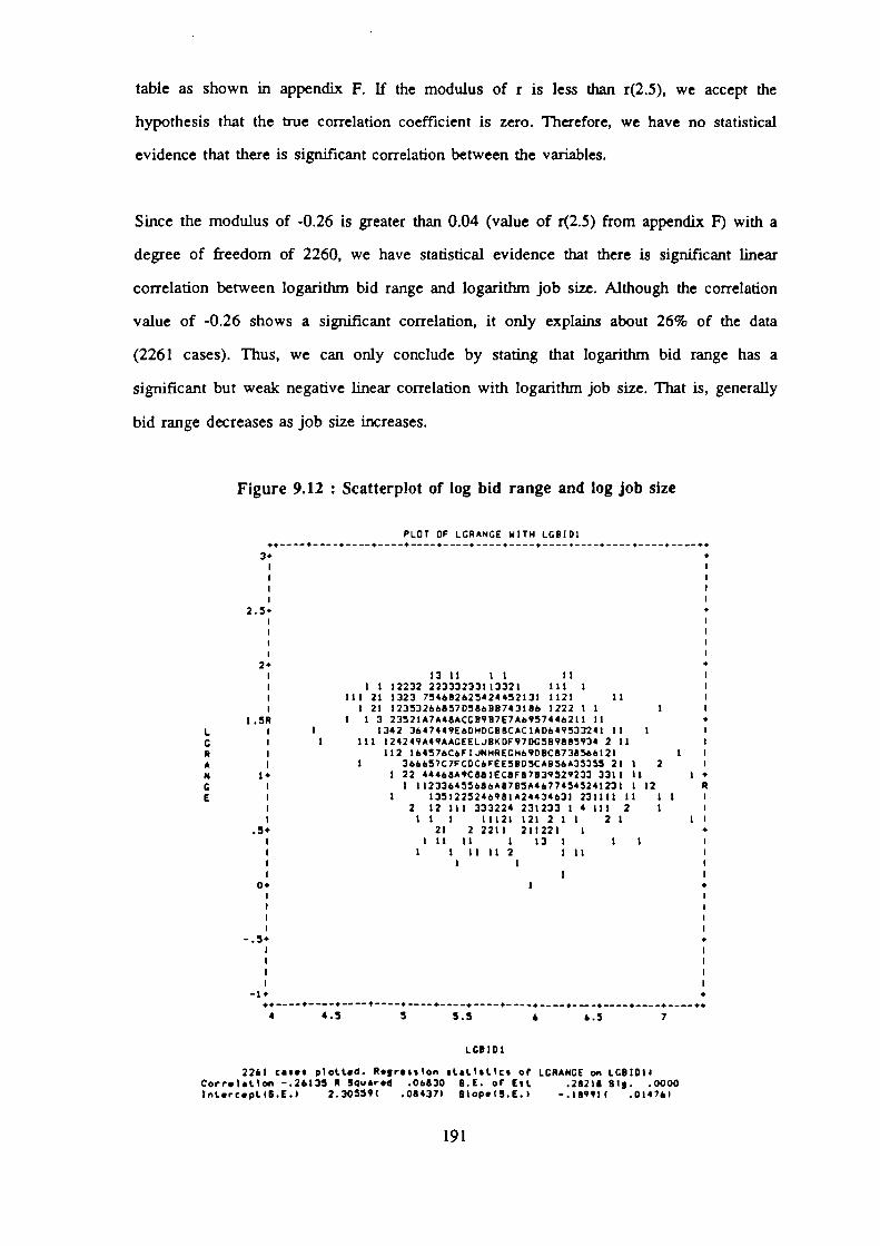
table as shown in appendix F. If the modulus of r is less than r(2.5), we accept the

hypothesis that the true correlation coefficient is zero. Therefore, we have no statistical

evidence that there is significant correlation between the variables.

Since the modulus of -0.26 is greater than 0.04 (value of r(2.5) from appendix F) with a

degree of freedom of 2260, we have statistical evidence that there is significant linear

correlation between logarithm bid range and logarithm job size. Although the correlation

value of -0.26 shows a significant correlation, it only explains about 26% of the data

(2261 cases). Thus, we can only conclude by stating that logarithm bid range has a

significant but weak negative linear correlation with logarithm job size. That is, generally

bid range decreases as job size increases.

Figure 9.12 : Scatterplot of log bid range and log job size

PLOT Of LGRANGE WITH LGBID1

3+

I i

1 i

I 1

I I

2.5+ •I I

1 I

i I

2 •+I 13 11 II 11 I

111

i 1 1 12232 22333233113321 1 I

I III 21 1323 754682625424452131 1121 II I

i 1 21 123532668570586813743186 1222 1 I 1 I

1.5R 1 1 3 23521A7448ACGB987E7A6957446211 11 •L I I 1342 3647449E6DHDC118CaC1AD649533241 II 1 Ic I I III 124249a4904ZEELJBaDf97DG51)9885934 2 11 IR 1 112 164576C6F1JNHREGH69DBC8738566121 I I

A I 1 366657C7FCDC6fEE5BD5Ca856a35355 21 I 2 I14 I* I 22 44468a9C881EC8F87839529233 3311 II 1 •G 1 1 112336455686a8785a46774545241231 1 12 RE I 1 1351225246981a24434631 731111 11 1 1 I

I 2 12 III 333224 231233 1 4 Ill 2 I 1

I II 1 11121 121 2 1 I 21 1!

.5+ 21 2 2211 211221 I •

I I 11 11 I 131 1 I I

I I 1 11 11 2 111 I

1 1 1 1

I I I

0+ I •1 i

I i

I I

1 I

-.5* •I I

1 I

I I

I I

-1+ •

4 4.5 5 5.5 6 6.5 7

2261 casts plotted. Regression statistics of LGRANG( on LG811)18Correlation -.26135 R Squared .06830 S.E. or Est .28218 Sig. .0000InterceptIB.E.) 2.30559( .08437) Slope(5.E.) -.189,11 .014761

191

b) Scatterplot of logarithm bid range and logarithm number of bidders

The scatterplot of logarithm bid range and logarithm number of bidders as shown in

figure 9.13 produces a correlation coefficient of 0.13. As compared to the statistical table

value of 0.04 (degrees of freedom = 2260) at the 5% significance level, 0.13 is slightly

greater than 0.04. Therefore, we have statistical evidence that there is significant but weak

positive linear correlation between logarithm bid range and logarithm number of bidders at

the 5% significance level.

Figure 9.13 : Scatterplot of log bid range and log number of bidders

PLOT OF LGRANGE WITH LGNOBID

3+ +

1 1

1 1

1 1I 1

2.5+ +

I 1

1 1

1 1

1 i

2+ +

I 1 3 4 2 I

I B 9 F A 1 2 I

1 I m v K 4 1 I

1 S z • o 9 A 1 I

1.5* • • • • A 6 1 +L I x • • * 0 6 7 4 I

G I • a a • 0 C 4 2 RR I • • s • J B 5 4 I

A R • • + a 0 7 1 2 1

N 1+ • • • • 6 3 3 +G I • • • v 7 1 1 I

E I R s N G 4 1 1 I

I N c a 4 1 1 1 1

I 5 a 5 2 1 1

.5+ E 5 1 1 •

I 7 3 3 I

I 6 1 4 1

I 2 I

1 1 I

0+ 1 *

1 1

I 1

I 1

I 1

-.5+ 4.

1 1

1 1

I 1

1 1

-1+ #

.4 .5 .6 .7 .8 .9 1

LCNOBID

2261 cases plotted. Regression statistics of LGRAHGE on LGNOBID:Correlation .13468 R Squared .01814 S.E. of Est .28968 Sig. .0000Intercept(S.E.) 1.01653( .03247) Slope(S.E.) .31070( .04809)

192

c) Scatterplot of logarithm bid RD and logarithm job size

The scatterplot of logarithm bid RD and logarithm job size as illustrated in figure 9.14

shows a correlation coefficient of -0.35. This value is significantly greater than 0.04 of the

statistical table (appendix F). Therefore, we strong statistical evidence that there is

significant negative linear correlation between logarithm bid RD and logarithm job size.

Figure 9.14 : Scatterplot of log bid RD and log job size

PLOT OF LGBIDRD WITH LGBIDI

2.5+ +

1 1

1 I

1 1

1 1

2+ +

1 1

I I 1

I 21 1 I

I 1 1 12 121 1111 21 1 I

1.5+ 111 11 442 32552224243 21 2 2 1 1 +

R 1 1113 1331583456827342644132 12 1 I

I 112123214A4A5CABF7A59C336747121222 1 I

I 11 1 154487 88BAD85JDDE47A7733525222 1 I

I 111 2331378569D0HK6F1HHBA56D9679315 211 I

1+ 11 1158846BB9B1MF6FBFA8DA8A243652541 1 +L I 1 2122488887F60EHE0BCE99H485AA426611211 I

G I 22323359DCFB9HKHF6A948874D2341314 1 1 IB I 1 1 3456545959BEC5GA6E5BA44413331124111 I II I 1 13 1123255649786637457724422425 1 12 1 1 RD .5+ 11 4 2 25526542424342311331 11 1 1 +R I III 313134 12 134311132 311 2 1 ID I 1 21 121 1112231241222 1 1 1 I

I 1 1 1 32 1 122 13 I

I 12 1 111 1 1 I

0+ t 122 •

1 1 1 I

1 I

I 1 1 I

I 1 I

-.5+ +

I I

1 I

1 1

I I

-1+ •

I I

1 I

1 I

1 I

-1.5+ +

4 4.5 5 5.5 6 6.5 7

LGBIDI

2261 cases plotted. Regression statistics of LGBIDRD on LGBID1)Correlation -.34539 R Squared .11929 S.E. of Est .27765 Sig. .0000Intercept(S.E.) 2.39539( .08301) Slope(S.E.) -.25400( .01452)

193

d) Scatterplot of logarithm bid RD and logarithm number of bidders

Figure 9.15 displays the scatterplot of logarithm bid RD and logarithm number of bidders.

A correlation coefficient of -0.12 was obtained which has a modulus slightly greater than

0.04 as shown in appendix F at the 5% significance leveL Thus, we have statistical

evidence that there is significant but weak negative linear correlation between logarithm

bid RD and logarithm number of bidders at the 5% significance level.

Figure 9.15 : Scatterplot of log bid RD and log number of bidders

PLOT OF LGBIDRD WITH LGNOBID

2.5+ +

1 1

I I

1 1

1 1

2+ +

I 1

1 1 I

I 2 1 1 I

I 6 5 3 3 1

1.5+ L I D 4 2 +

1 U N 0 F 1 2 1 1

I • • • W A 3 1

I • • • • 5 5 3 I

I • • • a B 9 2 I

IR a • • • E A 2 +L I • • • • U 8 5 2 I

G I • • • • E B 2 4 RB I • a • a E 4 4 5 I

1 I PI 0 id a 9 5 2 2 I

D .5+ B H G N 3 2 2 +R I D 6 F 6 6 I 1 ID I 8 7 a A 1 1 I

I 5 3 5 4 1 I

I 2 1 3 2 1 1

o+ 2 1 2 1 +

I 1 1 i

I 1

I 1 1 I

1 I I

-.5+ +

1 1

1 1

i 1

1 1

-1+ 4,

1 I

I I

1 1

I I

-1.5+ •

.4 .5 .6 .7 .8 .9 I

LGNOBID

2261 cases plotted. Regression statistics of LGBIDRD on LGNOBIDICorrelation -.12200 R Squared .01488 S.E. of Est .29364 Sig. .0000Intercept(S.E.) 1.13571( .03291) Slope(S.E.) -.28481( .04875)

194

e) Scatterplot of logarithm bid spread and logarithm job size

The scatterplot of logarithm bid spread and logarithm job size shows a negative linear

correlation as displayed in figure 9.16. The correlation coefficient of -0.23 which has a

modulus greater than 0.04 in the statistical table (appendix F). This indicates that we have

statistical evidence that logarithm bid spread has a significant but weak negative linear

correlation with logarithm job size at the 5% significance level.

Figure 9.16 : Scatterplot of log bid spread and log job size

PLOT OF LGBIDSPD WITH LCBIDI

3+ 4.

1 1

I 1

1 1

I I

2+ +

I 11 11 1 I

I 1 21 213432 2 1111 1 1 I

I 11 1213224344367445533 243 22 1 I

I 1 1 11311334257696AACD88666521412323111 I

IR 1 2224568C6AC8DDF1E1HH8E6663479333141 +

I 1 I 14 7888AAHLOJPKMWOGL9BF8CA5854451 23 1 I I

I 11211 22262A7C88BHKHPMOKFRH9ODDAN82856222 1 1 I

i 51262688779CAC0GEFB5H98H96880242312 1 12 I

I 121 122568A847C8C9597ADCD72453241374 111 1 I I

0+ 1 13 11 5794455479762354393342211 11 I I RL I 1 1222 15414373456914644233 231 1 11 1

G I I 4 131336222431 2412 2 22 2 11 I 1 IB I 1 2212 2242311142 214 I 111 1 I

1 I 2 2 2 72 11 2221312 1 1 I

0 -1+ 2 212 12 Iii •S I I 11 I I IP I 1 1 11 11 1 I

D I 111 I I

I 1 1 11 I

-2+ 1 3 +

I 1 I

I I I

1 1

I I-3+ +

1 1

I 1

i 1 I

1 1

-4+ +

I I

i 1

1 I

I 1

-5+ .«

4 4.5 5 5.5 6 6.5 7

LCBIDI

2259 cases plotted. Regression statistics of LGBIDSPD on LCBIDIICorrelation -.22867 R Squared .05229 S.E. of Est .54163 Sig. .0000Intercept(S.E.) 2.34071( .16194) Slope(S.E.) -.316101 .02833)

195

t) Scatterplot of logarithm bid spread and logarithm number of bidders

Figure 9.17 displays the scatterplot of logarithm bid spread and logarithm number of

bidders. A correlation coefficient of -0.21 was obtained. The modulus of -0.21 is greater

than 0.04 in the statistical table (appendix F). Thus, we have statistical evidence that

logarithm bid spread has a significant but weak negative linear correlation with logarithm

number of bidders in refurbishment work. That is, the bid spread of tender bids decreases

as the number of bidders per job increases.

Figure 9.17 : Scatterplot of log bid spread and

log number of bidders

PLOT OF LGE1105PD WITH LGNOSID

3+

I 1

I I

I I

I I2+

I 5 1

I c 2 8 1 1

I P 0 J e i 1

I • • w I 2 I

1+ • • • • E 6 1

R • • • • J A 4 3 I

I • • • • 8 0 5 2 I

I • • • • P 6 5 4 I

I 'V • • • 8 4 4 2 R

0+ J II . T U A 4 1L I c G I L 8 4 2 Ic I 6 a N M 2 5 1 1 I8 I 5 9 I • • 2 Ii I 7 7 7 a 3 ID -1+ 2 2 6 3S I 1 2 1 1 IP I 1 3 1 2 ID I 1 1 2 I

I 3 1 I

-2+ 1 1 1 1 •

I 1 I

I 1 I

I I

I I-3+

I I

I I

I 1 I

I I

-4. •

I 1

I I

I I

I I

-5+ •

.4 .5 .6 .7 .8 .9 1

LGNOBID

2259 cases plotted. Repression statistics of LGBIDSPD on LCNOBIDICorrelation -.19549 R Squared .03622 S.E. of Est .54563 Sig. .0000Intercept(S.E.) 1.10693( .06116) Slope(S.E.) -.858061 .09061)

196

9.4 Module 3 - Contractor's analysis

Using the performance indicators as described in chapter 6, it is possible to measure the

bidding performance of any contractors in the database. For the purpose of demonstrating

the output of this module, the bidding performance of one contractor is analysed and the

results are shown below.

9.4.1 Bidding performance of contractor A

The bidding performance of contractor A for 1984 to 1989 is shown in tables 9.28 and

9.29. As illustrated in table 9.28, contractor A has submitted a total of 567 bids over the

last six years (1984 to 1989) and has been successful on 147 contracts. The success rate

of the company for the six year period is about 25.9% (147*100/567=25.9%). This means

that on the average the firm has won one job out of every four contract bids submitted by

the firm.

As shown in table 9.28, the tender success rate of the firm varies from 0% in 1989 (only

11 cases are recorded) to 30.4% in 1984. Although the success rate of the firm is

maintained at about 25% in all the years, the average win margin has gradually increased

since 1984 (from 4.6% to 9.9%). This implies that the firm has been leaving more

"money on the table" in recent years and thus reflects upon the general decline in bidding

efficiency of the firm in competitive bidding.

The tender success value of the firm as shown in table 9.29 ranges from 1 : 2.9 (1984) to

1 : 5.4 (1985). The overall tender success value for 1984 to 1989 is 1 : 4.2 (£103m

divided by £428m). This indicates that contractor A has managed to secure one pound

worth of contract out of every four pounds of contract tendered by the firm.

A comparison of tender success value among different years shows that the contractor had

been more successful in 1984 than other years. This performance is further confirmed by

197

Table 9.28 : Bidding performance of contractor A

YEAR TOTAL NO.OF BIDS

SUBMITTED

NO. OFSUCCESSFUL

BIDS

SUCCESSRATE

AVERAGEWIN

MARGIN

AVERAGELOSE

MARGIN

(%) (%) (%)

1984 92 28 30.4 4.6 -9.4

1985 135 35 25.9 5.7 -10.1

1986 107 26 24.3 5.8 -9.8

1987 179 48 26.8 7.5 -11.0

1988 43 10 23.26 9.9 -12.3

1989 11 o o - -13.4

a) Total number of bids submitted (1984-1989) = 567b) Total number of successful bids = 147c) Tender success rate = 25.9%

Table 9.29 : Tender success value of contractor A

YEAR TOTAL VALUEOF CONTRACTSTENDERED

(Cm)

TOTAL VALUE OFCONTRACTS WON

(Cm)

TENDER SUCCESSVALUE

1984 57.8 20.2 1: 2.9

1985 95.4 22.8 1 : 4.2

1986 89.5 16.6 1: 5.4

1987 144.3 36.1 1: 4.0

1988 31.0 7.3 1: 4.3

1989 9.8 0 0

a) Total value of contracts tendered (1984-1989) = 428 million poundsb) Total value of contracts won = 103 million pounds

c) Tender success value = 1 : 4.2

198

the high success rate of 30.4% and a relatively small win margin of 4.6%. Thus, the

above measures clearly indicate that contractor A was relatively more efficient and

successful in 1984 than other years.

Therefore, the measurement of tender success rate, tender success value and the win/lose

margin provides useful feedback information to contractors in monitoring their bidding

performance in competitive bidding. In also enables contractors to adopt any corrective

actions to improve the efficiency and effectiveness of their existing bidding strategies

when necessary.

9.4.2 Win margin distribution of contractor A

As displayed in figure 9.18, the win margin distribution of contractor A is positively

skewed. The mean win margin is 6.3% and has a standard deviation of 6.9. The win

margin ranges from a minimum of 0.1% to a maximum of 43.6% and has a median of

4.7%. The median indicates that 50% of contractor A's bids were secured with win

margin of 4.7% or more.

The mean bid spread (win margin) of all refurbishment contracts is 6.2% as shown in

figure 9.8. Using this value as a yardstick (general standard of the industry) for measuring

bidding performance of contractors, the mean win margin (6.3%) of contractor A is only

slightly higher. Thus, we may consider contractor A's bidding performance as satisfactory.

However, as indicated by the median win margin, there is still more scope for increasing

the bidding efficiency of the firm.

9.4.3 Lose margin distribution of contractor A

The lose margin distribution of contractor A is negatively skewed as displayed in figure

9.19. The lose margin ranges from 0.1% to 45.2% and has a mean of 10.5%. This shows

that on the average, contractor A's unsuccessful bids are approximately 10% higher than

199

COM 1110111112 Ott S79302 MIMS APP101191711f 1.00 MM,11.1211

0 10 20 ao 40 seNISTOGRAM rusoncy

KKAS 8 286 STD 1111 .544 MIAS 4.19411001 1.434 ST1 Drf 4.810 T2111111 47.048FOSTOSIS 1.724 S I 017 .317 SKtV1t3S 2.447

S 1 SKtV .200 01111 43.414 0111101 .000111113211 43.814 SON 033.804

f1.1.211 C130 147 0121100 C/StS 0

• •

Figure 9.18 : Win margin distribution of Contractor A

the lowest bidder. It is also observed from the distribution that there are 92 (67+25 = 92

as shown in figure 9.19) contracts which contractor A had lost by a margin of between

0% to 2.5%. This implies that if contractor had reduced all his bids by 2.5%, he would

have secured another 92 contracts. But, this would also increase the win margin of his

successful contracts.

Based upon the distribution of unsuccessful bids and their respective lose margins as

shown in figure 9.19, it is observed that contractor A had been very competitive in

refurbishment work as a large proportion of his bids are lost at competitive margins.

Thus, the lose margin provides an useful measure for monitoring the competitiveness of a

contractor's bids.

200

etturr MIDPOINT OKI STOOL EQUALS 61/1OIIRS1ILT 1.60 OECURRESELS

O -47.6

1 -46.0 •O -42.6

1 -40.0 •

1 •37.6 •

2 -36.0 •

3 .32.6 50

3 -30.0 00-27.6

• -26.0

20 -22.5

20 -20.0

24 -17.6

27 -16.0

33 -12.6

41 -10.0

611 -7.6

67 -60

67 -2.6

26 .0

0 2.6

0 16 30 46 60 76

IISTOGRAA FREOULIC7

MIAS -10.441 ST, U.S .388 MEDIU -8.481

RODS -6.677 STD DE/ 7.160 /1.8I5ICI 63.116

KURTOSIS 1.114 S t KURT .238 SKEWNESS -1.117

3 g saw .111 tANCI 46.188 MINIMUM -46.327

RAID= - 1 410 SOW -4394.794

VALID CASES 420 MISSING CASKS 0

Figure 9.19 : Lose margin distribution of Contractor A

9.4.4 Contractor's bid to mean bid ratio

The contractor's bid to mean bid ratio of contractor A is displayed in figure 9.20. As

observed in the figure, the contractor's bid to mean bid ration is approximately normally

distributed. The mean ratio is 99.2% and has a standard deviation of 7.6. It ranges from a

minimum of 74.0% to 137.1%. This result indicates that contractor's A bids are quite

competitive as his bids are close to the bid mean of all bids in a contract.

9.4.5 Identification of strengths and weaknesses of contractor A

Table 9.30 displays a typical output from the decision support system showing a listing of

all past contracts of contractor A. The listing provides details on the job characteristics

and the bidding performance (win/lose margin) of the contractor. Thus, by analysing

201

CONTRACTOR'S BID TO MEAN BID RATIO

COUNT MIDPOINT ONE SYMBOL EQUALS APPROIIMITELT 4.00 OCCURRENCES

1 72.33

3 76.67 •

4 79.00 •

7 82.33 a.

14 66.67 de

26 69.00

63 92.33

120 96.67

108 99.00

67 102.33

69 105.67

37 109.00

26 112.33 O 116.673 119.00O 122.33O 126.67O 129.00O 132.332 136.67 •

O 139.00

40 80 120 160 200IISTOGR1M FREQUE2CY

KEAN 94.162 STD ERR .317 MEDIAN 96.609MODE 96.098 STD DEN 7.588 VARIANCE 67.096rums's 2.219 S E KURT .206 SKEWNESS .296S E SKEW .103 RANGE 63.113 MIIIMUM 73.996MiIIMUM 137.109 SUM 66224.703

VALID CASES 667 MISSING CASES 1694

Figure 9.20 : Contractor's bid to mean bid ratio distribution

tender bid records of past contracts, contractors will be able to understand and monitor the

bidding performance of their firms under various bidding situations.

Besides this, module 3 also provides a listing of past contracts in specific bidding

situations such as different job types or job sizes. Table 9.31 shows an example of the

decision support system's output on the past bidding performance of contractor A for

various job types. Thus, by monitoring the bidding performance of the company for

various bidding situations, the contractor will be able to formulate appropriate strategies

for various bidding situations. For example. if the above analysis shows that contractor A

had not been very successful in certain job types, appropriate actions may be taken to

improve the competitive position of the firm in the industry.

202

Table 9.30 : Computer output of past contracts of Contractor A

J0 C

J N B Lo Y a s IB E B 1 EN A I z No R D E I JOBTYPE LOCATION 81 82 83 84 85 B6 B7 88 89 BIO MARGIN

9501 2 5 12 8 4 21 237 120 4 1 0 0 0 0 0 17.757961 2 411 3 4 339 138 21 462 0 0 0 0 0 0 -24.379391 2 5 12 7 4 9 155 21 19 7 0 0 0 0 0 -2.818461 2 3 1 1 1 4 21 120 418 o 0 0 0 0 0 0 8.967781 2 5 1 1 3 4 25 27 21 215 247 0 0 0 0 0 -2.818641 2 4 2 1 3 4 19 21 3 317 0 0 0 0 0 0 -3.7575215741

22

34

2 22 1

58

44

3128

418384

21a

o21

00

00

00

00

00

00

-9.85-23.37

9471 2 4 2 1 3 4 253 28 322 21 0 0 0 0 0 0 -15.827031 2 4 2 1 8 4 84 106 21 83 0 0 0 0 0 0 -11.469231 2 3 2 1 3 4 28 321 21 0 0 0 0 0 0 0 -24.309151 2 4 22 3 4 2 95 463 21 0 0 0 0 0 0 -28.619201 2 3 2 2 8 4 321 21 9 0 0 0 0 0 0 0 -8.318301 2 4 22 3 4 21 369 244 22 0 0 0 0 0 0 1.938421 2 3 2 1 1 4 364 21 449 o 0 0 0 0 0 0 -9.438911 2 322 3 4 21 177 198 o 0 0 0 0 0 0 2.279121 2 4 22 1 4 422 21 131 19 0 0 0 0 0 0 -2.196321 2 3 2 2 3 4 19 16 21 o 0 0 0 0 0 0 -11.865651 2 5 2 1 7 4 83 21 9 151 1 0 0 0 0 0 -4.589131 2 4 2 1 8 4 192 137 47 21 0 0 0 0 0 0 -16.565991 2 4 22 8 4 321 9 192 21 0 0 0 0 0 0 -20.337551 2 3 2 2 3 4 5 21 167 o 0 0 0 0 0 0 -1.117731 2 6 2 1 8 4 268 227 35 12 131 21 0 0 0 0 -34.055541 2 3 2 1 3 4 5 384 21 o 0 0 0 0 0 0 -8.388491 2 5 3 2 1 4 21 9 372 28 418 0 0 0 0 0 2.576691 2 5 3 2 8 4 119 10 21 423 19 0 0 0 0 0 -9.316271 2 6 3 1 4 4 3 66 21 369 14 23 0 0 0 0 -1.087941 2 3 3 2 4 4 35 391 21 o 0 0 0 0 0 0 -11.426741 2 3 3 1 8 4 21 1 244 o 0 0 0 0 0 0 .42

9681 2 4 3 2 3 4 237 29 21 28 0 0 0 0 0 0 -7.736931 2 5 3 1 3 4 248 7 22 8 21 0 0 0 0 0 -5.759371 2 5 3 1 3 4 21 31 2 348 19 0 0 0 0 0 .029251 2 5 3 1 4 4 541 21 143 25 20 0 0 0 0 0 -2.04

7061 2 5 3 1 3 4 167 240 227 21 9 0 0 0 0 0 -12.62

9591 2 6 3 1 1 5 35 25 170 320 21 20 0 0 0 0 -15.387001 2 5 3 2 8 4 437 116 17 392 21 0 0 0 0 0 -23.93

7681 2 6 3 2 3 4 30 294 21 164 325 20 0 0 0 0 -6.42

8981 2 3 3 1 3 4 423 429 21 0 0 0 0 0 0 0 -7.22

8761 2 6 32 3 4 18 367 136 21 418 4 0 0 0 0 -5.28

9701 2 6 3 1 3 5 470 319 21 469 419 91 0 0 0 0 -4.52

7821 2 8 32 8 4 18 334 154 33 30 21 231 143 0 0 -13.56

7691 2 9 3 1 8 4 414 21 8 288 389 28 35 143 438 0 -.51

8871 2 4 3 2 7 4 1 10 108 21 0 0 0 0 0 0 -9.07

6631 2 4 31 3 4 21 251 322 34 0 0 0 0 0 0 10.31

812 3 32 3 4 214 21 4 19 7 0 0 0 0 0 -1.51

203

Table 9.31 : Computer output of past contracts of Contractor A

for different job type

Job type 1 (Transport and utility)

JDC

J NBLOYOSIBEB IENA I ZNORD ETJOBTYPE LOCATION B1 82 83 B4 85 86 87 88 B9 BIO MARGIN

8461 2 3 1 1 t 4 21 120 418 0 0 0 0 0 0 0 8.968421 2 3 2 I 1 4 364 21 449 0 0 0 0 0 0 0 -9.439121 2 4 2 2 1 4 422 21 131 19 0 0 0 0 0 0 -2.198491 2 5 3 2 1 4 21 9 372 28 418 0 0 0 0 0 2.579591 2 6 3 1 1 5 35 25 170 320 21 20 0 0 0 0 -15.387831 2 6 4 1 1 5 125 14 21 20 25 320 0 0 0 0 -8.73371 3 3 5 2 1 4 28 215 21 0 0 0 0 0 0 0 -3.33

3971 3 4 32 1 5 21 1 25 14 0 0 0 0 0 0 5.244711 3 5 3 1 1 4 20 198 21 196 215 0 0 0 0 0 -10.699831 3 6 14 1 1 4 8 198 21 26 215 20 0 0 0 0 -4.08760 4 3 32 1 4 1 19 21 0 0 0 0 0 0 0 -16.92

3868 4 4 3 2 1 4 198 5 29 21 0 0 0 0 0 0 -7.832251 5 7 3 1 1 5 237 391 4 21 17 131 23 0 0 0 -9.583813 5 4 3 1 1 4 772 230 21 773 0 0 0 0 0 0 -13.364063 5 4 1 2 1 4 104 202 21 611 0 0 0 0 0 0 -16.744495 5 5 1 2 1 4 17 722 21 419 322 0 0 0 0 0 -33.034893 5 3 2 1 1 4 276 21 253 0 0 0 0 0 0 0 -.148354 6 4 4 2 1 4 21 823 929 912 0 0 0 0 0 0 6.399032 6 5 4 2 1 5 960 234 II 823 21 0 0 0 0 0 -18.34

Job type 2 (Industrial)

J0 C

J NBLOYOSI8E8 IENA I ZNOR D ETJOBTYPE LOCATION 81 82 83 84 85 86 87 88 B9 810 MARGIN

2311 3 3 8 2 2 4 1 31 21 0 0 0 0 0 0 0 -2.072441 3 3 1 1 2 4 348 21 33 0 0 0 0 0 0 0 -1.27

41 3 3 3 1 2 4 242 20 21 0 0 0 0 0 0 0 -2.099801 3 5 3 2 2 5 21 519 294 33 10 0 0 0 0 0 13.211138 4 3 31 2 4 27 21 4 0 0 0 0 0 0 0 -4.28687 4 6 3 1 2 4 244 10 320 21 152 340 0 0 0 0 -3.82

2932 4 8 4 1 2 4 9 19 21 32 1 214 30 244 0 0 -3.782932 4 8 4 1 2 4 9 19 21 32 1 214 30 244 0 0 -3.781716 5 6 4 1 2 4 575 576 524 30 21 19 0 0 0 0 -19.414718 5 4 3 2 2 4 21 40 93 248 0 0 0 0 0 0 6.247697 6 5 3 1 2 5 21 215 823 8 880 0 0 0 0 0 7.757685 6 5 3 2 2 4 21 6 999 19 581 0 0 0 0 0 10.779023 6 3 4 2 2 4 906 21 524 0 0 0 0 0 0 0 -9.309161 6 3 3 2 2 4 833 912 21 0 0 0 0 0 0 0 -8.193012 7 5 3 1 2 4 27 872 21 93 237 0 0 0 0 0 -23.00

204

Job type 3 (Administration, public & office)

ja y8 ENA0 R

7961 27781 28641 29471 29231 29151 28301 28911 26321 27551 25541 29681 26931 29371 27061 27681 28981 28761 29701 26631 25581 28241 28471 27461 27.‘41 28111 26911 2

N0IIID

454434433334355636645675568

JDCIL81I EZ NE T JOBTYPE LOCATION

1 1 2 41 I 3 42 1 3 42 1 3 42 1 3 42 2 3 42 2 3 42 2 3 42 2 3 42 2 3 42 1 3 43 2 3 43 1 3 43 1 3 43 I 3 43 2 3 43 1 3 43 2 3 43 1 3 53 1 3 43 2 3 43 2 3 43 1 3 43 2 3 44 2 3 44 2 3 44 1 3 4

B1

3392519

25328

22121193I

237248

21167

30423

18470

21214

2121302119

103

112

138272128

32195

369177

1621

31429

731

240294429367319231

21515

9155

91021

13

2121

3322

21463244198

21167

212122

2227

2121

13621

3224

27211

21426

21215

84

462215317

210

212

2

3421

164

21469

3419

2421933

21431

320

15

24

2119

3250

411419

22248

20136

3325

11

92

0

9107

516

51230

_

I

00

3 12000

23

111

41

B 1111 NARC1N

-24.37-2.81-3.75

-15.62-24.30-28.61

1.932.27

-11.86-1.11-8.38-7.73-5.75

.02-12.62-6.42-7.22-5.28-4.5210.31-1.5116.57

.01-3.08

.42-2.16-5.70

Job type 4 (Health & welfare)

JDC

j NBLOYOSIBEB IENA I ZNOR 0 ETJOBTYPE LOCATION 81 92 83 B4 95 86 87 118 B9 810 MARGIN

6271 2 6 3 i 4 4 5 66 21 369 14 23 0 0 0 0 -1.087941 2 3 32 4 4 35 391 21 0 0 0 0 0 0 0 -11.429251 2 5 3 1 4 4 541 21 143 25 20 0 0 0 0 0 -2.047151 2 4 3 2 4 4 21 215 20 6 0 0 0 0 0 0 6.487161 2 5 4 2 4 4 21 215 20 6 244 0 0 0 0 0 7.126391 2 3 7 1 4 4 21 391 215 0 0 0 0 0 0 0 3.002591 3 3 1 1 4 4 21 210 33 0 0 0 0 0 0 0 10.563171 3 3 1 1 4 4 340 279 21 0 0 0 0 0 0 0 -19.083181 3 3 1 I 4 4 21 340 279 0 0 0 0 0 0 0 10.15

221 3 4 10 1 4 4 21 391 2 33 0 0 0 0 0 0 3.764041 3 4 2 1 4 4 33 2 131 21 0 0 0 0 0 0 -15.03

531 3 5 3 1 4 429 11!

91 95 31 0 0 0 0 0 .003451 3 5 2 1 4 4 348 131 21 0 0 0 0 0 -22.841491 3 6 2 1 4 4 21 2 31 66 340 421 0 0 0 0 1.091871 3 6 I 1 4 4 I 108 143 21 7 320 0 0 0 0 -16.983841 3 6 1 1 4 4 108 7 1 21 320 143 0 0 0 0 -11.932831 3 6 3 I 4 4 25 29 102 21 23 33 0 0 0 0 -3.814544 4 4 2 1 4 4 21 66 23 5 0 0 0 0 0 0 .731410 4 5 2 I 4 5 21 28 14 5 143 0 0 0 0 0 .292009 4 3 3 1 4 4 66 198 9 1 21 0 0 0 0 0 -7.432383 4 6 4 1 4 4 36 21 28 418 31 17 0 0 0 0 -2.652367 4 6 6 I 4 5 420 35 17 198 320 21 0 0 0 0 -10.59

205

Job type 5 (Refreshment, recreation & entertainment)

J

JDC

NBL0 Y 0 81BEB IENA I ZNOR D ETJOBTYPE LOCATION BI B2 83 B4 85 86 B7 88 89 810 MARGIN

7521 2 3 22 5 4 31 418 21 0 0 0 0 0 0 0 -9.851601 3 3 3 1 5 4 293 21 198 0 0 0 0 0 0 0 -6.433131 3 4 2 I 5 4 207 95 86 21 0 0 0 0 0 0 -9.69381 3 4 21 5 4 21 73 179 35 0 0 0 0 0 0 9.17

4451 3 5 4 I 3 4 21 23 131 27 106 0 0 0 0 0 1.509781 3 7 6 I 5 4 21 10 418 215 2 143 427 0 0 0 2.083152 4 3 4 2 5 5 30 14 21 0 0 0 0 0 0 0 -6.341451 4 422 5 4 21 3 4 131 0 0 0 0 0 0 1.79512 4 6 4 I 5 4 21 213 2 30 35 31 0 0 0 0 1.92

3977 4 6 2 I 3 4 290 21 348 131 244 22 0 0 0 0 -.38131 5 4 4 2 5 5 17 21 198 19 0 0 0 0 0 0 -6.81

2053 5 4 I 1 5 5 399 21 288 5 0 0 0 0 0 0 -.71572 5 4 5 2 5 4 5 29 21 30 0 0 0 0 0 0 -10.08644 3 6 4 2 5 4 294 30 21 19 28 29 0 0 0 0 -7.18763 5 6 3 2 5 5 17 19 21 327 241 27 0 0 0 0 -5.68763 5 6 3 2 5 4 17 19 21 327 241 27 0 0 0 0 -5.68

3669 5 4 7 2 3 4 19 21 13 I 0 0 0 0 0 0 -18.934493 5 3 2 2 5 4 541 322 21 0 0 0 0 0 0 0 -19.324517 5 6 6 2 5 4 40 416 21 727 33 316 0 0 0 0 -8.524676 5 5 3 2 5 4 51 79 418 21 30 0 0 0 0 0 -7.284923 5 4 3 2 5 4 391 33 21 131 0 0 0 0 0 0 -6.505366 5 4 3 I 5 4 21 25 490 805 0 0 0 0 0 0 14.47

Job type 6 (Religious)

J0 C

J NBLOYOSIBEB IENA I ZNOR D ETJOBTYPE LOCATION B1 B2 B3 B4 85 B6 87 98 89 BIO MARGIN

781 3 3 5 2 6 4 21 1 35 0 0 0 0 0 0 0 5.521267 4 5 3 2 6 4 21 33 103 66 321 0 0 0 0 0 2.21245 3 31 6 4 21 369 4 0 0 .0 0 0 0 0 5.35

229 5 4 1 2 6 4 391 21 7 103 0 0 0 0 0 0 -1.67682 5 6 4 2 6 4 21 1 19 532 131 9 0 0 0 0 7.41

4077 5 5 2 2 6 4 391 250 336 318 21 0 0 0 0 0 -20.427763 6 5 3 2 6 4 828 608 21 380 320 0 0 0 0 0 -31.55

206

Job type 7 (Education, information & scientific)

J0 C

J NBLOYOSIBEB IENA I ZNOR D ETJOBTYPE LOCATION B1 B2 B3 B4 B5 86 B7 88 B9 810 MARGIN

9391 2 5 1 2 7 4 9 155 21 19 7 0 0 0 0 0 -2.815651 2 5 2 1 7 4 83 21 9 151 1 0 0 0 0 0 -4.588871 2 4 3 2 7 4 1 10 108 21 0 0 0 0 0 0 -9.077391 2 8 3 1 7 4 131 214 320 248 143 21 193 115 0 0 -3.156111 2 4 32 7 4 21 155 7 9 0 0 0 0 0 0 1.435981 2 4 32 7 4 21 155 7 9 0 0 0 0 0 0 1.432721 3 4 2 1 7 4 21 360 420 252 0 0 0 0 0 0 4.972571 3 4 2 1 7 4 237 155 1 21 0 0 0 0 0 0 -9.653401 3 4 2 1 7 4 21 153 16 31 0 0 0 0 0 0 1.283481 3 6 2 1 7 4 21 104 28 10 244 271 0 0 0 0 6.193961 3 6 2 2 7 4 121 8 2 931 0 0 0 0 -.77321 3 6 3 1 7 4 365 120 21 28 23 10 0 0 0 0 -7.18

2681 3 6 2 2 7 4 147 115 365 21 23 197 0 0 0 0 -7.211851 3 6 2 1 7 4 206 28 337 21 105 214 0 0 0 0 -8.28331 3 6 3 1 7 4 198 27 17 21 19 30 0 0 0 0 -1.88

2821 3 6 3 1 7 4 143 175 21 424 410 14 0 0 0 0 -5.882461 3 6 2 I 7 4 17 198 21 25 27 23 0 0 0 0 -10.444071 3 7 3 1 7 4 260 4 21 320 418 247 108 0 0 0 -4.62871 3 8 3 1 7 4 143 409 16 391 10 21 320 23 0 0 -16.76

1791 3 8 5 1 7 4 79 320 402 143 418 378 21 135 0 0 -11.201921 3 9 4 1 7 4 206 61 105 214 190 28 21 418 19 0 -23.034767 4 4 2 I 7 5 19 21 131 423 0 0 0 0 0 0 -.37

Job type 8 (Residential)

J0 C

J NBLOYOSIBEB IENA I ZNOR D ETJOBTYPE LOCATION BI B2 B3 84 85 86 87 88 B9 810 MARGIN

9501 2 5 1 2 8 4 21 237 120 4 1 0 0 0 0 0 17.755741 2 4 21 8 4 28 384 8 21 0 0 0 0 0 0 -23.377031 2 4 21 8 4 84 106 21 83 0 0 0 0 0 0 -11.469201 2 3 22 8 4 321 21 9 0 0 0 0 0 0 0 -8.319131 2 4 2 1 8 4 192 157 47 21 0 0 0 0 0 0 -16.565991 2 4 2 2 8 4 321 9 192 21 0 0 0 0 0 0 -20.337751 2 6 2 1 8 4 268 227 35 12 131 21 0 0 0 0 -34.056691 2 5 3 2 8 4 119 10 21 423 19 0 0 0 0 0 -9.316741 2 3 3 1 8 4 21 1 244 0 0 0 0 0 0 0 .427001 2 5 3 2 8 4 457 116 17 392 21 0 0 0 0 0 -23.937821 2 8 3 2 8 4 18 354 154 33 30 21 231 143 0 0 -13.567691 2 9 3 1 8 4 414 21 8 288 389 28 35 143 458 0 -.516161 2 3 31 8 4 260 21 404 0 0 0 0 0 0 0 -10.118741 2 3 4 2 8 4 457 260 9 21 86 0 0 0 0 0 -4.139181 2 6 4 1 8 4 21 384 409 33 337 237 0 0 0 0 2.336681 2 6 4 2 8 4 4 21 215 280 244 131 0 0 0 0 -7.446381 2 6 5 1 8 4 391 5 21 31 28 143 0 0 0 0 -6.379341 2 3 5 2 8 4 21 152 131 0 0 0 0 0 0 0 3.605811 2 6 5 1 8 4 305 136 205 21 157 193 0 0 0 0 -17.698711 2 4 5 1 8 4 2 21 28 251 0 0 0 0 0 0 -3.016061 2 3 5 1 8 4 21 833 0 0 0 0 0 0 0 8.378721 2 6 5 1 8 4 2 131 21 414 28 251 0 0 0 0 -4.808011 2 6 5 1 8 4 136 389 131 30 21 418 0 0 0 0 -16.488181 2 5 5 1 8 4 21 12 120 9 6 0 0 0 0 0 7.416081 2 3 5 1 8 4 21 8 33 0 0 0 0 0 0 0 10.45

207

9.5 Module 4 - Competitors' analysis

The main purpose of this module is to provide information which will enable a contractor

to monitor the bidding performance of his firm against his competitors, particularly his

key competitors (contractors whom he frequently meets). For the purpose of demonstrating

the output of the decision support information produced by this module, we analyse the

bidding performance of one contractor (contractor A) against 10 of his key competitors

(K1 to K10).

9.5.1 Bidding performance of contractor A against his key competitors

Table 9.32 shows the bidding performance of contractor A against 10 of his frequently

encountered competitors in refurbishment work. The key competitors are listed in

descending order according to the frequency of encounters. As observed in table 9.32, the

success rate of contractor A against his key competitors ranges between 37.7% (K2) to

80.0% (K9). The measurement of success rate determines the competition power between

contractor A and his respective competitors. Thus, the above results show that contractor

A has relatively high competitive strength against most of his key competitors (success

rate over 50%) except K2, K7 and K10.

From table 9.32, it is observed that the mean win margin of contractor A against his key

competitors is quite large (about 9% to 10%) except for competitors K3 and K8. This

clearly shows that contractor A's bids are much more competitive than his key

competitors. Comparing the lose margin of contractor A against his key competitors, it is

observed that contractor A tends to lose by a larger margin to competitors K2 (9.9%) and

K3 (8.1%). Thus, the analysis of relative bidding performance between a contractor and

his key competitors provides essential feedback information to contractors. It also enables

a contractor to have a better understanding of the bidding behaviour of his key

competitors.

208

Table 9.32 : Bidding performance of Contractor A against

his key competitors

KEYCOMPETITORS

TOTAL NO.OF ENCOUNTERS

NUMBER OF BIDSWON BY

CONTRACTOR A

SUCCESSRATE

AVERAGEWIN

MARGIN

AVERAGELOSE

MARGIN

(%) (%) (%)

K1 70 38 54.3 9.9 -7.8

K2 61 23 37.7 12.5 -9.9

K3 60 33 55.0 7.2 -8.1

K4 59 39 66.1 10.5 -5.4

K5 58 33 56.9 10.6 -3.9

K6 58 34 58.6 10.8 -7.8

K7 52 23 44.2 9.3 -7.7

K8 47 28 59.6 8.0 -7.8

K9 45 36 80.0 8.7 -7.1

K10 36 14 38.9 10.4 -5.8

_

9.5.2 Identification of strengths and weaknesses of competitors

Table 9.33 displays a computer output showing the job characteristics, coded identities of

bidders and win/lose margin of past contracts where contractor A and his key competitor

K4 were in competition. The list of past contracts in divided into two parts. The first

listing provides a list of contracts where contractor A's bids were lower than his key

competitor K4. While the second listing displays contracts where contractor A's bids are

higher than competitor K4. Both the listings show the extent of margin (win/lose margin)

by which contractor A has won or lost in all the contracts. Thus, by relating the relative

bidding performance between a contractor and his key competitors under different contract

characteristics, the contractor will be able to identify the strengths and weaknesses of his

209

competitors. For instance, contractor A may find that key competitor K4 had been

consistently submitting lower bids than his firm for residential or office buildings. As

such, he may take appropriate actions to improve his competitive power against

competitor K4.

Table 9.33 : Computer output of past contracts of Contractor A

against his key competitor (K4)

JOBNO YEAR NO810 JOBSI2E CLIENT JOBTYPE LOCATION 81 112 83 84 11 86 B B1 W1N4

9121 2 4 2 2 4 422 21 131 19 0 32.016681 2 6 4 2 4 4 21 215 280 24 131 13.789341 2 3 5 2 4 21 152 131 0 10.283001 3 4 2 2 4 22 21 131 369 1.093941 3 4 3 1 4 21 131 120 106 4.974451 3 5 4 1 4 21 23 131 27 10 1.703431 3 5 4 I 4 398 28 21 131 17 6.544141 3 6 a I 4 420 21 30 8 13 39 4.391881 3 6 II 2 4 391 9 30 260 21 131 3.03911 3 6 2 1 4 21 369 131 423 21 34 2.37

4361 3 6 9 1 4 21 9 15 214 32 131 11.031051 3 6 5 I 4 21 253 152 131 25 10.194101 3 6 5 1 4 21 25 131 414 41 120 17.124721 3 8 3 2 4 21 8 2 320 28 31 13 13.264739 4 3 2 I 4 21 17 131 0 14.064767 4 4 2 I 5 19 21 131 423 11.72

136 4 4 7 I 4 21 33 131 5 10.521451 4 4 2 2 4 21 3 4 131 12.262568 4 5 3 I 5 12 21 240 198 131 13.262773 4 5 4 I 4 533 33 21 131 6 1.764827 4 6 5 I 4 84 256 533 21 131 3.443977 4 6 2 I 4 290 21 348 131 244 22 9.633112 4 6 3 I 4 27 5 21 131 23 425 1.29

JON° YEAR

77517391872180116451428140413451

4714736215542444260

341341951463596

32734974

0Number o

NOBID JOBSIZE CLIENT

6 26 36 56 55 64 34 25 26 33 55 47 27 64 64 65 66 39 36 49 5

cases read! 20

JOB

1II1I22

Number

YPE LOCATION 81

4 2684 1314 24 1364 2144 2204 334 94 354 94 2534 3914 1314 1314 1314 5244 2684 3914 2024 410

of cases 1141.4d1

82

227214131389192131

2391391131

6131136

3030

131360131354391

20

83

35320

21131131

33131348131

21131384

21212115

13121

131202

84

12248414

30212121

131244

02121

4183232

621

I21

4

85

131143

2821

24400

2121

0235

730

00

21259

7143420

16

2121

25141

13

I1

243667131

19

142

1

21

8

II

14

52 310

II LOSE4

.283.152.494.641.96

13.906.742.449.35

.49

.537.36

.8616.2016.2110.70

.792.495.532.16

210

9.5.3 Identification of specialities of competitors in refurbishment work

Tables 9.34 and 9.35 display a list of 30 refurbishment contractors who were frequent

lowest bidders under various job characteristic bidding conditions. From the tables, it is

possible to identify the specialities and interests of various contractors (most competitive

bidders for various conditions). For example, as illustrated in table 9.34 contractors C001

and C007 are very competitive bidders for jobs ranging between job sizes 1 to 11, as

indicated by the high frequency of successful bids. Both companies are keen on public

and private jobs. However, contractor C007 tends to be more selective in his job types

(job types 4, 6, and 8) while C001 seems to be competitive in all job types.

Thus, the information as displayed in table 9.34 enables contractors to understand which

competing contractors will be keen to tender for various job sizes, job types, client types

and job locations. Such information provides useful guidelines to management during

tender adjudication, especially when the identities of other bidders are known. By

understanding the speciality and interest of various bidders, contractors are better equipped

to formulate suitable bidding strategies to increase the success rate of the company.

Thus, by simply analysing the frequency of lowest bids of various contractors, significant

market information may be obtained at any point in time to identify the specialties and

interests of the most competitive bidders under various bidding conditions.

211

Table 9.34 : Identification of speciality of contractors

(job size)

CONTRACTORS JOB SIZE

1 2 3 4 5 6 7 8 9 10 11 12 13 14

C001 a * * • * • * • • *

C002 * • *C003 * * • *C004 *C005 *C006 * •

C007 * * * • * * • * •

C008 • *

C009 • *C010 *C011 * •C012 • * • • `C013 •C014 *C015 •C016 •C017 *C018 •C019 '

CO20 'CO21 •CO22 •CO23 '

C'024CO25CO26CO27CO28CO29CO30

(Note: • denotes that contractor has been frequent lowest bidder forthat job size range.)

212

Table 9.35 : Identification of speciality of contractors

(job type, client type, and job location)

CONTRACTORS JOB TYPE CLIENTTYPE

JOBLOCATION

1 2 3 4 5 6 7 8 1 2 4 5C001 • • • • • • • • • • « •

C002 • • • • •

C003 * • • •C004 • •C005 •C006 • •C007 • • • • • • a

C008 • •

C009 •C010 • • * • •C011 • •C012 • • • •

C013 •C014C015 •C016 • • •C017C018C019CO20CO21CO22CO23 • • •CO24 •CO25 • • •CO26 • •CO27 aCO28 •CO29 •CO30 •

(Note: • denotes that contractor has been frequent lowes bidderfor the job type, client type or job location.)

213

9.6 Module 5 - Bidding models

9.6.1 Description of bidding models

This module aims to fit past tender bids of refurbishment contacts (lump sum contracts)

into a Normal or Edgeworth distribution for the purpose of predicting (by means of order

statistics) the distribution of the lowest bid of future contracts. Its prime objective is to

provide a prediction model whereby contractors can determine the probability of success

when submitting a tender bid in competitive bidding.

9.6.2 Research methodology adopted for bidding models

A total of 1350 refurbishment contracts during the period between 1984 and 1987 were

analysed to determine the distributional characteristics of the tender bids. The tender bid

records were collected through the Builders' Conference in London as described in

chapter eight. All bids were indexed to the 1986 tender price level using the BCIS tender

indices as shown in appendix B . The data were keyed into a specially formatted data file

in the mainframe computer (DEC VAX 8700) at Heriot-Watt University. Statistical

analyses of the data were performed using the SPSS-X statistical package. Besides this, a

FORTRAN program was written by Dr W.F. Scott (co-supervisor of researcher) for

computing the Normal and Edgeworth distribution of the tender bids as shown in

appendix G.

Statistical tests of normality were conducted on the distribution of the tender bids. It was

found that tender bids of refurbishment contracts may fit into either a Normal or

Edgeworth distribution (which is slightly different from the Normal distribution). Hence,

two tender bid prediction models were developed based upon these two distributions.

The Normal distribution model implies that both the true skewness and true kurtosis of

tender bids are zero, even with varying true bid mean and variance. The Edgeworth

214

distribution model includes skewness and kurtosis terms, and is therefore slightly more

complicated. It is closely related to the normal distribution and arises from the Central

Limit theorem. It has four parameters : (i) true mean, (ii) true standard deviation, (iii) true

skewness and (iv) true kurtosis. The probability density curve of the standardised variable

is defined as follows:-a

272 4 2 3) – + –

f (x) = 0(x){1 + – 3x) + —(x – 6x + + ---11 (x8 15x 4 45x 2 15)16 24 72

and it has a distribution function as follows:-

F(x) = 1, (x) – cb(x){ 161(x 2 – 1) + – 3x) + 72(x5 – 10x 3 + 15x)}24

e0.5x2

where OW = (p.d.f. of the standard normal distribution)

In developing both the bidding models, various notations were adopted and these are

listed as follows:-

91 Sample skewness of tender bids per job.

g2 Sample kurtosis of tender bids per job.

True skewness of tender bids.

72 : True kurtosis of tender bids.

▪ : True mean of tender bids.

cr : True standard deviation of tender bids.

: Reciprocal of true coefficient of variation of bids.

n : Number of bidders against whom contractor is competing.

: Sample mean of tender bids per job

N : Total number of cases for each bidding set (3,4,5....10 bidders).

• : Cost estimate of proposed job.

215

9.6.3 Assumptions of bidding models

A number of assumptions were made in the development of the models. These were as

follows:-

a) There exists a true bid mean price for each contract and all bidders share the same

opinion with regard to this price. The true coefficient of variation (and, for the

Edgeworth model, skewness and kurtosis) also exists and is the same for all

bidders.

b) The contractor knows the number of bidders against whom he is competing for the

proposed contract.

c) It is possible to predict the estimated true bid mean of future contracts from the

cost estimate of the job and the past tender bid records of the contractor. The ratios

of cost estimate to bid mean of past contracts is used to estimate the true bid mean

of future projects.

9.6.4 Parameters required for bidding models

There are several parameters which must be estimated in order to apply the prediction

models. These parameters are partly derived from the past tender bid records of the

contractors or other sources of information. They are listed as below:-

a) The number of bidders against whom the contractor is competing.

b) The true skewness and true kurtosis of tender bids (for Edgeworth model only).

c) The reciprocal of true coefficient of variation of tender bids.

d) The cost estimate of the proposed job.

e) The bid mean of the proposed job.

216

9.6.5 Development and testing of bidding models

The development and testing of the bidding models were carried out in three main stages.

The principal activities involved in each stage are logically listed as follows:-

a) Step 1 - Determination of tender bid distribution.

i) Computation of sample skewness and kurtosis of tender bids.

ii) Testing for normality of tender bids ( z-tests and Chi-square tests).

iii) Testing for independence of skewness and kurtosis with respect to the

number of bidders and job type.

b) Step 2 - Fitting of Normal or Edgeworth distributions.

i) Determination of an unbiased estimator (R) for the reciprocal of true

coefficient of variation of tender bids.

ii) Testing for independence of R with respect to the number of bidders, job

type and bid mean.

iii) One-way analysis of variance of R by number of bidders, job type and bid

mean.

iv) Two-way analysis of variance of R by number of bidders, job type and bid

mean.

iv) Correlation and regression analysis of R.

c) Stage 3 - Testing of bidding models.

i) Testing of models on contractors A to E.

ii) Testing of reliability and accuracy of bid predictions.

217

9.6.5.1 Step 1: Determination of tender bid distribution

9.6.5.1.1 Computation of sample skewness and kurtosis of tender bids

The first stage of the model development involved the determination of the tender bid

distribution characteristics of the 1350 refurbishment contracts. Each refurbishment

contract was considered as a random observation comprising a set of tender bids. The

skewness and kurtosis of each contract were then determined. However, the sample

kurtosis is not an unbiased estimator of the true kurtosis. If the tender bids are assumed to

be normally distributed, this bias can be removed by using the adjusted kurtosis, that is,

Adjusted kurtosis = Kurtosis + [6/(n+1)]. Thus, the skewness and adjusted kurtosis of

the tender bids for different bidding sets (3,4,5...10 bidders) are computed as shown in

table 9.36.

Table 9.36 : Skewness and adjusted kurtosis of tender bids

Number of

bidders

Number of

cases

Mean

Skewness

Mean adjusted

Kurtosis

3 277 0.02 *(0.00)

4 331 0.09 -0.04

5 317 0.12 0.08

6 288 0.07 0.02

7 76 0.07 0.00

8 43 0.05 0.06

9 12 0.14 -0.15

10 6 0.18 0.41

All bids 1350 0.076 0.016

( * when n=3, the adjusted kurtosis is always zero)

218

9.6.5.1.2 Testing for normality of tender bids

To test for normality of the tender bid distribution, let us consider the skewness and

adjusted kurtosis of the tender bids for each category of bidding set separately. For the

purpose of illustrating the test procedures, we conduct the normality test on one set of

tender bids (number of bidders = 3) as described below.

As shown in table 9.36, there are 277 contracts (N) with three bidders. We compute the

sample skewness of the i th case,

g 1( 1) for i = 1 to 277

If the bids are normal N(p (i) , 0 (02 ) , where 1.1.0 and 0.01 may vary for each case, then

each g 1 0) has a mean of zero and variance 6(n-2)/((n+1)(n+3)) (denoted by V) as proved

by Cramer (6) in section 29.37. Although the distribution of each 1; 1 ( 1 ) is not normal, it is

the same for each case (that is, for i=1,2,3 N). Thus, according to the Central Limit

theorem, the mean of the skewness of the bids for the set of contracts , that is,

(1) (2)g = g1 +91 +

277

(277)+91 N(0, Kr)

is approximately N(0,V/N), where N=277 in this instance.

Once the sample skewness and kurtosis of tender bids for different bidding sets (number

of bidders = 3,4,5...10) are determined, we can then proceed to perform tests of normality

on the skewness and kurtosis using the following methods:-

Method 1 z-test on skewness and kurtosis.

Method 2 :- Chi-square test on skewness and kurtosis.

In the z-test, we compute the I§I of each bidding set and then compare with

If 1§1 > l.96/, we reject the null hypothesis that the original tender bids are normally

219

distributed, at the 5% significance level. This test can be conducted for each category of

number of bidders (3,4,5,...10 bidders).

Alternatively, in method 2, we can combine the individual tests of each category of

bidders into a single test. In this case, we compute rn =A

) and compare Enio_37.42

with Xrn2 ( P) , where m = 10-2 = 8 and P is the significance level per cent. If En10 3 7,! >

x,n2 (P) , we reject the null hypothesis that the original tender bids are normally

distributed at the P per cent significance level. Similarly, the above procedures may be

performed on the adjusted kurtosis to test normality of tender bids. The procedure is

similar except that V is defined as follows:-

V = 24n(7-2)(n.-3)

/14-1)2(n+3)(n4-5)

and we ignore the cases when n=3 since the adjusted kurtosis is identically zero,

so m = 10 - 3 = 7.

(i) z-test for skewness

The results of the z-tests for various categories of number of bidders are shown in table

9.37. From the table, it is observed that there are two groups of tender bids (contracts

with 4 or 5 bidders) with igi > 1.96j . We would expect rejection to occur in 5% of

the tests on average, so this rather more than expected.

(ii) Chi-square test for skewness

Using the Chi-square test for normality, the value of Elo 2 ;

n=3 rn LS 26.6813 as shown in

table 9.38. We compare this value with the chi-square value in the chi-square distribution

as shown in appendix F. The observed significance level is 0.001. Thus, we have strong

statistical evidence to reject the null hypothesis of normality of the original tender bids.

Therefore, based upon the test of skewness of the bids, the distribution of bids for

220

refurbishment contracts is probably not normal.

Table 9.37 : Method 1 - Test of skewness of tender bids

Number of

bidders

Number of

cases

Mean

skewness

1.96j Hypothesis

3 277 0.02 0.059 Accept

4 331 0.09 0.063 Reject

5 317 0.12 0.067 Reject

6 288 0.07 0.071 Accept

7 76 0.07 0.138 Accept

8 43 0.05 0.180 Accept

9 12 0.14 0.335 Accept

10 6 0.18 0.464 Accept

Table 9.38 : Method 2 - Test of skewness of tender bids

Number of

bidders

Number of

cases

Mean

skewness

V 2r n = --rrrN/ i7

r2n

3 277 0.02 0.2500 0.666 0.4436

4 331 0.09 0.3429 2.796 7.8176

5 317 0.12 0.3750 3.489 12.1731

6 288 0.07 0.3810 1.925 3.7056

7 76 0.07 0.3750 0.997 0.9940

8 43 0.05 0.3636 0.544 0.2959

9 12 0.14 0.3500 0.820 0.6724

10 6 0.18 0.3357 0.761 0.5791

TOTAL 26.6813

221

(iii) z-test for adjusted kurtosis

As illustrated in table 9.39, there is only one category of bids (contracts with 5 bidders)

where we reject the null hypothesis that the tender bids are normally distributed. We

would expect rejection to occur in 1 test out of 20, so this is not conclusive either way.

(iv) Chi-square test of adjusted kurtosis

v•io 2

The chi-square test of adjusted kurtosis produced a computed value of ,,, •=4 7., equal

to 15.3664 as shown in table 9.40. We compare this value with the chi-square value in

the chi-square distribution with 7 degrees of freedom, as shown in appendix F. The

observed significance level is approximately 0.025. Therefore, we have moderate statistical

evidence that the tender bids are not normally distributed.

Table 9.39 : Method 1 - Test of adjusted kurtosis of tender bids

Number of

bidders

Number of

cases

Mean adjusted

Kurtosis

1.96j Hypothesis

4 331 -0.04 0.0376 Accept

5 317 0.08 0.0550 Reject

6 288 0.02 0.689 Accept

7 76 0.00 0.1487 Accept

8 43 0.06 0.2108 Accept

9 12 -0.15 0.4158 Accept

10 6 0.41 0.6039 Accept

222

Table 9.40 : Method 2 - Test of adjusted kurtosis of tender bids

Number of

bidders

Number of

cases

Mean adjusted

kurtosis

V rt, = (- 77.7 ) r!

4 331 -0.04 0.1219 -2.084 4.3430

5 317 0.08 0.2020 2.849 8.1168

6 288 0.02 0.3562 0.569 0.3238

7 76 0.00 0.4375 0.000 0.0000

8 43 0.06 0.4973 0.558 0.3114

9 12 -0.15 0.5400 -0.707 0.4998

10 6 0.41 0.5696 1.331 1.7716

TOTAL 15.3664

From the above tests, it can be concluded that it is reasonable to fit the tender bids into

either a Normal or Edgeworth distribution. The Edgeworth is theoretically more accurate

but more complicated than the normal model. In our work the two models are quite

similar, because the skewness and kurtosis coefficients are small.

9.6.5.1.3 Test of independence for distribution parameters

In order to adopt the Normal or Edgeworth distribution for prediction purposes, it is

necessary to decide whether the parameters (skewness, adjusted kurtosis and coefficient of

variation) of each respective distribution are affected by the number of bidders and job

type. One-way analysis of variance tests were thus performed to test whether the

population means of the above parameters are equal for different categories of number of

bidders and job types. Theoretically, the following two conditions must be fulfilled before

an one-way analysis of variance test could be properly carried out.

223

ONEWIY

Variable SKEW

By Variable NOBID number of bidders

ANALYSIS OF VARIANCE

SUM OF MEAN F FSOURCE D.F. SQUARES SQUARES RATIO PROB.

BETWEEN GROUPS

WITHIN GROUPS

TOTAL

7

1342

1349

1.7959

501.5162

503.3121

.2566

.3737

.6865 .6836

a) Each of the groups must be a random sample from a normal population.

b) The true variances in all groups must be equal.

Although these conditions are not satisfied, in practice, the one-way analysis of variance

is still considered to be a robust procedure for the above data. The results of the analysis

are shown in the SPSS-X output as displayed in tables 9.41 to 9.44.

(i) One-way analysis of variance of skewness by number of bidders

As indicated in table 9.41, the observed significance level is approximately 0.6836.

Therefore, we accept the null hypothesis that the population means of skewness are the

same for different numbers of bidders. This indicates that skewness of tender bids is not

affected by the number of bidders.

Table 9.41 : One-way analysis of variance of skewness by number of bidders

(ii) One-way analysis of variance of skewness by job type

Similarly, the test result for the one-way analysis of variance of skewness by job type has

an observed significance level of 0.0321 as shown in table 9.42. Thus, we accept the null

224

ONEWAY

Variable SKEW

By Variable JOBTTPE type of job

ANALYSIS OF VARIANCE

SUM OF MEANSOURCE

D.P. SQUIRES SQUARES

RATIO PROB.

BETWEEN GROUPS

WITHIN GROUPS

TOTAL

7

1342

1349

5.7042

497.6079

503.3121

.8149

.3708

2.1977 .0321

hypothesis that the population means of skewness are equal for different job types as

0.0321 is reasonably large.

Table 9.42 : One-way analysis of variance of skewness by job type

(iii) One-way analysis of variance of kurtosis by number of bidders

The one-way analysis of variance of kurtosis by number of bidders produced an observed

significance level of approximately 0.0440 as shown in table 9.43. We accept the

hypothesis that the population means of kurtosis are equal for different numbers of

bidders as 0.0440 is reasonably large.

Table 9.43 : One-way analysis of variance of adjusted

kurtosis by number of bidders

ONEWLY

Variable IDJKURT

By Variable NOBID number of bidders

ANALYSIS OF VARIANCE

SUM OF MEAN

SOURCE D.F. SQUARES SQUARES RATIO PROB.

BETWEEN CROUPS

WITHIN GROUPS

TOTAL

7

1342

1349

3.7155

344.2896

348.0051

.5308

.2565

2.0689 .0440

225

ONEWAY

Variable ADJKURT

By Variable JOBTYPE type of job

ANALYSIS OF VARIANCE

SUM OF MEAN F F

SOURCE D.F. SQUARES SQUARES RATIO PROB.

BETWEEN GROUPS

WITHIN GROUPS

TOTAL

7

1342

1349

1.1459

346.8592

348.0051

.1637

.2585

.6334 .7286

(iv) One-way analysis of variance of kurtosis by job type

As for the testing of kurtosis for different job types, the observed significance level is

approximately 0.7286 as shown in table 9.44. Since this probability is high, we accept the

null hypothesis that the true mean kurtosis is independent of the type of job.

Table 9.44 : One-way analysis of variance of adjusted

kurtosis by job type

Thus, the results of one-way analysis of variance tests confirmed that both skewness and

kurtosis of tender bids are independent of job type and number of bidders. The true

skewness and kurtosis of tender bids for refurbishment contracts were thus estimated as

shown in figures 9.21 and 9.22. The sample means of both the mean skewness and

adjusted kurtosis of the each bidding set may be considered to be approximately equal to

the true skewness and true kurtosis respectively, since the sample of tender bids is

relatively large (1350 cases) and the estimates are unbiased. We conclude that, for our

Edgeworth model, the values of true skewness and true kurtosis may be taken as 0.076

and 0.016 respectively. (These are the sample mean values from figures 9.21 and 9.22).

For the normal model, we naturally have true skewness and true kurtosis equal to zero.

226

Figure 9.21 : Distribution of skewness of tender bids (1984 - 1987)

C01717 MIDPOINT ONE SYMBOL 'OVALS APPROXIMATILY 4.00 OCCII1ULENCLS

1 -1.6

4 -1.6 •

13 -1.4 •04

13 -1.2 •00

40 1.0

73 .8

117 .6

124 .4

117 .2

171 .0

114 .2

162 .4

164 .6

60 .8

41 1.0

44 1.2

11 1.4 000

7 1.8 •0

2 1.8 •

0 2.0

2.2

0 40 SO 120

IISTOCRAM FREQUENCY

160 200

'rum .076 STD WI .017 MEDIAN .083

MOD! -.381 STD DET .811 VARIANCE .373

EUITOSIS -.266 S & rola .133 SKEWERS -.042

S I SKEW .067 RANGE 3 946 MINIMUM -1.762

nianni 2.202 CVO 102 014

VALID CASKS 1360 MISSING CASES 0

Figure 9.22 : Distribution of adjusted kurtosis of tender bids (1984 - 1987)

G0047 mortar! ru g stoat 16000.0 APPROXIMATELY 5.00 warruzcss

1 -031

14 -1.00 •.

117 .76

170 .60

164 .26

148 80

213 .21

117 .60

46 .76

30 1.00

17 1.21 00

10 1.80 •

6 1.76 •

1 2.80

3 2.21

2 2.60

0 2.70

0 3.00

0 3.26

0 110

1 3.71

0 00 100

IISTOGRA11240 320 400

RAN .016 STO OA .017 MEDIAN -.021

4001 - 713 EIN OCT .670 VARIANCI .326617170313 2.327 6 t EMU .144 31294136 .066

S t SERV 076 RANGg 4.783 MINIMUM -1.132•.1111076 3.660 WC IT 409

CASE3 1073 4113106 CASES 0

(18 0a17 1011 4 Sr more Ulda Sr. c.44ms•4 411 tie adja•ted

tior

3 1,14. I. sere)

227

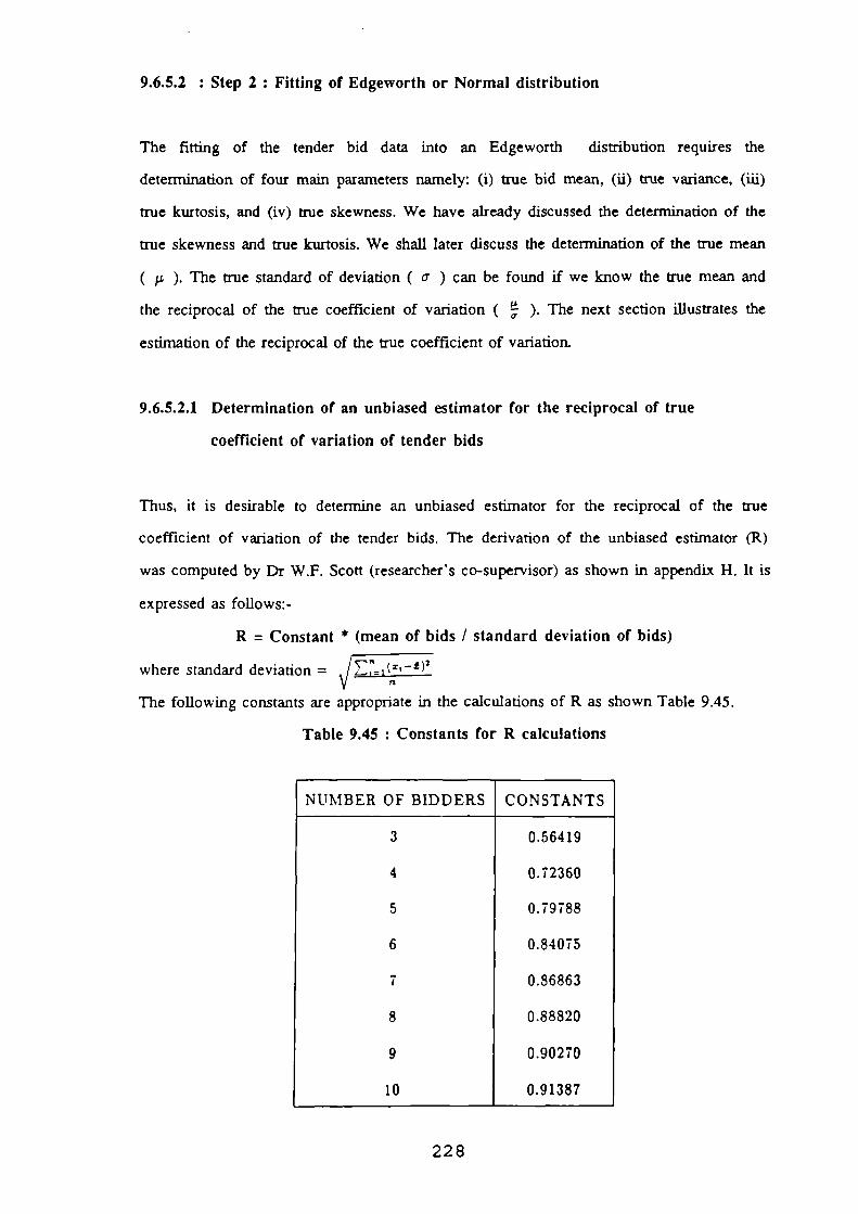
9.6.5.2 : Step 2 : Fitting of Edgeworth or Normal distribution

The fitting of the tender bid data into an Edgeworth distribution requires the

determination of four main parameters namely: (i) true bid mean, (ii) true variance, (iii)

true kurtosis, and (iv) true skewness. We have already discussed the determination of the

true skewness and true kurtosis. We shall later discuss the determination of the true mean

( p. ). The true standard of deviation ( a ) can be found if we know the true mean and

the reciprocal of the true coefficient of variation ( 12; ). The next section illustrates the

estimation of the reciprocal of the true coefficient of variation.

9.6.5.2.1 Determination of an unbiased estimator for the reciprocal of true

coefficient of variation of tender bids

Thus, it is desirable to determine an unbiased estimator for the reciprocal of the true

coefficient of variation of the tender bids. The derivation of the unbiased estimator (R)

was computed by Dr W.F. Scott (researcher's co-supervisor) as shown in appendix H. It is

expressed as follows:-

R = Constant * (mean of bids / standard deviation of bids)

I/where standard deviation = F.7.1(x,-1)2 n

The following constants are appropriate in the calculations of R as shown Table 9.45.

Table 9.45 : Constants for R calculations

NUMBER OF BIDDERS CONSTANTS

3 0.56419

4 0.72360

5 0.79788

6 0.84075

7 0.86863

8 0.88820

9 0.90270

10 0.91387

228

The mean values of R were determined for different bidding sets and different job types

as shown in tables 9.46 and 9.47.

Table 9.46 : Mean values of R for different numbers of bidders

NO. OF

BIDDERS

NO. OF

CASES

MEAN VALUE

OF R

3 277 14.476

4 231 15.953

5 317 18.542

6 288 17.850

7 76 18.639

8 43 17.089

9 12 20.349

10 6 24.965

Table 9.47 : Mean values of R for different job types

JOB TYPE NO. OF CASES MEAN VALUE

OF R

1 63 17.181

2 30 20.564

3 468 19.760

4 96 16.013

5 55 18.313

6 17 19.167

7 130 19.561

8 491 13.228

229

9.6.5.2.2 Testing for independence of R against number of bidders, job type

and bid mean

The unbiased estimator (R) was also tested for independence with respect to different

numbers of bidders, job types and bid mean using the one-way analysis of variance test.

In order to conduct the analysis of variance test of R for different bid mean, it is

necessary to categorise the bid means into suitable groupings. The classification of the bid

mean is shown in table 9.48 (in 1986 prices).

Table 9.48 : Classification of bid mean

CATEGORY VALUE RANGE OF BID MEAN

1 Len than /100,000

2 L'100,000 to /250,000

3 /250,000 to /500,000

4 /500,000 to /750,000

5 £750,000 to r1,000,000

6 £1,000,000 to 1'1,250.000

7 /1.250,000 to 1'1,500,000

8 /1,500,000 to /1,750,000

9 /1,750.000 to /2,000,000

10 /2.000,000 to /2,250.000

11 /2.250.000 to £2,500,000

12 /2.500.000 to 12.750,000

13 12,750.000 to 11.000.000

14 More than .C3,000.000

9.6.5.2.3 One-way analysis of variance of R by number of bidders, job type

and bid mean

The results of the one-way analysis tests were shown in tables 9.49 to 9.51. As shown in

table 9.49, the observed significance level is quite small (0.0079). Therefore, we reject the

null hypothesis that the population means of R are the same for different numbers of

bidders at the 1% significance level. This indicates that R is probably affected by the

230

ONEWIY

Variable R

By Variable NOBID number of bidders

ANALYSIS OF VARIANCE

SUM OF MEIN F FSOURCE D.F. SQUARES SQUIRES RATIO PROB.

BETWEEN GROUPS 7 3803.9758 543.4251 2.7436 .0079WITHIN GROUPS 1342 265810.8414 198.0707TOTAL 1349 269614.8172

number of bidders, although we shall see (in tables 9.50 and 9.51) that the other two

factors are more important.

Table 9.49 : One-way analysis of variance of R by

number of bidders

Similarly, the observed significance level is approximately 0 (as shown in table 9.50) for

the one-way analysis of variance test of R for different job types. Thus, we also reject the

null hypothesis that the population means of R are equal for different types of job.

Therefore, we assume that R is also affected by job type.

Table 9.50 : One-way analysis of variance of R by job type

ONEWIY

Variable R

By Variable JOBTYPE type of job

ANALYSIS OF VARIANCE

SUM OF MEAN F F

SOURCE D.F. SQUARES SQUARES RATIO PROB.

BETWEEN GROUPS 7 12049.5195 1721.3599 8.9689 .0000

WITHIN GROUPS 1342 257565.2977 191.9265

TOTAL 1349 269614.8172

231

ONEWIT

Variable R

By Variable BMW

ANALYSIS OF VARIANCE

SUM OF MEAN F F

SOURCE D.F. SQUARES SQUARES RATIO PROB.

BETWEEN GROUPS 13 24231.8745 1863.9903 10.1486 .0000

WITHIN GROUPS 1336 245382.9427 183.6699

TOTAL 1349 269614.8172

Table 9.51 : One-way analysis of variance of R by bid mean

As shown in table 9.51, the one-way analysis of variance of R against different categories

of bid mean produced an observed significance level of 0. Hence, we reject the null

hypothesis that the population means of R are the same for different categories of bid

mean. We therefore assume that R is also affected by bid mean.

Thus, the above results show that the population mean of R varies according to the

number of bidders, job type and bid mean. As a result, it is necessary to determine

whether there is any interaction effect of the above factors (number of bidders, job type

and bid mean) on R. The test of possible interaction effect of the factors on R was

performed using the two-way analysis of variance test. The SPSS-X output of the tests

were shown in tables 9.52 to 9.54.

9.6.5.2.4 Two-way analysis of variance of R by number of bidders, job type

and bid mean

As shown in table 9.52. the F value associated with the bid mean (denoted by BMEAN)

and job type interaction is 2.066. The observed significance level is approximately 0.

Hence, we have strong statistical evidence that there is an interaction effect between the

bid mean and job type.

232

The observed significance level for the testing of interaction effect between the number of

bidders and bid mean on R is 0.433 as illustrated in table 9.53. Thus, we accept the null

hypothesis that there is no interaction effect between the number of bidders and bid mean

on R. Therefore, we have no statistical evidence that R is affected by the interaction of

number of bidders and bid mean.

As illustrated in table 9.54, the observed significance level is approximately 0.112 for the

interaction effect between number of bidders and job type. Similarly, we also accept the

null hypothesis and statistically confirm that we have no evidence that R is affected by

the interaction of number of bidders and job type.

Table 9.52 : Two-way analysis of variance of R by bid mean and job type

*** ANALYSIS OF VARIANCE ***

by BMEAN

JOBTYPE type of job

Sum of Mean Sig

Source of Variation Squares OF Square F of F

Main Effects 38453.446 20 1922.672 11.630 .000

BMEAN 26403.926 13 2031.071 12.286 .000

JOBTYPE 14221.571 2031.653 12.290 .000

2-Way Interactions 22204.911 65 341.614 2.066 .000

MEAN JOBTYPE 22204.911 65 341.614 2.066 .000

Explained 60658.357 85 713.628 4.317 .000

Residual 208956.460 1264 165.314

Total 269614.817 1349 199.863

1350 cases were processed.

0 cases (.0 pct) were missing.

233

Table 9.53 : Two-way analysis of variance of R by number of bidders

and bid mean

••• ANALYSIS OF VARIANCE •••

by NOBID number of bidders

BMEIN

Sum of Mean SigSource of Variation Squares DF Square F of FMain Effects 25480.765 20 1274.038 6.942 .000

NOBID 1248.890 7 178.413 .972 .450BMEAN 21676.789 13 1667.445 9.086 .000

2-Way Interactions 11801.977 63 187.333 1.021 .433NOBID BMEiN 11801.977 63 187.333 1.021 .433

Explained 37282.741 83 449.190 2.448 .000Residual 232332.076 1266 183.517Total 269614.817 1349 199.863

1350 cases were processed.

0 cases (.0 pct) were missing.

Table 9.54 : Two-way analysis of variance of R number of bidders

and job type

• • ANALYSIS OF VARIANCE...

by

ft

NOBID

JOBTTPE

number of bidders

type of job

Sum of Mean SigSource of Variation Squares OF Square F of F

Main Effects 15759.074 14 1125.648 6.968 .000NOBID 3709.555 7 529.936 2.810 .007

JOBTTPE 11955.099 7 1707.871 9.055 .000

2-Way Interactions 9041.669 37 244.369 1.296 .112NORIO JOBTTPE 9041.669 37 244.369 1.296 .112

Explained 24800.744 51 486.289 2.578 .000

Residual 244814.073 1298 188.609

Total 269614.817 1349 199.863

1350 cases were processed.

0 cases (.0 pct) were missing.

234

9.6.5.2.5 Correlation and regression analysis of R

From the results of the two-way analysis of variance tests, it seems necessary to segregate

the job type factor when determining the R value. Hence, the determination of any

possible relationship between R and the number of bidders and bid mean (the actual bid

mean value is adopted) is considered separately for different job types. Scatterplot and

correlation analysis were performed to determine the nature and strength of linear

relationship between R, number of bidders and bid mean. The SPSS-X output for the

scatterplot of the above variables is displayed in appendix I. As observed in appendix I

the L-shaped plots of the data are not suitable for correlation analysis. Thus, as explained

in chapter 9 section 9.3.4, the logarithm (base 10) transformation (transformation of all

variables, that is, logarithm R, logarithm number of bidders and logarithm bid mean) is

also adopted for the correlation analysis of the variables, as shown in appendix I. The

correlation coefficients of both the untransformed and transformed variables are tabulated

in tables 9.55 and 9.56.

Table 9.55 : Pearson Correlation Coefficient of R

and number of bidders for different job types

JobType

No.of

cases

r r(* logarithm)

Percentagepoints of r

(1% Sig. level)

1 63 0.047 0.120 0.32232 30 -0.383 -0.351 0.46293 468 0.058 0.177 0.11924 96 0.227 0.291 0.26175 55 0.177 0.318 0.34466 17 0.219 0.392 0.60557 130 0.178 0.349 0.22528 491 0.165 0.248 0.1164

(Note : * indicates that both R and number of bidders are transformed using logarithm)

235

Table 9.56 : Pearson Correlation Coefficient of R

and bid mean for different job types

JobType

No.of

cases

r r(* logarithm)

Percentagepoints of r

(1% Sig. level)

1 63 0.341 0.383 0.32232 30 0.068 -0.003 0.46293 468 0.161 0.332 0.11924 96 0.702 0.634 0.26175 55 0.243 0.492 0.34466 17 -0.001 -0.006 0.60557 130 0.469 0.578 0.22528 491 0.267 0.354 0.1164

(Note : * indicates that both R and bid mean are transformed using logarithm)

In order to determine whether there is significant association between the variables, we

conduct the test at 1% significance level of the hypothesis that the true correlation

coefficient is zero. We compare the modulus of r with r(0.5) from the correlation

coefficient table as shown in appendix F. If the modulus of r is less than r(0.5), we accept

the hypothesis at the 1% significance level. This suggests that there is no linear

correlation between the variables. Conversely, if the modulus of r is greater than r(0.5), it

indicates that there is significant linear correlation between the variables.

As shown in table 9.55, the moduli of r for all job types except job type 8 of the

untransformed variables (R and number of bidders) are less than their corresponding table

values [1(0.5)] for two-sided tests at the 1% significance level. This suggests there is no

significant linear correlation between R and number of bidders for job types 1 to 7.

However, there are some job types (job types 3, 4, 7, and 8) with significant correlation

and some (job types 1,2, 5, and 6) without significant correlation after the logarithm

transformation as illustrated in table 9.55. Table 9.56 shows that all except job types 2

and 6 have significant linear correlation between R and bid mean at the 1% significance

236

level. The above results suggest that bid mean is a more important explanatory variable

for R than number of bidders. Hence, regression analysis was performed using logarithm

R as the dependent variable and logarithm bid mean and number of bidders as

independent variables. A step-wise regression analysis was conducted so as to select the

important variable(s) for the regression equations of logarithm R for different job types.

The SPSS-X output of the regression analysis is displayed in appendix J. A summary of

the respective regression equations for various job types is shown in table 9.57.

As illustrated in appendix J, the step-wise regression analysis shows that number of

bidders is a less important variable for predicting the value of logarithm R (the probability

associated with the F statistics exceeds 0.05). Hence, regression equations for logarithm R

and logarithm bid mean were determined for various job types as shown in table 9.57, the

variable n (number of bidders) being omitted. As expected, no regression equation is

formed for job types 2 and 6 as the correlation coefficients of both job types are

relatively small (see tables 9.55 and 9.56). Therefore, the value of R for these two job

types may be considered to be equal to the mean value of R for the respective job types

(Industrial=20.564 and Religious=19.167) as shown in table 9.46).

Table 9.57 : Regression equations for Log R for different job types

CODE JOB TYPE REGRESSION EQUATIONS

1 Transport and Utility LogR = -0.288 + 0.259LogBidmean

3 Administration and Office Log!? = -0.158 + 0.238LogBidmean

4 Health and Welfare LogR = -1.201 + 0.421LogBidnican

5 Refreshment, Entertainment and Recreation Log R = -0.917 + 0.372Log Bldmean

7 Education, Scientific and information Log R = -1.092 + 0.412LogBiclmean

8 Residential Log R = -0.346 + 0.243LogBidmcan

_

Note: a)

For job type 2 (Industrial buildings): R=20.564 and job type 6 (Religious buildings): R=19.167.

b)

Bid mean is expressed at 1986 prices)

C)

The above equations are only suitable for contracts up to Lam (bidmean).

237

9.6.5.3 Step 3 : Testing of bidding models

9.6.5.3.1 Testing of models on contractors A to E

The bidding models were tested on five contractors who have provided detailed tender bid

information to the researcher. Three contractors provided only 14 contracts which they

had tendered in 1986 while the remaining two contractors supplied 29 contracts which

they have tendered recently (1987 to 1989). In order to test the model, it is necessary to

divide the number of jobs supplied equally so that half the number of cases could be used

to estimate the true bid mean of each new job while the remaining jobs may be utilised

for testing the prediction accuracy of the model. For instance, if contractor A provides a

total of 14 bids, 7 of the 14 will be used to determine the cost estimate and bid mean

ratio while the remaining 7 will be used for testing the accuracy of the model. The test

procedures for both the Normal and Edgeworth distribution models are as follows:-

a) Determine the cost estimate of new job.

b) Predict the true bid mean using past records (cost estimate / bid mean ratio).

c) Determine the value of R using the appropriate regression equation for the job type

d) Determine the number of bidders against whom the contractor is competing.

e) State the desired probability of success (P.20, 0.50 or 0.90).

0 Determine the k value from the Normal or Edgeworth distribution (appendix K).

g) Compute the theoretical new bid (Theoretical new bid = Predicted bid mean + k *

true standard deviation of bids).

h) Compare the actual lowest bid with the theoretical new bid to determine the

success rate achieved by both the prediction models.

The above test procedure is illustrated by testing on the tender bid records as provided by

contractor A. Contractor A has supplied the researcher 29 contracts with each tender

record containing the following information.

238

a) Date of tender.

b) Type of job.

c) Cost estimate of firm.

d) Tender bid of firm.

e) Tender bids of other competitors.

The data were keyed into a spreadsheet as illustrated in table 9.58. Let the first 14 jobs to

be past tender records, while the next 15 jobs are future contracts used for testing the

prediction model. Using the first 14 jobs, we compute the cost estimate/bid mean ratio for

each contract and determine the average (denoted by Z) of these cost estimate/bid mean

ratios. With the value of Z, we estimate the bid mean for the next 15 future contracts as

shown in column 5 in table 9.58. Thereafter, using the respective regression equation for

different job type, we compute Log R and subsequently the value of R for each of the 15

new contracts. Once R is determined, it is possible to compute the value of the true

standard deviation of bids using the formula:- true bid mean / R. With the predicted bid

mean and the true standard deviation of bids, the new theoretical bid for each contract can

thus be computed using the appropriate k values as obtained from either the Normal or

Edgeworth distribution (appendix K).

The test was conducted using three levels of probability (0.2, 0.5, 0.9) for both the

Normal and Edgeworth distribution models. The results of the test for contractor A are

shown in table 9.59. From the results, it would appear that both the Normal and

Edgeworth bidding models provide very similar predictions. The above test procedures

were also carried out on the other 4 contractors as shown in tables 9.60 to 9.63. Besides

this, the margin by which a contractor has won or lost a contract was also computed as

shown in tables 9.54 to 9.63. The margin analysis provides a measure to indicate the

extent in which the predicted bids are close to the actual lowest bids. It is defined as

follows:-

Margin = lowest bid - contractor's bid

Margin % = (lowest bid - contractor's bid) 100/contractor's bid

239

Weighted win margin = sum of win margins of successful bids /

total value of successful contracts

Weighted lose margin = sum of lose margins of unsuccessful bids /

total value of unsuccessful contracts

(Note: "Value" means contractor's bids)

If a contract is won (ie. the predicted bid of the contractor is lower than the lowest bid),

the margin (win margin) is negative. Conversely, a positive margin (lose margin) indicates

the reduction in the price which the contractor would have to make in order to win the

contract.

9.6.5.3.2 Testing reliability and accuracy of bid predictions

In order to determine the reliability and accuracy of the bidding models, confidence

interval tests and margin analysis were performed on the bid prediction results as shown

in tables 9.64 and 9.65. As illustrated in tables 9.64 and 9.65, both Edgeworth and

Normal models have 11 cases out of 15 (73.3%) where the theoretical success rate (P)

falls within the 90% confidence interval. This shows that our bidding models are

reasonably successful. That is, a contractor using our techniques with a given value of P

(eg. 50%) will have approximately this success rate.

We now consider the win and lose margins (see tables 9.64b and 9.65b), and first

consider the weighted win margins (%). These represent the relative proportionate loss of

money by bidding too low when winning. They vary from about -4% to about -8% as P

varies from 20% to 90%. (these margins are of course based on a fairly small sample).

One would expect the win margin to behave like this as the probability of success

increases, as with a high value of P one tends to win more contracts by bidding low. Let

us now compare the actual experience of the 2261 refurbishment contracts described in

240

section 9.3.1.3. The average win margin is -6.20% (which is measured as bid spread in

figure 9.8). Since there were, on average, nearly 5 bidders (see figure 9.1) per job, this

bid spread is to be compared with the -4% of our method when P=20%. This argument is,

of course, only roughly applicable, but it shows that our win margins are probably smaller

than the average for the industry.

The lose margins vary from about 5.6% to 3.5% as P varies from 20% to 90%. We

would expect this trend, because in the case when P is 90% there will be comparatively

few losing bids and they will tend to be only a little more than the winning bid.

The results of the Normal and Edgeworth models are quite similar as shown in tables

9.64 and 9.65. This suggests that both the Normal and Edgeworth models provide

reasonably accurate tender bid predictions.

9.6.6 Conclusion

In conclusion, this module shows that tender bids of refurbishment contracts (lump sum

contracts) may be fitted into either a Normal or Edgeworth distribution for the purpose of

predicting the probability of success when submitting a tender bid. Both the Normal and

Edgeworth distribution models were tested using tender bids provided by five

refurbishment contractors. It was shown that both models predict quite similar and

reasonably accurate results, as confirmed by the confidence interval test. The margin

analysis showed that win margins were very probably better than the industry average.

This implies that the models enable contractors to attain higher profitability in their

contracts (as a result of reducing the amount of money lost by bidding too low when

winning). However, it must be noted that the bidding models were tested on a relatively

small sample of contracts (5 contractors, each with between 14 and 29 jobs) and thus

should be applied in caution in practice.

241

Table 9.58 : Tender bid data of contractor A in spreadsheet format

CONTRACTOR

JOBNO NOBID JOBTTI1 COST ST BIDMIAN COST 1ST/ FRED MEIN

BIDMEAN

LOG R I SIGH

1 4 8 3523275 3904269 .90242

2 4 2 1743348 1837959 .94852

3 3 8 1354046 1379125 .98182

4 6 8 1735962 1824534 .95146

5 5 5 2614197 2888274 .90511

6 3 3 1879234 2113266 .88926

7 4 8 767062 827208 .92729

8 4 8 2173209 2332746 .93161

9 6 8 2032674 2080594 .97697

10 6 7 3033774 3394883 .89363

11 6 8 1542325 1537640 1.00305

12 7 5 1009380 980062 1.02991

13 6 8 5729941 5540836 1.03413

14 5 3 822281 776295 1.05924

15 5 8 2800911 2893439 .96802 2918832 1.2260 16.8285 173446

16 5 5 3460000 3838208 .90146 3605669 1.5222 33.2812 108340

17 7 8 1700105 1737873 .97827 1771681 1.1734 14.9059 118858

18 7 8 1093273 1096897 .99670 1139301 1.1268 13.3895 85089

19 4 5 458745 523565 .87619 478059 1.1958 15.6952 30459

20 5 3 1510769 1575693 .95880 1574374 1.3169 20.7449 75892

21 6 8 1846638 1871985 .98646 1924383 1.1821 15.2084 126534

22 6 3 495669 566030 .87569 516537 1.2017 15.9118 32463

23 6 8 3753637 4267829 .87952 3911668 1.2569 18.0694 216480

24 5 8 449296 522552 .85981 468212 1.0329 10.7874 43404

25 5 8 1701256 1664215 1.02226 1772880 1.1734 14.9083 118919

28 6 3 807674 973564 .82961 841678 1.2522 17.8725 47094

29 4 4 119391 139157 .85796 124417 .94 8.7891 14156

30 4 8 2726039 3269693 .83373 2840808 1.2232 16.7181 169924

31 3 3 1177035 1156019 1.01818 1226589 1.2911 19.5484 62746

AVERAGE COST ESTIMATE /BID MEAN RATIO FOR JOBS 1-14 : 95960

(Note : Sigsa : true standard deviation of tender bids)

242

Table 9.59 : Testing of bidding model on Contractor A

(a) Edgeworth distribution model

TIST 1 . 7101 : 02

0000 JOITTPI 7110 1111 $1110 I III 111 LOV BID SOCCISS 111111 111611121

I 2118832 173441 - 44621 2141441 2717742 10 -133171 -4.105 3605661 101340 -.44620 3557321 3336564 10 -221164 -6.21I 1711611 111151 -.72613 1615210 1610481 10 -74111 -4.44I 1131311 15019 -.12693 1071441 927631 10 -141101 -13.905 471051 30451 - 22602 411175 461833 10 -3342 -.713 1574314 75112 -.44621 1540511 1496051 10 -44461 -2.11I 1924383 126534 -.10111 1147171 1535765 10 -312114 -16.113 516537 32463 -.60461 496110 505640 115 1731 1.76I 3111661 216411 -.61461 3710712 4152799 !IS 212117 1.111 461212 43414 - 44121 441145 511014 TIS 52231 11.641 1772110 118111 -.44621 1711111 1512211 10 -217557 -12.073 141171 47194 -.61411 113214 151016 015 37192 4664 124411 14156 - 22602 121217 11091 10 -23126 -11 01I 2140101 169924 - 22602 2802402 2726031 10 -76363 -2.723 1226511 62141 12111 1234125 1174143 10 -151112 -12 II

ICTO I SOCC1SS 1111 : 26 671

TIST 2 7101 : 1 $

10111 J011771 7110 1111 $1111 I Ill 110 0.00 01) SOCC1SS 111111 111111(2)

5 1 2111132 113446 - 11737 2745142 2707762 10 -31111 -0315 5 3605669 101340 - 19137 3497614 3336564 10 -161151 -4601 I 1171611 111151 -112311 1126211 1610411 10 -15721 - 117 I 1131301 15011 -121111 1135154 127631 10 -117515 -11 314 5 411059 31451 - 12212 453110 467133 015 14133 327S 3 1574374 15112 - 91731 1491612 1496051 10 -2631 - II6 1 1124313 126534 -I 12461 1712071 1535765 10 -246314 -13 126 3 516537 32463 -1 12461 411026 505641 TIS 25114 5346 I 3111661 211411 -1 12461 3668115 4152711 115 314614 11 415 1 461212 43404 - 91737 424122 511114 TIS 71142 17125 1 1112110 111111 - 11737 1654214 1512261 00 -142113 -ISO6 3 141611 47014 -1 12469 711712 151096 115 12314 7104 4 124417 14156 - 12272 112711 11091 10 -14610 -13 124 1 2140101 119924 - 12272 2111101 2726031 TIS 25131 133 3 1226511 62746 - 55126 1191174 1114943 10 -116131 -III

ICTOIL SICCISS 1111 :40 001

TIST 3 7101 , 1 1

10111 JOITYPI 7110 1111 5I111 1 1111 BID LOY IID SOCCISS 111111 111111(1)

5 I 2911132 173446 -110116 2587169 2707'62 TIS 119113 4635 5 3605661 101340 -1 00116 3391939 3336564 10 -62375 -0047 1 1771611 111151 226135 1525960 1611411 115 14521 5547 1 1131301 85089 .206735 963312 127131 10 -35753 -3 714 5 471059 30451 71192 423510 467039 115 44263 10 455 3 1574374 75892 -110006 1429560 1416151 115 66411 1656 I 1124383 126534 99697 167108 1535165 10 -135133 -III6 3 516537 32463 - 11697 151109 505641 115 53131 00146 1 3111661 216410 -091607 3419364 4052791 115 573435 16 415 1 461212 43414 -100116 315391 501014 YIS 115614 30 125 1 1712110 111911 - 90116 1545964 1512261 10 -33103 -2106 3 141618 41094 - 9969' 747633 151196 11$ 103463 13 144 4 124417 14156 - 7 1192 19093 91011 10 -1112 -III4 1 2840108 169024 -010012 2536121 2126031 !IS 111211 1463 3 1226519 62746 -060067 1125526 1074969 10 -51513 -441

1C1011. SOCCISS 1111 , 60008

243

Table 9.59 : Testing of bidding model on Contractor A

(b) Normal distribution model

TIST 1 : 0.2

10810 J0871P1 PHD 1111 SIGH I 100810 LOW BID SOCCISS 111011 11101111)

5 1 2918132 173146 - 43641 2843133 2707162 MO -135371 -4.76

5 5 3605669 101340 - 43644 3558315 3336564 10 -221121 -1.23

7 I 1171611 111851 - 12151 1615915 1610181 00 -75434 -4.17

1 1 1139301 85089 -.72158 1077902 927639 10 -151263 -13.94

4 5 471059 30451 -.21420 471535 467133 10 -3712 -.79

5 3 1574374 75192 - 13114 1541252 1496051 10 -45201 -2.93

6 1 1924383 126534 - 59110 1848130 1535765 10 -313015 -16.13

6 3 516537 32163 - 59710 497153 505640 TIS 6417 1.71

s I 3911668 216461 - 9710 3782401 4052799 TIS 210391 7.15

s I 418212 43401 - 13614 149269 501084 TIS 51815 11.53

5 1 1772180 111119 - 43644 1720919 1512261 10 -208718 -12.13

1 3 111671 47094 -.59710 113598 151096 IIS 37531 4.61

4 4 121417 14156 - 21420 121385 11091 10 -23294 -19.11

4 1 2140108 169921 - 21420 2601410 2726039 10 -71371 -2.79

3 3 1226589 62746 13270 1234915 1071943 10 -159972 -12.95

&MIL SOCCISS 1111 : 26 611

TIST 2 P101 : 0 5

10110 JOITTPI PHD 1111 SIGH I III 110 LOB 110 SOCCISS 311011 111011111

5 1 2111132 173446 - 99115 2745717 2707712 11 -31945 -IIIS 5 3605669 181340 - 99115 3491929 3336564 10 -160965 -4.617 I 1171611 111151 -123132 1125329 1610481 PO -11141 - II1 1 1131301 15181 -123131 1031529 121639 10 -106191 -10 334 5 411051 30451 • 11933 193103 467833 TIS 14730 025S 3 1514374 79112 - 99115 1496622 1496051 10 -2571 - 176 8 1124360 12031 -11290* 1711526 1535765 10 -215161 -13 796 3 511531 32463 -111901 419116 505640 TIS 25154 5316 1 3911661 216410 -I 12900 3661262 4052799 TIS 385537 1* 515 1 461212 43404 - M15 124111 501084 115 76116 1713

5 I 1112110 111111 - 11115 1654111 1512261 10 -111920 -1916 3 111(11 41014 -1 12911 71150 151096 115 62517 714I 4 124117 14156 - 11933 112111 11011 10 -14721 -13 05

4 1 2110101 169924 - 11933 2111561 2721031 TIS 24459 II3 3 1221519 62746 - 51419 1192391 1074943 10 -111453 -185

ICTIIL SOCCISS 1111 : 41 001

7151 3 P101 : 0 I

10111 JOITTPI PIID 1111 61011 I Ill III LO1 Ill SOCCISS 111011 11101111)

5 1 2111132 113446 -11432* 2511712 2717712 fIS 129171 4 II5 5 3405661 111341 -111320 3315143 3336564 PO -91571 -9737 1 1711611 111151 -211151 1521121 1111111 8I5 11152 5811 1 1131311 15011 -2 11052 151111 121631 00 -32011 -3344 5 471151 30491 -1 11121 422671 461133 TIS 45157 10 (I5 3 1574311 75112 -111311 1426901 1416151 TIS 61151 4856 1 1924313 121534 -2 13641 1161700 1539765 10 -130135 -III6 3 511537 32163 -2 03111 451421 515611 TIS 55213 12 266 1 3111661 216411 -203617 3470113 4052111 TIS 511116 16 775 1 461212 43404 -114021 313169 501014 TIS 117215 30545 1 1772110 111911 -114311 1511111 1912261 10 -29536 -9926 3 141671 47094 -103111 749772 151096 TIS 115324 14 12I 4 124417 14156 -111111 11677 11011 10 -516 - 511 I 2140100 169924 -111121 2531131 2726031 TIS 111200 7173 3 1226511 62746 -163222 1124114 1114943 10 -41231 -435

ICTBIL SOCCISS 1111 : 61 10%

244

Table 9.60 : Testing of bidding model on Contractor B

(a) Edgeworth distribution model

TEST 1 P101:0 2

1101110 JOBTIPI PIID MI 51011 I PIA BID LOA BID SUCCESS 111011 110C11111

4 2 1141119 55786 - 22602 1131570 1084421 10 -50149 -4.42

5 2 319489 13613 - 44620 313415 287630 10 -25185 -1.23

4 8 1015422 17989 -.22602 991795 876719 PO -121006 -12.13

5 8 502887 45816 - 44620 482444 455001 10 -27431 -5.69

4 5 825254 42916 -.22602 815554 743502 PO -72052 -6 83

4 1 439207 25691 - 22602 433399 315207 60 -41192 -11.12

6 I 1030192 78806 - 60461 983197 1044103 YIS 60906 1.196 7 1246630 47456 - 60461 1217931 1113831 PO -104101 -1.556 3 842640 47135 - 60461 814142 662733 AO -151409 -11.606 3 913194 50113 - 60461 882195 135491 10 -147404 -16.70

6 1 951016 40624 - 60161 932454 913217 10 -19171 -2.065 8 574216 51655 - 44620 551614 498379 NO -53235 -9.65

5 I 414606 43152 -.44620 455039 456594 115 1555 .34

i 5 1154201 166591 -.60461 7053555 1610621 PO -372934 -5.295 1 461182 26641 - 44620 455292 445189 10 -10103 -2.22

ICTOIL SUCCESS 1111 :03 330

TEST 2 PI01:0 50

60110 JOITYPI PIID 1111 SIGII 1 III IID LOA IID SUCCESS 111611 111011111

4 2 1117179 55716 - 12272 1101213 1014421 10 -16162 -1.53S 2 319119 13613 - 99731 305112 217630 10 -11212 -5.91

4 6 1015122 11989 - 12212 951259 876789 PO -74471 -7.13

5 I 502817 45116 - 19731 457191 455007 PO -2184 -.414 5 125254 42516 - 82272 789916 743502 10 -46444 -III

4 7 439207 25691 - 82272 411066 385207 10 -32659 -7.86

6 I 1030192 76866 • 12469 942170 1044103 115 101933 1182

6 7 1246630 47456 -1 12449 1193257 1113137 10 -79421 -6.66

6 3 142610 47135 -112461 789621 662733 PO -126895 -16 07

i 3 913194 50113 -102469 156132 '35491 10 -121341 -14 166 7 951016 40624 1 12469 911327 919277 115 1950 21

5 I 571216 50655 - 99737 523694 498978 10 -25315 -453

5 8 474606 43852 - 99137 130869 156594 115 25725 511

6 5 1154211 166597 -I 12469 6966911 1680621 AO -216290 -411

5 7 467112 26641 - 99 7 3 7 440604 445189 YIS 4585 004

ICTOIL SOCCISS 1111-26 61

TEST 3

10810

P101:I 90

J0171PI PIID IIII 51611 I 11114 IID LOA IID S0CZ1SS 116511 511011111

4 2 1141178 55716 -078092 1047312 1084421 115 37039 351$ 2 319489 13613 - 10616 293513 217630 10 5883 -2584 I 1005422 77919 71192 175906 876789 115 813 105 I 502817 45116 -18080€ 415463 455007 115 39544 8524 5 125254 42116 -070092 141411 743502 10 4979 • 674 1 139207 25117 -078012 393237 385207 110 1030 -2845 I 1030192 78816 -181697 173359 1014103 1IS 170714 115$6 7 1246630 47456 -099611 1151112 1113137 10 -31025 -3306 3 142640 17125 99691 141513 662733 10 -15710 11 466 3 913194 50113 -099697 113120 735181 00 77629 -9556 7 951016 40624 -099597 175811 913277 TIE 37386 4175 I 574216 50655 90116 477551 498319 YIS 20121 4365 I 174606 43152 -110115 310921 156514 11S 65665 0600i 5 7154211 161591 -119607 6121592 6611621 10 -140971 -2075 7 467112 26611 -19011€ 411333 415119 11$ 21156 193

ICTOIL SUCCESS 1111:53 331

245

Table 9.60 : Testing of bidding model on Contractor B

(b) Normal distribution model

TIS7 1 : P1011:0 20

10110 JOIITTP1 P310 1101 51611 I 1111 110 LOW 11D S1CCISS 111611 111611(1)

4 2 1147171 55116 -.21420 1135230 1014421 10 -50101 -4.415 2 311411 13613 -.43144 313541 211630 10 -25111 -1 274 I 1115422 77111 -.21420 191717 176111 10 -121921 -12 215 I 502117 45116 -.43644 412111 455007 10 -21114 -5.774 5 125254 42916 -.21421 116061 143502 10 -72559 -1.114 7 431207 25617 -.21421 433703 315207 10 -41496 -11 116 I 1030192 71116 - 51110 913711 1144113 IIS 61314 6)31 7 1241631 47456 -.51111 1211294 1113137 10 -114457 -1.576 3 142640 41135 -.59710 114416 662733 10 -151713 -11 636 3 913114 51113 -.51111 113272 735491 10 -147711 -16.73i 7 151116 40124 -.51711 132751 113271 It -11412 -2.115 1 $14211 $0655 - 43644 $52101 491371 10 -53721 -0135 I 414606

6 $ 7154211

43152

166517

-.43644

-.51710

455461

1054106

65096

6110621

lOS

-37 1411 - 75 9 211$ 1 461112 26641 -.43644 455552 445111 10 -11363 -221

ICTI1L SOCCISS 1171 :13.339

1IS7 2 PI08:0 50

10118 JOBT1P1 PHD 1111 51611 I 1111 BID LOW 110 SOCCISS 111111 111611(1)

4 2 1147119 $5716 - 11933 1101472 1014421 10 -11151 -1 $5

5 2 311419 13613 - 99115 305901 281630 10 -11271 -5 17

4 1 1015422 11989 - 11933 951523 816769 10 -74734 -705

5 1 502111 45116 - 91115 457156 455001 10 -2149 - 47

4 5 125254 42916 - 11933 790092 743502 10 -46590 -$11

4 7 431207 25691 - 11933 411153 315207 10 -32946 -III

6 I 1030192 78116 -1 12900 941130 1044103 TIS 102213 11 16

6 7 1246630 41456 -1 12900 1193052 1113137 10 -71215 -(64

6 3 142640 47135 -1 12900 19425 662133 10 -126112 -16 OS

1 3 113114 51113 -1 12900 856616 '35491 10 -121125 -14 14

6 7 157016 41624 -1 12900 911152 913277 115 2125 23

5 1 $14216 51655 - 19115 523655 491371 10 -25276 -4.13

5 I 474606 43152 - 11115 430135 456594 11$ 25151 5.11

6 5 7154211 161591 -1 12900 6966193 6610621 10 -215512 -III

5 1 467112 26641 - 19115 440583 445119 TiS 4606 105

1CTOIL SOCCISS 1111 :26 in

TIP 1 PI01:1 10

10118 J0111PI P1111 1111 51611 1 Ill 1111 LOW 110 SOCCISS 1006111106111%)

4 2 1141111 $5716 -111121 1145744 1014421 715 370

3-156471:5 2 311411 13613 -104320 213036 217631 10 -III

4 I 1015422 77161 -111021 173616 176789 135 3173 31

5 1 502111 45116 -114321 413157 455001 IIS 411$1 114

4 5 125254 42916 -111120 141221 743502 10 -3711

4 1 439202 25612 -1 11121 392413 315202 10 -7211 -11 15

6 1 1030192 21116 -203641 170243 1144103 115 123161 11 11

6 7 1246630 47416 -203641 1149911 1113131 10 -31151 -3 14

6 3 142640 4713$ -202647 746651 662733 10 -13911 -11 24

6 3 913114 51113 -2 03647 1 ..140 135491 10 -71141 -133

6 1 951t16 40624 -2 03647 174216 913217 715 31111 4.41

5 I 574216 50655 -194321 415 1 13 498379 115 22596 475

5 1 474606 43151 -194320 319393 451514 115 61201 0721

6 5 1154211 166511 203647 6115111 6610621 10 -134311 -117S 1 417112 26641 -1 14321 415401 445119 TIS 21111 II?

ICTOIL SOCCISS :53 331

246

FRED MEAN SIGMA NEWINOBID JOBTTP1 LOW BID SUCCESS MARGIN MARGIN(%)

4 3 1035774 55182 -1.7889 937058 971999 TES 34941 3.73

6 3 798159 45222 -1.9970 707852 756691 TES 48839 6.90

5 3 885795 48966 -1.9082 792360 805614 TES 13254 1.67

4 3 2073301 93603 -1.7889 1905853 2000549 TES 94696 4.97

5 3 1603575 76947 -1.9082 1456748 1565481 TES 108733 7.46

5 3 2178004 97189 -1.9082 1992552 2042375 TES 49823 2.50

6 3 692060 40566 -1.9970 611051 655417 TES 44366 7.26

247

Table 9.61 : Testing of bidding model on Contractor C

(a) Edgeworth distribution model

TEST 1: PROB:0.2

FRED SIGMAJOBTTP1 MEINNOBID 1 NEW BID LOW BID SUCCESS MARGIN MARGIN(%)

4 3 1035774 55182 -.2260 1023302 971999 10 -51303 -5.01

6 3 798159 45222 -.6046 770817 756691 NO -14126 -1.83

5 3 885795 48966 -.4462 863946 805614 NO -58332 -6.75

4 3 2073301 93603 -.2260 2052147 2000549 10 -51598 -2.51

5 3 1603575 76947 -.4462 1569241 1565481 NO -3760 -.24

5 3 2178004 97189 -.4462 2134638 2042375 NO -92263 -4.32

6 3 692060 40566 -.6046 667534 655417 NO -12117 -1.82

ACTUAL SUCCESS RATE : 0%

TEST 2: PROB:0.5

NOBID JOBTTP1 FRED MEIN SIGMA I NEW BID LOW BID SUCCESS MARGIN MARGIN(%)

4 3 1035774 55182 -.8227 990375 971999 NO -18376 -1.86

6 3 798159 45222 -1.1247 747298 756691 TES 9393 1.26

5 3 885795 48966 -.9974 836958 805614 NO -31344 -3.74

4 3 2073301 93603 -.8227 1996292 2000549 TES 4257 .21

5 3 1603575 76947 -.9974 1526830 1565481 YES 38651 2.53

5 3 2178004 97189 -.9974 2081071 2042375 10 -38696 -1.86

6 3 692060 40566 -1.1247 646436 655417 TES 8981 1.39

ACTUAL SUCCESS RITE : 57.14%

TEST 3: PROB:0.9

ACTUAL SUCCESS ROE : 100%

Table 9.61 : Testing of bidding model on Contractor C

(b) Normal distribution model

TEST 1: PROB:0.2

NOBID JOBTYPE FRED MEIN SIGMA 1 NEW BID LOW BID SUCCESS MARGIN MARGIN(Z)

4 3 1035774 55182 -.2142 1023954 971999 KO -51955 -5.07

6 3 798159 45222 -.5971 771157 756691 10 -14466 -1.88

5 3 885795 48966 -.4364 864424 805614 NO -58810 -6.80

4 3 2073301 93603 -.2142 2053251 2000549 NO -52702 -2.57

5 3 1603575 76947 -.4364 1569992 1565481 NO -4511 -.29

5 3 2178004 97189 -.4364 2135587 2042375 NO -93212 -4.36

6 3 692060 40566 -.5971 667838 655417 NO -12421 -1.86

SUCCISS RITE : 0%

TEST 2 : PROB:0.5

NOBID JOBTTP1 FRED MEAN SIGMA 1 NEW BID LOW BID SUCCESS MARGIN MARGIN()

4 3 1035774 55182 -.8193 990562 971999 NO -18563 -1.87

6 3 798159 45222 -1.1290 747103 756691 YES 9588 1.28

5 3 885795 48966 -.9982 836920 805614 KO -31306 -3.74

4 3 2073301 93603 -.8193 1996609 2000549 TES 3940 .20

5 3 1603575 76947 -.9982 1526770 1565481 TES 38711 2.54

5 3 2178004 97189 -.9982 2080995 2042375 NO -38620 -1.86

6 3 692060 40566 -1.1290 646261 655417 TES 9156 1.42

ACTUAL SUCCESS RATE : 57.14%

TEST 3: PROB:0.9

NOBID JOBTTP1 FRED MEIN SIGMA I NEW BID LOW BID SOCC1SS MARGIN MARGIN(Z)

4 3 1035774 55182 -1.8183 935438 971999 TES 36561 3.91

6 3 798159 45222 -2.0365 706066 756691 TES 50625 7.17

5 3 885795 48966 -1.9432 790644 805614 TES 14970 1.89

4 3 2073301 93603 -1.8183 1903105 2000549 YES 97444 5.12

5 3 1603575 76947 -1.9432 1454052 1565481 YES 111429 7.66

5 3 2178004 97189 -1.9432 1989146 2042375 TES 53229 2.68

6 3 692060 40566 -2.0365 609449 655417 TES 45968 7.54

ACTUAL SUCCESS RATE : 100.00%

248

Table 9.62 : Testing of bidding model on Contractor D

(a) Edgeworth distribution model

TEST 1: PROB : 0.2

ROBID JOBTTP1 FRED MEAN SIGMA I NEW BID LOW BID SUCCESS MARGIN MARGIN(%)

4 3 692820 40702 -.2260 683621 653374 NO -30247 -4.42

4 3 995995 53537 -.2260 983895 971999 NO -11896 -1.21

4 3 691393 40534 -.2260 682232 676789 NO -5443 -.80

7 8 485971 44649 -.7269 453514 488967 TES 35453 7.82

5 3 115034 10335 -.4462 110423 107812 NO -2611 -2.36

5 3 2203641 98049 -.4462 2159892 2042375 NO -117517 -5.44

6 3 804661 45511 -.6046 777145 655417 NO -121728 -15.66

ACTUAL SUCCESS RITE : 14.29%

TEST 2: PROB : 0.5

NOBID JOBTTP1 FRED NEAR SIGMA I NEW BID LOW BID SUCCESS MARGIN MARGIN()

4 3 692820 40702 -.8227 659334 653374 NO -5960 -.90

4 3 995995 53537 -.8227 951949 971999 TES 20050 2.11

4 3 691393 40534 -.8227 658045 676789 TES 18744 2.85

7 8 485971 44649 -1.2240 431322 488967 TES 57645 13.36

5 3 115034 10335 -.9974 104726 107812 TES 3086 2.95

5 3 2203641 98049 -.9974 2105850 2042375 NO -63475 -3.01

6 3 804661 45511 -1.1247 753475 655417 NO -98058 -13.01

ACTUAL SUCCESS RATE : 57.14%

TEST 3: PROB : 0.9

NOBID JOBTTPE FRED MEAN SIGMA I NEW BID LOW BID SUCCESS MARGIN MARGIN(%)

4 3 692820 40702 -1.7889 620007 653374 TES 33367 5.38

4 3 995995 53537 -1.7889 900222 971999 TES 71777 7.97

4 3 691393 40534 -1.7889 618881 676789 TES 57908 9.36

7 8 485971 44649 -2.0674 393666 488967 TES 95301 24.21

5 3 115034 10335 -1.9082 95313 107812 TES 12499 13.11

5 3 2203641 98049 -1.9082 2016548 2042375 TES 25827 1.28

6 3 804661 45511 -1.9970 713777 655417 NO -58360 -8.18

ACTUAL SUCCESS RATE : 85.71%

249

Table 9.62 : Testing of bidding model on Contractor D

(b) Normal distribution model

TEST 1: PROB : 0.2

NOBID JOBTTP1 FRED SIAM SIM I NEW BID LOW BID SUCCESS NARGIN MGM%)

4 3 692820 40702 -.2142 684102 653374 MO -30728 -4.49

4 3 995995 53537 -.2142 984527 971999 10 -12528 -1.27

4 3 691393 40534 -.2142 682711 676789 MO -5922 -.87

7 8 485971 44649 -.7216 453753 488967 TES 35214 7.76

5 3 115034 10335 -.4364 110523 107812 NO -2711 -2.45

5 3 2203641 98049 -.4364 2160848 2042375 NO -118473 -5.48

6 3 804661 45511 -.5971 777486 655417 10 -122069 -15.70

ACTUAL SUCCESS RATE : 14.29%

TEST 2: PROB : 0.5

NOBID JOBTTP1 FRED NIAN SIGMA I NEW BID LOW BID SUCCESS MARGIN MARGIN(%)

4 3 692820 40702 -.8193 659472 653374 NO -6098 -.92

4 3 995995 53537 -.8193 952131 911999 TES 19868 2.09

4 3 691393 40534 -.8193 658182 676789 TES 18607 2.83

7 8 485971 44649 -1.2313 430994 488967 TES 57973 13.45

5 3 115034 10335 -.9982 104718 107812 TES 3094 2.95

5 3 2203641 98049 -.9982 2105773 2042375 10 -63398 -3.01

6 3 804661 45511 -1.1290 753279 655417 10 -97862 -12.99

ACTUAL SUCCESS RITE : 57.14%

TEST 3: PROB : 0.9

NOBID JOBTTP1 HID 1111 SIGMA 1 MEW BID LOW BID SUCCESS MARGIN MARGIN()

4 3 692820 40702 -1.8183 618812 653374 TES 34562 5.59

4 3 995995 53537 -1.8183 898650 971999 YES 73349 8.16

4 3 691393 40534 -1.8183 617691 676789 YES 59098 9.57

7 8 485971 44649 -2.1105 391738 488967 TES 97229 24.82

5 3 115034 10335 -1.9432 94951 107812 TES 12861 13.54

5 3 2203641 98049 -1.9432 2013112 2042375 TES 29263 1.45

6 3 804661 45511 -2.0365 711979 655417 NO -56562 -7.94

ACTUAL SUCCESS RITE : 85.71%

250

Table 9.63 : Testing of bidding model on Contractor E

(a) Edgeworth distribution model

TEST 1 : PROB : 0.2

10BID JOBTTP1 PR1D MEAN SIGMA 1 NEW BID LOW BID SUCCESS MARGIN MARGIN(%)

4 3 676666 37879 -.22602 668105 653374 NO -14731 -2.20

3 3 122849 10867 .12011 124154 120097 NO -4057 -3.27

5 3 356609 24478 -.44620 345687 343852 NO -1835 -.53

5 3 111507 10094 -.44620 107003 107812 TES 809 .76

I 3 1099989 9989 -.22602 1097731 1076150 10 -21581 -1.97

5 3 259655 19221 -.44620 251079 256871 YES 5792 2.31

4 3 955013 51852 -.22602 943293 819596 NO -123697 -13.11

ACTUAL SUCCESS RITE : 28.57%

TEST 2: PROB = 0.5

NOBID JOBTTPE FRED MEIN SIGMA 1 111 BID LOW BID SUCCESS MARGIN MARGIN(%)

4 3 676666 37879 -.82272 645502 653374 TES 7872 1.22

3 3 122849 10867 -.55326 116837 120097 TES 3260 2.79

5 3 356609 24478 -.99737 332195 343852 TES 11657 3.51

5 3 111507 10094 -.99737 101440 107812 TES 6372 6.28

4 3 1099989 9989 -.82272 1091771 1076150 PO -15621 -1.43

5 3 259655 19221 -.99737 240485 256871 71S 16386 6.81

4 3 955013 51852 -.82272 912353 819596 NO -92757 -10.17

ACTUAL SUCCESS RATE: 71.43%

TEST 3: PROB : 0.9

NOBID JOBTTP1 FRED MEIN SIGMA 1 111 BID LOW BID SUCCESS MARGIN MARGIN(S)

4 3 676666 37879 -1.78892 608903 653374 TES 44471 7.30

3 3 122849 10867 -1.61067 105346 120097 YES 14751 14.00

5 3 356609 24478 -1.90816 309901 343852 YES 33951 10.96

5 3 111507 10094 -1.90816 92246 107812 TES 15566 16.87

4 3 1099989 9989 -1.78892 1082119 1076150 NO -5969 -.55

5 3 259655 19221 -1.90816 222978 256871 TES 33893 15.20

4 3 955013 51852 -1.78892 862254 819596 10 -42658 -4.95

ACTUAL SUCCESS RATE : 71.43%

251

NOBID JOBTTP1 FRED MEAN SIGMA I NEW BID LOW BID SUCCESS MARGIN MARGIN(%)

4 3 676666 37879 -.21420 668552 653374 NO -15178 -2.27

3 3 122849 10867 .13270 124291 120097 NO -4194 -3.37

5 3 356609 24478 -.53644 343478 343852 TES 314 .11

5 3 111501 10094 -.53644 106092 107812 TES 1720 1.62

4 3 1099989 9989 -.21420 1097849 1076150 NO -21699 -1.98

5 3 259655 19221 -.53644 249344 256871 TES 7527 3.02

4 3 955013 51852 -.21420 943906 819596 NO -124310 -13.17

JOBTTP1 FRED MEAN SIGMA 1 NEW BID LOW BID SUCCESS MARGIN MARGIN(%)NOBID

4 3 676666 37879 -1.81828 607791 653374 TES 45583 7.50

3 3 122849 10867 -1.63222 105112 120097 TES 14985 14.26

5 3 356609 24478 -1.94320 309043 343852 TES 34809 11.26

5 3 111507 10094 -1.94320 91892 107812 TES 15920 17.32

4 3 1099989 9989 -1.81828 1081826 1076150 NO -5676 -.52

5 3 259655 19221 -1.94320 222305 256871 TES 34566 15.55

4 3 955013 51852 -1.81828 860732 819596 PO -41136 -4.78

252

Table 9.63 : Testing of bidding model on Contractor E

(b) Normal distribution model

TEST 1 : PROB : 0.2

ACTUAL SUCCESS RATE = 42.86%

TEST 2: PROB : 0.5

NOBID JOBTTP1 FRED MEIN SIGMA

I NEW BID LOW BID SUCCESS MARGIN MARGIN(S)

4 3 676666 37879 -.81933 645631 653374 TES 7743 1.20

3 3 122849 10867 -.54495 116927 120097 TES 3170 2.71

5 3 356609 24478 -.99815 332176 343852 TES 11676 3.51

5 3 111507 10094 -.99815 101432 107812 TES 6380 6.29

4 3 1099989 9989 -.81933 1091805 1076150 NO -15655 -1.43

5 3 259655 19221 -.99815 240470 256871 TES 16401 6.82

4 3 955013 51852 -.81933 912529 819596 10 -92933 -10.18

ACTUAL SUCCESS RATE : 71.43%

TEST 3: PROB : 0.9

ACTUAL SUCCESS RITE : 71.43%

Table 9.64 : Testing of bid predictions (Edgeworth distribution model)

(a) Confidence interval test

Theoretical success rate (P). 20%

CONTRACTOR NO OF JOBS NO OF SUCCESSES 90% CONFIDENCEINTERVAL (CI)

DOES C.I.CONTAIN P?

A 15 4 0.1186 to 0.4759 Yes

B 15 2 0.0394 to 0.3226 Yes

C 7 0 0.0003 to 0.2325 YesD 7 1 0.0258 to 0.4404 NoE 7 2 0.1043 to 0.6592 Yes

TOTAL 51 9 0.0887 to 0.2643 Yes

Theoretical success rate (P) = 50%

CONTRACTOR NO OF JOBS NO OF SUCCESSES 90% CONFIDENCEINTERVAL (CI)

DOES CICONTAIN P?

A 15 6 0.2169 to 0.6094 Yes

B 15 4 0.1186 to 0.4759 NoC 7 4 0.2808 to 0.8254 YesD 7 4 0.2808 to 0.8254 YesE 7 5 0.4071 to 0.9119 Yet

TOTAL 51 23 0.3813 to 0.5266 Yes

Theoretical success rate (P) = 90%

CONTRACTOR NO OF JOBS NO OF SUCCESSES 90% CONFIDENCEINTERVAL (CI)

DOES CA.CONTAIN P?

A 15 9 0.3906 to 0.7831 NoB 15 8 0.3294 to 0.7286 NoC 7 7 0.7675 to 0.9997 Yes

D 7 6 0.5596 to 0.9742 YesE 7 5 0.4071 to 0.9119 Yes

TOTAL 51 35 0.6213 to 0.7512 No

(b) Margin analysis

CONTRACTOR PROB.OF

SUCCESS

NO. OFSUCCESSES

TOTALWIN

MARGIN(r)

TOTALLOSE

MARGIN(/)

WEIGHTEDWIN

MARGIN (0)

WEIGHTEDLOSE

MARGIN I Ne 1

A 0.2 4 370878 -1405194 -6.69 744B 0.2 2 62461 -1202983 -4.34 7.48C 0.2 0 0 -283499 0 3.12D 0.2 1 35453 -289439 -7.82 5.36E 0.2 2 6601 -165901 -1.84 5.22

AVERAGE -4.14 5.72

A 0.5 6 588628 -844926 -6.91 5.58B 0.5 4 134193 -830362 -4.92 5.78C 0.5 4 61282 -88415 -1.25 2.80D 0.5 4 99525 -167493 -4.64 4.76E 0.5 5 45548 -108378 -3.17 5.41

AVERAGE -4.18 4.87

A 0.9 9 1350902 -319349 -9.96 3.63B 0.9 8 400937 -361296 -7.46 3.29C 0.9 7 394653 0 -4.70 0D 0.9 6 296679 -58260 -6.39 8.89E 0.9 5 142631 48627 -11.42 2.50

AVERAGE -7.99 1.66

253

Table 9.65 : Testing of bid predictions (Normal distribution model)

(a) Confidence interval test

Theoretical success rate (P) = 20%

CONTRACTOR NO OF JOBS NO OF SUCCESSES 90% CONFIDENCEINTERVAL (CI)

DOES Cl.CONTAIN PT

A 15 4 0.1186 to 0.4759 YesB 15 2 0.0394 to 0.3226 YesC 7 0 0.0003 to 0.2325 YesD 7 1 0.0258 to 0.4404 NoE 7 3 0.1746 to 0.7192 Yes

TOTAL 51 10 0.1405 to 0.2517 Yes

Theoretical success rate (P) = 50%

CONTRACTOR NO OF JOBS NO OF SUCCESSES 90% CONFIDENCEINTERVAL (CI)

DOES C.I.CONTAIN Pi

A 15 6 0.2169 to 0.6094 YesB 15 4 0.1186 to 0.4759 NoC 7 4 0.2808 to 0.8254 YesD 7 4 0.2808 to 0.8254 YesE 7 5 0.4071 to 0.9119 Yes

TOTAL 51 23 0.3813 to 0.5266 Yes

Theoretical success rate (P) = 90%

CONTRACTOR NO OF JOBS NO OF SUCCESSES 90% CONFIDENCEINTERVAL (Cl)

DOES C.I.CONTAIN P?

A 15 9 0.3906 to 0.7831 NoB 15 8 0 3294 to 0.7286 NoC 7 7 0.7675 to 0.9997 YesD 7 6 0.5596 to 0.9742 YetE 7 5 0.4071 to 0.9119 Yes

TOTAL 51 35 0.6213 to 0.7512 No

(b) Margin analysis

CONTRACTOR PROB.

OF

SUCCESS

NO. OF

SUCCESSES

TOTAL

WIN

MARGIN

(r)

TOTAL

LOSE

MARGIN

IL)

WEIGHTED

WIN

MARGIN 0-c)

WEIGHTED

LOSE

MARGIN (%)

A 0.2 4 368231 -1415213 -6.64 7.48

B 0.2 2 61441 -1209353 -4.27 5 16

C 0.2 0 0 -288078 0 3.17

D 0.2 1 35214 -292432 -7.76 5.42

E 0.2 3 9621 -165382 -1.40 5.83

AVERAGE -4.01 5.41

A 0.5 6 589258 -843081 -6.92 5.57

B 0.5 4 134763 -829620 -4.95 5.78

C 0.5 4 61394 -88488 -1.25 2.26

D 0.5 4 99542 -167358 -4.64 4 76

E 0.5 5 45371 -108588 -3.16 542

AVERAGE -4.18 4.76

A 0.9 9 1383867 -300947 -10.22 3.43

B 0.9 8 415436 -346508 -7.75 2.75

C 0.9 7 410227 0 -5.14 0

D 0.9 6 306361 -56562 -6.61 8.63

E 0.9 5 145863 46812 -10.92 2.41

AVERAGE -8.13 3.44

254

9.7 Module 6 - Risk management system

9.7.1 Questionnaire survey of risk management of contractors

In this study, the main research technique employed to identify the risk management

strategies of contractors when tendering for refurbishment contracts is by means of

questionnaire survey. A total of one hundred refurbishment contractors were surveyed.

Forty-seven contractors responded and returned the survey questionnaires. This consists of

twenty-seven refurbishment specialists and twenty general contractors from thirteen small,

fifteen medium and nineteen large sized firms. The size of firm is classified according to

the annual turnover of construction activities of the company as shown in table 9.66

below:-

Table 9.66 : Classification of size of firm

Turnover of Firm Size of firm

Less than £20m

Between £20m to £70m

Over .C70m

Small

Medium

Large

The classification of the firms into refurbishment specialists and general contractors is

based solely on the response of the question relating to firm specialism. As such, this

classification is based on what the contractors consider themselves to be or how other

firms view the company in the refurbishment industry.

Three main categories of information were obtained through the survey questionnaire as

follows:-

a) Tender adjudication factors.

255

b) Risk management strategy of contractors.

c) General information of firm.

9.7.1.1 Tender adjudication factors

(a) Ranking of tender adjudication factors

Table 9.67 provides a list of factors commonly considered by contractors during tender

adjudication. The factors are arranged in ascending order ranked according to their

respective mean score of rating. The mean scores of these factors range from a minimum

of 2.68 to a maximum score of 6.34. This clearly shows that some factors are more

significant than others. The more important tender adjudication factors include accuracy of

cost estimate, credit worthiness of client, contractual liabilities, job type, client and

consultant relationship with contractor, work load of contractor, complexity of work, job

size and amendments to standard contract form.

The accuracy of cost estimate is ranked as the most important factor by all the

contractors. The standard error of the mean score is 0.12 (0.82 I , LiW) thus giving an

approximate 95% confidence interval for the true mean score of 6.10 (6.34 - 0.24) to 6.58

(6.34 + 0.24). The importance of attaining high accuracy in the cost estimate is self

explanatory as it has undue influence on the profitability of the project and the chance of

tender success. This finding is supported by the results obtained by Quah (1) in her study

on risk management of refurbishment work.

The standard deviation of the various scores of other tender adjudication factors varies

between 0.82 to 2.00 as shown in table 9.67. This measure provides an indication of the

general agreement in the rating of various tender adjudication factors among the

contractors. As shown in table 9.67, there is a general consensus in the rating of factors

among the forty-seven contractors as evidenced by the relatively low standard deviations.

256

Table 9.67 : Ranking of tender adjudication factors

S/NO TENDER ADJUDICATIONFACTORS

RANK MEANSCORE

STD DEV

1 Accuracy of cost estimate 1 6.34 0.822 Credit worthiness of client 2 5.89 1.423 Contractual liabilities 3 5.77 1.13

4 Type of job 4 5.55 1.065 Relationship with consultants 5 5.53 1.146 Relationship with client 6 5.47 1.25

7 Work load commitment of contractor 7 5.32 1.228 Complexity of work 8 5.30 1.40

9 Size of job 9 5.28 1.2310 Amendments to standard form 10 5.22 1.47

11 Management and expertise availability 11 5.17 1.1012 Contract period 12 5.09 1.3813 Job location 13 4.98 1.1514 Number of bidders 14 4.84 1.4915 Type of contract 15 4.60 1.3516 Material, plant and labour availability 16 4.47 1.4617 Identity of bidders 17 4.13 1.87

18 Proportion of priceable builder's work 18 4.11 1.3719 Proportion of preliminaries 19 4.02 1.4520 Economic conditions (job availability) 20 3.98 1.2021 Inflation 21 3.93 1.5622 Proportion of domestic sub-contractor's work 22 3.72 1.2123 Proportion of NSC 'suppliers' work 23 3.67 1.08

24 Financial availability of contractor 24 3.66 2.0025 Technological conditions 25 3.59 1.5026 Scope for claims 26 3.28 1.7527 Political conditions 27 2.68 1.55

Except for credit worthiness of client, amendments to standard form and complexity of

work, the first ten adjudication factors in table 9.67 indicate that the distributions of the

ratings of various factors are relatively narrow.

The differences in ratings of the above three factors could be attributed to the size and

speciality of firms. Large and medium sized contractors normally conduct independent

checks on the financial viability of clients in the early stage of tendering and thus do not

consider clients' credit worthiness during tender adjudication. Furthermore, larger firms

have much higher financial resources and thus their financial stability is not threatened by

the relatively small refurbishment contracts (usually less than L3m).

257

The same reasoning applies to larger firms which have more capability to cope with more

contractual liabilities as compared to small sized firms. The varied judgements on the

complexity of work is mainly attributable to the relative experience and specialism of

firms. Most refurbishment specialists are capable of undertaking a wide range of

complicated projects. With such experience, they may sometimes consider what seems to

be a complex job to a general contractor as relatively simple. Thus, the assessment of the

complexity of a project is dependent on the capability and capacity of a firm.

(b) Classification of tender adjudication factors

A simple classification as depicted in table 9.68 was adopted to categorise all the tender

adjudication factors into six groupings namely: (i) job characteristics, (ii) personnel

relationship, (iii) contractual liabilities, (iv) resource availability, (v) work content, and (iv)

market conditions.

The main purpose of this classification is to determine whether there is any aggregation of

tender adjudication factors in any of these groupings. A visual inspection of the ratings

assigned to various factors shows that most contractors tend to place more emphasis on

personnel relationships when adjudicating their tender. This is plausibly due to the policies

of many firms, particularly large and medium sized companies who desire to maintain

good working relationships with clients and consultants.

From experience, most contractors have realised the potential benefits which accrue from

establishing co-operative working relationships especially with consultants. With the

co-operation of consultants, projects will be completed on time without much hindrance in

the flow of work. Clients will be pleased to make payment especially when they can

receive early returns for their investment as a result of timely completion of the project.

Besides this, contractors are also more likely to be invited to tender for future contracts.

This is particularly important especially in times of intense competition and in depressed

market conditions.

258

Table 9.68 : Classification of tender adjudication factors

S/NO CLASSIFICATION TENDER ADJUDICATION FACTORS

1 Job characteristics a) Type of jobb) Size of jobc) Job locationd) Contract periode) Complexity of work

2 Personnel relationships a) Relationship with clientb) Relationship with consultantc) Credit worthiness of client

3 Contractual liabilities a) Type of contractb) Amendments to standard formc) Contractual liabilities

4 Resource availability a) Workload commitment of contractorb) Material, plant and labour availabilityc) Management and expertise availability

5 Work content a) Accuracy of cost estimateb) Proportion of priceable builders' workc) Proportion of domestic sub-contractors' workd) Proportion of nominated sub-contractors' worke) Proportion of preliminariesf) Scope for claims

6 Market conditions a) Political conditionsb) Economic conditions (job availability)c) Technological conditionsd) Inflatione) Number of biddersf) Identity of bidders

It was observed that factors in the market conditions category were rated to be of low

importance to the contractors during tender adjudication. This is probably due to the fact

that most contractors are generally aware of their local market conditions and thus do not

rank these factors as vital when adjusting their tender during tender adjudication.

(c) Distributional characteristics of rating of tender adjudication factors

A frequency count analysis was performed on the rating responses of the tender

adjudication factors as shown in table 9.69. This analysis determines the distribution

pattern of the rating scores of various factors. From the analysis of the distributional

patterns of the frequency response on various tender adjudication factors, five distinct

259

distributional characteristics may be observed as shown in table 9.70. They are listed as

follows:-

i) Factors with significantly negatively skewed distribution.

Factors with slightly negatively skewed distribution.

Factors with normal distribution.

iv) Factors with significantly positively skewed distribution.

v) Factors with uniform / bi-modal distribution.

Examples of each distributional characteristic are displayed in figures 9.23 to 9.28.

Table 9.69 : Frequency analysis of rating scores of tender

adjudication factors

S/NO TENDER ADJUDICATIONFACTORS

FREQUENCY COUNT FORDIFFERENT RATINGS

1 2 3 4 5 6 7

1 Accuracy of cost estimate 0 0 17 242 Credit worthiness of client 1 2 0 3 5 17 193 Contractual liabilities 0 1 1 3 11 18 13

4 Type of job 0 0 2 5 14 17 9

5 Relationship with consultants 0 0 0 13 7 16 116 Relationship with client 0 0 1 14 7 12 137 Work load commitment of contractor 0 1 1 10 15 10 108 Complexity of work 0 1 5 6 13 9 129 Size of job 0 1 4 6 13 16 710 Amendments to standard form 1 1 3 9 11 10 1111 Management and expertise availability 0 0 2 12 14 12 612 Contract period 0 3 1 12 13 9 913 Job location 0 0 4 14 13 11 514 Number of bidders 0 4 5 7 8 7 615 Type of contract 0 3 8 11 10 13 216 Material, plant and labour availability 3 2 2 17 12 8 317 Identity of bidders 4 7 8 7 8 7 618 Proportion of priceable builder's work 1 5 9 15 8 8 119 Proportion of preliminaries 3 4 6 18 8 520 Economic conditions (job availability) 2 3 7 21 8 5 021 Inflation 5 3 5 18 7 5 222 Proportion of domestic sub-contractor's work 2 5 11 17 8 3 023 Proportion of NSC/suppliers' work 1 7 9 18 11 0 024 Financial availability of contractor 10 6 2 9 9 425 Technological conditions 6 5 7 17 7 3 126 Scope for claims 8 11 8 8 7 2 327 Political conditions 11 16 6 10 1 1 2

260

Table 9.70 : Distributional characteristics of ratings

of tender adjudication factors

TENDER ADJUDICATION FACTORS SKEWNESS KURTOSIS

A) SIGNIFICANTLY NEGATIVELY SKEWED FACTORS

1) Accuracy of cost estimate -1.22 1.162) Credit worthiness of client -1.86 3.563) Contractual liabilities -1.13 1.75

B) SLIGHTLY NEGATIVELY SKEWED FACTORS

1) Type of job -0.49 -0.152) Relationship with consultants -0.17 -1.383) Relationship with client -0.14 -1.424) Work load commitment of contractor -0.28 -0.255) Complexity of work -0.42 -0.686) Size of job -0.63 -0.077) Amendments to standard form -0.65 0.188) Management and expertise availability 0.05 -0.809) Contract period -0.37 -0.2410) Job location 0.13 -0.8211) Type of contract -0.21 -0.8912) Material, plant and labour availability -0.62 0.56.

C) NORMALLY DISTRIBUTED FACTORS

1) Proportion of priceable builder's work -0.04 -0.522) Proportion of preliminaries -0.18 0.013) Proportion of domestic sub-contractor's work -0.22 -0.094) Proportion of NSC/suppliers' work -0.53 -0.525) Economic conditions (job availability) -0.44 0.476) Inflation -0.26 -0.157) Technological conditions -0.16 -0.36

D) SIGNIFICANTLY POSITIVELY SKEWED FACTORS -

1) Scope for claims 0.49 -0.602) Political conditions 1.08 0.97

El UNIFORMLY / BI-MODALLY DISTRIBUTED FACTORS

1) Number of bidders -0.37 -0.692) Identity of bidders -0.03 -1.113) Financial availability of contractor 0.02 -1.22

261

30

25

5

0

30

25

5

,

•

Figure 9.23 : Significantly negatively skewed factor

(accuracy of cost estimate)

1. 2 e b

Degree of importance

Figure 9.24 : Slightly negatively skewed factor

(size of job)

Degree of importance

262

Ca- N

It°

AlFi-,

30

25

5

0

30

25

CO CO

,̂1-7 ru r--i Fli

Figure 9.25 : Normally distributed factor

(proportion of priceable builder's work)

\fr 60-

\SP

No.

Degree of importance

Figure 9.26 : Significantly positively skewed factor

(political conditions)

1

6

o`n1,

+.7*%.

Degree of Importance

263

Figure 9.27 : Uniformly distributed factor

(identity of bidders)

30

25

5

0

so.%

Decree of importance

Figure 9.28 : Bi-modally distributed factor

(financial availability of contractor)

30

25

: 20

'V 5 1. fa I! '1• •

431..ss. \SP

.e.o`NP

Degree of Lmportance

264

Factors with significantly negatively skewed distributions refer to those which the

contractors consider as extremely important in affecting their decisions during tender

adjudication. These include accuracy of cost estimate, credit worthiness of client and

contractual liabilities.

The second category of factors as in table 9.70 have responses scattered mainly between

ratings 4, 5 and 6. Most contractors share similar opinions that such factors are significant

but not extremely important. However, there are some contractors who regard these

factors to be of lesser importance. For instance, as indicated in table 9.69, some

contractors have rated material, plant and labour availability as extremely important while

some have rated it as the least important. The differences in such judgements may be

attributed to the difference in size of firms. As explained before, larger firms have more

resource capacity and thus do not encounter many difficulties in undertaking most

refurbishment work.

The third group of factors have ratings which are normally distributed. In this category,

judgements among contractors vary considerably and a large proportion of contractors

have rated the factors to be of average importance. These factors refer mainly to the

constituents of work (distribution of work between main and sub-contractors) and the

general economic conditions. As observed from the mean scores of these factors in table

9.71, small sized firms have relatively higher scores than medium and large sized

contractors.

This implies that smaller firms are more concerned with the composition of work and

fluctuations of economic conditions. One possible reason for this trend is that small sized

firms have limited capacities and capabilities and are generally more vulnerable to

economic fluctuations (bankruptcy).

Political conditions and scope for claims have been considered by most contractors to be

of least importance when adjudicating a tender. This result shows that contractors are

265

generally not too concerned about these factors when pricing their tenders. This finding is

rather surprising and contradictory to the results obtained by Quah (1). In an investigation

of forty-two refurbishment contractors, she found that tender documentation in

refurbishment work contains more contentious items of work providing many opportunities

for scope of claims by contractors. However, in this study a total of twenty-two

refurbishment contractors were interviewed, and only one contractor mentioned that scope

of claims has undue influence on his firm's tendering strategy. While most contractors

prefer to tender for contracts where the scope of work is well defined in unambiguous

tender documentation. Perhaps the present trend towards negotiated contracts especially for

large and medium sized firms is accountable for this change of contractor's attitude in

using scope for claims as a tendering strategy. This trend is also explicitly expressed by

some contractors who remarked that they would prefer to know the actual commitment of

resources for a proposed job instead of relying on contentious items in the tender

documentation for making a profit.

(d) Analysis of variance of tender adjudication factors by firm size

A two-way analysis of variance test (using Minitab's LPLOT and TWOWAY ANOVA

procedures) was conducted to determine whether the mean score of rating is affected by

different tender adjudication factors and different size of firm. The mean scores of rating

of the various sizes of firms for different tender adjudication factors are shown in table

9.71 while the Minitab' LPLOT and TWOWAY ANOVA are displayed in figure 9.29.

There seem to be some systematic differences among small, medium and large sized firms

for various tender adjudication factors. The mean scores of medium and large sized firms

are also consistently lower than the small sized firms for most factors. Large sized

contractors also have significantly lower mean scores for the following factors:-

a) Number of bidders.

b) Material, plant and labour availability.

c) Proportion of priceable builder's work.

266

d) Proportion of preliminaries.

e) Economic conditions.

Proportion of domestic sub-contractors' work.

g) Proportion of nominated sub-contractors' work.

h) Finance availability of contractor.

i) Management and expertise availability.

Table 9.71 : Comparison of mean scores of tender adjudication

factors by size of firm

S/NO TENDER ADJUDICATION FACTORS

MEAN SCORES OF RATINGS

SMALLFIRM

MEDIUMFIRM

LARGEFIRM

1 Accuracy of cost estimate 6.23 6.40 6.372 Credit worthiness of client 6.46 5.87 5.533 Contractual liabilities 6.15 5.47 5.744 Type of job 6.15 5.27 5.375 Relationship with consultants 6.08 5.40 5.266 Relationship with client 5.92 5.27 5.327 Work load commitment of contractor 5.92 5.27 4.958 Complexity of work 5.69 5.00 5.289 Size of job 5.85 4.67 5.3710 Amendments to standard form 5.85 4.87 5.0611 Management and expertise availability 5.62 5.20 4.8312 Contract period 5.54 4.53 5.2113 Job location 5.46 4.93 4.6814 Number of bidders 5.77 5.00 4.0615 Type of contract 4.85 4,47 4.5316 Material, plant and labour availability 5.39 4.33 3.9517 Identity of bidders 4.77 3.67 4.0518 Proportion of priceable builder's work 4.69 4.07 3.7419 Proportion of preliminaries 4.25 4.13 3.7920 Economic conditions (job availability) 4.31 4.20 3.5621 Inflation 4.36 3.53 4.0022 Proportion of domestic sub-contractor's work 4.23 3.73 3.3323 Proportion of NSC/suppliers' work 4.31 3.87 3.0624 Financial availability of contractor 5.00 3,73 2.6525 Technological conditions 4.00 3.47 3.3926 Scope for claims 3.39 2.80 3.5827 Political conditions 2.77 3.07 2.32

267

k ,I I 1

.

—— LARGE

MEDIUMSMALL

ARMFIRM

FIRM

•A1°n‘*4\.‘ .

Si'

Ate

\a, ./' ‘a

"

‘r. '

a••.

..,

t\

1' °

1

6.5

6.0

2-5

2_0

Figure 9.29 : Minitab LPLOT and TWO-WAY ANOVA of mean rating scores of

tender adjudication factors by size of firm

0 2 4 6 a to 12 14 16 18 20 22 24 26 28 30

Tender adjudication factors

TWO-WAY ANALYSIS OF VARIANCE

SOURCE DF SS MS

FACTORS 26 64.635 2.486

SIZE 2 8.583 4.291

ERROR 52 5.741 0.110

TOTAL 80 78.958

(Note: Tender adjudication factors are arranged according to table 9.67)

The above factors are mainly concerned with resource availability. Large firms do not

have much difficulty in obtaining resources as most refurbishment contacts are of

268

relatively small sizes as compared to new build work (in terms of contract value).

Furthermore, with their resource capacity and capability, larger firms also have more

flexibility in tendering for a wider range of refurbishment jobs. As such, they are less

affected by the above factors during tender adjudication.

The two-way analysis of variance output is shown in figure 9.29 displaying the sum of

squares (SS), degree of freedom (DF) and the mean square of both the tender adjudication

factors and the size of firm. To determine whether there is statistically significant

evidence of a difference in the mean score among different sizes of firm, we compute the

F-ratio : (MS SIZE) / (MS ERROR) = 4.291 / 0.110 = 39.009. We compare this result

with the value from the F-table (appendix F) corresponding to 2 degrees of freedom in the

numerator and 52 degrees of freedom in the denominator. The F-value is 3.183 at the 5%

significance level. Since 39.009 is much greater than 3.183, we have very strong statistical

evidence that the mean score varies between small, medium and large sized firms. This

confirms the finding based on examination of figure 9.29.

Similarly, the computed F-ratio for the tender adjudication factors is (MS FACTORS) /

(MS ERROR) = 2.486 / 0.110 = 22.600. This value is also significantly greater than the

corresponding F-table value of 1.737 with 26 degrees of freedom in the numerator and 52

degrees of freedom at the 5% significance level. Therefore, we also have strong statistical

evidence that the mean score varies among different tender adjudication factors.

(e) Analysis of variance of tender adjudication factors and specialism of firm

A similar comparison of the mean rating scores was also made between refurbishment

specialists and general contractors as shown in table 9.72. As displayed in figure 9.30, the

LPLOT of both refurbishment specialists and general contractors displays very similar

characteristics. Except for factors such as job type, complexity of work, job size,

amendments to standard form, management and expertise availability, contract period, job

location and identity of bidders, there is no significant difference in the mean scores of

269

other tender adjudication factors. It was observed that those factors that are different

(assigned different ratings by specialist and general contractors) are mainly related to job

characteristics. This could be attributed to the nature and complexity of jobs undertaken

by the contactors. Refurbishment specialists usually tender for relatively larger and more

complex projects and thus would consider factors such as job type, complexity, job

location and management expertise as important factors influencing their pricing decisions.

Conversely, general contractors especially small refurbishment firms normally undertake a

wider range of simpler refurbishment jobs. As such, the above factors are less frequently

or not considered when they are adjudicating their tender.

Table 9.72 : Comparison of mean scores of tender adjudication factors

by specialism of firm

S/NO TENDER ADJUDICATION FACTORS

MEAN SCORES OF RATINGS

SPECIALISTCONTRACTORS

GENERALCONTRACTORS

1 Accuracy of cost estimate 6.48 6.152 Credit worthiness of client 5.89 5.903 Contractual liabilities 5.85 5.654 Type of job 5.78 5.255 Relationship with consultants 5.37 5.756 Relationship with client 5.44 5.507 Work load commitment of contractor 5.33 5.308 Complexity of work 5.42 5.159 Size of job 5.44 5.05

10 Amendments to standard form 5.31 5.1011 Management and expertise availability 5.31 5.0012 Contract period 5.22 4.9013 Job location 5.15 4.7514 Number of bidders 4.89 4.7815 Type of contract 4.52 4.7016 Material, plant and labour availability 4.52 4.4017 Identity of bidders 3.93 4.4018 Proportion of priceable builder's work 4.04 4.2019 Proportion of preliminaries 3.96 4.1120 Economic conditions (job availability) 3.96 4.0021 Inflation 3.85 4.0522 Proportion of domestic sub-contractor's work 3.65 3.8023 Proportion of NSC/suppliers' work 3.73 3.6024 Financial availability of contractor 3.58 3.7825 Technological conditions 3.67 3.4726 Scope for claims 3.15 3.4527 Political conditions 2.63 2.75

270

1 I—GENERAL

SPECIA— US

\5:1444,,io•06k\,..,Ø.

\\

\,..\

x..,.4

–ir N.i.... -t

wiligk

4.

-- n

k.

1

6.5

8.0

5.5

5.0

4.5

4.0

3.5

3.0

2_5

Figure 9.30 : Minitab LPLOT and TWO-WAY ANOVA of mean rating scores of

tender adjudication factors by specialism of firm

0 2 4 6 8 10 12 14 LS 16 20 22 24 26 28 30

Tender adjudication factors

TWO-WAY ANALYSIS OF VARIANCE

SOURCE DF SS MS

FACTORS 26 42.6334 1.6397

SPECIAL 1 0.0235 0.0235

ERROR 26 0.8783 0.0338TOTAL 53 43.5352

(Note: Tender adjudication factors are arranged according to table 9.67)

As shown in figure 9.30, the F-ratio for the specialist contractors is (MS SPECIAL) / (MS

ERROR) = 0.0235 / 0.0338 = 0.695. We compare this value with the F-table value with 1

271

degree of freedom in the numerator and 26 in the denominator. The F-table value is 4.225

at the 5% significance level. Since 0.695 is much lesser than 4.225, we have no statistical

evidence that mean score differs between refurbishment specialists and general contractors.

(t) Analysis of variance of tender adjudication factors and position of respondent

The comparison of mean scores of rating between directors and estimators is shown in

table 9.73. As illustrated in figure 9.31, the LPLOT shows that there is no discernible

difference in the ratings of various tender adjudication factors between directors and

estimators. The close plots as shown in figure 9.31 indicate that directors and estimators

share similar opinion in assessing the importance of various factors when adjudicating a

tender. The F-ratio obtained is (MS DIRECTOR) / (MS ERROR) = 0.2364 / 0.0847 =

2.791. Comparing with the F-table value in appendix F with 1 degree of freedom in the

numerator and 26 in the denominator. The F-table value is 4.225 at the 5% significance

level. Since 2.791 is less than 4.225, we have no statistical evidence that mean score

varies between directors and estimators.

(g) Decision making strategy of contractors

Figure 9.32 shows that 37 contractors (78.72%) adopt group decision making while

adjudicating a tender as compared to 10 firms which make decisions individually. The

decision-making strategy for different sizes of firms is also displayed in table 9.74.

There is no distinct pattern differentiating the decision-making strategies of small, medium

and large sized firms as observed in table 9.74. However, most firms employed group

decision-making. This was confirmed by the contractors during the personal interviews.

272

Table 9.73 : Comparison of mean scores of tender adjudication factors

by position of respondent

S/NO TENDER ADJUDICATION FACTORS

MEAN SCORES OF RATINGS

DIRECTORS ESTIMATORS

1 Accuracy of cost estimate 6.33 6.35

2 Credit worthiness of client 5.83 6.00

3 Contractual liabilities 5.83 5.65

4 Type of job 5.83 5.06

5 Relationship with consultants 5.47 5.65

6 Relationship with client 5.27 5.83

7 Work load commitment of contractor 5.30 5.35

8 Complexity of work 5.38 5.18

9 Size of job 5.43 5.00

10 Amendments to standard form 5.14 5.35

11 Management and expertise availability 5.14 5.24

12 Contract period 5.20 4.88

13 Job location 5.13 4.71

14 Number of bidders 5.25 4.13

15 Type of contract 4.57 4.65

16 Material, plant and labour availability 4.53 4.35

17 Identity of bidders 4.53 3.41

18 Proportion of priceable builder's work 4.13 4.06

19 Proportion of preliminaries 4.00 4.06

20 Economic conditions (job availability) 3.97 4.00

21 Inflation 3.86 4.06

22 Proportion of domestic sub-contractor's work 3.66 3.82

23 Proportion of NSC/suppliers' work 3.69 3.65

24 Financial availability of contractor 3.89 3.29

25 Technological conditions 3.72 3.35

26 Scope for claims 3.27 3.29

27 Political conditions 2.53 2.94

273

——ESTIMATOR

DIRECTOR

kA:1

'1.

I^

41\e„1

. .

Y '-i,:P

*1 i .V, -\

8.5

3.5

3.0

2.5

6.0

k 5.0

GO 4.0

Figure 9.31 : Minitab LPLOT and TWO-WAY ANOVA of mean rating scores of

tender adjudication factors by position of respondent

0 2 4 6 8 10 12 14 16 16 20 22 24 26 26 30

Tender adjudication factors

TWO-WAY ANALYSIS OF VARIANCE

SOURCE DF SS MS

FACTORS 26 43.5286 1.6742

POSITION 1 0.2364 0.2364ERROR 26 2.2019 0.0847

TOTAL 53 45.9669

(Note : Tender adjudication factors are arranged according to table 9.67)

274

35

30

001n 25to

0 20

a

40

Figure 9.32 : Decision-making strategy of contractors

Individual Group

Decision—making strategy

Table 9.74 : Decision-making strategy for different sizes of firm

FIRM SIZE DECISION-MAKING STRATGEY

Individual Group

Small 2 11

Medium 4 11

Large 4 15

(h) Pricing difficulties of different job types

In an attempt to investigate the financial risks involved in pricing different types of job,

contractors were requested to rank the order of pricing difficulties they have experienced

275

for eight different categories of refurbishment jobs. A concordance test was performed

using Kendall's Coefficient of Concordance to determine whether there is general

agreement in the order of ranking (job types) among contractors. The SPSS-X computer

output is shown in Table 9.75. This test was performed on only 42 out of the 47

contractors as five contractors have not responded to this question. The observed

significance level (probability-value) is approximately 0. Therefore, we have very strong

statistical evidence that there is a high degree of concordance among contractors in the

order of ranks for different job types. The 8 job categories are listed in order of pricing

difficulties as shown in table 9.76.

Table 9.75 : Kendall's Coefficient of Concordance test

KENDALL COEFFICIENT OF CONCORDANCE

MEAN RINK VARIABLE

4.57 TRANS Transport and utility

6.86 INDUS Industrial

5.60 OFFICE Office and Administration

2.70 HEALTH Health and welfare

3.40 REFRESH Entertainment and refreshment

3.01 RELIC Religious

4.02 EDUC Education

5.83 RESD Residential

CASES

W CHI-SQUARE D.F. SIGNIFICANCE

42 .3687 108.3974 - 7 .0000

Health and welfare buildings have been ranked as most difficult to price in refurbishment

contracts. This could be ascribed to the relatively high proportion of complex services in

these buildings especially in hospitals. Furthermore, these premises are also more sensitive

to noise and dust pollution. Contractors undertaking such work often find it extremely

difficult to estimate the cost of providing the necessary protective measures. This problem

is further aggravated especially when the project has to be carried out in work phases in

occupied buildings. As remarked by one contractor.-

276

"It is difficult to ascertain the amount of man-hours needed to keep these premises clean

and free from noise disturbances during construction."

Table 9.76 : Ranking of job types in order of pricing difficulties

S/NO TYPES OF JOBS RANK MEANRANK

STD DEV

1 Health and Welfare 1 2.64 1.76

2 Religious 2 2.98 1.97

3 Refreslunent and Recreation 3 3.36 1.67

4 Education, Scientific and Information 4 3.98 1.47

5 Transport and Utility 5 4.52 2.08

6 Administration and Office 6 5.45 1.74

7 Residential 7 5.74 2.13

8 Industrial 8 6.74 1.88

(Note: Rank 1 = most difficult and Rank 8 = least difficult)

Furthermore, the difficulty of pricing health and welfare buildings is well reflected in the

high tender bid variability as measured by the relative dispersion of bids (RD). The

statistical analysis of 2261 refurbishment contracts produces a mean RD of 11.01% for

health and welfare buildings which is much higher than other categories of job type (as

shown in table 9.7).

The main problems faced in the pricing of refurbishment work for religious buildings lie

in the estimation of labour hours of skilled craftsmen. This kind of work (mainly

traditional Victorian churches) entails highly skilled labour which is costly and scarce in

277

the present market conditions. The restoration of such buildings also involves much higher

financial risks to the contractor as the condition of buildings is often difficult to assess.

This is true especially for timber work and ornamental fittings which may sometimes

conceal dry rot.

The refurbishment of refreshment and recreational buildings is normally carried out while

they are occupied as most clients prefer to continue business activities during construction.

The renovation of such premises is usually executed in phases. Under such circumstances,

contractors must provide additional noise, dust and safety protective measures which may

be difficult to price. Besides this, the phasing of work impairs productivity of work force

and plant. It also causes many problems in the co-ordination and supervision of work. The

effect on the disruption of productivity due to the above factors is difficult to foresee and

measure. Furthermore, the moving of labour, materials and plant between different parts of

the building may affect the progress of work. Depending on the occupants, sometimes

contractors may face court injunctions to stop work during certain hours. The difficulty in

ascertaining the sensitivity and tolerance level of the occupants is well emphasised by one

contractor as follows:-

"We really do not know how the occupants will react. In one case, we were asked to stop

work because occupants in the other parts of the building could not bear the smell of

paint arising from the work section."

Most contractors tend to agree that the refurbishment of industrial buildings are relatively

simple and straightforward. This is indicated by the relatively low RD of tender bids of

9.29% as shown in table 9.7. The main reason is that such work is usually carried out in

large and spacious vacated buildings and does not involve many trades and complicated

services. These jobs are also mainly located outside London in less congested sites

thereby reducing accessibility problems.

278

9.7.1.2 Risk management of contractors

(a) Ranking of construction risk factors (financial risk)

Table 9.77 provides a list of construction risk factors commonly encountered by

contactors in refurbishment work. The factors are ranked in decreasing order according to

the level of financial risks involved. Accessibility of work and productivity of work force

and plant emerged as the most pertinent risk factors. There is also general consensus

among contractors in the assessment of these two factors as reflected by the low standard

deviations of the mean scores (1.32 and 1.28 respectively). Furthermore, the mean scores

are not so spread out as compared to those tender adjudication factors as shown in table

9.67.

Due to the inherent nature and characteristics of refurbishment work which is normally

carried out indoors, limitation of access is a common phenomenon. Restriction of access

has dramatic impact on the productivity of labour and plant as explained before. It also

affects the choice of plant and storage of materials. As a result, more provisions need to

be made for in congested sites.

On the other hand, refurbishment work is usually not adversely affected by weather

conditions as it is normally performed in existing buildings (especially if work is carried

out indoors). This relatively low exposure to weather conditions risk is clearly reflected in

the low mean score of 2.91 as shown in table 9.77. Progress of work is normally not

disrupted by weather except for work involving the refurbishment of external facade of

building or re-roofing.

279

Table 9.77 : Ranking of construction risk factors

RANK CONSTRUCTION RISKFACTORS

MEANSCORE

STD DEV SKEWNESS KURTOSIS

1 Accessibility of work 5.15 1.32 -0.64 -0.15

2 Productivity of work force and plant 5.00 1.28 -0.07 -0.60

3 Restriction on working hours 4.87 1.73 -0.41 -0.81

4 Storage and handling of materials 4.84 1.57 -0.25 -1.05

5 "Matching up" of refurbished workwith existing work

4.70 1.63 -0.19 -0.84

6 Programming of work 4.67 1.49 -0.77 0.51

7 Noise and dust protection 4.66 1.36 -0.71 1.08

8 Supervision and co-ordination ofwork force

4.62 1.50 -0.03 -0.91

9 Protection of existing building 4.60 1.50 -0.44 -0.08

10 Removal of rubbish and debris 4.52 1.46 -0.41 -0.36

11 Security 4.48 1.60 0.11 -0.62

12 Selection of labour 4.47 1.36 -0.30 -0.06

13 Protection of occupants/passer-by 4.13 1.69 0.24 -0.59

14 Weather conditions 2.91 1.59 0.88 0.44

(b) Common risk management strategy adopted by eontractors

Question 5 in the survey questionnaire provides an indication of the common risk

management strategies employed by contractors in competitive bidding. Four main

categories of risk management strategies were listed and contractors were asked to rate the

frequency of use of various strategies. The ranking of various types of risk management

strategies based upon their respective mean rating scores is displayed in table 9.78. Thus,

it was observed that there are three main types of risk management strategies commonly

adopted by contractors in competitive tendering for refurbishment work. They are namely;

280

(i) risk reduction through information gathering, (ii) risk reduction through qualification of

tender, and (iii) risk retention through provision of risk allowance in tender. The least

frequently used strategy is risk retention where contractors make no risk provision in their

tender. This view is shared by most contractors as indicated by the extremely low

standard deviation of the mean score (0.95). There is also general consensus on the risk

avoidance strategies (standard deviation = 1.38 and 1.39) as shown in table 9.78.

Table 9.78 : Risk management strategies of contractors

S/NO RISK MANAGEMENT STRATEGIES RANK MEANRANK

STD DEV

1 Risk reduction - Reduce risk through information gathering 1 5.26 1.41

2 Risk reduction - Qualifying tender documents 2 5.06 1.66

3 Risk retention - Provision of risk allowance in tender 3 4.96 1.50

4 Risk transfer - Transferring risks to sub-contractors 4 3.87 1.78

5 Risk transfer - Taking up insurance polices 5 2.41 1.51

6 Risk avoidance - Pricing uncompetitive bid (cover bid) 6 2.15 1.38

7 Risk avoidance - Return tender documents unpriced 7 2.02 1.39

8 Risk retention - Taking all risks without any provisions 8 1.49 0.95

(Note : Rank 1 = Most frequently adopted and Rank 7 = Least frequently adopted)

Thus, as illustrated in table 9.78, most refurbishment contractors utilised information

search as a risk reduction strategy in managing risks in competitive tendering. In practice,

there are several sources of information which are frequently used by contractors as

follows:-

i) Tender documentation.

ii) Enquiries from clients and consultants.

281

iii) Site visit.

iv) Contractor's own records.

v) Published cost and price data.

vi) Sub-contractors' and suppliers' quotations.

vii) Independent organisations (for example, Builders' Conference).

viii) Other informal sources such as grapevine information.

9.7.1.3 General information of firm

The turnover in refurbishment work for all the forty-seven contractors is shown in figure

9.33. About 50% (28 contractors) of the contractors have turnovers of less than £20m.

Only 3 large firms have a turnover of over £70m.

The median tender success rate of firms in competitive bidding is about 20% (1 in 4

jobs) as shown in figure 9.34. It is also noted that a large proportion of contractors (41

contractors) performed tender analysis to monitor both their bidding performance and the

performance of their respective competitors as displayed in figure 9.35. The main sources

of information commonly used by contractors to conduct tender appraisal are listed in

table 9.79. Most firms rely on independent organisation such as the Builders' Conference

or their own tender records to obtain the necessary information to audit their bidding

performance.

282

40

35

30

0. 254.)I.

O 20

0

O

•

15

cm.10

so•ta

toto

.t°

Turnover of firms

SOO

SOO

Figure 9.33 : Turnover of firms (refurbishment work)

Figure 9.34 : Tender success rate of firms (refurbishment work)

SUCCESS Success rate of firm

COUNT MIDPOINT ONE ST13OL EQUALS APPROIIMATILT .40 OCCURAENCES

1 01 67 107 16

13 2011 25

6 30O 35O 40O 46O SOO 51O 60O 86O 70

O 76

O 80O 86

O 80O 96

2 100

0 4 S 12

II 20IISTOCRAM PREOUENCV

MEAN 22.563 STD ERR 2.573MODE 20.000 STD DEV 17.837KURTOSIS 14.408 S i KURT .681S L SKEW .347 RANGE 98.000MAXIMUM 99.000 SUM 1060.000

VALID CASKS 47 MISSING CASES

MEDIU 20.000VAR/INCE 311.079SKEWNESS 3.578MINIMUM 1.000

283

45

40

35

90

15

10

Figure 9.35 : Response rate of contractors who perform tender analysis

YES NO

PERFORM TENDER ANALYSIS

Table 9.79 : Information sources for monitoring bidding performance

S/NO INFORMATION SOURCES RANK MEANRANK

STD DEV

1 From independent organisation (eg Builders' Conference) 1 5.17 2.06

2 From past tender bids 2 4.43 1.92

3 From informal contact with competitors 3 3.80 1.70

4 Grapevine information 4 3.78 1.77

284

9.7.2 Analysis of Repertory Grid data

As discussed in chapter four, there are five main analytical techniques commonly adopted

for the analysis of grid data namely: (i) Frequency analysis, (ii) Content analysis, (iii)

Visual focusing, (iv) Principal Component analysis, and (v) Cluster analysis. In this

section, the results of each analysis will be presented highlighting the main findings of the

Repertory Grid Interview. Only four of the five techniques were adopted to analyse the

fully rated grid data as visual focusing is only used on raw grid with ticks and crosses

rather than a rated grid.

9.7.2.1 Frequency analysis of grid

(a) Frequency analysis of free-response constructs

The main purpose of the frequency counts analysis is to identify risk perception constructs

which are frequently mentioned by those contractors (directors and estimators) which were

interviewed. As shown in table 9.80, the frequency counts analysis of the full grid data

shows that the free-response risk perception constructs of the twenty-two contractors

interviewed are wide ranging. A total of 89 constructs have been elicited from the group

of contractors. This comprises 36 different types of risk perception constructs of the

contractors.

Although, most contractors often claim that there are innumerable factors which must be

considered when assessing the risk involved in any particular bidding situation and that

each bidding situation is unique, this result provides evidence that only certain factors are

significant. Based upon the frequency analysis, only a few constructs appear to be

frequently utilised by the contractors in discriminating between high risk and low risk

bidding situations. The more commonly adopted constructs include: (i) intensity of work,

(ii) tender documentation (Bills of Quantities), (iii) occupation of building, and (iv) noise

and/or dust protection.

285

S/NO

BIPOLAR DIMENSIONS OF CONSTRUCTS

FREQUENCY

Good documentation (BQ) Poor documentation 92 Low intensity of work High intensity of work 83 Vacant building Occupied building 84 No or little noise and dust protection Lots of noise and dust protection 75 No protection of existing building Protection of existing building 56 Low vandalism/security High vandalism/security 47 Reasonable contract period Unreasonable contract period 48 No public protection Public protection 39 Standard contract form Modified contract form 310 Low liquidated damages High liquidated damages 311 No protection of listed

building and expensive itemsProtection of listed buildingand expensive items

3

12 Low degree of temporary work High degree of temporary work 213 No structural work Lots of structural work 214 Good quality of design information Poor quality of design information 215 Low degree of demolition work High degree of demolition work 216 Single phase work Working in multiple phases 217 No restriction on working hours Restriction on working hours 218 Vacant domestic building Occupied domestic building 219 Low quality requirement High quality requirement20 No collateral warranty Presence of collateral warranty21 Timely start of project Delay start of project22 No protection of new work Protection of new work23 Clear specification of work hours Unclear specification of work hours24 High competence of consultant Low competence of consultant25 Good buildability Poor buildability26 Low complexity of own work High complexity of own work27 Low proportion of own labour High proportion of own labour28 Low complexity of sub contract work High complexity of sub contract work29 Low percentage of retention High percentage of retention30 Low degree of ground work High degree of ground work31 Non commercial client Commercial client32 Internal refurbishment External refurbishment33 Familiar work Unfamiliar work34 High percentage of new work Low percentage of new work35 Disinterested client Fussy client36 Low percentage of specialist work High percentage of specialist work

TOTAL

89

Table 9.80 : Frequency analysis of free-response risk perception

constructs of contractors

The main reasons as provided by the contractors for adopting the above constructs are

described as follows:-

a) Intensity of work - The intensity of work refers to the value of work which must

be carried out per week or per month. It is normally determined by dividing the

286

contract value (tender sum) by the contract period. Most contractors desire to tender

for contracts with high intensity in order to achieve their targeted turnover. High

intensity contracts usually demand a large input of resources from the contractors

within a short period and thus would normally impose higher risks on contractors.

While jobs of lower intensity are usually less risky in nature.

b) Documentation (BQ) - The presentation and clarity of documentation namely the

Bills of Quantities has undue influence on the risk perception of contractors.

Inadequate and badly structured bills can cause much difficulty to estimators in the

pricing of work. This problem is further aggravated when the bill is badly

structured thereby increasing the risks of misinterpretation or omission of items.

Thus, the extent and clarity in which information is provided to the contractors has

undue influence on their risk assessment. This point is well emphasised by one

refurbishment specialist who commented:-

"We do not want a chunk of papers (bills of quantities) to confuse us What we

need is a simple, concise and well-structured document to enable us to appreciate

the kind of work we will be committing..."

c) Noise and/or dust protection - A large proportion of refurbishment work is

normally carried out in city areas. Furthermore, they are often either carried out in

occupied buildings or in vacant buildings with surrounding occupied buildings.

Consequently, the problem of providing adequate measures to reduce noise and dust

is highly complicated. Very often, the amount of protection required is dependent

upon the tolerance level of the occupants. As a result, consultants find much

difficulty in determining and specifying these protective measures thus resulting in

contractual disputes at a later stage. Contractors frequently have to rely on their

experience from past projects in various locations to estimate the extent of noise

and dust protection required for the proposed contract. However, their estimates

could sometimes be wrong thus causing much disruption to work and financial

287

losses. From the interview of contractors, it was found that most contractors tend to

agree that occupants of commercial and industrial buildings have a relatively higher

tolerance level (with respect to noise and dust disturbances) as compared to those

in domestic and hospital premises.

d) Occupation of building - The main difficulties involved in refurbishing an

occupied buildings are (i) liabilities to injury to third party (ii) restriction in

movement of both materials, plant and labour, and (iii) organisation and

productivity of work force. Ideally, contractors would prefer to work in vacant

buildings thus avoiding the above mentioned risks. However, in practice, many

clients particularly commercial client, prefer to resume their business operations

while refurbishment work is in progress.

(b) Frequency analysis of pre-determined constructs

Similarly, a frequency analysis was performed on the pre-determined constructs of the

contractors. As shown in table 9.81, there is a total of 120 pre-determined constructs

elicited from the twenty-two refurbishment contactors. A visual inspection of the

frequency count shows that there are five constructs which are frequently utilised by

contractors in distinguishing between high and low risk bidding situations as described

below.

1) Degree of difficulty of pricing the cost estimate - The accuracy of the cost

estimate is of vital importance in enabling the contractor to secure the proposed

contract and make a profit. Generally, the accuracy of cost estimate is affected by a

number of factors such as the clarity of tender documentation, availability and

accuracy of cost information and the experience and skills of the estimator. In this

study, the degree of pricing difficulty is used as a measure to indicate the accuracy

of the cost estimate. Both the researcher and the interviewee shared similar

understanding that a contract which is difficult to price is one that has low accuracy

288

and high risk and vice versa.

2) Client relationship - The relationship between the client and the contractor is of

paramount importance for reasons such as smooth and rapid payment of work and

repeat work. With good client relationship, contractors are able to work smoothly

and keep up with the agreed construction programme. Many large and medium

sized firms place more emphasis in selecting jobs with good client relationships. In

the present competitive market, these firms usually wish to establish good rapport

with clients so as to secure future contracts either through selective tendering or

negotiated contracts.

3) Access - Working in congested or restricted sites is common in refurbishment work

especially in city areas. Restricted access poses many problems to contractors such

as restricting the movement of materials and workers, storage of materials and the

choice of plant. The main impact of restricted sites is on the productivity of plant

and labour which most estimators find it difficult to judge and allow for appropriate

provisions in the tender.

4) Complexity - Most refurbishment work is usually complicated in nature particularly

when it involves structural alterations and renovation of complex services.

However, different contractors perceive risks in complexity differently depending on

their management expertise and experience. What may seem to be a complex job to

one contractor may be viewed as a relatively straightforward by another contractor.

Generally, refurbishment specialists prefer to tender for complex and high risk jobs.

The reason being such jobs are usually less competitive and more profitable.

Besides this, they also provide much challenge and motivation to both the

estimating and site staff of the company. From the interview, it was found that

most refurbishment contractors are competent to perform a reasonable range of

contracts. Normally, it is the availability of manpower at the time of tendering that

determines whether the contractor is keen on the particular job. This point is well

emphasised by one contractor as follows:-

289

"We are capable of refurbishing most types of work. But, most of the time we are

constrained by the availability of resources (whether there is a right person

available to manage the job) more than the nature of the work."

5) Consultant relationship - As in client relationship, most contractors think that

good consultant relationship contributes much to the success of a project. A cordial

and co-operative relationship must be established in order to facilitate good

progress of the proposed work. Through the years, most contractors have mentally

'compiled' a list of consultants which he had worked with. Each individual

contractor has a unique list of consultants which he would prefer to work with.

Very often, this knowledge of past experiences with consultants provides the

necessary guidelines to support the decision of contractors when tendering.

However, sometimes due to various reasons such as good relationship with client or

low workload, contractors may bid for projects where consultant relationship is not

so preferable. Under such circumstances, contractors would make certain provisions

in the tender bid by means of contingency or risk allowance.

Table 9.81 : Frequency analysis of pre-determined risk perception

constructs of contractors

S/NO BIPOLAR DIMENSIONS OF CONSTRUCTS FREQUENCY

1 Easy cost estimate Difficult cost estimate 202 Good client relationship Poor client relationship 203 Easy access Restricted access 184 Low complexity High complexity 185 Good consultant relationship Poor consultant relationship 186 High client credit Low client credit 107 High workload Low workload 108 Few bidders (less than or equal to 4) Many bidders 29 Small size job Large size job 2

10 Known identity of bidders Unknown identity of bidders 2

TOTAL 120

290

Thus, from the frequency counts analysis of both the free-response and pre-determined

constructs, there are several constructs which appear to contribute more significantly in

assisting contractors to discriminate high and low risk bidding situations. Table 9.82

provides a list of the more frequently adopted constructs together with the preference of

high low risk poles of each construct by the contractors. The more frequently adopted

constructs are listed as follows;-

0 Intensity of work.

ii) Tender documentation (Bills of quantities).

iii) Occupation of building.

iv) Noise and/or dust protection.

v) Degree of difficulty of pricing the cost estimate.

vi) Client relationship.

vii) Consultant relationship.

viii) Access.

ix) Complexity of work.

Table 9.82 : Frequency analysis of preferences for most frequent constructs

S/NO HIGH RISK CONSTRUCT POLESFREQUENCY OF OCCURRENCES

PREFER NEUTRAL DO NOT PREFER

1 High intensity of work 7 0 12 Poor documentation 0 0 93 Occupied building 2 0 64 Severe noise and dust protection 0 2 55 Difficult cost estimate 3 4 136 Poor client relationship o 0 207 Poor consultant relationship 0 o 188 Restricted access 3 5 109 High complexity 9 4 5

9.7.2.2 Content analysis of grid

The content analysis enables the comparison of constructs for different categories of

elements or constructs. Elements (bidding situations), constructs or the respondents may

291

be grouped into various categories with respect to their similarities in content area. For

example, bidding situations may be grouped into high or low risk situations so that

frequency analysis may be performed to determine the distribution of risk perception of

construct for high and low risk situations.

(a) Analysis of risk perception constructs by size of firm

Table 9.83 provides a comparison of risk perception constructs between small, medium

and large sized construction firms. There are no discernible patterns or trends observed in

the three groups of firms although it seems that both small and large firms employed the

intensity of work and documentation constructs more frequently. This could be attributable

to the size of job undertaken and the experience of both small and large sized firms.

Small firms are generally less experienced and would normally tender for small contracts

as constrained by their capability and capacity. They would normally tender for jobs of

lower intensity (less than £30,000 per week). Jobs at the lower end of the market (less

than £500,000) are also relatively more competitive as there are many firms eligible to

undertake such work. Furthermore, most small jobs are of short duration. The contract

documents are usually prepared by small and inexperienced consultancy firms which may

sometimes produce poor documentation. Thus, the quality of documentation coupled with

the limited experience of the firms have undue influence on the risk perception of small

refurbishment contractors.

On the other hand, large contractors are usually more keen to tender for jobs of higher

intensity (over £50,000 per week) so as to achieve their targeted turnover and recoup their

high overheads. They have many more capabilities and a larger capacity to tender for a

wide range of contracts. Most large firms would prefer to tender for larger and more

complex projects. But refurbishment contracts of this job range are usually highly

complicated and thus tender documentation may be onerous. As such, intensity of work

and tender documentation have significant influence on the risk perception of these

contractors.

292

(b) Analysis of risk perception constructs by specialism of firm

A comparison of frequency and type of constructs elicited from both the specialist and

general refurbishment contractors reveals subtle differences between them as illustrated in

table 9.84. Constructs from specialist contactors tend to be wide ranging and of a more

complicated job nature. 140 constructs were elicited out of a list of 39 different constructs

(both free response and pre-determined constructs) from 15 specialist finns. While the

general contractors provided a total of 69 constructs out of 29 different constructs. A

close examination of the nature of constructs of both types of firms shows that specialist

firms are more concerned with the nature of job in their risk assessment. This could be

due to the relatively more complex projects which they are usually involved in.

Conversely, general contractors tend to tender for less complicated jobs and thus do not

adopt any these constructs (related to job complexity) in their risk assessment.

Although there are some differences in the characteristics of risk perception constructs

between refurbishment specialists and general contractors, they do share some common

constructs in discriminating between high and low risk bidding situations as described

below:-

(A) Free response constructs

i) Intensity of work.

ii) Documentation.

iii) Occupation of building.

iv) Noise and dust protection.

(B) Pre-determined constructs

i) Cost estimate.

ii) Client relationship.

iii) Access.

iv) Complexity.

v) Consultant relationship.

293

Table 9.83 : Comparison of risk perception constructs by size of firm

S/NO CONSTRUCTS FREQUENCY OF OCCURRENCES

Smallftrm

Mediumfirm

Largefirm

(A) Free-response constructs1 Documentation (HQ) 3 1 52 Intensity of work 4 2 23 Occupation of building 1 4 34 Noise and dust protection 1 2 45 Protection of existing building 1 0 46 Vandalism/Security 2 0 27 Contract period 1 0 38 Public protection 1 0 29 Standard contract form 0 1 210 Liquidated damages 0 2 111 Protection of listed building/expensive items 0 2 112 Degree of temporary work 1 1 013 Degree of structural work 0 1 114 Quality of design information 1 1 015 Degree of demolition work 1 1 016 Work phase 0 1 117 Restriction on working hours 0 1 118 Vacant domestic building 2 0 019 Quality requirement 0 0 120 Collateral warranty 0 0 121 Timely start of project 1 9 022 Protection of new work 0 0 123 Clear specification of work hours 0 1 024 Competence of consultant 0 1 025 Buildalulity 1 0 026 Complexity of own work 1 0 027 Proportion of nsrn labour 1 0 028 Complexity of sub contract work 1 0 029 Percentage of retention 1 0 030 Degree of ground work 0 1 031 Commercial client 0 1 032 internal external refurbishment 1 0 011 numb/vitt of scork 0 0 134 Percentage of new work 0 1 035 Disinterested fussy client 0 1 036 Percentage of specialist work 1 0 0

TOTAL 27 26 36

S/NO CONSTRUCTS FREQUENCY OF OCCURRENCES

Smallfirm

Mediumfirm

Largefirm

(B) Pre-determined constructs

1 Cost estimate 7 6 72 Client relationship 7 6 73 Access 6 7 54 Complekity 5 6 75 Consultant relationship 7 5 66 Client credit 4 4 27 Workload 5 2 3

8 Number of bidders 1 I 09 Job size I 0 110 Identity of bidders 1 0 1

TOTAL 44 37 39

294

Table 9.84 : Comparison of risk perception constructs by specialism of firm

S/NO CONSTRUCTS FREQUENCY OF OCCURRENCES

Specialistfirms

Generalfirms

(A) Free-response constructs1 Documentation (BQ) 6 32 Intensity of work 5 33 Occupation of building 6 24 Noise and dust protection 5 25 Protection of existing building 4 16 Vandalism/Security 3 17 Contract period 2 28 Public protection 1 29 Standard contract form 3 0

10 Liquidated damages 3 011 Protection of listed building/expensive items 3 012 Degree of temporary work 1 113 Degree of structural work 1 114 Quality of design information 1 115 Degree of demolition work 1 1

16 Work phase 2 017 Restnction on working hours 2 018 Vacant domestic building 1 119 Quality requirement 0 120 Collateral warranty 1 021 Timely start of project 0 122 Protection of new work 1 023 Clear specification of work hours 0 124 Competence of consultant 1 025 Hada&lity 1 026 Complexity of own work 1 027 Proportion of own labour 1 028 Complexity of sub contract work 1 029 Percentage of retention 1 030 Degree of ground work 1 031 Commercial client 1 032 Internal external refurbishment 0 133 Familiantv of work 0 134 Percentage of new work 1 035 Disinterested fussy client 1 036 Percentage of specialist work 0 1

TOTAL 62 27

S NO CONSTRUCTS FREQUENCY OF OCCURRENCES

Specialistfirms

Generalfirms

(B) Pre-determined constructs1 Cost estimate 14 62 Client relationship 13 73 Access 13 5

4 Complexity 12 65 Consultant relationship 11 7

6 Client credit 7 37 Workload 6 4

8 Number of bidders 1 19 Job sue 1 110 Identity of bidders 0 2

TOTAL 78 42

295

(c) Analysis of risk perception constructs by position of respondent

Table 9.85 displays the different risk perception constructs provided by both the directors

and estimators of the firms. There appears to be no discernible difference in the nature

and distribution of the elicited constructs. Logically, it would be expected that estimators

will be more concerned with estimating and construction risks while directors would pay

more attention on the general aspects of risks involved in a project such as economic

conditions, competitive pressures, inflation, client and consultant relationship. However,

the distribution of constructs as shown in table 9.85 does not reveal any difference in the

characteristic of constructs between directors and estimators. Thus, based upon the content

analysis of constructs, there appears to be no distinction in the risk perception of directors

and estimators.

(d) Content analysis of elements (bidding situations) by client type

In conducting the content analysis of the elements (bidding situations), the characteristics

of both the high and low risk bidding situations were grouped into different categories

such as job type, client type, job size and location (Table 9.86). The purpose of this

analysis is to determine whether high or low risk bidding situations possess any unique or

specific job characteristics. For instance, the elements may be classified into different job

types so that frequency analysis may be performed to determine the number of high or

low risk bidding situations in each job type category.

Besides this, Chi-square and Contingency table tests were conducted on each category.

The main objective of these tests is to determine whether the proportion of high and low

risk elements are the same for different categories of job characteristics.

296

Table 9.85 : Comparison of risk perception constructs by

position of respondent

S/NO CONSTRUCTS FREQUENCY OF OCCURRENCES

DirectorsEstimators

(A) Free-response constructs1 Documentation (BQ) 7 22 Intensity of work 6 23 Occupation of building 5 34 Noise and dust protection 4 35 Protection of existing building 4 16 Vandalism/Security 2 27 Contract period 2 28 Public protection 3 09 Standard contract form 3 010 Liquidated damages 3 011 Protection of listed building/expensive items 2 112 Degree of temporary work 2 013 Degree of structural work 2 014 Quality of design information 1 115 Degree of demolition work 1 116 Work phase 2 017 Restriction on working hours 2 018 Vacant domestic building 0 219 Quality remurement 1 020 Collateral warranty 1 021 Timely start of project 1 022 Protection of new work 1 023 Clear specification of work hours 1 014 Competence of consultant 1 025 Buildability 0 126 Complexity of own work 0 127 Proportion of own labour 0 128 Complexity of sub contract work 0 129 Percentage of retention 0 130 Degree of ground work 0 131 Commercial client 1 032 Internal external refurbishment 0 133 FairuLanri of work 0 134 Percentage of new work 1 035 Disinterested fussy client 1 036 Percentage of specialist work 1 0

TOTAL 61 28

S/NO CONSTRUCTS FREQUENCY OF OCCURRENCES

Estimators Directors

(B) Pre-determined constructs1 Cost estimate 14 62 Client relationship 12 83 Access 13 54 Complexity 13 55 Consultant relationship 11 76 Client credit 8 27 Workload 6 48 Number of bidders 2 09 lob size 2 0

10 Identity of bidders 0 2

TOTAL 81 39

297

Table 9.86 : Characteristics of elements (bidding situations)

CHARACTERISTICS OF ELEMENTS FREQUENCY OF OCCURRENCES

HIGH RISKELEMENTS

LOW RISKELEMENTS

A) JOBTYPE

1) Transport and Utility 2 42) Industrial 2 43) Office 26 234) Health and Welfare 7 35) Recreation and Refreshment 11 56) Religious 0 17) Education, Scientific and information 4 118) Residential 13 15

B) CLIENT TYPE

1) Public 6 122) Private 60 54

C) JOBSIZE

1) Less than £100,000 2 42) /100,000 to £250,000 6 63) £250,000 to £500,000 12 134) £500,000 to £750,000 8 115) £750,000 to £1,000,000 7 96) £1,000,000 to £1,250,000 5 37) £1,250,000 to £1,500,000 2 48) £1,500,000 to £1,750,000 3 09) £1,750,000 to £2,000,000 6 610) /2,000,000 to 1'2,250,000 0 311) £2,250,000 to £2,500,000 1 012) £2,500,000 to £2,750,000 o 113) £2,750,000 to /3,000,000 0 014) More than £3,000,000 14 6

D) LOCATION

1) London and Greater London 37 462) Outer London 19 10

The frequency counts of both high and low risk elements for different client types namely

private and public were tabulated in table 9.87. A chi square value of 1.34 was computed.

This is less than the chi square value (3.84 at the 5% significance level and one degree of

freedom) obtained from the chi square distribution table (appendix F). Thus, there is no

difference in the proportion of high and low risk elements between different client types.

298

MINITAB OUTPUT

Expected counts are printed below observed counts

1

2

Total

ChiSq =

df = 1

High Risk Low Risk

6 12

8.26 9.74

50 54

47.74 56.26

56 66

0.619 + 0.526 +

0.107 + 0.091 = 1.343

Total

18

104

122

Table 9.87 : Chi-square test of elements by client type

ELEMENTS /CLIENT TYPE

HIGH RISKELEMENTS

LOW RISKELEMENTS

Public

Private

6

50

12

54

(d) Content analysis of elements by job location

Similarly, the chi square test of elements by job location produced a chi-square value of

3.77 as shown in table 9.88. This is less than the corresponding chi-square table value of

3.84 at the 5% significance level (appendix F). Thus, we confirm that there is no

difference in the proportion of high and low risk elements for different job locations.

299

MINITAB OUTPUT

Expected counts are printed below observed counts

High Risk Low Risk Total

1 37 46 83

41.50 41.50

2 19 10 29

14.50 14.50

Total 56 56 112

ChiSq = 0.488 + 0.488 +

1.397 + 1.397 = 3.769

df = 1

Table 9.88 : Chi-square test of elements by job location

ELEMENTS /JOB LOCATION

HIGH RISKELEMENTS

LOW RISKELEMENTS

London and Outer London

Outside London

37

19

46

10

(e) Content analysis of elements by job type

The contingency table of elements by different job types as shown in table 9.89 produced

a chi-square value of 9.36 with 5 degrees of freedom. Since 9.36 is lesser than 11.07 in

the chi-square distribution table. We therefore also confirm that there is no difference in

the proportion of high and low risk elements for different job types.

300

MINITAB OUTPUT

Expected counts Sr. printed below observed counts

High

Risk

Lou

Risk

Total

1 26 23 49

24.31 24.69

2 7 3 10

4.96 5.04

3 11 5 16

7.94 8.06

4 4 11 15

7.44 7.56

5 13 15 28

13.89 14.11

6 4 9 13

6.45 6.55

Total 65 66 131

ChiSci . 0.117 • 0.115 •

0.837 • 0.825 •

1.180 • 1.162 •

1.592 • 1.568 •

0.057 • 0.057 •

0.931 • 0.917 = 9.359

df • 5

Table 9.89 : Contingency table test of elements by job type

ELEMENTS /JOB TYPE

HIGH RISKELEMENTS

LOW RISKELEMENTS

Office 26 23Health and Welfare 7 3Recreation and Refreshment 11 5Education, Information and Scientific 4 11Residential 13 15Transport, Industrial and Religious 4 9

TOTAL 65 66

(f) Content analysis of elements by job size

The contingency table test of elements by job type produced a chi-square value of 4.23 as

shown in table 9.90. This value is also lesser than the chi-square table value of 9.49 at

the 5% significance level (degrees of freedom = 4). Therefore, we confirm that there is no

301

MINITAB OUTPUT

Expected counts Sr. printed bab y observed counts

HighRisk

LoyRisk

Total

1 8 10 188.88 9.12

2 12 13 2512.33 12.67

3 IS 20 3517.26 17.74

4 24 26 5024.66 25.34

5 14 6 209.86 10.14

Total 73 75 148

Chx5q m 0.087 • 0.085 •0.009 • 0.009 ...0.297 • 0.266 •0.010 • 0.017 •1.733 • 1.687 • 4.230

d1 • 4

302

difference in the proportion of high and low risk elements for different job sizes.

Table 9.90 : Contingency table test of elements by job size

ELEMENTS / JOB SIZE HIGH RISKELEMENTS

LOW RISKELEMENTS

1) Less than £250,000 8 102) £250,000 to £500,000 12 133) .C500,000 to £1,000,000 15 204) .C1,000,000 to £3,000,000 24 265) Over £3,000,000 14 6

TOTAL 73 75

Besides analysing the elements, content analysis was also performed to identify common

characteristics among the elicited constructs of the contractors. From the analysis, it was

found that risk perception constructs of directors and estimators in competitive tendering

for refurbishment work may be broadly grouped into six categories (as shown in table

9.91) as follows:-

a) Contract related constructs - These constructs refer to the contractual liabilities

and responsibilities imposed on the contractor by the client. They are normally

written in the contract conditions or the specifications of the bills of quantities.

b) Information related constructs - These constructs are related to information

sources both from inside and outside a construction firm. Provided information such

as tender documentation, contractor's own cost data and information with regard to

market conditions and competition are vital determinants in influencing the risk

perception of contractors.

c) Protection related constructs - These constructs are concerned with protective

measures required to ensure the safety of buildings and people during construction.

These items of work are usually difficult to price because of varying subjective

standards imposed by the clients and consultants.

d) Personnel related constructs - This category of constructs arises mainly due to

public relations between the client, consultants and contractor. It also relates to the

competence and personality of the three parties.

e) Work content related constructs - Constructs which describe the content of work

fall into this category. These constructs define the scope of work and the extent of

commitment needed of the contractor. They also describe the distribution of work

(percentage of main contractor and sub-contractors' work) between the main

contractor and sub-contractors.

f) Work nature related constructs - These constructs determine the difficulty and

complexity of the project. They are usually associated with the type of building and

the nature of work undertaken by the contractor.

303

Table 9.91 : Content analysis of risk perception constructs of contractors

CATEGORY CONSTRUCTS

1) Contract related constructs a) Contract formb) Liquidated damagesc) Contract periodd) Restrictions on working hourse) Quality requirementsf) Collateral warrantyg) Specification of work hoursh) Percentage of retention

2) Information related constructs a) Documentation (Bills of quantities)b) Design informationc) Cost estimate .d) Number of bidderse) Riskf) Identify of bidders

3) Protection related constructs a) Noise and dust protectionb) Public protectionc) Protection of listed buildings and expensive itemsd) Securitye) Protection new of workf) Protection of existing building

4) Personnel related constructs a) Consultant relationshipb) Competence of consultantsc) Commercial clientd) Familiar cliente) Client relationshipf) Client credit

5) Work content related constructs a) Intensity of workb) Phase workc) Timely start of projectd) Buildabilitye) Complexity of contractor's own workf) Proportion of contractor's own workg) Proportion of new workh) Complexity of sub-contract worki) Proportion of specialist workj) Size of jobk) Work load of contractorI) Familiarity of work

6) Work nature related constructs a) Occupation of buildingb) Degree of temporary workc) Degree of structural workd) Degree of demolition worke) Occupation of domestic buildingf) Degree of ground workg) Internal or External refurbishmenth) Complexity of jobi) Restriction of access

304

MINITAB OUTPUT

Expected counts Sr. printed below ob d counts

CI C2 c3 C4 C6 C6 Total

1 3 20 6 18 16 18 784 92 19 68 7 38 17.92 10.89 17.22

2 4 16 3 18 6 21 674.23 16.90 6 34 16.39 9.39 14.79

3 7 20 13 16 10 12 77

Tot •I

4.86

14

19 42

66

7.28

21

17.6,

61

10.76

31

17.00

49 222

Ch16.4 • 0.749 • 0 006 • 0.767 • 0.000 • 2.396 • 0.086 •0 012 • 0.048 • 1.768 • 0.442 • 2.028 • 2.609 •0.947 • 0.017 • 4.486 • 0.409 • 0.063 • 1.468 • 18.279

di • 10

305

(g) Analysis of category of constructs by size of firm

Similarly, chi-square and contingency table tests were performed to determine whether the

distribution of constructs (in their respective categories) are equal for different firm size,

firm specialism and position of respondent. Tables 9.92 shows the distribution of various

categories of constructs for small, medium and large sized firms. The chi square value

obtained from the contingency table is 18.28. This value is slightly less than 18.31

obtained from appendix F at 10 degrees of freedom. Therefore, the null hypothesis is

accepted and we conclude that the proportions in the 6 categories of constructs are similar

for small, medium and large sized contractors. This result infers that the size of firm does

not influence the risk perception of contractors in discriminating between high or low

risk bidding situations.

Table 9.92 : Contingency table test of constructs by firm size

FIRMSIZE

CATEGORY OF CONSTRUCTS

CONTRACT

ILIIL•TID

INFORMATION

IMAM)

FROTICTION

ILMILATISD

P•RSONN1L

ROLAT•D

WORK CONTINT

RBI.,•TID

WORK N•TURI

RBL•11111)

Small

Medium

Large

3

4

7

20

16

20

5

3

13

18

18

15

16

5

10

16

21

12

MINITAB OUTPUT

Expected counts are printed below observed counts

Cl C2 C3 C4 CS C6 Total

1 10 36 15 34 20 33 1489.33 37.33 14.00 34.00 20.67 32.67

2 4 20 6 17 11 16 744.67 18.67 7.00 17.00 10.33 16.33

Total 14 56 21 51 31 49 222

ChiSq 0.048 • 0.048 + 0.071 • 0.000 • 0.022 + 0.003 •0.095 + 0.095 + 0.143 • 0.000 + 0.043 • 0.007 • 0.575

df

(h) Analysis of category of constructs by specialism of firm

Similarly, the contingency table test as shown in table 9.93 has a chi-square value of 0.58

which is much lesser than the chi-square distribution table value (11.07) at the 5%

significance level and with 5 degrees of freedom. Thus, we confirm that there is no

difference in the proportion of constructs for different specialism of firms.

Table 9.93 : Contingency table test of constructs by specialism of firm

imam

SPICIALISM

CATEGORY OF CONSTRUCTS

CONTRACT

RALATSD

INFORMATION

RALATID

FROTICTION

RALATOD

PRXSONNIL

RILATID

WORXCONTINT

RILATBD

'NOM( NATOLI

!MATZO

Specialist

General

10

4

36

20

15

6

34

17

20

11

33

16

(i) Analysis of category of constructs by position of respondent

As displayed in table 9.94, the contingency table test of constructs by position of

respondent produced a chi-square value of 3.01 which is much lesser than the chi-square

value in the table (11.07 as shown in appendix F). We therefore also confirm that there is

306

MINITAB OUTPUT

Expected counts are printed belov observed counts

Cl C2 C3 C4 CS C6 Total

1 12 37 14 34 19 30 1469.25 37.00 13.87 33.69 20.48 31.71

2 2 19 7 17 12 18 754.75 19.00 7.13 17.31 10.52 16.29

Total 14 56 21 51 31 48 221

ChiSq = 0.818 • 0.000 • 0.001 • 0.003 • 0.107 • 0.092 •1.593 • 0.000 • 0.002 • 0.005 • 0.208 • 0.180 = 3.010

df • 5

no difference in the proportion of constructs between directors and estimators.

Table 9.94 : Contingency table test of constructs by position of respondent

RASPONDINT

CATBOORY

CATEGORY OF CONSTRUCTS

CONTRACT

RBLATID

INFORMATION

R1LATSD

PROTBCTION

RIIL•TED

PIM/0MM

RILATID

WORK CONT/INT

RILATIIID

WORK NATIJR/

ILBLAT•D

Estimators

Directors

12

2

37

19

14

7

34

17

19

12

30

18

Thus, the above statistical tests shows that risk perception of contractors is not influenced

by the size of firm, specialism of firm and the position of the respondent.

9.7.2.3 Principal Component analysis (PCA)

This analysis aims to identify major or key dimensions which can be used to describe the

risk perception of contractors in competitive bidding. In this research, the Flexigrid

program version 4.0 as developed by Finn Tschudi (7) of the University of Oslo was

adopted for analysing the fully rated grid. This program runs on a micro-computer and is

307

written in the BASIC language. It provides a comprehensive and flexible method for

analysing both the principal component analysis and cluster analysis. A friendly user

interface has been developed to facilitate the input of data and analysis. Information

obtained from the fully rated grid of the twenty-two contractors were coded and keyed

into the program interactively. For the purpose of demonstrating the output of the

program, the following example is provided displaying the results of one contractor.

In the principal component analysis, the main computer output as shown in tables 9.95 to

9.100 are briefly listed as follows:-

i) Table of minimum, mean, maximum and standard deviation score of each

construct (table 9.95).

ii) A correlation table displaying relationships between the constructs (table

9.96).

iii) Table of principal components and factor scores (table 9.97).

iv) Table of varimax rotated components (table 9.98).

v) Graphical representations of elements and constructs to major dimensions

(table 9.99 and figure 9.36)

As shown in table 9.95, the construct statistics are listed displaying the minimum, mean,

maximum, standard deviation and the total percentage of variation of the assigned scores

of each construct (in each row). The sum of squares of deviation from the mean is also

calculated for each construct and the grand total of the variation of all the constructs (V)

is aggregated. The percentage contributed by each construct to V is then computed and

listed in the last column of table 9.95.

308

Table 9.95 : Table of construct statistics (PCA)

This table provides you with the minimum, mean, ma v imum and standard deviation of each variableMI MC Mill il*******HIFIMEMMMMIUMIFIMMIIIIMMUFIEMIIMMIMIIMIM

POLE /CONTPAST

good documentation /poor documentation

vacant bldg /occupied bldg

low intensity /high intensity

low vandalism /high vandalism

good quality design info /poor quality design info

low % of specialist work /high % of specialist work

easy cost estimate /difficult cost estimate

good client relationship /poor client relationship

9 , 0d consultant relation /poor consultant relation

low wnrkload /high workload

low risk /high risk

low complexity /high complexity

M. MIN. MEAN MAX. STD . DEV. % OF TOTAL VAP.1 1 3.50 7 2.22 12.97

2 1 3.17 6 1.57 6.52

3 1 2.50 6 1.71 7.69

4 1 3.00 6 1.83 8.70

5 1 3.50 7 2.22 12.076 2 3.67 6 1.37 4.08

7 1 3.50 7 1.11 10.33

8 2 3.00 5 1.15 3.52

0 3 4.50 7 1.38 5.05In 2 3.83 7 1.67 7.4011 1 3.50 6 1.89 9.4512 1 3.50 7 1 .18 10.33

Total mean 7.47 mean var. 3.16

Table 9.96 : Correlation matrix of constructs (PCA)

r orrelation ta h lt, showing the relationships hetwten all the variables

12

3

d

5

6

7

89

10

1112

1

1.000.12

0•24

0. n9

0.97

0. 9 3

040

0.52

0.84

0.88

0.97

0.89

2

1.00

0. 9 0

0.06

0.31

0.41

0.40

-0.55

-0.11

0.52

0.20

0.40

3

1.00

0.32

0.46

0.57

0.62

-0.34

044

047

0.39

0.62

4

1.00

0.25

0.20

0.32

0.55

-0.20

0.27

0.14

0•32

5

1.00

0•98

0.'47

0.46

0.73

0.°6

0.97

0.97

6

140

0.98

0.32

0.70

0.°°

0.96

OM

7

1.00

0.36

0.70

0.98

0.96

1.00

8

1.00

0.42

0.26

0.46

0.36

°

1.00

0.61

046

0.70

140

0 . °2

0.98

11

1.00

0.°6

12

1.00

Intensity (root mean square)

40.667 Mean absolute value 40.510

(Note: Constructs numbered according to table 9.95)

309

Table of principal components

/CONTRAST VOL 1 2 3 01ST. VAR-R 1ACC./poor documentation 1 0.936 -0.274 -0.161 0.988 1. 0 0 0 97.638/occupied bldg 2 0.365 0.907 -0.028 0.978 1.000 95.594/high intensity 3 0.550 0.800 0.170 0.985 1.000 17.091/high vandalism 4 0.265 -0.004 0.960 0.996 1.000 99.289/poor quality design info 5 0.989 -0.024 -0.005 0.992 1.000 98.373/high 1 of specialist work 6 0.990 0.059 -0.058 0.993 1.000 98.631/difficult cost estimate 7 0.99 4 0.060 0.056 0.997 1.000 99.385/poor client relationship 8 0.396 -0.780 0 . 468 0 . 993 1.000 98.515/poor consultant relation 9 0.739 -!.426 -0.436 0.958 1.000 91.838/high workload 10 0.979 0.177 0.022 0.995 1.000 99.008/high risk 11 0.976 -0.121 -0.124 0.999 1.000 99.757/high complexity 12 0.994 0.060 0.056 0.997 1.000 99.385

66.066 20.036 11.772 97.875

POLE

good documentationvacant bldglow intensitylow vandalismgood quality design infolaw 1 of specialist workeasy cost estimategood client relationshipgood consultant relationlow workload

low risklow complexity%VARIANCE

Factor scores****** Iffffff

VOL. 1 2 3 01ST-N * DIST. VAR-R tACC.1 1.677 1.294 0.694 2.228 * 1 . 5 0 0 2.250 99.9832 n.967 -1.367 -1.374 2.166 o 1.102 1.218 99.6823 -0 . 289 -1.322 1.766 2.225 * 0.879 0.774 99.903

If 4 -1.198 0.660 -0.190 1.381 o 1.020 1.061 97.9635 -0 . 762 0.405 -0.257 0 .900 * 0 .651 n .458 92.5306 -0.395 0.331 -0.633 0.820 1 0.416 0.239 72.166

Variance of transformed data= 1 Variance of derived data= .9787523Correlation transformed, derived .9893191

Table of VARNA! rotated componentsf ffffff ffifffIffff fffffff fffffIffff

POLE /CONTRASTgood documentation /poor documentationvacant bldg /occupied bldglow intensity /high intensitylow vandalise /high vandalismgood quality design info /poor quality design infolow 1 of specialist work /high 1 of specialist work

easy cost estimate /difficult cost estimategood client relationship /poor client relationshipgood consultant relation /poor consultant relationlow workload /high workloadlow risk

/high risklow complexity

/high complexity!VARIANCE

1 2 3 01ST.

0.985 -0.062 0 . 039 0.988

0 . 161 0.964 -0 . 033 0.978

0.321 0.909 0.205 0.985

0.063 0.092 0.990 0.996

0 . 963 0.150 0.185 0.992

0.945 0.278 0.123 0.993

0.926 0.284 0.235 0.997

0.451 -0.653 0.595 0.993

0.885 -0 . 265 -0.254 0.9580.894 0.393 0.189 0.995

0.9 9 5 0.018 0.075 0.993

0.926 0.284 0 . 235 0.992

61.807 22.354 13.715 97.875

VOL.1

234

56789

10

11

12

310

Table 9.97 : Table of principal components and factor scores (PCA)

Table 9.98 : Table of varimax rotated components (PCA)

COMPONENT 2

vacant bldg

low intensity

poor client reistionship

COMPONENT 2

occupied bldg

high intensity

IRECE[fifftIECECIECIICHECIffifffiff good clie n t relationship

Table 9.99 : Graphical representation of constructs and elements

on key dimensions (PCA)

FLEIIGRIDvd.0 Feb. POI. File: contIS Time: II:4:40

GRID TITLE: cont15

TAPGET liffffiffIlliff fffff filf, ttttttttttt ffffffffff lif#1.

ANALYSIS based on rotated results

Definition of ELEMENTS: TYPICAL A

IDEAL o

WORST f

Position of ELEMENTS

NEGATIVE

POSITIVE

2

5

NEGATIVE POLE

POSITIVE POLE

CO M PoNEN T / EOMPONENT I

ttflIff CLICEIIMMICCCCEL

high risk

poor documentation

poor quality design info

high t of specialist work

low risk

good documentation

good duality design info

low I of specialist work

COMPoNENT

COMPONENT

high vandalise low vandalise

poor cli e nt relationship

good client relationship

faffEEMEItiffffff

20 in ''11:1

' MAPrS 14FOPTANCE CF rjimPirrur

311

2 A

3

IA

6712

5

4:11

IF

COMPONENT 1

Figure 9.36 : Plot of elements and constructs on key dimensions (PCA)

FLEXI6PIDvd.n Feb. 1147. File: conc15 lime: 11:43:41

GPID TITLE : cont15

PLOT

ANALYSIS based on rotated results

Axis 1 has been reflected

ELEMENT 4 picked as an IDEAL

10 high workload 2 occupied bldg

7 difficult cost estimate 3 high intensity

12 high complexity 4 high vandalism

6 high of specialist work

5 poor quality design info

11 high risk

8 good client relationship 9 good consultant relation

I good documentation

COMPONENT 2

II

:4

5

9 7612

10

C

3

2

1 poor documentation 8 poor client relationship d low vandalise

1 poor consultant relation 3 low intensity

2 vacant bldg

II low risk

5 good quality design info

6 low 1 of specialist Rork

12 lom complexity

7 easy cost estimate

10 lom vortload

ffffffffffffffffffffffffffffffffffffffffffffffffff I ffffffffffffffffffff IffiffIffliff fffff IfffliffliffIllfffIlliff11111111fIffff.

312

The graphical output as shown in figure 9.36 describes the mathematical structure of the

grid. Both the elements and constructs are located in relation to the first two components

(as indicated by the X and Y axes in figure 9.36). Since the constructs are bi-polar, the

two ends of each pole occur on the opposite sides of the origin. Constructs with extreme

variation (extreme ratings) are located further from the origin and are normally considered

to be the key constructs of the individual. Further information may be obtained by

comparing contrasting pairs of elements along specific dimensions (those dimensions

parallel to the elements). For example, figure 9.36 shows that the difference between the

ideal (element 4) and worst (element 1) bidding situation for this contractor is seen along

the low workload/high workload dimension (as indicated by the parallel lines).

Thus, the above procedure was performed on each of the twenty-two contractors so as to

identify the key dimensions of their risk perception in competitive bidding for

refurbishment work. From table 9.95, it is possible to identify the most variable constructs

of each contractor. A summary of the three most variable constructs for each contractor

was compiled from the computer printouts of the principal component analysis as shown

in table 9.100. This listing shows the three most variable constructs contributing to the

total variation of all constructs. Theoretically, it is possible to assume that those constructs

with greater contributions to the total variation are those which the contractors adopt to

discriminate between high and low risk situations. As depicted in table 9.100, it is

observed that different contractors employ different constructs when distinguishing high or

low risk bidding situations. There is no distinct general pattern across the twenty-two

contractors. However, some constructs such as cost estimate, documentation and client

relationship were frequently adopted by a number of contractors.

In order to identify the major dimensions required to describe the inter-relationships of the

grid data, it is necessary to examine the percentage of variance explained by each of these

dimensions. The percentages of variance of each key dimension of all the contractors were

tabulated in table 9.101. The last column is an aggregation of all the variances of the key

dimensions. The total variance determines the amount of variation of the grid data that is

313

explained by the respective key dimensions of various contractors.

Table 9.100 : Most variable constructs for individual contractors (PCA)

CONTRACTOR CODE MOST VARIABLE CONSTRUCTS

20 Cost estimate Workload Client relation5 Client credit Documentation Risk9 Workload Documentation Liquated damages

29 Contract form Public protection Collateral warranty613 Noise/dust protection Risk Cost estimate27 Security Intensity of work Risk16 Familiar client Vacant building Complicated job24 Construction programme Risk Familiar work30 Client relation Vacant building Contract form14 Proportion of new work Access Work phase83 Familiar client Workload Risk190 Vacant building Risk Protection of expensive

items/listed buildings13 Risk Structural work Client relation

349 Complex Risk Access33 Intensity of work Vacant building Liquidated damages15 Documentation Design information Cost estimate7 Client credit Public protection Access

31 Access Cost estimate Client relation371 Percentage of retention Access Buildability18 Vandalism Access Cost estimate

383 Number of bidders Job size Intensity of work293 Vacant domestic building Cost estimate Internal/external

refurbishment

The extraction of key dimensions from all the contractors shows that between 84% to

98% of the total variance of all constructs is attributable to 2 or 3 dimensions. Thus, it

could be inferred that the risk perception of the contractors may be adequately represented

by these major dimensions. Based on the percentage of variance contributed by each

construct to each dimension, the most significant (highly associated) constructs for various

major dimensions are listed in table 9.102. An attempt was made to examine the content

of these highly associated constructs, there appeared to be a random spread of various

categories of constructs in these dimensions. However, for some contractors it is possible

to identify specific constructs which are influencing their risk perception. For example,

contractor 9 (as shown in table 9.102) has the client relationship construct occurring in all

314

his key dimensions. This implies that the client relationship is an important aspect of

consideration in discriminating between a high or low risk bidding situation.

Table 9.101 : Cumulative percentage of total variation explained

by different key dimensions (PCA)

CONTRACTOR CODE KEY DIMENSIONS TOTAL VARIANCE1 2 3

20 54.34 22.81 11.93 89.08

5 51.55 22.83 14.13 88.51

9 54.85 21.00 12.23 88.08

29 58.85 23.00 13.06 94.91

613 73.08 12.16 - 85.24

27 77.54 10.33 7.15 95.02

16 54.24 27.29 10.63 92.16

24 48.18 25.45 12.44 86.07

30 44.53 23.65 15.86 84.04

14 37.81 30.70 17.80 86.31

83 64.07 19.99 10.63 94.69

190 49.39 31.46 16.38 97.23

13 63.20 23.55 8.47 95.22

349 51.29 24.17 13.69 89.15

33 58.55 30.83 - 89.38

15 66.07 20.04 11.77 97.88

7 52.88 27.32 12.31 92.51

31 52.50 29.93 15.28 97.71371 45.57 32.58 13.70 91.8518 45.47 29.99 18.30 93.76

383 37.32 29.09 19.98 86.39293 45.53 27.09 13.73 86.35

Although no common dimension could be identified from the twenty-two contractors, the

key dimensions of each contractor do correspond closely to the groups of constructs

emerging from the cluster analysis (which is described later).

315

Table 9.102 : Constructs related to key dimensions of individual

contractors (PCA)

CONTRACTORCODE

MAJOR DIMENSIONSDIMENSION 1 DIMENSION 2 DIMENSION 3

20 Noise/dust protectionQuality requirementIntensity of workComplexity

Work loadCost estimateConsultant relationRisk

AccessStructural workPublic protectionIntensity of work

16 Vacant buildingDocumentationSimple jobAccess

Familiar clientSecurityConsultant relationSimple job

Work loadRiskCost estimateAccess

5 ComplexityProtect existing buildingDocumentationAccess

RiskCost estimateClient relationJob size

Consultant relationAccessClient creditProtect existing building

9 Intensity of workLiquidated damagesWork loadClient relation

Client relationCost estimateWork loadClient relation

ComplexityAccessConsultant relationClient relation

29 Collateral warrantyContract formCost estimateProtect existing building

Client relationClient creditRiskContract form

ComplexityConsultant relationPublic protectionClient relation

613 Intensity of workDocumentationRiskCost estimate

Protect existing buildingNoise/dust protectionClient relationCost estimate

27 Contract formRiskIntensity of workWork phase

Protect existing buildingAccessSecurityWork phase

Protect new workComplexityNoise/dust protectionRestriction of work hours

24 Client relationVacant buildingCompetitionNoise/dust protection

Contract periodRiskFamiliar workCompetition

ComplexityRiskFamiliar workNoise/dust protection

30 ComplexityVacant buildingCost estimateRisk

Contract formClient relationConsultant relationClient credit

Liquidated damagesNoise/dust protectionAccessCost estimate

14 Tender informationProportion of new workCost estimateFussy client

RiskAccessComplexityfussy client

Work phaseFussy clientCost estimateComplexity

316

Table 9.102 : Constructs related to key dimensions of individual

contractors (cont'd)

CONTRACTORCODE

MAJOR DIMENSIONSDIMENSION 1 DIMENSION 2 DIMENSION 3

83 RiskConsultant relationWork loadClient relation

AccessComplexityConsultant relationClient relation

Specification of hoursClient creditCost estimateDocumentation

190 ComplexityCost estimateStructural demolition

Client relation

Consultant relationVacant buildingProtection of buildinglisted buildingClient relation

RiskAccessProtection oflisted buildingClient relation

13 Cost estimateComplexityStructural workAccess

Vacant buildingClient relationClient creditConsultant competence

Work loadConsultant competenceClient creditNumber of bidders

349 RiskClient relationComplexityAccess

Client relationComplexityAccessClient relation

Ground workConsultant relationRiskClient credit

33 RiskCommercial clientIntensity of workliquidated damages

Client relationConsultant relationVacant buildingCost estimate

15 RiskDocumentationDesign informationProportion ofspecialist work

Vacant buildingIntensity of workClient relationWork load

VandalismClient relationConsultant relationCost estimate /complexity

Protect existing buildingTemporary workTimely start of projectAccess

Public protectionDocumentationRiskConsultant relation

ComplexityCost estimateConsultant relationClient credit

31 ComplexityRiskAccessCost estimate

Consultant relationClient creditIntensity of workRisk

Work loadClient relationDocumentationClient credit

371 Complexity of own workRiskCost estimateBuildability

Retention percentageComplexity of sub workClient relationConsultant relation

Client creditNoise/dust protectionWork loadConsultant relation

18 Cost estimateAccessRiskWork load

VandalismVacant domestic buildingComplexityWork load

Consultant relationClient relationComplexityVandalism

383 AccessCost estimateTemporary workConsultant competence

Client CreditNumber of biddersClient relationIntensity of work

Job sizeRiskIntensity of workConsultant competence

293 Vacant domestic buildingRiskAccessCost estimate

Consultant relationClient relationInternal/External refurbCompetition

Work loadCompetitionInternal / External refurbCost estimate

317

An investigation was also carried out to determine the relationship between the

pre-determined risk construct (which refers to the overall risk assessment rating of the

respective bidding situation) and other elicited constructs. The main purpose is to identify

whether specific constructs are often present in high risk bidding situations. Table 9.103

provides a list of constructs which are frequently and closely associated with the risk

construct of the selected sample of contractors. As shown in table 9.103, three constructs

were found to be highly correlated to the risk construct. They are listed in descending

order of frequency of occurrences as follows:-

a) Degree of difficulty in pricing cost estimate.

b) Restriction of access.

c) Degree of complexity of work.

Table 9.103 : Frequency analysis of constructs associated with risk construct

SNO CONSTRUCTS ASSOCIATED WITHRISK CONSTRUCT

FREQUENCY

1 Cost estimate 112 Access 83 Complexity 64 Work load 45 Intensity of work 46 Documentation 47 Job size 28 Contract form 29 Noise dust protection 210 Consultant relation 211 Collateral warranty 112 Public protection 113 Restriction of work hours 114 Contract period 115 Client relation 116 Structural work 117 Number of bidders 118 Vacant building 119 Ground work 1 *20 Commercial client 121 Proportion of specialist work 122 Design information 123 Complexity of own work 124 Buidability 125 Vacant domestic building 1

318

The preparation of cost estimate involves much financial risks such as cost overrun or

abortive tendering costs. Its accuracy is influenced by numerous factors both within the

control and beyond the control of the estimator. The degree of difficulty in pricing a cost

estimate depends on the tender documentation, nature of work and the experience of the

estimator. Information is the key determinant influencing the extent of risk faced by the

contractor when tendering.

As illustrated in table 9.103, access restrictions and the degree of complexity of work

have much influence on the risk assessment of the contractors during tendering. As

described in chapter two, one of the unique and problematic characteristic of

refurbishment is accessibility of work. Very often, contractors are faced with much

difficulty in assessing the impact on restricted access on the productivity of labour, costs

of material handling and storage, co-ordination and control of work, costs of providing

various protective measures. The relationship between risk and complexity of job is

mainly attributed to the capacity and capability of the contractors. Complex jobs are often

referred to those that demand a large input of management effort in planning and co-

ordinating the construction process.

Table 9.104 provides a description of various construct poles which are related to the

worst bidding situation of individual contractors. There are no distinct constructs which

are commonly adopted to describe the worst bidding situation. Each individual contractor

has an unique set of constructs associated to his own worst bidding situation. This is

probably due to the characteristic strengths and weaknesses of individual contractors. The

worst bidding situation is also influenced and conditioned by the past experiences of

individual contractors. Most contractors perceive different characteristics of a bidding

situation as high or low risk to his company. The evidence from the data clearly shows

that different contractors perceived their least preferred bidding situation differently.

319

Table 9.104 : Construct poles related to the worst bidding situation

of individual contractors

CONTRACTOR CODE CONSTRUCTS20 Low work load

Easy cost estimatePoor consultant relationLow risk

16 Occupied buildingPoor documentationHigh ComplexityDifficult access

5 High riskDifficult cost estimatePoor client relationSmall job size

9 HIgh riskDifficult cost estimateHigh work loadPoor client relation

29 No collateral warrantyStandard contract formEasy cost estimateNo protection of existing building

613 No protection of existing buildingPoor client relationDifficult cost estimate

27 No protection of existing buildingEasy accessLow securitySingle phase

24 Reasonable contract periodLow riskUnfamiliar workKnown competition

14 Low riskEasy accessLow complexity

30 High complexityVacant buildingDifficult cost estimateHigh risk

83 Easy accessLow complexity

320

Table 9.104 : Construct poles related to the worst bidding situation

of individual contractors (cont'd)

CONTRACTOR CODE CONSTRUCTS

190 Low complexityEasy cost estimate

No structural demolitionGood client relationship

13 Vacant buildingPoor client relationLow consultant competenceHigh client credit

349 Low complexityHigh client credit

33 Low riskNon commercial client

Low Liquidated damagesLow intensity of work

15 High riskPoor documentationPoor design informationHigh proportion of specialist work

7 No public protectionPoor documentationHigh riskPoor consultant relation

31 High complexityHigh riskDifficult accessEasy cost estimate

371 High retentionHigh complexity of sub-contract workHigh complexity

18 Low vandalismVacant domestic buildingHigh complexity

383 Easy accessDifficult cost estimateNo temporary work

good consultant relation

293 Vacant domestic building

Low riskEasy accessEasy cost estimate

321

During the grid interview, each contractor was also requested to describe the

characteristics of an ideal bidding situation to his firm. The main purpose is to explore

whether all contractors share the same opinion with regard to their ideal bidding situation.

The list of characteristics which were employed were listed in table 9.105. A frequency

count analysis was performed to determine which characteristics are most frequently

mentioned by the contractor. From table 9.105, an ideal bidding situation is characterised

by the following features:-

a) High intensity of work.

b) Good client relationship.

C) Prime location.

Table 9.105 : Characteristics of ideal bidding situations as described

by contractors

SNO IDEAL BIDDLNG SITUATIONCHARACTERISTICS

FREQUENCY

1 High intensity of work 132 Good client relationship 103 Prime location (Publicity) 74 Office building 65 Complex job 56 Good consultant relationship 47 Low risk 38 Client with repeat work 29 Near office location 2

10 Residential building 211 Occupied building 212 Lots of structural work 213 High risk 214 Good quality building 215 Good competition mix 216 Difficult access 217 Good documentation 218 Involves steelwork alteration 119 Reasonable mix trades 120 Well established client 121 Good client credit 122 Reasonable contract period 123 Classical refurbishment work 124 Few bidders 125 High profit 126 Hospital building 127 Prestigious job 128 Fitting out job 129 Reasonably designed 1

322

Thus, the Principal Component analysis shows that the key dimensions of risk perception

vary among individual contractors. This result confirms that individual contractor

perceives risk differently in competitive tendering for refurbishment work.

9.7.2.4 Cluster analysis of grid

The cluster analysis of the constructs provides another method of analysing the

relationships of constructs for individual constructs. This attempts to group constructs and

elements of contractors in clusters so as to identify the relationships between the elements

and constructs. The main computer output for the cluster analysis are listed as follows:-

i) Matching scores for construct matrix (table 9.106).

ii) Matching scores for element matrix (table 9.107).

iii) Element tree (figure 9.37) .

iv) Construct tree (figure 9.38).

From the cluster analysis of individual contractor, the main clusters of constructs for each

individual contractor are shown in table 9.108. From table 9.108, it is observed that the

clustering of constructs is unique to each individual contractor. A visual inspection of the

constructs indicates that most contractors adopt two or three groups of constructs to

discriminate between high and low risk bidding situations.

323

Table 9.106 : Matching scores of construct matrix

Matching scores for CONSTRUCTS oatriv is focused

Upper righ t port gives matching scores - 5I8I1ARITIES

Lower loft port gives matching scores Oleo the token of CONSTRUCTS is renected

e d 3 2 6 In 12 7 s II e

8 e 67 3 1 20 56 50 50 50 50 50 50 39

4 '0 61 31 dd 31 3 1 31.9 31 31 28

3 e 6 -17 71 61 56 56 56 dd 44 56 22

2 428 6 -22 61 56 44 44 33 33 dd 33

6 a 33 11 4 17 94 13 83 72 72 03 61

10 0 28 6 -11 11 6 89 81 78 67 78 56

12 17-6 -22 0 -6 -11 10089 78 81 44

1 0 17 -6 -22 0 -6 -11 -22 81 78 01 44

o -6 -22 n -17 -27 -31 -33 81 81 44

1 s 6 6 -II A -17 -22 -33 -7 1 -44 91 56

11 17 6 -11 11 -6 -11 -?2 -22 -33 -'1

'3 li g31 dd 28 27 11 11 0 0 11

CENTRALITY and TOTAL CONNECTEDNESS

8 47 52 45 70 69 61 61 65 63 61 114 60

Note : Constructs - same as sequence as in GRID above.

8 good client relationship/poor client relationship.

4 low vandalism/high vandalism.

3 low intensity/high intensity.

2 vacant building/occupied building.

6 low % of specialist work/high % of specialist work.

10 low workload/high workload.

12 low complexity/high complexity.

7 easy cost estimate/difficult cost estimate.

5 good quality design info/poor quality design info.

1 good documentation/poor documentation.

11 low risk/high risk.

9 good consultant relation/poor consultant relation.

324

matching mean similarity

between clusters

03.33 % 83

77.781 6 A

61.11 % 50

30.561 31

22.22 1 -3

Oeodness of fit correlation (cophenetic co r relation) 0.903

d 5 6 3 2 1

To draw the ELEMENT TREE

join 5 and 6 above Into cluster 7

Jen 4 and? above into cluster 8

Join 8 and 3 above into cluster A

Join 2 and 1 above into 'luster 10

loin A and In above into cluster 11

77

83

Table 9.107 : Matching scores of element matrix

Matching scores for ELEMENTS matrix is focused

ad 5 6 3 2 IIffil ffffffffff I ffffff

4 * 78 61 33 -11 -36

5 '78 83 56 11 -1A

6 '6! 83 61 22-3

3 * 33 56 61 22-8

2 *-11 1 1 22 22 31

I *- 1 6 -11 -3 -8 31

CENTFALITY and TOTAL CONNECTEDNESS

25 42 45 33 15 -7 26

Figure 9.37 : Element tree

FORKED 81110

22 1

30

61

inner

simi

middle difference z-score

sill83 33 50 I.44

74 13 61 2.480

62 -3 65 2014.

31 -3 33 O.A66

25 0 0 0.000

mean z-score 1.932..

(Note: Elements 1 to 5 refer to different bidding situations)

325

Figure 9.38 : Construct tree

4 5 6 7 2 I

8 4 2 2 2 5 4 is

4 4 2 2 2 6 I 5# d

1 I 2 2 3 I I 44

2 I d 3 3 1 2 6 4 2

f 2 1 3 7 5 6* 6

10#11115761

M 3 ho blog ItY015 for f0 PfSf rWf fPFF

inn no !y. 7n at 50 dn In 2n 10 n

12 s I 2 1 1 5 71

>37 # I 2 3 3 5 74 7

s I I 2 2 6 7 1 5

I # I 2 2 3 7 ta 1

11 f I 2 7 : 6 6 s II -----------j 7

7 7 d 7 5#

cmi ci p ir y c tapp t p l g ooff if in PIP #601

(Note: Sequence of constructs as in table 9.106)

Thus, the results of the cluster analysis confirm that most contractors employ two to three

key dimensions in discriminating between high and low risk bidding situations. It also

shows that individual contractors have unique set of key dimensions which describe their

risk perception in competitive bidding.

326

Table 9.108 : Cluster analysis of constructs of

individual contractors

CONTRACTOR

CODE

GROUPING OF CONSTRUCTS

CLUSTER 1 CLUSTER 2 CLUSTER 3

20 Intensity of workRiskNoise/dust protectionQuality requirement

Public protectionAccessCost estimate

Structural workComplexityClient relationshipConsultant relationshipWorkload

16 DocumentationComplexityCost estimateConsultant relationSecurityVacant building

RiskWork loadAccessFamiliarity of client

5 Client creditDocumentationClient relationship

Cost estimateRiskJob sizeConsultant relation

ComplexityProtect existing bldgAccess

9 Vacant buildingAccessComplexity

DocumentationClient relationConsultant relationIntensity of workLiquidated damages

Cost estimateRisk

29 ComplexityClient relationConsultant relationClient credit

Cost estimateRiskContract formCollateral warrantyPublic protectionProtect existing bldg

613 Intensity of workDocumentationCost estimateRisk

Protect existing bldgClient relationship

27 Work phaseCost estimateContract formComplexity

Restriction of work hoursNoise dust protectionIntensity of workRisk

SecurityAccessProtect exist bldg

24 CompetitionClient relationVacant building

Contract periodRisk

327

Table 9.108 : Cluster analysis of constructs of

individual contractors (cont'd)

CONTRACTOR

CODE

GROUPING OF CONSTRUCTS

CLUSTER 1 CLUSTER 2 CLUSTER 3

14 Cost estimateComplexityRiskAccess

Prop. of new workTender informationFussy client

30 Liquidated damagesProtection of listed bldgNoise/dust protectionConsultant relationshipClient credit

ComplexityCost estimateAccessRiskClient relationshipContract form

Temporary workOccupied building

83 Work loadConsultant relationRiskClient relationshipDocumentation

Spec of work hoursClient credit

complexityAccess

190 Structural demolitionComplexityCost estimate

Protect expensive itemsConsultant relationshipClient relationshipVacant building

RiskAccess

13 Structural workComplexityCost estimateNumber of biddersAccessRiskVacant building

Work loadConsultant competenceClient relationClient credit

349 Client creditClient relationshipConsultant relationshipGround work

AccessComplexityRisk

33 Restrict work hoursIntensity of workLiquidated damages •Access

Commercial clientRiskNoise/dust protection

Cost estimateClient relationshipConsultant relationship

15 Client relationshipVandalismIntensity of workVacant building

Prop. of specialist workWork loadComplexityCost estimateDesign informationDocumentationRisk

328

Table 9.108 : Cluster analysis of constructs of

individual contractors (cont'd)

CONTRACTOR

CODE

GROUPING OF CONSTRUCTS

CLUSTER 1 CLUSTER 2 CLUSTER 3

7 RiskDocumentationConsultant relationship

Contract periodTimely startProtect existing bldgClient relationshipClient creditTemporary workCost estimate

31 Intensity of workRiskComplexityDocumentationCost estimate

Client relationshipClient creditConsultant relationshipWorkload

371 Client creditWork loadComplexity of sub workClient relationshipConsultant relationship

Complexity of own workRiskBuildabilityNoise/dust protectionCost estimateProp of own labourAccess

18 AccessCost estimateRiskWork load

ComplexityConsultant relationshipClient relationshipVacant domestic bldg

383 Temporary workCost estimateAccess

Number of biddersClient creditClient relationshipConsultant competenceComplexity

RiskJob sizeIntensity of work

293 RiskCost estimateVacant domestic buildingAccess

Consultant relationshipClient relationshipWork loadNumber of biddersInternal External refurb

329

CHAPTER TEN

CONCLUSIONS AND FUTURE WORK

CHAPTER TEN

SUMMARY OF FINDINGS AND CONCLUSIONS

10.1 Introduction

This chapter summarises the main findings of this study. It restates the main objectives of

the research and discusses the strengths and weaknesses of the adopted research

methodology in fulfilling the objectives. The results of the findings are organised

according to the modules of the decision support and risk management system. Besides

this, recommendations are also made to direct future research efforts into other potential

areas of risk management in the construction industry.

10.2 Main findings of research

The main findings of the research are summarised as follows:-

A) Module 1 - Databases of tender bid records and repertory grid data

The decision support and risk management system has two main databases namely: (i)

tender bid records, and (ii) repertory grid data. The tender bid database consists of 2261•

cases of refurbishment contracts (lump sum contracts) and was set up in the mainframe

computer (DEC VAX 8700) at Heriot-Watt University. The repertory grid data consists of

fully rated grid obtained through the interview of twenty-two refurbishment contractors

(directors and estimators). It contains information on the risk perception constructs of

contractors (directors and estimators) in competitive tendering. This information is stored

in a micro-computer which uses a specially developed program called Flexigrid for

analysis.

330

B) Module 2 - General information of bidding characteristics

i) Descriptive statistics of tender bids (Population analysis)

1) The distribution of the number of bidders per contract is positively skewed with

more contracts having four to five bidders (49.3% of all contracts). The mean

number of bidders for the refurbishment work studied is 4.80 and has a standard

deviation of 1.42. A comparison of mean number of bidders between new-build and

refurbishment shows that refurbishment work had relatively fewer bidders in

competition per contract. This implies that refurbishment contracts are generally less

competitive as compared to new-build work.

2) A large proportion of refurbishment contracts (52.6%) was within the £100,000 to

£500,000 value range. While only 2.2% of all refurbishment contracts in the sample

(2261 contracts) had contract values exceeding E3m.

3) The refurbishment of office (28.3%) and residential (37.3%) buildings constituted a

large proportion of all refurbishment work in London (from 1984 to 1989). While

the refurbishment of religious buildings accounted for only 1.2% of all contracts.

4) The histogram of tender bids arranged according to job location shows that most

refurbishment contracts (73.6%) of the sample were concentrated in London and

Greater London.

5) There was an equal distribution of jobs between the public (46.6%) and private

(53.4%) sectors in the sample of refurbishment contracts.

6) The distribution of bid range of tender bids indicates that bid range varied

considerably between 1.0% and 88.8% in refurbishment work. The mean bid range

was 20.6% and thus indicates that the risk perception of contractors varied quite

331

differently when tendering for refurbishment contracts.

7) The distribution of bid RD is positively skewed and has a mean of 11.0%. It ranges

from 0.4% to 62.2% and thus confirms that tender bids were widely spread in

refurbishment work. This could be attributed to the inherently precarious nature of

refurbishment work.

8) The distribution of bid spread is significantly positively skewed with a mean of

6.2% and standard deviation of 6.8%. The median bid spread is 4.1% which

implies that 50 percent of all refurbishment contracts were secured by contractors

with at least 4% of contract value being "left on the table". The comparison of jobs

with bid spread greater than or equal to any given amount between new-build and

refurbishment work displays similar trends. This suggests that the proportions of

jobs with various bid spread were equal for both new-build and refurbishment

work.

9) The skewness of tender bids in refurbishment work has a mean of 0.1 and standard

deviation of 0.6. This clearly shows that refurbishment contracts are approximately

symmetrically distributed and thus are less competitive in nature.

10) The kurtosis of bids varies considerably between -2.9 and 3.0. The mean kurtosis is

-1.1 and has a standard deviation of 0.6. This result indicates that the peakedness of

tender bids for each contract varies quite considerably.

ii) Descriptive statistics of tender bids (Sub-population analysis)

The descriptive statistics of tender bids under different job characteristics are provided in

tables 9.5, 9.7, 9.9, 9.12, 9.14, and 9.16. The results of the one-way analysis of variance

of various bidding characteristics by job characteristics are summarised in table 10.1.

332

Table 10.1 : One-way analysis of variance of bidding characteristics

BIDDINGCHARACTERISTICS

ACCEPT OR REJECT HYPOTHESISYEAR OFTENDER

JOBTYPE

JOBSIZE

CLIENTTYPE

JOBLOCATION

NO. OFBIDDERS

Number of bidders Reject Reject Reject Reject Reject -Bid range Reject Reject Reject Accept Reject RejectBid RD Reject Reject Reject Accept Reject Reject

Bid spread Accept Reject Reject Reject Reject RejectSkewness Reject Accept Accept Accept Accept AcceptKurtosis Accept Reject Reject Accept Reject Reject

Note: a)

Reject hypothesis indicates that we have statistical evidence that the population means of the specified

bidding characteristic are not equal for different categories of the job characteristics.

b)

Accept hypothesis indicates that we have no statistical evidence that the specified bidding characteristic

is affected by different categories of the specified Job characteristic.

iii) Competitive pattern of tender bids

1) Number of bidders and job size - Contracts which are less than £250,000 tended

to attract 3 to 4 bidders (about 60-70% of all contracts) and thus are generally less

competitive in nature. However, as project size increases, the number of bidders in

competition also increases. This pattern is more discernible in jobs of value

between £250,000 and £1.75m. This range of contracts usually attracted 3 to 10

bidders in competition indicating more intense competition. On the other extreme,

large contracts which were over £3m tended to have relatively fewer bidders (5 to

6) in competition.

2) Number of bidders and job type - The refurbishment of industrial, recreation and

entertainment, and religious buildings had generally fewer bidders (usually less than

7 bidders) in competition as compared to education, scientific and information.

office and administration, and residential buildings.

333

3) Number of bidders and year of tender - The analysis of number of bidders

shows that in all years (1984 to 1989), most refurbishment contracts tended to

attract between 3 and 6 bidders. However, there were relatively more jobs with 5 or

more bidders in 1986 and 1989 indicating higher competition in those years.

4) Bid spread and job size - The bid spread varied considerably particularly for jobs

below £750,000. It was found that a large proportion of small contracts (less than

£500,000) had bid spread over 14%. This is mainly attributed to the mix of

competition (contractors of different firm sizes and capabilities) for these small

contracts. On the other hand, large jobs of over £2m had relatively lower bid

spread (about 2% to 4%). This is mainly due to the comparability of bidders

competing for such contracts.

5) Bid spread and job type - Most job types had a large proportion of contracts

(60% to 70%) with bid spread between 0% and 6%. However, industrial buildings

tended to have relatively more contracts with lower bid spread (less than 3%) while

residential buildings had comparatively more contracts with bid spread over 14%.

6) Bid spread and year of tender - There is no discernible pattern observed in the

distribution of jobs with various bid spread for different years of tender.

7) Bid RD and job size - It was found that there were more contracts in the lower

job range (less than £500,00) with high bid RD (over 18%) as compared to those

jobs over £2m. The bid RD of tender bids tends to decrease as job size increases.

8) Bid RD and job type - Industrial buildings had more contracts with lower bid RD

(less than 3%) while a large proportion of residential buildings had bid RD over

18%. This suggests that the refurbishment of industrial buildings was less risky in

nature than residential premises.

334

9) Bid spread and year of tender - There is no discernible difference in the

distribution of jobs with various bid RD for different years of tender. In most years

(1984 to 1989). a large proportion of contracts had bid RD between 3% and 9%.

iv) Correlation analysis of bidding variables

The correlation analysis of various bidding variables shows that both the dispersion of

tender bids (bid range and bid RD) and level of competitiveness (bid spread) are

influenced by job size and number of bidders. Generally, both bid dispersion and level of

competitiveness tended to decrease as job size and number of bidders increased. The

results of the analysis are summarised in table 10.2.

Table 10.2 : Correlation analysis of bidding variables

BIDDING VARIABLES(LOGARITHM)

CORRELATIONCOEFFICIENT

REMARKS

Bid range vs Job size -0.26 Significant but weak linear correlationBid range vs No. of bidders 0.13 Significant but weak linear correlation

Bid RD vs Job size -0.35 Significant but weak linear correlation

Bid RD vs No. of bidders -0.12 Significant but weak linear correlationBid spread vs Job size -0.23 Significant but weak linear correlationBid spread vs No. of bidders -0.21 Significant but weak linear correlation

C) Module 3 - Contractor's analysis

A simple information search framework has been developed whereby tender bid

information of past contracts of contractors may be retrieved in an understandable form to

assist contractors to monitor their bidding performance and that of their competitors. The

main measures adopted for evaluating and monitoring bidding performance include tender

success rate, tender success value, win/lose margin distribution, and contractor's bid to

mean bid ratio.

335

D) Module 4 - Competitors' analysis

Using the same approach as discussed above, this module provides a framework which

enables a contractor to monitor the bidding performance of his competitors. Besides this,

it also identifies the strengths and weaknesses of the competitors with respect to different

bidding situations.

E) Module 5 - Bidding models

Two bidding models are developed by fitting past tender records of refurbishment

contracts into either a Normal distribution or an Edgeworth distribution. The distribution

of tender bids and the test of normality (using skewness and kurtosis test) indicates that

the distribution of tender bids in refurbishment work (lump sum contracts) is

approximately normal. Thus, it is reasonable to assume normality in the distribution of

bids or to fit the bids into an Edgeworth distribution using the principles of the Central

Limit Theorem.

From the fitted distributions (Normal or Edgeworth), it is possible to predict the

distribution of the lowest bid of each contract using Order statistics. As such, it enables a

contractor to predict the probability of success when submitting a bid in various bidding

situations. The main parameters required for both models are as follows:-

i) Number of bidders against whom the contractor is competing.

if) True skewness and true kurtosis of tender bids.

iii) Reciprocal of true coefficient of variation of tender bids.

iv) Cost estimate of proposed job.

v) The predicted bid mean of the proposed job.

Both bidding models have been tested on five refurbishment contractors with reasonable

success. The predictions obtained from both models (Normal and Edgeworth distribution

336

models) are very similar. However, it must be noted that these models have been tested

on a relatively small sample of contractors and thus must be applied with caution in

practice bearing in mind the assumptions made in the models.

F) Module 6 - Risk management system

i) Questionnaire survey of contractors

1) From the questionnaire survey of 47 refurbishment contractors, the most significant

factors affecting the pricing decisions of contractors during tender adjudication are

identified as follows:-

a )

Accuracy of contractor's cost estimate.

b)

Credit worthiness of client.

c)

Contractual liabilities.

d)

Type of job.

e)

Relationship with consultants.

f)

Relationship with clients.

g)

Workload commitment of contractor.

h)

Complexity of work.

i )

Size of job.

j)

Amendments to standard contract form.

2) A closer examination of the ratings which have been assigned to various tender

adjudication factors shows that most contractors tended to place more emphasis on

personnel relationships when adjudicating their tender. While factors relating to the

general market and political conditions were of least importance when adjudicating

a tender.

337

3) The frequency analysis of the rating responses of various tender adjudication factors

reveals five distinct types of distributions of the rating as follows:-

a) Significantly negatively skewed factors.

b) Slightly negatively skewed factors.

c) Normally distributed factors.

d) Significantly positively skewed factors.

e) Uniformly / Bi-modally distributed factors.

4) The two-way analysis of variance test provides strong statistical evidence that the

mean score rating varies both between tender adjudication factors and different

sizes of firm (small, medium and large firms). The test also confirms that there is

no discernible difference in the mean score between refurbishment specialists and

general contractors. Statistical evidence has also shown that the mean score of

rating does not vary between directors and estimators. Thus, the above results

indicate that differences in judgement among contractors on the importance of

various tender adjudication factors is influenced by the size of the firm.

5) The Kendall's Coefficient of Concordance test shows that all contractors were in

agreement that the order of pricing difficulty (in terms of assessing the financial

risks involved) for different job types are as follows:-

a) Health and Welfare (most difficult in pricing).

b) Religious.

c) Refreshment, Recreation and Entertainment.

d) Education, Scientific and Information.

e) Transport and Utility.

f) Administration and Office.

g) Residential.

h) Industrial (least difficult in pricing).

338

6) Most refurbishment contractors (78.8%) adopt group decision making strategy when

adjudicating a tender. There is no discernible differentiating pattern observed

between small, medium and large sized firms.

7) The main construction risks faced by contractors in refurbishment work are (i)

accessibility of work (mean rating score = 5.2) and (ii) productivity of work force

and plant (mean rating score = 5.0).

8) The most commonly adopted risk management strategy in competitive bidding is

risk reduction strategy. Most refurbishment contractors attempt to reduce risk by

obtaining information from various sources such as clients, consultants, sub-

contractors, suppliers, independent organisations (for example, Builders'

Conference), and their own records.

ii) Risk perception of contractors (Repertory Grid Interview)

1) From the frequency analysis of the personal constructs (both free response and pre-

determined constructs) of the twenty-two refurbishment contractors (directors and

estimators) interviewed, the most frequent constructs which were adopted by

refurbishment contractors in discriminating between high or low risk bidding

situations are as follows:-

a) Degree of difficulty in pricing cost estimate.

b) Client relationship.

c) Restricted access.

d) Degree of complexity of work.

e) Consultant relationship.

f) Workload of contractor.

g) Number of bidders.

h) Size of job.

339

i) Identity of bidders.

2) The Chi-square tests on the frequency of different job characteristics (client type,

job type, job size and job location) indicate that high and low risk bidding

situations are distributed in similar proportions in different job characteristic

categories.

3) From the Content analysis of the elicited constructs, it is possible to group the risk

perception constructs of refurbishment contractors into six main categories:-

a) Contract related constructs.

b) Information related constructs.

c) Protection related constructs.

d) Personnel related constructs.

e) Work content related constructs.

f) Work nature related constructs.

4) The Contingency table test reveals that the distribution of various categories of

constructs are in the same proportion for different firm size, different firm

specialism and different respondent type.

5) The most variable constructs as determined by the Principal Component analysis

are different for all contractors. However, the more common variable constructs

among the contractors are as follows:-

a) Degree of difficulty in pricing cost estimate.

b) Relationship with client.

c) Tender documentation.

340

6) The Principal Component analysis identifies that most contractors' risk perception

constructs may be explained by two or three major dimensions. The key dimensions

for each contractor are unique and different from other contactors. The analysis

shows that between 84% to 98% of the total variance of all constructs for each

individual contractor is attributable to two or three key dimensions. The highly

correlated constructs of each dimension of individual contractors are also different

among individual contractors.

7) The most frequent constructs that are related to the risk construct of all contractors

are as follows:-

a) Degree of difficulty in pricing cost estimate.

b) Restriction of access.

c) Degree of complexity of work.

8) The construct poles related to the worst bidding situation of individual contractors

also vary considerably. This is mainly attributed to the respective strengths and

weaknesses of individual contractors and their past experiences.

9) The common characteristics present in the various respective ideal bidding

situations of contractors are as follows:-

a) High intensity of work.

b) Good client relationship.

c) Prime location.

10) The Cluster analysis shows that the risk perception constructs of most contractors

may be grouped into two or three clusters. These clusters of constructs differ

between contractors but do correspond very closely to those highly correlated

constructs obtained in the Principal Component analysis.

341

10.3 Conclusions and discussions

This study aims to provide a systematic and objective approach to risk management in

competitive tendering for refurbishment work. It attempts to develop a framework

whereby both quantitative (tender bid information) and qualitative (risk perception of

bidders) information may be organised so as to provide strategic information to support..

the decision making processes of contractors in competitive bidding.

From the analysis of 2261 tender bid records (lump sum refurbishment contracts), a

questionnaire survey of forty-seven refurbishment contractors, and personal interviews of

twenty-two estimators/directors of construction firms, a decision support and risk

management system is developed. This system consists of six main modules namely:- (i)

Databases of tender bid records and repertory gird data, (ii) General information of

bidding characteristics, (iii) Contractor's analysis, (iv) Competitors' analysis, (v) bidding

models, and (iv) Risk management system.

The research adopts both quantitative and qualitative approaches to risk management in

competitive tendering. Using a combination of both archival and opinion research

methodologies, two main databases comprising tender bid records and information on the

risk perception of contractors (directors and estimators) are set up in the decision support

and risk management system. The main advantages of the archival research method is that

it provides a flexible and versatile approach to collecting a relatively large sample of data

and also provides the means for accessing and manipulating the data. As such, this

approach has been adopted to collect and analyse the 2261 tender bid records which were

obtained through the Builders' Conference in London. However, this method does suffer

some limitations such as selective deficiencies, selective suicidal, selective retrieval,

"filling in the gap", and biases from the researcher.

With regard to the collection of information on risk perception of contractors, the opinion

research methodology is considered to be appropriate as the required information is highly

342

subjective and sensitive. Two principal techniques, namely: (i) questionnaire survey, and

(ii) Repertory Grid interview, were utilised to elicit information on the risk management

strategies and risk perception of contractors. There are numerous benefits which accrue

from the use of the opinion research methodology. It provides a simple, direct,

inexpensive, effective and consistent means of obtaining qualitative information. However,

this approach also suffers from certain deficiencies, particularly in the use of the

questionnaire survey which is often criticised for failing to obtain an adequate response

rate and response bias. In this study, attempts have been made to overcome such

weaknesses through the use of various follow-up techniques.

Thus, despite the above limitations, this study has made a significant contribution to the

management of risks in competitive bidding. It has provided a new dimension and

approach which enables contractors to identify and manage risks more effectively.

Common problems faced by contractors as a result of lack of information have been

identified and the proposed decision support and risk management system has proved to

be an effective risk management tool. The system enables contractors to obtain strategic

information about their competitive environment and the bidding behaviour of their firms

and their respective competitors. It also enhances the understanding of contractors with

respect to risk management in competitive tendering and thus improves the quality of their

decisions in competitive tendering.

Besides this, pertinent risk factors which affect the risk assessment of contractors under

different tendering situations were also identified. This has increased the knowledge and

understanding of contractors and has also provided useful guidelines for contractors to

focus their efforts on managing these risks more effectively.

However, it must be noted that the results of this research are based upon 2261 tender bid

records, a questionnaire survey of forty-seven contractors and personal interviews of

twenty-two contractors. Although the sample is statistically representative of refurbishment

contractors in the London area, it does not represent all refurbishment contractors in the

343

United Kingdom construction industry. Furthermore, due to constraints imposed by the

availability of tender bid information, only significant bidding variables such as bid

dispersion, level of competitiveness, and various job characteristics (year of tender, job

type, job size, client type, job location and number of bidders) were considered in the

analysis. This study has not specifically considered the impact of market forces such as

political, social, technological and economic factors on the bidding characteristics of

refurbishment contractors although the questionnaire survey and repertory grid interview

do provide indications of how contractors perceive such factors in tendering.

Another factor to be considered is that the analysis of the tender bids is based upon past

tender data under market conditions and the tendering policies of various firms at that

time. As a result, such information could only be used as a guide for predicting the future

behaviour of competitors (as bidding behaviour and policies of competitor will probably

change). However, the decision support and risk management system does provide the

flexibility for updating its databases so as to provide more updated information on the

bidding characteristics of refurbishment work and the behaviour of contractors and

competitors.

10.4 Recommendations for future work

As discussed above, this study has provided an integrated approach to risk management in

competitive tendering for refurbishment work (lump sum contracts). It has demonstrated

that both bidding and risk management theories may be combined to develop a decision

support system aimed at improving the decision-making processes of contractors in

tendering. However, this research has only concentrated on a particular aspect of

competitive bidding (management of risks in refurbishment work in the London area).

Thus, further research effort may be directed to investigate the management of risks in

other aspects of competitive tendering as described below.

344

a) A similar approach may be adopted to investigate the risk management strategy and

perception of refurbishment contractors in the United Kingdom construction

industry generally. Comparative studies can thus be performed to determine how

contractors perceive risks under different market conditions and regional conditions.

Such investigation would greatly enhance the understanding of contactors and also

provide useful guidelines in the formulation of marketing strategies.

b) Ditto in new-build contracts.

c) In recent years, the role of sub-contractors has increased significantly, particularly

in the refurbishment industry. Quotations obtained from domestic sub-contractors

have undue influence on the tender success rate and profit margin of main

contractors. As such, it would be useful if a decision support or expert system

could be set up to assist contractors to evaluate the risks involved in the selection

of sub-contractors. Such a system would provide a more consistent and objective

approach to risk management in the selection of sub-contractors.

d) This study has also found that risk factors pertaining to personnel relationship and

tender documentation, and accuracy of cost estimates have significant influences on

the risk perception of contactors. An in-depth investigation into methods of

improving the tender documentation (in terms of standardisation of format and

clarity of description of work), further use of computers to increase efficiency and

accuracy of cost estimating and understanding of factors influencing the working

relationships between contractor, client and consultant would be of paramount

importance in reducing the risks involved in competitive tendering.

In conclusion, a knowledge base may also be incorporated into the proposed decision

support and risk management system to develop an expert system for the management of

risks in competitive bidding for refurbishment work.

345

REFERENCES

REFERENCES

Chapter One

1) Hakannson H. and Wootz B., "Supplier selection in an internationalenvironment - An experimental study", Journal of Marketing Research, Vol XII,Feb 1975, pp 46-51.

2) John W. Buckley, Marlene H. Buckley and Hung Fu Chiang, Researchmethodology and business decisions, 1975, National Association of Accounts andthe Society of Industrial Accountants of Canada.

Chapter Two

1) Patricia M. Hillebrandt, Analysis of the British Construction Industry, 1984,Macmillan Publishers Ltd.

2) DOE, English House Condition Survey 1981, Part 1, Report of the physicalcondition survey, Housing survey, Report 12 (HMSO, 1982).

3) Norman Douglas,"Refurbisfunent, rehabilitation and renovation", CIB conferenceproceedings, 1988.

4) The Chartered Institute of Building, Code of estimating practice supplementnumber one, "Refurbishment and Modernisation", 1986.

5) George T. Hall, Revision notes on building maintenance and adaptation,Butterworths, 1984.

6) Michael Evamy, "A weighty matter of some substance", Contract Journal, Sept 29,1988, pp24-25.

7) Adrian Baker, "Knocking down the old barriers", Contract Journal, Sept 10, 1987,pp26-27.

8) The Chartered Institute of Building, Code of Estimating Practice, 1972.

9) Bennett et. al., Construction Cost Database, Property Services Agency, Departmentof the Environment, 1st and 2nd Report, 1979.

Chapter Three

1) Department of Trade and Industry, Insolvency : General annual report for theyear 1988, HMSO books, 1989.

2) Orsaah Sylvester, Perception and management of risk in the construction industry,Ph.D. thesis, University of Strathclyde, 1984.

3) R.A. Muckleston, Risk management for the smaller company, The Association ofInsurance and Risk managers in Industry and Commerce, 1977.

346

4) Pollatsek A. and Tversky A., "A Theory of Risk", Journal of MathematicalPsychology, No 7, 1970, pp541.

5) Cooley P. L., "A multidimensional analysis of institutional investors' perception ofrisk", Journal of Finance, Vol XXXII, No 1, March 1977, pp77.

6) Chapman C. B. and Cooper D. F., "Risk analysis: Testing some prejudices", Eur.J. Operational Research, 1983, 14, pp238-247.

7) Van Horne, Financial Management Policy, 4th edition, Prentice-Hall, N.J., 1977,pp 115.

8) Sharpe W. F., Portfolio analysis and capital markets, McGraw Hill, New York,1970, pp25-26.

9) Knight F. H., Risk Uncertainty and Profit, Houghton Mifflin Co., N.Y., 1965.

10) Duncan B. R., "Characteristics of Organisational Environments and PerceivedEnvironmental Uncertainty ", Administrative Science Quarterly, Vol 17, No 3,1972, pp37-38.

11) Fellows R. F. and Langford D. A., "Decision theory and tendering", BuildingTechnology and Management, October 1980, pp36-39.

12) Green P. E., "Risk attitudes and chemical investment decisions", ChemicalEngineering Progress, Vol 59, No 1 , Jan 1963, pp35-40.

13) Nicosia F. M., "Perceived risk, Information processing and Consumer behaviour",Journal of Business, Vol 42, 1969, pp163.

14) Hertz R. B., Risk analysis and its applications, John Wiley and Sons, 1984.

15) Bauer R. A., "Consumer behaviour on risk taking", in Cox D.F. (ed), Risk takingand information handling in consumer behaviour, Boston, Harvard University, 1967,pp389-398.

16) Taylor W. J., "The role of risk in consumer behaviour", Journal of Marketing, Vol38, April 1974, pp56.

17) Perry J. G, and Haynes R. W., "Risk and its management in constructionprojects", Proc. Instn Civil Engrs, Part 1, June 1985, 78, pp499-521.

18) Hill R. W. and Hiller T. J., Organisational buying behaviour, The MacmillanPress, London, 1982.

19) Shaffer S. L., "Risk analysis for large capital projects using risk elements",Transactions of the American Association of Cost Engineers, 1974, pp218-223.

20) Otto Mendel, "Risk management in construction : The contractor's viewpoint",Transactions of the American Association of Cost Engineers, Meeting June,Milwaukee, Wisconsin.

21) Langford D. S. and Wong C. W., "Towards assessing risks", Building andTechnology Management, April 1979, pp21-22.

22) John G. M. Mckirdy, "Risks in contracting", Building and TechnologyManagement, August 1971, pp15-16.

23) Pim J. C., "Competitive tendering and bidding strategy", National Builder, 1974,55(11): pp541-5, 56(2): pp56-57, 56(10): pp361-65, 57(3): pp68-70.

347

24) Hakannson H. and Wootz B., "Supplier selection in an international environment,An experimental study", Journal of Marketing Research, Vol XII, Feb 1975, pp46-51.

25) Covello et. al., Risk evaluation and management, New York, Plenum Press, 1986.

26) Whittaker J. D., A study of competitive bidding with particular reference to theconstruction industry, Ph.D. thesis, City University, London, 1970.

27) Bennett J. and Barnes M., "Six factors which influence bills, Outline of a theoryof measurement", Chartered Quantity Surveyor, Vol 2, No 3, Oct 1979, pp53-56.

28) Flanagan R. and Norman G., "Sealed bid auction, an application to the buildingindustry", Construction Management and Economics, 1985, (3), pp145-161.

29) Cussack M., Time cost models, their use in decision making in the constructionindustry, Ph.D. thesis, University of Bath, 1981.

30) Cottam G. D. G., "Planning for realism in estimating", Conference Institute ofBuilding, "Building - What next?", Nov 1974.

31) Ashley D.B. et. al., "Critical decision making during construction", J. ConstructionEngineering and Management, Proc. ASCE, June 1983, 109, No 2, pp146-162.

32) Lifson Shaifer, Construction Management and Engineering, John Wiley and Sons,1982.

33) Von Neuman J. and 0. Morgenstern, Theory of games and economic behaviour,3rd edition, Princeton University Press, Princeton, New Jersey, 1953.

34) Herbert A. Simon, The new science of management decision, New York, Harperand Row, 1960.

Chapter Four

la) Kelly G. A., The psychology of personal constructs, Vol 1 and 2, W. W. Nortonand Co Inc, 1955, New York.

lb) Kelly G. A., Clinical Psychology and Personality : the selected papers of GeorgeKelly, Edited by B.A. Maher, 1969, Wiley, New York.

1c) Kelly G. A., Behaviour is an experiment. In "Perspectives in Personal ConstructTheory, Edited by D. Bannister, 1970, Academic Press, London and New York.

2) Fransella F. and Bannister D., A manual for Repertory Grid technique, AcademicPress, 1977, London and New York.

3) Maureen L. Pope and Terence R. Keen, Personal Construct Psychology andEducation, Academic Press, London and New York, 1981.

4) Bonarius J. C. J., Personal construct psychology and extreme response style,Swets and Zeitlinger, 1970, Amsterdam.

5) Adams-Webber J. R., "Elicited versus provided constructs in repertory gridtechnique : a review", British Journal of Medical Psychology, 43, 1970, pp349-353.

6) Keen T. R. and Bell R., "One thing leads to another: a new approach to elicitationin the repertory grid technique", Int. Journal Man-Machine studies, Special edition,Sept 1980.

348

7a) Bannister D., An application of Personal Construct Theory (Kelly) to schizoidthinking, Ph.D. thesis, 1959, London University.

7b) Bannister D., New perspectives in Personal Construct Theory, Academic Press,London and New York, 1977.

8) Bannister D. and Mair J. M. M., The evaluation of personal constructs,Academic Press, 1968, London and New York.

9) Shaw M. L. G. and Thomas L. F., "FOCUS on education- an interactivecomputer system for the development and analysis of repertory grids", Int. JournalMan-Machine studies 10, pp138-173, 1978.

10) Slater P., Dimensions of intrapersonal space, Vol 2, 1977, John Wiley, New York.

Chapter Five

1) Friedman L., "A competitive bidding strategy", Operations Research, 1(4), pp104-112, 1956.

2a) Park W. R., The strategy of contracting for profit, Prentice-Hall, 1966.

2b) Park W. R., Cost Engineering analysis, John Wiley, New York, 1972.

2c) Park W. R., "Comparison of Friedman's and Gates' competitive bidding models-discussion, Journal of the Construction Division, Proceedings of the AmericanSociety of Civil Engineers, 106(CO2), 1980, pp225-6.

3a) Gates M., "Statistical and Economic analysis of a bidding trend", Journal of theConstruction Division, ASCE, 86(CO3), 1960, pp 13-35.

3b) Gates M., "Bidding strategies and probabilities", Journal of the ConstructionDivision, ASCE, 93(C01), 1967, pp75-107.

3c) Gates M., "Bidding contingencies and probabilities, Journal of the ConstructionDivision, ASCE, 97(CO2), 1971, pp277-303.

4) Casey B. J. and Shaffer L. R., An evaluation of some competitive bid strategymodels for contractors, Report No. 4, Department of Civil Engineering, Universityof Illinois, 1964.

5) Whittaker J. D., A study of competitive bidding with particular reference to theconstruction industry, Ph.D. thesis, City University, London, 1970.

6a) Benjamin N. B. H., "Competitive bidding: the probability of winning", Journal ofthe Construction Division, Proc. ASCE, 98(CO2), 1972, pp313-30.

6b) Benjamin N. B. H., Competitive bidding for building construction contracts, Ph.D.dissertation, Stanford University, 1969.

7) Broemser G. M., Competitive bidding in the construction industry, Ph.D.dissertation, Stanford University, 1968.

8a) Howard R., "Information Value Theory", IEEE Transactions on System Scienceand Cybernetics, Vol SSC-2, August 1966, pp22-26.

8b) Howard R., "Value of information lotteries", IEEE Transactions on System Scienceand Cybernetics, Vol SSC-3, June 1967, pp54-60.

349

8c) Howard R., "The foundations of Decision Analysis", IEEE Transactions on SystemScience and Cybernetics, Vol SSC-4, No. 3, Sept. 1968, pp211-219.

9a) Flanagan R., Tender price and time prediction of construction work, Ph.D. thesis,University of Aston in Birmingham, 1980.

9b) Flanagan R. and Norman G., "An examination of tendering pattern of individualbuilding contractors", Building Technology and Management, April 1982, pp25-28.

9c) Flanagan R. and Norman G., "Sealed bid auctions: an application to the buildingindustry", Construction Management and Economics, 3, 1985, pp145-161.

10a) Shaffer L. R. and Micheau T. W., "Bidding with competitive strategy models",Journal of the Construction Division, Proc. ASCE, 97(C01), 1971, pp113-126.

10b) Shaffer L. R. and Micheau T. W., "Discussion- bidding with competitive strategymodels", Journal of the Construction Division, Proc. ASCE, 99(C01), 1973, pp205-206.

11) Oren S. S. and Rothkopf M. H., "Optimal bidding in sequential auctions",Operations Research, 23(6), 1975, pp1080-90.

12) Wade R. L. and Harris B., "LOMARK: a bidding strategy", Journal of theConstruction Division, Proc. ASCE, 102(C01), 1976, pp197-211.

13a) Sugrue P. K., The design and evaluation of three competitive bidding models forapplication in the construction industry, Ph.D. thesis, University of Massachusetts,1977.

13b) Sugrue P. K., "An optimum bid approximation model", Journal of the ConstructionDivision, Proc. ASCE, 106(C04), 1980, pp499-505.

14a) Skitmore R. M., Bidding dispersion - an investigation into a method of measuringthe accuracy of building cost estimate, M.Sc. thesis, University of Salford, 1981.

14b) Skitmore R. M., "Why do tenders vary?", Chartered Quantity Surveyor, 4, 1981,pp128-9.

14c) Skitmore R. M., A bidding model. In Brandon, P. S. (ed), Building CostTechniques: New directives, pp278-289, E and F N Spon, 1982.

14d) Skitmore R. M., A model of the construction project selection and biddingdecision, Ph.D. thesis, University of Salford, 1986.

14e) Skitmore R. M., Contract bidding in construction, Longman Scientific andTechnical, 1989.

15) Sundaram T. K., Contract management (A rational approach to constructioncontract pricing), Ph.D. thesis, Indian Institute of Technology, July 1989.

16a) Weverbergh M., "Competitive bidding - games, decision making and costuncertainty, Ph.D. thesis, Universitaire Faculteiten Sint-Ignatius te Antwerpen-UFSIA, 1977.

16b) Weverbergh M., "The Gates-Friedman controversy: a critical review", Workingpaper 78-1, April 1978, Centnim voor Bedrijfseconomie Universiteit Antwerpen -UFSIA.

16c) Weverbergh M., "Competitive bidding models- an overview", Working paper 81-72, August 1981, Centrum voor Bedrijfseconomie Universiteit Antwerpen -UFSIA.

350

16d) Weverbergh M., "Competitive bidding: estimating the joint distribution of bids",Working paper 82-79, Dec. 1982, Centrum voor Bedrijfseconomie UniversiteitAntwerpen -UFSIA.

17) Capen et. al., "Competitive bidding in high risk situations", Journal of PetroleumTechnology, June 1971, pp641-653.

18) Morin T. L. and Clough R. H., "OPBlD - competitive bidding strategy model",Journal of Construction Division, Proc. ASCE, 95(C01), 1969, pp85-106.

19) Rickwood A. K., An investigation into the tenability of bidding theory andtechniques, and proposals for a bidding game, M.Sc. thesis, LougboroughUniversity of Technology, 1972.

20a) Fine B., "Tendering strategy", Building, 25 Oct. 1974, pp115-121.

20b) Fine B., "Simulation technique challenges management", Construction Progress, 14July 1970, pp3-4.

20c) Fine B. and Hakemar G., "Estimating and bidding strategy", Building Technologyand Management, Sept 1970, pp8-9.

21a) Beeston D. T., "Estimating market variance", In Brandon P. S. (ed), Building CostTechniques: New directions, E and F N Spon, 1982, pp265-277.

21b) Beeston D. T., "One statistician's view of estimating", Cost study No. 3 RICS,Building Cost Information Service, 1974.

21c) Beeston D. T., Statistical methods for building price data, E and F N Spon, 1983.

22a) McCaffer R., Contractor's bidding behaviour and tender price prediction, Ph.D.thesis, Lougborough University of Technology, 1976.

22b) McCaffer R., "The effect of estimating accuracies", The Project Manager, 1(5),1976, pp3-5.

22c) McCaffer R. and Pettitt A. N., "Distribution of bids for buildings and roadcontracts", Operational Research Quarter/y, 27(4i), 1976, pp835-843.

23) deNeufville R. D., Hani E. N. and Lesage Y., "Bidding model: effects of bidders'risk aversion", Journal of the Construction Division, Proc. ASCE, 103(C01), 1977,pp57-70.

24) Bernoulli D., "Expositions of a new theory of the measurement of risk" in Page A.N., Utility Theory: A book of readings, John Wiley & Sons, New York, 1968.

25) Willenbrock J. H., A comparative study of expectary mometary value andexpected utility value bidding strategy models, Ph.D. thesis, The Pennsylvania StateUniversity, 1972.

26a) Carr R. I., "General bidding model", Journal of the Construction Division, Proc.ASCE, 108(C04), 1982, pp639-650.

26b) Carr R. I., "Impact of number of bidders on competition", Journal of ConstructionEngineering and Management, Proc. ASCE, 109(1), 1983, pp61-73.

26c) Carr R. I. and Sandahl J. W., "Bidding strategy using multiple regression",Journal of the Construction Division, ASCE, 104(C01), 1978, pp15-26.

27) Ibbs C. W. and Crandall K. C., "Construction risk: multi-attribute approach",Journal of the Construction Division, Proc. ASCE, 108(CO2), 1982, pp187-200.

351

28) Fondahl J. W. and Bacarreza R. R, Construction contract markup related toforecasted cashflow, Technical Report No. 161, The Construction Institute,Department of Civil Engineering, Standford University, Nov. 1972.

29a) Vergara A. J., Probabilistic estimating and applications of portfolio theory inconstruction, Ph.D. dissertation, University of Illinois, 1977.

29b) Vergara A. J. and Boyer L. T., "Probabilistic approach to estimating and costcontrol", Journal of the Construction Division, Proc. ASCE, 100(C04), 1974,pp543-552.

30) Wilson R., "A bidding model for perfect competition", Review of EconomicStudies, 44, 1979, pp511-518.

31) Griesmer J. H., Levitan R. E. and Subik M., "Towards a study of biddingprocesses, part 4: games with unknown costs", Naval Research Logistics Quarterly,14, 1967, pp415-433.

32) Ortega-Reichert A., Models for competitive bidding under uncertainty, TechnicalReport 103, Department of Operations Research, Standford University, 1968.

33) Christenson C., Strategic aspects of competitive bidding for corporate securities,Boston Division of Research, Graduate School of Business Administration, HarvardUniversity, 1965, pp72-89.

34) Elliot D. A., "Tender patterns and evaluation" in The Practice of Estimating,Chartered Institute of building, 1981.

35) Okoroh Mike, Tendering strategy in the construction industry, M.Sc. dissertation,Heriot-Watt University, 1986.

36) Lee F. K., Competition matrices and their use in determining competitiveadvantage in bidding strategy, M.Sc. dissertation, Heriot-Watt University, 1986.

37) William Hung, A statistical study of tender bids for refurbishment projects, M.Sc.dissertation, Heriot-Watt University, 1987.

38) Teo Ho Pin, An investigation of bidding performance of contractors forrefurbishment work, M.Sc. dissertation, Heriot-Watt University, 1987.

39) Quah L. K., An evaluation of the risks in tendering and estimating forrefurbishment work, Ph.D. thesis, Heriot-Watt University, 1988.

40) Li H. H. and Low S. P., "An analysis of bidding strategies in Singapore",Building Technology and Management, Jul/Aug 1986.

41) Curtis F. J. and Maines P. W., "Closed competitive bidding", OMEGA, 1(5),1973, pp613-619.

42) Stark R. M., "An estimating technology for unbalancing bid proposals". In Biddingand auctioning procedures and allocations, Ch. 3, pp21-34, 1976.

43) Wong C., Bidding strategy in the building industry, M.Sc. thesis, BrunelUniversity, 1978.

44) Lansley P., Maintaining the company's workload in a changing market, TheChartered Institute of Building, 1981.

45) Woodward J. F., Quantitative methods in construction management and design,Macmillan, 1975.

352

Chapter Six

1) Scott Morton M. S., Management decision systems- Computer based support fordecision making, Division of Research, Harvard University, Cambridge, Mass,1971.

2) Keen P. G. W. and Scott Morton M. S., Decision Support Systems: Anorganisational perspective, Addison-Wesley Publishing Company, 1978.

3) Mittra S. S., Decision Support Systems- Tools and techniques, John Wiley andSons, 1986.

4) Cussack M., Time cost models, their use in decision making in the constructionindustry, Ph.D. thesis, University of Bath, 1981.

5) Skitmore R. M., Contract bidding in construction, Longman Scientific andTechnical, 1989.

6) Sprague R. H. and Watson H. J., Decision Support Systems:- Putting theory intopractice, Prentice-Hall, 1986.

7a) Keen P. G. W. and Scott Morton S. S., Decision Support Systems: Anorganisational perspective, Addison-Wesley Publishing Company, 1978.

7b) Keen P. G. W., "Decision support systems: A research perspective", in DecisionSupport Systems: Issues and challenges, Oxford, England, Pergamon Press, 1981.

8a) Alter S. and Keen, "A taxonomy of Decision Support Systems", SloanManagement Review, 19, No. 1 (Fall 1977), pp39-56.

8b) Alter S., Decision Support Systems: Current practice and continuing challenges,Reading, Mass: Addison-wesley, 1980.

9) Murray M., "A degree of competition", The Quantity Surveyor, Oct 1980, pp187-188.

Chapter Seven

1) Friedman L., "A competitive bidding strategy", Operations Research, Vol 4, 1956,pp 104-112.

2a) Gates M., "Statistical and economic analysis of a bidding trend", Journal of theConstruction Division ASCE, Vol 86, No C003, 1960, pp13-35.

2b) Gates M., "Bidding strategies and probabilities", Journal of the ConstructionDivision ASCE, Vol 93, No C001, March 1967, pp75-107.

2c) Gates M., "Bidding contingencies and probabilities", Journal of the ConstructionDivision, ASCE, Vol 97, No C002, 1971, pp277-303.

3) Park W. R., The strategy of contracting for profit, Prentice-Hall, 1966.

4) McCaffer R., Contractor's bidding behaviour and tender price prediction, Ph.D.thesis, Loughborough University of Technology, 1976.

5) Skitmore R. M., Bidding dispersion - An investigation into a method of measuringthe accuracy of building cost estimates, M.Sc. thesis, University of Salford, 1981.

353

6) Buckley John W., Buckley Marlene H. and Hung Fu Chiang, Researchmethodology and business decisions, 1975, National Association of Accounts andthe Society of Industrial Accountants of Canada.

7) Robert F. Murdick, Business Research : Concept and Practice, ScrantonPennsylvania : International textbook company, 1969.

8) Quah L. K., An evaluation of the risks in estimating and tendering forrefurbishment work, Ph.D. thesis, Heriot-Watt University, 1988.

9) Fine B., "Tendering strategy", Building, 25 October 1974, pp115-121.

10) Teo Ho Pin, An investigation of bidding performance of contractors forrefurbishment work, M.Sc. thesis, Heriot-Watt University, 1987.

11) Sinclair M. A., "Questionnaire design", Applied Ergonomics, 1975, 6.2, pp73-80.

12) Kelly's directories, Kelly's business directory, Information Services Limited,London, 1986.

13) Kerlinger F. N., Foundations of Behavioural Research, Holt, Rinehart andWinston, 1973.

14) Adams and J. Stacey, "An experiment on question and response bias", PublicOpinion Quarterly, 20 Fall 1956, pp593-598.

15) Dillman Don A., "Increasing mail questionnaire response in large samples of thegeneral public", Public Opinion Quarterly, 36 Summer 1972, pp254-257.

16) Leslie Kanuk and Conrad Berenson, "Mail surveys and response rates: Aliterature review", Journal of Marketing Research, Vol XII, Nov 1975, pp440-453.

17) Myers, James H. and Arne F. Haug, "How a preliminary letter affects mailsurvey returns and costs", Journal of Advertising Research, 9, Sept 1969, pp37-39.

18) Heaton Eugene E. Jr., "Increasing mail questionnaire returns with a preliminaryletter", Journal of Advertising Research, 5, Dec 1965, pp36-39.

19) Levine, Sol and Gerald Gordon, "Maximizing returns on mail questionnaires",Public Opinion Quarterly, 22, Winter 1958, pp568-75.

20) Robins Lee N., "The reluctant respondent", Public Opinion Quarterly, 27, Summer1963, pp276-286.

21) Eckland Bruce, "Effects of prodding to increase mail back returns", Journal ofApplied Psychology, 49, June 1965, pp165-169.

22) Boyd McCandless, "Who answers questionnaires?", Journal of Applied Psychology,24, Dec 1940, pp758-769.

Chapter Eight

1) Quah L. K., An evaluation of the risks in estimating and tendering forrefurbishment work, Ph.D. thesis, Heriot-Watt University, 1988.

2) National building specifications, Royal Institute of British Architects, 1972.

3) Park W. R., The strategy of contracting for profit, Prentice-Hall, 1968.

354

4) SPSS-X User's guide, 3rd edition, SPSS Inc., Chicago, 1988.

5) Minitab Reference Manual, Release 7, April 1989, Minitab Inc.

Chapter Nine

1) Quah L. K., An evaluation of the risks in estimating and tendering forrefurbishment work, Ph.D. thesis, Heriot-Watt University, 1988.

2) Park W. R., The strategy of contracting for profit, Prentice-Hall, 1966.

3) Skitmore R. M., Bidding dispersion - An investigation into a method of measuringthe accuracy of building cost estimate, M.Sc. thesis, University of Salford, 1981.

4) Flanagan R., Tender price prediction for construction work, Ph.D. thesis,University of Aston, 1980.

5) Murray David, "A degree of competition", The Quantity Surveyor, Oct 1980,pp187-188.

6) Cramer H., Mathematical methods of statistics, Princeton University Press, 1974.

7) Finn Tschudi, Flexigrid program, version 4.0, University of Oslo, Norway, 1987.

355

BIBLIOGRAPHY

BIBLIOGRAPHY

Ackoff R. I. and Sasieni M., "Competitive problems of operations research", John Wiley,New York, Ch. 13, 1968.

Adrian Barker, "Making a profit out of a tight situation", Building Technology andManagement, Sept 10, 1970.

Agnew R. A., "Sequential bid selection by stochastic approximation", Naval ResearchLogistics Quarterly, 19, 1972, pp137-143.

Alan Chapman, "Tendering the canadian way", Contract Journal, Jul/Aug 1985, pp17-18.

Alexander A. B., "What price estimating accuracy?", Paper 534, Metal FabricatingInstitute, Rockford Illinois, 1970.

Arps J. J., "A strategy for sealed bidding", Journal of Petroleum Technology, 17, 1965,pp1033-1039.

Ashworth A., Regression analysis for building contractors: An assessment of its potential,M.Sc. thesis, Loughborough University of Technology, 1977.

Ashworth A. and Skitmore R. M., Accuracy in estimating, The Chartered Institute ofBuilding, Occasional Paper No 27, 1983.

Atkins K. J., Bidding, finance and cash flow in the construction industry, Ph.D. thesis,University of Bradford, 1975.

Bacarreza R. R., The construction project mark up decision under conditions ofuncertainty, Ph.D. dissertation, Stanford University, 1973.

Banerjee B. P. and Ghosh P. K., "A problem of sequential competitive bidding. In RaoH.S., Raiswal N.K. and Ghosal A (eds), Advancing Frontiers in Operational Research,Hindustan Publishing Company, Delhi, 1969.

Barcia R. M., Handa V. K. and Brox J. A., "Forecasting contractor's opponents'behaviour",

Barnard R. H., "A strategic appraisal for small firms", Building Technology andManagement, Sept 1981, pp21-24.

Barnes N. M. L., The design and use of experimental bills of quantities for civilengineering contacts, Ph.D. thesis, University of Manchester Institute of Science andTechnology, 1971.

Barnes N. M. L. and Lau K. T., "Bidding strategies and company performance inprocess plant contracting". In Transactions Third International Cost EngineeringSymposium, ASCE, 1974.

Beckmann M. J., "A note on cost estimation and the optimal bidding strategy",Operations Research, 22, 1974, pp51-513.

Beech D. J. and Jenkins D. J., "Simulating the work of a tendering technical company",Journal of Operational Research Society, Vol 20, No. 12, pp1203-1208.

Beeston D. T., "Estimating market variance", In Brandon P.S. (ed) , Building costtechniques: new directions, E and F N Spon, 1982, pp265-277.

356

Beeston D. T., "One statistician's view of estimating", Cost study No 3, RICS, BuildingCost Information Service, 1974.

Beeston D. T., Statistical methods for building price data, E and F N Spon, 1983.

Bennett J. and Barnes M., "Six factors which influence bills.measurement", Chartered Quantity Surveyor, 2(3), 1979, pp53-56.

Bennett J. and Ormerod R. N., "Simulation applied toConstruction Management and Economics, 2, pp225-263, 1984.

Benson P. H., "Selecting price quotations for an industrial firm's sale of individualcontract projects", Operations Research, 18, 1970, pp 1220-1224.

Berdie D. R., "Questionnaire length and response rate", Journal of Applied Psychology,58, 1973, pp278-280.

Bishoff E. E., Aspects of project selection, M.Sc. thesis, University College of Swansea,University of Wales, 1976.

Bjorn Linn, "Conservation of old buildings", Swedish Building Research Summaries, D6,1975.

Blockley D. I., "Towards risk analysis through knowledge based system", Proc ofICASPS- 5th Intl. Conference on "Applications of statistics and probabilities in soil andstructural engineering", 2, Vol 1, May 1987, pp158-164.

Booth A. E., The design of management information systems to handle uncertainty andcomplexity: a critical review of current practice, MPhil. thesis, North East LondonPolytechnic, 1981.

Brown K. C., A theoretical and statistical study of decision making under uncertainty-competitive bidding for leases of offshore petroleum tracts, Ph.D. thesis, SouthernMethodist University, Dallas, 1966.

Calin Popescu, "Interactice bidding game in construction cost control", IEEE Proc.-Frontiers in Education Conference, Columbia, Oct 1982, pp93-101.

Capen E. C., Clapp R. V. and Campbell W. M., "Competitive bidding in high risksituations", Journal of Petrol Technology, June 1971, pp641-653.

Case K. E., "Considerations of variability in cost engineering", IEEE Transactions onEngineering Management, 19(4), 1972.

Cauwelaert F. V. and Heynig E., "Correction of bidding errors: the Belgian solution",Journal of the Construction Division, ASCE, 105(C01), 1978, pp13-23.

Christenson C., Strategic aspects of competitive bidding for corporate securities, BostonDivision of Research, Graduate School of Business Administration, Harvard University,1965, pp72-89.

Cooper D. F. and Chapman C. B., Risk analysis for large projects: models, methodsand cases, John Wiley and Sons, 1987.

Cottam G. D. G., "Planning for realism in estimating", Conference- Institute of Building,Building- What next?, Nov 1974.

Daniels R., "Keeping tabs on tender", Building, 30 June 1978, pp49.

David wells, "The tender trap: Bidding success in the market place", Contract Journal,August 7, 1986.

Outline of a theory of

construction projects",

357

David wells, "What does the estimator place on a job's location?", Contract Journal,March 6, 1986.

Davies F. A. W., "Preparation and settlement of competitive tenders for building works",IOB estimating information service, No 16, April 1975.

Dickenson G. A., Utility theory and attitude towards risk in management decisionmaking, MLitt. thesis, University of Glasgow, 1979.

Diekmann J. E., Mayer R. H. and Stark R. M., "Coping with uncertainty in unit pricecontracting", Journal of the Construction Division, Proc. ASCE, 108(CO3), 1982, pp379-389 .

Dillman D. A. and Frey J. H., "Contribution of personalisation to main questionnaireresponse as an element of providing test method", Journal of Applied Psychology, 54, 3,1974, pp297-301.

Donald H. Woods, "Improving estimates that involve uncertainty", HBR, July/August1966.

Dougherty E. L. and Nozaki M., "Determining optimum bid fraction", Journal of PetrolTechnology, March 1975, pp349-356.

Duff A. R., "Control of costs allowances for uncertainty", Building Technology andManagement, July/August 1976, pp19.

Eaglestone F. N., "Builders' risks and insurance", Building Technology and Management,Feb 1971, pp4-6.

Edelmann F., "Art and science of competitive bidding", Harvard Business Review, 43,July/August 1965, pp53-66

Edgar Lion, Building renovation and recycling, John Wiley and Sons, 1982.

Elliott D. A.,"Tender patterns and evaluation", IOB estimating information service, No.25, Summer 1977.

Emond L. J., "Analytical strategy for the competitive price setter", Cost andManagement, Sept/Oct 1971, pp6-11.

Erikson C. A. and Boyer L. T., "Estimating- state of the art", Journal of theConstruction Division, ASCE, 102(CO3), 1976, pp455-464.

Financial Times Survey, Refurbishing and renovation, May 21, 1979, pp23-27.

Financial Times Survey, Refurbishing, July 31, 1980, pp27-30.

Financial Times Survey, Property refurbishment, May 18, 1981, pp21-25.

Financial Times Survey, Refurbishing, March 31, 1982, pp15-18.

Financial Times Survey, Refurbishment, March 18, 1983, pp13-16.

Financial Times Survey, Refurbishing, April 10, 1984, pp5.

Fine B., "Simulation technique challenges management", Construction Progress, 14 July,1970, pp3-4.

Fine B. and Hackemar G., "Estimating and bidding strategy", Building Technology andManagement, Sept 1970, pp8-9.

358

Flanagan R. and Norman G., Patterns of competitive bidding, Report of SERC grant,GC/C3345/1986.

Flanagan R., KendeII A. and Norman G., "Life cycle costing and risk management",Construction Management and Economics, 5, 1987, ppS33-S71.

Flanagan R. and Norman G., "Risk analysis:- An extension of price predictiontechniques for building work", Construction Papers, Vol 1, No. 3.

Flanagan R. and Norman G., "The accuracy and monitoring of quantity surveyors' priceforecasting", 1983, pp157-180.

Flanagan R. and Norman G., "Making good use of low bids", Chartered QuantitySurveyor, March 1982.

Franks J., "An exercise in cost (price?) estimating", Building, 12 June, 1970, pp133-134.

Furest M., "Bidding models: truths and comments", Journal of the Construction Division,ASCE, 102(C01), 1976, pp167-177.

Furest M., "Theory of competitive bidding", Journal of the Construction Division, ASCE103(C01), 1977, pp139-152.

Griemser J. H., Levitan R. E. and Subik M., "Towards a study of bidding processes,part 4: games with unknown costs", Naval Research Logistics Quarterly, 14, 1967, pp415-433.

Grinyer P. H., "Systematic strategic planning for construction firms", BuildingTechnology and Management, 10(2), 1972, pp8-14.

Grinyer P. H. and Whittaker J. D., "Managerial judgement in a competitive biddingmodel", Operations Research Quarterly, 24(2), 1973, pp181-191.

Grover Wm. Rodich, "Will today's bidding strategies work in the future?", Proc. andabstracts- American Institute of Decision Science, 13th Annual Meeting, March 1984,pp213.

Hackemar G. C., "Profit and competition: estimating and bidding strategy", BuildingTechnology and Management, Dec 1970, pp6-7

Hagger K. R. and Revell P. J., "Prestige refurbishment for West Ham town hall",Building Technology and Management, Dec 1986/Jan 1987, pp8-10.

Hanssmann F. and Rivett B. H. P., "Competitive bidding", Operational ResearchQuarterly, 10(1), 1959, pp49-55.

Harding P., "The construction company and its systems", In Barton P. (ed), Informationsystems in construction management; principles and applications, ch 14, 1985, pp210-222.

Harris F. and McCaffer R., Modern construction management, 2nd ed, Granada, 1983.

Harrison R. S., Estimating and tendering:- some aspects of theory and practice, TheChartered Institute of Building, Estimating Information Service, No. 41, 1981.

Harrison R. S., "Tendering policy and strategy", In Burgess R.A. (ed), Constructionprojects, their financial policy and control, Ch. 7, Construction Press, 1982, pp51-61.

Harvey J. R., Competitive bidding on Canadian public construction contracts, stochasticanalysis for optimisation, Ph.D. thesis, School of Business Administration, University ofWestern Ontario, 1979.

359

Helmstadter G. C., Research concepts in human behaviour, Appleton-Century Crofts,1970.

Hira N. Ahuja and Valliappa Arunachalam, "A simulation model to aid bid-nobiddecision", Proc. 4th Intl. Symposium on Organisation and Management of Construction,Waterloo, July 1984, Vol 2 , pp323-332.

Hossein B. R., Risk analysis of tendering policies for capital projects, Ph.D. thesis,University of Bradford, 1977.

Ibbs C. W. and Crandall K. C., "Construction risk: multiattribute approach", Journal ofthe Construction Division, Proc. ASCE, 108(CO2), 1982, pp187-200.

James D. Blinn, Mitchell J. Cole and Douglas G. Hoffman, "Building a riskmanagement information system", Risk Management, May 1982, pp12-20.

James H. Griesmer and Martin Shubik, "Toward a study of bidding process: someconstant-sum games", Naval Research Logistics Quarterly, Vol 10, 1963, pp11-21.

Jan Brochner, "Economic aspects of housing rehabilitation", Swedish Building ResearchSummaries, S19, 1983.

Jan Brochner and Roy Larsson, "Assessment of building condition in connection withrehabilitation", Swedish Building Research Summaries, 1976.

John E. Biegel and Mark E. Bearden, "Building an expert system for cost estimating",International Industrial Engineering Conference, 1986, pp504-510.

John G. Mckirdy, "Risks in contracting", Building Technology and Management, August1971, pp15-16.

John J. Yanoviak, "Competitive bidding strategies", Proc. 29th annual meeting of theAmerican Association of Cost Engineers, Denver, June 1985.

John M. Carroll, "Decision support and risk analysis", Computers and Security, Vol 2,Part 3, Nov 1983, pp230-236.

John M. Dixie, "Bidding models- The final resolution of a controversy", Journal of theConstruction Division, Proc. ASCE, Sept 1974, CO3, pp265-271.

John R. Baldwin and James M. Manthel and Harold Rothbart and Robert B.Harris, "Causes of delays in the construction industry", Proc. ASCE Journal of theConstruction Division, Nov 1971, CO2, pp177-187.

John W. Fripp, The effectiveness of models for decision making in a business gameenvironment", Ph.D. thesis, Brunel University, May 1982.

John W. Hackney, "Analysis of estimating accuracy", AACE Bulletin, Sept 1965.

Johnston R. H., Optimisation of the selective competitive tendering system by theconstruction client, Transport and Road Laboratory Report 855 DOG, 1978.

Kahneman D. and Tversky A., "Prospect theory: an analysis of decision under risk",Econometrica, 47, 1979, pp263-291.

Kangari R. and Boyer L. T., "Project selection under risk", Journal of the ConstructionDivision, Proc. ASCE, 107(C04), 1981, pp597-608.

Lange J. E., The bidding process in the construction industry, Ph.D. Thesis, HarvardUniversity , Cambridge, Massachusetts, 1973.

360

Lansley P., Maintaining the company's workload in a changing market, The CharteredInstitute of Building, 1981.

Larew R. E., A quantitative approach to estimating and pricing in a constructioncompany, Ph.D, thesis, University of Lowa, 1976.

Lawerence C. Miller, Successful management for contractors, Mcgraw Hill Book Inc,New York, 1962.

Li H. H. and Low S. P., "An analysis of bidding strategies in Singapore", BuildingTechnology and Management, Aug/Sept 1986.

Lifson, Construction management and Engineering, John Wiley and Sons, 1982.

Lindblom C. E., "The science of muddling through", Public Administration Review,19(2), 1959, pp79-88.

Lorenzoni A., "Recipe for estimating- it works", Trans. AACE, 1974, pp13-16.

McCaffer R., "A brief review of bidding strategy and its uses", Estimating in Buildingand Civil Engineering Conference- Loughborough, March 1974, pp27-33.

McCaffer R., McCaffrey M. J. and Thorpe A., "The disparity between constructioncost and tender-price movement", Construction Papers, Vol 2, No 2, pp17-27.

McCall F. E., "Pricing for profits", World Construction, 30(5), 1970, pp65, 68, 70-71.

Mannerings R., A study of factors affecting success in tendering for building works,M.Sc. thesis, University of Manchester Institute of Science and Technology, 1970.

Melvin F. Lifson and Shaffer E. F., Decision and risk analysis for constructionmanagement, John Wiley and Sons, 1982.

Michael Curran, "A scientific approach to bidding: range estimating", Constructor, Jan1975, pp27-33.

Michael Evamy, "A weighty matter of some substance", Contract Journal, 29 Sept, 1988.

Mil Waukee, "Risk management in construction: A contractor's viewpoint", Trans AACE21st Meeting, June 1977.

Milgrom P. R., "Rational expectations, information acquisitions and competitive bidding",Econometrica 49(4), 1981, pp921-943.

Mitchell M. S., "The probability of being the lowest bidder", Applied Statistics, 2(2),1977, pp191-194.

Morrison N., "The accuracy of quantity surveyors' cost estimating", ConstructionManagement and Economics, 2(1), 1984, pp57-75.

Moyles B. F., An analysis of the contractor's estimating process, M.Sc. thesis, 1973,Loughborough University of Technology.

Muckleston R. A., Risk management for the smaller company, The Association ofinsurance and risk managers in industry and commerce, 1977.

Mudd D. R., "Administration of a tender", IOB estimating information service, No 33,Summer 1979.

Naert P. A. and Weverbergh M., "Cost uncertainty in competitive bidding models",Journal of the Operational Research Society, 29(4), 1978, pp361-372.

361

Neo R. B., International construction contracting, Ph.D. thesis, Heriot-Watt University,1976.

Noel Stacey, "Estimates of uncertainty", Building, Oct 19, 1979.

Nolan J. A., "Identifying the dimensions of brand image", Proc. of theESOMAR/WAPOR Conference- "From experience to innovation", Helsinki, August 1971,pp255-277.

Oren S. S. and Rothkopf M. H., "Optimal bidding in sequential auctions", OperationsResearch, 23(6), 1975, pp1080-1090.

Orhon I., Giritli H. and Sozen Z., "Effects of risk factors on contractual relationships",Third International Symposium on Building Economics, National Research Council,Canada, Working Commision W55,Vol 4, pp34-41.

Otway H. and Pahner P., Risk assessment, In Dowie J. and Lefrere P. (eds), Risk andchance, Ch. 8, 1980, Open University Press, pp I48-160.

Parmanand Kumar, "Selecting mark-up for successful bidding", Trans. 5th Intl. CostEngineering Congress, Utrecht, Oct 1978, pp155-157.

Patrick Slater, Explorations of intrapersonal space, John Wiley and Sons, 1976.

Paul Baybutt, "Procedures for the use of risk analysis in decision making", Proc. 2ndSymposium, West Germany, Heavy gas and risk assessment, may 1982, pp261-277.

Perry J. G., "Dealing with risk in contracts", Building Technology and Management,April 1986, pp23-26.

Peter Bill, "New lamps for old's work magic for the industry fortunes", Contract Journal,Sept 27, 1984.

Porter M. E., Competitive strategy, The Free Press, 1980.

Raymond E. Levitt, David B. Ashley and Rob, "Allocating risk and incentive inconstruction", ASCE, CO3, Sept 1980, pp297-305.

Richard and Sarah Catt, Conversion, improvement and extension of buildings, TheEstate Gazette Ltd, 1981.

Richard Catt, "Hamptom court- A phoenix of ashes", Building Technology andManagement, Dec 1986/Jan 1987.

Rob Stewart, "Refurb- A cost effective", Building, Nov 21 1986.

Robert C. Doyle, "How good is your estimate?", AACE Bulletin, May/June 1977, pp93-97.

Robert E. Megill, Introduction to risk analysis, Pennwell, 1984.

Robert I. Carr, "Paying the price for construction risk", ASCE, C01, March 1977,pp153-161.

Robert L. Elmore, "Risk management in a construction environment", Proc. of theProject Management Institute 14th annual seminar/symposium, Toronto Canada, Oct 1982,pp VN1-VN8.

Rothkopf M. H., "A model of rational competitive bidding", Management Science, 15(7),1969, pp362-373.

362

Rothkopf M. H., "On multiplicative bidding strategies", Operations Research, 28(3),1980, pp570-577.

Royal Institute of Chartered Surveyors, Refurbishment and alteration work, 1982.

Royal Institute of Chartered Surveyors, Rehabilitation or new building?, RICS, Jan1981.

Roozbeh Kangari, "Construction risk management", Civil Engineering System, Vol 5, Pt3, 1988, pp114-120.

Roozbeh Kangari and Boyer L. T., "Project selection under risk", ASCE, C04, Dec1981, pp597-608.

Roozbeh Kangari and Boyer L. T., "Knowledge based systems and fuzzy sets in riskmanagement", Microcomputers in Civil Engineering, Vol 2, Pt 4, Dec 1987, pp273-283.

Rune Augustus and Ingar Hakman, "More rational alteration work", Swedish BuildingResearch Summaries, 1978.

Runeson G., "An analysis of the accuracy of estimating and the distribution of tenders",Construction Management and Economics, 6, 1988, pp 357-370

Runeson G. and Benett J., "Tendering and the price level in the New Zealand buildingindustry", Construction Papers, Vol 2.

Samuels E. Bodily, Modem decision making, Mcgraw Hill Book Company, 1985.

Samuels J. A., "Research to help plan the future of a seaside resort", Proc. of the 16thannual conference of the Market Research Society, London 1973.

Sheldon I. M., Competitive bidding and objectives of the firm, with reference to the UKprocess plant contracting industry, Occasional Paper 8210, Dept. of Management Science,The University of Manchester Institute of Science and Technology, 1982.

Sidwell A., "Management of opportunities", Building Technology and Management, 22(6),1984, pp21-22.

Shmuel S. Oren and Michael H. Rothkopf, "Optimal bidding in sequential auctions",Operations Research, Vol 23, No 6, Nov/Dec 1975.

Simmonds K., "Competitive bidding: deciding the best conditions for non-price features",Operational Research Quarterly, 19(1), 1968, pp5-14.

Simmonds K., "Adjusting bias in cost estimates: viewpoints", Operational ResearchQuarterly, 19(1), 1968, pp325.

Sitansu S. Mittra, Decision Support Systems- Tools and techniques, John Wiley andSons, 1986.

South L. E., Construction companies and demand fluctuations, M.Sc. thesis,Loughborough University of Technology, 1979.

Southwell J., Building cost forecasting. Selected papers on a systematic approach toforecasting building costs presented to the Quantity Surveyors (Research and information)Committee, Royal Institute of Chartered Surveyors, 1971.

Spooner J. E., "Bidding with competitive strategy models- discussion", Journal of theConstruction Division, Proc. ASCE, 100(C01), 1974, pp65-77.

Stacey N., "Estimates of uncertainty", Building, Oct 1979, pp63-64.

363

Stark R. M. and Mayer R. H., "Some multi-contract decision-theoretic competitivebidding models", Operations Research, 19, 1971, pp469-483.

Summers and Fellows R. F., "How to refurbish occupied building", Building Technologyand management, Aug/sept 1987, pp34-35.

Tanunliong E. and B. Muthuswamy, "CEDSS: Construction estimating decision supportsystem", IEEE Proc of intl. Conference on Cybernetics- Construction estimating decision,Nov 1985, pp1003-1007.

The Chartered Institute of Building, Refurbishment and Modernisation, 1988.

The Chartered Institute of Building, The practice of estimating, June 1981.

Tversky A. and Kahneman D., "Judgement under uncertainty: heuristics and biases",Science, 185, 1974, pp1124-1131.

Vergara A. J., Probabilistic estimating and applications of portfolio theory inconstruction, Ph.D. dissertation, University of Illinois, 1977.

Vergara A. J. and Boyer L. T., "Probabilistic approach to estimating and cost control",Journal of the Construction Division, Proc. ASCE, 100(C04), 1974, pp543-552.

William H. Douglas, "Lower bound of a bid", Paper to ASCE Convention andExposition, April 1979, 17pp.

Wilson R., "A bidding model of perfect competition", Review of Economic Studies, 44,1979, pp511-518.

Wong C., Bidding strategy in the building industry, M.Sc. thesis, Brunel University,1978.

Woodward J. F., Quantitative methods in construction management and design,Macmillan, 1975.

Mercer A. and Russell J. I. T., "Recurrent competitive bidding", Operational ResearchQuarterly, Vol 20, No.2, 1969, pp209-221.

364

APPENDICES

APPENDIX A

SURVEY QUESTIONNAIRE AND REPERTORY GRID FORM

(i) Survey questionnaire for risk management in refurbishment work

Section A : Tender adjudication

1) Please rate the degree of importance given to the following variables during tender adjudication.

(Please tick one box in each row)

VariablesDegree of importance

Low HighImportance Importance1 2 3 4

a) Type of jobb) Size of jobc) Job locationd) Contract periode) Complexity of workf) Relationship with clientg) Relationship with client's consultantsh) Credit worthiness of clienti) Type of contractj) Amendments to standard formk) Contractual liabilities1) Work load commitment of contractorm) Material,plant and labour availabilityn) Financial availability of contractoro) Management and expertise availabilityp) Accuracy of contractor's cost estimateq) Proportion of priceable building workr Proportion of domestic sub-contractor's works) Proportion of NSC / supplier's workt) Proportion of preliminariesu) Scope for claimsv) Political conditionsw) Economic conditions (job availability)x) Technological conditionsy) Inflation: 1

z) Number of biddersaa) Identity of biddersab) Other factors , please specifyac)ad)

2) Is decision making during tender adjudication made by individual or croup ?

IndividualGroup

365

Types of jobs Rank NumberTransport and UtilityIndustrialAdministration and OfficeHealth and WelfareRefreshment and EntertainmentReligiousEducation and InformationResidential

3) Arrange the following job types in order of difficulty in pricing withrank 1 assigned to the most difficult job type , rank 2 to thenext most difficult job type etc.

Section B : Risk management

4) Please rate the level of financial risk involved when pricing the followingitems in refurbishment work. (Tick one box in each row)

Variables

Level of RiskLow HighRisk Risk

2 3 4 5 6 7a) Protection of occupants / passer-byb) Protection of existing buildingsc) Accessibility of workd) Noise and dust protectione) Supervision and co-ordination of work forcef) Productivity of work force and plantsg) Selection of labourh) Weather conditionsi) Restrictions on working hoursj) Removal of debris and rubbishk) Storage and handling of materials

I) Securitym Programming of workn) "Matching up" refurbished work with existingo) Others, please specify

13)

366

rpercent I

5) Below are listed a number of strategies commonly adopted during tenderingPlease indicate how frequently your firm uses the strategies.

(Tick one box in each row)

VariablesFrequency of Use

Least VeryFrequent Frequent

1 2 3 5 7a) Risk avoidance - Return tender documents unpricedb) Risk avoidance - Pricing uncompetitive bid (cover bids)c) Risk reduction - Reduce risk through information gatheringd) Risk reduction - Qualifying tender documentse) Risk transfer - Taking up insurance policiesf) Risk transfer - Transferring risks to sub-contractorsg) Risk retention - Provision of risk allowance in tenderh) Risk retention - Taking all risks without any provisions

Section C : General information

6) What is the average annual turnover of refurbishment work in your firm?

Less than 20 million poundsBetween 20 to 70 million poundsOver 70 million pounds

7) Is your firm a refurbishment specialist ?

YesNo

8) How many years have the firm been in operation as a refurbishment contractor ?

Less than 2 yearsBetween 2 to 5 yearsOver 5 years

9) What is the average percentage of jobs won by the firm in bidding for refurbishment work.

367

ArchitectEngineerQuantity SurveyorBuilderOthers, please specify

ChairmanManaging directorEstimatorOthers, please specify

10) Does the firm perform any tender analysis to monitor its bidding performanceand its competitors ?

YesNo

If Yes, please state the frequency of use of the following sources of information.

(Tick one box in each row)

Sources of informationFrequency of Use

Least VeryFrequent Frequent

1 2 3 4 5 6a) Grapevine informationb) From past tender bidsc) From Independent organisation (eg. Builders' conference)d) From informal contact with competitorse) Others, please specifyf)

11) Please state your professional training background.

12) Would you agree to a personal interview 7

YesNo

13) Position of respondent in firm.

368

i I pounds I

(ii) Repertory Grid interview

(a) Questionnaire for repertory grid interview

1) What is the size of your firm ?

SmallMediumLarge

2) What is the turnover of refurbishment work in your firm ?

3) How many years has your firm been operating in refurbishment work ?

II years I

4) What value of job size would you consider as small, medium or large contract.

Small contractMedium contractLarge contract

5) Is your firm a refurbishment specialist ?

Yes INo

6) What amount of money would be considered as high or low loss to the firm.

High lossLow loss

7) Which type of building is your firm most experienced in refurbishing ?

8) Name of firm :

(b) Pre-determined constructs of repertory grid interview

Construct Elements Construct

AB CDEFGHLow accuracy incost estirnate

High Accuracy incost estimate

Poor relationshipwith client

Good relationshipwith client

Poor relationshipwith consultants

Good relationshipwith consultants

Low workloadof contractor

High workloadof contractor

Low credit worthinessof client

High credit worthinessof client

Few bidders(3 or 4 bidders)

Many bidders( more than 5 bidders)

Small job size Large job size

Low risk High risk

Easy locationof work

Difficult locationof work

Low complexity High complexity

Know identityof bidders

Do not knowidentity of bidders

1) Which of the project (A - H) is the most preferred bidding situation 7

2) Which of the project (A - H) is the least preferred bidding situation 7

3) Which of the project (A - H) is a typical bidding situation ?

370

(c) Repertory grid form

RandomElement

SetsElementsConstruct Construct

1 2 3 A B C E G H

371

APPENDIX B

BCIS TENDER INDICES

ABa3Indices

December 1988Superseding September 1988

Tender Price Indices 1983 to date ABa3

1

2 3Quarter

Tender Price Index Firm Price Index - Fluctuating Price Index

Index No. inSample

Index No. inSample

Index No. inSample

1983 i 213 78 220 50 199 28Ii 214 65 216 40 211 25

iii 213 61 214 36 209 25iv 219 50 226 31 206 19

1984 i 223 68 226 35 219 33ii 223 59 225 37 220 22

iii 225 61 225 38 223 23iv 235 68 235 44 232 24

1985 i 233 81 237 54 224 27Ii 246 60 250 40 236 20

iii 241 82 242 67 232 15iv 250 53 253 44 230 9

1986 1 242 77 242 68 232 9ii 246 78 248 64 233 14

111 252 70 254 61 231 9iv 249 79 247 74 254 5

1987 i 260 87 258 83 264 4

11 257 87 255 79 262 Eiii 259 93 258 87 251 Eiv 279 81 277 76 287 5

1988 i 287 84 286 79 286 5ii 297 51 294 48 313 3

111 321 31 323 27 292 4

Forecastiv 330 328 5

1989 1 340ii 349

111 355iv 360

1990 1 368ii 376

111 379iv 382

Tender Price Index 1950-1974 see ABa8Tender Price Index Forecast see A8a9For a description of the indices see notes on ABal

372

APPENDIX C

DERIVATION OF INTERQUARTILE RANGE AND RELATIVE DISPERSION

(ATHOL KORABINSKI)

The interquartile range (or midspread as it is more commonly known now) can

be considered as a measure of spread which is preferable to the standard

deviation in the situation where sample sizes are small and outliers are a

possible danger. It is robust or resistant against the effect of

out

If the quartiles are very carefully defined the interquartile range can be

considered to be independent of the sample size and there fore the spread of

projects with differing numbers of bids can be conveniently compared.

Denoting the lower and upper quartiles by Q and Q , respectively, and the

1 3

median by Q , then

2

interquartile range IR = Q —Q and

3 1

relative dispersion RD =

IRK)

2

On the assumption that the given bids, denoted by

x k x x < x ,2 3

are a random sample from a normal distribution with a mean tt and standard

deviation T- , the expected value of IR is found to be k :7 — , where k can

be determined from tables of expected values of normal order statistics

373

-1.1630, -0.4950,0, +0.4950, +1.1630

Therefore

E(Q ) = Au+ [-1 . 1630 + 3(-0.4950)1 = -0.662 1-•1

E(Q ) = .L + 1.16301U- = .,Q4-0.6623

Thus, E(IR) = 1.324 7- , giving k = 1.32 to 2 decimal places, greater

accuracy being unwarranted.

TABLE 2: VALUES OF k = E(IR)/ q-

3 1.27

4 1.33

5 1.32

6 1.28

7 1.31

8 1.33

9 1.32

10 1.31

(1) Lindley, D.V. and Scott, W.F., New Cambridge Elementary Statistical Tables

Cambridge University Press, 1984

374

Th 3X 1 + X X + 3X 3

4 4

3

2

5

•

\ X- X

+ 3X1

6 —x x X- XX-- X

r

2 2

X 3X

4

Xc

(normal scores) [1]. Thus IR/k could be used to estimate However it

is found that by carefully defining the quartiles for the small sample

sizes being used, namely N = 3, 4, 10. The value of k is almost

constant. Therefore IR itself can be used for the purpose of comparing the

spread of bids in projects with differing numbers of bidders.

Table 1 below shows how the quartiles are defined by interpolation between

order statistics. The table is for N = 3,4,5 and 6 and is easily extended

to the higher sample sizes of N = 7,8,...., as required.

TABLE 1: DEFINITION OF QUARTILES

Illustration

2

3

4 X

•

X K ,X XI X, + X 3 XI + X,

I I

Table 2 below shows the resulting value of k, i.e. E(IR)P5—

for sample

sizes N = 3,4,...., 10. To illustrate how k is calculated, c , nsider the

case of N = 5. From tables, the expected values of the normal scores are

375

APPENDIX D

ONE-WAY ANALYSIS OF VARIANCE AND SCHEFFE TEST OF BIDDING

VARIABLES

ANALYSIS OF VARIANCE

Criterion Variable NOBID number of bidders

Broken Down by TEAR yea: which bid is submitted

Value Label

Sum Mean Std Del, Sum of Sq Cases

2 1984 1923 4.6877 1.3178 729.3207 4213 1986 2633 4.8340 1.4334 1074.6663 6244 1988 1287 6.1480 1.4829 647.6240 2606 1987 2813 4.7277 1.4664 1269.8924 6966 1988 1726 4.8060 1.3623 664.3610 3697 1989 679 6.1898 1.3882 207.7788 112

Within Groups Total

10880 4.8032 1.4100 4483.4202 2261

Sum of MeanSource Squares D.F. Square F Sig.

Between Groups 71.9989 6. 14.3994 7.2424 .0000

Within Groups 4483.4202 2266 1.9882

Eta • .1267 Eta Squared • .0168

ANALYSIS OF VARIANCECriterion Variable BIDRANG

Broken Down by TEAR year which bid is submitted

Value Label

Sum Mean Std De. Sum of Sq Cases

2 1984 8086.22 19.2048 12.1986 82497.9230 4213 1986 11270.83 21.6092 14.4641 109286.046 6244 1988 4708.17 18.8327 12.1629 38776.3091 2606 1987 12896.31 21.8728 14.8402 130817.197 6966 1988 7083.68 19.7314 12.4406 66404.2907 3697 1989 2681.88 22.8738 14.1229 22139.4948 112

Within Groups Total

48804.98 20.6126 13.6970 418901.280 2261

Sum of Mean

Source Squares D.F. Square F Sig.

Between Groups 3687.8773 6. 713.6766 3.8697 .0017

Within Groups 418901.2801 2266 184.8788

Eta • .0921 Eta Squared • .0086

376

ANALYSIS or ViRIANCICriterion Variable BIND

8 Dom by TUX year which bid is stbnitted

Value Label Sum Mean Std Dew Sam of Si Calle•

2 1964 4464.06 10.6416 6.8044 15468.6773 4213 11186 6013.16 11.4766 8.0368 33757.3410 6244 1964 2394.20 9.6771 4.3481 10024.2413 2146 1147 6462.47 11.6472 4.1000 34572.2242 6448 1084 3767.64 10.4444 4.4671 16342.4424 3157 1464 1265.42 11.2493 4.2764 4371.9229 112

4retpe Total 24757.16 10.5476 7.3442 122028.184 2241

Sem et NonaSource Squares 0 I. Square r Sig.

Betwees Croups 544.3317 6. 123.2443 3.6714 .0032 •

VVVVVV Croups 122026 1684 2261 64.1146

Its • .0884 It. Squared • .0075

ANALYSIS or Vil l 48C1

Criterlos Variable 81121/118 Does by TSAI year which bid io submitted

Talus Label Son Ream Sad Der Sem of Sq Cuss

2 1544 2444.52 6.1312 6 2612 16446.8442 4213 1086 3176.14 4 0614 4 4010 24404 9221 6244 1964 1361.30 6 4462 6 4034 8476 1664 2606 11147 3502 44 4 6691 7.1674 30426 1046 6464 1486 2365 07 4 6712 6 1474 17626 5140 3457 1444 741 16 6 4504 7 4661 7077 6324 112

bbbbbb Creeps 0./a1 14024 00 6 2036 6 6266 106084 806 2261

Sum of SloanSource Squares 0 P quare P hg

Group. 414 7213 6 63 5464 1 0013 1043

Within Croup. 106464 1444 2266 46 4017Ile • 0431 toe Squared • 0040

ANALYSIS or 1$1111C1C llllllll Variable SUN Dees by 7141 year bbbbb bid to submitted

Value Label S.. MLR Sod Dew SYI.r

2 1464 21 7 3 0704 .8218 142 314d 4213 1446 44 86 0461 4194 200 431d 6244 1944 16 46 0668 1524 87 4347 2106 1947 40 81 0464 6431 214 0124 61144 1488 '21 80 - 0447 6737 117 8304 3457 1464 - 44 - 0041 6344 41 0248 112

....................................................aaaaaa Crean. Total 114 36 06114 4044 511 3814 2261

Sum of nousSource Sqadi3O 0 V Square r

Sig

I Groupe 6 2681 6 1 2634 3 4084 0046

bbbbbb Croups 824 3818 2266 31170Ita • 0864 Eta Squared 0074

377

AVALTS1S OF VARIAIICE

C llllllll Variable 81717

Doom by TUX

Valse Sum Meam Sul Deo Sam of Sq Cu..

2 -467.68 -1.1116 .6837 133.4771 4213 -653.26 -1.0746 .6078 163.2211 6244 -264.23 -1.0181 .1687 60.5254 2606 -653.21 -1.0960 .5621 161.0851 566

• -406.64 -1.1327 .6126 64.0258 3637 -112.86 -1.0076 .6640 37 8635 112

Vltblo Groups Total -2468.26 -1.0873 .6661 720.1660 2261

Sum of Ream

Source Squares D.F. Sq..:. Sig.

8 Croups 3.0821 5. .8184 1.9300 .0863

YtchtiA Groupe

720.1690 2266 .3100

Eta • .0663 Eta Squared • .0043

ABILTSI 3 OF VARIANCECritoriou Tax/able YOSID number of bidders Down by 2017771 typo of job

falue Cobol

Sou Mews Std Dow Son of Sq Cu..

1 Trazsport t Utility 558 4 $167 1 6213 210.0328 1222 Industrial 320 4.8486 1 4277 132.4848 663 'duals .offic 3027 4.7267 1 4066 1268.2359 6404 Ilealtb 8 Wolisre 666 4.5465 1.4671 374.5371 1756 Refr•shmelit,Eat•riat 532 4.7500 1.1668 156 0000 112• 11•ligious 126 4.6667 1.2089 35.0000 277 Edu c a t ioa.Sciestific 1413 6 1194 1 5244 836 0543 2768 5•oideutia1 3960 4 7307 I 348 7 1623 8743 843

Wits. Croups Total 10860 4 8032 1 4157 4515 2163 2261

Sum of

Mime

Square.

F

Squaro F Sig

Crimps 40 16' 75.'425 2.8664 0066

llllll Group.

4615 2193 2263 2 0041

Ito • 0939 Cl. Sqaered • 2088

AIALTSIS OF TAAIAICE

1 llllllll Varioblo 1124580

trot.' Does by 108TTPE typo of job

Vale. Label

Sam Moos Sid Dew Som ef Sq Cu..

1 Transport A Otility 2275 42 21 1100 16 4034 32657 6760 1222 1,10 1126 76 17 1176 10 6627 7417 8240 e.3 Adaim .0661. 11623 75 18 1621 12 8181 104610 413 5404 foals,/ I Welfare 3500 74 20 0043 13 661' 32001 9731 1'66 II •fr••timoilt.fat•riaa 2101 75 IS 7656 12 3 7 61 1'001 6860 112

Religious 5701 30 21 3444 13 1022 4463 326' 277 Educeties.Sciestific 5053 04 18 3080 11 6164 31060 0706 2'68 5•iiid•atial 20044 22 23 7'72 14 :22' 16'136 644 843

Ottbis 2r:ups Total

46604 98 20 6126 13 4144 405416 613 2261

Sum •0

M•aa

Soarc•

Squer••

D F

squar•

Si'

Creep. 15046 2240 • 2141 8861 11 6474 0000

dithio Groups 406416 9134 2263 176 6467Eta • 1822 Eta Squared • .0358

378

Coo

12264

640176112

27278143

2261

IIILTSIS OF fAILIASCECrt aaaaaa Vartable 111110

5 Do.. by MOTO type of job

Talus Label

So Moo Sol Do 5an of Sq Casco

1 Transport 1 Utility 1306 24 10.7068 7.7607 7286.7677 1222 Indostrol 613.07 9.2869 6.4231 1911.6306 663 id= .o500e 6212.23 11.7066 6.11064 30470.5643 6404 lealth 1 Wellaro 1127.21 11.0126 6.9198 8626.5848 1765 5. osit,boortat 1115.10 9.9634 8.1772 4235 4611 112• 1.liva. 216.33 10.9763 73514 1485.7607 277 tducattoa,Sc 00000 f1c 2588.93 9.3802 6.9347 13224.8881 276• loodosol 10137.64 12.7374 7.7974 61192.6299 843

Vitals Crops Tool 247117.56 10.6671 7 2472 118333.286 2261

Sum of NosSour.. Squares 0.7. Square 7 Slg.

Croups 4661.2140 7. 666.8877 12.8781 .0000

Within Groom 118333.2860 2263 62.5225Co • 1147 Co Squared • .03711

IVIL7515 OF TAAIASCOCrlt aaaaa Variable BIDSPO

look.. Dews by 3081711 type of Job

Vol.. Label Sun

1 Traaspert A 0111157 710 402 I. 372 323 Hulot aaaaa ite, aaaaa 3618 234 loaltb 5 0o11are 1066 336 lofroskost.Latertal 671 60• leligioas 171 347 Snot aaaaa .Sciestiftc 1606 278 1 8022.60

Celts Crop. Total

14026 00

Moo SO Do Sun of Sq

6 1604 8 3603 5417.77716 6413 7 6767 1830 66616 4972 6 2690 21033 04916 0362 7 4120 10062 10166 6206 6 1104 4144.36446 3440 6 3701 760 00286 4636 6 6363 6426 81177 1443 7 1642 43467.7734

8 2036 8 16014 104221 516

Sun 06 1166.6

Source Soars. P F Square Stg

Comps 1285 1017 7 183 6471 3 0467 0003

witOs Comps 104221 6146 2263 66 2610St. • 1104 [to Soared • 0122

AAAAAA I 3 OF TAI/A1C1C 00000000 Tariablo UMW

Broke. Deo by 3087771 type ef job

Vol.. Label

Son Seas Sad Dew Sun ef Sq Ca...

1 Tranoport 0 °stilly 16 11 1304 5413 34 6122 1222 0s aaaaa 1a1 4 30 0661 1632 20 6201 643 Ada .e0010 41 82 0663 6111 221 3370 GO4 lealtb 1 Welfare - 47 - 0027 6704 14 6481 1766 lefroloe•t . La 70 10 1830 6716 36 2664 1128 leltgiess 6 81 2077 6660 12 2004 277 Id .Scio aaaaaa 6 60 0236 6187 119 3004 2768 5eon 1 20 20 0240 6164 319 8664 643

tttttt Croup. Total

114 36 .0604 6072 530 7134 2261

Son of 1.166A

Soares 0 F Soar. P Sig

4 8166 7 6938 1 8814 0686

830 7934 2263 3647It. • 0762 [to Squared • 0064

379

Sem ofSitar..

4.11406

7 10.4206 2263 3111

Kt. • 0820 ft. Sgsaro4 • .0047

7 Sig.

Neu

0 . 7 Saisare

1444 2.1776 .0334

Soar,.

Creep.

Vitb18 Orempa

AAAAAAAA OF 11416101

Cr! rot, Dews by )011771

Vales Som Moan St4 Dow Sao of Se tames

1 -140.64 -1 1621 6746 21.11768 1222 -74.81 -1.1104 11712 21 0147 1143 -701.23 -1.0167 6316 160.1412 8404 -1117 PO -1 1309 4600 40.0611 1766 -121.64 -1.0871 6344 31.8167 112

• -26.60 -.0483 .6440 1.11816 277 -270.10 -.11794 .401 112.8137 274

8 -024.34 -1.01167 6701 274.4270 643

Visbla Groups Total -2466 21 -1.0673 .6647 718.4206 2241

015270 13 OF VAR7ANC1

Crt AAAAAA Variable 10811 'saber of bidder.8 Dews by 30113121 el. et job

Val.. Label

Sus Mao 014 Deo Sim of Se Case,

1 leaa *0m 100000 103 4.0300 1731 14 1100 1002 100000-210000 2163 4 2164 1 1241 1144 11026 6133 260000-600000 1130 1 6436 I ma 1116 0414 1784 100000- 7 10000 1716 6 0 7 40 1 1447 611 1601 3186 7110000-1000000 114 A 068O 1 4360 348 6778 Igo

• 1000000-1210000 706 6 3194 1 3104 263 3064 1447 1260000-1600000 442 6 6647 1 9138 263 3341 781 1600000-1 7 10000 101 6 67 41 1 6438 143 2037 14O 1710000-2000000 222 6 6600 1 70110 113 6000 40

10 2220000-2260000 47 6 1644 1 1484 83 4389 pa

It 2260000-2600000 131 6 1146 1 1880 62 0146 2212 2600000-2760000 68 4 1411 1 4013 4 4364 1113 2710000-3000000 106 6 6243 1 4670 36 7164 11114 mere them 1000000 102 4 0400 1 9194 III 3100 60

Vitals Croopo 71041

10110 4 1031 t 3211 3141 331 722111

Sas or ANA

SNIC• Sgyare• D 7 Sovero Us

Itetoreo Croope 614 0664 13 46 0636 26 6213 0000

Nttbs• Grasps 33411 331 72247 1 7446St• • 364 7Ilt• Sqoarel • 1217

40411113 or 111111106

Crl ...... Varlabla SUMAS/

1.4.0 Doom by 3013111 sia. of job

/aloe Labol Sad Deo Soo of Si Cameo

1 1ase tbaa 100000 1036 91 30 3611 14 1443 21144 2770 100

2 100000-260000 12740 10 74 8346 14 4542 13614 824 613

3 210000-600000 lllll 42 20 3796 12 1618 103014 MS 871

4 120000- 7 60000 8368 74 IS 8114 12 644 14021 1064 338

6 710000-1000000 3140 00 17 6060 tO 1414 4010 6006 160

• 1000000-12110000 2102 64 IS 0732 11 1114 20642 WOO 144

I 1710000-1100000 1477 62 4 1424 17 07 41 11142 6004 14

• 1100000-1710000 1143 44 16 7304 0 1421 3847 S703 1411 010000-2210000 121 46 13 2343 7 4316 2413 4443 40

10 2020000-7260000 602 311 11 4662 7 8110 2183 7 969 3411 2210000-2600000 348 01 0 6367 1 7 314 1266 1448 2212 2600000-2 7 10000 168 DO 14 4141 4 6824 434 6001 It23 260000-3000000 274 18 14 4724 11 1466 2310 1803 If

14 sere 304a 1000000 612 01 12 0414 10 4660 6614 00 7 1 10

..... Croups T•ts1 44604 II 70 1124 13 1812 3411430 814 2241

Ism of ""Seas. Squares 0 F Soave r Sig

0e5ee.a Oroope 30633 7182 13 7371.7878 13 8770 0000

WIthio Creeps 381436 81112 2247 171 4027St. • yyog Ste Sovare4 • 0733

380

AlliLTIIS OF TillINCB

Cr1 %%%%%% Variable 111414

Book.. Dews by 3083I0E 610e of job

Tales Label

1 leso okam 1000002 100000-2600003 260000-6000004 600000-710000t 710000-1000000• 1000000-12600007 1260000-1600000• 1600000-17100001 1710000-2000000

10 2000000-226400011 2210000-210000012 2600000-276000013 2710000-300000014 mono alias 3000000

Sum Neu Sod Deo Sum et SI Co...

1706.64 17 0484 7 6414 6067.3104 100

7022.81 13 6618 8 8382 38204.2451 613

7466.02 11 0740 6.6078 31264.04711 676

3227.13 0 6460 6 1422 12714.0421 331

1660.32 II 3166 0 03041 6609.11194 140

1331.03 o 2714 7.0111 7021.1847 144

662.84 I 3702 6.04111 2 7 24.2111 78

427.18 7 11107 3.8724 7041.0324

237.07 6 1268 2.4642 668.0113 40

326.24 1 1183 6.44441 1046 1427 34

191.10 8.6862 6.0227 621.7774 22

70.22 6.3636 3.6012 121.6814

144.88 7.8360 6.3003 736.03417 19

304.37 6.0473 6 8364 1640 06413 60

• Cloompii ?via1 24707.16 10 116716 6.1143 101924.604 2241

Slam of ReamSoors•

0 F. Sqsare Sig.

Groupe 13041 6437 13 1001 3411 20 14011 0000

lhill. Crosse 109924.6043 2247 48.0207

Rua • .3240 Eta Squared • 1043

ANALYSIS OP VARIANCEC rrrrr lea Variable BIDSPD

Broke. Den by JOBSIZE •iee ef job

Talmo Label

Sam 0444 Sld Dog 0.. of Sq Cases

1 loos abam 100000 046 611 1 4611 7 41111 6600 2830 1002 100000-260000 4370 62 8 6/116 1 2133 434411 2170 6133 210000-100000 4267 21 6 21178 6 1490 26621 1711 1764 400000-710000 1713 79 6 188 76 6401 10720 0327 3346 760000-1000000 784 21 4 36674 21611 3182 1170 140• 1000000-1760000 678 70 4 0162 3 4680 2740 1847 1447 1210000-1600000 430 00 6 6282 6 8633 1616 6162 78• 1100000-1 7 10000 241 01 4 44131 4 3162 1024 3213 144 1 7 10000-2000000 166 311 3 4018 4 0770 $44 6440 40

10 1000000-2210003 124 46 3 4673 2 1183 167 0668 1411 2210000-2600000 113 91 6 17 7 11 6 1621 '44 6677 2212 3600000-2760003 34 16 3 2873 3 7201 136 3116 ll13 27 10000-3000000 67 34 3 6466 3 41140 220 002.3 1014 sore tbaa 3000000 164 01 3 1618 6 4608 1476 7124 60

tttttt Grosps Total 14034 00 6 2036 6 6241 45664 8117 2261

Sow of NeuSource 0 F

▪

Cr••ps 6861 7 686 13 627 0607 i2 0046 0000

t tttt Crosse 064164 11367 2247 42 1011[to • 2648 Boa Sqsazed • 0641

ANALYSIS OF 111314:1tosserlea larisble 41211

3 3404 by .101V02 me of job

Val.. Lobel Sam Sod Row Sum of Sq

1 l000 046 100000 m ft 0846 6365 3' 4451 1002 100000-260000 24 41 0476 064• 162 2430 1123 210000-400000 13 St 0304 111150 230 1742 4'64 00000c•'50000 14 it 5420 6438 134 3304 336S 'SO000-1000000 If 21 10'2 6046 44 2602 :00S :000000-1210000 18 64 1306 6103 6/ 4085 344' 1200000-1530000 4 SS 0067 '5:0 44 11562 '68 3570000-1'50000 - 0131 1164 :8 844 7544 i-S0000-2000000 -2 68 - 0664 '13' if 663' 40

10 3000000-3250000 4 SI 1271 033 11 5054 351: 2350000-3500000 - 57 • 0008 ":8 :3 5104 :212 300000-2'40000 2 31 3171 8113 ' 4433 :113 : 7 50000-3000000 46 0101 0460 0 2766 :1114 more 1644 3000000 41 25 1210 11'63 32 3466 SO

tttttt Cross. Total

114 36 0504 6064 831 60111 3241

Soo of loamSear. Squares 0 0 Sq... St'

0 tttttt Cr.,. 3 2101 13. .3070 6216 6211

tttttt Croviss 831 65611 2247 3701

Um • 0411 tee $quared • .0044

381

ANALYSTS OF 1111116110EC llllllll Variable CURT

8 00000 Doss by JOISIZE

Sam Mesa Std Des Sum of Sq Camas

1 -123.64 -1.2366 .3876 14.8721 1002 -630.33 -1.2267 .4467 101.7200 5133 -761.26 -1.1262 4962 166.6134 6764 -346.21 -1.0302 .5132 116.6724 3385 -186.71 -1.0322 .5163 64.0750 1606 -136.66 -.6428 .7016 70.4263 1447 -66.72 -.7272 .8616 51.8474 76

8 -66 38 -1.0441 .5766 17 7630 sa2 -31.03 -.7758 .6411 16.04112 40

10 -37.67 -1.0546 .$644 11.1106 3611 -18.54 -.8436 .6541 $ 1635 2212 -6.21 -.5715 .9602 1.0216 11

13 -21.75 -1.1447 .5501 6.4442 1114 -41.66 -.8330 .6501 20.7600 80

1111thia Groups Total -2418.211 -1.0673 6618 664.2186 2261

Sum of Neu

Source Square. D.F. Squara Sig.

Groups 31 0426 13. 3.0044 5 1671 0000

listbia Group.

684 21116 2247 .3045

Eta • 2324 Eta Squarad .0140

111ALTSIS OF VARIANCEC rrrrr lob Variabla //0110 aaaber of biddars

000000 Dews by CIIM type of olio.,

Vela. Labol Sea Rosa Std Der Sum of Sq Cases

1 publsc 5276 5 0123 t 5201 2430 1315 10532 private 5562 4 6201 1 :1111 7036 3543 1206

6105. Groups Total 10660 4 6032 1 4066 4461 1136 2261

San of Rea.Source Squares 0 F Square Sig

Detwoes :reap. 84 2233 66 2233 43 56:4 0000

660510 Croup. 4466 1136 2256 1 1784Cl. • 1376 Eta Squared • 0181

AIALTS/S OF 1111111CtCriteria. Variable 1101880

Dora by CLIEBT type of sliest

Value label

Sum Ream Sod Duo Sus ef Sq Casa.

1 public :1544 36 20 4400 13 3115 166635 420 10532 private 21060 51 20 '455 13 914 :33"1" 154 1106

Vitbia Grasps Total

46604 118 20 6126 13 642: 42743 :'6 :261

Sum st 4eav

SO.f. Squares 0 F Square r Sig

6 000000 Groups 46 1613 41 8613 :464 6117

ditbia Groups 420423 2760 2216 166 1103Eta • 0104 Cl. Squared • 0001

382

6151.15 15 0? VARIANCE

Criterion Variable IIDRD

Broken Down by CLIENT type of client

Value Label

Sua Kean Std De. Stia of Sq Cases

1 public 11426.68 10.6608 7.2939 66966.5567 10532 p 13371.67 11.0693 7.4606 67000.7921 1208

Within Groups Total

Source

Between Groups

Within Groups

24797.56 10.9676 7.3750 122967.648 2261

Sot of MeanSquares D.F. Square P Sig.

26.8622 1. 26.8622 .4933 .4825

122967.6478 2259 54.4346

Eta • .0148 Eta Squared • .0002

ANILISIS OF VARIANCE

Criterion Variable BIDSPD

Broken Down by CLIENT type of client

Value Label Sum Mean Std Dew Sum of Sq Camas

1 public 6073.36 5.7677 6.3287 42134.7359 10532 private 7962.66 6 5833 7 2246 62997.5972 1208

WithIn Groups Total 14026.00 6 2035 6 8220 105132.333 2261

Slia of keenSource Squares D.F. Square r Sig

I Groups 374 2911 1. 374 2911 6 3426 0046

Within Groups 105132 3331 2259 46 5393Eta • 0596 Eta Squared • 0035

151.15I5 OF VARIANCE

table SKEWBroken Down by CUM type of client

Value Label

1 public2p

WithIn Groups Total

Sua geas Std De. Sun of Sq Cases

.0 07 0665 5999 3'6 5781 106344 29 0367 6150 456 5694 1206

114.36 0606 6080 635.1475 2261

Sum of Roes

Source Squares D.F. Square r Sig.

9 Groups .5024 1. 5024 1 3590 2436

W lllll Groups 636.1476 2269 3697

Eta • 0246 Eta Squared • .0006

383

A NALYSIS OF VARIINCECriterion Variable rm.

Broken Down by CLIENT

Value

Sum Mean Std De. Sun of Sq Cases

1

-1131.38 -1.0744 .5859 361.1849 10532

-1326.92 -1.0944 .5475 381.7915 1208

Within Croups Total -2458.29 -1.0873 .5e57 722.9664 2241

Sun of MeanSource Squares D.F. Square F Sig.

Croups 3247 1. .3247 1.0144 .3139

Within Groups 722.9584 2259 .3200

Eta • .0212 Eta Squarod • .0004

ANALYSIS OF VIR/ASCE

Criterion Variable NOBID numbor of bidders

Broken Down by LOCATION location of job

Value Label

Sum Mean Std Dew Sun of Sq Cases

4 Inner and Outer Land

7722 4.7028 1.3599 3034.9471 1842

S Outside London

3138 5.0696 1.5370 1460 0129 619

Witbia Croups Total 10860 4.8032 1 4106 4494.9800 2261

Sun of gean

Soarce Squaznie 0 F Squat,. r Sig

Setae.. Croups 60 4370 1 60 4370 30 3733 0000

Within Groups 4494.9800 2259 1 9898

Eta • 1152 Eta Squared • 0133

SSSSSSSS OF VARIANCE

Cri SSSSSS Variable BIDRAJIC

Osaka's Down by LOCATION location of job

Value Label

Son Moab Std Dew Sun of Sq Cases

4 Inner and Outer Load 34755 70 21 1491 13 8960 314874.274 1442

5 Outaide London 11845 28 19 1342 12 8305 101736.960 619

Within Croups Total

48404 98 20 6126 13 4128 418611.234 2241

Sam of Mean

Source Squaras D.F Square Sig.

Croups 1867 9031 1. 1457 9031 10 0260 0016

Within Croups 418811.2342 2259 115.3082

Eta • .0465 Eta Squaris4 • 0044

384

ANALYSIS OF VARIANCE

Critorion Variable VIM

Broken Down by LOCATION location of job

Value Label

Sum Neon Std Dow Sum of Sq Cases

4 Inner and Outer Lund 18728.06 11.4016 7.6007 94601.2143 1642

Outside London 6069.47 6.6063 6.6149 27041.9466 619

Within Groups Total

24797.55 10.9675 7.3442 121843.161 2261

Source

Between Groups

Within Groups

Sun of Mean

Squares D.F. Square r Sig.

1151.3390 1. 1151.3390 21.3461 .0000

121643.1610 2259 53.9366

Eta • .0968 Eta Squared • .0094

ANALYSIS OF VARIANCE

Criterion Variable BIOSPD

Broteo Boum by LOCATION location of job

Yalu. Label

Sum lean Std Dor Sua of Sq Cases

4 Inner and Outer Lond 10529 94 6 4129 6 8073 '6042.6852 1642

S Outside London 3496.07 S 6479 6.8739 29200.6991 619

Within Groups Total

14026 00 6 2035 6 6256 105243.584 2261

Sun of

Mean

Source

Squat...

F

Square P Sig

Demon Groups

263 0399 263 0399 5 6460 0176

Within Groups

105243 5643 2251 46 5866

Eta • 0499 Eta Squared • 0025

AIALISIS OV VAIIANCE

Criterion Variable SIM

Broken Does by LOCAT208 location of job

Value Label Sam Mean led Dow So. of sq Cases

4 Inner and Outs*. Loud 60 OS 0488 6052 601 0709 1642

S Outside London 34.31 .0554 6161 234 5590 619

....................................................Wirhin Groups Total 114 36 0606 6062 635 6299 2261

Sus of Moms

Sourco Squares D., Square F Sig

Sotween Groups .0200 1. 0200 0540 6163

Within Groups 835 6291 2259 3696

Eta • 0046 Eta Squared • .0000

385

ABILTSIS OF 051/4106

Criterioa Variable NOIT

Delm by LOCATION

San Mean Std Deo Sad of Sq Cases

4 -1616.17 -1.1061 .66416 611.4404 1642

-442.12 -1.0373 .6418 201.2170 611

Within Croups Total . 2464.24 •1.0873 .6660 721.1681 2261

Susi of head

Source Squares D.F. Square P Sig.

Creeps 2.1230 1. 2.1230 6.6602 .0100

Within Creeps

721.1661 2264 .3142

So.. • .0642 tta Squared • .0021

ANALYSIS OF 4111IINC6

C rrrrr lea Variable BIDIWO

'rotes Dews by HUD somber of bidder.

Value Label

Sun Mesa Std Deo Sad of Sq Cases

3 three bidders 4761 38 16 4630 14 0006 43107.0200 476

4 four bidders 10844.66 20 3064 13 5254 47504.4403 534

S five bidders 12762.62 21 9671 14.4003 120065.106 680

• sit bidders 9542.60 21.2066 13.1664 77741.0264 460

7 bidders 2513.62 20 6061 11 3601 15615 4045 122

8 eigbt bidder. 1464 64 23.5434 12 4434 10220.2470 62

4 aine bidders 472.36 111 6413 4 3666 1607.0074 24

10 tea bidder, 231 04 17 7724 6.1023 444 6670 13

Witham Gros?* Total 46604.94 20 6126 13 5434 416307.064 2261

Sam of Need

Soares Square. D F Square r Sig

letseea Creeps 4161.1766 554 4541 3 2171 0071

Withis Croups 416307 ?gar 2253 164 7744

[Is • 0446 Eta Squared • 0094

I8I17515 OF VAIIAICt

C rrrrrrrr Variable STUD

Broke& Dews by 1108I0 member of bidders

Vela@ Label

Sum heaa Std Deo Si. ef Sq 248.4

3 three 1412 1 712 2121 6 4668 33986 9172 474

4 fear bidders 6307 60 11 6120 • 4313 21434 8636 534

6 floe bidders 6242 02 10 8311 • 27 41 30436 4444 680

• sir bidders 4377 64 4 7266 6 4261 16641.1'46 440

' moves 1150 64 4 4314 6 6260 6312 4476 122

• .1(110 bidders 664 07 4 4206 5 2374 16'3 2411 42

4 eta• bidders 207 4 78 6444 6 3071 647 44•5 24

10 tea b '4 63 5 '656 1.3665 23 0334 13

Within Croups Total 2447 56 10 8475 7 3056 120266 200 2261

Sun of

Neu

Squares

F

Square P Sig.

Croups 2736.3002 341 1657 7 3264 0000

Witbia Crisps 120256 19114 2253 63 3760

Lea • .1492 Its Squared • 0223

386

Value Label

3 tares bidders

4 fear bidders

6 fl ys bidders

• six bidderS

7 men bidders

• eigbt bidders

6 slue bldderil

10 tee bidders

Groups Total

Vslue Label

Sum

3 tires bidders 6 18

4 fear bidders 17 13

6 fire bidders 44 60

6 six bidders 24.61

bidders 12.16

8 eight bidders 3.17

6 aide bidders 82

10 tee bidders 1 11

Vitbis Group. Total

114 36

1150.15I0 OF 5451LICECroton.. Variable 8I5055

Broke. Dews by 80211 dumber of bidders

Sum Mega Sid Der Sem of Sq Cases

4240.63 8.6063 1.4638 42142.7021 476

3410.29 6.3863 6.1304 20032.2121 634

3340.10 1.7688 6.46311 24161.4181 6110

2166.02 4.6686 4.8641 10768.0761 410

461.13 3.7718 2.6612 1063.8346 122

2611.83 4.3621 4.1666 1063.8784 62

74.36 3.0678 2.1666 106.6977 24

42.66 3.3036 2.3661 66.1063 13

14026.00 6.2036 6.6667 66806.6465 2261

So of Mead

Sparc. Squares 11.7 Square I Sig.

8 Groups 5701.0177 7. 814.4316 16.3660 .0000

111551a Groups 66806 6666 2263 44.2990

Eta • 2326 [se Squared • 0640

Mead Std Der Sus of Sq Cases

0163 4614 117 5386 476

0336 1643 166 7144 634

0766 6666 266.7166 680

0647 6473 11/6 6361 460

09114 .6274 47 6261 122

0440 6726 27 6203 62

0342 0.321 6 6108 24

0613 6471 6.6271 13

....................................................

0606 sous 634 2941 2261

Sem of Mead

Solace Squares D 7 Square 7 Sig

Iletvises Groups 1 3668 7 1937 6230 8177

Valais Creeps 634 21141 2263 3703

Ltd • 13403 tta Squared • 0016

lI5L1515 OF VAIIAICt

Crit ..... Variable 1417

Brakes Dews by Nom

Value Sso Mead Sid Des Sem of Sq Cs...

3 -714 14 -1 1011 0171 1062 476

4 -617 32 -1 2306 3166 67 6742 134

O - 544 16 - 6416 1316 163 6640 5.80

6 -367 67 - 8614 6427 186 4377 460

7 -63 61 - 7473 '121 61 4710 122

• -16 7' - 6416 118110 47 •7 62 62

6 -17 68 - '321 7126 11 876 24

10 -1 '0 - 1310 I 2107 17 6,01 13

Iiitbia Groups Total -2468 211 -1 7173 4667 616 7372 7261

1103.15I1 OF 011711111

Cr 0000000 Variable MY Doss by 10810 nuaber of bidders

Searce

letwess Groups

Ifitkia Croups

Sea ef Read

Sqstres D.F Square P Sig

167 14311 7 23 6348 97 0336 0000

616 7372 2263 2447

Eta • 4613 Ltd Sqsared • 2316

387

••

Vartable 1101110 number et bidder.

11 fertabls TEAR year wbick bid is "butted

MULTIPLE SANG! TEST

SCIEYFE PROCEDURERANGES FOR TIE 0.010 LEVEL -

4.71 4.71 4.71 4.71 4.71TIE SINGES AIOTE AEI TESLE RANGES.TIE VALUE ACTUiLLT COPIPIRED SITE MEAM(J)-KEIN(/) 13..

0.1870 • palm! • 05017(1/1(I) • 1/6(2))(0 DOORS PAILS OF GROUPS SIGN/F/CAITLT DIFILLEFT IT TIE 0.040 LEVEL

0

PPPPPP

Pm Group 2 1 6 3 4 7

4.1477 Grp 24.7277 Grp I

4 6060 Grp 6

4.6240 Grp6 1460 Grp 4

1696 Grp 7 •

Tarieble I/DID

By Variable TEAL year Ouch Sod te eabmitted

MULTIPLE RANGE TEST

SCIEFTE PROCEDURELANCES FOR TIE 0 010 LEVEL -

4 71 4.71 4 71 4 71 4 71

TIE RA10E3 11011 11.1 TOILE RANGES.TIE VALUE ACTUALLY CCIPARLD dI71 4EAR(.1,-KEAN(I) :S

6 2011 • IMAGE • DSORT(I/V(/) • 1/11(1))(0 DEVOTES PAIRS OF SNOOPS S/GNIFTCAATLY DIFFIVEY7 AT TIE 0 OSO LEVEL

PPPPPP

Seas Group 4 6 2 • 2 S

6 7'1 Grp 4

10 6164 Grp 6

10 6411 Grp 2

II 2482 Grp

11 4716 Grp 3

11 1672 lip $

Variable SIMI

Sy tartable TEAR year whIcb btd is •u141t0ed

MULTIPLE SANG! TEST

SCRIPT! PROCEDUREURGES FOR TIE 0 OSO LETEL

4 7 1 4 7 1 4 . 1 4 71 4 71TIE RANGES /JOVE ARE 71SLE RANCESTIE TUVE 1C7V1ILY COMPARED d171 mEAN(3 1 - 4EANC: IS

0 4266 • LANGE • 0501T(1/11(1) • 1 6(2,)(0 DENOTES PAIRS OF GROUPS SIGNIF/CANTLY DIFFER/IT AT TIE 2 no .ETEL

PPPPPP

Mesa Group 6 1 4 S 2 2

- 0614 Grp 6ow Grp

0666 Grp 4

0414 Grp 60704 Grp 2

0161 Grp 3 •

388

Yarteblo MOM somber et bldderoBy V 1. JOITTPE Type of job

MULTIPLE LANGE TEST

SCIEFFE PROCEDURE

RANCLS FOR TIE 0.060 LIM •

6 31 6.31 6.31 6.31 6.31 6.31 6.31

TIE 100015 AIOTT OA/ TOILE RANGES.

TIE VALUE ACTUOLLY COMPOSED VIII MEII(J)-MIAN(/) IS..

1.0010 • LANGE • 0051TC1/11(1) • 1/11(3)/

(0 DENOTES PI113 OF GROUPS SIGNIPICOATLY DIPPEALIT AT nue 0.000 LEVEL

Amu Gresp

48887 Grp 6

4.7217 Grp 3

4.7307 Grp 6

4.7600 Grp

4.8117 Grp 1

4.6486 Grp 2

41418 Grp 4

6.1196 Grp 7

00006000

rrr rrrrr

PAPPPPAP

63861247

?amble 1101010

ly YarAablo JOATTPE rype of )ob

MULTIPLE RANCE TEST

SCUFF! PROCEDURE

LANCES FOR rIE 0 OSO LEPEL -

S 31 6.31 S 31 6.31 6 31 6 31 1.31

TIE LiNCLS tIOTE ARE TOILE RANGES.

TIE VALUE ACTUALLY COMPARED VIII YEAS(J)-KEAN(1) 13..

11 4620 • SLICE • 000117(1/11(1) • 1/11()))

C . 7130713 PAIRS OF GROUPS SIGNIFICANTLY DIFFTIEJIT AT 71i 0 000 LEVEL

GGG1GGGG

PPPPPPPP

ReyGresp 23704188

17 1176 Grp 2

18 1821 Grp 3

18 3081 Grp •

16 '608 Grp

20 7041 Grp 4

20 4413 Grp 1

21 3444 Grp 6

23 7772 Grp 6

• • •

Tarsabl• VIDSPD

Sy Tarlable 108TTPE type of job

MULTIPLE SANCE TUT

SCIEFFE PROCEDURE

ILLIGES FOA TIE 0 000 LEVEL -

135 531 135 134 535 031 534

TIE IUNCES ABOVE 11E TULE SAUCES

TIE VALVE ACTUALLY COMPLIED 4111 oEAN(1)-oXIN(1) IS

4 6013 • RANGE • 20301': III) • 1 I(J)/

C . ZENOTES PLIAS OF GROUPS SIZNIFICANTLY 011,FEALAT IT TIE 0 060 LEVEL

O 0003000

3 rrrrrrr

PAPPAPPP

M•ao Gre4p 7 362 4168

O 4031 Grp •

6 49 7 2 Grp 3

6 6200 Grp

6 6413 Grp 2

50382 Grp 4

6 1008 Grp 1

83480 Grp

• 1443 Grp 6 •

389

• • •

• •

• • •

• •

1671611e 61060By aaaaaa le 20112111 t7y. of jell

MULTIPL2 RANGE TEST

SCIE7F1 PR0C2-011166LANGE] FOR Ti! 0.060 LZTEL •

6 31 6.31 6.31 6.31 6.31 6.31 6 31TIE LANGIS LIOYE LIZ TABU RAIGES.712 WiLUE ACTUALLY COIVILED 111171 4216(.0-41611(1) IS..

6.1243 • RAIGt • 03017(1/1(1) • 1/110S)f . ) 2210723 P1113 OF GROUPS SIGNIFICASTIT 011/11212 UT 716 0.060 LEM

00006511

FP PPP POP

0e4a Gros' 2 7 aaaaaa

1.2661 Orp6.3602 Grp 76.7066 Grp 3▪ 0634 Grp 6

10 7761 Grp 110.1763 Grp 611 0126 Grp 412.7374 Grp 6

• • •

Tarlable 1101I0 •6ab4r of MaderoBy 6.1.616 3063121 slre of Job

MULTIPLE LANGL TEST

SCIEFFE PROC2DUlltILLIGLS FOR 71E 0 060 LEM -

6.70 6 70 6.70 6 70 6.70 4 70 6.70 6 '0 6 70 6.704'O 670 570

712 WILLS ABOTZ 111 TULE 1111626TIE Y6LUT ACTUALLY CORP/AU 1111 1411(3)-42.61(I) IS..

O 131e • 116611 • 25011(1/1(0) • 1/11(3))C . ) 02110773 raas OF GROUP! SIGNIFICArTLY DIFFUL12 IT TLC 0 060 LtTCL

CCCCGCGCG1101C

1 1 111

boo Gro46 1 2 3 4 0 6 3 PP P PP 2

4 0300 Grp 14 2164 Grp 24 6431 Grp 36 0740 Grp 46 0601 Grp 6

6 1044 Grp10

6 3104 Grp 6

6 6263 Grp13

6 6000 Grp 11O 6 7 41 Grp 6

O 666' Grp6 6646 Grpll

▪ 0400 Grp14

6 1616 Grp12

PPPPPP lo 1176_tNG17 Yarsablo J01012/ •100 of 2•b

MUI.TIPLI RANG! TUT

SCIEFIt 7110715002056113 FOR 711 0 ISO LrTz. •

• '0 6 '0 6 '0 6 '0 I '0 I '0 4 To • . 0 s . 0 -0• '0 I 70 6 70

nt RANGES 55041 ALE 71612 LANCES716 VALUX ACrUALLT T3MPILL1 0:11 421I f .P . 4266(1) IS

• 30'4 • 4111CL • 06117 . 1 Rt:' • 1 11.:'(., 0260723 P1:03 o p 1!2777 0I1III:7.1717 2 n72142/17 AT Ti! : :CO LITC

11111111

4.44 Croup

13 3414 0r41413 2343 Crp I14 4361 2rp1214 4724 Grp1311 '304 Grpld 4662 Grp1017 6006 Grp1 7 4367 criu,

16 0733 Cop 4II 7666 Cop 4II 6426 Cr, 720 3716 Co, ]24 6346 Cop30 3161 Cr, 1

PPPPOPIPPPPPFP1 11 14 2 3 0 S I 4 3 3 1

• • • • •

• • • • • • • • • •

390

•• • • • • • • •

• ••

Variable BIDRD

By Variable JOBSIZE size of job

MULTIPLE RANGE TEST

SCHEFFE PROCEDURE

RANGES FOR THE 0.060 LEVEL -

6.70 6.70 6.70 6.70 6.70 6.70 6.70 6.70 6.70 8.70

6.70 6.70 6.70

THE RANGES ABOVE ARE TABLE RANGES.

THE VALUE ACTUALLY COMPARED WITH MEAN(J)-MEAN(I) IS..

4.9469 • RANGE • DSORT(1/11(I) • 1/11(J))

( 0 ) DENOTES PAILS OF GROUPS SIGNIFICANTLY DIFFERENT AT THE 0.060 LEVEL

G GGGGGGGGGGGGG

3 rrrrrrrrrrrrr

PPPPPPPPPPPPPPIll. 11

Moan Group 9 4 2 3 6 7 1 0 5 6 4 3 2 1

6.9268 Grp 9

6.0873 Grp14

6.3836 Grp12

7.8360 Grp13

7.9207 Grp 8

8.3702 Grp 7

8.6662 Grpll

9.1183 Grp10

9 2184 Grp

9.2710 Grp 6

9.6739 Grp 4

11.0740 Grp 3

13.6896 Grp 2

17.0684 Grp 1

Yarloblo BIDSPD

By Variable JOBSIZE size of job

MULTIPLE RANCE TEST

SCHEFFE PROCEDURE

RANGES FOR THE 0 050 LEVEL -

6.70 6.70 670 6.70 6.70 670 6.70 6.70 6.70 670

6.70 6.70 6.70

TIE RIMCES ABOVE ARE TABLE RANGES.

THE VALUE ACTUALLY COMPARED WITH KTAX(J)-KEIN(I) IS..

4 6664 • RANGE • DSORT(1/11(7) • 1/11(J))

( 0 ) DENOTES PAIRS OF GROUPS SIGNIFICANTLY DIFFELEXT AT TIE 0 050 LEVEL

G GGGGGGGGGGGGG

3 rrrrrrrrrrrrr

PP PPPP PPPP PPPP

1111 1

Moan Group 4 2 0 3 9 6 5 8 1 4 7 3 2 1

3.1618

3.2873

3.4673

3.6466

3.9098

4.0162

4.3667

4.4631

6.1779

5.1667

5 6282

6.2978

8.6196

9.4669

Grp14

Grp 12

Grp 10

Grp13

Grp 9

Grp 6

Grp

Grp 8

Grpll

Grp 4

Grp 7

Grp 3

Grp 2

Grp 1

391

Variable KURT

By Variable JOBSIZE size of job

MULTIPLE RANGE TEST

SCHEFFE PROCEDURE

RANGES FOR THE 0.050 LEVEL -

6.70 6.70 6.70 6.70 6.70 6.70 6.70 6.70 6.70 6.70

6.70 6.70 6.70

THE RANGES ABOVE ARE TABLE RANGES.

THE VALUE ACTUALLY COMPARED WIT! MEAN(J)-MEAN(I) IS..

0.3902 • RANGE • DSORT(1/1(I) • 1/6(J))

( 6 ) DEMOTES PAIRS OF GROUPS SIGNIFICANTLY DIFFERENT AT TIE 0.060 LEVEL

G GGOGGGGOGGGCO

3 rrrrrrrrrrrrr

PPPPPPPPPPPPPP1 1 11 1

Mean Group 1 2 3 3 0 8 5 4 6 1 4 9 7 2

-1.2368 Grp 1

-1.2287 Grp 2

-1.1447 Grp13

-1.1262 Grp 3

-1.0546 Grp10

-1.0441 Grp 8

-1.0322 Grp 5

-1.0302 Grp 4

• 9628 Grp 6- 8436 Grp11

-.8330 Grp14 •-.7758 Grp 9 •- 7272 Grp 7 • • •

-.5715 Grp12

Variable BIDRD

By Variable NOBID number of bldders

MULTIPLE RANGE TEST

SCHEFFE PROCEDURE

RANGES FOR TEE 0.050 LEVEL -

5.31 5 31 5.31 5.31 5.31 5.31 5 31

TIE RANGES ABOVE ARE TABLE RANGES

THE VALUE ACTUALLY COMPARED NIT! MELN(1)-4Ei6(I) IS..

5.1657 • RANGE • DSO/MI/VI) • 1/6(3))

(..) DENOTES PAIRS OF GROUPS SIGNIFICANTLY DIFFERENT AT THE 0 050 LEVEL

GGGGGGGG

rrrrrrrr

PPPPPPPP

Mean

5.75566.6448

9.4205

9.4319

9.7286

10.8456

11.8120

12.2131

Group

Grp10

Grp 9

Grp 8

Grp 7

Grp 6

Grp 5

Grp 4

Grp 3

1

0 9 7 6 5

••

4 3

392

•

• •

• •

• •

• • •

Variable 6126085

Iy Veriablo 0010 number of bidders

MULTIPLE RANGE TEST

SCIEFFE PROCEDURE

RANGES FOR TIE 0.010 LEVEL •

1.31 5 31 5.31 S 31 5.31 1.31 5.31

TIE RANGES ABOVE TABLE RANGES.

TIE VALUE ACTUALLY COMPARED 0011 KEAN(J)-MEACI)

9.6094 • RANGE • DSORT/1/11(1) • 1/11(1))

C . ) DENOTES PAIRS OF GROUPS SIGNIFICANTLY DIFFEJLIJfT AT TIE 0.050 LEVEL

00000100

PPPPPPPP

Mean Group 0 3 4 7 6 S 8

17 7724 Grp10

16 4630 Grp 3

II 6613 Grp I

20.3084 Grp 4

20.6011 Cr, 7

21.2016 Grp 6

21.1621 Grp 5 •

23 5434 Grp 8

Variable DIDSPO

By Variable NOBID number of bidders

MULTIPLE RANGE TEST

SCIEFFE PROCEDUYLE

RANGES FOR rsc o 050 LEVEL -

13! 131 531 1.31 53! 531 131

TIE RAISES 1807t ALE TABLE RANGES

TIE VALUE ACTUALLY COMPARED 6171 ME11(7)-WEIN(I) /S..

4.7063 • RANGE • 0505T(1/11(I • 1/11(.1))

/. GEIOTIS PAIRS 3? GROUPS SIONIFI:INTLY 0IP7LILEY7 AT 71E 0 050 LEVEL

Ream Group

309'I C•p

3 3036 Grp10

3 7 7 96 Crp

35:1 Cry 8

4 8581 Zrp 6S '588 Grp 5

• 3863 Grp 4

• 6013 Grp 3

G CGGC:CC

3rrrrrrr

PPPPPPPP

9 07 8 6 5 4 3

•

Variablo rulTIv Varsablo 60810 number of bidders

MULTIPLE LANGE TEST

SCIEFFE PROCEDURE

RA/GES FOR TIE 0 OSO LEVE1 -

31 531 53! 53! 53! 53! III

Ti! RANGES ABOVE ARE /ABLE 44455.5

TIE VALUE ACTUALLY CC •PilLE: 0171 eEA111)- .EAN /) IS

0 351: • RANCE • DSORT 1 6(1) • 1 Illfl)

(.) DEMOTES PAIRS 31, GRCUPS st:s:rt:ArrLY DIFFERENT AT TRE 0 CSO LEVEL

Meam Group

5011 Grp 3

-1 2301 Crp 4

• 1416 Grp S

- 0614 G7P

- 7673 Grp 7

- 7 325 Grp IP

- 0416 Grp 6

- 1310 Grp10

CCZCZGGC

rr rrrrrr

PP PPPPPP

3 4 S 6 7 9 1 0

393

APPENDIX E

SCATTERPLOTS OF BIDDING VARIABLES

PLOT Of 11101PD 111114 1401111

70. •1

1 11

160•

111

30.1

11

40.1

▪ 11o•

130•

O 11

20*

11

to•

0.

-10.

•

11

23 1

11 2 11 1 1

I2 11 25 5 3 1• 3 1 1A 4 2• 311 A 6 1• C • 1

6 2• • II 4 1 2• • D 7 4 I• • T 1 5 2• • • 0 9• • 4 1 5 2 •

•4.11, . • . • • •

0 2 4 • 10 12

•w6bar of 1116416,4

2261 ..... plott•d• 1146••%* tow •1. tatIct of SIDSPD • NOSIDsCor • •latIcos -.21443 • 66.•••• •• .04344 1.1. 1s1. 6.417314 I Ig . .0000int•rc•Nt.111.6./ 11.160131 .44036i 1166.,11,6.1 -1.03146% .0466121

1.1.0 , Of SIDS P O 111714 0101

•70:I

1 1

1 11

O. •

1 ;I

1 1

/ 11

V.:1

I •i

I I

I I 1

I i

Wei23 •27 1 1

• I II 11 1 14 1• 1 751 I• 30 32 •:P 1711 1D 1 1721 1

1 343 2 1 1AD 1

20 : 1141211 .CF 1 I110•6 21 t

I

I I•752 i1.146461 2 I7.03221 •10:0ae4A7771 1 1 I

1 •••101351122 I 1

I ••••b/I1181312 1 1 1i •••••ImoSASI 272 I II I 2 1

O. 4"o0744512 2 1 1 1 11 1 •

1 1

I I

I 1

1 1

-10* •

- 4000000 0 4000000 6000000 12000000 16000000 20000000

1•.ll. III

2261 ..... II • R01,111010.Corr. 10. ion -.17077 n 42116 1.1. •a CBt161.11,C•41.10.E.1 7.047641 .176241 0104•t4.0.1

PD ow 11011•.73377 11. .0000

.000001 .000001

394

PLOT OF 11112R0 WITH NO810

707

1:I

I I I

.0TT

, 1

I I

i I I

so: •II

I I I

I 3 2 I

I I I

40 4 1 2 2 •

I 3 2 I• I I 3 II I 5 4 IO I II 5 3 2 I III 30; 7 I 6 I •ID 5 4 5 4

I • 5 6 4 I I

I D 1:1 A 5 1 1 I

I E E D 0 2 I

20; I 4 G II 6 3 •1K NUH 2 IK Y U X 2 3 3

R

I I• • • T 8 4 1• • • • 7 6 1 I

10 • • • • • C A 2 •II • • • v 6 5 2• • • • K F 5 7 III• •• •• •• j 7 4 4

7

. w w • 0 9 3 2I 1 3 3

0;:

i I

i I

i 1-104 •

2 4 6 8 10 12

number of bidders

2261 casits plotted. Repression statistics of 81DRO on 108101Correlation -.14432 R S .02083 S.C. or Est 7.30102 Sig. .0000InterceptI1.E0 14.572881 .541791 Slopet5.E.1 -.749841 .108171

PLOT OF 81010 WITH SIDI

•707

•60•

1

1

50! •1 1

1

1 41

40!1

3 II14211441891

• 30 4 881110 58311

1 985Fi4411 100754

20 4 14•4412 111.C521111*J755 1

1 "Pf7i311 1

V.SC8122 1

10! W*03643631 1•4•V111871121 1T0..09134353 1 1 1L•••P9C925 11211 1 12 I 2W440562232 1 21I411 10;

1

1 1

-104 •

-4000000 0 4000000 8000000 12000000 16000000 20000000

lowest Old

2261 CIISOS plotted. Regression statistics of 810RD on 81011Correlation -.22170 R Squared .04915 S.C. or Est 7.19465 Sig. .0000IntorcoptiS.E.1 12.182571 .1111131 1 sl 000(s . c. 1.00000t .00000)

395

PLOT OF 8IDRAKG WITH NOSIO

1007

•

•

280 : I 2 1 •

21

2 2 3 54 2 11

•60 ,

12 4 25 3 4

••

•1 7 7 • 5 1

6 9 AA 8 J 5 2

A 40: 7 14 5 • I •Po I 1. K E a 5

J 0 • P 6 4• U 5 3 3 1• C 5 • 3

20. • • • L A 4 2 •• • • K C 5 •• • • I • 3 2• • • C 2 3• 1. A I 3 1

0 : 4 2 •

-207 •

-40: •0 2 4 6 4 10 12

number of bidders

2261 cases ploltisd. Regression statistics of VIORANG on 1401101Correlation .06267 R Squared .00393 I.E. of Est 13.61187 84. .0029Intercept111.E.1 17.714871 1.010101 SlopeIII.E., .601/51 .20168)

PLOT OF BIDaMC WITH 8101

120•I

I i

I i

100:I

1 1

1 1

80 :12 IT

1

1 1

I III i

i Se 2 i

311:67 1

60i

• I 5112 1 :I I D€31 iCI EC611 I IR I C3111 1A 40. GW634 1

:•• st aG52G 1 aC551111 1

I o•tmcol• II 1

LoTL$2til 1

20:Ta•F1504 21•..PG'S ,' 2 1 1

:i ***** 7•56322 1 II i

I u•0/P8C54341 1 221i111 10.1.1.17532141 21 1 I 1

0: 421

I 1

I ii

-20: •4

I i

I I1

-40: •

-4000000 0 4000000 8000000 12000000 16000000 20000000

lowest bid

2261 cases plotted. "'erasion statistics or •IDRAMG on 81011

Correlation N Sowared .03186 S.E. of Est 13.41966 SIR. .0000

InterCeptI8.E.1 22.408,11 .351241 SlopaS.E.I .000001 .000001

396

APPENDIX F

STATISTICAL TABLES

V-1)(-

2 r-4riv _ 2‘ frtp, (t -e) -r dr = Phoo.

2

Let r be a partial correlation coefficient, after variables havebeen eliminated, in a sarnple of size n from • multivariatenormal population with corresponding true partial correlationcoefficient p o, and let e = n-s. llus table gives upperP per cent points of r; the corresponding lower P per centpoints are given by -r(P), and the tabulated values are alsoupper 2P per cent points of .1. For: o we have sandr is the ordinary correlation coefficient. When v > to usethe results that r is approximately normally distributed with

zero mean and variance -, or (more accurately) thatY-

tanh-' • is approximately normally distributed with

zero mean and variance (cf. Tables 16 and 17).V-3

(This shape applies for v 5 only. When 4 the dienbutionis uniform and when v 3 the probability density function isU-shaped.)

Tables of the distribution of • for venous values of p aregiven by, for example, F. N. David, Tables of the Ordinate:and Probability Integral of the Dub-dna:on of the CorrelationCoefficient in Small Sample:, Cambridge Universiry Press( 1 954). and R. E. Odeh, 'Critical values of the sampleproduct-moment correlation coefficient in the bivanatenormal distribution', COMINTUR. Stann.- Sisrula Computa.II (1) (i982), pp. 1-26. The x-transformation may also beused (cf. Tables z6 and 17).

PERCENTAGE POINTS OF THE CORRELATION

COEFFICIENT r WHEN p = 0

The function tabulated is r(P) '(Ply) defined by theequation

2 . 5 5 05 0.1 5 2'5 I 0-5 0-1

Y = 3 0.9877 0 9969 0 9995 0 9999 0999995 49 0.2638 01120 02-3665 04026 04741

4 '9000 95 00 .9800 9900 9980 42 '2573 3044 •3578 3932 -4633

567

0.8044-72936694

o 87838114

• 7543

093438.822'8329

0958791728745

440 985946

963348

9350

-2512

24552403

'2973'2907-2845

'3496-34203348

384337613683

'4533'44304351

8 .6515 7067 7887 .8343 '9049 54 0.2343 0'2787 0 . 3281 o 3610 04267

9 .3822 6664 '7498 '7977 8751 52 •2306 •2732 • 3218 '3542 4188

10II12

0 5494.42144973

0-6319-6021•5769

01155-68st•658t

0.7646

7348•7079

540 8.46756819958

7950

•22622221

•2181

2681-2632-206

'3 1 5 8-3102

' 3048

'34773415

'3357

'4114'4043

3976

13 4762 '5529 -6339 6835 7717 6o 0.2144 0.2442 0•2997 01301 0-391214 '4575 5324 -6129 '6°4 •7501 62 .2108 .2500 2948 3248 3850

15

17

0-440942594124

05140

'49734821

0.5923

5742'5577

0.6411-6226

.6°55

640.730166

7114 63'6040

207520422042

24612423

.2387

2902.2858•18l6

'3198'3150•31°4

379237363683

zo.4000•3887

'4683'4555

5425.5285

'5897•5751

.67776624

7072

o.198:.1954

0 23522319

0-2776.2737

0.3060•3017

0'3632

3583so2122

03783'3687'3598

0.443843294227

0.315350344921

0 56:4

'54875368

06481 74766346786219

•1927•19011876

228722572227

2700-26642630

.29772938

-29oo

•353634903447

23

24

.35,5

.3438

•4132

'404448154716

•52565151

60995986

$03a

o :8521829

0 21992172

0•1597•2565

0 2864-2830

034053364

2526

272829

03365•3297.3233.3172'3115

0-396138823809

'3739•3673

04612

45344.45143724297

0.5052

495848694785'4705

0'587957765679

55875499

84$688

9092

180717861765

0-17451726

214611102096

o 2072-2040

2535•2505

2477

02'2449•2422

279627642732

0'17022673

332532873241

0'32153181

3032323334

030613009

-2960•2913•2869

0.36103550

'3494'34403388

0 41 264 1 5 8

'4°93'40323972

0 4629

45564487

4421'4357

0 54155334

'525751845113

949698

toolos

1707•16891671

0.16541614

.20282006

•1986

0.1966.1918

-2396•2371.2347

0 . 23 24•2268

2645'2617

2591

0 ' 2 5 6 5•2404

31483116

3085

03054-2983

3336373$39

02826.2785.274h.2709.2673

033383291

3246.3202•3160

0 39163862

•38to-37603712

04296

4238.418241284976

0.5045

4979.4916.4846'4797

110

130

125130

-15761541

.1509

01478•1449

18741832

1793

01757.1723

•3216• 2167. 2122

0-2079.2039

-2446.2393

'2343

0-2296• 2232

2915-2853

'2794

027382686

397

The function tabulated is

THE x%DISTRIBUTION FUNCTIONf)r)

F(x) 2" r(i) 5 e at

for integer v 4 25. F(x) is the probability that a randomvariable X, distributed as A. with v degrees of freedom, willbe less than or equal to x. Note that .F1(x) 20(x l)- i (cf.Table 4). For certain values of x and v > 25 use may be madeof the following relation between the e. and Poissondistributions:

F,(x) - F(iv - z ix)

where F(.114) is the Poisson distribution function (seeTable 2). If V > 25, X is approximately normally distributed

(The above shape applies for v 3 only. When < 3 the mode isat the origin.)

with mean v and variance 21,. A better approximation isusually obtained by using the formula

F(x) 180.1-2;- J21+7--

where 0(s) is the normal distribution function (see Table 4).Omitted entries to the left and right of tabulated values are

1 and o respectively (to four decimal places).

V a V 2 = 2 V a 3 V a 3

x c•o o•oocio X = 4•0 09545 0 .0 0'0000 X 4 .0 0-8647 x = 0•0 0•0000 X = 40 01385•1 .2482 9571 • 5 .0488 -87t3 •5 0082 '2 1593.2 '3453 •2 9596 '2 12952 '2 '8775 .2I 0224 '4 /786'3 4161 .9619 '3 '1393 '3 '8835 '3 '0400 .6 '7965'4 4729 -9641 '4 '1813 '4 .8892 '4 0598 .8 .8t3o

0 .5 05205 4 .5 0.966/ 01 02212 45 o-8946 0-5 o.o8 1 5 . 0 0-8282.6 .5614 .6 .968o •6 .2592 •6 .8997 -6 •1036 '2 '8423'7 '5972 '7 '9698 '7 '2953 '7 '9046 '7 • 2b8 '4 '8553-8 .6289 .8 '9715 •8 •3297 .8 '9093 .8 -15o5 -6 -8672• 9

I•0

.6572

0.6827

'9 '9731 •5,

0.9747 I-0

.3624

03935

'9

5'0

'9137 '9

04179 • I•0

•1746

0' /987

• 11

6-o

.8782

0.8884• x 7057 -9761 •1 4231 • I '9219 I; .5 2229 -2 8977.2 .7267 •2 9774 4512 '2 .9257 -2 •2470 '4 '9063'3'4

'7458.7633

'3 9787 '39799 '4

'47805034

'3'4

'9293 '3'9328 '4

2709-2945

-6•8

9142•9214

z•5 0'7793 S'S o.98 so z•5 05276 SI 09361 03177 70 0.928-6 .7941 .6 .9820 .6 '5507 .6 -9392 .6 3406 .2 '9342'7.8

'8077•8203

'7 -9830 '7.984o -8

.5726P5934

'7-8

'9422 !I '7'9450 -8

'3631.385z

'4-6

'9398.945o

'9 •83t9 '9 '9849 '9 -6133 '9 '9477 .9 .4o66 .8 '9497

2•0 0-8427 6.0 09857 0.6325 6.o 0-9502 2'0 0.4276 8 . o 09540•I •8527 .5 .9865 -5 .65ot '2 9550 •I -4481 '2 '9579

•862o .2 -9872 .2 -6671 '4 9592 '4681 '4 '9616'3 .8706 '3 9879 '3 .6834 -6 9631 '3 4875 -6 '9649'4 -8787 '4 .9886 '4 .6988 .8 -9666 '4 '5064 •8 •967o

2-5 0.8862 6-5 0.9892 2 . 5 01135 7•0.1.10-9698 7•5 05247 9'0 0-9707

.6 . 893 t .6 -9898 -6 /275 •a .9727 -6 '5425 9733'7 '8997 '7 '9904 .7 '7408 '4 '9753 C; '7 '5598 '4 '9756'8'9

'9057'9114

-8'9

'9909'9914

•8'9

'7534'7654

.6.8

9776 •8'9798 n I '9

'5765'5927

-6.8

97779797

3 .0 42-9167 70 0-99 a 3'0 0-7769 8-o 0-9817 I. 30 0-6o84 I0•3 0-9814• I'2

'3

.9217-9264'9307

.s

.2

'3

9923'9927'9931

*I'2

'3

'78787981

-8o8o

-2

'4.6

'983498509864 '3

-6235-6382.6524

•2

'4-6

'98319845'9859

'4 '9348 '4 9933 '4 .8:73 .8 9877 '4 -666o -8 .9871

3 .5 0.9386 7.5 09938 0-8262 9'0 0-9889 3.5 0'6792 110 0.9883.6 .9422 -6 '9942 -6 -8347 '2 9899 !I 6 .6920 '2 9893'7 '9456 '7 '9945 • 7 -8428 '4 '9909 '7 '7043 '4 9903'8 '9487 '8 '9948 '8 '8504 -6 -9918 -8 .716z -6 '9911'9 '9517 '9 '9951 '9 '8577 .8 .9926 '9 '7275 .8 9919

4 0 09545 8 . 0 0'9953 II 4-0 0-8647 10-0 0.9933 4 .0 0'7385 12'0 0'9926

398

x

10 . 4 5 6

THE x 2-DISTRIBUTION FUNCTION

7 8 9 zo zz 12 23 14

0 . 5 0'0265 00079 00022 0'0006 0•0001I • 0 *0902 '0374 *0144 .0052 '0018 croco6 0 .0002 000011 , 5 •1734 .0869 *0405 *0177 .6973 .0029 •0011 -0004 0-000120 '2642 '1509 '0803 -0402 •0190 '0085 •0037 *0015 .0306 0 . 0002 w000t

2 . 5 0.3554 0 . 2235 0 . 1315 0 .0729 0 . 0383 0 .0191 0 .0091 00042 0.0018 0,0008 0.00033 . 0 '4422 .3000 .1912 '1150 06 56 '0357 '0186 10993 '0045 '0021

072231 .5221 •3766 '2560 '1648 •loo8 '0589 '0329 '0177 •0091 -0046

4 0 '5940 '4506 *3233 ' 2202 '1429 .0886 .0527 .0301 *0166 -0088 '004545 '6575 5201 '3997 '2793 •1906 .1245 .0780 *0471 -0274 .0154 -0084

s o 07127 o 5841 04562 03400 02424 0'1657 0'1088 0.0688 00420 00248 0'0142

5 *7603 .6421 .5185 .4008 '2970 '2113 '1446 -0954 -0608 .0375 '02246 . o •goo9 '6938 '5768 '4603 • 3528 '2601 '1847 '1266 '0839 -0538 -0335

6 . 5 .8352 '7394 *6304 '5173 . 4086 .31 io *2283 .1620 *1112 .0739 .04777 .0 .8641 '7794 •6792 .5711 '46 34 .3629 .2746 '2009 '1424 '0978 '0653

7 . 5 08883 0-8140 0 . 7229 0 . 6213 0.5162 0 . 4148 0 . 3225 0 . 2427 0 . 1771 01254 0.08638o .9084 '8438 .7619 '6674 .5665 46 59 '3712 .2867 .2149 .1564 -1107

8 5 '9251 '8693 '7963 '7094 '6138 . 5154 .4199 •332/ .2551 '1904 .138390 .9389 .8909 .8264 '7473 '6577 '5627 .4679 .3781 .2971 '2271 .16899 . 5 *9503 .9093 .8527 .7813 .6981 ' 6075 *5146 *4242 '3403 -2658 '2022

100 0.9596 0 9248 0 . 8753 0 . 8114 0 . 7350 0 . 6495 0 . 559„5 0 . 4696 0-3840 0. 3061 0.237810311 . 0

'9672'9734

9378'9486

'8949-9:16

8380*8614

.7683*7983

.6885'7243

•6022•6425

-514.0.5567

-4278.4711 :338%742 52-.327140

Irs '9785 9577 '9259 .8818 825t *7570 •68oi .5976 *5134 '4310 '353612 o *9826 -9652 -9380 *8994 .8488 -7867 '7149 '6364 '5543 '4724 '3937

12 5 0 9860 0 9715 0 9483 0 .9147 08697 0 8134 0. 7470 0-6727 0-5936 0. 5129 04338

13 0 '9887 '9766 9570 .9279 8882 8374 '7763 .7067 -6310 .5522 '4735133 9909 9809 9643 *9392 9042 858; 8030 .7381 -6662 5900 '5 1 24140 9927 984.4 9488 .9182 8777 8270 -7670 -6993 6262 5503

14 5 '9941983 .97705459

9570 *9304 *8944 8486 '7935 '7301 .6604 -5868

15 015 5

0.9953'9962

09891!'9016

097979833

0 96409699

0 . 94099499

o 9091'9219

086798851

0 . 8 1 758393

0.69222678 062518-651

z6 o 9970 9932 9862 9749 9576 9331 9004 8589

077504886485

8088 '7509 6866

16 S -699 9944 9887 9 791 9642 '9429 9138 8764 83 06 7768 .7162

17 o 9981 9955 '9907 9826 9699 '9513 9256 8921

8

800; 7438

175 09985 09964 09924 09856 09747 09586 0 9360 0906! 0 8683 08226 07695

,8o 9988 9971 '9938 988o 9788 9648 9450 0184 8843 8425 793218 5 .9990 99-0 9949 9901 '9h22 9702 9529 9293 8987 8606 .8151

190 .9992 .9981 9958 9918 '9851 '9748 '9597 '9389 9115 8769 8351195 *9994 '9984 *9966 9932 -9876 9787 9850 9473 '9228 8916 8533

20 o 9995 09988 09972 0 9944 0 989; o 9821 0 9707 0 9547 o 9329 0-9048 o 86992122

'99979998

'9992-9995

9982-9988

'99029975

9929'9951

987399z 1

97898'949

'9066'9756

94969625

92719446

.89849214

2; '9999 '9997 *9992 9983 9966 9938 9893 9823 9723 '95S3 '9397

24 '9999 '9998 ' 9995 9989 '9977 '9957 '9924 9873 9797 9689 '9542

25 0 9999 0-9999 o 9997 0 9992 0 9984 0 99-0 00947 o 9909 09852 09769 0 965426 *9999 '9998 '9995 9989 9980 9963 9935 '9893 '9830 '9741272.8

'9999 '9999.9999

9997'9998 9999935

99869990

99749982

99549968

99239945

98769910

98079858

29 '9999 '9999 9997 '9994 '9988 9977 9961 9935 9895

30 0. 9999 0 9998 0 9996 0 9991 o 9984 09972 0 9953 0 9924

399

25 16

I mg 3 e•3004 0 .00024 .2023 •00

5 00079 000426 -0223 .01197 •0424 02678 0702 05119 •1225 •CS66

zo c-ISO) 0 . 1334

12 '2474 •1905

12 •321.7 '2560

3977 •327213 '

1 4 '4745 .4013

Is 2. 5456 0'4754

26 •6179

17 •6811 •70•6414.4'7373

18 6701'7

19 '7S3 313

20 C SZSI 0'7745

21 •:0)::: •52:5

22 '59:: •8 508

23 '9159 •558 3

24 '9349 •9125

25 C 05:: e 9322

26 .962.2 •0480

27 9713 '9555

25 '9754 '9654

29 '9539 '9761

2.9581 e 95209912 9665'9936 '9920'9053 *9026'9966 9946

C 9975 0 9960902 '9971'9957 '9979' 9991 '9955'9994 '9959

0.9995 0 9992'9997 '9994'9908 '9096'9948 '9997'9999 9995

09999 009999999 •9999

'9999

303 13.23334

3536373539

404 14.24344

4546474 849

30

THE x :-DISTRIBUTION FUNCTION17 18 19 20 21 22 23 24 23

00001• coo 5 0 . occ 2 00001

0'0022-0065

00011-0033

0 0006

00210 0003

0011c ecc 1 c 00031000 00001

42165 •009,9 0058 0033 '00 19Cc02

•0010

0005 0 000(00;0931

.0335 .0214 '0133 00 5 r -co.-20900s

-oo16'0597 .0403 '0265 0171 •c 1 z.S 2067 '0040 0024

0-0964 0 . 0661 00471 0231! 002!!

. 2054

02137 000S7 0-0055 0.0033'1434 • :256 .0762 2538 2372 •2253 0165 -01:0 '0071•191)9 •152S 't 14.4 2539 2824 e426 0295 .0201 12134. 2638 -1614 •1228 -0914 -0665 •04So 12339 0235•3329 '2729 •2163 '1645 1324 0955 0731 '0333

0. :00307814435:.300000

0'4045 0 • 33S0 o 2774 C 22.6 01770 0'137S 01034 00792 o o5S6'57 6 2.4456 '4075

*'41012234 •23 •23 '1541 '1744 -1119 -0552

.4769 '3470 21.11,9 .2306 .1907 1513 -i82i.6112 '5443

:06;047437:6427

40 '2423 1970 •1576'6713 '6052 4722

.3

47

5:

S7

o4149 •2958 2450 •2029

0'7255 0-6672 05421 C'477C

-294

97;'.:3 7510 0-3551 0 . 3032 0 2532'7737 722,0 6632 8:29 -541 z 3613-5153 .7680 '7157 6545 8c.-2 5 •19S797 .4207•5527 5094 •7627 •71: 2 85 '.7.

:5465390125 535392 -45422 -4224

•SS(26 •5450 Sc35 '7576 72•:.-3 5962 5354

0-9253 C'551 0'8 395 ,1c 7'1 2 c 752S C24) 0-6497 05942'9255 '9002 5695 '534' '7936 •6991 .6468 •5924'9419 •9210 •5953 5,:,47 S:01

1r SS774521S33

'7440 6055'9551-9655

*93799516

.9166'9340

592691=2

•5595•S'2,80 1

'75428197

420'7'7799

00....49:76336641732:4s7s:34906:

-692t•7361

09737 09626 o'948: e 932t c 9280 c .5515 o'806 o Si :2-9Soo '9712 *9546 :4454 9283 '9039 '8772 '8462-9550 9750 .9687 '9414 •9226 5999 '8730 .8420-9557 .9533 •9780 9603 -9535 9351 .9189 '8959-9916 9574 -9.576 9732 9638 9529

S

'9153 •892:

0-9035 O992; c ()SOO c 97 ,74 C971! 0-9613 0'94S0 0'9316 o 91:5'9954 '9920 '094 984'2 4721 9896 9557 •9451-0966 45:990901 •90:: 4)3 •9832 '9763

6-0502 '9423

*9075 9041' 9.11

41,71 9817 :7 47: 9653 95 37'9952 '9972 9956 99133 '9902 9559 9502 '9727 '9632

0 9979 0 9967 0' 0 9926 0 9592 0-9846 0•9786 0 9712SOr'9999099:175'9955 '9976 9963

99

99509944 •9915 -9882 '9833 '9770

'9903

-9997

-9959

999924: 99

-9952.9957'9991

72'99509955

9955'9969'9977

9937'99539965

'9929'99319947

'9571-9901'9924

•93209860'9892

04)998 0-9996 0 9993 09089 0-9983 09973 09960 09942 0'9916'9995 '9997 '9995 '9902 9957 '9950 '9972 '9956 9936'9499 •099S -9996 '999 '9991 -9955 '9978 '9967 9951'9999'9999

'999S'999 •99 •'9:9987

'9996'9997

'9993'9995

'9989'9992

.9953-9958

-9975'9981

'99639972

0'9999 2'9999 2'9995 0'9996 0'9994 0'999 1 0 '9986 0'9979

PERCENTAGE POINTS OF THE x2-DISTRIBUTION

This table gives percentage points x,',(P) defined by theequation

P I reiax''''' e''' dx.

ice 2'3 r(i) ix:(P)If X is a variable distributed as x' with v degrees of freedom,

P/100

0

P/102 is the probability that X g(p).For v > zoo, %fa is approximately normally distributed

with mean1,217. 7 and unit variance.

so 40 30 20 10

(The above shape applies for vat the origin.)

5 25 I

3 only. When v < 3 the mode is

0-5 01 0.05

=, 5 04549 0.7083 1074 1642 2706 3841 5024 6.635 7.879 10-83 12'122 1.386 1.833 2.408 3219 4605 5991 7378 9210 10.60 1382 1520

34

23663'357

2.9464'045

36654878

46425'989

6'2517'779

7.8159.488

934811.14

113413.28

12-8414 86

16'2718'47

17'732000

$ 4151 5•132 6-064 7289 9236 1107 12'83 1509 16'75 2052 22116 5.348 6.211 7-231 8'558 1064 1259 1445 :6.81 18.55 2246 24'10

7 6.346 7-283 8.383 9'803 14•07 ifrot 1848 20'28 24%32 26'02

8 7344 8351 9524 1103 1336 151.= 17'53 201119 21-95 26'12 27879 8.343 9-414 10.66 1224 1468 16'92 1902. 21'67 23'59 2788 29'67

10 0-342 10.47 1178 13'44 15'99 18.31 20'48 2321 2519 2959 31421/ 1014 11•53 1290 14.63 27.28 19-68 2192. 2472 26-76 31'26 331412 1134 1258 1401 15.82 x13.55 2103 23'34 - 2622 28.30 32'91 34.8213 1234 1364 1512 16.98 1981. 22'36 2474 27'69 29.82 34'53 36-48

14 1334 1469 16'22 :8-25 2106 2368 26.z 2914 3132 3612 38-11

1 5 14'34 1573 1732 1931 2231 2500 2749 30-58 3280 37-70 39'72x6 15'34 16.78 18'42 20-47 2354 2630 a885 3200 34'27 3925 413117 1634 1782 1951 21.61 2477 2719 3019 33'41 35'72 4079 42'8818 1734 18.87 20-60 22'76 2599 28.87 3153 34-8 t 37.16 42-31 44'431 9 1834 1991 21-69 2390 27'20 30-14 32-85 36-19 38.58 43'82 45'97

20 19'34 20'95 2277 2504 2841 3141 34'17 37-57 4000 45.31 475021 20-34 2199 23-86 2617 2962 32.67 35-48 38'93 41'40 46-80 49.0:22 2134 2303 2494 2730 3081 3392 36.78 4029 42 so 48.27 50.5123 2234 2407 26-oz 28 43 3201 3517 38-08 41'64 44 18 49'73 5200.

24 2334 25'11 2710 2955 33-20 36'42 39'36 4298 4556 52.18 5348

25 2.434 26.14 28 17 3o-68 3438 37-65 40.65 4431 4693 5262 54'9526 2534 27.18 2925 31'79 35'56 38.89 4192 45'64 48 29 54'05 56-4:

27 2634 28-21 3012 3291 36.74 4011 4319 46.96 49-64 55-48 57'8628 2734 29.25 3139 34.03 3792 4134 44.46 4828 5099 56 139 59'3029 28'34 30.28 32-46 35•14 3909 42'56 45 72 49'59 52-34 5830 60-73

30 2934 3132 33'53 36.25 40-26 43'77 4668 50.89 53.67 59-70 62-16

32 31'34 3338 3566 38 47 4258 46-19 4948 53.49 56-33 62-49 65 oo

34 33'34 35'44 37-80 40.68 4490 4860 5197 56'06 58 q6 65-25 67-8o36 35'34 37'50 39.92 42 88 47-21 5100 54 44 58.62 61'58 67-99 70'5938 37.34 39-56 4205 45-08 49'51 53'38 5690 61-16 64-18 70'70 73'35

40 3934 41-62 44.16 4727 51.131 5576 59'34 63.69 66 77 73-40 76-09

SO 49'33 5189 5472 58 t6 63.17 67.50 7 1 42 76-15 79-49 86-66 89.566o 59.33 6213 65 23 68 97 7440 79-08 8 3 30 88.38 9195 99.6t 1027

70 69.33 7236 75 69 79 71 85'53 9053 9502 1004 1 04 2 112.3 215-6

SO 79'33 8257 86.1z 9041 96-58 101-9 106-6 112-3 116.3 124-8 128-3

90 8933 9276 96 52 1011 1076 1131 tt8.t 1241 1283 1372 140'8

100 99•33 102'9 106'9 111'7 118'5 124'3 129 6 235.8 140.2 149.4 153-2

401

F(P)

(This shape applies only when v i 3. When y i < 3 the mode iaat the origin.)

7 8 so 12 24 CO

2368 2389 2419 2439 2491 2543

1935 1937 19 40 7941 7945 /9.50

8-887 8-845 8 7S0 8745 8-639 8-5266.094 6.041 5.964 5-912 5774 5.628

4.876 4818 4735 4.678 4527 43654207 4147 4060 4'coo 3841 3.6693787 3.726 3.637 3'575 3'410 3230

3500 3438 3347 3-284 3-115 2928

3293 3230 3'137 3-073 2-goo 2707

3•135 3072 2.978 2.913 2737 25383.012 2948 2854 2.788 2.609 24042.913 2849 2753 2.687 25o5 22962.832 2 767 2671 2.604 2420 2206

2-764 2 699 2602 2534 2349 2131

2 707 2641 2-544 2475 2288 2066

2657 2591 2494 2425 2 235 2'010

2614 2548 2450 2-38! 2190 19602577 2•510 2.412 2 342 2 150 1917

2544 2 477 2.378 2308 2 114 I 878

2514 2 447 2348 2278 2 082 1 8432 488 2 420 2 321 2250 2 054 I 812

2464 2 397 2 297 2 226 2 028 1783

2442 2 375 2 275 2204 1 757

2423 2155 2 255 2 183 984 1733

2 405 2 337 2 236 2 165 1 964 1711

2-388 2321 2 220 2148 1 946 6912.373 2 305 2 204 2 132 1 930 1 672

2 359 2 291 2 190 2118 915 1654

2 346 2 278 2 177 2104 190! I 638

2 334 266 2165 2 092 1 887 I 622

2 313 2 244 2 142 2 070 1 864 1 5942 294 2 225 2 123 2050 1 843 1 5692 277 2 209 2 106 2 033 I 824 1 5472 262 a 194 2 091 2017 I 808 1 527

2 249 2 I Sc 2 077 2 003 1 793 1 5092 167 2 097 1 993 I 917 1 700 13892 087 20'6 I 910 1 834 1 608 125 42 010 1 9 38 1 831 1 752 1 517 1 000

5 PER CENT POINTS OF THE F-DISTRIBUTION

TI P = ).11/-X2 , where X1 and X, are independent randomP1

variables distributed as e with 1' 1 and P, degrees of freedomrespectively, then the probabilities that F F(P) and thatF r(P) are both equal to Pilo°. Linear interpolation invi an d VI will generally be sufficiently accurate except wheneither P I > ix or v, > 40, when harmonic interpolationshould be used.

= I 2 3 4 6

1'1 = 2 1614 1995 2157 2246 2302 23402 18 51 19-00 1916. 19.25 1930. 1933.3 10 . 13 9552 9.277 9-117 9.013 8-941

4 7709 6'944 6.591 6.388 6.256 6.163

s 6 . 608 5.786 5.409 5.192 5.050 4-9506 5 . 987 5143 4 757 4534 4387 42847 5 59 1 4737 4347 4.1240 3.972 3 8668 5 518 4459 4066 3-838 3 687 3581

9 5117 4256 3 863 3633 3482 3374

20 4965 4103 3708 3478 3.326 3.21711 4 844 3.982 3 587 3'357 3 204 3.09512 4'747 3 885 3 490 3259 3106 299613 4 667 3 806 3 411 3179 3025 2.915

14 4 60o 3 739 3•344 3 112 2 958 2 848

zs 4 543 3.682 3 287 3,056 2 901 2 79016 4'494 3 634 3 239 3 007 2 852 2'74117 4451 3 592 3 797 2-965 2 810 2699z8 4414 3 555 3 16o z 928 2773 2661z9 4 381 3 522 3 127 2 895 2740 2628

29 435! 3 493 3 098 2 866 2711 2 599

21 4 325 3 467 30'2 2 840 2-685 2 57322 4 301 3.443 3 049 2817 2 661 254923 4 279 3 422 3 1028 2 796 2 640 2'528

24 4 260 3 403 3 009 2 776 2 621 2-508

25 4242 3 385 2 991 2 759 2 603 2 49026 4 225 3 369 2 975 2 743 2 587 2 47427 4 210 3 354 2960 2 728 2 572 2-45928 4 196 3340 2 447 2 714 2 558 2 44529 4 183 3.3a8 2 934 2 701 2 545 2 432

30 4 171 3.316 2 922 2690 2 534 24.2!

32 4 149 3 295 2001 2 668 2 512 2 399

34 4 1 3 0 3 276 2 883 2 650 2 494 238036 4113 3 259 2 866 2 634 2 477 2 36438 4098 3.245 2 852 2 619 2 463 2 349

40 4 085 3232 2 839 z 6o6 2 449 2 336

69 4001 3150 2 758 2525 2 368 2 254120 3920 3072 2 680 2 447 2 290 2 175

CO 3841 2 996 2 605 2 372 2 214 2 099

402

0311F1DDICE LDIITS MR A 111711311AL PARA143t

Suppose that we have obtained an observation. r. from a binomial distributionwith index n and unknown parameter p. The following Table gives Bayeslanconfidence limits for p. assuming an Improper prior density proportional to101-911 . The median and the lower and upper quartiles of the posteriordistribution of p ars also given. When n > SO. one may use the approximateformula

x(r) #7.-1

where i and x(P) is the upper P • 1 (100-C) point of the standard normaldistribution (see Table 3). C being the confidence level per cent.

9t= 2

2

ft.= 3

90

0.00090.09730.4307

0.56930.90270.9991

95

CONFIDENCE LEVEL Pi

99 99.9LOWERQUARTILE MEDIAN

UPPEROJARTILE

0.25290.70200.9778

0.00020.06080.3332

0.66680.93920.9998

0.00000.02060.1800

0.82000.97941.0000

0.00000.00440.0729

0.92710.99561.0000

0.02220.29800.7471

0.09550.50000.9045

4: 0 0.0006 0.4441 0.0002 0.5356 0.0000 0.6987 0.0000 0.8409- 0.0153 0.0674 0.18251 0.0624 0.7645 0.0387 0.8233 0.0130 0.9084 0.0028 0.9638 0.1994 0.3525 0.53062 0.2355 0.9376 0.1767 0.9613 0.0916 0.9870 0.0362 0.9972 0.4694 0.6475 0.8006 -3 0.5559 0.9994 0.4644 0.9998 0.3013 1.0000 0.1591 1.0000 0.8165 0.9326 0.9845

• _ . -•

ft= 4 !

irm 0 0.0005 0.3623 0.0001 0.4441 0.0000 0.4020 0.0000- 0.7347 0.0119 0.0320 01420-r-0.0460 0.6507 0.0285 0.7162 0.0096 0.8234 0.0020 0.9099 0.1499 0.2718 0.4239-- •

2 0.1653 0.5347 0.1228 0.11772 0.0627 0.9373 0.024k 0.9734 0.3455 0.5000 0.6545--3 0.3493 0.9540 0.2938 0.9715 0.1766 0.9904 0.0905 0.9900 0.576t 0.7282 0.8501--4

vs= 5

0.6375 0.9995 0.5552 0.9999 0.3980 1.0000 0.2433 1.0000 0.8562 0.9480 0.91181

40 0.0004 0.3057 0.0001 0.3794 0.0000 0.3264 0.0000 0.6826 0.0094 0.0423 0.11821 0.0364 0.5628 0.0225 0.6286 0.0075 0.7440 0.0016 0.8483 0.1201 0.2211 0.35232 0.1275 0.7394 0.0944 0.7906 0.0479 0.8718- 0.0187 0.9351 0.2739 0.4068 0.55003 0.2606 0.8722 0.2094 0.9056 0.1282 0.9521 0.0444 0.9813 0.4500 0.5932 0.72414 0.4372 0.9636 0.3714 0.9773 0.2560 0.9925 0.1517 0.9984 0.6477 0.7789 0.8799

5 0.6943 0.9996 0.6206 0.9999 0.4736 1.0000 0.3174 1.0000 0.8811 0.9577 0.9904

/V= 6

.0%:0 0.0003 0.2642 0.0001 0.3304 0.0000 0.4666 0.0000 0.6192 0.0081 0.0357 0.10031 0.2302 0.4945 0.0186 0.5581 0.0062 0.6746 0.0013 0.7883 0.1003 0.1863 0.'0112 0.1043 0.6592 0.07611 0.7136 0.0388 0.8058 0.0151 0.8865 0.2271 0.3429 0.47323 0.2089 0.7911 0.1668 0.8332 0.1012 0.8988 0.0509 0.9491 0.3702 0.5000 0.62984 0.3408 0.8957 0.2864 0.9232 0.1942 0.9612 0.1135 0.91149 0.5264 0.6571 0.7729

5 0.5055 0.9698 0.4419 0.9814 0.3254 0.9938 0.2117 0.9987 0.4969 0.8137 0.119976

gar. 7

0.7358 0.9997 0.6694 0.9999 0.5334 1.0000 0.3808 1.0000 0.8997 0.9643 0.9919

4• 1201234

0.00030.02580.08810.17460.2808

0.23250.44040.59290.71 9 20.5254

0.00010.01590.06470.13890.23 4 5

0.29240.50080.64770.76550.8611

0.00000.00530.03260.08370.1574

0.41860.61510.74480.5 4 260.9163

0.00000.00110.01260.04190.0912

0.36530.73290.83640.90880.9581

0.00700.08600.19400.31450.4452

0.03090.16100.29620.43200.5640

0.08720.26280.41490.55480.6852

567

ert.rza

0.40710.55960.7675

0.91190. 974 20.9997

0.35230.4 99 20.7076

0.93530.98410.9 9 99

0.25520.38490.5814

0.96740.99471.0000

0.16360.26710.4347

0. 9 8740.99891.0000

0.58310.73720.9128

0.70380.83900.9691

0.80600.91400.9930

..qr=0t234

0.00020.02250.07630.15010.2393

0.20730.39670.5373L.6572

0.7607

c.003i0.01380.05600.11 9 00.1990

1.28220.45370.5 9 160.70520.9010

0.00000.00460.02310.07150.1326

0.37920.56430.69010.78870.5674

0.00000.00100.01090.03570.0765

0.51930.68280.78800.86570.9235

0.00610.07530.16930.27390.3860

0.02720.14170.26080.38030.5000

0.07700.23320.36920.49520.6140

567A

0.34280.46220.60330.7925

0.849 90.92370.97750.9998

0.2 94 80. 4 0540.5 4 630.7378

0.58100.94400.98620.9999

0.21130.30990.43570.4208

0. 9 2150.97190.99541.0000

0.13430.21200.31720.4807

0.. 9 6430.98910.999 01.0000

0.504$0.63080.76680.9230

0.61970.73920.85830.9728

0.72610.83070.92470.9939

403

COW/DM! Lxvia. pta czwr

90 93 999 99.9Lcflfirmr!..AM Ulcvm4149EILE

ft= 9 • .•

4•=0 0.0002 0.1374 0.0002 0.2376 0.0000 0.3465 0.0000 0.4799 0.0055 0.0243 0.06901 0.0299 o.3a07 0.0123 0.4145 0.0041 0.5207 0.0009 0.6361 0.0670 0.1266 0.20952 0.0673 0.4916 0.0493 0.5438 0.0247 0.6417 0.0096 0.7428 0.1503 0.2329 0.33243 0.1317 0.6040 0.1042 0.6522 0.0624 0.7386 0.0311 0.8229 0.2425 0.3396 0.44704 0.2087 0.7032 0.1730 0.7459 0.1147 0.3192 0.0659 0.3858 0.3408 0.4465 0.55575 0.2968 0.7913 0.2541 0.9270 0.1808 0.8853 0.1142 0.9341 0.4443 0.5535 0.65926 0.3960 0.9683 0.3476 0.9958 0.2612 0.9376 0.1771 0.9669 0.5530 0.6604 0.75757 0.5084 0.9327 0.4562 0. 9 507 0.3583 0.9753 0.2572 0.9904 0.6676 0.7671 0.84978 0.6393 0. 9 801 0.5855 0.9877 0.4793 0.9959 0.3619 0.9991 0.7905 0.8734 0.93309 0.9126 0.99 9 8 0.7624 0.9999 0.6535 1.0000 0.5201 1.0000 0.9310 0.9757 0.9943

ni.v. 10

40 0.0002 0.1706 0.0000 0.2272 0.0000 0.3188 0.0000 0.4457 0.0049 0.0219 0.06250.0179 0.3306 0.0110 0.3313 0.0037 0.4830 0.0003 0.5981 0.0603 0.1143 0.1901

2 0.0602 0.4525 0.0441 0.5023 0.0221 0.5988 0.0085 0.7011 0.1351 0.2104 0.30233 0.1173 0.5581 0.0927 0.6058 0.0553 0.6934 0.0275 0.7819 0.2176 0.3068 0.40724 0.1851 0.6527 0.1531 0.6963 0.1011 0.7736 0.0579 0.6475 0.3052 0.4034 0.5071

.-5 0.2619 0.7381 0.2235 0.7765 0.1582 0.8418 0.0995 0.9005 0.3971 0.5000 0.60296 0.3473 0.3149 0.3037 0.8469 0.2264 0.8989 0.1525 0.9421- 0.4924 0.3966 0.69487 0.4429 0.9927 0.3942 0.9073 0.3060 0.9447 0.21111 0.9725 0.59211 0.6932 0.78248 0.5475 0.93 9 8 0.4972 0.9559 0.4012 0.9779 0.2989 0.9915 0.6977 0.7896 0.86499 0.6694 0.9821 0.6187 0.9890 0.5170 0.9963 0.4019 0.9992 0.6099 0.6857 0.9397

10 0.3292 0.9995 0.7829 1.0000 0.6812_ 1.0000 0.5541 1.0000. 0.9373 0.9781 0.995k-

,t= 11•0 0.0002 0.2569 0.0000 0.2000 0.0000 0.2957 0.0000 0.4160 0.0045 0.0200 0.0571 -

1 0.0162 0.3050 0.0100 0.3530 0.0033 0.4501 0.0007 . 0.5623 0.0549 0.1043 0.17412 0.0545 0.4190 0.0398 0.4672 0.0199 0.5608 0.0077 0.6630 0.1226 0.1918 0.27713 0.1059 0.5184 0.0835 0.5651 0.0497 0.6525 0.024 . 0.7434- 0.1973 0.2798 0.37384 0.1664 0.6082 0.1373 0.6520 0.0903 0.7313 0.0517- 0.8101-0.2764 0.3678 0.4662

5 0.2345 0.6903 0.1997 0.7301 0.1408 0.7999 0.0832-0.3659 0.3591 0.4559 0.55516 0.3097 0.7655 0.2699 0.8003 0.2001 0.8592 0.1341 0.9118 0.4449 0.5441 0.64097 0.3 9 18 0.9336 0.3480 0.8627 0.2687 0.9095 0.2699 0.9483 0.5338 0.6322 0.72368 0.46:6 0.9942 0.4349 0.9165 0.3475 0.9503 0.2566 0.9753 0.6262 0.7202 0.80279 0.580 0.9455 0.5328 0.9602 0.4392 0.9801 0.3370 0.9923 0.7229 0.8092 0.8774

10 0.6950 0. 9 838 0.6470 0.9900 0.5499 0.9967 0.4377 0.9 .993 0.8259 0.8957 0.945111 0.3431 0.9998 0.6000 1.0000 0.7041 1.0000 0.5840 t.0000. 0.9429 0.9600 0.9955

A= 12

4. = 0 0.0002 0.' 4 1 0.0000 0.2853 0.0000 0.2748 0.0000 0.3393 0.0041 0.0164 0.05261 0.0149 0.2831 0.0091 0.3285 0.0030 0.4213 0.0007 0.5303 0.0503 0.0958 0.16052 0.04 9 7 0.2 9 00 0.0363 0.4362 0.0182 0.5271 0.0070 0.6263 0.1123 0.1763 0.25583 0.0964 0. 4 838 0.0759 0.5292 0.0452 0.6155 0.0224 0.7076 0.1605 0.2571 0.34544 0.15:1 0.5691 0.1245 0.6124 0.0818 0.6925 0.0467 0.7745 0.2526 0.3380 0.4313

3 0.2124 0.6477 0.1805 0.6681 0.1268 0.7605 0.0793 0.8316 0.3278 0.4190 0.51426 0.27 9 6 0.7204 0.2430 0.7570 0.1794 0.8206 0.1198 0.9802 0.4055 0.5000 0.59457 0.3522 0.7676 0.3119 0.111 95 0.2395 0.8732 0.1664 0.9207 0.4358 0.5810 0.67228 0. 4 309 0.8489 0.3676 0.3755 0.3075 0.9162 0.2255 0.9533 0.3687 0.6620 0.74749 0.5162 0.9036 0.4708 0.9241 0.3845 0.9548 0.2,24 0.9776 0.6546 0.7429 0.8195

10 0.6100 0.9503 0.5636 0.9637 0.4729 0.9818 0.3717 0.9930 0.7442 0.6237 0.887711 0.7169 0.9851 0.6715 0.9909 0.5787 0.9970 0.4697 0.9993 0.3393 0.9042 0.949712

:• 13

0.854, 0.9998 0.11147 1.0000 0.7252 1.0000 0.6102 1.0000 0.9474 0.9816 0.9959

1"=0 0.0001 0.1349 0.0000 0.1726 0.0000 0.2571 0.0000 0.3667 0.0038 0.0270 0.04170.02217 0.2642 0.0084 0.3071 0.0023 0.3959 0.0006 0.5016 0.0465 0.0866 0.1489

2 0•0 4 59 0.3646 0.0334 0. 4 0 9 0 0.0167 0.4969 0.0064 0.3966 0.1036 0.2631 0.23753 0.0835 0.4533 0.0697 0.4974 0.0414 0.5821 0.0203 0.6744 0.1664 0.2379 0.32104 0.2395 0.5344 0.1139 0.5770 0.0747 0.6569 0.0426 0.7408 0.2326 0.3127 0.4012

5 0.2942 0.60 9 5 0.2647 0.6500 0.1134 0.7236 0.0720 0.7983 0.3015 0.3876 0.47866 0.25 49 0.0 79 7 0.2211 0.7171 0.1627 0.7837 0.2063 0.11486 0.3727 0.4625 0.55417 0.3203 :.7 4 51 0.29: 9 0.7729 0.2163 0.8373 0.1514 0.9917 0.4459 0.5375 0.62738 0.3905 0.3058 2.3500 0.3353 0.2762 0.3846 0.2015 0.9280 0.5212 0.6124 0.69859 0.4656 0.3625 0.4230 0.9861 0.3431 0.9253 0.2592 0.9574 0.5968 0.6873 0.7674

10 0.5467 0.9115 3.5026 0.9303 0.4279 0.9566 0.3256 0.9793 0.6790 0.7621 0.933611 0.6354 0.9542 0.5910 0.9666 0.5031 0.93:3 0.4034 0.9936 0.7625 0.8369 0.696422 0.7359 0.9863 0.6929 0.9916 0.6041 0.9972 0.4984 0.9994 0.6511 0.9114 0.953513 0.8651 C.9999 0.3274 1.0000 0.7429 1.0000 0.6333 1.0000 0.9513 0.9630 0.9962

404

90.

CDcrILENCE LEVEL PM CZNT

93 1.1NrIER99.9 CUARTILE ICD1At1 QuATILE

0.0001 0.1261 0.0000 0.1616 0.0000 0.2414 0.0000 0.3461 0.0036 0.0158 0.04541 0.0127 0.2475 0.0078 0.28114 0.0026 0.3733 0.0006 0.4756 0.0431 0.0825 0.13882 0.0424 0.3424 0.0309 0.3849 0.0154 0.4699 0.0060 0.5676 0.0962 0.1517 0.22173 0.0813 0.4264 0.0643 0.4690 0.0382 0.5519 0.0189 0.6437 0.15 4 3 0.2213 0.29994 0.1277 0.5035 0.1050 0.5453 0.0688 0.6245 0.0391 0.7093 0.2156 0.2909 0.3750

0.1739 0.5753 0.1515 0.6155 0.1059 0.6898 0.0659 0.7669 0.2792 0.3606 0.44786 0.2343 0.6428 0.2029 0.6806 0.1489 0.7490 0.0989 0.8177 0.34 4 8 0.4303 0.51877 0.2938 0.7062 0.2539 0.7411 0.1972 0.8023 0.1377 0.8623 0.4122 0.5000 0.58788 0.3572 0.7657 0.3194 0.7971 0.2510 0.8511 0.1823 0.9011 0.4813 0.5697 0.65529 0.4247 0.8211 0.3845 0.8485 0.3102 0.8941 0.2331 0.9341 0.5522 0.6394 0.7208

10 0.4965 0.8723 0.4547 0.8950 0.3755 0.9312 0.2907 0.9609 0.6250 0.7091 0.784411 0.5736 0.9182 0.5310 0.9357 0.4481 0.9618 0.3563 0.9811 0.7001 0.7787 0.845712 0.6576 0.9576 0.6151 0.9691 0.5301 0.9846 0.4324 0.9940 0.7783 0.8483 0.903813 0.7525 0.9873 0.7116 0.9922 0.6267 0.9974 0.5244 0.9994 0.8612 0.9175 0.956914 0.3739 0.9999 0.3384 1.0000 0.7586 1.0000 0.6539 1.0000 0.9546 0.9842 0.9964

9t= 13

1-= 0 0.0001 0.1183 0.0000 0.1518 0.0000 0.2276 0.0000 0.3276 0.0033 0.0148 0.04251 0.0129 0.2328 0.0073 0.2713 0.0024 0.3531 0.0005 0.4521 0.0403 0.0771 0.12012 0.0396- 0.3226 0.0288 0.3634 0.0144 0.4456 0.0055 0.5412 0.0897 0.1418 0.20783 0.0760 0.4024 0.0598 0.4436- 0.0354 0.5245 0.0175 0.6153 0.1438 0.2068 0.28134 0.1186 0.4759 0.0974 0.5166 0.0637 0.5947 0.0362 0.6796 0.2008 0.2720 0.3520

_

5 0.1638 0.5446 0.1403 0.5842 0.0979 0.6584 0.0608- 0.7369- 0.259/ 0.3371 0.42066 0.2169 0.6094 0.1875 0.6472 0.1373 0.7164. 0.0910 0.7879 0.3208 0.4023 0.48757 0.2714 0.6706 0.2388 0.7061 0.181* 0.7699 0.1262 0.8334 0.3832 0.4674 0.55298 0.3294 0.7:86 0.2939 0.7612 0.2301 0.8186: 0.1664r 0.1731 0.4471 0.5326- 0.61689 0.2906 0.7831 0.3528 0.8125 0.2834 0.8027 0.2121 0.9090 0.5125 0.5977-0.6792

- •

10 0.4554 0.8342 0.4158 0.8597 0.3416 0.9021- 0.2631 0.9392 0.5794 0.662. 0.7401Ii 0.5242 0.9814 0.4834 0.9026 0.4051 0.9341 0.3202 0.9633 0.6480 0.7280 0.1992-12 0.5976 0.9240 0.5564 0.9402 0.4755 0.9646 0.3147 0.9825 0.7187 0.7932 0.851213 0.6774 0.9606 0.6366 0.9712 0.5544 0.9856- 0.45811 0.9945 0.7922 0.8512- 0.910214 0.7672 0.9881 0.7282 0.9927 0.6469 0.9473 0.5479 0.9995 0.8699 0.922.- 0.9597

- -15 0.3817 0.9999 0.8482 1.0000 0.7724 1.0000 0.6724-1.0000-0.9573- 0.9152 0.9947

•

tic. 16 •-

.4=0 0.0001 0.1115 0.0000 0.1432 0.0000- 0.2152 0.0000 0.3210 0.0021 0.0239 0.03991 0.0111 0.21 9 8 0.0068 0.2569 0.0023 -0.3349 0.0005 0.4307 0.0378 0.0724 0.12232 0.0369 0.2050 0.0269 0.3442 0.0234 0.4236 0.0052 0.5169 0.0842- 0.1331 0.19563 0.0710 0.3809 0.0558 0.4208 0.0331 0.4995 0.0263 0.5891 0.1347 0.1942 0.26414 0.1107 0.4510 0.0908 0.4907 0.0591 0.3675 0.0337 0.6323 0.1880 0.2552 0.3316

- -------- -5 0.1545 0.5168 0.1306 0.5557 0.0910 0.6294- 0-.0565 0.7087 0.2432 0.3165 0.39656 0.2013 0.5791 0.1743 0.6166 0.1273 0.686* 0.01142 0.7595 0.3000 0.3774 0.45987 0.2523 0.6382 0.2216 0.6739 0.1679 0.7390 0.1164t 0.11053 0.3511 0.4388 0.5217

0.3056 0.6944 0.2722 0.7278 0.2125 0.7875 0.1534 0.8444 0.4176 0.5000 0.31249 0.3618 0.7477 0.3261 0.7784 0.2610 0.8321 0.1947 0.1134 0.4783 0.5612 0.4419

10 0.4209 0.7982 0.3134 0.3257 0.3133 0.11727 0.2405 0.9153_ 0.5402 0.6224 0.7000

11 0.4832 0.8415 0.44 4 3 0.11694 0.3706 0.9090 0.2913 0.9433 0.6035 0.6135 0.754812 0.5400 0.8893 0.5092 0.9092 0.4325 0.9407 0.3477 0.9663 0.6684 0.7447 0.812013 0.6191 0.9290 0.5792 0.9442 0.5005 0.9669 0.4109 0.9837 0.7352 0.8058 0.865314 0.6950 0.9631 0.6538 0.9732 0.5764 0.9866 0.4832 0.9941 0.8044 0.8669 0.9159

15 0.7802 0.9889 0.7432 0.9932 0.6651 0.9977 0.5693 0.9 4195 0.8777 0.9276 0.962216 0.8885 0.9999 0.8568 1.0000 0.7848 1.0000 0.6890 1.0000 0. 9 602 0.9861 0.9969

.6t6t 17

f0 0.0001 0.2053 0.0000 0.1335 0.0000 0.2042 0.0000 0.2960 0.0029 0.0131 0.03761 0.014 0.2032 0.0064 0.2436 0.0021 0.3285 0.0005 0.4112 0.0336 0.0682 0.11552 0.0347 0.2892 0.0233 0.3261 0.0126 0.4036 0.0049 0.4947 0.0701 0.1255 0.111473 0.0666 0.3616 0.0523 0.4001 0.0310 0.4768 0.0133 0.5649 0.1267 0.2830 0.23024 0.1037 0.4286 0.0851 0.4672 0.0555 0.5425 0.0315 0.6266 0.1767 0.2406 0.3134

5 0.14 4 7 0.4916 0.1222 0.5298 0.0850 0.6026 0.0527 0.4822 0.2283 0.2982 0.37496 0.1388 0.5515 0.1629 0.5886 0.1188 0.6583 0.0784 0.7325 0.2817 0.3539 0.43307 0.2357 0.6085 0.2068 0.6442 0.1563 0.7100 0.1083 0.7783 0.3362 0.4135 0.49393 0.2852 0.6629 0.2536 0.6967 0.1974 0.7510 0.1422 0.3200 0.3917 0.4712 0.55169 0.3371 0.7148 0.3033 0.7464 0.2420 0.8026 0.1600 0.5578 0.4444 0.5288 0.6063

10 0.3915 0.76 4 3 0.3539 0.7932 0.2900 0.3437 0.2217 0.8917 0.5061 0.5865 0.663811 0.4485 0.3112 0.4124 0.3371 0.3417 0.3812 0.2675 0. 9 216 0.5650 0.6441 0.718312 0.5084 0.8553 0.47C2 0.5778 0.3978 0.9250 0.3178 0.9473 0.6251 0.7018 0.771513 0.5714 0.963 0.5328 0.9149 0.4575 0.9445 0.3734 0.9685 0.6866 0.7504 0.823314 0.6384 0.9334 0.5909 0.0477 0.5232 0.9690 0.4352 0.9847 0.7 4 98 0.1170 0.1733

15 0.7103 0.9653 0.6732 0.9747 0.5964 0.9874 0.5053 0.9951 0.8153 0.8745 0.020916 0.7918 0.9896 0.7564 0.9936 0.6815 0.9979 0.5888 0.9995 0.11845 0.9318 0.96441 7 0.19 4 7 0.9999 0.8645 2.0000 0.7959 1.0000 0.7040 1.0000 0.9624 0.9869 0.9971

405

APPENDIX G

FORTRAN PROGRAM FOR COMPUTATION OF K VALUES FOR NORMAL

AND EDGEWORTH DISTRIBUTION (DR W. F. SCOTT)

REAL W(600)

INTEGER IW(102)

DIMENSION 1(3), F(3)

COMMON N,G1,G2

EXTERNAL FST

EPSABS=1.0E-6

EPSREL=1.0E-6

N=3

PROB=0.6

G1=0.076

02=0.016

X(1)=-3.0

I(2)=+3.0

DO 100 J=1,60

E=ABS(X(1)-X(2))

IF (E.LT.1.0E-6) GOTO 200

1(3)=0.64,(1(1)+X(2))

DO 60 1=1,3

IFAIL=0

Am-10.0

BmX(I)

CALL DO1AJE(FST,A,B,EPSABS,EPSREL,RESULT,ABSERR,W,

+800,IW,102,IFAIL)

F(I)=1.0-RESULT-PROB

60 CONTINUE

IF (F(1).0F(3).GT.0) X(1)=X(3)

IF (F(2)4T(3).GT.0) I(2)=X(3)100 CONTINUE

200 WRITE(6,300) PROB, N. 1(3)300 FORMAT(1X,F10.6,I6,F10.6)

STOP

END

REAL FUNCTION FST(I)

REAL I

COMMON N,G1,G2

IFAIM=0

FF=S16ABE(X,IFAIM)

AA=0.3969422804

FmAAmEXP(-0.6mX•X)

AAA=(ImI-1).41/6.0

AAA1=(I*X.X-3.044)*G2/24.0

AAA2m(I+4.6-10.0•1m1.I+16.0.01),41,0G1/72.0

FF=FF-F4,(AAA+AAA1+AAA2)

BBB=1“ImX*X-3.0,0X)*G1/6

BBB=BB8+(Xom4-6.0*.X$X+3)*G2/24.0

BBB=BBB*(Im.06-16.0.x..4+45.041411-16.0),41.41/72.0

F=F$BBB

FST=10(1-FF)**(N-1)

FST=FSTO

RETURN

END

APPENDIX H

DERIVATION OF AN UNBIASED ESTIMATOR (R) FOR RECIPROCAL OF

TRUE COEFFICIENT OF VARIATION (DR W. F. SCOTT)

We use the notation as adopted by Cramer (1, page 382)

= (fl)2

n — 1

has density(ii — 1)/c,.,_1((n — 1)x)

SO,

1=

nn-1

has mean

Lo. -1(n — 1)(n — 1)c=i2-1)r(Y)-te-(a-14-r -r dr

1,1)1

Now let

= — 1)z

SO

dy = (n — 1 )dx

yil (n —, dy

(n — 11 :11 2"-ia r("-(n — 1)(--1)1

= v n — 1 fc.' dy-10

I.vn— 12-1-1-(=z1)

2

21,1art n-11

n — 1 r(i)11 2 r(')

Now,—

r..i --) =3

(using "t")

So.

Therefore,

is an unbiased estimator of

E() te(1)3 Cr 3

2 (r)

rr i 2 ) v n;1 3

(with s having a = 1)

(1, Cramer H., Mathematical methods of statistics, Princeton University Press, 1974)

407

2

2

APPENDIX I

SCATTERPLOTS OF R, NUMBER OF BIDDERS AND BID MEAN FOR

DIFFERENT JOB TYPES

14-Jan-,0 Com petitive 1140144 for 4114wwelshm4n1 work Rage 4,12107140 Marisa-Watt UnlversIts on WAIAII VMS 45.2

PtEr OE R wITM 40410..

40.

50:

40:

20:

I

20: 3

72

3 2 23

10: 2

0.

-10!

1

-20.

2 3 6 5 6 a

nea p* , of 014d4ws

47 Cases pIot1.0111 .os statist CS o r A om 45420:co.noietion .04545 • sa..,••aa .conra S E o r Est 10.1244! SI,. .7110166 pet.p6IS.E., 15.56435 4.54054 SIcoe SA. ; .27304t .400151

15-aam-40 [almost t • se Ts, 4.',.b, ,....t .om a Pogo 50170704C woriol-w41.t 00Iwowt11, oO wAs • I I vmS v5.2

Et0 E OE 0 eIl e 1614004

40:

30.

40:

230:

122

11

23120:

1 1453 II31: I

104 231

I III3'

01.

- 10.

-20...---.---- ......... •••n ....... ------ -----

-2000000 0 2000000 0000000 0000000 1000000 10000000

111,004(4w

63 cases II • •lrg eess I on slaLIstIcs ofEommelatI. .34040 4 Sen••ese .11607 1.1. o r 1s0In14•1041,4.1.1 17.504761 1.36.061 4144,0.1.1

4 ass 410004m14.525,3 SI,. .0043.000001 .000001

408

-100........

2 3 4 S 5 7

111-.1.5 .10 Co5551.11.1.5 Oloolno for A bbbbb 1 000000 wor5 Page 5212,07,40 me,,ot-Watt OniverslAr DV VAIA ; VMS 55.2

PLOT OF A WITO NOCIO

70: •

11

70•

SO: •1

11

2 •1

1 11

20:

2 1

1 2

10: 2 2 77

1I 7

1

0:

ous por of 01046.6

30 cases 01 . Regre.1or 0.85.1151. of 0 on 401110,E5r.15151.15. -.30324 A 0,.. 5 . 511 .14507 5.E. o f Eat 13.322.2 Si,. .03661,6.,60.(o.c.) 60.41460 5.575771 51006 . S.f. -3.443871 1.746301

11-Jan- O0 C0000t 1 0.5 0,10 n, C. 5 5f,r5 ,•55,1210140 Her 41.-8•LL Vw.••• n ,1.4 441 ',II.:

.045 ft.:

P 6: -: 0:06066

70.

60•

SO:

40•

11

O.

20:1

1

1 21 1

1

10 . 2I,

0:

-10.

500000 1000000 :500000 2000000 2500000 3000000

30 ces61 olottod. scattel,Cs of I r OI0601wl

Corr• 141i.os.06432 41 3146,66 00467 1.1. o f W. 16.7..22 $1,. .7144

1 15.00 14.210374 5.760301 Slopo . S.1.. .00000. .000001

409

•

2 73

2

II-Jon-40 Com p/tit.. Slaalmg for g ofurb./roomt wore Page 5512107142 MerIol- goll or ValAis VMS 15.2

PLOT OR R 6 : 79 40110..

300:

250•

200:

150•

100•

50,41

0•

0•

1

-1004

0 2

nwolooe of pi

46S cm, p lotted. g ogroosion 44oits4.44 of ICorrelotler .05767 g Savd•ree .00232 5.1. •r (IL1 IS E.. 11.322251 2.87512/ Sl000lS.E.,

M01110.

17.100441 515. .2131.7270.1 .513071

IS-Ja r - PO C00 0et . t •e I Id l , Nor lierweb sro4-4 voro Page 5612107143 1. e r, o1.-6.41.4 vr v e r • I L, or ont.:: VMS VS.:

01.0. .

300.

250*

200•

5

150!

100:

21111211111 I I I I 1 I 1371 III 2

1SOA 4 31 2121 2 1 26 0.11131 7 13212 2 1

C ....06433 11122431 20:

-501

-100•

0 2000000 4000000 6000000 000000C 10000000 12000000

1110PEam

g eg resotor ttttttt . fs O f 0 64. 11/00E0m1Cor PolaL 1 o4,.111006 1.1 Savored .025 4 1 SA. o f (IL 17. lg. .0005 15.1.1 17.054042 1.00555; 51o5..5.1.1 .00000. .00000.

410

li-J0.- 60 Cos00ttliw4 1144.na for RofwrOismoonl work

Gage 5012 1 0714 4 Norlot-Watt. Universit. 00 Y6.6.1:

005 07.2

01.67 Or R 41 7 0 110010

32001

1 1

1100:

111

60:

11

60:I

1 11 I

I I40:

1 1 ?

42 1

1 I I I I m

20:

1 1 3 2 .

2 a 3 13 3 I 3 1

a 6 2 I 7 2 1

I 4 2 2 2 I

1 1I I

I i

-20;

I I

I II

-40...................................

2 3 4 5 a 7

000 00 f of Oldaert

66 ca•. lolotted. 0.,..6s , 06 stallItles or R con 60016:C6••• 61.1.106 •2644 0 5 .07137 S.E. of (63 12.517.6 6,g. .024.4

4.6070, 5.07176 1l00e13.1.1 :.240421 1.013441

II-Jar- 4C Comoot , t, y4 210o.ma for ...... ii.mfmt woo.,

57

12.0,S44 wkIkt: 075 07.2

PLC7 R 6:7 0 1:00(56

120-

100-

60•

40:

1 2111 1 II II

2 11 1121521121:5322 21

1C733 12.22

06

.406

*----1000000 0 3000000 7000000 3000000 4000000 3000000

1 1 00140

.6 cm; 01633•1. •66.66000 st61.16t1, 6 or 0 00 1112.(6011CR.,•1.1.1. .70243 0 111.0,01 .463.6 S.C. or (it 0.14710 l i g. .0000163,000(6.0., 7.177221 1.131 4 03 SlogOIS.E., .000011 .000001

411

2 32 3

23

2

14-J4n- 60 C000etItIv6 111114tm, foe Worst...At worM 4.6,4 6112107.45 Mar1ot-w4tt Unl yersILF o v41Aii VMS v.s.:

PLOT OF 11 WITH M0515

-201

1

1-40.

2 a 7

AmSbOr or 0110,

05 444es Slott64. Rey..4«14, stet.stles or 11 on MOS1D1Co•••lat o on .17663 R S 03120 0.E. or Est 14.1'51 s.g. .to7c 15.1.: 4.403411 7 .523 , 11 .0104• 1 5.E. 1 1..41107 1.5163S,

2t6o61. L . « • n or my r o , Re,wrt“S".., 00 . . •f•1210 7 .5 me n ot-4041.1. 4A : sOS

4 .0 * Or a w:Tm S100E4m

120.•

2111312

20 314421 2$2 1

1232 1132

O.

.207

.401

-2000000 0 2000000 4000000 6000000 $000000 10000000

55 c43o1 slotted. •.9 .641.6m 41.41. 1 404, or A 2.7 IID.Ekm:Co,....i•Lta. .20250 a g . .00400 S.E. o r Est 13.42340 US. .074C1444,44 4t 1 S.E. 1 15.41513. 2.25 231 Sleo41S.E., .00000. .00000

412

14-J4 k -90 Coso41.1t1.6 111441n, for herwr41 nnnnnn work 4844 6412107145 kerlot-katt Untwers114 ok V41411 vmS 05.2

41.OT OF 0 WITM 00410

140:

120.

1

$O:

60:

111

40:

2071 1

14

0:

.20.

2 2 5 6 7

nwobe, of 17,0ders

:7 aaaaa oloLtod. • e4r4ssior .lat,it,cs of 6 fr, 40410;tor r4141.1on .21411 0S .04601 S.E. of EIS 22.14641 SI,. .24111InSe r 0e41. 1 5.E., -.21225 22. 41112 1 5100410.5.1 4.278541 4.410261

temarbt , tN y e I 00 , ., For Rorurpl aaaaa t •asp• 051210 1145 .1. ,. 0t-4att Unl.o,s.t. cc V•I • I vmS v5.2

P LO , P 1,117 . COMEOP

140.

:20!

100 *

100:

•

7

40:

20 4 11 1

1

III

-20.

0 200000 400000 600000 400000 1000000 1200000

1110mE4M

17 cases 41 . 4 6g ross,o r stot,s0cs of 4 cc 1110nEh5t,111,••1 4 1.1 4. -.00107 I s .00000 S.C. or Ott 23.7,642 14. ,•467InSo f f44t11.11.! 10.206441 11.146411 Si.k w14.g., .000001 .000021

413

120.

1

1

100:

11

20:

1

160:

14

t60:

111

20:

0:

-20:

1

-60.

0 2

11

2 211 2

1 6 62 4 71 7 34 I 76 1 1

12

22

2 2

2

-207

1

-40.

•-•0

C00021.1tIve 11221m, for

Ithe2lit worlt •6,7 27

1207166 m6,161.-1061.1. UntworsILY on 141611 002 13.2

1.1.07 07 ft w174 140210 •

nu604tr 6, 61

130 Cat. 0101.tre. 266,vsslon .1..6tIgLic. of om 608101Co..* 1 at ttot .17832 0S 03160 4.1. o r [It

13.30605 fq. .08271 ...... int8.1. 1 11.27363 4.21633 51262,2.2.1

1.376•01 .761041

16-46 . - 60 Coe pat t .6 • . 00"n for 461. ..... •6... &age 68:7107 1 46 ... 1 61-6.tt 1.4141:

N1.0 . 00 G 110.866

- •

500000 1000000 1500000 2000000 2200000 3000000

130 Cl... 816%A.68. 0 88 .6.6tow Itat s 61. 1 86 0 7 4 6. 810.8661•4• 0 33 I 1•...• • 671 .22026 2.2. 6 , Est 11.04346 84. .0000

1.1.6.7681.111.E. 113.11378. 1.7 8 8 8 0 616.646.E., .000011 .00000,

414

14-J4m - 40 OomPotitI.e 11100/ kg re, .00001. worm

12107144 Mer , ot-wal.t Unlve r 41tv or 1111111:M414 71

vmS V5.2

14-Jan- 40 Co600.1tIv. 111401mg for Rofurb1401ment work Pale 70

12'07144 Morlot-11141.1. Vn I vorsity 00 VALsol VMS V0.2

PLOT OF I WITH 60110• • •

1 20•I 1I 1I 1I I

100:I•

I II II I

10: 7

A

.0 7

I s

7

I60: 1

, I7

,I

25

44

1I

I 3 6 AI10 : 6 A / R

• C G 3 3i I I 0 7 3 I

744

•L

I.,

7 I.

i1 IIi

II

-20: ,.i

iI1

1 1-40•

• nn . vn • ... 4nnn • n.4,0

0 2 4 4 20 12

66s6or 64* 0

44 1 ..... p lottod. 00100.100 statI4lIcs of R or 00110,Cor rol4t I om .14497 R 51“.41 .02722 S.C. of Est 4.77434 41s. .0002IntorcoptIS.E./ $.317031 1.345441 Sle0641.E., 1.026031 .27734,

PLOT Of R WI.. II/20E40

12001

100*

DO*

02.

1

II

606 1

1 I II

I 121 11 11

1 12111 I I 1 III I

2443 221 22 11 1 II

20 0 1542314122213 II I

3546'621443721211 2 : I I 2

4100 0 33324)22 4111211 11441.01f744647214131 I III I

1411.42372 31 I 1Ok

-20.11

-40•..... ••••—••- .....................

0 1000000 2000000 3000000 4000000 5000000 6000000

4,1 tests Al . Rogro4s I or •tallst I cs of II 00 4100E441Correlat I or .24714 lowered .07136 E.E. er 1.1 6.57265 Sig. .00001...... p S .1 . 1 O. 7430• .54010) SI 64. I . . 000001 .00000/

415

..

1.1*

1.4:

21.4:

1.2:

222

1:

.6:

•6

..7

•

.2.

4.8 3.2 3.6 • 4.4

16-Jan-60 Coae61.1t I ve lidding for MMMMMM • mmmmm work page 14i1i3311, M•rlot-641.1. VolvorsIL7 Ce 10•JI • I I VMS VS.:

PLOT Sc LOWS 1I74 LOGOIDPID

.4 .5 . .7 . . a

LOCNOBID

42 oat. ploat.d. Megr.slon stat..1.1. or LOGO cm Loc.obto.

co,..14L,e. .11445 0 low•red .0143: 6.1. 0 4 Est .227,3 St,. .2502lote , co p tId.E./ 1.010271 .1.5401 dIpp. 6.1., .23018. .244541

1g.Jan-e0 C64440‘1.. 81441.1 roe Rerure , ...est wore Page 1511133120 mer1o1.-Oatt unl.ersItT so v4s4,: wed v5.2

PLOT O F LOG, elle .000(40

1.0044144

42 ..... p lotted. MOVVWOR SLAIliSt n C$ Or LOP op Locmg4geC•rrel•tl. .36337 ft tee•rod .16647 6.6. or 66% 47476 616. .001e1 4. 4 ,4. 8% 1 8.6. 1-.288261 .448401 Sl00eIS.I., .259031 .07040:

416

C4o pot11.144 lidding ror I snaont worn Poo*11.03131 ii.,) -4411. Unl yorelly on 4044Ao t All V3.2

PLOT OF LOCI WIT)) LOCOVOID ..-••

2.

1.1 0 3 •

1.6 4 •

2

1.44

0

1.2i 22

7

..T

.6•

1 11

1•

• ••• •••••• ••• • • •• ••. .4 .3 .6 .7 .1 1

LOC61011

30 ...•• 6101.1e4. Rogro4s1on 41.441stIcs or LOCI on 103001101Corr414tIon -.33121 A 0om.-44 .13140 S.E. lor 144 .26790 Sip. .0770In Pt 11.1.1 1.66646( .24376) 01oo4111.E.1 -.6172141 .351221

141S-Jan-90 C0000t11.1.14 11101tn4 for 44rwrolsnoont w6rx11133121 nerlo4-watl. Unlvo sssss r V•141 I VHS 90.2

019.07 Or 10614 41174 1061(41 . . .

24

I...

.••.

III

.••I

1 10 1

1.2! 1 12 1

11 11

17

11

Pane

•1

•

.4.1•••••••••••• .......... ••-- ..... ••••••••••••• .....

4,4 4.1 3.2 3.6 6 6.4 6.6

LOCM/601

30 ..... p lotLod. nogreselon .......... or LOP 66 10311611C•rrelation -.00343 I Sower./ .00001 11.1. • 141 .24614 SI. .4134Int..r c•m. 11.1 .) 1.731671 .935821 1114,411.E. 1 -.003011 .164011

417

IS-Jan- 90 Competitive lidding roe Reurbl ...... vorK Pogo 2211153140 14...let-Mott Univer41tY On VASA. VHS V5.2

PLOT Of 1.0CR WITH LOCROSID

3.I iI II 1

0 t2.5:

I•

I I1 II i

2:12

1 I 2 2 21 2 2 3 214 4 3

1.5: A A.1

79 2 2 11 1

IJ D K A 3 2L I I C F 2 IO I C F A 4 5C J• A A I 3I I F A 9 2 1

1 9 21 3 1

•• .. • • .......5 .6 .7 .0 .1 1

L00101110

464 case. piettod. Reg•e4sion statistic, of LO CR on L00000111Correlation .17692 R Seir•,41 .03130 S.E. or Est .2e511 Sig. .0001Intencoe1.11.1./ .025441 .061191 11.0.11.1.1 .4051121 .104511

II-J•n- 90 Ce666tit,.6 111001ne for Reforelovaont v0a . 14 P. 2311:53840 noriet-watt Un 1.6 , 1 1 tv on v•z•o: onS v5.2

PLDT 0 4 LOGO 1110 LOCTE66

1

1

1

2.5:

1I I2:

a al

al

I I11211 I 11 I

1 I1113111 111 11

1.5:I 11 III 21 13247322 II I 2 1 I •III I 21 III 1632 2122 12 121 31 2 21 I 1

1 13 1327133145242 63213532 2 3 221 $1• I II 23 1221 I 141542223121211 132 1O 1 2 111211122512342433 1231 22 II I

I . I 131 21 12114641 3 61 II 12 1 II I

! I22 2 1222313 24114211122121 21II 21 221322 211 2111

1 I 21 I 1111

1 1

.5:I1

I

I 2 127

1

1

1

•

4.0 5.2 5.6 6 6.4 6.0 7.2

LOCHEAR

440 ..... pietLad. Reg,e4sion stativtics of LO CII en LOCREAR.

C00• 0.141.1on .33216 I Smo•ne0 .11033 S.E. or Est .27301 01p. .0000 10.1.1 -.151211 .1711051 Sieee1S.E.1 .230341 .031361

418

P.,. 2611/33.53 Nor1ot-Wakt Uriwors110,16-J4n- 90 Coo polltlwo 61441m6 for 1 nnnnn t work

or v41411 vmS v3.2

PLOT OF LOCO WITH LOGI/01110*4 • •n• .n.* • .. •

2.1

1 1

11.6:

1

11.67

1 2 11 2

3 1

11

2. 1

1.2:1 2

1I 2 311I I 3 2I 1 I I 1

31 3 2 3 1

7 I 1

.17

1 n21 I1 2 1

2 1

.6:

1 111 1

.4444

.4 .3 .7 .6 .1

LOCNOSID

. MogrossIon skaLlsOcs of LOG* on LocmosioCorr/4141.14o .20073 4 Sow•roe .044:2 S.E. of Est .27424 111. .0041InS00 004t1S.E./ .626441 .16413 Slo4e11.6.1 .710141 .241051

16,4,- 00 C0000tIi i 4o 1144146 Nor 64rwrol ..... t work Pig* 2712153133 rorlot-kakt tortworsIts at04sa:: *PS *5.2

PLO T O f LOOP wI TP LOOMEAft

2:

1.1!

1.8!

2 1

1 1111 I 2 I

1111II II I 1

11 I2 I

I. 11 1

21 2 113

1

, I 1 I II

11

1 II

211.64

11 1

.44..... - ----------- ----4----4- ------- ------

4.4 4.6 3.2 5.4 • 4.4 4.6

96 f444. O lottod. 961 rOss l or 11.41.,st/cs o f LOGO o r a/CPI/sheC•rr•lat t o. .63344 4 1•4/•,•4 40153 S.I. o r Est .22331 I. .0000I ------ ptIS.E.I -1.2006Oi .2,1241 1144416.1.1 .420321 .032491

419

14-J4n-,0 C82.441.11,1. 01001n, for A ,,,,, 1 ...... woo* Pag• 3011154804 Unlver4ILy On VAZAI I VMS 05.2

PLOT Of LOCR WITH LOCMOBID......... - ..... • ......

2.201

24

1.44

1.44

O

11

▪ 1.4 42

12

1 21.2•

1111

I•2

1.4.

3

1

.44•• • -*

.4 .3 .7 .0 .0

LOGNOSID

55 ..... plotted. 14,44141on 41.41. 1 stles or LINA o4 LOCR01101Corr•latlao .31442 R Se44444 .10134 5.0. o r Eat .2533! 188. .01781 1I.L./ .700448 .1417,1 $140411.(8) .714071 .2114125i

11-444- 40 Coelmtit 1 418 11,418 4 4 (o4 oorR P.04 21

11154 1 0 4 M4410.-mall 14.48414,11.4 an VOIAI I VMS V5.2

PLO, OF LOGI

LOCRE4444- • -• . .

2.24

2;

I

1.0! oR

I11

1.4!:

1 1 I 1L I 1 I

1 10iC 1.4! 1 1 I

:S I 2 1I II 1

1 I3I

I

I 21 1 i

1.2:I

:I I1

III

I i

I I ,I:

:

1 i

1 11 1

.sa a i

III

1 i

I 1 i

I i

AI . . -4 .. *. ..• n •••

4.11 5.2

5.4

I. 4

6.0 7.2

LOC,11411

15 [m4 111 41444.441o4 41,040(4 of 100/1 on LOCKE451C4, 8441081444.44222 R .24220 S.C. or [It .23244 1119. .0001

141.44c4018.10 -.Vi444, .510141 Slop 415.1.1 .372041 .040381

420

5 art 32wk9 43.2

2.24

11T-Jan- 90 CoopotItIw• Sliming for Roforble aaaaa work P.,. 34

11 1 541 21 Nerlot-MatL OnlvortIty or VAXASI vITS V5.2

PLOT OF LOCH WITH LOGROSID

.3 .4 .5 .11 .7 .1 .9

L005 01110

17 ----- plottod. Rogrosslok s1.41.1.1.1. of LOCH or LOON01101

Cor rolst 1 ok .30244 I 1em44s4 .15414 S.E. of Est .27040 Sip. .1190IkLorcoptIS.E./ .533301 .341111 ilopoIS.E.I .044821 .514001

111-.14 0 -90 C000et.1.1. I ORIng (or R 1 ----- t work1115412: me r lot-o4Lt VT...4,1LT

PLO T OF LOCH 411w LozmEko

2.2;

2*

I I.

.47

1

••-•-•-- -------- ------------- - ----- --...• nnn ••••

5.4 5 5.2 5.4 5.6 5.1 •

LOCAERN

17 94494 s1otLod. R oirelsIon 41.41. ------ o r LOP on LOCRE4m,Cor rel•tloo -.00413 5 5.4 1 95 .00004 5 .5. 5 , 555 .20400 III. .51114In1.o r toPt1S.E./ 1.111331 1.754031 SlooeIS.E.1 -.005741 .242121

421

14-Jen-90 C404etItive Oiddine tor Perwrbionoont work 1149• 3411154132 MorIot-idatt University en V4.411 vMS V5.2

PLOT OP LOGI, WITsi LOGMOD1D

27

1.4:

1.672 2

4a

21.47 3

2

2 4 23 25 3 4

O

•

1.27 4 3

2 I 42

a

2 2

1 .52

3

.sT

2

.67

11

.40

••• • • • •

.4 .5 .6 .7 .8 .9

LOGNOBID

130 G4$•1 0000000 . Reg ression 11.4t1slIcs or LOG4 en L004011111,Corrolat i ess .34110 R 5ow•reo .121117 1.1. or III. .25911 516. .6300Intorceptii.C.1 ,644131 Slo6415.[.1 .766321 .111121

14-49r- 90 G000etitive D do re 1 0- I ..... t wo r k •a9e 391:15ss32 he r 01.-111ILL 1.10 Iv *.la ..5 vt.2

PLO' 0 1 vIT.

2.

1.6!

1.4:: 1

1, II 1 1

1.4.

1 1 1 1

I I a 1

2 7

1 II 12111.

2

I 21 131 I0C 1.2:

1 II, 1212 11III III

1 a

n I I II III'1 II t it

1 I a a

1 tiIt 1aT 1 12

III 11

1 2 I 1111 11

1 1

III

6 7 .i

1 1

1 III

m 1

.•• .

I I

I I

I I

I I.4. 1 .....-.-.--.•---.----. ------ .--.. ....... -.----.----.---•---.---..

4.4 4.4 3.2 3.6 6 6.4 6.0

LOC616.1

130 ..... 6 16656n. In4 P11 1 ,06 166 51 sl i cs of LOP eft tOC4fAlltC6r9914,100 .57435 a 4 4.4,44 .23441 1.1. ,r tt .22557 1ks. .0000I nter est/ 1.MA./ -1.092321 .24'261 4166011.9.1 .412491 .051431

7

77

7

422

1

2 3

75

7 44 6• 5• 7A 76 53 7A6 2• 45 7

5275

I

2

2

3 2

Is-J•n-40 096461.11.1ve Il44InC p. A lemsent wer4jj124142 mv,o1-10.LL ICy a. 9A2411 1 VMS 115.2

PLOT Of 1.0411 WITH 1.0040110

0

** 2.

1

21

1.41

t.27

7 4

.4 ! 77223

.6!2

1

.4.***

.4 .7 .4

LOCNO110

.5

491 eat. plotted. Reiress I O, statistics of OCR oA LOGNOSID.Corrol•tlom .24424 M 54.•PO4 .06162 S.C. e t Est .24622 S1o. .0000Into. cmot,S.E.1 .718761 .054701 Slepelt.L., •492961 .047171

Cee pot I ti.. 1,e0,,, t o, Ae t .,6 l .A.9 ,T an1:104:44 A p. ,At-HaLl V41•1:

veli V3.2

4t0 0 4 .303 .CaM(49

1.11:

1.6:

1 1 1 21 1

1 1 I: 1 1

Ill I 22

1.4. 1 1 221 It :1 II I

121 I 212 211 1 a1 4 1 III / I 1 12 1

• 1 2 1 12:2: I 1 212 11 I IO I II 1 1 1211 2 12121 2 I 2O 1.24 2 II :12122 11:22 I

, 14 I 11 Ill 2 31223 212 1 1

1 2 31 II 3213112 1 212112 1

2 II 1 1 2141 1 :22 11 I 11

1 12:22221 : :1 I : 1

1131 121 2143311 1 I :I;

1 1 11:22 23121 1 1 1

II i • 17 1 321 1 1 21 3 i12 II 1 1: . 2221:21

1 21: 3 1 :1:21:2: 3221 1

.47 71 1331 II I 1

1 21 2 122 11 121 2 1 11

7: 2 13 1211

II 121

11 122 1 I 1/

1 1 1.6:

1 1131 1

1 1

.4!

4.4 4.4 5.2 5.6•

6.4 6.4

L00404

491 oases 'tette'. 4 69,6.16. 11.41.1.1.lts or LUX on 1.0071E051Co,rvIst1o0 .35423 5 SOW•f011 .125 116 4.1. Of tot .22781 II,. .0000ip,..p.pLig.g., -.244741 .166211 1le0e 1 1.I.1 .242421 .021991

423

Variable

Variable

APPENDIX J

STEPWISE REGRESSION FOR LOG R FOR DIFFERENT JOB TYPES

1) Transport and Utility

•••• MULTIPLE REDRESS/ON ••••

Listwise Dilation of Missing Data

Equation Numbor 1 Dependent Variable.. LOGR

Beginning Block Number 1. Method: Stepwise

Variable(s) Entered on Step Number

/.. LOGIVEAR

Multiple II .31337

R Square .14617

idjuoted I Square .13211

Standard Error .23176

laalysis of Variance

DV Sun of Squares Moan Square

Rog 1 .60416 .60416

Residual 61 3.60661 .05748

IP • 10 61006

Sicnif P • .0011

Variable. IA the Eq

SE 1 Beta T Sig T

LOCKER. 256033 079901 .363371 3.242 0011

(Constant) - 286264 .448716 - 642 .5231

End Block Number 1 POUT • 100 Limits reached.

2) °Rice and •dminiNtratien

•••• MULTIPLE IEGEISS/02 ••••

/. Del

f PlIestag Data

[goalies Number 1 Dopendeax Variable. LOCI

Baginarng Block Wunder 1 Method Stepwise

Variable(s) Entered oa Stop Number

1. LOGNIAN

Multiple 1 33216

1 Square 11033

idjustod I Square 10842

Standard Error 27317

Ana17sts of Vartanco

DV Sun of Squares Mean Sqoar.

1 4 33782 4 33782

Residual 466 34 17671 07506

67 '9016 Strait' P • 0000

Varisbles in Ike Equation

SE 1 Beta

LOGMEIN 238392 031361 332161 7.602 0000

(Conetant) - 158314 178047 -.661 3744

Lad Block Number 1 MOUT • 100 Lliette reached.

424

Variable T Sig T

3 ) Health and welfare

•••• MULTIPLE REGRESSION ••••

Listvise Deletion of Missing DataEquation Number I Dependent Variable.. LOGR

Beginning Block Number 1. Method: Stepwise

Variable(s) Entered on Step Number

1.. LOWMAN

Multiple R .63366

R Square .40163

Adjusted R Square .39618

Standard Error .22338

Analysis of VarianceOF Sum of Squares Mean Square

Regression 1 3.14694 3.14694

Residual 94 4.69042 .04990

F • 63.06742 Signif F • .0000

Variables in the Equation

SE B Bets,

LOGMEAN .420818 .052990 .633866 7.941 .0000

(Constant) -1.200892 .291239 -4.123 .0001

End Block Number I POUT • .100 Limits reached.

4) Recreation, refreshment and entertainment

•••• MULTIPLE RE GRESSION •••

Listwise Deletion of Missing Data

Equation Number 1 Dependent Variable.. LOGR

Beginning Block Number I. Method: Stepwis.

Variable(s) Entered on Step Number

1.. LOGMEAN

Multiple ft .49222

R Square .24228

Adjusted R Square .22799

Standard Error .23268

Analysis of VarianceOF Sum of Squares Mean Square

Regression 1 .91747 .91747

Residual 53 2.86932 .06414

F • 16.94692 Signif F • .0001

Variables in the Equation

Variable B SE B Beta T Sig T

LOGMEAN .372062 .090380 .492222 4.117 .0001

(Constant) -.916944 .510193 -1.797 .0780

End Block Number

1 POUT • .100 Limits reached.

425

Variables in the Equation

SE B BetaVariable T Sig

5) Education, scientific and information

• • • MULTIPLE REG RESSION .••.

Listviss Dsoistion of Missing Data

Equation Number 1 Dependent Variable.. LOGR

Beginning Block Number 1. Method: Stepwise

Variable(s) Entered on Step Number

1.. LOGMEIN

Multiple R .57835

R Square .33449

Adjusted A Square .32929

Standard Error .22557

Analysis of Variance

DP Sum of Squares Mean SquareRegression 1 3.27347 3.27347

Residual 126 6.51296 .osolle

F • 64.33384 Signif F • .0000

Variables in the Equation

Variable B SE B Beta T Sig

LOGMEIN .412490 .051427 .570352 8.021 .0000

(Constant) -1.092324 .287258 -3.803 .0002

End Block Number 1 POUT • .100 Limits reached.

6) Residential

• • • • MULTIPLE REGRESSION • • •

LlSt111110 Diolotion of Missing Data

Equation Numbs:. I Dopondsns Variable.. 1008

Beginning Block Number 1. Method: Stepwise

Variable(s) Entered on Step Number

I.. LOGMEIN

Multiple R .36423

R Square .12640

Adjusted R Square .12369

Standard Error .23781

Analysis of Variance

OF Sum of Squares Mean Square

Regression 1 3.96772 3.96772

Residual 489 27.65367 .05655

70.16130 Signif F • .0000

LOGMEIN .242827 .028990 .354226 8.376 .0000

(Constant) -.344744 .166307 -2.073 .0387

End Block Number 1 POUT • .100 Limits reached.

426

APPENDIX K

TABLE OF K VALUES FOR NORAML AND EDGEWORTH DISTRIBUTION

(i) k values of Edgeworth distribution

NUMBER OFBIDDERS

PROBABILITY OF SUCCESS0.1 0.2 0.3 0.4 0.5

2 0.46797 0.12011 -0.13224 -0.34918 -0.553263 0.07730 -0.22602 -0.44808 -0.64045 -0.822724 -0.16906 -0.44620 -0.65035 -0.82812 -0.997375 -0.34525 -0.60461 -0.79658 -0.96437 -1.12469

6 -0.48064 -0.72693 -0.90989 -1.07029 -1.223987 -0.58966 -0.82580 -1.00174 -1.15638 -1.30487

8 -0.68037 -0.90832 -1.07859 -1.22856 -1.372839 -0.75771 -0.97886 -1.14442 -1.29049 -1.43125

10 -0.82487 -1.04027 -1.20183 -1.34459 -1.48235

NUMBER OF

BIDDERS

PROBABILITY OF SUCCESS

0.6 0.7 0.8 0.9

2 -0.75879 -0.98048 -1.24248 -1.610673 -1.00761 -1.20860 -1.44826 -1.788924 -1.16988 -1.35837 -1.58443 -1.90816

5 -1.28868 -1.46852 -1.68513 -1.99697

6 -1.38162 -1.55499 -1.76449 -2.067357 -1.45753 -1.62581 -1.82970 -2.12542

8 -1.52143 -1.68557 -1.88486 -2.174729 -1.57646 -1.73712 -1.93254 -2.21746

10 -1.62467 -1.78235 -1.97446 -2.25512

427

(ii) k values of Normal distribution

NUMBER OFBIDDERS

PROBABILITY OF SUCCESS0.1 0.2 0.3 0.4 0.5

2 0.47827 0.13270 -0.11991 -0.33836 -0.544953 0.08996 -0.21420 -0.43835 -0.63353 -0.819334 -0.15691 -0.43644 -0.64360 -0.82485 -0.998155 -0.33439 -0.59710 -0.79263 -0.96430 -1.12900

6 -0.47132 -0.72158 -0.90848 -1.07304 -1.23132

7 -0.58191 -0.82248 -1.00264 -1.16163 -1.31487

8 -0.67416 -0.90688 -1.08158 -1.23605 -1.385209 -0.75296 -0.97917 -1.14932 -1.30001 -1.44574

10 -0.82153 -1.04220 -1.20848 -1.35596 -1.49877

NUMBER OFBIDDERS

PROBABILITY OF SUCCESS0.6 0.7 0.8 0.9

2 -0.75407 -0.98082 -1.25042 -1.632223 -1.00867 -1.21546 -1.46338 -1.818284 -1.17555 -1.37022 -1.60490 -1.943205 -1.29814 -1.48441 -1.70984 -2.036476 -1.39430 -1.57426 -1.79274 -2.110527 -1.47300 -1.64799 -1.86096 -2.171718 -1.53937 -1.71030 -1.91876 -2.223729 -1.59660 -1.76412 -1.96879 -2.2688610 -1.64680 -1.81141 -2.01281 -2.30868

428