Clustering high dimensional data using subspace and projected clustering algorithms
Upload
khangminh22Category
view
1download
0
Clustering for Decision Support in the Fashion Industry
Ana Lisa Amorim do Monte
Orientação: Prof. Dr. Carlos Soares Co-orientação: Prof. Dr. Pedro Brito
Dissertação de Mestrado em Economia e Administração de Empresas
Setembro, 2012

CLUSTERING FOR DECISION SUPPORT IN THE
FASHION INDUSTRY
por
Ana Lisa Amorim do Monte
Dissertação de Mestrado em Economia e Administração de Empresas
Orientada por
Prof. Dr. Carlos Soares
Co-orientada por
Prof. Dr. Pedro Quelhas Brito
2012

III
Nota Biográfica
Ana Lisa Amorim do Monte nasceu a 8 de Novembro de 1981 na cidade da
Póvoa de Varzim. Licenciou-se em Gestão na Faculdade de Economia da Universidade
do Porto (FEP) em 2005. Durante o curso participou no 44th
European Congress of
European Regional Science Association (ERSA) como Assistente em 2004.
Após ter terminado a licenciatura, iniciou em 2006 um estágio profissional do
IEFP na empresa Monte-SGPS, S.A. na Póvoa de Varzim na área de gestão. Concluído
o estágio em 2007, ingressou durante um período de 2 anos no Banco Popular Portugal,
S.A., onde executou funções de Caixa e de Gestor de Clientes Particulares numa das
suas agências em Portugal. Foi durante a sua permanência no banco, que decidiu
integrar o Mestrado em Economia e Administração de Empresas na FEP, tendo iniciado
no ano lectivo 2009/2010.
Em 2009, finda a sua passagem pela área da banca, ingressa numa experiência
internacional. Participa no Programa de Estágios Internacionais da AICEP, o “Inov
Contacto”, através do qual colabora, durante um período de seis meses, com a empresa
Sonae Sierra, nos seus escritórios localizados em Atenas na Grécia, na área de
Reporting Operacional.
Terminado esse estágio internacional em 2010, regressa a Portugal e nesse
mesmo ano inicia um estágio interno, com duração de um ano, no Shared Service
Center da empresa alemã Infineon Tecnologies, situada no TECMAIA - Parque de
Ciência e Tecnologia da Maia - onde integra o departamento de Accounts Payable.
Em finais de 2011, terminado esse estágio interno, a sua dedicação focou-se na
finalização do Mestrado, tendo já concluído a parte curricular.


V
Agradecimentos
Este trabalho só foi possível realizar através da colaboração e incentivo de um
conjunto de pessoas e entidades.
Agradeço ao meu orientador, o Professor Doutor Carlos Manuel Milheiro de
Oliveira Pinto Soares, pela atenção, disponibilidade, simpatia, dinamismo, sentido
crítico construtivo e acima de tudo pela confiança que depositou neste projecto e na
minha pessoa.
Ao meu co-orientador, o Professor Doutor Pedro Manuel dos Santos Quelhas
Taumaturgo de Brito, que aceitou contribuir neste projecto com a sua preciosa ajuda e
disponibilidade e com os seus incontestáveis conhecimentos na área que mais domina.
Ao LIAAD - Laboratory of Artificial Intelligence and Decision Support, unidade
associada do INESC TEC - INESC Tecnologia e Ciência, que me acolheu
simpaticamente cedendo o seu espaço e meios para poder realizar este trabalho.
À empresa Bivolino que disponibilizou os seus dados que serviram de base em
todo este trabalho, pela sua contribuição e simpatia.
The research leading to these results has received funding from the European
Union Seventh Framework Programme (FP7/2007-2013) under grant agreement n°
260169 (Project CoReNet - www.corenet-project.eu).
A todos os meus amigos e colegas, à minha família e ao meu namorado que
sempre me apoiaram e incentivaram a não desistir e lutar pelos meus objectivos, que
sempre me fizeram acreditar nas minhas capacidades.

VII
Resumo
O tema deste trabalho é a segmentação das encomendas de uma empresa belga, a
Bivolino, cuja actividade se foca essencialmente na comercialização de camisas feitas à
medida de cada cliente. Essa segmentação é feita com a ajuda de técnicas de Data
Mining, tendo sido utilizada neste trabalho a técnica de Clustering, a qual é considerada
uma das mais importantes técnicas de Data Mining. Esta técnica faz a partição dos
dados de acordo com um dado critério de similaridade ou distância, sendo a Distância
Euclidiana o mais comummente utilizado.
O método de Clustering seleccionado para fazer a partição dos dados foi o K-
Medoids, dado este ser menos sensível a outliers do que outros métodos e
principalmente por poder lidar com dados nominais. A computação deste método foi
realizada com recurso a um software para Data Mining, o chamado RapidMiner. Das
várias experiências efectuadas com os dados no RapidMiner, foram seleccionados os
resultados que seriam objecto de análise e interpretação quer numa perspectiva técnica
quer numa perspectiva de Marketing.
Os resultados mostram que é possível identificar as tendências de moda nas
camisas da Bivolino para apoiar as decisões da empresa a nível do Design e do
Marketing. Este trabalho contribui para demonstrar a potencialidade da utilização de
ferramentas de Data Mining para analisar grandes quantidades de dados de empresas
transformando-os em informação útil e daí extraírem conhecimento acerca do seu
negócio. Será esse conhecimento que lhes vai permitir tomar importantes decisões em
tempo útil e obter vantagens competitivas.
Palavras-chave: Data Mining, Clustering, K-Means, K-Medoids, Marketing,
Segmentação

IX
Abstract
The scope of this work is the segmentation of the orders of a Belgian company,
named Bivolino, which sells custom tailored shirts. The segmentation was done with the
help of Data Mining techniques, namely Clustering. Clustering is considered one of the
most important Data Mining techniques. Its goal is to partition the data according to
some similarity/distance criterion, where the most commonly used is the Euclidian
Distance.
In this study, we used the K-Medoids clustering method, because it is less
sensitive to outliers than other methods and it can handle nominal variables. The Data
Mining software used was RapidMiner. Out of the many experiments that were carried
out a few results were selected to be then analyzed and interpreted from technical and
Marketing perspectives.
The results show that it is possible to identify fashion trends in Bivolino shirts to
support the decisions of the company concerning Design and Marketing. This work
provides further evidence of the potential of Data Mining tools to analyze large amounts
of business data. The results of this analysis is useful knowledge from which companies
can extract regarding their business. This knowledge will allow those companies to
make important business decisions in time and, thus, obtain competitive advantages.
Keywords: Data Mining, Clustering, Cluster, K-Means, K-Medoids, Marketing,
Segmentation


XI
Table of Contents
Nota Biográfica ............................................................................................... III
Agradecimentos ................................................................................................ V
Resumo .......................................................................................................... VII
Abstract ........................................................................................................... IX
List of Tables................................................................................................. XV
List of Figures ............................................................................................. XVII
Abbreviations ............................................................................................... XIX
PART I .............................................................................................................. 1
1. INTRODUCTION ......................................................................................... 3
1.1. Structure ................................................................................................. 4
2. DATA MINING ............................................................................................ 6
2.1. Data Mining Definition ........................................................................... 7
2.2. Data Mining Tasks .................................................................................. 8
2.3. Data Mining Process ............................................................................... 9
2.3.1. Identify the Business Opportunity ................................................. 9
2.3.2. Transform Data using Data Mining Techniques .......................... 10
2.3.3. Take Action ................................................................................ 10
2.3.4. Measure the Results .................................................................... 10
2.4. Data Mining Methodology .................................................................... 11
2.4.1. Hypothesis Testing ..................................................................... 11
2.4.2. Knowledge Discovery................................................................. 11
2.4.2.1. Directed Knowledge Discovery ............................................... 12
2.4.2.2. Undirected Knowledge Discovery ............................................ 12
3. CLUSTERING ............................................................................................ 13
3.1. Clustering Definition............................................................................. 13
3.2. Clustering Goals ................................................................................... 14
3.3. Clustering Stages .................................................................................. 14
XII
3.4. Clustering Algorithms ........................................................................... 15
3.4.1. K-Means Clustering .................................................................... 17
3.4.2. K-Medoids Clustering................................................................. 20
3.5. Cluster Validity ..................................................................................... 21
4. SEGMENTATION IN MARKETING ......................................................... 27
4.1. Segmentation Definition ....................................................................... 27
4.2. Segmentation Effectiveness................................................................... 27
4.3. Segmentation Process ........................................................................... 29
4.4. Levels of Market Segmentation ............................................................. 30
4.4.1. Mass Marketing .......................................................................... 31
4.4.2. Segment Marketing..................................................................... 31
4.4.3. Niche Marketing ......................................................................... 31
4.4.4. Micro Marketing ......................................................................... 32
4.5. Segmentation Bases .............................................................................. 32
4.5.1. Observable General Bases .......................................................... 33
4.5.2. Observable Product-Specific Bases ............................................. 33
4.5.3. Unobservable General Bases ....................................................... 33
4.5.4. Unobservable Product-Specific Bases ......................................... 34
4.6. Segmentation Methods .......................................................................... 35
4.6.1. A Priori Descriptive Methods ..................................................... 36
4.6.2. Post Hoc Descriptive Methods .................................................... 36
4.6.3. A Priori Predictive Methods ....................................................... 36
4.6.4. Post Hoc Predictive Methods ...................................................... 37
4.7. Segmentation Methodology – Clustering Methods ................................ 38
4.7.1. Non-overlapping Methods .......................................................... 40
4.7.2. Overlapping Methods ................................................................. 41
4.7.3. Fuzzy Methods ........................................................................... 41
PART II........................................................................................................... 43
5. RESULTS ANALYSIS IN A TECHNICAL PERSPECTIVE ...................... 45
5.1. Selection of the Clustering Result ......................................................... 45

XIII
5.2. Interpretation of Clusters ....................................................................... 46
5.3. Conclusions of the Clustering Results ................................................... 65
6. RESULTS ANALYSIS IN A MARKETING PERSPECTIVE ..................... 67
6.1. Identification of Segments..................................................................... 67
6.2. Identification of Segmentation Variables ............................................... 70
6.3. Interpretation of Segments .................................................................... 73
6.4. Conclusions of the Results .................................................................... 91
7. CONCLUSION ........................................................................................... 97
7.1. Summary .............................................................................................. 97
7.2. Recommendations ................................................................................. 99
7.3. Limitations of the Study ...................................................................... 100
7.4. Future Work ........................................................................................ 101
APPENDICES ............................................................................................... 103
APPENDIX A ............................................................................................... 105
APPENDIX B ............................................................................................... 109
ANNEXES .................................................................................................... 129
ANNEX A ..................................................................................................... 131
ANNEX B ..................................................................................................... 139
ANNEX C ..................................................................................................... 143
ANNEX D ..................................................................................................... 145
ANNEX E ..................................................................................................... 153
ANNEX F ..................................................................................................... 157

XV
List of Tables
Table 2.1 – Data Mining Tasks.........................................................................................8
Table 3.1 – Clustering Perspectives................................................................................13
Table 3.2 – K-Means: Common choices for proximity, centroids and objective
functions..........................................................................................................................19
Table 3.3 – Selected Distance Functions between Patterns x and y...............................20
Table 3.4 – Internal Validity Indices..............................................................................22
Table 3.5 – External Validity Indices.............................................................................24
Table 4.1 – Requirements for an Effective Segmentation..............................................28
Table 4.2 – Steps in Segmentation Process....................................................................29
Table 4.3 – Levels of Marketing Segmentation..............................................................30
Table 4.4 – Classification of Segmentation Bases..........................................................32
Table 4.5 – Evaluation of Segmentation Bases..............................................................34
Table 4.6 – Classification of Segmentation Methods.....................................................35
Table 4.7 – Evaluation of Segmentation Methods..........................................................37
Table 5.1 –Shirts Attributes Values of Cluster 1............................................................47
Table 5.2 – Representation of Binominal Attributes......................................................54
Table 5.3 – Shirts Attributes Values of Cluster 2...........................................................55
Table 5.4 – Similarities against Cluster 1.......................................................................56
Table 5.5 – Shirts Attributes Values of Cluster 3...........................................................57
Table 5.6 – Similarities against Cluster 1 and Cluster 2.................................................58
Table 5.7 – Shirts Attributes Values of Cluster 4...........................................................59
Table 5.8 – Similarities against Cluster 1, Cluster 2 and Cluster 3................................60
Table 5.9 – Shirts Attributes Values of Cluster 5...........................................................61
Table 5.10 – Similarities against Cluster 1, Cluster 2, Cluster 3 and Cluster 4..............62
Table 5.11 – Shirts Attributes Values of Cluster 6.........................................................63
Table 5.12 – Similarities against Cluster 1, Cluster 2, Cluster 3, Cluster 4 and
Cluster 5...........................................................................................................................64
Table 6.1 – Representation of Distinct Attributes Values of Segment 2........................69
Table 6.2 –Representation of Bivolino Orders by Gender.............................................69
Table 6.3 – Classification of Segmentation Variables....................................................72
Table 6.4 – Customers Attributes Values of Segment 1.................................................73
XVI
Table 6.5 – Obesity of Male Customers measured by the Collar Size...........................77
Table 6.6 – Obesity of Male Customers.........................................................................78
Table 6.7 – Bivolino Gift Vouchers Usage analysis.......................................................79
Table 6.8 – Customers Attributes Values of Segment 2.................................................80
Table 6.9 – Obesity of Female Customers measured by the Collar Size........................84
Table 6.10 - Obesity of Female Customers....................................................................84
Table 6.11 - Customers Attributes Values of Segment 3................................................85
Table 6.12 - Similarities against Segment 1...................................................................85
Table 6.13 - Customers Attributes Values of Segment 4................................................86
Table 6.14 - Similarities against Segment 1 and Segment 3...........................................87
Table 6.15 - Customers Attributes Values of Segment 5................................................88
Table 6.16 - Similarities against Segment 1, Segment 3 and Segment 4........................88
Table 6.17 - Customers Attributes Values of Segment 6................................................90
Table 6.18 - Similarities against Segment 1, Segment 3, Segment 4 and Segment 5.....90
XVII
List of Figures
Figure 2.1 – The four stages of Data Mining Process......................................................9
Figure 3.1 – Hierarchical Clustering..............................................................................16
Figure 3.2 – Partitional Clustering..................................................................................16
Figure 3.3 – A Taxonomy of Clustering Approaches.....................................................16
Figure 3.4 – K-Means Clustering Steps..........................................................................18
Figure 3.5 – K-Means algorithm Process.......................................................................19
Figure 3.6 – A Simplified Classification of Validation Techniques..............................26
Figure 4.1 – Levels of Marketing Segmentation............................................................30
Figure 4.2 – Classification of Clustering Methods.........................................................39
Figure 4.3 – Clustering Methods: (a) nonoverlapping, (b) overlapping, (c) fuzzy........39
Figure 4.4 – Nonoverlapping Hierarchical Clustering Methods....................................40
Figure 5.1 – Result of K-Medoids Clustering Extract Cluster Prototype for k=6..........45
Figure 5.2 – Representation of Cluster 1........................................................................46
Figure 5.3 – Illustration of Designing a Men Shirt on Bivolino website – Shirt
attributes..........................................................................................................................48
Figure 5.4 – Illustration of Designing a Men Shirt on Bivolino website – Customers
attributes..........................................................................................................................49
Figure 5.5 – Fabrics of Men Shirts.................................................................................49
Figure 5.6 – Fabric Colors of Men Shirts.......................................................................50
Figure 5.7 – Fabric Design and Pattern of Men Shirts...................................................50
Figure 5.8 – Fabric Finish of Men Shirts........................................................................51
Figure 5.9 – Fabric Structure of Men Shirts...................................................................51
Figure 5.10 – Fabric Material of Men Shirts..................................................................52
Figure 5.11 – Collar of Men Shirts.................................................................................52
Figure 5.12 – Cuff of Men Shirts....................................................................................53
Figure 5.13 – Placket of Men Shirts...............................................................................53
Figure 5.14 – Hem of Men Shirts...................................................................................54
Figure 5.15 – Representation of Cluster 2......................................................................55
Figure 5.16 – Representation of Cluster 3......................................................................57
Figure 5.17 – Representation of Cluster 4......................................................................59
Figure 5.18 – Representation of Cluster 5......................................................................61
XVIII
Figure 5.19 – Representation of Cluster 6......................................................................63
Figure 6.1 – Result of K-Medoids Clustering Extract Cluster Prototype for k=6 with
extra variables..................................................................................................................67
Figure 6.2 – Representation of Segment 1......................................................................73
Figure 6.3 – Representation of Men Orders by country.................................................74
Figure 6.4 – Age Groups of Male Customers.................................................................74
Figure 6.5 – Height Groups (in cm) of Male Customers................................................75
Figure 6.6 – Weight Groups (in kg) of Male Customers................................................75
Figure 6.7 – BMI measures of Male Customers.............................................................76
Figure 6.8 – Collar Groups of Male Customers.............................................................77
Figure 6.9 – Representation of Segment 2......................................................................78
Figure 6.10 – Bivolino Gift Vouchers............................................................................80
Figure 6.11 – Representation of Women Orders by Country.........................................81
Figure 6.12 – Age Groups of Female Customers...........................................................81
Figure 6.13 – Height Groups (in cm) of Female Customers..........................................82
Figure 6.14 – Weight Groups (in kg) of Female Customers..........................................82
Figure 6.15 – BMI measures of Female Customers.......................................................83
Figure 6.16 – Collar Groups of Female Customers........................................................83
Figure 6.17 – Representation of Segment 3....................................................................84
Figure 6.18 – Representation of Segment 4....................................................................86
Figure 6.19 - Representation of Segment 5....................................................................87
Figure 6.20 - Relation between Age and BMI for Male Customers...............................89
Figure 6.21 - Representation of Segment 6....................................................................89
Figure 6.22 - Relation between Country and Affiliate for Male customers...................91
Figure 6.23 - Relation between Fit and Age for Male Customers..................................92
Figure 6.24 - Fit choices of Men Shirts..........................................................................92
Figure 6.25 - Relation between Pocket and Age for Male Customers...........................93
Figure 6.26 - Type of Pocket for Men Customers..........................................................93
Figure 6.27 - Total Orders by Country of Bivolino Shirts in 2011................................94
Figure 6.28 - Total Orders by Affiliate of Bivolino Shirts in 2011................................94

XIX
Abbreviations
AID – Automatic Interaction Detection
ANN – Artificial Neural Network
BMI – Body Mass Index
CART – Classification and Regression Trees
CHAID – AID for Categorical Dependent Variables
CRISP-DM – Cross Industry Standard Process for Data Mining
DM – Data Mining
KD – Knowledge Discovery
MAID - AID for Multiple Dependent Variables


PART I
“Theory helps us to bear our ignorance of facts.”
By George Santayana, a Spanish philosopher

3
1. INTRODUCTION
“There are no secrets to success.
It is the result of preparation, hard work,
and learning from failure.”
By Colin Powell, an American statesman
This dissertation is focused on the problem of supporting fashion industry in its
production/design and marketing decisions based on Data Mining (DM) approaches.
Short life cycles, high volatility, low predictability, and high impulse purchasing is
being appointed has characteristics of fashion industry (Lo et al, 2008).
The data that companies collect about their customers is one of its greatest assets
(Ahmed, 2004). However, companies increasingly tend to accumulate huge amounts of
customer data in large databases (Shaw et al, 2001) and within this vast amount of data
is all sorts of valuable information that could make a significant difference to the way in
which any company run their business, and interact with their current and prospective
customers and gaining competitive edge on their competitors (Ahmed, 2004).
Given that and the fact that companies have to be able to react rapidly to the
changing market demands both locally and globally (Ahmed, 2004), it is urgent that
they manage efficiently the information about their customers. So, companies can
utilize DM techniques to extract the unknown and potentially useful information about
customer characteristics and their purchase patterns (Shaw et al, 2001). DM tools can,
then, predict future trends and behaviors, allowing businesses to make knowledge-
driven decisions that will affect the company, both short term and long term (Ahmed,
2004).
DM is also being used in e-commerce industry to study and identify the
performance limitations and to analyze data for patterns and, at the same time, is
helping it to increase sale and remove political and physical boundaries (Ahmed, 2004).
The identification of such patterns in data is the first step to gaining useful marketing
insights and making critical marketing decisions (Shaw et al, 2001). In today’s
environment of complex and ever changing customer preferences, marketing decisions
4
that are informed by knowledge about individual customers become critical (Shaw et al,
2001). Today’s customers have such a varied tastes and preferences that it is not
possible to group them into large and homogeneous populations to develop marketing
strategies. In fact, each customer wants to be served according to his individual and
unique needs (Shaw et al, 2001). Thus, the move from mass marketing to one-to-one
relationship marketing requires decision-makers to come up with specific strategies for
each individual customer based on his profile (Shaw et al, 2001).
In short, DM is a very powerful tool that should be used for increasing customer
satisfaction providing best, safe and useful products at reasonable and economical prices
as well for making the business more competitive and profitable (Ahmed, 2004).
1.1. Structure
This dissertation is divided mainly in two parts: PART I, that refers to literature
review concerning Data Mining, Clustering and Segmentation concepts, and PART II,
that refers to the practical applicability of those theoretical concepts to the Bivolino case
study and where the results are presented and analyzed.
PART I covers Chapter 1 – Introduction, Chapter 2 – Data Mining, Chapter 3 –
Clustering and Chapter 4 – Segmentation in Marketing. Chapter 2 refers to a brief
overview about DM including its definition, tasks, process and methodology. Chapter 3
describes in more detail the task of DM that is the focus of this work, i.e., the
Clustering, and comprises its definition, goals (or its most common types of problems),
stages, algorithms and its validation. With respect to clustering algorithms, we describe
in some detail the K-Means that is the most used in practice and cited on literature and
also one of its extensions, the K-Medoids. Chapter 4 describes the Segmentation, a very
important dimension of Marketing, starting on its definition, and then exposing the
requirements for its effectiveness, its process, its different levels, bases, methods and
finally its methodology (the clustering methods).
PART II covers Chapter 5 – Results in a Technical Perspective and Chapter 6 –
Results in a Marketing Perspective. In Chapter 5 and Chapter 6 are presented the two
results of the clustering process that were chosen to be analyzed, the first in a technical
perspective and the second in a marketing perspective.
5
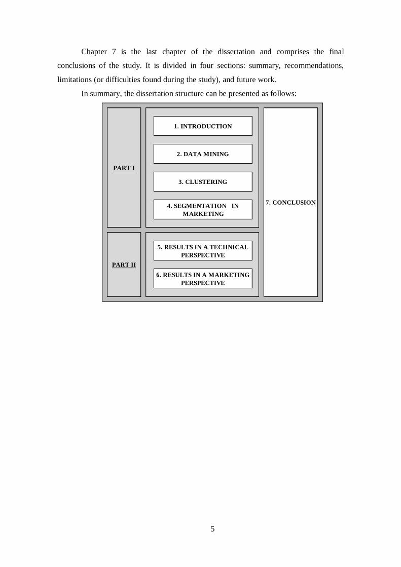
Chapter 7 is the last chapter of the dissertation and comprises the final
conclusions of the study. It is divided in four sections: summary, recommendations,
limitations (or difficulties found during the study), and future work.
In summary, the dissertation structure can be presented as follows:
1. INTRODUCTION
2. DATA MINING
3. CLUSTERING
4. SEGMENTATION IN
MARKETING
5. RESULTS IN A TECHNICAL
PERSPECTIVE
6. RESULTS IN A MARKETING
PERSPECTIVE
PART I
7. CONCLUSION
PART II

7
2. DATA MINING
“Almost all quality improvement comes via
Simplification of design, manufacturing
...layout, processes, and procedures.”
By Tom Peters, an American businessman
2.1. Data Mining Definition
According to Berry and Linoff (1997) Data Mining is “the exploration and
analysis, by automatic or semiautomatic means, of large quantities of data in order to
discover meaningful patterns and rules.” They assume that “the goal of data mining is to
allow a corporation to improve its marketing, sales, and customer support operations
through better understanding of its customers.”
Another widely used definition, even by Berry and Linoff (1997), is the one
given by the Gartner Group which says that “DM is the process of discovering
meaningful new correlations, patterns, and trends by sifting through large amounts of
data stored in repositories and by using pattern recognition technologies as well as
statistical and mathematical techniques.”
8
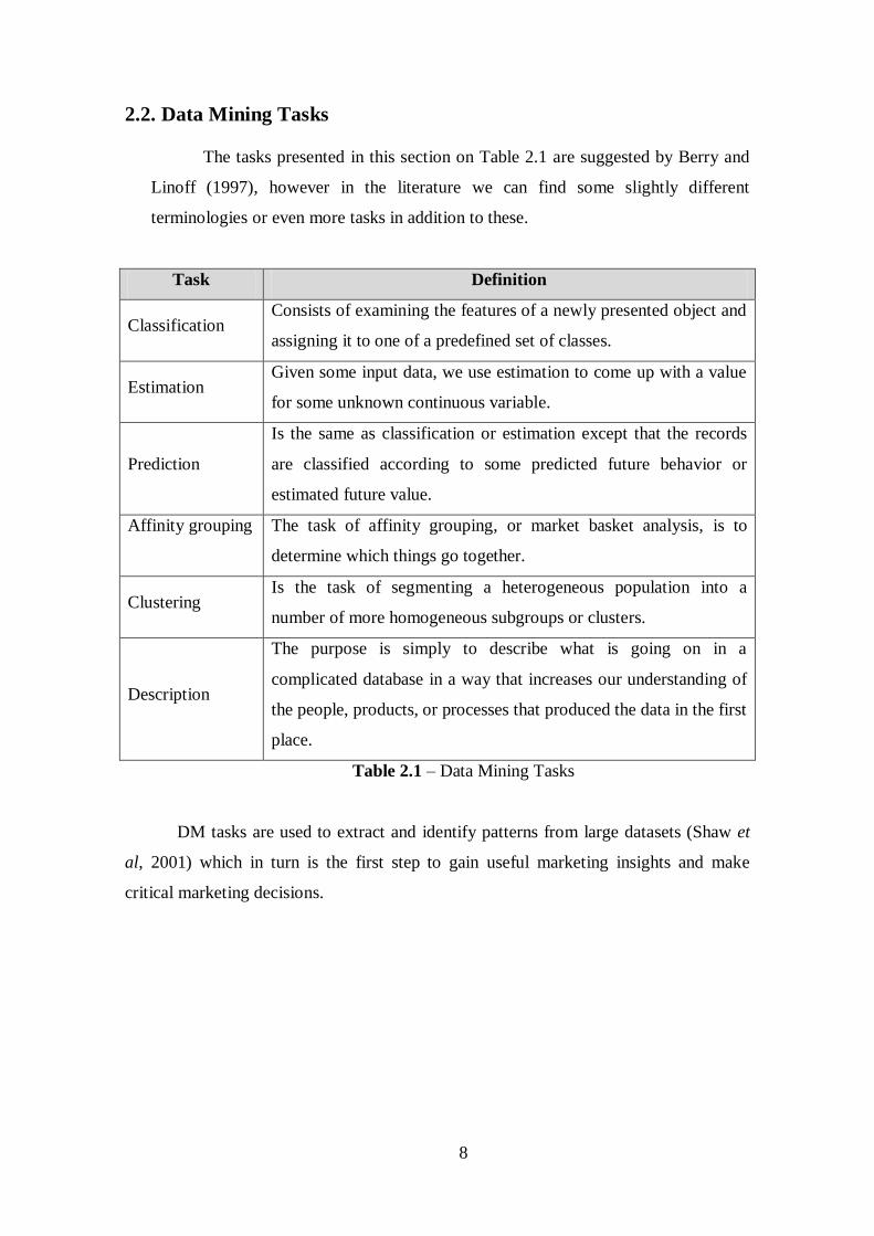
2.2. Data Mining Tasks
The tasks presented in this section on Table 2.1 are suggested by Berry and
Linoff (1997), however in the literature we can find some slightly different
terminologies or even more tasks in addition to these.
Task Definition
Classification Consists of examining the features of a newly presented object and
assigning it to one of a predefined set of classes.
Estimation Given some input data, we use estimation to come up with a value
for some unknown continuous variable.
Prediction
Is the same as classification or estimation except that the records
are classified according to some predicted future behavior or
estimated future value.
Affinity grouping
The task of affinity grouping, or market basket analysis, is to
determine which things go together.
Clustering Is the task of segmenting a heterogeneous population into a
number of more homogeneous subgroups or clusters.
Description
The purpose is simply to describe what is going on in a
complicated database in a way that increases our understanding of
the people, products, or processes that produced the data in the first
place.
Table 2.1 – Data Mining Tasks
DM tasks are used to extract and identify patterns from large datasets (Shaw et
al, 2001) which in turn is the first step to gain useful marketing insights and make
critical marketing decisions.
9
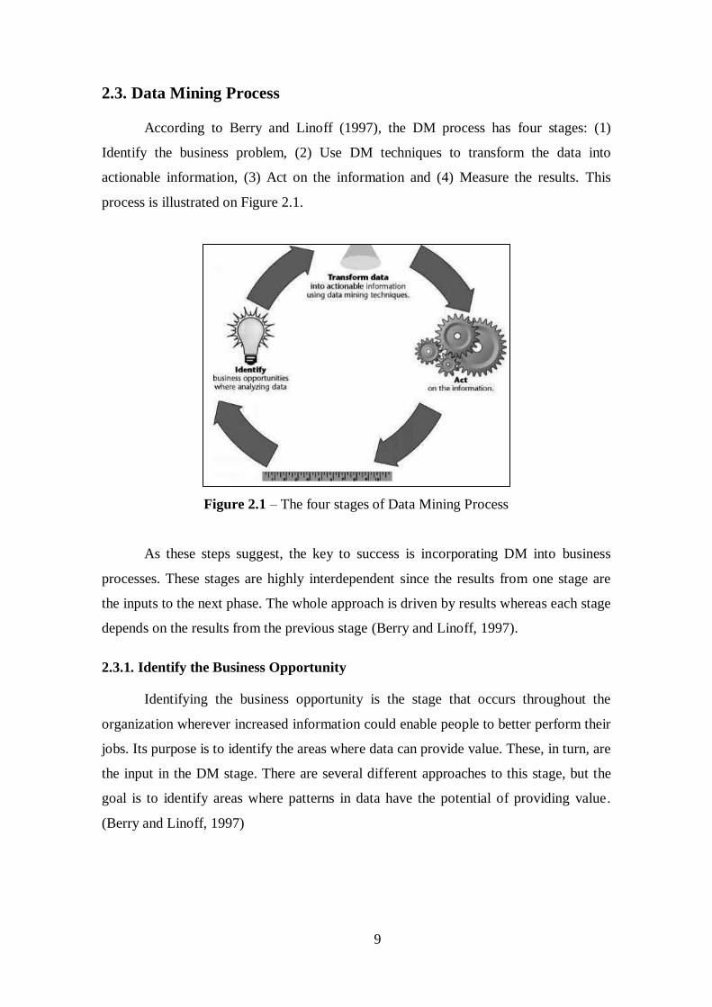
2.3. Data Mining Process
According to Berry and Linoff (1997), the DM process has four stages: (1)
Identify the business problem, (2) Use DM techniques to transform the data into
actionable information, (3) Act on the information and (4) Measure the results. This
process is illustrated on Figure 2.1.
Figure 2.1 – The four stages of Data Mining Process
As these steps suggest, the key to success is incorporating DM into business
processes. These stages are highly interdependent since the results from one stage are
the inputs to the next phase. The whole approach is driven by results whereas each stage
depends on the results from the previous stage (Berry and Linoff, 1997).
2.3.1. Identify the Business Opportunity
Identifying the business opportunity is the stage that occurs throughout the
organization wherever increased information could enable people to better perform their
jobs. Its purpose is to identify the areas where data can provide value. These, in turn, are
the input in the DM stage. There are several different approaches to this stage, but the
goal is to identify areas where patterns in data have the potential of providing value.
(Berry and Linoff, 1997)
10
2.3.2. Transform Data using Data Mining Techniques
DM takes data, business opportunities and produces actionable results for the
Take Action stage. However, it is important to understand what results it must give to
make the DM process successful and also to pay attention to the numerous problems
that can interfere with it. Some usual problems are, for example, bad data formats,
confusing data fields, lack of functionality, timeliness (Berry and Linoff, 1997).
2.3.3. Take Action
This is where the results from DM are acted upon and results are fed into the
Measurement stage. The question here is how to incorporate information into business
processes. The business processes must provide the data feedback needed for the DM
process be successful (Berry and Linoff, 1997).
2.3.4. Measure the Results
Measurement provides the feedback for continuously improving results.
Measurement here refers specifically to measures of business value that go beyond
response rates and costs, beyond averages and standard deviations. The question here is
what to measure and how to approach the measurement so it provides the best input for
future use. The specific measurements needed depend on a number of factors: the
business opportunity, the sophistication of the organization, past history of
measurements (for trend analysis), and the availability of data. We can see that this
stage depends critically on information provided in the previous stages (Berry and
Linoff, 1997).
In short, DM process places DM into a context for creating business value. In
the business world, DM provides the ability to optimize decision-making using
automated methods to learn from past actions. Different organizations adapt DM to their
own environment, in their own way (Berry and Linoff, 1997).
11
2.4. Data Mining Methodology
DM methodology refers to stage two of DM process, i.e., the stage where the
actual mining of data takes place and where the resulting information is smelted to
produce knowledge (Berry and Linoff, 1997).
There are, essentially, two basic approaches of DM, the hypothesis testing and
the knowledge discovery. The first is a top-down approach that attempts to substantiate
or disprove preconceived ideas. The second is a bottom-up approach that starts with the
data and tries to get it to tell us something we didn´t already know (Berry and Linoff,
1997).
2.4.1. Hypothesis Testing
A hypothesis is a proposed explanation whose validity can be tested. Testing the
validity of a hypothesis is done by analyzing data that may simply be collected by
observation or generated through an experiment, such as test mailing (Berry and Linoff,
1997).
The process of hypotheses testing comprises the following steps: (1) Generate
good ideas (hypothesis); (2) Determine what data would allow these hypotheses to be
tested; (3) Locate data; (4) Prepare data for analysis; (5) Build computer models based
on the data; (6) Evaluate computer models to confirm or reject hypotheses (Berry and
Linoff, 1997).
2.4.2. Knowledge Discovery
Knowledge discovery can be either directed or undirected. In the first, the task is
to explain the value of some particular field in terms of all the others; we select the
target field and direct the computer to tell us how to estimate, classify, or predict it. In
the second, there is no target field; we ask the computer to identify patterns in the data
that may be significant (Berry and Linoff, 1997). In other words, we use undirected KD
to recognize relationships in the data and directed KD to explain those relationships
once they have been found (Berry and Linoff, 1997).
12
2.4.2.1. Directed Knowledge Discovery
Directed KD is characterized by the presence of a single target field whose value
is to be predicted in terms of the other fields in the database (Berry and Linoff, 1997). It
is the process of finding meaningful patterns in data that explain past events in such a
way we can use the patterns to help predict future events (Berry and Linoff, 1997).
The steps of this process are: (1) Identify sources of preclassified data; (2)
Prepare data for analysis; (3) Build and train a computer model; and (4) Evaluate the
computer model (Berry and Linoff, 1997).
2.4.2.2. Undirected Knowledge Discovery
Undirected KD is different from directed KD, in the way that there is no target
field. The DM tool is simply let loose on the data in the hope that it will discover
meaningful structure (Berry and Linoff, 1997).
The process of undirected KD have the following steps: (1) Identify sources of
data; (2) Prepare data for analysis; (3) Build and train a computer model; (4) Evaluate
the computer model; (5) Apply computer model to new data; (6) Identify potential
targets for directed KD; and (7) Generate new hypothesis to test (Berry and Linoff,
1997).
In this work the DM methodology used was the undirected KD, more precisely,
the CRISP-DM methodology. This methodology and its different steps are described in
Annex B.
13
3. CLUSTERING
“Science never solves a problem
without creating ten more.”
By George Bernard Shaw, an Irish dramatist
3.1. Clustering Definition
According to Velmurugan and Santhanam (2010) clustering consists of “creating
groups of objects based on their features in such a way that the objects belonging to the
same groups are similar and those belonging to different groups are dissimilar.”
In operational terms, clustering can be defined as follows: “Given a
representation of n objects, find k groups based on a measure of similarity such that the
similarities between objects in the same group are high while the similarities between
objects in different groups are low” (Jain, 2009).
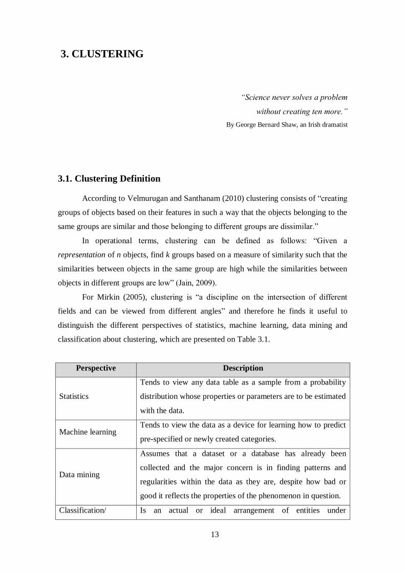
For Mirkin (2005), clustering is “a discipline on the intersection of different
fields and can be viewed from different angles” and therefore he finds it useful to
distinguish the different perspectives of statistics, machine learning, data mining and
classification about clustering, which are presented on Table 3.1.
Perspective Description
Statistics
Tends to view any data table as a sample from a probability
distribution whose properties or parameters are to be estimated
with the data.
Machine learning Tends to view the data as a device for learning how to predict
pre-specified or newly created categories.
Data mining
Assumes that a dataset or a database has already been
collected and the major concern is in finding patterns and
regularities within the data as they are, despite how bad or
good it reflects the properties of the phenomenon in question.
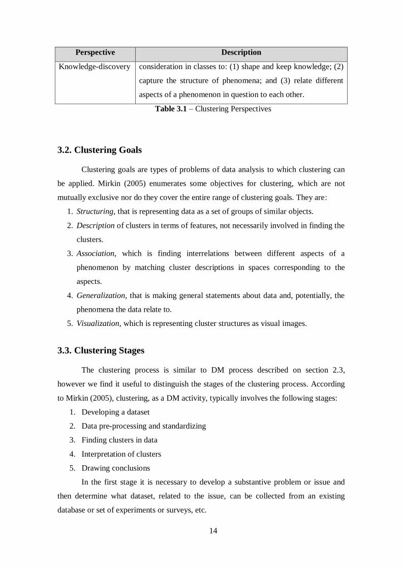
Classification/ Is an actual or ideal arrangement of entities under
14
Perspective Description
Knowledge-discovery consideration in classes to: (1) shape and keep knowledge; (2)
capture the structure of phenomena; and (3) relate different
aspects of a phenomenon in question to each other.
Table 3.1 – Clustering Perspectives
3.2. Clustering Goals
Clustering goals are types of problems of data analysis to which clustering can
be applied. Mirkin (2005) enumerates some objectives for clustering, which are not
mutually exclusive nor do they cover the entire range of clustering goals. They are:
1. Structuring, that is representing data as a set of groups of similar objects.
2. Description of clusters in terms of features, not necessarily involved in finding the
clusters.
3. Association, which is finding interrelations between different aspects of a
phenomenon by matching cluster descriptions in spaces corresponding to the
aspects.
4. Generalization, that is making general statements about data and, potentially, the
phenomena the data relate to.
5. Visualization, which is representing cluster structures as visual images.
3.3. Clustering Stages
The clustering process is similar to DM process described on section 2.3,
however we find it useful to distinguish the stages of the clustering process. According
to Mirkin (2005), clustering, as a DM activity, typically involves the following stages:
1. Developing a dataset
2. Data pre-processing and standardizing
3. Finding clusters in data
4. Interpretation of clusters
5. Drawing conclusions
In the first stage it is necessary to develop a substantive problem or issue and
then determine what dataset, related to the issue, can be collected from an existing
database or set of experiments or surveys, etc.

15
The second is the stage of preparing data processing by a clustering algorithm. It
normally includes developing a uniform dataset from a database, checking for missing
or unreliable entries, rescaling and standardizing variables, deriving a unified similarity
measure, etc.
Finding clusters in data is the third stage and involves the application of a
clustering algorithm which results in a cluster structure1 to be presented, along with
interpretation aids, to substantive specialists for an expert judgment and interpretation.
At this stage, the expert may not see relevance in the results and suggest a modification
of the data by adding/removing features and/or entities. The modified data is subject to
the same processing procedure.
The final stage is drawing conclusions from the interpretation of the results
regarding the issue in question. The more focused the regularities are implied in the
findings, the better the quality of conclusions are.
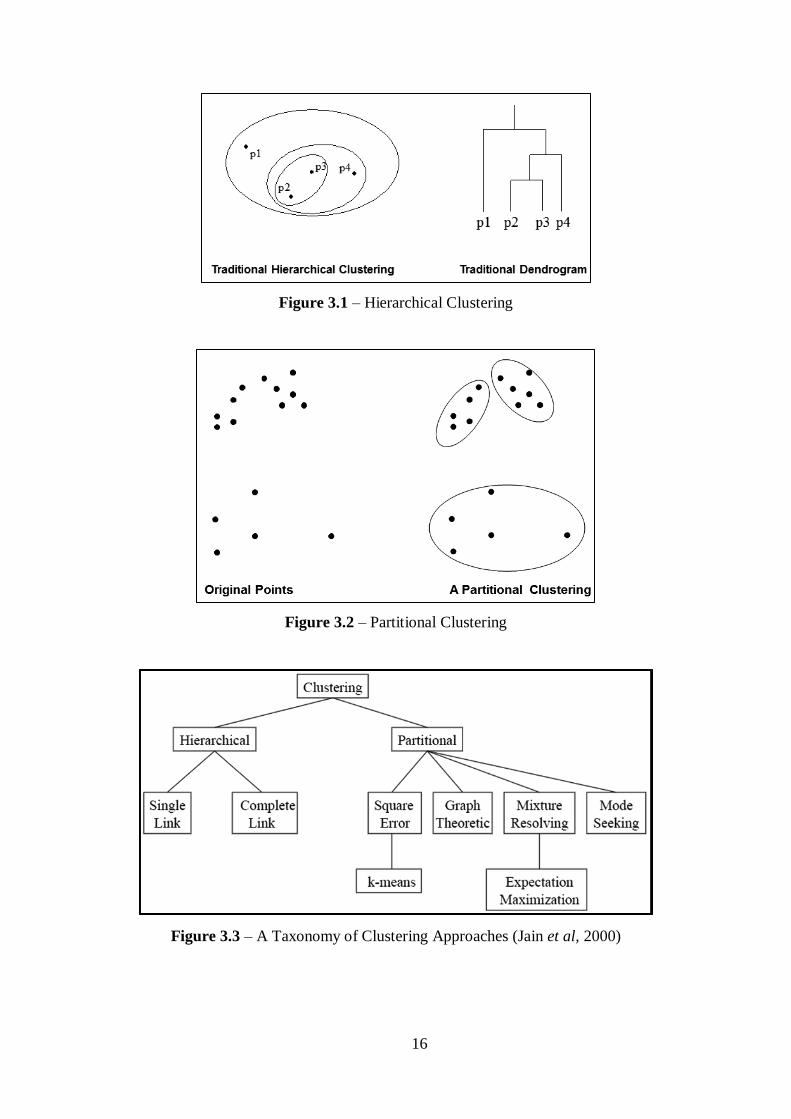
3.4. Clustering Algorithms
Clustering algorithms can be divided in two groups: (1) hierarchical and (2)
partitional. Hierarchical clustering algorithms (Figure 3.1) recursively find nested
clusters either in agglomerative mode (starting with each data point in its own cluster
and merging the most similar pair of clusters successively to form a cluster hierarchy)
or in divisive (top-down) mode (starting with all the data points in one cluster and
recursively dividing each cluster into smaller clusters). Partitional clustering algorithms
(Figure 3.2) find all the clusters simultaneously as a partition of the data and do not
impose a hierarchical structure (Jain, 2009).
Input to a hierarchical algorithm is a n x n similarity matrix, where n is the
number of objects to be clustered while a partitional algorithm can either use a n x d
pattern matrix, where n objects are embedded in a d-dimensional feature space, or a n x
n similarity matrix (Jain, 2009)
The most well-known hierarchical algorithms are single-link and complete-link
(Jain 2009) and the most popular and simplest partitional algorithm is K-Means. Figure
3.3 synthetizes these clustering approaches.
1 According to Mirkin (2005), a cluster structure is “a representation of an entity set I as a set of clusters
16
Figure 3.1 – Hierarchical Clustering
Figure 3.2 – Partitional Clustering
Figure 3.3 – A Taxonomy of Clustering Approaches (Jain et al, 2000)
17
3.4.1. K-Means Clustering
K-Means is one of the most widely used algorithms for clustering. The main
reasons for its popularity are: (1) ease of implementation, (2) simplicity, (3) efficiency,
and (4) empirical success (Jain, 2009). Likewise, Mirkin (2005) finds K-Means
computationally easy, fast and memory-efficient. However, he points out some
problems related to the initial setting and stability of results.
Mirkin (2005) defines and resumes K-Means as “a major clustering method
producing a partition of the entity set into non-overlapping clusters along with within-
cluster centroids2. It proceeds in iterations consisting of two steps each: one step
updates clusters according to the minimum distance rule3; the other step updates
centroids as the centers of gravity of clusters. The method implements the so-called
alternating minimization algorithm for the square error criterion4. To initialize the
computations, either a partition or a set of all k tentative centroids must be specified.”
An example of a K-Means algorithm is given by Jain (2009) and is described as
follows:
Let { }, i = 1,…, n be the set of n d-dimensional points to be clustered into
a set of K clusters, { }, k = 1,…, K. K-Means algorithm finds a partition such that
the squared error between the empirical mean of a cluster and the points in the cluster is
minimized. Let µk be the mean of cluster ck. The squared error between µk and the points
in cluster ck is defined as ( ) ∑
. The goal of K-Means is to
minimize the sum of the squared error over all the k clusters,
( ) ∑ ∑
. K-Means starts with an initial partition with K
clusters and assign patterns to clusters so as to reduce the squared error. Since the
squared error always decreases with an increase in the number of clusters K (with J(C) =
0 when K = n), it can be minimized only for a fixed number of clusters.
2 According to Mirkin (2005), a centroid is a multidimensional vector minimizing the summary distance
to cluster’s elements. If the distance is Euclidean squared, the centroid is equal to the center of gravity of
the cluster. 3 According to Mirkin (2005), minimum distance rule is the rule which assigns each of the entities to its
nearest centroid. 4 According to Mirkin (2005), the square error criterion is the sum of summary distances from cluster
centroids, which is minimized by K-means. The distance used is the Euclidean distance squared which is
expressed by the equation ( ) ∑ ( )
(Hastie et al, 2001).
18
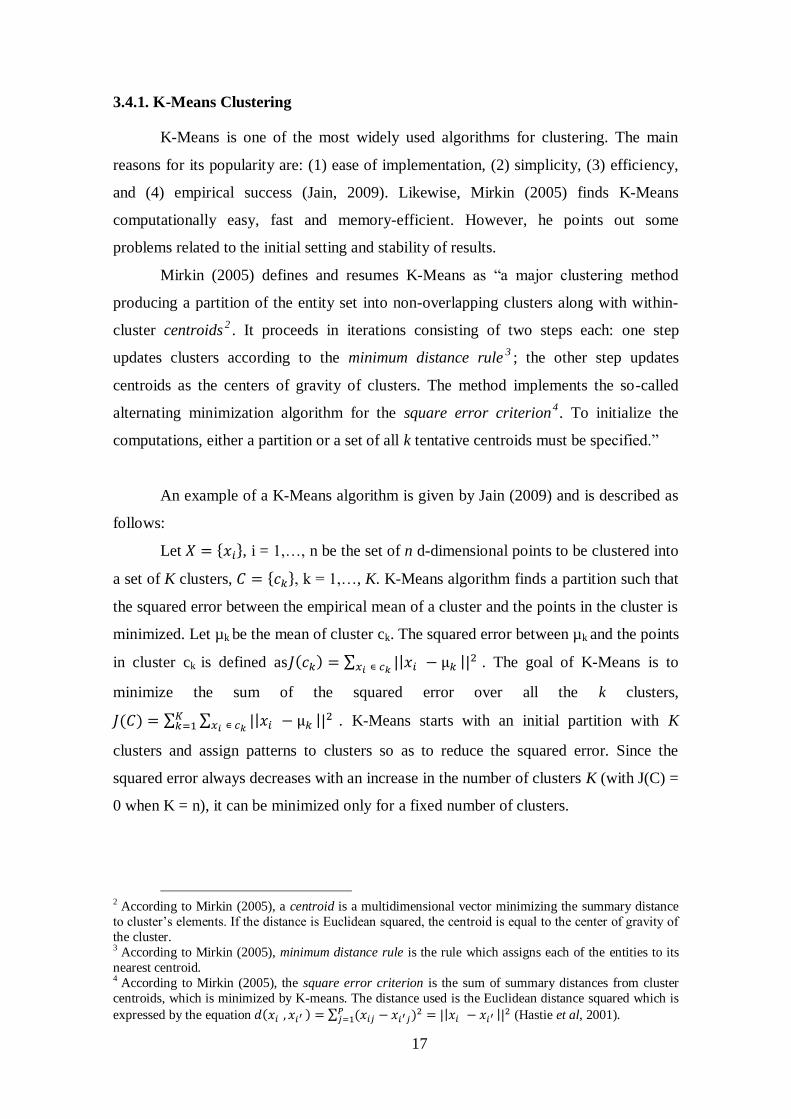
So, the main steps of K-Means algorithm are:
1. Select an initial partition with k clusters (repeat steps 2 and 3 until cluster
membership stabilizes).
2. Generate a new partition by assigning each pattern to its closest cluster center.
3. Compute new cluster centers.
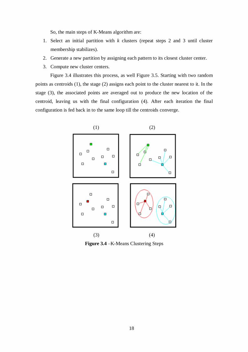
Figure 3.4 illustrates this process, as well Figure 3.5. Starting with two random
points as centroids (1), the stage (2) assigns each point to the cluster nearest to it. In the
stage (3), the associated points are averaged out to produce the new location of the
centroid, leaving us with the final configuration (4). After each iteration the final
configuration is fed back in to the same loop till the centroids converge.
(1) (2)
(3) (4)
Figure 3.4 –K-Means Clustering Steps
19
Figure 3.5 – K-Means Algorithm Process
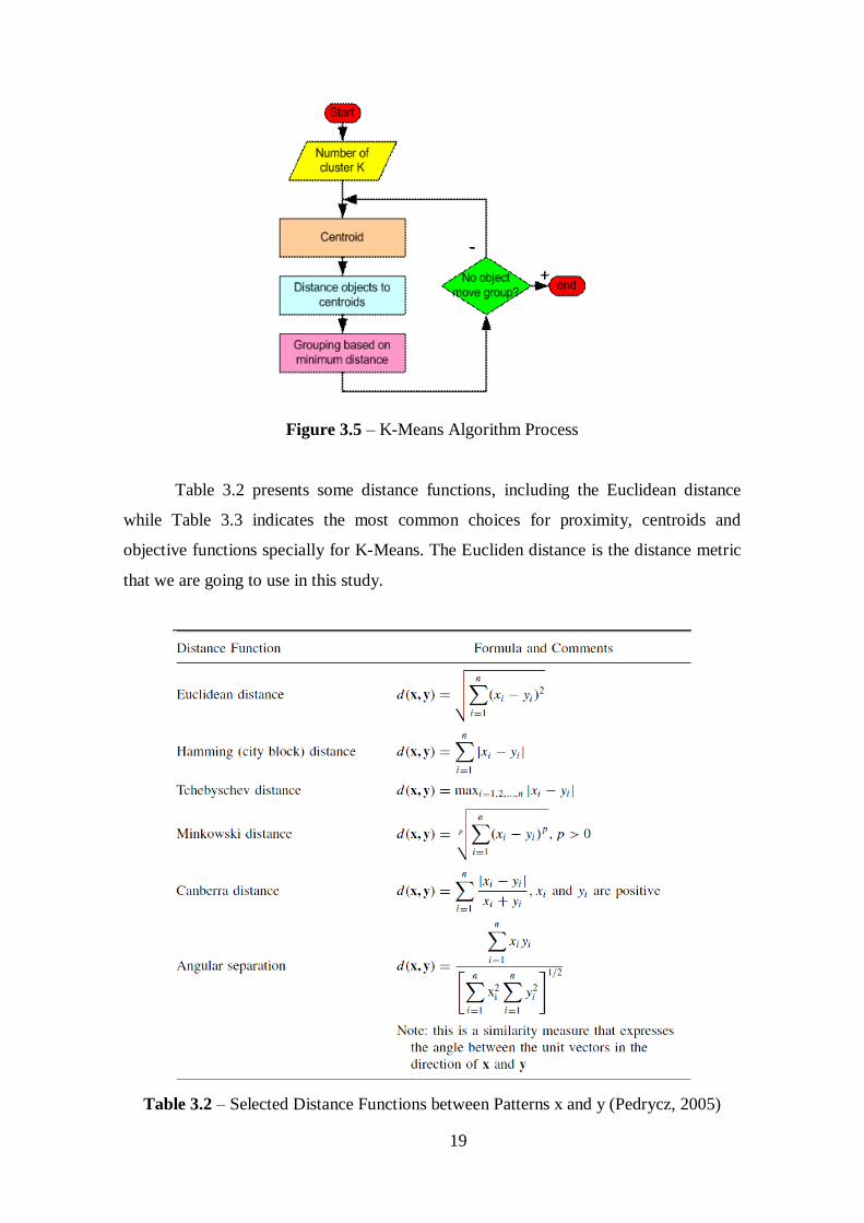
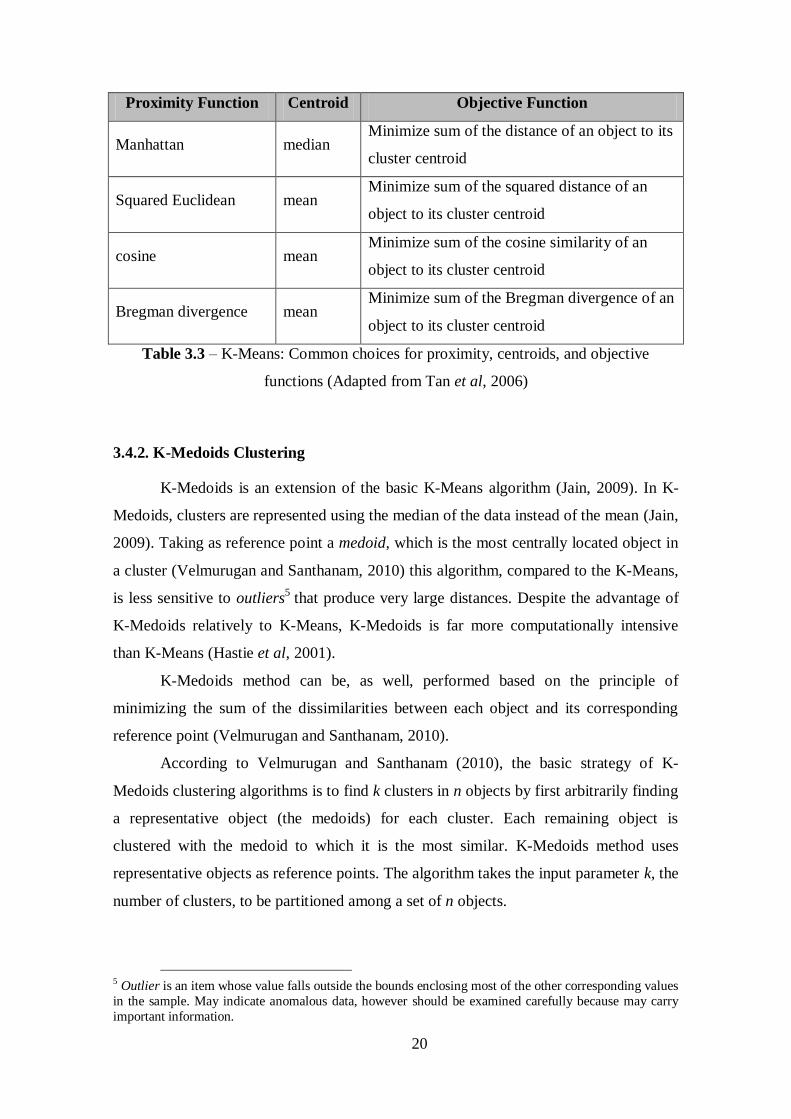
Table 3.2 presents some distance functions, including the Euclidean distance
while Table 3.3 indicates the most common choices for proximity, centroids and
objective functions specially for K-Means. The Eucliden distance is the distance metric
that we are going to use in this study.
Table 3.2 – Selected Distance Functions between Patterns x and y (Pedrycz, 2005)
20
Proximity Function Centroid Objective Function
Manhattan median Minimize sum of the distance of an object to its
cluster centroid
Squared Euclidean mean Minimize sum of the squared distance of an
object to its cluster centroid
cosine mean Minimize sum of the cosine similarity of an
object to its cluster centroid
Bregman divergence mean Minimize sum of the Bregman divergence of an
object to its cluster centroid
Table 3.3 – K-Means: Common choices for proximity, centroids, and objective
functions (Adapted from Tan et al, 2006)
3.4.2. K-Medoids Clustering
K-Medoids is an extension of the basic K-Means algorithm (Jain, 2009). In K-
Medoids, clusters are represented using the median of the data instead of the mean (Jain,
2009). Taking as reference point a medoid, which is the most centrally located object in
a cluster (Velmurugan and Santhanam, 2010) this algorithm, compared to the K-Means,
is less sensitive to outliers5 that produce very large distances. Despite the advantage of
K-Medoids relatively to K-Means, K-Medoids is far more computationally intensive
than K-Means (Hastie et al, 2001).
K-Medoids method can be, as well, performed based on the principle of
minimizing the sum of the dissimilarities between each object and its corresponding
reference point (Velmurugan and Santhanam, 2010).
According to Velmurugan and Santhanam (2010), the basic strategy of K-
Medoids clustering algorithms is to find k clusters in n objects by first arbitrarily finding
a representative object (the medoids) for each cluster. Each remaining object is
clustered with the medoid to which it is the most similar. K-Medoids method uses
representative objects as reference points. The algorithm takes the input parameter k, the
number of clusters, to be partitioned among a set of n objects.
5 Outlier is an item whose value falls outside the bounds enclosing most of the other corresponding values
in the sample. May indicate anomalous data, however should be examined carefully because may carry
important information.
21
Velmurugan and Santhanam (2010) present a typical K-Medoids algorithm for
partitioning based on medoid, as follows:
Input: K = number of clusters and D = dataset containing n objects
Output: A set of k clusters that minimizes the sum of the dissimilarities of all the
objects to their nearest medoid.
Method: Arbitrarily choose k objects in D as the initial representative objects.
Repeat: Assign each remaining object to the cluster with the nearest medoid;
Randomly select a non medoid object Orandom; Compute the total points S of swap point
Oj with Orandom; If S<0 then swap Oj with Orandom to form the new set of k medoid until
no change.
Velmurugan and Santhanam (2010) compared the two algotrithms and
concluded that “K-Means algorithm is more efficient for smaller datasets and K-
Medoids algorithm seems to perform better for large datasets.”
3.5. Cluster Validity
After applying a clustering algorithm, we would like to know if the results
reflect or not an innate property of the data (Mirkin, 2005). In other words, we want to
know whether the cluster structure found is valid or not (Mirkin, 2005).
So, cluster validity refers to formal procedures that evaluate the results of cluster
analysis in a quantitative and objective manner (Jain, 2009). Before a clustering
algorithm is applied to the data, we should determine if data has, in fact, a clustering
tendency6 (Jain, 2009).
In literature we can find several measures for cluster validation, including many
cluster validity indices which can be defined based on three different criteria: internal,
relative or external (Jain, 2009). Internal indices assess the fit between the structured
imposed by the clustering algorithm (clustering) and the data using only the data. The
better the indices value, the more reliable is the cluster structure Mirkin (2005). Relative
indices compare multiple structures (generated by different algorithms, for example)
and decide which of them is better in some sense. External indices measure the
performance by matching cluster structure to the a priori information. Typically,
clustering results are evaluated using the external criterion.
6 Mirkin (2005) defines cluster tendency as a description of a cluster in terms of the advantage values of
relevant features.
22
Furthermore, according to Mirkin (2005), it is still possible to use another
procedure for validating a cluster structure or clustering algorithm, it is called
resampling. A resampling is used to see whether the cluster structure is stable when the
data is changed. The cluster stability is measured as the amount of variation in the
clustering solution over different subsamples drawn from the input data and different
measures of that variation can be used to obtain different stability measures (Jain,
2009). For instance, in model based algorithms, as K-Means, the distance between the
models found for different subsamples can be used to measure the stability.
In general, cluster validity indices are usually defined by combining
compactness and separability. Compactness measures the closeness of cluster elements,
being a common measure of that the variance. Separability indicates how distinct two
clusters are being the distance between representative objects of two clusters a good
example. This measure has been widely used due to its computational efficiency and
effectiveness (Rendón et al, 2011).
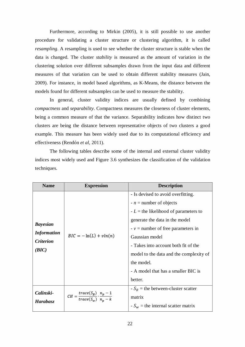
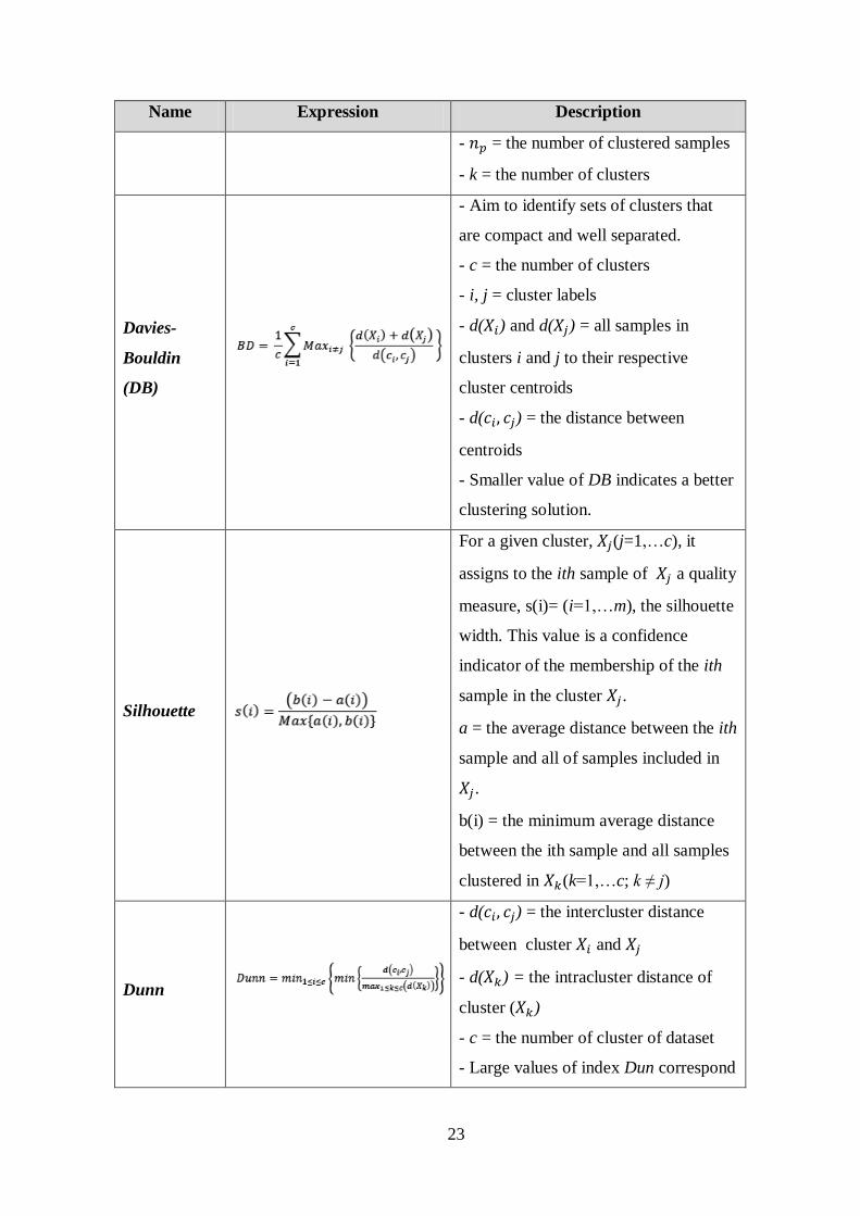
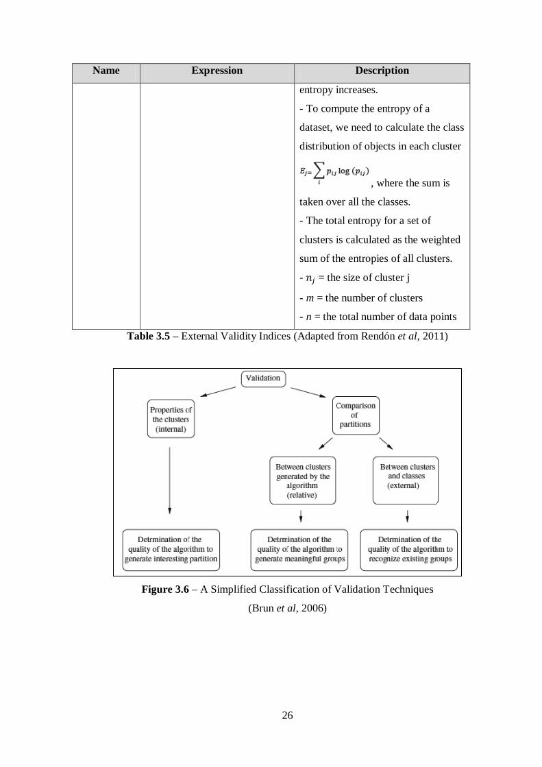
The following tables describe some of the internal and external cluster validity
indices most widely used and Figure 3.6 synthesizes the classification of the validation
techniques.
Name Expression Description
Bayesian
Information
Criterion
(BIC)
- Is devised to avoid overfitting.
- n = number of objects
- L = the likelihood of parameters to
generate the data in the model
- v = number of free parameters in
Gaussian model
- Takes into account both fit of the
model to the data and the complexity of
the model.
- A model that has a smaller BIC is
better.
Calinski-
Harabasz
- = the between-cluster scatter
matrix
- = the internal scatter matrix
23
Name Expression Description
- = the number of clustered samples
- k = the number of clusters
Davies-
Bouldin
(DB)
- Aim to identify sets of clusters that
are compact and well separated.
- c = the number of clusters
- i, j = cluster labels
- d( ) and d( ) = all samples in
clusters i and j to their respective
cluster centroids
- d( ) = the distance between
centroids
- Smaller value of DB indicates a better
clustering solution.
Silhouette
For a given cluster, (j=1,…c), it
assigns to the ith sample of a quality
measure, s(i)= (i=1,…m), the silhouette
width. This value is a confidence
indicator of the membership of the ith
sample in the cluster .
a = the average distance between the ith
sample and all of samples included in
.
b(i) = the minimum average distance
between the ith sample and all samples
clustered in (k=1,…c; k ≠ j)
Dunn
- d( ) = the intercluster distance
between cluster and
- d( ) = the intracluster distance of
cluster ( )
- c = the number of cluster of dataset
- Large values of index Dun correspond
24
Name Expression Description
to good clustering solution.
NIVA
- { }
- (i=1,2,…,N)
-N = the number cluster from C
- Compac (C): average of compactness
product (Esp( )) of c groups and
separability between them (SepxS( ))
- SepxG (C): average separability of C
groups
- The smaller value NIVA(C) indicates
that avalid optimal partition to the
different given partitions was found.
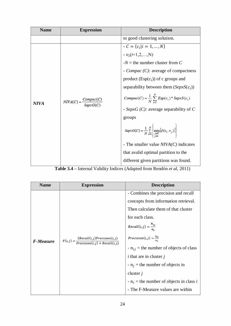
Table 3.4 – Internal Validity Indices (Adapted from Rendón et al, 2011)
Name Expression Description
F-Measure
- Combines the precision and recall
concepts from information retrieval.
Then calculate them of that cluster
for each class.
- = the number of objects of class
i that are in cluster j
- = the number of objects in
cluster j
- = the number of objects in class i
- The F-Measure values are within
25
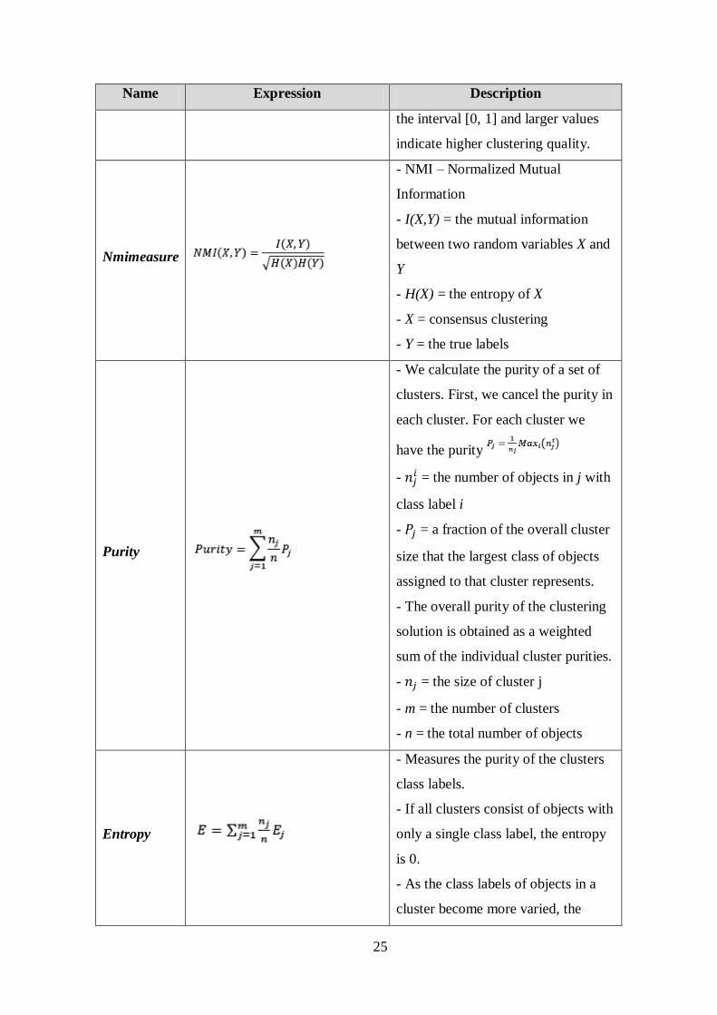
Name Expression Description
the interval [0, 1] and larger values
indicate higher clustering quality.
Nmimeasure
- NMI – Normalized Mutual
Information
- I(X,Y) = the mutual information
between two random variables X and
Y
- H(X) = the entropy of X
- X = consensus clustering
- Y = the true labels
Purity
- We calculate the purity of a set of
clusters. First, we cancel the purity in
each cluster. For each cluster we
have the purity
- = the number of objects in j with
class label i
- = a fraction of the overall cluster
size that the largest class of objects
assigned to that cluster represents.
- The overall purity of the clustering
solution is obtained as a weighted
sum of the individual cluster purities.
- = the size of cluster j
- m = the number of clusters
- n = the total number of objects
Entropy
- Measures the purity of the clusters
class labels.
- If all clusters consist of objects with
only a single class label, the entropy
is 0.
- As the class labels of objects in a
cluster become more varied, the
26
Name Expression Description
entropy increases.
- To compute the entropy of a
dataset, we need to calculate the class
distribution of objects in each cluster
, where the sum is
taken over all the classes.
- The total entropy for a set of
clusters is calculated as the weighted
sum of the entropies of all clusters.
- = the size of cluster j
- m = the number of clusters
- n = the total number of data points
Table 3.5 – External Validity Indices (Adapted from Rendón et al, 2011)
Figure 3.6 – A Simplified Classification of Validation Techniques
(Brun et al, 2006)
27
4. SEGMENTATION IN MARKETING
“Do not buy market share.
Figure out how to earn it.”
Philip Kotler in Marketing Management, 11th Edition
4.1. Segmentation Definition
Kotler (2005) defines market segmentation as “the act of dividing a market into
smaller groups of buyers with distinct needs, characteristics, or behaviors who might
require separate products and/or marketing mixes.” Despite that definition, there is
another one that is considered the best by marketers given by Smith (1956): “market
segmentation involves viewing a heterogeneous market as a number of smaller
homogeneous markets, in response to differing preferences, attributable to the desires of
consumers for more precise satisfaction of their varying wants.”
According to Wedel and Kamakura (2002), in market segmentation one
distinguishes homogeneous groups of customers who can be targeted in the same
manner because they have similar needs and preferences. For them, market segments are
not real entities naturally occurring in the marketplace, but groupings created by
managers to help them develop strategies that better meet consumer needs at the highest
expected profit for the company. Therefore, segmentation is a very useful concept to
managers.
4.2. Segmentation Effectiveness
According to Kotler (2000), an effective segmentation must meet some criteria.
The segments must be measurable (the size, purchasing power, profiles of segments can
be measure), substantial (segments must be large or profitable enough to serve),
accessible (segments must be effectively reached and served), differentiable (segments
must respond differently to different marketing mix elements and actions), and
actionable (must be able to attract and serve the segments).
28
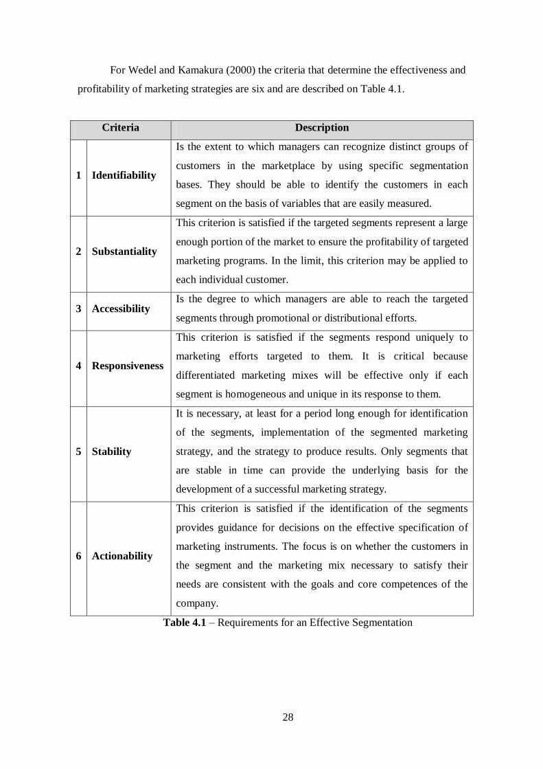
For Wedel and Kamakura (2000) the criteria that determine the effectiveness and
profitability of marketing strategies are six and are described on Table 4.1.
Criteria Description
1 Identifiability
Is the extent to which managers can recognize distinct groups of
customers in the marketplace by using specific segmentation
bases. They should be able to identify the customers in each
segment on the basis of variables that are easily measured.
2 Substantiality
This criterion is satisfied if the targeted segments represent a large
enough portion of the market to ensure the profitability of targeted
marketing programs. In the limit, this criterion may be applied to
each individual customer.
3 Accessibility Is the degree to which managers are able to reach the targeted
segments through promotional or distributional efforts.
4 Responsiveness
This criterion is satisfied if the segments respond uniquely to
marketing efforts targeted to them. It is critical because
differentiated marketing mixes will be effective only if each
segment is homogeneous and unique in its response to them.
5 Stability
It is necessary, at least for a period long enough for identification
of the segments, implementation of the segmented marketing
strategy, and the strategy to produce results. Only segments that
are stable in time can provide the underlying basis for the
development of a successful marketing strategy.
6 Actionability
This criterion is satisfied if the identification of the segments
provides guidance for decisions on the effective specification of
marketing instruments. The focus is on whether the customers in
the segment and the marketing mix necessary to satisfy their
needs are consistent with the goals and core competences of the
company.
Table 4.1 – Requirements for an Effective Segmentation
29
4.3. Segmentation Process
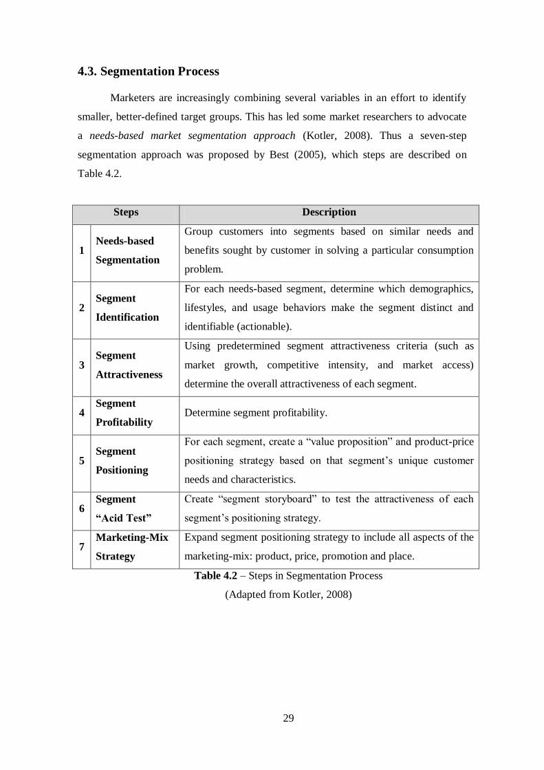
Marketers are increasingly combining several variables in an effort to identify
smaller, better-defined target groups. This has led some market researchers to advocate
a needs-based market segmentation approach (Kotler, 2008). Thus a seven-step
segmentation approach was proposed by Best (2005), which steps are described on
Table 4.2.
Steps Description
1 Needs-based
Segmentation
Group customers into segments based on similar needs and
benefits sought by customer in solving a particular consumption
problem.
2 Segment
Identification
For each needs-based segment, determine which demographics,
lifestyles, and usage behaviors make the segment distinct and
identifiable (actionable).
3 Segment
Attractiveness
Using predetermined segment attractiveness criteria (such as
market growth, competitive intensity, and market access)
determine the overall attractiveness of each segment.
4 Segment
Profitability Determine segment profitability.
5 Segment
Positioning
For each segment, create a “value proposition” and product-price
positioning strategy based on that segment’s unique customer
needs and characteristics.
6 Segment
“Acid Test”
Create “segment storyboard” to test the attractiveness of each
segment’s positioning strategy.
7 Marketing-Mix
Strategy
Expand segment positioning strategy to include all aspects of the
marketing-mix: product, price, promotion and place.
Table 4.2 – Steps in Segmentation Process
(Adapted from Kotler, 2008)
30
4.4. Levels of Market Segmentation
Because buyers have unique needs and wants, each buyer is potentially a
separate market. Ideally, then, a seller might design a separate marketing program for
each buyer. However, although some companies attempt to serve buyers individually,
many others face larger numbers of smaller buyers and do not find complete
segmentation worthwhile. Instead, they look for broader classes of buyers who differ in
their product needs or buying responses. Thus, market segmentation can be carried out
at several different levels (Kotler, 2008).
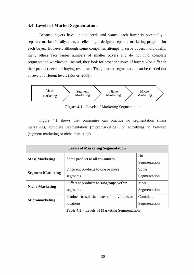
Figure 4.1 – Levels of Marketing Segmentation
Figure 4.1 shows that companies can practice no segmentation (mass
marketing), complete segmentation (micromarketing), or something in between
(segment marketing or niche marketing).
Levels of Marketing Segmentation
Mass Marketing Same product to all consumers No
Segmentation
Segment Marketing Different products to one or more
segments
Some
Segmentation
Niche Marketing Different products to subgroups within
segments
More
Segmentation
Micromarketing Products to suit the tastes of individuals or
locations
Complete
Segmentation
Table 4.3 – Levels of Marketing Segmentation
Mass
Marketing
Segment Marketing
Niche Marketing
Micro Marketing
31
4.4.1. Mass Marketing
Companies have not always practiced target marketing. In fact, for most of the
1900s, major consumer products companies held fast to mass marketing—mass
producing, mass distributing, and mass promoting about the same product in about the
same way to all consumers. The traditional argument for mass marketing is that it
creates the largest potential market, which leads to the lowest costs, which in turn can
translate into either lower prices or higher margins. However, many factors now make
mass marketing more difficult. The proliferation of distribution channels and
advertising media has also made it difficult to practice "one-size-fits-all" marketing
(Kotler, 2008).
4.4.2. Segment Marketing
A company that practices segment marketing isolates broad segments that make
up a market and adapts its offers to more closely match the needs of one or more
segments. Segment marketing offers several benefits over mass marketing. The
company can market more efficiently, targeting its products or services, channels, and
communications programs toward only consumers that it can serve best and most
profitably. The company can also market more effectively by fine-tuning its products,
prices, and programs to the needs of carefully defined segments. The company may face
fewer competitors if fewer competitors are focused on this market segment (Kotler,
2008).
4.4.3. Niche Marketing
Market segments are normally large, identifiable groups within a market. Niche
marketing focuses on subgroups within the segments. A niche is a more narrowly
defined group, usually identified by dividing a segment into sub segments or by
defining a group with a distinctive set of who may seek a special combination of
benefits. Whereas segments are fairly large and normally attract several competitors,
niches are smaller and normally attract only one or a few competitors. Niche marketers
presumably understand their niches' needs so well that their customers willingly pay a
price premium (Kotler, 2008).
32
4.4.4. Micro Marketing
Segment and niche marketers tailor their offers and marketing programs to meet
the needs of various market segments. At the same time, however, they do not
customize their offers to each individual customer. Thus, segment marketing and niche
marketing fall between the extremes of mass marketing and micro marketing. Micro
marketing is the practice of tailoring products and marketing programs to suit the tastes
of specific individuals and locations. Micro marketing includes local marketing
(involves tailoring brands and promotions to the needs and wants of local customer
groups—cities, neighborhoods, and even specific stores) and individual marketing
(tailoring products and marketing programs to the needs and preferences of individual
customers) (Kotler, 2008).
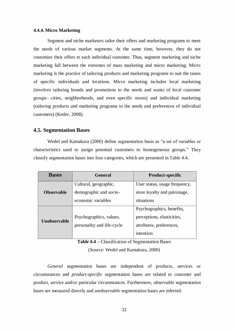
4.5. Segmentation Bases
Wedel and Kamakura (2000) define segmentation basis as “a set of variables or
characteristics used to assign potential customers to homogeneous groups.” They
classify segmentation bases into four categories, which are presented in Table 4.4.
Bases General Product-specific
Observable
Cultural, geographic,
demographic and socio-
economic variables
User status, usage frequency,
store loyalty and patronage,
situations
Unobservable Psychographics, values,
personality and life-cycle
Psychographics, benefits,
perceptions, elasticities,
attributes, preferences,
intention
Table 4.4 – Classification of Segmentation Bases
(Source: Wedel and Kamakura, 2000)
General segmentation bases are independent of products, services or
circumstances and product-specific segmentation bases are related to customer and
product, service and/or particular circumstances. Furthermore, observable segmentation
bases are measured directly and unobservable segmentation bases are inferred.
33
4.5.1. Observable General Bases
In market segmentation, a widely number of bases are used in this category, such
us cultural variables, geographic variables, neighborhood, geographic mobility,
demographic and socio-economic variables, postal code classifications, household life
cycle, household and company size, standard industrial classifications and
socioeconomic variables. Also used are media usage and socioeconomic status (Wedel
and Kamakura, 2000). The observable general bases play an important role in
segmentation studies, whether simple or complex, and are used to enhance the
accessibility of segments derived by other bases (Wedel and Kamakura, 2000).
4.5.2. Observable Product-Specific Bases
This kind of segmentation bases include variables that are related to buying and
consumption behavior, like user status, usage frequency, brand loyalty, store loyalty,
store patronage, stage of adoption and usage situation. These variables have been used
both for consumer and business markets (Wedel and Kamakura, 2000).
4.5.3. Unobservable General Bases
Three groups of variables in this class of segmentation bases are identified: (1)
personality traits, (2) personal values and (3) lifestyle.
The first may include dogmatism, consumerism, locus of control, religion and
cognitive style. The most frequently used scale for measuring general aspects of
personality in marketing is the Edward’s personal schedule.
Relatively to the second, the most important instrument to measure human
values and to identify value systems is the Rokeach value survey.
The third is based on three components: activities (work, hobbies, social events,
vacation, entertainment, clubs, community, shopping, sports), interests (family, home,
job, community, recreation, fashion, food, media, achievements) and opinions (of
oneself, social issues, politics, business, economics, education, products, future,
culture).The lifestyle typology most used is the VALS system, which has been recently
reviewed giving its place to the VALS2 system. It is defined by two main dimensions:
resources (income, education, self-confidence, health, eagerness to buy, intelligence,
etc.) and self-orientation (principle-oriented, self-oriented and status-oriented).These
three groups of variables are used almost exclusively for consumer markets giving us “a
34
more lifelike picture of consumers and a better understanding of their motivations”
(Wedel and Kamakura, 2000).
4.5.4. Unobservable Product-Specific Bases
This class of segmentation bases comprises product-specific psychographics,
product-benefit perceptions and importance, brand attitudes, preferences and behavioral
intentions. In these order, the variables form a hierarchy of effects, as each variable is
influenced by those preceding it. Many of these variables are used for consumer
markets; however they can also be used for segmenting business markets (Wedel and
Kamakura, 2000).
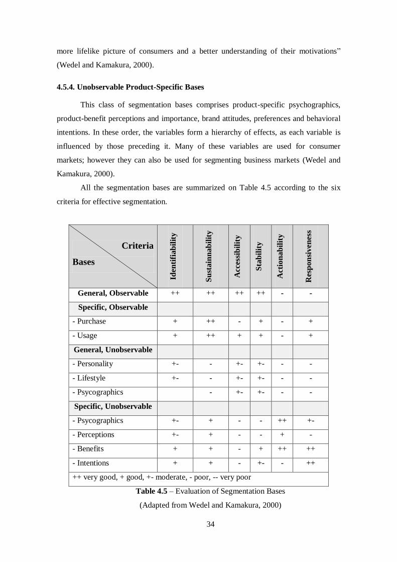
All the segmentation bases are summarized on Table 4.5 according to the six
criteria for effective segmentation.
Criteria
Bases
Iden
tifi
ab
ilit
y
Su
stain
nab
ilit
y
Acc
essi
bil
ity
Sta
bil
ity
Act
ion
ab
ilit
y
Res
pon
siven
ess
General, Observable ++ ++ ++ ++ - -
Specific, Observable
- Purchase + ++ - + - +
- Usage + ++ + + - +
General, Unobservable
- Personality +- - +- +- - -
- Lifestyle +- - +- +- - -
- Psycographics - +- +- - -
Specific, Unobservable
- Psycographics +- + - - ++ +-
- Perceptions +- + - - + -
- Benefits + + - + ++ ++
- Intentions + + - +- - ++
++ very good, + good, +- moderate, - poor, -- very poor
Table 4.5 – Evaluation of Segmentation Bases
(Adapted from Wedel and Kamakura, 2000)
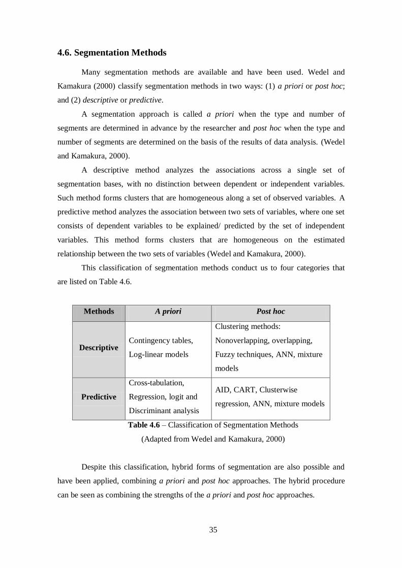
35
4.6. Segmentation Methods
Many segmentation methods are available and have been used. Wedel and
Kamakura (2000) classify segmentation methods in two ways: (1) a priori or post hoc;
and (2) descriptive or predictive.
A segmentation approach is called a priori when the type and number of
segments are determined in advance by the researcher and post hoc when the type and
number of segments are determined on the basis of the results of data analysis. (Wedel
and Kamakura, 2000).
A descriptive method analyzes the associations across a single set of
segmentation bases, with no distinction between dependent or independent variables.
Such method forms clusters that are homogeneous along a set of observed variables. A
predictive method analyzes the association between two sets of variables, where one set
consists of dependent variables to be explained/ predicted by the set of independent
variables. This method forms clusters that are homogeneous on the estimated
relationship between the two sets of variables (Wedel and Kamakura, 2000).
This classification of segmentation methods conduct us to four categories that
are listed on Table 4.6.
Methods A priori Post hoc
Descriptive Contingency tables,
Log-linear models
Clustering methods:
Nonoverlapping, overlapping,
Fuzzy techniques, ANN, mixture
models
Predictive
Cross-tabulation,
Regression, logit and
Discriminant analysis
AID, CART, Clusterwise
regression, ANN, mixture models
Table 4.6 – Classification of Segmentation Methods
(Adapted from Wedel and Kamakura, 2000)
Despite this classification, hybrid forms of segmentation are also possible and
have been applied, combining a priori and post hoc approaches. The hybrid procedure
can be seen as combining the strengths of the a priori and post hoc approaches.
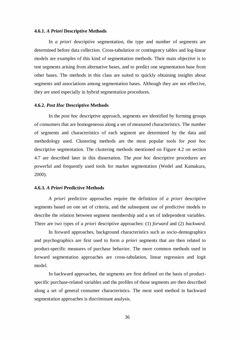
36
4.6.1. A Priori Descriptive Methods
In a priori descriptive segmentation, the type and number of segments are
determined before data collection. Cross-tabulation or contingency tables and log-linear
models are examples of this kind of segmentation methods. Their main objective is to
test segments arising from alternative bases, and to predict one segmentation base from
other bases. The methods in this class are suited to quickly obtaining insights about
segments and associations among segmentation bases. Although they are not effective,
they are used especially in hybrid segmentation procedures.
4.6.2. Post Hoc Descriptive Methods
In the post hoc descriptive approach, segments are identified by forming groups
of consumers that are homogeneous along a set of measured characteristics. The number
of segments and characteristics of each segment are determined by the data and
methodology used. Clustering methods are the most popular tools for post hoc
descriptive segmentation. The clustering methods mentioned on Figure 4.2 on section
4.7 are described later in this dissertation. The post hoc descriptive procedures are
powerful and frequently used tools for market segmentation (Wedel and Kamakura,
2000).
4.6.3. A Priori Predictive Methods
A priori predictive approaches require the definition of a priori descriptive
segments based on one set of criteria, and the subsequent use of predictive models to
describe the relation between segment membership and a set of independent variables.
There are two types of a priori descriptive approaches: (1) forward and (2) backward.
In forward approaches, background characteristics such as socio-demographics
and psychographics are first used to form a priori segments that are then related to
product-specific measures of purchase behavior. The more common methods used in
forward segmentation approaches are cross-tabulation, linear regression and logit
model.
In backward approaches, the segments are first defined on the basis of product-
specific purchase-related variables and the profiles of those segments are then described
along a set of general consumer characteristics. The most used method in backward
segmentation approaches is discriminant analysis.
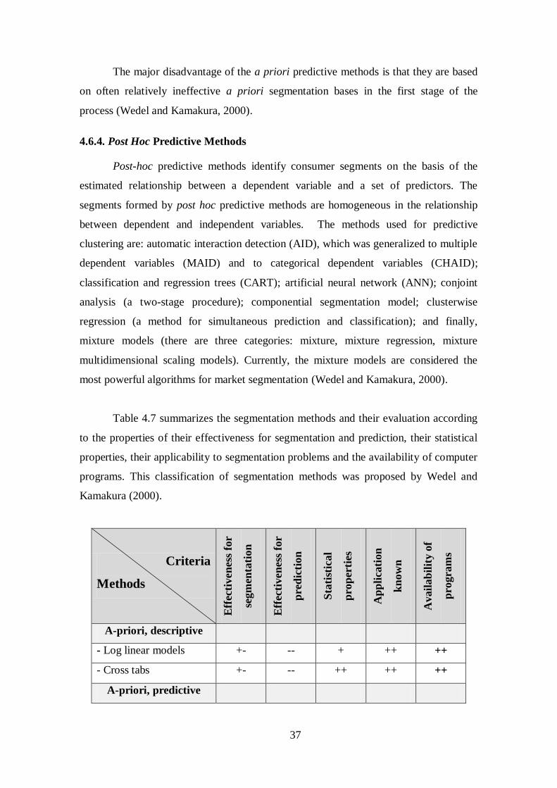
37
The major disadvantage of the a priori predictive methods is that they are based
on often relatively ineffective a priori segmentation bases in the first stage of the
process (Wedel and Kamakura, 2000).
4.6.4. Post Hoc Predictive Methods
Post-hoc predictive methods identify consumer segments on the basis of the
estimated relationship between a dependent variable and a set of predictors. The
segments formed by post hoc predictive methods are homogeneous in the relationship
between dependent and independent variables. The methods used for predictive
clustering are: automatic interaction detection (AID), which was generalized to multiple
dependent variables (MAID) and to categorical dependent variables (CHAID);
classification and regression trees (CART); artificial neural network (ANN); conjoint
analysis (a two-stage procedure); componential segmentation model; clusterwise
regression (a method for simultaneous prediction and classification); and finally,
mixture models (there are three categories: mixture, mixture regression, mixture
multidimensional scaling models). Currently, the mixture models are considered the
most powerful algorithms for market segmentation (Wedel and Kamakura, 2000).
Table 4.7 summarizes the segmentation methods and their evaluation according
to the properties of their effectiveness for segmentation and prediction, their statistical
properties, their applicability to segmentation problems and the availability of computer
programs. This classification of segmentation methods was proposed by Wedel and
Kamakura (2000).
Criteria
Methods
Eff
ecti
ven
ess
for
segm
enta
tion
Eff
ecti
ven
ess
for
pre
dic
tion
Sta
tist
ical
pro
per
ties
Ap
pli
cati
on
kn
ow
n
Avail
ab
ilit
y o
f
pro
gra
ms
A-priori, descriptive
- Log linear models +- -- + ++ ++
- Cross tabs +- -- ++ ++ ++
A-priori, predictive
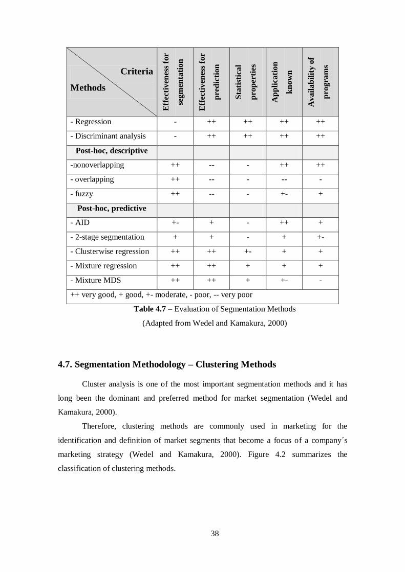
38
Criteria
Methods
Eff
ecti
ven
ess
for
segm
enta
tion
Eff
ecti
ven
ess
for
pre
dic
tion
Sta
tist
ical
pro
per
ties
Ap
pli
cati
on
kn
ow
n
Avail
ab
ilit
y o
f
pro
gra
ms
- Regression - ++ ++ ++ ++
- Discriminant analysis - ++ ++ ++ ++
Post-hoc, descriptive
-nonoverlapping ++ -- - ++ ++
- overlapping ++ -- - -- -
- fuzzy ++ -- - +- +
Post-hoc, predictive
- AID +- + - ++ +
- 2-stage segmentation + + - + +-
- Clusterwise regression ++ ++ +- + +
- Mixture regression ++ ++ + + +
- Mixture MDS ++ ++ + +- -
++ very good, + good, +- moderate, - poor, -- very poor
Table 4.7 – Evaluation of Segmentation Methods
(Adapted from Wedel and Kamakura, 2000)
4.7. Segmentation Methodology – Clustering Methods
Cluster analysis is one of the most important segmentation methods and it has
long been the dominant and preferred method for market segmentation (Wedel and
Kamakura, 2000).
Therefore, clustering methods are commonly used in marketing for the
identification and definition of market segments that become a focus of a company´s
marketing strategy (Wedel and Kamakura, 2000). Figure 4.2 summarizes the
classification of clustering methods.
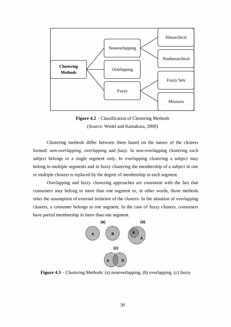
39
Figure 4.2 – Classification of Clustering Methods
(Source: Wedel and Kamakura, 2000)
Clustering methods differ between them based on the nature of the clusters
formed: non-overlapping, overlapping and fuzzy. In non-overlapping clustering each
subject belongs to a single segment only. In overlapping clustering a subject may
belong to multiple segments and in fuzzy clustering the membership of a subject in one
or multiple clusters is replaced by the degree of membership in each segment.
Overlapping and fuzzy clustering approaches are consistent with the fact that
consumers may belong to more than one segment or, in other words, those methods
relax the assumption of external isolation of the clusters. In the situation of overlapping
clusters, a consumer belongs to one segment. In the case of fuzzy clusters, consumers
have partial membership in more than one segment.
Figure 4.3 – Clustering Methods: (a) nonoverlapping, (b) overlapping, (c) fuzzy
Clustering
Methods
Nonoverlapping
Hierarchical
Nonhierarchical
Overlapping
Fuzzy
Fuzzy Sets
Mixtures
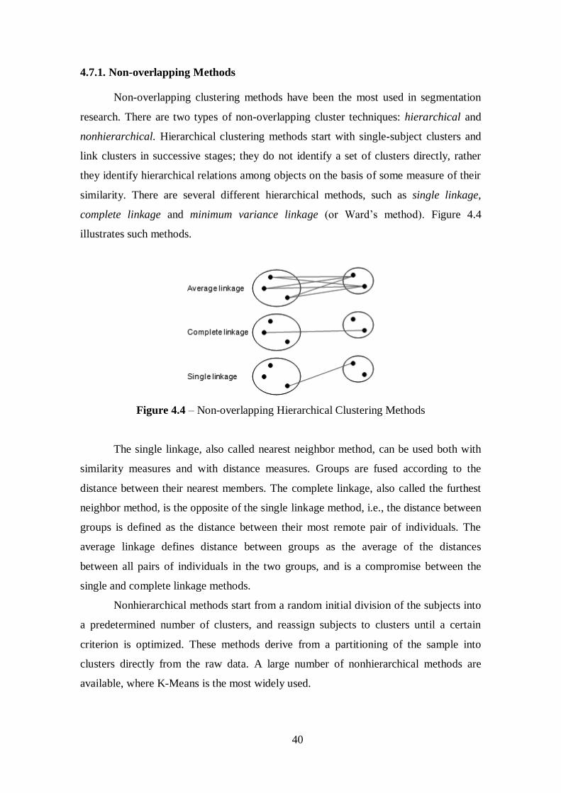
40
4.7.1. Non-overlapping Methods
Non-overlapping clustering methods have been the most used in segmentation
research. There are two types of non-overlapping cluster techniques: hierarchical and
nonhierarchical. Hierarchical clustering methods start with single-subject clusters and
link clusters in successive stages; they do not identify a set of clusters directly, rather
they identify hierarchical relations among objects on the basis of some measure of their
similarity. There are several different hierarchical methods, such as single linkage,
complete linkage and minimum variance linkage (or Ward’s method). Figure 4.4
illustrates such methods.
Figure 4.4 – Non-overlapping Hierarchical Clustering Methods
The single linkage, also called nearest neighbor method, can be used both with
similarity measures and with distance measures. Groups are fused according to the
distance between their nearest members. The complete linkage, also called the furthest
neighbor method, is the opposite of the single linkage method, i.e., the distance between
groups is defined as the distance between their most remote pair of individuals. The
average linkage defines distance between groups as the average of the distances
between all pairs of individuals in the two groups, and is a compromise between the
single and complete linkage methods.
Nonhierarchical methods start from a random initial division of the subjects into
a predetermined number of clusters, and reassign subjects to clusters until a certain
criterion is optimized. These methods derive from a partitioning of the sample into
clusters directly from the raw data. A large number of nonhierarchical methods are
available, where K-Means is the most widely used.
41
In literature we find that nonhierarchical methods are superior to hierarchical
methods as they are more robust to outliers and to the presence of irrelevant attributes.
However the general problem of those methods is the determination of the number of
clusters present in data.
4.7.2. Overlapping Methods
The overlapping clustering methods have a limited potential regarding
segmentation problems.
4.7.3. Fuzzy Methods
Regarding fuzzy clustering methods, two types can be distinguished: (1) the
fuzzy sets and (2) mixtures. The first assigns a degree of membership for objects to a
class. It assumes that consumers actually have partial memberships in several segments.
The second is based on the assumption that the data arise from a mixture of distributions
and estimates the probability that objects belong to each class. It assumes that segments
are non-overlapping but, because of limited information contained in the data, subjects
are assigned to segments with uncertainty, which are reflected in probabilities of
membership. Both the fuzzy and the mixture approaches provide membership values
between zero and one.


PART II
“Practice is the best of all instructors.”
By Publilius Syrus, a Roman writer

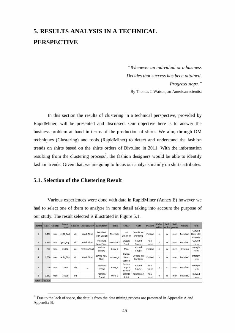
45
5. RESULTS ANALYSIS IN A TECHNICAL
PERSPECTIVE
“Whenever an individual or a business
Decides that success has been attained,
Progress stops.”
By Thomas J. Watson, an American scientist
In this section the results of clustering in a technical perspective, provided by
RapidMiner, will be presented and discussed. Our objective here is to answer the
business problem at hand in terms of the production of shirts. We aim, through DM
techniques (Clustering) and tools (RapidMiner) to detect and understand the fashion
trends on shirts based on the shirts orders of Bivolino in 2011. With the information
resulting from the clustering process7, the fashion designers would be able to identify
fashion trends. Given that, we are going to focus our analysis mainly on shirts attributes.
5.1. Selection of the Clustering Result
Various experiences were done with data in RapidMiner (Annex E) however we
had to select one of them to analyze in more detail taking into account the purpose of
our study. The result selected is illustrated in Figure 5.1.
7 Due to the lack of space, the details from the data mining process are presented in Appendix A and
Appendix B.
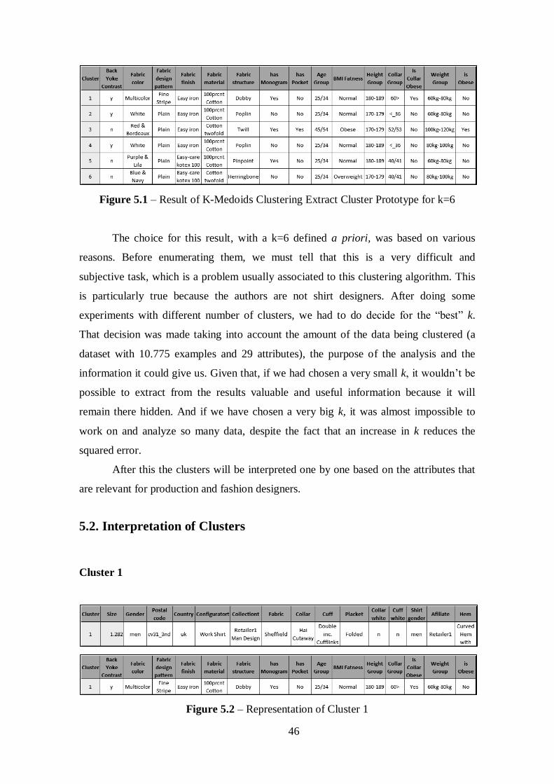
46
Figure 5.1 – Result of K-Medoids Clustering Extract Cluster Prototype for k=6
The choice for this result, with a k=6 defined a priori, was based on various
reasons. Before enumerating them, we must tell that this is a very difficult and
subjective task, which is a problem usually associated to this clustering algorithm. This
is particularly true because the authors are not shirt designers. After doing some
experiments with different number of clusters, we had to do decide for the “best” k.
That decision was made taking into account the amount of the data being clustered (a
dataset with 10.775 examples and 29 attributes), the purpose of the analysis and the
information it could give us. Given that, if we had chosen a very small k, it wouldn’t be
possible to extract from the results valuable and useful information because it will
remain there hidden. And if we have chosen a very big k, it was almost impossible to
work on and analyze so many data, despite the fact that an increase in k reduces the
squared error.
After this the clusters will be interpreted one by one based on the attributes that
are relevant for production and fashion designers.
5.2. Interpretation of Clusters
Cluster 1
Figure 5.2 – Representation of Cluster 1
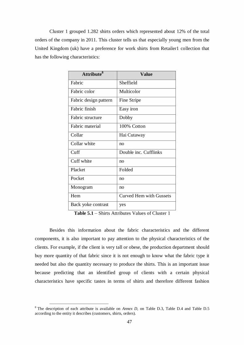
47
Cluster 1 grouped 1.282 shirts orders which represented about 12% of the total
orders of the company in 2011. This cluster tells us that especially young men from the
United Kingdom (uk) have a preference for work shirts from Retailer1 collection that
has the following characteristics:
Attribute8 Value
Fabric Sheffield
Fabric color Multicolor
Fabric design pattern Fine Stripe
Fabric finish Easy iron
Fabric structure Dobby
Fabric material 100% Cotton
Collar Hai Cutaway
Collar white no
Cuff Double inc. Cufflinks
Cuff white no
Placket Folded
Pocket no
Monogram no
Hem Curved Hem with Gussets
Back yoke contrast yes
Table 5.1 – Shirts Attributes Values of Cluster 1
Besides this information about the fabric characteristics and the different
components, it is also important to pay attention to the physical characteristics of the
clients. For example, if the client is very tall or obese, the production department should
buy more quantity of that fabric since it is not enough to know what the fabric type it
needed but also the quantity necessary to produce the shirts. This is an important issue
because predicting that an identified group of clients with a certain physical
characteristics have specific tastes in terms of shirts and therefore different fashion
8 The description of each attribute is available on Annex D, on Table D.3, Table D.4 and Table D.5
according to the entity it describes (customers, shirts, orders).
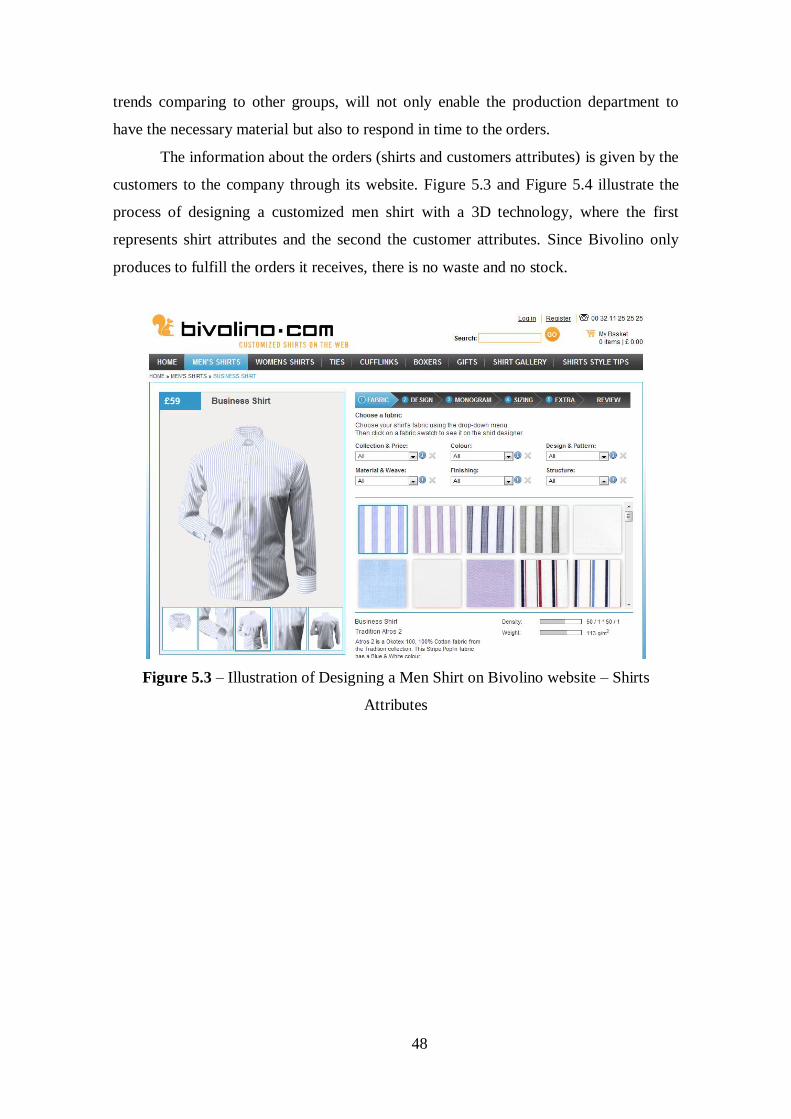
48
trends comparing to other groups, will not only enable the production department to
have the necessary material but also to respond in time to the orders.
The information about the orders (shirts and customers attributes) is given by the
customers to the company through its website. Figure 5.3 and Figure 5.4 illustrate the
process of designing a customized men shirt with a 3D technology, where the first
represents shirt attributes and the second the customer attributes. Since Bivolino only
produces to fulfill the orders it receives, there is no waste and no stock.
Figure 5.3 – Illustration of Designing a Men Shirt on Bivolino website – Shirts
Attributes
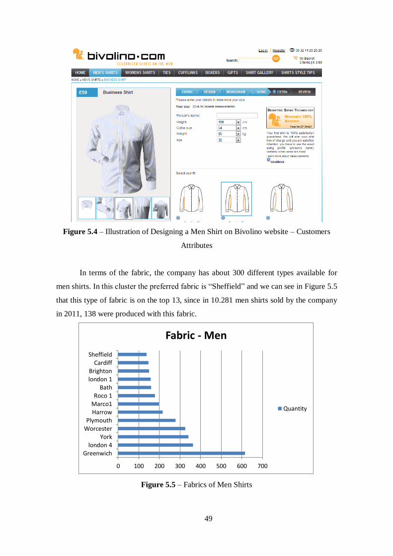
49
Figure 5.4 – Illustration of Designing a Men Shirt on Bivolino website – Customers
Attributes
In terms of the fabric, the company has about 300 different types available for
men shirts. In this cluster the preferred fabric is “Sheffield” and we can see in Figure 5.5
that this type of fabric is on the top 13, since in 10.281 men shirts sold by the company
in 2011, 138 were produced with this fabric.
Figure 5.5 – Fabrics of Men Shirts
0 100 200 300 400 500 600 700
Greenwichlondon 4
YorkWorcesterPlymouth
HarrowMarco1Roco 1
Bathlondon 1Brighton
CardiffSheffield
Fabric - Men
Quantity
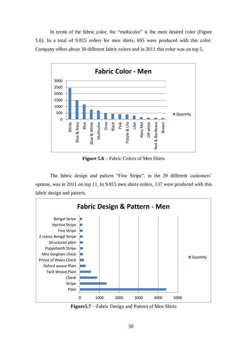
50
In terms of the fabric color, the “multicolor” is the most desired color (Figure
5.6). In a total of 9.815 orders for men shirts, 695 were produced with this color.
Company offers about 30 different fabric colors and in 2011 this color was on top 5.
Figure 5.6 – Fabric Colors of Men Shirts
The fabric design and pattern “Fine Stripe”, in the 39 different customers’
options, was in 2011 on top 11. In 9.815 men shirts orders, 137 were produced with this
fabric design and pattern.
Figure5.7 – Fabric Design and Pattern of Men Shirts
0
500
1000
1500
2000
2500
3000
Wh
ite
Blu
e &
Nav
y
Blu
e
Blu
e &
Wh
ite
Mu
ltic
olo
r
Gre
y
Bla
ck
Pin
k
Pur
ple
& L
ila
Lila
c
Nav
y M
ix
Off
wh
ite
Red
& B
ord
eau
x
Bro
wn
Fabric Color - Men
Quantity
0 1000 2000 3000 4000 5000
Plain
Stripe
Check
Twill Weave Plain
Oxford weave Plain
Prince of Wales Check
Mini Gingham check
Puppytooth Stripe
Structured plain
2 colour Bengal Stripe
Fine Stripe
Hairline Stripe
Bengal Stripe
Fabric Design & Pattern - Men
Quantity
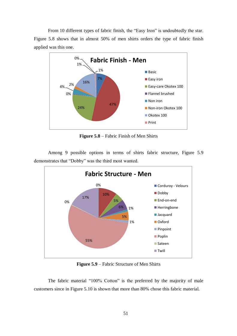
51
From 10 different types of fabric finish, the “Easy Iron” is undoubtedly the star.
Figure 5.8 shows that in almost 50% of men shirts orders the type of fabric finish
applied was this one.
Figure 5.8 – Fabric Finish of Men Shirts
Among 9 possible options in terms of shirts fabric structure, Figure 5.9
demonstrates that “Dobby” was the third most wanted.
Figure 5.9 – Fabric Structure of Men Shirts
The fabric material “100% Cotton” is the preferred by the majority of male
customers since in Figure 5.10 is shown that more than 80% chose this fabric material.
7%
47% 24%
0%
4% 2%
16%
1%
0%
1%
Fabric Finish - Men
Basic
Easy iron
Easy-care Okotex 100
Flannel brushed
Non iron
Non-iron Okotex 100
Okotex 100
0%
10%
5%
6% 1%
5%
1%
55%
0% 17%
Fabric Structure - Men
Corduroy - Velours
Dobby
End-on-end
Herringbone
Jacquard
Oxford
Pinpoint
Poplin
Sateen
Twill

52
Figure 5.10 – Fabric Material of Men Shirts
The collar “Hai Cutaway” was the third most wanted in 27 varieties available. In
Figure 5.11 we can see that more than 1.000 shirts sold had this type of collar.
Figure 5.11 – Collar of Men Shirts
In Figure 5.12 we can note that the cuff “Double inc. Cufflinks” is the second
most wanted (24% of total men shirt orders) among 9 different options.
82%
0% 1%
1% 0%
5%
2% 8%
0%
Fabric Material - Men
100% Cotton
100% Linen
76%cotton /24%Silk
80%Cotton /20%Silk
Cotton - Linen
Cotton - Polyester
Cotton stretch
Cotton twofold
Egyptian cotton 2fold
0
500
1000
1500
2000
2500
3000
3500
Collar - Men
Quantity
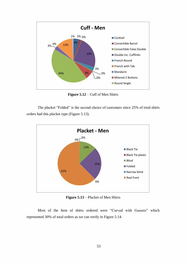
53
Figure 5.12 – Cuff of Men Shirts
The placket “Folded” is the second choice of customers since 25% of total shirts
orders had this placket type (Figure 5.13).
Figure 5.13 – Placket of Men Shirts
Most of the hem of shirts ordered were “Curved with Gussets” which
represented 30% of total orders as we can verify in Figure 5.14.
4%
2% 0%
24%
3%
0%
0%
6% 44%
3% 0% 13%
1%
Cuff - Men
Cocktail
Convertible Barrel
Convertible False Double
Double inc. Cufflinks
French Round
French with Tab
Mandarin
Mitered 2 Buttons
Round Single
0% 0%
13%
25%
0%
62%
Placket - Men
Black Tie
Black Tie pleats
Blind
Folded
Narrow blind
Real front
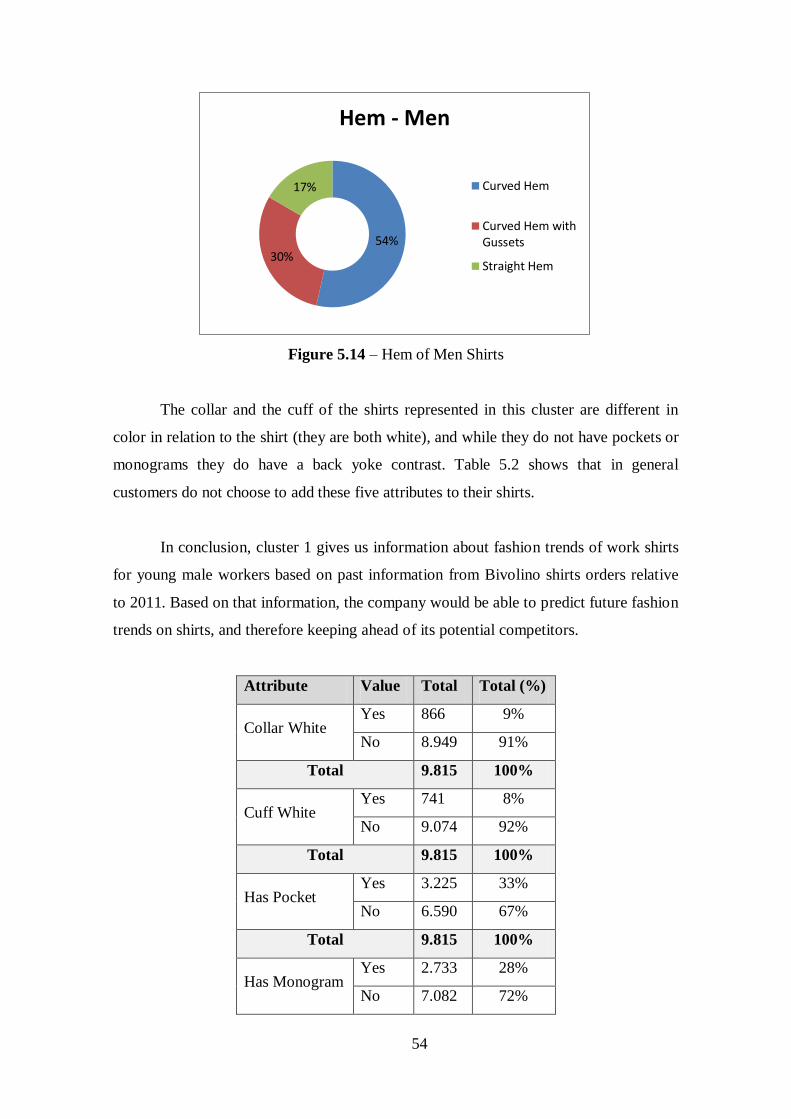
54
Figure 5.14 – Hem of Men Shirts
The collar and the cuff of the shirts represented in this cluster are different in
color in relation to the shirt (they are both white), and while they do not have pockets or
monograms they do have a back yoke contrast. Table 5.2 shows that in general
customers do not choose to add these five attributes to their shirts.
In conclusion, cluster 1 gives us information about fashion trends of work shirts
for young male workers based on past information from Bivolino shirts orders relative
to 2011. Based on that information, the company would be able to predict future fashion
trends on shirts, and therefore keeping ahead of its potential competitors.
Attribute Value Total Total (%)
Collar White Yes 866 9%
No 8.949 91%
Total 9.815 100%
Cuff White Yes 741 8%
No 9.074 92%
Total 9.815 100%
Has Pocket Yes 3.225 33%
No 6.590 67%
Total 9.815 100%
Has Monogram Yes 2.733 28%
No 7.082 72%
54% 30%
17%
Hem - Men
Curved Hem
Curved Hem withGussets
Straight Hem
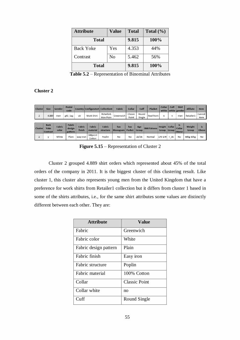
55
Attribute Value Total Total (%)
Total 9.815 100%
Back Yoke
Contrast
Yes 4.353 44%
No 5.462 56%
Total 9.815 100%
Table 5.2 – Representation of Binominal Attributes
Cluster 2
Figure 5.15 – Representation of Cluster 2
Cluster 2 grouped 4.889 shirt orders which represented about 45% of the total
orders of the company in 2011. It is the biggest cluster of this clustering result. Like
cluster 1, this cluster also represents young men from the United Kingdom that have a
preference for work shirts from Retailer1 collection but it differs from cluster 1 based in
some of the shirts attributes, i.e., for the same shirt attributes some values are distinctly
different between each other. They are:
Attribute Value
Fabric Greenwich
Fabric color White
Fabric design pattern Plain
Fabric finish Easy iron
Fabric structure Poplin
Fabric material 100% Cotton
Collar Classic Point
Collar white no
Cuff Round Single
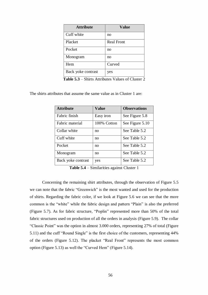
56
Attribute Value
Cuff white no
Placket Real Front
Pocket no
Monogram no
Hem Curved
Back yoke contrast yes
Table 5.3 – Shirts Attributes Values of Cluster 2
The shirts attributes that assume the same value as in Cluster 1 are:
Attribute Value Observations
Fabric finish Easy iron See Figure 5.8
Fabric material 100% Cotton See Figure 5.10
Collar white no See Table 5.2
Cuff white no See Table 5.2
Pocket no See Table 5.2
Monogram no See Table 5.2
Back yoke contrast yes See Table 5.2
Table 5.4 – Similarities against Cluster 1
Concerning the remaining shirt attributes, through the observation of Figure 5.5
we can note that the fabric “Greenwich” is the most wanted and used for the production
of shirts. Regarding the fabric color, if we look at Figure 5.6 we can see that the more
common is the “white” while the fabric design and pattern “Plain” is also the preferred
(Figure 5.7). As for fabric structure, “Poplin” represented more than 50% of the total
fabric structures used on production of all the orders in analysis (Figure 5.9). The collar
“Classic Point” was the option in almost 3.000 orders, representing 27% of total (Figure
5.11) and the cuff “Round Single” is the first choice of the customers, representing 44%
of the orders (Figure 5.12). The placket “Real Front” represents the most common
option (Figure 5.13) as well the “Curved Hem” (Figure 5.14).
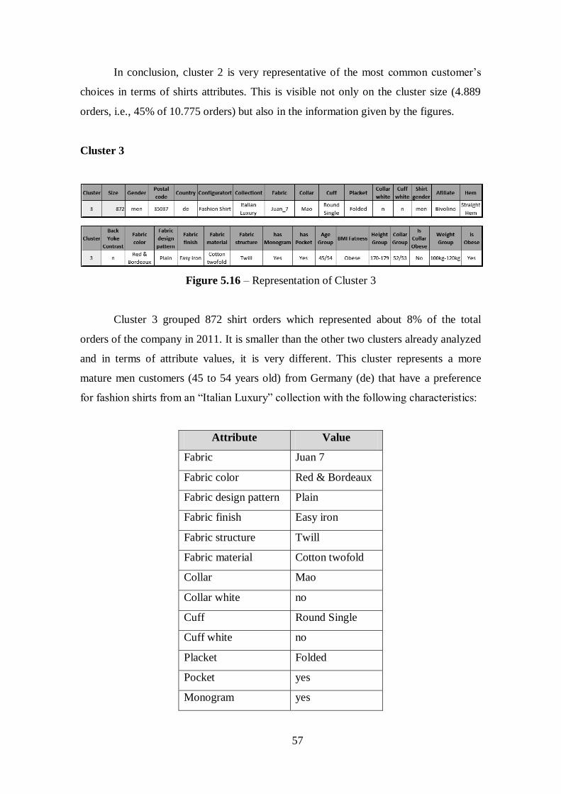
57
In conclusion, cluster 2 is very representative of the most common customer’s
choices in terms of shirts attributes. This is visible not only on the cluster size (4.889
orders, i.e., 45% of 10.775 orders) but also in the information given by the figures.
Cluster 3
Figure 5.16 – Representation of Cluster 3
Cluster 3 grouped 872 shirt orders which represented about 8% of the total
orders of the company in 2011. It is smaller than the other two clusters already analyzed
and in terms of attribute values, it is very different. This cluster represents a more
mature men customers (45 to 54 years old) from Germany (de) that have a preference
for fashion shirts from an “Italian Luxury” collection with the following characteristics:
Attribute Value
Fabric Juan 7
Fabric color Red & Bordeaux
Fabric design pattern Plain
Fabric finish Easy iron
Fabric structure Twill
Fabric material Cotton twofold
Collar Mao
Collar white no
Cuff Round Single
Cuff white no
Placket Folded
Pocket yes
Monogram yes
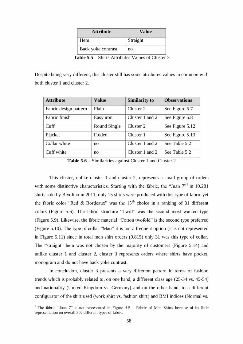
58
Attribute Value
Hem Straight
Back yoke contrast no
Table 5.5 – Shirts Attributes Values of Cluster 3
Despite being very different, this cluster still has some attributes values in common with
both cluster 1 and cluster 2.
Attribute Value Similarity to Observations
Fabric design pattern Plain Cluster 2 See Figure 5.7
Fabric finish Easy iron Cluster 1 and 2 See Figure 5.8
Cuff Round Single Cluster 2 See Figure 5.12
Placket Folded Cluster 1 See Figure 5.13
Collar white no Cluster 1 and 2 See Table 5.2
Cuff white no Cluster 1 and 2 See Table 5.2
Table 5.6 – Similarities against Cluster 1 and Cluster 2
This cluster, unlike cluster 1 and cluster 2, represents a small group of orders
with some distinctive characteristics. Starting with the fabric, the “Juan 7”9 in 10.281
shirts sold by Bivolino in 2011, only 15 shirts were produced with this type of fabric yet
the fabric color “Red & Bordeaux” was the 13th
choice in a ranking of 31 different
colors (Figure 5.6). The fabric structure “Twill” was the second most wanted type
(Figure 5.9). Likewise, the fabric material “Cotton twofold” is the second type preferred
(Figure 5.10). The type of collar “Mao” it is not a frequent option (it is not represented
in Figure 5.11) since in total men shirt orders (9.815) only 31 was this type of collar.
The “straight” hem was not chosen by the majority of customers (Figure 5.14) and
unlike cluster 1 and cluster 2, cluster 3 represents orders where shirts have pocket,
monogram and do not have back yoke contrast.
In conclusion, cluster 3 presents a very different pattern in terms of fashion
trends which is probably related to, on one hand, a different class age (25-34 vs. 45-54)
and nationality (United Kingdom vs. Germany) and on the other hand, to a different
configurator of the shirt used (work shirt vs. fashion shirt) and BMI indices (Normal vs.
9 The fabric “Juan 7” is not represented in Figure 5.5 – Fabric of Men Shirts because of its little
representation on overall 302 different types of fabric.
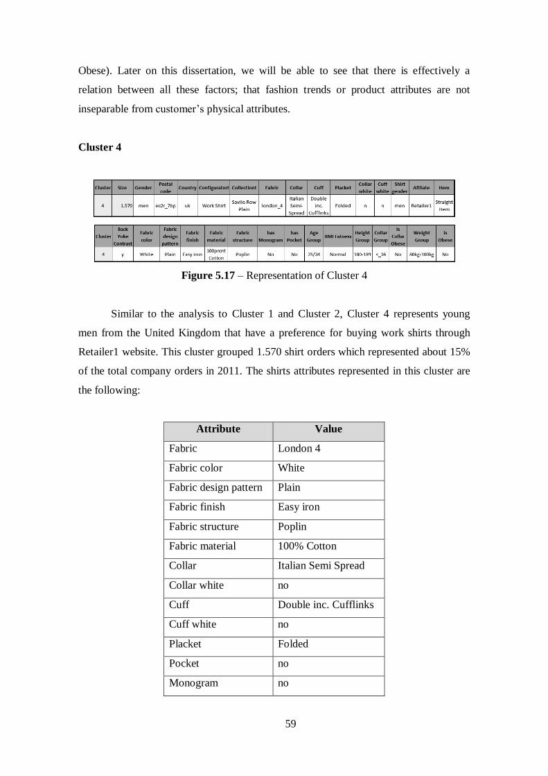
59
Obese). Later on this dissertation, we will be able to see that there is effectively a
relation between all these factors; that fashion trends or product attributes are not
inseparable from customer’s physical attributes.
Cluster 4
Figure 5.17 – Representation of Cluster 4
Similar to the analysis to Cluster 1 and Cluster 2, Cluster 4 represents young
men from the United Kingdom that have a preference for buying work shirts through
Retailer1 website. This cluster grouped 1.570 shirt orders which represented about 15%
of the total company orders in 2011. The shirts attributes represented in this cluster are
the following:
Attribute Value
Fabric London 4
Fabric color White
Fabric design pattern Plain
Fabric finish Easy iron
Fabric structure Poplin
Fabric material 100% Cotton
Collar Italian Semi Spread
Collar white no
Cuff Double inc. Cufflinks
Cuff white no
Placket Folded
Pocket no
Monogram no
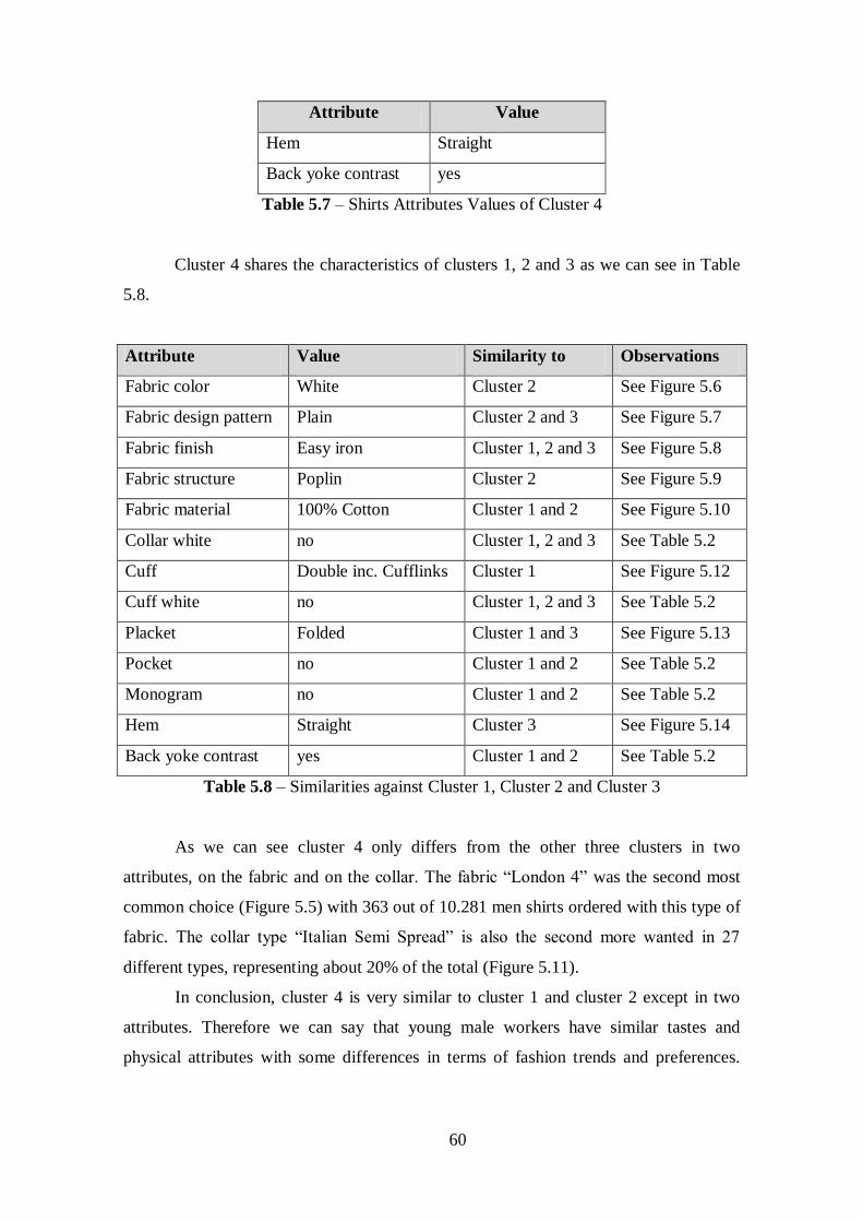
60
Attribute Value
Hem Straight
Back yoke contrast yes
Table 5.7 – Shirts Attributes Values of Cluster 4
Cluster 4 shares the characteristics of clusters 1, 2 and 3 as we can see in Table
5.8.
Attribute Value Similarity to Observations
Fabric color White Cluster 2 See Figure 5.6
Fabric design pattern Plain Cluster 2 and 3 See Figure 5.7
Fabric finish Easy iron Cluster 1, 2 and 3 See Figure 5.8
Fabric structure Poplin Cluster 2 See Figure 5.9
Fabric material 100% Cotton Cluster 1 and 2 See Figure 5.10
Collar white no Cluster 1, 2 and 3 See Table 5.2
Cuff Double inc. Cufflinks Cluster 1 See Figure 5.12
Cuff white no Cluster 1, 2 and 3 See Table 5.2
Placket Folded Cluster 1 and 3 See Figure 5.13
Pocket no Cluster 1 and 2 See Table 5.2
Monogram no Cluster 1 and 2 See Table 5.2
Hem Straight Cluster 3 See Figure 5.14
Back yoke contrast yes Cluster 1 and 2 See Table 5.2
Table 5.8 – Similarities against Cluster 1, Cluster 2 and Cluster 3
As we can see cluster 4 only differs from the other three clusters in two
attributes, on the fabric and on the collar. The fabric “London 4” was the second most
common choice (Figure 5.5) with 363 out of 10.281 men shirts ordered with this type of
fabric. The collar type “Italian Semi Spread” is also the second more wanted in 27
different types, representing about 20% of the total (Figure 5.11).
In conclusion, cluster 4 is very similar to cluster 1 and cluster 2 except in two
attributes. Therefore we can say that young male workers have similar tastes and
physical attributes with some differences in terms of fashion trends and preferences.
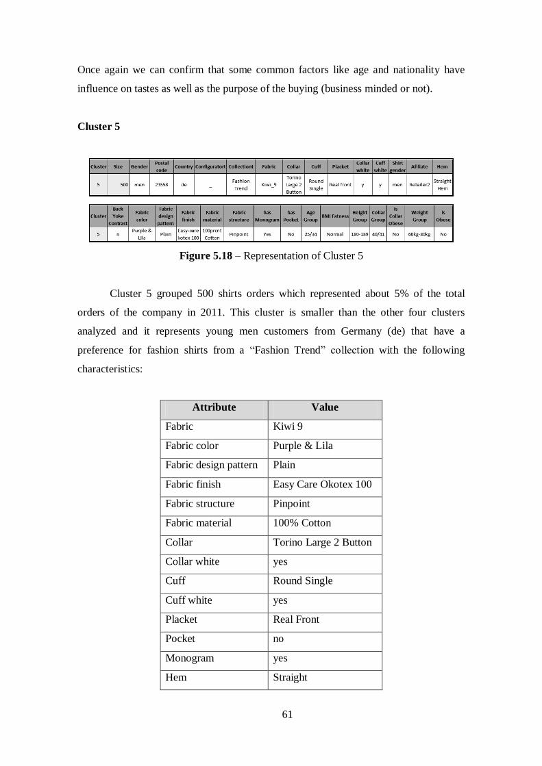
61
Once again we can confirm that some common factors like age and nationality have
influence on tastes as well as the purpose of the buying (business minded or not).
Cluster 5
Figure 5.18 – Representation of Cluster 5
Cluster 5 grouped 500 shirts orders which represented about 5% of the total
orders of the company in 2011. This cluster is smaller than the other four clusters
analyzed and it represents young men customers from Germany (de) that have a
preference for fashion shirts from a “Fashion Trend” collection with the following
characteristics:
Attribute Value
Fabric Kiwi 9
Fabric color Purple & Lila
Fabric design pattern Plain
Fabric finish Easy Care Okotex 100
Fabric structure Pinpoint
Fabric material 100% Cotton
Collar Torino Large 2 Button
Collar white yes
Cuff Round Single
Cuff white yes
Placket Real Front
Pocket no
Monogram yes
Hem Straight
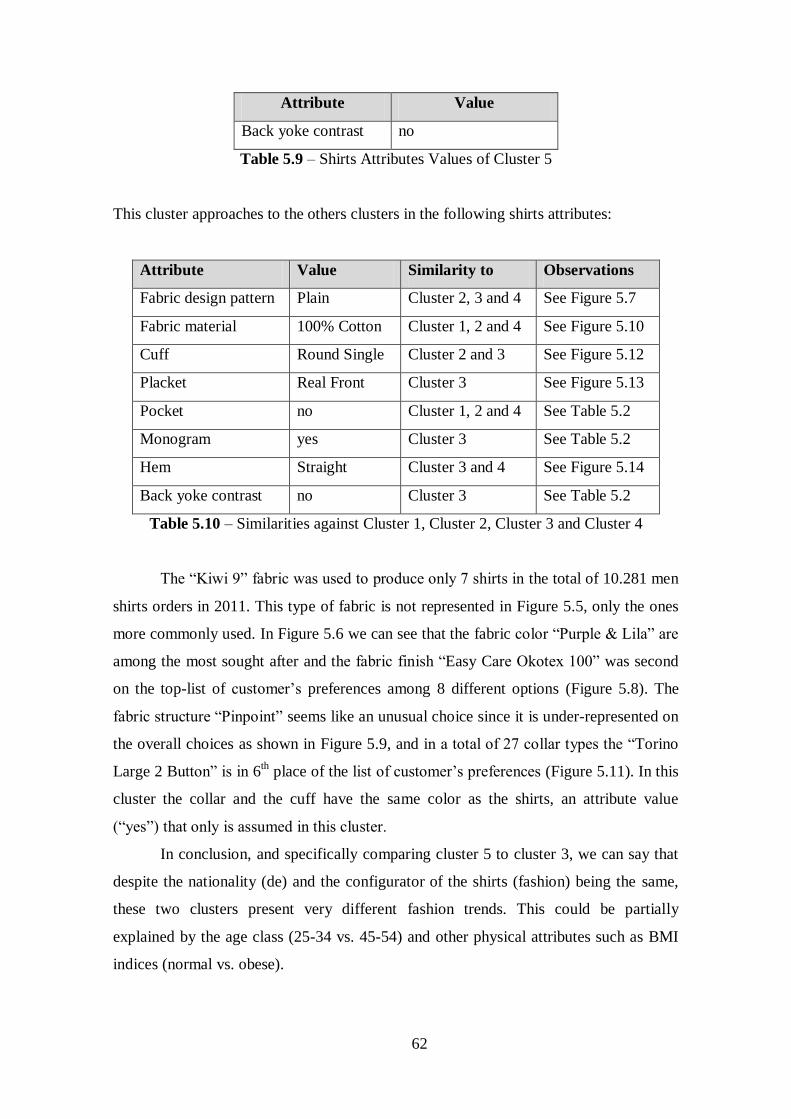
62
Attribute Value
Back yoke contrast no
Table 5.9 – Shirts Attributes Values of Cluster 5
This cluster approaches to the others clusters in the following shirts attributes:
Attribute Value Similarity to Observations
Fabric design pattern Plain Cluster 2, 3 and 4 See Figure 5.7
Fabric material 100% Cotton Cluster 1, 2 and 4 See Figure 5.10
Cuff Round Single Cluster 2 and 3 See Figure 5.12
Placket Real Front Cluster 3 See Figure 5.13
Pocket no Cluster 1, 2 and 4 See Table 5.2
Monogram yes Cluster 3 See Table 5.2
Hem Straight Cluster 3 and 4 See Figure 5.14
Back yoke contrast no Cluster 3 See Table 5.2
Table 5.10 – Similarities against Cluster 1, Cluster 2, Cluster 3 and Cluster 4
The “Kiwi 9” fabric was used to produce only 7 shirts in the total of 10.281 men
shirts orders in 2011. This type of fabric is not represented in Figure 5.5, only the ones
more commonly used. In Figure 5.6 we can see that the fabric color “Purple & Lila” are
among the most sought after and the fabric finish “Easy Care Okotex 100” was second
on the top-list of customer’s preferences among 8 different options (Figure 5.8). The
fabric structure “Pinpoint” seems like an unusual choice since it is under-represented on
the overall choices as shown in Figure 5.9, and in a total of 27 collar types the “Torino
Large 2 Button” is in 6th place of the list of customer’s preferences (Figure 5.11). In this
cluster the collar and the cuff have the same color as the shirts, an attribute value
(“yes”) that only is assumed in this cluster.
In conclusion, and specifically comparing cluster 5 to cluster 3, we can say that
despite the nationality (de) and the configurator of the shirts (fashion) being the same,
these two clusters present very different fashion trends. This could be partially
explained by the age class (25-34 vs. 45-54) and other physical attributes such as BMI
indices (normal vs. obese).
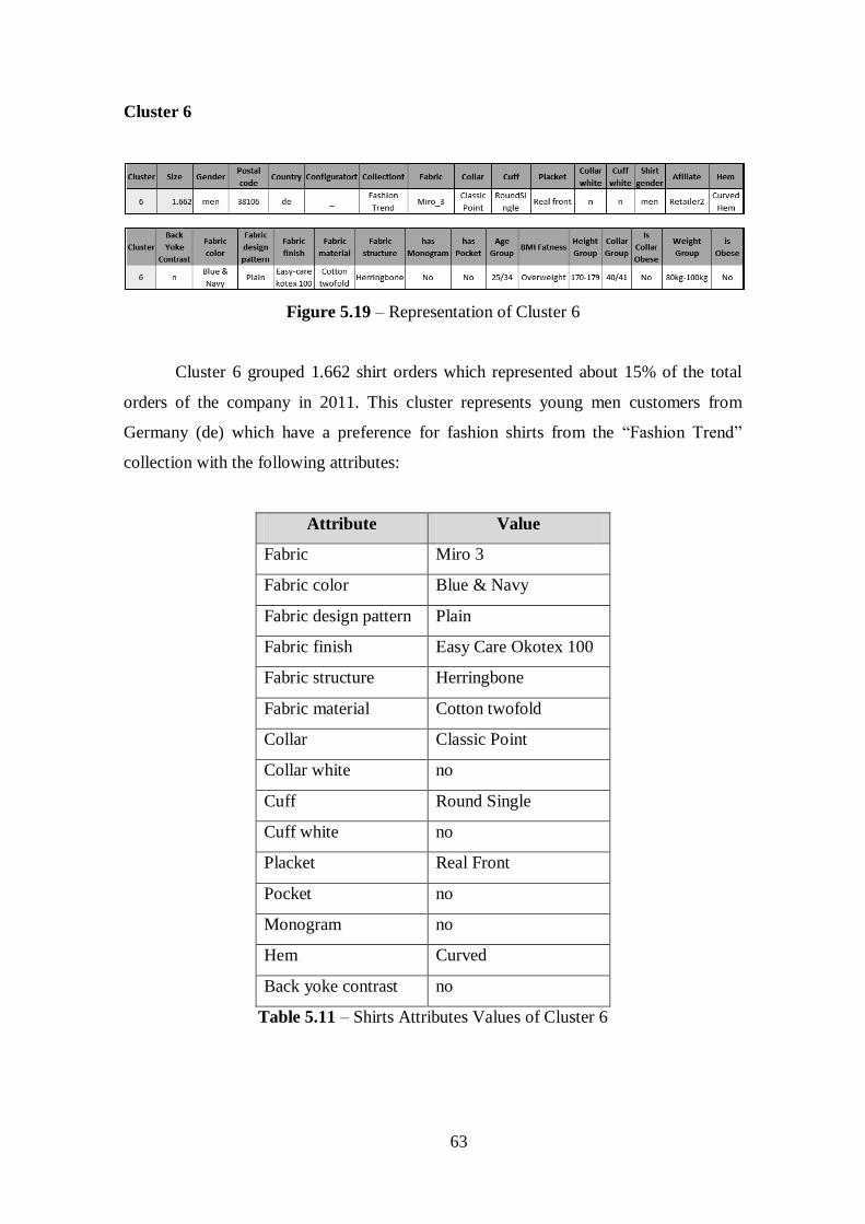
63
Cluster 6
Figure 5.19 – Representation of Cluster 6
Cluster 6 grouped 1.662 shirt orders which represented about 15% of the total
orders of the company in 2011. This cluster represents young men customers from
Germany (de) which have a preference for fashion shirts from the “Fashion Trend”
collection with the following attributes:
Attribute Value
Fabric Miro 3
Fabric color Blue & Navy
Fabric design pattern Plain
Fabric finish Easy Care Okotex 100
Fabric structure Herringbone
Fabric material Cotton twofold
Collar Classic Point
Collar white no
Cuff Round Single
Cuff white no
Placket Real Front
Pocket no
Monogram no
Hem Curved
Back yoke contrast no
Table 5.11 – Shirts Attributes Values of Cluster 6
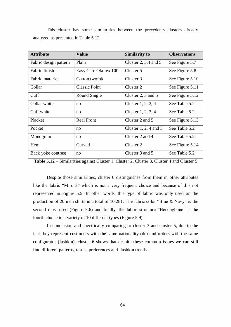
64
This cluster has some similarities between the precedents clusters already
analyzed as presented in Table 5.12.
Attribute Value Similarity to Observations
Fabric design pattern Plain Cluster 2, 3,4 and 5 See Figure 5.7
Fabric finish Easy Care Okotex 100 Cluster 5 See Figure 5.8
Fabric material Cotton twofold Cluster 3 See Figure 5.10
Collar Classic Point Cluster 2 See Figure 5.11
Cuff Round Single Cluster 2, 3 and 5 See Figure 5.12
Collar white no Cluster 1, 2, 3, 4 See Table 5.2
Cuff white no Cluster 1, 2, 3, 4 See Table 5.2
Placket Real Front Cluster 2 and 5 See Figure 5.13
Pocket no Cluster 1, 2, 4 and 5 See Table 5.2
Monogram no Cluster 2 and 4 See Table 5.2
Hem Curved Cluster 2 See Figure 5.14
Back yoke contrast no Cluster 3 and 5 See Table 5.2
Table 5.12 – Similarities against Cluster 1, Cluster 2, Cluster 3, Cluster 4 and Cluster 5
Despite those similarities, cluster 6 distinguishes from them in other attributes
like the fabric “Miro 3” which is not a very frequent choice and because of this not
represented in Figure 5.5. In other words, this type of fabric was only used on the
production of 20 men shirts in a total of 10.281. The fabric color “Blue & Navy” is the
second most used (Figure 5.6) and finally, the fabric structure “Herringbone” is the
fourth choice in a variety of 10 different types (Figure 5.9).
In conclusion and specifically comparing to cluster 3 and cluster 5, due to the
fact they represent customers with the same nationality (de) and orders with the same
configurator (fashion), cluster 6 shows that despite these common issues we can still
find different patterns, tastes, preferences and fashion trends.
65
5.3. Conclusions of the Clustering Results
In this section we analyzed the results of a K-Medoids clustering for a k number
of clusters established a priori (k = 6) based in a dataset of 10.775 examples (n =
10.775) which correspond to the number of shirts orders of Bivolino in 2011.
The analysis was focused on 29 attributes which were divided into three
different categories according to the entity it describes, they are the orders, the shirts
and the customers (Table D.2, Table D.3 and Table D.4 on Annex D). We focused the
study mainly on the attributes that describe the shirts and the orders because our
purpose was to identify the shirts fashion trends based on the customers choices in
terms of shirts attributes.
Once the most common attributes values in shirts orders were identified, the
production and/or purchasing department and the fashion designers would be able to
better perform their tasks, because they already have information about the type and
quantity of the raw material needed as well the shirts fashion trends.
In short, we can say that DM tools and techniques are indeed valuable
instruments to better understand consumer tastes and preferences allowing companies to
be more efficient and responsive to customer’s requests and gaining a competitive
advantage.

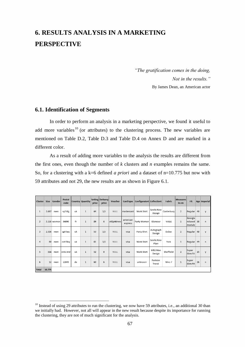
67
6. RESULTS ANALYSIS IN A MARKETING
PERSPECTIVE
“The gratification comes in the doing,
Not in the results.”
By James Dean, an American actor
6.1. Identification of Segments
In order to perform an analysis in a marketing perspective, we found it useful to
add more variables10
(or attributes) to the clustering process. The new variables are
mentioned on Table D.2, Table D.3 and Table D.4 on Annex D and are marked in a
different color.
As a result of adding more variables to the analysis the results are different from
the first ones, even though the number of k clusters and n examples remains the same.
So, for a clustering with a k=6 defined a priori and a dataset of n=10.775 but now with
59 attributes and not 29, the new results are as shown in Figure 6.1.
10
Instead of using 29 attributes to run the clustering, we now have 59 attributes, i.e., an additional 30 than
we initially had. However, not all will appear in the new result because despite its importance for running
the clustering, they are not of much significant for the analysis.
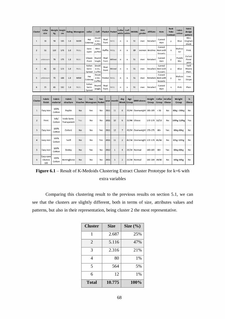
68
Figure 6.1 – Result of K-Medoids Clustering Extract Cluster Prototype for k=6 with
extra variables
Comparing this clustering result to the previous results on section 5.1, we can
see that the clusters are slightly different, both in terms of size, attributes values and
patterns, but also in their representation, being cluster 2 the most representative.
Cluster Size Size (%)
1 2.687 25%
2 5.116 47%
3 2.316 21%
4 80 1%
5 564 5%
6 12 1%
Total 10.775 100%
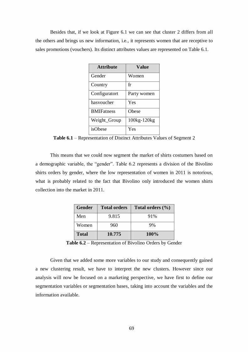
69
Besides that, if we look at Figure 6.1 we can see that cluster 2 differs from all
the others and brings us new information, i.e., it represents women that are receptive to
sales promotions (vouchers). Its distinct attributes values are represented on Table 6.1.
Attribute Value
Gender Women
Country fr
Configuratort Party women
hasvoucher Yes
BMIFatness Obese
Weight_Group 100kg-120kg
isObese Yes
Table 6.1 – Representation of Distinct Attributes Values of Segment 2
This means that we could now segment the market of shirts costumers based on
a demographic variable, the “gender”. Table 6.2 represents a division of the Bivolino
shirts orders by gender, where the low representation of women in 2011 is notorious,
what is probably related to the fact that Bivolino only introduced the women shirts
collection into the market in 2011.
Gender Total orders Total orders (%)
Men 9.815 91%
Women 960 9%
Total 10.775 100%
Table 6.2 – Representation of Bivolino Orders by Gender
Given that we added some more variables to our study and consequently gained
a new clustering result, we have to interpret the new clusters. However since our
analysis will now be focused on a marketing perspective, we have first to define our
segmentation variables or segmentation bases, taking into account the variables and the
information available.
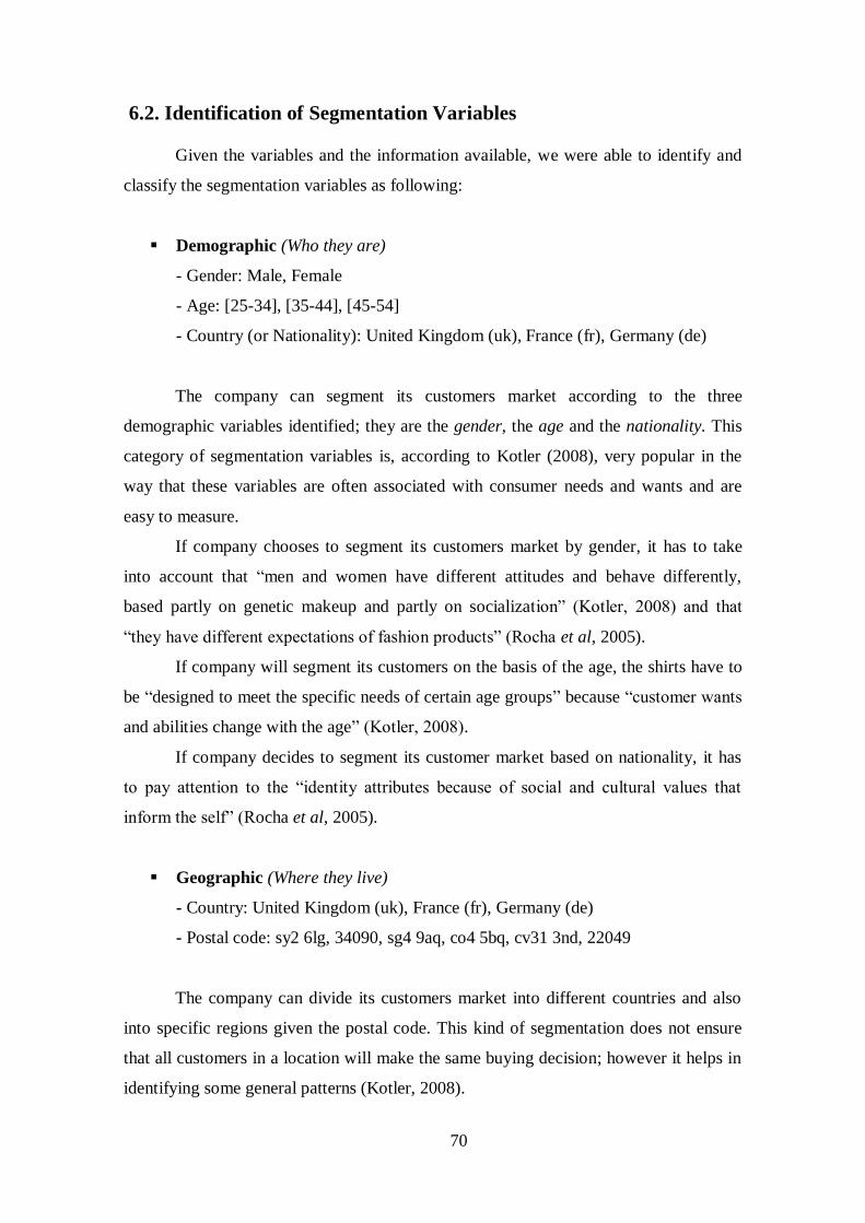
70
6.2. Identification of Segmentation Variables
Given the variables and the information available, we were able to identify and
classify the segmentation variables as following:
Demographic (Who they are)
- Gender: Male, Female
- Age: [25-34], [35-44], [45-54]
- Country (or Nationality): United Kingdom (uk), France (fr), Germany (de)
The company can segment its customers market according to the three
demographic variables identified; they are the gender, the age and the nationality. This
category of segmentation variables is, according to Kotler (2008), very popular in the
way that these variables are often associated with consumer needs and wants and are
easy to measure.
If company chooses to segment its customers market by gender, it has to take
into account that “men and women have different attitudes and behave differently,
based partly on genetic makeup and partly on socialization” (Kotler, 2008) and that
“they have different expectations of fashion products” (Rocha et al, 2005).
If company will segment its customers on the basis of the age, the shirts have to
be “designed to meet the specific needs of certain age groups” because “customer wants
and abilities change with the age” (Kotler, 2008).
If company decides to segment its customer market based on nationality, it has
to pay attention to the “identity attributes because of social and cultural values that
inform the self” (Rocha et al, 2005).
Geographic (Where they live)
- Country: United Kingdom (uk), France (fr), Germany (de)
- Postal code: sy2 6lg, 34090, sg4 9aq, co4 5bq, cv31 3nd, 22049
The company can divide its customers market into different countries and also
into specific regions given the postal code. This kind of segmentation does not ensure
that all customers in a location will make the same buying decision; however it helps in
identifying some general patterns (Kotler, 2008).
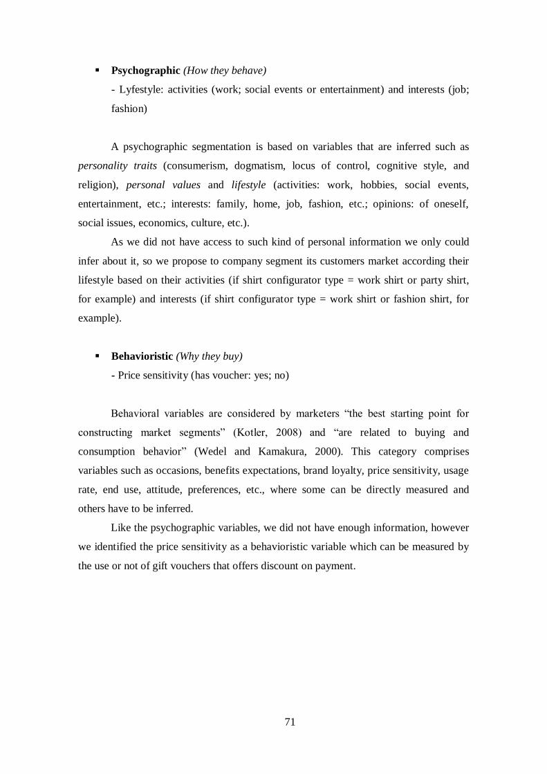
71
Psychographic (How they behave)
- Lyfestyle: activities (work; social events or entertainment) and interests (job;
fashion)
A psychographic segmentation is based on variables that are inferred such as
personality traits (consumerism, dogmatism, locus of control, cognitive style, and
religion), personal values and lifestyle (activities: work, hobbies, social events,
entertainment, etc.; interests: family, home, job, fashion, etc.; opinions: of oneself,
social issues, economics, culture, etc.).
As we did not have access to such kind of personal information we only could
infer about it, so we propose to company segment its customers market according their
lifestyle based on their activities (if shirt configurator type = work shirt or party shirt,
for example) and interests (if shirt configurator type = work shirt or fashion shirt, for
example).
Behavioristic (Why they buy)
- Price sensitivity (has voucher: yes; no)
Behavioral variables are considered by marketers “the best starting point for
constructing market segments” (Kotler, 2008) and “are related to buying and
consumption behavior” (Wedel and Kamakura, 2000). This category comprises
variables such as occasions, benefits expectations, brand loyalty, price sensitivity, usage
rate, end use, attitude, preferences, etc., where some can be directly measured and
others have to be inferred.
Like the psychographic variables, we did not have enough information, however
we identified the price sensitivity as a behavioristic variable which can be measured by
the use or not of gift vouchers that offers discount on payment.
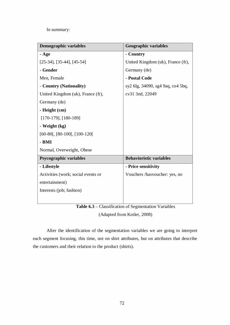
72
In summary:
Demographic variables Geographic variables
- Age
[25-34], [35-44], [45-54]
- Gender
Men, Female
- Country (Nationality)
United Kingdom (uk), France (fr),
Germany (de)
- Height (cm)
[170-179], [180-189]
- Weight (kg)
[60-80[, [80-100[, [100-120[
- BMI
Normal, Overweight, Obese
- Country
United Kingdom (uk), France (fr),
Germany (de)
- Postal Code
sy2 6lg, 34090, sg4 9aq, co4 5bq,
cv31 3nd, 22049
Psycographic variables Behavioristic variables
- Lifestyle
Activities (work; social events or
entertainment)
Interests (job; fashion)
- Price sensitivity
Vouchers /hasvoucher: yes, no
Table 6.3 – Classification of Segmentation Variables
(Adapted from Kotler, 2008)
After the identification of the segmentation variables we are going to interpret
each segment focusing, this time, not on shirt attributes, but on attributes that describe
the customers and their relation to the product (shirts).
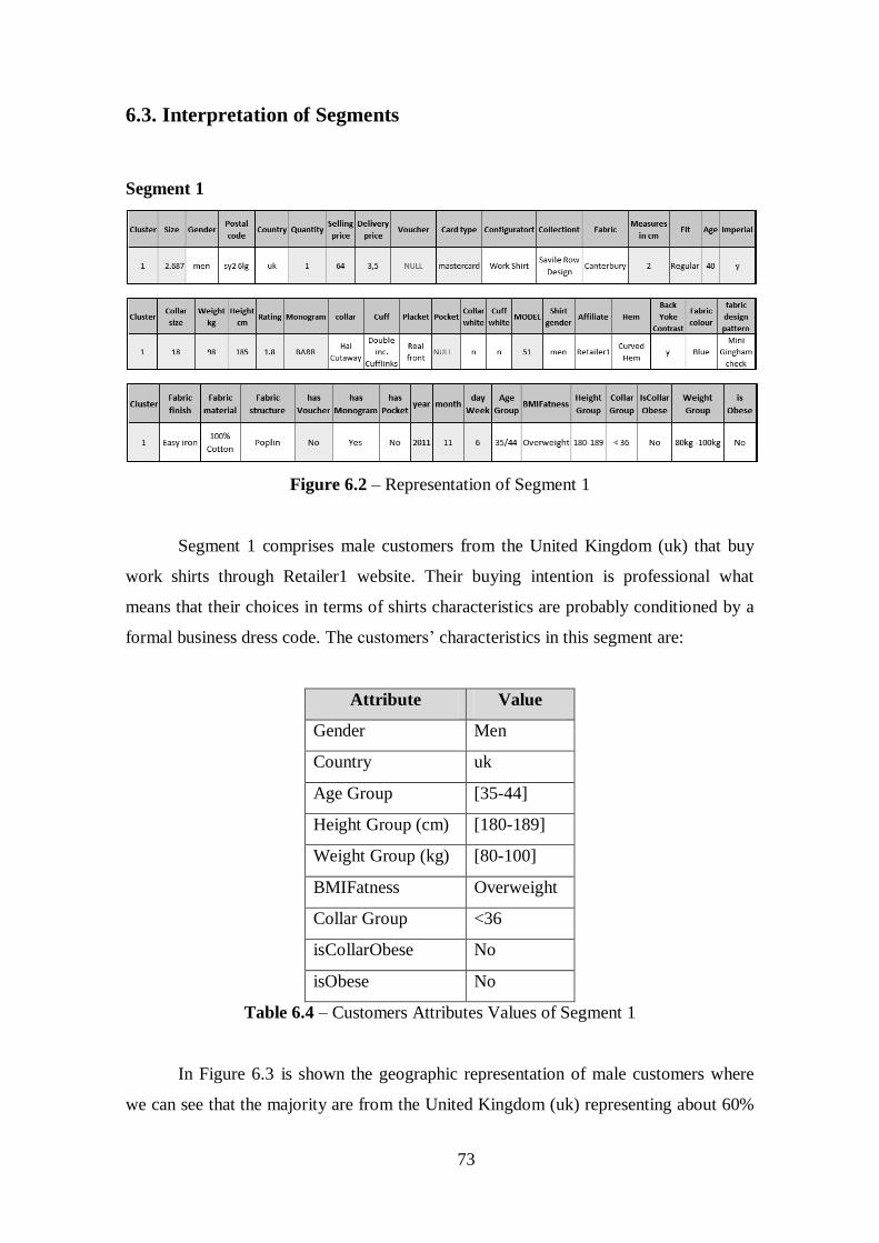
73
6.3. Interpretation of Segments
Segment 1
Figure 6.2 – Representation of Segment 1
Segment 1 comprises male customers from the United Kingdom (uk) that buy
work shirts through Retailer1 website. Their buying intention is professional what
means that their choices in terms of shirts characteristics are probably conditioned by a
formal business dress code. The customers’ characteristics in this segment are:
Attribute Value
Gender Men
Country uk
Age Group [35-44]
Height Group (cm) [180-189]
Weight Group (kg) [80-100]
BMIFatness Overweight
Collar Group <36
isCollarObese No
isObese No
Table 6.4 – Customers Attributes Values of Segment 1
In Figure 6.3 is shown the geographic representation of male customers where
we can see that the majority are from the United Kingdom (uk) representing about 60%
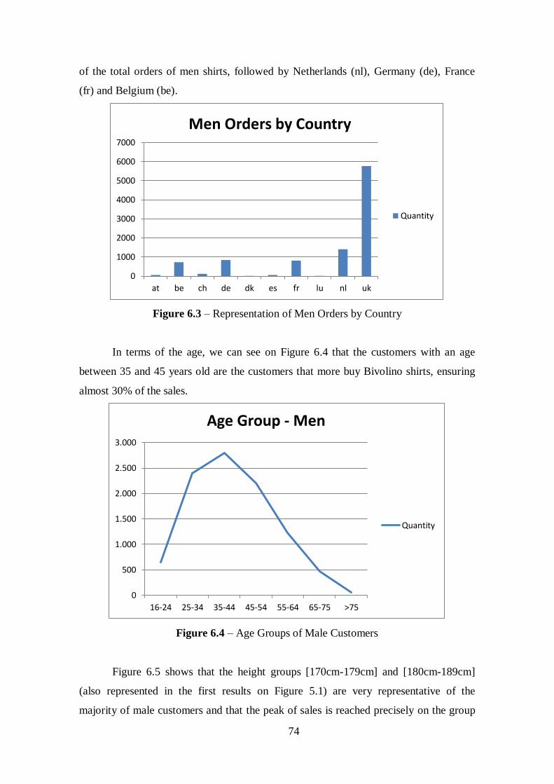
74
of the total orders of men shirts, followed by Netherlands (nl), Germany (de), France
(fr) and Belgium (be).
Figure 6.3 – Representation of Men Orders by Country
In terms of the age, we can see on Figure 6.4 that the customers with an age
between 35 and 45 years old are the customers that more buy Bivolino shirts, ensuring
almost 30% of the sales.
Figure 6.4 – Age Groups of Male Customers
Figure 6.5 shows that the height groups [170cm-179cm] and [180cm-189cm]
(also represented in the first results on Figure 5.1) are very representative of the
majority of male customers and that the peak of sales is reached precisely on the group
0
1000
2000
3000
4000
5000
6000
7000
at be ch de dk es fr lu nl uk
Men Orders by Country
Quantity
0
500
1.000
1.500
2.000
2.500
3.000
16-24 25-34 35-44 45-54 55-64 65-75 >75
Age Group - Men
Quantity
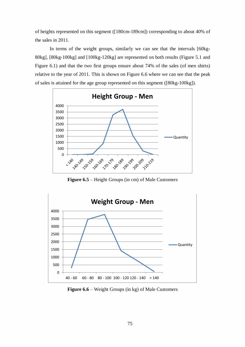
75
of heights represented on this segment ([180cm-189cm]) corresponding to about 40% of
the sales in 2011.
In terms of the weight groups, similarly we can see that the intervals [60kg-
80kg], [80kg-100kg] and [100kg-120kg] are represented on both results (Figure 5.1 and
Figure 6.1) and that the two first groups ensure about 74% of the sales (of men shirts)
relative to the year of 2011. This is shown on Figure 6.6 where we can see that the peak
of sales is attained for the age group represented on this segment ([80kg-100kg]).
Figure 6.5 – Height Groups (in cm) of Male Customers
Figure 6.6 – Weight Groups (in kg) of Male Customers
0
500
1000
1500
2000
2500
3000
3500
4000
Height Group - Men
Quantity
0
500
1000
1500
2000
2500
3000
3500
4000
40 - 60 60 - 80 80 - 100 100 - 120 120 - 140 > 140
Weight Group - Men
Quantity
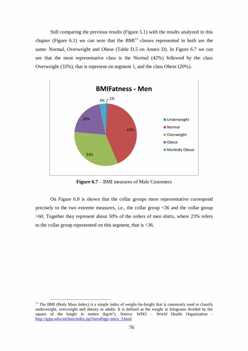
76
Still comparing the previous results (Figure 5.1) with the results analyzed in this
chapter (Figure 6.1) we can note that the BMI11
classes represented in both are the
same: Normal, Overweight and Obese (Table D.5 on Annex D). In Figure 6.7 we can
see that the most representative class is the Normal (42%) followed by the class
Overweight (33%), that is represent on segment 1, and the class Obese (20%).
Figure 6.7 – BMI measures of Male Customers
On Figure 6.8 is shown that the collar groups more representative correspond
precisely to the two extreme measures, i.e., the collar group <36 and the collar group
>60. Together they represent about 50% of the orders of men shirts, where 23% refers
to the collar group represented on this segment, that is <36.
11 The BMI (Body Mass Index) is a simple index of weight-for-height that is commonly used to classify
underweight, overweight and obesity in adults. It is defined as the weight in kilograms divided by the
square of the height in meters (kg/m2). Source: WHO – World Health Organization -
http://apps.who.int/bmi/index.jsp?introPage=intro_3.html
1%
42%
33%
20%
3%
BMIFatness - Men
Underweight
Normal
Overweight
Obese
Morbidly Obese
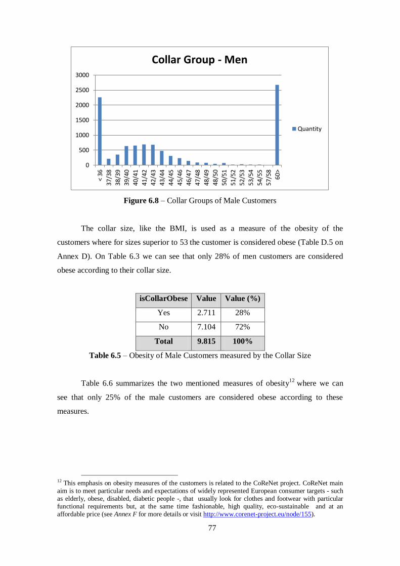
77
Figure 6.8 – Collar Groups of Male Customers
The collar size, like the BMI, is used as a measure of the obesity of the
customers where for sizes superior to 53 the customer is considered obese (Table D.5 on
Annex D). On Table 6.3 we can see that only 28% of men customers are considered
obese according to their collar size.
isCollarObese Value Value (%)
Yes 2.711 28%
No 7.104 72%
Total 9.815 100%
Table 6.5 – Obesity of Male Customers measured by the Collar Size
Table 6.6 summarizes the two mentioned measures of obesity12
where we can
see that only 25% of the male customers are considered obese according to these
measures.
12 This emphasis on obesity measures of the customers is related to the CoReNet project. CoReNet main
aim is to meet particular needs and expectations of widely represented European consumer targets - such
as elderly, obese, disabled, diabetic people -, that usually look for clothes and footwear with particular
functional requirements but, at the same time fashionable, high quality, eco-sustainable and at an
affordable price (see Annex F for more details or visit http://www.corenet-project.eu/node/155).
0
500
1000
1500
2000
2500
3000
< 36
37/3
8
38/3
9
39/4
0
40/4
1
41/4
2
42/4
3
43/4
4
44/4
5
45/4
6
46/4
7
47/4
8
48/4
9
48/5
0
50/5
1
51/5
2
52/5
3
53/5
4
54/5
5
57/5
8
60
>
Collar Group - Men
Quantity
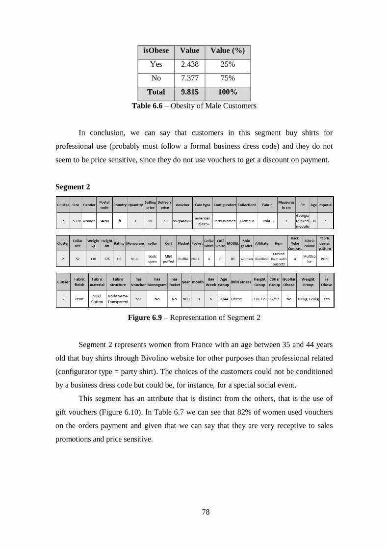
78
isObese Value Value (%)
Yes 2.438 25%
No 7.377 75%
Total 9.815 100%
Table 6.6 – Obesity of Male Customers
In conclusion, we can say that customers in this segment buy shirts for
professional use (probably must follow a formal business dress code) and they do not
seem to be price sensitive, since they do not use vouchers to get a discount on payment.
Segment 2
Figure 6.9 – Representation of Segment 2
Segment 2 represents women from France with an age between 35 and 44 years
old that buy shirts through Bivolino website for other purposes than professional related
(configurator type = party shirt). The choices of the customers could not be conditioned
by a business dress code but could be, for instance, for a special social event.
This segment has an attribute that is distinct from the others, that is the use of
gift vouchers (Figure 6.10). In Table 6.7 we can see that 82% of women used vouchers
on the orders payment and given that we can say that they are very receptive to sales
promotions and price sensitive.
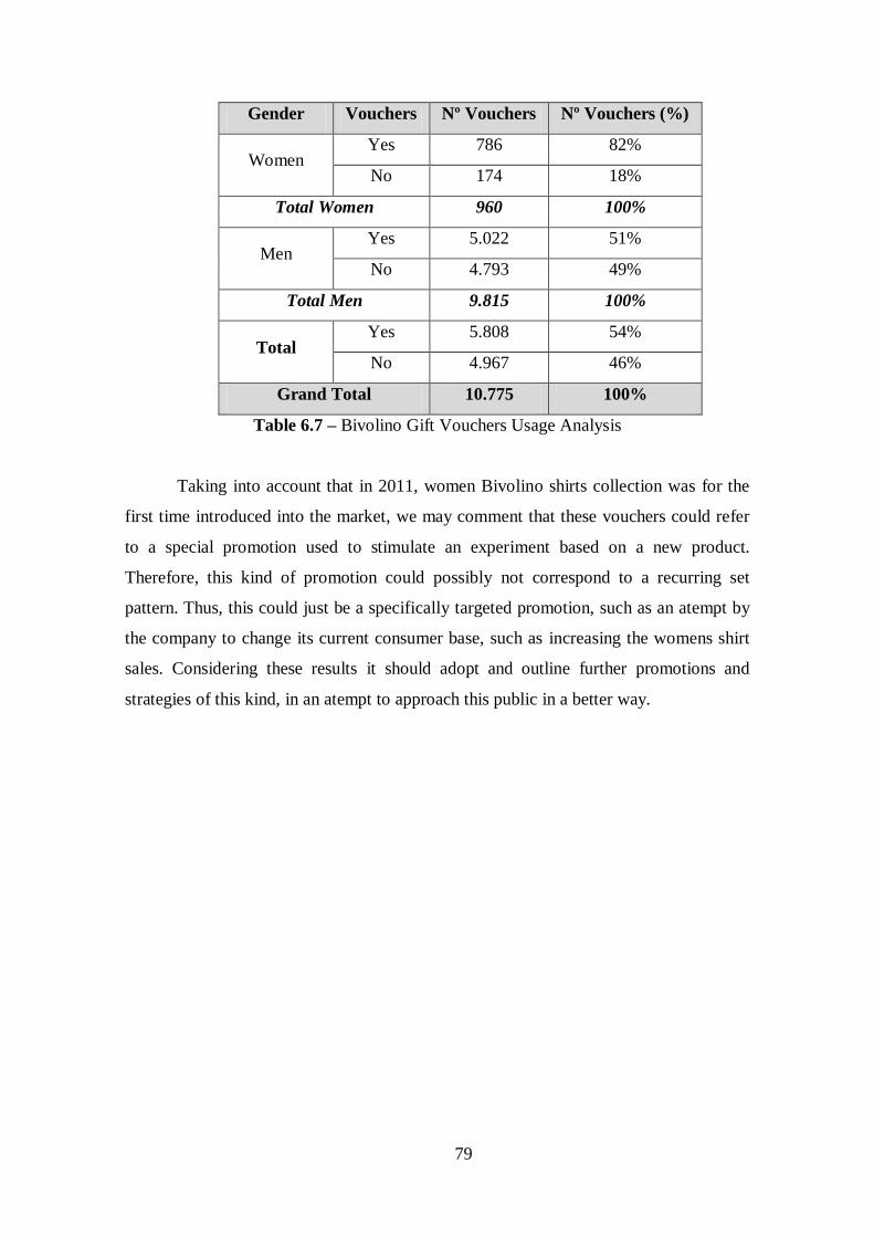
79
Gender Vouchers Nº Vouchers Nº Vouchers (%)
Women Yes 786 82%
No 174 18%
Total Women 960 100%
Men Yes 5.022 51%
No 4.793 49%
Total Men 9.815 100%
Total Yes 5.808 54%
No 4.967 46%
Grand Total 10.775 100%
Table 6.7 – Bivolino Gift Vouchers Usage Analysis
Taking into account that in 2011, women Bivolino shirts collection was for the
first time introduced into the market, we may comment that these vouchers could refer
to a special promotion used to stimulate an experiment based on a new product.
Therefore, this kind of promotion could possibly not correspond to a recurring set
pattern. Thus, this could just be a specifically targeted promotion, such as an atempt by
the company to change its current consumer base, such as increasing the womens shirt
sales. Considering these results it should adopt and outline further promotions and
strategies of this kind, in an atempt to approach this public in a better way.
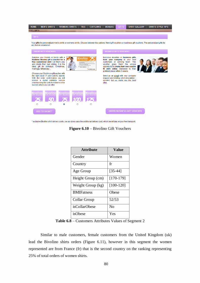
80
Figure 6.10 – Bivolino Gift Vouchers
Attribute Value
Gender Women
Country fr
Age Group [35-44]
Height Group (cm) [170-179]
Weight Group (kg) [100-120]
BMIFatness Obese
Collar Group 52/53
isCollarObese No
isObese Yes
Table 6.8 – Customers Attributes Values of Segment 2
Similar to male customers, female customers from the United Kingdom (uk)
lead the Bivolino shirts orders (Figure 6.11), however in this segment the women
represented are from France (fr) that is the second country on the ranking representing
25% of total orders of women shirts.
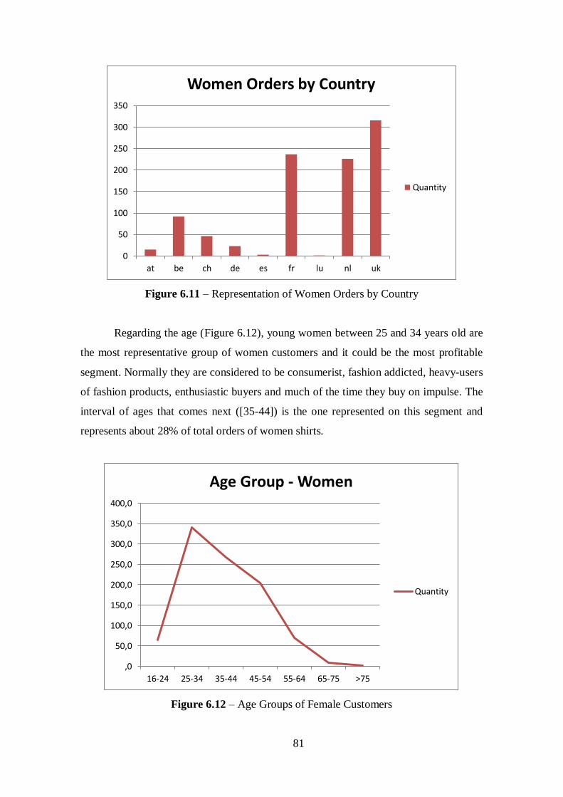
81
Figure 6.11 – Representation of Women Orders by Country
Regarding the age (Figure 6.12), young women between 25 and 34 years old are
the most representative group of women customers and it could be the most profitable
segment. Normally they are considered to be consumerist, fashion addicted, heavy-users
of fashion products, enthusiastic buyers and much of the time they buy on impulse. The
interval of ages that comes next ([35-44]) is the one represented on this segment and
represents about 28% of total orders of women shirts.
Figure 6.12 – Age Groups of Female Customers
0
50
100
150
200
250
300
350
at be ch de es fr lu nl uk
Women Orders by Country
Quantity
,0
50,0
100,0
150,0
200,0
250,0
300,0
350,0
400,0
16-24 25-34 35-44 45-54 55-64 65-75 >75
Age Group - Women
Quantity
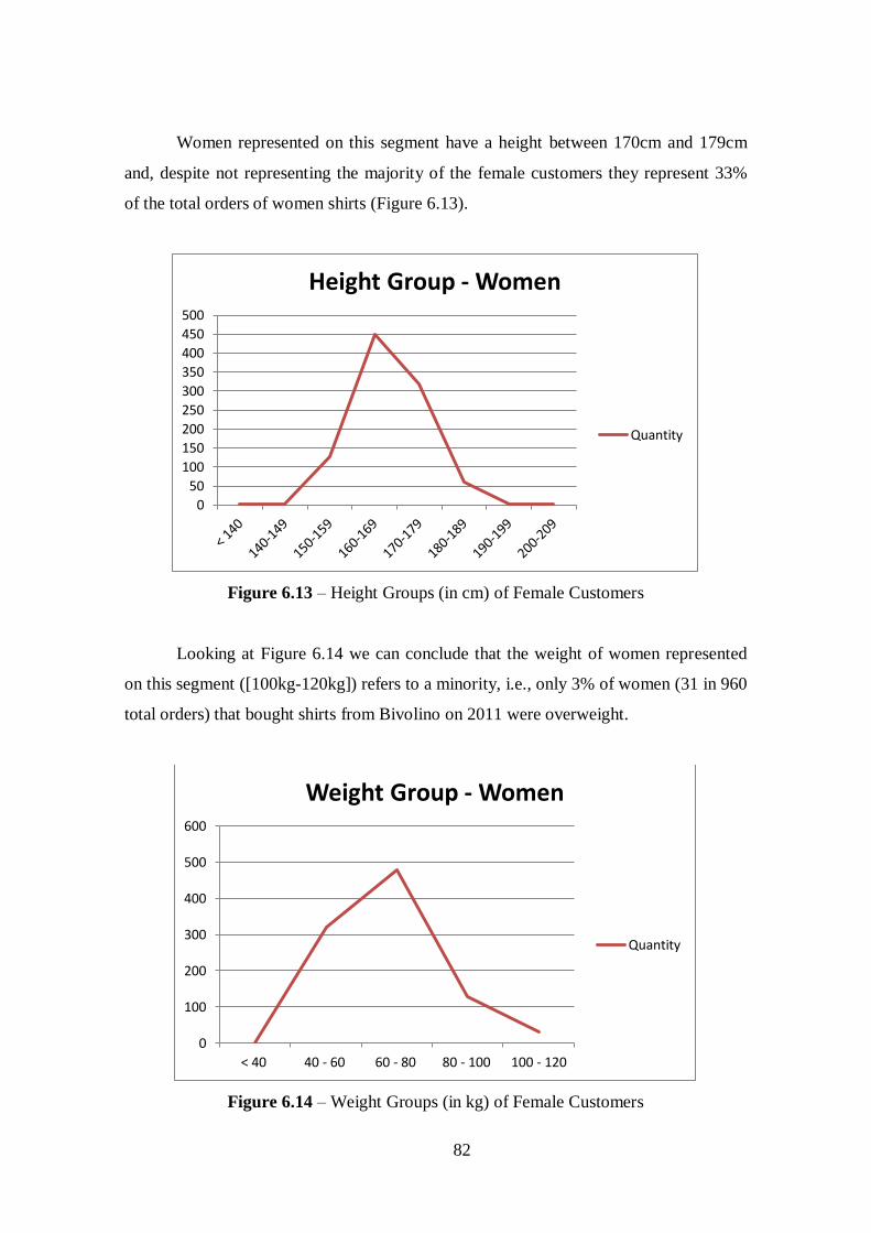
82
Women represented on this segment have a height between 170cm and 179cm
and, despite not representing the majority of the female customers they represent 33%
of the total orders of women shirts (Figure 6.13).
Figure 6.13 – Height Groups (in cm) of Female Customers
Looking at Figure 6.14 we can conclude that the weight of women represented
on this segment ([100kg-120kg]) refers to a minority, i.e., only 3% of women (31 in 960
total orders) that bought shirts from Bivolino on 2011 were overweight.
Figure 6.14 – Weight Groups (in kg) of Female Customers
0
50
100
150
200
250
300
350
400
450
500
Height Group - Women
Quantity
0
100
200
300
400
500
600
< 40 40 - 60 60 - 80 80 - 100 100 - 120
Weight Group - Women
Quantity
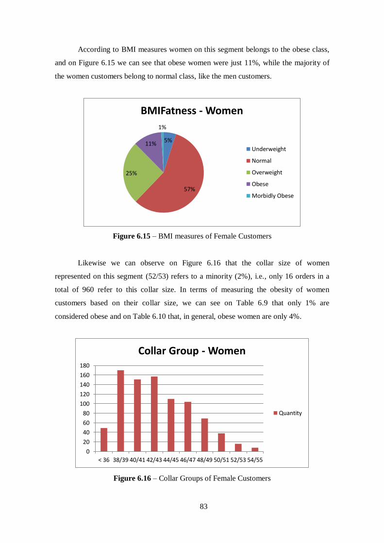
83
According to BMI measures women on this segment belongs to the obese class,
and on Figure 6.15 we can see that obese women were just 11%, while the majority of
the women customers belong to normal class, like the men customers.
Figure 6.15 – BMI measures of Female Customers
Likewise we can observe on Figure 6.16 that the collar size of women
represented on this segment (52/53) refers to a minority (2%), i.e., only 16 orders in a
total of 960 refer to this collar size. In terms of measuring the obesity of women
customers based on their collar size, we can see on Table 6.9 that only 1% are
considered obese and on Table 6.10 that, in general, obese women are only 4%.
Figure 6.16 – Collar Groups of Female Customers
5%
57%
25%
11%
1%
BMIFatness - Women
Underweight
Normal
Overweight
Obese
Morbidly Obese
0
20
40
60
80
100
120
140
160
180
< 36 38/39 40/41 42/43 44/45 46/47 48/49 50/51 52/53 54/55
Collar Group - Women
Quantity
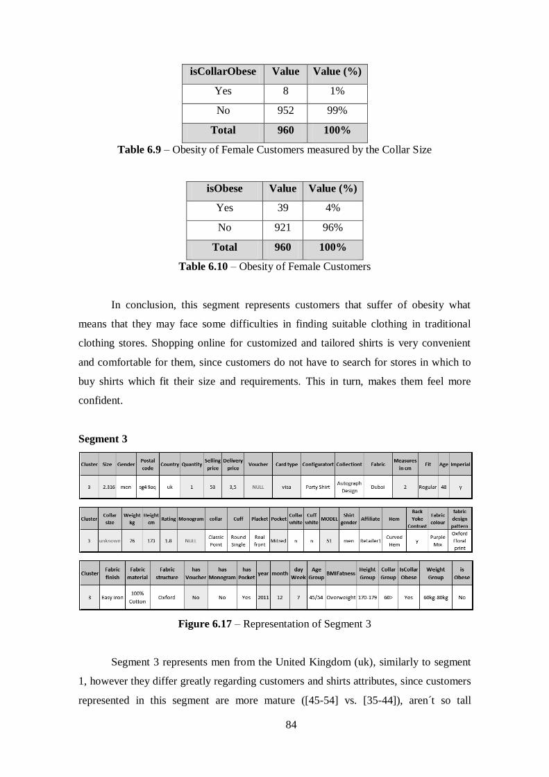
84
isCollarObese Value Value (%)
Yes 8 1%
No 952 99%
Total 960 100%
Table 6.9 – Obesity of Female Customers measured by the Collar Size
isObese Value Value (%)
Yes 39 4%
No 921 96%
Total 960 100%
Table 6.10 – Obesity of Female Customers
In conclusion, this segment represents customers that suffer of obesity what
means that they may face some difficulties in finding suitable clothing in traditional
clothing stores. Shopping online for customized and tailored shirts is very convenient
and comfortable for them, since customers do not have to search for stores in which to
buy shirts which fit their size and requirements. This in turn, makes them feel more
confident.
Segment 3
Figure 6.17 – Representation of Segment 3
Segment 3 represents men from the United Kingdom (uk), similarly to segment
1, however they differ greatly regarding customers and shirts attributes, since customers
represented in this segment are more mature ([45-54] vs. [35-44]), aren´t so tall
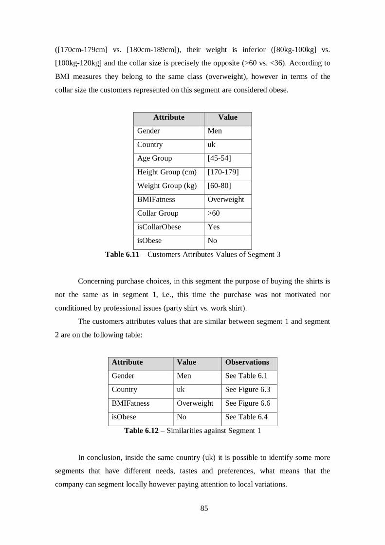
85
([170cm-179cm] vs. [180cm-189cm]), their weight is inferior ([80kg-100kg] vs.
[100kg-120kg] and the collar size is precisely the opposite (>60 vs. <36). According to
BMI measures they belong to the same class (overweight), however in terms of the
collar size the customers represented on this segment are considered obese.
Attribute Value
Gender Men
Country uk
Age Group [45-54]
Height Group (cm) [170-179]
Weight Group (kg) [60-80]
BMIFatness Overweight
Collar Group >60
isCollarObese Yes
isObese No
Table 6.11 – Customers Attributes Values of Segment 3
Concerning purchase choices, in this segment the purpose of buying the shirts is
not the same as in segment 1, i.e., this time the purchase was not motivated nor
conditioned by professional issues (party shirt vs. work shirt).
The customers attributes values that are similar between segment 1 and segment
2 are on the following table:
Attribute Value Observations
Gender Men See Table 6.1
Country uk See Figure 6.3
BMIFatness Overweight See Figure 6.6
isObese No See Table 6.4
Table 6.12 – Similarities against Segment 1
In conclusion, inside the same country (uk) it is possible to identify some more
segments that have different needs, tastes and preferences, what means that the
company can segment locally however paying attention to local variations.
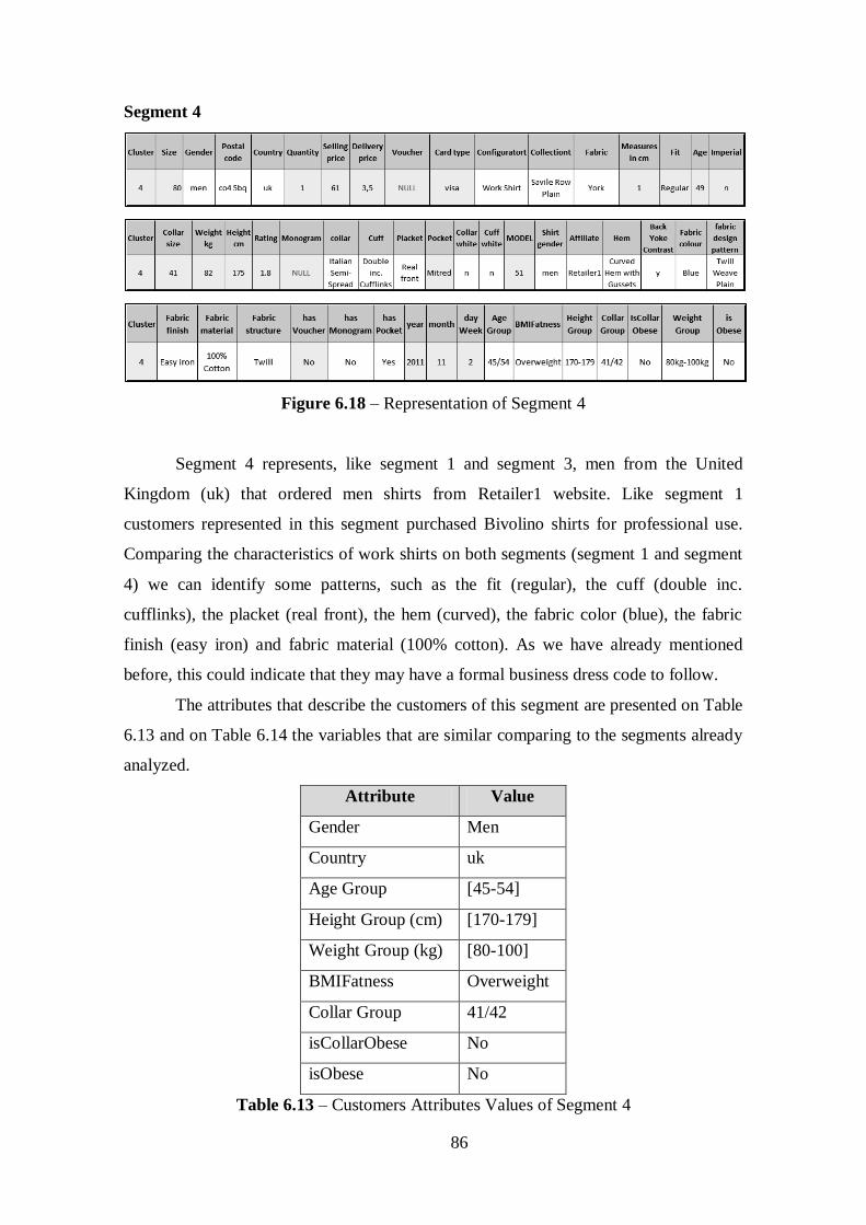
86
Segment 4
Figure 6.18 – Representation of Segment 4
Segment 4 represents, like segment 1 and segment 3, men from the United
Kingdom (uk) that ordered men shirts from Retailer1 website. Like segment 1
customers represented in this segment purchased Bivolino shirts for professional use.
Comparing the characteristics of work shirts on both segments (segment 1 and segment
4) we can identify some patterns, such as the fit (regular), the cuff (double inc.
cufflinks), the placket (real front), the hem (curved), the fabric color (blue), the fabric
finish (easy iron) and fabric material (100% cotton). As we have already mentioned
before, this could indicate that they may have a formal business dress code to follow.
The attributes that describe the customers of this segment are presented on Table
6.13 and on Table 6.14 the variables that are similar comparing to the segments already
analyzed.
Attribute Value
Gender Men
Country uk
Age Group [45-54]
Height Group (cm) [170-179]
Weight Group (kg) [80-100]
BMIFatness Overweight
Collar Group 41/42
isCollarObese No
isObese No
Table 6.13 – Customers Attributes Values of Segment 4
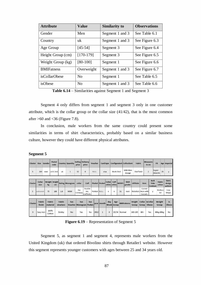
87
Attribute Value Similarity to Observations
Gender Men Segment 1 and 3 See Table 6.1
Country uk Segment 1 and 3 See Figure 6.3
Age Group [45-54] Segment 3 See Figure 6.4
Height Group (cm) [170-179] Segment 3 See Figure 6.5
Weight Group (kg) [80-100] Segment 1 See Figure 6.6
BMIFatness Overweight Segment 1 and 3 See Figure 6.7
isCollarObese No Segment 1 See Table 6.5
isObese No Segment 1 and 3 See Table 6.6
Table 6.14 – Similarities against Segment 1 and Segment 3
Segment 4 only differs from segment 1 and segment 3 only in one customer
attribute, which is the collar group or the collar size (41/42), that is the most common
after >60 and <36 (Figure 7.8).
In conclusion, male workers from the same country could present some
similarities in terms of shirt characteristics, probably based on a similar business
culture, however they could have different physical attributes.
Segment 5
Figure 6.19 – Representation of Segment 5
Segment 5, as segment 1 and segment 4, represents male workers from the
United Kingdom (uk) that ordered Bivolino shirts through Retailer1 website. However
this segment represents younger customers with ages between 25 and 34 years old.
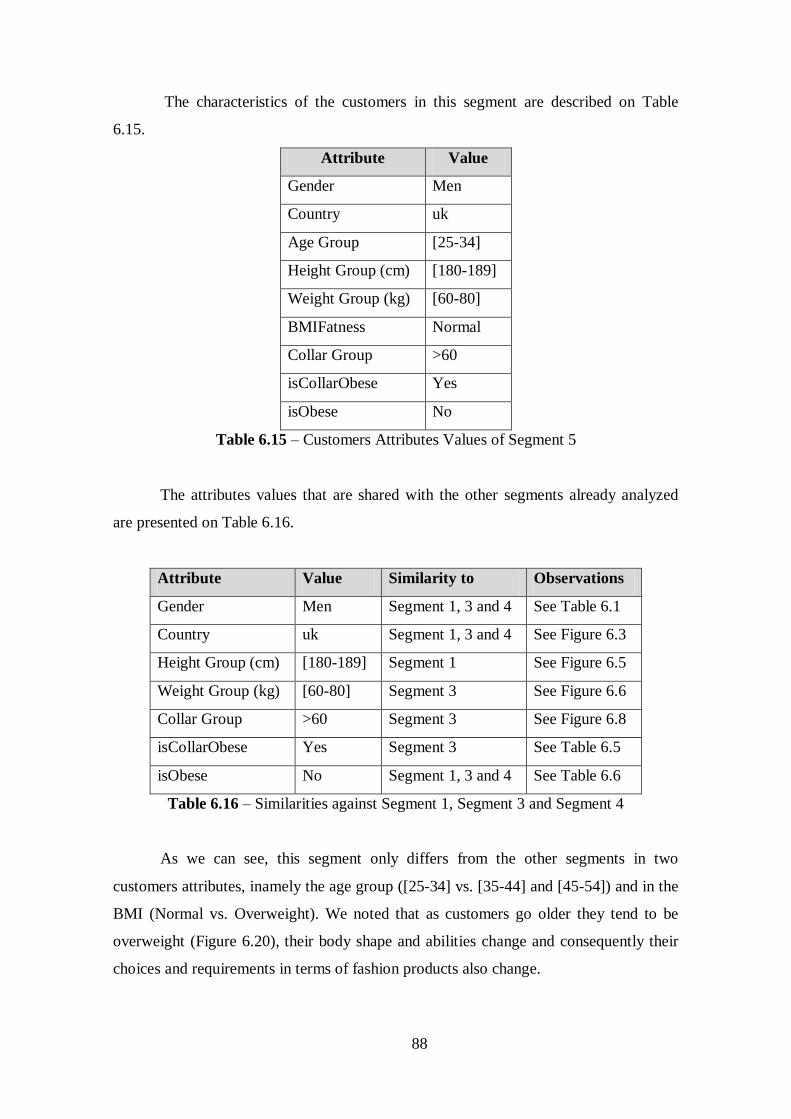
88
The characteristics of the customers in this segment are described on Table
6.15.
Attribute Value
Gender Men
Country uk
Age Group [25-34]
Height Group (cm) [180-189]
Weight Group (kg) [60-80]
BMIFatness Normal
Collar Group >60
isCollarObese Yes
isObese No
Table 6.15 – Customers Attributes Values of Segment 5
The attributes values that are shared with the other segments already analyzed
are presented on Table 6.16.
Attribute Value Similarity to Observations
Gender Men Segment 1, 3 and 4 See Table 6.1
Country uk Segment 1, 3 and 4 See Figure 6.3
Height Group (cm) [180-189] Segment 1 See Figure 6.5
Weight Group (kg) [60-80] Segment 3 See Figure 6.6
Collar Group >60 Segment 3 See Figure 6.8
isCollarObese Yes Segment 3 See Table 6.5
isObese No Segment 1, 3 and 4 See Table 6.6
Table 6.16 – Similarities against Segment 1, Segment 3 and Segment 4
As we can see, this segment only differs from the other segments in two
customers attributes, inamely the age group ([25-34] vs. [35-44] and [45-54]) and in the
BMI (Normal vs. Overweight). We noted that as customers go older they tend to be
overweight (Figure 6.20), their body shape and abilities change and consequently their
choices and requirements in terms of fashion products also change.
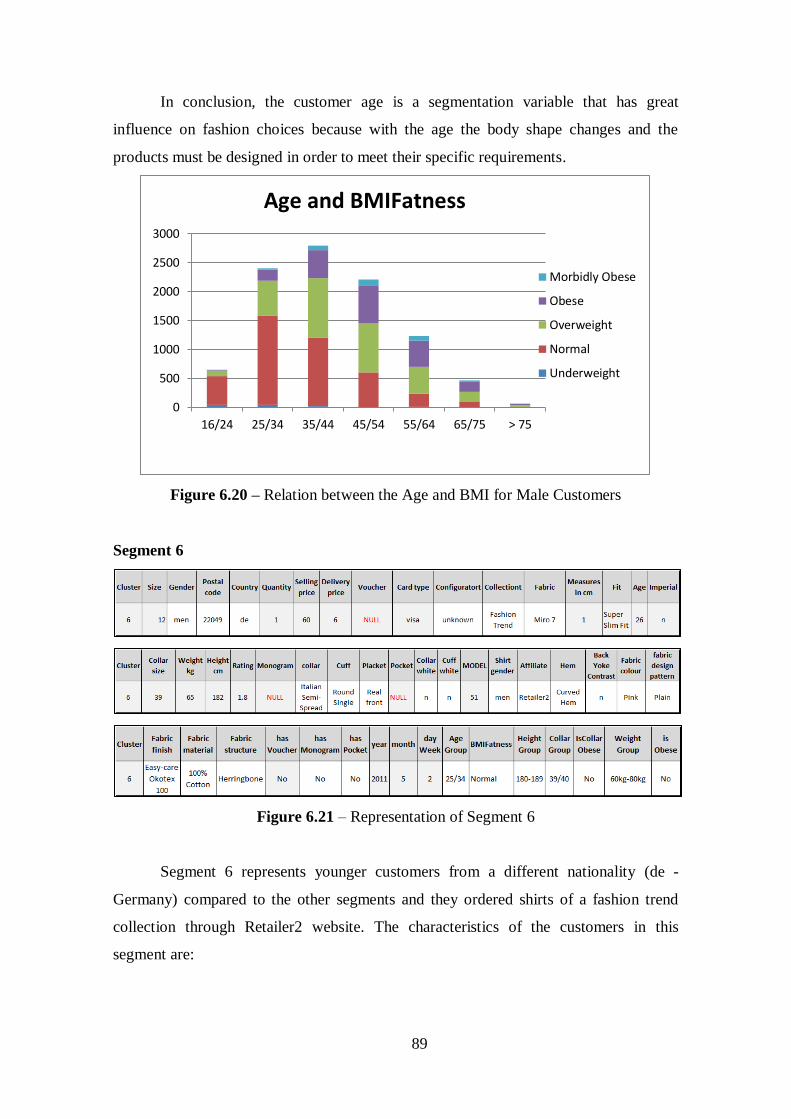
89
In conclusion, the customer age is a segmentation variable that has great
influence on fashion choices because with the age the body shape changes and the
products must be designed in order to meet their specific requirements.
Figure 6.20 – Relation between the Age and BMI for Male Customers
Segment 6
Figure 6.21 – Representation of Segment 6
Segment 6 represents younger customers from a different nationality (de -
Germany) compared to the other segments and they ordered shirts of a fashion trend
collection through Retailer2 website. The characteristics of the customers in this
segment are:
0
500
1000
1500
2000
2500
3000
16/24 25/34 35/44 45/54 55/64 65/75 > 75
Morbidly Obese
Obese
Overweight
Normal
Underweight
Age and BMIFatness
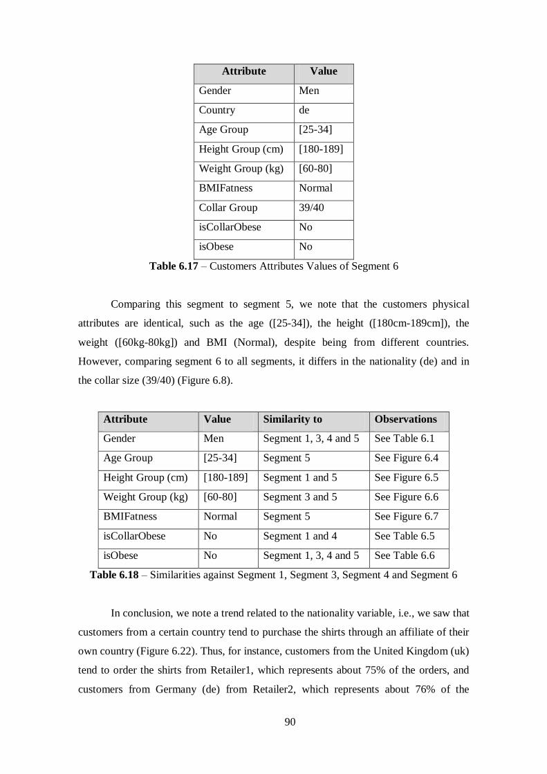
90
Attribute Value
Gender Men
Country de
Age Group [25-34]
Height Group (cm) [180-189]
Weight Group (kg) [60-80]
BMIFatness Normal
Collar Group 39/40
isCollarObese No
isObese No
Table 6.17 – Customers Attributes Values of Segment 6
Comparing this segment to segment 5, we note that the customers physical
attributes are identical, such as the age ([25-34]), the height ([180cm-189cm]), the
weight ([60kg-80kg]) and BMI (Normal), despite being from different countries.
However, comparing segment 6 to all segments, it differs in the nationality (de) and in
the collar size (39/40) (Figure 6.8).
Attribute Value Similarity to Observations
Gender Men Segment 1, 3, 4 and 5 See Table 6.1
Age Group [25-34] Segment 5 See Figure 6.4
Height Group (cm) [180-189] Segment 1 and 5 See Figure 6.5
Weight Group (kg) [60-80] Segment 3 and 5 See Figure 6.6
BMIFatness Normal Segment 5 See Figure 6.7
isCollarObese No Segment 1 and 4 See Table 6.5
isObese No Segment 1, 3, 4 and 5 See Table 6.6
Table 6.18 – Similarities against Segment 1, Segment 3, Segment 4 and Segment 6
In conclusion, we note a trend related to the nationality variable, i.e., we saw that
customers from a certain country tend to purchase the shirts through an affiliate of their
own country (Figure 6.22). Thus, for instance, customers from the United Kingdom (uk)
tend to order the shirts from Retailer1, which represents about 75% of the orders, and
customers from Germany (de) from Retailer2, which represents about 76% of the
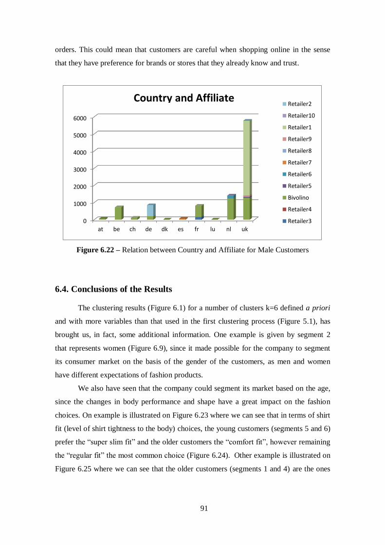
91
orders. This could mean that customers are careful when shopping online in the sense
that they have preference for brands or stores that they already know and trust.
Figure 6.22 – Relation between Country and Affiliate for Male Customers
6.4. Conclusions of the Results
The clustering results (Figure 6.1) for a number of clusters k=6 defined a priori
and with more variables than that used in the first clustering process (Figure 5.1), has
brought us, in fact, some additional information. One example is given by segment 2
that represents women (Figure 6.9), since it made possible for the company to segment
its consumer market on the basis of the gender of the customers, as men and women
have different expectations of fashion products.
We also have seen that the company could segment its market based on the age,
since the changes in body performance and shape have a great impact on the fashion
choices. On example is illustrated on Figure 6.23 where we can see that in terms of shirt
fit (level of shirt tightness to the body) choices, the young customers (segments 5 and 6)
prefer the “super slim fit” and the older customers the “comfort fit”, however remaining
the “regular fit” the most common choice (Figure 6.24). Other example is illustrated on
Figure 6.25 where we can see that the older customers (segments 1 and 4) are the ones
0
1000
2000
3000
4000
5000
6000
at be ch de dk es fr lu nl uk
Retailer2
Retailer10
Retailer1
Retailer9
Retailer8
Retailer7
Retailer6
Retailer5
Bivolino
Retailer4
Retailer3
Country and Affiliate
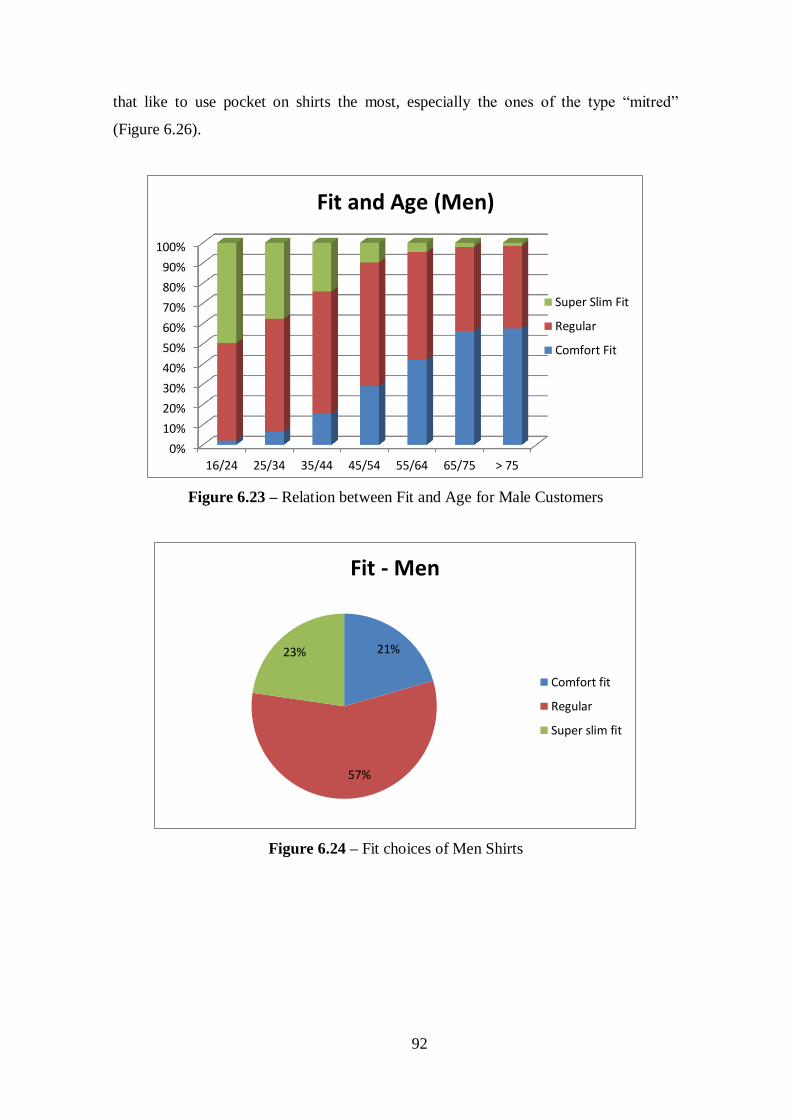
92
that like to use pocket on shirts the most, especially the ones of the type “mitred”
(Figure 6.26).
Figure 6.23 – Relation between Fit and Age for Male Customers
Figure 6.24 – Fit choices of Men Shirts
0%
10%
20%
30%
40%
50%
60%
70%
80%
90%
100%
16/24 25/34 35/44 45/54 55/64 65/75 > 75
Super Slim Fit
Regular
Comfort Fit
Fit and Age (Men)
21%
57%
23%
Fit - Men
Comfort fit
Regular
Super slim fit
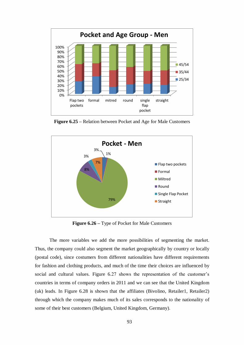
93
Figure 6.25 – Relation between Pocket and Age for Male Customers
Figure 6.26 – Type of Pocket for Male Customers
The more variables we add the more possibilities of segmenting the market.
Thus, the company could also segment the market geographically by country or locally
(postal code), since costumers from different nationalities have different requirements
for fashion and clothing products, and much of the time their choices are influenced by
social and cultural values. Figure 6.27 shows the representation of the customer’s
countries in terms of company orders in 2011 and we can see that the United Kingdom
(uk) leads. In Figure 6.28 is shown that the affiliates (Bivolino, Retailer1, Retailer2)
through which the company makes much of its sales corresponds to the nationality of
some of their best customers (Belgium, United Kingdom, Germany).
0%10%20%30%40%50%60%70%80%90%
100%
Flap twopockets
formal mitred round singleflap
straight
45/54
35/44
25/34
Pocket and Age Group - Men
3% 1%
79%
8%
3%
7%
Pocket - Men
Flap two pockets
Formal
Miltred
Round
Single Flap Pocket
Straight
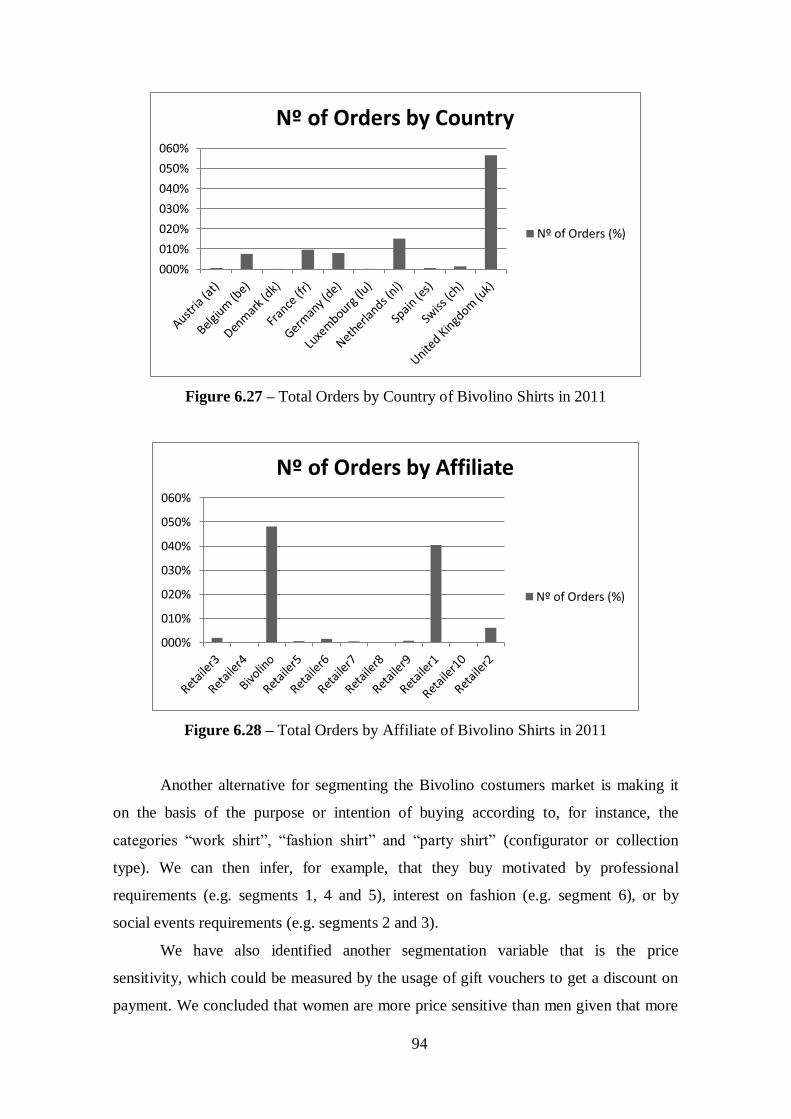
94
Figure 6.27 – Total Orders by Country of Bivolino Shirts in 2011
Figure 6.28 – Total Orders by Affiliate of Bivolino Shirts in 2011
Another alternative for segmenting the Bivolino costumers market is making it
on the basis of the purpose or intention of buying according to, for instance, the
categories “work shirt”, “fashion shirt” and “party shirt” (configurator or collection
type). We can then infer, for example, that they buy motivated by professional
requirements (e.g. segments 1, 4 and 5), interest on fashion (e.g. segment 6), or by
social events requirements (e.g. segments 2 and 3).
We have also identified another segmentation variable that is the price
sensitivity, which could be measured by the usage of gift vouchers to get a discount on
payment. We concluded that women are more price sensitive than men given that more
000%
010%
020%
030%
040%
050%
060%
Nº of Orders by Country
Nº of Orders (%)
000%
010%
020%
030%
040%
050%
060%
Nº of Orders by Affiliate
Nº of Orders (%)

95
than 82% used a voucher (Table 6.7) on shirts payment. Women are generally more
receptive to promotions of this type and more open to experimenting new products than
men. However we do not know if it was related to a specific promotion with the
intention of allowing the experiment of a new product, however if yes the company
should study other ways of attract the female public and improve sales.
In short, in this chapter we analyzed the profile of Bivolino customers and their
relation to the product (shirts) based on some segmentation variables that were
identified. We concluded that their choices in terms of shirts attributes are greatly
influenced and conditioned by numerous factors such as, their physical attributes, age,
gender, nationality (country), purpose of buying. Given that, the company must pay
attention to those differences and adjust its product and marketing strategies to the
different segments identified.

97
7. CONCLUSION
“It's more fun to arrive a conclusion
Than to justify it.”
By Malcolm Forbes, an American publisher
7.1. Summary
The aim of this work was to show the practical applicability of Data Mining
(DM) techniques and tools to market segmentation in the context of the customized
fashion industry. The study was based on data provided by Bivolino, a Belgian
company that produces and sells custom tailored shirts, relative to its shirts orders of
2011.
We started the work by doing some literature review about the subjects covered.
We aimed to give an overview about DM (definition, tasks, process, and methodology),
Clustering (definition, goals, stages, algorithms and validation) and Segmentation in
Marketing (definition, effectiveness, process, levels, bases, methods and methodology).
We then described what we did in practice based on those theoretical insights
and the data available. We followed the steps of CRISP-DM (business understanding,
data understanding, data preparation, modeling, evaluation and deployment), a general
methodology to support the DM process. The modeling step was carried out using the
DM software RapidMiner. In terms of the segmentation methodology, we adopted a
non-overlapping (each subject belongs to a single segment only) non-hierarchical (start
from a random initial division of the subjects into a predetermined number of clusters,
and reassign subjects to clusters until a certain criterion is optimized) clustering method
called K-Medoids. As we know, clustering methods are commonly used in marketing
for the identification and definition of market segments that help companies focus their
marketing strategies. Then, we proceeded with the market segmentation and identified
possible segmentation bases according to the classic segmentation variables for
consumer markets (demographic, geographic, psychographic and behavioristic)
suggested by Kotler and complemented by Wedel and Kamakura.
98
In this study we run the clustering process twice for a dataset of n = 10.775 shirts
orders and a number of clusters k = 6 defined a priori, with the difference on the
number of attributes (describing the orders, shirts and customers) used. On the first
clustering process we used 29 attributes and on the second we added 30 more. The
choice of the attributes to use in each process depended on the scope of the analysis, i.e.,
the first analysis was based on a technical perspective (production and design of the
shirts) and the second on a marketing perspective (segmentation of shirts customers). At
the end, we were able to see how results from a clustering process could differ simply
changing the number of the attributes.
Given the results we started by analyzing the first results mainly focusing on the
attributes that describe the shirts attributes (fabric color, material, design and pattern,
finish, structure, etc.) with the purpose of finding some patterns in the data that could be
transformed into useful information to support the company’s decisions in terms of
production and design. Then we analyzed the second result mainly focusing on the
attributes that describe the customers (gender, age, country, height, weight, BMI, collar
size, etc.) in an attempt to divide the market of Bivolino shirts customers into distinct
groups of buyers who have different needs, characteristics, or behaviors, and who might
require separate products or marketing programs.
The analysis of both results allows us to conclude that DM techniques and tools
are indeed very useful when analyzing vast quantities of data. The first clustering result
allowed us to answer one of the aspects from our business problem, i.e., how could the
fashion designers identify and predict the fashion profiles and trends. Similarly, the
second clustering results enabled us to respond to another aspect of our business
problem that is how the company could segment its market in different groups of
customers with distinct characteristics, needs, preferences, tastes and behaviors and then
adapt or adjust its strategies to respond more effectively to their requirements. It will
also allow the company to identify which segments are most profitable and focus its
efforts in that direction.
99
7.2. Recommendations
This study gave us new insights about the fashion industry. Thus, based on the
data about Bivolino customers database and on the results obtained from clustering and
segmenting the data, we recommend:
The company should strengthen its efforts to expand into the women’s clothing
market, since they represent a market segment that is very attentive to fashion
issues and receptive to sales promotions and to experimenting new products.
Gift vouchers were the strategy adopted so far by Bivolino to address this new
segment. Given the positive response of this important segment, the company
should consider adopting promotions of different types.
As the older-age consumer market is increasing, the company should also
expand in that direction. They should be inclusive in their marketing and
promotional campaigns, highlighting the benefits of fashion products as older
consumers consider their clothing consumption in a more strategic manner than
younger consumers. Understanding the attitudes and behavior of the mature
consumers will, on one hand, provide guidance for product development and
design and, on the other hand, create opportunities and challenges for the
fashion business to focus on this increasingly important market.
The company should be aware of the implications of the age in fashion
consumer choices, since consumers of all ages psychologically need to express
their individual style and taste through a choice of better quality products.
Designers should add value via fashion products that transcend all ages. They
should particularly promote the inclusion aspect of the process of buying
clothes, not only in the case of older customers but also in the case of customers
with some kind of disability or pathology.
Beyond the age and physical conditions, other factors have much influence on
customers fashion choices and the company must have to take it into account
when designing the shirts. They are, for instance, the gender (men and women
have different expectations of fashion products), the nationality (customers from
different countries have influence of social and cultural values with which they
identify), the purpose of the buying (for example, professional), etc.
100
The company should focus on the market segments that were identified as being
the most profitable and adopt different strategies for each segment taking into
account the different customers characteristics they represent (attributes that
describe customers) and corresponding fashion choices (attributes that describe
the shirts). Not only the shirts should be customized and tailored but also the
marketing-mix should be adjusted to each segment unique characteristics.
7.3. Limitations of the Study
During our study we faced some difficulties derived from several reasons. The
first is related to the inherited limitations of the method adopted. The clustering
algorithm K-Medoids, despite being less sensitive to outliers than the K-Means because
of the use of the median instead of the mean, still requires the definition of k number of
clusters a priori. Deciding the best or optimal k number of clusters is a difficult task,
which is well known (Jain et al, 2000). According to Jain et al (2000) the algorithm, in
practice, is typically run multiple times with different starting states, and the best
configuration obtained from all of the runs is used as the output of clustering. Therefore,
this method results in becoming extremely time consuming even from a computational
perspective. Each clustering process on RapidMiner took too much time, which is
largely related to the vast quantity of data clustered (too many examples and too many
attributes), even though, partitional methods have advantages in applications involving
large data sets (Jain et al, 2000).Another difficulty related to the clustering method is
how to know if the clustering results is a ‘good’ or a ‘poor’ one. All clustering
algorithms will, when presented with data, produce clusters regardless of whether the
data contain clusters or not. If data does contain clusters, some clustering algorithms
may obtain ‘better’ cluster than others (Jain et al, 2000). Nevertheless, given the type of
the attributes used in the study (binominal and polynomial, i.e., non-numeric) and our
task (clustering), the choice of the algorithm was very limited. Most of the clustering
algorithms available on RapidMiner did not accept categorical data (data separable into
categories that are mutually exclusive, such as age groups). However, the algorithm
selected proved to be suitable for the problem at hand.
As we can see, clustering is a very subjective task, i.e., the same dataset may
need to be partitioned differently for different purposes (Jain et al, 2000). In our study
101
we clustered the same dataset twice but changing the number of the attributes according
to the purpose of the analysis.
Other difficulties are related to the marketing analysis in the way that we have
not access to the necessary information about the customers, specially referring to
behavioristic and psychographic attributes (personality traits, lifestyles, interests,
occupation, education, etc.). However, it was possible to identify same segmentation
variables based on the available information. Nevertheless, we couldn’t go further in the
study.
In sum, the difficulties faced in the study were:
Deciding the number of clusters k;
High computational cost of the methods;
Limitations imposed by the types of the attributes, which strongly constraints the
selection of the algorithm;
Subjective nature of the evaluation process;
Insufficient data to characterize customers.
7.4. Future Work
Taking into account the difficulties encountered during this study and the
limitations they imposed on it, we find that future work is needed and should focus on
the following issues, which are mainly related to the problems of clustering itself:
Find a general theoretical solution to find the optimal number of clusters for any
given dataset;
Reduce time complexity when dealing with large number of dimensions and
large number of data items;
Find a way to help on the interpretation of the result of a clustering algorithm
(that in many cases can be arbitrary itself), as it can be interpreted in different
ways;
Transform the data to enable the use of different clustering algorithms, compare
the different results and decide which is the best;
Reduce the dependency of the effectiveness of the clustering method on the
definition of “distance” (for distance-based clustering);
Alternatively to the previous suggestion, it would be interesting to find a way of
defining a distance measure, that is specific to the business problem;


APPENDICES

105
APPENDIX A
Data Mining Methodology: CRISP-DM
The DM methodology used in this work was the CRISP-DM (Cross Industry
Standard Process for Data Mining), which is explained in more detail in Annex B. Now
we will describe the phases of the DM methodology followed during the study.
A. Business Understanding
First, we tried to understand the project objectives and requirements from a
business perspective, and then convert it into a DM problem. So, our business problem
is how Bivolino13
can reach specific market niches while responding more effectively
to their unique needs and preferences. This is achieved by identifying profiles of shirts
sold. Converting it to a DM problem, the goal is to find clusters in the data provided by
Bivolino relative to shirts ordered in 2011. The results of this project are to be useful for
marketing purposes but mainly important for the design of new products.
B. Data Understanding
Understanding the data14
is the first step and one of the most important. In order
to become familiar with the data, identify data quality problems, discover first insights
into the data, and/or detect interesting subsets to form hypothesis regarding hidden
information, we performed an exploratory data analysis15
and identified some
interesting insights and patterns (Table A.1).
Besides the findings presented in Table A.1, we can intuitively define some
segments with the data for market niches, such as obese and very tall people, for
example. These kinds of people face difficulties in finding clothing with appropriate
measurements for them, so it is very useful and comforting for them to have a company
like Bivolino providing clothing where they do not have to face such a problem.
C. Data Preparation
Data preparation is the phase where we have to make the data ready to be
processed by the DM tools. This is done by working on the initial raw data and applying
several operations to construct the final dataset to be modeled by DM tools. This
13 See Annex A to better know the Bivolino Company or visit http://www.bivolino.com/. 14
See Annex D, Table D.1 – Data Table. 15 Exploratory Data Analysis is the use of graphical and descriptive statistical techniques to learn about
the structure of a dataset.
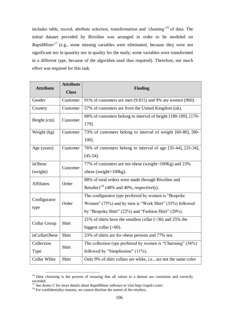
106
includes table, record, attribute selection, transformation and ‘cleaning’16
of data. The
initial dataset provided by Bivolino was arranged in order to be modeled on
RapidMiner17
(e.g., some missing variables were eliminated, because they were not
significant nor in quantity nor in quality for the study; some variables were transformed
in a different type, because of the algorithm used thus required). Therefore, not much
effort was required for this task.
Attribute Attribute
Class Finding
Gender Customer 91% of customers are men (9.815) and 9% are women (960).
Country Customer 57% of customers are from the United Kingdom (uk).
Height (cm) Customer 68% of customers belong to interval of height [180-189], [170-
179].
Weight (kg) Customer 73% of customers belong to interval of weight [60-80], [80-
100].
Age (years) Customer 76% of customers belong to interval of age [35-44], [25-34],
[45-54].
isObese
(weight) Customer
77% of customers are not obese (weight<100Kg) and 23%
obese (weight>100kg).
Affiliates Order 88% of total orders were made through Bivolino and
Retailer118
(48% and 40%, respectively).
Configurator
type Order
The configurator type preferred by women is “Bespoke
Women” (75%) and by men is “Work Shirt” (35%) followed
by “Bespoke Shirt” (22%) and “Fashion Shirt” (20%).
Collar Group Shirt 21% of shirts have the smallest collar (<36) and 25% the
biggest collar (>60).
isCollarObese Shirt 23% of shirts are for obese persons and 77% not.
Collection
Type Shirt
The collection type preferred by women is “Charming” (56%)
followed by “Simplissime” (11%).
Collar White Shirt Only 9% of shirt collars are white, i.e., are not the same color
16 Data cleansing is the process of ensuring that all values in a dataset are consistent and correctly
recorded. 17 See Annex C for more details about RapidMiner software or visit http://rapid-i.com/. 18 For confidentiality reasons, we cannot disclose the names of the retailers.
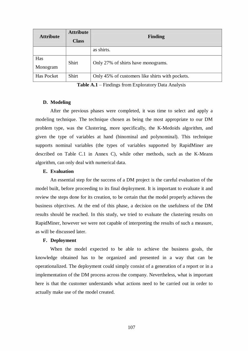
107
Attribute Attribute
Class Finding
as shirts.
Has
Monogram Shirt Only 27% of shirts have monograms.
Has Pocket Shirt Only 45% of customers like shirts with pockets.
Table A.1 – Findings from Exploratory Data Analysis
D. Modeling
After the previous phases were completed, it was time to select and apply a
modeling technique. The technique chosen as being the most appropriate to our DM
problem type, was the Clustering, more specifically, the K-Medoids algorithm, and
given the type of variables at hand (binominal and polynominal). This technique
supports nominal variables (the types of variables supported by RapidMiner are
described on Table C.1 in Annex C), while other methods, such as the K-Means
algorithm, can only deal with numerical data.
E. Evaluation
An essential step for the success of a DM project is the careful evaluation of the
model built, before proceeding to its final deployment. It is important to evaluate it and
review the steps done for its creation, to be certain that the model properly achieves the
business objectives. At the end of this phase, a decision on the usefulness of the DM
results should be reached. In this study, we tried to evaluate the clustering results on
RapidMiner, however we were not capable of interpreting the results of such a measure,
as will be discussed later.
F. Deployment
When the model expected to be able to achieve the business goals, the
knowledge obtained has to be organized and presented in a way that can be
operationalized. The deployment could simply consist of a generation of a report or in a
implementation of the DM process across the company. Nevertheless, what is important
here is that the customer understands what actions need to be carried out in order to
actually make use of the model created.

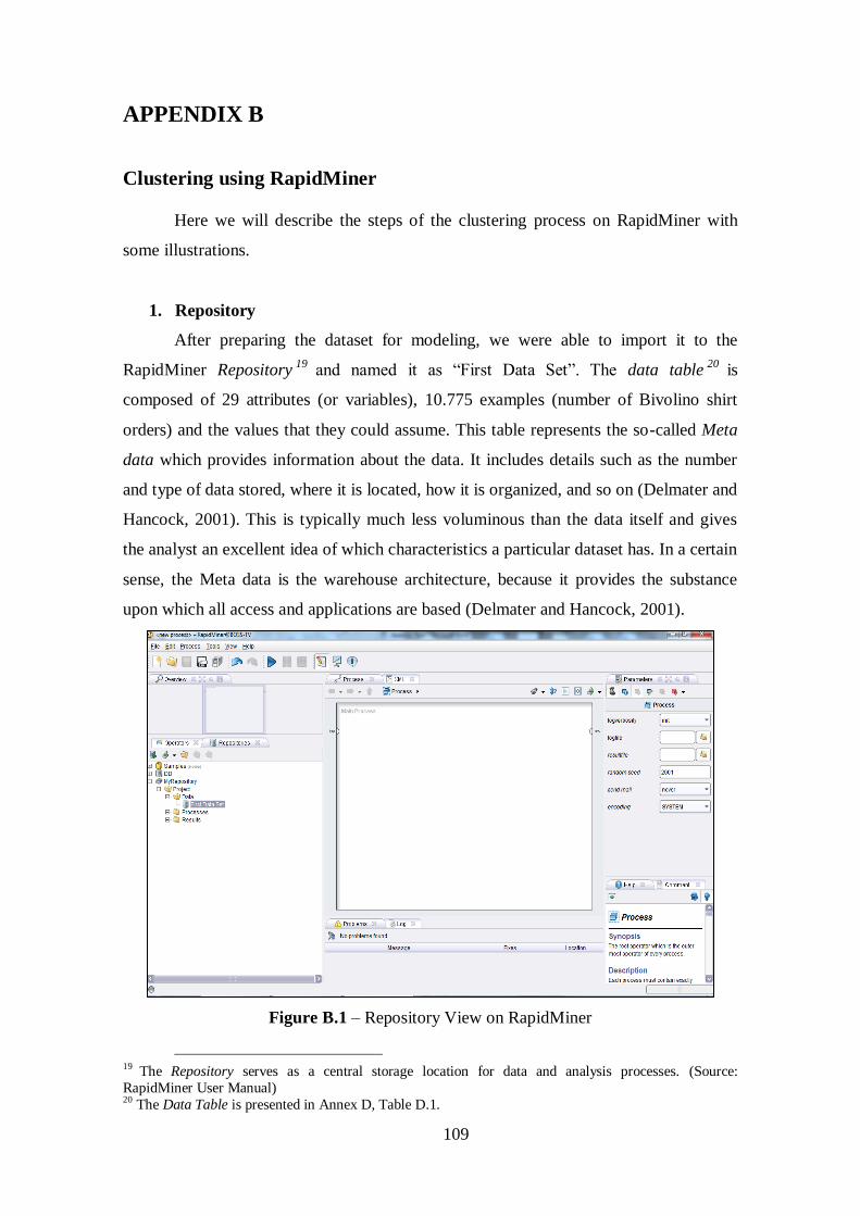
109
APPENDIX B
Clustering using RapidMiner
Here we will describe the steps of the clustering process on RapidMiner with
some illustrations.
1. Repository
After preparing the dataset for modeling, we were able to import it to the
RapidMiner Repository19
and named it as “First Data Set”. The data table20
is
composed of 29 attributes (or variables), 10.775 examples (number of Bivolino shirt
orders) and the values that they could assume. This table represents the so-called Meta
data which provides information about the data. It includes details such as the number
and type of data stored, where it is located, how it is organized, and so on (Delmater and
Hancock, 2001). This is typically much less voluminous than the data itself and gives
the analyst an excellent idea of which characteristics a particular dataset has. In a certain
sense, the Meta data is the warehouse architecture, because it provides the substance
upon which all access and applications are based (Delmater and Hancock, 2001).
Figure B.1 – Repository View on RapidMiner
19
The Repository serves as a central storage location for data and analysis processes. (Source:
RapidMiner User Manual) 20 The Data Table is presented in Annex D, Table D.1.
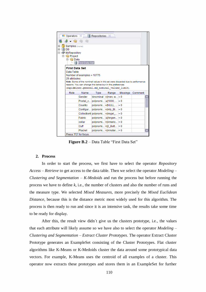
110
Figure B.2 – Data Table “First Data Set”
2. Process
In order to start the process, we first have to select the operator Repository
Access – Retrieve to get access to the data table. Then we select the operator Modeling –
Clustering and Segmentation – K-Medoids and run the process but before running the
process we have to define k, i.e., the number of clusters and also the number of runs and
the measure type. We selected Mixed Measures, more precisely the Mixed Euclidean
Distance, because this is the distance metric most widely used for this algorithm. The
process is then ready to run and since it is an intensive task, the results take some time
to be ready for display.
After this, the result view didn´t give us the clusters prototype, i.e., the values
that each attribute will likely assume so we have also to select the operator Modeling –
Clustering and Segmentation – Extract Cluster Prototypes. The operator Extract Cluster
Prototype generates an ExampleSet consisting of the Cluster Prototypes. Flat cluster
algorithms like K-Means or K-Medoids cluster the data around some prototypical data
vectors. For example, K-Means uses the centroid of all examples of a cluster. This
operator now extracts these prototypes and stores them in an ExampleSet for further
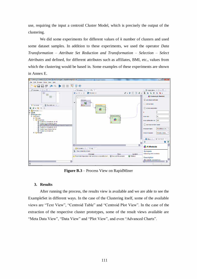
111
use, requiring the input a centroid Cluster Model, which is precisely the output of the
clustering.
We did some experiments for different values of k number of clusters and used
some dataset samples. In addition to these experiments, we used the operator Data
Transformation – Attribute Set Reduction and Transformation – Selection – Select
Attributes and defined, for different attributes such as affiliates, BMI, etc., values from
which the clustering would be based in. Some examples of these experiments are shown
in Annex E.
Figure B.3 – Process View on RapidMiner
3. Results
After running the process, the results view is available and we are able to see the
ExampleSet in different ways. In the case of the Clustering itself, some of the available
views are “Text View”, “Centroid Table” and “Centroid Plot View”. In the case of the
extraction of the respective cluster prototypes, some of the result views available are
“Meta Data View”, “Data View” and “Plot View”, and even “Advanced Charts”.
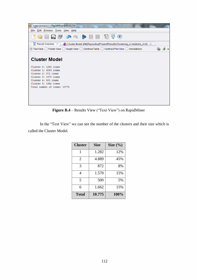
112
Figure B.4 – Results View (“Text View”) on RapidMiner
In the “Text View” we can see the number of the clusters and their size which is
called the Cluster Model.
Cluster Size Size (%)
1 1.282 12%
2 4.889 45%
3 872 8%
4 1.570 15%
5 500 5%
6 1.662 15%
Total 10.775 100%
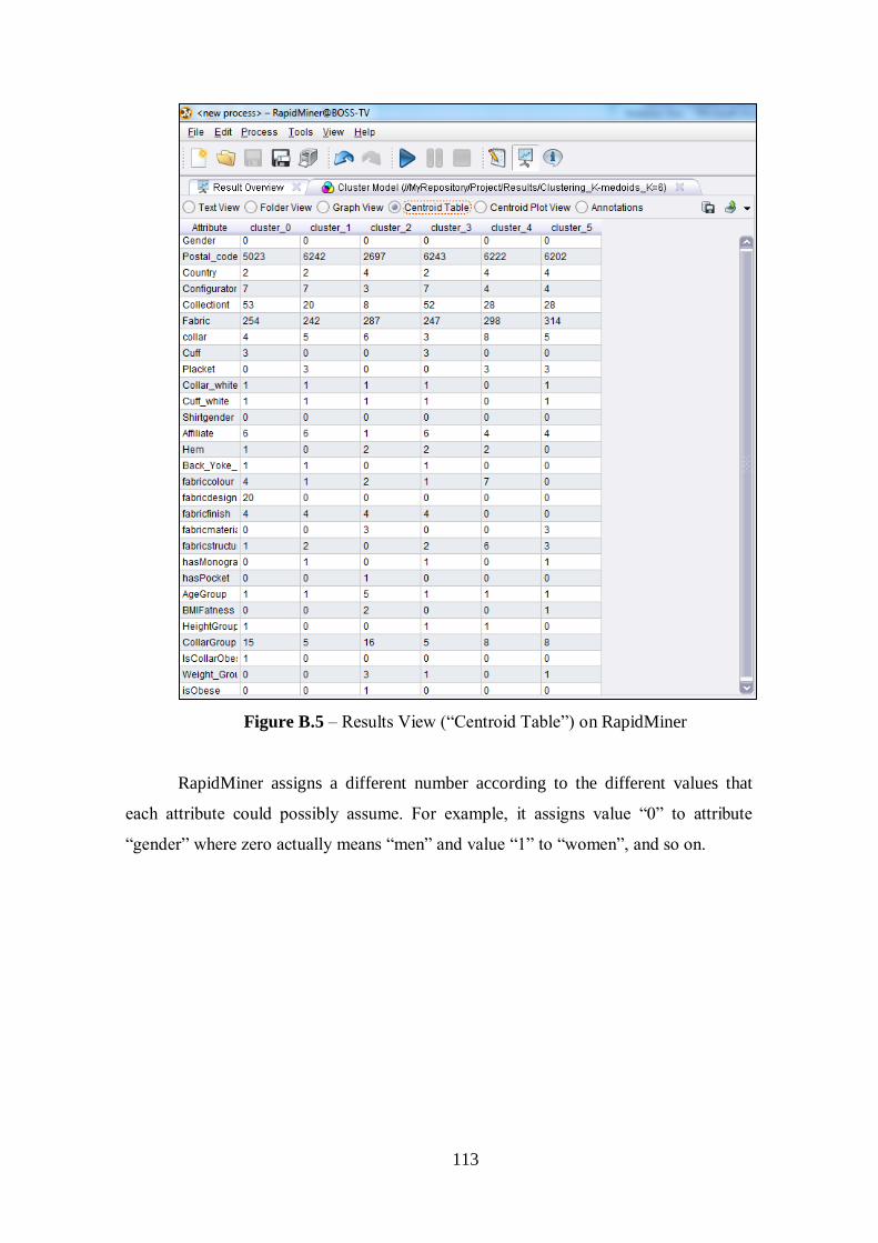
113
Figure B.5 – Results View (“Centroid Table”) on RapidMiner
RapidMiner assigns a different number according to the different values that
each attribute could possibly assume. For example, it assigns value “0” to attribute
“gender” where zero actually means “men” and value “1” to “women”, and so on.
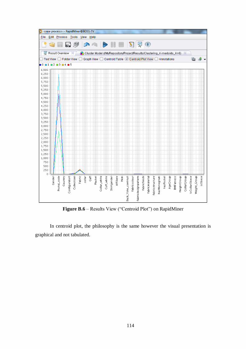
114
Figure B.6 – Results View (“Centroid Plot”) on RapidMiner
In centroid plot, the philosophy is the same however the visual presentation is
graphical and not tabulated.

115
Figure B.7 – Results View (“Meta Data”) on RapidMiner
In data view (Figure B.8) we can see the cluster prototypes, information that
complements the Cluster Model (Figure B.4).
Figure B.9 (“Plot View”) shows one of the numerous possibilities for
visualization of the dataset available on RapidMiner.
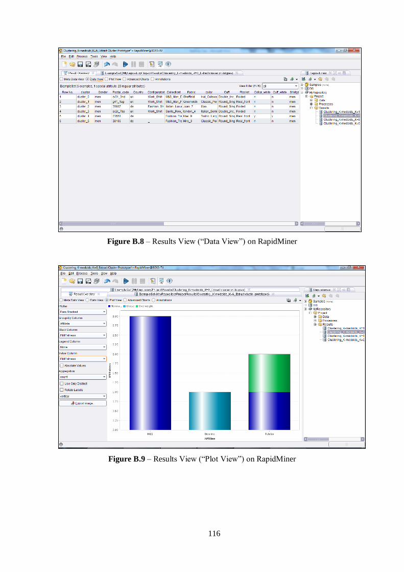
116
Figure B.8 – Results View (“Data View”) on RapidMiner
Figure B.9 – Results View (“Plot View”) on RapidMiner
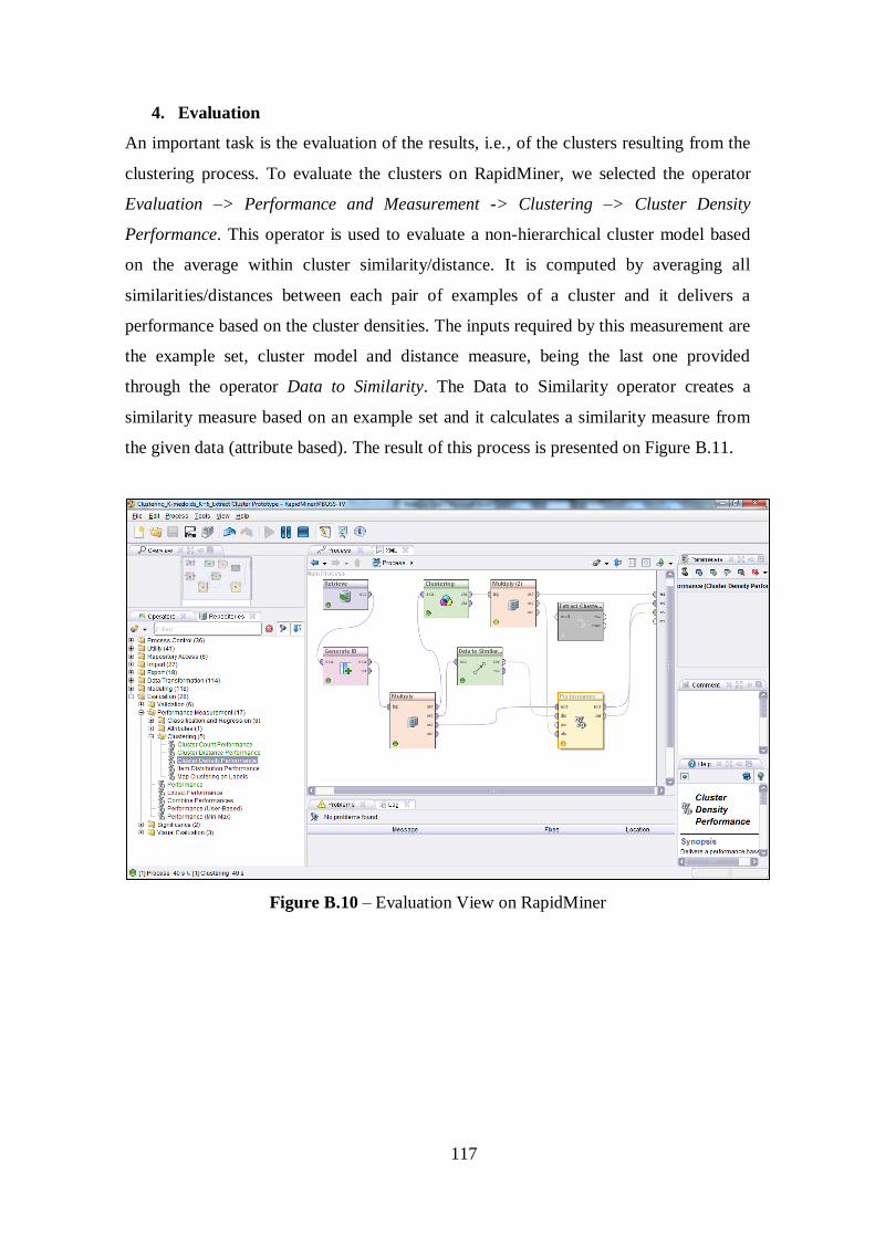
117
4. Evaluation
An important task is the evaluation of the results, i.e., of the clusters resulting from the
clustering process. To evaluate the clusters on RapidMiner, we selected the operator
Evaluation –> Performance and Measurement -> Clustering –> Cluster Density
Performance. This operator is used to evaluate a non-hierarchical cluster model based
on the average within cluster similarity/distance. It is computed by averaging all
similarities/distances between each pair of examples of a cluster and it delivers a
performance based on the cluster densities. The inputs required by this measurement are
the example set, cluster model and distance measure, being the last one provided
through the operator Data to Similarity. The Data to Similarity operator creates a
similarity measure based on an example set and it calculates a similarity measure from
the given data (attribute based). The result of this process is presented on Figure B.11.
Figure B.10 – Evaluation View on RapidMiner

118
Figure B.11 – Results of Evaluation View on RapidMiner
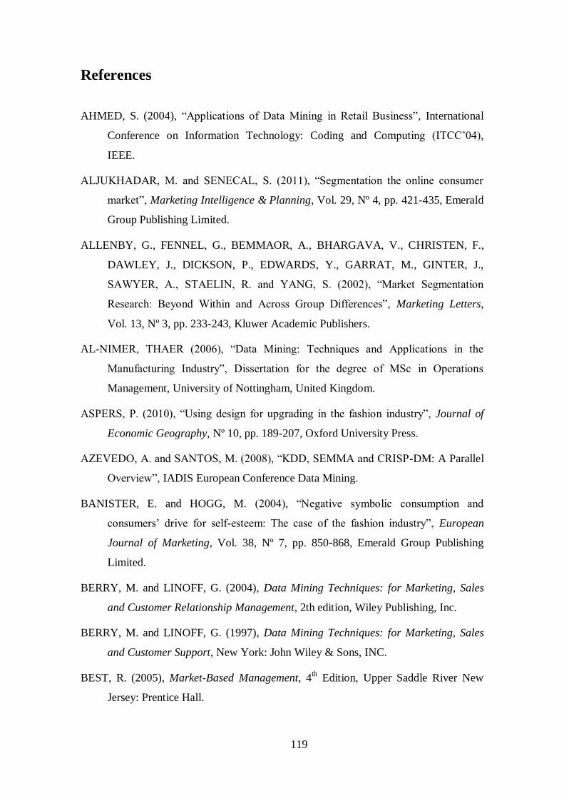
119
References
AHMED, S. (2004), “Applications of Data Mining in Retail Business”, International
Conference on Information Technology: Coding and Computing (ITCC’04),
IEEE.
ALJUKHADAR, M. and SENECAL, S. (2011), “Segmentation the online consumer
market”, Marketing Intelligence & Planning, Vol. 29, Nº 4, pp. 421-435, Emerald
Group Publishing Limited.
ALLENBY, G., FENNEL, G., BEMMAOR, A., BHARGAVA, V., CHRISTEN, F.,
DAWLEY, J., DICKSON, P., EDWARDS, Y., GARRAT, M., GINTER, J.,
SAWYER, A., STAELIN, R. and YANG, S. (2002), “Market Segmentation
Research: Beyond Within and Across Group Differences”, Marketing Letters,
Vol. 13, Nº 3, pp. 233-243, Kluwer Academic Publishers.
AL-NIMER, THAER (2006), “Data Mining: Techniques and Applications in the
Manufacturing Industry”, Dissertation for the degree of MSc in Operations
Management, University of Nottingham, United Kingdom.
ASPERS, P. (2010), “Using design for upgrading in the fashion industry”, Journal of
Economic Geography, Nº 10, pp. 189-207, Oxford University Press.
AZEVEDO, A. and SANTOS, M. (2008), “KDD, SEMMA and CRISP-DM: A Parallel
Overview”, IADIS European Conference Data Mining.
BANISTER, E. and HOGG, M. (2004), “Negative symbolic consumption and
consumers’ drive for self-esteem: The case of the fashion industry”, European
Journal of Marketing, Vol. 38, Nº 7, pp. 850-868, Emerald Group Publishing
Limited.
BERRY, M. and LINOFF, G. (2004), Data Mining Techniques: for Marketing, Sales
and Customer Relationship Management, 2th edition, Wiley Publishing, Inc.
BERRY, M. and LINOFF, G. (1997), Data Mining Techniques: for Marketing, Sales
and Customer Support, New York: John Wiley & Sons, INC.
BEST, R. (2005), Market-Based Management, 4th Edition, Upper Saddle River New
Jersey: Prentice Hall.
120
BROCHADO, ANA (2007), “Segmentação de Mercado e Modelos de Mistura de
Regressão: Critérios para a Determinação do Número de Segmentos”, Tese de
Doutoramento em Ciências Empresariais, Faculdade de Economia do Porto,
Porto.
BRUN, M., SIMA, C., HUA, J., LOWEY, J., CARROLL, B., SUH, E. and
DOUGHERTY, E. (2006), “Model-based evaluation of clustering validation
measures”, Pattern Recognition Society, Nº40, pp. 807–824, Elsevier Ltd.
CANEVER, M.D., TRIJP, H. and LANS, I. (2007), “Benefit-feature segmentation: a
tool for the design of supply-chain strategy”, Marketing Intelligence & Planning,
Vol. 25, Nº5, pp. 511-533, Emerald Group Publishing, Ltd.
CAO, F., LIANG, J., Li, D., BAI, L. and DANG, C. (2012), “A dissimilarity measure
for the k-Modes clustering algorithm”, Knowledge-Based Systems, Nº26, pp. 120–
127, Elsevier B.V.
CARDOSO, P. COSTA, H. and NOVAIS, L. (2010), “Fashion consumer profiles in the
Portuguese market: involvement, innovativeness, self-expression and
impulsiveness as segmentation criteria”, Faculty of Social and Human Sciences,
University Fernando Pessoa, Porto, Portugal, International Journal of Consumer
Studies, Nº34, pp. 638–647, Blackwell Publishing Ltd.
CARROL, K. and GROSS, K. (2010), “An Examination of Clothing Issues and
Physical Limitations in the Product Development Process”, Family & Consumer
Sciences Research Journal, Vol. 39, Nº 1, American Association of Family and
Consumer Sciences.
CHEN, M., CHIU, A. and CHANG, H. (2005), “Mining changes in customer behavior
in retail marketing”, Expert Systems with Applications, Nº 28, pp. 773-781,
Elsevier Ltd.
CHOO, H., JUNG, J. and CHUNG, I., (2009), “Buyer-supplier relationships in
Dongdaemun fashion market: relationship quality model”, Journal of Fashion
Marketing and Management, Vol. 13 No. 4, pp. 481-500, Emerald Group
Publishing Limited.
CHOY, K. L., CHOW, K. H., MOON, K. L., ZENG, X., LAU, H., CHAN, F. and HO,
G.T.S. (2009), “A RFID-case-based sample management system for fashion
121
product development”, Engineering Applications of Artificial Intelligence, Nº22,
pp. 882-896, Elsevier Ltd.
CLEVELAND, M., PAPADOPOULOS, N. and LAROCHE, M. (2011), “Identity,
demographics, and consumer behaviors: International market segmentation across
product categories”, International Marketing Review, Vol. 28, Nº 3, pp. 244-266,
Emerald Group Publishing Limited.
COOIL, B., AKSOY, L. and KEININGHAM, T. (2007), “Approaches to Customer
Segmentation”, Journal of Relationship Marketing, Vol. 6, No 3-4, pp. 9-39, The
Haworth Press, Inc.
CUNHA, N. (2009), “Metodologia de Selecção de Segmentações Diversificadas: Um
Caso de Aplicação de Técnicas de Data Mining em Dados de Consumo para
Avaliação de Portfólios de Cartões Bancários”, Dissertação de Mestrado em
Gestão Comercial, Faculdade de Economia do Porto, Universidade do Porto,
Porto.
DELMATER, R. and HANCOK, M. (2001), Data Mining Explained: a manager’s
guide to costume-centric business intelligence, Boston: Digital Press.
DIAS, J. and VERMUNT, J. (2007), “Latent class modeling of website users’ search
patterns: Implications for online market segmentation”, Journal of Retailing and
Consumer Services, Nº 14, pp. 359-368, Elsevier Ltd.
DIBB, S. and SIMKIN, L. (2009), “Bridging the segmentation theory/ practice divide”,
Journal of Marketing Management, Vol. 25, Nº 3-4, pp. 219-225, Westburn
Publishers Ltd.
DING, WEI (2007), “Mass Customization for Clothing Industry – On an E-commerce
Environment”, Dissertation for the Degree of MSc Operations Management,
University of Nottingham, United Kingdom.
DOLNICAR, S. (2002), “A Review of Unquestioned Standards in Using Cluster
Analysis for Data-Driven Market Segmentation”, Australian and New Zealand
Marketing Academy Conference (ANZMAC 2002), Deakin University,
Melbourne.
DOLNICAR, S. (2003), “Using cluster analysis for market segmentation – typical
misconceptions, established methodological weaknesses and some
122
recommendations for improvement”, Australasian Journal of Market Research,
11(2), pp. 5-12.
DOLNICAR, S., and LEISCH, F. (2003), “Data-Driven Market Segmentation – A
Structure-Based Conceptual Framework for Management Decision Support”,
Australian and New Zealand Management Academy Conference, Adelaide, South
Australia, 1-3 December.
FAYYAD, U. and UTHURUSAMY, R. (2002), “Evolving Data Mining into Solutions
for Insights”, Communications of the ACM, Vol. 45, Nº 8.
HAND, D., MANNILA, H. and SMITH, P. (2001), Principles of Data Mining, The MIT
Press, Massachusetts Institute of Technology.
HALKIDI, M., BATISTAKIS, Y. and VAZIRGIANNIS, M. (2001), “On Clustering
Validation Techniques”, Journal of Intelligent Information Systems, Vol. 17:2/3,
pp. 107-145, Kluwer academic Publishers.
HALKIDI, M., BATISTAKIS, Y. and VAZIRGIANNIS, M. (2002), “Cluster Validity
Methods: Part I”, SIGMOND Record, Vol. 31, Nº 2.
HARDING, J.A., SHAHBAZ, M., SRINIVAS and KUSIAK, A. (2006), “Data Mining
in Manufacturing: A Review”, Journal of Manufacturing Science and
Engineering, Vol. 128.
HASTIE, T., TIBSHIRANI, R. and FRIEDMAN, J. (2001), The Elements of Statistical
Learning: Data Mining, Inference, and Prediction, Springer-Verlag New York,
Inc.
HSU, C. (2009), “Data mining to improve industrial standards and enhance production
and marketing: an empirical study in apparel industry”, Expert Systems with
Applications, Nº36, pp. 4185-4191, Elsevier Ltd.
JAIN, A.K., MURTY, M.N. and FLYNN, P.J. (2000), “Data Clustering: A Review”,
ACM Computing Surveys, Vol. 31, Nº 3.
JAIN, A. K. (2009), “Data clustering: 50 years beyond K-Means”, Pattern Recognition
Letters, Elsevier B.V.
KANTARDZIC, M. (2003), Data Mining - Concepts, Models, Methods, and
Algorithms, John Wiley & Sons, INC.
123
KAU, A., TANG, Y. and GHOSE, S. (2003), “Typology of online shoppers”, Journal
of Consumer Marketing, Vol. 20, nº 2, pp. 139-156, MCB UP Limited.
KETTENRING, J. (2009), “A patent analysis of cluster analysis”, Applied Stochastic
Models in Business and Industry, Nº25, pp. 460-467.
KIM, K. and AHN, H. (2008), “A recommender system using GA K-Means clustering
in an online shopping market”, Expert Systems with Applications, Nº34, pp. 1200-
1209, Elsevier Ltd.
KO, E., KIM, E., TAYLOR, C., KIM, K. and KANG, I. (2007), “Cross-national market
segmentation in the fashion industry: A study of European, Korean, and US
consumers”, International Marketing Review, Vol. 24, Nº 5, pp. 629-651, Emerald
Group Publishing Limited.
KOTLER, P. and KELLER, K. (2012), A Framework for Marketing Management, 5th
ed. International ed. - Boston: Pearson.
KOTLER, P. and ARMSTRONG, G. (2012), Principles of Marketing, 14th edition,
Pearson Education, Inc.
KOTLER, P. and KELLER, K. (2012), Marketing Management, 14th ed. global
ed. Harlow: Pearson.
KOTLER, P. and KELLER, K. (2008), Marketing Management, 13th edition, Prentice
Hall.
KOTLER, P., WONG, V., SAUNDERS, J. and ARMSTRONG, G. (2005), Principles
of Marketing, 4th European Edition, Pearson Education Ltd.
KOTLER, P., RACKHAM, N. and KRISHNASWAMY, S. (2006), “Ending the War
between Sales and Marketing”, Harvard Business Review.
KOTLER, P. (1999), “Kotler on Marketing: How to Create, Win, and Dominate
Markets”, USA: The Free Press (FP).
KOZAR, J. and DAMHORST, M. (2008), “Older women’s responses to current fashion
models”, Journal of Fashion Marketing and Management, Vol. 12, Nº 3, pp. 338-
350, Emerald Group Publishing limited.
LAROSE, D. (2005), Discovering Knowledge in Data: An Introduction to Data
Mining, John Wiley & Sons, Inc.
124
LEE, S. J. and SIAU, K. (2001), “A review of data mining techniques”, Industrial
Management & Data Systems, Vol. 101, Nº 1, pp. 41-46, MCB University Press.
LEGÁNY, C., JUHÁSZ, S. and BABOS, A. (2006), 5th
WSEAS Int. Conf. on Artificial
Intelligence, Knowledge Engineering and Data Bases, Madrid, Spain, February
15-17, pp. 388-393.
LEVINE, EREL (1999), “Un-Supervised Estimation of Cluster Validity – Methods and
Applications”, MSc Thesis, Feinberg Graduate School, Weizmann Institute of
Science, New York, United States of America.
LIM, J., CURRIM, I. and ANDREWS, R. (2005), “Consumer heterogeneity in the
longer-term effects of price promotions”, International Journal Research in
Marketing”, Nº 22, pp. 441-457, Elsevier B.V.
LO, W., HONG, T. and JENG, R. (2008), “A framework of E-SCM multi-agent
systems in the fashion industry”, International Journal of Production Economics,
Nº114, pp. 594–614, Elsevier B.V.
MACCARTY, J. and HASTAK, M. (2007), “Segmentation approaches in data-mining:
A comparison of RFM, CHAID, and logistic regression”, Journal of Business
Research, Nº60, pp. 656-662, Elsevier inc.
MIRKIN, B. (2005), Data Clustering for Data Mining: A Data Recovery Approach,
Boca Raton: Chapman and Hall.
MOOI, E. and M. SARSTEDT (2011), A Concise Guide to Market Research, Springer-
Verlag Berlin Heidelberg.
MOORE, M. and FAIRHURST, A. (2003), “Marketing capabilities and firm
performance in fashion retailing”, Journal of Fashion Marketing and
Management, Vol. 7, Nº 4, pp. 386-397, MCB UP Limited.
NEWBERY, M., MEULEN, K. (2010), “Tomorrow’s clothing retail: sectors, markets
and routes”, United Kingdom: Aroq Ltd.
NGAI, E.W.T., XIU, L. and CHAU, D.C.K. (2009), “Application of data mining
techniques in customer relationship management: A literature review and
classification”, Expert Systems with Applications, Nº36, pp. 2592–2602, Elsevier
Ltd.
125
O’CASS, A. (2004), “Fashion clothing consumption: antecedents and consequences of
fashion clothing involvement”, European Journal of Marketing, Vol. 38, Nº 7, pp.
869-882, Emerald Group Publishing Limited.
PARK, H. and JUN, C. (2009), “A simple and fast algorithm for K-Medoids
clustering”, Expert Systems with Application,s Nº36, pp. 3336–3341, Elsevier Ltd.
PARK, JUNG HYUN (2009), “Technical Considerations for the Design of Smart
Apparel for the Overweight”, Thesis for the Degree of Master of Science, Faculty
of North Carolina State University, Raleigh, United States of America.
PASCUAL, D., PLA, F. and SÁNCHEZ, J. (2010), “Cluster validation using
information stability measures”, Nº 31, pp. 454-461, Elsevier B.V.
PEDRYCZ, W. (2005), Knowledge-Based Clustering: From Data to Information
Granules, New Jersey: John Wiley & Sons, Inc.
PHAM, D. T., DIMOV, S. S. and C. D. NGUYEN (2005), “Selection of K in K-Means
clustering”, Journal of Mechanical Engineering Science, Vol. 219, Part C,
IMechE.
PHAU, I., and LO, C. (2004), “Profiling fashion innovators: A study of self-concept,
impulsive buying and Internet purchase intent”, Journal of Fashion Marketing
and Management, Vol. 8, Nº 4, pp. 399-411, Emerald Group Publishing Limited.
PRIEST, A. (2005), “Uniformity and differentiation in fashion”, International Journal
of Clothing Science and Technology, Vol. 17, Nº 3/4, pp. 253-263, Emerald
Group Publishing Limited.
RENDÓN, E., ABUNDEZ, I., ARIZMENDI, A. and QUIROZ, E. (2011), “Internal
versus External cluster validation indexes”, International Journal of Computers
and Communications, Issue 1, Vol. 5.
RYGIELSKI, C., WANG, J. and YEN, D. (2002), “Data Mining techniques for
customer relationship management”, Technology in Society, Nº24, pp. 483-502,
Elsevier Science Ltd.
ROCHA, M., HAMMOND, L., HAWKINS, D. (2005), “Age, gender and national
factors in fashion consumption”, Journal of Fashion Marketing and Management,
Vol. 9, Nº4, pp. 390-390, Emerald Grouping Publishing Limited.
126
RUD, O. (2001), Data Mining Cookbook: modeling data for marketing, risk and
customer relationship management, New York: John Wiley & Sons, Inc.
SCHAFER, J., KONSTAN, J. and RIEDL, J. (2001), “E-commerce Recommendation
Applications”, Data Mining and Knowledge Discovery, Nº 5, pp. 115-153,
Kluwer Academic Publishers.
SCOTT, D. (2007), The New Rules of Marketing & PR, New York: John Wiley & Sons,
Inc.
SHAW, M., SUBRAMANIAM, C., TAN, G. and WELGE, M. (2001), “Knowledge
management and data mining for marketing”, Decision Support Systems, Nº31,
pp. 127-137, Elsevier Science B.V.
SIDDIQUI, N., O’MALLEY, A., MCCOLL, J. and BIRTWISTLE, G. (2003), “Retailer
and consumer perceptions of online fashion retailers: Web site design issues”,
Journal of Fashion Marketing and Management, Vol. 7, Nº 4, pp. 345-355, MCB
UP Limited.
SINGH, S. and CHAUCHAN, N. C. (2011), “K-Means vs. K-Medoids: A Comparative
Study”, National Conference on Recent Trends in Engineering & Technology,
B.VM. Engineering College, V. V. Nagar, Gujarat, India.
SIVOGOLOVKO, E. (2012), “Validating cluster structures in Data Mining tasks”,
EDBT/ICDT Workshops March 26-30, Berlin, Germany, ACM.
SMITH, W. (1956), “Product differentiation and market segmentation as alternative
marketing strategies”, Journal of Marketing, 21, 3-8.
SU, Z. and XU, D. (2011), “Lifestyle of Obese Population and Brand Choosing of
Personalized Clothing”, IEEE.
TAN, P., STEINBACH, M. and KUMAR, V. (2006), Introduction to Data Mining:
Instructor’s Solution Manual, Pearson Addison-Wesley.
TRINH, G., DAWES, J. and LOCKSHIN, L. (2009), “Do product variants appeal to
different segments of buyers within a category?”, Journal of Product & Brand
Management, 18/2, pp. 95-105, Emerald Group Publishing Limited.
127
TURQUIN, E., WITHER, J., BOISSIEUX, L., GANI, M. and HUGHES, J. (2007), “A
Sketch-Based Interface for Clothing Virtual Characters”, IEEE Computer
Graphics and Applications.
VELMURUGAN, T. and SANTHANAM, T. (2010), “Computational Complexity
between K-Means and K-Medoids Clustering Algorithms for Normal and
Uniform Distributions of Data Points”, Journal of Computer Science 6 (3): pp.
363-368, Science Publications.
WEDEL, M. and KAMAKURA, W. (2002), “Introduction to the Special Issue on
Market Segmentation, International Journal of Research in Marketing, Vol. 19,
Nº 3, pp. 181-183, Elsevier Science B.V.
WEDEL, M. and KAMAKURA, W. (2000), Market Segmentation: Conceptual and
Methodological Foundations, Kluwer Academic Publishers.
WEDEL, M., KAMAKURA, W. and BÖCKENHOLT, U. (2000), “Marketing data,
models and decisions”, International Journal of Research in Marketing, Nº 17,
pp. 203-208, Elsevier Science B.V.
WU, J., XIONG, H. and CHEN, J. (2009), “Adapting the Right Measures for K-Means
Clustering”, KDD’09, Paris, France, ACM.
WU, J., XIONG, H. and CHEN, J. (2009), “Adapting the Right Measures for K-Means
Clustering”, KDD’09, Paris, France, ACM.
YATSKIV, I. and GUSAROVA, L. (2005), “The Methods of Cluster Analysis Results
Validation”, Transport and Telecommunication, Vol. 6, Nº 1, International
Conference RelStat’04.


ANNEXES

131
ANNEX A
BIVOLINO
The information contained in this annex is from Bivolino website
(http://www.bivolino.com/).
“Made to measure shirts”
Bivolino was born in 1954 in a sandy area where the squirrel feels at home. Each
Bivolino customized shirt is embroidered with the squirrel as the symbol of the perfect
biometric fitting guarantee. Today Bivolino supports two projects focusing on
preventing the red squirrel extinction: The Save Your Logo initiative as well as the Red
Squirrel in South Scotland action.
Bivolino Brand Story
A. The Beginning
Over its 50 year history, Bivolino has built a reputation as a leading supplier of
beautifully tailored shirts – crafted with the ultimate combination of precision and
design. But few people know the story behind the brand and how it spearheaded the
design innovation we see in shirt manufacturing today.
The Bivolino story began in 1954, when brothers Louis and Jacques Byvoet
founded the company with a joint investment of 8 million francs. Their grandfather,
Jacques, had been in the linen trade since 1900 and the name Bivolino was chosen to
represent both the family name of Byvoet and linen – the fabric from which Bivolino
shirts would be made from. They based the company in Hasselt, in the heart of Campine
in Belgium.
B. The Origins
With the opening of the Byvoet brothers first premises, the foundations of the
Bivolino brand were laid – paving the way for Bivolino to become a pioneer within the
shirt market, a symbol that guarantees quality and the perfect bespoke cut with a
fashionable twist.
132
At the time, consumers were looking for something different from the classic
white shirt – they wanted fashionable styles in an array of colours, styles and fabrics –
and this demand is what formed the cornerstone of the Bivolino concept.
The Bivolino logo, two squirrels sitting on a distaff holding the letter B, was
inspired by the location of the brothers’ workshop, where they could see squirrels
running freely through the sandy pine forests of Hasselt.
C. The Shirt
Under the direction of Byvoet brothers, the company soon grew to become the
market leader in shirt manufacturing, running a small plant with 80 employees
producing 350.000 shirts a year. This record productivity was possible due to the
Byvoet’s investment in the very best modern machinery of the time, highlighting the
role of technology in the manufacturing process. At this point, export to Netherlands,
Luxemburg, Germany and Switzerland represented 35% of the business.
D. The Squirrel
The humble squirrel logo chosen in 1954 has today become a symbol of high
quality fashion; a guarantee of Bivolino’s skillful, professional production techniques
that have been honed over many years.
It has been said that the Bivolino brand has similarities to the squirrel – it has a
personalized style, and moves quickly and elegantly with freedom. In homenage to the
animal that inspired the brand logo, Bivolino currently supports two projects in fighting
the extinction of red squirrels in Scotland.
E. The Science
In 1969, Bivolino built on their early investment in technology by introducing
groundbreaking new ergonomic measurement system – allowing each shirt to be
individually fitted to the body at first time.
This system was the first of its kind in Europe, and was created in partnership
with IBM. Using 1.200.000 measurements of the body, Bivolino was able to reinvent a
new fit completely adapted to the body shape.
At the same time as the ergonomic measurement system was introduced,
Bivolino was also introducing innovative new fabrics to surprise and excite consumers
and the industry, including Terlenka soil release, jacquard and polyester, as well as the
133
self-ironing popelines Belofast. Meanwhile consumers were looking for bright, bold
colours such as blues and reds, along with neutral white, with large stripes and graphic
patterns becoming popular.
F. The Development
During the recession of the 1970’s, there was a shift in consumer spending
patterns that saw people buying less than before but thinking more consciously about
the quality of their purchases. The inherent craftsmanship and quality of Bivolino shirts
was therefore more important to the business than ever, and the brand worked hard to
produce impeccable products that would stand the test of time, wash after wash wear
after wear. In 1981, Bivolino became the first shirt label to take the daring step towards
computerized production, which automatically produces the pattern making gradations
in a fraction of time – a real revolution in the shirt manufacturing process for the time.
By now, and using this new technology, Bivolino was producing 900,000 shirts a year
and employing 270 people.
G. The Fashion
Each season, a select group of designers create a new Bivolino collection under
the guidance of a graduate fashion designer from the renowned Academy of Antwerp.
The latest fabrics, color trends, styles and cuts are researched and developed by the
styling team to create the latest collection of Bivolino shirts for the fashion conscious
consumer, ensuring that the brand stays at the forefront of shirt design.
One of the biggest challenges for the Bivolino brand came on 13th October 1987,
when an enormous fire ruined the Bivolino factory – taking with it 33 years of passion
for shirt making and reducing it to ashes. Over the next year, sales decreased by 80% as
the company struggled to recover, and production was moved to Tunisia and Romania.
It was during this difficult time for the Byvoet brothers that they decided to pass on the
family business to Louis’ son, Michel, starting the next step in the Bivolino journey.
H. The Digital Revolution
The growth of the internet opened up a new world of possibilities for Bivolino
and the brand established a new digital studio in the Hight Tech Science Park Limburg.
As the company embraced new technology, sewing machines made way for computers
134
as Bivolino moved into the digital age and in 1997 the first shirt was sold from
Bivolino.com.
Customers could now shop online to create a completely bespoke Bivolino shirt
with just a few clicks on the mouse. They could choose the fabric, collar and cuffs, or
personalize the design with a name or initials with the finished shirt arriving within 2-3
weeks. At this stage customers still had to take their own measurements at home, but
Bivolino already had plans to revolutionize this aspect of the design process.
I. The Biometric Shirt
The year 2000 brought with it the dot com bubble burst, but where others failed,
Bivolino saw opportunities. Taking the moto that you have to innovate to survive,
Bivolino launched the possibly its most innovative tool yet: biometric sizing
technology. After two years of anthropometric research supported by university
scientists, the company solved the magic formula to calculate the perfect cut and size
for every Bivolino customer – without the need for them to use a tape measure.
Bivolino shoppers just need to provide their height, weight, collar size and age, and
from this each customer is guaranteed a cut that fits like a second skin. The first shirt
ordered is 100% satisfaction guaranteed.
J. The Awards
Bivolino’s innovative approach to shirt design has earned the company
numerous awards in several countries. In the Netherlands, Bivolino was given the
“Starter Award” from the Dutch home shopping trading association, Thuiswinkle.org.
In 2006, the company was awarded the “BeCommerce” prize in Belgium, and this was
followed by French magazine Capital giving Bivolino the best position for its cost
effectiveness in 2008. In the UK, consumer magazine Which? declared Bivolino’s
biometric sizing technology to be better performing than the bespoke tailors of Savile
Row.
K. The 3D Technology
In 2010, Bivolino launched its latest piece of technology – a 3D shirt design
tool. The result of several years of research, the tool was developed thanks to the Open
Garments research project, and was supported by European Commission research funds.
A new zoom function on the collar, cuffs and pockets means that customers can now
135
see their shirt presented as realistically as possible, all in real time. Endless design
combinations are now also possible – from choosing contrasting fabrics, inner collars,
cuffs, yoke and back panels to contrasting sleeves, stitching, removable bones, buttons
and more, allowing customers to create the ultimate bespoke shirt. When using the
design tool, customers can choose from one of four categories: Business, Fashion, Party
and Arty.
L. The Arty Shirt
At the end of 2010, Bivolino partnered with ten Dutch painters to create bespoke
artwork that could be used to customize shirts. This new creative playground for
customers was made possible by the Amsterdam Fashion Institute, who brought the
group painters together, and digital printing technology. Each artist has their own
unique style and themes include mysterious landscapes, Indian culture, the female face
and Spring frogs – all of which are available to customers to use a contrasting collars or
cuffs, or even as an allover print.
M. The Women’s Shirt
In 2011, Bivolino introduced collection women’s shirts for the first time,
offering women the luxury of creating a bespoke tailored shirt for any occasion with a
few clicks of the mouse.
Customers can experiment with fabrics, choosing different cottons, stretch or
transparent options, or mixing and matching prints such as Liberty flowers and stripes
as well as adding contrasting collars, cuffs or pockets. Sleeve lengths can be tailored to
the season, with full length, three quarter, short and sleeveless options all available.
Customers can also add a decorative flower motif, personalized buttons or contrasting
stitching to complete the shirt in style.
Bivolino’s biometric sizing technology uses the customer’s weight, height, age
and bra size measurements to create the perfect fit – with a 100% satisfaction guarantee.
ELLE called the service “a revolution”.
N. The Planet
Bivolino is passionate about the planet and has developed its service to be as
green as possible. Since 2008, each shirt is packaged in a biodegradable envelope,
created from non-polluting plastic and Bivolino has made significant progress in
136
reducing the size of packaging used in delivery. Due to Bivolino’s patented biometric
sizing technology, the percentage of returns is just 3.8%, reducing the use of transport to
return goods. Finally, as each Bivolino shirt is made to order in the company’s ethical
manufacturing plants in Tunisia and Romania there is no stock of goods – resulting in
no waste; in a perfectly adapted business model which Bivolino calls “Mass
Customization”.
Bivolino and the Environment
“By creating, buying and sharing at Bivolino, you go Green!”
Bivolino is constantly looking for ways to further reduce its environmental
impact.
A. A Sustainable Business Model
At Bivolino, customer creates buys and shares his customized shirt. The making
of his bespoke shirt starts immediately in Bivolino apparel manufacturing plans just
after his order has been confirmed online. This means that there is no stock of shirts
waiting somewhere that eventually need to be absorbed. It is what the company calls a
Made-to-Order business model or a Consumer Driven Manufacturing business model
which reduces stock wastes and promotes a real sustainable supply chain. These savings
result in a win-win situation for everybody taking part in the supply chain. Customer is
part of it and can enjoy a high quality personalized service at very competitive prices.
This is also what company calls “Mass Customization”.
B. Reducing Returns
Since 2004, the right size is guaranteed by Bivolino biometric sizing technology
(patent Nr EEC-EP1341427 & US-7346421) which means that customer get the right
size without trying his shirt or without using any tape measurement. Only by giving his
height, weight, age and collar size or cup size for women, he will get a bespoke shirt cut
to the bones! For customer first Bivolino shirt the company even remake the shirt if
needed till his 100% satisfaction. This worldwide unique biometric sizing technology
helps company to make a record low return rate of 3.8% in total. From this amount,
137
Bivolino repairs as much as possible so that waste is reduced to a strict minimum.
Those “default” remaining shirts are then offered to those of us who are in real need
through charity organizations.
C. New Biodegradable Packaging
Since 2008, Bivolino customized shirts are individually or duo packed in a new
biodegradable branded bag. The bags are manufactured in a famous environmental-
friendly plastic material, the Ethylene Vinyl Acetate or also called EVA. Its applications
and performance are very similar to PVC while reducing the risk of infringing any
toxicity regulations. It is biodegradable after a period of maximum one year with no
pollution to environment after disposal and incineration. This green packaging approach
is reinforced by the will to reduce packaging waste.
D. Reducing Packaging Waste
Since 2007, Bivolino has made significant progress to reduce excess packaging
in its shipments to customers and has introduced additional types of recyclable packing
materials to protect items while in transit. Each Bivolino shirt is packed in a bag to
protect its high quality fabric. When customer order two shirts, the company still use the
same bag in order to save packaging and call it then a Bivolino duo pack. The bag is put
in a bubble envelope which size is perfectly matching with the size of a Bivolino shirt
which means that there is no space waste. It is what the company calls a frustration-Free
packaging.
E. Fabric Swatches
Bivolino decided not to send out fabric samples any more. It would be indeed
not ecologically responsible (packaging, delivery, fabric waste) if the company would
continue to send fabric swatches.
F. Logistics and delivery
As a matter of fact, online shopping is inherently more environmentally friendly
than traditional retailing. The efficiencies of online shopping result in a greener
shopping experience. This study explains some of the benefits of the online shopping
model. It was found that, on average, having goods delivered to your home by parcel
138
carrier generates significantly less carbon dioxide than making a special trip to the
shops to buy the same item. The research compared the carbon footprints of online and
conventional shopping for small goods such as books, CDs, clothing, cameras and
household items. The work focused on the final stage in the delivery process, the so-
called ‘last mile’, when goods are either delivered to the home or customers travel to the
shops to collect them in person. It was found that a typical van-based home delivery
produced 181g CO², compared with 4274g CO² for an average trip to the shops by car.
In other words, when a customer drives to the shops and buys fewer than 24 small, non-
food items per trip, home delivery is more environmentally-friendly.
G. Green Digital Clothing
Bivolino provides a vision of the future which encompasses the evolution of
digital clothing supply chains, from design to retail, that minimize returns and, in turn,
reduce waste. This “webified” supply chain is the “Googlification” of the apparel
industry and trade (referring to the book ‘What would Google do?‘ from Jeff Jarvis)
focusing on e-configurators, digital design toolkits, online dressing facilities and the
development of "controlled" virtual shopping communities. Waste can be controlled as
part of a lean manufacturing, or sustainable initiative. Technology also plays a role in
developing a more sustainable supply chain. Bivolino uses sustainable technologies
including computerized sketching, CAD pattern design, digital grading and marker-
making, digital printing and computer numerical control (CAM) single-ply cutting. In
fact, any technology which allows the product to remain in digital form until later in the
process is considered to be more sustainable. Why is it more sustainable to create and
buy a garment in a digital form? Surely you need to see real product samples?
Whenever a physical sample is created, waste is introduced into the process. At
Bivolino, customer indeed creates and buys a shirt which is digitally displayed and
configurated, without real samples or photos. This is worldwide unique!
H. Ethical Manufacturing Plants
Bivolino offshore manufacturing plants have received the SEDEX label in 2007.
This means recognition of Bivolino ethical performance. The points that have been
successfully audited were: 1. Employment freely chosen; 2. Freedom of association; 3.
Safety & hygienic conditions; 4. Child labour; 5. Wages & benefits; 6. Working hours;
7. Discrimination; 8. Regular employment; and 9. Harsh or inhumane treatment.
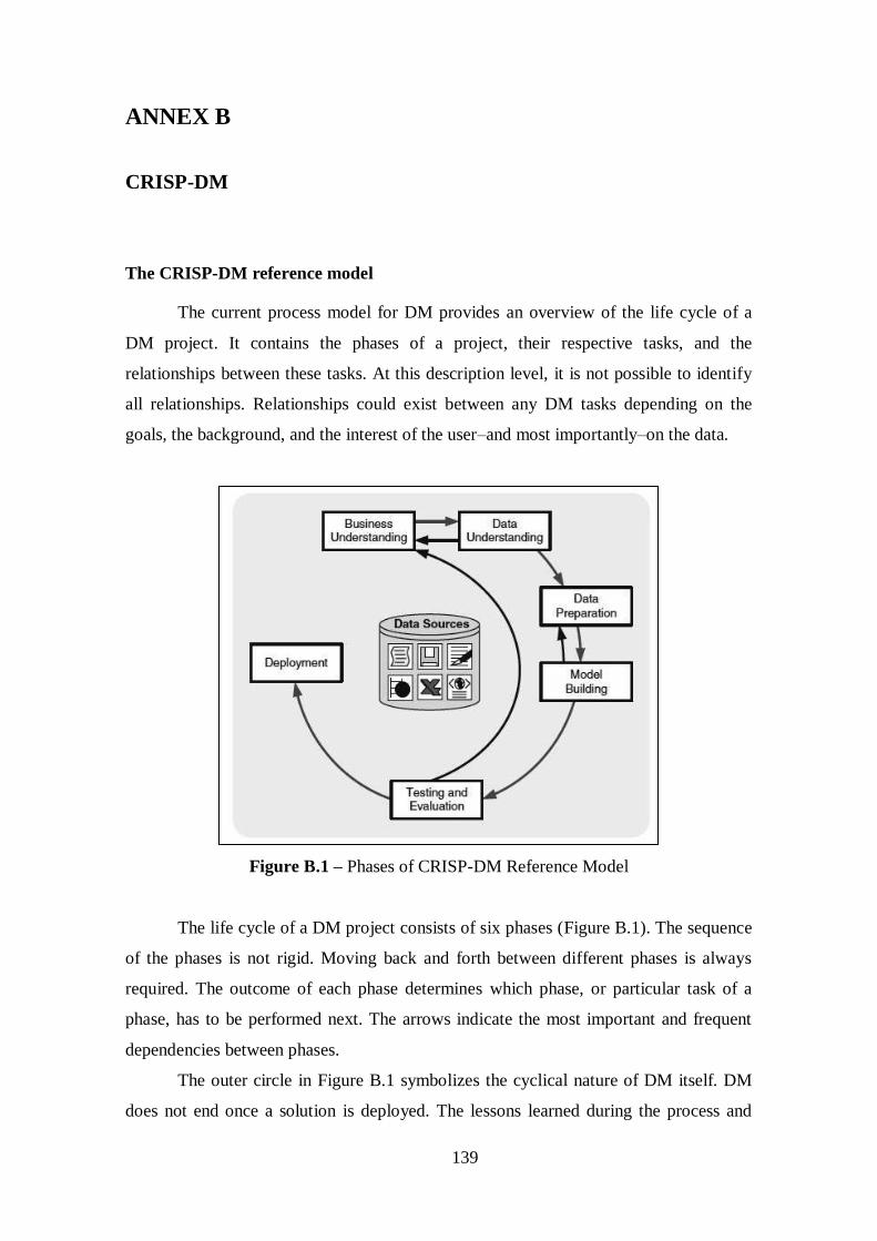
139
ANNEX B
CRISP-DM
The CRISP-DM reference model
The current process model for DM provides an overview of the life cycle of a
DM project. It contains the phases of a project, their respective tasks, and the
relationships between these tasks. At this description level, it is not possible to identify
all relationships. Relationships could exist between any DM tasks depending on the
goals, the background, and the interest of the user–and most importantly–on the data.
Figure B.1 – Phases of CRISP-DM Reference Model
The life cycle of a DM project consists of six phases (Figure B.1). The sequence
of the phases is not rigid. Moving back and forth between different phases is always
required. The outcome of each phase determines which phase, or particular task of a
phase, has to be performed next. The arrows indicate the most important and frequent
dependencies between phases.
The outer circle in Figure B.1 symbolizes the cyclical nature of DM itself. DM
does not end once a solution is deployed. The lessons learned during the process and

140
from the deployed solution can trigger new, often more-focused business questions.
Subsequent DM processes will benefit from the experiences of previous ones. In the
following, we briefly outline each phase:
1. Business understanding
This initial phase focuses on understanding the project objectives and
requirements from a business perspective, then converting this knowledge into a DM
problem definition and a preliminary plan designed to achieve the objectives.
2. Data understanding
The data understanding phase starts with initial data collection and proceeds
with activities that enable you to become familiar with the data, identify data quality
problems, discover first insights into the data, and/or detect interesting subsets to form
hypotheses regarding hidden information.
3. Data preparation
The data preparation phase covers all activities needed to construct the final
dataset (data that will be fed into the modeling tool(s)) from the initial raw data. Data
preparation tasks are likely to be performed multiple times and not in any prescribed
order. Tasks include table, record, and attribute selection, as well as transformation and
cleaning of data for modeling tools.
4. Modeling
In this phase, various modeling techniques are selected and applied, and their
parameters are calibrated to optimal values. Typically, there are several techniques for
the same DM problem type. Some techniques have specific requirements on the form of
data. Therefore, going back to the data preparation phase is often necessary.
5. Evaluation
At this stage in the project, you have built a model (or models) that appear to
have high quality from a data analysis perspective. Before proceeding to final
deployment of the model, it is important to thoroughly evaluate it and review the steps
executed to create it, to be certain the model properly achieves the business objectives.
A key objective is to determine if there is some important business issue that has not
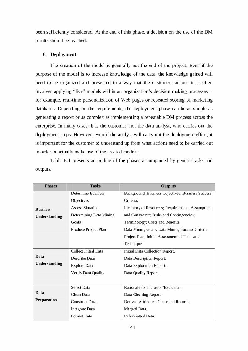
141
been sufficiently considered. At the end of this phase, a decision on the use of the DM
results should be reached.
6. Deployment
The creation of the model is generally not the end of the project. Even if the
purpose of the model is to increase knowledge of the data, the knowledge gained will
need to be organized and presented in a way that the customer can use it. It often
involves applying “live” models within an organization’s decision making processes—
for example, real-time personalization of Web pages or repeated scoring of marketing
databases. Depending on the requirements, the deployment phase can be as simple as
generating a report or as complex as implementing a repeatable DM process across the
enterprise. In many cases, it is the customer, not the data analyst, who carries out the
deployment steps. However, even if the analyst will carry out the deployment effort, it
is important for the customer to understand up front what actions need to be carried out
in order to actually make use of the created models.
Table B.1 presents an outline of the phases accompanied by generic tasks and
outputs.
Phases Tasks Outputs
Business
Understanding
Determine Business
Objectives
Assess Situation
Determining Data Mining
Goals
Produce Project Plan
Background, Business Objectives; Business Success
Criteria.
Inventory of Resources; Requirements, Assumptions
and Constraints; Risks and Contingencies;
Terminology; Costs and Benefits.
Data Mining Goals; Data Mining Success Criteria.
Project Plan; Initial Assessment of Tools and
Techniques.
Data
Understanding
Collect Initial Data
Describe Data
Explore Data
Verify Data Quality
Initial Data Collection Report.
Data Description Report.
Data Exploration Report.
Data Quality Report.
Data
Preparation
Select Data
Clean Data
Construct Data
Integrate Data
Format Data
Rationale for Inclusion/Exclusion.
Data Cleaning Report.
Derived Attributes; Generated Records.
Merged Data.
Reformatted Data.
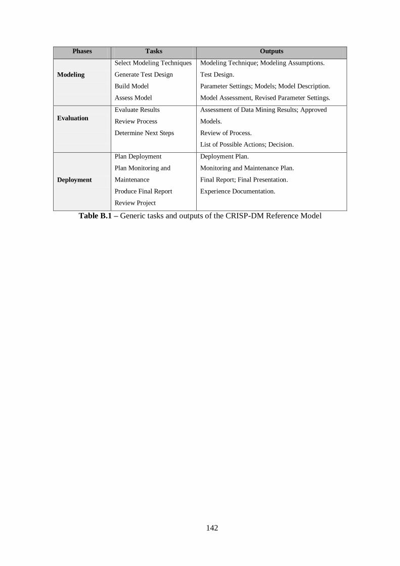
142
Phases Tasks Outputs
Modeling
Select Modeling Techniques
Generate Test Design
Build Model
Assess Model
Modeling Technique; Modeling Assumptions.
Test Design.
Parameter Settings; Models; Model Description.
Model Assessment, Revised Parameter Settings.
Evaluation
Evaluate Results
Review Process
Determine Next Steps
Assessment of Data Mining Results; Approved
Models.
Review of Process.
List of Possible Actions; Decision.
Deployment
Plan Deployment
Plan Monitoring and
Maintenance
Produce Final Report
Review Project
Deployment Plan.
Monitoring and Maintenance Plan.
Final Report; Final Presentation.
Experience Documentation.
Table B.1 – Generic tasks and outputs of the CRISP-DM Reference Model
143
ANNEX C
RAPIDMINER
The information contained in this annex is from RapidMiner website
(http://rapid-i.com/).
RapidMiner is the world's leading open source DM software. RapidMiner does
the best among the most important open source DM tools both in terms of technology
and applicability. This reflects the focus of the development work which has always
been put on a user-friendly combinability of the latest as well as established DM
techniques. This combining gives RapidMiner a high flexibility when defining analysis
processes. The processes of RapidMiner combine the power of development
environments, as known from programming languages, with the simplicity of visual
programming. The modular approach also has the advantage that even internal analysis
processes can be examined in the greatest detail and utilized.
RapidMiner contains more than 500 operators altogether for all tasks of
professional data analysis, i.e., operators for input and output as well as data processing,
modeling and other aspects of DM. But also methods of text mining, web mining, the
automatic sentiment analysis from Internet discussion forums (sentiment analysis,
opinion mining) as well as the time series analysis and prediction are available to the
analyst. In addition, RapidMiner contains more than 20 methods to also visualize high-
dimensional data and models.
Innovations that have been made on RapidMiner support the optimization of
direct mailing and marketing campaigns, churn reduction, the increase of customer
retention and the cost-benefit optimized acquisition of customers.
Data
On RapidMiner there are different value types for attributes and they could also
be transformed into other types. We speak of value type text in the case of free text, of
the value type numerical in the case of numbers and of the value type nominal in the
case of only few values being possible (like with the two possibilities “yes" and “no" for
the target attribute).
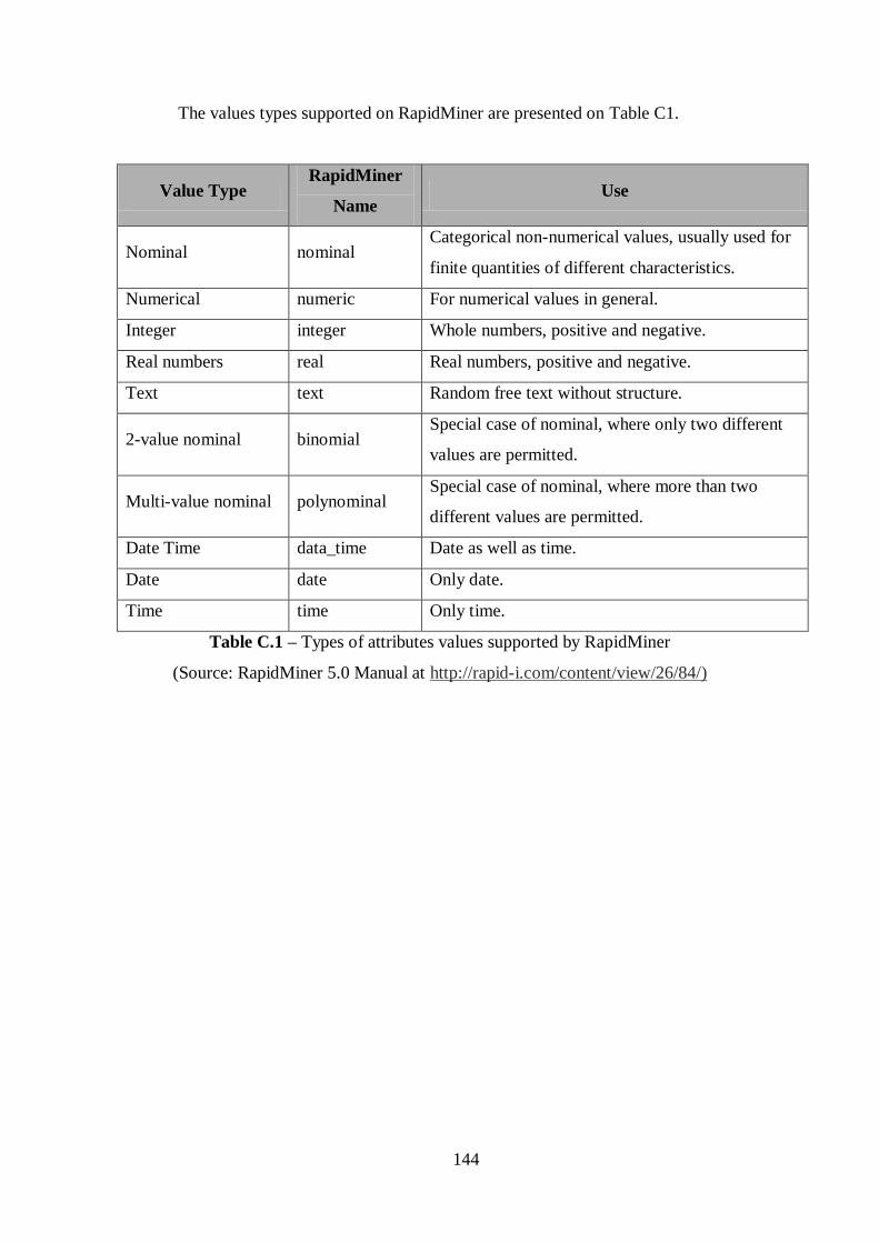
144
The values types supported on RapidMiner are presented on Table C1.
Value Type RapidMiner
Name Use
Nominal nominal Categorical non-numerical values, usually used for
finite quantities of different characteristics.
Numerical numeric For numerical values in general.
Integer integer Whole numbers, positive and negative.
Real numbers real Real numbers, positive and negative.
Text text Random free text without structure.
2-value nominal binomial Special case of nominal, where only two different
values are permitted.
Multi-value nominal polynominal Special case of nominal, where more than two
different values are permitted.
Date Time data_time Date as well as time.
Date date Only date.
Time time Only time.
Table C.1 – Types of attributes values supported by RapidMiner
(Source: RapidMiner 5.0 Manual at http://rapid-i.com/content/view/26/84/)
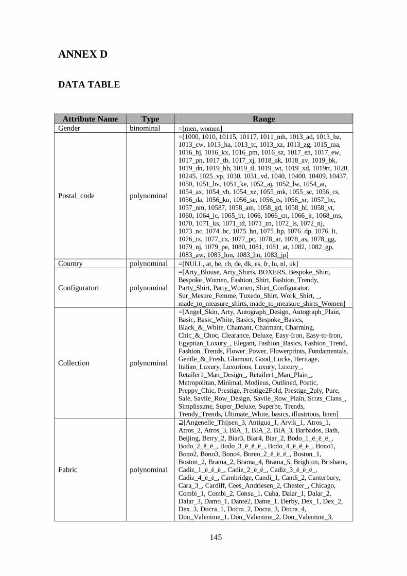
145
ANNEX D
DATA TABLE
Attribute Name Type Range Gender binominal =[men, women]
Postal_code polynominal
=[1000, 1010, 10115, 10117, 1011_mh, 1013_ad, 1013_bz, 1013_cw, 1013_ha, 1013_tc, 1013_xz, 1013_zg, 1015_ma,
1016_hj, 1016_kx, 1016_pm, 1016_sz, 1017_en, 1017_ew,
1017_pn, 1017_tb, 1017_xj, 1018_ak, 1018_av, 1019_bk,
1019_dn, 1019_hb, 1019_tl, 1019_wt, 1019_xd, 1019rt, 1020,
10245, 1025_vp, 1030, 1031_vd, 1040, 10400, 10409, 10437,
1050, 1051_bv, 1051_ke, 1052_aj, 1052_lw, 1054_at,
1054_ax, 1054_vb, 1054_xz, 1055_mk, 1055_sc, 1056_cs,
1056_da, 1056_kn, 1056_se, 1056_ts, 1056_xr, 1057_hc,
1057_nm, 10587, 1058_am, 1058_gd, 1058_hl, 1058_vt,
1060, 1064_jc, 1065_bt, 1066, 1066_cn, 1066_jr, 1068_ms,
1070, 1071_ks, 1071_td, 1071_zn, 1072_ls, 1072_nj, 1073_nc, 1074_bc, 1075_hn, 1075_hp, 1076_dp, 1076_lt,
1076_tx, 1077_cx, 1077_pc, 1078_ar, 1078_as, 1078_gg,
1079_nj, 1079_pe, 1080, 1081, 1081_at, 1082, 1082_gp,
1083_aw, 1083_hm, 1083_hn, 1083_jp]
Country polynominal =[NULL, at, be, ch, de, dk, es, fr, lu, nl, uk]
Configuratort polynominal
=[Arty_Blouse, Arty_Shirts, BOXERS, Bespoke_Shirt,
Bespoke_Women, Fashion_Shirt, Fashion_Trendy,
Party_Shirt, Party_Women, Shirt_Configurator,
Sur_Mesure_Femme, Tuxedo_Shirt, Work_Shirt, _,
made_to_measure_shirts, made_to_measure_shirts_Women]
Collection polynominal
=[Angel_Skin, Arty, Autograph_Design, Autograph_Plain,
Basic, Basic_White, Basics, Bespoke_Basics, Black_&_White, Chamant, Charmant, Charming,
Chic_&_Choc, Clearance, Deluxe, Easy-Iron, Easy-to-Iron,
Egyptian_Luxury_, Elegant, Fashion_Basics, Fashion_Trend,
Fashion_Trends, Flower_Power, Flowerprints, Fundamentals,
Gentle_&_Fresh, Glamour, Good_Lucks, Heritage,
Italian_Luxury, Luxurious, Luxury, Luxury_,
Retailer1_Man_Design_, Retailer1_Man_Plain_,
Metropolitan, Minimal, Modieus, Outlined, Poetic,
Preppy_Chic, Prestige, Prestige2Fold, Prestige_2ply, Pure,
Sale, Savile_Row_Design, Savile_Row_Plain, Scots_Clans_,
Simplissime, Super_Deluxe, Superbe, Trends, Trendy_Trends, Ultimate_White, basics, illustrious, linen]
Fabric polynominal
⊇[Angenelle_Thijsen_3, Antigua_1, Arvik_1, Atros_1,
Atros_2, Atros_3, BIA_1, BIA_2, BIA_3, Barbados, Bath,
Beijing, Berry_2, Biar3, Biar4, Biar_2, Bodo_1_ë_ë_ë_,
Bodo_2_ë_ë_, Bodo_3_ë_ë_ë_, Bodo_4_ë_ë_ë_, Bono1,
Bono2, Bono3, Bono4, Boreo_2_ë_ë_ë_, Boston_1,
Boston_2, Brama_2, Brama_4, Brama_5, Brighton, Brisbane,
Cadiz_1_ë_ë_ë_, Cadiz_2_ë_ë_, Cadiz_3_ë_ë_ë_,
Cadiz_4_ë_ë_, Cambridge, Candi_1, Candi_2, Canterbury,
Cara_3_, Cardiff, Cees_Andriesen_2, Chester_, Chicago,
Combi_1, Combi_2, Consu_1, Cuba, Dalar_1, Dalar_2,
Dalar_3, Damo_1, Dante2, Dante_1, Derby, Dex_1, Dex_2, Dex_3, Docra_1, Docra_2, Docra_3, Docra_4,
Don_Valentine_1, Don_Valentine_2, Don_Valentine_3,
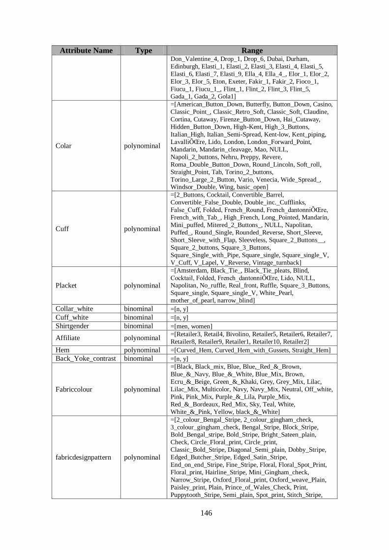
146
Attribute Name Type Range Don_Valentine_4, Drop_1, Drop_6, Dubai, Durham,
Edinburgh, Elasti_1, Elasti_2, Elasti_3, Elasti_4, Elasti_5,
Elasti_6, Elasti_7, Elasti_9, Ella_4, Ella_4_, Elor_1, Elor_2,
Elor_3, Elor_5, Eton, Exeter, Fakir_1, Fakir_2, Fioco_1,
Fiucu_1, Fiucu_1_, Flint_1, Flint_2, Flint_3, Flint_5, Gada_1, Gada_2, Gola1]
Colar polynominal
=[American_Button_Down, Butterfly, Button_Down, Casino,
Classic_Point_, Classic_Retro_Soft, Classic_Soft, Claudine,
Cortina, Cutaway, Firenze_Button_Down, Hai_Cutaway,
Hidden_Button_Down, High-Kent, High_3_Buttons,
Italian_High, Italian_Semi-Spread, Kent-low, Kent_piping,
LavalliÕŒre, Lido, London, London_Forward_Point,
Mandarin, Mandarin_cleavage, Mao, NULL,
Napoli_2_buttons, Nehru, Preppy, Revere,
Roma_Double_Button_Down, Round_Lincoln, Soft_roll,
Straight_Point, Tab, Torino_2_buttons,
Torino_Large_2_Button, Vario, Venecia, Wide_Spread_, Windsor_Double, Wing, basic_open]
Cuff polynominal
=[2_Buttons, Cocktail, Convertible_Barrel,
Convertible_False_Double, Double_inc._Cufflinks,
False_Cuff, Folded, French_Round, French_dantonniÕŒre,
French_with_Tab_, High_French, Long_Pointed, Mandarin,
Mini_puffed, Mitered_2_Buttons_, NULL, Napolitan,
Puffed_, Round_Single, Rounded_Reverse, Short_Sleeve,
Short_Sleeve_with_Flap, Sleeveless, Square_2_Buttons__,
Square_2_buttons, Square_3_Buttons,
Square_Single_with_Pipe, Square_single, Square_single_V,
V_Cuff, V_Lapel, V_Reverse, Vintage_turnback]
Placket polynominal
=[Amsterdam, Black_Tie_, Black_Tie_pleats, Blind,
Cocktail, Folded, French_dantonniÕŒre, Lido, NULL, Napolitan, No_ruffle, Real_front, Ruffle, Square_3_Buttons,
Square_single, Square_single_V, White_Pearl,
mother_of_pearl, narrow_blind]
Collar_white binominal =[n, y]
Cuff_white binominal =[n, y]
Shirtgender binominal =[men, women]
Affiliate polynominal =[Retailer3, Retail4, Bivolino, Retailer5, Retailer6, Retailer7,
Retailer8, Retailer9, Retailer1, Retailer10, Retailer2]
Hem polynominal =[Curved_Hem, Curved_Hem_with_Gussets, Straight_Hem]
Back_Yoke_contrast binominal =[n, y]
Fabriccolour polynominal
=[Black, Black_mix, Blue, Blue,_Red_&_Brown,
Blue_&_Navy, Blue_&_White, Blue_Mix, Brown,
Ecru_&_Beige, Green_&_Khaki, Grey, Grey_Mix, Lilac,
Lilac_Mix, Multicolor, Navy, Navy_Mix, Neutral, Off_white,
Pink, Pink_Mix, Purple_&_Lila, Purple_Mix,
Red_&_Bordeaux, Red_Mix, Sky, Teal, White,
White_&_Pink, Yellow, black_&_White]
fabricdesignpattern polynominal
=[2_colour_Bengal_Stripe, 2_colour_gingham_check,
3_colour_gingham_check, Bengal_Stripe, Block_Stripe, Bold_Bengal_stripe, Bold_Stripe, Bright_Sateen_plain,
Check, Circle_Floral_print, Circle_print,
Classic_Bold_Stripe, Diagonal_Semi_plain, Dobby_Stripe,
Edged_Butcher_Stripe, Edged_Satin_Stripe,
End_on_end_Stripe, Fine_Stripe, Floral, Floral_Spot_Print,
Floral_print, Hairline_Stripe, Mini_Gingham_check,
Narrow_Stripe, Oxford_Floral_print, Oxford_weave_Plain,
Paisley_print, Plain, Prince_of_Wales_Check, Print,
Puppytooth_Stripe, Semi_plain, Spot_print, Stitch_Stripe,
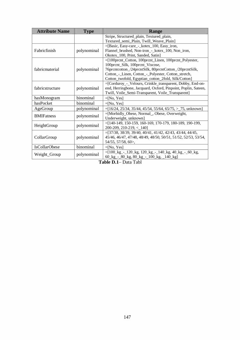
147
Attribute Name Type Range Stripe, Structured_plain, Textured_plain,
Textured_semi_Plain, Twill_Weave_Plain]
Fabricfinish polynominal =[Basic, Easy-care_-_kotex_100, Easy_iron,
Flannel_brushed, Non-iron_-_kotex_100, Non_iron,
Okotex_100, Print, Sanded, Satin]
fabricmaterial polynominal
=[100prcnt_Cotton, 100prcnt_Linen, 100prcnt_Polyester,
100prcnt_Silk, 100prcnt_Viscose, 76prcntcotton_/24prcntSilk, 80prcntCotton_/20prcntSilk,
Cotton_-_Linen, Cotton_-_Polyester, Cotton_stretch,
Cotton_twofold, Egyptian_cotton_2fold, Silk/Cotton]
fabricstructure polynominal =[Corduroy_-_Velours, Crinkle_transparent, Dobby, End-on-
end, Herringbone, Jacquard, Oxford, Pinpoint, Poplin, Sateen,
Twill, Voile_Semi-Transparent, Voile_Transparent]
hasMonogram binominal =[No, Yes]
hasPocket binominal =[No, Yes]
AgeGroup polynominal =[16/24, 25/34, 35/44, 45/54, 55/64, 65/75, >_75, unknown]
BMIFatness polynominal =[Morbidly_Obese, Normal_, Obese, Overweight,
Underweight, unknown]
HeightGroup polynominal =[140-149, 150-159, 160-169, 170-179, 180-189, 190-199,
200-209, 210-219, <_140]
CollarGroup polynominal =[37/38, 38/39, 39/40, 40/41, 41/42, 42/43, 43/44, 44/45,
45/46, 46/47, 47/48, 48/49, 48/50, 50/51, 51/52, 52/53, 53/54,
54/55, 57/58, 60>,
IsCollarObese binominal =[No, Yes]
Weight_Group polynominal =[100_kg_-_120_kg, 120_kg_-_140_kg, 40_kg_-_60_kg,
60_kg_-_80_kg, 80_kg_-_100_kg, _140_kg]
Table D.1– Data Tabl
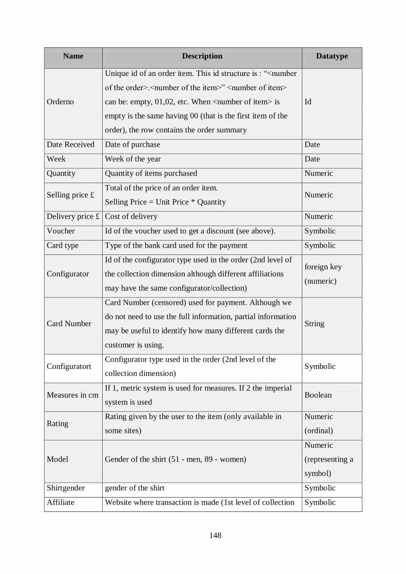
148
Name Description Datatype
Orderno
Unique id of an order item. This id structure is : “<number
of the order>.<number of the item>” <number of item>
can be: empty, 01,02, etc. When <number of item> is
empty is the same having 00 (that is the first item of the
order), the row contains the order summary
Id
Date Received Date of purchase Date
Week Week of the year Date
Quantity Quantity of items purchased Numeric
Selling price £ Total of the price of an order item.
Selling Price = Unit Price * Quantity Numeric
Delivery price £ Cost of delivery Numeric
Voucher Id of the voucher used to get a discount (see above). Symbolic
Card type Type of the bank card used for the payment Symbolic
Configurator
Id of the configurator type used in the order (2nd level of
the collection dimension although different affiliations
may have the same configurator/collection)
foreign key
(numeric)
Card Number
Card Number (censored) used for payment. Although we
do not need to use the full information, partial information
may be useful to identify how many different cards the
customer is using.
String
Configuratort Configurator type used in the order (2nd level of the
collection dimension) Symbolic
Measures in cm If 1, metric system is used for measures. If 2 the imperial
system is used Boolean
Rating Rating given by the user to the item (only available in
some sites)
Numeric
(ordinal)
Model Gender of the shirt (51 - men, 89 - women)
Numeric
(representing a
symbol)
Shirtgender gender of the shirt Symbolic
Affiliate Website where transaction is made (1st level of collection Symbolic
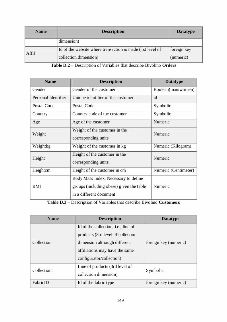
149
Name Description Datatype
dimension)
Affil Id of the website where transaction is made (1st level of
collection dimension)
foreign key
(numeric)
Table D.2 – Description of Variables that describe Bivolino Orders
Name Description Datatype
Gender Gender of the customer Boolean(man/women)
Personal Identifier Unique identifier of the customer id
Postal Code Postal Code Symbolic
Country Country code of the customer Symbolic
Age Age of the customer Numeric
Weight Weight of the customer in the
corresponding units Numeric
Weightkg Weight of the customer in kg Numeric (Kilogram)
Height Height of the customer in the
corresponding units Numeric
Heightcm Height of the customer in cm Numeric (Centimeter)
BMI
Body Mass Index. Necessary to define
groups (including obese) given the table
in a different document
Numeric
Table D.3 – Description of Variables that describe Bivolino Customers
Name Description Datatype
Collection
Id of the collection, i.e., line of
products (3rd level of collection
dimension although different
affiliations may have the same
configurator/collection)
foreign key (numeric)
Collectiont Line of products (3rd level of
collection dimension) Symbolic
FabricID Id of the fabric type foreign key (numeric)
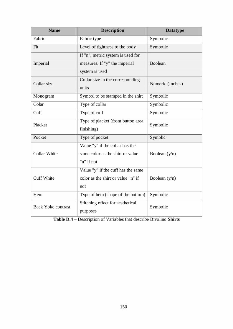
150
Name Description Datatype
Fabric Fabric type Symbolic
Fit Level of tightness to the body Symbolic
Imperial
If "n", metric system is used for
measures. If "y" the imperial
system is used
Boolean
Collar size Collar size in the corresponding
units Numeric (Inches)
Monogram Symbol to be stamped in the shirt Symbolic
Colar Type of collar Symbolic
Cuff Type of cuff Symbolic
Placket Type of placket (front button area
finishing) Symbolic
Pocket Type of pocket Symblic
Collar White
Value "y" if the collar has the
same color as the shirt or value
"n" if not
Boolean (y/n)
Cuff White
Value "y" if the cuff has the same
color as the shirt or value "n" if
not
Boolean (y/n)
Hem Type of hem (shape of the bottom) Symbolic
Back Yoke contrast Stitching effect for aesthetical
purposes Symbolic
Table D.4 – Description of Variables that describe Bivolino Shirts
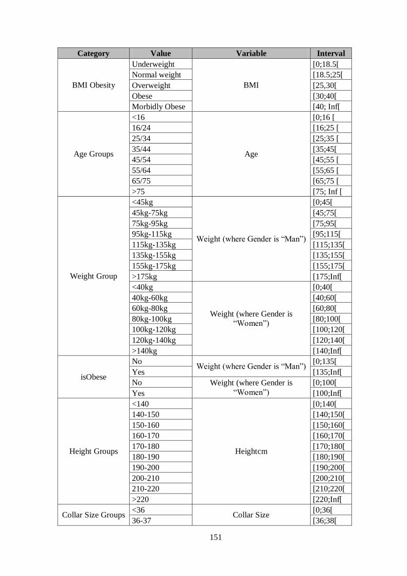
151
Category Value Variable Interval
BMI Obesity
Underweight
BMI
[0;18.5[
Normal weight [18.5;25[
Overweight [25,30[
Obese [30;40[
Morbidly Obese [40; Inf[
Age Groups
<16
Age
[0;16 [
16/24 [16;25 [
25/34 [25;35 [
35/44 [35;45[
45/54 [45;55 [
55/64 [55;65 [
65/75 [65;75 [
>75 [75; Inf [
Weight Group
<45kg
Weight (where Gender is “Man”)
[0;45[
45kg-75kg [45;75[
75kg-95kg [75;95[
95kg-115kg [95;115[
115kg-135kg [115;135[
135kg-155kg [135;155[
155kg-175kg [155;175[
>175kg [175;Inf[
<40kg
Weight (where Gender is
“Women”)
[0;40[
40kg-60kg [40;60[
60kg-80kg [60;80[
80kg-100kg [80;100[
100kg-120kg [100;120[
120kg-140kg [120;140[
>140kg [140;Inf[
isObese
No Weight (where Gender is “Man”)
[0;135[
Yes [135;Inf[
No Weight (where Gender is
“Women”)
[0;100[
Yes [100;Inf[
Height Groups
<140
Heightcm
[0;140[
140-150 [140;150[
150-160 [150;160[
160-170 [160;170[
170-180 [170;180[
180-190 [180;190[
190-200 [190;200[
200-210 [200;210[
210-220 [210;220[
>220 [220;Inf[
Collar Size Groups <36
Collar Size [0;36[
36-37 [36;38[
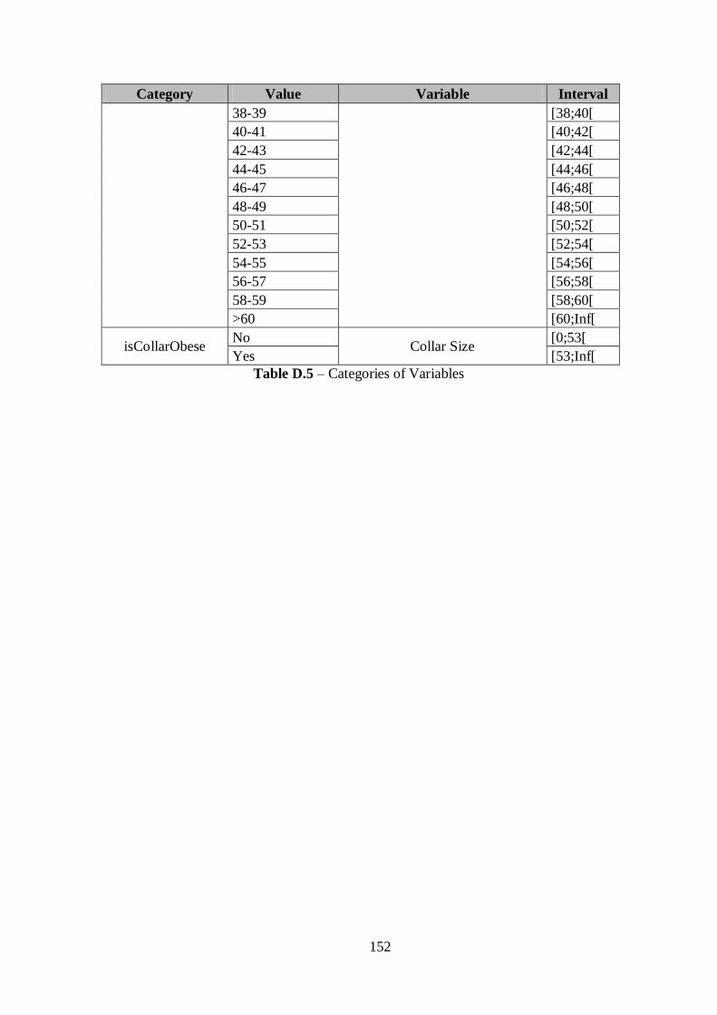
152
Category Value Variable Interval
38-39 [38;40[
40-41 [40;42[
42-43 [42;44[
44-45 [44;46[
46-47 [46;48[
48-49 [48;50[
50-51 [50;52[
52-53 [52;54[
54-55 [54;56[
56-57 [56;58[
58-59 [58;60[
>60 [60;Inf[
isCollarObese No
Collar Size [0;53[
Yes [53;Inf[
Table D.5 – Categories of Variables
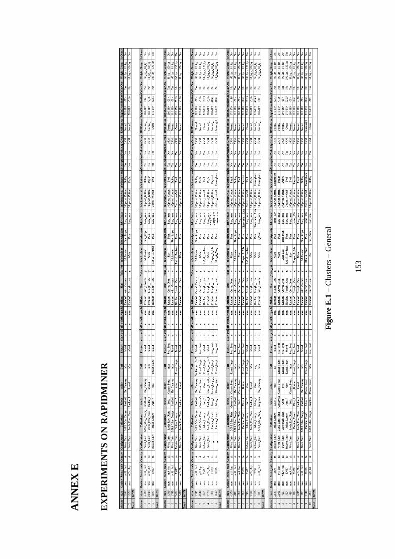
153
AN
NE
X E
EX
PE
RIM
EN
TS
ON
RA
PID
MIN
ER
Fig
ure
E.1
– C
lust
ers
– G
ener
al
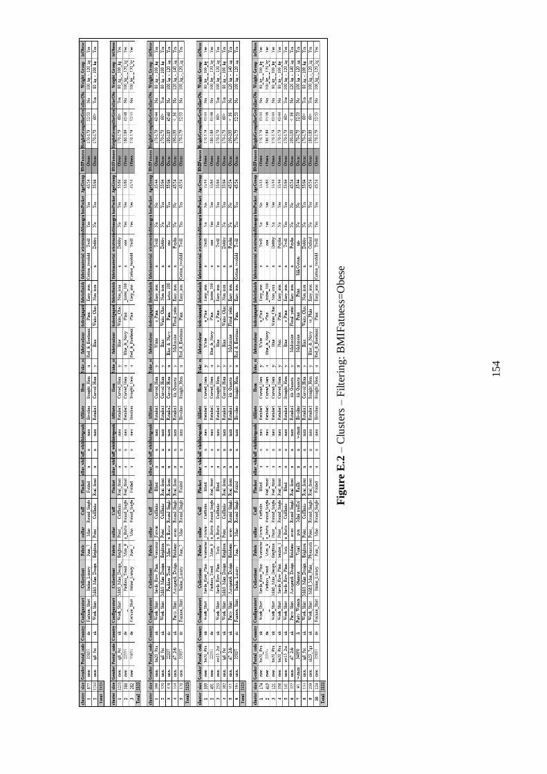
154
Fig
ure
E.2
– C
lust
ers
– F
ilte
ring:
BM
IFat
nes
s=O
bes
e
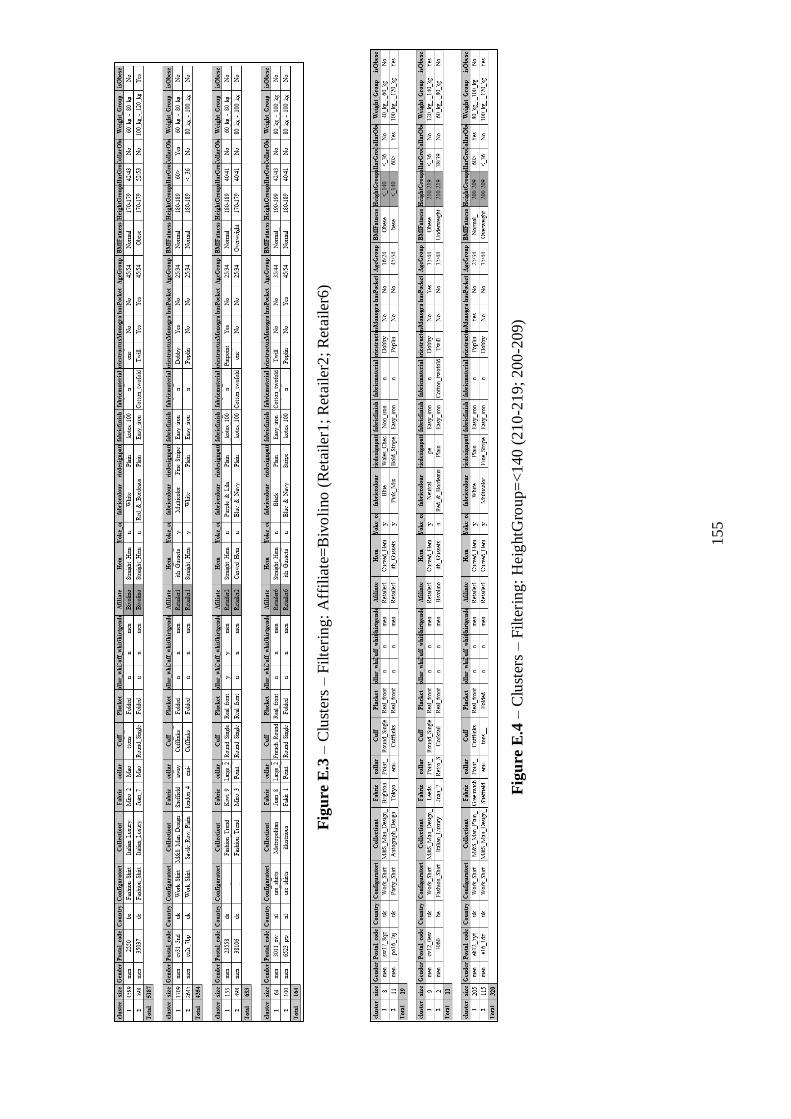
155
Fig
ure
E.3
– C
lust
ers
– F
ilte
ring:
Aff
ilia
te=
Biv
oli
no
(R
etai
ler1
; R
etail
er2
; R
etail
er6
)
Fig
ure
E.4
– C
lust
ers
– F
ilte
ring:
Heig
htG
roup=
<140 (
210
-219;
200
-209)

156
Fig
ure
E.5
– C
lust
ers
– F
ilte
ring:
Weig
ht_
Gro
up=
120kg
-140kg (
>140kg)
157
ANNEX F
CORENET
The information contained in this annex is from CoReNet website
(http://www.corenet-project.eu/).
Summary
CoReNet project was launched the 1st June 2010 under the framework of the
call FoF.NMP.2010-2 (Grant Agreement: 260169).
CoReNet main aim is to meet particular needs and expectations of widely
represented European consumer targets - such as elderly, obese, disabled, diabetic
people -, that usually look for clothes and footwear with particular functional
requirements but, at the same time fashionable, high quality, eco-sustainable and at an
affordable price.
Adopting the CoReNet framework, based on methods and tools for a cost and
eco-efficient collaborative networking, the European Textile, Clothing and Footwear
Industry (TCFI) will be able to provide small series of customized fashionable goods for
such relevant social niches by enabling products to stay as long as possible digital and
to produce on-demand.
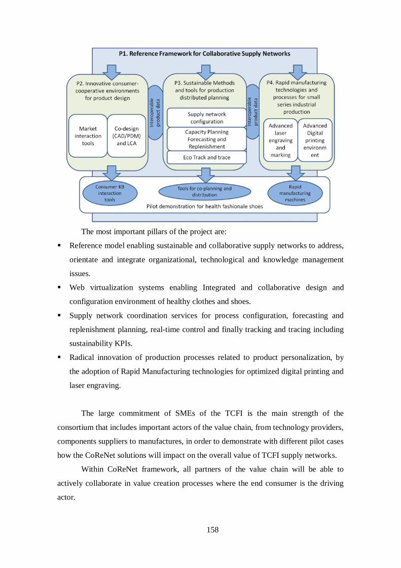
158
The most important pillars of the project are:
Reference model enabling sustainable and collaborative supply networks to address,
orientate and integrate organizational, technological and knowledge management
issues.
Web virtualization systems enabling Integrated and collaborative design and
configuration environment of healthy clothes and shoes.
Supply network coordination services for process configuration, forecasting and
replenishment planning, real-time control and finally tracking and tracing including
sustainability KPIs.
Radical innovation of production processes related to product personalization, by
the adoption of Rapid Manufacturing technologies for optimized digital printing and
laser engraving.
The large commitment of SMEs of the TCFI is the main strength of the
consortium that includes important actors of the value chain, from technology providers,
components suppliers to manufactures, in order to demonstrate with different pilot cases
how the CoReNet solutions will impact on the overall value of TCFI supply networks.
Within CoReNet framework, all partners of the value chain will be able to
actively collaborate in value creation processes where the end consumer is the driving
actor.

159
CoReNet methods and tools will enable design changes and production
processes adaptation for easy and sustainable product customizations.
CoReNet results will be tested and demonstrated within industrial plants,
showing the full potential of the proposed sustainable collaborative networking
approach.
Approach
CoReNet project addresses the design, production and distribution of small
series of healthy fashionable goods for specific target groups of wide impact in terms of
market for the European industry as elderly, disables, diabetics and obese people.
CoReNet will do this supporting the whole value chain to:
get and manage consumer data to know their needs,
involve consumer into design and product configuration phases,
exchange consumer data through adequate data models and secure systems,
manage the collaboration with suppliers in order to plan and distribute on time,
implement innovative manufacturing machines in particular for Digital Printing and
Laser Engraving,
delivering the product to the final customer,
monitoring the quality and sustainability of products.
The CoReNet approach is based on a new holistic framework, meant as a set of
methods, tools and technologies for sustainable small series industrial value creation of
health fashionable goods.
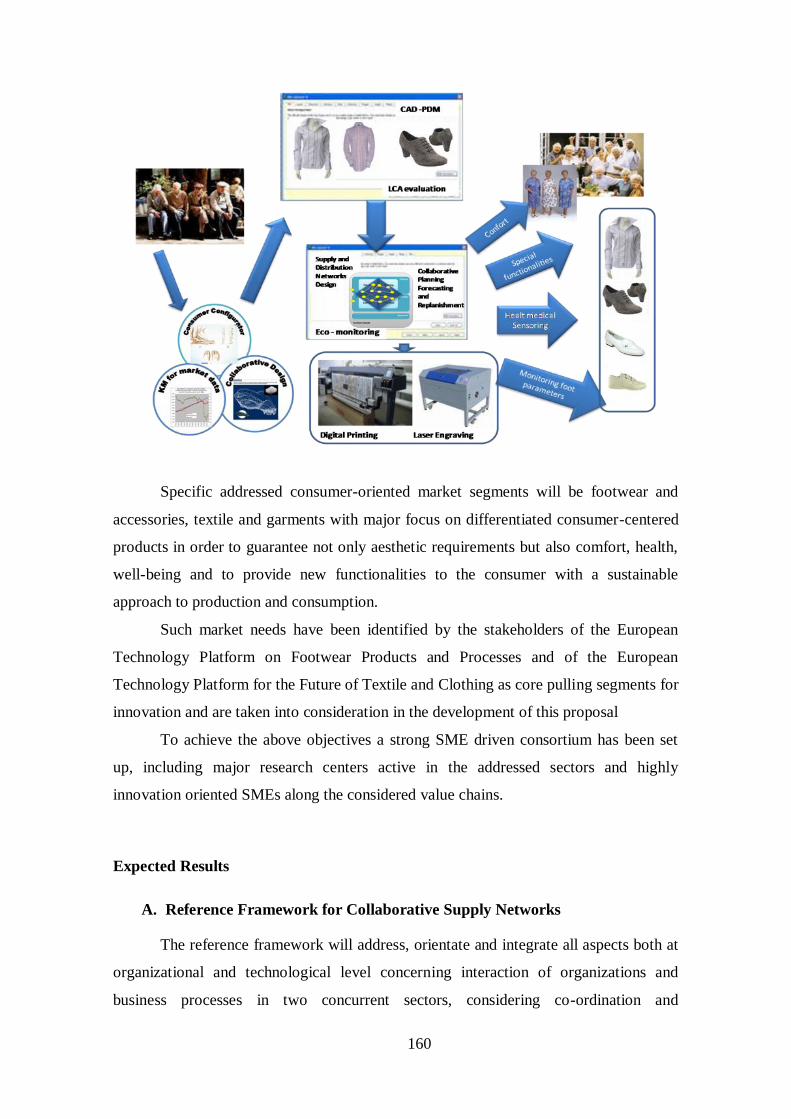
160
Specific addressed consumer-oriented market segments will be footwear and
accessories, textile and garments with major focus on differentiated consumer-centered
products in order to guarantee not only aesthetic requirements but also comfort, health,
well-being and to provide new functionalities to the consumer with a sustainable
approach to production and consumption.
Such market needs have been identified by the stakeholders of the European
Technology Platform on Footwear Products and Processes and of the European
Technology Platform for the Future of Textile and Clothing as core pulling segments for
innovation and are taken into consideration in the development of this proposal
To achieve the above objectives a strong SME driven consortium has been set
up, including major research centers active in the addressed sectors and highly
innovation oriented SMEs along the considered value chains.
Expected Results
A. Reference Framework for Collaborative Supply Networks
The reference framework will address, orientate and integrate all aspects both at
organizational and technological level concerning interaction of organizations and
business processes in two concurrent sectors, considering co-ordination and

161
synchronization of contents, as well as information exchange and software application
modularity, in order to create a seamless flow of information from market to design and
development, to production and distribution.
B. Innovative consumer-driven environments for product design
This result will address the implementation of innovative environments for
collaboration and knowledge management during design phase. The goal is to create a
novel concept that enables the vision of an “empowered-to-design” consumer from one
side, and the creation of market and design knowledge from the history of consumer-to-
designer, consumer-to-consumer and designer-to-designer interactions within a social
network environment.
C. Methods and tools for supply network configuration and distributed
production planning including consumer-oriented Collaborative Planning
Innovative and adaptive services for production process modeling and supply
networks formation and management will be based on a distributed interaction system
to integrate different actors (components suppliers, outsourcers, service providers,
retailers, customers) of different sectors collaborating in dynamic networks. Product
quality control based on environmental impact parameters will be developed through a
shared platform for eco-monitoring.
Small series and personalized products will require totally different supply
networks structures, where each company should be able to produce the complete
product (all or most of the operations) and will be specialized by the type of product or
market segment.
In this context a supply network will have to be configured for each customer
order and tend to include a small number of companies. The key selection criteria will
be the ability to perform the required operations for the desired delivery date, with the
expected cost.
D. Rapid manufacturing technologies for small series industrial production
This result will enable the flexible, energy and eco-efficient production of
specific added value components/parts of consumer personalized goods through rapid
manufacturing multi-purpose machines. In particular reduction of set-up time is crucial
in the production of small series in order to avoid loss of time when changing models.

162
Two particular phases of production process (printing and engraving) will be taken into
consideration because they represent critical steps for the personalization of fabric and
leather in the definition of the new collections.
These results will be all integrated in real demonstration environments.
Integrated demonstrator can be considered a result in terms of functioning pilot
collaborative supply network offering integrated small series of clothing and shoes to
target groups. The pilot demonstrator will be composed of manufacturing companies
collaborating with technologies providers along product lifecycle where coordination
has to be managed at supply network and not at company level.
Copyright © 2022 FDOKUMEN