
Data profiling - efficient discovery of dependencies - publish.UP
152
Hasso Plattner Institute Information Systems Group Data Profiling – Efficient Discovery of Dependencies Dissertation zur Erlangung des akademischen Grades “Doktor der Naturwissenschaften” (Dr. rer. nat.) in der Wissenschaftsdisziplin “Informationssysteme” eingereicht an der Fakult¨ at Digital Engineering der Universit¨ at Potsdam von Thorsten Papenbrock Dissertation, Universit¨ at Potsdam, 2017
-
Upload
khangminh22 -
Category
Documents
-
view
0 -
download
0
Transcript of Data profiling - efficient discovery of dependencies - publish.UP

Hasso Plattner InstituteInformation Systems Group
Data Profiling
–
Efficient Discovery of Dependencies
Dissertationzur Erlangung des akademischen Grades
“Doktor der Naturwissenschaften”(Dr. rer. nat.)
in der Wissenschaftsdisziplin “Informationssysteme”
eingereicht an derFakultat Digital Engineering
der Universitat Potsdam
vonThorsten Papenbrock
Dissertation, Universitat Potsdam, 2017

This work is licensed under a Creative Commons License: Attribution – Share Alike 4.0 International To view a copy of this license visit http://creativecommons.org/licenses/by-sa/4.0/
Reviewers Prof. Dr. Felix Naumann Hasso-Plattner-Institut, Universit�at Potsdam Prof. Dr. Wolfgang Lehner Technische Universit�at Dresden Prof. Dr. Volker Markl Technische Universit�at Berlin Published online at the Institutional Repository of the University of Potsdam: URN urn:nbn:de:kobv:517-opus4-406705 http://nbn-resolving.de/urn:nbn:de:kobv:517-opus4-406705
Abstract
Data profiling is the computer science discipline of analyzing a given dataset
for its metadata. The types of metadata range from basic statistics, such
as tuple counts, column aggregations, and value distributions, to much more
complex structures, in particular inclusion dependencies (INDs), unique col-
umn combinations (UCCs), and functional dependencies (FDs). If present,
these statistics and structures serve to efficiently store, query, change, and
understand the data. Most datasets, however, do not provide their metadata
explicitly so that data scientists need to profile them.
While basic statistics are relatively easy to calculate, more complex structures
present difficult, mostly NP-complete discovery tasks; even with good domain
knowledge, it is hardly possible to detect them manually. Therefore, various
profiling algorithms have been developed to automate the discovery. None of
them, however, can process datasets of typical real-world size, because their
resource consumptions and/or execution times exceed effective limits.
In this thesis, we propose novel profiling algorithms that automatically dis-
cover the three most popular types of complex metadata, namely INDs,
UCCs, and FDs, which all describe different kinds of key dependencies. The
task is to extract all valid occurrences from a given relational instance. The
three algorithms build upon known techniques from related work and com-
plement them with algorithmic paradigms, such as divide & conquer, hy-
brid search, progressivity, memory sensitivity, parallelization, and additional
pruning to greatly improve upon current limitations. Our experiments show
that the proposed algorithms are orders of magnitude faster than related
work. They are, in particular, now able to process datasets of real-world, i.e.,
multiple gigabytes size with reasonable memory and time consumption.
Due to the importance of data profiling in practice, industry has built var-
ious profiling tools to support data scientists in their quest for metadata.
These tools provide good support for basic statistics and they are also able
to validate individual dependencies, but they lack real discovery features even
though some fundamental discovery techniques are known for more than 15
years. To close this gap, we developed Metanome, an extensible profil-
ing platform that incorporates not only our own algorithms but also many
further algorithms from other researchers. With Metanome, we make our
research accessible to all data scientists and IT-professionals that are tasked
with data profiling. Besides the actual metadata discovery, the platform also
offers support for the ranking and visualization of metadata result sets.

Being able to discover the entire set of syntactically valid metadata naturally
introduces the subsequent task of extracting only the semantically meaningful
parts. This is challenge, because the complete metadata results are surpris-
ingly large (sometimes larger than the datasets itself) and judging their use
case dependent semantic relevance is difficult. To show that the complete-
ness of these metadata sets is extremely valuable for their usage, we finally
exemplify the efficient processing and effective assessment of functional de-
pendencies for the use case of schema normalization.
Zusammenfassung
Data Profiling ist eine Disziplin der Informatik, die sich mit der Analyse
von Datensatzen auf deren Metadaten beschaftigt. Die verschiedenen Typen
von Metadaten reichen von einfachen Statistiken wie Tupelzahlen, Spaltenag-
gregationen und Wertverteilungen bis hin zu weit komplexeren Strukturen,
insbesondere Inklusionsabhangigkeiten (INDs), eindeutige Spaltenkombina-
tionen (UCCs) und funktionale Abhangigkeiten (FDs). Diese Statistiken und
Strukturen dienen, sofern vorhanden, dazu die Daten effizient zu speichern,
zu lesen, zu andern und zu verstehen. Die meisten Datensatze stellen ihre
Metadaten aber nicht explizit zur Verfugung, so dass Informatiker sie mittels
Data Profiling bestimmen mussen.
Wahrend einfache Statistiken noch relativ schnell zu berechnen sind, stellen
die komplexen Strukturen schwere, zumeist NP-vollstandige Entdeckungsauf-
gaben dar. Es ist daher auch mit gutem Domanenwissen in der Regel nicht
moglich sie manuell zu entdecken. Aus diesem Grund wurden verschiedenste
Profiling Algorithmen entwickelt, die die Entdeckung automatisieren. Kein-
er dieser Algorithmen kann allerdings Datensatze von heutzutage typischer
Große verarbeiten, weil entweder der Ressourcenverbrauch oder die Rechen-
zeit effektive Grenzen uberschreiten.
In dieser Arbeit stellen wir neuartige Profiling Algorithmen vor, die automa-
tisch die drei popularsten Typen komplexer Metadaten entdecken konnen,
namlich INDs, UCCs, und FDs, die alle unterschiedliche Formen von Schlussel-
Abhangigkeiten beschreiben. Die Aufgabe dieser Algorithmen ist es alle gulti-
gen Vorkommen der drei Metadaten-Typen aus einer gegebenen relationalen
Instanz zu extrahieren. Sie nutzen dazu bekannte Entdeckungstechniken aus
verwandten Arbeiten und erganzen diese um algorithmische Paradigmen wie
Teile-und-Herrsche, hybrides Suchen, Progressivitat, Speichersensibilitat, Par-
allelisierung und zusatzliche Streichungsregeln. Unsere Experimente zeigen,
dass die vorgeschlagenen Algorithmen mit den neuen Techniken nicht nur
um Großenordnungen schneller sind als alle verwandten Arbeiten, sie er-
weitern auch aktuelle Beschrankungen deutlich. Sie konnen insbesondere nun
Datensatze realer Große, d.h. mehrerer Gigabyte Große mit vernunftigem
Speicher- und Zeitverbrauch verarbeiten.
Aufgrund der praktischen Relevanz von Data Profiling hat die Industrie ver-
schiedene Profiling Werkzeuge entwickelt, die Informatiker in ihrer Suche
nach Metadaten unterstutzen sollen. Diese Werkzeuge bieten eine gute Un-
terstutzung fur die Berechnung einfacher Statistiken. Sie sind auch in der

Lage einzelne Abhangigkeiten zu validieren, allerdings mangelt es ihnen an
Funktionen zur echten Entdeckung von Metadaten, obwohl grundlegende Ent-
deckungstechniken schon mehr als 15 Jahre bekannt sind. Um diese Lucke zu
schließen haben wir Metanome entwickelt, eine erweiterbare Profiling Plat-
tform, die nicht nur unsere eigenen Algorithmen sondern auch viele weitere
Algorithmen anderer Forscher integriert. Mit Metanome machen wir unsere
Forschungsergebnisse fur alle Informatiker und IT-Fachkrafte zuganglich, die
ein modernes Data Profiling Werkzeug benotigen. Neben der tatsachlichen
Metadaten-Entdeckung bietet die Plattform zusatzlich Unterstutzung bei der
Bewertung und Visualisierung gefundener Metadaten.
Alle syntaktisch korrekten Metadaten effizient finden zu konnen fuhrt natur-
licherweise zur Folgeaufgabe daraus nur die semantisch bedeutsamen Teile
zu extrahieren. Das ist eine Herausforderung, weil zum einen die Mengen der
gefundenen Metadaten uberraschenderweise groß sind (manchmal großer als
der untersuchte Datensatz selbst) und zum anderen die Entscheidung uber
die Anwendungsfall-spezifische semantische Relevanz einzelner Metadaten-
Aussagen schwierig ist. Um zu zeigen, dass die Vollstandigkeit der Meta-
daten sehr wertvoll fur ihre Nutzung ist, veranschaulichen wir die effiziente
Verarbeitung und effektive Bewertung von funktionalen Abhangigkeiten am
Anwendungsfall Schema Normalisierung.

Acknowledgements
I want to dedicate the first lines to my advisor Felix Naumann, who owns
my deepest appreciation and gratitude. As the epitome of a responsible and
caring mentor, he supported me from the very beginning and taught me every
detail of scientific working. We have spent countless hours discussing ideas,
hitting walls, and then coming up with solutions. Not only did his knowledge
provide me guidance throughout my journey, his support in difficult times
always helped me to get back on track. For all that I am truly thankful.
My gratitude also goes to all my wonderful colleagues for their help and
friendship. This PhD would not have been such a wonderful experience with-
out all the people with whom I had the pleasure to work and consort with.
Here, I want to express special thanks go to my close co-workers Sebas-
tian Kruse, Hazar Harmouch, Anja Jentzsch, Tobias Bleifuß, and Maximilian
Jenders with whom I could always share and discuss problems, ideas, and so-
lutions. Also, many thanks to Jorge-Arnulfo Quiane-Ruiz and Arvid Heise,
who dragged me through my first publications with remarkable patience and
became valuable co-advisors to me.
This work would not have been possible without the help of Jakob Zwiener,
Claudia Exeler, Tanja Bergmann, Moritz Finke, Carl Ambroselli, Vincent
Schwarzer, and Maxi Fischer, who not only built the Metanome platform,
but also contributed many own ideas. I very much enjoyed working in this
team of excellent students.
Finally and most importantly, I want to thank my family and my friends for
their support. You are a constant well of energy and motivation and I am
deeply moved by your help. Urte, you are my brightest star – thank you.

viii
Contents
1 Data Profiling 1
1.1 An overview of metadata . . . . . . . . . . . . . . . . . . . . . . . . . . . 2
1.2 Use cases in need for metadata . . . . . . . . . . . . . . . . . . . . . . . . 5
1.3 Research questions . . . . . . . . . . . . . . . . . . . . . . . . . . . . . . . 9
1.4 Structure and contributions . . . . . . . . . . . . . . . . . . . . . . . . . . 10
2 Key Dependencies 11
2.1 The relational data model . . . . . . . . . . . . . . . . . . . . . . . . . . . 11
2.2 Types of key dependencies . . . . . . . . . . . . . . . . . . . . . . . . . . . 12
2.3 Relaxation of key dependencies . . . . . . . . . . . . . . . . . . . . . . . . 16
2.4 Discovery of key dependencies . . . . . . . . . . . . . . . . . . . . . . . . . 17
2.5 Null semantics for key dependencies . . . . . . . . . . . . . . . . . . . . . 22
3 Functional Dependency Discovery 25
3.1 Related Work . . . . . . . . . . . . . . . . . . . . . . . . . . . . . . . . . . 26
3.2 Hybrid FD discovery . . . . . . . . . . . . . . . . . . . . . . . . . . . . . . 27
3.3 The HyFD algorithm . . . . . . . . . . . . . . . . . . . . . . . . . . . . . . 30
3.4 Preprocessing . . . . . . . . . . . . . . . . . . . . . . . . . . . . . . . . . . 32
3.5 Sampling . . . . . . . . . . . . . . . . . . . . . . . . . . . . . . . . . . . . 33
3.6 Induction . . . . . . . . . . . . . . . . . . . . . . . . . . . . . . . . . . . . 37
3.7 Validation . . . . . . . . . . . . . . . . . . . . . . . . . . . . . . . . . . . . 39
3.8 Memory Guardian . . . . . . . . . . . . . . . . . . . . . . . . . . . . . . . 42
3.9 Evaluation . . . . . . . . . . . . . . . . . . . . . . . . . . . . . . . . . . . . 43
3.10 Conclusion & Future Work . . . . . . . . . . . . . . . . . . . . . . . . . . 52
4 Unique Column Combination Discovery 53
4.1 Related Work . . . . . . . . . . . . . . . . . . . . . . . . . . . . . . . . . . 54
4.2 Hybrid UCC discovery . . . . . . . . . . . . . . . . . . . . . . . . . . . . . 54
i
CONTENTS
4.3 The HyUCC algorithm . . . . . . . . . . . . . . . . . . . . . . . . . . . . . 57
4.4 Evaluation . . . . . . . . . . . . . . . . . . . . . . . . . . . . . . . . . . . . 60
4.5 Conclusion & Future Work . . . . . . . . . . . . . . . . . . . . . . . . . . 62
5 Inclusion Dependency Discovery 63
5.1 Related Work . . . . . . . . . . . . . . . . . . . . . . . . . . . . . . . . . . 64
5.2 BINDER Overview . . . . . . . . . . . . . . . . . . . . . . . . . . . . . . . 66
5.3 Efficiently Dividing Datasets . . . . . . . . . . . . . . . . . . . . . . . . . 69
5.4 Fast IND Discovery . . . . . . . . . . . . . . . . . . . . . . . . . . . . . . . 74
5.5 IND Candidate Generation . . . . . . . . . . . . . . . . . . . . . . . . . . 78
5.6 Evaluation . . . . . . . . . . . . . . . . . . . . . . . . . . . . . . . . . . . . 82
5.7 Conclusion & Future Work . . . . . . . . . . . . . . . . . . . . . . . . . . 91
6 Metanome 93
6.1 The Data Profiling Platform . . . . . . . . . . . . . . . . . . . . . . . . . . 95
6.2 Profiling with Metanome . . . . . . . . . . . . . . . . . . . . . . . . . . . . 98
6.3 System Successes . . . . . . . . . . . . . . . . . . . . . . . . . . . . . . . . 101
7 Data-driven Schema Normalization 103
7.1 The Boyce-Codd Normal Form . . . . . . . . . . . . . . . . . . . . . . . . 104
7.2 Related Work . . . . . . . . . . . . . . . . . . . . . . . . . . . . . . . . . . 108
7.3 Schema Normalization . . . . . . . . . . . . . . . . . . . . . . . . . . . . . 110
7.4 Closure Calculation . . . . . . . . . . . . . . . . . . . . . . . . . . . . . . . 113
7.5 Key Derivation . . . . . . . . . . . . . . . . . . . . . . . . . . . . . . . . . 117
7.6 Violation Detection . . . . . . . . . . . . . . . . . . . . . . . . . . . . . . . 118
7.7 Constraint Selection . . . . . . . . . . . . . . . . . . . . . . . . . . . . . . 120
7.8 Evaluation . . . . . . . . . . . . . . . . . . . . . . . . . . . . . . . . . . . . 122
7.9 Conclusion & Future Work . . . . . . . . . . . . . . . . . . . . . . . . . . 127
8 Conclusion and Future Work 129
References 131
ii

1
Data Profiling
Whenever a data scientist receives a new dataset, she needs to inspect the dataset’s
format, its schema, and some example entries to determine what the dataset has to offer.
Then, she probably measures the dataset’s physical size, its length and width, followed
by the density and distribution of values in certain attributes. In this way, the data
scientist develops a basic understanding of the data that allows her to effectively store,
query, and manipulate it. We call these and further actions that systematically extract
knowledge about the structure of a dataset data profiling and the gained knowledge
metadata [Naumann, 2013].
Of course, data profiling does not end with the inspection of value distributions.
Many further profiling steps, such as data type inference and dependency discovery, are
necessary to fully understand the data. The gathered metadata, then, enable the data
scientist to not only use but also manage the data, which includes data cleaning, nor-
malization, integration, and many further important maintenance tasks. Consequently,
data profiling is – and ever was – an essential toolbox for data scientists.
A closer look into the profiling toolbox reveals that the state-of-the-art profiling
techniques perform very well for most basic types of metadata, such as data types, value
aggregations, and distribution statistics. According to Gardner [Judah et al., 2016],
market leaders for commercial profiling solutions in this segment are Informatica, IBM,
SAP, and SAS with their individual data analytic platforms. Research prototypes for
the same purpose are, for instance, Bellman [Dasu et al., 2002], Profiler [Kandel et al.,
2012], and MADLib [Hellerstein et al., 2012], but a data scientist can profile most basic
metadata types likewise with a text editor, SQL or very simple programming. Profiling
techniques for the discovery of more complex structures, such as functional dependencies
or denial constraints, are, however, largely infeasible for most real-world datasets, because
their discovery strategies do not scale well with the size of the data. For this reason,
most profiling tools refrain from providing true discovery features; instead, they usually
offer only checking methods for individual metadata candidates or try to approximate
the metadata.
The trend of ever growing datasets fuels this problem: We produce, measure, record,
and generate new data at an enormous rate and, thus, often lose control of what and
how we store. In these cases, regaining the comprehension of the data is a downstream
1

1. DATA PROFILING
task for data profiling. Many discovery techniques are, however, hopelessly overloaded
with such large datasets.
In this thesis, we focus on profiling techniques for the discovery of unique column com-
binations (UCCs), functional dependencies (FDs), and inclusion dependencies (INDs),
which are the most important types of metadata in the group of currently overloaded
discovery algorithms [Levene and Vincent, 1999; Toman and Weddell, 2008]. All three
types of metadata describe different forms of key dependencies, i.e., keys of a table,
within a table, and between tables. They form, inter alia, the basis for Wiederhold’s
and El-Masri’s structural model of database systems [Wiederhold and El-Masri, 1979]
and are essential for the interpretation of relational schemata as entity-relationship mod-
els [Chen, 1976]. In other words, UCCs, FDs, and INDs are essential to understand the
semantics of a dataset.
In this introductory chapter, we first give an overview on the different types of meta-
data. Afterwards, we set the focus on UCCs, FDs, and INDs and discuss their importance
for a selection of popular data management use cases. We then introduce the research
questions for this thesis, our concrete contributions, and the structure for the following
chapters.
1.1 An overview of metadata
There are many ways to categorize the different types of metadata: One could, for
instance, use their importance, their use cases, or their semantic properties. The most
insightful categorization, however, is to group the metadata types by their relational
scope, which is either single-column or multi-column as proposed in [Naumann, 2013].
Single-column metadata types provide structural information about individual columns,
whereas multi-column metadata types make statements about groups of columns and
their correlations.
To illustrate a few concrete metadata statements, we use a dataset from bulbagarden.
net on Pokemon – small, fictional pocket monsters for children. The original Pokemon
dataset contains more than 800 records. A sample of 10 records is depicted in Figures 1.1
and 1.2. The former figure annotates the sample with some single-column metadata and
the latter with some multi-column metadata.
Figure 1.1 highlights the format of the dataset as one single-column metadata type.
The format in this example is relational, but it could as well be, for instance, XML,
RDF, or Json. The format basically indicates the representation of each attribute and,
therefore, an attribute’s schema, position, and, if present, heading. These information
give us a basic understanding on how to read and parse the data. The size, then,
refers to the number of records in the relation and the relations physical size, which
both indicate storage requirements. The attributes’ data types define how the individual
values should be parsed and what value modifications are possible. Together, these three
types of metadata are the minimum one reasonably needs to make use of a dataset. The
remaining types of single-column metadata have more statistical nature: The density, for
instance, describes the information content of an attribute, which is useful to judge its
2

1.1 An overview of metadata
ID Name Evolution Location Sex Weight Size Type Weak Strong Special
25 Pikachu Raichu Viridian Forest m/w 6.0 0.4 electric ground water false
27 Sandshrew Sandslash Route 4 m/w 12.0 0.6 ground gras electric false
29 Nidoran Nidorino Safari Zone m 9.0 0.5 poison ground gras false
32 Nidoran Nidorina Safari Zone w 7.0 0.4 poison ground gras false
37 Vulpix Ninetails Route 7 m/w 9.9 0.6 fire water ice false
38 Ninetails null null m/w 19.9 1.1 fire water ice true
63 Abra Kadabra Route 24 m/w 19.5 0.9 psychic ghost fighting false
64 Kadabra Alakazam Cerulean Cave m/w 56.5 1.3 psychic ghost fighting false
130 Gyarados null Fuchsia City m/w 235.0 6.5 water electric fire false
150 Mewtwo null Cerulean Cave null 122.0 2.0 psychic ghost fighting true
format
INTEG
ER
CH
AR(1
6)
CH
AR(1
6)
CH
AR(8
)
FLO
AT
CH
AR(3
)
BO
OLEAN
CH
AR(8
)
CH
AR(8
)
data types
ranges
min = 0.4
max = 2.0
aggregations
sum = 14.3
avg = 1.43
distributions density
#null = _3
%null = 30
size # = 10
FLO
AT
CH
AR(3
2)
0
1
2
3
0
1
2
3
0
1
2
3
Figure 1.1: Example relation on Pokemon with single-column metadata.
relevance and the quality of the dataset; range information and aggregations help to query
and analyse certain properties of the data; and detailed distribution statistics enable
domain investigations and error detection. For example, distributions that follow certain
laws, such as Zipf’s law [Powers, 1998] or Benford’s law [Berger and Hill, 2011] indicate
specific domains and suspicious outliers. Overall, single-column metadata enable a basic
understanding of their datasets; we can calculate them in linear or at least polynomial
time. For further reading on single-column metadata, we refer to [Loshin, 2010].
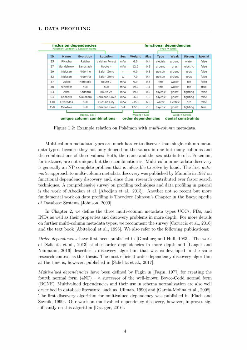
Multi-column metadata, as shown in Figure 1.2, provide much deeper insights into
implicit connections and relationships. Implicit means that these connections and rela-
tionships are (usually) no technical constraints – although declaring them as such often
makes sense for technical reasons; they are, instead, determined by those real-world
entities, facts, and processes that the data tries to describe. So we find, for instance,
attributes or sets of attributes that naturally identify each entity in the relation. In our
Pokemon example, it is a combination of name and sex that is unique for each pocket
monster. Information like this are provided by unique column combinations. Further-
more, an inclusion dependency states that all values in one specific attribute(set) are also
contained in some other attribute(set) so that we can connect, i.e., join these two sets.
In our example, we find that all locations of our Pokemon also occur in a different table,
which might offer additional information on these locations. Moreover, an order depen-
dency shows that sorting the listed Pokemon by their weight also sorts them by their
size, which is a useful information for query optimization and indexing. The functional
dependency in our example expresses that the type of a Pokemon defines its weakness,
which means that there are no two Pokemon with same type but different weakness.
So if we know a Pokemon’s type and the general type-weakness mapping, we can easily
infer its weakness. The denial constraint in our example tells us that weaknesses are
always different from strengths, a general insight that helps, for example, to understand
the meaning of the attributes weak and strong.
3
1. DATA PROFILING
unique column combinations {Name, Sex} Weak ≠ Strong
denial constraints
inclusion dependencies Pokemon.Location ⊆ Location.Name
order dependencies Weight » Size
functional dependencies Type Weak
ID Name Evolution Location Sex Weight Size Type Weak Strong Special
25 Pikachu Raichu Viridian Forest m/w 6.0 0.4 electric ground water false
27 Sandshrew Sandslash Route 4 m/w 12.0 0.6 ground gras electric false
29 Nidoran Nidorino Safari Zone m 9.0 0.5 poison ground gras false
32 Nidoran Nidorina Safari Zone w 7.0 0.4 poison ground gras false
37 Vulpix Ninetails Route 7 m/w 9.9 0.6 fire water ice false
38 Ninetails null null m/w 19.9 1.1 fire water ice true
63 Abra Kadabra Route 24 m/w 19.5 0.9 psychic ghost fighting false
64 Kadabra Alakazam Cerulean Cave m/w 56.5 1.3 psychic ghost fighting false
130 Gyarados null Fuchsia City m/w 235.0 6.5 water electric fire false
150 Mewtwo null Cerulean Cave null 122.0 2.0 psychic ghost fighting true
Figure 1.2: Example relation on Pokemon with multi-column metadata.
Multi-column metadata types are much harder to discover than single-column meta-
data types, because they not only depend on the values in one but many columns and
the combinations of these values: Both, the name and the sex attribute of a Pokemon,
for instance, are not unique, but their combination is. Multi-column metadata discovery
is generally an NP-complete problem that is infeasible to solve by hand. The first auto-
matic approach to multi-column metadata discovery was published by Mannila in 1987 on
functional dependency discovery and, since then, research contributed ever faster search
techniques. A comprehensive survey on profiling techniques and data profiling in general
is the work of Abedian et al. [Abedjan et al., 2015]. Another not so recent but more
fundamental work on data profiling is Theodore Johnson’s Chapter in the Encyclopedia
of Database Systems [Johnson, 2009]
In Chapter 2, we define the three multi-column metadata types UCCs, FDs, and
INDs as well as their properties and discovery problems in more depth. For more details
on further multi-column metadata types, we recomment the survey [Caruccio et al., 2016]
and the text book [Abiteboul et al., 1995]. We also refer to the following publications:
Order dependencies have first been published in [Ginsburg and Hull, 1983]. The work
of [Szlichta et al., 2013] studies order dependencies in more depth and [Langer and
Naumann, 2016] describes a discovery algorithm that was co-developed in the same
research context as this thesis. The most efficient order dependency discovery algorithm
at the time is, however, published in [Szlichta et al., 2017].
Multivalued dependencies have been defined by Fagin in [Fagin, 1977] for creating the
fourth normal form (4NF) – a successor of the well-known Boyce-Codd normal form
(BCNF). Multivalued dependencies and their use in schema normalization are also well
described in database literature, such as [Ullman, 1990] and [Garcia-Molina et al., 2008].
The first discovery algorithm for multivalued dependency was published in [Flach and
Savnik, 1999]. Our work on multivalued dependency discovery, however, improves sig-
nificantly on this algorithm [Draeger, 2016].
4

1.2 Use cases in need for metadata
Denial constraints are a universally quantified first order logic formalism, i.e., a rule
language with certain predicates [Bertossi, 2011]. Denial constraints can express most
other dependencies and are, therefore, particularly hard to fully discover. A first discov-
ery algorithm has already been published in [Chu et al., 2013]; another, more efficient
discovery algorithm that is based on the discovery techniques for functional dependencies
introduced in this thesis can be found in [Bleifuß, 2016].
Matching dependencies are an extension of functional dependencies that incorporate
a notion of value similarity, which is, certain values can be similar instead of strictly
equal [Fan, 2008]. Due to the incorporated similarity, matching dependencies are espe-
cially valuable for data cleaning, but the similarity also makes them extremely hard to
discover. A first discovery approach has been published in [Song and Chen, 2009]. Our
approach to this discovery problem is slightly faster but also only scales to very small,
i.e., kilobyte-sized datasets [Mascher, 2013].
1.2 Use cases in need for metadata
As we motivated earlier, every action that touches data requires some basic metadata,
which makes metadata an asset for practically all data management tasks. In the fol-
lowing, however, we focus on the most traditional use cases for UCCs, FDs, and INDs.
We provide intuitive explanations and references for further reading; detailed discussions
are out of the scope of this thesis.
1.2.1 Data Exploration
Data exploration describes the process of improving the understanding of a dataset’s
semantic and structure. Because it is about increasing knowledge, data exploration
always involves a human who usually runs the process interactively. In [Johnson, 2009],
Johnson defines data profiling as follows: “Data profiling refers to the activity of creating
small but informative summaries of a database”. The purpose of metadata is, therefore,
by definition to inform, create knowledge and offer special insights.
In this context, unique column combinations identify attributes with special mean-
ing, as these attributes provide significant information for each entity in the data, e.g.,
with Name and Sex we can identify each Pokemon in our example dataset. Functional
dependencies highlight structural laws and mark attributes with special relationships,
such as Type, Weak, and Strong in our example that stand for elements and their inter-
action. Inclusion dependencies, finally, suggest relationships between different entities,
e.g., all Pokemon of our example relation link to locations in another relation.
1.2.2 Schema Engineering
Schema engineering covers the reverse engineering of a schema from its data and the
redesign of this schema. Both tasks require metadata: Schema reverse engineering uses,
among other things, unique column combinations to rediscover the keys of the relational
5

1. DATA PROFILING
instance [Saiedian and Spencer, 1996] and inclusion dependencies to identify foreign-
keys [Zhang et al., 2010]; schema redesign can, then, use the UCCs, FDs, and INDs to
interpret the schema as an entity-relationship diagram [Andersson, 1994] – a representa-
tion of the data that is easier to understand and manipulate than bare schema definitions
in, for example, DDL statements.
A further subtask of schema redesign is schema normalization. The goal of schema
normalization is to remove redundancy in a relational instance by decomposing its re-
lations into more compact relations. One popular normal form based on functional
dependencies is the Boyce-Codd normal form (BCNF) [Codd, 1970]. In the normaliza-
tion process, FDs represent the redundancy that is to be removed, whereas UCCs and
INDs contribute new keys and foreign-keys [Zhang et al., 2010]. An extension of BCNF is
the Inclusion Dependency normal form (IDNF), which additionally requires INDs to be
noncircular and key-based [Levene and Vincent, 1999]. We deal with the normalization
use case in much more detail in Chapter 7.
1.2.3 Data Cleaning
Data cleaning is the most popular use case for data profiling results, which is why
most data profiling capabilities are actually offered in data cleaning tools, such as Bell-
man [Dasu et al., 2002], Profiler [Kandel et al., 2012], Potter’s Wheel [Raman and Heller-
stein, 2001], or Data Auditor [Golab et al., 2010], which all focus on data cleaning. The
general idea for data cleaning with metadata is the same as for all rule based error de-
tection systems: The metadata statements, which we can extract from the data, are
rules and all records that contradict a rule are potential errors. To repair these errors,
equality-generating dependencies, such as functional dependencies, enforce equal values
in certain attributes if their records match in certain other attributes; tuple-generating
dependencies, such as inclusion dependencies, on the other hand, enforce the existence
of a new tuple if some other tuple was observed. So in general, equality-generating de-
pendencies impose consistency and tuple-generating dependencies impose completeness
of the data [Golab et al., 2011].
Of course, metadata discovered with an exact discovery algorithm, which all three
algorithms proposed in this thesis are, will have no contradictions in the data. To allow
the discovery of these contradictions, one could approximate the discovery process by,
for instance, only discovering metadata on a (hopefully clean) sample of records [Diallo
et al., 2012]. This is the preferred approach in related work, not only because it introduces
contradictions, but also because current discovery algorithms do not scale up to larger
datasets. With our new discovery algorithms, we instead propose to calculate the exact
metadata and, then, generalize the discovered statements gradually: The UCC {Name,
Sex}, for instance, would become {Name} and {Sex} – two UCCs that could be true
but made invalid by errors. The former UCC {Name} has only one contradiction in
our example Table 1.2, which is the value “Nidoran” occurring twice, but the latter has
seven contradictions, which are all “m/w”. We, therefore, conclude that “Nidoran” could
be an error and {Name} a UCC, while {Sex} is most likely no UCC. This systematic
6
1.2 Use cases in need for metadata
approach does not assume a clean sample; it also approaches the true metadata more
carefully, i.e., metadata calculated on a sample can be arbitrarily wrong.
Most state-of-the-art approaches for metadata-based data cleaning, such as [Bohan-
non et al., 2007], [Fan et al., 2008], and [Dallachiesa et al., 2013], build upon conditional
metadata, i.e., metadata that counterbalance contradictions in the data with conditions
(more on conditional metadata in Chapter 2). The discovery of such conditional state-
ments is usually based on exact discovery algorithms, e.g. CTane is based on Tane [Fan
et al., 2011] and CFun, CFD Miner, and FastCFDs are based on Fun, FD Mine,
and FastFDs, respectively [Diallo et al., 2012]. For this reason, one could likewise use
the algorithms proposed in this thesis for the same purpose. The cleaning procedure with
conditional metadata is, then, the same as for exact metadata; the only difference is that
conditional metadata captures inconsistencies better than their exact counterparts [Cong
et al., 2007].
A subtask of data cleaning is integrity checking. Errors in this use case are not only
wrong but also missing and out of place records. One example for an integrity rule are
inclusion dependencies that assure referential integrity [Casanova et al., 1988]: If an IND
is violated, the data contains a record referencing a non-existent record so that either
the first record is out of place or the second is missing.
Due to the importance of data quality in practice, many further data cleaning and
repairing methods with metadata exist. For a broader survey on such methods, we refer
to the work of Fan [Fan, 2008].
1.2.4 Query Optimization
Query optimization with metadata aims to improve query loads by either optimizing
query execution or rewriting queries. The former strategy, query execution optimiza-
tion, is the more traditional approach that primarily uses query plan rewriting and
indexing [Chaudhuri, 1998]; it is extensively used in all modern database management
systems. The latter strategy, query rewriting, tries to reformulate parts of queries with
semantically equivalent, more efficient query terms [Gryz, 1999]; if possible, it also re-
moves parts of the queries that are obsolete. To achieve this, query rewriting requires
more in-depth knowledge about the data and its metadata.
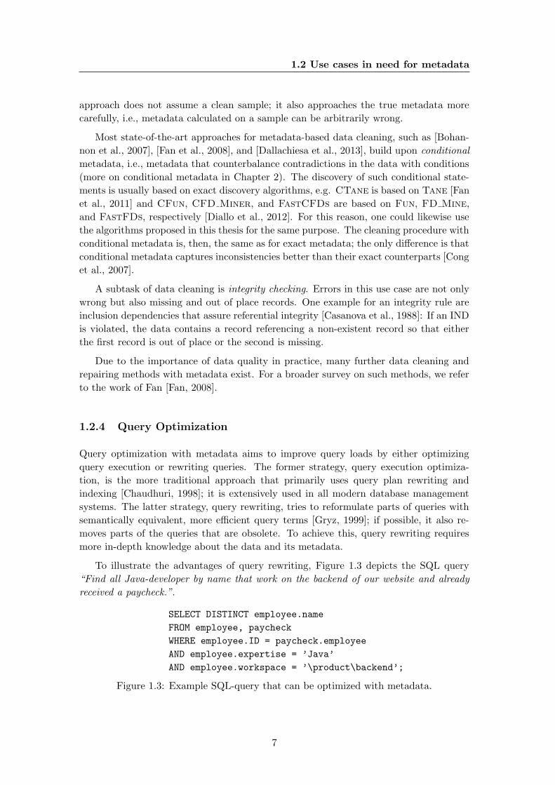
To illustrate the advantages of query rewriting, Figure 1.3 depicts the SQL query
“Find all Java-developer by name that work on the backend of our website and already
received a paycheck.”.
SELECT DISTINCT employee.name
FROM employee, paycheck
WHERE employee.ID = paycheck.employee
AND employee.expertise = ’Java’
AND employee.workspace = ’\product\backend’;
Figure 1.3: Example SQL-query that can be optimized with metadata.
7
1. DATA PROFILING
The query joins the employee table with the paycheck table to filter only those
employees that received a paycheck. If we know that all employees did receive a paycheck,
i.e., we know that the IND employee.ID ⊆ paycheck.employee holds, then we find that
the join is superfluous and can be removed from the query [Gryz, 1998].
Let us now assume that, for our particular dataset, {employee.name} is a UCC,
i.e., there exist no two employees with same names. Then, the DISTINCT duplicate
elimination is superfluous. And if, by chance, {employee.expertise} is another UCC,
meaning that each employee has a unique expertise in the company, we can support
the “Java”-expertise filter with an index on employee.expertise [Paulley and Larson,
1993].
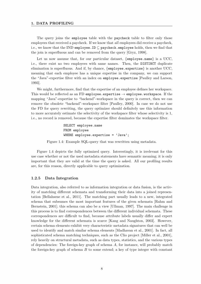
We might, furthermore, find that the expertise of an employee defines her workspace.
This would be reflected as an FD employee.expertise → employee.workspace. If the
mapping “Java”-expertise to “backend”-workspace in the query is correct, then we can
remove the obsolete “backend”-workspace filter [Paulley, 2000]. In case we do not use
the FD for query rewriting, the query optimizer should definitely use this information
to more accurately estimate the selectivity of the workspace filter whose selectivity is 1,
i.e., no record is removed, because the expertise filter dominates the workspace filter.
SELECT employee.name
FROM employee
WHERE employee.expertise = ’Java’;
Figure 1.4: Example SQL-query that was rewritten using metadata.
Figure 1.4 depicts the fully optimized query. Interestingly, it is irrelevant for this
use case whether or not the used metadata statements have semantic meaning; it is only
important that they are valid at the time the query is asked. All our profiling results
are, for this reason, directly applicable to query optimization.
1.2.5 Data Integration
Data integration, also referred to as information integration or data fusion, is the activ-
ity of matching different schemata and transforming their data into a joined represen-
tation [Bellahsene et al., 2011]. The matching part usually leads to a new, integrated
schema that subsumes the most important features of the given schemata [Rahm and
Bernstein, 2001]; this schema can also be a view [Ullman, 1997]. The main challenge in
this process is to find correspondences between the different individual schemata. These
correspondences are difficult to find, because attribute labels usually differ and expert
knowledge for the different schemata is scarce [Kang and Naughton, 2003]. However,
certain schema elements exhibit very characteristic metadata signatures that can well be
used to identify and match similar schema elements [Madhavan et al., 2001]. In fact, all
sophisticated schema matching techniques, such as the Clio project [Miller et al., 2001],
rely heavily on structural metadata, such as data types, statistics, and the various types
of dependencies: The foreign-key graph of schema A, for instance, will probably match
the foreign-key graph of schema B to some extend; a key of type integer with constant
8
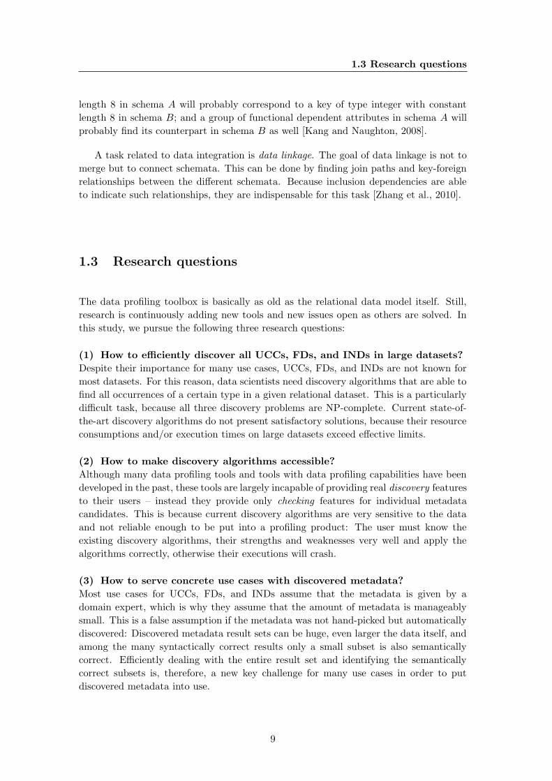
1.3 Research questions
length 8 in schema A will probably correspond to a key of type integer with constant
length 8 in schema B; and a group of functional dependent attributes in schema A will
probably find its counterpart in schema B as well [Kang and Naughton, 2008].
A task related to data integration is data linkage. The goal of data linkage is not to
merge but to connect schemata. This can be done by finding join paths and key-foreign
relationships between the different schemata. Because inclusion dependencies are able
to indicate such relationships, they are indispensable for this task [Zhang et al., 2010].
1.3 Research questions
The data profiling toolbox is basically as old as the relational data model itself. Still,
research is continuously adding new tools and new issues open as others are solved. In
this study, we pursue the following three research questions:
(1) How to efficiently discover all UCCs, FDs, and INDs in large datasets?
Despite their importance for many use cases, UCCs, FDs, and INDs are not known for
most datasets. For this reason, data scientists need discovery algorithms that are able to
find all occurrences of a certain type in a given relational dataset. This is a particularly
difficult task, because all three discovery problems are NP-complete. Current state-of-
the-art discovery algorithms do not present satisfactory solutions, because their resource
consumptions and/or execution times on large datasets exceed effective limits.
(2) How to make discovery algorithms accessible?
Although many data profiling tools and tools with data profiling capabilities have been
developed in the past, these tools are largely incapable of providing real discovery features
to their users – instead they provide only checking features for individual metadata
candidates. This is because current discovery algorithms are very sensitive to the data
and not reliable enough to be put into a profiling product: The user must know the
existing discovery algorithms, their strengths and weaknesses very well and apply the
algorithms correctly, otherwise their executions will crash.
(3) How to serve concrete use cases with discovered metadata?
Most use cases for UCCs, FDs, and INDs assume that the metadata is given by a
domain expert, which is why they assume that the amount of metadata is manageably
small. This is a false assumption if the metadata was not hand-picked but automatically
discovered: Discovered metadata result sets can be huge, even larger the data itself, and
among the many syntactically correct results only a small subset is also semantically
correct. Efficiently dealing with the entire result set and identifying the semantically
correct subsets is, therefore, a new key challenge for many use cases in order to put
discovered metadata into use.
9

1. DATA PROFILING
1.4 Structure and contributions
This thesis focuses on the discovery, provision and utilization of unique column combi-
nations (UCCs), functional dependencies (FDs), and inclusion dependencies (INDs). In
particular, we make the following contributions:
(1) Three novel metadata discovery algorithms
We propose three novel metadata discovery algorithms: HyUCC for UCC discovery,
HyFD for FD discovery, and Binder for IND discovery. The algorithms build upon
known techniques from related work and complement them with algorithmic paradigms,
such as additional pruning, divide-and-conquer, hybrid search, progressivity, memory
sensitivity, and parallelization to greatly improve upon current limitations. Our experi-
ments show that the proposed solutions are orders of magnitude faster than related work.
They are, in particular, now able to process real-world datasets, i.e., multiple gigabytes
size with reasonable memory and time consumption.
(2) A novel profiling platform
We present Metanome, a profiling platform for various metadata discovery algorithms.
The platform supports researchers in the development of new profiling algorithms by
providing a development framework and access to legacy algorithms for testing; it also
supports data scientists and IT-professions in the application of these algorithms by
easing the algorithm parametrization and providing features for result management. The
idea of the Metanome framework is to treat profiling algorithms as external resources.
In this way, it is very easy to extend Metanome with new profiling capabilities, which
keeps the functionality up-to-date and supports collaborative research.
(3) Novel metadata processing techniques
We exemplify the efficient processing and effective assessment of functional dependencies
for the use case of schema normalization with a novel algorithm called Normalize. This
algorithm closes the gab between the discovered results and an actual use case: It shows
how to efficiently calculate the closure of complete sets of FDs and how to effectively select
semantically correct FDs as foreign-keys. Normalize, in general, shows that discovered
metadata sets are not despite their size, but because of it extremely supportive for many
use cases.
The remainder of this study is structured as follows: In Chapter 2, we discuss the
theoretical foundations for key dependencies and their discovery. Then, we introduce
our FD discovery algorithm HyFD in Chapter 3 [Papenbrock and Naumann, 2016], our
UCC discovery algorithm HyUCC in Chapter 4 [Papenbrock and Naumann, 2017a],
and our IND discovery algorithm Binder in Chapter 5 [Papenbrock et al., 2015d]. All
three algorithms (and others) have been implemented for Metanome – a data profiling
platform that we present in Chapter 6 [Papenbrock et al., 2015a]. In Chapter 7, we then
propose the (semi-)automatic algorithm Normalize that demonstrates how discovered
metadata, i.e., functional dependencies can be used to efficiently and effectively solve
schema normalization tasks [Papenbrock and Naumann, 2017b]. We finally conclude this
study in Chapter 8 by summing up our results and discussing open research questions
for future work on data profiling.
10
2
Key Dependencies
This section discusses the theoretical foundations of functional dependencies, unique
column combinations, and inclusion dependencies. We refer to these three types of
metadata as key dependencies, because they propose attributes that serve as valid key
or foreign-key constraints for certain other attributes. After reviewing the relational
data model in Section 2.1, we carefully define the three key dependencies in Section 2.2
and survey their relaxations in Section 2.3. Section 2.4 then introduces the discovery
problem and basic discovery techniques. We end in Section 2.5 with a discussion on null
semantics.
2.1 The relational data model
A data model is a notation for describing data. It consists of three parts [Garcia-Molina
et al., 2008]: The structure defines the physical and conceptual data layout; the con-
straints define inherent limitations and rules of the data; and the operations define
possible methods to query and modify the data. In this thesis, we focus on the relational
data model [Codd, 1970], which is not only the preferred model for the leading data-
base management systems [Edjlali and Beyer, 2016] but also is today’s most widely used
model for data [DB-ENGINES, 2017]. The structure of the relational model consists of
the two building blocks schema and instance:
Schema A relational schema R is a named, non-empty set of attributes. In theory,
these attibutes have no order in the schema, but we usually assign an order for practical
reasons, such as consistent presentation of a schema and its data. Each attribute A ∈ Rrepresents a property of the entities described by the schema. The possible values of
an attribute A are drawn from its domain dom(A). Because datasets usually consist of
multiple schemata, we call the set of schemata a database schema. For illustration, the
schema of our Pokemon dataset introduced in Section 1.1 is
Pokemon(ID, Name, Evolution, Location, Sex, Weight, Size, Type, Weak, Strong, Special)
Instance The relational instance, or relation r for short, of a schema R is a set of records.
A record t of a relational schema R is a function t : R →⋃A∈R dom(A) that assigns
11
2. KEY DEPENDENCIES
to every attribute A ∈ R a value t[A] ∈ dom(A). Note that we use the notation t[X]
to denote the projection of record t to the values of X ⊆ R. Because we consider the
attributes to be ordered, we often refer to records as tuples, which are ordered lists of
|R| values [Elmasri and Navathe, 2016]. So the first tuple in our Pokemon dataset is
(25, Pikachu, Raichu, Viridian Forest, m/w, 6.0, 0.4, electric, ground, water, false)
Operations permitted in the relational data model are those defined by relational
algebra and relational calculus. The structured query language (SQL) is a practical
implementation and extension of these [Abiteboul et al., 1995]; it is the defacto standard
for all relational database systems [ISO/IEC 9075-1:2008]. In this thesis, however, we
focus on the constraints part of the relational model, i.e., inherent rules and dependencies
of relational datasets.
The most important constraint in the relational model is a key [Codd, 1970]. A key
is a set of attributes X ⊆ R that contains no entry more than once. So all values in
X are unique and distinctively describe their records. A primary key is a key that was
explicitly chosen as the main identifier for all records; while there can be arbitrary many
keys, a schema defines only one primary key. A foreign-key is a set of attributes in
one schema that uniquely identify records in another schema; a foreign-key can contain
duplicate entries, i.e., it is not a key for its own schema, but it must reference a key in
the other schema.
The enforcement of keys and constraints in general requires special structures, so
called integrity constraints that prevent inconsistent states. Because such integrity con-
straints are expensive to maintain, most constraints are not explicitly stated. The records
in a relational instance, however, naturally obey all their constraints, which means that
every relational instance r implies its set of metadata Σ. We express this implication
as r |= Σ [Fagin and Vardi, 1984]. The observation that relational instances imply their
metadata is crucial to justify data profiling, i.e., the discovery of metadata from relational
instances.
Although we focus on profiling techniques for the relational data model in this thesis,
other data models and their model-specific constraints are, of course, also subject to
data profiling. Key dependencies, for instance, are also relevant in XML [Buneman
et al., 2001] and RDF [Jentzsch et al., 2015] datasets. The most promissing profiling tool
for the discovery of metadata in RDF datasets is ProLOD++, which is a sister project
of our Metanome tool [Abedjan et al., 2014a]. In general, however, research on profiling
techniques for non-relational data is still scarce.
2.2 Types of key dependencies
Unique column combinations, functional dependencies, and inclusion dependencies de-
scribe keys of a table, within a table, and between tables, respectively [Toman and
Weddell, 2008]. In this section, we formally define all three types of key dependencies in
detail and state our notations. Note that we often write XY or X,Y to mean X ∪ Y ,
i.e., the union of attributes or attribute sets X and Y .
12

2.2 Types of key dependencies
2.2.1 Functional Dependencies
A functional dependency (FD) written as X → A expresses that all pairs of records
with same values in attribute combination X must also have same values in attribute
A [Codd, 1971]. The values in A functionally depend on the values in X. More formally,
functional dependencies are defined as follows [Ullman, 1990]:
Definition 2.1 (Functional dependency). Given a relational instance r for a schema
R. The functional dependency X → A with X ⊆ R and A ∈ R is valid in r, iff
∀ti, tj ∈ r : ti[X] = tj [X]⇒ ti[A] = tj [A].
We call the determinant part X of an FD the left-hand-side, in short Lhs, and the
dependent part A the right hand side, in short Rhs. Moreover, an FD X → A is
a generalization of another FD Y → A if X ⊂ Y and it is a specialization if X ⊃ Y .
Functional dependencies with the same Lhs, such as X → A and X → B can be grouped
so that we write X → A,B or X → Y for attributs A and B with {A,B} = Y . Using this
notation, Armstrong formulated the following three axioms for functional dependencies
on attribute sets X, Y , and Z [Armstrong, 1974; Beeri and Bernstein, 1979]:
1. Reflexivity : If Y ⊆ X, then X → Y .
2. Augmentation: If X → Y , then X ∪ Z → Y ∪ Z.
3. Transitivity : If X → Y and Y → Z, then X → Z.
An FD X → Y is called trivial if Y ⊆ X, because all such FDs are valid according
to Armstrong’s reflexivity axiom; vice versa, the FD is non-trivial if X 6⊆ Y and fully
non-trivial if X ∩ Y = ∅. Furthermore, an FD is minimal if no B exists such that
X\B → A is a valid FD, i.e., if no valid generalization exists. To discover all FDs in a
given relational instance r, it suffices to discover all minimal, non-trivial FDs, because
all Lhs-subsets are non-dependencies and all Lhs-supersets are dependencies by logical
inference following Armstrong’s augmentation rule.
Because keys in relational datasets uniquely determine all other attributes, they
are the most popular kinds of FDs, i.e., every key X is a functional dependeny X →R \X. Functional dependencies also arise naturally from real-world entities described in
relational datasets. In our Pokemon dataset of Section 1.1, for instance, the elemental
type of a pocket monster defines its weakness, i.e., Type → Weak.
2.2.2 Unique Column Combinations
A unique column combination (UCC) X is a set of attributes X ⊆ R\X whose projection
contains no duplicate entry on a given relational instance r [Lucchesi and Osborn, 1978].
Unique column combinations or uniques for short are formally defined as follows [Heise
et al., 2013]:
13
2. KEY DEPENDENCIES
Definition 2.2 (Unique column combination). Given a relational instance r for a schema
R. The unique column combination X with X ⊆ R is valid in r, iff ∀ti, tj ∈ r, i 6= j :
ti[X] 6= tj [X].
By this definition, every UCC X is also a valid FD, namely X → R \ X. For this
reason, UCCs and FDs share various properties: A UCC X is a generalization of another
UCC Y if X ⊂ Y and it is a specialization if X ⊃ Y . Furthermore, if X is a valid UCC,
then any X∪Z with Z ⊆ R is a valid UCC, because Armstrong’s augmentation rule also
applies to UCCs. According to this augmentation rule, a UCC is minimal if no B exists
such that X\B is still a valid UCC, i.e., if no valid generalization exists. To discover all
UCCs in a given relational instance r, it suffices to discover all minimal UCCs, because
all subsets are non-unqiue and all supersets are unique by logical inference.
From the use case perspective, every unique column combination indicates a syn-
tactically valid key. In our example dataset of Section 1.1, for instance, the column
combinations {ID}, {Name, Sex}, and {Weight} are unique and, hence, possible keys
for pocket monsters. Although UCCs and keys are technically the same, we usually
make the distinction that keys are UCCs with semantic meaning, i.e., they not only hold
by chance in a relational instance but for a semantic reason in any instance of a given
schema [Abedjan et al., 2015].
Because every valid UCC is also a valid FD, functional dependencies seem to subsume
unique column combinations. However, considering the two types of key depentencies
separately makes sense for the following reasons:
1. Non-trivial inference: A minimal UCC is not necessarily a minimal FD, because
UCCs are minimal w.r.t. R and FDs are minimal w.r.t. some A ∈ R. If, for
instance, X is a minimal UCC, then X → R is a valid FD and no Y ⊂ X exists
such that X \ Y → R is still valid. However, X \ Y → A with A ∈ R can still be a
valid and minimal. For this reason, not all minimal UCCs can directly be inferred
from the set of minimal FDs; to infer all minimal UCCs, one must systematically
specialize the FDs, check if these specializations determine R entirely, and if they
do, check whether they are minimal w.r.t. R.
2. Duplicate row problem: The FD X → R \ X does not necessarily define a UCC
X if duplicate records are allowed in the relational instance r of R. A duplicate
record invalidates all possible UCCs, because it puts a duplicate value in every
attribute and attribute combination. A duplicate record, however, invalidates no
FD, because only differing values on an FD’s Rhs can invalidate it. As stated in
Section 2.1, the relational model in fact forbids duplicate records and most rela-
tional database management systems also prevent duplicate records; still duplicate
records occur in practice, because file formats such as CSV cannot ensure their
absence.
3. Discovery advantage: UCC discovery can be done more efficient than FD discovery,
because UCCs are easier to check and the search space is smaller. We show this in
Section 2.4 and Chapter 4. So if a data scientist must only discover UCCs, making
a detour over FDs in the discovery is generally a bad decision.
14
2.2 Types of key dependencies
2.2.3 Inclusion Dependencies
An inclusion dependency (IND) Ri[X] ⊆ Rj [Y ] over the relational schemata Ri and Rjstates that all entries in X are also contained in Y [Casanova et al., 1982]. We use the
short notations X ⊆ Y for INDs Ri[X] ⊆ Rj [Y ] if it is clear from the context that X ⊆ Ydenotes an IND (and not an inclusion of same attributes). Inclusion dependencies are
formally defined as follows [Marchi et al., 2009]:
Definition 2.3 (Inclusion dependency). Given two relational instances ri and rj for
the schemata Ri, and Rj , respectively. The inclusion dependency Ri[X] ⊆ Rj [Y ] (short
X ⊆ Y ) with X ⊆ Ri, Y ⊆ Rj and |X| = |Y | is valid, iff ∀ti[X] ∈ ri, ∃tj [Y ] ∈ rj : ti[X] =
tj [Y ].
We call the dependent part X of an IND the left-hand-side, short Lhs, and the
referenced part Y the right hand side, short Rhs. An IND X ⊆ Y is a generalization of
another IND X ′ → Y ′ if X ⊂ X ′ and Y ⊂ Y ′ and it is a specialization if X ⊃ X ′ and
Y ⊃ Y ′. The size or arity n of an IND is defined by n = |X| = |Y |. We call INDs with
n = 1 unary inclusion dependecies and INDs with n > 1 n-ary inclusion dependecies.
A sound and complete axiomatization for INDs is given by the following three inference
rules on schemata Ri, Rj , and Rk [Casanova et al., 1982]:
1. Reflexivity : If i = j and X = Y , then Ri[X] ⊆ Rj [Y ].
2. Permutation: IfRi[A1, ..., An] ⊆ Rj [B1, ..., Bn], thenRi[Aσ1, ..., Aσm] ⊆ Rj [Bσ1, ..., Bσm]
for each sequence σ1, ..., σm of distinct integers from {1, ...,m}.
3. Transitivity : If Ri[X] ⊆ Rj [Y ] and Rj [Y ] ⊆ Rk[Z], then Ri[X] ⊆ Rk[Z].
An IND Ri[X] ⊆ Ri[X] for any i and X is said to be trivial, as it is always valid
according to the reflexivity rule. For valid INDs, all generalizations are also valid INDs,
i.e., if Ri[X] ⊆ Rj [Y ] is valid, then Ri[X \Ak] ⊆ Rj [Y \Bk] with same attribute indices
k is valid as well [Marchi et al., 2009]. Specializations of a valid IND can, however, be
valid or invalid. An IND Ri[X] ⊆ Rj [Y ] is called maximal, iff Ri[XA] ⊆ Rj [Y B] is
invalid for all attributes A ∈ Ri and B ∈ Rj whose unary inclusion Ri[A] ⊆ Rj [B] is
no generalization of Ri[X] ⊆ Rj [Y ]. If Ri[A] ⊆ Rj [B] is a generalization, then adding
it to Ri[X] ⊆ Rj [Y ] always results in a valid IND, but the mapping of A to B would
be redundant and, therefore, superfluous – the maximal IND would, in a sense, not be
minimal. To discover all INDs of a given relational instance r, it therefore suffices to
discover all maximal, non-trivial INDs.
Usually, data scientists are interested in inclusion dependencies between different
relations Ri and Rj , such as Pokemon[Location] ⊆ Location[Name] in our Pokemon
dataset of Section 1.1, because these INDs indicate foreign-key relationships. Inclusion
dependencies inside the same shema are, however, also interesting for query optimization,
integrity checking, and data exploration. In our example, for instance, we also find the
IND Pokemon[Evolution] ⊆ Pokemon[Name], which tells us that every evolution of a
pocket monster must be a pocket monster as well.
15
2. KEY DEPENDENCIES
2.3 Relaxation of key dependencies
An exact dependency must be syntactically correct for the given relational instance. The
correctness exactly follows the definition of the dependency and it does not allow contra-
dictions, exceptions or special cases. When we talk about dependencies in this work, we
always refer to exact dependencies. For many use cases, however, it is beneficial to relax
the definition of a dependency. The three most popular types of relaxed dependencies
are approximate, partial, and conditional dependencies [Abedjan et al., 2015]. These
relaxations apply equally to all key dependencies – in fact, they also apply to most other
dependencies, such as order, multivalued, and matching dependencies. For this reason,
we use the notation X ` Y to denote a generic type of dependency `. In the following,
we discuss the three relaxation types in more detail:
Approximate: An approximate or soft dependency relaxes the hard correctness con-
straint of an exact dependency [Ilyas et al., 2004]. Although an approximate dependency
is supposed to be correct, its correctness is not guaranteed. This means that contradic-
tions might exist in the relational instance, but their number and location is unknown. In
some scenarios, however, it is possible to guess the confidence of an approximate depen-
dency or to state a certain worst-case confidence [Kruse et al., 2017]. Because approxi-
mate dependencies must not assure their correctness, their discovery can be much more
efficient than the discovery of exact dependencies [Kivinen and Mannila, 1995]. Common
techniques for approximate dependency discovery are sampling [Brown and Hass, 2003;
Ilyas et al., 2004] and summarization [Bleifuß et al., 2016; Cormode et al., 2012; Kruse
et al., 2017; Zhang et al., 2010]. Note that a set of dependencies is called approximate
if it relaxes completeness, correctness, and/or minimality of its elements [Bleifuß et al.,
2016].
Partial: A partial dependency also relaxes the correctness constraint of an exact de-
pendency, but in contrast to approximate dependencies the error is known and in-
tended [Abedjan et al., 2015]. Partial dependencies do not approximate exact depen-
dencies; instead, their validity is strictly defined given a certain error threshold: The
dependency X `Ψ≤ε Y is valid, iff the known error Ψ of X ` Y is smaller or equal than
the error threshold ε [Caruccio et al., 2016]. A partial dependency is minimal, iff all
generalizations (or specializations for INDs) exceed the error threshold. Partial depen-
dencies are useful if the given data is expected to contain errors, because such errors can,
if not deliberately ignored, hide semantically meaningful dependencies. A popular error
measure is the minimum number of records that must be removed to make the partial
dependency exact [Huhtala et al., 1999], but other measures exist [Caruccio et al., 2016;
Kivinen and Mannila, 1995]. Note that despite the fundamental difference between ap-
proximate and partial dependencies, many related works, such as [Huhtala et al., 1999]
and [Marchi et al., 2009], do not explicitly distinguish partial and approximate.
Conditional: A conditional dependency, such as a conditional IND [Bravo et al., 2007]
or a conditional FD [Fan et al., 2008], complements a partial dependency with conditions.
These conditions restrict the scope of a partial dependency to only those records that
exactly satisfy the dependency. The common way to formulate such conditions are sets
16
2.4 Discovery of key dependencies
of pattern tuples that mismatch all dependency contradicting tuples while at the same
time match possibly many dependency satisfying tuples in the relational instance. The
set of pattern tuples is called pattern tableau or simply tableau [Bohannon et al., 2007].
Formally, a conditional dependency is a pair (X ` Y, Tp) of a dependency X ` Y and
a pattern tableau Tp. The pattern tableau Tp is a set of tuples t ∈ Tp where each t[A]
with A ∈ X ∪Y is either a constant or wildcard [Bravo et al., 2007]. With these pattern
tableaux, conditional dependencies are not only able to circumvent errors in the data,
they also provide additional semantics about the described dependencies, namely which
parts of the data fulfill a certain criterion and which do not. The discovery of conditional
dependencies is, however, much more difficult than the discovery of exact, approximate
and partial dependencies [Diallo et al., 2012], because the generation of pattern tableaux
is expensive: Finding one optimal tableau for one partial dependency is an NP-complete
task, which was proven in [Golab et al., 2008].
For a much broader survey on relaxation properties, we refer to [Caruccio et al.,
2016]. In this thesis, we propose three efficient algorithms for the discovery of exact
dependencies. In [Kruse et al., 2017] and [Bleifuß et al., 2016], we show that their sister
algorithms, i.e., algorithms that use similar ideas, can discover approximate dependencies
even faster. We do not cover the discovery of partial and conditional dependencies in this
work, because most discovery algorithms in these categories build upon exact discovery
algorithms [Diallo et al., 2012; Fan et al., 2011] and, as motivated in Chapter 1, no
current algorithm is able to efficiently discover exact dependencies in real-world sized
datasets.
2.4 Discovery of key dependencies
The focus of this thesis is the descovery of all minimal, non-trivial unique column com-
binations, all minimal, non-trivial functional dependecies, and all maximal, non-trivial
inclusion dependencies. The search space for all three discovery tasks can best be modeled
as a graph coloring problem – in fact, we model the search spaces for most multi-column
metadata in this way: The basis of this model is a power set of attribute combina-
tions [Devlin, 1979]; every possible combination of attributes represents one set. Such
a power set is a partially ordered set, because reflexivity, antisymmetry and transitivity
hold between the attribute combinations [Deshpande, 1968]. Due to the partial order,
every two elements have a unique supremum and a unique infimum. Hence, we can model
the partially ordered set as a lattice, i.e., a graph of attribute combination nodes that
connects each node X ⊆ R to its direct subsets X \A and direct supersets X ∪B (with
A ∈ X, B ∈ R and B 6∈ X). For more details on lattice theory, we refer to [Crawley
and Dilworth, 1973]. A nice visualization of such lattices are Hasse diagrams, named
after Helmut Hasse (1898–1979), who did not invent but made this type of diagram pop-
ular [Birkhoff, 1940]. Figure 2.1 I depicts an example lattice as Hasse diagram for an
example relation R(A,B,C,D). Note that we do not include X = ∅ as a node, because ∅is neither a valid UCC candidate and nor is ∅ ⊆ Y a valid IND candidate for any Y ⊆ R.
Any FD candidate ∅ → Y , however, is possible and valid, if the column Y is constant,
i.e., it contains only one value.
17

2. KEY DEPENDENCIES
A B C D E
AB AC AD AE BC BD BE CD CE DE
ABC ABD ABE ACD ACE ADE BCD BCE BDE CDE
ABCD ABCE ABDE ACDE BCDE
ABCDE attribute lattice for R(A,B,C,D,E)
UCC
non-UCC
A B C D E
AB AC AD AE BC BD BE CD CE DE
ABC ABD ABE ACD ACE ADE BCD BCE BDE CDE
ABCD ABCE ABDE ACDE BCDE
ABCDE
FD
non-FD A B C D E
AB AC AD AE BC BD BE CD CE DE
ABC ABD ABE ACD ACE ADE BCD BCE BDE CDE
ABCD ABCE ABDE ACDE BCDE
ABCDE
A B C D E
AB AC AD AE BC BD BE CD CE DE
ABC ABD ABE ACD ACE ADE BCD BCE BDE CDE
ABCD ABCE ABDE ACDE BCDE
ABCDE
IND
non-IND
I
II
III
IV
Figure 2.1: The search spaces of UCCs, FDs, and INDs visualized as lattices.
We now map the search spaces for UCCs, FDs, and INDs to the lattice of attribute
combinations:
UCC discovery: For UCC discovery, each node X represents one UCC candidate, i.e.,
an attribute combination that is either unique or non-unique with respect to a given
relational instance. To discover all UCCs, we need to classify all nodes in the graph
and color them accordingly. Figure 2.1 II shows an examplary result of this process. In
all such lattices, UCCs are located in the upper part of the lattice while non-UCCs are
located at the bottom. The number of UCC candidates in level k for m attributes is(mk
),
which makes the total number of UCC candidates for m attributes∑m
k=1
(mk
)= 2m − 1.
Figure 2.2 visualizes the growth of the UCC candidate search space with an increasing
number of attributes. The depicted growth is exponential in the number of attributes.
18
2.4 Discovery of key dependencies
Total: 1 3 7 15 31 63 127 255 511 1,023 2,047 4,095 8,191 16,383 32,767
15 1
14 1 15
13 1 14 105
12 1 13 91 455
11 1 12 78 364 1,365
10 1 11 66 286 1,001 3,003
9 1 10 55 220 715 2,002 5,005
8 1 9 45 165 495 1,287 3,003 6,435
7 1 8 36 120 330 792 1,716 3,432 6,435
6 1 7 28 84 210 462 924 1,716 3,003 5,005
5 1 6 21 56 126 252 462 792 1,287 2,002 3,003
4 1 5 15 35 70 126 210 330 495 715 1,001 1,365
3 1 4 10 20 35 56 84 120 165 220 286 364 455
2 1 3 6 10 15 21 28 36 45 55 66 78 91 105
1 1 2 3 4 5 6 7 8 9 10 11 12 13 14 15
1 2 3 4 5 6 7 8 9 10 11 12 13 14 15
Total: 0 2 6 24 80 330 1,302 5,936 26,784 133,650 669,350 3,609,672 19,674,096 113,525,594 664,400,310
15 0
14 0 0
13 0 0 0
12 0 0 0 0
11 0 0 0 0 0
10 0 0 0 0 0 0
9 0 0 0 0 0 0 0
8 0 0 0 0 0 0 0 0
7 0 0 0 0 0 0 0 17,297,280 259,459,200
6 0 0 0 0 0 0 665,280 8,648,640 60,540,480 302,702,400
5 0 0 0 0 0 30,240 332,640 1,995,840 8,648,640 30,270,240 90,810,720
4 0 0 0 0 1,680 15,120 75,600 277,200 831,600 2,162,160 5,045,040 10,810,800
3 0 0 0 120 840 3,360 10,080 25,200 55,440 110,880 205,920 360,360 600,600
2 0 0 12 60 180 420 840 1,512 2,520 3,960 5,940 8,580 12,012 16,380
1 0 2 6 12 20 30 42 56 72 90 110 132 156 182 210
1 2 3 4 5 6 7 8 9 10 11 12 13 14 15
Total: 0 2 9 28 75 186 441 1,016 2,295 5,110 11,253 24,564 53,235 114,674 245,745
15 0
14 0 15
13 0 14 210
12 0 13 182 1,365
11 0 12 156 1,092 5,460
10 0 11 132 858 4,004 15,015
9 0 10 110 660 2,860 10,010 30,030
8 0 9 90 495 1,980 6,435 18,018 45,045
7 0 8 72 360 1,320 3,960 10,296 24,024 51,480
6 0 7 56 252 840 2,310 5,544 12,012 24,024 45,045
5 0 6 42 168 504 1,260 2,772 5,544 10,296 18,018 30,030
4 0 5 30 105 280 630 1,260 2,310 3,960 6,435 10,010 15,015
3 0 4 20 60 140 280 504 840 1,320 1,980 2,860 4,004 5,460
2 0 3 12 30 60 105 168 252 360 495 660 858 1,092 1,365
1 0 2 6 12 20 30 42 56 72 90 110 132 156 182 210
1 2 3 4 5 6 7 8 9 10 11 12 13 14 15
Number of attributes: m
Nu
mb
er o
f le
vels
: k
Number of attributes: m
Number of attributes: m
Nu
mb
er o
f le
vels
: k
Nu
mb
er o
f le
vels
: k
UCCs
FDs
INDs
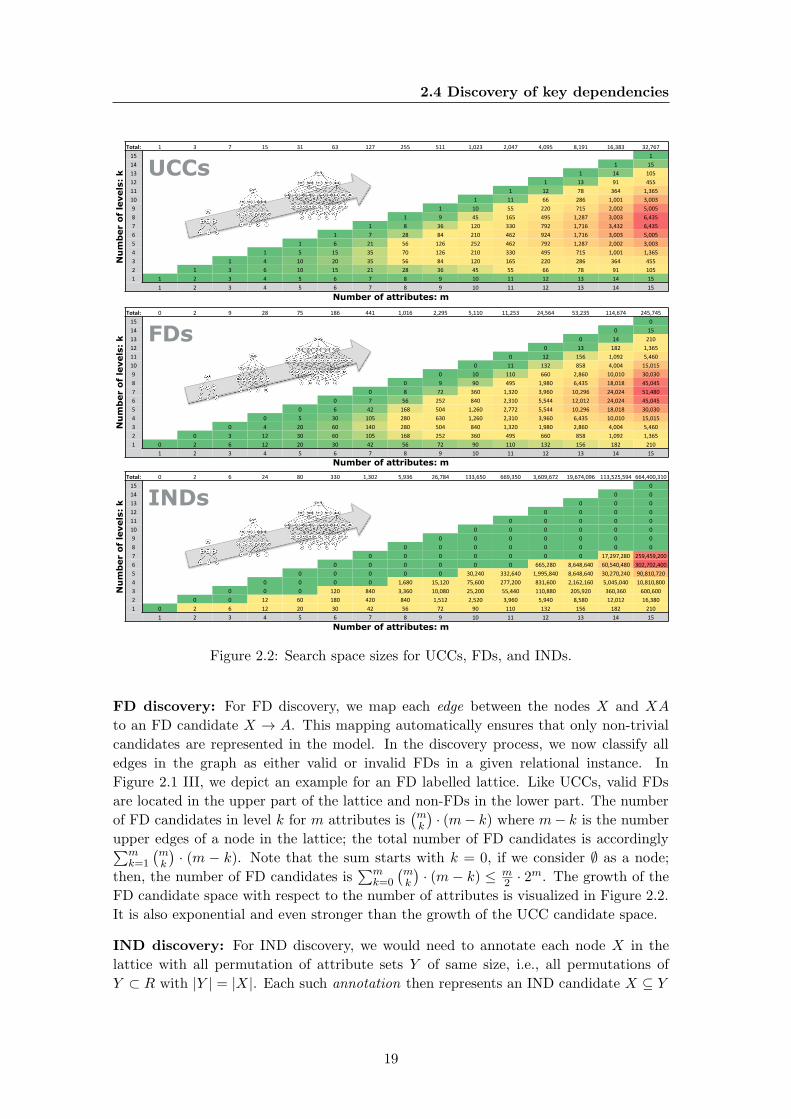
Figure 2.2: Search space sizes for UCCs, FDs, and INDs.
FD discovery: For FD discovery, we map each edge between the nodes X and XA
to an FD candidate X → A. This mapping automatically ensures that only non-trivial
candidates are represented in the model. In the discovery process, we now classify all
edges in the graph as either valid or invalid FDs in a given relational instance. In
Figure 2.1 III, we depict an example for an FD labelled lattice. Like UCCs, valid FDs
are located in the upper part of the lattice and non-FDs in the lower part. The number
of FD candidates in level k for m attributes is(mk
)· (m− k) where m− k is the number
upper edges of a node in the lattice; the total number of FD candidates is accordingly∑mk=1
(mk
)· (m − k). Note that the sum starts with k = 0, if we consider ∅ as a node;
then, the number of FD candidates is∑m
k=0
(mk
)· (m− k) ≤ m
2 · 2m. The growth of the
FD candidate space with respect to the number of attributes is visualized in Figure 2.2.
It is also exponential and even stronger than the growth of the UCC candidate space.
IND discovery: For IND discovery, we would need to annotate each node X in the
lattice with all permutation of attribute sets Y of same size, i.e., all permutations of
Y ⊂ R with |Y | = |X|. Each such annotation then represents an IND candidate X ⊆ Y
19
2. KEY DEPENDENCIES
and can be classified as either valid or invalid with respect to a given relational instance.
By the definition of an IND, these annotations also include trivial combinations, such as
A ⊆ A and X ⊆ X, and combinations with duplicate attributes, such as AA ⊆ BC and
ABC ⊆ BCB. Most IND discovery algorithms, however, ignore trivial combinations and
combinations with duplicates, because these INDs have hardly practical relevance. The
number of candidates is even without these kinds of INDs still so high that we restrict
our visualization of the search space even further – note that this is necessary only for
the exploration of the search space in this chapter and that our discovery algorithm can
overrule this last restriction: We consider only those INDs X ⊆ Y where Y ∩ X = ∅,which was also done in [Liu et al., 2012]. The example in Figure 2.1 IV then shows
that due to Y ∩ X = ∅ the annotations only exist up to level bm2 c. It also shows
that, other than UCCs and FDs, valid INDs are located at the bottom and the invalid
INDs at the top of the lattice – as stated in Section 2.2.3, INDs might become invalid
when adding attributes while UCCs and FDs remain (or become) valid. The number
of IND candidates in level k for m attributes is with the Y ∩ X = ∅ restriction still(mk
)·(m−kk
)· k! where
(m−kk
)are all non-overlapping attribute sets of a lattice node and
k! all permutations of such a non-overlapping attribute set. With that, we can quantify
the total number of IND candidates as∑m
k=1
(mk
)·(m−kk
)· k!. Figure 2.2 shows that this
number of candidates is much larger than the number of UCC or FD candidates on same
size schemata although IND candidates only reach to half the lattice height.
The discovery of UCCs, FDs, and INDs is a process that, in one form or another,
involves data preparation, search space traversal, candidate generation, and candidate
checking. The candidate checks are the most expensive action in the discovery processes.
For this reason, most algorithms utilize the inference rules discussed in Section 2.2 as
pruning rules to quickly infer the (in-)validity of larger sub-graphs. For instance, if
X was identified as a UCC, all X ′ with X ′ ⊃ X must also be valid UCCs. In this
way, the algorithms avoid checking each and every candidate. To maximize the pruning
effect, various checking strategies have been proposed based on the lattice search space
model, most importantly breadth-first bottom-up [Huhtala et al., 1999], breadth-first top-
down [Marchi and Petit, 2003], and depth-first random walk [Heise et al., 2013].
To improve the efficiency of the UCC and FD candidate checks, many discovery algo-
rithms rely on an index structure called position list index (Pli), which are also known as
stripped partitions [Cosmadakis et al., 1986]. A Pli, denoted by πX , groups tuples into
equivalence classes by their values of attribute set X. Thereby, two tuples t1 and t2 of
an attribute set X belong to the same equivalence class if ∀A ∈ X : t1[A] = t2[A]. These
equivalence classes are also called clusters, because they cluster records by same values.
For compression, a Pli does not store clusters with only a single entry, because tuples
that do not occur in any cluster of πX can be inferred to be unique in X. Consider, for ex-
ample, the relation Class(Teacher, Subject) and its example instance in Table 2.1. The Plis
π{Teacher} and π{Subject}, which are also depicted in Table 2.1, represent the partitions of
the two individual columns; the Pli π{Teacher,Subject} = π{Teacher} ∩ π{Subject} describes
their intersection, which is the Pli of the column combination {Teacher, Subject}.
A unique column combination X is valid, iff the πX contains no cluster. In this case,
all clusters in πX have size 1 and no value combination in X occurs more than once. To
20
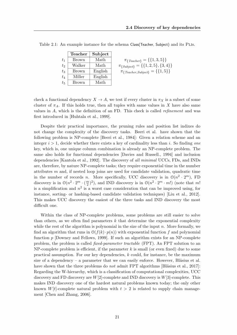
2.4 Discovery of key dependencies
Table 2.1: An example instance for the schema Class(Teacher, Subject) and its Plis.
Teacher Subject
t1 Brown Math π{Teacher} = {{1, 3, 5}}t2 Walker Math π{Subject} = {{1, 2, 5}, {3, 4}}t3 Brown English π{Teacher,Subject} = {{1, 5}}t4 Miller English
t5 Brown Math
check a functional dependency X → A, we test if every cluster in πX is a subset of some
cluster of πA. If this holds true, then all tuples with same values in X have also same
values in A, which is the definition of an FD. This check is called refinement and was
first introduced in [Huhtala et al., 1999].
Despite their practical importance, the pruning rules and position list indixes do
not change the complexity of the discovery tasks. Beeri et al. have shown that the
following problem is NP-complete [Beeri et al., 1984]: Given a relation scheme and an
integer i > 1, decide whether there exists a key of cardinality less than i. So finding one
key, which is, one unique column combination is already an NP-complete problem. The
same also holds for functional dependencies [Davies and Russell., 1994] and inclusion
dependencies [Kantola et al., 1992]. The discovery of all minimal UCCs, FDs, and INDs
are, therefore, by nature NP-complete tasks; they require exponential time in the number
attributes m and, if nested loop joins are used for candidate validation, quadratic time
in the number of records n. More specifically, UCC discovery is in O(n2 · 2m), FD
discovery is in O(n2 · 2m · (m2 )2), and IND discovery is in O(n2 · 2m ·m!) (note that m!
is a simplification and n2 is a worst case consideration that can be improved using, for
instance, sorting- or hashing-based candidate validation techniques) [Liu et al., 2012].
This makes UCC discovery the easiest of the three tasks and IND discovery the most
difficult one.
Within the class of NP-complete problems, some problems are still easier to solve
than others, as we often find parameters k that determine the exponential complexity
while the rest of the algorithm is polynomial in the size of the input n. More formally, we
find an algorithm that runs in O(f(k) ·p(n)) with exponential function f and polynomial
function p [Downey and Fellows, 1999]. If such an algorithm exists for an NP-complete
problem, the problem is called fixed-parameter tractable (FPT). An FPT solution to an
NP-complete problem is efficient, if the parameter k is small (or even fixed) due to some
practical assumption. For our key dependencies, k could, for instance, be the maximum
size of a dependency – a parameter that we can easily enforce. However, Blasius et al.
have shown that the three problems do not admit FPT algorithms [Blasius et al., 2017]:
Regarding the W-hierarchy, which is a classification of computational complexities, UCC
discovery and FD discovery are W [2]-complete and IND discovery is W [3]-complete. This
makes IND discovery one of the hardest natural problems known today; the only other
known W [t]-complete natural problem with t > 2 is related to supply chain manage-
ment [Chen and Zhang, 2006].
21
2. KEY DEPENDENCIES
2.5 Null semantics for key dependencies
Data is often incomplete, which means that we either do not know the value of a certain
attribute or that the attribute does not apply to all entities in the relation. In such cases,
null values ⊥ are used to signal no value [Garcia-Molina et al., 2008]. For the discovery
of dependencies, null values are an issue, because the validity of a dependency relies on
the existence of values that either support or contradict it.
The standard solution for null values in data profiling is to define a semantics for
null comparisons: Expressions of the form null = x with some value x always evaluate
to false, because one null value is usually compared to many different x values and
the assumption that the same null value is simultaneously equal to all these x values
leads to inconsistent conclusions. The expression null = null, however, consistently
evaluates to true or false – either we consider all null values to represent the same
value or different values.
The decision for either the null = null or the null 6= null semantic has a direct
influence on the key dependencies. Consider, for example, the schema R(A,B) with two
tuples t1 = (⊥, 1) and t2 = (⊥, 2). Depending on whether we choose null = null or null
6= null, the UCC {A} and the FD A→ B are both either false or true. When switching
the semantics from null 6= null to null = null, the minimal UCCs of a dataset tend
to become larger on average, because more attributes are needed to make attribute
combinations with null values unique. The minimal FDs, however, can become both
smaller and larger, i.e., null values in Lhs attributes introduce violations that demand
for additional Lhs attributes and null values in Rhs attributes resolve violations that
must no longer be counterbalanced with certain Lhs attributes. In general, null =
null is the pessimistic perspective and null 6= null the optimistic perspective for key
dependencies.
To choose between the two null semantics, one obvious idea is to consult the handling
of null values in SQL. In SQL, null = null evaluates to unknown, which is neither true
nor false [Garcia-Molina et al., 2008]. In some cases, unknown is effectively treated as
false, e.g., null values do not match in join statements. In other cases, however,
unknown is treated as true, e.g., in group-by statements. For this reason, SQL does not
help to decide for one of the two semantics.
The algorithms proposed in this work support both null semantics. In our exper-
iments, we use the pessimistic null = null semantics for the following three reasons:
First, we believe it to be more intuitive, because a completely empty column, for instance,
should not functionally determine all other columns; second, it is the more challenging se-
mantics, because many dependencies are located on higher lattice levels; third, the null
= null semantics was chosen in all related works so that we use the same semantics for
a comparable evaluation [Papenbrock et al., 2015b].
Note that the agreement on a null semantics is in fact a simplification of the null
problem. A precise interpretation of a null value is no information [Zaniolo, 1984], which
was first introduced for functional dependencies and constraints in [Atzeni and Morfuni,
1986]. Kohler and Link derived two validity models for this null interpretation, namely
22

2.5 Null semantics for key dependencies
the possible world model and the certain world model: A dependency is valid in the
possible world model, iff at least one replacement of all null values exists that satisfies
the dependency; the dependency is valid in the certain world model, iff every replacement
of the null values satisfies the dependency [Kohler and Link, 2016; Kohler et al., 2015].
To ensure possible and certain world validity, the discovery algorithms require some
additional reasoning on null replacements. Because null reasoning is not the focus
of this work, we use the traditional null semantics. For more details on possible and
certain world key dependencies, we refer to [Le, 2014].
23

2. KEY DEPENDENCIES
24

3
Functional Dependency Discovery
The discovery of functional dependencies aims to automatically detect all functional
dependencies that hold in a given relational instance. As discussed in Section 2.2, it
suffices to find all minimal, non-trivial FDs, because the remaining FDs can be efficiently
inferred using Armstrong axioms. Due to the importance of functional dependencies for
various use cases, many discovery algorithms have already been proposed. None of them
is, however, able to process datasets of real-world size, i.e., datasets with more than 50
columns and a million rows, as we could show in [Papenbrock et al., 2015b]. Because the
need for functional dependency discovery usually increases with growing dataset sizes,
larger datasets are those for which FDs are most urgently needed. The reason why
current algorithms fail on larger datasets is that they optimize for either many records
or many attributes. This is a problem, because the discovery of functional dependencies
is, as discussed in Section 2.4, by nature exponential in the number attributes and, for
naıve approaches, quadratic in the number of records. Therefore, any truly scalable
algorithm must be able to cope with both large schemata and many rows.
In this chapter, we present a hybrid discovery algorithm called HyFD, which is also
described in [Papenbrock and Naumann, 2016]. HyFD dynamically switches its discov-
ery method depending on which method currently performs best: The first discovery
method carefully extracts a small subset of records from the input data and calculates
only the FDs of this non-random sample. Due to this use of a non-random subset of
records, this method performs particularly column-efficiently. The result is a set of FDs
that are either valid or almost valid with respect to the complete dataset. The second
discovery method of HyFD validates the discovered FDs on the entire dataset and re-
fines such FDs that do not yet hold. This method is row-efficient, because it uses the
previously discovered FDs to effectively prune the search space. If the validations be-
come inefficient, HyFD is able to switch back to the first method and continue there
with all results discovered so far. This alternating, two-phased discovery strategy exper-
imentally outperforms all existing algorithms in terms of runtime and scalability, while
still discovering all minimal FDs. In detail, our contributions are the following:
(1) FD discovery. We introduce HyFD, a hybrid FD discovery algorithm that is faster
and able to handle much larger datasets than state-of-the-art algorithms.
25
3. FUNCTIONAL DEPENDENCY DISCOVERY
(2) Focused sampling. We present sampling techniques that leverage the advantages of
dependency induction algorithms while, at the same time, requiring far fewer compar-
isons.
(3) Direct validation. We contribute an efficient validation technique that leverages the
advantages of lattice traversal algorithms with minimal memory consumption.
(4) Robust scaling. We propose a best-effort strategy that dynamically limits the size
of resulting FDs if these would otherwise exhaust the available memory capacities.
(5) Comprehensive evaluation. We evaluate our algorithm on more than 20 real-world
datasets and compare it to seven state-of-the-art FD discovery algorithms.
In the following, Section 3.1 discusses related work. Then, Section 3.2 provides the
theoretical foundations for our hybrid discovery strategy and Section 3.3 an overview on
our algorithm HyFD. Sections 3.4, 3.5, 3.6, and 3.7 describe the different components
of HyFD in more detail. Section 3.9 evaluates our algorithm and compares it against
seven algorithms from related work. We then conclude in Section 3.10 and discuss other
algorithms that HyFD has inspired.
3.1 Related Work
In [Papenbrock et al., 2015b], we compared seven popular algorithms for functional de-
pendency discovery and demonstrated their individual strengths and weaknesses. Some
effort has also been spent on the discovery of approximate [Huhtala et al., 1999] and con-
ditional [Bohannon et al., 2007; Cormode et al., 2009] functional dependencies, but those
approaches are orthogonal to our research: We aim to discover all minimal functional de-
pendencies without any restrictions or relaxations. Parallel and distributed dependency
discovery systems, such as [Garnaud et al., 2014] and [Li et al., 2015], form another
orthogonal branch of research. They rely on massive parallelization rather than efficient
pruning to cope with the discovery problem. We focus on more sophisticated search
techniques and show that these can still be parallelized accordingly. In the following, we
briefly summarize current state-of-the-art in non-distributed FD discovery.
Lattice traversal algorithms: The algorithms Tane [Huhtala et al., 1999], Fun [Nov-
elli and Cicchetti, 2001], FD Mine [Yao et al., 2002], and Dfd [Abedjan et al., 2014c]
conceptually arrange all possible FD candidates in a powerset lattice of attribute combi-
nations and then traverse this lattice. The first three algorithms search through the can-
didate lattice level-wise bottom-up using the apriori-gen candidate generation [Agrawal
and Srikant, 1994], whereas Dfd applies a depth-first random walk. Lattice traversal
algorithms in general make intensive use of pruning rules and their candidate validation
is based on position list indixes (see Section 2.4). They have been shown to perform
well on long datasets, i.e., datasets with many records, but due to their candidate-driven
search strategy, they scale poorly with the number of columns in the input dataset. In
this chapter, we adopt the pruning rules and the position list index data structure from
these algorithms for the validation of functional dependencies.
26
3.2 Hybrid FD discovery
Difference- and agree-set algorithms: The algorithms Dep-Miner [Lopes et al.,
2000] and FastFDs [Wyss et al., 2001] analyze a dataset for sets of attributes that agree
on the values in certain tuple pairs. These so-called agree-sets are transformed into
difference-sets from which all valid FDs can be derived. This discovery strategy scales
better with the number of attributes than lattice traversal strategies, because FD candi-
dates are generated only from concrete observations rather than being generated system-
atically. The required maximization of agree-sets or minimization of difference-sets re-
spectively, however, reduces this advantage significantly. Furthermore, Dep-Miner and
FastFDs scale much worse than the previous algorithms with the number of records,
because they need to compare all pairs of records. Our algorithm HyFD also compares
records pair-wise, but we carefully choose these comparisons.
Dependency induction algorithms: The Fdep [Flach and Savnik, 1999] algorithm
also compares all records pair-wise to find all invalid functional dependencies. This set is
called negative cover and is stored in a prefix tree. In contrast to Dep-Miner and Fast-
FDs, Fdep translates this negative cover into the set of valid functional dependencies,
i.e., the positive cover, not by forming complements but by successive specialization:
The positive cover initially assumes that each attribute functionally determines all other
attributes; these functional dependencies are then refined with every single non-FD in
the negative cover. Apart from the fact that the pair-wise comparisons do not scale with
the number of records in the input dataset, this discovery strategy has proven to scale
well with the number of attributes. For this reason, we follow a similar approach during
the induction of functional dependency candidates. However, we compress records before
their comparison, store the negative cover in a more efficient data structure, and optimize
the specialization process.
Parallel algorithms: Parallelization is besides a clever discovery strategy and effective
pruning rules a third technique to improve the efficiency of the FD discovery. Pa-
raDe [Garnaud et al., 2014] is currently the only known FD discovery algorithm that
implements parallelization techniques for compute-intensive subtasks. Similarly, we can
use parallelization in HyFD for such subtasks that are independent from one another,
i.e., record comparisons and FD validations.
The evaluation section of this chapter provides a comparison of our algorithm HyFD
with all mentioned related work algorithms.
3.2 Hybrid FD discovery
Before we dive into the technical details of our algorithm, this section explains the
intuition of our hybrid FD discovery. To aid the understanding, we first revisit the search
space lattice of Section 2.4. Figure 3.1 depicts an example lattice with its FDs and non-
FDs. In all such lattices, FDs are located in the upper part of the lattice; non-FDs are
located at the bottom. In this lattice, we also explicitly distinguish between minimal
and non-minimal FDs, because a discovery algorithm only searches for the minimal FDs.
Now note that a virtual border separates the FDs and non-FDs. All minimal FDs, which
we aim to discover, reside on this virtual border line. Our hybrid discovery approach
27

3. FUNCTIONAL DEPENDENCY DISCOVERY
minimal FDs non-FDs
AB AC AD AE BC BD BE CD CE DE
ABC ABD ABE ACD ACE ADE BCD BCE BDE CDE
ABCD ABCE ABDE ACDE BCDE
ABCDE
non-minimal FDs
A B C D E
Ø
Figure 3.1: FD discovery in a power set lattice.
uses this observation: We use sampling techniques to approximate the minimal FDs from
below and pruning rules to discard non-minimal FDs in the upper part of the lattice.
Sampling-based FD discovery. For a relational instance r, a sample r′ of r contains
only a subset of records r′ ⊂ r. Because r′ is (much) smaller than r, discovering all
minimal FDs on r′ is expected to be cheaper than discovering all minimal FDs on r
(with any FD discovery algorithm). The resulting r′-FDs can, then, be valid or invalid
in r, but they exhibit three properties that are important for our hybrid algorithm:
(1) Completeness: The set of r′-FDs implies the set of r-FDs, i.e., we find an X ′ → A
in r′ for each valid X → A in r with X ′ ⊆ X. Hence, all X → A are also valid in r′ and
the sampling result is complete. To prove this, assume X → A is valid in r but invalid
in r′. Then r′ must invalidate X → A with two records that do not exist in r. So it is
r′ 6⊂ r, which contradicts r′ ⊂ r.
(2) Minimality: If a minimal r′-FD is valid on the entire instance r, then the FD must
also be minimal in r. This means that the sampling cannot produce non-minimal or
incomplete results. In other words, a functional dependency cannot be valid in r but
invalid in r′. This property is easily proven: If X → A is invalid in r′, then r′ contains
two records with same X values but different A values. Because r′ ⊂ r, the same records
must also exist in r. Therefore, X → A must be invalid in r as well.
(3) Proximity: If a minimal r′-FD is invalid on the entire instance r, then the r′-FD is
still expected to be close to specializations that are valid in r. In other words, r′-FDs
are always located closer to the virtual border, which holds the true r-FDs, than the
FDs at the bottom of the lattice, which are the FDs that are traditionally checked first.
Therefore, any sampling-based FD discovery algorithm approximates the real FDs. The
distance between r′-FDs and r-FDs still depends on the sampling algorithm and the
entire data.
In summary, a sampling-based FD discovery algorithm calculates a set of r′-FDs that
are either r-FDs or possibly close generalizations of r-FDs. In terms of Figure 3.1, the
result of the sampling is a subset of solid lines.
28
3.2 Hybrid FD discovery
The hybrid approach. In [Papenbrock et al., 2015b], we made the observation that
current FD discovery algorithms either scale well with the number of records (e.g., Dfd)
or they scale well with the number of attributes (e.g., Fdep). None of the algorithms,
however, addresses both dimensions equally well. Therefore, we propose a hybrid al-
gorithm that combines column-efficient FD induction techniques with row-efficient FD
search techniques in two alternating phases.
In Phase 1, the algorithm uses column-efficient FD induction techniques. Because
these are sensitive to the number of rows, we process only a small sample of the input.
The idea is to produce with low effort a set of FD candidates that are according to
property (3) proximity close to the real FDs. To achieve this, we propose focused sam-
pling techniques that let the algorithm select samples with a possibly large impact on
the result’s precision. Due to sampling properties (1) completeness and (2) minimality,
these techniques cannot produce non-minimal or incomplete results.
In Phase 2, the algorithm uses row-efficient FD search techniques to validate the
FD candidates given by Phase 1. Because the FD candidates and their specializations
represent only a small subset of the search space, the number of columns in the input
dataset has a much smaller impact on the row-efficient FD search techniques. Further-
more, the FD candidates should be valid FDs or close to valid specializations due to
sampling property (3) proximity. The task of the second phase is, hence, to check all FD
candidates and to find valid specializations if a candidate is invalid.
Although the two phases match perfectly, finding an appropriate, dataset-independent
criterion for when to switch from Phase 1 into Phase 2 and back is difficult. If we switch
too early into Phase 2, the FD candidates approximate the real FDs only poorly and the
search space remains large; if we remain too long in Phase 1, we might end up analyz-
ing the entire dataset with only column-efficient FD induction techniques, which is very
expensive on many rows. For this reason, we propose to switch between the two phases
back and forth whenever the currently running strategy becomes inefficient.
For Phase 1, we track the sampling efficiency, which is defined as the number of new
observations per comparison. If this efficiency falls below an optimistic threshold, the
algorithm switches into Phase 2. In Phase 2, we then track the validation efficiency,
which is the number of discovered valid FDs per validation. Again, if this efficiency
drops below a given threshold, the validation process can be considered inefficient and
we switch back into Phase 1. In this case, the previous sampling threshold was too
optimistic, so the algorithm dynamically increases it.
When switching back and forth between the two phases, the algorithm can share
insights between the different strategies: The validation phase obviously profits from the
FD candidates produced by the sampling phase; the sampling phase, in turn, profits
from the validation phase, because the validation hints on interesting tuples that already
invalidated some FD candidates. The hybrid FD discovery terminates when Phase 2
finally validated all FD candidates. We typically observe three to eight switches from
Phase 2 back into Phase 1 until the algorithm finds the complete set of minimal functional
dependencies. This result is correct, complete, and minimal, because Phase 1 is complete
and minimal, as we have shown, and Phase 2 finally releases a correct, complete, and
minimal result as shown by [Huhtala et al., 1999].
29
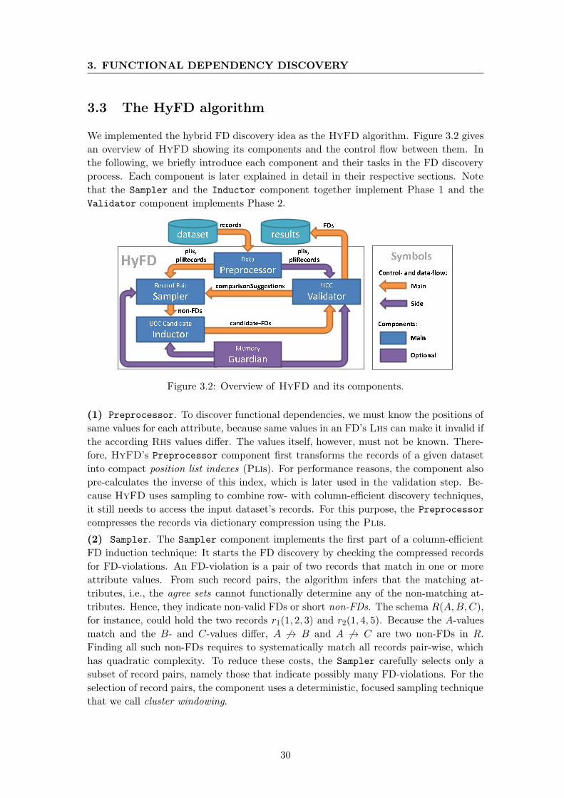
3. FUNCTIONAL DEPENDENCY DISCOVERY
3.3 The HyFD algorithm
We implemented the hybrid FD discovery idea as the HyFD algorithm. Figure 3.2 gives
an overview of HyFD showing its components and the control flow between them. In
the following, we briefly introduce each component and their tasks in the FD discovery
process. Each component is later explained in detail in their respective sections. Note
that the Sampler and the Inductor component together implement Phase 1 and the
Validator component implements Phase 2.
Figure 3.2: Overview of HyFD and its components.
(1) Preprocessor. To discover functional dependencies, we must know the positions of
same values for each attribute, because same values in an FD’s Lhs can make it invalid if
the according Rhs values differ. The values itself, however, must not be known. There-
fore, HyFD’s Preprocessor component first transforms the records of a given dataset
into compact position list indexes (Plis). For performance reasons, the component also
pre-calculates the inverse of this index, which is later used in the validation step. Be-
cause HyFD uses sampling to combine row- with column-efficient discovery techniques,
it still needs to access the input dataset’s records. For this purpose, the Preprocessor
compresses the records via dictionary compression using the Plis.
(2) Sampler. The Sampler component implements the first part of a column-efficient
FD induction technique: It starts the FD discovery by checking the compressed records
for FD-violations. An FD-violation is a pair of two records that match in one or more
attribute values. From such record pairs, the algorithm infers that the matching at-
tributes, i.e., the agree sets cannot functionally determine any of the non-matching at-
tributes. Hence, they indicate non-valid FDs or short non-FDs. The schema R(A,B,C),
for instance, could hold the two records r1(1, 2, 3) and r2(1, 4, 5). Because the A-values
match and the B- and C-values differ, A 6→ B and A 6→ C are two non-FDs in R.
Finding all such non-FDs requires to systematically match all records pair-wise, which
has quadratic complexity. To reduce these costs, the Sampler carefully selects only a
subset of record pairs, namely those that indicate possibly many FD-violations. For the
selection of record pairs, the component uses a deterministic, focused sampling technique
that we call cluster windowing.
30
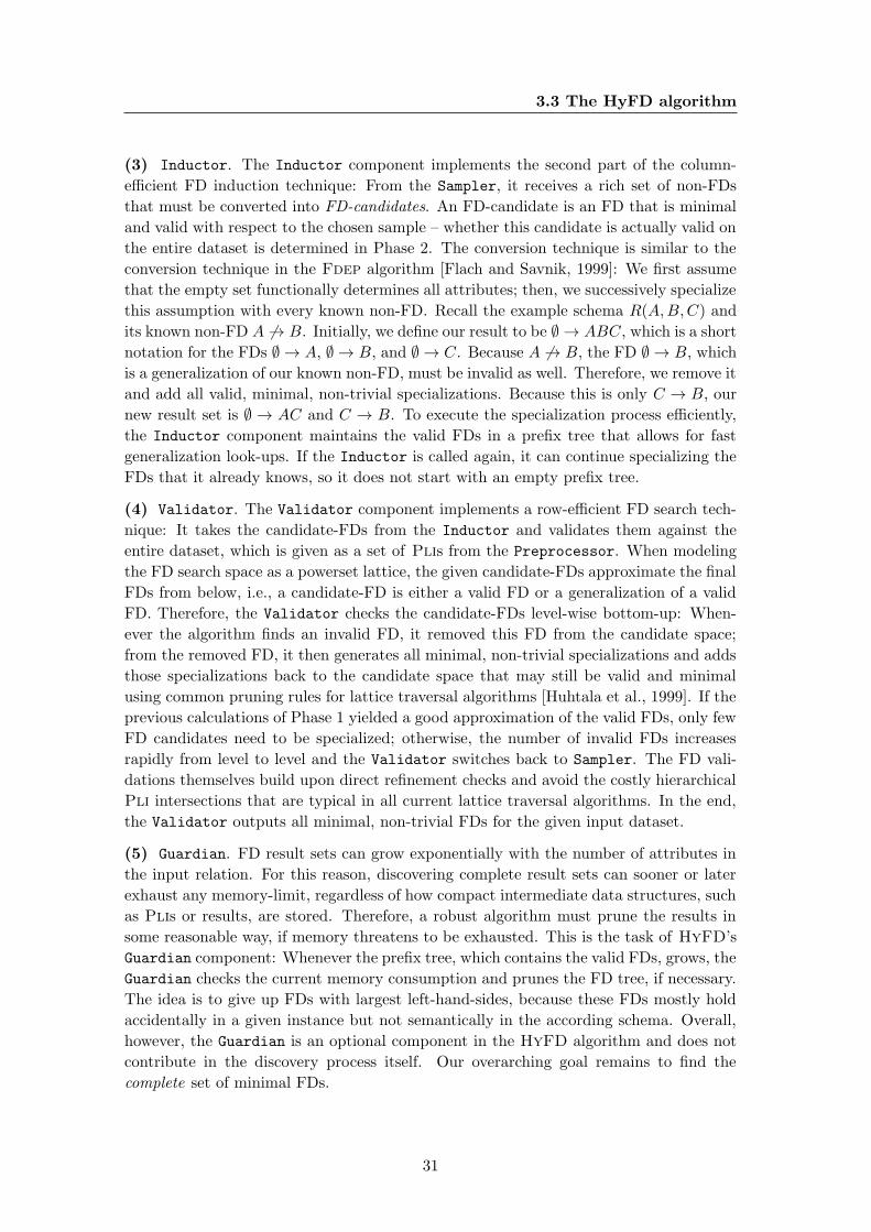
3.3 The HyFD algorithm
(3) Inductor. The Inductor component implements the second part of the column-
efficient FD induction technique: From the Sampler, it receives a rich set of non-FDs
that must be converted into FD-candidates. An FD-candidate is an FD that is minimal
and valid with respect to the chosen sample – whether this candidate is actually valid on
the entire dataset is determined in Phase 2. The conversion technique is similar to the
conversion technique in the Fdep algorithm [Flach and Savnik, 1999]: We first assume
that the empty set functionally determines all attributes; then, we successively specialize
this assumption with every known non-FD. Recall the example schema R(A,B,C) and
its known non-FD A 6→ B. Initially, we define our result to be ∅ → ABC, which is a short
notation for the FDs ∅ → A, ∅ → B, and ∅ → C. Because A 6→ B, the FD ∅ → B, which
is a generalization of our known non-FD, must be invalid as well. Therefore, we remove it
and add all valid, minimal, non-trivial specializations. Because this is only C → B, our
new result set is ∅ → AC and C → B. To execute the specialization process efficiently,
the Inductor component maintains the valid FDs in a prefix tree that allows for fast
generalization look-ups. If the Inductor is called again, it can continue specializing the
FDs that it already knows, so it does not start with an empty prefix tree.
(4) Validator. The Validator component implements a row-efficient FD search tech-
nique: It takes the candidate-FDs from the Inductor and validates them against the
entire dataset, which is given as a set of Plis from the Preprocessor. When modeling
the FD search space as a powerset lattice, the given candidate-FDs approximate the final
FDs from below, i.e., a candidate-FD is either a valid FD or a generalization of a valid
FD. Therefore, the Validator checks the candidate-FDs level-wise bottom-up: When-
ever the algorithm finds an invalid FD, it removed this FD from the candidate space;
from the removed FD, it then generates all minimal, non-trivial specializations and adds
those specializations back to the candidate space that may still be valid and minimal
using common pruning rules for lattice traversal algorithms [Huhtala et al., 1999]. If the
previous calculations of Phase 1 yielded a good approximation of the valid FDs, only few
FD candidates need to be specialized; otherwise, the number of invalid FDs increases
rapidly from level to level and the Validator switches back to Sampler. The FD vali-
dations themselves build upon direct refinement checks and avoid the costly hierarchical
Pli intersections that are typical in all current lattice traversal algorithms. In the end,
the Validator outputs all minimal, non-trivial FDs for the given input dataset.
(5) Guardian. FD result sets can grow exponentially with the number of attributes in
the input relation. For this reason, discovering complete result sets can sooner or later
exhaust any memory-limit, regardless of how compact intermediate data structures, such
as Plis or results, are stored. Therefore, a robust algorithm must prune the results in
some reasonable way, if memory threatens to be exhausted. This is the task of HyFD’s
Guardian component: Whenever the prefix tree, which contains the valid FDs, grows, the
Guardian checks the current memory consumption and prunes the FD tree, if necessary.
The idea is to give up FDs with largest left-hand-sides, because these FDs mostly hold
accidentally in a given instance but not semantically in the according schema. Overall,
however, the Guardian is an optional component in the HyFD algorithm and does not
contribute in the discovery process itself. Our overarching goal remains to find the
complete set of minimal FDs.
31
3. FUNCTIONAL DEPENDENCY DISCOVERY
3.4 Preprocessing
The Preprocessor is responsible for transforming the input data into two compact data
structures: plis and pliRecords. The first data structure plis is an array of position list
indexes (Pli), which we already introduced in Section 2.4. A Pli πX groups tuples
into equivalence classes by their values of attribute set X. Such Plis can efficiently
be implemented as sets of record ID sets, which we wrap in Pli objects. A functional
dependency X → A is then checked by testing if every cluster in πX is a subset of some
cluster of πA, which is true iff the FD is valid. This check is called refinement (see
Section 3.7) and was first introduced in [Huhtala et al., 1999].
Algorithm 1 shows the Preprocessor component and the two data structures it pro-
duces: The already discussed plis and a Pli-compressed representation of all records,
which we call pliRecords. For their creation, the algorithm first determines the number
of input records numRecs and the number of attributes numAttrs (Lines 1 and 2). Then,
it builds the plis array – one π for each attribute. This is done by hashing each value
to a list of record IDs and then simply collecting these lists in a Pli object (Line 4).
We call the lists of record IDs cluster, because they cluster records with a same value
in the respective attribute. When created, the Preprocessor sorts the array of Plis in
descending order by the number of clusters (including clusters of size one, whose num-
ber is implicitly known). This sorting improves the focussed sampling of non-FDs in
the Sampler component (see Section 3.5), because it groups effective attributes, i.e., at-
tributes that contain violations to potentially many FD candidates at the beginning of the
list and non-effective attributes at the end; the sorting also improves the FD-candidate
validations in the Validator component (see Section 3.7), because the attributes at the
beginning of the sorted list then constitute the most efficient pivot elements.
Algorithm 1: Data Preprocessing
Data: records
Result: plis, invertedPlis, pliRecords
1 numRecs ← |records|;2 numAttrs ← |records[0]|;3 array plis size numAttrs as Pli;
4 plis ← buildPlis (records);
5 plis ← sort (plis, DESCENDING);
6 array invertedPlis size numAttrs × numRecs as Integer;
7 invertedPlis ← invert (plis);
8 array pliRecords size numRecs × numAttrs as Integer;
9 pliRecords ← createRecords (invertedPlis);
10 return plis, invertedPlis, pliRecords ;
The clusters in each Pli object are stored in an arbitrary but fixed order so that we
can enumerate the clusters. This allows the Preprocessor to calculate the inverse of
each Pli, i.e., an array that maps each record ID to its corresponding cluster ID (Lines 6
and 7). If no cluster exists for a particular record, its value must be unique in this
attribute and we store −1 as a special ID for unique values. With the invertedPlis, the
32

3.5 Sampling
Preprocessor finally creates dictionary compressed representations of all records, the
pliRecords (Lines 8 and 9). A compressed record is an array of cluster IDs where each
field denotes the record’s cluster in attribute A ∈ [0, numAttrs[. We extract these rep-
resentations from the plis that already map cluster IDs to record IDs for each attribute.
The Pli-compressed records are needed in the sampling phase to find FD-violations and
in the validation phase to find Lhs- and Rhs-cluster IDs for certain records.
3.5 Sampling
The idea of the Sampler component is to analyze a dataset, which is represented by the
pliRecords, for FD-violations, i.e., non-FDs that can later be converted into FDs. To
derive FD-violations, the component compares records pair-wise. These pair-wise record
comparisons are robust against the number of columns, but comparing all pairs of records
scales quadratically with their number. Therefore, the Sampler uses only a subset, i.e.,
a sample of record pairs for the non-FD calculations. The record pairs in this subset
should be chosen carefully, because some pairs are more likely to reveal FD-violations
than others. In the following, we first discuss how non-FDs are identified; then, we
present a deterministic focused sampling technique, which extracts a non-random subset
of promising record pairs for the non-FD discovery; lastly, we propose an implementation
of our sampling technique.
Retrieving non-FDs. A functional dependency X → A can be invalidated with two
records that have matching X and differing A values. Therefore, the non-FD search is
based on pair-wise record comparisons: If two records match in their values for attribute
set Y and differ in their values for attribute set Z, then they invalidate all X → A with
X ⊆ Y and A ∈ Z. The corresponding FD-violation Y 6→ Z can be efficiently stored in
bitsets that hold a 1 for each matching attribute of Y and a 0 for each differing attribute
Z. To calculate these bitsets, we use the match ()-function, which compares two Pli-
compressed records element-wise. Because the records are given as Integer arrays (and
not as, for instance, String arrays), this function is cheap in contrast to the validation
and specialization functions used by other components of HyFD.
Sometimes, the sampling discovers the same FD-violations with different record pairs.
For this reason, the bitsets are stored in a set called nonFds, which automatically elimi-
nates duplicate observations. For the same task, related algorithms, such as Fdep [Flach
and Savnik, 1999], proposed prefix-trees, but our evaluation in Section 3.9 and in par-
ticular the experiments in Section 3.9.5 show that these data structures consume much
more memory and do not yield a better performance. Reconsidering Figure 3.1, we can
easily see that the number of non-FDs is much larger than the number of minimal FDs,
so storing the non-FDs in a memory-efficient data structure is crucial.
Focused sampling. FD-violations are retrieved from record pairs, and while certain
record pairs indicate important FD-violations, the same two records may not offer any
new insights when compared with other records. So an important aspect of focused
sampling is that we sample record pairs and not records. Thereby, only record pairs
that match in at least one attribute can reveal FD-violations; comparing records with
33

3. FUNCTIONAL DEPENDENCY DISCOVERY
no overlap should be avoided. A focused sampling algorithm can easily assure this
by comparing only those records that co-occur in at least one Pli-cluster. But due to
columns that contain only few distinct values, most record pairs co-occur in some cluster.
Therefore, more sophisticated pair selection techniques are needed.
The problem of finding promising comparison candidates is a well known problem in
duplicate detection research. A popular solution for this problem is the sorted neighbor-
hood pair selection algorithm [Hernandez and Stolfo, 1998]. The idea is to first sort the
data by some domain-dependent key that sorts similar records close to one another; then,
the algorithm compares all records to their w closest neighbors, where w is a window-
ing. Because our problem of finding violating record pairs is similar to finding matching
record pairs, we use the same idea for our focused sampling algorithm.
At first, we sort similar records, i.e., records that co-occur in certain Pli-clusters,
close to one-another. We do this for all clusters in all Plis with different sorting keys each
(we discuss possible sorting keys soon). Then, we slide a window of size w = 2 over the
clusters of each Pli and compare all record pairs within this window, which are all direct
neighbors. Because some Plis produce better sortations than others in the sense that
they reveal more FD-violations than others, the algorithm shall automatically prefer more
efficient sortations over less efficient ones. This can be done with a progressive selection
technique, which is also known from duplicate detection [Papenbrock et al., 2015c]: The
algorithm first compares all records to their direct neighbors and counts the results;
afterwards, the result counts are ranked and the sortation with the most results is chosen
to run a slightly larger window (w+ 1). The algorithm stops continuing best sortations,
when all sortations have become inefficient. In this way, the algorithm automatically
chooses most profitable comparisons. When adapting the same strategy for our FD-
violation search, we can save many comparisons: Because efficient sortations anticipate
most informative comparisons, less efficient sortations become quickly inefficient.
Finally, the focused sampling must decide on when the comparisons of records in a
certain sortation, i.e., for a certain Pli, become inefficient. We propose to start with
a rather strict definition of efficiency, because HyFD returns into the sampling phase
anyway, if the number of identified FD-violations was too low. So an efficiency threshold
could be 0.01, which is one new FD-violation within 100 comparisons – in fact, Section 3.9
shows that this threshold performs well on all tested dataset sizes. To relax this threshold
in subsequent iterations, we double the number of comparisons whenever the algorithm
returns to the sampling phase.
The sampling algorithm. Algorithm 2 implements the focused sampling strategy
introduced above. It requires the plis and pliRecords from the Preprocessor and the
comparisonSuggestions from the Validator. Figure 3.3 illustrates the algorithm with
an example.
The priority queue efficiencyQueue is a local data structure that ranks the Plis by
their sampling efficiency. If the efficiencyQueue is empty (Line 1), this is the first time
the Sampler is called. In this case, we need to sort the records in all clusters by some
Pli-dependent sorting key (Lines 2 to 4). As shown in Figure 3.3.1, we sort the records
in each cluster of attribute Ai’s Pli by their cluster number in attribute Ai−1; if numbers
are equal or unknown, the sorting uses the cluster number in Ai+1 as a tiebreaker. The
34
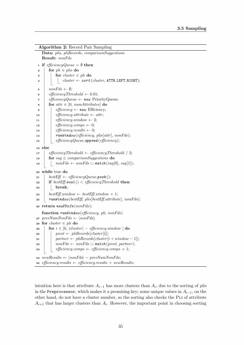
3.5 Sampling
Algorithm 2: Record Pair Sampling
Data: plis, pliRecords, comparisonSuggestions
Result: nonFds
1 if efficiencyQueue = ∅ then
2 for pli ∈ plis do
3 for cluster ∈ pli do
4 cluster ← sort (cluster, ATTR LEFT RIGHT);
5 nonFds ← ∅;6 efficiencyThreshold ← 0.01;
7 efficiencyQueue ← new PriorityQueue;
8 for attr ∈ [0, numAttributes [ do
9 efficiency ← new Efficiency;
10 efficiency.attribute ← attr ;
11 efficiency.window ← 2;
12 efficiency.comps ← 0;
13 efficiency.results ← 0;
14 runWindow (efficiency, plis [attr ], nonFds);
15 efficiencyQueue.append (efficiency);
16 else
17 efficiencyThreshold ← efficiencyThreshold / 2;
18 for sug ∈ comparisonSuggestions do
19 nonFds ← nonFds ∪ match (sug [0], sug [1]);
20 while true do
21 bestEff ← efficiencyQueue.peek ();
22 if bestEff.eval () < efficiencyThreshold then
23 break;
24 bestEff.window ← bestEff.window + 1;
25 runWindow (bestEff, plis [bestEff.attribute], nonFds);
26 return newFDsIn (nonFds);
function runWindow (efficiency, pli, nonFds)
27 prevNumNonFds ← |nonFds|;28 for cluster ∈ pli do
29 for i ∈ [0, |cluster| − efficiency.window [ do
30 pivot ← pliRecords [cluster [i]];
31 partner ← pliRecords [cluster [i+ window − 1]];
32 nonFds ← nonFds ∪ match (pivot, partner);
33 efficiency.comps ← efficiency.comps + 1;
34 newResults ← |nonFds| − prevNumNonFds ;
35 efficiency.results ← efficiency.results + newResults ;
intuition here is that attribute Ai−1 has more clusters than Ai, due to the sorting of plis
in the Preprocessor, which makes it a promising key; some unique values in Ai−1, on the
other hand, do not have a cluster number, so the sorting also checks the Pli of attribute
Ai+1 that has larger clusters than Ai. However, the important point in choosing sorting
35
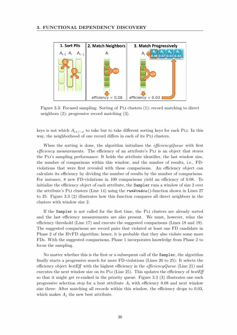
3. FUNCTIONAL DEPENDENCY DISCOVERY
Figure 3.3: Focused sampling: Sorting of Pli clusters (1); record matching to direct
neighbors (2); progressive record matching (3).
keys is not which Ai+/−x to take but to take different sorting keys for each Pli. In this
way, the neighborhood of one record differs in each of its Pli clusters.
When the sorting is done, the algorithm initializes the efficiencyQueue with first
efficiency measurements. The efficiency of an attribute’s Pli is an object that stores
the Pli’s sampling performance: It holds the attribute identifier, the last window size,
the number of comparisons within this window, and the number of results, i.e., FD-
violations that were first revealed with these comparisons. An efficiency object can
calculate its efficiency by dividing the number of results by the number of comparisons.
For instance, 8 new FD-violations in 100 comparisons yield an efficiency of 0.08. To
initialize the efficiency object of each attribute, the Sampler runs a window of size 2 over
the attribute’s Pli clusters (Line 14) using the runWindow ()-function shown in Lines 27
to 35. Figure 3.3 (2) illustrates how this function compares all direct neighbors in the
clusters with window size 2.
If the Sampler is not called for the first time, the Pli clusters are already sorted
and the last efficiency measurements are also present. We must, however, relax the
efficiency threshold (Line 17) and execute the suggested comparisons (Lines 18 and 19).
The suggested comparisons are record pairs that violated at least one FD candidate in
Phase 2 of the HyFD algorithm; hence, it is probable that they also violate some more
FDs. With the suggested comparisons, Phase 1 incorporates knowledge from Phase 2 to
focus the sampling.
No matter whether this is the first or a subsequent call of the Sampler, the algorithm
finally starts a progressive search for more FD-violations (Lines 20 to 25): It selects the
efficiency object bestEff with the highest efficiency in the efficiencyQueue (Line 21) and
executes the next window size on its Pli (Line 25). This updates the efficiency of bestEff
so that it might get re-ranked in the priority queue. Figure 3.3 (3) illustrates one such
progressive selection step for a best attribute Ai with efficiency 0.08 and next window
size three: After matching all records within this window, the efficiency drops to 0.03,
which makes Aj the new best attribute.
36
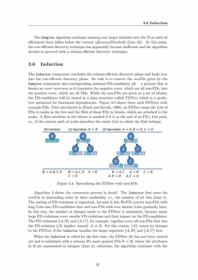
3.6 Induction
The Sampler algorithm continues running ever larger windows over the Plis until all
efficiencies have fallen below the current efficiencyThreshold (Line 22). At this point,
the row-efficient discovery technique has apparently become inefficient and the algorithm
decides to proceed with a column-efficient discovery technique.
3.6 Induction
The Inductor component concludes the column-efficient discovery phase and leads over
into the row-efficient discovery phase. Its task is to convert the nonFds given by the
Sampler component into corresponding minimal FD-candidates fds – a process that is
known as cover inversion as it translates the negative cover, which are all non-FDs, into
the positive cover, which are all FDs. While the non-FDs are given as a set of bitsets,
the FD-candidates will be stored in a data structure called FDTree, which is a prefix-
tree optimized for functional dependencies. Figure 3.4 shows three such FDTrees with
example FDs. First introduced in [Flach and Savnik, 1999], an FDTree maps the Lhs of
FDs to nodes in the tree and the Rhs of these FDs to bitsets, which are attached to the
nodes. A Rhs attribute in the bitsets is marked if it is at the end of an FD’s Lhs path,
i.e., if the current path of nodes describes the entire Lhs to which the Rhs belongs.
∅ → 𝐴, 𝐵, 𝐶, 𝐷 ∅ → 𝐴, 𝐶, 𝐷 ∅ → 𝐴, 𝐶
(1) Specialize: 𝐷 → 𝐵 (2) Specialize: 𝐴 → 𝐷, 𝐵 → 𝐷, 𝐶 → 𝐷
𝐴 → 𝐵 𝐶 → 𝐵 𝐴, 𝐶 → 𝐷 𝐴, 𝐵 → 𝐷
1 1 1 1
∅ 1 1 1 1
∅
0 1 0 0
𝐶 0 1 0 0
𝐴
1 1 1 1
∅
0 1 0 0
𝐶 0 1 0 1
𝐴
0 0 0 1
𝐶 0 0 0 1
𝐵
𝐴 → 𝐵 𝐶 → 𝐵
(0) Initialize:
Figure 3.4: Specializing the FDTree with non-FDs.
Algorithm 3 shows the conversion process in detail. The Inductor first sorts the
nonFds in descending order by their cardinality, i.e., the number of set bits (Line 1).
The sorting of FD-violations is important, because it lets HyFD convert non-FDs with
long Lhss into FD-candidates first and non-FDs with ever shorter Lhss gradually later.
In this way, the number of changes made to the FDTree is minimized, because many
large FD-violations cover smaller FD-violations and their impact on the FD-candidates.
The FD-violations {A,B} and {A,C}, for example, together cover all non-FDs that also
the FD-violation {A} implies, namely A 6→ R. For this reason, {A} causes no changes
to the FDTree, if the Inductor handles the larger supersets {A,B} and {A,C} first.
When the Inductor is called for the first time, the FDTree fds has not been created
yet and is initialized with a schema R’s most general FDs ∅ → R, where the attributes
in R are represented as integers (Line 4); otherwise, the algorithm continues with the
37
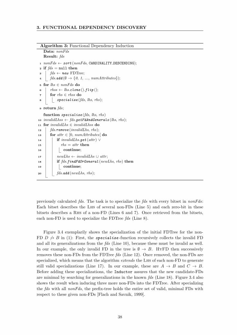
3. FUNCTIONAL DEPENDENCY DISCOVERY
Algorithm 3: Functional Dependency Induction
Data: nonFds
Result: fds
1 nonFds ← sort (nonFds, CARDINALITY DESCENDING);
2 if fds = null then
3 fds ← new FDTree;
4 fds.add (∅ → {0, 1, ..., numAttributes});5 for lhs ∈ nonFds do
6 rhss ← lhs.clone ().flip ();
7 for rhs ∈ rhss do
8 specialize (fds, lhs, rhs);
9 return fds ;
function specialize (fds, lhs, rhs)
10 invalidLhss ← fds.getFdAndGenerals (lhs, rhs);
11 for invalidLhs ∈ invalidLhss do
12 fds.remove (invalidLhs, rhs);
13 for attr ∈ [0, numAttributes [ do
14 if invalidLhs.get (attr) ∨15 rhs = attr then
16 continue;
17 newLhs ← invalidLhs ∪ attr ;
18 if fds.findFdOrGeneral (newLhs, rhs) then
19 continue;
20 fds.add (newLhs, rhs);
previously calculated fds. The task is to specialize the fds with every bitset in nonFds :
Each bitset describes the Lhs of several non-FDs (Line 5) and each zero-bit in these
bitsets describes a Rhs of a non-FD (Lines 6 and 7). Once retrieved from the bitsets,
each non-FD is used to specialize the FDTree fds (Line 8).
Figure 3.4 exemplarily shows the specialization of the initial FDTree for the non-
FD D 6→ B in (1): First, the specialize -function recursively collects the invalid FD
and all its generalizations from the fds (Line 10), because these must be invalid as well.
In our example, the only invalid FD in the tree is ∅ → B. HyFD then successively
removes these non-FDs from the FDTree fds (Line 12). Once removed, the non-FDs are
specialized, which means that the algorithm extends the Lhs of each non-FD to generate
still valid specializations (Line 17). In our example, these are A → B and C → B.
Before adding these specializations, the Inductor assures that the new candidate-FDs
are minimal by searching for generalizations in the known fds (Line 18). Figure 3.4 also
shows the result when inducing three more non-FDs into the FDTree. After specializing
the fds with all nonFds, the prefix-tree holds the entire set of valid, minimal FDs with
respect to these given non-FDs [Flach and Savnik, 1999].
38
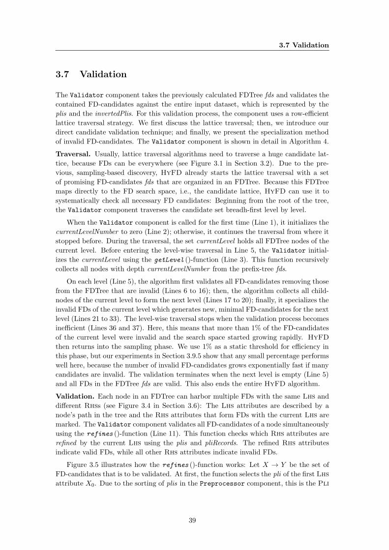
3.7 Validation
3.7 Validation
The Validator component takes the previously calculated FDTree fds and validates the
contained FD-candidates against the entire input dataset, which is represented by the
plis and the invertedPlis. For this validation process, the component uses a row-efficient
lattice traversal strategy. We first discuss the lattice traversal; then, we introduce our
direct candidate validation technique; and finally, we present the specialization method
of invalid FD-candidates. The Validator component is shown in detail in Algorithm 4.
Traversal. Usually, lattice traversal algorithms need to traverse a huge candidate lat-
tice, because FDs can be everywhere (see Figure 3.1 in Section 3.2). Due to the pre-
vious, sampling-based discovery, HyFD already starts the lattice traversal with a set
of promising FD-candidates fds that are organized in an FDTree. Because this FDTree
maps directly to the FD search space, i.e., the candidate lattice, HyFD can use it to
systematically check all necessary FD candidates: Beginning from the root of the tree,
the Validator component traverses the candidate set breadh-first level by level.
When the Validator component is called for the first time (Line 1), it initializes the
currentLevelNumber to zero (Line 2); otherwise, it continues the traversal from where it
stopped before. During the traversal, the set currentLevel holds all FDTree nodes of the
current level. Before entering the level-wise traversal in Line 5, the Validator initial-
izes the currentLevel using the getLevel ()-function (Line 3). This function recursively
collects all nodes with depth currentLevelNumber from the prefix-tree fds.
On each level (Line 5), the algorithm first validates all FD-candidates removing those
from the FDTree that are invalid (Lines 6 to 16); then, the algorithm collects all child-
nodes of the current level to form the next level (Lines 17 to 20); finally, it specializes the
invalid FDs of the current level which generates new, minimal FD-candidates for the next
level (Lines 21 to 33). The level-wise traversal stops when the validation process becomes
inefficient (Lines 36 and 37). Here, this means that more than 1% of the FD-candidates
of the current level were invalid and the search space started growing rapidly. HyFD
then returns into the sampling phase. We use 1% as a static threshold for efficiency in
this phase, but our experiments in Section 3.9.5 show that any small percentage performs
well here, because the number of invalid FD-candidates grows exponentially fast if many
candidates are invalid. The validation terminates when the next level is empty (Line 5)
and all FDs in the FDTree fds are valid. This also ends the entire HyFD algorithm.
Validation. Each node in an FDTree can harbor multiple FDs with the same Lhs and
different Rhss (see Figure 3.4 in Section 3.6): The Lhs attributes are described by a
node’s path in the tree and the Rhs attributes that form FDs with the current Lhs are
marked. The Validator component validates all FD-candidates of a node simultaneously
using the refines ()-function (Line 11). This function checks which Rhs attributes are
refined by the current Lhs using the plis and pliRecords. The refined Rhs attributes
indicate valid FDs, while all other Rhs attributes indicate invalid FDs.
Figure 3.5 illustrates how the refines ()-function works: Let X → Y be the set of
FD-candidates that is to be validated. At first, the function selects the pli of the first Lhs
attribute X0. Due to the sorting of plis in the Preprocessor component, this is the Pli
39
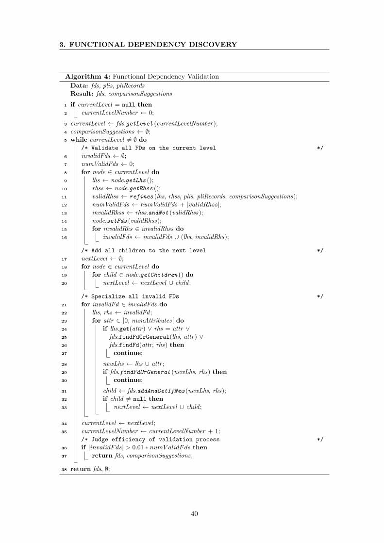
3. FUNCTIONAL DEPENDENCY DISCOVERY
Algorithm 4: Functional Dependency Validation
Data: fds, plis, pliRecords
Result: fds, comparisonSuggestions
1 if currentLevel = null then
2 currentLevelNumber ← 0;
3 currentLevel ← fds.getLevel (currentLevelNumber);
4 comparisonSuggestions ← ∅;5 while currentLevel 6= ∅ do
/* Validate all FDs on the current level */
6 invalidFds ← ∅;7 numValidFds ← 0;
8 for node ∈ currentLevel do
9 lhs ← node.getLhs ();
10 rhss ← node.getRhss ();
11 validRhss ← refines (lhs, rhss, plis, pliRecords, comparisonSuggestions);
12 numValidFds ← numValidFds + |validRhss|;13 invalidRhss ← rhss.andNot (validRhss);
14 node.setFds (validRhss);
15 for invalidRhs ∈ invalidRhss do
16 invalidFds ← invalidFds ∪ (lhs, invalidRhs);
/* Add all children to the next level */
17 nextLevel ← ∅;18 for node ∈ currentLevel do
19 for child ∈ node.getChildren () do
20 nextLevel ← nextLevel ∪ child ;
/* Specialize all invalid FDs */
21 for invalidFd ∈ invalidFds do
22 lhs, rhs ← invalidFd ;
23 for attr ∈ [0, numAttributes [ do
24 if lhs.get(attr) ∨ rhs = attr ∨25 fds.findFdOrGeneral(lhs, attr) ∨26 fds.findFd(attr, rhs) then
27 continue;
28 newLhs ← lhs ∪ attr ;
29 if fds.findFdOrGeneral (newLhs, rhs) then
30 continue;
31 child ← fds.addAndGetIfNew (newLhs, rhs);
32 if child 6= null then
33 nextLevel ← nextLevel ∪ child ;
34 currentLevel ← nextLevel ;
35 currentLevelNumber ← currentLevelNumber + 1;
/* Judge efficiency of validation process */
36 if |invalidFds| > 0.01 ∗ numV alidFds then
37 return fds, comparisonSuggestions ;
38 return fds, ∅;
40

3.7 Validation
with the most and, hence, the smallest clusters of all Lhs attributes. For each cluster in
X0’s Pli, the algorithm iterates all record IDs ri in this cluster and retrieves the according
compressed records from the pliRecords. A compressed record contains all cluster IDs in
which a record is contained. Hence, the algorithm can create one array containing the
Lhs cluster IDs of X and one array containing the Rhs cluster IDs of Y . The Lhs array,
then, describes the cluster of ri regarding attribute combination X. To check which Rhs
Pli these Lhs clusters refine, we map the Lhs clusters to the corresponding array of
Rhs clusters. We fill this map while iterating the record IDs of a cluster. If an array
of Lhs clusters already exists in this map, the array of Rhs clusters must match the
existing one. All non-matching Rhs clusters indicate refinement-violations and, hence,
invalid Rhs attributes. The algorithm immediately stops checking such Rhs attributes
so that only valid Rhs attributes survive until the end.
plis[X0]
Validation of 𝑿 → 𝒀
2
5
8
0
4
1
3
6
7
0 2 2
1 1 0
1 1 0
4 0 3
4 0 3
3 3 3
2 1 4
2 1 4
3 0 1
0:
1:
2:
2 4 1
4 5 4
4 5 0
5 2 -
0 2 -
- 4 -
- 0 -
- 0 -
- 3 -
Figure 3.5: Directly validating FD-candidates X → Y .
In comparison to other Pli-based algorithms, such as Tane, HyFD’s validation tech-
nique avoids the costly hierarchical Pli intersections. By mapping the Lhs clusters to
Rhs clusters, the checks are independent of other checks and do not require intermediate
Plis. The direct validation is important, because the Validator’s starting FD candi-
dates are – due to the sampling-based induction part – on much higher lattice levels
and successively intersecting lower level Plis would undo this advantage. Furthermore,
HyFD can terminate refinement checks very early if all Rhs attributes are invalid, be-
cause the results of the intersections, i.e., the intersected Plis are not needed for later
intersections. Not storing intermediate Plis also has the advantage of demanding much
less memory – most Pli-based algorithms fail at processing larger datasets, for exactly
this reason [Papenbrock et al., 2015b].
41
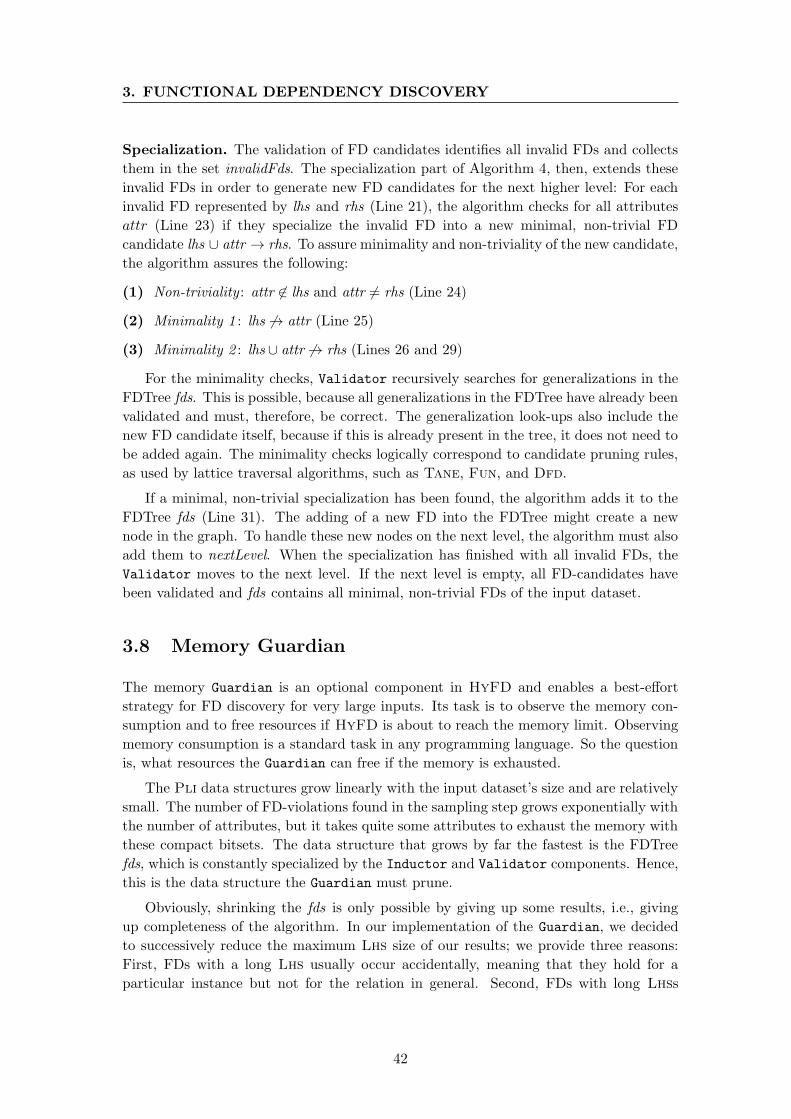
3. FUNCTIONAL DEPENDENCY DISCOVERY
Specialization. The validation of FD candidates identifies all invalid FDs and collects
them in the set invalidFds. The specialization part of Algorithm 4, then, extends these
invalid FDs in order to generate new FD candidates for the next higher level: For each
invalid FD represented by lhs and rhs (Line 21), the algorithm checks for all attributes
attr (Line 23) if they specialize the invalid FD into a new minimal, non-trivial FD
candidate lhs ∪ attr → rhs. To assure minimality and non-triviality of the new candidate,
the algorithm assures the following:
(1) Non-triviality : attr 6∈ lhs and attr 6= rhs (Line 24)
(2) Minimality 1 : lhs 6→ attr (Line 25)
(3) Minimality 2 : lhs ∪ attr 6→ rhs (Lines 26 and 29)
For the minimality checks, Validator recursively searches for generalizations in the
FDTree fds. This is possible, because all generalizations in the FDTree have already been
validated and must, therefore, be correct. The generalization look-ups also include the
new FD candidate itself, because if this is already present in the tree, it does not need to
be added again. The minimality checks logically correspond to candidate pruning rules,
as used by lattice traversal algorithms, such as Tane, Fun, and Dfd.
If a minimal, non-trivial specialization has been found, the algorithm adds it to the
FDTree fds (Line 31). The adding of a new FD into the FDTree might create a new
node in the graph. To handle these new nodes on the next level, the algorithm must also
add them to nextLevel. When the specialization has finished with all invalid FDs, the
Validator moves to the next level. If the next level is empty, all FD-candidates have
been validated and fds contains all minimal, non-trivial FDs of the input dataset.
3.8 Memory Guardian
The memory Guardian is an optional component in HyFD and enables a best-effort
strategy for FD discovery for very large inputs. Its task is to observe the memory con-
sumption and to free resources if HyFD is about to reach the memory limit. Observing
memory consumption is a standard task in any programming language. So the question
is, what resources the Guardian can free if the memory is exhausted.
The Pli data structures grow linearly with the input dataset’s size and are relatively
small. The number of FD-violations found in the sampling step grows exponentially with
the number of attributes, but it takes quite some attributes to exhaust the memory with
these compact bitsets. The data structure that grows by far the fastest is the FDTree
fds, which is constantly specialized by the Inductor and Validator components. Hence,
this is the data structure the Guardian must prune.
Obviously, shrinking the fds is only possible by giving up some results, i.e., giving
up completeness of the algorithm. In our implementation of the Guardian, we decided
to successively reduce the maximum Lhs size of our results; we provide three reasons:
First, FDs with a long Lhs usually occur accidentally, meaning that they hold for a
particular instance but not for the relation in general. Second, FDs with long Lhss
42

3.9 Evaluation
are less useful in most use cases, e.g., they become worse key/foreign-key candidates
when used for normalization and they are less likely to match a query when used for
query optimization. Third, FDs with long Lhss consume more memory, because they
are physically larger, and preferentially removing them retains more FDs in total.
To restrict the maximum size of the FDs’ Lhss, we need to add some additional
logic into the FDTree: It must hold the maximum Lhs size as a variable, which the
Guardian component can control; whenever this variable is decremented, the FDTree
recursively removes all FDs with larger Lhss and sets their memory resources free. The
FDTree also refuses to add any new FD with a larger Lhs. In this way, the result
pruning works without changing any of the other four components. However, note that
the Guardian component prunes only such results whose size would otherwise exceed the
memory capacity, which means that the component in general does not take action.
3.9 Evaluation
FD discovery has shown to be exponential in the number of attributes m, simply because
the results can become exponentially large (see Section 2.4). For this reason, HyFD’s
runtime is in O(m2 · 2m) as well: In Phase 1, the comparison costs for record pairs
are linear in m, but the induction of the positive cover is in O(m2 · 2m), because in the
worst case 2m−1 Lhs attribute combinations must be refined on average m−12 times in the
negative cover for each of the m possible Rhs attributes – HyFD prevents the worst case
by sorting the non-FDs descendingly in the negative cover before inducing the positive
cover. Phase 2 is in O(m2 · 2m), because this represents the worst case number of FD
candidates that need to be tested – HyFD reduces this number via minimality pruning
and the use of Phase 1’s results. Due to the threshold-bounded windowing in Phase 1
and the Pli-based validations in Phase 2, HyFD’s runtime is (like other runtimes of
lattice-based FD algorithms) about linear in the number of records n.
Note that each phase can (potentially) discover all minimal FDs without the other.
The following experiments, however, show that HyFD is able to process significantly
larger datasets than state-of-the-art FD discovery algorithms in less runtime. At first,
we introduce our experimental setup. Then, we evaluate the scalability of HyFD with
both a dataset’s number of rows and columns. Afterwards, we show that HyFD performs
well on different datasets. In all these experiments, we compare HyFD to seven state-
of-the-art FD discovery algorithms. We, finally, analyze some characteristics of HyFD
in more detail and discuss the results of the discovery process.
3.9.1 Experimental setup
Metanome. HyFD and all algorithms from related work have been implemented for
the Metanome data profiling framework (www.metanome.de), which defines standard in-
terfaces for different kinds of profiling algorithms. Metanome also provided the various
implementations of the state of the art. Common tasks, such as input parsing, result
formatting, and performance measurement are standardized by the framework and de-
coupled from the algorithms. We cover more details on Metanome in Chapter 6.
43
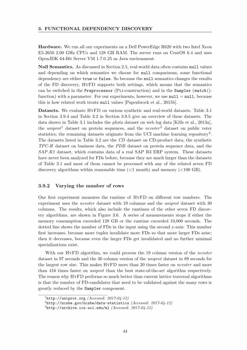
3. FUNCTIONAL DEPENDENCY DISCOVERY
Hardware. We run all our experiments on a Dell PowerEdge R620 with two Intel Xeon
E5-2650 2.00 GHz CPUs and 128 GB RAM. The server runs on CentOS 6.4 and uses
OpenJDK 64-Bit Server VM 1.7.0 25 as Java environment.
Null Semantics. As discussed in Section 2.5, real-world data often contains null values
and depending on which semantics we choose for null comparisons, some functional
dependency are either true or false. So because the null semantics changes the results
of the FD discovery, HyFD supports both settings, which means that the semantics
can be switched in the Preprocessor (Pli-construction) and in the Sampler (match ()-
function) with a parameter. For our experiments, however, we use null = null, because
this is how related work treats null values [Papenbrock et al., 2015b].
Datasets. We evaluate HyFD on various synthetic and real-world datasets. Table 3.1
in Section 3.9.4 and Table 3.2 in Section 3.9.5 give an overview of these datasets. The
data shown in Table 3.1 includes the plista dataset on web log data [Kille et al., 2013a],
the uniprot1 dataset on protein sequences, and the ncvoter2 dataset on public voter
statistics; the remaining datasets originate from the UCI machine learning repository3.
The datasets listed in Table 3.2 are the CD dataset on CD-product data, the synthetic
TPC-H dataset on business data, the PDB dataset on protein sequence data, and the
SAP R3 dataset, which contains data of a real SAP R3 ERP system. These datasets
have never been analyzed for FDs before, because they are much larger than the datasets
of Table 3.1 and most of them cannot be processed with any of the related seven FD
discovery algorithms within reasonable time (<1 month) and memory (<100 GB).
3.9.2 Varying the number of rows
Our first experiment measures the runtime of HyFD on different row numbers. The
experiment uses the ncvoter dataset with 19 columns and the uniprot dataset with 30
columns. The results, which also include the runtimes of the other seven FD discov-
ery algorithms, are shown in Figure 3.6. A series of measurements stops if either the
memory consumption exceeded 128 GB or the runtime exceeded 10,000 seconds. The
dotted line shows the number of FDs in the input using the second y-axis: This number
first increases, because more tuples invalidate more FDs so that more larger FDs arise;
then it decreases, because even the larger FDs get invalidated and no further minimal
specializations exist.
With our HyFD algorithm, we could process the 19 column version of the ncvoter
dataset in 97 seconds and the 30 column version of the uniprot dataset in 89 seconds for
the largest row size. This makes HyFD more than 20 times faster on ncvoter and more
than 416 times faster on uniprot than the best state-of-the-art algorithm respectively.
The reason why HyFD performs so much better than current lattice traversal algorithms
is that the number of FD-candidates that need to be validated against the many rows is
greatly reduced by the Sampler component.
1http://uniprot.org (Accessed: 2017-04-12)2http://ncsbe.gov/ncsbe/data-statistics (Accessed: 2017-04-12)3http://archive.ics.uci.edu/ml (Accessed: 2017-04-12)
44
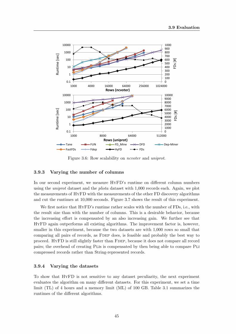
3.9 Evaluation
01002003004005006007008009001000
0.1
1
10
100
1000
10000
1000 4000 16000 64000 256000 1024000
FDs
[#]
Ru
nti
me
[se
c]
Rows (ncvoter)
010002000300040005000600070008000900010000
0.1
1
10
100
1000
10000
1000 8000 64000 512000
FDs
[#]
Ru
nti
me
[se
c]
Rows (uniprot) Tane FUN FD_Mine DFD Dep-Miner
FastFDs Fdep HyFD FDs
Figure 3.6: Row scalability on ncvoter and uniprot.
3.9.3 Varying the number of columns
In our second experiment, we measure HyFD’s runtime on different column numbers
using the uniprot dataset and the plista dataset with 1,000 records each. Again, we plot
the measurements of HyFD with the measurements of the other FD discovery algorithms
and cut the runtimes at 10,000 seconds. Figure 3.7 shows the result of this experiment.
We first notice that HyFD’s runtime rather scales with the number of FDs, i.e., with
the result size than with the number of columns. This is a desirable behavior, because
the increasing effort is compensated by an also increasing gain. We further see that
HyFD again outperforms all existing algorithms. The improvement factor is, however,
smaller in this experiment, because the two datasets are with 1,000 rows so small that
comparing all pairs of records, as Fdep does, is feasible and probably the best way to
proceed. HyFD is still slightly faster than Fdep, because it does not compare all record
pairs; the overhead of creating Plis is compensated by then being able to compare Pli
compressed records rather than String-represented records.
3.9.4 Varying the datasets
To show that HyFD is not sensitive to any dataset peculiarity, the next experiment
evaluates the algorithm on many different datasets. For this experiment, we set a time
limit (TL) of 4 hours and a memory limit (ML) of 100 GB. Table 3.1 summarizes the
runtimes of the different algorithms.
45

3. FUNCTIONAL DEPENDENCY DISCOVERY
Dataset
Cols
Row
sS
izeF
Ds
Tane
Fun
FD
Mine
Dfd
Dep-M
iner
Fast
FDs
Fdep
HyFD
[#]
[#]
[KB
][#
]
iris5
1505
41.1
0.1
0.20.2
0.20.2
0.1
0.1
balan
ce-scale5
6257
11.2
0.1
0.20.3
0.30.3
0.20.1
chess
728,056
5191
2.91.1
3.81.0
174.6
164
.2125.5
0.2
ab
alone
94,177
187137
2.10.6
1.81.1
3.02.9
3.8
0.2
nu
rsery9
12,9601,024
14.1
1.87.1
0.912
1.2118
.946.8
0.5
breast-can
cer11
69920
462.3
0.62.2
0.81.1
1.1
0.5
0.2
brid
ges13
1086
1422.2
0.64.2
0.90.5
0.6
0.2
0.1
echocard
iogram13
1326
5271.6
0.469.9
1.20.5
0.5
0.2
0.1
ad
ult
1448,842
3,52878
67.4111.6
531.55.9
6039.260
33.8
860.21.1
letter17
20,000695
61260.0
529.07204.8
6.01090.0
1015.5291.3
3.4
ncvoter
191,000
151758
4.34.0
ML
5.111.4
1.91.1
0.4
hep
atitis20
1558
8,25012.2
175.9M
L326.7
557
6.59.5
0.80.6
horse
27368
25128,727
457.0T
LM
LT
LT
L385
.87.2
7.1
fd-red
uced
-3030
250,00069,581
89,57141.1
77.7M
LT
L377.2
382.4
TL
513.0
plista
631,000
568178,152
ML
ML
ML
TL
TL
TL
26.921.8
flig
ht
1091,000
575982,631
ML
ML
ML
TL
TL
TL
216.553.4
un
iprot
2231,000
2,439>
2,437,556M
LM
LM
LT
LT
LT
LM
L>
5254.7
Resu
ltslarger
than
1,000F
Ds
areon
lycou
nted
TL
:tim
elim
itof
4h
ours
exceed
edM
L:
mem
orylim
itof
100
GB
exceed
ed
Tab
le3.1
:R
untim
esin
second
sfor
severalreal-w
orld
datasets.
Tane
[Hu
htala
etal.,
1999]Fun
[Novelli
and
Cicch
etti,2001]
FD
Mine
[Yao
etal.,
2002]Dfd
[Ab
edjan
etal.,
2014c]
Dep-M
iner
[Lop
eset
al.,2000]
Fast
FDs
[Wyss
etal.,
2001]Fdep
[Flach
and
Sav
nik
,1999]
HyFD
[Pap
enb
rock
and
Nau
man
n,
2016]
46
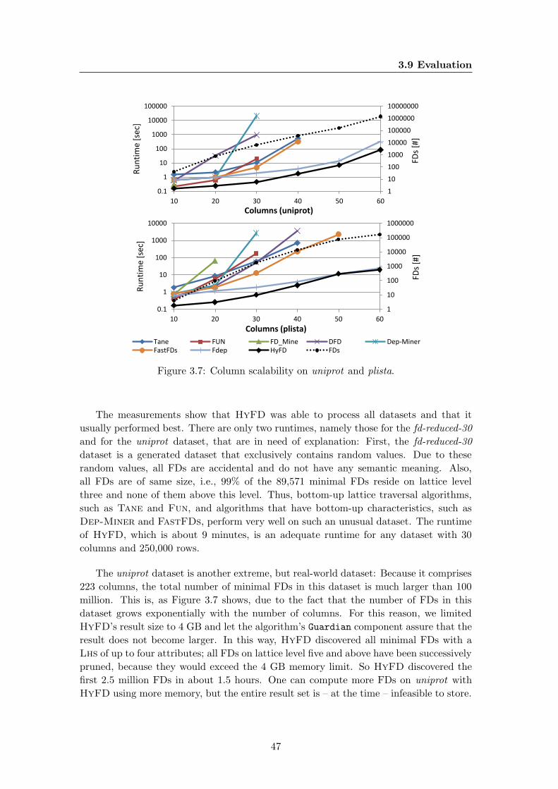
3.9 Evaluation
1
10
100
1000
10000
100000
1000000
10000000
0.1
1
10
100
1000
10000
100000
10 20 30 40 50 60
FDs
[#]
Ru
nti
me
[se
c]
Columns (uniprot)
1
10
100
1000
10000
100000
1000000
0.1
1
10
100
1000
10000
10 20 30 40 50 60
FDs
[#]
Ru
nti
me
[se
c]
Columns (plista)
Tane FUN FD_Mine DFD Dep-MinerFastFDs Fdep HyFD FDs
Figure 3.7: Column scalability on uniprot and plista.
The measurements show that HyFD was able to process all datasets and that it
usually performed best. There are only two runtimes, namely those for the fd-reduced-30
and for the uniprot dataset, that are in need of explanation: First, the fd-reduced-30
dataset is a generated dataset that exclusively contains random values. Due to these
random values, all FDs are accidental and do not have any semantic meaning. Also,
all FDs are of same size, i.e., 99% of the 89,571 minimal FDs reside on lattice level
three and none of them above this level. Thus, bottom-up lattice traversal algorithms,
such as Tane and Fun, and algorithms that have bottom-up characteristics, such as
Dep-Miner and FastFDs, perform very well on such an unusual dataset. The runtime
of HyFD, which is about 9 minutes, is an adequate runtime for any dataset with 30
columns and 250,000 rows.
The uniprot dataset is another extreme, but real-world dataset: Because it comprises
223 columns, the total number of minimal FDs in this dataset is much larger than 100
million. This is, as Figure 3.7 shows, due to the fact that the number of FDs in this
dataset grows exponentially with the number of columns. For this reason, we limited
HyFD’s result size to 4 GB and let the algorithm’s Guardian component assure that the
result does not become larger. In this way, HyFD discovered all minimal FDs with a
Lhs of up to four attributes; all FDs on lattice level five and above have been successively
pruned, because they would exceed the 4 GB memory limit. So HyFD discovered the
first 2.5 million FDs in about 1.5 hours. One can compute more FDs on uniprot with
HyFD using more memory, but the entire result set is – at the time – infeasible to store.
47
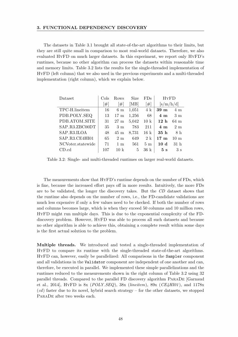
3. FUNCTIONAL DEPENDENCY DISCOVERY
The datasets in Table 3.1 brought all state-of-the-art algorithms to their limits, but
they are still quite small in comparison to most real-world datasets. Therefore, we also
evaluated HyFD on much larger datasets. In this experiment, we report only HyFD’s
runtimes, because no other algorithm can process the datasets within reasonable time
and memory limits. Table 3.2 lists the results for the single-threaded implementation of
HyFD (left column) that we also used in the previous experiments and a multi-threaded
implementation (right column), which we explain below.
Dataset Cols Rows Size FDs HyFD
[#] [#] [MB] [#] [s/m/h/d]
TPC-H.lineitem 16 6 m 1,051 4 k 39 m 4 m
PDB.POLY SEQ 13 17 m 1,256 68 4 m 3 m
PDB.ATOM SITE 31 27 m 5,042 10 k 12 h 64 m
SAP R3.ZBC00DT 35 3 m 783 211 4 m 2 m
SAP R3.ILOA 48 45 m 8,731 16 k 35 h 8 h
SAP R3.CE4HI01 65 2 m 649 2 k 17 m 10 m
NCVoter.statewide 71 1 m 561 5 m 10 d 31 h
CD.cd 107 10 k 5 36 k 5 s 3 s
Table 3.2: Single- and multi-threaded runtimes on larger real-world datasets.
The measurements show that HyFD’s runtime depends on the number of FDs, which
is fine, because the increased effort pays off in more results. Intuitively, the more FDs
are to be validated, the longer the discovery takes. But the CD dataset shows that
the runtime also depends on the number of rows, i.e., the FD-candidate validations are
much less expensive if only a few values need to be checked. If both the number of rows
and columns becomes large, which is when they exceed 50 columns and 10 million rows,
HyFD might run multiple days. This is due to the exponential complexity of the FD-
discovery problem. However, HyFD was able to process all such datasets and because
no other algorithm is able to achieve this, obtaining a complete result within some days
is the first actual solution to the problem.
Multiple threads. We introduced and tested a single-threaded implementation of
HyFD to compare its runtime with the single-threaded state-of-the-art algorithms.
HyFD can, however, easily be parallelized: All comparisons in the Sampler component
and all validations in the Validator component are independent of one another and can,
therefore, be executed in parallel. We implemented these simple parallelizations and the
runtimes reduced to the measurements shown in the right column of Table 3.2 using 32
parallel threads. Compared to the parallel FD discovery algorithm ParaDe [Garnaud
et al., 2014], HyFD is 8x (POLY SEQ), 38x (lineitem), 89x (CE4HI01 ), and 1178x
(cd) faster due to its novel, hybrid search strategy – for the other datasets, we stopped
ParaDe after two weeks each.
48
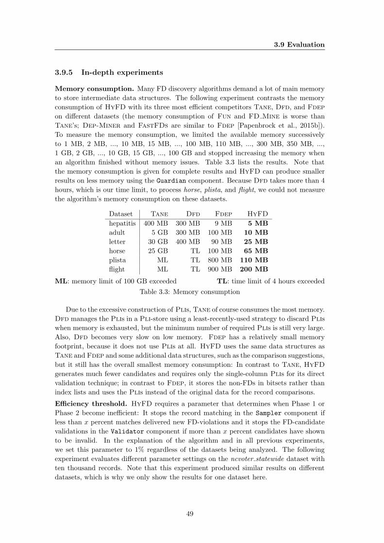
3.9 Evaluation
3.9.5 In-depth experiments
Memory consumption. Many FD discovery algorithms demand a lot of main memory
to store intermediate data structures. The following experiment contrasts the memory
consumption of HyFD with its three most efficient competitors Tane, Dfd, and Fdep
on different datasets (the memory consumption of Fun and FD Mine is worse than
Tane’s; Dep-Miner and FastFDs are similar to Fdep [Papenbrock et al., 2015b]).
To measure the memory consumption, we limited the available memory successively
to 1 MB, 2 MB, ..., 10 MB, 15 MB, ..., 100 MB, 110 MB, ..., 300 MB, 350 MB, ...,
1 GB, 2 GB, ..., 10 GB, 15 GB, ..., 100 GB and stopped increasing the memory when
an algorithm finished without memory issues. Table 3.3 lists the results. Note that
the memory consumption is given for complete results and HyFD can produce smaller
results on less memory using the Guardian component. Because Dfd takes more than 4
hours, which is our time limit, to process horse, plista, and flight, we could not measure
the algorithm’s memory consumption on these datasets.
Dataset Tane Dfd Fdep HyFD
hepatitis 400 MB 300 MB 9 MB 5 MB
adult 5 GB 300 MB 100 MB 10 MB
letter 30 GB 400 MB 90 MB 25 MB
horse 25 GB TL 100 MB 65 MB
plista ML TL 800 MB 110 MB
flight ML TL 900 MB 200 MB
ML: memory limit of 100 GB exceeded TL: time limit of 4 hours exceeded
Table 3.3: Memory consumption
Due to the excessive construction of Plis, Tane of course consumes the most memory.
Dfd manages the Plis in a Pli-store using a least-recently-used strategy to discard Plis
when memory is exhausted, but the minimum number of required Plis is still very large.
Also, Dfd becomes very slow on low memory. Fdep has a relatively small memory
footprint, because it does not use Plis at all. HyFD uses the same data structures as
Tane and Fdep and some additional data structures, such as the comparison suggestions,
but it still has the overall smallest memory consumption: In contrast to Tane, HyFD
generates much fewer candidates and requires only the single-column Plis for its direct
validation technique; in contrast to Fdep, it stores the non-FDs in bitsets rather than
index lists and uses the Plis instead of the original data for the record comparisons.
Efficiency threshold. HyFD requires a parameter that determines when Phase 1 or
Phase 2 become inefficient: It stops the record matching in the Sampler component if
less than x percent matches delivered new FD-violations and it stops the FD-candidate
validations in the Validator component if more than x percent candidates have shown
to be invalid. In the explanation of the algorithm and in all previous experiments,
we set this parameter to 1% regardless of the datasets being analyzed. The following
experiment evaluates different parameter settings on the ncvoter statewide dataset with
ten thousand records. Note that this experiment produced similar results on different
datasets, which is why we only show the results for one dataset here.
49
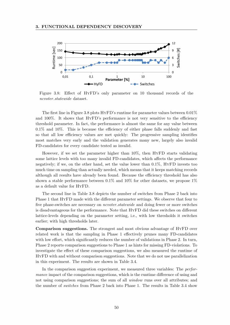
3. FUNCTIONAL DEPENDENCY DISCOVERY
0
3
6
9
12
0
50
100
150
200
0,01 0,1 1 10 100
Swit
ches
[#
]
Ru
nti
me
[se
c]
Parameter [%] HyFD Switches
Figure 3.8: Effect of HyFD’s only parameter on 10 thousand records of the
ncvoter statewide dataset.
The first line in Figure 3.8 plots HyFD’s runtime for parameter values between 0.01%
and 100%. It shows that HyFD’s performance is not very sensitive to the efficiency
threshold parameter. In fact, the performance is almost the same for any value between
0.1% and 10%. This is because the efficiency of either phase falls suddenly and fast
so that all low efficiency values are met quickly: The progressive sampling identifies
most matches very early and the validation generates many new, largely also invalid
FD-candidates for every candidate tested as invalid.
However, if we set the parameter higher than 10%, then HyFD starts validating
some lattice levels with too many invalid FD-candidates, which affects the performance
negatively; if we, on the other hand, set the value lower than 0.1%, HyFD invests too
much time on sampling than actually needed, which means that it keeps matching records
although all results have already been found. Because the efficiency threshold has also
shown a stable performance between 0.1% and 10% for other datasets, we propose 1%
as a default value for HyFD.
The second line in Table 3.8 depicts the number of switches from Phase 2 back into
Phase 1 that HyFD made with the different parameter settings. We observe that four to
five phase-switches are necessary on ncvoter statewide and doing fewer or more switches
is disadvantageous for the performance. Note that HyFD did these switches on different
lattice-levels depending on the parameter setting, i.e., with low thresholds it switches
earlier; with high thresholds later.
Comparison suggestions. The strongest and most obvious advantage of HyFD over
related work is that the sampling in Phase 1 effectively prunes many FD-candidates
with low effort, which significantly reduces the number of validations in Phase 2. In turn,
Phase 2 reports comparison suggestions to Phase 1 as hints for missing FD-violations. To
investigate the effect of these comparison suggestions, we also measured the runtime of
HyFD with and without comparison suggestions. Note that we do not use parallelization
in this experiment. The results are shown in Table 3.4.
In the comparison suggestion experiment, we measured three variables: The perfor-
mance impact of the comparison suggestions, which is the runtime difference of using and
not using comparison suggestions; the sum of all window runs over all attributes; and
the number of switches from Phase 2 back into Phase 1. The results in Table 3.4 show
50
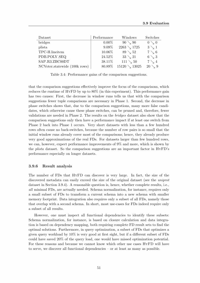
3.9 Evaluation
Dataset Performance Windows Switches
bridges 0.00% 90 ↘ 90 0 ↘ 0
plista 9.09% 2263 ↘ 1725 3 ↘ 1
TPC-H.lineitem 10.06% 89 ↘ 52 7 ↘ 6
PDB.POLY SEQ 24.52% 33 ↘ 21 6 ↘ 3
SAP R3.ZBC00DT 38.11% 111 ↘ 50 7 ↘ 4
NCVoter.statewide (100k rows) 80.89% 15120 ↘ 13025 20 ↘ 9
Table 3.4: Performance gains of the comparison suggestions.
that the comparison suggestions effectively improve the focus of the comparisons, which
reduces the runtime of HyFD by up to 80% (in this experiment). This performance gain
has two causes: First, the decrease in window runs tells us that with the comparison
suggestions fewer tuple comparisons are necessary in Phase 1. Second, the decrease in
phase switches shows that, due to the comparison suggestions, many more false candi-
dates, which otherwise cause these phase switches, can be pruned and, therefore, fewer
validations are needed in Phase 2. The results on the bridges dataset also show that the
comparison suggestions only then have a performance impact if at least one switch from
Phase 2 back into Phase 1 occurs. Very short datasets with less than a few hundred
rows often cause no back-switches, because the number of row pairs is so small that the
initial window runs already cover most of the comparisons; hence, they already produce
very good approximations of the real FDs. For datasets larger than few hundred rows,
we can, however, expect performance improvements of 9% and more, which is shown by
the plista dataset. So the comparison suggestions are an important factor in HyFD’s
performance especially on longer datasets.
3.9.6 Result analysis
The number of FDs that HyFD can discover is very large. In fact, the size of the
discovered metadata can easily exceed the size of the original dataset (see the uniprot
dataset in Section 3.9.4). A reasonable question is, hence, whether complete results, i.e.,
all minimal FDs, are actually needed. Schema normalization, for instance, requires only
a small subset of FDs to transform a current schema into a new schema with smaller
memory footprint. Data integration also requires only a subset of all FDs, namely those
that overlap with a second schema. In short, most use-cases for FDs indeed require only
a subset of all results.
However, one must inspect all functional dependencies to identify these subsets:
Schema normalization, for instance, is based on closure calculation and data integra-
tion is based on dependency mapping, both requiring complete FD result sets to find the
optimal solutions. Furthermore, in query optimization, a subset of FDs that optimizes a
given query workload by 10% is very good at first sight, but if a different subset of FDs
could have saved 20% of the query load, one would have missed optimization potential.
For these reasons and because we cannot know which other use cases HyFD will have
to serve, we discover all functional dependencies – or at least as many as possible.
51
3. FUNCTIONAL DEPENDENCY DISCOVERY
3.10 Conclusion & Future Work
In this chapter, we proposed HyFD, a hybrid FD discovery algorithm that discovers
all minimal, non-trivial functional dependencies in relational datasets. Because HyFD
combines row- and column-efficient discovery techniques, it is able to process datasets
that are both long and wide. This makes HyFD the first algorithm that can process
datasets of relevant real-world size, i.e., datasets with more than 50 attributes and a
million records. On smaller datasets, which some other FD discovery algorithms can
already process, HyFD offers the smallest memory footprints and the fastest runtimes;
in many cases, our algorithm is orders of magnitude faster than the best state-of-the-
art algorithm. Because the number of FDs can grow exponentially with the number of
attributes, we also proposed a component that dynamically prunes the result set, if the
available memory is exhausted.
The two-phased search technique of HyFD has also inspired the development of
other algorithms in the area of dependency discovery. Our algorithm Aid-FD [Bleifuß
et al., 2016], for example, uses the same combination of sampling and validation phases
to discover approximate FDs, i.e., we sacrifice the guarantee for a correct result in return
for further performance improvements. Other sister algorithms of HyFD are MvdDe-
tector [Draeger, 2016], an algorithm for the discovery of multivalued dependencies, and
Hydra [Bleifuß, 2016], an algorithm for the discovery of denial constraints. In the next
chapter, we also present HyUCC, a sister algorithm of HyFD that discovers all unique
column combinations in relational datasets.
A task for future work in FD discovery is the development of use-case-specific al-
gorithms that leverage FD result sets for query optimization, data integration, data
cleansing, and many other tasks. In addition, knowledge of the use-case might help
develop specific semantic pruning rules to further speed-up detection. The only general
semantic pruning we found was removing FDs with largest left-hand-sides, because these
are most prone to being accidental, and we only apply it when absolutely necessary.
52

4
Unique Column Combination
Discovery
Given a relational datasets, the discovery of unique column combinations is a task that
aims to automatically detect all unique column combinations, i.e., attribute sets whose
projection has no duplicate entries. To achieve this, it suffices to find all minimal UCCs,
because we can infer all other UCCs with Armstrong’s augmentation rule (see Sec-
tion 2.2.2). Furthermore, most use cases, such as database key discovery [Mancas, 2016],
are interested in only the minimal UCCs. The need for unique column combinations in
many applications has led to the development of various discovery algorithms, such as
Gordian [Sismanis et al., 2006], Hca [Abedjan and Naumann, 2011], and Ducc [Heise
et al., 2013]. All these approaches experience serious difficulties when datasets of typical
real-world size, i.e., datasets with more than 50 attributes and a million records, need
to be processed. Similar to the task of FD discovery, this is because most of these algo-
rithms focus on only one discovery strategy that either performs well for many columns
or many rows in a dataset.
In this chapter, we present the hybrid discovery algorithm HyUCC that automati-
cally detects all minimal unique column combinations in relational datasets. This algo-
rithm and most parts of this chapter have been published in [Papenbrock and Naumann,
2017a]. HyUCC uses the same combination of row- and column-efficient techniques as
its sister algorithm HyFD, which we introduced in Chapter 3: The interplay of fast
candidate approximation and efficient candidate validation allows HyUCC to process
datasets that are both wide and long. The hybrid search not only outperforms all exist-
ing approaches, it also scales to much larger datasets. In fact, with HyUCC the discovery
time becomes less of an issue than the ability of the executing machine to cope with the
size of the UCC result set, which can grow exponentially large. The main contributions
of HyUCC can thus be summarized as follows:
The two algorithms HyFD and HyUCC are, in fact, very similar, which means that
only few changes are necessary to let HyUCC discover UCCs instead of FDs. These
changes are, in a nutshell: the use of a prefix tree for UCCs, a cover inversion algorithm
for UCCs, a candidate validation function for UCCs, and pruning rules for UCCs. As
these changes are relatively straightforward, the main contribution of HyUCC and its
53
4. UNIQUE COLUMN COMBINATION DISCOVERY
evaluation is a proof of concept that the hybrid discovery strategies, which we originally
developed for FD discovery, work as well for other discovery problems in data profiling.
The remainder of chapter is structured as follows: Section 4.1first discusses related
work. Then, we introduce the intuition of our hybrid approach for UCCs in Section 4.2.
Section 4.3 shows how these ideas can be algorithmically implemented and emphasizes
the differences between HyUCC and HyFD. In Section 4.4, we evaluate our algorithm
and conclude in Section 4.5.
4.1 Related Work
There are basically two classes of UCC discovery algorithms: row-based discovery al-
gorithms, such as Gordian [Sismanis et al., 2006], and column-based algorithms, such
as Hca [Abedjan and Naumann, 2011]. Row-based algorithms compare pairs of records
in the dataset, derive so-called agree or disagree sets, and finally derive the UCCs from
these sets. This discovery strategy performs well with increasing numbers of attributes,
but falls short when the number of rows is high. Column-based algorithms model the
search space as a powerset lattice and then traverse this lattice to identify the UCCs.
The traversal strategies usually differ, but all algorithms of this kind make extensive use
of pruning rules, i.e., they remove subsets of falsified candidates from the search space
(these must be false as well) and supersets of validated candidates (which must be valid
and not minimal). The column-based family of discovery algorithms scales well with
larger numbers of records, but large numbers of attributes render them infeasible. Be-
cause both row- and column-efficient algorithms have their strengths, we combine these
two search strategies in our HyUCC algorithm.
A previous, efficient UCC discovery algorithm, which also belongs to the column-
based algorithm family, is Ducc [Heise et al., 2013]. The algorithm pursues a random
walk approach in the search space lattice to maximize the effect of the known superset-
und subset-pruning rules. Because this algorithm was shown to be faster than both
Gordian and Hca, it serves as a baseline for our evaluation.
4.2 Hybrid UCC discovery
The core idea of hybrid UCC discovery is to combine techniques from column-based
and row-based discovery algorithms into one algorithm that automatically switches back
and forth between these techniques, depending on which technique currently performs
better. The challenge for these switches is to decide when to switch and to convert the
intermediate results from one model into the other, which is necessary to let the strategies
support each other. In the following, we first describe the two discovery strategies for
UCCs; then, we discuss when and how intermediate results can be synchronized.
Row-efficient strategy. Column-based UCC discovery algorithms, which are the fam-
ily of algorithms that perform well on many rows, model the search space as a powerset
lattice of attribute combinations where each node represents a UCC candidate. The
54
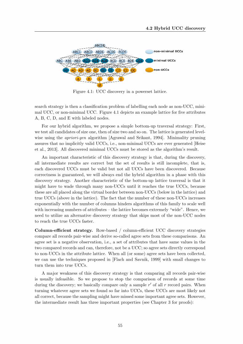
4.2 Hybrid UCC discovery
Figure 4.1: UCC discovery in a powerset lattice.
search strategy is then a classification problem of labelling each node as non-UCC, mini-
mal UCC, or non-minimal UCC. Figure 4.1 depicts an example lattice for five attributes
A, B, C, D, and E with labeled nodes.
For our hybrid algorithm, we propose a simple bottom-up traversal strategy: First,
we test all candidates of size one, then of size two and so on. The lattice is generated level-
wise using the apriori-gen algorithm [Agrawal and Srikant, 1994]. Minimality pruning
assures that no implicitly valid UCCs, i.e., non-minimal UCCs are ever generated [Heise
et al., 2013]. All discovered minimal UCCs must be stored as the algorithm’s result.
An important characteristic of this discovery strategy is that, during the discovery,
all intermediate results are correct but the set of results is still incomplete, that is,
each discovered UCCs must be valid but not all UCCs have been discovered. Because
correctness is guaranteed, we will always end the hybrid algorithm in a phase with this
discovery strategy. Another characteristic of the bottom-up lattice traversal is that it
might have to wade through many non-UCCs until it reaches the true UCCs, because
these are all placed along the virtual border between non-UCCs (below in the lattice) and
true UCCs (above in the lattice). The fact that the number of these non-UCCs increases
exponentially with the number of columns hinders algorithms of this family to scale well
with increasing numbers of attributes – the lattice becomes extremely “wide”. Hence, we
need to utilize an alternative discovery strategy that skips most of the non-UCC nodes
to reach the true UCCs faster.
Column-efficient strategy. Row-based / column-efficient UCC discovery strategies
compare all records pair-wise and derive so-called agree sets from these comparisons. An
agree set is a negative observation, i.e., a set of attributes that have same values in the
two compared records and can, therefore, not be a UCC; so agree sets directly correspond
to non-UCCs in the attribute lattice. When all (or some) agree sets have been collected,
we can use the techniques proposed in [Flach and Savnik, 1999] with small changes to
turn them into true UCCs.
A major weakness of this discovery strategy is that comparing all records pair-wise
is usually infeasible. So we propose to stop the comparison of records at some time
during the discovery; we basically compare only a sample r′ of all r record pairs. When
turning whatever agree sets we found so far into UCCs, these UCCs are most likely not
all correct, because the sampling might have missed some important agree sets. However,
the intermediate result has three important properties (see Chapter 3 for proofs):
55
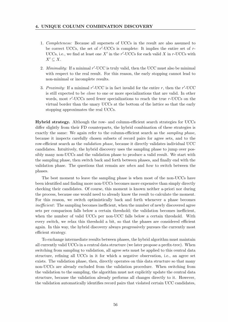
4. UNIQUE COLUMN COMBINATION DISCOVERY
1. Completeness: Because all supersets of UCCs in the result are also assumed to
be correct UCCs, the set of r′-UCCs is complete: It implies the entire set of r-
UCCs, i.e., we find at least one X ′ in the r′-UCCs for each valid X in r-UCCs with
X ′ ⊆ X.
2. Minimality: If a minimal r′-UCC is truly valid, then the UCC must also be minimal
with respect to the real result. For this reason, the early stopping cannot lead to
non-minimal or incomplete results.
3. Proximity: If a minimal r′-UCC is in fact invalid for the entire r, then the r′-UCC
is still expected to be close to one or more specializations that are valid. In other
words, most r′-UCCs need fewer specializations to reach the true r-UCCs on the
virtual border than the unary UCCs at the bottom of the lattice so that the early
stopping approximates the real UCCs.
Hybrid strategy. Although the row- and column-efficient search strategies for UCCs
differ slightly from their FD counterparts, the hybrid combination of these strategies is
exactly the same: We again refer to the column-efficient search as the sampling phase,
because it inspects carefully chosen subsets of record pairs for agree sets, and to the
row-efficient search as the validation phase, because it directly validates individual UCC
candidates. Intuitively, the hybrid discovery uses the sampling phase to jump over pos-
sibly many non-UCCs and the validation phase to produce a valid result. We start with
the sampling phase, then switch back and forth between phases, and finally end with the
validation phase. The questions that remain are when and how to switch between the
phases.
The best moment to leave the sampling phase is when most of the non-UCCs have
been identified and finding more non-UCCs becomes more expensive than simply directly
checking their candidates. Of course, this moment is known neither a-priori nor during
the process, because one would need to already know the result to calculate the moment.
For this reason, we switch optimistically back and forth whenever a phase becomes
inefficient : The sampling becomes inefficient, when the number of newly discovered agree
sets per comparison falls below a certain threshold; the validation becomes inefficient,
when the number of valid UCCs per non-UCC falls below a certain threshold. With
every switch, we relax this threshold a bit, so that the phases are considered efficient
again. In this way, the hybrid discovery always progressively pursues the currently most
efficient strategy.
To exchange intermediate results between phases, the hybrid algorithm must maintain
all currently valid UCCs in a central data structure (we later propose a prefix-tree). When
switching from sampling to validation, all agree sets must be applied to this central data
structure, refining all UCCs in it for which a negative observation, i.e., an agree set
exists. The validation phase, then, directly operates on this data structure so that many
non-UCCs are already excluded from the validation procedure. When switching from
the validation to the sampling, the algorithm must not explicitly update the central data
structure, because the validation already performs all changes directly to it. However,
the validation automatically identifies record pairs that violated certain UCC candidates,
56
4.3 The HyUCC algorithm
and these record pairs should be suggested to the sampling phase for full comparisons as
it is very likely that they indicate larger agree sets. In this way, both phases can benefit
from one another, as we already showed for FDs in Section 3.9.5.
4.3 The HyUCC algorithm
We now describe our implementation of the hybrid UCC discovery strategy HyUCC.
Because this algorithm is largely equal to the FD discovery algorithm HyFD, we omit
various details that can be found in Chapter 3. The differences that make HyUCC
discover unique column combinations instead of functional dependencies are in particular
a prefix tree (trie) to store the UCCs, a cover inversion algorithm for UCCs, a UCC-
specific validation, and UCC-specific pruning rules.
HyUCC
records
plis, pliRecords
non-UCCs
candidate-UCCs
UCCs
plis, pliRecords
comparisonSuggestions
results
UCC
Validator
dataset
UCC Candidate
Inductor
Record Pair
Sampler
Memory
Guardian
Data
Preprocessor Control- and data-flow:
Main
Side
Components:
Main
Optional
Symbols
Figure 4.2: Overview of HyUCC and its components.
Figure 4.2 gives an overview of HyUCC and its components. Given a relational
dataset as a collection of records, the algorithm first runs them through a Preprocessor
component that transforms the records into the two smaller index structures Plis and
PliRecords. Then, HyUCC starts the sampling phase in the Sampler component. When
the sampling has become inefficient, the algorithm passes the discovered agree sets, i.e.,
the non-UCCs, to the Inductor component, which turns them into candidate-UCCs:
UCCs that hold true on the sample of record pairs that was seen so far. Afterwards,
the algorithm switches to the validation phase in the Validator component. This com-
ponent systematically (level-wise, bottom-up) checks and creates candidate-UCCs. If
the checking becomes inefficient, HyUCC switches back into the sampling phase hand-
ing over a set of comparison suggestions; otherwise, the validation continues until all
candidates have been checked and all true UCCs can be returned. We now discuss the
components of HyUCC in more detail.
Data Preprocessor. The Preprocessor in HyUCC is the same as the Preprocessor
HyFD: It transforms all records into compact position list indexes (Plis) and dictionary
compressed PliRecords. These two data structures are needed for the record compar-
isons in the Sampler component and the UCC candidate validations in the Validator
component.
57
4. UNIQUE COLUMN COMBINATION DISCOVERY
Record Pair Sampler. The Sampler component compares the PliRecords to derive
agree sets, i.e., non-UCCs. As stated earlier, a non-UCC is simply a set of attributes
that have same values in at least two records. Because the sampling phase should be
maximally efficient, the Sampler chooses the record pairs for the comparisons deliber-
ately: Record pairs that are more likely to reveal non-UCCs are progressively chosen
earlier in the process and less promising record pairs later. Intuitively, the more values
two records share, the higher their probability of delivering a new non-UCC is. Vice
versa, records that do not share any values cannot deliver any non-UCC and should not
be compared at all.
To focus the comparisons on those record pairs that share possibly many values,
we use these same progressive strategy as in the HyFD algorithm: Because the Plis
group records with at least one identical value, HyUCC compares only records within
same Pli clusters. For all records within same Pli clusters, we must define a possibly
effective comparison order. For this purpose, we again first sort all clusters in all Plis
with a different sorting key (see Section 3.5). This produces different neighborhoods for
each record in each of the record’s clusters, even if the record co-occurs with same other
records in its clusters. After sorting, the Sampler iterates all Plis and compares each
record to its direct neighbor. In this step, the algorithm also calculates the number of
discovered non-UCCs per comparison for each Pli. This number indicates the sampling
efficiency achieved with this particular Pli. In a third step, the Sampler can then rank
the different Plis by their efficiency, pick the most efficient Pli, and use it to compare
each record to its second neighbor. This comparison run updates the efficiency of the
used Pli, so that it is re-ranked with the other. The Sampler then again picks the most
efficient Pli for the next round of comparisons. This process of comparing records to
their n+1 next neighbors progressively chooses most promising comparisons; it continues
until the top ranked Pli is not efficient any more, which is the condition to switch to
the validation phase.
UCC Candidate Inductor. The Inductor component updates the intermediate result
of UCCs with the non-UCCs from the Sampler component. We store these UCCs in a
prefix tree, i.e., a trie, where each node represents exactly one attribute and each path
a UCC. Such a UCC tree allows for fast subset-lookups, which is the most frequent
operation on the intermediate results of UCCs. The UCC tree in HyUCC is much
leaner than the FD tree used in HyFD, because no additional right-hand-sides must be
stored in the nodes; the paths alone suffice to identify the UCCs.
Initially, the UCC tree contains all individual attributes, assuming that each of them
is unique. The Inductor then refines this initial UCC tree with every non-UCC that it
receives from the Sampler: For every non-UCC, remove the UCC and all of its subsets
from the UCC tree, because these must all be non-unique. Then, create all possible
specializations of each removed non-UCC by adding one additional attribute; these could
still be true UCCs. For each specialization, check the UCC tree for existing subsets
(generalizations) or supersets (specialization). If a generalization exists, the created
UCC is not minimal; if a specialization exists, it is invalid. In both cases, we ignore the
generated UCC; otherwise, we add it to the UCC tree as a new candidate.
58
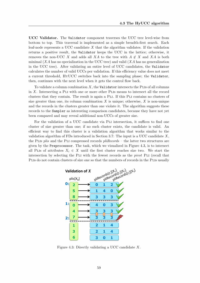
4.3 The HyUCC algorithm
UCC Validator. The Validator component traverses the UCC tree level-wise from
bottom to top. This traversal is implemented as a simple breadth-first search. Each
leaf-node represents a UCC candidate X that the algorithm validates. If the validation
returns a positive result, the Validator keeps the UCC in the lattice; otherwise, it
removes the non-UCC X and adds all XA to the tree with A 6∈ X and XA is both
minimal (XA has no specialization in the UCC tree) and valid (XA has no generalization
in the UCC tree). After validating an entire level of UCC candidates, the Validator
calculates the number of valid UCCs per validation. If this efficiency value does not meet
a current threshold, HyUCC switches back into the sampling phase; the Validator,
then, continues with the next level when it gets the control flow back.
To validate a column combination X, the Validator intersects the Plis of all columns
in X. Intersecting a Pli with one or more other Plis means to intersect all the record
clusters that they contain. The result is again a Pli. If this Pli contains no clusters of
size greater than one, its column combination X is unique; otherwise, X is non-unique
and the records in the clusters greater than one violate it. The algorithm suggests these
records to the Sampler as interesting comparison candidates, because they have not yet
been compared and may reveal additional non-UCCs of greater size.
For the validation of a UCC candidate via Pli intersection, it suffices to find one
cluster of size greater than one; if no such cluster exists, the candidate is valid. An
efficient way to find this cluster is a validation algorithm that works similar to the
validation algorithm of FDs introduced in Section 3.7: The input is a UCC candidate X,
the Plis plis and the Pli compressed records pliRecords – the latter two structures are
given by the Preprocessor. The task, which we visualized in Figure 4.3, is to intersect
all Plis of attributes Xi ∈ X until the first cluster reaches size two. We start the
intersection by selecting the Pli with the fewest records as the pivot Pli (recall that
Plis do not contain clusters of size one so that the numbers of records in the Plis usually
plis[X0]
Validation of 𝑿
2
5
8
0
4
7
1
3
6
0 1 2
3 3 3
1 4 0
4 0 3
3 3 3
3 3 3
2 1 4
2 1 4
3 0 1
0:
1:
2:
Figure 4.3: Directly validating a UCC candidate X.
59
4. UNIQUE COLUMN COMBINATION DISCOVERY
differ). This pivot Pli requires the least number of intersection look-ups with the other
Plis to become unique. For each cluster in the pivot Pli, the validation algorithm now
does the following: It iterates all record IDs and, for each record ID, looks-up the cluster
numbers of all other attributes of X in the pliRecords ; then, it stores each retrieved list
of cluster numbers in a set – each element represents a cluster of the intersection result
and contains, if the candidate is a unique, only one record. If this set already contains
a cluster number sequence equal to the sequence the Validator wants to insert, then
the algorithm found a violation and can stop the validation process for this candidate.
In Figure 4.3, this happens in the second cluster. The current record and the record
referring to the cluster number sequence in the set are, in the end, sent to the Sampler
as a new comparison suggestion.
Memory Guardian. The Guardian is an optional component that monitors the mem-
ory consumption of HyUCC. If at any point the memory threatens to become exhausted,
this component gradually reduces the maximum size of UCCs in the result until suffi-
cient memory becomes available. Of course, the result is then not complete any more,
but correctness and minimality of all reported UCCs is still guaranteed. Also, the result
limitation only happens if the result becomes so large that the executing machine cannot
store it any more; other algorithms would break in such cases. To reduce the size, the
Guardian deletes all agree sets and UCC candidates that exceed a certain maximum size.
It then forbids further insertions of any new elements of this or greater size.
4.4 Evaluation
We evaluate HyUCC and compare it to its sister algorithm HyFD [Papenbrock and
Naumann, 2016] and to the state-of-the-art UCC discovery algorithm Ducc [Heise et al.,
2013]. All three algorithms have been implemented for our Metanome data profiling
framework (www.metanome.de) in order to use the framework’s standard functionality
for data I/O and result management. Our experiments use a Dell PowerEdge R620
with two Intel Xeon E5-2650 2.00 GHz CPUs and 128 GB RAM. The server runs on
CentOS 6.4 and uses OpenJDK 64-Bit Server VM 1.7.0 25 as Java environment. Details
about our experimental datasets can be found in Section 3.9 and on our repeatability
website1. Note that the experiments use the null = null semantics, because this was
also used in related work; HyUCC can compute UCCs with null 6= null as well, which
makes the search faster, because columns with null values become unique more quickly.
4.4.1 Varying the datasets
In this first experiment, we measure the discovery times for the three algorithms on eight
real-world datasets. The datasets, their characteristics, and the runtimes are listed in
Table 4.1. The results show that HyUCC clearly outperforms the current state-of-the-
art algorithm Ducc: On most datasets, HyUCC is about 4 times faster than Ducc;
on the flight dataset, it is even more than 1,000 times faster. Only on zbc00dt Ducc
1www.hpi.de/naumann/projects/repeatability.html
60
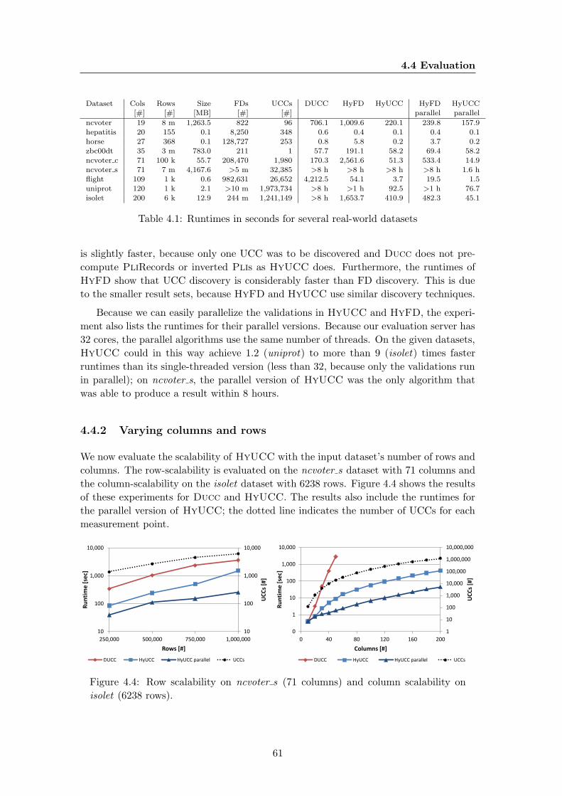
4.4 Evaluation
Dataset Cols Rows Size FDs UCCs DUCC HyFD HyUCC HyFD HyUCC[#] [#] [MB] [#] [#] parallel parallel
ncvoter 19 8 m 1,263.5 822 96 706.1 1,009.6 220.1 239.8 157.9hepatitis 20 155 0.1 8,250 348 0.6 0.4 0.1 0.4 0.1horse 27 368 0.1 128,727 253 0.8 5.8 0.2 3.7 0.2zbc00dt 35 3 m 783.0 211 1 57.7 191.1 58.2 69.4 58.2ncvoter c 71 100 k 55.7 208,470 1,980 170.3 2,561.6 51.3 533.4 14.9ncvoter s 71 7 m 4,167.6 >5 m 32,385 >8 h >8 h >8 h >8 h 1.6 hflight 109 1 k 0.6 982,631 26,652 4,212.5 54.1 3.7 19.5 1.5uniprot 120 1 k 2.1 >10 m 1,973,734 >8 h >1 h 92.5 >1 h 76.7isolet 200 6 k 12.9 244 m 1,241,149 >8 h 1,653.7 410.9 482.3 45.1
Table 4.1: Runtimes in seconds for several real-world datasets
is slightly faster, because only one UCC was to be discovered and Ducc does not pre-
compute PliRecords or inverted Plis as HyUCC does. Furthermore, the runtimes of
HyFD show that UCC discovery is considerably faster than FD discovery. This is due
to the smaller result sets, because HyFD and HyUCC use similar discovery techniques.
Because we can easily parallelize the validations in HyUCC and HyFD, the experi-
ment also lists the runtimes for their parallel versions. Because our evaluation server has
32 cores, the parallel algorithms use the same number of threads. On the given datasets,
HyUCC could in this way achieve 1.2 (uniprot) to more than 9 (isolet) times faster
runtimes than its single-threaded version (less than 32, because only the validations run
in parallel); on ncvoter s, the parallel version of HyUCC was the only algorithm that
was able to produce a result within 8 hours.
4.4.2 Varying columns and rows
We now evaluate the scalability of HyUCC with the input dataset’s number of rows and
columns. The row-scalability is evaluated on the ncvoter s dataset with 71 columns and
the column-scalability on the isolet dataset with 6238 rows. Figure 4.4 shows the results
of these experiments for Ducc and HyUCC. The results also include the runtimes for
the parallel version of HyUCC; the dotted line indicates the number of UCCs for each
measurement point.
10
100
1,000
10,000
10
100
1,000
10,000
250,000 500,000 750,000 1,000,000
UC
Cs
[#]
Ru
nti
me
[se
c]
Rows [#]
DUCC HyUCC HyUCC parallel UCCs
1
10
100
1,000
10,000
100,000
1,000,000
10,000,000
0
1
10
100
1,000
10,000
0 40 80 120 160 200
UC
Cs
[#]
Ru
nti
me
[se
c]
Columns [#]
DUCC HyUCC HyUCC parallel UCCs
Figure 4.4: Row scalability on ncvoter s (71 columns) and column scalability on
isolet (6238 rows).
61
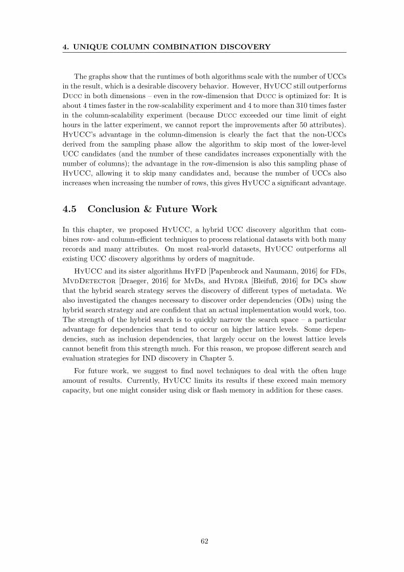
4. UNIQUE COLUMN COMBINATION DISCOVERY
The graphs show that the runtimes of both algorithms scale with the number of UCCs
in the result, which is a desirable discovery behavior. However, HyUCC still outperforms
Ducc in both dimensions – even in the row-dimension that Ducc is optimized for: It is
about 4 times faster in the row-scalability experiment and 4 to more than 310 times faster
in the column-scalability experiment (because Ducc exceeded our time limit of eight
hours in the latter experiment, we cannot report the improvements after 50 attributes).
HyUCC’s advantage in the column-dimension is clearly the fact that the non-UCCs
derived from the sampling phase allow the algorithm to skip most of the lower-level
UCC candidates (and the number of these candidates increases exponentially with the
number of columns); the advantage in the row-dimension is also this sampling phase of
HyUCC, allowing it to skip many candidates and, because the number of UCCs also
increases when increasing the number of rows, this gives HyUCC a significant advantage.
4.5 Conclusion & Future Work
In this chapter, we proposed HyUCC, a hybrid UCC discovery algorithm that com-
bines row- and column-efficient techniques to process relational datasets with both many
records and many attributes. On most real-world datasets, HyUCC outperforms all
existing UCC discovery algorithms by orders of magnitude.
HyUCC and its sister algorithms HyFD [Papenbrock and Naumann, 2016] for FDs,
MvdDetector [Draeger, 2016] for MvDs, and Hydra [Bleifuß, 2016] for DCs show
that the hybrid search strategy serves the discovery of different types of metadata. We
also investigated the changes necessary to discover order dependencies (ODs) using the
hybrid search strategy and are confident that an actual implementation would work, too.
The strength of the hybrid search is to quickly narrow the search space – a particular
advantage for dependencies that tend to occur on higher lattice levels. Some depen-
dencies, such as inclusion dependencies, that largely occur on the lowest lattice levels
cannot benefit from this strength much. For this reason, we propose different search and
evaluation strategies for IND discovery in Chapter 5.
For future work, we suggest to find novel techniques to deal with the often huge
amount of results. Currently, HyUCC limits its results if these exceed main memory
capacity, but one might consider using disk or flash memory in addition for these cases.
62
5
Inclusion Dependency Discovery
The discovery of all inclusion dependencies in a relational dataset is an important part
of any data profiling effort. Apart from the detection of foreign key relationships, INDs
support data integration, query optimization, integrity checking, schema (re-)design, and
many further use cases. We have shown in Section 2.4 that the discovery of inclusion
dependencies is one of the hardest tasks in data profiling: Appart from the complexity of
the search problem, aggravating circumstances are the relatively high costs for candidate
checks, which require the actual values and not only positions of same values, and the
limited effect of candidate pruning, i.e., subset-pruning, because most INDs reside on the
lowest lattice levels. Current state-of-the-art IND discovery algorithms propose several,
quite efficient discovery techniques based on inverted indexes or specialized sort-merge
joins to cope with these issues. Still, each of these algorithms has certain shortcomings
when the dataset volumes increase and most them solve the IND discovery problem only
for either unary or higher level n-ary INDs.
To this end, this chapter presents Binder, an IND detection algorithm that is ca-
pable of detecting both unary and n-ary INDs. The algorithm and most parts of this
chapter were published in [Papenbrock et al., 2015d]. Binder utilizes divide & con-
quer techniques to split the data and with it the overall discovery problem into smaller
chunks allowing it to scale with the size of the input data. In contrast to most related
works, Binder does not rely on existing database functionality nor does it assume that
inspected datasets fit into main memory. With its own method for candidate valida-
tion, Binder outperforms related algorithms in both unary (Spider [Bauckmann et al.,
2006]) and n-ary (Mind [Marchi et al., 2009]) IND discovery contributing the following:
(1) Divide & conquer-based IND discovery. We propose an approach to efficiently divide
datasets into smaller partitions that fit in main memory, lazily refining too large parti-
tions. This lazy refinement strategy piggybacks on the actual IND validation process,
saving many expensive I/O operations.
(2) Dual-index-based validation. We propose a fast IND validation strategy that is
based on two different indexes (“inverted” and “dense”) instead of on a single index or
on sorting. Additionally, our IND validation strategy applies two new non-statistics-
based pruning techniques to speed up the process.
63

5. INCLUSION DEPENDENCY DISCOVERY
(3) Systematic candidate generation. We present a robust IND candidate generation
technique that allows Binder to apply the same strategy to discover both all unary and
all higher level n-ary INDs, i.e., with n > 1. This makes Binder easy to maintain.
(4) Comprehensive evaluation. We present an exhaustive validation of Binder on many
real-world datasets as well as on two synthetic datasets. We experimentally compare
it with two other state-of-the-art approaches: Spider [Bauckmann et al., 2006] and
Mind [Marchi et al., 2009]. The results show the high superiority of Binder. It is up to
more than one order of magnitude (26 times) faster than Spider and up to more than
three orders of magnitude (more than 2500 times) faster than Mind.
The rest of this chapter is structures as follows: We first introduce related work in
Section 5.1. We give an overview of Binder in Section 5.2 and then present the three
major components of Binder in detail: the Bucketizer (Section 5.3), the Validator
(Section 5.4), and the CandidateGenerator (Section 5.5). We discuss our experimental
results in Section 5.6 and finally conclude with Section 5.7.
5.1 Related Work
The discovery of inclusion dependencies is a task that has been shown to be not only
NP-complete but also PSPACE-complete [Casanova et al., 1988]. The algorithms that
aim to solve this task can be grouped into three classes: Unary IND discovery algorithms,
which discover only unary INDs; n-ary IND discovery algorithms, which also solve the
discovery task for INDs of size greater than one; and foreign key discovery algorithms,
which discover INDs only between relations and often apply additional pruning for non-
foreign-key-like INDs. Our algorithm Binder solves the discovery task for unary and
n-ary INDs; it can also easily be restricted to discover only inter-relation INDs. Note
that our related work focuses on exact discovery algorithms, because any approximation
significantly simplifies the problem and most use cases for INDs require exact results.
Unary IND discovery. Bell and Brockhausen introduced an algorithm [Bell and Brock-
hausen, 1995] that first derives all unary IND candidates from previously collected data
statistics, such as data types and min-max values. It then validates these IND candidates
using SQL join-statements. Once validated, IND candidates can be used to prune yet
untested candidates. The SQL-based validations require the data to be stored in a data-
base and each candidate validation must access the data on disk, which is very costly.
For this reason, efficient discovery algorithms could adapt the statistics-based candidate
generation, but the validation technique is infeasible for larger candidate sets.
De Marchi et al. proposed an algorithm [Marchi et al., 2009] that transforms the data
into an inverted index pointing each value to the set of all attributes containing the value.
One can then retrieve valid INDs from the attribute sets by intersecting them. Despite
this efficient technique, the algorithm yields poor performance, because it applies the
attribute set intersections for all values, without being able to discard attributes that
have already been removed from all their IND candidates. Furthermore, building such an
inverted index for large datasets that do not fit in main memory is very costly, because
it involves many I/O operations. Binder solves both of these issues.
64
5.1 Related Work
Bauckmann et al. proposed Spider [Bauckmann et al., 2006], which is an adapted
sort-merge-join approach. First, it individually sorts the values of each attribute, removes
duplicate values, and writes these sorted lists to disk. Then it applies an adapted (for
early termination) sort-merge join approach to validate IND candidates. Spider also
prunes those attributes from the validation process that have been removed from all
their IND candidates. This technique makes Spider the most efficient algorithm for
unary IND detection in related work. However, Spider still comes with a large sorting
overhead that cannot be reduced by its attribute pruning. And if a column does not fit
into main memory, external sorting is required. Furthermore, Spider’s scalability in the
number of attributes is technically limited by most operating systems, because they limit
the number of simultaneously open file handles and Spider requires one per attribute.
Another algorithm for unary IND discovery is S-IndD [Shaabani and Meinel, 2015],
which was developed at the same time as our algorithm Binder. The authors of the
algorithm claim that S-IndD is a special case of Spider and the similarity is, in fact,
so clear that we cannot reproduce the experiments that show S-IndD being superior
to Spider: Both algorithms use, inter alia, sorting to build their intermediate data
structures, early termination for the IND candidate validations, and value files on disk.
No explanation is given for the performance improvement. However, S-IndD circumvents
Spider’s file-handle-issue by merging the value lists in multiple phases.
N-ary IND discovery. De Marchi et al. introduced the bottom-up level-wise algorithm
Mind [Marchi et al., 2009] to detect n-ary INDs with n > 1. Mind first utilizes the algo-
rithm of [Marchi et al., 2009] to detect unary INDs; then, it applies an apriori-gen-based
approach [Agrawal and Srikant, 1994] for n-ary IND candidate generation and validates
these candides using SQL-join-statements. Because Mind validates all candidates indi-
vidually and using costly SQL-statements, Binder outperforms this algorithm in n-ary
IND detection with a more efficient validation strategy based on data partitioning.
With Find2 [Koeller and Rundensteiner, 2002], Koeller and Rundensteiner proposed
an efficient algorithm for the discovery of high-dimensional n-ary INDs. The algorithm
models known INDs as hypergraphs, finds hypercliques in these hypergraphs and forms
IND candidates from the discovered hypercliques. In this way, Find2 effectively gener-
ates candidates of high arity. The ZigZag algorithm [Marchi and Petit, 2003] by De
Marchi and Petit also proposes a technique to identify large n-ary INDs: It combines a
pessimistic bottom-up with an optimistic depth-first search. Both of these approaches,
Find2 and ZigZag, again, test the IND candidates using costly SQL-statements, which
does not scale well with the number of INDs. The Clim approach [Marchi, 2011] discusses
an idea to avoid these single SQL checks by applying closed item set mining techniques
on a new kind of index structure. The feasibility of such an algorithm has, however,
not been shown. Another algorithm for the discovery of high-dimensional n-ary INDs
is Mind2 [Shaabani and Meinel, 2016] by Shaabani and Meinel: First, Mind2 uses the
S-IndD [Shaabani and Meinel, 2015] algorithm to detect all unary INDs; then, the algo-
rithm calculates so called IND coordinates for the unary INDs, from which it can directly
infer all maximal n-ary INDs – a technique that has shown to outperform the Find2 al-
gorithm. The basic assumption of all these algorithms, i.e., Find2, ZigZag, Clim, and
Mind2 is that most n-ary INDs are very large and, hence, occur on high lattice levels. If
65
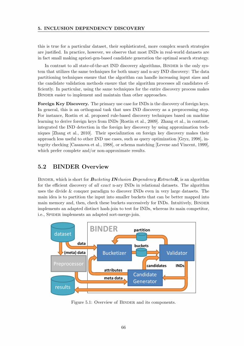
5. INCLUSION DEPENDENCY DISCOVERY
this is true for a particular dataset, their sophisticated, more complex search strategies
are justified. In practice, however, we observe that most INDs in real-world datasets are
in fact small making apriori-gen-based candidate generation the optimal search strategy.
In contrast to all state-of-the-art IND discovery algorithms, Binder is the only sys-
tem that utilizes the same techniques for both unary and n-ary IND discovery: The data
partitioning techniques ensure that the algorithm can handle increasing input sizes and
the candidate validation methods ensure that the algorithm processes all candidates ef-
ficiently. In particular, using the same techniques for the entire discovery process makes
Binder easier to implement and maintain than other approaches.
Foreign Key Discovery. The primary use case for INDs is the discovery of foreign keys.
In general, this is an orthogonal task that uses IND discovery as a preprocessing step.
For instance, Rostin et al. proposed rule-based discovery techniques based on machine
learning to derive foreign keys from INDs [Rostin et al., 2009]. Zhang et al., in contrast,
integrated the IND detection in the foreign key discovery by using approximation tech-
niques [Zhang et al., 2010]. Their specialization on foreign key discovery makes their
approach less useful to other IND use cases, such as query optimization [Gryz, 1998], in-
tegrity checking [Casanova et al., 1988], or schema matching [Levene and Vincent, 1999],
which prefer complete and/or non-approximate results.
5.2 BINDER Overview
Binder, which is short for Bucketing INclusion Dependency ExtractoR, is an algorithm
for the efficient discovery of all exact n-ary INDs in relational datasets. The algorithm
uses the divide & conquer paradigm to discover INDs even in very large datasets. The
main idea is to partition the input into smaller buckets that can be better mapped into
main memory and, then, check these buckets successively for INDs. Intuitively, Binder
implements an adapted distinct hash-join to test for INDs, whereas its main competitor,
i.e., Spider implements an adapted sort-merge-join.
results
BINDER
(meta) data
data buckets
meta data
candidates
partition
INDs
Validator
Preprocessor
Bucketizer
Candidate Generator
dataset
attributes
Figure 5.1: Overview of Binder and its components.
66
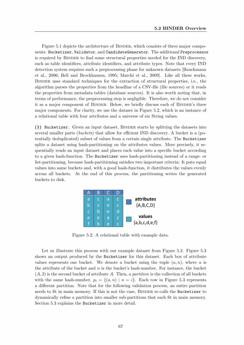
5.2 BINDER Overview
Figure 5.1 depicts the architecture of Binder, which consists of three major compo-
nents: Bucketizer, Validator, and CandidateGenerator. The additional Preprocessor
is required by Binder to find some structural properties needed for the IND discovery,
such as table identifiers, attribute identifiers, and attribute types. Note that every IND
detection system requires such a preprocessing phase for unknown datasets [Bauckmann
et al., 2006; Bell and Brockhausen, 1995; Marchi et al., 2009]. Like all these works,
Binder uses standard techniques for the extraction of structural properties, i.e., the
algorithm parses the properties from the headline of a CSV-file (file sources) or it reads
the properties from metadata tables (database sources). It is also worth noting that, in
terms of performance, the preprocessing step is negligible. Therefore, we do not consider
it as a major component of Binder. Below, we briefly discuss each of Binder’s three
major components. For clarity, we use the dataset in Figure 5.2, which is an instance of
a relational table with four attributes and a universe of six String values.
(1) Bucketizer. Given an input dataset, Binder starts by splitting the datasets into
several smaller parts (buckets) that allow for efficient IND discovery. A bucket is a (po-
tentially deduplicated) subset of values from a certain single attribute. The Bucketizer
splits a dataset using hash-partitioning on the attributes values. More precisely, it se-
quentially reads an input dataset and places each value into a specific bucket according
to a given hash-function. The Bucketizer uses hash-partitioning instead of a range- or
list-partitioning, because hash-partitioning satisfies two important criteria: It puts equal
values into same buckets and, with a good hash-function, it distributes the values evenly
across all buckets. At the end of this process, the partitioning writes the generated
buckets to disk.
A B C D a b c e f
c c b e b
a e e a e
c c d c c
attributes {A,B,C,D}
values {a,b,c,d,e,f}
Figure 5.2: A relational table with example data.
Let us illustrate this process with our example dataset from Figure 5.2. Figure 5.3
shows an output produced by the Bucketizer for this dataset. Each box of attribute
values represents one bucket. We denote a bucket using the tuple (a, n), where a is
the attribute of the bucket and n is the bucket’s hash-number. For instance, the bucket
(A, 2) is the second bucket of attribute A. Then, a partition is the collection of all buckets
with the same hash-number, pi = {(a, n) | n = i}. Each row in Figure 5.3 represents
a different partition. Note that for the following validation process, an entire partition
needs to fit in main memory. If this is not the case, Binder re-calls the Bucketizer to
dynamically refine a partition into smaller sub-partitions that each fit in main memory.
Section 5.3 explains the Bucketizer in more detail.
67
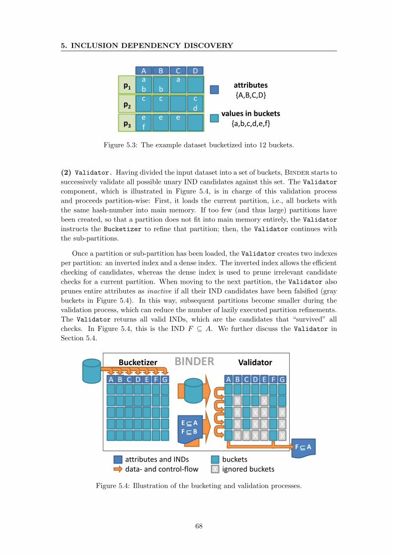
5. INCLUSION DEPENDENCY DISCOVERY
p2
p3
p1 attributes {A,B,C,D}
values in buckets {a,b,c,d,e,f}
c
c
c d
e f
e
e
a b
b
a
A B C D
Figure 5.3: The example dataset bucketized into 12 buckets.
(2) Validator. Having divided the input dataset into a set of buckets, Binder starts to
successively validate all possible unary IND candidates against this set. The Validator
component, which is illustrated in Figure 5.4, is in charge of this validation process
and proceeds partition-wise: First, it loads the current partition, i.e., all buckets with
the same hash-number into main memory. If too few (and thus large) partitions have
been created, so that a partition does not fit into main memory entirely, the Validator
instructs the Bucketizer to refine that partition; then, the Validator continues with
the sub-partitions.
Once a partition or sub-partition has been loaded, the Validator creates two indexes
per partition: an inverted index and a dense index. The inverted index allows the efficient
checking of candidates, whereas the dense index is used to prune irrelevant candidate
checks for a current partition. When moving to the next partition, the Validator also
prunes entire attributes as inactive if all their IND candidates have been falsified (gray
buckets in Figure 5.4). In this way, subsequent partitions become smaller during the
validation process, which can reduce the number of lazily executed partition refinements.
The Validator returns all valid INDs, which are the candidates that “survived” all
checks. In Figure 5.4, this is the IND F ⊆ A. We further discuss the Validator in
Section 5.4.
A B C D E F G A B C D E F G
X X
X X X X
X X X X
X X X X X
F A
Bucketizer Validator
X attributes and INDs data- and control-flow
BINDER
buckets ignored buckets
E A F B
Figure 5.4: Illustration of the bucketing and validation processes.
68
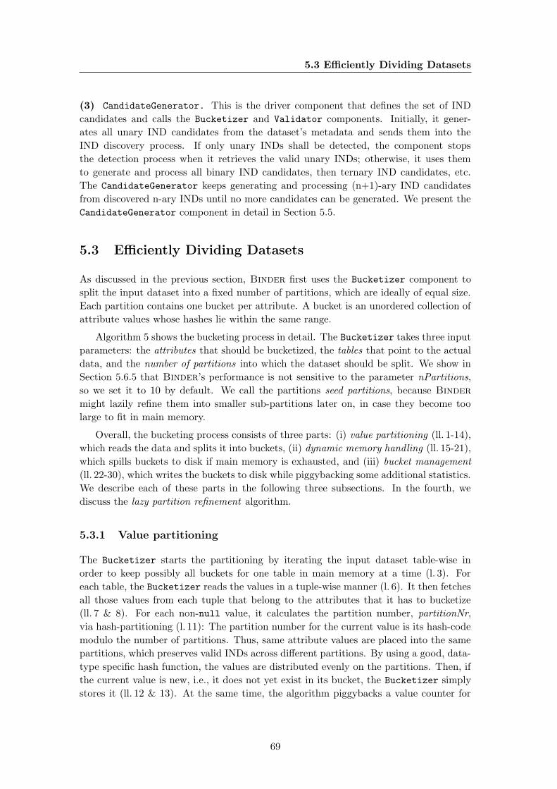
5.3 Efficiently Dividing Datasets
(3) CandidateGenerator. This is the driver component that defines the set of IND
candidates and calls the Bucketizer and Validator components. Initially, it gener-
ates all unary IND candidates from the dataset’s metadata and sends them into the
IND discovery process. If only unary INDs shall be detected, the component stops
the detection process when it retrieves the valid unary INDs; otherwise, it uses them
to generate and process all binary IND candidates, then ternary IND candidates, etc.
The CandidateGenerator keeps generating and processing (n+1)-ary IND candidates
from discovered n-ary INDs until no more candidates can be generated. We present the
CandidateGenerator component in detail in Section 5.5.
5.3 Efficiently Dividing Datasets
As discussed in the previous section, Binder first uses the Bucketizer component to
split the input dataset into a fixed number of partitions, which are ideally of equal size.
Each partition contains one bucket per attribute. A bucket is an unordered collection of
attribute values whose hashes lie within the same range.
Algorithm 5 shows the bucketing process in detail. The Bucketizer takes three input
parameters: the attributes that should be bucketized, the tables that point to the actual
data, and the number of partitions into which the dataset should be split. We show in
Section 5.6.5 that Binder’s performance is not sensitive to the parameter nPartitions,
so we set it to 10 by default. We call the partitions seed partitions, because Binder
might lazily refine them into smaller sub-partitions later on, in case they become too
large to fit in main memory.
Overall, the bucketing process consists of three parts: (i) value partitioning (ll. 1-14),
which reads the data and splits it into buckets, (ii) dynamic memory handling (ll. 15-21),
which spills buckets to disk if main memory is exhausted, and (iii) bucket management
(ll. 22-30), which writes the buckets to disk while piggybacking some additional statistics.
We describe each of these parts in the following three subsections. In the fourth, we
discuss the lazy partition refinement algorithm.
5.3.1 Value partitioning
The Bucketizer starts the partitioning by iterating the input dataset table-wise in
order to keep possibly all buckets for one table in main memory at a time (l. 3). For
each table, the Bucketizer reads the values in a tuple-wise manner (l. 6). It then fetches
all those values from each tuple that belong to the attributes that it has to bucketize
(ll. 7 & 8). For each non-null value, it calculates the partition number, partitionNr,
via hash-partitioning (l. 11): The partition number for the current value is its hash-code
modulo the number of partitions. Thus, same attribute values are placed into the same
partitions, which preserves valid INDs across different partitions. By using a good, data-
type specific hash function, the values are distributed evenly on the partitions. Then, if
the current value is new, i.e., it does not yet exist in its bucket, the Bucketizer simply
stores it (ll. 12 & 13). At the same time, the algorithm piggybacks a value counter for
69

5. INCLUSION DEPENDENCY DISCOVERY
Algorithm 5: Bucketing
Data: attributes, tables, nPartitions
Result: attrSizes, checkOrder
1 array attrSizes size | attributes | as Long;
2 array emptyBuckets size nPartitions as Integer;
3 foreach table ∈ tables do
4 array buckets size | table.attr | × nPartitions as Bucket;
5 array nValsPerAttr size | table.attr | as Integer;
6 foreach tuple ∈ read(table) do
7 foreach attr ∈ table.attr do
8 if attr /∈ attributes then continue;
9 value ← line[attr ];
10 if value = null then continue;
11 partitionNr ← hashCode (value) % nPartitions ;
12 if value /∈ buckets [attr ][partitionNr ] then
13 buckets [attr ][partitionNr ] ← buckets [attr ][partitionNr ] ∪ value;
14 nValsPerAttr [attr ] ← nValsPerAttr [attr ] + 1;
15 if memoryExhausted() then
16 lAttr ← max (nValsPerAttr);
17 foreach bucket ∈ buckets [lAttr ] do
18 attrSizes [lAttr ] ← attrSizes [lAttr ] + sizeOf (bucket);
19 writeToDisk (bucket);
20 bucket ← ∅;21 nValsPerAttr [lAttr ] ← 0;
22 foreach attr ∈ table.attr do
23 foreach bucket ∈ buckets [attr ] do
24 if bucket = ∅ then
25 emptyBuckets [attr ] ← emptyBuckets [attr ] + 1;
26 else
27 attrSizes [attr ] ← attrSizes [attr ] + sizeOf (bucket);
28 writeToDisk (bucket);
29 checkOrder ← orderBy (emptyBuckets);
30 return checkOrder, attrSizes ;
each attribute, nValsPerAttr, that it increases with every new value (l. 14). nValsPerAttr
is an array that Binder uses later, to decide which buckets should be spilled to disk if
main memory is exhausted.
70
5.3 Efficiently Dividing Datasets
5.3.2 Dynamic memory handling
Every time the Bucketizer partitions a tuple, it checks the overall memory consumption.
If the main memory is exhausted (e.g., if less than 10% of the memory is free), it spills
the buckets with the largest number of attribute values, nValsPerAttr, to disk (ll. 15
& 21). Spilling only the largest buckets has two major benefits: First, spilling small
buckets introduces the same file handling overhead as for large buckets, but the gain in
terms of freed memory is smaller. Second, spilling to disk might cause duplicate values
within a bucket, because the values on disk cannot be checked again in the remainder of
the bucketing process for efficiency reasons; large buckets contain many different values
anyway and are, hence, less likely to receive same values over and over again, which causes
them to generate fewer duplicate values when being spilled to disk. The buckets of a
table’s primary key attribute, for instance, contain no duplicates. To find the largest
attribute lAttr (and hence the largest buckets), the max() function queries an index
that keeps track of the maximum value in the nValsPerAttr array (l. 16). Then, the
Bucketizer iterates the largest buckets and writes them to disk (ll. 17-19). Afterwards,
it clears the spilled buckets to free main memory and resets the spilled attribute in the
nValsPerAttr-field (ll. 20 & 21).
5.3.3 Bucket management
Once the Bucketizer has partitioned a table, it writes all current buckets to disk from
where the Validator can read them later on (ll. 22-28). In this way, it can reuse the
entire main memory for bucketing the next table. While writing buckets to disk, the
component also piggybacks the collection of two statistics: attrSizes and emptyBuckets
(ll. 25 & 27). We describe each of these below:
(1) The attribute sizes array, attrSizes, stores the in-memory size of each bucketized
attribute. It is later used to identify partitions that do not fit in main memory in the
validation process. The Bucketizer computes the byte-size of a bucket as follows:
sizeOf(bucket) =∑
string∈bucket8 + 8 ·
⌈64 + 2 · |string|
8
⌉
This calculation assumes an implementation in Java and a 64 bit system, on which
strings need 64 byte for pointers, headers, and length and 2 bytes for each character.
After normalizing to a multiple of 8 byte, which is the smallest addressable unit, we add
another 8 byte for index-structures needed in the validation phase. For instance, the size
of bucket (A,1) in our running example (see Figure 5.3) is 160 byte, because it contains
two values of length one.
(2) The empty buckets array, emptyBuckets, counts the number of empty buckets in
each partition to later determine the most promising checking order, checkOrder, for
the Validator. The intuition is to prioritize the partitions with the smallest number
of empty buckets, because the Validator cannot use empty buckets to invalidate IND
candidates. So, the Validator aims at identifying and discarding inactive attributes
71
5. INCLUSION DEPENDENCY DISCOVERY
early on by checking those attributes with the lowest number of empty buckets first. For
instance, the emptyBuckets array for our example in Figure 5.3 is [1,1,1], because each
partition contains one empty bucket. If all buckets contain the same number of empty
buckets – like in this example – the emptyBuckets array does not indicate an optimal
checking order and the partitions’ initial order is used. Note that empty buckets mainly
arise from attributes containing only a few distinct values, such as gender -attributes,
which typically contain only two unique values.
5.3.4 Lazy partition refinement
Once the Bucketizer has finished splitting an input dataset into buckets, the Validator
successively uploads seed partitions into main memory to validate IND candidates. Some-
times, however, seed partitions are larger than the main memory capacity. Thus, the
Bucketizer needs to refine such seed partitions, which means that it splits a partition
into smaller sub-partitions that fit into main memory. Refining a seed partition is, how-
ever, a costly operation as one has to read and write most values again. We could, indeed,
collect some statistics about the input data, such as its size or length, to estimate the
right number of seed partitions and avoid refining them. Unfortunately, collecting such
statistics would introduce a significant overhead to the preprocessing step; the perfectly
partitioned initial bucketing could also become very fine-grained for large datasets, i.e.,
it would cause the creation of numerous superfluous bucket-files on disk that lead to
many file operations (create, open, and close) and, hence, could dominate the execution
time of the bucketing process and with it the execution time of the entire IND discovery.
For this reason, Binder does not try to estimate the perfect bucketing a priori.
Instead, the Bucketizer lazily refines the partitions whenever necessary. The main
idea is to split large seed partitions into smaller sub-partitions while validating INDs.
Assume, for instance, that Binder needs to check p1 of Figure 5.3 and that only two
values fit into main memory; Binder then lazily refines p1 into [{a},{ },{a},{ }] and
[{b},{b},{ },{ }]. This lazy refinement also allows Binder to dynamically reduce the
number of sub-partitions when the number of active attributes decreases from one seed
partition to the next one. For instance, if all IND candidates of an attribute are inval-
idated in some partition, Binder does not need to refine the attribute’s buckets in all
subsequent partitions, saving much I/O. In contrast to estimating the number of seed
partitions, lazy refinement creates much fewer files and, therefore, much less overhead
for three reasons: (i) the number of required sub-partitions can be determined more pre-
cisely in the validation process, (ii) the number of files decreases with every invalidated
attribute, and (iii) some small attributes can even stay in memory after refinement.
Algorithm 6 details the lazy refinement process. To refine a partition, the Bucketizer
requires three inputs: attrSizes (size of the attributes’ buckets in byte), partitionNr (iden-
tifier of the partition to be refined), and activeAttr (attributes to consider for refinement).
Overall, the refinement process consists of two parts: (i) the sub-partition number calcu-
lation (ll. 1-5), which calculates the number of sub-partitions in which a seed partition
has to be split, and (ii) the value re-bucketing (ll. 6-11), which splits a large partition
into smaller sub-partitions. We explain these two parts below.
72

5.3 Efficiently Dividing Datasets
Algorithm 6: Lazy Refinement
Data: activeAttr, attrSizes, partitionNr
Result: attrSizes, checkOrder
1 availMem ← getAvailableMemory ();
2 partSize ← 0;
3 foreach attr ∈ activeAttr do
4 partSize ← partSize + attrSizes[attr]/nPartitions;
5 nSubPartitions ← dpartSize/availMeme;6 tables ← getTablesFromFiles (activeAttr, partitionNr);
7 if nPartitions > 1 then
8 checkOrder, attrSizes ← bucketize (activeAttr, tables, nSubPartitions);
9 return checkOrder ;
10 else
11 return {partitionNr};
(1) Sub-partition number calculation. To decide if a split is necessary, the Bucketizer
needs to know the in-memory size of each attribute in a partition. The component can
get this information from the attrSizes array, which it collected during the bucketing
process (see Section 5.3.3). Let availMem be the available main memory and attr one
attribute. As the hash function created seed partitions of equal size, the Bucketizer
can now calculate the size of an attributes’s bucket independently of the actual bucket
number as:
size(attr) = attrSizes[attr]/nPartitions
The Bucketizer then calculates the size of a partition partitionNr as the sum of the
sizes of all its active attributes:
partSize =∑
attr∈activeAttr
size(attr)
Thus, given a seed partition, the Bucketizer simply returns the seed partition number
without refinement if availMem > partSize. Otherwise, it needs to split the seed
partition into nPartitions sub-partitions as follows:
nSubPartitions = dpartSize/availMeme
(2) Value re-bucketing. If refinement is needed, Binder re-applies the bucketing process
depicted in Algorithm 5 on the bucket files. To this end, the Bucketizer first calls the
function getTablesFromFiles(), which interprets each bucket as a table containing
only one attribute (l. 6). Then, it successively reads the buckets of the current partition,
re-hashes their values, and writes the new buckets back to disk (l. 8).
It is worth noting that distributing values from a bucket into different sub-partitions in an
efficient manner is challenging for two reasons: (i) the values in each bucket are already
similar with respect to their hash-values and thus redistributing them becomes harder,
73

5. INCLUSION DEPENDENCY DISCOVERY
and (ii) refining seed partitions requires two additional I/O operations (for reading from
and writing back to disk) for each value of an active attribute in a seed partition. Binder
addresses these two aspects as follows:
(i) To redistribute the values in a bucket, the Bucketizer re-partitions the values into
nSubPartitions as follows:
x =hash(value) % (nPartitions · nSubPartitions)− partitionNr
nPartitions
Here, x is the sub-bucket number with x ∈ [0,nSubPartitions−1] denoting the sub-bucket
for the given value. Taking the hashes of the values modulo the number of seed partitions
nPartitions multiplied by the number of required sub-partitions nSubPartitions leaves us
with nSubPartitions different numbers. For instance, if nPartitions = 10, partitionNr =
8, and nSubPartitions = 2, we obtain numbers in {8, 18}, because the hash-values modulo
nPartitions always give us the same number, which is partitionNr. By subtracting the
current partition number partitionNr from the modulo and, then, dividing by nPartitions,
we get an integer x in [0, nSubPartitions−1] assigning the current value to its sub-bucket.
(ii) Concerning the additional I/O operations, we consider that each attribute can allo-
cate at most m = availMem/ |activeAttr| memory for each of its buckets. However, in
practice, most buckets are much smaller than m. Thus, our Bucketizer saves many I/O
operations by not writing and reading again the sub-buckets of such small buckets, i.e.,
whenever m < sizeattr.
5.4 Fast IND Discovery
Given a set of IND candidates, the Validator component successively checks them
against the bucketized dataset. Algorithm 7 shows the validation process in detail.
While the Validator reads the bucketized dataset directly from disk, it requires three
additional inputs: the IND candidates that should be checked, the checkOrder defining
the checking order of the partitions, and the attrSizes indicating the in-memory size of
each bucket. See Section 5.3.3 for details about the checkOrder and attrSizes structures.
The candidates input is a map that points each possible dependent attribute (i.e., in-
cluded attribute) to all those attributes that it might reference (i.e., that it might be
included in).
During the validation process, the Validator removes all invalid INDs from the
candidates map so that only the valid INDs survive until the end of the process. Overall,
the validation process consists of two parts: (i) the partition traversal (ll. 1-6), which
iterates the partitions and maintains the attributes, and (ii) the candidate validation
(ll. 7-22), which checks the candidates against a current partition. We explain both
parts in the following two sections. Afterwards, we take a closer look at the candidate
pruning capabilities of Binder and discuss our design decisions.
74

5.4 Fast IND Discovery
Algorithm 7: Validation
Data: candidates, checkOrder, attrSizes
Result: candidates
1 activeAttr ← getKeysAndValues (candidates);
2 foreach partitionNr ∈ checkOrder do
3 subPrtNrs ← refine (activeAttr, attrSizes, partitionNr);
4 foreach subPartitionNr ∈ subPrtNrs do
5 activeAttr ← getKeysAndValues (candidates);
6 if activeAttr = ∅ then break all;
7 map attr2value as Integer to {};8 map value2attr as String to {};9 foreach attr ∈ activeAttr do
10 bucket ← readFromDisk (attr, subPartitionNr);
11 attr2value.get(attr) ← bucket ;
12 foreach value ∈ bucket do
13 value2attr.get(value) ← value2attr.get(value) ∪ attr ;
14 foreach attr ∈ activeAttr do
15 foreach value ∈ attr2value.get(attr) do
16 if candidates.get(attr) = ∅ then break;
17 if value /∈ value2attr.keys then continue;
18 attrGrp ← value2attr.get(value);
19 foreach dep ∈ attrGrp do
20 candidates.get(dep) ← candidates.get(dep) \ attrGrp;
21 value2attr.remove(value);
22 return candidates ;
5.4.1 Partition traversal
As its first step, the Validator collects all active attributes activeAttr, which are all
attributes that participate in at least one IND candidate (l. 1). The Validator uses
activeAttr to prune inactive attributes during the validation (l. 6): If an attribute is re-
moved from all IND candidates, it is also removed from this set and ignored for the rest
of the validation process. The Validator checks the IND candidates against the buck-
etized dataset in the checking order, checkOrder, previously defined by the Bucketizer
(l. 2). Before validation, the Validator calls the Bucketizer to refine the current seed
partition into smaller sub-partitions if necessary (l. 3), which is, if the partition does not
fit in main memory (see Section 5.3.4). Notice that the current seed partition is the only
sub-partition if no refinement was needed.
After the refinement process, the Validator iterates the sub-partitions to check the
candidates against them (l. 4). As the Validator might invalidate candidates on the
current sub-partition in each iteration, it first updates the activeAttr set before starting
75
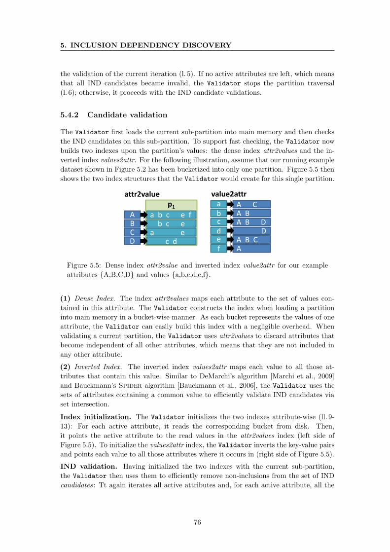
5. INCLUSION DEPENDENCY DISCOVERY
the validation of the current iteration (l. 5). If no active attributes are left, which means
that all IND candidates became invalid, the Validator stops the partition traversal
(l. 6); otherwise, it proceeds with the IND candidate validations.
5.4.2 Candidate validation
The Validator first loads the current sub-partition into main memory and then checks
the IND candidates on this sub-partition. To support fast checking, the Validator now
builds two indexes upon the partition’s values: the dense index attr2values and the in-
verted index values2attr. For the following illustration, assume that our running example
dataset shown in Figure 5.2 has been bucketized into only one partition. Figure 5.5 then
shows the two index structures that the Validator would create for this single partition.
p1
A B C D
a b c e f b c e a e c d
a
A C
b
c
d
e
f
A B A B D D A B C A
attr2value value2attr
Figure 5.5: Dense index attr2value and inverted index value2attr for our example
attributes {A,B,C,D} and values {a,b,c,d,e,f}.
(1) Dense Index. The index attr2values maps each attribute to the set of values con-
tained in this attribute. The Validator constructs the index when loading a partition
into main memory in a bucket-wise manner. As each bucket represents the values of one
attribute, the Validator can easily build this index with a negligible overhead. When
validating a current partition, the Validator uses attr2values to discard attributes that
become independent of all other attributes, which means that they are not included in
any other attribute.
(2) Inverted Index. The inverted index values2attr maps each value to all those at-
tributes that contain this value. Similar to DeMarchi’s algorithm [Marchi et al., 2009]
and Bauckmann’s Spider algorithm [Bauckmann et al., 2006], the Validator uses the
sets of attributes containing a common value to efficiently validate IND candidates via
set intersection.
Index initialization. The Validator initializes the two indexes attribute-wise (ll. 9-
13): For each active attribute, it reads the corresponding bucket from disk. Then,
it points the active attribute to the read values in the attr2values index (left side of
Figure 5.5). To initialize the values2attr index, the Validator inverts the key-value pairs
and points each value to all those attributes where it occurs in (right side of Figure 5.5).
IND validation. Having initialized the two indexes with the current sub-partition,
the Validator then uses them to efficiently remove non-inclusions from the set of IND
candidates : Tt again iterates all active attributes and, for each active attribute, all the
76
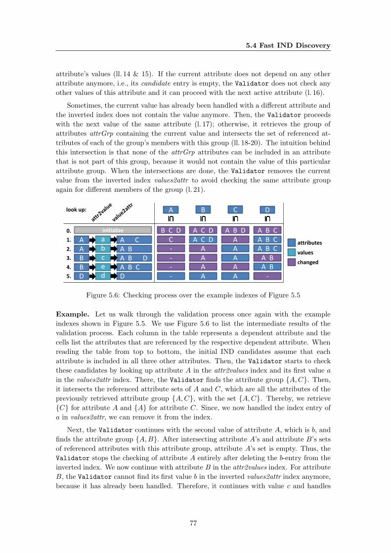
5.4 Fast IND Discovery
attribute’s values (ll. 14 & 15). If the current attribute does not depend on any other
attribute anymore, i.e., its candidate entry is empty, the Validator does not check any
other values of this attribute and it can proceed with the next active attribute (l. 16).
Sometimes, the current value has already been handled with a different attribute and
the inverted index does not contain the value anymore. Then, the Validator proceeds
with the next value of the same attribute (l. 17); otherwise, it retrieves the group of
attributes attrGrp containing the current value and intersects the set of referenced at-
tributes of each of the group’s members with this group (ll. 18-20). The intuition behind
this intersection is that none of the attrGrp attributes can be included in an attribute
that is not part of this group, because it would not contain the value of this particular
attribute group. When the intersections are done, the Validator removes the current
value from the inverted index values2attr to avoid checking the same attribute group
again for different members of the group (l. 21).
a
A C A b
A B A c
A B D B e
A B C B d
D D
A B C D
1.
2.
3.
4.
5.
look up:
B C D A C D A B D A B C 0.
C A C D A A B C - A A A B C - A A A B - A A A B - A A -
initialize
attributes
values
changed
Figure 5.6: Checking process over the example indexes of Figure 5.5
Example. Let us walk through the validation process once again with the example
indexes shown in Figure 5.5. We use Figure 5.6 to list the intermediate results of the
validation process. Each column in the table represents a dependent attribute and the
cells list the attributes that are referenced by the respective dependent attribute. When
reading the table from top to bottom, the initial IND candidates assume that each
attribute is included in all three other attributes. Then, the Validator starts to check
these candidates by looking up attribute A in the attr2values index and its first value a
in the values2attr index. There, the Validator finds the attribute group {A,C}. Then,
it intersects the referenced attribute sets of A and C, which are all the attributes of the
previously retrieved attribute group {A,C}, with the set {A,C}. Thereby, we retrieve
{C} for attribute A and {A} for attribute C. Since, we now handled the index entry of
a in values2attr, we can remove it from the index.
Next, the Validator continues with the second value of attribute A, which is b, and
finds the attribute group {A,B}. After intersecting attribute A’s and attribute B’s sets
of referenced attributes with this attribute group, attribute A’s set is empty. Thus, the
Validator stops the checking of attribute A entirely after deleting the b-entry from the
inverted index. We now continue with attribute B in the attr2values index. For attribute
B, the Validator cannot find its first value b in the inverted values2attr index anymore,
because it has already been handled. Therefore, it continues with value c and handles
77
5. INCLUSION DEPENDENCY DISCOVERY
the corresponding attribute group {A,B,D}. The same follows for e. Because the
Validator has checked all values of B now, it moves to attribute C. As all of attribute
C’s values have also been handled, it directly continues checking attribute D. Here, it
finds the value d unchecked, which disassociates attribute D from A and B. Finally, the
Validator terminates yielding the two inclusion dependencies B ⊆ A and C ⊆ A.
5.4.3 Candidate pruning
A common practice to prune IND candidates is to collect some statistics about the
buckets, such as min and max values, with which the algorithm can prune some attributes
before even reading their first buckets. However, in early evaluations, we found that
collecting such statistics is often more expensive than their actual pruning effect: We
observed that the bucketing process dominates the entire IND discovery process by taking
up 95% of the execution time; hence, additional costs for statistics collection in this
step dominate any possible pruning-gain. Therefore, the Validator relies on two non-
statistics-based pruning techniques to significantly speed up the validation process: intra-
partition and inter-partition pruning.
Intra-partition pruning. During the validation of a partition, some attributes become
independent of all other attributes, such as attribute A in our example. This means that
they no longer appear as a dependent attribute in any IND candidate. In these cases, the
Validator directly prunes the rest of the attribute’s values from the validation process
by skipping to the next active attribute in the attr2values index. The value f in our
example, for instance, is never checked. In real-world datasets, many of such values
exist, because attributes containing a large number of different values have an especially
high chance of not being included in any other attribute.
Inter-partition pruning. After validating a partition, attributes become inactive if
they neither depend on other attributes nor get referenced. Thus, by frequently updating
the activeAttr set, the Validator can prune entire attributes from further validation
processes. In consequence, the partitions become smaller and smaller, which continuously
reduces the time needed for partition refinement, bucket loading, and index creation.
Fewer attributes also reduce the average size of attribute groups in the values2attr index,
which in turn makes the intersections faster.
In summary, the Validator does not need to read and check all attributes entirely due
to the two indexes and its lazy bucketing and refinement techniques (if not all attributes
participate in any inclusion dependency). All candidates that “survive” the validation
on all partitions are valid inclusion dependencies.
5.5 IND Candidate Generation
The CandidateGenerator is the driver component of the entire IND discovery process.
It first generates the IND candidates, then it instructs the Bucketizer to partition
the data accordingly, thereafter it calls the Validator to check the candidates on the
bucketized dataset and finally the component restarts the process for the next larger IND
78
5.5 IND Candidate Generation
candidates. This iterative process allows Binder to use the same efficient components,
i.e., bucketing, validation, and candidate generation to discover both unary and n-ary
INDs. Using the same algorithm for all sizes of INDs also improves the maintainability
of Binder.
With Algorithm 8, we show the candidate generation process in detail. It takes four
parameters: the three arrays attributes, tables, and dataTypes, which store metadata
about the dataset, and the nPartitions variable, which defines the number of seed par-
titions. At first, the CandidateGenerator generates all unary IND candidates and runs
them through the bucketing and validation processes (ll. 1-12). If n-ary INDs should
be detected as well, the CandidateGenerator then starts a level-wise generation and
validation process for n-ary IND candidates (ll. 13-21). Each level represents the INDs of
size i. The iterative process uses the already discovered INDs of size i to generate IND
candidates of size i + 1. While this traversal strategy is already known from previous
works [Agrawal and Srikant, 1994; Marchi et al., 2009], our candidate validation tech-
niques contribute a significant improvement and simplification to the checking of n-ary
IND candidates.
5.5.1 Unary IND detection
The CandidateGenerator starts by defining the dep2refs map, in which we store all
valid INDs, and the candidates map, in which we store the IND candidates that still
need to be checked (ll. 1 & 2). Both data structures map dependent attributes to lists of
referenced attributes. The algorithm then calls the Bucketizer to partition the dataset
for the unary IND detection (l. 3). The Bucketizer splits all attributes of all tables into
nPartitions buckets as explained in Section 5.3. Next, the CandidateGenerator collects
all empty attributes in the emptyAttr set using the previously measured attribute sizes
(l. 4). An empty attribute is an attribute that contains no values. Using the attributes,
their data types, and the set of empty attributes, the CandidateGenerator iterates the
set of all possible unary IND candidates, which is the cross product of all attributes (l. 5).
Each candidate cand is a pair of one dependent attribute cand [0] and one referenced
attribute cand [1]. If both are the same, the IND is trivial and is discarded (l. 6).
Like most state-of-the-art IND discovery algorithms, such as [Marchi et al., 2009]
and [Bauckmann et al., 2006], the CandidateGenerator also discards candidates con-
taining differently typed attributes (l. 7). However, if INDs between differently typed
attributes are of interest, e.g., if numeric columns can be included in string columns,
this type-filter can be omitted. Furthermore, the CandidateGenerator excludes empty
attributes, which are contained in all other attributes by definition, from the validation
process and adds their INDs directly to the output (ll. 8-10). After discarding some
first candidates, the remaining candidates are either valid per definition, which is when
their dependent attribute is empty (l. 9), or they need to be checked against the data
(l. 11). For the latter, the CandidateGenerator calls the Validator to check the IND
candidates (see Secion 5.4) and places the valid INDs into the dep2refs map (l. 12). If
only unary INDs are required, the algorithm stops here; otherwise, it continues with the
discovery of n-ary INDs.
79

5. INCLUSION DEPENDENCY DISCOVERY
Algorithm 8: Candidate Generation
Data: attributes, tables, dataTypes, nPartitions
Result: dep2refs
1 map dep2refs as Integer to {};2 map candidates as Integer to {};
// Unary IND detection
3 checkOrder, attrSizes ← bucketize (attributes, tables, nPartitions);
4 emptyAttr ← {a ∈ attributes | attrSizes[a] = 0};5 foreach cand ∈ attributes × attributes do
6 if cand [0] = cand [1] then continue;
7 if dataTypes [cand [0]] 6= dataTypes [cand [1]] then continue;
8 if cand [0] ∈ emptyAttr then
9 dep2refs.get(cand [0]) ← dep2refs.get(cand [0]) ∪ cand [1];
10 continue;
11 candidates.get(cand [0]) ← candidates.get(cand [0]) ∪ cand [1];
12 dep2refs ← dep2refs ∪ validate (candidates, checkOrder, attrSizes);
// N-ary IND detection
13 lastDep2ref ← dep2refs ;
14 while lastDep2ref 6= ∅ do
15 candidates ← generateNext (lastDep2ref );
16 if candidates = ∅ then break;
17 attrCombinations ← getKeysAndValues (candidates);
18 checkOrder, attrSizes ← bucketize (attrCombinations, tables, nPartitions);
19 lastDep2ref ← validate (candidates, checkOrder, attrSizes);
20 dep2refs ← dep2refs ∪ lastDep2ref
21 return dep2refs ;
5.5.2 N-ary IND detection
For the discovery of n-ary INDs, the CandidateGenerator incrementally generates and
checks ever larger candidates. The generation is based on the apriori-gen algorithm,
which traverses the lattice of attribute combinations level-wise [Agrawal and Srikant,
1994]. In detail, the CandidateGenerator first copies the already discovered unary
INDs into the lastDep2ref map (l. 13), which stores all discovered INDs of the lastly
finished lattice level, i.e., the last validation iteration. While the lastDep2ref map is not
empty, i.e., the last validation iteration found at least one new inclusion dependency, the
CandidateGenerator keeps generating and checking ever larger INDs (ll. 14-20).
Candidate generation. To generate the n-ary IND candidates nAryCandidates of
size n+ 1 from the valid INDs lastDep2ref of size n, the CandidateGenerator uses the
generateNext() function (l. 15). Given that X and Y are attribute sets, A, B, C, and
D are single attributes, and Rj [XA] ⊆ Rk[Y C] and Rj [XB] ⊆ Rk[Y D] are known INDs
of size n = |XA|, then this function forms the IND candidate Rj [XAB] ⊆ Rk[Y CD] of
80
5.5 IND Candidate Generation
size n + 1, iff A < C and B 6= D. Note that we consider the attributes to be ordered
so that X and Y respectively are same prefixes for the single attributes in the INDs of
size n. The matching prefixes together with A < C assure that the algorithm creates
no candidate twice; otherwise, Rj [XAB] ⊆ Rk[Y CD] and Rj [BAX] ⊆ Rk[DCY ] would
represent the same IND due to the permutation property of INDs. Because the number
of Rj [XAB] ⊆ Rk[Y CD] candidates is huge and most use cases require only those INDs
for which the dependent and referenced attributes are disjoint, Binder and related
algorithms also use XAB ∩ Y CD = ∅ as a rule to reduce the number of candidates.
Re-bucketing. Having generated the next nAryCandidates, the CandidateGenerator
needs to bucketize again the dataset according to these new candidates. It cannot reuse
the bucketized dataset from the previous run, because the information about co-occurring
values of different attributes gets lost when the values are bucketized. For instance, if
the CandidateGenerator has to check the candidate Rj [AB] ⊆ Rk[CD], then it checks
if ∀r ∈ Rj [AB] : r ∈ Rk[CD]. As record r cannot be reconstructed from previous
bucketings, the CandidateGenerator has to re-execute the bucketing algorithm with one
small difference: Instead of single attribute values, Algorithm 5 bucketizes records from
attribute combinations attrCombinations that either occur as a dependent or referenced
attribute combination in any IND candidate. Technically, the Bucketizer can simply
combine the values of such records with a dedicated separator character to then bucketize
the combined values. For instance, consider that we need to check the IND candidate
Rj [AB] ⊆ Rk[CD]. Now, assume that the Bucketizer reads the record (f, b, e, c) from
our example schema R1[A,B,C,D]. Then, it partitions the value ′f#b′ for R1[AB] and′e#c′ for R1[CD].
It is worth emphasizing that the resulting buckets can become much larger than
the buckets created for the unary IND checking: First, the combined values for n-ary
IND candidates of size i are i-times larger on average than the single values, without
counting the separator character. Second, the number of non-duplicate values increases
exponentially with the size of the IND candidates so that more values are to be stored.
Binder can still handle this space complexity through its dynamic memory handling
(Section 5.3.2) and the lazy partition refinement (Section 5.3.4) techniques.
Validation. After the bucketing, the CandidateGenerator calls the Validator with
the current set of n-ary IND candidates. Here, the validation of n-ary candidates is the
same as the validation of unary candidates. The Validator has just to consider that
the buckets refer to attribute combinations, e.g., to R[AB]. After validating the n-ary
IND candidates of size n + 1, the CandidateGenerator supplements the final result
dep2ref with the set of newly discovered INDs. In case that no new INDs are found,
the CandidateGenerator stops the level-wise search, because all unary and n-ary INDs
have already been discovered. As a result, Binder reports the dep2ref map that now
contains all valid INDs.
81

5. INCLUSION DEPENDENCY DISCOVERY
5.6 Evaluation
We evaluate and compare the performance of Binder with two state-of-the-art sys-
tems for IND discovery. In particular, we carried out this evaluation with five questions
in mind: How good does Binder perform when (i) varying the number of rows (Sec-
tion 5.6.2) and (ii) varying the number of columns (Section 5.6.3)? How well does Binder
behave when processing (iii) different datasets (Section 5.6.4)? What is the performance
impact regarding the (iv) internal techniques of Binder (Section 5.6.5) and how does
Binder perform for (v) discovering n-ary INDs with n > 1 (Section 5.6.6)?
5.6.1 Experimental setup
Our experiments compare Binder against two other algorithms from related work,
namely Spider [Bauckmann et al., 2006], which to date is the fastest algorithm for
unary IND discovery, and Mind [Marchi et al., 2009], which is the most cited algorithm
for n-ary IND discovery with n > 1. We implemented all three algorithms within our
Metanome data profiling tool (www.metanome.de) using Java 7. Binder and the other
algorithms’ binaries are publicly available1. For all experiments, we set Binder’s input
parameter nPartitions to 10 and show in Section 5.6.5 why this is a good default value.
Hardware. All experiments were run on a Dell PowerEdge R620 with two Intel Xeon
E5-2650 2.00 GHz CPUs and 128 GB DDR3 RAM. The server runs CentOS 6.4 as
operating system. For some experiments, we reduce the server’s memory to 8 GB in
order to evaluate the algorithm’s performance on limited memory resources.
Data storage. Our experiments consider both a database and raw files as data storage,
because this choice influences the system’s runtimes. Spider, for instance, uses SQL
order-by statements on database inputs for its sorting phase and external memory sorting
on files. Mind uses SQL for all inclusion checks and, hence, only runs on databases.
Binder reads an input dataset only once and then maintains the data itself, which is
why the algorithm executes equally on both storage types. In our experiments, we use
CSV-formatted files and the IBM DB2 9.7 database in its default setup. For database
inputs, no indexes other than the relations’ primary key indexes are given.
Datasets. Our experiments build upon both synthetic and real-world datasets. The
real-world datasets we use are: COMA, WIKIPEDIA, and WIKIRANK, which are small
datasets containing image descriptions, page statistics, and link information, respectively,
that we crawled from the Wikipedia knowledge base; SCOP, BIOSQL, ENSEMBLE,
CATH, and PDB, which are all excerpts from biological databases on proteins, dna, and
genomes; CENSUS, which contains data about peoples’ life circumstances, education,
and income; LOD, which is an excerpt of linked open data on famous persons and stores
many RDF-triples in relational format; and PLISTA [Kille et al., 2013b], which contains
anonymized web-log data provided by the advertisement company Plista. The last two
datasets TESMA and TPC-H are synthetic datasets, which we generated with the db-
tesma tool for person data and the dbgen tool for business data, respectively. Table 5.1
1http://hpi.de/en/naumann/projects/repeatability/data-profiling/ind
82

5.6 Evaluation
Table 5.1: Datasets and their characteristics
Name File Size Attributes Unary INDs N-ary INDs nmax
COMA 20 KB 4 0 0 1
SCOP 16 MB 22 43 40 4
CENSUS 112 MB 48 73 147 6
WIKIPEDIA 540 MB 14 2 0 1
BIOSQL 560 MB 148 12463 22 2
WIKIRANK 697 MB 35 321 339 7
LOD 830 MB 41 298 1361005 8
ENSEMBL 836 MB 448 142510 100 4
CATH 908 MB 115 62 81 3
TESMA 1,1 GB 128 1780 0 1
PDB 44 GB 2790 800651 unknown
PLISTA 61 GB 140 4877 unknown
TPC-H 100 GB 61 90 6 2
lists these datasets with their file size on disk, number of attributes, number of all unary
INDs, number of all n-ary INDs with n > 1, and the INDs’ maximum arity nmax.
Usually, most n-ary INDs are of size n = 2, but in the LOD dataset most n-ary INDs
are of size n = 4. A link collection to these datasets and the data generation tools is
available online1.
5.6.2 Varying the number of rows
We start evaluating Binder with regard to the length of the dataset, i.e., the number of
rows. For this experiment we generated five TPC-H datasets with different scale factors
from 1 to 70. The two left-side charts in Figure 5.7 show the result of the experiment
for 128 GB (top) and 8 GB (bottom) of main memory.
We observe that with 128 GB of main memory, Binder is up to 6.2 times faster on
file inputs and up to 1.6 times faster on a database than Spider. Binder outperforms
Spider for three main reasons: First, building indexes for the IND validation is faster
than Spider’s sorting. Second, the indexes are not constructed for all attribute values,
because some inactive attributes can be discarded early on. Third, Binder reads the
data once, whereas Spider queries the data multiple times in order to sort the different
attributes. The results also show that Binder performs worse on database inputs than on
file inputs although the algorithm is exactly the same. In fact, its execution time almost
doubles. The reason is the database overhead of query parsing, record formatting, and,
in particular, inter-process data transfer. Spider, on the other hand, profits from a
database: It uses the databases’ built-in sorting algorithms, which are highly optimized
for data that lives inside the database. Additionally, by directly eliminating duplicate
values, the database also reduces the amount of data that it sends to the validation
process. Despite these advantages, Binder still clearly outperforms Spider even on
database inputs.
83
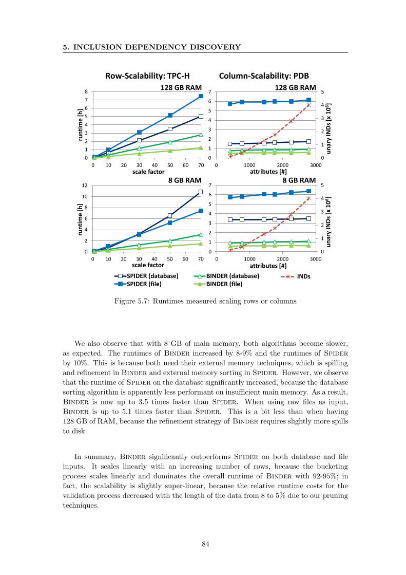
5. INCLUSION DEPENDENCY DISCOVERY
0
1
2
3
4
5
6
7
8
0 10 20 30 40 50 60 70
run
tim
e [
h]
scale factor
0
2
4
6
8
10
12
0 10 20 30 40 50 60 70
run
tim
e [
h]
scale factor
0
1
2
3
4
5
0
1
2
3
4
5
6
7
0 1000 2000 3000
un
ary
IND
s [x
10
6]
attributes [#]
0
1
2
3
4
5
0
1
2
3
4
5
6
7
0 1000 2000 3000
un
ary
IND
s [x
10
6]
attributes [#]
Row-Scalability: TPC-H Column-Scalability: PDB
128 GB RAM
8 GB RAM
128 GB RAM
8 GB RAM
012345010
0 5000
SPIDER (database)SPIDER (file)
012345010
0 1000 2000 3000
BINDER (database)BINDER (file)
012345010
0 2000 4000
INDs
Figure 5.7: Runtimes measured scaling rows or columns
We also observe that with 8 GB of main memory, both algorithms become slower,
as expected. The runtimes of Binder increased by 8-9% and the runtimes of Spider
by 10%. This is because both need their external memory techniques, which is spilling
and refinement in Binder and external memory sorting in Spider. However, we observe
that the runtime of Spider on the database significantly increased, because the database
sorting algorithm is apparently less performant on insufficient main memory. As a result,
Binder is now up to 3.5 times faster than Spider. When using raw files as input,
Binder is up to 5.1 times faster than Spider. This is a bit less than when having
128 GB of RAM, because the refinement strategy of Binder requires slightly more spills
to disk.
In summary, Binder significantly outperforms Spider on both database and file
inputs. It scales linearly with an increasing number of rows, because the bucketing
process scales linearly and dominates the overall runtime of Binder with 92-95%; in
fact, the scalability is slightly super-linear, because the relative runtime costs for the
validation process decreased with the length of the data from 8 to 5% due to our pruning
techniques.
84
5.6 Evaluation
5.6.3 Varying the number of columns
We now evaluate Binder with regard to the width of the dataset, i.e., the number
of attributes. In these experiments we used the PDB dataset, which comprises 2,790
attributes in total. We start with a subset of 411 attributes and continuously add tables
from the PDB dataset to its subset. Note that we had to increase the open files limit
in the operating system from 1,024 to 4,096 for Spider, to avoid the “Too many open
files” exception.
The two right-side charts in Figure 5.7 show the result of the experiment for 128 GB
(top) and 8 GB (bottom). We additionally plot the number of discovered INDs (red line
in the charts) in these charts as they increase with the number of attributes. Similar to
the row scalability experiment, Binder significantly outperforms Spider: (i) it is up to
1.8 times faster on a database and up to 10.7 times faster on raw files with 128 GB of
main memory; and (ii) it is up to 3.1 times faster on a database and up to 9.9 times
faster on raw files with 8 GB of main memory. We see that these improvement factors
stay constant when adding more attributes, because the two IND validation strategies
have the same complexity with respect to the number of attributes. However, it is
worth noting that although the number of INDs increases rapidly, the runtimes of both
algorithms only increase slightly. This is because the bucketing (for Binder) and sorting
(for Spider) processes dominate the runtimes with 95% and 99% respectively.
5.6.4 Varying the datasets
The previous sections have shown that Binder’s performance does not depend on the
number of rows or columns in the dataset. As the following experiments on several
real-world and two synthetic datasets will show, it instead depends on four other char-
acteristics of the input datasets: (i) the dataset size, (ii) the number of duplicate values
per attribute, (iii) the average number of attributes per table, and (iv) the number of
prunable attributes, i.e., attributes not being part of any IND. Thus, to better evaluate
Binder under the influence of these characteristics, we evaluated it on different datasets
and compare its performance to that of Spider.
Figure 5.8 shows the results of these experiments. We again executed all experiments
with 128 GB (top) and 8 GB (bottom) main memory. Notice that only the runtimes for
the large datasets differ across the two memory settings. Overall, we observe that Binder
outperforms Spider on all datasets, except the very small COMA and SCOP datasets.
We now examine these results with respect to the four characteristics mentioned above:
(1) Dataset size. As we observed in the scalability experiments in Sections 5.6.2
and 5.6.3, the improvement of Binder over Spider does not depend on the number
of rows or columns if the datasets are sufficiently large. The current results, however,
show that Binder is slower than Spider if the datasets are very small, such as the
COMA dataset with only 20 KB. This is because the file creation costs on disk dominate
the runtimes of Binder: The algorithm creates ten files per attribute2 whereas Spider
2In contrast to Spider, Binder only opens one of these files at a time.
85
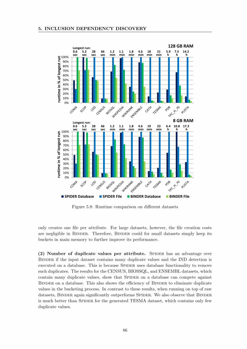
5. INCLUSION DEPENDENCY DISCOVERY
0%
10%
20%
30%
40%
50%
60%
70%
80%
90%
100%ru
nti
me
in %
of
lon
gest
ru
n
128 GB RAM
8 GB RAM Longest run: 0.6 5.2 28 66 1.2 1.1 1.8 4.6 19 23 6.4 10.8 17.3 sec sec sec sec min min min min min min h h h
Longest run: 0.6 5.2 28 66 1.2 1.1 1.8 4.6 18 21 5.9 7.5 14.2 sec sec sec sec min min min min min min h h h
0%
10%
20%
30%
40%
50%
60%
70%
80%
90%
100%
run
tim
e in
% o
f lo
nge
st r
un
SPIDER Database SPIDER File BINDER Database BINDER File
Figure 5.8: Runtime comparison on different datasets
only creates one file per attribute. For large datasets, however, the file creation costs
are negligible in Binder. Therefore, Binder could for small datasets simply keep its
buckets in main memory to further improve its performance.
(2) Number of duplicate values per attribute. Spider has an advantage over
Binder if the input dataset contains many duplicate values and the IND detection is
executed on a database. This is because Spider uses database functionality to remove
such duplicates. The results for the CENSUS, BIOSSQL, and ENSEMBL datasets, which
contain many duplicate values, show that Spider on a database can compete against
Binder on a database. This also shows the efficiency of Binder to eliminate duplicate
values in the bucketing process. In contrast to these results, when running on top of raw
datasets, Binder again significantly outperforms Spider. We also observe that Binder
is much better than Spider for the generated TESMA dataset, which contains only few
duplicate values.
86

5.6 Evaluation
(3) Average number of attributes per table. The experiments in Section 5.6.3
have shown that the overall number of attributes does not influence the performance
difference between Binder and Spider. However, we particularly observed that if the
average number of attributes per table is high, Binder’s performance is not affected
as much as the performance of Spider: Spider needs to access a large table once for
reading each of its attributes, which introduces a large overhead especially if the dataset
needs to be read from files. Binder, on the other hand, needs to spill buckets more
often to disk, but this introduces only a small overhead as the buckets are written to
disk anyway. The results for the TESMA and PLISTA dataset show this aspect best:
Having 32 and 35 attributes per table on average, respectively, Binder significantly
outperforms Spider.
0%
10%
20%
30%
40%
50%
60%
70%
80%
90%
100%
1 2 3 4 5 6 7 8 9 10
acti
ve a
ttri
bu
tes
partition number
COMA
SCOP
CENSUS
LOD
WIKIRANK
BIOSQL
WIKIPEDIA
CATH
ENSEMBL
TESMA
PDB
PLISTA
TPC_H_70
Figure 5.9: Active attributes per partition for the different datasets
(4) Number of prunable attributes. In contrast to Spider, which cannot prune
inactive attributes before or during sorting values, Binder fully profits from attributes
that are not part of any IND thanks to the inter-partition pruning (Section 5.4.3). For
the SCOP dataset, for instance, Binder performs as good as Spider even if this dataset
is still very small (16 MB). This is because Binder already prunes all attributes that are
not part of any IND while processing the first partition. In this way, Binder saves sig-
nificant indexing time whereas Spider cannot save sorting time for prunable attributes.
Figure 5.9 shows the pruning effect in more detail: It lists the percentage of active at-
tributes for the different partitions showing how many attributes Binder pruned in the
different partitions. Notice that all attributes that survive as active attributes until Par-
tition 10 are part of at least one valid IND. For instance, 50% of the attributes finally
appear in at least one IND for the TPC-H dataset. The experiment shows that Binder
achieved the highest pruning effect on the COMA, TESMA, WIKIPEDIA, and SCOP
datasets: It pruned almost all unimportant attributes within the first partitions. This
means that the values of these attributes are not read, indexed, or compared in the fol-
lowing partitions. Nonetheless, we see that the pruning capabilities of Binder have no
effect for the LOD and PDB datasets, because all of their attributes either depend on
another attribute or reference another attribute.
87

5. INCLUSION DEPENDENCY DISCOVERY
5.6.5 BINDER in-depth
So far, we have shown Binder’s advantage over Spider for unary IND discovery. We
now evaluate Binder to study the impact of: (i) the nPartitions parameter; (ii) the data
structures used in the validation process; and (iii) the index-based candidate checking.
(1) Number of seed buckets. Recall that the nPartitions parameter specifies the
number of seed buckets that Binder initially creates. Although one could use any value
for this parameter – thanks to the lazy refinement used in the validations –, the number
of seed buckets influences the performance of Binder as shown in Figure 5.10. It shows
both the runtime of Binder for different nPartitions values and the percentage of
refined partitions for each number of seed buckets on the TPC-H 70 dataset. Note that
we observed identical results for the PLISTA and PDB datasets and very similar results
for the other datasets. As expected, on the one hand, we observe that taking a small
number of seed partitions (two to three) decreases the performance of Binder, because
the algorithm needs more costly bucket refinements. On the other hand, we observe
that choosing a large number of seed partitions, e.g., 50, also reduces the performance of
Binder, because more initial partitions increase the file overhead: Binder creates more
files than it actually needs. In between very small and very large values, we see that
Binder is not sensitive but robust to the nPartitions parameter. It is worth noting that
Spider takes 7.4 hours to compute the same dataset, which is still more than 4 times
slower than the worst choice of nPartitions in Binder.
0%
25%
50%
75%
100%
0
0,5
1
1,5
2
0 10 20 30 40 50 refi
ned
par
titi
on
s
run
tim
e [
h]
nPartitions runtime refined partitions
Figure 5.10: The nPartitions parameter on TPC-H 70 using 8 GB RAM
(2) Lists vs. BitSets. In the validation process, Binder checks the generated IND
candidates against the bucketized dataset by intersecting the candidates referenced at-
tribute sets with those sets of attributes that all contain a same value. Technically, we
can maintain the attribute sets as Lists or BitSets. BitSets have two advantages over
Lists if most bits are set: They offer a smaller memory footprint and their intersection is
faster. Thus, we implemented and tested both data structures. In our experiments, we
did not observe a clear performance difference between the two data structures. This is
because the attribute sets are typically very small and the intersection costs become al-
most constant [Marchi et al., 2009]. However, we observed a higher memory consumption
for BitSets on datasets with many attributes, e.g., 41% higher on the PDB dataset, be-
cause they are very sparsely populated. Furthermore, the number of candidates increases
quadratically with the number of attributes but while the candidate number shrinks over
time using Lists, they stay large using BitSets. For these reasons, Binder uses Lists.
88
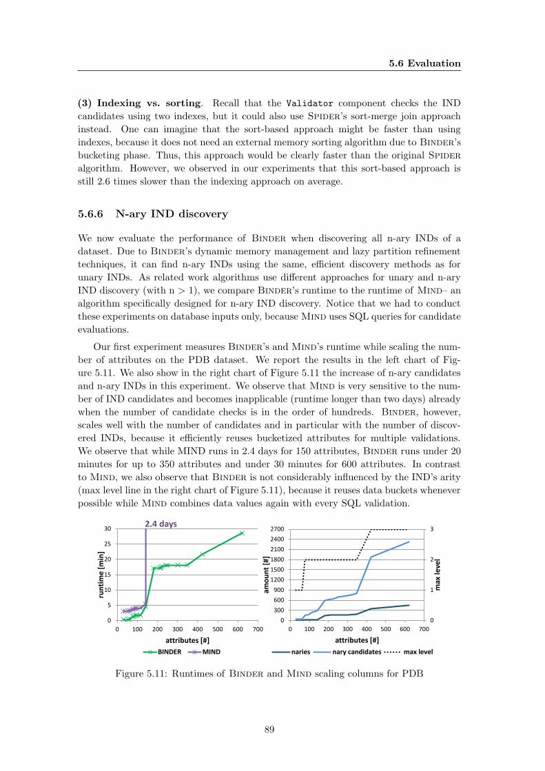
5.6 Evaluation
(3) Indexing vs. sorting. Recall that the Validator component checks the IND
candidates using two indexes, but it could also use Spider’s sort-merge join approach
instead. One can imagine that the sort-based approach might be faster than using
indexes, because it does not need an external memory sorting algorithm due to Binder’s
bucketing phase. Thus, this approach would be clearly faster than the original Spider
algorithm. However, we observed in our experiments that this sort-based approach is
still 2.6 times slower than the indexing approach on average.
5.6.6 N-ary IND discovery
We now evaluate the performance of Binder when discovering all n-ary INDs of a
dataset. Due to Binder’s dynamic memory management and lazy partition refinement
techniques, it can find n-ary INDs using the same, efficient discovery methods as for
unary INDs. As related work algorithms use different approaches for unary and n-ary
IND discovery (with n > 1), we compare Binder’s runtime to the runtime of Mind– an
algorithm specifically designed for n-ary IND discovery. Notice that we had to conduct
these experiments on database inputs only, because Mind uses SQL queries for candidate
evaluations.
Our first experiment measures Binder’s and Mind’s runtime while scaling the num-
ber of attributes on the PDB dataset. We report the results in the left chart of Fig-
ure 5.11. We also show in the right chart of Figure 5.11 the increase of n-ary candidates
and n-ary INDs in this experiment. We observe that Mind is very sensitive to the num-
ber of IND candidates and becomes inapplicable (runtime longer than two days) already
when the number of candidate checks is in the order of hundreds. Binder, however,
scales well with the number of candidates and in particular with the number of discov-
ered INDs, because it efficiently reuses bucketized attributes for multiple validations.
We observe that while MIND runs in 2.4 days for 150 attributes, Binder runs under 20
minutes for up to 350 attributes and under 30 minutes for 600 attributes. In contrast
to Mind, we also observe that Binder is not considerably influenced by the IND’s arity
(max level line in the right chart of Figure 5.11), because it reuses data buckets whenever
possible while Mind combines data values again with every SQL validation.
0
1
2
3
0
300
600
900
1200
1500
1800
2100
2400
2700
0 100 200 300 400 500 600 700
max
leve
l
amo
un
t [#
]
attributes [#]
naries nary candidates max level
0
5
10
15
20
25
30
0 100 200 300 400 500 600 700
run
tim
e [m
in]
attributes [#]
BINDER MIND
2.4 days
Figure 5.11: Runtimes of Binder and Mind scaling columns for PDB
89
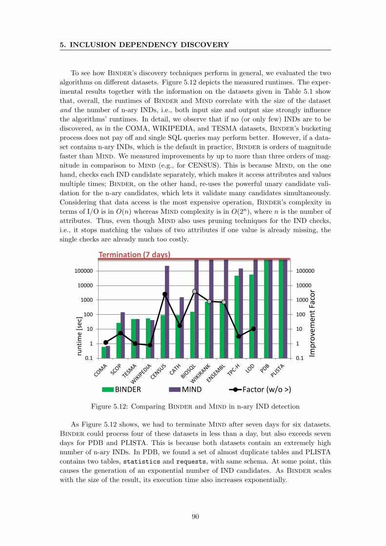
5. INCLUSION DEPENDENCY DISCOVERY
To see how Binder’s discovery techniques perform in general, we evaluated the two
algorithms on different datasets. Figure 5.12 depicts the measured runtimes. The exper-
imental results together with the information on the datasets given in Table 5.1 show
that, overall, the runtimes of Binder and Mind correlate with the size of the dataset
and the number of n-ary INDs, i.e., both input size and output size strongly influence
the algorithms’ runtimes. In detail, we observe that if no (or only few) INDs are to be
discovered, as in the COMA, WIKIPEDIA, and TESMA datasets, Binder’s bucketing
process does not pay off and single SQL queries may perform better. However, if a data-
set contains n-ary INDs, which is the default in practice, Binder is orders of magnitude
faster than Mind. We measured improvements by up to more than three orders of mag-
nitude in comparison to Mind (e.g., for CENSUS). This is because Mind, on the one
hand, checks each IND candidate separately, which makes it access attributes and values
multiple times; Binder, on the other hand, re-uses the powerful unary candidate vali-
dation for the n-ary candidates, which lets it validate many candidates simultaneously.
Considering that data access is the most expensive operation, Binder’s complexity in
terms of I/O is in O(n) whereas Mind complexity is in O(2n), where n is the number of
attributes. Thus, even though Mind also uses pruning techniques for the IND checks,
i.e., it stops matching the values of two attributes if one value is already missing, the
single checks are already much too costly.
0.1
1
10
100
1000
10000
100000
0.1
1
10
100
1000
10000
100000
Imp
rove
men
t Fa
cor
run
tim
e [s
ec]
BINDER MIND Factor (w/o >)
Termination (7 days)
Figure 5.12: Comparing Binder and Mind in n-ary IND detection
As Figure 5.12 shows, we had to terminate Mind after seven days for six datasets.
Binder could process four of these datasets in less than a day, but also exceeds seven
days for PDB and PLISTA. This is because both datasets contain an extremely high
number of n-ary INDs. In PDB, we found a set of almost duplicate tables and PLISTA
contains two tables, statistics and requests, with same schema. At some point, this
causes the generation of an exponential number of IND candidates. As Binder scales
with the size of the result, its execution time also increases exponentially.
90
5.7 Conclusion & Future Work
With the TPC-H dataset, the experiment proves that even though the number of
INDs (and IND candidates) is low, Binder can still outperform Mind. This is because
the SQL checks become unproportionally expensive on high numbers of attribute values.
Note that we tried different validation queries based on LEFT OUTER JOIN, NOT IN, and
EXCEPT statements (limited on the first not joinable tuple) for Mind all showing the
same limitation. Especially when the tables or the IND candidates’ left and right hand
sides become larger, the SQL-queries become clearly slower.
In summary, our experiments showed that only if tables are small and their number of
n-ary IND candidates is low, Mind can compete with Binder. But as most real world
datasets are large and contain many n-ary INDs, Binder is by far the most efficient
algorithm for exact and complete n-ary IND discovery.
5.7 Conclusion & Future Work
We presented Binder, the currently most effective algorithm for exact and complete
unary and n-ary IND discovery. The use of the divide & conquer principle allows it
to efficiently handle very large datasets. Due to the partitioning, the algorithm can
apply known pruning techniques and a novel IND-checking strategy at partition-level.
In contrast to most related work, Binder does not rely on existing database functionality
nor does it assume that the dataset fits into main memory. Our experimental results
show that Binder is more than one order of magnitude (26 times) faster than Spider
and up to more than three orders of magnitude (more than 2500 times) faster than Mind.
The experimental results also show that Binder scales to much larger datasets than the
state-of-the-art.
Because Binder’s performance is I/O bound, we also developed a distributed IND
discovery algorithm called Sindy [Kruse et al., 2015]. The distribution in Sindy comes at
the cost of a less effective candidate pruning, but the gains in parallel I/O can compensate
this disadvantage at some point. Another sister algorithm of Binder is Faida [Kruse
et al., 2017]. In Faida, we relax the correctness constraint of the result to improve
the discovery performance even further. Relaxing correctness means that the result set
of discovered INDs is still complete, but false positives might occur – in fact, however,
Faida’s result sets were 100% correct on all tested datasets. In another line of research,
we studied IND discovery on short tables, because Binder’s divide & conquer strategy
is an optimization only for long datasets with many thousand records and more. Some
datasets, such as web table data or sample data, however, consist of rather short tables
that only have 10 or less records per table on average. To efficiently process datasets of
such unusual shortness, we developed Many [Tschirschnitz et al., 2017], an algorithm
that, first, heavily prunes the search space using Bloomfilters and, then, validates the
remaining candidates in memory. Within the same project scope of Binder, we also
developed the RDFind algorithm [Kruse et al., 2016a]. This algorithm was designed to
discover conditional INDs in RDF datasets, i.e., INDs that hold for certain subsets of
RDF triples. Hence, RDFind is orthogonal research to Binder, as we left the relational
world and found an alternative definition for INDs in the RDF format.
91

5. INCLUSION DEPENDENCY DISCOVERY
IND discovery is the most difficult task known in data profiling. Binder is currently
the most efficient, exact solution for this problem, but its memory consumption on
disk can still be an issue for n-ary IND discovery: The number of candidates can grow
exponentially and with it the algorithm’s memory consumption. In future work, we aim
to solve this problem with additional, use case specific pruning rules that a priori reduce
the number of attributes and, hence, buckets on disk. To find foreign keys, one could,
for instance, drop all attributes with boolean or floating point values, because these are
inappropriate data types for key constraints.
92

6
Metanome
Data profiling is an important preparation step for many practical use cases. For this
reason, data scientists and IT professionals are frequently confronted with this special
task. Only very few of these people have a technical unterstanding of data profiling and
know how profiling algorithms work – they are usually experts for their use case but not
necessarily in dependency discovery. So their success in data profiling relies mostly on
available tool support for this task. As we already discussed in Chapter 1, current pro-
filing tools, indeed, offer comprehensive functionality for basic types of metadata, which
are easy to compute, but they usually lack automatic and efficient discovery functionality
for complex metadata types; in particular, tool support for those metadata types that
involve multiple columns, such as functional dependencies, unique column combinations,
and inclusion dependencies, is sparse.
In this chapter, we propose Metanome1, an extensible and open profiling platform
that incorporates many state-of-the-art profiling algorithms for relational data. The first
fully functional version of Metanome was presented as a demonstration in [Papenbrock
et al., 2015a]. The profiling platform is able to calculate simple profiling statistics, but
its main focus lies on the automatic discovery of complex metadata, i.e., those tasks that
related profiling tools have difficulties with. For this purpose, Metanome’s goal is to
make novel profiling algorithms from research accessible to all experts tasked with data
profiling: It guides the configuration and execution of metadata discovery algorithms
and offers ranking and visualization features for the discovered metadata result sets.
Through its modular and extensible architecture, Metanome also supports developers in
building, testing, and evaluating new algorithms: The framework itself handles common
functionality for data access and result management and defines standard interfaces for
fair algorithm benchmarking. Note that all algorithms of this thesis, which are HyFD,
HyUCC, Binder, and their sister algorithms, have been implemented in this framework.
In summary, the contributions of Metanome are the following:
(1) Data profiling support. Metanome assists database administrators and IT pro-
fessionals with state-of-the-art discovery algorithms in their effort to analyze relational
datasets for metadata.
1www.metanome.de
93
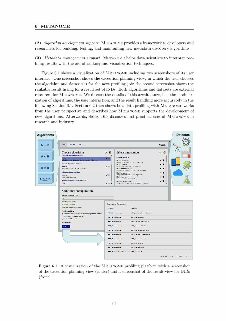
6. METANOME
(2) Algorithm development support. Metanome provides a framework to developers and
researchers for building, testing, and maintaining new metadata discovery algorithms.
(3) Metadata management support. Metanome helps data scientists to interpret pro-
filing results with the aid of ranking and visualization techniques.
Figure 6.1 shows a visualization of Metanome including two screenshots of its user
interface: One screenshot shows the execution planning view, in which the user chooses
the algorithm and dataset(s) for the next profiling job; the second screenshot shows the
rankable result listing for a result set of INDs. Both algorithms and datasets are external
resources for Metanome. We discuss the details of this architecture, i.e., the modular-
ization of algorithms, the user interaction, and the result handling more accurately in the
following Section 6.1. Section 6.2 then shows how data profiling with Metanome works
from the user perspective and describes how Metanome supports the development of
new algorithms. Afterwards, Section 6.3 discusses first practical uses of Metanome in
research and industry.
Algorithms Datasets
A → B
A ⊂ B
A » B
A B C D
Figure 6.1: A visualization of the Metanome profiling platform with a screenshot
of the execution planning view (center) and a screenshot of the result view for INDs
(front).
94

6.1 The Data Profiling Platform
6.1 The Data Profiling Platform
In this section, we discuss the architecture of Metanome. The Metanome project is
an open source project available on GitHub2. Links to the most recent builds and to
more detailed documentation for both users and developers can be found on the same
page. The overall development of Metanome goes by the following three design goals:
1. Simplicity: Metanome should be easy to setup and use, i.e., a user should be able
to simply download and start the tool, add data, and begin to profile it.
2. Extensibility: New algorithms and datasets should be easily connectable to the
system without needing to change the system itself.
3. Standardization: All common tasks, such as tooling, input parsing, and result hand-
ling, should be integrated into the Metanome framework allowing the algorithms
to focus on their specific solution strategies and allowing competitive evaluations
to fairly compare algorithms by their performance.
4. Flexibility: Metanome should make as few restrictions to the algorithms as pos-
sible in order to enable possibly many algorithmic ideas.
In the following, we describe how these goals influenced Metanome’s architecture,
the framework’s tasks, and the modularization of profiling algorithms.
6.1.1 Architecture
Metanome is a web-application that builds upon a classical three-tier architecture. Fig-
ure 6.2 illustrates this architecture: The data tier comprises the Metanome store, the
input sources, and the profiling algorithms ; the logic tier appears as backend component;
and the presentation tier is represented by the frontend component. The division into a
server (data and logic tier) and a client (presentation tier) component is an important
design decision, because data profiling is usually conducted from an IT professional’s
workstation (client) on a remote machine (server) that holds the data and the neces-
sary compute resources. Hence, the client can steer the profiling and analysis processes
while the server performs the expensive profiling. For small profiling tasks, however,
Metanome can also run as a desktop application. We now discuss the three tiers in
more detail:
Data tier. The Metanome store is a light-weight HSQLDB database that stores op-
erational metadata for the tool, such as configuration parameters, links to external re-
sources, and statistics about previous profiling runs. The database is shipped with the
Metanome tool and does not need to be installed separately. The data tier further com-
prises the input sources, which can be files or databases, and the profiling algorithms,
which are precompiled jar-files. Both sources and algorithms are managed dynamically,
meaning that they can be added or removed at runtime.
2https://github.com/HPI-Information-Systems/Metanome
95
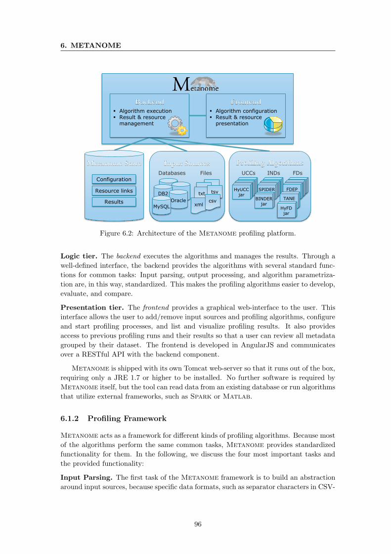
6. METANOME
Algorithm execution Result & resource
management
Algorithm configuration Result & resource
presentation
Configuration
Resource links
Results
HyUCC jar txt tsv
xml csv
DB2
Oracle
MySQL
FDEP jar
SPIDER jar
BINDER jar
TANE jar
HyFD jar
UCCs INDs FDs Databases Files
Figure 6.2: Architecture of the Metanome profiling platform.
Logic tier. The backend executes the algorithms and manages the results. Through a
well-defined interface, the backend provides the algorithms with several standard func-
tions for common tasks: Input parsing, output processing, and algorithm parametriza-
tion are, in this way, standardized. This makes the profiling algorithms easier to develop,
evaluate, and compare.
Presentation tier. The frontend provides a graphical web-interface to the user. This
interface allows the user to add/remove input sources and profiling algorithms, configure
and start profiling processes, and list and visualize profiling results. It also provides
access to previous profiling runs and their results so that a user can review all metadata
grouped by their dataset. The frontend is developed in AngularJS and communicates
over a RESTful API with the backend component.
Metanome is shipped with its own Tomcat web-server so that it runs out of the box,
requiring only a JRE 1.7 or higher to be installed. No further software is required by
Metanome itself, but the tool can read data from an existing database or run algorithms
that utilize external frameworks, such as Spark or Matlab.
6.1.2 Profiling Framework
Metanome acts as a framework for different kinds of profiling algorithms. Because most
of the algorithms perform the same common tasks, Metanome provides standardized
functionality for them. In the following, we discuss the four most important tasks and
the provided functionality:
Input Parsing. The first task of the Metanome framework is to build an abstraction
around input sources, because specific data formats, such as separator characters in CSV-
96

6.1 The Data Profiling Platform
files, are irrelevant for the profiling algorithms. Hence, algorithms can choose between
four standardized types of inputs:
1. Relational: The algorithm accepts any kind of relational input. The input source
can be a file or a table in a database. The input is read sequentially while
Metanome performs the parsing of records depending on the actual source.
2. File: The algorithm accepts raw files as input. It can, then, decide to either read
and parse the content itself or, if the content is relational, to use Metanome
functionality for the parsing. In this way, a Metanome algorithm can read non-
relational formats, such as JSON, RDF, or XML if it handles the parsing itself.
3. Table: The algorithm accepts database tables as input. The advantage of only
accepting database tables is that the algorithm is able to use database functionality
when reading the tables. For instance, the tables can be read sorted or filtered by
some criterion.
4. Database: The algorithm accepts an entire database as input. It must, then, select
the tables itself, but it is also able to access metadata tables containing schema
and data type information that can be used in the profiling process. To do so,
Metanome also provides the type of database, e.g., DB2, MySQL, or Oracle, to
the algorithm, because the name and location of metadata tables is vendor-specific.
Output Processing. Metanome’s second task is to standardize the output formats
depending on the type of metadata that the algorithm discovers. This is important,
because Metanome can process and automatically analyze the results if it knows their
type. To build a graphical visualization of an inclusion dependency graph, for instance,
Metanome must know that the output contains inclusion dependencies and it must
distinguish their dependent and referenced attributes. The most important, currently
supported types of metadata are unique column combinations (UCCs), inclusion depen-
dencies (INDs), functional dependencies (FDs), order dependencies (ODs), multivalued
dependencies (MvDs), and basic statistics. The metadata type “basic statistics” is de-
signed for simple types of metadata, such as minimum, maximum, average, or median
that do not require individual output formats; it also captures those types of metadata
that have no dedicated implementation in Metanome, yet, such as denial constraints
(DCs), matching dependencies (MDs), and several conditional dependencies.
Parametrization Handling. Besides input and output standardization, Metanome
also handles the parametrization of its algorithms. For this purpose, the profiling algo-
rithms need to expose their configuration variables and preferably default values. The
variables can then be set by the user. In this way, an algorithm can, for example, ask
for a maximum number of results or a search strategy option.
Temporary Data Management. Sometimes, algorithms must write intermediate
results or operational data to disk, for instance, if memory capacity is low. For these
cases, Metanome provides dedicated temp-files. An algorithm can store its temporary
data in such files, while Metanome places them on disk and cleans them when the
algorithm has finished.
97
6. METANOME
6.1.3 Profiling Algorithms
To run within Metanome, a profiling algorithm needs to implement a set of light-weight
interfaces: The first interface defines the algorithm’s output type and the second interface
its input type as described in Section 6.1.2. Choosing one output and one input type
is mandatory. A holistic profiling algorithm, i.e., an algorithm that discovers multiple
types of metadata, might choose more than one output type. Further interfaces can
optionally be added to request certain types of parameters or temp files. For instance,
an algorithm could request a regular expression for input filtering using the String-
parameter interface. The algorithm can also define the number of required parameter
values. An IND discovery algorithm, for instance, would require multiple relations to
discover foreign key candidates between them.
Apart from the interface, the profiling algorithms work fully autonomously, i.e., they
are treated as foreign code modules that manage themselves, providing maximum flexi-
bility for their design. So an algorithm is able to, for instance, use distributed systems
like MapReduce, machine learning frameworks like Weka, or subroutines in other pro-
gramming languages like C without needing to change the Metanome framework. This
freedom is also a risk for Metanome, because foreign code can produce memory leaks if
it crashes or is terminated. Therefore, algorithms are executed in separate processes with
their own address spaces. Apart from memory protection, this also allows Metanome to
limit the memory consumption of profiling runs. Of course, Metanome cannot protect
itself against intentionally harmful algorithms; the profiling platform is rather designed
for a trusted research community. The following algorithms are already contained in
Metanome and publicly available3:
� UCCs: Ducc [Heise et al., 2013], HyUCC [Papenbrock and Naumann, 2017a]
� INDs: Spider [Bauckmann et al., 2006], Binder [Papenbrock et al., 2015d],
Faida [Kruse et al., 2017], Many [Tschirschnitz et al., 2017]
� FDs: Tane [Huhtala et al., 1999], Fun [Novelli and Cicchetti, 2001], FD Mine [Yao
et al., 2002], Dfd [Abedjan et al., 2014c], Dep-Miner [Lopes et al., 2000], Fast-
FDs [Wyss et al., 2001], Fdep [Flach and Savnik, 1999], HyFD [Papenbrock and
Naumann, 2016], Aid-FD [Bleifuß et al., 2016]
� ODs: Order [Langer and Naumann, 2016]
� MvDs: MvdDetector [Draeger, 2016]
� Statistics: Scdp
6.2 Profiling with Metanome
In this section, we examine Metanome from two user perspectives: an IT professional,
who uses Metanome as a profiling tool on his data, and a scientist, who develops a new
profiling algorithm using Metanome as a framework.
3https://hpi.de/naumann/projects/data-profiling-and-analytics/
metanome-data-profiling/algorithms.html
98
6.2 Profiling with Metanome
6.2.1 Metadata Discovery
Given a single dependency candidate, it is easy to validate it on some dataset. The
challenge in data profiling is to discover all dependencies, i.e., to answer requests such
as “Show me all dependencies of type X that hold in a given dataset”. Metanome is
designed for exactly such requests. To start a profiling run, an IT professional needs to
specify at least a dataset and the type of dependency that should be discovered.
The need for data profiling usually arises when IT professionals already possess the
data or have access to it. This data can be in file or database format. To profile the
data, a user must register the dataset with its format definition, e.g., the separator,
quote, and escape characters for file sources or the URL, username, and password for
database sources. After registration, the new dataset appears in Metanome’s list of
profilable datasets (see Figure 6.1 center screenshot right list).
To add a new profiling algorithm, the user simply copies the algorithm’s jar-file into
Metanome’s algorithm folder and, then, selects it in the frontend. This will make the
algorithm appear in the list of profiling algorithms. Each algorithm defines the type(s)
of metadata that can be discovered (see Figure 6.1 center screenshot left list).
Starting a profiling run is easy: Select an algorithm, choose a data source and,
if needed, set some algorithm-specific parameters; pressing the execute button, then,
starts the profiling task (see Figure 6.1 center screenshot bottom panel). Metanome
executes the profiling tasks in seperate processes to control their resources and protect
the application’s own memory; it also starts the profiling tasks asynchronously, which
allows the user to run multiple tasks in parallel.
During execution, Metanome measures the algorithm’s runtime and reports on its
progress if the algorithm’s implementation supports progress measurement. In case an
execution lasts too long, users can safely cancel it, which will shoutdown the respective
process. On regular termination, the results are listed in the frontend (see Figure 6.1
front screenshot). As profiling results can be numerous, Metanome uses pagination and
loads only a subset of any large result set into the frontend. The list of results can then
be browsed, ranked, and visualized to find interesting dependencies.
Because already small datasets can harbor large amounts of metadata, Metanome
introduces various result management techniques for metadata management: When a
profiling run has finished, the user is first provided with a list of profiling results. This
list can be scrolled, filtered, and sorted by different criteria, such as lexicographical or-
der, length, or coverage. For some types of metadata, such as INDs, FDs, and UCCs,
Metanome then proposes different visualizations. These higher level abstractions pro-
vide an overview on the data and indicate certain patterns.
For the visualization of functional dependencies, for instance, Metanome uses col-
lapsible prefix-trees (see Figure 6.3) and zoom-able sunburst diagrams (see Figure 6.4).
These visualizations, which were developed in [Neubert et al., 2014], let the user ex-
plore the results incrementally. The sunburst diagram, in particular, also indicates if
one attribute is determined by particularly many other attributes or if its relatively
independent, which is an indicator for redundance in this attribute.
99

6. METANOME
Figure 6.3: Prefix-tree visualization of functional dependencies [Neubert et al., 2014].
Figure 6.4: Sunburst visualization of functional dependencies [Neubert et al., 2014].
Figure 6.5, shows an exemplary visualization of inclusion dependencies: The bub-
ble chart on the left indicates inclusion dependency clusters, i.e., sets of tables that are
connected via INDs. These connections indicate possible foreign-key relationships and,
hence, possible join paths. Clicking one cluster in the left chart opens its graph repre-
sentation on the right side. Each node represents a table, and each edge one (or more)
inclusion dependencies. This visualization not only allows the user to find topic-wise
related tables but also shows how to link their information. We recently published the
IND visualization in [Tschirschnitz et al., 2017] and its integration into the Metanome
platform is currently work in progress.
100
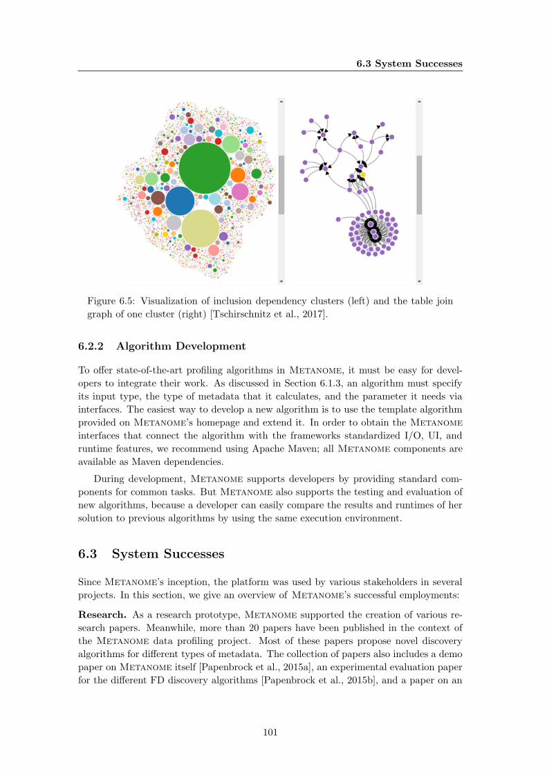
6.3 System Successes
Figure 6.5: Visualization of inclusion dependency clusters (left) and the table join
graph of one cluster (right) [Tschirschnitz et al., 2017].
6.2.2 Algorithm Development
To offer state-of-the-art profiling algorithms in Metanome, it must be easy for devel-
opers to integrate their work. As discussed in Section 6.1.3, an algorithm must specify
its input type, the type of metadata that it calculates, and the parameter it needs via
interfaces. The easiest way to develop a new algorithm is to use the template algorithm
provided on Metanome’s homepage and extend it. In order to obtain the Metanome
interfaces that connect the algorithm with the frameworks standardized I/O, UI, and
runtime features, we recommend using Apache Maven; all Metanome components are
available as Maven dependencies.
During development, Metanome supports developers by providing standard com-
ponents for common tasks. But Metanome also supports the testing and evaluation of
new algorithms, because a developer can easily compare the results and runtimes of her
solution to previous algorithms by using the same execution environment.
6.3 System Successes
Since Metanome’s inception, the platform was used by various stakeholders in several
projects. In this section, we give an overview of Metanome’s successful employments:
Research. As a research prototype, Metanome supported the creation of various re-
search papers. Meanwhile, more than 20 papers have been published in the context of
the Metanome data profiling project. Most of these papers propose novel discovery
algorithms for different types of metadata. The collection of papers also includes a demo
paper on Metanome itself [Papenbrock et al., 2015a], an experimental evaluation paper
for the different FD discovery algorithms [Papenbrock et al., 2015b], and a paper on an
101
6. METANOME
holistic discovery algorithm that jointly discovers INDs, UCCs, and FDs [Ehrlich et al.,
2016]. Metanome also enabled a scientific case study on data anamnesis using the Mu-
sicBrainz dataset [Kruse et al., 2016b]. We furthermore know that Metanome and/or
Metanome algorithms are used by research groups in France, Italy, USA, Canada, New
Zealand, India, and China, because researchers from these countries contacted us via
email; we hope that further, anonymous users of Metanome exist.
Industry. We used the Metanome platform not only in research but also in two
industry projects: With FlixBus, a European logistics company, we successfully used
Metanome to analyze travel data for business objects, patterns, and optimization po-
tential; with idealo, a German online price comparison service, we deployed Metanome
for data exploration and data preparation. Besides these industry projects, we also co-
operated with data profiling teams of IBM and SAP: IBM re-implemented most core
ideas of Metanome, such as external algorithm management and I/O standardization,
for their own Open Discovery Framework (ODF) and we currently collaborate to make
Metanome algorithms also executable within ODF; SAP also successfully took over
some ideas from Metanome and its algorithms into their data profiling tool suite and
we are now extending our collaboration with a long-term project on utilizing data pro-
filing results in concrete use cases.
Teaching. Metanome served as a teaching vehicle in various lectures, seminars, and
student projects: On the one hand, the platform and its algorithms were used to explain
the different, existing profiling algorithms; on the other hand, meanwhile more than 200
studends used Metanome for the development of own profiling algorithms as part of
their course-work, through master’s theses, and as homework assignments. Only the best
algorithms are included in the distribution of Metanome.
Competition. Most recently, the Metanome project won the business idea competition
of the German 10. Nationalen IT-Gipfel, which not only shows the need for modern
profiling solutions in industry and academia but also Metanome’s potential for sparking
a spin-off company.
102
7
Data-driven Schema
Normalization
Our experiments with Metanome have shown that discovered metadata result sets can
be huge, i.e., millions of dependencies and more. For most use cases, only a small subset
of these dependencies is actually relevant and processing the entire result set with use case
specific standard solutions is infeasible. Hence, dependency discovery research created a
paradigm shift from hard-to-understand datasets to hard-to-understand metadata sets.
The new challenge for data profiling is now to find metadata management techniques
that are able to whittle discovered metadata sets down to such subsets that are actually
relevant. Unfortunately, this task has no universal solution, because the relevance of
a discovered dependency depends on the use case: For data exploration, relevant de-
pendencies are those that express insightful rules; for schema normalization, we require
dependencies that yield reliable foreign-key constraints; for query optimization, the de-
pendencies must match the SQL expressions in some query load; and for data cleaning,
useful dependencies are those that indicate data errors – to mention just a few examples
for use case specific demands. We call a use case data-driven if it uses metadata that
was obtained from the data via profiling; thus, use cases that use expert-defined, i.e.,
manually obtained metadata are non-data-driven.
One relevance criterion that appears in multiple use cases is sematic correctness, i.e.,
the question if a dependency is only incidentally true on a given instance or if it expresses
a real-world rule that makes it logically true on all instances of a given schema. In fact,
the majority of discovered dependencies are incidental and only few dependencies are
semantically meaningful. This is because the candidate space for dependencies is, as
shown in Section 2.4, exponentially large although only a few of these candidates have
a semantic meaning; and only a limited number of the meaningless candidates finds an
invalidation in their relational instances.
In this chapter, we exemplify efficient and effective metadata management for the
concrete use case of schema normalization. The aim of schema normalization is to change
the schema of a relational instance in a way that reduces redundancy in the data without
reducing the schema’s capacity. Like many other use cases that are based on discovered
103
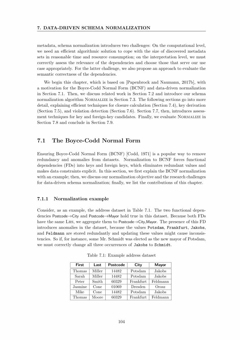
7. DATA-DRIVEN SCHEMA NORMALIZATION
metadata, schema normalization introduces two challenges: On the computational level,
we need an efficient algorithmic solution to cope with the size of discovered metadata
sets in reasonable time and resource consumption; on the interpretation level, we must
correctly assess the relevance of the dependencies and choose those that serve our use
case appropriately. For the latter challenge, we also propose an approach to evaluate the
semantic correctness of the dependencies.
We begin this chapter, which is based on [Papenbrock and Naumann, 2017b], with
a motivation for the Boyce-Codd Normal Form (BCNF) and data-driven normalization
in Section 7.1. Then, we discuss related work in Section 7.2 and introduce our schema
normalization algorithm Normalize in Section 7.3. The following sections go into more
detail, explaining efficient techniques for closure calculation (Section 7.4), key derivation
(Section 7.5), and violation detection (Section 7.6). Section 7.7, then, introduces assess-
ment techniques for key and foreign-key candidates. Finally, we evaluate Normalize in
Section 7.8 and conclude in Section 7.9.
7.1 The Boyce-Codd Normal Form
Ensuring Boyce-Codd Normal Form (BCNF) [Codd, 1971] is a popular way to remove
redundancy and anomalies from datasets. Normalization to BCNF forces functional
dependencies (FDs) into keys and foreign keys, which eliminates redundant values and
makes data constraints explicit. In this section, we first explain the BCNF normalization
with an example; then, we discuss our normalization objective and the research challenges
for data-driven schema normalization; finally, we list the contributions of this chapter.
7.1.1 Normalization example
Consider, as an example, the address dataset in Table 7.1. The two functional depen-
dencies Postcode→City and Postcode→Mayor hold true in this dataset. Because both FDs
have the same Lhs, we aggregate them to Postcode→City,Mayor. The presence of this FD
introduces anomalies in the dataset, because the values Potsdam, Frankfurt, Jakobs,
and Feldmann are stored redundantly and updating these values might cause inconsis-
tencies. So if, for instance, some Mr. Schmidt was elected as the new mayor of Potsdam,
we must correctly change all three occurrences of Jakobs to Schmidt.
Table 7.1: Example address dataset
First Last Postcode City Mayor
Thomas Miller 14482 Potsdam Jakobs
Sarah Miller 14482 Potsdam Jakobs
Peter Smith 60329 Frankfurt Feldmann
Jasmine Cone 01069 Dresden Orosz
Mike Cone 14482 Potsdam Jakobs
Thomas Moore 60329 Frankfurt Feldmann
104
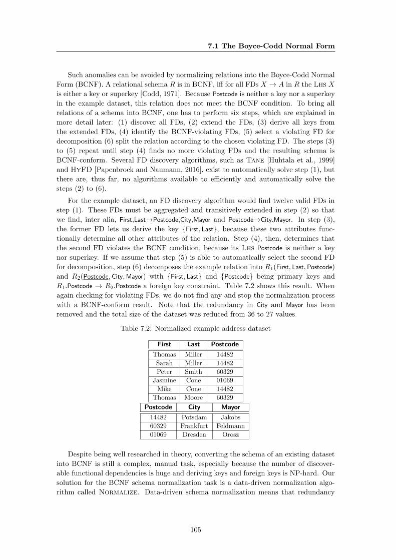
7.1 The Boyce-Codd Normal Form
Such anomalies can be avoided by normalizing relations into the Boyce-Codd Normal
Form (BCNF). A relational schema R is in BCNF, iff for all FDs X → A in R the Lhs X
is either a key or superkey [Codd, 1971]. Because Postcode is neither a key nor a superkey
in the example dataset, this relation does not meet the BCNF condition. To bring all
relations of a schema into BCNF, one has to perform six steps, which are explained in
more detail later: (1) discover all FDs, (2) extend the FDs, (3) derive all keys from
the extended FDs, (4) identify the BCNF-violating FDs, (5) select a violating FD for
decomposition (6) split the relation according to the chosen violating FD. The steps (3)
to (5) repeat until step (4) finds no more violating FDs and the resulting schema is
BCNF-conform. Several FD discovery algorithms, such as Tane [Huhtala et al., 1999]
and HyFD [Papenbrock and Naumann, 2016], exist to automatically solve step (1), but
there are, thus far, no algorithms available to efficiently and automatically solve the
steps (2) to (6).
For the example dataset, an FD discovery algorithm would find twelve valid FDs in
step (1). These FDs must be aggregated and transitively extended in step (2) so that
we find, inter alia, First,Last→Postcode,City,Mayor and Postcode→City,Mayor. In step (3),
the former FD lets us derive the key {First, Last}, because these two attributes func-
tionally determine all other attributes of the relation. Step (4), then, determines that
the second FD violates the BCNF condition, because its Lhs Postcode is neither a key
nor superkey. If we assume that step (5) is able to automatically select the second FD
for decomposition, step (6) decomposes the example relation into R1(First, Last,Postcode)
and R2(Postcode,City,Mayor) with {First, Last} and {Postcode} being primary keys and
R1.Postcode → R2.Postcode a foreign key constraint. Table 7.2 shows this result. When
again checking for violating FDs, we do not find any and stop the normalization process
with a BCNF-conform result. Note that the redundancy in City and Mayor has been
removed and the total size of the dataset was reduced from 36 to 27 values.
Table 7.2: Normalized example address dataset
First Last Postcode
Thomas Miller 14482
Sarah Miller 14482
Peter Smith 60329
Jasmine Cone 01069
Mike Cone 14482
Thomas Moore 60329
Postcode City Mayor
14482 Potsdam Jakobs
60329 Frankfurt Feldmann
01069 Dresden Orosz
Despite being well researched in theory, converting the schema of an existing dataset
into BCNF is still a complex, manual task, especially because the number of discover-
able functional dependencies is huge and deriving keys and foreign keys is NP-hard. Our
solution for the BCNF schema normalization task is a data-driven normalization algo-
rithm called Normalize. Data-driven schema normalization means that redundancy
105
7. DATA-DRIVEN SCHEMA NORMALIZATION
is removed only where it can actually be observed in a given relational instance. With
Normalize, we propose a (semi-)automatic algorithm so that a user may or may not
interfere with the normalization process. The algorithm introduces an efficient method
for calculating the closure over sets of functional dependencies and novel features for
choosing appropriate constraints. Our evaluation shows that Normalize can process
millions of FDs within a few minutes and that the constraint selection techniques support
the construction of meaningful relations during normalization.
7.1.2 Normalization objective
Because memory became a lot cheeper in the last years, there is a trend of not normalizing
datasets for performance reasons. Normalization is, for this reason, today often claimed
to be obsolete. This claim is false and ignoring normalization is dangerous for the
following reasons [Date, 2012]:
1. Normalization removes redundancy and, in this way, decreases error susceptibility
and memory consumption. While memory might be relatively cheep, data errors can
have serious and expensive consequences and should be avoided at all costs.
2. Normalization does not necessarily decrease query performance; in fact, it can even
increase the performance. Some queries might need some additional joins after normal-
ization, but others can read the smaller relations much faster. Also, more focused locks
can be set, increasing parallel access to the data, if the data has to be changed. So the
performance impact of normalization is not determined by the normalized dataset but
by the application that uses it.
3. Normalization increases the understanding of the schema and of queries against
this schema: Relations become smaller and closer to the entities they describe; their
complexity decreases making them easier to maintain and extend. Furthermore, queries
become easier to formulate and many mistakes are easier to avoid. Aggregations over
columns with redundant values, for instance, are hard to formulate correctly.
In summary, normalization should be the default and denormalization a conscious
decision, i.e., “we should denormalize only at a last resort [and] back off from a fully
normalized design only if all other strategies for improving performance have failed,
somehow, to meet requiremnts”, C. J. Date, p. 88 [Date, 2012].
Our objective is to normalize a given relational instance into Boyce-Codd Normal
Form. Note that we do not aim to recover a certain schema nor do we aim to design a new
schema using business logic. To solve the normalization task, we propose a data-driven,
(semi-)automatic normalization algorithm that removes all FD-related redundancy while
still providing full information recoverability. Again, data-driven schema normalization
means that all FDs used in the normalization process are extracted directly from the
data so that all decomposition proposals are based solely on data-characteristics.
The advantage of a data-driven normalization approach over state-of-the-art schema-
driven approaches is that it can use the data to expose all syntactically valid normaliza-
tion options, i.e., functional dependencies with evidence in the data, so that the algorithm
106
7.1 The Boyce-Codd Normal Form
(or the user) must only decide for a normalization path and not find one. The number
of FDs can, indeed, become large, but we show that an algorithm can effectively propose
the semantically most appropriate options. Furthermore, knowing all FDs allows for a
more efficient normalization algorithm as opposed to having only a subset of FDs.
7.1.3 Research challenges
In contrast to the vast amount of research on normalization in the past decades, we do
not assume that the FDs are given, because this is almost never the case in practice. We
also do not assume that a human data expert is able to manually identify them, because
the search is difficult by nature and the actual FDs are often not obvious. The FD
Postcode→City from our example, for instance, is commonly believed to be true although
it is usually violated by exceptions where two cities share the same postcode; the FD
Atmosphere→Rings, on the other hand, is difficult to discover for a human but in fact
holds on various datasets about planets. For this reason, we automatically discover all
(minimal) FDs. This introduces a new challenge, because we now deal with much larger,
often spurious, but complete sets of FDs.
Using all FDs of a particular relational instance in the normalization process further
introduces the challenge of selecting appropriate keys and foreign keys from the FDs (see
Step (5)), because most of the FDs are coincidental, i.e., they are syntactically true but
semantically false. This means that when the data changes these semantically invalid
FDs could be violated and, hence, no longer work as a constraint. So we introduce
features to automatically identify (and choose) reliable constraints from the set of FDs,
which is usually too large for a human to manually examine.
Even if all FDs are semantically correct, selecting appropriate keys and foreign keys is
still difficult. The decisions made here define which decompositions are executed, because
decomposition options are often mutually exclusive: If, for instance, two violating FDs
overlap, one split can make the other split infeasible. This happens, because BCNF
normalization is not dependency preserving [Garcia-Molina et al., 2008]. In all these
constellations, however, some violating FDs are semantically better choices than others,
which is why violating FDs must not only be filtered but also ranked by such quality
features. Based on these rankings, we propose a greedy selection approach, which always
picks the in the current state most suitable FD for the next split.
Another challenge, besides guiding the normalization process in the right direction,
is the computational complexity of the normalization. Beeri and Bernstein have proven
that the question “Given a set of FDs and a relational schema that embodies it, does the
schema violate BCNF?” is NP-complete in the number of attributes [Beeri and Bernstein,
1979]. To test this, we need to check that the Lhs of each of these FDs is a key or a
super key, i.e., if each Lhs determines all other attributes. This is trivial if all FDs
are transitively fully extended, i.e., they are transitively closed. For this reason, the
complexity lies in calculating these closures (see Step (2)). Because no current algorithm
is able to solve the closure calculation efficiently, we propose novel techniques for this
sub-task of schema normalization.
107

7. DATA-DRIVEN SCHEMA NORMALIZATION
7.1.4 Contributions
We propose a novel, instance-based schema normalization algorithm called Normalize
that can perform the normalization of a relational dataset automatically or supervised by
an expert. Allowing a human in the loop enables the algorithm to combine its analytical
strengths with the domain knowledge of an expert. Normalize makes the following
contributions:
(1) Schema normalization. We show how the entire schema normalization process can be
implemented as one algorithm, which no previous work has done before. We discuss each
component of this algorithm in detail. The main contribution of our (semi-)automatic
approach is to incrementally weed out semantically false FDs by focusing on those FDs
that are most likely true.
(2) Closure calculation. We present two efficient closure algorithms, one for general
FD result sets and one for complete result sets. Their core innovations include a more
focused extension procedure, the use of efficient index-structures, and parallelization.
These algorithms are not only useful in the normalization context, but also for many
other FD-related tasks, such as query optimization, data cleansing, or schema reverse-
engineering.
(3) Violation detection. We propose a compact data structure, i.e., a prefix tree, to
efficiently detect FDs that violate BCNF. This is the first approach to algorithmically
improve this step. We also discuss how this step can be changed to discover violating
FDs for normal forms other than BCNF.
(4) Constraint selection. We contribute several features to rate the probability of key and
foreign key candidates for actually being constraints. With the results, the candidates
can be ranked, filtered, and selected as constraints during the normalization process.
The selection can be done by either an expert or by the algorithm itself. Because all
previous works on schema normalization assumed all input FDs to be correct, this is the
first solution for a problem that has been ignored until now.
(5) Evaluation. We evaluate our algorithms on several datasets demonstrating the effi-
ciency of the closure calculation on complete, real-world FD result sets and the feasibility
of (semi-)automatic schema normalization.
7.2 Related Work
Normal forms for relational data have been extensively studied since the proposal of
the relational data model itself [Codd, 1969]. For this reason, many normal forms have
been proposed. Instead of giving a survey on normal forms here, we refer the interested
reader to [Fagin, 1979]. The Boyce-Codd Normal Form (BCNF) [Codd, 1971] is a popular
normal form that removes most kinds of redundancy from relational schemata. This is
why we focus on this particular normal form in this chapter. Most of the proposed
techniques can, however, likewise be used to create other normal forms. The idea for our
108

7.2 Related Work
normalization algorithm follows the BCNF decomposition algorithm proposed in [Garcia-
Molina et al., 2008] and many other text books on database systems. The algorithm
eliminates all anomalies related to functional dependencies while still guaranteeing full
information recoverability via natural joins.
Schema normalization and especially the normalization into BCNF are well stud-
ied problems [Beeri and Bernstein, 1979; Ceri and Gottlob, 1986; Mannila and Raiha,
1987]. Bernstein presents a complete procedure for performing schema synthesis based
on functional dependencies [Bernstein, 1976]. In particular, he shows that calculating
the closure over a set of FDs is a crucial step in the normalization process. He also
lays the theoretical foundation for this chapter. But like most other works on schema
normalization, Bernstein takes the functional dependencies and their semantic validity
as a given – an assumption that hardly applies, because FDs are usually hidden in the
data and must be discovered. For this reason, existing works on schema normalization
greatly underestimate the number of valid FDs in non-normalized datasets and they
also ignore the task of filtering the syntactically correct FDs for semantically meaningful
ones. These reasons make those normalization approaches inapplicable in practice. In
this chapter, we propose a normalization system that covers the entire process from FD
discovery over constraint selection up to the final relation decomposition. We show the
feasibility of this approach in practical experiments.
There are other works on schema normalization, such as the work of Diederich and
Milton [Diederich and Milton, 1988], who understood that calculating the transitive
closure over the FDs is a computationally complex task that becomes infeasible facing
real-world FD sets. As a solution, they propose to remove so called extraneous attributes
from the FDs before calculating the closure, which reduces the calculation costs signifi-
cantly. However, if all FDs are minimal, which is the case in our normalization process,
then no extraneous attributes exist, and the proposed pruning strategy is futile.
A major difference between traditional normalization approaches and our algorithm
is that we retrieve all minimal FDs from a given relational instance to exploit them for
closure calculation (syntactic step) and constraint selection (semantic step). The latter
has received little attention in previous research. In [Andritsos et al., 2004], the authors
proposed to rank the FDs used for normalization by the entropy of their attribute sets:
The more duplication an FD removes, the better it is. The problem with this approach
is that it weights the FDs only for effectiveness and not for semantic relevance. Entropy
is also expensive to calculate, which is why we use different features. In fact, we use
techniques inspired by [Rostin et al., 2009], who extracted foreign keys from INDs.
Schema normalization is a sub-task in schema design and evolution. There are numer-
ous database administration tools, such as Navicat1, Toad2, and MySQL Workbench3,
that support these overall tasks. Most of them transform a given schema into an ER-
diagram that a user can manipulate. All manipulations are then translated back to the
schema and its data. Such tools are partly able to support normalization processes, but
none of them can automatically propose normalizations with discovered FDs.
1https://www.navicat.com/ (Accessed: 2017-04-12)2http://www.toadworld.com/ (Accessed: 2017-04-12)3http://www.mysql.com/products/workbench/ (Accessed: 2017-04-12)
109
7. DATA-DRIVEN SCHEMA NORMALIZATION
In [Beeri and Bernstein, 1979], the authors propose an efficient algorithm for the
membership problem, i.e., the problem of testing whether one given FD is in the cover
or not. This algorithm does not solve the closure calculation problem, but the authors
propose some improvements in that algorithm that our improved closure algorithm uses
as well, e.g., testing only for missing attributes on the Rhs. They also propose derivation
trees as a model for FD derivations, i.e., deriving further FDs from a set of known FDs
using Armstrong’s inference rules. Because no algorithm is given for their model, we
cannot compare our solution against it.
As stated above, the discovery of functional dependencies from relational data is a
prerequisite for schema normalization. Fortunately, FD discovery is a well researched
problem and we find various algorithms to solve it. For this work, we utilize our HyFD
algorithm that we introduced in Chapter 3. HyFD discovers – like almost all FD dis-
covery algorithms – the complete set of all minimal, syntactically valid FDs in a given
relational dataset. We exploit these properties, i.e., minimality and completeness in our
closure algorithm.
7.3 Schema Normalization
To normalize a schema into Boyce-Codd Normal Form (BCNF), we implement the
straightforward BCNF decomposition algorithm shown in most textbooks on database
systems, such as [Garcia-Molina et al., 2008]. The BCNF-conform schema produced by
this algorithm is always a tree-shaped snowflake schema, i.e., the foreign key structure is
hierarchical and cycle-free. Our normalization algorithm is, for this reason, not designed
to (re-)construct arbitrary non-snowflake schemata. It, however, removes all FD related
redundancy from the relations. If other schema design decisions that lead to alternative
schema topologies are necessary, the user must (and can!) interactively choose different
decompositions other than the ones our algorithm can propose.
In the following, we propose a normalization process that takes an arbitrary relational
instance as input and returns a BCNF-conform schema for it. The input dataset can
contain one or more relations, and no other metadata than the dataset’s schema is
required. This schema, which is incrementally changed during the normalization process,
is globally known to all algorithmic components. We refer to a dataset’s schema as
its set of relations, specifying attributes, tables, and key/foreign key constraints. For
instance, the schema of our example dataset in Table 7.2 is {R1(First, Last,Postcode),
R2(Postcode,City,Mayor)}, where underlined attributes represent keys and same attribute
names represent foreign keys.
Figure 7.1 gives an overview of the normalization algorithm Normalize. In con-
trast to other normalization algorithms, such as those proposed in [Bernstein, 1976]
or [Diederich and Milton, 1988], Normalize does not have any components responsible
for minimizing FDs or removing extraneous FDs. This is because the set of FDs on
which we operate, is not arbitrary; it contains only minimal and, hence, no extraneous
FDs due to the FD discovery step. We now introduce the components step by step and
discuss the entire normalization process.
110
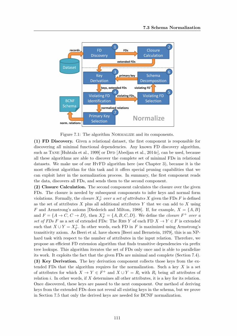
7.3 Schema Normalization
Normalize
FD Discovery
Closure Calculation
Key Derivation
Schema Decomposition
Violating FD Selection
Violating FD Identification
records FDs
extended FDs
keys, extended FDs violating FD
primary key
violating FDs
norm. relations
Dataset
1 2
3 6
4 5
Primary Key Selection
7 normalized relations
BCNF Schema
Figure 7.1: The algorithm Normalize and its components.
(1) FD Discovery. Given a relational dataset, the first component is responsible for
discovering all minimal functional dependencies. Any known FD discovery algorithm,
such as Tane [Huhtala et al., 1999] or Dfd [Abedjan et al., 2014c], can be used, because
all these algorithms are able to discover the complete set of minimal FDs in relational
datasets. We make use of our HyFD algorithm here (see Chapter 3), because it is the
most efficient algorithm for this task and it offers special pruning capabilities that we
can exploit later in the normalization process. In summary, the first component reads
the data, discovers all FDs, and sends them to the second component.
(2) Closure Calculation. The second component calculates the closure over the given
FDs. The closure is needed by subsequent components to infer keys and normal form
violations. Formally, the closure X+F over a set of attributes X given the FDs F is defined
as the set of attributes X plus all additional attributes Y that we can add to X using
F and Armstrong’s axioms [Diederich and Milton, 1988]. If, for example, X = {A,B}and F = {A→ C, C → D}, then X+
F = {A,B,C,D}. We define the closure F+ over a
set of FDs F as a set of extended FDs: The Rhs Y of each FD X → Y ∈ F is extended
such that X ∪ Y = X+F . In other words, each FD in F is maximized using Armstrong’s
transitivity axiom. As Beeri et al. have shown [Beeri and Bernstein, 1979], this is an NP-
hard task with respect to the number of attributes in the input relation. Therefore, we
propose an efficient FD extension algorithm that finds transitive dependencies via prefix
tree lookups. This algorithm iterates the set of FDs only once and is able to parallelize
its work. It exploits the fact that the given FDs are minimal and complete (Section 7.4).
(3) Key Derivation. The key derivation component collects those keys from the ex-
tended FDs that the algorithm requires for the normalization. Such a key X is a set
of attributes for which X → Y ∈ F+ and X ∪ Y = Ri with Ri being all attributes of
relation i. In other words, if X determines all other attributes, it is a key for its relation.
Once discovered, these keys are passed to the next component. Our method of deriving
keys from the extended FDs does not reveal all existing keys in the schema, but we prove
in Section 7.5 that only the derived keys are needed for BCNF normalization.
111

7. DATA-DRIVEN SCHEMA NORMALIZATION
(4) Violating FD Identification. Given the extended FDs and the set of keys, the
violation detection component checks all relations for being BCNF-conform. Recall that
a relation R is BCNF-conform, iff for all FDs X → A in that relation the Lhs X is either
a key or superkey. So Normalize checks the Lhs of each FD for having a (sub)set in
the set of keys; if no such (sub)set can be found, the FD is reported as a BCNF violation.
Note that one could setup other normalization criteria in this component to accomplish
3NF or other normal forms. If FD violations are identified, these are reported to the next
component; otherwise, the schema is BCNF-conform and can be sent to the primary key
selection. We propose an efficient technique to find all violating FDs in Section 7.6.
(5) Violating FD Selection. As long as some relations are not yet in BCNF, the
violating FD selection component is called with a set of violating FDs. In this case, the
component scores all violating FDs for being good foreign key constraints. With these
scores, the algorithm creates a ranking of violating FDs for each non-BCNF relation.
From each ranking, a user picks the most suitable violating FD for normalization; if no
user is present, the algorithm automatically picks the top ranked FD. Note that the user,
if present, can also decide to pick none of the FDs, which ends the normalization process
for the current relation. This is reasonable if all presented FDs are obviously semantically
incorrect, i.e., the FDs hold on the given data accidentally but have no real meaning.
Such FDs are presented with a relatively low score at the end of the ranking. Eventually,
the iterative process automatically weeds out most of the semantically incorrect FDs
by selecting only semantically reliable FDs in each step. We discuss the violating FD
selection together with the key selection in Section 7.7.
(6) Schema Decomposition. Knowing the violating FDs, the actual schema decom-
position is a straight-forward task: A relation R, for which a violating FD X → Y is
given, is split into two parts – one part without the redundant attributes R1 = R\Yand one part with the FD’s attributes R2 = X ∪ Y . Now X automatically becomes the
new primary key in R2 and a foreign key in R1. With these new relations, the algorithm
goes back into step (3), the key selection, because new keys might have appeared in
R2, namely those keys Z for which Z → X holds. Because the decomposition itself is
straightforward, we do not go into more detail for this component.
(7) Primary Key Selection. The primary key selection is the last component in the
normalization process. It makes sure that every BCNF-conform relation has a primary
key constraint. Because the decomposition component already assigns keys and foreign
keys when splitting relations, most relations already have a primary key. Only those
relations that had no primary key at the beginning of the normalization process are
processed by this component. For them, the algorithm (semi-)automatically assigns a
primary key: All keys of the respective relation are scored for being a good primary
key; then, the keys are ranked by their score and either a human picks a primary key
from this ranking, or the algorithm automatically picks the highest ranked key as the
relation’s primary key. Section 7.7 describes the scoring and selection of keys in detail.
Once the closure of all FDs is calculated, the components (3) to (6) form a loop:
This loop drives the normalization process until component (4) finds the schema to be
in BCNF. Overall, the proposed components can be grouped into two classes: The first
class includes the components (1), (2), (3), (4), and (6) and operates on a syntactic level;
112
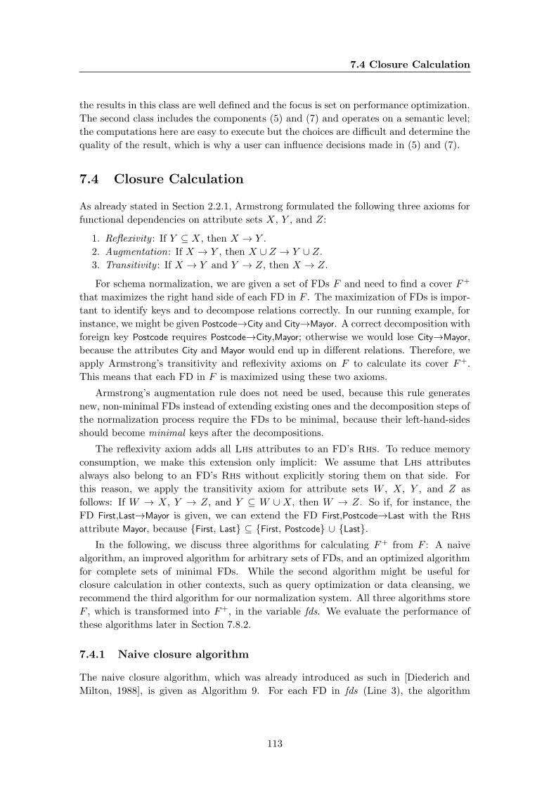
7.4 Closure Calculation
the results in this class are well defined and the focus is set on performance optimization.
The second class includes the components (5) and (7) and operates on a semantic level;
the computations here are easy to execute but the choices are difficult and determine the
quality of the result, which is why a user can influence decisions made in (5) and (7).
7.4 Closure Calculation
As already stated in Section 2.2.1, Armstrong formulated the following three axioms for
functional dependencies on attribute sets X, Y , and Z:
1. Reflexivity : If Y ⊆ X, then X → Y .
2. Augmentation: If X → Y , then X ∪ Z → Y ∪ Z.
3. Transitivity : If X → Y and Y → Z, then X → Z.
For schema normalization, we are given a set of FDs F and need to find a cover F+
that maximizes the right hand side of each FD in F . The maximization of FDs is impor-
tant to identify keys and to decompose relations correctly. In our running example, for
instance, we might be given Postcode→City and City→Mayor. A correct decomposition with
foreign key Postcode requires Postcode→City,Mayor; otherwise we would lose City→Mayor,
because the attributes City and Mayor would end up in different relations. Therefore, we
apply Armstrong’s transitivity and reflexivity axioms on F to calculate its cover F+.
This means that each FD in F is maximized using these two axioms.
Armstrong’s augmentation rule does not need be used, because this rule generates
new, non-minimal FDs instead of extending existing ones and the decomposition steps of
the normalization process require the FDs to be minimal, because their left-hand-sides
should become minimal keys after the decompositions.
The reflexivity axiom adds all Lhs attributes to an FD’s Rhs. To reduce memory
consumption, we make this extension only implicit: We assume that Lhs attributes
always also belong to an FD’s Rhs without explicitly storing them on that side. For
this reason, we apply the transitivity axiom for attribute sets W , X, Y , and Z as
follows: If W → X, Y → Z, and Y ⊆ W ∪ X, then W → Z. So if, for instance, the
FD First,Last→Mayor is given, we can extend the FD First,Postcode→Last with the Rhs
attribute Mayor, because {First, Last} ⊆ {First, Postcode} ∪ {Last}.In the following, we discuss three algorithms for calculating F+ from F : A naive
algorithm, an improved algorithm for arbitrary sets of FDs, and an optimized algorithm
for complete sets of minimal FDs. While the second algorithm might be useful for
closure calculation in other contexts, such as query optimization or data cleansing, we
recommend the third algorithm for our normalization system. All three algorithms store
F , which is transformed into F+, in the variable fds. We evaluate the performance of
these algorithms later in Section 7.8.2.
7.4.1 Naive closure algorithm
The naive closure algorithm, which was already introduced as such in [Diederich and
Milton, 1988], is given as Algorithm 9. For each FD in fds (Line 3), the algorithm
113
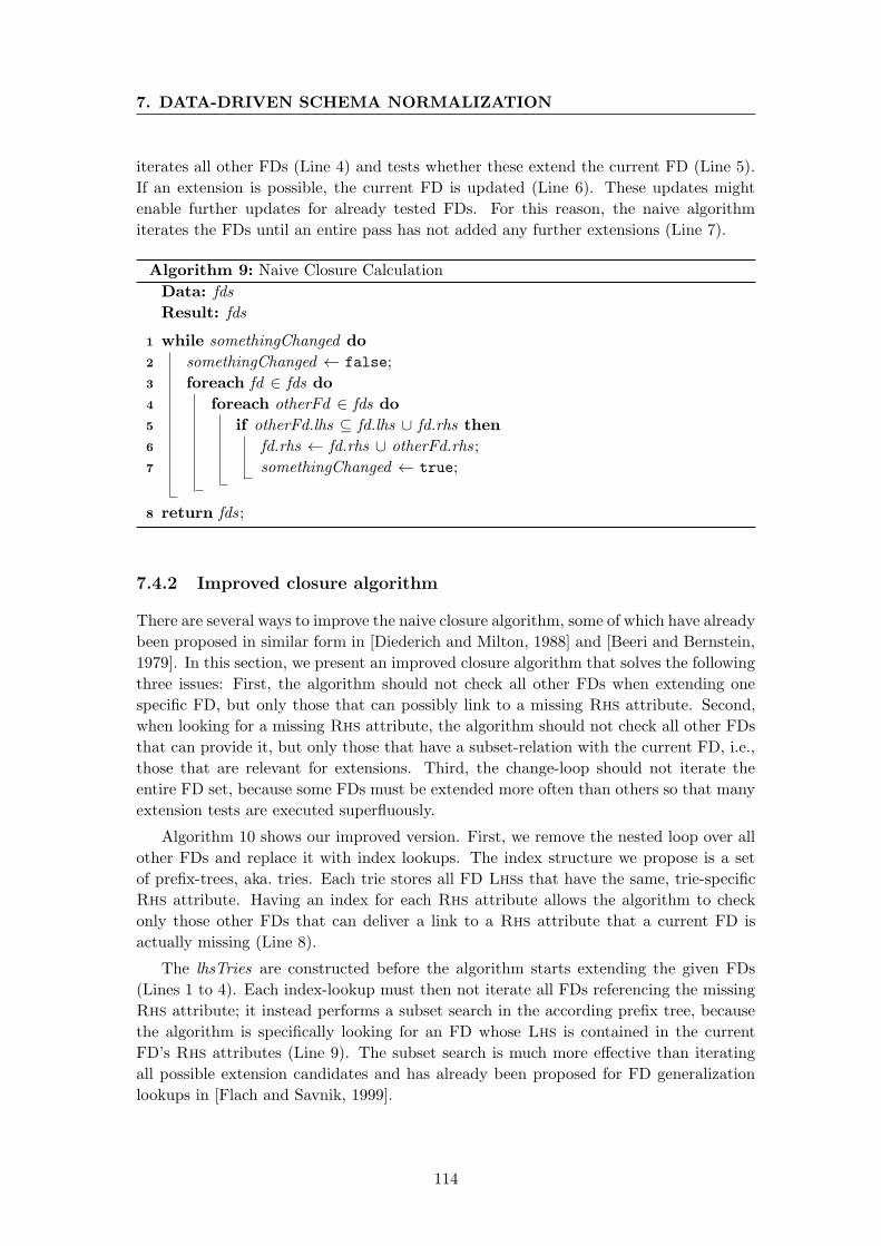
7. DATA-DRIVEN SCHEMA NORMALIZATION
iterates all other FDs (Line 4) and tests whether these extend the current FD (Line 5).
If an extension is possible, the current FD is updated (Line 6). These updates might
enable further updates for already tested FDs. For this reason, the naive algorithm
iterates the FDs until an entire pass has not added any further extensions (Line 7).
Algorithm 9: Naive Closure Calculation
Data: fds
Result: fds
1 while somethingChanged do
2 somethingChanged ← false;
3 foreach fd ∈ fds do
4 foreach otherFd ∈ fds do
5 if otherFd.lhs ⊆ fd.lhs ∪ fd.rhs then
6 fd.rhs ← fd.rhs ∪ otherFd.rhs ;
7 somethingChanged ← true;
8 return fds ;
7.4.2 Improved closure algorithm
There are several ways to improve the naive closure algorithm, some of which have already
been proposed in similar form in [Diederich and Milton, 1988] and [Beeri and Bernstein,
1979]. In this section, we present an improved closure algorithm that solves the following
three issues: First, the algorithm should not check all other FDs when extending one
specific FD, but only those that can possibly link to a missing Rhs attribute. Second,
when looking for a missing Rhs attribute, the algorithm should not check all other FDs
that can provide it, but only those that have a subset-relation with the current FD, i.e.,
those that are relevant for extensions. Third, the change-loop should not iterate the
entire FD set, because some FDs must be extended more often than others so that many
extension tests are executed superfluously.
Algorithm 10 shows our improved version. First, we remove the nested loop over all
other FDs and replace it with index lookups. The index structure we propose is a set
of prefix-trees, aka. tries. Each trie stores all FD Lhss that have the same, trie-specific
Rhs attribute. Having an index for each Rhs attribute allows the algorithm to check
only those other FDs that can deliver a link to a Rhs attribute that a current FD is
actually missing (Line 8).
The lhsTries are constructed before the algorithm starts extending the given FDs
(Lines 1 to 4). Each index-lookup must then not iterate all FDs referencing the missing
Rhs attribute; it instead performs a subset search in the according prefix tree, because
the algorithm is specifically looking for an FD whose Lhs is contained in the current
FD’s Rhs attributes (Line 9). The subset search is much more effective than iterating
all possible extension candidates and has already been proposed for FD generalization
lookups in [Flach and Savnik, 1999].
114
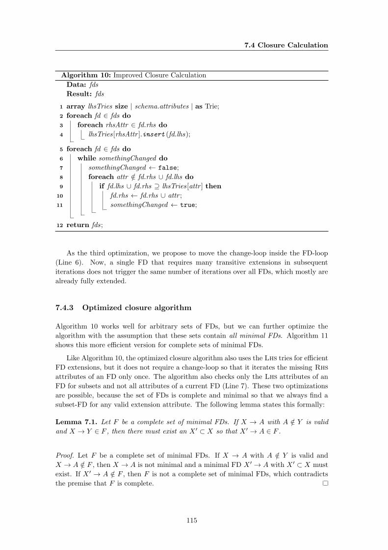
7.4 Closure Calculation
Algorithm 10: Improved Closure Calculation
Data: fds
Result: fds
1 array lhsTries size | schema.attributes | as Trie;
2 foreach fd ∈ fds do
3 foreach rhsAttr ∈ fd.rhs do
4 lhsTries [rhsAttr ].insert (fd.lhs);
5 foreach fd ∈ fds do
6 while somethingChanged do
7 somethingChanged ← false;
8 foreach attr /∈ fd.rhs ∪ fd.lhs do
9 if fd.lhs ∪ fd.rhs ⊇ lhsTries [attr ] then
10 fd.rhs ← fd.rhs ∪ attr ;
11 somethingChanged ← true;
12 return fds ;
As the third optimization, we propose to move the change-loop inside the FD-loop
(Line 6). Now, a single FD that requires many transitive extensions in subsequent
iterations does not trigger the same number of iterations over all FDs, which mostly are
already fully extended.
7.4.3 Optimized closure algorithm
Algorithm 10 works well for arbitrary sets of FDs, but we can further optimize the
algorithm with the assumption that these sets contain all minimal FDs. Algorithm 11
shows this more efficient version for complete sets of minimal FDs.
Like Algorithm 10, the optimized closure algorithm also uses the Lhs tries for efficient
FD extensions, but it does not require a change-loop so that it iterates the missing Rhs
attributes of an FD only once. The algorithm also checks only the Lhs attributes of an
FD for subsets and not all attributes of a current FD (Line 7). These two optimizations
are possible, because the set of FDs is complete and minimal so that we always find a
subset-FD for any valid extension attribute. The following lemma states this formally:
Lemma 7.1. Let F be a complete set of minimal FDs. If X → A with A /∈ Y is valid
and X → Y ∈ F , then there must exist an X ′ ⊂ X so that X ′ → A ∈ F .
Proof. Let F be a complete set of minimal FDs. If X → A with A /∈ Y is valid and
X → A /∈ F , then X → A is not minimal and a minimal FD X ′ → A with X ′ ⊂ X must
exist. If X ′ → A /∈ F , then F is not a complete set of minimal FDs, which contradicts
the premise that F is complete.
115

7. DATA-DRIVEN SCHEMA NORMALIZATION
Algorithm 11: Optimized Closure Calculation
Data: fds
Result: fds
1 array lhsTries size | schema.attributes | as Trie;
2 foreach fd ∈ fds do
3 foreach rhsAttr ∈ fd.rhs do
4 lhsTries [rhsAttr ].insert (fd.lhs);
5 foreach fd ∈ fds do
6 foreach attr /∈ fd.rhs ∪ fd.lhs do
7 if fd.lhs ⊇ lhsTries [attr ] then
8 fd.rhs ← fd.rhs ∪ attr ;
9 return fds ;
The fact that all minimal FDs are required for Algorithm 11 to work correctly has
the disadvantage that complete sets of FDs are usually much larger than sets of FDs that
have already been reduced to meaningful FDs. Reducing a set of FDs to meaningful ones
is, on the contrary, a difficult and use-case specific task that becomes more accurate if
the FDs’ closure is known. For this reason, we perform the closure calculation before the
FD selection and accept the increased processing time and memory consumption.
In fact, the increased processing time is hardly an issue, because the performance
gain of Algorithm 11 over Algorithm 10 on same sized inputs is so significant that larger
sets of FDs can still easily be processed. We show this in Section 7.8. The increased
memory consumption, on the other hand, becomes a problem if the complete set of
minimal FDs is too large to be held in memory or maybe even too large to be held on
disk. We then need to prune FDs. But which FDs can be pruned so that Algorithm 11
still computes a correct closure on the remainder? To fully extend an FD X → Y , the
algorithm requires all subset-FDs X ′ → Z with X ′ ⊂ X to be available. So if we prune
all superset-FDs with larger Lhs than |X|, the calculated closure for X → Y and all
its subset-FDs X ′ → Z would still be correct. In general, we can define a maximum
Lhs size and prune all FDs with a larger Lhs size while still being able to compute the
complete and correct closure for the remaining FDs with Algorithm 11. This pruning fits
our normalization use-case well, because FDs with shorter Lhs are semantically better
candidates for key and foreign key constraints as we argue in Section 7.7. Normalize
achieves the maximum Lhs size pruning for free, because it is already implemented in
the HyFD algorithm that we proposed using for the FD discovery.
All three closure algorithms can easily be parallelized by splitting the FD-loops
(Lines 3, 2, and 5 respectively) to different worker threads. This is possible, because
each worker changes only its own FD and changes made to other FDs can, but do not
have to be seen by this worker.
Considering the complexity of the three algorithms with respect to the number of in-
put FDs, the naive algorithm is in O(|fds|3), the improved in O(|fds|2), and the optimized
116
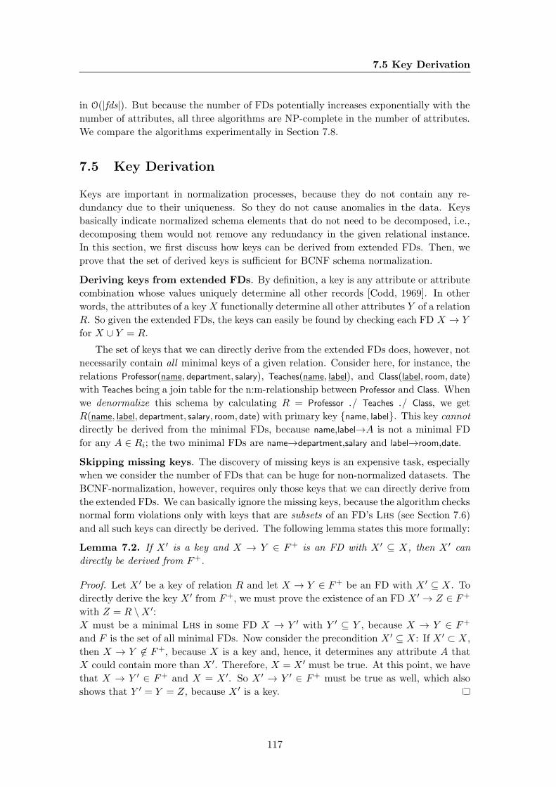
7.5 Key Derivation
in O(|fds|). But because the number of FDs potentially increases exponentially with the
number of attributes, all three algorithms are NP-complete in the number of attributes.
We compare the algorithms experimentally in Section 7.8.
7.5 Key Derivation
Keys are important in normalization processes, because they do not contain any re-
dundancy due to their uniqueness. So they do not cause anomalies in the data. Keys
basically indicate normalized schema elements that do not need to be decomposed, i.e.,
decomposing them would not remove any redundancy in the given relational instance.
In this section, we first discuss how keys can be derived from extended FDs. Then, we
prove that the set of derived keys is sufficient for BCNF schema normalization.
Deriving keys from extended FDs. By definition, a key is any attribute or attribute
combination whose values uniquely determine all other records [Codd, 1969]. In other
words, the attributes of a key X functionally determine all other attributes Y of a relation
R. So given the extended FDs, the keys can easily be found by checking each FD X → Y
for X ∪ Y = R.
The set of keys that we can directly derive from the extended FDs does, however, not
necessarily contain all minimal keys of a given relation. Consider here, for instance, the
relations Professor(name, department, salary), Teaches(name, label), and Class(label, room, date)
with Teaches being a join table for the n:m-relationship between Professor and Class. When
we denormalize this schema by calculating R = Professor ./ Teaches ./ Class, we get
R(name, label, department, salary, room, date) with primary key {name, label}. This key cannot
directly be derived from the minimal FDs, because name,label→A is not a minimal FD
for any A ∈ Ri; the two minimal FDs are name→department,salary and label→room,date.
Skipping missing keys. The discovery of missing keys is an expensive task, especially
when we consider the number of FDs that can be huge for non-normalized datasets. The
BCNF-normalization, however, requires only those keys that we can directly derive from
the extended FDs. We can basically ignore the missing keys, because the algorithm checks
normal form violations only with keys that are subsets of an FD’s Lhs (see Section 7.6)
and all such keys can directly be derived. The following lemma states this more formally:
Lemma 7.2. If X ′ is a key and X → Y ∈ F+ is an FD with X ′ ⊆ X, then X ′ can
directly be derived from F+.
Proof. Let X ′ be a key of relation R and let X → Y ∈ F+ be an FD with X ′ ⊆ X. To
directly derive the key X ′ from F+, we must prove the existence of an FD X ′ → Z ∈ F+
with Z = R \X ′:X must be a minimal Lhs in some FD X → Y ′ with Y ′ ⊆ Y , because X → Y ∈ F+
and F is the set of all minimal FDs. Now consider the precondition X ′ ⊆ X: If X ′ ⊂ X,
then X → Y 6∈ F+, because X is a key and, hence, it determines any attribute A that
X could contain more than X ′. Therefore, X = X ′ must be true. At this point, we have
that X → Y ′ ∈ F+ and X = X ′. So X ′ → Y ′ ∈ F+ must be true as well, which also
shows that Y ′ = Y = Z, because X ′ is a key.
117
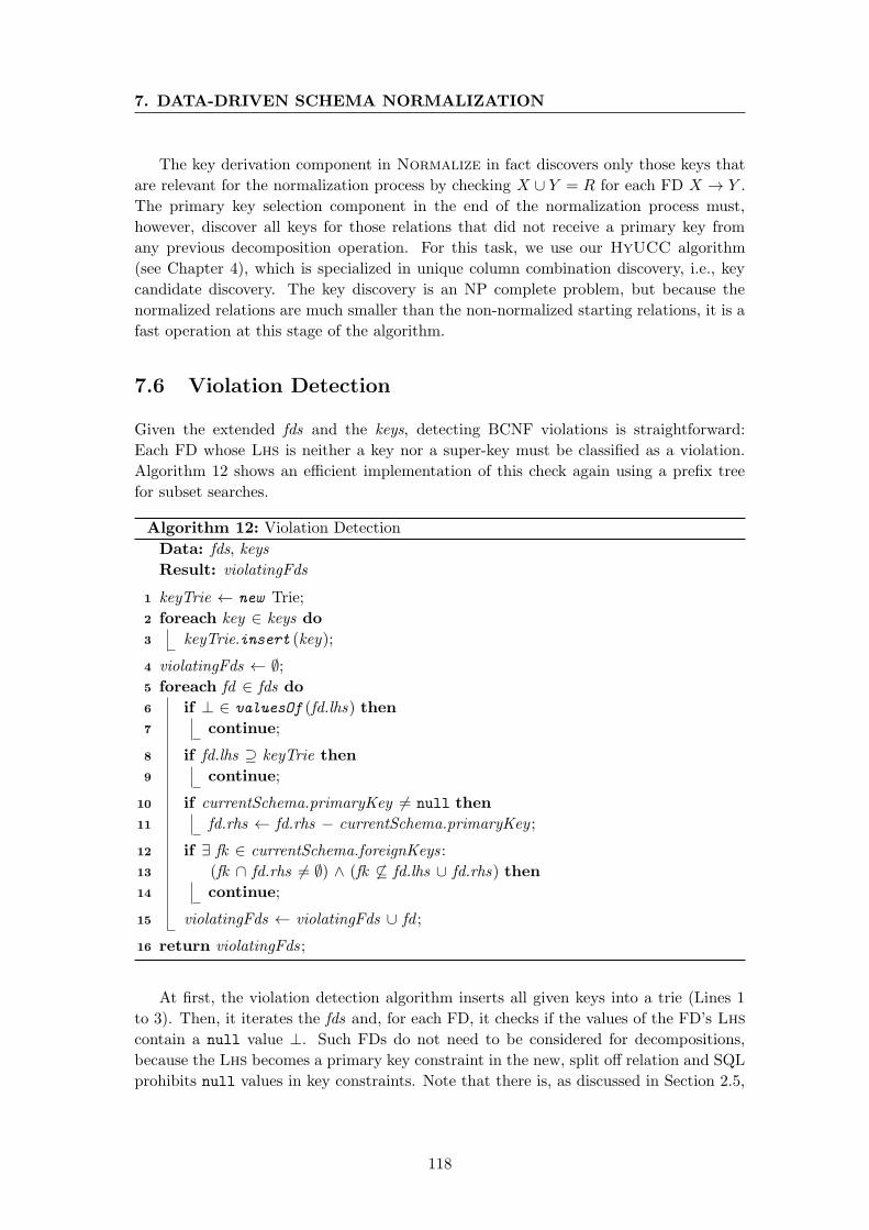
7. DATA-DRIVEN SCHEMA NORMALIZATION
The key derivation component in Normalize in fact discovers only those keys that
are relevant for the normalization process by checking X ∪ Y = R for each FD X → Y .
The primary key selection component in the end of the normalization process must,
however, discover all keys for those relations that did not receive a primary key from
any previous decomposition operation. For this task, we use our HyUCC algorithm
(see Chapter 4), which is specialized in unique column combination discovery, i.e., key
candidate discovery. The key discovery is an NP complete problem, but because the
normalized relations are much smaller than the non-normalized starting relations, it is a
fast operation at this stage of the algorithm.
7.6 Violation Detection
Given the extended fds and the keys, detecting BCNF violations is straightforward:
Each FD whose Lhs is neither a key nor a super-key must be classified as a violation.
Algorithm 12 shows an efficient implementation of this check again using a prefix tree
for subset searches.
Algorithm 12: Violation Detection
Data: fds, keys
Result: violatingFds
1 keyTrie ← new Trie;
2 foreach key ∈ keys do
3 keyTrie.insert (key);
4 violatingFds ← ∅;5 foreach fd ∈ fds do
6 if ⊥ ∈ valuesOf (fd.lhs) then
7 continue;
8 if fd.lhs ⊇ keyTrie then
9 continue;
10 if currentSchema.primaryKey 6= null then
11 fd.rhs ← fd.rhs − currentSchema.primaryKey ;
12 if ∃ fk ∈ currentSchema.foreignKeys :
13 (fk ∩ fd.rhs 6= ∅) ∧ (fk 6⊆ fd.lhs ∪ fd.rhs) then
14 continue;
15 violatingFds ← violatingFds ∪ fd ;
16 return violatingFds ;
At first, the violation detection algorithm inserts all given keys into a trie (Lines 1
to 3). Then, it iterates the fds and, for each FD, it checks if the values of the FD’s Lhs
contain a null value ⊥. Such FDs do not need to be considered for decompositions,
because the Lhs becomes a primary key constraint in the new, split off relation and SQL
prohibits null values in key constraints. Note that there is, as discussed in Section 2.5,
118
7.6 Violation Detection
work on possible/certain key constraints that permit ⊥ values in keys [Kohler et al.,
2015], but we continue with the standard for now. If the Lhs contains no null values,
the algorithm queries the keyTrie for subsets of the FD’s Lhs (Line 8). If a subset is
found, the FD does not violate BCNF and we continue with the next FD; otherwise, the
FD violates BCNF.
To preserve existing constraints, we remove all primary key attributes from a violating
FD’s Rhs, if a primary key is present (Line 11). Not removing the primary key attributes
from the FD’s Rhs could cause the decomposition step to break the primary key apart.
Some key attributes would then be moved into another relation breaking the primary
key constraint and possible foreign key constraints referencing this primary key. Because
the current schema might also contain foreign key constraints, we test if the violating FD
preserves all such constraints when used for decomposition: Each foreign key fk must
stay intact in either of the two new relations or otherwise we do not use the violating
FD for normalization (Line 13). The algorithm finally adds each constraint preserving
violating FD to the violatingFds result set (Line 15). In Section 7.7 we propose a method
to select one of them for decomposition.
When a violating FD X → Y is used to decompose a relation R, we obtain two new
relations, which are R1(R\Y ∪X) and R2(X ∪Y ). Due to this split of attributes, not all
previous FDs hold in R1 and R2. It is obvious that the FDs in R1 are exactly those FDs
V → W for which V ∪W ⊆ R1 and V → W ′ ∈ F+ with W ⊆ W ′, because the records
for V → W are still the same in R1; R1 just lost some attributes that are irrelevant for
all V →W . The same observation holds for R2 although the number of records has been
reduced:
Lemma 7.3. The relation R2(X∪Y ) produced by a decomposition on FD X → Y retains
exactly all FDs V →W , for which V ∪W ⊆ R2 and V →W is valid in R.
Proof. We need to show that (1) any V → W of R is still valid in R2 and (2) no valid
V →W of R2 can be invalid in R:
(1) Any valid V → W of R is still valid in R2: Assume that V → W is valid in R but
invalid in R2. Then R2 must contain at least two records violating V → W . Because
the decomposition only removes records in V ∪W and V ∪W ⊆ R2 ⊆ R, these violating
records must also exist in R. But such records cannot exist in R, because V → W is
valid in R; hence, the FD must also be valid in R2.
(2) No valid V → W of R2 can be invalid in R: Assume V → W is valid in R2 but
invalid in R. Then R must contain at least two records violating V → W . Because
these two records are not completely equal in their V ∪W values and V ∪W ⊆ R2, the
decomposition does not remove them and they also exist in R2. So V → W must also
be invalid in R2. Therefore, there can be no FD valid in R2 but invalid in R.
Assume that, instead of BCNF, we would aim to assure 3NF, which is slightly less
strict than BCNF: In contrast to BCNF, 3NF does not remove all FD-related redundancy,
but it is dependency preserving. Consequently, no decomposition may split an FD other
than the violating FD [Bernstein, 1976]. To calculate 3NF instead of BCNF, we could
additionally remove all those groups of violating FDs from the result of Algorithm 12
119
7. DATA-DRIVEN SCHEMA NORMALIZATION
that are mutually exclusive, i.e., any FD that would split the Lhs of some other FD. To
calculate stricter normal forms than BCNF, we would need to have detected other kinds
of dependencies. For example, constructing 4NF requires all multi-valued dependencies
(MVDs) and, hence, an algorithm that discovers MVDs. The normalization algorithm,
then, would work in the same manner.
7.7 Constraint Selection
During schema normalization, we need to define key and foreign key constraints. Syn-
tactically, all keys are equally correct and all violating FDs form correct foreign keys,
but semantically the choice of primary keys and violating FDs makes a difference. Judg-
ing the relevance of keys and FDs from a semantic point of view is a difficult task for
an algorithm – and in many cases for humans as well – but in the following, we define
some quality features that serve to automatically score keys and FDs for being “good”
constraints, i.e., constraints that are not only valid on the given instance but are true
for its schema.
The two selection components of Normalize, i.e., primary key selection and violat-
ing FD selection use the quality features to score the key and foreign-key candidates,
respectively. Then, they sort the candidates by their score. The most reasonable candi-
dates are presented at the top of the list and likely accidental candidates appear at the
end. By default, Normalize uses the top-ranked candidate and proceeds; if a user is
involved, she can choose the constraint or stop the process. The candidate list can, of
course, become too large for a full manual inspection, but (1) the user always needs to
pick only one element, i.e., she does not need to classify all elements in the list as either
true or false, (2) the candidate list becomes shorter in every step of the algorithm as
many options are implicitly weeded out, and (3) the problem of finding a split candidate
in a ranked enumeration of options is easier than finding a split without any ordering,
as it would be the case without our method.
7.7.1 Primary key selection
If a relation has no given primary key, we must assign one from the relation’s set of keys.
To find the semantically best key, Normalize scores all keys X using these features:
(1) Length score: 1|X|
Semantically correct keys are usually shorter than random keys (in their number of
attributes |X|), because schema designers tend to use short keys: Short keys can more
efficiently be indexed and they are easier to understand.
(2) Value score: 1max(1,|max(X)|−7)
The values in primary keys are typically short, because they serve to identify records
and usually do not contain much business logic. Most relational database management
systems (RDBMS) also restrict the maximum length of values in primary key attributes,
because primary keys are indexed by default and indices with too long values are more
120

7.7 Constraint Selection
difficult to manage. So we downgrade keys with values longer than 8 characters using
the function max(X) that returns the longest value in attribute (combination) X; for
multiple attributes, max(X) concatenates their values.
(3) Position score: 12( 1|left(X)|+1 + 1
|between(X)|+1)
When considering the order of attributes in their relations, key attributes are typically
located further at the beginning and without non-key attributes between them. This
is intuitive, because humans tend to place keys first and logically coherent attributes
together. The position score exploits this by assigning decreasing score values to keys
depending on the number of non-key attributes left left(X) and between between(X) key
attributes X.
The formulas we propose for the ranking reflect only our intuition. The list of features
is most likely also not complete, but the proposed features produce good results for key
scoring in our experiments. For the final key score, we simply calculate the mean of
the individual scores. In this way, the perfect key in our ranking has one attribute, a
maximum value length of 8 characters and position one in the relation, which produces
a key score of 1; less perfect keys have lower scores.
After scoring, Normalize ranks the keys by their score and lets the user choose a
primary key amongst the top ranked keys; if no user interaction is desired (or possible),
the algorithm automatically selects the top-ranked key.
7.7.2 Violating FD selection
During normalization, we need to select some violating FDs for the schema decompo-
sitions given the keys of the schema. Because the selected FDs become foreign key
constraints after the decompositions, the violating FD selection problem is similar to the
foreign key selection problem [Rostin et al., 2009], which scores inclusion dependencies
(INDs) for being good foreign keys. The viewpoints are, however, different: Selecting for-
eign keys from INDs aims to identify semantically correct links between existing tables;
selecting foreign keys from FDs, on the other hand, is about forming redundancy-free
tables with appropriate keys.
Recall that selecting semantically correct violating FDs is crucial, because some de-
compositions are mutually exclusive. If possible, a user should also discard violating
FDs that hold only accidentally in the given relational instance. Otherwise, Normalize
might drive the normalization a bit too far by splitting attribute sets – in particular
sparsely populated attributes – into separate relations. In the following, we discuss our
features for scoring violating FDs X → Y as “good” foreign key constraints:
(1) Length score: 12( 1|X| + |Y |
|R|−2)
Because the Lhs X of a violating FD becomes a primary key for the Lhs attributes
after decomposition, it should be short in length. The Rhs Y , on the contrary, should
be long so that we create large new relations: Large right-hand sides not only raise the
confidence of the FD to be semantically correct, they also make the decomposition more
effective. Because the Rhs can be at most |R| − 2 attributes long in relation R (one
121
7. DATA-DRIVEN SCHEMA NORMALIZATION
attribute must be X and one must not depend on X so that X is not a key in R), we
weight the Rhs’s length by this factor.
(2) Value score: 1max(1,|max(X)|−7)
The value score for a violating FD is the same as the value score for a primary key X,
because X becomes a primary key after decomposition.
(3) Position score: 12( 1|between(X)|+1 + 1
|between(Y )|+1)
The attributes of a semantically correct FD are most likely placed close to one another
due to their common context. We expect this to hold for both the FD’s Lhs and Rhs.
The space between Lhs and Rhs attributes, however, is only a very weak indicator,
and we ignore it. For this reason, we weight the violating FD anti-proportionally to the
number of attributes between Lhs attributes and between Rhs attributes.
(4) Duplication score: 12(2− |uniques(X)|
|values(X)| −|uniques(Y )||values(Y )| )
A violating FD is well suited for normalization if both LhsX and Rhs Y contain possibly
many duplicate values and, hence, much redundancy. The decomposition can, then,
remove many of these redundant values. As for most scoring features, a high duplication
score in the Lhs values reduces the probability that the FD holds by coincidence, because
only duplicate values in an FD’s Lhs can invalidate the FD and having many duplicate
values in LhsX without any violation is a good indicator for its semantic correctness. For
scoring, we estimate the number of unique values in X and Y with |uniques()|; because
exactly calculating this number is computationally expensive, we create a Bloom-filter
for each attribute and use their false positive probabilities to efficiently estimate the
number of unique values.
We calculate the final violating FD score as the mean of the individual scores. In this
way, the most promising violating FD is one that has a single Lhs attribute determining
almost the entire relation with short and few distinct values. Like for the key scoring,
the proposed features reflect our intuitions and observations; they might not be optimal
or complete, but they produce reasonable results for a difficult selection problem: In
our experiments the top-ranked violating FDs usually indicate the semantically best
decomposition points.
After choosing a violating FD for becoming a foreign key constraint, we could in
principle decide to remove individual attributes from the FD’s Rhs. One reason might be
that these attributes also appear in another FD’s Rhs and can be used in a subsequent
decomposition. So when a user guides the normalization process, we present all Rhs
attributes that are also contained in other violating FDs. He/she can then decide to
remove such attributes. If no user is present, nothing is removed.
7.8 Evaluation
In this section, we evaluate the efficiency and effectiveness of our normalization algorithm
Normalize. At first, we introduce our experimental setup. Then, we evaluate the
performance of Normalize and, in particular, its closure calculation component. In the
end, we assess the quality of the normalization output.
122

7.8 Evaluation
7.8.1 Experimental setup
Hardware. We ran all our experiments on a Dell PowerEdge R620 with two Intel Xeon
E5-2650 2.00 GHz CPUs and 128 GB DDR3 RAM. The server runs on CentOS 6.7 and
uses OpenJDK 64-Bit 1.8.0 71 as Java environment.
Datasets. We primarily use the synthetic TPC-H 4 dataset (scale factor one), which
models generic business data, and the MusicBrainz 5 dataset, which is a user-maintained
encyclopedia on music and artists. To evaluate the effectiveness of Normalize, we
denormalized the two datasets by joining all their relations into a single, universal re-
lation. In this way, we can compare the normalization result to the original datasets.
For MusicBrainz, we had to restrict this join to eleven selected core tables, because the
number of tables in this dataset is huge. We also limited the number of records for
the denormalized MusicBrainz dataset, because the associative tables produce an enor-
mous amount of records when used for complete joins. For the efficiency evaluation, we
use four additional datasets, namely Horse, Plista, Amalgam1, and Flight. We provide
these datasets and more detailed descriptions on our web-page6. In our evaluation, each
dataset consists of one relation with the characteristics shown in Table 7.3; the input of
Normalize can, in general, consist of multiple relations.
Table 7.3: A summary of the datasets we used for our evaluations
Name Size Attributes Records FDs FD-Keys
Horse 25.5 kB 27 368 128,727 40
Plista 588.8 kB 63 1000 178,152 1
Amalgam1 61.6 kB 87 50 450,020 2,737
Flight 582.2 kB 109 1000 982,631 25,260
MusicBrainz 1.2 GB 106 1,000,000 12,358,548 0
TPC-H 6.7 GB 52 6,001,215 13,262,106 347,805
7.8.2 Efficiency analysis
Table 7.3 lists six datasets with different properties. The amount of minimal functional
dependencies in these datasets is between 128 thousand and 13 million, and thus too
great to manually select meaningful ones. The column FD-Keys counts all those keys
that we can directly derive from the FDs. Their number does not depend on the number
of FDs but on the structure of the data: Amalgam1 and TPC-H have a snow-flake schema
while, for instance, MusicBrainz has a more complex link structure in its schema.
We executed Normalize on each of these datasets and measured the execution time
for the components (1) FD Discovery, (2) Closure Calculation, (3) Key Derivation, and
(4) Violating FD Identification. The results are shown in Table 7.4. The first two
components, i.e., FD discovery and closure calculation are parallelized so that they fully
4http://tpc.org/tpch5https://musicbrainz.org6https://hpi.de/naumann/projects/repeatability
123

7. DATA-DRIVEN SCHEMA NORMALIZATION
Table 7.4: The processing times of Normalize’s components on different datasets
Name FD Disc. Closureimpr Closureopt Key Der. Viol. Iden.
Horse 4,157 ms 1,765 ms 486 ms 40 ms 246 ms
Plista 9,847 ms 6,652 ms 857 ms 49 ms 55 ms
Amalgam1 3,462 ms 745 ms 333 ms 7 ms 25 ms
Flight 20,921 ms 132,085 ms 1,662 ms 77 ms 93 ms
MusicBrainz 2,132 min 215.5 min 1.4 min 331 ms 26 ms
TPC-H 3,651 min 3.8 min 0.5 min 163 ms 4093 ms
use all 32 cores of our evaluation machine. Despite the parallelization, the necessary
discovery of the complete set of FDs still requires 36 and 61 hours on the two larger
datasets, respectively.
First of all, we notice that the key derivation and violating FD identification steps
are much faster than the FD discovery and closure calculation steps; they usually finish
in less than a second. This is important, because the two components are executed
multiple times in the normalization process and a user might be in the loop interacting
with the system at the same time. In Table 7.4, we show only the execution times for
the first call of these components; subsequent calls can be handled even faster, because
their input sizes shrink continuously. The time needed to determine the violating FDs
depends primarily on the number of FD-keys, because the search for Lhs generalizations
in the trie of keys is the most expensive operation. This explains the long execution time
of 4 seconds for the TPC-H dataset.
For the closure calculation, Table 7.4 shows the execution times of the improved
(impr) and optimized (opt) algorithm. The naive algorithm already took 13 seconds for
the Amalgam1 dataset (compared to less than 1 s for both impr and opt), 23 minutes for
Horse (<2 s and <1 s for impr and opt, respectively), and 41 minutes for Plista (<7 s and
<1 s). These runtimes are so much worse than the improved and optimized algorithm
versions that we stopped testing it. The optimized closure algorithm, then, outperforms
the improved version by factors of 2 (Amalgam1) to 159 (MusicBrainz), because it can
exploit the completeness of the given FD set. The more extensions of right-hand sides
the algorithm must perform, the higher this advantage becomes. The average Rhs size
for Amalgam1 FDs, for instance, increases from 32 to 56, whereas the average Rhs size
for MusicBrainz FDs increases from 3 to 40. For TPC-H, the average Rhs size increases
from 10 to 23. The runtimes of the optimized closure calculation are, overall, acceptable
when compared to the FD discovery time. Therefore, it is not necessary to filter FDs
prior to the closure calculation.
Because closure calculation is not only important for normalization but for many
other use cases as well, Figure 7.2 analyses the scalability of this step in more detail.
The graphs show the execution times of the improved and the optimized algorithm for
an increasing number of input FDs. The experiment takes these input FDs randomly
from the 12 million MusicBrainz FDs; the number of attributes is kept constant to 106.
We again omit the naive algorithm, because it is orders of magnitude slower than both
other approaches.
124

7.8 Evaluation
0
40
80
120
160
200
240
280
320
360
400
0 2,000,000 4,000,000 6,000,000 8,000,000
Ru
nti
me
[se
c]
Functional Dependencies [#]
Optimized Improved
Figure 7.2: Scaling the number of input FDs for closure calculation.
Both runtimes in Figure 7.2 appear to scale almost linearly with the number of FDs,
because the extension costs for each single FD are low due to the efficient index lookups.
Nevertheless, the index lookups become more expensive with an increasing number of
FDs in the indexes (and they would also become more numerous, if we would increase
the number of attributes as well). Because the improved algorithm performs the index
lookups more often than the optimized version (i.e. changed loop) and with larger search
keys (i.e. Lhs and Rhs), the optimized version is faster and scales better with the number
of FDs: It is from 4 to 16 times faster in this experiment.
7.8.3 Normalization quality
For a fair effectiveness analysis, we perform the normalization automatically, i.e., without
human interaction. Under human supervision, better (but possibly also worse) schemata
than presented below can be produced. For the following experiments, we focus on TPC-
H and MusicBrainz, because we denormalized these datasets before so that we can use
their original schemata as gold standards for their normalization results.
Figure 7.3 shows the BCNF normalized TPC-H dataset. The color coding indicates
the original relations of the different attributes. We first notice that Normalize almost
perfectly restored the original TPC-H schema: We can identify all original relations in
the normalized result. The automatically selected constraints, i.e., keys and foreign keys
are all correct w.r.t. the original schema, which is possible because the original schema
was snow-flake shaped. Note that the normalization does not automatically produce
meaningful table names for the new relations and we labeled the reconstruced relations
with their previous names; finding good names for new relations is still an open research
topic.
Nevertheless, we also observe two interesting flaws in the automatically normalized
schema: First, Normalize decomposed the LINEITEM relation a bit too far; syntacti-
cally, the result is correct and perfectly BCNF-conform, but semantically, the splits with
125

7. DATA-DRIVEN SCHEMA NORMALIZATION
Figure 7.3: Relations after normalizing TPC-H.
only one dependent and more than three foreign key attributes are not reasonable. Sec-
ond, the attribute shippriority originally belongs to the ORDERS relation but was placed
into the REGION relation. This is syntactically a good decision, because the region also
determines the shipping priority in the given data and putting the attribute into this
relation removes more redundant values than putting it into the ORDERS relation.
Figure 7.4 shows the BCNF-normalized MusicBrainz dataset. Although MusicBrainz
has originally no snow-flake schema, Normalize was still able to reconstruct almost all
original relations. Only ARTIST CREDIT NAME was not reconstructed and its attributes
now lie in the semantically related ARTIST relation. Because MusicBrainz is originally
not snow-flake shaped, the normalization produced a new top-level relation that repre-
sents all many-to-many relationships between artists, places, release labels, and tracks.
This top-level relation can be likened to a fact table.
Most mistakes are made for the ARTIST CREDIT relation, which was the first pro-
posed split. This split took away some attributes from other relations, because these
attributes do not contain many values and assigning them to the ARTIST CREDIT rela-
tion makes syntactically sense. A human expert, if involved, would have likely avoided
that, because Normalize does report to the user that these attributes are also depen-
dent on other violating FDs Lhs attributes. Overall, however, the normalization result
is quite satisfactory, keeping in mind that no human was involved in creating it.
We also tested Normalize on various other datasets with similar findings: If datasets
have been de-normalized before, we can find the original tables in the proposed schema;
if sparsely populated columns exist, these are often moved into smaller relations; and
if no human is in the loop, some decompositions become detailed. All results were
BCNF-conform and semantically understandable.
126

7.9 Conclusion & Future Work
Figure 7.4: Relations after normalizing MusicBrainz.
7.9 Conclusion & Future Work
We proposed Normalize, an instance-driven, (semi-) automatic algorithm for schema
normalization. The algorithm has shown that functional dependency profiling results of
any size can efficiently be used for the specific task of schema normalization. We also
presented techniques for guiding the BCNF decomposition algorithm in order to produce
semantically good normalization results that also conform to changes of the data.
Our implementation is publicly available at http://hpi.de/naumann/projects/
repeatability. It is currently console-based, offering only basic user interaction. Future
work shall concentrate on emphasizing the user-in-the-loop, for instance, by employing
graphical previews of normalized relations and their connections. We also suggest re-
search on other features for the key and foreign key selection that may yield even better
results. Another open research question is how normalization processes should handle
dynamic data and errors in the data.
127

7. DATA-DRIVEN SCHEMA NORMALIZATION
128
8
Conclusion and Future Work
In this thesis, we introduced the three novel profiling algorithms HyFD, HyUCC, and
Binder for the discovery of the three most popular types of complex metadata: FDs,
UCCs, and INDs. With the use of algorithmic paradigms, such as divide-and-conquer,
hybrid search, progressivity, memory sensitivity, parallelization, and additional pruning,
our algorithms greatly improve upon the performance of related discovery algorithms; in
particular, they are now able to process datasets of real-world, i.e., multiple gigabytes
size. The algorithms also sparked the development of various further profiling algorithms
that discover other types of metadata with the same algorithmic techniques.
We also developed Metanome, a prototype for a next generation profiling platform.
Metanome was built to make state-of-the-art profiling techniques available to data
scientists and IT-professionals. Its core features are the flexible integration of profiling
algorithms, the standardization of the profiling process, and first metadata management
features. The prototype already influenced the development of commercial profiling
products at SAP and IBM.
Being able to discover large amounds of metadata introduced a new challenge to data
profiling, namely the utilization of these results for actual use cases. With Normalize,
we showed how these large metadata sets can be used to efficiently and effectively trans-
form a schema into BCNF: The algorithm proposes a data-driven, (semi-)automatic
normalization process that iteratively selects semantically most suitable dependencies.
Other use cases might require alternative solutions, but Normalize exemplified that
complete, discovered metadata sets can improve the way these use cases are solved.
During my PhD-study, I also co-developed several profiling algorithms that I could
not discuss in this thesis due to its limited scope. These algorithms include MDMin-
der [Mascher, 2013], Sindy [Kruse et al., 2015], Aid-FD [Bleifuß et al., 2016], Mvd-
Detector [Draeger, 2016], RDFind [Kruse et al., 2016a], Muds [Ehrlich et al., 2016],
Faida [Kruse et al., 2017], and Many [Tschirschnitz et al., 2017].
Although we could already improve several aspects of data profiling within the
Metanome project, several profiling tasks are still insufficiently solved and, therefore,
demand for future work:
129
8. CONCLUSION AND FUTURE WORK
Partial and conditional dependencies In this work, we focussed on the exact dis-
covery of dependencies. The next step is to extend the discovery algorithms for partial
and conditional versions of these dependencies. To achive this, the algorithms require a
notion of error tolerance and the ability to counterbalance these errors with conditions.
As discussed in Section 1.2.3, related work has already shown how such extensions could
be build.
Distributed data profiling The use of parallelization has clearly improved the runtime
of HyFD and HyUCC. We did not use parallelization in Binder, because Binder is
mostly I/O bound, i.e., reading and writing bucket files. Distributing these and other
profiling algorithms could, therefore, have further beneficial effects on their performances,
because it allows to not only parellelize processing efforts but also I/O operations. The
challenge in developing distribution profiling algorithms is to efficiently communicate
necessary pruning decisions between the different computing nodes. For IND discovery,
our Sindy algorithm [Kruse et al., 2015], which is not contained in this thesis, has shown
that distribution does pay off at a certain degree of parallelization.
Data-driven use cases Data profiling algorithms are now able to discover the metadata
of real-world sized datasets and these metadata results are surprisingly large – larger, in
particular, than most state-of-the-art solutions for use cases of metadata expect. A task
for future work is, therefore, to develop new solutions that are able to utilize these large
metadata sets. With Normalize, we already exemplified the deployment of discovered
functional dependencies for the use case of schema normalization. Other use cases that
still require data-driven solutions are, for instance, data exploration, query optimization,
schema matching, and data cleaning.
Incremental data profiling Most datasets are non-static, i.e., they are subject to
change. Changes, which are inserts, updates, and deletes, also change the datasets’
metadata making it necessary to frequently re-profile the data. Because exhaustive data
profiling processes are expensive, incremental profiling methods are needed to main-
tain the metadata under the event of data changes. The works of [Wang et al., 2003]
and [Abedjan et al., 2014b] are first approaches to this research area.
130

References
Ziawasch Abedjan and Felix Naumann. Advancing the Discovery of Unique Column
Combinations. In Proceedings of the International Conference on Information and
Knowledge Management (CIKM), pages 1565–1570, 2011.
Ziawasch Abedjan, Toni Grutze, Anja Jentzsch, and Felix Naumann. Profiling and
mining RDF data with ProLOD++. In Proceedings of the International Conference
on Data Engineering (ICDE), pages 1198–1201, 2014a.
Ziawasch Abedjan, Jorge-Arnulfo Quiane-Ruiz, and Felix Naumann. Detecting unique
column combinations on dynamic data. In Proceedings of the International Conference
on Data Engineering (ICDE), pages 1036–1047, 2014b.
Ziawasch Abedjan, Patrick Schulze, and Felix Naumann. DFD: Efficient Functional
Dependency Discovery. In Proceedings of the International Conference on Information
and Knowledge Management (CIKM), pages 949–958, 2014c.
Ziawasch Abedjan, Lukasz Golab, and Felix Naumann. Profiling Relational Data: A
Survey. VLDB Journal, 24(4):557–581, 2015.
Serge Abiteboul, Richard Hull, and Victor Vianu, editors. Foundations of Databases:
The Logical Level. Addison-Wesley Longman Publishing Co., 1 edition, 1995. ISBN
0201537710.
Rakesh Agrawal and Ramakrishnan Srikant. Fast Algorithms for Mining Association
Rules in Large Databases. In Proceedings of the International Conference on Very
Large Databases (VLDB), pages 487–499, 1994.
Martin Andersson. Extracting an entity relationship schema from a relational database
through reverse engineering, pages 403–419. Springer, Heidelberg, 1994. ISBN 978-3-
540-49100-2.
Periklis Andritsos, Renee J. Miller, and Panayiotis Tsaparas. Information-Theoretic
Tools for Mining Database Structure from Large Data Sets. In Proceedings of the
International Conference on Management of Data (SIGMOD), pages 731–742, 2004.
W. W. Armstrong. Dependency structures of database relationships. Information Pro-
cessing, 74(1):580–583, 1974.
131

REFERENCES
Paolo Atzeni and Nicola M. Morfuni. Functional dependencies and constraints on null
values in database relations. Information and Control, 70(1):1–31, 1986.
Jana Bauckmann, Ulf Leser, and Felix Naumann. Efficiently Computing Inclusion De-
pendencies for Schema Discovery. In ICDE Workshops, page 2, 2006.
Catriel Beeri and Philip A. Bernstein. Computational Problems Related to the Design of
Normal Form Relational Schemas. ACM Transactions on Database Systems (TODS),
4(1):30–59, 1979.
Catriel Beeri, Martin Dowd, Ronald Fagin, and Richard Statman. On the Structure of
Armstrong Relations for Functional Dependencies. Journal of the ACM, 31(1):30–46,
1984.
Siegfried Bell and Peter Brockhausen. Discovery of Data Dependencies in Relational
Databases. Technical report, Universitat Dortmund, 1995.
Zohra Bellahsene, Angela Bonifati, and Erhard Rahm. Schema Matching and Mapping.
Springer, Heidelberg, 1 edition, 2011. ISBN 978-3-642-16517-7.
Arno Berger and Theodore P. Hill. A basic theory of Benford’s Law. Probability Surveys,
8(1):1–126, 2011.
Philip A. Bernstein. Synthesizing Third Normal Form Relations from Functional Depen-
dencies. ACM Transactions on Database Systems (TODS), 1(4):277–298, 1976.
Leopoldo E. Bertossi. Database Repairing and Consistent Query Answering.
Morgan & Claypool Publishers, 2011. URL http://dx.doi.org/10.2200/
S00379ED1V01Y201108DTM020.
G. Birkhoff. Lattice Theory. American Mathematical Society, Charles Street, Providence,
RI, USA, 1 edition, 1940. ISBN 9780821810255.
Thomas Blasius, Tobias Friedrich, and Martin Schirneck. The Parameterized Complexity
of Dependency Detection in Relational Databases. In Proceedings of the International
Symposium on Parameterized and Exact Computation (IPEC), pages 6:1–6:13, 2017.
Tobias Bleifuß. Efficient Denial Constraint Discovery. Master’s thesis, Hasso-Plattner-
Institute, Prof.-Dr.-Helmert-Str. 2-3, D-14482 Potsdam, 2016.
Tobias Bleifuß, Susanne Bulow, Johannes Frohnhofen, Julian Risch, Georg Wiese, Se-
bastian Kruse, Thorsten Papenbrock, and Felix Naumann. Approximate Discovery
of Functional Dependencies for Large Datasets. In Proceedings of the International
Conference on Information and Knowledge Management (CIKM), pages 1803–1812,
2016.
Philip Bohannon, Wenfei Fan, and Floris Geerts. Conditional functional dependencies
for data cleaning. In Proceedings of the International Conference on Data Engineering
(ICDE), pages 746–755, 2007.
132
REFERENCES
Loreto Bravo, Wenfei Fan, and Shuai Ma. Extending Dependencies with Conditions. In
Proceedings of the International Conference on Very Large Databases (VLDB), pages
243–254, 2007.
Paul G. Brown and Peter J. Hass. BHUNT: Automatic Discovery of Fuzzy Algebraic
Constraints in Relational Data. In Proceedings of the VLDB Endowment, pages 668–
679, 2003.
Peter Buneman, Susan Davidson, Wenfei Fan, Carmem Hara, and Wang-Chiew Tan.
Keys for XML. In Proceedings of the International World Wide Web Conference
(WWW), pages 201–210, 2001.
Loredana Caruccio, Vincenzo Deufemia, and Giuseppe Polese. Relaxed Functional De-
pendencies - A Survey of Approaches. IEEE Transactions on Knowledge and Data
Engineering (TKDE), 28(1):147–165, 2016.
Marco A. Casanova, Ronald Fagin, and Christos H. Papadimitriou. Inclusion Depen-
dencies and Their Interaction with Functional Dependencies. In Proceedings of the
Symposium on Principles of Database Systems (PODS), pages 171–176, 1982.
Marco A. Casanova, Luiz Tucherman, and Antonio L. Furtado. Enforcing Inclusion
Dependencies and Referencial Integrity. In Proceedings of the International Conference
on Very Large Databases (VLDB), pages 38–49, 1988.
S. Ceri and G. Gottlob. Normalization of Relations and Prolog. Communications of the
ACM, 29(6):524–544, 1986.
Surajit Chaudhuri. An Overview of Query Optimization in Relational Systems. In
Proceedings of the Symposium on Principles of Database Systems (PODS), pages 34–
43, 1998.
Jianer Chen and Fenghui Zhang. On product covering in 3-tier supply chain models:
Natural complete problems for W[3] and W[4]. Theoretical Computer Science, 363(3):
278–288, 2006.
Peter Pin-Shan Chen. The Entity-relationship Model – Toward a Unified View of Data.
ACM Transactions on Database Systems (TODS), 1(1):9–36, 1976.
Xu Chu, Ihab F. Ilyas, and Paolo Papotti. Discovering Denial Constraints. Proceedings
of the VLDB Endowment, 6(13):1498–1509, 2013.
E. F. Codd. Derivability, Redundancy and Consistency of Relations Stored in Large
Data Banks. Technical Report RJ599, IBM, San Jose, California, 1969.
E. F. Codd. A Relational Model of Data for Large Shared Data Banks. Communications
of the ACM, 13(6):377–387, 1970.
E. F. Codd. Further Normalization of the Data Base Relational Model. IBM Research
Report, San Jose, California, RJ909, 1971.
133
REFERENCES
Gao Cong, Wenfei Fan, Floris Geerts, Xibei Jia, and Shuai Ma. Improving Data Quality:
Consistency and Accuracy. In Proceedings of the International Conference on Very
Large Databases (VLDB), pages 315–326, 2007.
Graham Cormode, Lukasz Golab, Korn Flip, Andrew McGregor, Divesh Srivastava,
and Xi Zhang. Estimating the Confidence of Conditional Functional Dependencies.
In Proceedings of the International Conference on Management of Data (SIGMOD),
pages 469–482, 2009.
Graham Cormode, Minos Garofalakis, Peter J. Haas, and Chris Jermaine. Synopses for
Massive Data: Samples, Histograms, Wavelets, Sketches. Foundations and Trends in
Databases, 4(1–3):1–294, 2012.
Stavros S. Cosmadakis, Paris C. Kanellakis, and Nicolas Spyratos. Partition semantics
for relations. Journal of Computer and System Sciences, 33(2):203–233, 1986.
P. Crawley and R. P. Dilworth. Algebraic Theory of Lattices. Prentice-Hall, Englewood
Cliffs, 1 edition, 1973.
Michele Dallachiesa, Amr Ebaid, Ahmed Eldawy, Ahmed Elmagarmid, Ihab F. Ilyas,
Mourad Ouzzani, and Nan Tang. NADEEF: A Commodity Data Cleaning System.
In Proceedings of the International Conference on Management of Data (SIGMOD),
pages 541–552, 2013.
Tamraparni Dasu, Theodore Johnson, S. Muthukrishnan, and Vladislav Shkapenyuk.
Mining Database Structure; or, How to Build a Data Quality Browser. In Proceedings
of the International Conference on Management of Data (SIGMOD), pages 240–251,
2002.
C. J. Date. Database Design & Relational Theory. O’Reilly Media, 2012. ISBN 978-1-
4493-2801-6.
Scott Davies and Stuart Russell. P-completeness of searches for smallest possible feature
sets. Technical Report FS-94-02, Computer Science Division, University of California,
1994.
DB-ENGINES. DBMS popularity broken down by database model. http://
db-engines.com/en/ranking_categories, 2017. Online; accessed 21 February 2017.
J. V. Deshpande. On continuity of a partial order. In Proceedings of the American
Mathematical Society, pages 383–386, 1968.
Keith J. Devlin. Fundamentals of contemporary set theory. Springer, Heidelberg, 1
edition, 1979. ISBN 0-387-90441-7.
Thierno Diallo, Noel Novelli, and Jean-Marc Petit. Discovering (frequent) constant
conditional functional dependencies. International Journal of Data Mining, Modelling
and Management (IJDMMM), 4(3):205–223, 2012.
134
REFERENCES
Jim Diederich and Jack Milton. New Methods and Fast Algorithms for Database Nor-
malization. ACM Transactions on Database Systems (TODS), 13(3):339–365, 1988.
Rodney G. Downey and M. R. Fellows. Parameterized Complexity. Springer, Heidelberg,
1 edition, 1999. ISBN 978-1-4612-0515-9.
Tim Draeger. Multivalued Dependency Detection. Master’s thesis, Hasso-Plattner-
Institute, Prof.-Dr.-Helmert-Str. 2-3, D-14482 Potsdam, 2016.
Roxane Edjlali and Mark A. Beyer. Magic Quadrant for Data Warehouse and Data
Management Solutions for Analytics. Gartner, Stamford, USA, 1 edition, 2016. ISBN
G00275472.
Jens Ehrlich, Mandy Roick, Lukas Schulze, Jakob Zwiener, Thorsten Papenbrock, and
Felix Naumann. Holistic Data Profiling: Simultaneous Discovery of Various Meta-
data. In Proceedings of the International Conference on Extending Database Technol-
ogy (EDBT), pages 305–316, 2016.
Ramez Elmasri and Shamkant B. Navathe. Fundamentals of Database Systems. Pearson,
7 edition, 2016. ISBN 0-13-397077.
R. Fagin and M. Vardi. The theory of data dependencies – an overview. In Proceedings
of the International Colloquium on Automata, Languages and Programming (ICALP),
pages 1–22, 1984.
Ronald Fagin. Multivalued Dependencies and a New Normal Form for Relational Data-
bases. ACM Transactions on Database Systems (TODS), 2(3):262–278, 1977.
Ronald Fagin. Normal Forms and Relational Database Operators. In Proceedings of the
International Conference on Management of Data (SIGMOD), pages 153–160, 1979.
Wenfei Fan. Dependencies Revisited for Improving Data Quality. In Proceedings of the
Symposium on Principles of Database Systems (PODS), pages 159–170, 2008.
Wenfei Fan, Floris Geerts, Xibei Jia, and Anastasios Kementsietsidis. Conditional Func-
tional Dependencies for Capturing Data Inconsistencies. ACM Transactions on Data-
base Systems, 33(2):6:1–6:48, 2008.
Wenfei Fan, Floris Geerts, Jianzhong Li, and Ming Xiong. Discovering conditional
functional dependencies. IEEE Transactions on Knowledge and Data Engineering
(TKDE), 23(5):683–698, 2011.
Peter A Flach and Iztok Savnik. Database dependency discovery: a machine learning
approach. AI Communications, 12(3):139–160, 1999.
Hector Garcia-Molina, Jeffrey D. Ullman, and Jennifer Widom. Database Systems: The
Complete Book. Prentice Hall Press, Upper Saddle River, NJ, USA, 2 edition, 2008.
ISBN 9780131873254.
135

REFERENCES
Eve Garnaud, Nicolas Hanusse, Sofian Maabout, and Noel Novelli. Parallel mining of
dependencies. In Proceedings of the International Conference on High Performance
Computing & Simulation (HPCS), pages 491–498, 2014.
Seymour Ginsburg and Richard Hull. Order dependency in the relational model. Theo-
retical Computer Science, 26(1–2):149–195, 1983.
Lukasz Golab, Howard Karloff, Flip Korn, Divesh Srivastava, and Bei Yu. On Generating
Near-optimal Tableaux for Conditional Functional Dependencies. Proceedings of the
VLDB Endowment, 1(1):376–390, 2008.
Lukasz Golab, Howard Karloff, Flip Korn, and Divesh Srivastava. Data Auditor: Explor-
ing Data Quality and Semantics Using Pattern Tableaux. Proceedings of the VLDB
Endowment, 3(1-2):1641–1644, 2010.
Lukasz Golab, Flip Korn, and Divesh Srivastava. Efficient and Effective Analysis of Data
Quality using Pattern Tableaux. IEEE Data Engineering Bulletin, 34(3):26–33, 2011.
Jarek Gryz. Query Folding with Inclusion Dependencies. In Proceedings of the Interna-
tional Conference on Data Engineering (ICDE), pages 126–133, 1998.
Jarek Gryz. Query rewriting using views in the presence of functional and inclusion
dependencies. Information Systems (IS), 24(7):597–612, 1999.
Arvid Heise, Jorge-Arnulfo Quiane-Ruiz, Ziawasch Abedjan, Anja Jentzsch, and Felix
Naumann. Scalable Discovery of Unique Column Combinations. Proceedings of the
VLDB Endowment, 7(4):301–312, 2013.
Joseph M. Hellerstein, Christoper Re, Florian Schoppmann, Daisy Zhe Wang, Eugene
Fratkin, Aleksander Gorajek, Kee Siong Ng, Caleb Welton, Xixuan Feng, Kun Li,
and Arun Kumar. The MADlib Analytics Library: Or MAD Skills, the SQL. In
Proceedings of the International Conference on Very Large Databases (VLDB), pages
1700–1711, 2012.
Mauricio A. Hernandez and Salvatore J. Stolfo. Real-world Data is Dirty: Data Cleansing
and The Merge/Purge Problem. Data Mining and Knowledge Discovery, 2(1):9–37,
1998.
Yka Huhtala, Juha Karkkainen, Pasi Porkka, and Hannu Toivonen. TANE: An efficient
algorithm for discovering functional and approximate dependencies. The Computer
Journal, 42(2):100–111, 1999.
Ihab F. Ilyas, Volker Markl, Peter Haas, Paul Brown, and Ashraf Aboulnaga. CORDS:
Automatic Discovery of Correlations and Soft Functional Dependencies. In Proceedings
of the International Conference on Management of Data (SIGMOD), pages 647–658,
2004.
ISO/IEC 9075-1:2008. Information technology – Database languages – SQL – Part
1: Framework (SQL/Framework). Standard, American National Standards Institute
(ANSI), 2016.
136

REFERENCES
Anja Jentzsch, Hannes Muhleisen, and Felix Naumann. Uniqueness, Density, and Key-
ness: Exploring Class Hierarchies. In Proceedings of the International Semantic Web
Conference (ISWC), 2015.
Theodore Johnson. Data Profiling. In Ling Liu and M. Tamer Zsu, editors, Encyclopedia
of Database Systems. Springer, Heidelberg, 2009.
Saul Judah, Mei Yang Selvage, and Ankush Jain. Magic Quadrant for Data Quality
Tools. Technical Report G00295681, Gartner, 2016.
Sean Kandel, Ravi Parikh, Andreas Paepcke, Joseph M. Hellerstein, and Jeffrey Heer.
Profiler: Integrated Statistical Analysis and Visualization for Data Quality Assess-
ment. In Proceedings of the International Working Conference on Advanced Visual
Interfaces, pages 547–554, 2012.
J. Kang and J. F. Naughton. Schema Matching Using Interattribute Dependencies. IEEE
Transactions on Knowledge and Data Engineering (TKDE), 20(10):1393–1407, 2008.
Jaewoo Kang and Jeffrey F. Naughton. On Schema Matching with Opaque Column
Names and Data Values. In Proceedings of the International Conference on Manage-
ment of Data (SIGMOD), pages 205–216, 2003.
Martti Kantola, Heikki Mannila, R. Kari-Jouko, and Harri Siirtola. Discovering func-
tional and inclusion dependencies in relational databases. International Journal of
Intelligent Systems, 7(7):591–607, 1992.
Benjamin Kille, Frank Hopfgartner, Torben Brodt, and Tobias Heintz. The plista Data-
set. In Proceedings of the International Workshop and Challenge on News Recom-
mender Systems, pages 16–23, 2013a.
Benjamin Kille, Frank Hopfgartner, Torben Brodt, and Tobias Heintz. The Plista Data-
set. In NRS Workshops, pages 16–23, 2013b.
Jyrki Kivinen and Heikki Mannila. Approximate inference of functional dependencies
from relations. Theoretical Computer Science, 149(1):129–149, 1995.
Andreas Koeller and E. A. Rundensteiner. Discovery of High-Dimensional Inclusion
Dependencies. In ICDE, 2002.
Henning Kohler and Sebastian Link. SQL Schema Design: Foundations, Normal Forms,
and Normalization. In Proceedings of the International Conference on Management of
Data (SIGMOD), pages 267–279, 2016.
Henning Kohler, Sebastian Link, and Xiaofang Zhou. Possible and Certain SQL Keys.
Proceedings of the VLDB Endowment, 8(11):1118–1129, 2015.
Sebastian Kruse, Thorsten Papenbrock, and Felix Naumann. Scaling Out the Discovery
of Inclusion Dependencies. In Proceedings of the Conference Datenbanksysteme in
Buro, Technik und Wissenschaft (BTW), pages 445–454, 2015.
137
REFERENCES
Sebastian Kruse, Anja Jentzsch, Thorsten Papenbrock, Zoi Kaoudi, Jorge-Arnulfo
Quiane-Ruiz, and Felix Naumann. RDFind: Scalable Conditional Inclusion Depen-
dency Discovery in RDF Datasets. In Proceedings of the International Conference on
Management of Data (SIGMOD), pages 953–967, 2016a.
Sebastian Kruse, Thorsten Papenbrock, Hazar Harmouch, and Felix Naumann. Data
Anamnesis: Admitting Raw Data into an Organization. IEEE Data Engineering Bul-
letin, 39(2):8–20, 2016b.
Sebastian Kruse, Thorsten Papenbrock, Christian Dullweber, Moritz Finke, Manuel Heg-
ner, Martin Zabel, Christian Zoellner, and Felix Naumann. Fast Approximate Discov-
ery of Inclusion Dependencies. In Proceedings of the Conference Datenbanksysteme in
Buro, Technik und Wissenschaft (BTW), pages –, 2017.
Philipp Langer and Felix Naumann. Efficient Order Dependency Detection. VLDB
Journal, 25(2):223–241, 2016.
Van Tran Bao Le. On the Discovery of Semantically Meaningful SQL Constraints from
Armstrong Samples: Foundations, Implementation, and Evaluation. PhD thesis, Vic-
toria University of Wellington, 6140 Wellington, New Zealand, 2014.
Mark Levene and Millist W. Vincent. Justification for Inclusion Dependency Normal
Form. IEEE Transactions on Knowledge and Data Engineering (TKDE), 12:2000,
1999.
Weibang Li, Zhanhuai Li, Qun Chen, Tao Jiang, and Hailong Liu. Discovering Functional
Dependencies in Vertically Distributed Big Data. Proceedings of the International
Conference on Web Information Systems Engineering (WISE), pages 199–207, 2015.
Jixue Liu, Jiuyong Li, Chengfei Liu, and Yongfeng Chen. Discover Dependencies from
Data – A Review. IEEE Transactions on Knowledge and Data Engineering (TKDE),
24(2):251–264, 2012.
Stephane Lopes, Jean-Marc Petit, and Lotfi Lakhal. Efficient discovery of functional
dependencies and Armstrong relations. In Proceedings of the International Conference
on Extending Database Technology (EDBT), pages 350–364, 2000.
D. Loshin. Master Data Management. Elsevier Science, 1 edition, 2010. ISBN
9780080921211.
Claudio L. Lucchesi and Sylvia L. Osborn. Candidate keys for relations. Journal of
Computer and System Sciences, 17(2):270–279, 1978.
Jayant Madhavan, Philip A. Bernstein, and Erhard Rahm. Generic Schema Matching
with Cupid. In Proceedings of the International Conference on Very Large Databases
(VLDB), pages 49–58, 2001.
Christian Mancas. Perspectives in Business Informatics Research, chapter Algorithms
for Database Keys Discovery Assistance, pages 322–338. Springer, 2016.
138
REFERENCES
Heikki Mannila and Kari-Jouko Raiha. Dependency Inference. In Proceedings of the
International Conference on Very Large Databases (VLDB), pages 155–158, 1987.
Fabien De Marchi. CLIM: Closed Inclusion Dependency Mining in Databases. In ICDM
Workshops, pages 1098–1103, 2011.
Fabien De Marchi and Jean-Marc Petit. Zigzag: A New Algorithm for Mining Large
Inclusion Dependencies in Databases. In Proceedings of the International Conference
on Data Mining (ICDM), pages 27–34, 2003.
Fabien De Marchi, Stephane Lopes, and Jean-Marc Petit. Unary and n-ary inclusion
dependency discovery in relational databases. Journal of Intelligent Information Sys-
tems, 32:53–73, 2009.
Andrina Mascher. Discovering Matching Dependencies. Master’s thesis, Hasso-Plattner-
Institute, Prof.-Dr.-Helmert-Str. 2-3, D-14482 Potsdam, 2013.
Renee J. Miller, Mauricio A. Hernandez, Laura M. Haas, Ling-Ling Yan, C. T. Howard
Ho, Ronald Fagin, and Lucian Popa. The Clio Project: Managing Heterogeneity.
SIGMOD Record, 30(1):78–83, 2001.
Felix Naumann. Data profiling revisited. SIGMOD Record, 42(4):40–49, 2013.
Tommy Neubert, Daniel Roeder, Marie Schaeffer, Alexander Spivak, Thorsten Papen-
brock, and Felix Naumann. Interpreting Data Profiling Results. Master’s thesis,
Hasso-Plattner-Institute, Prof.-Dr.-Helmert-Str. 2-3, D-14482 Potsdam, 2014.
Noel Novelli and Rosine Cicchetti. FUN: An efficient algorithm for mining functional and
embedded dependencies. In Proceedings of the International Conference on Database
Theory (ICDT), pages 189–203, 2001.
Thorsten Papenbrock and Felix Naumann. A Hybrid Approach to Functional Depen-
dency Discovery. In Proceedings of the International Conference on Management of
Data (SIGMOD), pages 821–833, 2016.
Thorsten Papenbrock and Felix Naumann. A Hybrid Approach for Efficient Unique
Column Combination Discovery. In Proceedings of the Conference Datenbanksysteme
in Buro, Technik und Wissenschaft (BTW), pages 195–204, 2017a.
Thorsten Papenbrock and Felix Naumann. Data-driven Schema Normalization. In Pro-
ceedings of the International Conference on Extending Database Technology (EDBT),
pages 342–353, 2017b.
Thorsten Papenbrock, Tanja Bergmann, Moritz Finke, Jakob Zwiener, and Felix Nau-
mann. Data Profiling with Metanome. Proceedings of the VLDB Endowment, 8(12):
1860–1863, 2015a.
Thorsten Papenbrock, Jens Ehrlich, Jannik Marten, Tommy Neubert, Jan-Peer Rudolph,
Martin Schonberg, Jakob Zwiener, and Felix Naumann. Functional Dependency Dis-
covery: An Experimental Evaluation of Seven Algorithms. Proceedings of the VLDB
Endowment, 8(10):1082–1093, 2015b.
139
REFERENCES
Thorsten Papenbrock, Arvid Heise, and Felix Naumann. Progressive Duplicate De-
tection. IEEE Transactions on Knowledge and Data Engineering (TKDE), 27(5):
1316–1329, 2015c.
Thorsten Papenbrock, Sebastian Kruse, Jorge-Arnulfo Quiane-Ruiz, and Felix Naumann.
Divide & Conquer-based Inclusion Dependency Discovery. Proceedings of the VLDB
Endowment, 8(7):774–785, 2015d.
G. N. Paulley and Per-Ake Larson. Exploiting Uniqueness in Query Optimization. In
Proceedings of the Conference of the Centre for Advanced Studies on Collaborative
Research: Distributed Computing, pages 804–822, 1993.
Glenn Norman Paulley. Exploiting Functional Dependence in Query Optimization. Tech-
nical report, University of Waterloo, 2000.
David M. W. Powers. Applications and Explanations of Zipf’s Law. In Proceedings of
the Joint Conferences on New Methods in Language Processing and Computational
Natural Language Learning, pages 151–160, 1998.
Erhard Rahm and Philip A. Bernstein. A survey of approaches to automatic schema
matching. Proceedings of the VLDB Endowment, 10(4):334–350, 2001.
Vijayshankar Raman and Joseph M. Hellerstein. Potter’s Wheel: An Interactive Data
Cleaning System. In Proceedings of the International Conference on Very Large Data-
bases (VLDB), pages 381–390, 2001.
Alexandra Rostin, Oliver Albrecht, Jana Bauckmann, Felix Naumann, and Ulf Leser. A
Machine Learning Approach to Foreign Key Discovery. In WebDB, 2009.
Hossein Saiedian and Thomas Spencer. An Efficient Algorithm to Compute the Candi-
date Keys of a Relational Database Schema. The Computer Journal, 39(2):124–132,
1996.
Nuhad Shaabani and Christoph Meinel. Scalable Inclusion Dependency Discovery. In
Proceedings of the International Conference on Database Systems for Advanced Appli-
cations (DASFAA), pages 425–440, 2015.
Nuhad Shaabani and Christoph Meinel. Detecting Maximum Inclusion Dependencies
without Candidate Generation. In Proceedings of the International Conference on
Database and Expert Systems Applications (DEXA), pages 118–133, 2016.
Yannis Sismanis, Paul Brown, Peter J. Haas, and Berthold Reinwald. GORDIAN: Effi-
cient and Scalable Discovery of Composite Keys. In Proceedings of the VLDB Endow-
ment, pages 691–702, 2006.
Shaoxu Song and Lei Chen. Discovering Matching Dependencies. In Proceedings of the
International Conference on Information and Knowledge Management (CIKM), pages
1421–1424, 2009.
140
REFERENCES
Jaroslaw Szlichta, Parke Godfrey, Jarek Gryz, and Calisto Zuzarte. Expressiveness and
Complexity of Order Dependencies. Proceedings of the VLDB Endowment, 6(14):
1858–1869, 2013.
Jaroslaw Szlichta, Parke Godfrey, Lukasz Golab, Mehdi Kargar, and Divesh Srivastava.
Effective and Complete Discovery of Order Dependencies via Set-based Axiomatiza-
tion. Proceedings of the VLDB Endowment, pages –, 2017.
David Toman and Grant Weddell. On Keys and Functional Dependencies as First-Class
Citizens in Description Logics. Journal of Automated Reasoning, 40(2):117–132, 2008.
Fabian Tschirschnitz, Thorsten Papenbrock, and Felix Naumann. Detecting Inclusion
Dependencies on Very Many Tables. ACM Transactions on Database Systems (TODS),
1(1):1–30, 2017.
Jeffrey D. Ullman. Principles of Database and Knowledge-Base Systems: Volume II:
The New Technologies. W. H. Freeman & Co., New York, NY, USA, 1990. ISBN
071678162X.
Jeffrey D. Ullman. Information integration using logical views, pages 19–40. Springer,
Heidelberg, 1997. ISBN 978-3-540-49682-3.
Shyue-Liang Wang, Wen-Chieh Tsou, Jiann-Horng Lin, and Tzung-Pei Hong. Mainte-
nance of Discovered Functional Dependencies: Incremental Deletion, pages 579–588.
Springer, Heidelberg, 2003. ISBN 978-3-540-44999-7.
Gio Wiederhold and Remez El-Masri. A Structural Model for Database Systems. Tech-
nical Report STAN-CS-79-722, Department of Computer Science, Stanford University,
1979.
Catharine Wyss, Chris Giannella, and Edward Robertson. FastFDs: A heuristic-driven,
depth-first algorithm for mining functional dependencies from relation instances ex-
tended abstract. In Proceedings of the International Conference of Data Warehousing
and Knowledge Discovery (DaWaK), pages 101–110, 2001.
Hong Yao, Howard J Hamilton, and Cory J Butz. FD Mine: discovering functional
dependencies in a database using equivalences. In Proceedings of the International
Conference on Data Mining (ICDM), pages 729–732, 2002.
Carlo Zaniolo. Database relations with null values. Journal of Computer and System
Sciences, 28(1):142–166, 1984.
Meihui Zhang, Marios Hadjieleftheriou, Beng Chin Ooi, Cecilia M. Procopiuc, and Di-
vesh Srivastava. On Multi-column Foreign Key Discovery. Proceedings of the VLDB
Endowment, 3(1-2):805–814, 2010.
141

Selbststandigkeitserklarung
Ich erklare hiermit, dass ich die vorliegende Doktorarbeit mit dem Thema:
Data Profiling – Efficient Discovery of Dependencies
selbststandig verfasst und keine anderen als die angegebenen Quellen und
Hilfsmittel benutzt habe.
Potsdam, den 29. Juni 2017


![HiN : Alexander von Humboldt im Netz [III, 4 (2002)] - publish.UP](https://static.fdokumen.com/doc/165x107/6337acd740a96001d4010ca2/hin-alexander-von-humboldt-im-netz-iii-4-2002-publishup.jpg)