D 2.8 - CORDIS
103
D 2.8 Dissemination Level: • Dissemination level: PU = Public, RE = Restricted to a group specified by the consortium (including the Commission Services), PP = Restricted to other programme participants (including the Commission Services), CO = Confidential, only for members of the consortium (including the Commission Services) Ref. Ares(2016)787773 - 15/02/2016
-
Upload
khangminh22 -
Category
Documents
-
view
0 -
download
0
Transcript of D 2.8 - CORDIS

D2.8
DisseminationLevel:
• Disseminationlevel:PU=Public,RE = Restricted to a group specified by the consortium (including the CommissionServices),PP = Restricted to other programme participants (including the CommissionServices),CO = Confidential, only formembers of the consortium (including the CommissionServices)
08Fall
08
Ref. Ares(2016)787773 - 15/02/2016

FP7–ICT–GA318137 2DISCUS
Abstract:ThisdeliverablefocusesonthemodellingactivitiesdevelopedwithintheDISCUS project. Models developed in other work packages are brieflydescribed for completeness while the techno-economic cash flowmodeldevelopedinWP2isdescribedinsomedetail.

FP7–ICT–GA318137 3DISCUS
COPYRIGHT© Copyright by the DISCUS Consortium. The DISCUS Consortium consists of: Participant Number
Participant organization name Participant org. short name
Country
Coordinator 1 Trinity College Dublin TCD Ireland Other Beneficiaries 2 Alcatel-Lucent Deutschland AG ALUD Germany 3 Coriant R&D GMBH COR Germany 4 Telefonica Investigacion Y Desarrollo SA TID Spain 5 Telecom Italia S.p.A TI Italy 6 Aston Universtity ASTON United
Kingdom 7 Interuniversitair Micro-Electronica Centrum
VZW IMEC Belgium
8 III V Lab GIE III-V France 9 University College Cork, National University of
Ireland, Cork Tyndall & UCC Ireland
10 Polatis Ltd POLATIS United Kingdom
11 atesio GMBH ATESIO Germany 12 Kungliga Tekniska Hoegskolan KTH Sweden
This document may not be copied, reproduced, or modified in whole or in part for any purpose without written permission from the DISCUS Consortium. In addition to such written permission to copy, reproduce, or modify this document in whole or part, an acknowledgement of the authors of the document and all applicable portions of the copyright notice must be clearly referenced. All rights reserved.

FP7–ICT–GA318137 4DISCUS
Name Affiliation
David Payne TCD/ASTON
Marco Ruffini TCD
Christian Raack atesio
Roland Wessaly atesio
Andrea Di Giglio TI
MarcoSchiano TI
Luis Quesada UCC
Deepak Mehta UCC
Alejandro Arbelaez UCC
Internal reviewers:
Name Affiliation
David Payne TCD/ASTON

FP7–ICT–GA318137 5DISCUS
TABLEOFCONTENTS
1 INTRODUCTION......................................................................................................................72 OVERVIEWOF(PREVIOUS)DISCUSMODELLINGACTIVITIES.................................7
2.1 UPDATEDCOREARCHITECTUREVISIONANDMODEL...............................................................................................72.1.1 MigrationfromHierarchicaltoFlatOpticalCoreNetworks.............................................................92.1.2 Opticalequipmentcostandpowerconsumptionmodels.................................................................12
2.2 SUMMARYOFOPTIMISATIONMODELSANDRESULTS............................................................................................142.2.1 OptimizingtheODN...........................................................................................................................................152.2.2 OptimizingtheBackhaulNetwork..............................................................................................................162.2.3 Fibreroutingandcost......................................................................................................................................182.2.4 Nodeandedgedisjointedness.......................................................................................................................192.2.5 TradingDistanceforreducingCapacityofMCnodes........................................................................192.2.6 OptimizingtheCorenetwork........................................................................................................................223 TRAFFICMODEL..................................................................................................................26
3.1 TRAFFICGENERATEBYAPPLICATIONS.....................................................................................................................273.2 INTER-DATACENTRETRAFFICMODELLING.............................................................................................................303.3 LEASEDLINESTRAFFICMODELLING.........................................................................................................................30
4 CASHFLOWMODELLING..................................................................................................304.1 EXCHANGEDATABASE.................................................................................................................................................324.1.1 Geotypes................................................................................................................................................................324.1.2 Exchangedatabaseparameters............................................................................................................35
4.2 DATABASEBUILDMETHODOLOGIES–ODN,CABLECHAINANDINFRASTRUCTUREDIMENSIONINGMODELS 35
4.2.1 DPservingarea:..................................................................................................................................................404.2.2 Cabinetservingarea:........................................................................................................................................414.2.3 LocalExchangeservingArea.........................................................................................................................434.2.4 Exchangedatabasesummary......................................................................................................................43
4.3 ACCESSANDMETRO-NETWORK.................................................................................................................................434.3.1 OperatorownedONUandDropmodel.....................................................................................................434.3.2 CustomerownedONUandDropmodel....................................................................................................444.3.3 Cablechainmodels:dimensioningandgrowth...................................................................................454.3.4 D-sideCableChainmodel................................................................................................................................474.3.5 Numberoffibresfromcablechainsenteringthecabinetnode:....................................................494.3.6 Backhaulnetworkcablechains....................................................................................................................524.3.7 Optimizingthebackhaulnetwork...............................................................................................................544.3.8 LR-PONamplifiernodes...................................................................................................................................56
4.4 METRO-CORENODEMODELSTRUCTURES...............................................................................................................574.4.1 Integrationofthemetro-corenodeandtheaccess&backhaulmodels....................................59
4.5 OPEXANDREVENUEMODELS....................................................................................................................................594.5.1 Opexmodel............................................................................................................................................................594.5.2 Revenuemodel.....................................................................................................................................................61
4.6 ROLLOUTSTRATEGIES.................................................................................................................................................624.7 CUMULATIVECASH-FLOWMODELS...........................................................................................................................64
5 POWERCONSUMPTIONMODELLING............................................................................665.1 ASICPOWERCONSUMPTIONASAFUNCTIONOFFEATUREGEOMETRYSIZEANDTHERELATIONSHIPTOROUTERANDSWITCHPOWERCONSUMPTION........................................................................................................................66
5.1.1 PowerconsumptionevolutionofVLSI.......................................................................................................665.2 CONCLUSIONS................................................................................................................................................................76
6 SUMMARY..............................................................................................................................76

FP7–ICT–GA318137 6DISCUS
7 REFERENCES.........................................................................................................................798 APPENDICES..........................................................................................................................81
8.1 APPENDIX1-LINEARCOSTPARAMETERS-“AVERAGE”COSTMODELS............................................................818.2 APPENDIX2-AVERAGEDISTANCEFORUNIFORMPOINTDISTRIBUTIONS........................................................838.3 APPENDIX3EXCHANGEDATABASEPARAMETERS................................................................................................848.4 APPENDIX4INFRASTRUCTUREMODELS.................................................................................................................908.4.1 D-sideCableChainmodel................................................................................................................................918.4.2 PointtoPointfibreDPcablechainmodel...............................................................................................958.4.3 E-sideCableChainmodels..............................................................................................................................97
8.5 APPENDIX5VORONOIPOLYGONSFOREXCHANGEAREAESTIMATES.................................................................999 ABBREVIATIONS...............................................................................................................102

FP7–ICT–GA318137 7DISCUS
1 IntroductionTheanalysisoftheDISCUSarchitectureandcomparisonwithalternativemoreconventionalor business as usual (BAU) architectures requires a range of models for all parts of thenetwork.Theoverallanalysisusedforcomparisonsiseconomicusingcashflowmodels.Cashflowhastheadvantageoftakingintoaccountoperationalcostbenefitsandalsotheeconomicadvantagesofcapitalexpenditurethatcanbeassociatedimmediatelywitharevenuestream,that is, a just in time (JIT) rather upfront expenditure that has no immediate revenueassociatedwithitandisthereforeriskcapital.We also describe the power consumption modelling which is closely linked to the costmodellingwithinthecashflowmodel.Atthebeginningoftheprojectitwasthoughtthatthiswouldbeafairlystraightforwardactivitywhichwouldusetheresultsfromthecomponentand subsystem volume calculations and data from public sources for power consumptionhowever this has proved more difficult than expected due to the inconsistences in theliteratureandthelackofaphysicsbasedmodelforpowerconsumptionprojectionsforfutureequipment. We have therefore built a model based on VLSI feature size for these futurepredictions. The physical layer models for the cost models required for the capitalexpenditure component of the cash flowmodels has also beenmore complex and difficultthan originally envisaged. Originally it was expected that simple updates to models builtbeforeDISUSstartedwouldbesufficientbutagainmoredetailandawiderrangeoftechnicaloptions was required which slowed development and extended the time required for themodellingactivity.To make this deliverable a self-contained report describing modelling activity across theprojectandnot just thedirectcash flowmodellingactivitiescarriedout inworkpackage2,thefirsttwosectionsgiveanoverviewofsupportingmodellingactivitiescarriedoutinotherworkpackagesandreportedinmoredetailinotherdeliverables.Thedeliverabledescribesthecoremodellingwork,theoptimisationmodelsandtheaccessandbackhaulnetworkmodelsand the cash flowmodel structuresandgives someexampleresultsinsectionn
2 Overviewof(previous)DISCUSmodellingactivities
2.1 Updatedcorearchitecturevisionandmodel
This section provides an updated vision of the DISCUS core network architecture andmodellingbasedonthedimensioningresultsattainedindeliverableD7.7.InD7.7wehavedimensionedtheUKreferencecorenetworkwith73MetroCore(MC)nodesinterconnectedwith159bidirectionalfibrelinksusingachallengingtrafficforecastprovidedbyworkpackage2 (57.5Mbit/sdownstreambusyhour sustained rate foreachPONuser).Foritstopological,geographical,andnumberofuserscharacteristicsthisnetworkprovidesaparadigm of the DISCUS core network applicable to all large European countries and can

FP7–ICT–GA318137 8DISCUS
therefore be considered as a representative network for the larger countries in Europe. ItshouldbenotedfromD7.7resultsthatthetrafficofferedtothecorenetworkisverylargeforthis challenging traffic scenario, the total core traffic is 3003 Tbit/s including the overdimensioningthatderivesfromtheresiliencerequirementsofaMCnodecatastrophicfailure.Thetrafficmatrixisfullymeshedandonly321trafficdemandsoutof2628aresmallerthan40 Gbit/s. This valuewas set in deliverable D6.1 as a threshold for accommodating trafficeither on the packet transport layer or on the photonic layer, but the number of demandssmallerthan40Gbit/sbeingsosmall, itseemsreasonabletoaccommodatealltrafficonthephotoniclayer,thusavoidingabarelyexploitedpackettransportlayer.Wecanconcludethat,atleastinthehighesttrafficscenarioconsideredinDISCUS,thepackettransportlayerisnolongernecessary.Itcanbepossiblyusedtransitorilywhencoretrafficisstillmoderate,but,inthesehightrafficscenarios,transportonthephotoniclayerbecomesmuchcheaper(seenextsection).Thesecondarchitecturalrevisionimpactsonthephotoniclayernodearchitecture.Thehightraffic volume makes a conventional ROADM insufficient in many MC nodes even if 1x20Wavelength Selective Switches (WSS) are used in combination with wideband optical linesystems(seedeliverableD7.7).Thus,inasmanyas58nodestheadoptionofastackedOpticalCross Connect (OXC) architecture is required. The stacked OXC architecture is shown inFigure2-1anddescribedin[1].
EachelementaryOXCshowninFigure2-1isaROADMbuiltby1x20WSSinrouteandselectarchitectureasexplainedindeliverablesD6.5andD7.7(thebroadcastandselectarchitectureshown in Figure 2-1 comes from the assumptions of reference [1] and is not applicable toDISCUS).TheOXCinthestackedarchitectureareinterconnectedwitheachotherinaringorlineararchitecturetoallowOpticalChannel(OCh)switchingbetweentheelementaryOXCs.Asstatedin[1],thisarchitectureisnotfullynon-blockingwhenanOChhastobeswitchedbetween two elementary OXC, but a careful network design can make this blocking issuenegligible.Amajor transmission technology changehas alsobeendescribed inD7.7.Due to thehighnumberofOCh inmany links, if traditional35nmopticalbandwidthEDFAamplification isused,thenumberoffibrepairsrequiredinsomelinksbecomesveryhigh.Tocopewiththisissue, a 100 nm wideband Raman amplification is proposed. This technology is not yet
Figure 2-1 OXC stacked architecture (from [1])

FP7–ICT–GA318137 9DISCUS
commercially available, but field transmission experiment have already been performedsuccessfully [2]. Also 100 nm wideband WSS, although not commercially available today,seem to be in the range of present photonic technologies capabilities [3]. Of course, lesschallengingnetworkscanbebuiltwithtraditionalEDFAsandCbandopticalcomponentsorhigherrateopticalchannelstoreducethetotalnumbersoffibrerequired.
2.1.1 MigrationfromHierarchicaltoFlatOpticalCoreNetworks
Metro-andcorenetworkshavehistoricallybeenstructuredashierarchicalnetworkswhichconsolidateandgroomtrafficatgatewaynodesusingpacketprocessing.ThesehierarchicallevelswouldtypicallybethebackhaulnetworkfromtheLocalExchangestothefirst tieroroutercorenetworknodes.Theoutercorenodesthenconnecttoaninnertieroflargercorenodes, which are often fully meshed. Hierarchical networks enable efficient use oftransmissioncapacitybymultiplexingtrafficontomoreefficienthighcapacitylinksbyaddinganddroppingtrafficattheinnercoregatewaynodes.However, as traffic grows, the amount of traffic passing between any pair of core nodesincreasestolevelsthatalsoefficientlyfillsopticalwavelengthchannels.Whenthisoccursthealternative architectural option of a flat optical core network performs better than thehierarchical network. Asmentioned above and shown in D7.6 and D7.7, cost-optimal corenetwork topologies are flat for larger traffic scenarios.Moreover, recent results see belowshow that for the UK reference network and customer bandwidth >~7Mb/s (total trafficvolumesoforder90Tbit/s)flattopologiesoutperformhierarchicalarchitectures.However, today we still have hierarchical core networks. It follows that an effective andgraceful evolution strategy is needed. This strategy should enable the continuation of thehierarchicalcore,whereitismostcosteffective,butitshould(automatically)transitiontoaflatcorearchitecture,wheresignificanttrafficincreasedrivesuptheinter-nodetraffic.InthissectionwegiveanupdateontheresultsfromD7.6andintroduceamigrationstrategythat outperforms the flat core at low bandwidths and the hierarchical topologies at higherbandwidthsprovidinganoptimalsolutionforalltrafficdemands.
(a)
(b)
(c)
(d)
Figure 2-2: Migration from two-level hierarchy with inner core (a) to flat optical core (d)
Wefirstestablisharelationshipbetweenusertrafficgrowthandcostevolutionforthetwoarchitectures(hierarchicalandflat).Westartfromatwo-levelhierarchicaltopology(Figure2-2(a)),typicaloftoday’snetworks,consistingofanoutercoreandafullymeshedinnercore.Atrafficdemandbetweentwocorenodesisrealizedbyatransmissionpath.PathswithmorethanonehopinvolveOEOconversionandgroomingataninnercorenode.Flatcorenetworks((Figure2-2(d))insteadhaveafulllogicalmeshoflightpathsbetweenallnodesinthecorenetwork.AsinD7.6andD7.7weassumeabrown-fieldscenariousingtheUKreferencenetworkwith73MCnodesand159fibre/cablelinks.Wefurtherusethebasetrafficscenariosdevelopedin

FP7–ICT–GA318137 10DISCUS
D2.4., which takes into consideration both residential and business data requirements andgeneratestrafficconsideringanumberofapplicationsthatusedatacentres,Internetpeeringpoint and peer-to-peer as data sources. The traffic model also considers the additionalcapacityrequiredbyinterdata-centretrafficandleasedlines.Insteadofafixedtrafficmatrix,weuse thesametrafficdistributionandvary the total trafficvolumebetween20and1000Tbit/s.ForswitchingweassumeMPLS-TPswitcheswith400Gslotsandshortreachlinecardswithgrey interfacesofcapacity40G,100Gand400G.EachMPLS-TP link isrealizedasanopticalpathusingappropriatetranspondersatbothendsthatconnecttothegreyswitchinterfaces.Weassume interfacecapacitiesandcircuitspeedsof40Gbit/s,100Gbit/s,400Gbit/s.FibresareequippedwithWDMterminalsatbothendsandlineamplifiersevery80km.Weprovide1+1 protection to ensure that services are protected against single fibre and single nodefailures.Forcost-modellingwerefertoD2.6,D7.7andfollowingsectionsinthisdeliverable.The values for the costs per unit of traffic are assumed to decrease over time (as true fortypicalpricelearningcurves[4]).Westudyaflatarchitecture(flat)amongthe73corenodesandhierarchicalnetworkswith5, 15, and 25 inner core nodes (twolevel-5, twolevel-15, twolevel-25), selected among thebiggesttrafficsources.Forallservicesandinbothlayerstheoptimization(describedinmoredetail in D7.6) determines a near-optimal routing among a huge (not complete) set ofpotentialpathsusingexactmethodsfromIntegerProgramming.Wenotethatinallscenariosthedesignatedtopology(flatorhierarchical)stronglyrestrictsthesolutionspaceofpossibleroutingsandhardwarerealizations.Infact,theroutingintheMPLS-TPdomainismainlyfixedforeachpairofactivenodesbythegivengroominggatewaynodes.Theoptimizationdecideswhich grooming location is used forwhich service, how channels shouldbe realized in thefibre topology for1+1protection,andwhichcircuit speedsareusedbetweenwhichpairofnodes.Results for amoderate trafficof around30Tbit/s core traffic volume (2Mbit/s sustainedbandwidth per user in the busy hour) are shown in Figure 2-3. Costs are categorized asswitchesplus interface linecards(yellow),WDMequipment(red)andoptical transponders(blue).For thismoderate traffic level thetwomainobservationswemakeare: (i)Costsaremainly driven by transponders and switching equipment required to terminate thewavelength channels and forward the packets. (ii) The hierarchical structure with 5 innernodesismostcosteffective.
Figure 2-3: Brown field network cost in 1000 ICU, busy hour traffic per customer 2 Mb/s

FP7–ICT–GA318137 11DISCUS
However,theoverallnetworkcostisstronglydependentonusertrafficgrowthandwethusconsideredarangeofaveragebusyhourcustomertrafficpatternsupto35Mbit/s.Astrafficgrowswecompletelyre-optimizeall topologies.Figure2-4showstheaccumulatedupgradecost(applyingpricelearningcurves)withuserbandwidthgrowth.Clearly,astrafficincreasesflatterarchitecturesbecomemorecosteffective.Theflatcorehasthelargestupfrontcostbutalso the smallest slope and outperforms all other studied network topologies when usertrafficexceedsaround10-20Mbit/sforthemodelparametersused.Our results show that as user traffic increases the most cost-effective network solutionmovesfromahierarchicalstructuretoonebasedonfullymeshedopticalislands.Inordertoefficientlymigratetoday’shierarchicalnetworkswesuggestthefollowingstrategy:ConsiderahierarchicalcorenetworkwithasubsetofthenodesformingafullymeshedinnercoreasinFigure2-2(a).Theremainingoutercorenodesareconnectedtoinnercorenodesby(atleast)two(disjoint)connections.The innercorenodesareconsolidating traffic fromanumberofouter core nodes and will be the largest traffic nodes. As network traffic grows theconsolidatedtrafficbetweenapairofnodes(trafficthatneedsOEOconversionatbothnodes)will also grow. If that traffic exceeds a threshold of, e.g., 40Gb/s a direct optical channelconnectionisprovidedoverwhichalltheconsolidatedtrafficissent.Thisthresholdisinlinewith using 100 Gb/s light paths and is the value defined in deliverable D6.1 foraccommodating traffic directly on the photonic layer but other values could also beconsideredwhichcouldenabletheuseoflowercapacitylightpathstobecompared,thiswas
notdoneinthecurrentmodellingduetotimeandresourcelimitations.Asaresult, inthefirstphaseoutercorenodeswillgetconnectedtomostoftheinnercorenodes.Later,withtrafficgrowthmorelightpathscanbedirectlyconnectedbetweenpairsofnodeswithouttheOEOconversionsandeventuallyevensmalleroutercorenodeswillhaveadirectchannelconnection.ThisprocessisillustratedinFigure2-2.Todemonstratetheefficiencyofthisparticularmigrationstrategy,westartedwithaninnercore of the 5 largest nodes in the UK and optimized the network for a relatively low usercapacityutilizationi.e.,400kb/ssustainedrateperuser~4xtodayssustainedrates)leadingtoasparselyconnectedtwolevelhierarchicaltopologyasinFigure2-2.Wethenincreasedtheuserbandwidthandcheckedtheconsolidatedtrafficforallnon-connectedpairsofMCnodes.Iftheconsolidatedbandwidthsexceededthethresholdof40Gbit/snewdirectchannelswereimplementedbetweenthenodepairsandtheroutingchangedasdescribedabove.
Figure 2-4: Cumulative upgrade costs for different network topologies in 1000 ICU

FP7–ICT–GA318137 12DISCUS
Figure2-5(migration-5-40G)showsthatthistransitionstrategyoutperformstheflatcoreatlowbandwidthsandthe two levelhierarchical topologyathigherbandwidths,providinganoptimalsolutionforalltrafficdemands.Webelievethatthismigrationstrategyshouldnowbeimplementedtoensurenetworksremainat lowestcostandlowestpowerintothefuture.Itperfectlysuitsthetransitionfromtoday’snetworktopologiestoarchitecturesthatfollowtheDISCUSprinciplesleadingtothelowestcostandmostefficientfuturenetwork.
2.1.2 Opticalequipmentcostandpowerconsumptionmodels
TheDISCUScorenetworkopticalequipmentcostparametershavebeenmostlyderivedfromthemodelsdevelopedintheEUIDEALISTproject[3](thatisinturnanenhancementoftheworkdoneintheEUSTRONGESTproject[6]),withsomemoreforecastsonfuture,innovativecomponents introduced in the DISCUS network. Cost parameters are expressed in theIDEALIST Cost Unit (ICU) that corresponds to the cost of a 100 Gbit/s fixed DP-QPSKtransponder. In general, for the costs of flexgrid component a 20% increment has beenassessedw.r.t.thefixedgridcomponentsusedintheSTRONGESTproject.StartingfromthegeneralarchitectureofROADMandOLAdevelopedforDISCUS[7],[8],thecost and energy consumption of each functional block, namely line interfaces, add/dropblocksandlineamplifiershavebeenobtainedbyaddingthecostsandpowersrequiredforallthecardsthatcomposethesubsystems.TheresultsaresummarizedinTable1.In particular, the calculation on line interfaces includes the data on cost and powerconsumptionoftwo1x20WBWSS,oneWBRamanbooster,oneWBRamanpre-amplifier,oneControlboard,oneOpticalPerformanceMonitoring(OPM)cardandoneOpticalSupervisorychannel (OSC) card. The WBWSS cost has been calculated summing up the cost of threeconventional WSS (each covering 1/3 of the 100 nm bandwidth), reduced by 25% as anestimation of the economy of scale arising from the component integration in one singlepackage.Thepowerconsumptionhasbeenestimatedtohavea30%increaseduetocontrolcircuitsincreasedcomplexityw.r.t.thepresentdevice.
Item Cost(ICU)Powerconsumption(W)
Notes
Figure 2-5: Cumulative upgrade costs in 1000 ICU over time

FP7–ICT–GA318137 13DISCUS
Lineinterfaces 3.1 260 1dualWBWSSand2WBRamanamp.
Lineamplifier 1.6 200 2WBRamanamp.
DualMulticastSwitch8x321 1.3 45 1foreachgroupof32transponders
Table1 -Powerandcostmodelofthephotonicswitchingfunctionalblocks
ThecostandenergyconsumptionoftheWBRamanboosterandpre-amplifierusedforthelineinterfaceshavebeencalculatedasthe75%ofthecostoftheWBRamanusedforthelineamplifiers.TheOLAWBRamanpricehasbeenquotedto0,8ICU,about10%lessthan3timesthecostofacommonEDFAplusRamanamplifier,with35nmopticalbandwidth.ThepowerconsumptionofaWBRamanamplifiershasbeenestimated100W.The cost and energy consumption of the Colorless, Directionless and Contentionlessadd/dropfunctionalblock,namelythedual8x32Multicastswitch(MS),includes8amplifierswhosecostandenergycanbeconsideredequaltosimple,single-stageEDFAamplifiers,whilethevaluesforthe8x32MShasbeenderivedfromtheIDEALISTcostofa16x16MSswitch.Table 2 summarizes the cost and power consumption values for the Bandwidth VariableTransponders(BVTs)andtheSliceableBandwidthVariableTransponders(S-BVTs),thatareconnectedtothetributaryportsoftheMSswitch.ThecostofthesinglecarrierBVThasbeenquotedsubstantiallyequaltotheICUunit,whilethe power consumptionhas been reduced of about 25%w.r.t. to the IDEALIST cost due topowersavingexpectedfromphotoniccomponentsintegration.TheDISCUSforecastoncostandpowerconsumptionofthequadruplecarrierS-BVTarejustthree times the corresponding values of single carrier BVT. This can be considered areasonable figure considering components integration and consequent cost and energyreduction.Table2-PowerandcostmodelofS-BVTsfortheDISCUScorenetwork
1.Single-carrierBVT
N. ofopticalcarriers
N. of37.5GHzslots
Configurations(services)
Clientsignals
Modulationformat
Cost(ICU)
Powerconsumption(W)
1 1
Single40GE 1x40GE DP-BPSK 0.95 140
Single100GE 1x100GE DP-QPSK 1 150
Dual100GE 2x100GE DP-16QAM 1.1 160
2.Quadruple-carrierS-BVT
N. ofopticalcarriers
N.of37.5GHzslots
Configurations(services)
Clientsignals
Modulationformat
Cost(ICU)
Powerconsumption(W)
4 4 Single400GE 1x400GE DP-QPSK 3 4401EstimatedbyTI.

FP7–ICT–GA318137 14DISCUS
Twin400GE 2x400GE DP-16QAM 3.2 450
Twin100GE 2x100GE DP-BPSK 3 440
2.2 Summaryofoptimisationmodelsandresults
AsdiscussedinDeliverableD2.6[12],wethefollowingarethethreehigh-leveloptimizationactivitieswithinDiscus(see):• Intheoptimizationoftheopticaldistributionnetwork(ODN)afterassigningcustomers
tolocalexchanges(LE)andfibreaccessnetworkusingapassiveopticalnetwork(PON)architecture, is designed optimizing both the cable tree routing and the location ofpassiveopticalsplitters.
• In the optimization of theBackhaulwedetermine the number and location ofmetro-core(MC)nodessothatalllocalexchangescanbeconnectedtotwodifferentsuchMCsviadisjointfibreroutes(directlyorwithinachainorpartialringtopology).
• In the optimizationof the corenetworkwe study the connectionofMCnodes amongeach other including core fibre routing, the embedding of light-paths,wavelength (orspectrum)assignment,thelocationof(Raman/EDFA)amplifiers,andoptimalMCnodecorenetworkhardware.
Clearly as each sub-problem is solved independently, decisionsmade inonenetworkmayimpactdecisionstakeninanotherpartofthenetwork.Thereforewetookcaretoinvestigatedifferentcriteriaandparametrizationsleadingtodifferentsub-solutionsandhenceahugesetof possible combinations that could be evaluatedwith respect to different criteria such as
cost,powerconsumption,orresiliency.
Figure 2-6 Discus end-to-end optimization process

FP7–ICT–GA318137 15DISCUS
As a basis for all optimization activitieswe used various reference networks for differentEuropean countries. These reference networks have been developed as a combination ofoperator specific data such as LE locations in Italy, Spain, the UK, and Ireland and publicavailabledatasuchasstreetnetworkstructures.Thenetworksareusedtodecidethelocationofnodes (splitters,MCnodes)and theroutingof fibres in theODN,backhaul,andcore, seeFigure2-7asanexampleofresults.
2.2.1 OptimizingtheODN
Intheopticaldistributionnetwork(ODN)opticalfibresareroutedfromalocal-exchangesitetoasetofcustomersformingthedistributionnetwork.Theopticalsignalattenuationinpassiveopticalnetworks(PONs)isduetothesplitterlossdeterminedby thenumberofoptical splits required forconnectingagivennumberofend-userstothePONandthelengthofthefibrebetweenthelocal-exchangesiteandthecustomer.ThetotalpathlossisoneoftheconstraintstobeobservedwithintheoptimisationoftheODN.Placement anddistributionof the splitters also affects path length andof course costs. Forexample,placingallthesplittersinalocal-exchangesiteandthenusingpointtopointfibretodirectly connect customer to the to the local-exchange leads to shorter path connections.However, the drawback is the increased cost of the total amount of fibre cable used. Theoptimisationthereforeplacesthesplitterstominimisethetotalfibrelengthandcost.Itisimportanttonoticethattheproblemhasamulti-criteriaobjectivefunction:minimisingthenumberofPONsandthetotalcablefibrecost.Thesetwoobjectivesmightbeinconflict,i.e.,thesolutionprovidingtheminimumnumberofPONsmightnotgivetheoverallminimumcablefibrecostandvice-versa.Generallyspeaking,westartbyfirstminimisingthenumberofPONs for a local-exchange site to maximise average PON utilisation and afterwards weminimizethecablecost,andwefocusourattentiontothreePONsplitterconfigurationswithamaximumsplitof512,256,and128customerslocatedatmaximumdistancesof10km,20km, or 30 km from the local-exchange site, respectively.Note the split of the PON is beingtradedfordistancetomeetthepowerbudgetrequirements.
Figure 2-7: Reference networks for the UK: (i) metro fiber network

FP7–ICT–GA318137 16DISCUS
Irelandcasestudy.
IrelandistheleasturbanisedcountryinEuropeandisthereforeaninterestingcasestudy.Wehavedataon the Irishpopulationof2,189,120customer sites connected to1120 local-exchangesitesdistributedthroughoutthecountry.
As expected the majority of the customers are located very close to the local-exchange.Indeed, as observed around 95% of the customers in Ireland arewithin 10kms from theirclosestLEseeFigure2-8:DistancefromcustomertoclosestLE.Therefore,the512PONtypewillcoverabout97%ofthepopulation,andPONtypes256and128arecoveringabout1.96%and0.74%respectively.Additionally, forthebackhaulnetworkconnectingtheLEsitestotheircorrespondingMC-nodeswe furtheroptimize the cable costsbyusing the cable chainmodel.Unlike the cabletreemodelwhereeachPONshouldbedualparentedbyexplicit fibreconnections fromthePONto theprimaryandsecondarymetro-corenodes, in thechainmodelasetofPONsandtheirassociatedLesarechainedthroughafibrecableandthemetro-corenodesterminatethetwo ends of the chain. However, in order to build chains, a set of constraints, includingdistancebetweenPONOLTsandcustomersONTmustbefulfilled.Wehaveobservedthatthechain model helps to reduce the cable link distance by 65 to 67% compared to directconnectionstometro-corenodes.
2.2.2 OptimizingtheBackhaulNetwork
TheDISCUSLR_PONisbasedonadual-homingarchitecture(seeD2.1[10]andD2.3[11]),whichassignseachLEsitetotwodifferentMCnodesbydisjointfibre-pathswithtotalLR-PONdistances(ONUtoOLT)upto125km.In thedeliverablesD2.6 [12],D4.5 [13], andD4.10 [14] we showedhow tooptimise thenumberofMClocationsgivenacountry-widedistributionoflocalexchangesandthetaskofassigningLEtoMCnodesunderdistanceanddual-homingconstraints.Thecoreof thisproblem isa facility locationproblem thatwesolvedusingmethods frommixedintegerandconstraintprogramming.The‘facilities’inthiscontextarethepotentialMCnode locations, and the ‘clients’ are the LE nodes that want to connect to the MCs.
Figure 2-8: Distance from customer to closest LE
FP7–ICT–GA318137 17DISCUS
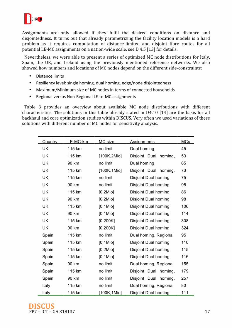
Assignments are only allowed if they fulfil the desired conditions on distance anddisjointedness. It turnsout thatalreadyparametrizing the facility locationmodels isahardproblem as it requires computation of distance-limited and disjoint fibre routes for allpotentialLE-MCassignmentsonanation-widescale,seeD4.5[13]fordetails.Nevertheless,wewereabletopresentaseriesofoptimizedMCnodedistributionsforItaly,Spain, the UK, and Ireland using the previously mentioned reference networks. We alsoshowedhownumbersandlocationsofMCnodesdependonthedifferentside-constraints:
• Distancelimits• Resiliencylevel:singlehoming,dualhoming,edge/nodedisjointedness• Maximum/MinimumsizeofMCnodesintermsofconnectedhouseholds• RegionalversusNon-RegionalLE-to-MCassignments
Table 3 provides an overview about available MC node distributions with differentcharacteristics. The solutions in this table already stated inD4.10 [14] are the basis for allbackhaulandcoreoptimizationstudieswithinDISCUS.VeryoftenweusedvariationsofthesesolutionswithdifferentnumberofMCnodesforsensitivityanalysis.
Country LE-MC-km MC size Assignments MCs UK 115 km no limit Dual homing 45
UK 115 km [100K,2Mio] Disjoint Dual homing, Relaxed
53
UK 90 km no limit Dual homing 65
UK 115 km [100K,1Mio] Disjoint Dual homing, Relaxed
73
UK 115 km no limit Disjoint Dual homing 75
UK 90 km no limit Disjoint Dual homing 95
UK 115 km [0,2Mio] Disjoint Dual homing 86 UK 90 km [0,2Mio] Disjoint Dual homing 98
UK 115 km [0,1Mio] Disjoint Dual homing 106
UK 90 km [0,1Mio] Disjoint Dual homing 114
UK 115 km [0,200K] Disjoint Dual homing 308
UK 90 km [0,200K] Disjoint Dual homing 324
Spain 115 km no limit Dual homing, Regional 95
Spain (continent)
115 km [0,1Mio] Disjoint Dual homing 110
Spain 115 km [0,2Mio] Disjoint Dual homing 115 Spain 115 km [0,1Mio] Disjoint Dual homing 116
Spain 90 km no limit Dual homing, Regional 155
Spain 115 km no limit Disjoint Dual homing, Regional
179
Spain 90 km no limit Disjoint Dual homing, Regional
257
Italy 115 km no limit Dual homing, Regional 80
Italy 115 km [100K,1Mio] Disjoint Dual homing 111

FP7–ICT–GA318137 18DISCUS
Italy 115 km [100K,2Mio] Disjoint Dual homing 111
Italy 115 km [0,1Mio] Disjoint Dual homing 111
Italy 115 km [0,2Mio] Disjoint Dual homing 111
Italy 90 km no limit Dual homing, Regional 120
Italy 115 km no limit Disjoint Dual homing, Regional
116
Italy 90 km no limit Disjoint Dual homing, Regional
171
Ireland 115 km no limit Dual homing 12 Ireland 90 km no limit Dual homing 17
Table 3: MC active nodes necessary to connect customers to LR-PONs using the DISCUS architecture. We report on maximal LE-to-MC distances in kilometre, constraints on the MC size (stated as an interval of households), the resiliency level, the allowed assignments and eventually the number of MCs. In the Spain (continent) instance we removed the 6 MCs for the Balearic Islands.
In the following we review somemore detailed studies that go beyond the aspects fromTable3.
2.2.3 Fibreroutingandcost
In D4.10 [14] we elaborated on the aspect of fibre, cable, and duct cost in the backhaulsection(betweenLEandMC).BasedontheUKreferencenetworkandMCnodedistributionsbetween75and324MCswestudiedtwodifferentfibreroutingprinciples:(i)fibreroutingtominimizethetotalfibrekilometresand(ii)fibreroutingtominimizethecommonlyusedtrailkilometres. These principles can be seen as two conflicting extreme solutions. While themotivationfor(i)istohaveshortfibreroutes,themotivationfor(ii)istosharecableandductresources.We made three major observations, which are crucial for end-to-end evaluations of costincludingthecorenetwork.• Thereissignificantcostoffsetinthebackhaulforprovidingthecableandductsystem.
We estimated the cost to be at least 500 Mio EUR. Surprisingly, the cost differencesbetween the different MC node distributions (75 nodes are even 324 nodes) arerelatively small. generally the backhaul costs increaseswith decreasingMC numbers.However,forthesamecost-modelandfibreroutingprincipleweobservedamaximumcostdifferenceofatmost150MioEUR.As thecost for theODNis independentof thenumber of MC nodes and the cost in the core drastically decreases with smaller MCnumbersthereisaclearindicatortohaveasfewMCnodesaspossible.
• Thedifferenceincostbetweenthetwoextremeroutingprinciplesofminimisingtrailsorminimisingfibredistance(oranyoptimizedsolution inbetween) is insignificant, inparticular forMCnodedistributionswith fewMCnodes (below20MioEUR). In fact,keepingthenumberofMCssmallandincreasingtheLE-to-MCdistancemeanslesspathalternativeswhichtogetherwiththerequirementtohavedisjointfibreroutesleadstoasituation where the solution space is actually limited. Optimizing fibre/cable/ductroutesdoesnotpayoffindependentlyofthecostmodel.
• Whichofthetwoprinciples(i)or(ii)ismostcost-efficientstronglydependsonthecost-modelsused.Withasimplecableandductmodel(cablesizeindependentofthenumber

FP7–ICT–GA318137 19DISCUS
of active fibresandductavailabilityprobability independentof thenumberof cables)solutionsthatshareresources(principle(ii))have lowercost(savingshoweverbelow100MioEUR).However, if amoredetailed cost-modelwas assumed (cables installedbased on the number of fibres, duct probability increaseswith the number of cables)then principle (ii) surprisingly led to more expensive solutions. The gain from thedecrease in the cost-per-fibre was not enough to accommodate the increase in fibrekilometres.
2.2.4 Nodeandedgedisjointedness
In the access network we have considered dual-homed solutions with two protectionmechanisms.Edge-disjointsolutionprotectslinksintheconnectivitybetweenthemetro-corenetworkandthelocal-exchangesites, that is, thesolutionallowsswitchingtoanalternativepathwheneverasinglelinkfailsinthenetwork.Node-disjointsolutionallowsswitchingtoanalternative pathwhenever a node fails. Certainly, node-disjoint solutions are stronger thanedge-disjointsolutions;however,anode-disjointsolutionisusuallymoreexpensiveduetoalongersecondarypathtotheprotectionMC-node.In this project we have observed that the actual cost of the solution varies according tomultiplefactors.Forinstance,providingonlydual-homedsolutionsto80%ofthepopulationandtheremaining20%withedgedisjointedness(withrespecttonode-disjointedness)onlyincreases the cost up to 0.3% w.r.t. to fully dual-homed solutions. Alternatively, anotherimportant factor in the cost is the population coverage;we have observed a total solutionreduction of 166% when limiting coverage to up to 80% of the customers for the Italiannetwork.
2.2.5 TradingDistanceforreducingCapacityofMCnodes
GivenafixedMCnodedistributionandwithoutanyspecialconstraintitisgenerallyoptimalto assign LEs to the two closestMCs tominimise the corresponding fibre/cable resources.Only when adding additional constraints such as the disjointedness of the fibre routes,minimal/ maximal customer constraints at the MC nodes or assigning LE sites to optimalbackhaulcablechains,doesthisnotnecessarilyholdanymore.InthissectionweelaborateontheeffectofrelaxingtheparentingconstraintbetweenlocalexchangesandMCnodescomparedtoforcingthatthetwoMCnodesassociatedwithalocalexchangeshouldbetheclosestandthesecondclosest. InourrelaxationapproachweallowthetwoMCnodestobefurtherawayaslongastheycanbothcoverthelocalexchange.

FP7–ICT–GA318137 20DISCUS
Weevaluatethreesolutionscomputedusingtheover-provisionapproachpresentedin[13].In this approach the extra capacity needed at each node to support single failures isminimised.PreviousexperimentshaveshownthatthisapproachtendstobalancetheprimaryloadoftheMCnodes.
In Figure 2-9we show the load distributions obtained for three different numbers ofMCnodes (45, 55, and 85) considering a maximum PON reach of 125km. Even though it ispossibletodoublecoverUKwith45MCnodeswith125kmreach,themaximumprimaryloadissignificantlyabovethesuggestedmaximumtargetvalueof~1million.InFigure2-9thexaxisisthenumberofcustomers(inmillions)andtheyaxisistheprobabilityofhavingaMCnode covering at least that many customers. That is a point (x, y) should be read as “theprobabilityofhavingatleastxmillioncustomersisy”.Thefigureshowsthedistributionforboththeprimaryloadandthesecondaryload.
Figure 2-9 Load distribution for three MC node placements for UK using the over provision approach

FP7–ICT–GA318137 21DISCUS
Figure2-10showstheresultsaftertheparentingrelaxation.AsweseeinFigure2-10(a)wecan substantially reduce the load without increasing much the total distance from localexchanges to their twoMCnodes.Apoint (x,y) in thisplotmeans that to enforce anupper
bound on the primary load of x, an increment of y% on the total distance is required. Forinstance, inordertoachievethe1,075,137upperboundontheprimary loadusingthe55nodes solution, an incrementof0.7% (less than1%) is required. Figure2-10(b) shows thenewloaddistributions.Thistimewearealsoshowingtheover-provisiondistribution(op).Asit can be observed in the figure, the over-provision is always below the primary load
Figure 2-10 Results obtained after the relaxation of the parenting constraint
Figure 2-11 Showing how restricting the load reduces the reach of the MC node

FP7–ICT–GA318137 22DISCUS
threshold.Thisisexpectedsinceintheworstcaseasecondarynodewilltakethefullprimaryloadofoneitsneighbours,whichisbelowthethreshold.Wecanalsoobservethatformorethan80%ofthenodes,theover-provisionisbelow500,000.Figure2-11showsfourMCnodes(representedbybuildingsofthecorrespondingcolour)inthe 55-node solution and the corresponding primary local exchanges. In awaywe can saythat, by relaxing the parenting constraint, we are adapting the reach of the MC nodedependingonthedensityofitsneighbourhood.IndeedtheareaofcoverageoftheorangeMCnodeissignificantlysmallerthantheotheronesbecauseitiscoveringbiggerlocalexchanges.CertainlyoneconsequenceofrelaxingtheparentingconstraintisthatthesecondaryMCnodecanbecloserthantheprimarynode(helpswithbalancingtheprimaryload),butasbothneedtobeconnectedtothelocalexchangethatwouldnotincreasethetotalcabledistance.
2.2.6 OptimizingtheCorenetwork
The DISCUS architecture envisages a transparent flat optical core network where all MCnodepairshaveadirectopticalchannelconnection.Theadvantageoftransparentnetworksisthe absence of OEO conversion, which is one of the major sources of cost and powerconsumption in optical core networks. The disadvantage is that the number of physicalconnectionsrequiredtointerconnecttheMCnodesgrowswiththesquareoftheirnumber.Already in deliverable D7.2 [15] we learned that for typical European countries a singletransparentopticalislandsufficestoconstructcorenetworksintermsofsignalreachesandflex-grid design. Moreover, in D7.6 we demonstrated that as user traffic grows beyond athreshold value the transparent flat optical core is themost cost-efficient among differentarchitecture alternatives that are based on hierarchical structures or several connectedopticalislands.Moreprecisely,tosavecostitturnsoutthatitisbesttodirectlyconnectapairofMCnodeswitha light-path connectiononce the trafficbetween thesenodesexceeds thecapabilityoftheexistinginterfacecapacity(e.g.40Gb/sor100Gb/s)andnewcapacitywouldneedtobeadded.seepreviousdiscussioninsection2.1Inthesamesection,wealsointroduceanupgradestrategythatshowshowtosafelymigratefromtoday’shierarchicalnetworkstoflatopticalcorenetworkswhenthetrafficincreases.A first challenge in the optimization of theDISCUS core is to design a fibre topology thatminimisesthetotallengthofthefibrelinkswhileguaranteeingthatthedistancebetweenanypair of MC nodes is within a given threshold in order to ensure transparency andguaranteeing that there exist light-path alternatives in order to ensure disjoint pathprotection.Thesecondchallengeistodimensionthenetworkoptimallyintermsoffibresandtransponders.The costof anation-wide corenetwork is typicallydominatedby the costofconnections between pairs of MC nodes (which includes the cost of fibre deployment,placementofopticalamplifiersatregularintervalsetc.),andthecostoftranspondersplacedat each MC node.We demonstrate the impact of different network designs on the cost ofdimensioningsuchnetworksbyconsideringnationalnetworksof Ireland, theUK, Italy,andSpainwithdifferentnumbersofMCnodes.Themostimportantelementsfordimensioningatransparentopticalcorenetworktopologyfor a given a traffic matrix are transponders and optical fibres. To determine how manytranspondersofwhattypesarerequiredateachMCnodeoneneedstodecidewhattypeofopticalchannelsshouldbeusedforeachtrafficdemand.Todeterminethenumberoffibresineachphysicallink,oneneedstosolvetheroutingandspectrumallocationproblemforagivensetofopticalchannels.Dimensioningagivenopticalcorenetworktopologyinvolvesfinding

FP7–ICT–GA318137 23DISCUS
therightbalancebetweenthecostofthetranspondersandthecostoftheopticalfibrecable.Oneoptiontodesigna transparentopticalcorenetwork is toconnectallpairsofMCnodesusingshortestpathsintheinputgraph.Thistopologyisreferredasthe“InitialSizeNetwork”(ISN). The advantage of ISN is that the average path length between all pairs ofMC nodeswouldbeminimum.Thiswouldallowustodimensionthenetworkwithtranspondersintheleast expensive way. However, the disadvantage is that the size of the network would bebiggerasthetotallengthoflinksisgoingtobeveryhigh.Intheworst-caseeachpairofMCnodesiscouldbeconnecteddirectlywithitsowncableroutewhichwouldincreasethecostofopticalfibrecableandinstallationsignificantly.AnotherpossibilityistodesignanetworkbyselectingonlyasubsetofthelinksLsuchthatthetotallengthofthesumofthelinkconnectionsisminimumandthedistancebetweenanypairofMCnodesdoesnotexceedthemaximumopticalsignalreach.Wecallthisnetworkthe“Minimum Size Network” (MSN). The MSN can be obtained by solving the Diameter andDegree Constrained Network Design problem (DDCND). The advantage of MSN is that itwould allow sharing more optical fibre and might reduce the cost of fibre. However, thedisadvantageisthattheaveragepathlengthwouldincreasewhichmightnotallowtheuseoftranspondersofhighcapacityandmightincreasethenumberoftranspondersandultimatelyincreasethetransponderscost.Although the size of ISN is significantly more than that of the MSN the average distancebetweenapairofMCnodesintheformerislessthanthatofthelatter.Consequently,awiderapplicabilityofdifferentopticalsignalsisfeasibleinISNasshowninTable4.Weremarkthatthere are 2 optical signals associated with each distance limit of 2430, 1170 and 500KMsrespectively.
Table 4: Signal Type Distributions for Initial and Minimum Size Networks
Ononehand theaveragedistancebetweenapairofMCnodes is less in ISN (as shown inTable4),whichmeansthatmoreopticalchannelsofhighercapacitycanbeusedtoefficientlyroutethetraffic.ConsequentlythenumberofopticalchannelsrequiredbyISNcouldbelessthan that required byMSN. Therefore, the cost of transponderswould be less for ISN andmoreforMSN.OntheotherhandthetotallengthofphysicalconnectionsbetweenpairsofMCnodesissignificantlylessforMSNwhichmighthelpinconsolidatingthetrafficinfewerfibres.ConsequentlythetotallengthoffibrescouldbelessforMSNthanthatofISN.Therefore,thecostoffibredeploymentcouldbelessforMSNandmoreforISN.Certainly,thereisatrade-offbetweenthetotal lengthofthefibresandthenumberofopticalchannels.Thistrade-offnotonly depends on the total length of physical connection and the applicability of differentopticalsignalsbutalsoonthetrafficmatrixandtheinherentcharacteristicsofthereferencenetworkitself.We therefore analyse this trade-off andpresent thedimensioning results forUK and Italyinstanceswith74and132nodesrespectively.Ouranalysisisbasedoniterativelyincreasing
FP7–ICT–GA318137 24DISCUS
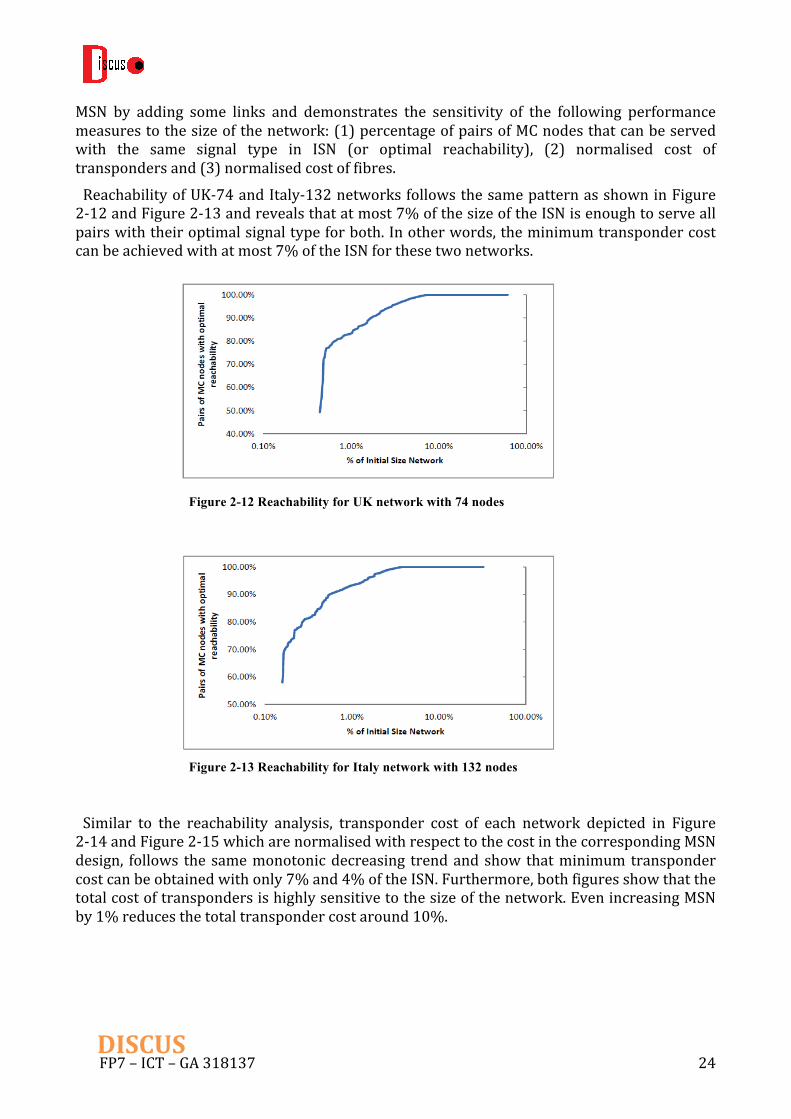
MSN by adding some links and demonstrates the sensitivity of the following performancemeasurestothesizeofthenetwork:(1)percentageofpairsofMCnodesthatcanbeservedwith the same signal type in ISN (or optimal reachability), (2) normalised cost oftranspondersand(3)normalisedcostoffibres.ReachabilityofUK-74andItaly-132networksfollowsthesamepatternasshowninFigure2-12andFigure2-13andrevealsthatatmost7%ofthesizeoftheISNisenoughtoserveallpairswiththeiroptimalsignaltypeforboth.Inotherwords,theminimumtranspondercostcanbeachievedwithatmost7%oftheISNforthesetwonetworks.
Similar to the reachability analysis, transponder cost of each network depicted in Figure2-14andFigure2-15whicharenormalisedwithrespecttothecostinthecorrespondingMSNdesign, follows the samemonotonicdecreasing trendandshow thatminimumtranspondercostcanbeobtainedwithonly7%and4%oftheISN.Furthermore,bothfiguresshowthatthetotalcostoftranspondersishighlysensitivetothesizeofthenetwork.EvenincreasingMSNby1%reducesthetotaltranspondercostaround10%.
Figure 2-12 Reachability for UK network with 74 nodes
Figure 2-13 Reachability for Italy network with 132 nodes

FP7–ICT–GA318137 25DISCUS
ThenormalisedcostoffibresfollowsthesametrendforbothUK74andItaly132nodesasshowninFigure2-16andFigure2-17.WenoticethatincreasingMSNslightlyhelpstoreducethe total fibre cost up to a certain point (i.e., 1% of ISN) in both networks.WhenMSN isincreased slightly, it reduces the length of the paths for some pairs of MC nodes andeventually makes it possible to use the optical channels in ISN. Using ISN channels alsoreduces the number of slots required and consequently, fibre consumption too. But afterincreasingMSNto1%of ISN, thenumberofpairsofMCnodesthatcanbeservedwithISNchannels does not change with the same ratio of increase in the length of the fibres.Furthermore,sharingoffibresbydifferentpairsofMCnodesisdiminishing.Therefore,totalcostoffibresstartstoincrease.
Figure 2-16: Fibre cost for UK network with 74 nodes
Figure 2-15 Transponder cost for UK network with 74 nodes
Figure 2-14 Transponder cost for Italy network with 132 nodes

FP7–ICT–GA318137 26DISCUS
Figure 2-17: Fibre cost for Italy network with 132 nodes
Inthissection,weprovidedadimensioninganalysistodemonstratetheeffectofthesizeofthe network on the cost of transponders and fibres. Our empirical results show that thenetworkofminimumsize isprovidingaverygoodqualitybasesolution tobeextended forminimumcostoftranspondersandfibres.Furthermore,fornetworkssuchasUKandItaly,atmostonly8%oftheinitialsizenetworkisrequiredtoservealltrafficwithminimumcostoftransponders, which is the most dominant cost component if the network is brown (i.e.existing fibres can be re-used for a significant portion of the new network). However, ifnetworks are green (i.e. requiring new fibre build) the fibre cost can be also an importantfactor,butlessthan2%oftheinitialsizenetworkresultstheminimumfibredeploymentcost.
3 TrafficmodelForecasting trafficgrowth isanotoriouslydifficultproblem.Short-termpredictionscanbemade with some accuracy, considering previous trends, and the CISCO Visual NetworkingIndex (VNI) has been in the past quite successful estimating traffic growth. Predictionshowevertendtobecomehighlyinaccurateinthemediumtolongterm,asthecorrelationofpast and future trends become weaker and weaker. Indeed simple extrapolation of pasttrendsovermanyyearsinthefuturehasprovendangerousasitisbelievedtohavetriggeredthe telecommunications bubble around the year 2000. The issue with extrapolatingaggregatedpast trafficmatrices is that itdoesnotrationalisethetrafficestimationwiththeuserapplicationsthatcouldgeneratesuchtraffic.Withoutsuchrationalisationitiseasytofallinto the temptation of extrapolating exponential traffic growths too far into the future,generatingscenariosthatarehighlyunlikelytooccur.Operatorshave typicallysolved the issuebyplanning forgrowthonanannualbasisusingshort-term extrapolations and typically a medium-term 5 year rolling plan for technologyupgrades and investment planning. Planning rules for a level of overprovisioning in thenetworkareusedtocounteruncertaintiesintheshorttomediumtermforecasts,withgoodprobabilities that traffic demand would not exceed the available capacity for the periodconsidered. While metro and core networks can be gradually upgraded and increased incapacity so that the operators can react to increase in traffic as demand arises, the accessnetworkismoreproblematicoftenrequiringanewgenerationoftechnologytobeinstalledforsignificantupgrades.Trafficpredictionconstitutesanimportanttoolforaccessnetworks,as many network operators will need to choose the next access technology to replaceoutdated copper pairs using xDSL lines.Upgrading the access has a high cost per user and

FP7–ICT–GA318137 27DISCUS
under the present climate of ever-decreasing operatingmargins, operators do notwant tooverestimate the traffic demand and upgrade prematurely. This high cost per user has, atleastinEurope,beenoneofthereasonsthathasdelayedFTTHdeployment.InDISCUSwehaveproposeamethodtorationalizetrafficdemandpredictionsbygeneratingaggregated demands in access networks from estimated statistical behaviour of individualusers.Whilewedonotpretendtobeabletoaccuratelypredictwhatthetrafficwillbeinthetimeline considered, the tool relates traffic growth to application usage thus allowinginformeddiscussionoverthegrowthpredictionsobtained.The traffic modelling tool developed by DISCUS has been thoroughly described inDeliverable D2.4. In this section we report the scenarios that have been investigated andpotentialtimelinesforidentifyingtrafficgrowth.Inorder tocarryouta comparisonofdifferentaccess technologiesoverdifferent levelsoftrafficdemands,weusethreeserviceusagescenarios:thefirstforaconservativescenarioforthe short-term, the second amoderate scenario for themedium termand the third for thelong term which is more bullish and assumes FTTH will drive significant growth in highcapacityservices.The traffic model we have created is made up of three individual components. The firstcomponent considers traffic generated by users (we differentiate between moderateresidential user, high residential user and small business user); the second componentconsiders the inter-datacentre traffic; the thirdcomponent considers trafficassociatedwithleasedlines(thusincludingmediumandlargerbusinesses).
3.1 Trafficgeneratebyapplications
Application-generatedtrafficisgeneratedbyatrafficmodellingtoolwehaveimplementedinMatlabandrecentlyreleasedasopensourcesoftware.Thisconsidersthetrafficproducedbyend-userapplications.Forthistool,theshort,mediumandlong-termscenariosdifferintermsofapplicationsavailable(eachwithadifferentdatarate)anduserbehaviour(i.e.,probabilityofusingagivenapplicationduringtheday,mostlikelytimeofusage,numberofapplicationinstancesusedduringthedayandtheirduration).Asmentionedabovewealsodefinethreetypesofuserbehaviour:moderateresidentialuser,highresidentialuserandsmallbusinessuser. Foreachapplication,withineachscenarioandusertypeweassociatedtoaparticularsetofbetadistributions.While itwouldbe tedious to reportherea fullmatrixwithall theparametersusedtodefinethedifferentstatisticaldistributionsofsuchscenarios,wereportinTable5thestatisticalmeansforthedistributionsusedforthehighresidentialusertypeforthethirdscenario.Lookingatthistablethereadercanunderstandthetypesofapplicationsandusagethatwehaveforexampleenvisagedforthelongerterm.Itshouldalsobenoticedthatthetooldifferentiatesapplicationsdependingondatasourcing,i.e.,datacentresources,Internetexchangesourcesorpeer-to-peersources.Eachapplicationcanbeassociatedwithanyoneofthesesourcesorwithamixofthem.
Table 5 Statistical distribution parameters for high residential user for scenario 3
Service Mean Duration[h]
MeanSessions Avg.downstreamcapacity[Mb/s]
Avg. upstreamcapacity[Mb/s]
e-life 0.25 1.14 10 10

FP7–ICT–GA318137 28DISCUS
e-commerce 0.25 3.43 10 1
e-learning 1.9 1.9 10 4
e-social 0.54 6.67 2 1
VoD4K 1.67 4 120 1
VoD1080p 0.2 6 30 1
VideoConf720p 0.5 4 30 30
Onlinegaming 1.67 2 20 20
VoIP 0.05 9.14 0.2 0.2
Filesharing 0.83 1.14 16 4
Theresults in termsofaveragedailydownloadandaveragebusyhourdownloadratearereportedinTable6.
Table 6 Summary of scenarios parameters
Scenario Averagedailydownload[GB] Averagebusyhourdownloadrate[Mb/s]
Scenario1 4 1.3
Scenario2 35 7.5
Scenario3 250 58
Figure3-1showsanexampleofadailydownstreamtrafficpatterngeneratedbyassumingscenario3 traffic levelson100PONswithapossible512waysplitbutwith thenumberofconnected customersperPON selected randomly fromauniformdistribution spanning therange100to500customers.thenumberofactiveuserseachcurveinthefigurerepresentsthe traffic pattern for one of the PONs, the lower curves being the smaller take up orcustomersperPONandhighertrafficlevelsbeinghighnumbersofcustomersperPON.

FP7–ICT–GA318137 29DISCUS
Figure 3-1 Daily downstream traffic pattern
Forthepurposeofthecashflowmodel,itisalsoimportanttotryanddefineatimelineforsuch traffic growth. For this purpose we have defined three traffic growth scenarios: apessimistic scenario,amediumscenarioandanoptimistic scenario,allofwhichwebelieveare potentially realistic. The pessimistic scenario puts the Compound Annual Growth Rate(CAGR)at20%,whichislowerthanthatpredictedintheshorttermbytheCISCOVNI(at29%fortheUSAforpeaktimes);themediumscenarioconsidersaCAGRof40%,whichwebelievecanberealisticwithmoderateFTTHdeployment;theoptimisticscenarioconsidersaCAGRof60%.Thisisquitehighfordevelopedcountries,butsomeoperators,suchasBTforexample,haveexperiencedsuchtrafficgrowthinthepastfewyears,thisisdrivenbytherapiduptakeofFTTCabintheUKandwebelievethatawidescaleFTTHdeploymentwouldstimulateatleastsimilarifnotevengreatergrowthsifservicesbecomeavailabletoexploittheadditionalcapacityandhighbandwidthssupportedbyFTTHnetworks.Wedonotconsiderrateshigherthanthisbecausealthoughtheyhavebeenmeasuredinthepast, theytendtobeassociatedwithshortperiodsofunsustainablegrowth(e.g.,duringtheyearsofthemillenniumtelecommbubble)andthusarenotpracticableaslong-termforecast.Table 7 shows the potential years when the CAGR traffic growths discussed above areassociatedwith theserviceScenarios2and 3couldoccur if thosegrowthsaremaintained.Scenario1 is not represented as that corresponds to the CISCO VNI prediction for20182(averagingbetweenEuropeandtheUS).
Table 7 Traffic scenario timelines in relation to CAGR
Growthrate Scenario2timeline Scenario3timeline
20% 2028 2039
40% 2023 2029
60% 2021 2026
2TheVNIindexisonlyavailableupto2018.Whileitisnotourscopetodefineprecisetimelines,extrapolatingthecurrent20%annualgrowthrate,wouldputscenario2aboutadecadeaway,whilescenario3twodecadesaway.

FP7–ICT–GA318137 30DISCUS
3.2 Inter-datacentretrafficmodelling
Inter-datacentre traffic is calculated as a percentage (45%, from and extrapolation of theCISCOGCI indexstudyref79[16])of thetotaldatacentretrafficdeliveredtotheendusers.ThevalueobtainedisthenaddedtotheoverallcoretrafficmatrixthatdeterminesthetrafficdemandbetweenMetro-Corenodes.
3.3 Leasedlinestrafficmodelling
For the estimation of leased lines we have followed an approach where we consider thenumberoflinestobeafunctionofthenumberofbusinessesinagivencountry(datafortheU.K. for examplewas taken from refs [17] & [18] and growth in numbers proportional tooverall traffic growth. The leased line capacities are then also related to the size of thebusiness.WehaveusedanumberofpointstoidentifycurvesfordifferentMCnodesizes,andthenusedextrapolationtofitthescenariounderexamination.The points used for scenario 3 were calculated using a model within the Metro-coredimensioningandcostmodelbasedon theUKdata in refs [17]& [18]andare reported inTable8.
Table 8 Values used for extrapolating leased line services for scenario 3
MC node size[thousand oflines]
Number of 1Glines
Number of10Glines
Number of40Glines
Number of100Glines
Number ofwavelengthservices
50 1104 0 7 0 181
300 6666 0 44 0 1108
800 17785 0 117 0 2957
From the values obtained, we assumed that an average 70% of leased lines will beterminatedwithin thesamenode,while theremaining30%aredirected towardsotherMCnodes.These values generated by the leased line component are then added to the core trafficdemandmatrixtogeneratethematrixthatisusedformodellingthearchitecture.
4 CashflowmodellingCumulativediscountedcashflowmodellingratherthansimplecostmodellingwaschosenasthemethodologyforeconomiccomparisonoftheDISCUSsolution,anditsvariants,withthealternative,moreconventional,solutionsforFTTHusingGPON,pointtopointfibreorhybridfibre copper solutions such as FTTCab. Cash flow models can give results that are bettereconomic comparatorsbecause itproduces risk indicators and time toapositive returnoninvestmentthatcostmodellingalonecannotdo.Capitals expenditure has two important components the balance of which can affect thebusinesscasechoicedespitecostsbeingequivalentorevenwhenthebetterbusinesscasehas

FP7–ICT–GA318137 31DISCUS
higher costs. These twoexpenditure components areupfront expenditure and just in time(JIT) expenditure. Upfront expenditure can be defined as capital expenditure that is riskcapitalwithnoguaranteedlinktorevenuereturn.Thejustintimeexpenditureisexpenditurethatisonlyincurredwhenenablingarevenuestream.In the network build situation, the upfront expenditure is the capital required to buildnetwork infrastructure to “pass” potential customers and is usually up to the pointwherefurtherinfrastructurebuildisnotsharedacrossothercustomers.TheJITexpenditureisthenthe expenditure required to “connect” the customer to the upfront provisioned network,becausearequestforservicehasbeenreceivedandarevenuestreamcomesonline.Upfrontexpenditurehasasignificanteffectonthetimetocashflowpositiveandthelevelofrisk investment. While Just in time expenditure has relatively little effect on those sameparameters.ItisthereforeeconomicallyexpedienttodesignnetworksthatminimiseupfrontexpenditureevenattheexpenseofincreasedJITexpenditure.Toshowtheseeconomiceffectsonbusinesscases it isnecessarytogobeyondcostmodellingand intocash flowmodelling.Cumulativediscountedcashflowmodelsrequiremodelsfor;capitalexpenditure,operational
expenditure, revenue, network rollout time lines and deployment strategies which ideallyneedtobeincludedintoanintegratedmodel.ThemodelstructuredevelopedwithinDISCUSis outlined in Figure 4-1, the various model components are described in the followingsubsections.Themodel components are built as relatively independentmodules that pass results andparameters between them. The models have been constructed in Microsoft Excel usingworksheet functions where ever possible and VBA coded modules where additionalfunctionality is necessary. The modules are being continuously developed and additionalmodules can be added in the future if new projects can be found to extend thework. ForDISCUS themain focus has been to compare theDISCUS architecture consisting of LR-PON
User B’W(t)From traffic models Access and metro
network models
Metro-core node model
Core network model
Cost & power Database
Revenue model
Roll out strategies
Opex. model
Exchange Database
Metro-node & LE parenting Database
+ LE Chain structures Cumulative discounted cash
flow model
CumulativeCash flowCurves
Optimisation Models
Power Consumption
model
Figure 4-1 Cash flow modelling structure and process

FP7–ICT–GA318137 32DISCUS
plusflatopticalcorewithasmallsetofmetrocorenodesagainstamoreconventionalGPON,point to point fibre based FTTH and FTTCab access networks with local exchanges left inplaceandametroaccessbackhaulnetworktoconnecttheseLEstoasetofoutercorenodes.
4.1 ExchangeDatabase
A key part of the model input data is the exchange database, network operators havedetailedknowledgeoftheirnetworkstatistics,infrastructurelocationsanddimensioningbutthis data is usually kept confidential and is not available for outside parties to use formodellingactivities.ThereforeforprojectssuchasDISCUSwhichneedsadetaileddatabasefor the internal models these “Exchange Databases” need to be built from much sparsersource data. The most basic data that can be available from public domain sources ispopulationdensitydata,forexamplefrom[21],roadnetworkssuchasopenstreetmapandnumber of potential address sites (sites where a telecommunications service could bedelivered to). This data is oftenopen source and is available freeof charge.There are alsosourcesfromcommercialsurveys,reportsandstudiesbutthesecanbeexpensive.InDISCUSwe have been able to get limited data from our partners and for the UK there is a publicdomaindatasourcefrom[22]whichgivesditheredlocationsofexchangebuildingsandthebusinessandresidential linesservedby thoseexchanges.ForDISCUStherefore thestartingdatasetistypically:DitheredExchangesitelocationNumberofresidentialsitesconnectedNumberofbusinesssitesconnected(theselattertwofiguremaybecombined)Thedithered locationsonlyproduce small errors in cabledistances in general and canbeignored a bigger problem is if the LE physical cable route degree is derived from theplacementof theLeonto the streetmaps.Thedithered locationmaywellplace theLe inaroad(degree2ratherthanaroadjunction(degree3orgreater)orvica-versa.HoweverinthecurrentmodelExchangedegreesweresimplyallocatedtoobtainnationalaveragefiguresAnadditionalparameterthatisessentialisthephysicalservingareaofeachlocalexchange.Thisisnotgenerallygiveninpublicsourcesandneedstobederivedindirectly,oneapproachistouseVoronoipolygonswhichalthoughtheydonotgivetrueexchangeboundariescangiveagoodapproximationtothetotalareaofalocalexchangeandcanthenbeusedforgeotypeclassification. Voronoipolygonsarepolygonssurroundingapoint inasetofpoints (inourcase the points are the LE site locations) where for a point within the boundaries of thepolygonthenearestLEwillbetheonesurroundedbythepolygon.Attheedgeofthenetworkthephysicalboundaryofthecountryformssomeofthepolygonedges.(SeeappendixnforamethodologyweuseforcomputingVoronoipolygons)Given the exchange area and the number of customer sites within the area a geotypeclassificationcanbeapplied.
4.1.1 Geotypes
Geotypes are a commonly used classification of exchanges used by operators for variousmodellingandanalysisactivities.Thereisnostrictdefinitionofwhatconstitutesaparticulargeotypebutitisusuallyassociatedwithcustomersitedensityormoretypically,historically,telephonelinedensity.ThislatterdefinitionisoflimitedvaluetodayandinDISCUSweuseasitedensityclassificationsystem.

FP7–ICT–GA318137 33DISCUS
Oncethegeotypesaredefinedandtheexchangesclassifiedsomegeneralstatisticsabouttheexchange areas can be generated that aid other parameter calculations. For the UK theSamknowsdatabasecanbeusedasastartingpointandthegeotypeclassificationshowninTable9canthenbedefined.
Geotype Site Density (lower bound)
Exchange Count No. sites Ave
sites/exch Ave site density
Sparse 0.02105500 1383.0 563,329 407 5.3 Rural 3 15.0 1405.0 1,428,985 1,017 26.4 Rural 2 45.0 1010.0 2,970,893 2,941 77.7 Rural 1 135.0 666.0 4,484,930 6,734 220.4 Urban 3 365.0 414.0 5,639,119 13,621 508.4 Urban 2 730.0 350.0 6,162,699 17,607 992.0 Urban 1 1460.0 250.0 4,458,268 17,833 1,899.7 Metro 2920.0 77.0 1,398,025 18,156 3,731.8 City 5840.0 24 384,453 16,018 7,022.5
Table 9 Geotypes definitions for UK network
Wehavedefinedninegeotypesfromsparseruraltodensecity.Toclassifytheexchangesthesitedensityislookedupandfittedintotheboundsdefinedbythevaluesinthesecondcolumnofthetable,“SiteDensity(lowerbound)”.Adjustmentoftheseboundseffectivelydeterminesthe distribution of geotypes for the exchange data set and determines the site distributionacross the geotypes. The distribution of sites across the geotypes using the classificationdefinedintable3fortheUKnetworkisshowninFigure4-2.The number of geotypes is fairly arbitrary and is chosen so that a reasonable statisticalvariationbetweengeotypesexistswithouttheedgeeffectsofmisclassifyingexchangesbeingtoo important to theoverall costmodel calculations.Also the chosen classification is solelyused within DISCUS and any similarity with classifications used by other organisations ispurely coincidental.
01,000,0002,000,0003,000,0004,000,0005,000,0006,000,0007,000,0008,000,0009,000,00010,000,000
Nu
mb
er o
f si
tes
Geotype Site Distribution
Figure 4-2 Distribution of customer sites across the geotypes using the definitions shown in Table 9.
The readermay have noticed that the lower bound for sparse rural geotype is non zero,whereasitwouldbeexpectedtobezeroasitisthelowestdensityclassification,thereasonitisnotzeroforthisdensityisthattheSamknowsdatasethasafewanomalousentrieswithafew exchange having zero sites connected (possible a core exchange with no directlyconnected customers or an error in the data set, or possible sites that they are not localexchanges but simply a remote multiplexer parented off a local exchange site). These are

FP7–ICT–GA318137 34DISCUS
ignored and removed from this classification. In the model they are captured forcompletenessbutinfrastructureisnotbuiltinthoseareas.Thereareonly7suchexchangesintheUKdatasetoutofatotalof5586exchangessotheomissionisnegligibleandeffectivelyneighbouringexchangessubsumetheareaofthefewLEswhencomputingtheexchangeareas.Thisgeotype classification is thenused to calculateanumberofparameters that areusedwithin the costmodel.Where possible these parameters are consistent with any availablenational network statistics, if they are known, such as proportion of overhead plant toundergroundplant,totalnumberofDPsandcabinetsetc.TheresultsinTable10showsomeofthederivedparametersfortheUKnetworkgeotypeclassifications.
Geotype PCP Degree
DP splitter size
% drop cable OH
% drop cable UG
Target PCP size (sites)
% D-side cable OH
% D-side cable UG
% D-side cable DB
Ave LE ODN degree
% E-side cable OH
% E-side cable UG
% E-side cable DB
Sparse 2 8 100% 0% 128 95% 0% 5% 2 90% 5% 5% Rural 3 2 8 100% 0% 256 90% 0% 10% 3 80% 10% 10% Rural 2 2 16 100% 0% 384 80% 5% 15% 3 70% 15% 15% Rural 1 3 16 90% 10% 384 65% 5% 30% 4 55% 25% 20% Urban 3 3 32 60% 40% 512 50% 10% 40% 4 40% 50% 10% Urban 2 3 32 40% 60% 512 20% 55% 25% 4 20% 80% 0% Urban 1 4 32 20% 80% 512 0% 90% 10% 4 0% 100% 0% Metro 4 32 0% 100% 640 0% 100% 0% 4 0% 100% 0% City 4 32 0% 100% 768 0% 100% 0% 4 0% 100% 0%
Table 10 A selection of derived parameters for geotype classification
The LE and PCP degree is an arbitrary but hopefully pragmatic allocation of the averagephysicalcableroutedegreefromtheLE/PCPbygeotype.theyareparametersneededintheaccesscostmodelsandisusedaspartofthecalculationforE-sideandD-sidecablesizes.TheDPsplittersizeistheaveragesizedsplitterassignedtothegeotypeclassification.Inthereal network there would be a distribution of splitter sizes to meet local variations thesefiguresareusedasan “average” size for thegeotypebasedon sitedensityand theneed tolimitaveragedroplengths.A separate study at Trinity College Dublin, outside of the DISCUS project, is applyingoptimisation techniques to fibre cable and splitter layouts in sparse rural areas in Irelandusing road layout and site locationdata,when thiswork is complete it couldbe applied toothercountriesandusedtogeneratebetterstatisticsforsparseruralareas.The DISCUSmodel computes the costs of overhead (OH) cable and drop separately fromunderground (UG) cable and drop and so the relative percentages of these technologydeploymentsareneededforthedifferentgeotypes.ThepercentagesshowninTable10meetnationallyknownstatisticsfortheUKbutthefiguresshownforthedistributionsacrossthegeotypesareassumed.ThetargetPCPsizeistheprobablytheparameterthatwillbemostdifferentfromrealworldstatistics, this is because the figures in the table are derived to fit binary splitter sizes. Toaccommodate the real world, non-binary, cabinet sizes spare splitter ports from smallercabinets would be routed over the cable chain to larger cabinets on the cable chain. It isassumedthatcabinetsplittersarefullyutilised(oratleastveryhighlyutilised)splitterportsparecapacityforgrowthisprovidedattheDPsitesnotthecabinetsites.Thecabinetsizeisthe cabinet splittermultiplied by the subsequentDP splitter sizes, so for example a sparserural geotype with DP splitter size od 8 would have a cabinet splitter size of 16 toaccommodatethetargetcabinetsizeof128.Theadditionalinfrastructurecolumnwith“DB”

FP7–ICT–GA318137 35DISCUS
asan infrastructure type is fordirectburiedcables.This isa cablingpracticeused in somecountriesandwasusedintheUKinthe1970sand1980sitiscablethatisdirectlytrenchedintothegroundwithoutfirstinstallingductways.Thisisalowercostinstallationpracticebuthasmajorimplicationsforupgradecostsandoperationalcostswhencablesgetdamagedasthesecablescannoteasilyberecoveredandreplaced.Therehavebeendevelopmentsforremovingthecopperpairsfromthesecablesandleavingthesheathintheground.Thissheathcanthenbeusedforinsertionofablowncableorblownfibre tube which can then have optical cables/fibre installed within them. This is still anexpensiveprocesscomparedwithproperlyductedroutesbut isclaimedtobecheaperthaninstallingnewduct.Howeverinthecostmodelwecosttheseregionsasfullductrebuildasitisnotknownhowwellthesealternativetechniquesworkinpracticeorifoperatorswilladoptthem.The average LEODNdegree is the average physical degree from the LE site,which is thenumberofseparatephysicalcableroutesintoandoutoftheLE.Theassumptionsarethatinruralareasvillagestendtohaveamainroadrunningthroughthemandexchangesarenearthat road and cables run from the exchange in both directions along that road beforebranchingtosideroads. Indenserarea there isgreaterprobability thatexchangesarenearjunctionsthatincreasethepotentialcableroutedegree.AswiththePCPdegreeitisusedtodetermineE-sidecablesizes.
4.1.2 Exchangedatabaseparameters
Thegeotypeclassification is justanaid topopulating theExchangedatabaseandensuringthatoverallnationalstatisticsareadheredto.Thedatabasehasalargenumberofparametersthatneedtobecalculated,manyof themare intermediateparametersusedtocalculate theparametersusedwithinthecostmodels
4.2 Database build methodologies – ODN, Cable chain and infrastructuredimensioningmodels
TheODN is the optical distribution network from the local exchange site to the customerpremises,thisisthecasealsoforLR-PONswheretheLEsiteisby-passedandreplacedwithanopticalamplifiernode.TheODNstructurehasevolvedfromtheoriginalcoppernetworkinfrastructure and consists of anE-sidewhich is the cable network from the LE site to theCabinetorPCP(PrimaryCrossConnect)sites,theD-sidewhichisthecablenetworkfromthecabinetstothedistributionpoints(DPs)andthedropsectionwhichprovidestheconnectionsfromindividualcustomerpremisestotheDPs.TelecommunicationcablesintheE-sideandD-sidegenerallyfollowtheroadlayoutsthisisthegenerally thecaseeven inruralareas,butoccasionallyoverheadcablerouteswillcrossfields rather than follow roads to save cable length, however these are relatively rare asaccess to infrastructure is much easier if placed along public roads. The road layout willproduceatendencyforcablestopassthroughsuccessivecabinetsorDPSinchainstructures.Withthecoppernetworkthischainstructurewasimplementedasatreeandbranchstructurewith largercablesnear theexchangewhichwouldbranchtosmallercablesascabinetsandDPswerepassed.Asimilarstructurecouldbeusedforopticalcablesbuteachbranchingpointrequiresasplicingjointtoconnectthelargercablestothesmallercablesanalternativethatisavailable for optical cables particularly with blown cable and blown fibre technology is tolimit these jointhousing to theCabinetandDPsitesandprovidecablesbetween these site

FP7–ICT–GA318137 36DISCUS
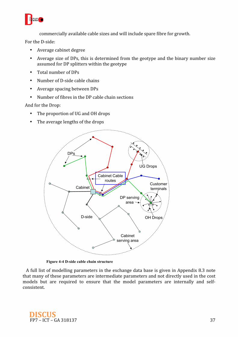
without additional branching points. This would mean that cabinets and DPs would beprovisionedandconnectedbydedicatedcablechains.It would require a detailed study on real network areas to determine which of the twoapproaches is actually the lowest cost and only operators or network owners have thedetaileddata forsuchananalysisalthoughouroptimisationworkisattemptingtocompereoptimisedODN cable layouts (see previous sections onODNoptimisation). For theDISCUScashflowmodelwewillassumeacablechainmodelratherthanacablebranchingmodel.Ahypothetical example of a cable chain layout for the E-side andD-side parts of theODN isshowninFigure4-3andFigure4-4respectively.Fromthesestructuresanumberofparametersneedtobederivedorbegivenassourcedataforcostmodellingpurposessuchas:FortheE-side:
• Exchangedegree, this isgivenfromthegeotypedefinitionspreviouslydescribed it isused primarily to ensure that there is a least one cable chain for each LE spatialdegreeorcablerouteoutoftheLE.
• Averagesizeofcabinets
• TotalnumberofcabinetsinLEarea
• NumberofcablechainsforEsidecablenetwork
• Average spacing between cabinets, this would be derived as a radial (straight line)spacingandthenaroutingfactorappliedtorepresentactualcablelengths.
• Number of fibres required in each cable chain section – this is then converted to
Figure 4-3 Hypothetical E-side cable chain structure
FP7–ICT–GA318137 37DISCUS
commerciallyavailablecablesizesandwillincludesparefibreforgrowth.FortheD-side:
• Averagecabinetdegree
• AveragesizeofDPs,this isdeterminedfromthegeotypeandthebinarynumbersizeassumedforDPsplitterswithinthegeotype
• TotalnumberofDPs
• NumberofD-sidecablechains
• AveragespacingbetweenDPs
• NumberoffibresintheDPcablechainsectionsAndfortheDrop:
• TheproportionofUGandOHdrops
• Theaveragelengthsofthedrops
Afull listofmodellingparametersintheexchangedatabaseisgiveninAppendix8.3notethatmanyoftheseparametersareintermediateparametersandnotdirectlyusedinthecostmodels but are required to ensure that the model parameters are internally and self-consistent.
Cabinet
DPs
Cabinet serving area
Customer terminals
OH Drops
Cabinet Cable routes
DP serving area
UG Drops
D-side
Figure 4-4 D-side cable chain structure

FP7–ICT–GA318137 38DISCUS
To simplify theanalysis and tomeet theassumption thatonlyminimal initialdatawill beavailable, a number of simplifying assumptions are made to aid calculation of the criticalnetworkparameters:
• UniformcustomersitedensitywithintheLEarea,Dcustomers/km2,
• CircularlysymmetricLE,CabinetandDPcoverageareas
• Nominaloptimaltriangularpackingofinfrastructurenodeswithinthecoverageareas,essentiallythisishexagonalpackingwithnodesatallvertices
TheseassumptionsareillustratedinFigure4-3,Figure4-4andFigure4-5.NotethatalthoughthecabinetandDPlocationsareassumedtobesimilartothoseusedforthecoppernetwork,whenconsideringanexistinginfrastructuresituation,thisdoesnotneedtobethecaseforpassiveopticalnetworkinstallationsparticularlytheLR-PONcasewithleanfibre infrastructure. Efficient fill or utilisation of the PON splitters is an importantconsideration in thedesignof thephysical layout for theopticalnetworkand therefore theoptimal location of the splitter points may not coincide with the copper networkinfrastructure locations. Further work to analyse and compare the strict use of legacylocations and more optimised locations for cabinet and DP particularly in the LR-PONscenariowouldbenecessarytodetermineandquantifytheadvantages,howeverthisanalysisrequiresdetailedknowledgeofexistinginfrastructuresowouldprobablyneedtobecarriedout by the network operator and is beyond the scope of theDISCUS project. But note thatmoving the splitter locations away from copper cabinet and DP locations is not a difficultoperation as the splitter housing can fit in UG footway boxes and do not need the streetfurniture associated with the copper infrastructure, so that the surface cabinets used ascopperpaircrossconnectpointsarenolongerrequiredandcanberemovedwhenfullFTTHdeploymenthasoccurredandthecopperlegacyhasbeenremoved.Thedropstoeachcustomerarethecable infrastructurebetweentheDPandthecustomerpremisesnetworkterminationequipment(NTE)(notetheNTEcanbetheONTorONUiftheoperator owns this equipment. Otherwise it will be a wall boxwhere the external fibre isterminated and connected to internal fibre for connection to an internal ONU (note thatinternal cable materials are different from external cables due to environmental and fireregulationrequirementsandexternalcableshouldnotbeusedinternally).Generallythedropand NTE are provided only when the customer takes services. To “pass” a customer theoperatoronlyneedstobuildnetworkinfrastructuretotheDP.ThedropandNTEinstallationcan be referred to as just in time (JIT) provisioning whereas the infrastructure to passcustomers isupfrontorpre–provisionedandasdiscussedpreviously thishasan impactonthecashflowandeconomicviabilityofspecificnetworkdesigns.There are two main drop cable systems in use within communication networks;underground drop cabling (UG drops) and overhead drop cabling (OH drops). A commoncablinginfrastructureforUGcablingiscalled“frontagetee”whereacableorcablesarerunfromtheDPalongthestreetorfrontageofpremisesandteejunctionsareusedateachofthepremisepassedtoroutedropstotheindividualpremises.ThisisillustratedintheUGDropsdiagraminFigure4-4.TheOHdropsuseapolewitharadialpointtopointdropcablesystemtoallthepremiseswithinsomemaximumdistancetypicallyaround70metresfromthepole.The drops can be longer than this if multiple pole hops are used but rarely exceed threeadditionalpolehops (except insparseruralareaswherevery longdroppoleroutescanbefound.TheDPcanbefedbyeitheraerialcableorUGcablethelatterbeingtypicalinbuiltup

FP7–ICT–GA318137 39DISCUS
areasandtheformerbeingmorecommoninruralareas.ThissystemisillustratedintheOHdropsdiagraminFigure4-4.Fromtheaboveitcanbeseenthattherearethreeinfrastructurecoverageareas:
• TheDPcoveragearea
• Thecabinetcoveragearea
• TheLEsitecoverageareaAssumingthebasesourcedatahasthenumberof customers in the exchange area andwe alsohave an estimate of the physical coverage area(either given or estimated e.g. using Voronoipolygons) thenassumingauniformdistributionof those customers within the exchange areaestimates for the infrastructure nodeseparationsandsizesof thenodescanbemadeusinggeometricalarguments:Considerasetofinfrastructurenodesoptimallypacked such that they form a triangular (orhexagonal) optimal packing structure as showninFigure4-5.
Thenodecaptureareais 2
233 RA =
Theseparationbetweennodesis Rh 32 =
The number of infrastructure nodes orcustomer sites captured by the infrastructure
nodecoveragearea sitesP ADN =
WhereDsites=thecustomersiteorinfrastructurenodedensity.IfitissitedensitythenitisgivenbyALE/NLEsiteswhereALE=theLEservingareaandNLEsites=thetotalsiteswithintheLEarea.Usingthegeotypeclassificationsandtakingintoaccountthebinarynumbersforthesplittersizeattheinfrastructurenodelocationsthevariousareasoftheinfrastructureservingareascanbeestimatedandthenthevaluesfortheseparationscalculated.The pattern of node locations in Figure 4-5 looks very idealistic and indeed it is, so thequestion therefore arises; does it bear any relation to real networks for cost evaluationpurposes?Fortunately it does as longas cable costs are linear functionsof lengthwhich inpractice isusually thecase. Inappendix1 it isshownthatevenwithanarbitrarystatisticaldistributionofcablelengthswithinaninfrastructurenodeservingarea(varyingcablelengthsisequivalenttoadistributionofnodespacing’swhichmoreinlinewithrealworldsituations),ifthecostofthecableisalinearfunctionoftheforma+bl.Where: a is the length independent cost such as splice housings and splicing etc. b is thelengthdependentcomponentofthecablecostandlisthelengthsothatthethetotalcostisgivenby lppT bNaNC µ+= .
R h
Figure 4-5 hexagonal optimal packing assumption of infrastructure nodes

FP7–ICT–GA318137 40DISCUS
Where:Npisthetotalnumberofsitesservedintheservingareaandµl isthemeanofthelengthdistribution.Soalthoughtheseparationofthenodes2hisarandomvariabletheonlyparameterrequiredisthemeanandforauniformdistributionwithtightpackingasassumedthen Rhl 32 ==µ .
ThedensityofpointsinthevariousservingareascanbeconsideredasahierarchystartingatthecustomersitelevelthentheDPnodes,thenthecabinetnodesandfinallytheLEsitesforthebackhaulnetworktotheMC-nodes.ThedensityoftheDPandcabinetnodeswillthereforedependontheaveragesizeofthesenodes.Usingthishierarchicalconceptwecanbuildatableofdensitiesanddistancesasafunctionofgeotypestatistics.Intheactualcostmodeleachexchangeisdealtwithinturnandtheactualdensitiesforeachexchangeisusedforthesecalculations.
4.2.1 DPservingarea:
ThereareanumberofparametersintheexchangedatabasefortheDPservingarea,threeofwhichfeeddirectlytothecashflowcostmodeltheseare:TherelativepercentageofOHandUGdropsandtheaveragelengthofthedrop,theotherparametersaidderivationofthelengthparametersforOHandUGdrops.FromthebasedatatheexchangeareaandnumberofcustomersitesisknownandfromthegeotypeclassificationtheDPsplittersizeisdefined.ApplyingafillfactorforfuturegrowthanaveragenumberofsitesperDP isobtained. Usingthetotalnumberofsites, thenumberofDPsfortheexchangeareacanbecalculatedfromwhichtheaveragesizeADPoftheDPservingarea isobtained.Given theDPservingarea the radiusRDPassuminga circularly symmetricservingareaiscalculated.ThatisthenumberofcustomersperDP=NDPCust=SDP*ffWhereSDP=DPsplittersizeandff=thedesignfillfactorforfuturegrowth
ThereforetheDPservingarearadiusisSites
DPCustDPDP D
NARππ
==
MeanDPtocustomerradialdistanceSites
DPCustDPDP D
NRRπ3
232
==
The factor2/3comes fromthemeandistance fromapoint toallotherpoints inacircularsegmentofrandomlydistributedpointsaboutthepoint,seeappendix8.2.Oncethemeandropradiusisknownthenthedropcablingcostcanbederived.OHdropscanuse the radial figure directly as OH drop are radial distances from the DP, for UG drops aroutingfactorof 2 isusedfortheaveragedroplength.NotethatOHdropsinruralareascanbelongerthantheallowablesinglespanlengthfromapole(about70metres)andmorethanonepoleisused.Howeverforsimplicityinthemodelitisassumedthatthepoleinfrastructureisalreadyinplacefortheexistingcoppernetworkandisreusedforthefibredropinstallationandthereforeonlythefibredropcableisincludedinthecostmodel.

FP7–ICT–GA318137 41DISCUS
4.2.2 Cabinetservingarea:
ThesameapproachcanbeusedforthecabinetservingareawhichisalsooftencalledtheD-sidenetworkfor“distributionside”.TheCabinetisaflexiblecross-connectpointrequiredfortheoriginal coppernetwork. It isnot a required flexibilitypoint forPONnetworksbut is aconvenientsplitterpointasD-sidecableroutescometogetheratthesepointsinthephysicalductandcablenetwork.TheD-sidecablenetworkcanbeconsideredtobeequivalenttothedropnetworkfortheDPservingareasbutthepointsinthenetworktobeservedbythecabinetlocationsarenowDPsrather than customer sites. The density of DPs is the customer site density divided by the
averagenumberofcustomersperDPi.e.DP
SitesDP N
DD =
TheCabinet size in termsof customer sites is given in thegeotype tableand is an integermultipleof128tofacilitatea100%filltargetofcabinetbasedopticalsplitters,thatiseachD-sidesplitterportatthecabinetwillconnecttoaDPinthecabinetservingarea.Itneedstoberecognisedthatthesecabinetsizesmaydeviatefromtheoriginalcoppercabinetsizes(weareassuming that this original data is not available,which is generally the case except for theincumbentoperator).Thispotentialdifference incabinetsizecanbeaccommodate tosomeextentbypassingspareportsfromonecabinetintheE-sidecablechain(discussedlater)ontoothercabinets,inthesamechain,thatmaybeshortofports.AlsoforsmallsplitPONsinthemoredenseLEareastheremaybenocabinetsplitters,allthePONsplitbeingaccommodatedattheDPlocations(thiscanbetypicalfor32waysplitGPONsystems).Letthecabinetsize=NC;whereNCisthenumberofcustomers(opticalterminations)inthecabinetservingarea.ThecabinetcoverageareaisthereforeNC/DSiteskm2.
AndtheradiusofcabinetservingareaSites
CC D
NRπ
= .
Themeancabinet toDPradialdistancecanbecalculated inasimilarmannerused for theaverageDPtocustomerradialdistancecalculation.LetthenumberofDPsinthecabinetarea=NDP=NC/NDPCust
ThentheaverageradialdistancecabinettoDP CC RR32
=
HoweverfortheD-sidenetworkcableswillnotbeprovidedirectlyfromthecabinettotheDPbutrather therewillbecablechains fromthecabinet, thatserveDPsas thecablechainroute progresses from the cabinet location to the edge of the cabinet serving area. Thisrequirestwoadditionalparameterstobefound:ThenumberofDPsinacablechainandtheaverageseparationbetweenDPs.With theseadditionalparameters cable chain lengthsandcablesectionsizescanbederivedandthencostsdetermined.Theaverageseparation(lDP)ofDPscanbedeterminedusingthemethoddescribedaboveintheintroductorysub-sectionand DPDP Rl 3=
DeterminingavalueforthenumberofDPsinacablechainismoreproblematicastherearenorigorousrulesorapproachesfordoingthis.

FP7–ICT–GA318137 42DISCUS
ThemethodusedinthemodelforcalculatingthenumberofDPsinacablechainistoselectthelowerofthreebounds:
• The first bound is calculated for the specific LE by taking the number of DPs percabinetanddividingbythecabinetdegree(numberofphysicalcableroutesoutofthecabinet).Thisensuresthatat leastonecablechainperdegreewillexistbutwillalsoproducethelongestchainsastheDPsaresharedacrosstheminimumnumberofcablechains for the cabinet serving area. In general these chains would be longer thanlengthsderivedbytheothermethodsandwillberarelyselectedwithinthemodel
• AsecondboundusestheaveragecableroutelengthfromcabinettoDPsattheedgeofthecabinetareadividedbytheaverageseparationofDPs,thisgivesamorepragmaticvalueforthenumberofDPsexpectedalongatypicalcablechainroute.
• A third bound is an arbitrarymaximum bound of 8 DPs per cable chain a limit notexpected to be seen but a bound that aids implementation of the code of the Excelmodel.
Theminimumoftheseboundsisselectedforthemodelvalue.InpracticethecalculationsinthemodelnearlyalwaysselectsthevaluefromtheaveragecableroutelengthdividedbytheDPseparation.The abovemethodology derives aworking value for the number of DPs in a D-side cablechain. This is generally a fractional value and of course only integer numbers of DPs canphysicallyexist inacablechain.This ishandled in themodelbyusing two lengthsofcablechainwithonechainlengthbeingtheintegerpartoftheaveragenumberofDPsperchainandthelongerchainbeingthislengthplus1.TheratioofthetwoDPs/chainnumbersiscalculatedtofittheaveragevalueofDPsperchainpreviouslyderived.The cable installation techniques in the D-side network are Overhead, Underground andDirectBuried(DB).Directburiedisanalternativeundergroundcableinstallationtechnologythatwasused in the1970sand80sandwasa lowcost installationbydirectlyburying thecableintothegroundwithoutpre-installingduct.Althoughthishaslowerinstallationcostandthereforereducesupfrontcapitalinvestmentithasseriousoperationalproblemsinthatitisdifficulttomaintainandveryexpensivetoreplace.Becauseoftheselimitationsitwasn’tusedto a great extent after these early years when it was fashionable but unfortunately it isscatteredacrossthenetworkandtherearegenerallynotgoodrecordskeptofwhereitwasinstalled. It is also the case that not all operators adopted the practice and the extent ofdeploymentvariedgreatlybetweendifferentcountries.To accommodate DB deployment of cable a percentage figure for different geotypes isincorporatedintothegeotypetableandthesepercentagefiguresarefedintothecostmodeltogether with the OH and normal ducted UG percentages so that all cable routes in theexchangeareasofgeotypeswhereitisdeterminedtohavebeendeployedwillhaveamixofthese cable installation types. The percentage allocations are consistent with the nationalstatisticsforthiscabletypedeployment.UsingthederivedresultsfortheD-sidestaticswithintheexchangedatabasethecostsoftheDPsplitterinstallationsandthecableinstalledinthecablechainsarederivedaspartoftheaccessnetworkmodel

FP7–ICT–GA318137 43DISCUS
4.2.3 LocalExchangeservingArea
The E-side network is that part of the ODN from the local exchange site to the cabinetlocations. The modelling requires very similar parameter values to those for the D-sidenetworkandthemajoritycanbecalculatedviathesameprocesses/methods.InthiscasethenodesarethecabinetsandthecablechainsarefromthelocalexchangesiteoutwardstothelocalexchangeareaedgepickingupandservingcabinetsalongtheE-sidecablechainroute.One parameter that is different for the E-side is the occurrence of direct exchange lines(DELs). These are a hangover from the copper network and are copper lines connecteddirectlytocustomerswithoutgoingthroughacabinetbutinsteadgodirectlyfromtheLEtoaDPandthentothecustomerspremises.ForthelongreachPONsolutionthesecaneasilybeaccommodated by placing a cabinet splitter at the LE site with a cable directly to theassociatedDPs(itcouldwellbe that thiscablecouldbeasharedcablewithothercabinets,thatisthefirstcabinetinthisparticularE-sidecablechainistheLEsite.TheproblemforDELconnected customers is forFTTCabbecauseVDSL signals cannotbe fedover copper cablesfrom the LE while ADSL is present. This stops those customers getting the high speedbroadbandservicesofferedbyFTTCabeventhoughitisavailablewithintheirexchangeareaandtheyaretheclosestcustomerstotheexchange.InfrastructurecostscanbecalculatedinasimilarmannertotheD-sideinfrastructurecostsaspreviouslydescribesbutnowusingtheE-sidedataparameterswithintheExchangedatabase.
4.2.4 Exchangedatabasesummary
TheExchangedatabase is constructed assuming that very sparse real data is available asdetailed infrastructure data is usually kept strictly confidential by the networkoperator/owner.Howeversomebasicdatacanoftenbefoundandourstartingassumptionisthatwegetaminimumofditheredexchangesitelocations,andanindicativevalueofthetotalnumberofcustomersitesconnectedtothelocalexchanges.Wealsoassumetherearesomeglobal statistics available about the network that can be used to help proportioninfrastructuretypesacrosstheexchangesandalsohelpclassifytheexchangesintogeotypes.Themost critical other parameter required is the Exchange serving area size. If this is notgiven then it must be derived in some way, for DISCUS we use Voronoi polygons as areasonablemethodologyforgettingpragmaticexchangeareasizes.All other infrastructure parameters are then derived as described in the previous sub-sectionsforafullsetoftheexchangedatabaseparameterswithdescriptionsseeappendix8.3
4.3 Accessandmetro-network
Thissectionoutlinesthemainfeaturesofthephysical layermodelusedforcostmodellingpurposes within the cash flow model. For a fuller description of the current modellingmethodology see appendix 4 note this is a snap shot of the modelling process as this iscontinuously being updated and extended and will continue after DISCUS finishes. Thedescription starts at the customer termination options and progresses up the networktowardstheLEsite.
4.3.1 OperatorownedONUandDropmodel

FP7–ICT–GA318137 44DISCUS
Thediagramin Figure4-6showsthemodelscenarioweareassumingwhentheOperatorownstheONUandNTE.InthiscasetheoperatorusuallyinstallstheONUontheoutsideofthepremises and also provides battery backup, power is usually supplied from the customer’spremises. The ONU connects via a copper cable to a copper technology NTE inside thecustomerpremiseswhichthecustomercanplughisequipmentinto.ThiscopperNTEisthephysical and legal demarcation point between the Operator’s network and the customer’snetwork. The ONU forms the boundary of the optical network and therefore there is noseparateopticalNTE.TheONUisconnectedtothecopperNTEinsidethecustomerpremisesbyacoppercablee.g.Coax,UTP,Cat5etc.Anelectronicrouter/hub,whichcouldbecustomerowned,wouldplug into thiscopperNTE(therouter functioncouldalsobepartof theONU
functionalityifdesired).The model includes the cost of the above installed equipment with the exception of thecustomerhub,thiscanbeoptionallyincludedtogetacompletesystemcost(servicecannotbereceivedwithoutit).Inthecurrentversionofthemodelitisnotincluded.Note:all theabovecostsareincurredona“just intime”(JIT)basis inthecashflowmodelandarethereforeassociatedwitharevenueflownotupfrontriskcapital.TheNTEandONTareincludedwithintheCPEcomponentsinthemodel.TheLR-PONONUprice=GPONONU-GPONoptics+driveelectronics+2.5*GPONoptics+driveelectronics.CurrentlyinthemodeltheGPONoptics+driveelectronicsisassumedtobe25%oftheGPONONUcost.
4.3.2 CustomerownedONUandDropmodel
Inthisversionofthemodel,illustratedinFigure4-7,weareassumingthecustomerwillowntheONUandconnectsitintoanopticalNTEownedbytheoperatorwhichformsthephysicalandlegaldemarcationbetweentheoperator’snetworkandthecustomer’snetwork.Note:inthisscenarioitisassumedthatbatteryback-upisthecustomer’sresponsibilityandtheybearthecostiftheychoosetoimplementite.g.theONUcouldbesupportedbyacustomerownedUPSdeviceorcustomersuppliedbatteriesiftheysodesired.BecausetheinternalONUdoesnothavetobeasruggedoroperateinsuchaharshenvironmentastheexternalONUthecostof the External ONU is set 30% higher than the internal ONU. Note that the wall plate isalways fitted to separate the external cable from internal cable but the gas block is onlyrequired for UG drop cable feeds this small cost difference is ignored in the model. The
DP Splitter
ON
U
ONU + battery back-up + wall plate with gas block that terminates the external cable and keeps it separate from the internal cable. ONU fitted on external wall. Note if drops are OH the gas block is not required this is ignored in the cost model.
Installed Drop
Drop length
DP spliceCustomer
spliceCopper
NTE
Hub to NTE lead. e.g. Cat5e.6 with RJ45 connectors for 1GE connections.
Hub
Wall
Figure 4-6 Operator owned ONU and NTE model structure

FP7–ICT–GA318137 45DISCUS
choicesforONUownershipstrategycanbetoggledwithinthemodeltoenablecomparisonoftheeconomicimpactsofthetwoapproaches.
4.3.3 Cablechainmodels:dimensioningandgrowth
Using cable chainsassumes that cableswill runalong streets anddropoff fibre to serviceDPsandCabinetsasrequired.AsdiscussedabovethenumberofcablechainsandthenumberofDPsorcabinetsinacablechainarederivedwithintheExchangedatabaseusedwithinthecash flow model. These values are based on geometrical assumptions and uniformdistributionsofcustomerswithintheservingareasofstreetfurnitureandbuildingnodes.Forsimplicitythefirstversionofthemodelwilluseseparatecablesforeachchain.Thiscouldbemodifiedlatertoassumebranchingpointsalongphysicalductroutesthatsharecablechainroutes. In thesesituations theremaybeadvantages incombiningsmallercables into largercableswhichcouldreduceperfibrecostsfurtherifthecableshavenotalreadyexceededthemaximumcablesizeusedinthemodel(276fibrecables).HoweverthesesavingsareoffsetbytheneedtohaveacablejointatthecablebranchingpointsitthesedonotoccuratthecabinetandDPlocationssoweexpectrelativelysmallcostsdifferencetooccurinpractice.Withtheexchangedatabasepopulatedasdiscussedinprevioussub-sectionsthecablesizesandlengthsforallthecablesectionsintheexchangeareaarebecomputed.ThedropsectioniscomputedfirstthentheD-sidecablechainsofDPsthentheE-sidecablechainsofcabinets.Thebackhaulchainsof localexchangesthatspanapairofmetro-nodesarecomputedusingoptimisation modelling described in section 4.3.7.1. The cable model needs to be genericenoughtoaccommodateLR-PON,GPON(andotherPONvariants thatcouldbeadded later)andalsopointtopoint fibrecablesolutions,FortheFTTCabmodelapointtopoint fibreE-sidemodelwillbecomputed.G.FastsolutioncouldbeaddedatalaterstagebutthisisbeyondtheresourcesavailableinDISCUSandwouldneedtobeaddedinfollowonprojects,howeverthemodularstructureofthemodelshouldreadilyenableadditionaltechnologymodulestobeaddedaftertheendoftheDISCUSproject.Themaincomplexity isdecidingon thesplitterhousingstructurewhich inaddition to thesplitter and associated splicesmust accommodate the spare fibre handlingwhich includesbespokefibreandfibreforfuturePONgrowth.Thefundamentalassumptionhereisthattherewillbeanallowanceforgrowthinthedayonebuildanddimensioning.Thisisprovidedforbyincluding a fill factor across the model. Typically this is set at 80% allowing 20% sparecapacityforgrowth.HoweverinPONsolutionsthenumberofsparefibreneedstoreduceas
DP Splitter
ON
U
Wall plate with gas block separates external cable from internal cable
Installed Drop
Drop length
DP spliceCustomer
splice
Optical NTE
Flexible optical lead with connectors
Wall
Figure 4-7 Customer Owned ONU model

FP7–ICT–GA318137 46DISCUS
thecablesrunfromthecustomerpremisethroughtheD-side,thentheE-sideandthroughthebackhaulnetworktothecore.Thisisbecausemostgrowthwillberandomlydistributedandnot all growthprovidednear the customerneeds tobe translatedup through thenetwork.Also for PON solutions additional splitter nodes would be added which reduces uppernetworkfibrecounts.Makingthissparingscalableandinternallyself-consistentaddsfurthercomplexity to the model and it is necessary to get the sparing strategy and methodologyclearlydefinedupfront.Tomakespare resourceeffective, access to spare fibreneeds tobeavailableat theaccessedge i.e. at the DP position. However it is neither necessary nor economic to carry all thesparefibreattheedgedeeperthannecessaryintothenetwork.WethereforewillhavesparefibresunterminatedandnotsplicedthroughatintermediatestreetfurniturenodesintheD-sideandE-sidecablenetworks,accommodationof thesenon-splicedfibres inhousingsalsoneedstobeincluded.Thebasicdesignrulesusedwithinthemodelarethereforeasfollows:1. The number of spare fibres entering the LE site should be working fibres *(1 - fill
factor).2. TheD-sidecablechainneedstocarryfourcategoriesoffibre:
• FibresfeedingthePONsplitters(includesfibreforadditionalnetwork-sidesplitterportsifNxMsplittersaredeployed).
• Fibresforthebespokenetworksthatusededicatedfibre-usuallyonlyverylargeorspecialistcustomerswouldwantthiscapability.
• Sparefibreforgrowth(additionalPONS)
• Spare fibre arising from fitting actual cable sizes to the required fibre count (thefittedcablesizewill invariablybeofgreatersizethantheminimumrequiredfibrecountwhichincludesfibresforgrowth).
Asmentionedabove,notallthesparefibreneedstobesplicedthroughatintermediateDPandcabinet locations in thecablechainsand thatcableson the inputandoutputsidesofasplitterpositionwillgenerallynothaveequalnumbersofsparefibres.Splicingthroughsparefibreaddscostattheinitial“dayone”installationandcouldbeomitteduntilrequiredinthefuture,however tominimise futuredisturbance, all spare fibre inaD-side cable chain, thatcanbesplicedthroughwillbespliced,throughtothecabinetlocation,regardlessofstatisticaldemand. This is to minimise the number of future network visits required to implementgrowthorbespokefibrelinksandtominimiseinterventionfaults.Thisstrategymaximisesa“hands off” operational network strategy which can reduce operational costs and increasenetworkreliability,howeverquantifyingtheseadditionalbenefitswasbeyondtheresourceoftheDISCUSproject.IfNxMsplittersareusedwhereM>1,theadditionalupstreamsplitterportfibrescanbeusedforanumberofoperations,aminimumofoneportisofcourserequiredfortheworkingPON,anotherportcouldbeatestaccessportforfieldengineerstoaidfaultfindinganddiagnostics,otherportscouldbeusedforsplitby-pass,forexampletoaccommodatedifferentwavelengthbandsortoaccommodatesystemsthatcannottoleratethelongerroundtriptimeoftheaccessnetworkofLR-PONs.Opticalfiltersmayalsobeappliedtotheseportfibrestospatiallyisolateor separate different wavelength bands. The model will enable comparison of different

FP7–ICT–GA318137 47DISCUS
splitterinstallationstrategies,withdifferentnumbersofupstreamsplitterports,whichissetbeavariableparameterinthemodel,andtheeffectsonupfrontcostandpaybacktimes.
4.3.4 D-sideCableChainmodel
Thissubsectionandthefollowingsectionsbrieflydescribestheinfrastructuremodels,thatiscabledimensioningandsplitternodesdesignsetc.Forfullerdescriptionsseeappendix8.4(noteallthefiguresinthesesectionsarealsoreproducedintheappendixfortheconvenienceofthereader).Aspreviouslymentionthefibrenetworkuptothemetro-corenodecanbeconsideredasaseriesofinfrastructuresectionsfromCPEandcustomerdrop,DPsandD-sidecablenetwork,CabinetsandE-sidecablenetworkLEsiteequipment,Backhaul(ormetro-access)network.TheD-sidenetworkconsistsoftheD-sidecablesandtheDPswhichhousesplittersforPONsolutions or are just splice housings for point to point solutions. For the model we haveimplemented it isassumedthatopticalcablesrunfromcabinets tothecabinetservingareaedge passing and servingDPs on route as previously described. This effectively breaks thecablechainintoanumberofsectionswithreducingfibrecountsasthecablepassesDPsfromthecabinettothecabinetservingareaedgethisisillustratedinFigure4-8.
AsfibresfromthecabinetlocationpasstheDPsfewerfibresneedtobecarriedthroughtoserve successiveDPs. Themodel calculates the number of fibres for the various categoriesdescribesinsection4.3.3anditcanbeseenthatsomefibrearesplicedthroughandothersarestoredonsplicetraysintheDPhousingwithoutsplicing.ThevariablesinFigure4-8are:SDP=DPsplittersizeM=numberofD-sidesplitterportsM=2n;wheren=0,1,2.CH=numberofDPsinthecablechain.b=numberoffibresperDPreservedforbespokefibreservices.
No. DPs in chain = CH
bNg
SDPM
Sf(CH)
bNg
SDPM
Sf(r-1)
bNg
SDPM
Sf(r)
bNg
SDPM
Sf(1)
CS(CH)Cable sizes CS(r-1) CS(r) CS(1)
Figure 4-8 D-Side cable chain model structure

FP7–ICT–GA318137 48DISCUS
Ng=fibresreservedforfutureadditionalPONsforcustomernumbersgrowthNote there is also a variable ffwhich is the fill factor parameter that reserves spare DPsplitterportsforcustomergrowthontheexistingPON/s,theNgsparefibresareforgrowththatexceedsthisfactorandenablesadditionalPONstobeaddedtoprovideadditionalfibreconnections.SF(r)=Thesparefibresfromthemismatchbetweenactualcablesizeandrequirednumberoffibre in a cable section. The model computes the required fibre count in a cable section,includingtheallowanceforgrowth,andthenlooksupthesmallestcablesizethatisgreaterorequaltothisvalueasthesectioncablesize.CS(r)=Therthsectioncablesize.Decidinghowmanyofthesparefibresthatlinktheinputcabletotheoutputcabletosplicethroughat aDPsite isquitea complexprocess.Themaximumnumberof spare fibres thatspanthewholechainduetocablesizesexceedingtherequirednumberoffibreseithersideofaDPistheminimumofthesetofabsolutevaluesofthesparefibrecountdifferenceabouttheset of DPs in the chain and these spare fibres should be distributed across the DPs in thechain.Howeverthisisacomplexplanningruletopracticallyimplementforfieldstaffintermsof fibre splicing of these spare fibres at the DPs. Therefor, although there is a small costpenalty, a simplerplanning rule is assumed for themodelwhich is to splice all spare fibrethroughateachDP,thisnumberofsplicesattherthDPis:Spicedthroughsparefibres=ABS(CS(r)-CS(r+1)–(2CH-2r+1)(b+(1+f)(Ng+MDP))).ThisdoesmeanmoresplicingattheDPsbutisasimpleruleforfieldstafftoimplementandalthoughthisincreasesthenumberofsparefibressplicedthroughtothecabinettheydonotallneedtobesplicedthroughtothelocalexchangeovertheE-sidecables.TheDPsplitterwillbeinstalledwithsplicetraysfortheincomingfibrecable/fibreunitandthedropfibreunits.Dropfibrespliceshoweverarenotincludedinthesplitternodecostastheyareincludedinthecustomerdropcostsasa“JustinTime”cost(JIT).Note:Oftenthedropfibreunitwillbetwoorfourfibres.Forthismodel it isassumedthatonlyonefibreissplicedforsinglefibreworking(typical)ortwofibresfortwofibreworking.Any spare fibres in thedrop fibreunit areassumed tobe storedon the splice tray for thatdropcable,butwithoutsplices,withup to twosplicesper tray.For theurbanareas typicalsplittersizesattheDPlocationwillbe32waywithsome16waysplittersandinthesparserruralareassplittersassmallas8way.InthecurrentversionofthecashflowmodeltheDPsplittersizeisaninputvariableandthecabinetsplittersizeiscalculatedusingtheDPsplittersizevalue,italsoassumesallDPsplittersintheexchangeareawillbethesamesize.InsparseruralareastheDPsplitterscouldbesplitintoadditionaltierswithsmallerendpointsplitters,as small as4-wayandmaybeoccasionally2-way.Optimisation techniques to fit cables andsplitters to these areas arebeingdevelopedoutsideof theDISCUSprojectbut theyarenotincluded in the cash flowmodel atpresentand sparse rural is accommodatedbyassuminglongerdroplengthsdependentonmeancustomerdensity.

FP7–ICT–GA318137 49DISCUS
ThemodelfortheDPsplitternodeisshowninFigure4-9andshowstheequationsfortheinputandoutputcablesizesfortherthnodeinaD-sidecablechain.ThecostfortheinstalledDPsplitterhousing=costofhousing+costofsplitters+costofsplicetrays+costofsplicing+
costofinstallation+costofsitevisit.ForpointtopointfibresystemsthereisofcoursenosplitterattheDPandtheDPhousingissimplyasplicejointhousing.ThemodelforthepointtopointfibreDPnodeinapointtopointD-sidecablechainisshowninFigure4-10andalsoshowstheinputandoutputcablesizesfortherthDPnode inaD-sidecablechain.Again intheDPpointtopoint fibrecablechainthecablesizesontheinputandoutputsizewillgenerallybelargerthanthecalculatedrequirednumberof fibreandspare fibrewillbeavailable.Thesamesimpleruleofsplicingall sparefibres thatcanbespliced throughateachDPnodecanbeappliedandanyadditionalsparefibreintheinputoroutputcablearestoredonsplicetrayswithoutsplices.
4.3.5 Numberoffibresfromcablechainsenteringthecabinetnode:
Figure 4-11shows a D-side cable chain entering the cabinet node. This cabinet node willhouse a splitter for LR-PON and other larger split PON solutions or just a splicing jointhousingforpointtopointfibresolutionsorsmallersplitPONSwhereallthesplitisplacedattheDPposition.
Splice trays for drop fibre. Splices only made on installation of drop and ONT termination (1 fibre per splice tray)
Through fibre splice trays For successive DP splitter fibres bespoke fibres and spare fibres for growth (2 fibres per tray).
Single fibre workingonly requires one splitter.A second splitter would be added for two fibre working.
Drop cables
b bespoke fibres (2 fibres per splice tray)
DP(r)
Splice trays for none spliced spare fibres (2 fibres per tray)
)))(1()(1(
)))(1()(1()))(1(()(.
gDPH
gDPgDPH
NMfbrCNMfbrNMfbCrfibresMin
++++−=
+++−−+++=
Input cable sizeCSr ≥ Min. fibres(r)
)))(1()((
)))(1(()))(1(()1(.
gDPH
gDPgDPH
NMfbrCNMfbrNMfbCrfibresMin
+++−=
+++−+++=+
CS(r+1) ≤ CSr
Ng fibres for growth (1fibre per splice tray)
MDPXN =SDP
Figure 4-9 DP splitter node model

FP7–ICT–GA318137 50DISCUS
Fibreenteringthecabinetfromthechainare:FibresfromDPsplitters=CHMDP(1+f)thefactorf=0forsinglefibreworkingandf=1fortwofibreworking(thereasontheflagfis0or1ratherthansetas1or2isbecausetheflagstatein theExcel implementation is sometimes testedvia functions that returna logicalvalueoftrueorfalsewhichneeded1tobeaddedtogettheappropriatemultiplier)Bespokefibres=CHb;(Minimumb=2)Growthfibres=CHNg(1+f)Sparefibrefromcable=CS1–Min.fibres(1);r=1forthefirstcablesectionfromthecabinetAtthecabinetCH(1+f)splitterfibreswillbeconnectedtocabinetsplittersandthenumberofE-sidefibresforservicingthesesplitterswillbeCH(1+f)/SC.perD-sidecablechain.WhereSC=cabinetsplitsize).AnoptionisprovidedinthemodeltoeitherpasstheremainingsplitterfibresuptotheLEsiteorjuststoretheminthecabinetforfutureuseasrequired(thisissetwithaflagf2).AweightingfactorWbisalsousedtoreducethenumberofbespokefibrescarrieduptotheLEsitetoreflecttherelativelylowprobabilitythatanyoneDPwillusebespokefibresandtominimise E-side cable sizes. This parameter is assigned by geotype as therewill be higherprobability in city areas and lower probability in sparse rural areas that such fibrewill berequired. In the model bespoke fibres are not spliced through to the E-side cable at thecabinetuntilrequiredbutarestoredonsplicetrays(twofibrespertray).
DP(r)
CSr ≥ ∑∑−=
=
=
=
−1
1)(
1)(
ri
iiDP
Ci
iiDP NN
H
Min. fibres(r) =CS(r+1) ≤ CSr
∑∑=
=
=
=
−ri
iiDP
Ci
iiDP NN
H
1)(
1)(Min. fibres(r+1) =
NDP(r) drop splice trays(fibre drops only spliced and fitted on a JIT basis)
No. input spare fibres Sin = CSr- Min. fibres(r)Splice trays for none spliced spare fibres (2 fibres per tray)
Figure 4-10 DP node model for point to point fibre systems
DP(1)
PCP
DP(2)DP(r)DP(r+1)DP(CH-1)DP(CH)
NDP(1)NDP(2)NDP(r)NDP(r+1)NDP(CH-1)NDP(CH)
CS1
Cable size
CS2CSr
)))(1(()1(. gDPH NMfbCfibresMin +++=Total potential drop fibres per DP(Additional drops could be added by exploiting the spare fibres)
)))(1()(1(
)))(1((()))(1(()2(.
gDPH
gDPgDPH
NMfbCNMfbNMfbCfibresMin
+++−=
+++−+++=)))(1())(1(
)))(1()(1()))(1(()(.
gDPH
gDPgDPH
NMfbrCNMfbrNMfbCrfibresMin
++++−=
+++−−+++=
Figure 4-11 D-side cable chain showing fibre count entering the Cabinet

FP7–ICT–GA318137 51DISCUS
Growth fibre for futureadditionalPONswouldbeconnected to furthercabinetsplitters inthe future and therefore can be divided by SC, the cabinet splitter size, for the E-side fibrecount.
Withinthemodelit isassumedthattheDPcablechainis installedasonejobandsitevisittravellingtimeandinstallationtimeareaveragedoverallDPsandthereforeasinglevaluefor
DP cable chainsAssume one cable per DP cable chain
Splice trays for none spliced spare fibres in the output cable (12 fibres per tray) = CS(r+1) – Min.fibres(r)out
Output cable sizeCS(r+1) ≤ CSr
Splice trays for none spliced spare fibres in the input cable (12 fibres per tray). We assume single circuit fibre management is not required for these fibres
CSr = input cable size
Splice trays for none spliced spare fibres in the DP chain cables (2 fibres per tray)Totals spare fibres = NDPCH(CS!-Min fires 1
))/11()(1())1(()(. bfCDPHDPCHCBCH bWfNfCNrNinrfibresMin +++−−=
))/11()(1()()(. bfCDPHDPCHCBCH bWfNfCNrNoutrfibresMin +++−=
NTP Splice trays for D-side customer connection ports spare fibre for growth and bespoke fibres.for DP chains
2/))/11()1(( bfCDPHDPCHTP bWfNfCNN +++= ))/11()(1()1(. bfCDPH bWfNfCfibresMin +++=
Splice trays for fibres spliced through = Min.fibres(r)out:; (12 fibres per tray)These trays should not need to be touched again once spliced through so single circuit management is not necessary
NDPCH DP cables chains(1per DP chain)
Cable size = CS1; Spare fibres = CS1 - Min.fibres(1)
Consider rth node in chain
Figure 4-13 Model structure for point to point fibre cabinet node
Single fibre working only requires one splitter/DP cable chain.A second splitter would be added for two fibre working.
DP cable chainsAssume one cable per DP cable chain
McX
Sc
Splice trays for none spliced spare fibres in the output cable (12 fibres per tray)
Output cable sizeCS(r+1) ≤ CSr
McX
Sc
Splice trays for none spliced spare fibres in the input cable (12 fibres per tray). We assume single circuit fibre management is not required for these fibres
CSr = input cable size
NTM = Splice trays for input splitter ports 1( for 1xN splitter and M for MxN splitters.
Splice trays for none spliced spare fibres in the DP chain cables (2 fibres per tray)
Splice trays for growth & spare fibres in DP chains from rth
cabinet.
)1( fMCN NSTM ++=
NTP Splice trays for D-side cabinet splitter ports
)1( fSCN CNSTP +=))1(()1(. gH NbfMCfibresMin +++=
Splice trays for bespoke fibresin DP chains from rth cabinet.= NDPCHCHb
Splice trays for fibres spliced throughThese trays should not need to be touched again once spliced through so single circuit management is not necessary therefore :(12 fibres per tray)
NDPCH DP cables chains(1per DP chain)
Cable size = CS1; Spare fibres = CS1 - Min.fibres(1)
))1)(1(/)1(())1(()(. 2ffMSNbWCNrNinrfibresMin CgbHDPCHCBCH +−+++−−=))1)(1(/)1(()()(. 2ffMSNbWCNrNoutrfibresMin CgbHDPCHCBCH +−+++−=
Figure 4-12 The model structure for a cabinet splitter node
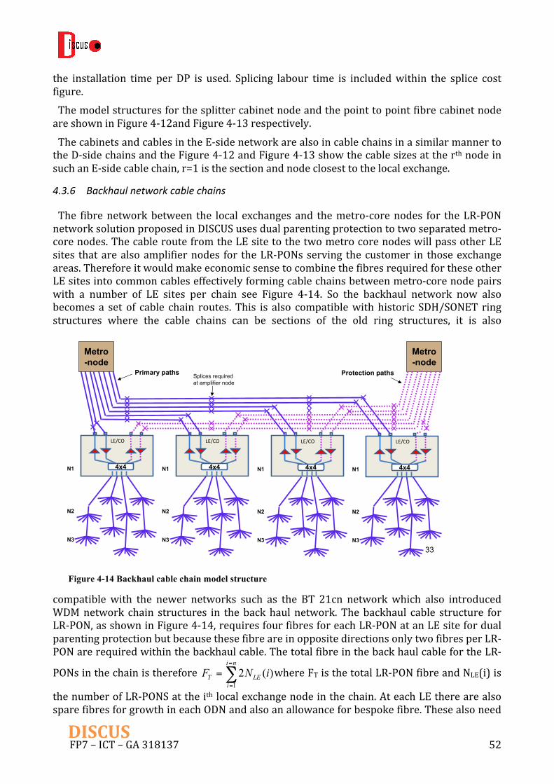
FP7–ICT–GA318137 52DISCUS
the installation time perDP is used. Splicing labour time is includedwithin the splice costfigure.ThemodelstructuresforthesplittercabinetnodeandthepointtopointfibrecabinetnodeareshowninFigure4-12andFigure4-13respectively.ThecabinetsandcablesintheE-sidenetworkarealsoincablechainsinasimilarmannertotheD-sidechainsandtheFigure4-12andFigure4-13showthecablesizesattherthnodeinsuchanE-sidecablechain,r=1isthesectionandnodeclosesttothelocalexchange.
4.3.6 Backhaulnetworkcablechains
The fibrenetworkbetween the local exchanges and themetro-corenodes for theLR-PONnetworksolutionproposedinDISCUSusesdualparentingprotectiontotwoseparatedmetro-corenodes.ThecableroutefromtheLEsitetothetwometrocorenodeswillpassotherLEsites thatarealsoamplifiernodes for theLR-PONsserving thecustomer in thoseexchangeareas.ThereforeitwouldmakeeconomicsensetocombinethefibresrequiredfortheseotherLEsitesintocommoncableseffectivelyformingcablechainsbetweenmetro-corenodepairswith a number of LE sites per chain see Figure 4-14. So the backhaul network now alsobecomes a set of cable chain routes. This is also compatiblewith historic SDH/SONET ringstructures where the cable chains can be sections of the old ring structures, it is also
compatible with the newer networks such as the BT 21cn networkwhich also introducedWDMnetwork chain structures in thebackhaulnetwork.Thebackhaul cable structure forLR-PON,asshowninFigure4-14,requiresfourfibresforeachLR-PONatanLEsitefordualparentingprotectionbutbecausethesefibreareinoppositedirectionsonlytwofibresperLR-PONarerequiredwithinthebackhaulcable.ThetotalfibreinthebackhaulcablefortheLR-
PONsinthechainistherefore ∑=
=
=ni
iLET iNF
1
)(2 whereFTisthetotalLR-PONfibreandNLE(i)is
thenumberofLR-PONSattheithlocalexchangenodeinthechain.AteachLEtherearealsosparefibresforgrowthineachODNandalsoanallowanceforbespokefibre.Thesealsoneed
33
N2
N3
N2
N3
N2
N3
N2
N3
Metro-node
LE/CO
4x4
Protection pathsPrimary paths
N1
LE/CO
4x4N1
LE/CO
4x4N1
LE/CO
4x4N1
Metro-node
Splices required at amplifier node
Figure 4-14 Backhaul cable chain model structure

FP7–ICT–GA318137 53DISCUS
to be supported by additional fibre in the backhaul cable chain. Again there is a designdecisionwhether toprovide all thebackhaulbespokeand spare fibre entering theLE sitesfrom theODNsor just a percentagebasedon statistical estimates of the total bespoke andspare fibre required for the LEs in each cable chain. The latter is selected in the cash flowmodelbutatogglecanbeaddedtocomputetheimpactofprovidingallthatfibreatdayone.TheactualnumberofthesefibresisderivedfromthesizeofthecablesfromtheE-sidecablechains entering the LE node sites as previously discussed. Any statistical factor to reducethesefibrecountswithinthecablechainisasimplemultiplierofthesumofall thesefibresenteringtheLEnodesfromtheE-sidecables.Thespareandbespokefibrewillbeterminatedonsplicetraysinthehousing,thiscouldbetheamplifiernodehousing, ifspacepermits,oraseparatehousing forcablesplicingcanbeemployed.Inthemodelweassumethesesplicesareintheamplifiernodehousingalthoughuntildevelopmentofsuchanodeiscarriedoutthepracticalityofthatapproachisuncertain.Onceallthefibresareknownthecablesizeandcostscanbedetermined.Togeneratethesebackhauldualparentedchainstructuresoptimisationmodelswereusedas described below, an example of results for a 73 metro-core node solution for the UKnetworkisshowninFigure4-15.Theoptimisationmodellingalsolookedattreeandbranchcable topologies for thebackhaul networkhowever for the cash flowmodel only the chain
topologywasimplementedForcompatibilitywhencomparingLR-PONsolutionswithmoreconventionalsolutionsthatdo not bypass the LE sites the same cable chain structures are assumed for all solutionsalthoughthecablessizescanchangebetweensolutions.The cash flow model computes each LE area sequentially to determine the costs of thevariouselementsmakingupthesolution.Fromthesecoststhecostpercustomerpassedandconnectedcanbedetermined.Thesecostsvarywithuserbandwidthandalsodependontheroll-out ratewhich gives a time line for expendituredependingon the rollout strategy andrate. For the backhaul network it is required that a cost per customer as a function of thesame user bandwidth parameters is also calculated for each exchange the difference nowhoweveristhatthebackhaulcablechaincostissharedoverotherLEareasonthesamecable
Figure 4-15 Example of backhaul cable chain structure for UK network
197980
202980
207980
212980
217980
222980
388110 398110 408110 418110 428110 438110 448110
Northings(Y
)
Eastings(X)
4LEChainsbetweenMC-nodesBoarsHillandCheltenham

FP7–ICT–GA318137 54DISCUS
chain.Todimensionthechain,thenumberoffibresrequiredforeachLEonthechainneedstobecalculated.ThiscomplicatesrolloutstrategiesasitimpliesthatalltheLEareasonacablechainshouldberolledouttogether.Howeveronceallthefibrerequirementsareknownthecablesizecanbedeterminedandthecostscanbecalculatedforthetotalcablechain.Thiscostis then divided by all the customers on all the LEs on the cable chain to get an averagebackhaul cost per customer. This simple strategy implies rollout on a chain by chain basiswhichcanrestrictsomeroll-outoptionse.g.tacklingruralexchangeareasfirsttoaddressthedigital divide, as an urban LE might share a common chain with the rural exchanges andwould therefore also need to be included. Oneway round this problem is to compute thebackhaul cable requirements for 100% roll out and derive the average backhaul cost percustomer for each LE. Thenwhen applying roll out strategies these cost per customer areused even if the other LEs in the chains would not be part of the build being considered.There are practical, economic, and subsidy argument issueswith this approach but it doesenablesimplerolloutstrategiestobecompared
4.3.7 Optimizingthebackhaulnetwork
This section describes the optimisation methodology used for generating the backhaulnetworkcablechainsandalsocomparesthechaintopologywithtreeandbranchtopologies.The objective is to design the optimum cable fibre network between a set ofMC nodes toconnecttheirsetsofLEsitessuchthattherearetwo-boundednodedisjointpathsfromeachLE site to its twoMCnodesFigure4-16 showsanexample for the twoalternatives, in thisexampleweobservetwoMCnodesm1,m2,andsixLEsites.LetusassumethateachLEsiteintheset{a,d,e,f}requires1PON,andeachLEsiteintheset{b,c}requires2PONs.ForeachPONweneedfourfibrestoconnecttotheirtwoMCnodes(i.e.,twofibresperPONperMConeforupstreamandonefordownstream).In the tree topology fibres are distributed from MC nodes to LE sites through cablesconsistingoffibresthatformatreedistributionnetwork.Thetreedistributionnetworkmustberesilienttoedgeandnodefailures,thatis,thetwopathstothetwoMCneedtobedisjointso that the PON can switch to the alternative path whenever an edge or node in thedistributionnetworkfails.Figure4-16(a)depictsanillustrativeexample,blackarrowsshowsthecabledistributionnetworkforMCnodem1andgreyarrowsforMCnodem2.Theweightsassociatedwith theedges indicate the lengthof the link (left)and theminimumnumberoffibresrequired(right).Forinstance,(e,f)requires2fibresaseandfonlyuseonePONeachandthedistancebetweeneand f is1KM;thelinkbetween(a,b)requireseightfibres: fourfibres for LE a (with two PONs) and four fibres for c (with two PONs) and the distancebetweenaandbis3KMs.CompletedetailsofthetreetopologyareavailableinDeliverables2.6and4.10.In the chain topology fibres are distributed from theMC nodes to LE sites through cablechains. In the chain LE sites are connected one after another with no branches in thesequence, the first and last LE sites in the chain are directly connected to the MC nodes.UnlikethetreetopologywhereweneedfibresfromtwodifferentcablesforaPONtodesignaresilientnetwork,inthechaintopologyweonlyneedonecabletoconnecttotwoMCnodesfor any PON. Figure 4-16 (b) depicts a chain solution for our example, in the exampleweobserve two chains, one highlightedwith black arrows and another onewith grey arrows.Similarlytothetreetopologytheweightsintheedgesindicatesthelengthandthenumberoffibresforeachlink.Inthistoyexampleweobservethatthetreetopologyrequires306kmoffibreandthechaintopologyrequires280kmoffibre.

FP7–ICT–GA318137 55DISCUS
4.3.7.1 Optimizationmethodology
Consideringthecombinatorialnatureoftheproblem,weusealocalsearch(LS)approachtocomputenear-optimalsolutionsbyminimizingthecostofthesolution.Broadlyspeaking,theLSalgorithmstartswithaninitialsolutionanditerativelyimprovesthesolution,littlebylittle,by performing small changes. In order to move from one solution to another we use thefollowing4-stepprocedure:
1. SelectarandomLEefromthecurrentchainc.2. Removeefromc.3. Identifythebestlocation(i.e.,anewchainc’)foresatisfyingallconstraints.4. Inserteinc’.
Additionally,theLSalgorithmisequippedwithincrementalwayofmaintaininginformationrelatedtocheckingconstraintsandcomputingthecostofthesolution.
Table11Optimisationmodellingresults for treeandchain topologiessummaries the totaltraildistance(i.e.,sumofthedistanceofalledgesinthesolution),cable,andfibrerequiredforthetreeandchaintopologies.WerecallthatconnectingtwoLEsitesmightrequiremorethanasinglecableiftherequirednumberoffibresexceeds276(max.numberoffibresinacableusedinthemodel).Inthetableweobservethatthetreetopologytendstousefewercablekmsthanthechainatthecostof increasing the totalnumberof fibres.Werecall that thechain topologyrequirestwo fibres per PONwhile the tree topology requires four. In fact, in all the experimentedscenariosthetreetopologyuseslesscable(about12%)thanthechaintopology,however,atthe same time, the tree topology usesmore fiber (about 15%). The reason is that the treetopologyaggregatesmorefibresinatrail(orlinkbetweentwoLEsites). OnaverageintheUK scenario the tree and chain topologies deploy 244 and 144 fibres per km, roughly
Figure 4-16 Backhaul network example for two MC nodes and 6 LE sites. The weight of the edges indicate the distance in kms of the link (left) and the total fibers required for the link (right), assuming that LEs a, b, c, e, and f are associated with 1 PON and LEs b

FP7–ICT–GA318137 56DISCUS
speaking,akmofthedistributionnetworkneedsa144-fibercableforthechaintopologyanda276-fibercableforthetreetopology.
Country Number ofMCs Topology
Trail Cable Fibre
Thousandsofkms
UKLEs in model=5393
75Tree 110.2 164.9 23,865
Chain 171.9 197.5 21,570
80Tree 108.3 165.3 24,324
Chain 167.4 192.0 21,533
85Tree 106.3 161.2 23,544
Chain 160.4 185.2 20,694
90Tree 103.7 158.4 23,318
Chain 150.9 175.3 20,057
ItalyLEs in model=10708
100Tree 168.8 236.1 32,516
Chain 267.3 287.3 29,143
120Tree 160.6 227.0 31,793
Chain 236.3 254.7 27,090
140Tree 156.0 221.2 30,764
Chain 218.8 240.2 26,213
160Tree 151.5 211.8 29,148
Chain 212.4 231.4 25,072
Table 11 Optimisation modelling results for tree and chain topologies for UK and Italiannetworks
4.3.8 LR-PONamplifiernodes
FortheLR-PONsolutiontheopticalamplifiersrequiredforincreasingthepowerbudgetforthelargersplitreachand10Gb/ssymmetricallinespeedareplacedatLEexchangesite.ThestructurefortheamplifiernodeisshowninFigure4-17.

FP7–ICT–GA318137 57DISCUS
Theamplifiernodecontainsthemx4splitter(typicallym=4,sothesplitteristypicallya4x4), the LR-PON amplifiers plus tap splitter for PON monitoring and amplifier nodemanagementandanyadditional splitters required for the ruralamplifier chainstructure inthe backhaul cable network. The current cost model only has the amplifier node for the“lollipop” version of the LR-PON design with only the LR-PON 4x4 splitter installed. Thestructure shown in Figure 4-17 e shows a configuration for 4 LR-PONs. Themainmoduleassembly includingsplitters is factoryassembledso that theonly fieldoperation is splicingtheE-Sideandbackhaulfibresandpossiblyinstallingcardsforthesystemcapacityrequired.
The structure includes four EDFA amplifiers per LR-PON, an element manager whichincludes an ONU for communication back to the metro-core node OLTs. There is also thepowersupplyandbatteriespackforstandbypowerwhenthemainssupplyfails.Thispowerunit is assumed to be outside themain amplifiermodule housing. There are also separatesplicetrayassemblies for theE-side(totheODN)andthebackhauls fibrecableswhichwillcontaintraysforsplicesforthroughfibreandfibreterminatingonthenodeandalsotraysforstoring spare fibres and bespoke fibres if they are not used at initial installation,which isassumedtobethecaseforthemodel.Notealthoughthehousing inFigure4-17 isshowndualended forconvenienceandclaritytheactualhousingmaywellbesingleendedwithODNandbackhaulcableenteringfromthesame end. In either case the fibre management would allow interconnect and splicingbetween E-side (ODN) fibre and amplifier node splitters or backhaul fibres and backhaulthrough fibre etc, in a protected and managed fibre environment. From a cost modelperspective the total number of splices and splice trays are calculated and the fibremanagementandinstallationcostsdeterminedfromthosevalues.
4.4 Metro-corenodemodelstructures
The metro core node model was described in some detail in D6.1[23], it focused on thedimensioningaspectsofthecostmodelwhichareofcoursethecorecalculationsthatneedtobeperformedforthecostmodelling.Inthissubsectiononlytheupdatestothemodelwillbedescribed.ThemodelsstructuresfortheopticalswitchnowincludesthetwosidednonblockingClosswitch, the non-blocking single sided Clos switch and the single sided partitioned switch.These options are selectable in the model and for the partitioned structure the degree of
Blown fibre cables
Blown fibre cables
2 x AMP.
Managem
ent
splitter
Fibre management
Backhaul
Splice trays
Power supplies
Cards for one LR-PON
Factory assembled
unit
1st stage LR-PON optical splitter e.g. 4x4 splitter
and taps
Optical amplifier card (contains an
upstream and down stream amplifier)
splitter
splitter
splitter
2 x AMP.
2 x AMP.
2 x AMP.
2 x AMP.
2 x AMP.
2 x AMP.
2 x AMP.
Managem
ent
Managem
ent
Managem
ent
Element manager (ONU)
Mains power supply +
battery backup
E-Side Splice trays
Figure 4-17 LR-PON amplifier node model structure - four LR-PON ODNs can be supported

FP7–ICT–GA318137 58DISCUS
partitioningcanalsobepreselected.Thesinglesidedclosswitchwiththefirststagesusing2-sidedmatriceshas alsobeen included for completenessbut isnot anoption thatwouldbeused.ThedesignusingbothstagesassinglesidedmatricesisthepreferredsolutionforboththefullsinglesidedClosswitchandthesinglesidedpartitionedswitch.Theelectroniclayer2andlayer3packetswitchingandrouterstructureshavebeenrevisedinthelightofthepowerconsumptionmodellingwhichrequiredmoredetailedstructuresthanoriginallyincludedinthecostmodel.ThevariousstructureshavehoweverbeenkeptgenericandareshowninFigure4-18whichalsoshowstheconfigurationofthepacketswitchesand
routers, the transponder shelves for both fixed and flex-grid systems and the opticalmultiplexingtocorefibres,theopticalswitchinglayerisshownwithportsontwosides,thisisnottoimplyatwosidedswitchstructurebutisdrawninthiswayforclarityofthefigure.The routers and layer 2 switches are generic with an assumed common scalable switchfabric that have the router or switch slot cards which contains the forwarding engineelectronicsandintowhichplugthelinecards.Wealsohaveanoptionforembeddedfixedgridtransponders in the layer3 routersavoiding the interconnectinggreyopticalportsand theneedfortranspondershelvesasseparateequipment.Thelinecardsareshowngenericallytorepresent both the access side and the core side of thepacket switch layers. Theport/linecardsforbotharecalculatedseparatelytomatchthearchitecturebeingmodelled,thesizeofthemetro-corenodeandcustomerbandwidthdemanditneedstoservice.Thedifferencebetweenthelayer2switchandlayer3routerfunctionalityisassumedtobehandled in the slot card forwardingenginewith the router functionalitybeinggreater thanthat of the layer 2 switch. In the model this is reflected in the relative cost and powerconsumptionofrouterandlayer2switchslotcards.Intheversionofthemodeldescribedin
Switchor
RouterCorefabric
Transpon
dershe
lfPolatisOpticalswitch
WSSforflex-grid
Slotcards LinecardsGreySR
Transceivermodules
Transpondercards
TransponderTransceivers
Tocorefibres
EmbeddedfixedgridTransponders(forlowerratetransponders) FixedGrid
DWDMAWGs
Figure 4-18 Configuration of electronic subsystems in the metro-core node

FP7–ICT–GA318137 59DISCUS
D6.1themaximumportrateconsideredwas100Gb/sthathasbeenincreasedto400Gb/sandwould be easy to increase further to say 1Tb/s ports capacities. The model also assumesgenericshelfandrackstructuressothatinterconnect,coolingandpowersupplycostscanbetaken into account. For example the switch fabric cards for switches and routers can, forsmaller switches,be include in the shelveswith the switchblades containing the slot cardsandlineinterfaceorportcards.Theseswitchcardsareinturnassumedtobeaprogrammablefabric that enables them to function as any stage in a Benes re-arrangeable non-blockingswitchstructure.Ifmorecapacitythanasingleshelfisrequiredtheswitchfabriccardshavecapacity for inter-shelf connectivityallowingup to fourshelves tobeconfiguredasasingleswitch.Iffurthercapacityisrequiredswitchfabricshelvesareintroducedwhichonlycontainswitch fabric cards. These switch fabric shelves are in turn interconnected using theprogrammableswitchfabriccardswithadditionalcapacityforinterconnectpurposessothattheswitchcanbeexpandedgracefullytoverylargesizes.ThegeneralconceptissimilartotheCISCOCSR3routerfabricstructure.
4.4.1 Integrationofthemetro-corenodeandtheaccess&backhaulmodels
Itwasoriginallyintendedtofullyintegratethemetro-corenodemodelwiththeaccessandbackhaulnetworkmodels.Howevertheunforeseenadditionalcomplexityandworkrequiredonthedetailedstructureswithinthemodelplustherequirementsofthepowerconsumptionmodel has meant that full integration has not been possible within the project resources.However to use results for end to end analysis we can run the metro-core node modelseparatelyfromtheaccessandbackhaulmodelandgeneratesetsofresultsintermsofcostpercustomerasafunctionofmetro-corenodesizeanduserbandwidthrequirements.Theseresultscanthenbeusedaslook-upvaluesforthecashflowmodel.Effectivelybecausethetwomajorinputvariablesforthemetro-corenodemodelisthesizeof themetro-corenode and the requireduser sustainedbandwidth.The cost per customercanbeevaluatedfor therequiredrangeof thesevariablesandthesevaluesusedwithinthecapex elements of the cash flowmodel. In thisway themetro-coremodel is preconfiguredwithachosenconfiguration,thatisalldesignoptionsarepre-selectedandthenthemodelisrun for the bandwidth and metro-core node size ranges required. Full integration is stillplannedandwouldbeanadvantageasawiderrangeofscenarioscouldquicklybeexaminedandcomparedbutthiswillprobablybecompletedaftertheformalendoftheDISCUSproject.If results of the integration are completed before the project review then results will bepresentedatthatreview.Themajordisadvantageofnothavingafullyintegratedmodelisthattheimpactofchangingconfiguration options for given access and backhaul parameters is more difficult toinvestigateandquicklygenerateresults.
4.5 OpexandRevenuemodels
4.5.1 Opexmodel
Acash flowmodel requires capital expenditure, revenueandoperational expenditureasafunction of time. The capital expenditure is derived from the costmodels described abovecoupledwitharolloutordeploymenttime line,seesection4.6.Operationalexpenditure isacomplexsubjectinitsownrightandafullmodeliswellbeyondthescopeandresourcesofaproject likeDISCUS.Howeversomemeaningfuloperationalexpenditureparameterneedstobeincludedinthecashflowmodeliftheresultsaretohaveanyrealvalue.Tocutthroughthe
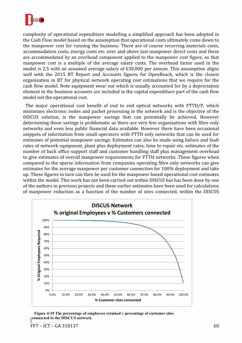
FP7–ICT–GA318137 60DISCUS
complexityofoperationalexpendituremodellingasimplifiedapproachhasbeenadopted intheCashFlowmodelbasedontheassumptionthatoperationalcostsultimatelycomedowntothemanpowercost for running thebusiness.Thereareof course recurringmaterials costs,accommodationcosts,energycostsetc.overandabovejustmanpowerdirectcostsandtheseareaccommodatedbyanoverheadcomponentappliedtothemanpowercostfigure,sothatmanpower cost is a multiple of the average salary costs. The overhead factor used in themodel is2.5withanassumedaveragesalaryof£30,000perannum.Thisassumptionalignswell with the 2015 BT Report and Accounts figures for OpenReach, which is the closestorganisation inBT for physical network operating cost estimations thatwe require for thecashflowmodel.Noteequipmentwearoutwhichisusuallyaccountedforbyadepreciationelementinthebusinessaccountsareincludedinthecapitalexpenditurepartofthecashflowmodelnottheoperationalcost.The major operational cost benefit of end to end optical networks with FTTH/P, whichminimizeselectronicnodesandpacketprocessinginthenetworkandistheobjectiveoftheDISCUS solution, is the manpower savings that can potentially be achieved. Howeverdeterminingthosesavingsisproblematicasthereareveryfeworganisationswithfibreonlynetworksandeven lesspublic financialdataavailable.However therehavebeenoccasionalsnippetsofinformationfromsmalloperatorswithFTTHonlynetworksthatcanbeusedforestimatesofpotentialmanpowersavings.Estimatescanalsobemadeusingfailureandfaultratesofnetworkequipment,plantplusdeploymentrates,timetorepairetc.estimatesofthenumberofbackofficesupportstaffandcustomerhandlingstaffplusmanagementoverheadtogiveestimatesofoverallmanpowerrequirementsforFTTHnetworks.Thesefigureswhencomparedtothesparseinformationfromcompaniesoperatingfibreonlynetworkscangiveestimatesfortheaveragemanpowerpercustomerconnectionfor100%deploymentandtakeup.Thesefiguresinturncanthenbeusedforthemanpowerbasedoperationalcostestimateswithinthemodel.ThisworkhasnotbeencarriedoutwithinDISCUSbuthasbeendonebyoneoftheauthorsinpreviousprojectsandtheseearlierestimateshavebeenusedforcalculationsofmanpower reduction as a function of the number of sites connected,within the DISCUS
0%
10%
20%
30%
40%
50%
60%
70%
80%
90%
100%
0.0% 10.0% 20.0% 30.0% 40.0% 50.0% 60.0% 70.0% 80.0% 90.0% 100.0%
%Orig
inalEmployeesR
equired
%Customersitesconnected
DISCUSNetwork%originalEmployeesv%Customersconnected
Figure 4-19 The percentage of employees retained v percentage of customer sites connected to the DISCUS network

FP7–ICT–GA318137 61DISCUS
cashflowmodel.The curve in Figure 4-19 shows the assumed relationship between the percentage ofemployeesrequiredandthepercentageofcustomersconnectedtotheLR-PONbasedDISCUSnetworkfor100%takerate.Atlowerservicetakeratesthemanpowersavingwillbereducedpro-rata. Also because of the dependencies on business models and the competitiveenvironmentetc.theactualmanpowerreductionachievablecouldvaryconsiderablyfromthemodel parameters. Therefore a selectable toggle is built into the model that turns off themanpower saving parameter in the opex cost saving, so that networks can be comparedwithoutassumingmanpowersavingsintheopexcosts.Alsoalltheparametersaffectingthepotential manpower savings are accessible variables in the model and if better publishedempirical data from use cases of FTTH deployments become available then the modelparameterscanbesimplyadjustedtoreflectthenewdata.Otherarchitecturessuchaspointto point fibre, FTTCab and GPON have also had manpower saving estimates made forcomparisonpurposes.
4.5.2 Revenuemodel
Thethirdparameterrequiredforcashflowmodellingisarevenuetimeline.Revenuewillbedirectly related to the number of customer sites that are connected to the network beingevaluated.Itisalsodependentontheeconomicclimate,thedistributionofdisposableincome,regulationandthecompetitiveenvironmentamongstothermarketfactors.HoweverfortheDISCUS cash flowmodel we consider three revenue parameters to encompass all revenuescenarios,theseare:
• Fixedupfrontconnectioncharge
• Flatratemonthlycharge
• NetworkusagechargeThe upfront connection charge, if used, is usually applied to offset the one-off cost ofphysicallyconnectingthecustomertothenetwork,thatis;providingthecustomerdrop,thecustomerpremisesterminationandtheCPEnecessarytoconnecttoserviceproviders(ifthisisownedbythenetworkprovider).Thisisoftenwaivedintoday’scompetitiveenvironmentandrecoupedaspartofthemonthlyrentalparticularlyifthecontractisforaminimumterme.g.1year,asisoftenthecase.Butupfrontcharginghashistoricallybeenextensivelyusedandis often used in the mobile market where a mobile handset is part of the mobile servicecontract.The monthly charge is, in today’s market, the usual method for operators to receive themajorityoftheircustomerrevenue.Itisusuallyaflatratechargebasedonaservicebundle.Thebundlingelementinthechargeleviedisoftentheclosestoperatorsgettoausagerelatedcharge. Historicallythiswasnotthecaseandbeforethebroadbanddataeramostrevenueswerereceivedviatheusagecharge.Thedependenceonamonthlychargehasbeenattractivetothecustomerbaseastheirservicecostiseasilypredictableandthereisnofinancialbarriertousingtheservices.Butitdoesproducedistortionsandalevelofunfairnesstothemarket,forexampleheavyusersoftheservicescangetmuchbettervaluethanlightusers.Flatratecharging,whichthemonthlychargemodelisaversionof,alsoeffectivelydecouplesrevenuesfromserviceusageand thesubsequentdemandonnetworkresources; this in turnreducestheincentiveforoperatorstoinvestinthenetworkcapacityasthereisnodirectlinktothatnetworkinvestmentandanyincreasedrevenuestreamtopayforit.

FP7–ICT–GA318137 62DISCUS
Ausagecharge, the thirdparameter in themodelwashistoricallyvery importantand is acharge leviedforsomemeasureoftheusagethecustomermakesofthenetworkresources,usuallyrelatedtotheinformationtransmittedtoorfromthecustomersite,e.g.Gigabytespermonthofdatausage.Howeverthischargeisveryoftenwaivedandineffectthereisnousagechargeand little relationshipbetween customer revenueand theirusageof thenetwork. Itdoeshowevergetused forbandwidth capping if customerspassausage thresholdorevenwhenon “unlimited”contracts thecustomer isdeemed tobeanunfairuserof thenetworkresource(andlimitingaccessforothercustomers).Asthebandwidthcapabilityofnetworksincreases in the future cappingmay become untenable or at least impracticable in a trulysuperfastbroadbandfuturewherecustomerscouldbeusingbandwidthsordersofmagnitudegreaterthantoday’saveragerates.Thismightrequireareturntosomeformofregularusagecharging inorder to couplenetwork investment to revenuestreams to recoup thenetworkbuild cost required to support the high bandwidth demand. Although the chargemight bemoreservicerelatedthandirectbandwidthusagechargingitwouldneedtobelinkedtothesustainedusedbandwidthinsomewayandinthemodelthisparameteriscoupleddirectlytouserbandwidthforsimplicityandtoavoidthecomplexityofserviceusagemodels.Inthemodeltherevenueparametersarepre-settoinitial“dayone”valuespercustomerandthen a revenue growth parameter is applied to reflect anticipated revenue gains as newbroadbandservicesareintroducedovertimeandasuserbandwidthsincrease.A complexity in setting initial values is definingwhat constitutes legitimate revenues thatcanbeused fornewnetworkbuildandgrowth.Foran incumbentoperatorshouldexistingservice revenue be allowed to be incorporated as part of the revenue streams of the newnetwork?Theseoperatorshavetheproblemthattheseexistingservicesarealreadyprovidedonthecurrentnetworkandtherevenuesearnedarerequiredtosupportthatlegacynetwork.The alternative is to only allow incremental revenue growth due to the enhanced servicecapability thenewnetworkenables tobeusedas the revenuestream for thenewnetworkbuild. This is a much more difficult business case to achieve and of course forces servicepackagesonthenewnetworktobeatahigherpricethantheservicepackagesontheexistingnetwork,whichcouldlimittakeup.Newbuildoperatorshowevercanuseallrevenuestreamsagainst their network build as they have no legacy network or legacy services to supporthowevertheymayhavegreaterinfrastructurebuildcostsastheymayhavelimitedaccesstoexisting network infrastructure. To cut through these complexities in the model acompromise revenue streamof~50%of today’s super-fast (FTTCab) broadbandpublishedrevenueratesareusedasinitialvaluesforthemodel.Thesevaluescanofcoursebechangedtoanyvaluesinordertoseethesensitivityandchallengesproducedbyvaryingrevenues.
4.6 Rolloutstrategies
Inordertogeneratethetimelinesforcapitalexpenditure,opexexpenditureandrevenuesarolloutofnetworkbuildandcustomertake-upovertimeisrequired.Intheearlierversionofthis model the rollout strategy was a simple total sites per annum figure and either arepresentativeexchangewasusedforthecashflowcalculationsagainstthatvolumerolloutoreachexchangewascalculatedinturn,afterbeingorderedinsomeway,andthecostsandrevenueaccumulateduntiltheperannumnumberofcustomerswascaptured.Thiswasthenrepeated for each successive year. It should also be noted that in this earlier model theinstallation costs only included the access and backhaul transmission network up to themetro-core node. The switching and routing functions in the metro-core node were notincluded.

FP7–ICT–GA318137 63DISCUS
Thisbasicprocesshasbeencontinuedinthecurrentversionofthemodelwithmetro-corenodecosts(includingcoretransmissiontransponderequipment)included.Howevertheuseofbackhaulcablechainshascomplicatedtherollout.Toimplementthechainandderivethecostsequitablythewholechainneedstobeincludedwithinthecalculationwhichbydefaultimpliestheyareincludedintherollout.Thecablechaincablesizecouldbepre-computedandspare fibres reserved for all the exchanges that will ultimately be in the cable chain but,depending on the roll-out scenario, all the exchanges may not be included at initialdeployment.The problemwith that approach is the derivation of the cost per customer for the initialdeployment. In thisapproachtherewillbecapitalspend forexampleonthebackhaulcablethat is shared over relatively few customers. This would artificially put up the cost percustomer for those early deployments making them more expensive. We have thereforedecided that for all rollout strategies the full chain and all exchange on the chain will becomputed and an average cost per customer for the back haul for each LE is derived. Thisderived cost per customer will then be used for the rollout regardless of whether all theexchanges in the backhaul cable chain are included. It recognises that this causes someeconomic and possibly subsidisation issues that would need addressing with a real worldrolloutbut it isapragmaticwayofnotburdeningareaswithcoststhatwouldultimatelybeshared.Therolloutstrategiesconsideredare:
• Rolloutbygeotype,
• Rolloutbygeographicalarea
• Rolloutbycustomerdemographics
• RolloutbyexchangesizeThe strategies can be chosen to address various political and economic scenarios, forexamplerollingoutbygeotypecouldbeusedforearlyaddressingoftheproblemofthedigitaldivide whereby rural areas could be targeted first on the grounds that they are the mostdeprivedareaswhenitcomestobroadbandserviceprovisionandthetownandcityareaswillalreadybeservedbyDSLandFTTCab.Indeedsuchastrategycouldinvertthedigitaldivideasthe rural areas having an ultra-fast FTTH solution deployed, would have better servicecapabilitythanthedenseareas.Thiscouldhelptoattractinwardinvestmenttotheseareasbycompanieswishingtoexploittheadvantagesofthesenetworksandofferattractiveareasfortheir employees to live. Deployment via demographics could be an economic strategy totargetareaswithparticularcustomertypesthatmighttake-upspecificsuperfastbroadbandservices. Rollout by geographic region or area could be amore pragmatic approach for anoperatorenablingmoreefficientuseofmanpowerandequipmentresourcesetc.Whateverstrategyisadoptedtheyallareeffectivelyaparticularorderingorselectionoftheexchanges within the exchange database, the software routine sequentially selects theexchanges from the chosen ordering and for each exchange selected finds the associatedexchangesinthesamebackhaulcablechain.Afterthenecessarycostandrevenuecalculationstheseexchangesarethenremovedfromthesearchandthenextexchangeandcablechainisfound until the required number for the assumed rollout rate is obtained. The cash flowresultsarecalculatedandstoredandthenthenexttrancheofexchangesselecteduntilalltheexchangesinthedatabaseorthesearchrolloutrangeofinteresthavebeenselected.

FP7–ICT–GA318137 64DISCUS
4.7 Cumulativecash-flowmodels
While implementation of the cumulative discounted cash flowmodel is quite complex thebasic concepts are fairly straight forward. Cash flow is cash in minus cash out, if this ispositivethenthebusinessisinastateofpositivecashflowandcashinexceedscashout.Cashflowhowever itselfhasnohistoryandthe financialstateof thebusinessneeds to take intoaccount the cash flow history and produce cumulative cash flow figures. This is simplysummingovertimethetotalcashinandsubtracting,forthesameperiod,thetotalcashout,whenthefiguregoespositivethebusinessisatabreakevenpoint.Doingthisperiodicallyoreven continuously a cumulative cash flow curve can be produced. The income andexpendituretimelinesareusuallydifferentcurvesandtofurtherrefinethebreakevenpointfutureexpenditureand incomeshouldbediscountedback toanettpresentvalue(NPV). Inthiswaydiscountedcashflowsimplytakesintoaccountthatfuturemoneyisworthlessthanpresentmoney.In themodel a periodic accounting period of 1 year is used and a curve is fitted to thesediscretepointstogeneratethecumulativediscountedcashflowresults.Majorparametersinthecashflowmodelare:
• Takerate
• Interestrate
• Learningcurvesappliedtoplantandequipmentcosts
• Discountrate
• Manpoweroverheadfactor
• Installationrate
• percustomervaluesforthecapex,opexandrevenue
• Networkdimensioningparameters suchas totalnetworksize,numberof customers,numberofemployeesatyearone(forincumbentmodel)
Thetakerateissimplytheproportionofcustomerspassedthatactuallyareconnectedandgenerate revenue, it is used for computing cost per customer connected and cost percustomerpassed.The interest rate is the interest charge on the negative cash flow values prior to thebreakevenpoint.Itisassumedforconsistencythatnegativecashflowissupportedvialoanswhichwillhaveanassociatedinterestcharged.Thereisatoggleinthemodelthatallowsthistobe turnedoff to see the effect of interest rateon time tobreakeven. Interest charges, aswouldbeexpected,willdelaythetimetobreakeven.The learningcurve is the techniqueused in themodel to take intoaccountvolumerelatedpricedeclinesofnetworkequipmentandinfrastructure.Mostoftheequipmentiselectronicsbased and is assumed to have the industry norm of an 80% learning curve that is as thevolumeoftheequipmentdoublesthepricewillfallto80%ofthepreviousprice.Describinglearningcurvesasapercentageisusualpractice.Thepriceperunitofequipmentorunitofbandwidthasafunctionofvolumeisgivenby:
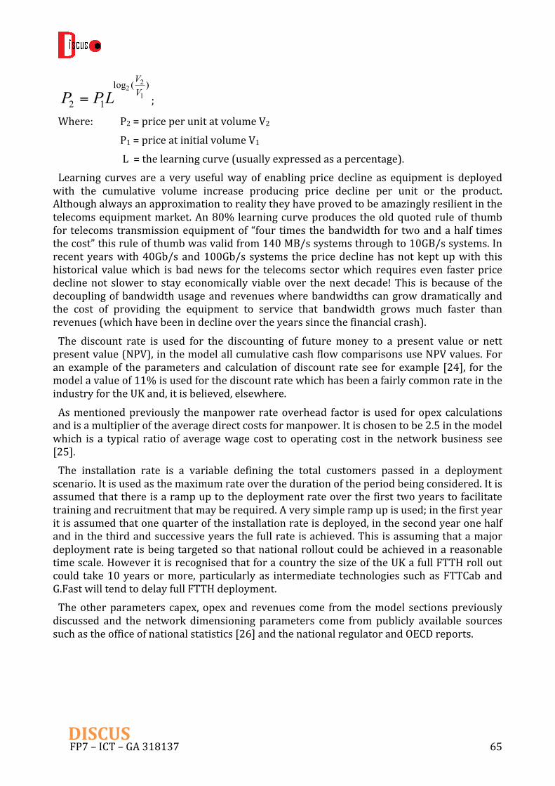
FP7–ICT–GA318137 65DISCUS
)(log
121
22 VV
LPP = ;
Where: P2=priceperunitatvolumeV2 P1=priceatinitialvolumeV1
L=thelearningcurve(usuallyexpressedasapercentage).Learning curves are a veryusefulwayof enablingpricedecline as equipment is deployedwith the cumulative volume increase producing price decline per unit or the product.Althoughalwaysanapproximationtorealitytheyhaveprovedtobeamazinglyresilientinthetelecomsequipmentmarket.An80%learningcurveproducestheoldquotedruleof thumbfor telecomstransmissionequipmentof “four timesthebandwidth for twoandahalf timesthecost”thisruleofthumbwasvalidfrom140MB/ssystemsthroughto10GB/ssystems.Inrecentyearswith40Gb/sand100Gb/s systems thepricedeclinehasnotkeptupwith thishistoricalvaluewhich isbadnews for the telecomssectorwhich requireseven fasterpricedeclinenot slower to stay economically viableover thenextdecade!This is becauseof thedecouplingofbandwidthusageandrevenueswherebandwidthscangrowdramaticallyandthe cost of providing the equipment to service that bandwidth grows much faster thanrevenues(whichhavebeenindeclineovertheyearssincethefinancialcrash).The discount rate is used for the discounting of futuremoney to a present value or nettpresentvalue(NPV),inthemodelallcumulativecashflowcomparisonsuseNPVvalues.Foranexampleof theparametersandcalculationofdiscountratesee forexample [24], for themodelavalueof11%isusedforthediscountratewhichhasbeenafairlycommonrateintheindustryfortheUKand,itisbelieved,elsewhere.Asmentionedpreviously themanpower rateoverhead factor isused foropexcalculationsandisamultiplieroftheaveragedirectcostsformanpower.Itischosentobe2.5inthemodelwhich is a typical ratioof averagewage cost tooperating cost in thenetworkbusiness see[25].The installation rate is a variable defining the total customers passed in a deploymentscenario.Itisusedasthemaximumrateoverthedurationoftheperiodbeingconsidered.Itisassumedthatthereisarampuptothedeploymentrateoverthefirsttwoyearstofacilitatetrainingandrecruitmentthatmayberequired.Averysimplerampupisused;inthefirstyearitisassumedthatonequarteroftheinstallationrateisdeployed,inthesecondyearonehalfandinthethirdandsuccessiveyearsthefullrateisachieved.Thisisassumingthatamajordeploymentrateisbeingtargetedsothatnationalrolloutcouldbeachievedinareasonabletimescale.HoweveritisrecognisedthatforacountrythesizeoftheUKafullFTTHrolloutcould take10yearsormore,particularlyas intermediate technologies suchasFTTCabandG.FastwilltendtodelayfullFTTHdeployment.Theotherparameters capex,opexand revenues come from themodel sectionspreviouslydiscussed and the network dimensioning parameters come from publicly available sourcessuchastheofficeofnationalstatistics[26]andthenationalregulatorandOECDreports.

FP7–ICT–GA318137 66DISCUS
5 PowerconsumptionmodellingThe cost model within the cumulative cash flow models are closely linked to the powerconsumption modelling and the additional detail that was required for the powerconsumptionmodelforswitchesandrouterswasfedbackintomoredetailedcostmodelsfortheseitemsofequipmentintheaccessandmetro-corenodemodels.Thedominantnetworkpowerconsumption(neglectingtheCPE)istheaccessnetworkterminationequipment(OLTsshelvesandracks)andthelayer2switchesandlayer3routersinthemetro-corenodes.The problemwhen trying to build a power consumptionmodel, thatwas both consistentwithhistoricallyperformancedataandalsocapableofprojectingfuturepowerconsumptionperformance, was that there are considerable inconsistencies in the published literature.Althoughthiswasrecognisedinsomepublicationsthebasicproblemappearstobethelackofa model based on the physical properties of VLSI technology that links performanceimprovementstotechnologyimprovements.ItwasthereforedecidedtobuildourownmodelbasedonlinkingswitchandrouterenergyefficiencytotheimprovementsinVLSIfeaturesize.
5.1 ASIC power consumption as a function of feature geometry size and therelationshiptoRouterandSwitchpowerconsumption
In addition to the inconsistencies in publically available power consumption data fornetworkequipmentand inparticular the routersandswitches, therearealsouncertaintiesabout the definition of router and switch capacity, both bi-directional and unidirectionalcapacities (unidirectional isused for transmission systemcapacity) areusedand it is oftenunclear which definition is being adopted. For example the Cisco CRS 1 data sheet usesunidirectional capacity while datasheets for the CRS 3 uses bidirectional capacity. It nowappearsthatCiscoandothervendorsareusingthebi-directionaldefinitionofcapacitybutitisnotcertainthatisalwaysthecase.Toaddresstheinconsistencyproblems,whichhasmadepowerconsumptionmodellingandprojectionsmuchmoredifficultthanoriginallyanticipateditwasnecessarytobuildapowerconsumptionmodelthathasitsfoundationsfirmlybasedonVLSIphysicaldesignparameters.It is theperformance improvementsof theunderlyingVLSItechnologythathasenabledtheperformance improvements and the power consumption reductions obtained during theevolutionof switches and routers over thepast coupleof decades andpower consumptioncalculationsneedtobebasedontheintrinsicpropertiesoftheVLSItechnologyusedfortheASICswithinsuchequipment,The model therefore takes the underlying energy performance trends of the VLSI-ASICtechnologies lying at the heart of routers and switches and fits them to the historicalperformance data that appears to be the most reliable in the published literature. ThefollowingsectionsdescribetheanalysisandtheproposedsolutionforthepowerconsumptionmodellingworkinDISCUS.
5.1.1 PowerconsumptionevolutionofVLSI
Thepowerconsumptionofintegratedcircuitshastwopartsoneisthepowerusedmovingchargeintothegateregionsofthetransistorstoswitchthetransistorstatefromontoofforofftoon.Theamountofchargetobemovedisproportionaltothecapacitancewhichinturndepends of feature geometry sizeW.How fast the charge has to bemoved also affects the
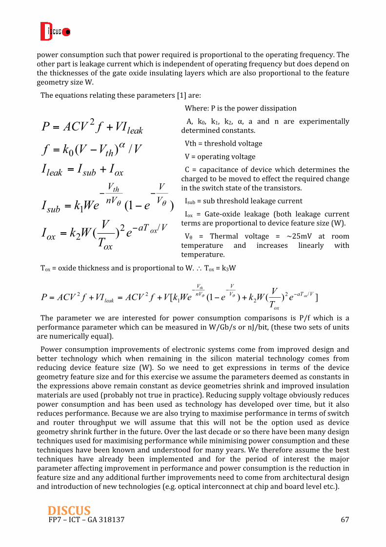
FP7–ICT–GA318137 67DISCUS
powerconsumptionsuchthatpowerrequiredisproportionaltotheoperatingfrequency.TheotherpartisleakagecurrentwhichisindependentofoperatingfrequencybutdoesdependonthethicknessesofthegateoxideinsulatinglayerswhicharealsoproportionaltothefeaturegeometrysizeW.Theequationsrelatingtheseparameters[1]are:
Where:PisthepowerdissipationA, k0, k1, k2, α, a and n are experimentallydeterminedconstants.Vth=thresholdvoltageV=operatingvoltageC = capacitance of devicewhich determines thechargedtobemovedtoeffecttherequiredchangeintheswitchstateofthetransistors.Isub=subthresholdleakagecurrentIox = Gate-oxide leakage (both leakage currenttermsareproportionaltodevicefeaturesize(W).Vθ = Thermal voltage = ~25mV at roomtemperature and increases linearly withtemperature.
Tox=oxidethicknessandisproportionaltoW.∴Tox=k3W
The parameter we are interested for power consumption comparisons is P/f which is aperformanceparameterwhichcanbemeasuredinW/Gb/sornJ/bit,(thesetwosetsofunitsarenumericallyequal).Power consumption improvements of electronic systems come from improveddesign andbetter technology which when remaining in the silicon material technology comes fromreducing device feature size (W). So we need to get expressions in terms of the devicegeometryfeaturesizeandforthisexerciseweassumetheparametersdeemedasconstantsintheexpressionsaboveremainconstantasdevicegeometriesshrinkandimprovedinsulationmaterialsareused(probablynottrueinpractice).Reducingsupplyvoltageobviouslyreducespower consumption and has been used as technology has developed over time, but it alsoreducesperformance.Becausewearealsotryingtomaximiseperformanceintermsofswitchand router throughput we will assume that this will not be the option used as devicegeometryshrinkfurtherinthefuture.Overthelastdecadeorsotherehavebeenmanydesigntechniquesusedformaximisingperformancewhileminimisingpowerconsumptionandthesetechniqueshavebeenknownandunderstoodformanyyears.Wethereforeassumethebesttechniques have already been implemented and for the period of interest the majorparameteraffectingimprovementinperformanceandpowerconsumptionisthereductioninfeaturesizeandanyadditionalfurtherimprovementsneedtocomefromarchitecturaldesignandintroductionofnewtechnologies(e.g.opticalinterconnectatchipandboardleveletc.).
VaT
oxox
VV
nVV
sub
oxsubleak
th
leak
ox
th
eTVWkI
eWekI
IIIVVVkf
VIfACVP
/22
1
0
2
)(
)1(
/)(
−
−−
=
−=
+=
−=
+=
θθ
α
])()1([ /221
22 VaT
ox
VV
nVV
leakox
th
eTVWkeWekVfACVVIfACVP −
−−
+−+=+= ϑϑ

FP7–ICT–GA318137 68DISCUS
Withtheaboveassumptionswecansimplifytheaboveequations:
The capacitancedArC 0ε= ; The area parameter Ar will be proportional to W2 and the
distance parameter d will be proportional to W, so that WC ε= where ε is a constant.Therefore:
SubstitutingforTox=k3W,then:
The first two terms are proportional to W and therefore as the device geometry size Wshrinksthepowerconsumptionreduces,seeFigure5-1fortheevolutionofVLSIfeaturesize.
The third term which is the leakage current associated with the oxide thickness in thejunctions and the insulating properties of additional insulating layers is inverselyproportional toW (this ismodifiedby the exponential termwhichdecreasewithW so theoveralleffectisnotasbadasaninverserelation).ItisthistermhoweverthatwillstopsiliconelectronicscontinuingtoimproveasMoore’slaw.
])()1([ /221
2 VaT
ox
VV
nVV
ox
th
eTVWkeWekVfWVAP −
−−
+−+= ϑϑε
VWakVV
nVV
eWkkVeeVWkfWVAP
th/
23
23
12 3)1( −
−−+−+= θθε
1
10
100
1000
1980 1985 1990 1995 2000 2005 2010 2015 2020
Featuresiz
e(nm)
EvolutionofVLSIFeaturesize
Figure 5-1 Reduction in VLSI feature size with time

FP7–ICT–GA318137 69DISCUS
Assuming all constants have remained constant over the time of interest except supplyvoltageandthresholdvoltagetheequationbecomes:
WhereA’=Aε; 23
2'kk
k = and 3akD = ;
The first term is thedynamicpower consumptionwithout leakage current effects the lastthreetermsarecomponentsoftheleakagecurrent,ofthesethelasttermistheleakageduetooxide layer thickness or high k insulation layer thickness. In the early dayswith relativelylargedevicefeaturesizestheleakagecurrenttermswouldbesmallcomparedtothedynamicpowerconsumptiontermandtheequationcouldbeapproximatedto:
TheperformanceparameterP/f=A’WV2reducesinproportiontoWandV2andisalowerboundfortheperformanceimprovementrelationship,anyleakagetermswillalwaysbetothedetriment of this bound. To apply this lower bound equation to router performance theconstantA’canbeapproximatelyestimatedbyfittingtoearlyexamplesofroutertechnologywith5-voltsupplyvoltagesandfamiliesoftechnologiesusingknownfeaturesize.Avalueof0.0391J/nm/V2wasselectedbythisempiricalfittingprocess
The core supply voltage V and the transistor threshold voltage Vth have also reduced asgeometrieshaveshrunkhoweverthethresholdvoltagehasreducedataslowerratethanthesupplyvoltageandthereisprobablylittleprospectofsignificantfuturereductionsinsilicontechnology see Figure 5-2 and [27]. The core supply voltage also needs to be significantlygreater than the threshold voltage to ensure high performance and good switchingcharacteristics. The expected power consumption improvement for dynamic powerperformancecanbederivedusingtheaboveequationsandanassumptionforthetechnologyfeaturesizeasafunctionoftime.
VDWnVV
nVV
VDWnVV
nVV
VDWVV
nVV
nVV
VDWVV
nVV
nVV
VDWVV
nVV
eWkVVWekVWekfWVA
eWkVeeVWkfWVA
eWkVeeVWkfWVA
eWkVeeeVWkfWVA
eWkVeVWekfWVAP
thth
thth
thth
thth
th
/3
112
/3
12
/3
12
/3
12
/3
12
''
')('
')('
')('
')1('
−−−
−−−
−−−
−−−−
−−−
+−+=
+−+=
+−+=
+−+=
+−+=
θ
θ
θ
θθ
θθθ
θθ
fWVAP 2'=

FP7–ICT–GA318137 70DISCUS
In order to perform this comparison an assumption for the technology feature size as afunctionof timemustbeassumed, this isbasedon theemergencedatesof reduced featuresizesinVLSI.Itmaybeoptimistictoassumerouterandswitchtechnologyadoptedthefeaturesizereductionsimmediatelyastherecouldbeatimelagbetweenchiptechnologycapabilitybecomingavailableandrouterdesign implementationsusing that technology.The time lineusedisasshowninFigure5-1forsourceofdatasee[28]A public domain source of router energy performancewith some identified products is apublicationbyNielson,thedataareshowninFigure5-3[29]isshowninTucker’sGreentouchpresentationwhichreferencesNielson’sresults.
By using the above power equations with the data in Figure 5-1to Figure 5-3 potentialenergy efficiency evolution curves can be fitted to the Nielson data to show expectedimprovement trends. The Neilson results seem to be based on the unidirectionalrouter/switchcapacitydefinition.
Figure 5-2 Evolution of VLSI supply and threshold voltages
1.0
10.0
100.0
1000.0
10000.0
1986 1991 1996 2001 2006 2011
Energy/bit(nJ)
Routers(Nielson2011)(nJ/bit)
CiscoCRS1
CiscoCRS3
Figure 5-3 Router energy performance (Nielson 2011)

FP7–ICT–GA318137 71DISCUS
Thecurvesderivedfromthetechnologypowerequationsabovewilltendtobelowerboundsonenergyefficiencyimprovementswhichmaynotbemetbecausemanufacturersarenotjustdesigning for energy efficiency but also need to design for performance and these tworequirementstendtohaveconflictingdemandsonthetechnologydesigns.IfwetakethepowerperformanceequationaboveanddividebyftoarriveattheexpressionP/fwhich is typicallyused forpowerperformancecomparison (nJ/bitorW/Gb/s; theyarenumericallythesame)then:
feWkVVWekVWekWVAfP
eWkVVWekVWekfWVAP
VDWnVV
nVV
VDWnVV
nVV
thth
thth
/)'('/
''
/3
112
/3
112
−−−
−−−
+−+=
+−+=
θ
θ
Wenowhave the leakage term inverselyproportional to theoperating frequency fbutwe
can substitute f for the expression α)1(0 VV
kf th−= where ko and α are experimentally
derivedconstantssothat:
α
α
θ
θ
)(/)'('
/)(/)'('/
0/
42
12
12
0/
3
112
thVDWnV
VnVV
thVDWnV
VnVV
VVkeWkVWeVkWeVkWVA
VVVkeWkVVWekVWekWVAfP
thth
thth
−+−+=
−+−+=
−−−
−−−
The aboveequation shows the functional formof thepowerperformance relationship thefirst term being the dynamic power performance and the second term being the result ofleakagecurrents.Howevertherearenowanumberofunknownconstantsthatrequirevaluesto be assigned in order to get a curve fit to Nielson’s router power performance figures.Usuallytheconstantsareexperimentallydeterminedbutwecanonlyfitvaluestomatchtheavailabledataasfaraspossible.Theproblemisthatthecurvegeneratedfromtheequationsshowthepowerperformance thatcouldbeachieved ifpowerperformancewas thedrivinggoaloftherouterdesignhoweverthisisprobablynotthecaseandperformanceisanequallylikely if notmore important driver formanufactures particularly in the earlier yearswhenpower consumptionwas less of an issue. For example the potential supply voltage declineshowninFigure5-2maynotbeadoptedandhighervoltagesforincreasedperformancemightbe used. Supply voltage is a major parameter affecting both performance and powerconsumption and although the trend shown in Figure 5-2 is reducing supply voltagemanufactures may not be able to take full advantage of the potential reduction if highperformanceisalsoanimportantdesignconsideration,thiswillbediscussedagainlater.Therearesomeindicativevaluespublishedforsomeoftheparameters;ina2003paperbyNamSungKimetal“Leakagecurrent:Moore’sLawmeetsstaticpower”fromIEEEExplore,αisquotedas~1.3,Vθisquotedtobe~25mVatroomtemperaturebutincreaseslinearlywithtemperature,thetemperatureco-efficientisnotgivenbutthisvaluecanbeusedinitially.The

FP7–ICT–GA318137 72DISCUS
value for A’ was previously assigned to fit the dynamic power curve through the CRS1performancepoint.Theremainingunknownsarethereforek0,k1,k’,nandD.Theparameterk0 is related to operating frequency which is taken to be the operating frequency of themajorityoftransistorsintheVLSIchips.Becauseofthedegreeofparallelismthatwillbeusedwithin the chip design the transistor operating frequency will be a fraction of the devicethroughput speed and will be of the order of 100 to 200 Mb/s, a compromise figure of150Mb/s was chosen for high speed devices e.g. devices with ~3Gb/s clock frequency forprocessorchips,thefrequencyparameterfwillthenscalewithVandVthonceavaluefork0isderived. The chosen point for the voltages to determine k0 are those assumed for thetechnologyoftheCRS1routerwhichgivesafigurefork0=200.Theotherconstantsshouldmaketheleakagetermsrelativelysmallcomparedtothedynamicpowercomponentinearlieryears,e.g.early90s,andthenmodifytheothertermstoapproachtheCRS3performanceforthe 2010/2011 time scale assuming these routers were designed for reasonable balancebetweengoodenergyefficiencyandperformance(whichmaynothavebeenthecase).Wecanthen extrapolate the curve to future years to estimate probable performance figures andcomparewithrecentlyquotedbutuncertainvalues.The results shown in figure 4 follow empirical fitting of parameter values to get a closematch to themostenergyefficientof theroutersshown inFigure5-3.Thosevalues for theconstantsafterempiricalfittingareshowninTable12.
Constant ValueA' 0.0391k0 200k1 1.148k' 144.5Vθ 0.025n 43.52a 1.3D 0.00150
Table 12 empirically fitted values for the constants in the power efficiency equations
Thethinnerpalegreenlineisthedynamicpowerperformancecurvealoneandthebrightergreenandthickerlineisthepowerperformancecurvewithleakagecurrenttermsincluded.This lattercurve is fittedtothemostenergyefficientroutewhich is theAviciTRSandthenparameters are adjusted to get close to the Cisco CSR3 router without impacting futureperformance too seriously and also keeping the impact of leakage in early years relativelysmall compared to dynamic power performancewhichwas the situation at that time. Thedashed curves show the leakage current terms. Of these the third term is the one thatdamagesfutureperformanceandisassumedtobehavinganimpactfrom2008onwardsanddoesaffecttheenergyefficiencyoflaterrouterssuchastheCRS3.

FP7–ICT–GA318137 73DISCUS
ItcanbeseenfromFigure5-4thatearlierrouterswerenotasefficientastheycouldhavebeen but this is reasonable as theywere almost certainly designed for performance ratherthanenergyefficiency.ItcanalsobeseenthatthelatergenerationroutersincludingtheCRS3do not follow the power performance curve even when the leakage current affects areincluded. This possibly indicates the continuing need to target performance and trade offpowerefficiency.Oneobviouswayoftradingperformanceagainstpowerefficiencyisnottofully follow the voltage decline curve and operate at higher than the minimum supplyvoltages. To illustrate this the supply voltage curve in Figure 5-2 is approximated by alogistics curve with the lower asymptote set higher than the minimum voltage this waschosentobe1.5Voltsratherthan0.7volts.ThecurveselectedtobeusedisshowninFigure5-6 the minimum voltage of 1.5 v is a compromise between trying to match the powerconsumptionoftheCRS3routerandnothavingtoogreatanimpactontheleakagecurrentsinthe later years. The third termwhich is the gate leakage termhas aV3 relationship and isthereforesensitivetohighvaluesofV.
0.0
0.1
1.0
10.0
100.0
1000.0
10000.0
Pow
er p
erfo
man
ce (n
j/bit
or W
/Gb/
s)
Derived router dynamic power usage performance against real router performance (Nielson)
Routers (Nielson 2011) (nJ/bit)
Leakage + dynamic (min V)
P/f (dynamic energy/bit) (nJ/bit)
Leakage 1st term (Used V)
Leakage 2nd term (Used V)
Leakage 3rd term (Used V)
CiscoCSR1
CiscoCSR3
AviciTSR
Figure 5-4 Comparison of dynamic VLSI chip power performance and router power performance
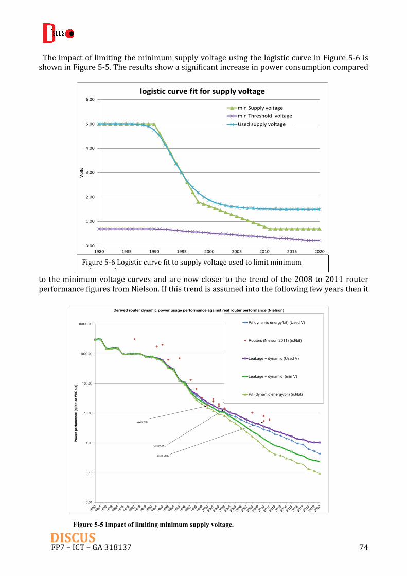
FP7–ICT–GA318137 74DISCUS
TheimpactoflimitingtheminimumsupplyvoltageusingthelogisticcurveinFigure5-6isshowninFigure5-5.Theresultsshowasignificantincreaseinpowerconsumptioncompared
to theminimumvoltagecurvesandarenowcloser to the trendof the2008to2011routerperformancefiguresfromNielson.Ifthistrendisassumedintothefollowingfewyearsthenit
Figure5-6Logisticcurvefittosupplyvoltageusedtolimitminimumvoltagevalues
0.00
1.00
2.00
3.00
4.00
5.00
6.00
1980 1985 1990 1995 2000 2005 2010 2015 2020
Volts
logisticcurvefitforsupplyvoltage
minSupplyvoltageminThresholdvoltageUsedsupplyvoltage
0.01
0.10
1.00
10.00
100.00
1000.00
10000.00
Pow
er p
erfo
man
ce (n
j/bit
or W
/Gb/
s)
Derived router dynamic power usage performance against real router performance (Nielson)
P/f dynamic energy/bit) (Used V)
Routers (Nielson 2011) (nJ/bit)
Leakage + dynamic (Used V)
Leakage + dynamic (min V)
P/f (dynamic energy/bit) (nJ/bit)
CiscoCSR1
CiscoCSR3
AviciTSR
Figure 5-5 Impact of limiting minimum supply voltage.

FP7–ICT–GA318137 75DISCUS
canbeusedasindicativeofpotentialrouterpowerconsumptionperformance.We can now compare the purple (leakage +dynamic (Used V) curvewith other projectedperformance figures and also with the layer 2 switch energy efficiency which has powerconsumptionperformanceoforder50%lowerthanrouterpowerperformancefigures.ThesecomparisonsareshowninFigure5-7Derivedresultscomparedtosomepublishedvaluesforrouter and layer 2 switches power performance they also illustrate the discrepancies thathaveappearedinpublishedsources.
Thethicklighterbluelineshowsthelayer2switchperformancecurveandcanbecomparedtothethickpurplerouterpowerperformancecurve.Thiswasderivedbyassumingthesameratiosapplyforrouterstolayer2switchesastheresultsfromtheTammetalpaperindicatesrefError!Referencesourcenotfound.HoweveritwouldappearfromtheseresultsthattheTammpaper results are anover estimateof router and layer2 switchpower consumptionalthough they continue to be used and references in presentation and papers (e.g.GreenTouchref[29]The 2 red points are the values for theMPLS-TE switch described in DISCUS D7.1, whencomparedto thebluethick line for layerenergyefficient layer2switches thesevaluesnowseem reasonable if 2016 technology is assumed for their implementation. It is quite
0.0
0.1
1.0
10.0
100.0
1000.0
10000.0
Pow
er p
erfo
man
ce (n
j/bit
or W
/Gb/
s)
Derived router dynamic power usage performance against real router performance (Nielson)Routers (Nielson 2011) (nJ/bit)
Leakage + dynamic (Used V)
Leakage + dynamic (min V)
P/f (dynamic energy/bit) (nJ/bit)
Routers (Tamm et al 2010) (nJ or W/Gb/s)
Packet Switch (Tamm etal 2010) (nJ or W/Gb/s)
DISCUS D7.1 MPLS-TE switch config A
DISCUS MPLS-TE switch config B
IDEALIST Edge (Router?)
IDEALIST Core (layer2)
IDEALIST Aggregation (layer 2/MPLS?))
Layer2 switch (Ethernet or MPLS-TE)
CiscoCSR1
CiscoCSR3
AviciTSR
Figure 5-7 Derived results compared to some published values for router and layer 2 switches power performance

FP7–ICT–GA318137 76DISCUS
reasonable that the lowerboundcurves forroutersandswitchesarenotmet inpracticeasswitcheswillneedtobedesignedforperformanceaswellasenergyefficiencyandthereforesomeenergyefficiencieswillneedtobesacrificedforperformancegains.The 3 purple points are for the Huawei “cloud switches” reported in the IDEALISTdeliverableD1.5ref[32].Thesearebelowtheblueandpurplecurvesandappeartobefartoolow, these points are actually doubled compared to the figures actually quoted in D1.5 ref[32]tonormalisethemtotheunidirectionaldefinitionforswitchandroutercapacityusedintheabovegraphs.AlthoughnotexplicitlystateditisbelievedthecapacityfigurequotedintheIDEALISTreportareusingthebidirectionalcapacitydefinition,butevenwiththisadjustmentthefiguresseemtobetoolowandrequirefurtherinvestigation.
5.2 Conclusions
ModellingfundamentalVLSIchipperformanceandfittingtheequationstopublishedroutervalues are a method of indicating minimum expected energy efficiency performance forrouters and switches.Byprojecting the results andmaking someassumption about energyefficiencyandperformancetrade-offssomepragmatic lowerboundperformancecurvescanbeproduced.Theseare the“leakage+dynamic(usedV)” (darkpurplecurve inFigure5-7)andthe“layer2switch“EthernetorMPLS-TE”(thickbluecurvesinFigure5-7).Inpracticeitisreasonabletoexpectrouterandlayer2switchpowerconsumptiontobeabovetheselines,depending on the relative importance of energy efficiency compared to router/switchperformance. The simple logistic curve used to implement the energy efficiency toperformancetrade-offsintheresultsofFigure5-6andFigure5-7couldbemodifiedifthereisbetterdata available to fit the curves to thatwouldaidbetterpower consumption forecastestimatestobemade..
6 SummaryThemodellingactivitieswithintheDISCUSprojecthavebeenverybroadlybasedandareacrucialpartoftheevaluationprocessofthearchitecturalproposals.Ithasbeenacrossprojectactivity involving many of the partners on various parts of the modelling problems. Theoverall objectives of the modelling activity have been largely achieved despite the totalmodelling task being much more complex and difficult than originally anticipated at thebeginningoftheproject.Oneareawhereprogresshasnotbeenasfarasoriginallyhopedfor,isthefullintegrationofthecashflownetworkmodelcomponents.Currentstatusisthatthecore model, the metro-node model and the access network models still need to be runindependentlyandresultsincorporatedintothecashflowmodel(whichisembeddedintotheaccess and metro-network model). There is also further work incorporating optimisationresultsintotheaccessandbackhaulnetworkmodelsisrequiredsothatthelatestversionofthecashflowmodelcurrentlydoesnotproducemeaningfulcashflowresults.Wehaveearlier,simplerandmorelimitedcashflowmodelsworking.Thelackofintegrationmakesitmoredifficulttocomparetherangeofeffectsontheendtoendnetworkeconomicperformanceoftheindividualparametervariablesinspecificareasofthenetwork.ForexampletheMetro-corenodemodelhasalotofconfigurationoptionswhichcurrentlyhave tobepreselectedandthen theMC-nodeperformancepre-calculated for thatconfigurationforarangeofnodesizesanduserbandwidthrequirements.Thoseresultsare

FP7–ICT–GA318137 77DISCUS
thenpassedtothecashflowmodeltobecombinedwithacorrespondingsetofresultsfromthe core network model and results from the access and metro-network model. It is stillintended to complete themodel integration but thatwill now have to be carried out afterDISCUSformallyends.Theresultsofmodellingwithintheprojecthavehoweverconfirmedthevalidityofmanyofthe proposed benefits arising from adoption of the DISCUS architecture andwhich formedpartoftheoriginalprojectobjectivessuchas:
• Reduction in buildings housing electronic switching, routing and transmissionequipmentbyclosureofthemajorityofLE/COsandsimplificationofthecorenetwork− This was achieved by the optimisation modelling that showed LE site
assignmentsofMC-nodes coupledwith the flat corenetworkmodelling couldenableremovaloftrafficprocessingroutersswitcheslinecardsetc. fromleast98%ofLEsitesinthesmallestandlargestcountriesinEurope
• Reductionincustomernetworkports(cf.xDSL)(byincreasingLR-PONsplit to~500ways)~99.8%.− Thiswasachievedbypowerbudgetmodellingandexperimentaldemonstration
(notdescribedinthisdeliverableseeD4.6andD8.5)andshowedthe512waysplitrequiredfortheobjectivecouldbeachievedbothforthe“lollipop”LR-PONdesignfordenseareasandtheamplifierchaindesignforsparseruralareas.
• Reduction in network ports (by elimination ofmetro network and using flat opticalcore)~70%− Thiswasachievedbyshowingthatthelongreachof100kmto125kmcanbe
achieved, again via power budget modelling and technology demonstrationshowing that thereachandsplitcanbesimultaneouslybeachieved. ThenbytheoptimisationandcoremodellingfortheMC-nodeplacementwhichenablesthe small number of MC nodes for the Flat core requirements, reduces thenumberofbackhaullinksrequiredandeliminatestheseparatemetro-networktransmissionsystems.andassociatedportcards
• Reduction innetworkpowerconsumption (neglectingCPE)withrespect toBusinessasUsual (BAU) (fromeliminationofLE/COs,backhaul transmissionsystemsand flatcircuitswitchedopticalcoretominimisepacketprocessing)~95%.− Themuchimprovedpowerconsumptionmodellinghasshownthatthepower
consumption for the DISCUS architecture is even better than originallyproposedintheprojectproposalseefigure.
All these objectiveswere important to establish in order to demonstrate that the DISCUSarchitectureisthemostpromisingandviablefuture,superfastbroadbandnetwork.

FP7–ICT–GA318137 78DISCUS
• • Scalableto>1000timestoday’s(2012)ADSLbroadbandcapacity.
− Themodelsscalebeyond200Mb/ssustainedbandwidthpercustomerthisis over 1000 times todays bandwidth which is in the region 100 to200kb/s.
.
0.00
10.00
20.00
30.00
40.00
50.00
60.00
70.00
80.00
0 5 10 15 20
PowerperUser(Watts)
UserBandwdith(Mb/s)
ComparisonofDISCUSpower/userwithBAUandoriginalestimate
DISCUSmetro-node+ONU
BAUWatts
LR-PON+flatcore(orginal)
Figure 6-1 Improved power consumption for DISCUS architecture compared to BAU and original proposals

FP7–ICT–GA318137 79DISCUS
7 References[1] H. Hasegawa, "Large Scale Optical Cross-connect: architecture, performance analysis, and
feasibilitydemonstration,"inOpticalFiberCommunicationConference2015,OSATechnicalDigest,paperW3J.1
[2] Puc,A.;Grosso,G.;Gavrilovic,P.;Fevrier,H.;Kaminski,A.;Burtsev,S.;Chang,D.;Foster,M.;Pelouch, W.; Perrier, P., "Ultra-wideband 10.7 Gb/s NRZ terrestrial transmission beyond3000kmusingall-Ramanamplifiers,"31stEuropeanConferenceonOpticalCommunication,2005,ECOC2005.,pp.17,18vol.1,25-29Sept.2005
[3] Do-ilChang,WaynePelouch,PhilippePerrier,HerveFevrier,SergeyTen,ChristopherTowery,andSergejsMakovejs, "150x120Gb/sunrepeatered transmissionover409.6kmof largeeffectiveareafiberwithcommercialRamanDWDMsystem,"Opt.Express22,31057-31062(2014)
[4] RalfHuelsermannandAndreasGladischandRomanKlahneandRolandWessa}lyn,"Applyinga Discounted Cost Model and a Time-Dependent Demand Model to Access Network CostEvaluation",ProceedingsoftheCTTE,pages1--10,2011,Berlin,Germany
[5] IDEALISTproject,http://www.ict-idealist.eu/[6] RambachF.,KonradB.,DembeckL.,GebhardU.,GunkelM.,QuagliottiM.,SerraL.,LopezV.,"A
Multilayer Cost Model for Metro/Core Networks" in Journal of Optical CommunicationNetworks,Vol.5,No.3,March2013
[7] DISCUS Deliverable D6.5, “Final report on the specification of the Metro Core nodearchitecture”,July31st2015
[8] DISCUSDeliverableD7.7,“Consolidated/integratedopticalcoredesign”,July31st2015[9] VanHeddeghemW.,IdzikowskiF.,VereeckenW.,ColleD.,PickavetM.,DemeesterP.,“Power
consumptionmodelinginopticalmultilayernetworks”,inPhotonicNetworks,January2012[10] DISCUS, Deliverable 2.1 Initial reference architecture, The DISCUS Project (FP7 Grant
318137),2014.[11] DISCUS, Deliverable 2.3, Updated reference architectur, The DISCUS Project (FP7 Grant
318137),2014.[12] DISCUS, Deliverable 2.6, Architectural optimization for different geo-type, The DISCUS
Project(FP7Grant318137),2014.[13] DISCUS, Deliverable 4.5, Optimization models for long-reach access networks . Technical
report,TheDISCUSProject(FP7Grant318137),2014.[14] DISCUS,Deliverable4.10,Updatedoptimizationmodelsandmethodsforwireless/wireline
integration,TheDISCUSProject(FP7Grant318137),2014.[15] DISCUS,Deliverable7.2,Opticalislanddescription,TheDISCUSProject(FP7Grant318137),
2014.[16] http://www.cisco.com/c/en/us/solutions/collateral/service-provider/global-cloud-index-
gci/Cloud_Index_White_Paper.pdf

FP7–ICT–GA318137 80DISCUS
[17] http://stakeholders.ofcom.org.uk/binaries/consultations/bcmr/statement/research.pdf[18] https://www.gov.uk/government/statistics/business-population-estimates-2015[19] DISCUS, Deliverable 7.4, Preliminary quantitative results for flat optical network, The
DISCUSProject(FP7Grant318137),2014.[20] DISCUS, Deliverable 7.6 Core network optimization and resilience strategies, The DISCUS
Project(FP7Grant318137),2014.[21] http://sedac.ciesin.columbia.edu/data/collection/grump-v1[22] https://www.samknows.com/[23] DISCUSD6.1metrocorenode[24] http://www.investopedia.com/university/dcf/dcf3.asp[25] BTOpenReachreportandaccounts2015[26] http://www.ons.gov.uk/ons/index.htm[27] PlummerandGriffin:MaterialandprocesslimitsinsiliconVLSItechnology,Proceedingsof
theIEEE,Vol.89,[28] Die size reduction source data:.
https://en.wikipedia.org/wiki/Semiconductor_device_fabrication[29] Nielson,RouterpowerdissipationhistoricaldatasECOC2011presentation.[30] Oliver Tamm and Christian Hermsmeyer and AllenM.Rush", "Eco-sustainable system and
networkarchitecturesforfuturetransportnetworks",BLTJV14(4)2010[31] www.greentouch.org/uploads/documents/Rod_Tucker-TIAChartingaPathtoSustainable
andScalableICTNetworks.pdf[32] http://cordis.europa.eu/docs/projects/cnect/9/317999/080/deliverables/001-
IDEALISTD15Ares20144048842.pdf

FP7–ICT–GA318137 81DISCUS
8 Appendices8.1 Appendix1-Linearcostparameters-“average”costmodels
Consider an area containing a uniform distribution of NP points and a reference point P.Assumethedistributionofdistances(cablelengths)fromPtoanyotherpointPrisasshowninFigure8-1withameanµlandastandarddeviationσlwealsoassumethedistribution is
truncatedat maxl
Thedistribution isdivided inton samplegroupsofmean lengths l1 to lnwith spacingΔl =lmax/n.
Therefore l1=Δl/2; l2=Δl+Δl/2; l3=2Δl+Δl/2
lr=(r-1)Δl+Δl/2&ln=(n-1)Δl+Δl/2
Thenumberofcablelengthsintherthsamplegroup=P[lr]Np
Thecostofaninstalledcablelength=a+bl
Where a = fixed, length independent, cost; it includes such things ashousings, traveltime,splicingetc.
b=thelengthdependentcost. l=lengthofcable
Thereforethecostofinstallingtherthsamplegroup )+(]= rprr blaNlPC [
µl
σl
l1 l2 - - - - - - lnlr
P[l] µl
σl
l1 l2 - - - - - - lnlr
P[l]
Figure 8-1 Assumed distribution of distances (cable lengths)

FP7–ICT–GA318137 82DISCUS
Thetotalcost ∑ ∑=
=
=
=
)+(]==nr
r
nr
rrprrT blaNlPCC
1 1[ -----(A1)
∑=
=
]+]=nr
rprrpr NlPblNlaP
1[[
∑ ∑=
=
=
=
]+]=nr
r
nr
rprrpr NlPblNlaP
1 1[[
∑ ∑=
=
=
=
]+ ]=nr
r
nr
rrrprp lPlbNlPaN
1 1[[
However∑=
=
= ]nr
rrlP
11[ and ∑
=
=
=nr
rrrl lPl
1][µ
And lppT bNaNC µ+=
Thereforewedonotneedtoworkwithactualdistributionstocalculatethecablecostinanareaonlythemeanlengthsofcableroutesarerequiredsoan“average”modelsufficesforthecostmodellingpurposesaslongascosthasalinearrelationshiptolength.Optimisationtechniquescanbeappliedtooptimisecablelayoutswithinexampleareas/geo-types so that representative means can be determined but optimised layouts for wholecountriesarenotrequiredforcountrywidecostmodelanalyses.

FP7–ICT–GA318137 83DISCUS
8.2 Appendix2-Averagedistanceforuniformpointdistributions
Consider a point P about which there is a circularly symmetric segment of radius R andangularwidthθ (forafullcircleθ=2π).ThesegmentcontainsNpointsuniformlydistributedsothattheaveragedensityisDpoints/unitarea;wewishtofindthemeandistancetothesepointsfrompointP.
Consideranannularsegment(orannulusforafullcircle)ofradiusrandwidthδrsothattheinnerradiusisr-δr/2andtheouterradiusisr+δr/2seefigureA2.1
Theareaoftheannularsegment rrAa θδ≈ ;thenumberofpointsfallingwithintheannularsegment rDrNA θδ≈
LetLTA=thesumofthelengthsfrompointPtothepointsfallingwithintheannularsegment.Then rrrDLTA δθ≈
Limit 0→rδ then drrDdrrDrLTA2θθ ==
Let LT = the total length to all points from point P in the segment area.
Therefore 32
3RDdrrDL
R
oT
θθ == ∫
Butthetotalpointsinthecircularsegment 2
2RDN θ
=
Themeandistance RRDRDNLT
l 32
2/
323 ===
θθµ
Figure A2.1 Circular segment radius r angle θ with uniform distribution of network locations with density D points/km2
ө δr
r
R
P

FP7–ICT–GA318137 84DISCUS
8.3 Appendix3Exchangedatabaseparameters
Thetableinthisappendixliststheparametersstoredintheexchangedatabasemostofthevaluesarenotgiveandhavetobeestimatedorcalculatedusingsimplegeometricassumptionabouttheexchange,cabinetandDPservingarea.
Parameter Type Notes
exchange name Given NamefromSamKnowsdatabase
exchCode Given IDfromSamKnowsdatabase
pcode Given PostcodefromSamKnowsdatabase
Eastings Given OS6fig.EastingsfromSamKnowsdatabase
Northings Given OS6fig.nothingsfromSamKnowsdatabase
serve Res Given NumberofresidentialsitesinLEarea
serve NonRes Given NumberofbusinesssitesinLEarea
Total sites Calculated SumofResplusBussitesinLEarea
Estimated population Estimated GivenRessitesxaveragehouseholdsize
Area km2 Calculated/given
CalculatedfromVoronoipolygonsorgiven
Site Density Calculated CalculatedfromTotalsitesandLEarea
Geo-type Defined/Calculated
FromGeotypetable.Definedbysitedensity
Edge or middle Defined/Calculated
Defined by Voronoi polygon boundary , if at leastoneedgeisanareaboundarythenexchangeisEdge
Number of DELs Estimated
A problem for FTTCab. Defined by the number ofsites covered by average cabinet area placed atexchange location. Can be ignored for FTTH andassumed captured by first cabinet in e-side cablechain.
Average density of cabinets Calculated LEarea/numberofcabinets
Average Cabinets per Exchange Calculated TotalsitesinLE/(Cabinetsize*fillfactor).Cabinet
sizedefinedbygeotype.
Ave. E-side radial distance to cabinets (km) Calculated
Mean radialdistance fromLE to cabinets assuming
uniformspecialdistribution.=Cab
Cabs
DN3
)/(2 π
Average radius of E-side (km) CalculatedRadius assuming circular LE area,
)/( πLELE AR =

FP7–ICT–GA318137 85DISCUS
Parameter Type Notes
Average cabinets spacing (km) CalculatedThis is derived from a simple triangular packingmodel for cabinets uniformly distributed within theExchangearea. 3CabCab RL =
E-side cable route degree Defined FromGeotype
Average Cabinets per Exchange Degree Calculated AvecabinetsperLE/E-sidedegree
Ave. Exch to LE area edge route length/Cab separation
ThisiscalculatedfromthenumberofCabinetsintheexchangedividedbythenumberofCabinetspercablechain.
Average Cabs per E-side cable chain
Themethod for calculating the average number ofCabinetsinanE-sidecablechainusedforthemodelistoselectthelowerofthreebounds:
•ThefirstboundiscalculatedforthespecificLEbytaking the number of Cabinets in the LE area anddividing by the Cabinet degree. This ensures that atleast one cable chain per degree (cable route out ofthe Exchange) will exist but will also produce thelongest chains as theCabinets are shared across theminimumnumberof cable chains for theLEarea. Ingeneral these chains would be much longer thanderived by the other methods and will be rarelyselectedwithinthemodel
• A second bound uses the average cable routelengthfromLEtoCabinetsattheedgeoftheLEareadivided by the average separation of Cabinets; thisgives a more pragmatic value for the number ofCabinetsexpectedalongatypicalcablechainroute.
•Athirdboundisanarbitrarymaximumboundof8Cabinets per cable chain a limit not expected to beseen but a bound to keep a limit that aidsimplementationofthemodel.
The minimum of these bounds is selected for themodelvalue.Inpracticethecalculationsinthemodelnearly always selects the value from the averagecableroutelengthdividedbytheCabinetseparation.
Ave No. E-side cables per exchange area
ThisiscalculatedfromthenumberofCabinetsintheexchangedividedbythenumberofCabinetspercablechain.
Average cables per Exchange degree
Calculated by dividing the number of E-side cablesbytheExchangeE-sidecabledegree.
Itcouldbeconsideredthatifcablebranchingpointsexist then the cables per degree could beconsolidated into larger fibre count cables to reducecost.
ThefirstbranchingpointcouldbeassumedtobethefirstCabinet in thechainandasecondat thesecond

FP7–ICT–GA318137 86DISCUS
Parameter Type Notes
Cabinet in the chains. After the second Cabinet allcable chains could be considered as separate. Forsimplicity separate cables per chain are assumed inthemodel
% e-side cable OH FromGeotype
% e-side cable UG FromGeotype
%e-side cable DB FromGeotype
Target Cabinet size (sites)
Thistargetcabinetsizematchesthebinarysplitsizethat would give good average PON utilization if itwere achievable. Note that this figure includes thegrowth provided by the fill factor parameter. ThevalueisfetchedfromtheGeotypetable.
Average density of DPs (DPs/km2) This iscalculatedbydividingtheLEsitedensityby
theaveragenumberofsitesperDP
Average DPs per PCP
ThisisthenumberofDPspercabinettofullyutilisethe cabinet serving area given the DP splitter size,note the target cabinet size is the size including thegrowthprovidedbythefilfactorparameter
Average D-side (PCP to DPs) radial distance (km)
This uses the relationship betweenDP site densityassuminguniformspatialdistributionofDPsandthemean radial distance to those DPs from the cabinet.ThatrelationshipisRave=(2/3)Sqrt(Ndp/(pi()Ddp)
Mean radius of cabinet area (km)
This uses the mean radius in the previous cellmultiplied by 3/2 to derive the equivalent circularcabinetarearadius
Average radial spacing between DPs (km)
Thisaverageseparationassumesoptimaltriangularpacking of DPs across an assumed circular cabinetserving area and is therefore given by sqrt(3) x DParearadius.
Average number of Cabinets in Exchange area
Thisisthetotalsitesintheexchangeareadividedbythecabinetsizewithoutthesparesitecapacity,thatiscabinetsizexfillfactor
Ave. D-side cable route degree
Fetchedfromthegeotypetable.
This is the average physical degree from the PCPsites (the number of separate physical cable routesinto andoutof thePCP). This is adifficult figure toderive if not given in the exchange data set but inorder to have a figure that relates to the exchangetyperatherthanjustanationalaveragefigureappliedto all PCPs an assumption related to geotypes ismade:
The degree range is 2, 3 or 4 and is related to thegeo-typesasfollows:

FP7–ICT–GA318137 87DISCUS
Parameter Type Notes
City,Metro,Urban1areassumedtobedegree4
Urban2,Urban3,Rural1areassumedtobedegree3
Rural2,Rural3,Sparseareassumedtobedegree2
Average DPs per Cabinet Degree Simply calculated from the DPs/cabinet divided by
thecabinetdegree.
Ave. Cab route length to area edge/DP radial separation
This value is the radius of the cabinet areamultiplied by the route factor to represent amaximum cabinet cable length. This length is thendivided by the DP radial separation to determine afigureforthepotentialnumberofDPsinacablechainfrom cabinet to the cabinet area edge. This value isprobablyalowerboundonthenumberofDPsalongacabinet cable route capturing DPs as these cableroutesmaybelongerthanaradialdistancemultipliedbyaroutefactor.TheradialseparationofDPsisusedasDPsarerelativelyclosetogetherandthecableswillgenerally runa longa relative straightpieceof roadtoreachthenextDPhoweverateachDPtherecouldbe a junction that deviates the route hence the totalrouteradiusmultipliedbyaroutingfactor.
Average DPs per D-side cable chain
Themethod for calculating thenumberofDPs in acablechainusedforthemodelistoselectthelowerofthreebounds:
•ThefirstboundiscalculatedforthespecificLEbytakingthenumberofDPspercabinetanddividingbythe Cabinet degree. This ensures that at least onecablechainperdegree(cablerouteoutofthecabinet)will existbutwill alsoproduce the longest chainsasthe DPs are shared across the minimum number ofcable chains for the cabinet serving area. In generalthese chainswould bemuch longer than derived bytheothermethodsandwillberarelyselectedwithinthemodel
• A second bound uses the average cable routelengthfromcabinettoDPsattheedgeofthecabinetarea divided by the average separation of DPs, thisgivesamorepragmaticvalue for thenumberofDPsexpectedalongatypicalcablechainroute.
•Athirdboundisanarbitrarymaximumboundof8DPs per cable chain a limit not expected to be seenbutaboundtokeepalimitthataidsimplementationofthemodel.
The minimum of these bounds is selected for themodelvalue.Inpracticethecalculationsinthemodelnearly always selects the value from the averagecableroutelengthdividedbytheDPseparation.
Number D-side cables per Exchange area Derived by dividing the number of DPs in the
exchangeareabythenumberofDPspercablechain.

FP7–ICT–GA318137 88DISCUS
Parameter Type Notes
Ave. number of D-side cables per Cabinet Derivedbydividingthenumberofcablechainsper
LEareabythenumberofcabinetsintheLEarea
Ave. number of D-side cables per Cab. degree Derivedbydividingthenumberofcablechainsper
cabinetbythecabinetdegree
% d-side cable OH FromGeotype
% d-side cable UG FromGeotype
% d-side cable DB FromGeotype
Target mean DP splitter size FromGeotype
Target Average sites/DP
This is simply the target splitter sizemultiplied bythegeneralfillfactorthatallowsforsparefibreendsforfuturegrowthofthecustomerbase.Atthisstageitis left as a fractional value to minimise roundingerrorslaterinthemodelcalculations.
Average sites per DP used in model
Number of DPs in Exchange area This is simply the total number of sites in the LE
areadividedbytheaveragenumberofsitesperDP
Average radius of DP area (m)
This is the radius of a circular area defined by thenumber of customer per DP and the customer sitedensity. Basically assume a radial capture areaaroundtheDP.
Mean drop length for Geotype (radial OH) (m)
Forauniformdistributionofsites insidearadiusRthemeandistancetothosesitesis2R/3.howeverthisassumesthecustomersarespatiallyspreadinasinglehorizontalplaneanddoesnottakeintoaccountmultifloor dwellings and offices. a crude accommodationforthismultifloorbuildingsisprovidedbyensuringaminimum drop length defined in cell AX12 (the cellabovethiscell)
Mean drop length for Geotype (UG (m)
To accommodate UG drops which are not radial arouting factor similar to cable routing factor to theradialOHdistanceforsimplicitythisroutingfactorissimplykeptatSQRT(2).
Mean drop length (UG+OH)
This computes the average drop length across UGandOHdrops for theexchangeareausing theOHtoUGdistributiondefinedinthegeotypetable.Itisonlyused for estimating average VDSL and ADSLbandwidths for the exchange area. So that coppertechnologies performance limits can be taken intoaccountwhencomparingwithFTTHtechnologies.
% drop cable OH FromGeotype

FP7–ICT–GA318137 89DISCUS
Parameter Type Notes
% drop cable UG FromGeotype
% sites taking bespoke fibre ccts
BecausetheDISCUSarchitecturehashugepotentialforprovidingprivatecctsetc.(upto100Gb/sovertheLR-PON aces-metro infrastructure) the demand forbespokefibrenetworksisassumedtobeconfinedtothelargeandverylargebusinesspremisesandthesearefurtherassumedtobeconfinedtothemetroandcity geotypes. However in order to have somedistribution of bespoke network capability in allgeotypesabasicminimumof0.1%ofcustomersitesinallothergeotypes isalsoprovidedfor. If forsmallexchanges this yields less than 2 fibres per E-sidecablechainthentheminimumvalueof2fibreperE-sidechainisset.
Metro-node Chain ID The Id number of the backhaul cable chain thatconnectstheLEtotheprimaryandsecondarymetro-codenodes
First Metro-node EitherthePrimaryorSecondaryMCnodeattheendofabackhaulcablechainarbitrarilycalledthefirst.
Second Metro-node Either the Primary or Secondary MC node at theother end of the backhaul cable chain arbitrarilycalledthesecond.
Chain length km
Chain cable size
Average distance Cabinet to customer Used for ADSL and FTTCab average bandwidth
performanceestimates
"Max" distance cabinet to customer Used for ADSL and FTTCab minimum bandwidth
performanceestimates
Average VDSL2 BW (Mb/s) Average FTTCab for Exchange area using averageCabinettocustomerdistance.
Min VDSL2 BW
This isnottheabsoluteminimumbandwidthintheexchange areas due to line length but merely anindicator of the range of bandwidth based whenassumingacircularexchangeandcabinetareas.
Average ADSLK2+ BW
Min ADSL2+ BW

FP7–ICT–GA318137 90DISCUS
8.4 Appendix4Infrastructuremodels
Using cable chainsassumes that cableswill runalong streets anddropoff fibre to serviceDPsandCabinetsasrequired.ThenumberofcablechainsandthenumberofDPsorcabinetsinacablechainarederivedwithintheExchangedatabaseusedwithinthecashflowmodel.Thesevaluesarebasedongeometricalassumptionsanduniformdistributionsofcustomerswithintheservingareasofstreetfurnitureandbuildingnodes.Forsimplicitythefirstversionofthemodelwilluseseparatecablesforeachchain.Thiscouldbemodifiedlatertoassumebranchingpointsalongphysicalductroutesthatsharecablechainroutes.Inthesesituationstheremaybeadvantagesofcombiningsmallercables into largercableswhichcouldreduceperfibrecostsfurtherifthecableshavenotalreadyexceededthemaximumcablesizeusedinthemodel(276fibrecables)howeverthissavingwillbeoffsetbyadditionalsplicehousingsandsplicingatthecablebranchingpointsandmorecomplexplanningrules.Thebasicdataassumedtobepublicallyavailable isexchange locationsandthenumberofsites being servedby the exchanges. From the locationdata size of the exchange areas arecomputed using Voronoi polygons (this also needs coastal and country boundary data forexchangesadjacenttotheedgesofthecountryorregion).Oncetheareadataiscomputedtheexchanges are classified into geotypes based on site density. Assumptions are then madeaboutdistributionsofbasicparametersacrossthesegeotypesthatmatchanyknownnationalstatistics. Once these assignments are completed all other parameters are computed usinggeometricalandaveragemodels,againcheckingagainstknownnationalstatistics,whentheseareavailable,fornormalisationofvaluesanddistributions.Withtheexchangedatabasepopulatedthecablesizesandlengthsforallthecablesectionsintheexchangeareaneedtobecomputed.Thedropsectioniscomputedfirstthenthed-sidecablechainsofDPsthentheE-sidechainsofcabinetsandfinallythebackhaulchainsoflocalexchanges that spanapairofmetro-nodes.Thecablemodelneeds tobegenericenough toaccommodateLR-PON,GPONandpointtopointfibre,FortheFTTCabmodelapointtopointfibree-sidemodelisusedalthoughhighcapacityPONssuchasthatproposedbyDISCUScouldalsoserviceCabinetlocations,iftimeallowsaLR-PONFTTCabsolutionwillalsobeaddedforcomparison. FTTCurb or G.Fast solutionwill be added at a later stage but this is probablybeyond the resources available in DISCUS, however the modular structure of the modelshouldreadilyenableadditionaltechnologymodulestobeaddedaftertheendoftheDISCUSproject.The main complexity is deciding on the splitter housing structure and the spare fibrehandling which includes bespoke fibre and fibre for future PON growth. The fundamentalassumption here is that there will be an allowance for growth in the day one build anddimensioning.Thisisprovidedforbyincludingafillfactoracrossthemodel.Typicallythisissetat80%allowing20%sparecapacityforgrowth.HoweverinPONsolutionsthenumberofsparefibreneedstoreduceasthecablesrunfromthecustomerpremisetowardstheLEsitethrough the D-side, then the E-side and through the backhaul network to the core. This isbecause most growth will be randomly distributed and not all growth provided near thecustomerneeds tobe translatedup through thenetwork.Also forPONsolutionsadditionalsplitternodeswouldbeaddedwhichreducesuppernetworkfibrecounts.Makingthissparingscalableandinternallyself-consistentaddscomplexitytothemodelanditisnecessarytogetthesparingstrategyandmethodologyclearlydefinedupfront.Tomake sparing effect spare fibre needs to be available at the access edge i.e. at the DPposition.Howeveraspreviouslymentionedit isneithernecessarynoreconomictocarryall

FP7–ICT–GA318137 91DISCUS
thespare fibreat theedgedeeper thannecessary into thenetwork.We thereforewillhavespare fibreunterminated andnot spliced through at intermediate street furniturenodes intheD-sideandE-sidecablenetworks.Thebasicdesignrulesusedwithinthemodelarethereforeasfollows:1. Thenumber of spare fibres entering the LE site should be~working fibres *(1 - fill
factor).2. TherewillbeaminimumoftwofibresperDPforbespokefibrenetworks(generally
willonlyberequiredbylargerbusinesscustomers)3. TheD-sidecablechaincarriesfourcategoriesoffibre:
• FibresfeedingthePONsplitters(includesfibreforadditionalnetworksidesplitterportsifNxMsplittersaredeployed).
• Fibresforthebespokenetworks
• Sparefibreforgrowth(additionalPONS)
• Spare fibre arising from fitting actual cable sizes to the required fibre count (thefittedcablesizewill invariablybeofgreatersizethantheminimumrequiredfibrecountwhichincludesfibresforgrowth).
NotallthesesparefibresneedorcantobesplicedthroughatintermediateDPlocationsintheDPcablechain,fortworeasons:StatisticalconsiderationsmeanthatnotallthesparecapacityneedstobepassedupthechainbutalsothecablesontheinputandoutputsidesofaDPpositionwillgenerallynothaveequalnumbersofsparefibresandonlythesmalleroftheinputoroutputspare fibre cane spliced through.Howeveralthough splicing through spare fibreadds costatdayoneinstallation,tominimisefuturedisturbance,allsparefibreinaD-sidecablechainthatcanbe spliced throughwillbe spliced through to thecabinet location, regardlessof statisticaldemand.Thisistominimisethenumberoffuturenetworkvisitsrequiredtoimplementgrowthandtominimiseinterventionfaultsandmaximisea“handsoff”operationalnetworkstrategy.
8.4.1 D-sideCableChainmodel
No. DPs in chain = CH
bNg
SDPM
Sf(CH)
bNg
SDPM
Sf(r-1)
bNg
SDPM
Sf(r)
bNg
SDPM
Sf(1)
CS(CH)Cable sizes CS(r-1) CS(r) CS(1)

FP7–ICT–GA318137 92DISCUS
FibrecountsatCabinet:Bespokefibre=CHbwhereb=numberofbespokefibres/DPSparefibresforgrowth=CHNg(1+f);(1+f)iffortwoorsinglefibreworkingFibreforupstreamsplitterports=CHMDP(1+f)(fisaflag,f=1fortwofibreworkingODN)MinimumfibresincableCS(1)=MinCS(1)=CHb+(1+f)CH(Ng+MDP)=CH(b+(1+f)(Ng+MDP))(assumesallsparesplitterports,fibresforgrowthandDPbespokefibrearesplicedthroughtothecabinet)SparefibresincableCS(1)=CS(1)–MinCS(1)=CS(1)-CH(b+(1+f)(Ng+MDP))Minimum fibres in cable at rth DP = MinCS(r) = MinCS(1) – (r-1)CH(b + (1+f)(Hg+ MDP)) =CH(b+(1+f)(Ng+MDP))-(r-1)CH(b+(1+f)(Ng+MDP))=(CH-r+1)(b+(1+f)(Ng+MDP))SparefibresincableCS(r)=CS(r)-(CH-r+1)(b+(1+f)(Ng+MDP))andsparefibresincableCS(r+1)=CS(r+1)-(CH–r)(b+(1+r)(b+(1+f)(Hg+MDP))ThemaximumnumberofsparefibresthatspanthewholechainduetocablesizesexceedingtherequirednumberoffibreeithersideofaDPistheminimumofthesetofabsolutevalesofthesparefibrecountdifferenceaboutthesetofDPsinthechain.ThesesparefibresshouldbedistributedacrosstheDPsinthechain.HoweverthisisacomplexplanningruleintermsoffibresplicingofthesesparefibresattheDPs.AlthoughthereisasmallcostpenaltyasimplerplanningrulewouldbetospliceallsparefibrethroughateachDP,thisnumberofsplicesattherthDPis:ABS(CS(r)–(CH-r+1)(b+(1+f)(Ng+MDP))-CS(r+1)+(CH-r)(b+(1+f)(Ng+M)))=ABS(CS(r)-CS(r+1)- ((CH - r +1) + (CH – r))(b+(1+f)(Hg+MDP))) = ABS(CS(r) - CS(r+1) –(2CH - 2r +1)(b+(1+f)(Ng+MDP))).ThismaximisesthenumberofsparefibressplicedthroughtothecabinetbuttheydonotallneedtobesplicedthroughtothelocalexchangeovertheE-sidecables.TheDPsplitterwillbe installedwithsplicetrays forthe incomingfibrecable/unitandthedropfibreunits.Dropfibrespliceshoweverarenotincludedinthesplitternodecostastheyareincludedinthecustomerdropcostsasa“JustinTime”cost(JIT).Note:Oftenthedropfibreunitwillbetwoorfourfibres.Forthismodel it isassumedthatonlyonefibreissplicedforsinglefibreworking(typical)ortwofibresfortwofibreworking.Any spare fibres in thedrop fibreunit areassumed tobe storedon the splice tray for thatdropbutwithoutsplices,twofibrespertray.FortheurbanareastypicalsplittersizesattheDPlocationwillbe32waywithsome16waysplitters,andinthesparserruralareas8way.InthecurrentversionofthecashflowmodeltheDPsplittersizedeterminesthecabinetsplittersizeandassumesallDPsplitters intheexchangeareawillbethesamesize. Insparseruralareas theDPsplitterscouldbesplit intoadditional tierswithsmallerendpointsplittersassmallas4-wayandoccasionally2-way.Optimisationtechniquestofitcablesandsplitterstotheseareasarebeingdeveloped,theyarenotincludedinthecashflowmodelatpresentandsparseruralisaccommodatedbyassuminglongerdroplengthsdependentonmeancustomerdensity.AveragenumberofDPsinChain=CH

FP7–ICT–GA318137 93DISCUS
ThevalueofCHneeds tobedetermined if not given in thebase exchangedatawhichwillusuallybethecase.Foragivenexchangeareawewillhavethetotalsitesandafigureforareacovered either givenor calculated (thiswill be doneusingVoronoi polygons). The averagenumberofDPscanbeassumedtobethenumberofcustomerterminationsintheexchangeareadividedby the targetnumber for theaveragecustomersperDP.The targetnumber isdefinedbythetargetsplittersizemultipliedbythedesignfillfactortoallowforgrowth.Thesplittersizeisdeterminedbygeotype.Itisgenerally32waysplitbutdropsto16waysplitforRural2andthento8fortheRural3andSparsegeotypestoreducedroplengthsThereareNDP(r) fibredropsatrthDP(actualnumberfitteddependsontakeratebut100%assumed to be passed), NDP(r) = Number customers passed at the rth DP divided by the fillfactorfftoallowsparefibreforgrowth.SplittersizeatDP=SDP=2n;n=3,4,5ways.ThesplittersareNxMDPwhereMDP=2m;m=0,1,2AteachDPtheminimumnumberofD-sidecablefibres=MDP+b+Ng;whereMDP=splitterD-sideports,b=No.bespokefibres/DP,Ng=fibresforgrowth/DP=roundup(MDP*(1-ff),,0).To minimise intervention at DPs except for adding new customers all these fibres areassumedtobepassedupthecablechaintothecabinetlocation.ForPONsweassumetheDPsplittersareallequalandareplacedinapositiontomaximiseaverageutilisation.ToaccommodatefractionalvaluesofthenumberofDPchainsrequiredforaspecificexchangeareaaproportionofthechainswillbe1DPlonger.TotalNo.fibredropsalongchain(100%passed)= ;Numberofdropsplitterports=CHxDPsp
∴Utilisation=
DP(1)
PCP
DP(2)DP(r)DP(r+1)DP(CH-1)DP(CH)
NDP(1)NDP(2)NDP(r)NDP(r+1)NDP(CH-1)NDP(CH)
CS1
Cable size
CS2CSr
)))(1(()1(. gDPH NMfbCfibresMin +++=Total potential drop fibres per DP(Additional drops could be added by exploiting the spare fibres)
)))(1()(1(
)))(1((()))(1(()2(.
gDPH
gDPgDPH
NMfbCNMfbNMfbCfibresMin
+++−=
+++−+++=)))(1())(1(
)))(1()(1()))(1(()(.
gDPH
gDPgDPH
NMfbrCNMfbrNMfbCrfibresMin
++++−=
+++−−+++=
No.Fibresfromeachcablechainenteringcabinet:Fibres fromsplitters=CHMDP(1+f)the factor f=0 forsingle fibreworkingandf=1fortwofibreworkingBespokefibres=CHb(Min.b=2)Growthfibres=CHNg(1+f)Sparefibrefromcable=CS1–Min.fibres(1)AtthecabinetCH(1+f)splitterfibrewillbeconnectedtocabinetsplittersandthenumberofE-sidefibrewillbeCH(1+f)/SC(SC=cabinetsplitsize)perD-sidecablechain.AnoptionneedstobeselectedtopasstheremainingsplitterfibresuptotheLEsiteorjuststoretheminthecabinetforfutureuseasrequired(thiswillbesetwithaflagf2).
∑=
=
HCi
iiDPN
1)(
∑=
=
HCi
iiDP
spHN
DPC 1)(
1

FP7–ICT–GA318137 94DISCUS
AweightingfactorWbisusedtoreducethenumberofbespokefibrescarrieduptotheLEsite(duetotherelativelylowprobabilitythatanyoneDPwillusebespokefibres).Bespokefibreswillnotbesplicedthroughatthecabinetuntilrequiredbutarestoredonsplicetrays(twofibrespertray).Growth fibre for futureadditionalPONswouldbeconnected to furthercabinetsplitters inthefutureandthereforecanbedividedbySCfortheE-sidefibrecount.
Splice trays for drop fibre. Splices only made on installation of drop and ONT termination (1 fibre per splice tray)
Through fibre splice trays For successive DP splitter fibres bespoke fibres and spare fibres for growth (2 fibres per tray).
Single fibre workingonly requires one splitter.A second splitter would be added for two fibre working.
Drop cables
b bespoke fibres (2 fibres per splice tray)
DP(r)
Splice trays for none spliced spare fibres (2 fibres per tray)
)))(1()(1(
)))(1()(1()))(1(()(.
gDPH
gDPgDPH
NMfbrCNMfbrNMfbCrfibresMin
++++−=
+++−−+++=
Input cable sizeCSr ≥ Min. fibres(r)
)))(1()((
)))(1(()))(1(()1(.
gDPH
gDPgDPH
NMfbrCNMfbrNMfbCrfibresMin
+++−=
+++−+++=+
CS(r+1) ≤ CSr
Ng fibres for growth (1fibre per splice tray)
MDPXN =SDP
CostforDPsplitterhousing=costofhousing+costofsplitters+costofsplicetrays+costofsplicing+costofinstallationandsitevisitCostofsplittersCSP=(1+f)(MDP+SDP)*CSPPWheref=1or0fortwoorsinglefibreworking.SDP=splittersize,MDP=NumberD-sidesplitterportsandCSPP=costpersplitterport.Number of splice trays: single fibre circuit management are assumed for the Drop fibresplicesi.e.IsplicepertraywhensinglefibreworkingisusedandtwosplicespertrayfortwofibreworkingNo.DroptraysDT=N+roundup(b/2,0)+Ng;TwofibreworkingisassumedforbespokefibresNo.throughfibretraysTT=roundup((Min.fibres(r+1)+Min(Sin,Sout)/2,0)Where Sin=sparefibresininputcable=CS®–Min.fibres(r) Sout=sparefibresinoutputcable=CS(r+1)–Min.fibres(r+1)Sp=traysforsparefibresnotsplicedthrough=ABS((Sin–Sout)/2);StorestwofibrepertrayTotalsplicetraysTTOT=DT+TT+SP

FP7–ICT–GA318137 95DISCUS
∴TTOT=N+roundup(b/2,0)+Ng+roundup((Min.fibres(r+1)+Min(Sin,Sout)/2,0)+ABS((Sin–Sout)/2).Totalsplicesatinstallation=TSP=Min.fibres(r+1)+Min(Sin,Sout)+MDPWithinthemodelit isassumedthattheDPcablechainis installedasonejobandsitevisittravellingtimeandinstallationtimeareaveragedoverallDPsandthereforeasinglevalueforthe installation time perDP is used. Splicing labour time is includedwithin cost per splicefigure.Variables:CH=No.DPsinD-sidecablechainSDP=splittersizeMDP=No.networksidesplitterportsb=No.bespokefibres/DPNg=No.fibresforgrowth/DPr=positioninchainf=aflagforsingleortwofibreworkingf=1fortwofibresand0forsinglefibreworking
8.4.2 PointtoPointfibreDPcablechainmodel
TotalDPsinChain=CHNDP(r)fibredropsatrthDP(actualnumberfitteddependsontakeratebut100%assumedtobepassed)NDP(r)=NumbercustomerspassedattherthDPdividedbythefillfactorfftoallowsparefibreforgrowth.Assumebespokefibresarenowincludedwithinsparefibrecount.TotalNo.fibredropsalongchain(100%passed)=
DP(1)
PCP
DP(2)DP(r)DP(r+1)DP(CH-1)DP(CH)
NDP(1)NDP(2)NDP(r)NDP(r+1)NDP(CH-1)NDP(CH)
CS1
Cable size
CS2CSr
∑=
=
HCi
iiDPN
1)(Min. fibres(1) =
)1(1
)( )( DP
Ci
iiDP NN
H
−∑=
=Min. fibres(2) =
∑∑−=
=
=
=
−1
1)(
1)(
ri
iiDP
Ci
iiDP NN
H
Min. fibres(r) =Total potential drop fibres per DP, for 100% customer passed.(Additional drops could be added by exploiting the spare fibres)
∑=
=
HCi
iiDPN
1)(

FP7–ICT–GA318137 96DISCUS
DP(r)
CSr ≥ ∑∑−=
=
=
=
−1
1)(
1)(
ri
iiDP
Ci
iiDP NN
H
Min. fibres(r) =CS(r+1) ≤ CSr
∑∑=
=
=
=
−ri
iiDP
Ci
iiDP NN
H
1)(
1)(Min. fibres(r+1) =
NDP(r) drop splice trays(fibre drops only spliced and fitted on a JIT basis)
No. input spare fibres Sin = CSr- Min. fibres(r)Splice trays for none spliced spare fibres (2 fibres per tray)
No.outputsparefibresSout=CS(r+1)-Min.fibres(r+1)CostforDPsplitterhousing=costofhousing+costofsplicetrays+costofsplicing+costofinstallationandsitevisitNumbersplicetraysfornon-splicesparefibresSp=roundup(ABS((Sout–Sin)/2),0)Numberthroughfibresforpotentialdrops=Min.fibres(r+1)Numbersparefibressplicedthrough=MIN(Sin,Sout)Totalsplicetraysforsplicedthroughfibres=roundup((Min.fibres(r+1)+MIN(Sin,Sout))/2,0)Total splice tray for DP(r) = roundup((Min.fibres(r+1) + MIN(Sin, Sout))/2,0) +roundup(ABS((Sout–Sin)/2),0)+NDP(r)Total splices = Min.fibres(r+1) + Min(Sin, Sout); Drop fibre splices are included within thedropinstallationcostNote: to relate theequations to thePONsplitter caseassumeanaveragenumberofcustomersperDPsothatNDP(i)=NDPave=SDPffandMin.fibres(1)=CHSDPMin.fibres(r)=CHSDP-(r-1)SDP=SDP(CH-r+1)Min.fibres(r+1)=CHSDP-rSDP=SDP(CH–r)

FP7–ICT–GA318137 97DISCUS
8.4.3 E-sideCableChainmodels
No. Cabinets in chain = NCBCH
MCCNS =MCNDPCHCH/SCE-side splitter portsPer cabinet
Cable sizes
CES(r+1) CES(r) CES(1)
NDPCHD-side cable chainsper cabinet
CNS=NDPCHCH/SCSplitters per cabinet
)ES(CCBCHC
NDPCHCHNggrowth fibres inNDPCHCHNG/SCgrowth fibres outper cabinet
NDPCHCHb bespoke fibres in.NDPCHCHbWbbespoke fibres outper cabinet
(1+f)NDPCHCHMDPDP Splitter port fibres in(1+f)NDPCHCH/SC+(1+f)(MDP-1)f2out per cabinet
FibrecountsatLEperCabinetChain:MinimumfibresatCabinetfromallDPchains=NDPCHCH(b+(1+f)(Ng+MDP));NDPCH=Ave.No.DPchains/cabinet;CH=theaveragenumberofDPsperDPchain,bisthenumberofbespokefibresperDP,fisaflag,f=1fortwofibreworkingODN,NgisthesparefibreforfuturePONsandMDPisthenumberofD-sidesplitterportsfromeachDPsplitter.ThethreecategoriesoffibresinthisexpressiondonotallneedtobecarriedovertheE-sidecable:Thebespokefibres(b)donotallneedtobesplicedthroughasonlyasmallproportion(Wb)of all the customerswill ever take bespoke fibre services,Wb is calculated by geotype andplaced into the exchange data base, the number of E-side bespoke fibres required per DPchainisthereforeCHbWb.andpercabinet=NDPCHCHbWb.ThesparefibresarereservedforfuturePONsandwouldfeedadditionalDPsplitters,theyinturn would be connected to cabinet splitters and therefore the number of E-side fibresrequiredwillbetheD-sidegrowthfibresdividedbythecabinetsplittersize(SC).ThenumberofE-sidefibresfromthecabinettoservicetheDPsparefibres=(1+f)NDPCHCHNg/SC.TheD-sidesplitterportsfromtheDPsplitters(MDP)intheDPchainsneedstobesplitintotwoparts,oneofthesplitterportswillbesplicedtothecabinetsplitter,theMDP-1additionalsplitterports(ifMDP>1)caneitherbeterminatedinthecabinetorconnectedtoE-sidefibrefor transport to theLEsite.Toaccommodatethisa flag f2 is incorporated(f2=1 if fibresareprovidedintheE-sidecableandf2=0ifterminatedinthecabinet),ThereforethenumberoffibrestosupporttheDPsplitterportshere are also the Mc ports from the cabinet splitters, there are (1+f)NDPCHCH/SC cabinetsplitters each with Mc E-side ports, at least one of these ports/splitter must be splicedthrough to theLE site.TheotherMc-1ports canbeoptionally connected throughas in thecase for theadditionalDPsplitterports.Thesameflag f2canthereforebeused(these flagscouldbekeptindependentifrequired)sothenumberofcabinetE-sideCabinetsplitterportfibresCNS=(1+f)NDPCHCH/SC+(1+f)(Mc-1)f2NDPCHCH/SC=(1+f)NDPCHCH(1+(Mc-1)f2)/SC.
.1)f-(MCf)N(1/SCf)N(1 2DPHDPCHCHDPCH +++=
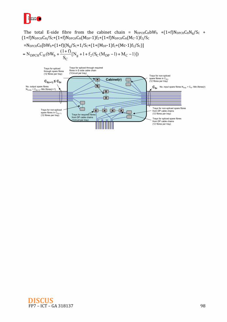
FP7–ICT–GA318137 98DISCUS
The total E-side fibre from the cabinet chain = NDPCHCHbWb +(1+f)NDPCHCHNg/SC +(1+f)NDPCHCH/SC+(1+f)NDPCHCH(MDP-1)f2+(1+f)NDPCHCH(MC-1)f2/SC=NDPCHCH[bWb+(1+f)(Ng/SC+1/SC+(1+(MDP-1)f2+(Mc-1)f2/SC)]
Cabinet(r)
CSr
CS(r+1) ≤ CSr
No. input spare fibres NInSp = CSr- Min.fibres(r)
Trays for non-spliced spare fibres in CS(r)(12 fibres per tray)
Trays for non-spliced spare fibres in CS(r+1)(12 fibres per tray)
Trays for spliced through spare fibres(12 fibres per tray)
Trays for non-spliced spare fibres from DP cable chains(12 fibres per tray)Trays for required fibres
from DP cable chains(1circuit per tray) Trays for spliced spare fibres
from DP cable chains(12 fibres per tray)
No. output spare fibres NOutSp = CS(r+1)- Min.fibres(r+1)
Trays for spliced through required fibres in E-side cable chain(1Circuit per tray)
1)])M)1(M(Sf1[NSf)(1(bWCN CDPC2gC
bHDPCH −+−+++
+=

FP7–ICT–GA318137 99DISCUS
8.5 Appendix5Voronoipolygonsforexchangeareaestimates
A simple method for Voronoi polygons given relatively equidistance points i.e. localexchangeshavesimilarseparationsinagivenregionisdescribed.Considertheexchangeatxi,yiandanearestneighbourexchangesatxj,yj.J=1,2,3,4,….Thepointxp,ypisthecircumcentreofthetriangle(xi,yi),(xj,yj),(xj+1,yj+1).Thecircumcentreliesinsidethetriangleifitisacuteandoutsideifobtuse,CartesiancoordinatesUx,UyofthecircumcentreforgeneraltriangleABCare:Ux=((Ax2+Ay2)(By-Cy)+(Bx2+By2)(Cy-Ay)+(Cx2+Cy2)(Ay-By))/DUy=((Ax2+Ay2)(Cx-Bx)+(Bx2+By2)(Ax-Cx)+(Cx2+Cy2)(Bx-Ax))/DwhereD=2(Ax(By-Cy)+Bx(Cy-Ay)+Cx(Ay-By)).
xi,yi
xj,yj
X4-5,y4-5
xn,yn
xc,yc
3
1
5
4
6
2
7
n
0xj+1,yj+1
xp,yp
Figure A5-1 Local Exchange at point x1, y1 surrounded by set of neighbouring LEs

FP7–ICT–GA318137 100DISCUS
ThesidesoftheVoronoipolygonis formedbythesetofsidesthatarethebisectorsoftheradiusvectorsfromxi,yitothenearestneighboursetofsurroundingLEsandpointsxj,yj.Thequestion iswhich nearest neighbours to count into the Voronoi computation andwhich toleaveoutwithouthavingtocheckallexchanges.Itcanbeseenfromthefigurethatthepointxn,ynhasabisector justoutside theredVoronoipolygon if ithadbeencloser itwouldhavepassedinsidethevertexoftheVoronoipolygonatx4-5,y4-5andformedanotherside.SoifthedistancetoapointoutsidetheVoronoipolygonisgreaterthantwicetheprojectionoftheadjacentverticesontotheradiusvectortothepointxn,ynthenthepointcanbeignored.Also any further additional points that add sides will tend to reduce the Voronoi verticesradiusvectorssothepointcanalwaysbeignored.
A process for constructing Voronoi polygons for any middle exchange i.e. an exchangesurroundedbyotherexchangesandnotadjacenttoaboundaryline(e.g.coastlineorestuary)canbe:
xi,yi
xj,yj
X4-5,y4-5
xn,yn
xc,yc
3
1
5
4
6
2
7
n
0xj+1,yj+1
φ
Figure A5-2 The LE at point Xn, Yn lies outside Voronoi polygon

FP7–ICT–GA318137 101DISCUS
1. FindNnearestneighbourswithinasearchrangeofapproximately2xmeanexchangespacingfromtargetexchangeatexchangelocationxi,yiandcalculatetheradiusvectorsfromthepointxi,yitotheseexchangesi.e.positionangleandradius.
2. Find theM (M~6will be a typical number)nearest and sort inposition angleorder(rotationofco-ordinatesystemisarbitrarysolet0=north).
3. Calculate the circumcentre coordinates for the triangle (using the equation in theprevious slide (xi,yi),(xj,yj),(xj+1,yj+1) starting at j=1, repeat for all j back to j=1. ThisshouldproduceamaximumofMverticesofanMsidedVoronoipolygonaroundthepointxi.yi.Storethesecoordinatesinanarray.
4. SortalltheremainingN-MnearestexchangesinpositionangleorderandcalculatetheprojectionoftheVoronoiverticesontotheadjacentradiusvectorsofthenearestoftheN-Mexchanges(e.g.ontoexchangeatxn,yninthefigure.Thisprojectionforthex4-5,y4-5radiusvectorontothexn,ynradiusvectorisgivenby:r’=((x4-5-xi)2+(y4-5-yi)2)1/2Cos(f);
5. CheckthethatthedistancetothesurroundingN-Mmoredistantexchanges(e.g.xn,yninthefigure)isgreaterthantwicetheadjacentverticesprojections.
6. IftheabovedistancestotheN-MexchangesaregreaterthantwicetheprojectionsoftheadjacentVoronoipolygonverticesthenthoseexchangescanbediscardedastheydonotaffecttheVoronoipolygon.
7. Iftheabovedistancesarelessthantwicetheprojectionsthenthoseexchangesneedtobe include in the set ofM closest exchanges that affect the Voronoi polygon and anadditionalsideisadded.
8. ThenextstepistocalculatetheenclosedareaoftheVoronoipolygon.Thiscanbedoneby calculating the area of the triangles formed by the point (xi,yi) and two adjacentvertices of theVoronoi polygon.Note the height of these triangles is half the radiusvectortotheMnearestexchanges.ThelengthofthesidesoftheVoronoipolygonformthebasesofthetrianglesandcanbecalculatedfromthex,ycoordinatesoftheVoronoipolygonverticescalculatedpreviouslyviathecircumcentrecalculations.Lengthofthejthsideistherefore:bj=((xvj-xvj+1)2+(yvj-yvj+1)2)1/2.Wherexvj,yvjarethecoordinatesofthejthvertexoftheVoronoipolygon.

FP7–ICT–GA318137 102DISCUS
9 Abbreviations
BAU Businessasusual
CAGR Compoundannualgrowthrate
CO Centraloffice
DDCND DiameterandDegreeConstrainedNetworkDesignproblem
DP Distributionpoint
EDFA Erbiumdopedfibreamplifier
GPON GigabitPON
ICU Idealistcostunit
ISN InitialSizeNetwork
LE Localexchange
LR-PON Long-ReachPON
JIT Justintime
MC Metrocore
MSN MinimumSizeNetwork
MPLS Multiprotocollabelswitching
MPLS-TP MPLSTransportprofile
NTE Networkterminationequipment
OCh Opticalchannel
ODN Opticaldistributionnetwork
OH Overhead
ONU OpticalNetworkUnit
ONT OpticalNetworkTerminal
OPM Opticalperformancemonitoring
OXC OpticalCrossConnect
PON Passiveopticalnetwork
PCP PrimaryCrossConnect
ROADM Reconfigurableadddropmultiplexer
S-BVTs Sliceablebandwidthvariabletransponders
UG Underground
VLSI Verylargescaleintegration

FP7–ICT–GA318137 103DISCUS
WDM Wavelengthdivisionmutliplexing
WSS Wavelengthselectiveswitch
Version Datesubmitted Comments
V1.0 05/02/2016 FirstversionsenttotheEU.