Cyclic steady state of simulated moving bed processes for enantiomersseparation

Mirjana Minceva, Luis S. Pais, Alirio E. Rodrigues *

Laboratory of Separation and Reaction Engineering (LSRE), Faculty of Engineering, University of Porto, Rua Dr. Roberto Frias s/n, 4200-465 Porto,

Portugal

Received 17 August 2001; received in revised form 25 February 2002; accepted 15 March 2002

Abstract

Simulated moving bed (SMB) technology developed by UOP in early 1960s has expanded greatly in the last decade, finding new

applications in the area of natural products, fine chemistry and pharmaceutical industry. SMB processes are periodic processes

designed to operate in cyclic steady state (CSS) and, therefore, the correct determination of CSS is needed for the assessment of the

SMB performance. Two approaches can be used for determination of CSS: the dynamic simulation until CSS is reached and direct

prediction of CSS. The direct prediction of CSS could be obtained in two ways: (i) considering that at CSS the spatially distributed

SMB unit state at the end of the cycle is identical to that at its beginning (Method 1); or (ii) considering that at CSS the spatially

distributed SMB unit state at the end of a switching time interval is identical to the state at the beginning of the interval, apart from a

shift of exactly one column length (Method 2). The mathematical models assume axial dispersion flow and linear driving force

(LDF) approximation for intraparticle mass transfer. Mathematical models were solved using the gPROMS (general Process

Modelling System) software package. Both approaches (dynamic simulation and direct CSS prediction) were applied to the

prediction of cyclic steady state of SMB unit for 1,1?-bi-2-naphthol enantiomers separation. The direct CSS predictions were

compared with the standard dynamic simulation CSS prediction in terms of accuracy of SMB performance and computing time

requirements; the Method 2 for CSS prediction is more efficient than the standard dynamic simulation.

# 2002 Elsevier Science B.V. All rights reserved.

Keywords: Simulated moving bed; Direct cyclic steady state prediction; Dynamic simulation; Enantiomers separation

1. Introduction

Simulated moving bed (SMB) technology developed

by UOP in early 1960s [1] has emerged as a powerful

tool for continuous countercurrent separation of binary

mixtures of components with different adsorption

affinities. Compared with batch chromatographic pro-

cesses, the continuous SMB process reduces solvent

consumption as much as 10-fold and uses less column

packing [2].

SMB separation technology has been extensively used

for the large-scale fractionation of sugars and xylene

isomers for more than 30 years. Recently, this technol-

ogy has been brought into the field of fine chemistry and

pharmaceutical industry [3].

The SMB process basic principle is a flow scheme that

takes advantages of continuous and countercurrent

movement of liquid and solid phase without actual

movement of the adsorbent. This countercurrent move-

ment is simulated by an appropriated flow switching

sequence: the adsorbent bed is divided into a number of

fixed bed columns, while the inlet and outlet lines move

simultaneously one column at fixed time intervals in the

direction of the liquid phase flow [4].The modelling of chromatographic systems presents

an interesting challenge since the process conditions are

simple enough to allow a reasonably realistic mathema-

tical description of the system. The first studies of the

behaviour of SMB units through detailed models date

back to the 1980s. The effect of changes in the operating

parameters and in the layout of the unit has been

* Corresponding author. Tel.: �/351-22-508-1671; fax: �/351-22-

508-1674.

E-mail address: arodrig@fe.up.pt (A.E. Rodrigues).

Chemical Engineering and Processing 42 (2003) 93�/104

www.elsevier.com/locate/cep

0255-2701/02/$ - see front matter # 2002 Elsevier Science B.V. All rights reserved.

PII: S 0 2 5 5 - 2 7 0 1 ( 0 2 ) 0 0 0 3 8 - 7

analysed by modelling SMB units directly or by explor-

ing the equivalence between SMB and true moving bed

unit (TMB) [5]. Namely, two main strategies of model-

ling of SMB process can be distinguished in the openliterature. The first one treats the SMB system as the

equivalent true moving system. The second strategy

represents the actual SMB configuration. Each of these

two modelling strategies leads to models that can be

different according to the description of the unit

operation (staged or distributed plug flow system), the

mass transfer resistance (equilibrium stage or mass

transfer resistance within the fluid and/or solid phase)and adsorption equilibria (linear, Langmuir, bi-Lang-

muir or modified Langmuir). A review of these models

can be found in Ruthven and Ching [6] and Pais [7].

The main difference between true moving bed and

SMB units is their stationary regime: the TMB is

designed to operate under steady state and the SMB

under cyclic steady state, characterised by an identical

transient concentration profiles during each periodbetween two valve switches. The cyclic steady state

(CSS) is particularly reached after a certain number of

cycles, but the system state is still varying over the time

because of the periodic movement of the inlet and outlet

ports along the columns. Practically, increasing the

number of the columns in the SMB system and

decreasing their length, the SMB approaches the TMB

system. Therefore, it is expected that the behaviour ofSMB unit could be satisfactory predicted by considering

it as an equivalent TMB unit just in the case of the SMB

unit with sufficiently high number of columns [8�/11].

The initial design and optimisation of the SMB

processes is generally accomplished by reference to the

equivalent TMB system [9�/18]. The reasons for model-

ling of an equivalent unit instead of the real simulated

moving unit lie into different level of difficulty involvedin the solution of the two models and the required time

for their computation. Since the true moving bed

operates in steady state, the stationary behaviour is

described by a set of ordinary differential and algebraic

equations (DAEs). This is not the case for SMB,

whereas the transient response requires the solution of

a set of partial differential equations and algebraic

equations. The cyclic steady state of SMB is normallycalculated by running a dynamic simulation starting

from given initial conditions and carrying out cycle by

cycle until CSS is reached. Usually more than ten cycles

are needed for the SMB to reach the cyclic steady state.

The time required to compute stationary regime using

simulated moving bed strategy is normally five to ten

times longer than using equivalent true moving bed

strategy [7].In the last decade various methods were proposed in

the aim of acceleration of CSS convergence. For

instance, Ding and Le Van [19] proposed acceleration

toward CSS for pressure swing adsorption (PSA) and

temperature swing adsorption (TSA) processes using

hybrid Newton�/Broyden methods. Todd et al. [20]

illustrated the advantage of node refinement as a useful

tool for accelerating convergence to CSS of PSA andvacuum swing adsorption (VSA) processes. Smith and

Westerberg [21] considered a shooting method that

explicitly combines the CSS conditions within the

process model. All these acceleration procedures are

developed and applied in simulation of PSA/TSA/VSA

processes, which could require thousands of cycles to

achieve a CSS.

Nilchan and Pantelides [22] developed a method fordirect determination of CSS of rapid pressure swing

adsorption (RPSA), in view of process optimisation.

The method consists in replacing the initial conditions

specification by a periodicity condition demanding that

the system state at the end of each cycle is identical to

that at its start. The system of partial differential

equations and algebraic equations (PDAEs), which

describes the RPSA behaviour, was reduced to a set ofnonlinear algebraic equations (AEs) by simultaneous

discretisation of both spatial and temporal variations.

The orthogonal collocation on finite elements discretisa-

tion method is applied to the spatial domain and the

second order backward finite difference method is

applied to the temporal domain. The resulting system

of algebraic equations is solved using a Newton type

iterative method implemented in general Process Mod-elling System (gPROMS) [23].

Kloppenburg and Gilles [24] suggested a method for

direct computation of periodic SMB state. A CSS is

identified by the fact that the spatially distributed SMB

unit state at the end of a switching time interval is

identical to the state at the beginning of the interval,

apart from a shift of exactly one column length. In order

to directly compute the CSS the mathematical model isdiscretised with respect to time using trapezoidal rule.

They used two alternative methods for the solution of

model equations: (i) formulation of the model as a

FORTRAN subprogram using DIVA code generator [25]

and solution with the nonlinear equation solver NLEQ1S

[26] and (ii) formulation of the model in AMPL [27]

modelling language and solution with the solver LAN-

CELOT [28]. The second alternative is more efficient interms of computation time, since LANCELOT is specially

designed for large-scale systems.

In this work two methods for direct cyclic steady state

calculation, proposed by Nilchan and Pantelides [22]

and Kloppenburg and Gilles [24], were applied in the

prediction of cyclic steady state of SMB unit for 1,1?-bi-

2-naphthol enantiomers separation. The cyclic steady

state was also predicted using the standard method forcyclic steady state determination, i.e. dynamic simula-

tion starting from given initial conditions over a large

number of cycles until the cyclic steady state is reached.

Mathematical models were solved using the gPROMS [23]

M. Minceva et al. / Chemical Engineering and Processing 42 (2003) 93�/10494

software package. Direct CSS predictions were com-

pared with CSS predicted by dynamic simulation in

terms of accuracy of SMB performance and computing

time requirements.

2. Mathematical modelling of SMB

The SMB unit is constituted by a set of identical fixed

bed columns connected in a series (Fig. 1). The inlet

streams are the feed, which contains the binary mixture

to be separated, and the eluent. The outlet streams are

the extract, a mixture of more strongly adorbed

component (A) and eluent, and the raffinate, which

includes the less adsorbed component (B) and eluent.

The counter current movement of the liquid and solid

phases is simulated by shifting the inlet and outlet ports

one column ahead in the direction of the fluid flow at

regular time intervals (switching time period). Inlet and

outlet points divide the unit in four sections, each of

which performs a different function. Zone 1 is located

between eluent and extract nodes and its purpose is to

regenerate the adsorbent; zone 2 is between extract and

feed nodes and its function is to desorb component B,

zone 3 is placed between feed and raffinate nodes and its

function is to adsorb component A; zone 4 is located

between raffinate and eluent nodes and its purpose is to

regenerate the eluent.

The stationary regime of the SMB is a cyclic steady

state, characterised by an identical transient concentra-

tion profiles during each period between two valve

switches. The CSS is particularly reached after a certain

number of cycles, but the system states are still varying

over the time because of the periodic movement of the

inlet and outlet ports along the columns. The correct

determination of CSS is needed for the assessment of the

SMB performance.

In this work the simulated moving bed strategy of

modelling was used in the prediction of the stationary

state of the SMB. In model formulation, the following

assumptions have been considered.

. Negligible thermal effects;

. bed void fraction, radius and porosity of the particlesare constant along the columns;

. constant flow rates in each section;

. negligible pressure drop;

. no radial variation occurs in the columns;

. axial dispersion flow for the liquid phase,

. the intraparticle mass transfer is described by a linear

driving force (LDF) for the intraparticle mass

transfer (i.e. parabolic intraparticle concentrationprofile)

The model equations are:

Mass balance in a volume element of the column j

o@c(i; j; z; t)

@t�(1�o)

@q(i; j; z; t)

@t

�oDL(j)@2c(i; j; z; t)

@z2�ov(j)

@c(i; j; z; t)

@z(1)

where i for component (i�/A, B), j for the column (k�/

1, 2, . . .. N )

Particle mass balance

@q(i; j; z; t)

@t�k(i)(q�(i; j; z; t)�q(i; j; z; t)) (2)

Adsorption equilibrium isotherm

q�(i; j; z; t)�f (c(i; j; z; t)) (3)

Boundary conditions

z�0;

cin(i; j; t)�c(i; j; z; t)�DL(j)

v(j)

@c(i; j; z; t)

@z

(4)

z�Ldc(i; j; z; t)

dz�0 (5)

According to the scheme in Fig. 1, it appears that the

SMB unit includes N columns. Due to the switching of

inlet and outlet ports, each column plays a differentfunction during a whole cycle, depending on its location

(zone). The complete model of the SMB unit is

constituted by a set of mass balance equations for

each of the N columns, connected with each other by

simple material balances at the connecting nodes. With

each switching of the inlet and outlet ports, each column

should be updated in terms of flowrate and inlet

concentrations. The flowrate in each column, accordingto its location (zone), can be calculated by mass balance

around the inlet and outlet nodes. The inlet concentra-

tion of each column is equal to the outlet concentrationFig. 1. Schematic diagram of SMB unit.

M. Minceva et al. / Chemical Engineering and Processing 42 (2003) 93�/104 95

of the previous column [c (i , j , t )out�/c (i , j�/1, t)in],

except for the feed and eluent nodes.

Mass balances at the nodes of the inlet and outlet lines

of the SMBEluent node:

c(i; j; t)outQ4�c(i; j�1; t)inQl (6)

Feed node:

c(i; j; t)outQ2�ci; F QF �c(i; j�1; t)inQ3 (7)

From the mathematical point of view, the SMB

processes can be classified as distributed parameter

systems in which the dependent variables vary with

respect to axial position as well as time. The SMB

operation is described by a set of partial differentialequations (mass balance equations) and algebraic equa-

tions (equilibrium isotherms and node mass balances).

These PDAEs are highly coupled, which makes it

impossible to obtain analytical solutions. Thus, the

simulation of such processes relies on numerical meth-

ods employing space and time discretisation.

3. Prediction of CSS of SMB

In this work two approaches to cyclic steady state

have been studied: the standard approach to CSS by

dynamic simulation and the direct approach to CSS.

3.1. Dynamic simulation of CSS

The standard approach to CSS consist in carrying out

dynamic simulation, starting from given initial condi-

tions Eq. (8) and simulating cycle by cycle through

successive substitution, where bed conditions from the

previous cycle become initial conditions for the nextcycle, continuing so forth until CSS is reached.

Initial conditions

t�0; c(i; j; z; t)�c0 q(i; j; z; t)�q0 (8)

3.2. Direct determination of CSS

Two methods for direct CSS prediction have been

used.

The first one, proposed by Nilchan and Pantelides

[22], based on the fact that at cyclic steady state the

conditions at the end of the cycle is identical to those at

its beginning in both liquid and solid phases. Therefore,the initial conditions are replaced by the above periodi-

city conditions:

c(i; j; z; 0)�c(i; j; z; Tcycle) i � (A; B)

j � (1; 2; :::; N) z � (0; L)

q(i; j; z; 0)�q(i; j; z; Tcycle) i � (A; B)

j � (1; 2; :::; N) z � (0; L)(9)

The second method for direct CSS prediction, pro-

posed by Kloppenburg and Gilles [24], is based on the

fact that at CSS the spatially distributed SMB unit state

at the end of a switching time interval is identical to the

state at the beginning of the interval, apart from a shiftof exactly one column length. Therefore, the initial

conditions are expressed as:

c(i; j; z; 0)�c(i; j�1; z; t�)

i � (A; B) j � (1; 2; :::; N) z � (0; L)

q(i; j; z; 0)�q(i; j�1; z; t�)

i � (A; B) j � (1; 2; :::; N) z � (0; L)(10)

Both methods are based on the same concept; the only

difference is that the first method concerns the simula-

tion of the whole cycle and the second one the

simulation of just one switching time.In the following sections the Nilchan and Pantelides

[22] method for direct CSS prediction would be referred

as Method 1 and Kloppenburg and Gilles method [24]

as Method 2.

3.3. Numerical considerations

The dynamic model equations Eqs. (1)�/(8) and direct

CSS model equations (Eqs. (1)�/(7) and (9) for Method 1and Eqs. (1)�/(7) and (10) for Method 2) were solved

using the gPROMS [23], a software package for modelling

and simulation of processes with both discrete and

continuous as well as lumped and distributed character-

istics. gPROMS is a high-level PDE package. No knowl-

edge of programming language is necessary. The

problems are described in gPROMS language, which

allows symbolic specification of PDAEs, boundaryconditions, initial conditions and appropriate coeffi-

cients. The system of PDAE is numericaly solved using

the method of lines (MOL) [29]. This involves discretisa-

tion of the distributed equations with respect to all

spatial domains, which results in a mixed set of time

depended DAEs. gPROMS modelling language allows the

user to specify the type of the spatial approximation

method (e.g. finite difference or finite elements), as wellas the granularity (e.g. number of the finite difference

nodes, number of finite elements) and the order (e.g.

first, second, etc.) of the approximation. The numerical

discretisation is applied automatically. The resulting

system of time depended DAEs can be solved by one of

the integration codes implemented in gPROMS. More

information on the package can be found in Barton and

Pantelides [30] and Oh [31].The dynamic model PDAE system Eqs. (1)�/(8) was

reduced into a set of ordinary DAEs in time by

discretisation of the axial domain. A third order

M. Minceva et al. / Chemical Engineering and Processing 42 (2003) 93�/10496

orthogonal collocation method in finite elements (OC-

FEM) comprising two internal collocation points was

used for this purpose. The resulting system of DAE was

integrated over time by employing DASOLV integrationcode. DASOLV is integrated in gPROMS, it is based on

backward differentiation formulae, and automatically

adjusts the time step size as well as the integration order

to maintain the error of integration within a user

specified tolerance. An absolute and relative tolerance

of 10�5 was used.

In the case of the Method 1 and 2 for direct

determination of CSS (Eqs. (1)�/(7) and (9), and Eqs.(1)�/(7) and (10)) both space and temporal domains were

discretised simultaneously. A third order OCFEM

comprising two internal collocation points was used in

the discretisation of spatial domain and a second order

backward difference method (BFDM) was used for

discretisation of temporal domain. The PDAE systems

(Eqs. (1)�/(7) and (9) and Eqs. (1)�/(7) and (10)) are

reduced directly into a set of nonlinear algebraicequations and solved using a Newton-type iterative

method implement in gPROMS. The iterations were

initialised with a chosen value for the concentration in

the liquid (0.8 g l�1) and solid phase (2.45 g g�1).

All simulations were performed on Pentium IV 1700

MHz processor with 1548 Mb RAM memory.

4. Simulation results and discussion

The most recent SMB application is related with

chiral technology. The separation of enantiomers is an

important issue in various areas and particularly in the

health-related field. It is well known that isomers can

have different therapeutical effects and there is pressureof regulatory agencies for the separation of isomers [32].

In this work the chromatographic resolution of 1,1?-bi-2-naphthol enantiomers was considered for the simu-

lation purpose. The chiral stationary phase used in this

system was 3,5-dinitrobenzoyl phenylglycine bonded to

silica gel, and a mixture of 72/28 (v/v) heptane/isopro-

panol was used as eluent. The limit of solubility in this

eluents is 3 g l�1 of each enantiomer [7]. The adsorptionequilibrium isotherms, measured at 25 8C, are of bi-

Langmuir type as proposed by the Separex group [33]:

qA��3:73cA

1 � 0:0336cA � 0:0466cB

�0:30cA

1 � cA � 3cB

(11)

qB��2:69cB

1 � 0:0336cA � 0:0466cB

�0:10cB

1 � cA � 3cB

(12)

where A refers to the more-retained component, i.e.

extract component and B to the less-retained compo-nent, i.e. raffinate component.

The operating conditions and model parameters used

in the simulation study are presented in Table 1.

4.1. Dynamic simulation of CSS

First the cyclic steady state behaviour was simulated

using the standard approach, i.e. cycle by cycle until

reaching cyclic steady state. The model equations (Eqs.

(1)�/(8)) were solved starting from the initial conditions

where no feed components are presented in the SMB

unit, the columns are filled with eluent.

In order to determine when the steady state isachieved, the relative error was defined as sum of:

1) the relative error between the average concentra-

tions (evaluated during a whole cycle) of each

component in the extract (X) and raffinate (R)

stream for the successive cycles:

(X�R) relative error%

�100

�jcAXk

� cAXk�1

jcA

Xk

�jcB

Xk� cB

Xk�1j

cBXk

�

��jcA

Rk� cA

Rk�1j

cARk

�jcB

Rk� cB

Rk�1j

cBRk

�(13)

The comparison of the extract and raffinate average

concentrations in two consecutive cycles, instead of

comparison of their concentration histories was

considered, since there was no significant difference

between the relative errors calculated in both ways

and2) the mass balance (MB) relative error, i.e. relative

error between the total amount of each component

that enters (in the feed stream) and leaves (in the

extract and raffinate stream) the system (evaluated

during a full cycle):

MB relative error%

�100jQFcA

F � (QXcAX � QRcA

R)jQFcA

F

�jQFcB

F � (QXcBX � QRcB

R)jQF cB

F

(14)

A relative error of 1% was considered since this

Table 1

SMB operation conditions and model parameters

SMB unit geome-

try

Operating conditions Model parameters

Lc�10.5 cm QF��3.64 ml min�1,

T�25 8CPe�vk Lk /

Dl*�2000

dc�2.6 cm QX��17.98 ml min�1,

t *�3 min

k�0.1 s�1

Number of

columns: 8

QR��7.11 ml min�1,

CF�2.9 g l�1, each

o�0.4

Configuration:

2-2-2-2

QE��21.45 ml min�1

QREC� �35.38 ml min�1

M. Minceva et al. / Chemical Engineering and Processing 42 (2003) 93�/104 97

could provide the estimation of the SMB perfor-

mances with satisfactory accuracy and acceptable

computing time.

First of all the minimum number of the axial domain

elements, i.e. number of finite elements per column used

in OCFEM, which enables CSS prediction satisfying therelative error defined above was defined. Some simula-

tions were carried out, starting with three elements per

column, and increasing the number of finite elements

until eight. CSS was achieved in 13 cycles. After 20

cycles the relative error approach to zero. Table 2 shows

the average extract and raffinate concentrations calcu-

lated over the whole cycle at CSS, the corresponding

extract and raffinate purities, the relative error and CPUtimes needed for dynamic simulation of CSS using

different number of finite elements per column. It can

be seen that (i) for the all number of elements used the

relative error was less than 1% and (ii) there was no

significant advantage of using more finite elements per

column, in terms of extract and raffinate concentrations

and their purities. Therefore, three subdivisions per

column for the axial domain were selected for thefurther simulation studies.

4.2. Direct determination of CSS

The Methods 1 and 2 for direct determination of CSS

require simultaneous discretisation of axial and tem-

poral domain. A third orthogonal collocation method

was applied for discretisation of spatial domain using

the selected number of finite elements (3) from the

dynamic simulation study. A second order BFDM wasused for the discretisation of the temporal domain.

First, the CSS was predicted by Method 1, simulating

one cycle and requiring that the conditions at the end of

the cycle are identical to those at its beginning in both

liquid and solid phases (Eq. (9)). Some simulations were

carried out in order to determine the number of finite

elements in the BFDM that enables prediction of CSS

within the considered relative error (1%). The simula-tions were initialised with time step 0.3 min (cycle time

divided in 80 finite elements) until time step 0.1667 min

(cycle time divided in 144 finite elements). The max-

imum number of time steps tested was practically the

maximum number of time steps supported by thecomputer performance.

Since the methods for direct determination of CSS

predict the stationary state directly, the relative error is

calculated only by the Eq. (14). The relative error and

CPU time for different time steps are presented in Table

3 and Fig. 2. It can be seen that computing time

increases significantly with increasing the number of

the finite elements for the time domain. The relativeerror shows linear tendency of decreasing with increas-

ing the number of the finite elements and is expected to

further decrease with increasing the number of finite

elements per column.

The above procedure was also followed in the direct

CSS prediction using Method 2. In this case the process

was simulated during just one switching time requiring

that the spatially distributed SMB unit state at the endof a switching time interval is identical to the state at the

beginning of the interval, apart from a shift of exactly

one column length (Eq. (10)). The simulations were

initialised with time step 0.3 min (switching time divided

in ten finite elements) until time step 0.125 min (switch-

ing time divided in 24 finite elements). The relative error

and CPU time for different time steps are presented in

Table 4. The CSS within relative error of 1% could bedetermined using at least ten finite elements (0.3 min

time step) for the time domain.

4.3. Comparison of dynamic simulation and direct

determination of CSS

The dynamic CSS prediction and both methods for

direct CSS prediction were compared in terms of:

concentration profiles, extract and raffinate histories,

extract and rafinate purities and CPU times. For the

comparison following simulation runs were selected:

i) dynamic simulation of CSS (three elements percolumn).

Table 2

Relative error and CPU time for different number of finite elements for the spatial domain-prediction of CSS by dynamic simulation

Number of finite elements Average X concentration

(g l�1)

Average R concentration

(g l�1)

X purity (%) R purity (%) Relative error (%) CPU time (s)

A B A B

3 0.5798 0.0257 0.0183 1.4124 95.75 98.72 0.83 32

4 0.5796 0.0256 0.0188 1.4125 95.77 98.69 0.85 39

5 0.5796 0.0256 0.0190 1.4126 95.77 98.67 0.86 48

6 0.5795 0.0255 0.0192 1.4126 95.78 98.66 0.86 57

7 0.5795 0.0255 0.0192 1.4126 95.78 98.66 0.87 67

8 0.5795 0.0255 0.0193 1.4126 95.78 98.65 0.87 80

M. Minceva et al. / Chemical Engineering and Processing 42 (2003) 93�/10498

ii) Method 1 for direct CSS prediction (three elementsper column, 144 elements for the cycle time-corre-

sponding to 0.1667 min time step).

iii) Method 2 for direct CSS prediction (three elements

per column, 18 elements for the switching time,

corresponding to 0.1667 min time step).

The CSS internal concentration profiles calculated by

(i) dynamic simulation; (ii) Method 1 and (iii) Method 2

are presented in Fig. 3. The corresponding cyclic steady

state extract and raffinate concentration histories during

one switching time are presented in Fig. 4.

There is no significant difference in the prediction ofCSS concentration profiles using the standard dynamic

approach and both direct CSS approaches. The more

significant difference could be observed in the extract

and raffinate histories predicted directly using Method 1

(Fig. 4a and b) and those predicted by dynamic

simulation and Method 2. This was expected since the

relative error in the case of direct CSS prediction using

Method 1 is significant (around 5%).The extract and raffinate purities calculated from the

selected simulation runs are presented in Table 5. The

relative error between the extract and raffinate purities

determined by the dynamic simulation and the methods

for direct CSS prediction was calculated using the

following equation:

relative error%�100

j(dynamic simulation) � (direct CSS simulation)j(dynamic simulation)

(15)

The values of the extract and raffinate relative errors

are presented in Table 5. It could be seen that there is

small relative difference between the extract and raffi-

nate purities calculated by both approaches (dynamic

approach and direct CSS approach). Since in bothapproaches the axial domain is discretised using the

same method, third order OCFEM, and the same

number of finite elements (3), the relative error between

the dynamic simulation and the methods for direct cyclic

steady state prediction arise mainly from the discretisa-

tion of the temporal domain.

Table 3

Relative error and CPU time for different number of finite elements for the temporal domain in the direct CSS prediction using Method 1

Number of finite elements Time step (min) Relative error (%) CPU time (s)

80 0.3000 8.85 2279

96 0.2500 7.22 3807

104 0.2308 6.70 5669

120 0.2000 5.83 9912

128 0.1875 5.50 10451

144 0.1666 4.91 15812

Fig. 2. Relative error and CPU time vs. time step used in temporal

discretisation in the case of direct prediction of CSS by Method 1 (*/

2*/ relative error, */j*/ CPU time).

Table 4

Relative error and CPU time for different number of finite elements for the temporal domain in the direct CSS prediction using Method 2

Number of finite elements Time step (min) Relative error (%) CPU time (s)

10 0.3000 0.84 6

12 0.2500 0.79 12

13 0.2308 0.76 14

16 0.1875 0.68 19

18 0.1667 0.63 48

20 0.1500 0.59 68

24 0.1250 0.52 86

M. Minceva et al. / Chemical Engineering and Processing 42 (2003) 93�/104 99

The comparison of the CPU times (Table 5) shows

that dynamic simulation and Method 2 require similar

computation time for prediction of CSS. We need to

take into consideration that the simulation run for

Method 2 chosen for the comparison predicts the CSS

with relative error 0.63% (Table 4) and dynamic

simulation with relative error 0.83%. If we compare

the dynamic simulation CSS prediction with CSS

predicted with Method 2 for similar relative error

(around 0.8%), we can see that Method 2 (time step

0.3 min, Table 5, values in brackets) requires around 5

times less computation time than dynamic simulation

(32 s CPU for dynamic simulation of CSS, against 6 s

CPU time for Method 2 for direct prediction of CSS).

The Method 2 for direct prediction of CSS would be

even more competitive in the cases of dynamic simula-

tion where more cycles are needed to achieve the cyclic

steady state of a SMB unit.

There is high difference in the CPU times required for

direct prediction of CSS using Method 1 and those from

dynamic simulation and direct prediction using Method

2. Part of the explanation arises from the special

treatment of the time domain in gPROMS. All variables

are assumed to be distributed with respect to time

without being declared explicitly in the model. The

numerical treatment of the time domain in dynamic

simulation is different from that of the other distribu-

tion domains, but there is also the possibility in gPROMS

to treat the time as just another distribution domain

declared and handled explicitly [31]. This option was

used for the direct determination of CSS. Both the

computer memory and the computation cost required by

the explicit handling of the time domain are likely to be

higher than those associated with the implicit alterna-

tive. Also the guaranteed control of the temporal

discretisation error is lost [31]. There is still enormous

difference in the computation time required for direct

prediction of CSS using Method 1 and Method 2. In

both methods the same time step was used (0.1667 min)

that implies ratio 8:1�/number of ODE’s in Method 1/

number of ODE’s in Method 2, since in Method 1 one

whole cycle is simulated and in Method 2 only one

switching time. It was shown before that the computing

time increases significantly with increasing the number

of the finite elements for the time domain (Fig. 2).

Therefore, linearity between number of ODE’s and

computation time for Method 1 and 2 should not be

expected.

However, Method 1 may be advantageous in certain

circumstances, as the PSA/VSA/TSA processes where

one or two adsorption columns are normally used and

thousands of cycles could be needed for achieving CSS

[22].

Dynamic simulation could be more competitive in the

study of the effect of some model parameters. Namely, if

all planned simulations runs (comprising different

values of examined model parameter) are carried out

as a sequence, using as initial conditions the CSS

conditions of the previous simulation. To illustrate this

a sequence of dynamic simulation using different switch-

ing times was carried out. The operation conditions used

in the simulation sequence are those from Table 1,

except the switching time. The switching time was

increased starting from t*�/2.7 min until t*�/3.1 min,

with step of 0.1 min. In the first dynamic CSS simulation

(t*�/2.7 min) the initial conditions where no feed

components are presented in the SMB unit were used.

In the next simulation (t*�/2.8 min) the CSS concen-

Fig. 3. Cyclic steady state concentration profiles obtained by: */j*/ dynamic simulation, */^*/ Method 1 and */I*/ Method 2.

M. Minceva et al. / Chemical Engineering and Processing 42 (2003) 93�/104100

tration profiles in liquid and solid of previous simulation

were imposed as initial conditions. All sequence was

carried out in this manner. The dynamic simulations of

CSS for all switching times were repeated for the initial

condition of no feed component present in the SMB

unit. The comparison results are presented in Table 6. It

could be seen that using the CSS conditions as initial

conditions in the sequential study leads to a decrease in

cycles needed to reach CSS by 4. In this kind of studies

the knowledge of the influence of the model parameters

is essential in the choice of: the interval in which the

particular model parameter would be varied, the ampli-tude of the change and the direction of the change, i.e.

increasing or decreasing the value of the model para-

meter in the chosen interval of variation. Just for

illustration, if we use the CSS corresponding to t*�/

3.5 min as initial condition in the prediction of CSS

corresponding to t*�/3 min, more cycles would be

needed to reach the CSS than when we start the

simulation with null initial conditions (big step changeof t* and wrong direction of change of t*). In the case of

t*�/3.5 the SMB operates out of the separation region,

i.e. no pure extract and raffinate, which results from the

shift of the extract and raffinate component concentra-

tion profiles in undesirable direction.

This procedure cannot be generalised for all process

parameters. For instance, the procedure is not efficient

in the study of the effect of mass transfer parameter (k )on the SMB process performance. Increasing the mass

transfer parameter the concentration profiles become

steeper and fine grids should be used in the discretisation

of the axial domain for accurate prediction of CSS. On

the other hand one of the requirements of the sequential

simulations is the use of the same number of finite

elements in all simulations.

For example, in the case of mass transfer parameterk�/6 min�1 three elements per column are needed; in

the case of k�/12 min�1, ten elements per column and

in the case of k�/18 min�1, 15 per column are needed to

simulate CSS within a relative error of 1%. In Table 7

the CPU time and the number of the cycles needed to

achieve CSS for mass transfer parameter k�/12 min�1

(i) using null initial conditions for ten elements (coarse

grid) and 15 elements (fine grid) per column; and (ii)using CSS of the simulation run corresponding to k�/6

min�1 (coarse grid) and CSS corresponding to k�/18

min�1 (fine grid) are presented. It could be seen that less

CPU time consuming is the case where the CSS is

predicted using the CSS profiles of the simulation run

for k�/6 min�1. The initialisation of the CSS dynamic

simulation using CSS corresponding to k�/18 min�1

would decreases the number of cycles needed to archivethe CSS, but also require longer computation time, since

more fine elements have to be used.

5. Conclusions

Cyclic steady state of SMB 1,1?-bi-2-naphthol enatio-

mers separation has been computed using two modellingapproaches: (i) the standard approach, i.e. dynamic

simulation cycle by cycle till steady state is achieved; and

(ii) direct approach to CSS.

Fig. 4. Concentration histories in (a) the extract and (b) raffinate at

cyclic steady state, during one switching time period, */*/*/ dynamic

simulation, �/ �/ �/ �/ �/ direct CSS prediction using Method 1, -------

direct CSS prediction using Method 2.

M. Minceva et al. / Chemical Engineering and Processing 42 (2003) 93�/104 101

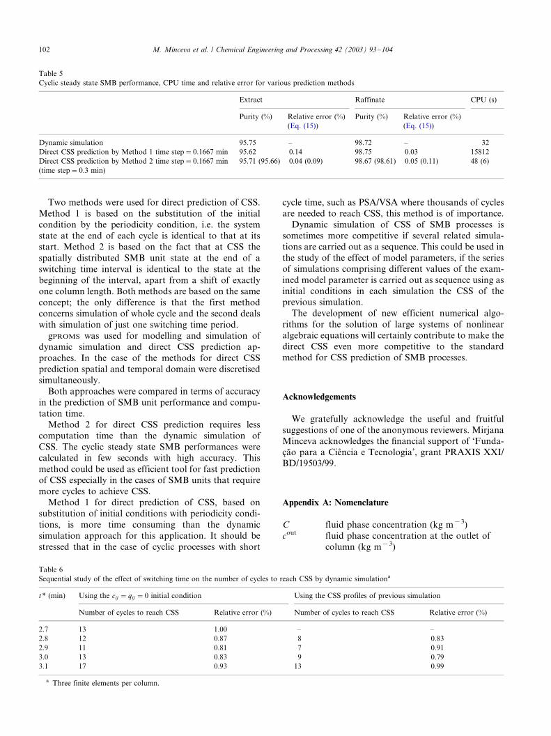
Two methods were used for direct prediction of CSS.

Method 1 is based on the substitution of the initial

condition by the periodicity condition, i.e. the system

state at the end of each cycle is identical to that at its

start. Method 2 is based on the fact that at CSS the

spatially distributed SMB unit state at the end of a

switching time interval is identical to the state at the

beginning of the interval, apart from a shift of exactly

one column length. Both methods are based on the same

concept; the only difference is that the first method

concerns simulation of whole cycle and the second deals

with simulation of just one switching time period.

gPROMS was used for modelling and simulation of

dynamic simulation and direct CSS prediction ap-

proaches. In the case of the methods for direct CSS

prediction spatial and temporal domain were discretised

simultaneously.

Both approaches were compared in terms of accuracy

in the prediction of SMB unit performance and compu-

tation time.

Method 2 for direct CSS prediction requires less

computation time than the dynamic simulation of

CSS. The cyclic steady state SMB performances were

calculated in few seconds with high accuracy. This

method could be used as efficient tool for fast prediction

of CSS especially in the cases of SMB units that require

more cycles to achieve CSS.

Method 1 for direct prediction of CSS, based on

substitution of initial conditions with periodicity condi-

tions, is more time consuming than the dynamic

simulation approach for this application. It should be

stressed that in the case of cyclic processes with short

cycle time, such as PSA/VSA where thousands of cycles

are needed to reach CSS, this method is of importance.

Dynamic simulation of CSS of SMB processes is

sometimes more competitive if several related simula-

tions are carried out as a sequence. This could be used in

the study of the effect of model parameters, if the seriesof simulations comprising different values of the exam-

ined model parameter is carried out as sequence using as

initial conditions in each simulation the CSS of the

previous simulation.

The development of new efficient numerical algo-

rithms for the solution of large systems of nonlinear

algebraic equations will certainly contribute to make the

direct CSS even more competitive to the standardmethod for CSS prediction of SMB processes.

Acknowledgements

We gratefully acknowledge the useful and fruitful

suggestions of one of the anonymous reviewers. Mirjana

Minceva acknowledges the financial support of ‘Funda-

cao para a Ciencia e Tecnologia’, grant PRAXIS XXI/

BD/19503/99.

Appendix A: Nomenclature

C fluid phase concentration (kg m�3)

cout fluid phase concentration at the outlet of

column (kg m�3)

Table 5

Cyclic steady state SMB performance, CPU time and relative error for various prediction methods

Extract Raffinate CPU (s)

Purity (%) Relative error (%)

(Eq. (15))

Purity (%) Relative error (%)

(Eq. (15))

Dynamic simulation 95.75 �/ 98.72 �/ 32

Direct CSS prediction by Method 1 time step�0.1667 min 95.62 0.14 98.75 0.03 15812

Direct CSS prediction by Method 2 time step�0.1667 min

(time step�0.3 min)

95.71 (95.66) 0.04 (0.09) 98.67 (98.61) 0.05 (0.11) 48 (6)

Table 6

Sequential study of the effect of switching time on the number of cycles to reach CSS by dynamic simulationa

t* (min) Using the cij �qij �0 initial condition Using the CSS profiles of previous simulation

Number of cycles to reach CSS Relative error (%) Number of cycles to reach CSS Relative error (%)

2.7 13 1.00 �/ �/

2.8 12 0.87 8 0.83

2.9 11 0.81 7 0.91

3.0 13 0.83 9 0.79

3.1 17 0.93 13 0.99

a Three finite elements per column.

M. Minceva et al. / Chemical Engineering and Processing 42 (2003) 93�/104102

cin fluid phase concentration at the inlet of

column (kg m�3)

DL axial dispersion coefficient (m2 s�1)

dc column diameter (m)

k intraparticle mass-transfer coefficient

(min�1)

Lc column length (m)Q fluid flow-rate (m3 s�1)

q average adsorbed phase concentration (kg

m�3)

q* adsorbed phase concentration in equilibrium

with c (kg m�3)

t time (s)

t* switching time (s)

Tcycle cycle time (s)v interstitial fluid velocity (m s�1)

Z axial coordinate (m)

o bed porosity, dimensionless

Subscripts and superscripts

i adsorbable components (i�/A, B)

j number of column (j�/1, 2, . . ...N )

E, X, F,R

eluent, extract, feed and raffinate streams

References

[1] D.B. Broughton, C.G. Gerhold, US Pat. 2,985,589 (1961).

[2] R.-M. Nicoud, R.E. Majors, Simulated moving bed chromato-

graphy for preparative separations, LCGC 18 (2000) 680.

[3] J.E. Rekoske, Chiral separation, AIChE J. 47 (2001) 2.

[4] L.S Pais, J.M. Loureiro, A.E. Rodrigues, Separation of enentio-

mers of a chiral epoxide by simulated moving bed chromato-

graphy, J. Chromatogr. A 827 (1998) 215.

[5] C. Migliorini, A. Gentilini, M. Mazzotti, M. Morbidelli, Design

of simulated moving bed units under nonideal conditions, Ind.

Eng. Chem. Res. 38 (1999) 2400.

[6] D.M. Ruthven, C.B. Ching, in: G. Ganetsos, P.E. Barker (Eds.),

Preparative and Production Scale Chromatography, Marcel

Dekker, New York, 1993, p. 629.

[7] L.S. Pais, Chiral separation by simulated moving bed chromato-

graphy, Ph.D.Thesis, Faculy of Engineering, University of Porto,

1998.

[8] K. Hidajat, C.H. Ching, D.M. Ruthven, Simulated counter-

current adsorption processes: a theoretical analysis of the effect of

subdividing the adsorbed bed, Chem. Eng. Sci. 41 (1986) 2953.

[9] D.M. Ruthven, C.H. Ching, Counter-current and simulated

counter-current adsorption separation processes, Chem. Eng.

Sci. 44 (1989) 1011.

[10] K.H. Chu, M.A. Hashim, Simulated counter-current adsorption

processes: a comparison of modelling strategies, Chem. Eng. J. 56

(1995) 59.

[11] L.S. Pais, J.M. Loureiro, A.E. Rodrigues, Modelling strategies for

enantiomers separation by SMB chromatography, AIChE J. 44

(1998) 561.

[12] D.C.S Azevedo, A.E. Rodrigues, Design of a simulated moving

bed in the presence of mass-transfer resistance, AIChE J. 45

(1999) 956.

[13] Z. Ma, N.-H.L., Standing wave analysis of SMB chromatogra-

phy: linear systems, AIChE J. 43 (1997) 2488.

[14] A.S.T. Chiang, Continuous chromatographic process based on

SMB technology, AIChE J. 44 (1998) 1930.

[15] G. Storti, M. Masi, S. Carra, M. Morbidelli, Optimal design of

multicomponent counter-current adsorption separation processes

involving nonlinear equilibria, Chem. Eng. Sci. 44 (1989) 1329.

[16] G. Storti, R. Baciocchi, M. Mazzoti, M. Morbidelli, Design of

optimal operating conditions of simulated moving bed adsorptive

separation units, Ind. Eng. Chem. Res. 34 (1995) 288.

[17] M. Mazzotti, G. Storti, M. Morbidelli, Robust design of counter-

current adsorption separation processes. 2. Multicomponent

systems, AIChE J. 40 (1994) 1825.

[18] M. Mazzotti, G. Storti, M. Morbidelli, Optimal operation of

simulated moving bed units for nonlinear chromatographic

separations, J. Chromatogr. A 769 (1997) 3.

[19] Y. Ding, M.D. Le Van, PSA and TSA simulations: enhancements

for accelerated convergence to the periodic state, AIChE Annual

Meeting, Los Angeles, CA, 13�/17 November 2000; Paper 158g.

[20] R.S. Todd, J. He, P.A. Webley, C. Beh, S. Wilson, M.A. Lloyd,

Fast finite-volume method for PSA/VSA cycle simulation-experi-

mental validation, Ind. Eng. Chem. Res. 40 (2001) 3217.

[21] O.J. Smith, A.W. Westerberg, Acceleration of cyclic steady-state

convergence for ressure swing adsorption models, Ind. Eng.

Chem. Res. 31 (1992) 1569.

[22] S. Nilchan, C. Pantelides, On optimization of periodic adsorption

processes, Adsorption 4 (1998) 113.

[23] gPROMS v1.7 User Guide, Process System Enterprise Ltd.,

London, 1999.

[24] E. Kloppenburg, E.D. Gilles, A new concept for operating

simulated moving-bed processes, Chem. Eng. Tech. 22 (1999) 813.

[25] K.D. Mohl, A. Spieker, E. Stein, E. Gilles, in: A. Kuhn, S. Wenzel

(Eds.), DIVA-Eine Umgenbung zur Simulation, Analyse und

Optimierung verfahrenstechnischer Prozesse, Simulationstechnik.

ASIM-Symposium in Dortmund, vol. 11, Veiweg Verlag,

Braunschweig/Wiesbaden, 1997, pp. 278�/283.

Table 7

Influence of the type of the initial conditions on the number of the cycles needed to reach CSS and the computation time by dynamic simulation for

k�12 min�1

Type of the grid used in discretisation of axial domain Type of the initial conditions

Null initial conditions CSS profiles of previous simulation

cycles CPU (s) Cycles CPU (s)

Coarse grid (10 elements per column) 15 104 12a 92

Fine grid (15 elements per column) 15 174 11b 142

a CSS for k�6 min�1.b CSS for k�18 min�1.

M. Minceva et al. / Chemical Engineering and Processing 42 (2003) 93�/104 103

[26] P. Deuflhard, U. Nowak, M. Wulkow, Recent developments in

chemical computing, Comp. Chem. Eng. 14 (1990) 1249.

[27] R. Fourer, D.M. Kernighan, B.W. Kernighan, AMPL. A Modeling

Language for Mathematical Programming, Boyd & Fraser

Publishing Company, 1993.

[28] A.R. Conn, LANCELOT*/A FORTRAN Package for Large-Scale

Nonlinear Optimization (Release A), 1992.

[29] W.E. Schiesser, The Numerical Method of Lines, Academic Press,

New York, 1991.

[30] P.I. Barton, Pantelides, Modeling of combined discrete/contin-

uous processes, AIChE J. 40 (1994) 966.

[31] M. Oh, Modelling and simulation of combined lumped and

distributed processes, Ph.D. Thesis, University of London,

1995.

[32] R.A. Sheldon, Chirotechnology: Industrial Synthesis of Optically

Active Compounds, Marcel Dekker, New York, USA,

1993.

[33] R.M. Nicoud, A. Seidel-Morgenstern, Adsorption isotherms:

experimental determination and application to preparative chro-

matography, in: R.M. Nicoud (Ed.), Simulated Moving Bed

Basics and Applications, Institut Nacional Politechnique de

Lorraine, Nancy, France, 1993.

M. Minceva et al. / Chemical Engineering and Processing 42 (2003) 93�/104104