Numerical investigation on applications simulated via using ...

Numerical investigation on applications simulated via

using lattice Boltzmann method

Article-based thesis by

Bo An

ADVERTIMENT La consulta d’aquesta tesi queda condicionada a l’acceptació de les següents condicions d'ús: La difusió d’aquesta tesi per mitjà del r e p o s i t o r i i n s t i t u c i o n a l UPCommons (http://upcommons.upc.edu/tesis) i el repositori cooperatiu TDX ( h t t p : / / w w w . t d x . c a t / ) ha estat autoritzada pels titulars dels drets de propietat intel·lectual únicament per a usos privats emmarcats en activitats d’investigació i docència. No s’autoritza la seva reproducció amb finalitats de lucre ni la seva difusió i posada a disposició des d’un lloc aliè al servei UPCommons o TDX. No s’autoritza la presentació del seu contingut en una finestra o marc aliè a UPCommons (framing). Aquesta reserva de drets afecta tant al resum de presentació de la tesi com als seus continguts. En la utilització o cita de parts de la tesi és obligat indicar el nom de la persona autora. ADVERTENCIA La consulta de esta tesis queda condicionada a la aceptación de las siguientes condiciones de uso: La difusión de esta tesis por medio del repositorio institucional UPCommons (http://upcommons.upc.edu/tesis) y el repositorio cooperativo TDR (http://www.tdx.cat/?locale- attribute=es) ha sido autorizada por los titulares de los derechos de propiedad intelectual únicamente para usos privados enmarcados en actividades de investigación y docencia. No se autoriza su reproducción con finalidades de lucro ni su difusión y puesta a disposición desde un sitio ajeno al servicio UPCommons No se autoriza la presentación de su contenido en una ventana o marco ajeno a UPCommons (framing). Esta reserva de derechos afecta tanto al resumen de presentación de la tesis como a sus contenidos. En la utilización o cita de partes de la tesis es obligado indicar el nombre de la persona autora. WARNING On having consulted this thesis you’re accepting the following use conditions: Spreading this thesis by the i n s t i t u t i o n a l r e p o s i t o r y UPCommons (http://upcommons.upc.edu/tesis) and the cooperative repository TDX (http://www.tdx.cat/?locale- attribute=en) has been authorized by the titular of the intellectual property rights only for private uses placed in investigation and teaching activities. Reproduction with lucrative aims is not authorized neither its spreading nor availability from a site foreign to the UPCommons service. Introducing its content in a window or frame foreign to the UPCommons service is not authorized (framing). These rights affect to the presentation summary of the thesis as well as to its contents. In the using or citation of parts of the thesis it’s obliged to indicate the name of the author.

http://upcommons.upc.edu/tesis

http://www.tdx.cat/

http://www.tdx.cat/

http://upcommons.upc.edu/tesis)

http://www.tdx.cat/?locale-attribute=es

http://www.tdx.cat/?locale-attribute=es

http://upcommons.upc.edu/tesis

http://www.tdx.cat/?locale-attribute=en

http://www.tdx.cat/?locale-attribute=en

1

Numerical investigation on applications simulated via

using lattice Boltzmann method

Presented by Bo AN

Department of Fluid Mechanics, Universitat Politécnica de Catalunya, 08222, colon 7-11, Terrassa, Barcelona, Spain

Supervisors: Josep M. Bergadà1 and Fernando Mellibovsky2

1Department of Fluid Mechanics, Universitat Politécnica de Catalunya, 08222, colon 7-11,

Terrassa, Barcelona, Spain 2Department of Physics, Aerospace Engineering Division, Universitat Politécnica de Catalunya,

08034, Barcelona, Spain

(Thesis presented as a summary of publications)

2

Abstract

The present doctoral thesis is about the numerical investigation simulated via using lattice Boltzmann method

(LBM), the applications cover a large scale of subjects, including

1. Mathematical-physical equations

A new lattice Boltzmann method (LBM) 9-bit model is presented to solve mathematical-physical equations, such as,

Laplace equation, Poisson equation, Wave equation and Burgers equation. The main benefits of the new model

proposed is that is faster than the previous existing models and has a better accuracy.

2. Lid-driven isosceles right-angled triangular cavity

We employ lattice Boltzmann simulation to numerically investigate the two-dimensional incompressible flow inside

a right-angled isosceles triangular enclosure driven by the tangential motion of its hypotenuse. We analyze the

bifurcation sequence that takes the flow from steady to periodic and then quasi-periodic and show that the invariant

torus is finally destroyed in a period-doubling cascade of a phase-locked limit cycle. As a result, a strange attractor

arises that induces chaotic dynamics.

3. Improvements for the numerical stability of original LBM

In order to study the flow behavior at high Reynolds numbers, two modified models, known as the multiple-

relaxation-time lattice Boltzmann method (MRT-LBM) and large-eddy-simulation lattice Boltzmann method (LES-

LBM), have been employed. The MRT-LBM was designed to improve numerical stability at high Reynolds

numbers, by introducing multiple relaxation time terms, which consider the variations of density, energy,

momentum, energy flux and viscous stress tensor. The LES-LBM model implements the large eddy simulation

turbulent model into the conventional LBM, allowing to study the flow at turbulent Reynolds numbers. LES-LBM

combined with Quadruple-tree Cartesian cutting grid (tree grid) was employed for the first time to characterize the

flow dynamics over a cylinder and a hump, at relatively high Reynolds numbers.

Abstract

La tesi doctoral està centrada en simulacions numèriques utilitzant la metodologia de lattice Boltzmann method

(LBM), les aplicacions desenvolupades inclouen. 1. Equacions Físic-Matemàtiques

Un nou mètode de lattice Boltzmann (LBM) anomenat 9-bit model, es utilitzat per resoldre equacions físic-

matemàtiques, tal com l'equació de Laplace, l'equació de Poisson, l'equació de Ones i la de Burguers. Els majors

beneficis de aquest nou model proposat son que necessita menys temps computacional i es mes precís que els

models precedents.

2. Cavitat triangular isòsceles amb tapa superior lliscant.

El mètode de Lattice Boltzmann ha sigut utilitzat per investigar el flux incompressible bidimensional en el interior

de una cavitat triangular isòsceles on la tapa superior es desplaça. S'ha trobat tot el col·lectiu de bifurcacions que

apareixen desde el flux estacionari, passant per el periòdic i per quasi-periòdic, s'ha demostrat que la estructura

toroïdal es destrueix al augmentar el número de Reynolds en forma de cascada period-doubling de un cicle limit

tipus phase-locked. Com a resultat, flux caòtic es induït.

3. Millores de la estabilitat numèrica del mètode original LBM

Per tal de estudiar el comportament del flux a alts números de Reynolds, dos models modificats coneguts com el

model de multiple-relaxation-time lattice Boltzmann method (MRT-LBM), i el model large-eddy-simulation lattice

Boltzmann method (LES-LBM), han sigut utilitzats. El model MRT-LBM fou dissenyat per millorar la estabilitat

numèrica a alts números de Reynolds introduint múltiples termes de relaxació, els quals consideren les variacions de

densitat, energia, quantitat de moviment, flux de energia i del tensor de tensions viscoses. El model LES-LBM

implementa el model de turbulència de large-eddy-simulation al model convencional de LBM, permetent així

estudiar fluxos turbulents a alts números de Reynolds. El model LES-LBM combinat amb un mallat tipus tree grid,

Quadripole-tree Cartesian cutting grid, ha sigut emprat per primera vegada per tal de caracteritzar el flux al voltant

de un cilindre i de mig cilindre a alts números de Reynolds.

3

Index

Abstract…………………………………………………………………………………….……..2

Introduction and the state of the art…………………………………………….…….………..4

Discussion of the results and conclusions…………………………………………….………...7

Chapter 1 (papers published)………………………..……….………………….……………...9

1.1 Mathematical-physical equations..…………………….…………………….…………….10

1.2 Flow inside a isosceles right-angled triangular lid-driven cavity…….……..…………...36

1.3 Numerical stability of LBM……..…………………….…………………….……………..70

Acknowledgements……………..………………………….…………………….………..…..105

Appendix……………..………………………….…………………….………..……………..106

1 Transitional study in wall-moving cavities….…….……...…………………....…………..107

2 Numerical investigation on and POD….…….………….…...…………………....………..133

4

Introduction 1. Mathematical-physical equations

Many scholars have made great contributions in simulating mathematical-physical equations, such as, Laplace

equation, Poisson equation, wave equation, Burgers equation, KdV equation, Schrödinger equation, Euler equation

and N-S equation. The aim of this paper is to construct a series of 9-bit models as an inheritance and improvement

of those predecessors’ work. Zhang et al, presented a 5-bit model in their work, this model works well in dealing

with the Laplace equation. Chai and Shi presented a lattice Boltzmann model to solve the 2D and 3D Poisson

equations, in the model they presented there was a genuine solver to the Poisson equation, the transient term was

eliminated. For 2D Poisson equation, they developed a 5-bit model, which was tested by numerical cases. In 2000,

Yan developed a lattice Boltzmann model for 1D and 2D wave equations with truncation error of order two. In his

paper, the author presented a 5-bit model and a 9-bit model with tested numerical cases. In his model, it is not

necessary to have an ensemble average to get the macroscopic quantity, so the statistical errors disappear. Duan and

Liu developed a special lattice Boltzmann model to simulate 2D unsteady Burgers equation. The maximum principle

and the stability were proved in their work. Their study indicates that lattice Boltzmann model is highly stable and

efficient even for the problems with severe gradient. This model is a 4-bit model without the stationary state in

discrete velocities. They developed another lattice Boltzmann model to solve the modified Burgers equation in 2008.

In this new paper, they presented a 2-bit model without stationary state in discrete velocities for 1D modified

Burgers equation. Zhang and Yan proposed a higher-order moment lattice Boltzmann method for 1D and 2D

Burgers equation. In order to achieve higher order accuracy, they used seven and four moments of the equilibrium

distribution functions in 1D and 2D models respectively. In their paper, they presented a 5-bit model with verified

numerical cases.


The triangular and trapezoidal cavities have received attractions from some researchers, yet, still they are not

investigated comprehensively and sophisticatedly. In 1991, Darr and Vanka investigated the separated structure of

the flow in a trapezoidal cavity based on the finite-difference solution of Navier-Stokes equations. Compared with

the substantial studies of square enclosure, according to Darr and Vanka, it is the first time that a more complex

shape, like a trapezoidal cavity was numerically studied at that moment. In their work, they designed two cases with

different driven conditions, the topline driven and top & baseline both driven. Back in 1994, Ribbens et al studied

the flow in an equilateral triangular cavity, according to the authors, for the first time. Mainly, they focused on a

series of low Reynolds numbers from 1 to 500. They realized that the simulations with high Reynolds numbers

would require a finer mesh and assumed an upwind difference scheme may be capable of solving the cases with

higher Reynolds numbers. In the same year, McQuain et al presented a numerical study of steady viscous flow in a

trapezoidal cavity. They found out that streamlines and vortices distributions were sensitive to geometric used. In

1995, Jyotsna and Vanka researched lid driven isosceles triangular cavity via using a multigrid solution procedure

for the Navier-Stokes equations discretized on triangular grids at low Reynolds numbers. They presented a deep

triangular cavity with long hypotenuses for code validation. Because the special geometry they used, there are four

vortices, hierarchically located, with different size along the vertical central line of the cavity. The top vortex moves

to the right as Reynolds number increase, while the small lower ones remain the same. One year later, Li and Tang

presented accurate and efficient computation of the flow inside a triangular cavity by solving the Navier-Stokes

equations based on finite differences. They researched different shape of triangular cavities, including equilateral

and scalene geometries. In 1999, Gaskell et al also investigated the steady viscous flow in triangular cavities, yet,

different from previous work, this time they employed a finite element methodology to solve the Navier-Stokes

equations. They found out, as the stagnant corner angle is increased beyond approximately 40。

, the secondary re-

circulations diminish in size rapidly. Kohno and Bathe presented a flow-condition-based interpolation finite element

scheme for solving the incompressible Navier–Stokes equations inside an equilateral triangular cavity. Low

Reynolds numbers, 100 and 500, as well as a relatively high Reynolds number 5000 were tasted. In order to make a

comparison, they presented two kinds of triangular mesh, equilateral triangle mesh and rectangular triangle mesh. In

2007, Erturk and Gokcol presented a numerical simulation of a lid-driven triangular cavity based on a very fine

mesh. And in order to compare their results with several different triangular cavity studies with different triangle

geometries, they introduced a general triangle mapped onto a computational domain. The Reynolds numbers ranging

from 0 to 7500 were tested for different geometries. They proved that for an equilateral triangular cavity flow,

Batchelor’s mean-square law is not as successful as it was in square or rectangle cavity flows, due to small stagnant

corner angle. In, 2008, Pasquim and Mariani presented a numerical study about the flow inside triangular cavities by

solving the N-S equations by finite-volume-method based on Cartesian grid. In their work, they proved the total

5

kinetic energy gave converged values and decreased with the Reynolds number while the enstrophy increased and

observed the interior of the primary vortex had almost constant stream function and vorticity for reasonable large

Reynolds number. In 2010, Zhang et al performed a lattice Boltzmann simulation of lid-driven flow in trapezoidal

cavities, Reynolds numbers were varied from 100 to 15000 and top angle was varied from 50 to 90. They found that

the vortex near the bottom wall broke up into two smaller vortices as top angle increased up to a critical value.

González et al investigated linear three-dimensional modal instability of steady laminar 2D states inside a lid-driven

isosceles triangular cavity in their work, where two different motions, motion towards the rectangular corner and

motion way from rectangular corner, were tested respectively at low Reynolds numbers, varying from 100 to 780.

The numerical predictions, as well as experimental data were introduced and compared. Sidik and Munir studied the

flow inside the lid driven square and triangular enclosures via using the lattice Boltzmann method, the popular

LBGK-D2Q9 model was hired in their work, where the Reynolds numbers covered from 100 to 10000 and three

different motion conditions were presented. It was found the flow structure in square and triangular cavities has been

successfully reproduced and compared with the benchmark solution available in the literature. Four years ago,

Ahmed and Kuhlmann conducted a numerical study about the flow inside the right-angled isosceles triangular

cavities with five different cross-sectional aspect ratios R. From their investigation, it was found that in shallow

cavities with 0.1 R 0.43 the instabilities are elliptic in nature. Within this range of shallow cavities three

different types of instabilities were identified, two of which are oscillatory. The two instabilities for R > 0.43 are

recognized as centrifugal instabilities. Recently, in 2014, Jagannathan et al presented a spectral collocation method

to predict the characteristics of incompressible, viscous flow inside a lid-driven right triangular cavity with wall

motion away from the right angle at three Reynolds numbers, 100, 500 and 1000. The Chebyshev–Gauss–Lobatto

grid was employed and they recognized that a third order Adams Bashforth/Backward differentiation method

appears to provide excellent numerical stability for the scheme and also permits a larger critical time step. Gaspar et

al launched several numerical simulations of the flow in the triangular cavity, aiming at the efficient implementation

of a multi-grid algorithm for solving the Navier-Stokes equations at low Reynolds numbers. In their work, the

Navier-Stokes equations were solved by finite element method, the authors proved the efficiency of multi-grid

algorithm, yet, a slight deterioration of the convergence factor is suffered due to the anisotropy of the grid. Until

now, according to the present authors’ knowledge, numerical studies of the flow inside triangular and trapezoidal

cavities have drawn a certain attraction, though, there is still vacancy left for further study. The present research

covering both laminar and turbulent flows inside triangular and trapezoidal cavities. Because of the previous study

about laminar flows done by other scholars, the present paper will mainly focus on the turbulent flows.


Providing the grid spacing remains constant, the original LBM relaxation time approaches 0.5 as Reynolds number

increases, numerical stability is being compromised. The numerical stability of LBM can-be improved through grid

refinement, but this is impractical, especially at very large Reynolds numbers. A great deal of research had been

done to improve the stability behavior of LBM at high Reynolds numbers. Several ways to mitigate the issue are the

entropic lattice Boltzmann Method, the regularized lattice Boltzmann method, the multiple relaxation time LBM

(MRT-LBM), and the large eddy simulation LBM (LES-LBM). In the present paper, the MRT-LBM and LES-LBM

were used to improve the numerical stability of conventional LBM at high Reynolds numbers. In order to further

optimize the lattice Boltzmann method, the quadruple-tree Cartesian cutting grid (tree grid), generated by the local

grid refinement technology, was also employed. In the present study, several numerical examples were initially

evaluated to validate the in-house code. The multiple-relaxation-time lattice Boltzmann method applied to the

numerical simulation of wall-driven cavities at high Reynolds numbers, including three different flow driving

conditions, cases (a), (b) and (c) were considered. Case (a) represents the usual lid-driven cavity, case (b)

characterizes the top and bottom wall-driven cavity moving in the same direction and case (c) describes the cavity

flow with the top and bottom walls moving in opposite directions. Considering case (a) at high Reynolds numbers,

the results delivered by Chai et al, where the multiple-relaxation-time lattice Boltzmann method was used to

simulate the lid-driven cavity flow at high Reynolds numbers, were used for comparison. The evaluation of cases (b)

and (c) at high Reynolds numbers, via employing MRT-LBM are completely new and they are presented in this

paper for the first time. Notice that these two particular geometries at Reynolds numbers up to 2000, were

previously studied by Perumal and Dass using the conventional lattice Boltzmann method. Via using the novel LES-

LBM combined with Quadruple-tree Cartesian cutting grid (tree grid), the flow around two different bluff bodies, a

cylinder and a hump, at relatively high Reynolds numbers was evaluated. It is important to highlight that the

coupling between LES-LBM and tree grid, required the use of a set of new schemes in order to be able to construct

the macroscopic quantities in the virtual boundaries. When considering the flow over a hump, in the present paper,

the new results obtained from the present in-house code was compared with the results introduced by Suzuki at

6

Reynolds number, 4000. He investigated in 2D at Reynolds number 4000 the compressible unsteady, laminar flow

over a hump by using direct numerical simulation. Body forces as well as vortex shedding were analyzed.

When considering the cylinder case, the results of the flow past a cylinder at Reynolds number 100, were compared

with the ones obtained by other researchers. Ding et al investigated 2D circular cylinders arranged in tandem and

side-by-side via using the mesh free least square-based finite difference method at Reynolds numbers 100 and 200.

Meneghini et al studied the 2D circular cylinders via using a fractional step method at Reynolds numbers 100 and

200. In order to have a better description of the boundary layer, they used a very fine mesh close to the cylinder wall.

Harichandan and Roy, solved the Navier-Stokes equations by the finite volume method, to simulate the flow past an

array of two and three cylinders located in parallel and in tandem. The single cylinder case was also run and

compared at two different Reynolds numbers 100 and 200. Behara and Mittal, numerically studied the oblique

shedding generated by the flow past a 2D circular cylinder via using stabilized finite element method at three

Reynolds numbers 60, 100 and 150.

The flow over a cylinder at Reynolds number 3900 was employed to further study the LES-LBM coupled with tree

grid in-house code advantages. The comparison between the present prediction and previous research undertaken at

Reynolds number 3900 by is presented in section 5. In the research done by Beaudan and Moin, Mittal and Moin,

Kravchenko and Moin and You and Moin, they evaluated a modified Smagorinsky sub-grid-scale eddy-viscosity

model, which was implemented in the LES turbulent model. They also checked the accuracy of the upwind-biased,

central finite-difference and B-splines numerical methods, observing that the B-splines method agrees better with

the experimental results. Lehmkuhl et al, carefully studied in 3D via direct numerical simulation, the downstream

vortex shedding on a circular cylinder at Reynolds number 3900. They observed the large-scale quasi-periodic

motion seems to be related with the modulation of the recirculation bubble, which causes its shrinking and

enlargement over time. As previously done by You and Moin and Rajani et al, applied the Smagorinsky sub-grid

scale algorithm implemented in the LES turbulent model, their simulations were based on assessing the limitation

and accuracy level of the present algorithm. Comparisons with a large number of previous researchers work were

made. Pereira et al simulated the flow past a circular cylinder at the same Reynolds number via using 2D and 3D

RANS, DDES and XLES models. They observed the three dimensional DDES and XLES models produced more

accurate results. Wang et al, proposed a 2D numerical large eddy simulation (LES) method combined with the

characteristic-based operator-splitting finite element method, to solve Navier-Stokes equations at Reynolds number

3900. In Breuer, two sub-grid scale models (Smagorinsky and dynamic model) coupled with LES were employed,

also the LES model without any sub-grid model was evaluated. Their work focused in evaluating numerical and

modelling aspects affecting the LES simulations. Different resolutions were considered.

7

Discussion of the results and conclusions 1. Mathematical-physical equations

In this study, a lattice Boltzmann method 9-bit model is presented, and applied to a series of 1D and 2D

mathematical-physical equations. Several test cases are presented to compare the 9-bit model and numerical

predictions generated in this paper, with the work undertaken by previous researchers or with analytic solutions. In

all cases studied, the 9-bit model performed well. Some main conclusions are summarized below.

New equilibrium distribution functions were derived for the present 9-bit model to solve each target equation,

see equations, 16, 30 and 42.

To match with the discrete velocities lattice, the artificial constrains were chosen, they were the same for all

cases evaluated and different from previous researchers work.

It turns out that the present 9-bit model is numerically more effective and accurate in solving the studied target

equations than the previous models evaluated.

Numerical results show that the 9-bit model is capable of solving 2D problems with both straight and curved

geometries. It also solves 1D problems.

This 9-bit model can solve the Laplace-Poisson and wave equation, which are recovered from LBE, in a general way,

by introducing the out-force term. The relation between the out-force term and the source term is to be seen as

different versus the previous existing ones.


Evolving in time the equations of fluid motion with a lattice-Boltzmann approach, we have unfolded the bifurcation

sequence that leads to chaotic dynamics of the incompressible two-dimensional flow within a right-angled isosceles

triangular enclosure driven by the tangential motion of its hypothenuse. The steady solutions branch that originates

at zero Reynolds number (Stokes flow limit) remains stable for a wide range of flow regimes. This base state (state

A) acts as a global attractor up to Re 4908, at which point a second branch of steady solutions (state B) emerges in

a saddle-node bifurcation. The nodal stable solution, characterized by an intense jet diagonally crossing the cavity,

becomes unstable in a slightly subcritical Hopf bifurcation at Re 8040, whereby a branch of periodic solutions is

issued. Time dependence comes in the form of a periodic oscillation of the jet, and due to the subcritical character of

the bifurcation, the solutions are unstable at onset. They become stable, and therefore accessible through time

evolution, in a fold of cycles, thus leaving a small range of coexistence of steady and oscillating jet solutions. A

second incommensurate frequency arises in a supercritical Neimark-Sacker bifurcation at Re 8565, rendering the

dynamics quasiperiodic. The jet remains oscillatory, but the oscillation amplitude incorporates a modulation. As Re

is further increased, the quasiperiodic solution traverses a series of Arnold tongues. The frequency-locking episode

that occurs in the vicinity of Re 10530 is different from all preceding episodes in that the phase-locked periodic

orbit undergoes a period-doubling cascade that results in the emergence of a strange attractor at Re 10550. This

transition path to chaotic dynamics, one of the three possible torus-breakdown scenarios advanced by Afraimovich

& Shilnikov (1983), is however shortly reversed at slightly higher Re before a second transition of the same nature

leaves the flow chaotic from Re 10600 on. The dynamics progressively become ever more involved and the

broadband noise in the spectrum steadily raises, gradually masking the underlying characteristic frequency peaks.

However, phase map trajectories clearly incorporate frequent visits to phase-space regions not previously explored,

following bursting events (one such event is highlighted in dark gray) that take the dynamics away from the location

of the original chaotic set and then back. Especially significant is the occasional wandering at the top-right corner of

the phase map, magnified in the inset, where trajectories seem to shadow the unstable manifold of some sort of

mildly unstable state, possibly the missing saddle solution. For a while, the flow in the center of the cavity stays

nearly quiescent, an indication that the diagonal jet that is characteristic of B-type states is momentarily dismantled.

The most quiet stage of the approach is shown in the second inset, where two full pseudo-periods have been

indicated (black) to convey the dynamic properties of the underlying state that trajectories appear to orbit for a while.

We conjecture that the aforementioned saddle solution might be responsible for piercing the chaotic attractor at a

slightly higher Re in a boundary crisis. We shall not explore the issue further, as the resolution and the

computational resources required to fully clarify the situation are well beyond the scope of this study, but leave it for

future investigation.


A new code implementation, is introduced to combine the tree grid technology with the LES-LBM model, and

it was used to evaluate the flow over several obstacles. The use of tree grid reduces the total number of cells

8

employed in a given simulation, thus, reducing the time required for the simulations. The hardware

requirements are also, reduced to a minimum when employing tree grid technology. This new code

implementation is opening a door for the LBM CFD tool to be widely applied in many complex geometries.

Making as well the application of LBM in three dimensional simulations, computationally less expensive.

A set of new schemes, were generated to obtain the macroscopic quantities in the virtual boundaries between

two different grid levels. The novel virtual boundary condition considers the mesh density on both sides of the

boundary and the streaming time required for a fluid particle on each side of the mesh boundary.

It is proved that, without the need of using body-fitted meshes, the LES-LBM model using tree grid technology

generates, for the present cases, very accurate results.

In the present study, using MRT-LBM in two-sided wall-driven cavities, top and bottom lids moving in the

same direction or in opposite directions, were for the first time investigated under turbulent conditions, the

Reynolds number range was between 42 10 and 61 10 .

For case (b), it was obtained that the flow quasi-symmetry remained until a Reynolds number 52 10 . Small

scale positive and negative randomly located vortices, start appearing for a Reynolds number between 52 10

and 53 10 .

For case (c), the flow quasi-symmetry disappeared for a Reynold number between 44 10 and 45 10 . The

appearance of randomly located positive and negative vortices, was observed for a Reynolds number around 51 10 .

Three very popular schemes employed in curved boundary conditions were tested in the present manuscript.

The scheme producing more accurate results, was used in the present applications.

9

Chapter 1 (papers published and accepted)

1. B. AN and J.M. Bergadà, A 8-Neighbour Model Lattice Boltzmann Method Applied to Mathematical-

Physical Equations, Applied Mathematical Modelling, Volume 42, February 2017, pp. 363-381. DOI:

10.1016/j.apm.2016.10.016

2. B. AN, J.M. Bergadà, and F. Mellibovsky, The lid-driven right-angled isosceles triangular cavity flow,

Journal of Fluid Mechanics, Volume 875, 25 September 2019, pp. 476-519. DOI: 10.1017/jfm.2019.512

3. B. AN, J.M. Bergadà, F. Mellibovsky, and W.M. Sang, New applications of numerical simulation based

on lattice Boltzmann method at high Reynolds numbers, Computers and Mathematics with Applications,

accepted

Applied Mathematical Modelling 42 (2017) 363–381

Contents lists available at ScienceDirect

Applied Mathematical Modelling

journal homepage: www.elsevier.com/locate/apm

A 8-neighbor model lattice Boltzmann method applied to

mathematical–physical equations

Bo An

a , ∗, J.M. Bergadà b

a Escuela Técnica Superior de Ingenieros Aeronáuticos, Univeridad politécnica de Madrid, Madrid 20852, Spain b BarcelonaTech, ESEIAAT-UPC Colom, Univeritat Politècnica de Catalunya, Terrassa 11 08222, Spain

a r t i c l e i n f o

Article history:

Received 29 September 2015

Revised 22 June 2016

Accepted 6 October 2016

Available online 19 October 2016

Keywords:

8-neighbor model

(9-bit model)

Lattice Boltzmann method

Mathematical–physical equations

a b s t r a c t

A lattice Boltzmann method (LBM) 8-neighbor model (9-bit model) is presented to solve

mathematical–physical equations, such as, Laplace equation, Poisson equation, Wave equa-

tion and Burgers equation. The 9-bit model has been verified by several test cases. Nu-

merical simulations, including 1D and 2D cases, of each problem are shown, respectively.

Comparisons are made between numerical predictions and analytic solutions or available

numerical results from previous researchers. It turned out that the 9-bit model is compu-

tationally effective and accurate for all different mathematical–physical equations studied.

The main benefits of the new model proposed is that it is faster than the previous existing

models and has a better accuracy.

© 2016 Elsevier Inc. All rights reserved.

1. Introduction

Lattice Boltzmann method (LBM) is a relatively new alternative of computational fluid mechanics. It was generated and

developed from lattice gas automata (LGA) [1–3] and the kinetic theory of Boltzmann equation [4,5] . This method has been

studied and researched for over 30 years since it was born, and it gradually became a hot topic worldwide. LBM is based on

the mechanism of gas molecules. But, it is different from the traditional numerical methods. Besides, it is a discrete method

in macroscopic scale, while, a continuous method in microscopic scale [6] . It is known that LBM can be employed in many

research fields, such as microscopic flow [7] , crystal growth [8] , magnetic fluid [9,10] , biological fluid [11,12] , porous media

flows [13–15] , turbulence [16,17] , burning chambers [18] , multiphase flows [19,20] , micro-nanoscopic and non-equilibrium

flows [21,22] , non-Newtonian and transcritical flows [23,24] etc., where the traditional numerical methods are very difficult

to be applied. Many scholars have made great contributions in simulating mathematical–physical equations, such as, Laplace

equation, Poisson equation, wave equation, Burgers equation, KdV equation, Schrödinger equation, Euler equation and N–

S equation. The aim of this paper is to construct a series of 9-bit models as an inheritance and improvement of those

predecessors’ work [25–32] . Zhang et al., presented a 5-bit model in their work [28] , this model works well in dealing with

the Laplace equation. Chai and Shi presented a lattice Boltzmann model to solve the 2D and 3D Poisson equations [25] , in

the model they presented there was a genuine solver to the Poisson equation, the transient term was eliminated. For 2D

Poisson equation, they developed a 5-bit model, which was tested by numerical cases. In 20 0 0, Yan [27] developed a lattice

Boltzmann model for 1D and 2D wave equations with truncation error of order two. In his paper, the author presented a

5-bit model and a 9-bit model with tested numerical cases. In his model, it is not necessary to have an ensemble average

∗ Corresponding author. Fax: + 34 937398101.

E-mail address: [email protected] (B. An).

http://dx.doi.org/10.1016/j.apm.2016.10.016

0307-904X/© 2016 Elsevier Inc. All rights reserved.


http://www.ScienceDirect.com

http://www.elsevier.com/locate/apm

http://crossmark.crossref.org/dialog/?doi=10.1016/j.apm.2016.10.016&domain=pdf

mailto:[email protected]


364 B. An, J.M. Bergadà / Applied Mathematical Modelling 42 (2017) 363–381

Nomenclature

c the lattice sound speed

C 0 α coefficients to be determined



� e α unit velocities vector along discrete directions

f ( u ) source term in mathematical–physical equations

F α out-force term of lattice Boltzmann equation

F (2) α multiple scale expansion term of out-force term of lattice Boltzmann equation

f ( � r , t) distribution functions

f α discrete distribution functions

f (1) α multiple scale expansion term of discrete distribution functions around f

eq α

f (2) α multiple scale expansion term of discrete distribution functions around f

eq α

f eq α the equilibrium state of discrete distribution functions

f neq α the non-equilibrium state of discrete distribution functions

� r space position vector

� r b space position vector of point b

� r f space position vector of point f

� r f f space position vector of point ff

� r w

space position vector of point w

Re Reynolds number

t time

t 1 expansion term of time scale

t 2 expansion term of time scale

t 0 present time step used in fourth order Runge–Kutta scheme

u macroscopic quantities in mathematical–physical equations

u t 0 u of present time step

u t 0 +�t u of next time step

k 1, 2, 3, 4 parameters of fourth order Runge–Kutta scheme

α discrete directions

β a parameter of wave equation to be determined

�e embed depth

�t time step

�x grid spacing

ε small Knudsen number

λ a parameter to be determined

ν kinematic viscosity coefficient

σ ij Kronecker symbol

τ single relaxation time

ω α weight coefficient

ω̄ α weight coefficient in Chai’s model

∇

2 Laplace operator

∇u gradient of macroscopic quantity u

∇ partial differential operator

∇ 1 space expansion term of partial differential operator

Superindices

αi α represents discrete directions and i = 1, 2 represents the coordinates in x and y directions

αj α represents discrete directions and j = 1, 2 represents the coordinates in x and y directions

eq represents equilibrium

neq represents no-equilibrium

to get the macroscopic quantity, so the statistical errors disappear. Duan and Liu [26] developed a special lattice Boltzmann

model to simulate 2D unsteady Burgers equation. The maximum principle and the stability were proved in their work. Their

study indicates that lattice Boltzmann model is highly stable and efficient even for the problems with severe gradient. This

model is a 4-bit model without the stationary state in discrete velocities. They developed another lattice Boltzmann model

to solve the modified Burgers equation in 2008 [30] . In this new paper, they presented a 2-bit model without stationary

state in discrete velocities for 1D modified Burgers equation. Zhang and Yan [32] proposed a higher-order moment lattice

B. An, J.M. Bergadà / Applied Mathematical Modelling 42 (2017) 363–381 365

Boltzmann method for 1D and 2D Burgers equation. In order to achieve higher order accuracy, they used seven and four

moments of the equilibrium distribution functions in 1D and 2D models, respectively. In their paper, they presented a 5-bit

model with verified numerical cases.

2. Lattice Boltzmann method

In 1988, Mcnamara and Zanetti presented the earliest lattice Boltzmann model [2] . In their model, the evolution equation

of lattice gas automata was replaced by Boltzmann equation. Since then (1988), many effort s have been done to improve and

develop the lattice Boltzmann method in order to increase its numerical stability, accuracy, applicability and other numerical

properties. In 1989, Higuera and Jimenez proposed a simplified model [33] via introducing the equilibrium distribution

function, which linearize the collision operator. In the same year, Higuera et al. proposed an improved model [34] with the

enhanced collision operator to improve the numerical stability of the model itself. These two models above eliminated the

statistical noise of the lattice gas automata and overcame the complexity of collision operator.

In 1991, Chen et al. advanced a single-relaxation-time model [9] , simplifying the collision operator even further. In 1992,

Qian et al. presented a similar method called LBGK model [35] , the model in their work was based on the collision the-

ory [36] presented by Bhatnagar et al., which is aiming to simplify the complex collision term in the Boltzmann equation.

Besides, many researchers have developed new models like multiple-relaxation-time LB model and regularized LB model.

In 2001, d’Humières developed the multiple-relaxation-time LB model, in his work [37] , he demonstrated the superior nu-

merical stability of the multiple-relaxation-time lattice Boltzmann equation over the popular lattice BGK equation. Recently,

Li et al. [38] used a double MRT model to simulate 3D fluid with heat transfer, it turned out this double MRT model had

a good performance in 3D natural convection numerical simulations. Latt and Chopard [39] , presented the regularized LB

model, where they proved that the new scheme was both more accurate and stable in the hydrodynamic regime. Montes-

sori et al. [40] , investigated the accuracy and performance of the regularized version of the single-relaxation-time lattice

Boltzmann equation. As a numerical methodology, LBM has been well developed in many aspects, nowadays, thanks to re-

searchers’ contributions, LBM can be successfully applied to many research fields. Regarding future LBM perspectives, Succi

[41] predicted some possibilities for the next 25 years.

In the present approach, the variables f ( � r , t) are defined as the particles distribution function. The lattice Boltzmann BGK

equation is defined as

f α( � r +

� e α�t , t + �t ) − f α( � r , t ) =

1

τ[ f α(

←

r , t ) − f α( ←

r , t)] . (1)

This equation is the same as the one previously used by other researchers in order to solve Navier–Stokes equations [35] .

Regarding the definition of macroscopic quantities used in the present paper, Eq. (2a) is given to define u in Laplace–Poisson

and Burgers equations, Eq. (2b) defines the term

∂u ∂t

in wave equation.

The macroscopic quantities u and

∂u ∂t

are defined as ⎧ ⎪ ⎨

⎪ ⎩

u =

∑

α

f α( a )

∂u

∂t =

∑

α

f α( b) . (2)

To satisfy the conservation condition, it is assumed,

u =

∑

α

f α =

∑

α

f eq α . (3)

For simplicity, the macroscopic quantity u is defined in a general way in all target equations. However, this variable u

characterizes a different physical meaning in each equation. Notice that all equations and variables presented in the present

paper are non-dimensional. These three equations above, which were also used by other researchers [25–32] , are the key-

stone equations in solving mathematical–physical equations with LBM.

Being a numerical methodology, like other kinds of traditional computational methods, lattice Boltzmann method also

needs research of stability analysis. In 1996, Sterling and Chen [42] presented an analysis of the stability of lattice Boltz-

mann models with a 7-velocity hexagonal lattice, a 9-velocity square lattice, and a 15-velocity cubic lattice. In their work

[42] , they proved that, for lattice BGK model, the single relaxation term τ must be greater than 0.5. In 2006, Banda et al.

[43] introduced a stability analysis requirement for the lattice Boltzmann method and derived some relations of parameters

for several lattice Boltzmann models. The present 9-bit model introduced in this paper, can be characterized by the same

stability analysis of the lattice Boltzmann method [42,43] introduced above. Since the discrete velocities lattice employed in

the present paper is the same as the one used in [42,43] .

3. Recovering the target equations from LBE

In this section, the target equations are recovered from the lattice Boltzmann equation, and the equilibrium distribution

functions are constructed for each mathematical–physical equation studied in this paper.


Fig. 1. The two dimensional 9-bit model, which describes the discrete velocities, where ω α are the weight coefficients applied in the 9-bit model.

Fig. 1 presents the two dimensional 9-bit model where the discrete velocities � e α are introduced, the term ω α , called the

weight coefficients applied in the 9-bit model, is also presented.

3.1. Laplace–Poisson equations

The target equation is written as

∇

2 u = f (u ) , (4)

where f ( u ) is the source term that is zero for the Laplace equation. If it is not zero, the equation becomes the Poisson

equation. In order to recover the target equation from the LBE the following assumptions were considered: ⎧ ⎪ ⎪ ⎪ ⎪ ⎨

⎪ ⎪ ⎪ ⎪ ⎩

∑

α

f eq α = u

∑

α

f eq α �

e α = 0

∑

α

f eq α �

e αi � e α j = λu σi j

, (5)

where � e αi ( i = 1 , 2 ) represent the unit velocities vector along discrete directions and i = 1, 2 denotes x or y directions in

2-dimensional Cartesian coordinates.

The lattice Boltzmann equation (LBE), with out-force term, is given by

f α( � r +

� e α�t , t + �t ) − f α( � r , t ) = − 1

τ[ f α( � r , t) − f eq

α ( � r , t)] + �t F α. (6)

F α is the out-force term of lattice Boltzmann equation. Via implementing the out-force term, the relation between this term

and the source term of Eq. (4) can be obtained. This relation will allow to recover the Laplace–Poisson equation from lattice

Boltzmann equation, allowing as well to solve both equations via using the present 9-bit model.

With the use of second-order Taylor expansion to the equation above, it is obtained

�t

(∂

∂t +

� e α · ∇

)f α +

�t 2

2

(∂

∂t +

� e α · ∇

)2

f α = − 1

τ( f α − f eq

α ) + �t F α. (7)

Via using the multi-scale expansion given in [36,44] , the following equations can be derived. ⎧ ⎪ ⎪ ⎪ ⎪ ⎨

⎪ ⎪ ⎪ ⎪ ⎩

f α = f eq α + ε f (1)

α + ε 2 f (2) α

F α = εF (2) α

∇ = ε ∇ 1

∂

∂t = ε 2

∂

∂ t 2

, (8)

where ε is a small Knudsen number and ∇ =

∂ ∂ x i

is the partial differential operator, where x i ( i = 1, 2) denote x or y directions

in 2-dimensional Cartesian coordinates.

Introducing Eqs. (8) into Eq. (7) . The equation to the first order of ε is presented as:

ε 1 : �t � e α · ∇ 1 f eq α = − 1

τf (1) α . (9)


The equation to the second order of ε is called ε 2 and takes the form:

ε 2 : ∂

∂ t 2 f eq α +

� e α · ∇ 1 f

(1) α +

�t

2

( � e α · ∇ 1 ) 2 f eq

α = − 1

τ�t f (2) α + F (2)

α . (10)

Performing the operation ε ×Eq. (9) + ε 2 ×Eq. (10) , the following equation is obtained:

∂

∂t f eq α + �t � e α · ∇ f eq

α + (0 . 5 − τ )�t ( � e α · ∇) 2 f eq α = −ε

1

τf (1) α + F α. (11)

It must be noticed that in Eq. (11) , u is time independent. Summarizing Eq. (11) , it is obtained

�t(0 . 5 − τ ) λ∇

2 u =

∑

α

F α, (12)

where λ is a parameter to be determined.

Then the Laplace–Poisson equation has been recovered as

∇

2 u = f (u ) . (13)

Hence, it is obtained that F α = ω α f ( u )(0.5 −τ ) �t λ.

At this point it is assumed that the equilibrium distribution function has the following form:

f eq α = C 0 αu + C 1 αu

2 + C 2 αu

3 . (14)

C 0 α , C 1 α and C 2 α are coefficients to be determined.

Empirically, in order to close the system, it is necessary to introduce some artificial complementary conditions which are

given by ⎧ ⎨

⎩

C 0 1 = C 0 2 = C 0 3 = C 0 4

C 0 5 = C 0 6 = C 0 7 = C 0 8

C 0 1 = 4 C 0 5

. (15)

Introducing Eqs. (5) and (15) into Eq. (14) , the equilibrium distribution function is obtained. ⎧ ⎪ ⎪ ⎪ ⎨

⎪ ⎪ ⎪ ⎩

f eq 0

=

(1 − 5

3 c 2

)λu

f eq 1 , 2 , 3 , 4

=

u

3 c 2 λ

f eq 5 , 6 , 7 , 8

=

u

12 c 2 λ,

(16)

where c = �x / �t . Notice that the present 9-bit model is capable of solving the Laplace and Poisson equation in a general

way, which is different from the 5-bit model presented in Zhang’s et al. work [28] , where the equilibrium distribution

function was given by the following equation: {

f eq 1 , 2 , 3 , 4

=

1

2

λu

f eq 0

= (1 − 2 λ) u

. (17)

It is also different from the model presented in Chai and Shi’s work [25] , where the equilibrium distribution function

was given by the following equation: {f eq α = ( ̄ω α − 1) u, α = 0

f eq α = ω̄ αu, α = 1 , 2 , 3 , 4

. (18)

3.2. Burgers equations

The Burgers equation is a fundamental partial differential equation in fluid mechanics. It is written as

∂u

∂t + u ∇u + ν∇

2 u = 0 , (19)

where ν =1/ Re .


Following the process described in the previous section, it is defined f α as the particle distribution function with discrete

directions denoted by α. In order to recover the Burgers equation from the LBE, the following assumptions are considered. ⎧ ⎪ ⎪ ⎪ ⎪ ⎪ ⎨

⎪ ⎪ ⎪ ⎪ ⎪ ⎩

∑

α

f eq α = u

∑

α

f eq α �

e α =

u

2

2 ∑

α

f eq α �


. (20)

The macroscopic quantity u and conservative condition are defined in the same way as presented in the former section.

The LBE without the out-force term is the one to be used in the present case, which is Eq. (6) without the out-force term,

the last term.

By using second order Taylor expansion and multiple expansion technology, it is obtained. ⎧ ⎪ ⎪ ⎨

⎪ ⎪ ⎩

f α = f eq α + ε f (1)

α + ε 2 f (2) α

∂

∂t = ε 2

∂

∂ t 2 ∇ = ε ∇ 1

. (21)

The equation to the first order of ε is given as

ε 1 : � e α · ∇ 1 f eq α +

1

τ�t f (1) α = 0 . (22)

The equation to the second order of ε, ε 2 takes the form:

ε 2 : ∂

∂ t 2 f eq α +

� e α · ∇ 1 f

(1) α +

�t

2

( � e α · ∇ 1 ) 2 f eq

α +

1

τ�t f (2) α = 0 . (23)

When introducing Eq. (22) into Eq.(23) , the following equation is obtained.

∂

∂ t 2 f eq α + �t(0 . 5 − τ ) ( � e α · ∇ 1 )

2 f eq α +

1

τ�t f (2) α = 0 . (24)

Performing the following operation ε ×Eq. (22) + ε 2 ×Eq. (24) , the next equation is reached.

∂

∂t f eq α +

� e α · ∇ f eq

α +

ε

τ�t f (1) α + ε 2 �t(0 . 5 − τ ) ( � e α · ∇ 1 )

2 f eq α = 0 . (25)

Summarizing Eq. (25) , it is obtained the following equation given by

∂u

∂t + ∇

u

2

2

+ λ(0 . 5 − τ )�t ∇

2 u = 0 . (26)

Then, the Burgers equation has been recovered and given by

∂u

∂t + u ∇u + ν∇

2 u = 0 , (27)

where ν = λ(0.5 −τ ) �t and τ is the single relaxation time.

In the same way, it is assumed that the equilibrium distribution function has the form given by Eq. (14) . Again, the

following two equations are some empirical manmade conditions required to close the system of equations. ⎧ ⎨

⎩

C 0 1 = C 0 2 = C 0 3 = C 0 4

C 0 5 = C 0 6 = C 0 7 = C 0 8

C 0 1 = 4 C 0 5

. (28)

⎧ ⎨

⎩

C 1 1 = C 1 2 = −C 1 3 = −C 1 4

C 1 5 = C 1 6 = −C 1 7 = −C 1 8

C 1 1 = 4 C 1 5

. (29)


Introducing Eqs. (20) , ( 28 ) and ( 29 ) into Eq. (14) , the equilibrium distribution function is addressed as follows: ⎧ ⎪ ⎪ ⎪ ⎪ ⎪ ⎪ ⎪ ⎪ ⎪ ⎪ ⎪ ⎪ ⎨

⎪ ⎪ ⎪ ⎪ ⎪ ⎪ ⎪ ⎪ ⎪ ⎪ ⎪ ⎪ ⎩

f eq 0

=

(1 − 5 λ

6 c 2

)u

f eq 1 , 2

=

λ

6 c 2 u +

u

2

10 c

f eq 3 , 4

=

λ

6 c 2 u − u

2

10 c

f eq 5 , 6

=

λ

24 c 2 u +

u

2

40 c

f eq 7 , 8

=

λ

24 c 2 u − u

2

40 c

. (30)

It is to be highlighted that Eq. (30) is different from the equilibrium distribution function presented in Ref. [32] , where

the equilibrium distribution function was written in the following form. ⎧ ⎪ ⎪ ⎪ ⎪ ⎪ ⎨

⎪ ⎪ ⎪ ⎪ ⎪ ⎩

f eq 0

=

(1 − 2 λ

c 2

)u − 2 u

3

3 c 2

f eq 1 , 2

=

λu

2 c 2 +

u

2

4 c +

u

3

6 c 2

f eq 3 , 4

=

λu

2 c 2 − u

2

4 c +

u

3

6 c 2

. (31)

For 1D case, the model presented in [30] was addressed as ⎧ ⎪ ⎨

⎪ ⎩

f eq 1

=

u

2 c 2 +

u

2

4 c

f eq 2

=

u

2 c 2 − u

2

4 c

. (32)

3.3. Wave equations

Here is the last application presented in this paper. The target equation is written as

∂ 2 u

∂ t 2 = β∇

2 u + f (u ) , (33)

where f ( u ) is called the source function because in practice it describes the effects of the sources of waves on the medium

carrying them and β is a parameter of wave equation to be determined. When f ( u ) equals zero, the target equation becomes

the wave equation we are familiar with. Otherwise, this equation is called inhomogeneous wave equation. Following the

same procedure previously described, it is defined the macroscopic quantity ∂u ∂t

as [27]

∂u

∂t =

∑

α

f α. (34)

The conservative condition is the same as that of Eq. (3) . In order to recover the wave equation from LBE, the same

assumptions as the ones described by Eq. (5) were used. Introducing the LBE with out-force term and using the second

order Taylor expansion and multiple scale expansion, it is reached. ⎧ ⎪ ⎪ ⎪ ⎪ ⎨

⎪ ⎪ ⎪ ⎪ ⎩

f α = f eq α + ε f (1)

α + ε 2 f (2) α

F α = εF (2) α

∇ = ε ∇ 1

∂

∂t = ε

∂

∂ t 1 + ε 2

∂

∂ t 2

. (35)

The first order equation of ε takes the form:

ε 1 :

(∂

∂ t 1 +

� e α · ∇ 1

)f eq α +

1

τ�t f (1) α = 0 . (36)

The second order equation of ε, named ε 2 is given as

ε 2 : ∂

∂ t 2 f eq α +

(∂

∂ t 1 +

� e α · ∇ 1

)f (1) α +

�t

2

(∂

∂ t 1 +

� e α · ∇ 1

)2

f eq α +

1

τ�t f (2) α = F (2)

α . (37)


Introducing Eq. (36) into Eq. (37) , the following equation is obtained.

∂

∂ t 2 f eq α + �t(0 . 5 − τ )

(∂

∂ t 1 +

� e α · ∇ 1

)2

f eq α +

1

τ�t f (2) α = F (2)

α . (38)

Building the following operation ε ×Eq. (36) + ε 2 ×Eq. (38) , it is reached.

∂

∂t

(∂u

∂t

)+ (0 . 5 − τ )�t ∇

2 f eq α e αe α =

∑

α

F α. (39)

Hence, the wave equation has been recovered as

∂ 2 u

∂ t 2 − β∇

2 u = f (u ) , (40)

where β =λ( τ −0.5) �t and F α =ω α f ( u ).

As already done in the two previous target equations, it is assumed that the equilibrium distribution function has the

form given by Eq. (14) . In order to close the system, some artificial conditions are introduced and written as Eq. (15) . For

Wave equations, the assumption defined in Eq. (5) is now modified as the following equation. ⎧ ⎪ ⎪ ⎪ ⎪ ⎪ ⎨

⎪ ⎪ ⎪ ⎪ ⎪ ⎩

∑

α

f eq α =

∂u

∂t ∑

α

f eq α �

e α = 0

∑

α

f eq α �


. (41)

Introducing Eqs. (41) and (15) into Eq. (14) , it is obtained. ⎧ ⎪ ⎪ ⎪ ⎨

⎪ ⎪ ⎪ ⎩

f eq 0

=

∂u

∂t − 5

3 c 2 λu

f eq 1 , 2 , 3 , 4

=

u

3 c 2 λ

f eq 5 , 6 , 7 , 8

=

u

12 c 2 λ

. (42)

Comparing the present case with the model presented in Yan’s work [27] , where the equilibrium distribution function

was addressed as Eq. (43) , it can clearly be seen that the distribution functions are different from the previous ones pre-

sented in this paper. ⎧ ⎨

⎩

f eq 0

=

∂u

∂t − 2

c 2 λu, α= 0

f eq α =

u

4 c 2 λ, α= 1 , 2 , 3 , 4 , 5 , 6 , 7 , 8

. (43)

For the wave equations, the conservative condition is given as

∂u

∂t =

∑

α

f α =

∑

α

f eq α . (44)

After each evolution of lattice Boltzmann equation, the new value of ∂u ∂t

is obtained. In order to solve u for next time

step, the fourth order Runge–Kutta scheme was used. The scheme is written as ⎧ ⎪ ⎪ ⎪ ⎪ ⎪ ⎪ ⎪ ⎪ ⎪ ⎪ ⎪ ⎨

⎪ ⎪ ⎪ ⎪ ⎪ ⎪ ⎪ ⎪ ⎪ ⎪ ⎪ ⎩

u

t 0 +�t = u

t 0 +

1

6

( k 1 + k 2 + k 3 + k 4 )

k 1 = �t ∂u

∂t ( t 0 , u

t 0 )

k 2 = �t ∂u

∂t ( t 0 + 0 . 5�t, u

t 0 + 0 . 5 k 1 )

k 3 = �t ∂u

∂t ( t 0 + 0 . 5�t, u

t 0 + 0 . 5 k 2 )

k 4 = �t ∂u

∂t ( t 0 + �t, u

t 0 + k 3 )

, (45)

where t 0 is the initial time, u t 0 is u for the present time step, u t 0 +�t is u for the next time step and k 1, 2, 3, 4 are parameters

in fourth order Runge–Kutta scheme.


Fig. 2. The straight wall boundary condition, where points A , B and C are flow points, while points D , E and F are wall boundary points.

4. Boundary conditions

The treatment of boundary conditions is very important to numerical simulations of computational fluid mechanics, and

it has a big influence on computational results. In this section, the treatment of boundary conditions involved in this paper

is presented.

4.1. Straight wall boundary condition

The non-equilibrium extrapolation scheme presented in [45] is employed to treat the straight wall boundary condition

in the current numerical simulations. The general idea of this scheme is that the distribution function of each direction can

be classified into two parts, known as the non-equilibrium part and the equilibrium part.

Fig. 2 is presenting the boundary condition for straight boundaries involved in the present numerical cases, it has to be

noticed that points A , B , C characterize the flow points, while points D , E , F , define the wall boundaries.

Taking the point E for example, the distribution functions of each direction are written as

f α(E, t) = f eq α (E, t) + f neq

α (E, t) . (46)

With the non-equilibrium extrapolation scheme, Eq. (46) becomes

f α(E, t) = f eq α (E, t) +

(1 − 1

τ

)[ f α(B, t) − f eq

α (B, t)] . (47)

4.2. Curved wall boundary condition

For curved wall boundaries, Fig. 3 , the unknown parts of distribution functions can be determined through a special

linear interpolation.

Taking the point f for example, only the distribution function of direction 6 (shown in Fig. 1 ), addressed as f 6 , is unknown

after the first evolution process. In Chen et al. paper [46] , they presented an accurate curved boundary treatment, which is

also used in the present paper. Taking the point b for example, after each evolution, the equilibrium distribution function of

point f along direction 6 is unknown and constructed as

f 6 ( � r f , t + �t) = f 6 ( � r w

, t + �t) +

�e

1 + �e [ f 6 ( � r f f , t + �t) − f 6 ( � r w

, t + �t)] , (48)

where: �e =

| � r f −� r w |

| � r f −� r b | .

However, the distribution function of point w along direction 6 is also unknown. According to the non-slip condition, it

is obtained the following form to address the distribution function of point w along direction 6.

f 6 ( � r w

, t + �t) = f 8 ( � r w

, t + �t) . (49)

The distribution function of point w along direction 8 (shown in Fig. 1 ) is obtained through a linear interpolation and

written as the following form:

f 8 ( � r w

, t + �t) = f 8 ( � r f , t + �t) + �e [ f 8 ( � r b , t + �t) − f 8 ( � r f , t + �t)] . (50)

Introducing Eqs. (49) and ( 50 ) into Eq. ( 48 ), the distribution functions of the point b along direction 6 is obtained. As a

result of this development, the streaming operation, from the point b to the point f , can be smoothly finished. In the present


Fig. 3. The curved wall boundary condition, point ff and point f belong to flow points, while point w is a wall boundary point and point b is an internal

wall point (virtual point).

research, Mei’s et al. scheme [47] and Guo’s et al. scheme [48] were also evaluated, it turned out they all work well with

the curved wall boundaries.

5. Test cases

In this section, different numerical cases will be evaluated, the 9-bit model proposed in this paper will be tested and

compared with the previous models or with the analytical solutions. The benefits of the present model will be highlighted,

indicating why this model should be seen as an advanced one for the cases studied.

Case 1.

In this case, the 2D Laplace equation is simulated in a square zone, the test equation is written as ⎧ ⎨

⎩

∇

2 u = 0(0 ≤ x ≤ 1 , 0 ≤ y ≤ 1)

u (x, 0) = 0 , u (x, 1) = sin (πx )

u (0 , y ) = u (1 , y ) = 0

. (51)

The exact solution presented in Zhang’s et al. work [28] , is u (x, y ) =

sin (πx ) sinh (πy ) sinh (π )

, where they also presented a 5-bit

model for 2D Laplace equation.

Fig. 4 introduces the comparison between the 9-bit model presented in this paper and the exact solution already pre-

sented in Zhang’s work. The figure on the left, represents the variable u obtained via numerical prediction of the present

9-bit model by using a 100 × 100 mesh size, with constants designed as c = 1.0, τ= 1.5, and λ= 0.5. Notice that the agreement

is good.

Since Fig. 4 is just giving an overall view of the comparison, to further evaluate the model performance, it is required

a 2D projected view between the analytical results, Zhang’s et al. ones [28] and the 9-bit model introduced in the present

paper, such view is presented in Fig. 5 . The solid purple line represents the analytic solution, the dashed green line is the

result of Zhang’s et al. model [28] and the dotted red line is the prediction of the present research. Notice that the three

results are almost identical, the small maximum differences are presented in Table 2.

In the present case, three different mesh sizes were evaluated, 50 ×50, 100 ×100 and 200 ×200, for the three cases, the

parameters c = 1.0, τ= 1.5, λ= 0.5 and contour number = 15, were kept constant.

Table 1 presents the comparison between the computational time required for the present model and Zhang et al. model.

Comparison is being made for three different grid sizes. Notice that independently of the grid size used, the 9-bit model

introduced in this paper, is converging faster. The ratio ( t 1/ t 2) is the computational time between Ref. [28] model and the

present 9-bit model. Table 2 introduces the maximum error obtained when comparing the exact solution with the one ob-

tained by Zhang’s et al. model and the present 9-bit model, regardless of the grid size used, the actual model is producing a

smaller error than the Zhang’s et al. one. At this point, it is important to clarify that to obtain all tables presented in all dif-

ferent cases evaluated, except Table 7 , the models developed by previous researchers as well as the 9-bit model introduced


Fig. 4. A comparison of 3D view of the numerical prediction of the present 9-bit model, left hand side, with the exact solution of 2D Laplace equation,

right hand side. Mesh size was 100 ×100, c = 1.0, τ = 1.5, λ = 0.5 and contour number is 15.

Fig. 5. Comparison between the prediction of this paper, numerical result of Zhang et al. [28] model and exact solution. Mesh size was 100 ×100, c = 1.0,

τ = 1.5, λ = 0.5 and contour number is 15. (For interpretation of the references to color in this figure, the reader is referred to the web version of this

article).


Table 1

t 1 is the time that consumed by 5-bit model [28] , t 2 is the counterpart that

of 9-bit model presented in this paper.

Mesh size Data source Convergence condition Ratio ( t 1/ t 2)

(50, 50) Present paper 10( −6) 2.174

Ref. [28] (5-bit) 10( −6)

(100, 100) Present paper 10( −6) 2.115

Ref. [28] (5-bit) 10( −6)

(20 0, 20 0) Present paper 10( −6) 2.019

Ref. [28] (5-bit) 10( −6)

Table 2

The comparison of maximum value of error with different resolutions between

9-bit model and Zhang et al. model [28] .

Mesh size Data source Maximum error Convergence condition

(50, 50) Ref. [28] (5-bit) 0.0 0 037896 10( −6)

Present paper 0.0 0 02135 10( −6)

(100, 100) Ref. [28] (5-bit) 0.0 0 0247 10( −6)

Present paper 0.0 0 0136 10( −6)

(20 0, 20 0) Ref. [28] (5-bit) 0.001035 10( −6)

Present paper 0.0010153 10( −6)

Table 3

The comparison between 9-bit model and Zhang’s 5-bit model. t 1 is the time that con-

sumed by 5-bit model [28] , t 2 is the counterpart that of 9-bit model presented in this

paper.

Model Mesh size Maximum error Convergence condition t 1/ t 2

5-bit Zhang [28] 8649 0.003977 10( −6) 1.58

9-bit 8649 0.001408 10( −6)

in this paper, were programmed and computed on the same computer, being the boundary conditions identical, therefore

the results obtained are fully comparable and just depend on the model itself. The results presented in Table 7 , were taken

directly from the data given by previous researchers.

As a conclusion from Tables 1 and 2 , it can be said that the 9-bit model is computationally efficient and accurate.

Case 2.

In this case, the 2D Laplace equation is simulated in a curved zone, the aim of this case is to prove that the 9-bit model

presented in this paper is capable of solving the 2D Laplace equation with curved boundaries, the test equation is written

as

⎧ ⎨

⎩

∇

2 u = 0

u (x, y ) = sin (πy ) cos (πx )

(x, y ) ∈ x 2 + y 2 = 1

. (52)

Considering the target Eq. (52) , it is difficult to get the analytic solution. Hence, the numerical solution, calculated by

finite-difference method, with convergence condition 10(-10) is introduced to substitute the analytic solution. For simplicity,

the numerical solution calculated by FDM will be addressed as analytic solution in this case. Fig. 6 presents the 3D view

of 2D Laplace equation obtained using the actual 9-bit model, left hand side, the comparison with numerical solution cal-

culated by finite-difference method, is presented on the right hand side. Both figures show exactly the same results. Fig. 7

introduces the 2D plain view plot of Fig. 6 . The solid green line represents the analytic solution and the dotted red line is

the prediction of this paper. As can be seen from Fig. 7 , the numerical result shows a very good agreement with the analytic

solution.

The mesh used was a non-uniform Cartesian grid, having 8649 cells. The parameters were c = 1.0, τ= 1.2, λ= 1/2 and the

contour number was 15. The disk diameter employed was 1.

Table 3 introduces the comparison between the computational time obtained by Zhang et al. [28] model and the present

model, it also presents the maximum error generated by these two models when compared with the exact solution. Results

show that the present 9-bit model is computationally efficient and accurate when solving 2D Laplace equation with curved

boundary.


Fig. 6. 3D view of 2D Laplace equation in case 2. The variable u at the left side is calculated by using 9-bit model presented in this paper. The variable Z

at the right side is numerical solution calculated by finite-difference methods (FDM).

Table 4

t 1 is the time that consumed by 5-bit model, t 2 is the counterpart that

of 9-bit model presented in this paper.

Mesh size Data source Convergence condition Ratio ( t 1/ t 2)

(50, 50) 9-bit 10( −6) 1.413

5-bit 10( −6)

(100, 100) 9-bit 10( −6) 1.399

5-bit 10( −6)

(20 0, 20 0) 9-bit 10( −6) 1.380

5-bit 10( −6)

Case 3.

In this case, the 2D Poisson equation is simulated in a square zone, the test equation is written as ⎧ ⎪ ⎪ ⎨

⎪ ⎪ ⎩

∇

2 u = −2 π2 cos (πx ) sin (πy )

0 ≤ x ≤ 1 , 0 ≤ y ≤ 1

u (x, 0) = u (x, 1) = 0

u (0 , y ) = sin (πy ) , u (1 , y ) = − sin (πy )

. (53)

The analytic solution is u ( x, y ) = cos ( πx )sin ( πy ).

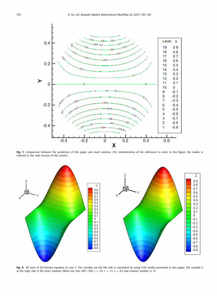
Fig. 8 , left hand side, presents the 3D view of 2D Poisson equation obtained using the present 9-bit model, for compar-

ison, the analytic solution is to be found on the right hand side. The figure shows that the numerical prediction and the

analytical solution are almost identical. Nevertheless, in order to closely compare these results, Fig. 9 is presented.

Fig. 9 introduces the 2D plain view plot of Fig. 8 . The solid red line represents the analytic solution and the dotted blue

line is the prediction from this paper. In order to show the advantage of the actual 9-bit model, the Zhang’s et al. 5-bit

model was further developed in this paper to deal with Poisson equation, because the original one could only be applied to

solve the Laplace equation. Table 4 presents the comparison between the computational time obtained by the 5-bit modified

model from Zhang’s et al. and the current model. Table 5 presents the maximum error generated by the current model and

the 5-bit modified Zhang’s et al. model, when compared with the exact solution. In both tables, the comparisons were done

for three different mesh sizes.

From Tables 4 and 5 , it can be seen that the 9-bit model is computationally efficient and accurate when solving the

2D Poisson equation, yet, a small particularity was found when evaluating the (50, 50) resolution. For this particular case,


Fig. 7. Comparison between the prediction of this paper and exact solution. (For interpretation of the references to color in this figure, the reader is

referred to the web version of this article).

Fig. 8. 3D view of 2D Poisson equation in case 3. The variable u at the left side is calculated by using 9-bit model presented in this paper. The variable Z

at the right side is the exact solution. Mesh size was 100 ×100, c = 1.0, τ = 1.1, λ = 0.5 and contour number is 15.


Fig. 9. Comparison between the prediction of this paper and exact solution. Mesh size was 100 ×100, c = 1.0, τ = 1.1, λ = 0.5 and contour number is 15.

(For interpretation of the references to color in this figure, the reader is referred to the web version of this article).

Table 5

The comparison of maximum value of error with different

resolutions between 9-bit model and 5-bit model.

Mesh size Data source Maximum error

(50, 50) Modified Zhang’s 5-bit 0.0 0 0315

Present 9-bit 0.0 0 0337

(100, 100) Modified Zhang’s 5-bit 0.0 0 0255


(20 0, 20 0) Modified Zhang’s 5-bit 0.0 0 0755


the modified Zhang’s 5-bit model, presented a slightly smaller error than the 9-bit model one. The authors believe that the

reason behind this mismatch, could be connected with the fact that a 9-bit model is a very accurate one, and the (50, 50)

resolution grid is too coarse to show any advantage of the present model over a lower level model.

Case 4.

In this case, the 2D wave equation will be simulated, the test equation is written as {

∂ 2 u

∂ t 2 = β∇

2 u + f (x, y, t)

(x, y ) ∈ (0 , 1) × (0 , 1) , t ≥ 0

, (54)

where β =1. The boundary and initial conditions are ⎧ ⎪ ⎪ ⎪ ⎨

⎪ ⎪ ⎪ ⎩

u (0 , y, t) = u (1 , y, t) = 0

u (x, 0 , t) = u (x, 1 , t) = 0

u (x, y, 0) = x (1 − x ) y (1 − y )

∂u

∂t (x, y, 0) = 0

, (55)

and the source term is given as the following equation:

f (x, y, t) = (2 x − 2 x 2 + 2 y − xy + x 2 y − 2 y 2 + x y 2 − x 2 y 2 ) cos (t) . (56)


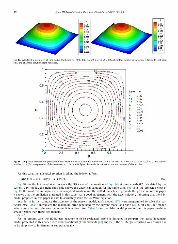
Fig. 10. Calculated u in 3D view at time t = 0.2. Mesh size was 100 ×100, c = 5.0, τ = 1.2, β = 1.0 and contour number is 15. Actual 9-bit model, left hand

side, and analytical solution, right hand side.

Fig. 11. Comparison between the prediction of this paper and exact solution at time t = 0.2. Mesh size was 100 ×100, c = 5.0, τ = 1.2, β = 1.0 and contour

number is 15. (For interpretation of the references to color in this figure, the reader is referred to the web version of this article).

For this case, the analytical solution is taking the following form:

u (x, y, t) = x (1 − x ) y (1 − y ) cos (t) . (57)

Fig. 10 , on the left hand side, presents the 3D view of the solution of Eq. (54) at time equals 0.2, calculated by the

current 9-bit model, the right hand side shows the analytical solution for the same time. Fig. 11 is the projected view of

Fig. 10 , the solid red line represents the analytical solution and the dotted black line represents the prediction of this paper,

it shows that the prediction presented in this paper has a good agreement with the exact solution, indicating that the 9-bit

model proposed in this paper is able to accurately solve the 2D Wave equation.

In order to further compare the accuracy of the present model, Yan’s models [27] , were programmed to solve this par-

ticular case. Table 6 introduces the maximum error generated by the current model and Yan’s [27] 5-bit and 9-bit models

when compared with the exact solution. It is noticed from Table 6 that the 9-bit model presented in this paper produces

smaller errors than these two models.

Case 5.

For the present case, the 1D Burgers equation is to be evaluated, case 5 is designed to compare the lattice Boltzmann

model presented in this paper with other traditional (CFD) methods [49] and [50] . The 1D Burgers equation was chosen due

to its simplicity to implement it computationally.


Table 6

The comparison of maximum value of error with different resolutions between

present 9-bit model and Yan’s 5-bit and 9-bit model [27] .

Mesh size Data source Maximum error Convergence condition

(100, 100) Present 9-bit model 0.0 0 0 086 10( −6)

Yan’s 9-bit model 0.007712 10( −6)

Yan’s 5-bit model 0.0 0 0 090 10( −6)

Fig. 12. The lines represent the numerical prediction at different time. The mesh size is 100, c = 5.0, τ = 1.5.

The test equation is written as

∂u

∂t + u

∂u

∂x = ν

∂ 2 u

∂ x 2 . (58)

According to [49,50] , ν =0.01/ π and the boundary and initial conditions are ⎧ ⎨

⎩

u (x, 0) = − sin (πx )

−1 ≤ x ≤ 1

u (−1 , t) = u (1 , t) = 0

. (59)

Fig. 12 presents the solution of Eq. (58) for different time, as expected, the slope of the curve increases as time increases.

The left side of Fig. 12 introduces the results calculated based on the model presented in this paper, and the right side

presents the numerical results obtained in Vassilis’s work [49] . From Fig. 12 , it can be seen that the two results are almost

the same, especially when considering the tendency of the slope with time increase. In order to compare the present results

with the ones obtained by Vassilis [49] and Macaraeg and Streett [50] , it is typically used the curve slope at time equals 0.5.

From Vassilis [49] and Macaraeg and Streett’s work [50] , the values of the slope at time t = 0.5 were respectively 152 . 0052

and 152 . 0049. In the present work and for the same time, it is found that the value of the slope is 152.0067. As a conclusion

it can be stated that the present lattice Boltzmann model is able to solve 1D Burgers equation.

Case 6.

For the present case, the 1D modified Burgers equation is to be evaluated, the test equation is written as

∂u

∂t + u

2 ∂u

∂x = ν

∂ 2 u

∂ x 2 . (60)

According to [30] , ν =0.01 and the boundary and initial conditions are ⎧ ⎨

⎩

u (x, 0) = − sin (πx )

0 ≤ x ≤ 1

u (0 , t) = u (1 , t) = 0

. (61)

Fig. 13 introduces the solution of Eq. (60) when using the present model for different non-dimensional times, ranging

from 0.5 to 2.5. The left hand side of Fig. 13 presents the numerical prediction of this paper and the right hand side of

Fig. 13 introduces the results computed in Ref. [30] . It can be seen from Fig. 13 that the two results are nearly the same.


Fig. 13. The value of u calculated in this paper at different time.

Table 7

Comparison of the value of u at different position along coordi-

nate x at t = 2.0.

Coordinate x Present paper Ref. [20] Ref. [35]

0.10 0.11179 0.11194772 0.11013979

0.20 0.20683 0.20710153 0.20614825

0.30 0.28477 0.28512152 0.28477813

0.40 0.34997 0.35038171 0.35045112

0.50 0.40619 0.40665374 0.40700602

0.60 0.45598 0.4564 94 86 0.45704614

0.70 0.50092 0.50155303 0.50224419

0.80 0.54138 0.54199420 0.54265295

0.90 0.534529 0.53547356 0.53225529

In order to further validate the results obtained from the previous simulations, Table 7 was created. It can be seen that

the comparison has been made between the results calculated by present model, the results proposed in Ref. [30] and the

results presented in Ref. [51] , where the collocation method with quantic splines was applied. It is found that the present

model is capable of solving the 1D modified Burgers equation and the numerical results are acceptable when compared

with the two other computed results.

6. Conclusions

In this paper, a lattice Boltzmann method 9-bit model is presented, and applied to a series of 1D and 2D mathematical–

physical equations. Several test cases are presented to compare the 9-bit model and numerical predictions generated in this

paper, with the work undertaken by previous researchers or with analytic solutions. In all cases studied, the 9-bit model

performed well. Some main conclusions are summarized below.

• New equilibrium distribution functions were derived for the present 9-bit model to solve each target equation, see Eqs.

(16) , (30) and ( 42 ). • To match with the discrete velocities lattice, the artificial constrains were chosen, they were the same for all cases

evaluated and different from previous researchers work. • It turns out that the present 9-bit model is numerically more effective and accurate in solving the studied target equa-

tions than the previous models evaluated. • Numerical results show that the 9-bit model is capable of solving 2D problems with both straight and curved geometries.

It also solves 1D problems. • This 9-bit model can solve the Laplace–Poisson and wave equation, which are recovered from LBE, in a general way, by

introducing the out-force term. The relation between the out-force term and the source term is to be seen as different

versus the previous existing ones.


Acknowledgments

The first author of this paper wishes to express his gratitude to Professor SANG Weimin. Thanks to his generous assis-

tance, the present paper could be accomplished.

References

[1] U. Frisch , B. Hasslacher , Y. Pomeau , Lattice-gas automata for the Navier–Stokes equation, Phys. Rev. Lett. 56 (1986) 1505–1508 .

[2] G.R. McNamara , G. Zanetti , Use of the Boltzmann to simulate lattice automata, Phys. Rev. Lett. 61 (1988) 2322–2335 . [3] DieterA. Wolf-Gladrow , Lattice-gas Cellular Automata and Lattice Boltzmannn Modles: An Introduction, 1725, Berlin: Springer, 20 0 0 .

[4] X.Y. He , S.Y. Chen , G.D. Doolen , A novel thermal model for the lattice Boltzmann method in incompressible limit, J. Comput. Phys. 146 (1) (1998) 283–300 .

[5] S. Succi , Lattice Boltzmann Equation For Fluid Dynamics And Beyond, Clarendon Press, Oxford, 2001 .

[6] H. Yaling , W. Yong , L. Qing , Lattice Boltzmann Method: Theory and applications, Science Press, Beijing, 2008 . [7] D. Raabe , Overview of the lattice Boltzmann method for nano- and microscale fluid dynamics in materials science and engineering, Model. Simul.

Mater. Sci. Eng. 12 (2004) 13–46 . [8] W. Miller , S. Succi , A lattice Boltzmann model for anisotropic crystal growth from melt, J. Stat. Phys. 107 (1) (2002) 173–186 .

[9] S. Chen , H.D. Chen , D. Martinez , W. Matthaeus , Lattice Boltzmann model for simulation of magnetohydrodynamics, Phys. Rev. Lett. 67 (27) (1991) 3776–3779 .

[10] S. Succi , M. Vergassola , R. Benzi , Lattice Boltzmann scheme for two-dimensional magnetohydrodynamics, Phys. Rev. A 43 (1991) 4521 .

[11] X.Y. Kang , D.H. Liu , J. Zhou , Y.J. Jin , Simulation of blood flow at vessel bifurcation by lattice Boltzmann method, Chin. Phys. Lett. 22 (11) (2005) 2873 . [12] M. Bernaschi , S. Melchionna , S. Succi , M. Fyta , E. Kaxiras , J.K. Sircar , A parallel multi physics/scale code for high performance bio-fluidic simulations,

Comput. Phys. Commun. 180 (9) (2009) 1495–1502 . [13] Z.L. Guo , T.S. Zhao , Lattice Boltzmann model for incompressible flows through porous media, Phys. Rev. E. 66 (32B) (2002) 036301–036304 .

[14] S. Succi , E. Foti , F. Higuera , Three-dimensional flows in complex geometries with the lattice Boltzmann method, EPL (Europhys. Lett.) 10 (5) (2007) 433 .

[15] P. Prestininzi , A. Montessori , M. la. Rocca , S. Succi , Reassessing the single relaxation time Lattice Boltzmann method for the simulation of Darcy ́s flows,

Int. J. Mod. Phys. C 27 (04) (2016) 1650037 . [16] H.D. Chen , S. Kandasamy , S. Orszag , R. Shock , S Succi , V. Yakhot , Extended Boltzmann kinetic equation for turbulent flows, Science 301 (2003) 633–636 .

[17] Z.H. Xia , Y.P. Shi , Y. Chen , M.R. Wang , S.Y. Chen , Comparisons of different implementations of turbulence modelling in lattice Boltzmann method, J. Turbul. 16 (1) (2015) 67–80 .

[18] H. Yu , L.S. Luo , S.S. Girimaji , Scalar mixing and chemical reaction simulations using lattice Boltzmann method, Int. J. Comput. Eng. Sci. 3 (1) (2002) 73–87 .

[19] T. Inamuro , T. Ogata , S. Tajima , A lattice Boltzmann method for incompressible two phase flows with large density differences, J.Com put. Phys. 198 (2)

(2004) 628–644 . [20] A. Montessori , G. Falcucci , M.la Rocca , S. Ansumali , S. Succi , Three-dimensional lattice pseudo-potentials for multiphase flow simulations at high

density ratios, J. Stat. Phys. 161 (6) (2015) 1404–1419 . [21] M. Sbragaglia , S. Succi , Analytical calculation of slip flow in lattice Boltzmann models with kinetic boundary conditions, Phys. Fluid. 17 (2005) 093602 .

[22] A. Montessori , P. Prestininzi , M.la Rocca , S. Succi , Lattice Boltzmann approach for complex nonequilibrium flows, Phys. Rev. E. 92 (2015) 043308 . [23] S. Gabbaneli , G. Drazer , J. Koplik , Lattice Boltzmann method for non-Newtonian fluids, Phys. Rev. E. 72 (2005) 046312 .

[24] M. La Rocca , A. Montessori , P. Prestininzi , S. Succi , A multispeed discrete Boltzmann model for transcritical 2D shallow water flows, J. Comput. Phys.

284 (2015) 117–132 . [25] Z.H. Chai , B.C. Shi , A novel lattice Boltzmann model for the Poisson equation, Appl. Math. Model. 32 (10) (2008) 2050–2058 .

[26] Y.L. Duan , R.X. Liu , Lattice Boltzmann model for two-dimensional unsteady Burgers’ equation, J. Comput. Appl. Math. 206 (1) (2007) 432–439 . [27] G.W. Yan , A lattice Boltzmann equation for waves, J. Comput. Phys. 161 (1) (20 0 0) 61–69 .

[28] J.Y Zhang , G.W. Yan , Y.F. Dong , A new lattice Boltzmann model for the Laplace equation, Appl. Math. Comput. 215 (2) (2009) 539–547 . [29] C.F. Ma , A new lattice Boltzmann model for kdv-Burgers equation, Chin. Phys. Lett. 22 (9) (2005) 2313 .

[30] Y.L. Duan , L.R.X. Liu , Y.Q. Jiang , Lattice Boltzmann model for the modified Burgers’ equation, Appl. Math. Comput. 202 (2) (2008) 4 89–4 97 .

[31] G.W. Yan , Y.S. Chen , S.X. Hu , Simple lattice Boltzmann model for simulating flows with shock wave, Phys. Rev. E. 59 (1999) 454 . [32] J.Y. Zhang , G.W. Yan , Lattice Boltzmann method for one and two-dimensional Burgers equation, Phys. A. 387 (19–20) (2008) 4471–4786 .

[33] F.J. Higuera , J. Jimenez , Boltzmann approach to lattice gas simulation, Europhys. Lett. 9 (7) (1989) 663–668 . [34] F.J. Higuera , S. Succi , R. Benzi , Lattice gas dynamics with enhanced collisions, Europhys. Lett. 9 (7) (1989) 345–349 .

[35] Y.H. Qian , D.d H́umières , P. Lallemand , Lattice BGK models for Navier–Stokes equation, Europhys. Lett. 17 (6) (1992) 479–484 . [36] P.L. Bhatnagar , E.P. Gross , M. Krook , A model for collision processes in gases. I. Small amplitude processes in charged and neutral one-component

systems, Phys. Rev. 94 (1954) 511–525 . [37] D.d. Humières , Multiple-relaxation-time lattice Boltzmann models in three dimensions, Philos. Trans. A Math. Phys. Eng. Sci. 15 (360) (2002) 437–451

1792 .

[38] Z. Li , M. Yang , Y.W. Zhang , Lattice Boltzmann method simulation 3D natural convection with double MRT model, Int. J. Heat Mass Transf. 94 (2016) 222–238 .

[39] J. Latt , B. Chopard , Lattice Boltzmann method with regularized pre-collision distribution functions, Math. Comput. Simul. 72 (2006) 2–6 . [40] A. Montessori , G. Falcucci , P. Prestinizi , M.la Rocca , S. Succi , Regularized lattice Bhatnagar–Gross–Krook model for two and three-dimensional cavity

flow simulations, Phys. Rev. E 89 (2014) 053317 . [41] S. Succi, “Lattice Boltzmann 2038,” EPL (Europhys. Lett.) 109, 50 0 01 (2015).

[42] J.D. Sterling , S.Y. Chen , Stability analysis of lattice Boltzmann methods, J. Comput. Phys. 123 (1996) 196–206 .

[43] M.K. Banda , W.A. Yong , A. Klar , A stability notion for lattice Boltzmann equations, SIAM J. Sci. Comput. 27 (6) (2006) 2098–2111 . [44] R.W. Mei , D.Z Yu , S.Y. Wei , An accurate curved boundary treatment in the lattice Boltzmann method, J. Comput. Phys. 161 (1999) 680–699 .

[45] Z.L. Guo , C.G. Zheng , B.C. Shi , Non-equilibrium extrapolation method for velocity and boundary conditions in the lattice Boltzmann method, Chin. Phys. 11 (4) (2002) 0366–0374 .

[46] Y. Chen , Z.H. Xia , Q.D. Cai , Lattice Boltzmann method with tree structured mesh and treatment of curved boundaries, Chin. J. Comput. Phys. 27 (1) (2010) 23–30 .

[47] R.W. Mei , L.S. Luo , W. Shyy , Force evaluation in the lattice Boltzmann method involving curved geometry, Phys. Rev. E 65 (2002) 041203 .

[48] Z.L. Guo , C.G. Zheng , B.C. Shi , An extrapolation method for boundary conditions in lattice Boltzmann method, Phys. Fluid. 14 (6) (2002) 2007–2010 . [49] T. Vassilis , On the resolution of critical flow regions in inviscid linear and nonlinear instability calculations, J. Eng. Math. 34 (1998) 111–129 .

[50] M.G. Macaraeg , C.L. Streett , Improvements in spectral collocation discretization through a multiple domain technique, Appl. Numer. Math. 2 (2) (1986) 95–108 .

[51] MohamedA. Ramadan , TalaatS. El-Danaf , Numerical treatment for the modified Burgers equation, Math. Comput. Simulat 70 (2) (2005) 90–98 .

http://refhub.elsevier.com/S0307-904X(16)30531-5/sbref0001































































































































































































Dow

nloa

ded

from

http

s://w

ww

.cam

brid

ge.o

rg/c

ore.

Kea

n U

nive

rsity

, on

22 J

ul 2

019

at 1

4:18

:30,

sub

ject

to th

e C

ambr

idge

Cor

e te

rms

of u

se, a

vaila

ble

at h

ttps:

//ww

w.c

ambr

idge

.org

/cor

e/te

rms.

http

s://d

oi.o

rg/1

0.10

17/jf

m.2

019.

512

~

~

J. Fluid Mech. (2019), vol. 875, pp. 476–519. doi:10.1017/jfm.2019.512

Qc Cambridge University Press 2019 476

The lid-driven right-angled isosceles triangular cavity flow

B. An1, J. M. Bergada1 and F. Mellibovsky2,†

1Department of Fluid Mechanics, Universitat Politècnica de Catalunya, 08034, Barcelona, Spain 2Department of Physics, Aerospace Engineering Division, Universitat Politècnica de Catalunya,

08034, Barcelona, Spain

(Received 25 December 2018; revised 19 June 2019; accepted 19 June 2019)

We employ lattice Boltzmann simulation to numerically investigate the two-dimensional incompressible flow inside a right-angled isosceles triangular enclosure driven by the tangential motion of its hypotenuse. While the base flow, directly evolved from creeping flow at vanishing Reynolds number, remains stationary and stable for flow regimes beyond Re � 13 400, chaotic motion is nevertheless observed from as low as Re 10 600. Chaotic dynamics is shown to arise from the destabilisation, following a variant of the classic Ruelle–Takens route, of a secondary solution branch that emerges at a relatively low Re 4908 and appears to bear no connection to the base state. We analyse the bifurcation sequence that takes the flow from steady to periodic and then quasi-periodic and show that the invariant torus is finally destroyed in a period-doubling cascade of a phase-locked limit cycle. As a result, a strange attractor arises that induces chaotic dynamics.

Key words: bifurcation, chaos

ATTENTION¡¡ Pages 29 to 72 of the thesis are available at the editor’s web

https://www.cambridge.org/core/journals/journal-of-fluid-mechanics/article/abs/liddriven-rightangled-isosceles-triangular-cavity-flow/06AC2A104F18327D5095E0D5B83FAF76#article

† Email address for correspondence: [email protected]

http://www.cambridge.org/core

http://www.cambridge.org/core

http://www.cambridge.org/core/terms

http://www.cambridge.org/core/terms

https://orcid.org/0000-0003-0497-9052

https://orcid.org/0000-0003-0497-9052




Ms. Ref. No.: CAMWA-D-19-01038R2 Title: New applications of numerical

simulation based on lattice Boltzmann method at high Reynolds numbers

Computers and Mathematics with Applications

Dear Mr. BO AN,

I am pleased to inform you that your paper "New applications of numerical

simulation based on lattice Boltzmann method at high Reynolds numbers" has

been accepted for publication in Computers and Mathematics with

Applications.

Thank you for submitting your work to Computers and Mathematics with

Applications.

Yours sincerely,

Daniele Boffi

Editor-in-Chief

Computers and Mathematics with Applications

******************************************

For further assistance, please visit our customer support site at

http://help.elsevier.com/app/answers/list/p/7923. Here you can search for

solutions on a range of topics, find answers to frequently asked questions

and learn more about EES via interactive tutorials. You will also find our

24/7 support contact details should you need any further assistance from

one of our customer support representatives.

10/04/2019

Corresponding author. Tel.: +34 691173315; fax: +34 937398101.

E-mail address: [email protected] (BO AN)

New applications of numerical simulation based on lattice

Boltzmann method at high Reynolds numbers

Bo ANa, J.M. Bergadàa, F. Mellibovskyb and W.M. Sangc

aDepartment of Fluid Mechanics, Universitat Politécnica de Catalunya, 08034, Barcelona, Spain

bDepartment of Physics, Aerospace Engineering Division, Universitat Politécnica de Catalunya, 08034, Barcelona, Spain cSchool of Aeronautics, Northwestern Polytechnical University, Xi’an, China

Abstract

In order to study the flow behaviour at high Reynolds numbers, two modified models, known as the multiple-

relaxation-time lattice Boltzmann method (MRT-LBM) and large-eddy-simulation lattice Boltzmann method

(LES-LBM), have been employed in this paper. The MRT-LBM was designed to improve numerical stability

at high Reynolds numbers, by introducing multiple relaxation time terms, which consider the variations of

density, energy, momentum, energy flux and viscous stress tensor. As a result, MRT-LBM is capable of

dealing with turbulent flows considering energy dispersion and dissipation. In the present paper, this model

was employed to simulate the flow at turbulent Reynolds numbers in wall-driven cavities. Two-sided wall

driven cavity flow was studied for the first time, based on MRT-LBM, at Reynolds numbers ranging

from42 10 to

61 10 , and employing a very large resolution 2048 2048 . It is found that whenever top and

bottom lids are moving in the opposite directions, and the Reynolds number is higher than 42 10 , the flow is

chaotic, although some quasi-symmetric properties still remain, fully disappearing at Reynolds numbers

between 52 10 and

53 10 . Furthermore, between this Reynolds numbers range,52 10 Re

53 10 , the

quasi-symmetric structures turn into a much smaller and fully chaotic eddies. The LES-LBM model

implements the large eddy simulation turbulent model into the conventional LBM, allowing to study the flow

at turbulent Reynolds numbers. LES-LBM combined with Quadruple-tree Cartesian cutting grid (tree grid)

was employed for the first time to characterize the flow dynamics over a cylinder and a hump, at relatively

high Reynolds numbers. In order to construct the macroscopic quantities in the virtual boundaries separating

two different grid levels, a set of new schemes were designed. The coupling of the LES-LBM and tree grid

drastically reduced the computational time required to perform the simulations, thus, allowing to minimize the

hardware requirements. LES-LBM model is shown to be much more efficient when combined with the tree

grid instead of using the standard Cartesian grid.

Keywords: lattice Boltzmann method, large eddy simulation, multiple-relaxation time, wall driven cavity, flow over obstacles, tree grid

1. Introduction

1.1. Numerical stability associated to the LBM at high Reynolds numbers

As a vigorous and rational numerical methodology, the lattice Boltzmann method was originated and

evolved from the lattice gas automata (LGA) [1]. Due to the continuous developments made by researchers [2,

3], the lattice Boltzmann method gradually improved as a mature methodology. It turned out that the lattice

Boltzmann method is numerically capable of solving many mathematical and physical problems, including


2 Bo AN, J.M. Bergadà, F.Mellibovsky and W.M. Sang / (2019)

model PDEs [4, 5], thermodynamics problems [6, 7], combustion [8, 9], fluid mechanics [10, 11], and other

research applications.

From previous researchers’ work [12-22], it is noticed that LBM applicability was mostly limited to low

Reynolds numbers due to a deficiency of lattice Boltzmann method, known as the numerical instability.

Besides, the numerical applications of the original LBM at high Reynolds numbers, require a very high grid

resolution [23]. Many studies have shown that the numerical stability of LBM deteriorates as the Reynolds

number increases [12-22].

Providing the grid spacing remains constant, the original LBM relaxation time approaches 0.5 as

Reynolds number increases, and according to [2, 3], numerical stability is being compromised. The numerical

stability of LBM can-be improved through grid refinement, but this is impractical, especially at very large

Reynolds numbers. A great deal of research had been done to improve the stability behaviour of LBM at high

Reynolds numbers. Several ways to mitigate the issue are the entropic lattice Boltzmann Method [24, 25], the

regularized lattice Boltzmann method [26, 27], the multiple relaxation time LBM (MRT-LBM) [12-17], and

the large eddy simulation LBM (LES-LBM) [18-22]. In the present paper, the MRT-LBM and LES-LBM

were used to improve the numerical stability of conventional LBM at high Reynolds numbers. In order to

further optimise the lattice Boltzmann method, the quadruple-tree Cartesian cutting grid (tree grid), generated

by the local grid refinement technology, was also employed in this paper.

In the present paper, several numerical examples were initially evaluated to validate the in-house code. The

multiple-relaxation-time lattice Boltzmann method applied to the numerical simulation of wall-driven cavities

at high Reynolds numbers, including three different flow driving conditions, cases (a), (b) and (c) were

considered. Case (a) represents the usual lid-driven cavity, case (b) characterizes the top and bottom wall-

driven cavity moving in the same direction and case (c) describes the cavity flow with the top and bottom

walls moving in opposite directions. Considering case (a) at high Reynolds numbers, the results delivered by

Chai et al [22], where the multiple-relaxation-time lattice Boltzmann method was used to simulate the lid-

driven cavity flow at high Reynolds numbers, were used for comparison. The evaluation of cases (b) and (c)

at high Reynolds numbers, via employing MRT-LBM are completely new and they are presented in this paper

for the first time. Notice that these two particular geometries at Reynolds numbers up to 2000, were

previously studied by Perumal and Dass [23] using the conventional lattice Boltzmann method.

Via using the novel LES-LBM combined with Quadruple-tree Cartesian cutting grid (tree grid), the flow

around two different bluff bodies, a cylinder and a hump, at relatively high Reynolds numbers was evaluated.

It is important to highlight that the coupling between LES-LBM and tree grid, required the use of a set of new

schemes in order to be able to construct the macroscopic quantities in the virtual boundaries. When

considering the flow over a hump, in the present paper, the new results obtained from the present in-house

code was compared with the results introduced by Suzuki [28] at Reynolds number, 4000. He investigated in

2D at Reynolds number 4000 the compressible unsteady, laminar flow over a hump by using direct numerical

simulation. Body forces as well as vortex shedding were analyzed.

When considering the cylinder case, the results of the flow past a cylinder at Reynolds number 100, were

compared with the ones obtained by other researchers [29-32]. Ding et al [29] investigated 2D circular

cylinders arranged in tandem and side-by-side via using the mesh free least square-based finite difference

method at Reynolds numbers 100 and 200. Meneghini et al [30] studied the 2D circular cylinders via using a

fractional step method at Reynolds numbers 100 and 200. In order to have a better description of the boundary

layer, they used a very fine mesh close to the cylinder wall. Harichandan and Roy [31], solved the Navier-

Stokes equations by the finite volume method, to simulate the flow past an array of two and three cylinders

located in parallel and in tandem. The single cylinder case was also run and compared at two different

Reynolds numbers 100 and 200. Behara and Mittal [32], numerically studied the oblique shedding generated

by the flow past a 2D circular cylinder via using stabilized finite element method at three Reynolds numbers

60, 100 and 150.

The flow over a cylinder at Reynolds number 3900 was employed to further study the LES-LBM coupled

Bo AN, J.M. Bergadà, F.Mellibovsky and W.M. Sang / (2019) 3

with tree grid in-house code advantages. The comparison between the present prediction and previous

research undertaken at Reynolds number 3900 by [33-41] is presented in section 5. In the research done by

Beaudan and Moin [33], Mittal and Moin [34], Kravchenko and Moin [35] and You and Moin [37], they

evaluated a modified Smagorinsky sub-grid-scale eddy-viscosity model, which was implemented in the LES

turbulent model. They also checked the accuracy of the upwind-biased, central finite-difference and B-splines

numerical methods, observing that the B-splines method agrees better with the experimental results.

Lehmkuhl et al [36], carefully studied in 3D via direct numerical simulation, the downstream vortex shedding

on a circular cylinder at Reynolds number 3900. They observed the large-scale quasi-periodic motion seems

to be related with the modulation of the recirculation bubble, which causes its shrinking and enlargement over

time. As previously done by You and Moin, [37], Rajani et al [38], applied the Smagorinsky sub-grid scale

algorithm implemented in the LES turbulent model, their simulations were based on assessing the limitation

and accuracy level of the present algorithm. Comparisons with a large number of previous researchers work

were made. Pereira et al [39] simulated the flow past a circular cylinder at the same Reynolds number via

using 2D and 3D RANS, DDES and XLES models. They observed the three dimensional DDES and XLES

models produced more accurate results. Wang et al [40], proposed a 2D numerical large eddy simulation

(LES) method combined with the characteristic-based operator-splitting finite element method, to solve

Navier-Stokes equations at Reynolds number 3900. In Breuer [41], two sub-grid scale models (Smagorinsky

and dynamic model) coupled with LES were employed, also the LES model without any sub-grid model was

evaluated. Their work focused in evaluating numerical and modelling aspects affecting the LES simulations.

Different resolutions were considered.

1.2. Original lattice Boltzmann equations

In what follows, a brief description of the original LBM is presented, this introduction will be later used to

implement the MRT-LBM and LES-LBM methodologies. The continuous Boltzmann equation is given by

equation (1), notice that all parameters presented in this equation, as well as the ones introduced in the rest of

the equations presented in this paper are non-dimensional. As in many previous applications [10, 11, 14, 17,

21], the very common binary collision assumption is employed in the present paper to obtain equation (1).

2

1 2 1 2 1

( , , ) ( , , ) ( , , )(F F ) cosD

f r t f r t f r ta f f d g d d

t r

(1)

The term ( , , )f r t is called the distribution function, r is the spatial position vector, t is the non-dimensional

time, is the velocity vector, a is the particle acceleration, Dd is the particle diameter, 1 2F ,F and 1 2,f f are the

post- and pre- collision distribution functions of two fluid particles, g is the vertical component of 1 2

and d is the angle differential. The left hand side of equation (1) represents the streaming term, the right

hand side represents an integral-differential term, which is called the collision term. To simplify the collision

term, Bhatnagar, Gross and Krook [42], presented the famous BGK approximation, where the collision term

was replaced by a simple collision operator f , as a result, the Boltzmann-BGK equation reads

( , , ) ( , , ) ( , , ) 1( , ) ( , , )eq

f

f r t f r t f r ta f r f r t

t r

(2)

where is the singular relaxation time term and ( , )eqf r is the equilibrium distribution function.


Discretizing equation (2) both in space and time, the lattice Boltzmann equation is obtained as

1( , ) ( , ) ( , ) ( , , )eq

ff r e t t t f r t f r f r t

(3)

where represents the direction of discrete velocities, ( , )f r e t t t and ( , )f r t are the discrete -post

and -pre collision distribution functions vector and f

is the discrete collision operator in direction .

Notice that, the external forces term is neglected from equations (1), (2) and (3), since in the present

applications, no external forces are involved. It is common knowledge that the Navier-Stokes equations are

recovered from the discrete lattice Boltzmann equation [11, 20, 43, 44]. In order to solve fluid-flow related

problems, the physical quantities, density , velocity u and internal energy E , must be defined as [45]

2( )2

f

u e f

DRTE e u f

(4)

where D is the space dimension, R is the non-dimensional gas constant and T refers to the non-dimensional

temperature.

The LBGK model for solving the Navier-Stokes equations was presented by Qian et al [11], and it is one

of the most popular models used in LBM when applied to fluid dynamics problems. This model is also

employed in the present paper. According to Qian et al [11], the equilibrium distribution functions, for the 9

discrete velocities (9-bit model), are determined by

2 2

2 4 2

( )1 0,1,...,8

2 2

eq

s s s

e u e u uf

c c c

(5)

where are the weight coefficients, and sc is the non-dimensional sound speed. The discrete velocities of

LBGK two dimensional 9-bit model D2Q9 are given by

2

2 2

2 2

0 1 0 -1 0 1 -1 -1 1

0 0 1 0 -1 1 1 -1 -1

4 9 0

1 9 3

1 36 2

s

e c

ec

c e c

e c

(6)

where 1c x t is the non-dimensional lattice velocity, and , x t are the lattice grid non-dimensional

spacing and the non-dimensional time step respectively.


Figure 1 shows the discrete velocities of the LBGK D2Q9 model employed in all simulations presented in

this paper.

Fig. 1. Discrete velocities of lattice Boltzmann D2Q9 model.

Nomenclature (all parameters are non-dimensional)

a Acceleration of molecules

sc Sound speed

c Lattice velocity

C Constant of Smagorinsky eddy

PC Temporal pressure coefficient

LC Lift coefficient

DC Drag coefficient

fC Skin friction coefficient

D Space dimension

Dd Particle diameter

e Unit velocities vector along discrete directions

E Macroscopic quantity, internal energy

g The vertical component of velocity vector difference

xF x components of total body force of the object

yF y components of total body force of the object

( , , )f r t Distribution function

( , )eqf r Equilibrium distribution function

1 2F ,F Post-collision distribution function of two fluid particles


1 2,f f Pre-collision distribution function of two fluid particles

f Discrete distribution functions on directions

F Discrete distribution functions on directions after collision

( , )f r e t t t Discrete –post collision distribution functions vector

( , )f r t Discrete –pre collision distribution functions vector

eqf Nine-ordered vector of discrete equilibrium distribution functions

f Discrete distribution functions vector after collision

neqf The non-equilibrium state of distribution functions

vf Virtual distribution functions

evf The virtual equilibrium distribution functions

nevf The virtual non-equilibrium distribution functions

L Characteristic length

m Momentum vector

eqm Equilibrium momentum vector

M Switch matrix

m Momentum vector after collision

N Number of cells along x and y axis

p Surface static pressure

p Free stream static pressure

Re Reynolds number

R Gas constant

r Spatial position vector

br Spatial position of point b

wr Spatial position of point w

cr Spatial position of point c

ar Spatial position of point a

S A diagonal matrix


ijS Magnitude of large scale strain rate tensor

t Time

T Temperature

T2 Computational time per time unit with standard Cartesian grid

T1 Computational time per time unit with tree grid

u Macroscopic quantity, velocity

bu Velocity of point b

wu Velocity of point w

au Velocity of point a

cu Velocity of point c

U Initial velocity of the flow field

dU Wall driven velocity

xU Horizontal component of velocity

yU Vertical component of velocity

U Far field velocity

, Discrete directions (from 0 to 8 in the present LBGK D2Q9 model)

Parameter to be determined

x Grid spacing

t Time step

nx Grid spacing of nth grid level

0x Grid spacing of root grid

e Embed depth

coarsex Grid spacing of coarse grid

finex Grid spacing of fine grid

f Filter scale

Function of macroscopic quantities

Kinematic viscosity of laminar flow

t Kinematic viscosity of turbulence flow


total Total kinematic viscosity

,i j Non-equilibrium stress tensor

Macroscopic quantity, density

0 Initial density

Single relaxation time term

total Total relaxation time

lid Shear stresses on the lid

f Collision operator

f

Discrete collision operator on directions

d Integral infinitesimal of angle

Weight Coefficients

Velocity vector of molecules

1 2 Vectorial difference of velocity

Linear interpolation factor

Collision matrix

2. Mesh

2.1. Standard Cartesian Grid

The application of standard Cartesian grid is very common in LBM, because of its particular structural

advantages that fit the streaming-collision theory of LBM. The standard Cartesian grid, however, usually

generates a huge computational burden, involving long computational time and high hardware requirements,

therefore restricting LBM applications. Nevertheless, for simple geometries, the standard Cartesian grid is

widely employed, and in the present paper it will be used to evaluate the flow inside wall-driven cavities. Two

main cases are presented in this paper, the classic lid-driven cavity flow, case (a), which will be compared

with the results presented by Chai et al [12], and the two-sided wall-driven cavity flow, cases (b) and (c). The

resolution used for case (a), was 512 512 , being this resolution the one already used in reference [12]. The

mesh resolution employed to evaluate the flow inside the two-sided wall-driven cavity, was of 2048 2048

for all the Reynolds numbers evaluated. Notice that this mesh is four times denser than the largest one used in

reference [12]. Considering the simulation of complex geometries with high Reynolds numbers, the mesh

refinement is an essential point to be considered, yet, a blind and undisciplined refinement through the whole

domain is illogical and impractical, as computational resources are poorly used. Technically, the refinement is

required in the regions where fluid variables are expected to suffer severe temporal or spatial changes.


2.2. Quadruple-tree Cartesian cutting Grid (tree Grid)

The tree grid is a typical example of Cartesian non-uniform grid. More and more researchers are

employing such grid, due to its excellent merits shown in many practical applications [46, 47].

In this paper, the tree grid was employed in the numerical simulations launched using LES-LBM. As

required by the cell structure, a given cell zone was divided into several levels with different grid/cell spacing,

the grid spacing x changed in each grid level. In the present paper, the models studied were two dimensional,

the quadruple-tree structure [46, 47], was employed to generate the tree grid. The basic idea is that a flow

field is viewed as a big single cell, known as the root cell, and via using the theory of tree grid, it generates 22

sub-cells ( 32 in three dimensions). In the next step of the process, each of these four sub-cells also generates

another four sub-cells. Through this loop, the final mesh of the whole flow field was accomplished. Figure 2

shows the quadruple-tree structure and the process of grid generation.

Fig. 2. Quadruple-tree structure and grid generation.

The grid level at the left side of figure 2 presents different degrees of grid refinement. It is to be noticed

that the root cell is defined as level 0. The grid spacing of each grid level [48-50] is to be obtained by equation

(7), which is written as

0 2n

nx x (7)

where nx refers to the grid spacing of the nth grid level and 0x is the grid spacing of the root cell. Figure 3

shows the tree grid of a cylinder and a hump, which will be employed in section 5.1 to evaluate the flow

around these obstacles. It is important to notice that both obstacles, a circular cylinder and a hump, have the

same characteristic length 1.0L . The total mesh cells were, 16652 for the flow past a circular cylinder and

55748 for the flow over a hump. In the same figure, are also presented the boundary conditions employed for

these two geometries. At the inlet, Dirichlet boundary conditions for all variables were used. At the outlet and

far-field boundaries, Neumann boundary conditions for density and xU velocity were used, Dirichlet boundary

conditions for yU velocity were employed. In all walls, Dirichlet boundary conditions for velocities and

Neumann boundary conditions for density were used.


(a) Cylinder

(b) Hump

Fig. 3. Tree grid used for simulating the flow around these two particular geometries.

3. Mathematical background of the methodologies employed

The original lattice Boltzmann method is usually applied to simulate incompressible flow, being the

Reynolds number commonly limited to low values. In order to clarify why the numerical stability deteriorates

at high Reynolds numbers, the following two essential equations are to be considered

eR UL (8)

2(2 1) (6 )x t (9)

Introducing equation (8) into equation (9), it is obtained

2e (2 1) (6 )UL R x t (10)

where U is the initial velocity and L is the characteristic length.

From equation (10) and considering the definition of the lattice non-dimensional velocity presented in

section 1.2, the value of the single relaxation time is given by, equation (11). Notice that the single

relaxation time is initially introduced in equation (2).


3 ( e ) 0.5UL R x (11)

Empirically, when the relaxation time is close to 0.5, the stability of LBM is compromised. For numerical

simulations involving high Reynolds numbers, the grid spacing x must be small enough to maintain the

relaxation time well above 0.5. As a result, at high Reynolds numbers a mesh refinement is inevitable,

although this will greatly increase the computational burden. This is the main reason why the original LBM

cannot be directly applicable to numerical simulations at high Reynolds numbers. The MRT-LBM and LES-

LBM approaches are used in the present manuscript as mathematical tools to numerically stabilize the

conventional LBM at high Reynolds numbers, these mathematical tools are discussed and explained in the

following sub-sections. According to the authors’ knowledge, this is the first time the combination of tree grid

technology with LES-LBM is being employed.

3.1. Multiple-relaxation-time lattice Boltzmann method

The main difference between the MRT-LBM approach [12-17] and the LBGK model, is that in the first

approach, multiple relaxation time terms are used to construct an nth order vector, while on the second one a

single relaxation time term is required. The evolution equations of the MRT-LBM and the LBGK are shown

respectively as

( , ) ( , ) 1 ( ( , ) ( , , ))

( , ) ( , ) [ ( , ) ( , , )]

eq

eq

f r e t t t f r t f r f r t LBGK Single

f r e t t t f r t f r f r t LBM MRT

(12)

where f is a nine-order vector and is a 9 9 collision diagonal matrix given by

1

2

3

1 0 0 0 0 0 0 0 0

0 1 0 0 0 0 0 0 0

0 0 1 0 0 0 0 0 0

0

4

5

6

0 0 1 0 0 0 0 0

0 0 0 0 1 0 0 0 0

0 0 0 0 0 1 0 0 0

0 0 0

7

8

9

0 0 0 1 0 0

0 0 0 0 0 0 0 1 0

0 0 0 0 0 0 0 0 1

(13)

Equation (12) explains the evolution process of the distribution functions. Considering the MRT-LBM, the

collision process is accomplished by the operation of matrices and vectors. The relation between the

distribution functions vector and the moment vector m is obtained from

1; m M f f M m

(14)

where M is a 9 9 switch matrix and f is the distribution functions vector. The collision process in MRT-

LBM is defined by

eqf f f f (15)


f is the distribution functions vector after the collision step. Multiplying the switch matrix M on both

sides of the equation (15), it is obtained

eqm m S m m (16)

whereeq eqm M f is the vector of the equilibrium moment and

1

1 2( , ,..., )nS M M diag s s s

is

a diagonal matrix.

After the collision process, the collided distribution functions vector 1f M m

are obtained. The

computational approach of the MRT-LBM is addressed as follows:

1) Initializing the whole flow field with macroscopic quantities and computing the equilibrium

distribution functions.

2) Calculating the vector of velocity distribution functions1f M m

and moment m M f .

3) Performing the evolution process, including collision step 1 eqf f M m m

and

streaming step.

4) Computing the macroscopic quantities and resetting the distribution functions on the boundaries.

3.2. Large-eddy-simulation lattice Boltzmann method

The large-eddy-simulation LBM [18-22, 51]is another method to improve the numerical stability of the

original lattice Boltzmann method. By using the Smagorinsky eddy viscosity model, the total kinematic

viscosity equals the sum of the fluid kinematic viscosity and the eddy kinematic viscosity t ,

total t (17)

where 2

t f ijC S is the eddy kinematic viscosity. C is the constant coefficient of the Smagorinsky eddy

viscosity model. f is the filter scale and ijS is the magnitude of large scale strain rate tensor. According to

reference [27], the total relaxation time can be obtained from equation (18)

23( ) 0.5total f ijC S (18)

The non-equilibrium stress tensor, used to determine the large scale strain rate tensor, is given by

, ( )eq

i j i je e f f . It is important to realize that whenever equation (18) is implemented in equation (3),

the original LBGK model is transformed into LES-LBM. Notice that the collision operator used in the LES-

LBM, defined as the right hand side term of equation (3), is essentially the same as the one used in the

conventional LBM, the only difference is that the relaxation time term , used in conventional LBM, is

replaced by total in LES-LBM.

The computational steps to follow in order to implement the LES-LBM are addressed as follows:

1) Initializing the whole flow field with macroscopic quantities and computing the equilibrium

distribution functions.

2) Filtering process, obtaining the processed macroscopic quantities ( , )u .


3) Computing the processed equilibrium distribution functions eqf , and eqf f .

4) Performing the evolution (collision and streaming) process.

5) Computing macroscopic quantities and resetting the distribution functions on the boundaries.

4. Boundary Conditions

4.1. Far-field, inlet and outlet boundary conditions

The non-equilibrium extrapolation scheme presented by Guo et al [52] was employed to define the far-field

boundary condition in the current numerical cases. The basic idea behind this scheme is that the distribution

function of each direction can be classified into two parts, known as the non-equilibrium term and the

equilibrium term.

Fig. 4. Far-field boundary.

As shown in Fig. 4, grid nodes A, B and C are flow points, grid nodes D, E and F are far-field boundary

points. For the points E and B. the distribution function of each direction is written as

( , ) ( , ) ( , )eq neqf E t f E t f E t (19)

( , ) ( , ) ( , )eq neqf B t f B t f B t (20)

The equilibrium part ( , )eqf E t is obtained from the macroscopic quantities of point E. While, the non-

equilibrium distribution functions of point E can be replaced by those of point B.

( , ) ( , )neq neqf E t f B t (21)

Hence, the distribution functions of point E become

( , ) ( , ) ( , ) ( , )eq eqf E t f E t f B t f B t (22)


4.2. Wall boundary conditions

For the straight wall boundaries involved in all cases, the same non-equilibrium extrapolation scheme

presented in reference [52] is used in the present paper. When considering the curved wall boundaries, there

are several popular schemes [53-55] to be considered. In the present paper, all three schemes were tested

when evaluating the flow around a hump and a cylinder. Based on the case of the flow around a cylinder at

Reynolds number 100, and once evaluated the results presented in section 5.1, tables 1 and 3, it is concluded

that the most appropriate scheme for the present applications was the one from Mei et al [53]. This particular

scheme is outlined next.

Fig. 5. Curved wall boundary.

In figure 5, grid nodes a and c are fluid-domain points, grid node w belongs to wall boundary points and

grid node b is a virtual internal wall point. Mei et al [53], presented an accurate curved boundary treatment,

according to their theory, taking point b for instance, the virtual distribution function, on direction 6 see figure

1, is constructed by linear interpolation of points b, c and w, and given by

6 8 8 8 62

3( , ) (1 ) ( , ) ( , ) 2v ev

b c b wf r t F r t f r t e uc

(23)

where wu is the non-dimensional velocity of the point w, which is 0 in the present cases, and is the linear

interpolation factor obtained by equation (25). The equilibrium virtual distribution function on direction 8 (see

figure 1), is given by.

2

8 8 8 82 4 4

3 9 3( , ) ( , ) 1 ( )

2 2

ev

b c b c c cf r t r t e u e u u uc c c

(24)

where cu is the velocity of the point c, and bu is the unknown virtual velocity of the point b. This velocity is

presented in equation (25) as a function of the embedded depth e .


2 1 1 2 ,

2

1 2 11 1 2 ,

0.5

e

e b c

e e

e b c w

e e

if u u and

if u u u and

(25)

Substituting equations (24) and (25) into equation (23) the virtual distribution function of point b is

obtained. In this way, the streaming operation from point b to point c is smoothly achieved.

4.3. Virtual boundary condition

The virtual boundary condition is only considered when the tree grid is used in the numerical simulations.

The process to construct the macroscopic quantities and the distribution functions in the virtual boundaries, is

defined in this sub-section. In this paper, none of the nodes in virtual boundaries were involved in the

streaming process. The distribution functions of each node, were calculated by a set of new schemes

developed by the present authors based on the initial concepts given in references [48-50]. After obtaining the

macroscopic quantities, the distribution functions in the virtual boundaries, were calculated with the use of the

non-equilibrium extrapolation scheme [52]. In order to construct the macroscopic terms in the virtual

boundaries, there is a need to perform an interpolation process, using the macroscopic quantities on both sides

of virtual boundaries. In the present paper, the grid spacing relation existing between both sides of the virtual

boundaries, is given by

2coarse finex x (26)

From equation (26) and for a constant non-dimensional time step t , the lattice Boltzmann equation

evolves only once on the coarse cell, while it evolves twice on the fine grid. Hence, the interpolation process

outlined in the previous paragraph is actually a simultaneous space-time interpolation.

It can be seen from figure 6 (a) that, point A is a coarse grid node, while point B is an overlapping point of

coarse and fine boundaries, and point C is a fine grid node. Considering a half time step 0.5 t , the

macroscopic quantities of the point B can be constructed as

0.5 0.5 0.5( ) ( ( ) 2 ( ) ) 3t t t t t tB A C (27)

where is the generic function of a macroscopic quantity, like velocity, density, pressure, etc. The time

interpolation scheme at any given node, say node A, is evaluated according to the following equation.

0.5( ) 0.5( ( ) ( ) )t t t t tA A A (28)

(a) (b)


Fig. 6. Virtual boundaries.

In figure 6 (b), points A and D are both coarse grid nodes, point C is a fine grid node and point B is a

hanging point of virtual boundaries. The macroscopic quantities of the point B can be constructed as

0.5 0.5 0.5 0.5( ) (0.5 ( ) 0.5 ( ) 2 ( ) ) 3t t t t t t t tB A D C (29)

where the time interpolation scheme at points A and D follow the same pattern presented in equation (28).

It is to be realized that the macroscopic quantities at point B for both positions defined in figures 6 (a) and

(b), need to be determined at a half time step, 0.5 t , and after a full time step t . In order to obtain the

macroscopic quantities at point B after a full time step, the equations (30) and (31) need to be respectively

applied.

( ) ( ( ) 2 ( ) ) 3t t t t t tB A C (30)

( ) (0.5 ( ) 0.5 ( ) 2 ( ) ) 3t t t t t t t tB A D C (31)

To sum up, from equations (27) to (31), the macroscopic quantities of each grid node at different time steps

on the virtual boundaries are obtained. Once the macroscopic quantities at each grid node and at different time

steps have been obtained, the distribution functions of each node on the virtual boundaries, at different time

steps, can be calculated through the non-equilibrium extrapolation scheme defined in equation (22).

5. Results and discussion

5.1. Application using tree grid technology in combination of LES-LBM

5.1.1 Flow over a circular cylinder

For all cases studied in the present paper, the upstream non-dimensional velocity was 0.1U and the

initial non-dimensional fluid density was 1.0. As a first case to test the LES-LBM model based on the tree

grid, the flow over a cylinder is considered. Initially, the three different schemes for curved boundaries

introduced in section 4.2 are evaluated at Reynolds number 100, and the results obtained are presented in

table 1. At this low Reynolds number the flow is periodic, therefore, the information presented in table 1, was

extracted once the simulation was fully converged, 15 seconds were run, and using a single oscillation cycle.

Based on the results introduced in table 1 and after comparing them with those reported in references [29-32],

it was decided to employ the scheme from Mei et al [52] for all curved boundaries studied in the present paper.

Table 1 compares the lift coefficient amplitude, the average value of drag coefficient and the Strouhal number,

obtained from the present simulation and several previous studies [29-32]. The agreement of all these

parameters is very good.

Table 1. Comparison of the lift coefficient amplitude, drag coefficient mean value and Strouhal number obtained from the present paper

with three different boundary schemes and several previous investigations at Re=100.

Data source Amplitude of

Cl

Mean value

of Cd

Strouhal

number

Present work scheme [53]

0.286 1.39 0.164

Present work 0.32 1.414 0.1643


scheme [54]

Present work scheme [55]

0.265 1.383 0.1646

Ref.[29] 0.287 1.356 0.166

Ref.[30] -- 1.37 0.165

Ref.[31] 0.278 1.352 0.161

Ref.[32] 0.287 -- --

Table 2. The ratio of computational time required between standard Cartesian grid (SG) and tree grid (TG) at Re=40. T2 characterizes the

computational time per time unit whenever the standard Cartesian grid (SG) is used, and T1 represents the same time when the tree grid

(TG) is employed.

Grid spacing Total cells Ls/L Computational time per

time unit

Δx=0.009766 TG 16652

SG 1042792

4.4192

4.4275

T1=0.00515625s

T2=0.104s

In order to evaluate the efficiency of the tree grid over the standard Cartesian grid, table 2 presents the

computational time per time unit of the standard Cartesian grid (T2) and the tree grid (T1) at a steady

Reynolds number 40, notice that the time ratio of T2 over T1 is 20.17. The first column of table 2 defines the

minimum grid spacing used in both meshes. The second column represents the total number of cells used for

each mesh, and the third column characterizes the length ratio between the downstream steady bubble length

and the cylinder diameter. It can be concluded from the table that, with the same minimum grid spacing, the

standard Cartesian grid requires much longer computational time than the tree grid does, while still retaining

an acceptable accuracy. For the present simulation, the computational time required is over 15 times smaller

when employing the tree grid technology. It is the first time that LES-LBM model combined with the tree grid

is proved much more efficient over the standard Cartesian grid. In reality, the tree grid technology is allowing

to refine the mesh on the particular areas where the flow is having large momentum interchanges, therefore

drastically reducing the total number of cells required.

In order to further assess the in-house code reliability, the flow for a turbulent Reynolds number, Re= 3900,

was evaluated. The reason why laminar and turbulent Reynolds numbers were chosen, is to prove that the

model proposed is capable of producing good results under both conditions. Figure 7 (b) presents the vortex

shedding process for a Reynolds number 3900. On each graph, the streamlines plots are presented on the left

hand side alongside vorticity contour plots. Both plots are introduced at different time steps defined in figure

7 (a). The same vortex evolution process was observed in the work done by Pereira et al [39] figure 9 and

Wang et al [40] figure 8.


(a) Probes at different time steps

(b) 0 29.8014t s

(c) 1 29.8187t s

(d) 2 29.8361t s


(e) 3 29.8545t s

(f) 4 29.8719t s

Fig. 7. Comparison of streamlines between snapshots from the present paper at different time steps at Reynolds number 3900.

Table 3 introduces the Strouhal number and mean drag coefficient value obtained in the present simulation and when using two mesh densities. The result presented in table 3, were obtained after the simulations were fully converged, over 50 seconds were simulated, a set of over 140 cycles lasting over ten seconds, were used to obtain the parameters defined table 3. These values are compared with the 2D ones obtained in references [37, 39-43]. It is observed that even for the largest grid spacing 0.009766x , used in the present paper, and thanks to the use of the tree grid, the results obtained are very accurate.

Table 3. Comparison of the drag coefficient mean value and Strouhal number obtained from the present paper and several previous

investigations at Re=3900.

Data source Total

number of cells

Strouhal

number

Mean value

of Cd

The present work

Δx=0.009766

16652 0.242 1.6

The present work Δx=0.000305

3567008 0.2287 1.575

Ref.[35] 7543680 0.23 1.65

Ref.[37] 7543680 0.22 1.55

Ref.[38] 5575680 0.244 1.65

Ref.[39] -- 0.244

Ref.[40] -- 0.243 1.749

Ref.[41] 871200 0.215 0.005 1.625

Figure 8 introduces the comparison between the temporal averaged pressure coefficient along the upper

surface obtained in the present simulation and the ones obtained by four previous researches [33-36]. The

agreement is very good, further enhancing the code reliability, proving as well that the new LES-LBM model

coupled with tree grid is numerically stable for this Reynolds number.


Fig. 8. Lift and drag coefficients on the cylinder, and mean pressure coefficient on the cylinder upper surface at Reynolds number

3900.

5.1.2 Flow over a hump

Another typical bluff body configuration considered, to further evaluate the new LES-LBM coupled with

tree grid, is the flow over a hump. Very interesting research has been undertaken on this configuration, see for

example reference [28], yet according to the authors’ knowledge no attempt to use LES-LBM based on tree

grid to simulate flow over this particular bluff body has undertaken. One of the main advantages of using the

proposed methodology, is that it allows to evaluate relatively large Reynolds numbers, well into the turbulent

regime, and thanks to the use of the tree grid structure, considerable computational time reduction is obtained,

see references [48-50]. Figure 9 introduces the vortex shedding period divided in eight different time steps at

Reynolds number 4000. It can be observed that, the vortices appear in a periodic cycle, attaching, detaching

and streaming at different iteration steps. Regardless of the time step chosen, when comparing vortex shape

and dimensions with reference [28] figure 10, the agreement is very good. Moreover, the Strouhal numbers

obtained by the present simulation and Suzuki’s work [28], were respectively 0.163 and 0.16. As a conclusion,

it can be said the combination of the tree grid with the LES-LBM model at Reynolds number 4000, is

producing very accurate results.

(a) Iteration time step=12500 (b) Iteration time step=13400

(c) Iteration time step=14300 (d) Iteration time step=15200


(e) Iteration time step=16100 (f) Iteration time step=17000

(g) Iteration time step=17900 (h) Iteration time step=18800

Fig. 9. Vortex shedding period divided in eight different time steps of the flow over a hump at Reynold number 4000. The figures

presented here are comparable with those obtained by Suzuki [30].

5.2 Applications of MRT-LBM

5.2.1 Lid driven cavity, case (a)

In this section, case (a) characterizing the lid driven cavity flow at Reynolds numbers varying from 42 10

to 61 10 was considered. The non-dimensional wall driven velocity was maintained at 0.1lidU . Figure 10

introduces the numerical results obtained in the present paper, streamlines and vorticity contours are

respectively presented on the left and right hand side of each figure. In the present paper as well as in

reference [12], the MRT-LBM model was employed, the mesh density and boundary conditions were the

same in both cases. The authors believe the small differences between figure 10 and figure 1 in reference [12],

are due to the instant each snapshot is taken, notice that the flow is turbulent and unsteady, and so it is time

dependent. As can be seen from figure 10, the fluid unsteady behaviour deteriorates as the Reynolds number

increases. When the Reynolds numbers are relatively low, around 42 10 and

51 10 , the flow instability is

localised at some particular positions of the domain, namely the corners. On the contrary, the results at higher

Reynolds numbers gradually show that the global instability appears throughout the cavity. For very high

Reynolds numbers, Re>55 10 , the flow configuration evolves in a highly random fashion, fluid motion is

chaotic and no clear flow patterns can be identified. This would explain why the flow structures obtained in

the present paper are very similar to the ones obtained in reference [12] but not exactly the same. As a

conclusion, it can be said that, the computational results obtained in this paper at Reynolds numbers lower

than 51 10 show a good agreement with the data provided in reference [12]. Considering the chaotic flow

time dependence typical at this regimes, the agreement is quite acceptable. Notice that as Reynolds number

increases, the turbulent motions become statistically isotropic, as stablished in the Kolmogorov’s hypothesis

of local isotropy.


(a) Re= 42 10 (b) Re= 45 10 (c) Re= 51 10

(d) Re=55 10 (e) Re=

61 10

Fig. 10. Streamlines and vortex contours of the top wall driven velocity with different Reynolds numbers. Case (a) shows the numerical

prediction obtained in this paper.

(a) Re=

45 10 (b) Re=51 10 (c) Re=

55 10 (d) Re=61 10

Fig. 11. xU profiles along the vertical center lines at different Reynolds numbers.

(a) Re=

45 10 (b) Re=51 10 (c) Re=

55 10 (d) Re=61 10

Fig. 12. yU profiles along the horizontal center lines at different Reynolds numbers.

In order to further evaluate the results obtained in the present simulation, figures 11 and 12 present the

time-average non-dimensional velocity components xU and yU , respectively along the vertical and

horizontal central lines at Reynolds numbers ranging from 42 10 to

61 10 . The solid line represents the

temporal average velocity components. The standard deviation is computed in the same figures and

presented through enclosures formed by lines 2U and 2U . Following the patterns presented in

figure 10, it is seen that for Re51 10 , the respective xU and yU velocity distributions show a clear pattern

characteristic of a forced vortex. Whenever Re55 10 , the time average velocity distributions still show the

fluid is rotating clockwise. Figures 11 and 12 also show that, the velocity gradient along the radial direction

keeps decreasing with the Reynolds number increase, indicating the fluid is becoming fully chaotic. From


these figures and considering the flow is highly turbulent, it is observed that the prediction presented in this

paper has a good agreement with the results reported in reference [12], marked by symbols ( ).

Table 4. Time-averaged shear force and energy density of the lid-driven flow cavity at several Reynolds numbers.

Re 42 10 45 10 51 10 55 10 61 10

Skin friction coefficient

50.76556 20.33536 10.1937 4.0785 2.0422178

Energy density 13.41241 13.40949 13.40793 13.36985 13.36904

A few global values of the flow are reported in table 4. The skin friction coefficient is defined as 2(0.5 )f lid lidC U , where 1 2( ) [(4 3 ) ]NY NY NYdu dy u u u y , obtained through a second

order accuracy scheme. The energy density is defined according to 2 21( ( ) )2

x yE U U N N , where the

parameter N is the number of cells in any x or y directions. Notice that the friction force is generated due to

the shear stresses acting on the lid. It is interesting to see that as the Reynolds increases, the skin friction

coefficient on the lid tends to decrease. This performance seems to be the opposite than the one expected, but

the results obtained can be understood when considering that the Reynolds number increase was achieved via

reducing the fluid viscosity, not by increasing the lid velocity. Table 4 also presents the fluid kinetic energy

density as a function of the Reynolds number. It can be observed that the energy density is pretty much

constant regardless of the Reynolds number chosen, just a very small decrease is observed as Reynolds

number increases. To understand such outcome, it needs to be remembered that the energy is transferred by

the driven lid, and the lid velocity remains constant for all Reynolds numbers.

5.2.2 Two sided wall-driven cavity, top and bottom walls moving in opposite directions, case (b), at

turbulent Reynolds numbers

In this sub-section, the in-house new code will be used to study the two-sided wall-driven cavities at

turbulent Reynolds numbers. Based on the authors’ knowledge, this case under the proposed Reynolds

numbers, has not been studied before. To perform this study, it was decided to use a very fine mesh, having a

resolution of 2048 2048 . The use of such resolution, allows a more accurate understanding of the chaotic

behaviour of the flow inside the cavity, as well as the visualization of the process followed by large-scale

structures when breaking into smaller eddies. Notice that the y after performing the simulation at the largest

Reynolds number tested for case (b) was 0.34. Before presenting the new results, it is important to note that,

during the present investigation and via using a rotational symmetry parameter as well as a mirror symmetry

parameter, not presented in this paper, which evaluated the temporal xU and yU velocities from two probes

located at 2, 4x L y L and 2, 3 4x L y L , the authors observed the flow loose its symmetry at

Reynolds number 42 10 . Therefore, for cases (b) and (c) presented in this paper, the flow is chaotic, yet for

the smallest Reynolds numbers presented in these cases, the flow still retains a quasi-symmetry.

Figure 13 introduces at Reynolds numbers 43 10 ,

45 10 , 52 10 ,

53 10 and 61 10 , the new numerical

results of the cavity flow with top and bottom walls moving in opposite directions. Each figure shows

streamlines on the left hand side and the vorticity contours on the right. It can be observed that for Reynolds

numbers smaller or equal than52 10 , streamlines and even vorticity contours reveal a rotational quasi-

symmetry. This rotational quasi-symmetry disappears at a Reynolds numbers higher than52 10 , due to the

high vorticity embedded in the fluid. Notice that at Reynolds numbers 53 10 or higher, small positive and

negative vortices appear that are randomly distributed across the fluid domain.


Regarding the vorticity associated to the fluid, it is realized that in all figures, 13 and 16, the small scale

vortices flourish as the Reynolds number increases. This small scale vorticity takes full control of the fluid

movement whenever the Reynolds number is between 52 10 and 53 10 for cases (b) and (c), and based on

the results presented in figure 10, the same happens between the Reynolds number 51 10 and 55 10 for case

(a). These small scale eddies keep reducing in size as the Reynolds number increases, see figures 10, 13 and

16. Such effect is so overwhelming that for these very high Reynolds numbers, any sort of rotational quasi-

symmetry completely vanishes. As a general trend it can be said that, a rise on the Reynolds number generates

an increase of fluid vortex intensity.

(a) Re=43 10 (b) Re=

45 10 (c) Re=52 10

(d) Re=53 10 (e) Re=

61 10

Fig. 13. Streamlines, left figures, and vorticity contours, right figures, generated when the top and bottom walls are driven towards

opposite directions, case (b). Different Reynolds numbers were tested.

(a) Re=

43 10 (b) Re=45 10


(c) Re=53 10 (d) Re=

61 10

Fig. 14. xU velocity profiles along the vertical center lines at different Reynolds numbers ( 0.5x ).

(a) Re=

43 10 (b) Re=45 10

(c) Re=53 10 (d) Re=

61 10

Fig. 15. yU profiles along the horizontal center lines at different Reynolds numbers ( 0.75y ).


Figures 14 and 15 present the non-dimensional velocity profiles, xU along the central y axis and yU along

the horizontal axis located at 3 / 4y L . The standard deviation is introduced in the same figures, and

presented through enclosures formed by lines 2U and 2U . Notice that the rotational quasi-

symmetry is observed, in figure 13, until the Reynolds number is around 52 10 . At higher Reynolds

numbers, there is an initial sudden drop of the fluid velocity nearby both walls, see figures 14 and 15 (c), (d).

The energy is almost instantaneously transferred from the moving walls to small scale vortices, and although

there is a general flow circulation of the fluid around the cavity, see figures 13 (d) and (e), the average non-

dimensional velocities xU and yU , across the measuring y and x axes, are tending to zero, see figure 14 and

15 (c), (d). All this indicates, that at very high Reynolds numbers, the fluid tends to lose its general turning

speed and tends to be characterized by many small vortical structures randomly localized.

Table 5. Time-averaged skin friction coefficient and energy density of the two-sided wall-driven cavity at several Reynolds numbers.

Re 42 10 43 10

44 10 45 10

51 10

Skin friction

coefficient

40.8694 27.2178 20.3812 16.35406 8.1882

Energy density 13.3536 13.3532 13.3506 13.3503 13.348

Re 52 10 53 10

54 10 55 10

61 10

Skin friction

coefficient

4.0692 2.72406 2.04326 1.63358 0.818

Energy density 13.346 13.3458 13.3456 13.34503 13.3446

Table 5 introduces the skin friction coefficient and energy density for case (b) as a function of the

Reynolds number. The trend of these values is the same as the one provided in table 4, the clarification of

such trend was already established when introducing table 4.

Four videos, characterizing the flow dynamics at Reynolds numbers 43 10 , 45 10 , 54 10 and 61 10 are

presented as supplementary materials (Appendix). The first video at Reynolds number 43 10 , describes the

vortex evolution inside the whole domain. It can be seen from it that, a huge primary vortex dominates the

domain with few small scale secondary eddies around the top-left and bottom-right corners, both turning anti-

clockwise. For this Reynolds number, the flow is rotational quasi-symmetric. The same characteristics can be

observed at Reynolds number 45 10 , the main difference resides in what can be observed in the centre of the

domain, then at this particular Reynolds number, four secondary structures can be seen turning anti-clockwise.

Whenever the Reynolds number increases to 54 10 , from the video it can be noticed that, the quasi-

symmetry inherited from the steady solutions completely disappears. The domain is dominated by many

secondary small scale eddies, since the primary topology no longer exists, the flow becomes fully chaotic.

The same mechanism was discovered when Reynolds number reaches at 61 10 , although the eddies are much

smaller, indicating the flow is on an even higher level of randomness.

5.2.3 Two sided wall-driven cavity, top and bottom walls moving in the same direction, case (c), at

turbulent Reynolds numbers

The novel case (c) at turbulent Reynolds numbers from 43 10 to

61 10 , is introduced in figure 16, where

streamlines and vorticity contours are presented in each graph. The fluid flow pattern observed at Reynolds

numbers smaller or equal than 44 10 , resembles what it is observed under laminar flow conditions, see

reference [56]. Large upper and lower vortices turning in opposite directions, cover the entire domain.

Nevertheless, as Reynolds number increases, small scale vortices start appearing around the two main vortices.

The number of these small structures increases with Reynolds number, indicating that fluid inertial forces are

taking over the bulk fluid motion. It is also interesting to realize that for Reynolds numbers smaller than


44 10 , the vortical structures appearing on the fluid upper side have associated a negative sign, while the

ones appearing on the fluid lower side are turning counter-clockwise. The mirror quasi-symmetry of the flow,

appears to be existing until this particular Reynolds number. In fact, it was observed that the quasi-symmetry

disappears at Reynolds numbers between 44 10 and 45 10 . Whenever the Reynolds number is smaller

than 51 10 , the two main structures still dominate the fluid movement. At Reynolds number 51 10 the two

main structures have completely disappeared, the flow becomes random and unpredictable, streamlines and

vorticity contours are temporarily dependent, and the small positive and negative vortical structures are

distributed randomly across the flow. Notice from figures 16 (e) and (f), that as Reynolds number increases,

the size of the vortical structures keep decreasing. The same observation can be made from figures 10 and 13

(d), (e).

(a) Re=43 10 (b) Re=

44 10 (c) Re=45 10

(d) Re=51 10 (e) Re=

54 10 (f) Re=61 10

Fig. 16. Streamlines, left figures, and vorticity contours, right figures, when the top and bottom walls are driven towards the same

direction. Different Reynolds numbers were tested.

(a) Re=

43 10 (b) Re=45 10


(c) Re=54 10 (d) Re=

61 10

Fig. 17. xU velocity profiles along the vertical center lines at different Reynolds numbers ( 0.5x ).

(a) Re=

43 10 (b) Re=45 10

(c) Re=54 10 (d) Re=

61 10

Fig. 18. yU profiles along the horizontal center lines at different Reynolds numbers ( 0.75y ).

Figures 17 and 18 present for several Reynolds numbers, the horizontal and vertical non-dimensional

velocity profiles xU and yU along the vertical central line and horizontal line located at 3 / 4y L


respectively. As already stated in the previous two cases, the velocity xU profiles remain rather unaltered

until reaching a Reynolds number between 44 10 and 45 10 , following the trend expected under laminar

conditions, see reference [56]. As already observed in case (b), at higher Reynolds numbers, the velocity

changes abruptly nearby the walls, the average velocity xU is pretty much constant along the y axis and

having a value around zero. This abrupt change in velocity, is caused by the high kinetic energy transferred to

the low viscosity fluid. Regarding the velocity profiles yU along the horizontal axis, it is observed that

regardless of the Reynolds number, the velocity distribution remains rather constant and having a value

around zero. At Reynolds numbers below 45 10 , the yU velocity distribution increases the magnitude

nearby the walls suddenly dropping to zero at the walls. For higher Reynolds numbers, no significant

variations are found at any point. In fact, as the Reynolds number increases, just the standard deviation keeps

suffering an increase, which characterizes the degree of randomness associated to the fluid. As Reynolds

numbers overcome 54 10 , the vorticity embedded in the fluid takes full control of the fluid motion and

streamline patterns are very time-dependent, irregular and chaotic.

Following what was introduced in case (b), four videos, characterizing the flow dynamics at Reynolds

numbers 43 10 , 45 10 , 54 10 and 61 10 , and showing the flow evolution from quasi-symmetric to fully

chaotic, are presented as supplementary materials (Appendix). The first movie introduces the dynamics of

vorticity contour inside the enclosure at Reynolds number 43 10 . The mirror quasi-symmetry was captured,

which is similar on structure to the results at laminar Reynolds numbers. Large scale vortices dominate the

domain, which is, in general, quite similar to what happened in case (b) at the same Reynolds number. At

Reynolds number 45 10 , from the video it can be outlined that, the mirror quasi-symmetry disappears, still,

large scale primary structures dominate the domain. When Reynolds number increases to 54 10 , the large

scale vortices no longer exists, which are replaced by many small scale secondary eddies, revealing that the

flow is already fully chaotic. The last movie is showing a similar degree of randomness, compared with the

result of case (b) at the same Reynolds number.

Table 6. Time-averaged skin friction coefficient and energy density of the two-sided wall-driven cavity at several Reynolds numbers.

Re 42 10 43 10

44 10 45 10

51 10

Skin friction coefficient

40.8988 27.2698 20.45 16.35406 8.14668

Energy density 13.3567 13.3563 13.3548 13.3545 13.3495

Re 52 10 53 10

54 10 55 10

61 10

Skin friction

coefficient

4.0749 2.7166 2.068 1.630214 0.814

Energy density 13.3483 13.3475 13.3467 13.34501 13.3447

As already introduced in cases (a) and (b), table 6 presents the lid force and energy density for case (c).

The trend of the parameters and its origin has already been explained in tables 4 and 5.


(a) (b)

Fig. 19. Energy density and shear force versus Reynolds number for both cases (b) and (c).

Figure 19 introduces the energy density and shear force for the new cases (b) and (c), information

previously presented in tables 5 and 6. It is observed that the energy density slightly decreases as Reynolds

number increases. With the increase of Reynolds number, the large scale vortices break into tiny scale eddies,

tending to reach the Kolmogorov scale vortices.

Four different energy levels are seen in figure 19 (a) and tables 5 and 6. The energy density associated to

Reynolds numbers smaller than43 10 , is quite constant, notice that until this particular Reynolds number, the

main vortical structures still exist. It is proved in the present paper, for both cases (b) and (c), that whenever

the Reynolds number is between 43 10 and

51 10 , the energy density drops fast. In this range of Reynolds

number, the size of the vortical structures keep decreasing with the Reynolds number increase, and the large

vortical structures progressively disappear. Whenever the Reynolds number is between 51 10 and

55 10 ,

the flow is fully chaotic, vortical structures randomly appear across the fluid domain, and the size of these

vortical structures decrease with the Reynolds number increase. At Reynolds numbers ranging from 55 10 to

61 10 , the randomly localized vortical structures are already very tiny, and despite the fact that such

structures keep reducing its size as the Reynolds number increases, there is a negligible modification of the

vorticies dimensions. Looking at figure 19 (b), which is presenting the skin friction coefficient evaluated on

the top lid, it is observed a similar trend than the one shown in figure 19 (a). For all cases, the wall-driven

velocity is 0.1, which is constant for all tested Reynolds numbers, as a result, the viscosity has to be decreased

in order to increase the Reynolds number, therefore, explaining the modulus of the shear force decrease.

In order to further understand the energy associated to the different vortical structures, for two given

Reynolds numbers61 10 and

42 10 , case (b), it is obtained the spectral decomposition from the temporary

xu obtained from a probe located at ( 4, 4)x L y L . It is very interesting to observe that in the inertial

subrange, the energy decays with a slope very close to -5/3. We can conclude that the MRT-LBM with the

grid resolution 2048 2048 , is capable of properly evaluating the energy cascade, although as can be seen in

figures 20 (a) and 21 (a), the mesh is not dense enough to evaluate the dissipation range, Kolmogorov scales.

Regarding the spectral decomposition presented in figure 20 (a),6e=1 10R , it cannot be seen any

particular relevant frequency peaks associated to the flow vortical structures. This fact is being understood

when observing figures 20 (b) and 20 (c), which represent the streamlines and vorticity contours respectively.

The entire flow domain is covered by small scale eddies, turning clockwise and anti-clockwise and


transferring energy to smaller ones, it cannot be seen any vortical structure which is much bigger than the rest.

The flow is homogenous and isotropic, being these the characteristics of fully chaotic flow.

(a) (b) (c)

Fig. 20. (a) Spectral decomposition, (b) streamlines and (c) vorticity contours at Reynolds number 61 10 for case (b).

Figure 21 presents the spectral decomposition, streamlines and vorticity contours of case (b) at Re=2x104.

At this particular Reynolds number, the flow is chaotic and quasi-symmetric. When looking at the spectral

decomposition, it can be observed several relevant frequency peaks, defined as 1f to 5f . The smallest

frequency 1f , represents the energy associated to mean flow, main central vortex. The second frequency 2f ,

characterizes the vortices located in the center of the cavity, the very neat frequency 3f is associated to the

largest vortices located on the opposite corners. The last two frequencies 4f and 5f are connected to the pair of

smaller vortices located as well on the opposite corners. As a conclusion that can be said that, the largest

vortices contains the higher level of energy, as the vortices decrease in scale, their energy associated decreases

and their frequency increases.

(a) (b) (c)

Fig. 21. (a) Spectral decomposition, (b) streamlines and (c) vorticity contours at Reynolds number42 10 for case (b).

6. Conclusions

A new code implementation, is introduced to combine the tree grid technology with the LES-LBM

model, and it was used to evaluate the flow over several obstacles. The use of tree grid reduces the total

number of cells employed in a given simulation, thus, reducing the time required for the simulations. The

hardware requirements are also, reduced to a minimum when employing tree grid technology. This new

code implementation is opening a door for the LBM CFD tool to be widely applied in many complex


geometries. Making as well the application of LBM in three dimensional simulations, computationally

less expensive.

A set of new schemes, were generated to obtain the macroscopic quantities in the virtual boundaries

between two different grid levels. The novel virtual boundary condition considers the mesh density on

both sides of the boundary and the streaming time required for a fluid particle on each side of the mesh

boundary.

It is proved that, without the need of using body-fitted meshes, the LES-LBM model using tree grid

technology generates, for the present cases, very accurate results.

In the present study, using MRT-LBM in two-sided wall-driven cavities, top and bottom lids moving in

the same direction or in opposite directions, were for the first time investigated under turbulent

conditions, the Reynolds number range was between 42 10 and 61 10 .

For case (b), it was obtained that the flow quasi-symmetry remained until a Reynolds number 52 10 .

Small scale positive and negative randomly located vortices, start appearing for a Reynolds number

between 52 10 and 53 10 .

For case (c), the flow quasi-symmetry disappeared for a Reynold number between 44 10 and 45 10 .

The appearance of randomly located positive and negative vortices, was observed for a Reynolds number

around 51 10 .

Three very popular schemes employed in curved boundary conditions were tested in the present

manuscript. The scheme producing more accurate results, was used in the present applications.

Acknowledgements

The authors would like to acknowledge the financial support from Chinese Scholarship Council (CSC),

from which, the first author received a four-year scholarship as a PhD scholar. The present paper presents part

of the results obtained thanks to a competitive research project number FIS0016-77849-R founded by Spanish

economy ministry.

Appendix

A total of eight videos are provided in this paper. Four videos characterizing case (b) at Reynolds numbers 43 10 , 45 10 , 54 10 and 61 10 , are used to define the evolution of the fluid from the quasi-symmetric to

the fully chaotic stages. Another four videos, define the same fluid evolution for case (c) at the same Reynolds

numbers.

References

[1] McNamara, G.R. and Zanetti, G. Use of the Boltzmann equation to simulate lattice automata. Phys. Rev.

Lett. 61, 20, 2332-2335. (1998) DOI: 10.1103/PhysRevLett.61.2332

[2] Succi, S. Lattice Boltzmann Equation for Fluid Dynamics and Beyond. Oxford: Clarendon Press. (2001)

[3] He, Y.L., Wang, Y. and Li, Q. Lattice Boltzmann Method: Theory and Applications. Science Press,

Beijing. (2008)

[4] Chai Z.H. and Shi, B.C. A novel lattice Boltzmann model for the Poisson equation. Applied

Mathematical Modelling. 32, 2050-2058 (2008). DOI: 10.1016/j.apm.2007.06.033

https://doi.org/10.1016/j.apm.2007.06.033


[5] An B. and Bergada, J.M. A 8-neighbor model lattice Boltzmann method applied to mathematical-

physical equations. Applied Mathematical Modelling. 42, 363-381 (2017). DOI:

10.1016/j.apm.2016.10.016

[6] He, X.Y., Chen, S.Y. and Doolen, G.D. A novel thermal model for the lattice Boltzmann method in

incompressible limit. Journal of Computational Physics. 146, 1, 282-300 (1998). DOI:

10.1006/jcph.1998.6057

[7] Deng, L., Zhang, Y., Wen, Y.W., Shan B. and Zhou, H.M. Afractional-step thermal lattice Boltzmann

model for high Peclet number flow. Computers & Mathematics with Applications, 70, 5, 1152-1161

(2015). DOI: 10.106/j.camwa.2015.07.006

[8] Filippova O. and Hänel, D. Lattice-BGK model for low Mach number Combustion. Int. J. Mod. Phys. C.

9, 8, (1998). DOI: 10.1142/S0129183198001308

[9] Ashna, M., Rahimian M.H. and Fakhari, A. Extended lattice Boltzmann scheme for droplet combustion.

Physical Review E, 95, 5, 053301 (2017). DOI: 10.1103/PhysRevE.95.053301

[10] Chen, S. and Doolen, G.D. Lattice Boltzmann method for fluid flows. Annual Review of Fluid

Mechanics. 30, 1, 329-364 (1998). DOI: 10.1146/annurev.fluid.30.1.329

[11] Qian, Y.H., d ́Humières, D. and Lallemand, P. Lattice BGK models for Navier-Stokes equation.

Europhysics Letters. 17, 6, 479-484 (1992). DOI: 10.1209/0295-5075/17/6/001

[12] Chai, Z.H., Shi, B.C. and Zheng L. Simulating high Reynolds number flow in two-dimensional lid-

driven cavity by multi-relaxation-time lattice Boltzmann method. Chinese Physics. 15, 8. (2006) DOI:

10.1088/1009-1963/15/8/038

[13] Perumal, D.A. and Dass, A.K. Simulation of Incompressible Flows in Two-Sided Lid-Driven Square

cavities. Part II-LBM. CFD Letters, 2(1), 25-38. (2010)

[14] Lu, J.H., Han, H.F., Shi, B.C. and Guo, Z.L. Immersed boundary lattice Boltzmann model based on

multiple relaxation times. Physical Review E. 85, 016711 (2012). DOI: 10.1103/PhysRevE.85.016711

[15] Fakhari, A. and Lee, T. Multiple-relaxation-time lattice Boltzmann method for immiscible fluids at

high Reynolds numbers. Physical Review E. 87, 023304. (2013) DOI: 10.1103/PhysRevE.87.023304

[16] Lallemand, P. and Luo, L.S. Theory of the lattice Boltzmann method: Dispersion, dissipation, isotropy,

Galilean invariance, and stability. Phys. Rev. E, 61, 6546. (2000) DOI: 10.1103/PhysRevE.61.6546

[17] Suga, K., Kuwata, Y. and Takashima, K. A D3Q27 multiple-relaxation-time lattice Boltzmann method

for turbulent flows. Computers and Mathematics with Applications. 69, 518-529 (2015). DOI:

10.1016/j.camwa.2015.01.010

[18] Hou, S., Sterling, J., Chen, S. and Doolen, G. D. A Lattice Boltzmann Subgrid Model for High

Reynolds Number Flows, Pattern Formation and Lattice Gas Automata. Fields Institute Communications

[19] Guo, M., Tang, X.L., Su, Y.W., Li X.Q. and Wang, F.J. Applications of Three-Dimensional LBM-LES

Combined Model for Pump Intakes. Communications in Computational Physics, 24, 1, 104-122 (2018).

DOI: 10.4208/cicp.OA-2017-0092

[20] Yu, H.D., Girimaji, S.S. and Luo, L.S. DNS and LES of decaying isotropic turbulence with and without

frame rotation using lattice Boltzmann method. Journal of Computational Physics. 209(2), 599-616

(2005). DOI: 10.1016/j.jcp.2005.03.022

[21] Dong, Y.H., Sagaut, P. and Marie, S. Inertial consistent subgrid model for large-eddy simulation based

on the lattice Boltzmann method. Physics of Fluids. 20, 035104 (2008). DOI: 10.1063/1.2842379

[22] Chen, S. A large-eddy-based lattice Boltzmann model for turbulent flow simulation. Applied

Mathematics and Computation. 215, 2, 591-598 (2009). DOI: 10.1016/j.amc.2009.05.040

[23] Benim, A.C., Aslan, E. and Taymaz, I. Investigation into LBM Analysis of Incompressible Laminar

Flows at High Reynolds Numbers. WSEAS TRANSACTIONS on FLUID MECHANICS, 4(4). (2009)

[24] Ansumali, S. and Karlin, I.V. Entropy function approach to the lattice Boltzmann method. J. Stat Phys,

107(1), 291-308. (2002) DOI: 10.1023/A:1014575024265


[25] Bösch, F., Chikatamarla, S.S. and Karlin, I.V. Entropic multirelaxation lattice Boltzmann models for

turbulent flows. Physical Review E, 92(4), 043309. (2015) DOI: 10.1103/PhysRevE.92.043309

[26] Zhang, R.Y., Shan, X.W. and Chen, H.D. Efficient kinetic method for fluid simulation beyond the

Navier-Stokes equation. Physical Review E, 74(4), 046703. (2006) DOI: 10.1103/PhysRevE.74.046703

[27] Montessori, A., Falcucci, G., Prestininzi, P., la Rocca, M. and Succi, S. Regularized lattice Bhatnagar-

Gross-Krook model for two-and three-dimensional cavity flow simulations. Physical Review E, 89(5),

053317. (2014) DOI: 10.1103/PhysRevE.89.053317

[28] Suzuki, T. Effects of a synthetic jet acting on a separated flow over a hump. J. Fluid Mech., 547, 331-

359 (2006) DOI: 10.1017/S0022112005007366

[29] Ding, H., Shu, C., Yeo, K.S. and Xu, D. Numerical simulation of flows around two circular cylinders by

mesh-free least square-based finite difference methods. International Journal for Numerical Methods in

Fluids. 53(2), 305-332. (2007) DOI: 10.1002/fld.1281

[30] Meneghini, J.R., Saltara, F., Siqueira, C.L.R. and Ferrari JR, J.A. Numerical simulation of flow

interference between two circular cylinders in tandem and side-by-side arrangements. Journal of Fluids

and Structures. 15(2): 327-350. (2001) DOI: 10.1006/jfls.2000.0343

[31] Harichandan, A.B. and Roy, A. Numerical investigation of low Reynolds number flow past two and

three circular cylinders using unstructured grid CFR scheme. International Journal of Heat and Fluid

Flow, 31, 2, 154-171. (2010) DOI: 10.1016/j.ijheatfluidflow.2010.01.007

[32] Behara, S. and Mittal, S. Flow past a circular cylinder at low Reynolds number: Oblique vortex

shedding. Physics of Fluids. 22(5), 054102. (2010) DOI:10.1063/1.3410925

[33] Beaudan, P. and Moin, P. Numerical experiments on the flow past a circular cylinder at sub-critical

Reynolds number. Ph.D. Thesis, Stanford University. (1995)

[34] Mittal, R. and Moin, P. Suitability of Upwind-Biased Finite Difference Schemes for Large-Eddy

Simulation of Turbulent Flows. AIAA Journal, 35, 8, 1415-1417. (1997) DOI: 10.2514/2.253

[35] Kravchenko, G. and Moin, P. Numerical studies of flow over a circular cylinder at ReD=3900. Phys.

Fluids, 12(2), 403. (2000) DOI: 10.1063/1.870318

[36] Lehmkuhl, O., Rodriguez, I., Borrell, R. and Oliva, A. Low-frequency unsteadiness in the vortex

formation region of a circular cylinder. Phys. Fluids, 25(8), 085109. (2013) DOI: 10.1063/1.4818641

[37] You, D. and Moin, P. A dynamic global-coefficient subgrid-scale eddy-viscosity model for large eddy

simulation in complex geometries. Physics of Fluids, 19(6), 065110. (2007) DOI: 10.1063/1.2739419

[38] Rajani, B.N., Kandasamy, A. and Majumdar, S. LES of Flow past Circular Cylinder at Re=3900.

Journal of Applied Fluid Mechanics, 9(3), 1421-1435. (2016) DOI: 10.18869/acadpub.jam.68.228.24178

[39] Pereira, F.S., Vaz, G. and Eça, L. A Comparison between RANS and Hybrid Turbulence Models for a

Low Reynolds Number. ASME 2015 34th International Conference on Ocean, Offshore and Arctic

Engineering, OMAE2015-41235, V002T08A006. (2015)

[40] Wang, D.G., Hu, B. and Shui, Q.X. Large Eddy Simulation Combined With Characteristic-Based

Operator-Split Finite Element Method. Computer Modeling in Engineering & Science, 107(4), 297-320.

(2015) DOI:10.3880/j.issn.1006-7647.2017.02.005

[41] Breuer, M. Numerical and modeling influence on large eddy simulations for the flow past a circular

cylinder. Journal of Heat and Fluid Flow, 19(5), 512-521. (1998) DOI: 10.1016/S0142-727X(98)10015-

2

[42] Bhatnagar, P.L., Gross, E.P. and Krook, M. A model for collision processes in gases. I. Small amplitude

processes in charged and neutral one-component systems. Physical Review, 94(3), 511-525. (1954) DOI:

10.1103/PhysRev.94.511

[43] Chen, H.D., Chen, S.Y. and Matthaeus, W.H. Recovery of the Navier-Stokes equations using a lattice-

gas Boltzmann method. Physical Review A, 45(8), R5339. (1992) DOI: 10.1103/PhysRevA.45.R5359

[44] Ladd, A.J.C. Numerical simulations of particulate suspensions via a discretized Boltzmann equation.

Part I. Theoretical foundation. J. Fluid Mech., 271, 285-309. (1994) DOI: 10.1017/S0022112094001771

http://adsabs.harvard.edu/cgi-bin/author_form?author=Boesch,+F&fullauthor=B%c3%b6sch,%20Fabian&charset=UTF-8&db_key=PHY


[45] Guo, Z.L. and Zheng, C.G. Theory and Applications of Lattice Boltzmann Method. Science Press,

Beijing, 2008.

[46] Sang, W.M. Numerical simulation of Euler/N-S equation based on the self-adaptive Cartesian grid,

PhD. Dissertation, school of aeronautics, Northwestern Polytechnical University, Xi’an. (2002)

[47] Sang, W.M. and Li, F.W. Numerical analysis of flows around 3-D high-lift system by adaptive

Cartesian grid method. Chinese Journal of Theoretical and Applied Mechanics, 37, 80-86. (2005)

[48] Zhang, Y. Numerical simulation of flow around airfoil based on LBM and Cartesian grid Master

Dissertation, school of aeronautics, Northwestern Polytechnical University. Xi’an. (2012)

[49] AN, B. Numerical study of the flow around airfoil and ice accretion based on LBM, Master Dissertation,

school of aeronautics, Northwestern Polytechnical University. Xi’an. (2013)

[50] AN, B. and Sang, W.M. The Numerical Study of Lattice Boltzmann Method Based on Different Grid

Structure. Chinese Journal of Theoretical and Applied Mechanics, 45(5), 699-706. (2013) DOI:

10.6052/0459-1879-12-333

[51] Jiang, R.Q. Applications of LBM under High Reynolds Number. Master, Dissertation, Harbin

Engineering University. Harbin. (2008)

[52] Guo, Z.L., Zheng, C.G. and Shi, B.C. Non-equilibrium extrapolation method for velocity and boundary

conditions in the lattice Boltzmann method. Chinese Physics, 11(4), 366-374. (2002) DOI: 10.1088/1009-

1963/11/4/010

[53] Mei, R.W., Yu, D.Z. and Shyy, W. An accurate curved boundary treatment in the lattice Boltzmann

method. Journal of Computational Physics, 155(2), 307-330. (1999) DOI: 10.1006/jcph.1999.6334

[54] Chen, Y., Xia, Z.H. and Cai, Q.D. Lattice Boltzmann Method with Tree-structured Mesh and Treatment

of Curved Boundaries. Chinese Journal of Computational Physics, 27(1): 23- 30. (2010)

[55] Guo, Z.L., Zheng, C.G. and Shi, B.C. An extrapolation method for boundary conditions in lattice

Boltzmann method. Physics of Fluids, 14(6), 2007-2010. (2002) DOI: 10.1063/1.1471914

[56] Arun, S. and Satheesh, A. Analysis of flow behavior in a two sided lid driven cavity using lattice

Boltzmann technique. Alexandaria Engineering Journal, 54(4), 795-806. (2015) DOI:

10.1016/j.aej.2015.06.005

105

Acknowledgements

After a five-year study, I finally reach the end of my PhD journey. I have definitely learned many things during this

precious experience, which enlighten me academically and in life and will direct my future path. So many moments

to remember and so many people to appreciate.

Specially, I want to give my great gratitude to my supervisor, professor Josep M. Bergadà, thanks to his generous help

in everywhere and only because of his help I could survive this long journey with remarkable achievements.

I also need to thank the other supervisor of mine, professor Fernando Mellibovsky, who sacrificed a lot of his time

and energy and made a huge contribution to my work, improving the work I have been working on, to another higher

level.

The last but not the least, I want to appreciate professor Sang Weimin, who helped me all the way from my Master

study in China to the PhD study here in Terrassa. His help never delays, arriving just in time whenever I need.

Also, I want to thank some fellows that I have been working with, they are, Dr. Waseem Sarwar, Dr. Reda el Mansy,

Dr. Navid Toussi, Dr. Masoud Baghaie and Dr. I appreciate all the generous help they provided during my time here.

I am always and will be grateful when thinking about the grant the Chinese Scholarship Council offered to me few

years back. To me, it is the start of this incredible journey.

Finally, my deep gratitude to my parents for their support all the time, which encourages me move forward bravely.

106

Appendix (papers under review) 1. Towards the understanding of wall driven square cavities via using the Lattice Boltzmann method, (under

review)

2. Numerical study of the passive flow control over a 2D square cylinder via using LBM and POD technology

(under review)

Corresponding author. Tel. 1: +34 691173315; Tel. 2: +34 937398771.


Towards the understanding of wall driven square cavities via

using the Lattice Boltzmann method

Bo ANa, F. Mellibovskyb, J.M. Bergadàa and W.M. Sangc

aDepartment of Fluid Mechanics, Universitat Politécnica de Catalunya, 08034, Barcelona, Spain

bDepartment of Physics, Aerospace Engineering Division, Universitat Politécnica de Catalunya, 08034, Barcelona, Spain cSchool of Aeronautics, Northwestern Polytechnical University, Xi’an, China

Abstract

Wall driven square cavities have long been studied, yet it appears some main flow characteristics are not fully

investigated. In the one-sided lid driven cavity (S1), some previous research has been done in order to obtain

the critical Reynolds numbers separating the laminar steady and unsteady flows. For the two-sided wall driven

cavities, the case (S2p) characterizes two parallel walls moving in the same direction, while the case (S2a)

represents two parallel walls moving in opposite directions, no critical Reynolds numbers characterizing

transitional flows have yet been investigated. In the present paper, for all the cavities considered, the critical

values for the Hopf and Neimark-Sacker bifurcations, are found within a reasonable range. It is reported as

well the threshold for transition to chaos. The symmetries of the solutions are also monitored across the

various bifurcations for the two-sided wall driven cavities. The LBM in-house code is validated for the three

geometries. Among the results obtained, it is interesting to highlight that for the case S2p, the mirror

symmetry disappears shortly before the Hopf bifurcation appears. For the case S2a, a similar phenomenon is

observed, the Reynolds number range at which pi-rotational symmetry disappears, is found to be around the

Hopf bifurcation.

Keywords: lattice Boltzmann method, wall driven cavities, transitional flow, symmetry property

1. Introduction

As a relatively new and rational numerical tool, the lattice Boltzmann method was originated and

developed from the lattice gas automata (LGA) [1-3]. Based on the work performed by previous scholars [4-

6], the lattice Boltzmann method gradually improved to be a trustable numerical methodology. It turned out

that the lattice Boltzmann method is numerically capable of solving many mathematical and physical

problems, including mathematical-physical equations [7-10], acoustic [11-12], multi-phase flow [13-14],

combustion [15-16], fluid mechanics [17-18], and other research applications.

The present manuscript, focuses on the study of three wall-driven cavities with different driven conditions.

The classic lid-driven cavity flow (S1), the cavity flow driven by the tangential motion of two opposing walls

with equal speed and parallel (S2p) and anti-parallel directions (S2a).

The present study starts with the in-house code validation, followed by the resolution study and ends with

the new results and discussions on the transitional flow inside the cavities with three different driven

conditions (S1, S2a and S2p). In order to validate the numerical models presented, the results from references

[19 and 20] are used to make the comparison with the simulated results of case S1. Ghia et al [19] presented a

vorticity-stream function based method to solve the 2D incompressible Navier-Stokes equation. In reference

[20], Schreiber et al provided a numerical method combined with a linear system solution, a Newtown-

likewise non-linear system and a continuation procedure, covering a set of Reynolds numbers ranging from 1


2 Bo AN, F.Mellibovsky, J.M. Bergadà and W.M. Sang / (2019)

to 10000. When considering cases S2p and S2a, the computational results from reference [21] were used to

compare with the results generated in the present paper.

Regarding some of the latest research on the square cavity, Hegele et al [22] presented a study about the

flow inside a 3D square cavity by using lattice Boltzmann method, where they implemented a special

boundary condition to stabilize the turbulent model, the largest tested Reynolds number was 45 10 .

Samantaray and Das [23] introduced a numerical study on incompressible turbulent flow inside a 3D lid

driven cavity with a series of span-wise and depth-wise aspect ratios. In their work, they employed the

dynamic Smagorinsky model to simulate the turbulent flow at Reynolds number 11800.



sc Sound speed

c Lattice velocity

D Space dimension



E Macroscopic quantity, internal energy









f Discrete distribution functions vector after collision


L Non-dimensional characteristic length

Re Reynolds number

R Gas constant


Bo AN, F.Mellibovsky, J.M. Bergadà and W.M. Sang / (2019) 3

t Time

T Temperature


U Initial velocity of the flow field

U Steady solution of the velocity time series on x direction

V Steady solution of the velocity time series on y direction

lidU Non-dimensional wall driven velocity

xu Horizontal component of velocity

*

xu Unified non-dimensional horizontal component of velocity

yu Vertical component of velocity

*

yu Unified non-dimensional vertical component of velocity

u Perturbation of velocity on x direction

v Perturbation of velocity on y direction

Discrete directions (from 0 to 8 in the present LBGK D2Q9 model)

x Grid spacing

t Time step

Kinematic viscosity


0 Initial density


A Mirror symmetry parameter

B Pi-rotational symmetry parameter


f



Weight Coefficients



2. Mathematical background

2.1. Original lattice Boltzmann equations

Equation (1) is presenting the continuous Boltzmann equation, all parameters defined in this equation, as

well as the others introduced in the rest of the equations presented in this paper are non-dimensional.

2

1 2 1 2 1

( , , ) ( , , ) ( , , )(F F ) cosD


t r

(1)

The term ( , , )f r t represents the distribution function, r stands for the spatial position vector, t indicates the

non-dimensional time, defines the velocity vector, a denotes the particle acceleration, Dd characterizes the

particle diameter, 1 2F ,F and 1 2,f f are given as the post- and pre- collision distribution functions of two fluid

particles, g is the vertical component of 1 2 and d is the angle differential. Looking at equation (1), the

terms observed on the left hand side, represent the streaming term, the ones on the right hand side,

characterize the collision term, which essentially, is an integral-differential term. Based on the work

performed by Bhatnagar et al [24], the collision term on the right hand side of equation (1) can be simplified

through the BGK approximation, see in equation (2), where the collision term is replaced by a simple collision

operator f , as a result, the Boltzmann-BGK equation reads

( , , ) ( , , ) ( , , ) 1( , ) ( , , )eq

f


t r

(2)

The parameter represents the singular relaxation time term and ( , )eqf r characterizes the equilibrium

distribution function.

The lattice Boltzmann equation is obtained through a time and space discretization process, being equation

(3) the resulting discretized equation.

1( , ) ( , ) ( , ) ( , , )eq


(3)

The term represents the direction of discrete velocities, ( , )f r e t t t and ( , )f r t characterize the

discrete -post and -pre collision distribution functions vector respectively, and f

is the discrete collision

operator on directions. It has been proved by many scholars [17, 25, 26], that the Navier-Stokes equation is

able to be recovered from the discrete lattice Boltzmann equation. Based on this recognition, the relations

between the following macroscopic physical quantities, density , velocity u and internal energy E , and the

microscopic scale movements, are usually introduced in reference [27], they are defined in equation (4)


2( )2

f

u e f

DRTE e u f

(4)

where D stands for the space dimension, R means the non-dimensional gas constant and T refers to the non-

dimensional temperature.

Qian et al [17] presented the LBGK model when investigating the Navier-Stokes equations, which turned

out to be a reliable model for two-dimensional simulations, and it is quite popular among the LBM related

applications. This model is employed in the present paper for all the numerical predictions, and according to

the LBGK model [17], the equilibrium distribution functions, for the 9 discrete velocities (9-bit model), are

determined by

2 2

2 4 2

( )1 0,1,...,8

2 2

eq

s s s

e u e u uf

c c c

(5)

where represents the weight coefficients, and sc denotes the non-dimensional lattice sound speed. The

discrete velocities of LBGK two-dimensional 9-bit model D2Q9 are given by

2

2 2

2 2

0 1 0 -1 0 1 -1 -1 1

0 0 1 0 -1 1 1 -1 -1

4 9 0

1 9 3

1 36 2

s

e c

ec

c e c

e c

(6)

where 1c x t defines the non-dimensional lattice velocity, x and t represent the lattice grid non-

dimensional spacing and the non-dimensional time step respectively.

2.2. Boundary conditions

The non-equilibrium extrapolation scheme [28], is employed to define the wall boundary conditions in the

current numerical cases. Please notice that there is just a single boundary condition, which is on the walls. The

basic idea behind this scheme is that the distribution function of each direction is able to be classified in two

parts, known as the non-equilibrium term and the equilibrium term.


Fig. 1. Discrete velocities of lattice Boltzmann D2Q9 model for straight wall boundaries.

As shown in Fig. 1, which represents the wall boundary conditions, grid nodes A, B and C are flow points,

grid nodes D, E and F are wall boundary points. For the points E and B. the distribution function of each

direction is written as

( , ) ( , ) ( , )eq neqf E t f E t f E t (7)

( , ) ( , ) ( , )eq neqf B t f B t f B t (8)

The equilibrium part ( , )eqf E t is obtained from the macroscopic quantities of the point E. While, the non-

equilibrium distribution functions of the point E can be replaced by the homologous of the point B.

( , ) ( , )neq neqf E t f B t (9)

Hence, the distribution functions of the point E become


2.3. Code validation

The cases evaluated in this paper are based on studying the 2D flow inside wall driven cavities. As

presented in figure 2, several wall boundary conditions can be considered. Case S1 characterizes a wall driven

cavity flow, where the upper lid moves horizontally towards the positive x direction. Case S2p presents a

cavity with top and bottom walls moving in the same direction. Case S2a defines a cavity with top and bottom

walls moving in opposite directions. For all cases, the non-dimensional wall driven velocity lidU is 0.1.


(a) Case S1 (b) Case S2p (c) Case S2a

Fig. 2. Wall boundary and initial conditions of each cavity.

(a) Case S1 (b) Case S2p (c) Case S2a

Fig. 3. Streamlines and vorticity lines of each case, the Reynolds number of cases S1, S2p and S2a is 1000. The resolution of each

cavity is 256 256 .

In order to validate the in-house code, the three wall-driven cavity cases just presented, cases S1, S2p and

S2a, are studied at Reynolds 1000. Figure 3 shows the streamlines and vorticity contours of each cavity case

evaluated in this paper. The mesh used in the present section, is having a resolution of 256 256 . For case S1,

a huge central negative vortex is almost covering the entire domain, two very small positive vortices appear at

the lower corners. For case S2p, a pair of small vortices can also be spotted at the central part of the vertical

right hand side static wall. For the case S2a, a main negative vortex is dominating the flow, and two rather

elongated positive vortices appear at the opposite corners, on the locations where the minimum pressure is to

be found.

Table 1 presents the central positions of all vortices, appearing in the lid-driven cavity, case S1, at

Reynolds number 1000. The numerical predictions are compared respectively with the data presented in

references [19, 20]. Notice that the comparison is very good, the maximum relative error from table 1 is about

5.5%.


Table 1. Comparison of vortices’ positions between the results from the present paper and references [19 and 20], case S1, Re=1000,

resolution 256 256 .

Position This paper Ref.[19] Ref.[20]

Left secondary Vortex

X 0.081148 0.0859 0.0857

Y 0.075355 0.0781 0.0714

Right

secondary Vortex

X 0.864711 0.8594 0.8643

Y 0.113206 0.1094 0.1071

Primary

Vortex

X 0.532912 0.5313 0.5286

Y 0.566457 0.5625 0.5643

Table 2 introduces the same vortices positions defined in table 1 but for different grid resolutions. The

comparison between the results presented in table 2 and some of the previous researchers’ ones, can be done

when comparing tables 1 and 2. Among these cases, all parameters are kept constant except the grid

resolution. It is noticed that, the computational results are becoming more accurate as the grid resolution

increases. It is also observed that the computational results are acceptable and accurate enough when the grid

resolution is around or above 200 200 . According to the results presented in tables 1 and 2, it can be stated

that the lattice Boltzmann method is validated for the Reynolds number evaluated.

Table 2. Grid independency test of top wall driven cavity, case S1, the Reynolds number is 1000.

Resolution (50,50) (100,100) (200,200) (300,300)

Left

secondary Vortex

X 0.070775 0.07914 0.08146 0.081255

Y 0.062431 0.07332 0.07518 0.075214

Right Secondary Vortex

X 0.862163 0.86334 0.86443 0.864734

Y 0.11589 0.11407 0.113 0.113114

Primary

Vortex

X 0.536735 0.53366 0.5327 0.532948

Y 0.576075 0.5687 0.56665 0.5666489

In order to further check the performance of the LBM approach used, the velocity profiles along the

vertical central line, at 0.5x , and the horizontal central line, at 0.75y , are presented in figure 4, for cases

S2p and S2a. The comparison between the numerical predictions calculated in the present paper and the data

from reference [21] is also made to validate the feasibility of LBM model at Reynolds number 1000. It can be

seen that the agreement is very good.

(a) Case S2p (b) Case S2a

Fig. 4. Comparison of the velocity profiles between the computed results from the present paper, cases S2p and S2a, and the data

from reference [21], Re =1000.


2.4. Resolution study

According to the related literature review study on wall driven square cavities, it is found that Ghia et al

[19] using the resolution 256 256 , studied the lid driven cavity flow with Reynolds numbers up to 10000.

Schreiber et al [20] employed the resolution 180 180 to investigate the lid driven cavity flow at Reynolds

numbers ranging from 1 to 10000. Arun et al [21] launched a study on the two-sided lid driven cavity at

Reynolds number 5000 with a resolution of 258 258 . Bruneau and Jouron [29] employed the resolution

256 256 in the study of the lid driven cavity flow at Reynolds numbers up to 5000. Huser et al [30]

introduced a study regarding the lid driven cavity, the largest Reynolds number 30000, was studied with the

resolution 160 160 . Fortin et al [31] researched the lid driven cavity with a resolution of 60 60 for a

Reynolds number 8000. Auteri et al [32] studied the bifurcation inside the lid driven cavity with

resolution160 160 , the largest Reynolds number was 10000. Peng et al [33] studied the transition in the lid

driven cavity with the resolution 120 120 and they did a grid independency test at Reynolds number 5000,

reporting a relative error of 46.8 10 . Sahin et al [34] did a high Reynolds number study in the lid driven

cavity, he employed a resolution of 256 256 at Reynolds numbers up to 10000. Brueau and Saad [35],

introduced a series of grid independency tests, the largest Reynolds number tested was 10000 based on a

resolution of 1024 1024 . For a periodic solution at Re 8200, they reported identical results with both

resolutions 512 512 and1024 1024 . Yet, they used a resolution of 2048 2048 , to evaluate the results at

Reynolds number 5000.

Figure 5 shows several computational results, for cases S2p and S2a, see figure 2, when using different

grid resolutions. It is observed that, for the Reynolds number evaluated, Re=1000, the grid resolution between

200 200 and 300 300 produces very accurate results. Notice that, in each figure right hand side, the

zoomed view of the curve main discrepancy area is presented.

(a) Case S2p (b) Case S2a

Fig. 5. Grid independency test of two-wall driven cavity at Re =1000. Each figure shows the zoomed zone where the small

disagreement is spotted.

At a steady Reynolds number 1000, table 3 provides a further quantification of the accuracy by measuring

the relative error of xu at the cavity central point with respect to the highest resolution used, case S1. It is

realised that the relative error is very small whenever resolutions are higher than 200 200 . The relative error

was calculated when comparing any resolution results to the ones obtained with a resolution of 512 512 .

Based on this study, it is observed that using resolutions higher than 300 300 at Reynolds 1000 produce very

accurate results. Recalling the work done by several previous researchers [19-21], at a laminar steady


Reynolds number 1000, a resolution of 512 512 is able to perform a very accurate simulation. From the

results presented, it can be concluded that the lattice Boltzmann method is appropriate to evaluate the case S1

at Reynolds number 1000, when resolutions are higher than 300 300 .

Table 3. Relative error of different grid spacing over the minimum grid spacing (0.00195) at Reynolds number 1000, case S1.

Resolution 50,50 100,100 200,200 300,300 400,400 512,512

Relative error 0.3912 0.224 0.007687 0.003638 0.001324 0.0

Table 4. Frequencies of time series of xu with different resolutions for case S2p at Reynolds number 9900.

Resolution 100,100 200,200 300,300 512,512 800,800 1024,1024

Frequency steady steady steady 2.83137 2.846 2.8819

In order to extend the grid independency study for transitional flows, the results obtained when using

different resolutions, were evaluated for the case S2p at Reynolds number 9900. Table 4 shows the

frequencies of a periodic solution based on different resolutions, ranging from 100 to 1024. The results were

obtained from a probe 1 ( , )x yP located at position 2, 2x L y L , see figure 2 (a). It is observed that as

the Reynolds number increases, the mesh needs to be refined to obtain trustable results. Therefore, for the rest

of the paper, a resolution of 1024 1024 is employed for all cases. For all the cases, the mesh used is a

standard Cartesian grid.

3. Results and discussion

3.1. Transitional flow study for case S1

According to different authors, the critical Reynolds number of the transitional flow from laminar steady to

laminar unsteady in case S1 are expected to have the following values, 7500 [29, 33], 6000-8000 [38-40],

8000 [30, 31, 32, 35], 8000-8300 [11] and 8000-8051 [34, 42-45]. In reference [36, 37], Koseff and Street

experimentally investigated the lid driven cavity flow and determined the critical Reynolds number for the

Hopf bifurcation was between 6000 and 8000. This conclusion was also obtained by Prasad and Koseff [38]

in their experiments. Bruneau and Jouron [29], numerically investigated the Hopf bifurcation via employing

2D finite differences, obtaining a value of 7500. Peng et al [33] found that the critical Reynolds number was

7500 via analyzing the velocity history, phase-space trajectories of velocity yu vs. velocity xu , and Fourier

spectra of velocity xu . In the work performed by Bruneau and Saad [35], using as well 2D finite differences,

the critical Reynolds number was found via solving a series of Lyapunov exponents at different Reynolds

numbers. They claimed that the critical Reynolds number was 8000. Via linearizing the N-S equations and

obtaining a pair of eigenvalues from the Jacobian matrix which crosses the imaginary axis, Fortin et al [31]

obtained the critical Reynolds number 8000. Auteri et al [32] figured out the critical Reynolds number 8000

via using a second-order spectral projection method. In two further articles undertaken by Zhuo et al [39] and

Lin et al [40], by using lattice Boltzmann method, they presented the ranges of the Hopf bifurcation, which

were appearing around 8200,8250 and 8325,8350 respectively. In the research performed by Murdock et

al [41], they reported the Hopf bifurcation happens in the Reynolds number interval 7988.2 19 . Sahin and

Owens [34] investigated the linear stability properties via using a novel implicit finite volume method, which

was also combined with the Arnoldi’s method, together performing a linear stability analysis. The critical

Reynolds number they detected was 8031.93. In other studies performed by different scholars [42-45], they

presented the value of the Hopf bifurcation at Reynolds numbers 8018.2 0.6 [42], 8026.7[43], 8025.9[44]

and 8051[45] respectively.


(a) (b)

(c) (d)

Fig. 6. (a) Perturbation of velocity history ( u and v ) of the monitoring point at Re=8000, (b) Phase trajectory of the perturbation at

Re=8000, (c) Streamlines topology at Re=8000. (d) Periodic orbit at Re=8050.

Figures 6 (a), (b) and (d), were obtained using a probe 1 ( , )x yP located at centre of the

cavity 2, 2x L y L , see figure 2 (a). The same probe was employed to obtain the results presented in

figure 7. Figure 6 (c) shows the flow topology of the steady state at Re=8000 through depicting a collection of

streamlines. For Reynolds numbers 8000 and below, time evolution drives the flow towards the well known

steady state, consisting of a large clockwise vortex occupying the centre of the cavity and flanked by three

anti-clockwise vortices on the left wall close to the top corner and at the two bottom corners. These later ones

are followed by a cascade of ever smaller counter-rotating vortices as the corners are approached. Figures 6

(a) and (b) show the decay of a perturbed initial flow field onto the steady state. The top left panel depicts the

time evolution of the horizontal and vertical velocity perturbation read by a probe located at the center of the

cavity ( 1 ( , )x yP ), see figure 2 (a). It is clear that after some initial transients, the signal asymptotically

approaches a constant value that characterizes the steady state. The top right panel shows the phase trajectory

of velocity perturbation u versus v . Notice that both perturbations decay until reaching a null value. Direct

time evolution at Re=8050, with the frequency 0.44032, see figure 6 (d), shows that convergence does no

longer lead to a steady state but to a periodic state, as a zoom to the velocity signal at the same location in the


cavity once the transients have been overcome clearly indicates. This result is perfectly compatible for the

occurrence of a Hopf bifurcation in the Reynolds number interval (8000, 8050) as already well established in

the literature [42-45]. It is believed that the Hopf bifurcation appears between the Reynolds number 8000 and

8050, beyond this Reynolds, perturbations are expected to grow rendering the steady state unstable.

The critical Reynolds numbers separating periodic from quasi-periodic and quasi-periodic from chaotic

flows have been studied in figure 7, by introducing the time series of velocity xu , the phase-space trajectories

of yu versus xu , and the Fourier transformation of the velocity xu . By performing a systematic study on a set

of different Reynolds numbers, ranging from 8000 to 20000, it is found that the second critical value appears

at a Reynolds number between 13500 and 14000, at Re=13500 the flow is periodic and at Re=14000 the flow

is quasi-periodic. Chaotic characteristics appear at Reynolds number between 16500 and 17000.

Figure 7 demonstrates the different properties embedded in the flow at different stages. Since the range of

borders for three critical values have been approximately determined, three Reynolds numbers 8800, 14000

and 20000, have been chosen to represent three different status of the flow, laminar unsteady periodic,

laminar unsteady quasi-periodic and chaotic.

Figure 7 (a) shows a periodic solution at Re=8800, well beyond the Hopf bifurcation. A phase map

projection on the ( xu , yu ) plane, where xu and yu are the horizontal and vertical velocities at the probe in

the center of the cavity ( 1 ( , )x yP ), clearly illustrates the periodic nature of the solution as the trajectory exactly

closes on itself. It also depicts the spectrum of the xu signal (see the upper inset). A sharp peak at

0.4374f accompanied by a series of harmonics, indicates that phase map trajectories wind with a period

1 2.2862T f , which can be identified with the time period of the periodic solution.

Further increase in Reynold numbers destabilizes the periodic solution into quasi-periodicity, as illustrated

by the converged solution at Re=14000 shown in Figure 7 (b). The phase map projection clearly fails to close

after a period and the loops keep drifting while winding on and densely filling an invariant two-torus. The

spectrum retains the fundamental peak and harmonics of the periodic solution 1 0.66048f , but incorporates

a second incommensurate frequency peak at 2 0.2944f and the secondary peaks at all linear combinations

of 1f and 2f .

If Reynolds number is increased further, the quasiperiodic solution is replaced by chaotic motion, as shown

in Figure 7 (c) for Re=20000. The phase map projection winds haphazardly in the region of phase space

where the quasiperiodic solution used to be, but a certain degree of deterministic chaos can be observed. As a

matter of fact, while the spectrum still shows some indication of the original 1f frequency, the fundamental

peaks are now surrounded by broadband noise associated to chaotic dynamics.


(a) Re=8800 (b) Re=14000

(c) Re=20000

Fig. 7. Time series of velocity xu versus advective time, phase trajectory of yu versus xu and Fourier transform of time series xu for

case S1 at different Reynolds numbers. (a) Describes the periodic orbit at Re=8800. (b) Introduces the quasi-periodic solution at

Re=14000. (c) Presents the chaotic solution at Re=20000.

To understand the energy associated to the different vortical structures, at a turbulent Reynolds number

20000, case S1, the spectral decomposition from the temporal velocity signal xu obtained from the

probe 1 ( , )x yP , is presented in figure 8 (a). Notice that in the inertial subrange, the energy decays with a slope

very close to -5/3. Proving that LBM with a grid resolution of1024 1024 , is capable of properly evaluating

the energy cascade, although as can be seen in figure 8 (a), the mesh is not dense enough to evaluate the

dissipation range defined by the Kolmogorov scales. Figures 8 (b) and (c) present the streamlines topology

and the vorticity contours for the same case and Reynolds number. At this particular Reynolds number, the

flow is chaotic and quasi-symmetric. When observing the spectral decomposition, it can be seen two relevant

frequency peaks, defined as 1f and 2f . At frequency 1f , the energy level associated to the mean flow, main

central vortex, see figure 8 (b), is particularly high. The very neat frequency 2f is associated to the largest

vortex located on the upper left hand corner. The set of small peaks appearing at higher frequencies,

characterize the frequencies associated to the small and medium vortices located on both bottom corners. As a

conclusion, it can be said that, the largest vortices contains the higher level of energy, as the vortices decrease

in scale, their energy associated decreases and their frequency increases.

(a) (b) (c)

Fig. 8. (a) Spectral decomposition of time series xu . (b) Introduces the streamlines at Re=20000. (c) Presents the vorticity contours at

Re=20000.


Three videos, characterizing three different flow status, periodic, quasi-periodic and chaotic at Reynolds

numbers 8800, 14000 and 20000 respectively, are presented as supplementary materials in the Appendix.

3.2. Transitional flow study for case S2p

For the case S2p, the same procedure as for the case S2a has been used. The main difference between cases

S1 and S2p, resides in that the information presented for case S2p, figures 9 and 10, were obtained using a

probe 3 ( , )x yP located at 2, 3 4x L y L , see figure 2 (a). Regarding the Hopf bifurcation, for the present

configuration, it appears at a Reynolds number between 9500 and 9600. The base steady state for the S2p

cavity preserves the problem symmetry as is clear from figure 9 (c), where the flow topology is again

illustrated by streamlines. At Re=9500, two large counter-rotating vortices, squeezed in the vertical direction,

occupy the top and bottom hemispheres of the cavity. Each of the vortices has similar features to the core

vortex of the S1 case, with a smaller vortex on the stationary wall close to the corner from which the driving

walls are moving away. The bottom stationary wall boundary of the S1 cavity is now replaced by a symmetry

plane that acts as a slip wall. As a result, the upstream bottom vortex disappears while the downstream bottom

corner persists, albeit largely modified, with no cascading of ever smaller vortices as happened for the S1

case.

As already introduced in figures 6 (a) and (b), figures 9 (a) and (b) introduce the decay of the flow field

perturbation onto the steady state at Reynolds number 9500. The time evolution of the horizontal and vertical

velocity perturbation, is presented in the top left panel. Notice that the signal asymptotically approaches to a

constant value. The top right panel presents the trajectory of the velocity perturbation u versus v , as already

observed in figure 6 (b), both perturbations decay until reaching a null value. At Re=9600, the frequency is

1.4404, figure 9 (d) shows that convergence no longer leads to the steady state, but to a periodic solution

instead. The instability has been pushed to higher Reynold numbers as compared to the S1 cavity as a result of

the lower mean shear induced by two parallelly moving walls as compared to a moving wall and stationary

opposing wall. These results show that at Reynolds number 9500, the flow is steady and at Reynolds number

9600, the flow is periodic. Figure 9 (c), simply presents the streamlines topology for a Reynolds number

9600, at which flow is steady. Although not presented in figure 9, at Reynolds number 9550, it was observed

the frequency was 1.435, showing that at this particular Reynolds number the flow is already periodic.

Using the same methodology already presented in case S1, which is by evaluating a large set of different

Reynolds numbers, it is obtained that the flow changes from periodic into quasi-periodic at a Reynolds

number between 12250 and 13000. The critical value delimitating the appearance of the chaotic flow, is found

to be between Reynolds numbers 16500 and 17000.

(a) (b)


(c) (d)

Fig. 9. (a) Perturbation of velocity history ( u and v ) of the monitoring point at Re=9500, (b) Phase trajectory of the perturbation at

Re=9500, (c) Streamlines topology at Re=9500. (d) Periodic orbit at Re=9600.

(a) Re=10000 (b) Re=14000

(c) Re=18000



case S2p at different Reynolds numbers. (a) Describes the periodic orbit at Re=10000. (b) Introduces the quasi-periodic solution at


Following the same trend introduced in figure 7, figure 10 presents the time series of velocity xu , the

phase-space trajectories of the velocity xu versus yu , and the Fourier transformation plots for three Reynolds

numbers,10000, 14000 and 18000, at which flow is unsteady periodic, quasi-periodic and chaotic respectively.

At Re=10000, the phase map projection of figure 10 (a) shows that the solution is still periodic. As a matter of

fact, the signal seems to preserve a space-time symmetry, where evolving half a period is equivalent to a

reflection with respect to the 2y L plane. The fundamental peak of the spectrum reveals that the frequency

of the solution is 1.4387f , which has the same order of magnitude as that for the S1 cavity but is somewhat

lower as a result of the smaller characteristic size of the vortices that are destabilized.

Figure 10 (b) shows how the space-time-symmetric stable periodic orbit has been replaced by a

quasiperiodic solution at Re=14000. Quasi-periodicity enforces a final disruption of the symmetry which is no

longer present except from a statistical point of view if sufficiently long time series are considered. The

spectrum remains discrete but peaks arise at all linear combinations of the main 1 1.4541f and secondary

2 1.022f frequency peaks. At Re=18000 quasi-periodicity has already degenerated into plain chaotic

dynamics. Trajectories evolve chaotically, yet structurally, in phase space and the spectrum has become

continuous and broadband.

Figures 11 (a), (b) and (c) present the spectral decomposition, the streamlines topology and the vorticity

contours for case S2p at Reynolds number 18000, the flow is chaotic and quasi-symmetric. Six relevant

frequency peaks, defined as 1f to 6f , and obtained from the probe 3 ( , )x yP , can be seen in figure 11 (a). The

energy associated to the mean flow, the two main central vortices of figure 11 (b), has associated a broad

frequency peak 1f , the wide shape of the peak, is due to the oscillations generated on the two main vortical

structures, this particularity can be better seen in the video presented in Appendix. The second peak

characterized by frequency 2f , is the second harmonic of the main frequency. The very neat peaks of

frequency 3f and 4f , are associated to the secondary vortices appearing at the central horizontal line and

attached to the right hand side wall. These two vortices are very similar in shape, therefore their frequencies

are also very close. The peak defined by the frequency 5f , is characterizing the two vortices appearing at left

wall upper and lower corners. The tiny eddies appearing around the secondary and tertiary vortices, have

associated a frequency around 6f , notice that in reality several peaks can be spotted around this particular

frequency, characterizing the different dimensions of these tiny eddies.

(a) (b) (c)


Fig. 11. (a) Spectral decomposition of time series xu . (b) Introduces the streamlines at Re=18000. (c) Presents the vorticity contours

at Re=18000.


numbers 10000, 14000 and 18000 respectively, are presented as supplementary materials in the Appendix.

3.3. Transitional flow study for case S2a

In order to investigate at which Reynolds number flow unsteadiness occurs, the probe 3 ( , )x yP located

at 2, 3 4x L y L , see figure 2 (a), was employed. As already introduced in the figures 6 (c) and 9 (c),

figure 12 (c) characterizes for the present case, the streamlines topology at which the flow inside the cavity is

steady.

Although the mean shear across a vertical line is double that of the regular S1 cavity, the actual physics and

location of the instability are such that the base steady state remains stable for a Reynold number smaller than

10100, as exemplified by figures 12 (a) and (b). The flow topology, see figure 12 (c), now retains the core

vortex and the left top secondary vortex of case S1, but now replicated at the two downstream corners of the

moving lids. The steady state at Re=10100 clearly preserves the pi-rotation symmetry. At Re=10300, time

series no longer converge unto a steady value but keep oscillating, with the frequency 1.2186, see figure 12

(d). Although not presented in figure 12, in order to further investigate the flow characteristics, a simulation at

Re=10200 was also studied. It was found that at this Reynolds number, the flow was no longer steady but

appearing to be periodic with the frequency 1.2218f .

(a) (b)


(c) (d)

Fig. 12. (a) Perturbation of velocity history ( u and v ) of the monitoring point at Re=10100, (b) Phase trajectory of the perturbation

at Re=10100, (c) Streamlines topology at Re=10100. (d) Periodic orbit at Re=10300.

The Neimark-Sacker bifurcation, is obtained when systematically evaluating several Reynolds numbers

higher than 10300. The outcome is, the quasi-periodic stage appears between the periodic solution at

Re=11000 and the quasi-periodic orbit at Re=11100, the two frequencies associated to the quasi-periodic

solution were 1 1.2015f and 2 0.13653f . For the chaotic stage, so far, it is obtained that it appears for a

range of Reynolds numbers between 17000 and 17500. It has to be highlighted that the critical values

presented in this paper are independent of the probe location chosen. In reality, the shape of the plots

representing the velocity time series, do depend on the location of the probe, also the phase trajectory is

dependent on the probe location, yet the critical values are not.

(a) Re=11000 (b) Re=14000


(c) Re=18000


case S2a at different Reynolds numbers. (a) Describes the periodic orbit at Re=11000. (b) Introduces the quasi-periodic solution at


The three different flow categories for case S2a, periodic, quasi-periodic and chaotic, are represented in

figure 13, the following respective Reynolds numbers, 11000, 14000 and 18000 were chosen to characterize

each category.

At Re=11000, the solution is periodic. The phase map and spectrum, see figure 13 (a), demonstrates the

periodicity of the solution and allow to estimate its frequency as 1.2083f . This frequency is roughly double

that of the S1 cavity 0.6102f at the same Reynolds number, such that it might indicate a different

instability mechanism. At Re=14000, trajectories have become quasi-periodic as illustrated by phase map

projections and spectrum of the velocity signal based on the readings of the probe 3 ( , )x yP . A new

modulational frequency 2 0.135177f has appeared on top of the oscillatory frequency 1 1.2902f inherited

from the Hopf bifurcation.

Somewhere in between Re=16500 and 17000, the flow becomes chaotic. The phase map trajectory and the

Fourier transform of the horizontal velocity signal at 3 ( , )x yP shown in figure 13 (c) clearly shows that the

solution is highly chaotic at Reynolds number 18000.

Figures 14 (a), (b) and (c) introduce the spectral decomposition, the streamlines topology and the vorticity

contours for case S2a at Reynolds number 18000. From the spectral decomposition, three relevant frequency

peaks, defined as 1f , 2f and 3f are observed. Frequency 1f , characterizes the highest energy level associated to

the mean flow, main central vortex, see figure 14 (b). The neat peak of frequency 2f , is associated to the

secondary vortices appearing on the upper-left and lower-right corners. Around this particular peak, several

similar peaks are also appearing, the authors believe those peaks have the same origin, the two vortices at the

upper-left and lower-right corners, then as it can be seen in the video attached in Appendix, the secondary

vortices are not temporally stable generating different frequencies. The frequency 3f is connected to the

tertiary vortices appearing as well on the upper-left and lower-right corners.


(a) (b) (c)

Fig. 14. (a) Spectral decomposition of time series xu . (b) Introduces the streamlines at Re=18000. (c) Presents the vorticity contours

at Re=18000.


numbers 11000, 14000 and 18000 respectively, are presented as supplementary materials in Appendix.

3.4. Symmetry properties for wall driven cavities (cases S2p and S2a)

In the present subsection, and considering the driven conditions employed for cases S2p and S2a, the

symmetry properties along with their critical Reynolds numbers will be investigated. In order to do so, for

these two cases, two probes 2 ( , )x yP and 3 ( , )x yP were respectively located at positions 2, 4x L y L

and 2, 3 4x L y L . The time history of the velocity components xu and yu were recorded in each of

these two probes. The norm of the difference between these velocities is chosen as the parameter to evaluate

flow symmetry. Regarding the symmetry, for case S2p, the symmetry parameter employed to describe the

mirror symmetry, is defined in equation (12), while for case S2a, the symmetry parameter defined in equation

(11) is used to evaluate the pi-rotational symmetry.

/ 2, /4 /2,3 /4 /2, /4 /2,3 /4 /2, /4 /2,3 /4 /2, /4 /2,3 /4( ) ( ) ( ) ( )A x x x x y y y yL L L L L L L L L L L L L L L Lu u u u u u u u (11)

/ 2, /4 /2,3 /4 /2, /4 /2,3 /4 /2, /4 /2,3 /4 /2, /4 /2,3 /4( ) ( ) ( ) ( )B x x x x y y y yL L L L L L L L L L L L L L L Lu u u u u u u u (12)

This symmetry parameter is defined as a combination of the horizontal and vertical velocities measured on

both probes. Notice that the difference between equations (11) and (12) resides on the sign associated to the

velocity component xu , measured in one of the probes. This modification is required since the xu velocities

on both probes have different directions in case S2a, they have the same direction for case S2p. It is found that

the symmetry properties disappear at the following Reynolds numbers interval, (9500, 9550) and (10100,

10200) respectively for cases S2p and S2a. Figure 15 highlights this point.


(a) Case S2p Re=9500 and 9600 (b) Case S2p Re=9550

(c) Case S2a Re=10100 and 10300 (d) Case S2a Re=10200

Fig. 15. Symmetric parameter versus iteration steps at different Reynolds for cases S2p and S2a.

Figure 15 indicates the time series of the symmetry parameter for cases S2p and S2a. The Reynolds

number range of each case was obtained via calculating the amplitude of the respective symmetry parameter.

Figures 15 (a) and (c) are composed of two figures, the main one represents the temporal variation of the

symmetry parameter versus advective time. The insets are the zoomed view of the respective symmetry

parameter. Notice that two Reynolds numbers are presented in each figure. For the small one, the flow is

symmetric, for the large one, the symmetry no longer exist. At this point, it is very important to realize, that

the critical Reynolds numbers range, (9500, 9550), at which the flow becomes asymmetric for case S2p, is the

same as the range at which the flow becomes periodic. This means, whenever the flow becomes periodic it

also loses its mirror symmetry. This is also happening for case S2a, the pi-rotational symmetry is lost at a

Reynolds number range between 10100 and 10200. And at this exact Reynolds number range, the flow

becomes periodic. It is interesting to realize from the two periodic insets in figures 15 (a) and (c), that their

frequency is twice the frequency associated to the time series of xu . This outcome was to be expected when

realizing that the symmetry parameters are defined as a combination of the xu and yu velocities from two

different probes, equations (11) and (12). The smallest Reynolds numbers at which symmetry no longer exist,

are presented for the cases S2p and S2a, in figures 15 (b) and (d) respectively. Notice that the values of the

symmetry parameters are very small, indicating the onset of the asymmetry is around these Reynolds

numbers.


Figure 16 shows the symmetry and asymmetry topologies of streamlines for cases S2p and S2a. As it can

be found in the figure, the asymmetry is highlighted in the marked box, in which the onset of asymmetry

occurs around small scale eddies.

To understand why for case S2p, the mirror symmetry disappears when the flow becomes periodic, figure

16 (b), which represents the flow topology at Reynolds number 9900, was generated. Figure 16 (a), presents

the same flow topology at Reynolds number 9000, where the mirror symmetry still exist. When analysing the

two small vortices located on the right hand side of the figure, inside the box, it is observed that, the upper one

turns anti-clockwise, while the lower one turns clockwise. Which means, on the central horizontal line

separating these two small vortices, the flow is particularly unstable, at this boundary, momentum interchange

between particles is likely to appear. Notice that the turning speed associated to these small vortices is over

five times bigger than the one associated to the main ones. The conclusion is, the line separating these small

vortices, has to be the location where the symmetry initially disappears.

When analysing figures 16 (c) and (d), which characterize the rotational symmetric and asymmetric flow

structure at Reynolds numbers 9000 and 11500 respectively, it is observed, the fluid along the curves

separating the primary vortex and the ones located in the opposite corners (secondary vortices), always flows

in the same direction. The same occurs on the separation curves between the secondary vortices and the rest

of the vortices. In reality, for this case, just a very thin elongated vortex, not visible in figure 16 (d) but

zoomed on the right hand side of the figure, is observed between the driving walls and secondary vortices.

These small elongated vortices, prevents the fluid from flowing towards different directions nearby the

respective moving lids, but the area around the thin elongated vortices is particularly unstable, then as in the

previous case, the turning speed associated to these vortices is particularly high, being this the point where the

rotational symmetry initially disappears.

(a) Case S2p Re=9000 (b) Case S2p Re=9900


(c) Case S2a Re=9000 (d) Case S2a Re=11500

Fig. 16. Rotational symmetric and asymmetric structures of streamlines for cases S2p and S2a at different Reynolds numbers.

4. Conclusions

For case S1, it is found that the Hopf bifurcation appears at Reynolds number between 8000 and 8050. It

is also presented by many scholars that, unsteadiness shows at Reynolds number between 8000 and 8051.

By systematically analyzing a set of different Reynolds numbers, it is found the range where the

Neimark-Sacker bifurcation is located, it has to be between 13500 and 14000.

For cases S2p and S2a, the range of Reynolds numbers where the Hopf bifurcations are expected to

appear, are respectively (9500, 9550) and (10100, 10200). Regarding the Neimark-Sacker bifurcation, at

which the flow changes from periodic to quasi-periodic, it falls within the following intervals, (12250,

13000) and (11000, 11100) respectively for the cases S2p and S2a.

As for the chaotic study, for case S1, it is discovered that the critical value separating quasi-periodic from

chaotic flow is found to be at Reynolds number between 16500 and 17000. It is also found that, whenever

the Reynolds number is between 16500 and 17000, the flow goes to chaotic for cases S2p and S2a.

The symmetric property is also investigated for cases S2p and S2a. Considering case S2p, it is observed

the mirror symmetry disappears at the same time the unsteadiness shows up, it is found the mirror

symmetry is lost within the Reynolds number range (9500, 9550). For case S2a, a similar phenomenon

was observed, the Reynolds number range at which pi-rotational symmetry disappears, is found to be the

same as that obtained for the Hopf bifurcation, being the Reynolds number range (10100, 10200).

From the spectral decomposition of cases S1, S2p and S2a at chaotic Reynolds numbers, it is observed the

energy cascade and the frequency associated to each vortical structure, realizing that the biggest vortical

structure contains a higher level of energy.

Acknowledgements

The authors would like to acknowledge the financial support from the Chinese Scholarship Council (CSC),

from which the first author received a four-year scholarship to accomplish his PhD degree. The present paper

presents part of the results obtained thanks to a competitive research project number FIS0016-77849-R

founded by Spanish economy ministry.


Appendix

A total of 9 videos are provided in this paper. Three videos characterize case S1 at Reynolds numbers 8800,

14000 and 20000, representing three stages (periodic, quasi-periodic and chaotic) of the flow. Three videos

introduce the three different flow status (periodic, quasi-periodic and chaotic) for case S2p at Reynolds

numbers 10000, 14000 and 18000. The rest of the videos show transitional change among periodic, quasi-

periodic and chaotic at Reynolds numbers 11000, 14000 and 18000 for case S2a.

References

[1] J.E. Broadwell, “Shock structure in a simple discrete velocity gas,” The Physics of Fluids. 7, 1243-1247.

(1964).

[2] U. Frisch, B. Hasslacher, and Y. Pomeau, “Lattice-gas automata for the Navier-Stokes equations,” Phys.

Rev. Lett. 56, 1505-1508 (1986).

[3] G.R. McNamara, and G. Zanetti, “Use of the Boltzmann equation to simulate lattice automata,” Phys.

Rev. Lett. 61, 20, 2332-2335. (1998)

[4] D.A. Wolf-Gladrow, “Lattice-gas Cellular Automata and Lattice Boltzmann Models: An Introduction,”

Springer, New York. (2000)

[5] S. Succi, “Lattice Boltzmann Equation for Fluid Dynamics and Beyond,” Oxford: Clarendon Press.

(2001)

[6] Y.L. He, Y. Wang, and Q. Li, “Lattice Boltzmann Method: Theory and Applications,” Science Press,

Beijing. (2008)

[7] Z.H. Chai and B.C. Shi, “A novel lattice Boltzmann model for the Poisson equation,” Applied

Mathematical Modelling. 32, 2050-2058 (2008).

[8] Y.L. Duan, and R.X. Liu, “Lattice Boltzmann model for two-dimensional unsteady burger’s equation,”

Journal of Computational and Applied Mathematics. 206, 432-439 (2007).

[9] B.AN, and J.M. Bergadà, “A 8-neighbor model lattice Boltzmann method applied to mathematical-

physical equations,” Applied Mathematical Modelling. 43, 363-381 (2016).

[10] J.Y Zhang, G.W. Yan, and Y.F. Dong, “A new lattice Boltzmann model for the Laplace equation,”

Applied Mathematics and Computation. 215, 539-547 (2009).

[11] E.M. Viggen, “Acoustic multipole sources for the lattice Boltzmann method,” Physical Review E, 87, 2,

023306, (2013).

[12] Y.A. Cai, J.H. Lu, and S. Li, “Direct simulation of acoustic scatter problems involving fluid-structure

interaction using an efficient immersed boundary-lattice Boltzmann method,” Journal of the Acoustical

Society of America. 144, 4, 2256-2268 (2018).

[13] R.Z. Huang, and H.Y. Wu, “Total enthalpy-based lattice Boltzmann method with adaptive mesh

refinement for solid-liquid phase change,” Journal of Computational Physics. 315, 65-83 (2016).

[14] H. Amirshaghaghi, M.H. Rahimian, H. Safari, and M. Krafczyk, “Large eddy simulation of liquid sheet

breakup using a two-phase lattice Boltzmann method,” Computers & Fluids. 160, 93-107 (2018).

[15] S. Chen and C.G. Zheng, “Counterflow diffusion flame of hydrogen-enriched biogas under MILD oxy-

fuel condition,” International Journal of Hydrogen Energy, 36, 23, 15403-15413 (2011).

[16] S. Chen, Z.H. Liu, Z. He, C. Zhang, Z.W. Tian, and C.G. Zheng, “A new numerical approach for fire

simulation,” International Journal of Moden Physics C. 18, 2, 187-202 (2007).

[17] Y.H. Qian, D. d ́Humières, and P. Lallemand, “Lattice BGK models for Navier-Stokes equation,”

Europhysics Letters. 17, 6, 479-484 (1992).

[18] C. Cheng, S.A. Galindo-Torres, X.B. Zhang, P. Zhang, A. Scheuemann, and L. Li, “An improved

immersed moving boundary for the coupled discrete element lattice Boltzmann method,” Computers &

Fluids, (2018).


[19] U. Ghia, K.N. Ghia, C.T. Shin, “High-Re solutions for incompressible flow using the Navier-Stokes

equations and a multigrid method,” Journal of Computational Physics, 48, 3, 387-411. (1982)

[20] R. Schreiber, and H.B. Keller, “Driven cavity flows by efficient numerical techniques,” J. Comput.

Phys. 49, 310-333. (1983)

[21] S. Arun, and A. Satheesh, “Analysis of flow behavior in a two sided lid driven cavity using lattice

Boltzmann technique,” Alexandaria Engineering Journal. 54, 4, 795-806. (2015)

[22] Hegele, L.A. Scagliarini, A., Sbragaglia, M., Mattila, K.K., Philippi, P.C., Puleri, D.F., Gounley, J. and

Randles, A., “High-Reynolds-number turbulent cavity flow using the lattice Boltzmann method,”

Physical Review E. 98, 4. (2018)

[23] Samantaray, D. and Das M.K., “High Reynolds number incompressible turbulent flow inside a lid-

driven cavity with multiple aspect ratios,” Physics of Fluids. 30, 7. (2018)

[24] P.L. Bhatnagar, E.P. Gross, and M. Krook, “A model for collision processes in gases. I. Small

amplitude processes in charged and neutral one-component systems,” Physical Review, 94, 511-525.

(1954)

[25] H.D. Chen, S.Y. Chen, and W.H. Matthaeus, “Recovery of the Navier-Stokes equations using a lattice-

gas Boltzmann method,” Physical Review, 45, R5339. (1991)

[26] A.J.C. Ladd, “Numerical simulations of particulate suspensions via a discretized Boltzmann equation.

Part I. Theoretical foundation,” J. Fluid Mech., 271, 285. (1994)

[27] Z.L. Guo, and C.G. Zheng, “Theory and Applications of Lattice Boltzmann Method,” Science Press,

Beijing, 2008.

[28] Z.L. Guo, C.G. Zheng, and B.C. Shi, “Non-equilibrium extrapolation method for velocity and boundary

conditions in the lattice Boltzmann method,” Chinese Physics, 11 (4):0366-0374. (2002)

[29] C.H. Bruneau, and C. Jouron, “An efficient scheme for solving steady incompressible Navier-Stokes

equations,” Journal of Computational Physics. 89, 2, 389-413. (1990)

[30] A. Huser, and S. Biringen, “Calculation of two-dimensional shear-driven cavity flows at high Reynolds

numbers,” International Journal for Numerical Methods in Fluids. 14, 9, 1087-1109. (1992)

[31] A. Fortin, M. Jardak, J.J. Gervais, and R. Pierre, “Localization of Hopf bifurcations in fluid flow

problems,” International Journal for Numerical Methods in Fluids. 24, 11, 1185-1210. (1997)

[32] F. Auteri, N. Parolini, and L. Quartapelle, “Numerical Investigation on the Stability of Singular Driven

Cavity Flow,” Journal of Computational Physics. 183, 1, 1-25. (2002)

[33] Y.F. Peng, Y.H. Shiau, and R.R. Hwang, “Transition in a 2D lid-driven cavity flow,” Computers &

Fluids. 32, 3, 337-352. (2002)

[34] M. Sahin, and R.G. Owens, “A novel fully-implicit finite volume method applied to the lid-driven

cavity problem Part I: High Reynolds number flow calculations,” International Journal for Numerical

Methods in Fluids. 42, 1, 57-77. (2003)

[35] C.H. Brueau, and M. Saad, “The 2D lid-driven cavity problem revisited,” Computers & Fluids. 35, 3,

326-348. (2006)

[36] J.R. Koseff, and R.L. Street, “The Lid-Driven Cavity Flow: A Synthesis of Qualitative and Quantitative

Observations,” J. Fluids. Eng. 106, 4, 390-398. (1984)

[37] J.R. Koseff, and R.L. Street, “Visualization Studies of a Shear Driven Three-Dimensional Recirculating

Flow,” J. Fluids. Eng. 106, 1, 21-27. (1984)

[38] A.K. Prasad, and J.R. Koseff, “Reynolds number and end-wall effects on a lid-driven cavity flow,”

Physics of Fluids A. fluid Dynamics. 1, 2, 208-218. (1989)

[39] C.S. Zhuo, C.W. Zhong, and J. Cao, “Filter-matrix lattice Boltzmann simulation of lid-driven deep-

cavity flows, Part II – Flow bifurcation,” Computers and Mathematics with Applications. 65, 1883-1893.

(2013)

[40] L.S. Lin, H.W. Chang, and C.A. Lin, “Multi relaxation time lattice Boltzmann simulations of transition

in deep 2D lid driven cavity using GPU,” Computers & Fluids. fluid Dynamics. 80, 381-387. (2013)


[41] J.R. Murdock, J.C. Ickes, and S.L. Yang, “Transition Flow with an In compressible Lattice Boltzmann

Method,” Advances in Applied Mathematics and Mechnics. 9, 5, 1271-1288. (2017)

[42] F. Auteri, N. Parolini, and L. Quartapelle, “Numerical investigation on the stability of singular driven

cavity flow,” Journal of Coputational Physics. 183, 1-25. (2002)

[43] V.B.L. Boppana, and J.S.B. Gajjar, “Global flow instability in a lid-driven cavity,” International Journal

for Numerical Methods in Fluids. 62, 827-853. (2010)

[44] J.C. Kalita, and B.B. Gogoi, “A biharmonic approach for the global stability analysis of 2D

incompressible viscous flows,” Applied Mathematical Modelling. 40, 6831-6849. (2016)

[45] A.N. Nuriev, A.G. Egorov and O.N. Zaitseva, “Bifurcation analysis of steady-state flows in the lid-

driven cavity,” Fluid Dynamics Research. 48, 061405. (2016)

Corresponding author. Tel.: +34 691173315.


Numerical study of the passive flow control over a 2D square

cylinder via using LBM and POD technology

Bo ANa, J.M. Bergadàa, W.M. Sangb, C. XIc and R. El Mansya

aDepartment of Fluid Mechanics, Universitat Politécnica de Catalunya, 08034, Barcelona, Spain bSchool of Aeronautics, Northwestern Polytechnical University, Xi’an, China

cChinese Flight Test Establishment, Xi’an, China

Abstract

The present study focuses on the flow over a 2D square cylinder, with a plate placed in front of it. An in-

house code using the lattice Boltzmann method (LBM) was employed for all the simulations presented. Few

cases were simulated using the open source code Nektar++, the results obtained from both methodologies

were compared. Regarding the plate, three related parameters, velocity ratio, distance between the plate and

cylinder, and the thickness of the plate, were studied in order to evaluate the impact of these parameters on the

flow behavior. The interactions between these parameters were as well investigated. The POD technology was

also employed to predict the flow behavior based on the existing information. It turned out the POD

technology is a trustable methodology to mathematically pre-investigate the flow field, therefore it is capable

of saving large computational resources. From the present results predicted by the POD technology, it was

observed that the number of the existing modes has a crucial impact on the results, the higher the number of

modes, the better the predicted results.

Keywords: lattice Boltzmann method, proper othogonal decomposition, passive flow control, flow over a square cylinder

1. Introduction

1.1. Passive flow control of the flow over a square cylinder

During the past few decades, investigations about flow around bluff bodies have always been a hot topic

in computational fluid dynamics, not just in theoretical studies but also in practical applications. Specifically,

the circular and square cylinders under laminar flow conditions, see references [1-3] and [4-11] respectively,

were well studied for more than a half century using both experimental and computational means. Tritton [1]

launched some experiments about flow around a circular cylinder at low Reynolds numbers ranging from 0.5

to 100, the body forces were measured and the vortex shedding process was also captured. Braza et al [2]

numerically studied the pressure and velocity fields of the unsteady incompressible laminar wake behind a

circular cylinder by using the second order accuracy finite volume method, body forces were calculated at

Reynolds numbers 100, 200 and 1000. Allicvi and Bermejo [3] performed a numerical study on the flow past

a cylinder via using the finite element modified method, lift and drag coefficients at Reynolds number 100

were presented. Regarding the square cylinder, in 1982, Okajima [4] performed a series of experiments

finding out the Strouhal number associated to each Reynolds number and as a function of width-to-height

ratio of the rectangular cylinders. The Reynolds number was varied from 70 to42 10 , width-to-height ratio


2 Bo AN, J.M. Bergadà, W.M. Sang, C. Xi and R. El Mansy / (2019)

varied from 1 to 4. The experimental results were confirmed by numerical calculations. Kelkar and Patankar

[5] investigated the 2D flow around a square cylinder at different Reynolds numbers via using linear stability

analysis. The onset of unsteadiness was studied and analyzed through various time-stepping techniques, the

main purpose was to determine the most appropriate technique for studying the perturbations growth. A

simulation at Reynolds number beyond the critical value was also performed to find out the periodic

characteristics of the flow. They found the critical Reynolds number between steady and unsteady flow was

53. In 1995, Sohankar et al [6] investigated the laminar flow around a square cylinder at Reynolds numbers

ranging from 45 to 250. For each Reynolds number tested, they predicted the lift, drag, pressure coefficient

and Strouhal number. It turned out that at Reynolds number 55, the flow exhibited a well-defined vortex

shedding frequency but at Reynolds number 50 the flow was still steady. Four years later, Sohankar et al [7]

undertook another study on flow around a 3D square cylinder at moderate Reynolds numbers, where based on

their experiments [8] they reported that the steady/unsteady Reynolds critical value was 47 2 , from the

simulations performed, they observed that the Reynolds number at which the flow became 3D, was between

150 and 200. Luo et al [9] investigated experimentally the flow transition in the wake of a square cylinder. In

their study they determined two different unstable modes, modes A and B, their respective Reynolds numbers

associated were 188-190 and 230-260. They concluded that the vortex formation mechanism in circular and

square cylinders was the same, due to the similar vortical structures they observed between corresponding

modes for these two bluff bodies. In 2009, Ul-Islam and Zhou [10] investigated the flow around a square

cylinder at Reynolds number 100 via using the lattice Boltzmann method, the aim was to determine the

influence of the different boundary conditions on the downstream flow characteristics. In the same year, Ali et

al [11] conducted a grid convergence study for 2D flow around a square cylinder at Reynolds number 150.

They noticed that the grid independency was achieved when the first cell was placed at a non-dimensional

distance of 0.005 from the solid surface.

Recently, the flow control technology has been applied to the flow over bluff bodies, most of the work

refers to the passive flow control [12-18], where the flow is being modified via using static devices, being this

the kernel idea of passive flow control. In 1998, Sohankar et al [12] conducted several simulations on the flow

around a square cylinder by introducing an adjustable parameter, angle of attack (AOA), ranging from 0 to 45.

They observed when using a null value of AOA, that the critical Reynolds number was found to be 51.2 1.0 .

For the full range of the AOA studied angles, [0, 45] , the onset of unsteadiness occurred within the Reynolds

number interval (40,55) . Zhou et al [13] researched the flow around a square cylinder with a control plate

upstream. They placed a vertical plate in front of the square cylinder and introduced the height of the plate as

a changeable parameter, they investigated its influence on the downstream vortex shedding wake. Cheng et al

[14] performed a series of calculations via using the lattice Boltzmann method, to study the flow

characteristics of a linear shear flow past a square cylinder at Reynolds numbers from 50 to 200. The authors

presented a controllable parameter known as shear rate, via modifying such parameter, at Re=50 they noticed

the steady flow could be disturbed and turned into unsteady. Doolan [15] investigated the interaction between

a square cylinder and a horizontal downstream detached plate at Re=150. In his study, the 2D N-S equations

were solved using the finite volume methodology implemented in OpenFOAM. He reported the perturbation

caused by the plate could bring a non-negligible influence on the Strouhal number and force coefficients. In

Ali et al [16], they investigated a square cylinder with a splitter plate attached to the rear, they introduced the

plate length as a modifiable parameter. Numerically, they discovered that the splitter plate can fundamentally

change the flow structure of the wake. Ul-Islam et al [17] performed a similar study but with a thick detached

splitter plate. In their study, they took the distance between the square cylinder and the plate as a modifiable

parameter. In 2016, Wang et al [18] presented a study on the flow around a square cylinder, with a porous

vertical plate near the wake. They concluded that the drag coefficient decreased to some extent compared with

the one associated to the cylinder without a plate. The Strouhal number was also reduced, and under some

conditions the vortex shedding could even be suppressed.

In the present study, a horizontal splitter plate was placed upstream of a square cylinder. Four parameters,

Bo AN, J.M. Bergadà, W.M. Sang, C. Xi and R. El Mansy / (2019) 3

velocity ratio *r , distance between cylinder and plate *D , thickness of the plate *Tk and Reynolds number Re,

were evaluated. The maximum value of Reynolds number below the splitter plate is 56, being this maximum

value of the Reynolds number based on the velocity above the plate 224. Having four adjustable parameters

under consideration, and in order to properly study the impact of each parameter, a large amount of

simulations need to be performed, being very expensive computationally, especially when considering the

large mesh (19800000 cells) used in present study. Therefore, in the present paper, it was employed a

mathematical technology known as the proper orthogonal decomposition (POD) to predict with a tolerant

error, the flow field characteristics under any combination of the controllable parameters.

2. Mathematical background

2.1. Lattice Boltzmann method (LBM)

In what follows, a brief description of the original LBM is presented. The continuous Boltzmann equation

is given by equation (1), notice that all parameters presented in this equation, as well as the ones introduced in

all equations presented in this paper are non-dimensional.

2

1 2 1 2 1

( , , ) ( , , ) ( , , )(F F ) cosD


t r

(1)

The left hand side of equation (1) represents the streaming term, the right hand side represents an integral-

differential term, which is called the collision term. Simplified by Bhatnagar-Gross-Krook (BGK) operator,

equation (1) reads as

( , , ) ( , , ) ( , , ) 1[ ( , ) ( , , )]eq

f


t r

(2)

where is the singular relaxation time term and ( , )eqf r is the equilibrium distribution function.

Discretizing equation (2) both on space and time, the lattice Boltzmann equation is obtained and given by

equation (3)

1

( , ) ( , ) [ ( , ) ( , , )]eq


(3)

where represents the direction of discrete velocities, ( , )f r e t t t and ( , )f r t are the discrete -post

and -pre collision distribution functions vector and f

is the discrete collision operator on directions. The

relation between the molecular movements and flow filed, in the present study, is introduced in equation (4)

f

u e f

(4)

where is the fluid density and u represents velocity field.


According to the LBGK model [19], the equilibrium distribution functions, for the 9 discrete velocities (9-

bit model), are determined by

2 2

2 4 2

( )[1 ] 0,1,...,8

2 2

eq

s s s

e u e u uf

c c c

(5)

where are the weight coefficients, and sc is the non-dimensional sound speed. The discrete velocities of

LBGK two dimensional 9-bit model D2Q9 are given by

2

2 2

2 2

0 1 0 -1 0 1 -1 -1 1

0 0 1 0 -1 1 1 -1 -1

4 9 0

1 9 3

1 36 2

s

e c

ec

c e c

e c

(6)

where 1c x t is the non-dimensional lattice velocity, x and t are the lattice grid non-dimensional

spacing and the non-dimensional time step respectively.

Figure 1 shows the discrete velocities of the LBGK D2Q9 model employed in all simulations presented in

this paper.

Fig. 1. Discrete velocities of lattice Boltzmann D2Q9 model.

2.2. Proper orthogonal decomposition (POD)

The proper orthogonal decomposition (POD), as a post-processing technique, was introduced in physical

applications four decades ago, the original and elementary investigation was performed by Lumley [20] and

Sirovich [21]. According to Lumley, POD is a very efficient tool to predict the dominant representation of a

physical field with a finite number of modes. The basic idea of POD is obtaining the best orthogonal basis

from the existing data via performing an orthogonal transformation of the sample covariance matrix, then with

the best orthogonal basis, the physical domain will be reconstructed with a tolerant residual. The snapshots

method introduced in Sirovich’s work [21] is also used in the present study, due to its efficiency and

convenience. In reference [22], Liang et al. presented a study about the introduction of some of the different

kinds of POD, Karhunen-Loeve decomposition (KLD), principal component analysis (PCA), and singular

value decomposition (SVD), as well as their applications. In 1996, Holmes et al [23] introduced the POD in

turbulence studies of computational fluid dynamics (CFD) applications. In the present study, the snapshots


POD approach, first introduced by Sirovich [21], is coupled with a cubic spline interpolation procedure to

develop reliable, fast, low-order models for accurately predicting flow fields for the different parameters

involved in this study. In what follow, a brief introduction of the snapshots POD method employed in the

present paper will be presented.

Theoretically, any kind of physical field can be represented in the form of an infinite series, as shown in

equation (7).

1( , ) ( ) ( )

M i

i i iiy x m m x

(7)

Where, ( , )iy x m stands for a physical field, x represent any physical quantity, like velocity, pressure or

temperature, im describes different modes for the field, M is the number of the modes, ( )i im are called the

empirical coefficients and ( )i x refers to the base eigen-functions. For each mode, the physical field forms a

row vector 1 2[ ( , ), ( , ),..., ( , )]i i N iy y x m y x m y x m with N elements, where N is the number of snapshots. With

all the modes together, a M N matrix is obtained, which is also known as the sample matrix.

According to the POD theory, the empirical coefficients ( )i im and the basis eigen-functions extracted

from the sample matrix, must satisfy equation (8), which finally leads to an eigenvalue problem [24] shown in

equation (9).

2( ( ), ( , ))

( ( ), ( ))

ix y x mMaximize

x x

(8)

Where, , denotes the averaging operation, , refers to the Euclidean inner product and is the

eigenvalue.

( , ), ( , ) ( ) ( )i iy x m y x m x dx x

(9)

Where, * *

1

1( , ), ( , ) ( , ) ( , )

M

i i i i

i

y x m y x m y x m y x mM

is the averaged auto-correlation function,

* ( , )iy x m denotes the Hermitian matrix of ( , )iy x m .

The snapshots POD method, makes easier to solve the eigenvalue problem addressed in equation (9), by

introducing the idea that basis eigen-functions are actually a linear combination of snapshots. Therefore, the

eigenvalue problem has been reduced and simplified to solve the eigen-values of a correlated matrix ijA ,

where

1

( , ) ( , ) 1,2,..., 1,2,..., 1,2,...,N

ij k i k j

k

xA y x m y x m i M j M k N

N

(10)

After obtaining the correlated matrix, the base eigen-functions will be calculated by equation (11) and the

empirical coefficients will be obtained by equation (12)

( ) , ( , )i

i ix v y x m (11)


Where iv is the eigen-vector obtained from correlated matrix ijA

( ) ( , ), ( )i

i i im y x m x (12)

The physical field characterizing a target mode, will be represented by equation (13), which is constructed

from equations (11) and (12).

1

( , ) ( ) ( )M

i

i i i

i

y x m m x

(13)



ijA Correlated matrix

sc Sound speed

c Lattice velocity

Cd mean Drag coefficient

Cd A Amplitude of drag coefficient time series

D Space dimension

*D Distance between the cylinder and plate






1 2F ,F Post-collision distribution function of two fluid particles

1 2,f f Pre-collision distribution function of two fluid particles








L Characteristic length (edge)

vL Vortex length for steady flow

M The number of modes

im Different modes for the physical field

N The number of snapshots

Re Reynolds number

R Gas constant

*r Velocity ratio


St Strouhal number

t Time

*Tk Thickness of the plate


U Initial velocity component in horizontal direction

u Velocity component in horizontal direction

v Velocity component in vertical direction

iv Eigen vector obtained from correlated matrix

( , )iy x m A physical field

y Non-dimensional wall distance

x Grid spacing

t Time step

Average thickness of the flapping layer on the upper cylinder surface

( )i im Empirical coefficient

( )i x Base eigen-fucntion

Eigenvalue


0 Initial density




f



Weight Coefficients


1 2 Vectorial difference of velocity

3. Mesh & Boundary Conditions

Figure 2 states the physical problem and boundary conditions employed in the present geometry. The

domain considered in the present application consists of a square cylinder located downstream of a detached

splitter plate. At the inlet, the velocity fields below and above the plate are related by a given velocity

ratio,*r . Providing the square cylinder characteristic length is L, the distance between the plate and the

cylinder is initially 3.0L, being the splitter plate length also 3.0L. The outlet is located at a distance of 24.0L

downstream of the square cylinder, the upper and lower boundaries are located at a distance 8.0L from the

cylinder centre line. For further information of why such distances were chosen it is recommended to see

Sohankar et al. [12], where they clarified that under laminar conditions such distances are required to make

sure that boundaries do not affect the internal flow. A set of different cases involving several Reynolds

numbers, splitter-plate square cylinder distances, different velocity ratios and different splitter plate

thicknesses were evaluated, over 150 cases were simulated. Boundary conditions are a key point in CFD,

having a crucial influence on the computational results. As can be seen in figure 2, for the up and down far-

field boundaries as well as for the outlet, Neumann boundary conditions were employed for all flow

quantities. At the inlet, Dirichlet boundary conditions for velocities u and v were employed, Neumann

boundary conditions for pressure were used. Notice that the component of the velocity towards the x direction

above the splitter plate is defined as*r times the same component of the velocity below the splitter plate. In all

solid boundaries, non-slip boundary conditions for velocities u and v were employed, Neumann boundary

conditions for pressure were used. It is interesting to realize that the boundary conditions for pressure, are in

reality given as boundary conditions for density, in LBM and for incompressible flow, the relation between

pressure and density is given as 3p .


Fig. 2. Physical domain and boundary conditions

The application of standard Cartesian grid is very common in LBM, because of its particular structural

advantages that fit the streaming-collision theory of LBM. Figure 3 shows the standard Cartesian mesh

employed for the present application. On the left hand side, the full domain is presented, the total number of

cells was 19800000 and the grid spacing was 0.005, the right hand side of figure 3 presents a zoomed view of

the mesh.

(1) (2)

Fig. 3. Uniform Cartesian mesh used to evaluate the flow around a square cylinder.

In the current numerical cases, the non-equilibrium extrapolation scheme [25] is employed to define the

inlet, outlet, solid and far-field boundary conditions. The basic idea behind this scheme is that the distribution

function of each direction can be classified into two parts, known as the non-equilibrium term and the

equilibrium term.

Fig. 4. Spatial discretization to be used in the inlet, outlet, solid and far-field boundaries.

As shown in Figure 4, the grid nodes A, B and C are flow points, the grid nodes D, E and F are boundary

points (inlet, outlet, solid and far-field). For points E and B, the distribution function of each direction is

written as


( , ) ( , ) ( , )eq neqf E t f E t f E t (14)

( , ) ( , ) ( , )eq neqf B t f B t f B t (15)

The equilibrium part ( , )eqf E t is obtained from the macroscopic quantities of point E. While, the non-

equilibrium distribution functions of point E can be replaced by the homologous of point B.

( , ) ( , )neq neqf E t f B t (16)

Hence, the distribution functions of point E become


4. Code validation

In this section, the present code was validated at three different Reynolds numbers, 50, 52 and 150, the

splitter plate was not considered in these validation cases. Tables 1 and 2 compare some of the results

obtained using the present code with the ones obtained from previous investigations. Table 1 compares the

downstream bubble lengh at two different Reynolds numbers, 50 and 52, gathered from the present simulation

and from references [6, 26], notice that under these conditions there is no vortex shedding. Table 2 compares

the average drag coefficient and the Strouhal number at Reynolds 150 obtained from the present simulations,

using LBM and Nektar++, with the references [7, 11, 15, 18]. Based on the results presented in these two

tables it can be concluded that, within the Reynolds numbers studied, the in-house code generated has a very

good degree of accuracy. Notice that the same boundary conditions and the minimum value of grid spacing

were used for both simulations, LBM and Nektar++. The maximum value of y at Reynolds 150 was found

to be 0.544.

Table 1. The comparison of the flow parameters at Reynolds 50 and 52.

Data source This paper

LBM

Ref.[6]

Ref.[26]

Re=50 vL L 3.726 3.55 3.68

Re=52 vL L 4.089 -- 4.1

Table 2. The comparison of the flow parameters at Reynolds 150.

Data source This paper

LBM

This paper

Nektar++

Ref.[7] Ref.[15] Ref.[18] Ref.[11]

Cd mean 1.5411 1.54 1.44 1.44 1.4737 1.47

St 0.16102 0.162 0.165 0.156 0.160 0.160

From these initial simulations it was stated that at Re=150, the flow is unsteady with periodic vortex

shedding. Notice that in reference [11,18], the smallest grid spacing was respectively of 0.0667 and 0.01,

clearly the grid spacing used in the present simulation, which is of 0.005, allows to obtain a higher degree of

precision. Figure 5 presents a full period of the vortex shedding process. It is interesting to observe that the

vortices grow alternatively from the downstream upper and lower corners, and are being shed downstream in

a typical Von Karman vortex street.


(1) t0=13.0217s (2) t1=13.0397s (3) t2=13.0576s

(4) t3=13.0756s (5) t4=13.0936s (6) t5=13.11148s

Fig. 5. Streamlines of the flow around a square cylinder without a plate at Reynolds number 150.

5. New results and analysis

The results about to be presented are divided in four main sections, initially all cases will be analyzed via

directly modelling the flow using LBM. On a second step and based on the results obtained from the initial

modelling, the POD technique will be used to extrapolate results for other cases not considered in the first

section. As a final section, some of the cases extrapolated via POD will be fully simulated using LBM and the

comparison of the results obtained when employing both methodologies will be undertaken.

5.1. Evaluation of the splitter plate-square cylinder distance effect on the flow field.

The parameters remaining constant were, the splitter plate thickness *Tk =0.0L and the velocity

ratio*r =1.0. Physically, as the Reynolds number increases, the flow field changes from laminar steady to

laminar unsteady periodic, followed by unsteady quasi-periodical and finally goes to chaotic. According to the

investigation performed by Sohankar et al [7], the flow around a square cylinder is starting to show 3D

characteristics at Reynolds numbers between 150 and 200, indicating that the present study based on a 2D

model is appropriate. In fact, studies undertaken by the present researchers indicate that for a square cylinder

without a plate and affected by a constant velocity upstream, at Reynolds number 163 three dimensional

structures start appearing. In references [6 and 12], Sohankar et al observed that the first critical Reynolds

number, characterizing the boundary between steady and unsteady periodic flow, for a square cylinder

without the splitter plate, was respectively 52 and 51.2 1.0 . In the present study, it was found that the critical

Reynolds number between steady and unsteady periodic, for square cylinder was 53, when using a

convergence criterion of610. When studying section 4, it was observed that at Reynolds numbers 50 and 52,

the flow was not really stable when using a convergence criterion of710, in reality the flow maintained a

steady status for about 13 seconds, and slowly became transient with a very small amplitude and frequency.


When employing this smaller convergence criterion, and allowing the simulations to run for over 17 seconds,

the critical Reynolds number was found to be 48. According to the experimental investigation performed by

Sohankar et al [8], the critical Reynolds number is 47 2 , which has a good agreement with the result

obtained in the present study.

Besides the square cylinder without the splitter plate, the other two geometries, geometry A and B, studied

in the present section are shown in figure 6. In both geometries the splitter plate length was 3.0L, for geometry

A the distance between the splitter plate and the square cylinder was also 3.0L. In geometry B, the splitter

plate was attached to the square cylinder upstream face.

(1) Geometry A (2) Geometry B

Fig. 6. Geometries A and B with different distance*D .

Table 3. The critical Reynolds numbers for the three different geometries studied, distinguishing laminar steady from unsteady flows.

Geometry Square cylinder

A B

Critical Re

LBM

48 56 59

Critical Re Nektar++

48 56 59

Table 3 introduces the critical Reynolds numbers separating steady from unsteady periodic flows and for

the three geometries studied, these values were obtained once the total relative error between two consecutive

iterations was kept to810. It is concluded that the critical Reynolds number increases as the distance splitter

plate-square cylinder decreases from infinite to zero. This conclusion was obtained not only by the in-house

LBM code, but also by the open source software Nektar++. Although in this paper only three values of the

distance were tested, it is believed by the present authors that, the critical Reynolds numbers obtained are

defining the upper and lower limits of all possible critical Reynolds numbers, regardless of the upstream

splitter plate position and providing the splitter plate length is maintained constant at 3.0L. The plate thickness

was negligible,* 0.0Tk L . Notice that it is the first time this particular splitter plate location is considered.

Table 4. Vortex length over the characteristic length for different geometries with different distances between the plate and the square

cylinder.

Geometry Square

cylinder

A B

Critical Re 47 55 58

vL L 3.48710 3.0686 2.9159

Table 4 introduces the length of the steady trailing vortex vL over the characteristic length of the

edge L and for the three geometries studied in this section. For each geometry, the largest Reynolds number at

which the flow remains steady is presented. It can be seen, that the length of the downstream laminar bubble


decreases as the splitter plate is displaced towards the square cylinder, as clarified before under these

conditions the critical Reynolds number increases.

(a) Streamlines (b) Pressure contour lines

(1) Square cylinder without splitter plate at Re=47


(2) Geometry A, * * *3.0 , 1.0, 0.0D L r Tk L at Re=55



(3) Geometry B, * * *0.0 , 1.0, 0.0D L r Tk L at Re=58

Fig. 7. Streamlines at the largest steady Reynolds numbers of three geometries (Square cylinder, geometries A and B) in the present

study. (1) Square cylinder without splitter plate, Re=47. (2) Geometry A,* 3.0D L ,

* 0.0Tk L , Re=55. (3) Geometry B,* 0.0D L ,

* 0.0Tk L , Re=58. For all cases the velocity ratio * 1.0r .

Figure 7 presents the streamlines, left hand side of the figure and the pressure contour lines, right hand

side, at the largest Reynolds number for each geometry, at which the flow is steady. The boundary layer, the

mixing layer and the wake, can be clearly differentiated in these figures. Notice for example that the mixing

layer does not exist for the cases without the plate and with the plate attached to the square cylinder. The

mixing layer will become much more relevant whenever the cases considering an upstream velocity ratio will

be evaluated. Regarding the pressure contour lines, it is observed that the use of a splitter plate, regardless of

its position, tends to reduce the pressure on the square cylinder upstream face, the pressure acting on the

downstream face, suffers a negligible increase as the plate is moved downstream. Based on this results and

providing the Reynolds number would remain constant, it could be estimated that the overall drag force on the

square cylinder decreases as the splitter plate moves downstream. In the cases presented in figure 7, the

Reynolds numbers are different, the critical Reynolds numbers increase as the plate is moved downstream, yet

and due to fact that the Reynolds number increase is small, the force acting on the square cylinder front face

slightly decreases as the plate displaces towards the cylinder. Such non-dimensional force is 0.1129975 for

the square cylinder, 0.112251 for configuration A, and 0.111821 for configuration B, the respective forces on

the downstream vertical wall were 0.1104375, 0.1105775 and 0.1105545. In other words, as the plate moves

towards the cylinder, the forces acting on the square cylinder decrease, even though the critical Reynolds

numbers characterizing the three geometries presented in figure 7 are different.

5.2. Evaluation of the velocity ratio (*r ) effect on the flow field

The parameters remaining constant were, the upstream length *D =3.0L, and the splitter plate thickness

*Tk =0.0L. Figure 8 presents the average drag coefficient and the non-dimensional frequency as a function of

the velocity ratio, and for five slightly different Reynolds numbers, defined based on the velocity below the

plate. It is observed that, regardless of the Reynolds number employed, both parameters increase with the

velocity ratio increase. As the velocity ratio increases, the boundary layer temporal average thickness , on

the square cylinder upper horizontal surface keeps decreasing. The equation characterizing such decrease at

Reynolds number 52, measured at the center of the upper horizontal surface, reads as follows

* 3 * 2 *0.015( ) 0.1414( ) 0.5375 1.1511r r r (18)

A decrease of the flapping layer thickness has associated an increase of the flapping layer stiffness, the

flapping amplitude keeps decreasing, and as a result, the frequency associated to the flapping layer fluctuation

increases. This is the explanation of the non-dimensional frequency increase observed in figure 8 (2). In the

same figure, it is observed that for velocity ratios higher than 3.0, the curves at different Reynolds numbers,

tend to separate from each other. The authors believe, this phenomenon is associated to the onset of the three

dimensional structures appearing in the fluid, notice that at higher Reynolds numbers, the curves further

separate from the rest. The evolution of the drag coefficient as a function of the velocity ratio, figure 8 (1),

shows no appreciable difference, between the different Reynolds numbers, at any of the velocity ratios

evaluated. The initial appearance of the three dimensional structures do not seem to have a relevant effect on

the drag coefficient.


(1) Mean value of Drag coefficient (2) Non-dimensional frequency

Fig. 8. The mean value of drag coefficient and the non-dimensional frequency versus the parameter *r at Reynolds number from 48

to 56.

In order to further understand the effects the velocity ratio is causing on the vortex shedding and boundary

layer thickness, the vorticity contours for a given Reynolds number 52 and a given time t=1.7414s

are introduced in figure 9 (1). Four different velocity ratios are compared. Whenever the velocity ratio is 1.0,

the flow is steady, as observed in figure 9 (1-a) as well as in figure 7. Under these conditions, a steady laminar

bubble appears downstream of the square cylinder. For velocity ratios 2.0 and 3.0, see figures 9 (1-b) and 9

(1-c), the downstream vortex shedding is controlled by Kelvin-Helmholtz instabilities. Notice that the

boundary layer acting on the square cylinder lower horizontal surface, generates a very low-intensity vorticity

which dissipates downstream, the negative vortex generated on the square cylinder upper horizontal surface,

takes control of the flow. A much richer downstream vortex generation is observed for a velocity ratio 4.0, see

figure 9 (1-d). Under these conditions, vortex shedding is generated from both, upper and lower, square

cylinder horizontal surfaces. The negative vortex generated on the upper surface, has the maximum intensity

associated and it will dominate the downstream vortex shedding. From the square cylinder lower surface, a

pair of positive and negative vortices are coupled together, their respective origin is, the flapping of the

boundary layer appearing at the square cylinder lower surface, and the flow interaction at the mixing layer,

just before the square cylinder front face. The Fourier transformation of the dynamic drag forces acting on the

square cylinder, clearly shows two main non-dimensional frequencies, the dominant one 1 0.1699f is

associated to the main vortex generated on the upper surface, and it is due to the boundary layer flapping. This

is the only frequency reported in figures 8 (2) and 10 (2) for velocity ratio* 4.0r . The secondary

frequency 2 0.24272f , is associated to the low intensity positive vortices, generated due to the boundary

layer flapping at the square cylinder bottom surface. In fact, a second phenomenon, which is associated to the

fluid entrainment at the mixing layer existing between the splitter plate and the square cylinder front face, is

generating small intensity negative vortices, which couple with the positive vortices created below the

cylinder. This pair of coupled vortices dissipate downstream, leaving a typical Kelvin-Helmholtz vortex

shedding flow as the remaining one. Notice that under these conditions, the flow is quasi-periodic. All the

process just explained, can be more clearly seen in figure 9 (2), where the fluid entrainment at the mixing

layer is more clearly observed. As a matter of a fact, in figure 9 (2) at time steps t1=1.7362s and t2=1.7388s,

it is observed that a small negative vortex is generated at the mixing layer, and it is transported downstream

merging/coupling with the positive vortices generated below the square cylinder, which dissipate downstream.

It is interesting to highlight that, under these conditions, the vortices generated in the mixing layer are always

negative, and always merge with the positive vortices appearing below the cylinder.

(1)


(a) Ratio=1.0 (b) Ratio=2.0 (c) Ratio=3.0 (d) Ratio=4.0

(2)

(a) t1=1.7362s (b) t2=1.7388s (c) t3=1.7414s (d) t4=1.7440s

(3) Re=52 and Ratio=4.0

Fig. 9. (1)Vorticity contours reference bar. (2) Vortex shedding process at a given time with four different velocity ratios at Re=52.

(3) Vortex shedding process at four different time steps with velocity ratio * 4.0r at Re=52. In both figures, the plate thickness is null,

* 0.0Tk L

In order to further evaluate the effect of the distance between splitter plate and square cylinder front

face,*D , at Reynolds number 52 figure 10 was generated. For each of the velocity ratios considered, four

different distances from 1.0L to 4.0L were studied. Based on the results presented in figure 10, it can be stated

that the dominant parameter conducting the flow dynamics, is the velocity ratio. Then, neither the drag

coefficient nor the non-dimensional frequency, appeared to be much affected by the distance*D . Based on

what can be observed in figure 10 (2), it seems at low velocity ratios, the distance*D shows some relevance on

the final vortex shedding frequency, small distances tend to generate a slightly higher frequency.

(1) Mean value of Drag coefficient (2) Non-dimensional frequency

Fig. 10. Mean value of the drag coefficient and the non-dimensional frequency versus the velocity ratio*r , as a function of four

different splitter plate square cylinder distances, from 1.0L to 4.0L. Reynolds number 52.


5.3. Evaluation of the effect of different plate thicknesses on the flow characteristics

In this section, the flow effects when changing the plate thickness *Tk were investigated. Four

thicknesses,* 0.0 , 0.1 , 0.2 and 0.3Tk L L L L , were considered. The parameters remaining constant were, the

upstream length *D =3L and the velocity ratio *r =1.0.

Table 5 compares, for three different Reynolds numbers, 100, 120 and 150, the average drag coefficient

and the non-dimensional frequencies, as a function of the four values of the plate thickness. From this table, it

can be observed that for the Reynolds numbers 100 and 120, the mean value of the drag coefficient, increases

as the plate thickness increases. At Reynolds number 150, the mean value of the drag coefficient has an initial

decrease and whenever the plate thickness is 0.2L or higher, it increases. This effect is explained whenever the

average pressure at the upstream/downstream vertical walls is studied. At Reynolds numbers 100 and 120,

when the plate thickness increases from 0.0L to 0.3L, the average non-dimensional pressure at the leading

face increases respectively by 0.19% and 0.11%, while the average non-dimensional pressure at the trailing

vertical wall decreases respectively by 0.268% and 0.249%. For these two Reynolds numbers at which the

flow is mostly periodic, the increase of drag coefficient is mostly affected by the decrease of the downstream

non-dimensional pressure. At Reynolds number 150, for a plate thickness of 0.0L, the flow is periodic and

becomes quasi-periodic as the plate thickness increases to 0.1L. This particular change of the flow structure,

generates a decrease of the average non-dimensional pressure at the front face of 0.2%, generating as well a

small decrease at the downstream vertical wall average non-dimensional pressure of 0.036%. As the plate

thickness keeps increasing, the percentage decrease of the average non-dimensional pressure at the front face,

tends to zero, while the percentage decrease at the downstream face, increases sharply, therefore clarifying

why the average drag coefficient increases. Notice from figure 12 (2), that for a plate thickness of 0.3L, two

alternative vortices, positive and negative, appear at the mixing layer. These vortices, once coupled with the

square cylinder upper and lower boundary layers, the decisively affect the downstream non-dimensional

pressure, decreasing it further. As a general trend, it can be said that the downstream average pressure tends to

decrease as the plate thickness increases.

For a given plate thickness, as Reynolds number increases from 100 to 150, the average value of Cd

decreases. This happens for all plate thicknesses. The physical explanation of why is this happening, is again

to be found when checking the pressure on the upstream/downstream surfaces. For any given plate thickness

as Reynolds number increases, the pressure at the front at rear faces increases, but the percentage increase of

the non-dimensional pressure at the rear face, is always higher than the one at the front face, explaining why

the drag coefficient decreases. As an example, it can stated that for plate thickness of 0.0L, when the Reynolds

number goes from 100 to 150, the front face average non-dimensional pressure increases by 0.228%, while

the average non-dimensional pressure at the rear face increases by 0.26%. For the case of an isolated square

cylinder, the decrease of the drag coefficient when the Reynolds number increases, was previously reported

by other scholars [6, 7, 13, 18, 27-29]. See for example table 3 in reference 1, figure 3 in reference 2, figure 3

in reference 3, figure 4 (a) in reference 4, figure 10 (a) inference 5, table 1 in reference 6 and table 2 in

reference 7. When considering the drag coefficient amplitude, it is observed, it increases sharply as the plate

thickness increases, clearly indicating that under these conditions, the boundary layer thickness increases. For

a given plate thickness, as the Reynolds number increases, the drag coefficient amplitude slightly increases.

This is explained when observing the coupling effect of the mixing layer with the boundary layers located on

the top and bottom surfaces of the square cylinder. As Reynolds number increases, the mixing layer upstream

of the square cylinder is further enhanced, and the alternative coupling between the mixing and boundary

layers, brings a small increase on the boundary layer flapping amplitude. Regarding the non-dimensional

frequency, at Reynolds number 100, it slightly increases as the plate thickness increases. Notice that whenever

the plate thickness is 0.3L, the flow becomes quasi-periodic, therefore two main frequencies characterize the

flow fluctuations. The quasi-periodicity of the flow, is observed at smaller plate thicknesses when Reynolds

number increases.


Table 5. Flow parameters for different geometries with different thickness at Reynolds number 100, 120 and 150.

Re Thickness

100 0.0L 0.1L 0.2L 0.3L

Cd mean 1.98145 2.01554 2.07416 2.15264

Cd amp 0.1903 0.2069 0.24625 0.4325

frequency 0.34794f 0.34897f 0.34995f 1 0.35f

2 0.6285f

Re

Thickness

120

0.0L 0.1L 0.2L 0.3L

Cd mean 1.92409 1.97099 2.03013 2.11732

Cd amp 0.1983 0.20245 0.24775 0.4375

frequency 0.34889f 0.35f 1 0.35044f

2 0.6301f

1 0.35f

2 0.63201f

Re

Thickness

150

0.0L 0.1L 0.2L 0.3L

Cd mean 1.95524 1.84719 1.93105 1.98879

Cd amp 0.2061 0.2172 0.3197 0.44625

frequency 0.34909f

1 0.351111f

2 0.6311f

1 0.3512f

2 0.632f

1 0.352f

2 0.63321f

Figure 11 represents characteristic periodic and quasi-periodic stages of the flow. Each plot is divided into

two sub-plots, the inset represent the time series of the drag coefficient, and the main panel introduces the

Fourier transformation obtained from this time signal. A typical periodic solution, for Re=100

and* 0.0Tk L is presented in figure 11 (1). Notice that a single frequency is observed in the main panel. In

figure 11 (2), one of the quasi-periodic solutions, defined by Re=150, * 0.3Tk L , is introduced, where the

two characteristic frequencies are observed.

(1) Re=100,* 0.0Tk L (2) Re=150, * 0.3Tk L

Fig. 11. (1) Re=100,* 0.0Tk L , the periodic signal of the time series of drag coefficient. (2) Re=150,

* 0.3Tk L , the quasi-

periodic orbit of the time series of drag coefficient.


In order to visualize the coupling between the mixing and boundary layers, figure 12 was generated. In this

figure and for a Reynolds number 150, several snapshots taken at different time steps, are compared for two

plate thicknesses 0.0L and 0.3L. The first thing which is observed is that in both cases, the flow is controlled

by the Von Karman vortex shedding. When observing the snapshots presented in figure 12 (1), it is seen that

the mixing layer appearing before the square cylinder, it is very thin and suffers an alternative flapping.

Whenever the mixing layer reaches the square cylinder front face, it merges/couples alternatively with the

boundary layers located on the top and bottom surface of the square cylinder. As the plate thickness increases

to 0.3L, see figure 12 (2), the mixing layer is further enhanced, being now capable of generating alternative

positive and negative vortices just before the square cylinder front face. Whenever the low intensity

alternative vortices generated by the mixing layer reach the square cylinder front face, if they are negative,

they merge/couple with the square cylinder bottom boundary layer, from which the Von Karman positive

vortices are generated. On then other hand, the mixing layer negative vortices merge/couple with the square

cylinder top boundary layer, generating the Von Karman negative vortices.

(a) t1=1.7362s (b) t2=1.7388s (c) t3=1.7414s (d) t4=1.7440s

(1) Re=150 and Thickness=0.0L

(a) t1=1.7362s (b) t2=1.7388s (c) t3=1.7414s (d) t4=1.7440s


Fig. 12. Introduces the vortex shedding process for a given Reynolds number 150, at two plate thicknesses. (1)* 0.0Tk L .

(2)* 0.3Tk L .

The effect on vortex shedding when modifying the Reynolds number, is introduced in figure 13. When

comparing the snapshots introduced in figures 13 (1) and (2), it is observed, that as Reynolds number

increases, the flow entrainment existing on the mixing layer is more intense. Notice from figure 13 (2), that

alternative positive and negative vortices appear upstream of the square cylinder. Due to the weaker mixing

layer appearing at Reynolds number 100, see figure 13 (1), this upstream alternative vortices do not appear. In

any case, regardless of the existence of upstream vortices, the mixing layer couples alternatively with the

boundary layers appearing on the square cylinder top and bottom surfaces, generating the typical downstream

Von Karman vortex shedding. As a conclusion, a similar effect appears when increasing the splitter plate

thickness or the Reynolds number, in both cases alternative positive and negative vortices are generated on

the mixing layer upstream of the square cylinder. Although, the ones generated when the plate thickness is

increased, are more clearly delimitated.

(a) t1=1.7362s (b) t2=1.7388s (c) t3=1.7414s (d) t4=1.7440s



(a) t1=1.7362s (b) t2=1.7388s (c) t3=1.7414s (d) t4=1.7440s


Fig. 13. Introduces the vortex shedding process for given plate thickness * 0.2Tk L at two Reynolds numbers. (1) Re=100. (2)

Re=150.

5.4. Application of the POD technology .

5.4.1 Application of the POD technology for steady cases and for different distances between splitter plate

and square cylinder,*D .

In this section, the parameters which remained constant and their respective values were *r =1.0 and

*Tk =0.0L. The range of Reynolds numbers evaluated fall between 5 and 30. Initially, a set of new cases

defined in tables 7 and 8, were simulated using LBM, and the pressure fields obtained were gathered to build

the sample matrix required for the POD technology. Once the sample matrix was obtained, it was used to

predict the pressure fields at different cases not previously studied. In order to validate the new results, the

pressure fields predicted by using the POD technology were compared with the ones simulated with LBM and

for the same conditions.

The classic snapshot POD method presented by Sirovich [21] was employed in the present study. The

computational approach followed in the present work is concluded in the following steps.

1. Obtaining sample matrix based on M existing results (modes), each of modes contains N snapshots.

2. Solving the eigen-values and eigen-vectors of the matrix obtained by equation (10).

3. Constructing the eigen-function base with the eigen-values and eigen-vectors by equation (11).

4. Calculating the empirical coefficients by equation (12).

5. Computing the target empirical coefficients based on the empirical coefficients of existing modes by

2D bi-cubic spline interpolation.

6. Reconstructing the aiming mode with the obtained target empirical coefficients by equation (13).

In figure 14 (1), the pressure contour lines around the square cylinder, for Re=20, plate thickness * 0.0Tk L and plate square distance

* 2.0D L , obtained from the POD prediction, are compared with the

ones simulated using LBM. For this particular POD prediction, all the cases introduced in table 6 were

initially simulated using LBM, the pressure fields from these cases were employed to generate the sample

matrix. Notice that just 12 cases/modes were used to generate the POD sample matrix. Due to the fact, that

few modes were employed for the POD prediction, some clear differences can be observed between the

predicted and simulated results. In figure 14 (2), the same predicted and simulated results are presented, for

this particular case a total of 35 modes, introduced in table 7, were used to create the POD sample matrix.

Clearly when the number of the modes increases, the predicted results gain in accuracy, this is why in figure

14 (2), both predicted and simulated results are almost identical.

Table 6. Different calculated modes (12 modes) used for POD prediction for different plate square distances.

Existing modes

No.1 No.2 No.3 No.4 No.5 No.6 No.7 No.8 No.9 No.10 No.11 No.12

Re 10 10 10 15 15 15 25 25 25 30 30 30

*D 1.0L 2.0L 3.0L 1.0L 2.0L 3.0L 1.0L 2.0L 3.0L 1.0L 2.0L 3.0L


Table 7. Different calculated modes (35 modes) used for POD prediction for different plate square distances.

Existing modes

No.1 No.2 No.3 No.4 No.5 No.6 No.7 No.8 No.9 No.10

Re 5 5 5 5 5 5 5 10 10 10

*D 0.0L 0.5L 1.0L 1.5L 2.0L 2.5L 3.0L 0.0L 0.5L 1.0L

Existing modes


Re 10 10 10 10 15 15 15 15 15 15

*D 1.5L 2.0L 2.5L 3.0L 0.0L 0.5L 1.0L 1.5L 2.0L 2.5L

Existing

modes


Re 15 25 25 25 25 25 25 25 30 30

*D 3.0L 0.0L 0.5L 1.0L 1.5L 2.0L 2.5L 3.0L 0.0L 0.5L

Existing

modes

No.31 No.32 No.33 No.34 No.35

Re 30 30 30 30 30

*D 1.0L 1.5L 2.0L 2.5L 3.0L

(1) (2)

Fig. 14. Pressure contour lines compared between LBM simulation and POD prediction (12 and 35 modes), at Reynolds number 20

with* 2.0D L and

* 0.0Tk L .

5.4.2 Application of the POD technology for unsteady cases and for different velocity ratios,*r .

For the present section, the parameters which were kept constant are, the plate thickness*Tk =0.0L and the

distance between splitter plate and the square cylinder*D =3.0L. As the flow is meant to be unsteady, the

Reynolds numbers range evaluated goes from 48 to 56. For each of the different Reynolds numbers, several

velocity ratios ranging from 1.2 to 4.0 were considered. As in the previous case, two different number of

modes, introduced in tables 8 and 9, were employed.

Table 8. Different calculated modes (9 modes) used for POD prediction for different velocity ratios.

Existing

modes

No.1 No.2 No.3 No.4 No.5 No.6 No.7 No.8 No.9

Re 48 48 48 52 52 52 56 56 56

*r 1.2 2.6 4.0 1.2 2.6 4.0 1.2 2.6 4.0


Table 9. Different calculated modes (25 modes) used for POD prediction for different velocity ratios.

Existing modes


Re 48 48 48 48 48 50 50 50 50

*r 1.2 1.9 2.6 3.3 4.0 1.2 1.9 2.6 3.3


Re 50 52 52 52 52 52 54 54 54

*r 4.0 1.2 1.9 2.6 3.3 4.0 1.2 1.9 2.6

No.19 No.20 No.21 No.22 No.23 No.24 No.25

Re 54 54 56 56 56 56 56

*r 3.3 4.0 1.2 1.9 2.6 3.3 4.0

In order to compare the results obtained from the predictions and the simulations, a new case at Reynolds

number 53 and velocity ratio 3.1, is defined in table 10 and figure 15. Three variables were used for

comparison in table 10, the drag coefficient average value, amplitude and the non-dimensional frequency.

When the prediction was done using the 9-mode sample matrix introduced in table 8, some clear differences

are observed when comparing with the results obtained via using LBM. As the number modes increased to 25,

see table 9, the precision sharply increased, yet it appears that 25-mode sample matrix might still not be

sufficient to obtain very accurate results. In order to further analyze the dynamic results, figure 15 was

presented. In this figure, it is introduced the temporal value of the drag coefficient obtained using LBM and

the POD predictions with 9 and 25 modes. Under the macroscopic point of view, all three results are very

similar, although the zoomed view clarifies that the prediction obtained using 9 modes clearly differ from the

LBM simulation, once 25 modes are employed, the agreement is much closer. In any case, and in order to

further increase the agreement with the dynamic results, a higher number of modes should be employed.

Table 10.Three variables obtained from the LBM simulation and POD prediction.

Aiming Mode Parameters LBM simulation POD 9 modes POD 25 modes

Re=53

*r =3.1

Cd mean 7.10937 7.20294 7.14396

Cd amp 0.81088 1.92009 0.76099

f 0.3256 0.339 0.3296

Fig. 15. Pressure contour lines compared between LBM simulation and POD prediction (9 and 25 modes), at Reynolds number 53

with* 3.1r .


5.4.3 Application of the POD technology for unsteady cases and for different plate thicknesses *Tk .

For the present section, the parameters being kept constant are, the velocity ratio*r =1.0 and the distance

between splitter plate and the square cylinder*D =3.0L. Table 11 is presenting all the cases initially simulated

using LBM, and used to generate the sample matrix for the present section. Three different Reynolds numbers

100, 120 and 150, as well as four different plate thicknesses, were considered. A total of 12 cases/modes were

simulated. The flow dynamics behind these cases were already presented section 5.3.

Table 11. Different calculated modes (12 modes) used for POD prediction for different plate thicknesses.

Existing

modes


Re 100 100 100 100 120 120 120 120 150 150

*Tk 0.0L 0.1L 0.2L 0.3L 0.0L 0.1L 0.2L 0.3L 0.0L 0.1L

No.11 No.12

Re 150 150

*Tk 0.2L 0.3L

As in the previous section, to analyze the results, a table and a figure were generated. Table 12 compares

the results obtained from the LBM simulation and the POD prediction at Reynolds number 125 and plate

thickness * 0.0Tk L . Three variables, the drag coefficient average value, amplitude and the non-dimensional

frequency were evaluated. The comparison LBM simulated/POD predicted, was good for the three of them.

The dynamic results are presented in figure 16, from where it is observed that the predicted drag coefficient

amplitude exceeds by 9 percent the one obtained from the LBM simulation. On the other hand, the oscillation

frequency is exactly the same. As already observed in the previous section, an increase of the number of the

modes would improve the results accuracy.

Table 12. Three variables obtained from the LBM simulation and POD prediction.

Aiming Modes Parameters LBM simulation POD 12 modes

Re=125

*Tk =0.0L

Cd mean 1.8755 1.9275

Cd amp 0.2796 0.3075

f 0.35 0.3498

(1) Time series of drag coefficient (2) Fourier transformation of Cd


Fig. 16. (1) Time series of drag coefficient obtained LBM and POD. (2) The Fourier transformation of the signals presented in figure

16 (1).

6. Conclusions

In the present work, a numerical investigation of passive flow control over a square cylinder was

performed through three changeable parameters, the velocity ratio, the plate thickness and the distance

between the plate and the square cylinder, different laminar Reynolds numbers were considered. It is

concluded that

For a given velocity ratio * 1.0r and a given plate thickness * 0.0Tk L , the distance *D affects the

critical value of the Hopf bifurcation, which separate the steady and unsteady periodic flows. From three

values of the parameter *D , infinite, 3.0L and 0.0L, it is obtained that the respective critical values are 48,

56 and 59.

For a given distance* 3.0D L and a given plate thickness

* 0.0Tk L , the parameter velocity

ratio*r ranging from 1.2 to 4.0 was studied. The tested Reynolds numbers range from 48 to 56. For a

given Reynolds number, the drag coefficient mean value and the non-dimensional frequency increase as

the velocity ratio increases. For a given velocity ratio, the drag coefficient mean value and the non-

dimensional frequency slightly increase as the Reynolds number increases. It is found that the mixing

layer was dramatically affected by this parameter*r , the mixing layer interacts with the boundary layer

flapping at the top and bottom of the square cylinder, changing the downstream vortex shedding from

Von Karman to Kelvin-Helmholtz.

For a given distance* 3.0D L , a given plate thickness

* 0.0Tk L and a given Reynolds number 52, the

effect of the velocity ratio*r versus the distance

*D was analyzed. It is found that, compared with the plate

square distance*D , the velocity ratio

*r plays a more important role to modify the flow structure, due to

its effect on the mixing layer upstream of the square cylinder.

For a given velocity ratio* 1.0r and a given distance

* 3.0D L , the thickness*Tk brought forward the

appearance of the Neimark-Sacker bifurcation, which defines the border between unsteady periodic and

quasi-periodic flows. It is observed that, for a given thickness, the drag coefficient mean value decreases

as the Reynolds number increases. Yet, for a given Reynolds number, the drag coefficient mean value

increases as the thickness increases.

From the POD predictions, it is concluded that based on a sample matrix with limited modes, the POD

technology is a very appropriate tool reduce the computational costs via using the existing data.

The number of the modes has a very crucial impact on the performance of the POD applications. In order

to have a very accurate dynamic predictions, a large number of the modes shall be needed.

In order to have a trustable prediction, the aiming mode should be falling in the sample matrix range.

Acknowledgements

The authors would like to acknowledge the financial support from Chinese Scholarship Council (CSC).

The present paper presents part of the results obtained thanks to a competitive research project number

FIS0016-77849-R founded by Spanish economy ministry.


References

[1] D.J. Tritton, “Experiments on the Flow past a Circular Cylinder at Low Reynolds Numbers,” Journal of

Fluid Mechanics, 6, 04, 547-567. (1959)

[2] M. Braza, P. Chassaing, and H. Ha Minh, “Numerical study and physical analysis of the pressure and

velocity fields in the near wake of a circular cylinder,” Journal of fluid Mechanics, 165, 79-130. (1986)

[3] A. Allicvi, and R. Bermejo, “Numerical simulation of laminar flow past a circular cylinder,” Applied

Mathematical Modelling, 33, 1228-1247. (2009)

[4] A. Okajima, “Strouhal numbers of rectangular cylinders,” J. Fluid Mech., 123, 379-398. (1982)

[5] K.M. Kelkar and S.V. Patankar, “Numerical prediction of vortex shedding behind a square cylinder,”

International Journal for Numerical Methods in Fluids, 14, 327-341. (1992)

[6] A. Sohankar, L. Davison and C. Norberg, “Numerical simulation of unsteady flow around a square two-

dimensional cylinder,” Twelfth Australian fluid mechnics conference, the university of Sydney,

Australia. (1995)

[7] A. Sohankar, C. Norberg and L. Davidson, “Simulation of three-dimensional flow around a square

cylinder at moderate Reynolds numbers,” Physics of Fluids, 11, 2, 288-306. (1999)

[8] A. Sohankar, C. Norberg and L. Davidson, “Numerical simulation of unsteady flow around a rectangular

two-dimensional cylinder at incidence,” J. Wind Eng. Ind. Aero. 69, 189 (1997)

[9] S.C. Luo, X.H. Tong and B.C. Khoo, “Transition phenomena in the wake of a square cylinder,” Journal

of fluids and structures, 23, 227-248. (2007)

[10] S. Ul-Islam and C.Y. Zhou, “Characteristics of flow past a square cylinder using the lattice Boltzmann

method,” Information Technology Journal, 8, 8, 1094-1114. (2009)

[11] M.S.M. Ali and C.J. Doolan and V. Wheatley, “Grid convergence study for a two-dimensional

simulation of flow around a square cylinder at a low Reynolds number,” Seventh International

Conference on CFD in the Minerals and Process Industries CSIRO, Melbourne, Australia, 9-11. (2009)

[12] A. Sohankar, C. Norberg and L. Davidson, “Low-Reynolds-number flow around a square cylinder at

incidence: study of blockage, onset of vortex shedding and outlet boundary condition,” International

journal for numerical methods in fluids, 26, 39-56. (1998)

[13] L. Zhou, M. Cheng and K.C. Hung, “Suppression of fluid force on a square cylinder by flow control,”

Journal of fluids and structures, 21, 151-167. (2005)

[14] M. Cheng, D.S. Whyte and J. Lou, “Numerical simulation of flow around a square cylinder in uniform-

shear flow,” Journal of fluids and structures, 23, 207-226. (2007)

[15] C.J. Doolan, “Flat-Plate interaction with the near wake of a square cylinder,” AIAA Journal, 47, 2, 475-

479. (2009)

[16] M.S.M. Ali, C.J. Doolan and V. Wheatley, “Low Reynolds number flow over a square cylinder with a

splitter plate,” Physics of Fluids, 23, 1-12. (2011) [17] S. Ul-Islam, H. Rahman, W.S. Abbasi, U. Noreen and A. Khan, “Suppression of fluid force on flow

past a square cylinder with a detached flat plate at low Reynolds number for various spacing ratios,”

Journal of Mechanical science and Technology, 28, 12, 4969-4978. (2014)

[18] J.S. Wang, Y.K. Xu and H.J. Cheng, “Features of flow past square cylinder with a perforated plate,”

Transactions of Tianjin University, 22, 6, 544-554. (2016)

[19] Y.H. Qian, D. d ́Humières, and P. Lallemand, “Lattice BGK models for Navier-Stokes equation,”

Europhysics Letters. 17, 6, 479-484 (1992).

[20] J.L. Lumley, “Stochastic Tools in Turbulence,” New York: Academic, (1970)

[21] L. Sirovich, “Turbulence and the dynamics of coherent structures part I: coherent structures,” Quarterly

of Applied Mathematics, XLV, 3, 561-571, (1987)

[22] Y.C. Liang, H.P. Lee, S.P. Lim, W.Z. Lin, K.H. Lee and C.G. Wu, “Proper Orthogonal Decomposition

and its Applications-Part I: Theory,” Journal of Sound and Vibration 252, 3, 527-544. (2002)


[23] P. Holmes, J.L. Lumley and G. Berkooz, “Turbulence Coherent structures, Dynamical Systems and

Symmetry,” Cambridge University Press, (1996)

[24] G. Berkooz, P. Holmes and J.L. Lumley, “The proper orthogonal decomposition in the analysis of

turbulent,” Annu. Rev. Fluid Mech., 25, 539-575, (1993)

[25] Z.L. Guo, C.G. Zheng, and B.C. Shi, “Non-equilibrium extrapolation method for velocity and boundary

conditions in the lattice Boltzmann method,” Chinese Physics, 11 (4):0366-0374. (2002)

[26] A. Mushyam and J.M. Bergada, “A numerical investigation of wake and mixing layer interactions of

flow past a square cylinder,” Meccanica, 52, 1-2, 107-123. (2017)

[27] M. Breuer, J. Bernsdorf, T. Zeiser and F. Durst, “Accurate computations of the laminar flow past a

square cylinder based on two different methods: lattice-Boltzmann and finite -volume,” International

Journal of Heat and Fluid Flow. 21, 186-196, (2000)

[28] B. Gera, P.K. Sharma, and R.K. Singh, “CFD analysis of 3D unsteady flow around a square cylinder,”

International Journal of Applied Engineering Research, Dindigul.1, 3, (2010)

[29] R. Franke, W. Rodi, and B. Schönung, “Numerical calculation of laminar vortex-shedding flow past

cylinders,” Journal of Wind Engineering and Industrial Aerodynamics. 35, 237-257, (1990)

https://www.sciencedirect.com/science/article/pii/0167610590902193#!

Numerical investigation on applications simulated via using ...

Documents

Transcript of Numerical investigation on applications simulated via using ...