Fuzzy simulated evolution algorithm for VLSI cell placement

Habib Youssef a,1, Sadiq M. Saitb,*, Hussain Alic,2

aDepartment of Computer Engineering, KFUPM Box# 5065, Dhahran-31261, Saudi ArabiabDepartment of Computer Engineering, KFUPM Box# 673, Dhahran-31261, Saudi ArabiacDepartment of Computer Engineering, KFUPM Box# 914, Dhahran-31261, Saudi Arabia

Abstract

Placement is a major step encountered during the design of very large scale integrated circuits. It is a

generalization of the quadratic assignment problem with numerous constraints, several objectives, and a very noisy

solution space. Besides the NP-hard nature of this problem, many circuit parameters such as area, interconnect

delays, wire requirements, etc. can only be imprecisely estimated before completing the remaining design

automation steps and committing the circuit to silicon. Further, the best placement is usually one that combines

several desirable physical characteristics. There has not been a consensus on how to accommodate all these

(conflicting) requirements in the search for near optimal feasible solutions. In this paper, we present a fuzzy

simulated evolution (FSE) algorithm to tackle this problem. Identification of near optimal solutions is achieved

through a novel goal-directed fuzzy search approach. This approach can be followed by other iterative (meta-)

heuristics to find desirable solutions to optimization problems with noisy search space and possibly more than one

objective. This approach is dominance preserving, i.e. if a solution A dominates another solution B with respect to

all objective criteria, then A will surely have a higher membership in the fuzzy set of good solutions than solution

B. Further, the approach scales well with larger problem instances and/or a larger number of objective criteria.

Also, the operators of all stages of simulated evolution have been implemented using fuzzy logic to exploit the

nature of fuzzy information of the problem domain. Experiments with benchmark tests demonstrate a noticeable

improvement in solution quality.

q 2002 Published by Elsevier Science Ltd.

Keywords: Combinatorial optimization; Meta-heuristic; Very large scale integrated; Standard-cell layout; Placement;

Simulated evolution; Fuzzy logic

0360-8352/03/$ - see front matter q 2002 Published by Elsevier Science Ltd.

PII: S0360-8352(02)00177-8

Computers & Industrial Engineering 44 (2003) 227–247www.elsevier.com/locate/dsw

1 Tel.: þ96-63-860-2217; fax: þ96-63-860-3059.2 Tel.: þ96-63-860-3550; fax: þ96-63-860-3059.

* Corresponding author. Tel.: þ96-63-860-2217; fax: þ96-63-860-3059.E-mail addresses: sadiq@ccse.kfupm.edu.sa (S.M. Sait), youssef@ccse.kfupm.edu.sa (H. Youssef), hussain@ccse.kfupm.

edu.sa (H. Ali).

1. Introduction

Most phases of VLSI design automation comprise very large and complex combinatorial optimization

problems with numerous constraints and a very noisy solution space. A category of algorithms that have

been found robust in tackling this class of problems are stochastic iterative heuristics. These heuristics

are characterized by hill climbing property that allows occasional acceptance of inferior solutions (Sait

& Youssef, 1999). Heuristics like genetic algorithm (Goldberg, 1989), simulated annealing (Kirkpatrick,

Gelatt, & Vecchi, 1983), tabu search (Glover & Laguna, 1997), simulated evolution (Kling & Banerjee,

1989), and stochastic evolution (Saab & Rao, 1990) are examples of general stochastic iterative

heuristics. These heuristics belong to the general class of meta-heuristics. Detailed description of these

heuristics can be found in (Sait & Youssef, 1999), and an interesting classification of some of them is

given in (Glover & Laguna, 1997).

In this work, we adopt simulated evolution (SE) to solve VLSI placement which is an important

problem encountered during the design of VLSI circuits. Besides the NP-hard nature of this problem,

many circuit parameters such as area, interconnect delays, wire requirements, etc. can only be

imprecisely estimated before completing the remaining design automation steps and committing the

circuit to silicon. Further, the best placement is usually one that combines several desirable physical

characteristics such as small area, short wire-length, and low delay. These desirable characteristics as

well as some of the designer expert knowledge can best be expressed in linguistic terms, where each

linguistic term represents a range of values rather than a single crisp value. Fuzzy logic provides a

rigorous algebraic notation and operators to represent and manipulate such important expert human

knowledge.

Many placement algorithms have been reported in the past like Sechen and Sangiovanni-Vincentelli

(1986), Razaz (1993), Razaz and Gan (1990), Ball, Kraus, and Mlynski (1994), Kang, Lin, and

Shragowitz (1994) and Mackey and Carothers (1996). Except of a few studies like Lin and Shragowitz

(1992), Kang, Lin, and Shragowitz (1994), and Shragowitz, Youssef, Sait, and Adiche (1997), none of

the reported heuristics exploited the existence of imprecise expert knowledge in the search of near

optimal solutions to the placement problem. Further, the majority of the reported approaches describe

deterministic algorithms. For over-constrained multi-objective optimization problems such as

placement, modern meta-heuristics such as SE are better alternatives in identifying superior solutions

than those found by their constructive and/or deterministic counterparts. Because of the very large

search space and the many constraints, constructive/deterministic approaches will usually make steady

progress toward a local optimum. They may even fail to find a feasible solution.

Iterative (meta-) heuristics have been used for the VLSI cell placement. The use of genetic algorithm

(GA) for placement is proposed by Sait, Youssef, Nassar, and Benten (1998), Shahookar and Mazumder

(1990), and Holt and Tyagi (1996). Similarly use of simulated annealing (SA) for VLSI cell placement is

discussed by Sechen and Sangiovanni-Vincentelli (1986), Sait and Youssef (1995), Shahookar and

Mazumder (1991). There are some concerns about the execution time of these schemes (Tao & Zhao,

1993) and premature convergence of GA (Fogel, 1994). In order to overcome these problems, Kling and

Banerjee proposed the SE meta-heuristic (Kling, 1990), which combines iterative improvement and

constructive perturbation. It saves itself from getting trapped in local optima by using stochastic

selection of solution components for perturbation. This heuristic has a lower execution time than SA and

GA (Kling & Banerjee, 1989).

In this paper we present a placement algorithm based on SE. We propose a new fuzzy goal-directed

H. Youssef et al. / Computers & Industrial Engineering 44 (2003) 227–247228

search strategy, a general approach for multi-objective optimization problems. The proposed strategy

relies on the flexibility and expressive power of fuzzy logic to easily accommodate any number of

objectives and/or designer preferences. We also suggest improvements to the SE algorithm.

The rest of this paper is organized as follows. Section 2 covers background material such as problem

definition, the SE algorithm, and a brief introduction on fuzzy logic. The proposed fuzzy goal directed

search approach is described in Section 3. Section 4 describes the proposed fuzzy simulated evolution

(FSE) algorithm. Experimental results are given in Section 5. We conclude in Section 6.

2. Background

Many combinatorial optimization problems can be formulated as follows (Saab & Rao, 1990): given a

finite set M of distinct movable elements and a finite set L of locations, a state is defined as an assignment

function S : M ! L satisfying certain constraints. The placement problem fits this generic model. For

this problem, given a set of modules M ¼ {m1;m2;…;mn} and a set of signals S ¼ {s1; s2;…; sk}; we

associate with each module mi [ M a set of signals Smi; where Smi

, eqS: Similarly with each signal

sj [ S we associate a set of modules Msj; where Msj

¼ {milsj [ Smi} is said to be a signal net. Also

available are a set of slots or locations L ¼ {L1; L2;…;Lp}; where p $ n: The objective of placement is

to assign each mi [ M to a unique location Lj such that some criteria are optimized, which are function

of technology and layout style (Sait & Youssef, 1995). In the past, minimization of interconnect wire-

length has been widely used as the objective of VLSI placement. However, advancement in technology

has resulted in reduction of gate switching delays, making the interconnect delays a prominent factor in

overall circuit speed (Sait & Youssef, 1997). Reduction of interconnect delays and layout area along

with wire-length are important objectives in the placement stage.

In standard-cell layout style all the circuit modules or cells are constrained to have the same height,

while width of the cell is variable and depends upon its complexity (Sait & Youssef, 1995). Cells are

placed in horizontal rows and the cell rows are separated by horizontal routing channels. In order to

connect cells within a row or cells from two different rows, channels are used for running interconnect

wires. Connecting cells from two non-adjacent rows requires feed through cells in intermediate rows.

The feed through cells allow running vertical wires from cell rows. Fig. 1 shows a generic standard-cell

layout.

Unlike constructive algorithms, which produce a solution only at the end of the design process,

iterative algorithms operate with design solutions defined at each iteration. In order to compare

alternative placement solutions of a circuit, the cost of each placement is estimated for the objectives

under consideration. Important placement objectives are the minimization of circuit area, interconnects

length, and circuit delay. The cost of the placement due to interconnects length is determined by adding

the wire-length estimates for all the nets in the circuit. Steiner tree approximation is a quick and accurate

way to estimate net length (Sait & Youssef, 1995; Shahookar & Mazumder, 1991). This method

estimates the net-length as follows (see Fig. 2). The smallest rectangle enclosing all the pins of the net is

drawn. Then a line is run through the rectangle gravity center (assuming each pin is of mass 1) in the

direction of the longer sides of the rectangle. Let W be the length of that line and hi be the distance of pin

i to the line, 1 # i # n: Then the estimate of the net-length is set equal to W þPn

i¼1 hi:The number of cell rows and wiring channel height are estimated based on past circuits of similar

complexity, and are assumed known. This assumption of having a fixed number of cell rows and fixed

H. Youssef et al. / Computers & Industrial Engineering 44 (2003) 227–247 229

routing channel height leaves only layout width to be considered as a cost parameter instead of area. The

layout width depends upon the longest cell row in the solution. The circuit delay cost, the third objective

criterion, is computed by accumulating the switching delays and the propagation delays of all the cells

and nets of the longest path in the placement solution (Sait & Youssef, 1997). A path is a sequence of

cells and nets whose source and sink are controlled by a single clock cycle (or the same clock phase for

multi-phase clocking).

2.1. SE algorithm

SE is a stochastic evolutionary search strategy that falls in the general category of meta-heuristics. It

was first proposed by Kling and Banerjee (1989). SE adopts the generic state model described above,

where a solution is seen as a population of movable elements. Each element i is characterized by a

goodness measure gi [ ð0; 1Þ where gi ¼ Oi=Ci: Ci is the estimated real cost of module mi in its position

in current state, and Oi is a lower bound on the cost of mi: For example, in the case of VLSI cell

placement, the cost of a given module mi could be taken as the length of all the nets connected to the

module. For each module mi; Oi can be estimated by packing all the modules connected to mi near each

other and computing the wire-length of the interconnections. In that case, a goodness near 1 indicates a

highly fit individual with respect to wire-length.

Fig. 1. Layout of a standard-cell placement.

Fig. 2. Steiner tree approximation to estimate the length of a net.

H. Youssef et al. / Computers & Industrial Engineering 44 (2003) 227–247230

Starting from a given initial solution, SE repetitively executes in sequence three steps, evaluation,

selection, and allocation, until stopping conditions are met.

The pseudo-code of the SE algorithm is given in Fig. 3. The evaluation step estimates the goodness of

each element in its current location. The goodness of an element is a ratio of its optimum cost to its actual

cost estimate, and therefore belongs to the interval [0,1]. It is a measure of how near each element is to its

optimum position. The higher the goodness of an element, the closer is that element to its optimum

location with respect to the current configuration. In selection step, the algorithm probabilistically

selects elements for relocation. Elements with low goodness values have higher probabilities of getting

selected. A selection bias (B ) is used to compensate errors made in the estimation of goodness measure.

Its objective is to inflate or deflate the goodness of elements. A high positive value of bias decreases the

probability of selection and vice versa. Fig. 4 shows the effect of bias on various aspects of the SE

algorithm. A low bias value results in large selection sets, leading to longer run-times. Large selection

sets also degrade the solution quality due to uncertainties created by large perturbations (Kling &

Banerjee, 1991). Similarly, for high bias values the size of the selection set is small, which degrades the

quality of solution due to limitations of algorithm to escape local minima (Kling & Banerjee, 1991). A

carefully tuned bias value results in good solution quality and reduced execution time (Kling &

Banerjee, 1991). A suitable bias value can be found by doing several trial runs of the algorithm for each

instance of the problem with different bias values. The bias value found this way will be constant

throughout the execution of the actual run for that instance of the problem. The plots of Fig. 4 are

obtained with one placement instance and clearly indicate that the most appropriate value of bias to use

with that particular problem instance is 0.2.

The selected elements during the selection step are reassigned to new locations in a constructive

allocation step so as to improve their goodness values, thereby reducing the overall cost of the solution.

Different constructive allocation schemes are proposed in Kling and Banerjee (1989). One such scheme

is sorted individual best fit, where all the selected elements are sorted in descending order with respect to

their connectivity with the partial solution and placed in a queue. The sorted elements are removed one at

a time and trial moves are carried out for all the available empty positions. The element is finally placed

in a position where maximum reduction in cost for the partial solution is achieved. This process is

continued until the selected queue is empty. The overall complexity of this scheme is Oðs2Þ where s is the

number of selected elements. Other more elaborate allocation schemes are weighted bipartite matching

allocation and branch-and-bound search allocation (Kling & Banerjee, 1989). However, these

allocation schemes are more complex and have higher run-time requirement than ‘sorted individual best

fit’, with marginal improvement in the quality of solution (Kling & Banerjee, 1989). In this work we

adopted sorted individual best fit fuzzy allocation. Note that the selection and allocation steps determine

and dictate the search directions, while the evaluation step provides feedback to the search.

Though SE falls in the category of meta-heuristics such as SA and GA, there are significant

differences between these heuristics. In SA, a perturbation of current state (solution) is a single move,

while for SE it is a compound move. For SA the elements involved in the move are selected at random,

while for SE the elements (usually more than two) are selected based on their fitness values. Moreover,

for SA the degree of randomness in the search is controlled by a parameter called temperature. In the

early hot regime the search is nearly random and as the temperature is lowered, the search resembles

more and more a gradient descent. On the other hand, the randomness in the SE search is always

controlled by domain specific knowledge embodied in the evaluation and allocation steps of the

algorithm.

H. Youssef et al. / Computers & Industrial Engineering 44 (2003) 227–247 231

There are also significant differences between GA and SE. GA works on a population of solutions and

relies on genetic reproduction through crossover operators. SE works on a single solution and relies on a

complex mutation operation to achieve evolution. Thus, SE falls in the category of algorithms which

emphasize the behavioral link between parent and offspring, or between reproductive populations, rather

than the genetic link (Sait & Youssef, 1999). Another difference is that GA computes the fitness of

complete solution while SE computes the goodness of each individual element of a solution.

A classification of meta-heuristics proposed by Glover and Laguna (1997) is based on three basic

features: (1) the use of adaptive memory where the letter A is used if the meta-heuristic employs adaptive

Fig. 3. General structure of the SE algorithm.

Fig. 4. Effect of bias on the SE algorithm. (a) Quality of solution generated, (b) execution time of the algorithm, (c) cardinality

of selection set against frequency of solutions.

H. Youssef et al. / Computers & Industrial Engineering 44 (2003) 227–247232

memory and the letter M is used if it is memoryless; (2) the kind of neighborhood exploration, where the

letter N is used if the meta-heuristic performs a systematic neighborhood search and the letter S is used if

stochastic sampling is followed; and (3) the number of current solutions carried from one iteration to the

next, where the digit 1 is used if the meta-heuristic maintains a single solution, and the letter P is used if a

parallel search is performed with a population of solutions of cardinality P. For example, according to

this classification, Genetic algorithm is M/S/P, tabu search is A/N/1, and both SA and SE are M/S/1.

2.2. Fuzzy logic and fuzzy set theory

Many engineering problems face imprecise non-statistical information. Fuzzy set theory (FST) is a

powerful and robust mathematical framework introduced by Zadeh (1965) to model and exploit such

information.

A crisp set is normally defined as a collection of elements or objects x [ X; where each element can

either belong to a set or not. However, in many real-life situations, objects do not have crisp (1 or 0)

membership criteria. FST aims to represent imprecise linguistic information, like ‘small area’ and ‘quite

small area’, which are difficult to represent in classical (crisp) set theory. In fuzzy sets, an element may

partially belong to a set. Fuzzy linguistic terms abstract a range of numerical values which actually

represent what has been termed a fuzzy set. Formally, a fuzzy set is characterized by a membership

function which provides a measure of the degree of presence for every element in the set (Zadeh, 1965).

A fuzzy set A of a universe of discourse X is defined as A ¼ {ðx;mAðxÞlx [ X}; where mAðxÞ is a

membership function of x [ X being an element in A (Zadeh, 1965).

Like crisp sets, operations such as union, intersection, and complementation, are also defined on fuzzy

sets. There are many implementations of fuzzy union and fuzzy intersection operators. Fuzzy unions are

known as s-norm operators while fuzzy intersections as t-norm. Generally, s-norm is implemented using

max function and t-norm as min function, i.e. mA<BðxÞ ¼ maxðmAðxÞ;mBðxÞÞ; and mA>BðxÞ ¼

minðmAðxÞ;mBðxÞÞ: However, the formulation of multi-criteria decision functions do not desire pure

‘anding’ of t-norm nor the pure ‘oring’ of s-norm. The reason for this is the complete lack of

compensation of t-norm for any partial fulfillment and complete submission of s-norm to fulfillment of

any criteria. Also the indifference to the individual criteria of each of these two forms of operators led to

the development of Ordered weighted averaging (OWA) operators (Yager, 1988). This operator falls in

the category of compensatory fuzzy operators and allows easy adjustment of the degree of ‘anding’ and

‘oring’ embedded in the aggregation. According to Yager (1988), ‘orlike’ and ‘andlike’ OWA for two

fuzzy sets A and B are implemented as given in Eqs. (1) and (2) respectively.

mAS

BðxÞ ¼ b maxðmA;mBÞ þ ð1 2 bÞ 12ðmA þ mBÞ ð1Þ

mAT

BðxÞ ¼ b minðmA;mBÞ þ ð1 2 bÞ 12ðmA þ mBÞ ð2Þ

b is a constant parameter in the range [0,1]. It represents the degree with which OWA operator resembles

the pure ‘or’ or pure ‘and’ respectively.

In order to represent imprecise ideas, Zadeh (1973) introduced the concept of linguistic variable. A

linguistic variable is a variable whose values are words or sentences in natural or artificial language (Lin,

1994). The set of values a linguistic variable can take is called a term set. This set is constructed by

means of primary terms and by placing modifiers known as hedges such as more, many, few, quite, etc.

H. Youssef et al. / Computers & Industrial Engineering 44 (2003) 227–247 233

before primary terms. For example area may be a fuzzy variable with the term set quite small, small,

large, and quite large. The term set represents a precise syntax in order to form a vast range of values the

linguistic variable can take.

Reasoning in the fuzzy domain is called fuzzy reasoning. Fuzzy reasoning is achieved with fuzzy

logic rules constructed with fuzzy operators and fuzzy logic values. A fuzzy rule is a proposition

expressing human reasoning. Unlike classical reasoning in which propositions are either true or false,

fuzzy logic establishes approximate truth value of propositions based on linguistic values and inference

rules. A proposition is an IF–THEN rule. The IF part (antecedent) is a fuzzy predicate defined in terms

of fuzzy values and operators (also called connectors ) like AND, OR and NOT. The THEN part is the

consequent of the rule. In our case it specifies a fuzzy value of the objective function. For example, If a

good placement is one with small area, short wire-length, and low delay, then the following fuzzy rule

may be used to state such fact.

IF small area AND short wire-length AND low delay THEN good placement

The terms good placement, small area, short wire-length, and low delay, are all fuzzy values for the

base variables placement, area, wire-length, and delay. The result of evaluation of the antecedent of the

above fuzzy rule identifies the degree of membership of the given placement solution in the fuzzy subset

of good placements, with respect to the rule in question.

3. Fuzzy goal based cost computation

A placement is evaluated against several objective criteria, namely, wire-length, delay and layout

width. The best placement is one which scores lowest with respect to all objectives. A notion of

optimality that respects the integrity of each of the separate criteria is the concept of Pareto optimality

(Horn, Nafpliotis, & Goldberg, 1994). However, the Pareto optimality concept does not assist in making

a single choice. Further, the set of Pareto-optimal solutions can be extremely large. Also, one usually has

to tradeoff the various objectives. In such a case, the concept of optimum is not clear. Traditional

approach consists of combining all objectives in a weighted sum utility or cost function, and the

placement with lowest weighted sum is reported as the best solution (Sait & Youssef, 1997). This

approach is at best controversial. Furthermore, the individual placement objectives are very imprecise

due to errors in their computation. These errors are due to the fact that there remain subsequent design

steps which may considerably change earlier estimates of these objectives. In addition, in the presence of

several objectives, achieving optimality of all criteria will most likely be unattainable. Usually, from the

point of view of a designer, a desirable placement is one whose wire-length, delay, and area, are as small

as possible. However, lower-bounds for these objectives can only be imprecisely known and are most

conveniently expressed in fuzzy algebra. In this work we adopt a fuzzy goal directed search approach,

where the best placement is the one that satisfies as much as possible a user specified vector of fuzzy

goals.

Let there be p solutions generated by the SE algorithm. Assume that we are optimizing a p-valued

cost vector given by CðxÞ ¼ ðC1ðxÞ;C2ðxÞ;…;CpðxÞ where x [ P: Assume that a vector F ¼

ðF1;F2;…;FpÞ gives lower bound estimates on individual objectives, i.e. Fi # CiðxÞ ;i; ;x [ p:These are lower bounds on each objective which do not have to be achievable in practice. Further,

H. Youssef et al. / Computers & Industrial Engineering 44 (2003) 227–247234

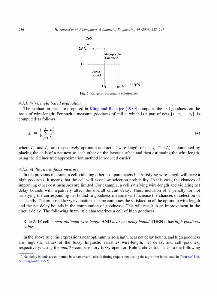
assume that there is a user specified goal vector G ¼ ðg1; g2;…; gpÞ which indicates the relative

acceptable limits for each objective. It means that x will be an acceptable solution if CiðxÞ # giFi where

;i; gi $ 1:0: For a 2-valued cost vector problem, Fig. 5 shows the region of acceptable solutions.

In the proposed scheme, the acceptable solution set is a fuzzy set. For VLSI cell placement problem of

minimizing three objective criteria, we propose the following rule to determine the membership in the

fuzzy set of acceptable solution.

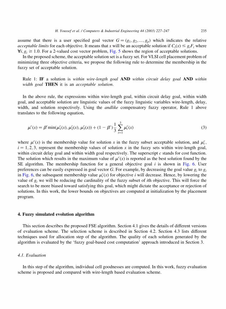
Rule 1: IF a solution is within wire-length goal AND within circuit delay goal AND within

width goal THEN it is an acceptable solution.

In the above rule, the expressions within wire-length goal, within circuit delay goal, within width

goal, and acceptable solution are linguistic values of the fuzzy linguistic variables wire-length, delay,

width, and solution respectively. Using the andlike compensatory fuzzy operator, Rule 1 above

translates to the following equation,

mcðxÞ ¼ bcminðmc1ðxÞ;m

c2ðxÞ;m

c3ðxÞÞ þ ð1 2 bcÞ

1

3

X3

i¼1

mci ðxÞ ð3Þ

where mcðxÞ is the membership value for solution x in the fuzzy subset acceptable solution, and mci ;

i ¼ 1; 2; 3; represent the membership values of solution x in the fuzzy sets within wire-length goal,

within circuit delay goal and within width goal respectively. The superscript c stands for cost function.

The solution which results in the maximum value of mcðxÞ is reported as the best solution found by the

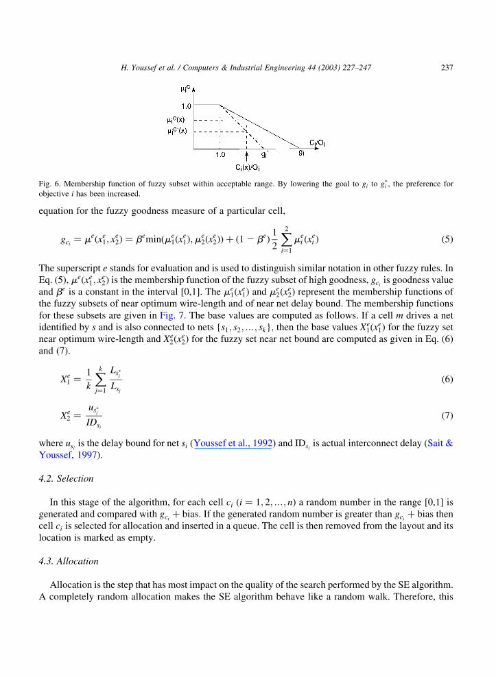
SE algorithm. The membership function for a general objective goal i is shown in Fig. 6. User

preferences can be easily expressed in goal vector G. For example, by decreasing the goal value gi to gi

in Fig. 6, the subsequent membership value mci ðxÞ for objective i will decrease. Hence, by lowering the

value of gi we will be reducing the cardinality of the fuzzy subset of ith objective. This will force the

search to be more biased toward satisfying this goal, which might dictate the acceptance or rejection of

solutions. In this work, the lower bounds on objectives are computed at initialization by the placement

program.

4. Fuzzy simulated evolution algorithm

This section describes the proposed FSE algorithm. Section 4.1 gives the details of different versions

of evaluation scheme. The selection scheme is described in Section 4.2. Section 4.3 lists different

techniques used for allocation step of the algorithm. The quality of each solution generated by the

algorithm is evaluated by the ‘fuzzy goal-based cost computation’ approach introduced in Section 3.

4.1. Evaluation

In this step of the algorithm, individual cell goodnesses are computed. In this work, fuzzy evaluation

scheme is proposed and compared with wire-length based evaluation scheme.

H. Youssef et al. / Computers & Industrial Engineering 44 (2003) 227–247 235

4.1.1. Wirelength based evaluation

The evaluation measure proposed in Kling and Banerjee (1989) computes the cell goodness on the

basis of wire-length. For such a measure, goodness of cell ci which is a part of nets {s1; s2;…; sk}; is

computed as follows.

gci¼

1

k

Xk

j¼1

Lpsj

Lsj

ð4Þ

where Lpsj

and Lsjare respectively optimum and actual wire-length of net sj: The Lp

siis computed by

placing the cells of a net next to each other on the layout surface and then estimating the wire-length,

using the Steiner tree approximation method introduced earlier.

4.1.2. Multicriteria fuzzy measure

In the previous measure, a cell violating other cost parameters but satisfying wire-length will have a

high goodness. It means that the cell will have low selection probability. In this case, the chances of

improving other cost measures are limited. For example, a cell satisfying wire-length and violating net

delay bounds will negatively affect the overall circuit delay. Thus, inclusion of a penalty for not

satisfying the corresponding net bound in goodness measure will increase the chances of selection of

such cells. The proposed fuzzy evaluation scheme combines the satisfaction of the optimum wire-length

and the net delay bounds in the computation of goodness.3 This will result in an improvement in the

circuit delay. The following fuzzy rule characterizes a cell of high goodness.

Rule 2: IF cell is near optimum wire-length AND near net delay bound THEN it has high goodness

value.

In the above rule, the expressions near optimum wire-length, near net delay bound, and high goodness

are linguistic values of the fuzzy linguistic variables wire-length, net delay, and cell goodness

respectively. Using the andlike compensatory fuzzy operator, Rule 2 above translates to the following

Fig. 5. Range of acceptable solution set.

3 Net delay bounds are computed based on overall circuit timing requirement using the algorithm introduced in (Youssef, Lin,

& Shragowitz, 1992).

H. Youssef et al. / Computers & Industrial Engineering 44 (2003) 227–247236

equation for the fuzzy goodness measure of a particular cell,

gci¼ meðxe

1; xe2Þ ¼ beminðme

1ðxe1Þ;m

e2ðx

e2ÞÞ þ ð1 2 beÞ

1

2

X2

i¼1

mei ðx

ei Þ ð5Þ

The superscript e stands for evaluation and is used to distinguish similar notation in other fuzzy rules. In

Eq. (5), meðxe1; x

e2Þ is the membership function of the fuzzy subset of high goodness, gci

is goodness value

and be is a constant in the interval [0,1]. The me1ðx

e1Þ and me

2ðxe2Þ represent the membership functions of

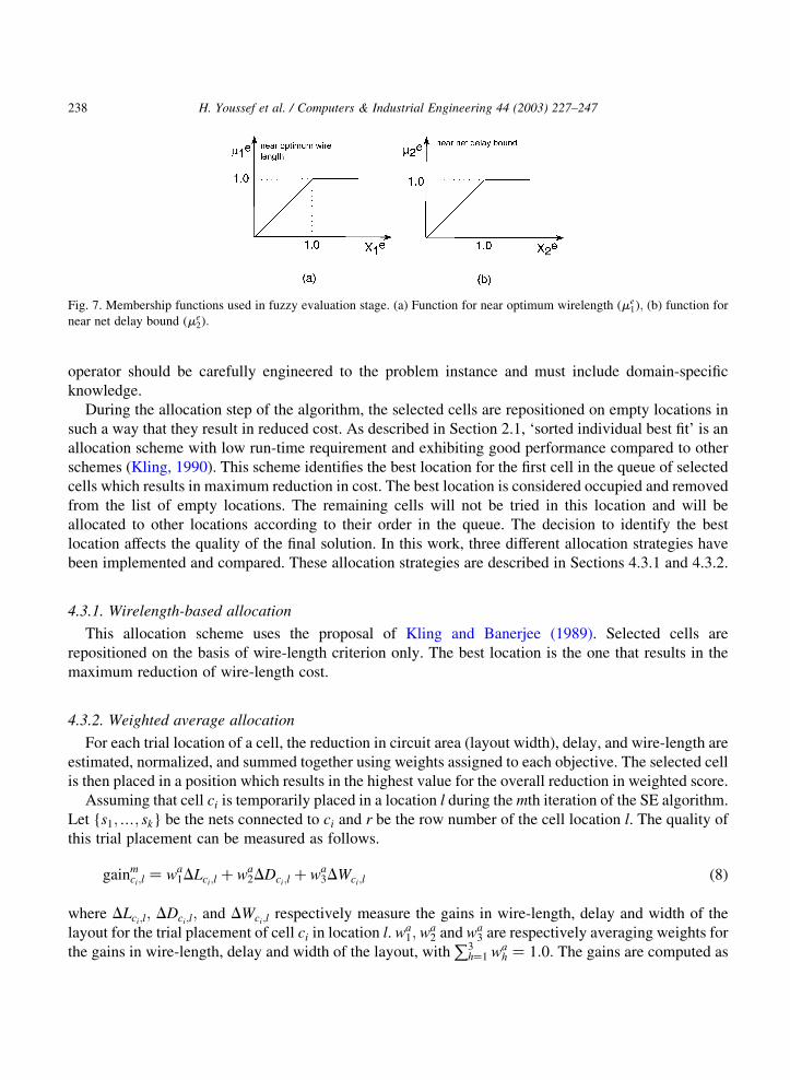
the fuzzy subsets of near optimum wire-length and of near net delay bound. The membership functions

for these subsets are given in Fig. 7. The base values are computed as follows. If a cell m drives a net

identified by s and is also connected to nets {s1; s2;…; sk}; then the base values Xe1ðx

e1Þ for the fuzzy set

near optimum wire-length and Xe2ðx

e2Þ for the fuzzy set near net bound are computed as given in Eq. (6)

and (7).

Xe1 ¼

1

k

Xk

j¼1

Lspj

Lsj

ð6Þ

Xe2 ¼

uspi

IDsi

ð7Þ

where usiis the delay bound for net si (Youssef et al., 1992) and IDsi

is actual interconnect delay (Sait &

Youssef, 1997).

4.2. Selection

In this stage of the algorithm, for each cell ci ði ¼ 1; 2;…; nÞ a random number in the range [0,1] is

generated and compared with gciþ bias: If the generated random number is greater than gci

þ bias then

cell ci is selected for allocation and inserted in a queue. The cell is then removed from the layout and its

location is marked as empty.

4.3. Allocation

Allocation is the step that has most impact on the quality of the search performed by the SE algorithm.

A completely random allocation makes the SE algorithm behave like a random walk. Therefore, this

Fig. 6. Membership function of fuzzy subset within acceptable range. By lowering the goal to gi to gpi , the preference for

objective i has been increased.

H. Youssef et al. / Computers & Industrial Engineering 44 (2003) 227–247 237

operator should be carefully engineered to the problem instance and must include domain-specific

knowledge.

During the allocation step of the algorithm, the selected cells are repositioned on empty locations in

such a way that they result in reduced cost. As described in Section 2.1, ‘sorted individual best fit’ is an

allocation scheme with low run-time requirement and exhibiting good performance compared to other

schemes (Kling, 1990). This scheme identifies the best location for the first cell in the queue of selected

cells which results in maximum reduction in cost. The best location is considered occupied and removed

from the list of empty locations. The remaining cells will not be tried in this location and will be

allocated to other locations according to their order in the queue. The decision to identify the best

location affects the quality of the final solution. In this work, three different allocation strategies have

been implemented and compared. These allocation strategies are described in Sections 4.3.1 and 4.3.2.

4.3.1. Wirelength-based allocation

This allocation scheme uses the proposal of Kling and Banerjee (1989). Selected cells are

repositioned on the basis of wire-length criterion only. The best location is the one that results in the

maximum reduction of wire-length cost.

4.3.2. Weighted average allocation

For each trial location of a cell, the reduction in circuit area (layout width), delay, and wire-length are

estimated, normalized, and summed together using weights assigned to each objective. The selected cell

is then placed in a position which results in the highest value for the overall reduction in weighted score.

Assuming that cell ci is temporarily placed in a location l during the mth iteration of the SE algorithm.

Let {s1;…; sk} be the nets connected to ci and r be the row number of the cell location l. The quality of

this trial placement can be measured as follows.

gainmci;l ¼ wa

1DLci;l þ wa2DDci;l þ wa

3DWci;l ð8Þ

where DLci;l; DDci;l; and DWci;l respectively measure the gains in wire-length, delay and width of the

layout for the trial placement of cell ci in location l. wa1; wa

2 and wa3 are respectively averaging weights for

the gains in wire-length, delay and width of the layout, withP3

h¼1 wah ¼ 1:0: The gains are computed as

Fig. 7. Membership functions used in fuzzy evaluation stage. (a) Function for near optimum wirelength ðme1Þ; (b) function for

near net delay bound ðme2Þ:

H. Youssef et al. / Computers & Industrial Engineering 44 (2003) 227–247238

follows:

DLci;l ¼

Pkj¼1ðL

m21sj

2 LmsjÞPk

j¼1Lm21sj

ð9Þ

DDci;l ¼

Pkj¼1ðD

m21sj

2 DmsjÞPk

j¼1Dm21sj

ð10Þ

DWci;l ¼Wopt 2 Wm

r

Wopt

ð11Þ

In Eq. (9), Lm21sj

and Lmsj

are respectively wire-length estimates for net sj in m 2 1st and mth iterations of

the SE algorithm. Similarly Dm21sj

and Dmsj

in Eq. (10) are propagation delays for net sj in m 2 1st and mth

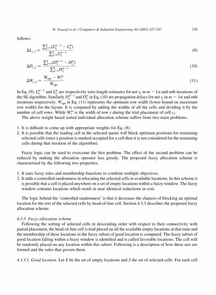
iterations respectively. Wopt in Eq. (11) represents the optimum row width (lower bound on maximum

row width) for the layout. It is computed by adding the widths of all the cells and dividing it by the

number of cell rows. While Wmr is the width of row r during the trial placement of cell ci:

The above weight based sorted individual allocation scheme suffers from two main problems.

1. It is difficult to come up with appropriate weights for Eq. (8).

2. It is possible that the leading cell in the selected queue will block optimum positions for remaining

selected cells (once a position is marked occupied for a cell then it is not considered for the remaining

cells during that iteration of the algorithm).

Fuzzy logic can be used to overcome the first problem. The effect of the second problem can be

reduced by making the allocation operator less greedy. The proposed fuzzy allocation scheme is

characterized by the following two properties.

1. It uses fuzzy rules and membership functions to combine multiple objectives.

2. It adds a controlled randomness in relocating the selected cells in available locations. In this scheme it

is possible that a cell is placed anywhere on a set of empty locations within a fuzzy window. The fuzzy

window contains locations which result in near identical reductions in cost.

The logic behind the ‘controlled randomness’ is that it decreases the chances of blocking an optimal

location for the rest of the selected cells by head-of-line cell. Section 4.3.3 describes the proposed fuzzy

allocation scheme.

4.3.3. Fuzzy allocation scheme

Following the sorting of selected cells in descending order with respect to their connectivity with

partial placement, the head-of-line cell is trial placed on all the available empty locations at that time and

the membership of these locations in the fuzzy subset of good location is computed. The fuzzy subset of

good location falling within a fuzzy window is identified and is called favorable locations. The cell will

be randomly placed on any location within this subset. Following is a description of how these sets are

formed and the rules that govern them.

4.3.3.1. Good location. Let E be the set of empty locations and S the set of selected cells. For each cell

H. Youssef et al. / Computers & Industrial Engineering 44 (2003) 227–247 239

ci [ S; a location l [ E will be a member in the fuzzy set good location with membership function

maciðlÞ: The determination of this membership function is expressed by the following fuzzy rule:

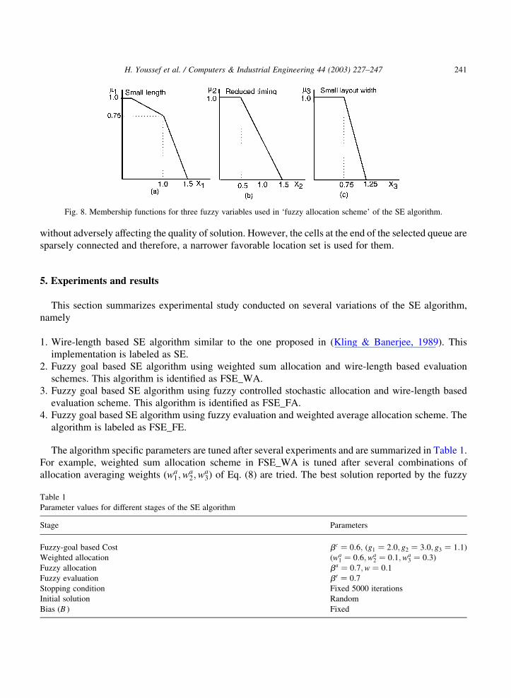
Rule 3: IF a location results in small length AND reduced timing AND small layout width THEN it is

a good location.

Using the andlike compensatory fuzzy operator, Rule 3 above translates to the following equation for

the membership of a given cell ci is the fuzzy subset good location:

maciðlÞ ¼ baminðma

1ðlÞ;ma2ðlÞ;m

a3ðlÞÞ þ ð1 2 baÞ

1

3

X3

i¼1

mai ðlÞ ð12Þ

where maciðlÞ is the fuzzy set of good locations and ba is a constant parameter in the range [0,1]. The

values mai ðlÞ; i ¼ 1; 2; 3; are the membership values of location l in fuzzy sets small length, reduced

timing and small layout width respectively. The base values XiðlÞ; for the membership functions mai ðlÞ;

i ¼ 1; 2; 3; are computed below using the notation of Eqs. (9)–(11).

X1ðlÞ ¼

Pkj¼1Lm

sjPkj¼1Lm21

sj

ð13Þ

X2ðlÞ ¼

Pkj¼1Dm

sjPkj¼1Dm21

sj

ð14Þ

X3ðlÞ ¼Wm

r

Wopt

ð15Þ

The above base variables XiðlÞ; i ¼ 1; 2; 3 constitute measures of the improvement in wire-length,

timing, and width if cell ci is assigned to location l. Following the computation of the base values,

memberships in respective fuzzy sets are determined using the functions given in Fig. 8. These functions

are tuned after several experiments.

4.3.3.2. Favorable locations. A subset of the fuzzy set good locations is named as favorable locations.

The upper and lower boundaries for favorable locations are determined by a fuzzy window. For a cell

ci [ S; location l [ E will fall within fuzzy window if it satisfies the following inequality:

max;e[E

ðmaciðeÞÞ 1:0 2 w

No: of unplaced cells

No: of selected cells

� �# ma

ciðlÞ # max

;e[Eðma

ciðeÞÞ ð16Þ

where E is the set of empty locations, S is the set of selected cells and w is a small positive value which

determines the lower limit of maciðlÞ for presence in fuzzy window. It controls the randomness in the fuzzy

allocation scheme. All locations falling in the fuzzy window will be identified as favorable locations.

The cell will be placed randomly in any of the locations within this set. The presence of the ratio of

number of unplaced cells to selected cells will make sure that the size of favorable location set will

decrease as allocation progresses. At the beginning of allocation all selected cells are unplaced and the

ratio is equal to 1. Therefore, since the head-of-line cell is strongly connected with the partial layout,

there will be many locations with near identical gains. The cell can be placed on any of these locations

H. Youssef et al. / Computers & Industrial Engineering 44 (2003) 227–247240

without adversely affecting the quality of solution. However, the cells at the end of the selected queue are

sparsely connected and therefore, a narrower favorable location set is used for them.

5. Experiments and results

This section summarizes experimental study conducted on several variations of the SE algorithm,

namely

1. Wire-length based SE algorithm similar to the one proposed in (Kling & Banerjee, 1989). This

implementation is labeled as SE.

2. Fuzzy goal based SE algorithm using weighted sum allocation and wire-length based evaluation

schemes. This algorithm is identified as FSE_WA.

3. Fuzzy goal based SE algorithm using fuzzy controlled stochastic allocation and wire-length based

evaluation scheme. This algorithm is identified as FSE_FA.

4. Fuzzy goal based SE algorithm using fuzzy evaluation and weighted average allocation scheme. The

algorithm is labeled as FSE_FE.

The algorithm specific parameters are tuned after several experiments and are summarized in Table 1.

For example, weighted sum allocation scheme in FSE_WA is tuned after several combinations of

allocation averaging weights ðwa1;w

a2;w

a3Þ of Eq. (8) are tried. The best solution reported by the fuzzy

Fig. 8. Membership functions for three fuzzy variables used in ‘fuzzy allocation scheme’ of the SE algorithm.

Table 1

Parameter values for different stages of the SE algorithm

Stage Parameters

Fuzzy-goal based Cost bc ¼ 0:6; ðg1 ¼ 2:0; g2 ¼ 3:0; g3 ¼ 1:1ÞWeighted allocation ðwa

1 ¼ 0:6;wa2 ¼ 0:1;wa

3 ¼ 0:3ÞFuzzy allocation ba ¼ 0:7;w ¼ 0:1Fuzzy evaluation be ¼ 0:7Stopping condition Fixed 5000 iterations

Initial solution Random

Bias (B ) Fixed

H. Youssef et al. / Computers & Industrial Engineering 44 (2003) 227–247 241

goal-based cost measure for each weight combination is identified. As a result, the weights of wa1 ¼ 0:6;

wa2 ¼ 0:1 and wa

3 ¼ 0:3 are used in subsequent runs of FSE_WA for all circuits. These algorithms are

tested on eight ISCAS-85 benchmark circuits. The smallest circuit has 56 cells and the largest has 2243

cells. For all instances of the problem, initial solutions are randomly generated and saved in respective

files. For all experiments the same identical solution is used as initial solution. The experiments are

carried out under identical conditions. The code of the algorithm is written in the C programming

language and executed on Sun Ultra-1 SPARC machines. The values of other constants are given in

Table 2. The solution is represented as a two dimensional array with alternating rows of cells and routing

channels.

5.1. Effect of the size of the fuzzy window on FSE_FA

In the proposed fuzzy allocation scheme, the presence in the fuzzy set favorable locations is bounded

by Eq. (16). The size of this window is controlled by a parameter w. For example if w ¼ 0:1 and

maxðmas ðeÞ ¼ 0:7 then the lower range for the fuzzy window will start from 0.63. It means that all the

locations with membership functions in the fuzzy set good locations in the range ½0:63; 0:7� will be

members of favorable locations. For higher values of w, the size of fuzzy window will increase. In order

to understand the effect of the size of this window on quality of solution, FSE_FA algorithm is executed

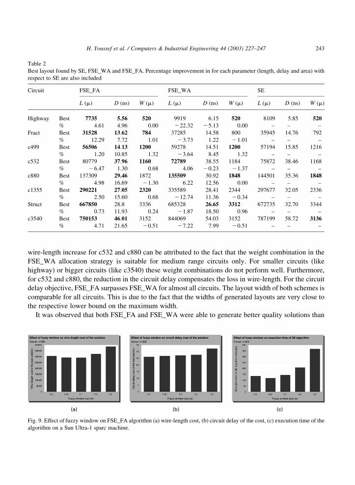
with different values of w. Fig. 9 shows the effect of different fuzzy window sizes on wire-length, delay

and algorithm execution time for circuit c1355. Similar results are obtained for other circuits. From Fig.

9(c), it is clear that by increasing the value of w, the algorithm run-time increases. This is because of

additional computation carried out to maintain the fuzzy set of favorable locations. As clear from Fig.

9(a) and (b) the quality of final solution for small values of w is better than the solution generated by

w ¼ 0: This improvement is due to the fact that the algorithm probabilistically leaves few best locations

for remaining cells in the selected queue. This allows some of the remaining cells to be better placed,

resulting in improvement in the solution quality. At the same time, the window size for leading cells is

small (in the range ½0:05; 0:1�). This ensures that these cells will be placed in near identical quality

positions with respect to the best position. However, for high values of w, quality of the best reported

solution decreases. A large fuzzy window allows the presence of inferior locations in the set favorable

locations. This will make the allocation more random, increasing by the same token the randomness of

the search. From experiments, it is observed that a small value of w ð0:1Þ gives better results for most test

circuits. This value has been used in subsequent runs of FSE_FA.

5.2. Comparison of proposed schemes

In order to see the performance of proposed fuzzy allocation scheme (FSE_FA), it is compared with

two versions of SE algorithm: SE and FSE_WA. SE is implemented as originally reported in Kling and

Banerjee (1989). It is a single objective SE algorithm. SE tries to optimize wire-length only and reports

the solution with the minimum wire-length cost. While FSE_WA is a multi-objective optimization

algorithm and uses weighted average allocation scheme. Both FSE_FA and FSE_WA use a fuzzy-goal

based cost computation to identify the best generated solution.

The cost parameters of the best layout generated by all three schemes are reported in Table 2. It is

clear that except for few cases (like c532 and c880) the proposed fuzzy allocation scheme (FSE_FA) was

able to generate a better quality solution in terms of reduced wire-length cost (L ) than FSE_WA. The

H. Youssef et al. / Computers & Industrial Engineering 44 (2003) 227–247242

wire-length increase for c532 and c880 can be attributed to the fact that the weight combination in the

FSE_WA allocation strategy is suitable for medium range circuits only. For smaller circuits (like

highway) or bigger circuits (like c3540) these weight combinations do not perform well. Furthermore,

for c532 and c880, the reduction in the circuit delay compensates the loss in wire-length. For the circuit

delay objective, FSE_FA surpasses FSE_WA for almost all circuits. The layout width of both schemes is

comparable for all circuits. This is due to the fact that the widths of generated layouts are very close to

the respective lower bound on the maximum width.

It was observed that both FSE_FA and FSE_WA were able to generate better quality solutions than

Table 2

Best layout found by SE, FSE_WA and FSE_FA. Percentage improvement in for each parameter (length, delay and area) with

respect to SE are also included

Circuit FSE_FA FSE_WA SE

L (m) D (ns) W (m) L (m) D (ns) W (m) L (m) D (ns) W (m)

Highway Best 7735 5.56 520 9919 6.15 520 8109 5.85 520

% 4.61 4.96 0.00 222.32 25.13 0.00 – – –

Fract Best 31528 13.62 784 37285 14.58 800 35945 14.76 792

% 12.29 7.72 1.01 23.73 1.22 21.01 – – –

c499 Best 56506 14.13 1200 59278 14.51 1200 57194 15.85 1216

% 1.20 10.85 1.32 23.64 8.45 1.32 – – –

c532 Best 80779 37.96 1160 72789 38.55 1184 75872 38.46 1168

% 26.47 1.30 0.68 4.06 20.23 21.37 – – –

c880 Best 137309 29.46 1872 135509 30.92 1848 144501 35.36 1848

% 4.98 16.69 21.30 6.22 12.56 0.00 – – –

c1355 Best 290221 27.05 2320 335589 28.41 2344 297677 32.05 2336

% 2.50 15.60 0.68 212.74 11.36 20.34 – – –

Struct Best 667850 28.8 3336 685328 26.65 3312 672735 32.70 3344

% 0.73 11.93 0.24 21.87 18.50 0.96 – – –

c3540 Best 750153 46.01 3152 844069 54.03 3152 787199 58.72 3136

% 4.71 21.65 20.51 27.22 7.99 20.51 – – –

Fig. 9. Effect of fuzzy window on FSE_FA algorithm (a) wire-length cost, (b) circuit delay of the cost, (c) execution time of the

algorithm on a Sun Ultra-1 sparc machine.

H. Youssef et al. / Computers & Industrial Engineering 44 (2003) 227–247 243

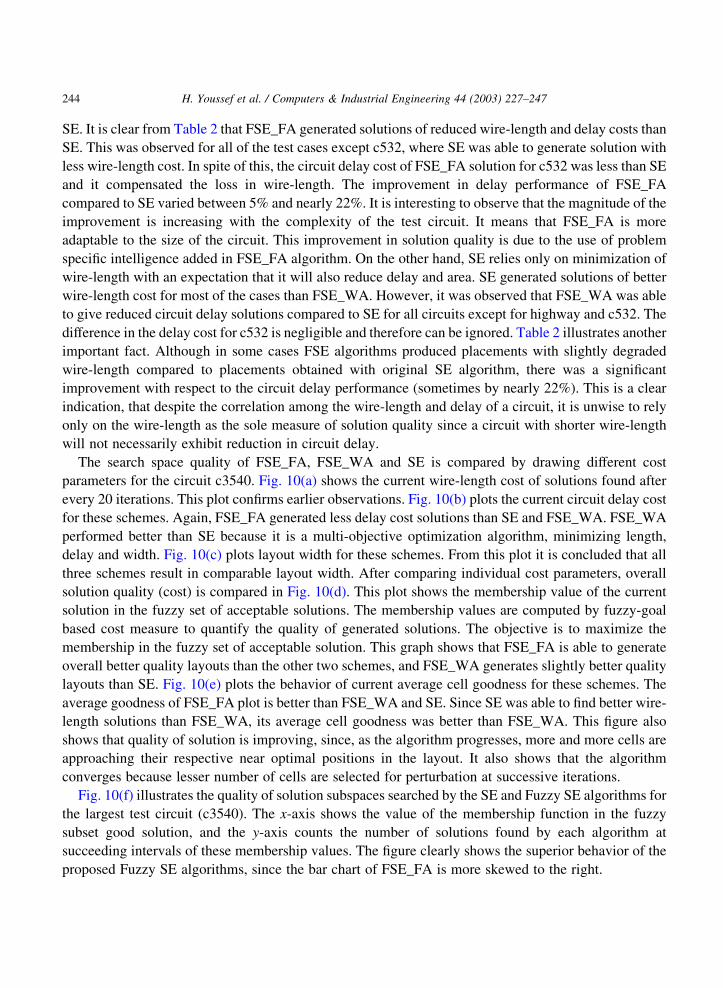
SE. It is clear from Table 2 that FSE_FA generated solutions of reduced wire-length and delay costs than

SE. This was observed for all of the test cases except c532, where SE was able to generate solution with

less wire-length cost. In spite of this, the circuit delay cost of FSE_FA solution for c532 was less than SE

and it compensated the loss in wire-length. The improvement in delay performance of FSE_FA

compared to SE varied between 5% and nearly 22%. It is interesting to observe that the magnitude of the

improvement is increasing with the complexity of the test circuit. It means that FSE_FA is more

adaptable to the size of the circuit. This improvement in solution quality is due to the use of problem

specific intelligence added in FSE_FA algorithm. On the other hand, SE relies only on minimization of

wire-length with an expectation that it will also reduce delay and area. SE generated solutions of better

wire-length cost for most of the cases than FSE_WA. However, it was observed that FSE_WA was able

to give reduced circuit delay solutions compared to SE for all circuits except for highway and c532. The

difference in the delay cost for c532 is negligible and therefore can be ignored. Table 2 illustrates another

important fact. Although in some cases FSE algorithms produced placements with slightly degraded

wire-length compared to placements obtained with original SE algorithm, there was a significant

improvement with respect to the circuit delay performance (sometimes by nearly 22%). This is a clear

indication, that despite the correlation among the wire-length and delay of a circuit, it is unwise to rely

only on the wire-length as the sole measure of solution quality since a circuit with shorter wire-length

will not necessarily exhibit reduction in circuit delay.

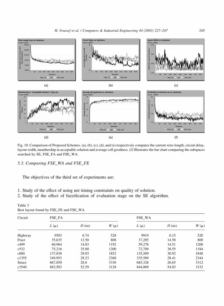
The search space quality of FSE_FA, FSE_WA and SE is compared by drawing different cost

parameters for the circuit c3540. Fig. 10(a) shows the current wire-length cost of solutions found after

every 20 iterations. This plot confirms earlier observations. Fig. 10(b) plots the current circuit delay cost

for these schemes. Again, FSE_FA generated less delay cost solutions than SE and FSE_WA. FSE_WA

performed better than SE because it is a multi-objective optimization algorithm, minimizing length,

delay and width. Fig. 10(c) plots layout width for these schemes. From this plot it is concluded that all

three schemes result in comparable layout width. After comparing individual cost parameters, overall

solution quality (cost) is compared in Fig. 10(d). This plot shows the membership value of the current

solution in the fuzzy set of acceptable solutions. The membership values are computed by fuzzy-goal

based cost measure to quantify the quality of generated solutions. The objective is to maximize the

membership in the fuzzy set of acceptable solution. This graph shows that FSE_FA is able to generate

overall better quality layouts than the other two schemes, and FSE_WA generates slightly better quality

layouts than SE. Fig. 10(e) plots the behavior of current average cell goodness for these schemes. The

average goodness of FSE_FA plot is better than FSE_WA and SE. Since SE was able to find better wire-

length solutions than FSE_WA, its average cell goodness was better than FSE_WA. This figure also

shows that quality of solution is improving, since, as the algorithm progresses, more and more cells are

approaching their respective near optimal positions in the layout. It also shows that the algorithm

converges because lesser number of cells are selected for perturbation at successive iterations.

Fig. 10(f) illustrates the quality of solution subspaces searched by the SE and Fuzzy SE algorithms for

the largest test circuit (c3540). The x-axis shows the value of the membership function in the fuzzy

subset good solution, and the y-axis counts the number of solutions found by each algorithm at

succeeding intervals of these membership values. The figure clearly shows the superior behavior of the

proposed Fuzzy SE algorithms, since the bar chart of FSE_FA is more skewed to the right.

H. Youssef et al. / Computers & Industrial Engineering 44 (2003) 227–247244

5.3. Comparing FSE_WA and FSE_FE

The objectives of the third set of experiments are:

1. Study of the effect of using net timing constraints on quality of solution.

2. Study of the effect of fuzzification of evaluation stage on the SE algorithm.

Fig. 10. Comparison of Proposed Schemes. (a), (b), (c), (d), and (e) respectively compares the current wire-length, circuit delay,

layout width, membership in acceptable solution and average cell goodness. (f) Illustrates the bar chart comparing the subspaces

searched by SE, FSE_FA and FSE_WA.

Table 3

Best layout found by FSE_FE and FSE_WA

Circuit FSE_FA FSE_WA

L (m) D (ns) W (m) L (m) D (ns) W (m)

Highway 9503 6.74 528 9919 6.15 520

Fract 35,635 13.50 808 37,285 14.58 800

c499 60,964 14.83 1192 59,278 14.51 1200

c532 75,216 35.80 1200 72,789 38.55 1184

c880 137,838 29.03 1852 135,509 30.92 1848

c1355 349,953 28.23 2368 335,589 28.41 2344

Struct 667,850 28.8 3336 685,328 26.65 3312

c3540 883,503 52.59 3128 844,069 54.03 3152

H. Youssef et al. / Computers & Industrial Engineering 44 (2003) 227–247 245

FSE_FE uses a fuzzy evaluation scheme in which goodness of an individual cell has two components.

One component is satisfaction of wire-length and the second component represents the satisfaction of the

net timing bounds (constraints). These two components are expressed using a fuzzy rule and appropriate

membership functions. While FSE_WA uses only one component, that is, satisfaction of optimum wire-

length. Both these algorithms use a weighted average allocation scheme described in Section 4.3. The

values of allocation weights are wa1 ¼ 0:6; wa

2 ¼ 0:1 and wa3 ¼ 0:3: The results of this experiment are

summarized in Table 3.

Generally, fuzzy evaluation (FSE_FE) gave inferior results than FSE_WA with respect to wire-

length. However, it was able to reduce the circuit delay for most of the circuits. The wire-length cost of

FSE_FE increased because cells were not selected on the basis of wire-length only. Having a component

for the net constraints satisfaction in cell goodness resulted in non-selection of many wire-length

violating nets. On the other hand, many nets satisfying wire-length constraints were selected because

they were violating the net constraints. These factors resulted in the increase in wire-length.

From this experiment we conclude that net constraints when used with wire-length based goodness

measure in the selection step result in improvement in circuit delay. On the other hand, they cause

increase in wire-length cost.

6. Conclusion

This paper describes a FSE algorithm for VLSI standard-cell placement problem. The proposed

algorithm relies on a novel fuzzy goal-based search approach. This approach avoids the problems

associated with the controversial weighted sum approach. It also allows easy incorporation of user

preferences for different objectives. It offers a practical alternative to dealing with multi-objective

combinatorial optimization problems. We have also used fuzzy logic in the evaluation and allocation

steps of the SE algorithm. The suggested fuzzy allocation approach combines controlled randomness

with the purely constructive sorted individual best fit allocation technique. The identification of

favorable locations for a cell is carried out through the use of fuzzy decision maker. Being the most

important stage of SE algorithm, fuzzy allocation results in noticeable improvement in the quality of

final solution. In the fuzzy evaluation scheme two parameters are combined to compute the goodness of

each cell. The proposed fuzzy SE algorithm produced superior results than those obtained with

traditional SE. For the largest circuit, delay and wire-length improved by nearly 22 and 5% respectively.

Acknowledgements

Authors acknowledge King Fahd University of Petroleum and Minerals, Dhahran, Saudi Arabia, for

all support.

References

Ball, C. F., Kraus, P. V., & Mlynski, D. A. (1994). Fuzzy partitioning applied to VLSI-oorplanning and placement. IEEE

International Symposium on Circuits and Systems, ISCAS, 1, 177–180.

H. Youssef et al. / Computers & Industrial Engineering 44 (2003) 227–247246

Fogel, D. B. (1994). An introduction to simulated evolutionary optimization. IEEE Transactions on Neural Networks, 5(1),

3–14.

Glover, F., & Laguna, M. (1997). Tabu search. Dordrecht: Kluwer Academic Publishers.

Goldberg, D. E. (1989). Genetic algorithms in search, optimization and machine learning. Reading, MA: Addison-Wesley.

Holt, G., & Tyagi, A. (1996). GEEP: A low power genetic algorithm layout system. 39th Mid-west Symposium on Circuits and

Systems, 1337–1340.

Horn, J., Nafpliotis, N., & Goldberg, D. E. (1994). Niched Pareto genetic algorithm for multiobjective optimization.

Proceedings of 1st International Conference on Evolutionary Computation, 82–87.

Kang, Q. E., Lin, R., & Shragowitz, E. (1994). Fuzzy logic approach to VLSI placement. IEEE Transactions on Very Large

Scale Integration (VLSI) Systems, 2(4), 489–501.

Kirkpatrick, S., Gelatt, C., Jr., & Vecchi, M. (1983). Optimization by simulated annealing. Science, 220(4598), 498–516.

Kling, R. M (1990). Optimization by simulated evolution and its application to cell placement. PhD Thesis, University of

Illinois, Urbana.

Kling, R. M., & Banerjee, P. (1989). ESP: Placement by simulated evolution. IEEE Transactions on Computer-Aided Design,

8(3), 245–255.

Kling, R. M., & Banerjee, P. (1991). Empirical and theoretical studies of the simulated evolution method applied to standard

cell placement. IEEE Transactions on Computer-Aided Design, 10(10), 1303–1315.

Lin, R. B., & Shragowitz, E. (1992). Fuzzy Logic Approach to Placement Problem. 29th ACM/ICEE Design Automation

Conference, 153–158.

Mackey, C. A., & Carothers, J. D. (1996). Performance-driven macro cell placement. 15th Annual International Conference on

Computers and Communications, 427–433.

Razaz, M., & Gan, J. (1990). Fuzzy set based initial placement for IC layout. Proceedings of the IEEE European Design

Automation Conference EDAC, 9, 655–659.

Razaz, M. (1993). A fuzzy C-means clustering placement algorithm. IEEE International Symposium on Circuits and Systems,

ISCAS, 3, 2051–2054.

Saab, Y., & Rao, V. (1990). Stochastic evolution: A fast effective heuristic for some generic layout problems. 27th ACM/IEEE

Design Automation Conference, 26–31.

Sait, S. M., & Youssef, H. (1999). Iterative computer algorithms and their application to engineering. Silver Spring, MD: IEEE

Computer Society Press.

Sait, S. M., & Youssef, H. (1995). VLSI physical design automation: Theory and practice. Europe: McGraw-Hill Book

Company, also co-published by IEEE Press, New York.

Sait, S. M., Youssef, H., Nassar, K., & Benten, M. S. T. (1998). Timing driven genetic placement. Computer Systems Sciences

& Engineering, 13(6), 125–133.

Sait, S. M., & Youssef, H. (1997). Timing-in uenced general-cell genetic oorplanner. Micro-electronics Journal, 28(2),

151–166.

Sechen, C., & Sangiovanni-Vincentelli, A. L. (1986). Timberwolf3.2: A new standard cell placement and global routing

package. 23rd Design Automation Conference, 432–439.

Shahookar, K., & Mazumder, P. (1990). A genetic approach to standard cell placement using meta-genetic parameter

optimization. IEEE Transactions on Computer-Aided Design, 9(5), 500–511.

Shahookar, K., & Mazumder, P. (1991). VLSI cell placement techniques. ACM Computing Surveys, 143–220.

Shragowitz, E., Youssef, H., Sait, M. S., & Adiche, H. (1997). Fuzzy genetic algorithm for floorplanning. Proceedings of SPIE,

36–47.

Tao, L., & Zhao, Y. (1993). Multi-way graph partition by stochastic probe. Computers Operations Research, 20(3), 321–347.

Yager, R. R. (1988). On ordered weighted averaging aggregation operators in multicriteria decisionmaking. IEEE Transaction

on Systems, MAN, and Cybernetics, 18(1), 183–190.

Youssef, H., Lin, R., & Shragowitz, E. (1992). Bounds on net delays for VLSI circuits. IEEE Transactions on Circuit and

Systems—II: Analog and Digital Signal Processing, 39(11), 815–824.

Zadeh, L. A. (1965). Fuzzy Sets. Information Control, 8, 338–353.

Zadeh, L. A. (1973). Outline of a new approach to the analysis of complex systems and decision processes. IEEE Transaction

Systems Man and Cybernetics, SMC-3(1), 28–44.

H. Youssef et al. / Computers & Industrial Engineering 44 (2003) 227–247 247