Numerical analysis of some basic fluid communication models via parallel block methods

ELSEVIER

computer communications

Computer Communications 19 (1996) 539-552

Numerical analysis of some basic fluid communication models via parallel block methods

T. Tsiligirides*

Informatics Laboratory, Department of General Sciences, Agricultural University of Athens, Iera Odos 75, Athens 118 55, Greece

Received 17 February 1995; revised 2 June 1995

Abstract

In this work we propose a general method for the solution of some basic delayed feedback schemes used in long haul, high speed data transport. In such cases, simple batch Poisson models do not describe packet delays well, while the propagation delay is now becoming a major factor. Two basic virtual circuit networks of balanced form are examined; the single-hop network which aggregates many virtual circuits in parallel, and the multi-hop virtual circuit network having M nodes in tandem. Using well known adaptive algorithms to dynamically adjust the window size, the above networks are presented as linear systems of some delay differential equations in which the rate of transmission and the queue occupancy are modelled as fluids. Although these systems are locally unstable (in a Liapounov sense), we identify the appropriate scale for the parameters so that the systems will perform near their optimal theoretical values for a wide range of speeds. In addition, we propose a general method for their numerical solution which in reality are large and complex. The approach is based on parallel block methods that are used to solve the systems of the ordinary differential equations in which the original systems of the delay differential equations have been transformed. The basic theory underlying the parallel block methods is developed and numerical stability of low order is deduced.

Keywords: Balanced networks; Virtual circuits; Delay differential equations; Parallel block methods; Stability

1. Introduction

It is well known that the ATM (Asynchronous Traffic Mode), an internationally standardised basis for B- ISDN (Broadband-Integrated Services Digital Network), is a technique best suited to satisfy the requirements of integrated broadband networks. It is the first switching technique capable of supporting both the circuit switching and packet switching approaches within a single integrated switching mechanism. Obviously, any attempt to introduce ATM for data communication must take into consideration existing communication protocols which have been implemented in a wide variety of existing systems. Furthermore, it must also be ensured that the existing data networks are capable of operating as an access to ATM networks. This applies especially to LANs along with their inter working units, such as bridges, routers and gateways. However, these devices will soon be able to convert LAN protocols directly to ATM in order that ATM-based user-network interfaces can be used.

ATM is a switching and multiplexing technique that

* Email: [email protected]

0140-3664/96/$15.00 0 1996 Elsevier Science B.V. All rights reserved PIZ SO140-3664(96)01077-8

uses constant length packets (cells) as the basic data units. An ATM cell, as defined by ITU (formerly CCITT) recommendation 1.361, contains 48 bytes of user information and 5 bytes of control information. The control part, or ‘header’, consists primarily of VPI/VCI (Virtual Path/Channel Identifiers). An ATM virtual channel, as it is available to a user, is uniquely defined by a combination of VP1 and VCI in every transmission system along the path taken by all cells belong- ing to the same connection. Groups of virtual channels with the same VP1 value can be transferred as a virtual path without taking the VCI into consideration. ATM can scale from small multiplexers to very large switches in both an aggregate capacity and in the number of access ports. It can accommodate access ports from low speeds (1.5 Mbps and 6 Mbps) to very high speeds (2.4Gbps). It is designed to handle multimedia traffic and will be deployed in the public network as the future B-ISDN. Obviously, besides the protocols controlling the data transfer traffic control functions, supporting statistical multiplexing plays a key role in exploiting the potential of ATM networks.

Typical data applications that are currently supported

540 T. TsiligiridesjComputer Communications 19 (1996) 539-552

by existing networks, together with a number of future applications that will most likely gain in importance with the introduction of high speed data networks, include real-time video (MPEG), low rate interactive date applications, electronic mail, browsing in graphics databases, animation of graphics, software download, etc. Thus, traffic is often bursty or belongs to multiple classes, such as packetised voice, short data messages, bulk files, etc. However, since the traffic characteristics are unknown, the vast majority of these data applications are incapable of predicting their own bandwidth requirements. Moreover, many of these data applications are relatively tolerant against delays causing quite opposite effects on sojourn time, namely the time a customer spends in the system.

To prevent or reduce overload situations in ATM networks, and to optimise network resources, it has been proposed to use a closed loop feedback control mechanism that allows the network to control the cell emission process at each source. Each virtual connection must have an independent control loop, since each connection may follow a different path through the network. Using feedback control, sending terminals contributing to congestions can be forced to reduce the speed at which they are sending. Two classes of feedback schemes have been proposed. The first is a credit based, link-by-link, per connection window flow control mechanism, while the second is a rate based, end-to-end load control mechanism. Credit based mechanisms are similar to existing data networks (e.g. the sliding window procedures used in X.25 networks). With rate based mechanisms, the maximum rate at which a source may send can be dynamically adapted, depending on network load conditions.

ITU recommendation I.371 provided the possibility to support a rate based reactive load control mechanism by means of EFCI (Explicit Forward Congestion Indica- tion). Congested nodes may set a congestion indication in the cell header of cells that pass congested nodes. The receiving terminal will then relay the congestion information to the sending terminal using a higher layer proto- col. It has also been proposed that the receiving terminal could use resource management cells for this purpose. Resource management cells indicating congestion could also be sent directly from congested nodes to the terminal, thus providing BECI (Backward Explicit Conges- tion Indication).

The major problem of reactive close loop control in high speed wide area networks is the large amount of data (equal to the delay-bandwidth-product) that may be under way in the network. In wide area high-speed networks, the fibres used for transmission become large buffers that cannot be easily controlled. Note that a multiplexer may be fed by a number of high speed links, each of which can store a large amount of data. For example, 0.28 Mbytes of data can be on its way in a

fibre of 3000 km in length operating at 150 Mbps. Under unfavourable conditions, a congested multiplexer indicating congestion may have to buffer many Mbytes before the congestion indication will show any effect. On the other hand, the load situation may have changed by the time the control mechanism has taken effect. In particular, this is a problem when round trip delays are large. Thus, with the ever increasing speeds in data transmission the round trip propagation delay is now becoming a major factor. A further example in long haul, high speed data transport is the case of a virtual circuit network in which the service is always available, and in which sequenced delivery of packets in either direction between the two end users is ensured. Assuming the propagation delay is neglected, the sliding window mechanism to control the congestion may be applied [1,2]. However, if the propagation delay cannot be neglected, new design procedures have to be established. Much work to date on flow control in high-speed networks may be found elsewhere [3-81.

Propagation delays do exist in geographically dis- persed long haul data networks. For example, in US the round trip propagation delay through a fibre link is approximately 47-ms (one round trip propagation delay is approximately the distance across the continental US divided by the speed of light). With a transmission rate of 45 Mbits/s and packet size of 1 Kbyte a representative service rate p of 264 for the various nodes is obtained. At the other end, with the optical transmission rate of 1.7 Gbits/s, and keeping the other two parameters constant, p is about 9989. Clearly, high transmission rates and non-scalable propagation delays give rise to large p. An interesting asymptotic analysis has been developed [9] to face the problem of scaling. As it appears, keeping delay and packet loss within acceptable levels, high effi- ciency cannot be provided using only static (non adaptive to the variations of traffic) control schemes. Thus, dynamic schemes that adaptively conform to the traffic environment are always used. In such schemes the large propagation delays and the high speeds must be included in the analysis. Several dynamic algorithms for congestion control/avoidance already exist in the literature [lo- 161, but the following is of interest here.

Fendic et al. [lo] studied the stability properties of a large class of dynamic control algorithms with delayed feedback, as well as how parameters should scale with the speed. The analysis was restricted to a single session and a single bottleneck node to avoid complexities (see Fig. 1). The network has been presented as a system of DDEs (Delay Differential Equations) in which the rate of transmission and the queue occupancy are modelled as fluids. It is assumed that the acknowledgements carry information about the state of the queue at the bottleneck node, and that this information is used to control the transmission rate through a control function which may not be linear. Note that, in general, the standard

T. TsiligiridesjComputer Communications 19 (1996) 539-552 541

Source Node

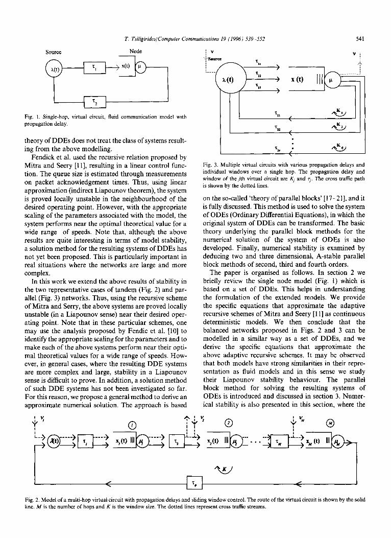
Fig. 1. Single-hop, virtual circuit, fluid communication model with propagation delay.

theory of DDEs does not treat the class of systems resulting from the above modelling.

Fendick et al. used the recursive relation proposed by Mitra and Seery [l 11, resulting in a linear control function The queue size is estimated through measurements on packet acknowledgement times. Thus, using linear approximation (indirect Liapounov theorem), the system is proved locally unstable in the neighbourhood of the desired operating point. However, with the appropriate scaling of the parameters associated with the model, the system performs near the optimal theoretical value for a wide range of speeds. Note that, although the above results are quite interesting in terms of model stability, a solution method for the resulting systems of DDEs has not yet been proposed. This is particularly important in real situations where the networks are large and more complex.

In this work we extend the above results of stability in the two representative cases of tandem (Fig. 2) and parallel (Fig. 3) networks. Thus, using the recursive scheme of Mitra and Serry, the above systems are proved locally unstable (in a Liapounov sense) near their desired operating point. Note that in these particular schemes, one may use the analysis proposed by Fendic et al. [lo] to identify the appropriate scaling for the parameters and to make each of the above systems perform near their optimal theoretical values for a wide range of speeds. How- ever, in general cases, where the resulting DDE systems are more complex and large, stability in a Liapounov sense is difficult to prove. In addition, a solution method of such DDE systems has not been investigated so far. For this reason, we propose a general method to derive an approximate numerical solution. The approach is based

.

. ‘Iti ; 45 \

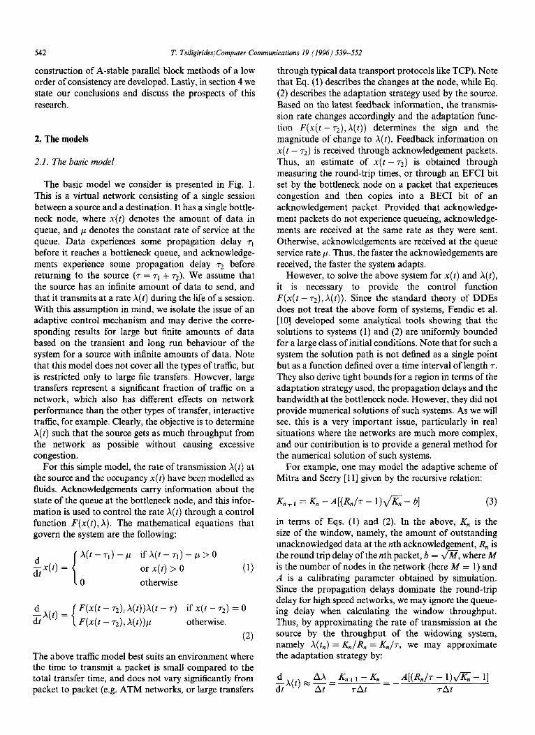
Fig. 3. Multiple virtual circuits with various propagation delays and individual windows over a single hop. The propagation delay and window of the jth virtual circuit are Kj and q. The cross traffic path is shown by the dotted lines.

on the so-called ‘theory of parallel blocks’ [ 17-211, and it is fully discussed. This method is used to solve the system of ODES (Ordinary Differential Equations), in which the original system of DDEs can be transformed. The basic theory underlying the parallel block methods for the numerical solution of the system of ODES is also developed. Finally, numerical stability is examined by deducing two and three dimensional, A-stable parallel block methods of second, third and fourth orders.

The paper is organised as follows. In section 2 we brietly review the single node model (Fig. 1) which is based on a set of DDEs. This helps in understanding the formulation of the extended models. We provide the specific equations that approximate the adaptive recursive schemes of Mitra and Seery [l l] as continuous deterministic models. We then conclude that the balanced networks proposed in Figs. 2 and 3 can be modelled in a similar way as a set of DDEs, and we derive the specific equations that approximate the above adaptive recursive schemes. It may be observed that both models have strong similarities in their repre- sentation as fluid models and in this sense we study their Liapounov stability behaviour. The parallel block method for solving the resulting systems of ODES is introduced and discussed in section 3. Numer- ical stability is also presented in this section, where the

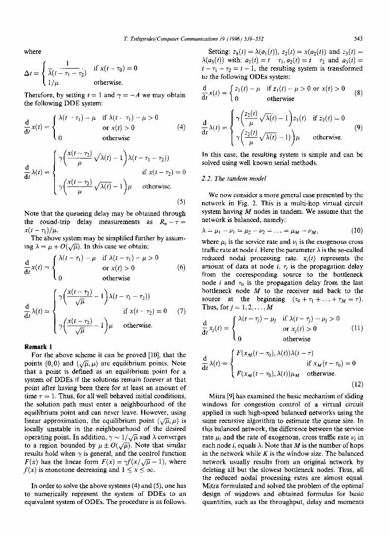
Fig. 2. Model of a multi-hop virtual circuit with propagation delays and sliding window control. The route of the virtual circuit is shown by the solid line. M is the number of hops and K is the window size. The dotted lines represent cross traffic streams.

542 T. TsiligirideslComputer Communications 19 (1996) 539-552

construction of A-stable parallel block methods of a low order of consistency are developed. Lastly, in section 4 we state our conclusions and discuss the prospects of this research.

2. The models

2.1. The basic model

The basic model we consider is presented in Fig. 1. This is a virtual network consisting of a single session between a source and a destination. It has a single bottleneck node, where x(t) denotes the amount of data in queue, and p denotes the constant rate of service at the queue. Data experiences some propagation delay r1 before it reaches a bottleneck queue, and acknowledgements experience some propagation delay r2 before returning to the source (T = 7-i + ~~2). We assume that the source has an infinite amount of data to send, and that it transmits at a rate x(t) during the life of a session. With this assumption in mind, we isolate the issue of an adaptive control mechanism and may derive the corresponding results for large but finite amounts of data based on the transient and long run behaviour of the system for a source with infinite amounts of data. Note that this model does not cover all the types of traffic, but is restricted only to large file transfers. However, large transfers represent a significant fraction of traffic on a network, which also has different effects on network performance than the other types of transfer, interactive traffic, for example. Clearly, the objective is to determine x(t) such that the source gets as much throughput from the network as possible without causing excessive congestion.

For this simple model, the rate of transmission x(t) at the source and the occupancy x(t) have been modelled as fluids. Acknowledgements carry information about the state of the queue at the bottleneck node, and this information is used to control the rate A(t) through a control function P(x( t), A). The mathematical equations that govern the system are the following:

$x(t) =

(

x(t-7,)-p ifX(t-rl)-->O

or x(t) > 0 (1)

0 otherwise

$X(t) = {

F(x(t - TV), A(t))x(t - T) if x(t - 7-*) = 0

F(x(t - 72),X(4)P otherwise.

(2)

The above traffic model best suits an environment where the time to transmit a packet is small compared to the total transfer time, and does not vary significantly from packet to packet (e.g. ATM networks, or large transfers

through typical data transport protocols like TCP). Note that Eq. (1) describes the changes at the node, while Eq. (2) describes the adaptation strategy used by the source. Based on the latest feedback information, the transmission rate changes accordingly and the adaptation function F(x(l - TV), x(t)) determines the sign and the magnitude of change to x(t). Feedback information on x(t - ~~2) is received through acknowledgement packets. Thus, an estimate of x(t - TV) is obtained through measuring the round-trip times, or through an EFCI bit set by the bottleneck node on a packet that experiences congestion and then copies into a BECI bit of an acknowledgement packet. Provided that acknowledgement packets do not experience queueing, acknowledgements are received at the same rate as they were sent. Otherwise, acknowledgements are received at the queue service rate CL. Thus, the faster the acknowledgements are received, the faster the system adapts.

However, to solve the above system for x(t) and x(t), it is necessary to provide the control function F(x( t - TV), A(t)). Since the standard theory of DDEs does not treat the above form of systems, Fendic et al. [lo] developed some analytical tools showing that the solutions to systems (1) and (2) are uniformly bounded for a large class of initial conditions. Note that for such a system the solution path is not defined as a single point but as a function defined over a time interval of length T. They also derive tight bounds for a region in terms of the adaptation strategy used, the propagation delays and the bandwidth at the bottleneck node. However, they did not provide mumerical solutions of such systems. As we will see, this is a very important issue, particularly in real situations where the networks are much more complex, and our contribution is to provide a general method for the numerical solution of such systems.

For example, one may model the adaptive scheme of Mitra and Seery [ 1 l] given by the recursive relation:

K n+i =&-A[(&+1)&-b] (3)

in terms of Eqs. (1) and (2). In the above, K, is the size of the window, namely, the amount of outstanding unacknowledged data at the nth acknowledgement, R, is the round trip delay of the nth packet, b = a, where M is the number of nodes in the network (here M = 1) and A is a calibrating parameter obtained by simulation. Since the propagation delays dominate the round-trip delay for high speed networks, we may ignore the queueing delay when calculating the window throughput. Thus, by approximating the rate of transmission at the source by the throughput of the widowing system, namely A(&,) = KJR, = KJT, we may approximate the adaptation strategy by:

AA &+I-& -$(t)=at= = _ A[(&/r - l)a - 11 TAt -rat

T. TsiligiridesjComputer Communications 19 (19961 539-552 543

where

1

At = A(t - ,rl - ~~‘2) if x(t - ~a) = 0

otherwise.

Therefore, by setting t = 1 and y = -A we may obtain the following DDE system:

Setting: z,(t) = A(q(t)), zz(t) = x(az(t)) and z3(t) = A(a,(t)) with: al(t) = t - ~~,az(t) = t - 72 and q(t) = t - q - r2 = t - 1, the resulting system is transformed to the following ODES system:

$x(t) = zl(t) -p if zl(t) -p > 0 or x(t) > 0

0 otherwise (8)

$x(t) =

X(t-7i)--p ifX(t-7i)--->O

$X(t) = Y ($m-- l)z,(t) if z2(t) = 0

or x(t) > 0 (4) (9) 0 otherwise Y r$ m - 1)) p otherwise.

I 7

$X(t) =

x(t ; 72) Jqq - 1) A( t - 7-l - 72))

if x(t - 72) = 0

Y X(t /I 72) m - 1) ,u otherwise.

(5) Note that the queueing delay may be obtained through the round-trip delay measurements as R, - 7 =

x(t - Tl )/CL. The above system may be simplified further by assum-

ing X = p + O(@). In this case we obtain:

$x(t) =

X(t-7,)-p ifX(t-3-i)--->>

or x(t) > 0 (6)

0 otherwise

-&A(t) = I ifx(t-7*)=0 (7)

y otherwise.

Remark 1 For the above scheme it can be proved [lo], that the

points (0,O) and (,/i&p) are equilibrium points. Note that a point is defined as an equilibrium point for a system of DDEs if the solutions remain forever at that point after having been there for at least an amount of time 7 = 1. Thus, for all well behaved initial conditions, the solution path must enter a neighbourhood of the equilibrium point and can never leave. However, using linear approximation, the equilibrium point (fi, p) is locally unstable in the neighbourhood of the desired operating point. In addition, y N l/& and X converges to a region bounded by p f 0( &). Note that similar results hold when y is general, and the control function F(x) has the linear form F(x) = $(x/d - l), where f(x) is monotone decreasing and 1 I x 5 co.

In order to solve the above systems (4) and (5), one has to numerically represent the system of DDEs to an equivalent system of ODES. The procedure is as follows.

In this case, the resulting system is simple and can be solved using well known serial methods.

2.2. The tandem model

We now consider a more general case presented by the network in Fig. 2. This is a multi-hop virtual circuit system having M nodes in tandem. We assume that the network is balanced, namely:

x = pi - vi = & - v2 = . . . = PM - I/M, (10)

where pi is the service rate and Vi is the exogenous cross traffic rate at node i. Here the parameter X is the so-called reduced nodal processing rate. xi(t) represents the amount of data at node i, Ti is the propagation delay from the corresponding source to the bottleneck node i and 7. is the propagation delay from the last bottleneck node M to the receiver and back to the source at the beginning (70 + 71 + . . . + TM = 7). Thus,forj= 1,2 ,..., M

%Xj(t) =

i

X( t - q) - & if X( t - 7j) - pj > 0

or xj(t) > 0 (11)

0 otherwise

$x(t) =

i

F(xM(t - TO), x(t))x(t - T,

ifxM(t-To)=0

P(xM(t - To), ii(t))p, otherwise.

(12)

Mitra [9] has examined the basic mechanism of sliding windows for congestion control of a virtual circuit applied in such high-speed balanced networks using the same recursive algorithm to estimate the queue size. In this balanced network, the difference between the service rate pi and the rate of exogenous, cross traffic rate Vi in each node i, equals X. Note that M is the number of hops in the network while K is the window size. The balanced network usually results from an original network by deleting all but the slowest bottleneck nodes. Thus, all the ‘reduced nodal processing rates are almost equal. Mitra formulated and solved the problem of the optimal design of windows and obtained formulas for basic quantities, such as the throughput, delay and moments

544 T. Tsiligirides/Computer Communications 19 (1996) 539-552

of packet queues. He showed that the optimum window size if X + O(a). All his results are asymptotic and are based on a design equation which relates the mean response to the window size. This equation is used to adjust the window based on measurements. It is interesting to note that the asymptotic theory developed can be extended to non-balanced networks as well.

Again, one may model the adaptive scheme of Mitra and Serry [l l] in terms of Eqs. (11) and (12). The recursive relation is now given by:

K n+l =Kn -A[(R&- I)&- @I, (13)

where K,,, R, and A have been defined previously. From the above it is clear that the rate of acknowledgements will also dictate the rate of adaptation. Thus, when packets find all the queues empty, acknowledgements return at the same rate as the packets that are being acknowledged when transmitted.

Alternatively, when packets find any of the queues non-empty, it is assumed that acknowledgements return at the rate at which packets are served at the Mth queue. Note that, since the propagation delays dominate the round trip delay, the queueing delays at various nodes may be ignored when calculating the window throughput. Therefore, A(&) = KJR, = K,/T. However, the queueing delays may be obtained through the round trip delay measurements at each node; namely at the Mth node: R,, -7 = xM(t - ~)/p~.

Thus, we can approximate the adaptation strategy by:

Ax &+I-Kn t&(t) E-&= = -A[(R&- 1)x& - fll

TAt 7At

where the time between adaptations is determined by:

At=

1

1

x(t - 71 - 3-2 - . . . - 7, - T())

ifx&t-rO) =0

l/W otherwise.

Taking into account Eq. (10) and setting t = 1 and y= -A for allj= 1,2,... , M, we obtain the following DDEs system:

-$(t) =

X(t_7j)-/lj ifA(t-7j)--j>O

or Xj(t) > 0 (14)

0 otherwise

’ Y

iA(t) = <

xX(t - 71 - . . . - 7-M - To))

ifx,(t-To)=0

Y x~;;Q@-&+&

\ otherwise. (15)

The above system has M + 1 equations and A4 + 1 unknowns, namely, the A(t) and Xj(t); i = 1,. . . , M. It may be simplified further by assuming that pj are all equal with CL, a representative service rate, and X = p+ O(G). In this case we obtain:

[ A(t - 7j) - p if x(t - 7j) - p > 0

~Xj(t) =

1

or Xj(t) > 0 (16)

l0 otherwise

I Y ( XY(& 70) _ a)

$(t) =

xA(t - 7-l - . . . - 7-M - To))

ifx,(t-To)=0

I otherwise.

Remark 2

(17)

For the above scheme one may show, using linear approximation (indirect Liapounov theorem), that the equilibrium point:

e’=: (X,Xi,XZ )“.) x&l)== (PL,@G>&G...,~)T

is locally unstable in the neighbourhood of the desired operating point. In addition, y N l/JTi and X converges to a region bounded by ,u & O(G). Note that similar results hold when y is general and the control function is of the linear form: F(x~) = yf(xM/fi - &@), where f(~~) is monotone decreasing and 1 5 xM 5 00.

To solve the above system (14) and (15), one has to numerically represent the system of DDEs to an equivalent system of ODES. The procedure is as follows:

iXj(t) =

Zj(t) - pj if Zj(t) - /..lj > 0

OrXj(t)>OVj=l,2,...,M

0 otherwise

(18) y ix(t) = if z*(t) = 0

Y y m - d%)pM otherwise,

(1% where Zj(t) =A(aj(t)); j= l,...,M; ZM+l(t) =

xdaM+l(t)); Z~+2(t) = x(a,+,(t)), and aj(t) = t - 5;

j=l )...) M; Qf+1(t) = t-3-0; &4+2(t) = t-q -... -rM - 3-o.

As one may observe, in case M is small, the resulting system is simple and can be solved using well known serial methods. However, in case M is large, some

T. TsiligirideslComputer Communications 19 (1996) 539-552 545

more efficient methods have to be derived in order to provide a numerical stable solution. This problem will be faced in the subsequent sections.

2.3. The parallel model

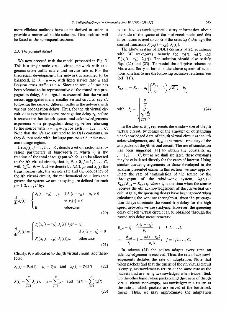
We now proceed with the model presented in Fig. 3. This is a single node virtual circuit network with exogenous cross traffic rate v and service rate p. For the theoretical development, the network is assumed to be balanced, i.e. X = p - Y, with fixed service rate p and Poisson cross traffic rate I/. Since the unit of time has been selected to be representative of the round trip propagation delay, X is large. It is assumed that the virtual circuit aggregates many smaller virtual circuits, say C, following the same or different paths in the network with various propagation delays. Thus, for the jth virtual circuit, data experiences some propagation delay Ttj before it reaches the bottleneck queue, and acknowledgements experience some propagation delay T2j before returning to the source with q = Trj + T2j for each j = 1,2,. . . , C. Note that the 5’s are assumed to be 0( 1) constants, so they do not scale with the large parameter X under mod- erate usage regime.

Letdj(t);j= 1,2,..., C, denote a set of fractional allocation parameters of bandwidth in which 0, is the fraction of the total throughput which is to be allocated to the jth virtual circuit, that is, 0, > 0, j = 1,2,. . . , C, with c,c!l 6” = 1. If we denote by xi(t), pj and xj(t) the transmission rate, the service rate and the occupancy of the jth virtual circuit, the mathematical equations that govern the system we are analysing are defined for each j= 1,2,...,Cby:

gXj(I) =

i

Aj(t_71j)-pj ifAj(t-71j)-pj>O

or Xj(t) > 0

0 otherwise

(20)

(

Fj(xj(t - T2j), xj(t))xj(t - 7j)

$Aj(l) = if Xj(t - T2j) = 0

FjCxjCt - T2j)j),Aj(t))Pj otherwise.

(21)

Clearly, ej is allocated to thejth virtual circuit, and therefore:

xj(t) = 0,x(t), pj = 0jp and xj(t) = ejx(t) (22)

x(t) = gAj(‘)> P = 2Pj and x(t) = gxj(t). j=l j=l j=l

(23)

Note that acknowledgements carry information about the state of the queue at the bottleneck node, and this information is used to control the rates x,(t) through the control functions Fj(Xj(t - 72j), Xi(t)).

The above system of DDEs consists of 2C equations with 3C unknowns, namely the xi(t), xi(t) and Fj(xj(t - 72j), xi(t)). The solution should also satisfy Eqs. (22) and (23). To model the adaptive scheme of Mitra and Seery in terms of the above system of equations, one has to use the following recursive relations (see Ref. [ 111):

Kj,n+l = Kj,n - aj [e-l)&-bj]

with bj = 7j 1 cBi’ (24)

c i=rY

In the above, Kj,n represents the window size of thejth virtual circuit, by means of the amount of outstanding unacknowledged data of the jth virtual circuit at the nth acknowledgement, and Rj,n is the round trip delay of the nth packet of thejth virtual circuit. The use of simulation has been suggested [l l] to obtain the constants aj, j= 1,2 , . . . , C, but as we shall see later, these constants may be calculated directly for the cases of interest. Using similar queueing arguments to those developed in the analysis presented earlier in this section, we may approximate the rate of transmission of the source by the throughput of the windowing system, Aj( tn) =

Kj,,lRj,, = Kj,n/q, where t, is the time when the source receives the nth acknowledgement of the jth virtual circuit. Again, the queueing delays have been ignored when calculating the window throughput, since the propagation delays dominate the round-trip delay for the high speed networks we are studying. However, the queueing delay of each virtual circuit can be obtained through the round-trip delay measurements:

Rj,n - q = xj(f - T2j)

Pj ’ j= 1,2,...,C

R. or E-l= xj(t - 72j)

; j=1,2 ,..., C. 7j Pjui7j

In scheme (24) the source adapts every time an acknowledgement is received. Thus, the rate of acknowledgements dictates the rate of adaptation. Note that when packets find that the queue of the jth virtual circuit is empty, acknowlements return at the same rate as the packets that are being acknowledged when transmitted. On the other hand, when packets find the queue of the jth virtual circuit non-empty, acknowledgements return at the rate at which packets are served at the bottleneck queue. Thus, we may approximate the adaptation

546 T. TsiligirideslComputer Communicafions 19 (1996) 539-552

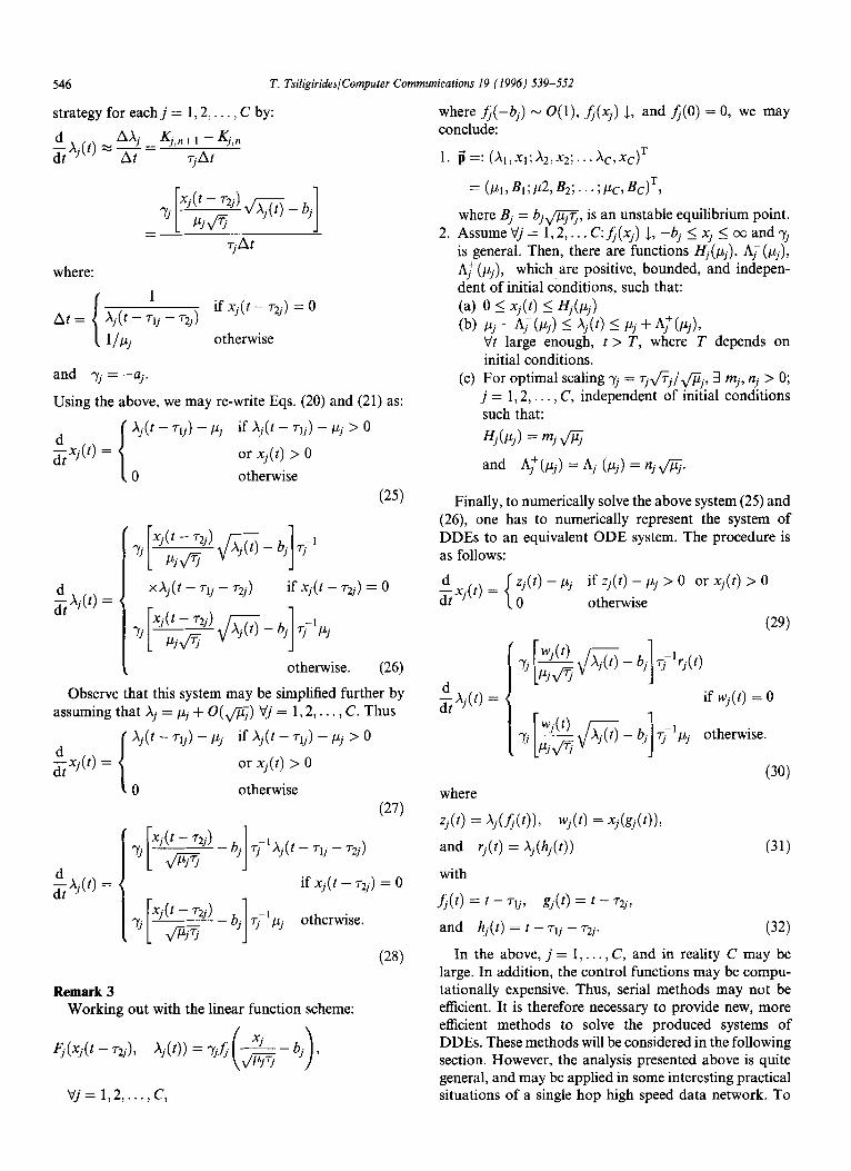
strategy for each j = 1,2, . . . , C by:

Ax’ Kj,n+l - Kj,n -$j(‘) x+= 7jAt

where:

1 .

& = Aj(t _ 71j _ T2j) lfxj(t - T2j) = '

llPj otherwise

and rj = -aj.

Using the above, we may re-write Eqs. (20) and (21) as:

$Xj(t) =

Aj(t-TU)-_j ifXj(t-TV)-_j>O

or Xj(t) > 0

0 otherwise

XAj(t - Tlj - T2j) if Xj(t - T2j) = 0

rj xj(t - T2j)

CLifi

otherwise. (26)

Observe that this system may be simplified further by assuming that Xj = hj + O(@) Vj = 1,2, . . . , C. Thus

$Xj(t) = 1 Aj(t-Tlj)-pj ifxj(t-71j)-pj>O

or Xj(t) > 0

\O otherwise

(27)

Yj p($$) - bj] T”pj otherwise.

(28)

Remark 3 Working out with the linear function scheme:

Vj= 1,2 ,..., C,

where fj(-bj) - O(l), f;.(Xj) J,, and fi(0) = 0, we may conclude:

a==: (X1,XI;X2,X2;...XC,XC)=

= (111,B,;~2,B2;...;I1C,BC)=,

where Bj = bjm, is an unstable equilibrium point. AssumeVj= 1,2,... C:fj(xj) 1, -bj 5 Xj 5 00 and 3 is general. Then, there are functions Hj(pj), A)‘(/+)> Aj’(~j), which are positive, bounded, and independent of initial conditions, such that:

(a) 0 5 xj(t) 5 Hj(Pj)

(b) pj - AI’ 5 xj(t) I Pj + A,‘(Pji>,

Vt large enough, t > T, where T depends on initial conditions.

(c) For optimal scaling ri = qfij/&j; 3 mj, nj > 0; j= 1,2,..., C, independent of initial conditions such that:

Hj(Pj) = mj fi

and AT (pj) = A/ (pj) = nj fi.

Finally, to numerically solve the above system (25) and (26), one has to numerically represent the system of DDEs to an equivalent ODE system. The procedure is as follows:

$Xj(t) = Zj(t) - /lj if Zj(t) - pj > 0 or Xj(t) > 0

0 otherwise

(2%

[

wj(t> - xj(t) I-4ifi d- - bj

1 ~~

[

wj(f) - xj(t) &fi J- - bj

1 3’

-‘Yj(t)

if Wj(t) = 0

-I/+ otherwise.

where (30)

zj(t) = xj(fj(t))> wj(t) = xj(gj(t)),

and rj(t) = Aj(hj(t))

with

(31)

fi(t) = - T1j, gjCt) = t - T2j,

and hj(t) = t - T1j - T2j. (32)

In the above, j= I,..., C, and in reality C may be large. In addition, the control functions may be compu- tationally expensive. Thus, serial methods may not be efficient. It is therefore necessary to provide new, more efficient methods to solve the produced systems of DDEs. These methods will be considered in the following section. However, the analysis presented above is quite general, and may be applied in some interesting practical situations of a single hop high speed data network. To

T. TsiligirideslCompurer Communications 19 (1996) 539-552 547

facilitate the examination, the following classification has been adopted.

1st case: No of nodes: 1, No of VCs: C, unequal propagation delays, unequal allocation of bandwidth.

This is the case presented above. It corresponds to the most general situation of a single node network. The adaption algorithm for the jth VC, j = 1,2, . . . , C, following the path with propagation delay 3 and having a fraction of the total throughput 0, is given by Eq. (24). Note that for each VC, j = 1,2, . . . , C, the parameters 3 and ej may all be different. Clearly, the corresponding system of ODES is that of Eqs. (29) and (30), while the solution should also satisfy Eqs. (31) and (32). However, an interesting case may allow groups to be considered as well. As an example, we may consider the case of a single node network with two paths, ‘long’ and ‘short’ propagation delays rL and rs (rL/rs = 2), and many VCs in each path, say CL and C,, respectively (C = CL + C,).

2nd case: No of nodes: 1, No of VCs: C, unequal propagation delays, fair allocation of bandwidth.

This is the case in which a virtual circuit aggregates many smaller virtual circuits, each of which follows a different path with different propagation delay q; j= 1,2,... , C, and shares an equal allocation of bandwidth. The adaptation algorithm, and the resulting system of ODES is derived from Eqs. (24) and (29) to (32), with t9, = l/C; j = 1,2,. . . , C.

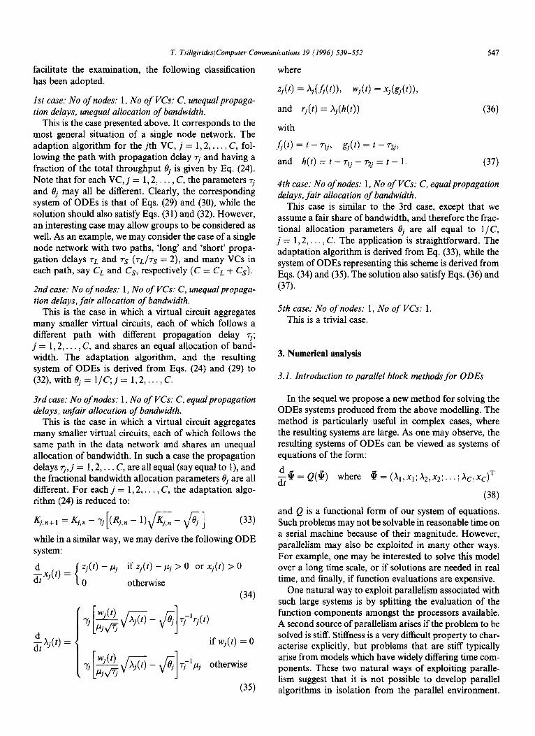
3rd case: No of nodes: 1, No of VCs: C, equal propagation delays, unfair allocation of bandwidth.

This is the case in which a virtual circuit aggregates many smaller virtual circuits, each of which follows the same path in the data network and shares an unequal allocation of bandwidth. In such a case the propagation delays q, j = 1,2, . _ . C, are all equal (say equal to l), and the fractional bandwidth allocation parameters 0, are all different. For each j = 1,2,. . . , C, the adaptation algorithm (24) is reduced to:

K. ~,n+l =K/,n-Yj[(Rj,n- l)&- fi] (33)

while in a similar way, we may derive the following ODE system:

iXj(t) =

Zj(t) - /J,j if Zj(t) - /_Lj > 0 or Xj(t) > 0

0 otherwise

(34)

if wj(t) = 0

otherwise

(35)

where

zj(t> = xj(fj(t>>, wj(t) = xjkj(t)>,

and rj(t) = Aj(h(t)) (36)

with

J(t) = t - Tlj, gj(t) = t - 72j,

and h(t) = t - 71j - 72j = t - 1. (37)

4th case: No of nodes: 1, No of VCs: C, equal propagation delays, fair allocation of bandwidth.

This case is similar to the 3rd case, except that we assume a fair share of bandwidth, and therefore the fractional allocation parameters 0, are all equal to l/C, j= 1,2,... , C. The application is straightforward. The adaptation algorithm is derived from Eq. (33), while the system of ODES representing this scheme is derived from Eqs. (34) and (35). The solution also satisfy Eqs. (36) and

(37).

5th case: No of nodes: 1, No of VCs: 1, This is a trivial case.

3. Numerical analysis

3.1. Introduction to parallel block methods for ODES

In the sequel we propose a new method for solving the ODES systems produced from the above modelling. The method is particularly useful in complex cases, where the resulting systems are large. As one may observe, the resulting systems of ODES can be viewed as systems of equations of the form:

$$ = Q(g) where $= (X,,X,;X~,X~;...;X~,X~)~

(38)

and Q is a functional form of our system of equations. Such problems may not be solvable in reasonable time on a serial machine because of their magnitude. However, parallelism may also be exploited in many other ways. For example, one may be interested to solve this model over a long time scale, or if solutions are needed in real time, and finally, if function evaluations are expensive.

One natural way to exploit parallelism associated with such large systems is by splitting the evaluation of the function components amongst the processors available. A second source of parallelism arises if the problem to be solved is stiff. Stiffness is a very difficult property to char- acterise explicitly, but problems that are stiff typically arise from models which have widely differing time components. These two natural ways of exploiting parallelism suggest that it is not possible to develop parallel algorithms in isolation from the parallel environment.

548 T. TsiligirideslComputer Communications 19 (1996) 539-552

However, currently there are no general purpose parallel scientific libraries, and while there have been some attempts at creating codes which can be ported between different parallel environments, this has only focused on the basic elements of array manipulation. Note that, according to the taxonomy in Ref. [21], four basic types of parallelism can be identified, that is, SISD (Single Instruction stream, Single Data stream), SIMD (Single Instruction stream, Multiple Data stream), MISD (Multiple Instruction stream, Single Data stream) and MIMD (Multiple Instruction stream, Multiple Data stream). In addition, new architectures are being proposed which are hybrid in nature, having elements from many different categories.

Both Gear [19] and Franklin [20], in their review papers, gave a taxonomy of available modes of parallelism in the numerical solution of first order Initial Value Problems (IVP) of the form:

;? = @(t,<(t)), ? : [to, T] x R” + R” P(t,) = ?o.

(39)

Their classifications include parallelism across space, equation segmentation methods, methods in which specific subsystems in Eq. (39) are assigned to separate processors, parallel predictor-corrector methods, parallelism across time, parallel block methods, and finally, other methods which accommodate some mode of parallelism, or they are adaptable to parallel computations. Gear [ 191 identified the major impediments to parallelism in ODE solvers as:

The narrowness of the computational lattices inherit in most conventional algorithms which adopt error and stepwise control. The extensive communications between processes, particularly in the case of stiff algorithms which are implicit and which are solved through some variants of Newton’s scheme introducing independence of the components of the dependent variable.

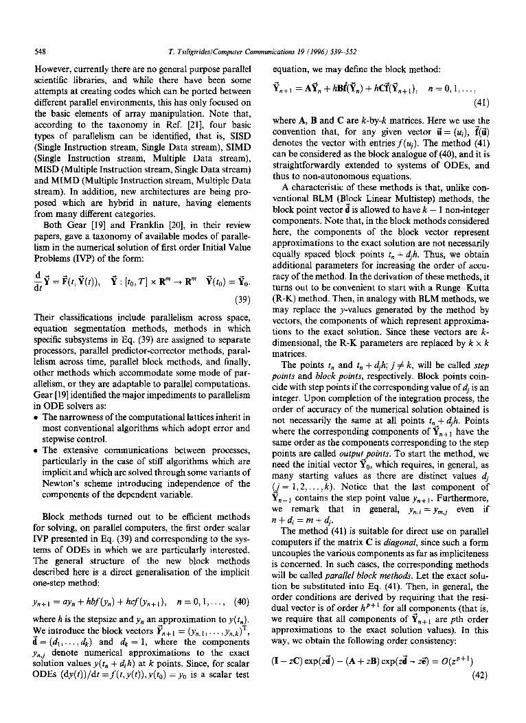
Block methods turned out to be efficient methods for solving, on parallel computers, the first order scalar IVP presented in Eq. (39) and corresponding to the systems of ODES in which we are particularly interested. The general structure of the new block methods described here is a direct generalisation of the implicit one-step method:

where h is the stepsize and yn an approximation to y( r,). We introduce the block vectors Fn,, 1 = (y,, , , . . . , y,,JT, a’= (dl,...,dk) and dk = 1, where the components yn,j denote numerical approximations to the exact solution values y(t, + dih) at k points. Since, for scalar ODES (dy(t))/dt =f(l,y(t)),y(ts) = y. is a scalar test

equation, we may define the block method:

?n+l = A& + hBi(?,) + hC@,+ I)1 n = 0, 1, . . . ,

(41)

where A, B and C are k-by-k matrices. Here we use the convention that, for any given vector u’ = (ui), i(a) denotes the vector with entries f(nj)- The method (41) can be considered as the block analogue of (40), and it is straightforwardly extended to systems of ODES, and thus to non-autonomous equations.

A characteristic of these methods is that, unlike conventional BLM (Block Linear Multistep) methods, the block point vector a’ is allowed to have k - 1 non-integer components. Note that, in the block methods considered here, the components of the block vector represent approximations to the exact solution are not necessarily equally spaced block points tn + djh. Thus, we obtain additional parameters for increasing the order of accuracy of the method. In the derivation of these methods, it turns out to be convenient to start with a Runge-Kutta (R-K) method. Then, in analogy with BLM methods, we may replace the y-values generated by the method by vectors, the components of which represent approximations to the exact solution. Since these vectors are k- dimensional, the R-K parameters are replaced by k x k matrices.

The points tn and tn + 4h; j # k, will be called step points and block points, respectively. Block points coin- cide with step points if the corresponding value of dj is an integer. Upon completion of the integration process, the order of accuracy of the numerical solution obtained is not necessarily the same at all points tn + djh. Points where the corresponding components of ?n+l have the same order as the components corresponding to the step points are called output points. To start the method, we need the initial vector qo, which requires, in general, as many starting values as there are distinct values dj

y= 1,2,..., k). Notice that the last component of

?I+1 contains the step point value y,, + 1. Furthermore, we remark that in general, y,,i = ym,j even if n+di=m+dj.

The method (41) is suitable for direct use on parallel computers if the matrix C is diagonal, since such a form uncouples the various components as far as impliciteness is concerned. In such cases, the corresponding methods will be called parallel block methods. Let the exact solution be substituted into Eq. (41). Then, in general, the order conditions are derived by requiring that the resi- dual vector is of order hp+’ for all components (that is, we require that all components of gn+i are pth order approximations to the exact solution values). In this way, we obtain the following order consistency:

(I - zC) exp(za) - (A + zB) exp(za - zq = O(zp+‘)

(42)

T. Tsiligirideslcornputer Communications 19 (1996) 539-552 549

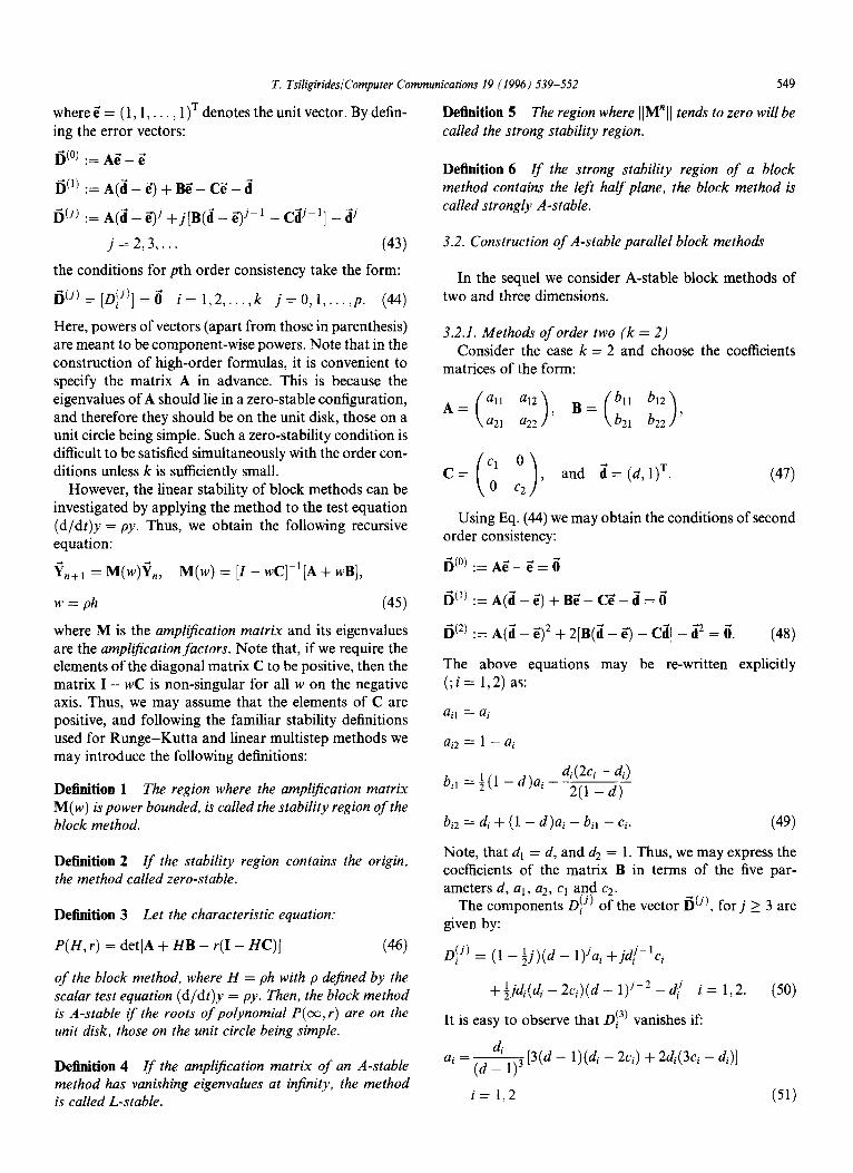
wheree’= (l,l,... , l)T denotes the unit vector. By defin- ing the error vectors:

I=j(O) := A;_ e’

Definition 5 The region where ]]M”]] tends to zero will be called the strong stability region.

Ij(‘):=A(;-s)++-C&a

a(j) := A(a _ s)j +j[B(; _ s)j-’ _ C&i] _ @

j = 2,3,. . . (43)

the conditions for pth order consistency take the form:

IjCj) = @iJ] = 0’ ,

i = 1 2 > 7”‘) k j=O,l,..., p. (44)

Here, powers of vectors (apart from those in parenthesis) are meant to be component-wise powers. Note that in the construction of high-order formulas, it is convenient to specify the matrix A in advance. This is because the eigenvalues of A should lie in a zero-stable configuration, and therefore they should be on the unit disk, those on a unit circle being simple. Such a zero-stability condition is difficult to be satisfied simultaneously with the order conditions unless k is sufficiently small.

However, the linear stability of block methods can be investigated by applying the method to the test equation (d/dt)y = py. Thus, we obtain the following recursive equation:

%+ 1 = Wd,, M(w) = [I - WC]-‘[A + wB],

u’ = ph (45)

where M is the ampltfication matrix and its eigenvalues are the ampltfication factors. Note that, if we require the elements of the diagonal matrix C to be positive, then the matrix I - WC is non-singular for all w on the negative axis. Thus, we may assume that the elements of C are positive, and following the familiar stability definitions used for Runge-Kutta and linear multistep methods we may introduce the following definitions:

Definition 1 The region where the ampltfication matrix M(w) is power bounded, is called the stability region of the block method.

Definition 2 Zf the stability region contains the origin, the method called zero-stable.

Definition 3 Let the characteristic equation:

P(H, r) = det[A + HB - r(1 - HC)] (46)

of the block method, where H = ph with p defined by the scalar test equation (d/dt)y = py. Then, the block method is A-stable tf the roots of polynomial P(w, r) are on the unit disk, those on the unit circle being simple.

Definition 4 Zf the amplification matrix of an A-stable method has vanishing eigenvalues at infinity, the method is called L-stable.

Definition 6 Zf the strong stability region of a block method contains the left half plane, the block method is called strongly A-stable.

3.2. Construction of A-stable parallel block methods

In the sequel we consider A-stable block methods of two and three dimensions.

3.2.1. Methods of order two (k = 2) Consider the case k = 2 and choose the coefficients

matrices of the form:

and a’= (d, l)T. (47)

Using Eq. (44) we may obtain the conditions of second order consistency:

a(o) :=Ae’-e’=ti

~(‘):=A(a-e’)+fBe’-Ce’-a=o

fic2) := A(d - Z)’ + 2[B(;i - Z) - C;i] - 2 = 0’. (48)

The above equations may be re-written explicitly (;i = 1,2) as:

ai1 = ai

ai = 1 - aj

bil =J(l -d)ai+ di(2ci - di)

2(1 -d)

bi2 = di + (1 - d)ai - bil - Ci. (49)

Note, that dI = d, and d2 = 1. Thus, we may express the coefficients of the matrix B in terms of the five parameters d, al, a2, cl and c2.

The components @ of the vector c(j), forj 2 3 are given by:

@j) = (1 - &j)(d - l)ja, +j&ici

+~jdi(di-2ci)(d-l)i-2-d~ i= 1,2. (50)

It is easy to observe that Dj3) vanishes if:

ai =L [3(d - l)(di - 2ci) + 2dt(3ci - di)] (d - 1)3

i= 1,2 (51)

550 T. Tsiligiri&s/Computer Communications 19 (1996) 539-552

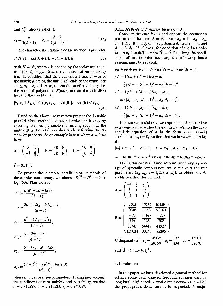
and D!4) also vanishes if: I

d d-2

‘i=2(d+l)’ ‘*=2(d- (52)

The characteristic equation of the method is given by:

P(H, r) = det[A + HB - r(1 - HC)] (53)

with H = ph, where p is defined by the scalar test equation (d/dt)y = py. Thus, the condition of zero-stability (i.e. the condition that the eigenvalues 1 and al - a2 of the matrix A are on the unit disk) leads to the condition: -1 2 al - a2 < 1. Also, the condition of A-stability (i.e. the roots of polynomial P(co,r) are on the unit disk) leads to the conditions:

[hc2 + b22c11 I qc2[qc2 + det(B)], det(B) 6 CICZ.

(54)

Based on the above, we may now present the A-stable parallel block methods of second order consistency by choosing the free parameters ai and Ci such that the matrix B in Eq. (49) vanishes while satisfying the A- stability property. As an example in case where d = 0 we have:

ii = (0, l)=.

To present the A-stable, parallel block methods of three-order consistency, we choose Di3) = @’ = 0 in Eq. (50). Thus we find:

a1 = d(d* - 3d + 6q)

(d - 1)3 ’

a2 = 3d + 12c2 - 6dc2 - 5

(d - 1)3

bll = d* - 2dq - d2c1

(d-l)* ’

b12 = d - 2dq - cl

(d _ l)*

b2I = 2 - 5c2 - d + 2dc2

(d-l)* ’

b22 = (d - 2)2 - c2(d2 - 6d + 8)

(d - 1)2

where d, cl, c2 are free parameters. Taking into account the conditions of zero-stability and A-stability, we find d = 0.917387, cl = 0.319523, c2 = 0.347067.

3.2.2. Methods of dimension three (k = 3) Consider the case k = 3 and choose the coefficients

matrices of the form A = [au], with ai = 1 - ait - ai2, 4= 1,2,3, B = [bv], C = [c& diagonal, with Cii = ci and d = (d,, d2, l)=. Clearly, the condition of the first order accuracy is satisfied, since d, = 0’. Requiring the conditions of fourth-order accuracy the following linear systems must be satisfied:

bil + bi2 + bi3 + ci = df - oil (dl - 1) - aiz(d2 - 1)

(d, - l)bil + (d2 - l)bi2 + dici

= 4 [df - ail (d, - l)* - o;2(d2 - l)*]

(d, - l)*bil + (d2 - l)*bi2 + dfci

= f [d! - ail (dl - 1)3 - aiz(d2 - 1)3]

(d, - 1)3bil + (d2 - 1)3bi2 + dfci

=$[d;-ajl(d, - 1)4 - on(d2 - 1)4].

To ensure zero-stability, we require that A has the two extra eigenvalues within the unit circle. Writing the characteristic equation of A in the form P(z) = (z - 1) x(z* + toz + SO) = 0, we find that we have zero-stability if:

Itol<so+l, so< 1, t0 = a31 + a32 - all - a22

sO = alla12 + u31a12 + a32a21 - alla32 - a21a12 - u22a31*

Taking this constraint into account, and using a pack- age of symbolic computation, we search over the free parameters (ail, Ui2, i = 1,2,3, dl, d2), to obtain the A- stable fourth-order method:

A=

2795 15161 103501 - - ~ 2048 3168 92160

-467 B= ; ~ -259

i 1

126 702’

80345 54419 41927 ~ - - 129024 30240 55296

16939 277 16001 C diagonal with cl = 28160, c2 = 234, c3 = 23040

and d’ = (5,13/4, I)=.

4. Conclusions

In this paper we have developed a general method for solving some basic delayed feedback schemes used in long haul, high speed, virtual circuit networks in which the propagation delay cannot be neglected. A major

T. Tsiligirideslcomputer Communications 19 (1996) 539-552 551

problem in such networks is the statistical interaction among the traffic flows to be controlled. Two basic virtual circuit networks of a balanced form are examined. These are the single-hop networks which aggregate many virtual circuits in parallel, and the M-hop tandem network. These networks are presented as systems of DDEs with unknown control functions, in which the rate of transmission and the queue occupancy are modelled as fluids. We used the well known adaptive algorithms of Mitra and Seery [l l] to dynamically adjust the window size and to impose linear structure control. As a result, the examined networks are presented as linear systems of some DDEs.

Using linear approximation, the above schemes are proved unstable (in a Liapounov sense). However, we identified the appropriate scaling for the parameters so as to make the above schemes to perform near their optimal theoretical values for a wide range of speeds. Since the standard theory of DDEs does not treat the class of systems we considered, stability in a Liapounov sense is very difficult to prove. Thus new tools have to be developed. In addition, and more importantly, a solution method of such DDE systems has not been investigated so far, particularly in general cases, where the resulting DDE systems are more complex and large. For this reason, we proposed a general method, by means of parallel block methods, and we derived an approximate numerical solution. This method is used to solve the systems of the ODES in which the original systems of DDEs have been transformed. The basic theory underlying the parallel block methods for the numerical solution of the system of ODES has been developed and fully discussed. Finally, we examined the numerical stability by deducing two and three dimensional, A- stable parallel block methods of second, third and fourth order consistency.

The results found leave open the question of whether further improvements are possible. Since this work directly applies to the adaptive control of frame relay and ATM networks, both of which provide feedback to users on congestion, the results found are even more important. However, one may observe that the principal concerns here are the accuracy of the results and the time required to obtain them. Of course, on the analytical side, accuracy is an issue only if the model or the solution method is approximate. In either case, one should seek a means of determining bounds on the errors of approximations, as they reflected in the performability values that are ultimately determined. If both the model and the solution method are approximate (as in this case), there is a need to understand the interaction between the two types of approximation; the concern being in incompatibility which causes excessive errors when the two are used together. Therefore, further study is needed

in order to provide more accurate models, so that any improvement in the numerical stability, by means of providing high-order A-stable parallel block methods, will become viable.

References

[II

PI

]31

[41

151

161

[71

]81

I91

1101

1111

[121

]131

[141

[151

[161

M. Schwartz, Telecommunications Networks: Protocols, Model- ling and Analysis. Addison-Wesley, Reading, 1987. D. Bertsekas and R. Gallager, Data Networks. Prentice-Hall, Englewood Cliffs, NJ, 1987. D. Browning, Flow control in high-speed communication networks. IEEE Trans. Commun., 42 (1994) 2480-2489. L. Dittmann, S. B. Jacobsen and K. Moth, Flow enforcement algorithms for ATM networks. IEEE J. Select. Areas Commun., 9 (1991) 3433350. R. Jain, Congestion control in computer networks: Issues and trends. IEEE Network Mag. (May 1990) 230-244. S.-Y.R. Li, Algorithms for flow control and call set-up in multi- hop broadband ISDN. IEEE INFOCOM, 1990, pp. 889-895. R. Dighe, C. J. May and C. Ramamurthy, Congestion avoidance strategies in broadband packet networks. INFOCOM, 1991, pp. 295-303. W.E. Leland, Window-based congestion management in broadband ATM networks: The performance of three access-control policies. GLOBECOM, 1989, pp. 1794-1800. D. Mitra, Asymptotically optimal design of congestion control for high speed data networks. IEEE Trans. Comm., 40 (1992) 301- 311. F. W. Fendick, M. A. Rontrigues and A. Weiss, Analysis of a rate- based feedback control strategy for long haul data transport. Per- for. Evaluat., 16 (1992) 67-84. D. Mitra and J.B. Seery, Dynamic adaptive windows for high speed data networks with multiple paths and propagation delays. Computer Networks & ISDN Systems, 25 (1993) 663-679. R. Jain, A delay-based approach for congestion avoidance in interconnected heterogeneous computer networks. Rep. DEC- TR-556, Digital Equipment Corp., 1988. V. Jacobson, Congestion avoidance and control. Proc. ACM SIG- COMM, Stanford, CA, 1988, pp. 314-329. K.K. Ramkrishnan and R. Jain, A binary feedback scheme for congestion avoidance in computer networks with a connectionless network layer. Proc. ACM SIGCOMM, Stanford, CA, 1988, pp. 303-313. J.C. Bolot and U.A. Shankar, Dynamical behaviour of rate-based flow-control mechanisms. Comput. Comm. Rev., 40(2) (1990) 35-49. E.L. Hahne, C.R. Kalmanek and S.P. Morgan, Fairness and congestion control on a large ATM data network with dynamically adjustable windows. 13th Int. Teletraffic Conf., Italy, July 1991.

[ 171 K. Burrage, Parallel methods for initial value problems. Applied Numerical Mathematics, 11 (1993) 5-25.

[18] P. Amodio and D. Trigiante, A parallel direct method for solving initial value problems for ordinary differential equations. Applied Numerical Mathematics, 1 I (1993) 85-93.

[19] C.W. Gear, The potential for parallelism in ODES. In: S.O. Fatunla (ed.) Computational Mathematics II. Boole Press, Dublin, Ireland, 1987, pp. 33-48.

[20] M.A. Franklin, Parallel solution of ODES. IEEE Trans. Comput., 27 (1978) 413-420.

[21] M.F. Flynn, Some computer organisations and their effectiveness. IEEE Trans. Comput., 23 (1972) 948-960.

552 T. Tsiligirides/Computer Communications 19 (1996) 539-552

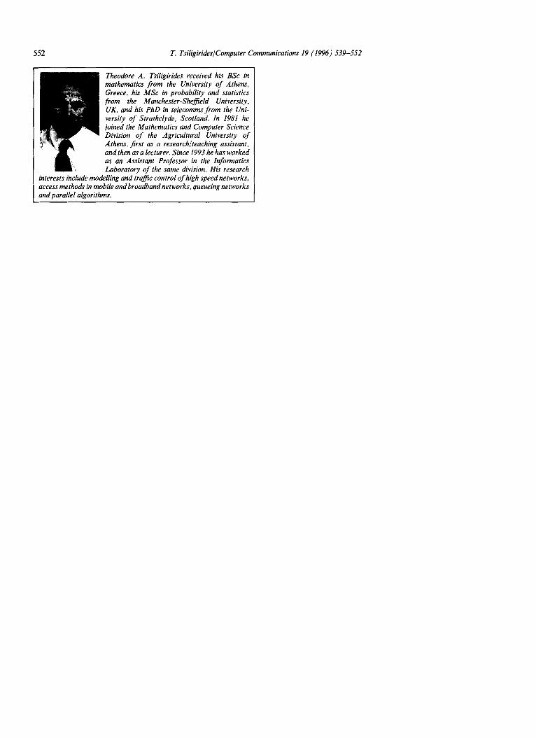
Theodore A. Tsiligirides received his BSc in mathematics from the University of Athens, Greece, his MSc in probability and statistics from the Manchester-Shefield University, UK, and his PhD in telecomms from the Uni- versity of Strathclyde, Scotland. In 1981 he joined the Mathematics and Computer Science Division of the Agricultural University of Athens, first as a research/teaching assistant, and then as a lecturer. Since 1993 he has worked as an Assistant Professor in the Informatics Laboratory of the same division. His research

interests include modelling and trafic control of high speed networks, access methods in mobile and broadband networks, queueing networks and parallel algorithms.

Numerical analysis of some basic fluid communication models via parallel block methods

Documents

Transcript of Numerical analysis of some basic fluid communication models via parallel block methods