Critical Points of Ambrosio-Tortorelli converge tocritical points of Mumford-Shah in the one-dimensional

Dirichlet case

Gilles A. Francfort ∗, Nam Q. Le†, and Sylvia Serfaty ‡

February 27, 2008

Abstract

Critical points of a variant of the Ambrosio-Tortorelli functional, for which non-zero Dirichlet boundary conditions replace the fidelity term, are investigated. Theyare shown to converge to particular critical points of the corresponding variant of theMumford-Shah functional; those exhibit many symmetries. That Dirichlet variantis the natural functional when addressing a problem of brittle fracture in an elasticmaterial.

1 Introduction

In the late 80’s, D. Mumford & J. Shah proposed a new functional for image segmentation intheir celebrated paper [13]. If g ∈ L∞(Ω; [0, 1]) represents a continuous interpolation of thecollected pixelated data over the image domain Ω ⊂ IR2, then the proposed segmentationconsists in minimizing

(u, K) 7→ MS(u, K) :=

∫Ω\K

|∇u|2 dx + 2H1(K) + λ

∫Ω

(u− g)2 dx,

among all compact subsets K ⊂ Ω and all u ∈ H1(Ω\K). In that functional, λ is a positiveweight left to the investigator’s appreciation, K represents the contours of the image, andu the resulting grey contrast (0 ≤ u(x) ≤ 1).

∗LPMTM, Universite Paris 13, Ave. J. B. Clement, 93430 Villetaneuse, France. Email: francfor@galilee.univ-paris13.fr, partially supported by ANR-06-BLAN-0082

†Courant Institute of Mathematical Sciences, 251 Mercer St, New York, NY 10012, USA. Email: quan-gle@cims.nyu.edu, partially supported by a Vietnam Education Foundation graduate Fellowship

‡Courant Institute of Mathematical Sciences, 251 Mercer St, New York, NY 10012, USA. Email: ser-faty@cims.nyu.edu, supported by NSF CAREER grant #DMS0239121 and a Sloan Foundation Fellowship

1

2

Proving existence for minimizers of that functional was not a trivial task and it gave riseto a abundant literature spearheaded by the work of E. De Giorgi and that of L. Ambrosioon the space SBV (Ω); see e.g [1]. The underlying idea was to view MS(u, K) as a onefield functional

(1.1) MS(u) =

∫Ω

|∇u|2 dx + 2H1(S(u)) + λ

∫Ω

(u− g)2 dx,

over SBV (Ω), the space of functions u ∈ L1(Ω) such that their distributional derivative isa Radon measure Du with finite total variation |Du|(Ω), jump set S(u) (the complement ofthe set of Lebesgue points for u), and no Cantor part. The next step was to prove existenceof a minimizer um of MS in that space, and then to show that the pair (um, S(um)) wasactually a minimizer for MS. That program was successfully completed, culminating in[8].

From a computational standpoint, the search for a minimizer of (1.1) is not easy,because the test fields exhibit discontinuities at unknown locations and the implementationof classical finite element methods becomes a perilous endeavor. A possible remedy consistsin resorting to variational convergence, specifically Γ-convergence, so as to approximate MSby a more regular functional – denoted henceforth by ATε – whose minimizers are easierto evaluate. For more information on Γ-convergence, we refer the interested reader toe.g. [7] and merely emphasize for now that an important property of Γ-convergence isthat (approximate) minimizers of ATε that converge as ε 0 will converge to bona fideminimizers of MS.

There is by now an abundant literature on the approximation of the Mumford-Shahfunctional and many approximating sequences have been proposed. The most computa-tionally efficient in our opinion is that originally proposed by L. Ambrosio & V. Tortorelliin [3], [4], in the footstep of the functional proposed by L. Modica and S. Mortola for theapproximation of the perimeter [12]. Consider

ATε(u, v) =

∫Ω

((ηε + v2)|∇u|2 + ε|∇v|2 +

(1− v)2

ε

)dx + λ

∫Ω

(u− g)2 dx,

with 0 < ηε << ε. It is proved in [3], [4] that ATε Γ(B(Ω)×B(Ω))-converges to MS, suitablyextended to a two-field functional as

MS(u, v) =

MS(u) if v ≡ 1

+∞ otherwise.

Above, B(Ω) stands for the set of all Borel functions on Ω, and the convergence is theconvergence in measure. Actually, we can also view the convergence as taking place inL2(Ω)× L2(Ω).

The functional ATε is easily seen, through the direct method of the Calculus of Varia-tions, to admit at least one minimizing pair (uε, vε) ∈ H1(Ω)×H1(Ω), for any fixed valueof ε. The associated sequence is bounded in e.g. L∞(Ω)× L∞(Ω), and a subsequence can

3

be shown to converge in measure (and also strongly in L2(Ω)×L2(Ω)) to (u, v ≡ 1), which,by the already evoked property of Γ-convergence, will be a minimizer for MS.

In an apparently disconnected context, recent years have witnessed the birth of a varia-tional theory of brittle fracture evolution. One of its constitutive elements is that, at eachtime, the total energy of the system, the sum of the elastic and surface energies, is to beminimized among all admissible competitors [10]. That total energy is a close parent ofthe Mumford-Shah functional MS for image segmentation. It is given – say in anti-planeshear, for which the dispacement field is unidirectional, and for normalized shear modulusand fracture toughness – by

(1.2) F(u, v) =

∫

Ω

|∇u|2 dx + 2H1(S(u)) if u ∈ SBV (Ω), and v ≡ 1

+∞ otherwise.

In the context of fracture, the displacement field u is typically constrained by boundaryvalues, say U on ∂Ω, and the crack may go to the boundary of Ω. Thus we should imposethat

u = U on ∂Ω \ S(u),

u being considered as an element of SBV (IR2) such that u ≡ U on IR2 \Ω with U definedon IR2 (say U ∈ H1(IR2)). The relevant literature speaks of a hard device in this situation.In any case, the above quoted Γ-convergence result still applies in the current setting, sothat F , trivially extended to some Ω′ ⊃ Ω, can be variationally approximated by Eε, aclose variant of ATε defined as

(1.3) Eε(u, v) :=

∫Ω′

((ηε + v2)|∇u|2 + ε|∇v|2 +

(1− v)2

ε

)dx,

with (u, v) ∈ H1(Ω′)×H1(Ω′) and u ≡ U on Ω′ \ Ω.

Remark 1.1 The extension to a larger domain Ω′ permits the introduction of boundaryjumps (boundary cracks) without modification of the resulting surface energy. In theremainder of the study, we prefer to restrict the functional to Ω, while imposing that theadmissible fields u belong to SBV (IR2) with u = U on IR2 \ Ω. In that case, the correctsurface energy for the Γ(B(Ω)× B(Ω))-limit of Eε is

2H1(S(u) ∩ Ω) +H1(S(u) ∩ ∂Ω).

Although the functional Eε is immediately seen to admit minimizers at fixed ε, those arenot so easily determined computationally because Eε is not convex in its two arguments,but only separately in each of them. This is a cause of major difficulties, as explained in [6].The most expedient computational algorithm consists in performing alternate minimizationin each variable at fixed ε. According to [6], that algorithm asymptotically convergesto a critical point (uε, vε) of Eε. Thus, algorithmically, we should investigate the limit

4

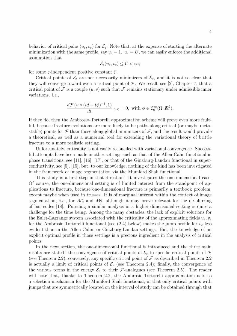
behavior of critical pairs (uε, vε) for Eε. Note that, at the expense of starting the alternateminimization with the same profile, say vε = 1, uε = U , we can easily enforce the additionalassumption that

Eε(uε, vε) ≤ C < ∞,

for some ε-independent positive constant C.Critical points of Eε are not necessarily minimizers of Eε, and it is not so clear that

they will converge toward even a critical point of F . We recall, see [2], Chapter 7, that acritical point of F is a couple (u, v) such that F remains stationary under admissible innervariations, i.e.,

dF (u (id + tφ)−1, 1)

dt|t=0 = 0, with φ ∈ C∞0 (Ω; IR2).

If they do, then the Ambrosio-Tortorelli approximation scheme will prove even more fruit-ful, because fracture evolutions are more likely to be paths along critical (or maybe meta-stable) points for F than those along global minimizers of F , and the result would providea theoretical, as well as a numerical tool for extending the variational theory of brittlefracture to a more realistic setting.

Unfortunately, criticality is not easily reconciled with variational convergence. Success-ful attempts have been made in other settings such as that of the Allen-Cahn functional inphase transitions, see [11], [16], [17], or that of the Ginzburg-Landau functional in super-conductivity, see [5], [15], but, to our knowledge, nothing of the kind has been investigatedin the framework of image segmentation via the Mumford-Shah functional.

This study is a first step in that direction. It investigates the one-dimensional case.Of course, the one-dimensional setting is of limited interest from the standpoint of ap-plications to fracture, because one-dimensional fracture is primarily a textbook problem,except maybe when used in trusses. It is of marginal interest within the context of imagesegmentation, i.e., for ATε and MS, although it may prove relevant for the de-blurringof bar codes [18]. Pursuing a similar analysis in a higher dimensional setting is quite achallenge for the time being. Among the many obstacles, the lack of explicit solutions forthe Euler-Lagrange system associated with the criticality of the approximating fields uε, vε

for the Ambrosio-Tortorelli functional (see (2.4) below) makes the jump profile for vε lessevident than in the Allen-Cahn, or Ginzburg-Landau settings. But, the knowledge of anexplicit optimal profile in those settings is a precious ingredient in the analysis of criticalpoints.

In the next section, the one-dimensional functional is introduced and the three mainresults are stated: the convergence of critical points of Eε to specific critical points of F(see Theorem 2.2); conversely, any specific critical point of F as described in Theorem 2.2is actually a limit of critical points of Eε (see Theorem 2.4); finally, the convergence ofthe various terms in the energy Eε to their F -analogues (see Theorem 2.5). The readerwill note that, thanks to Theorem 2.2, the Ambrosio-Tortorelli approximation acts asa selection mechanism for the Mumford-Shah functional, in that only critical points withjumps that are symmetrically located on the interval of study can be obtained through that

5

approximation and that, thanks to Theorem 2.4, all of those are actually attained as limitsof critical points of Eε. Also, Theorem 2.5 demonstrates that, generically, the Ambrosio-Tortorelli energy evaluated at one of its critical points converges to the Mumford-Shahenergy, evaluated at the limit of that (sequence of) critical point(s). Section 3 establishessome general a priori estimates, and most notably bounds the discrepancy (see (3.3)), apivotal quantity in the study of critical points because of its link to the energy momentumtensor (see e.g. [5], [14]). Section 4 is devoted to the proof of the first theorem; Section 5carries out that of the second theorem, while Section 6 details that of the third theorem.

2 Statement of the results

Throughout, C stands for a generic positive constant (so that e.g. C = 2C) and L is thelength of the interval under consideration.

For ε > 0, we consider the following ε-indexed one-dimensional Ambrosio-Tortorellitype functional (see (1.3)):

(2.1) Eε(u, v) =

∫ L

0

((ηε + v2)(u

′)2 + ε(v

′)2 +

(1− v)2

ε

)dx.

In (2.1), ηε is a positive number, and (uε, vε) belongs to the space Yε defined by

Yε := u, v ∈ H1(0, L), u(0) = 0, u(L) = aε

with aε > 0. Note that these boundary constraints are not really restrictive in one dimen-sion (up to translation of u).

We assume that, as ε 0,

(2.2) aε → a > 0; ηε/ε → 0, i.e., ηε ε.

We also introduce, for u ∈ SBV (IR), the one dimensional Mumford-Shah functional(see (1.2) and Remark 1.1):

(2.3) F(u, v) =

∫ L

0

(u′)2 dx + 2# (S(u) ∩ (0, L)) + # (S(u) ∩ 0, L) if v ≡ 1

+∞ otherwise.

In (2.3), u′ denotes the approximate derivative of u, i.e., the density of the absolutelycontinuous part of the measure Du with respect to the Lebesgue measure, while S(u)denotes the jump set of u, defined as the complement in IR of the set of Lebesgue pointsof u.

As explained in the introduction, we wish to impose Dirichlet type boundary conditionson the test fields. Thus, the pair (u, v) should lie in Y defined as

Y := u ∈ SBV (IR) : u ≡ 0 on (−∞, 0), u ≡ a on (L, +∞) × L∞((0, L)),

6

so that, in particular, S(u) ⊂ [0, L].The spaces Yε and Y are endowed with the L2((0, L), IR2) topology. We recall that

Eε Γ-converges to F hence minimizers of Eε converge to minimizers of F . Those are veryeasy to identify: for a <

√L the only minimizer is u ≡ ax/L, while for a >

√L they

are u = aχ(L,∞), or u = aχ(0,∞), where χ denotes the characteristic function of a set (for

a =√

L all of the above are minimizers). Thus we see that fracture is indeed induced bythis model, even for minimizers, by a boundary “tug” when a large enough. Minimizationfavors boundary cracks because the associated surface energy has a lesser weight (1 versus2). In the context of Remark 1.1, an energy that would weigh equally (0, L) and 0, Lwould produce, for a >

√L, a minimizer of the form u = aχ(b,∞) for any b ∈ [0, L].

However, our results below would prove that not all of these minimizers are produced bythis limit process.

As announced in the introduction, we propose to study the convergence property of crit-ical points other than the minimizers. The critical points of the one dimensional Mumford-Shah functional are easily identified from (7.42) in [2], Ch. 7, as those pairs (u, v) withv ≡ 1, and u piecewise constant with a finite number of jumps, or u ≡ ax/L.

Let (uε, vε) be critical points of the Ambrosio-Tortorelli functional (2.1), i.e., pairs offunctions (uε, vε) ∈ Yε that satisfy the Euler-Lagrange equations

(2.4)

−εv′′

ε + vε(u′

ε)2 +

vε − 1

ε= 0

[u′

ε(ηε + v2ε)]

′ = 0

uε(0) = 0, uε(L) = aε

v′

ε(0) = v′

ε(L) = 0.

Our main goal is to study the limit properties of (uε, vε) as ε goes to 0, provided additionallythat

(2.5) Eε(uε, vε) ≤ C < ∞.

The above bound is natural from a computational standpoint, as already emphasized inthe introduction.

Note that the second equation of (2.4) implies that

(2.6) u′

ε(ηε + v2ε) = cε,

for some constant cε. It follows that u′ε has a constant sign. The Dirichlet boundary

conditions on uε imply that cε > 0 and thus that

(2.7) uε from 0 to aε.

7

One can substitute the relation (2.6) into the first equation of (2.4), and obtain

(2.8)−εv

′′

ε +vεc

2ε

(ηε + v2ε)

2+

vε − 1

ε= 0

v′

ε(0) = v′

ε(L) = 0.

It is a crucially convenient feature of the one-dimensional case that the system of ODE’scan be reduced to this single second-order ODE (up to the unknown parameter cε though)with Neumann boundary conditions. We will use the properties, in particular symmetryproperties, of solutions to this type of ODE’s. However it is not our goal to completelyclassify the solutions to (2.8) or perform their stability analysis. Rather we focus on theε → 0 asymptotic analysis and we look to employ, as much as possible, arguments that areindependent of the dimension and could be recast in dimensions higher than 1.

Remark 2.1 Equation (2.6) would still hold true if Neumann boundary conditions, namelyu′ε(0) = u′ε(L) = 0, were imposed on uε, in lieu of the adopted Dirichlet boundary condi-tions. But then, u′ε ≡ 0, vε ≡ 1, and the problem becomes trivial.

It is the presence of the fidelity term∫ L

0|u− g|2 dx of image segmentation that renders

the Neumann problem non-trivial. As mentioned in the introduction, our present focus isthe Dirichlet case, where no fidelity term is present.

Our main result is the following. It states on the one hand the symmetry properties ofthe solutions to (2.4), and on the other hand the more difficult fact that cε can only clusterto the two values 0 and a/L.

Theorem 2.2 At the possible expense of extracting a subsequence of ε 0, cε → c0

where c0 ∈ 0, a/L and (uε, vε) converges to a critical point (u, 1) of F . In other words,uε(x) → u(x)(∈ SBV (IR)) and vε(x) → 1, for a.e. x ∈ (0, L).

If c0 = a/L, the limit critical point is u ≡ ax/L.If c0 = 0, there exists a fixed number n such that, at the possible expense of extracting

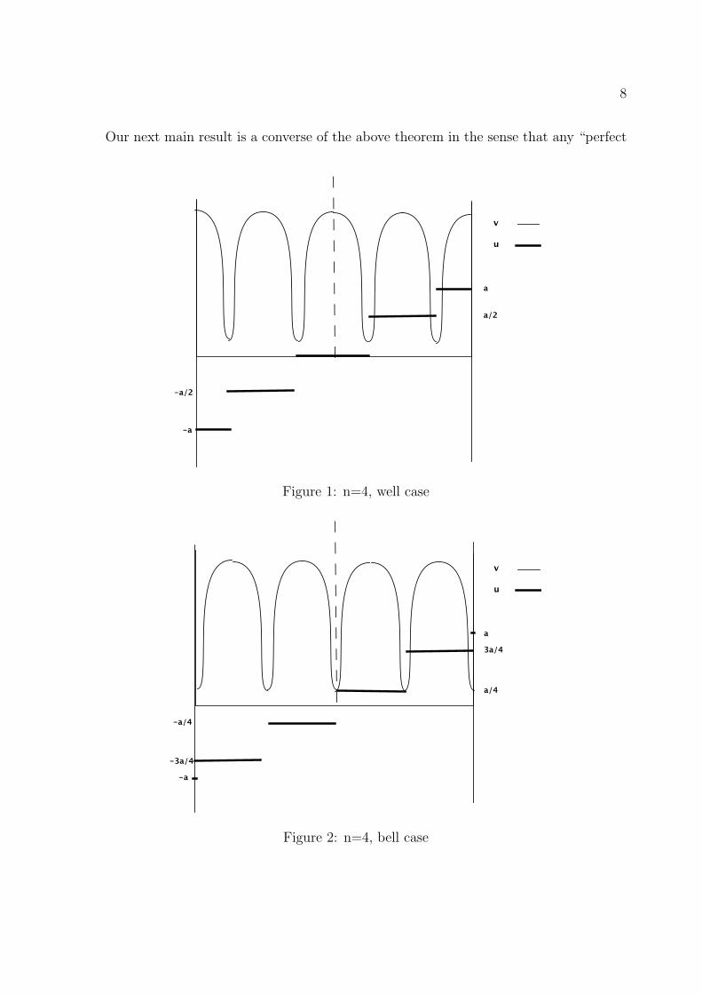
a subsequence of ε 0, vε – extended by symmetry to (−L, L) – is a juxtaposition ofn identical graphs. The repeated subgraph exhibits either a strict minimum point (“wellcase”), for all ε’s, or a strict maximum point, for all ε’s (“bell case”). The limit criticalpoint u – extended by anti-parity to (−L, L) – is constant on (−L,−L + L/n), with value−a in the former case (see Figure 1), or on (−L,−L + 2L/n), with value −(n− 1)a/n inthe latter case (see Figure 2), then it jumps by a value of 2a/n at the end of each intervalof length 2L/n .

Remark 2.3 The Ambrosio-Tortorelli functional acts as a selector for the critical pointsof the Mumford-Shah functional, in that it asymptotically equi-distributes the possiblejumps of u over the interval [0, L]. The graph of u extended by antiparity looks like a pieceof a “perfect staircase”: all steps have the same height and the same width.

8

Our next main result is a converse of the above theorem in the sense that any “perfect

a

a/2

-a

-a/2

v

u

Figure 1: n=4, well case

a

3a/4

-a

-3a/4

v

u

a/4

-a/4

Figure 2: n=4, bell case

9

staircase” critical point of the Mumford-Shah functional F as described in Theorem 2.2 isactually a limit of critical points of the Ambrosio-Tortorelli functional Eε.

Theorem 2.4 Let u be a “perfect staircase” function on [0, L] with n steps when viewed asa function on [−L, L] as described in Theorem 2.2. Then, for all ε sufficiently small, thereexists a critical point (uε, vε) (i.e., with v

′ε(0) = v

′ε(L) = 0 and uε(0) = 0, uε(L) = aε), of

Eε such that vε has exactly n isolated local maxima in [−L, L] and

(2.9) limε→0

‖uε − u‖L2((0,L) or equiv. (−L,L)) = 0.

We are also in a position to evaluate the measure limits of each of the terms enteringthe energy functional defined in (2.1). This is the object of the following

Theorem 2.5 If uε → u, a critical point for the Mumford-Shah functional, as given inTheorem 2.2, then

• The limit measure of (ηε + v2ε)(u

′ε)

2dx is (u′)2dx, u′, the approximate gradient of u,being 0 or a/L;

• The limit measure of ε(v′ε)2dx, which is also that of (1− vε)

2/εdx, is a finite sumof Dirac masses which, in the case that u is piecewise constant (c0 = 0), are locatedat the end of each step of the “perfect staircase” that represents u. Each of thosemasses has weight 1 when the mass is located inside (0, L) and 1/2 if it is located atx = 0, L, if any.

Remark 2.6 In the case c0 = a/L, we expect that, for ε small enough, uε(x) = aεx/Land vε(x) = L2/(L2 + a2

εε), which would prove that vε has no v-jump in the sense ofDefinition 3.5 below, and thus that the resulting measure limit is always

∑x∈S(u)∩(0,L) δx +

1/2∑

x∈S(u)∩0,L δx.

3 Preliminary Estimates

3.1 Classical a priori estimates

In this section, we establish a few canonical estimates that will prove instrumental in theproof of Theorems 2.2, 2.5. These estimates are completely standard but we include theirproofs for convenience of the reader. The a priori bound (2.5) is essential in all that follows.

First note that, from (2.5) and (2.6),

C ≥ Eε(uε, vε) ≥∫ L

0

(ηε + v2ε)(u

′

ε)2dx =

∫ L

0

cεu′

εdx = aεcε,

so that

cε ≤Caε

.

10

Hence, up to the possible expense of extracting a subsequence,

(3.1) cε → c0, ε 0.

The proof of Theorem 2.2 will hinge on the actual values that c0 can take. This will bethe object of Lemma 4.4 in the next section.

For now, we prove some elementary estimates on the critical points (uε, vε) of (2.1),which, by the way, are smooth by elliptic regularity.

A first result is a maximum principle for vε, namely,

Lemma 3.10 ≤ vε ≤ 1.

Proof. Multiplying both sides of the first equation of (2.4) by v−ε = max(0,−vε), we get∫ L

0

−εv′′

ε v−ε dx +

∫ L

0

vε(u′

ε)2v−ε dx +

∫ L

0

vε − 1

εv−ε dx = 0.

Because of the Neumann boundary conditions on vε, this yields∫ L

0

εv′

ε(v−ε )

′dx +

∫ L

0

vε(u′

ε)2v−ε dx +

∫ L

0

vε − 1

εv−ε dx = 0,

or still

(3.2) −∫ L

0

ε((v−ε )′)2dx−

∫ L

0

(v−ε )2(u′

ε)2dx−

∫ L

0

(v−ε + 1)

εv−ε dx = 0.

Each term on the right hand side of (3.2) is nonpositive. Thus,∫ L

0

(v−ε + 1)

εv−ε dx = 0,

hence v−ε ≡ 0.Multiplication of the first equation of (2.4) by (vε − 1)+ = max(0, vε − 1) would yield

the other inequality.

Next, we establish the convergence properties of the pair (uε, vε).

Lemma 3.2vε → 1, strongly in L2((0, L)),

and, modulo extraction,

uε → u ∈ BV ((0, L)), strongly in L1((0, L)),

u′ε → c0, a.e. in (0, L).

Further, |Du|((0, L)) ≤ a and c0 ≤ a/L.

11

Proof. The energy bound (2.5) immediately implies the first convergence. The monotonecharacter (2.7) of uε, together with (2.2), implies that uε is bounded in BV ((0, L)). Bythe compactness of BV in L1 (see [9]), a subsequence of uε converges in L1((0, L)) tou ∈ BV ((0, L)).

Because of the weak lower semi-continuous character of the total variation,

|Du|((0, L)) ≤ lim infε

|Duε|((0, L)) = lim infε

aε = a,

hence the bound on |Du|((0, L)).By virtue of (2.6),

u′

ε(x) → c0 as ε → 0 for a.e x ∈ (0, L).

Fatou’s lemma then yields the following refined bound on c0:

c0L =

∫ L

0

limε→0

u′

ε ≤ limε→0

∫ L

0

u′

ε = a.

It is also standard that, in such a context, a Noether type conservation law holds, asstated in the following

Proposition 3.3 1

2

((1− vε)

2

ε− (ηε + v2

ε)(u′

ε)2 − ε(v

′

ε)2

)′

= 0.

Proof. The left hand side of the previous expression also reads as

Aε :=(vε − 1)v

′ε

ε− εv

′

εv′′

ε − vεv′

ε(u′

ε)2 − (v2

ε + ηε)u′

εu′′

ε

= v′

ε(−εv′′

ε − vε(u′

ε)2 +

vε − 1

ε)− (v2

ε + ηε)u′

εu′′

ε .

The first and second equation of (2.4) then imply that

Aε = −v′

ε(2vε(u′

ε)2)− (v2

ε + ηε)u′

εu′′

ε = −u′

ε[u′′

ε (ηε + v2ε) + 2vεv

′

εu′

ε] = −u′

ε[u′

ε(ηε + v2ε)]

′ = 0.

An immediate consequence of the proposition above is that

(3.3)(1− vε)

2

ε− (ηε + v2

ε)(u′

ε)2 − ε(v

′

ε)2 = dε

for some constant dε. Furthermore, we can estimate this discrepancy constant dε as follows

|dε|L =

∫ L

0

|dε| dx =

∫ L

0

∣∣∣∣(1− vε)2

ε− (ηε + v2

ε)(u′

ε)2 − ε(v

′

ε)2

∣∣∣∣ dx

≤∫ L

0

(1− vε)

2

ε+ (ηε + v2

ε)(u′

ε)2 + ε(v

′

ε)2

dx ≤ C.

12

Thus,

(3.4) |dε| ≤ C.

This bound is key to the following gradient estimates.

Lemma 3.4 For ε small enough,∥∥∥u′

ε

∥∥∥∞≤ C

(εηε)1/2and

∥∥∥v′

ε

∥∥∥∞≤ C

ε.

Whenever c0 > 0, the following refined estimates hold true:∥∥∥u′

ε

∥∥∥∞≤ C

ε,

vε(x) ≥ C√

ε, ∀x ∈ (0, L).

Proof. From (3.3) and (3.4), we find that

(3.5) ε(v′

ε)2 =

(1− vε)2

ε− (ηε + v2

ε)(u′

ε)2 − dε ≤

(1− vε)2

ε+ C ≤ 1

ε+ C,

from which the L∞-estimate of v′ε follows. Moreover,

(3.6) cεu′

ε = (ηε + v2ε)(u

′

ε)2 =

(1− vε)2

ε− ε(v

′

ε)2 − dε ≤

(1− vε)2

ε+ C ≤ 1

ε+ C ≤ 2

ε

from which the refined estimate on the L∞-norm of u′ε follows if c0 > 0. The lower bound

for vε is in turn immediate from (3.6), (2.6) and (2.2).Finally, because u

′ε = cε/(ηε + v2

ε), we deduce from (3.6) that

(u′

ε)2 ≤ 2

εcε

cε

ηε + v2ε

≤ 2

εηε

and thus obtain the first estimate on the L∞-norm of u′ε, independently of the value of c0.

3.2 Definition of v-jump

We start by the following remark: recalling that u′ε = cε/(ηε + v2ε), we may rewrite (3.3)

in the form

(3.7)(1− vε)

2

ε− c2

ε

ηε + v2ε

− ε(v′

ε)2 = dε.

Consequently, if xε is a critical point of vε, i.e. v′ε(xε) = 0 and, using the fact that vε ≤ 1,

we have(ηε + v2

ε(xε))(1− vε(xε))2 ≤ ε(c2

ε + |dε|).

13

It easily follows that either vε(xε) > 1−2√

ε√

c2ε + |dε| or vε(xε) < 2

√ε√

c2ε + |dε|. Recall-

ing that cε and |dε| are both bounded independently of ε, we can write that there existsa constant C such that the extremal values of vε are either > 1 − C

√ε or < C

√ε. Let

us denote by mε = min[0,L] vε and Mε = max[0,L] vε it follows that two cases are possible:either

(3.8) mε > 1− C√

ε,

or

(3.9) mε < C√

ε and 1− C√

ε < Mε.

Indeed, the case Mε < C√

ε would violate the energy bound (2.5).This motivates the

Definition 3.5 We call xε ∈ [0, L] a v-jump if xε is a critical point of vε with vε(xε) ≤C√

ε.

In view of the above discussion, it is equivalent (for ε small enough) to define a v-jump asa critical point of vε such that vε(xε) ≤ aε with aε ≤ α for any threshhold value α < 1.Moreover case (3.8) happens if and only if there is no v-jump, and case (3.9) if and only ifthere is at least a v-jump.

Note that the pair(uε, vε) =

(aεx/L, L2/(L2 + εa2

ε))

is always a solution of (2.4).We now show that in the case (3.8), or the case of no v-jump, it is the only possible

solution.

Lemma 3.6 If, for some ε sufficiently small, vε has no v-jump in (0, L) then the onlysolution to (2.4) is (uε, vε) = (aεx/L, L2/(L2 + εa2

ε)) .

Proof. Differentiating equation (2.6), we get u′′ε (ηε + v2

ε) + 2vεv′εu

′ε = 0 and therefore

(3.10) u′′ε =−2vεu

′εv

′ε

ηε + v2ε

.

Differentiating the first equation in (2.4) gives

(3.11) −εv′′′

ε + v′

ε(u′

ε)2 + 2vεu

′

εu′′

ε +v

′ε

ε= 0.

Substituting (3.10) into (3.11), we find that

−εv′′′

ε + v′

ε

[(u

′

ε)2 +

1

ε− 4

(vεu′ε)

2

ηε + v2ε

]= 0.

14

With w := v′ε, the above equation becomes

(3.12)

−εw

′′+ weε = 0

w(0) = 0, w(L) = 0,

where

eε = (u′

ε)2 +

1

ε− 4

(vεu′ε)

2

ηε + v2ε

and substituting (2.6)

eε =1

ε+

c2ε

(ηε + v2ε)

2− 4

c2εv

2ε

(ηε + v2ε)

3=

(ηε + v2ε)

3 + εc2ε(ηε − 3v2

ε)

ε(ηε + v2ε)

3

When there is no v-jump then, as remarked above, vε ≥ 12

and one can easily show thatthen eε > 0. Multiplying (3.12) by w and after suitable integration by parts, it followsthat (3.12) has a unique solution w ≡ 0. Thus vε is a constant. Hence the result.

An obvious corollary of Lemma 3.6 is

Remark 3.7 Whenever c0 = 0, then there exists a v-jump for a subsequence of ε 0.

4 Proof of Theorem 2.2

4.1 Symmetry properties

We start by stating some relatively easy symmetry properties of the solutions to (2.4).These follow from the equation (2.8) which we recall here

(4.1)

−εv′′

ε +vεc

2ε

(ηε + v2ε)

2+

vε − 1

ε= 0

v′

ε(0) = v′

ε(L) = 0.

Observe that that equation is of the form

(4.2)

v

′′

ε = fε(vε)

v′

ε(0) = v′

ε(L) = 0,

with fε of class C2. Symmetry properties follow.

Lemma 4.1 The graph of vε is symmetric with respect to all the vertical lines passingthrough its critical points, which in turn are all (including boundary points) absolute max-ima or minima of vε.

15

Proof. If xcε is a critical point of vε, then we can symmetrize the graph of vε through

the vertical line x = xcε. The uniqueness provided by the Cauchy-Lipschitz theorem for

(4.2) imply the symmetry of the graph of vε around this line. In particular the graph ofvε can be symmetrized with respect to x = 0 and vε can thus be extended into an evenfunction on [−L, L]. Given xc

ε a critical point of vε, the above mentioned symmetry impliesthe maximality or minimality of xc

ε on (−L, 2xcε + L), and ultimately, by reiteration, on

(−L, L). In the sequel we will often consider this extension of vε to [−L, L], still denoting it vε.With the same symmetry argument, we obtain the following more precise description

of the graph of vε.

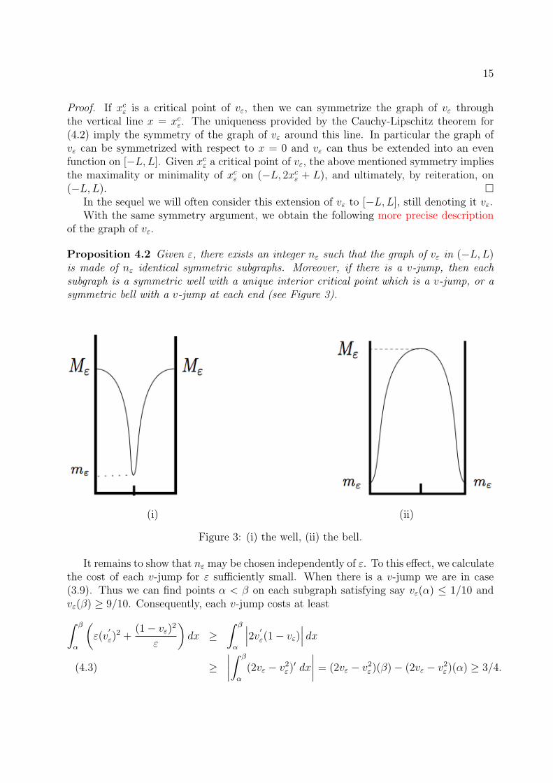
Proposition 4.2 Given ε, there exists an integer nε such that the graph of vε in (−L, L)is made of nε identical symmetric subgraphs. Moreover, if there is a v-jump, then eachsubgraph is a symmetric well with a unique interior critical point which is a v-jump, or asymmetric bell with a v-jump at each end (see Figure 3).

(i) (ii)

Figure 3: (i) the well, (ii) the bell.

It remains to show that nε may be chosen independently of ε. To this effect, we calculatethe cost of each v-jump for ε sufficiently small. When there is a v-jump we are in case(3.9). Thus we can find points α < β on each subgraph satisfying say vε(α) ≤ 1/10 andvε(β) ≥ 9/10. Consequently, each v-jump costs at least∫ β

α

(ε(v

′

ε)2 +

(1− vε)2

ε

)dx ≥

∫ β

α

∣∣∣2v′

ε(1− vε)∣∣∣ dx

≥∣∣∣∣∫ β

α

(2vε − v2ε)′ dx

∣∣∣∣ = (2vε − v2ε)(β)− (2vε − v2

ε)(α) ≥ 3/4.(4.3)

16

Thus, because of the energy bound (2.5), nε must be bounded.So, up to possible subsequence extraction, we can consider that nε is a constant n for

all ε sufficiently small.

Remark 4.3 The uniqueness of the “well” and “bell” profiles is not clear to us at thistime. If it is the case, then solutions to (2.4) would be completely determined by theirnumber of jumps (+ boundary values).

4.2 Characterisation of the possible limiting slopes

We prove that cε can only converge to two possible values.

Lemma 4.4 c0 ∈ 0, a/L.

Proof. Note that, by Lemma 3.2, c0 ≤ a/L. Assume by contradiction that 0 < c0 < a/L.We first explain the idea of the proof. By Lemma 3.6, the difficulty in the proof can

only come from the smallness of vε. In other words, there must be a v-jump. Then,let xε ∈ [0, L] be the miniminal point of vε on [0, L]; according to (3.9), vε(xε) ≤ Cε1/2.Combining this with the lower bound on v in Lemma 3.4, we obtain that

min[0,L]

vε ∼√

ε.

Our proof is then based on the estimate on the size of the set vε ≤ M√

ε, for M largeenough.

Recalling that u′ε = cε/(ηε + v2

ε), we rewrite the first equation of (2.4) as

−εv′′

ε +vεc

2ε

(ηε + v2ε)

2+

vε − 1

ε= 0.

Intergrate this equation over vε ≤ M√

ε to obtain

(4.4)

∫vε≤M

√ε

εv′′

ε dx =

∫vε≤M

√ε

vεc2ε

(ηε + v2ε)

2dx +

∫vε≤M

√ε

vε − 1

εdx.

We now recall that(4.5)The number of connected components of Dε :=vε ≤ M

√ε is bounded by a constant C.

Indeed the study of the previous subsection implies that the number of connected compo-nents of Dε is precisely the number of periods of vε, hence that it is bounded by nε +1 ≤ C.

On each connected component (ai, bi) of Dε, we obtain, by virtue of the gradient boundof Lemma 3.4, ∣∣∣∣∫ bi

ai

εv′′

ε

∣∣∣∣ =∣∣∣εv′

ε(bi)− εv′

ε(ai)∣∣∣ ≤ C.

17

Then, with (4.5), the left hand side of (4.4) is bounded from above by C. Because c0 > 0,Lemmata 3.1, 3.4 imply that 1 ≥ vε(x) ≥ C

√ε, ∀x ∈ [0, L]. It follows that, for ε sufficiently

small, v2ε(x) ηε, ∀x ∈ [0, L]. Thus the right hand-side is bounded from below by∫

vε≤M√

ε

Cvε

v4ε

dx−|vε ≤ M√

ε|ε

≥ C |vε ≤ M√

ε|M3ε3/2

−|vε ≤ M√

ε|ε

≥ C |vε ≤ M√

ε|M3ε3/2

.

Therefore, for ε sufficiently small,

C ≥ C |vε ≤ M√

ε|M3ε3/2

,

implying in turn that

(4.6)∣∣vε ≤ M

√ε

∣∣ ≤ CM3ε3/2.

Using this inequality and the refined gradient bound for uε in Lemma 3.4 yields

aε =

∫ L

0

u′

εdx =

∫vε≤M

√ε

u′

εdx +

∫M

√ε≤vε≤ 1

2u

′

εdx +

∫vε≥ 1

2u

′

εdx

≤ CM3ε1/2 +

∫M

√ε≤vε≤ 1

2u

′

εdx +

∫ L

0

u′

εχvε≥ 12dx =: CM3ε1/2 + Jε + Kε.(4.7)

Next, we bound Jε and Kε from above.Because u

′ε(x) → c0 a.e x ∈ (0, L) and χvε≥ 1

2(x) → χ(0,L)(x) a.e x ∈ (0, L), it follows

that wε(x) := u′ε(x)χvε≥ 1

2(x) → c0χ(0,L)(x) a.e. x ∈ (0, L). On the other hand, for all

x ∈ (0, L),

|wε(x)| = cε

ηε + v2ε(x)

χvε≥ 12(x) ≤ 4cε ≤ C.

Hence, by Lebesgue’s dominated convergence theorem,

(4.8) Kε =

∫ L

0

wεdx →∫ L

0

c0χ(0,L)dx = c0L.

From the energy bound (2.5), it follows that

C ≥∫ L

0

(1− vε)2

εdx ≥

∫vε≤1/2

(1− vε)2

εdx ≥

∫vε≤1/2

1

4εdx =

1

4ε|vε ≤ 1/2| ,

yielding the estimate

(4.9)∣∣M√

ε ≤ vε ≤ 1/2∣∣ ≤ |vε ≤ 1/2| ≤ Cε.

On M√

ε ≤ vε ≤ 1/2, we recover, for ε small enough, the refined estimate on u′ε fromLemma 3.4, that is

(4.10) u′

ε =cε

ηε + v2ε(x)

≤ cε

v2ε

≤ cε

M2ε≤ 2c0

M2ε.

18

Inserting inequalities (4.9), (4.10) into the expression for Jε produces the following uniformupper bound:

(4.11) Jε =

∫M

√ε≤vε≤ 1

2u

′

ε ≤2c0

M2εCε =

CM2

.

Coalescing (4.7), (4.8) and (4.11) and letting ε tend to 0 finally leads to

a ≤ CM2

+ c0L.

We let M tend to ∞ and obtain a contradiction since a > c0L. Thus c0 ∈ 0, a/L asdesired.

Remark 4.5 In this proof we have tried again to make minimal use of one-dimensionalarguments. The only place where the symmetry of the solution is used for simplicity is inthe proof of (4.5). But this can easily be avoided: we can show instead directly from (2.8)that the number of connected components of Dε is bounded by Cε−1/3 and this suffices inthe proof.

4.3 Form of u

It remains for us to establish the form of the limit critical point. Note that uε is alsoextended by reflection about 0 so that

(4.12) uε(−L) = −aε.

Proposition 4.2 immediately implies the following quantization property for the functionuε:

(4.13) uε(−L +2kL

n) = −aε +

2kaε

nfor 0 ≤ k ≤ n.

Indeed, recalling (2.6),(4.12),

2aε =

∫ L

−L

cε

ηε + v2ε

dx = n

∫ −L+2L/n

−L

cε

ηε + v2ε

dx = n

(uε

(−L +

2L

n

)+ aε

).

Now, denote by n the number of times vε reaches its minimal value (n = n in the wellcase and n = n+1 in the bell case). Because of the quantization property (4.13), it sufficesto consider the case n = 1 in the well case, and n = 2 in the bell case.

Assume first – well case – that vε(−L) = vε(L) = Mε and that vε reaches its minimum(a v-jump) at x = 0 and that 0 is the only critical point for vε on (−L, L).

Fix δ < L. Then, for ε sufficiently small, vε converges to 1 uniformly on K := [δ, L].Indeed, the closed set Aε := x ∈ (−L, L) | vε(x) ≤ 1 − ε1/4 is centered around 0, asimmediately seen from the assumption that there is only one critical point at 0. Further,

C ≥∫ L

−L

(1− vε)2

ε≥

∫Aε

(ε1/4)2

ε=|Aε|ε1/2

,

19

hence diam (Aε) ≤ Cε1/2 < δ for ε ≤ ε0.Consequently, u

′ε = cε/(ηε + v2

ε) converges uniformly to c0(= 0) on K. Thus for anyx ∈ K

(4.14) uε(x) = uε(L)−∫ L

x

u′

ε(t)dt = aε −∫ L

x

u′

ε(t)dt −→ a− c0(L− x).

Using the arbitrariness of δ, we conclude, since c0 = 0, that u = a on (0, L]. Similarly, wewould find that u = −a on (−L, 0).

Assume now – bell case – that vε(−L) = vε(L) = mε and that vε reaches its maximumat x = 0 and that 0 is the only critical point for vε on (−L, L). An argument identical tothat above would demonstrate that u′ε converges uniformly to 0 on K := [−L + δ, L − δ],for δ small. But we know that uε(0) = 0, so that, for any x ∈ (−L, L),

(4.15) uε(x) = uε(0) +

∫ x

0

u′

ε(t)dt = 0 +

∫ x

0

u′

ε(t)dt −→ c0x.

Using the arbitrariness of δ, we conclude, since c0 = 0, that u = 0 on (−L, L).

Remark 4.6 Note that all results of this subsection hold true in the case c0 6= 0, inparticular (4.14), (4.15), provided that vε admits a v-jump.

Finally we examine the case c0 = a/L. If there is no v-jump then in view of Lemma3.6, the result is that announced in Theorem 2.2. If there is a v-jump, then according toRemark 4.6, all results of the previous case hold true and, in particular, (4.14), (4.15).Hence the result upon replacing c0 by a/L.

5 Proof of Theorem 2.4

In this section, we prove Theorem 2.4. To this end, we will use the Γ-convergence ofthe Ambrosio-Tortorelli functional Eε to the Mumford-Shah functional F together with theequi-distribution of the v-jumps of any critical point (uε, vε) of Eε.

Suppose now that u is a piecewise constant function with n steps in [0, L] as describedin Theorem 2.2. Because our method is general enough to handle all possible configurationsof u, we can assume from now on that, with N := n − 1, u ≡ 0 on (0, L/2N), jumps bya/N at L/2N , and then jumps by a value of a/N at the end of each interval of length L/N .We will construct critical points of Eε – points that satisfy the Euler-Lagrange equations(2.4) – that converge to (u, 1).

Before going into the details of the proof, we briefly explain the ideas. Suppose wehave found (uε, vε). Then, from Theorem 2.2, we know that vε has a periodic structurewith an equi-distribution of v-jumps. Furthermore, the function uε enjoys a quantizationproperty: its values at v-jumps are explicit, depending only on aε, L and the number ofjumps. By our assumption on the structure of u, the graph of vε is expected to consist

20

of N symmetric wells on [0, L]. Then, we have uε(0) = 0 and uε(kL/2N) = kaε/2N for0 ≤ k ≤ 2N . Furthermore, the graph of vε on [0, L/2N ] is a half-well with a sink atx = L/2N . This sink is clearly a v-jump. If we are able to construct a critical point(uε, vε) of Eε on [0, L/2N ] having one v-jump with uε(0) = 0 and uε(L/2N) = aε/2N , thenwe can glue appropriately identical pieces of this critical point to produce a critical pointof Eε on [0, L], still denoted by (uε, vε), such that uε(0) = 0, uε(L) = aε and also that vε hasN v-jumps and n = N +1 local maxima. The gluing process is always possible because thefirst equation of (2.4) is satisfied on each interval of length L/2N and also, since v

′ε = 0,

at the gluing points. We can thus assume without loss of generality that N = 1 and thatthe v-jump is at x = L. In this case, for ε small, the graph of the function vε, if it exists,is a half-well and u = 0 in [0, L) with u(L) = a. We now investigate the details.

The sought functions vε clearly belong to

U := v ∈ H1(0, L) : µ ≤ v(0) ≤ 2− µ; v(L) ≤ α.

In the above definition, 0 < α < µ < 1, both are independent of ε. Further conditions onµ and α will be added later on whenever necessary.

The heuristic argument above suggests that we seek local minimizers (uε, vε) in thefollowing set

Bε := (u, v) ∈ (H1(0, L))2 : u(0) = 0, u(L) = aε, v ∈ U.

We use the following notation:

Fε(v, r, s) :=

∫ s

r

(ε(v

′)2 +

(1− v)2

ε

)dx

for 0 ≤ r ≤ s ≤ L and note that, for f(x) = x − x2/2, then, for all v ∈ H1(0, L) and forall 0 ≤ x1 ≤ x2 ≤ x3 ≤ L,

(5.1) Fε(v, x1, x3) ≥ 2 |f(v(x1)) + f(v(x3))− 2f(v(x2))| .

Indeed, assume with no loss of generality that v ∈ C1(0, L). Then, by Cauchy’s in-equality,

Fε(v, x1, x3) =

∫ x3

x1

(ε(v

′)2 +

(1− v)2

ε

)dx ≥

∫ x3

x1

2∣∣∣v′

(1− v)∣∣∣ dx

= 2

∫ x2

x1

∣∣∣∣(v − v2

2)

′∣∣∣∣ dx + 2

∫ x3

x2

∣∣∣∣(v − v2

2)

′∣∣∣∣ dx

≥ 2

∫ x2

x1

(v − v2

2)

′dx + 2

∫ x3

x2

−(v − v2

2)

′dx

= 2(2f(v(x2))− f(v(x1))− f(v(x3))).

Arguing similarly, we also obtain

Fε(v, x1, x3) ≥ 2(f(v(x1)) + f(v(x3))− 2f(v(x2)))

21

and thus (5.1) follows.In a first step, we establish a universal lower bound for Eε over Bε as well as an

upper bound for the infimum of Eε over Bε. In fact, for all (u, v) ∈ Bε, we have

(5.2) Eε(u, v) ≥ Fε(v, 0, L) ≥ 2(f(µ)− f(α)),

while there exists (uε, vε)) ∈ Bε such that, for ε small,

(5.3) Eε(uε, vε) ≤ 1 + o(1).

To see (5.2), let (u, v) ∈ Bε. Then, using (5.1) with x1 = x2 = 0 and x3 = L, we get

Fε(v, 0, L) ≥ 2(f(v(0))− f(v(L))) ≥ 2( minx∈[µ,2−µ]

f(x)−maxx≤α

f(x)) = 2(f(µ)− f(α)).

Assertion (5.3) is derived upon constructing a sequence (uε, vε) which is very similarto that used in the proof of the Γ-limsup of the Ambrosio-Tortorelli functional in [4]. Weomit the details.

The direct method of the calculus of variations immediately implies that the minimumof Eε over Bε is achieved at, say (uε, vε). By (5.3),

(5.4) Eε(uε, vε) = min(u,v)∈Bε

Eε(u, v) ≤ 1 + o(1).

For a suitable choice of (µ, α), a minimizer (uε, vε) of Eε over Bε is actually a criticalpoint of Eε for ε sufficiently small. This is the object of the following

Lemma 5.1 There exists (µ, α), independent of ε, such that if (uε, vε) is a minimizer ofEε over Bε then it is a critical point of Eε if ε is small enough.

Proof. To prove the criticality of (uε, vε), it suffices to prove the following inequalitieswith a suitable choice of (µ, α):(i) µ < vε(0) < 2− µ, and(ii) vε(L) < α.

Indeed, then (uε, vε) is not on the boundary of Bε but rather in its interior, hence it isa local minimizer of Eε and thus a critical point.

Our proof is by contradiction. We assume that there exists a sequence εj → 0 suchthat either (i), or (ii) is not satisfied. Then, for each j, we have at least an equality ineither (i), or (ii). However, through relabelling, we can assume that either (i), or (ii) isnever satisfied.

Suppose that, for all ε, either vε(0) = µ, or vε(0) = 2− µ. It is enough to consider thefirst case because f(µ) = f(2− µ) and only the value of f(v(0)) enters the proof.

We introduce the following special points xε. From (5.4), we know that∫ 3L/4

L/4

(1− vε)2

εdx ≤ Eε(uε, vε) ≤ 1 + o(1).

22

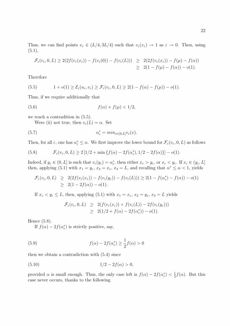
Thus, we can find points xε ∈ (L/4, 3L/4) such that vε(xε) → 1 as ε → 0. Then, using(5.1),

Fε(vε, 0, L) ≥ 2(2f(vε(xε))− f(vε(0))− f(vε(L))) ≥ 2(2f(vε(xε))− f(µ)− f(α))

≥ 2(1− f(µ)− f(α))− o(1).

Therefore

(5.5) 1 + o(1) ≥ Eε(uε, vε) ≥ Fε(vε, 0, L) ≥ 2(1− f(α)− f(µ))− o(1).

Thus, if we require additionally that

(5.6) f(α) + f(µ) < 1/2,

we reach a contradition in (5.5).Were (ii) not true, then vε(L) = α. Set

(5.7) α∗ε = minx∈[0,L]vε(x).

Then, for all ε, one has α∗ε ≤ α. We first improve the lower bound for Fε(vε, 0, L) as follows

(5.8) Fε(vε, 0, L) ≥ 2 [1/2 + min f(α)− 2f(α∗ε), 1/2− 2f(α)]− o(1).

Indeed, if yε ∈ (0, L] is such that vε(yε) = α∗ε, then either xε > yε, or xε < yε. If xε ∈ (yε, L]then, applying (5.1) with x1 = yε, x2 = xε, x3 = L, and recalling that α∗ ≤ α < 1, yields

Fε(vε, 0, L) ≥ 2(2f(vε(xε))− f(vε(yε))− f(vε(L))) ≥ 2(1− f(α∗ε)− f(α))− o(1)

≥ 2(1− 2f(α))− o(1).

If xε < yε ≤ L, then, applying (5.1) with x1 = xε, x2 = yε, x3 = L yields

Fε(vε, 0, L) ≥ 2(f(vε(xε)) + f(vε(L))− 2f(vε(yε)))

≥ 2(1/2 + f(α)− 2f(α∗ε))− o(1).

Hence (5.8).If f(α)− 2f(α∗ε) is strictly positive, say,

(5.9) f(α)− 2f(α∗ε) ≥1

2f(α) > 0

then we obtain a contradiction with (5.4) since

(5.10) 1/2− 2f(α) > 0,

provided α is small enough. Thus, the only case left is f(α) − 2f(α∗ε) < 12f(α). But this

case never occurs, thanks to the following

23

Proposition 5.2 Take α1 ∈ (0, α), independent of ε, such that f(α) ≥ 4f(α1). Then,

(5.11) minx∈[0,L]

vε(x) = α∗ε ≤ α1,

and thus (5.9) is always satisfied.

Proof. Assume that (5.11) is false, i.e.,

(5.12) vε(x) ≥ α1 ∀ x ∈ [0, L].

We show that the energy Eε(uε, vε) is actually greater than 1 and thus reach a new contra-diction. Since (uε, vε) minimizes Eε over Bε, (uε, vε) is, at the least, a critical point of Eε on(0, L) with respect to compactly supported variations in both vε and uε. Thus, on (0, L),

(5.13)−εv

′′

ε + vε(u′

ε)2 +

vε − 1

ε= 0

[u′

ε(ηε + v2ε)]

′ = 0.

The second equation of (5.13) shows that, on (0, L),

(5.14) u′

ε(x)(ηε + v2ε(x)) = cε a.e. x

for some constant cε. From (5.4), (5.14), and, since uε is in particular in W 1,1(0, L),

o(1) + 1 ≥ Eε(uε, vε) ≥∫ L

0

(ηε + v2ε)(u

′

ε)2 =

∫ L

0

cεu′

ε = aεcε,

so that

cε ≤Caε

.

Hence, at the possible expense of extracting a subsequence,

(5.15) cε → c0, ε 0.

On the other hand, the energy bound Eε(uε, vε) ≤ 1 + o(1) implies that vε converges to 1in L2(0, L) and thus vε(x) → 1 a.e x ∈ (0, L). Therefore

u′

ε(x) =cε

ηε + v2ε(x)

→ c0 as ε → 0 for a. e. x ∈ (0, L).

In view of (5.12), (5.14), u′ε is bounded. Therefore, by Lebesgue’s dominated convergence

theorem,

aε =

∫ L

0

u′

εdx →∫ L

0

c0dx = c0L.

24

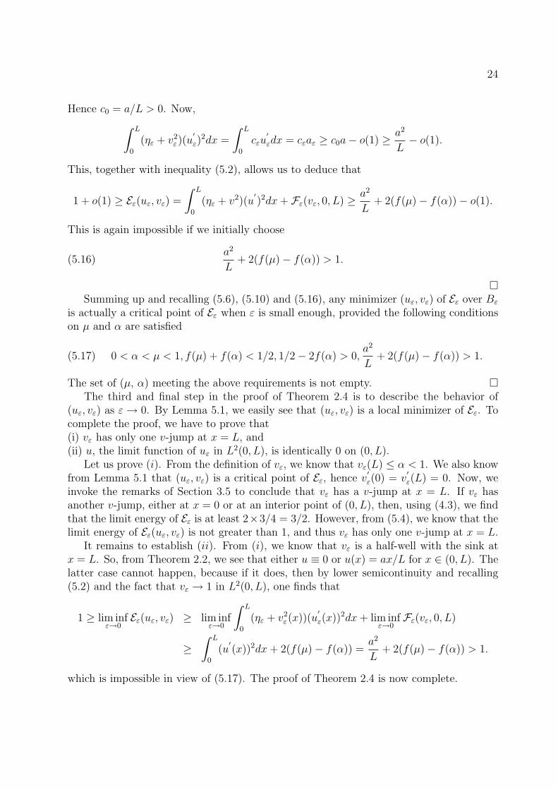
Hence c0 = a/L > 0. Now,∫ L

0

(ηε + v2ε)(u

′

ε)2dx =

∫ L

0

cεu′

εdx = cεaε ≥ c0a− o(1) ≥ a2

L− o(1).

This, together with inequality (5.2), allows us to deduce that

1 + o(1) ≥ Eε(uε, vε) =

∫ L

0

(ηε + v2)(u′)2dx + Fε(vε, 0, L) ≥ a2

L+ 2(f(µ)− f(α))− o(1).

This is again impossible if we initially choose

(5.16)a2

L+ 2(f(µ)− f(α)) > 1.

Summing up and recalling (5.6), (5.10) and (5.16), any minimizer (uε, vε) of Eε over Bε

is actually a critical point of Eε when ε is small enough, provided the following conditionson µ and α are satisfied

(5.17) 0 < α < µ < 1, f(µ) + f(α) < 1/2, 1/2− 2f(α) > 0,a2

L+ 2(f(µ)− f(α)) > 1.

The set of (µ, α) meeting the above requirements is not empty. The third and final step in the proof of Theorem 2.4 is to describe the behavior of

(uε, vε) as ε → 0. By Lemma 5.1, we easily see that (uε, vε) is a local minimizer of Eε. Tocomplete the proof, we have to prove that(i) vε has only one v-jump at x = L, and(ii) u, the limit function of uε in L2(0, L), is identically 0 on (0, L).

Let us prove (i). From the definition of vε, we know that vε(L) ≤ α < 1. We also knowfrom Lemma 5.1 that (uε, vε) is a critical point of Eε, hence v

′ε(0) = v

′ε(L) = 0. Now, we

invoke the remarks of Section 3.5 to conclude that vε has a v-jump at x = L. If vε hasanother v-jump, either at x = 0 or at an interior point of (0, L), then, using (4.3), we findthat the limit energy of Eε is at least 2×3/4 = 3/2. However, from (5.4), we know that thelimit energy of Eε(uε, vε) is not greater than 1, and thus vε has only one v-jump at x = L.

It remains to establish (ii). From (i), we know that vε is a half-well with the sink atx = L. So, from Theorem 2.2, we see that either u ≡ 0 or u(x) = ax/L for x ∈ (0, L). Thelatter case cannot happen, because if it does, then by lower semicontinuity and recalling(5.2) and the fact that vε → 1 in L2(0, L), one finds that

1 ≥ lim infε→0

Eε(uε, vε) ≥ lim infε→0

∫ L

0

(ηε + v2ε(x))(u

′

ε(x))2dx + lim infε→0

Fε(vε, 0, L)

≥∫ L

0

(u′(x))2dx + 2(f(µ)− f(α)) =

a2

L+ 2(f(µ)− f(α)) > 1.

which is impossible in view of (5.17). The proof of Theorem 2.4 is now complete.

25

Remark 5.3 If N = 1 and the v-jump is at the boundary of (0, L) then the critical points(uε, vε) of Eε constructed in Theorem 2.4 are also local minimizers of Eε. We conjecturethat if N = 1 and the v-jump is at L/2 or if N ≥ 2, then the critical points (uε, vε) foundin Theorem 2.4 are also local minimizers of Eε.

6 Proof of Theorem 2.5

The measure limit of (ηε + v2ε)(u

′ε)

2dx is immediately computed upon remarking that,thanks to (2.6),

(ηε + v2ε)(u

′ε)

2 = cεu′ε,

so that the measure limit of (ηε + v2ε)(u

′ε)

2dx is that of cεu′εdx. Testing with a smooth

compactly supported function ϕ, we obtain∫ L

0

cεu′εϕ dx = −cε

∫ L

0

uεϕ′ dx −→ −c0

∫ L

0

uϕ′ dx,

so that, upon recalling Theorem 2.2, we obtain the desired result. The reader will havenot failed to note the fortuitousness of the value of c0, i.e., 0, when u jumps; the resultwould be false if u could jump for non-zero values of c0!

The computation of the measure limit of the other two terms is more delicate. Wefirst establish that there is no concentration of energy for those two terms away from thejump points. We will only use the property that there is a finite ε-independent number jofv-jumps on [0, L], denoted by x1

ε, ...., xjε, with xk

ε → xk, k = 1, ..., j.

Lemma 6.1 For any compact subset K ⊂ [0, L] \ ∪k=1,...,jxk, we have∫K

(ε(v′ε(x))2 + (1− vε(x))2/ε

)dx ≤ CKε1/4,

where CK may depend only on K.

Proof. Consider Aε := x ∈ [0, L] : vε(x) ≤ 1 − ε1/4. Then, from the energy bound(2.5), |Aε| ≤ C

√ε, while x1

ε, ..., xjε ⊂ Aε. For a given compact subset K of [0, L] \

∪k=1,...jxk, set δ := 1/2 mink=1,...,j dist(xk, K). If ε is small enough, x1, ..., xj ⊂ Aε ⊂Uδ := ∪k=1,...,j[xk − δ, xk + δ], so that, K ∩ Aε = ∅. Because K ⊂ [0, L] \ Uδ, it suffices toprove that

(6.1)

∫[0,L]\Uδ

(ε(v′ε(x))2 + (1− vε(x))2/ε

)dx ≤ CKε1/4.

Let us denote Vδ = [0, L]\Uδ. Multiplying both sides of the first equation of (2.4) by vε−1and integrating over Vδ, we get

(6.2)

∫Vδ

−εv′′

ε (x)(vε(x)− 1)dx +

∫Vδ

vε(x)(u′

ε(x))2(vε(x)− 1)dx +

∫Vδ

(vε(x)− 1)2

εdx = 0.

26

Note that Vδ is a union of a finite ε-independent number J (≤ j + 1) of intervals on [0, L]:Vδ = ∪k=1,...,J [ak

ε , bkε ]. Now, integrating by parts the first term of (6.2), recalling (2.6) and

rearranging, one obtains

(6.3)∫Vδ

ε(v′

ε(x))2dx +

∫Vδ

(vε(x)− 1)2

εdx =

J∑k=1

ε(v

′

ε(bkε)(vε(b

kε)− 1)− v

′

ε(akε)(vε(a

kε)− 1)

)+

∫Vδ

c2ε

(ηε + v2ε(x))2

vε(x)(1− vε(x))dx.

By the definitions of Aε and Vδ, we have |1− vε| ≤ ε1/4 on Vδ. Combining this fact withthe gradient bound for vε in Lemma 3.4 yields that the right hand side of (6.3) is boundedfrom above by CKε1/4 for some constant CK which may depend only on K. Hence thedesired result stated in (6.1) follows.

Remark 6.2 The previous lemma shows that the measure limits of ε(v′ε(x))2 dx, andof (vε(x) − 1)2/ε dx are Dirac masses concentrated at x1, ..., xj. We will evaluate theirrespective weight in the fourth and final step below.

Also note that, thanks to Lemma 3.6, those limits are immediately computed (andfound to be 0!) in the absence of v-jumps.

The second step consists in computing the limit d0 of the discrepancy dε defined in(3.3), which exists, at least for a well chosen subsequence, by the boundedness (3.4) of dε.To this effect, we prove the following

Lemma 6.3 d0 + c20 = 0.

Proof. Recalling (3.3), (2.6), we obtain

(6.4) dε + cεu′ε(x) =

(vε(x)− 1)2

ε− ε(v′ε(x))2,

and thus

(6.5) |dε + cεu′ε(x)| =

∣∣∣∣(vε(x)− 1)2

ε− ε(v′ε(x))2

∣∣∣∣ .

Let Aε, K with |K| > 0 and δ be as in the proof of Lemma 6.1. Then, on K, one has1 − ε1/4 ≤ vε ≤ 1. By virtue of (2.6), u

′ε is bounded on K. Upon integrating (6.5) over

K, recalling Lemma 3.2 and letting ε 0, we have by Lebesgue’s dominated convergencetheorem

(6.6) |K|∣∣d0 + c2

0

∣∣ = limε→0

∫K

|dε + cεu′ε(x)| dx = lim

ε→0

∫K

∣∣∣∣(vε(x)− 1)2

ε− ε(v′ε(x))2

∣∣∣∣ dx.

27

In view of Lemma 6.1, the last term of the above equation is 0. Thus d0 + c20 = 0 as

claimed.

The third step consists of the following equi-partition result

Lemma 6.4 For all x in [0, L],

|v′ε(x)| ≤ 1− vε(x)

ε.

Further,

limε→0

∫ L

0

|ε(v′ε(x))2 − (vε(x)− 1)2/ε| dx = 0.

Proof. According to (6.4), the term (vε(x)− 1)2/ε − ε(v′ε(x))2 attains, for a fixed ε, itsminimum on [0, L] precisely where u′ε = cε/(ηε + v2

ε) attains its minimum, or still, wherevε attains its maximum. But, at such points, v′ε cancels, so that the minimum of that termis non-negative. Thus,∫ L

0

∣∣∣∣(vε(x)− 1)2

ε− ε(v′ε(x))2

∣∣∣∣ dx =

∫ L

0

((vε(x)− 1)2

ε− ε(v′ε(x))2

)dx

=

∫ L

0

(dε + cεu′ε(x)) dx = Ldε + cεaε

→ Ld0 + c0a = L(d0 + c20) = 0,

in view of Lemma 6.3.

The fourth and final step consists in evaluating the respective weights of the Diracmasses making up the limit of ε(v′ε(x))2 dx and of (vε(x)− 1)2/ε dx.

To this effect, we first remark that, at the possible expense of extending vε by re-flection around x = 0 and/or x = L, we may always compute the measure limit µ of(ε(v′ε(x))2 + (vε(x)−1)2/ε) dx over some I ⊃ [0, L], so that µ(∂I) = 0, in which caseµ(I) = limε

∫I(ε(v′ε(x))2 + (vε(x)−1)2/ε) dx, while Lemma 6.4 still applies over I.

Note that∫I

(ε(v′ε(x))2 +

(vε(x)−1)2

ε− 2|v′ε(x)|((1−vε(x))

)dx =

∫I

(ε1/2|v′ε(x)|− (1−vε(x))

ε1/2

)2

dx

≤∫

I

∣∣∣∣ε(v′ε(x))2− (1−vε(x))2

ε

∣∣∣∣ dx,

which goes to 0 with ε, according to Lemma 6.4 above. Thus, the total mass of the measurelimit of (ε(v′ε(x))2 +(vε(x)−1)2/ε) dx, is also that of 2|v′ε(x)|((1−vε(x)) dx. But, we know,according to Proposition 4.2, that the graph of vε is symmetric around each v-jump, sothat it suffices to compute the mass of measure limit of 2|v′ε(x)|((1−vε(x)) dx over a halfwell, that is, ∫

x:vε(x)∈[mε,Mε]2|v′ε(x)|((1−vε(x)) dx,

28

or still, since v′ε(x) > 0 on x : vε(x) ∈ [mε, Mε],∫ Mε

mε

2(1− y) dy = (2Mε −M2ε )− (2mε −m2

ε) −→ 1,

as ε 0, since Mε 1, while mε 0. Hence the measure limit µ is given by

µ = 2∑

x: x is a v-jump

δx.

The proof of Theorem 2.5 is now complete.

Acknowledgements: The authors are grateful to the referees for their comments and criticismswhich resulted in a hopefully improved version of the original manuscript.

References

[1] L. Ambrosio. Existence theory for a new class of variational problems. Arch. Ration.Mech. Anal., 111:291–322, 1990.

[2] L. Ambrosio, N. Fusco, and D. Pallara. Functions of Bounded Variation and FreeDiscontinuity Problems. Oxford University Press, 2000.

[3] L. Ambrosio and V.M. Tortorelli. Approximation of functionals depending on jumpsby elliptic functionals via Γ-convergence. Comm. Pure Appl. Math., 43(8):999–1036,1990.

[4] L. Ambrosio and V.M. Tortorelli. On the approximation of free discontinuity problems.Boll. Un. Mat. Ital. B (7), 6(1):105–123, 1992.

[5] F. Bethuel, H. Brezis, and F. Helein. Ginzburg-Landau vortices. Progress in NonlinearDifferential Equations and their Applications, 13. Birkhauser Boston Inc., Boston,MA, 1994.

[6] B. Bourdin. Numerical implementation of the variational formulation of brittle frac-ture. Interfaces Free Bound., 9:411–430, 2007.

[7] A. Braides. Γ-convergence for Beginners, volume 22 of Oxford Lecture Series in Math-ematics and its Applications. Oxford University Press, 2002.

[8] E. De Giorgi, M. Carriero, and A. Leaci. Existence theorem for a minimum problemwith free discontinuity set. Arch. Ration. Mech. Anal., 108:195–218, 1989.

[9] L.C. Evans and R.F. Gariepy. Measure theory and fine properties of functions. CRCPress, Boca Raton, FL, 1992.

29

[10] G.A. Francfort and J.-J. Marigo. Revisiting brittle fracture as an energy minimizationproblem. J. Mech. Phys. Solids, 46(8):1319–1342, 1998.

[11] J. E. Hutchinson and Y. Tonegawa. Convergence of phase interfaces in the van derWaals-Cahn-Hilliard theory. Calc. Var. Partial Differential Equations, 10(1):49–84,2000.

[12] L. Modica and S. Mortola. Il limite nella Γ–convergenza di una famiglia di funzionaliellittici. Boll. Un. Mat. Ital. A (5), 14(3):526–529, 1977.

[13] D. Mumford and J. Shah. Optimal approximations by piecewise smooth functions andassociated variational problems. Comm. Pure Appl. Math., XLII:577–685, 1989.

[14] P. J. Olver. Applications of Lie groups to differential equations, volume 107 of GraduateTexts in Mathematics. Springer-Verlag, New York, 1986.

[15] E. Sandier and S. Serfaty. Vortices in the magnetic Ginzburg-Landau model. Progressin Nonlinear Differential Equations and their Applications, 70. Birkhauser Boston Inc.,Boston, MA, 2007.

[16] Y. Tonegawa. Phase field model with a variable chemical potential. Proc. Roy. Soc.Edinburgh Sect. A, 132(4):993–1019, 2002.

[17] Y. Tonegawa. A diffused interface whose chemical potential lies in a Sobolev space.Ann. Sc. Norm. Super. Pisa Cl. Sci. (5), 4(3):487–510, 2005.

[18] T. Wittman. Lost in the supermarket: decoding blurry barcodes. SIAM News, 37(7),September 2004.