arX

iv:c

ond-

mat

/030

5193

v2 [

cond

-mat

.str

-el]

13

Oct

200

3

Weak magnetism and non-Fermi liquids near heavy-fermion critical points

T. SenthilDepartment of Physics, Massachusetts Institute of Technology, Cambridge MA 02139

Matthias VojtaInstitut fur Theorie der Kondensierten Materie, Universitat Karlsruhe, Postfach 6980, 76128 Karlsruhe, Germany

Subir SachdevDepartment of Physics, Yale University, P.O. Box 208120, New Haven CT 06520-8120

(Dated: February 2, 2008)

This paper is concerned with the weak-moment magnetism in heavy-fermion materials and itsrelation to the non-Fermi liquid physics observed near the transition to the Fermi liquid. We explorethe hypothesis that the primary fluctuations responsible for the non-Fermi liquid physics are thoseassociated with the destruction of the large Fermi surface of the Fermi liquid. Magnetism is suggestedto be a low-energy instability of the resulting small Fermi surface state. A concrete realization ofthis picture is provided by a fractionalized Fermi liquid state which has a small Fermi surface ofconduction electrons, but also has other exotic excitations with interactions described by a gaugetheory in its deconfined phase. Of particular interest is a three-dimensional fractionalized Fermiliquid with a spinon Fermi surface and a U(1) gauge structure. A direct second-order transitionfrom this state to the conventional Fermi liquid is possible and involves a jump in the electronFermi surface volume. The critical point displays non-Fermi liquid behavior. A magnetic phasemay develop from a spin density wave instability of the spinon Fermi surface. This exotic magneticmetal may have a weak ordered moment although the local moments do not participate in theFermi surface. Experimental signatures of this phase and implications for heavy-fermion systemsare discussed.

I. INTRODUCTION

The competition between the Kondo effect and inter-moment exchange determines the physics of a large classof materials which have localized magnetic moments cou-pled to a separate set of conduction electron [1]. Whenthe Kondo effect dominates, the low-energy physics iswell described by Fermi liquid theory (albeit with heavilyrenormalized quasiparticle masses). In contrast when theinter-moment exchange dominates, ordered magnetismtypically results.

A remarkable experimental property of such magneticstates is that the magnetism is often very weak – theordered moment per site is much smaller than the mi-croscopic local moment that actually occupies each site.The traditional explanation of this feature is that themagnetism arises out of imperfectly Kondo-screened lo-cal moments. In other words, the magnetism is to beviewed as a spin density wave that develops out of theparent heavy Fermi liquid state. We will henceforth de-note such a state as SDW. Clearly a SDW state may bea small moment magnet.

A different kind of magnetic metallic state is also pos-sible in heavy-fermion materials where the moments or-der at relatively large energy scales, and simply do notparticipate in the Fermi surface of the metal. In sucha situation, the saturation moment in the ordered statewould naively be large, i.e., of order the atomic moment.

Often the distinction between these two kinds of mag-netic states can be made sharply: the two Fermi surfacesin the two states may have different topologies (albeit,

the same volume modulo the volume of the Brillouin zoneof the ordered state), so that they cannot be smoothlyconnected to one another.

In recent years, a number of experiments have un-earthed some fascinating phenomena near the zero tem-perature (T ) quantum transition between the heavy-fermion liquid and the magnetic metal. In particu-lar, many experiments do not fit easily [2, 3, 4, 5]into a description in terms of an effective Gaussian the-ory for the spin density wave fluctuations, renormalizedself-consistently by quartic interactions [6, 7, 8, 9, 10].This theory makes certain predictions on deviations fromFermi liquid behavior as the heavy Fermi liquid stateapproaches magnetic ordering induced by the condensa-tion of the spin density wave mode; those predictionsare, however, in disagreement with experimental findings.This conflict raises the possibility that the magnetic statebeing accessed is not in the first category discussed above:a SDW emerging from a heavy Fermi liquid. Rather, itmay be the second kind of magnetic metal where the localmoments do not participate at all in the Fermi surface.In other words, the experiments suggest that the Kondoeffect (crucial in forming the Fermi liquid state) is itselfsuppressed on approaching the magnetic state.

This proposal clearly raises several serious puzzles.How do we correctly describe the non-Fermi liquidphysics near the transition? If this non-Fermi liquid be-havior is accompanied by the suppression of the Kondoeffect, how do we reconcile it with the weak momentsfound in the magnetic state? The traditional explana-tion for the weak magnetism is apparently in conflict

2

with the picture that the Kondo effect and the resultantheavy Fermi liquid state are destroyed on approachingthe magnetic state. In other words, the naive expecta-tion of a large saturation moment in a magnetic metalwhere the local moments do not participate in the Fermisurface must be revisited.

The weakness of the ordered moment in the magneticstate may be reconciled with the apparent suppression ofthe Kondo effect if we assume that there are strong quan-tum fluctuations of the spins that reduce their moment.Such strong quantum effects may appear to be unusualin three-dimensional systems, but may be facilitated bythe coupling to the conduction electrons (even if thereis no actual Kondo screening). In this paper we studyspecific states where such quantum fluctuations have sig-nificantly reduced the ordered moment (or even caused itto vanish), and the evolution of such states to the heavyFermi liquid.

We begin with several general pertinent observations.First, consider the heavy Fermi liquid state. This Fermiliquid behavior is accompanied by a Fermi surface which,remarkably, satisfies Luttinger’s theorem only if the lo-cal moments are included as part of the electron count.(Such a Fermi surface is often referred to as the “largeFermi surface”, and we will henceforth refer to sucha phase as FL). The absorption of the local momentsinto the Fermi volume is the lattice manifestation of theKondo screening of the moments. We take as our startingpoint the assumption that the Kondo effect becomes sup-pressed on approaching the magnetic state. What thenhappens to the large Fermi surface?

In thinking about the resulting state theoretically, itis important to realize that once magnetic order sets in,there is no sharp distinction between a large Fermi vol-ume which includes the local moments, and a Fermi vol-ume that excludes the local moments – the latter is oftenloosely referred to as “small”. This is because the Fermivolumes can only be defined modulo the volume of theBrillouin zone, and the onset of magnetic order at leastdoubles the unit cell and hence at least halves the Bril-louin zone volume. (There can, however, be a distinctionbetween the Fermi surfaces topologies in the two situa-tions.)

In this paper we will take the point of view that theprimary transition involves the destruction of the largeFermi surface, and that the resulting small Fermi surfacestate has a distinct physical meaning even in the absenceof magnetic order. The magnetic order will be viewedas a low-energy instability of the resulting state in whichthe local moments are not to be included in the Fermivolume.

Evidence in support of this point of view exists. Inthe experiments the non-Fermi liquid behavior extendsto temperatures well above the Neel ordering tempera-ture even far away from the critical point. This suggeststhat the fluctuations responsible for the non-Fermi liq-uid behavior have very little to do with the fluctuationsof the magnetic order parameter. Some further support

is provided by the results of inelastic neutron scatter-ing experiments that apparently see critical behavior ata range of wave-vectors including (but not restricted to)the one associated with magnetic ordering in the mag-netic metal [5]. Finally, there even exist materials inwhich the non-Fermi liquid features persist into the mag-netically ordered side – this is difficult to understand ifthe non-Fermi liquid physics is attributed to critical fluc-tuations of the magnetic order parameter.

Conceptually, as we asserted above, it pays to allow forthe possibility of a non-magnetic state in which the sup-pression of the Kondo effect removes the local momentsfrom the Fermi volume, resulting in a “small Fermi sur-face”, even though such a state may not actually be aground state in the system of interest. In our previouswork [11] we argued that such states do exist as groundstates of Kondo lattice models in regular d-dimensionallattices, and that the violation of Luttinger’s theorem insuch a state was intimately linked to the presence of neu-tral S = 1/2 and S = 0 excitations induced by topologi-cal order (see also Appendix A): we dubbed such groundstates FL∗.

Clearly, it is worthwhile to explore metallic magneticstates that develop out of such FL∗ states (just as theusual SDW state develops out of the Fermi liquid). Suchstates, which we will denote SDW∗, represent a thirdclass of metallic magnetic states distinct from both theconventional SDW and the conventional local-momentmetal described above. As we will see, in such mag-netic states the local moments do not participate in theFermi surface. Nevertheless they may have a weak or-dered moment. Thus these states offer an opportunityfor resolution of the puzzles mentioned above. The prop-erties and the evolution of such states, and their parentFL∗ states, to the Fermi liquid will be the subject of thispaper. The SDW∗ states inherit neutral spin S = 1/2spinon excitations and S = 0 “gauge” excitations fromthe FL∗ states, which will be described more preciselybelow; these excitations coexist with the magnetism andthe metallic behavior. The experimental distinction be-tween the SDW and SDW∗ states is however subtle, andwill also be described in this paper. (The FL and FL∗

states can be easily distinguished by the volumes of theFermi surfaces, but this distinction does not extend tothe SDW and SDW∗ states.)

We emphasize that a wide variety of heavy-fermion ma-terials display non-Fermi liquid physics in the vicinity ofthe onset of magnetism that is, to a considerable extent,universal. However, the detailed behavior at very lowtemperature appears to vary across different systems. Inparticular, in some materials a direct transition to themagnetic state at very low temperature does not occur(due for instance to intervention of a superconductingstate). In other materials, such a direct transition doesseem to occur at currently accessible temperatures. Inview of this, we will not attempt to predict the detailedphase diagram at ultra-low temperatures. We focus in-stead on understanding the universal non-Fermi liquid

3

physics not too close to the transition and its relation tothe magnetic state.

A. Summary of results

Our analysis is based upon non-magnetic translation-invariant states that have a small Fermi surface (FL∗),and the related transitions to the heavy Fermi liquid(FL). As we showed previously [11], the FL∗ state hasa Fermi surface of long-lived electron-like quasiparticleswhose volume does not count the local moments. Thelocal moments are instead in a state adiabatically con-nected to a spin-liquid state with emergent gauge exci-tations. Such spin liquids can be classified by the gaugegroup determining the quantum numbers carried by theneutral S = 1/2 spinon excitations and the gauge exci-tations, and previous work [12, 13] has shown that themost prominent examples are Z2 and U(1) spin liquids.The Z2 spin liquids are stable in all spatial dimensionsd ≥ 2, while the U(1) spin liquids exist only in d ≥ 3 (thelatter correspond to the existence of a Coulomb phase ina compact U(1) gauge theory in d ≥ 3, as discussed inRef. 14). Correspondingly, we also have the metallic Z2

FL∗ and U(1) FL∗ states. Our previous work [11] consid-ered primarily the Z2 FL∗ state, whereas here we focuson the U(1) FL∗ state.

As we have already discussed, these non-magneticstates may lead to magnetic order at low energies, or inproximate states in a generalized phase diagram. In thismanner the FL state leads to the SDW state, while theFL∗ states lead to the Z2 SDW∗ and the U(1) SDW∗

states. The relation between the metallic SDW andSDW∗ states has a parallel to that between the insulatingNeel state and the AF∗ state of Refs. 13, 15.

We will also discuss the evolution from the U(1) SDW∗

state to the conventional Fermi liquid. As explained ear-lier, the underlying transition is that between FL andFL∗ states which controls the nature of the Fermi sur-face. In Ref. 11, we argued that the spinon pairing inthe Z2 FL∗ state implied that there must be a super-conducting state in between the FL and Z2 FL∗ states.There is no such pairing in the U(1) FL∗ state, and hencethere is the possibility of a direct transition between theFL and U(1) FL∗ states: this transition and the natureof the states flanking it are the foci of our paper. Notethat the volume of the Fermi surface jumps at this tran-sition. Nevertheless the transition may be second order.This is made possible by the vanishing of the quasipar-ticle residue on an entire portion of the Fermi surface (a“hot” Fermi surface) on approaching the transition fromthe FL side. Non-Fermi liquid physics is clearly to beexpected at such a second order Fermi-volume changingtransition. We reiterate that the U(1) FL∗ state is onlybelieved to exist in d > 2.

We study the FL and U(1) FL∗ states by the “slave”boson method, introduced in the context of the single-moment Kondo problem [16]. In this method, the con-

JK

T

0U(1) FL* FL

Quantum

critical

0b ≠

JKc

FIG. 1: Crossover phase diagram for the vicinity of the d = 3quantum transition involving breakdown of Kondo screening.JK is the Kondo exchange in the Hamiltonian introduced inSection III. The only true phase transition above is that atthe T = 0 quantum critical point at JK = JKc between theFL and FL∗ phases. The “slave” boson b measures the mix-ing between the local moments and the conduction electronsand is also described in Section III. The crossovers are sim-ilar to those of a dilute Bose gas as a function of chemicalpotential and temperature, as discussed in Refs. 19, 20—thehorizontal axis is a measure of the boson chemical potentialµb. The boson is coupled to a compact U(1) gauge field; atT = 0 this gauge field is in the Higgs/confining phase in theFL state, and in the deconfining/Coulomb phase in the FL∗

state. There is no phase transition at T > 0 between a phasewith 〈b〉 6= 0 and a phase with 〈b〉 = 0 because such a transi-tion is absent in a theory with a compact U(1) gauge field ind = 3 [21] (the mean-field theories of Sections. III and IVC doshow such transitions, but these will turn into crossovers uponincluding gauge fluctuations). The compactness of the gaugefield therefore plays a role in the crossovers in the “renormal-ized classical” regime above the FL state (this has not beenworked out in any detail here). However, the compactnessis not expected to be crucial in the quantum-critical regime.The crossover line displayed between the FL and quantumcritical regimes can be associated with the “coherence” tem-perature of the heavy Fermi liquid. At low T , as discussed inthe text, there are likely to be additional phases associatedwith magnetic order (the SDW and SDW∗ phases), and theseare not shown above but are shown in Fig. 2; they also appearin the mean-field phase diagram in Fig. 4.

densation of the slave boson marks the onset of Kondo co-herence that characterizes the FL phase. In contrast theslave boson is not condensed in the FL∗ phase. Fluctua-tions about this mean-field description lead to the criticaltheory of the transition involving a propagating bosoncoupled to a compact U(1) gauge field, in the presence ofdamping from fermionic excitations.

We note that earlier studies [17, 18] of single-impurityproblems found a temperature-induced mean-field tran-sition between a state in which the slave boson is con-densed (and hence the local moment is Kondo screened)and a state in which the boson has no condensate: how-ever, it was correctly argued that this transition is anartifact of the mean-field theory, and no sharp transitionexists in the single-moment Kondo problem at T > 0.If we now naively generalize this single-impurity model

4

T

JK

FL

U(1) FL*

U(1) SDW*

Quantum

critical

SDW

FIG. 2: Expected phase diagram and crossovers for the evolu-tion from the U(1) SDW∗ phase to the conventional FL. Twodifferent transitions are generically possible at zero tempera-ture: Upon moving from the SDW∗ towards the Fermi liquid,the fractionalization is lost first followed by the disappear-ance of magnetic order. Nevertheless the higher temperaturebehavior in the region marked ‘quantum critical’ is non-fermiliquid like, and controlled by the Fermi volume changing tran-sition from FL to FL∗. This may be loosely associated to thebreakdown of Kondo screening.

to the lattice, we will find that the T = 0 ground statealways has Kondo screening. It is only upon includingfrustrating inter-moment exchange interactions – equiva-lent to having “dispersing” spinons – that it is possible tobreakdown Kondo screening and reach a state in whichthe slave boson is not condensed. This transition is notan artifact of mean-field theory, we show here that it re-mains sharply defined in d = 3.

Our analysis of the above d = 3 U(1) gauge theoryleads to the schematic crossover phase diagram as a func-tion of the Kondo exchange JK and T shown in Fig 1.

The crossover phase diagram in Fig. 1 is similar to thatof a dilute Bose gas as a function of chemical potentialand temperature [19, 20]. Here the bosons are coupled toa U(1) gauge field, and this is important for many of thecritical properties to be described in the body of the pa-per. Notably, in Fig. 1 the density of bosons is not fixed,and varies as a function of T , JK and other couplings inthe Hamiltonian. Indeed, the contours of constant bosondensity have a complicated structure, which are similarto those in Ref. 20. This variation in the boson densityis a crucial distinction from earlier analyses [22, 23] ofboson models coupled to damped U(1) gauge fields: inthese earlier works, the boson density was fixed at a T -independent value. As we will see, allowing the bosondensity to vary changes the critical properties, and hassignificant consequences for the structure of the crossoverphase diagram and for the T dependence of observables.

We will show that non-Fermi liquid physics obtains inthe quantum critical region of this transition. Further-more, we argue that fluctuation effects may lead to a spin

density wave developing out of the spinon Fermi surfaceof the U(1) FL∗ phase, thereby obtaining the U(1) SDW∗

phase. The expected phase diagram and crossovers forthe evolution from the U(1) SDW∗ phase to the FL phaseis shown in Fig. 2. We examine few different kinds ofsuch U(1) SDW∗ phases depending on the details of thespinon Fermi surface. We also describe a number of spe-cific experimental signatures of the U(1) SDW∗ phasewhich may help to distinguish it from more conventionalmagnetic metals.

B. Relation to earlier work

We have already mentioned a number of precursors toour ideas in our discussion so far. Here, we completethis by noting some other related developments in theliterature.

Early on, Andrei and Coleman [24] and Kagan et al.

[25] discussed the possibility of the decoupling of localmoments and conduction electrons in Kondo lattice mod-els. Andrei and Coleman had the local moments in aspin-liquid state which is unstable to U(1) gauge fluctu-ations, and did not notice violation of Luttinger’s theo-rem. The possibility of small electronic Fermi surfaceswas noted by Kagan et al., but no connection was madeto the requirement this imposes on emergent gauge exci-tations [11].

More recently, Burdin et al. described many aspectsof the physics we are interested in a dynamical mean-field theory of a random Kondo lattice [26]. In this work,they obtained a state in which local moments formed aspin liquid and stayed essentially decoupled from the con-duction electrons. They emphasized that the transitionbetween such a state (which is the analog of our FL∗

states) and a conventional heavy Fermi liquid (the FLstate) should be understood as a Fermi volume changingtransition. However questions of emergent gauge struc-ture were not addressed by them.

Demler et al. [27] discussed fractionalized phases ofKondo lattice models. However, they did not considerany states with long-lived electron-like quasiparticles, asare present in the FL∗ phase.

Recently Essler and Tsvelik [28] discussed the fate ofone-dimensional Mott insulator under a particular long-range inter-chain hopping. At intermediate tempera-tures, they obtain a state with a small Fermi surface, inthat the Fermi surface volume does not count the localmoments [29]. However, their construction does not leadto a state with emergent gauge excitations in higher di-mensions, and as they conclude, their state is unstable tomagnetic order at low temperatures. We believe this low-T state is an ordinary SDW state, and any realizationsof small Fermi surfaces at intermediate temperatures areremnants of one-dimensional physics. In contrast, all ourconstructions are genuinely higher-dimensional, and onlywork for d ≥ 2.

The physics of the destruction of the large Fermi sur-

5

face by the vanishing of Kondo screening has been ad-dressed in interesting recent works [30, 31, 32] using an“extended dynamical mean-field theory”. We have ar-gued in our discussion above that vanishing of Kondoscreening is conceptually quite a different transition fromthe onset of magnetic order; consistent with this expec-tation, Sun and Kotliar [31] found two distinct pointsassociated with these transitions. It is our contentionthat the critical theory of the FL to U(1) FL∗ transition(discussed in the present paper) is the d = 3 realization ofthe large-dimensional critical point with vanishing Kondoscreening found by Sun and Kotliar.

C. Outline

The rest of the paper is organized as follows: In Sec-tion II, we briefly review the properties of various frac-tionalized Fermi liquids (FL∗). A specific U(1) FL∗ statewhere the spinons form a Fermi surface is considered. InSection III, we construct a mean-field description of thisstate and its transition to the heavy Fermi liquid. Thistransition involves a jump in the Fermi surface volumebut is nevertheless shown to be second order within themean-field theory. This is made possible by the vanishingof the quasiparticle residue Z on an entire Fermi surface(a “hot” Fermi surface) as one moves from the heavyFermi liquid to the fractionalized Fermi liquid. Fluctua-tions about this mean-field description are then consid-ered. In Section IV, we first consider fluctuation effectson the phases – in particular the FL∗ phase. We ar-gue that the specific heat coefficient γ diverges logarith-mically once the leading-order fluctuations are included.Furthermore, fluctuations also make possible a spin den-sity wave instability of the spinon Fermi surface, leadingto a U(1) SDW∗ state. To illustrate possible phases, wewill discuss an improved mean-field theory which includesthe SDW order parameter, and present phase diagramsshowing the influence of temperature and magnetic field.We then examine fluctuation effects at the critical pointof the transition between FL∗ and FL in Section V. Weargue that the logarithmic divergence of the specific heatcoefficient persists in the quantum critical region, andalso that non-Fermi liquid transport obtains there. InSection VI, we discuss the properties of the U(1) SDW∗

phase in greater detail with particular attention to itsidentification in experiments. A discussion of the impli-cations for various experiments in Sec. VII will concludethe paper.

II. FRACTIONALIZED FERMI LIQUIDS

The existence of non-magnetic translation invariant“small Fermi surface” states was shown in a recent articleby us [11] with a focus on two-dimensional Kondo lat-tices. Such states were obtained when the local-momentsystem settles into a fractionalized spin liquid (rather

than a magnetically ordered state) due to inter-momentinteractions. A weak Kondo coupling to conduction elec-trons does not disrupt the structure of the spin liquidbut leaves a sharp Fermi surface of quasiparticles whosevolume counts the conduction electron density alone (asmall Fermi surface). Thus these states have fraction-alized excitations that coexist with conventional Fermi-liquid-like quasiparticle excitations. We dubbed thesestates FL∗ (to distinguish them from the conventionalFermi liquid FL). We also pointed out an intimate con-nection between the disappearance of the large Fermi sur-face and fractionalization, and this is discussed further inAppendix A.

The FL∗ phase can be further classified by the natureof the spin liquid formed by the local moments. Recentyears have seen considerable progress in our understand-ing of fractionalized spin liquids. An important feature ofspin liquid states in d ≥ 2 is that they possess emergentgauge structure. Put simply, this means that the dis-tinct excitations in such phases interact with each otherthrough long ranged interactions which can be mathe-matically encapsulated as gauge interactions. In otherwords, the effective field theory of the state is a gaugetheory in its deconfined phase. The two natural possi-bilities are that the emergent gauge group is either Z2

or U(1). The former is allowed in any dimension d ≥ 2while the latter is only allowed in d = 3 (or higher).

The Z2 states have been discussed at length in the lit-erature and in the present context in our earlier work[11]. In contrast, the U(1) states have not been dis-cussed much, though their possible occurrence (in d = 3)and their universal properties have been appreciated bymany workers in the field. We therefore provide a quickdiscussion: The distinct excitations in the d = 3 U(1)spin liquid phases are neutral spin-1/2 spinons, a gap-less (emergent) gauge photon, and a gapped point defect(the “monopole”). The spinons are minimally coupledto the photon and hence interact through emergent longranged interactions. For simple microscopic models thatrealize such phases, see Ref. 14, 33. A crucial distinctionbetween the Z2 spin liquids is that the spinons in thisphase are not generically paired, i.e., the spinon numberis conserved [34].

Several classes of spin liquids are theoretically possiblewith the same gauge structure. These may be charac-terized by the statistics of the spinons, their band struc-ture, etc. For the rest of this paper, we will focus on aparticular three-dimensional U(1) spin liquid state withfermionic spinons that form a Fermi surface. A specifictoy model which displays this phase is presented in Ap-pendix B.

As with the Z2 spin liquids discussed in Ref. 11, thegauge structure in the U(1) spin liquid state is also stableto a weak Kondo coupling to conduction electrons [35].The resulting U(1) FL∗ state consists of a spinon Fermisurface coexisting with a separate Fermi surface of con-duction electrons. There will also be gapless photonand gapped monopole excitations. The physical electron

6

Fermi surface (as measured by de-Haas van Alphen ex-periments for instance) will have a small volume that isdetermined by the conduction electrons alone.

In our previous work, we pointed out that the transi-tion from a Z2 FL∗ phase to the heavy FL will genericallybe preempted by superconductivity. This is due to thepairing of spinons in the Z2 phase. In contrast, we ex-pect that due to conservation of spinon number a directtransition between the U(1) FL∗ and heavy FL phasesshould be possible.

III. MEAN-FIELD THEORY

A simple mean-field theory allows a description bothof a U(1) FL∗ phase and its transition to the heavy FL.Consider a three-dimensional Kondo-Heisenberg model,for concreteness on a cubic lattice:

H =∑

k

ǫkc†kαckα +

JK2

∑

r

~Sr · c†rα~σαα′crα′

+ JH∑

〈rr′〉

~Sr · ~Sr′ . (1)

Here ckα represent the conduction electrons and ~Sr thespin-1/2 local moments on the sites of a cubic lattice,summation over repeated spin indices α is implicit. Weuse a fermionic “slave-particle” representation of the lo-cal moments:

~Sr =1

2f †rα~σαα′frα′ (2)

where frα describes a spinful fermion destruction opera-tor at site r.

Proceeding as usual, we consider a decoupling of boththe Kondo and Heisenberg exchange using two auxiliaryfields in the particle-hole channel. Treating the fluctua-tions of these auxiliary fields by a saddle point approxi-mation (formally justified for a large-N SU(N) general-ization), we obtain the mean-field Hamiltonian

Hmf =∑

k

ǫkc†kαckα − χ0

∑

〈rr′〉

(

f †rαfr′α + h.c.

)

+ µf∑

r

f †rαfrα − b0

∑

k

(

c†kαfkα + h.c.)

(3)

where we assumed χ0 and b to be real, and have droppedadditional constants to H . The mean-field parametersb0, χ0, µf are determined by the conditions

1 = 〈f †rαfrα〉 , (4)

2b0 = JK〈c†rαfrα〉 , (5)

2χ0 = JH〈f †rαfr′α〉 . (6)

In the last equation r, r′ are nearest neighbors.There are two qualitatively different zero-temperature

phases. First, there is the usual Fermi liquid (FL) phase

when b0, χ0, µf are all non-zero. (Note that b0 6= 0 im-plies that χ0 6= 0). This phase is readily seen to have alarge Fermi surface as expected. Second, there is a phase(FL∗) where the Kondo hybridization b0 = 0 but χ0 6= 0.(In this phase µf = 0.) This mean-field state repre-sents a situation where the conduction electrons are de-coupled from the local moments and form a small Fermisurface. The local-moment system is described as a spinfluid with a Fermi surface of neutral spinons. We expectthat χ0 ∼ JH .

The transition between these two different states canalso be examined within the mean-field theory. Interest-ingly, the transition is second order (despite the jump inFermi volume) and is described by b0 → 0 on approach-ing it from the Fermi liquid side. How can a second ordertransition be associated with a jump in the volume ofthe electron Fermi surface? This can be understood byexamining the Fermi surfaces closely in this mean-fieldtheory.

The mean-field Hamiltonian is diagonalized by thetransformation

ckα = ukγkα+ + vkγkα−,

fkα = vkγkα+ − ukγkα−. (7)

Here γkα± are new fermionic operators in terms of whichthe Hamiltonian takes the form

Hmf =∑

kα

Ek+γ†kα+γkα+ + Ek−γ

†kα−γkα−, (8)

with

Ek± =ǫk + ǫkf

2±

√

(

ǫk − ǫkf2

)2

+ b20. (9)

Here ǫkf = µf − χ0

∑

a=1,2,3 cos(ka). The uk, vk intro-duced above are determined by

uk = − b0vkEk+ − ǫk

, u2k + v2

k = 1 . (10)

Consider first the FL∗ phase where b0 = 0 = µf , butχ0 6= 0. The electron Fermi surface is determined bythe conduction electron dispersion ǫk and is small. Thespinon Fermi surface encloses one spinon per site and hasvolume half that of the Brillouin zone. For concreteness,we will consider the situation where the electron Fermisurface does not intersect the spinon Fermi surface. Wewill also assume that the conduction electron filling isless than half.

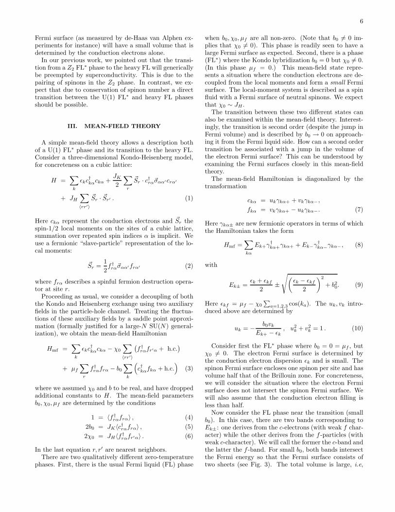
Now consider the FL phase near the transition (smallb0). In this case, there are two bands corresponding toEk±: one derives from the c-electrons (with weak f char-acter) while the other derives from the f -particles (withweak c-character). We will call the former the c-band andthe latter the f -band. For small b0, both bands intersectthe Fermi energy so that the Fermi surface consists oftwo sheets (see Fig. 3). The total volume is large, i.e,

7

Hot Fermisurface

Cold Fermi surface

Spinon Fermisurface

Small electron fermi surface

Fermi Liquid Fractionalized Fermi Liquid

FIG. 3: Fermi surface evolution from FL to FL∗: close to thetransition, the FL phase features two Fermi surface sheets(the cold c and the hot f sheet, see text). Upon approach-ing the transition, the quasiparticle residue Z on the hot fsheet vanishes. On the FL∗ side, the f sheet becomes thespinon Fermi surface, whereas the c sheet is simply the smallconduction electron Fermi surface.

includes both local moments and conduction electrons.Upon moving toward the transition to FL∗ (b0 decreas-ing to zero), the c-Fermi surface expands in size to matchonto the small Fermi surface of FL∗. On the other hand,the f -Fermi surface shrinks to match onto the spinon

Fermi surface of FL∗.Upon increasing b0 in the FL state and depending on

the band structure, another transition is possible, wherethe c band becomes completely empty. Then, the Fermisurface topology changes from two sheets to a single sheet– such a transition between two conventional Fermi liq-uids is known as Lifshitz transition and will not be furtherconsidered here.

The quasiparticle weight Z close to the FL–FL∗ transi-tion is readily calculated in the present mean-field theory.For the electron Green’s function we find

G(k, iων) =u2k

iων − Ek++

v2k

iων − Ek−. (11)

Therefore at the Fermi surface of the c-band (which hasdispersion Ek+, the quasiparticle residue Z = u2

k. At thisFermi surface, Ek+ ≈ ǫk ≈ 0 so that

Ek+ ≈ ǫk +b20

ǫk − ǫkf⇒ uk ≈ −JH

b0vk. (12)

Using Eqs. (10), we then find Z ≈ 1 on the c-Fermisurface.

At the Fermi surface of the f -band on the other hand,Z = v2

k. Also near this Fermi surface, |ǫk − ǫkf | ≈ twhere t is the conduction electron bandwidth. We haveassumed as is reasonable that t ≫ JH . Thus for thef -Fermi surface,

Ek+ ≈ ǫk +b20

ǫk − ǫkf⇒ uk ≈ − t

b0vk. (13)

This then gives

Z = v2k ≈

(

b0t

)2

. (14)

Thus the quasiparticle residue stays non-zero on the c-Fermi surface while it decreases continuously to zero onthe f -Fermi surface on moving from FL to FL∗. (Thef -Fermi surface is “hot” while the c-Fermi surface is“cold”.)

Clearly the critical point is not a Fermi liquid. Z van-ishes throughout the hot Fermi surface at the transition,and non-Fermi liquid behavior results. It is interestingto contrast this result with the spin-fluctuation model(Hertz-Moriya-Millis criticality) where the non-Fermi liq-uid behavior is only associated with some “hot” lines inthe Fermi surface, and consequently plays a subdominantrole.

Despite the vanishing quasiparticle weight Z, the effec-tive mass m∗ of the large Fermi surface state does not di-verge at the transition in this mean-field calculation, be-cause the electron self-energy is momentum-dependent.Physically, the quasiparticle at the hot Fermi surface isessentially made up of the f -particle for small b; evenwhen b goes to zero the f -particle (the spinon) continuesto disperse due to the non-vanishing χ0 term. Indeed thelow-temperature specific heat C ∼ γT with γ non-zeroin both phases. As we argue below, this is an artifactof the mean-field approximation and will be modified byfluctuations.

The detailed shape of the spinon Fermi surface in theFL∗ phase (or the hot Fermi surface which derives fromit in the FL phase) depends on the details of the lat-tice and the form of the local moment interactions. Forthe particular model discussed above, the spinon Fermisurface is perfectly nested. In more general situations, anon-nested spinon Fermi surface will obtain. In all cases,however, the volume of the spinon Fermi surface will cor-respond to one spinon per site.

IV. FLUCTUATIONS: MAGNETISM ANDSINGULAR SPECIFIC HEAT

Fluctuation effects modify the picture obtained in themean-field theory in several important ways. We firstdiscuss fluctuation effects in the two phases. The heavyFermi liquid phase is of course stable to fluctuations- their main effect being to endow the f -particle witha physical electric charge thereby making it an elec-tron [36, 37]. Fluctuation effects are more interesting inthe FL∗ state, and are described by a U(1) gauge theoryminimally coupled to the spinon Fermi surface (whichcontinues to be essentially decoupled from the conduc-tion electron small Fermi surface). This may be madeexplicit by parameterizing the fluctuations in the actionin the FL∗ phase as follows:

χrr′(τ) = eiarr′ (τ)χ0rr′ . (15)

8

The action then becomes

S = Sc + Sf + Sfc + Sb , (16)

Sc =

∫

dτ∑

k

ck(∂τ − ǫk)ck ,

Sf =

∫

dτ∑

r

fr(∂τ − ia0)fr

−∑

〈rr′〉

χ0

(

eiarr′ frfr′ + h.c.

)

,

Scf = −∫

dτ∑

r

(brcrfr + h.c.) ,

Sb =

∫

dτ∑

r

4|br|2JK

.

As usual, the field a0 is introduced to impose the con-straint that there is one spinon per site and may be inter-preted as the time component of the gauge field. By as-sumption br is not condensed. It is useful to start by com-pletely ignoring all coupling between c and f fermions.The action for the f particles describes a Fermi surfaceof spinons coupled to a compact U(1) gauge field.

An important simplification for the three-dimensionalsystems of interest (as compared to d = 2) is that theU(1) gauge theory admits a deconfined phase where thespinons potentially survive as good excitations of thephase. In what follows we will assume that the systemis in such a deconfined phase. (This is formally justifiedin the same large-N limit as the one for the mean fieldapproximation.) This deconfined phase has a Fermi sur-face of spinons coupled minimally to a gapless “photon”(U(1) gauge field). (Due to the compactness of the un-derlying gauge theory, there is also a gapped monopoleexcitation.) Thus two static spinons interact with eachother through an emergent long range 1/r Coulomb in-teraction. Putting back a small coupling between thec and f particles will not change the deconfined natureof this phase. (In particular the monopole gap will bepreserved.) This is the advocated U(1) FL∗ phase.

A. Specific heat

The coupling of the massless gauge photon to thespinon Fermi surface leads to several interesting modi-fications of the mean field results. First, consider theeffect of the spatial components of the gauge field. It is

useful to work in the gauge ~∇ · ~a = 0 so that the vectorpotential is purely transverse. Unless otherwise stated,we assume a generic spinon Fermi surface (without flatportions) henceforth. Integrating out the spinons and ex-panding the resulting action to quadratic order gives thefollowing well-known form for the propagator for thesetransverse gauge fluctuations:

Dij(~k, iωn) ≡ 〈ai(~k, iωn)aj(−~k,−iωn)〉

=δij − kikj/k

2

Γ|ωn|/k + χfk2. (17)

Here Γ, χf are positive constants that are determined bythe details of the spinon dispersion, and ωn is an imag-inary Matsubara frequency. Note that the gauge fluctu-ations are overdamped in the small q limit. As was firstshown in a different context by Holstein et al. [38] (and re-viewed in Appendix D), this form of the gauge field actionleads to a T ln 1/T singularity in the low-temperaturespecific heat. Thus the specific heat coefficient γ = C/Tdiverges logarithmically at low temperature in the U(1)FL∗ phase.

We also briefly mention the effect of the longitudinal(time-component) of the gauge field. This couples to thelocal f fermion density, and so its influence is very muchlike a repulsive density-density interaction. The longitu-dinal gauge field propagator has a structure very similarto that of a standard RPA density fluctuation propaga-tor, and so does not lead to any non-Fermi liquid behav-ior.

B. Magnetic instability

The repulsive interaction mediated by the longitudinalpart of the gauge interaction can lead to various instabil-ities of the spinon Fermi surface. In particular, it is inter-esting to consider an SDW instability of the spinon Fermisurface. The resulting state will have magnetic long rangeorder that could potentially have a weak moment as it isan SDW state that is formed out of the spinon Fermi sur-face. However, in contrast to the traditional view of theweak magnetism, here the SDW instability is not that ofthe large Fermi surface heavy Fermi liquid. Despite theoccurrence of magnetic long range order, this magneticstate is far from conventional. Because the SDW orderparameter is gauge neutral, the presence or absence of aSDW condensate has little substantive effect on the struc-ture of the gauge fluctuations. Indeed, the latter remainas in the U(1) FL∗ state, even after the magnetic orderhas appeared in the descendant U(1) SDW∗ state. Thespinons continue to be deconfined and are coupled to agapless U(1) gauge field. Further, the monopole survivesas a gapped excitation – this yields a sharp distinctionwith more conventional magnetic phases. These gaugeexcitations coexist with the gapless magnons associatedwith broken spin rotation invariance and with a Fermisurface of the conduction electrons. However, due to thebroken translational symmetry in this state, there is nosharp distinction between small and large Fermi surfaces.So to reiterate, the exotic magnetic metal, dubbed U(1)SDW∗, emerges as a low-energy instability of the spinonFermi surface of the parent U(1) FL∗ state.

Different possibilities emerge for the formation of thespin density wave out of the parent U(1) FL∗ phase, de-pending on the details of the spinon Fermi surface andthe strength of the interactions driving the SDW insta-bility. We enumerate some of them below:

9

• (A) Perfectly nested spinon Fermi surface:

In this case, arbitrarily weak interactions will drivean SDW instability. In the resulting state, thespinons are gapped. So upon integrating out thespinons, the effective action for the gauge field canbe expanded safely in spatial and temporal gradi-ents, with no long-range couplings. Gauge invari-ance now demands that these terms in the gaugefield action have the standard Maxwell form. Con-sequently, the photon becomes a sharp propagatingmode at low energies (below the spinon gap) withlinear dispersion. Despite clearly being a distinctphase from conventional spin density wave metals,the experimental distinction is subtle.

• (B) Generic spinon Fermi surface, weak interaction:

For a generic spinon Fermi surface, the leading spindensity wave instability (which will require an in-teraction strength beyond some threshold value)will be at a wavevector that matches one of the“2kF” wavevectors of the spinon Fermi surface. Inthe resulting state, a portion of the spinon Fermisurface (away from points connected by the order-ing wavevector) survives intact. The damping ofthe gapless U(1) gauge fluctuations due to couplingto gapless spinons is preserved. Consequently thelow-temperature specific heat will continue to be-have as C(T ) ∼ T ln(1/T ). Thus for this particu-lar U(1) SDW∗ state its non-Fermi liquid nature isreadily manifested by specific heat measurements,providing a concrete example of a weak momentSDW metal with non-Fermi liquid thermodynam-ics at low temperature.

• (C) Generic spinon Fermi surface, strong interac-tion:

If the interactions are strong enough, even for anon-nested spinon Fermi surface, the spinons candevelop a full gap with no portion of their Fermisurface remaining intact. The resulting phase isthe same as that obtained in (A), and has a sharppropagating linear dispersing photon at low ener-gies.

In Section VI we discuss experimental probes that canhelp distinguish these U(1) SDW∗ phase from the con-ventional spin density wave metals.

C. Mean-field theory with magnetism

In view of the possible occurrence of SDW phases wewill now consider a modified mean-field theory which cap-tures the magnetic instability at the mean-field level, butdoes no longer correspond to a large-N saddle point. Wewill discuss the fully self-consistent solution of the mean-field equations for arbitrary temperature and externalmagnetic field.

0 0.5 1 1.5 2

Kondo coupling JK

0

0.01

0.02

0.03

0.04

Tem

pera

ture

T

U(1) FL*

SDW

FL

decoupled

U(1) SDW*

FIG. 4: Mean-field phase diagram of Hmf (18) on the cubiclattice, as function of Kondo coupling JK and temperatureT . Parameter values are electron hopping t = 1, Heisenberginteraction JH = 0.1, decoupling parameter x = 0.2, andconduction band filling nc = 0.7. Thin (thick) lines are sec-ond (first) order transitions. The “decoupled” phase is anartifact of the mean-field theory, and the corresponding tran-sitions will become crossovers upon including fluctuations, aswill the transition between the FL and U(1) FL∗ phases; thetransitions surrounding the SDW and SDW∗ phases will ofcourse survive beyond mean-field theory.

0 0.5 1 1.5 2

Kondo coupling JK

1

0.8

0.6

0.4

0.2

0

M /

Msa

t

T = 0T = 0.0067

FIG. 5: Staggered magnetization determined from the mean-field solution Hmf (18). Parameter are as in Fig. 4, the twocurves correspond to two horizontal cuts of the phase diagramin Fig. 4. At T = 0, the first-order character of the SDW–FL transition is clearly seen. Note that smaller values of thedecoupling parameter x yield smaller values of the magneti-zation in the SDW and SDW∗ phases.

The mean-field Hamiltonian, written down explicitlyfor SU(2) symmetry, takes the following form:

Hmf =∑

k

ǫkc†kαckα −

∑

〈rr′〉

(

χ∗rr′f

†rαfr′α + h.c.

)

+∑

r

µf,rf†rαfrα −

∑

r

br(

c†rαfrα + h.c.)

10

+1

2

∑

r

( ~Heff,r + ~Hext) · f †rα~σαα′frα′

+1

2~Hext ·

∑

r

c†rα~σαα′crα′ + Econst (18)

where ~Hext is the external field, and we have allowed fora spatial dependence of the mean-field parameters µf,r,

χrr′ , br, ~Heff,r. They have to be determined from thefollowing equations:

1 = 〈f †rαfrα〉 , (19)

2br = JK〈c†rαfrα〉 , (20)

2χrr′ = (1 − x)JH〈f †rαfr′α〉 , (21)

~Heff,r = xJH∑

r′

~Mr′ , ~Mr =1

2〈f †rα~σαα′frα′〉 , (22)

where the last sum runs over the nearest neighbors r′ ofsite r. We have introduced a parameter x which allowsto control the balance between ordered local-momentmagnetism and spin-liquid behavior of the f electrons.A value x = 1/2 would correspond to an unrestrictedHartree-Fock treatment of the original Heisenberg inter-action; we will employ values x < 1/2 in order to modela weak magnetic instability of the spinon Fermi surfacestate. The constant piece of the Hamiltonian reads

Econst = −∑

r

µf,r +∑

r

2b2rJK

(23)

+∑

rr′

2|χrr′ |2(1 − x)JH

− 1

2

∑

r

~Heff,r · ~Mr .

For simplicity, we consider a simple cubic lattice, andassume a tight-binding dispersion for the conduction elec-trons, ǫk = −2t

∑

a=1,2,3 cos(ka) − µc, where µc controlsthe conduction band filling. The mean-field equationscan be self-consistently solved using a large unit cell, al-lowing for spatially inhomogeneous phases [39]. In thissection we restrict our attention to mean-field solutionswhere the χrr′ = χ0 fields are real (time-reversal invari-ant) and obey the full lattice symmetries, and br = b0 issite-independent. We employ a 2× 1 unit cell, then anti-

ferromagnetism is characterized by ~Mr·x = Ms exp(iQ·r)where Q = (π, π, π) is the antiferromagnetic wavevector,and x is the magnetization axis (which is arbitrary inzero external field).

In Fig. 4 we show a phase diagram obtained from self-consistently solving (18) together with the above mean-field equations at zero external magnetic field. A U(1)FL∗ phase with b0 = 0 and χ0 6= 0 is realized at interme-diate temperatures. As expected, it is unstable to mag-netic order at low T , resulting in a U(1) SDW∗ groundstate for small JK – this phase has in addition Ms 6= 0.For the present parameter values, the spinon Fermi sur-face is gapped out in the SDW∗ phase. Increasing JKdrives the system into the FL phase with b0 6= 0, χ0 6= 0,and Ms = 0; at low temperatures a conventional SDW

phase intervenes where all b0, χ0, Ms are non-zero. Notethat the transition between FL and SDW is weakly firstorder at low temperatures. At high temperature, themean-field theory only has a “decoupled” solution withb0 = χ0 = Ms = 0 – this decoupling is a well-knownmean-field artifact and reflects the presence of incoher-ent excitations.

In the FL phase, the above mentioned Lifshitz tran-sition occurs at JK ≈ 1.7 in the low-temperature limit,i.e., for JK > 1.7 only a single Fermi surface sheet re-mains. Note that this transition does not lead to strongsingularities in the mean-field parameters.

The staggered magnetization of the SDW and SDW∗

states as determined from the mean-field solution areshown in Fig. 5; we can expect that fluctuation correc-tions will significantly reduce these mean-field values. Wehave also studied different values of the decoupling pa-rameter x; in particular smaller values of x lead to asuppression of ordered magnetism in favor of the non-magnetic FL∗ state, i.e., the SDW instability of FL∗ isshifted to lower temperatures (and becomes completelysuppressed at small x); similarly, the ordered moment inthe SDW phases is decreased with decreasing x.

Interesting physics obtains when an external magneticfield is turned on, and the corresponding mean-field phasediagram is discussed in Appendix C.

V. FLUCTUATIONS NEAR THE FERMIVOLUME CHANGING TRANSITION

We now turn to the effects of fluctuations beyond themean-field theory at the phase transition between the FLand U(1) FL∗ phases. In mean-field theory, this transi-tion occurs through the condensation of the slave bosonfield b. Such a condensation survives as a sharp transitionbeyond mean-field only when T = 0.

We begin by observing that in the mean-field theory allthe important changes near the transition occur at thehot Fermi surface. The cold Fermi surface (essentiallymade up of c-particles) plays a spectator role. We there-fore integrate out the c-fields completely from the actionin Eq. (16) to obtain an effective action involving theb, f and gauge fields alone. We also partially integrateout f excitations well away from the hot Fermi surface:this changes the b effective action from the simple localterm in (16), and endows it with frequency and momen-tum dependence. In this manner we obtain the followingeffective action at long distance and time scales:

S = Sb + Sf , (24)

Sb =

∫

dτd3r

[

b

(

∂τ − µb − ia0 −(~∇r − i~a)2

2mb

)

b

+u

2|b|4 + ....

]

, (25)

and Sf has the same form as in (16). Notice that the

11

b field has become a propagating boson, with the sameterms in the action as a microscopic canonical boson:here these terms arise from a (b,f) fermion polarizationloop integrated well away from the f Fermi surface. Theparameters µb,mb may be interpreted as the chemicalpotential and mass of the bosons respectively. The (b,f)fermion loop will also lead to higher time and spatial gra-dient terms as well as a density-density coupling betweenb and f in (24), but all these are formally irrelevant nearthe quantum critical point of interest.

A key feature of (24), induced by taking the spatialand temporal continuum limit, is that we have lost in-formation on the compactness of the U(1) gauge fielda, i.e., the continuum action is now no longer periodicunder arr′ → arr′ + 2π, as was the case for the latticeaction (16). The U(1) gauge field is now effectively non-compact, and consequently monopole excitations havebeen suppressed. The monopole gap is finite in the U(1)FL∗ phase (which is the analog of the “Coulomb” phaseof the compact gauge theory) [40]. In the FL phase, themonopoles do not exist – they are confined to each other.This occurs due to the condensation of the boson field.However, the monopole gap is not expected to close atthe transition [42], and so neglecting the compactnessof the gauge field is permissible. Indeed, the continuumaction (24) provides a satisfactory description of the crit-ical properties of the FL to U(1) FL∗ transition at T = 0.However, as we noted in the caption of Fig 1, the com-pactness of the gauge field is crucial in understanding theabsence of a T > 0 phase transition above the FL phase[21].

The action in Eq. (24) above is similar to that pop-ular in gauge theory descriptions [22, 23] of the normalstate of optimally doped cuprates but with some crucialdifferences. Here the chemical potential of the bosons isfixed while in Refs. 22, 23 the boson density was fixed; aswe will see below, this significantly modifies the physicalimplications of the critical theory, and the nature of thenon-Fermi liquid critical singularities as T > 0. Further-more, we are interested specifically in d = 3, as opposedto the d = 2 case considered in Refs. 22, 23.

The phase diagram of the action (24) was sketched inFig 1. The horizontal axis, represented in Fig 1 by JK ,is now accessed by varying µb. Without any additional(formally irrelevant) second-order time derivative termsfor b in the action, the quantum critical point betweenthe FL and U(1) FL∗ phases occurs precisely at µb = 0,T = 0. We will now discuss the physical properties inthe vicinity of this critical point first at T = 0, and thenat T > 0, followed by an analysis of transport propertiesusing the quantum Boltzmann equation in Section VC.The final subsection VD will comment on the effect ofthe SDW or SDW∗ phases that may appear at very lowtemperatures (these are not shown in Fig. 1, but sketchedin Fig. 2).

A. Zero temperature

In a mean-field analysis of (24), we see that the FL∗

phase (the “Coulomb” phase of the gauge theory) obtainsfor µb < 0 with 〈b〉 = 0, while the FL phase (the “Higgs”phase of the gauge theory) obtains for µb > 0.

Consider fluctuations for µb < 0 in the FL∗ phase.Here, there are no bosons in the ground state, and all self-energy corrections associated with the quartic coupling uvanish [41]. The gauge field propagator is given by (17),and this does contribute a non-zero boson self energy. Atsmall momenta p and imaginary frequencies ǫ, the bosonself-energy has the structure (determined from a singlegauge-boson exchange process, as in Refs. 22, 23)

Σb(k, iǫ) ∼ k2(1 + c1|ǫ| ln(1/|ǫ|) + . . .), (26)

where c1 is some constant. Apart from terms whichrenormalize the boson mass mb, these self-energy correc-tions are less relevant than the bare terms in the action,and so can be safely neglected near the critical point. No-tice also that Σb(0, 0) = 0, and so the quantum criticalpoint remains at µb = 0.

The critical exponents can now be determined as inRefs. 20, 41, and are simply those of the mean-field theoryof (24):

ν = 1/2 ; z = 2 ; η = 0. (27)

As in (26) we can also determine the fate the boson quasi-particle pole as influenced by the gauge fluctuations; weobtain

ImΣb

(

k, ǫ =k2

2mb

)

∼ sgn(ǫ)ǫ2 ln(1/|ǫ|). (28)

The boson lifetime is clearly longer than its energy, andthis pole remains well defined. Finally, we recall ourstatement in Section IVA that the gauge fluctuationslead to a T ln(1/T ) specific heat in the FL∗ phase, witha diverging γ co-efficient. This behavior remains all theway up to, and including, the critical point. Parentheti-cally, we note that the same calculation in d = 2 dimen-sions will yield C ∝ T 2/3.

We turn next to µb > 0, in the FL phase. Here thebosons are condensed, and (26) or explicit calculationsshow that

〈b〉 ≡ b0 ∼ (µb)1/2 ∼ (JK − JKc)

1/2, (29)

where JKc is the position of the critical point in Fig 1.The transverse gauge field propagator may be obtainedas in Section IVA by integrating out both the bosons andfermions and expanding the resulting action to quadraticorder; the boson condensate leads to a “Meissner” termin the gauge propagator so that (17) is replaced by

Dij(~k, iωn) ≡ 〈ai(~k, iωn)aj(−~k,−ωn)〉

=δij − kikj/k

2

Γ|ωn|/k + χfk2 + ρs. (30)

12

Here ρs is the boson “superfluid density”, and we haveρs ∼ b20. The presence of such a Meissner term cuts offthe singular gauge fluctuations. The divergence of thespecific heat coefficient γ(T ) as a function of temperatureat the critical point implies that it diverges at T = 0 onapproaching the transition from the FL side. As shownin Appendix D, this is indeed the case, and we find that γdiverges as γ ∼ ln(1/b0). In experiments, such a diverg-ing γ is sometimes interpreted as a diverging effectivemass. Importantly, the divergence of γ is unrelated tothe singularity in the quasiparticle residue on the “hot”Fermi sheet, Z, which obeys Z ∼ b20 as shown in (14),and so vanishes linearly as a function of JK − JKc.

B. Non-zero temperatures

A crucial change at T > 0 is that it is now no-longertrue that Σb(0, 0) = 0 in a region with 〈b〉 = 0. Instead,as in earlier studies of the dilute Bose gas [19, 20], wehave

Σb(0, 0) = 2u

∫

ddk

(2π)d1

exp [k2/(2mbT )]− 1

= uζ(3/2)

4π3/2(2mbT )3/2 in d = 3 (31)

This behavior determines the crossover phase boundariesshown in Fig 1. The physical properties are determinedby the larger of the two “mass” terms in the b Green’sfunction, |µb| or Σb(0, 0) – consequently, the crossoverphase boundaries in Fig. 1 lie at T ∼ |µb|2/3 ∼ |JK −JKc|2/3. These boundaries separate the U(1) FL∗ regionat low T and µb < 0, and the FL region at low T andµb > 0, from the intermediate quantum critical region.Note that there is no phase transition in the FL region atT > 0: this is due to the compactness of the underlyingU(1) gauge theory, and the fact that the “Higgs” and“confining” phases are smoothly connected in a compactU(1) gauge theory in three total dimensions [21].

We now briefly comment on the nature of the elec-trical transport in the three regions of Fig 1. The be-havior is quite complicated, and we will first highlightthe main results by simple estimates in the present sub-section. A more complete presentation based upon thequantum Boltzmann equation appears in Section VC.

The conventional FL region is the simplest, with theusual T 2 dependence of the resistivity—the gauge fluc-tuations are quenched by the “Meissner effect”.

In the U(1) FL∗ region, there is an exponentially smalldensity of thermally excited b quanta, and so the bosonconductivity σb is also exponentially small. As in earlierwork [43], the resistances of the b and f quanta add inseries, and so the total b and f conductivity remains ex-ponentially small. The physical conductivity is thereforedominated by that of the c fermions, which again has aconventional T 2 dependence.

Finally, we comment on the transport in the quan-tum critical region. This we will estimate following the

method of Ref. 22, with a more complete calculation ap-pearing in the following subsection. A standard Fermi’sGolden rule computation of scattering off low-energygauge fluctuations shows that a boson of energy ǫ hasa transport scattering rate

1

τbtr(ǫ)∼ T

√ǫ (32)

for energies ǫ ≪ T 2/3. From this, we may obtain theboson conductivity by inserting in the expression

σb ∼∫

d3k τbtr(ǫbk)k2

(

−∂n(ǫbk)

∂ǫbk

)

(33)

where n(ǫ) = 1/(eǫ/T − 1) is the Bose function, andǫbk = k2/(2mb) + Σb(0, 0) = k2/(2mb) + c2T

3/2 for someconstant c2. Estimating the integral in (33) we find thatthere is an incipient logarithmic divergence at small kwhich is cutoff by Σb(0, 0) ∼ T 3/2, and so σb divergeslogarithmically with T :

σb ∼ ln(1/T ). (34)

There are no changes to the estimate of the f conductiv-ity from earlier work [22, 23], and we have σf ∼ T−5/3.Using again the composition rule of Ref. 43, we see thatthe asymptoptic low-temperature physical conductivityis dominated by the behavior in (34).

As an aside, we note that for the theory (24) in two spa-tial dimensions the result of Eq. (34) continues to hold,whereas the fermion part becomes σf ∼ T−4/3. This im-plies that the asymptoptic low-T physical conductivity isdominated by (34) in d = 2 as well.

C. Quantum Boltzmann equation

We now address electrical transport properties of thetheory (24) in more detail, using a quantum Boltzmannequation. The analysis is in the same spirit as the work ofRef. 44 but, as we have discussed in Section I A, the vari-ation in the boson density as a function of temperatureleads to very different physical properties, and requires adistinct analysis of the transport equation.

We saw in Section VB that the electrical conductiv-ity was dominated by the b boson contribution, and sowe focus on the time (t) dependence described by thedistribution function

f(~k, t) = 〈b†k(t)bk(t)〉 (35)

In the absence of an external (physical) electric field ~E,

we have the steady state value f(~k, t) = f0(k) with

f0(k) ≡1

exp [(k2/(2mb) − µb + Σb(0, 0))/T ]− 1, (36)

with Σb(0, 0) given in (31). The transport equation in

the presence of a non-zero ~E(t) can be derived by stan-dard means, and most simply by an application of Fermi’s

13

0 0.5 1 1.5 2_k

0

5

10

15

20_

_

k4 ψ(k

)T = 10-4, u = 0.1

T = 10-4, u = 1

T = 10-2, u = 0.1

T = 10-2, u = 1

_ _

_ _

_ _

_ _

FIG. 6: Plot of the function k4ψ(k) for a few values of thereduced temperature T and the interaction parameter u (40).ψ(k) is defined in Eqs. (38) and (41), and has been obtainedfrom the numerical solution of the quantum Boltzmann equa-tion (42).

golden rule. The bosons are assumed to scatter off a fluc-tuating gauge field with a propagator given by (17) or(30), and this yields the equation

∂f(~k, t)

∂t+ ~E(t) · ∂f(~k, t)

∂~k=

−∫ ∞

−∞

dΩ

π

∫

ddq

(2π)dIm

[

kiDij(~q,Ω)kjm2b

]

×(2π)δ

(

k2

2mb− (~k + ~q)2

2mb− Ω

)

×[

f(~k, t)(1 + f(~k + ~q, t))(1 + n(Ω))

− f(~k + ~q, t)(1 + f(~k, t))n(Ω)

]

(37)

where n(Ω) is the Bose function at a temperature T asabove.

We will now present a complete numerical solution of(37) for the case of a weak, static electric field, to lin-

ear order in ~E. The analysis near the quantum criticalpoint parallels that of Ref. 45, with the main change be-ing that instead of the critical scattering appearing fromthe boson self-interaction u, the dominant scattering isfrom the gauge field fluctuations (note, however, that itis essential to include the interaction u to first order inthe self-energy shift in (36)). We write

f(~k, t) = f0(k) + ~k · ~Ef1(k), (38)

where notice that f1 depends only on the modulus of kand is independent of t. We now have to insert (38) intothe transport equation (37) and the expression for theelectrical current

~J(t) =

∫

ddk

(2π)d

~k

mbf(~k, t), (39)

10-4 10-3 10-2 10-1 100

_T

10-1

100

101

_ _

σ(T

)

0 0.2 0.4 0.6 0.8 1

_T

0

5

10

_

_1/

σ(T

)

u = 0.1

u = 1

u = 2.5

_

_

_

FIG. 7: Scaling function for the boson conductivity, σ =σb/(mbχf ), as function of the reduced temperature T for dif-ferent values of the interaction parameter u (40). The re-sults are obtained from the numerical solution of the quantumBoltzmann equation (42) together with (43). Top panel: con-ductivity σ(T ) on a log-log scale. Bottom panel: resistivity1/σ(T ) on a linear scale.

linearize everything in ~E, and so determine the propor-

tionality between ~J and ~E.It is useful to re-write the equations in dimensionless

quantities Ω = Ω/T , k = k/√

2mbT , σ = σb/(mbχf ).Then it is easy to see that the solution of the quantumBoltzmann equation at the critical coupling, µb = 0, ischaracterized by two parameters,

T =χ2f

Γ2(2mb)

3 T ,

u = uζ(3/2)

4π3/2

Γ

χf, (40)

where T is a reduced temperature, and u parametrizesthe temperature dependence of the effective “mass” ofthe bosons from Eq. (31); Γ and χf are the parametersof the gauge propagator (17). The linearized form of theBoltzmann equation (37) for the function

f1(k) ≡ ψ(k/√

2mbT ) (41)

is obtained as

− f ′0(k) =

∫ ∞

0

dk1

[

K1(k, k1)ψ(k) +K2(k, k1)ψ(k1)]

(42)

with f ′0(x) = ∂/(∂x2)[exp(x2 + u

√T )− 1]−1; the expres-

sions for the functions K1,2 are given in Appendix E.

14

From the solution of Eq. (42) one obtains the conductiv-ity according to

σ(T , u) =1

6π2√T

∫ ∞

0

dk k4 ψ(k) . (43)

The integral equation (42) was solved by straightfor-ward numerical iteration on a logarithmic momentumgrid. We show sample solutions for the function k4 ψ(k)in Fig. 6. The final results for the scaling functionof the conductivity are displayed in Fig. 7. For smalltemperatures, the logarithmic divergence of σb(T ) an-nounced in Eq. (34) is clearly seen; for larger tempera-tures the conductivity is exponentially suppressed due tothe temperature-dependent boson mass. In the crossoverregion, the results could be fitted with a power law overa restricted temperature range of roughly one decade,however, no extended power-law regime emerges. Incomparison with experiments, one has to keep in mindthat the physical resistivity is given by a sum of bosonand fermion resistivities, and that the logarithmically de-creasing low-temperature part of 1/σb(T ) cannot be eas-ily distinguished from a residual resistivity arising fromimpurities.

D. SDW order

Our discussion so far has focused primarily on thecrossover between the FL to U(1) FL∗ phases, as thiscaptures the primary physics of the Fermi volume chang-ing transition. At low T , we discussed in Section IV Bthat the longitudinal part of the gauge fluctuations mayinduce SDW order on the spinon Fermi surface of theFL∗ phase (leading to the SDW∗ phase). On the FLside of the transition, the gauge fluctuations are formallygapped by the Anderson-Higgs mechanism. They will,however, still mediate a repulsive (though finite ranged)interaction between the quasiparticles at the hot Fermisurface. Furthermore the shape of the hot Fermi sur-face evolves smoothly from the spinon Fermi surface ifthe FL∗ phase. Consequently, it is to be expected thatthe SDW order will continue into the FL region up tosome distance away from the transition. Thus it seemsunlikely that there will be a direct transition from SDW∗

to FL at zero temperature. The actual situation thenhas some similarities to the mean-field phase diagram inFig 4. However, fluctuations will strongly modify the po-sitions of the phase boundaries, and we expect that theU(1) FL∗ region actually occupies a larger portion of thephase diagram. Also there is no sharp transition betweenthe FL and U(1) FL∗ regions (unlike the mean-field sit-uation in Fig 4), and there is instead expected to be alarge intermediate quantum-critical region as shown inFig. 2.

VI. EXPERIMENTAL PROBES OF THE U(1)SDW∗ STATE

In this Section, we discuss experimental signatures ofthe U(1) SDW∗ phase focusing particularly on the dis-tinctions with more conventional SDW metals.

We begin by considering a U(1) SDW∗ phase in whicha portion of the spinon Fermi surface remains intact. Asdiscussed in Section IV, the coupling between the gap-less spinons and the gauge field leads to singularities inthe low-temperature thermodynamics in this phase. Inparticular the specific heat behaves as C(T ) ∼ T ln(1/T )at low temperature. Thus this phase is readily distin-guished experimentally from a conventional SDW. Elec-trical transport in this U(1) SDW∗ phase will be throughthe conduction electrons with no participation from thespinons. Thus electrical transport will be Fermi liquid-like. In contrast thermal transport will receive contribu-tions from both the conduction electrons and the gaplessspinons. Consequently the thermal conductivity will bein excess of that expected on the basis of the Wiedemann-Franz law with the free electron Lorenz number.

The distinction with conventional SDW phases is muchmore subtle for U(1) SDW∗ phases where the spinonshave a full gap. In this case, there is a propagating gap-less linear dispersing photon which is sharp. The pres-ence of these gapless photon excitations potentially pro-vides a direct experimental signature of this phase. It isextremely important to realize that the emergent gaugestructure of a fractionalized phase is completely robustto all local perturbations, and is not to be confused withany modes associated with broken symmetries. Thus de-spite its gaplessness the photon is not a Goldstone mode.In fact, the gaplessness of the photon is protected evenif there are small terms in the microscopic Hamiltonianthat break global spin rotation invariance. Being gap-less with a linear dispersion, the photons will contributea T 3 specific heat at low T which will add to similarcontributions from the magnons and the phonons of thecrystal lattice. In addition, the conduction electrons willcontribute a linear T term. The phonon contribution ispresumably easily subtracted out by a comparison be-tween the heavy Fermi liquid and magnetic phases. Todisentangle the magnon and photon contributions, it maybe useful to exploit the robustness of the photons toperturbations. Thus for materials with an easy-planeanisotropy, application of an in-plane magnetic field willgap out the single magnon, but the photon will stay gap-less and will essentially be unaffected (at weak fields).Thus careful measurements of field-dependent specificheat may perhaps be useful in deciding whether the U(1)SDW∗ phase is realized.

Finally, quasi-elastic Raman scattering has been sug-gested as a probe of the U(1) gauge field fluctuations[46] in the context of the cuprates—the same predictionapplies essentially unchanged here to the fractionalizedphases in d = 3.

Conceptually the cleanest signature of the U(1) SDW∗

15

phase would be detection of the gapped monopole. How-ever at present we do not know how this may be directlydone in experiments. Designing such a “monopole detec-tion” experiment is an interesting open problem.

VII. DISCUSSION

The primary question which motivates this paper ishow to reconcile a weak moment magnetic metal withnon-Fermi liquid behavior close to the transition to theFermi liquid. We have explored one concrete route to-ward such a reconciliation. The U(1) SDW∗ magneticstates discussed in this paper may be dubbed spin-chargeseparated spin density wave metals. They constitute aclass distinct from both the conventional spin densitywave metal and the local-moment metal mentioned in theIntroduction. However, they share a number of similari-ties with both conventional metals. Just as in the conven-tional local-moment metal, in the U(1) SDW∗ state thelocal moments do not participate in the Fermi surface.Despite this the ordering moment may be very small.Indeed this state may be viewed as a spin density wavethat has formed out of a parent non-magnetic metallicstate with a “small Fermi surface”. This parent state isa fractionalized Fermi liquid in which the local momentshave settled into a spin liquid and essentially decoupledfrom the conduction electrons. The spinons of the spinliquid form a Fermi surface which undergoes the SDWtransition – this transition does not affect the deconfine-ment property of the gauge field, because the SDW orderparameter is gauge neutral and thus does not effectivelycouple to the gauge field excitations.

We showed that in the region of evolution from thisstate to the conventional Fermi liquid, non-Fermi liq-uid behavior obtains (at least at intermediate temper-atures). We also argued that the underlying transitionthat leads to this non-Fermi liquid physics is the Fermivolume changing transition from FL to FL∗. Despite thejump in the Fermi volume, this transition is continuousand characterized by the vanishing of the quasiparticleresidue Z on an entire sheet of the Fermi surface (the“hot” Fermi surface) on approaching the transition fromthe FL side.

A specific heat that behaves as T ln(1/T ) is commonlyobserved in a variety of heavy-fermion materials close tothe transition to magnetism. In the context of the ideasexplored in this paper, such behavior of the specific heatis naturally obtained in three-dimensional systems. Asmall number of heavy-fermion materials exhibit such asingular specific heat even in the presence of long-rangedmagnetic order. As we have emphasized, precisely suchnon-Fermi liquid specific heat obtains in one of the ex-otic magnetic metals discussed in this paper (the U(1)SDW∗ phase with a partially gapped spinon Fermi sur-face). It would be interesting to check for violations ofthe Wiedemann-Franz law at low temperature in suchmaterials.

A general point emphasized in this paper is that theobserved non-Fermi liquid physics near the onset of mag-netism actually has little to do with fluctuations of themagnetic order parameter. Rather we propose that thenon-Fermi liquid physics is associated with the destruc-tion of the large Fermi surface. The concrete realizationof this picture explored in this paper is that the destruc-tion of the large Fermi surface leads to a fractionalizedFermi liquid which eventually (at low temperature) de-velops spin density wave order. As we discussed exten-sively, the resulting spin density wave state is an exoticmagnetic metal.

It is also of interest to consider a different scenarioin which the small Fermi surface state is unstable at lowtemperature toward confinement of spinons and magneticorder. It is particularly interesting to consider such a sce-nario in d = 2. The physics of the Fermi-volume changingfluctuations is again described by a theory of condensa-tion of a slave boson field coupled to a Fermi surface ofspinons by a U(1) gauge field. For a non-compact U(1)gauge field, such a theory has a number of interestingproperties. As noticed by Altshuler et al. [47], the spinsusceptibility at extremal wavevectors of the spinon fermisurface have (possibly divergent) singularities due to thegauge fluctuations. Indeed the spin physics of this modelis critical and described by a non-trivial fixed point. Thedynamical susceptibility at these extremal wavevectorsand at a frequency ω is expected to satisfy ω/T scal-ing. For a general spinon Fermi surface these extremalwavevectors will chart out one-dimensional lines in theBrillouin zone at which critical scattering will be seen ininelastic neutron scattering. A spin density wave insta-bility can develop out of this critical state at a particularextremal wavevector where the amplitude of the diverg-ing susceptibility is the largest. Arguments very similarto those in Section VB also show that transport will begoverned by non-Fermi liquid power laws in this theory.

There is a striking qualitative resemblance betweenthese results and the experiments on CeCu6−xAux. Atthe critical Au concentration neutron scattering experi-ments see critical scattering on lines in the Brillouin zonesatisfying ω/T scaling [5]. Magnetic ordering occurs atparticular wavevectors on this line. Furthermore, em-pirically the spin fluctuations appear to be quasi two-dimensional, suggesting that the ideas sketched abovemay indeed be relevant. We note that they significantlydiffer from earlier proposals to explain the behavior ofCeCu6−xAux [48]. As mentioned in the text, the spe-cific heat in the d = 2 quantum critical region will havethe form C/T ∼ T−1/3; interestingly, such a behaviorhas been observed in YbRh2Si2 in the low-temperatureregime near a quantum-critical point [49]. On the theo-retical front, there are a number of conceptual issues [50]related to the legitimacy of ignoring the compactness ofthe gauge field in d = 2. Developing a more concrete the-oretical description of these general ideas is an interestingchallenge for future work.

16

Acknowledgments

We thank P. Coleman, M.P.A. Fisher, E. Fradkin,A. Georges, L. Ioffe, Y.-B. Kim, G. Kotliar, A. Millis,N. Prokof’ev, T. M. Rice, Q. Si, M. Sigrist, A. Tsvelik,and X.-G. Wen for useful discussions. T.S is particu-larly grateful to Patrick Lee for a number of enlighteningconversations that clarified his thinking. This researchwas supported by the MRSEC program of the US NSFunder grant number DMR-0213282 (T.S.), by US NSFGrant DMR 0098226 (S.S.), and by the DFG Center forFunctional Nanostructures at the University of Karlsruhe(M.V.). T.S. also acknowledges funding from the NECCorporation, and the Alfred P. Sloan Foundation and thehospitality of Harvard University where part of this workwas done.

APPENDIX A: OSHIKAWA’S ARGUMENT ANDTOPOLOGICAL ORDER

Oshikawa has presented [51] an elegant non-perturbative argument demonstrating that the volumeof the Fermi surface is determined by the total numberof electrons in the system. In our previous work [11], andin the present paper, we have argued for the existence ofa non-magnetic FL∗ state with a different Fermi surfacevolume. As we discussed earlier [11], this apparent con-flict is resolved when we allow for global topological ex-citations in Oshikawa’s analysis; such excitations emergenaturally in the gauge theories we have discussed for theFL∗ state. In other words, Oshikawa’s argument impliesthat violation of Luttinger’s theorem must be accompa-nied by topological order.

In this Appendix, we briefly recall the steps in Os-hikawa’s argument, and show how it can be modified toallow for a small Fermi surface in a FL∗ state. As far aspossible, we follow the notation of Oshikawa’s paper [51].

For definiteness, consider a two-dimensional Kondolattice with a unit cell of lengths ax,y. The ground stateis assumed to be non-magnetic, with equal numbers of upand down spin electrons. Place it on a torus of lengthsLx,y, with Lx/ax, Ly/ay co-prime integers. Adiabati-cally insert a flux Φ = 2π (h = c = e = 1) into one of theholes of the torus (say the one enclosing the x circum-ference), acting only on the up-spin electrons. Then theinitial and final Hamiltonians are related by a unitarytransformation generated by

U = exp

(

2πi

Lx

∑

r

nr↑

)

(A1)

where nr↑ is the number operator of all electrons (includ-ing the local moments) with spin up on the site r. Afterperforming the unitary transformation to make the finalHamiltonian equivalent to the initial Hamiltonian, thefinal and initial states are found to have a total crystal

momentum which differs by

∆Px =2π

Lx

LxLyv0

ρa2

(

mod2π

ax

)

(A2)

where v0 = axay is a volume of a unit cell, the secondfactor on the r.h.s. counts the number of unit cells in thesystem, and ρa = 2ρa↑ is the mean number of electrons inevery unit cell. Clearly the crystal momentum is definedmodulo 2π/ax, and hence the modulus in (A2).

Now imagine computing the change in crystal momen-tum by studying the response of the quasiparticles to theinserted flux. As shown by Oshikawa, the quasiparticlesassociated with a Fermi surface of volume V lead to achange in momentum which is

∆P qx =2π

Lx

V(2π)2/(LxLy)

(

mod2π

ax

)

, (A3)

where the second factor on the r.h.s. counts the numberof quasiparticles within the Fermi surface. Equating ∆Pxand ∆P qx , and the corresponding expressions for ∆Pyand ∆P qy , Oshikawa obtained the conventional Luttingertheorem, which applies to the volume V = VFL of theFermi surface in the FL state

2v0

(2π)2VFL = ρa(mod 2) (A4)

In the FL∗ state, there are additional low-energy ex-citations of the local moments that yield an additionaltopological contribution to the change in crystal momen-tum. Indeed, the influence of an insertion of flux Φis closely analogous to the transformation in the Lieb-Schultz-Mattis [52] argument, and it was shown [53, 54]that a spin liquid state in d = 2 acquires the momentumchange

∆P tx =π

ax

Lyay

(

mod2π

ax

)

(A5)

where the second factor on the r.h.s. now counts thenumber of rows which have undergone the Lieb-Schultz-Mattis transformation. Now using ∆Px = ∆P qx + ∆P tx,we now obtain the modified Luttinger theorem obeyed inthe FL∗ phase:

2v0

(2π)2VFL∗ = (ρa − 1)(mod 2). (A6)

It is clear that the above argument is easily extendedto a Z2 FL∗ state in d = 3. The case of U(1) FL∗ statein d = 3 is somewhat more delicate because there is nowa gapless spectrum of gauge fluctuations which can con-tribute to the evolution of the wavefunction under theflux insertion; nevertheless, the momentum change in(A5) corresponds to an allowed gauge flux, and we ex-pect that (A5) continues to apply.

17

APPENDIX B: TOY MODEL WITH U(1)FRACTIONALIZATION AND A SPINON FERMI

SURFACE

In this Appendix, we will display a concrete model inthree spatial dimensions that is in a U(1) fractionalizedphase in three dimensions, and has a Fermi surface ofspinons coupled to a gapless U(1) gauge field. As dis-cussed earlier, this spinon Fermi surface could eventually(at low energies) undergo various instabilities includingin particular to a spin density wave state.

Consider the following model:

H = Htψ +H∆ +Hb +Hu +HU , (B1)

Htψ = −∑

〈rr′〉

t(

ψ†rψr′ + h.c.

)

,

H∆ = ∆∑

〈rr′〉

eiφrr′

(

ψ†r↑ψ

†r′↓ − ψ†

r′↑ψ†r↓

)

+ h.c. ,

Hb = −w∑

[rr′r′′]

cos(φrr′ − φrr′′) ,

Hu = u∑

〈rr′〉

n2rr′ ,

HU = U∑

r

(Nr − 1)2 .

Here ψr destroys a spinful charge-1 electron at each site ofa cubic lattice in three spatial dimensions; eiφrr

′ creates acharge-2, spin-0 “Cooper pair” that resides on the links.nrr′ is conjugate to φrr′ and may be regarded as theCooper pair number associated with each link. Nr is thetotal charge associated with each site and is given by

Nr =∑

r′∈r

nrr′ + ψ†rψr. (B2)

The Hamiltonian H may be regarded as describing a sys-tem of electrons coupled with strong phase fluctuations.The first term in Hb represents Josephson coupling be-tween two “nearest neighbor” bonds. Hu penalizes fluc-tuations in the Cooper pair number at each bond. HU

penalizes fluctuations in the total charge Nr that can beassociated with each lattice site. The total charge of thefull system clearly is

Ntot =∑

r

Nr. (B3)

Depending on the various model parameters, severaldistinct phases are possible. Here we focus on the limitof large U . Diagonalizing HU requires that the groundstate(s) satisfy Nr = 1 at all sites r. There is a gapof order U to states that do not satisfy this condition.Clearly the system is insulating in this limit.

The condition Nr = 1 for all r still allows for a hugedegeneracy of ground states which will be split once theother terms in the Hamiltonian are included. This split-ting may be described by deriving an effective Hamilto-nian that lives in the space of degenerate states specified

by Nr = 1. As discussed in Ref. 14, this effective Hamil-tonian may be usefully viewed as a (compact) U(1) gaugetheory. This may be explicitly brought out in the presentcase by the change of variables

φrr′ = ǫrarr′ ,

nrr′ = ǫrErr′ (B4)

ψrα = frα for r ∈ A ,

ψrα = iσyαβf†rβ for r ∈ B . (B5)

Here ǫr = +1 on the A sublattice and −1 on the Bsublattice. In terms of these variables, the constraintNr = 1 reads

~∇ · ~E + f †r fr = 1 (B6)

at each site r. (We note that both ~a and ~E may beregarded as vector fields defined on the lattice). At orderw2/U, u, t,∆, the effective Hamiltonian takes the form

Heff = HK +Hu +Hf , (B7)

HK = −K∑

P

cos(~∇× ~a) ,

Hu = +u∑

r

~E2 ,

Hf = −∆∑

〈rr′〉

(

eiarr′ f †rfr′ + h.c.

)

.

Here K = 2w2/U , and the sum∑

P runs over elemen-tary plaquettes. Heff together with the constraint may beviewed as a Hamiltonian for a compact U(1) gauge the-ory coupled to a gauge charge-1 fermionic matter fieldf . (Note that to leading order the t term does not con-tribute). Heff still admits several different phases de-pending on its parameters. Of interest to us is the limitK ∼ w2/U ≫ u. In this limit, monopoles of the compactU(1) gauge field will be gapped. Consequently at lowenergies, we may take the gauge field to be non-compact.

The cos(~∇×~a) term can then be expanded to quadraticorder to get the usual Maxwell dynamics for the gaugefield. The f -particles form a Fermi surface which is cou-pled to this gapless U(1) gauge field. Note that in thelow-energy manifold with Nr = 1 at all r, all excitationshave zero physical electric charge. Thus the f particlesare neutral fermionic spinons.

As with any Fermi surface, this spinon Fermi surfacestate could at low energies further undergo various insta-bilities to other states (density waves, pairing, etc) de-pending on the residual interactions between the spinons.There are various sources of such interactions: First thereis the gauge interaction that is explicit inHeff in the lead-ing order. Then the t term contributes to Heff at secondorder and leads to a quartic spinon-spinon interaction aswell. The specific low-energy instability of the spinonFermi surface will be determined by the details of thecompetition between these various sources of interaction,and will not be discussed further here for this model.

18

0 0.5 1 1.5 2

Kondo coupling JK

0

0.1

0.2M

agne

tic f

ield

H

f canted

SDW

f fully polarized

U(1) SDW*

FL3

FL2

FL

FIG. 8: Mean-field phase diagram of Hmf (18) on the cubiclattice, now as function of Kondo coupling JK and externalfield Hz at T = 0. Parameter values are as in Fig. 4. For adescription of the phases see text.

Apart from the deconfined phase discussed above, themodel possesses confined phases; for large U those occurfor smaller u, and the deconfinement transition occursthrough the condensation of monopoles in the gauge field.

APPENDIX C: MEAN-FIELD PHASE DIAGRAMIN AN EXTERNAL ZEEMAN MAGNETIC FIELD

In this Appendix we briefly discuss the behavior of themean-field theory of Sec. IVC in an externally appliedfield. A sample zero-temperature phase diagram is dis-played in Fig. 8, which shows very rich behavior.

The phases at small fields are straightforward general-izations of the low-temperature zero-field phases of Fig. 4:The U(1) SDW∗ has weakly polarized conduction elec-trons, b0 = 0, non-zero χ0 indicating spinon hopping, and

a canted spinon magnetization ~Mr with a staggered com-ponent along x and a uniform component along z. TheSDW phase has similar characteristics, but now b0 6= 0indicating a conventional weakly field-polarized magnetwith confinement. Finally, the FL phase has b0 6= 0,χ0 6= 0, weakly polarized heavy quasiparticles, and the

mean-field parameter ~Mr has only a uniform z compo-nent.

In the small-JK region, increasing external field pro-gressively suppresses the effect of JH . At intermediatefield, a phase with “canted” f moments arises, where now

χ0 = b0 = 0 (no spinon hopping), and ~Mr is canted asdescribed above. Larger fields fully polarize the local mo-

ments, i.e., ~Mr points uniformly along z with maximumamplitude, and χ0 = b0 = 0. This phase is also realizedfor larger JK and large fields – here the field quenches theKondo effect. On the Fermi-liquid side of the phase dia-gram, two more phases arise in the present mean-field

theory which are labelled by FL2 and FL3 in Fig. 8;both have non-zero b0 and χ0. In FL2, the mean-field

parameter ~Mr has both staggered and uniform compo-nents, i.e., this phase describes canted, weakly screenedlocal moments. Turning to the FL3 phase, this high-fieldphase has the same symmetry characteristics as FL atintermediate fields, but a different Fermi surface topol-ogy. Whereas FL phase at intermediate fields has a singleFermi surface sheet for one spin direction (the major-ity spin have one full and one empty band whereas theminority spins have one partially filled and one emptyband), in FL3 the upper band of the majority spins be-comes partially filled, too. FL and FL3 are separatedby a strongly first-order transition in mean-field theory.There are numerous other phase transitions associatedwith a change in the Fermi surface topology – those donot display strong thermodynamic signatures and are notshown. We note that for the field range displayed in

Fig. 8, | ~Hext| ≪ t, the conduction electrons are in gen-eral weakly affected by the field; significant polarizationof them occurs only at much higher fields.

Notably, smaller values of the decoupling parameter xadmit yet another field-induced transition in the small-JK region: If the magnetism is very weak, i.e., thespinons have a small gap compared to their bandwidth,then a small applied field can close the spinon gap with-out significantly affecting their band structure. Such atransition would yield a kink in the magnetization of thelocal-moment subsystem as function of the applied field,implying a “metamagnetic” behavior which is here gener-ically associated with a continuous transition.

APPENDIX D: SPECIFIC HEAT SINGULARITY

Here we present some details on the calculation of thesingular specific heat coming from gauge fluctuations.The calculations in the FL∗ phase and at the criticalpoint are standard. We will therefore only consider theFL phase. In this phase close to the critical point, trans-verse gauge fluctuations are described by the action

S =

∫

d3k

(2π)31

β

∑

ωn

( |ωn|k

+ k2 + ρs

)

|~a(~k, ωn)|2. (D1)

As explained in Section V, close to the transition ρs ∼ b20.This gives a free energy

F =2

β

∑

ωn

∫

d3k

(2π)3ln

( |ωn|k

+ k2 + ρs

)

. (D2)

To calculate the low-temperature specific heat, we needthe change in free energy on going from zero to a smallnon-zero temperature. After a Poisson resummation thisis given by

δF (T ) ≡ F (T ) − F (0) (D3)

19

= 2

∫

~k

∑

m 6=0

∫

dω

2πeiβmω ln

( |ω|k

+ k2 + ρs

)

= 2

∫

~k,ω

∫ ∞

0

dλ∑

m 6=0

keiβmω

|ω| + k(k2 + ρs + λ)

= 2

∫

~k,ω,λ

∑

m 6=0

k

∫ ∞

0

dueiβmω−u(|ω|+k(k2+ρs+λ)) .

The ω, λ integrals may now be performed to obtain

δF (T ) =4

π

∫

~k

∞∑

m=1

∫

due−uk(k

2+ρs)

u2 + (mβ)2

=

∫ Λ

0

dkk2

2π3

∫

u

(πuT coth(πuT ) − 1)e−uk(k2+ρs)

u2.

In the last equation we have introduced an upper cut-offΛ for the momentum integral. The remaining integralscan now be straightforwardly evaluated for small T , andwe find

δF (T ) =T 2

12πln

(

Λ2

ρs

)

. (D4)

Thus the specific heat

C(T ) = γT (D5)

with γ ∼ ln(1/ρs) ∼ ln(1/b0). Setting ρs = 0, a similarcalculation also shows that C(T ) ∼ T ln(1/T ) in the FL∗

phase.For completeness, we mention the corresponding be-

havior in two dimensions. In analogy to the above cal-culations, we find C(T ) ∝ T 2/3 in the quantum-criticaland FL∗ regions.

APPENDIX E: DETAILS OF THE QUANTUMBOLTZMANN EQUATION

In the following we describe a few details of the deriva-tion of the linearized version of the quantum Boltzmann

equation (42) in Sec. VC. Inserting the ansatz (38) intoEq. (37) leads to a scalar equation for f1. The frequencyintegral is easily performed; the remaining momentumintegral can be split into radial and angular part. Thisdirectly yields Eq. (42), with

K1(k, k1) =[

1 + f0(k1) + n(k2 − k21)]

(E1)

× k k21

4π2

∫ 1

−1

dxK

(

x,k1

k, k√

T

)

,

K2(k, k1) =[

f0(k) − n(k2 − k21)]

(E2)

× k k21

4π2

∫ 1

−1

dxxk1

kK

(

x,k1

k, k√

T

)

with f0(x) = [exp(x2 + u√T ) − 1]−1 and n(x) = (ex −

1)−1. The kernel K(x, k1/k, k√T ) is given by

K(x, α, λ) = Im

(

−i 1 − α2

√α2+1−2αx

+ λ(α2+1−2αx)

)−1

×(

1 − (αx− 1)2

α2 + 1 − 2αx

)

.

The integrals necessary for the evaluation of K1,2 are ofthe form

∫

dyyn−1/2

y3 + C

with n = 0, . . . , 3 and can be performed analytically.

The numerical solution of Eq. (42) is done by re-writingit in the form

ψ(k) = −f ′0(k)

×(∫ ∞

0

dk1

[

K1(k, k1) +K2(k, k1)ψ(k1)

ψ(k)

])−1

which allows for a stable numerical iteration.

[1] S. Doniach, Physica B 91, 231 (1977).[2] P. Coleman, C. Pepin, Q. Si, and R. Ramazashvili, J.

Phys: Condens. Matt. 13, 723 (2001).[3] G. R. Stewart, Rev. Mod. Phys. 73, 797 (2001).[4] H. v. Lohneysen, J. Phys. Cond. Matter 8, 9689 (1996).[5] A. Schroder, G. Aeppli, R. Coldea, M. Adams, O. Stock-

ert, H. v. Lohneysen, E. Bucher, R. Ramazashvili, andP. Coleman, Nature 407, 351 (2000).

[6] M. T. Beal-Monod and K. Maki, Phys. Rev. Lett. 34,1461 (1975).

[7] J. A. Hertz, Phys. Rev. B 14, 1165 (1976).[8] T. Moriya, Spin Fluctuations in Itinerant Electron Mag-

netism, Springer-Verlag, Berlin (1985); T. Moriya and

T. Takimoto, J. Phys. Soc. Jpn. 64, 960 (1995).[9] G. G. Lonzarich and L. Taillefer, J. Phys. C 18, 4339

(1985); G. G. Lonzarich, in Electron, M. Springford ed.,Cambridge University Press, Cambridge (1997).

[10] A. J. Millis, Phys. Rev. B, 48, 7183 (1993).[11] T. Senthil, S. Sachdev, and M. Vojta, Phys. Rev. Lett.

90, 216403 (2003).[12] N. Read and S. Sachdev, Phys. Rev. Lett. 66, 1773

(1991); X.-G. Wen, Phys. Rev. B 44, 2664 (1991).[13] T. Senthil and M. P. A. Fisher, Phys. Rev. B 62, 7850

(2000); Phys. Rev. B 63, 134521 (2001).[14] O. I. Motrunich and T. Senthil, Phys. Rev. Lett. 89,

277004 (2002); X.-G. Wen, Phys. Rev. B 68, 115413

20

(2003).[15] L. Balents, M. P. A. Fisher and C. Nayak, Phys. Rev. B

60, 1654 (1999).[16] A. C. Hewson, The Kondo Problem to Heavy Fermions,

Cambridge University Press, Cambridge, 1993.[17] D. M. Newns and N. Read, Adv. in Phys. 36, 799 (1987).[18] P. Coleman, Phys. Rev. B 35, 5072 (1987).[19] P. B. Weichman, M. Rasolt, M. E. Fisher, and

M. J. Stephen, Phys. Rev. B 33, 4632 (1986).[20] Chapter 11 of S. Sachdev, Quantum Phase Transitions,

Cambridge University Press, Cambridge, 1999.[21] The absence of a phase transition in three spacetime di-

mensions for the theory of a complex scalar coupled to acompact U(1) gauge field was noted e.g. in N. Nagaosaand P. A. Lee, Phys. Rev. B 61, 9166 (2000). The the-ory of a complex scalar coupled to a non-compact U(1)gauge field is well known to be dual to the XY model(C. Dasgupta and B. I. Halperin, Phys. Rev. Lett. 47,1556 (1981)), with the dual XY field representing a vor-tex operator. Under the same duality transformation, thecompact theory maps onto the XY model in a “magnetic”field, with the “magnetic” field allowing for monopoles atwhich vortex lines can terminate. The XY model in a fieldis not expected to have any phase transition.

[22] L. B. Ioffe and G. Kotliar, Phys. Rev. B 42, 10348 (1990).[23] P. A. Lee and N. Nagaosa, Phys. Rev. B 46, 5621 (1992).[24] N. Andrei and P. Coleman, Phys. Rev. Lett. 62, 595

(1989).[25] Yu. Kagan, K. A. Kikoin, and N. V. Prokof’ev, Physica

B 182, 201 (1992).[26] S. Burdin, D. R. Grempel, and A. Georges, Phys. Rev.

B 66, 045111 (2002).[27] E. Demler, C. Nayak, H.-Y. Kee, Y.-B. Kim, and

T. Senthil, Phys. Rev. B 65, 155103 (2002).[28] F. H. L. Essler and A. M. Tsvelik, Phys. Rev. B 65,

115117 (2002).[29] In our paper, we are using the term “Luttinger’s theo-

rem” to simply be equivalent to the statement that thevolume enclosed by the Fermi surface counts all electrons.With this definition, the state proposed by Essler andTsvelik [28] does amount to a violation of “Luttinger’stheorem”. However, in their case, the violation of theformal many body proof of Oshikawa can be understoodin the context of renormalized perturbation theory. Inour models, the violation is intimately linked to topolog-ical order, and cannot be understood by any perturbativeanalysis of the electron Hamiltonian.

[30] Q. Si, S. Rabello, K. Ingersent, and J. L. Smith, Nature413, 804 (2001) and Phys. Rev. B 68, 115103 (2003).

[31] P. Sun and G. Kotliar, Phys. Rev. Lett. 91, 037209(2003).

[32] J.-X. Zhu, D. R. Grempel, and Q. Si, cond-mat/0304033.[33] M. Hermele, L. Balents, M.P.A. Fisher,

cond-mat/0305401.[34] Quite generally a U(1) deconfined state necessarily re-

quires a conserved U(1) gauge charge for the spinons. Incontrast, in a state described by a deconfined Z2 gaugetheory, consistency only requires a conserved Z2 chargefor the spinons: this implies that the spinons will gener-

ically be paired in Z2 states but not in the U(1) states.[35] In particular, the monopole gap will survive a weak

Kondo coupling.[36] N. Read, D. M. Newns, and S. Doniach, Phys. Rev. B

30, 3841 (1984).[37] A. J. Millis and P. A. Lee, Phys. Rev. B 35, 3394 (1987).[38] T. Holstein, R. Norton, and P. Pincus, Phys. Rev. B

8, 2649 (1973); M. Yu. Reizer Phys. Rev. B 40, 11571(1989).

[39] Depending on the model parameters, a number of mean-field phases in which the χ fields break translational sym-metry are possible. In particular, the FL∗ and SDW∗

states of Sec. IVC are unstable to dimerization; notethat in three dimensions this instability is weaker thanthe corresponding one in d = 2. For the square lattice, ithas been found that ring exchange stabilizes spatially ho-mogeneous mean-field solutions (O. I. Motrunich, privatecommunication), therefore we expect that the inclusionof ring exchange can yield stable spin-liquid saddle pointsin d = 3 as well.

[40] E. Fradkin and S. Shenker, Phys. Rev. D 19, 3682(1979).

[41] M. P. A. Fisher, P. B .Weichmann, G. Grinstein, andD. S. Fisher, Phys. Rev. B 40, 546 (1989).

[42] The fate of the monopoles at this transition is analogousto the fate of gapped spinons on going from a spin liq-uid to a spin-Peierls state: though the spin gap does notclose, the spinons exist only on one side of the transi-tion and play no role in the universal low-energy criticalproperties.

[43] L. Ioffe and A. Larkin, Phys. Rev. B 39, 8988 (1989).[44] Y.-B. Kim, P. A. Lee, and X.-G. Wen, Phys. Rev. B 52,

17275 (1995).[45] K. Damle and S. Sachdev, Phys. Rev. B 56, 8714 (1997).[46] N. Nagaosa and P. A. Lee, Phys. Rev. B 43, 1233 (1991).[47] B. L. Altshuler, L. B. Ioffe, and A. J. Millis, Phys. Rev. B

50, 14048 (1994); B. L. Altshuler, L. B. Ioffe, A. I. Larkin,and A. J. Millis, Phys. Rev. B 52, 4607 (1995).

[48] Rosch et al. [Phys. Rev. Lett. 79, 159 (1997)] consid-ered two-dimensional spin fluctuations coupled to three-dimensional electrons to explain the T lnT behavior ofthe specific heat in CeCu6−xAux; this theory cannot eas-ily account for the neutron scattering results of Ref. [5].Si et al. [30] proposed an extended dynamical mean-fieldtheory which, in d = 2, aims on modelling the resultsof Ref. [5]. In d = 3, this theory leads to a conventionalSDW transition of a Fermi liquid.

[49] P. Gegenwart, J. Custers, C. Geibel, K. Neumaier, T.Tayama, K. Tenya, O. Trovarelli, and F. Steglich, Phys.Rev. Lett. 89, 056402 (2002).

[50] See, e.g., S. Sachdev and K. Park, Annals of Physics,N.Y. 298, 58 (2002).

[51] M. Oshikawa, Phys. Rev. Lett. 84, 3370 (2000).[52] E. H. Lieb, T. Schultz, and D. J. Mattis, Ann. Phys.

(N.Y.) 16, 407 (1961).[53] N. E. Bonesteel, Phys. Rev. B 40, 8954 (1989).[54] G. Misguich, C. Lhuillier, M. Mambrini, and P. Sindzin-

gre, Eur. Phys. J. B 26, 167 (2002).