Bryn Mawr CollegeScholarship, Research, and Creative Work at Bryn MawrCollege

Physics Faculty Research and Scholarship Physics

1990

Correlation-Dimension Calculations forBroadband Intensity Fluctuations in Emission froma Heavily Saturated Source of AmplifiedSpontaneous EmissionB. Das

Alfonso M. AlbanoBryn Mawr College, aalbano@brynmawr.edu

N. B. Abraham

Let us know how access to this document benefits you.

Follow this and additional works at: http://repository.brynmawr.edu/physics_pubs

Part of the Physics Commons

This paper is posted at Scholarship, Research, and Creative Work at Bryn Mawr College. http://repository.brynmawr.edu/physics_pubs/39

For more information, please contact repository@brynmawr.edu.

Custom CitationB. Das, A.M. Albano and N.B. Abraham, Phys. Rev. A 41, 6162 (1990).

PHYSICAL REVIEW A VOLUME 41, NUMBER 11 1 JUNE 1990

Correlation-dimension calculations for broadband intensity fiuctuationsin emission from a heavily saturated source of amplified spontaneous emission

B.Das, * A. M. Albano, and N. B.AbrahamDepartment ofPhysics, Bryn Mawr College, Bryn Mater, Pennsyluania 19010289-9

(Received 22 May 1989; revised manuscript received 2 March 1990)

Broadband intensity fluctuations from a heavily saturated source of amplified spontaneous emis-

sion (ASE) operating on the 3.51-pm transition of xenon show no evidence of a dynamical originrepresented by a low-dimensional underlying chaotic attractor. The broadband coupled-mode fluc-

tuations in ASE thus seem to be stochastic when contrasted with the recently reported deterministicnature of similar broadband fluctuations of single-mode lasers operating on the same transition.

I. INTRODUCTION

Spontaneous emission from a collection of independentincoherently excited atoms is a random stochastic pro-cess. As a sum of many randomly phased contributionsfrom different atoms, spontaneous emission has a Gauss-ian field amplitude probability distribution function andan exponential intensity probability distribution function(IPDF) in its fluctuations, just as for thermal radiation.Amplified spontaneous emission (ASE), whose onlysource is the spontaneously emitted radiation within theoptical amplifier, also has Gaussian amplitude statisticswhen the amplifier gain is linear. However, since thegain becomes nonlinear when the intensity reaches a levelat which stimulated emission reduces the number of ex-cited atoms, statistical properties of the emitted radiationare significantly changed when an appreciable portion ofthe intensity fluctuations approach this characteristic sat-uration intensity.

In contrast, the spectral properties of ASE changein both the linear and nonlinear regimes. The spectralwidth decreases significantly with increasing amp1ifica-tion while the process remains linear. The spectral widthdecreases more slowly as saturation sets in for a homo-geneously broadened medium while it increases as thegain saturates for an inhomogeneously broadened medi-um. Experimental measurements and theoretical analy-ses confirm these characteristics.

When only a single mode of the radiation field interactswith the medium, gain saturation tends to reduce thevariance of the fluctuations, as is also true in a single-mode laser when it is brought above threshold. In ASE,however, competition between different radiation modesfor the finite energy supplied at a constant rate to the ex-cited medium causes fluctuations in each mode to persisteven under the condition of heavy gain saturation.

Nevertheless, even in the presence of mode competi-tion, as the gain saturates one expects that the amplitudestatistics should be different from the Gaussian statisticsof thermal sources. Theoretical analyses and experimen-tal measurements have shown unambiguously that thereis a significant reduction of the fluctuations of each modeof an ASE source. However, it is also found that the sat-

uration efl'ects reach a limit in which the IPDF of eachmode reaches a shape which depends on the number ofmodes present. ' The limiting IPDF's found for simplerate equation models' obey negative polynomial distribu-tions whose power depends only on the number of modes.The IPDF's converge to that of a thermal distributionwhen the number of modes approaches infinity. Becauseof the coupling of the modes, the intensity fluctuations oftwo orthogonally polarized components of the outputfrom one end of an ASE tube were found to besignificantly anticorrelated in a heavily saturated mediumbut were uncorrelated in an unsaturated medium. ' '

Under heavily saturated conditions the ASE outputshows some evidence of nonstochastic behavior in theform of ringing in the intensity following large ASEpulses. ' This is usually assumed to be correlated withcoherent evolution of the collective material polarizationsas described by a Bloch vector. If this is the explanationin our case, the ringing represents a kind ofsuperfluorescent emission which clearly is not found inthe emission from an unsaturated medium at the same ex-citation density. It is then pertinent to ask whether thereis long-term dynamical behavior in the coherent ringingwhich can be used to distinguish it from the stochasticrandom intensity fluctuations of spontaneous emission ofan unsaturated optical amplifier.

In addition, our preliminary reports of this work' ledHopf to an analysis' of situations under which chaoticbehavior might be induced in a saturating laser amplifier.His analysis concluded that there might be spatial chaosunder circumstances of a quasiperiodic input. However,for our experimental conditions, even with high satura-tion, he suggested that the time-dependent output wouldremain stochastic.

Because of the puzzling mixture of partially dynamicalbehavior that we have observed and which Hopf predict-ed, we undertook a more systematic study than that de-scribed in Ref. 18 in order to more completely character-ize the experimental situation. We report the results ofthat search for evidence of deterministic chaos in thedynamical behavior underlying the ASE fluctuationsfrom a heavily saturated source. During the past decadechaotic behavior has been identified in a wide variety of

41 6162 1990 The American Physical Society

41 CORRELATION-DIMENSION CALCULATIONS FOR BROADBAND. . . 6163

seemingly unpredictable and seemingly random phenom-ena in hydrodynamic, chemical, biological, optical, andelectronic systems. The identification has sometimesbeen qualitative, as in the observation of one of a smallnumber of universal routes to chaotic behavior. Morequantitative measures have also been used to characterizethe complicated signals which have broadband powerspectra in order to verify that they are truly chaotic.These methods can identify when the signal arises fromchaotic behavior corresponding to motion on a low-dimensional "strange attractor, " so-called because thesystem is found to have settled into a particular orderedsubset of the possible values in its phase space. Deter-ministic processes are those for which there are definiteprescriptions for all their future behavior based onpresent or past information. However, it is possible for adeterministic system to evolve over long times in an irreg-ular fashion, such that the specific future is unpredictablein practice because of uncertainties in precisely specifyingthe system and its very sensitive dependence on the initialconditions. The evolution of these systems, in principle,is completely determined by the initial conditions and theprescribed equations of motions. It is this type of deter-ministic behavior that is used to define deterministicchaos. This is different from stochastic irregular behav-ior resulting from the combination of an extremely largenumber of independent variables. A stochastic randomprocess can be described only in terms of average proper-ties determined by its probability distribution. Hencespectral studies are not suitable for detailed classificationor comparison of different kinds of complex behavior oreven for the discrimination between deterministic chaosand purely stochastic noise.

Quantitative methods can be used to analyze digitizedtime series of one of the variables to differentiate stochas-tic noise from deterministic chaos. ' These methodsalso have been refined, thereby reducing the original re-quirement of large data sets, and making them applicablefor data sets blurred by noise. The distinction of noisefrom chaos has been made possible by reliable estimatesof quantities such as dimensions, ' metric entro-pies, ' ' and Lyapunov exponents. These quantitiesprovide a quantitative means of following the system as itevolves from one kind of behavior to another. Moreover,the dimensions defined for an attractor provide estimatesof the number of independent variables that may be ulti-mately needed to model the dynamics.

II. CORRELATED-DIMENSION CALCULATION—THEORETICAL BACKGROUND

The correlation dimension is the most widely usedmeasure of chaotic behavior because of the relative easewith which it can be calculated from a time series.The calculation of correlation dimension (or ordertwo information dimension) can be performed usingthe algorithms developed by Grassberger and Procac-cia. ' ' From each of the sets of N numbers U;

(i=1,2, . . . , N), one forms m-dimensional time delay

vectors x—:(U, , U +,, . . . , v, +,) and evaluates thecorrelation integral

N

C (e):—lim g e(e ~x;—x.~} .

N N —1

Here e is the Heaviside function. The correlation di-mension is then given by

lnC (e)D2=lim lim

&~0 m ~ 00 lnE'

Thus the technique of measuring Dz is essentially the fol-lowing: The measurements are made by recording onevariable of the system with successive values equallyspaced in time. Then one plots the trajectory in a spacewhose coordinates are sequential values of the measuredvariable which are delayed from each other by equalamounts (not necessarily the time delay between succes-sive points in the original data set). This procedure iscalled "embedding the time series" in a higher-dimensional space. In this embedding space one mea-sures the relative separation of points to find out thecorrelation integral. The embedding theorem establishesconditions under which a sufficiently high-dimensionalreconstruction properly recovers the topology of the at-tractor. Hence, if the extracted dimension converges fora range of embedding dimensions one can infer that it isthe correlation dimension of the attractor. In calcula-tions, one cannot take the limits. Instead, one takes thesmallest e not obscured by noise and the largest m onecan compute in a reasonable amount of time.

It is assumed in the Grassberger-Procaccia method ofanalysis that the algorithm parameters have been chosenwisely to provide an appropriate reconstruction of the at-tractor in the new embedding space. If the "samplingtime" r, (time interval between successive data points) istoo small, information contained in successive com-ponents of the embedding vectors would be redundant. Ifr, is too large the components of the vectors would betoo uncorrelated. If v. represents the appropriate time be-tween the components of the vectors and ~, & ~, thenclearly smaller ~, should be used. If r, &r, then oneshould use values of the time series which are separatedby appropriate time intervals by "skipping" over valuesof the time series in forming the successive componentsof each embedding vector. Determining an appropriatetime scale is thus an important factor in this method ofanalysis. This method also presupposes that propervalues of the embedding dimension are to be used toreconstruct the system's trajectory. Theorems due toTakens and Mane state that, in order to have a properembedding, the embedding dimension m and the dimen-sion d should satisfy the inequality m 2d+1. Since d isnormally not known a priori, the most effective choice ofm is determined by trial and error —that is, by scanningm from small to large values and noticing the m valuewhere slopes no longer increase with increasing m. How-ever, the presence of noise in the data and the need to usehigh embedding dimensions may lead to overlap betweenthe two "noisy regions" (small in@ and large inc}. In thiscase no "plateau" may be observed.

6164 B. DAS, A. M. ALBANO, AND N. B. ABRAHAM 41

Other dimension algorithms have been proposed by,e.g. , Badii and Politi. Studies by various authors indi-cate that this method is rather more accurate than that ofGrassberger and Procaccia for large-dimensional attrac-tors. However, the Grassberger-Procaccia (GP) methodhas been used by some to find dimensions within10—20% accuracy for values up to 8. Because the GPmethod has been shown to be sufhcient to identify noisein large-dimensional systems and because the methods ofBadii and Politi typically require more data values thanwere available to us, we settled on the GP method asmodified (see below) as sufficient for our purposes.

The procedure has been improved by Albano et al.who adapted the GP method to a technique for findingthe smallest Euclidean space in which a trajectory is em-

I

bedded as well as the orthonormal basis vectors spanningthis space. The basis vectors c; are the eigenvalues of the"covariance matrix"

p; =—g X;(k )X,.(k ),1

k

where

pe;=a;e; .

The symmetries of p are such that 0.; are greater than orequal to zero and e; e =5; 0, is the mean-square projec-2

tion of the embedding vectors on the axis i in this basis.Here N is the total number of embedding vectors and

X,(k) is the ith component of the kth embedding vector

X(k)=(Xi(k),X2(k), . . . , X~(k))

=(v(1+(k —1)J),u(1+(k —1)J+p), . . . , u(1+(k —1)J+(m —1)p)),

where v(t) represents the time series measured at sam-

pling time intervals r„p is the "lag" (number of samplingintervals between successive components of each embed-ding vector), and J is the number of sampling intervalsbetween the first components of successive vectors. Thetime (rn —1)p, spanned by each embedding vector, iscalled the "window length" of the embedding. Broom-head and King suggested that an optimum windowlength is given by 1 lni', where ro', the band limiting fre-quency, is the highest frequency that significantly con-tributes to the power spectrum of the time series. Sincethe autocorrelation function and its power spectrum areFourier transforms (Wiener-Khintchine theorem) of eachother, the autocorrelation time and I/c0' are of the sameorder of magnitude.

Thus in the Albano et al. method of analysis, startingfrom the time series, one forms the covariance matrix pand calculates its eigenvalues and eigenvectors. Eigenval-ues and eigenvectors are obtained by diagonalizing thecovariance matrix by using the singular value decomposi-tion technique. Since the matrix of the eigenvectors of pis an orthogonal transformation of the embedding space,Euclidean distances between embedding vectors arepreserved. The correlation integral and, hence, the corre-lation dimension are then invariant in the transformation.In the absence of noise the number of nonzero eigenval-ues (that is the rank of the covariance matrix) is the di-mension of the smallest subspace of the embedding spacethat contains the reconstructed trajectory. Since noiseprevents any eigenvalues from becoming zero, dimensionis actually estimated by computing the GP correlation in-tegral in this new transformed space corresponding to achosen embedding dimension m.

III. EXPERIMENTS AND RESULTS

The ASE signal was provided by a single multianodelaser amplifier tube made of Pyrex of length 300 cm and

1000.000

~10

CL)

1.OQQE-440

Xe = 182 mTorr, He = 2.4 Torr0 000-- ~~O~I I

~~0.000--

1.000--

0. 100--

0.010 -yIi

0.001--

0 ~&)~~ ~O

~W ~Oo~

0Xe = 182 mTorr, He = 0.0 Torr

00

120 160 200 240 280

Discharge Length (cm)

FIG. 1. Variation of average intensity with discharge lengthfor the inhomogeneously broadened and the relatively homo-geneously broadened ASE.

of inner diameter 4 mm. The rube was dc excited by a1 —10 kV, 15 mA regulated power supply with a 300—750ballast resistance in series to damp out any plasma oscil-lations. The experimental setup and measurement ap-paratus were as described elsewhere. ' In order to get aninhomogeneously broadened medium the discharge tubewas filled with 182 mTorr of 90% single isotope Xe-136.This resulted in a homogeneous linewidth of about 7MHz compared with an inhomogeneous Dopplerlinewidth estimated to be about 110 MHz. For a morerelatively homogeneously broadened medium thedischarge tube was filled with 182 mTorr of Xe and 2.4Torr of 99.9 wt. % He which provided a total homogene-ously broadened linewidth of about 54 MHz. Thedischarge current used in the experiments was 3.7 mA—a low value was used in order to avoid cataphoresis. One

41 CORRELATION-DIMENSION CALCULATIONS FOR BROADBAND . ~ . 6165

linearly polarized component of the 3.51-pm ASE signalwas detected, amplified, and digitized using a fast tran-sient recorder. A Tektronix fast digitizer was used in ini-tial experiments providing ten-bit resolution and a max-imum digitizing rate of 1 GHz but digitized sequenceswere limited to only 512 data points. For longer timeseries a Lecroy fast transient recorder (model TR8828C)was used providing eight-bit resolution, maximum digi-tizing rate of 200 MHz/sec (5-ns sampling time), anddata sets of up to 128 000 points. We found special valuein comparing the analysis of data from these two digitiz-ers because they provide typical experimental compensat-ing trade-offs among digitizing resolution, digitizing rate,and the length of the data stream. The average intensityof the ASE signal was recorded by chopping the ASE sig-nal and using a lock-in amplifier. As a reference noisesignal, the output from a Hewlard-Packard 461Aamplifier was also digitized and used in the dimensionanalysis for comparison with the ASE results.

Variation of the average intensity with source length isshown in Fig. 1 for the inhomogeneously broadened andfor the relatively homogeneously broadened cases, respec-tively. The less than exponential growth at longerdischarge lengths indicates that the ASE signal is heavilysaturated. This is also confirmed by the spectral re-broadening in the inhomogeneously broadened case andthe significant decrease of the rebroadening rate' (notshown here) for the more homogeneously broadened case.

A FORTRAN program implementing the GP algorithmwas used to compute the correlation integral of theembedding trajectories. In order to check the results,longer data sets were analyzed with different embeddingdimensions and for data sets from different experimentalconditions. As a cross check, we calculated the dimen-sion using the method of Albano et al. of projecting theembedded attractor onto subspaces spanned by its princi-pal axes. The power spectrum (homodyne) of the ASEsignal was obtained by fast Fourier transforming (andthen squaring) the digitized intensity time series.

Figures 2(a) and 2(b) show the intensity time series andpower spectrum, respectively, of a digitized homogene-ously broadened (Xe= 182 m Torr, He = 1 Torr,current=4 mA) ASE signal of 512 points taken at a sam-pling time of 10 ns with ten-bit resolution. Figures 2(c)and 2(d) show corresponding plots of slopes versus lnC„for the GP correlation integral for embedding dimensionsbetween 10, 12, 14, 16, 18, and 20 for different "lag"(time delays between components of a vector) values.The slopes increase steadily with increasing embeddingdimension. However, though this data set had betterresolution than the data sets analyzed in Figs. 3 and 4, itwas limited to 512 data points which prohibited recon-struction of attractors with large embedding dimensionand which inhibited variation of the parameters of theembedding. These limitations prevented us from drawingstrong conclusions about the existence of an attractorfrom these analyses.

In Figs. 3 and 4 we show analyses of longer time series(5000 points) of lower (eight-bit) resolution taken with aLecroy digitizer with a sample interval of 5 ns. Thecorrelation time of these signals is about 20 ns. ' A sam-

900

800

700

~ 6oo

500~ trelÃC

400

300

200 0

5a

100 200 300 400 500Time (1 is equivalent to 8.3 ns)

(b)

600

3O-

bQ02O-

10

10

50 100 150Frequency (MHz)

200 250

8-

cn

o

2I

-12

12

-10I

-8I

-6

ln C„

I

-4 -2

10-

s-

I

!

I

~

0-12

I

-2-10I

-6 0ln C„

FIG. 2. (a) Intensity time series, (b) power p spectra of theASE at discharge length of 180 cm for the relatively homogene-ously broadened case (Xe=182 mTorr, He=1 Torr, current=4mA). (c) and (d): slope vs inc for embedding lag = 1 and lag =2,respectively, for embedding dimensions 10 to 20, in steps of 2.The base-line spectral density in (b) is caused by noise and thelimited digitizing precision.

6166 B. DAS, A. M. ALBANO, AND N. B.ABRAHAM

275

250—

225

200—

175—

~ ~C 150—V

125—

100—

75I I

200 400I

600I I I I I I

800 1000 1200 1400 1600 1800 2000

Time (l is equivalent to 5 ns)

80

60-

CO

50—0

I&I/

is)~ I

IIIIII'I

'

Pl]II I

30I

101

20I

301

501 1

40 60

Frequency (MHz)

l

701

80I

90 100

FIG. 3. (a) Intensity time series, (b) power spectra, (c} lnC„vs 1ent, (d) slope vs lnC„, (e) slope vs Inc [{c)-(e)for embedding dimen-sions 2 to 20, in steps of 2], and (I) slope vs embedding dimension (for Inc= —3.0) for the ASK signal from the inhomogeneouslybroadened case at a discharge length of 300 cm.

pling time interval of 5 ns clearly satisfies the criterion forproper embeddings. Figure 3(a) shows the intensity timeseries of the inhomogeneously broadened ASE signal ob-tained at 300-cm discharge length (29.1 unsaturated gainlengths). The power spectrum shown in Fig. 3(b) is clear-ly broadband. Figures 3(c}—3(e) show the plots of inc„versus inc, slope versus lnC„, and slope versus in@. In theanalysis all embedding vectors are used for each embed-ding dimension in the computation of the GP correlation

integral. The length scale e is normalized to the largestinterpoint distance in each embedding. Again in this casethe slope increases steadily with increasing embedding di-mension. To see the nature of this variation, the valuesof the slopes obtained at a particular value of inc are plot-ted versus the embedding dimension in Fig. 3(Q.

Figure 4(a) shows the corresponding analysis of 4000points of an intensity time series for the relatively homo-geneously broadened ASE obtained at discharge length of

41 CORRELATION-DIMENSION CALCULATIONS FOR BROADBAND. . . 6167

—25—

—50—

~ -10.0—

I leeeaaeOONIOsoseoeteseooeeeooesslls00011teeleaaeaeaeo01% ~

~ l~ 1

II~"Ig)N+'

W~ ~ o~ ~ ~ ~~ ~

~0~ ~ 0~ ~ 0

~ 0 ~ ~ ~,t~ ~ ~ ss~I 0 0 ~ ~ ~

~ 0 0 ~ ~~ 0 ~ ~ ~ ~ Oo~0~ ~ ~ ~ Qs

~ ~ ~ s0 ~ 0 ~OO ~ gs

OO ~ ~ ~ Is~0 ~ ~, tl~ ~ ~

F 000 ~ ~ ~oI0 0 aol

~!~ ~~ ~ ~ I~

~ ~ ~ ~I~0 ~ ~ ~ I~

~0~a

~ o s~~ ~ 1~

~ ~ I ~

~ s+e 0 +so

~ ~~ ~ tO

~ ~~ 0

~ ~~ ~ ~ I"~ ~ ~

~ ~~ ~ ~ ~

~ ~ ~ ~~ ~

~ ~ ~ ~ ~

~ ~ s ~~ ~ ~ ~ ~

~ ~ ~ ~~0

~'

& ~~ ~~ ~

~ ~~ ~ ~~ ~

' ~

~ ~

~ ~~0 ~ ~

—1 7.5I

—71

—6

1n e

I

—3

10

0—-16

I

-14 I

-10l-6 I

—4 0

FIG. 3. (Continued).

300 cm (51 unsaturated gain lengths). Its broadbandspectrum is shown in Fig. 4(b). Figures 4(c)—4(e) showthe plots of lnC„versus in@, slope versus lnC„, and slopeversus inc. Here again the slope increases with increasingembedding dimension at a rate shown by the plot in Fig.4(f).

The analyses were repeated with different data sets ob-tained under different experimental conditions withdifferent sampling intervals ranging from 5 —20 ns and fordifferent lag values. In all such analyses the slopes alwaysincreased with increasing embedding dimension.

For comparison with the ASE results, digitized noisefrom the HP-461 video amplifier (cutoff frequency -200MHz) was also analyzed using the GP algorithm. Thedata set consisted of 5000 points of eight-bit resolutiontaken with a 5-ns sampling interval. Figure 5(a) showsthe slope versus lnC„ for embedding dimensions 2 to 16in steps of 2. In computations of the correlation integralall embedding vectors are used. The slope at any particu-lar value of e increases with the embedding dimension, asexpected for random noise. The increase is seen as thepositive slope in Fig. 5(b). Interestingly, the increase with

6168 B. DAS, A. M. ALBANO, AND N. B. ABRAHAM 41

'V'i

0 I-6 I—5

ln e,

I-2

8 10

Embedding Dimension

I

16I

18

FIG. 3. (Continuedj.

embedding dimension in Fig. 5(b) for the amplifier noiseis difFerent from the increases for the ASE data setsshown in Figs. 3(fl and 4(fl. The rates of increase for thetwo ASE data sets also di5er among themselves. The rateof increase with embedding dimension correlates with thespectral bandwidth, being lowest for the relatively homo-geneously broadened ASE (40 MHz) while it is greatestfor the amplifier noise (200 MHz). This clarifies one ofthe subtleties of the dimension calculations. One shouldexpect an increase of the apparent attractor dimensionwith increasing embedding dimension for colored noise tobe related to the ratio of the time delay between com-

ponents of a vector (the lag) to the correlation time of thesignal.

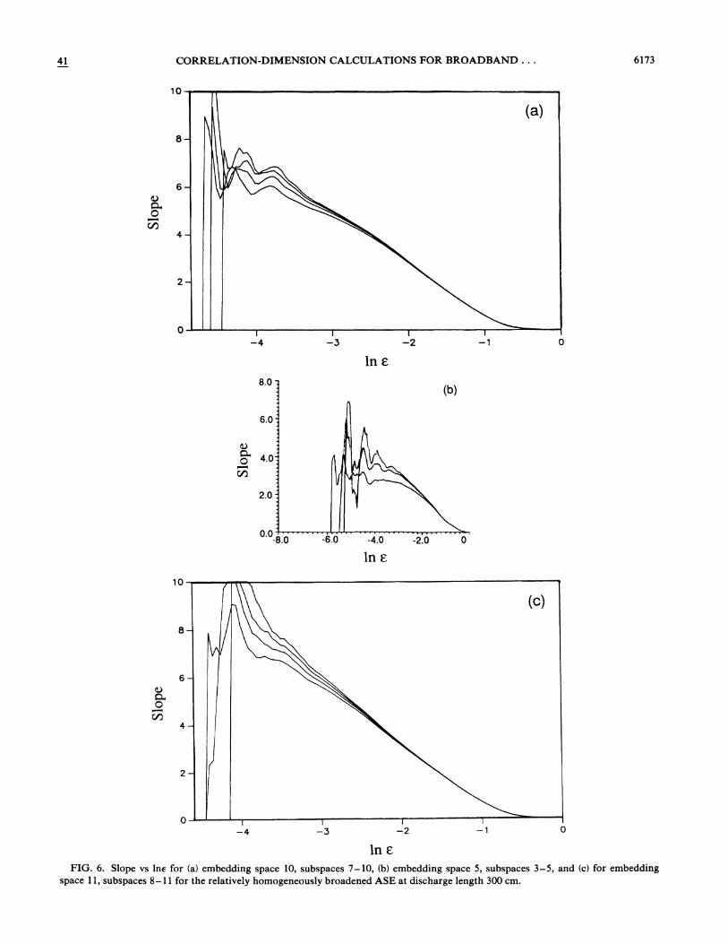
Even longer data sets were analyzed using the im-proved method of Albano et a/. Figure 6 provides theresults of analysis of a data set of 100000 points sampledat 5-ns intervals with eight-bit resolution for the relative-ly homogeneously broadened ASE obtained at dischargelength 300 cm. The 100000 points were used to con-struct 10000 vectors. Choosing 10 to be the embeddingdimension, a singular value decomposition was per-formed to 6nd the principal axes of embedding. Embed-ding vectors were selected uniformly from the entire data

41 CORRELATION-DIMENSION CALCULATIONS FOR BROADBAND. . . 6169

250

22S—

200-~ l~~l

175-

150-~ ~C

g 125-

I 1 l I I

600 800 1000 1200 1 400 1 600 1 800 2000

Time (1 is equivalent to 5 ns)

80

70=

so-

C4CO

bQ 500

40-

I

lpI

20I

30I

4pI

50 60

Frequency (MHz)

I

7QI

80I

90 100

FIG. 4. (a) Intensity ™eseries, (b) power spectra, (c) lnC„vs inc, (d) slope vs lnC„, (e) slope vs In@ [(c)—(e) for embedding dimen-sions 2 to 20, in steps of 2], and (I) slope vs embedding dimension (for in@= —3.0) for the &SE from the relatively homogeneouslybroadened case at a discharge length of 300 cm.

set. The normalized eigenvalues of the singular valueanalysis were 0.396, 0.267, 0.173, 9.15 X 104.25 X 10, 1.70X 10, 7.57X10, 3.14X 101.50 X 10, and 8.94 X 10 . The trajectory matrix wasthen rotated to get the matrix of the principal com-ponents which was then used to calculate the GP correla-tion integral. Figure 6(a) shows the slope of the correla-tion integral versus inc for subspaces 7, 8, 9, and 10. Fig-

ure 6(b) shows the same plot for a subset of the same dataset where 10000 points were used to construct 1000 vec-tors. The embedding dimension was chosen to be 5 andthe calculation was done for subspaces 3, 4, and 5. Fig-ure 6(c) shows the same plot for a different data set of therelatively homogeneously broadened ASE at the samedischarge length 300 cm. This data set also has eight-bitresolution and sampled at 5-ns intervals. In the analysis

6170 B. DAS, A. M. ALBANO, AND N. B.ABRAHAM 41

-2.5—

-10.0—

NIIIIN«~ —--~$8s$ $$$

~ S

~$$ ~s~$0 sf

~$$ ~!.~$ ]4~ $$

~$ ~$$~$$$ ~ $$

~ $$$ ~ ~ ~

~ ~ ~~$$$$$$ ~ ~ ~

~ ~ ~ ~~ ~ ~$

$$ ~ ~ ~ ~~ ~

~ ~ ~ ~~ ~ ~ ~

~ ~ ~~ ~

~$~ ~ ~ ~

~ ~ ~~ ~ ~ ~

~ $ ~ ~~$ ~ ~ ~~ ~ $ ~

~ ~ ~~$ ~ ~

~$~ ~~$$

~ ~~ ~

-12.5—~$

~ ~ ~~ ~

~ ~

-15.0—I-8 I-6

~$$$$$$$$$$$$$$$$$

1

~ ~

I

—4

1n e,

10

6—V

0Cf}

I

—12I

—10I

—6I

—4I

—2

FIG. 4. (Continued)

100000 points are used to construct 9000 vectors. Theembedding dimension was chosen to be 11 and the calcu-lation was done for subspaces 8, 9, 10, and 11. Normal-ized eigenvalues are 0.373, 0.282, 0.169, 9.25X104.57X10, 2.08X10, 8.84X10, 3.95 X 102. 19X10,1.33X10,and 9.95X10

Figure 7(a) shows a plot of slope versus lne for a dataset from the inhomogeneously broadened ASE where inthe analysis 100000 points were used to construct 10000vectors. The data set was taken at the discharge length300 cm (gain length 29.1) with the same sampling time in-terval of 5 ns. The embedding dimension was 10 and re-sults for subspaces 7, 8, 9, and 10 are shown. The nor-

malized eigenvalues were 0.413, 0.260, 0.171,8.73X10, 4. 14X10, 1.64X10, 6.52X102. 52 X 10, 1. 11 X 10, and 6.83 X 10 . Figure 7(b)shows a similar plot of slope versus lne for a differentdata set of the inhomogeneously broadened ASE obtainedat the discharge length 180 cm (gain length 17.5). Thisdata set also had eight-bit resolution and sampling time 5ns. 100000 points were used to construct 9000 vectors.The embedding dimension was 11 and the calculation wasdone for the subspaces 8, 9, 10, and 11. Normalized ei-genvalues are 0.487, 0.239, 0.139, 6.95 X 103.24X10, 1.34X10, 6.64X10, 4.22X103.57X10,2.87X10, and 2.55X10

41 CORRELATION-DIMENSION CALCULATIONS FOR BROADBAND. . . 6171

10

1-7 t-6l-4

1n e

-2

2—I

l

108 12

Embedding Dimension

I

16I

18 20

FIG. 4. (Continued)

In all three cases there is no "plateau" in the slopewhich would be indicative of a dimension and thereby in-dicating the existence of an attractor. Instead, the slopeincreases with embedding dimension which is charac-teristic of noise. The convergence of the slope curves forlarger values of e may indicate that there is some charac-teristic density distribution of the embedded data sets onlarger length scales, but it is not that of a fractal set.

IV. DISCUSSION

We conclude that there is no evidence of a low-dimensional strange attractor as a cause for the ASE in-

tensity fluctuations with broadband power spectra and ir-regular time series from the heavily saturated 3.51-pmsource. The slopes of the correlation integrals do notconverge to show any common plateau for any of theconditions. Instead, the slopes always increase with in-creasing embedding dimension —a behavior observed andexpected for stochastic random noise. Thus there is noevidence of a fractal dimension which would be expectedfor a deterministic chaotic system.

One might have expected some deterministic featuresin the case of ASE caused by the coherent evolution andringing after the intense pulses. Instead, the absence ofany common plateau in the plots of the correlation in-

6172 B. DAS, A. M. ALBANO, AND N. B.ABRAHAM

1 7.5

15.0—(a)

1 2.5—

7.5—

10.0—

0C/}

5.0—

2.5—

0.0—8

I

—7I

—6

1n E

I

—2

10—

8—

0M

2—

l I I

148 10 12

Embedding Dimension

I

16l

18 20

FIG. 5. {a) Slope vs 1nC„ for embedding dimensions 2 to 16, step 2 and {b) slope vs embedding dimension {for 1ne= —2.2) for elec-tronic noise from a HP-461A amplifier {flat from 1 kHz to 150 MHz).

tegrals, obtained from a wide range of operating condi-tions, makes it clear that the broadband fluctuations inthe heavily saturated ASE are associated with a stochas-tic state for which the concept of correlation dimensiondoes not have any meaning or, even if it does, it is notdiscernible with the present techniques of analysis evenwhen the analysis is carried out in reconstructed sub-spaces of dimension up to 20 (the maximum embeddingdimension used in the computations).

It is noteworthy, in this connection, that this type of

noisy origin of the broadband fluctuations of heavily sa-turated ASE sharply contrasts with that of the low-dimensional chaotic output of unstable 3.51-pm xenonlasers. * ' In the lasers there is a clear evidence offractal dimensions between 2 and 3 for data sets withbroadband optical power spectra similar to those of theASE signals. However, though they both have broad-band spectra they differ in other ways. One difference isin their autocorrelation functions. The intensity auto-correlation functions for the chaotic laser signals show

41 CORRELATION-DIMENSION CALCULATIONS FOR BROADBAND. . . 6173

10

a)

0—l

—4

8.0 -.

ln e

I-2

~ I

6.0 ,

~I

~I

~ I

~ I

~ I

4.0 .

2.0 -.

0.0 -6.0 -4.0 -2.0 0

ln c,

10

(c)

1

—4I

—3I

—2

FIG. 6. Slope vs inc for (a) embedding space 10, subspaces 7—10, (b) embedding space 5, subspaces 3—5, and (c) for embeddingspace 11, subspaces 8—11 for the relatively homogeneously broadened ASE at discharge length 300 cm.

6174 B. DAS, A. M. ALBANO, AND N. B.ABRAHAM 41

10

l

—4

ln e

10

0-l-4 -2

FIG. 7. Slope vs in@ for (a) embedding space 10, subspaces 7—10 at discharge length 300 cm and (b) embedding space 11, subspaces8—11 at discharge length 180 cm for the inhomogeneously broadened ASE.

clear ringing and a slow decay of the envelope instead ofsingle-peaked, rapidly decaying results for the ASE."The chaotic lasers also differ from the ASE in their inten-sity probability distribution functions. However, thereare forms of fully developed chaos which would not bedistinguishable from the ASE based on spectra, correla-tion functions, or probability distributions. Thus thecomputation of quantities such as correlation dimensionand autocorrelation functions enables us to unambiguous-ly discriminate low-dimensional chaos from these ran-domly Auctuating intensities. We conclude that in this

case stochastic processes underlie the long-term evolutionof ASE signals.

ACKNOWLEDGMENTS

We are pleased to thank J. R. Tredicce and L. M. Nar-ducci at Drexel University for the loan of the Tektronixtransient digitizer. We are grateful for experimental as-sistance and a critical reading of the manuscript by G.Alman. The assistance of the Academic ComputingCenter, Bryn Mawr College, is also gratefully acknowl-edged.

41 CORRELATION-DIMENSION CALCULATIONS FOR BROADBAND. . . 6175

'Present address: Department of Physics, University of Neva-da, Las Vegas, 4505 Maryland Parkway, Las Vegas, NV89154.

B. Das, Ph.D. thesis, Bryn Mawr College, 1988, available fromUniversity Microfilms.

~L. W. Casperson and A. Yariv, IEEE J. Quantum Electron.QE-S, 80 (1972).

L. W. Casperson, J. Appl. Phys. 48, 256 (1977).4H. Maeda and A. Yariv, Phys. Lett. 43A, 383 (1983).5D. H. Schwamb and S. R. Smith, Phys. Rev. A 23, 896 (1980).6R. W. Gray and L. W. Casperson, IEEE J. Quantum Electron.

QE-14, 893 (1978).7H. Gamo and H. Osada, Coherence and Quantum Optics IV,

edited by L. Mandel and E. Wolf (Plenum, New York, 1975),p. 583.

sF. A. Hopf, IEEE J.Quantum Electron. QK-10, 717 (1974).D. C. Newitt and N. B. Abraham, Opt. Commun. 31, 393

(1979).N. B. Abraham and E. B. Rockower, Opt. Acta 26, 1297(1979).N. B. Abraham, D. Kranz, J. Huang, and E. B. Rockower,Phys. Rev. A 24, 2556 (1981).B.Das and N. B.Abraham (unpublished).

' B. Das, G. Alman, N. B. Abraham, and E. B. Rockower,Phys. Rev. A 39, 5153 (1989).N. B.Abraham, Phys. Rev. A 21, 1595 (1980).N. B. Abraham and S. R. Smith, Opt. Commun. 38, 372(1981).

'sS. P. Adams and N. B. Abraham, in Coherence and QuantumOptics V, edited by L. Mandel and E. Wolf (Plenum, NewYork, 1984), p. 233.B.Das and N. B.Abraham (unpublished).N. B. Abraham, A. M. Albano, B. Das, T. Mello, M. F. H.Tarroja, N. Tufillaro, and R. S. Gioggia, in Optical Chaos,Proceedings of the International Society for Optical En-gineering, Bellingham, WA, 1986, edited by J. Chrostowskiand N. B. Abraham [Proc. Soc. Photo-Opt. Instrum. Eng.667, 2 (1986)].F. A. Hopf, Phys. Rev. Lett. 56, 2800 (1986);private commun-ication.

E. N. Lorenz, J. Atmos. Sci. 20, 130 (1963).B. A. Huberman and J. P. Crutchfield, Phys. Rev. Lett. 43,1743 (1979).

J. P. Gollub and H. Swinney, Phys. Rev. Lett. 35, 927 (1975).J. P. Gollub and S. V. Benson, J. Fluid Mech. 100, 449 (1980).N. B. Abraham, J. P. Gollub, and H. S. Swinney, Physica D11,252 (1984).

A. M. Albano, J. Abounadi, T. H. Chyba, C. E. Searle, S.Yong, R. S. Gioggia, and N. B.Abraham, J. Opt. Soc. Am. B2, 47 (1985).M. W. Derstine, H. M. Gibbs, F. A. Hopf, and D. L. Kaplan,Phys. Rev. A 27, 3200 (1983).N. B. Abraham, A. M. Albano, B. Das, T. Mello, M. F. H.Tarroja, and N. Tufillaro, in Ref. 18, p. 2.J.D. Farmer, Physica D 4, 566 (1982).P. Grassberger and I. Procaccia, Phys. Rev. A 28, 2591 (1983);Phys. Rev. Lett. 50, 346 (1983); A. Ben Mizrachi, I. Procac-cia, and P. Grassberger, Phys. Rev. A 29, 975 (1984).J. D. Farmer, E. Ott, and J. A. Yorke, Physica D 7, 153(1983).

'P. Grassberger and I. Procaccia, Physica D 13, 34 (1984).F. Takens, in Dynamical Systems and Turbulence, edited byD. A. Rand and L. S. Young (Springer, Berlin, 1981),p. 365.R. Mane, in Lecture Notes in Mathematics, edited by D. A.Rand and L. S. Young (Springer-Verlag, Berlin, 1981); seealso J.-P. Eckmann and D. Ruelle, Rev. Mod. Phys. 57, 617(1985).

~4R. Badii and A. Politi, J. Stat. Phys. 40, 725 (1985).~5A. M. Albano, J. Muench, C. Schwartz, A. I. Mees, and P. E.

Rapp, Phys. Rev. A 38, 3017 (1988).D. S. Broomhead and G. P. King, Physica D 10, 217 (1986).N. B. Abraham, A. M. Albano, D. K. Bandy, B. Das, G. de-Guzman, T. Issacs, M. F. H. Tarroja, S. Yong, S. P. Adams,and R. S. Gioggia, in Optical Instabilities, edited by R. W.Boyd, M. G. Raymer, and L. M. Narducci (Cambridge Uni-versity Press, Cambridge, 1985), p. 224.N. B.Abraham, A. M. Albano, B.Das, and M. F. H. Tarroja,in Fundamentals of Quantum Optics II, edited by F. Ehlotzky(Springer-Verlag, Berlin, 1987), p. 32.