Correlated destructive generalized power series cure rate models and associated inference with an...

Computational Statistics and Data Analysis 56 (2012) 1703–1713

Contents lists available at SciVerse ScienceDirect

Computational Statistics and Data Analysis

journal homepage: www.elsevier.com/locate/csda

Correlated destructive generalized power series cure rate models andassociated inference with an application to a cutaneous melanoma dataPatrick Borges a,∗, Josemar Rodrigues b, Narayanaswamy Balakrishnan c

a Departamento de Estatística, Universidade Federal do Espírito Santo, Brazilb Departamento de Estatística, Universidade Federal de São Carlos, Brazilc Department of Mathematics and Statistics, McMaster University, Hamilton, Ontario, Canada

a r t i c l e i n f o

Article history:Received 11 July 2011Received in revised form 13 October 2011Accepted 13 October 2011Available online 21 October 2011

Keywords:Initiated cellsCure rate modelsIGPS distributionAdditional parameter ρ

Correlation structure

a b s t r a c t

In this paper, we propose a new cure rate survival model, which extends the modelof Rodrigues et al. (2011) by incorporating a structure of dependence between theinitiated cells. To create the structure of the correlation between the initiated cells, weuse an extension of the generalized power series distribution by including an additionalparameter ρ (the inflated-parameter generalized power series (IGPS) distribution, studiedby Kolev and Minkova (2000)). It has a natural interpretation in terms of both a‘‘zero-inflated’’ proportion and a correlation coefficient. In our approach, the numberof initiated cells is assumed to follow the IGPS distribution. The IGPS distribution is anatural choice for modeling correlated count data that exhibit overdispersion. The primaryadvantage of this distributional assumption is that the correlation structure induced bythe additional parameter ρ results in a natural characterization of the association betweenthe initiated cells. Moreover, it provides a simple and realistic interpretation for thebiological mechanism of the occurrence of the event of interest as it includes a process ofdestruction of tumor cells after an initial treatment or the capacity of an individual exposedto irradiation to repair initiated cells that result in cancer being induced. This meansthat what is recorded is only the undamaged portion of the original number of initiatedcells not eliminated by the treatment or repaired by the repair system of an individual.Parameter estimation of the proposed model is then discussed through the maximumlikelihood estimation procedure. Finally,we illustrate the usefulness of the proposedmodelby applying it to real cutaneous melanoma data.

© 2011 Elsevier B.V. All rights reserved.

1. Introduction

Cure rate survival modelling plays an important role in reliability and survival analysis. It pertains to survival studieswherein a proportion of the subjects might not be susceptible to the event of interest due to different competingcauses. These models have found important applications in such diverse areas as biomedical studies, finance, criminology,demography,manufacturing and industrial reliability. For instance, in biomedical data, an event of interest can be a patient’sdeath, which can occur due to different competing causes or a tumor recurrence that may arise due to a number ofmetastasis-component tumor cells that are left active after an initial treatment of the individual. A metastasis-componenttumor cell is a tumor cell which has the potential for metastasizing; see Yakovlev (1994), Yakovlev et al. (1993), Yakovlevand Tsodikov (1996), and Ibrahim et al. (2001).

∗ Correspondence to: Departamento de Estatística, Universidade Federal do Espírito Santo, Av. Fernando Ferrari 514, Goiabeiras, CEP 29075-910, Vitøria,Espírito Santo, Brazil.

E-mail address: [email protected] (P. Borges).

0167-9473/$ – see front matter© 2011 Elsevier B.V. All rights reserved.doi:10.1016/j.csda.2011.10.013

http://dx.doi.org/10.1016/j.csda.2011.10.013

http://www.elsevier.com/locate/csda

http://www.elsevier.com/locate/csda

mailto:[email protected]

http://dx.doi.org/10.1016/j.csda.2011.10.013

1704 P. Borges et al. / Computational Statistics and Data Analysis 56 (2012) 1703–1713

The classical Berkson–Gage model (Berkson and Gage, 1952), discussed further by Farewell (1982, 1986), Goldman(1984), Sy and Taylor (2000), and Banerjee and Carlin (2004), as well as the most recent and comprehensive models ofYakovlev and Tsodikov (1996), Chen et al. (1999), Ibrahim et al. (2001), Chen et al. (2002), and Yin and Ibrahim (2005)include in their formulation the possibility of evaluating the cured rate. It is reasonable to presume that the occurrence ofthe event of interest might be due to one of many competing causes (Gordon, 1990), with the number of causes and thedistribution of survival times associated with each cause (Cox and Oakes, 1984, p. 147) being unknown, which leads to so-called latent competing causes. Another approach, taken by Cooner et al. (2007), stochastically forms an arranged sequenceof latent causes that induces the occurrence of the event of interest.

Cure rate models, with the number of latent competing causes following a Poisson, negative binomial, geometric orBernoulli distribution, have been studied by Rodrigues et al. (2009), Chen et al. (1999), and Cooner et al. (2007). The well-known Berkson–Gage model (Berkson and Gage, 1952) corresponds to case where the number of latent causes follows aBernoulli distribution and where there is at most one latent cause.

However, in most survival models incorporating a surviving fraction that are used in analyzing data from cancer clinicaltrials, there are two basic weaknesses:

1. first, the assumption that each initiated cell (competing cause or risk factor) becomes cancerous with probability 1, and2. next, the assumption of biological independence of initiated cells while becoming cancerous.

For overcoming Weakness 1 mentioned above, in a recent paper, Rodrigues et al. (2011), motivated by the work ofKlebanov et al. (1993), proposed a stochastic damage model for survival data with a surviving fraction (also known as adestructive weighted Poisson cure rate model) for describing the biological process of elimination of initiated cells aftersome specific treatment, but assuming biological independence of cells. With regard to Weakness 2, Haynatzki et al. (2000)pointed out that the biological independence assumption may not be valid when the dynamics of the cell population of anormal tissue is considered. Similarly, there are also indications that premalignant (initiated) andmalignant cells in a tissueinfluence each other’s development to some extent. Moreover, the interaction between healthy and premalignant cells inthe tissue should not be excluded from consideration either. It is, therefore, quite desirable to construct mathematicallytractable models that can adequately incorporate biological dependence, and this is the primary motivation for the presentresearch work.

The main purpose of this paper is to propose a new cure survival model which extends the models of Rodrigues et al.(2011) by incorporating a structure of dependence between the initiated cells. To create the structure of dependencebetween these initiated cells, we use an extension of the generalized power series distributions by including an additionalparameter ρ (the inflated-parameter generalized power series (IGPS) distribution; see Kolev and Minkova (2000)). This hasa natural interpretation in terms of both the ‘‘zero-inflated’’ proportion and the correlation coefficient. In our approach,we assume the number of initiated cells to follow an IGPS distribution, which is a natural choice for modeling correlatedcount data that possess overdispersion. The advantage of this assumption is that the correlation structure induced by thisadditional parameter ρ of the model results in a natural characterization of the association between the initiated cells.Moreover, it provides a simple and meaningful interpretation of the underlying biological mechanism of the occurrenceof the event of interest as it includes a process of destruction of tumor cells after an initial treatment or the capacity of anindividual exposed to irradiation to repair initiated cells that result in cancer being induced. In otherwords, what is recordedis only the undamaged portion of the original number of initiated cells not eliminated by the treatment or repaired by therepair system of an individual, which is represented by a compound variable.

The rest of the paper is organized as follows. In Section 2, we describe the model formulation. Some specific models andspecial cases are given in Section 3. In Section 4, we discuss themaximum likelihood estimation of themodel parameters. InSection 5, data onmelanoma are used to illustrate the usefulness of the proposedmodel. Finally, some concluding commentsare made in Section 6.

2. The model formulation

For an individual in the population, let N denote the number of initiated cells related to the occurrence of a tumor.Assume that the unobserved latent variable N has an inflated-parameter generalized power series (IGPS) distribution withprobability mass function (p.m.f .) given by

p(n; θ, ρ) = P[N = n; θ, ρ] =1

g(θ)

n1,n2,...

anθ(1 − ρ)

∞i=1

niρ

∞i=2

(i−1)ni, n = 0, 1, 2, . . . , ρ ∈ [0, 1), (1)

where an depends only on n, g(θ) =

∞

n=0 anθn is a positive, finite and differentiable function and θ ∈ (0, s) (s can be ∞) is

such that g(θ) is finite, and the summation is over the set of all nonnegative integers n1, n2, . . . such that

∞

i=1 ini = n. Formore details on the IGPS distribution, onemay refer to Kolev andMinkova (2000) andMinkova (2002). The parameter ρ is ameasure of the association between the tumor cells. Large values of ρ indicate high association between cells, while ρ → 0implies less association between cells. It is of interest to note that when ρ = 0 (i.e., when there is independence betweencells), the IGPS distribution reduces to a generalized power series distribution (Gupta, 1974; Consul, 1990). Table 2.1 presents

P. Borges et al. / Computational Statistics and Data Analysis 56 (2012) 1703–1713 1705

Table 2.1The choices of an , g(θ) and the parameter θ for some special cases of IGPS distributions.

Distribution an g(θ) θ s

IP 1n1 !n2 !···

eθ η ∞

IB

mm−n1−n2−···,n1,n2,...

(1 + θ)m π

1−π1

INBΓ

φ−1

+

∞i=1 ni

Γ (φ−1)

∞i=1 ni

!

(1 − θ)−φ−1 φη

1+φη∞

ILS (−1+n1+n2+···)!

n1 !n2 !···− log(1 − θ) 1 − π 1

the choices of an, g(θ) and the parameter θ corresponding to some special cases of IGPS distributions, namely, inflated-parameter Poisson (IP), negative binomial (INB), binomial (IB) and logarithmic series (ILS) distributions. In the IB and INBcases, the additional parameters m ∈ Z+ (the set of nonnegative integers) and the φ > −1 are to be treated as nuisanceparameters.

The probability generating function (p.g.f .) of the inflated-parameter generalized power series random variable N isgiven by

AN(z) =gθz(1 − ρ)(1 − zρ)−1

g(θ)

for 0 ≤ z ≤ 1. (2)

Now, after a prolonged treatment, we have as an immediate consequence the formation of possibly precancerous lesionsin a genome of the cells. LetN = n be the number of such lesions or initiated cells after the treatment, and Xj, j = 1, 2, . . . , n,be independent random variables, independent of N , having a Bernoulli distribution with success probability p indicatingthe presence of the jth lesion with p.g.f .

AXj(z) = 1 − p(1 − z), for 0 ≤ z ≤ 1. (3)

The variable D, representing the total number of cells, among the N initiated cells, not eliminated by the treatment, is thengiven by

D =

Nj=1

Xj, if N > 0

0, if N = 0.

(4)

By damaged or unrepaired irradiation, we mean that D ≤ N .This view of (4) was suggested earlier by Yang and Chen (1991) in the context of a bioassay study. They assumed that the

initial risk factors are primary initiatedmalignant cells, where Xj in (4) denotes the number of livingmalignant cells that aredescendants of the jth initiated malignant cell during some time interval. In this context, D then denotes the total numberof living malignant cells at some specific time.

In the competing causes scenario (Cox and Oakes, 1984), the number of unrepaired lesions D in (4) and the time V takento transform these lesions into a detectable tumor are both not observable (latent variables). We will call V a progressiontime. So, the time from the start of the treatment to tumor detection (which is the event of interest) for a given individualis defined by the random variable

Y = min{V1, V2, . . . , VD} (5)

forD ≥1, and Y = ∞ ifD = 0, which leads to a proportion p0 of the populationwhose lesions are repaired by the treatment,also called the ‘‘cured fraction’’. We assume that V1, V2, . . . are independent of D, and that, conditional on D, the variablesVj are i.i.d.

According to Rodrigues et al. (2011), the long-term survival function of the random variable Y in (5) is given by

Spop(y) = P[Y ≥ y] = AD(S(y)) =

∞d=0

P[D = d]{s(Y )}d = AN

AXj

S(y)

,

where S(·) denotes the common survival function of the unobserved lifetimes in (5) and AD(·) is the probability generatingfunction for the compound variable D, which converges when z = S(y) ∈ [0, 1]. Upon taking into account (2) and (3), thelong-term survival function of the observed lifetime of a detectable tumor in (5) is expressed by

Spop(y) =

g

θ1 − ρ

1 − pF(y)

1 −

1 − pF(y)

ρ−1

g(θ)

, (6)

where F(y) = 1 − S(y). If we take specifically ρ = 0, we get the generalized power series long-term survival function.


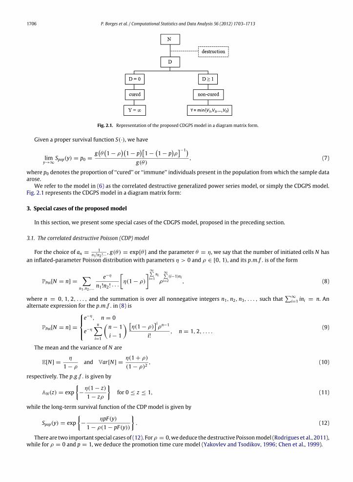
Fig. 2.1. Representation of the proposed CDGPS model in a diagram matrix form.

Given a proper survival function S(·), we have

limy→∞

Spop(y) = p0 =gθ1 − ρ

1 − p

1 −

1 − p

ρ−1

g(θ), (7)

where p0 denotes the proportion of ‘‘cured’’ or ‘‘immune’’ individuals present in the population fromwhich the sample dataarose.

We refer to the model in (6) as the correlated destructive generalized power series model, or simply the CDGPS model.Fig. 2.1 represents the CDGPS model in a diagram matrix form:

3. Special cases of the proposed model

In this section, we present some special cases of the CDGPS model, proposed in the preceding section.

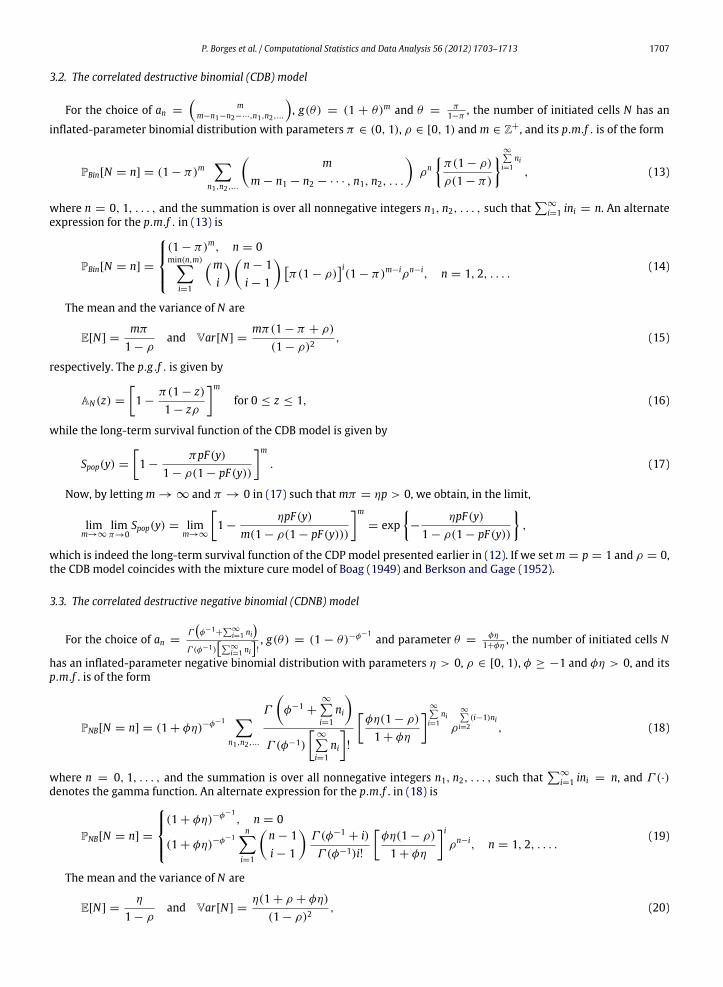
3.1. The correlated destructive Poisson (CDP) model

For the choice of an =1

n1!n2!···, g(θ) = exp{θ} and the parameter θ = η, we say that the number of initiated cells N has

an inflated-parameter Poisson distribution with parameters η > 0 and ρ ∈ [0, 1), and its p.m.f . is of the form

PPoi[N = n] =

n1,n2,...

e−η

n1!n2! · · ·

η(1 − ρ)

∞i=1

ni

ρ

∞i=2

(i−1)ni, (8)

where n = 0, 1, 2, . . . , and the summation is over all nonnegative integers n1, n2, n3, . . . , such that

∞

i=1 ini = n. Analternate expression for the p.m.f . in (8) is

PPoi[N = n] =

e−η, n = 0

e−ηn

i=1

n − 1i − 1

η(1 − ρ)

iρn−1

i!, n = 1, 2, . . . .

(9)

The mean and the variance of N are

E[N] =η

1 − ρand Var[N] =

η(1 + ρ)

(1 − ρ)2, (10)

respectively. The p.g.f . is given by

AN(z) = exp−

η(1 − z)1 − zρ

for 0 ≤ z ≤ 1, (11)

while the long-term survival function of the CDP model is given by

Spop(y) = exp−

ηpF(y)1 − ρ(1 − pF(y))

. (12)

There are two important special cases of (12). Forρ = 0,wededuce the destructive Poissonmodel (Rodrigues et al., 2011),while for ρ = 0 and p = 1, we deduce the promotion time cure model (Yakovlev and Tsodikov, 1996; Chen et al., 1999).


3.2. The correlated destructive binomial (CDB) model

For the choice of an =

m

m−n1−n2−···,n1,n2,...

, g(θ) = (1 + θ)m and θ =

π1−π

, the number of initiated cells N has an

inflated-parameter binomial distribution with parameters π ∈ (0, 1), ρ ∈ [0, 1) and m ∈ Z+, and its p.m.f . is of the form

PBin[N = n] = (1 − π)m

n1,n2,...

m

m − n1 − n2 − · · · , n1, n2, . . .

ρn

π(1 − ρ)

ρ(1 − π)

∞i=1

ni, (13)

where n = 0, 1, . . . , and the summation is over all nonnegative integers n1, n2, . . . , such that

∞

i=1 ini = n. An alternateexpression for the p.m.f . in (13) is

PBin[N = n] =

(1 − π)m, n = 0min(n,m)

i=1

mi

n − 1i − 1

π(1 − ρ)

i(1 − π)m−iρn−i, n = 1, 2, . . . . (14)


E[N] =mπ


mπ(1 − π + ρ)

(1 − ρ)2, (15)


AN(z) =

1 −

π(1 − z)1 − zρ

m

for 0 ≤ z ≤ 1, (16)

while the long-term survival function of the CDB model is given by

Spop(y) =

1 −

πpF(y)1 − ρ(1 − pF(y))

m

. (17)

Now, by letting m → ∞ and π → 0 in (17) such thatmπ = ηp > 0, we obtain, in the limit,

limm→∞

limπ→0

Spop(y) = limm→∞

1 −

ηpF(y)m(1 − ρ(1 − pF(y)))

m

= exp−

ηpF(y)1 − ρ(1 − pF(y))

,

which is indeed the long-term survival function of the CDP model presented earlier in (12). If we setm = p = 1 and ρ = 0,the CDB model coincides with the mixture cure model of Boag (1949) and Berkson and Gage (1952).

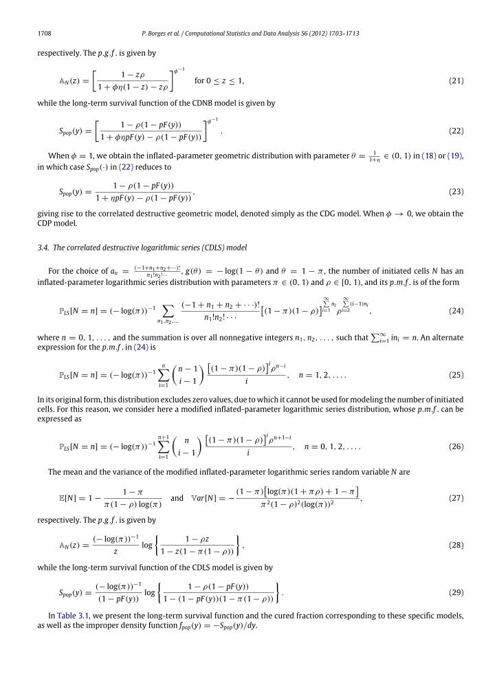
3.3. The correlated destructive negative binomial (CDNB) model

For the choice of an =Γ

φ−1

+

∞i=1 ni

Γ (φ−1)

∞i=1 ni

!

, g(θ) = (1 − θ)−φ−1and parameter θ =

φη

1+φη, the number of initiated cells N

has an inflated-parameter negative binomial distribution with parameters η > 0, ρ ∈ [0, 1), φ ≥ −1 and φη > 0, and itsp.m.f . is of the form

PNB[N = n] = (1 + φη)−φ−1 n1,n2,...

Γ

φ−1

+

∞i=1

ni

Γ (φ−1)

∞i=1

ni

!

φη(1 − ρ)

1 + φη

∞i=1

niρ

∞i=2

(i−1)ni, (18)


∞

i=1 ini = n, and Γ (·)denotes the gamma function. An alternate expression for the p.m.f . in (18) is

PNB[N = n] =

(1 + φη)−φ−1

, n = 0

(1 + φη)−φ−1n

i=1

n − 1i − 1

Γ (φ−1

+ i)Γ (φ−1)i!

φη(1 − ρ)

1 + φη

i

ρn−i, n = 1, 2, . . . .(19)


E[N] =η


η(1 + ρ + φη)

(1 − ρ)2, (20)



AN(z) =

1 − zρ

1 + φη(1 − z) − zρ

φ−1

for 0 ≤ z ≤ 1, (21)

while the long-term survival function of the CDNB model is given by

Spop(y) =

1 − ρ(1 − pF(y))

1 + φηpF(y) − ρ(1 − pF(y))

φ−1

. (22)

When φ = 1, we obtain the inflated-parameter geometric distribution with parameter θ =1

1+η∈ (0, 1) in (18) or (19),

in which case Spop(·) in (22) reduces to

Spop(y) =1 − ρ(1 − pF(y))

1 + ηpF(y) − ρ(1 − pF(y)), (23)

giving rise to the correlated destructive geometric model, denoted simply as the CDG model. When φ → 0, we obtain theCDP model.

3.4. The correlated destructive logarithmic series (CDLS) model

For the choice of an =(−1+n1+n2+···)!

n1!n2!···, g(θ) = − log(1 − θ) and θ = 1 − π , the number of initiated cells N has an

inflated-parameter logarithmic series distribution with parameters π ∈ (0, 1) and ρ ∈ [0, 1), and its p.m.f . is of the form

PLS[N = n] = (− log(π))−1

n1,n2,...

(−1 + n1 + n2 + · · ·)!

n1!n2! · · ·

(1 − π)(1 − ρ)

∞i=1

niρ

∞i=2

(i−1)ni, (24)


∞

i=1 ini = n. An alternateexpression for the p.m.f . in (24) is

PLS[N = n] = (− log(π))−1n

i=1

n − 1i − 1

(1 − π)(1 − ρ)

iρn−i

i, n = 1, 2, . . . . (25)

In its original form, this distribution excludes zero values, due towhich it cannot be used formodeling the number of initiatedcells. For this reason, we consider here a modified inflated-parameter logarithmic series distribution, whose p.m.f . can beexpressed as

PLS[N = n] = (− log(π))−1n+1i=1

n

i − 1

(1 − π)(1 − ρ)

iρn+1−i

i, n = 0, 1, 2, . . . . (26)

The mean and the variance of the modified inflated-parameter logarithmic series random variable N are

E[N] = 1 −1 − π

π(1 − ρ) log(π)and Var[N] = −

(1 − π)log(π)(1 + πρ) + 1 − π

π2(1 − ρ)2(log(π))2

, (27)


AN(z) =(− log(π))−1

zlog

1 − ρz

1 − z(1 − π(1 − ρ))

, (28)

while the long-term survival function of the CDLS model is given by

Spop(y) =(− log(π))−1

(1 − pF(y))log

1 − ρ(1 − pF(y))

1 − (1 − pF(y))(1 − π(1 − ρ))

. (29)

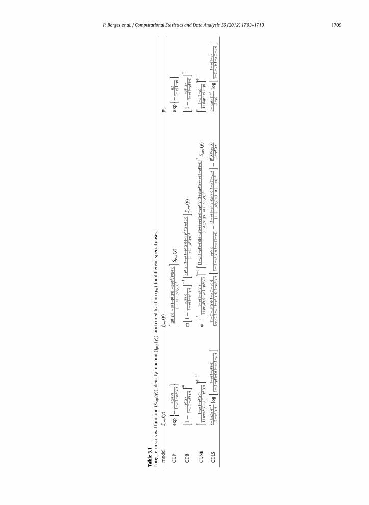
In Table 3.1, we present the long-term survival function and the cured fraction corresponding to these specific models,as well as the improper density function fpop(y) = −Spop(y)/dy.


Table3.1

Long

-term

survival

func

tion

(Spo

p(y)

),de

nsity

func

tion

(fpo

p(y)

),an

dcu

redfractio

n(p

0)ford

ifferen

tspe

cial

cases.

mod

elS p

op(y

)f pop

(y)

p 0

CDP

exp

−ηpF

(y)

1−ρ(1

−pF

(y))

η

pf(y

)[1−

ρ(1

−pF

(y))

]−ηρp2

f(y)F(

y)[1

−ρ(1

−pF

(y))

]2

S pop

(y)

exp

−ηp

1−ρ(1

−p)

CD

B 1

−πpF

(y)

1−ρ(1

−pF

(y))

mm

1−

πpF

(y)

1−ρ(1

−pF

(y))

−1πpf

(y)[1−

ρ(1

−pF

(y))

]−πp2

F(y)

ρf(y)

[1−

ρ(1

−pF

(y))

]2

S pop

(y)

1−

πpF

(y)

1−ρ(1

−pF

(y))

mCD

NB

1−

ρ(1

−pF

(y))

1+φηpF

(y)−

ρ(1

−pF

(y))

φ−1φ

−1

1−ρ(1

−pF

(y))

1+φηpF

(y)−

ρ(1

−pF

(y))

−1[1

−ρ(1

−pF

(y))

][φηpf

(y)+

ρpf

(y)]

−ρpf

(y)[1+

φηpF

(y)−

ρ(1

−pF

(y))

]

[1+

φηpF

(y)−

ρ(1

−pF

(y))

]2

S pop

(y)

1−ρ(1

−p)

1+φηp−

ρ(1

−p)

φ−1CD

LS(−

log(

π))

−1

(1−pF

(y))

log

1−ρ(1

−pF

(y))

1−(1

−pF

(y))

(1−

π(1

−ρ))

[1

−(1

−pF

(y))

(1−

π(1

−ρ))

]

log(

π)(1−

ρ(1

−pF

(y))

)(1−

pF(y

))

ρpf

(y)

1−(1

−pF

(y))

(1−

π(1

−ρ))

−(1

−ρ(1

−pF

(y))

)pf(y)

(1−

π(1

−ρ))

[1−

(1−pF

(y))

(1−

π(1

−ρ))

]2

−pf

(y)S

pop(

y)1−

pF(y

)

(−log(

π))

−1

(1−p)

log

1−ρ(1

−p)

1−(1

−p)

(1−

π(1

−ρ))


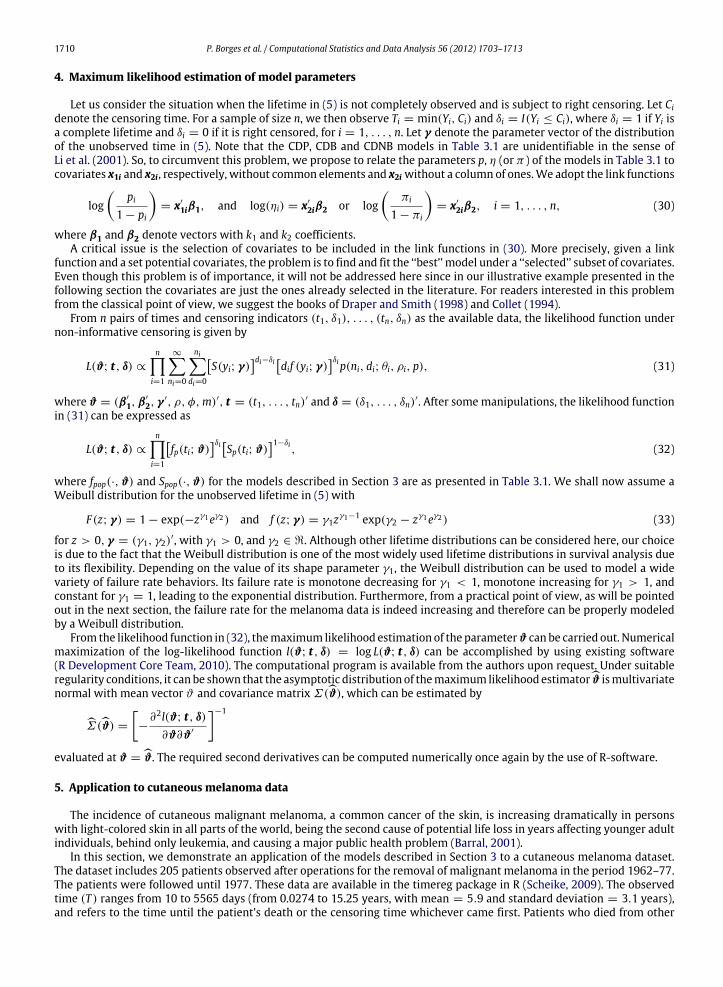
4. Maximum likelihood estimation of model parameters

Let us consider the situation when the lifetime in (5) is not completely observed and is subject to right censoring. Let Cidenote the censoring time. For a sample of size n, we then observe Ti = min(Yi, Ci) and δi = I(Yi ≤ Ci), where δi = 1 if Yi isa complete lifetime and δi = 0 if it is right censored, for i = 1, . . . , n. Let γ denote the parameter vector of the distributionof the unobserved time in (5). Note that the CDP, CDB and CDNB models in Table 3.1 are unidentifiable in the sense ofLi et al. (2001). So, to circumvent this problem, we propose to relate the parameters p, η (or π ) of the models in Table 3.1 tocovariates x1i and x2i, respectively, without common elements and x2i without a column of ones.We adopt the link functions

log

pi1 − pi

= x′

1iβ1, and log(ηi) = x′

2iβ2 or log

πi

1 − πi

= x′

2iβ2, i = 1, . . . , n, (30)

where β1 and β2 denote vectors with k1 and k2 coefficients.A critical issue is the selection of covariates to be included in the link functions in (30). More precisely, given a link

function and a set potential covariates, the problem is to find and fit the ‘‘best’’ model under a ‘‘selected’’ subset of covariates.Even though this problem is of importance, it will not be addressed here since in our illustrative example presented in thefollowing section the covariates are just the ones already selected in the literature. For readers interested in this problemfrom the classical point of view, we suggest the books of Draper and Smith (1998) and Collet (1994).

From n pairs of times and censoring indicators (t1, δ1), . . . , (tn, δn) as the available data, the likelihood function undernon-informative censoring is given by

L(ϑ; t, δ) ∝

ni=1

∞ni=0

nidi=0

S(yi; γ)

di−δidif (yi; γ)δip(ni, di; θi, ρi, p), (31)

where ϑ = (β′

1, β′

2, γ′, ρ, φ,m)′, t = (t1, . . . , tn)′ and δ = (δ1, . . . , δn)

′. After somemanipulations, the likelihood functionin (31) can be expressed as

L(ϑ; t, δ) ∝

ni=1

fp(ti; ϑ)

δiSp(ti; ϑ)1−δi

, (32)

where fpop(·, ϑ) and Spop(·, ϑ) for the models described in Section 3 are as presented in Table 3.1. We shall now assume aWeibull distribution for the unobserved lifetime in (5) with

F(z; γ) = 1 − exp(−zγ1eγ2) and f (z; γ) = γ1zγ1−1 exp(γ2 − zγ1eγ2) (33)

for z > 0, γ = (γ1, γ2)′, with γ1 > 0, and γ2 ∈ ℜ. Although other lifetime distributions can be considered here, our choice

is due to the fact that the Weibull distribution is one of the most widely used lifetime distributions in survival analysis dueto its flexibility. Depending on the value of its shape parameter γ1, the Weibull distribution can be used to model a widevariety of failure rate behaviors. Its failure rate is monotone decreasing for γ1 < 1, monotone increasing for γ1 > 1, andconstant for γ1 = 1, leading to the exponential distribution. Furthermore, from a practical point of view, as will be pointedout in the next section, the failure rate for the melanoma data is indeed increasing and therefore can be properly modeledby a Weibull distribution.

From the likelihood function in (32), themaximum likelihood estimation of the parameterϑ can be carried out. Numericalmaximization of the log-likelihood function l(ϑ; t, δ) = log L(ϑ; t, δ) can be accomplished by using existing software(R Development Core Team, 2010). The computational program is available from the authors upon request. Under suitableregularity conditions, it can be shown that the asymptotic distribution of themaximum likelihood estimatorϑ ismultivariatenormal with mean vector ϑ and covariance matrix Σ(ϑ), which can be estimated by

Σ(ϑ) =

−

∂2l(ϑ; t, δ)∂ϑ∂ϑ′

−1

evaluated at ϑ = ϑ. The required second derivatives can be computed numerically once again by the use of R-software.

5. Application to cutaneous melanoma data

The incidence of cutaneous malignant melanoma, a common cancer of the skin, is increasing dramatically in personswith light-colored skin in all parts of the world, being the second cause of potential life loss in years affecting younger adultindividuals, behind only leukemia, and causing a major public health problem (Barral, 2001).

In this section, we demonstrate an application of the models described in Section 3 to a cutaneous melanoma dataset.The dataset includes 205 patients observed after operations for the removal of malignant melanoma in the period 1962–77.The patients were followed until 1977. These data are available in the timereg package in R (Scheike, 2009). The observedtime (T ) ranges from 10 to 5565 days (from 0.0274 to 15.25 years, with mean = 5.9 and standard deviation = 3.1 years),and refers to the time until the patient’s death or the censoring time whichever came first. Patients who died from other


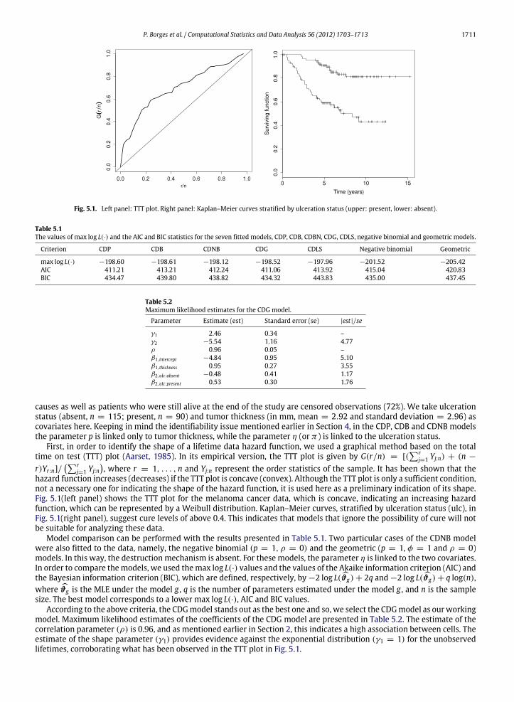
Fig. 5.1. Left panel: TTT plot. Right panel: Kaplan–Meier curves stratified by ulceration status (upper: present, lower: absent).

Table 5.1The values of max log L(·) and the AIC and BIC statistics for the seven fitted models, CDP, CDB, CDBN, CDG, CDLS, negative binomial and geometric models.

Criterion CDP CDB CDNB CDG CDLS Negative binomial Geometric

max log L(·) −198.60 −198.61 −198.12 −198.52 −197.96 −201.52 −205.42AIC 411.21 413.21 412.24 411.06 413.92 415.04 420.83BIC 434.47 439.80 438.82 434.32 443.83 435.00 437.45

Table 5.2Maximum likelihood estimates for the CDG model.

Parameter Estimate (est) Standard error (se) |est|/se

γ1 2.46 0.34 –γ2 −5.54 1.16 4.77ρ 0.96 0.05 –β1,intercept −4.84 0.95 5.10β1,thickness 0.95 0.27 3.55β2,ulc:absent −0.48 0.41 1.17β2,ulc:present 0.53 0.30 1.76

causes as well as patients who were still alive at the end of the study are censored observations (72%). We take ulcerationstatus (absent, n = 115; present, n = 90) and tumor thickness (in mm, mean = 2.92 and standard deviation = 2.96) ascovariates here. Keeping in mind the identifiability issue mentioned earlier in Section 4, in the CDP, CDB and CDNB modelsthe parameter p is linked only to tumor thickness, while the parameter η (or π ) is linked to the ulceration status.

First, in order to identify the shape of a lifetime data hazard function, we used a graphical method based on the totaltime on test (TTT) plot (Aarset, 1985). In its empirical version, the TTT plot is given by G(r/n) = [(

rj=1 Yj:n) + (n −

r)Yr:n]/r

j=1 Yj:n, where r = 1, . . . , n and Yj:n represent the order statistics of the sample. It has been shown that the

hazard function increases (decreases) if the TTT plot is concave (convex). Although the TTT plot is only a sufficient condition,not a necessary one for indicating the shape of the hazard function, it is used here as a preliminary indication of its shape.Fig. 5.1(left panel) shows the TTT plot for the melanoma cancer data, which is concave, indicating an increasing hazardfunction, which can be represented by a Weibull distribution. Kaplan–Meier curves, stratified by ulceration status (ulc), inFig. 5.1(right panel), suggest cure levels of above 0.4. This indicates that models that ignore the possibility of cure will notbe suitable for analyzing these data.

Model comparison can be performed with the results presented in Table 5.1. Two particular cases of the CDNB modelwere also fitted to the data, namely, the negative binomial (p = 1, ρ = 0) and the geometric (p = 1, φ = 1 and ρ = 0)models. In this way, the destruction mechanism is absent. For these models, the parameter η is linked to the two covariates.In order to compare themodels, we used themax log L(·) values and the values of the Akaike information criterion (AIC) andthe Bayesian information criterion (BIC), which are defined, respectively, by −2 log L(ϑg) + 2q and −2 log L(ϑg) + q log(n),where ϑg is the MLE under the model g , q is the number of parameters estimated under the model g , and n is the samplesize. The best model corresponds to a lower max log L(·), AIC and BIC values.

According to the above criteria, the CDGmodel stands out as the best one and so, we select the CDGmodel as ourworkingmodel. Maximum likelihood estimates of the coefficients of the CDG model are presented in Table 5.2. The estimate of thecorrelation parameter (ρ) is 0.96, and as mentioned earlier in Section 2, this indicates a high association between cells. Theestimate of the shape parameter (γ1) provides evidence against the exponential distribution (γ1 = 1) for the unobservedlifetimes, corroborating what has been observed in the TTT plot in Fig. 5.1.


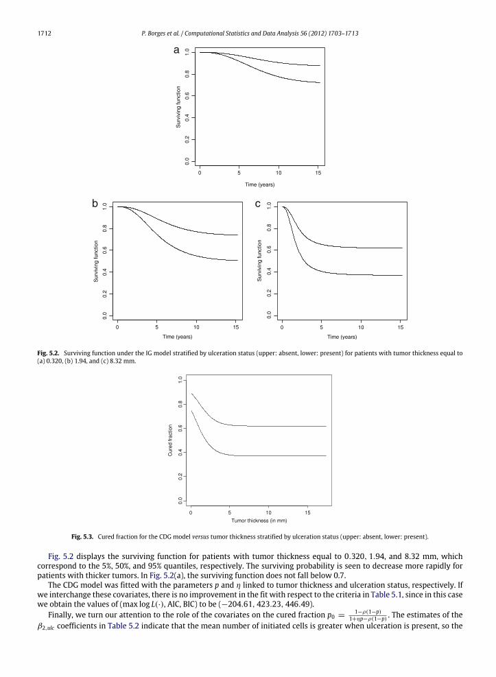
Fig. 5.2. Surviving function under the IG model stratified by ulceration status (upper: absent, lower: present) for patients with tumor thickness equal to(a) 0.320, (b) 1.94, and (c) 8.32 mm.

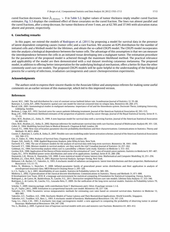
Fig. 5.3. Cured fraction for the CDG model versus tumor thickness stratified by ulceration status (upper: absent, lower: present).

Fig. 5.2 displays the surviving function for patients with tumor thickness equal to 0.320, 1.94, and 8.32 mm, whichcorrespond to the 5%, 50%, and 95% quantiles, respectively. The surviving probability is seen to decrease more rapidly forpatients with thicker tumors. In Fig. 5.2(a), the surviving function does not fall below 0.7.

The CDG model was fitted with the parameters p and η linked to tumor thickness and ulceration status, respectively. Ifwe interchange these covariates, there is no improvement in the fit with respect to the criteria in Table 5.1, since in this casewe obtain the values of (max log L(·), AIC, BIC) to be (−204.61, 423.23, 446.49).

Finally, we turn our attention to the role of the covariates on the cured fraction p0 =1−ρ(1−p)

1+ηp−ρ(1−p) . The estimates of theβ2,ulc coefficients in Table 5.2 indicate that the mean number of initiated cells is greater when ulceration is present, so the


cured fraction decreases. Since β2,thickness > 0 in Table 5.2, higher values of tumor thickness imply smaller cured fractionestimates. Fig. 5.3 displays the combined effect of these covariates on the cured fraction. The lines run almost parallel andthe cured fractions, after a steep decrease, for tumor thickness of over 5mm, are at 62.78% and 37.94%with ulceration statusabsent and present, respectively.

6. Concluding remarks

In this paper, we extend the models of Rodrigues et al. (2011) by proposing a model for survival data in the presenceof latent dependent competing causes (tumor cells) and a cure fraction. We assume an IGPS distribution for the number ofinitiated cells and a Weibull model for the lifetimes, and obtain the so-called CDGPS model. The CDGPS model incorporatesinto the analysis a biological dependence between the tumor cells. The advantage of this assumption is that we canmeasurethe interdependence between the cells in an initiated tissue developing into a malignant tumor. The estimation procedurefor the parameters of the proposed model is achieved through the maximum likelihood method. The practical relevanceand applicability of the model are then demonstrated with a real dataset involving cutaneous melanoma. The proposedmodel, in addition to offering better interpretation for the underlying biological mechanism, offers a better fit than the othercommonly used cure rate models. The proposed CDGPS models will be quite helpful in the understanding of the biologicalprocess for a variety of infections, irradiation carcinogenesis and cancer chemoprevention experiments.

Acknowledgments

The authors wish to express their sincere thanks to the Associate Editor and anonymous referees for making some usefulcomments on an earlier version of this manuscript, which led to this improved version.

References

Aarset, M.V., 1985. The null distribution for a test of constant versus bathtub failure rate. Scandinavian Journal of Statistics 12, 55–68.Banerjee, S., Carlin, B.P., 2004. Parametric spatial cure rate model for interval-censored time-to-relapse data. Biometrics 60, 268–275.Barral, A.M., 2001. Immunological studies in malignant melanoma: importance of tnf and the thioredoxin system. Doctorate Thesis, Linköping University,

Linköping, Sweden.Berkson, J., Gage, R.P., 1952. Survival curve for cancer patients following treatment. Journal of the American Statistical Association 42, 501–515.Boag, J.W., 1949. Maximum likelihood estimates of the proportion of patients cured by cancer therapy. Journal of the Royal Statistical Society, Series B 11,

15–53.Chen, M.H., Ibrahim, J.G., Sinha, D., 1999. A new bayesian model for survival data with a surviving fraction. Journal of the American Statistical Association

94, 909–919.Chen, M.H., Ibrahim, J.G., Sinha, D., 2002. Bayesian inference for multivariate survival data with cure fraction. Journal of Multivariate Analysis 89, 101–126.Collet, D., 1994. Modelling Survival Data in Medical Research. Chapman & Hall, London, UK.Consul, P.C., 1990. New class of location-parameter discrete probability distributions and their characterizations. Communications in Statistics. Theory and

Methods 19, 4653–4666.Cooner, F., Banerjee, S., Carlin, B., Sinha, D., 2007. Flexible cure ratemodelling under latent activation schemes. Journal of theAmerican Statistical Association

102, 560–572.Cox, D., Oakes, D., 1984. Analysis of Survival Data. Chapman & Hall, London, UK.Draper, N.R., Smith, H., 1998. Applied Regression Analysis. John Wiley & Sons, New York.Farewell, V.T., 1982. The use of mixture models for the analysis of survival data with long term survivors. Biometrics 38, 1041–1046.Farewell, V.T., 1986. Mixture models in survival analysis: are they worth the risk? Canadian Journal of Statistics 14, 257–262.Goldman, A.I., 1984. Survivorship analysis when cure is a possibility: a Monte Carlo study. Statistics in Medicine 3, 153–163.Gordon, N.H., 1990. Application of the theory of finitemixtures for the estimation of ‘‘cure’’ rates of treated cancer patients. Statistics inMedicine 9, 397–407.Gupta, R.C., 1974. Modified power series distributions and some of its applications. Sankhya, Series B 35, 288–298.Haynatzki, G.R., Weron, K., Haynatzka, V.R., 2000. A new statistical model of tumor latency time. Mathematical and Computer Modelling 32, 251–256.Ibrahim, J.G., Chen, M.H., Sinha, D., 2001. Bayesian Survival Analysis. Springer-Verlag, New York.Klebanov, L.B., Rachev, S.T., Yakovlev, A., 1993. A stochastic model of radiation carcinogenesis: latent time distributions and their properties. Mathematical

Biosciences 113, 51–75.Kolev, N., Minkova, L., Neytchev, P., 2000. Inflated-parameter family of generalized power series distributions and their application in analysis of

overdispersed insurance data. ARCH Research Clearing House 2, 295–320.Li, C.S., Taylor, J., Sy, J., 2001. Identifiability of cure models. Statistics & Probability Letters 54, 389–395.Minkova, L., 2002. A generalization of the classical discrete distributions. Communications in Statistics. Theory and Methods 31, 871–888.R Development Core Team. 2010. R: a language and environment for statistical computing. R Foundation for Statistical Computing. Vienna, Austria.Rodrigues, J., de Castro, M., Balakrishnan, N., Cancho, V.G., 2011. Destructive weighted Poisson cure rate models. Lifetime Data Analysis 17, 333–346.Rodrigues, J., de Castro, M., Cancho, V.G., Louzada-Neto, F., 2009. On the unification of the long-term survival models. Statistics & Probability Letters 79,

753–759.Scheike, T., 2009. timereg package, with contributions from T. Martinussen and J. Silver. R package version 1.1-6.Sy, J.P., Taylor, J.M.G., 2000. Estimation in a proportional hazards cure model. Biometrics 56, 227–336.Yakovlev, A.Y., 1994. Parametric versus nonparametric methods for estimating cure rates based on censored survival-data. Statistics in Medicine 13,

983–985.Yakovlev, A.Y., Tsodikov, A.D., 1996. Stochastic Models of Tumor Latency and Their Biostatistical Applications. World Scientific, Singapore.Yakovlev, A.Y., Tsodikov, A.D., Bass, L., 1993. A stochastic-model of hormesis. Mathematical Biosciences 116, 197–219.Yang, G.L., Chen, C.W., 1991. A stochastic two-stage carcinogenesis model: a new approach to computing the probability of observing tumor in animal

bioassays. Mathematical Biosciences 104, 247–258.Yin, G., Ibrahim, J., 2005. A general class of bayesian survival models with zero and nonzero cure fractions. Biometrics 61, 403–412.

Correlated destructive generalized power series cure rate models and associated inference with an...

Documents

Transcript of Correlated destructive generalized power series cure rate models and associated inference with an...