Magnetic Induction Tomography for Non-destructive ...
153
University of Bath PHD Magnetic Induction Tomography for Non-destructive Evaluation and Process Tomography Ma, Lu Award date: 2014 Awarding institution: University of Bath Link to publication Alternative formats If you require this document in an alternative format, please contact: [email protected] Copyright of this thesis rests with the author. Access is subject to the above licence, if given. If no licence is specified above, original content in this thesis is licensed under the terms of the Creative Commons Attribution-NonCommercial 4.0 International (CC BY-NC-ND 4.0) Licence (https://creativecommons.org/licenses/by-nc-nd/4.0/). Any third-party copyright material present remains the property of its respective owner(s) and is licensed under its existing terms. Take down policy If you consider content within Bath's Research Portal to be in breach of UK law, please contact: [email protected] with the details. Your claim will be investigated and, where appropriate, the item will be removed from public view as soon as possible. Download date: 24. Jul. 2022
-
Upload
khangminh22 -
Category
Documents
-
view
5 -
download
0
Transcript of Magnetic Induction Tomography for Non-destructive ...

University of Bath
PHD
Magnetic Induction Tomography for Non-destructive Evaluation and ProcessTomography
Ma, Lu
Award date:2014
Awarding institution:University of Bath
Link to publication
Alternative formatsIf you require this document in an alternative format, please contact:[email protected]
Copyright of this thesis rests with the author. Access is subject to the above licence, if given. If no licence is specified above,original content in this thesis is licensed under the terms of the Creative Commons Attribution-NonCommercial 4.0International (CC BY-NC-ND 4.0) Licence (https://creativecommons.org/licenses/by-nc-nd/4.0/). Any third-party copyrightmaterial present remains the property of its respective owner(s) and is licensed under its existing terms.
Take down policyIf you consider content within Bath's Research Portal to be in breach of UK law, please contact: [email protected] with the details.Your claim will be investigated and, where appropriate, the item will be removed from public view as soon as possible.
Download date: 24. Jul. 2022

Magnetic Induction Tomography forNon-destructive Evaluation and Process
Tomography
Lu Ma
A thesis submitted for the degree of Doctor of PhilosophyUniversity of Bath
Department of Electronic and Electrical Engineering
October 2014

Declaration
Attention is drawn to the fact that copyright of this thesis rests with the author. A copyof this thesis has been supplied on condition that anyone who consults it is understoodto recognise that its copyright rests with the author and that they must not copy it or usematerial from it except as permitted by law or with the consent of the author.
Signature of Author . . . . . . . . . . . . . . . . . . . . . . . . . . . . . . . . . . . . . . . . . . . . . . . . . . . . . . . . . . . . . .Lu Ma
Date . . . . . . . . . . . . . . . . . . . . . . . . . . . . . . . . . . . . . . . . . . . . . . . . . . . . . . . . . . . . . . . . . . . . . . . . . . . .21/10/2014
i

Abstract
Magnetic induction tomography (MIT) is an exciting yet challenging research topic. It issensitive to all passive electromagnetic properties, and as such it has great appeal to manyindustries. This thesis presents an experimental investigation of MIT within two broad ar-eas of application: non-destructive evaluation (NDE) and industrial process tomography.
Within both areas, MIT is presented as a low cost and non-invasive inspection tool withconsiderable developmental potential with regard to commercial applicability. Experi-mental investigations into the use of MIT demonstrate its versatility in imaging conduc-tive substances ranging from metallic structures, such as pipelines (s ⇡ 106�108S/m) tonew composite material, such as carbon fibre reinforced polymers (s ⇡ 104 � 105S/m),as well as substances in a state of flow (s < 10S/m).
Research innovations presented in this thesis constitute (i) the first experimental evalu-ation of MIT for pipeline inspection, an application never before attempted in the areaof NDE, (ii) the development of a novel limited region algorithm, which can improve thetraditional resolution from 10% to 2%, (iii) the first experimental 3D planar MIT study forsubsurface imaging, which opens many opportunities for MIT as a limited access tomog-raphy technique, (iv) an in-depth experimental evaluation of the MIT system responsetowards various fluid measurements for the first time, while also reporting some of thefirst flow rig tests in this field.
In addition, for each specific application, the capabilities of the prototype MIT systems areassessed with regard to (v) their flexibility in accommodating different sensor geometries,including circular, dual planar, planar and arc, (vi) situations in which the imaging subjecthas limited access, and (vii) their capacity to reconstruct a viable image of the subjectgiven limited measurement data.
Altogether, the results provide an evidential basis for future exploitation of this tech-nique. From the experimental investigations, it is concluded that the major limitationsof this technique lie in both the hardware development in order to meet the standards ofwidespread commercial applications and the software capability for fully automated realtime image reconstruction and structural analysis of the imaging subject. Nevertheless,with consistent development in both aforementioned areas, MIT could eventually be usedas a rapid NDE technique for structural health monitoring and process tomography, assuch contributing both to the social economy and public safety.
ii

I lovingly dedicate this thesis to my family
and
In memory of my grandfather
Ma Chang Jian
1931–2014
iii

Acknowledgements
I would like to offer my sincere gratitude to, firstly, my supervisor, Dr. ManuchehrSoleimani, for his consistent support, encouragement and willingness in helping me de-velop as an independent researcher; I am truly grateful to have experienced his tutelageand my time in his laboratory is one in which I feel I have grown significantly as an in-dividual. Without his influence and experience, I do not feel this PhD would have beenpossible, and most of all, I have been inspired for the future by his enthusiasm for, anddedication to, science.
Secondly, I am indebted to David Parker and Andy Matthews, technicians at the Depart-ment of Electronic and Electrical Engineering at the University of Bath, for sharing theirknowledge regarding the necessary hardware for my research; I would especially like toacknowledge David for manufacturing all the pipeline samples used in my experiments,and for his all-round assistance and support.
I would also like to thank Dr. Duncan Allsopp and Dr. Weijia Yuan for their criticalfeedback on my interim report.
In addition, I owe many thanks to all my friends and fellow colleagues for their helpthroughout this journey. I would particularly like to thank Dr. Hsin-Yu Wei, with whom Ihad many in-depth discussions about various research problems, and Dr. Stephen J. Bushfor taking the time to proofread my manuscripts and this thesis.
Finally, I would like to thank the UK Research Centre in Non-Destructive Evaluation fora feasibility grant for pipeline inspection, the Schlumberger Foundation for awarding aFaculty for the Future fellowship, and iPhase Ltd. for research funding with regard to thetwo-phase flow imaging project.
iv

Contents
Declaration i
Abstract ii
Acknowledgements iv
List of Symbols xiv
Nomenclature xv
1 Introduction 1
1.1 Background . . . . . . . . . . . . . . . . . . . . . . . . . . . . . . . . . 1
1.2 Aims and Objectives . . . . . . . . . . . . . . . . . . . . . . . . . . . . 3
1.3 Thesis Organisation . . . . . . . . . . . . . . . . . . . . . . . . . . . . 4
2 Methodologies of MIT 6
2.1 Fundamental Principles . . . . . . . . . . . . . . . . . . . . . . . . . . 6
2.2 Forward Problem . . . . . . . . . . . . . . . . . . . . . . . . . . . . . . 9
2.2.1 Maxwell’s Equations . . . . . . . . . . . . . . . . . . . . . . . . 10
2.2.2 Eddy Current Formulation . . . . . . . . . . . . . . . . . . . . . 11
2.3 Inverse Problem . . . . . . . . . . . . . . . . . . . . . . . . . . . . . . 14
2.3.1 Linear Back Projection . . . . . . . . . . . . . . . . . . . . . . 15
2.3.2 Newton One Step Error Reconstruction . . . . . . . . . . . . . . 15
2.3.3 Tikhonov Regularisation . . . . . . . . . . . . . . . . . . . . . . 16
2.3.4 Landweber Iteration Method . . . . . . . . . . . . . . . . . . . . 17
2.3.5 Laplacian Regularisation Method . . . . . . . . . . . . . . . . . 18
2.3.6 Selection of Regularisation Parameters . . . . . . . . . . . . . . 18
2.4 MIT Systems . . . . . . . . . . . . . . . . . . . . . . . . . . . . . . . . 19
2.4.1 MK-I System . . . . . . . . . . . . . . . . . . . . . . . . . . . . 20
2.4.2 MK-II System . . . . . . . . . . . . . . . . . . . . . . . . . . . 22
2.5 Literature Review . . . . . . . . . . . . . . . . . . . . . . . . . . . . . . 24
v

CONTENTS CONTENTS
3 Pipeline Inspection 27
3.1 Introduction . . . . . . . . . . . . . . . . . . . . . . . . . . . . . . . . . 27
3.2 Overview . . . . . . . . . . . . . . . . . . . . . . . . . . . . . . . . . . 27
3.3 Eight-channel Coil Array . . . . . . . . . . . . . . . . . . . . . . . . . . 32
3.4 Forward Model Validation . . . . . . . . . . . . . . . . . . . . . . . . . 33
3.5 NBPF Method . . . . . . . . . . . . . . . . . . . . . . . . . . . . . . . . 35
3.6 Experimental Results . . . . . . . . . . . . . . . . . . . . . . . . . . . . 36
3.6.1 Inspection of External Structural Damage . . . . . . . . . . . . . 36
3.6.2 Further Enhancement of Structural Inspection . . . . . . . . . . 38
3.7 Discussion . . . . . . . . . . . . . . . . . . . . . . . . . . . . . . . . . 41
4 CFRP Inspection 44
4.1 Introduction . . . . . . . . . . . . . . . . . . . . . . . . . . . . . . . . . 44
4.2 Dual Plane Array . . . . . . . . . . . . . . . . . . . . . . . . . . . . . . 46
4.3 System Analysis . . . . . . . . . . . . . . . . . . . . . . . . . . . . . . . 47
4.4 Results . . . . . . . . . . . . . . . . . . . . . . . . . . . . . . . . . . . . 51
4.5 Discussion . . . . . . . . . . . . . . . . . . . . . . . . . . . . . . . . . . 53
5 Subsurface Imaging 55
5.1 Introduction . . . . . . . . . . . . . . . . . . . . . . . . . . . . . . . . . 55
5.2 Planar Sensor Array . . . . . . . . . . . . . . . . . . . . . . . . . . . . 56
5.3 Method . . . . . . . . . . . . . . . . . . . . . . . . . . . . . . . . . . . 58
5.4 Simulations & Experiments . . . . . . . . . . . . . . . . . . . . . . . . . 59
5.4.1 Detectability of PMIT System . . . . . . . . . . . . . . . . . . . 59
5.4.2 Depth Detection of PMIT System . . . . . . . . . . . . . . . . . 61
5.4.3 Quantitative Evaluation of Depth Detection . . . . . . . . . . . . 66
5.5 Discussion . . . . . . . . . . . . . . . . . . . . . . . . . . . . . . . . . . 67
6 Limited Data Study 70
6.1 Introduction . . . . . . . . . . . . . . . . . . . . . . . . . . . . . . . . . 70
6.2 32-Sensor Array . . . . . . . . . . . . . . . . . . . . . . . . . . . . . . . 71
6.3 Experimental Results . . . . . . . . . . . . . . . . . . . . . . . . . . . . 72
6.3.1 Experiment Setup . . . . . . . . . . . . . . . . . . . . . . . . . . 72
6.3.2 Undersampled Data Imaging . . . . . . . . . . . . . . . . . . . 74
6.3.3 Limited Angle Imaging . . . . . . . . . . . . . . . . . . . . . . 78
6.4 A 3D Case Study . . . . . . . . . . . . . . . . . . . . . . . . . . . . . . 81
6.4.1 3D MIT Sensor . . . . . . . . . . . . . . . . . . . . . . . . . . 81
vi

CONTENTS CONTENTS
6.4.2 Experimental Results . . . . . . . . . . . . . . . . . . . . . . . 82
6.4.3 Evaluation of the Missing Planes . . . . . . . . . . . . . . . . . . 84
6.5 Discussion . . . . . . . . . . . . . . . . . . . . . . . . . . . . . . . . . 86
7 Two-phase Flow Imaging 88
7.1 Introduction . . . . . . . . . . . . . . . . . . . . . . . . . . . . . . . . . 88
7.2 Static Results . . . . . . . . . . . . . . . . . . . . . . . . . . . . . . . . 90
7.2.1 Experimental Setup . . . . . . . . . . . . . . . . . . . . . . . . . 90
7.2.2 Fluid Distribution Patterns in a Free Space Background . . . . . 91
7.2.3 Fluid Distribution Patterns in a Silicone Oil Background . . . . . 96
7.2.4 Fluid Distribution Patterns in a Saline Solution Background . . . 96
7.2.5 Fluid Distribution Patterns in a Tap Water Background . . . . . . 98
7.2.6 Non-homogenous Conductive Fluid Imaging in a Free Space Back-ground . . . . . . . . . . . . . . . . . . . . . . . . . . . . . . . 99
7.3 Quasi-static Results . . . . . . . . . . . . . . . . . . . . . . . . . . . . . 100
7.4 Discussion . . . . . . . . . . . . . . . . . . . . . . . . . . . . . . . . . . 107
8 Conclusions 109
8.1 Summary . . . . . . . . . . . . . . . . . . . . . . . . . . . . . . . . . . 109
8.2 Remarks . . . . . . . . . . . . . . . . . . . . . . . . . . . . . . . . . . . 109
8.3 Limitations & Immediate Research . . . . . . . . . . . . . . . . . . . . . 111
8.4 Contributions to Knowledge . . . . . . . . . . . . . . . . . . . . . . . . 112
8.5 Future Work . . . . . . . . . . . . . . . . . . . . . . . . . . . . . . . . . 112
8.5.1 Forward and Inverse Problems . . . . . . . . . . . . . . . . . . . 112
8.5.2 System Improvements . . . . . . . . . . . . . . . . . . . . . . . 113
8.5.3 Multi-frequency MIT . . . . . . . . . . . . . . . . . . . . . . . . 114
A List of publications 116
Bibliography 118
vii

List of Figures
2.1 Fundamental principles. . . . . . . . . . . . . . . . . . . . . . . . . . . 7
2.2 Equivalent circuit of mutual inductance theory. . . . . . . . . . . . . . . 7
2.3 Illustration of MIT forward model. . . . . . . . . . . . . . . . . . . . . 10
2.4 Eddy current region. . . . . . . . . . . . . . . . . . . . . . . . . . . . . 10
2.5 Illustration of MIT inverse model. . . . . . . . . . . . . . . . . . . . . . 14
2.6 Flow chart for the solving process of an iterative Tikhonov method. . . . 17
2.7 L-curve for selecting the regularisation parameter. . . . . . . . . . . . . 19
2.8 Generic MIT system architecture. . . . . . . . . . . . . . . . . . . . . . 20
2.9 MK-I MIT system with 8 channel coil array. . . . . . . . . . . . . . . . 21
2.10 MK-I MIT system signals, measured from a 8-channel coil array. . . . . 22
2.11 MK-II MIT system with 16 channel coil array. . . . . . . . . . . . . . . . 23
2.12 MK-II MIT system signal levels. . . . . . . . . . . . . . . . . . . . . . 24
2.13 Reconstructed images for (a) an aluminium rod lying diagonally acrossthe measuring space, and (b) an aluminium cone-shaped object in thecentre of the measuring space. . . . . . . . . . . . . . . . . . . . . . . . 26
3.1 Structure of a pipeline. . . . . . . . . . . . . . . . . . . . . . . . . . . . 28
3.2 MK-I MIT system with an eight-channel coil array. . . . . . . . . . . . . 32
3.3 Top view of an eight-sensor coil array. . . . . . . . . . . . . . . . . . . . 33
3.4 Signal to noise ratio of first cycle measurements when first coil used asexcitation. . . . . . . . . . . . . . . . . . . . . . . . . . . . . . . . . . 33
3.5 Mesh model of an eight-channel MIT system. . . . . . . . . . . . . . . . 34
3.6 Comparison of induced voltages due to full pipe sample using simulationand experimental data. . . . . . . . . . . . . . . . . . . . . . . . . . . . 34
3.7 (a) Narrowband region, (b) Narrowband pass filter applied to the radius. . 35
3.8 Comparative results using PBRM and NPFM for a full pipe inspection. . 36
3.9 (a) Hollow pipe inspection, (b) Inspection of pipe with a metal inside, (c)Reconstructed images for (a) and (b). . . . . . . . . . . . . . . . . . . . 36
viii

LIST OF FIGURES LIST OF FIGURES
3.10 Aluminium pipe inspection results showing true samples and reconstruc-tion of external metal losses: (a) a full pipe sample, (b) 4.34mm thicknessof wall loss, (c) a 4.34mm thickness of wall loss on one side and a 1.10mmthickness of wall loss on the other side. . . . . . . . . . . . . . . . . . . 37
3.11 Singular value decompositions for PBRM and NPFM. . . . . . . . . . . 38
3.12 Aluminium pipe inspection results showing true samples and reconstruc-tion of metal losses for internal and external parts: (a) 4.34mm thick-ness of external wall loss, (b) 1.10mm thickness of external wall loss,(c) 4.30mm thickness of internal wall loss, and (d) 1.90mm thickness ofinternal wall loss. . . . . . . . . . . . . . . . . . . . . . . . . . . . . . . 39
3.13 Steel pipe inspection results showing true samples and reconstruction ofmetal losses for external parts: (e) 3.44mm thickness of external wall loss,and (f) 2.13mm thickness of external wall loss. . . . . . . . . . . . . . . 40
3.14 Comparison of induced voltages due to different testing profiles. . . . . . 40
3.15 Inspection of defected plastic pipelines using NPFM based ECT system. 42
4.1 (a) Dual plane sensor array, and (b) the coil sequence of the first planararray. . . . . . . . . . . . . . . . . . . . . . . . . . . . . . . . . . . . . 46
4.2 Block diagram of the dual plane MIT system. . . . . . . . . . . . . . . . 47
4.3 Signal to noise ratio, after the excitation of coil 1, for measurements ob-tained when the dual planes are separated by distances of 2,4,6,8 and10cm. . . . . . . . . . . . . . . . . . . . . . . . . . . . . . . . . . . . . 48
4.4 Sensitivity maps for (a) a neighbouring measurement from coil 1 and 2,(b) an opposite measurement from coil 1 and 10, (c) a diagonal measure-ment from coil 1 and 9, and (d) a diagonal measurement from coil 1 and18. . . . . . . . . . . . . . . . . . . . . . . . . . . . . . . . . . . . . . 49
4.5 Measurements obtained from a dual plane of coils when coil 1 is excited,and the remaining coils are used as receivers. . . . . . . . . . . . . . . . 49
4.6 Detection of steel samples in different locations. . . . . . . . . . . . . . . 51
4.7 CFRP samples with (a) one hidden defect, and (b) four hidden defects. . 52
4.8 CFRP samples with one and four defects (a and d, respectively), alongsidetheir reconstructed images using slice visualisation (b and e, respectively),and 3D contour visualisations (c and f, respectively). . . . . . . . . . . . 53
5.1 (a) coil dimensions, (b) coil sequence. . . . . . . . . . . . . . . . . . . . 57
5.2 Top view of a 4⇥4 planar coil array. . . . . . . . . . . . . . . . . . . . 57
5.3 Block diagram of the proposed PMIT system. . . . . . . . . . . . . . . . 57
5.4 Signal to noise ratio of first cycle measurements when first coil used asexcitation. . . . . . . . . . . . . . . . . . . . . . . . . . . . . . . . . . . 58
ix

LIST OF FIGURES LIST OF FIGURES
5.5 Sensitivity map coupling between: (a) coil 1 and coil 2, (b) coil 1 and coil11 and (c) coil 1 and coil 16, the coil number sequence can be seen inFigure 5.1 (b). . . . . . . . . . . . . . . . . . . . . . . . . . . . . . . . 59
5.6 Detectability of PMIT using simulated data. . . . . . . . . . . . . . . . . 60
5.7 Detectability of PMIT using experimental data. . . . . . . . . . . . . . . 61
5.8 Depth detection using simulated data. . . . . . . . . . . . . . . . . . . . 62
5.9 Depth detection using one object. . . . . . . . . . . . . . . . . . . . . . 64
5.10 Depth detection using two objects. . . . . . . . . . . . . . . . . . . . . . 65
5.11 Graph of volume deformation. . . . . . . . . . . . . . . . . . . . . . . . 67
5.12 The distribution of sensitive region against the imaging depth. . . . . . . 69
6.1 MK-I MIT system with a 32-sensor coil array. . . . . . . . . . . . . . . 71
6.2 Top view of the 32-sensor coil array. . . . . . . . . . . . . . . . . . . . . 71
6.3 Signal to noise ratio of first cycle measurements when first coil used asexcitation. . . . . . . . . . . . . . . . . . . . . . . . . . . . . . . . . . 72
6.4 Single and multiple objects detection using undersampling data. . . . . . 75
6.5 Singular value decay for undersampled measurements. . . . . . . . . . . 76
6.6 Graph of 1D conductivity distribution for undersampled 16 sensors andfull 32 sensors; referring to two objects detection in Figure 6.4. . . . . . . 78
6.7 Single and multiple objects detection using limited angle imaging. . . . . 79
6.8 Singular value decay for limited angle imaging. . . . . . . . . . . . . . . 80
6.9 Graph of 1D conductivity distribution using limited angle imaging of 45�,90�, 180�, 240� and full angle of 360�; referring to two objects detectionin Figure 6.7. . . . . . . . . . . . . . . . . . . . . . . . . . . . . . . . . 81
6.10 Schematic representation of a 3D cube sensor model. . . . . . . . . . . . 82
6.11 Reconstructed images of a metal cube under different missing plane sce-narios. The number of missing planes, by row, is 0, 1, 2, 3, 4 respectively. 84
6.12 Sensitivity maps. . . . . . . . . . . . . . . . . . . . . . . . . . . . . . . 85
6.13 Decay of the normalised singular value of sensitivity matrices for fivecases: case 1-full data scenario, case 2-five planes, case 3-four planes,case 4-three planes, case 5-two parallel planes. . . . . . . . . . . . . . . 85
6.14 Sum of the diagonal components of the resolution matrix at five missingplane cases. . . . . . . . . . . . . . . . . . . . . . . . . . . . . . . . . . 86
7.1 The experimental setup, in this case showing three inclusions within theimaging region. . . . . . . . . . . . . . . . . . . . . . . . . . . . . . . . 91
x

LIST OF FIGURES LIST OF FIGURES
7.2 Standard deviation of the norm value of the phase difference resultingfrom the position change of a single inclusion versus the area ratio of thatinclusion (2.28%, 8.69% and 14.57% respectively). Data is shown forfluids with three conductivities (red, blue and magenta for, respectively,conductivity values of 1.52S/m, 4.06S/m and 5.94S/m). . . . . . . . . . 92
7.3 Reconstructed images of one, two and three inclusions in a free spacebackground are shown in the first, second and third column; the first, sec-ond and third row shows the reconstructed images of small, medium andlarge dimensions of inclusions in a free space background respectively.The conductivity of the inclusion is 1.52S/m in all cases. . . . . . . . . . 93
7.4 Reconstructed images of small, medium and large dimensions of inclu-sions in a free space background are shown in the first, second and thirdcolumn; the first, second and third row shows the reconstructed imagesof one, two and three inclusions in a free space background respectively.The conductivities of the inclusions in the first, second and third columnsare 1.52S/m, 4.06S/m and 5.94S/m respectively. . . . . . . . . . . . . 94
7.5 The norm value of the phase difference against the change in area ra-tio (left, in black) and the change in conductivity level (right, in brown).Both sets of plots are produced using one, two or three inclusions (top tobottom, respectively). . . . . . . . . . . . . . . . . . . . . . . . . . . . . 95
7.6 Reconstructed images of one, two and three inclusions of saline solutionin a free space background are shown in the first, second and third column;the first, second and third row shows the reconstructed images of small,medium and large dimensions of saline solution in a free space back-ground respectively. The conductivity of the saline solution is 1.52S/m inall cases. . . . . . . . . . . . . . . . . . . . . . . . . . . . . . . . . . . 96
7.7 Reconstructed images of one, two and three inclusions of silicone oil ina saline solution background are shown in the first, second and third col-umn; the first, second and third row shows the reconstructed images ofsmall, medium and large dimensions of silicone oil in a saline solutionbackground respectively. The conductivity of the saline solution back-ground is 1.52S/m. . . . . . . . . . . . . . . . . . . . . . . . . . . . . . 97
7.8 Standard deviation of the norm value of the phase difference resultingfrom the position change of a single inclusion versus the area ratio ofthis inclusion (2.28%, 8.69% and 14.57% respectively) for two cases:silicone oil in a saline background (dashed red line), and saline solution(conductivity 1.52S/m) in a silicone oil background (dashed blue line). . . 98
xi

LIST OF FIGURES LIST OF FIGURES
7.9 Reconstructed images of one, two and three inclusions of silicone oil ina tap water background are shown in the first, second and third column;the first, second and third row shows the reconstructed images of small,medium and large dimensions of silicone oil in a tap water backgroundrespectively. The conductivity of the tap water background is 0.06S/m. . 99
7.10 Experimental setup (top) and reconstructed images (bottom) of three strata,each of non-homogeous conductive fluids in a free space background. Byvolume, strata are 200ml, 400ml and 650ml, from the left to the rightrespectively. . . . . . . . . . . . . . . . . . . . . . . . . . . . . . . . . 100
7.11 Bubble testing setup. . . . . . . . . . . . . . . . . . . . . . . . . . . . . 101
7.12 The norm value of the phase difference against the volume of the fluidfor backgrounds with five different conductivities (top). Shown in blue,red, magenta, black, and brown are conductivities of 0.06S/m, 1.81S/m,3.20S/m, 5.13S/m and 12.64S/m respectively. The norm value of thephase difference against the volume of the fluid for a tap water back-ground is shown in the bottom half of the figure. . . . . . . . . . . . . . 102
7.13 The norm value of the phase difference for five difference conductivitybackgrounds (0.06S/m, 1.81S/m, 3.20S/m, 5.13S/m and 12.64S/m re-spectively) when the flow rig is filled with 9 litres of fluid, measurementswere made between the coil pair Tx2 and Tx6. . . . . . . . . . . . . . . 103
7.14 Reconstructed images of bubble flow in various backgrounds. Back-ground conductivities are, by row, 12.64S/m, 5.13S/m, 3.20S/m, 1.81S/mand 0.06S/m respectively. . . . . . . . . . . . . . . . . . . . . . . . . . . 105
7.15 Experimental setup of a silicone oil inclusion in two conductive back-grounds, with associated images. (a) silicone oil inclusion within a 1.81S/mbackground, (b) silicone oil inclusion within a 12.64S/m background. . . 106
7.16 The norm value of the phase difference resulting from the movementof the silicone oil along the axial direction within two conductive back-grounds, 1.81S/m and 12.64S/m respectively. . . . . . . . . . . . . . . 107
xii

List of Tables
1.1 Existing hard field tomographic techniques. . . . . . . . . . . . . . . . . 1
1.2 Existing soft field tomographic techniques. . . . . . . . . . . . . . . . . 3
3.1 Comparison of the existing NDE techniques for pipeline inspection. . . . 31
3.2 Specifications of eight-channel MIT system. . . . . . . . . . . . . . . . 33
4.1 Physical properties of the HexPly M21 epoxy matrix. . . . . . . . . . . 52
5.1 Sensor model parameters. . . . . . . . . . . . . . . . . . . . . . . . . . 56
5.2 Volume deformation ratio. . . . . . . . . . . . . . . . . . . . . . . . . . 67
6.1 Specifications of 32-channel MIT system. . . . . . . . . . . . . . . . . . 72
6.2 Scenario one: Undersampling measurements. . . . . . . . . . . . . . . . 73
6.3 Scenario two: Limited angle imaging. . . . . . . . . . . . . . . . . . . . 73
6.4 Image quality parameter with respect to undersampled measurements. . . 77
6.5 Image quality parameter with respect to different angles. . . . . . . . . . 80
xiii

List of Symbols
A — Magnetic potential (V · s ·m�1)B — Magnetic flux density (T )D — Electric displacement field (C ·m�2)E — Electric field (V ·m�1)H — Magnetic field strength (A ·m�1)V — Electric potential (V )d — Skin depth (mm)e — Electrical permittivity (F ·m�1)µ — Magnetic permeability (H ·m�1))s — Electrical conductivity (S ·m�1)w — Angular frequency (rad/s)
xiv

Nomenclature
MIT — Magnetic Induction Tomography or Mutual Inductance Tomography
NDE — Non-destrutive Evaluation
MRI — Magnetic Resonance Imaging
ECT — Electrical Capacitance Tomography
EIT — Electrical Impedance Tomography
RMIT — Rotational Magnetic Induction Tomography
VMIT — Volumetric Magnetic Induction Tomography
PMIT — Planar Magnetic Induction Tomography
FEM — Finite Element Method
LBP — Linear Back Projection
NOSER — Newton One Step Error Reconstruction
LSS — Least Squares Solution
NI — National Instrument
NPFM — Narrowband Pass Filtering Method
CFRP — Carbon Fibre Reinforced Polymer
PBRM — Pixel Based Reconstruction Method
ROI — Region of Interest
SNR — Signal to Noise Ratio
CMOS — Complementary Metal-Oxide-Semiconductor
ADC — Analog to Digital Converter
DAC — Digital to Analog Converter
EC — Eddy Current
MFL — Magnetic Flux Leakage
RFT — Remote Field Testing
UI — Ultrasonic Inspection
EMAT — Electromagnetic Acoustic Transducer
ILI — In-Line Inspection
MPT — Magneto-static Permeability Tomography
xv

Chapter 1
Introduction
1.1 Background
Tomography is a technique for displaying a cross-sectional representation of an objectthrough the use of penetrating signals such as waves, electromagnetic fields or particles.Tomographic techniques are often divided into different categories according to the sens-ing techniques used. There are two main categories of tomographic technique, hard andsoft field tomography [1]. The commonly used hard field tomography techniques includeg � ray , X � ray and magnetic resonance imaging (MRI). The soft field tomographictechniques are primarily referred to as electrical tomography [2]. They differ in that, forhard field tomography, the path of the transmitting signal is in a straight line and the onlyfactor that can affect the signal strength is the material along that path, regardless of po-sition. In soft field tomography, the position of the material in the measuring region andthe distribution of electrical parameters both inside and outside the measuring region canaffect the transmitting signal. Each tomographic technique has its own characteristics,constraints and applications. There are also other tomography techniques, such as ultra-sound, thermal conduction tomography, that are neither hard nor soft field, and use othersensing techniques for imaging.
Technique Characteristics Applications
g � rayFast scanning speedRadioactive sources
Potentially fast
Industrial applicationsMedical imaging
X � rayHigh resolution
Mechanically scannedRadiation confinement
Industrial applicationsMedical imaging
MRINo use of radiationDetailed resolution
Non-invasive
Medical diagnosisClinical imaging
Table 1.1: Existing hard field tomographic techniques.
1

1.1. BACKGROUND CHAPTER 1. INTRODUCTION
Electrical tomography techniques can image the passive electromagnetic properties of anobject. In 1912, Conrad Schlumberger conducted the first electric field imaging experi-ment; which offered new possibilities for exploring the Earth. Over the past 100 years,electrical tomography has expanded to include work in the fields of geophysics, medicalimaging and process tomography. Electrical tomography techniques have several advan-tages. Despite their relatively modest image resolution, they have gradually proved tobe useful because of their imaging speed, low cost and non-invasive characteristics [3].Three electrical imaging techniques are listed in Table 1.2 with their sensing techniquesand applications.
Electrical Impedance Tomography (EIT) utilises multiple electrode sensors to measurethe impedance changes between pairs of electrodes. The conductivity distribution ofthe imaging subject can then be computed based on the measured impedance changes[4]. EIT is sometimes also called electrical resistance tomography, if the reactive capac-itive component of the measured impedance is negligible. Among the electrical imagingtechniques, EIT is the most well-developed technique and has been applied in medicalimaging as a diagnostic method [5].
Compared to the traditional electrode based technique, Electrical Capacitance Tomogra-phy (ECT) realises a contactless means of mapping the dielectric permittivity through theuse of capacitive sensors [6]. Typical materials that can be imaged by ECT include plastic,water and wood. Its use has been proposed for numerous applications, including flamevisualisation [7, 8, 9], visualisation of fluidised bed gas-solid concentration distributions[10], and two-phase flow identification [11, 12].
Magnetic Induction Tomography (MIT), also known as Mutual Inductance Tomographyor Electromagnetic Induction Tomography (EMT), is a tomographic technique that canpotentially map the distribution of all passive electromagnetic properties (conductivity,permeability and permittivity) of an object [3]. MIT is the most recent and least developedelectrical imaging technique, compared to EIT and ECT. MIT does not require electricalcontacts with the object and uses the interaction of an oscillating magnetic field with aconductive medium. This field, which is excited and registered by inductive coils arrangedaround the object, is perturbed by the generation of eddy currents in the object. Theconductivity (and/or other passive electromagnetic properties) can be reconstructed fromthe measurements of perturbed fields outside the objects. MIT has been applied to avariety of diverse applications, but most of this interest has been in either medical imaging[13, 14, 15, 16], examining cross-sectional images of the human body [17], or in non-destructive evaluations (NDE) for industrial applications, to visualise and monitor thedistribution of material in vessels and pipelines [18, 19, 20].
2

1.2. AIMS AND OBJECTIVES CHAPTER 1. INTRODUCTION
Technique SensorsMeasurement Property Applications
EIT ElectrodesImpedance s Medical imaging
Flow imaging
ECT Capacitive platesCapacitance e Flow imaging
Flaw detection
MIT Inductive coilsMutual inductance s ,µ,e Medical imaging
Industrial applications
Table 1.2: Existing soft field tomographic techniques.
1.2 Aims and Objectives
The aim of this study is to investigate the feasibility and sensitivity of MIT for non-destructive evaluation (NDE) and industrial process imaging. MIT is sensitive to electricalconductivity. As such it can be used for defect inspection of metallic and new compositematerials. In addition, conductive flow in multiphase flow imaging is a challenging topicas the existing techniques either do not distinguish the conductivity property or requireclose contact to the flow substances. Due to the advantages of MIT, this suggests thatMIT could be an alternative inspection and imaging technique for both fields. MIT haspreviously been considered as a potential candidate for NDE applications and industrialprocess tomography, however, the realisation of MIT remains limited. One of the majorissues is that MIT is an inherently low resolution technique. This is due to the fact theinverse problem is an underdetermined ill-posed problem. In order to improve the res-olution, efforts need to be made both in the forward problem and the image inversion.Furthermore, in order to meet the standard of NDE technique specification, the systemshould be equipped with the capability of real time data collection. These issues repre-sent the most influential factors that limit MIT’s applicability in the commercial arena.
The key questions relating to the use of MIT technique for NDE applications are:
• What is the intended application, and what is the motivation behind it?
• What are the fundamental and practical limitations of MIT for NDE applications?
• What is the design for the MIT coil array in order to facilitate the inspection?
• What type of damage and defect can be inspected?
• Can an image of the damage or defect be reconstructed?
• What is the imaging resolution that can be achieved?
The key questions relating to the use of MIT in industrial process tomography are:
• Where does MIT fit in the field of industrial process tomography?
3

1.3. THESIS ORGANISATION CHAPTER 1. INTRODUCTION
• What is the advantage of MIT compared to existing techniques?
• How can MIT be used in multiphase flow imaging?
• What is the sensitivity level and capability of MIT in this field of study?
• What is the future direction of MIT?
In this study, the author will investigate how to employ the Bath MK-I and MK-II systemsfor the aforementioned applications. As such, the system design is not within the scopeof this study. Nevertheless, there are improvements that can be made to accommodate theintended objective of the study. In general, the methodologies used in this research canbe categorised in four aspects:
• Investigating different geometries of MIT coil arrays for the intended applications.
• Establishing the forward models and calculating the sensitivity maps accordinglyto assist the imaging process and improve the imaging accuracy.
• Both adopting existing and developing novel algorithms for the image reconstruc-tion to improve the resolution of MIT.
• Conducting both simulations and experimental work to establish the capability ofMIT for the proposed applications.
1.3 Thesis Organisation
This thesis is organised in the following chapters. Chapter 2 introduces the methodologiesof MIT, including the fundamental principles, eddy current modelling, image reconstruc-tion algorithms and two types of MIT systems used throughout this research.
In chapter 3, MIT is proposed as a non-destructive evaluation (NDE) technique for pipelineimaging. The existing NDE techniques for pipeline inspection are reviewed and the mer-its and limitations of each technique are addressed. A Bath MK-I MIT system is proposedfor this application. Experimental evaluations are carried out based on laboratory investi-gations. In addition, a localised algorithm, narrowband pass filtering method (NPFM), isdeveloped specifically for the cylindrical pipe geometry. Comparative results using bothtraditional algorithms and this novel algorithm show that the NPFM can achieve an un-precedented resolution of 2%. Machined wall losses on metallic pipes are inspected andimages are reconstructed based on this method.
In addition to metallic structures, chapter 4 studies the applicability of MIT in the inspec-tion of carbon fibre reinforced polymers (CFRPs). One of the advantages of MIT is thatit is flexible with coil geometry. This indicates that the coil array of the system can bedesigned according to a specific application. In this case, a dual planar array is developedand used for hidden defect inspection in CFRP plates, which commonly occur during the
4

1.3. THESIS ORGANISATION CHAPTER 1. INTRODUCTION
initial manufacturing stage. Both single and multiple defects in CFRP plates are identifiedand 3D images reconstructed.
Expanding upon the concept of a dual planar MIT system, chapter 5 presents a singleplanar array MIT study for 3D near subsurface imaging as a means of limited accesstomography. This is more challenging compared to a dual planar MIT study as the accessis limited to one surface, resulting in limited measurement data. In this chapter, bothsimulated and experimental work are carried out. Qualitative evaluations of the 3D imagereconstruction results show a penetrative depth of 3� 4cm beneath the imaging subject.The system development, practical implications, capability and limitations of subsurfaceimaging are addressed.
Noticing that the coil geometry varies from circular, to dual planar to a single planar fromchapters 3 to 5, this results in missing data as a result of limited access to the imagingsubject. In chapter 6, the missing data effect is studied systematically in both 2D and3D cases. The Bath MK-I system with 32 sensors is introduced, which is specificallydesigned to study the effect of missing data on the quality of reconstructed images inMIT. Missing data is investigated by systematically removing the coil sensors throughan undersampling process and limited angle imaging. To examine a range of missingdata sets, two experimental scenarios were completed: undersampling measurements andlimited angle imaging. The former is carried out by evenly undersampling 4, 8, and 16sensors from a 32 sensors coil array and the latter is investigated by using limited angles of45�, 90�, 180� and 270�, compared to 360� full angle imaging. An image quality measureand 1D graph of the conductivity distribution are adopted to quantify the effect of missingdata on MIT images through experimental evaluation. This study has also been furtherextended in 3D. A cube sensor is designed for this purpose. The information loss due tosystematic removal of planes of sensors is evaluated using singular value decompositionand resolution matrix analysis. The observation of this 3D case study is consistent withthat of a 2D case.
Chapter 7 presents an experimental evaluation of MIT in conductive phase flow imag-ing. Experiments are conducted covering as broad a range of conductivity contrasts aspossible, so as to encompass several scenarios of potential interest in industrial flow en-vironments. Our evaluation of fluid experiments includes (a) the smallest conductivitycontrast in which image reconstruction in various non-conductive and conductive back-grounds is possible, (b) distinguishing three strata of non-homogenous conductive fluidsin a free space, and (c) imaging a flow of non-homogenous bubbles of gas in various con-ductive backgrounds. Taken together, various capabilities of an MIT system in conductivephase imaging are demonstrated.
Chapter 8 summarises the research output in this thesis, discusses the direction of thefuture work and highlights the associated challenges. The future work includes image re-construction improvement, system hardware enhancement and implementation of a multi-frequency MIT system.
5

Chapter 2
Methodologies of MIT
2.1 Fundamental Principles
Magnetic induction tomography utilises inductive coils to map the electromagnetic prop-erties of an object. The fundamental principles of MIT can be explained by using basicmutual inductance and eddy current theories. As shown in Figure 2.1, by passing an al-ternating current into an excitation coil, a primary magnetic field can be generated, whichinduces an electric field that can be detected by a measuring coil. From this field theinduced voltage can be measured. If there is a conductive object placed within this time-varying field, an eddy current arises, which can also generate a magnetic field, called thesecondary magnetic field. As such, the electric field on the measuring coil can be induced,in part, by both the primary and secondary fields. The induced voltages on the measur-ing coil therefore differ depending on whether a conductive object is present within thefield; if no such object is present, the induced voltage arises entirely due to the primaryfield, whereas if an object is present, the induced voltage arises due to both primary andsecondary fields. By analysing the difference in the induced voltages, one can obtain theproperties of the conductive object. Thus, the MIT problem is essentially an eddy currentproblem, hence it is also called eddy current tomography. Note that in the context of thisresearch, the electrical conductivity of the object is the focus of the passive electromag-netic properties.
6

2.1. FUNDAMENTAL PRINCIPLES CHAPTER 2. METHODOLOGIES OF MIT
Figure 2.1: Fundamental principles.
The fundamental principles in Figure 2.1 can be interpreted in terms of a simplified elec-tric circuit diagram (Figure 2.2). The excitation coil with a supplied alternating currentcan be seen as an AC source. Consider the excitation coil as inductor L1 and the measur-ing coil as inductor L2. The measured voltage on L2 due to induction is U2. The propertiesof the imaging subject can be simplified using a R�C circuit representation. As the eddycurrent is induced around the object, the imaging subject can be seen as a voltage sourceU3, whereby the inductance of the object is L3. The mutual inductance among L1, L2 andL3 are M12, M13 and M23 respectively. The goal is to derive a relationship between theprimary voltage and the secondary induced voltage using this circuit diagram.
Figure 2.2: Equivalent circuit of mutual inductance theory.Adapted from [21].
7

2.1. FUNDAMENTAL PRINCIPLES CHAPTER 2. METHODOLOGIES OF MIT
Using the magnetic flux equations, one can obtain
I =didt
= jwi = jw UjwL
=UL
(2.1)
The induced voltage U2 on inductor L2 consists of two parts, U 02 and U 00
2 . U 02 is the voltage
directly induced by the primary voltage U1. This primary voltage also results in U3, whichin turn induces U 00
2 .
U 02 =�M12
di1dt
=�M12U1
L1(2.2)
U 002 =�M23
di3dt
=�M23 jw I3 (2.3)
As U3 is also induced by the primary field, then:
U3 =�M13di1dt
=�M13U1
L1(2.4)
It is readily seen that:
Z3 = (R//1
jwC) =
R1+ jwRC
(2.5)
Hence:
I3 =U3
Z3(2.6)
As U2 = U 02 +U 00
2 , then combining the above equations 2.2 to 2.6:
U2 = {�M12 +M13M23( jw 1R�w2C)}U1
L1(2.7)
where Ui and Ii are the voltages and currents passing through the inductors, and Li and Mi j
are the self inductance and mutual inductance coefficients for the inductors respectively.Equation 2.7 suggests that the induced voltage is dependent on the frequency and theproperties of the imaging subject.
U2
U1µ w(� j
1R+wC) (2.8)
It is well known that both the resistance and capacitance of a given material (in this case,the imaging subject) can be defined using the electrical conductivity or permittivity of auniform specimen of the material.
The conductivity of a given specimen can be defined using the resistance of a given section
8

2.2. FORWARD PROBLEM CHAPTER 2. METHODOLOGIES OF MIT
of that specimen:
s =1R
lA
(2.9)
where l is the length of the section and A is the cross-sectional area of the section.
Similarly, the permittivity of a given specimen can be defined using the capacitance of agiven section of that specimen. The definition for capacitance is
C = e0erAd
(2.10)
where A is the area of overlap of the two plates and d is the separation between the platesfor a given cross section of the material.
As both lA and A
d can be considered constant for a specimen with given dimensions, thenequation 2.8 can also be formulated in the following manner:
U2
U1µ w(� js +we0er) (2.11)
This indicates that if the imaging subject is highly conductive, the real part can thereforebe neglected. The induced voltage can be considered proportionate to the amplitude of theconductivity |s |. For biomedical applications, focusing on living tissue, this conductivityis usually very low. As such, the imaginary part cannot be ignored as the induced voltagedepends on both the amplitudes and the phase shift of � js +we0er.
In [13], the authors considered the MIT problem from the point of view of electromagneticfield interaction, i.e., using a single channel MIT system to derive the relationship betweenthe primary magnetic field generated by an excitation coil and the secondary magneticfield induced by the eddy currents, and also reached the same conclusion as shown inequation 2.11.
2.2 Forward Problem
For an electromagnetic tomography imaging system, two problems need to be solved,namely the forward and inverse problems. Given the distribution of conductivity (or otherpassive electromagnetic properties) with an excitation current, the forward problem is tosolve the estimated measurement signals from the sensors [4, 22, 23]. This can be writtenin the following form [24]:
F =Z
vf (E, H)dv (2.12)
where F is a function of the electric and magnetic fields at a given point. The fields arethemselves implicit functions of the system parameters: the conductivity s , the perme-ability µ , the permittivity e , or any combination of the previous. The MIT forward modelcan be illustrated using Figure 2.3. In general, the fields and the system will take on dif-
9

2.2. FORWARD PROBLEM CHAPTER 2. METHODOLOGIES OF MIT
ferent values at each point in space, which are determined by the eddy current induced inthe system. Therefore, the forward problem is often called the eddy current problem.
Figure 2.3: Illustration of MIT forward model.
2.2.1 Maxwell’s Equations
The forward problem is solved under the condition of a quasi-static electromagnetic field.In this condition, a few assumptions need to be made. First, the displacement currentis neglected; second, the material is considered to have an isotropic character; third, theeddy current effect in the current source is also neglected. Note that there are two regionsin the quasi-static electromagnetic field, the non-conducting region and the eddy currentregion (shown in Figure 2.4).
Figure 2.4: Eddy current region.
Using the time-harmonic notation of Maxwell’s equations, in the eddy current region We:
—⇥H = Jeddy (2.13)
—⇥E =� jwB (2.14)
— ·B = 0 (2.15)
In the non-conducting region Wn:—⇥H = Js (2.16)
10

2.2. FORWARD PROBLEM CHAPTER 2. METHODOLOGIES OF MIT
— ·B = 0 (2.17)
In each region, the B and H fields satisfy that the normal component of the B field is zeroand the tangential component of the H field is zero. On the boundary between the tworegions Gne:
Be ·ne +Bn ·nn = 0 (2.18)
He ⇥ne +Hn ⇥nn = 0 (2.19)
where Jeddy is the eddy current density in We, Js is the current density due to the excitationin the non-conducting region Wn, n is the normal vector on the boundary, and Be, He, ne,Bn, Hn, nn refer to the the magnetic flux, magnetic field and normal vectors in regions ofWe and Wn respectively. The uniqueness of B and E are therefore ensured.
2.2.2 Eddy Current Formulation
Various eddy current formulations in three dimensions have been studied, using a combi-nation of the magnetic vector potential, magnetic scalar potential and electric scalar po-tential [25, 26, 27, 28, 29, 30, 31]. Regardless of the formulation, it has to comply to theuniqueness of the fields and the boundary conditions. The work presented in this thesis isbased on reduced magnetic vector potential formulations (Ar,Ar �f ) to avoid modellingthe structure of the coils using edge finite element method (FEM) [32, 33, 34, 35].
—⇥ 1µ
—⇥A+ jswA = Js (2.20)
where the current density, Js, can be prescribed by the magnetic vector potential accordingto the Biot-Savart Law.
The magnetic potential, A, is the sum of two parts: As, the impressed magnetic vectorpotential as result of current source Js, and Ar the reduced magnetic vector potential inthe eddy current region We.
In the non-conductive region Wn:—⇥Hs = Js (2.21)
where Hs is the magnetic field generated by an excitation coil, which can be directlycomputed from in any point P in free space from Js:
Hs =Z
Wn
Js(Q)⇥ rQP
4p | rQP |3 dWQ (2.22)
where rQP is the vector pointing from the source point Q to the field point P.
The impressed magnetic vector potential As can be written as:
—⇥As = µ0Hs (2.23)
11

2.2. FORWARD PROBLEM CHAPTER 2. METHODOLOGIES OF MIT
From equations 2.22 and 2.23, As is readily shown as:
As =Z
Wn
µ0Js(Q)
4p | rQP |2 dWQ (2.24)
In the entire region Wn +We, the magnetic flux density can be expressed by:
B = µ0Hs +—⇥Ar (2.25)
According to Faraday’s Law of induction, ignoring the displacement current, the inducedelectric field can be written in the following form:
—⇥E =� jw—⇥A (2.26)
The induced electric field can also be written using a magnetic vector potential and anelectric scalar potential:
E =� jw(A+—f) (2.27)
The eddy current arises when a conductor is exposed in a time-varying magnetic field;therefore, in the eddy current region We:
Jeddy = sE (2.28)
In the region of Wn +We, the magnetic field can be expressed by:
—⇥H = Jeddy + Js (2.29)
It is known that:B = µH (2.30)
where µ is the permeability of the medium.
Combining equations 2.21, 2.25, 2.27,2.29 and 2.30:
—⇥ (1µ
—⇥Ar)+ jwsAr + jws— ·f = —⇥ (1µ0
—⇥As)� jwsAs �—⇥ (1µ
—⇥As)
(2.31)
In MIT, the inductive coils are considered magneto-static not antennas; as such the wavepropagation effect can be ignored. Edge FEM is a useful technique to solve such problemsby approximating the system as a combination of linear equations in small elements withappropriate boundary conditions. In edge FEM on a tetrahedral mesh, a vector field isrepresented using a basis vector function Ni j associated with the edge between nodes iand j :
Ni j = Li—L j �L j—Li (2.32)
where Li is a nodal shape function. Applying the edge element basis function to Galerkin’sapproximation [36, 37, 38, 39], one can obtain:
12

2.2. FORWARD PROBLEM CHAPTER 2. METHODOLOGIES OF MIT
Z
We(—⇥N · 1
µ—⇥Ar)dv+
Z
WejwsN ·Ardv =
Z
Wc(—⇥N · 1
µ0—⇥As)dv�
Z
Wc(N · jwsAs)dv�
Z
Wc—⇥ (N · 1
µµ0—⇥As)dv (2.33)
where N is any linear combination of edge basis functions, We is the eddy current re-gion, and Wc is the coil region. The right hand side in equation 2.33 can be solved byequations 2.22 and 2.24. The only unknown variable is the reduced vector potential Ar.By applying edge FEM, the second order partial differential equations can be computedby a combination of system linear equations, which can then be solved. The Ar can beobtained using the BiConjugate Gradients Stabilized Method to solve the system linearequation [40, 41, 42, 43]:
SAr = b (2.34)
where S is system matrix and b is the right hand side current density. Assuming themedium has a constant permeability characteristic, equation 2.34 can be written as a linearsystem matrix form as:
[—⇥ ( 1
µ —⇥ ())+ jws() jws— · ()jws— · () jws— · ()
][Ar
f] = [
� jwsAs
� jws— ·As] (2.35)
The boundary equation is satisfied by:
n · ( jws— · (A+—f)) = 0 (2.36)
By solving the reduced magnetic vector potential Ar, one is able to evaluate the inducedvoltages in the measuring coils. The induced voltages can be calculated by using a volumeintegration form:
Vmn =� jwZ
WcA · J0dv (2.37)
where A = As +Ar, and J0 is a virtual unit current density passing through the coil.
The sensitivity matrix is essential in MIT as it realises the linearisation between the con-ductivity and the induced voltages. The elements of the Jacobian matrix can be expressedby [40, 42, 44]:
∂Vmn
∂sk=�w2
RWk
Am ·Andv
I0(2.38)
where Vmn is the measured voltage, sk is the conductivity of pixel k, Wk is the volume ofthe perturbation (pixel k), Am and An are, respectively, solutions of the forward problemwhen the excitation coil m is excited by I0 and when the sensing coil n is excited with unitcurrent.
13

2.3. INVERSE PROBLEM CHAPTER 2. METHODOLOGIES OF MIT
2.3 Inverse Problem
For a given mapping J: X ! B equation - for each b 2 B, w x 2 X , such that Jx = b is notalways true - the solution is neither unique nor stable. A small arbitrary perturbation of thedata can create an arbitrarily large perturbation of the solution. This is often referred to asan ill-posed problem. There are many inverse studies in MIT, where the sensitivity mapcomputations and various image reconstruction algorithms are reported [18, 45, 46, 47,48, 49, 50, 51, 52, 53, 54, 55, 56]. In this section, several well-known linear algorithmswill be used for solving the MIT inverse problem. These algorithms are used for the laterchapters based on the specific inverse problem one wishes to solve.
The inverse problem can usually be formulated in terms of optimising an object function.F represents physical measurements and the goal is to solve the distribution of conduc-tivity (or the other passive electromagnetic properties) while the measurement signals aregiven [57, 58]. Solving the inverse problem includes starting with a trial configuration ofthe system parameters and subsequently modifying this configuration using iterative ornon-iterative optimisation algorithms. The inverse problems can be illustrated in Figure2.5.
Figure 2.5: Illustration of MIT inverse model.
The MIT inverse problem usually makes use of the forward model as part of the solvingprocess, and it can be defined as:
Jx = b (2.39)
where b is a column vector consisting of M induced voltages (measurements from sen-sors), x is a column vector representing K pixels in a 2D case, and J is a M⇥K matrix ofthe sensitivity map, which can be computed from the forward model. In most cases, b isfar less than x, (i.e., M <K), with the consequence that J is non-reversible and non-unique,and the solution x is neither unique nor a continuous function of the data b. Therefore, theMIT inverse problem is an ill-posed problem. In addition to the ill-posedness of the MITinverse problem, there are several difficulties associated with the inverse of the sensitivitymatrix J such as having no direct inverse for the sensitivity matrix J, and a correlationbetween measurements and the pixels. Note that the sensitivity matrix is also known as aJacobian matrix; in this thesis, both terms are used.
14

2.3. INVERSE PROBLEM CHAPTER 2. METHODOLOGIES OF MIT
2.3.1 Linear Back Projection
Linear back projection (LBP) is a commonly used image reconstruction algorithm [59,60, 61, 62, 63]. It can be interpreted as projecting the measured mutual inductance backto each pixel using the same weights as it contributed to the mutual inductance [63]. Thisapproach is simple and effective for hard field tomography as the transmitting signal isin a straight line, i.e., if the sensitivity matrix has a rapidly oscillating sign. However thesensitivity map in a MIT problem usually varies slowly across the image region due to thecorrelation between the measurements and the pixels. As such, the reconstructed imageusing LBP is generally blurred. As discussed in equation 2.39, the J is non-reversible.The LBP takes the transpose of J as an approximation. As such it is a poor image recon-struction method and is simply written as:
x = JT b (2.40)
2.3.2 Newton One Step Error Reconstruction
The non-iterative methods are commonly used for image reconstruction, which are basedon the assumption that the conductivity does not differ very much from a constant. Theyare widely applied due to their simple computation and real time performance [17, 22, 49,50, 52, 64]. The Newton one step error reconstruction (NOSER) method approximateslinearisation. As a consequence, errors will occur. Let the errors be e. The problem istherefore formulated as:
b = Jx+ e (2.41)
The goal is to minimise the sum of the squared errors which arise from the approximatelinearisation. According to the least squares solution (LSS) [65], it takes the followingmanner to solve the ill-posed inverse problem:
minkb� Jxk2 = (b� Jx)T (b� Jx) (2.42)
∂∂x
[(b� Jx)T (b� Jx)] =�JT (b� Jx) = 0 (2.43)
x = (JT J)�1JT b (2.44)
From equation 2.44, it can be seen that the inverse of the sensitivity map can be approxi-mated as:
J�1 = (JT J)�1JT (2.45)
The LSS guarantees the uniqueness and existence, but not the stability, of the solution,therefore a constant needs to be applied to ensure the stability [66]. According to the
15

2.3. INVERSE PROBLEM CHAPTER 2. METHODOLOGIES OF MIT
regularisation approach, the solution can be formulated as the constrained minimisation:
min[aW(x)+kb� Jxk2] (2.46)
where W(x) is called a stabilising function and a is a constant known as a regularisationparameter. The NOSER algorithm uses W(x) = JT J for the constraining matrix, thus theequation 2.44 becomes [67]:
x = (JT J+aJT J)�1JT b (2.47)
2.3.3 Tikhonov Regularisation
In order to overcome ill-posedness, it is common practice to regularise the problem by im-posing additional information about the solution. As a nonlinear ill-posed inverse prob-lem, it is often first simplified via linearisation. A simple choice for the regularisationpenalty term is Tikhonov regularisation [45, 46, 53, 68, 69, 70]. The aim of this regu-larisation is to dampen the contribution of smaller singular values to the solution. TheTikhonov regularisation method uses a universal regularisation technique for solving theill-posed inverse problem and it has better performance and produced sharper images thanLBP [71]. The solving process of Tikhonov regularisation is similar to that of NOSER,apart from using an identity matrix as a constraining matrix.
x = (JT J+aI)�1(JT b) (2.48)
Similarly with NOSER, this is also referred to as a one-step Tikhonov regularisationmethod, but note that the image quality is expected to be improved when an iterativeprocess is introduced. This often requires a priori information for the initial estimate ofthe distribution of properties for the imaging subject. In this context only the conductivitydistribution is considered. Assuming the initial estimate of the conductivity distribution isxi, then inputting this into the forward model, one can calculate the simulated voltage mea-surements bi and the corresponding sensitivity map J. The next step is to use Tikhonovregularisation to calculate the estimated conductivity distribution, i.e., an estimation ofthe image.
4xi = JT (4bi) (2.49)
Incorporating equations 2.45 and 2.48 into equation 2.49, then:
4xi = (JT J+aI)�1JT (btrue �bi) (2.50)
where the btrue is the measured voltages. The final step is to correct the image:
4xi+1 = xi +4xi (2.51)
16

2.3. INVERSE PROBLEM CHAPTER 2. METHODOLOGIES OF MIT
The iteration process stops when a predefined condition is met, otherwise it goes to thefirst step for the next iteration, as shown in Figure 2.6.
Figure 2.6: Flow chart for the solving process of an iterative Tikhonov method.
2.3.4 Landweber Iteration Method
The Landweber iteration method is widely used in optimisation theory. A good way ofunderstanding it is that it is a method that looks for the steepest gradient descent [72].Recall the problem in equation 2.42, the Landweber iteration method searches the direc-tion in which f (x) decreases most quickly as the new direction for the next iteration. Assuch instead of calculating the gradient of the whole equation, as, for instance, in equation2.43, this method takes the gradient at the steepest point:
xi+1 = xi +a ∂∂xi
[(b� Jxi)T (b� Jxi)] (2.52)
xi+1 = xi +aJT (b� Jxi) (2.53)
where the constant a is known as the gain factor and is used to control the conver-gence rate. When initialized with zero, i.e., xi = 0, the iteration process converges tothe minimum-norm least-squares solution. A suitable convergence criterion is providedby k aJT J k2 < 2 , from which a suitable size of the gain factor can be estimated asa = 2/lmax, where lmax is the maximum eigenvalue of JT J [73]. The initial estimate canalso be made by using a LBP algorithm.
17

2.3. INVERSE PROBLEM CHAPTER 2. METHODOLOGIES OF MIT
2.3.5 Laplacian Regularisation Method
The Laplacian regularisation matrix adds smoothness to the solution of equation 2.46.Consider that the image region is formed by pixels at each point. The Laplacian regulari-sation matrix L smoothes the region as described by [74]:
L(i, i) =1N
N
Âj=1
L(i, j) (2.54)
where L(i, j) = �1 when j is a neighbouring pixel to pixel i, and zero otherwise. Notethat i 6= j. Incorporating equation 2.54 into equation 2.46:
x = (JT J+aL)�1(JT b) (2.55)
An additional regularisation matrix can also be added alongside with Laplacian matrixaccording to the target solution, i.e.,
x = (JT J+aL+bR)�1(JT b) (2.56)
where a and b are the parameters of the regularisation matrix L and R respectively. Thisis sometimes also called the hybrid image reconstruction method [75, 76]. This algorithmoffers a certain degree of flexibility. The algorithm equation 2.56 can be formulated intoeither equation 2.47 or equation 2.48 based on the selection of the regularisation parame-ters and matrices.
2.3.6 Selection of Regularisation Parameters
There are many methods can be used to select the regularisation parameters for a giveninverse problem, such as generalised cross-validation method [77, 78, 79], discrepancyprinciples method [80], and L-curve method [81]. Among which, the L-curve method isthe most recent and commonly used technique in electrical tomography research.
The underlying concept of L-curve accomplishes a trade-off between the two quantities ofthe objective function (2.41): the solution norm value versus the corresponding residualerror norm for each of the regularisation parameter values. Figure 2.7 shows such a plotfor a general inverse problem, where for larger values of regularisation parameter (i.e.,more filtering), the residual increases without a significant reduction in the norm of thesolution, and for smaller values of regularisation parameter (i.e., less filtering), the normof the solution increases rapidly without prominent decrease in the residual. The best fitregularisation parameter lies in the corner of the curve [82]. However, one should notethat not all curves have a pronounced corner to determine the best fit parameter, in whichcase the selection process is usually done empirically with the guidance from a L-curveplot.
18

2.4. MIT SYSTEMS CHAPTER 2. METHODOLOGIES OF MIT
Figure 2.7: L-curve for selecting the regularisation parameter.
2.4 MIT Systems
Regardless of its intended application, a generic MIT system consists of (i) an array ofinductive coils, (ii) a data acquisition component to obtain measurements from these coils,and (iii) a host PC for reconstructing images based on these measurements (Figure 2.8).Throughout this thesis, two in-house MIT systems, Bath MK-I and MK-II, are used forexperimental work. The design of both systems have been reported in [83, 84]. One of thekey differences between the two systems is that the MK-I system uses amplitudes of theinduced voltages for image reconstruction, and as such is designed to image materials withhigh conductivity (s > 105S/m), whereas the MK-II system uses phase perturbations forimage reconstruction, and as such is designed to image materials with low conductivity(s < 10S/m). This distinction is made because for s >> we , the phase change causedby eddy currents can be ignored for highly conductive imaging subjects. It can also beseen from the literature review that for applications relating to metallic structures, theoperational frequencies were chosen in the range of 5�500kHz, whereas for biomedicalimaging applications, the operational frequencies are usually much higher, varying from1 � 30MHz [85]. As shown in equation 2.11, the conductivity of biological tissue isusually many orders of magnitude lower than that of metals. In these cases, the fieldperturbation caused by eddy currents has a phase lag of 90 degrees; as such, amplitudedetection (i.e., use of the MK-I system) would lack sensitivity. Therefore it is commonpractice to supply higher frequencies for a MIT system for biomedical applications in anattempt to increase the signals [3]. Here we briefly introduce the architectures of bothsystems.
19

2.4. MIT SYSTEMS CHAPTER 2. METHODOLOGIES OF MIT
Figure 2.8: Generic MIT system architecture.
2.4.1 MK-I System
The MK-I system system consists of (i) a topward 8112 digital function generator, (ii) anarray of inductive coils arranged around the object periphery, (iii) a National Instrument(NI) based data acquisition system and (iv) a host computer.
The data acquisition component consist of two parts, a multiplexer circuit for channelswitching and a data acquisition card. An ADG406 multiplexer is used in this system toaccomplish the channel switching process. The ADG406 is a monolithic CMOS analogmultiplexer which switches one of the sixteen inputs to a common output that is controlledby a 4-bit binary address and control latches. An EN input on the device is used to enablethe device. When disabled, all the channels are switched off. The ADG406 is designed onan enhanced LC2MOS process that provides low power dissipation yet gives reasonableswitching speed. Each channel conducts equally well in both directions when in theON condition and has an input signal range which extends to the supplies. In the OFFcondition, the signal to the supplies are blocked. All channels exhibit break-before-makeswitching action, preventing momentary shorting when switching channels.
An NI6295 data acquisition device is connected through USB ports to interface betweenthe ADG406 multiplexer and a host PC. This device aims to collect individual data ef-ficiently, combine data effectively and display data in images to suit the needs of theimaging process. The NI6295 contains 32 analog input channels and 4 analog outputchannels. The data acquisition card has 48 bi-directional digital I/O which can be used tocontrol the ADG406 multiplexers. The built-in LabVIEW program is used to control themultiplexer and to acquire the signal outputs from NI6295. It measures the amplitudesof the induced voltages from the coils. The channel switching process is controlled by atable of binary codes written within the LabVIEW program.
Figure 2.9 shows the MK-I MIT system with an eight channel coil array. The coil arraycan be designed according to the intended application. Once designed, each of the in-ductive coils is in turn supplied with a 15V peak at a selected frequency from the signal
20

2.4. MIT SYSTEMS CHAPTER 2. METHODOLOGIES OF MIT
generator, while the remaining coils are floated as receivers. For a system with N coils, theunique coil pairs are: 1�2,1�3, ...,1�N, 2�3,2�4, ...,(N�1)�N, giving a full dataset consisting of M = N(N �1)/2 independent measurements. The image reconstructionmodule extracts M independent measurements, performs the reconstruction algorithms,then displays and updates the images.
As this system is designed to image materials with high conductivity (s > 105S/m), underthe condition of s >> we , the phase change caused by eddy currents can be ignored(equation 2.11). Therefore MK-I MIT system uses the amplitudes of | js | (i.e., inducedvoltages) for image reconstruction. Figure 2.10 shows the induced voltages measuredfrom an eight channel coil array.
This system is employed in the applications presented in chapters 3 to 5. A missing dataeffect study is also conducted based on this system (chapter 6). Although the same systemarchitecture is used in these chapters, their difference lies in the geometry of the coil array,which will be studied in more details in later chapters.
Figure 2.9: MK-I MIT system with 8 channel coil array.
21

2.4. MIT SYSTEMS CHAPTER 2. METHODOLOGIES OF MIT
Figure 2.10: MK-I MIT system signals, measured from a 8-channel coil array.
2.4.2 MK-II System
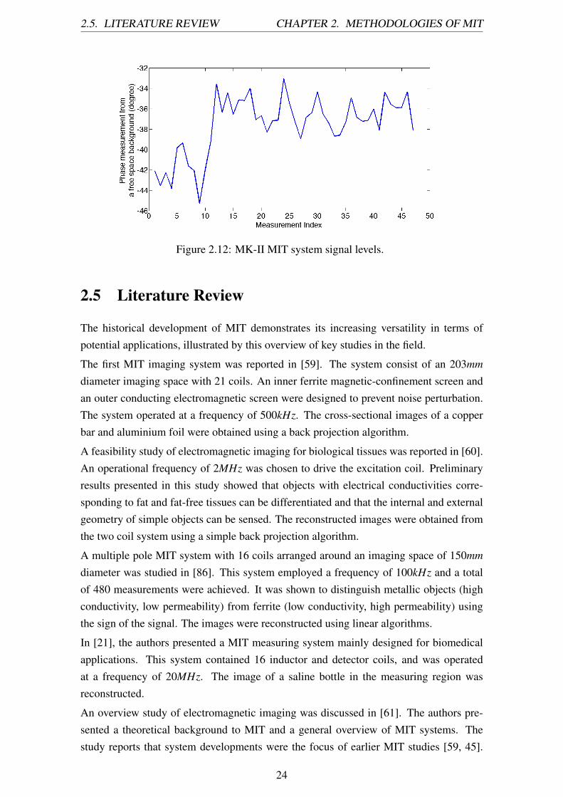
The MK-II system consists of (i) a coil array of equally spaced 16 air-core sensors, (ii) aNational Instrument (NI) based data acquisition system and (iii) a host computer (Figure2.11). The sensing zone has a diameter of 25cm. Each coil has 6 turns, a side length of1cm, and a radius of 2cm. The coil resonance frequency is 45MHz. Among 16 coils,8 coils are dedicated for transmitting signals, and the remaining 8 coils are used for re-ceiving signals. The total number of independent measurements is therefore 64. Notingthat the neighbouring measurements are eliminated to reduce the capacitive coupling ef-fect between the excitation and receiving coils,therefore 48 measurements are used in theinverse model to passively map the distributions of the imaging subject.
Unlike the MK-I MIT system, this system measures the phase change caused by imagingsubstances and uses that change for image reconstruction. Figure 2.12 shows the phasemeasurements collected from a free space background using this system. As the phaseperturbation resulting from a conductive imaging subject is usually very low, it is essentialto ensure low noise performance. A grounded aluminium shield is designed to ensure lownoise perturbation by reducing the susceptibility to external magnetic field interference,undesired electric fields and the coupling between the coils.
Buffering electronics are also required between the sensors and the NI instrumentationdevices for amplifying the signals. A fully differential amplifier T HS4500 is selected toamplify the transmitting output amplitude from 0.5V p–p single-ended to 8V p–p differen-tial signal in order to improve the field strength and phase stability. For the receivers, alow-noise, high-speed amplifier T HS4275 is chosen to buffer the receiving signals dueto its wide bandwidth, low voltage noise and high slew rate. It is worth noting that thisbuffer has a weak temperature coefficient, although this can be addressed for further sys-tem improvement.
As the signal perturbation caused by the secondary magnetic field is usually low, the mea-
22

2.4. MIT SYSTEMS CHAPTER 2. METHODOLOGIES OF MIT
surement system requires accurate measurement devices to improve the sensitivity. Inaddition to this, three additional criteria are considered to choose the appropriate devices.Firstly, the device is required to have the capability to generate a range of frequencies foroperational purposes. Secondly, a high-speed direct digitization device is desirable fortaking measurements from receiving coils without the need to down-convert the signalinto a lower frequency range in order to reduce the system complexity. Thirdly, the de-vices need to be capable of expanding the system beyond 16 channels. Based on these, aNI5781 is chosen for signal generation. It has the ability to generate frequencies rangingfrom a few kHz to up to 20MHz. The sampling rate is 100MS/s. A NI2953 is employedto realise the multi-channel switching process. The NI2953 is a 500MHz 16 : 1 multi-plexer that controls all the channel switching tasks for the system. In order to improve thesystem efficiency, a NI7951 FlexRIO board is utilised to accelerate the data acquisitionprocess. The driving frequency is 13MHz, with a 15V peak driving voltage and a drivingcurrent of 0.39A, the coil resonance frequency is 45MHz. The maximum thermal driftobserved is 85 millidegrees over a period of 5 hours. The application proposed in chapter7 is based on this system.
Figure 2.11: MK-II MIT system with 16 channel coil array.
23
2.5. LITERATURE REVIEW CHAPTER 2. METHODOLOGIES OF MIT
Figure 2.12: MK-II MIT system signal levels.
2.5 Literature Review
The historical development of MIT demonstrates its increasing versatility in terms ofpotential applications, illustrated by this overview of key studies in the field.
The first MIT imaging system was reported in [59]. The system consist of an 203mmdiameter imaging space with 21 coils. An inner ferrite magnetic-confinement screen andan outer conducting electromagnetic screen were designed to prevent noise perturbation.The system operated at a frequency of 500kHz. The cross-sectional images of a copperbar and aluminium foil were obtained using a back projection algorithm.
A feasibility study of electromagnetic imaging for biological tissues was reported in [60].An operational frequency of 2MHz was chosen to drive the excitation coil. Preliminaryresults presented in this study showed that objects with electrical conductivities corre-sponding to fat and fat-free tissues can be differentiated and that the internal and externalgeometry of simple objects can be sensed. The reconstructed images were obtained fromthe two coil system using a simple back projection algorithm.
A multiple pole MIT system with 16 coils arranged around an imaging space of 150mmdiameter was studied in [86]. This system employed a frequency of 100kHz and a totalof 480 measurements were achieved. It was shown to distinguish metallic objects (highconductivity, low permeability) from ferrite (low conductivity, high permeability) usingthe sign of the signal. The images were reconstructed using linear algorithms.
In [21], the authors presented a MIT measuring system mainly designed for biomedicalapplications. This system contained 16 inductor and detector coils, and was operatedat a frequency of 20MHz. The image of a saline bottle in the measuring region wasreconstructed.
An overview study of electromagnetic imaging was discussed in [61]. The authors pre-sented a theoretical background to MIT and a general overview of MIT systems. Thestudy reports that system developments were the focus of earlier MIT studies [59, 45].
24

2.5. LITERATURE REVIEW CHAPTER 2. METHODOLOGIES OF MIT
Back projection algorithms were used for image reconstructions as they can be run almostin real time, although the quality of reconstructed images was modest. Later MIT studiesstarted to address more specific issues, including sensor design [46, 47, 87], developmentof conditioning electronics [18], methods [88, 89], algorithms [57] and applications [90].
A number of coil designs were investigated in [46], including parallel, planar and ferritecore coils. The design of each type, and its advantages and limitations, were discussed.In the parallel coil design, the excitation coils surround the object space, which providesequally distributed excitation density. However, the independent measurements are lim-ited. A planar coil design can avoid the background coupling between adjacent coilsby overlapping the excitation and detection coils. Ferrite core coils have relatively highsensitivity compared to air core coils, but they experience flux loss due to ferromagneticmaterials and eddy currents induced in conductive materials.
In [18], a MIT system with 8 coils for a high contrast metal process application wasintroduced. Eight coils were evenly spaced along the circumference of a 160mm diameterimaging space. This system operated at a frequency of 5kHz. Images of copper andaluminium rods located in various places of the imaging space were reconstructed usingthe Tikhonov regularisation method.
A 16 channel MIT system was presented in [91], where a low conductive object wasimaged under an excitation frequency of 1MHz. This system researched the sensitivityand stability of a single sensor unit and the phase sensitivity of the system by simulatinga human brain with oedema and haematoma.
A National Instrument-based MIT system with an excitation frequency of 13MHz was de-veloped and proposed for biomedical applications [83], where 8 coils were used as trans-mitters and the remaining 8 coils were used as receivers. This system was later adaptedfor a feasibility study of cryosurgical monitoring using electromagnetic measurements[92].
A study of a digital MIT system based on half cycle demodulation was examined in [93].This system employed 8 sensors to form an imaging region of 150mm diameter. Thesystem performance was verified through experimental results. Images of various shapedmetal objects were reconstructed.
A fast deterministic algorithm was applied to obtain optimum receiver array designs fora given specific excitation [94]. This design strategy was based on the iterative exclu-sion of receiver locations, which realises a regionally focused MIT to increase the imageresolution in a particular region.
A rotational scheme based MIT (RMIT), where a 8 sensor coil array can be rotated withrespect to a central axis perpendicular to the plane of the coil array was implemented in[95]. It was shown that the rotational scheme can increase the image quality through bothsimulation and experimental data. This paper presented a comparison of reconstructedimages for two closely located screws under different rotation schemes. The images werereconstructed using Tikhonov regularisation through experimental data. The main contri-
25

2.5. LITERATURE REVIEW CHAPTER 2. METHODOLOGIES OF MIT
bution of this paper is the adaptation of several image quality measures for MIT imagequality evaluation.
A volumetric MIT (VMIT) system was developed to realise 3D imaging in [96]. In thispaper, both the system architecture and the forward 3D sensitivity modeling were pre-sented. Figure 2.13 gives an indication of the 3D visualisation of MIT using experimentaldata. This VMIT study was the first experimental volumetric study in the field and pro-vided the fundamental background for a four dimensional MIT reconstruction study[97].
(a) (b)
Figure 2.13: Reconstructed images for (a) an aluminium rod lying diagonally across themeasuring space, and (b) an aluminium cone-shaped object in the centre of the measuringspace.
26

Chapter 3
Structural Inspection of Pipelines
3.1 Introduction
Pipelines are one of the most widely used and important apparatus in industry. They canbe used to transport water, chemicals, petroleum oil, gas and so on. Pipelines are suscep-tible to internal and external corrosion, cracking, third party damage and manufacturingflaws. Damaged crude oil or chemical pipelines can have a catastrophic impact upon theenvironment and on public safety, alongside resulting in financial loss. As such, inspec-tion during both the initial manufacturing stage and in subsequent operation is invaluable.
The structural health monitoring of pipelines has become a great engineering challengesince the 1950s [98]. The majority of pipeline inspection techniques require direct contactor pre-installed devices inside the pipes to carry out the investigation, especially when thepipelines are covered by cladding. Consequently, the inspection can be costly, necessi-tating highly skilled technicians. Developing a rapid, efficient and low cost technique forthis application therefore has significant engineering importance.
In this chapter, MIT is proposed for pipeline inspection as a NDE technique. This chap-ter also reviews some of the most commonly used NDE techniques, summarising theirrespective strengths and weaknesses. It is argued that because of the low cost, contact-less and non-invasive nature of MIT, MIT could provide a great advantage over existingtechniques. The feasibility of MIT in this respect is demonstrated by the Bath MK-I MITsystem using metallic pipe samples.
3.2 Overview of Existing NDE Techniques
Traditionally, pipeline inspections were carried out visually, although there has been anincreasing reliance upon automated techniques. Visual inspection is the simplest and mostcost-effective approach, however it is obvious that it has limited practicality. During theinitial pipeline manufacturing stage, many pipelines are covered by layers of coating forprotective purposes, along with a final layer of insulation. These usually amount to up to
27

3.2. OVERVIEW CHAPTER 3. PIPELINE INSPECTION
10� 16mm of thickness outside the pipes (Figure 3.1). In these cases, inspecting pipesusing direct visual inspection becomes impossible. Pipeline inspection engineers laterdeveloped a way of dealing with this problem by sending a device inside the pipe to carryout the inspection. This device is called a pipeline inspection gauge, often called pigs ora pigging device in the field. Pigs travel inside the pipe to inspect, maintain and cleanthe pipeline, and have been widely applied using various NDE techniques including eddycurrent (EC) testing, magnetic flux leakage (MFL), remote field testing (RFT), ultrasonicinspection (UI), radiograph (X-ray), and electromagnetic acoustic emission transducer(EAMT) techniques.
Figure 3.1: Structure of a pipeline.
The eddy current (EC) testing technique uses the interaction between the electromagneticfield and the electrical properties of the testing sample for inspection [99]. Eddy currentsarise when applying alternating electromagnetic fields to a conductor through the useof probes or coils. The eddy currents thread around the conductor and in turn produce asecondary electromagnetic field. The conductor can be inspected by analysing the voltagemeasurements collected from the EC coils. This type of EC testing is also known as theconventional EC testing and is frequently recommended for crack detection on metallicstructures [100, 101, 102, 103]. The applicability of this technique has also been furtherexpanded to pipelines [104, 105, 106]. The advantages of this technique are that it isversatile and cost effective; however, it is not commonly used as an in-line inspection(ILI) tool for pipeline inspection due to speed limitations. Pulsed eddy current testingis a specialised eddy current method which overcomes the difficulties associated withthe conventional eddy EC testing method, which is that the EC probes require intimatecontact with the pipelines [107, 108, 109]. As such, pulsed eddy current testing hasbecome a popular method for detecting corrosion under insulation. However, it has thedrawback of not being as reliable for detecting ultra-localised corrosion, such as pitting[110].
Pigging devices based on the magnetic flux leakage (MFL) technique are the most widelyused in-line inspection tools and have been used for oil and gas pipes since the 1960s
28

3.2. OVERVIEW CHAPTER 3. PIPELINE INSPECTION
[111, 112, 113, 114, 115, 116, 117]. The operating principle of MFL is simple andstraightforward. A strong magnetic field is established in the pipe wall using either per-manent magnets or by supplying an electrical current into the steel. Damaged areas ofthe pipe cannot support as much magnetic flux as undamaged areas, and as such magneticflux leaks out of the pipe wall at the damaged sites. This means that the MFL techniquealso replies upon electromagnetic induction, and as a consequence this technique wouldnot work on non-ferromagnetic materials [118]. A typical MFL pig consists of a mag-net, hall sensors and a data acquisition component. There are some external parts thatare designed to hold the hall sensors against the inside of the pipe (fingers), which areessential as MFL requires intimate contact between the sensors and the pipe wall in orderto achieve adequate sensitivity to defects. Therefore it is understandable that the fingersmay get damaged when the pig passes through branches, valves and tees [98].
The technique of remote field testing (RFT) is relatively new, only having been commer-cialised since the late 1980s [98]. The basic principle of operation of a RFT tool is byenergising the pipe with an AC sine wave at frequencies between 1Hz and 1kHz. Theelectromagnetic wave passes through the pipe wall near an exciter and re-enters the tubeat various distances from the exciter. At approximately 3 tube diameters, the field insidethe tube is reduced to near zero, while the external field remains fairly strong. In areasof metal loss, the field arrives at the detector with a faster travel time (greater phase) andgreater signal strength (amplitude) due to the reduced path through the pipe wall. Hencethe dominant mechanism of RFT is through-transmission. It is because of this two-walltransmission path that RFT has gained its reputation of equal sensitivity to outside defect(O.D.) and inside defect (I.D.) wall loss [119, 120, 121]. One distinct disadvantage ofRFT is its inability to measure wall thickness through scale, coatings and liners, with ap-proximately equal sensitivity to O.D. and I.D. wall loss. The most common applicationsinclude the inspection of heat exchangers and boiler tubes using internal probes connectedto an external instrument. In more recent years, larger tools have been developed for ap-plications such as pipelines and water well casting [121].
Ultrasonic inspection (UI) is a useful and versatile NDE technique for pipeline inspec-tion, which also became available in 1980s [122]. Ultrasonic inspection uses an array oftransducers that emits a high frequency sound pulse perpendicular to the pipe wall andreceives echo signals from the inner surface and the outer surface of the pipe. This tech-nique measures the total time travelled between the arrival of the reflected echoes fromthe inner and outer surfaces in order to calculate the wall thickness. It can be used forflaw detection, flaw evaluation, dimensional measurements and material characterisation[123, 124, 125, 126].
X-ray inspection uses a source of radiation for material inspection. As the radiation canproduce good penetration, it can be used to detect pipeline corrosion without requiringinsulation removal; this is arguably the biggest advantage of this technique [127, 128,129, 130, 131]. One distinct disadvantage is that X-rays, by definition, are radioactive,
29

3.2. OVERVIEW CHAPTER 3. PIPELINE INSPECTION
and the precautions that need to be implemented during an inspection may be impracticalin many environments. In addition, X-ray inspection does not detect cracking and pitting;however, it can be very useful for inspecting other kinds of defects.
Electromagnetic acoustic transducer (EMAT) inspection is a relatively new technique forpipeline inspection. It uses a magnet and an electric coil. The magnet can be a permanentmagnet or an electromagnet, which produces a static or a quasi-static magnetic field. Theelectric coil is driven with an alternating current at ultrasonic frequency, typically in therange of 20kHz to 10MHz. Based on the application requirements, the signal can be acontinuous wave, a spike pulse, or a tone-burst signal. The electric coil, if supplied withAC current, also generates an AC magnetic field. Ultrasonic waves are generated close tothe test material by the interaction of the two magnetic fields.
Each technique has its advantages and disadvantages, and as such there is no universallyagreed approach in the field of pipeline inspection. Many factors need to be taken intoconsideration when choosing an appropriate technique, such as the material, dimensionsand locations of the pipes under inspection, as well as the expected outcomes. Somecombined methods have also been proposed in this area in an attempt to mitigate thedisadvantages of one individual technique [132, 133]. So far, the techniques of MFL andX-ray have reached commercial standards in terms of their accuracy, resolution and wideapplicability. As such, other NDE techniques also used in industrial environments areoften evaluated by comparison to MFL or X-ray techniques. Table 3.1 lists the widelyused NDE techniques for pipeline inspection.
30

3.2. OVERVIEW CHAPTER 3. PIPELINE INSPECTION
Technique EC testing MFL RFTILI No Yes Yes
Material
ConductiveFerromagneticFerritic steel
Austenitic steelAdmiralty brass
FerromagneticCarbon steel
FerromagneticNon-
ferromagneticCast/ductile steel
Drill steelCarbon steel
Application
External inspectionNear surface
Sub-surface crackFlaw detection
Internal scaleCorrosionPits sizing
Heat exchangerPressure tubes
Stress corrosionCasting wells
StrengthReliable for
discontinuous detectionPortable
High resolutionVarying levels ofsensitivity basedon testing needs
No need for closecontact/coating/
insulation removalEqual sensitivityto internal and
external defects
Limitation
Slow responseLimited depth
Need for insulation/coating removal
Generating verylarge data sets
Intimate contactProne to be damaged
Slow speedUnable todistinguishinternal and
external defectsTechnique UT X-ray EMAT
ILI Yes Yes Yes/NoMaterial All materials All materials Metallic and magnetic
Application Well detectionCrack detection
Corrosion anderosion detection
Measure thicknessQuality measure
Leak/flaw detectionOn-shore water/metallic pipes
Strengths
High sensitivityNo pipe wall
thickness constrainsDefect detection
insulation/coating
High resolutionFast speed
No requirementfor close contact/coating removal
No requirementfor close contact/
insulation removalMeasure metal loss
Measure wall thickness
LimitationsHard to pig
Produceflow restriction
RadiationHigh cost
Inability to detectcracking/pitting
Need for close contactRestrictions onhigh frequency
Table 3.1: Comparison of the existing NDE techniques for pipeline inspection.
In this chapter, pipeline inspection using MIT is proposed. From the above, it can beseen that MIT, EC testing, MFL and RFT have the same origins. Their fundamentalprinciples are all based on the Michael Faraday’s discovery of electromagnetic induction.All these techniques rely on voltages being generated and measured by sensors. Thereare several influencing factors on the induced voltages: the change in strength of themagnetic fields, the speed of the coil or device passing through a static magnetic field, thedriving frequency, the volume of the metal loss and the proximity of the sensing device
31

3.3. EIGHT-CHANNEL COIL ARRAY CHAPTER 3. PIPELINE INSPECTION
to the source of the change in the magnetic field. These factors manifest in different waysfor each technique. In this chapter, the author will investigate the feasibility of MIT forpipeline inspection through these factors and evaluate how MIT can be beneficial in thisarea.
3.3 Eight-channel Coil Array
Figure 3.2: MK-I MIT system with an eight-channel coil array.
The MK-I system is used for pipeline inspection. It consists of (i) an array of eight equallyspaced inductive coils arranged around the object periphery, (ii) a National Instrument(NI) based data acquisition system and (iii) a host computer, as shown in Figure 3.2.Each coil has a diameter of 42mm, a side length of 14mm and 50 turns. Eight air corecoils were constructed manually to form a 100mm diameter imaging region. Figure 3.3shows a top view of the eight-sensor coil array. Each one of the eight inductive coils inturns is supplied with an excitation signal, while the remaining coils are used as receivers.A list of specifications of this system is shown in Table 3.2. The signal to noise ratioin this MIT system is between 34dB (for measurement between two opposite coils) and56dB (for measurement between two neighboring coils) at a frequency of 20kHz. Figure3.4 shows the signal to noise ratio of first cycle measurements when the first coil used asexcitation.
32

3.4. FORWARD MODEL VALIDATION CHAPTER 3. PIPELINE INSPECTION
Figure 3.3: Top view of an eight-sensor coil array.
Number of sensors 8Number of measurements 28
Inner diameter of coil array (mm) 100Coil side length (mm) 14Coil diameter (mm) 42
Number of turns for each coil 50Operational frequency (kHz) 20
Coil type Air-core coil
Table 3.2: Specifications of eight-channel MIT system.
Figure 3.4: Signal to noise ratio of first cycle measurements when first coil used as exci-tation.
3.4 Forward Model Validation
In the simulated MIT system, eight coils are uniformly distributed around the imagingregion. In order to enhance the mesh density, three solid cylinders are simulated insidethe imaging region. The radius of the cylinders are 50mm, 30mm, 10mm respectively. The
33

3.4. FORWARD MODEL VALIDATION CHAPTER 3. PIPELINE INSPECTION
length of the cylinders are 40mm. The centre of the cylinders locate in (0,0,0) to matchthe centre of the coil array. The system is simulated in free space, which has 317768tetrahedral elements. In the actual imaging region, the number of tetrahedral elements is168072. Each one of the eight coils in turn is supplied with an sinusoidal current under20kHz, while the induced voltages are measured in the remaining coils. The total numberof independent measurements is therefore 28. The mesh model is shown in Figure 3.5.
Figure 3.5: Mesh model of an eight-channel MIT system.
In order to validate the forward model, a test scenario is generated by simulating a fullpipe in the centre of the region of interest (ROI). The induced voltage is compared withexperimental data. In this forward model, the pipe sample with inner radius of 25.40mmand outer radius of 31.60mm is simulated in the mesh geometry, which consists of 3814tetrahedral elements. The centre of the simulated pipe is located in the centre of the ROI.The induced voltages in the measuring coils due to this full pipe sample can be calculatedfrom equation 2.37. Figure 3.6 shows the comparison of the induced voltage betweenexperimental and simulation data.
Figure 3.6: Comparison of induced voltages due to full pipe sample using simulation andexperimental data.
34

3.5. NBPF METHOD CHAPTER 3. PIPELINE INSPECTION
3.5 Narrowband Pass Filtering Method
Research show that MIT is capable of imaging conductive materials. However, it is chal-lenging to use the traditional MIT pixel based reconstruction method (PBRM) for pipelineinspection because of the limited resolution. In order to improve the MIT resolution, anovel narrowband pass filtering method (NPFM) is developed as a more suitable image re-construction method. This proposed method can overcome the resolution limitations andproduce useful information of the pipe structures. This chapter presents the comparativeresults of pipeline inspection using both novel NPFM and traditional PBRM. The MITimage reconstruction problem is a challenging ill-posed inverse problem. A priori infor-mation is key to successful reconstruction process. In pipe imaging, a priori knowledgeof geometry will be fully explored in our NPFM.
The traditional PBRM is a searching algorithm looking for the best fit of imaging valuesto create an estimated measured data that matches the real measurements. In PBRM, theimaging domain is divided into small elements by uniform pixels in Cartesian coordinatesystem. The concept of applying NPFM can be implemented by transferring pixels fromthe Cartesian coordinate system (x,y) to the polar coordinate system (r,q). As we arespecifically looking at a pipe geometry using NPFM, it is important to notice that only thepixels in the ROI contribute to the final image. In this case, the ROI is limited to a narrowband region only; as shown in Figure 3.7 (a). We then filter the r component pixels thatare excluded in the ROI by defining the estimated size of pipe sample in terms of innerradius ri and outer radius ro as shown in 3.7 (b). The filtering process takes place beforethe image reconstruction stage. The filtering process will improve the image quality inthe pipe region by allowing the information to be extracted from a limited region.
(a) (b)
Figure 3.7: (a) Narrowband region, (b) Narrowband pass filter applied to the radius.
Figure 3.8 shows the comparative results of pipe inspection using both PBRM and NPFM.It can be seen that the NPFM can produce an image reflecting the shape of the pipe takingadvantage of targeted ROI for the imaging reconstruction. Note that the location of thepipe sample is crucial to the imaging process, the sample is placed in the centre of theimaging region in order to obtain equal sensitivity from all coils. The narrowband regionis selected to be exactly the same size as the pipe. This choice is suitable if we know thatthe centre of pipe matches that of the exact centre of the coil array. In practical terms,
35
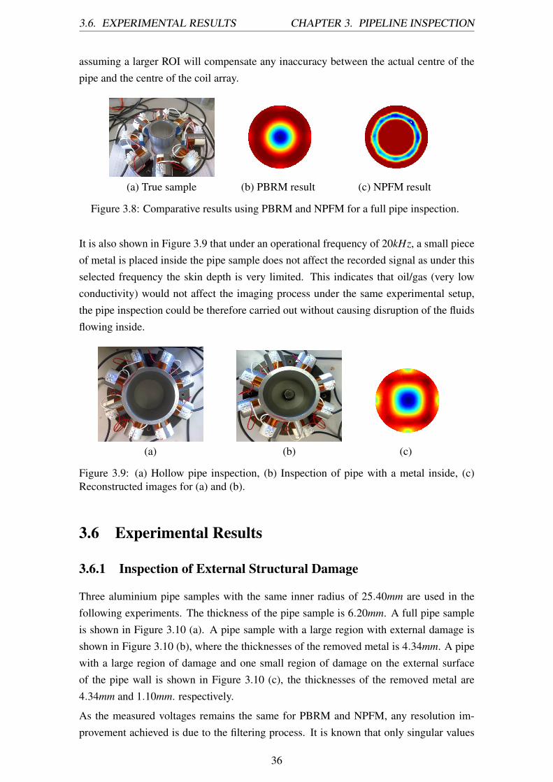
3.6. EXPERIMENTAL RESULTS CHAPTER 3. PIPELINE INSPECTION
assuming a larger ROI will compensate any inaccuracy between the actual centre of thepipe and the centre of the coil array.
(a) True sample (b) PBRM result (c) NPFM result
Figure 3.8: Comparative results using PBRM and NPFM for a full pipe inspection.
It is also shown in Figure 3.9 that under an operational frequency of 20kHz, a small pieceof metal is placed inside the pipe sample does not affect the recorded signal as under thisselected frequency the skin depth is very limited. This indicates that oil/gas (very lowconductivity) would not affect the imaging process under the same experimental setup,the pipe inspection could be therefore carried out without causing disruption of the fluidsflowing inside.
(a) (b) (c)
Figure 3.9: (a) Hollow pipe inspection, (b) Inspection of pipe with a metal inside, (c)Reconstructed images for (a) and (b).
3.6 Experimental Results
3.6.1 Inspection of External Structural Damage
Three aluminium pipe samples with the same inner radius of 25.40mm are used in thefollowing experiments. The thickness of the pipe sample is 6.20mm. A full pipe sampleis shown in Figure 3.10 (a). A pipe sample with a large region with external damage isshown in Figure 3.10 (b), where the thicknesses of the removed metal is 4.34mm. A pipewith a large region of damage and one small region of damage on the external surfaceof the pipe wall is shown in Figure 3.10 (c), the thicknesses of the removed metal are4.34mm and 1.10mm. respectively.
As the measured voltages remains the same for PBRM and NPFM, any resolution im-provement achieved is due to the filtering process. It is known that only singular values
36

3.6. EXPERIMENTAL RESULTS CHAPTER 3. PIPELINE INSPECTION
that are above the noise level contribute to the final images [81]. Figure 3.11 shows thesingular value decomposition for both NPFM and PBRM. This provides an useful tool interms of information content. In the 100mm imaging region, PBRM employs 41 by 41uniform pixels located in the Cartesian coordinate system, each pixel represents a con-ductivity value. It is demonstrated in Figure 3.11 that there are 26 singular values abovean assumed 1% noise level using PBRM, where the number of singular values above anassumed 1% noise level is 25 using NPFM. However, as the pipe sample does not occupythe entire imaging region, which means the number of singular values that contributesto the pipe region is less than 26. The NPFM accomplished a tradeoff between singularvalues and pixels. The pixels that are not in the ROI are excluded by the filtering pro-cess. The result of implementing the NPFM is that 1125 pixels are excluded from theimaging domain, leaving 556 useful pixels to reconstruct the final image, which indicatesthat a total of 25 singular values above the noise level are fully employed in the imagereconstruction.
Full pipe sample One damaged region Two damaged regions
PBRM result PBRM result PBRM result
NPFM result NPFM result NPFM result
(a) (b) (c)
Figure 3.10: Aluminium pipe inspection results showing true samples and reconstructionof external metal losses: (a) a full pipe sample, (b) 4.34mm thickness of wall loss, (c) a4.34mm thickness of wall loss on one side and a 1.10mm thickness of wall loss on theother side.
37

3.6. EXPERIMENTAL RESULTS CHAPTER 3. PIPELINE INSPECTION
Figure 3.11: Singular value decompositions for PBRM and NPFM.
Figure 3.10 presents comparative results of pipe inspection using both PBRM and NPFM.While the PBRM fails to detect damages in outer structure of the pipe, the NPFM cansuccessfully identify these damages. The advantage of this novel method is verified usingexperimental data from challenging test samples. It is well known that using a coil arraywith an imaging region of 100mm, the PBRM based MIT can retrieve information withaccuracy of 10mm (about 10%). With the proposed NPFM, a resolution of 2mm (whichis about 2%) is achieved using the same measured data.
3.6.2 Further Enhancement of Structural Inspection
In this section, more challenging pipe inspection results will be presented, including in-spection of both pipe external and internal wall losses. The NPFM takes advantage of apriori knowledge of the original pipe dimensions as reference information for one stepcalibration. The pipe must be central to the sensors in order to acquire equal sensitivityfrom the coils; the position of the pipe sample is crucial to the inspection. We suggestthat this inflexibility caused by the location of the pipe samples can be partly avoided bychoosing a slightly larger narrowband, which can tolerant the inaccuracy of the centralposition of the pipe sample.
Experimental results based on internal and external structure of aluminium pipes are pre-sented in Figure 3.12. The inner radius of the aluminium pipe is 25.40mm; the wall thick-ness is 6.20mm. The thicknesses of the removed metal are 4.34mm, 1.10mm, 4.30mm and1.90mm for pipes in Figure 3.12 (a), (b), (c), and (d) respectively. The imaging resultsare post-processed within a confident threshold range. Of particular interest is the recon-struction of the internal losses, which are successfully detected using the proposed NPFMbased MIT system.
38

3.6. EXPERIMENTAL RESULTS CHAPTER 3. PIPELINE INSPECTION
(a) (b) (c) (d)
Figure 3.12: Aluminium pipe inspection results showing true samples and reconstructionof metal losses for internal and external parts: (a) 4.34mm thickness of external wall loss,(b) 1.10mm thickness of external wall loss, (c) 4.30mm thickness of internal wall loss,and (d) 1.90mm thickness of internal wall loss.
There is strong industrial interest in steel pipe inspection. It is considered that inspectionof steel pipes would be more difficult than aluminium or stainless steel pipes, but theoret-ically possible. In this section, a steel pipe inspection is carried out. The steel pipes aresmaller and thinner compared to the aluminium pipes presented in Figure 3.12, each withan inner radius of 20.38mm and a thickness of 5mm.
Figure 3.13 shows the reconstruction of external damages from a cold steel pipe usingthe NPFM. As the permeability affects the skin depth, and the skin depth affects thepenetration, the internal structure of the same steel pipe can not be detected reliably underthe same operational frequency of 20kHz. The thickness of the external wall losses are3.44mm shown in Figure 3.13 (a) and 2.13mm shown in Figure 3.13 (b).
39

3.6. EXPERIMENTAL RESULTS CHAPTER 3. PIPELINE INSPECTION
(e) (f)
Figure 3.13: Steel pipe inspection results showing true samples and reconstruction ofmetal losses for external parts: (e) 3.44mm thickness of external wall loss, and (f) 2.13mmthickness of external wall loss.
The induced voltages can provide indication in terms of information content. Figure3.14 demonstrates the induced voltage for cases a to f (listed in Figure 3.12 and 3.13).It is shown that the amplitude of the induced voltage decreases as the dimension of thedefect becomes smaller. It is also clear that the induced voltages from internal defects aregenerally lower compared to the induced voltages from external defects. This is broadlydue to the skin depth effect. This issue could be addressed by implementing a multi-frequency MIT system, which will be discussed in chapter 8.
Figure 3.14: Comparison of induced voltages due to different testing profiles.
40

3.7. DISCUSSION CHAPTER 3. PIPELINE INSPECTION
3.7 Discussion
This chapter investigates pipeline inspection using NPFM based MIT system as a casestudy of limited region tomography. The imaging region is limited to a pipe geometry anda novel localised algorithm NPFM is specifically developed for this geometry to improveMIT resolution. The experimental results demonstrate the capability of the proposedNPFM as a more suitable image reconstruction method compared to traditional PBRM.Experimental results demonstrate that external and internal wall losses of aluminium pipesas well as external wall losses of steel pipes can be successfully inspected. It is shown thata resolution of 10�15% of the thickness of the pipes can be achieved using this proposedMIT methodology. More work is needed to remove the need for calibration against a fullpipe dimensions, sensitivity to the locations of pipes and to further enhance the internalstructure inspection of metallic pipelines.
The proposed NPFM can also be used to enhance the resolution of electrical capacitancetomography (ECT) for plastic pipelines. Due to the choice of the frequency and the skindepth effect, a resolution of 2% of the imaging region is the highest that can be achievedusing a MIT system. However, as there is no eddy current effect in ECT, using this methodcould significantly improve the ECT image resolution.
There are two plastic pipe samples used in the following experiments; a small pipe samplewith an external diameter of 88mm and an internal diameter of 76mm, and a larger pipewith an external diameter of 110mm and an internal diameter 90mm. The larger pipe ismade from polybutylene, a thermoplastic with good mechanical properties and chemicalresistance, and it is widely used for heating and plumbing applications in many properties.The smaller pipe is manufactured from polyethylene, commonly used in the corrosion-resistant piping and natural gas pipe system. The length of the small pipe and large pipeare 300mm and 113mm respectively. The schematic representations of the pipe samplescan be seen in the first row in Figure 3.15. The schematic on the left contains defect of25mm in length along the interior circumference and 2.5mm in depth, the 110mm diameterpipe in the middle has 2 defects, one defect spans 50mm on the interior circumference andthe other 20mm, located opposite one another both with a 3mm depth. The 88mm diameterpipe on the right hand side has a defect of 1.5mm depth. The pictures of the samples areshown in the second row in Figure 3.15, the sensor array has a diameter of 150mm. Thereconstructed images using both PBRM and NPFM for each case are shown in the thirdand fourth rows in Figure 3.15 respectively.
41
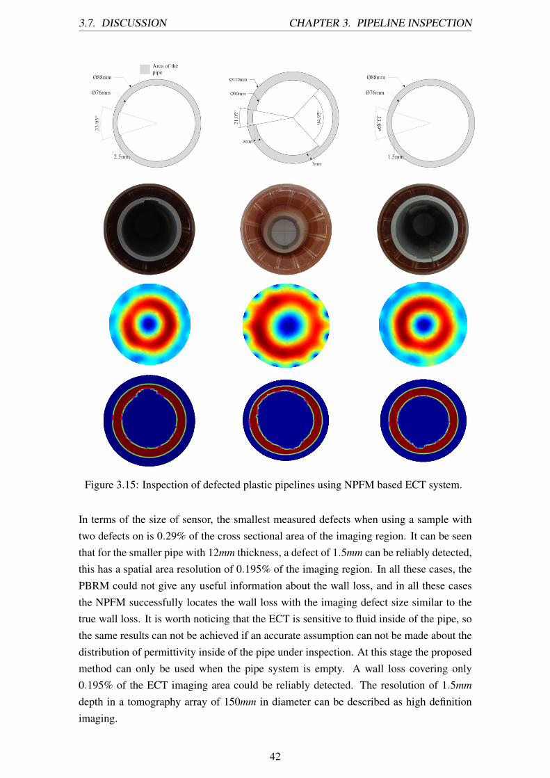
3.7. DISCUSSION CHAPTER 3. PIPELINE INSPECTION
Figure 3.15: Inspection of defected plastic pipelines using NPFM based ECT system.
In terms of the size of sensor, the smallest measured defects when using a sample withtwo defects on is 0.29% of the cross sectional area of the imaging region. It can be seenthat for the smaller pipe with 12mm thickness, a defect of 1.5mm can be reliably detected,this has a spatial area resolution of 0.195% of the imaging region. In all these cases, thePBRM could not give any useful information about the wall loss, and in all these casesthe NPFM successfully locates the wall loss with the imaging defect size similar to thetrue wall loss. It is worth noticing that the ECT is sensitive to fluid inside of the pipe, sothe same results can not be achieved if an accurate assumption can not be made about thedistribution of permittivity inside of the pipe under inspection. At this stage the proposedmethod can only be used when the pipe system is empty. A wall loss covering only0.195% of the ECT imaging area could be reliably detected. The resolution of 1.5mmdepth in a tomography array of 150mm in diameter can be described as high definitionimaging.
42

3.7. DISCUSSION CHAPTER 3. PIPELINE INSPECTION
For the same NPFM method, the resolution achieved using ECT is approximately 10 timeshigher compared to the resolution achieved using MIT. This further validates the pointmade earlier that the proposed NPFM is an effective way of enhancing the resolution. Thelimitation associated with it when implementing pipeline inspection using MIT lies withthe fundamental physics rather than the capability of this algorithm. However, there areseveral remaining issues need to be studied in this particular topic. How to obtain a prioriinformation of the pipe in order to predefine the parameter in the NPFM algorithm remainsa challenge. In oder to implement this pipeline inspection process, the sensitivity of thealgorithm to the location of the pipe needs to be addressed. Moreover, the correct designand careful production of MIT sensors is the key in obtaining valuable measurement.Many parameters like coil size, wire gauge, number of turns, measurements frequencyand source gain are important parameters to be determined. In particular there are manyeddy current coil types each suited for a specific inspection task. It requires a certain levelof experience to determine the right configuration.
In order to overcome the difficulties associated with the eddy current, the author proposethe magneto-static permeability tomography (MPT) approach [44, 134]. MPT can recon-struct the permeability distribution of an object using magneto-static measurements. Thedata for image reconstruction are external magnetic field measurements on the surface ofthe object due to an applied magneto-static field. As there is no alternating current, thereis no eddy current generated in the imaging object, the skin depth effect would not existin this case. The permeability can be therefore reconstructed. The internal defect andcorrosion in pipe with ferromagnetic materials could be potentially inspected.
In addition to our existing MK-I MIT system, we will aim to develop a 16 and a 32sensor coil array, which can be used for inspection of large scale pipelines. Furthermore,a planar geometry based MIT study will be carried out as a limited access tomography forpipeline inspection. Both computational and experimental evaluations will be conductedfor proposed sensor modalities to investigate the capability and limitation of MIT as apipeline imaging technique.
43

Chapter 4
Hidden Defect Identification in CarbonFibre Reinforced Polymer
Carbon fibre reinforced polymer (CFRP) materials pose new challenges to the non-destructiveevaluation (NDE) techniques. This study addresses the issue of large defect identificationin CFRP plates using electromagnetic measurements. A dual plane magnetic induction to-mography (MIT) technique is proposed as a method for damage localisation in compositeparts, where two arrays of planar sensors are utilised to measure the changes in inducedvoltages due to the changes in electrical conductivity properties. This geometry meets therequirements of damage inspection in plate structures and thus makes the imaging pro-cess feasible. The electrical voltage measurements are used as input to inversely map thespatial resolution of the samples in the region of interest. The stability and detectabilityof the dual plane system is examined using small metallic cubes. Both individual andmultiple instances of damage embedded in CFRP samples are created as a representationof possible manufacturing defects. Experimental study shows that the presence of dam-age can be identified in both cases using dual plane MIT system. With advanced sensingdesign, rapid data collection unit and improvement in resolution, MIT could become arapid NDE technique for the integrity inspection of the composite structures.
4.1 Introduction
A new breed of high strength material, CFRP, has found widespread application in com-mercial aircraft, industrial and transportation markets, where strength, stiffness, a lowerweight, and outstanding fatigue characteristics are crucial requirements. Structural healthmonitoring of the CFRP such as missing carbon-fibre bundles, lanes, suspensions, fringes,missing sewing threads, angle errors and hidden manufacturing defects is an invaluablequality control. Many non-destructive evaluation techniques have been applied in thisarea to CFRP, including low frequency vibration [135], ultrasonic methods [136, 137,138, 139], radiography [140, 141, 142], thermography [143, 144] and eddy current test-ing [145, 146, 147, 148, 149]. More recently, soft field tomography techniques have also
44

4.1. INTRODUCTION CHAPTER 4. CFRP INSPECTION
been used for damage detection in CFRP using electrical impedance tomography (EIT)[150, 151, 152]; however, the MIT-based research in this area remains very limited [153].
Although the image resolution of MIT is relatively low due to the fact that MIT imagereconstruction is an ill-posed problem, this technique benefits from its contact-less, non-invasive nature and high temporal resolution. Firstly, there is no requirement for directcontact with the material being tested, such as with gels (various ultrasonic methods),specially designed probes (injected current thermography) or electrodes attached to thecomposite parts (EIT). Secondly, MIT, in using electromagnetic induction to map thespatial resolution, has a non-hazardous data collection process, whereas compared to X-ray computed tomography, radiation safety precautions need to be considered, which canin certain circumstances be impractical. In addition, using MIT alongside Kalman filtersand 4D temporally correlated imaging permit rapid changes in electrical conductivity tobe captured [96, 154], potentially enabling the functional analysis of CFRP structures,which is not currently feasible with any of the existing techniques.
As the carbon fibres in CFRP exhibit electrical conductivity, MIT could be a potentialNDE technique providing a tomographic approach to traditional eddy current testing.MIT uses inductive coils to measure the induced voltages, which are associated with thepassive electromagnetic properties non-linearly. The fundamental physics of MIT derivefrom the mutual inductance and eddy current theories. By passing an alternating currentinto an exciting coil, the sensing coil experiences a time-varying magnetic field. If ma-terials with electrical properties are presented between this coil pair, the eddy currentsarise in the conducting region, resulting in a perturbation in the magnetic field that canbe sensed by the receiving coil. As such, the electrical properties can be revealed and thecharacteristics of the material presented in a reconstructed image, where the quality canbe assessed visually. This technique has been applied in both biomedical and industrialprocesses [13, 19, 21, 155]. Overall, both MIT and eddy current testing techniques sharemany similarities - both arose from the same theoretical background (that of Faraday’slaw of induction, and subsequent eddy current theories) and as such have similar mea-surement principles, and both are used to image conductive or ferromagnetic materials.Nevertheless, the techniques differ in their operations and data processing. The MIT tech-nique is a tomographic approach, utilising an array of sensors to provide a unifying toolto analyse the data, which makes the operation more robust, whereas eddy current test-ing targets a localised position using a pair of coils and requires a non-destructive testingspecialist to carry out the testing.
In this study, a dual plane MIT is proposed for the identification of large area hidden dam-age in CFRP. This dual plane sensor arrays realise the imaging process in 3D, providinginformtion about the geometry of the testing samples. This geometry can be potentiallyused in the inspection of production line at the manufacturing stage. The system resolu-tion is evaluated through both simulation and experiments. Results of the inspection ofembedded defects in CFRP are presented. With advanced excitation and sensing topology
45

4.2. DUAL PLANE ARRAY CHAPTER 4. CFRP INSPECTION
[156], a fast data collection component and improved resolution, MIT could evolve to arapid NDE technique for the structural health monitoring of CFRP.
4.2 Dual Plane Array
The dual plane array has been developed using two planar sensor arrays. The separa-tion between the two arrays is 4cm. Each array consists of 9 air-core cylindrical coils,which are arranged in a 3⇥3 matrix form. A non-conductive plate with a surface area of14⇥14cm2 is used to hold the sensors in place. Each coil has 100 turns, a side length of3.4cm, and the inner and outer diameters of the coils are 3.9cm and 4.1cm respectively(Figure 4.1a). The coil sequence of the first plane is shown in Figure 4.1b, the secondplanar array follows the same numbering system. It has previously been shown that slightmisalignments between the receivers in the MIT system and the simulation model cancause up to 20% deviations in the conductivity perturbation [157]. Therefore, the dimen-sions of the coil and dual planar arrays are modeled according to the sensor design toensure accuracy. The MIT measurement system block diagram is shown in Figure 4.2.
(a) (b)
Figure 4.1: (a) Dual plane sensor array, and (b) the coil sequence of the first planar array.
46

4.3. SYSTEM ANALYSIS CHAPTER 4. CFRP INSPECTION
Figure 4.2: Block diagram of the dual plane MIT system.
4.3 System Analysis
This MIT system was initially developed for imaging materials with high electrical con-ductivity, such as metal. There are 153 unique coil pairs: 1-2, 1-3, . . . , 1-18, 2-3, 2-4, . . . ,17-18, resulting in a total of 153 independent measurements. The image reconstructionmodule extracts these measurements, performs the reconstruction algorithms, displaysand updates the images. The signal to noise ratio (SNR) is taken to indicate the signallevel of the system to the background noise level, which can be defined using an ampli-tude ratio as [158]:
SNR = 20log10US
UN(4.1)
where US is the mean signal amplitude and UN is the standard deviation of the measuredsignal amplitude. Due to the geometry of this system, the system SNR also depends on theseparation of the two planar arrays. Figure 4.3 shows the SNR measurements with the firstexcitation coil when two planar arrays are separated at 2,4,6,8 and 10cm respectively, i.e.,when coil 1 is excited with an alternating current, the voltage measurements are obtainedfrom coil pairs 1�2, 1�3, ... 1�18, and the corresponding measurements index are 1,2, 3, ... 17.
47

4.3. SYSTEM ANALYSIS CHAPTER 4. CFRP INSPECTION
Figure 4.3: Signal to noise ratio, after the excitation of coil 1, for measurements obtainedwhen the dual planes are separated by distances of 2,4,6,8 and 10cm.
Several measurements are defined to analyse the system detectability, namely the neigh-bouring, opposite and diagonal measurement. The neighbouring measurement is used todescribe the induced voltage measured from a pair of neighbouring coils that are in thesame planar array (Figure 4.1b coil pair 1� 2 and coil pair 1� 4). The induced volt-age measured from the coils directly facing each other is called the opposite measurement(coil pair 1�10). The diagonal measurement refers to the induced voltage measured fromany pair of coils that are located diagonally. This can be coil pairs either from the sameplanar array (Figure 4.1b coil pair 1�6) or different planes (coil pair 3�16). In this MITstudy, the sensitivity maps demonstrate the relationship between the change in electricalproperties and the voxel perturbation for a selected excitation/detection coil pair. It pro-vides a visual approach to evaluate the system detectability in addition to the system SNR[61, 87, 24]. From a numerical point of view, the sensitivity map can be represented in amatrix form, which is also called the Jacobian matrix (equation 2.38).
Both front and side views of the sensitivity map for selected measurement pairs are shownin Figure 4.4, where Figure 4.4a shows the sensitivity contour for a neighbouring mea-surement, Figure 4.4b shows the sensitivity contour for an opposite measurement, andFigure 4.4c and 4.4d show the sensitivity contours for two diagonal measurements. In allcases, the sensitivity maps shown below are calculated for the free space scenario, i.e.,there is no conductive materials presented in between. The mean sensitivity for each caseis used for the isosurface contour plot. The level of sensitivity varies according to theorientation and distance of the coil pair, and the mean value gives an overall indication ofthe sensitivity across the region of coil coupling. The mean sensitivity value for coil pairs1�2, 1�10, 1�9, and 1�18 are 52.76, 30.78, 8.61 and 1.38 respectively.
48

4.3. SYSTEM ANALYSIS CHAPTER 4. CFRP INSPECTION
front view (a) side view (b) front view (c) side view (d)
Figure 4.4: Sensitivity maps for (a) a neighbouring measurement from coil 1 and 2, (b)an opposite measurement from coil 1 and 10, (c) a diagonal measurement from coil 1 and9, and (d) a diagonal measurement from coil 1 and 18.
The neighbouring measurement has a higher SNR due to a closer distance between aneighbouring coil pair. The opposite measurements capture the material property changefrom a different plane. Compared to the neighbouring and opposite measurements, thediagonal measurements have relatively lower induced voltages and as such, result in lowerSNR. However, the diagonal measurements contribute to the depth detection, which is animportant parameter to characterise the properties underneath the surface. The higherSNR usually comes from the coils in the same plane (Figure 4.3), providing that thedistance between neighbouring coils is smaller than the distance between opposite coils;as is the case in this study. This can be illustrated in Figure 4.5, showing the inducedvoltages from two planes 4cm apart. Taking the first cycle as an example, the strongestsignal is due to the two neighbouring measurements � measurements 1 and 3, where theinduced voltages of both are approximately 0.5V � and the highest measured voltage isinduced between an opposite measurement � measurement 9, where the induced voltageis just over 0.1V � is almost 5 times lower than measurement 1.
Figure 4.5: Measurements obtained from a dual plane of coils when coil 1 is excited, andthe remaining coils are used as receivers.
To allow the signal to penetrate the material under testing, an appropriate operating fre-quency and separation between two planes of planar coils are required. It was pointed outin [159] that for a single planar MIT system with a similar experimental setup, one can
49

4.3. SYSTEM ANALYSIS CHAPTER 4. CFRP INSPECTION
expect a maximum of 3� 4cm of depth detection underneath the array. The driving fre-quency is an important factor in a MIT system. Lower frequency measurements penetratethe surface of the material and high frequency measurements thread around the surface ofthe material. In order to determine the suitable driving frequency, one needs to take theskin depth into consideration. In the quasi-steady electromagnetic field, the skin effectdepth of general CFRP can be approximated by equation 4.2 [160]. As CFRP compositesare nonmagnetic materials, the relative magnetic permeability of the CFRP is set to 1.
d =
s2
p f s µ0(4.2)
where f is the driving frequency, s is the electrical conductivity, and µ0 is the unitypermeability. With frequencies in the range of 104Hz , the skin depth of widely usedCFRP is between 50� 100mm [160], providing the electrical conductivity of the CFRPsample is within 103 � 104S/m. For the normal conductance of a metallic material, theelectrical conductivity is higher than that of CFRP, which suggests that for the same givenfrequency, the skin depth of CFRP is larger than the eddy current penetration for metal.For a MIT system designed for metal detection, the driving frequency is usually around5 � 100kHz [3]. This is a suitable operational range for the damage identification ofcomposite material, in fact, if the system hardware allows, the driving frequency can beincreased to the MHz range in an attempt to increase the system SNR. In the lower MHzfrequency range, laminated CFRP composites can be assumed to be a homogeneous con-ductive material [161], and as such, it is feasible to use this dual plane MIT system forthis application. In this study, the conductivity and the thickness of the CFRP samples are2.1⇥104S/m and 10mm respectively (Figure 4.7), as derived from equation 4.2. The up-per threshold of the operational frequency, necessary to allow the signal to fully penetratethe samples, is 241.24kHz. Based on the nature of our in-house low frequency MIT sys-tem, design specification of the dual planar arrays, the SNR analysis, and the propertiesof the CFRP samples used in this study, a separation of 4cm between two planes and anoperational frequency of 50kHz are determined for experimental evaluation.
Three metallic cubes are used in the following experiments to test the stability and de-tectability of the this system (Figure 4.1a). The top two rows in Figure 4.6 show thedetection of two metallic cubes in three different locations in relation to each other. Thedimensions of the cubes are 1.4⇥1.4⇥1.2cm3 and 1.2⇥1.2⇥1.4cm3 respectively. Theremaining two rows in Figure 4.6 show the experimental results of a smaller individ-ual sample under testing. The dimension of the cube is 1.2⇥ 1.2⇥ 1cm3. In all cases,the samples are placed between two planar coils. The samples have a conductivity of1.45⇥106s/m and a relative permeability of 4000.
We use both slice visualisation and a 3D contour visualisation to present the reconstructedvolumetric images (NOSER algorithm, equation 2.47), as shown in Figure 4.6. As theslice visualisation only provides a cross-section of the 3D image at a given location, this
50

4.4. RESULTS CHAPTER 4. CFRP INSPECTION
does not entirely reflect the 3D shape of the reconstructed inclusion. As such, a 3D con-tour visualisation tool is developed to visually represent additional information about aninclusion. This visualisation takes the mean values of the raw reconstruction data andprojects those values onto a mesh consistent with both the coil and the dual planar geom-etry. Only those values which exceed a threshold are highlighted, such that the artifactsare not represented. The threshold is variable and is informed by a priori knowledgeof the tested material’s location with respect to the sensor arrays. For the 3D contourimages, the dual planar coils are simulated in addition to the reconstructed inclusion todemonstrate the positions of the inclusion in relation to the coils in free space. The samevisualisation approaches are used for the remaining experimental results in this chapter.
Figure 4.6: Detection of steel samples in different locations.
4.4 Inspection of Hidden Defect in CFRP
The CFRP samples used in this study are made of HexPly M21 epoxy matrix, which isa high performance, toughened epoxy resin system supplied in primary aerospace struc-tures. The physical properties of the epoxy matrix are listed in Table 4.1. The hiddendamages are created using polytetrafluoroethylene (PTFE) rings and embedded in the10mm thickness samples. The core is comprised of 35 layers of laminates CFRP , and
51

4.4. RESULTS CHAPTER 4. CFRP INSPECTION
is surrounded at each side by a further 10 layers of the same. An additional 10 layersare used to expand the sample to its final dimension of 10mm. Finally, a peel ply finishis applied to each side. The schematic representation of the CFRP samples are shown inFigure 4.7, where 4.7a shows a CFRP sample with one hidden defect in the centre, and4.7b shows a CFRP sample with four hidden defects.
Fibre Mass (g/m2) 194Nominal Prepreg Mass (g/m2) 294
Theoretical Calculated Cured Ply Thickness (mm) 0.184Theoretical Calculated Fibre Volume (%) 59.2
Resin Density (g/cm3) 1.28Fibre Density (g/cm3) 1.78
Theoretical Calculated Laminate Density (g/cm3) 1.58
Table 4.1: Physical properties of the HexPly M21 epoxy matrix.
(a) (b)
Figure 4.7: CFRP samples with (a) one hidden defect, and (b) four hidden defects.
The reconstructed images for both CFRP samples are shown using sliced image and 3Dcontour images (Figure 4.8). The background measurement is taken from an undamagedCFRP sample with the same dimensions. This is the first step of calibrating of the inputmeasurements in the inverse solver. The damages occur on the subsurface within the lam-inate architecture of the composite, which makes them invisible to inspectors. Therefore,in both Figure 4.8a and 4.8d, an approximation of the defected areas are marked in dashedline. In Figure 4.8b and 4.8e, the colour blue represent the CFRP samples with all othercolours representing the damaged areas. For 3D contour images in Figure 4.8c and 4.8f,the highlighted red areas are the CFRP samples.
52

4.5. DISCUSSION CHAPTER 4. CFRP INSPECTION
(a) (b) (c)
(d) (e) (f)
Figure 4.8: CFRP samples with one and four defects (a and d, respectively), alongsidetheir reconstructed images using slice visualisation (b and e, respectively), and 3D contourvisualisations (c and f, respectively).
4.5 Discussion
A dual plane MIT system is proposed for the identification of hidden defects in CFRP. TheMIT system used in this study is initially tested using metallic samples. The fundamentalphysics and the mathematical solving process of MIT are studied to extend this techniquein the area of CFRP inspection. The system stability and detectability is analysed throughboth simulation and experiments. Metallic samples as small as 1.2⇥ 1.2⇥ 1cm3 can beimaged using this dual planar MIT system in an imaging region of 14⇥ 14⇥ 4cm3, i.e.,we can detect samples that constitute 0.18% of the total region of interest. The exper-imental results show that different sizes and locations of hidden damage in CFRP platecan be identified using the proposed MIT system with the given sensor geometry and ex-perimental setup. A hidden defect as small as 0.74% of the total volume of the CFRPplate under inspection can be achieved, which is 0.14% of the imaging region. The CFRPsamples used in this study are considered to have isotropic conductivity. The skin depthcalculation shows that higher frequencies (up to a maximum of 241kHz in this case) canbe used to improve the system SNR and consequently lead to a higher imaging resolution.However, due to the low resolution of this technique, the size differences of the defectscannot be distinguished at this stage of the research. Nevertheless two samples are notsufficiently representative to cover all possible manufacturing defects or impact damagewhich may occur in real industrial environment. For examples, the impact damage couldresult in an altered electrical conductivity, which might not be as high contrast as the con-ductivity changes shown in this work. This study represents the proof of principle for MIT
53

4.5. DISCUSSION CHAPTER 4. CFRP INSPECTION
as a viable means to be developed as an in-service structural health monitoring techniquefor CFRP. Further development in this application are needed, including the study of MITsensor array topology, the development of multifrequency excitation, the design of a rapiddata handling unit and computational modeling of the forward and inverse problems foranisotropic eddy currents. These will be subjects of our follow up studies, in addition, thehigh temporal resolution MIT will be investigated for the functional analysis of the realtime imaging of the CFRP structures.
54

Chapter 5
Planar 3D Near Subsurface Imaging
Eddy current methods are widely used for non-destructive evaluation (NDE) in inspectionof metallic structures. Eddy current based NDE uses a single coil or a pair of coils to scanthe samples. As an emerging NDE technique, MIT scans the sample with a coil arraythrough an eddy current based tomographic approach. In this chapter, a planar array MITsystem (PMIT) is proposed for 3D near subsurface imaging. This is of great importanceas there are large numbers of potential applications for MIT that allow limited access tothe materials under testing. The system development, practical implication, capability andlimitations of PMIT are discussed. The fundamental principles are demonstrated throughsimulations. Experimental data are used to evaluate the capability and detectability thissystem as a potential 3D subsurface imaging tool.
5.1 Introduction
Magnetic Induction Tomography (MIT) is an emerging non-destructive evaluation tech-nique that is able to map passive electromagnetic properties without causing materialdamage. In recent years, MIT has had applications ranging from biomedical imaging toindustrial inspection. Many previous MIT systems were developed using coils that arearranged around the imaging periphery [18, 59, 61, 162]. This type of coil arrangementhas a circular geometry and free access around the complete periphery, thus full accesstomography can be achieved. However, there are numerous applications where accessis restricted and non-invasive measurements can only be taken from one surface [87].Consequently, the imaging process cannot be carried out by using a MIT system witha circular or near circular sensor array. Planar geometry can overcome this difficulty.As such, recent research has focused on developing planar sensors and estimating near-surface material properties using them [163, 164]. Inspecting product quality using planarsensors is also possible [165, 166]. A simulation study of planar MIT was reported in [87],where the 2D cross-sectional images of conductive bars were obtained using a simultane-ous iterative reconstruction technique. Paper [167] presented a planar MIT system for thedetection of conductivity inhomogeneity on the surface of a metallic plate. The sensors
55

5.2. PLANAR SENSOR ARRAY CHAPTER 5. SUBSURFACE IMAGING
were placed in a circular shape with their axes perpendicular to the plate. The 2D imageswere reconstructed using experimental data. It was shown that a spatial distinguish abilityof 10�20% of the array diameter was possible. In this chapter, a planar MIT (PMIT) isdeveloped as a type of limited access tomography, which realises 3D reconstruction fornear subsurface imaging. Recently, we have developed a 3D volumetric MIT system [83],and the techniques developed in 3D MIT enabled the development of a 3D PMIT, whichoffers an insight into the structures underneath the sensors by depth detection. The obser-vations in this chapter can be extended to other types of tomography and inverse problems[168, 169, 170, 171, 172, 173, 174, 175]. The development of planar sensor model andsystem setup are presented, followed by simulation results and experimental evaluation.The chapter presents the first 3D PMIT study for subsurface imaging. The PMIT hastwo main advantages over traditional scanning based eddy current NDE methods. Firstly,PMIT employs an array of coils so that the scanning speed can be improved. Secondly,measurements from non-neighboring coils offer greater depth detection compared to sin-gle coil or double coil based eddy current scanning techniques, which will help to gaininformation about the materials under testing.
5.2 Planar Sensor Array
The planar sensor array consists of 16 air core cylindrical coils. 16 coils are arranged in a4⇥4 matrix array and placed on a plastic square board with a surface area of 18⇥18cm2.The thickness of the plastic board is t = 0.3cm. The distance between each coil is 0.3cm.The important parameters for this sensor model are listed in Table 5.1. Figure 5.1 (a)shows the coil dimensions and Figure 5.1 (b) shows the arrangement of coil sequence.A top view of the planar sensor array is shown in Figure 5.2. The block diagram of thissystem is shown in Figure 5.3.
Parameters ValueNumber of coils 16
Number of turns for each coil 100Inner diameter for each coil: di (cm) 3.9Outer diameter for each coil: do (cm) 4.1
Coil height: H (cm) 5Coil side length: l (cm) 3.4
Self-inductance of each coil (µH) 380
Table 5.1: Sensor model parameters.
56

5.2. PLANAR SENSOR ARRAY CHAPTER 5. SUBSURFACE IMAGING
(a) (b)
Figure 5.1: (a) coil dimensions, (b) coil sequence.
Figure 5.2: Top view of a 4⇥4 planar coil array.
Figure 5.3: Block diagram of the proposed PMIT system.
The signal to noise ratio (SNR) is taken to indicate the signal level of this system to thebackground noise level, which can be defined using amplitude ratio as [158].
SNR = 20log10US
UN(5.1)
Where US is the mean signal amplitude and UN is the standard deviation of the measuredsignal amplitude. It can be seen from Figure 5.4 that for the coil arrangement showing inFigure 5.1 (b), the highest SNR of this PMIT system is 63.1dB (for measurement betweencoil 1 and coil 2) and the lowest SNR is 33.4dB ( for measurements between coil 1 andcoil 16).
57

5.3. METHOD CHAPTER 5. SUBSURFACE IMAGING
Figure 5.4: Signal to noise ratio of first cycle measurements when first coil used as exci-tation.
5.3 Method
In the previous section, the SNR is shown to indicate the signal level of the PMIT sys-tem. In this part, the sensitivity map will be used to evaluate how a pair of coils couplewith each other. The sensitivity map of the electromagnetic imaging problem describesthe system response to every voxel perturbation for a selected excitation/detection coilpair [61, 87, 24]. When the coils are close together, the system is sensitive to the surfacelayers, and as the coils become further apart, the sensitivity penetrates deeper underneaththe object under testing [87]. This can be demonstrated by Figure 5.5, where a selectionof sensitivity maps of this system are shown. When receiving coils are at an increaseddistance from excitation coils, a relatively larger sensitive region and a greater penetra-tion can be observed in the system response. A decreased sensitive contour can also beobserved due to the decreased strength of signals from the receiving coils. This can beseen in Figure 5.5 (c), showing a pair of coils with the greatest distance between them.The sensitive contour in Figure 5.5 (c) has the deepest penetration and the largest area,but the sensitivity in the middle is lower compared to other patterns, as shown in Figure5.5 (a) and Figure 5.5 (b).
58

5.4. SIMULATIONS & EXPERIMENTS CHAPTER 5. SUBSURFACE IMAGING
(a) (b) (c)
Figure 5.5: Sensitivity map coupling between: (a) coil 1 and coil 2, (b) coil 1 and coil 11and (c) coil 1 and coil 16, the coil number sequence can be seen in Figure 5.1 (b).
In this study, a standard Tikhonov regularisation method (equation 2.48) is used as aninverse solver to calculate the conductivity distribution according to equation 2.48. Notethat the column vector consisting of 120⇥1 changes of induced voltages, the conductivitycolumn vector representing changes in 193 ⇥1 voxels, the sensitivity map is a 120⇥193
matrix of the sensitivity field, which can be calculated using equation 2.38.
5.4 Simulation and Experimental Evaluation
5.4.1 Detectability of PMIT System
The PMIT is a challenging 3D inverse problem, in particular, because of limited accessto the object. The simulations presented in this section are used to study the underlyinginverse problems in the context of a linear model. The end view of a number of simulationmodels are presented in Figure 5.6 to evaluate the capability and detectability of the PMITsystem. The planar sensor array is simulated in (x,z) plane at y = 0. The first column inFigure 5.6 shows the simulated inclusions in different locations. The second column inFigure 5.6 includes the reconstructed images for each simulated case. The reconstructed3D contour images in the third column in Figure 5.6 provide an insight as to where theinclusion is with respect to the planar sensor array.
59

5.4. SIMULATIONS & EXPERIMENTS CHAPTER 5. SUBSURFACE IMAGING
Inclusions Sliced images 3D contour images
Figure 5.6: Detectability of PMIT using simulated data.
Aluminium rods of diameter 40mm are used as test samples in our experiments to validatethe simulations. These rods have a high electrical conductivity of 3.5⇥ 107S/m and arelative permeability of 1. The first column in Figure 5.7 shows the positions of truealuminium rods in relation to the planar sensor array. The second column in Figure 5.7shows the reconstructed images for each selected position. The reconstructed 3D contourimages are included in the third column in Figure 5.7, where the end view of the rodpositions with respect to the planar sensor model are shown. In these experiments, thealuminium rods are located against the planar sensor array with a fixed distance to thesensors. This fixed distance can be written as: D f = (H � l)/2+ t = 1.1cm, where H andl are the height and the side length of each coil sensor, and t is the thickness of the board
60

5.4. SIMULATIONS & EXPERIMENTS CHAPTER 5. SUBSURFACE IMAGING
(Table 5.1).
True samples Sliced images 3D contour images
Figure 5.7: Detectability of PMIT using experimental data.
5.4.2 Depth Detection of PMIT System
In the previous section, we investigated the detectability of the PMIT system in termsof different positions using simulations and experiments. It was shown that this PMITsystem is capable of detecting objects that are close to the sensors. For subsurface imag-ing, the imaging depth is a key parameter to assess the capability and detectability of
61

5.4. SIMULATIONS & EXPERIMENTS CHAPTER 5. SUBSURFACE IMAGING
this PMIT system. Therefore, a series of simulations and subsequent experiments arecompleted for this purpose.
In Figure 5.8, the top view of the simulation models are shown to demonstrate the princi-ple of near subsurface imaging using PMIT system. The planar sensor model is simulatedin (x,z) plane at y = 0. The first row in Figure 5.8 shows one simulated inclusion withhighlighted lines indicating the distance between the sensors and the inclusion at four se-lected depths: y = 3, y = 5, y = 8, and y = 10. The second row in Figure 5.8 presents thereconstruction of one inclusion at each selected depth. The same simulation proceduresare adopted for simulating two inclusions, as shown in the third row in Figure 5.8. Thereconstructed images are demonstrated in the bottom row in Figure 5.8. It can be seenfrom Figure 5.8 that the image quality degrades as the depth increases.
Figure 5.8: Depth detection using simulated data.
We have solved the inverse problem and detect a maximum imaging depth of 8� 10mmusing simulations. In order to verify the simulation models and evaluate the detectabledepth of the PMIT system using measured data, two sets of experiments are completed.Same aluminium rods are used as test samples.
Figure 5.9 presents the experimental setup and the reconstructed images using one rod forsubsurface imaging. The first row in Figure 5.9 shows the top view of the true sampleswith respect to the planar sensors.
62

5.4. SIMULATIONS & EXPERIMENTS CHAPTER 5. SUBSURFACE IMAGING
As mentioned in section 5.4.1, there is a fixed distance of D f = 1.1cm between the sensorarray and the samples due to the construction of the sensor model and the thickness ofthe board. Although short, it is crucial to take this distance into consideration whenevaluating the depth of this system, as it poses an additional barrier for eddy currentin MIT, particularly as the skin depth is limited under a driving frequency of 50kHz.Therefore, it cannot be neglected. The structure and layout of the sensor model need to beconsidered carefully if a highly accurate system is required. The moving distances fromthe planar sensors Dm are: 0cm, 1cm, 2cm, 3cm and 4cm respectively. Therefore, the totaldistance between the true sample and the front of the sensor array is D = D f +Dm. Thesliced images and 3D contour images for each depth are presented in the second and thirdrow in Figure 5.9.
63

5.4. SIMULATIONS & EXPERIMENTS CHAPTER 5. SUBSURFACE IMAGING
Figure 5.9: Depth detection using one object.
The same experimental procedures are repeated using two rods, as shown in Figure 5.10.The distance between two aluminium rods is 4cm. The true samples, sliced images and 3D
64

5.4. SIMULATIONS & EXPERIMENTS CHAPTER 5. SUBSURFACE IMAGING
contour images are shown in the first, second and third rows of Figure 5.10 respectively.
Figure 5.10: Depth detection using two objects.
65

5.4. SIMULATIONS & EXPERIMENTS CHAPTER 5. SUBSURFACE IMAGING
5.4.3 Quantitative Evaluation of Depth Detection
Both simulations and experiments produce satisfactory reconstructions for object(s) closeto the sensor array. In this section, we introduce an image quality parameter: volumedeformation ratio (VDR) to examine the image quality degradation using experimentaldata for object(s) distanced from the sensor array.
It can be seen from Figure 5.9 and Figure 5.10 that image reconstruction algorithms usu-ally reconstruct a circular image to match the true object, and display it in a position thatmatches the true position of the target. As the object is distanced from the planar sensors,the system becomes less sensitive, and the measurements become less accurate. In thiscase, image algorithms will create a larger spherical image to represent the true target, re-sulting in artifacts around the boundary of the reconstructed image [176]. Therefore, thevolume changes in reconstructed images due to the distance between sensors and objectsunder testing can be used to assess the image quality.
In order to calculate the VDR, a reference volume and a threshold are required. Both sim-ulations and experiments have shown that this PMIT system can detect object(s) close tothe sensors, and can reconstruct satisfactory images. Therefore, we take the reconstructedimage at this state (i.e., Dm = 0cm) as a reference image, and calculate the total volumeof the inclusion(s) in the reconstructed image as a reference volume. The volume change4v in the reconstructed image is proportional to the distance change 4d between the testsample(s) and the planar sensors within certain range. Finally, the slope 4v
4d can be usedto represent the deformation rate. Let the threshold of VDR be 50%. If VDR is greaterthan 50%, we consider the reconstructed image to be too distorted to be of use.
The definition of VDR can be written in the following manner:
V DR =|vi � vre f
vre f| (5.2)
where vi is the volume of the inclusion(s) in the reconstructed image with the object(s)placed at i cm away from the planar array. The vre f is the reference volume, which istaken from the volume of the reconstructed inclusion(s) with the object(s) placed are veryclose to the sensors (i.e., Dm = 0cm).
The volume of the inclusion(s) in reconstructed image can be calculated using the follow-ing equation [176]:
v =Â[4sk � 1
4max(4s)]
Âi14si
(5.3)
where 4sk represents a voxel which has an amplitude greater than one-fourth of themaximum amplitude in the reconstructed image. Note that in the numerator, a thresholdof one-fourth is chosen, which is the total number of voxels that contribute to most of thesignificant visual effects in the reconstructed image [176]. The denominator is the totalnumber of voxels in reconstructed image. As each voxel has the same volume, the total
66

5.5. DISCUSSION CHAPTER 5. SUBSURFACE IMAGING
volume of voxels can be calculated using the total number of the voxels.
It can be seen that from equation 5.2 that if a reconstructed image is severely ill-posed,the VDR can be inaccurate as the total volume of the voxels might be extremely large(vi = +•) or small (vi = �•), or just happen to be the same as the reference volume(vi = vre f ). In these cases, the VDR is not representative any more and cannot be takeninto consideration for image quality assessment.
A threshold of 50% is chosen as the purpose of the experiments is to find the object(s)under testing rather than to examine the accuracy of the depth detection of our PMITsystem. The threshold can be set lower if a higher sensitivity and accuracy are required.
Moving distance 1cm 2cm 3cm 4cmVDR
one object 1.54% 15.74% 41.48% 53.60%
VDRtwo objects 12.01% 42.55% 51.45% 56.13%
Table 5.2: Volume deformation ratio.
Figure 5.11: Graph of volume deformation.
5.5 Discussion
It can be seen from Figure 5.6 and Figure 5.7 that the PMIT system is capable of detectingboth single and multiple conductive objects, which are placed with an approximate fixeddistance of 1cm away from the sensors. However, the reconstructed images using exper-imental data showing in Figure 5.7 are generally compromised compared to the resultspresented in Figure 5.6.
A number of simulation models in Figure 5.8 demonstrate the principles of near sub-surface imaging using a PMIT system. It can be seen from Figure 5.8 that a depth of8� 10mm can be achieved through simulations. This further validates our system sensi-tivity analysis, as presented in Figure 5.5, where the sensitive contour does not penetrate
67

5.5. DISCUSSION CHAPTER 5. SUBSURFACE IMAGING
more than 10cm into the imaging region. The experimental results presented in Figure 5.9and Figure 5.10 reveal that the PMIT system can detect a depth of approximately 3�4mmbeneath the planar array.
It is clear from the 3D contour images shown in Figure 5.9 that the true sample can onlybe detected partially as the distance from the sensors increases. Moreover, comparingthe reconstructed images from two sets of experiments for evaluating depth detection, arapid degradation in image quality can be observed in Figure 5.10 compared to the re-sults in Figure 5.9. This image degradation is also quantitatively evaluated through animage quality measure VDR, as shown in Table 5.2 and Figure 5.11. The VDR of thereconstructed image at incrementally increased distance of 1cm for one object is 1.54%,while the VDR for two objects at the same distance away from planar sensors is 12.01%,significantly higher. As the distance is increased to 3cm, the VDR for two objects exceedsthe threshold of VDR, which means the reconstructed image is severely degraded. How-ever, this degradation in image quality is not associated with the number of objects undertesting. The system detectability depends on the distribution of the sensitive region andthe locations of the object(s) under testing.
In general, uniform detectability can be observed in the region that is close to the sen-sors. As the imaging depth increases, the sensitivity degrades from uniform detectability.The detectable area can be considered similar to a spherical region due to the decreasedsignals between coil pairs that are further away. It is shown in Figure 5.5 (c) that the mea-surement from the furthest coil pair contribute to most of the significant depth. However,the furthest coil pairs also have the lowest SNR, as shown in Figure 5.4, which means thesensitivity of such a coil pair is reduced compared to the sensitivity of neighbouring coilpairs. As the object moves further away from the planar sensors, the overall sensitivitydecreases. The areas that are close to the edge of the planar array is comparatively lesscovered by the sensor array. Hence, the sensitive region tends to have a trapezoidal orspherical shape, as shown in Figure 5.12.
The level of detectability between simulated and measured data differs for two reasons:noise in measured data, and the skin depth effect. In this study, at a driving frequencyof 50kHz, aluminium has a skin depth of approximately 366µm [18], which is far lessthan the diameter of the aluminium rod. This results in the eddy current threading on thesurface of the object. As such, very little information can be obtained from the back of thetest sample. The simulated models do not have issues associated with depth penetrationas a linear model is assumed.
68

5.5. DISCUSSION CHAPTER 5. SUBSURFACE IMAGING
Figure 5.12: The distribution of sensitive region against the imaging depth.
This chapter investigates the capability and detectability of a novel PMIT system. Thisgeometry makes it possible to study the near subsurface imaging using an eddy currentmethod. It is a very challenging imaging setup as access to the targeted object is limitedto one surface only. The fundamental principles are verified through simulation studies.Experimental results detect a limited depth in this PMIT system. Nevertheless, it demon-strates the potential this system has as a non-invasive subsurface imaging tool. In ourfuture work, we will aim to improve the depth detection by developing a multi-frequencyPMIT system. Non-linear image reconstruction in 3D PMIT will also be a subject of ourfuture study.
69

Chapter 6
Evaluation of the Missing Data Effect
6.1 Introduction
Pipeline inspection using traditional MIT system with a circular coil array is studied inchapter 3. The circular coil array provides a circular geometry and free access around thecomplete periphery, where full access tomography can be achieved in laboratory condi-tions. However, in real life situations, there are situations where access is highly restricted,consequently the imaging process can hardly be implemented by using a traditional MITsystem with circular or near circular sensor array.
In this chapter, a new 32-sensor coil model is developed to study the effect of the missingdata on the quality of reconstructed images in MIT [177]. Missing data can be causedby undersampling measurements in order to achieve fast speed tomography process orbecause of limited angle/access to the targeted object(s) being imaged. The MK-I MITsystem with 32 sensors provides a data set consisting of 496 measurements, where someof the data might be missing due to the nature of the imaging objectives. To examinea range of missing data sets, two experimental scenarios are completed: undersamplingmeasurements and limited angle imaging. The former is carried out by evenly activating4, 8, and 16 sensors from 32 sensors and the latter is investigated by using limited anglesof 45�, 90�, 180�, and 270�, compared to 360� full angle imaging. An edge finite elementmethod is used to calculate the forward problem and a linear algorithm is implemented asan inverse solver to reconstruct images. An image quality measure is adopted to quantifythe effect of missing data on MIT image quality through experimental evaluation. Theresults are evaluated qualitatively and quantitatively.
This chapter gives an insight to what to expect from limited angle imaging and highlightsthe challenges related to this. For pipeline inspection, we propose a combination of lim-ited angle and limited region tomography, which could improve the MIT reconstructions.
70

6.2. 32-SENSOR ARRAY CHAPTER 6. LIMITED DATA STUDY
6.2 MIT System with 32 Sensors
The MK-I system with a 32-channel coil array is shown in Figure 6.1. Each coil has adiameter of 20mm, a side length of 34mm and 205 turns. 32 air-cored and double layeredcoils are constructed to form a region of interest (ROI) of 210mm diameter. Figure 6.2shows a top view of the 32-sensor coil array. The SNR in this MIT system is between40dB (for measurement between two opposite coils) and 56dB (for measurement betweentwo neighbouring coils) at an operation frequency of 50kHz. Figure 6.3 shows the SNRof first cycle measurements.
Figure 6.1: MK-I MIT system with a 32-sensor coil array.
Figure 6.2: Top view of the 32-sensor coil array.
71

6.3. EXPERIMENTAL RESULTS CHAPTER 6. LIMITED DATA STUDY
Number of sensors 32Number of measurements 496
Inner diameter of coil array (mm) 210Coil side length (mm) 34Coil diameter (mm) 20
Number of turns for each coil 205Operational frequency (kHz) 50
Coil design Air core and double-layer coil
Table 6.1: Specifications of 32-channel MIT system.
Figure 6.3: Signal to noise ratio of first cycle measurements when first coil used as exci-tation.
6.3 Experimental Results
6.3.1 Experiment Setup
It is known that for an array of N transceivers (coil modules functioning as either exciteror sensor) fixed in position, N(N � 1) measurements will be possible. As these consistof reciprocal pairs, the number of independent measurements will be M = N(N � 1)/2.If only S number of sensors are selected, the total number of missing data points will beM
0= M�S(S�1)/2.
In scenario one, the missing data profile is generated by undersampling measurementsfrom a full data set of 496 measurements. Evenly spaced 4, 8 and 16 sensors are under-sampled individually from a 32-sensor coil array. This way, the dimension of the ROIremains unchanged, the only changing parameter is the number of sensors, which linksthe image quality directly to the missing data profile. Table 6.2 shows the relationshipbetween the number of sensors and the missing data profile, as well as the sensor layoutfor each undersampled case.
72

6.3. EXPERIMENTAL RESULTS CHAPTER 6. LIMITED DATA STUDY
Number of sensors (N) 4 8 16 32Measurements (M) 6 28 120 496Missing data (M
0) 490 468 376 0
ROI in diameter (mm) 210 210 210 210
Coil layout
Table 6.2: Scenario one: Undersampling measurements.
In scenario two, we consider missing data through limited angle imaging, which couldhappen due to limited access to imaging samples. In this study, several limited angles aresystematically considered to evaluate the effect of missing data has on the imaging pro-cess and image quality. Physical angles of 45�, 90�, 180� and 270� angles are evaluatedrespectively and compared to the 360� full access imaging. In this scenario, 4, 8, 16, 24and 32 sensors are implemented to realise the imaging process. It is worth noticing thatthe sensors are activated in sequence to form an arc of selected angle. This is the funda-mental difference between undersampling scenario and limited angle scenario. Table 6.3shows the relationship between limited angle and the missing data profile, as well as thecoil layout for each selected angle.
Number of sensors (N) 4 8 16 24 32Measurements (M) 6 28 120 276 496Missing data (M
0) 490 468 376 220 0
Angle (degree) 45� 90� 180� 270� 360�
Coil layout
Table 6.3: Scenario two: Limited angle imaging.
In scenario one, the distance between neighbouring coils increases as the number of un-dersampled sensors decreases; which means the measured voltages between neighbouringcoils become lower compared to full data case. The measured voltages between oppositecoils however remain the same for all undersampled cases due to unchanged dimensionof ROI. The undersampling process results in the sensitive area being shifted towards thecentral area and consequently the boundary area becomes less detectable.
For scenario two, limited angle imaging, the ROI varies according to the selected angle,which provides an unequal sensitivity compared to full angle imaging. However, with theboundary areas being closer to the sensing coils, these areas become more sensitive anddetectable compared to the central location.
73

6.3. EXPERIMENTAL RESULTS CHAPTER 6. LIMITED DATA STUDY
6.3.2 Undersampled Data Imaging
A large aluminium rod of 88mm diameter is used in the central location for single objectimaging, while smaller aluminium rods of diameter 64mm are used in other locationsin multiple objects imaging. The aluminium rods have high electrical conductivity of3.5⇥ 107S/m and relative permeability of 1. For single object detection, a large rod isplaced in the centre of the ROI in order to obtain equal sensitivity from undersampledsensors. For multiple objects detection, smaller rods are uniformly distributed in theROI for the same reason. The reconstructed images presented in Figure 6.4 show highconductivity contrast between air and metal. In this chapter, the inverse problem is solvedusing a linear Newton one step error reconstruction (NOSER algorithm, equation 2.47).The chosen regularisation parameters are included in Figure 6.4 for all cases.
It can be seen from column 4 in Figure 6.4 that the MIT system with 32 sensors is capableof detecting a single object and separating multiple objects. This is under the circumstanceof zero missing data; all 496 measurements are used to reconstruct images. Column 3 inFigure 6.4 shows the reconstructed images from the MIT system with undersampled 16sensors, where only 120 measurements are undersampled to reconstruct images. Theundersampling process makes the channel switching and data collection operation fastercompared to the full data case. Moreover, comparing the reconstructed images of one andtwo rods using undersampled 16 sensors and 32 sensors (shown in the second and fourthrow in Figure 6.4), the image quality degradation due to undersampling data process canhardly be observed. However, as the number of imaging objects increases, the image qual-ity starts to degrade. For the reconstruction of three and four rods using undersampled 16sensors, the images are blurred. As the number of measurements from the missing dataprofile increases to 468 in the case of undersampling 8 sensors, the system can not mapthe conductivity distribution accurately. Although the time consumption for image recon-struction is reduced, the final images are not favorable as shown in the second column inFigure 6.4. The first column of Figure 6.4 shows the reconstructed images, where only4 sensors are undersampled, the number of missing data is increased to 490. There is nouseful information but noise gained.
74

6.3. EXPERIMENTAL RESULTS CHAPTER 6. LIMITED DATA STUDY
Column1 Column 2 Column 3 Column 4
a=1e2 a=1e2 a=1e2 a=1e2
a=1e1 a=1e1 a=1e1 a=1e1
a=1e1 a=1e1 a=1e1 a=1e1
a=1e1 a=1e1 a=1e1 a=1e1
Figure 6.4: Single and multiple objects detection using undersampling data.
It is known that only singular values that are above the noise level contribute to the finalimages [81]. In order to compare the number of singular values above the noise level,the most noisy scenario is considered, which is the measurement with lowest SNR for
75

6.3. EXPERIMENTAL RESULTS CHAPTER 6. LIMITED DATA STUDY
all cases. The singular value decay combined with the noise level provides a useful toolin terms of information content. Figure 6.5 indicates the level of information loss dueto undersampling of the measured data. The number of singular values above the noiselevel for cases of 32, 16, 8 and 4 sensors are 101, 48, 21 and 6 respectively. It is provedthat as the amount of missing data increases, the number of singular values contributingto the final image reduces and hence the degradation in image quality that can be seenqualitatively in Table 6.4.
Figure 6.5: Singular value decay for undersampled measurements.
In this study we have filled the available surrounding area with 32 coils so that we canstudy the effect of missing data and the undersampled cases are chosen from the samecoil array. This should not be confused with how a MIT system with 8 or 16 sensorscould have performed in different scenarios with different dimensions of sensor and ROI[86, 178].
To further quantify the resolution loss due to missing data, an image quality parameterresolution (RES) is adopted to assess the image quality numerically. The RES measuresthe ratio of the image pixel amplitudes that contribute to the most visually significanteffects to the total image pixel amplitudes in reconstructed image [176]. It can be definedas:
RES =
raq
a0(6.1)
where aq = Âk[xk � 14max(xk)], xk represents each pixel in the reconstructed image, and
a0 is the total image pixel amplitudes in reconstructed image. A square-root is taken sothat RES gives length ratios rather than area ratios, RES should be close to 1 in order forthe technique to more accurately represent the true area of the conductivity distribution[83]. This is a useful measure when the image quality improvement or degradation cannot be observed directly from the reconstructed images. For example, the reconstruction
76

6.3. EXPERIMENTAL RESULTS CHAPTER 6. LIMITED DATA STUDY
of one and two objects using undersampled 16 sensor and full 32 sensors shown in Fig-ure 6.4. Note that the RES value is valid and can be used to analyse the image qualitynumerically under the condition of an acceptable image being reconstructed from a MITsystem. It is shown in the first and second column in Figure 6.4 that the MIT system withundersampled 4 and 8 sensors cannot accurately map the conductivity distribution of thetest materials, there is only noise obtained. The RES values under these cases are not validand therefore not shown in Table 6.4. The RES values are compared between the case ofundersampled 16 sensors and 32 sensors case. Table 6.4 shows that the values of RESdecreases as the quantity of missing data increases from 0 to 376 for both single and mul-tiple objects detection. This gives an indication of resolution loss due to undersamplingprocess.
N M0 RES
one objectsRES
two objectsRES
three objectsRES
four objects32 0 0.9412 0.9484 0.9233 0.899116 376 0.9389 0.9374 0.8855 0.85378 468 - - - -4 490 - - - -
Table 6.4: Image quality parameter with respect to undersampled measurements.
In addition to seeing the effect of missing data on image quality, 1D graphs of conductivitydistribution are plotted, taking two objects detection as an example. The conductivity in-tensity values are normalized against the maximum value for each case. Figure 6.6 showsthe 1D graphs using undersampled 16 sensors, 32 sensors, compared to the true case. Sim-ilar 1D plots for undersampled 4 and 8 sensors are not shown here because of the highlyinaccurate images that result. As we are using a linear one step reconstruction algorithm,the 1D graph is used to show the separation of two inclusions in the reconstructed images.It can be seen from the graph that both the MIT system with undersampled 16 sensorsand the full set of 32 sensors are capable of separating two inclusions side by side. Thisindicates that for this particular case, undersampling 16 sensors can achieve a reasonableimage quality. Although undersampling 16 sensors has an advantage of reducing the datacollection time, the conductivity distribution of the reconstructed image using 32 sensorsis more closer to the true case. This shows the compromise between image quality andhardware complexity as well data collection time.
77

6.3. EXPERIMENTAL RESULTS CHAPTER 6. LIMITED DATA STUDY
Figure 6.6: Graph of 1D conductivity distribution for undersampled 16 sensors and full32 sensors; referring to two objects detection in Figure 6.4.
6.3.3 Limited Angle Imaging
This section studies the missing data effect due to limited angle imaging. 32 sensorsform a circular imaging region with 360� coverage, where all the measurements are im-plemented to reconstruct images. For limited angle imaging, 4, 8, 16 and 24 sensors arearranged in arcs to form 45�, 90�, 180� and 270� respectively. Comparing to undersam-pling data scenario, where the ROI remains unchanged for all cases; the ROI in a limitedangle scenario is confined to a limited angle coverage and it varies according to the se-lected angle. Aluminium rods of 64 mm diameter are used in the following experiments.Figure 6.7 includes reconstructed images using different angles and the chosen regularisa-tion parameters for each case. The fifth column in Figure 6.7 shows that both single andmultiple objects can be successfully detected through 360� imaging. As the number ofmissing data is increased to 220, imaging of four objects can not be reconstructed with anangle of 270�, however, limited angle of 270� has demonstrated its capability of imagingup to three objects, shown in the fourth column in Figure 6.7. The results presented in thethird column in Figure 6.7 show that imaging of one or two objects is possible through180� imaging. With the number of missing data further increases to 468 and 490, it canbe seen from the second and first column in Figure 6.7 that limited angle of 90� and 45�
can only image one object.
This experiment validates a hypothesis that the object is detectable under the conditionthat the object is placed in the ROI, which is the area within a limited angle. Of particularinterest is the rod detection using 45� imaging, where one object placed in the ROI issuccessfully detected, which would be otherwise impossible for traditional MIT systemwith equally spaced 4 sensors coil array. Furthermore, comparing the image results in-cluded in the second column in Figure 6.4 and the second column in Figure 6.7, wherelimited angle of 90� is shown capable of detecting one object within its coverage, while
78

6.3. EXPERIMENTAL RESULTS CHAPTER 6. LIMITED DATA STUDY
undersampling 8 sensors does not provide useful information. Noticing that the numberof sensors and the number of measurements are the same for both cases. Limited angletomography is required when there is limited access to the object to be imaged, however,this comparison indicates that if a priori knowledge about the position of the object wasknown, limited angle imaging could be useful as it allows more sensors to be populatedaround the ROI.
Column1 Column2 Column3 Column4 Column5
a=1e2 a=1e2 a=1e2 a=1e2 a=1e1
a=1e2 a=1e2 a=1e1 a=1e1 a=1e1
a=1e2 a=1e2 a=1e1 a=1e1 a=1e1
a=1e2 a=1e2 a=1e1 a=1e1 a=1e1
Figure 6.7: Single and multiple objects detection using limited angle imaging.
79

6.3. EXPERIMENTAL RESULTS CHAPTER 6. LIMITED DATA STUDY
The singular value decay for limited angle imaging is shown in Figure 6.8. The systemresponses differently to each limited angle imaging, which means the system noise levelvaries accordingly. In here, the worst SNR scenario is considered to compare the numberof singular values above the noise level. The number of singular values above the noiselevel decreases from 141 to 98, 60, 24 and 6 as the angle decreases from 360� to 270�,180�, 90� and 45�, which causes the information loss.
Figure 6.8: Singular value decay for limited angle imaging.
It is difficult to assess the image quality visually for the case of single object detectionusing different angles, as shown in the second row in Figure 6.7. Using image qualitymeasure RES, we can assess the resolution loss due to missing data numerically. It canbe seen from Table 6.5 that the RES value gradually decreases as the number of missingdata increases. For limited angle imaging of 45� and 90�, only one object placed in theROI is successfully detected. When there is more than one object under inspection, thereis still only one object is shown in the reconstruction. Therefore, the RES values formultiple objects detection remain the same as the RES values for one object detection.This principle also applies to imaging three and four objects using limited angle of 180�,as well as imaging four objects using 270�. In these cases, the calculated RES values donot reflect the pixel amplitudes ratios anymore. Therefore, they are not shown in Table6.5 to avoid confusion.
Angle M0 RES
one objectsRES
two objectsRES
three objectsRES
four objects360� 0 0.9677 0.9355 0.9077 0.8791270� 220 0.9596 0.9332 0.8932 -180� 376 0.9547 0.9278 - -90� 468 0.9543 - - -45� 490 0.9543 - - -
Table 6.5: Image quality parameter with respect to different angles.
80

6.4. A 3D CASE STUDY CHAPTER 6. LIMITED DATA STUDY
Figure 6.9 shows 1D graphs of conductivity distribution of the reconstruction of two rodsfrom limited angle imaging. The values of conductivity intensity are normalised againstthe maximum value for each angle. It is shown in Figure 6.9 that 360�, 270� and 180�
are capable of separating two objects placed in a row, while limited angle of 90� and45� fail to do so. Comparing to the true case, 360� imaging provides the most accurateconductivity distribution of two inclusions. A good reconstruction is also produced using270� imaging compared to 180� imaging. It is clear from the graph that limited angle of90� and 45� can only map the conductivity distribution of one inclusion. This is consistentwith the results presented in Figure 6.7.
Figure 6.9: Graph of 1D conductivity distribution using limited angle imaging of 45�,90�, 180�, 240� and full angle of 360�; referring to two objects detection in Figure 6.7.
6.4 A 3D Case Study
This section presents a 3D case study for the purpose of evaluating the missing data effecton the quality of MIT image reconstruction. A cube coil model is designed for this study,with each plane consisting of 5 coils. There are 30 coils in total. We systematically re-move one plane of coils at a time to investigate the effect of missing data in limited accesstomography. A variety of geometries can be established during the removal process. Allgeometries are assessed using experimental data. The effect of missing data is evaluatedusing singular value decomposition (SVD) and a matrix resolution analysis.
6.4.1 3D MIT Sensor
A cube MIT sensor model is developed for this case study (Figure 6.10). The sensormodel consists of 6⇥5 sensors in total. The dimension of the cube model is 14⇥14⇥14cm3. Each inductive coil has a radius of 2cm, a side length of 3cm, and 100 turns.
81

6.4. A 3D CASE STUDY CHAPTER 6. LIMITED DATA STUDY
Figure 6.10: Schematic representation of a 3D cube sensor model.
6.4.2 Experimental Results
A steel cube sample is used for the following experiments. This cube has dimensionsof 3.8⇥ 3.8⇥ 3.8 cm3 and a conductivity of 3.5⇥ 107S/m. The experimental procedureis carried out by removing a plane of coils to create a missing data effect which can becompared to the full data scenario. The removal process will result in different sensorgeometries in different cases. In order to compare the reconstructed images in all cases, acube sample is placed in the centre of the imaging region.
Five cases are established representing situations whereby there are zero, one, two, three,or four planes of coils removed from the cube model (cases 1 to 5, respectively). Figure6.11 shows, by column, the geometry of the sensing array, a cross-sectional slice of a 3Dreconstructed image of the metallic cube sample, and a reconstructed image in Mayavivisualisation.
The first row in Figure 6.11 shows the reconstructed images using a complete cube sensorgeometry. In this case, an image of the metal cube is successfully reconstructed, shown asboth a sliced image and a Mayavi visualisation. The second row shows the reconstructedimage of a cube sample after one plane of coils is removed, leaving five planes of coilsfor imaging. Although compared to the full data case, removing one plane of coils re-sults in 135 missing measurements, the reconstructed image quality does not seem to becompromised. Removing two planes of coils could lead to a variety of coil geometries,however, in this study, we only investigate the case whereby two parallel planes of coilsare removed, as other geometries are neither common nor widely used. In this case, thelocation of the metal cube can still be accurately detected in the centre (third row in Fig-ure 6.11). Nevertheless, there is a noticeable shifting of the reconstructed inclusion, i.e.,the inclusion seems to be stretched towards the locations where two planes of coils areabsent. A similar observation was also found in a 3D electrical capacitance tomography
82

6.4. A 3D CASE STUDY CHAPTER 6. LIMITED DATA STUDY
study in a limited data scenario, described as a sphericity effect on a reconstructed image[179]. The fourth row in Figure 6.11 shows the reconstructed images using three planesof coils. The quality of the reconstructed images are noticeably degraded. In addition,there is also a strong sphericity effect of the inclusion in the reconstructed images. Afterremoving four planes from the cube model, there are only two planes of coils for mea-surement acquisition, which again, can form a variety of sensor geometries. In this study,we only study the case whereby two planes of coils are facing opposite each other, i.e., astwo parallel planes. The distance between two parallel planes is 14cm due to the dimen-sion of the cube model. In an ideal case, an optimum distance can be chosen based onthe SNR level of the system and the practical application one wishes to pursue [180]. Theapplication of this parallel planar geometry is studied in chapter 4. The sphericity effectis further enhanced in this case, although the location of the inclusion can still be reliablyimaged in the centre. The removal of five planes of coils from a cube model results in aplanar array for testing. The study and application of this particular geometry is presentedin chapter 5.
83

6.4. A 3D CASE STUDY CHAPTER 6. LIMITED DATA STUDY
Geometry Sliced image Mayavi visualisation
Figure 6.11: Reconstructed images of a metal cube under different missing plane scenar-ios. The number of missing planes, by row, is 0, 1, 2, 3, 4 respectively.
6.4.3 Evaluation of the Missing Planes
Figure 6.12 shows the sensitivity contours between pairs of coils in Mayavi visualisation.From left to right: the sensitivity contour for a central coil in the bottom plane and a
84
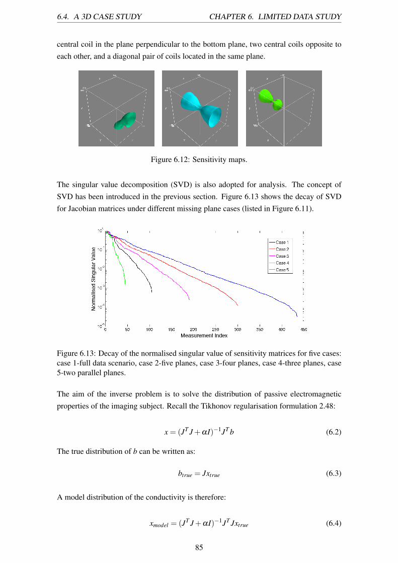
6.4. A 3D CASE STUDY CHAPTER 6. LIMITED DATA STUDY
central coil in the plane perpendicular to the bottom plane, two central coils opposite toeach other, and a diagonal pair of coils located in the same plane.
Figure 6.12: Sensitivity maps.
The singular value decomposition (SVD) is also adopted for analysis. The concept ofSVD has been introduced in the previous section. Figure 6.13 shows the decay of SVDfor Jacobian matrices under different missing plane cases (listed in Figure 6.11).
Figure 6.13: Decay of the normalised singular value of sensitivity matrices for five cases:case 1-full data scenario, case 2-five planes, case 3-four planes, case 4-three planes, case5-two parallel planes.
The aim of the inverse problem is to solve the distribution of passive electromagneticproperties of the imaging subject. Recall the Tikhonov regularisation formulation 2.48:
x = (JT J+aI)�1JT b (6.2)
The true distribution of b can be written as:
btrue = Jxtrue (6.3)
A model distribution of the conductivity is therefore:
xmodel = (JT J+aI)�1JT Jxtrue (6.4)
85

6.5. DISCUSSION CHAPTER 6. LIMITED DATA STUDY
A resolution matrix is defined by:
Rm = (JT J+aI)�1JT J (6.5)
This suggests that the closer the resolution matrix is to the identity matrix, the more stableand reliable the inverse model is [181]. The resolution matrix is a column vector, and thesum of the diagonal component of the resolution matrix reflects how close the value isto that of an identity matrix. Figure 6.14 show the sum of the diagonal componentsof the resolution matrix for five cases. The value decreases as the number of missingplanes increases. This is expected, and also consistent with the observations found in thepreviously discussed 2D MIT study.
Figure 6.14: Sum of the diagonal components of the resolution matrix at five missingplane cases.
6.5 Discussion
This chapter evaluates the effect of missing data through undersampling measurementsand limited angle imaging using experimental data. This is carried out in a systematicmanner and the images are assessed using an image quality measure RES and graphs of1D plots. It is important to distinguish this study from the optimisation of the number ofsensors in MIT. Here we choose a 32-channel MIT system, which produces acceptablequality images, and systematically remove coil sensors to study the effect of missingdata through undersampling and limited angle tomography. The quality of reconstructedimages are assessed to indicate the resolution loss caused by missing data in MIT. It isworth noticing that the proposed MIT system uses a sequential data collection strategy.In this context, the data acquisition in undersampled cases becomes faster but results inlower image quality. The limited angle could happen when there is only limited access tothe imaging subject. The results of this study illustrate what to expect from limited anglesituations and highlight the challenges related to this. The future direction of this study
86

6.5. DISCUSSION CHAPTER 6. LIMITED DATA STUDY
is to develop a compressed sampling technique to undersample MIT data, in particularwith a very large number of coils (for example, 256 coils [182]). A large number ofcoils can result in a large number of measurements, which could pose great difficultyto system hardware by slowing the data acquisition and image reconstruction processessignificantly. Unlike the systematic removal of coils in the 32-channel system presentedhere, we aim to find an optimal trade-off between the image quality and data acquisitiontime. This study provides a fundamental background for such work.
The 3D case study further investigates the effect of missing data on the quality of recon-structed images in a volumetric scenario. It is expected that removing planes of coilsresults in image quality degradation. This is validated by analysing the singular valuedecomposition and resolution matrix, and is consistent with our findings in a 2D case.Furthermore, among the missing plane cases, the parallel plane and single plane geome-tries have direct appeal in practical applications, as shown in chapters 4 and 5.
87

Chapter 7
Experimental Evaluation of Two-phaseFlow Imaging
Multi-phase flow imaging is a challenging topic in industrial process tomography. Inthis chapter, we present a non-invasive imaging technique for the electrically conductivephase of a multi-phase flow problem. Magnetic induction tomography (MIT) is sensitiveto the conductivity of the target, and as such has the potential to be used as an imagingtechnique to visualise the conductive components in a multi-phase flow application. TheMK-II MIT system is used for this study, among which eight excitation coils are suppliedwith a 15V peak, 13MHz sinusoidal signal in sequence from a signal generator, while theremaining eight coils are floated as receivers. The imaging region of this MIT system hasan inner and outer diameter of 190mm and 200mm respectively. Static fluid distributionpatterns are produced using several fluids with different conductivities and placed insidethe imaging region to form conductivity phase contrasts. Experimental results show thatthe smallest conductivity contrast that can be imaged is 0.06S/m for an inclusion thatoccupies 8.69% of the imaging region. An in-depth experimental evaluation of the systemresponse towards various fluid measurements is shown for the first time, as are results forquasi-static fluid experiments showing that a non-homogenous flow of gas bubbles canbe imaged in various conductive backgrounds. In sum, the analyses presented investigatethe feasibility and capability of MIT for this application, while also reporting some of thefirst flow rig tests in this field.
7.1 Introduction
Magnetic Induction Tomography (MIT) is also known as electromagnetic induction to-mography or eddy current tomography. It is a relatively low cost technique, although dueto its soft-field nature, the resolution of MIT has not yet met the standards for widespreadcommericalisation. The underlying principles of MIT is that a magnetic field is excitedand registered by inductive coils arranged around the imaging region; the spatial distribu-tion of magnetic field and the mutual coupling between the coils is then altered by material
88

7.1. INTRODUCTION CHAPTER 7. TWO-PHASE FLOW IMAGING
presented in the imaging region. Materials can be either ferromagnetic or conductive. In atypical 2D phantom study case, the cross-sectional images of the properties of the objectcan be reconstructed using the voltage or phase measurements collected from the induc-tive coils. Because of the non-hazardous, non-invasive and contactless natures of MIT,its use has been proposed for numerous applications, including geological exploration[3], foreign material monitoring [183], non-destructive evaluations [153, 167, 177], andbiomedical imaging [13, 90, 178, 184, 185, 186, 187, 188, 189, 190].
It is also considered more advantageous to use MIT in flow imaging compared to electri-cal resistance tomography techniques [191, 192, 193]. Due to the low resolution of thistechnique, the realisation of MIT as a smart imaging device for industrial process tomog-raphy remains a challenging topic. There have been reported cases where MIT is usedfor metal visualisation and solidification [18, 19, 194]; however, the experimental valida-tion in two-phase or multi-phase flow imaging using MIT is still limited. It is consideredthat MIT could be complementary to existing techniques for multi-phase flow imaging asMIT is sensitive to the conductive component of the flow mixtures [195, 196]. A feasibil-ity study of electromagnetic imaging in distinguishing two type of conductivities: fat andwater-bearing fat free tissues was presented in 1993. This study was primarily focused onthe imaging of biomedical tissue, however, the concept of MIT be used in flow processwas introduced and validated for the first time [60]. Albrechtsen et al [197] proposed asingle channel MIT system to measure the water content in multi-phase flow using ex-perimental phantom recordings. Based on the observations, the authors concluded thecorrelation between the position of the coil and the water/oil interface could be overcomeby a full tomographic system. Similar conclusions have also been drawn by Hammer etal [198]. Liu et al [199] proposed a parallel excitation structure for MIT in an attempt toimage conductive or ferromagnetic properties in two phase flow. However, this work waslimited in scope, focussing a simulation of the sensing field, and as such experimentalresults were not included in the publication. It was not until 2008 that a full MIT systemhad demonstrable feasibility for two phase flow imaging. Watson et al [200] studied aphantom simulated multi-phase flow in an oil pipeline, with the imaging conductivity ofthe system found to be below 10S/m. More recently, Wei et al [201] demonstrated an ex-perimental based two phase flow imaging using a 16 channel MIT system. Neverthelessthe experimental results were promising, showing that a conductivity contrast as small as1.58S/m can be imaged, the authors did not pursue further analysis of the results.
This chapter presents a critical evaluation of MIT for two phase flow imaging. Both staticand quasi-static experiments are presented to evaluate the MIT in variety of conditions.The practical difficulties, fundamental limitation, and potential improvement of this tech-nique are discussed.
89

7.2. STATIC RESULTS CHAPTER 7. TWO-PHASE FLOW IMAGING
7.2 Static Fluid Test Results
7.2.1 Experimental Setup
The MK-II MIT system is used for this study, which consists of 16 coils arranged aroundthe imaging periphery. The inner diameter, outer diameter and the length of the imagingregion are 190mm, 200mm and 90mm respectively. The driving frequency is 13MHz, witha 15V peak driving voltage and a driving current of 0.39A. The coil resonance frequencyis 45MHz, and the sampling rate of the system is 100MS/s [83].
A series of systematic experiments are conducted to demonstrate the likely conditions ofan industrial process environment using static fluid distribution patterns. Several termsare used throughout this study, hence it is worth giving the description for each term.
• Imaging region: the region of interest where the static fluid distribution pattern ismeasured using 16 inductive coils on the periphery.
• Background conductivity: the conductivity of the contents of the imaging region,excluding any inclusions.
• Inclusion: an area of differential conductivity within the imaging region, as com-pared to the background conductivity. As this study utilises fluids, the backgroundmaterial and the inclusion(s) of interest can both be fluid distribution patterns. Inthis case, the inclusion is kept distinct from the background by being bottled in anon-conductive object.
• Conductivity contrast: the difference between the conductivity of the backgroundand the inclusion.
• Area ratio: ratio of the cross-sectional area of the inclusion to the area of the totalimaging region.
• Norm value of phase difference: the norm value of the phase shift measurement be-tween the background and the inclusion (millidegrees), and it is calculated directlyfrom the raw measurements with no calibration. As a difference imaging is used inthis study, the norm value presents the phase shifts in a single value.
Two scenarios are considered to demonstrate the conductivity contrasts in the imagingregion, i.e., conductive inclusion(s) in a non-conductive background and non-conductiveinclusion(s) in a conductive background. A static fluid distribution pattern is introduced tothe background by bottling the fluid in a non-conductive cylindrical container. In each sce-nario, the inclusion is measured in three dimensions (28.70mm, 56.00mm and 72.52mm,hereafter small, medium and large respectively). As the fluid is bottled in a closed areain the imaging region, it is feasible to calculate the ratio of the cross-sectional area of the
90
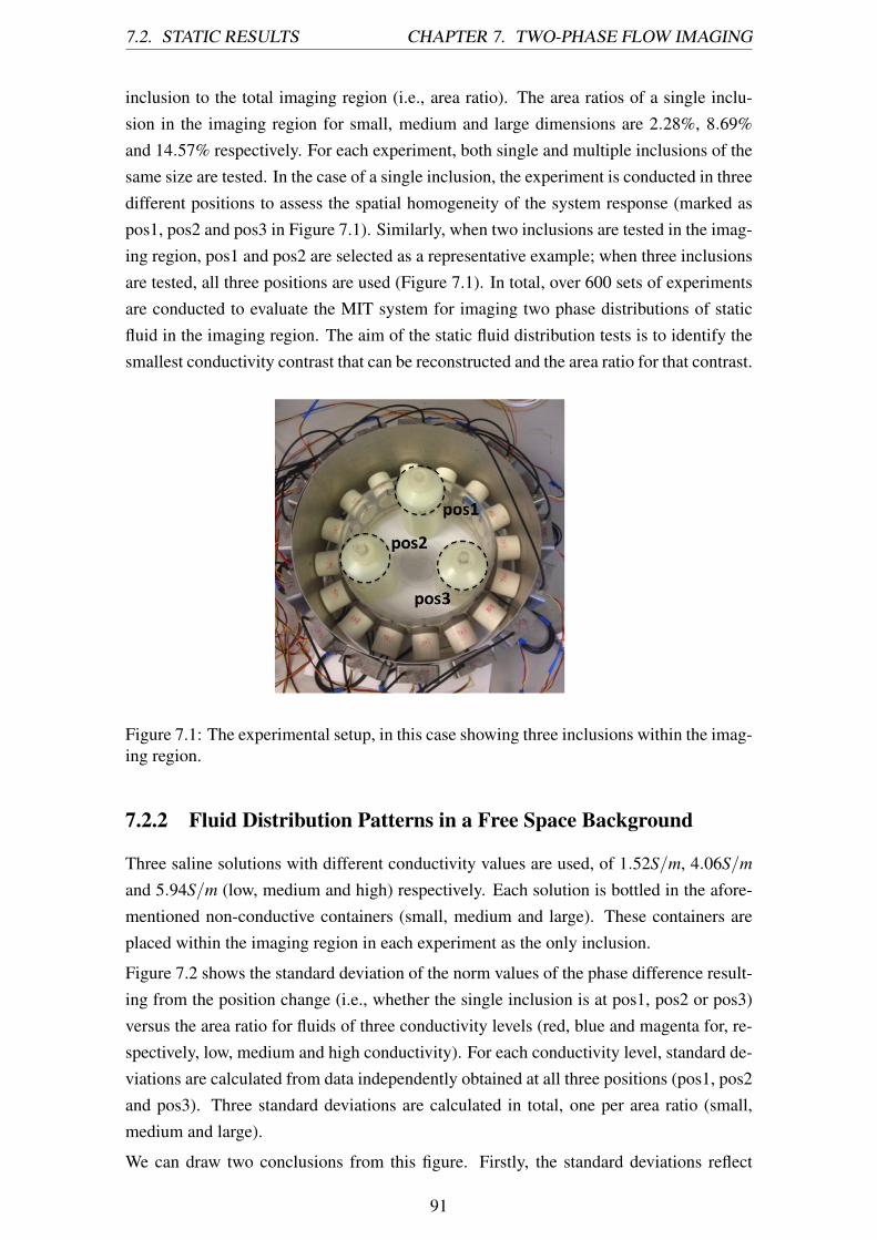
7.2. STATIC RESULTS CHAPTER 7. TWO-PHASE FLOW IMAGING
inclusion to the total imaging region (i.e., area ratio). The area ratios of a single inclu-sion in the imaging region for small, medium and large dimensions are 2.28%, 8.69%and 14.57% respectively. For each experiment, both single and multiple inclusions of thesame size are tested. In the case of a single inclusion, the experiment is conducted in threedifferent positions to assess the spatial homogeneity of the system response (marked aspos1, pos2 and pos3 in Figure 7.1). Similarly, when two inclusions are tested in the imag-ing region, pos1 and pos2 are selected as a representative example; when three inclusionsare tested, all three positions are used (Figure 7.1). In total, over 600 sets of experimentsare conducted to evaluate the MIT system for imaging two phase distributions of staticfluid in the imaging region. The aim of the static fluid distribution tests is to identify thesmallest conductivity contrast that can be reconstructed and the area ratio for that contrast.
Figure 7.1: The experimental setup, in this case showing three inclusions within the imag-ing region.
7.2.2 Fluid Distribution Patterns in a Free Space Background
Three saline solutions with different conductivity values are used, of 1.52S/m, 4.06S/mand 5.94S/m (low, medium and high) respectively. Each solution is bottled in the afore-mentioned non-conductive containers (small, medium and large). These containers areplaced within the imaging region in each experiment as the only inclusion.
Figure 7.2 shows the standard deviation of the norm values of the phase difference result-ing from the position change (i.e., whether the single inclusion is at pos1, pos2 or pos3)versus the area ratio for fluids of three conductivity levels (red, blue and magenta for, re-spectively, low, medium and high conductivity). For each conductivity level, standard de-viations are calculated from data independently obtained at all three positions (pos1, pos2and pos3). Three standard deviations are calculated in total, one per area ratio (small,medium and large).
We can draw two conclusions from this figure. Firstly, the standard deviations reflect
91

7.2. STATIC RESULTS CHAPTER 7. TWO-PHASE FLOW IMAGING
both the stability and repeatability of the data obtained for a given conductivity level,with lower standard deviations associated with more stable and more highly repeatabledata. Secondly, the standard deviations of the three conductivity levels are highly variabledepending on area ratio. Standard deviations for all three conductivity levels are similarfor small and medium area ratios, and highly divergent for large area ratios, suggestingthat in the latter case different conductivity levels are more readily distinguished.
Furthermore, the difference in standard deviations between the three area ratios reflectstheir distinguishability from each other - for instance, small inclusions (i.e., with smallarea ratio) have not only comparatively high standard deviations but their standard de-viations at each conductivity level are relatively similar. As such, small inclusions havethe most unstable measurements and accordingly are more difficult to distinguish by con-ductivity. For medium inclusions, the standard deviation for all three conductivity levelsis far lower than that of either small or large inclusions, reflecting that they have boththe highest stability of all the measurement data but also that they are the most difficultto distinguish by conductivity. In addition, the standard deviation of the norm value fora large inclusion of the highest conductivity is the greatest among all other cases, sug-gesting that although this represents a poorly-repeatable measurement, it unambiguouslydistinguishes high conductivity from medium or low. Thus, there is a trade-off betweenthe stability of the system and its ability to distinguish inclusions by their conductivity.
Figure 7.2: Standard deviation of the norm value of the phase difference resulting from theposition change of a single inclusion versus the area ratio of that inclusion (2.28%, 8.69%and 14.57% respectively). Data is shown for fluids with three conductivities (red, blueand magenta for, respectively, conductivity values of 1.52S/m, 4.06S/m and 5.94S/m).
Figure 7.3 shows the reconstructed images for, by row, one, two and three inclusions of,by column, small, medium and large area ratios. In all cases, the conductivity of theinclusion(s) is 1.52S/m. It can be seen that for small inclusions, conductivity contrastscannot be reliably reconstructed regardless of the position of the inclusion or the num-ber of inclusions in the imaging region (first row in Figure 7.3). For both medium andlarge inclusion, images of one, two or three inclusions can be reliably reconstructed. This
92

7.2. STATIC RESULTS CHAPTER 7. TWO-PHASE FLOW IMAGING
suggests that in this scenario, for a given conductivity contrast, if the inclusion cannot beimaged, increasing the number of inclusions does not contribute to any significant gainin information. However, by increasing the dimension of the inclusion, this could resultin an improved resolution in the reconstructed image. This suggests that in this case, thedimension of the inclusion is more informative with regard to image reconstruction thanthe number of inclusions being imaged. This phenomenon can be explained by referenceto the sensitivity distribution of the MIT system: areas nearer sensors are comparativelymore sensitive than regions farther away [40]. Furthermore, although the area ratio cov-ered by a small inclusion is, by definition, less than that of a medium or large inclusion,and increasing the number of inclusions further introduces a field perturbation into theimaging region, small inclusions still cover a less sensitive area compared to medium oflarge counterparts, resulting in unsuccessful image reconstruction.
Figure 7.3: Reconstructed images of one, two and three inclusions in a free space back-ground are shown in the first, second and third column; the first, second and third rowshows the reconstructed images of small, medium and large dimensions of inclusions ina free space background respectively. The conductivity of the inclusion is 1.52S/m in allcases.
In this section, the aim of the experiments is to investigate whether for the same numberof inclusions, of the same dimension and at the same testing positions, the conductivity ofthe inclusion affects its detectability. The first row in Figure 7.4 shows the reconstructedimages for a single inclusion in the same testing position for conductivities of 1.52S/m,4.06S/m and 5.94S/m (low, medium and high) respectively. Each column refers to a dif-
93
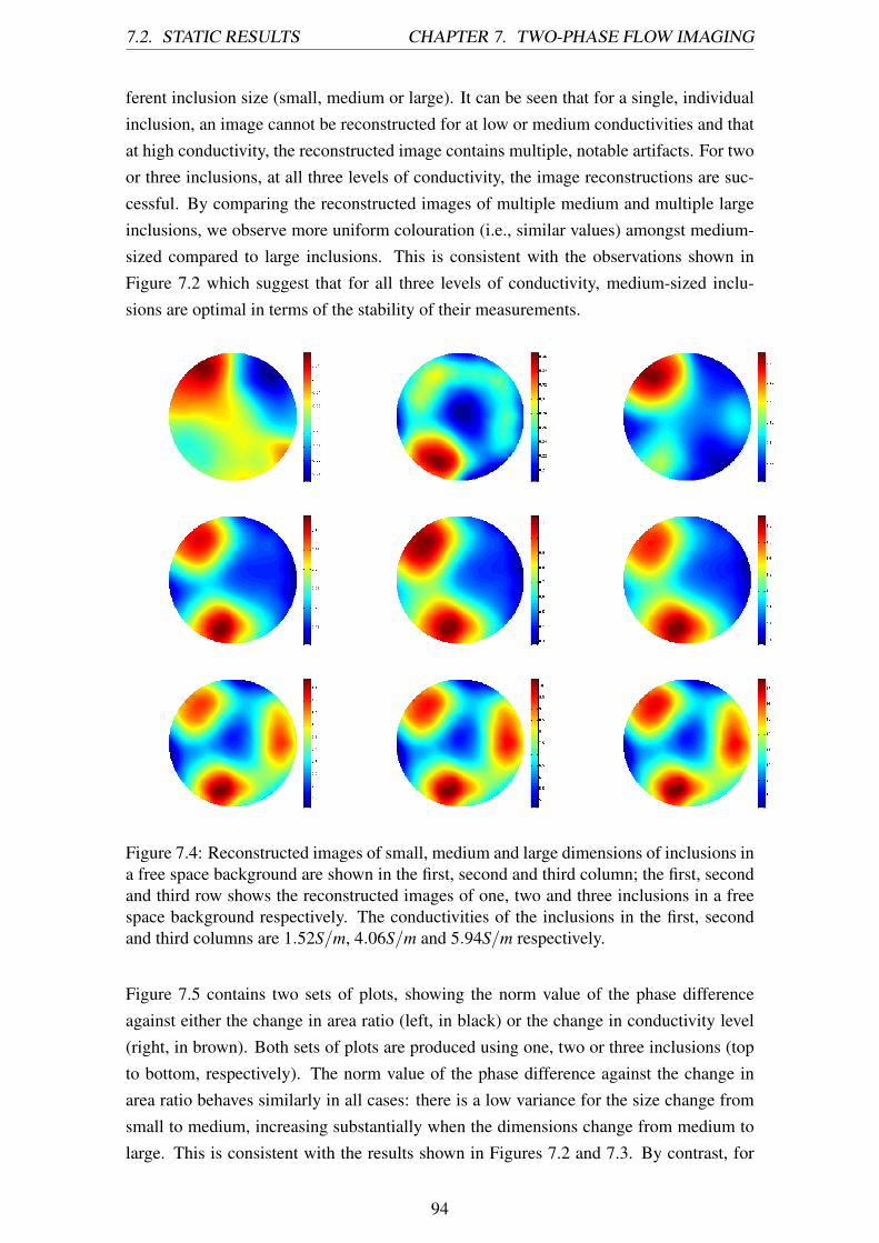
7.2. STATIC RESULTS CHAPTER 7. TWO-PHASE FLOW IMAGING
ferent inclusion size (small, medium or large). It can be seen that for a single, individualinclusion, an image cannot be reconstructed for at low or medium conductivities and thatat high conductivity, the reconstructed image contains multiple, notable artifacts. For twoor three inclusions, at all three levels of conductivity, the image reconstructions are suc-cessful. By comparing the reconstructed images of multiple medium and multiple largeinclusions, we observe more uniform colouration (i.e., similar values) amongst medium-sized compared to large inclusions. This is consistent with the observations shown inFigure 7.2 which suggest that for all three levels of conductivity, medium-sized inclu-sions are optimal in terms of the stability of their measurements.
Figure 7.4: Reconstructed images of small, medium and large dimensions of inclusions ina free space background are shown in the first, second and third column; the first, secondand third row shows the reconstructed images of one, two and three inclusions in a freespace background respectively. The conductivities of the inclusions in the first, secondand third columns are 1.52S/m, 4.06S/m and 5.94S/m respectively.
Figure 7.5 contains two sets of plots, showing the norm value of the phase differenceagainst either the change in area ratio (left, in black) or the change in conductivity level(right, in brown). Both sets of plots are produced using one, two or three inclusions (topto bottom, respectively). The norm value of the phase difference against the change inarea ratio behaves similarly in all cases: there is a low variance for the size change fromsmall to medium, increasing substantially when the dimensions change from medium tolarge. This is consistent with the results shown in Figures 7.2 and 7.3. By contrast, for
94

7.2. STATIC RESULTS CHAPTER 7. TWO-PHASE FLOW IMAGING
medium and large inclusions, there is a linear correlation between conductivity level andthe norm value of the phase difference. For small dimension, the plots for one, two andthree inclusion(s) are inconsistent with each other due to the low stability of the data, asalso shown in Figure 7.2. This also explains the unsuccessful image reconstruction shownin the top row of Figure 7.3.
Figure 7.5: The norm value of the phase difference against the change in area ratio (left,in black) and the change in conductivity level (right, in brown). Both sets of plots areproduced using one, two or three inclusions (top to bottom, respectively).
95

7.2. STATIC RESULTS CHAPTER 7. TWO-PHASE FLOW IMAGING
7.2.3 Fluid Distribution Patterns in a Silicone Oil Background
The silicone oil used in this study has an electrical insulation property, and as such canbe used as a non-conductive background. Figure 7.6 shows the reconstructed images ofone to three inclusions of a 1.52S/m saline solution in a silicone oil background (columnsleft to right, respectively), of either small, medium or large dimensions (first, second andthird rows, respectively). We show that the image quality increases as the dimensionof the inclusion increases, and that furthermore the ability to distinguish the location ofmultiple inclusions become more pronounced as their dimensions increase.
Figure 7.6: Reconstructed images of one, two and three inclusions of saline solution in afree space background are shown in the first, second and third column; the first, secondand third row shows the reconstructed images of small, medium and large dimensions ofsaline solution in a free space background respectively. The conductivity of the salinesolution is 1.52S/m in all cases.
7.2.4 Fluid Distribution Patterns in a Saline Solution Background
In this section, two phase liquid imaging is investigated using silicone oil to representa non-conductive inclusion and saline solution (conductivity 1.52S/m) as a conductivebackground. Figure 7.7 shows the reconstructed images of three sizes of inclusions -small, medium and large, as shown in the first, second and third rows, respectively. Al-though the conductivity contrast is the same as presented in Figure 7.6, the reconstructedimages notably differ. For instance, it appears that the dimension of the inclusion carries
96

7.2. STATIC RESULTS CHAPTER 7. TWO-PHASE FLOW IMAGING
comparatively little informative weight with regard to the quality of the image - this isin contrast to Figure 7.6, whereby increases in inclusion size from small to medium cannoticeably isolate the area of interest.
Figure 7.7: Reconstructed images of one, two and three inclusions of silicone oil in asaline solution background are shown in the first, second and third column; the first, sec-ond and third row shows the reconstructed images of small, medium and large dimensionsof silicone oil in a saline solution background respectively. The conductivity of the salinesolution background is 1.52S/m.
Figure 7.8 shows the standard deviation of the norm value of the phase difference re-sulting from position change for conductive inclusions in a non-conductive background(saline solution with 1.52S/m conductivity in a silicone oil background; dashed blue line)and non-conductive inclusions in a conductive background (silicone oil in saline; dashedred line). Unlike Figure 7.2, the effect of inclusion size differs in both cases. This sug-gests that the MIT imaging system shows a different response to different backgrounds.It can be seen that the standard deviation of the norm value increases more sharply forlarger area ratios in the case of conductive inclusions in a non-conductive background,compared to a more steady increase for non-conductive inclusions in a conductive back-ground. This supports the previous suggestion that inclusion dimension carries greaterinformative weight for the image reconstruction of conductive inclusions against a non-conductive background. This would also explain the substantial improvement in imagequality as the inclusion dimension increases in Figure 7.6, compared to Figure 7.7, where
97

7.2. STATIC RESULTS CHAPTER 7. TWO-PHASE FLOW IMAGING
the improvement in resolution is less discernible.
Figure 7.8: Standard deviation of the norm value of the phase difference resulting from theposition change of a single inclusion versus the area ratio of this inclusion (2.28%, 8.69%and 14.57% respectively) for two cases: silicone oil in a saline background (dashed redline), and saline solution (conductivity 1.52S/m) in a silicone oil background (dashedblue line).
7.2.5 Fluid Distribution Patterns in a Tap Water Background
Compared to the other conductive fluids previously discussed, tap water is not only morecommon but has comparatively low conductivity. As such, we repeated the above exper-iment using tap water as a background and silicone oil as an inclusion, in order to de-termine the smallest conductivity contrast at which image reconstruction is still feasible.Figure 7.9 shows the reconstructed images of one, two and three inclusion(s) of siliconeoil in a tap water background. Although image quality is poor in comparison to previousresults, this is nevertheless an encouraging finding, as it suggests the smallest conductiv-ity contrast at which image reconstruction is possible is 0.06S/m, for an inclusion thatoccupies 8.69% of the total imaging region.
98

7.2. STATIC RESULTS CHAPTER 7. TWO-PHASE FLOW IMAGING
Figure 7.9: Reconstructed images of one, two and three inclusions of silicone oil in atap water background are shown in the first, second and third column; the first, secondand third row shows the reconstructed images of small, medium and large dimensionsof silicone oil in a tap water background respectively. The conductivity of the tap waterbackground is 0.06S/m.
7.2.6 Non-homogenous Conductive Fluid Imaging in a Free SpaceBackground
A stratified flow regime is one of the classic flow regimes in industrial process tomogra-phy. A core aspect of this regime is the differentiation of multiple liquid flows, of variableconductivity, into strata. Our experimental setup does not allow the direct testing of flow,although it is nevertheless of interest to determine whether strata can be distinguished fornon-homogenous, albeit in this case static, liquids. The aim of this experiment is to im-age different volumes of conductive fluid within the imaging region to determine whetherthey can be distinguished by strata. In this experiment, a conductive fluid is used with aconductivity of 6.20S/m. This fluid is bottled in plastic containers with outer diameterof 37mm and a height of 79mm. Each container is fully filled with 50ml fluid. Strataare created within the imaging region by aligning multiple containers as shown in Figure7.10 (marked by dashed lines). As the conductivity and volume of fluid in each bottle isconstant, varying the number of bottles allowed us to vary the total volume of conductivefluid in each stratum. As the bottles are surrounded by free space, each strata is a non-
99

7.3. QUASI-STATIC RESULTS CHAPTER 7. TWO-PHASE FLOW IMAGING
homogenous mix of both conductive and non-conductive material. Three strata are tested,varying by total volume of conductive fluid (4, 8, and 13 containers, i.e., 200ml, 400mland 650ml, respectively). Reconstructed images shown from the left to the right in thebottom row of Figure 7.10.
Figure 7.10: Experimental setup (top) and reconstructed images (bottom) of three strata,each of non-homogeous conductive fluids in a free space background. By volume, strataare 200ml, 400ml and 650ml, from the left to the right respectively.
7.3 Quasi-static Fluid Measurements
This section investigates the feasibility of gas bubble imaging in a flow rig. The innerdiameter, outer diameter and the length of the flow rig are 190mm, 200mm and 800mmrespectively. The flow rig is positioned centrally in the imaging region with a 16 channelcoil array on the periphery (Figure 7.11).
100
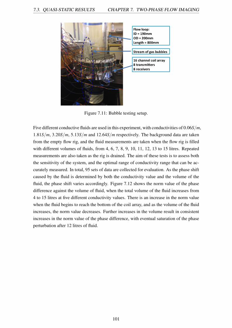
7.3. QUASI-STATIC RESULTS CHAPTER 7. TWO-PHASE FLOW IMAGING
Figure 7.11: Bubble testing setup.
Five different conductive fluids are used in this experiment, with conductivities of 0.06S/m,1.81S/m, 3.20S/m, 5.13S/m and 12.64S/m respectively. The background data are takenfrom the empty flow rig, and the fluid measurements are taken when the flow rig is filledwith different volumes of fluids, from 4, 6, 7, 8, 9, 10, 11, 12, 13 to 15 litres. Repeatedmeasurements are also taken as the rig is drained. The aim of these tests is to assess boththe sensitivity of the system, and the optimal range of conductivity range that can be ac-curately measured. In total, 95 sets of data are collected for evaluation. As the phase shiftcaused by the fluid is determined by both the conductivity value and the volume of thefluid, the phase shift varies accordingly. Figure 7.12 shows the norm value of the phasedifference against the volume of fluid, when the total volume of the fluid increases from4 to 15 litres at five different conductivity values. There is an increase in the norm valuewhen the fluid begins to reach the bottom of the coil array, and as the volume of the fluidincreases, the norm value decreases. Further increases in the volume result in consistentincreases in the norm value of the phase difference, with eventual saturation of the phaseperturbation after 12 litres of fluid.
101

7.3. QUASI-STATIC RESULTS CHAPTER 7. TWO-PHASE FLOW IMAGING
Figure 7.12: The norm value of the phase difference against the volume of the fluid forbackgrounds with five different conductivities (top). Shown in blue, red, magenta, black,and brown are conductivities of 0.06S/m, 1.81S/m, 3.20S/m, 5.13S/m and 12.64S/mrespectively. The norm value of the phase difference against the volume of the fluid for atap water background is shown in the bottom half of the figure.
The fluid reaches the centre of the imaging region when the flow rig is filled with 9 litresof fluid. Figure 7.13 shows the norm value of the phase difference for five differentconductivity backgrounds when the flow rig is filled with 9 litres of fluid. There is aconsistent increase in the norm value as the conductivity increases, which reaches itspeak value at a conductivity of 5.13S/m.
102

7.3. QUASI-STATIC RESULTS CHAPTER 7. TWO-PHASE FLOW IMAGING
Figure 7.13: The norm value of the phase difference for five difference conductivity back-grounds (0.06S/m, 1.81S/m, 3.20S/m, 5.13S/m and 12.64S/m respectively) when theflow rig is filled with 9 litres of fluid, measurements were made between the coil pair Tx2and Tx6.
Once the flow rig is filled with 15 litres of fluid, a stream of bubble gas is injected onthe periphery at 2 points opposite each other (labelled position 1 and position 2 in Figure7.14) to introduce the perturbation to the electromagnetic field. The aim of the experimentis to test whether the system can reconstruct an image of the bubbles. A snap shot of thebubble testing is reconstructed to show the average bubbles along the axial direction. Theimaging results are shown in Figure 7.14; note the value of the scale decreases as theconductivity of the background decreases. Although the gas bubbles are themselves non-conductive, they are injected into a conductive background; as such, the areas that areinjected with gas bubbles in fact have a non-homogenous non-conductive feature. Thisexperiment can be considered the opposite of the experiment shown in Figure 7.10, wherethe results show the reconstructed images of a non-homogenous conductive medium in anon-conductive background.
103

7.3. QUASI-STATIC RESULTS CHAPTER 7. TWO-PHASE FLOW IMAGING
Bubble position 1 Bubble position 2
104
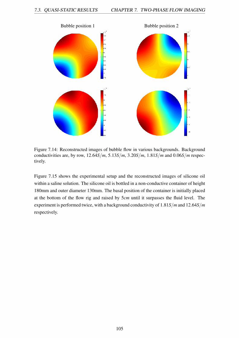
7.3. QUASI-STATIC RESULTS CHAPTER 7. TWO-PHASE FLOW IMAGING
Bubble position 1 Bubble position 2
Figure 7.14: Reconstructed images of bubble flow in various backgrounds. Backgroundconductivities are, by row, 12.64S/m, 5.13S/m, 3.20S/m, 1.81S/m and 0.06S/m respec-tively.
Figure 7.15 shows the experimental setup and the reconstructed images of silicone oilwithin a saline solution. The silicone oil is bottled in a non-conductive container of height180mm and outer diameter 130mm. The basal position of the container is initially placedat the bottom of the flow rig and raised by 5cm until it surpasses the fluid level. Theexperiment is performed twice, with a background conductivity of 1.81S/m and 12.64S/mrespectively.
105

7.3. QUASI-STATIC RESULTS CHAPTER 7. TWO-PHASE FLOW IMAGING
side-view top-view
(a) (b)
Figure 7.15: Experimental setup of a silicone oil inclusion in two conductive back-grounds, with associated images. (a) silicone oil inclusion within a 1.81S/m background,(b) silicone oil inclusion within a 12.64S/m background.
Figure 7.16 shows the norm value for the phase difference resulting from the movementof the silicone oil along the axial direction within the conductive background. The dis-tance whereby the silicone oil container is placed within the imaging region is set to bethe reference distance, i.e., 0cm along the axial direction. For a background with 1.81S/mconductivity, the norm value of the phase difference initially decreases; from �15cm andgreater, however, the value starts to increase. This is also called the fringe effect of thesensing region as the sensing area in the axial direction depends on the conductivity con-trast between the background and the inclusion [202], consistent with the observations inFigure 7.12. The norm value of the phase difference reaches its peak when the silicone oilcontainer arrives in the imaging region. Further increasing the distance, the value startsto decrease again. As the distance surpasses 15cm, the silicone oil does not seem to causeany distinct perturbation in the phase difference. For the background with conductivity12.64S/m, the overall norm value of the phase difference does not change as sharply asthat for 1.81S/m. At �20cm, the norm value of the phase difference caused by back-ground conductivities of 1.81S/m and 12.64S/m are 10.94 and 12.83 respectively. As
106

7.4. DISCUSSION CHAPTER 7. TWO-PHASE FLOW IMAGING
the norm value of the phase difference caused by a higher conductive background alreadyexceeds its counterpart, at this point, the fringe effect is not observed between �20 to�10cm.
Figure 7.16: The norm value of the phase difference resulting from the movement of thesilicone oil along the axial direction within two conductive backgrounds, 1.81S/m and12.64S/m respectively.
7.4 Discussion
The visualisation of conductive phase flow is a challenging problem in industrial pro-cess tomography, with a need to develop a cost-effective, non-invasive yet robust imagingtechnique in this area. This study investigates the feasibility of MIT for this applicationand also highlights the difficulties associated with it. Four background measurements arecollected by contrasting both non-conductive (free space and silicone oil) and conduc-tive fluids (saline solution and tap water, with conductivities of 1.52S/m and 0.06S/m,respectively) to represent a range of scenarios of potential interest in industrial processtomography. The results of static fluid tests confirm the viability of MIT in visualisingthe conductivity contrasts. We also found that the MIT phase measurements show a linearresponse with respect to electrical conductivity for a given dimension and location of aninclusion, while the phase changes arising from the changing dimensions of an inclusionhave a non-linear relationship.
In addition, it is commonplace to have fluids separated into different layers by density,weight or conductivity in industrial process tomography. Tests of non-homogenous con-ductive fluids suggest that different strata of conductive fluids can be distinguished, andalthough in this case the distribution of eddy currents could differ from an industrial flowenvironment, we nevertheless show the potential of MIT in this respect. In industrialenvironments, there may be bubble flows of gas in the uppermost part of the flow pipe,and water only in the lowest part. The quasi-static experiments demonstrate the capabil-ity of MIT in obtaining a 2D image of bubble flow along the axial dimension of various
107

7.4. DISCUSSION CHAPTER 7. TWO-PHASE FLOW IMAGING
conductive backgrounds, including water.
These quasi-static experiments also reveal that there is a strong fringing field effect ofthe MIT sensing region, consistent with similar observations in [203]. This suggeststhat a 3D MIT system might be more robust compared to a 2D system, particularly inobtaining the axial information of the fluid. Future studies will focus on this aspect withthe purpose to design a cost effective 3D system, and subsequently develop real time3D reconstruction algorithms. For any conductivity contrast lower than the conductivitycontrast presented in this study, other contactless imaging techniques such as electricalcapacitance tomography might be able to operate. A combined capacitance and inductivetomographic system will be studied in order to image both dielectric and conductive phasecontrasts. In our continued effort, we will develop a more robust MIT hardware capable ofworking in industrial environments, including both the mechanical design of the sensorsand improvement in hardware electronics.
Finally, it is worth mentioning that in principle, the inverse problem needs to be solved ac-cording to each specific imaging case. As such, the image reconstruction algorithm needsto be applied according to each individual imaging subject. This would introduce addi-tional parameters (i.e., the number of iterations, the regularisation parameters or matrices)to this study, alongside the number, size and position of inclusions, and the conductivitycontrast. Therefore, in this study, a universal linear inverse algorithm is used to recon-struct images with pre-calculated regularisation parameters for all cases (equation 2.56).This way, it is guaranteed that any change in the image reconstruction is in fact due tothe change in the fluid distribution patterns rather than the image reconstruction softwaremodel, although this does suggest that the inverse model might not be optimal for certaincases. In future studies, a nonlinear image reconstruction algorithm might be necessary toenhance the resolution of the two phase contrasts, if it can be developed in such a manneras to computationally efficient for the purpose of real time imaging.
108

Chapter 8
Conclusions
8.1 Summary
This thesis studies the feasibility and capability of MIT in non-destructive evaluation andprocess tomography applications. Topic of interests include the inspection of pipelines,identification of hidden defects in carbon fibre reinforced polymers, 3D subsurface imag-ing of metallic structures and visualisation of two-phase flow. The applications proposedin chapters 3 to 6 are based on the Bath MK-I MIT system, which was designed for imag-ing materials with conductivity higher than 105S/m. The application of two-phase flowimaging is presented in chapter 7, which is based on the Bath MK-II MIT system. Thissystem was designed for imaging subjects with conductivity lower than 10S/m. Althougheach chapter studies a specific research topic, they are consistent in several ways. Firstly,the coil arrays are designed specifically for the geometries of the imaging subjects in or-der to employ the flexibility of MIT in this respect. Secondly, each chapter presents anexperimental evaluation of MIT for the proposed application; as such the viability andcapability of MIT for its intended use can be demonstrated through experimental results.Thirdly, each chapter provides an insight as to how MIT can be used and further devel-oped towards a commercial technique in each field for the purpose of expanding the wideapplicability of MIT.
8.2 Remarks
Chapter 3 shows that MIT is capable of imaging structural damage to pipe samples, anapplication never before attempted. Both external and internal wall losses on aluniniumpipe walls and external damage to steel pipes are inspected using the proposed MIT sys-tem. A novel image reconstruction method is developed specifically for this application,which achieves an unprecedented resolution in the field of 2%. The simulated voltagesobtained from the forward model are validated against the experimental measurements,ensuring the accuracy of the software model. Altogether, these results demonstrate the
109

8.2. REMARKS CHAPTER 8. CONCLUSIONS
applicability of MIT as an NDE technique for industrial pipeline inspection, as a proof ofprinciple.
Chapter 4 presents a means by which MIT could be employed as a NDE technique forcarbon fibre reinforced polymers (CFRPs). This extends the employability of MIT fromtraditional metallic structures to new composite materials. A dual planar coil array is de-signed to accommodate the geometry of the imaging subject. The experimental resultsdemonstrate that both single and multiple hidden defects can be inspected, with recon-structed images of sufficient accuracy. It is worth noting that in this study, only CFRPswith an isotropic character are investigated. In a follow up study, one should modify theforward model to accommodate materials with anisotropic characteristics in order to ex-pand the employability of MIT. In addition, further studies should also focus on improvingthe system imaging speed for real time inspection. These suggest that with continued ef-fort, MIT could evolve be become a rapid inspection tool during the initial manufacturingstage of CFRPs.
In both chapters 3 and 4, the imaging subjects are accessible to the MIT system. Chapter5 aims to address a challenge whereby there is only limited access to the imaging tar-get, i.e., if the measurements can only be obtained from one surface, as is the case with3D surface imaging. By developing a planar array to provide volumetric and penetrablemeasurements beneath the imaging subject, this study provides a means by which 3D sur-face imaging is demonstrably viable. The detectable depth is shown to be approximately3� 4cm underneath the imaging surface. Although seemingly limited, this chapter rep-resents the first 3D experimental planar work in the field, and opens up opportunities forMIT to be used as a subsurface inspection tool. Implementing a multi-frequency MITcould be a solution to improve the penetration depth, which will be studied in a futurework.
It is apparent that in a MIT system, limited access to the imaging target results in a re-stricted number of measurements. As such, chapter 6 explores the relationship betweenimage quality and the number of available measurements in both a qualitative and quanti-tative manner, the latter by systematically creating missing data scenarios experimentallyin 2D. Two scenarios are established by undersampling the data and using limited angletomography. The interest of this work lies in the fact that these findings could offer insightinto how, for large scale MIT with a large quantity of data, undersampling of data may bean efficient means by which rapid data processing can be achieved without compromisingimage quality. We also extend the limited data concept to 3D imaging, with consistentobservations.
Chapter 7 presents an experimental evaluation of MIT in conductive phase flow imag-ing. Experiments are conducted covering as broad a range of conductivity contrasts aspossible, so as to encompass several scenarios of potential interest in industrial flow en-vironments. The fluid experiments include (a) the smallest conductivity contrast in whichimage reconstruction in various non-conductive and conductive backgrounds is possible,
110

8.3. LIMITATIONS & IMMEDIATE RESEARCH CHAPTER 8. CONCLUSIONS
(b) distinguishing three strata of non-homogenous conductive fluids in free space, and (c)imaging a flow of non-homogenous bubbles of gas in various conductive backgrounds.Taken together, this study demonstrates various capabilities of an MIT system in conduc-tive phase imaging.
8.3 Limitations and Immediate Research
Further development on pipeline inspection using MIT in chapter 3 should focus on sys-tem improvement in three aspects. Firstly, the system development should draw attentionto the design of an agile MIT sensing array in order to adapt to various pipeline geome-tries and accurately obtain the measurements for reconstruction. Secondly, a rapid datacollection and image reconstruction module are essential to ensure real time inspection.Thirdly, the overall system should be developed so as to be suitable for more diverseindustrial environments, such as those characterised by a high temperature, radiation orpressure, undersea conditions or buried pipelines.
As to the future study of the hidden defect identification in carbon fibre reinforced poly-mers (CFRPs) using MIT in chapter 4, an in-depth study of anisotropic characteristics ofCFRP is necessary in order to expand this applicability of MIT to various structures. Itis also worth investigating if the impact damage in CFRP can be inspected by MIT. Thiscould require a MIT system that is capable for real time inspection.
In addition to further improve the depth penetration of planar MIT (PMIT) system inchapter 5, the author will investigate what is the smallest volume of metallic structure inan imaging subject that can be detected underneath the sensing array, and the maximumdetection depth under these circumstances. To improve the penetration depth, implement-ing a multi-frequency MIT system could be a suitable approach.
The conclusions made in chapter 6 can be used to provide a guidance as to what extentundersampling the data is viable for achieving fast data collection without compromisingthe image resolution. In the absence of a large scale MIT system, the author will developa simulation model of a large scale MIT system - for instance, with 256 coils - to validatethe predications made in chapter 6.
Experimental investigation of conductive flow imaging using MIT in chapter 7 revealsthat 3D MIT could be the future direction in terms of system design in order to improvethe system’s ability and to be more efficient in capturing the axial dimension of the flowinformation. In addition, a classification work is needed to establish the boundaries ofMIT in imaging the conductive flow, as well as attempting to carry out testing on industrialflow regimes. This would also require the system to be equipped with real time datacollection capability.
The methodologies needed to achieve these goals are summarised in 8.5.
111

8.4. CONTRIBUTIONS TO KNOWLEDGE CHAPTER 8. CONCLUSIONS
8.4 Contributions to Knowledge
Considering the novel elements of the research undertaken, the following contributions toknowledge are claimed:
• The first proposed use of MIT for industrial pipeline inspection, after establishingthe feasibility and capability of MIT in imaging the structures of pipelines.
• The development of a novel image reconstruction algorithm, the narrow pass filter-ing method, which enables an unprecedented MIT resolution of 2% compared tothe traditional resolution of 10-15%.
• The first experimental work conducted on 3D planar MIT for near subsurface imag-ing, which demonstrates the ability of MIT as a limited access tomographic tech-nique to offer volumetric and penetrative measurements.
• The first experimental characterisation of the missing data effect in MIT based onresearching various coil array geometries both qualitatively and quantitatively, andin both 2D and 3D scenarios.
• A demonstration of the capability of MIT in inspecting hidden defects in carbonfibre reinforced materials using 3D experimental results.
• The first experimental evaluation of static fluids, quasi-static fluids and flow rigtesting in the field of MIT research, reporting the feasibility of MIT at distinguishingtwo-phase conductive flow.
During the course of this PhD, the outcomes of this research have been published in 9journal articles, and presented at several relevant national and international conferences.Detailed publications are attached in appendix A.
8.5 Future Work
8.5.1 Forward and Inverse Problems
MIT resolution suffers from poor spatial resolution as the inverse problem in MIT is inher-ently an ill-posed problem. In this respect, it is desirable to improve the image resolutionof MIT in order to expand the applicability of this technique. Chapter 3 presents pipelineinspection using a narrowband pass filtering method (NPFM) for image reconstruction.This is a case study of limited region tomography. The imaging region is limited to spe-cific pipe geometries by implementing a NPFM. This is an effective approach to improveMIT image resolution by increasing the number of useful pixels in the region of interest.However, this method requires the centre of the pipe to match the centre of the imagingregion. This is the main disadvantage of this method, which needs to be addressed if a
112

8.5. FUTURE WORK CHAPTER 8. CONCLUSIONS
priori information of the pipe is unknown. As discussed in chapter 6, missing data canfurther result in a degraded image quality. However, it is also shown that the targetedobjects are detectable as long as they are placed within the region of interest, as is thecase in several limited angle scenarios. This suggests that limiting the imaging region cancompensate for information loss, especially if access to the imaging subject is restricted.Based on the observation obtained from both chapters, it is anticipated that for limitedaccess scenarios, limiting the region could help to improve the image quality.
In future work, the author will aim to overcome the inflexibility of NPFM by using a levelset method [48, 168, 170]. The level set method can be used to establish the boundary ofthe conductive inclusion, and as such, it can provide an estimate of the location and the di-mension of the imaging subject. Implementing the level set method would require the useof a non-linear iterative method to solve the forward model, which could be computation-ally expensive. This also applies when modeling CFRPs with anisotropic characteristics- the forward problem needs to be solved according to a specific case in order to ensurethe accuracy of the sensitivity maps. The author proposes that the computational cost canbe overcome by implementing graphics processing units (GPUs) for high performancecomputing [204, 205, 206, 207, 208].
In addition, various MIT geometries such as planar and arc, as well as the limited data inboth 2D and 3D cases have been investigated in this thesis. These geometries are studiedas each of them has its own potential uses and interests. These geometries have limitedmeasurements, which consequently weakens the MIT resolution. In a future study, the au-thor will aim to develop more sophisticated algorithms specifically for these geometries,which could be of benefit to MIT resolution. More importantly, developing algorithmsthat can be run in real time is crucial in order to use MIT in an industrial environment.
8.5.2 System Improvements
One should note that there is no universal design approach for all MIT applications, andthat the hardware of a MIT system should be catered to its proposed application. Althoughthere are few studies which focus on the specific design of a MIT coil array [94, 209, 210,211, 212, 213], there is no study reported that covers the design of all sub-components ofa MIT system. Although hardware development is not the focus of this thesis, there areseveral improvements that can be made to the existing systems.
The MK-I system is designed for imaging material with conductivity above 105S/m. Thesystem was initially designed to accommodate 16 channels, and later expanded to 32channels by adding an additional multiplexer and an inverter for data switching. Thissuggests that for an array with more than 32 coils, this system will no longer be suitable,although this is not considered a pressing issue - currently used systems do not exceed 24coils. In addition to its channel capacity, one disadvantage of this system is that it is notideal for real time imaging, especially if all 32 channels are utilised. The measurementdata has to be collected and stored off-line for image reconstruction. This limitation
113

8.5. FUTURE WORK CHAPTER 8. CONCLUSIONS
needs to be overcome in order to expand the applicability of MIT in NDE applicationsand process tomography. Furthermore, in this thesis, all the coil arrays, pin connectionsand cabling were hand made. In an ideal case, these have to be designed in a sophisticatedmanner to ensure low noise perturbation and better transmission of the signals [214].
The MK-II MIT system was designed for material with conductivity value lower than10S/m, therefore it was proposed for conductive flow imaging, a challenging topic inindustrial process tomography. In chapter 7, it is shown that there is a strong fringingeffect in the sensor region. This suggests that a 3D MIT system might be more robustcompared to a 2D system, particularly in obtaining the axial information of the fluid.Future studies will focus on this aspect with the purpose of designing a cost effective 3Dsystem, and subsequently develop real time 3D reconstruction algorithms, in conjunctionwith section 8.5.1.
8.5.3 Multi-frequency MIT
The electrical conductivity s = s(x) contributes important functional information formany MIT applications. Although for a given system and a targeted problem the fre-quency is fixed, one should note that the conductivity is frequency dependent, i.e., s =
s(x,w). Developing an excitation source capable of providing multiple frequencies couldenhance the detectability of a MIT system [19, 184, 185]. In chapter 3, inspection of inter-nal damage was found particularly challenging as the chosen frequency cannot penetratethe steel pipe wall. This issue will become more prominent with increasingly thick pipewalls. This issue is also presented in chapter 5 for subsurface imaging. Decreasing the fre-quency will increase the skin depth, which is used to describe the penetration of magneticfield below the surface of the test object. The skin depth d , is defined as:
d =
s2
wµ0µrs
where w is angular frequency, µ0 and µr are unity and relative magnetic permeability, sis electrical conductivity. High frequency measurements give information regarding theproperties adjacent to the surface, whereas low frequency testing probes deeper insidethe test sample [19, 185]. For non-magnetic, electrically conductive metals, i.e., µr = 1,a single selected frequency might meet the skin depth requirement. However, for othermaterials such as steel, where both conductivity and permeability play important roles,using a single selected frequency cannot satisfy the image reconstruction demand. Aselection of frequencies for excitation in MIT could improve the information from a MITsystem and make it more robust against the depth of the anomaly.
The major challenges of implementing multi-frequency MIT fall on both conditioningelectronics and software control. It is desirable to design an excitation channel whichprovides a selection of frequencies. The signal demodulation also needs to be capable
114

8.5. FUTURE WORK CHAPTER 8. CONCLUSIONS
of demodulating one selected frequency to be fed into an excitation coil from a multi-frequency system. Additionally, enhancing the MIT software to be able to collect multi-frequency data as well as developing a spectral and frequency difference reconstructionare equally important, especially for anisotropic composite structures [215, 216]. Of par-ticular interest is frequency difference imaging, which could be useful if the test subjectsshow different responses to frequency variation. This study will be carried out in con-junction with the research topics discussed in sections 8.5.1 and 8.5.2.
115

Appendix A
List of publications
Journal Articles:
1. Ma, L., Hunt, A and Soleimani, M. (2014) Experimental evaluation of conduc-tive flow imaging using magnetic induction tomography. International Journal ofMultiphase Flow, under review.
2. Ma, L., Banasiak, R and Soleimani, M. (2014) Magnetic induction tomographywith high performance GPU implementation. International Journal of High Per-formance Computing Applications, under review.
3. Zhang, M., Ma, L. and Soleimani, M. (2014) Magnetic induction tomographyguided electrical capacitance tomography imaging with grounded conductors. Mea-surement, 53, pp. 171–181.
4. Ma, L. and Soleimani, M. (2014) Hidden defect identification in carbon fibre rein-forced polymer plates using magnetic induction tomography. Measurement Science& Technology, 25(5), pp. 055404.
5. Evangelidis, M., Ma, L., and Soleimani, M. (2013) High definition electrical capac-itance tomography for pipeline inspection. Progress In Electromagnetics Research,141, pp. 1- 15.
6. Ma, L., Wei, H.-Y. and Soleimani, M. (2013) Planar magnetic induction tomogra-phy for 3D near subsurface imaging. Progress In Electromagnetics Research, 138,pp. 65-82.
7. Ma, L. and Soleimani, M. (2012) Limited angle and limited data electromagneticinduction tomography: experimental evaluation of the effect of missing data. Mea-surement Science & Technology, 23 (12), pp. 125406.
8. Wei, H.-Y., Ma, L. and Soleimani, M. (2012) Volumetric magnetic induction to-mography. Measurement Science & Technology, 23 (5), pp. 055401.
116

APPENDIX A. LIST OF PUBLICATIONS
9. Ma, L. and Soleimani, M. (2012) Electromagnetic imaging for internal and exter-nal inspection of metallic pipes. Insight: Non-Destructive Testing and ConditionMonitoring, 54 (9), pp. 493-495.
10. Ma, L., Wei, H.-Y. and Soleimani, M. (2012) Pipeline inspection using magneticinduction tomography based on a narrowband pass filtering method. Progress InElectromagnetics Research M, 23, pp. 65-78.
Conference Articles:
1. Ma, L. and Soleimani, M. (2014) Critical evaluation of two phase low conductivityflow imaging using magnetic induction tomography. In: 5th International Work-shop on Process Tomography, Jeju, South Korea.
2. Zhang, M., Ma, L. and Soleimani, M. (2014) Dual modality ECT-MIT three-phaseflow imaging. In: 5th International Workshop on Process Tomography, Jeju, SouthKorea.
3. Ma, L. and Soleimani, M. (2014) A hybrid image reconstruction for medical mag-netic induction tomography: an experimental evaluation. In: 15th InternationalConference on Biomedical Applications of Electrical Impedance Tomography, Gananoque,Canada.
4. Ma, L. and Soleimani, M. (2013) Industrial pipeline inspection using magneticinduction tomography. In: 7th World Congress in Industrial Process Tomography(WCIPT7), Krakow, Poland.
5. Zhang, M., Ma, L., Ye, Z., Yang, C. L., Wei, H. Y., Banasiak, R. and Soleimani,M. (2013) Near subsurface 3D imaging using planar array: EIT, ECT, MIT. In: 7thWorld Congress in Industrial Process Tomography (WCIPT7), Krakow, Poland.
6. Ma, L., Wei, H.-Y. and Soleimani, M. (2012) Cryosurgical monitoring using elec-tromagnetic measurements: a feasibility study for magnetic induction tomography.In: 13th International Conference in Electrical Impedance Tomography, Tianjin,China.
7. Wei, H.-Y., Ma, L. and Soleimani, M. (2012) Three dimensional magnetic induc-tion tomography imaging using multi-plane coil arrays. In: 6th International Sym-posium on Process Tomography, Cape Town, South Africa.
8. Wei, H., Yang, C., Ma, L., Ye, Z., Yao, A. and Soleimani, M. (2012) Three-dimensional industrial process tomography using electrical and electromagnetic to-mography: recent developments. In: 2012 IEEE I2MTC - International Instrumen-tation and Measurement Technology Conference, Proceedings. IEEE, pp. 912-915.
117

Bibliography
[1] F. J. Dickin, B. S. Hoyle, A. Hunt, S. M. Huang, O. Ilyas, C. Lenn, R. C. Waterfall,R. A. Williams, C. G. Xie, and M. S. Beck. Tomographic imaging of industrialprocess equipment: techniques and applications. In Circuits, Devices and Systems,IEE Proceedings G, volume 139, pages 72–82. IET, 1992.
[2] A. J. Peyton. Electrical tomography for industrial applications (presentation).
[3] H. Griffiths. Magnetic induction tomography. Measurement Science and Technol-ogy, 12:1126–1131, 2001.
[4] David S. Holder. Electrical impedance tomography: methods, history, and appli-cations. CRC Press, Bristol, 2005.
[5] J. G. Webster and P. D. Hughes. Electrical impedance tomography. Journal ofClinical Engineering, 16(4):349, 1991.
[6] F. Sattar. Rot detection in wooden poles using electrical impedance tomography.Master’s thesis, Department of Electrical Engineering, University of Cape Town,2005.
[7] S. Liu, Q. Chen, X. Xiong, Z. Zhang, and J. Lei. Preliminary study on ect imagingof flames in porous media. Measurement Science and Technology, 19(9):094017,2008.
[8] Y. Yan, T. Qiu, G.Lu, M. Hossain, G. Gilabert, and S. Liu. Recent advances in flametomography. Chinese Journal of Chemical Engineering, 20(2):389–399, 2012.
[9] R. C. Waterfall, R. He, P. Wolanski, and Z. Gut. Flame visualizations using electri-cal capacitance tomography (ect). Process Imaging for Automatic Control, pages242–250, 2001.
[10] L.-S. Fan, W. Warsito, and B. Du. Electrical capacitance tomography imagingof gas-solid and gas-liquid-solid fluidized bed systems. Journal of Visualization,7(1):5, 2004.
[11] Z. Yingna and L. Qiang. Review of techniques for the mass flow rate measurementof pneumatically conveyed solids. Measurement, 44(4):589–604, 2011.
118

BIBLIOGRAPHY BIBLIOGRAPHY
[12] Z. Y. Huang, B. L. Wang, and H. Q. Li. Application of electrical capacitance to-mography to the void fraction measurement of two-phase flow. IEEE Transactionson Instrumentation and Measurement, 52(1):7–12, 2003.
[13] H. Griffiths, W. R. Stewart, and W. Gough. Magnetic induction tomography: ameasuring system for biological tissues. Annals of the New York Academy of Sci-ences, 873:335–345, 1999.
[14] G. Jin, J. Sun, M. Qin, Q. Tang, L. Xu, X. Ning, J. Xu, X. Pu, and M. Chen. A newmethod for detecting cerebral hemorrhage in rabbits by magnetic inductive phaseshift. Biosensors and Bioelectronics, 52:374–378, 2014.
[15] R. Merwa, K. Hollaus, O. Biró, and H. Scharfetter. Detection of brain oedemausing magnetic induction tomography: a feasibility study of the likely sensitivityand detectability. Physiological Measurement, 25(1):347–354, 2004.
[16] H. Scharfetter, P. Riu, M. Populo, and J. Rosell. Sensitivity maps for low-contrastperturbations within conducting background in magnetic induction tomography.Physiological Measurement, 23(1):195–202, 2002.
[17] L. F. Fuks, M. Cheney, D. Isaacson, D. G. Gisser, and J. C. Newell. Detection andimaging of electric conductivity and permittivity at low frequency. IEEE Transac-tions on Biomedical Engineering, 38(11):1106–1110, 1991.
[18] X. Ma, A. J. Peyton, S. R. Higson, A. Lyons, and S. J. Dickinson. Hardwareand software design for an electromagnetic induction tomography (emt) system forhigh contrast metal process applications. Measurement Science and Technology,17(1):111–118, 2006.
[19] X. Ma, A. J. Peyton, S. R. Higson, and P. Drake. Development of multiple fre-quency electromagnetic induction systems for steel flow visualization. Measure-ment Science and Technology, 19(9):094008, 2008.
[20] A. J. Peyton, Z. Yu, Z. Zhi, S. Al-Zeibak, N. H. Saunders, and A. R. Borges. Elec-tromagnetic imaging using mutual inductance tomography: potential for processapplications. Particle and Particle Systems Characterization, 12(2):68–74, 1995.
[21] A. Korjenevsky, V. Cherepenin, and S. Sapetsky. Magnetic induction tomography:experimental realization. Physiological Measurement, 21(1):89, 2000.
[22] M. Cheney, D. Isaacson, and J. C. Newell. Electrical impedance tomography. SIAMreview, 41(1):85–101, 1999.
[23] C. Ktistis, D. W. Armitage, and A. J. Peyton. Calculation of the forward problemfor absolute image reconstruction in mit. Physiological Measurement, 29:S455–S464, 2008.
119

BIBLIOGRAPHY BIBLIOGRAPHY
[24] D. N. Dyck, D. A. Lowther, and E. M. Freeman. A method of computing thesensitivity of the electromagnetic quantities to changes in the material and sources.IEEE Transactions on Magnetics, 30:3415–3418, 1994.
[25] C. S. Biddlecombe, E. A. Heighway, J. Simkin, and C. W. Trowbridge. Methods foreddy current computation in three dimensions. IEEE Transactions on Magnetics,18(2):492–497, Mar 1982.
[26] M. V. K. Chari, A. Konrad, M. Palmo, and J. D’Angelo. Three-dimensional vectorpotential analysis for machine field problems. IEEE Transactions on Magnetics,18(2):436–446, Mar 1982.
[27] T. Morisue. Magnetic vector potential and electric scalar potential in three-dimensional eddy current problem. IEEE Transactions on Magnetics, 18(2):531–535, Mar 1982.
[28] D. Rodger and J. F. Eastham. A formulation for low frequency eddy current solu-tions. IEEE Transactions on Magnetics, 19(6):2443–2446, Nov 1983.
[29] W. Renhart, H. Stogner, and K. Preis. Calculation of 3d eddy current problems byfinite element method using either an electric or a magnetic vector potential. IEEETransactions on Magnetics, 24(1):122–125, Jan 1988.
[30] M. N. Tek and N. G. Gencer. A new 3d fem formulation for the solution of potentialfields in magnetic induction problems. In Engineering in Medicine and Biology So-ciety, 1997. Proceedings of the 19th Annual International Conference of the IEEE,volume 6, pages 2470–2473, 1997.
[31] R. Merwa, K. Hollaus, B. Brandstatter, and H. Scharfetter. Numerical solutionof the general 3d eddy current problem for magnetic induction tomography (spec-troscopy). Physiological Measurement, 24(2):545–554, 2003.
[32] O. Biró. Edge element formulations of eddy current problems. Computer Methodsin Applied Mechanics and Engineering, 169:391–405, 1999.
[33] O. Biró and K. Preis. An edge finite element eddy current formulation using areduced magnetic and a current vector potential. IEEE Transactions on Magnetics,36(5):3128–3130, 2000.
[34] O. Biró, K. Preis, W. Renhart, K. R. Richter, and G. Vrisk. Performance of differ-nent vector potential formulations in solving multiply connected 3d eddy currentproblems. IEEE Transactions on Magnetics, 26(2):438–441, 1990.
[35] A. Kameari. Three dimensional eddy current calculation using edge element formagnetic vector potential. International Journal of Applied Electromagnetics andMechanics, pages 225–236, 1986.
120

BIBLIOGRAPHY BIBLIOGRAPHY
[36] D. C. Barber and B. H. Brown. Applied potential tomography. Journal of PhysicsE: Scientific Instruments, 17(9):723–734, 1984.
[37] N. A. Golias, C. S. Antonopoulos, T. D. Tsiboukis, and E. E. Kriezis. 3d eddycurrent computation with edge elements in terms of the electric intensity. The In-ternational Journal for Computation and Mathematics in Electrical and ElectronicEngineering, 17(5/6):667–673, 1998.
[38] V. Thomee. Galerkin Finite Element Methods for Parabolic Problems. Springer,2nd ed edition, 2006.
[39] B. Riviere. Discontinuous Galerkin methods for solving elliptic and parabolicequations: theory and implementation. Siam, 2008.
[40] M. Soleimani and W. R. B. Lionheart. Absolute conductivity reconstruction inmagnetic induction tomography using a nonlinear method. IEEE Transactions onMedical Imaging, 25(12):1521–1530, 2006.
[41] M. Soleimani, W. R. B. Lionheart, A. J. Peyton, X. Ma, and S. R. Higson. A three-dimensional inverse finite-element method applied to experimental eddy-currentimaging data. IEEE Transactions on Magnetics, 42(5):1560–1567, 2006.
[42] M. Soleimani, W. R. B. Lionheart, and A. J. Peyton. Image reconstruction for high-contrast conductivity imaging in mutual induction tomography for industrial appli-cations. IEEE Transactions on Instrumentation and Measurement, 56(5):2024–2032, 2007.
[43] H. Igarashi and T. Honma. On convergence of iccg applied to finite-element equa-tion for quasi-static fields. IEEE Transactions on Magnetics, 38(2):565–568, 2002.
[44] M. Soleimani and W. R. B. Lionheart. Image reconstruction in three-dimensionalmagnetostatic permeability tomography. IEEE Transactions on Magnetics,41:1274–1279, 2005.
[45] Z. Z. Yu, A. J. Peyton, and M. S. Beck. Optimum excitation field for non-invasiveelectrical and magnetic tomography sensors. In Proceedings of European Con-certed Action in Process Tomography, pages 311–320, Bergen, Norway, 1995.
[46] A. J. Peyton, M. S. Beck, A. R. Borges, J. E. de. Oliveira, G. M. Lyon, Z. Z. Yu,M. W. Brown, and J. Ferrerra. Development of electromagnetic tomography (emt)for industrial applications. part 1: sensor design and instrumentation. In 1st WorldCongress on Industrial Process Tomography, pages 306–312, Buxton, UK, 14-17April 1999.
[47] Z. Z. Yu, A. J. Peyton, and M. S. Beck. Electromagnetic tomography (emt), part i:Design of a sensor and a system with a parallel excitation field. In IEE Proceedings
121

BIBLIOGRAPHY BIBLIOGRAPHY
of Science, Measurement and Technology, pages 147–154, Oporto, Portugal, 24-26March 1994.
[48] M. Soleimani, O. Dorn, and W. R. B. Lionheart. A narrow-band level set methodapplied to eit in brain for cryosurgery monitoring. IEEE Transactions on Biomedi-cal Engineering, 53(11):2257–2264, 2006.
[49] R. S. Blue. Real-time three-dimensional linearized reconstruction algorithm gen-eralized for multiple planes of electrodes. PhD thesis, Rensselaer Polytechnic In-stitute,Troy, NY, 1997.
[50] A. P. Calderon. On an inverse boundary value problem. Seminar on NumericalAnalysis and Its Applications to Continuum Physics, Soc. Brasileira de Matemat-ica, Rio de Janeiro, pages 65–73, 1980.
[51] M. Cheney, D. Isaacson, and E. L. Isaacson. Exact solutions to a linearized inverseboundary value problem. Inverse Problems, 6(6):923–934, 1990.
[52] D. Isaacson and M. Cheney. Current problems in impedance imaging. InverseProblems In Partial Differential Equations, pages 141–149, 1990.
[53] M. Ziolkowski, S. Gratkowski, and R. Palka. Solution of three dimensional inverseproblem of magnetic induction tomography using tikhonov regularization method.International Journal of Applied Electromagnetics and Mechanics, 30(3 - 4):245–253, 2009.
[54] R. Merwa, P. Brunner, A. Missner, K. Hollaus, and H. Scharfetter. Solution of theinverse problem of magnetic induction tomography (mit) with multiple objects:analysis of detectability and statistical properties with respect to the reconstructedconducting region. Physiological Measurement, 27:S249–S259, 2006.
[55] R. Merwa and H. Scharfetter. Magnetic induction tomography: analysis of resolu-tion an object shifting. In Proceedings of the World Congress on Medical Physicsand Biomedical Engineering, Seoul, Südkorea, 2006.
[56] R. Merwa, K. Hollaus, P. Brunner, and H. Scharfetter. Solution of the inverseproblem of magnetic induction tomography (mit). Physiological Measurement,26(2):307–318, 2005.
[57] W. R. B. Lionheart, M. Soleimani, and A. J. Peyton. Sensitivity analysis in 3dmagnetic induction tomography. In Proceedings 3rd World Congress on IndustrialProcess Tomography, pages 239–244, Canada, 2003.
[58] G. S. Park and D. S. Kim. Development of a magnetic inductance tomographysystem. IEEE Transactions on Magnetics, 41(5):1932 – 1935, may 2005.
122

BIBLIOGRAPHY BIBLIOGRAPHY
[59] Z. Z. Yu, A. J. Peyton, W. F. Conway, L. A. Xu, and M. S. Beck. Imaging systembased on electromagnetic tomography (emt). Electronics Letters, 29(7):625–626,1993.
[60] S. Al. Zeibak and N. H. Saunders. A feasible study of in vivo electromagneticimaging. Physics in Medicine and Biology, 38:151–160, 1993.
[61] A. J. Peyton, Z. Z. Yu, G. Lyon, S. Al-Zeibak, J. Ferreira, J. Velez, F. Linhares,A. R. Borges, H. L. Xiong, N. H. Saunders, and M. S. Beck. An overview of elec-tromagnetic induction tomography: description of three different systems. Mea-surement Science and Technology, 7:261–271, 1996.
[62] F. Santosa and M. Vogelius. A backprojection algorithm for electrical impedanceimaging. SIAM Journal on Applied Mathematics, 50(1):216–243, 1990.
[63] W. Q. Yang and L. H. Peng. Image reconstruction algorithms for electric capaci-tance tomography. Measurement Science and Technology, 14(1):1–13, 2003.
[64] E. Somersalo, D. Isaacson, and M. Cheney. A linearized inverse boundary valueproblem for maxwell’s equations. Journal of computational and applied mathe-matics, 42(1):123–136, 1992.
[65] J. Lei, S. Liu, Z .H. Li, and M. Sun. Image reconstruction algorithm based on theextended regularized total least squares method for electrical capacitance tomogra-phy. IET Measurement Science and Technology, 2(5):326–336, 2008.
[66] N. B. Karayiannis and A. N. Venetsanopoulos. Regularization theory in imagerestoration-the stabilizing function approach. IEEE Transactions on Acoustics,Speech and Signal Processing, 38(7):1155–1179, 1990.
[67] M. Cheney, D. Isaacson, J. C. Newell, S. Simske, and J. Goble. Noser: an algorithmfor solving the inverse conductivity problem. International Journal of ImagingSystems and Technology, 2(2):66–75, 1990.
[68] D. Calvetti, S. Morigi, L. Reichel, and F. Sgallari. Tikhonov regularization andthe l-curve for large discrete ill-posed problems. Journal of Computational andApplied Mathematics, 123(1):423–446, 2000.
[69] F. Xu, M. Deshpande, and Y-K. Hue. Iterative nonlinear tikhonov algorithm withconstraints for capacitance tomography of two-phase system. IEEE Journal ofSelected Topics in Applied Earth Observations and Remote Sensing, 5(3):707–716,2012.
[70] L. Jing, S. Liu, L. Z. Hong, and S. Meng. An image reconstruction algorithmbased on the extended tikhonov regularization method for electrical capacitancetomography. Measurement, 42(3):368 – 376, 2009.
123

BIBLIOGRAPHY BIBLIOGRAPHY
[71] Z. Liu, X. Y. Tan, and W. Jia. An image reconstruction algorithm based on tikhonovregularization in electromagnetic tomography. In International Conference onMeasuring Technology and Mechatronics Automation, 2010.
[72] Y. Li and W. Q. Yang. Image reconstruction by non-linear landweber iteration forcomplicated distributions. Measurement, 19:094014, 2008.
[73] W. Q. Yang, D. M. Spink, T. A. York, and H. McCann. An image-reconstructionalgorithm based on landweber’s iteration method for electrical-capacitance tomog-raphy. Measurement Science and Technology, 10(11):1065, 1999.
[74] B. Brandstatter, G. Holler, and D. Watzenig. Reconstruction of inhomogeneitiesin fluids by means of capacitance tomography. COMPEL: The InternationalJounal for Computation and Mathematics in Electrical and Electronic Engineer-ing, 22(3):508–519, 2003.
[75] L. Hu, H. X. Wang, B. Zhao, and W. Q. Yang. A hybrid reconstruction algo-rithm for electrical impedance tomography. Measurement Science and Technology,18(3):813–818, 2007.
[76] T. Widlak and O. Scherzer. Hybrid tomography for conductivity imaging. InverseProblems, 28:084008, 2012.
[77] M. A. Lukas. Robust generalized cross-validation for choosing the regularizationparameter. Inverse Problems, 22(5):1883, 2006.
[78] M. A. Lukas. Strong robust generalized cross-validation for choosing the regular-ization parameter. Inverse Problems, 24(3):034006, 2008.
[79] G. H. Golub, M. Heath, and G. Wahba. Generalized cross-validation as a methodfor choosing a good ridge parameter. Technometricx, 21(2):215–223, 1979.
[80] L. O. Scherzer. The use of morzov’s discrepancy principle for tikhonov regularisa-tion for solving nonlinear ill-posed problems. Computing, 51:45–60, 1993.
[81] Per Christian Hansen. Rank-deficient and discrete ill-posed problems: numericalaspects of linear inversion, volume 4. Society for Industrial Mathematics, 1987.
[82] P. C. Hansen, T. Jensen, and G. Rodriguez. An adaptive pruning algorithm forthe discrete l-curve criterion. Journal of Computational and Applied Mathematics,198:483–492, 2007.
[83] H.-Y. Wei and M. Soleimani. Hardware and software design for a nationalinstrument-based magnetic induction tomography system for prospective biomed-ical applications. Physiological Measurement, 33(5):863–879, 2012.
124
BIBLIOGRAPHY BIBLIOGRAPHY
[84] H. Y. Wei and M. Soleimani. A magnetic induction tomography system forprospective industrial processing applications. Chinese Journal of Chemical Engi-neering, 20(2):406–410, 2012.
[85] S. Watson, R. J. Williams, H. Griffiths, W. Gough, and A. Morris. Frequencydownconversion and phase noise in mit. Physiological Measurement, 23:189–194,2002.
[86] G. M. Lyon, Z. Z. Yu, A. J. Peyton, and M. S. Beck. Developments in electro-magnetic tomography instrumentation. IEE Colloquium on Advances in ElectricalTomography (Digest No: 1196/143), 12:1–4, June 1996.
[87] S. Ramli and A. J. Peyton. Feasibility study of planar-array electromagnetic induc-tance tomography (emt). In 1st World Congress on Industrial Process Tomography,Buxton, Greater Manchester, April 14-17 1999. 1st World Congress on IndustrialProcess Tomography, Buxton, Greater Manchester.
[88] H. Scharfetter, P. Brunner, and R. Merwa. Magnetic induction tomography: single-step solution of the 3-d inverse problem for differential image reconstruction. In-ternational Journal of Information and System Science, 2(4):585–606, 2006.
[89] K. Hollaus, C. Magele, R. Merwa, and H. Scharfetter. Numerical simulation of theeddy current problem in magnetic induction tomography for biomedical applica-tions by edge elements. IEEE Transactions on Magnetics, 40(2):623–626, 2004.
[90] A. J. Peyton, R. Mackin, D. Goss, W. A. Wan-daud, E. Crescenzo, N. H. Saunders,and H. S. Tapp. Addressing the difficulties in using inductive methods to evalu-ating human body compositions. Proceedings of the international conference onrobotics, vision, information and signal processing, 21(1/2):69–77, 2003.
[91] W. He, H. Luo, Z. Xu, and J. Wang. Multi-channel magnetic induction tomographymeasurement system. In 3rd International Conference on Biomedical Engineeringand Informatics, volume 1, pages 402–405. IEEE, 2010.
[92] L. Ma, H.-Y. Wei, and M. Soleimani. Cryosurgical monitoring using electromag-netic measurements: A feasibility study for magnetic induction tomography. In13th International Conference in Electrical Impedance Tomography, Tianjin Uni-versity, Tianjin., 2012-05-23 - 2012-05-25 2012.
[93] W. Yin, G. Chen, L. Chen, and W. Mi. The design of a digital magnetic inductiontomography (mit) system for metallic object imaging on half cycle demodulation.IEEE Sensors Journal, 11:2233–2240, 2011.
[94] D. Gursoy and H. Scharfetter. Optimum receiver array design for magnetic in-duction tomography. IEEE Transactions on Biomedical Engineering, 56(5):1435–1441, 2009.
125

BIBLIOGRAPHY BIBLIOGRAPHY
[95] H. Y. Wei and M. Soleimani. Theoretical and experimental evaluation of rotationalmagnetic induction tomography. IEEE Transactions on Instrumentation and Mea-surement, pp:1–8, 2012.
[96] H. Y. Wei, L. Ma, and M. Soleimani. Volumetric magnetic induction tomography.Measurement Science and Technology, 23(5):055401, 2012.
[97] H. Y. Wei and M. Soleimani. Four dimensional reconstruction using magnetic in-duction tomography: experimental study. Progress In Electromagnetics Research,129:17–32, 2012.
[98] D. Russell and V. Shen. Increased use of remote field technology for in-line inspec-tion of pipelines proves the value of the technology for this application. In 17thWorld Conference on Nondestructive Testing, Shanghai, China, 25-28 Oct 2008.
[99] J. Garcia-Martin, J. Gomez-Gil, and E. Vazquez-Sanchez. Non-destructive tech-niques based on eddy current testing. Sensors, 11(3):2525–2565, 2011.
[100] M. Bohacova. Methodology of short fatigue crack detection by the eddy currentmethod in a multi-layered metal aircraft structure. Engineering Failure Analysis,35:597–608, 2013.
[101] D. Placko, T. Bore, and A. Rivollet. Imaging and detection of cracks in metallicstructures with eddy current sensors. In SPIE Smart Structures and Materials +Nondestructive Evaluation and Health Monitoring, page 86941Y, 2013.
[102] C. Yu, X. Jiang, and D. Zhang. An eddy current sensor array to detect defects on ametal surface. Advanced Materials Research, 503-504:1243–1246, 2012.
[103] D. J. Sadler and C. H. Ahn. On-chip eddy current sensor for proximity sensing andcrack detection. Sensors and Actuators A: Physical, 91(3):340–345, 2001.
[104] A. Washabaugh, S. Haque, D. Jablonski, and N. J. Goldfine. Eddy current sensorarrays for pipeline inspection with and without ccusensor. In 8th InternationalPipeline Conference, volume 1, pages 539–548, Calgary, CANADA, 2010.
[105] H. Almostaneer, Z. S. Jones, S. Liu, and D. L. Olson. In-situ repairs of pipelinesusing metal arc welding under oil (maw-uo) aided by eddy current crack detection.In AIP Conference Proceedings, Review of Progress in Quantitative NondestructiveEvaluation, volume 1430, pages 1243–1250, 2012.
[106] T. Takagi, H. Y. Huang, H. Fukutomi, and J. J. Tani. Numerical evaluation of cor-relation between crack size and eddy current testing signal by a very fast simulator.IEEE Transactions on Magnetics, 34(5):2581–2584, 1998.
126

BIBLIOGRAPHY BIBLIOGRAPHY
[107] Z. Y. Xu, X. J. Wu, J. Li, and Y. H. Kang. Assessment of wall thinning in insulatedferromagnetic pipes using the time-to-peak of differential pulsed eddy-current test-ing signals. NDT& E International, 51:24 – 29, 2012.
[108] M. Rourke, Y. Li, and G. Roberts. Multi-tubular corrosion inspection using a pulsededdy current logging tool. In International Petroleum Technology Conference, vol-ume 2, pages 1667–1672, 2013. cited By (since 1996)0.
[109] B. Lebrun, Y. Jayet, and J-C. Baboux. Pulsed eddy current signal analysis: appli-cation to the experimental detection and characterization of deep flaws in highlyconductive materials. NDT&E International, 30(3):163–170, 1997.
[110] Y. Li, L. Udpa, and S. S. Udpa. Three-dimensional defect reconstruction fromeddy-current nde signals using a genetic local search algorithm. IEEE Transactionson Magnetics, 40(2):410–417, 2004.
[111] M. Afzal and S. Udpa. Advanced signal processing of magnetic flux leakage dataobtained from seamless gas pipeline. NDT&E International, 35:449–457, 2002.
[112] Y. Li, J. Wilson, and G. Y. Tian. Experiment and simulation study of 3d magneticfield sensing for magnetic flux leakage defect characterization. NDT& E Interna-tional, 40:179–184, 2007.
[113] M. R. Kandroodi, B. N. Araabi, M. N. Ahmadabadi, F. Shirani, and M. M. Bassiri.Detection of natural gas pipeline defects using magnetic flux leakage measure-ments. In 21st Iranian Conference on Electrical Engineering, 2013. cited By(since 1996)0.
[114] R. Pohl, A. Erhard, H. J. Montag, H. M. Thomas, and H. W. Stenberg. Ndt tech-niques for railroad wheel and gauge corner inspection. NDT&E International,37(2):89–94, 2004.
[115] J. C. Drury and A. Marino. A comparison of the magnetic flux leakage and ul-trasonic methods in the detection and measurement of corrosion pitting in ferrousplate and pipe. In Proceedings 15th World Conference on Nondestructive Testing,2000.
[116] Q. Song, J. Shuai, X. Wang, and J. Gong. Tridimensional magnetic field analy-sis for magnetic flux leakage defect characterization. Advanced Science Letters,19(8):2277–2281, 2013.
[117] M. Salama, B. Nestleroth, M. Maes, C. Rodriguez, and D. C. Blumer. Charac-terization of the accuracy of the mfl pipeline inspection tools. In Proceedings ofthe International Conference on Offshore Mechanics and Arctic Engineering, vol-ume 6, pages 247–251, 2012.
127

BIBLIOGRAPHY BIBLIOGRAPHY
[118] H. S. Khatak and Baldev Raj. Corrosion of Austenitic Stainless Steel: Mechanism,Mitigation and Monitoring. Alpha Science International Ltd., 2002.
[119] D. Kim, L. Udpa, and S. Udpa. Remote field eddy current testing for detec-tion of stress corrosion cracks in gas transmission pipelines. Materials Letters,58(15):2102–2104, 2004.
[120] D. Robinson. Identification and sizing of defects in metallic pipes by remote fieldeddy current inspection. Tunnelling and Underground Space Technology, 13, Sup-plement 2(0):17 27, 1998.
[121] G. L. Burkhardt, T. H. Goyen, A. J. Parvin, R. H. Peterson, and R. F. Tennis.Remote-field eddy current inspection tool for small-diamater unpiggable pipelines.In IPC2008: Proceedings of the the ASME international pipeline conference-2008,volume 2, pages 41–44, Calgary, CANADA, 2008.
[122] L. Morgan. The performance of automated ultrasonic testing (aut) of mechanisedpipeline girth welds. In 8th ECNDT Proceedings European Conference on Nonde-structive Testing Barcelona, Spain, June 17-21 2002.
[123] E. Ginzel, R. Ginzel, B. Gross, M. Hoff, and P. Manuel. Developments in ultra-sonic inspection for total inspection of pipeline girth welds. In 8th Symposium onPipeline Research, Houston, Texas, August 1993.
[124] J. Bowers and E. Warren. The application of automatic ultrasonic (aut) inspectionfor subsea pipelines. In 24th Offshore Pipeline Technology Conference, Amster-dam, Febuary 2001.
[125] L. H. Lee, R. Rajkumar, L. H. Lo, C. H. Wan, and D. Isa. Oil and gas pipelinefailure prediction system using long range ultrasonic transducers and euclidean-support vector machines classification approach. Expert Systems with Applications,40(6):1925 – 1934, 2013.
[126] S. Y. Jing and D. Bo. Research on ultrasonic guided wave testing pipeline corrosionbased on wavelet transform. In 25th Chinese Control and Decision Conference,pages 2802–2805, 2013.
[127] S. B. Krasilnikov and G. I. Sonin. X-ray radiometric inspection of circumferentialwelded joints in the construction of transmission gas pipelines. Welding Interna-tional, 22(8):570–574, 2008.
[128] X. Zhang, J. Li, and H. Chen. Visual feature recognition of an x-ray based inspec-tion pipeline robot. In International Conference on Control and Automation, pages966–970, 2005.
128

BIBLIOGRAPHY BIBLIOGRAPHY
[129] W. Chen, Z. Miao, and D. Ming. Automated inspection using x-ray imaging. InIEEE 10th International Conference on Trust, Security and Privacy in Computingand Communications, pages 1769–1772, 2011.
[130] P. S. Ong, W. L. Anderson, B. D. Cook, and R. Subramanyan. A novel x-raytechnique for inspection of steel pipes. Journal of Nondestructive Evaluation,13(4):165–173, 1994.
[131] Z. Deng, F. Xu, X. Zhang, and H. Chen. Key techniques of the x-ray inspectionreal-time imaging pipeline robot. High Technology Letters, 10(2):54–56, 2004.
[132] I. J. Munns and G. A. Georgiou. Ultrasonic and radiographic ndt of butt fusionwelded polyethylene pipes. Insight, 41(5), 1999.
[133] D. Janda, C. Baet, and L. Bortels. A new approach to pipeline integrity - com-bining in-line inspection and cathodic protection simulation technology. NACE -International Corrosion Conference Series, 2013.
[134] W. R. B. Lionheart. Reconstruction algorithms for permittivity and conductivityimaging (key note). In Proceedings of the 2nd World Congress on Industrial Pro-cess Tomography, Hannover, Germany, August 2001.
[135] R. D. Adams and P. Cawley. A review of defect types and nondestructive testingtechniques for composites and bonded joints. NDT International, 21(4):208–222,1988.
[136] C. C. H. Guyotta, P. Cawleya, and R. D. Adamsb. The non-destructive testing ofadhesively bonded structure: a review. The Journal of Adhesion, 20(2):129–159,1986.
[137] D. E. W. Stone and B. Clarke. Ultrasonic attenuation as a measure of void contentin carbon-fibre reinforced plastics. Non-Destructive Testing, 8:137–145, 1975.
[138] J. L. Rose, M. J. Avioli, and R. Bilgram. A feasibility study on the nondestructiveevaluation of an adhesively bonded metal to metal bond: an ultrasonic pulse echoapproach. British Journal of Non-destructive Testing, 25:67–71, 1983.
[139] S. Yashiro, J. Takatsubo, N. Toyama, T. Okabe, and N. Takeda. Delaminationdetection in holed cfrp laminates using visualized ultrasound propagation. Trans-actions of the Japan Society of Mechanical Engineers Series A, 72(12):1882–1887,2006.
[140] A. Diaz, M. Guizar-Sicairos, A. Poeppel, A. Menzel, and O. Bunk. Characteri-zation of carbon fibers using x-ray phase nanotomography. Carbon, 67:98–103,2014.
129

BIBLIOGRAPHY BIBLIOGRAPHY
[141] D. J. Bull, L. Helfen, I. Sinclair, S. M. Spearing, and T. Baumbach. A comparisonof multi-scale 3d x-ray tomographic inspection techniques for assessing carbonfibre composite impact damage. Composites Science and Technology, 75:55–61,2013.
[142] U. Hassler, M. Rehak, and R. Hanke. Carbon fibre preform inspection by circularx-ray tomosynthesis. IEEE Nuclear Science Symposium Conference Record, pages590–592, 2008.
[143] S. A. Grammatikos, E. Z. Kordatos, T. E. Matikas, C. David, and A. S. Paipetis.Current injection phase thermography for low-velocity impact damage identifica-tion in composite laminates. Materials and Design, 55:429–441, 2014.
[144] G. Zauner, G. Mayr, and G. Hendorfer. Comparative defect evaluation of aircraftcomponents by active thermography. In Image Processing: Machine Vision Appli-cations II, volume 7251, 2009.
[145] M. P. De Goeje and K. E. D. Wapenaar. Non-destructive inspection of carbonfibre-reinforced plastics using eddy current methods. Composites, 23(3):147 – 157,1992.
[146] H. Heuer, M. H. Schulze, and N. Meyendorf. High resolution inspection of carbonfiber materials by eddy current techniques. 2nd International Symposium on NDTin Aerospace, Mo.2.A.3:1–13, 2010.
[147] M. H. Schulze, H. H. Heuer, M. Kuttner, and N. Meyendorf. High-resolution eddycurrent sensor system for quality assessment of carbon fiber materials. MicrosystemTechnologies, 16(5):791–797, 2010.
[148] K. Koyama, H. Hoshikawa, and G. Kojima. Eddy current nondestructive testingfor carbon fiber-reinforced composites. Journal of Pressure Vessel Technology,Transactions of the ASME, 135(4):041501–041505, 2013.
[149] G. Mook, R. Lange, and O. Koeser. Non-destructive characterisation of carbon-fiber-reinforced plastic by means of eddy-currents. Composites Science and Tech-nology, 61:865–873, 2001.
[150] A. Baltopoulos, N. Polydorides, L. Pambaguian, A. Vavouliotis, and V. Kostopou-los. Damage identification in carbon fiber reinforced polymer plates using electri-cal resistance tomography mapping. Jounal of composites materials, 47(26):3285–3301, 2012.
[151] B. R. Loyola, T. M. Briggs, L. Arronche, K. J. Loh, V. L. Saponara, G. O’Bryan,and J. L. Skinner. Detection of spatially distributed damage in fiber-reinforcedpolymer composites. Structural Health Monitoring, 12(3):225–239, 2013.
130

BIBLIOGRAPHY BIBLIOGRAPHY
[152] R. Schueler, S. P. Joshi, and K. Schulte. Damage detection in cfrp by electricalconductivity mapping. Composites science and technology, 61:921–930, 2001.
[153] A. Renner, W.-J. Fischer, and U. Marschner. A new imaging approach for in-situand ex-situ inspections of conductive fiber reinforced composites by magnetic in-duction tomography (mit). Journal of Intelligent Material Systems and Structures,25(9):1149–1162, 2014.
[154] M. Soleimani. Improving the temporal resolution of magnetic induction tomog-raphy for molten metal flow visualization. IEEE Transactions on Instrumentationand Measurement, 59(3):553–557, 2010.
[155] R. Casanas, H. Scharfetter, A. Altes, A. Remacha, P. Sarda, J. Sierra, R. Merwa,K. Hollaus, and J. Rosell. Measurement of liver iron overload by magnetic induc-tion using a planar gradiometer: preliminary human results. Physiological mea-surement, 25(1):315, 2004.
[156] L. Janousek. Influence of selected parameters on eddy currents attenuation in non-destructive inspection. Komunikacie, 15(2A):102–106, 2013.
[157] D. Gursoy and H. Scharfetter. Imaging artifacts in magnetic induction tomographycaused by the structural incorrectness of the sensor model. Measurement Scienceand Technology, 22(1):015502, 2011.
[158] R. Merwa and H. Scharfetter. Magnetic induction tomography: evaluation of thepoint-spread-function and analysis of resolution and image distortion. Physiologi-cal measurement, 28:313–324, 2007.
[159] L. Ma, H.-Y. Wei, and M. Soleimani. Planar magnetic induction tomography for3d near subsurface imaging. Progress In Electromagnetics Research, 138:65–82,2013.
[160] A. Todoroki. Skin effect of alternating electric current on laminated cfrp. AdvancedComposite Materials, 21(5-6):477–489, 2012.
[161] T. A. Ezquerra, M. T. Connor, S. Roy, M. Kulescza, J. Fernandes-Nascimento, andF. J. Balta-Calleja. Alternating-current electrical properties of graphite, carbon-black and carbon-fiber polymeric composites. Composites Science and Technology,61:903–909, 2001.
[162] L. Ma, H. Y. Wei, and M. Soleimani. Pipeline inspection using magnetic inductiontomography based on a narrowband pass filtering method. Progress In Electromag-netics Research M, 23:65–78, 2012.
[163] S. C. Mukhopadhyay. Quality inspection of electroplated materials using planartype micromagnetic sensors with post processing from neural network model. IEEProceedings Science, Measurement and Technology, 149:165–171, 2002.
131

BIBLIOGRAPHY BIBLIOGRAPHY
[164] S. C. Mukhopadhyay. Saxophone reed inspection employing planar electro-magnetic sensors. IEEE Transactions on Instrumentation and Measurement,56(6):2492–2503, 2007.
[165] S. C. Mukhopadhyay. A novel planar mesh-type microelectromagnetic sensor. parti. model formulation. IEEE Sensors Journal, 4(3):301–307, 2004.
[166] S. C. Mukhopadhyay, C. P. Gooneratne, S. Demidenko, and G. S. Gupta. Lowcost sensing system for dairy products quality monitoring. In Proceedings of theIEEE Instrumentation and Measurement Technology Conference, volume 1, pages244–249. IEEE, 2005.
[167] W. Yin and A. J. Peyton. A planar emt system for the detection of faults on thinmetallic plates. Physiological Measurement, 17(8):2130–2135, 2006.
[168] M. R. Hajihashemi and M. El-Shenawee. Inverse scattering of three-dimensionalpec objects using the level-set method. Progress In Electromagnetics Research,116:23–47, 2011.
[169] W.-K. Park. On the imaging of thin dielectric inclusions via topological derivativeconcept. Progress In Electromagnetics Research, 110:237–252, 2010.
[170] R. Banasiak, Z. Ye, and M. Soleimani. Improving three-dimensional electricalcapacitance tomography imaging using approximation error model theory. Journalof Electromagnetic Waves and Applications, 23(2-3):411–421(11), 2012.
[171] S. A. AlShehri, S. Khatun, A. B. Jantan, R. S. A. Raj Abdullah, R. Mahmood, andZ. Awang. 3d experimental detection and discrimination of malignant and benignbreast tumor using nn-based uwb imaging system. Progress In ElectromagneticsResearch, 116:221–237, 2011.
[172] S. Ren, W. Chang, T. Jin, and Z. Wang. Automated sar reference image preparationfor navigation. Progress In Electromagnetics Research, 121:535–555, 2011.
[173] S. J. Wei, X. L. Zhang, J. Shi, and G. Xiang. Sparse reconstruction for sar imagingbased on compressed sensing. Progress In Electromagnetics Research, 109:63–81,2010.
[174] Y. L. Chang, C. Y. Chiang, and K. S. Chen. Sar image simulation with applicationto target recognition. Progress In Electromagnetics Research, 119:35–57, 2011.
[175] O. Dorn, H. Bertete-Aguirre, J. G. Berryman, and G. C. Papanicolaou. A nonlinearinversion method for 3d-electromagnetic imaging using adjoint fields. In InverseProblems, pages 1523–1558, 1999.
132

BIBLIOGRAPHY BIBLIOGRAPHY
[176] A. Adler, J. H. Arnold, R. Bayford, A. Borsic, B. Brwon, P. Dixon, T. J. C. Faes,I. Frerichs, H. Gagnon, Y. Garbr, B. Grychtol, G. Hahn, W. R. B. Lionheart, A. Ma-lik, R. P. Patterson, J. Stocks, A. Tizzard, N. Weiler, and G. K. Wolf. Greit: a unifiedapproach to 2d linear eit reconstruction of lung images. Physiological Measure-ment, 30:S33–S55, 2009.
[177] L. Ma and M. Soleimani. Limited angle and limited data electromagnetic inductiontomography: experimental evaluation of the effect of missing data. MeasurementScience and Technology, 23(12):125406, 2012.
[178] L. Ma and M. Soleimani. Electromagnetic imaging for internal and external inspec-tion of metallic pipes. Insight-Non-Destructive Testing and Condition Monitoring,54(9):493–495, 2012.
[179] M. Soleimani, H. G. Wang, Y. Li, and W. Q. Yang. A comparative study of 3d elec-trical capacitance tomographic. International Journal of Information and SystemSciences, 3(2):292–306, 2007.
[180] H. Scharfetter, K. Hollaus, J. Rosell, and R. Merwa. Single step 3-d image recon-struction in magnetic induction tomography: theoretical limits of spatial resolutionand contrast to noise ratio. Annals of Biomedical Engineering, 34:1786–1798,2006.
[181] G. A. Oldenborger and P. S. Routh. The point-spread function measure of reso-lution for the 3-d electrical resistivity experiment. Geophysical Journal Interna-tional, 176:405–414, 2009.
[182] A. Javaherian and M. Soleimani. Compressed sampling for boundary measure-ments in three-dimensional electrical impedance tomography. Physiological Mea-surement, 34:1133–1149, 2013.
[183] W. Daily and A. Ramirez. Environmental process tomography in the united states.The Chemical Engineering Journal and the Biochemical Engineering Journal,56(3):159 – 165, 1995.
[184] J. Rosell-Ferrer, R. Merwa, P. Brunner, and H. Scharfetter. A multifrequency mag-netic induction tomography system using planar gradiometers: data collection andcalibration. Physiological Measurement, 27:S271–S280, 2006.
[185] H. Scharfetter, H. K. Lackner, and J. Rosell. Magnetic induction tomography:hardware for multi-frequency in biological tissue. Physiological Measurement,22(1):131–146, 2001.
[186] A. V. Korzhenevsky and S. A. Sapetsky. Visualization of the internal structure ofextended conducting objects by magnetoinduction tomography. Magnetoinductiontomography Bull. Russian Academy of Sciences Physics, 65:1945–1949, 2001.
133

BIBLIOGRAPHY BIBLIOGRAPHY
[187] B. U. Karbeyaz and N. G. Gencer. Electricalconductivity imaging via contactlessmeasurements: an experimental study. IEEE Transactions on Medical Imaging,22:627–635, 2003.
[188] C. H. Igney, S. Watson, R. J. Williams, H. Griffiths, and O. Dossel. Design andperformance of a planar-array mit system with normal sensor alignment. Physio-logical Measurement, 26:S263–S278, 2005.
[189] S. Watson, A. Morris, R. J. Williams, W. Gough, and H. Griffiths. The cardiff mag-netic induction tomography system. In Proceedings of the International Federa-tion for Medical and Biological Engineering EMBEC 02 Part 1, page 116, Vienna,Austria., December 04-08 2002.
[190] N. G. Gencer and M. N. Tek. Imaging tissue conductivity via contactless measure-ments: a feasibility study. Elektrik, 6(3):183–200, 1998.
[191] H. Jin, Y. Lian, S. Yang, G. He, and G. Guo. The parameters measurement of air-water two phase flow using the electrical resistance tomography (ert) technique in abubble column. Special Issue IWPT-4 in Flow Measurement and Instrumentation,31:55–60, 2013.
[192] L. Su, Z.-P. Song, B.-S. Wang, and L. Ding. Research on void fraction of gas-liquid two-phase flow based on comsol and matlab. Journal of Ship Mechanics,17(5):460–467, 2013.
[193] J. Zhang and F. Ma. Application of electrical resistance tomography to ice-water two-phase flow parameters measurement. Key Engineering Materials, 562-565:686–690, 2013.
[194] N. Terzija, W. Yin, G. Gerbeth, F. Stefani, K. Timmel, T. Wondrak, and A. J. Pey-ton. Use of electromagnetic induction tomography for monitoring liquid metal/gasflow rregime on a model of an industrial steel caster. Measurement Science andTechnology, 22:015501, 2011.
[195] R. Thorn, G. A. Johansen, and B. T. Hjertaker. Three-phase flow measurement inthe petroleum industry. Measurement Science and Technology, 24:012003, 2013.
[196] M. Zhang, L. Ma, and M. Soleimani. Magnetic induction tomography guided elec-trical capacitance tomography imaging with grounded conductors. Measurement,53:171–181, 2014.
[197] R. A. Albrechtsen, Z. Z. Yu, and A. J. Peyton. Preliminary experiments on theinvestigation of the inductive technique for measuring water content in multiphaseflow. In Proc. ECAPT, pages 205–213, Bergen, 1995.
134

BIBLIOGRAPHY BIBLIOGRAPHY
[198] E. A. Hammer and G. Fossdal. A new water-in-oil monitor based on high frequencymagnetic field excitation. In Proceedings of the 2nd international symposium onprocess tomography, pages 9–16, Wroclaw, Poland, 2002.
[199] Z. Liu, M. He, and H.-L. Xiong. Simulation study of the sensing field in electro-magnetic tomography for two-phase flow measurement. Flow Measurement andInstrumentation, 16(2):199 – 204, 2005.
[200] S. Watson, R. J. Williams, W. Gough, and H. Griffiths. A magnetic inductiontomography system for samples with conductivities below 10 s/m. MeasurementScience and Technology, 19(4):045501, 2008.
[201] H. Y. Wei and M. Soleimani. Two-phase low conductivity flow imaging usingmagnetic induction tomography. Progress In Electromagnetics Research, 131:97–115, 2012.
[202] J. T. Sun and W. Q. Yang. Fringe effect of electrical capacitance and resistancetomography sensors. Measurement Science and Technology, 24(7):074002, 2013.
[203] M. Vauhkonen, M. Hamsch, and C. H. Igney. Image reconstruction approachesfor philips magnetic induction tomograph. In IFMBE Proceedings:13th Interna-tional Conference on Electrical Bioimpedance and the 8th Conference on Electri-cal Impedance Tomography, volume 17, 2007.
[204] A. Borsic, E. A. Attardo, and R. J. Halter. Multi-gpu jacobian accelerated comput-ing for soft field tomography. Physiological Measurements, 33:1703–1715, 2012.
[205] R. S. Tavares, T. C. Martins, and M. S. G. Tsuzuki. Electrical impedance tomog-raphy reconstruction through simulated annealing using a new outside-in heuristicand gpu parallelization. Journal of Physics Conference Series, 407(Conference1):012015, 2012.
[206] P. Kapusta, M. Majchrowicz, D. Sankowski, and R. Banasiak. Application of gpuparallel computing for acceleration of finite element method based 3d reconstruc-tion algorithms in electrical capacitance tomography. Image Processing and Com-munications, 17(4):339–346, 2013.
[207] Y. Maimaitijiang, M. A. Roula, S. Watson, R. Patz, R. J. Williams, and H. Grif-fiths. Parallelization methods for implementation of a magnetic induction tomog-raphy forward model in symmetric multiprocessor systems. Parallel Computing,34(9):497 – 507, 2008.
[208] Y. Maimaitijiang, M. A. Roula, S. Watson, G. Meriadec, K. Sobaihi, and R. J.Williams. Evaluation of parallel accelerators for high performance image recon-struction for magnetic induction tomography. Journal of Selected Areas in SoftwareEngineering, 1-7, January Edition 2011.
135

BIBLIOGRAPHY BIBLIOGRAPHY
[209] D. Goss, R. O. Mackin, E. Crescenzo, H. S. Tapp, and A. J. Peyton. Understand-ing the coupling mechanisms in high frequency emt. In 3rd World Congress onIndustrial Process Tomography, pages 364–369, Banff, Canada, September 2003.
[210] H. Griffiths, M. Zolgharni, P. D. Ledger, and S. Watson. The cardiff mk2b mit headarray: optimising the coil configuration. In Journal of Physics: International Con-ference on Electrical Bioimpedance, volume Conference Series 224, page 012046,2010.
[211] S. Watson, C. H. Igney, O. Dossel, R. J. Williams, and H. Griffiths. A comparisonof sensors for minimizing the primary signal in planar-array magnetic inductiontomography. Physiological Measurement, 26:1–13, 2005.
[212] R. Merwa and H. Scharfetter. Magnetic inductiontomography: the influence of thecoil configuration on the spatial resolution. In 13th International Conference onElectrical Bioimpedance and the 8th Conference on Electrical Impedance Tomog-raphy IFMBE Proceedings, volume 17, pages 456–459, 2007.
[213] H. Scharfetter, R. Merwa, and K. Pilz. A new type of gradiometer for the receiv-ing circuit of magnetic induction tomography (mit). Physiological Measurement,26:S307–S318, 2005.
[214] C. H. Riedel, M. Keppelen, S. Nani, R. D. Merges, and O. Dossel. Planar system formagnetic induction conductivity measurement using a sensor matrix. Physiologicalmeasurement, 25:403–411, 2004.
[215] M. D. V. Hari Kishore, B. N. Singh, and M. K. Panditbr. Nonlinear static analysis ofsmart laminated composite plate. Aerospace Science and Technology, 15(3):224–235, 2011.
[216] B. M. Kolundzija. Electromagnetic modeling of composite metallic and dielectricstructures. IEEE Transactions on Microwave Theory and Techniques, 47:1021–1032, 1999.
136