Contrast Sensitivity and Vision-Related Quality of Life Assessment

in the Pediatric Low Vision Setting

THESIS

Presented in Partial Fulfillment of the Requirements for the Degree Master of Science in

the Graduate School of The Ohio State University

By

Gregory Robert Hopkins, II

Graduate Program in Vision Science

The Ohio State University

2014

Master's Examination Committee:

Angela M. Brown, PhD, Adviser

Roanne E. Flom, OD

Thomas W. Raasch, OD, PhD

Copyright by

Gregory Robert Hopkins, II

2014

ii

Abstract

A new test of contrast sensitivity (CS), the Stripe Card Contrast

Sensitivity (SCCS) test, could serve as a simple and efficient means for estimating the

maximum contrast sensitivity value of a given patient without having to use multiple

spatial frequency gratings, and without knowing the spatial frequency at which maximum

sensitivity occurs. This test could be useful for a wide range of patients with various

levels of visual acuity (VA), ages, and diagnoses.

We measured VA [Bailey-Lovie (BL), Teller Acuity Cards (TAC)] and CS [Pelli-

Robson (PR), SCCS, Berkeley Discs (BD)] in counterbalanced order with subjects at the

Ohio State School for the Blind (OSSB). Thus, we tested VA and CS using letter charts

(B-L, P-R), grating cards (TAC, SCCS) and a chart with shapes (BD).

Vision-related quality of life (QoL) surveys [The Impact of Visual Impairment in

Children (IVI_C) and Low Vision Prasad Functional Vision Questionnaire (LVP-FVQ)]

were used following vision testing. Additionally, we obtained Michigan Orientation &

Mobility (O&M) Severity Rating Scale (OMSRS) severity of need scores for some

participants.

Testing was performed over a two-year period for 51 participants at OSSB. We

have organized our work into three experiments: Experiment I was performed in the

2012-13 school year and included 27 participants who were tested monocularly using the

iii

patient’s preferred eye. The following year, we returned for repeat testing of 11

participants from the first year (“Experiment IIa”) and additional testing of 24 new

participants (“Experiment IIb”). Those assessments were performed on each eye

monocularly (where possible) rather than just with the preferred eye. QoL and O&M

results were obtained during both years of testing and are detailed in Experiment III.

Vision tests on the better eyes correlated positively and significantly with one

another, except for a non-significant correlation between the B-L and SCCS. The IVI_C

correlated significantly with all vision tests, except B-L acuity, with better visual function

always correlating with higher quality of life. The LVP-FVQ correlated significantly with

all metrics employed. The OMSRS scores did not correlate significantly with any of our

metrics, except the LVP-FVQ, probably because so few subjects provided data for the

OMSRS.

Both of the grating tests (SCCS and TAC) and the BD indicated better visual

performance than the corresponding letter acuity and contrast charts for subjects with

reduced vision. For measuring contrast sensitivity in those with reduced vision, the

simpler task and bolder patterns of the SCCS and BD may make them more likely to

reveal the maximum performance that a given patient can achieve.

iv

Dedication

This document is dedicated to Katya, my wife,

and our two daughters: Adelaide and Matilda.

v

Acknowledgements

Angela Brown has been a brilliant and gentle mentor to me throughout this

process and I have been fortunate to have had the opportunity to develop a deeper

understanding of vision science as a result of her attention and support.

I am truly fortunate to join a lineage of recognized field leaders by training with

Dr. Roanne Flom. It has been a privilege to have the opportunity to discuss low vision

history, practice, and research with Dr. Thomas Raasch.

I must thank the teachers and staff at The Ohio State School for the Blind,

particularly Nurse Judith Babka, Principals Marcom and Miller, and orientation &

mobility instructors Phil Northup and Mary Swartwout.

I’d also like to acknowledge Ian L. Bailey, OD, DSc(hc), FCOptom, FAAO,

professor at the University of California, Berkeley School of Optometry for providing the

spark from which this work was lit.

Finally, I’d like to acknowledge the substantial contributions Bradley E.

Dougherty, OD, PhD has made towards the analysis of the patient-reported outcome and

quality of life measures in my study. I would also like to thank him for the overall role he

has played in development of my career from a third year optometry student up through

post-graduate advanced practice fellowship work.

vi

Vita

June 2002 .......................................................Moeller High School

2006................................................................Biology, The Ohio State University

2010................................................................O.D., The Ohio State University

2012 to present ..............................................Advanced Practice Fellow in Low Vision

Rehabilitation, College of Optometry,

The Ohio State University

Publications

Hopkins, G.R., & Flom, R.E. (2013, October). Disability Determination: More Within

Our Means Now Than Ever. Poster presented at the annual meeting of the

American Academy of Optometry, Seattle, WA.

Hopkins, G.R., & Brown, A.M. (2013, May). Contrast Sensitivity Measurement in the

Pediatric Low Vision Setting. Poster presented at the annual meeting of

Association for Research in Vision and Ophthalmology, Seattle, WA.

Fields of Study

Major Field: Vision Science

vii

Table of Contents

Abstract ............................................................................................................................... ii

Dedication .......................................................................................................................... iv

Acknowledgements ............................................................................................................. v

Vita ..................................................................................................................................... vi

List of Tables ..................................................................................................................... xi

List of Figures ................................................................................................................... xii

List of Frequently Used Abbreviations ............................................................................. xv

Introduction ......................................................................................................................... 1

Purpose ............................................................................................................................ 1

Visual Acuity Measurement ........................................................................................... 2

Significance of Acuity Measurement .......................................................................... 2

Development of Acuity Measurement ........................................................................ 2

Grating Acuity Measurement. ..................................................................................... 7

Contrast Sensitivity Measurement ................................................................................ 10

Definition .................................................................................................................. 10

viii

Development of Contrast Sensitivity Testing ........................................................... 11

Techniques for Contrast Sensitivity Measurement ................................................... 15

Significance of Contrast Sensitivity Measurement ................................................... 22

Vision-Related Quality of Life Assessment ................................................................. 23

The IVI_C ................................................................................................................. 25

The LVP-FVQ .......................................................................................................... 26

Orientation and Mobility Assessment ........................................................................... 27

The Michigan Orientation and Mobility Severity Rating Scale ............................... 28

Experiment Overview. .................................................................................................. 29

Ethics............................................................................................................................. 31

Recruitment ................................................................................................................... 31

Participant Characteristics ............................................................................................ 33

Objectives ..................................................................................................................... 37

Experiment I...................................................................................................................... 38

Study Design ................................................................................................................. 38

Study Methods .............................................................................................................. 38

Letter Acuity Procedure ............................................................................................ 39

Grating Acuity Procedure ......................................................................................... 39

Letter Contrast Procedure ......................................................................................... 40

ix

Stripe Card Contrast Sensitivity Test ........................................................................ 41

The Berkeley Discs of Contrast Sensitivity .............................................................. 42

Results for Experiment I ............................................................................................... 42

Discussion for Experiment I ......................................................................................... 58

Experiment II – Separate Eye Testing .............................................................................. 60

Introduction to Experiment II ....................................................................................... 60

Methods for Experiment II............................................................................................ 60

Results for Experiment IIa: Repeat Testing .................................................................. 61

Repeatability between Experiments I and IIa ........................................................... 71

Results for Experiment IIb: New Subjects.................................................................... 73

Discussion for Experiment II ........................................................................................ 83

Experiment III – Quality of Life and Orientation and Mobility ....................................... 89

Vision-Related Quality of Life ..................................................................................... 89

Orientation and Mobility............................................................................................. 100

Discussion for Experiment III ..................................................................................... 108

Vision-Related Quality of Life ............................................................................... 108

Orientation and Mobility......................................................................................... 114

General Discussion ......................................................................................................... 116

Test Results ................................................................................................................. 116

x

Other Considerations .................................................................................................. 117

Stated Objectives ........................................................................................................ 118

References ....................................................................................................................... 122

Appendix A: Study Materials ......................................................................................... 129

xi

List of Tables

Table 1. Complete Participant List ................................................................................... 35

Table 2. Experiment I Participants.................................................................................... 43

Table 3. Experiment I Summary Test Results .................................................................. 44

Table 4. Experiment IIa Participants ................................................................................ 62

Table 5. Experiment IIa Summary Test Results ............................................................... 63

Table 6. Experiment IIa Repeatability Statistics ............................................................... 73

Table 7. Experiment IIb Participants ................................................................................ 74

Table 8. Experiment IIb Summary Results ....................................................................... 75

Table 9. Experiment I & II Better Eye Only ..................................................................... 84

Table 10. Experiment II Summary Results ....................................................................... 85

Table 11: Test Chart Correlations ..................................................................................... 88

Table 12. QoL and O&M Correlations ........................................................................... 107

xii

List of Figures

Figure 1: The original Snellen and Sloan Charts ................................................................ 4

Figure 2. Bailey-Lovie Chart .............................................................................................. 6

Figure 3. ETDRS LogMAR Chart ...................................................................................... 7

Figure 4. Teller Acuity Cards ........................................................................................... 10

Figure 5. Campbell-Robson CSF Chart ............................................................................ 13

Figure 6. Pelli-Robson Chart ............................................................................................ 18

Figure 7. The Stripe Card Contrast Sensitivity ................................................................. 21

Figure 8. The Berkeley Discs of Contrast Sensitivity ...................................................... 22

Figure 9. All OSSB Student Visual Acuities by Chart Report ......................................... 33

Figure 10. Participant Diagnoses ...................................................................................... 34

Figure 11. Experiment I Summary Plot Statistics ............................................................. 45

Figure 12. Experiment I B-L vs Chart Report .................................................................. 47

Figure 13. Experiment I Lettered Chart Results by Diagnosis ......................................... 48

Figure 14. Experiment I Striped Chart Results by Diagnosis ........................................... 49

Figure 15. Experiment I Shaped Chart Results by Diagnosis ........................................... 50

Figure 16. : Experiment I Acuity Results ......................................................................... 51

Figure 17. Experiment I P-R & SCCS Results ................................................................. 53

Figure 18. Experiment I P-R & SCCS Bins ...................................................................... 54

xiii

Figure 19. Experiment I P-R & BD Results ..................................................................... 55

Figure 20. Experiment I P-R & BD Bins .......................................................................... 56

Figure 21. Experiment I SCCS & BD Results .................................................................. 57

Figure 22. Experiment I SCCS & BD Bins ...................................................................... 58

Figure 23. Experiment IIa Summary Plot Statistics.......................................................... 64

Figure 24. Experiment IIa Acuity Results ........................................................................ 65

Figure 25. Experiment IIa P-R & SCCS Results .............................................................. 66

Figure 26. Experiment IIa P-R & SCCS Bins................................................................... 67

Figure 27. Experiment IIa SCCS & BD Results ............................................................... 68

Figure 28. Experiment IIa P-R & BD Bins ....................................................................... 69

Figure 29. Experiment IIa SCCS & BD Results ............................................................... 70

Figure 30. Experiment IIa SCCS & BD Bins ................................................................... 71

Figure 31. Experiment IIa Lettered Chart Test-Retest ...................................................... 72

Figure 32. Experiment IIa Striped Chart Test-Retest ....................................................... 72

Figure 33. Experiment IIa Shaped Chart Test-Retest ....................................................... 73

Figure 34. Experiment IIb Summary Plot Statistics ......................................................... 76

Figure 35. Experiment IIb Acuity Results ........................................................................ 77

Figure 36. Experiment IIb P-R & SCCS Results .............................................................. 78

Figure 37. Experiment IIb P-R & SCCS Bins .................................................................. 79

Figure 38. Experiment IIb P-R & BD Results .................................................................. 80

Figure 39. Experiment IIb P-R & BD Bins....................................................................... 81

Figure 40. Experiment IIb SCCS & BD Results............................................................... 82

xiv

Figure 41. Experiment IIb SCCS & BD Bins ................................................................... 83

Figure 42. Experiment II Summary Plot Statistics ........................................................... 86

Figure 43. IVI_C v B-L Regression .................................................................................. 91

Figure 44. IVI_C vs. P-R Regression ............................................................................... 92

Figure 45. IVI_C vs. TAC Regression.............................................................................. 93

Figure 46. IVI_C vs. SCCS Regression ............................................................................ 94

Figure 47. IVI_C vs. BD Regression ................................................................................ 95

Figure 48. LVP-FVQ vs. B-L Regression ........................................................................ 96

Figure 49. LVP-FVQ vs. P-R Regression ......................................................................... 97

Figure 50. LVP-FVQ vs. TAC Regression ....................................................................... 98

Figure 51. LVP-FVQ vs. SCCS Regression ..................................................................... 99

Figure 52. LVP-FVQ vs. BD Regression ....................................................................... 100

Figure 53. O&M vs. B-L Regression .............................................................................. 101

Figure 54. O&M vs. P-R Regression .............................................................................. 102

Figure 55. O&M vs. TAC Regression ............................................................................ 103

Figure 56. O&M vs. SCCS Regression .......................................................................... 104

Figure 57. O&M vs. BD Regression ............................................................................... 104

Figure 58. Average person scores for the IVI_C (left) and the LVP-FVQ (right) ......... 110

Figure 59. Subject-Item map for the IVI_C .................................................................... 112

Figure 60. Subject-Item map for the LVP-FVQ. ............................................................ 113

Figure 61. Person Score Linear Regression of LVP-FVQ vs. IVI_C ............................. 114

Figure 62. Cutoffs for normal SCCS Performance ......................................................... 120

xv

List of Frequently Used Abbreviations

B-L Bailey-Lovie Chart

BD Berkeley Discs of Contrast Sensitivity

c/deg Cycles per degree

CSF Contrast Sensitivity Function

HM Hand Motion Only

IVI_C Impact of Visual Impairment in Children Survey

LogCS Logarithm of the contrast sensitivity

LogMAR Logarithm of the minimum angle of resolution

LP Light Perception

LVP-FVQ Low Vision Prasad Functional Vision Questionnaire

MAR Minimum Angle of Resolution

NLP No Light Perception

O&M Orientation and Mobility

OMSRS The Michigan Orientation and Mobility Severity Rating Scale

OSSB The Ohio State School for the Blind

P-R Pelli-Robson Chart

QoL Quality of Life (related to vision)

RL Right and Left eye tested individually

SCCS Stripe Card Contrast Sensitivity

TAC Teller Acuity Cards

1

Introduction

Purpose

Measuring the functional ability of patients with ocular disorders is a classic

problem in clinical vision science. While objective assessments are certainly important,

functional visual assessments often yield the most appropriate management strategies for

patients with reduced vision. The intention of this research is to develop and validate

examination methodologies that best represent the functional visual abilities of persons

with reduced vision. This is important because, even when one’s underlying disorder

cannot be treated, care can still be given to maximize one’s success in life. Said another

way, “Even though it may be true that nothing more can be done for the eye, it is almost

never true that nothing more can be done for the patient” (Tandon, 1994). Traditional

methods of visual assessment include visual acuity, contrast sensitivity, color vision, and

visual field testing, among others. Eye care practitioners’ most well recognized

assessment methodology has customarily been visual acuity. However, it has been known

from the early testing days that acuity values do not represent a complete picture of a

given patient’s ocular health let alone his or her visual functioning. My purpose is to

assist in the development of a reliable and easy-to-use test of pediatric contrast

sensitivity. My hope is that by making this test available, we will encourage eye care

practitioners to consider including contrast sensitivity measurement as one component of

the testing that they perform when examining children with visual impairment.

2

Visual Acuity Measurement

Significance of Acuity Measurement. Visual acuity measurement has become an

integral part of eye care ever since the mid 1800s, when it was first introduced. Visual

acuity is usually the first testing procedure performed during any ocular examination.

Generally, visual acuity is a measure of the spatial resolving ability of the human eye,

combined with the visual system’s ability to process images as distinct based upon the

angle that these objects subtend upon the eye. The assessment of visual acuity is useful in

many ways. Some examples include, but are not limited to: monitoring the refractive

status, health and stability of a given patient’s eyes, determining a patient’s legal

blindness status, determining his or her ability to qualify for driving privileges, and

candidacy for cataract extraction (or other medical workup).

Development of Acuity Measurement. In the mid 1800s, early medical

practitioners developed many different methods of acuity measurement in their efforts to

standardize the task (Bennett, 1965). Early normative test results suggested that most

observers have a minimum angle of resolution (MAR) that is only slightly smaller than

one arc minute. Accordingly, practitioners designed eye charts so that the smallest

appreciable detail element would subtend less than one minute of arc from a practicable

test distance so that threshold measurements could be obtained. As will be discussed

further in the next section of this thesis, a ratio between the MAR and the overall size of

the optotype containing this detail element has conventionally been a 1 to 5 ratio.

Considering the smallest letter that a patient can identify, the MAR for his or her visual

acuity is given as the reciprocal of the ratio between the height of that barely identifiable

3

letter and a letter corresponding to one arc minute. This proportion is variously expressed

by its logarithm (logMAR) or, with numerator and denominator multiplied by 20 feet or 6

meters (as a “Snellen fraction”).

Detection, Localization, Resolution, Recognition or Identification Acuity. There

are various ways to go about discovering whether an observer can perceive fine detail.

One approach is to determine the smallest object that a given observer can detect against

a uniform background (detection task). A variation on this method is to force an observer

to choose whether or not a small object is present in one defined area versus a blank

space (localization task). Two alternative forced-choice experiments are often designed

with either two spatial or two temporal intervals, with the stimulus being presented in one

of those intervals. Another method is to use closely spaced lines or dots as visual stimuli,

and then describe the test distance at which they can be resolved as spatially distinct

(resolution task). If, instead, the acuity task is to describe orientation of an object, then

visual acuity can be measured using a wide variety of stimuli such as shapes, gratings or

letters (recognition task). Alternatively, one could present an array of identifiable

symbols such as shapes, numbers or letters (identification task) (Kramer & Mcdonald,

1986; Owsley, 2003).

The identification acuity approach lends itself very well to clinical practice. A

Dutch ophthalmologist named Hermann Snellen designed the original eye chart shown in

Figure 1 and is responsible for the popularization of unrelated letter identification as the

primary method of visual acuity measurement. The use of high-contrast capital letters as

optotypes was Snellen’s key innovation. It allowed for the rapid proliferation of visual

4

acuity measurement as a technique used by medical practitioners. For a patient stated to

have exactly “20/20” visual acuity using Snellen’s notation system, the smallest letter

identifiable by this patient will subtend 5 minutes of arc. The minimum angle of

resolution of a letter at threshold size is assumed to have a 1:5 ratio of the letter height, so

their MAR is one arc minute. Eye charts with various letter fonts were developed over the

years and many of them assumed the MAR to be 1/5th the letter height—even if the

stroke widths of those letters were not uniform. Subsequently, Louise Sloan developed a

letter series with roughly equal legibility and a 5 x 5 stroke width aspect ratio to solve the

problem of inconsistent typefaces. Sloan also advocated for equally spaced optotype

arrays that scaled geometrically (Sloan, 1959).

Figure 1: The original Snellen and Sloan Charts

Left, the original Snellen chart (from www.Precision-Vision.com);

Right, Sloan’s distance acuity charts (from Sloan, 1959)

5

Bailey-Lovie Acuity Chart. Ian Bailey and Jan Lovie developed the Bailey-Lovie

Acuity Chart to better assess the participants in their studies of Australian visual acuity

and contrast sensitivity in the 1970s. They designed their acuity charts following a letter

size progression based on steps equal to 0.10 LogMAR. This design feature allows for the

chart to be used with uniformity at any practicable test distance in order to best capture a

given observer’s threshold acuity value. Many of the design concepts they introduced

were incorporated in to subsequent acuity chart designs such as: approximately equally

legible optotypes, an equal number of letters on every row, uniform letter and row

spacing, a logarithmic size progression that covers a wide range of human vision, and the

use letter-by-letter LogMAR scoring (Bailey & Lovie, 1976).

The chart we used in the present study (see Figure 2) has seventy 5x4 sans serif

British standard letters total, with five letters per row. The LogMAR scores along the

right hand column of the chart are based on a standard testing distance of 6 meters, but

the actual letter sizes (in M units) were included to facilitate testing at any practical

distance. The original Bailey-Lovie chart covered a wide range of letter sizes from 3.2 M

to 63M. Acuity measurements from 6/3 (20/10) through 1/60 (20/12,000) could be

reasonably made with appropriate adjustments in testing distance. The chart we used is

also designed to cover more than a ten-fold range of acuity: from 20/12 through 20/250

when viewed from 10 feet away.

6

Figure 2. Bailey-Lovie Chart

(from Tasman, 1992)

Later Developments in Letter Acuity Measurement. The investigators in the

Early Treatment of Diabetic Retinopathy Study (ETDRS) created a backlit light box chart

to ensure equal illumination of the 5x5 letters from the Sloan series (Ferris, Kassoff,

Bresnick, & Bailey, 1982). Their chart, shown in Figure 3 below, is the current “gold

standard” for clinical research. Future developments in visual acuity testing will likely

include a move towards computerized methodologies, which will enable examiners to test

with even greater uniformity, precision and efficiency.

Practitioners who select well-designed eye charts benefit in many ways—

including the use of efficient scoring notation. Conversion of Snellen “20/__” or other

notation to LogMAR values allows for statistical analysis of acuity data sets. Acuity

scoring can be performed in a number of ways, but letter-by-letter scoring has been

shown to be the most repeatable (Raasch, Bailey, & Bullimore, 1998).

7

Figure 3. ETDRS LogMAR Chart

(from www.Precision-Vision.com)

Grating Acuity Measurement. Measurement of visual acuity in the classical

way, i.e., via the identification of carefully selected and arranged letters, requires an

observer who is cognitively capable of reading and reporting letters. Other methods have

been developed to measure visual acuity when a patient cannot read numbers or letters, or

even identify a shape or report its orientation. Approaches such as the observation of

optokinetic nystagmus, preferential looking and visual evoked potential are some

examples. These techniques often include stripes or other patterns as a measure of

resolution acuity or cortical response. Examiners have known since at least the 1960s that

the eyes of visual observers are preferentially drawn towards visible patterns versus blank

homogenous areas (Frantz, Ordy, & Udelf, 1962). To provide a measure of resolution

acuity, examiners developed visual stimuli using striped gratings.

Teller Acuity Cards. Davida Teller developed this test with her collaborators in

the mid-1980s for the purpose of rapid estimation of acuity in infants (McDonald et al.,

1985). Prior to this time, testing was done either in a very regimented and time-

8

consuming laboratory setting, or very informally by clinicians using “fix and follow”

penlight testing techniques.

The Teller Acuity test consists of a deck of sixteen 25.5 x 55.5 cm gray cards,

each with a 4 mm round peephole in the middle and a 12 x 12 cm region of vertical black

and-white grating centered on one half. The standard testing distance is 55.5 cm, the

length of one card. The spatial frequency progression of the Teller Cards starts at about

the minimum angle of resolution for a 20/20 optotype. That is, one half of a black/white

grating cycle (one black or white stripe) covers one minute of arc from a given distance.

This pattern is printed onto the first card (see Figure 4). A single stripe is always present

on the edge of each pattern box to minimize potential edge-detection artifacts. The spatial

frequencies shown on subsequent cards are scaled up systematically until many minutes

of arc fit within one black and white grating cycle (Dobson & Teller, 1978). Specifically,

the spatial frequency of the gratings increases by a factor of two (one octave, i.e., one

base-2 log unit) after every other card. Thus, the spatial frequency of each card is higher

than its predecessor by a factor of √2. Additionally, one of the cards is left blank to serve

as a control, and another has wide stripes of 0.23 cycles per cm (0.236 cy/deg, or

20/2,540 at 55.5 cm) covering an entire half to serve as a “low vision card.” By

presenting each of these two cards at least once, the examiner can attune herself or

himself to the particular strong “looking behavior” versus “non-looking behavior” of the

subject under examination

The “grating acuity” of the participant can be estimated by observing the looking

behavior of the participant or by simply asking a capable observer to point. When a card

9

is presented containing stripes so fine as to no longer be resolvable, the participant would

either display non-looking behavior or report that they cannot ascertain whether the

stripes are present on the right or left hand side. If an examiner shows cards in octave

steps until the observer fails to find the grating, the next logical card to display would be

the one whose stripes are ½ an octave wider. The cards progress by doubling the size of a

grating cycle from initially spanning only 2 minutes of arc all the way up to covering 128

minutes of arc. This final card approximates a visual acuity of 0.32 cycles per cm

(20/1,280 at 55.5 cm). This size progression, combined with preferential looking

techniques that were refined in the mid-1980s, allow the examiner to obtain spatial visual

information with good efficiency and validity for less-sophisticated patients (McDonald

et al., 1985).

Even though measurements obtained with Teller cards can be converted into

Snellen notation, “grating acuity” measurements made by this technique are not directly

comparable to optotype identification acuity tasks. Functional visual estimations for a

given task are best performed with measurement styles that most closely relate to the

task. For example, a prudent examiner interested in reading ability would use word or

sentence acuity cards. Conversely, word reading acuity would not be expected to describe

a patient’s orientation and mobility skills. The particular utility of grating acuity may be

that, once baseline measurements have been obtained, they allow for tracking the visual

development for less-sophisticated patients over time.

10

Figure 4. Teller Acuity Cards

(from www.Precision-Vision.com)

Contrast Sensitivity Measurement

Definition. In the context of monochromatic luminance assessments (i.e., not

considering equiluminant color contrast), the term “contrast” is meant to quantify how

the luminance of a given point makes it discrete from the average luminance of the

adjacent area. Spatial contrast sensitivity can be broadly defined as one’s ability to

perceive luminance variations across visual space. Contrast itself is expressed as a

percentage and can be taken from a visual scene in three main ways: as the magnitude of

luminance variation between points in a visual scene and the average luminance of that

scene (root-mean-square contrast), as the difference between the brightest and darkest

parts of a repeating pattern divided by the sum of those extreme luminance values

(Michelson contrast), or as the brightness increment between a small object and its

background divided by the average background luminance (Weber contrast).

Calculation of contrast via the Michelson formula lends itself particularly well to

quantifying the contrast of periodic stimuli (like gratings). In the case of stripes with a

11

50:50 duty cycle, Michelson and Weber contrast values are mathematically equivalent,

and are written formulaically as 𝐶 =𝐼𝑚𝑎𝑥−𝐼𝑚𝑖𝑛

𝐼𝑚𝑎𝑥+𝐼𝑚𝑖𝑛 and 𝐶 =

Δ𝐼

𝐼𝑎𝑣𝑒, respectively. Restating

Weber Contrast components as: ∆𝐼 = 𝐼𝑚𝑎𝑥−𝐼𝑚𝑖𝑛

2 and 𝐼𝑎𝑣𝑒 =

𝐼𝑚𝑎𝑥+𝐼𝑚𝑖𝑛

2 allows for the

following rearrangement: Δ𝐼

𝐼𝑎𝑣𝑒= 𝐶 =

𝐼𝑚𝑎𝑥−𝐼𝑚𝑖𝑛

𝐼𝑚𝑎𝑥+𝐼𝑚𝑖𝑛.

Calculation of contrast for small isolated symbols on a large background is

generally done using Weber’s approach, but this situation is found less-often in real

world settings.

A pattern or scene where all the dark elements emit zero luminance has bright

elements at 100% contrast, and visual stimuli with fainter shades of gray represent

different levels of contrast up to the point where no pattern exists and the scene is entirely

uniform (0% contrast). Clinically, contrast sensitivity values are given in log10 units as an

expression of the reciprocal of the contrast threshold, the lowest percentage contrast that

a patient is able to perceive.

Development of Contrast Sensitivity Testing. The analysis of spatial vision

(i.e., the perception of borders, lines and edges) beyond the single assessment of high

contrast visual acuity has been a topic of close investigation since the 1960s. To perform

this analysis, scientists first needed to understand the optical properties of the human eye.

The modulation transfer function is one method for quantifying the clarity of an optical

system. Physicists in the 1960s were generating sine waves with cathode ray tubes to

measure optical modulation transfer functions for cameras and televisions. Sine waves

make for a convenient testing target because a sinusoidal input will always result in a

12

sinusoidal output through a linear optical system. Physiological optics researchers

modified this modulation transfer approach to measure the modulation transfer function

of the human visual system. Once the optical transfer component of the eye was generally

established, the next step was to determine the neural component of visual processing.

Psychophysicists applied cathode ray display technology to generate sine wave

gratings for contrast detection measurements at different spatial frequencies. It was then

possible to obtain s-shaped psychometric functions, where the probability of sine wave

detection was shown as a function of the contrast value. For example, the threshold value

for contrast detection at a given spatial frequency may be derived from the psychometric

curve. The threshold is the amount of contrast underlying the point on the curve with the

steepest slope. Performing this procedure over various spatial frequencies allows for the

threshold results to be combined so that contrast sensitivity, plotted as a function of

spatial frequency, forms the contrast sensitivity function (CSF). The CSF can be

considered an envelope function made up of spatial frequency tuned channels coexisting

within the visual system. The image in Figure 5 was developed by Campbell and Robson

in order to serve as a demonstration of the CSF (Shapley & Lam, 1993). The image

shows a sine wave of increasing spatial frequency from left to right and decreasing

contrast from bottom to top. Any person observing the image should be able to appreciate

the band-pass shape of his or her own contrast sensitivity function. Scientists, e.g.,

DeValois and DeValois (1988), have shown that the use of a linear model for human

spatial vision is a practicable method. This approach allows investigators to use the CSF

13

to easily predict an observer’s ability to detect other objects or patterns based upon their

size and contrast level.

The use of sine waves as visual stimuli can be traced as far back as the 1800s

when the physicist Ernest Mach designed a spinning cylindrical apparatus with movable

dark strips of paper to produce s-shaped curves along a harmonic progression known as a

Fourier series (Campbell, Howell, & Robson, 1970). Fourier’s work on heat flow in 1822

described how any periodic pattern could be broken down into composite sine waves. His

theorem was readily applied to linear systems analysis in other areas such as acoustics.

However, aside from Mach’s early work, very few references to Fourier analysis being

applied to measuring the visibility of grating stimuli can be found until the 1950s.

Figure 5. Campbell-Robson CSF Chart

(from Izumi Ohzawa)

14

Campbell and Robson understood that a typical visual scene has very few pure

sine waves to behold, so they wanted to know if Fourier analysis would allow examiners

to predict an observer’s contrast threshold for more complex visual targets. Campbell and

Robson began by generalizing from sine waves to square, saw-tooth and rectangular

wave gratings (Campbell & Robson, 1968). Each wave contains a fundamental frequency

and higher harmonic frequencies. For example, a square wave contains a fundamental

frequency (f) and combination of odd harmonic frequencies (f, 3f, 5f, 7f, etc.—much like

the tone of a clarinet). The amplitude also decreases according to the following pattern

for each harmonic: 4/π*((sin(x) + 1/3(sin(3x)) + 1/5(sin(5x)) + …). Continuing with the

square wave as an example, Fourier theory predicts a 4/π higher sensitivity relative to a

pure sine wave. This is because a square wave contains a higher amplitude fundamental

than a sine wave by a factor of a 4/π. Campbell & Robson’s threshold response data

supported this prediction, and they also demonstrated that the square wave was

distinguishable from the sine wave just when the contrast was high enough for the

harmonics to reach threshold. The following year, Blakemore and Campbell

demonstrated that if an observer adapts to a square wave, the observer’s contrast

sensitivity is relatively lowered along his/her CSF only at the frequencies of the square

wave’s fundamental and third harmonic (Blakemore & Campbell, 1969a, 1969b).

Square waves are of particular interest because the detection of straight vertical or

horizontal edges is important in daily visual functioning. Around the 1960s, examiners

were beginning to understand that the neurology of the human visual cortex leaves us

predisposed towards edge detection. Investigation of cat and primate visual cortex cells

15

by Hubel and Wiesel demonstrated the presence of center-surround receptive field

organization in these animal models. This receptor array organization enhances edge

detection by lateral inhibition (Hubel & Wiesel, 1962). An example of this edge-detection

penchant comes from one of Ernest Mach’s early discoveries: the perceptual illusion of

“Mach Bands.” Mach designed a black and white mixing disc that had sectors, similar to

Masson’s spinning discs, but with an area containing a smooth curve of increasing black

shading from the center outwards (Ratliff, 1965). He found that humans seemed to

perceive edges at the smooth white-to-black gradient created by spinning the disc, as if

the sectors had a sharper “step-wise” shading transition.

The concept of lateral inhibition between center-surround ganglion cell receptive

fields is useful in describing the band-pass nature or “inverted U-shape” of the CSF.

Investigators struggled initially to explain this phenomenon because the gradual roll-off

in contrast sensitivity at low spatial frequencies was not as readily anticipated as the high

spatial frequency roll off (which results from optical restrictions and receptor spacing

limitations within the human eye). Once technology had advanced to the point at which

the general shape and underlying properties of the CSF were well known, practitioners

began to apply this knowledge to clinical vision assessment with increasing success.

Techniques for Contrast Sensitivity Measurement. The maximum sensitivity

found on the CSF curve for most observers requires contrast presentations of less than

1%. This fact makes designing and administering tests of contrast sensitivity a challenge.

A French scientist, Pierre Bouguer, made initial attempts at measuring the human contrast

threshold in 1760. Bouguer designed an experiment in which a wooden rod cast a faint

16

shadow from a distant candle onto an illuminated white screen. The further away the

candle was placed, the fainter the shadow, until it faded out of view (Pelli & Bex, 2013).

In 1845, another Frenchman, Antoine Masson, realized that it would be very difficult to

accurately print low contrast targets so he designed black and white mixing discs that

when spun would appear gray. Varying the size of the black sectors allowed for

accurately calibrated contrast assessments. In 1918, George Young attempted to print a

contrast sensitivity testing booklet using ink spots that were precisely diluted from page

to page (Shapley & Lam, 1993).

All of these early tests were attempts at measurement via detection tasks, in which

the observer is to report the faintest detectable stimulus. Such threshold techniques are

useful, but like today’s threshold visual field tests, this approach can pose clinical

reliability challenges when false positive and false negative responses occur. Localization

(is the target in one spot or another), recognition (which way is the stimulus oriented) and

identification (what optotype was seen) tasks lend themselves much more readily to

clinical assessments. This is one factor that may explain why the visual acuity and

contrast sensitivity measurement tests most frequently used today are letter identification

charts.

As stated above, renewed interest around contrast sensitivity testing arose with the

development of cathode ray tubes in the 1960s. Finally, the technology existed to

generate reliably calibrated stimuli. More clinical tests of contrast sensitivity were

developed at that time than ever before. Early examples include: the Arden Plates, the

Cambridge Low Contrast Grating Test and the Pelli-Robson letter contrast sensitivity test

17

(Arden, 1978; Pelli, Robson, & Wilkins, 1988; Wilkins, Della Sala, Somazzi, & Nimmo-

Smith, 1988).

Pelli-Robson Contrast Chart. Denis Pelli and John Robson developed this chart

in the 1980s in order to provide a simple and reliable clinical test of contrast sensitivity

that could be adopted by practitioners in order to estimate the maximum contrast

sensitivity of a patient (Pelli et al., 1988). Prior to the development of this chart, time-

intensive measurement of the complete contrast sensitivity curve using computer-

generated sine waves was the standard practice in laboratory studies. Pelli and Robson

designed their 60 x 85 cm chart with forty-eight Sloan letters arranged in triads of

decreasing contrast value (see Figure 6). The letter triads advance in steps of 0.15 log

units from approximately 100% to 0.56% contrast (LogCS 0.00 to 2.25). All the ten letter

options are contained within the first three rows and all letters are of equal in size

throughout the chart—subtending 2.8 degrees (20/672) from the recommended 1 meter

test difference. When viewed from 1 meter, these letters are well above the acuity

threshold of most patients. If the chart were held 3 meters from a subject, the spatial

frequency of the letters would fall within the range of a normal observer’s contrast

sensitivity maximum. Testing at a closer distance ensures that results are not obtained for

spatial frequencies that would correspond to the high spatial frequency roll-off region of

an observer’s contrast sensitivity curve.

18

Figure 6. Pelli-Robson Chart

(from www.Precision-Vision.com)

Further Developments of Contrast Sensitivity Testing. Following the

development of the Pelli-Robson chart, others were designed such as: the Rabin letter

contrast sensitivity test, the Vistech Chart, the Melbourne Edge Test, and the Mars letter

contrast sensitivity test (Arditi, 2005; Eperjesi, Wolffsohn, Bowden, Napper, &

Rubinstein, 2004; Haymes et al., 2006; Rabin & Wicks, 1996; Reeves, Wood, & Hill,

1991; Wolffsohn, Eperjesi, & Napper, 2005).

For the pediatric population, there are the Hiding Heidi test and the Lea Contrast

Sensitivity booklet among others (Susan J Leat & Wegmann, 2004). A sample of novel

tests currently under development include the Stripe Card Contrast Sensitivity, the

Berkeley Discs, the PL-CS Test, the Grating Contrast Sensitivity Test, the iPad Contrast

Sensitivity Test, and the qCSF (Bailey, Chu, Jackson, Minto, & Greer, 2011; Bittner,

19

Jeter, & Dagnelie, 2011; Dorr, Lesmes, Lu, & Bex, 2013; Kollbaum, 2014; Pokusa, Kran,

& Mayer, 2013).

Stripe Card Contrast Sensitivity Test. Angela Brown, Delwin Lindsey, and I are

in the process of refining the design for this novel test of contrast sensitivity. We expect

to fill the need for reliable contrast sensitivity testing of non-verbal or otherwise

developmentally delayed patients with this test. The Stripe Card Contrast Sensitivity test

(SCCS) is similar in many respects to the Teller Acuity cards. The prototype version we

used consists of a deck of 15 gray cards sized 55.5 x 25.5 cm with one side containing a

22 x 20 cm box of horizontal stripes that start 6 cm from the central peephole and extend

to the edge of the card at a fixed spatial frequency of 1 cycle per 6.8 cm (0.15 c/deg or

20/4,000 grating acuity from 57 cm). Contrast values for the stripes decrease in 0.15 log10

unit steps from approximately 100% to 1% contrast. This progression of ½ octave steps is

similar to the Pelli-Robson chart—i.e., contrast level differs by a factor of two for every-

other letter triad on the Pelli-Robson card and for every other card on the SCCS test.

Figure 7 demonstrates two typical cards from the deck: one at full contrast and one at

about 30% contrast. In the center of the card is a peephole through which the examiner

can observe the patient’s looking behavior. The peephole is especially useful if the

patient cannot point their fingers or speak. In this case, the examiner can show the cards

to the patient with the stripes on one end, and then flipped to the other. The patient’s eyes

should be drawn to one direction for the first presentation and then reliably to the

opposite direction when presented with the opportunity for a second look. If the contrast

is high enough so that the patient can see the stripes, then his or her eyes will first be

20

drawn towards the pattern when it is presented, and then again in the other way after the

pattern has been flipped.

Similar to the Pelli-Robson test, the SCCS test does not set out to completely map

the contrast sensitivity function of a given subject. Laboratory studies that obtain

threshold values using sine waves of different spatial frequencies are the classical way to

obtain the true peak of the contrast sensitivity function (CSF), e.g., Adams’ tests for

infants and children (Adams & Courage, 2003). However, these methods are time

intensive and currently impractical for clinical application (Lennie & Hemel, 2002).

Unlike the Pelli-Robson test, the SCCS does not attempt to test with optotypes sized at

the assumed normal peak of the CSF, which lies between 3-5 c/deg. Rather, the SCCS

takes advantage of the spatial harmonic properties of square waves, which activate cells

of the human visual cortex even when the fundamental frequency is below that of the cell

(Blakemore & Campbell, 1969a, 1969b; Campbell et al., 1970; Campbell & Robson,

1968). In this way, the SCCS can test at 0.15 c/deg to be sure to avoid the steep higher

spatial frequency roll-off portion of the CSF curve, which would otherwise cause the

examiner to significantly underestimate the threshold maximum. When testing is

performed with square waves at a spatial frequency that would ordinarily be in the

gradual low spatial frequency roll-off section of the CSF, higher harmonics present in the

stimulus prevent the drop in sensitivity that would be seen in that region otherwise. This

is because at low spatial frequencies, detection is mediated by the higher harmonics and

not the fundamental frequency as would be the case in higher spatial frequencies

(Campbell et al., 1970). Measuring in the low spatial frequency region with square waves

21

means that our readings will be independent of spatial frequency and scale with the

maximum contrast sensitivity of which the subject is capable. For a channel of fixed

bandwidth, the amount of harmonic energy within that bandwidth will be constant for the

square wave no matter what its spatial frequency is (as long as the fundamental frequency

is low enough).

Figure 7. The Stripe Card Contrast Sensitivity

The Berkeley Discs of Contrast Sensitivity. Professor Ian Bailey is in the process

of refining the design for this novel test of pediatric contrast sensitivity (pictured in

Figure 8 below). The test consists of three double-sided plastic cards, with each side

containing discs of 5 cm in diameter randomly positioned within a 7.5 cm six-cell grid.

Ian Bailey has presented some of his work on this chart alongside the newly released

Berkeley Rudimentary Vision Test at the Association for Research in Vision and

Ophthalmology (“ARVO”) conference in 2011. Testing was performed with this chart on

54 subjects from the California School for the Blind, The Orientation Center for the

Blind, and the San Francisco Lighthouse. Bailey et al. found that when contrast

sensitivity was poor, generally better scores were obtained with the Berkeley Discs than

22

with the Mars chart, presumably because of the larger target size and simpler task (Bailey

et al., 2011). Measurements from 0.00 (100%) log contrast sensitivity down to 1.95

(1.1%) are possible to the nearest 0.15 log unit. The three discs printed on a given card

face are separated by 0.60 log unit (4x or two-octave) steps starting from full-contrast,

with the in-between values shifted by a 0.30 log unit (2x or one-octave) step on the

reverse side. The discs on the second card are shifted 0.15 log units towards lower

contrast from those on the first card. Printing in this manner allows for a clinician to

move immediately from a card face on which a patient failed to detect a disc directly to

the corresponding front or back card face of the second card to measure to the nearest

0.15 log unit. The first two cards cover a range of log contrast sensitivity values from

0.00 (100%) to 1.65 (2.2%).

Figure 8. The Berkeley Discs of Contrast Sensitivity

Significance of Contrast Sensitivity Measurement. Contrast sensitivity

assessments can reveal hidden losses of visual function not captured by visual acuity

testing. Diseases such as age-related macular degeneration, diabetes and glaucoma can

cause vision losses that acuity measurements may fail to reveal. Visual impairment from

23

contrast sensitivity arises when LogCS values of less than 1.50 are obtained and visual

disability is classified as LogCS less than 1.05 (Susan J Leat, Legge, & Bullimore, 1999).

From work performed by Marron in the 1980’s, it turns out that contrast sensitivity has

been shown to be better correlated than acuity with orientation and mobility in patients

with reduced vision (Marron & Bailey, 1982). Contrast sensitivity measurements are

useful for a number of clinical purposes from post-surgical outcome monitoring and

disease progression to patient-centered outcomes such as: reading, visual task

performance, orientation and mobility, driving ability, facial recognition, and vision-

related quality of life (Arden, 1978; Bochsler, Legge, Kallie, & Gage, 2012; Ginsburg,

2003; Lovie-Kitchin, Bevan, & Hein, 2001; Owsley & Sloane, 1987; Owsley, 2003).

Vision-Related Quality of Life Assessment

Medical examiners classify visual disorders along a continuum where pathology

just “outside normal anatomical limits” worsens until an impairment of visual function

arises. Increasing levels of visual impairment can cause visual disability or even total

handicapping of the individual’s ability to complete the complex visual tasks required for

daily living (The World Health Organization, 1980). Aside from the magnitude of visual

loss, the activity level and visual goals of a person modify the effect size resultant from

vision loss along this continuum. Directly asking patients questions regarding their

perceived “functional reserve” for common visual tasks is a popular method for

measuring the impact of vision loss on quality of life. Functional reserve can be defined

as the difference between a person’s ability and the ability required to perform a given

task (Kirby & Basmajian, 1984). A typical approach for this method is to provide

24

examples of specific tasks, and then ask patients how difficult they perceive each task

would be for them to complete.

One confounding aspect for the questionnaire approach lies in the “latent factors”

related to a person’s visual functioning. As will be explained further in this section, latent

factors cannot be directly observed, but only inferred. For most complex tasks performed

in daily life, there is no obviously “correct” response to concretely quantify the amount of

visual difficulty associated with that task. Therefore, the difficulty of a specific visual

task must be obtained using psychometric approaches and statistical models. While direct

measurement isn’t possible, it is possible for the items to be arranged by order of relative

difficulty for a set of survey respondents.

The other side of the questionnaire approach is the person responding to the

questionnaire, and no two people are exactly alike. Each person has a different functional

reserve available to him or her for a given task. The latent ability of a given patient

cannot be directly measured either, but sorting by perceived ability level based upon

responses to a set of survey items is possible (Massof, 2002).

Georg Rasch, a Danish mathematician, developed a set of latent variable

measurement models in the 1960s for research in educational test development (Rasch,

1960). It has since been applied in the healthcare setting. The basic premise is that the

probability of selecting a given response is equal to the difference between the ability of

the person taking the survey and the difficulty of (or ability required for) a given test

item. Relative item difficulty and person ability levels should follow a normal

distribution in most cases. The probability of obtaining a score on the extreme ends of a

25

normal curve is much lower, so logits (logarithmic odds ratios between subject ability

and survey difficulty) are used to allow for the scores to scale evenly. If a person’s

overall logit score is positive, then they perceive their ability to be relatively higher than

the average ability required across all survey items. Total quality of life scoring and

standard error values are based on the results from the performance of all subjects on the

entire questionnaire.

A well-designed survey will effectively stratify the participants’ relative ability

levels and item difficulty levels (evidenced statistically by good separation indexes) so

that differences between respondents can be measured. It is also expected that a

histogram distribution of person ability will align well with the corresponding item

difficulty histogram for a survey. This kind of comparison is generally performed on a

“subject-item map.” Each item on the survey is checked for “fit statistics” to ensure that

all questions are valid. The items analyzed together in a questionnaire should all target

the same latent trait—perception of one’s visual ability, in this case—otherwise the

measurements cannot be considered together (Massof, 1998).

The IVI_C. Researchers developed the Impact of Visual Impairment on Children

(IVI_C) questionnaire in 2008 by working with focus groups in four Australian states

(Cochrane, Lamoureux, & Keeffe, 2008). The original survey had 30 questions. The

authors used Rasch analysis in 2011 to check the quality of the survey and found it to be

psychometrically valid for use on children with visual impairment from age 8 to 18

(Cochrane, Marella, Keeffe, & Lamoureux, 2011). The Rasch-modified survey lists 24

questions with five answer choices: “always,” “almost always,” “sometimes,” “almost

26

never,” and “never”. An additional answer choice of “no, for other reasons” allows

patients to describe an item that they cannot answer for non-visual reasons. One of the

defining features of the IVI_C is that it uses positive phrasing for the majority of the

survey questions. Many of the questions follow a pattern similar to: “how confident are

you about…” instead of “how difficult is it for you to…” Six of the questions are

negatively phrased and spaced within the survey to prevent a response bias. Naturally, the

responses to these six negative questions are reverse scored. The survey includes

questions regarding social aspects of a child’s school experience in addition to questions

pertaining to vision/mobility. The IVI_C has been applied outside of Australia and found

to have good transferability. The survey does have a slight bias towards the assessment of

students with lower ability levels and is therefore susceptible to a ceiling effect when

applied elsewhere (Cochrane et al., 2011).

The LVP-FVQ. Vijaya Gothwal collaborated in 2003 with Jan Lovie-Kitchen

and Rishita Nutheti to develop the Low Vision Prasad Functional Vision Questionnaire

(LVP-FVQ) (Gothwal, Lovie-Kitchin, & Nutheti, 2003). The work was performed in

Hyderabad, India, and the survey was developed for research on eye care service-delivery

models in rural South India. Rasch analysis was employed from the beginning of survey

development. The final nineteen-item questionnaire contains four functional vision

domains: 1) distance vision, 2) near vision, 3) color vision and 4) visual field extent. The

survey was designed to assess practical problems resultant from pediatric vision loss in

developing countries. Unlike some other QoL surveys, it does not include items

pertaining to social or emotional experiences (DeCarlo, McGwin, Bixler, Wallander, &

27

Owsley, 2012). All questions are phrased according to an estimated amount of difficulty

for a given complex visual task. The response options are: “no difficulty,” “a little

difficulty,” “a moderate amount of difficulty,” “a great deal of difficulty,” and “unable to

do.” An additional response option of “not applicable” was also included. The LVP-FVQ

survey concludes with a final question that differs from the nineteen preceding questions:

“How do you think your vision is compared with that of your normal-sighted friends? Do

you think your vision is As good as your friend’s A little bit worse than your friend’s

Much worse than your friend’s?” This question was designed to assess a patient’s overall

rating of their vision to see if the personal ability levels measured via Rasch analysis

would match up to this gold standard using a receiver operating characteristic curve.

The LVP-FVQ was revised recently and now includes twenty-three questions, six

of which were retained from the original survey, and two survey questions that are

actually derived from the IVI_C. The new survey still includes the final global rating of

visual impairment question (relative to normally-sighted friends) and now incorporates

that question into the Rasch analysis. An attempt was made to introduce mobility and

orientation specific questions into the new version of the survey, but Rasch analysis

revealed that doing so would affect the one dimensional nature of the survey and

adversely affect the measurement validity (Gothwal & Sumalini, 2012).

Orientation and Mobility Assessment

The orientation and mobility training techniques that exist today were developed

as a result of the demand generated for these services by the significant number of

traumatically blinded veterans returning from World War II. The Academy for

28

Certification of Vision Rehabilitation and Education Professionals has provided

accreditation for orientation and mobility (O&M) specialists for over thirty years. O&M

instructors teach individuals with reduced vision how to gain the capacity for confident

spatial awareness and safe travel.

Many people have investigated the correlation between reduced vision and

orientation and mobility (Black et al., 1997; Geruschat, Turano, & Stahl, 1998; Goodrich

& Ludt, 2003; Kuyk, Elliot, & Fuhr, 1998; Long, Rieser, & Hill, 1990). Sheila West and

her colleagues included mobility as a primary outcome measure in their Salisbury Eye

Evaluation (SEE) Project, which they performed to determine the association between

visual impairment and everyday task performance (West, Rubin, Broman, & Mun, 2002).

They determined the level of contrast sensitivity reduction that resulted in more than 50%

of their study population to perform various tasks at 1 standard deviation below the

population mean. They found that a LogCS of 1.35 or worse affected reading speed and

facial recognition. Additionally, West et al. stated that a LogCS of 0.90 or worse had a

measurable impact on mobility. Different cutoff points for different tasks were

anticipated because the level of visual demand for a given task varies. The ability to

detect low spatial frequencies in one’s environment is important for navigation.

Preferential looking tasks such as the SCCS and others are able to measure this ability.

For this reason, we will include orientation and mobility assessments in this research

(Susan J Leat & Wegmann, 2004).

The Michigan Orientation and Mobility Severity Rating Scale. The current

version of The Michigan Orientation and Mobility Severity Rating Scale (OMSRS) was

29

completed in 2008 by a task force of the Michigan Department of Education Low

Incidence Outreach. Instructors use the OMSRS to approximate the amount of time that a

student with visual impairment may require for orientation and mobility training.

Educators find this information is valuable when formulating individualized education

plans for their students.

The OMSRS consists of eight categories: 1) Medical level of vision [central and

peripheral], 2) Functional level of vision, 3) Use/proficiency of travel tools, 4)

Discrepancy in travel skills between present and projected levels, 5) Independence in

travel in current/familiar environments, 6) Spatial/environmental conceptual

understanding, 7) Complexity or introduction of new environment, and 8) Opportunities

for use of skills outside of school. Each of these categories are scored on a scale of 1-5

using a rubric where a higher score indicates greater severity of need and more time

devoted to O&M training. The OMSRS also lists several contributing factors that may be

used to adjust the scores given for the categories above (see Appendix A).

Experiment Overview.

Our approach to aid in the care of children and others who struggle with lettered

eye charts is to design a new test of contrast sensitivity that complements testing

performed with Teller Acuity Cards. Our research was geared towards ensuring that the

results from the new test are applicable and valid. We also aim to discover how well

these results align with vision-related quality of life as reported on survey questionnaires

designed specifically for children with visual impairments.

30

To validate the Stripe Card Contrast Sensitivity (SCCS), we tested a group of

students at The Ohio State School for the Blind (OSSB). Lettered charts used were the

Bailey-Lovie and Pelli-Robson (B-L, P-R) charts. Non-lettered charts included: The

Teller Acuity Cards (TAC), SCCS, and Berkeley Discs of Contrast Sensitivity (BD). A

good outcome would be if the SCCS test results were positively correlated with the

results from the other contrast tests, and if the TAC test results correlated with the other

visual acuity test results. It would also be good if the various vision tests positively

correlated with the measures of QoL and O&M. The details of the relationships between

the various tests might indicate which tests are better for different patients.

We related the results found with these eye charts to self reports of participant

vision-related quality of life (QoL) using two questionnaires: The Impact of Visual

Impairment in Children (IVI_C) and The Low Vision Prasad Functional Vision

Questionnaire (LVP-FVQ). Additionally, we obtained O&M scores for a subset of

participants evaluated by their instructors for relation back to the eye chart test results.

The rubric used by these instructors was The Michigan Orientation and Mobility Severity

Rating Scale (OMSRS) and it can be found in the Appendix.

Research performed in the 2012-13 school year included 27 participants who

were tested monocularly using the patient’s preferred eye. We will refer to the results of

these measurements as “Experiment I” below. Ocular dominance testing was performed

using an eye sighting technique if the patient was unable to report a preferred eye. We

initially chose the dominant eye for three reasons: 1) functional vision is generally driven

by the preferred eye, 2) if performance is not driven exclusively by the better eye, then

31

using a monocular condition should remove any ambiguity regarding the relative

contribution of each eye, and 3) testing only one eye streamlines the examination process.

The following year, we returned for repeat testing of 11 participants from the first

year (“Experiment IIa”) and additional testing of 24 new participants (“Experiment

IIb”). In an effort to increase the amount of data collected with our five vision tests,

Experiment II assessments were performed on each eye monocularly (where possible)

rather than just with the preferred eye. When able to test each eye, the study was initiated

using the participant’s right eye first.

We have obtained vision-related quality of life data for all but one subject. We

have also obtained orientation and mobility scores from O&M instructors for about half

of the subjects for whom the data was potentially available. The results of these non-

visual measures fall under Experiment III below.

Ethics

The protocol for the study was approved by the Biomedical Sciences Institutional

Review Board (IRB) of The Ohio State University and followed the tenets of the

Declaration of Helsinki. Full informed consent or parental permission and child assent

were obtained before the start of all experimental work and data collection.

Recruitment

The Ohio State School for the Blind is a publicly funded educational facility for

students with visual handicaps in grade school up through high school. Students range in

age from five to twenty-one years old, with the most common age being fifteen. The

student body at OSSB is about 25% under-represented minority, and about 16% of the

32

students there have other disabilities in addition to vision loss. Around half of the

students spend the entire week at the school. These residential students leave for home by

bus at early dismissal on Friday and then returning on Sunday afternoon. The school does

not operate during the summer, but does run summer camps open to all Ohio students

with visual impairment interested in attending.

OSSB is also a clinical outreach rotation site for fourth year students at the OSU

College of Optometry. The college furnishes an exam room located within the nurse’s

station for our exclusive use. An optometry student practices under the mentorship of a

clinical preceptor (the author) on Wednesday mornings for three months. Copies of the

examination results are kept at the College of Optometry and at OSSB. Approval was

obtained from the university’s IRB for a HIPAA waiver allowing study investigators to

view the eye care and medical records kept by the school to determine which students

may have measurable vision. At the time of our research project, total enrollment at

OSSB was approximately 115 students and the author determined by chart review that

approximately fifty-three (46%) of the students were likely to have sufficient vision for

testing (see Figure 9).

33

Figure 9. All OSSB Student Visual Acuities by Chart Report

Information packets regarding the study opportunity were assembled and sent via

metered mail to the guardians of all fifty-three students with vision recorded as hand

motion or better. Sample contents of these information packets can be found in Appendix

A. Briefly, each packet contained cover letters from the school principal and our study

group, a parental consent and HIPAA form, a response checklist and a self-addressed

envelope for returning signed documents.

Participant Characteristics

Forty-three of our fifty-one participants were students with partial sight, all of

whom were examined at the Ohio State School for the Blind (OSSB). Their ages were 5-

21 years old, thirty-three were males and most (forty-two subjects) were Caucasian race.

5%

44%

5%

22%

23%

UNK

20/###

HM

LP

NLP

Unable

34

Eight participants were students in the annual summer camps put on by OSSB with ages

from 11—18 years. Four of this group were female, and seven were Caucasian race.

As shown in Figure 10, optic nerve disorders characterized the majority of

primary diagnoses in our study sample, at 43% of the total sample. Participants with

retinopathy of prematurity were the next most prevalent, comprising 13% of our sample.

Various other disorders, including congenital cataract, cortical blindness, and genetic

conditions, made up the rest of our study population

Figure 10. Participant Diagnoses

35

Participants for Experiment I Only

ID Age MF Dx Eye(s) O&M

2 8 M Retinopathy of Prematurity OD

4 17 F Optic Nerve Hypoplasia OS

5 12 F Leber's Congenital Amaurosis OS

6 15 F Optic Nerve Hypoplasia OD

8 19 F Optic Atrophy OD

11 15 M High Myopia OD

18 11 F Cone Dystrophy OS X

24 12 F Optic Atrophy OS

34 8 M Congenital Cataract and Aphakia OD X

35 12 M Retinopathy of Prematurity OD

36 18 M Optic Atrophy OS

41 16 M Glaucoma OS X

43* 11 M Microphthalmus OS

46 13 M Cortical Blindness OD

48 15 F Optic Atrophy OD

50 21 M Septo-Optic Dysplasia OS X

Experiment IIa Repeat Participants

1 17 M Optic Nerve Hypoplasia RL X

12 16 M Retinopathy of Prematurity OS X

17 14 F Microphthalmus OS

26 18 M Optic Nerve Hypoplasia RL X

28 12 F Congenital Cataract and Aphakia RL

30 18 F Optic Atrophy RL X

37 18 M Aniridia RL X

45 20 F Optic Atrophy RL X

51 13 M Optic Atrophy RL

52 15 M Optic Atrophy RL

53 16 M Cortical Blindness RL Continued

Table 1. Complete Participant List

* Number 43 was only participant unable to provide Quality of Life Data.

36

Table 1 Continued

Experiment IIb Additional Participants

31 16 M Retinoblastoma OD

54 20 M Retinopathy of Prematurity NA X

55 19 F Leber's Congenital Amaurosis NA X

56 19 M Brain Tumor NA X

57 19 M Optic Nerve Hypoplasia NA X

58 18 F Leber's Congenital Amaurosis RL X

59 20 M Retinopathy of Prematurity NA X

60 18 M Retinopathy of Prematurity RL X

61 13 M Choroideremia RL

62 11 F Blind at age 2 (unexplained) RL

63 10 F Leber's Congenital Amaurosis RL

64 13 M Optic Atrophy OS

65 16 F Marfan's Disease RL

66 17 M High Myopia OD

67 10 M Cortical Blindness OS

68 12 M Aniridia RL

69 14 M Retinopathy of Prematurity RL

70 18 M Retinitis Pigmentosa NA X

71 15 M Best's Disease RL X

72 18 F Glaucoma OS X

73 17 F Optic Atrophy NA X

74 12 M Optic Nerve Hypoplasia NA

75 12 M Retinopathy of Prematurity NA

76 6 M Retinoblastoma NA

37

Objectives

The work underlying this thesis is intended to:

Ascertain whether the Stripe Card Contrast Sensitivity (SCCS) Test is easy to

administer and can be successfully used on a wide variety of participants.

Assess the SCCS test’s capability for validly measuring contrast sensitivity levels

of children with impaired vision.

Ascertain the relationship between SCCS test results and other functional

measurements such as: visual acuity, letter contrast sensitivity, vision-related

quality of life metrics, and orientation and mobility assessments.

38

Experiment I

Study Design

To ascertain the effectiveness and validity of the SCCS Test, assessments needed

to be performed on young patients with reduced vision because this is the intended

clinical population. In order to avoid possible fatigue effects from repeat vision

assessment, a pseudo-randomization scheme was necessary. Accordingly, a five item

balanced Latin square array guided the order of test presentation for each study

encounter. Duration of testing was recorded to the nearest second for each eye on each

chart. Room and chart illumination measurements were taken periodically using an iOS

application (Megaman LuxMeter). Vision-related quality of life assessments followed

vision testing in all cases, and the IVI_C was performed prior to administering the LVP-

FVQ in each case. More will be said about these surveys in another section.

Study Methods

The school nurse (or an aide) escorted eligible subjects to the OSSB examination

room, in which most have previously had routine eye care performed. Two 18 watt/950

lumen compact fluorescent flood lamps positioned just above and behind the subject

provided additional lighting in the range of the recommended 85 cd/m2 onto the front

surface of all the eye charts. An IRB approved verbal assent or consent form was read

aloud to all participants, and their responses were noted. Participants were invited to ask

questions or discontinue participation at any time. No potential subjects declined to

39

participate when read the assent/consent materials and only one participant discontinued

the study (just before beginning the QoL assessment).

Letter Acuity Procedure. When possible, each child in our study was examined

with the same version of a Bailey-Lovie acuity chart. Refraction was not performed prior

to the initiation of vision testing. Participants wore their habitual correction. Visual acuity

assessments were performed with the Bailey-Lovie chart at 2 meters (or closer when

necessary) and scoring was calculated using total number of letters read correctly without

any substitutions. Test distance variations were taken into account so that each letter

represented a value of 0.02 LogMAR. We employed letter-by-letter scoring in our

protocol, as this method has been shown to provide better reliability (Raasch et al., 1998).

We did not permit substitutions, such as accepting the letter “C” for “O,” but we did

remind participants that the list of possible letter choices was restricted to those letters

that could be found on the top three rows. The stopping rule was enforced whenever a

subject could not identify 3/5 of the letters on a given row. While the chart is available at

two different levels of contrast, we used only the high contrast version: Chart #4. The use

of this chart version was purely arbitrary, but we intended to maintain the use of this

version across all eyes tested in the experiment to control for any small amount of

variation that could be the result of employing a different optotype set.

Grating Acuity Procedure. We used a set of Teller Acuity Cards manufactured

in 1991 by Vistech in order to avoid luminance artifacts present in some of the cards

(Teller Acuity Cards II) made by the other major manufacturer, Stereo Optical.

Normative data exist for the Vistech cards, and they incorporate some design

40

modifications from the initial prototype set of Teller Cards (Mayer et al., 1995). Many of

the subjects who participated in our research were able to reliably point towards the

stripes when they saw them. Therefore, the use of a peephole was not necessary, but the

examiner did make assessments of the patient’s looking behavior throughout the

examination. The stopping rule was whenever a patient admitted that they could not see

the stripes or the examiner was convinced that they could not. We did not need to present

an initial blank card for the purpose of calibrating the examiner to the participant’s

looking behavior. In order to screen for potential luminance artifacts, we asked subjects

to explain whether or not it was the actual stripes they saw or if, instead, they were

detecting a “box” of different luminance than the rest of the card. Adjustments in

working distance or card orientation from horizontal to vertical are possible, and a “low

vision” test distance of 38 cm has been outlined in the Teller Acuity Card user guide, but

we did not find it necessary to employ those techniques at any point. We maintained a 55

cm test distance, recording the cy/deg of the last identifiable card by patient report.

Letter Contrast Procedure. We performed calibration testing with a

SpectraScan photometer on a Pelli-Robson chart and employed only this calibrated chart.

Naturally, the purpose of using only the calibrated chart was to control for any variability

that may result due to discrepancies between the nominal contrast and the actual

measured value. Two luminance values were obtained from the center of a given letter

stroke as well as the adjacent white background. These values were averaged separately

and then the contrast percentage was calculated using Michelson’s formula. The log

contrast values on the chart were close to being linearly related to the nominal log

41

contrast values on the chart. However, the contrast levels on the chart were lower than the

nominal ones (perhaps due to gradual fading), so the nominal values underestimate the

subject’s true contrast sensitivity by 0.36 ± 0.15 LogCS on average. I fit a trend line to

the calibration results with the following formula: y = 1.18x + 0.15 so as to generate

corrected P-R values. Here, I will report the nominal values in the tables and figures

below because those are the ones that every clinician will have available for clinical use.

The results obtained on the better eye (or second measurement) of each subject remain

statistically significant. The comparison between the P-R vs. SCCS is significantly

different at the p < .01 level using the calibrated values instead of p < 0.001 for the

nominal P-R values. The difference between the results obtained for the Berkeley Discs

and the calibrated P-R values continue to be not statistically significant.

We generally tested at the recommended distance of 1 meter, only shifting to

closer than 1 meter for a few students with very poor acuity. Scoring was letter-by-letter,

and each optotype counted for 0.05 log units (Dougherty, Flom, & Bullimore, 2005). The

stopping rule was whenever a subject could not get 2/3 of a letter triad correct.

Stripe Card Contrast Sensitivity Test. Calibration was performed on our SCCS

cards in a similar manner as was performed for the Pelli-Robson chart. Our calibrated

contrast values were only slightly lower than the nominal ones, requiring a greater

sensitivity of 0.013 ± 0.03 LogCS. We calibrated our cards prior to initiation of testing

and were able to measure down to 1.65 LogCS during the first year of testing (and down

to 2.00 during the second year of testing when additional cards were produced).

42

Test presentation style and stopping criteria were the same as for Teller cards,

with the preferential looking technique was used to determine a subject’s threshold

contrast sensitivity. We tested at one card length (57 cm) from the subjects and threshold

was determined to be the point at which the subject could no longer find the stripes.

The Berkeley Discs of Contrast Sensitivity. As stated earlier, the first two cards

cover a range of log contrast sensitivity values from 0.00 (100%) to 1.65 (2.2%).

Precision-Vision provided us with calibration readings for the two cards supplied, and we

obtained our own photometry measurements prior to vision testing. An additional third

card was not available for our testing due to production difficulties experienced by the

manufacturer (Precision-Vision). Thus, we could not evaluate performance at log contrast

sensitivity levels of 1.80 (1.6%) or 1.95 (1.1%).

Berkeley discs were presented at 40 cm with a rubberized wand for subjects to use

to point to discs. All card sides were presented even when performance was perfect on

the first card. The design of the cards allows for a clinician to move immediately from a

card face on which a subject failed to detect a disc directly to the corresponding card face

(front or back) of the second card to measure to the nearest 0.15 log unit. However, we

allowed our participants to view both sides of each card even if it were possible to skip

ahead. We did not enforce a stopping rule for the Berkeley Discs since we had only a

two-card set. Most subjects were able to see discs on all card faces, so we presented every

student with the opportunity to view both sides of each card.

Results for Experiment I

Below is a summary table for the results on all students tested in Experiment I.

43

ID Age S Diagnosis Eye B-L

LogMAR

TAC

LogMAR

P-R

LogCS

SCCS

LogCS

BD

LogCS

01 17 M Optic Nerve Hypoplasia OS 1.28 0.50 0.65 1.65 1.65

02 8 M Retinopathy of Prematurity OD 0.62 0.21 1.95 1.65 1.65

04 17 F Optic Nerve Hypoplasia OS 0.48 0.08 2.10 1.65 1.65

05 12 F Leber's Congenital Amaurosis OS 1.42 1.56 1.10 0.60 1.50

06 15 F Optic Nerve Hypoplasia OD 0.74 0.38 2.00 1.65 1.65

08 19 F Optic Atrophy OD 0.88 0.21 1.45 1.65 1.50

11 15 M High Myopia OD 0.94 0.99 1.35 1.65 1.65

12 16 M Retinopathy of Prematurity OS 0.54 0.68 1.80 1.65 1.50

17 14 F Microphthalmus OS 1.40 1.56 0.85 1.20 1.05

18 11 F Cone Dystrophy OS 0.70 0.81 1.40 1.65 1.65

24 12 F Optic Atrophy OS 1.16 0.50 1.65 1.65 1.35

26 18 M Optic Nerve Hypoplasia OS 1.02 0.21 1.80 1.65 1.65

28 12 F Congenital Cataract OD 1.16 0.50 1.65 1.65 1.65

30 18 F Optic Atrophy OS 0.88 0.38 1.00 1.50 1.65

34 8 M Congenital Cataract OD 0.22 0.21 1.65 1.65 1.50

35 12 M Retinopathy of Prematurity OD 0.82 0.68 1.75 1.65 1.65

36 18 M Optic Atrophy OS 1.60 0.81 0.90 1.65 1.65

37 18 M Aniridia OD 0.66 0.68 1.75 1.65 1.65

41 16 M Glaucoma OS 1.96 2.45 0.10 1.20 0.90

43* 11 M Microphthalmus OS — 1.56 — 0.75 0.00

45† 20 F Optic Atrophy OD — 1.11 — 1.35 0.30

46† 13 M Cortical Blindness OD — 0.84 — 1.35 0.75

48 15 F Optic Atrophy OD 1.20 0.68 1.15 1.65 1.50

50 21 M Septo-Optic Dysplasia OS 1.90 0.68 0.70 1.50 0.30

51 13 M Optic Atrophy OS 1.18 0.38 0.75 1.35 0.75

52 15 M Optic Atrophy OS 2.08 0.50 0.80 1.65 1.35

53 16 M Cortical Blindness OD 2.50 0.21 0.15 1.35 1.20

Table 2. Experiment I Participants

n = 27 students (27 eyes tested)

*Subject 43 was unable to provide quality of life data, nor was he testable by lettered charts.

†These subjects were not testable via lettered charts.

Result values of all test encounters are summarized in Tables 3 and 4 below,

along with average testing times per eye. For the SCCS test, 17/24 (71%) of subjects

obtained the maximum log contrast sensitivity value that we could measure (1.65). For

the BD test, 12/24 (50%) obtained the maximum contrast sensitivity value we could

measure (also 1.65).

44

B-L TAC P-R SCCS* BD*

Mean 1.13 (20/274) 0.66 (20/92) 1.27 1.65 1.58 Median

STDev ± 0.56 ± 0.54 ± 0.57 1.50 1.35 75th %

Time (sec) 54 ± 33 97 ± 67 61 ± 42 55 ± 45 31 ± 19 Time (sec)

Table 3. Experiment I Summary Test Results

Acuity and contrast sensitivity are presented in LogMAR and LogCS units, respectively.*Unable to measure

values better than 1.65. Note: if the calibrated P-R values are used, the results would be 0.30±0.15 LogCS higher.

Two-tailed t-test comparisons of pairwise findings for the acuity and contrast

sensitivity measures are shown below. Each comparison was run independently of the

others. It is understood that our data do not likely meet all the assumptions required to

run t-test analysis. However, parametric statistics have been attempted nonetheless.

45

Figure 11. Experiment I Summary Plot Statistics

Test results are shown with contrast values in the negative direction so as to keep the direction of better vision

consistent (higher values indicate poorer vision). Average values are shown for the B-L, TAC and P-R charts,

with error bars indicating standard deviations. *The SCCS and BD tests were limited to a ceiling of 1.65 logCS,

so their bar graphs represent median values and error bars extend up to the 75th percentile contrast value. Note:

if the calibrated P-R values are used, the difference between the P-R and SCCS is no longer statistically

significant (p < 0.14).

We compared the Bailey-Lovie letter acuity values obtained through my testing

with those reported for our subjects in their charts (Figure 12A). These charted acuity

values were obtained within 1-2 years of our testing by a different optometrist in concert

with a fourth year optometry student. Values were obtained using the same physical

Bailey-Lovie chart that we used, or with a Feinbloom number chart. Our testing was done

using letter-by-letter tallying, but the values in the record were obtained using a three out

of five correct identification criterion for the last row read. In the mean-difference plot

B - L T A C

P - R S C C S * B D *

- 2 . 5

- 2

- 1 . 5

- 1

- 0 . 5

0

0 . 5

1

1 . 5

2

2 . 5

p < 0.001**

p < 0.01**

p < 0.1 1

p < 0.15

46

below (Figure 12B), the average of my value and the chart value runs along the abscissa

and the difference between the reported value and my measurement is plotted on the y-

axis (Bland & Altman, 1986). The standard deviation of our measurement differences

from those in the record was ±3 lines. These results were within acceptable tolerances for

repeatability of visual acuity measures and therefore show good agreement with the

corresponding values reported in the participant’s records (Raasch et al., 1998).

47

Figure 12. Experiment I B-L vs Chart Report

Comparison between performance on the Bailey-Lovie chart and the visual acuities reported in the subject’s

patient file. A, Direct LogMAR comparison between the two data sets. Major diagonal is the equality line. Data

above the equality line indicate better performance noted in the patient’s file. Data below the equality line

indicate better performance when measured in our study. B, Data from A presented as a Bland-Altman plot.

I have used a novel format to show individual results for acuity and contrast

sensitivity testing for each eye tested. Figure 13 shows results that are clustered by

0

0.5

1

1.5

2

2.5

3

0.00 1.00 2.00 3.00

Mea

sure

d B

-L

Reported B-L

A

ReportedBetter

MeasuredBetter

-3-2.4-1.8-1.2-0.6

00.61.21.82.4

3

0 1 2 3Me

asu

red

-R

ep

ort

ed

Average B-L Values

B

48

primary diagnosis and sorted by visual acuity within diagnoses. As in Figure 11 above,

we graph contrast threshold instead of sensitivity in order to keep the direction of better

vision consistent (higher values indicate poorer vision).

Figure 13. Experiment I Lettered Chart Results by Diagnosis

LogMAR visual acuity and Log contrast sensitivity measured using lettered charts. Each red + blue bar

represents an individual subject’s visual performance. The upper edge of the blue bar on top is the subject’s

LogMAR acuity, and the lower edge of the red bar on the bottom is the subject’s LogCS. The bar as a whole is

lower for better performance. Bars are grouped by diagnosis and within diagnoses they are sorted by visual

performance on the LogMAR chart. Subsequent charts in this format maintain subject order from this graph.

** **** **

-2.7-2.4-2.1-1.8-1.5-1.2-0.9-0.6-0.3

00.30.60.91.21.51.82.12.42.7

ROPOptic NerveHypoplasia

CongenitalCataract

OpticAtrophy Other

CorticalBlindness

Go

od

Lo

gCS

Lo

gMA

R

Po

or

** Unable

B-L Acuity

P-R Contrast Sensitivity

49

Figure 14. Experiment I Striped Chart Results by Diagnosis

Log MAR visual acuity and log contrast sensitivity using striped charts. Conventions and subject order are as in

Figure 13. Note that the SCCS test had a ceiling of 1.65 LogCS (shaded area).

It is difficult to compare Berkeley disc data directly to Teller Acuity values in the

way that the SCCS can be. The Berkeley Discs certainly require a different amount of

visual search ability than the Bailey-Lovie and Teller Acuity Cards do. The results for the

Berkeley Discs are shown in Figure 15 against the average of Bailey-Lovie letter acuity

and Teller Acuity Card grating acuity, since there is a localization element to the

Berkeley Discs that is not present in the SCCS test.

-2.7-2.4-2.1-1.8-1.5-1.2-0.9-0.6-0.3

00.30.60.91.21.51.82.12.42.7

ROPOptic NerveHypoplasia

CongenitalCataract

OpticAtrophy Other

CorticalBlindness

Go

od

L

ogC

S L

ogM

AR

P

oo

r

SCCS

TAC

50

Figure 15. Experiment I Shaped Chart Results by Diagnosis

Experiment I Shaped Chart Results by Diagnosis. Here the average between B-L and TAC are used for the

acuity value given that the BD test is neither a letter nor a stripe chart and therefore not directly comparable to

either acuity measure employed. Conventions and subject order are the same as for Figure 13. Note that the BD

had a ceiling of 1.65 LogCS (shaded area).

The Teller Acuity card values were significantly better than those using the

Bailey-Lovie chart, especially for those subjects with acuity worse than LogMAR 1.0

(20/200) (see Figure 16). However, it was clear that the TAC values and the LogMAR

values were statistically significantly correlated with one another. These correlations will

be examined in a later section of the thesis.

-2.7-2.4-2.1-1.8-1.5-1.2-0.9-0.6-0.3

00.30.60.91.21.51.82.12.42.7

ROPOptic NerveHypoplasia

CongenitalCataract

OpticAtrophy Other

CorticalBlindness

Go

od

Lo

gCS

L

ogM

AR

Po

or Ave B-L & TAC

BD

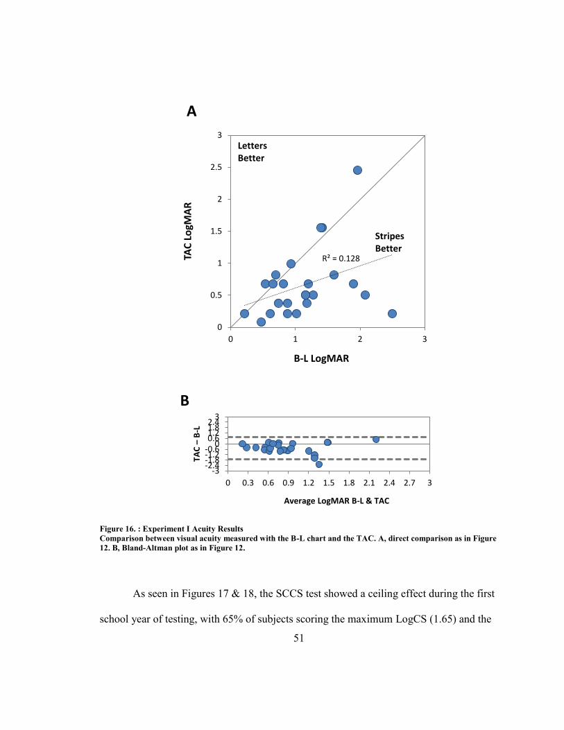
51

Figure 16. : Experiment I Acuity Results

Comparison between visual acuity measured with the B-L chart and the TAC. A, direct comparison as in Figure

12. B, Bland-Altman plot as in Figure 12.

As seen in Figures 17 & 18, the SCCS test showed a ceiling effect during the first

school year of testing, with 65% of subjects scoring the maximum LogCS (1.65) and the

R² = 0.128

0

0.5

1

1.5

2

2.5

3

0 1 2 3

TAC

Lo

gMA

R

B-L LogMAR

A

LettersBetter

StripesBetter

-3-2.4-1.8-1.2-0.6

00.61.21.82.4

3

0 0.3 0.6 0.9 1.2 1.5 1.8 2.1 2.4 2.7 3

TAC

–B

-L

Average LogMAR B-L & TAC

B

52

lower quartile scoring at least LogCS of 1.35. All contrast sensitivity plots have been

produced with negative values in order to maintain directional consistency with acuity

plots, where a lower value is indicative of better performance.

53

Figure 17. Experiment I P-R & SCCS Results

Comparisons between contrast sensitivity measured with the SCCS test and the Pelli-Robson chart. A, Direct

comparison as in Figure 12. B, Bland-Altman plot as in Figure 12.

R² = 0.2191

-2.25

-1.95

-1.65

-1.35

-1.05

-0.75

-0.45

-0.15

-2.25 -1.95 -1.65 -1.35 -1.05 -0.75 -0.45 -0.15

SCC

S Lo

gCS

Pelli-Robson LogCS

A

LettersBetter

StripesBetter

-2.25-1.65-1.05-0.450.150.751.351.95

-2.25 -1.95 -1.65 -1.35 -1.05 -0.75 -0.45 -0.15

SCC

S –

P-R

Average LogCS P-R & SCCS

B

54

Figure 17. Experime nt I P-R & SCC S Bins

Figure 18. Experiment I P-R & SCCS Bins

The number of subjects in each contrast sensitivity group for the Pelli-Robson and Stripe Card tests as shown in

Figure 17.

All but one of the subjects with impaired CS on the PR (according to Leat et al.,

PR<1.50) showed a better LogCS on the SCCS test than the PR test (sign test, p< 0.05, 2-

tailed; nonparametric test required because of the ceiling effect on the SCCS).

The results from the Berkeley Discs were also typically better than those found

with the Pelli-Robson chart as well, but not to the same degree as the SCCS test (as

shown in Figure 19).

0

2

4

6

8

10

12

14

16

18

2.1 1.95 1.8 1.65 1.5 1.35 1.2 1.05 0.9 0.75 0.6 0.45 0.3 0.15 0

Nu

mb

er o

f Su

bje

cts

LogCS

SCCS

P-R

55

Figure 19. Experiment I P-R & BD Results

Comparison between contrast sensitivity measured with the Berkeley Discs and the Pelli-Robson chart. A, direct

comparisons as in Figure 12. B, Bland-Altman plot as in Figure 12.

R² = 0.3637

-2.25

-1.95

-1.65

-1.35

-1.05

-0.75

-0.45

-0.15

-2.25 -1.95 -1.65 -1.35 -1.05 -0.75 -0.45 -0.15

BD

Lo

gCS

Pelli-Robson LogCS

A

LettersBetter

DiscsBetter

-2.25-1.65-1.05-0.450.150.751.351.95

-2.25 -1.95 -1.65 -1.35 -1.05 -0.75 -0.45 -0.15

BD

–P

-R

Average LogCS P-R & BD

B

56

Figure 20. Experiment I P-R & BD Bins

The number of subjects in each contrast sensitivity group for the Berkeley Discs and the Pelli-Robson chart as

shown in Figure 19.

A comparison was also possible between the results of the SCCS and Berkeley

Discs since both tests had a ceiling of 1.65 during the first year of testing. The data

corresponding to fifteen of the subjects below plot at the same location on the graph,

giving the appearance of less data than actually obtained. For this reason, bin count

figures have been generated to illustrate the level of overlap in our results.

0

2

4

6

8

10

12

14

2.1 1.95 1.8 1.65 1.5 1.35 1.2 1.05 0.9 0.75 0.6 0.45 0.3 0.15 0

Nu

mb

er o

f Su

bje

cts

LogCS

BD

P-R

57

Figure 21. Experiment I SCCS & BD Results

Comparison between contrast sensitivity measured by SCCS and BD. A, Direct comparison as in Figure 12. B,

Bland-Altman plot as in Figure 12.

R² = 0.1353

-2.25

-1.95

-1.65

-1.35

-1.05

-0.75

-0.45

-0.15

-2.25 -1.95 -1.65 -1.35 -1.05 -0.75 -0.45 -0.15

SCC

S Lo

gCS

BD LogCS

A

DiscsBetter

StripesBetter

-2.25-1.65-1.05-0.450.150.751.351.95

-2.25 -1.95 -1.65 -1.35 -1.05 -0.75 -0.45 -0.15

SCC

S -

BD

Average LogCS SCCS & BD

B

58

Figure 22. Experiment I SCCS & BD Bins

The number of subjects at each contrast level when tested with the Berkeley Discs and the SCCS test as shown in

figure 21.

Discussion for Experiment I

Both of the grating tests (SCCS and TAC) gave statistically significantly better

values than the corresponding letter charts. The average grating acuity value measured on

Teller cards was almost 3x better than the acuity value measured by the Bailey-Lovie

chart. Statistical analysis of our results by t-test demonstrated that the two acuity charts

gave significantly different results. Similarly, the contrast sensitivity values measured

with the SCCS were over 2x better than the Pelli-Robson values. Again, t-test results

show that the two charts give significantly different results.

Some of the inconsistency between the Pelli-Robson and SCCS test may be a

result of the LogCS 1.65 ceiling limiting the SCCS results. This fact affected our ability

0

2

4

6

8

10

12

14

16

18

2.1 1.95 1.8 1.65 1.5 1.35 1.2 1.05 0.9 0.75 0.6 0.45 0.3 0.15 0

Nu

mb

er o

f Su

bje

cts

LogCS

BD

SCCS

59

to employ a t-test without any reservations. We measured 2.4x the contrast sensitivity

despite this inability to measure lower levels of contrast during Experiment I. For

measuring contrast sensitivity in those with reduced vision, the simpler task and bolder

patterns of the SCCS may make it more likely to reveal the maximum performance that a

given patient can achieve.

The Berkeley Discs also demonstrated better results than the Pelli-Robson (a

factor of 2x), but not to the same level as the SCCS test (again, 2.4x). This was despite

the fact that both the BD and SCCS tests had the same LogCS 1.65 ceiling. Perhaps the

localization task for the BD test was more complex than for the SCCS.

There were also inconsistent BD responses by some subjects (report of seen

circles in blank areas), which make the test difficult to interpret at times. As you may

recall, we allowed our subjects to view every card face instead of skipping some.

Theoretically, the subjects should have seen every disc present on a card containing

contrast levels higher than previously detected. However, some of them failed to detect

all the discs on those card faces. In our case, we gave the participants credit for the lowest

contrast value reported, but this finding does affect the validity of our results.

60

Experiment II – Separate Eye Testing

Introduction to Experiment II

In this second phase of our study, we sought to examine each eye of our subjects

individually, whenever possible. We also opened up participation to students with no

measurable vision. These students without measurable vision were included to constrain

our vision-related quality of life data analysis, discussed under Experiment III. A second

information packet was mailed out to all students at the school in order to encourage

repeat assessments for some students, and to allow for the inclusion of students with no

measurable vision.

We also sought and obtained permission from the IRB to recruit participants from

OSSB’s summer camp activities. Angela Brown attended the registration event for

summer camp at OSSB between the first and second year of testing. She was able to

recruit interested participants by answering questions and distributing information

packets in person.

Methods for Experiment II

The methods for Experiment II were almost entirely the same as for Experiment I.

One difference was that all assessments were performed on each eye monocularly where

possible instead of just on the subject’s preferred eye. When both eyes were tested, the

right eye was tested first.

61

New SCCS cards were developed to extend our measurement range of LogCS

values from approximately 1.65 to 2.00. We calibrated the cards again prior to initiating

testing and found that our cards continue to be close enough to the nominal values for

good use.

The results below display testing performed on subjects allowing them to use each

eye to view our charts. We allowed subjects to use their “worse” eye (provided that they

had any measurable vision in that eye). Inclusion of testing for each eye, whenever

possible, for each subject in Experiment II rather than just the dominant (and presumably

better) eye as in Experiment I, was intended to increase the data at very low levels of

visual performance for comparison across the five vision tests.

Results for Experiment IIa: Repeat Testing

Table 4 below shows the re-test results for eleven subjects who also participated

in the Experiment I. Repeat testing was performed for at least one eye, and an additional

eye was measured when possible. The right eye was always tested first.

62

ID Age S Diagnosis Eye B-L

LogMAR

TAC

LogMAR

P-R

LogCS

SCCS

LogCS

BD

LogCS

01 17 M Optic Nerve Hypoplasia OD 1.58 1.11 0.85 1.95 1.05

01 17 M Optic Nerve Hypoplasia OS 1.32 0.68 1.20 2.00 1.05

12 16 M Retinopathy of Prematurity OS 0.68 0.68 1.90 2.00 1.65

17 14 F Microphthalmus OS 1.36 1.29 1.35 1.90 1.5

26 18 M Optic Nerve Hypoplasia OD 1.60 0.81 0.10 1.65 1.2

26 18 M Optic Nerve Hypoplasia OS 0.96 0.38 2.05 2.00 1.65

28 12 F Congenital Cataract OD 1.28 0.68 1.75 2.00 1.65

28 12 F Congenital Cataract OS 1.30 0.68 1.75 2.00 1.65

30 18 F Optic Atrophy OD 0.96 0.68 1.30 1.65 1.65

30 18 F Optic Atrophy OS 0.94 0.99 1.05 1.65 1.65

37 18 M Aniridia OD 0.96 0.38 1.50 1.65 1.65

37 18 M Aniridia OS 0.92 0.50 1.35 1.65 1.65

45† 20 F Optic Atrophy OD — 1.29 — 0.75 0

45† 20 F Optic Atrophy OS — 1.29 — 1.20 0.9

51 13 M Optic Atrophy OD 1.42 1.11 1.00 1.50 1.65

51 13 M Optic Atrophy OS 1.14 0.50 1.20 1.65 1.2

52 15 M Optic Atrophy OD 3.14 0.81 0.20 1.05 —

52 15 M Optic Atrophy OS 2.30 0.68 0.50 1.50 0.75

53 16 M Cortical Blindness OD 3.00 0.38 0.70 1.90 1.5

53 16 M Cortical Blindness OS 2.84 0.38 0.70 1.90 0.9

Table 4. Experiment IIa Participants

n = 11 (20 eyes tested)

†These subjects were not testable by lettered charts.

All test measurements are summarized in the table below, along with average

testing times per eye.

63

B-L TAC P-R SCCS* BD†

Mean 1.54 (20/689) 0.71 (20/101) 1.14 1.76 1.50 Median

STDev ± 0.76 ± 0.28 ± 0.56 ± 0.25 1.01 75th %

Time (sec) 65 ± 29 89 ± 67 76 ± 66 79 ± 43 57 ± 31 Time (sec)

Table 5. Experiment IIa Summary Test Results

*Unable to measure values better than 2.00

†Unable to measure values better than 1.65

Time of testing is for each individual eye. Note: if the calibrated P-R values are used, the results would be

0.30±0.15 LogCS higher.

Two-tailed t-test comparisons of findings for the acuity and contrast sensitivity

measures are shown below.

64

Figure 23. Experiment IIa Summary Plot Statistics

Conventions are as in Figure 11. The ceiling was extended for the SCCS test, so the average is reported and the

standard deviation is now shown for the SCCS error bar. The Berkeley Discs are still presented with median

and 75th percentile values. *The SCCS ceiling was LogCS 2.00 and the †Berkeley Discs ceiling was 1.65. Note: if

the calibrated values for the P-R are used, the difference between the P-R and the BD scores is no longer

statistically significant (p < .18)

Importantly, in Experiment II the SCCS test no longer had a ceiling of LogCS

1.65, but instead, we could measure up to LogCS 2.00. The Berkeley discs test continued

to have a ceiling of 1.65.

65

Figure 24. Experiment IIa Acuity Results

Comparison between acuity testing techniques of Teller Acuity and Bailey-Lovie Acuity for subjects for whom

we already have seen better-eye data in Experiment I. This plot includes repeat testing of the better eyes as well

as measurement of the worse eye where possible. All but two subjects contribute two eyes. A, Direct comparison

as in Figure 12. B, Bland-Altman plot as in Figure 12.

R² = 0.0133

0

0.5

1

1.5

2

2.5

3

0 1 2 3

TAC

Lo

gMA

R

B-L LogMAR

A

LettersBetter

StripesBetter

-3-2.4-1.8-1.2-0.6

00.61.21.82.4

3

0 0.3 0.6 0.9 1.2 1.5 1.8 2.1 2.4 2.7 3

TAC

–B

-L

Average LogMAR B-L & TAC

B

66

Figure 25. Experiment IIa P-R & SCCS Results

Comparison between contrast sensitivity values obtained by the SCCS test and the P-R chart for repeat

subjects’ better and worse eyes. All but two subjects contribute two eyes. A, Direct comparison as in Figure 12.

B, Bland-Altman plot.

R² = 0.3725

-2.25

-1.95

-1.65

-1.35

-1.05

-0.75

-0.45

-0.15

-2.25 -1.95 -1.65 -1.35 -1.05 -0.75 -0.45 -0.15

SCC

S Lo

gCS

Pelli-Robson LogCS

A

LettersBetter

StripesBetter

-2.25-1.65-1.05-0.450.150.751.351.95

-2.25 -1.95 -1.65 -1.35 -1.05 -0.75 -0.45 -0.15

SCC

S –

P-R

Average LogCS P-R & SCCS

B

67

Figure 26. Experiment IIa P-R & SCCS Bins

Number of subjects at each contrast sensitivity level when measured with the SCCS and P-R tests. These results

are not limited by a ceiling of 1.65 as in Experiment I. Instead, the SCCS has a ceiling of 2.00.

0

1

2

3

4

5

6

7

8

9

10

2.1 1.95 1.8 1.65 1.5 1.35 1.2 1.05 0.9 0.75 0.6 0.45 0.3 0.15 0

Nu

mb

er o

f Su

bje

cts

LogCS

SCCS

P-R

68

Figure 27. Experiment IIa SCCS & BD Results

Comparison between contrast sensitivity values measured with the BD test and the P-R chart. The BD test is

bounded by a ceiling of 1.65. A, Direct comparison as in Figure 12. B, Bland-Altman plot.

R² = 0.4349

-2.25

-1.95

-1.65

-1.35

-1.05

-0.75

-0.45

-0.15

-2.25 -1.95 -1.65 -1.35 -1.05 -0.75 -0.45 -0.15

BD

Lo

gCS

Pelli-Robson LogCS

A

LettersBetter

DiscsBetter

-2.25-1.65-1.05-0.450.150.751.351.95

-2.25 -1.95 -1.65 -1.35 -1.05 -0.75 -0.45 -0.15

BD

–P

-R

Average LogCS P-R & BD

B

69

Figure 28. Experiment IIa P-R & BD Bins

Number of subjects at various levels of contrast sensitivity when measured by BD and P-R tests. The BD test is

limited by a ceiling of 1.65.

0

1

2

3

4

5

6

7

8

9

10

2.1 1.95 1.8 1.65 1.5 1.35 1.2 1.05 0.9 0.75 0.6 0.45 0.3 0.15 0

Nu

mb

er o

f Su

bje

cts

LogCS

BD

P-R

70

Figure 29. Experiment IIa SCCS & BD Results

Comparison between contrast sensitivity measured with SCCS and BD test. Here, the SCCS is bounded by a

ceiling of 2.00, but the BD is bounded by a 1.65 ceiling. Many subjects obtained those ceiling values, resulting in

their data points plotting to the same spot on the graph. This gives the appearance of less data than was actually

obtained. A, Direct comparison as in Figure 12. B, Bland-Altman plot.

R² = 0.0068

-2.25

-1.95

-1.65

-1.35

-1.05

-0.75

-0.45

-0.15

-2.25 -1.95 -1.65 -1.35 -1.05 -0.75 -0.45 -0.15

SCC

S Lo

gCS

BD LogCS

A

DiscsBetter

StripesBetter

-2.25-1.65-1.05-0.450.150.751.351.95

-2.25 -1.95 -1.65 -1.35 -1.05 -0.75 -0.45 -0.15

SCC

S –

BD

Average LogCS SCCS & BD

B

71

Figure 30. Experiment IIa SCCS & BD Bins

Number of subjects at each contrast sensitivity level when measured with the BD and SCCS tests.

Repeatability between Experiments I and IIa. Since we had the opportunity to

retest eleven of our subjects, we were able to generate the graphs below. Naturally, these

subjects were a few months older during the retest than they were during the original

assessments, which may introduce some variability in test vs. retest findings. Figures 31-

33 demonstrate the value scored for the first eye tested next to the second eye(s)

examined.

0

1

2

3

4

5

6

7

8

9

10

2.1 1.95 1.8 1.65 1.5 1.35 1.2 1.05 0.9 0.75 0.6 0.45 0.3 0.15 0

Nu

mb

er o

f Su

bje

cts

LogCS

BD

SCCS

72

Figure 31. Experiment IIa Lettered Chart Test-Retest

Retest values for the better eyes of subjects who participated in Experiments I and IIa. Conventions are similar

to those in Figure 13. The fist test is shown to the left, and the repeat assessment follows to the right.

Figure 32. Experiment IIa Striped Chart Test-Retest

Retest values for the better eyes of subjects who participated in Experiments I and IIa. Conventions are similar

to those in Figure 13. The first test is shown to the left, and the repeat assessment follows to the right. The SCCS

was limited by a ceiling of 1.65 during Experiment I tests, but by 2.00 for Experiment IIa.

** **** **

-3.2-2.9-2.6-2.3

-2-1.7-1.4-1.1-0.8-0.5-0.20.10.40.7

11.31.61.92.22.52.83.1

Go

od

Lo

gCS

Lo

gMA

R

P

oo

r

** Unable

B-L Acuity

P-R Contrast Sensitivity

-3.2-2.9-2.6-2.3

-2-1.7-1.4-1.1-0.8-0.5-0.20.10.40.7

11.31.61.92.22.52.83.1

Go

od

Lo

gCS

Lo

gMA

R

P

oo

r TAC Acuity

SCCS Contrast Sensitiviy

73

Figure 33. Experiment IIa Shaped Chart Test-Retest

Retest values for the BD test shown with the average of each experiment’s acuity measurements as in Figure 15.

T-test comparisons demonstrate that the repeatability of our testing was good with

these subjects’ better eyes (Table 6).

B-L TAC P-R SCCS BD

p-value 2.11 1.20 1.90 3.60 0.121

Sig (<0.05) Not different Not different Not different Not different Not different

Table 6. Experiment IIa Repeatability Statistics

Results for Experiment IIb: New Subjects

Eight participants were students in the annual summer camps put on by OSSB.

Their subject ID numbers were #62-69. Ten of the subjects listed in the table below had

no measurable vision, but were able to provide quality of life data.

-3.2-2.9-2.6-2.3

-2-1.7-1.4-1.1-0.8-0.5-0.20.10.40.7

11.31.61.92.22.52.83.1

Go

od

Lo

gCS

Lo

gMA

R

P

oo

r Average B-L and TAC Acuity

BD Contrast Sensitivity

74

ID Age S Diagnosis Eye B-L

LogMAR

TAC

LogMAR

P-R

LogCS

SCCS

LogCS

BD

LogCS

31 16 M Retinoblastoma OD 0.98 0.68 1.75 2.00 1.65

54† 20 M Retinopathy of Prematurity — — — — — —

55† 19 F Leber's Congenital Amaurosis — — — — — —

56† 19 M Brain Tumor — — — — — —

57† 19 M Optic Nerve Hypoplasia — — — — — —

58 18 F Leber's Congenital Amaurosis OD 2.18 0.50 0.95 1.65 1.65

58 18 F Leber's Congenital Amaurosis OS 2.10 0.68 0.95 1.65 1.65

59† 20 M Retinopathy of Prematurity — — — — — —

60 18 M Retinopathy of Prematurity OD 1.56 0.99 1.00 1.50 0.6

6†0 18 M Retinopathy of Prematurity OS — 1.29 — 0.60 0.6

61 13 M Choroideremia OD 1.54 0.99 0.15 0.90 0.45

61 13 M Choroideremia OS 1.18 0.81 0.25 1.05 0.45

62 11 F Blind at age 2 (unexplained) OD 1.58 — 0.15 0.00 0.00

62 11 F Blind at age 2 (unexplained) OS 1.38 1.38 0.15 0.00 0.00

63 10 F Leber's Congenital Amaurosis OD 1.14 0.81 0.85 1.65 1.65

63 10 F Leber's Congenital Amaurosis OS 1.04 0.99 1.00 1.65 1.5

64 13 M Optic Atrophy OS 1.18 1.11 0.80 0.60 0.45

65 16 F Marfan's Disease OD 0.28 0.38 1.55 1.65 1.65

65 16 F Marfan's Disease OS 0.68 0.50 1.55 1.50 1.65

66 17 M High Myopia OD 0.08 0.21 2.00 1.50 1.65

67 10 M Cortical Blindness OS 1.79 0.99 0.90 1.20 1.35

68 12 M Aniridia OD 1.94 1.38 0.35 1.35 1.05

68 12 M Aniridia OS 1.04 0.68 1.80 2.00 1.65

69 14 M Retinopathy of Prematurity OD 0.98 0.99 1.40 1.90 1.65

69 14 M Retinopathy of Prematurity OS 0.98 0.68 1.55 2.00 1.65

70† 18 M Retinitis Pigmentosa — — — — — —

71 15 M Best's Disease OD 0.86 0.38 1.65 2.00 1.65

71 15 M Best's Disease OS 0.84 0.38 1.65 2.00 1.65

72 18 F Glaucoma OS 1.04 0.99 1.05 1.35 1.05

73† 17 F Optic Atrophy — — — — — —

74† 12 M Optic Nerve Hypoplasia — — — — — —

75† 12 M Retinopathy of Prematurity — — — — — —

76† 6 M Retinoblastoma — — — — — —

Table 7. Experiment IIb Participants

n = 34 (23 eyes tested)

†These subjects were not testable via lettered charts.

75

Result values of all test encounters with the new subjects are summarized in the

table below along with average testing times per eye. All but one student contributed two

eyes to these results.

B-L TAC P-R SCCS* BD†

Mean 1.20 (20/314) 0.79 (20/121) 1.07 1.41 1.65 Median

STDev ± 0.53 ± 0.32 ± 0.59 ± 0.59 0.71 75th %

Time (sec) 66 ± 45 86 ± 53 50 ± 26 49 ± 27 60 ± 39 Time (sec)

Table 8. Experiment IIb Summary Results

*Unable to measure values better than 2.00

†Unable to measure values better than 1.65

Time of testing is for each individual eye. Note: if the calibrated P-R values are used, the results would be

0.30±0.15 LogCS higher.

Two-tailed t-test comparisons of findings for the acuity and contrast sensitivity

measures are shown below.

76

Figure 34. Experiment IIb Summary Plot Statistics

Conventions are as in Figure 23.

The figures below are test results for new students who were added to the study in

the second year of testing and were not previously assessed.

B - L $ T A C

P - R S C C S * B D †

- 2 . 5

- 2

- 1 . 5

- 1

- 0 . 5

0

0 . 5

1

1 . 5

2

2 . 5

p < 0.01**

p < 0.71 p < 0.001**

p < 0.001**

77

Figure 35. Experiment IIb Acuity Results

Comparison of acuity measured by TAC and B-L for both eyes of new subjects during our second year of

testing. All but two subjects contribute two eyes. Conventions are as in Figure 12. A, Direct comparison, B,

Bland-Altman plot.

R² = 0.1467

0

0.5

1

1.5

2

2.5

3

0 1 2 3

TAC

Lo

gMA

R

B-L LogMAR

A

LettersBetter

StripesBetter

-3-2.4-1.8-1.2-0.6

00.61.21.82.4

3

0 0.3 0.6 0.9 1.2 1.5 1.8 2.1 2.4 2.7 3

TAC

–B

-L

Average LogMAR B-L & TAC

B

78

Figure 36. Experiment IIb P-R & SCCS Results

Comparison of contrast sensitivity values obtained by SCCS and P-R charts for new subjects. All but two

subjects contribute two eyes. Conventions are as in Figure 12. A, Direct comparison. B, Bland-Altman plot.

R² = 0.6142

-2.25

-1.95

-1.65

-1.35

-1.05

-0.75

-0.45

-0.15

-2.25 -1.95 -1.65 -1.35 -1.05 -0.75 -0.45 -0.15

SCC

S Lo

gCS

Pelli-Robson LogCS

A

LettersBetter

StripesBetter

-2.25-1.65-1.05-0.450.150.751.351.95

-2.25 -1.95 -1.65 -1.35 -1.05 -0.75 -0.45 -0.15

SCC

S –

P-R

Average LogCS P-R & SCCS

B

79

Figure 37. Experiment IIb P-R & SCCS Bins

Number of subjects at each contrast sensitivity level for the SCCS and P-R testing of new subjects. The SCCS is

bounded by a ceiling of LogCS 2.00.

0

1

2

3

4

5

6

7

2.1 1.95 1.8 1.65 1.5 1.35 1.2 1.05 0.9 0.75 0.6 0.45 0.3 0.15 0

Nu

mb

er o

f Su

bje

cts

LogCS

SCCS

P-R

80

Figure 38. Experiment IIb P-R & BD Results

Comparison of contrast sensitivity testing by BD and P-R chart for new subjects. The BD test is bounded by a

ceiling of 1.65. A, Direct comparison. B, Bland-Altman plot.

R² = 0.6582

-2.25

-1.95

-1.65

-1.35

-1.05

-0.75

-0.45

-0.15

-2.25 -1.95 -1.65 -1.35 -1.05 -0.75 -0.45 -0.15

BD

Lo

gCS

Pelli-Robson LogCS

A

LettersBetter

DiscsBetter

-2.25-1.65-1.05-0.450.150.751.351.95

-2.25 -1.95 -1.65 -1.35 -1.05 -0.75 -0.45 -0.15

BD

–P

-R

Average LogCS P-R & BD

B

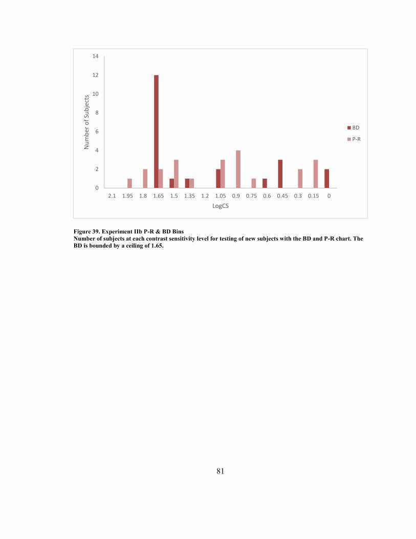
81

Figure 39. Experiment IIb P-R & BD Bins

Number of subjects at each contrast sensitivity level for testing of new subjects with the BD and P-R chart. The

BD is bounded by a ceiling of 1.65.

0

2

4

6

8

10

12

14

2.1 1.95 1.8 1.65 1.5 1.35 1.2 1.05 0.9 0.75 0.6 0.45 0.3 0.15 0

Nu

mb

er o

f Su

bje

cts

LogCS

BD

P-R

82

Figure 40. Experiment IIb SCCS & BD Results

Comparison of contrast sensitivity testing by BD and SCCS for new subjects. The BD is bounded by a 1.65

ceiling and the SCCS test by 2.00. Many subjects obtained the maximum values for each chart leading to their

data points plotting to the same location on the graphs. This gives the appearance of less data than actually

obtained. A, Direct comparison. B, Bland-Altman Plot.

R² = 0.8134

-2.25

-1.95

-1.65

-1.35

-1.05

-0.75

-0.45

-0.15

-2.25 -1.95 -1.65 -1.35 -1.05 -0.75 -0.45 -0.15

SCC

S Lo

gCS

BD LogCS

A

DiscsBetter

StripesBetter

-2.25-1.65-1.05-0.450.150.751.351.95

-2.25 -1.95 -1.65 -1.35 -1.05 -0.75 -0.45 -0.15

SCC

S –

BD

Average LogCS SCCS & BD

B

83

Figure 41. Experiment IIb SCCS & BD Bins

Number of new subjects at each contrast sensitivity level for the BD and SCCS tests. The BD is bounded by a

ceiling of 1.65, and the SCCS has a LogCS ceiling of 2.00.

Discussion for Experiment II

Some of the data that we have obtained through the efforts of Experiment I can be

added to the better eye results from Experiment II. In order to check correlations between

the five eye charts, it was necessary to generate a table containing test results for each

subject using only one eye—the better one. In the case of students tested only in

Experiment I, the results on the only tested eye appear. In the case of students tested in

both Experiment I and Experiment II, the results on the better eye in Experiment II are

listed. In the case of students tested only in Experiment II, the results on the better eye are

listed.

0

2

4

6

8

10

12

14

2.1 1.95 1.8 1.65 1.5 1.35 1.2 1.05 0.9 0.75 0.6 0.45 0.3 0.15 0

Nu

mb

er o

f Su

bje

cts

LogCS

BD

SCCS

84

ID Exp Diagnosis Eye B-L

LogMAR

TAC

LogMAR

P-R

LogCS

SCCS

LogCS

BD

LogCS

01 IIa Optic Nerve Hypoplasia OS 1.32 0.68 1.20 2.00 1.05

02 I Retinopathy of Prematurity OD 0.62 0.21 1.95 1.65 1.65

04 I Optic Nerve Hypoplasia OS 0.48 0.08 2.10 1.65 1.65

05 I Leber's Congenital Amaurosis OS 1.42 1.56 1.10 0.60 1.50

06 I Optic Nerve Hypoplasia OD 0.74 0.38 2.00 1.65 1.65

08 I Optic Atrophy OD 0.88 0.21 1.45 1.65 1.50

11 I High Myopia OD 0.94 0.99 1.35 1.65 1.65

12 IIa Retinopathy of Prematurity OS 0.68 0.68 1.90 2.00 1.65

17 IIa Microphthalmus OS 1.36 1.29 1.35 1.90 1.50

18 I Cone Dystrophy OS 0.7 0.81 1.40 1.65 1.65

24 I Optic Atrophy OS 1.16 0.5 1.65 1.65 1.35

26 IIa Optic Nerve Hypoplasia OS 0.96 0.38 2.05 2.00 1.65

28 IIa Congenital Cataract and Aphakia OD 1.28 0.68 1.75 2.00 1.65

30 IIa Optic Atrophy OS 0.94 0.99 1.05 1.65 1.65

31 IIb Retinoblastoma OD 0.98 0.68 1.75 2.00 1.65

34 I Congenital Cataract and Aphakia OD 0.22 0.21 1.65 1.65 1.50

35 I Retinopathy of Prematurity OD 0.82 0.68 1.75 1.65 1.65

36 I Optic Atrophy OS 1.6 0.81 0.90 1.65 1.65

37 IIa Aniridia OD 0.96 0.38 1.50 1.65 1.65

41 I Glaucoma OS 1.96 2.45 0.10 1.20 0.90

45 IIa Optic Atrophy OD — 1.29 — 0.75 0.00

46 I Cortical Blindness OD — 0.84 — 1.35 0.75

48 I Optic Atrophy OD 1.2 0.68 1.15 1.65 1.50

50 I Septo-Optic Dysplasia OS 1.9 0.68 0.70 1.50 0.30

51 IIa Optic Atrophy OS 1.14 0.5 1.20 1.65 1.20

52 IIa Optic Atrophy OS 2.3 0.68 0.50 1.50 0.75

53 IIa Cortical Blindness OD 3 0.38 0.70 1.90 1.50

58 IIb Leber's Congenital Amaurosis OS 2.1 0.68 0.95 1.65 1.65

60 IIb Retinopathy of Prematurity OD 1.56 0.99 1.00 1.50 0.60

61 IIb Choroideremia OS 1.18 0.81 0.25 1.05 0.45

62 IIb Blind at age 2 (unsure) OS 1.38 1.38 0.15 0.00 0.00

63 IIb Leber's Congenital Amaurosis OS 1.04 0.99 1.00 1.65 1.50

64 IIb Optic Atrophy OS 1.18 1.11 0.80 0.60 0.45

65 IIb Marfan's Disease OD 0.28 0.38 1.55 1.65 1.65

66 IIb High Myopia OD 0.08 0.21 2.00 1.50 1.65

67 IIb Cortical Blindness OS 1.79 0.99 0.90 1.20 1.35

68 IIb Aniridia OS 1.04 0.68 1.80 2.00 1.65

69 IIb Retinopathy of Prematurity OS 0.98 0.68 1.55 2.00 1.65

71 IIb Best’s Disease OD 0.86 0.38 1.65 2.00 1.65

72 IIb Glaucoma OS 1.04 0.99 1.05 1.35 1.05

Table 9. Experiment I & II Better Eye Only

n = 36 Subjects (36 eyes) Note: Subject 43 was not included here as he did not provide any QoL data.

85

This grouping of subjects allows for us to check for correlations across all the

tests we employed.

B-L TAC P-R SCCS* BD†

Mean 1.16 (20/287) 0.75 (20/112) 1.30 1.55 1.50 Median

STDev ± 0.58 ± 0.44 ± 0.54 ± 0.44 1.05 75th %

Time (sec) 62 ± 37 86 ± 60 61 ± 38 56 ± 32 47 ± 31 Time (sec)

Table 10. Experiment II Summary Results

*Unable to measure values better than 2.00

†Unable to measure values better than 1.65

Time of testing is for each individual eye. Note: if the calibrated P-R values are used, the results would be

0.30±0.15 LogCS higher.

86

Figure 42. Experiment II Summary Plot Statistics

Conventions are as in Figure 34. Here only one eye per subject is included—the better eye (or second test if

repeat data are available). Subject number 43 is not included in this analysis since he did not provide quality of

life data. Note: if the calibrated P-R values are compared to the SCCS, then p < 0.01.

When comparing results across the better eye for all subjects, all tests were

positively correlated with one another. These correlations were statistically significant in

all but one case—the B-L and the SCCS were not significantly correlated. As can be seen

in the table below, the B-L chart was most strongly correlated with the P-R, perhaps

because it was only other letter chart. The next strongest, correlation was with the TAC,

perhaps due to the fact that they are both acuity tests. Next, the BD showed a significant

correlation with the B-L chart, perhaps because both tests include a visual search

localization component where the stimulus to be detected or identified must be localized.

B - L T A C

P - R S C C S * B D †

- 2 . 5

- 2

- 1 . 5

- 1

- 0 . 5

0

0 . 5

1

1 . 5

2

2 . 5

p < 0.001**

p < 0.001** p < 0.001**

p < 0.05*

87

For the P-R chart, the strongest correlation was found with the BD test, followed

by the B-L chart, TAC and finally the SCCS. The SCCS was most strongly correlated

with the BD, followed by P-R, and then TAC.

88

PRLogCS TACLogMAR SCCSLogCS BDLogCS O&MScore IVI_C LVP-FVQ

BLLogMAR

Pearson Correlation .692** .401* .149 .389* .540 -.197 -.594**

Sig. (2-tailed) .000 .013 .372 .016 .057 .237 .000

N 38 38 38 38 13 38 33

PRLogCS

Pearson Correlation .653** .608** .738** .166 -.481** -.738**

Sig. (2-tailed)

.000 .000 .000 .588 .002 .000

N 38 38 38 13 38 33

TACLogMAR

Pearson Correlation .539** .450** .219 -.367* -.597**

Sig. (2-tailed)

.000 .004 .453 .020 .000

N 40 40 14 40 35

SCCSLogCS

Pearson Correlation .708** .165 -.576** -.512**

Sig. (2-tailed)

.000 .574 .000 .002

N 40 14 40 35

BDLogCS

Pearson Correlation .450 -.434** -.584**

Sig. (2-tailed) .106 .005 .000

N 14 50 45

Table 11: Test Chart Correlations

**. Correlation was very significant: at the 0.01 level (2-tailed).

*. Correlation was significant: at the 0.05 level (2-tailed).

Note: The table has been shaded to help the reader quickly visualize significant correlations (or the absence of correlation).

Subject 43 was not included in this analysis since he did not provide any QoL or O&M data. Table 13 Continued

89

Experiment III – Quality of Life and Orientation and Mobility

Vision-Related Quality of Life

Quality of life surveys were administered following vision testing for each

subject. In order to facilitate testing, we modified the surveys so that they would contain

appropriate phrasing (e.g., for one LVP-FVQ question: switch the word for a “rupee”

coin to a “nickel”). Copies of the verbal scripts actually used are in Appendix A. The first

five subjects tested (#01, 02, 05, 12, and 34) did not have the opportunity to complete the

LVP-FVQ, but did complete the IVI_C questionnaire. When both tests were

administered, the IVI_C was always administered before the LVP-FVQ. Although two

examiners were used, each participant was interviewed by the same examiner for both

surveys. Angela Brown administered 38 out of 50 IVI_C surveys (76%) and Greg

Hopkins administered the remainder.

We used a 26 item IVI_C survey, which included two questions that were

dropped when the IVI_C underwent Rasch analysis because they only received answers

in 4 out of 5 response categories (“Do you get the same information as the other

students?” and “…Are you confident about asking for help that you need?”).Our

research was initiated prior to the publication of the revised LVP-FVQ II survey, so we

did not have the opportunity to apply the new version.

90

Bradley Dougherty performed Rasch analysis on the results from the two surveys

that we used. The analysis generated person scores (and standard errors around those

scores) for each subject relative to the others who took the surveys. The Rasch analysis

was performed using all five-category responses, and the response option probability

curves were not ideal. Further work may require a three or four category structure.

Testing time for the IVI_C was 8 ± 9 minutes. Linear regressions for the IVI_C

versus the results for each eye chart are below. Error bars represent the standard error

value around the person scores for each participant. There were two subjects (marked

with the ∆ symbol), who could not perform letter acuity or contrast tasks, but were

testable with other charts. Subjects without measurable vision were spread apart on the x-

axis systematically for acuity and contrast plots.

91

Figure 43. IVI_C v B-L Regression

Data are for the better eye of all subjects with measurable vision. Subjects with no measurable vision are plotted

separately using open circles (not included in the regression trend line) by adding 0.25 LogMAR to the

maximum value for partially-sighted subjects and then systematically adding 0.01 LogMAR to shift each point

along the x-axis in order of subject number. Subjects marked with the ∆ symbol could not perform letter tasks.

Note: The B-L Chart was the only vision test not significantly correlated with the IVI_C results.

R² = 0.0387

-1.00

-0.50

0.00

0.50

1.00

1.50

2.00

2.50

3.00

0 0.5 1 1.5 2 2.5 3 3.5 4

IVI_

C P

erso

n S

core

B-L LogMAR Acuity

92

Figure 44. IVI_C vs. P-R Regression

Data are for the better eye of all subjects with measurable vision. Subjects with no measurable vision are plotted

separately (not included in the regression trend line) by starting at positive 0.25 LogCS and then systematically

shifting subjects along the x-axis by adding 0.0125 logCS in order of subject ID number.

R² = 0.2312

-1.00

-0.50

0.00

0.50

1.00

1.50

2.00

2.50

3.00

-2.5 -2 -1.5 -1 -0.5 0 0.5 1

IVI_

C P

erso

n S

core

P-R LogCS

93

Figure 45. IVI_C vs. TAC Regression

Data are for all subjects with measurable vision. Two subjects on this plot are included that could not be

measured via lettered charts. Their points have been marked with a ∆ symbol. Conventions for this plot are the

same as for Figure 43. Note: The TAC test was significantly correlated with the IVI_C only at the 0.05 level (2-

tailed).

R² = 0.1343

-1.00

-0.50

0.00

0.50

1.00

1.50

2.00

2.50

3.00

0 0.5 1 1.5 2 2.5 3 3.5 4

IVI_

C P

erso

n S

core

TAC LogMAR Acuity

94

Figure 46. IVI_C vs. SCCS Regression

Data are for the better eye of all subjects with measurable vision. Two subjects on this plot are included that

could not be measured via lettered charts. Their points have been marked with a ∆ symbol. Conventions for this

plot are the same as for Figure 44.

R² = 0.3313

-1.00

-0.50

0.00

0.50

1.00

1.50

2.00

2.50

3.00

-2.5 -2 -1.5 -1 -0.5 0 0.5 1

IVI_

C P

erso

n S

core

SCCS LogCS

95

Figure 47. IVI_C vs. BD Regression

Data are for the better eye of all subjects with measurable vision. Two subjects on this plot are included that

could not be measured via lettered charts. Their points have been marked with a ∆ symbol. Conventions for this

plot are the same as for Figure 44.

Testing time for the LVP-FVQ was 6 ± 2 minutes. Linear regressions for the

LVP-FVQ versus the results for each eye chart are below. Again, there were two subjects

(marked with the ∆ symbol), who could not perform letter acuity or contrast tasks, but

were testable with other charts.

R² = 0.1884

-1.00

-0.50

0.00

0.50

1.00

1.50

2.00

2.50

3.00

-2.5 -2 -1.5 -1 -0.5 0 0.5 1

IVI_

C P

erso

n S

core

BDLogCS

96

Figure 48. LVP-FVQ vs. B-L Regression

Data are for the better eye of all subjects with measurable vision. Conventions are the same as for Figure 43.

R² = 0.3525

-2

-1

0

1

2

3

4

0 0.5 1 1.5 2 2.5 3 3.5 4

LVP

-FV

Q P

erso

n S

core

B-L LogMAR Acuity

97

Figure 49. LVP-FVQ vs. P-R Regression

Data are for the better eye of all subjects with measurable vision. Conventions are the same as for figure 44.

R² = 0.5447

-2

-1

0

1

2

3

4

-2.5 -2 -1.5 -1 -0.5 0 0.5 1

LVP

-FV

Q P

erso

n S

core

P-R LogCS

98

Figure 50. LVP-FVQ vs. TAC Regression

Data are for the better eye of all subjects with measurable vision. Conventions are the same as for figure 43.

R² = 0.3569

-2

-1

0

1

2

3

4

0 0.5 1 1.5 2 2.5 3 3.5 4

LVP

_FV

Q P

erso

n S

core

TAC LogMAR Acuity

99

Figure 51. LVP-FVQ vs. SCCS Regression

Data are for the better eye of all subjects with measurable vision. Conventions are the same as for figure 44.

R² = 0.2623

-2

-1

0

1

2

3

4

-2.5 -2 -1.5 -1 -0.5 0 0.5 1

LVP

-FV

Q P

erso

n S

core

SCCS LogCS

100

Figure 52. LVP-FVQ vs. BD Regression

Data are for the better eye of all subjects with measurable vision. Conventions are the same as for figure 44.

Orientation and Mobility

We were able to obtain orientation and mobility data for nineteen of our subjects,

seven of whom had no measurable vision. We obtained the severity-of-need scores for

each student and modified the values by subtracting out the score for central visual

acuity. All other assessments by the orientation and mobility instructors (including

peripheral vision) were maintained in the score.

Linear regression for modified O&M severity-of-need score is displayed versus

the results for each eye chart. Those subjects without any vision have their O&M scores

displayed separately from those subjects with measurable vision. There was one subject

R² = 0.3407

-2

-1

0

1

2

3

4

-2.5 -2 -1.5 -1 -0.5 0 0.5 1

LVP

-FV

Q P

erso

n S

core

BDLogCS

101

(marked with a ∆ symbol), who could not perform letter acuity or contrast tasks, but was

testable with other charts. Subjects without measurable vision were spread apart on the x-

axis systematically for acuity and contrast plots. For the acuity plots, subjects with no

measurable vision begin at LogMAR 3.0 and then an additional 0.01 LogMAR was

added in the order of subject ID number. For the contrast sensitivity plots, subjects with

no measurable vision are shown on the positive side of the x-axis starting at zero and

adding 0.0125 logCS to each subject in order of ID number. All of the O&M regressions

below were appropriately related to the vision testing results, but none of them reach

statistical significance.

Figure 53. O&M vs. B-L Regression

Data are for the better eye of subjects with measurable vision. Subjects with no measurable vision are shown

separately (not included in the regression trend line) and spread out systematically on the x-axis. One subject

who could not complete letter charts is marked with a ∆ symbol.

R² = 0.2916

0

5

10

15

20

25

30

0 0.5 1 1.5 2 2.5 3 3.5

O&

M S

core

B-L LogMAR Acuity

102

Figure 54. O&M vs. P-R Regression

Data are for the better eye of subjects with measurable vision. Subjects with no measurable vision are shown

separately. One subject who could not complete lettered charts is marked with a ∆ symbol.

R² = 0.0275

0

5

10

15

20

25

30

-2.5 -2 -1.5 -1 -0.5 0 0.5

O&

M S

core

P-R LogCS

103

Figure 55. O&M vs. TAC Regression

Data are for the better eye of subjects with measurable vision. One subject is marked with a ∆ symbol because

that subject could not read lettered charts.

R² = 0.0478

0

5

10

15

20

25

30

0 0.5 1 1.5 2 2.5 3 3.5

O&

M S

core

TAC LogMAR Acuity

104

Figure 56. O&M vs. SCCS Regression

Data are for the better eye of subjects with measurable vision. One subject (marked with a ∆ symbol) could not

complete lettered charts.

Figure 57. O&M vs. BD Regression

Data are for the better eye of subjects with measurable vision. One subject is marked with a ∆ symbol. This

subject was only able to see the first circle on the BD test (LogCS 0.00).

R² = 0.0271

0

5

10

15

20

25

30

-2.5 -2 -1.5 -1 -0.5 0 0.5

O&

MSc

ore

SCCS LogCS

R² = 0.2027

0

5

10

15

20

25

30

-2.5 -2 -1.5 -1 -0.5 0 0.5

O&

M S

core

BDLogCS

105

Correlations for vision-related quality of life and orientation & mobility and our

vision test results are summarized in Table 15, where only the better eye for subjects with

measureable vision are included. Generally, the LVP-FVQ correlated best with our vision

testing, followed by the IVI_C and then the adjusted OMSRS scores (which do not

include central visual acuity). As expected, the two QoL surveys correlated positively and

highly significantly with one another. Taken as a whole, our contrast sensitivity testing

correlated with a higher significance level to the QoL metrics than our visual acuity

testing did. The IVI_C correlated appropriately with all vision tests, demonstrating that

higher ability scores match with lower LogMAR and better LogCS values. The

correlation between the IVI_C was highly significant with all charts except the TAC test

(2-tailed 0.05 level only). The B-L acuity chart was not significantly correlated with the

IVI_C. In addition, the LVP-FVQ correlated very significantly and appropriately with all

vision testing.

We adjusted the OMSRS data by removing “central acuity” from the total score.

It appears that the relationship between the adjusted O&M scores was appropriate for our

vision testing measures, where worse visual performance was indicative of greater need

for services and a higher score. Likewise, a higher O&M score related to a lower visual

ability level on both of our QoL surveys. However, the adjusted OMSRS data correlated

only with the LVP-FVQ, and only at the 0.05 level (2-tailed). Interestingly, if we

removed all vision data from the OMSRS, then the only significant correlation was with

B-L, and only at the 0.05 level (2-tailed). Otherwise, the O&M data we have obtained did

not correlate significantly with any of our vision tests. Clearly, our small sample size (13

106

subjects for letter charts and 14 for shaped charts) affected our power to detect

statistically significant relationships.

107

O&MScore IVI_C LVP-

FVQ

BLLogMAR PRLogCS TACLogMAR SCCSLogCS BDLogCS

IVI_C

Pearson

Correlation

-.372 .651** -.197 -.481** -.367* -.576** -.434**

Sig. (2-tailed) .097

.000 .237 .002 .020 .000 .005

N 21 45 38 38 40 40 40

LVP-FVQ

Pearson

Correlation

-.573* .651** -.594** -.738** -.597** -.512** -.584**

Sig. (2-tailed) .013 .000

.000 .000 .000 .002 .000

N 18 45 33 33 35 35 35

O&MScore

Pearson

Correlation

-.372 -.573* .540 .166 .219 .165 .450

Sig. (2-tailed)

.097 .013 .057 .588 .453 .574 .106

N 21 18 13 13 14 14 14

Table 12. QoL and O&M Correlations

**. Correlation was very significant: at the 0.01 level (2-tailed).

*. Correlation was significant: at the 0.05 level (2-tailed).

Note: conventions for this table are the same as for Table 14.

108

Discussion for Experiment III

Vision-Related Quality of Life. The IVI_C and LVP-FVQ can be administered

to students at OSSB, and it appears that scores were positively correlated with measures

of vision. However, some of the IVI_C content may not be well suited to students in

these specialized settings. Rehabilitation and classroom adaptations at OSSB are quite

good. It appears that the LVP-FVQ better targets the patient population at OSSB, as the

mean ability score for the survey participants was more closely aligned with the mean

item difficulty score of the survey.

It could be that some portion of the disability paradox was in play here: people

who are visually impaired place a higher value on vision than those who are not, yet

report better quality of life than expected (Albrecht & Devlieger, 1999). Perhaps with the

IVI_C (which contains social questions) we were not truly measuring functional reserve

but instead, overall happiness or some other construct. The high results we obtained on

the IVI_C could be due to the acclimation to vision loss that the student population at

OSSB exhibits. For instance, the least difficult question on the IVI_C by Rasch analysis

was: “Do your teachers understand your special needs?” Most people want to be happy,

and if they can find a way to adapt, they will be. The functional nature of the LVP-FVQ

may be better suited to assessing these students. Other measures like classroom

productivity may be appropriate as well.

Eight of our subjects were not OSSB students, but rather, were at OSSB for

summer camps. Their average person scores from the two surveys are shown in Figure 58

109

below. Generally, OSSB students with vision performed the best on the IVI_C. This

could be due to the fact that they are well adapted in their school environment. The

summer campers out performed OSSB students on the LVP-FVQ, perhaps due to the fact

that the LVP-FVQ is more functionally oriented, and these students function in

mainstream schools. In both cases, the OSSB students without measurable vision perform

the worst, and the difference is more dramatic on the LVP-FVQ. Error bars indicate the

standard error of measurement for each group. There were two blind students on the

LVP-FVQ who perceived their abilities to be quite high, resulting in a large range of

measurement for that group. One-way ANOVA analysis revealed a significant difference

between the subject groups (OSSB Partially-Sighted, Functionally Blind, and Summer

Campers) on the IVI_C only, but the effect was not confirmed by post-hoc analysis.

110

Figure 58. Average person scores for the IVI_C (left) and the LVP-FVQ (right)

Data are separated out by vision level and enrolment at OSSB.

The location of our summer school students relative to those other students who

took the two surveys can be seen on the subject-item maps in Figures 59 and 60. These

figures back up the assertion that summer campers generally perform better on the LVP-

FVQ than OSSB partially-sighted students and worse on the IVI_C.

It is also apparent from Figures 59 and 60 that the subject mean IVI_C is well

above the item mean. This confirms the fact that the IVI_C is perhaps more appropriate

for visually impaired students at mainstream schools and not at specialized school for the

blind settings.

111

Figure 60 demonstrates that the LVP-FVQ is better targeted for the subjects we

assessed, but our results do not follow a normal distribution. It is possible that increasing

the number of subjects would improve this distribution.

112

Figure 59. Subject-Item map for the IVI_C

Demonstrates Rasch-calibrated participant locations (x’s, left) and item locations (right). At the top of the map

are participants with higher perceived visual ability and questions thought to be more difficult. This map

demonstrates the targeting of the different response levels of each question to the respondents. Summer school

students have been marked with boxes. M, Mean; S, 1 SD from the mean; T, 2 SD from the mean.

113

Figure 60. Subject-Item map for the LVP-FVQ.

Conventions are the same as for Figure 59.

Linear regression between the Rasch-adjusted person scores for each individual

survey participant is demonstrated in Figure 61. It is clear that two functionally blind

subjects rated their perceived functional ability to be quite high on the LVP-FVQ, yet fell

in the middle of the pack (close to the y-axis) for the IVI_C. Likewise, there was one

subject in the functionally blind category on the IVI_C whose perceived visual ability

level was higher than the others in that group. His or her point can be found outlying the

trend line just above the abscissa.

114

Figure 61. Person Score Linear Regression of LVP-FVQ vs. IVI_C

Subjects with no measurable vision (or unable to perform lettered charts) are plotted with their standard errors

using the same symbol conventions as in Figure 39. All subjects are included in the regression in this case.

Orientation and Mobility. It does appear that, generally, subjects with

measurable vision receive a lower severity of need score. Thus, they need less time

devoted to orientation and mobility training. However, B-L acuity was the only factor

whose correlation reaches a level of statistical significance. This was despite the fact that

we adjusted the scores so as not to include B-L acuity. This may be due to the fact that

R² = 0.2436

-2

-1

0

1

2

3

4

-1 0 1 2 3

LVP

-FV

Q P

ers

on

Sco

re

IVI_C Person Score

115

the O&M teachers are aware of the child’s acuity and this awareness colors their

impressions for other items on the OMSRS.

We were only able to obtain a relatively small set of data for orientation and

mobility severity of need scores. This may affect our power to detect significant

statistical correlations.

116

General Discussion

Test Results

Our results in the tables above show that not all participants were able to complete

every aspect of the study protocol. Some participants (who were functionally blind) were

able to provide only quality of life questionnaire responses. We included those

participants for the purposes of balancing our Rasch analysis. We wanted to see if the

vision-related quality of life of functionally blind students tested as the same as those

with vision. It appears that they did not—students who lack measurable vision generally

clustered together at lower ability levels than sighted students. They were also generally

allocated more training time for orientation and mobility than their partially-sighted

classmates.

All vision tests were significantly correlated with one another except the B-L and

SCCS. This makes sense because the two charts are the least alike in terms of

measurement outcome and test methodology. As we hoped, we were able to measure a

variety of contrast sensitivity and acuity levels in this student population. However,

ceiling effects did come into play for some of our contrast sensitivity tests. Testing with

the striped cards (TAC and SCCS) cards consistently produced better results than the

lettered charts: B-L and P-R. With the SCCS cards, the majority of our subjects hit the

1.65 LogCS ceiling during our first year of testing. When we raised the ceiling to LogCS

2.00 for our second round of testing, again, the majority of subjects were able to see the

117

stripes on that card. The distribution of results for the P-R chart was much more

stratified—subjects who performed worse on the P-R chart gathered together with high

performing P-R subjects on the SCCS and BD test result graphs.

The Berkeley disc results were also better than the P-R test results, but were

limited by a 1.65 LogCS ceiling effect at all phases of our trial. The simpler task and

bolder patterns of the SCCS and the Berkeley Discs may make those tests more likely to

reveal the maximum performance that a given patient can achieve, even with the ceiling

in place. From the results of testing with a higher ceiling using the SCCS, it appears that

at least half of the subjects measured at 1.65 LogCS on the Berkeley Discs might have

been capable of 2.00 LogCS. These results are likely to be better transferrable to some

activities, such as O&M class, life skills, and gym. Performance in other courses, such as

English, Math, and Science may be better predicted by the results of our letter

identification tests.

Other Considerations

We did not screen for VF defects, which could affect a patient’s ability to locate

the discs within the grid or find the stimulus on the SCCS test. Based on my experience

testing these children, I believe that visual field status was only a factor during the testing

of three subjects: #5, #41 and #48.

Some subjects exhibited interesting behavior such as apparent malingering on the

Berkeley Discs and SCCS tests. One subject reported detecting our stimulus with his or

her “worse” eye on the blank half of the SCCS test 100% of the time (much higher than

chance) starting at the contrast threshold of the fellow and continuing all the way down to

118

the lowest contrast card. Perhaps he or she was unaware of the fact that intentionally

selecting the area absent a stimulus reveals the ability to discern stimulus location. On the

Berkeley Discs, several other subjects incorrectly reported discs in areas where none

were present. Perhaps this was in an attempt in their minds to try and get as many stimuli

identified as possible in an effort to boost their hit rate. It has been shown by other

investigators that children are much more prone to tolerating misses when reaching their

measurement thresholds, i.e., they’re willing to guess (Susan J Leat & Wegmann, 2004).

It is our opinion that these children were not intending to malinger, but instead were

experiencing false-positives throughout the entire test. This is because, given the design

of the Berkeley Discs, their threshold stimulus may be present in any cell on the grid.

Stated Objectives

Our goal was to ascertain whether the Stripe Card Contrast Sensitivity (SCCS)

Test was easy to administer and whether it could be successfully used on a wide variety

of participants. I believe that the test performed very well in this patient population and

would be appropriate to use in pediatric low vision settings whenever grating acuity

measurements are indicated.

We also wished to assess the SCCS test’s capability for validly quantifying

contrast sensitivity levels of children with impaired vision. It appears that this chart has

no trouble detecting the very high levels of contrast sensitivity performance that some

children with visual impairment are capable of. This is important because, while contrast

sensitivity measurement isn’t more useful than other standard examination procedures at

detecting disease, it does add valuable information regarding a patient’s expected level of

119

visual function. It seems that this patient population suffers less contrast impairment than

those who have visual impairment due to diseases more prevalent in the elderly such as

macular degeneration and diabetic retinopathy. However, we have not studied the SCCS

outside of the pediatric population as of yet.

Certainly, measurements from the SCCS test cannot be easily decimalized or

broken down in to smaller increments (such as LogCS 0.05) as is possible using letter-by-

letter scoring on the Pelli-Robson chart. This may affect the repeatability of the SCCS.

However, the target population for the SCCS is likely one where measurement by means

such as letter identification tasks simply isn’t possible. Test-retest variance would be

expected to be high in this group of patients for other functional reasons (such as autism

or developmental delay) and accuracy to the nearest 0.05 LogCS would not be a

consideration for most clinical examiners. It is likely that SCCS test results translate best

to daily living tasks for children that rely on low and middle spatial frequencies only such

as mobility, household, self-care, sports, and social activities. It may be useful to run the

SCCS test whenever input about a given student’s performance potential on these types

of tasks is a consideration for parents or educators.

I have calculated the SCCS contrast sensitivity values necessary for a subject to

have a vision-related quality of life score at the level found for the 75th percentile of our

functionally blind participants for both the IVI_C and the LVP-FVQ (See Figure 62).

Their contrast sensitivity would have to be approximately LogCS 1.02 for both the IVI_C

and the LVP-FVQ.

120

Figure 62. Cutoffs for normal SCCS Performance

The 75th percentile vision-related quality of life score was calculated for the students without measurable vision

and extended horizontally across the graph. The intersection point with the trend line was drawn vertically so

that the LogCS value on the abscissa demonstrates the expected contrast sensitivity level for partially-sighted

students with the same quality of life score. A, cutoff point for the IVI_C. B, cutoff point for the LVP-FVQ.

R² = 0.3313

-1.00

-0.50

0.00

0.50

1.00

1.50

2.00

2.50

3.00

-2.5 -2 -1.5 -1 -0.5 0 0.5 1

IVI_

C P

erso

n S

core

SCCS LogCS

A

R² = 0.2623

-2

-1

0

1

2

3

4

-2.5 -2 -1.5 -1 -0.5 0 0.5 1

LVP

-FV

Q P

erso

n S

core

SCCS LogCS

B

121

This means that successfully localizing the striped pattern on the SCCS test for

the LogCS 0.90 card (or worse) would be a reasonable cutoff indicative of performance

that is definitely abnormal. Indeed, this value corresponds well with cutoffs for

significantly impaired contrast sensitivity found in the literature and described in earlier

sections of this thesis (S J Leat & Woo, 1997; Susan J Leat et al., 1999; West et al.,

2002).

The findings in this section, taken together, demonstrate the Stripe Card Contrast

Sensitivity test to be a useful clinical measure for young, non-verbal or otherwise

developmentally delayed patients with visual impairment.

122

References

Adams, R. J., & Courage, M. L. (2003). Can the visual acuity of infants be predicted

from a measurement of contrast sensitivity? J Pediatr Ophthalmol Strabismus,

40(1), 35–38. Retrieved from

http://www.ncbi.nlm.nih.gov/entrez/query.fcgi?cmd=Retrieve&db=PubMed&dopt=

Citation&list_uids=12580270

Albrecht, G. L., & Devlieger, P. J. (1999). The disability paradox: high quality of life

against all odds. Social Science & Medicine (1982), 48(8), 977–88. Retrieved from

http://www.ncbi.nlm.nih.gov/pubmed/10390038

Arden, G. B. (1978). The importance of measuring contrast sensitivity in cases of visual

disturbance. British Journal of Ophthalmology, 62(4), 198–209.

doi:10.1136/bjo.62.4.198

Arditi, A. (2005). Improving the design of the letter contrast sensitivity test. Investigative

Ophthalmology & Visual Science, 46(6), 2225–9. doi:10.1167/iovs.04-1198

Bailey, I. L., Chu, M. A., Jackson, A. J., Minto, H., & Greer, R. B. (2011). Assessment of

vision in severely visually impaired populations. In ARVO Fort Lauderdale. Fort

Lauderdale, FL.

Bailey, I. L., & Lovie, J. (1976). New design principles for visual acuity letter charts. …

Journal of Optometry and Physiological Optics. Retrieved from

http://europepmc.org/abstract/MED/998716

Bennett, A. G. (1965). Ophthalmic test types. A review of previous work and discussions

on some controversial questions. The British Journal of Physiological Optics, 22(4),

238–71. Retrieved from http://www.ncbi.nlm.nih.gov/pubmed/5331332

Bittner, A. K., Jeter, P., & Dagnelie, G. (2011). Grating acuity and contrast tests for

clinical trials of severe vision loss. Optometry and Vision Science, 88(10), 1153–

1163.

Black, A. A., Lovie-Kitchin, J. E., Woods, R. L., Arnold, N., Byrnes, J., & Murrish, J.

(1997). Mobility performance with retinitis pigmentosa. Clinical Experimental

Optometry Journal of the Australian Optometrical Association, 80, 1–12. Retrieved

from http://dx.doi.org/10.1111/j.1444-0938.1997.tb04841.x

123

Blakemore, C., & Campbell, F. W. (1969a). Adaptation to spatial stimuli. The Journal of

Physiology. Retrieved from http://www.ncbi.nlm.nih.gov/pubmed/5761934

Blakemore, C., & Campbell, F. W. (1969b). On the existence of neurones in the human

visual system selectively sensitive to the orientation and size of retinal images. The

Journal of Physiology, 237–260. Retrieved from

http://jp.physoc.org/content/203/1/237.short

Bland, J. M., & Altman, D. G. (1986). Statistical methods for assessing agreement

between two methods of clinical measurement. Lance (Vol. 47, pp. 307–310).

Elsevier Ltd. Retrieved from http://www.ncbi.nlm.nih.gov/pubmed/2868172

Bochsler, T. M., Legge, G. E., Kallie, C. S., & Gage, R. (2012). Seeing steps and ramps

with simulated low acuity: impact of texture and locomotion. Optometry and Vision

Science, 89(9), E1299–307. doi:10.1097/OPX.0b013e318264f2bd

Campbell, F. W., Howell, E., & Robson, J. G. (1970). The appearance of gratings with

and without the fundamental Fourier component. The Journal of Physiology, 193–

201. Retrieved from http://europepmc.org/abstract/MED/5571919

Campbell, F. W., & Robson, J. G. (1968). Application of Fourier analysis to the visibility

of gratings. The Journal of Physiology, 197(3), 551. Retrieved from

http://www.ncbi.nlm.nih.gov/pmc/articles/PMC1351748/

Cochrane, G. M., Lamoureux, E. L., & Keeffe, J. E. (2008). Defining the content for a

new quality of life questionnaire for students with low vision (the Impact of Vision

Impairment on Children: IVI_C). Ophthalmic Epidemiology, 15(2), 114–20.

doi:10.1080/09286580701772029

Cochrane, G. M., Marella, M., Keeffe, J. E., & Lamoureux, E. L. (2011). The Impact of

Vision Impairment for Children (IVI_C): validation of a vision-specific pediatric

quality-of-life questionnaire using Rasch analysis. Investigative Ophthalmology &

Visual Science, 52(3), 1632–40. doi:10.1167/iovs.10-6079

DeCarlo, D. K., McGwin, G., Bixler, M. L., Wallander, J., & Owsley, C. (2012). Impact

of pediatric vision impairment on daily life: results of focus groups. Optometry and

Vision Science : Official Publication of the American Academy of Optometry, 89(9),

1409–16. doi:10.1097/OPX.0b013e318264f1dc

Dobson, V., & Teller, D. Y. (1978). Visual acuity in human infants: a review and

comparison of behavioral and electrophysiological studies. Vision Research, 18(11),

1469–83. Retrieved from http://www.ncbi.nlm.nih.gov/pubmed/364823

124

Dorr, M., Lesmes, L. a, Lu, Z.-L., & Bex, P. J. (2013). Rapid and reliable assessment of

the contrast sensitivity function on an iPad. Investigative Ophthalmology & Visual

Science, 54(12), 7266–73. doi:10.1167/iovs.13-11743

Dougherty, B. E., Flom, R. E., & Bullimore, M. A. (2005). An evaluation of the Mars

Letter Contrast Sensitivity Test. Optometry and Vision Science, 82(11), 970–5.

Retrieved from http://www.ncbi.nlm.nih.gov/pubmed/16317373

Eperjesi, F., Wolffsohn, J., Bowden, J., Napper, G., & Rubinstein, M. (2004). Normative

contrast sensitivity values for the back-lit Melbourne Edge Test and the effect of

visual impairment. Ophthalmic & Physiological Optics : The Journal of the British

College of Ophthalmic Opticians (Optometrists), 24(6), 600–6. doi:10.1111/j.1475-

1313.2004.00248.x

Ferris, F. L., Kassoff, A., Bresnick, G. H., & Bailey, I. L. (1982). New visual acuity

charts for clinical research. American Journal of Ophthalmology, 94(1), 91–96.

Retrieved from http://www.ncbi.nlm.nih.gov/pubmed/7091289

Frantz, R. L., Ordy, J. M., & Udelf, M. S. (1962). Maturation of pattern vision in infants

during the first six months. Journal of Comparative and Physiological Psychology.

doi:10.1037/h0044173

Geruschat, D., Turano, K. A., & Stahl, J. (1998). Traditional Measures of Mobility

Performance and Retinitis Pigmentosa. Optometry & Vision Science, 75(7), 525–

537. Retrieved from

http://journals.lww.com/optvissci/Abstract/1998/07000/Traditional_Measures_of_M

obility_Performance_and.22.aspx

Ginsburg, A. P. (2003). Contrast sensitivity and functional vision. International

Ophthalmology Clinics, 43(2), 5–15. Retrieved from

http://www.ncbi.nlm.nih.gov/pubmed/12711899

Goodrich, G. L., & Ludt, R. (2003). Assessing visual detection ability for mobility in

individuals with low vision. Visual Impairment Research, 5(2), 57–71. Retrieved

from http://informahealthcare.com/doi/abs/10.1076/vimr.5.2.57.26265

Gothwal, V. K., Lovie-Kitchin, J. E., & Nutheti, R. (2003). The Development of the LV

Prasad-Functional Vision Questionnaire: A Measure of Functional Vision

Performance of Visually Impaired Children. Investigative Ophthalmology & Visual

Science, 44(9), 4131–4139. doi:10.1167/iovs.02-1238

Gothwal, V. K., & Sumalini, R. (2012). The Second Version of the LV Prasad-Functional

Vision Questionnaire. Optometry & Vision Science, 89(11), 1601–10.

doi:10.1097/OPX.0b013e31826ca291

125

Haymes, S. A., Roberts, K. F., Cruess, A. F., Nicolela, M. T., LeBlanc, R. P., Ramsey,

M. S., … Artes, P. H. (2006). The letter contrast sensitivity test: clinical evaluation

of a new design. Investigative Ophthalmology & Visual Science, 47(6), 2739–45.

doi:10.1167/iovs.05-1419

Hubel, D., & Wiesel, T. (1962). Receptive fields, binocular interaction and functional

architecture in the cat’s visual cortex. The Journal of Physiology, 106–154.

Retrieved from http://www.ncbi.nlm.nih.gov/pmc/articles/PMC1359523/

Kirby, R., & Basmajian, J. (1984). The nature of disability and handicap. In Medical

Rehabilitation (pp. 14–18). Baltimore: Williams & Wilkins.

Kollbaum, P. (2014). Validation of an iPad test of letter contrast sensitivity. Optometry

and Vision Science: 91(3), 291–296. Retrieved from

http://pdfs.journals.lww.com/optvissci/9000/00000/Validation_of_an_iPad_Test_of

_Letter_Contrast.99023.pdf

Kramer, S. G., & Mcdonald, M. A. (1986). Diagnostic and surgical techniques,

assessment of visual acuity in toddlers. Survey of Ophthalmology, 31(3), 189–210.

Kuyk, T., Elliot, J., & Fuhr, P. (1998). Visual correlates of mobility in real world settings

in older adults with low vision. Optometry & Vision Science, 75(7), 538–547.

Retrieved from

http://journals.lww.com/optvissci/abstract/1998/07000/visual_correlates_of_mobilit

y_in_real_world.23.aspx

Leat, S. J., Legge, G. E., & Bullimore, M. A. (1999). What is low vision? A re-evaluation

of definitions. Optometry & Vision Science, 76(4), 198–211. Retrieved from

http://journals.lww.com/optvissci/Abstract/1999/04000/What_Is_Low_Vision__A_

Re_evaluation_of_Definitions.23.aspx

Leat, S. J., & Wegmann, D. (2004). Clinical testing of contrast sensitivity in children:

age-related norms and validity. Optometry and Vision Science, 81(4), 245–54.

Retrieved from http://www.ncbi.nlm.nih.gov/pubmed/15097766

Leat, S. J., & Woo, G. C. (1997). The validity of current clinical tests of contrast

sensitivity and their ability to predict reading speed in low vision. Eye (London,

England), 11 ( Pt 6)(519), 893–9. doi:10.1038/eye.1997.228

Lennie, P., & Hemel, S. B. V. (2002). Visual impairments: determining eligibility for

social security benefits. National Academy Press. Retrieved from

http://books.google.com/books?id=5QbtT8rzJcwC

126

Long, R., Rieser, J., & Hill, E. (1990). Mobility in individuals with moderate visual

impairments. Journal of Visual Impairment & Blindness, 84, 111–118.

Lovie-Kitchin, J. E., Bevan, J. D., & Hein, B. (2001). Reading performance in children

with low vision. Clinical & Experimental Optometry : Journal of the Australian

Optometrical Association, 84(3), 148–154. Retrieved from

http://www.ncbi.nlm.nih.gov/pubmed/12366326

Marron, J. A., & Bailey, I. L. (1982). Visual factors and orientation-mobility

performance. American Journal of Optometry and Physiological Optics, 59(5), 413–

426.

Massof, R. W. (1998). A systems model for low vision rehabilitation II. Measurement of

vision disabilities. Optometry & Vision Science, 75(5), 349. Retrieved from

http://journals.lww.com/optvissci/Abstract/1998/05000/A_Systems_Model_for_Lo

w_Vision_Rehabilitation__II_.25.aspx

Massof, R. W. (2002). The measurement of vision disability. Optometry and Vision

Science, 79(8), 516–52. Retrieved from

http://www.ncbi.nlm.nih.gov/pubmed/12199545

Mayer, D. L., Beiser, a S., Warner, a F., Pratt, E. M., Raye, K. N., & Lang, J. M. (1995).

Monocular acuity norms for the Teller Acuity Cards between ages one month and

four years. Investigative Ophthalmology & Visual Science, 36(3), 671–85. Retrieved

from http://www.ncbi.nlm.nih.gov/pubmed/7890497

McDonald, M. A., Dobson, V., Sebris, S. L., Baitch, L., Varner, D., & Teller, D. Y.

(1985). The acuity card procedure: a rapid test of infant acuity. Investigative

Ophthalmology & Visual Science, 2, 1158–1162. Retrieved from

http://www.iovs.org/content/26/8/1158.short

Owsley, C. (2003). Contrast sensitivity. Ophthalmology Clinics of North America, 16(2),

171–177. doi:10.1016/S0896-1549(03)00003-8

Owsley, C., & Sloane, M. E. (1987). Contrast sensitivity, acuity, and the perception of

“real-world” targets. The British Journal of Ophthalmology, 71(10), 791–796.

Retrieved from

http://www.ncbi.nlm.nih.gov/entrez/query.fcgi?cmd=Retrieve&db=PubMed&dopt=

Citation&list_uids=3676151

Pelli, D. G., & Bex, P. (2013). Measuring contrast sensitivity. Vision Research, 90, 10–4.

doi:10.1016/j.visres.2013.04.015

127

Pelli, D. G., Robson, J. G., & Wilkins, A. J. (1988). The design of a new letter chart for

measuring contrast sensitivity. Clin Vis Sci, 2(3), 187–199. Retrieved from

http://scholar.google.com/scholar?hl=en&btnG=Search&q=intitle:THE+DESIGN+

OF+A+NEW+LETTER+CHART+FOR+MEASURING+CONTRAST+SENSITIVI

TY#0

Pokusa, J. E., Kran, B. S., & Mayer, L. (2013). A pilot study of a preferential looking

contrast sensitivity test for individuals with vision and/or multiple impairments.

Seattle, WA.

Raasch, T. W., Bailey, I. L., & Bullimore, M. A. (1998). Repeatability of visual acuity

measurement. Optometry and Vision Science Official Publication of the American

Academy of Optometry, 75, 342–348. Retrieved from

http://www.ncbi.nlm.nih.gov/entrez/query.fcgi?cmd=Retrieve&db=PubMed&dopt=

Citation&list_uids=9624699

Rabin, J., & Wicks, J. (1996). Measuring resolution in the contrast domain: the small

letter contrast test. Optometry & Vision Science, 73, 398–403.

doi:10.1097/00006324-199606000-00007

Rasch, G. (1960). Probabilistic models for some intelligence and attainment tests.

Copenhagen.

Ratliff, F. (1965). Mach bands : quantitative studies on neural networks in the retina. San

Francisco, CA: Holden-Day.

Reeves, B. C., Wood, J. M., & Hill, A. R. (1991). Vistech VCTS 6500 charts--within-

and between-session reliability. Optometry and Vision Science, 68(9), 728–737.

Shapley, R. M., & Lam, D. (1993). Contrast Sensitivity. Cambridge, Mass: MIT Press.

Sloan, L. (1959). New test charts for the measurement of visual acuity at far and near

distances. American Journal of Ophthalmology, 48(Dec), 807–813.

Tandon, J. H. (1994). Nothing more can be done...a fable for our times. Ophthalmology,

(7), 203–205.

Tasman, W. (1992). Duane’s Foundations of Clinical Ophthalmology. Philadelphia, PA:

Lippincott Williams & Wilkins.

The World Health Organization. (1980). International Classification of Impairments,

Disabilities, and Handicaps (ICDH). Geneva: World Health Organization.

128

West, S. K., Rubin, G. S., Broman, A. T., & Mun, B. (2002). How does visual

impairment affect performance on tasks of everyday life?, 120(June).

Wilkins, A. J., Della Sala, S., Somazzi, L., & Nimmo-Smith, I. (1988). Age-related

norms for the Cambridge Low Contrast Gratings, including details concerning their

design and use. Clin Vis Sci, 2(3), 201–212. Retrieved from

http://www.essex.ac.uk/psychology/overlays/1988-75.pdf

Wolffsohn, J. S., Eperjesi, F., & Napper, G. (2005). Evaluation of Melbourne edge test

contrast sensitivity measures in the visually impaired. Ophthalmic & Physiological

Optics : The Journal of the British College of Ophthalmic Opticians (Optometrists),

25(4), 371–4. doi:10.1111/j.1475-1313.2005.00282.x

129

Appendix A: Study Materials

130

131

Dear Parent/Guardian,

We would like to share this invitation with you so that your child may join us (perhaps for the second time) in a

collaborative research study. As you may already know, the goal of our study will be to develop a new way to

measure a person’s ability to sense the contrast between light, gray, and dark. Unlike previous methods of measuring

the ability to sense contrast, this method will not require the patient to read the letters of an eye chart.

We would like to ask your child to take part in this study because s/he is partially sighted. If your child agrees to enter

the study, we may:

Ask your child some questions to find out how greatly his/her vision affects him/her in everyday life.

Measure his/her vision using regular lettered eye charts and charts with shapes

Measure his/her ability to see different shades of gray using letters and shapes

Give your child a $5 gift card to thank them for their help with our project.

If you give your permission for your child to participate, s/he will have the opportunity to choose not to participate. If

your child is uncomfortable answering any of the questions, s/he may just skip the questions s/he does not like. This

test does not involve eye drops of any kind. We will be testing one eye at a time, so we will ask your child to wear a

“pirate” type eye patch during testing. However, if your child prefers not to wear it, we will not insist. We do not need

to touch your child in any way, although we will be happy to help him/her put on the eye patch if s/he needs it.

If you wish to allow your child to participate, please read and sign the permission form, as well as the HIPAA form.

These are the standard forms that are used any time human subjects are involved in research projects. Please

complete and return all of the provided forms to us.

If you do NOT wish to allow your child to participate, please complete and return the response form enclosed with

this letter. On this form, you may request that we will remove your contact information from our records so that we

will not contact you again about this project.

If you have any questions or concerns about your child’s participation in this study, please do not hesitate to contact

us.

Thank you for your consideration and for potentially allowing your child to participate in our study!

Sincerely yours,

Angela M Brown, PhD Professor The OSU College of Optometry abrown@optometry.osu.edu o: 614-292-4423

Gregory R Hopkins, OD Senior Research Associate OSSB Extern Site Preceptor ghopkins@optometry.osu.edu o: 614-688-5542

Bradley E Dougherty, OD, MS OSU Clinical Attending Optometrist The OSU College of Optometry bdougherty@optometry.osu.edu

PARENTAL PERMISSION Biomedical/Cancer

IRB Protocol Number: 2011H0350

IRB Approval date: 4/4/12

Version: 2.0

132

The Ohio State University Parental Permission

For Child’s Participation in Research

Study Title: Pilot Study Pilot Study validation of the Stripe Card Contrast Sensitivity Test on

low-vision participants

Principal

Investigator: Angela M Brown, PhD

Sponsor:

The Center for Clinical and Translational Science

of the National Institutes of Health

National Eye Institute of the National Institutes of Health

This is a parental permission form for research participation. It contains important

information about this study and what to expect if you permit your child to participate. Please consider the

information carefully. Feel free to discuss the study with your friends and family and to ask questions

before making your decision whether or not to permit your child to participate.

Your child’s participation is voluntary. You or your child may refuse participation in this study.

If your child takes part in the study, you or your child may decide to leave the study at any time.

No matter what decision you make, there will be no penalty to your child and neither you nor your

child will lose any of your usual benefits.

Your decision will not affect your future relationship with The Ohio State University. If you

or your child is a student or employee at Ohio State, your decision will not affect your grades or

employment status.

Your child may or may not benefit as a result of participating in this study. Also, as explained

below, your child’s participation may result in unintended or harmful effects for him or her that

may be minor or may be serious depending on the nature of the research.

You and your child will be provided with any new information that develops during the

study that may affect your decision whether or not to continue to participate. If you permit

your child to participate, you will be asked to sign this form and will receive a copy of the form.

You are being asked to consider permitting your child to participate in this study for the reasons

explained below.

1. Why is this study being done?

This study is being done to develop a new method of measuring visual function in infants and children.

2. How many people will take part in this study?

56

PARENTAL PERMISSION Biomedical/Cancer

IRB Protocol Number: 2011H0350

IRB Approval date: 4/4/12

Version: 2.0

133

3. What will happen if my child takes part in this study?

Your child will have five vision tests: two visual acuity tests (one with letters and one with stripes) and

three contrast sensitivity tests (one with letters, one with stripes, and one with circles). Your child may also

be interviewed using a questionnaire to determine what impact his/her vision has on his/her everyday life.

This study does not involve any eye drops, and we will not be puffing your child’s eyes, or touching his/her

eyes in any way.

4. How long will my child be in the study?

For up to three sessions only, lasting no more than a half hour each.

5. Can my child stop being in the study?

Your child may leave the study at any time. If you or your child decides to stop participation in the study,

there will be no penalty and neither you nor your child will lose any benefits to which you are otherwise

entitled. Your decision will not affect your future relationship with The Ohio State University.

6. What risks, side effects or discomforts can my child expect from being in the study?

These tests are not associated with any known risks, side effects or discomforts.

7. What benefits can my child expect from being in the study?

We do not anticipate that your child will benefit from being in this study.

8. What other choices does my child have if he/she does not take part in the study?

You or your child may choose not to participate without penalty or loss of benefits to which you are

otherwise entitled.

9. Will my child’s study-related information be kept private?

Efforts will be made to keep your child’s study-related information confidential. However, there may be

circumstances where this information must be released. For example, personal information regarding your

child’s participation in this study may be disclosed if required by state law.

Also, your child’s records may be reviewed by the following groups (as applicable to the research):

Office for Human Research Protections or other federal, state, or international regulatory agencies;

U.S. Food and Drug Administration;

PARENTAL PERMISSION Biomedical/Cancer

IRB Protocol Number: 2011H0350

IRB Approval date: 4/4/12

Version: 2.0

134

The Ohio State University Institutional Review Board or Office of Responsible Research

Practices;

The sponsor supporting the study, their agents or study monitors; and

Your insurance company (if charges are billed to insurance).

If this study is related to your child’s medical care, your child’s study-related information may be placed in

their permanent hospital, clinic, or physician’s office records. Authorized Ohio State University staff not

involved in the study may be aware that your child is participating in a research study and have access to

your child’s information.

You may also be asked to sign a separate Health Insurance Portability and Accountability Act (HIPAA)

research authorization form if the study involves the use of your child’s protected health information.

10. What are the costs of taking part in this study?

There are no costs associated with participating in this study.

11. Will I or my child be paid for taking part in this study?

We will offer your child a gift card of $5.00. By law, payments to subjects are considered taxable income.

12. What happens if my child is injured because he/she took part in this study?

If your child suffers an injury from participating in this study, you should notify the researcher or study

doctor immediately, who will determine if your child should obtain medical treatment at The Ohio State

University Medical Center.

The cost for this treatment will be billed to you or your medical or hospital insurance. The Ohio State

University has no funds set aside for the payment of health care expenses for this study.

13. What are my child’s rights if he/she takes part in this study?

If you and your child choose to participate in the study, you may discontinue participation at any time

without penalty or loss of benefits. By signing this form, you do not give up any personal legal rights your

child may have as a participant in this study.

You and your child will be provided with any new information that develops during the course of the

research that may affect your decision whether or not to continue participation in the study.

You or your child may refuse to participate in this study without penalty or loss of benefits to which you

are otherwise entitled.

PARENTAL PERMISSION Biomedical/Cancer

IRB Protocol Number: 2011H0350

IRB Approval date: 4/4/12

Version: 2.0

135

An Institutional Review Board responsible for human subjects research at The Ohio State University

reviewed this research project and found it to be acceptable, according to applicable state and federal

regulations and University policies designed to protect the rights and welfare of participants in research.

14. Who can answer my questions about the study?

For questions, concerns, or complaints about the study you may contact Dr Angela M Brown, Professor,

the Ohio State University College of Optometry. 614-292-4423.

For questions about your child’s rights as a participant in this study or to discuss other study-related

concerns or complaints with someone who is not part of the research team, you may contact Ms. Sandra

Meadows in the Office of Responsible Research Practices at 1-800-678-6251.

If your child is injured as a result of participating in this study or for questions about a study-related injury,

you may contact Dr Angela M Brown.

Signing the parental permission form

I have read (or someone has read to me) this form and I am aware that I am being asked to provide

permission for my child to participate in a research study. I have had the opportunity to ask questions and

have had them answered to my satisfaction. I voluntarily agree to permit my child to participate in this

study.

I am not giving up any legal rights by signing this form. I will be given a copy of this form.

Printed name of subject

Printed name of person authorized to provide

permission for subject

Signature of person authorized to provide

permission for subject

AM/PM

Relationship to the subject Date and time

PARENTAL PERMISSION Biomedical/Cancer

IRB Protocol Number: 2011H0350

IRB Approval date: 4/4/12

Version: 2.0

136

Investigator/Research Staff

I have explained the research to the participant or his/her representative before requesting the signature(s)

above. There are no blanks in this document. A copy of this form has been given to the participant or

his/her representative.

Printed name of person obtaining consent Signature of person obtaining consent

AM/PM

Date and time

137

OSU-OSSB Contrast Sensitivity Study Response Form

Student Name: <Insert Name>

If at all possible, please use the enclosed envelope to return these forms to us within 10 days. If

we have not heard back from you after that time, you may be contacted via telephone or email

regarding this study. Thank you for your consideration regarding our collaborative research

study!

The Ohio State University College of Optometry Visual Perception Lab has contacted me to

invite my child to participate in a research project:

YES NO

I have completed and will enclose:

1. Parental Permission Form:

Filled-out/signed/dated top portion of the final page

2. Personal Health Information in Research Form:

Printed child’s name on first page

Initialed/dated bottom corner of first two pages

Signed/filled-out bottom portion of final page.

I prefer that my child

NOT participate in this study

I will return only this

form using the enclosed

envelope

Please remove our contact

information from your

records for the purpose of

this study

Parent/Guardian Signature: X ______________________________________________

Comments:

______________________________________________________________________________

______________________________________________________________________________

138

Verbal Consent Script

Pilot Study validation of the Stripe Card Contrast Sensitivity Test on Low-Vision Participants

Angela M Brown, PhD

Principal Investigator

Funded by the Center for Clinical and Translational Science and the National Eye Institute.

Hi, [student’s name]. My name is Dr/Mr/Ms [first tester’s name], and Dr/Mr/Ms [second

tester’s name] will be helping out today with this research project. If it’s OK with you, we want to test

your vision each of your eyes separately, and ask you some questions about your life (if we haven’t

already).

The goal of our study will be to develop a new way to measure a person’s ability to sense the

contrast between light, gray, and dark. The tests of your vision won’t be hard: you’ll just read five

different eye charts, two with letters and three with shapes. The questions about your life won’t be

hard at all either, since there are no “right” or “wrong” answers to any of them.

The information that you share with us will help us to learn how to do a better job testing

the vision of other students like yourself.

This project will take up to one half-hour of your time and after you finish, we will give you a $5 gift

card to say “thank you” for helping us today

There is a small risk of a breach of confidentiality, but all efforts will be made to keep everything we

learn about you in the strictest confidentiality. We will not link your name to anything that you say in

any of our publications.

There are no other expected risks of participation. Nothing bad will happen to you if you

participate. We won’t be using any eye drops at all and we won’t be puffing you in the eye. We would

like for you to put a pirate-patch while viewing the eye charts, but we will not be touching you at all,

unless you ask for help with the patch.

Participation is voluntary. If you decide not to participate, there will be no penalty or loss of

benefits to which you are otherwise entitled. You can, of course, decline to wear the pirate patch or to

answer any questions about your life that you are uncomfortable with, as well as to stop participating

at any time, without any penalty or loss of benefits to which you are otherwise entitled.

If you want to talk to your parents, teachers or friends about this before you decide, just let

us know. You can come back another day and we can test you then, if you want. We will only test you

if you say it is OK. If you have any additional questions concerning this research or your participation

in it, please feel free to contact us or our university research office at any time using the contact sheet

that we will provide you with today.

Do you have any questions for us right now before we start?

Is it OK if we do the eye tests today? Is it OK if we ask you the questions today? If everything

is OK, then let’s begin…

Student’s signature: x____________________________________ Printed name: ___________________________________

I have read this script to this student, and s/he indicated willingness to participate in this research.

First tester’s Signature: x _____________________________________ Date: ___ /___ /___

First tester’s Printed Name: ___________________________________ Time: ______ AM/PM

139

Verbal Assent Script

Pilot Study validation of the Stripe Card Contrast Sensitivity Test on Low-Vision

Participants

Angela M Brown, PhD

Principal Investigator

Funded by the Center for Clinical and Translational Science and the National Eye

Institute.

Hi, [student’s name]. My name is Dr/Mr/Ms [first tester’s name], and Dr/Mr/Ms [second tester’s

name] will be helping out today.

If it’s OK with you, we want to test your vision in each of your eyes separately, and ask you

some questions about your life (if we haven’t already). If you are under the age of 18, your parents

have already said it is OK for you to do these tests, but we want to make sure it is OK with you too.

We are doing this so we can learn how to do a better job testing the vision of students like

yourself.

The tests of your vision won’t be hard: you’ll just read five different eye charts, two with

letters and three with shapes. We would like for you to put a pirate-patch on the eye you don’t want

us to test, but if you don’t want to wear the patch, that would be OK too. If you want us to, we will

wear a pirate patch too, just for fun.

The questions about your life won’t be hard at all either, and there are no right or wrong

answers to any of them.

The tests and questions will take no more than a half hour.

You can say “No” or stop testing any time you want to. You won’t get into trouble if you say

“No” or want to stop.

Nothing bad will happen to you if you participate. We won’t be using any drops at all, and we

won’t be puffing you in the eye, and we will not be touching you at all, unless you ask for help. We

don’t expect anything good to happen either, though.

After you finish, we will give you a $5 gift card to say “thank you” for helping us today.

If you want to talk to your parents, teachers or friends about this before you decide, just let

us know. You can come back another day and we can test you then, if you want. We will only test

you if you say it is OK.

Is it OK if we do the eye tests? Is it OK if we ask you the questions?

Do you have any questions for us before we start?

Student’s signature: x______________________________ Printed name: ________________________

I have read this script to this student, and s/he indicated willingness to participate in this research.

First tester’s Signature: x _____________________________________ Date: ___ /___ /___

First tester’s Printed Name: ___________________________________ Time: ______ AM/PM

140

Testing Counterbalance No 1st Test 2nd Test 3rd Test 4th Test 5th Test 01 B-L P-R BD TAC SCCS 02 SCCS TAC BD P-R B-L 03 P-R TAC B-L SCCS BD 04 BD SCCS B-L TAC P-R 05 TAC SCCS P-R BD B-L 06 B-L BD P-R SCCS TAC 07 SCCS BD TAC B-L P-R 08 P-R B-L TAC BD SCCS 09 BD B-L SCCS P-R TAC 10 TAC P-R SCCS B-L BD 11 B-L P-R BD TAC SCCS 12 SCCS TAC BD P-R B-L 13 P-R TAC B-L SCCS BD 14 BD SCCS B-L TAC P-R 15 TAC SCCS P-R BD B-L 16 B-L BD P-R SCCS TAC 17 SCCS BD TAC B-L P-R 18 P-R B-L TAC BD SCCS 19 BD B-L SCCS P-R TAC 20 TAC P-R SCCS B-L BD 21 B-L P-R BD TAC SCCS 22 SCCS TAC BD P-R B-L 23 P-R TAC B-L SCCS BD 24 BD SCCS B-L TAC P-R 25 TAC SCCS P-R BD B-L 26 B-L BD P-R SCCS TAC 27 SCCS BD TAC B-L P-R 28 P-R B-L TAC BD SCCS 29 BD B-L SCCS P-R TAC 30 TAC P-R SCCS B-L BD 31 B-L P-R BD TAC SCCS 32 SCCS TAC BD P-R B-L 33 P-R TAC B-L SCCS BD 34 BD SCCS B-L TAC P-R 35 TAC SCCS P-R BD B-L 36 B-L BD P-R SCCS TAC 37 SCCS BD TAC B-L P-R 38 P-R B-L TAC BD SCCS 39 BD B-L SCCS P-R TAC 40 TAC P-R SCCS B-L BD 41 B-L P-R BD TAC SCCS

OSSB Vision Testing Worksheet Subject ID: ____ -______

Date: ______ /______ /______ Testing

Order #: ______

| Rx: N; Y | Eye: R; L | MM DD YY

141

OSSB Vision Testing Worksheet Subject ID: ____ -______

Date: ______ /______ /______ Testing

Order #: ______

| Rx: N; Y | Eye: R; L | MM DD YY

142

OSSB Human Subject Payment Receipt

Protocol #: 2011H0350

Subject ID: ____ -______

Date: ______ /______ /______

MM DD YY

143

144

The Impact of Visual Impairment in Children (IVI_C) Questionnaire:

I’m going to read some questions to you.

Please say which answer best describes what you do and feel most of the time.

There are no “right” or “wrong” answers.

Please answer the questions for yourself – we don’t want your family’s answers.

Please answer with one of the responses that I read out to you: Always, Almost Always,

Sometimes, Almost Never, Never.

Some things you won’t do. In this case, just answer, ‘No, for other reasons’.

These questions are all about how things are for you BECAUSE OF YOUR EYESIGHT:

01 Do you find it difficult to go down stairs or to step off the sidewalk?

02 Are you confident to make your own way to school?

03 Are you confident to use public transport (such as buses, trains, ferries) by yourself?

04 Are you confident in places you don’t know?

05 Are you confident that you can move around safely in places you don’t know in the daytime?

06 Are you confident that you can move around safely in places you don’t know at night-time?

07 Can you find your friends in the playground at lunch and play time?

08 When you are in a room, can you recognize people you know before they speak to you?

09 Can you take part in games or sports that you want to play with your friends?

10 Do you get the chance to go to activities other than sport (such as social groups)?

11 Has your eyesight stopped you from doing the things that you want to do?

12 Do other students help you when you ask them for help?

13 Do other students help you to join in with them?

14 Do you find it hard to join in with other students?

15 Do you get frustrated?

16 Do other students understand your special needs?

17 Do your teachers understand your special needs?

18 In the classroom, do you get all the same information as other students?

19 Do you get all the information at the same time as the other students?

20 Do you get enough time in school to complete the work set by the teacher?

21 When you are in the classroom, are you confident about asking for help you need?

22 When you ask for help, do people understand how much help you need?

23 Do people tell you that you can’t do the things that you want to do?

24 Do people stop you from doing the things you want to do?

25 Do you get yourself ready for school?

26 Can you recognize coins and paper money when paying for things?

145

The LV Prasad Visual Functioning Questionnaire (LVP_VFQ):

I’m going to read some questions to you.

Please say which answer best describes what you do and feel most of the time.

There are no “right” or “wrong” answers.

Please answer the questions for yourself - your family is important but we don’t want their answers, we want yours.

I will ask you how much difficulty you have with some typical activities.

Please answer with one of the responses that I read out to you: None, Little, Moderate, Great

Deal, Unable.

Some things you won’t do because you are too young or for other reasons. In this case, just

answer, ‘Does not apply’.

BECAUSE OF YOUR VISION, how much difficulty do you have with:

01 Making out whether the person you are seeing across the road is a boy or a girl (during the day)?

02 Seeing whether somebody is calling you by waving his or her hand from across the road?

03 Walking alone in the hallway at school without bumping into objects or people?

04 Walking home at night (from anywhere) without assistance when there are streetlights?

05 Copying from the blackboard while sitting on the first seat in your class?

06 Reading the bus numbers?

07 Reading the other details on the bus (such as its destination?)

08 Reading your textbooks at an arm’s length?

09 Writing along a straight line?

10 Finding the next line while reading when you take a break and then resume reading?

11 Locating dropped objects (pen, pencil, and eraser) within the classroom?

12 Threading a needle?

13 Distinguishing between a quarter and a nickel (without touching)?

14 Climbing up or down stairs?

15 Lacing your shoes?

16 Locating a ball while playing in the daylight?

17 Putting toothpaste on your toothbrush?

18 Locating food on your plate while eating?

19 Identifying colors (e.g., while coloring)?

20 How do you think your vision is compared with that of your normal-sighted friends?

As good as your friend’s? 2 A little bit worse than your friend’s? 3 Much worse than your friend’s?

146

Orientation & Mobility Severity Rating Scale (O&MSRS)

Severity of Need NONE

0 MILD

1 MODERATE

2 SEVERE

3 PROFOUND

4 SCORE

(1) Level of Vision

(Medical)

Distance Acuity

20/70 - 20/100 20/100 - 20/200 20/200 - 20/600 20/600 - LP

Light Perception to Nil

Peripheral Field

No loss No loss 30˚ - 10˚ field or

hemianopsia 10˚ field - 1˚ field

(2) Level of Vision (Functional)

Refer to Guidelines: page 4, Level of Vision

(Functional) #1

Visual impairment affects ability to travel in a few

selected environments

Visual impairment affects ability to travel in some environments

Visual impairment affects ability to travel in most environments

Visual impairment affects ability to travel

in all environments

(3) Use/proficiency of travel tool (cane/Alternate

Mobility Device)

Visual skills sufficient for safe, independent

travel w/o travel tool or

demonstrates mastery of cane skills

Travel tool used only for identification

or occasional instruction in cane

skills

Level of travel tool use moderately

impacts safe travel in some

environments

Level of travel tool use severely impacts

safe travel in most environments

Level of travel tool use profoundly impacts

safe travel in all environments

(4) Discrepancy in travel skills between present and projected levels

No discrepancy Discrepancy in a

few selected situations

Discrepancy in some situations

Discrepancy in most situations

Discrepancy in all situations

(5) Independence in travel in current/familiar

environments

Maintains & refines skills in all current

travel environments

Needs occasional instruction in current

environments to maintain travel

ability

Needs some instruction to

maintain current skills in current environments

Needs some instruction in new skills and regular

instruction to maintain current sills

Needs extensive instruction to introduce

new skills and maintain current skills in current environment

(6) Spatial/ Environmental conceptual understanding

Conceptual understanding sufficient for

development of travel skills

Progress in O&M is mildly inhibited by

conceptual understanding

Progress in O&M is moderately inhibited

by conceptual understanding

Progress in O&M is severely inhibited by

conceptual understanding

Progress in O&M is profoundly inhibited by

conceptual understanding

(7) Complexity or introduction of new

environment

Is able to learn new environment with no

specialized instruction

Learns new environment after brief introduction

Needs some instruction of skills in

new or future environments

Needs regular instruction in skills for new or future

environments

Needs extensive instruction in new or future environments

(8) Opportunities for use of skills outside of school

Student has multiple opportunities

Student has frequent

opportunities

Student has occasional

opportunities

Student has sporadic opportunities

Student rarely has opportunities

Adapted from Michigan Department of Education - Low Incidence Outreach - Revised 2012 Need Severity Score 0

147

CONTRIBUTING FACTORS TO SERVICE DELIVERY

Severity of Need Score Frequency add (.5) or subtract (-.5) points for each + or -

Total From Page 1 0 - 2 Service not indicated

Posture, gait and motor development Other physical or health impairment

2.5 - 4 1 - 5 times / year Nature of eye disease or condition Transition to new school, neighborhood, worksite, etc.

4.5 - 6 3 - 4 times / semester Recent vision loss New, hazardous, complex or difficult environment

6.5 - 12 1 - 2 times / month 20 - 60 minutes

each Potential for improvement of travel skills Age of onset of visual impairment

12.5 - 24 1 - 2 times / week 30 - 45 minutes

each Maturity and motivation Attendance

24.5 - 36 2 or more times/week 30 - 60 Team commitment for follow-up

Travel time needed to transport student to area of instruction affects frequency of instruction RECOMMENDATION OF SERVICES

Instruction in low vision aids (monocular, bioptic system) Final Severity of Need Score Frequency of Service Instruction in use of GPS

Other (explain)

Severity of Need Score

Contributing Factors + / -

Final Severity of Need Score