sustainability

Article

Construction and Use of a Simple Index ofUrbanisation in the Rural–Urban Interface ofBangalore, India

Ellen M. Hoffmann 1,*, Monish Jose 2, Nils Nölke 3 ID and Thomas Möckel 4 ID

1 Organic Plant Production and Agroecosystems Research in the Tropics and Subtropics,Organic Agricultural Sciences, Universität Kassel, 37213 Witzenhausen, Germany

2 Agricultural Economics and Rural Development, Agricultural Sciences,Georg-August Universität Göttingen, 37073 Göttingen, Germany; monish.jose@uni-goettingen.de

3 Forest Inventory and Remote Sensing, Forest Sciences, Georg-August Universität Göttingen,37077 Göttingen, Germany; Nils.Noelke@forst.uni-goettingen.de

4 Grassland Science and Renewable Plant Resources, Organic Agricultural Sciences, Universität Kassel,37213 Witzenhausen, Germany; thmoeck@uni-kassel.de

* Correspondence: ellen.hoffmann@uni-kassel.de; Tel.: +49-5542-98-1251

Received: 17 October 2017; Accepted: 17 November 2017; Published: 21 November 2017

Abstract: Urbanisation is a global trend rapidly transforming the biophysical and socioeconomicstructures of metropolitan areas. To better understand (and perhaps control) these processes,more interdisciplinary research must be dedicated to the rural–urban interface. This also callsfor a common reference system describing intermediate stages along a rural–urban gradient.The present paper constructs a simple index of urbanisation for villages in the Greater BangaloreArea, using GIS analysis of satellite images, and combining basic measures of building density anddistance. The correlation of the two parameters and discontinuities in the frequency distributionof the combined index indicate highly dynamic stages of transformation, spatially clustered inthe rural–urban interface. This analysis is substantiated by a qualitative assessment of villagemorphologies. The index presented here serves as a starting point in a large, coordinated studyof rural–urban transitions. It was used to stratify villages for random sampling in order toperform a representative socioeconomic household survey, along with agricultural experimentsand environmental assessments in various subsamples. Later on, it will also provide a matrix againstwhich the results can be aligned and evaluated. In this process, the measures and classificationsystems themselves can be further refined and elaborated.

Keywords: land use transition; landscape structure; peri-urban agriculture; village morphology;stratified random sample; correlation analysis; frequency distribution; discontinuity analysis;social–ecological system

1. Introduction

Since urbanisation has been recognised as a major global challenge for the next decades, researchinterest in the rural–urban interface has widely increased. Although the concept of a dichotomybetween interdependent “rural” and “urban” settings had a long tradition in agricultural, economic,and social sciences, scientists have become increasingly aware that there is no clear-cut border betweenthese settings [1,2]. The space between rural and urban areas has been described as the “peri-urbanor rural–urban fringe” [3,4], the “peri-urban interface” [5] or as the “rural–urban continuum” [6].When referring to the rural–urban interface here, we include the entire region around a (mega-)city thatis influenced by the growth and development of its urban core in any respect, be it infrastructurally,

Sustainability 2017, 9, 2146; doi:10.3390/su9112146 www.mdpi.com/journal/sustainability

Sustainability 2017, 9, 2146 2 of 21

environmentally, economically, or socially. We presume this to be a region in which highly dynamictransitions or regime shifts occur, either by gradual adaptations, or by sudden ruptures (breakdown andrestructuring [7]). Any analysis of urbanisation-related processes—and even more so interdisciplinarystudies—need a method to characterise the research objects (spatial units or communities) along theinterface in terms of their degree of rural versus urban character. With this in mind, the present studyconstructs a common reference system for a large, collaborative, interdisciplinary research project onsocial–ecological changes in the course of urbanisation. It aimed at drawing a representative sample ofvillages across the rural–urban interface of Bangalore, an emerging megacity in South India, in whichsubsequent surveys and field experiments shall be carried out that investigate in detail different aspectsof urbanisation.

Most previous attempts to define the rural–urban interface and characterise its internal structuresrelied on economic, social, and political indicators and arbitrary thresholds separating differentcategories, such as “urban, mixed urban, mixed rural, and rural” in a rural–urban density typology [8].Various attempts were made to replace these threshold approaches by quantitative, index-based,continuous matrices describing the degree of urbanity at any given point in an affected region.

In a study rooted in agricultural economics and aiming at a reliable baseline for rural developmentpolicies within the US, Waldorf [9] developed the “Index of relative rurality (IRR)”. It takes into accountfour dimensions of rurality: population size, population density, extent of urbanisation (based ondemographic rather than geographic information), and remoteness. The respective derived variableswere the logarithm of the population size, the logarithm of population density, the percentage of thepopulation living in an urban area (as defined by the U.S. Census Bureau), and the distance to theclosest metropolitan area, linked by calculating the unweighted average re-scaled to 0–1. That is, all theinput data relied on official government statistics. The IRR is continuous, as it can take any valuebetween 0 and 1, and comparative, as it “places the rurality of a spatial unit within the wider contextof the rurality of all spatial units considered” [9] (p. 11). The IRR was determined at the county leveland applied to check, e.g., for interactions of rurality with the educational profile of the population.It was later adapted to smaller scales (at the ZIP-code level) in a study directed to health care in ruralareas of the US [10]. As reviewed by Beynon et al. [11], other authors used larger sets of variablesand elaborate procedures of weighting and factor analysis to develop indices that capture multipledimensions of rurality such as population and housing, migratory, and social dynamics.

Where statistical data are scarce or less available, a geographical approach based on remotesensing data may be an alternative. In a recent study a “Urban-Rural Index (URI)” was developed fortwo West African cities [12,13] in order to study urban and peri-urban agricultural systems. This indexcombines a measure of urbanisation in terms of the kernel density of existing buildings derived fromhigh-resolution satellite imagery, and remoteness in terms of travel times to the city center, derived fromextracted street networks. The construction of this index thus relies entirely on spatial structures,but requires high resolution satellite images, advanced software and advanced skills in GIS-analysis.

The index proposed in the present study follows the logic of the URI in a simplified approach,as it uses publicly accessible spatial input data such as Landsat or Sentinel satellite images providedby USGS, and open source GIS software such a QGIS. It was constructed similarly to the IRR, as anunweighted average of two normalised input variables, and shares the comparative properties ofthe latter. It was developed to stratify villages in the Bangalore metropolitan region by their degreeof urbanity or rurality in order to draw a representative sample for a survey. Therefore, the indexwas termed “Survey Stratification Index (SSI)”. The need for the simplified index was thus justifiedby the available input data, available methods of analysis, and its intended application. The SSI,and the measures it is based on, also bear some information on the internal structure of therural–urban interface.

The analysis was further enriched by qualitative assessment of the landscape structures aroundthe villages and settlements, inspired by the concept of “urban morphologies” [14]. Rather than justquantifying proportions of land cover types in a given area, this approach takes into account the

Sustainability 2017, 9, 2146 3 of 21

patterns and geometries in which different patches are arranged in space, and the related implicationsfor land use. In particular, the approach of Gieseke et al. [14] associated certain morphologies withdifferent agricultural production systems. In the present paper, landscape structures are analysed forpatterns indicating different stages of rural–urban transitions. Synergies between quantitative andqualitative approaches are discussed.

2. Materials and Methods

Study region. In the context of a larger study which investigates social–ecological transitionprocesses in the rural–urban interface of the South Indian metropolis, Bangalore, two transects weredefined as a common space for interdisciplinary research. The Northern transect (N-transect) is arectangular stripe of 5 km width and 50 km length, as shown in Figure 1. The lower part of thistransect cuts into urban Bangalore, and the upper part contains rural villages. The Southern transect(S-transect) is a polygon covering a total area of ca. 300 km2 (Table 1).

Sustainability 2017, 9, 2146 3 of 21

different agricultural production systems. In the present paper, landscape structures are analysed for patterns indicating different stages of rural–urban transitions. Synergies between quantitative and qualitative approaches are discussed.

2. Materials and Methods

Study region. In the context of a larger study which investigates social–ecological transition processes in the rural–urban interface of the South Indian metropolis, Bangalore, two transects were defined as a common space for interdisciplinary research. The Northern transect (N-transect) is a rectangular stripe of 5 km width and 50 km length, as shown in Figure 1. The lower part of this transect cuts into urban Bangalore, and the upper part contains rural villages. The Southern transect (S-transect) is a polygon covering a total area of ca. 300 km2 (Table 1).

Figure 1. Bangalore and its rural–urban interface. The red area corresponds to the districts under Bangalore’s administrative authorities. The Outer Ring Road is shown in yellow. The blue contours indicate the Northern and Southern research transects, the star marks the reference point (Vidhana Soudha) in the city centre.

Table 1. Corner coordinates of the research transects (WGS84).

N-Transect S-Transect77.56452°E 13.06168°N 77.54041°E 12.91496°N 77.61002°E 13.06139°N 77.58161°E 12.89523°N 77.61119°E 13.40723°N 77.53850°E 12.74446°N 77.56321°E 13.40669°N 77.47762°E 12.66770°N

77.40577°E 12.66762°N 77.39460°E 12.75478°N

Village list and stratification unit. The list of villages and urban areas was compiled, based on the Bhuvan website [15] which was developed by the Indian Space Research Organization (ISRO) in 2009, and is a government of India satellite mapping tool similar to Google Earth and Wikimapia. The coordinates of the transects were overlaid on the Bhuvan 2D map of India to identify villages and urban areas located within the boundaries. Their names and centre point coordinates were recorded. Altogether, there were 93 villages and urban units in the N-transect and 98 in the S-transect

Figure 1. Bangalore and its rural–urban interface. The red area corresponds to the districtsunder Bangalore’s administrative authorities. The Outer Ring Road is shown in yellow. The bluecontours indicate the Northern and Southern research transects, the star marks the reference point(Vidhana Soudha) in the city centre.

Table 1. Corner coordinates of the research transects (WGS84).

N-Transect S-Transect

77.56452◦ E 13.06168◦ N 77.54041◦ E 12.91496◦ N77.61002◦ E 13.06139◦ N 77.58161◦ E 12.89523◦ N77.61119◦ E 13.40723◦ N 77.53850◦ E 12.74446◦ N77.56321◦ E 13.40669◦ N 77.47762◦ E 12.66770◦ N

77.40577◦ E 12.66762◦ N77.39460◦ E 12.75478◦ N

Village list and stratification unit. The list of villages and urban areas was compiled, based onthe Bhuvan website [15] which was developed by the Indian Space Research Organization (ISRO) in2009, and is a government of India satellite mapping tool similar to Google Earth and Wikimapia.The coordinates of the transects were overlaid on the Bhuvan 2D map of India to identify villagesand urban areas located within the boundaries. Their names and centre point coordinates wererecorded. Altogether, there were 93 villages and urban units in the N-transect and 98 in the S-transect

Sustainability 2017, 9, 2146 4 of 21

defining the populations. In order to draw a stratified random sample from these populations,settlements were chosen as the stratification unit. This was preferred over administrative units becausethe classification of administrative units differs in the urban part of the transect, which is underBangalore city administration, and is sub-divided into various wards. Since urban wards are muchbigger than rural administrative villages, this would cause inconsistencies in the same sampling frame.

Stratification variable. Following the logic of the Urban–Rural Index (URI, [12]) a simplifiedSurvey Stratification Index (SSI) was developed, whereby the simplification was twofold: in theapproach of Schlesinger and Drescher [12], the dimension of building density was calculated forevery image pixel as interpolated kernel density, whereas the SSI takes into account the percentage ofbuilt-up area in a defined perimeter around a village, thus cumulating over a large number of pixels.Secondly, rather than tracing travel paths along a given street network, the SSI refers to the lineardistance between a village centre and the city centre. Both components, building density and distance,were investigated separately before they were combined to calculate the SSI.

Distance to the city centre. The building of the state legislature, Vidhana Soudha (12.979◦N,77.59065◦E), was used as reference point for the city centre (see Figure 1). The Central BusinessDistrict along MG Road and Commercial Street, as well as the racecourse, lie within a 2 km radius.WGS84 coordinates were projected into UTM 43N coordinates, and the simple linear distance fromeach village central point to the city centre point was measured.

Percentage of built-up area. Based on Sentinel2 satellite images of 29 April 2016 and 19 February2016 for the Northern and Southern transect, respectively, a supervised classification was run in QGIS2.18 to distinguish the classes of land cover: built-up, vegetation, fallow, and water. The result wasthen re-classified to the two classes, built-up and non-built-up.

In a first approach, the transects were subdivided in 1 km2 square grid cells, and the percentageof built-up area was calculated for each cell. When mapped as graded colours, the resulting patternresembled the URI map of Bangalore presented in [13]. When the centre coordinates of the villageswere overlaid, however, some were close to or on the cell boundaries, such that the villages could notbe clearly allocated to a grid cell (not shown). In order to improve this breakdown and focus on theareas around different villages, a circular buffer zone of 1 km2 was finally defined around each villagecentre point, and the percentage of built-up area was determined within these circles.

Combined Survey Stratification Index (SSI). The distance to the centre and the built-up area areconsidered as a proxy for urbanisation. Since a high value of distance correlates to low urbanisation,whereas a high value of density indicates high urbanisation, the non-built-up area (100% minuspercentage of built-up area) was used for constructing the SSI. This brings both variables to a commonscale, in which low values correspond to urban character, and high values to rural character. The SSIis thus defined inversely as compared to the URI. Both the variables were normalised to a scale of0–1 using the formula.

zi = (xi − min(x))/(max(x) − min(x)) (1)

where, zi is the normalised variable, x is the distance or non-built-up area, min(x) is the minimum valuein the transect, max(x) is the maximum value in the transect. The two measures (non-built-up area anddistance) were then aggregated with equal weights to form the SSI, by calculating the geometric mean:

SSI =√(

(zi distance)(

zi non−built−up area

))(2)

The geometric mean was preferred over the arithmetic mean because it can accommodate extremevalues and produces smoother results. The geometric mean was previously used in combiningheterogeneous indices such as the Human Development Index [16], and in urbanisation vulnerabilitystudies, such as [17,18].

Stratification and random selection of settlements. For setting optimal stratum boundaries,a variety of statistical procedures have been developed. Commonly used methods to determine

Sustainability 2017, 9, 2146 5 of 21

stratum boundaries are the cumulative root frequency method [19], and the Lavallée–Hidiroglouiterative method [20] with Kozak’s [21] algorithm [22]. The strata boundaries constructed using thesemethods are listed in Table A1. In our analysis, we followed the most simple and straightforwardapproach and constructed six strata, which are evenly distributed over the entire range of potential SSIvalues by setting arbitrary boundaries at 0.167, 0.333, 0.5, 0.667, and 0.833. In total, one third of thesettlements were sampled (ca. 30 out of ca. 90 per transect), whereby the number of settlements perstratum was determined in proportion to the strata size. The bigger the stratum, the higher the numberof settlements selected from that stratum. This assured that the sample frame along the rural urbangradient was sufficiently representative. A lottery method without replacement was used to randomlyselect the settlements to be surveyed in each stratum. The complete list of villages within the researchtransects is provided in the Appendix A (Table A2), along with a map of the villages selected for thesurvey (Figure A1).

Assessment of village morphologies. In contrast to the quantitative methods of index constructionand stratification described above, village morphologies are a qualitative concept. The bufferzones around all villages in the transects were visually inspected on Google Earth, and on twoWorldview3 satellite images for the pattern and geometry of different land cover types. For example,rural landscapes were dominated by small compact villages surrounded by fields, whereas patchypatterns or vast empty layouts were often observed closer to the totally built-up urban area. The villageswere manually assigned to one of five classes, assumed to represent different degrees of urbanisation.

Evaluation. All of the above measures were analysed for correlations and frequency distributions,and were mapped across the rural–urban interface.

3. Results

3.1. Proportion of Built-Up Area

Based on the Bhuvan map, a total of 191 villages were detected inside the defined boundariesof both transects (Figure 2). The proportion of built-up land in the 1 km2 buffer zones around thesevillages ranged between 1% and 89%, with an overall average of 23%.

Sustainability 2017, 9, 2146    5 of 21 

iterative method [20] with Kozak’s [21] algorithm [22]. The strata boundaries constructed using these 

methods are listed in Table A1. In our analysis, we followed the most simple and straightforward 

approach and constructed six strata, which are evenly distributed over the entire range of potential 

SSI values by setting arbitrary boundaries at 0.167, 0.333, 0.5, 0.667, and 0.833. In total, one third of 

the settlements were sampled (ca. 30 out of ca. 90 per transect), whereby the number of settlements 

per stratum was determined in proportion to the strata size. The bigger the stratum, the higher the 

number of settlements selected from that stratum. This assured that the sample frame along the rural 

urban gradient was sufficiently representative. A lottery method without replacement was used to 

randomly select the settlements to be surveyed in each stratum. The complete list of villages within 

the research transects is provided in the Appendix A (Table A2), along with a map of the villages 

selected for the survey (Figure A1). 

Assessment  of  village  morphologies.  In  contrast  to  the  quantitative  methods  of  index 

construction and stratification described above, village morphologies are a qualitative concept. The 

buffer zones around all villages in the transects were visually inspected on Google Earth, and on two 

Worldview3 satellite images for the pattern and geometry of different land cover types. For example, 

rural landscapes were dominated by small compact villages surrounded by fields, whereas patchy 

patterns or vast empty layouts were often observed closer to the totally built‐up urban area. The villages 

were manually assigned to one of five classes, assumed to represent different degrees of urbanisation. 

Evaluation.  All  of  the  above  measures  were  analysed  for  correlations  and  frequency 

distributions, and were mapped across the rural–urban interface. 

3. Results 

3.1. Proportion of Built‐Up Area 

Based on the Bhuvan map, a total of 191 villages were detected inside the defined boundaries of 

both  transects  (Figure 2). The proportion of built‐up  land  in  the 1 km2 buffer zones around  these 

villages ranged between 1% and 89%, with an overall average of 23%. 

 

 

 (a)  (b)

Figure  2.  Sentinel2‐based  land  cover maps  of  the  research  areas  in  the  rural–urban  interface  of 

Bangalore (India). (a) Northern transect and (b) Southern transect with 1 km2 buffer zones around the Figure 2. Sentinel2-based land cover maps of the research areas in the rural–urban interface ofBangalore (India). (a) Northern transect and (b) Southern transect with 1 km2 buffer zones aroundthe detected villages. Land cover classes: built-up (red), vegetation (dark green), fallow (light green),and water (blue).

Sustainability 2017, 9, 2146 6 of 21

In the given population, villages with ca. 10% built-up area prevailed, and the sum of the intervalsaround 10% and 20% made up 65% of the total number of villages (Figure 3). Local minima werearound 35% and 70% built-up area.

Sustainability 2017, 9, 2146 6 of 21

In the given population, villages with ca. 10% built-up area prevailed, and the sum of the intervals around 10% and 20% made up 65% of the total number of villages (Figure 3). Local minima were around 35% and 70% built-up area.

Figure 3. Frequency distribution of villages around Bangalore (India) with different extent of built-up area (rounded to 10%).

3.2. Distances

The range of values for this parameter depends on the location and shape of the transects. In the Northern transect, the most proximal village was 9.2 km, and the most distal village 47.2 km from the urban centre (defined at Vidanha Soudha); in the Southern transect they were at 8.8 and 40.1 km, respectively. When distances are normalised, i.e., the shortest distance to city centre is set to zero and the largest distance to 100%, the results still depend on the shape of the transect, and N and S-transects are not directly comparable. In both transects, the frequency of distance values was homogeneously distributed.

3.3. Correlation of Built-Up Area and Distance

When the percentage of built-up area was plotted against the distance to the city centre, marked differences were observed between the Northern and Southern transect (Figure 4).

(a) (b)

Figure 4. Correlation of distance and percentage of built-up area in (a) the Northern and (b) the Southern research transect around Bangalore (India).

In the North, the two parameters were strongly and almost linearly (r2 = 0.748) correlated up to ca. 20 km away from the city centre: the closer to the city, the higher the percentage of built-up area.

0

10

20

30

40

50

60

70

80

90

100

0 10 20 30 40 50 60 70 80 90

Cou

nt o

f vill

ages

Built-up area (%)

Figure 3. Frequency distribution of villages around Bangalore (India) with different extent of built-uparea (rounded to 10%).

3.2. Distances

The range of values for this parameter depends on the location and shape of the transects. In theNorthern transect, the most proximal village was 9.2 km, and the most distal village 47.2 km fromthe urban centre (defined at Vidanha Soudha); in the Southern transect they were at 8.8 and 40.1 km,respectively. When distances are normalised, i.e., the shortest distance to city centre is set to zeroand the largest distance to 100%, the results still depend on the shape of the transect, and N andS-transects are not directly comparable. In both transects, the frequency of distance values washomogeneously distributed.

3.3. Correlation of Built-Up Area and Distance

When the percentage of built-up area was plotted against the distance to the city centre,marked differences were observed between the Northern and Southern transect (Figure 4).

Sustainability 2017, 9, 2146 6 of 21

In the given population, villages with ca. 10% built-up area prevailed, and the sum of the intervals around 10% and 20% made up 65% of the total number of villages (Figure 3). Local minima were around 35% and 70% built-up area.

Figure 3. Frequency distribution of villages around Bangalore (India) with different extent of built-up area (rounded to 10%).

3.2. Distances

The range of values for this parameter depends on the location and shape of the transects. In the Northern transect, the most proximal village was 9.2 km, and the most distal village 47.2 km from the urban centre (defined at Vidanha Soudha); in the Southern transect they were at 8.8 and 40.1 km, respectively. When distances are normalised, i.e., the shortest distance to city centre is set to zero and the largest distance to 100%, the results still depend on the shape of the transect, and N and S-transects are not directly comparable. In both transects, the frequency of distance values was homogeneously distributed.

3.3. Correlation of Built-Up Area and Distance

When the percentage of built-up area was plotted against the distance to the city centre, marked differences were observed between the Northern and Southern transect (Figure 4).

(a) (b)

Figure 4. Correlation of distance and percentage of built-up area in (a) the Northern and (b) the Southern research transect around Bangalore (India).

In the North, the two parameters were strongly and almost linearly (r2 = 0.748) correlated up to ca. 20 km away from the city centre: the closer to the city, the higher the percentage of built-up area.

0

10

20

30

40

50

60

70

80

90

100

0 10 20 30 40 50 60 70 80 90

Cou

nt o

f vill

ages

Built-up area (%)

Figure 4. Correlation of distance and percentage of built-up area in (a) the Northern and (b) theSouthern research transect around Bangalore (India).

In the North, the two parameters were strongly and almost linearly (r2 = 0.748) correlated up toca. 20 km away from the city centre: the closer to the city, the higher the percentage of built-up area.

Sustainability 2017, 9, 2146 7 of 21

Beyond that, however, they were not correlated. Here, the average value was around 10% built-upland cover, no matter how far from the city. In the S-transect, the plotted points fell in two clusters:villages with more than 40% built-up area were located less than 15 km away from the city centre,and villages with less than 40% lay beyond that threshold (with only few exceptions). The 15 kmperimeter corresponds approximately to the position of the Outer Ring Road (see Figure 1).

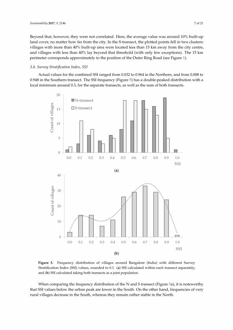
3.4. Survey Stratification Index, SSI

Actual values for the combined SSI ranged from 0.032 to 0.964 in the Northern, and from 0.008 to0.948 in the Southern transect. The SSI frequency (Figure 5) has a double-peaked distribution with alocal minimum around 0.3, for the separate transects, as well as the sum of both transects.

Sustainability 2017, 9, 2146 7 of 21

Beyond that, however, they were not correlated. Here, the average value was around 10% built-up land cover, no matter how far from the city. In the S-transect, the plotted points fell in two clusters: villages with more than 40% built-up area were located less than 15 km away from the city centre, and villages with less than 40% lay beyond that threshold (with only few exceptions). The 15 km perimeter corresponds approximately to the position of the Outer Ring Road (see Figure 1).

3.4. Survey Stratification Index, SSI

Actual values for the combined SSI ranged from 0.032 to 0.964 in the Northern, and from 0.008 to 0.948 in the Southern transect. The SSI frequency (Figure 5) has a double-peaked distribution with a local minimum around 0.3, for the separate transects, as well as the sum of both transects.

(a)

(b)

Figure 5. Frequency distribution of villages around Bangalore (India) with different Survey Stratification Index (SSI) values, rounded to 0.1. (a) SSI calculated within each transect separately; and (b) SSI calculated taking both transects as a joint population.

When comparing the frequency distribution of the N and S transect (Figure 5a), it is noteworthy that SSI values below the urban peak are lower in the South. On the other hand, frequencies of very rural villages decrease in the South, whereas they remain rather stable in the North.

0

5

10

15

20

0.0 0.1 0.2 0.3 0.4 0.5 0.6 0.7 0.8 0.9 1.0

Cou

nt o

f vill

ages

SSI

N-transect

S-transect

0

10

20

30

40

0.0 0.1 0.2 0.3 0.4 0.5 0.6 0.7 0.8 0.9 1.0

Cou

nt o

f vill

ages

SSI

Figure 5. Frequency distribution of villages around Bangalore (India) with different SurveyStratification Index (SSI) values, rounded to 0.1. (a) SSI calculated within each transect separately;and (b) SSI calculated taking both transects as a joint population.

When comparing the frequency distribution of the N and S transect (Figure 5a), it is noteworthythat SSI values below the urban peak are lower in the South. On the other hand, frequencies of veryrural villages decrease in the South, whereas they remain rather stable in the North.

Sustainability 2017, 9, 2146 8 of 21

3.5. Stratification and Village Sampling

The Northern and Southern transect were treated as separate populations when calculating theSSI and allocating them to the six arbitrary strata for random sampling (Table 2; mapped in Figure A1,see Appendix A).

Table 2. Village stratification and random sampling in the Northern and Southern transect ofBangalore (India).

Stratum SSI Boundaries

N-Transect S-Transect

Villages per Stratum Villages per Stratum

(Total) (Randomly Selected) (Total) (Randomly Selected)

1 (urban) <0.167 5 2 14 42 0.333 9 3 10 33 0.5 9 3 13 44 0.667 18 6 26 85 0.833 30 10 23 7

6 (rural) >0.833 22 7 12 4

Total 93 31 98 30

As mentioned before, the SSI values of the two transects are not directly comparable due to theirdifferent shapes. If both transects were treated as a single population, and SSI was recalculated onthat basis, some villages of the S-transect are classified to a neighbouring stratum (Table A3), but theoverall pattern of frequency distributions as presented above remained the same.

It should be noted here, again, that the strata for the random sampling of villages were definedarbitrarily, and did not coincide with the inherent structural discontinuities indicated above. The latter,however, may give some clues to delineate areas representing urban, transitional and rural villages,as discussed below.

3.6. Landscape Structures and Village/Urban Morphologies

When examining satellite images of the transects, and in particular, the buffer zones aroundthe villages, it was evident that there was also a change in the geometry and spatial patterns of thesurface features along the transects. They reflect a morphological transition from rural characteristics(abundant in the distal parts) to urban characteristics (clustered close to the city centre). By theirqualitative features, four basic classes were distinguished with a range of intermediate forms (Figure 6).In the Northern transect, 35 villages could be unambiguously described as a “compact settlementsurrounded by fields” (class A, total built-up area ranged between 3% and 23%), and 24 more villagesof this type showed first indications of disturbance, such as spreading out of settlements, patches oflarge buildings, or development of new layouts (class AB). When such disturbances outweighedthe underlying pattern, a new “mixed/patchy” morphology emerged, often combined with manynew layouts (class B, 15 villages, 10% to 60% built-up area), before closed, “dense settlements” prevailedwhich were only sparsely interrupted by green areas, such as parks, gardens, or a few residual fields(class D, 9 villages, 46% to 85% built-up area). In the Southern transect, another distinct landscapetype dominated by mostly empty layouts (“all-over layouts”, class C) was encountered, which hardlyever occurred in the Northern transect. Villages per class in the Southern transect counted 26 in classA, 20 in class AB, 18 in class B, 13 in class C, and 15 in class D.

In order to link the qualitative morphological village description to the quantitative SSI,the frequency distribution of the morphological classes over the entire range of SSI values is shown inFigure 7. This analysis supported the existence of an urban and a rural cluster (peaks at SSI < 0.3 andSSI > 0.5, respectively), whereas the mixed/patchy type peaked between 0.3 and 0.5, that is, in therange of the local minimum observed in the SSI frequency itself (Figure 5).

Sustainability 2017, 9, 2146 9 of 21Sustainability 2017, 9, 2146 9 of 21

Figure 6. Exemplary village morphologies for classes A, B, C, and D (images taken from Worldview3 scenes). The circle marks the 1 km2 buffer zone.

(a)

0

2

4

6

8

10

12

14

0 0.1 0.2 0.3 0.4 0.5 0.6 0.7 0.8 0.9 1

Cou

nt o

f vill

ages

SSI Intervals

A

AB

B

D

X

Figure 6. Exemplary village morphologies for classes A, B, C, and D (images taken from Worldview3scenes). The circle marks the 1 km2 buffer zone.

Sustainability 2017, 9, 2146 9 of 21

Figure 6. Exemplary village morphologies for classes A, B, C, and D (images taken from Worldview3 scenes). The circle marks the 1 km2 buffer zone.

(a)

0

2

4

6

8

10

12

14

0 0.1 0.2 0.3 0.4 0.5 0.6 0.7 0.8 0.9 1

Cou

nt o

f vill

ages

SSI Intervals

A

AB

B

D

X

Figure 7. Cont.

Sustainability 2017, 9, 2146 10 of 21Sustainability 2017, 9, 2146 10 of 21

(b)

Figure 7. Frequency distribution of morphological classes over SSI in (a) the Northern and (b) the Southern research transect around Bangalore (India). Classes: A—compact settlement surrounded by fields (rural); AB—class A with first disturbances; B—mixed/patchy; C—all-over layouts; D—dense settlements (urban); X—unclassified (unique structures or largely outside the satellite image).

In the Southern transect, this sequence was similar, with the peak of the mixed/patchy morphology shifted to slightly higher SSI values. Class C clustered in the shoulder of the urban peak, i.e., in-between classes B and D.

Although derived independently by different methods, there is obviously a correspondence between the morphological classification and the quantitative index, both representing an inherent spatial structure within the transects across the rural–urban interface.

3.7. Delineating Structural Strata

Based on the correlations, discontinuities and frequency distributions described above, the most suitable SSI thresholds for delineating a rural, transitional, and urban cluster were estimated.

In contrast to the arbitrary or statistical approaches aiming at equal SSI intervals, or at equally sized village strata, respectively, this approach takes into account the qualitative information derived from the morphological classification. The strata boundaries were adjusted to maximise the number of rural (classes A and AB), transitional (class B), and urban (classes C and D) settlements in the respective SSI interval (Figure 8). These boundaries were at 0.25 and 0.55 in the Northern transect, and at 0.35 and 0.62 in the South. Such “structural strata” might serve as a preliminary common reference for the projects targeting agronomic and ecological aspects of rural–urban transitions. Projected back on a spatial map, areas of different stages of transition can be outlined (Figures 9 and 10).

0

2

4

6

8

10

12

0 0.1 0.2 0.3 0.4 0.5 0.6 0.7 0.8 0.9

Cou

nt o

f vill

ages

SSI Intervals

A

AB

B

C

D

X

Figure 7. Frequency distribution of morphological classes over SSI in (a) the Northern and (b) theSouthern research transect around Bangalore (India). Classes: A—compact settlement surrounded byfields (rural); AB—class A with first disturbances; B—mixed/patchy; C—all-over layouts; D—densesettlements (urban); X—unclassified (unique structures or largely outside the satellite image).

In the Southern transect, this sequence was similar, with the peak of the mixed/patchymorphology shifted to slightly higher SSI values. Class C clustered in the shoulder of the urbanpeak, i.e., in-between classes B and D.

Although derived independently by different methods, there is obviously a correspondencebetween the morphological classification and the quantitative index, both representing an inherentspatial structure within the transects across the rural–urban interface.

3.7. Delineating Structural Strata

Based on the correlations, discontinuities and frequency distributions described above, the mostsuitable SSI thresholds for delineating a rural, transitional, and urban cluster were estimated.

In contrast to the arbitrary or statistical approaches aiming at equal SSI intervals, or at equallysized village strata, respectively, this approach takes into account the qualitative information derivedfrom the morphological classification. The strata boundaries were adjusted to maximise the number ofrural (classes A and AB), transitional (class B), and urban (classes C and D) settlements in the respectiveSSI interval (Figure 8). These boundaries were at 0.25 and 0.55 in the Northern transect, and at 0.35and 0.62 in the South. Such “structural strata” might serve as a preliminary common reference for theprojects targeting agronomic and ecological aspects of rural–urban transitions. Projected back on aspatial map, areas of different stages of transition can be outlined (Figures 9 and 10).

Sustainability 2017, 9, 2146 11 of 21

Sustainability 2017, 9, 2146 11 of 21

Figure 8. Structural strata and frequency of villages within them along the rural–urban transect crossing Bangalore (India).

(a) (b) (c)

Figure 9. Mapping of SSI, morphological classes, and structural strata in the Northern transect. (a) As the SSI is a continuous index, the transition from rural to urban character appears as a gradient in which defining boundaries is rather arbitrary; (b) The morphological classification reveals emerging hotspots of transition even in distant locations; (c) The overlay of both approaches approximates an in situ stratification in coherent rural, transitional, and urban areas.

0

5

10

15

20

25

30

35

40

rural transitional urban rural transitional urban

Cou

nt o

f vill

ages

Northern transect Southern transect

A

AB

B

C

D

SSI 1 0.55 0.25 0 1 0.62 0.35 0

Figure 8. Structural strata and frequency of villages within them along the rural–urban transect crossingBangalore (India).

Sustainability 2017, 9, 2146 11 of 21

Figure 8. Structural strata and frequency of villages within them along the rural–urban transect crossing Bangalore (India).

(a) (b) (c)

Figure 9. Mapping of SSI, morphological classes, and structural strata in the Northern transect. (a) As the SSI is a continuous index, the transition from rural to urban character appears as a gradient in which defining boundaries is rather arbitrary; (b) The morphological classification reveals emerging hotspots of transition even in distant locations; (c) The overlay of both approaches approximates an in situ stratification in coherent rural, transitional, and urban areas.

0

5

10

15

20

25

30

35

40

rural transitional urban rural transitional urban

Cou

nt o

f vill

ages

Northern transect Southern transect

A

AB

B

C

D

SSI 1 0.55 0.25 0 1 0.62 0.35 0

Figure 9. Mapping of SSI, morphological classes, and structural strata in the Northern transect. (a) Asthe SSI is a continuous index, the transition from rural to urban character appears as a gradient inwhich defining boundaries is rather arbitrary; (b) The morphological classification reveals emerginghotspots of transition even in distant locations; (c) The overlay of both approaches approximates an insitu stratification in coherent rural, transitional, and urban areas.

Sustainability 2017, 9, 2146 12 of 21Sustainability 2017, 9, 2146 12 of 21

Figure 10. Mapping of (a) SSI; (b) morphological classes; and (c) structural strata in the Southern transect. Explanations as above. Figure 10. Mapping of (a) SSI; (b) morphological classes; and (c) structural strata in the Southern transect. Explanations as above.

Sustainability 2017, 9, 2146 13 of 21

4. Discussion

4.1. Survey Stratification Index, SSI

The Survey Stratification Index (SSI) used in the present study provides a simple approach tocharacterising rural–urban gradients. The SSI was composed from the two variables, distance tothe city centre, and proportion of built-up area around defined settlements. An initial correlationanalysis of the two components revealed a breakpoint at a distance of 15 to 20 km of the city centre(Figure 4). In the Northern transect, this was a change from strong to low (or no) correlation betweenthe two parameters, whereas in the Southern transect, it separated two clusters of different buildingdensities. Taken together, this already suggests a transitional zone somewhere between the 15 and20 km perimeter, where urban construction activities are most rapid. This would be an easy indicatorto track city sprawl, as in the correlation analysis, landscape structures are entirely neglected. It wouldbe interesting to analyse how this zone moves with time as the city further expands.

The classification of land cover types had some shortcomings, such as misclassification of lakeedges as built-up land, which resulted in an overall accuracy of just 80%. This may be partly dueto misleading ground covers, such as tank linings or plastic foil-covered fields. An independentvalidation for the class “built-up” was performed using 4995 points digitised from the WorldView-3image. Here, the overall accuracy was 77%. However, in combination with the distance parameterthe SSI calculation still resulted in a meaningful representation of a gradient in rural–urban features.Besides the land cover classification, the actual SSI values depend on the shape of the selected transect,and on the size of the buffer zones. The size of 1 km2 chosen here was a compromise for capturingsufficient surrounding area for a wide range of built-up area proportions, while avoiding excessiveoverlaps between neighbouring villages. If overlaps occurred, they were ignored in the calculation ofSSI. In other landscape contexts, a suitable diameter of buffer zones might be deduced from an analysisof distances to the nearest neighbouring villages.

The use of buffer zones around a defined village centre point, however, offers two advantages.On one hand, the analysis is targeted to existing settlements rather than screening random locations,on the other hand, it averages spatial features over the given buffer area. In a suitable range of scaling,this enhances the gradient features. For example, if the buffer zones were only 1/10 of the presentsize (i.e., within the village limits), also the rural villages would become an almost completely built-uparea, whereas a histogram over the entire image area would blur the internal discontinuities (as shownfor the URI in [13] (p. 309, Figure 5). This illustrates how critical scale and resolution are for the spatialanalysis of a rural–urban gradient.

The chosen boundary conditions revealed a two-peaked frequency distribution of the SSI.This suggests that the first peak, around 0.1, represents urban settlements, the other one, around 0.7,a (variety of) rural structures. The local minimum at 0.3 would then indicate an unstable stage,i.e., the villages in this SSI range should be most actively transforming. While this overall pattern wassimilar in both transects, lower SSI values under the urban peak in the Southern transect indicatea higher degree of urbanisation, along with higher numbers of such settlements. The decreasingfrequency of very distant, rural villages in the South may be related to the influence of the neighbouringcity of Kanakapura in the southern direction, which perhaps triggers construction activities from thedistal end of the transect. Thus, the spatial distribution of SSI strata was somewhat irregular in theSouthern transect, but rather continuous and successive in the North.

The pixel size of the Sentinel2 pictures on which the SSI calculation was based, was 10 m.The impact of lower or higher resolution of the satellite imagery (e.g., 30 m in Landsat images, or 1.24 min Worldview3 products) merits further study. Likewise, the conclusion that the discontinuitiesin the correlation of distance and proportion of built-up area, or in the frequency distribution ofthe SSI, indicate a structurally unstable urban fringe, may be tested by time series analyses and atother locations.

Sustainability 2017, 9, 2146 14 of 21

4.2. Village Morphologies

Structural morphologies are a qualitative concept used in landscape and urban planning.Here, the definition of classes is entirely context specific. The WBGU has even defined a distinctdimension, termed “Eigenart” (a German word meaning “character”) [23] (p. 3) as a framework fordealing with sociocultural diversity and regional, specific development dynamics in urbanisation.Based on a careful inspection of the landscape context in the Bangalore region, it was evident thatrural settlements can be described as “compact village surrounded by fields” (Class A), whereasthe city centre was densely built-up, with only sparse interruptions by green areas (Class D).Class C, which is dominated by empty layouts, represents a state in which land use change(from agricultural to residential use) has already been completed but the corresponding landcover change (from open/vegetated to built-up) is still ongoing. In terms of social–ecologicaltransitions, however, this was accounted for as “urban” rather than actively transforming. Class B,the “mixed/patchy” morphology is presumed to be most unstable. The coincidence of a localminimum in SSI frequency distribution, with a peak in the abundance of a transitional morphology(Class B), can thus be understood as a triangulation for detecting the hotspots of transformation in therural–urban interface of Bangalore.

4.3. Other Approaches

It is obvious that our approach has qualitative elements that make it, to some degree, subjective.For example, the transitions between morphologies A and B are gradual, and it depends on theobserver where to delimit a new class. This is considered in the current analysis by introducing anintermediate Class AB for villages where the “pure” radially centred symmetry shows first disturbances.Nevertheless, a subjective component persists. To overcome this bias, landscape structures can beanalysed by quantitative, statistical measures, such as diversity and evenness indices [24], or byadvanced landscape metrics (FRAGSTATS [25]). Salvati et al. [24], for example, used the Shannondiversity index and the Pielou index to evaluate the variability of land use classes and their contributionto the total area. They were thus able to categorise the transition from urban to rural areas for the cityof Athens.

A more precise and dynamic approach for identifying the urban–rural fringe was presented byPeng et al. [26]. They developed a model which combined spatial continuous wavelet transform forthe detection of mutation points from a land use degree index map with a kernel density estimation.The latter generates a density surface map from the detected mutation points, which was then usedto set a threshold to produce the urban–rural fringe map. The model was successfully applied toBejing City, and was found to be superior to manual mutation point mapping.

In an attempt to combine land cover and morphological patterns Bechtel et al. [27] adapted theLocal Climate Zone mapping (originally developed for climate change research) to the analysis of urbanform and function. They aim at generating a worldwide database to describe the internal structure andtexture of cities, but the approach might well be extended to settlements in the rural–urban interface,and substantiate the classification suggested above.

Finally, the overall strategy followed in our present study, and in the cited examples, is notrestricted to a rural–urban context. Barve et al. [28] used the combination of a composite index basedon GIS analysis and ground measurement of selected ecological indicators to derive and validatethreat maps in a wildlife sanctuary in Southern India. The study area was divided in 30 ha grid cells,and the GIS-based parameters were the number of villages and roads in a 3 km buffer zone aroundeach grid cell, distance to the settlements and roads, and the average slope in and around each gridcell (all individually normalised to 0 to 1). Mapping of the weighted, composite threat index identifiedvulnerable zones at the edges of the sanctuary, and around plantations within it. The threat index wasthen used to define transects for determining ecological indicators, similar to our application of theSSI in stratifying the villages for random sampling. The ecological parameters, such as tree species

Sustainability 2017, 9, 2146 15 of 21

richness or proportion of cut and broken stems (due to human or livestock invasion), were highlycorrelated with the GIS-derived threat indices.

All of the approaches discussed above aim at structuring space, and they should not be seen asexclusive of each other. Instead, they capture different facets of a research region, such as a rural–urbaninterface, and the method of choice will depend on the goal and the stage of a given study. The meritof the simplified index, as compared to the cited examples of more elaborate methods of analysis,lies in the swiftness of providing results, which can be easily applied in various disciplinary contexts.Furthermore, the integration of the index with the morphological classification illustrates how toovercome methodological bias between disciplines that prefer qualitative over quantitative research,or vice versa.

5. Conclusions

In the context of our project, the SSI serves as a starting point for deeper investigation in differentresearch fields. It was applied, initially, to stratify villages for random sampling, in order to performa representative household survey, but it will also provide a matrix against which the results canbe aligned and evaluated. Coordinated research in the sampled villages, however, will not onlyaddress socioeconomic household characteristics, but also their agricultural practices in crop ordairy production, consumption practices, and attitudes to environmental issues. At the same time,experiments are carried out at selected locations to assess the actual environmental conditions, in termsof soil and crop quality, biodiversity, and provision of ecosystem services. Various rural–urbanparameters, and the locations to where they map in the research transects, will thus be a central toolfor synthesising interdisciplinary results. The measures and classification systems themselves will berefined and elaborated in this process, and it will be interesting to observe under which condition anumerical index, a morphology, or a location is predominant for gradients in other parameters.

Acknowledgments: This paper resulted from a collaboration of projects B02, C01, C02 and Z of the Research UnitFOR2432 (Social–Ecological Systems in the Indian Rural–Urban Interface: Functions, Scales and Dynamics ofTransition). The concept of spatial explicity and of using indices to describe the internal structure of the rural–urbaninterface was developed jointly by the participants of FOR2432. On behalf of the entire consortium we thankthe speakers, A. Bürkert and S. von Cramon-Taubadel, for inspiring discussions. We notably thank our scientificpartners in DBT-FOR2432 for their collaboration and support in several excursions exploring the rural–urbaninterface of Bangalore, in the communication with Indian authorities and stakeholders and in the coordination offieldwork, in particular, and on behalf of the entire Indian consortium, B.V. Chinnappa Reddy, K.N. Ganeshaiahand V.R.R. Parama at the University of Agricultural Sciences, Bangalore. We thank Eva Goldmann for performingthe land cover classification and basic GIS analysis, as well as Johannes Bettin and Johannes Wegmann forsupporting village extraction/mapping and ground truthing. The authors gratefully acknowledge the financialsupport provided by the German Research Foundation, DFG, through grant numbers BU 1308/14-1 (Z),WO 1470/3-1 (B02), KL894/23-1 (C02), and WA2135/4-1 (C01), as parts of the Research Unit FOR2432/1.

Author Contributions: In the work reported above, project C02 (Nils Nölke) provided the Sentinel2 satellitepictures on which the land cover analysis is based, and project C01 (Thomas Möckel) the Worldview3 scenesused in the village morphology classification. Thomas Möckel also prepared the maps presented in the paper.Monish Jose (B02) was responsible for drawing the stratified random sample of villages in the two transects,which included collecting information from Indian government authorities, village mapping, ground verification,mathematical definition of the SSI, choice of the stratification strategy, and contribution of the respectivepassages of the text. Ellen Hoffmann (Z) outlined the paper, designed the GIS analysis strategy, contributed themorphological classification, integrated and finalized the manuscript.

Conflicts of Interest: The authors declare no conflict of interest. The founding sponsors had no role in the designof the study; in the collection, analyses, or interpretation of data; in the writing of the manuscript, and in thedecision to publish the results.

Sustainability 2017, 9, 2146 16 of 21

Appendix A. Alternative Approaches to Stratification and Random Selection of Settlements

Table A1. Stratum boundaries determined by the cumulative root frequency method [19] and theLavallée–Hidiroglou iterative method [20] with Kozak’s [21] algorithm [22].

TransectStrata

Boundaries:Cum Root

Units inEach

Stratum

Number of Unitsto Sample inEach Stratum

StrataBoundaries:

LH

Units inEach

Stratum

Number of Unitsto Sample inEach Stratum

North <0.28 11 7 <0.29 12 80.5 12 6 0.44 16 6

0.64 16 6 0.62 13 50.74 18 4 0.75 24 80.86 18 4 0.85 16 3

>0.86 18 4 >0.85 20 5Total 93 31 93 31

South <0.1963 14 5 <0.1813 14 50.4363 14 8 0.3476 10 30.5407 17 3 0.5375 21 80.645 20 4 0.6505 20 40.7598 17 4 0.7859 20 5

>0.7598 16 6 >0.7859 13 5Total 98 30 98 30

Note: LH stands for Lavallée–Hidiroglou method of strata construction. LH method is used with Kozak’s algorithm;R: stratification package available from [29] is used for calculation.

Table A2. List of villages within the rural–urban research transects in Bangalore, India. Sampledvillages are highlighted in bold. (a) Northern transect; (b) Southern transect.

(a) Northern Transect

Village Name Distance (km) Built-Up Area (%) SSI Stratum Morphology Class

Addigandhalli 21.56 18.34 0.516 4 BAdinarayanahosahalli 33.09 6.63 0.764 5 A

Agrahara 22.42 4.31 0.578 4 BAlijenahalli 38.41 3.04 0.861 6 X

Allalasandra 11.60 54.69 0.176 2 DAluruguddanahalli 32.53 6.42 0.756 5 AB

Amruthahalli 9.43 66.82 0.064 1 DAnantapura 15.13 41.82 0.305 2 BArdeshahalli 26.97 12.09 0.641 4 A

Atturu 14.22 51.67 0.256 2 DAvalahalli 17.49 35.48 0.377 3 B

Ayyammanahalli 46.59 9.12 0.942 6 XBachchahalli 30.25 15.44 0.683 5 A

Bairadenahalli 34.46 3.09 0.801 5 ABannamangala 31.11 9.75 0.720 5 ABasavanapur 27.26 7.95 0.661 4 ABettahalasur 20.26 24.37 0.471 3 ABBettanahalli 25.37 7.34 0.628 4 AB

Bhumenahalli 44.22 9.77 0.908 6 ABidikere 40.45 6.21 0.875 6 A

Byatarayapur 9.57 77.42 0.060 1 DChikka Bommasandra 12.32 69.06 0.163 1 DChikka Hegganahalli 25.41 12.50 0.611 4 AB

Chikka Muddenahalli 47.16 6.23 0.964 6 AChikkanahosahalli 26.10 3.58 0.655 4 ADasagondenahalli 37.75 9.96 0.820 5 A

Devarahalli 28.81 7.19 0.691 5 ABDinnuru 30.84 6.49 0.729 5 A

Gandarajapura 39.66 10.98 0.842 6 AGantiganahalli 42.16 10.92 0.876 6 A

Garighatta 40.40 8.89 0.862 6 AGhantiganahalli 41.50 5.72 0.892 6 AB

Sustainability 2017, 9, 2146 17 of 21

Table A2. Cont.

(a) Northern Transect

Village Name Distance (km) Built-Up Area (%) SSI Stratum Morphology Class

Guddadahalli 32.33 18.12 0.704 5 ABHarohalli 16.73 25.59 0.387 3 B

Heggenahalli 26.50 11.60 0.634 4 ABHosuru 27.48 15.10 0.638 4 ABJakkuru 11.07 46.38 0.171 2 D

Jalige 27.32 13.98 0.640 4 ABJutnahalli 28.81 5.33 0.698 5 A

Kachahalli 43.07 23.14 0.824 5 AKamenahalli 27.05 31.53 0.566 4 ABKanchiganal 39.74 11.08 0.842 6 AKandasandra 43.94 23.60 0.832 5 X

Karanalu 42.33 10.58 0.880 6 ABKasavanahalli 29.08 5.13 0.704 5 AKenchenahalli 15.48 36.81 0.327 2 B

Kodihalli 36.61 13.50 0.787 5 ABKonaghatta 36.77 13.89 0.788 5 AKudaragere 22.91 8.63 0.575 4 ABKuruvegere 41.72 9.08 0.879 6 A

Lakshmidevipur 41.39 9.97 0.870 6 XLingahiragollonalli 30.47 6.84 0.721 5 AB

Manchihalli 15.04 13.27 0.370 3 BMaragondanahalli 24.81 3.92 0.629 4 AB

Maruthinagara 14.19 61.08 0.228 2 DMoparahalli 33.87 5.82 0.780 5 A

Muddanahalli 19.11 11.23 0.484 3 ABNagadarsanahalli 20.01 10.79 0.506 4 A

Nagadenahalli 33.69 15.38 0.736 5 ABNagenahalli 16.78 31.88 0.371 3 B

Naraganahalli 42.84 9.51 0.891 6 ANarasimhanahalli 44.06 9.22 0.909 6 A

Panditapur 29.52 2.45 0.721 5 APedda tammanahalli 46.02 6.94 0.946 6 A

Puttanahalli 14.47 60.22 0.237 2 BRaghunathpura 34.18 24.88 0.700 5 B

Rajaghatta 38.28 16.05 0.799 5 ABRajankunti 22.71 21.28 0.530 4 BS(h)ivapura 36.35 11.74 0.792 5 ASadenahalli 23.79 10.55 0.587 4 AB

Sahakara Nagar 9.21 84.96 0.032 1 DSatenahalli 44.43 10.65 0.906 6 ASettahalasur 16.59 33.86 0.362 3 B

Singanayakanahalli 18.79 30.30 0.421 3 XSonnappanahalli 36.02 8.26 0.802 5 A

Sugatta 18.26 9.16 0.468 3 BSulakunte 30.38 14.98 0.687 5 ABSunaghatta 30.91 7.56 0.726 5 A

Sunnagaddahalli 41.23 7.79 0.878 6 ATankashahosahalli 41.31 8.75 0.875 6 A

Tarahunase 22.08 13.68 0.542 4 ABTimmasandra_1 21.25 9.41 0.537 4 XTimmasandra_2 37.85 13.20 0.806 5 XTimmojamahalli 42.56 7.06 0.900 6 A

Tindlu_1 10.54 62.47 0.124 1 XTindlu_2 28.13 8.94 0.673 5 XTubagere 43.68 25.68 0.817 5 AB

Turuvanahalli 47.04 9.75 0.944 6 XVaradanahalli 30.86 15.78 0.691 5 AB

Venkatala 14.73 46.02 0.284 2 BVobadenahalli 32.83 10.85 0.743 5 BYeddalahalli 43.90 8.72 0.909 6 AYelahanka 13.52 64.86 0.203 2 D

Sustainability 2017, 9, 2146 18 of 21

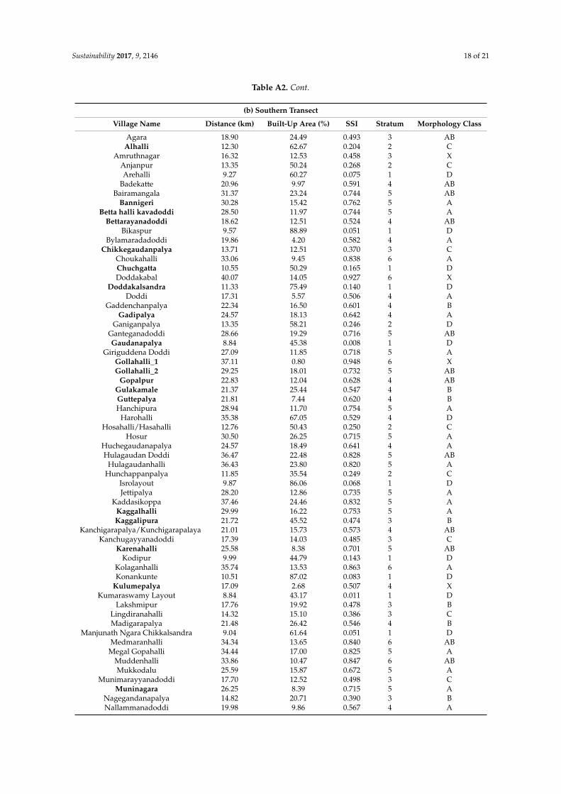
Table A2. Cont.

(b) Southern Transect

Village Name Distance (km) Built-Up Area (%) SSI Stratum Morphology Class

Agara 18.90 24.49 0.493 3 ABAlhalli 12.30 62.67 0.204 2 C

Amruthnagar 16.32 12.53 0.458 3 XAnjanpur 13.35 50.24 0.268 2 CArehalli 9.27 60.27 0.075 1 D

Badekatte 20.96 9.97 0.591 4 ABBairamangala 31.37 23.24 0.744 5 AB

Bannigeri 30.28 15.42 0.762 5 ABetta halli kavadoddi 28.50 11.97 0.744 5 A

Bettarayanadoddi 18.62 12.51 0.524 4 ABBikaspur 9.57 88.89 0.051 1 D

Bylamaradadoddi 19.86 4.20 0.582 4 AChikkegaudanpalya 13.71 12.51 0.370 3 C

Choukahalli 33.06 9.45 0.838 6 AChuchgatta 10.55 50.29 0.165 1 DDoddakabal 40.07 14.05 0.927 6 X

Doddakalsandra 11.33 75.49 0.140 1 DDoddi 17.31 5.57 0.506 4 A

Gaddenchanpalya 22.34 16.50 0.601 4 BGadipalya 24.57 18.13 0.642 4 A

Ganiganpalya 13.35 58.21 0.246 2 DGanteganadoddi 28.66 19.29 0.716 5 ABGaudanapalya 8.84 45.38 0.008 1 D

Giriguddena Doddi 27.09 11.85 0.718 5 AGollahalli_1 37.11 0.80 0.948 6 XGollahalli_2 29.25 18.01 0.732 5 AB

Gopalpur 22.83 12.04 0.628 4 ABGulakamale 21.37 25.44 0.547 4 BGuttepalya 21.81 7.44 0.620 4 BHanchipura 28.94 11.70 0.754 5 A

Harohalli 35.38 67.05 0.529 4 DHosahalli/Hasahalli 12.76 50.43 0.250 2 C

Hosur 30.50 26.25 0.715 5 AHuchegaudanapalya 24.57 18.49 0.641 4 AHulagaudan Doddi 36.47 22.48 0.828 5 AB

Hulagaudanhalli 36.43 23.80 0.820 5 AHunchappanpalya 11.85 35.54 0.249 2 C

Isrolayout 9.87 86.06 0.068 1 DJettipalya 28.20 12.86 0.735 5 A

Kaddasikoppa 37.46 24.46 0.832 5 AKaggalhalli 29.99 16.22 0.753 5 AKaggalipura 21.72 45.52 0.474 3 B

Kanchigarapalya/Kunchigarapalaya 21.01 15.73 0.573 4 ABKanchugayyanadoddi 17.39 14.03 0.485 3 C

Karenahalli 25.58 8.38 0.701 5 ABKodipur 9.99 44.79 0.143 1 D

Kolaganhalli 35.74 13.53 0.863 6 AKonankunte 10.51 87.02 0.083 1 D

Kulumepalya 17.09 2.68 0.507 4 XKumaraswamy Layout 8.84 43.17 0.011 1 D

Lakshmipur 17.76 19.92 0.478 3 BLingdiranahalli 14.32 15.10 0.386 3 CMadigarapalya 21.48 26.42 0.546 4 B

Manjunath Ngara Chikkalsandra 9.04 61.64 0.051 1 DMedmaranhalli 34.34 13.65 0.840 6 AB

Megal Gopahalli 34.44 17.00 0.825 5 AMuddenhalli 33.86 10.47 0.847 6 ABMukkodalu 25.59 15.87 0.672 5 A

Munimarayyanadoddi 17.70 12.52 0.498 3 CMuninagara 26.25 8.39 0.715 5 A

Nagegandanapalya 14.82 20.71 0.390 3 BNallammanadoddi 19.98 9.86 0.567 4 A

Sustainability 2017, 9, 2146 19 of 21

Table A2. Cont.

(b) Southern Transect

Village Name Distance (km) Built-Up Area (%) SSI Stratum Morphology Class

Narayanagurukul 18.56 31.94 0.460 3 BNayanakahalli 24.07 8.57 0.668 5 ABNoukalapalya 23.37 6.75 0.659 4 AObichudahalli 19.52 18.77 0.527 4 BParasanapalya 26.01 13.96 0.688 5 A

Pattareddypalya 22.59 21.28 0.589 4 BPerumanpalya/Peruvaiahnapalya 31.02 12.02 0.790 5 AB

Raghabanapalya 12.67 13.68 0.326 2 CRajanmadavu/Rachanamadu 15.91 6.23 0.461 3 AB

Ravugollu 27.45 15.02 0.712 5 ABSaludoddi 19.34 18.38 0.524 4 BSaluhanase 20.55 28.80 0.517 4 BSantenahalli 36.47 16.71 0.858 6 AB

Shylendradoddi 20.15 5.96 0.584 4 ASiddhanahallil 38.92 6.83 0.947 6 A

Silk farm 15.67 12.01 0.439 3 XSomanahalli 24.81 26.27 0.614 4 AB

Subramanyapur 10.56 60.96 0.147 1 BSunkadakatte 25.01 12.89 0.672 5 X

Talghatpur 13.48 58.05 0.250 2 CTaralu 22.42 18.08 0.597 4 B

Tataguni 17.36 31.03 0.434 3 BThattuguppe/Mariapura 23.85 25.50 0.598 4 AB

Timmaboyi doddi 28.90 4.94 0.781 5 ATimmagaudanapalya/Banjarapalya 20.39 5.14 0.593 4 AB

Timmagaudandoddi 31.97 20.63 0.767 5 ATimmayyanadoddi 19.90 4.52 0.582 4 A

Tipsandra 12.34 44.34 0.250 2 CTurahalli 11.40 52.67 0.197 2 CUdipalya 19.45 33.25 0.476 3 B

Uttarahalli 9.60 80.75 0.069 1 DUttarri 20.78 13.50 0.575 4 B

Vajarhalli 12.74 61.85 0.219 2 CVasantpur 10.41 77.26 0.107 1 D

Vasudevapur 21.80 20.28 0.575 4 BYalchenahalli 9.40 76.43 0.065 1 D

Stratification strategy. Due to the overall workflow and the different shapes of the two transects,the SSI values, as presented above, were determined separately. For comparison, both transects weretreated as a single population, and SSI was recalculated on that basis. As a result, some villages of theS-transect were classified to a neighbouring stratum (Table A3), but the overall pattern of frequencydistributions as presented above remained the same.

Table A3. Changes in village stratification around Bangalore (India) if both transects were treated asone joint population.

Number of Villages Original Stratum Allocation Allocation after Recalculation

2 2 11 3 29 4 313 5 46 6 5

Sustainability 2017, 9, 2146 20 of 21

Sustainability 2017, 9, 2146 19 of 21

Pattareddypalya 22.59 21.28 0.589 4 B Perumanpalya/Peruvaiahnapalya 31.02 12.02 0.790 5 AB

Raghabanapalya 12.67 13.68 0.326 2 C Rajanmadavu/Rachanamadu 15.91 6.23 0.461 3 AB

Ravugollu 27.45 15.02 0.712 5 AB Saludoddi 19.34 18.38 0.524 4 B Saluhanase 20.55 28.80 0.517 4 B Santenahalli 36.47 16.71 0.858 6 AB

Shylendradoddi 20.15 5.96 0.584 4 A Siddhanahallil 38.92 6.83 0.947 6 A

Silk farm 15.67 12.01 0.439 3 X Somanahalli 24.81 26.27 0.614 4 AB

Subramanyapur 10.56 60.96 0.147 1 B Sunkadakatte 25.01 12.89 0.672 5 X

Talghatpur 13.48 58.05 0.250 2 C Taralu 22.42 18.08 0.597 4 B

Tataguni 17.36 31.03 0.434 3 B Thattuguppe/Mariapura 23.85 25.50 0.598 4 AB

Timmaboyi doddi 28.90 4.94 0.781 5 A Timmagaudanapalya/Banjarapalya 20.39 5.14 0.593 4 AB

Timmagaudandoddi 31.97 20.63 0.767 5 A Timmayyanadoddi 19.90 4.52 0.582 4 A

Tipsandra 12.34 44.34 0.250 2 C Turahalli 11.40 52.67 0.197 2 C Udipalya 19.45 33.25 0.476 3 B

Uttarahalli 9.60 80.75 0.069 1 D Uttarri 20.78 13.50 0.575 4 B

Vajarhalli 12.74 61.85 0.219 2 C Vasantpur 10.41 77.26 0.107 1 D

Vasudevapur 21.80 20.28 0.575 4 B Yalchenahalli 9.40 76.43 0.065 1 D

Figure A1. Map of villages in the northern and southern transect of Bangalore (India). Villages sampled for the survey in FOR2432 are highlighted in colour. Within the selected villages the survey covered 1200 households for the general description of socio-economic parameters. Subsamples from this set are drawn for more specific investigations within various FOR2432 projects.

Figure A1. Map of villages in the northern and southern transect of Bangalore (India). Villages sampledfor the survey in FOR2432 are highlighted in colour. Within the selected villages the survey covered1200 households for the general description of socio-economic parameters. Subsamples from this setare drawn for more specific investigations within various FOR2432 projects.

References

1. Laquinta, D.; Drescher, A.W. Defining peri-urban: Understanding rural-urban linkages and their connectionto institutional contexts. In Proceedings of the 10th World Congress of the International Rural SociologyAssociation, Rio De Janeiro, Brazil, 30 July–5 August 2000.

2. Tacoli, C. The links between rural and urban development. Environ. Urban. 2003, 15, 3–12. [CrossRef]3. Pryor, R.J. Defining the rural-urban fringe. Soc. Forces 1968, 47, 202–215. [CrossRef]4. Simon, D. Urban environments: Issues on the peri-urban fringe. Ann. Rev. Environ. Resour. 2008, 33, 167–185.

[CrossRef]5. Adell, G. Theories and models of the peri-urban interface: A changing conceptual landscape. In Strategic

Environmental Planning and Management for the Peri-Urban Interface Research Project; Development PlanningUnit: London, UK, 1999.

6. DST (Desakota Study Team). Re-Imagining the Rural-Urban Continuum: Understanding the Role EcosystemServices Play in the Livelihoods of the Poor in Desakota Regions Undergoing Rapid Change; Institute for Social andEnvironmental Transition-Nepal (ISET-N): Kathmandu, Nepal, 2008. Available online: http://r4d.dfid.gov.uk/PDF/Outputs/EnvRes/FinalReport_Desakota-PartI.pdf (accessed on 16 November 2017).

7. Holling, C.S. Understanding the complexity of economic, ecological, and social systems. Ecosystems 2001, 4,390–405. [CrossRef]

8. Isserman, A.M. In the national interest: Defining rural and urban correctly in research and public policy.Int. Reg. Sci. Rev. 2005, 28, 465–499. [CrossRef]

9. Waldorf, B.S. A Continuous multi-dimensional measure of rurality: Moving beyond threshold measures.In Proceedings of the Annual Meeting of the American Agricultural Economics Association, Long Island,CA, USA, 24–27 July 2006; Available online: http://purl.umn.edu/21383 (accessed on 16 November 2017).

10. Inagami, S.; Gao, S.; Karimi, H.; Shendge, M.M.; Probst, J.C.; Stone, R.A. Adapting the Index of RelativeRurality (IRR) to estimate rurality at the ZIP code level: A rural classification system in health servicesresearch. J. Rural Health 2016, 32, 219–227. [CrossRef] [PubMed]

Sustainability 2017, 9, 2146 21 of 21

11. Beynon, M.J.; Crawley, A.; Munday, M. Measuring and understanding the difference between urban andrural areas. Environ. Plan. B Plan. Des. 2015, 43, 1136–1154. [CrossRef]

12. Schlesinger, J.; Drescher, A. Agriculture along the urban–rural continuum: A GIS-based analysisof spatiotemporal dynamics in two medium-sized African cities. Freibg. Geogr. Hefte 2013, 70.Available online: https://www.geographie.uni-freiburg.de/publikationen/abstracts/fgh70-en (accessed on16 November 2017).

13. Schlesinger, J. Using crowd-sourced data to quantify the complex urban fabric—OpenStreetMap andthe Urban–Rural Index. In OpenStreetMap in GIScience, Lecture Notes in Geoinformation and Cartography;Jokar Arsanjani, J., Zipf, A., Mooney, P., Helbich, M., Eds.; Springer: Basel, Switzerland, 2015; pp. 295–315.[CrossRef]

14. Giseke, U.; Kasper, C.; Mansour, M.; Moustanjidi, Y. E1 Connecting spheres: Urban agriculture as amultidimensional strategy: E1.4 Nine urban-rural morphologies. In Urban Agriculture for Growing CityRegions. Connecting Urban-Rural Spheres in Casablanca; Giseke, U., Gerster-Bentaya, M., Helten, F., Kraume, M.,Scherer, D., Spars, G., Amraoui, F., Adidi, A., Berdouz, S., Chlaida, M., et al., Eds.; Routledge: Abingdon, UK;New York, NY, USA, 2015; pp. 316–328, ISBN 978-0415825016.

15. ISRO. Bhuvan: Indian Geo-Platform of ISRO. Available online: http://bhuvan.nrsc.gov.in/state/KA(accessed on 4 October 2016).

16. Ravallion, M. Troubling tradeoffs in the Human Development Index. J. Dev. Econ. 2012, 99, 201–209.[CrossRef]

17. Qiu, B.; Li, H.; Zhou, M.; Zhang, L. Vulnerability of ecosystem services provisioning to urbanization: A caseof China. Ecol. Indic. 2015, 57, 505–513. [CrossRef]

18. Huang, Y.; Li, F.; Bai, X.; Cui, S. Comparing vulnerability of coastal communities to land use change:Analytical framework and a case study in China. Environ. Sci. Policy 2012, 23, 133–143. [CrossRef]

19. Dalenius, T.; Hodges, J.L., Jr. Minimum variance stratification. J. Am. Stat. Assoc. 1959, 54, 88–101. [CrossRef]20. Lavallee, P.; Hidiroglou, M.A. On the stratification of skewed populations. Surv. Methodol. 1988, 14, 33–43.21. Kozak, M. Optimal stratification using random search method in agricultural surveys. Stat. Transit. 2004, 6,

797–806.22. Er, S. Comparison of the efficiency of the various algorithms in stratified sampling when the initial solutions

are determined with geometric method. Int. J. Stat. Appl. 2012, 2, 1–10. [CrossRef]23. WBGU–Wissenschaftlicher Beirat der Bundesregierung Globale Umweltveränderungen. Der Umzug der

Menschheit: Die Transformative Kraft der Städte; WBGU: Berlin, Germany, 2016; Available online: http://www.wbgu.de/en/hg2016 (accessed on 16 November 2017).

24. Salvati, L.; Sateriano, A.; Saradakou, E.; Grigoriadis, E. ‘Land-use mixité’: Evaluating urban hierarchy andthe urban-to-rural gradient with an evenness-based approach. Ecol. Indic. 2016, 70, 35–42. [CrossRef]

25. McGarigal, K.; Cushman, S.A.; Ene, E. FRAGSTATS V4: Spatial Pattern Analysis Program for Categorical andContinuous Maps, version 4; Computer Software Program Produced by the Authors at the University ofMassachusetts; University of Massachusetts: Amherst, MA, USA, 2012; Available online: http://www.umass.edu/landeco/research/fragstats/fragstats.html (accessed on 16 November 2017).

26. Peng, J.; Zhao, S.; Liu, Y.; Tian, L. Identifying the urban-rural fringe using wavelet transform and kerneldensity estimation: A case study in Beijing City, China. Environ. Model. Softw. 2016, 83, 286–302. [CrossRef]

27. Bechtel, B.; Alexander, P.J.; Böhner, J.; Ching, J.; Conrad, O.; Feddema, J.; Mills, G.; See, L.; Stewart, I. Mappinglocal climate zones for a worldwide database of the form and function of cities. ISPRS Int. J. GeoInf. 2015, 4,199–219. [CrossRef]

28. Barve, N.; Kiran, M.C.; Vanaraj, G.; Aravind, N.A.; Rao, D.; Uma Shaanker, R.; Ganeshaiah, K.N.; Poulsen, J.G.Measuring and mapping threats to a wildlife sanctuary in Southern India. Conserv. Biol. 2005, 19, 122–130.[CrossRef]

29. Stratification: Univariate Stratification of Survey Populations. Available online: https://cran.r-project.org/web/packages/stratification/index.html (accessed on 13 February 2017).

© 2017 by the authors. Licensee MDPI, Basel, Switzerland. This article is an open accessarticle distributed under the terms and conditions of the Creative Commons Attribution(CC BY) license (http://creativecommons.org/licenses/by/4.0/).