arX

iv:1

006.

3507

v1 [

cond

-mat

.mtr

l-sc

i] 1

7 Ju

n 20

10APS/123-QED

Constrained Monte Carlo Method and

Calculation of the Temperature Dependence of Magnetic

Anisotropy

P. Asselin

Seagate Technology, Bloomington, MN 55435, USA

R. F. L. Evans,∗ J. Barker, and R. W. Chantrell

Department of Physics, University of York,

Heslington, York YO10 5DD United Kingdom

R. Yanes and O. Chubykalo-Fesenko

Instituto de Ciencia de Materiales de Madrid,

CSIC, Cantoblanco, Madrid 28049, Spain

D. Hinzke and U. Nowak

Universitat Konstanz, Fachbereich Physik,

Universitatsstraße 10, D-78464 Konstanz, Germany

(Dated: June 18, 2010)

1

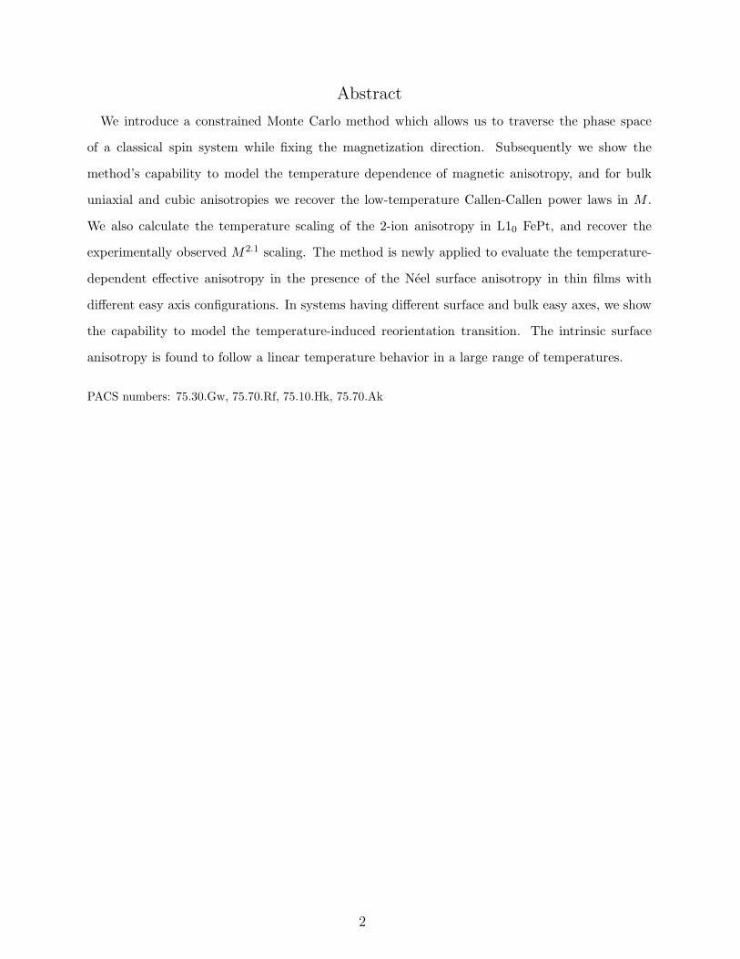
Abstract

We introduce a constrained Monte Carlo method which allows us to traverse the phase space

of a classical spin system while fixing the magnetization direction. Subsequently we show the

method’s capability to model the temperature dependence of magnetic anisotropy, and for bulk

uniaxial and cubic anisotropies we recover the low-temperature Callen-Callen power laws in M .

We also calculate the temperature scaling of the 2-ion anisotropy in L10 FePt, and recover the

experimentally observed M2.1 scaling. The method is newly applied to evaluate the temperature-

dependent effective anisotropy in the presence of the Neel surface anisotropy in thin films with

different easy axis configurations. In systems having different surface and bulk easy axes, we show

the capability to model the temperature-induced reorientation transition. The intrinsic surface

anisotropy is found to follow a linear temperature behavior in a large range of temperatures.

PACS numbers: 75.30.Gw, 75.70.Rf, 75.10.Hk, 75.70.Ak

2

I. INTRODUCTION

The temperature dependence of magnetocrystalline anisotropy of pure ferromagnets has

been well known for decades, following the Callen-Callen theory1. Examples of such systems

classed as pure ferromagnets in the anisotropic sense include Gadolinium (Uniaxial) and Fe

(Cubic). Other ferromagnets, such as Co, have a much more complicated temperature

dependence, due to the crystallographic origin of the anisotropy2. Indeed, with increased

temperature the anisotropy in Co exhibits a change in sign, indicating a transformation

from an easy-axis to easy-plane anisotropy. Such behavior is not explained by the Callen-

Callen theory. Other materials not exhibiting a simple temperature dependence of the

anisotropy are magnetic transition metal alloys such as FePt and CoPt. Here the origin of the

anisotropy is due to an ion-ion anisotropic exchange interaction, arising from the underlying

crystal symmetry. In FePt the anisotropy exhibits an unusual temperature dependence3,4

of Keffu ∝ M2.1. Other systems of technological interest include magnetic thin films and

nanoparticles, where surface effects can lead to unusual temperature dependent anisotropies.

In general the temperature dependence of anisotropy in many materials is not obvious, and

as such is still an active area of research some 40 years after the Callen-Callen theory.

Recently, the high temperature behavior of magnetic anisotropy has become important

due to the applications in heat-assisted magnetic recording (HAMR)5–7. The idea of HAMR

is based on the heating of the recording media to decrease the writing field of the high

anisotropy media (such as FePt) to values compatible with the writing fields provided by

conventional recording heads. Since the writing field is proportional to the anisotropy field

Hk = 2Keffu (T )/M(T ), the knowledge of the scaling behavior of the anisotropy Ku with the

magnetization M has become a paramount consideration for HAMR8. It should be noted

that even in relatively simple systems, a simple scaling behavior predicted by the Callen-

Callen theory is only valid at temperatures far from the Curie temperature. The systems

proposed for HAMR applications can also include more complex composite media such as

soft/hard bilayers9, FePt/FeRh with metamagnetic phase transition10,11, or exchange-bias

systems12.

The evaluation of the temperature dependence of magnetic anisotropy is also important

for the modeling of the laser-induced demagnetization processes. The thermal decrease of

the anisotropy during the laser-induced demagnetization has been shown to be responsi-

3

ble for the optically-induced magnetization precession13. Thus the ability to evaluate the

temperature dependence of the anisotropy in complex systems at arbitrary temperatures is

highly desired from the fundamental and applied perspectives.

In this sense magnetic thin films with surface anisotropy are a representative example of

this more complicated situation. In ultra-thin films, especially when in contact with a dif-

ferent non-magnetic matrix, the interplay between the broken symmetry, magnetostriction,

roughness, spin-orbit interaction and charge transfer can often be encompassed in a phe-

nomenological model as an additional surface anisotropy. Since the surface anisotropy has

a different temperature dependence from the bulk, multiple experiments on thin film have

demonstrated the occurrence of the spin reorientation transition from an out-of-plane to

in-plane magnetization both as a function of temperature and thin film thickness14–21. The

possibility to engineer the reorientation transition also requires the capability to evaluate

the temperature dependence of the surface anisotropy independently from the bulk.

In the following we present a new Monte Carlo method which can be applied to the com-

putation of both bulk and surface anisotropies at finite temperature. This article represents

a first step showing the possibility to calculate the temperature-dependent anisotropies in

principle. When combined with detailed magnetic information, such as that available from

ab-initio methods23, this forms a very powerful method of engineering the temperature de-

pendent properties of a magnetic system.

II. MODELING METHODS

For the calculations presented in the following we describe the magnetic properties of

the system by utilizing a classical atomistic spin model, similar to Nowak24, with a general

Hamiltonian of the form:

H = −∑

i 6=j

JijSi · Sj −Ku

∑

i

S2iz

−Kc

2

∑

i

(

S4ix + S4

iy + S4iz

)

−∑

i 6=j

Ks

2

(

Si · rij

)2

(1)

describing the exchange interaction (Jij), uniaxial (Ku), cubic (Kc), and Neel surface

anisotropies25 (Ks) respectively. Note that in the following text, we also refer to the ef-

4

fective temperature dependent values Keffu (uniaxial), Keff

c (cubic), and Keffs (surface). The

summations for the exchange and surface anisotropy are generally limited to nearest neigh-

bors only, except for the case of FePt where the full exchange up to 5 neighboring cells

(around 1300 neighbors) was taken into account.

The parameters are chosen to represent a generic ferromagnet, with a Curie

temperature(Tc) of around 1000K, and arbitrary anisotropy constants, where Ku, Kc ≪ Jij.

Note that all three anisotropy terms have been included within the same Hamiltonian for

brevity – in practice a system will only have cubic or uniaxial anisotropy, and clearly only

surface atoms will possess surface anisotropy.

We compute thermodynamic properties by averaging over the Boltzmann distribution

using the Metropolis algorithm26. Our innovation, which we call the constrained Monte Carlo

method (CMC), is to modify the elementary moves of the random walk so as to conserve

the average magnetization direction M ≡(∑

i Si

)

/‖∑

i Si‖. In this way we sample the

Boltzmann distribution over a submanifold of the full phase space. Thus we keep the system

out of thermodynamic equilibrium in a controlled manner, while allowing its microscopic

degrees of freedom to thermalize.

Because the system cannot reach full equilibrium, the average of the total internal torque

T =⟨

−∑

i Si × ∂H/∂Si

⟩

does not vanish. We show in Appendix C that this is equal to

the macroscopic torque −M × ∂F/∂M, where F(M) is the Helmholtz free energy, now a

function of M. Even though we cannot compute F directly, we can reconstruct its angular

dependence by integration,

F(M) = F(M0) +

∫

M

M0

(

M′ ×T′)

· dM′ (2)

where the integral on M′ can be taken along any path on which the system behaves

reversibly. This in turn gives us the anisotropy constants at any temperature.

In practice it is often simpler to recover the anisotropy constants directly from the deriva-

tives. We first initialize the system with uniform magnetization in a direction of our choice,

away from the anisotropy axes, where we expect a nonzero torque. Next we evolve the sys-

tem by constrained Monte Carlo until the length of the magnetization reaches equilibrium.

We then take a thermodynamic average of the torque over a large number constrained Monte

Carlo steps, typically 50,000. We repeat at other orientations and we finally reconstruct the

5

anisotropy constants from the angular dependence of the torque.

III. CONSTRAINED MONTE CARLO

The Metropolis algorithm works by generating trial moves at random and accepting or

rejecting each move based on the ratio of the Boltzmann probability densities exp(−βH),

β = 1/kT, at the initial and final states. This ratio depends only on the energy difference

between the two states. An accepted move yields a new state and a rejected move yields a

repetition of the initial state (“null move” in the following). There is considerable freedom in

the construction of trial moves. It is required only that each move have the same probability

density as the inverse move (reversibility), and that all states be reachable by a sequence of

moves (ergodicity). Under these conditions the random walk’s limiting distribution is the

Boltzmann distribution.

In the usual Monte Carlo method we generate our trial moves by drawing a vector v

from an isotropic normal distribution, choosing a spin Si at random, adding Si×v to it and

normalizing the result to obtain a trial spin S′i. The probability density of the move depends

only on the angle between Si and S′i, which ensures reversibility. Ergodicity is obvious. The

variance of the v distribution controls the size of the attempted moves and can be chosen

at will to improve the ratio of accepted to rejected moves, similarly to the parameter α in

reference 26. For our Hamiltonian, the energy difference involves only spin i and the few

neighboring spins to which it is coupled by exchange, so the decision to accept or reject the

move can be made quickly. A sequence of N moves, counting null moves, constitutes a step;

we compute quantities of interest once per step to average them.

In the constrained Monte Carlo method the trial moves act on two spins at a time. The

extra degrees of freedom allow us to fix M to any given unit vector, which we take here to

be the positive z axis since we can always reduce the problem to this case by means of a

global rotation. Ignoring the z coordinates for a moment, we simply displace two spins by

equal and opposite amounts in the XY plane. There are technical issues due to the fact

that Sx, Sy are not canonical coordinates; furthermore, we need to allow sign changes in the

z coordinates. In the end we settled on the following:

1. Choose a primary spin Si and a compensation spin Sj , not necessarily neighbors.

6

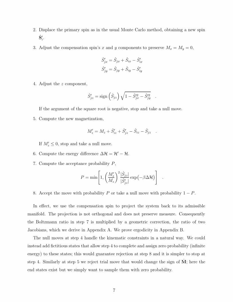
2. Displace the primary spin as in the usual Monte Carlo method, obtaining a new spin

S′i.

3. Adjust the compensation spin’s x and y components to preserve Mx = My = 0,

S ′jx = Sjx + Six − S ′

ix

S ′jy = Sjy + Siy − S ′

iy

4. Adjust the z component,

S ′jz = sign

(

Sjz

)

√

1− S ′2jx − S ′2

jy .

If the argument of the square root is negative, stop and take a null move.

5. Compute the new magnetization,

M ′z = Mz + S ′

iz + S ′jz − Siz − Sjz .

If M ′z ≤ 0, stop and take a null move.

6. Compute the energy difference ∆H = H′ −H.

7. Compute the acceptance probability P ,

P = min

[

1,

(

M ′z

Mz

)2|Sjz|

|S ′jz|

exp(

−β∆H)

]

.

8. Accept the move with probability P or take a null move with probability 1− P .

In effect, we use the compensation spin to project the system back to its admissible

manifold. The projection is not orthogonal and does not preserve measure. Consequently

the Boltzmann ratio in step 7 is multiplied by a geometric correction, the ratio of two

Jacobians, which we derive in Appendix A. We prove ergodicity in Appendix B.

The null moves at step 4 handle the kinematic constraints in a natural way. We could

instead add fictitious states that allow step 4 to complete and assign zero probability (infinite

energy) to these states; this would guarantee rejection at step 8 and it is simpler to stop at

step 4. Similarly at step 5 we reject trial move that would change the sign of M; here the

end states exist but we simply want to sample them with zero probability.

7

IV. CALCULATION OF BULK ANISOTROPIES

Given the originality of the constrained Monte Carlo method, it is important to ensure

that the method is reliable and conforms to existing results, especially regarding the low

temperature dependence of bulk anisotropy as predicted by Callen and Callen1, where uni-

axial anisotropy was shown to have an M3 dependence, and cubic anisotropy to have an

M10 dependence.

In the present work such bulk systems were approximated by simulating a generic ferro-

magnetic system with 16000 spin moments with periodic boundary conditions, to eliminate

surface effects and minimize finite size effects. Sample torque curves for the system with

uniaxial anisotropy are shown in Fig. 1. The points show the calculated torque and the

curves are fits to a sin (2θ) dependence, where θ is the angle from the easy axis. The sin (2θ)

-1

-0.5

0

0.5

1

0 π/4 π/2 3π/4 π

Sy

stem

To

rqu

e/K

u

Angle from Easy Axis

Tx [10 K]Tx (Fit) [10 K]

Tx [100 K]Tx (Fit) [100 K]

Tx [500 K]Tx (Fit) [500 K]

FIG. 1: Simulated and analytical angular dependence of the restoring torque for uniaxial

anisotropy at temperatures 10 K, 100 K, and 500 K. (Color Online)

relationship is seen to hold at all temperatures and the fitted proportionality constant gives

Keffu (T ). In a situation such as this, where all the torque curves have the same shape, the

anisotropy is described by a single parameter and it is sufficient to compute the torque at

the maximum.

In more general cases, such as those with surface anisotropy, it is necessary to compute

the torque at several angular positions. Finally, with every new system it is prudent to

verify the shape of the torque curves over many angles, both polar and azimuthal, before

reducing the number of points to the minimum necessary.

8

The uniaxial anisotropy, cubic anisotropy and magnetization for the generic system are

plotted against temperature in Fig. 2(a). In order to reduce the computational effort, the

torques were computed at a single angular position, θ = 45◦ in the uniaxial case and θ = 22.5◦

in the xz-plane for cubic anisotropy. In Fig. 2(b) the anisotropies are plotted against the

magnetization on logarithmic scales. As can be seen, the results show excellent agreement

0

0.1

0.2

0.3

0.4

0.5

0.6

0.7

0.8

0.9

1

0 200 400 600 800 1000 1200

M/M

s , K

ueff /

Ku ,

Kcef

f /K

c

Temperature [K]

MagnetisationUniaxial Anisotropy

Cubic Anisotropy

(a)Temperature dependence of magnetization, uniaxial,

and cubic anisotropies. The lines provide a guide to the

eye.

-5

-4

-3

-2

-1

0

-0.5 -0.4 -0.3 -0.2 -0.1 0

ln (

Kuef

f /K

u)

, ln

(K

ceff /

Kc)

ln (M/Ms)

Uniaxial Anisotropy

M3

Cubic Anisotropy

M10

(b)Temperature scaling of uniaxial and cubic

anisotropies.

FIG. 2: Simulation results for the temperature dependence and scaling of a pure ferromagnet with

uniaxial and cubic anisotropies. (Color Online)

at low-temperatures with the scaling behavior predicted by Callen and Callen. We note that

in these calculations the internal energy and free energy are almost interchangeable. That

9

is, ∂F/∂θ is nearly equal to ∂〈H〉/∂θ. The anisotropy is too weak to affect the entropy and

the difference 〈H〉 − F = TS is nearly independent of θ. We expect this to hold in most

magnetic systems, but in full generality the distinction between F and 〈H〉 must be kept.

In strong anisotropy systems and temperatures close to Tc we have found that the system

torque deviates from the expected sin(2θ) behavior. This is in agreement with previous

publications where it has been shown that at high temperatures strong magnetization fluc-

tuations lead to several interesting effects, related to the free energy behavior, such as the

change of the magnetization length on the saddle point27 or the elliptic character of domain

walls28.

V. CALCULATION OF ANISOTROPY IN FePt

FePt is a material of current interest because of its extremely high magnetocrystalline

anisotropy energy in the L10 crystal phase29. The material is also unusual due to the M2.1

low-temperature scaling of the effective anisotropy3,4. Ab-initio and Langevin dynamics

simulations by Mryasov et al30 managed to reproduce the observed scaling of the anisotropy

by calculation of the internal energy, and in this work we have applied the Constrained Monte

Carlo method to the same problem. We have utilized the same Hamiltonian as Mryasov et

al30 and simulated a system 6 nm3 with periodic boundary conditions. The key addition to

the generic Hamiltonian in Eq. (1) is a two-ion anisotropy term of the form:

H2−ion =∑

i 6=j

K(2)ij Sz

i Szj (3)

where K(2)ij is the anisotropy constant which is site and range dependent, as extracted form

the ab-initio calculations. The system also possesses an easy-plane anisotropy which is

an order of magnitude weaker than the easy-axis 2-ion anisotropy. The existence of these

competing anisotropies in fact gives rise to the unusual scaling exponent due to the different

temperature scaling of the anisotropic contributions, M2 for two-ion and M3 for single ion.

Due to the large value of the effective anisotropy in FePt, the torque deviates from the

expected sin(2θ) relationship at elevated temperatures, and so the free energy was obtained

by integration over θ. The torque curves were calculated by first equilibrating the system for

10000 steps at each temperature and angle, and then the thermal average of the torque was

calculated over a further 70000 steps. Plots of the change in free energy, ∆F , are shown in

10

−0.05

0

0.05

0.1

0.15

0.2

0.25

0.3

0.35

0 π/4 π/2 3π/4 π

∆F/

Ku

Angle from Easy Axis [K]

550 K

600 K

660 K

FIG. 3: Angular dependence of the free energy in L10 FePt at high temperatures. The curves are

sin2 θ fits to the data in the range 0:π/5. (Color Online)

Fig. 3, showing a deviation from the usual sin2 θ angular dependence at temperatures close

to Tc (700 K). In fact a consistent flattening of the free energy is seen in the proximity of the

hard axis - the high anisotropy energy causes a reduction in the length of the magnetization

which effectively means it is competing with the exchange interaction. The balance of these

effects is that the length of magnetization is slightly lower and therefore so is the torque,

leading to a flattening of the free energy in the maximum. This leads to a lower than

expected energy barrier which is important for the calculation of relaxation times at high

temperature. The low temperature scaling of the anisotropic free energy is plotted in Fig. 4,

-1.2

-1

-0.8

-0.6

-0.4

-0.2

0

-0.5 -0.4 -0.3 -0.2 -0.1 0

ln (

Kef

fF

ePt/

KF

ePt)

ln (M/Ms)

KFePt

M2.1

FIG. 4: Temperature scaling of anisotropy in L10 FePt.

showing excellent agreement with the previous theoretical and experimental results3,4,30.

11

VI. THIN FILM SYSTEMS WITH NEEL SURFACE ANISOTROPY

So far we have demonstrated the ability of the constrained Monte Carlo method to repro-

duce results which are well known. In the following the method is applied to a system where

the temperature dependent behavior is unknown - namely thin films with surface anisotropy.

Understanding surface anisotropy presents a number of challenges due to its complexity, es-

pecially in nanoparticles31. Due to symmetry thin films present a special case for surface

anisotropy, where the behavior is much simplified. Thin films have attracted a great deal of

research interest over the past 50 years and so a large body of experimental data exists17,18,32.

Nevertheless, achieving good experimental data on the temperature dependence of surface

anisotropy requires the creation of very thin films with very sharp interfaces, which has only

been technologically feasible within the last decade. This is because the influence of surface

anisotropy is usually determined by varying the thickness of the magnetic layer, so that

volume and surface contributions can be separated. For thick films the volume component

strongly dominates the overall anisotropy, leading to a large degree of uncertainty in the

strength of the surface contribution. Another problem arises with temperature dependent

atomic migration, structural changes and interface mixing, which cause a change in the

surface properties20.

Calculation of temperature dependent anisotropy

The constrained Monte Carlo method allows for a thorough investigation of the tem-

perature dependence of anisotropy in thin films with the Neel surface anisotropy. In the

case of a perfect single crystal magnetic film with a face-centered-cubic (fcc) or simple cubic

(sc) crystal structure with interfaces cut along the [001] direction, the on-site Neel surface

anisotropy yields a purely uniaxial anisotropy. In order to simulate a section of such a thin

film, a generic magnetic material with fcc (Tc = 1300K) or sc (Tc = 1000K) crystal structure

was chosen. In order to eliminate edge effects within the film, periodic boundary conditions

in the film plane were used. The surface anisotropy is normally found to be much stronger

than bulk-type anisotropy, and so a value of Ks = 10Ku was chosen. When studying thin

films with surface anisotropy, a number of basic combinations of anisotropies are possible.

Principally, in the case of bulk uniaxial anisotropy, the surface and bulk anisotropies can

12

have aligned or opposing easy axes, depending on the sign of the constant. Alternatively, a

material could possess a cubic bulk anisotropy and uniaxial surface anisotropy. In the fol-

lowing we present calculations of temperature dependent effects in these thin film systems

with surface anisotropy.

Where both bulk and surface anisotropies are uniaxial, the torque curves are similar to

ones presented in Fig. 1, showing a sin(2θ) angular dependence. In Fig. 5 we present a

more complicated situation, where the thin film has cubic bulk anisotropy and Neel surface

anisotropy. One of the easy axes of the cubic anisotropy coincides with the surface anisotropy

easy axis (perpendicular to the thin film surface). The torque curve clearly shows a sum-

mation of uniaxial and cubic anisotropy contributions. The temperature dependence of

both contributions is presented in Fig. 6. Similar to our results in the previous section,

the cubic anisotropy exhibits a much stronger temperature dependence than the uniaxial

(surface) part. Consequently, at low temperature the cubic anisotropy dominates while at

high temperature the uniaxial surface anisotropy dominates.

-1

-0.5

0

0.5

1

0 π/4 π/2 3π/4 π

Sy

stem

To

rqu

e/K

c

Angle from z-axis

FIG. 5: The torque curve in a thin film of Lz = 10 atomic planes with fcc structure, cubic bulk

anisotropy and Neel surface anisotropy perpendicular to the thin film plane and parallel to one of

the bulk anisotropy easy axes for T = 10K. The line provides a guide to the eye.

Modeling of the reorientation transition in thin films.

The temperature dependence of the surface anisotropy leads to a number of interesting

effects, such as a temperature dependent reorientation of the magnetization direction from

13

0

0.1

0.2

0.3

0.4

0.5

0.6

0.7

0.8

0.9

0 200 400 600 800 1000 1200

Kuef

f /K

u ,

Kcef

f /K

c

Temperature [K]

Kueff/Ku

Kceff/Kc

FIG. 6: Temperature dependence of uniaxial and cubic effective anisotropies in a thin film of

Lz = 10 atomic planes with fcc structure, cubic bulk anisotropy and Neel surface anisotropy

perpendicular to the thin film plane and parallel to one of the bulk anisotropy easy axes. The lines

provide a guide to the eye. (Color Online)

out-of-plane to in-plane and vice versa14–21. Such an effect can occur when the easy directions

of the surface and bulk anisotropies compete. At low temperatures the magnetization lies

along the surface easy direction, e.g. perpendicular to the plane. As the temperature

is increased the surface contribution to the anisotropy energy rapidly decreases, so the

system magnetization lies along the bulk easy direction, e.g. in the plane. The temperature

dependence of the effective anisotropy is plotted in Fig. 7 for different thin film thicknesses.

Given the large difference in the surface and bulk anisotropy constants, the ultrathin films

fail to show any reorientation transition. As the film thickness is increased the reorientation

transition becomes more pronounced and occurs at a lower temperature. These results are

comparable to mean-field calculations by Hucht et al22.

One other interesting property of the temperature dependent reorientation transition

is that, depending on the choice of non-magnetic interface material, the temperature of

the transition can be tuned. To illustrate this phenomenon, Fig. 8 shows a plot of the

temperature dependence of the total anisotropy for different Neel anisotropy constants,

emulating the effect of changing the interface material. Here the bulk anisotropy is assumed

to be perpendicular to the plane, and the surface anisotropy is easy plane.

14

-0.2

0

0.2

0.4

0.6

0.8

1

1.2

1.4

0 200 400 600 800 1000 1200

Kuef

f /K

u

Temperature [K]

Lz = 5Lz = 7Lz = 9

Lz = 10

FIG. 7: Temperature dependence of the effective anisotropy in thin films with in-plane bulk

anisotropy and perpendicular to the plane surface anisotropy for various thin film thicknesses. The

lines provide a guide to the eye. (Color Online)

−0.2

−0.1

0

0.1

0.2

0.3

0.4

0.5

0.6

0.7

0.8

0.9

0 200 400 600 800 1000 1200 1400

Kuef

f /K

u

Temperature [K]

Ks = 5 Ku

Ks = 10 Ku

Ks = 15 Ku

FIG. 8: Temperature dependence of effective anisotropy for a thin film with competing surface

(easy plane) and bulk (parallel to z axis) anisotropies for a system of 26 × 26 × 6 unit cells for

different magnitudes of Ks. The lines provide a guide to the eye. (Color Online)

Temperature dependence of surface anisotropy

The temperature dependent effective anisotropy in thin films with surface anisotropy is

not an intrinsic parameter since it is strongly dependent on the thin film thickness. In

this section we present two methods which enable the separation of the surface and bulk

anisotropy contributions as a function of temperature in thin films, for simplicity, with

15

parallel surface and bulk uniaxial anisotropy axes perpendicular to the thin film plane. This

allows the extraction of the intrinsic uniaxial and surface contributions, independent of the

thin film thickness.

The first method is based on the variation of the effective anisotropy with the number of

surface atoms via the following well known expression33:

Keff = Keffu +

Ns

N(Keff

s −Keffu ) (4)

where Ns and N are the number of surface and total atoms, and Keffs and Keff

u are the

effective surface and bulk anisotropies, respectively. In Fig.9 we present results at different

temperatures in thin films with a simple cubic lattice and different thicknesses. The data are

perfectly scaled with the ratio Ns/N and for increasing film thickness the effective anisotropy

tends towards the temperature dependent bulk value. The fitting of the data to Eq. (4) allows

the extraction of the surface anisotropy constant as a function of temperature, as presented

in Fig. 10. In this system the surface anisotropy shows a linear decrease with temperature,

similar to the experimental results19,34,35.

0.5

1

1.5

2

2.5

3

3.5

4

0 0.1 0.2 0.3 0.4 0.5 0.6 0.7

Kuef

f /K

u

Ns/N

T = 10 K

T = 100 K

T = 200 K

T = 300 K

T = 400 K

T = 500 K

FIG. 9: Scaling of the effective anisotropy with the ratio between surface and total number of

atoms Ns/N in a thin film with sc structure, uniaxial bulk anisotropy and Neel surface anisotropy

both perpendicular to the thin film plane. The lines show the fits to the data. (Color Online)

Since the surface atoms must be identified in order to calculate the Neel surface

anisotropy, one can also resolve the surface and bulk contributions to the restoring torque

curves. Fig. 11 shows the torque curves for the total, bulk and surface parts, evaluated for

16

0

0.2

0.4

0.6

0.8

1

0 50 100 150 200 250 300 350 400 450 500

2 K

seff /

Ks

Temperature [K]

FIG. 10: Temperature dependence of the effective surface anisotropy in a thin film with sc struc-

ture, uniaxial bulk anisotropy and Neel surface anisotropy perpendicular to the thin film plane

determined from the size scaling of the effective anisotropy. The line is a linear fit to the data.

the same thin film as above. As can be seen, the surface torque also follows the sin(2θ)

behavior and the effective surface anisotropy can therefore be extracted. The values of the

surface anisotropy obtained through this method are comparable with the ones obtained

through the scaling method shown in Fig. 10.

-2

-1.5

-1

-0.5

0

0.5

1

1.5

2

0 π/4 π/2 3π/4 π

Sy

stem

To

rqu

e/K

u

Angle from Easy Axis

Ty [total]

Ty [bulk]

Ty [surface]

FIG. 11: Simulated restoring torque in a thin film of Lz = 10 atomic planes with sc structure,

uniaxial bulk anisotropy and Neel surface anisotropy perpendicular to the thin film plane for

T = 10K. The lines show a fit of the data to sin 2θ. (Color Online)

In practice, the surface torque is a noisy quantity due to the relatively small number of

atoms. In order to obtain a good thermodynamic average it is generally necessary to use a

17

large number of steps. However, the total torque converges much more rapidly and requires

relatively few steps.

The scaling behavior of the anisotropy with magnetization

The separation of surface and bulk contributions to the anisotropy allows the investigation

of the temperature scaling of the surface anisotropy separately with respect to the surface

magnetization, Msurface, and bulk magnetization, Mbulk. We should bear in mind that the

magnetization fluctuations on the surface are dependent on the bulk so that in general the

corresponding scaling exponent is strongly system size dependent.

For an isolated surface layer the scaling of the surface anisotropy with respect to the sur-

face magnetization should follow Keffs ∼ M3

surface, as was found in the bulk case. In principle

this effect could be measured experimentally using a monolayer of magnetic material, though

such a structure is generally unstable at anything other than cryogenic temperatures.

We have found that a magnetic thin film with zero bulk anisotropy also follows the

Keffs ∼ M3

surface law, at least for the thin film thicknesses for which our calculations were

feasible. We have simulated a thin film system with fcc crystal structure, surface anisotropy

perpendicular to the thin film plane and with zero bulk anisotropy. This essentially ensures

that the only anisotropic contribution to the Hamiltonian comes from the surface. The

normalized magnetization and surface anisotropy calculated via the torque method as a

function of temperature are plotted in Fig. 12 for the system dimensions 32 × 32× 12 unit

cells. The surface, bulk and volume average magnetization are plotted, each having the

same Curie temperature but with a different criticality, as previously reported by Binder et

al36.

The reduced criticality in the surface magnetization arises from a reduction in coordina-

tion number. An isolated surface layer would also have a reduced Curie temperature, but in

our case the surface layer is polarized by the bulk and thus has the same Tc of around 1300

K. Fig. 13 shows the temperature scaling of the surface anisotropy with the surface magne-

tization showing a low temperature exponent of Keffs ∼ M3

surface, in excellent agreement with

the Callen-Callen theory for single ion uniaxial anisotropy.

The scaling of the total effective anisotropy in the presence of the Neel surface anisotropy

with total magnetization is unknown a-priori, and is coordination number, thin film thick-

18

0

0.2

0.4

0.6

0.8

1

0 200 400 600 800 1000 1200 1400

M/M

s , K

seff /

Ks

Temperature [K]

Kseff/Ks

Mbulk

Maverage

Msurface

FIG. 12: Plot of normalized magnetization and surface anisotropy against temperature for a thin

film with zero bulk anisotropy. The surface magnetization shows stronger criticality than the bulk

and average magnetization. The lines provide a guide to the eye. (Color Online)

-1.6

-1.4

-1.2

-1

-0.8

-0.6

-0.4

-0.2

0

-0.5 -0.4 -0.3 -0.2 -0.1 0

ln (

Ksef

f /K

s)

ln (Msurface/Ms)

Kseff/Ks

M3surface

FIG. 13: Plot of temperature scaling of surface anisotropy with surface magnetization, for a system

with zero bulk anisotropy.

ness and material dependent. Nevertheless, it is this scaling which would be measured

experimentally. To illustrate this effect we have calculated the effective scaling exponent

Keffu ∼ Mγ

average for a system with both uniaxial and surface anisotropies for different film

thicknesses, as shown in Fig. 14. For an isolated surface layer Ns = N the critical exponent

γ = 3 is recovered. The critical exponent has a maximum and should tend again to γ = 3

value for very thick films.

19

3

3.05

3.1

3.15

3.2

3.25

3.3

0 0.2 0.4 0.6 0.8 1

Sca

lin

g E

xp

on

ent

γ

Ns/N

FIG. 14: Plot of scaling exponent with thin film thickness in a thin film with Ks = 10Ku, parallel

out-of-plane easy axes and sc lattice. The line provides a guide to the eye.

VII. CONCLUSION

We have developed a constrained Monte Carlo method, by which we can compute ther-

modynamic properties of magnetic systems as a function of the magnetization direction.

We have shown its novel capability to evaluate the temperature dependence of the magnetic

anisotropy, which is an important quantity for technological applications in hard magnetic

materials. The method has been utilized to compute the temperature dependence of bulk

magnetic anisotropy and we have recovered numerically the analytic scaling law of Callen

and Callen.

The importance of the method resides in its potential to calculate temperature-dependent

effective anisotropies in complex materials. The present challenge for modeling of magnetic

materials is the multiscale approach, where the ab-initio information is passed to a different

scale with the aim to model larger sizes of material, using, for example micromagnetics.

The CMC method provides a real possibility to link the quantum mechanical scale with

micromagnetics, via the parameterization of a classical Heisenberg Hamiltonian23. This

Hamiltonian can be used to calculate temperature dependent equilibrium behavior. To

demonstrate this, we have applied the method to the calculation of the effective anisotropy

bulk FePt, using the model parameterized through ab-initio calculations, and have recovered

the experimentally observed KeffFePt ∼ M2.1 temperature scaling. Moreover, we have also

noted the appearance of a flattening of the free energy surface at the energy maximum, an

20

effect not previously seen with less subtle methods.

We have then applied the method to a variety of thin films with surface anisotropy, inves-

tigating the size dependent behavior and temperature dependence of surface anisotropy. We

have shown the capability of the method to simulate the temperature-dependent magneti-

zation reorientation transition. We also have shown that the method enables the separation

of the temperature dependent surface anisotropy as an intrinsic system parameter, indepen-

dent of the thin film thickness. Our results demonstrate a linear temperature dependence

of the surface anisotropy, consistent with the experimental results in Gd34,35, Ni35 and Fe19

grown on different substrates. However, when comparing with our results, various factors

should be taken into account, including structural changes with increased temperatures or a

lattice mismatch which could influence the bulk anisotropy. One other possibility is that of

an enhanced exchange interaction at the surface of the material37. An increased exchange

interaction would lead to an increase in the criticality of the surface layer and commensu-

rate reduction in the temperature dependence of the surface anisotropy. In the future, more

complicated models could take into account these effects.

Finally, we have investigated the scaling of the anisotropy in thin films with magnetiza-

tion. In thin films with zero bulk anisotropy, the surface anisotropy scales with the surface

magnetization following the Callen-Callen law. In other cases we report no universal scaling

behavior of the surface anisotropy.

To summarize, the constrained Monte Carlo method is a powerful tool, allowing to include

both thermodynamic fluctuations and entropy into the evaluation of macroscopic quantities

such as temperature dependent magnetic anisotropy. In the future we plan to apply the

method to model more realistic systems within a general trend to large-scale material mod-

eling aiming the design of novel materials with potential applications.

VIII. ACKNOWLEDGEMENTS

This work has been supported by the grants MAT2007-66719-C03-01 and CS2008-023

from the Spanish Ministry of Science and Education, and EC FP7 [Grants No. NMP3-

SL-2008-214469 (UltraMagnetron) and No. 214810 (FANTOMAS)]. The financial support

from the European COST P-19 Action and from Seagate Technology, USA, is also gratefully

acknowledged.

21

Appendix A: Jacobians in the trial moves

We are displacing two spins, whose combined volume element is d2Si d2Sj. However, we

plan to readjust Sj to keep M constant. Accordingly, we eliminate the variable Sj in favor of

M and rewrite the volume element as |J(Si, M)| d2Si d2M , expressing Sj in terms of M and

expecting the Jacobian J(Si, M) to be nontrivial. This allows us to view the trial move as

taking place in the Si, M variables. The Boltzmann probability density in these variables is

ρ ∝ |J | exp(−βH). Since our trial moves are reversible in(

Si, M)

, the Metropolis-Hastings

test ratio38 is just ρ′/ρ =|J ′/J | exp(

−β∆H)

. The fact that we always keep M′ ≡ M has no

bearing on the argument and we use the same ratio to decide whether to accept the move

from (Si, M) to (S′i, M).

The first result we need is the relationship between a spherical surface element and its

projection in the XY plane. We have

d2Si =dSix dSiy

|Siz|, d2Sj =

dSjx dSjy

|Sjz|(A1)

d2M =dMx dMy

|Mz|= dMx dMy . (A2)

Too see this, note that for any unit vector S the angle between the tangent plane to the

sphere at S and the XY plane is simply θ = cos−1(

|Sz|)

, therefore the projected area

dSx dSy is |cos(θ)| d2S = |Sz| d2S. Equations (A1) and (A2) are the inverse of this relation,

stated for the three vectors Si, Sj , M. In the case of M, Eq. (A2), the denominator |Mz| is

not necessary because we are locking M in the positive z direction, therefore Mz ≡ 1.

Next, we express dMx and dMy in terms of dSix, dSiy, dSjx and dSjy. We assume that

M lies in the z direction but we do not make the same assumption for M + dM. For the

unnormalized vector M, we have

dMx = dSix + dSjx , dMy = dSiy + dSjy (A3)

since the other spins are fixed. For the normalized M, we have

dM = d(

M−1M)

= M−1 dM−M−2M dM . (A4)

We only need the x and y component of (A4). Since M lies in the +z direction, the last

term contributes nothing to the in-plane components and we don’t need to calculate dM

22

(although it would be easy to do so). The remaining term gives

dMx = M−1 dMx , dMy = M−1 dMy . (A5)

We substitute (A3) in (A5) and replace M by Mz:

dMx = M−1z dSix +M−1

z dSjx

dMy = M−1z dSiy +M−1

z dSjy .(A6)

We rewrite (A6) in matrix form,

dSix

dSiy

dMx

dMy

=

1 0 0 0

0 1 0 0

M−1z 0 M−1

z 0

0 M−1z 0 M−1

z

dSix

dSiy

dSjx

dSjy

. (A7)

The Jacobian of the change of variables is the determinant of the matrix in (A7), namely

M−2z . Therefore, the volume elements are related by

dSix dSiy dMx dMy = M−2z dSix dSiy dSjx dSjy (A8)

and the inverse relation is

dSix dSiy dSjx dSjy = M2z dSix dSiy dMx dMy . (A9)

Dividing by |Siz| |Sjz| and using (A1), we obtain

d2Si d2Sj =

M2z

|Sjz|d2Si d

2M (A10)

Thus the Jacobian is |J | = M2z /|Sjz| and we accept each trial move with probability

P = min[

1, |J ′/J | exp(

−β∆H)]

= min

[

1,

(

M ′z

Mz

)2|Sjz|

|S ′jz|

exp(

−β∆H)

]

(A11)

as stated in step 7 of the algorithm.

Appendix B: Ergodicity

We show that every admissible state (i.e. with total magnetization along +z) can be

reached from any other admissible state by a sequence of constrained Monte Carlo trial

23

moves. In this context we may ignore the Metropolis acceptance test at step 8 of the

algorithm, but the trial moves must still pass the kinematic tests at steps 4 and 5. The

proof relies on two lemmas:

Lemma 1 Any spin with a negative z component can be moved to the hemisphere Sz > 0

by a sequence of trial moves, without any other spin crossing the plane z = 0.

Lemma 2 Assuming all the spins are in the hemisphere Sz > 0, one of them can be moved

to the z axis by a sequence of trial moves, without any spin crossing the plane z = 0.

Repeated applications of Lemma 1 allow us to move the spins one by one to the hemi-

sphere Sz > 0, at which point Lemma 2 becomes applicable.

Repeated applications of Lemma 2 allow us to move all the spins to the positive z axis.

After the first application we have one spin along +z; the remainingN−1 spins are perturbed

in the process, but they remain in the upper hemisphere and their final magnetization must

also point along +z. That is, they form an admissible state of N−1 spins, Lemma 2 becomes

applicable to them and we can iterate. Thus, any admissible state can be collapsed to the

saturated state by a sequence of trial moves. By chaining such a collapsing sequence with

the inverse of another one, we can connect any two admissible states.

Proof of Lemma 2

We use trial moves where the primary spin does not cross the plane z = 0. We write si

(lower case) for the projection (Six, Siy) in the XY plane. It is enough to consider the si

since the z components are uniquely determined by them, Siz = +√

1− ‖si‖2. The trial

moves can not fail at step 5, leaving only step 4 to consider. A trial move then consists in

displacing two points si, sj by equal and opposite amounts, while keeping both points in the

unit disk, ‖si‖, ‖sj‖ ≤ 1.

We want to show that, for any set of N points in the unit disk with centroid (0, 0), one of

the points can be shifted to (0, 0) by a combination of such moves. In fact we have a slightly

more general result: in any set of N points, one can be moved to the centroid, whether or

not the centroid is (0, 0).

We proceed by induction on N . For N < 2 there is nothing to prove. For N = 2, let

c = (s1+s2)/2 be the centroid. Since c is invariant, the condition ‖s2‖ ≤ 1 can be expressed

24

in terms of s1, ‖2c−s1‖ ≤ 1. Similarly we have ‖2c−s2‖ ≤ 1. This means that we can move

the two points symmetrically about c, as long as we keep them both within a lens-shaped

“admissible zone”, which is the intersection of the unit disk and of its inversion through c.

This is shown in Fig. 15. The admissible zone, being convex, contains c. Therefore we can

move both points to c, using several sub-moves if necessary.

FIG. 15: Admissible zone for projected trial moves in the proof of Lemma 2. The projections of

the two spins (black circles) can move symmetrically about their centroid (white circle) within the

region shown in white.

For N > 2 we assume by the induction hypothesis that the centroid cN−1 of the first N−1

points is already occupied by one of the sk. The full centroid cN = (sN + (N − 1)sk)/N

lies on the segment [sk, sN ] and is in the admissible zone of sk, sN . Therefore we can move

either point to the centroid. This proves the lemma.

Proof of Lemma 1

We want to reduce by one the number of spins with Sz ≤ 0. Our rules allow trial moves

where the primary spin flips its z component and the secondary spin does nothing, but we

would like to avoid these potentially low probability moves. Our strategy is to move the

offending spin close to the plane z = 0 so as to require only a small jump in Sz in the final

move. We proceed as in the proof of Lemma 2, using projections in the XY plane, but this

time we have to avoid rejection at step 5 of the algorithm.

25

Consider an admissible state where spin i has Siz < 0. Choose a j such that Sjz > 0

(there must be one, since Mz is positive). We use trial moves with Si as the primary spin

and Sj as the compensation spin. Let si, sj be the projections in the XY plane. The two

points si, sj are restricted to a lens-shaped admissible region as in the proof of Lemma 2,

but there may be a further restriction to ensure that Mz remains positive.

As before, we express sj in terms of si, sj = 2c− si. The contribution of spins i and j to

Mz is then

Siz + Sjz = −√

1− ‖si‖2 +√

1− ‖2c− si‖2 . (B1)

It can be shown that the contours of (B1) in the (six, siy) plane are arcs of ellipses centered

on c and tangent to the admissible zone, as shown in Fig. 16, and that (B1) increases

monotonically as si moves from the interior edge to the exterior edge of the admissible zone.

If si stays on the distal side of its starting contour, the value of Mz cannot become negative.

FIG. 16: Admissible zone for projected trial moves in the proof of Lemma 1. The dashed lines are

contours of Siz + Sjz as a function of Six, Siy. A possible path for the projection of the primary

spin is shown in black, with the matching path of the secondary spin in grey. If the primary spin

stays in the white region the total magnetization Mz cannot become negative.

This is represented by the white region in Fig. 16. We see that there is an ample supply of

paths that take si arbitrarily close to the edge of the unit disk. At that point a final trial

move can take Si across the plane Siz = 0. The only other spin involved, Sj , remains in the

positive z hemisphere throughout. This proves Lemma 1.

26

Appendix C: Macroscopic Torques

The magnetization direction M plays the role of a macroscopic parameter. In this section

we identify the generalized forces acting on M (torques) with the derivatives of the Helmholtz

free energy.

By way of introduction, consider a thermodynamic system with an external macroscopic

parameter q and microscopic states ξα. We treat α as a discrete index for simplicity. The

energy of each microscopic state is a function of q; the partition function and the Helmholtz

free energy are39

Z(q) =∑

α

exp(

−βH(ξα, q))

, (C1)

F(q) = −β−1 Ln(

Z(q))

. (C2)

Differentiation of (C2) with respect to q yields immediately

−dF/dq =∑

α

Z−1 exp(

−βH(ξα, q)) −∂H(ξα, q)

∂q

=⟨

−∂H/∂q⟩

(C3)

where in the second line of (C3) we recognized the sum over microstates as a thermodynamic

average, since the weights Z−1 exp(

−βH(ξα, q))

are the Boltzmann probabilities. Thus the

mean force conjugate to q is the negative derivative with respect to q of the Helmholtz free

energy F(q).

The right-hand side of (C3), being a thermodynamic average, can be computed by the

Metropolis algorithm. As a general rule, derivatives and differences of free energies are

computable in this way, even though the free energy itself is not.

The argument is not directly applicable to our case since M is not a parameter in the

Hamiltonian, but a restriction on the set of admissible states. One could in principle set

up a system of 2N − 2 coordinates that forms a complete set with M and treat M as a

parameter, but we never did this. Instead, we picked a temporary coordinate system for

each Monte Carlo move, to be discarded after the move. Indeed, the whole of appendix A

is a stratagem to avoid setting up global coordinates.

However we can recover a result similar to (C3). Given any two directions M and M′

we can find a rotation R that sends M to M′. If we apply this rotation globally to every

spin Si that constitutes a microstate ξ, we obtain a measure-preserving bijection between

27

the two admissible manifolds. This allows us to replace sums over the microstates of the

M′ manifold by sums over the microstates (rotated) of the M manifold. In particular, the

partition function Z ′ = Z(M′) is

Z ′ =∑

α

exp(

−βH(Rξα))

. (C4)

Dividing by Z and factoring out an exp(

−βH(ξα))

from each term,

Z ′/Z =∑

α

Z−1 exp(

−βH(ξα))

×

exp[

−β(

H(Rξα)−H(ξα))]

, (C5)

or

Z ′/Z =⟨

exp[

−β(

H(Rξ)−H(ξ))]

⟩

, (C6)

where the sums in (C4–C5) and the thermodynamic average in (C6) are over the admissible

manifold of M. Taking logarithms and dividing by −β, we have

F ′ −F = −β−1 Ln[⟨

exp[

−β(

H(Rξ)−H(ξ))]

⟩]

(C7)

where again the thermodynamic average is over the manifold of M.

Specializing to an infinitesimal rotation, Rv ≡ v+dθn×v+O(dθ2) and writing each mi-

crostate ξ as a collection of spins Si, the energy difference in the argument of the exponential

is

H(Rξ)−H(ξ) = dθ∑

i

(

n× Si

)

·∂H

∂Si

+O(dθ2) (C8)

= dθn ·∑

i

(

Si ×∂H

∂Si

)

+O(dθ2) . (C9)

As dθ approches zero the logarithm and exponential in (C7) become a no-op,

F ′ −F = dθn ·

⟨

∑

i

Si ×∂H

∂Si

⟩

+O(dθ2) . (C10)

Meanwhile, M′ is related to M by the same infinitesimal rotation and we can expand F ′ =

F(M′) in a Taylor series.

F ′ = F(

M+ dθn× M+O(dθ2))

(C11)

= F + dθ(

n× M)

·∂F

∂M+O(dθ2) (C12)

= F + dθn ·

(

M×∂F

∂M

)

+O(dθ2) (C13)

28

Combining the terms of order dθ in (C10) and (C13), we obtain

n ·

⟨

∑

i

Si ×∂H

∂Si

⟩

= n ·

(

M×∂F

∂M

)

. (C14)

Since the equality holds for all n, we have finally⟨

∑

i

Si ×∂H

∂Si

⟩

= M×∂F

∂M. (C15)

∗ Electronic address: rfle500@york.ac.uk

1 H. B. Callen and E. Callen, Journal of Physics and Chemistry of Solids, 27 1271 (1966)

2 P. Bruno. Physical Origins and Theoretical Models of Magnetic Anisotropy, 24 IFF-Ferienkurs,

Forschungszentrum Julich, (1993)

3 J. U. Thiele, K. R. Coffey, M. F. Toney, J. A. Hedstrom and A. J. Kellock, J. Appl. Phys. 91

6595 (2002)

4 S. Okamoto, N. Kikuchi, O. Kitakami, T. Miyazaki, Y. Shimada and K. Fukamichi, Phys. Rev.

B 66 024413 (2002)

5 H. F. Hamann, Y. C. Martin and H. K. Wickramasinghe Appl. Phys. Lett.84 810 (2004)

6 R.E Rottmayer et al IEEE Trans. Mag.42 2417 (2006)

7 T.W. McDaniel J. of Phys.: Cond. Mat.17 315 (2005)

8 A.Lyberatos and K.Yu.Guslienko J.Appl. Phys.94 1119 (2003)

9 F. Garcia-Sanchez, O. Chubykalo-Fesenko, O.N. Mryasov and R.W. Chantrell

J.Mag.Magn.Mat.303 282-286 (2006)

10 J.U. Thiele, S. Maat and E. Fullerton Appl. Phys. Lett.82 2859 (2003)

11 K.Yu. Guslienko, O.Chubykalo-Fesenko, O.Mryasov, R.W.Chantrell and D.Weller Phys. Rev.

B70 104405 (2004)

12 R.F.L. Evans, R. Yanes, O. Mryasov, R. W. Chantrell and O. Chubykalo-Fesenko Europhys.

Lett. 88 57004 (2009)

13 U. Atxitia et al. Appl. Phys. Lett. 91 232507 (2007)

14 B.Schulz and K.Baberschke, Phys. Rev. B 50 13467 (1994)

15 A.Berger and H.Hopster Phys. Rev. Lett. 76 519 (1996)

16 P.Bruno and J.P.Renaud Appl. Phys. A 49 499 (1989)

29

17 I.G. Baek, H.G. Lee, H.J. Kim and E. Vescovo Phys. Rev. B 67 075401(2003)

18 R. Allenspach and A. Bischof, Phys. Rev. Lett. 69 3385 (1992)

19 A.Enders et al.Phys. Rev. Lett. 90 217203 (2003)

20 A. Dinia, N. Persat, and H. Danan. Journal of Applied Physics 84 5668–5672 (1998)

21 M. Farle Rep. Prog. Phys. 61 755 (1998)

22 A. Hucht and K. D. Usadel, Phys. Rev. B 55 12309 (1997)

23 N. Kazantseva et al. Phys. Rev. B 77 184428 (2008)

24 U. Nowak, Annual Review of Computational Physics IX, World Scientific, Singapore 105 (2001)

25 L. Neel, J. Phys. Radium 15 225 (1954)

26 N. Metropolis, A. W. Rosenbluth, M. N. Rosenbluth, A. H. Teller, E. Teller, Journal of Chemical

Physics 21 1087–1092 (1953)

27 N. Kazantseva, D. Hinzke, R. W. Chantrell, and U. Nowak Europhys. Lett. 86 2009

28 D. Hinzke et al. Phys. Rev. B 77 094407 (2008)

29 D. Weller and A. Moser, IEEE Trans. Magn. 36 10 (1999)

30 O. N. Mryasov, U. Nowak, K. Y. Guslienko and R. W. Chantrell, Europhys. Lett. 69 805811

(2005)

31 R. Yanes, O. Chubykalo-Fesenko, H. Kachkachi, D. A. Garanin, R. Evans, and R.W. Chantrell,

Phys. Rev. B 76 064416 (2007)

32 D. S. Chuang, C. A. Ballentine and R. C. O’Handley Phys. Rev. B 49 15084 (1994)

33 C. Chappert and P. Bruno, J. Appl. Phys. 64 5736 (1988)

34 G. Andre, A. Aspelmeier, B. Schulz, M. Farle, and K. Baberschke Surface Science 326 275–284

(1995)

35 M.Farle et. al. J. Magn.Magn. Mat. 165 74 (1997)

36 K. Binder and P. C. Hohenberg Phys. Rev. B 9 2194–2214 (1974)

37 A. Buruzs et al, Physical Review B 76 064417 (2007)

38 W. K. Hastings, Biometrika 69 97 (1970)

39 Equations (1.3.30–32) in David L. Goodstein, States of Matter, Prentice-Hall, ISBN 0-13-

843557-X (1975)

30