Computer aided evaluation of the value of water for irrigation ...

Computer aided evaluation of the value of water for irrigationby William Glen Greiman

A thesis submitted in partial fulfillment of the requirements for the degree of Master of Science inAgricultural EngineeringMontana State University© Copyright by William Glen Greiman (1990)

Abstract:A method of determining a site specific value of water for irrigation is presented. The methodpresented uses designer interactive computer programs, which incorporate computer aided design(CAD) and spreadsheet software, to aid in the design and economic evaluation of an irrigation system.The value of water is found by budgeting all the costs and benefits of a farming operation before andafter irrigation development and comparing them. The difference between the farm's before-andafter-development return to land is attributed to the value of the irrigation water.

COMPUTER AIDED EVALUATION OF THE VALUE OF WATER FOR IRRIGATION

byWilliam Glen Greiman

A thesis - submitted in partial fulfillment of the requirements for the degree

ofMaster of Science

in

Agricultural Engineering

MONTANA STATE UNIVERSITY Bozeman, Montana

March 1990

a SS H11

APPROVAL

of a thesis submitted by William Glen Greiman

This thesis has been read by each member of the thesis committee and has been found to be satisfactory regarding content, English usage format citations, bibliographic style, and consistency, and is ready for submission to the College of Graduate Studies.

/ 2 . / ? p nDate Chairperson, Graduate Committee

Approved for Major Department

/Z /? TODate Head, Major Departmeneng

Approved for the College of Graduate Studies

/ f f oDate Graduate Dean

iii

STATEMENT OF PERMISSION TO USE

In presenting this thesis in partial fulfillment of the requirements for a master's degree at Montana State University, I agree that the Library shall make it available to borrowers under rules of the Library. Brief quotations from this thesis are allowable without special permission, provided that accurate acknowledgment of

; Isource is made. jPermission for extensive quotation from or reproduction of this !

thesis may be granted by my major professor, or in his/her absence, by the Director of Libraries when, in the opinion of either, the proposed !use of the material is for scholarly purposes. Any copying or use of the material in this thesis for financial gain shall not be allowed Iwithout my written permission.

SignatureDate

TABLE OF CONTENTS

PageAPPROVAL ...................................................... ii

STATEMENT OF PERMISSION TO USE ................................ iiiTABLE OF CONTENTS .............................................. ivLIST OF FIGURES.................................................... viLIST OF TABLES ........................... viiABSTRACT ...................................................... x

1. INTRODUCTION .............................................. I2. GENERAL COMPUTER SOFTWARE DESCRIPTION ...................... 10

AutoCAD.................................................. 10Lotus 1 2 3 ................................................ 12

3. METHODOLOGY .............................................. 14

4. IRRIGATION DESIGN AND ECONOMIC EVALUATION .................. 18AutoCAD Irrigation Design Initialization.................. 18Pivot Design LISP Program (PB/. Isp)....................... 20Wheel Line Design LISP Program (WL.lsp)................... 23Hand Line Design LISP Program (HL.l^p).................. 24Flood Design LISP Program (FLOOD. Isp)..................... 25Dam Design LISP Program (DAM. Isp)......................... 26Pipeline Design LISP Program (PNODE.lsp) ................ 27Exporting AutoCAD Information to Lotus 123................ 32Irrigation Design Analysis Spreadsheet Explanation......... 35

5. THE MACHINE USE SPREADSHEET..................... 48The Index r a n g e .......................................... 48The Economic Variables Range ............................ 50The Crop Variables Range ................................ 51The Equipment Parameters Range .......................... 52The Time-Table Range .................................... 57The Annual Use Range ................. 58The Used Equipment Option Range .......................... 59The Time-Budget Range .................................... 62The Fixed and Variable Cost Ranges ....................... 63The Equipment Cost Range ................................ 65The Summary and Sensitivity Analysis Range ................ 66

6. ENTERPRISE ANALYSIS SPREADSHEET ............................ 68The Index R a n g e .......................................... 68The System Variables Range .............................. 69

iv

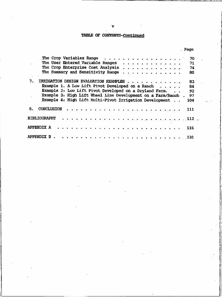
TABLE OF COMTEMTS-Continued

PageThe Crop Variables Range ............................. 70The User Entered, Variable Ranges ................ .. 71The Crop Enterprise Cost Analysis..................... 74The Summary and Sensitivity R a n g e .................... 80

7. IRRIGATION DESIGN EVALUATION EXAMPLES...................... 83Example I. A Low Lift Pivot Developed on a Ranch . . . . . . 84Example 2 s Low Lift Pivot Developed on a Dryland Farm. . . 92Example 3: High Lift Wheel Line Development on a Farm/Ranch . 97Example 4: High Lift Multi-Pivot Irrigation Development . . 104

8. CONCLUSION.............................. Ill

BIBLIOGRAPHY .................................. : . 112 , -APPENDIX A .................................................... 116APPENDIX B ................................................... . 131

V

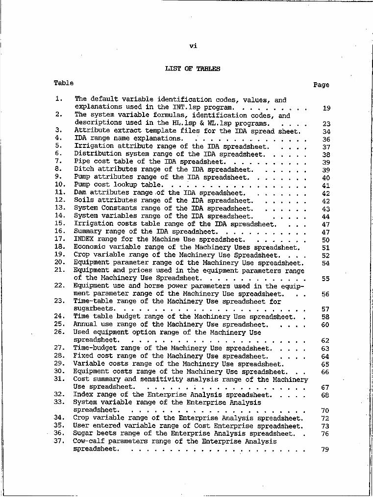
LIST OF TABLES

1. The default variable identification codes, values, andexplanations used in the INT. Isp program.................. 19

2. The system variable formulas, identification codes, anddescriptions used in the HL.lsp & ML.Isp programs......... 23

3. Attribute extract template files for the IDA spread sheet. 344. IDA range name explanations. ................ 365. Irrigation attribute range of the IDA spreadsheet......... 376. Distribution system range of the IDA spreadsheet.......... 387. Pipe cost table of the IDA spreadsheet.................... 398. Ditch attributes range of the IDA spreadsheet............. 399. Pump attributes range of the IDA spreadsheet.............. 4010. Pump cost lookup table. .................................. 4111. Dam attributes range of the IDA spreadsheet............... 4212. Soils attributes range of the IDA spreadsheet.............. 4213. System Constants range of the IDA spreadsheet.............. 4314. System variables range of the IDA spreadsheet. ......... 4415. Irrigation costs table range of the IDA spreadsheet. . . . 4716. Summary range of the IDA spreadsheet...................... 4717. INDEX range for the Machine Use spreadsheet............... 5018. Economic variable range of the Machinery Uses spreadsheet. 5119. Crop variable range of the Machinery Use Spreadsheet. . . . 5220. Equipment parameter range of the Machinery Use spreadsheet. 5421. Equipment and prices used in the equipment parameters range

of the Machinery Use Spreadsheet.......................... 5522. Equipment use and horse power parameters used in the equip

ment parameter range of the Machinery Use spreadsheet. . . 5623. Time-table range of the Machinery Use spreadsheet for

sugarbeets................................................ 5724. Time table budget range of the Machinery Use spreadsheet. . 5825. Annual use range of the Machinery Use spreadsheet. . . . . 6026. Used equipment option range of the Machinery Use

spreadsheet............................................... 6227. Time-budget range of the Machinery Use spreadsheet........ 6328. Fixed cost range of the Machinery Use spreadsheet.... 6429. Variable costs range of the Machinery Use spreadsheet. 6530. Equipment costs range of the Machinery Use spreadsheet. . . 6631. Cost summary and sensitivity analysis range of the Machinery

Use spreadsheet............... 6732. Index range of the Enterprise Analysis spreadsheet........ 6833. System variable range of the Enterprise Analysis

spreadsheet............................................... 7034. Crop variable range of the Enterprise Analysis spreadsheet. 7235. User entered variable range of Cost Enterprise spreadsheet. 7336. Sugar beets range of the Enterprise Analysis spreadsheet. . 7637. Cow-calf parameters range of the Enterprise Analysis

spreadsheet............................................... 79

vi

Table Page

LIST OF TflBUiS-Continued

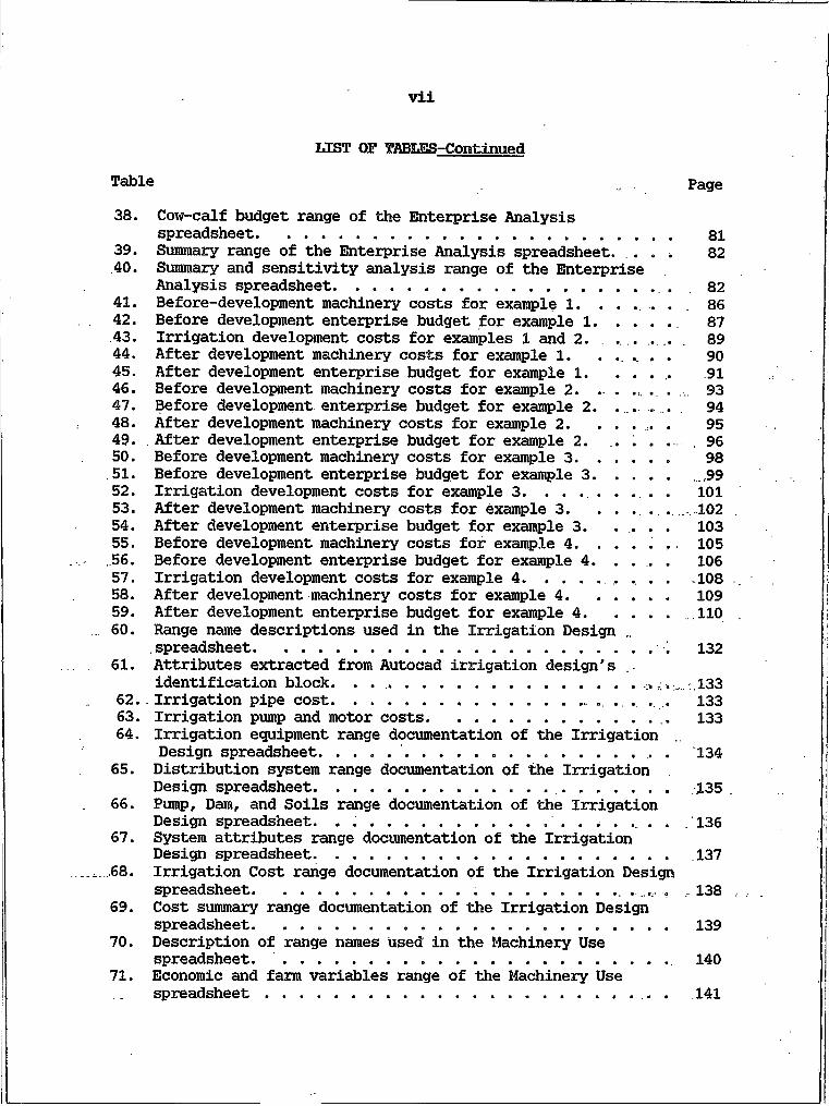
38. Cow-calf budget range of the Enterprise Analysisspreadsheet............................................... 81

39. Summary range of the Enterprise Analysis spreadsheet. . . . 82.40. Summary and sensitivity analysis range of the Enterprise

Analysis spreadsheet...................................... 8241. Before-development machinery costs for example I. . . . . . . 8642. Before development enterprise budget for example I........ . 8743. Irrigation development costs for examples I and 2. ...... . 8944. After development machinery costs for example I. . . . . . . 9045. After development enterprise budget for example I. . . . . 9146. Before development machinery costs for example 2. . . . . . .... 9347. Before development enterprise budget for example 2. ... . . 9448. After development machinery costs for example 2. . . . . . 9549. After development enterprise budget for example 2. . . . . . 9650. Before development machinery costs for example 3.......... 98.51. Before development enterprise budget for example 3. . . . . ,9952. Irrigation development costs for example 3. . . . . . . . . 10153. After development machinery costs for example 3. . . . . .. .. 10254. After development enterprise budget for example 3. . . . . 10355. Before development machinery costs for example 4. . . . . . 10556. Before development enterprise budget for example 4. . . . . 10657. Irrigation development costs for example 4.......... 10858. After development machinery costs for example 4.............. 10959. After development enterprise budget for example 4........... H O60. Range name descriptions used in the Irrigation Design .

. spreadsheet............................................... 13261. Attributes extracted from Autocad irrigation design's

identification block. . . ................................ .. 13362. Irrigation pipe cost. .................... 13363. Irrigation pump and motor costs........................... 13364. Irrigation equipment range documentation of the Irrigation

Design spreadsheet......... . 13465. Distribution system range documentation of the Irrigation

Design spreadsheet............................ 135 .66. Pump, Dam, and Soils range documentation of the Irrigation

Design spreadsheet. . . ..................... .13667. System attributes range documentation of the Irrigation

Design spreadsheet....................................... 13768. Irrigation Cost range documentation of the Irrigation Design

spreadsheet.......................................... ,13869. Cost summary range documentation of the Irrigation Design

spreadsheet................................. 13970. Description of range names used in the Machinery Use

spreadsheet. ............................................ 14071. Economic and farm variables range of the Machinery Use

spreadsheet................... . 141

vii

Table Page

viii

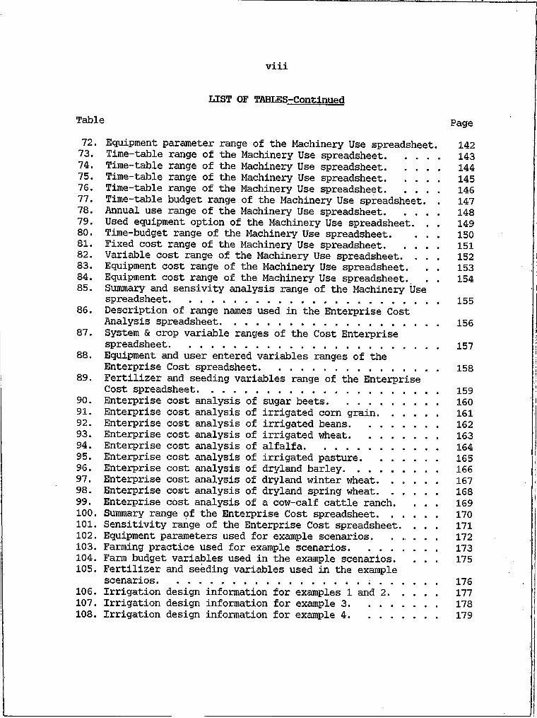
72. Equipment parameter range of the Machinery Use spreadsheet. 14273. Time-table range of the Machinery Use spreadsheet......... 14374. Time-table range of the Machinery Use spreadsheet......... 14475. Time-table range of the Machinery Use spreadsheet......... 14576. Time-table range of the Machinery Use spreadsheet......... 14677. Time-table budget range of the Machinery Use spreadsheet. . 14778. Annual use range of the Machinery Use spreadsheet...... 14879. Used equipment option of the Machinery Use spreadsheet. . . 14980. Time-budget range of the Machinery Use spreadsheet. . . . 15081. Fixed cost range of the Machinery Use spreadsheet...... 15182. Variable cost range of the Machinery Use spreadsheet. . . . 15283. Equipment cost range of the Machinery Use spreadsheet. . . 15384. Equipment cost range of the Machinery Use spreadsheet. . . 15485. Summary and sensivity analysis range of the Machinery Use

spreadsheet............................................ 15586. Description of range names used in the Enterprise Cost

Analysis spreadsheet................................... 15687. System & crop variable ranges of the Cost Enterprise

spreadsheet............................................ 15788. Equipment and user entered variables ranges of the

Enterprise Cost spreadsheet............................ 15889. Fertilizer and seeding variables range of the Enterprise

Cost spreadsheet....................................... 15990. Enterprise cost analysis of sugar beets.................... 16091. Enterprise cost analysis of irrigated corn grain........... 16192. Enterprise cost analysis of irrigated beans................ 16293. Enterprise cost analysis of irrigated wheat................ 16394. Enterprise cost analysis of alfalfa........................ 16495. Enterprise cost analysis of irrigated pasture.............. 16596. Enterprise cost analysis of dryland barley................. 16697. Enterprise cost analysis of dryland winter wheat........... 16798. Enterprise cost analysis of dryland spring wheat........... 16899. Enterprise cost analysis of a cow-calf cattle ranch. . . . 169100. Summary range of the Enterprise Cost spreadsheet....... 170101. Sensitivity range of the Enterprise Cost spreadsheet. . . . 171102. Equipment parameters used for example scenarios. . . . . . 172103. Farming practice used for example scenarios............... 173104. Farm budget variables used in the example scenarios. . . . 175105. Fertilizer and seeding variables used in the example

scenarios............................... .. . ; .......... 176106. Irrigation design information for examples I and 2......... 177107. Irrigation design information for example 3............... 178108. Irrigation design information for example 4............... 179

LIST OF TABLBS-ContinuedTable Page

LIST OF FIGUIffiSFigure Page1. Attribute blocks used in AutoCAD irrigation designs. . . . 112. Flow chart showing spreadsheet relationships. 153. Legend for AutoCAD irrigation design....................... 214. An example AutoCAD irrigation design....................... 225. Flow chart of PNODE.lsp LISP program....................... 286. Flow-chart of Machinery Use. spreadsheet................. .. 497. Irrigation design drawing for examples I and 2..... .... ; 888. Irrigation design drawing for example 3.............. 1009. Irrigation design drawing of example 4............... 10710. Autocad irrigation design initialization LISP program. . . 11711. Pivot design LISP program............................ 11912. Hand line design LISP program. . . . . . . . . . . . . . . 12013. Wheel line design LISP program....................... 12114. Flood design LISP program............................ 12215. Dam design LISP program.............................. 12316 . Ditch design LISP program............................ 124

, 17. Pipe line design LISP program................... . ..... , 127

ix

X

ABSTRACT

A method of determining a site specific value of water for irrigation is presented. The method presented uses designer interactive computer programs, which incorporate computer aided design (CAD) and spreadsheet software, to aid in the design and economic evaluation of an irrigation system. The value of water is found by budgeting all the costs and benefits of a farming operation before and after irrigation development and comparing them. The difference between the farm's before-and after-development return to land is attributed to the value of the irrigation water.

I

CHAPTER I

. INTRODUCTION

"Nature never gives anything to anyone: everything is sold. It is only in the abstraction of ideals that choice comes without consequences." Ralph Waldo Emerson.

Throughout our country's history, water has been, for the most part, perceived as an abundant resource. Water shortage problems have been in distribution rather than in actual water scarcity. This abundance of water has fostered a social and political attitude that demands an adequate supply of good quality water. The high demand for

water has spurred the development of large government-subsidized water projects, such as massive dams and water distribution systems in the water-short Southwest. Although multipurpose, water from these projects was primarily allocated to irrigation. Recent droughts and an ever increasing demand for water has focused attention on present and possible future areas of water scarcity.

Today, however, concern for the environment and government

.spending are making the development of new capital-intensive water projects more and more difficult. Past water projects have already

2claimed the most socially, economically, and environmentally

acceptable sites. Also, increasing environmental concerns have raised legal questions of minimum stream flows and water quality.

Complicating the problem is our country's antiquated method of water allocation. In the west water has been allocated by the legal doctrines of "first in time first in right" and "beneficial use". In other words, a user can acquire the right to use water for almost any purpose and that use has a priority date based on when the right was

acquired. As a result, the early mining and agricultural needs have priority over growing municipal and industrial needs.

All these factors, combined with the recent droughts and ever- increasing water demand, have focused attention on the problem of water scarcity and water allocation. The cost of water has been associated with the cost of development, delivery, and treatment with no value placed on the water itself. The growing demand for water has been accompanied by the realization that water is a natural resource and does have economic value. In many areas, conflicts are developing over competing uses for a limited supply of usable water. There are conflicts between states and among water users. One such conflict is

between the allocated rights of irrigation and other water uses in

already over-allocated areas. Another conflict is arising over which uses should have priority in future allocation of limited water supplies.

Future allocation or reallocation of water will have to be based on some evaluation of the competing uses. This thesis presents a method of using computers to determine the average, farm specific

3value of water for irrigation so that farmers and water planners can objectively evaluate alternatives.

A basic economic maxim is that the marginal value of a limited resource should be equal among competing uses in order to obtain

maximum economic efficiency. Marginal value of a resource is the change in benefit realized by the last increment of the resource developed. If economic efficiency is to be the measure of conflicting water uses, the marginal value of these uses must be determined. In a purely competitive market the price for a resource tends toward this equal marginal value. However, water is almost never purchased in a free market situation.

The marginal value of water has been estimated in a number of ways. An analytical approach relates the volume of water, used or

consumed, to the value of the end product with an empirical equation (Frank, 79). This demand curve can be differentiated to find water's marginal value, at any use level, and its. optimal use level and value. This method is mathematically exact for the empirical function, but the function requires large amounts of information that must be carefully examined to obtain their proper relationships. Another

approach budgets all the cost and incomes in an enterprise, including management costs, and attributes the balance to the value of water (Lacewell, 1974). This would give the average value of water for that situation, or an approximation of marginal value in a rational free market. Budgeting, however, is time consuming and requires that all resource and product prices, other than water, be known or estimated.

4Also, since it only gives average values for a situation, an optimal value and level of use are difficult to find.

Optimal levels of water use can be determined at different water values by using the variable costs from the budgeting approach with linear programing methods. Linear programing optimizes the solution to a set of linear equations. For example, one can determine the production costs and values for various crops through budgeting. Then linear equations that describe the water cost, crop yield, and crop prices are established. Linear programing can use these equations, subject to the appropriate constraints, to find the optimal level of production for each crop. When this is done, with increasing price levels of water, crops will drop out of the solution until no irrigated crops remain in the optimal solution. The water price at which a crop drops out of the optimal solution is its "optimal marginal water value". Thus, marginal water value can be calculated and compared to the range of crops raised.

Most user water demand is inelastic (Gibbons, 86). This means that for a given- change in price a user will use less water; in percentage terms, however, the change in use will be smaller than the change in price. Municipal water use provides a good example. In Colorado, where water is allowed to be traded freely, municipal water has a marginal value of $300/ac-ft (Gibbons, 86). Many industrial uses have threshold water price levels. For example, the cost of water would need to be $933 to $1300/ac-ft before a coal-fired power plant would change from once-through cooling to a dry cooling tower method (Gibbons, 86). In many industrial processes, water only contributes a

5small amount to the overall cost of the end product. In coal fired electrical production, for example, a $200/ac-ft water price increase would only raise the price of the electricity generated by 1-2% (Campbell, 85). The price of water to transport coal in coal slurry pipelines is estimated at $1600/ac-ft (Campbell, 85).

The demand for water in hydropower facilities is set by the load structure of the utilities. Utilities have the responsibility to meet consumer demand for electricity, which varies during the day and throughout the year. Established hydropower is generally the cheapest way to meet this demand in the Pacific Northwest, but the capacity is limited (Northwest Power Plan, 86). Most hydropower facilities have reservoirs that can store the water's potential energy, allowing power-generating levels to be quickly changed to meet varying load

demands. Thus, hydropower is usually used to meet peaking loads, while thermal cycle power units are used to supply the base load. The value of water for hydropower electrical generation is therefore considered, by some, to be the cost at peak load demand. While the amount of power that can be generated by ah acre-foot of water is easy to calculate, its value is subject to interpretation.

It is virtually impossible to place a dollar value on water for its environmental and aesthetic utility. Society is recognizing these uses by setting minimum allowable stream flow levels and reservoir draw down elevations, and by restricting water uses that degrade water quality. The value of water in these cases is considered to be zero as long as minimum flows and qualities are maintained. This is also the case with navigational uses of water. However, when minimum flow is

6not available, the loss of revenue to an economic system can be estimated for navigational uses of a river system. Alternatively, one can estimate the increased shipping tonnage that is gained by artificially maintaining a minimum required flow.

Irrigated agriculture has been and will continue to be the largest water consumer in the West. However, as water becomes increasingly scarce some reallocation of water from irrigation to other uses seems inevitable. This is important to both the farmer and the resource planner. The farmer needs to know the value of his irrigation water to make rational marketing decisions. Similarly, the resource planner needs to know the value of water for competing uses to make rational water allocation policies.

The value of water for irrigation is extremely variable and difficult to determine. Fluctuating product end prices, varying response characteristics, and operation-specific production costs can cause differing water values for similar crops in the same area. While statistical production functions can determine regional water values these values will at best be aggregate averages. They are of little value for estimating water values for specific situations (Young, 72).

Many studies have used production functions to estimate regional water values for irrigation. Frank (1979) found that the value of water for agriculture varied from $27.79/ac-ft in California, to $1.71 in Idaho (based on a nine variable Cobb-Douglas production function derived from regional agricultural statistics). Other production functions have indicated a marginal value of $120 for the first acre-inch of

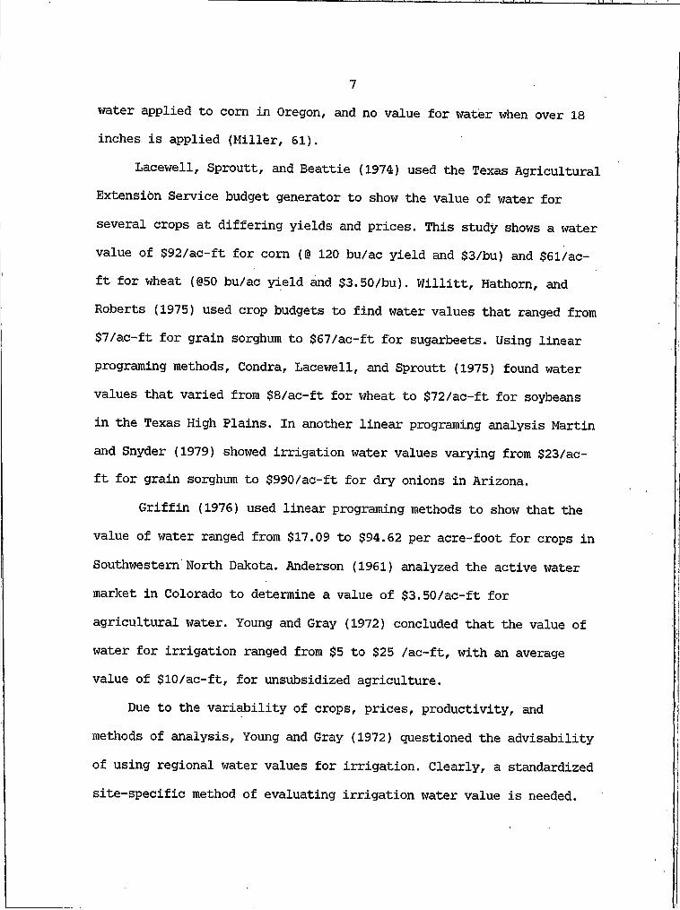
7water applied to c o m in Oregon, and no value for water when over 18 inches is applied (Miller, 61).

Lacewell, Sproutt, and Beattie (1974) used the Texas Agricultural Extensibn Service budget generator to show the value of water for

several crops at differing yields and prices. This study shows a water value of $92/ac-ft for c o m (@ 120 bu/ac yield and $3/bu) and $61/ac- ft for wheat (@50 bu/ac yield and $3.50/bu). Willitt, Hathom, and Roberts (1975) used crop budgets to find water values that ranged from $7/ac-ft for grain sorghum to $67/ac-ft for sugarbeets. Using linear programing methods, Condra, Lacewell, and Sproutt (1975) found water values that varied from $8/ac-ft for wheat to $72/ac-ft for soybeans in the Texas High Plains. In another linear programing analysis Martin and Snyder (1979) showed irrigation water values varying from $23/ac- ft for grain sorghum to $990/ac-ft for dry onions in Arizona.

Griffin (1976) used linear programing methods to show that the value of water ranged from $17.09 to $94.62 per acre-foot for crops in

Southwestern North Dakota. Anderson (1961) analyzed the active water market in Colorado to determine a value of $3.50/ac-ft for agricultural water. Young and Gray (1972) concluded that the value of water for irrigation ranged from $5 to $25 /ac-ft, with an average value of $10/ac-ft, for unsubsidized agriculture.

Due to the variability of crops, prices, productivity, and

methods of analysis. Young and Gray (1972) questioned the advisability of using regional water values for irrigation. Clearly, a standardized

site-specific method of evaluating irrigation water value is needed.

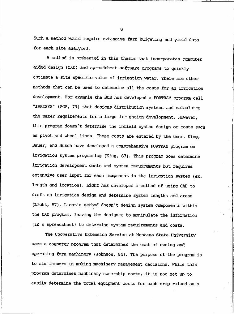
8Such a method would require extensive farm budgeting and yield data for each site analyzed. ,

A method is presented in this thesis that incorporates computer aided design (CAD) and spreadsheet software programs to quickly

estimate a site specific value of irrigation water. There are other methods that can be used to determine all the costs for an irrigation development. For example the SCS has developed a FORTRAN program call "IRRISYS" (SCS, 79) that designs distribution systems and calculates the water requirements for a large irrigation development. However, this program doesn't determine the infield system design or costs such as pivot and wheel lines. These costs are entered by the user. King, Sauer, and Busch have developed a comprehensive FORTRAN program on

irrigation system programing (King, 87). This program does determine

irrigation development costs and system requirements but requires extensive user input for each component in the irrigation system (ex. length and location). Licht has developed a method of using CAD to draft an irrigation design and determine system lengths and areas (Licht, 87). Licht's method doesn't design system components within the CAD program, leaving the designer to manipulate the information (in a spreadsheet) to determine system requirements and costs.

The Cooperative Extension Service at Montana State University uses a computer program that determines the cost of owning and operating farm machinery (Johnson, 84). The purpose of the program is to aid farmers in making machinery management decisions. While this program determines machinery ownership costs, it is not set up to easily determine the total equipment costs for each crop raised on a

9specific farm. Washington State Univetsity has developed a similat program (Mohasci, 84). The Cooperative Extension Service also produces enterprise cost studies that budget all the costs and revenues of selected farming scenarios (Fogle, 80)

These components can be used to budget the costs and revenues of an irrigation development. However, the process would be cumbersome and time consuming. This thesis presents a method for quickly generating site specific farm budgets. The costs of new irrigation developments are accounted for, including annual irrigation costs. Using the computer aided irrigation design and economic analysis method developed and explained in the following text, the task of evaluating the value of water for irrigation is both less difficult and more accurate. Both farmers and water resource planners will gain by the ability to obtain more site-specific irrigation water values.

10

CHAPTER 2

GENERAL COMPUTER SOFTWARE DESCRIPTION

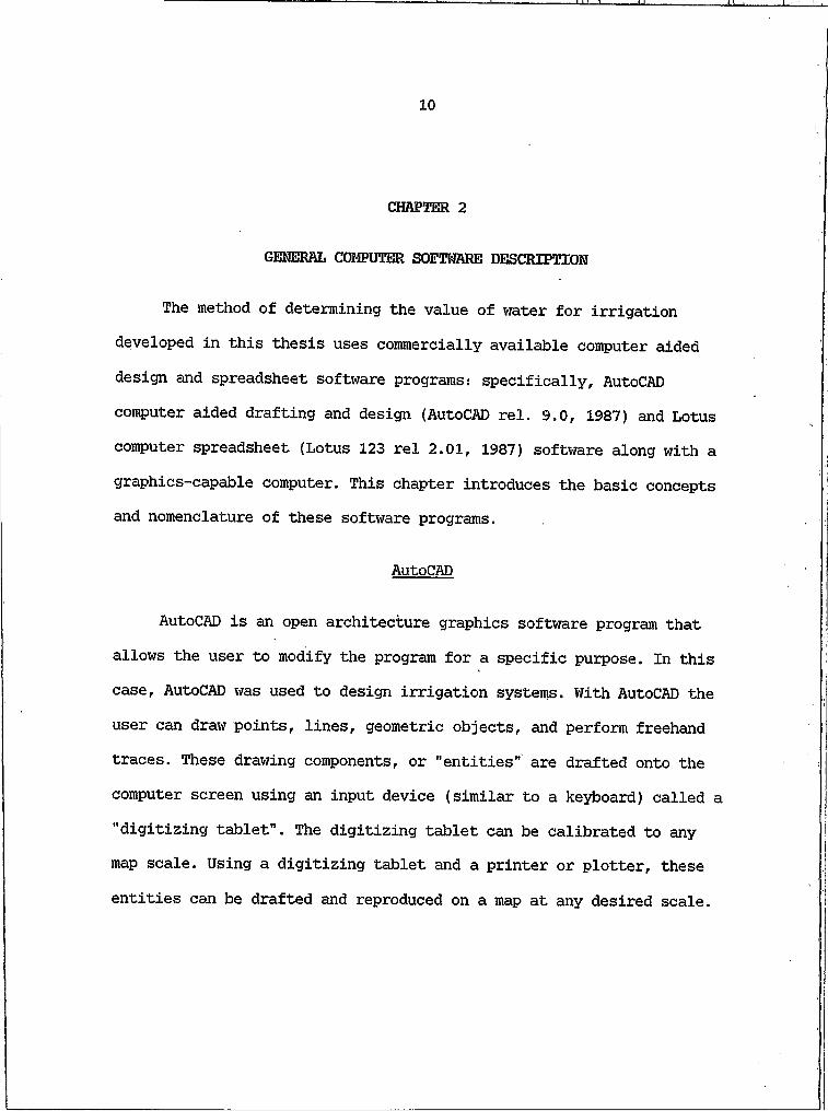
The method of determining the value of water for irrigation developed in this thesis uses commercially available computer aided

design and spreadsheet software programs: specifically, AutoCAD computer aided drafting and design (AutoCAD rel. 9.0, 1987) and Lotus computer spreadsheet (Lotus 123 rel 2.01, 1987) software along with a

graphics-capable computer. This chapter introduces the basic concepts and nomenclature of these software programs.

AutoCAD

AutoCAD is an open architecture graphics software program that allows the user to modify the program for a specific purpose. In this case, AutoCAD was used to design irrigation systems. With AutoCAD the user can draw points, lines, geometric objects, and perform freehand traces. These drawing components, or "entities" are drafted onto the computer screen using an input device (similar to a keyboard) called a "digitizing tablet". The digitizing tablet can be calibrated to any map scale. Using a digitizing tablet and a printer or plotter, these

entities can be drafted and reproduced on a map at any desired scale.

11

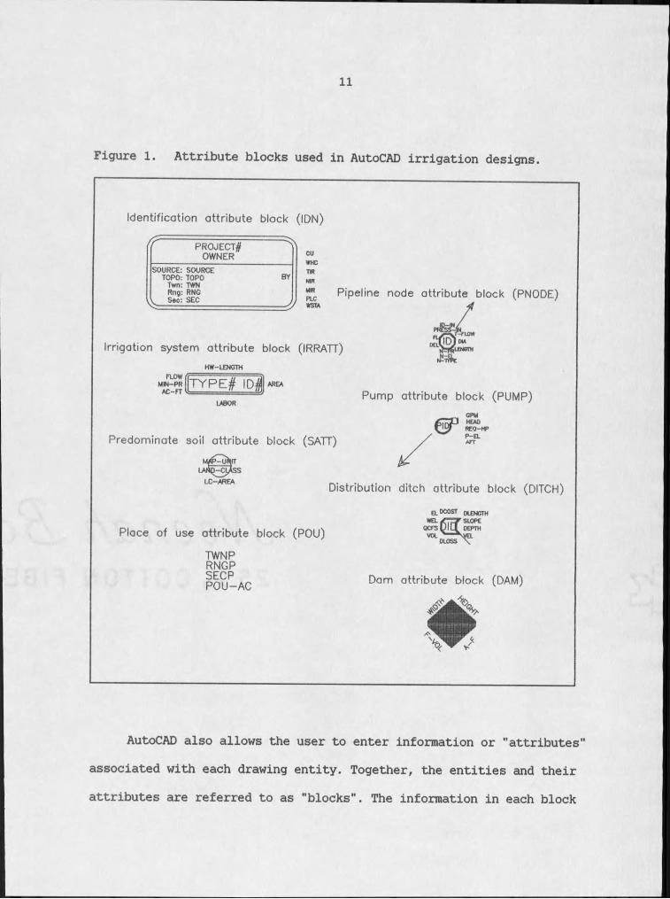
Figure I. Attribute blocks used in AutoCAD irrigation designs.

Identification attribute block (IDN)

fr PROJECT#OWNER

--------- ^

SOURCE: SOURCE TOPO: TOPO

Twn: TWN Rng: RNG

BY

See: SEC----------V

CU

WHCh r

NIRMHt

PLCPipeline node attribute block (PNODE)

Irrigation system attribute block (IRRATT)H W -LENGTH

AREAFLOW

M IN -P RA C -F T

T Y P E # ID#LABOR

Predominate soil attribute block (SATT)

P - u \ l TM ufrlITLANQ-CASSL C -A R E A

-SrM t

Pump attribute block (PUMP)

&GPMHEADR E O -H PP - E LATT

Distribution ditch attribute block (DITCH)

Place of use attribute block (POU)

TWNPRNGPSECPPOU-AC

EL DCOST olencth

WELQCFS

VOLDLOSS \

Dam attribute block (DAM)

AutoCAD also allows the user to enter information or "attributes associated with each drawing entity. Together, the entities and their

attributes are referred to as "blocks". The information in each block

12can be written to an ASCI file for use in Lotus 123 spreadsheets. Finally, AutoCAD allows the user to write interactive LISP programs. These programs can draw and manipulate entities and query the user for information used in entities' attributed blocks. There are eight attributed blocks used in the irrigation design process (Figure I).

Lotus 123

A spreadsheet is a computer program that allows the user to manipulate discrete units of information. It consists of numbered rows and alphabetically headed columns, where each cell has a unique "address" (e.g. All, Z182 ..). A cell can contain either an alpha-numeric label, a single number, or a mathematical formula. A cell formula can contain numbers, cell addresses, mathematical operators, or functions. The spreadsheet performs formula calculations, using values from other cells where indicated, and stores the result in that cell. The following is a list of mathematical operators in order of precedence:

A exponentiation* multiplication/ division+ addition

subtraction = equal< less than> greater than

A function enables the user to perform more complex mathematical manipulations. Functions are indicated by the character @ followed by an "argument", or list of values (e.g. @SUM(A1...A10)). The most

13commonly used spreadsheet functions are @SUM and @IF. The @SUM function totals the cell values contained within the "range", or group of cell addresses, specified in the argument. The @IF function is a logic statement that evaluates an argument. If the condition is true the spreadsheet calculates the value of the first argument; if it is false, it calculates the last argument. In the example @IF(A1<10,B15,0), if the value in cell Al is less than 10, the resulting value will be that of B15; but if the value of cell Al is equal to or greater than 10, the resulting value will be 0. (A listing of functions and their arguments can be found in LOTUS 123 manuals.)

In the spreadsheets developed in this thesis, "label cells" explain parts of the spreadsheet, designate units, or head columns and rows of data. Labels at the head of a row or column describe the data in that column or row. Cell values can be user input variables, standard parameters, calculated data, or summary result data. The spreadsheet is "protected" so that the only easily altered cells are user input variable cells. The spreadsheet is "menu" driven to make it more user friendly. The menu allows the user to view parts of the spreadsheet, change user input variables, and print sections of the

spreadsheet without directly accessing the entire spreadsheet.

14

CHAPTER 3

METHODOLOGY

To evaluate the economic feasibility of an irrigation development, one must analyze and compare before- and afterdevelopment scenarios. This analysis is done with the Farm Enterprise Analysis spreadsheet. The spreadsheet requires economic input data on crops raised (acres, yield, and prices), chemical use, irrigation

costs, and machinery costs. The output to be compared is the farm's return to land, including the break-even price and yield for each crop.

The Machinery Use spreadsheet calculates the costs of owning and operating machinery. This spreadsheet computes for each scenario the fixed and variable costs of machinery ownership based on input

variables on acres of crops raised, interest rate parameters, equipment used, number of annual equipment operations, and annual truck use.

AutoCAD and the Irrigation Design Analysis (IDA) spreadsheet are used to determine the annual costs of the irrigation systems. The designer enters the system components while AutoCAD answers program queries about the irrigation development site, storing the information in attribute blocks that are then transferred to Lotus 123. These blocks include information on size of equipment, amount and diameter of pipeline, required flow, number and size of pumps, and total water

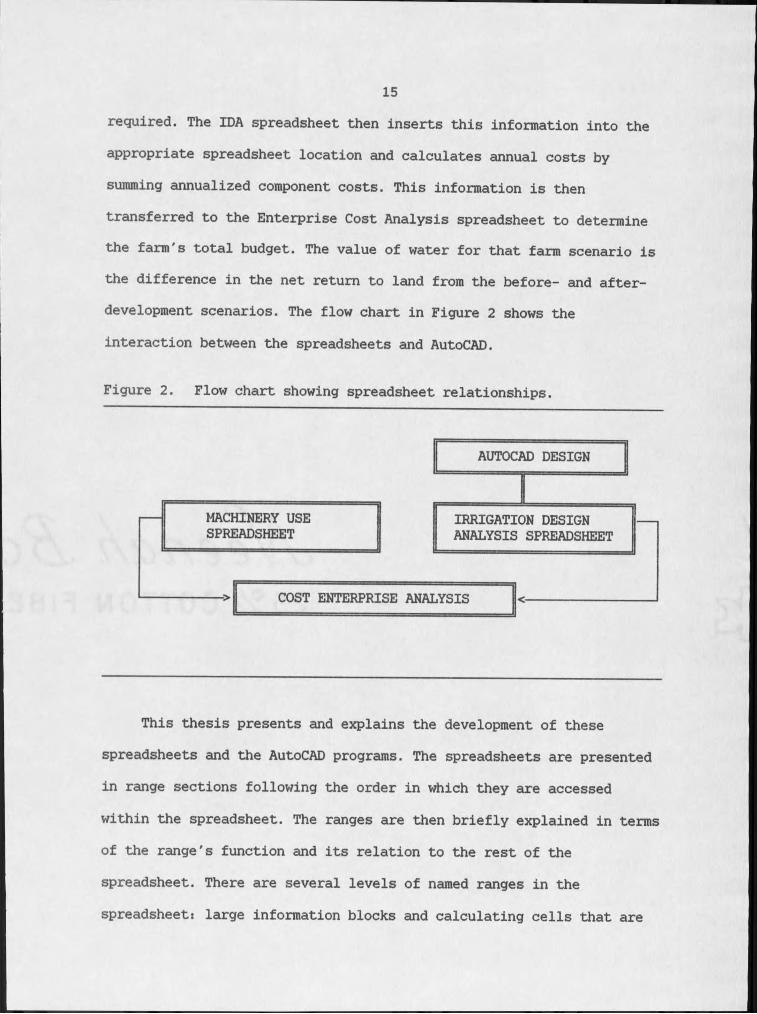
15required. The IDA spreadsheet then inserts this information into the appropriate spreadsheet location and calculates annual costs by summing annualized component costs. This information is then transferred to the Enterprise Cost Analysis spreadsheet to determine the farm's total budget. The value of water for that farm scenario is the difference in the net return to land from the before- and afterdevelopment scenarios. The flow chart in Figure 2 shows the interaction between the spreadsheets and AutoCAD.

Figure 2. Flow chart showing spreadsheet relationships.

AUTOCAD DESIGN

MACHINERY USE SPREADSHEET

IRRIGATION DESIGN ANALYSIS SPREADSHEET

COST ENTERPRISE ANALYSIS

This thesis presents and explains the development of these spreadsheets and the AutoCAD programs. The spreadsheets are presented in range sections following the order in which they are accessed

within the spreadsheet. The ranges are then briefly explained in terms of the range's function and its relation to the rest of the spreadsheet. There are several levels of named ranges in the

spreadsheets large information blocks and calculating cells that are

16used to organize the spreadsheet, titled columns and rows that indicate similar types of cell information or calculations, and individual cells for addressable input or parameter values. These ranges are capitalized and abbreviated as they appear in the

spreadsheet when referred to in the major range area explanations.Each range area explanation includes a table, which is a range printout followed by an explanation of calculating cell formulas. Many titled ranges contain similar formulas with addressed cells changing relative to the calculating cell's position, in which cases only the first cell formula in the range is listed and explained. A complete listing of cell formulas for each range presented is listed in Appendix B.

Chapter 8 demonstrates the method of determining the value of water for three irrigation development sites. Four example problems show the variability of irrigation water's value. The first example is for a large cattle ranch that develops a pivot close to the Missouri River. The second example is the same pivot irrigation system used in example one, developed by a dryland grain farming operation. The third example is a small farm-ranch developing two wheel lines on a high

terrace of the Missouri river. The last example is for a dryland farm developing a large six pivot irrigation project on a terrace of Belt Creek in Chouteau county.

Each example problem description contains a summary of the machinery use and enterprise cost spreadsheets for the before development scenario. Next, the irrigation development drawing is presented along with its annualized cost summary. This information is

17then included in the after-development enterprise cost analysis along with the new machinery costs. The value of water for each irrigation development scenario is then found by subtracting the net return to land of the before-development from the after-development scenario. A more complete listing of each scenario's spreadsheet output is presented in Appendix B.

18

CHAPTER 4

IRRIGATION DESIGN AND ECONOMIC EVALUATION

To begin the design, the designer calibrates the digitizing tablet to a base map of the proposed irrigation site. Then, with the aid of the AutoCAD LISP programs, the appropriate information is entered. While these programs do not make design decisions, they do make the design process easier, quicker, and more accurate. Once the design is finished, the attribute information is transferred to a spreadsheet that performs the economic analysis and formats the information in a report-ready form.

AutoCAD Irrigation Design Initialization

In order to run the initialization program (INT.lsp) - step one of the design process - the designer must gather basic information on the soils, climate, relief, and location of the project area. This information is obtained from topographic maps, soils maps, and the MT_TR21 consumptive use computer model (USDA 1987). The INT.lsp program asks the designer for site-specific design information and sets default variables for the rest of the design programs. The INT program displays the current values for peak consumptive crop use (PCU), soil water holding capacity (WHC), total crop consumptive use (TCU), net irrigation requirement (NIR), maximum soil intake rate (MIR), miles of required three-phase powerline construction (PLC), and

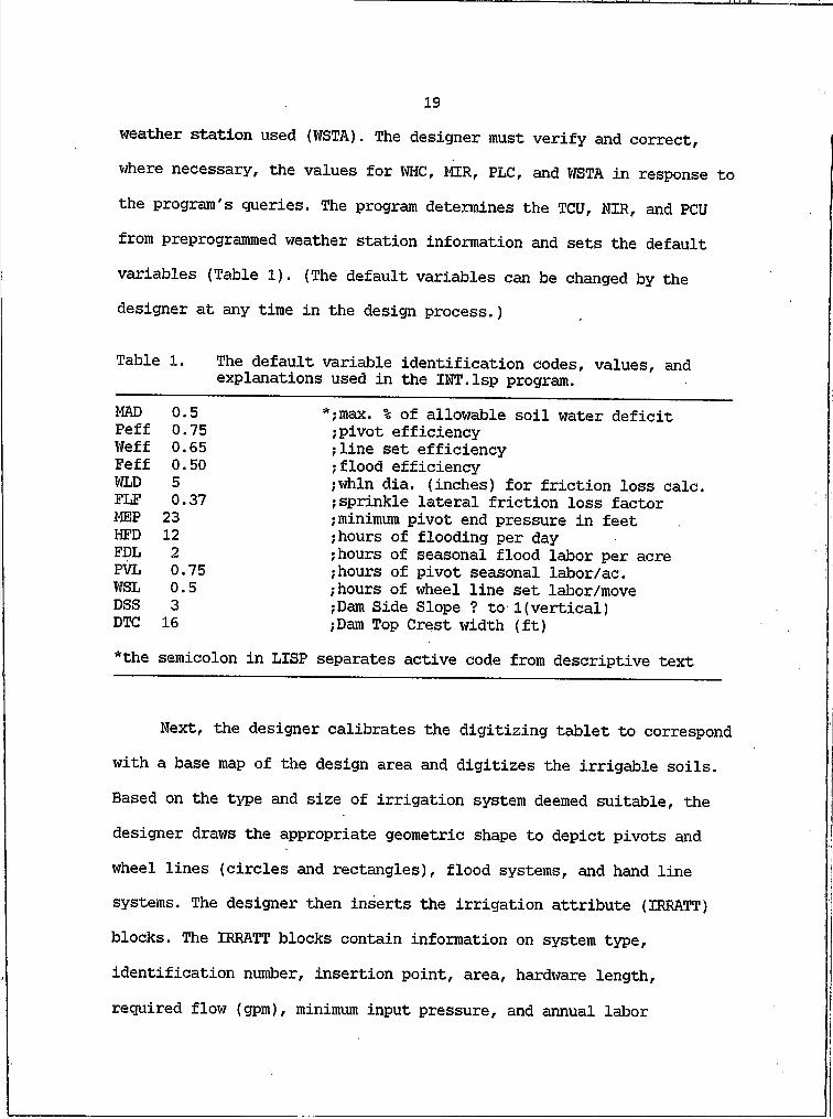
19weather station used (WSTA). The designer must verify and correct, where necessary, the values for WHC, MIR, PLC, and WSTA in response to the program's queries. The program determines the TCU, NIR, and PCU from preprogrammed weather station information and sets the default variables (Table I). (The default variables can be changed by the designer at any time in the design process.)

The default variable identification codes, values, and explanations used in the INT.lsp program.

*;max. % of allowable soil water deficit ;pivot efficiency ;line set efficiency ;flood efficiency;whln dia. (inches) for friction loss calc. ;sprinkle lateral friction loss factor ;minimum pivot end pressure in feet ;hours of flooding per day ;hours of seasonal flood labor per acre ;hours of pivot seasonal labor/ac.;hours of wheel line set labor/move ;Dam Side Slope ? to !(vertical);Dam Top Crest width (ft)

*the semicolon in LISP separates active code from descriptive text

Table I.

MAD 0.5Peff 0.75Weff 0.65Feff 0.50WLD 5FLF 0.37MEP 23HFD 12FDL 2PVL 0.75WSL 0.5DSS 3DTC 16*the semicc

Next, the designer calibrates the digitizing tablet to correspond with a base map of the design area and digitizes the irrigable soils. Based on the type and size of irrigation system deemed suitable, the designer draws the appropriate geometric shape to depict pivots and wheel lines (circles and rectangles), flood systems, and hand line systems. The designer then inserts the irrigation attribute (IRRATT) blocks. The IRRATT blocks contain information on system type, identification number, insertion point, area, hardware length,

required flow (gpm), minimum input pressure, and annual labor

requirement. The designer may either enter this information directly, or use the developed LISP programs. The IRRATT insertion programs use the calculated and set variable from the INT.Isp program and user- queried information to calculate and enter the IRRATT attribute information.

The four IRRATT insertion programs developed for irrigation design are pivot (PIV), wheel line (WL), hand line (HL), and flood (FLOOD). The sample drawing in Figure 4 shows the different types of irrigation equipment, a distribution pipe line, and a storage reservoir (legend shown in Figure 3).

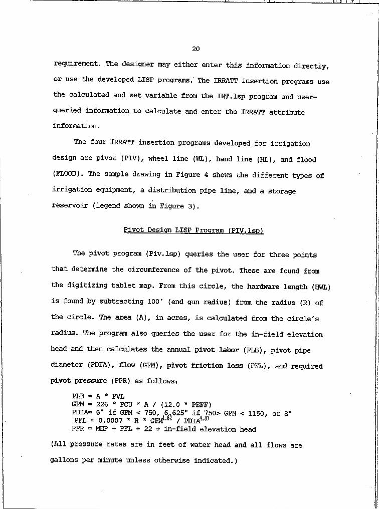
Pivot Design LISP Program (PIV.Is p )

The pivot program (Piv.lsp) queries the user for three points that determine the circumference of the pivot. These are found from the digitizing tablet map. From this circle, the hardware length (HWL) is found by subtracting 100' (end gun radius) from the radius (R) of the circle. The area (A), in acres, is calculated from the circle's radius. The program also queries the user for the in-field elevation head and then calculates the annual pivot labor (PLB), pivot pipe diameter (PDIA), flow (GPM), pivot friction loss (PFL), and required pivot pressure (PPR) as follows:

PLB = A * PVLGPM = 226 * PCU * A / (12.0 * PEFF)PDIA= 6" if GPM < 750, 6.625" if 750> GPM < 1150, or 8"PFL = 0.0007 * R * GPM1,82 / PDIA4,87PPR = MEP + PFL + 22 + in-field elevation head

(All pressure rates are in feet of water head and all flows are gallons per minute unless otherwise indicated.)

20

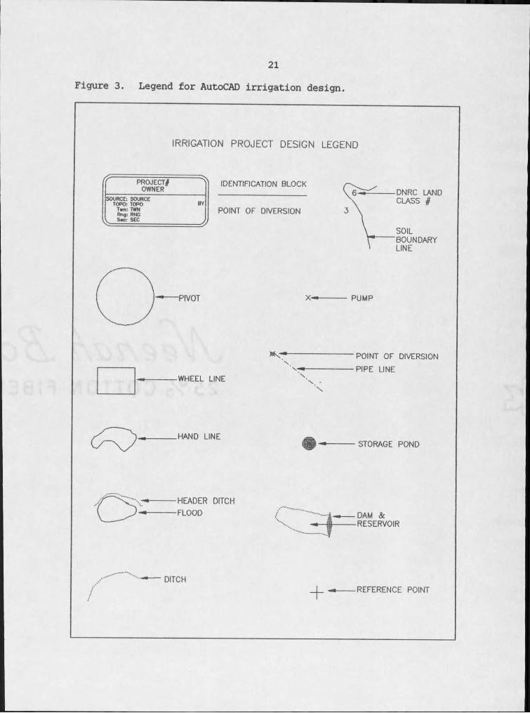
21Figure 3. Legend for AutoCAD irrigation design.

IRRIGATION PROJECT DESIGN LEGEND

PROJECT#OWNER

IDENTIFICATION BLOCKDNRC LAND CLASS #SOURCE: SOURCE

TORO: TOPO Tw n: TWN Rng: RNC

V Sec: SEC

POINT OF DIVERSION

SOILBOUNDARYLINE

PIVOT P U M P

POINT OF DIVERSION

PIPE LINEWHEEL LINE

HAND LINESTORAGE POND

HEADER DITCH

FLOOD DAM & RESERVOIR

DITCHREFERENCE POINT

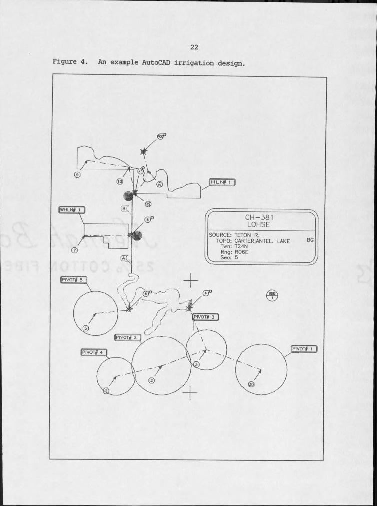
22Figure 4. An example AutoCAD irrigation design.

B PIVOT# 5

(Af

Cf CH-381LOHSE

SOURCE: TETON R.TORO: CARTER.ANTEL. LAKE BG

Twn: T24NRng: R06ESec: 5

— v y

![PIVOT# I

I

23Wheel Line Design LISP Program (WL.Iso)

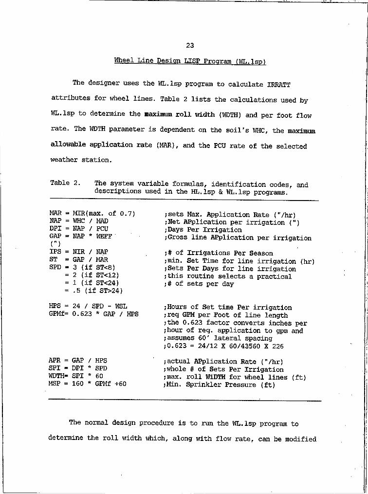
The designer uses the WL.Isp program to calculate IRRATT attributes for wheel lines. Table 2 lists the calculations used by WL.Isp to determine the maximum roll width (WDTH) and per foot flow rate. The WDTH parameter is dependent on the soil's WHC, the

allowable application rate (MAR), and the PCU rate of the selected weather station.

Table 2. The system variable formulas, identification codes, and descriptions used in the HL.lsp & WL.lsp programs.

MAR = MIR(max. of 0.7) NAP = WHC / MAD DPI = NAP / PCU GAP = NAP * WEFF (")IPS = NIR / NAP ST = GAP / MAR SPD = 3 (if ST<8)

= 2 (if ST<12)= I (if ST<24)= .5 (if ST>24)

;sets Max. Application Rate ("/hr);Net Application per irrigation (") ;Days Per Irrigation ;Gross line Application per irrigation;# of Irrigations Per Season ;min. Set Time for line irrigation (hr) ;Sets Per Days for line irrigation ;this routine selects a practical ;# of sets per day

HPS = 24 / SPD - WSL GPMf= 0.623 * GAP / HPS

APR = GAP SPI = DPI WDTH= SPI MSP = 160

/ HPS* SPD* 60* GPMf +60

;Hours of Set time Per irrigation ;req GPM per Foot of line length ;the 0.623 factor converts inches per ;hour of req. application to gpm and ;assumes 60' lateral spacing ;0.623 = 24/12 X 60/43560 X 226;actual Application Rate ("/hr);whole # of Sets Per Irrigation ;max. roll WIDTH for wheel lines (ft) ;Min. Sprinkler Pressure (ft)

The normal design procedure is to run the WL.lsp program to determine the roll width which, along with flow rate, can be modified

24by adjusting the soil WHC or MIR parameters. The program is terminated once a suitable roll length is determined. Next, the designer draws the symbols for the wheel line and the pipeline that feeds it, answering the program queries for: (I) the entity (depicting the wheel line), (2) the wheel line length (WLL), (3) the length of the wheel line from its feed point to the end of the line (LOL), and (4) in

field elevation head (FBH). The WLL and LOL distances can be entered from the keyboard but are more easily picked from the digitizing tablet. The area (A), in acres, of the selected entity and the other insert attributes of flow (GPM), minimum pressure (MPR), and annual labor (LWL) are calculated as:

A = area of entity / 43560 WLL = picked distance - 40 GPM = GPMf * (WLL + 40)

MPR = MSP + FEH + FLF * LOL * .0015 * (L0L * GPMf)1,85 / WLD4,87 WLB = IPS * SPI * WSL

The program pauses for the user to enter the block's location and

identification number and inserts the block into the drawing.

Hand Line Design LISP Program (HL.lsp)

The hand line program (HL.lsp) uses the same set-up calculations listed in Table 2. This program queries the designer for the entity that outlines the area to be irrigated. HL.lsp assumes that: (I) any shape can be irrigated, (2) the amount of hardware (HLL) needed is a function of the area (A) irrigated and the number of sets per irrigation (SPI), and (3) it takes two hours of labor to move a

25quarter-mile of hand line (personal experience). The calculations for the hand line IRRATT insert block are:

A = selected entity area (ft2) / 43,560 ft2/ac HLL = 726 ('length/ac/set)

HSL = 0.0015 * HLL

HHPS= 24 / SPD - HSL

GPM = 0.623 * HLL * GAP / HHPSMPR = MSP + 10HLB = IPS * SPI * HSL

A / SPI; (726'length/ac/set = 43560 ;ft2/ac / 60'width/set);Hand Set Labor(hr/ft);(0.0015 hr/ft = 2 hr /?1300'handline)

; Handline Hour Per Set;total flow required;Minimum PResure;annual Hours of LaBor

Like the other irrigation programs, HL.lsp pauses to allow the user to enter the insertion point and identification number.

Flood Design LISP Program (FLOOD.Is p )

The flood (FLOOD.Isp) program queries the designer for the irrigated area entity and the "ditch header entity", the in-field distribution system for the flooded fields entered as a "polyline" from the digitizing tablet. The program calculates the area of the field to be irrigated (A), the length of ditch header (DHL), and queries the user for the per-foot cost of ditch header (DHC). From

this information, and from the hours of flood irrigation per day (HFD) and flood labor per acre (FDL) variables, the program calculates total required flow (GPM) and annual required flooding labor (FLB). The calculations are as follows:

26GPM = (PCU / 12) * (A * 226 / Feff) * (24 / HFD)FLB = A * FDL

Again, the designer enters these variables in the IRRATT attributed block at the selected location.

Dam Design LISP Program (DAM.lsp)

The dam design program (DAM.Isp) estimates the fill volume (F- VOL) in cubic yards of earth and the volume of water stored in acre- feet (A-F). The designer uses a topographic map to digitize the high- water surface contour line of the proposed reservoir. This program queries the designer for the high-water line entity, the abutment points, the dam's maximum water height in feet (WHTH), the reservoir shape factor (RSF), and the basin shape factor (BSF). The RSF is used to estimate the volume of water stored in the reservoir and is generally between 0.4 and 0.6. The BSF is used to estimate the volume of fill needed to construct the dam. This coefficient depicts the dam's centerline profile and can range from 0.0 (rectangular) to 1.0 (triangular). These factors give the designer some flexibility in

estimating the per acre-foot cost of a reservoir when no precise field

information is available. The program adds five feet of free board to the WHTH parameter in order to obtain the actual dam height (HTH). The DAM.Isp program determines acres of water surface area (A) and then multiplies this by HTH and RSF to estimate the water storage volume in acre-feet.

To find the fill volume, the program queries the designer for the dam side slope (DSS) and top crest width (DTC). Using the abutment

27points previously entered, the program determines the dam's width (WDT) and estimates the cubic yard of earth fill volume (F-VOL) with the following formula:

F-VOL = ((DSS * HTH2 + DTC HTH) * (WDT + (2 * WDT *BSF))) / 81 (This formula is derived with the assumption that the dam is composed of two pyramidal sections with a uniform center section.) The program enters these variables in the DAM attributed block and inserts a

symbol depicting dam length and width between the selected abutment points.

Pipeline Design LISP Program (PNODE.Is p )

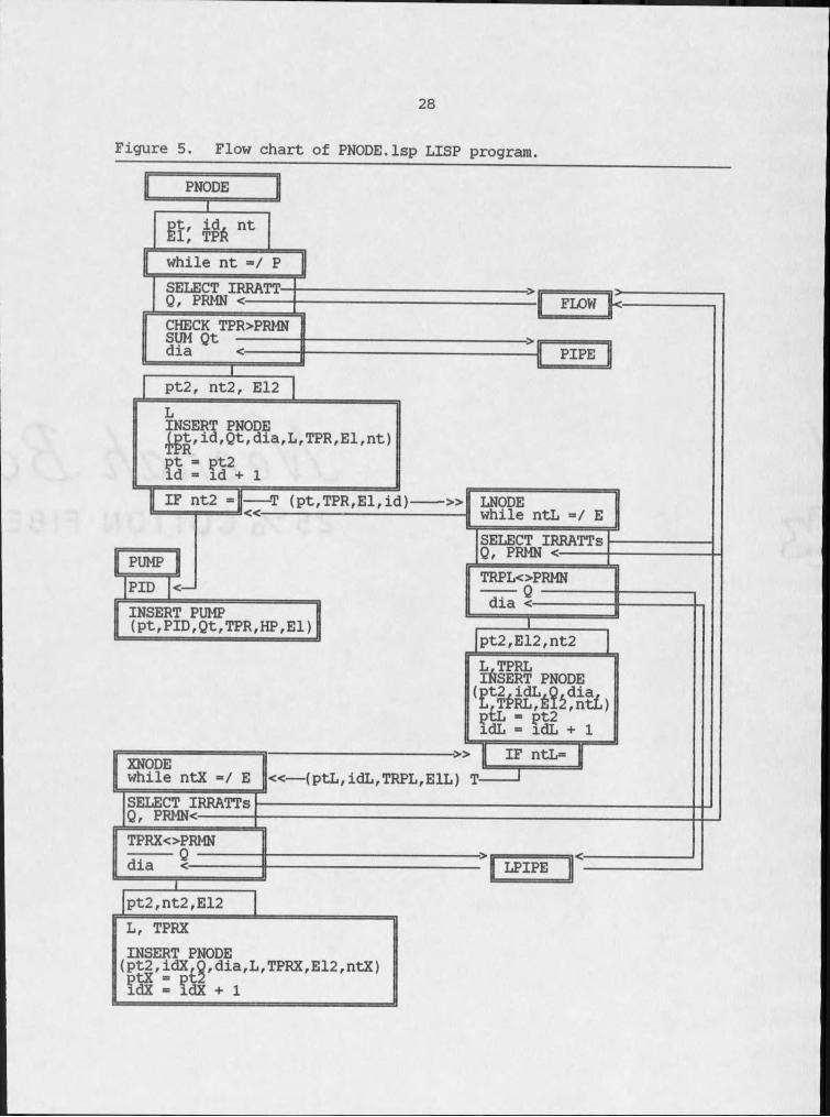
The PNODE.lsp program is used after entering all of the irrigation systems that will be serviced by a pipeline and the pipeline location. It determines the total required flow (Qt), pipe diameter (dia), and total pressure head (TPR) at designer-selected pipe node points. Figure 5 shows a flow chart of the PNODE.lsp program. This program queries the designer for node location, irrigation attribute blocks (IRRATT) serviced by the node, node

elevation, and node type. PNODE.lsp is a user-interactive program that allows the designer to quickly gather a large amount of information about a distribution system. PNODE uses five sub-programs: PIPE,LPIPE, LNODE, XNODE, and FLOW. The LNODE and XNODE sub-programs

function similarly to the PNODE program, except that they work away from the pump-end of a pipeline, while PNODE works toward the pump. LNODE calculates information for main lateral lines off the mainline, while XNODE calculates node information for sub-laterals.

28

Figure 5. Flow chart of PNODE.lsp LISP program.

I!: ntwhile nt =/ PSELECT IRRATT Q, PRMN <

I

L, TPRX INSERT PNODE(pt2,idX.Q,dia,L,TPRX,E12,ntX)Sg: ?S * i

29The FLOW sub-program transfers information on the required amount

of flow (Q) and minimum required pressure (PRHN) from a selected IRRATT block to the NODE programs. The PIPE and LPIPE programs take the current flow value (Qt or Q) and check it against a table of maximum allowable flows for standard PVC pipe sizes. (This table of flows can be based on maximum allowable velocity or on velocity and economic parameters.) The PIPE program selects the appropriate size of pipe (dia) from this table and returns it to the appropriate NODE program.

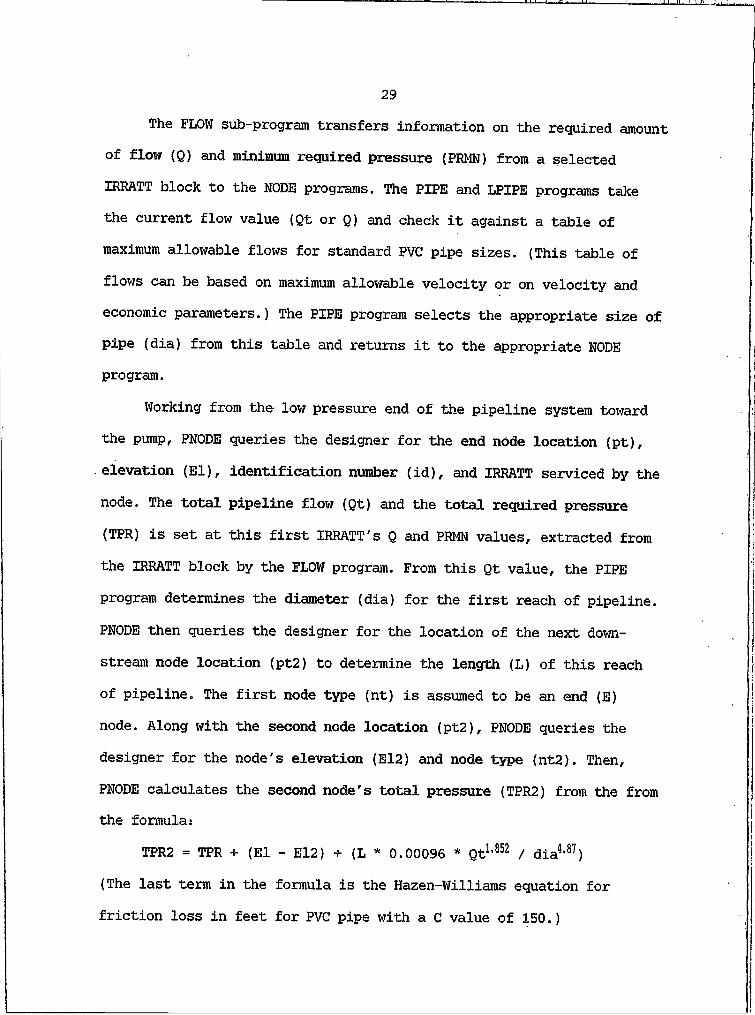
Working from the low pressure end of the pipeline system toward the pump, PNODE queries the designer for the end node location (pt), elevation (El), identification number (id), and IRRATT serviced by the node. The total pipeline flow (Qt) and the total required pressure

(TPR) is set at this first IRRATT's Q and PRMN values, extracted from the IRRATT block by the FLOW program. From this Qt value, the PIPE program determines the diameter (dia) for the first reach of pipeline.

PNODE then queries the designer for the location of the next downstream node location (pt2) to determine the length (L) of this reach of pipeline. The first node type (nt) is assumed to be an end (E) node. Along with the second node location (pt2), PNODE queries the designer for the node's elevation (E12) and node type (nt2). Then,PNODE calculates the second node's total pressure (TPR2) from the from the formula:

TPR2 = TPR + (El - E12) + (L * 0.00096 * Qt1,852 / dia4,87)(The last term in the formula is the Hazen-Williams equation for friction loss in feet for PVC pipe with a C value of 150.)

30

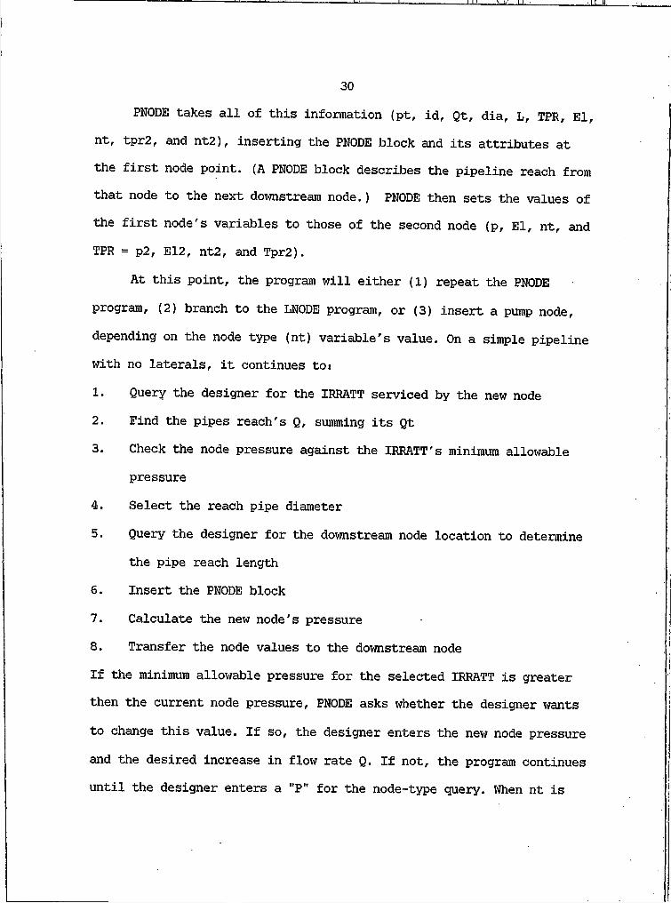
PNODE takes all of this information (pt, id, Qt, dia, L, TPR, El, nt, tpr2, and nt2), inserting the PNODE block and its attributes at the first node point. (A PNODE block describes the pipeline reach from that node to the next downstream node.) PNODE then sets the values of the first node's variables to those of the second node (p, El, nt, and TPR = p2, E12, nt2, and Tpr2).

At this point, the program will either (I) repeat the PNODE program, (2) branch to the LNODE program, or (3) insert a pump node, depending on the node type (nt) variable's value. On a simple pipeline with no laterals, it continues tor

1. Query the designer for the IRRATT serviced by the new node2. Find the pipes reach's Q, summing its Qt

3. Check the node pressure against the IRRATT's minimum allowable pressure

4. Select the reach pipe diameter

5. Query the designer for the downstream node location to determine the pipe reach length

6. Insert the PNODE block

7. Calculate the new node's pressure8. Transfer the node values to the downstream node

If the minimum allowable pressure for the selected IRRATT is greater then the current node pressure, PNODE asks whether the designer wants

to change this value. If so, the designer enters the new node pressure

and the desired increase in flow rate Q. If not, the program continues until the designer enters a "P" for the node-type query. When nt is

31

equal "P", PNODE queries the designer for the pump's identification number and calculates the required pump brake horse power as follows:

HP = TPR * Qt / (3960 * 0.75)

(The 0.75 factor is pump efficiency.) The program then inserts the PUMP block, along with the attribute values of total flow (Qt), total pressure (TPR), horse power (HP), and pump elevation (El), and then terminates.

For a (T) node type, PNODE branches to the LNODE program. The LNODE program takes the current node location (pt), pressure (TPR), elevation (El), and identification number (id) from PNODE and suffixes the parameter name with an "L". LNODE then queries the designer for the out node location, the node type, elevation, and all the IRRATTs serviced by the node. The FLOW program totals the flow for all irrigation attribute blocks selected and returns this Q, along with the minimum required pressure of the last selected IRRATT. Unlike the PNODE program, LNODE does not change the value of TPR if it is less than the return value of PRMN. Rather, it prints the statement "min.allowable pressure is ____", indicating to the designer that a boosterpump is required or that the main pump pressure should be increased.

LPIPE selects the pipe-reach diameter. LNODE then finds the TPRL of the out-node by adding the friction loss in the reach length (ptL<- >pt2) and the elevation head (E1L-E12) to the total pressure at the tee (TPR). The resulting PNODE block and its attributes are then inserted at the pt2 location, while the values of the second node variables are transferred to the L-suffixed node variables. At this point the LNODE checks the node type (ntL) to see if it should:

321. End the program and return to PNODE (ntL=E)

2. Branch to the sub-lateral program XNODE (ntL=T)3. Re-enter the LNODE program at the PNODE tee node (ntL=ELT), or4. Continue the LNODE program loop (ntL=/ E,T,or ELT)

When there is more than one lateral off the main-line at the same point, the program calculates the node variable values to the end of the first lateral. At the end of the first lateral, the designer

enters "ELT" at the node-type query. (This code can be thought of as "End Lateral Tee.") When nt equals "ELT", the program re-enters the LNODE program at the PNODE tee location. The mainline variable values are again transferred to the L-suffixed variables, and the process continues until the lateral node type equals "E". Now the PNODE program proceeds to the pump end of the pipeline.

If the lateral node type equals "T", the program transfers values of the L-suffixed variables to X-suffixed variable in the XNODE program. The XNODE program is identical to the LNODE program except for the variable suffixes, and no further tee laterals are allowed.With these programs, all the pertinent information about a complex distribution system can be quickly stored for use in a spreadsheet.

Exporting AutoCAD Information to Lotus 123

Soils information is stored in the SATT attributed block and can

be inserted with the SATT.lsp program. This AUTOLISP program queries

the designer for the soil mapping unit number and for the DNRC land class number, entering this information along with the area of the last selected entity. Using the "area" AutoCAD command the designer

I / I

33must select the area of the soils entities before the SATT.Isp program is run.

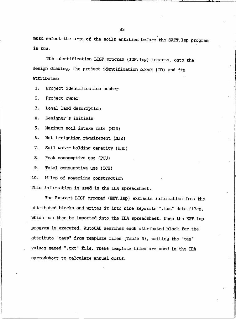
The identification LISP program (IDN.lsp) inserts, onto the design drawing, the project identification block (ID) and its attributes:

1. Project identification number2. Project owner3. Legal land description4. Designer's initials5. Maximum soil intake rate (MIR)6. Net irrigation requirement (NIR)7. Soil water holding capacity (WHC)8. Peak consumptive use (PCU)

9. Total consumptive use (TCU)10. Miles of powerline constructionThis information is used in the IDA spreadsheet.

The Extract LISP program (EXT.Isp) extracts information from the attributed blocks and writes it into nine separate ".txt" data files, which can then be imported into the IDA spreadsheet. When the EXT.Isp

program is executed, AutoCAD searches each attributed block for the attribute "tags" from template files (Table 3), writing the "tag" values named ".txt" file. These template files are used in the IDA spreadsheet to calculate annual costs.

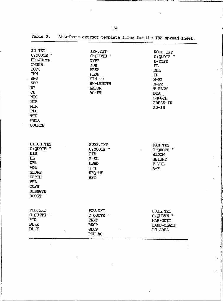
34Table 3. Attribute extract template files for the IDA spread sheet.

ID.TXT IRR.TXT NODE.TXTC:QUOTE " C sQUOTE " CsQUOTEPROJECT# TYPE N-TYPEOWNER ID# FLTOPO AREA DELTWN FLOW IDRNG MIN-PR N-ELSEC HW-LENGTH N-PRBY LABOR T-FLOWCU AC-FT DIAWHC LENGTHNIR PRESS-INMIR ID-INPLCTIRWSTASOURCE

DITCH.TXT PUMP.TXT DAM.TXTC sQUOTE " C sQUOTE " C sQUOTE "DID PID WIDTHEL P-EL HEIGHTWEL HEAD F-VOLVOL GPM A-FSLOPE REQ-HPDEPTH AFTVELQCFSDLENGTHDCOST

POD.TXT POU.TXT SOIL.TXTC sQUOTE " C sQUOTE " CsQUOTE "PID TWNP MAP-UNITBLsX RNGP LAND-CLASSBLsY SECP LC-AREAPOU-AC

35

Irrigation Design Analysis Spreadsheet Explanation

The irrigation design analysis (IDA) spreadsheet uses information from the AutoCAD irrigation design to determine the total system cost, annual costs, and annual per acre costs of that design. The spreadsheet imports information from the ". txt" files, that have been converted to ".pm" files, and inserts the information into the appropriate spreadsheet locations.

The IDA spreadsheet makes extensive use of range names to make spreadsheet documentation easier (Table 4). The ID range of the IDA spreadsheet is used as a project identifier for all output. It imports data from the ID.txt file regarding project number, owner name, legal land description, and designer's name. It also imports data on (I) peak consumptive use (PCU), (2) total consumptive use (TCU), (3) net irrigation requirement (NIR), (4) maximum soil intake rate (MIR), (5)

soil water holding capacity (WHC), and (6) miles of required powerline construction (PLC). This information is used to document AutoCAD design process variables and to calculate other spreadsheet variables.

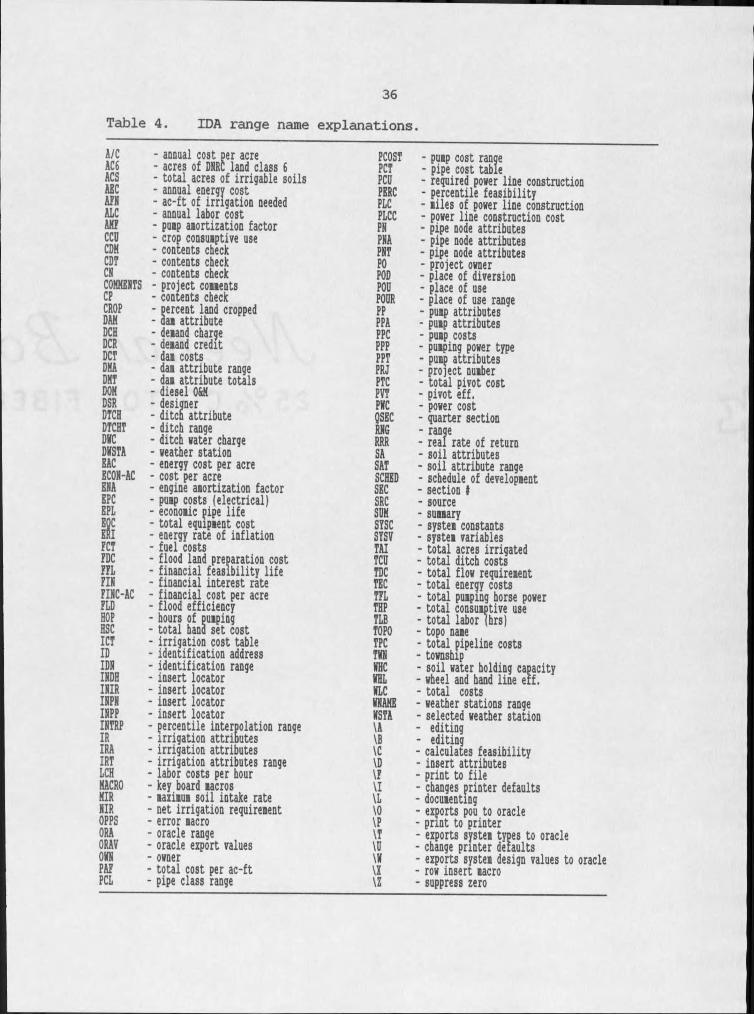
36Table 4. IDA range name explanations.A/CAC6ACSAECAfNALCAKfCCDCDHCDTCNCOMMENTSCFCROPDAMDCHDCRDCTDMADKTDOHDSRDTCHDTCHTDVCDVSTAEACECON-ACENAEPCEPLEOCERIFCTFDCFFLFINFINC-ACFLDHOPHSCICTIDIDNINDHINIRINPNINPPINTRPIRIRAIRTLCHMACROHIRNIROPPSORAORAVOVNPAFPCL

- annual cost per acre- acres of DNRC land class 6- total acres of irrigable soils- annual energy cost- ac-ft of irrigation needed- annual labor cost- pump amortization factor- crop consumptive use- contents check- contents check- contents check- project comments- contents check- percent land cropped- dam attribute- demand chargedemand credit- dam costs- dam attribute range- dam attribute totals- diesel O&N- designer- ditch attribute- ditch range- ditch water charge- weather station- energy cost per acre- cost per acreengine amortization factor- pump costs (electrical)- economic pipe life- total equipment cost- energy rate of inflation- fuel costsflood land preparation cost- financial feasibility life- financial interest rate- financial cost per acre- flood efficiency- hours of pumping- total hand set cost- irrigation cost table- identification address- identification range- insert locator- insert locator- insert locator- insert locator- percentile interpolation range- irrigation attributes- irrigation attributes- irrigation attributes range- labor costs per hour- key board macros- maximum soil intake rate- net irrigation requirement- error macro- oracle range- oracle export values- owner- total cost per ac-ft- pipe class range

PCOST - pump cost rangePCT - pipe cost tablePCD - required power line constructionPERC - percentile feasibilityPLC - miles of power line constructionPLCC - power line construction costPN - pipe node attributesPNA - pipe node attributesPNT - pipe node attributesPO - project ownerPOD - place of diversionPOD - place of usePOOR - place of use rangePP - pump attributesPPA - pump attributesPPC - pump costsPPP - pumping power typePPT - pump attributesPRJ - project numberPTC - total pivot costPVT - pivot eff.PVC - power costQSEC - quarter sectionRNG - rangeRRR - real rate of returnSA - soil attributesSAT - soil attribute rangeSCHED - schedule of developmentSEC - section ISRC - sourceSDK - summarySYSC - system constantsSYSV - system variablesTAI - total acres irrigatedTCD - total ditch costsTDC - total flow requirementTEC - total energy costsTFL - total pumping horse powerTHP - total consumptive useTLB - total labor (hrs)TOPO - topo nameTPC - total pipeline costsTVN - townshipVHC - soil water holding capacityVHL - wheel and hand line erf.VLC - total costsVNAME - weather stations rangeVSTA - selected weather station\A - editing\B - editing\C - calculates feasibility\D - insert attributes\F - print to file\I - changes printer defaults\L - documenting\0 - exports pou to oracle\P - print to printer\T - exports system types to oracle\D - change printer defaultsW - exports system design values to oracle\X - row insert macro\Z - suppress zero

37

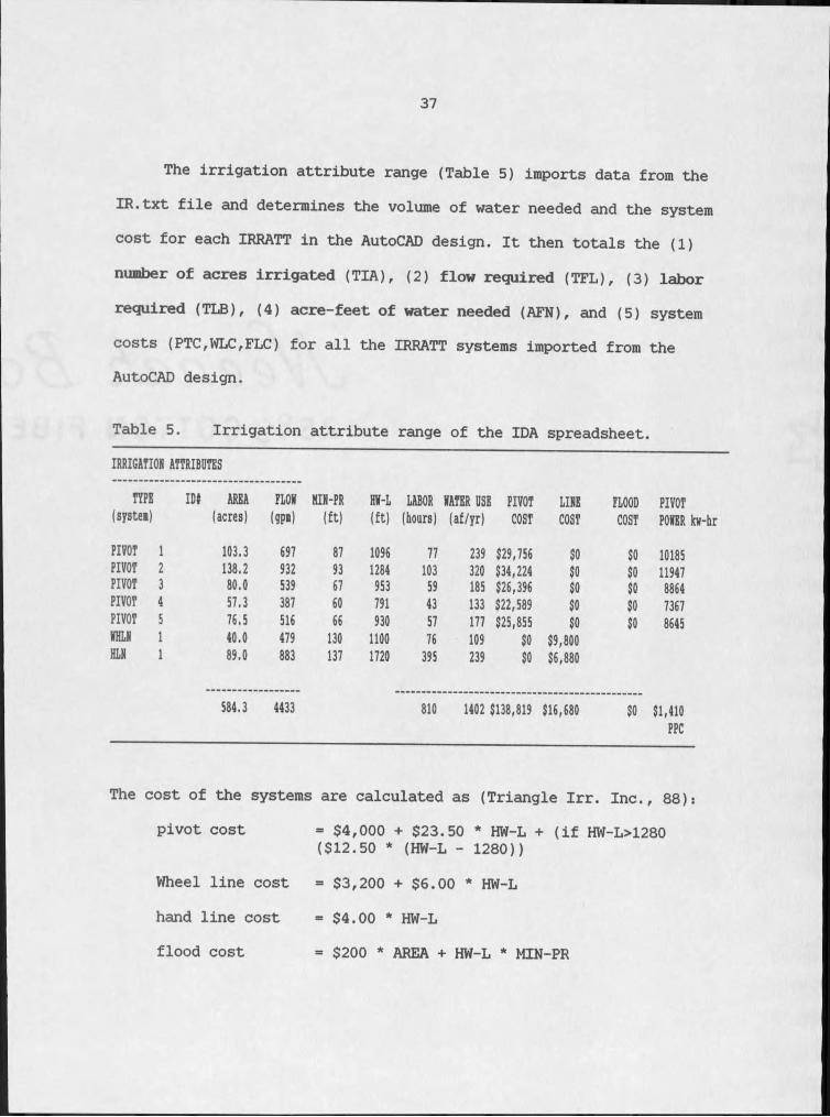
The irrigation attribute range (Table 5) imports data from the IR.txt file and determines the volume of water needed and the system cost for each IRRATT in the AutoCAD design. It then totals the (I) number of acres irrigated (TIA), (2) flow required (TFL), (3) labor required (TLB), (4) acre-feet of water needed (AFN), and (5) system costs (PTC,WLC,FLC) for all the IRRATT systems imported from the AutoCAD design.

Table 5. Irrigation attribute range of the IDA spreadsheet.IRRIGATION ATTRIBUTES

TYPE IDt AREA FLON KIN-PR HN-L(system) (acres) (gpi) (ft) (ft)PIVOT I 103.3 697 87 1096PIVOT 2 138.2 932 93 1284PIVOT 3 80.0 539 67 953PIVOT 4 57.3 387 60 791PIVOT 5 76.5 516 66 930NHLN I 40.0 479 130 1100HLN I 89.0 883 137 1720

LABOR NATER USE PIVOT LINE FLOOD PIVOT(hours) (af/yr) COST COST COST PONER kv-hr

77 239 $29,756 $0 $0 10185103 320 $34,224 $0 $0 1194759 185 $26,396 $0 $0 886443 133 $22,589 $0 $0 736757 177 $25,855 $0 $0 864576 109 $0 $9,800395 239 $0 $6,880

584.3 4433 810 1402 $138,819 $16,680 $0 $1,410PPC

The cost of the systems are calculated as (Triangle Irr. Inc., 88): pivot cost

Wheel line cost hand line cost

= $4,000 + $23.50 * HW-L + (if HW-L>1280 ($12.50 * (HW-L - 1280))

= $3,200 + $6.00 * HW-L= $4.00 * HW-L

flood cost = $200 * AREA + HW-L * MIN-PR

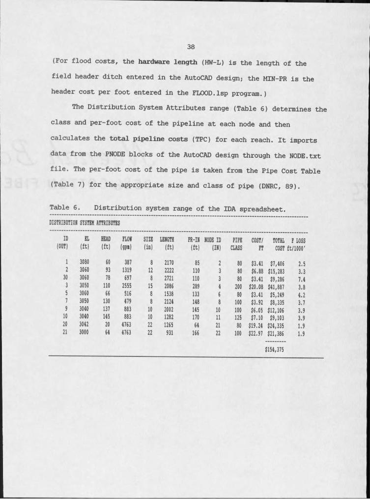
38(For flood costs, the hardware length (HW-L) is the length of the field header ditch entered in the AutoCAD design; the MIN-PR is the header cost per foot entered in the FLOOD.Isp program.)

The Distribution System Attributes range (Table 6) determines the class and per-foot cost of the pipeline at each node and then

calculates the total pipeline costs (TPC) for each reach. It imports data from the PNODE blocks of the AutoCAD design through the N0DE.txt file. The per-foot cost of the pipe is taken from the Pipe Cost Table (Table 7) for the appropriate size and class of pipe (DNRC, 89).

Table 6. Distribution system range of the IDA spreadsheet. DISTRIBUTION SYSTEM ATTRIBUTES

ID EL HEAD(OUT) (ft) (ft)

I 3080 602 3060 9330 3060 783 3050 HO5 3060 667 3050 1309 3040 13710 3040 14520 3042 2021 3000 64

FLOM SIZE LENGTH(URi) (in) (ft)387 8 21701319 12 2222697 8 27212555 15 2086516 8 1538479 8 2124883 10 2002883 10 12824763 22 12654763 22 931

PR-IN NODE ID PIPE(ft) (IM) CLASS85 2 80HO 3 80HO 3 80289 4 200133 6 80148 8 100145 10 100170 11 12564 21 80166 22 100

COST/ TOTAL F LOSSFT COST ft/1000'

$3.41 $7,406 2.5$6.88 $15,283 3.3$3.41 $9,286 7.4$20.08 $41,887 3.8$3.41 $5,249 4.2$3.92 $8,335 3.7$6.05 $12,106 3.9$7.10 $9,103 3.9$19.24 $24,335 1.9$22.97 $21,386 1.9

$154,375

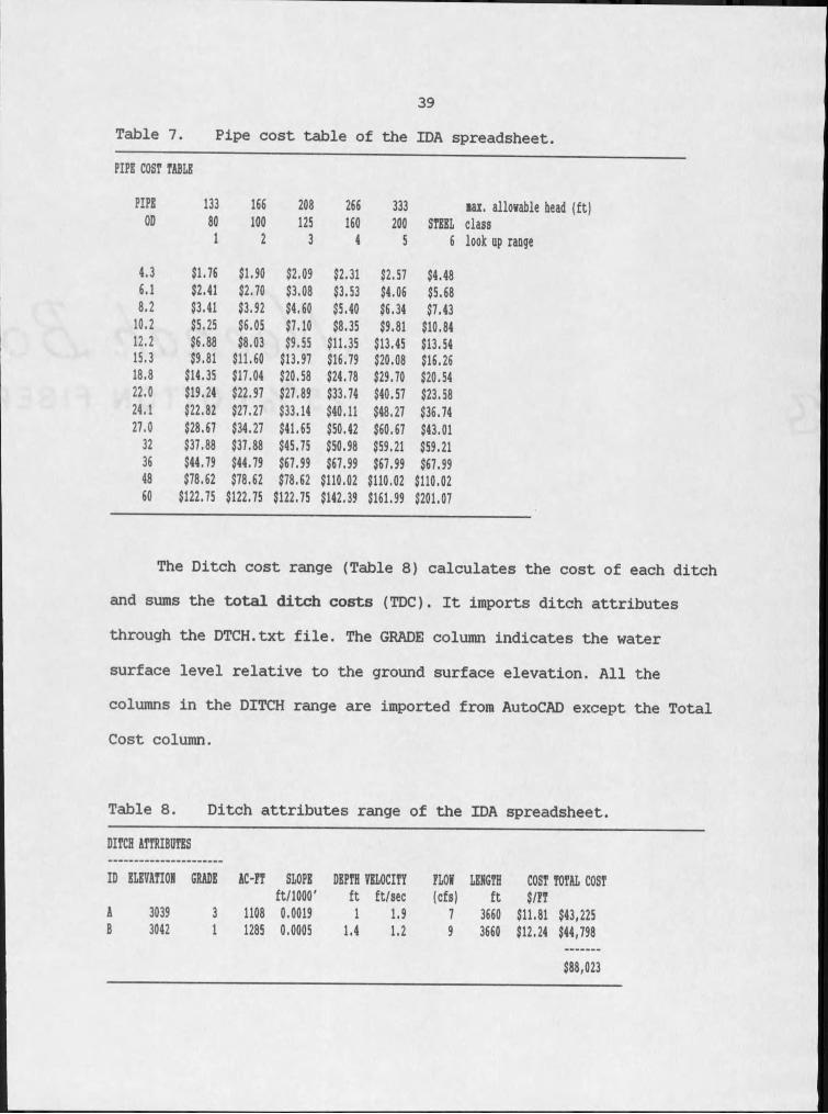
39Table 7. Pipe cost table of the IDA spreadsheet.PIPE COST TABLE

PIPE 133 166 208 266 333 iax. allowable head (ft)OD 80 100 125 160 200 STEEL classI 2 3 4 5 6 look up range4.3 $1.76 $1.90 $2.09 $2.31 $2.57 $4.486.1 $2.41 $2.70 $3.08 $3.53 $4.06 $5.688.2 $3.41 $3.92 $4.60 $5.40 $6.34 $7.4310.2 $5.25 $6.05 $7.10 $8.35 $9.81 $10.8412.2 $6.88 $8.03 $9.55 $11.35 $13.45 $13.5415.3 $9.81 $11.60 $13.97 $16.79 $20.08 $16.2618.8 $14.35 $17.04 $20.58 $24.78 $29.70 $20.5422.0 $19.24 $22.97 $27.89 $33.74 $40.57 $23.5824.1 $22.82 $27.27 $33.14 $40.11 $48.27 $36.7427.0 $28.67 $34.27 $41.65 $50.42 $60.67 $43.0132 $37.88 $37.88 $45.75 $50.98 $59.21 $59.2136 $44.79 $44.79 $67.99 $67.99 $67.99 $67.9948 $78.62 $78.62 $78.62 $110.02 $110.02 $110.0260 $122.75 $122.75 $122.75 $142.39 $161.99 $201.07

The Ditch cost range (Table 8) calculates the cost of each ditch and sums the total ditch costs (TDC). It imports ditch attributes through the DTCH.txt file. The GRADE column indicates the water surface level relative to the ground surface elevation. All the columns in the DITCH range are imported from AutoCAD except the Total Cost column.

Table 8. Ditch attributes range of the IDA spreadsheet. DITCH ATTRIBUTESID ELEVATI0H GRADE AC-FT SLOPE DEPTH VELOCITY FLOH LEHGTH COST TOTAL COST

ft/1000' ft ft/sec (cfs) ft $/FTA 3039 3 1108 0.0019 I 1.9 7 3660 $11.81 $43,225B 3042 I 1285 0.0005 1.4 1.2 9 3660 $12.24 $44,798

$88,023

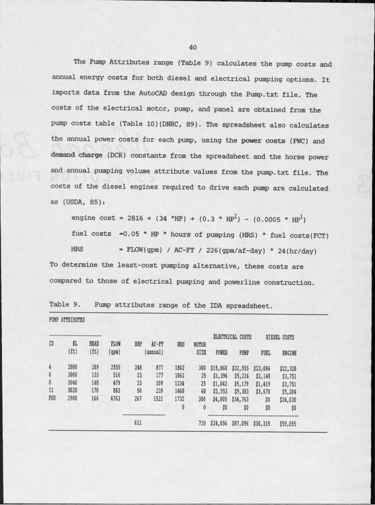
40The Pump Attributes range (Table 9) calculates the pump costs and

annual energy costs for both diesel and electrical pumping options. It imports data from the AutoCAD design through the Pump.txt file. The costs of the electrical motor, pump, and panel are obtained from the pump costs table (Table 10)(DNRC, 89). The spreadsheet also calculates the annual power costs for each pump, using the power costs (PWC) and

demand charge (DCR) constants from the spreadsheet and the horse power and annual pumping volume attribute values from the pump.txt file. The costs of the diesel engines required to drive each pump are calculated as (USDA, 85):

engine cost = 2816 + (34 *HP) + (0.3 * HP2) - (0.0005 * HP3) fuel costs =0.05 * HP * hours of pumping (HRS) * fuel costs(FCT) HRS - FLOW(gpm) / AC-FT / 226(gpm/af-day) * 24(hr/day)

To determine the least-cost pumping alternative, these costs are

compared to those of electrical pumping and powerline construction.

Table 9. Pump attributes range of the IDA spreadsheet. PUKP ATTRIBUTES

ELECTRICAL COSTS DIESEL COSTSID EL HEAD ELOK BHP AC-ET HRS KOTOR(ft) (ft) (gpi) (annual) SIZE POKER PUKP EUEL EKGIKE

4 2880 289 2555 248 877 1862 300 $15,060 $32,555 $23,086 $22,3206 3000 133 516 23 177 1861 25 $1,396 $5,216 $2,140 $3,7518 3040 148 479 23 109 1234 25 $1,042 $5,179 $1,419 $3,75111 3020 170 883 50 239 1468 60 $2,553 $9,383 $3,670 $5,204POD 2900 166 4763 267 1521 1732 300 $4,005 $34,763 $0 $24,0300 0 $0 $0 $0 $0

611 710 $24,056 $87,096 $30,315 $59,055

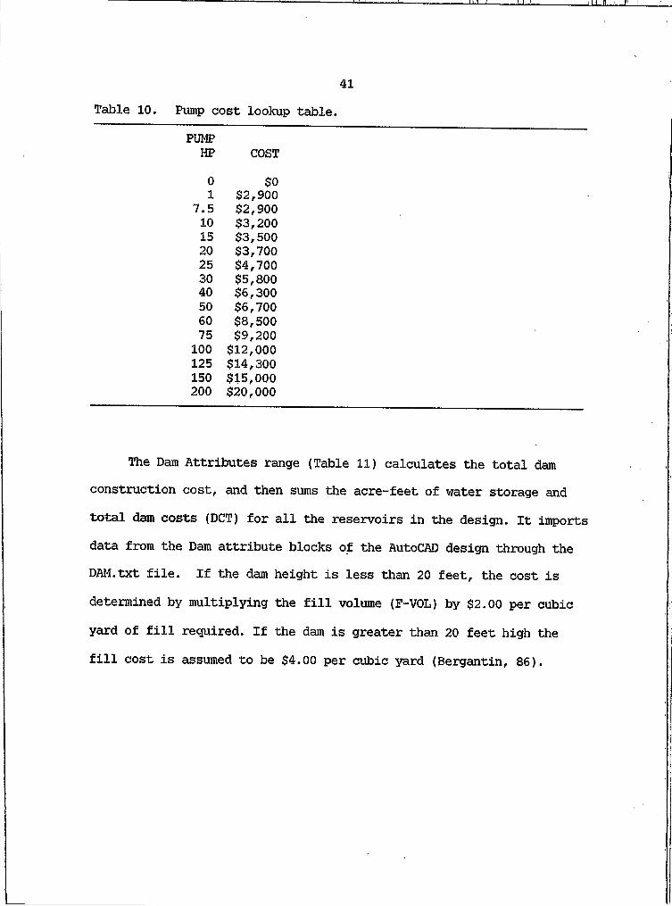
41Table 10. Pump cost lookup table.

PUMPHP COST0 $0I $2,900

7.5 $2,90010 $3,20015 $3,50020 $3,70025 $4,70030 $5,80040 $6,30050 $6,70060 $8,50075 $9,200100 $12,000125 $14,300150 $15,000200 $20,000

The Dam Attributes range (Table 11) calculates the total dam construction cost, and then sums the acre-feet of water storage and total dam costs (DCT) for all the reservoirs in the design. It imports data from the Dam attribute blocks of the AutoCAD design through the DAM.txt file. If the dam height is less than 20 feet, the cost is

determined by multiplying the fill volume (F-VOL) by $2.00 per cubic

yard of fill required. If the dam is greater than 20 feet high the fill cost is assumed to be $4.00 per cubic yard (Bergantin, 86).

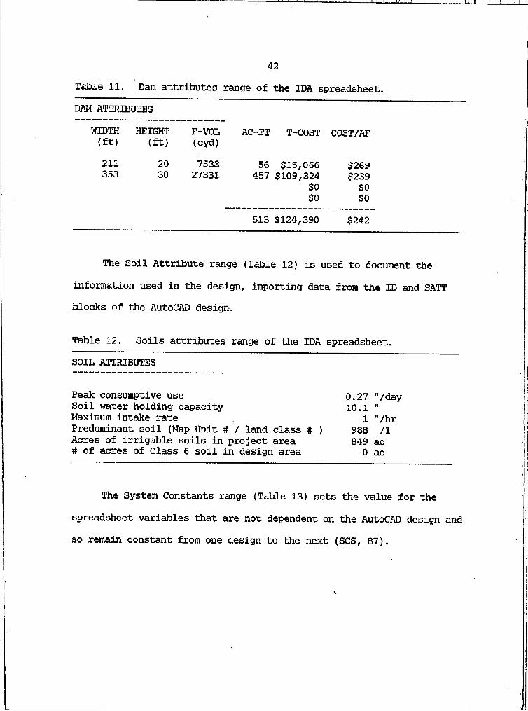
42Table 11. Dam attributes range of the IDA spreadsheet.DAM ATTRIBUTES

WIDTH HEIGHT F-VOL(ft) (ft) (cyd)211 20 7533353 30 27331

AC-FT T-COST COST/AF

56 $15,066 $269457 $109,324 $239

$0 $0$0 $0

513 $124,390 $242

The Soil Attribute range (Table 12) is used to document the information used in the design, importing data from the ID and SATT blocks of the AutoCAD design.

Table 12. Soils attributes range of the IDA spreadsheet. SOIL ATTRIBUTES

Peak consumptive use 0.27 "/daySoil water holding capacity 10.1 "Maximum intake rate I "/hrPredominant soil (Map Unit # / land class # ) 98B /IAcres of irrigable soils in project area 849 ac# of acres of Class 6 soil in design area 0 ac

The System Constants range (Table 13) sets the value for the spreadsheet variables that are not dependent on the AutoCAD design and so remain constant from one design to the next (SCS, 87).

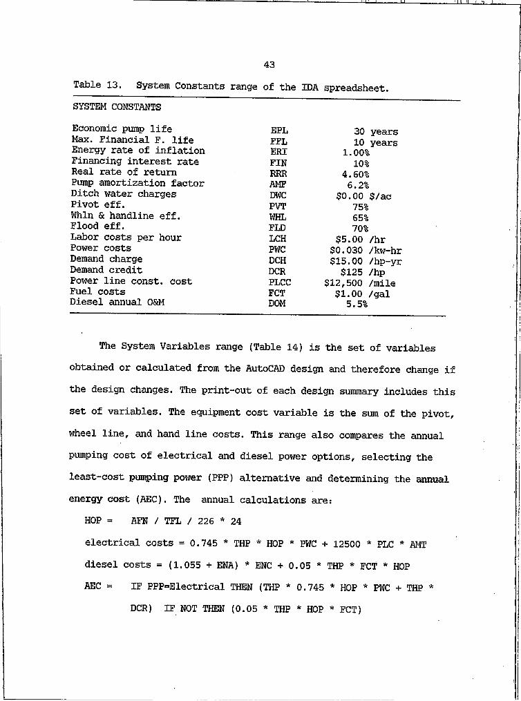
43Table 13. System Constants range of the IDA spreadsheet.SYSTEM CONSTANTSEconomic pump life Max. Financial F. life Energy rate of inflation Financing interest rate Real rate of return Pump amortization factor Ditch water charges Pivot eff.Whin & handline eff. Flood eff.Labor costs per hourPower costsDemand chargeDemand creditPower line const, costFuel costsDiesel annual OSeM

EPL 30 yearsFFL 10 yearsERI 1.00%FIN 10%RRR 4.60%AMF 6.2%DWC $0.00 $/acPVT 75%WHL 65%FLD 70%LCH $5.00 /hrPWC $0,030 /kw-hrDCH $15.00 /hp-yrDCR $125 /hpPLCC $12,500 /mileFCT $1.00 /galDOM 5.5%

The System Variables range (Table 14) is the set of variables obtained or calculated from the AutoCAD design and therefore change if the design changes. The print-out of each design summary includes this set of variables. The equipment cost variable is the sum of the pivot, wheel line, and hand line costs. This range also compares the annual pumping cost of electrical and diesel power options, selecting the least-cost pumping power (PPP) alternative and determining the annual energy cost (AEC). The annual calculations are;

HOP = AFN / TFL / 226 * 24

electrical costs = 0.745 * THP * HOP * PWC + 12500 * PLC * AMT diesel costs = (1.055 + ENA) * ENC + 0.05 * THP * FCT * HOP ABC = IF PPP=Electrical THEN (THP * 0.745 * HOP * PWC + THP *

DCR) IF NOT THEN (0.05 * THP * HOP * FCT)

44The pumping power variable (PPP) compares the annualized cost of

powerline construction plus the annual electric power cost against the annual cost of owning and operating a diesel engine. Diesel engine Iifs is set at 28,000 hours (ASAE, 84). Therefore, years of engine life is 28,000 hr divided by annual hours of pumping (HOP). The years of engine life is used to set the diesel engine amortization factor (ENA). The ownership costs of an electrical motor and pump are assumed to be equal to that of the engine clutch and pump, and so are not

accounted for in the comparison. Diesel fuel consumption is assumed to be 0.05 gal/hp-hr (ASAE, 84).

Table 14. System variables range of the IDA spreadsheet.SYSTEM VARIABLES

Require power line const. PLC 5.0 milesTotal consumptive use TCD 28 inchesRet irrigation requirement RIR 20.9 inchesTotal acres irrigated TAI 584 acAc-ft of water needed AfR 1402 ac-ft Total pump hp THP 611Total flow TfL 4433 gpm Hours of pumping HOP 1715Equipment costs EQC $155,499 Engine amort. ERA 8.8%flood costs FDC $0 Annual electrical cost $28,753Total pipe cost TPC $154,375 Annual diesel costs $46,374Total ditch cost TDC $88,023 Pumping power PPP ElectricalLabor cost ALC $4,050 Ann. energy costs AEC $25,466TR-21 weather station RSTA fort Benton Energy cost/ac EAC $43.58

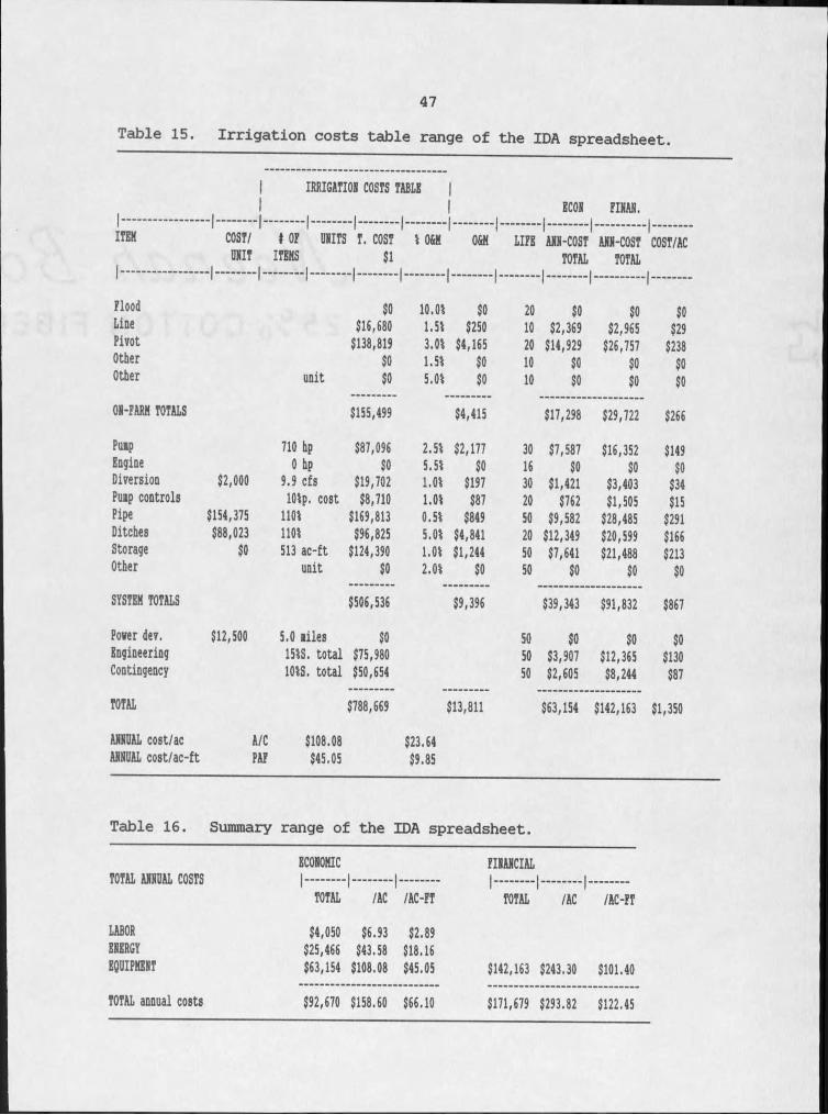
The Irrigation Costs Table range (Table 15) of the IDA spreadsheet annualizes the cost of the irrigation equipment used in the AutoCAD-designed system. (The table separates the on-farm irrigation equipment costs from the water delivery system costs. The engineering and contingency costs are based on the delivery system costs.) The range determines the total cost for each item, calculating

IIIH , t

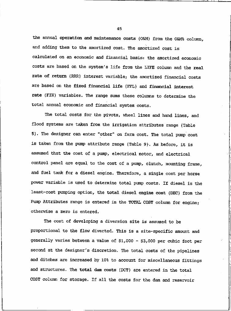
45the annual operation and maintenance costs (O&M) from the 0&M% column, and adding them to the amortized cost. The amortized cost is calculated on an economic and financial basis: the amortized economic costs are based on the system's life from the LIFE column and the real

of return (RRR) interest variable; the amortized financial costs are based on the fixed financial life (FFL) and financial interest rate (FIN) variables. The range sums these columns to determine the total annual economic and financial system costs.

The total costs for the pivots, wheel lines and hand lines, and flood systems are taken from the irrigation attributes range (Table 5). The designer can enter "other" on farm cost. The total pump cost is taken from the pump attribute range (Table 9). As before, it is assumed that the cost of a pump, electrical motor, and electrical control panel are equal to the cost of a pump, clutch, mounting frame, and fuel tank for a diesel engine. Therefore, a single cost per horse power variable is used to determine total pump costs. If diesel is the least-cost pumping option, the total diesel engine cost (DEC) from the Pump Attributes range is entered in the TOTAL COST column for engine; otherwise a zero is entered.

The cost of developing a diversion site is assumed to be proportional to the flow diverted. This is a site-specific amount and generally varies between a value of $1,000 - $3,000 per cubic foot per second at the designer's discretion. The total costs of the pipelines and ditches are increased by 10% to account for miscellaneous fittings and structures. The total dam costs (DCT) are entered in the total

COST column for storage. If all the costs for the dam and reservoir

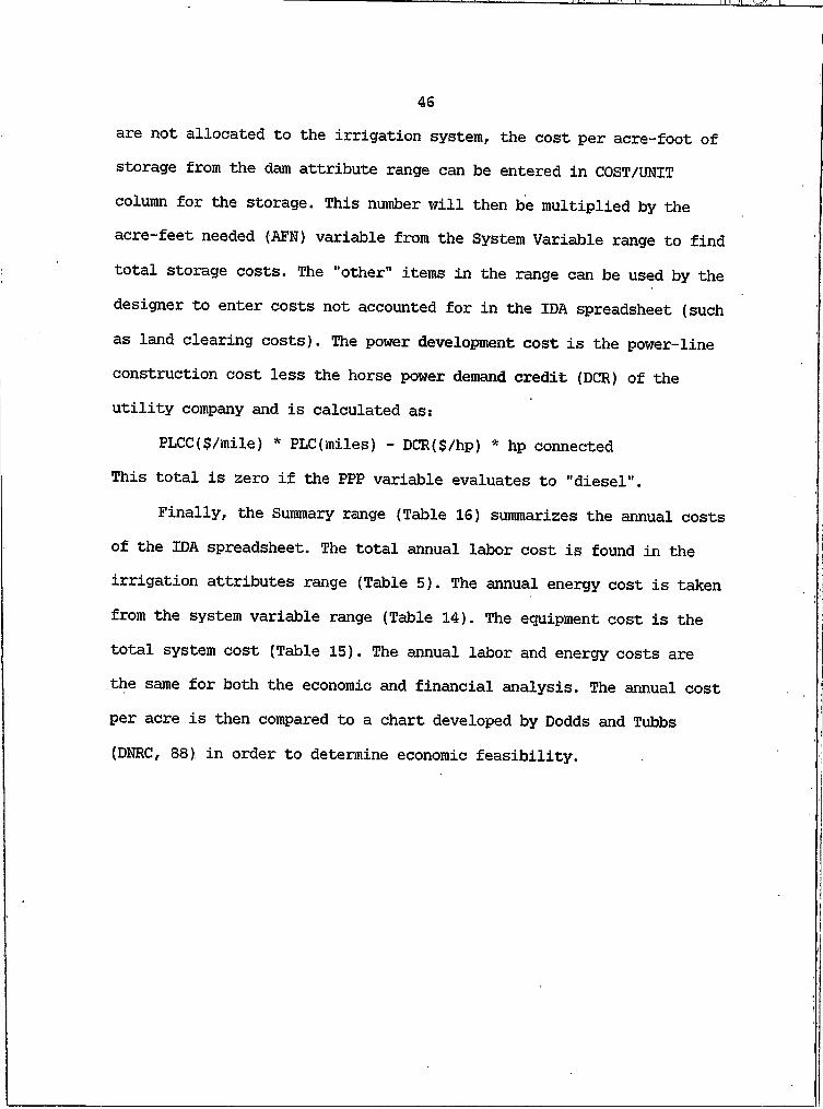
46are not allocated to the irrigation system, the cost per acre-foot of storage from the dam attribute range can be entered in COST/UNIT column for the storage. This number will then be multiplied by the acre-feet needed (AFN) variable from the System Variable range to find total storage costs. The "other" items in the range can be used by the designer to enter costs not accounted for in the IDA spreadsheet (such as land clearing costs). The power development cost is the power-line construction cost less the horse power demand credit (DCR) of the utility company and is calculated as:

PLCC($/mile) * PLC(miles) - DCR($/hp) * hp connected This total is zero if the PPP variable evaluates to "diesel".

Finally, the Summary range (Table 16) summarizes the annual costs of the IDA spreadsheet. The total annual labor cost is found in the irrigation attributes range (Table 5). The annual energy cost is taken from the system variable range (Table 14). The equipment cost is the total system cost (Table 15). The annual labor and energy costs are the same for both the economic and financial analysis. The annual cost per acre is then compared to a chart developed by Dodds and Tubbs (DNRC, 88) in order to determine economic feasibility.

47Table 15. Irrigation costs table range of the IDA spreadsheet.

I IRRIGATIOi COSTS TABLE |I I ECOH FIRAi.

. . . I- - - - 1- - - - 1- - - - 1- - - - 1- - - - 1- - - - 1- - - - 1- - - - - 1-- - -COST/ I OF UNITS T. COST \ 0&H Otil LIFE ANN-COST ANN-COST COST/AC MIT ITEMS $1 TOTAL TOTAL

Flood $0 10.01 $0 20 $0 $0 $0Line $16,680 I.Si $250 10 $2,369 $2,965 $29Pivot $138,819 3.0i $4,165 20 $14,929 $26,757 $238Other $0 i.Si $0 10 $0 $0 $0Other unit $0 5.Oi $0 10 $0 $0 $0ON-FARM TOTALS $155,499 $4,415 $17,298 $29,722 $266Puip 710 bp $87,096 2. Si $2,177 30 $7,587 $16,352 $149Engine 0 hp $0 5.51 $0 16 $0 $0 $0Diversion $2,000 9.9 cfs $19,702 1.01 $197 30 $1,421 $3,403 $34Puip controls lOtp. cost $8,710 1.01 $87 20 $762 $1,505 $15Pipe $154,375 not $169,813 0.51 $849 50 $9,582 $28,485 $291Ditches $88,023 not $96,825 5.01 $4,841 20 $12,349 $20,599 $166Storage $0 513 ac-ft $124,390 1.01 $1,244 50 $7,641 $21,488 $213Other unit $0 2.01 $0 50 $0 $0 $0SYSTEM TOTALS $506,536 $9,396 $39,343 $91,832 $867Power dev. $12,500 5.0 iiles $0 50 $0 $0 $0Engineering 15iS. total $75,980 50 $3,907 $12,365 $130Contingency IOtS. total $50,654 50 $2,605 $8,244 $87TOTAL $788,669 $13,811 $63,154 $142,163 $1,350ANNUAL cost/ac A/C $108.08 $23.64ANNUAL cost/ac-ft PAF $45.05 $9.85

Table 16. Summary range of: the IDA spreadsheet.

TOTAL ANNUAL COSTSECONOMIC FINANCIALII I

TOTAL /ACI/AC-FT

I—TOTAL

I I/AC /AC-FT

LABOR $4,050 $6.93 $2.89ENERGY $25,466 $43.58 $18.16EQUIPMENT $63,154 $108.08 $45.05 $142,163 $243.30 $101.40TOTAL annual costs $92,670 $158.60 $66.10 $171,679 $293.82 $122.45

u I l f \ I

CHftPTER 5

THE MftCHIKIE USE SPREADSHEET

The costs of owning and operating agricultural equipment vary greatly depending on farm situations and crop. These costs.must therefore be estimated to evaluate an irrigation development. The Machine Use spreadsheet, comprised of ten information areas (ranges), determines this information. A flow chart of these ranges is shown in (Figure 6). This chapter explains the use and function of each range.

The Index range

The Index range (Table 17) locates other ranges in the spreadsheet for editing or printing. The user may select a range area by pressing f5 (goto) and the two letter range name listed in the index. The range can be printed by pressing the "alt" key and the single letter print code, also listed in the index.

48

49Figure 6. Flow-chart of Machinery Use spreadsheet.

INDEX

ECONOMIC VARIABLES

CROP VARIABLES

TIME-TABLE (times over)

EQUIPMENT PARAMETERS

TIME BUDGETANNUAL USE (hours per season)

USED EQ. OP

FIXED & VARIABLE COST (per hour)

EQUIP. COST (per crop)

SUMMARY AND SENSITIVITY ANALYSIS

MACHINERY USE SPREADSHEET

IRRIGATION DESIGN SPREADSHEET

COST ENTERPRISE ANALYSIS

VALUE OF WATER FOR IRRIGATION

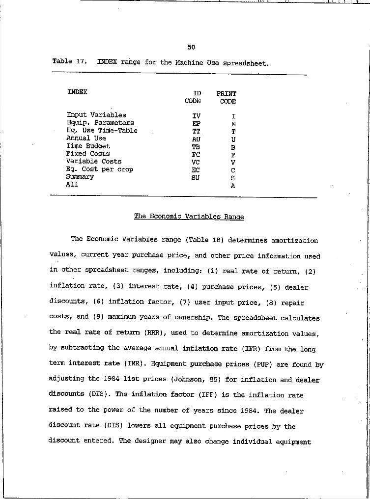
I JL II ■> I

50Table 17. INDEX range for the Machine Use spreadsheet.

INDEX ID PRINTCODE CODE

Input Variables IV IEquip. Parameters EP EEq. Use Time-Table TT TAnnual Use AU UTime Budget TB BFixed Costs FC FVariable Costs VC VEq. Cost per crop EC CSummary SU SAll A

The Economic Variables Range

The Economic Variables range (Table 18) determines amortization values, current year purchase price, and other price information used in other spreadsheet ranges, including: (I) real rate of return, (2)

inflation rate, (3) interest rate, (4) purchase prices, (5) dealer discounts, (6) inflation factor, (7) user input price, (8) repair costs, and (9) maximum years of ownership. The spreadsheet calculates the real rate of return (RRR), used to determine amortization values, by subtracting the average annual inflation rate (IFR) from the long term interest rate (INR). Equipment purchase prices (PUP) are found by adjusting the 1984 list prices (Johnson, 85) for inflation and dealer discounts (DIS). The inflation factor (IFF) is the inflation rate raised to the power of the number of years since 1984. The dealer discount rate (DIS) lowers all equipment purchase prices by the discount entered. The designer may also change individual equipment

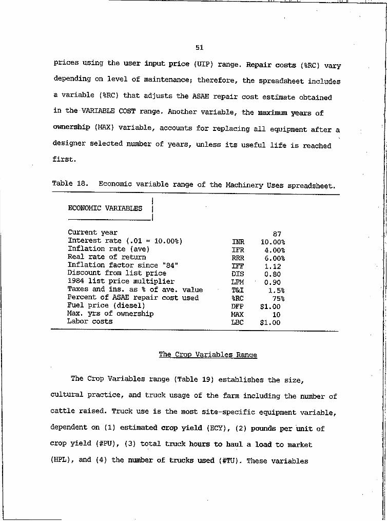
LI

prices using the user input price (UIP) range. Repair costs (%RC) vary depending on level of maintenance; therefore, the spreadsheet includes a variable (%RC) that adjusts the ASAE repair cost estimate obtained in the VARIABLE COST range. Another variable, the maximum years of

ownership (MAX) variable, accounts for replacing all equipment after a designer selected number of years, unless its useful life is reached first.

Table 18. Economic variable range of the Machinery Uses spreadsheet.

51

ECONOMIC VARIABLES jI

Current year 87Interest rate (.01 = 10.00%) INR 10.00%Inflation rate (ave) IFR 4.00%Real rate of return RRR 6.00%Inflation factor since "84" IFF 1.12Discount from list price DIS 0.801984 list price multiplier LPM 0.90Taxes and ins. as % of ave. value T&I 1.5%Percent of ASAE repair cost used %RC 75%Fuel price (diesel) DFP $1.00Max. yrs of ownership MAX 10Labor costs LBC $1.00

The Crop Variables Range

The Crop Variables range (Table 19) establishes the size, cultural practice, and truck usage of the farm including the number of cattle raised. Truck use is the most site-specific equipment variable, dependent on (I) estimated crop yield (ECY), (2) pounds per unit of crop yield (#PU), (3) total truck hours to haul a load to market I

(HPL), and (4) the number of trucks used (#TU). These variables

1

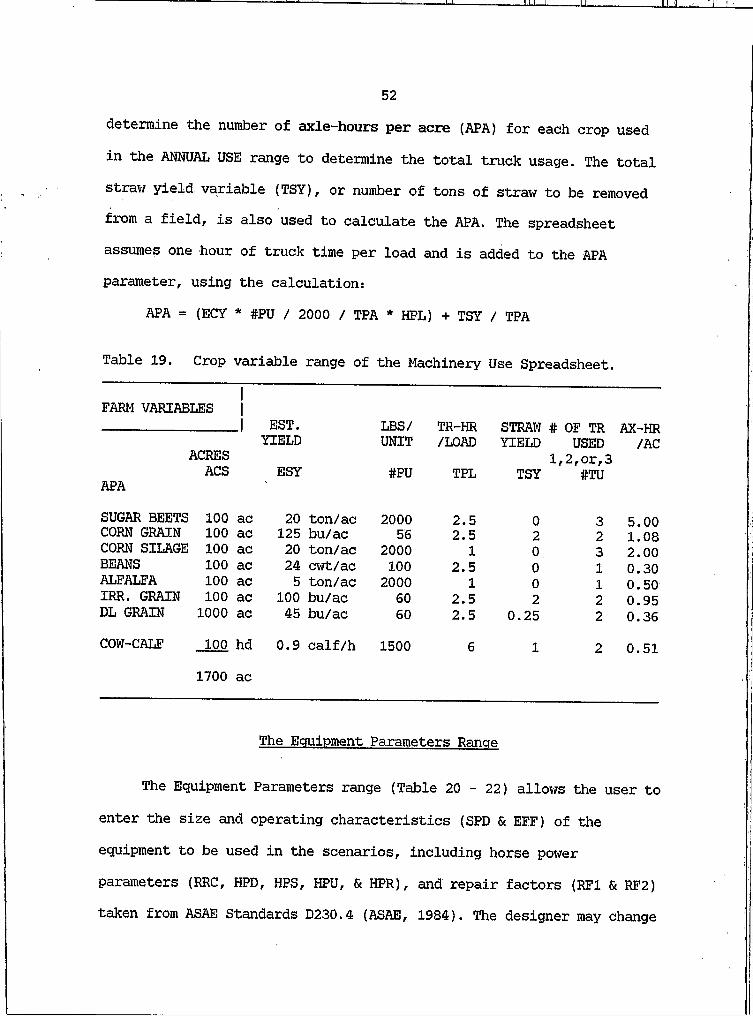
52determine the number of axle-hours per acre (APA) for each crop used

in the ANNUAL USE range to determine the total truck usage. The total straw yield variable (TSY), or number of tons of straw to be removed from a field, is also used to calculate the APA. The spreadsheet assumes one hour of truck time per load and is added to the APA parameter, using the calculation:

APA = (ECY * #PU / 2000 / TPA * HPL) + TSY / TPA

Table 19. Crop variable range of the Machinery Use Spreadsheet.

FARM VARIABLES |I EST. LBS / TR-HR STRAW # OF TR AX-HRYIELD UNIT /LOAD YIELD USED /ACACRES l,2,or,3ACS ESY #PU TPL TSY #TUAPA

SUGAR BEETS 100 ac 20 ton/ac 2000 2.5 0 3 5.00CORN GRAIN 100 ac 125 bu/ac 56 2.5 2 2 1.08CORN SILAGE 100 ac 20 ton/ac 2000 I 0 3 2.00BEANS 100 ac 24 cwt/ac 100 2.5 0 I 0.30ALFALFA 100 ac 5 ton/ac 2000 I 0 I 0.50IRR. GRAIN 100 ac 100 bu/ac 60 2.5 2 2 0.95DL GRAIN 1000 ac 45 bu/ac 60 2.5 0.25 2 0.36COW-CALF 100 hd 0.9 calf/h 1500 6 I 2 0.51

1700 ac

The Equipment Parameters Range

The Equipment Parameters range (Table 20 - 22) allows the user to

enter the size and operating characteristics (SPD & EFF) of the equipment to be used in the scenarios, including horse power parameters (RRC, HPD, HPS, HPU, & HPR), and repair factors (RF1 & RF2) taken from ASAE Standards D230.4 (ASAE, 1984). The designer may change

53equipment by entering an implement and its specifications in the appropriate cells, along with its estimated price in the user input price (UXP) range. Once an implement is changed, its named references are also changed in the rest of the spreadsheet the next time the spreadsheet is calculated.

The spreadsheet allows the designer to select either two or three tractors. If the designer enters zero for the first tractor horse power size variable (TRl) the spreadsheet uses the second tractor for all the first tractor-designated operations. The spreadsheet also allows the designer to purchase used equipment (N-U), for small farm operations where new equipment life extensively exceeds maximum years of ownership. The purchase price (PUP) is assumed to have a linear relationship with the equipment size, and is used to determine the cost for any equipment size selected with the calculation:

PUP = ("84" list price / equip, size) * SIZ * LPM

The designer may change this estimated price with the user input price, variable (UIP).

To determine the hours use per acre (HUA), the spreadsheet calculates:

HUA = 8.25 / SPD(mph) * SIZ * unit value * EFF The equipment operating speed (SPD) and field efficiency parameters (EFF) are set as medium recommended values established by ASAE standard D230.4 (ASAE, 1984). The "unit value" is the row crop spacing width in inches (RWD) converted to feet, and the unit value for "FT" is set equal to I; thus, SIZ times unit value is the equipment widthin feet.

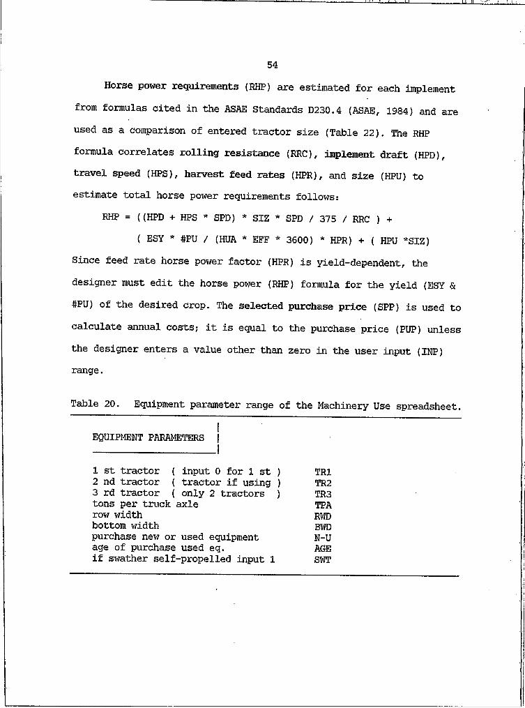
54Horse power requirements (RHP) are estimated for each implement

from formulas cited in the ASAE Standards D230.4 (ASAE, 1984) and are used as a comparison of entered tractor size (Table 22). The RHP formula correlates rolling resistance (RRC), implement draft (HPD), travel speed (HPS), harvest feed rates (HPR), and size (HPU) to estimate total horse power requirements follows:

RHP = ((HPD + HPS * SPD) * SIZ * SPD / 375 / RRC ) +( ESY * #PU / (HUA * EFF * 3600) * HPR) + ( HPU *SIZ)

Since feed rate horse power factor (HPR) is yield-dependent, the designer must edit the horse power (RHP) formula for the yield (ESY & #PU) of the desired crop. The selected purchase price (SPP) is used to calculate annual costs; it is equal to the purchase price (PUP) unless the designer enters a value other than zero in the user input (INP) range.

Table 20. Equipment parameter range of the Machinery Use spreadsheet.

IEQUIPMENT PARAMETERS jI

I st tractor ( input 0 for I st ) TRl2 nd tractor ( tractor if using ) TR23 rd tractor ( only 2 tractors ) TR3tons per truck axle TPArow width RWDbottom width BWDpurchase new or used equipment N-Uage of purchase used eq. AGEif swather self-propelled input I SWT

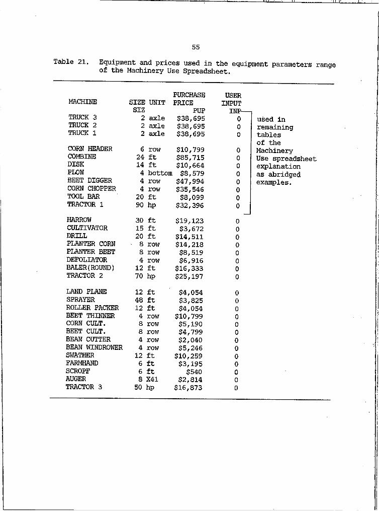
55

Table 21. Equipment and prices used in the equipment parameters rangeof the Machinery Use Spreadsheet.

PURCHASE USERMACHINE SIZE UNIT PRICE INPUTSIZ PUP INP-TRUCK 3 2 axle $38,695 0TRUCK 2 2 axle $38,695 0TRUCK I 2 axle $38,695 0

CORN HEADER 6 row $10,799 0COMBINE 24 ft $85,715 0DISK 14 ft $10,664 0PLOW 4 bottom $8,579 0BEET DIGGER 4 row $47,994 0CORN CHOPPER 4 row $35,546 0TOOL BAR 20 ft $8,099 0TRACTOR I 90 hp $32,396 0HARROW 30 ft $19,123 0CULTIVATOR 15 ft $3,672 0DRILL 20 ft $14,511 0PLANTER CORN 8 row $14,218 0PLANTER BEET 8 row $8,519 0DEFOLIATOR 4 row $6,916 0BALER(ROUND) 12 ft $16,333 0TRACTOR 2 70 hp $25,197 0LAND PLANE 12 ft $4,054 0SPRAYER 48 ft $3,825 0ROLLER PACKER 12 ft $4,054 0BEET THINNER 4 row $10,799 0CORN CULT. 8 row $5,190 0BEET CULT. 8 row $4,799 0BEAN CUTTER 4 row $2,040 0BEAN WINDROWER 4 row $5,246 0SWATHER 12 ft $10,259 0FARMHAND 6 ft $3,195 0SCROPF 6 ft $540 0AUGER 8 X41 $2,814 0TRACTOR 3 50 hp $16,873 0

used in remaining tables of the Machinery Use spreadsheet explanation as abridged examples.

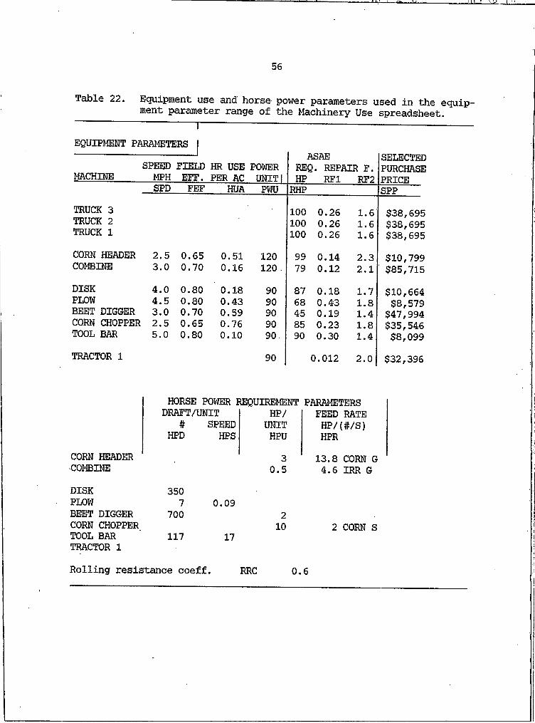
56

I — ----------- ----------Table 22. Equipment use and horse power parameters used in the equip

ment parameter range of the Machinery Use spreadsheet.


MACHINESPEEDMPH

FIELD EFF.

HR USE PER AC

POWERUNITI

ASAEREQ. REPAIR F. HP RFl RF2

SELECTEDPURCHASEPRICESPD FEF HUA PWU RHP SPP

TRUCK 3 100 0.26 1.6 $38,695TRUCK 2 100 0.26 1.6 $38,695TRUCK I 100 0.26 1.6 $38,695CORN HEADER 2.5 0.65 0.51 120 99 0.14 2.3 $10,799COMBINE 3.0 0.70 0.16 120 . 79 0.12 2.1 $85,715DISK 4.0 0.80 0.18 90 87 0.18 1.7 $10,664PLOW 4.5 0.80 0.43 90 68 0.43 1.8 $8,579BEET DIGGER 3.0 0.70 0.59 90 45 0.19 1.4 $47,994CORN CHOPPER 2.5 0.65 0.76 90 85 0.23 1.8 $35,546TOOL BAR 5.0 0.80 0.10 90 90 0.30 1.4 $8,099TRACTOR I 90 C.012 2.0 $32,396

HORSE POWER REQUIREMENT PARAMETERSDRAFT/UNIT HP/ FEED RATE

#HPD

SPEEDHPS

UNITHPU

HP/(#/S) HPR

CORN HEADER ■COMBINE

30.5

13.8 CORN G 4.6 IRR G

DISK 350PLOW 7 0.09BEET DIGGER 700 2CORN CHOPPER TOOL BAR TRACTOR I

117 1710 2 CORN S

Rolling resistance coeff RRC 0.6

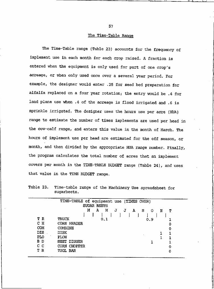
I I ,SI I

57The Time-Table Range

The Time-Table range (Table 23) accounts for the frequency of implement use in each month for each crop raised. A fraction is entered when the equipment is only used for part of one crop's acreage, or when only used once over a several year period. For example, the designer would enter .25 for seed bed preparation for alfalfa replaced on a four year rotation; the entry would be .4 for land plane use when .4 of the acreage is flood irrigated and .6 is

sprinkle irrigated. The designer uses the hours use per acre (HUA) range to estimate the number of times implements are used per head in the cow-calf range, and enters this value in the month of March. The hours of implement use per head are estimated for the off season, or month, and then divided by the appropriate HUA range number. Finally, the program calculates the total number of acres that an implement

covers per month in the TIME-TABLE BUDGET range (Table 24), and uses that value in the TIME BUDGET range.

Table 23. Time-table range of the Machinery Use spreadsheet for sugarbeets.

TIME-TABLE of equipment use (TIMES OVER)SUGAR BEETSMI I A M J J A S O

i i i i i i iN

I IT

T R I ITRUCK i i i i i i i0.1 0.9 I IIC H CORN HEADER 0

COM COMBINE 0DIS . DISK I IPLO PLOW I IB D BEET DIGGER I IC C CORN CHOPPER 0T B TOOL BAR 0

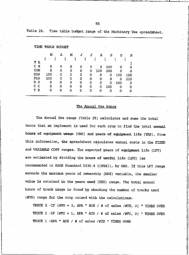
58Table 24. Time table budget range of the Machinery Use spreadsheet.

TIME TABLE BUDGET

T R C H COM DIS PLO B D C C T B

M' I

AI

MI

JI

J AI

SI

0I

NI

I0 0 0 0 0 0 100 0 00 0 0 0 0 '100 200 0 0100 0 0 0 0 0 0 100 100200 0 0 0 0 0 0 0 2250 0 0 0 0 0 0 100 00 0 0 0 0 0 100 0 00 0 0 0 0 0 0 0 0

The Annual Use Range

The Annual Use range (Table 25) calculates and sums the total hours that an implement is used for each crop to find the total annual hours of equipment usage (HRS) and years of equipment life (YRS). From this information, the spreadsheet calculates annual costs in the FIXED and VARIABLE COST ranges. The expected years of equipment life (LFY) are estimated by dividing the hours of useful life (LFH) (as recommended in ASAE Standard D230.4 (1984)), by HRS. If this LFY range exceeds the maximum years of ownership (MAX) variable, the smaller

value is retained in the years used (YRU) range. The total annual hours of truck usage is found by checking the number of trucks used (#TU) range for the crop raised with the calculations:

TRUCK 3 -IF (#TU = 3, APA * ACS / # of axles /#TU, 0) * TIMES OVERTRUCK 2 -IF (#TU > I, APA * ACS / # of axles /#TU, 0) * TIMES OVERTRUCK I -APA * ACS / # of axles /#TU * TIMES OVER

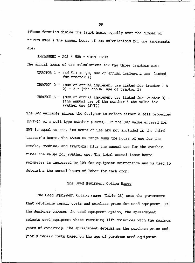
59(These formulas divide the truck hours equally over the number of trucks used.) The annual hours of use calculations for the implements are:

IMPLEMENT - ACS * HUA * TIMES OVER

The annual hours of use calculations for the three tractors are:TRACTOR I - (if TRl = 0,0, sum of annual implement use listed

for tractor I)

TRACTOR 2 - (sum of annual implement use listed for tractor I &2) - 2 * (the annual use of tractor I)TRACTOR 3 - (sum of annual implement use listed for tractor 3) -

(the annual use of the swather * the value for swather use (SWT))

The SWT variable allows the designer to select either a self propelled (SWT=I) or a pull type swather (SWT=O). If the SWT value entered for SWT is equal to one, its hours of use are not included in the third tractor's hours. The LABOR HR range sums the hours of use for the trucks, combine, and tractors, plus the annual use for the swather times the value for swather use. The total annual labor hours

parameter is increased by 10% for equipment maintenance and is used to determine the annual hours of labor for each crop.

The Used Equipment Option Range

The Used Equipment Option range (Table 26) sets the parameters that determine repair costs and purchase price for used equipment. If the designer chooses the used equipment option, the spreadsheet selects used equipment whose remaining life coincides with the maximum

years of ownership. The spreadsheet determines the purchase price and yearly repair costs based on the age of purchase used equipment

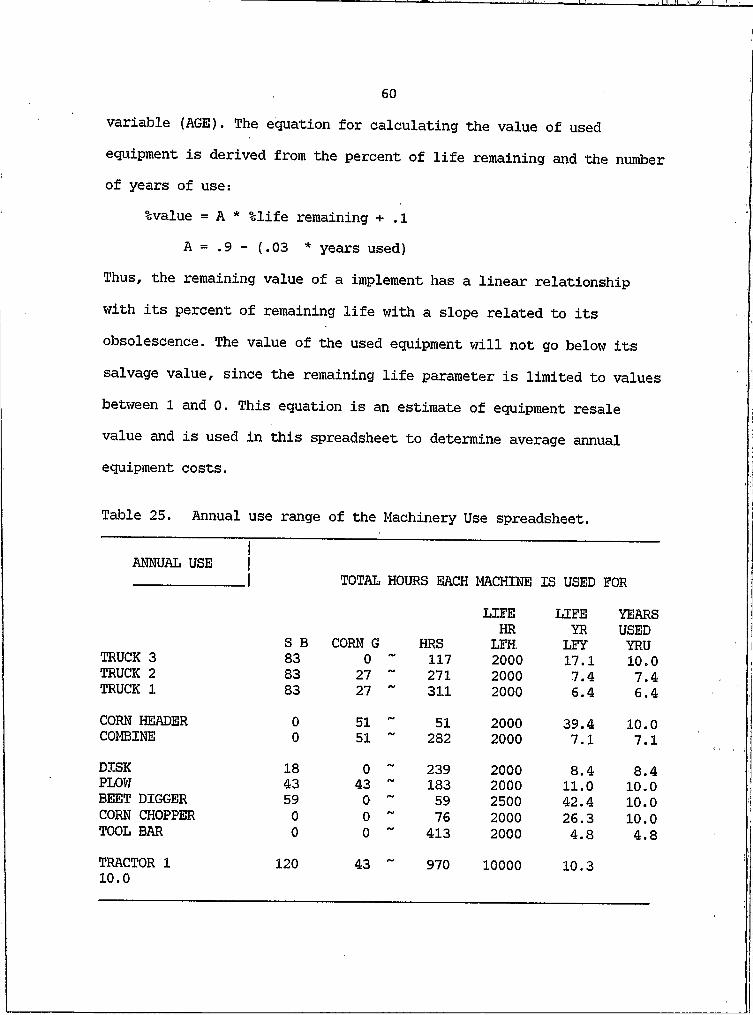
60variable (AGE). The equation for calculating the value of used equipment is derived from the percent of life remaining and the number of years of use:

%value = A * %life remaining + .1 A = .9 - (.03 * years used)

Thus, the remaining value of a implement has a linear relationship with its percent of remaining life with a slope related to its obsolescence. The value of the used equipment will not go below its salvage value, since the remaining life parameter is limited to values between I and 0. This equation is an estimate of equipment resale value and is used in this spreadsheet to determine average annual equipment costs.

Table 25. Annual use range of the Machinery Use spreadsheet.

ANNUAL USE |________________I TOTAL HOURS EACH MACHINE IS USED FOR

LIFE LIFE YEARSHR YR USEDS B CORN G HRS LFH LFY YRUTRUCK 3 83 0 117 2000 17.1 10.0TRUCK 2 83 27 271 2000 7.4 7.4TRUCK I 83 27 ~ 311 2000 6.4 6.4

CORN HEADER 0 51 51 2000 39.4 10.0COMBINE 0 51 282 2000 7.1 7.1DISK 18 0 239 2000 8.4 8.4PLOW 43 43 183 2000 11.0 10.0BEET DIGGER 59 0 59 2500 42.4 10.0CORN CHOPPER 0 0 76 2000 26.3 10.0TOOL BAR 0 0 413 2000 4.8 4.8TRACTOR I 10.0

120 43 970 10000 10.3

61

The percent of life used (LU%) range is the percent of total equipment life that would be used in the maximum years of ownership (MAX), and is used to determine the used purchase price (UP%). Its maximum value is limited to 75% of the total expected life (LFY) to

eliminate the ambiguities of purchasing almost new equipment. The used purchase price range calculations are:

UP% = .9 - ( .03 * AGE ) * LU% - 0.1

The total repair cost of equipment increases with age and is based on a percentage of original purchase price (PUP). The total equipment repair and maintenance costs are estimated by the equation (in accordance with ASAE (1984) Standard D230.4):

TOTAL REPAIR COST = PUP * RFl * (hour use/1000)ARF2 (The repair factors RFl and RF2 are taken from Table 22.) The TOTAL REPAIR COST for used equipment is found by subtracting the total estimated repair cost of the used equipment at time of purchase (PU%) from the total at its wearout life (W0%):

Total repair costs = PUP * (W0% -PU%)

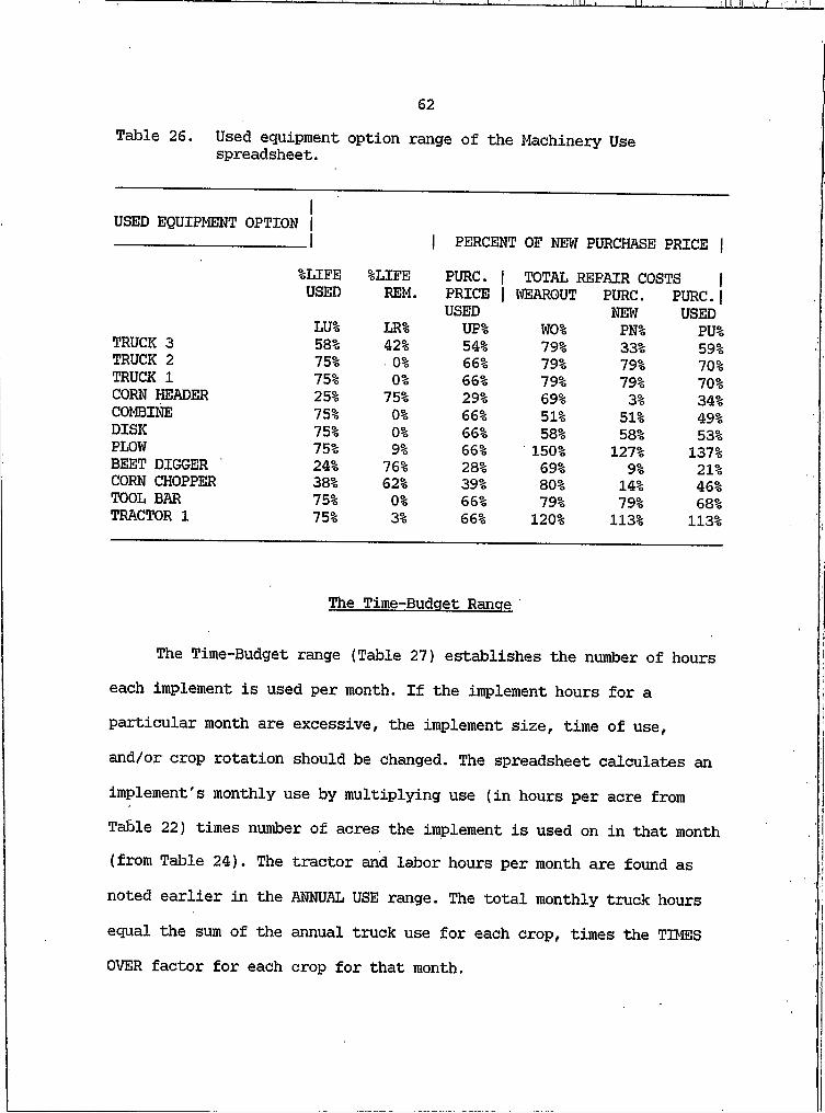
62Table 26. Used equipment option range of the Machinery Use

spreadsheet.

USED EQUIPMENT OPTION II

J I PERCENT OF NEW PURCHASE PRICE I%LIFE %LIFE PURC. I TOTAL REPAIR COSTS IUSED REM. PRICE I WEAROUT PURC. PURC.I

USED NEW USEDLU% LR% UP% W0% PN% PU%TRUCK 3 58% 42% 54% 79% 33% 59%TRUCK 2 75% 0% 66% 79% 79% 70%TRUCK I 75% 0% 66% 79% 79% 70%CORN HEADER 25% 75% 29% 69% 3% 34%COMBINE 75% 0% 66% 51% 51% 49%DISK 75% 0% 66% 58% 58% 53%PLOW 75% 9% 66% 150% 127% 137%BEET DIGGER 24% 76% 28% 69% 9% 21%CORN CHOPPER 38% 62% 39% 80% 14% 46%TOOL BAR 75% 0% 66% 79% 79% 68%TRACTOR I 75% 3% 66% 120% 113% 113%

The Time-Budget Range

The Time-Budget range (Table 27) establishes the number of hours each implement is used per month. If the implement hours for a particular month are excessive, the implement size, time of use,

and/or crop rotation should be changed. The spreadsheet calculates an implement's monthly use by multiplying use (in hours per acre from Table 22) times number of acres the implement is used on in that month (from Table 24). The tractor and labor hours per month are found as

noted earlier in the ANNUAL USE range. The total monthly truck hours equal the sum of the annual truck use for each crop, times the TIMES OVER factor for each crop for that month.

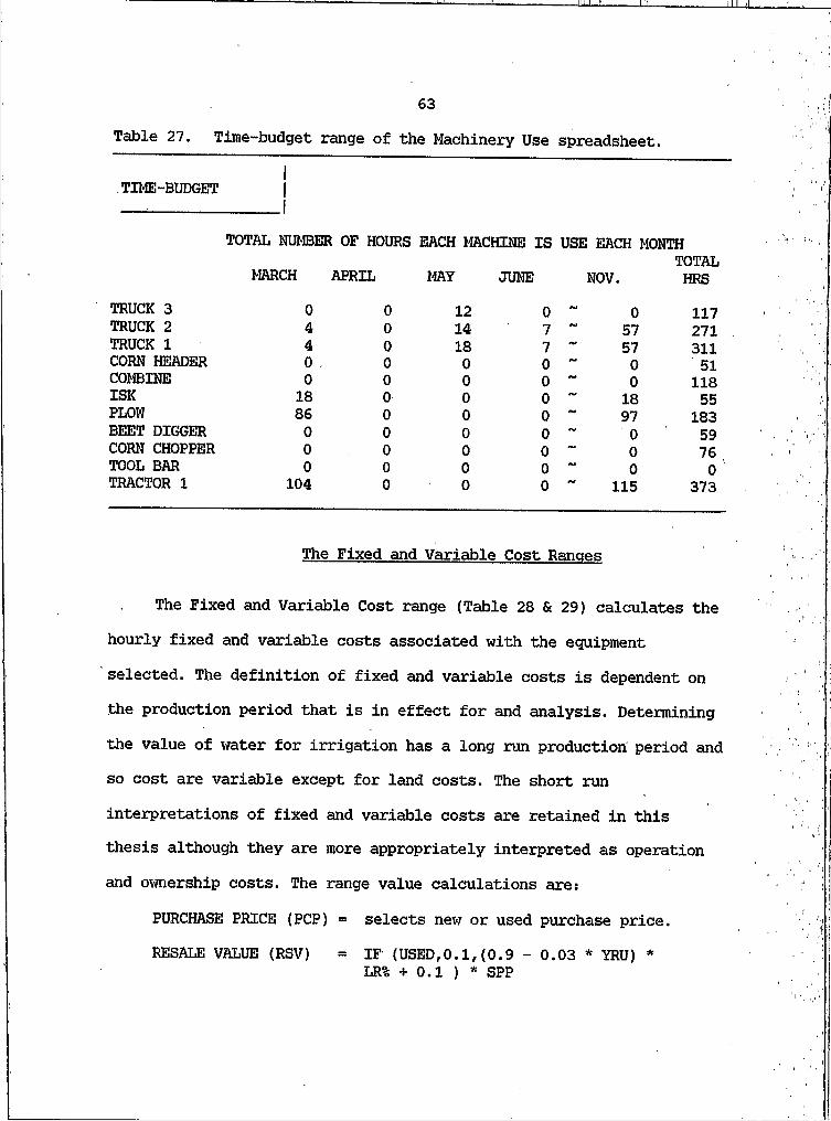
63Table 27. Time-budget range of the Machinery Use spreadsheet.

ITIME-BUDGET I

TRUCK 3

TOTAL NUMBER OF HOURS MARCH APRIL

0 0TRUCK 2 4 0TRUCK I 4 0CORN HEADER 0 . 0COMBINE 0 0ISK 18 0PLOW 86 0BEET DIGGER 0 0CORN CHOPPER 0 0TOOL BAR 0 0TRACTOR I 104 0

EACH MACHINE IS USE EACH MONTHTOTAL

MAY JUNE NOV. HRS12 0 0 11714 7 57 27118 7 57 3110 0 0 510 0 0 1180 0 18 550 0 97 1830 0 0 590 0 0 760 0 0 00 0 115 373

The Fixed and Variable Cost Ranges

The Fixed and Variable Cost range (Table 28 & 29) calculates the hourly fixed and variable costs associated with the equipment selected. The definition of fixed and variable costs is dependent on the production period that is in effect for and analysis. Determining the value of water for irrigation has a long run production period and so cost are variable except for land costs. The short run

interpretations of fixed and variable costs are retained in this thesis although they are more appropriately interpreted as operation and ownership costs. The range value calculations are:

PURCHASE PRICE (PCP) = selects new or used purchase price.RESALE VALUE (RSV) = IF (USED,0.1,(0.9 - 0.03 * YRU) *

LR% + 0.1 ) * SPP

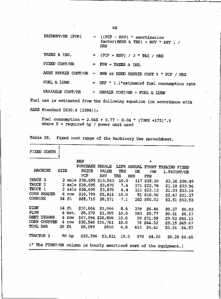
± L I l Il V ) ' I

PAYMENT/HR (PPH)

TAXES & INS.FIXED COST/HR ASAE REPAIR COST/HR FUEL & LUBE

VARIABLE COST/HR

64

((PCP - RSV) * amortization factor(@RRR & YRU) + RSV * RET ) /HRS

(PCP + RSV) / 2 * T&I / HRS PPH + TAXES & INS.

NEW or USED REPAIR COST % * PCP / HRS DFP * !.!^estimated fuel consumption rate REPAIR COST/HR + FUEL & LUBE

Fuel use is estimated from the following equation (in accordance with ASAE Standard D230.4 (1984)):

Fuel consumption = 2.64X + 0.77 - 0.04 * (738X +173)A.5 where X = required hp / power unit used

Table 28. Fixed cost range of the Machinery Use spreadsheet.

FIXED COSTS I

NEW *PURCHASE RESALE LIFE ANNUAL PYMNT TAX&INS FIXEDMACHINE SIZE PRICE VALUE YRS HR /HR I.5%C0ST/HRPCP RSV YRS HRS PPHTRUCK 3 2 axle $38,695 $13,543 10.0 117 $35.10 $3.36 $38.45TRUCK 2 2 axle $38,695 $3,870 7.4 271 $22.78 $1.18 $23.96TRUCK I 2 axle $38,695 $3,870 6.4 311 $22.13 $1.03 $23.16CORN HEADER 6 row $10,799 $5,914 10.0 51 $18.90 $2.47 $21.37COMBINE 24 ft $85,715 $8,571 7.1 282 $50.02 $2.51 $52.53

DISK 14 ft $10,664 $1,066 8.4 239 $6.46 $0.37 $6.83PLOW 4 hot. $8,579 $1,305 10.0 183 $5.77 $0.41 $6.17BEET DIGGER 4 row $47,994 $26,808 10.0 59 $71.59 $9.52 $81.11CORN CHOPPER 4 row $35,546 $16,761 10.0 76 $44.52 $5.15 $49.67TOOL BAR 20 ft $8,099 $810 4.8 413 $4.41 $0.16 $4.57TRACTOR I 90 hp $32,396> $3,831 10.0 970 $4.20 $0.28 $4.48(* The PYMNT/HR column is hourly amortized cost of the equipment.)

65Table 29. Variable costs range of the Machinery Use spreadsheet.

VARIABLE COSTS

ASAE 75%REPAIR REPAIR REPAIRCOST/HR COST/HR COST/YR

TRUCK 3 $11.04 $8.28 $966TRUCK 2 $15.25 $11.44 $3,094TRUCK I $15.25 $11.44 $3,552CORN HEAD $0.63 $0.47 $24COMBINE $22.05 $16.54 $4,657DISK $3.12 $2.34 $560PLOW $5.97 $4.48 $818BEET DIGG $7.38 $5.54 $326CORN CHOP $6.57 $4.93 $376TOOL BAR $3.21 $2.40 $992

TRACTOR I $3.77 $2.83 $2,741

FUEL & Variable TOTAL ANNUALLUBE COST/HR COST/HR COSTS$9.43 $17.71 $56.16 $6,552$9.43 $20.87 $44.83 $12,129$9.43 $20.87 $44.02 $13,671

$0.47 $21.83 $1,109$11.00 $27.53 $80.07 $22,546$8.40 $10.74 $17.57 $4,206$7.97 $12.45 $18.63 $3,401$9.56 $15.10 $96.21 $5,669$8.29 $13.22 $62.89 $4,789$8.55 $10.95 $15.52 $6,401

$2.83 $7.31 $7,085

The Equipment Cost Range

The Equipment Cost range (Table 30) allocates the selected equipment's fixed and variable costs per acre to the crops raised, calculated by multiplying the FIXED and VARIABLE COST/HR by the equipment's annual use (HRS) for each crop and dividing this value by the acres of that crop raised (ACS). By totaling these equipment costs, the spreadsheet obtains the total annual fixed and variable equipment cost per acre for each of the crops raised.

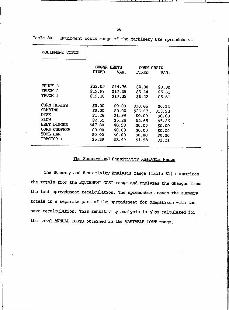
66Table 30. Equipment costs range of the Machinery Use spreadsheet.

EQUIPMENT COSTS

SUGAR BEETS CORN GRAINFIXED VAR. FIXED VAR.

TRUCK 3 TRUCK 2 TRUCK ICORN HEADER COMBINE DISK PLOWBEET DIGGER CORN CHOPPER TOOL BAR TRACTOR I

$32.05 $14.76$19.97 $17.39$19.30 $17.39$0.00 $0.00$0.00 $0.00$1.26 $1.98$2.65 $5.35

$47.80 $8.90$0.00 $0.00$0.00 $0.00$5.39 $3.40

$0.00 $0.00$6.44 $5.61$6.22 $5.61

$10.85 $0.24$26.67 . $13.98

$0.00 $0.00$2.65 $5.35$0.00 $0.00$0.00 $0.00$0.00 $0.00$1.93 $1.21

The Summary and Sensitivity Analysis Range

The Summary and Sensitivity Analysis range (Table 31) summarizes the totals from the EQUIPMENT COST range and analyzes the changes from the last spreadsheet recalculation. The spreadsheet saves the summary totals in a separate part of the spreadsheet for comparison with the next recalculation. This sensitivity analysis is also calculated for the total ANNUAL COSTS obtained in the VARIABLE COST range.

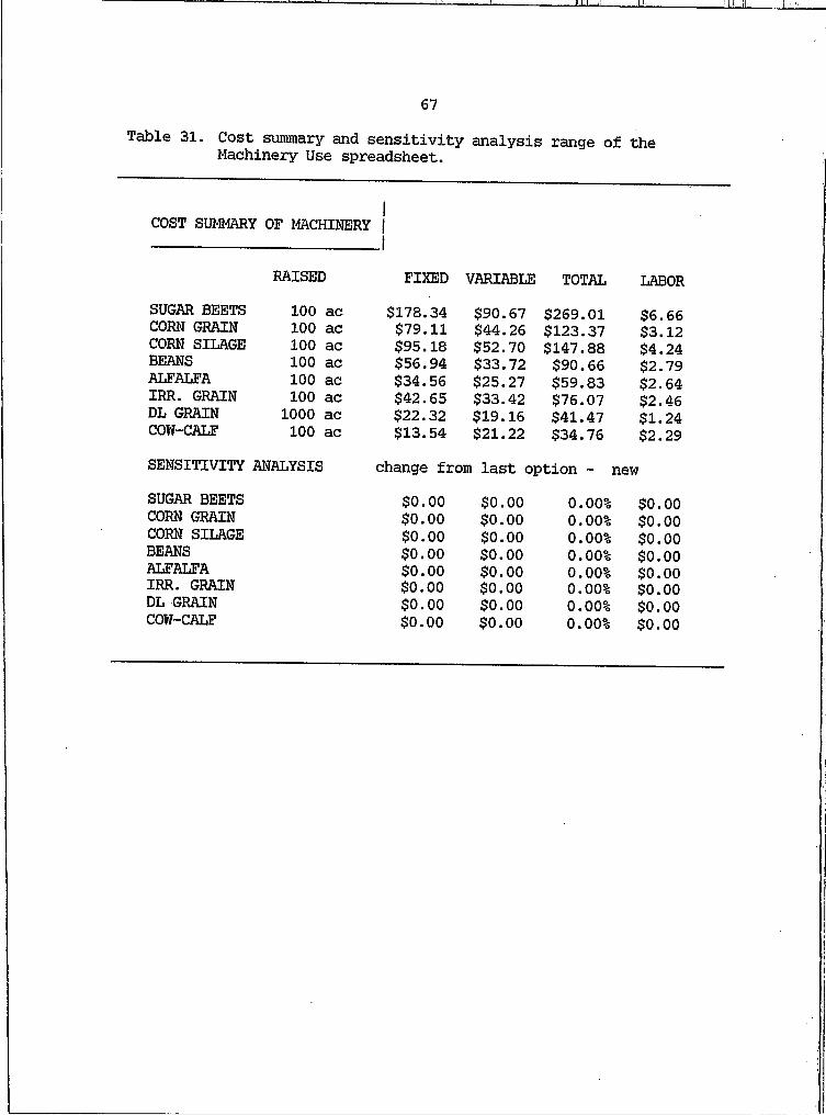
67Table 31. Cost summary and sensitivity analysis range of the

Machinery Use spreadsheet.

COST SUMMARY OF MACHINERY

SUGAR BEETS CORN GRAIN CORN SILAGE BEANS ALFALFA IRR. GRAIN DL GRAIN COW-CALFSENSITIVITYSUGAR BEETS CORN GRAIN CORN SILAGE BEANS ALFALFA IRR. GRAIN DL GRAIN COW-CALF

RAISED FIXED VARIABLE TOTAL LABOR100 ac $178.34 $90.67 $269.01 $6.66100 ac $79.11 $44.26 $123.37 $3.12100 ac $95.18 $52.70 $147.88 $4.24100 ac $56.94 $33.72 $90.66 $2.79100 ac $34.56 $25.27 $59.83 $2.64100 ac $42.65 $33.42 $76.07 $2.461000 ac $22.32 $19.16 $41.47 $1.24100 ac $13.54 $21.22 $34.76 $2.29

ALYSIS change from last option - new$0.00 $0.00 0.00% $0.00$0.00 $0.00 0.00% $0.00$0.00 $0.00 0.00% $0.00$0.00 $0.00 0.00% $0.00$0.00 $0.00 0.00% $0.00$0.00 $0.00 0.00% $0.00$0.00 $0.00 0.00% $0.00$0.00 $0.00 0.00% $0.00

68

CHAPTER 6

ENTERPRISE ANALYSIS SPREADSHEET

With the Enterprise Analysis Spreadsheet, the designer develops the individual crop budgets and total farm enterprise analyses. This chapter explains the use and function of the six ranges within this spreadsheet: index, system variables, crop variables, user entered variables, crop budgets, and summary.

The Index Range

As explained in chapter 5, the Index range (Table 32) locates other ranges in the spreadsheet for editing or printing.

Table 32. Index range of the Enterprise Analysis spreadsheet.

INDEX I RANGE PRINTI NAME CODE

INPUT IN/PUT NSugar B. SB BC o m G. CG CBeans BN EWheat SG GAlfalfa AF FIrr. past. IP IBarley DG JW Wheat WW DS Wheat SW HCow-Calf CC KSummary SU S

69The System Variables Range

The System Variables range (Table 33) sets up the basic economic parameters used to develop each crop budget. For each of three land- use types the spreadsheet calculates the current amount of land debt by multipling the land debt percentage by the land values. The three land use types considered are: (I) irrigated land (ILD), (2) dryland (DLD)7 and (3) grassland (GLD). This amount of land debt is used along with the (I) long term interest rate (INR)7 (2) land repayment terms (TRM)7 and (3) land values (ILV7 DLV7 & GLV) to determine the

amortized land repayment cost for each crop. In order to determine the amount of leased grassland that is required in the cow-calf enterprise range, the spreadsheet determines the total carrying capacity of the grassland owned (GLO) from the amount of grass available in annual animal unit months per acre (GAV).

The interest on operating capital (OCI) variable calculates annual interest charges for all variable costs. The return to farm (RET) variable determines land values in the summary range. Return to management (RTM) is the amount paid to farm management (not including labor cost), prorated on a weighted basis for the three land types. Vehicle miles (VMI) and other fixed costs (OTH) are also prorated on this same basis. The miscellaneous variable (MIS) allows the designer to increase the crop variable costs by a selected percentage, depending on confidence in the data. The designer may also choose the rate for land tax (LTX)7 federal crop insurance (CIN)7 and labor cost (LCT).

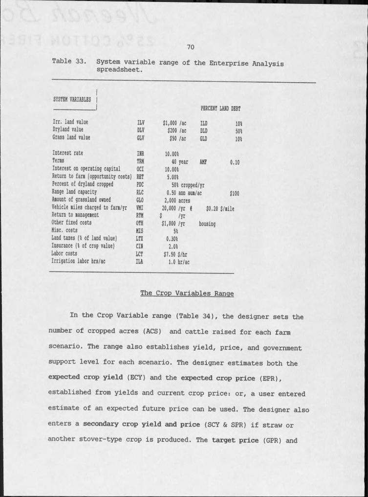
70Table 33. System variable range of the Enterprise Analysis

spreadsheet.

SYSTEM VARIABLES |

Irr. land value ILV Dryland value DLV Grass land value GLV

Interest rate m Tens TRM Interest on operating capital OCI Return to fan (opportunity costs) RET Percent of dryland cropped PDC Range land capacity RLC Amount of grassland owned GLO Vehicle miles charged to fan/yr VMI Return to management RTM Other fixed costs OTH Misc. costs MIS Land taxes (% of land value) LTX Insurance (i of crop value) CIM Labor costs LCT Irrigation labor hrs/ac ILA

PERCENT LAND DEBT$1,000 /ac ILD 101$200 /ac DLD 501$50 /ac GLD 101

10.00140 year AME 0.10

10.0015.001501 cropped/yr

0.50 ann aum/ac $1002.000 acres

20.000 /yr I $0.20 $/mile $ /yr$1,000 /yr housing

51 0.301 2.01

$7.50 $/hr1.0 hr/ac

The Crop Variables Range

In the Crop Variable range (Table 34), the designer sets the number of cropped acres (ACS) and cattle raised for each farm

scenario. The range also establishes yield, price, and government support level for each scenario. The designer estimates both the expected crop yield (ECY) and the expected crop price (EPR), established from yields and current crop price: or, a user entered

estimate of an expected future price can be used. The designer also enters a secondary crop yield and price (SCY & SPR) if straw or another stover-type crop is produced. The target price (GPR) and

71established crop yield variables (GCY) establish direct farm subsidy payments. There are several variables defining each cow-calf

enterprise: (I) size of cow herd (HD), (2) steer market price (SMP), and (3) calf market weight (CWT). In order to minimize the number of input variables heifer calf,, cull cow, and cull bull prices are calculated as a percent of SMP. These variables are used in the summary range to determine total farm income.

The general farm costs are weighted for each farm enterprise. The weighted land total acreage (WLT) sums irrigated acres and head of livestock then adds the sum of the dryland acres divided by four (this allocates farm costs more heavily to the irrigated acres). This WLT acreage is then used to allocate management, utility vehicle, and other fixed costs not directly allocable to an enterprise. These per weighted acre costs are found by dividing the management (WMC), vehicle WVC, and user entered fixed cost (FWC) by the WLT.

The User Entered Variable Ranges

The Equipment Variable range (Table 35) sets annual farm equipment and irrigation costs for each farm enterprise. It allows the

designer to adapt the spreadsheet to analyze crops for site specific situations. For established flood irrigation systems the water charge is entered as a fixed cost and incidental irrigation costs such as ditching and canal cleaning are entered as variable costs.

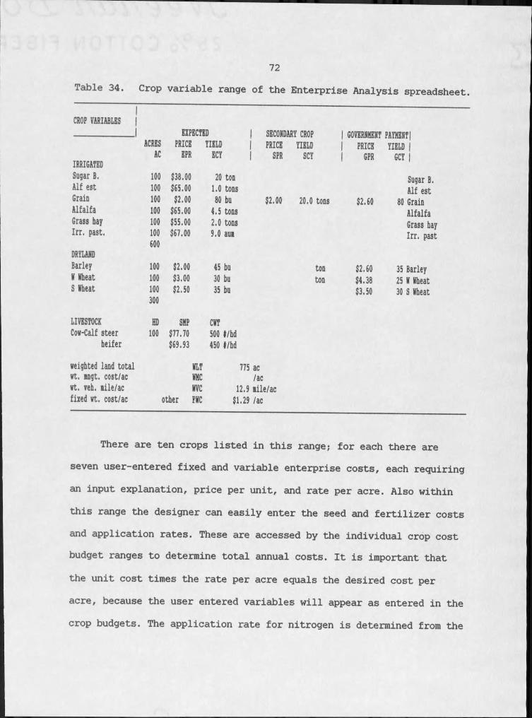
72T a b le 34. C rop v a r ia b le range o f th e E n te r p r is e A n a ly s is s p re a d s h e e t.

CROP VARIABLES |I EXPECTED I SECONDARY CROP | GOVERNMENT PAYMENT IACRES PRICE HELD | PRICE HELD I PRICE YIELD |

AC EPR ECY I SPR SCY I GPR GCY IIRRIGATEDSugar B. 100 $38.00 20 ton Sugar B.Alf est 100 $65.00 1.0 tons Alf estGrain 100 $2.00 80 bn $2.00 20.0 tons $2.60 80 GrainAlfalfa 100 $65.00 4.5 tons AlfalfaGrass hay 100 $55.00 2.0 tons Grass hayIn . past. 100

600$67.00 9.0 aui In . past

DRYLANDBarley 100 $2.00 45 bu ton $2.60 35 BarleyN Wheat 100 $3.00 30 bu ton $4.38 25 W WheatS Wheat 100 $2.50 35 bu $3.50 30 S Wheat

300

LIVESTOCK HD SHP CWTCow-Calf steer 100 $77.70 500 t/hd

heifer $69.93 450 t/hd

weighted land total WLT 775 acwt. mgt. cost/ac WKC /acwt. veh. lile/ac WVC 12.9 lile/acfixed wt. cost/ac other FWC $1.29 /ac

T h e re <a re te n c ro p s l i s t e d in t h i s ra n g e ; f o r each th e re a re

seven u s e r -e n te re d f i x e d and v a r ia b le e n te r p r is e c o s ts , each r e q u i r in g

an in p u t e x p la n a t io n , p r ic e p e r u n i t , and r a te p e r a c re . A ls o w i t h in

t h i s ra n g e th e d e s ig n e r can e a s i l y e n te r th e seed and f e r t i l i z e r c o s ts

and a p p l ic a t io n r a te s . These a re a cce sse d b y th e in d iv id u a l c ro p c o s t

b u d g e t ra n g e s t o d e te rm in e t o t a l a n n u a l c o s ts . I t i s im p o r ta n t t h a t

th e u n i t c o s t t im e s th e r a te p e r a c re e q u a ls th e d e s ir e d c o s t p e r

a c re , because th e u s e r e n te re d v a r ia b le s w i l l a p p e a r as e n te re d i n th e

c ro p b u d g e ts . The a p p l ic a t io n r a te f o r n i t r o g e n i s d e te rm in e d fro m th e

73crop estimated yield, soil nitrogen, and the yield response by the equation:

rate = yield X response - soil nitrogen

(This equation is inconsistent because input and output prices are ignored.)

Table 35. User entered variable range of Cost Enterprise spreadsheet.

EOflIPlfflHT VARIABLES

FIZEDSugar B.Grass bay $6.53Alf est $18.94Grain $28.78Alfalfa Irr. past. $17.97

Barley H Hbeat S Hheat$19.38

Cow-Calf $7.70

NACHIHERY COSTSVAR. TOTAL LABOR(hr/ac)$11.06 $17.59 3.75$30.20 $49.14 7.05$28.70 $57.49 5.16$31.20 $49.17 10.52

$28.59 $47.97 5.18

$12.39 $20.09 5.58

IRRIGATIOH COSTSFIZED LABOR ENERGY TOTAL$122.31 $4.94 $78.49 $205.74$122.31 $4.94 $78.49 $205.74$122.31 $4.94 $78.49 $205.74$122.31 $4.94 $78.49 $205.74$122.31 $4.94 $78.49 $205.74

DSBR EHTERED ENTERPRISE COSTS

INPUT PRICE /UNIT I CROP INPUT PRICE /UNIT RATE/flNIT■Alfalfasoil nitrogen $0.25 lb -12.5Furdan $1.00 oz 8.0V acV acTHINE ton 4.5F ac

EERTILIZER AND SEEDING VARIABLES

Cow-CalfHay $65.00 ton 1.4Straw ton 0.6Salt & minerals $25.00 cwt 0.2Protein sup. $8.00 cwt 2.9V $1.00 acF $1.00 ac

INPUTS IIugar B. irass hayA 11If estSoil N Ib/ac 60.0 60.0 60.0Response Ib-N/unit 8.0nitrooen $0.25 /lb act,phosphate $0.30 /lb act. 125.0 50.0 50.0potash $0.15 /lb act.fert appl $1.25 /ac 1.0 1.0 1.0seed cost $/lb $10.00 $4.00 $2.00seed rate Ib/ac 2.0 5.0 15.0

n A lfalfa :rr. pastBarley II : Hheat Hheat60.0 60.0 60.0 22.0 22.0 22.02.0 12.2 1.0 2.0 2.050 38 4828.0 50.0 60.0 15.0 15.0 15.01.0 1.0 1.0 1.0 1.0 1.0

0.10 $16.00 $0.10 $0.10 $0.1020.0 0.1 45.0 45.0 45.0

74

The Crop Enterprise Cost Analysis

There are ten crop enterprise ranges (Tables 36 to 38) in this

spreadsheet. Each of these ranges is standardized so a user can easily change crops by entering the crop name in the crop variable range and

modifying the inputs for that crop. In most cases, the designer only needs to modify information in the first four ranges. The irrigated pasture and cow-calf crop ranges, however, are crop specific: they

require the designer to enter extra site-specific data. All other crop

ranges can be modified in the crop and user entered variable ranges.

The format used in the crop enterprise cost analysis ranges is

patterned after the Cooperative Extension Service's Enterprise Costs studies (Fogle, 80). The first row in the range lists the crop name

and acres raised. The first column describes the information in that row, followed by the price of the item, measurement units, per acre

quantity used, and per acre item cost (the price per unit times the

quantity used). These values are taken from the system, crop,

equipment, and user entered ranges. All variable and fixed costs are listed and totaled separately.

The "interest on variable costs" line item sums all the variable costs, entering the total in its price column. It is then multiplied

by the operating capital interest (OCI) variable, and entered in the

system variable range, which determines both the short term interest

rate and the level of short term farm debt. Miscellaneous costs, other

L I W I

75then operating debt costs, are calculated as a percent of total

variable costs. This percentage is entered as the MIS variable in the system variable ranges. These per acre costs are summed to find the annual variable cost.

The spreadsheet sums all fixed and variable costs to find the total annual per acre cost for each crop, and subtracts it from the

gross revenue to find the per acre return to land. (Gross revenue is

the expected crop yield (ECY) times its expected price (EPR) plus the SCY times the SPR). The break even price is calculated by dividing the

total cost of the crop by its ECY; break even yield is total cost

divided by EPR. Interest on land debt is found by multiplying the long

term interest rate times the per acre land debt. The land debt is the

land value times the land debt percentage entered in the system

variable range. This land debt interest amount is used for cash flow

considerations and is not included return to land calculations. The

crop summary at the end of each range lists the return over variable

cost (ROVC), return to land, labor costs, benefit cost ratio (return

to land/total costs), government payment, and total farm expense.

The sugar beet crop budget (Table 36) shows the format used in the first five crop budgets. The enterprise budget for irrigated

pasture requires more information. In this budget steers are purchased

in the spring, fattened on the irrigated pasture, and sold in the

fall. To determine the number of steers purchased per acre (STR), the

spreadsheet divides the pasture's carrying capacity (in animal unit

months (AUM)) by four months per season and by .7 animal units (AU)

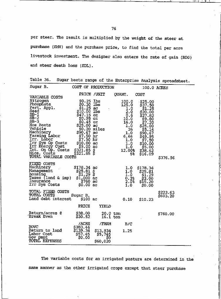
76per steer. The result is multiplied by the weight of the steer at

purchase (SMW) and the purchase price, to find the total per acre livestock investment. The designer also enters the rate of gain (ROG) and steer death loss (SDL).

Table 36. Sugar beets range of the Enterprise Analysis spreadsheet. Sugar B. COST OF PRODUCTION 100.0 ACRES

VARIABLE COSTS Nitrogen Phosphate Fert. Appl.SeedSB-ISB-2SB-3Hoe BeetsVehicleMachineryFarming LaborIrr. LaborIrr Sys Op CostsIrr Energy CostInt. On Op. Costs SMies. Costs STOTAL VARIABLE COSTS

PRICE /UNIT QUANT.$0.25 lbs 100.0$0.30 lbs 125.0$1.25 ac 1.0$10.00 lbs 2.0$47.15 OZ 0.6$0.98 OZ 10.0$0.45 OZ 16.0$25.00 ac 1.0$0.20 miles 26$90.67 ac 1.0$7.50 hr 6.66$7.50 hr 1.0$10.00 ac 1.0$5.00 ac 1.0321.85321.85 I 12.00%5%

COST$25.00$37.50$1.25$20.00$27.82$9.80$7.20$25.00$5.16$90.67$49.95$7.50$10.00$5.00$38.62$16.09 $376.56

FIXED COSTSMachinery $178.34 acManagement $25.81 $housing $1.29 $Taxes (land & imp) $1,000 ac Insurance $760 acIrr Sys Costs $0.00 acTOTAL FIXED COSTSTOTAL COSTS Sugar B.Land debt interest $100 ac

Retum/acres @ Break Even

ROVCReturn to land Labor Cost Gov pmnt TOTAL EXPENSES

PRICE$38.00$30.52/ACRE$383.44$139.34$57.45$0.00

/FARM$13,934S5'7!o$60,020

1.01.01.00.3%2.0%1.0

YIELD20.0 ton16.1 ton

B/C1.25

$178.34$25.81$1.29$3.00$15.20$0.00

0.10 $10.23$223.63$603.20

$760.00

The variable costs for an irrigated pasture are determined in thesame manner as the other irrigated crops except that steer purchase

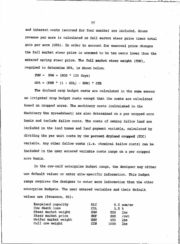
77and interest costs (accrued for four months) are included. Gross revenue per acre is calculated as fall market steer price times total gain per acre (GPA). In order to account for seasonal price changes the fall market steer price is assumed to be ten cents lower than the entered spring steer price. The fall market steer weight (FMW), required to determine GPA, is shown below:

FMW = SMW + (ROG * 120 days)GPA = (FMW * (I - SDL) - SMW) * STR

The dryland crop budget costs are calculated in the same manner as irrigated crop budget costs except that the costs are calculated based on cropped acres. The machinery costs (calculated in the Machinery Use spreadsheet) are also determined on a per cropped acre basis and include fallow costs. The costs of owning fallow land are included in the land taxes and land payment variable, calculated by dividing the per unit costs by the percent dryland cropped (PDC)

variable. Any other fallow costs (i.e. chemical fallow costs) can be included in the user entered variable costs range on a per cropped acre basis.

In the cow-calf enterprise budget range, the designer may either use default values or enter site-specific information. This budget range requires the designer to enter more information than the other enterprise budgets. The user entered variables and their default values are (Peterson, 86):

Rangeland capacity RLC 0.5 aum/iCow death loss CDL 1.5 %Steer market weight SMW 500 lbsSteer market price SMP $80 /CWtHeifer market weight HMW 450 lbsCull cow weight CCW 1000 lbs

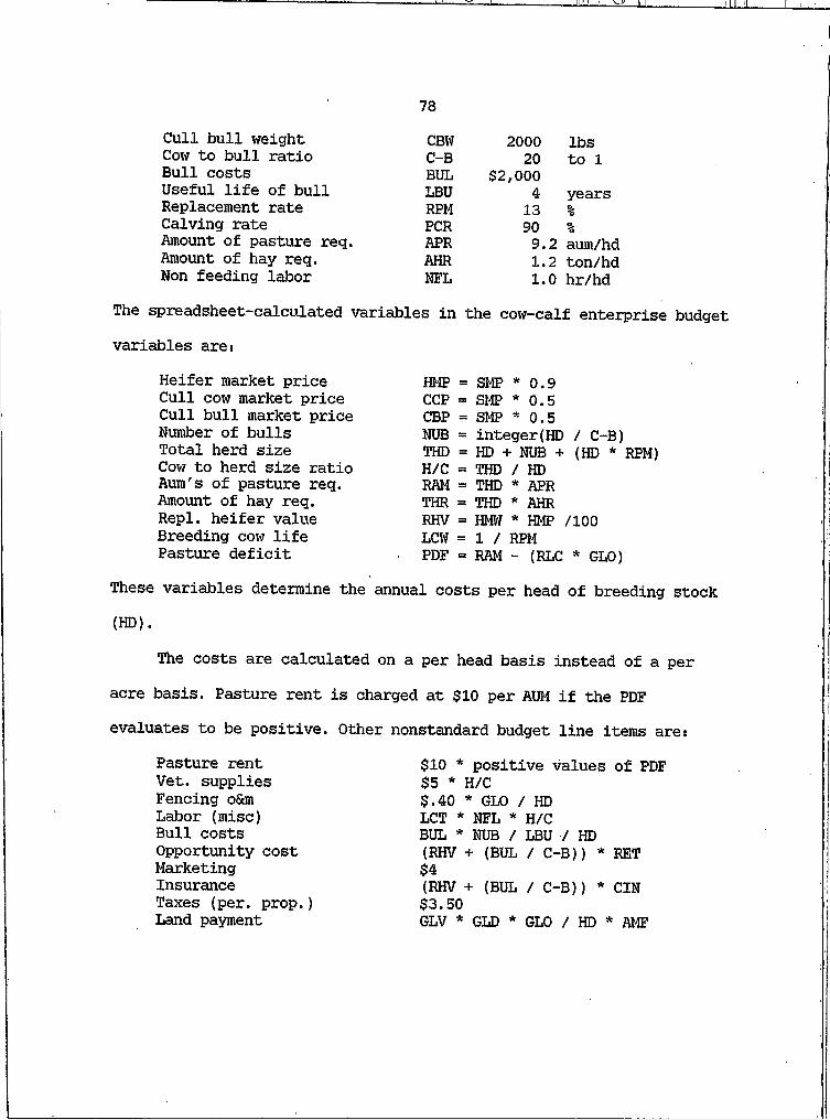
78Cull bull weight Cow to bull ratio Bull costs Useful life of bull Replacement rate Calving rate Amount of pasture req. Amount of hay req.Non feeding labor

CBW 2000 lbsC-B 20 to IBULLBU

$2,0004 years

RPM 13 %PCR 90 %APR 9.2 aum/hdAHR 1.2 ton/hdNFL 1.0 hr/hd

The spreadsheet-calculated variables in the cow-calf enterprise budget variables are:

Heifer market price Cull cow market price Cull bull market price Number of bulls Total herd size Cow to herd size ratio Aum's of pasture req. Amount of hay req.Repl. heifer value Breeding cow life Pasture deficit

HMP = SMP * 0.9 CCP = SMP * 0.5 CBP = SMP * 0.5 NUB = integer(HD / C-B)THD = HD + NUB + (HD * RPM)H/C = THD / HDRAM = THD * APRTHR = THD * AHRRHV = HMW * HMP /100LCW = I / RPMPDF = RAM - (RLC * GLO)

These variables determine the annual costs per head of breeding stock(HD).

The costs are calculated on a per head basis instead of a peracre basis. Pasture rent is charged at $10 per AUM if the PDFevaluates to be positive. Other nonstandard budget line items are:

Pasture rent Vet. supplies Fencing o&m Labor (misc)Bull costs Opportunity cost Marketing Insurance Taxes (per. prop.)Land payment

$10 * positive values of PDF$5 * H/C$.40 * GLO / HDLCT * NFL * H/CBUL * NUB / LBU / HD(RHV + (BUL / C-B)) * RET$4(RHV + (BUL / C-B)) * CIN $3.50GLV * GLD * GLO / HD * AMF

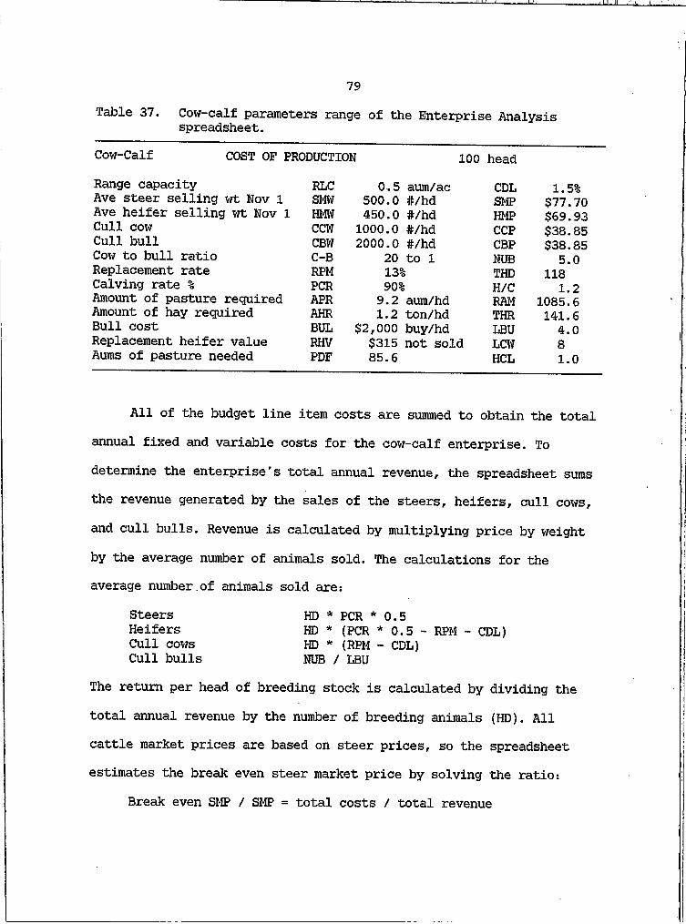
1 1 Jl I

79Table 37. Cow-calf parameters range of the Enterprise Analysis

spreadsheet.Cow-Calf COST OF PRODUCTION 100 headRange capacity RLC 0.5 aum/ac CDL 1.5%Ave steer selling wt Nov I SMW 500.0 #/hd SMP $77.70Ave heifer selling wt Nov I HMW 450.0 #/hd HMP $69.93Cull cow CCW 1000.0 #/hd CCP $38.85Cull bull CBW 2000.0 #/hd CBP $38.85Cow to bull ratio C-B 20 to I NUB 5.0Replacement rate RPM 13% THD 118Calving rate % PCR 90% H/C 1.2Amount of pasture required APR 9.2 aum/hd RAM 1085.6Amount of hay required AHR 1.2 ton/hd THR 141.6Bull cost BUL $2,000 buy/hd LBU 4.0Replacement heifer value RHV $315 not sold LCW 8Aums of pasture needed PDF 85.6 HCL 1.0

All of the budget line item costs are summed to obtain the total annual fixed and variable costs for the cow-calf enterprise. To

determine the enterprise's total annual revenue, the spreadsheet sums the revenue generated by the sales of the steers, heifers, cull cows,

and cull bulls. Revenue is calculated by multiplying price by weight by the average number of animals sold. The calculations for theaverage number.of animals sold are:

Steers Heifers Cull cows Cull bulls

HD * PCR * 0.5HD * (PCR * 0.5 - RPM - CDL)HD * (RPM - CDL)NUB / LBU

The return per head of breeding stock is calculated by dividing the total annual revenue by the number of breeding animals (HD). All cattle market prices are based on steer prices, so the spreadsheet estimates the break even steer market price by solving the ratio:

Break even SMP / SMP = total costs / total revenue

JJ I I 11 I f •

80Return to land is the difference between total revenue and total cost per head of breeding stock.

The Summary and Sensitivity Range

The summary range (Table 39) lists individual crop enterprise budget totals and sums total farm information. The sensitivity analysis (Table 40) shows the changes that result from modifications made since the last spreadsheet recalculation.

The maximum per person subsidy payment is $50,000. This spreadsheet totals the government payments for each crop and, where in excess, reduces each crop payment by the factor of the maximum payment divided by the calculated total payment.

The total farm return to land is the sum each crop's return to land plus its government payment. The total labor cost sums all listed labor line items. The total farm expense is the sum of all farm crop budget expenses; it determines the B/C ratio (return to farm/total farm expenses) for the individual farm, and can also be used to determine secondary benefits to the local economy. Again, the interest on land debt is totaled for the farmers cash flow considerations.

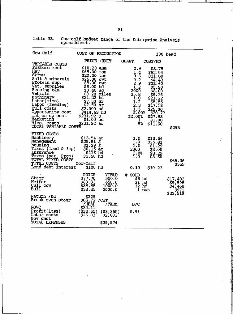
81Table 38. Cow-calf budget range of the Enterprise Analysisspreadsheet.

Cow-Calf COST OF PRODUCTION 100 headVARIABLE COSTS Pasture rent Hay StrawSalt & minerals Protein sup.Vet. supplies Fencing o&m Vehicle machinery Labor(mics)Labor (feeding)Bull costs Opportunity cost Int on op cost MarketingMics. costs vTOTAL VARIABLE COSTSFIXED COSTS Machinery Management housing Taxes (land

PRICE /UNIT QUANT. COST/HD$10.23 aum 0.9 $8.75$65.00 ton 1.4 $92.04$20.00 ton 0.6 $11.80$25.00 CWt 0.2 $4.43$8.00 CWt 2.9 $23.60$5.00 hd 1.2 $5.90$0.40 ac 2000 $8.00$0.20 miles 25.8 $5.16$21.22 hd 1.0 $21.22$7.50 hr 1.2 $8.85$7.50 hr 2.3 $17.18$2,000 hd 1.3 $25.00$414.6E) hd 5.00% $20.73

____ & imp)Insurance Taxes (per. Prop)TOTAL FIXED COSTS TOTAL COSTS Cow-CalfLand debt interest $100

$1.00$231.92

13.5425.811.290.15$415$3.50

hdac

acIac

12.00%I5%

1.01.01.020002.0%1.0

$27.83$1.00$11.60

513.54525.81$1.29$3.00$8.29$3.50

$293

Steer Heifer Cull cow BullReturn /hd Break even steerROVCProfit(Ioss) Labor costs Gov pmnt TOTAL EXPENSES

PRICE$77.70$69.93$38.85$38.85$325 $85.72 /CWT /HEAD /FARM $32.11($33.55) ($3,355) $26.03 $2,603

IYIELD

0.10 $10.23# SOLD

$65.66$359

500.0 45 hd $17,483450.0 31 hd $9,5981000.0 12 hd $4,4682000.0 I CWt $971$32,519

B/C0.91

$35,874

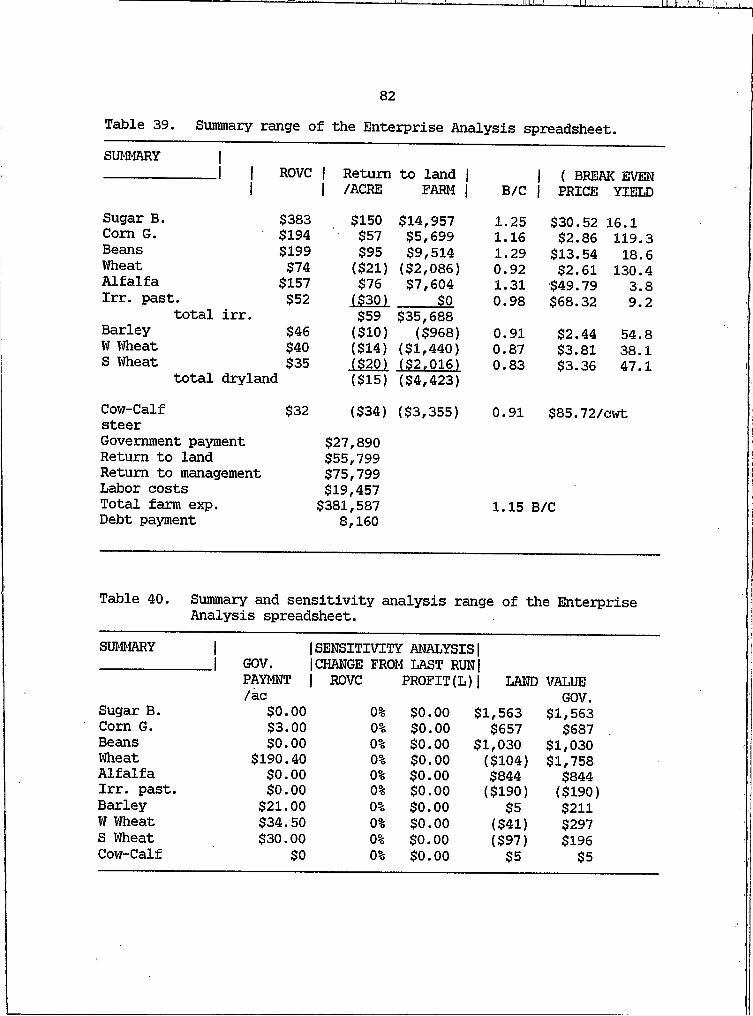
LI. H ( 11! I : ' •>

82Table 39. Summary range of the Enterprise Analysis spreadsheet.SUMMARY I

I I ROVC I Return to land I I ( BREAK EVENI I /ACRE FARM I B/C I PRICE YIELD

Sugar B. $383 $150 $14,957 1.25 $30.52 16.1C o m G. $194 $57 $5,699 1.16 $2.86 119.3Beans $199 $95 $9,514 1.29 $13.54 18.6Wheat $74 ($21) ($2,086) 0.92 $2.61 130.4Alfalfa $157 $76 $7,604 1.31 $49.79 3.8Irr. past. $52 ($30) $0 0.98 $68.32 9.2total irr. $59 $35,688Barley $46 ($10) ($968) 0.91 $2.44 54.8W Wheat $40 ($14) ($1,440) 0.87 $3.81 38.1S Wheat $35 ($20) ($2,016) 0.83 $3.36 47.1total dryland ($15) ($4,423)Cow-Calf $32 ($34) ($3,355) 0.91 $85.72/cwtsteerGovernment payment $27,890Return to land $55,799Return to management $75,799Labor costs $19,457Total farm exp. $381,587 1.15 B/CDebt payment 8,160

Table 40. Summary and sensitivity analysis Analysis spreadsheet.

range of the Enterprise

SUMMARY II GOV.

PAYMNT /ac

I SENSITIVITY ANALYSIS I !CHANGE FROM LAST RUN|I ROVC PROFIT(L)I LAND VALUE

GOV.Sugar B. $0.00 0% $0.00 $1,563 $1,563Corn G. $3.00 0% $0.00 $657 $687Beans $0.00 0% $0.00 $1,030 $1,030Wheat $190.40 0% $0.00 ($104) $1,758Alfalfa $0.00 0% $0.00 $844 $844Irr. past. $0.00 0% $0.00 ($190) ($190)Barley $21.00 0% $0.00 $5 $211W Wheat $34.50 0% $0.00 ($41) $297S Wheat $30.00 0% $0.00 ($97) $196Cow-Calf $0 0% $0.00 $5 $5

83

CHAPTER 7

IRRIGATION DESIGN EVALUATION EXAMPLES

This chapter describes three potential irrigation sites that are included in Cascade and Chouteau Conservation Districts Missouri River water reservation applications. (These applications were prepared by the Department of Natural Resources and Conservation.) There are four irrigation development examples presented which demonstrate the procedures explained in this thesis. The farm/ranch size and agricultural practices used in the before- and after-development scenarios are hypothetical.

Each example shows the net return to irrigation water and includes a table summarizing the machinery cost and farm enterprise analysis spreadsheet for the before- and after-development scenarios. The farm machinery summary includes: acreage of each crop raised, the major equipment parameters, and the annual equipment cost associated with each crop. The farm enterprise analysis summary includes: the

expected price and yield of each crop, the government support payment, net farm return to land, and the value of water. This value is calculated by dividing the acres of irrigated crops into the net return of the irrigated crops. This value does not compare the before- and after-development scenarios.

Each example presentation also includes a design drawing of the proposed irrigation development and a cost summary of the Irrigation

H M I f \ I I I I I ill I

Design spreadsheet for that development. The design drawings show the irrigated area and type of irrigation, as well as pipeline and pump location. The Irrigation Design spreadsheet summary includes the number of acres irrigated, water requirements, and project costs.

For each example, the value of water for irrigation is found by subtracting the revenue netted in the be fore-development scenario from the revenue netted in the after-development scenario. There are two assumptions made within these examples. The first is that the crop raised on the developed acres is alfalfa, on an eight year rotation. The second is that, the alfalfa is assumed to be well managed, so that yield is a function of the total consumptive water use for the site. The total consumptive use is found using the Soil Conservation Service's TR21 computer model (USDA, 87). The yield is then calculated using an empirical function developed by the Department of Natural Resources and Conservation (DNRC, 88). The price and yield information for other crops are ten-year averages for Montana (MDA, 87). The yields and prices used in the following examples are intended for comparison purposes only.

Example I. A Low Lift Pivot Developed on a Ranch

The first example is a cattle ranching operation with 100 acres of irrigated grain, 300 acres of dryland hay, 1000 acres of dryland grain, and 500 head of cattle.

84

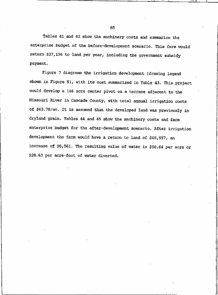
85Tables 41 and 42 show the machinery costs and summarize the

enterprise budget of the before-development scenario. This farm would return $37,196 to land per year, including the government subsidy payment.

Figure 7 diagrams the irrigation development (drawing legend shown in Figure 5), with its cost summarized in Table 43. This project would develop a 146 acre center pivot on a terrace adjacent to the

Missouri River in Cascade County, with total annual irrigation costs of $63.78/ac. It is assumed that the developed land was previously in dryland grain. Tables 44 and 45 show the machinery costs and farm enterprise budget for the after-development scenario. After irrigation development the farm would have a return to land of $45,557, an increase of $8,561. The resulting value of water is $58.64 per acre or $28.63 per acre-foot of water diverted.

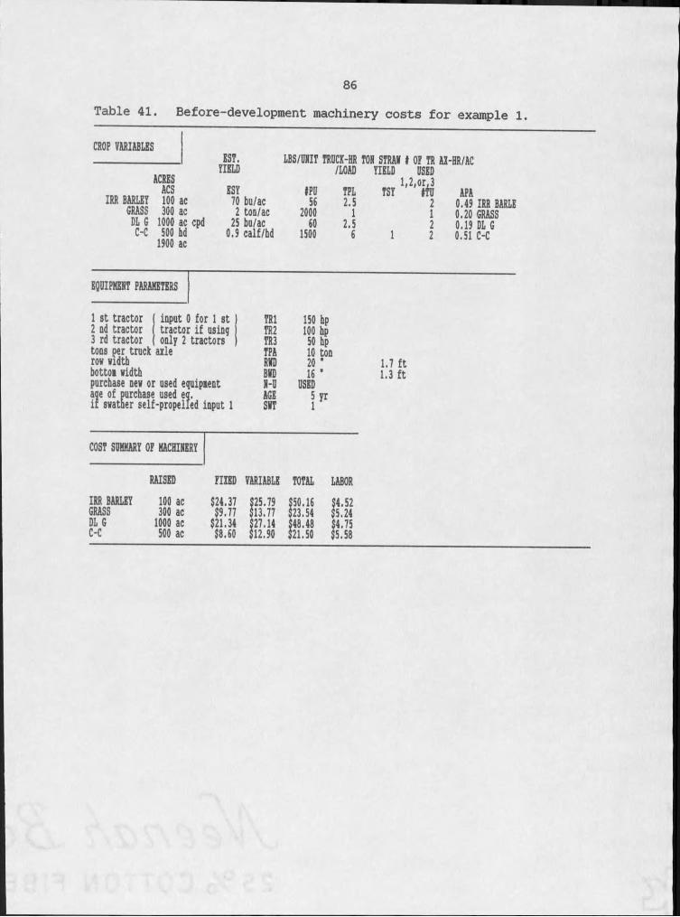
8 6

Table 41. Before-development machinery costs for example I.

CROP VARIABLES

ACRESEST.YIELD LBS/UNIT TRUCK-HR TON STRAN t OF TR AI-HR/AC /LOAD YIELD USED

1.2.or.3IRR BARLEY ACS ESY IPU TPL TSY ITU APA100 ac 70 bu/ac 56 2.5 2 0.49 IRR BARLE

tikASii 300 ac 2 ton/ac 2000 I I 0.20 GRASSDL G 1000 ac cpd 25 bu/ac 60 2.5 2 0.19 DL GC-C 500 hd 1900 ac 0,9 calf/bd 1500 6 I 2 0.51 C-C


input 0 tor I st tractor if using only 2 tractors

1 st tractor2 nd tractor3 rd tractor tons per truck axle row width bottom widthpurchase new or used equipment age of purchase used eg, it swatner self-propelled input

TRl 150 bpTR2 100 hpTR3 50 hpTPA 10 tonRND 20 1BND 16 ■N-U USEDAGE 5 yrSNT I

1.7 ft 1.3 ft

COST SUMMARY OP MACHINERY

RAISED FIXED VARIABLE TOTAL LABORIRR BARLEY 100 ac $24.37 $25.79 $50.16 $4.52GRASS 300 ac $9.77 $13.77 $23,54 $5.24DL G 1000 ac $21.34 27.14 $48.48 $4.75C-C 500 ac $8.60 $12.90 $21.50 $5.58

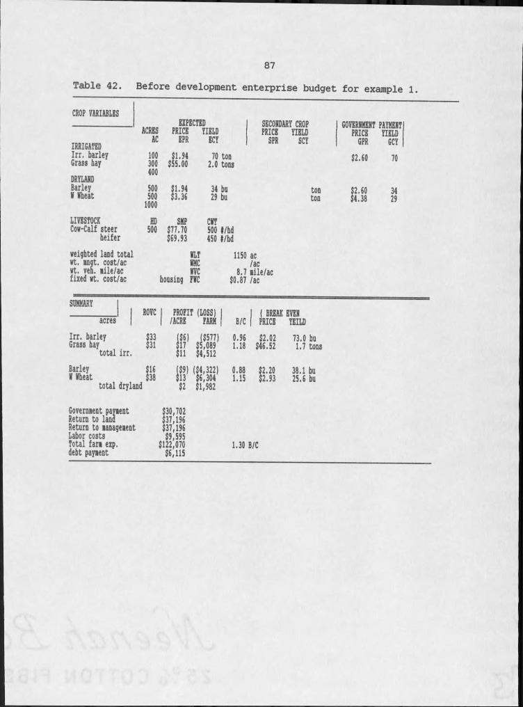
87Table 42. Before development enterprise budget for example I.

CROP VARIABLESEXPECTED SECONDARY CROP GOVERNMENT PAYMENTACRES PRICE YIELD PRICE YIELD PRICE YIELD

IRRIGATED AC EPR ECY SPR SCY GPR GCYIrr. barley 100 $1.94 70 ton $2.60 70Grass bay 300 $55.00 2.0 tons400DRYLANDBarley 500 51.94 34 bu ton $2.60 34K Mbeat 500 $3.36 29 bu too $4.38 291000LIVESTOCK HD SMP CMTCow-Calf steer 500 $77.70 500 t/hdbeifer $69.93 450 l/hdweighted land total MLT 1150 acwt. mngt, cost/ac MHC /acwt, veh. mile/ac MVC 8.7 mile/acfixed wt. cost/ac housing PMC $0.87 /ac

SUMMARYacres | ROVC I PROFIT (LOSS) I

/ACRE FARM I B/C ( BREAK EVEN PRICE YEILD

Irr. barley Grass haytotal irr.

$33$31 IiS1 p$11 $4,512

0.961.18 $2.02$46.52 73.0 bu 1.7 tons

Barley M Mheattotal dryland

$16$38 III' '!Iiloi1$2 $1,982

0.881.15 $2.20$2.93 38.1 bu 25.6 bu

Government payment 530,702 Return to land 537,196 Return to management $37,196 Labor costs $9,595 Total farm exp. $122,070 debt payment $6,115 1.30 B/C

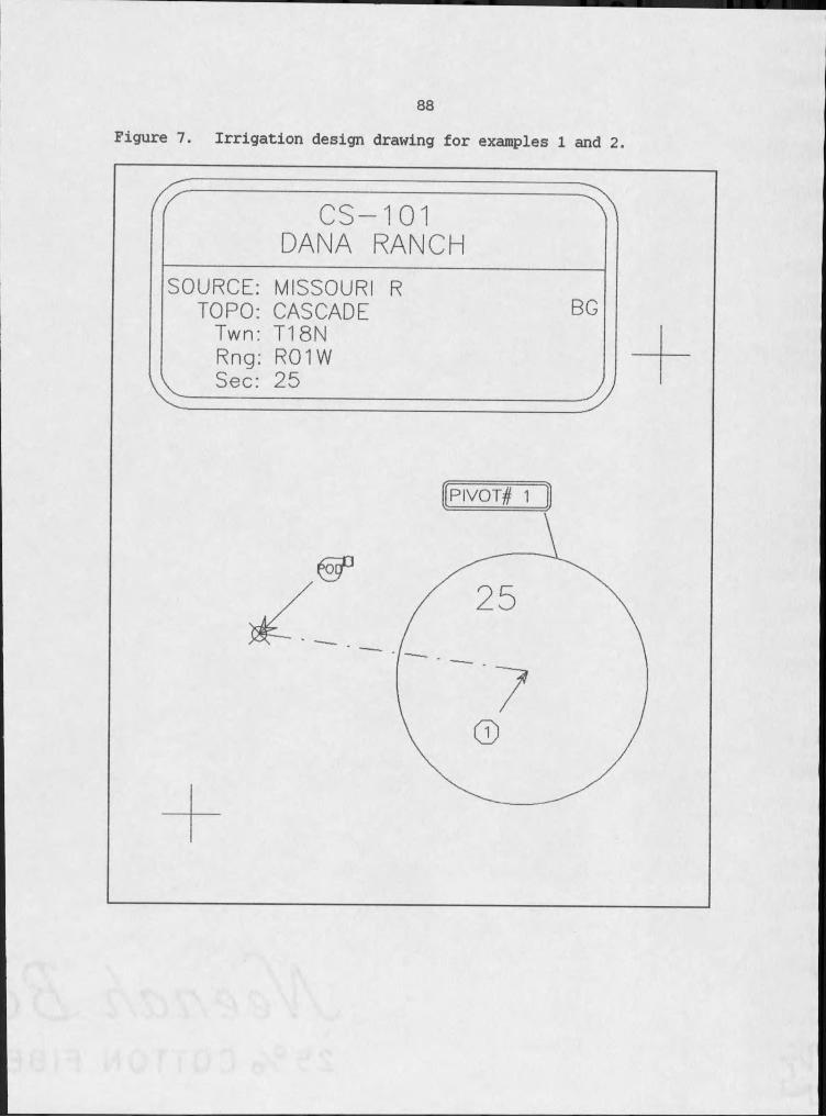
88Figure 7. Irrigation design drawing for examples I and 2.

CS-101 DANA RANCH

S O U R C E : M I S S O U R I R T O P O : C A S C A D E

T w n : T 1 S NR n g : R O I W S e c : 2 5

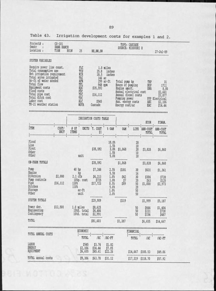
89Table 43. Irrigation development costs for examples I and 2.Project# I CS-IOlOwner : DASA RASCHLocation , T18S ROlV 25 SE,HS,SV

TOPO: CASCADE SOURCE.' MISSOURI R27-Jul-89

SYSTEM VARIABLESRequire power line const. Total consumptive use Set irrigation requirement Total acres irrigated Ac-ft of water needed Total flow Equipment costs Flood costs Total pipe cost Total ditch cost Labor costTR-21 weather station

PLCTCUSIRTAIAFS

1.0 miles 25.8 inches 18.5 inches 146 ae 299 ac-ft Total pump hp THP 31TFL 948 gpm Hours of pumping HOP 1711

E $35,592 Engine amort. ENA 8.81FDCTPC $16,112 Annual electrical cost Annual diesel costs $2,661$3,877TDC$545 Pumping power PPP ElectricalALC Ann. energy costs AEC $2,106IfSTA Cascade Energy cost/ac EAC $14.44

====::======5z==z=:z====5==r======szrz5zi=:==s====--=s===::----:.:==-----.=..--s--,.

IRRIGATION COSTS TABLEECON FINAN.

Item COST/ # OF ' UNITS 1T. COST ' I O&M O&M LIFE ANN-COST ANN-COSTI- - - - - - - - - UNIT ITEMS ,.. ?!_ TOTAL TOTALI

Flood 10.01 20Line 1.51 10Pivot $35,592 3.01 $1,068 20 $3,828 $6,860Other 1.51 10Other unit 5.01 10ON-FARM TOTALS $35,592 $1,068 $3,828 $6,860Pump 40 hp $7,248 2.51 $181 30 $631 $1,361Engine hp 5.51 16Diversion $2,000 2.1 cfs $4,213 1.01 $42 30 $304 $728Pump controls IOlp. cost $725 1.01 $7 20 $63 $125Pipe $16,112 1101 $17,723 0.51 $89 50 $1,000 $2,973Ditches 1101 5.01 20Storage ac-ft 1.01 50Other unit 2.01 50SYSTEM TOTALS $29,909 $319 $1,999 $5,187Power dev. $12,500 1.0 miles $8,625 50 $444 $1,404Engineering ISIS, total $4,486 50 $231 $730Contingency IOlS. total $2,991 50 $154 $487TOTAL $81,603 $1,387 $6,655 $14,667z z z z z z z z z z z z z z z z z z z z z z z z z z z z z z z z z z z z z z z z z z z z z z z z z z z z z z z z z z z z z z z z z z z z z z z z z z z z z z z z z z z z z z z z z z z z z z z z z z z z z

ECONOMIC FINANCIALTOTAL ANNUAL COSTS I ............... I . .. _____ I.

TOTAL /AC /AC-FT ' TOTAL /AC /AC-FTLABOR $545 $3.74 $1.82ENERGY $2,106 $14.44 $7.05EQUIPMENT $6,655 $45.61 $22.26 $14,667 $100.53 $49.06TOTAL annual costs $9,306 $63.78 $31.12 $17,319 $118.70 $57.92

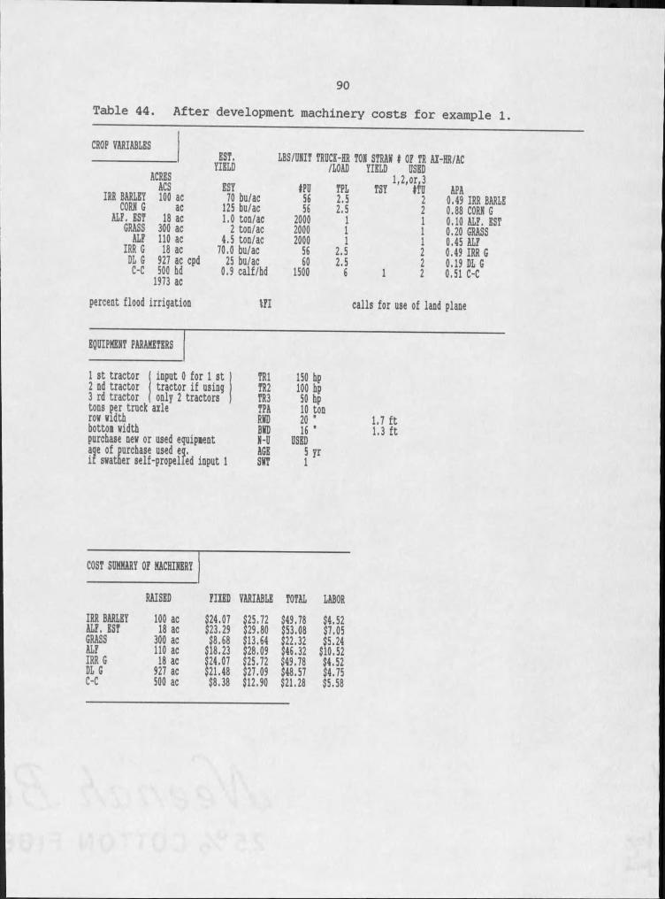
90Table 44. After development machinery costs for example I.

CROP VARIABLES

ACRESACS

EST.YIELD LBS/UNIT TRUCK-HR TON STRAN t OP TR AK-HR/AC /LOAD YIELD USED

IRR BARLEY ESY tPU TPL l,2,orJ TSY tfu APA100 ac 70 bu/ac 56 2.5 2 0.49 IRR BARLECORN G ac 125 bu/ac 56 2.5 2 0.88 CORN GALF, FSt 18 ac 1.0 ton/ac 2000 I I 0.10 ALP. ESTIikASS 300 ac 2 ton/ac 2000 I I 0.20 GRASSAEF H O ac 4.5 ton/ac 2000 I I 0.45 ALPIRR G 18 ac 70.0 bu/ac 56 2.5 2 0.49 IRR GDL 6 927 ac cpd 25 bu/ac 60 2.5 2 0.19 DL GC-C 500 hd

1973 ac 0.9 calf/hd 1500 6 I 2 0.51 C-C

percent flood irrigation til calls for use of land plane

EgffIPHENf PARAMETERS

input O for I st tractor if using only 2 tractors

1 st tractor2 nd tractor3 rd tractor tons per truck axle row width bottom widthpurchase new or used equipment age of purchase used eg. if swatner self-propelled input I

TRl 150 hpTR2 100 hpTR3 50 hpTPA 10 tonRND 20 *BND 16 *N-U USEDAGE 5 yrSNT I

1.7 ft 1.3 ft


RAISED PIKED VARIABLE TOTAL LABORIRR BARLEY 100 ac S24.07 $25.72 $49.78 $4.52ALP. EST 18 ac $23.29 $29.80 $53.08 $7.05GRASS 300 ac $8.68 $13.64 $22.32 $5.24ALP H O ac $18.23 $28.09 $46.32 $10.52IRRG 18 ac $24.07 $25.72 $49.78 $4.52DL G 927 ac $21.48 $27.09 $48.57 $4.75C-C 500 ac $8.38 $12.90 $21.28 $5.58

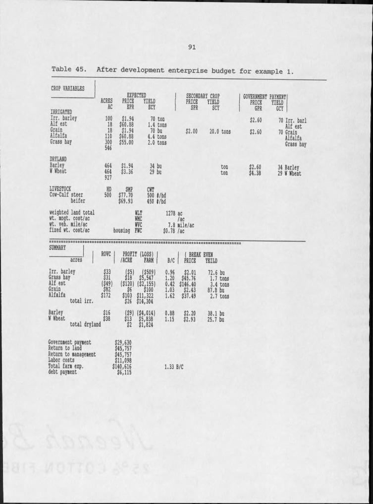
91

Table 45. After development enterprise budget for example I.

CROP VARIABLESEFFECTEDACRES PRICE YIELD

IRRIGATED AC EPR ECYIrr, barley 100 $1.94 70 tonAlf est 18 $60.88 1.4 tonsGrain 18 $1.94 70 buAlfalfa HO $60,88 4.4 tonsGrass hay 300546 $55.00 2.0 tons

DRYLANDBarley 464 $1,94 34 buW Wheat 464927 $3.36 29 bu

SECONDARY CROP GOVERNMENT PAYMENTPRICE YIELD PRICE YIELDSPR SCY GPR GCY$2.60 70 Irr. barl

$2,00 Alf est20.0 tons $2.60 70 GrainAlfalfa Grass hay

ton $2.60 34 Barleyton $4.38 29 W Wheat

LIVESTOCK HO SHP CWTCos-Calf steer 500 $77.70 500 l/hdheifer $69.93 450 t/hd

weighted land total st. m o t . cost/ac st. ven. lile/ac fixed st. cost/ac

WLT 1278 acWKC /acWVC 7.8 lile/achousing FWC $0,78 /ac

r s s s s s s s s s r s s s c s s s s s s s a s s s s s s s s s s s s a s s s s t r r s s s s s s s s s s s s s s s s a s s s s s s s s s s B s s s s s s = = = =SUMMARYacres

Irr. barley Grass hay Alf est Grain Alfalfa total irr.Barley W Wheat

total dryland

ROVC PROFIT (LOSS) I I ( BREAK EVENI /ACRE FARM ( B/C I PRICE YEILD

$33$31 III' sill!!1 0.961.20 $2.01$45.76 72.6 bu 1.7 tonsI 49) lilS2!1 is2Ji m i0.42 $146.40 3,4 tons$82 1.03 $2.43 87.8 bu$172 $103 $11,322 $26 $14,304 1.62 $37.49 2.7 tons

$16$38 III' 1M 1 0.881.15 $2.20

$2.93 38.1 bu 25.7 bu$2 $1,824

Goverment payient $29,630 Return to land $45,757 Return to ianageient $45,757 Labor costs $11,098 Total fan exp. $140,616 debt payient $6,115 1.33 B/C

92

Example 2: Low Lift Pivot Developed on a Dryland Farm

Example 2 is a dryland farm with 1000 cropped acres of winter wheat and barley. It uses the same irrigation development as Example I. The before- and after-development scenarios are presented in Tables 46 through 49. As in Example I, this scenario develops 146 acres of dry farmland for irrigating alfalfa. This farm's return to land is $22,235 before development, and $29,392 with irrigation development: a $7,285 benefit attributable to irrigation. Therefore, the value of irrigation water in this scenario is $49.71 per irrigated acre or $24.27 per acre-foot of water diverted. (When government subsidy payments are ignored the value of the water increases to $57.05 per irrigated acre. This occurs because fewer acres of subsidized crops are raised in the irrigation development scenario.)

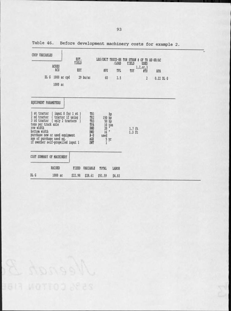
93

Table 46. Before development machinery costs for example 2.

CROP VARIABLES

ACRESEST.

YIELD LBS/0NIT TRUCK-HR TON STRAW I OF TR AX-HR/AC /LOAD YIELD USED 1.2.or.3ACS ESY tPU TPL TSY ITU APA

DL G 1000 ac cpd 1000 ac

29 bu/ac 60 2.5 2 0.22 DL G

EgniPKENT PARAMETERS

input 0 for I st tractor if using only 2 tractors1 st tractor2 nd tractor3 rd tractor tons per truck axle row widthbottom widthpurchase new or used equipment age of purchase used eg. if swather self-propelled input

TRl bpTR2 150 hpTR3 50 hpTPA 10 tonRWD 20 "BWD 16 *N-U usedAGE 5 yrSWT I

1.7 ft 1.3 ft

COST SOKKART OF MACHINERY

RAISED FIXED VARIABLE TOTAL LABOR DL G 1000 ac $22.98 $28.61 $51.59 $4.83

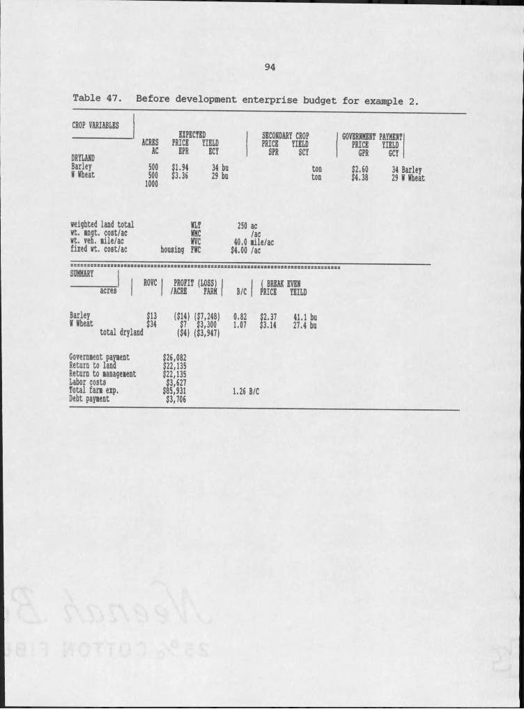
94

Table 47. Before development enterprise budget for example 2.

CROP VARIABLES

DRYLANDACRESAC

EXPECTED PRICE YIELDEPR ECYSECONDARY CROP PRICE YIELDSPR SCY

GOVERNMENT PAYMENT PRICE YIELDGPR GCYBarley 500 $1.94 34 bu ton $2.60 34 Barley 29 I !beatI Iheat 500

I A n n$3.36 29 bu ton $4.38

weighted land total ILT 250 acwt. mngt. cost/ac INC /acwt. veb. mile/ac NVC 40.0 mile/acfixed wt, cost/ac housing PNC $4.00 /ac

SUMMARY

Barley I Iheat

i s s s r s s s s s s s s

I I ROVC I PROFIT (LOSS) I I ( BREAK EVEN I PRICE YEILDacres | /ACRE FARM | B/C

$13 ($14) ($7,248) 0.82 $2.37 41.1 bu$34total dryland $7 $3,300

($4) ($3,947)1.07 $3.14 27.4 bu

Goyernient payment $26,082 Return to Iano $22,135 Return to management $22,135 Labor costs $3,627 Total farm exp. $85,931 Debt payment $3,706 1.26 B/C

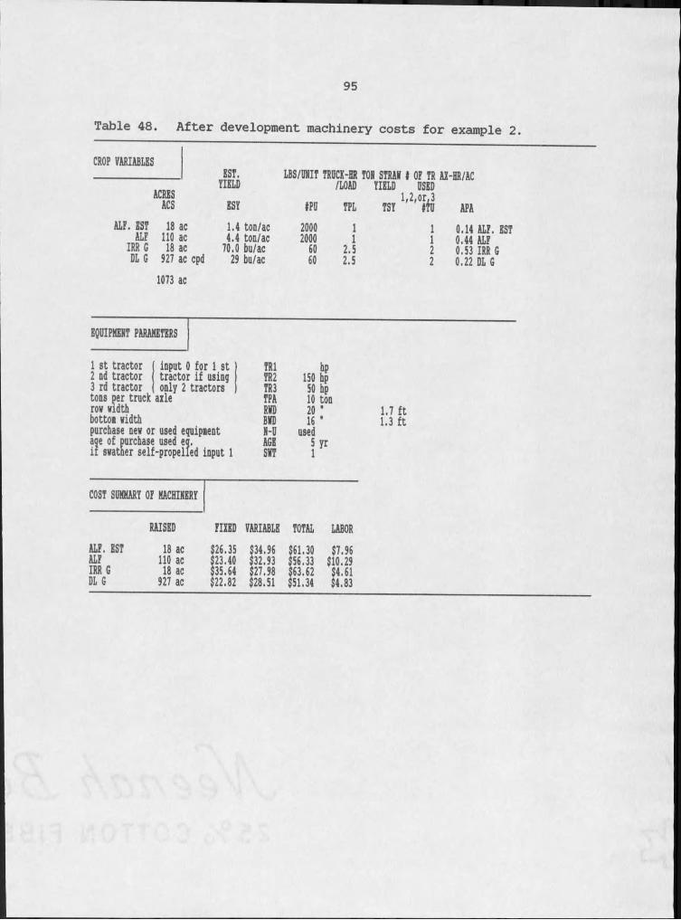
95

Table 48. After development machinery costs for example 2.

CROP VARIABLES

ACRESEST. YIELD LBS/UNIT TRUCK-SR TON STRAV t OP TR AX-HR/AC /LOAD YIELD USED I.2.or.3ACS ESY tPU TPL TSY »fU APA

ALP. EST 18 ac 1.4 ton/ac 2000 I I 0.14 ALP. ESTALF HO ac 4.4 ton/ac 2000 I I 0.44 ALPIRR G 18 ac 70.0 bu/ac 60 2.5 2 0.53 IRR GDL G 927 ac cpd 1073 ac

29 bu/ac 60 2.5 2 0.22 DL G


1 st tractor ( input 0 for I st2 nd tractor tractor if using3 rd tractor ( only 2 tractors tons per truck arlerow width bottom widthpurchase new or used equipment age of purchase used eg. if swatner self-propelled input I

TRl bpTR2 150 hpTR3 50 hpTPA 10 tonRVD 20 1BVD 16 *N-U usedAGE 5 yrSVT I

1.7 ft 1.3 ft


RAISED PIKED VARIABLE TOTAL LABORALP. EST 18 ac $26.35 $34.96 $61.30 $7.96ALP H O ac $23.40 $32.93 $56.33 $10.29IRR G 18 ac $35.64 $27.98 $63.62 $4.61DL G 927 ac $22.82 $28.51 $51.34 $4.83

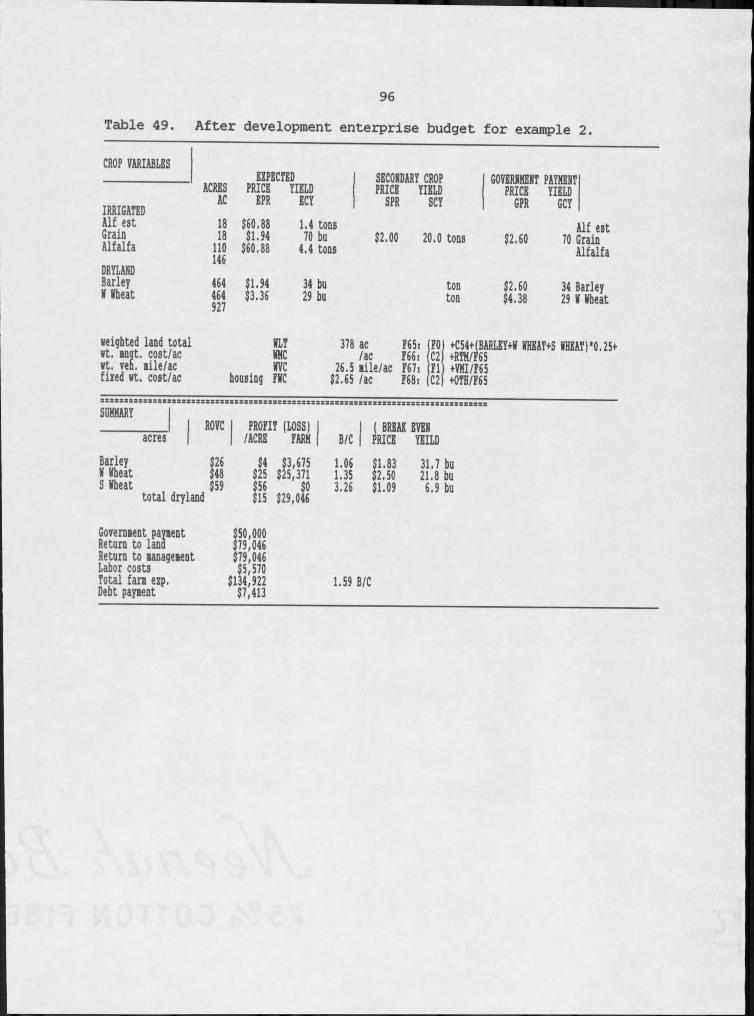
96Table 49. After development enterprise budget for example 2.

CROP VARIABLESEXPECTEDACRES PRICE YIELD

IRRIGATED AC EPR ECYAlf est 18 $60.88 1.4 tonsGrain 18 $1.94 70 buAlfalfaDRYLAND

no146 $60.88 4.4 tons

Barley 464 $1.94 34 buV Vheat 464927 $3.36 29 bu

SECONDARY CROP GOVERNMENT PAYMENTPRICE YIELD PRICE YIELDSPR SCY GPR GCYHf est$2.00 20.0 tons $2.60 70 Grain Alfalfa

ton $2.60 34 Barleyton $4.38 29 V Wheat

weighted land total wt, moot, cost/ac wt, veh. lile/ac fixed wt. cost/ac

VLT 378 ac F65, FOIWMC /ac F66: C2W C 26.5 lile/ac F67s Fljhousing FVC $2.65 /ac F68: C2j+VHI/F65tOrH/F65

a s s s s s s s s s s s s c s s a s a s s s a s s s s s a s r s s s s s a s s a s s s s s s s s s s s s s s s s r z s s s s s s s s s s s s s s s r r S=S=S=SUMMARYROVC I PROFIT (LOSS) I I ( BREAK EVENacres I /ACRE FARM I B/C I PRICE YEILD

Barley $26 $4 $3,675 1.06 $1.83 31.7 buW Wheat $48 $25 $25,371 1.35 $2.50 21.8 buS Wheat $59 $56 $0 3.26 $1.09 6.9 butotal dryland $15 $29,046

Governient payient Return to land $50,000$79,046Return to ianageient $79,046Labor costs $5,570Total fan exp. $134,922 1.59 B/CDebt payient $7,413

97

Example 3: High Lift Wheel Line Development on a Farm/Ranch

Example 3 presents a dryland farm and small cattle ranching operation, with 1500 cropped acres, 1500 fallow acres, 200 acres of irrigated grass, and 200 head of cattle. The development scenario for this farm irrigates 77 acres of alfalfa, pumping Missouri River water up 280 feet to two wheel lines (Figure 8). The alfalfa is farmed on an eight year rotation: in the first year the crop is established, followed by six years of full production, and an eighth year of small grain production. The wheel lines service 77 acres of alfalfa at peak use, supplying water to the grain and first-year alfalfa in the spring and fall.

The before- and after-development scenarios for Example 3 are presented in Tables 50 through 54. Without development this farm would produce an annual return to land of $57,847; with the irrigation development the return to land would be $50,693. Therefore, the value of the irrigation water is a negative $92.91 per irrigated acre, or a negative $34.73 per acre-foot of water diverted.

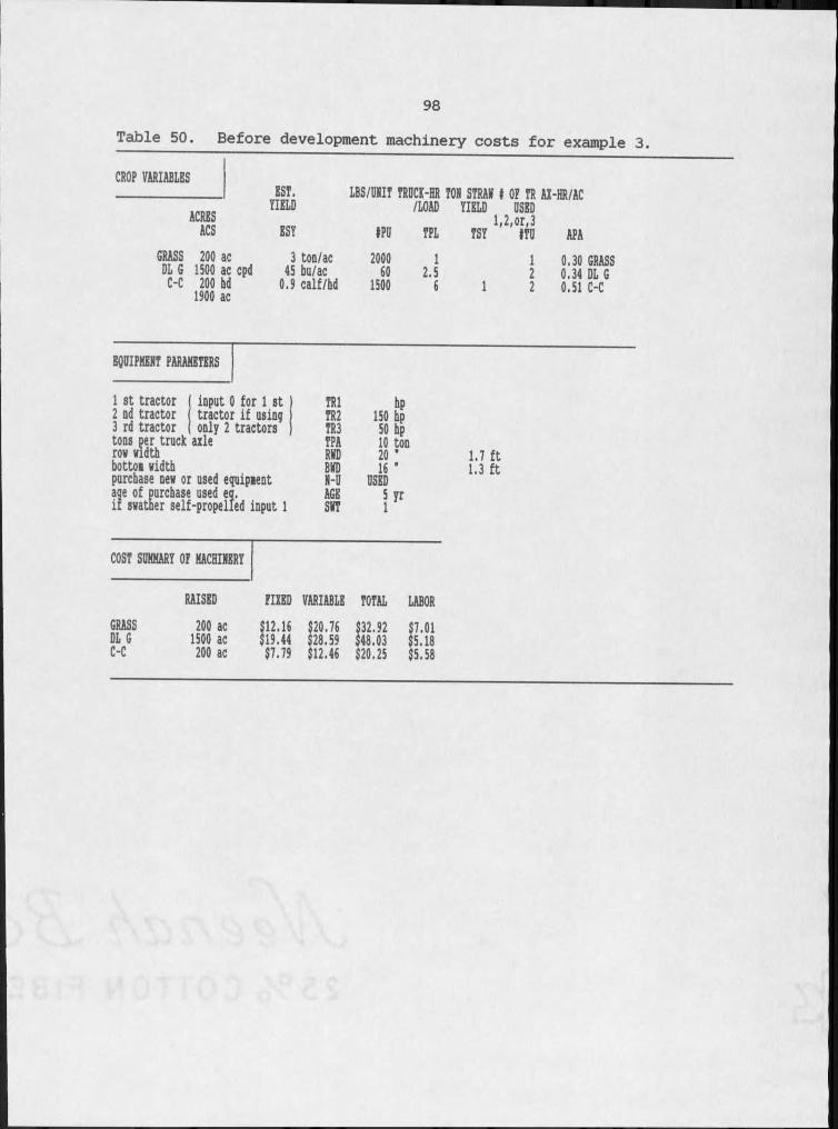
98Table 50. Before development machinery costs for example 3.

CROP VARIABLES

ACRESESI.YIELD LBS/UNIT TRBCK-HR TON STRAW I OF TR AK-HR/AC

/LOAD YIELD BSED 1.2.or,3ACS ESY IPB TPL TSY ITD APAGRASS 200 ac 3 ton/ac 2000 I I 0.30 GRASSDL G 1500 ac cpd 45 bu/ac 60 2.5 2 0,34 DL GC-C 200 hd

1900 ac 0.9 calf/hd 1500 6 I 2 0.51 C-C

EgaiPHENT PARAMETERS

1 st tractor2 nd tractor3 rd tractor tons per truck axle row width bottom width

input O for I st tractor if using only 2 tractors

purchase new or used equipment age of purchase used eg. if swatner self-propelled input I

TRl bpTR2 150 hpTR3 50 hpTPA 10 tonRWD 20 1BWD 16 'N-B DSEDAGE 5 yrSWT I

1.7 ft 1.3 ft

COST SBKMARY OF MACHINERY

RAISED FIXED VARIABLE TOTAL LABORGRASS 200 ac $12.16 $20.76 $32.92 $7.01DL G 1500 ac $19.44 $28.59 $48.03 $5.18C-C 200 ac $7.79 $12.46 $20.25 $5.58

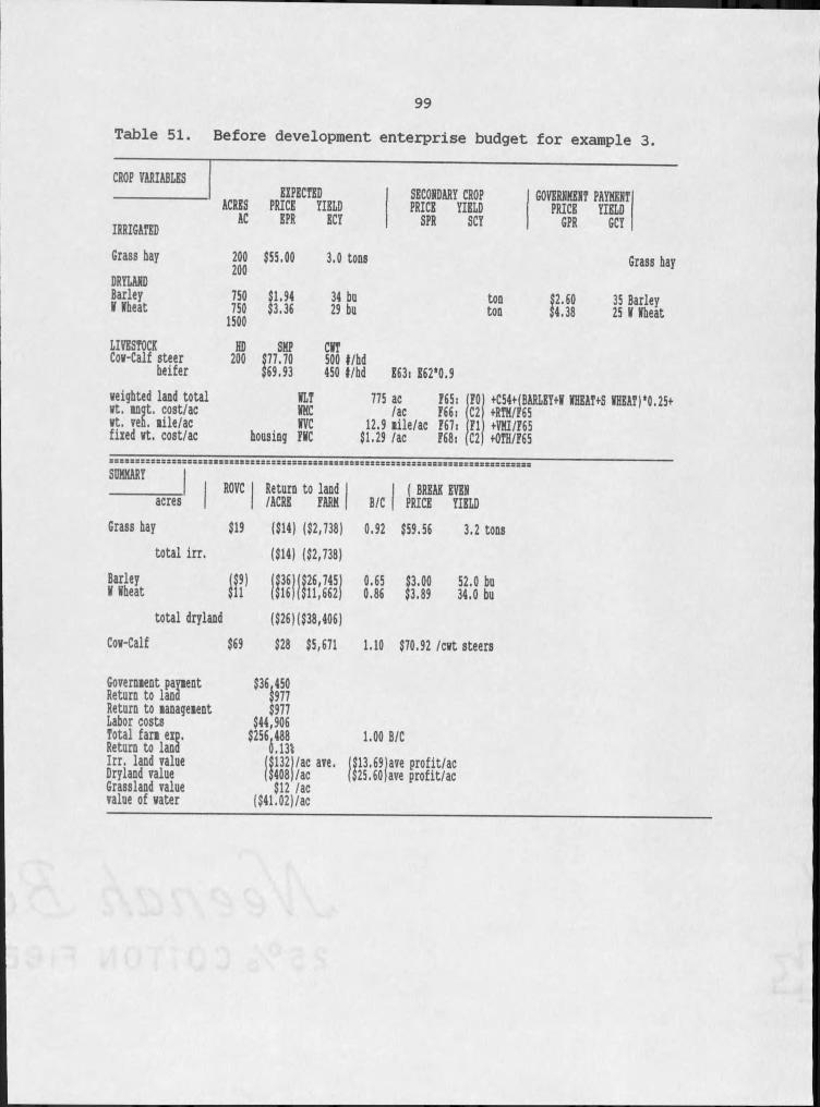
99Table 51. Before development enterprise budget for example 3.

CROP VARIABLES

IRRIGATEDACRES

ACEFFECTED PRICE YIELDEPR ECY

Grass bay DRYLAND

200200 $55.00 3.0 tons

Barley 750 $1.94 34 buW Wheat 7501500 $3.36 29 bu

LIVESTOCK HD SMP CWTCow-Calf steer heifer 200 $77.70$69.93 500 4/hd 450 4/hd

SECONDARY CROP GOVERNMENT PAYMENTPRICE YIELD PRICE YIELDSPR SCY GPR GCY

Grass hay

ton $2.60 35 Barleyton $4.38 25 W Wheat

E63: E62*0.9weighted land total wt. angt, cost/ac wt. ven. lile/ac fixed wt. cost/ac

KlTWNCWVChousing PWC

775 ac P65:/ac P66i12.9 lile/ac F67: $1.29 /ac F68:

tCM+jBMLEY+W WHEATiS WHEAT)‘0.25iiVNI/F65iOTH/F65

s s s s s s s s s a s s s s s s s s r s s s s s s s s s s s s s s s s s s s s s s s a s a s s r r s s s s s a s s s s s s s s r S==Ss s s s s s s s s s s a sSOKXAHY Iacres ROVC Return to land I

/ACRE FARM | B/C ( BREAK EVEN PRICE YIELD

Grass hay $19 ($14) ($2,738) 0.92 $59.56 3.2 tonstotal irr. ($14) ($2,738)

Barley W Wheat Iii1 S Ifc 7IlI 0.650,86 $3.00$3.89 52.0 bu34.0 butotal dryland ($26)($38,406)

Cow-Calf $69 $28 $5,671 1.10 $70.92 /cwt steers

Government payment Return to land Return to management Labor costs Total farm exp. Return to land Irr. land value Dryland value Grassland value value of water

$36,450$977$977$44,906

$256,4880.131($132 /ac ave. ($408j/ac $12 /ac ($41.02)/ac

1.00 B/CI$13.691ave profit/ac ($25.60)ave profit/ac

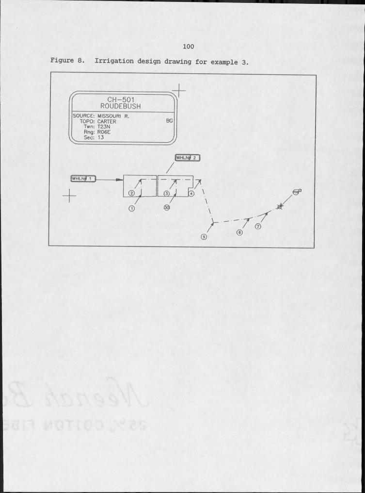
100Figure 8. Irrigation design drawing for example 3.

' ( —C H - 5 0 1

R O U D E B U S H----- 1

SOURCE: TOPO:

Twn: Rng: See:

MISSOURI R.CARTERT23NR06E13

BG

---------- I

jWHLN# 2 Il

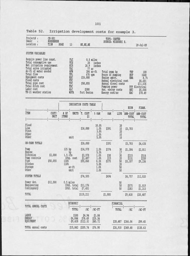
101

Table 52. Irrigation development costs for example 3.Project* i CH-501Owner s ROUDEBUSHLocation : T23N ROSE 13 NB,HE,HE

TOPO: CARTER SOURCE: MISSOURI R.20-Jul-89

SYSTEM VARIABLESRequire power line const. Total consumptive use Net irrigation requirement Total acres irrigated Ac-ft of water needed Total flow Equioment costs Flood costs Total pipe cost Total ditch cost Labor costTR-21 weather station

PLCTCUHIRTAIAFNTFLEQCFDCTPCTDCALCVSTA

0.5 miles 28 inches 20.9 inches 77 ac 206 ac-ft 670 gpm $26,080

$50,055$380

Fort Benton

Total pump hp Hours of pumping Engine amort.Annual electrical cost Annual diesel costs Pumping power Ann. energy costs Energy cost/ac

THP 108HOP 1668ENA 8.71$6,601$11,636PPP ElectricalAEC $6,044EAC $78.49

:=:ss=s=::3sssss:sss=sssssrsssssssrsssrsssrsssssssssss:sssssssssrs:sss

IRRIGATION COSTS TABLEECON FINAN.

ITEM COST/ » OF ' UNITS 'r. COST 1 I O&M O&M ' LIFE ANN-COST ANN-COSTI ---------------------

UNIT ITEMS .. ?L, TOTAL TOTALI

Flood 10.01 20Line $26,080 1.51 $391 10 $3,703Pivot 3.01 20Other 1.51 10Other unit 5.01 10OH-FARM TOTALS $26,080 $391 $3,703 $4,636Pump 125 hp $14,970 2.51 $374 30 $1,304 $2,811Engine hp 5.51 17Diversion $2,000 1.5 cfs $2,978 1.01 $30 30 $215 $514Pump controls IOlp. cost $1,497 1.01 $15 20 $131 $259Pipe $50,055 1101 $55,060 0.51 $275 50 $3,107 $9,236Ditches 1101 5.01 20Storage ac-ft 1.01 50Other unit 2.01 50SYSTEM TOTALS $74,505 $694 $4,757 $12,820Power dev. $12,500 0.5 miles 50Engineering 151S. total $11,176 50 $575 $1,819Contingency IOlS. total $7,451 50 $383 $1,213TOTAL $119,211 $1,085 $9,418 $20,487SSr5=S3S=S=S333S==rS3S3=3SSS3SSSSS3S=SS3S3SSSSSSSS=S3SSSSSSS=SSSSS=S=S-=SS3S8SS3rSSS5S3=S3SS=S=333333

TOTAL ANNUAL COSTS ECONOMICI........ I........ I ........

FINANCIALI____ II________ I

' TOTAL /AC /AC-FT ' TOTAL /AC /AC-FTLABORENERGYEQUIPMENT

$380$6,044$9,418$4.94$78.49$122.31

$1.84$29.34$45.72 $20,487 $266,06 $99.45

TOTAL annual costs $15,842 $205.74 $76.90 $26,910 $349.48 $130.63

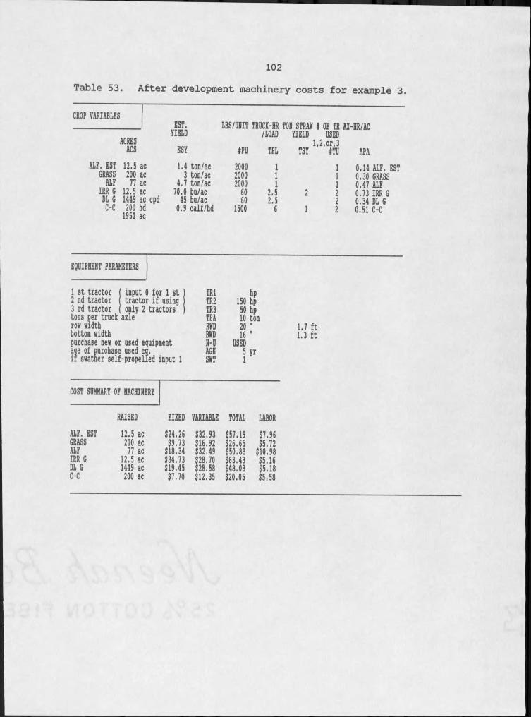
1 0 2

Table 53. After development machinery costs for example 3.

CROP VARIABLES

ACRESEST. YIELD LBS/DRIT TRDCK-HR TOR STRAW I OF TR AI-HR/AC /LOAD YIELD DSED I.2.or.3ACS ESY IPU TPL TSY It'D APA

ALF. EST 12.5 ac 1.4 ton/ac 2000 I I 0.14 ALF. ESTGRASS 200 ac 3 ton/ac 2000 I I 0.30 GRASSALF 77 ac 4.7 ton/ac 2000 I I 0.47 ALFIRR G 12,5 ac 70.0 bu/ac 60 2.5 2 2 0.73 IRR GDL G 1449 ac cpd 45 bu/ac 60 2.5 2 0.34 DL GC-C 200 hd 1951 ac 0.9 calf/hd 1500 6 I 2 0.51 C-C

EODIPKEIiT PARAMETERS

1 st tractor2 nd tractor3 rd tractor tons per truck axle row width bottom width

input 0 for I st tractor if using only 2 tractors

purchase new or used equipment age of purchase used eg. if swatner self-propelled input I

TRl hpTR2 150 hpTR3 50 hpTPA 10 tonRWD 20 1BWD 16 1R-D USEDAGE 5 yrSWT I

1.7 ft 1.3 ft

COST SUMMARY OF NACHIRERY

RAISED FIXED VARIABLE TOTAL LABORALF. EST 12.5 ac $24.26 $32.93 $57.19 $7.96GRASS 200 ac $9.73 $16.92 $26.65 $5.72ALF 77 ac $18.34 $32.49 $50.83 $10.98IRR G 12.5 ac $34.73 $28.70 $63.43 $5.16DL G 1449 ac $19.45 $28.58 $48.03 $5.18C-C 200 ac $7.70 $12.35 $20,05 $5.58

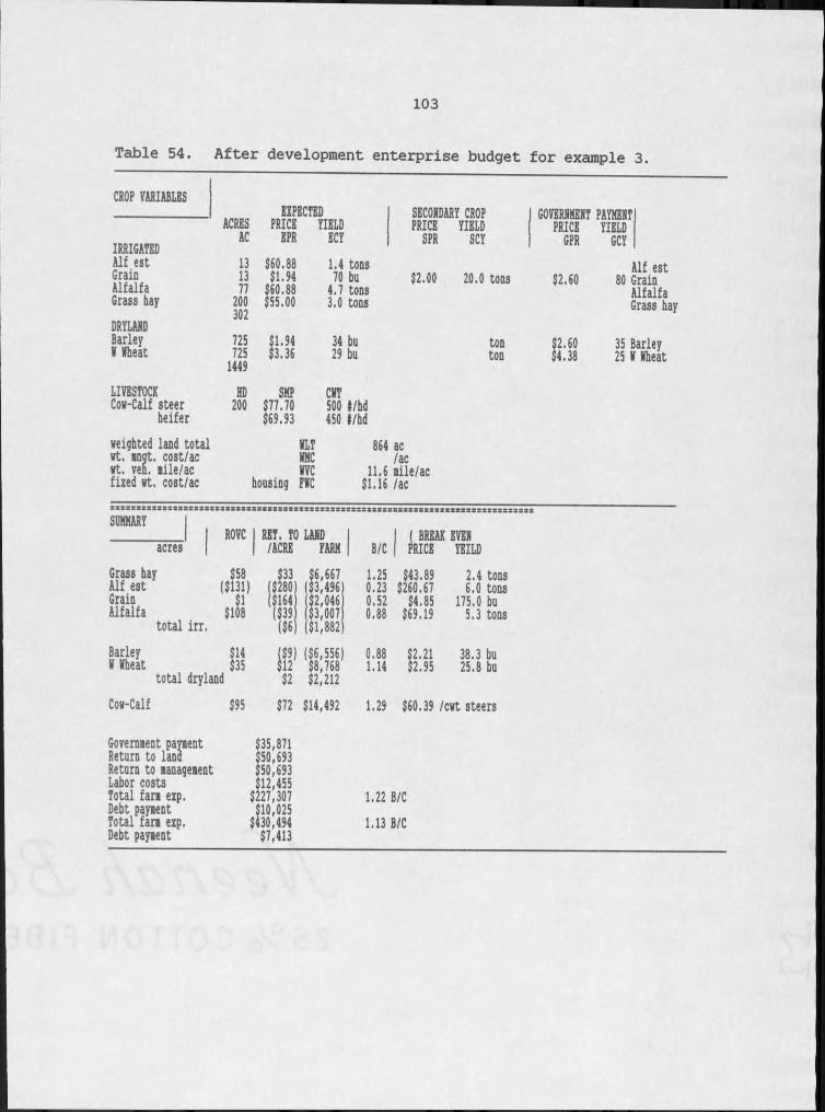
103

Table 54. After development enterprise budget for example 3.

CROP VARIABLES

IRRIGATED AIf est Grain Alfalfa Grass hayDRYLAND Barley E Eheat

LIVESTOCK Cow-Calf steer heifer

EXPECTED SECONDARY CROP GOVERNKENT PAYKENTACRES PRICE YIELD PRICE YIELD PRICE YIELDAC EPR ECY SPR SCY GPR GCY13 $60.88 1.4 tons Alf est13 $1.94 70 bu $2.00 20.0 tons $2.60 80 Grain77 $60.88 4.7 tons Alfalfa200

302 $55.00 3.0 tons Grass hay

725 $1.94 34 bu ton $2.60 35 Barley7251449 $3.36 29 bu ton $4.38 25 E Eheat

HD SKP CET200 $77.70 500 l/hd$69.93 450 t/hdweighted land total wt. ingt. cost/ac wt. veh. nile/ac fixed wt. cost/ac

ELT 864 acENC /acEVC 11.6 lile/achousing PEC $1.16 /ac

SDHKARYROVC I RET. TO LAND I I BREAK EVENacres I /ACRE PARK B/C I PRICE YEILD

Grass hay Alf est Grain Alfalfa

total irr

$58y$108 $33($280iI $6,667$3,496$2,046$3,007$1,882

1.250.230.520.88

$43.89$260.67$4,85$69.19

2.4 tons 6.0 tons 175,0 bu 5,3 tons

Barley E Eheat IS!total dryland Si!1 1II:!!!1 $2 $2,212

0.881.14 $2.21$2,95 38.3 bu 25.8 bu

Cow-Calf $95 $72 $14,492 1.29 $60.39 /cwt steers

Govemient payment Return to land Return to management Labor costs Total farm exp.Debt payment Total farm exp.Debt payment

$35,871$50,693$50,693$12,455$227,307$10,025$430,494$7,413

1.22 B/C 1.13 B/C

1 1 1 1 I I1 !

104

Example 4: High Lift Multi-Pivot Irrigation Development

Example 4 is a 4,000 acre dryland farm, with 1343 acres developed by center pivot irrigation. The irrigation system pumps water from Belt Creek up 300 feet to a distribution ditch, which delivers the water to a storage pit where it is pumped to six low pressure center pivots (Figure 9).

The before- and after-development scenarios for Example 4 are presented in Tables 55 through 59. For this farm, the annual return to land would be $79,046 before irrigation development; with development the return to land would be $54,139. Thus, the value of the irrigation water in this scenario is a negative $18.55 per acre developed, or a negative $8.00 per acre-foot diverted.

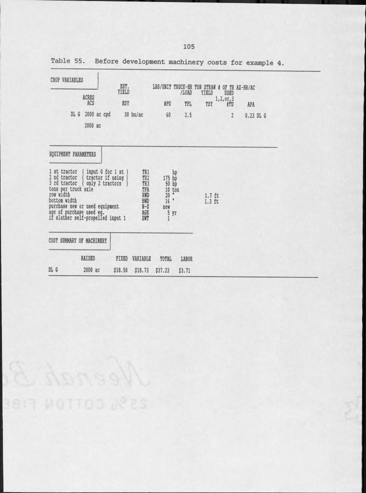
105Table 55. Before development machinery costs for example 4.

CROP VARIABLES— EST.YIELD LBS/UNIT TRUCK-HR TON STRAN I OF TR AX-HR/AC /LOAD YIELD USEDACRESACS ESY FPU TPL TSI ll2llM APADL G 2000 ac cpd

2000 ac30 bu/ac 60 2.5 2 0.23 DL G

EQUIPKERT PARAMETERS


1 st tractor2 nd tractor3 rd tractor tons per truck axle row width bottom widthpurchase new or used equipment age of purchase used eg. if slather self-propelled input I

TRl bpTR2 175 hpTR3 50 hpTPA 10 tonRND 20 "BND 16 •N-U newAGE 5 yrSNT I

1.7 ft 1,3 ft

COST SUMMARY OF MACHINERY

RAISED FIXED VARIABLE TOTAL LABOR DL G 2000 ac $18.50 $18.73 $37.23 $3.71

106Table 56. Before development enterprise budget for example 4.CROP VARIABLES

EXPECTEDACRES PRICE YIELDIRRIGATED AC EPR ECY

DRYLANDBarley 1000 $1.94 34 buM Vheat 1000

2000$3.36 29 bu

SECONDARY CROP GOVERNMENT PAYMENTPRICE YIELD PRICE YIELDSPR SCY GPR GCY

ton $2.60 34 Barleyton $4.38 29 V Mbeat

weighted land total wt. mat. cost/ac vt. ven. lile/ac fixed wt. cost/ac

VLTMMCMVChousing TMC

500 ac /ac

20.0 lile/ac $2,00 /acissrzsssrsssrsssssssszssssssrsrsssrsssessssssszssszssssssszssrssssssssssrss==

SUMMARYacres ROVC PROFIT (LOSS) I

/ACRE FARM | B/C I( BREAK EVEN PRICE YEILD

Barley M Mheat I2648 $25 $3,675$25,371 1,061.35 $1.83$2.50 31.7 bu21.8 butotal dryland $15 $29,046

Government payment Return to land Return to management Labor costs Total fan exp.Debt payment

$50,00079,046$79,046$5,570$134,922$7,413 1.59 B/C

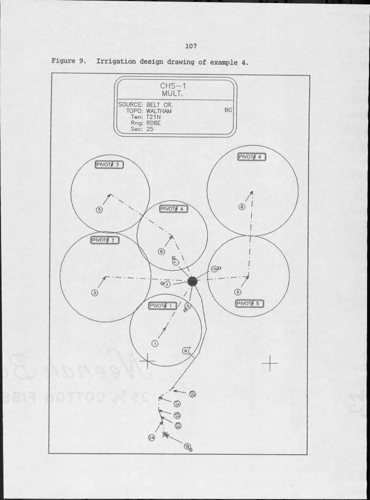
107Figure 9. Irrigation design drawing of example 4.

( ( CHS— 1MULT.

---------------- ^

SOURCE: BELT CR.TORO: WALTHAM BG

Twn; T 21NR ng : R 06ES ec : 2 5

— --------

108Table 57. Irrigation development costs for example 4.Project# : CHS-IOwner : HDLT.Location i T21N R06E

SYSTEM VARIABLESRequire power line const. Total consumptive use Ret irrigation requirement Total acres irrigated Ac-ft of water needed Total flow Emiipment costs Flood costs Total oipe cost Total ditch cost Labor costTR-21 weather station

TOPOi HALTHAM25 RE,RH,SH SODRCEi BELT CR.

23-Aug-89

PLC 10.0 milesTCD 28 inchesRIR 20.9 inchesTAI 1343 acAFR 3117 ac-ft Total pump hp THP 1511TFL ,„9064 OPi Hours of pumping HOP 1865EQC $285,228 Engine amort. ERA 9.41FDC Annual electrical cost $98,032TPC $383,206 Annual diesel costs $173,091TDC $94,280 Pumping power PPP ElectricalALC $5,020 Ann. energy costs AEC $92,546HSTA Fort Benton Energy cost/ac EAC $68.90ssssSssssssssssasrssssssasssssssssasssBsssaassssssssssstsasrsssssssssssssssrsasssrssssssssssssssss

IRRIGATIOR COSTS TABLEI

ECOR FIRAR.ITEMI ------------------------

COST/DRIT I OF ' DRITS ITEMS ' T. COST

I. . . f1I O M O&H LIFE

.1 .1ARR-Co s t1TOTALI I

ARR-COSTTOTALI

FloodLinePivotOtherOther

I I

unit

I

$285,22810. Ot 1.5t 3.0t 1.51 5.01

$8,5572010201010

$30,674 $54,976

OH-FARM TOTALS $285,228 $8,557 $30,674 $54,976PumpEngineDiversionPump controlsPipeDitchesStorageOther

$2,000$383,206$94,280$1,500

1600 hp20.1 cfs

lOip. cost 1101 not81 ac-ft unit

$185,864$40,284$18,586$421,527

$103,708$120,853

2.515.51 1.01 1.01 0.515.011.01 2.01

$4,647$403$186$2,108$5,185$1,209

3015302050205050

$16,192$2,905$1,627$23,786$13,227$7,424

$34,895$6,959$3,211$70,709$22,063$20,877

SYSTEM TOTALS $890,822 $13,737 $65,161 $158,714Power dev.EngineeringContingency

$12,500 10.0 miles 151S. total IOIS. total $133,623

$89,082505050 $6,872

$4,581 $21,747$14,498

TOTAL $1,398,756 $22,294 $107,288 $249,935ssssssaaaaaaaaaaaaaaaaasaasaaaaaaaaaaaaaasaaaaaaaaaaaaaaraaaaaaaaaaaraaaaaasaaaaaaaaaaaaaasaaaaaaaaaaaa

ECOROMIC FIRARCIALvfivii. m n n . nnsvs I. . . . I_ _ _ _ i. . i _ _ _ i_ _ _ _ iTOTAL /AC /AC-FT ' TOTAL ' /AC ' /AC-FT

LABORERERGYEgDIPMERT

$5,020$92,546$107,288

$3.74$68.90$79.88

$1.61$29.69$34.42 $249,935 $186.07 $80.18

TOTAL annual costs $204,855 $152.51 $65.72 $347,501 $258.71 $111.49aaaaaaaaaaaaaaaaaaaaaaaaaaaaaaaaaaaaaaaaaaaaaaaaaaaaaaaaaaaaaaaaaaaaaaaaaaaaaaaaaaaaaaaaaaaaaaaaaaaaaaa

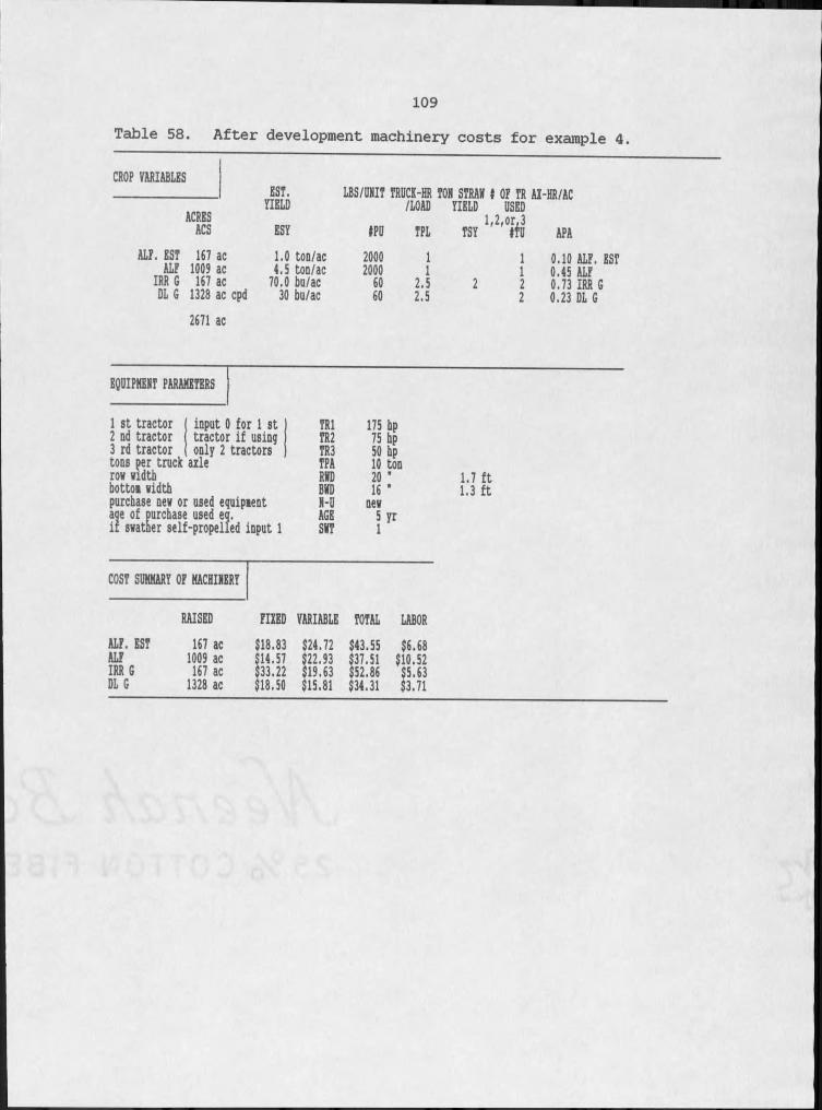
109Table 58. After development machinery costs for example 4.

CROP VARIABLES

ACRESACS

EST. YIELD LBS/UNIT TRUCK-HR TON STRAW t OF TR Al-HR/AC /LOAD YIELD USEDESY IPU TPL IS! ''2llIil APA

ALF. EST 167 ac 1.0 ton/ac 2000 I I 0.10 ALF. ESTALF 1009 ac 4.5 ton/ac 2000 I I 0.45 ALFIRR G 167 ac 70.0 bu/ac 60 2.5 2 2 0.73 IRR GDL G 1328 ac cpd 2671 ac

30 bu/ac 60 2.5 2 0.23 DL G

EQUIPKEliT PARAMETERS


1 st tractor2 nd tractor3 rd tractor tons per truck axle row width bottom widthpurchase new or used equipment age of purchase used eg. if swather self-propelled input I

TRl 175 hpTR2 75 bpTR3 50 hpTPA 10 tonRWD 20 "BWD 16 'N-U newAGE 5 yrSWT I

1.7 ft 1.3 ft

COST SUMMARY OF MACHIMERY

RAISED FIXED VARIABLE TOTAL LABORALF. EST 167 ac $18.83 $24.72 $43.55 $6.68ALF 1009 ac $14.57 $22.93 $37.51 $10.52IRR G 167 ac $33.22 $19,63 $52.86 $5.63DL G 1328 ac $18.50 $15.81 $34.31 $3.71

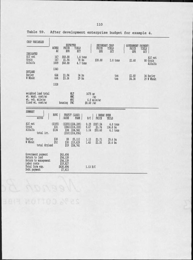
HOTable 59. After development enterprise budget for example 4.

CROP VARIABLESEXPECTED SECONDARY CROP GOVERNMENT PAYMENTACRES PRICE YIELD PRICE YIELD PRICE YIELDAC EPR ECY SPR SCY GPR GCYIRRIGATEDAlf est 167 $60.88 1.4 tons Alf estGrain 167 $1.94 70 bu $20.00 2.0 tons $2.60 80 GrainAlfalfa 1009 $60.88 4.7 tons Alfalfa

1343DRYLANDBarley 664 $1.94 34 bu ton $2.60 34 BarleyN Wheat 664 $3.36 29 bu ton $4.38 29 W Wheat

1328

weighted land total WLT 1675 acwt, mngt. cost/ac WMC /acwt. veh. nile/ac WVC 6.0 mile/acfixed wt. cost/ac housing FWC $0.60 /acsssssssssassssssSsssssssssssssssssrsssssssssssssasssBsssssssssrssssssrsssssssssssSUMMARY

ROVC I PROFIT (LOSS) I I ( BREAK EVENacres I /ACRE FARM | B/C I PRICE YEILDAlf estGrainAlfalfa

total irrliSSl1$134 W I K I$34 $34,542 ($10)($14,056)

0.290.671.14

$207.54$3.74$53.60

4.8 tons 134.8 bu 4.1 tons

Barley W Wheat $30

$52total dryland$8 $5,112 $30 $19,629 $19 $24,741

1.131.43

$1.71$2.35 29.6 bu

20.6 bu

Government payment $43,454 Return to land $54,139 Return to management $54,139 Labor costs $19,827 Total farm exp. $430,494 Debt payment $7,413 1.13 B/C

Ill

CHAPTER 8

CONCLUSION

Water shortages are causing water planners and legislators to review their water allocation policies. As competition for water increases, more emphasis is being placed on allocating water to its highest valued use. This could be done through legislation and/or by allowing freemarket trading of water rights. Since agriculture is the largest consumer of water in the West, there is a need to determine the value of water for irrigated agriculture.

Most of the water values developed for irrigated agriculture have been regional, and not site specific. Recent development in computer hardware and software have made it practical to evaluate individual farm irrigation waters.

This thesis has presented a method for determining farm specific irrigation water values by comparing before- and after- development scenarios. The examples used show that irrigation water values can vary dramatically depending both on the farming practices and the method of.irrigation. This thesis is not meant to establish any specific value of irrigation water (because it can be different for each situation.) It does, however, provide a procedure that can quickly estimate the value of water for a given situation.

JJ JI I

112

BIBLIOGRAPHYAmerican Society of Agricultural Engineers, Standards 1984. ASAE

0230.2. Agricultural Machinery Management Data, revised December 1983.

American Society of Agricultural Engineers, Standards 1984. ASAE Engineering Practice: ASAE EP391.1., Agricultural Machinery Management, revised December 1983.

Anderson, R. L., The Irrigation Water Rental Market. Agricultural Economic Research, 13:54-8, 1961.

AUTODESK, Inc., Sausalito California, Release 10, 1988.Bergantin, Ralf, SCS, Personal Communications, May 1986.Boehlje, Michael D., and Eidman, Vernon R., Farm Management. New York:

John Wiley & Sons, 1984

Campbell, Gregg A., "Competing Uses for Limited Water", Journal AWWA.September 1985, pp 34-39. ;

Condra, Gary D., Lacewell, Ronald D., and Adams, J. Michael, A Modelfor Estimating Demand for Irrigation Water on the Texas Hich ;Plains. Texas Water Resources Institute, Technical Report no. 68,College Station, Texas A&M University, May 1975.

Fogle, V e m , and Luft, LeRoy D., Enterprise Costs For Irrigated Alfalfa Hay, Winter Wheat. Bariev. Spring Wheat, and Seed Potatoes in Lake County. Cooperative Extension Service, Montana State University, Bulletin 1245, November 1980.

Frank, Micheal Dean, The Economic Value of Irrigation Water in the Western United States: An Application of Ridge Regression.Doctoral Dissertation, Department of Agricultural Economics,Texas A&M University, 1979.

Gibbons, Diana C., The Economic Value of Water. Washington D.C.:Resources for the Future,Inc., 1986.

Griffin, G. C., The Economic Value of Water for Selected Uses inSouthwestern North Dakota. N. Dakota Water Resources Institute,Report No. WI-221-034-76, Feburary 1976.

Johnson, James, Miller, Calvin R., and Watts, Myles J., The Cost ofOwning and Operating Farm Machinery in Montana for Profitability Considerations 1984. Cooperative Extension Service, Montana State University, Bulletin 1329, (revised) 1984.

113King, Bradley A., Sauer, Brian A., and Busch, John R., Microcomputer

Program Development for On-Farm Irrigation System Planning. Idaho Water Resources Research Institute, University of Idaho, May 1987.

Lacewell, Ronald, Sproutt, J. Micheal, and Beattie, Bruce R., Value of Irrigation Water With Alternative Input Prices. Product Prices and Yield Levels; Texas High Plains and Lower Rio Grande Valiev. Texas Water Resources Institute, Texas A&M University, Technical Report No. 58, 1974.

Licht, Lou, "Irrigation System Design by CAD". AgriculturalEngineering, American Society of Agricultural Engineers, St. Joseph, Michigan, Mar/Apr 1986, pp. 24-26.

Lotus Development Corporation, Cambridge Massachusetts, version 2,1985.

Martin, William E. and Snyder, Gary B., Valuation of Water and Forage from the Salt-Verde Basin of Arizona. Report to the U.S. Forest Service, September 1979.

Miller, S. F., and Boersma, L., An Economic Analysis of Water.Nitrogen and Seeding Relationships in C o m Production on Woodbum Soils. Oregon Agricultural Experiment Station, Tech. Bull. 98, December 1961.

Mohasci, Steve, Willett, Gayle, and Kirpes, Daniel, The Cost of Owning Farm Machinery in Washington. Cooperative Extension College of Agriculture, Washington State University, Extension Bulletin 1055, 1979.

Montana Department of Natural Resources and Conservation, unpublished working paper by John Tubbs, 1989.

Montana Department of Natural Resources and Conservation, unpublished Computer Spreadsheet, 1989.

Montana Department of Agriculture, Montana Crop and LivestockReporting Service. Montana Agricultural Statistics 1983-1984.1985.

Peterson, M. K., Professor of Animal Nutrition, Montana State University, Personal Communications, 1986.

Triangle Irrigation Inc., Personal Communications, May 1988.U. S. Department of Agriculture, The Stirling Engine: Its Market

Potential For Irrigation Pumping and Other Irrigation Energy- Conservation Concepts. Report by the Agricultural Research Service, January 1985.

114U. S. Department of Agriculture, Irrigation Water Requirements. Soil

Conservation Service, Technical Release Mo. 21, April 1967.U. S. Department of Agriculture, "IRRISYS", Computer program developed

by Ralf Bergantin, Soil Conservation Service, 1988.Willitt, Gayle S., Hathom, Scott, JR., and Robertson, Charles E., The

Economic Value of Water Used to Irrigate Field Crops in Central and Southern Arizona, 1975. Department of Agricultural Economics, Report no. 9, Tucson, University of Arizona, September 1975.

Young R. A. and Gray S. L., Economic Value of Water? Concepts and Empirical Estimates. Technical Report to the National Water Commission, NTIS no. PB210356, pp. 144-146, 1972.

APPENDICES

APPENDIX A LISP Programs

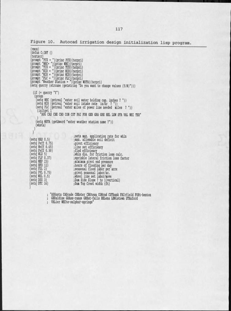
117

Figure 10. Autocad irrigation design initialization lisp program.VlOD)defun CiHT () textscr) prompt PCD = ' prompt "KHC= "I pfinc KHCI prompt "TCD = (princ TCDprompt "KIR prompt "KIR prompt "PLC

(princ PCD (terpri) terpril terpriprinc KIR princ KIR princ PLC;prompt "Heather Station =

terpriterpriterpri(princ KSTA)(terpri)setq querry (strcase (getstring "Do you want to change values (Y/K)")))(if (= querry "Y")(progn

setq KHC getreal "enter soil water holding cap. inches ? ")) setq KIR getreal "enter soil intake rate in/nr ? ")) setq PLC getreal "enter miles of power line needed miles ? ")) (imtget"ADG CAS CHE CHO COK CDT PAI POR GER GRA GRE HEL LEK STA VAL KHI TER"

Isetq KSTA (getkword "enter weather station name ?"))

setq MAD 0.5) setq Peff 0.75 setq Keff 0.65 setq Peff 0.50 setq KLD 5) setq FLP 0.37) setq HEP 23) setq HPD 12) setq PDL 2) setq PVL 0.75) setq KSL 0.5) setq DSS 3) setq DTC lb)

sets max. application rate for whin max. allowable soil deficit pivot efficiency line set efficiency flod efficiencywhin dia. for friction loss calc, sprinkle lateral friction loss factor Iiiimui pivot end pressure hours of flooding per day seasonal flood labor per acre pivot seasonal labor/ac. wheel line set labor/move Dam Side Slope ? to !(vertical)Dam Top Crest width (ft)

; "ADGusta CAScade CHBster CHOteau COKrad CDTbank FAIrfield PORt-benton ; GERaldine GRAss-range GREat-falls HELena LBKistown STAnford ; VALier KHIte-sulphur-springs"

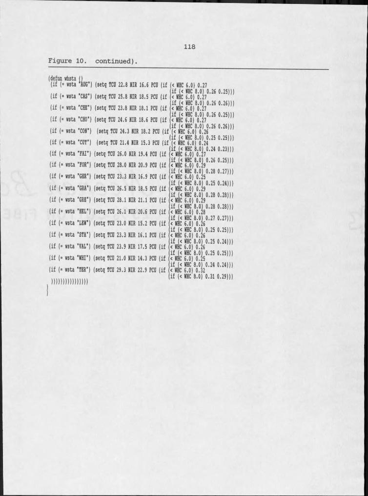
118Figure 10. continued).

(defun whsta ()(if (- wsta ‘MG') (setq TCD 22.8 NIR 16.6 PCD (if(if (■ wsta "CM") (setq TCD 25.8 NIR 18.5 PCD (if(if (* wsta "CHE") (setq TCO 23.8 NIR 18.1 PCD (if(if (= wsta "CHO") (setq TCD 24.6 NIR 18.6 PCD (if(if (■ wsta "CON") (setq TCO 24.3 NIR 18.2 PCD (if (< f eToji'oti'^ (if I'(if (■(if (■(if (■(if I- (if (■(if (■(if (■(if (■(if (■(if (- (if (■

< NHC 6.0) 0.27I ^ S l W 2 f u s i 1 1ifj< NHC 8.0) 0.26 0.26))< NHC 6.0) 0.27

< NHC 8.0] 0.26 0.25))IC 6.0) 0.27

iy=< s , t i u i u 3 "iy; SiViA2fuil1if ' — -

wsta "COT") (setq TCO 21.4 NIR 15.3 PCD (if[(< iHcTot'o.H'^ °‘2511 wsta "PM") (setq TCO 26.0 NIR 19.4 PCD (ifwsta "FOR") (setq TCD 28.0 NIR 20.9 PCD (ifwsta "GBR") (setq TCD 23.3 NIR 16.9 PCD (ifwsta "GRA") (setq TCD 26.5 NIR 18.5 PCD (ifwsta "GRE") (setq TCD 28.1 NIR 21.1 PCD (ifwsta "HBL") (setq TCD 26.1 NIR 20.6 PCD (ifwsta "1EN") (setq TCD 23.0 NIR 15.2 PCD (ifwsta "STA") (setq TCD 23.3 NIR 16.1 PCD (ifwsta "VAl") (setq TCO 23.9 NIR 17.5 PCD (ifwsta 'KHI") (setq TCD 21.0 NIR 14.3 PCD (ifwsta "TER") (setq TCD 29.3 NIR 22.9 PCD (if

))))))))))))))))

< NHC 8.0) 0.28 0.27)) IC 6.0) 0.25 if (< NHC 8.0) 0.25 0.24))< NHC 6.0) 0.29if < NHC 8.0] 0.28 0.28))< NHC 6.0) 0.29ifj< NHC 8.0] 0.28 0.28))< NHC 6,0) 0.28if (< NHC 8.0] 0.27 0.27))< NHC 6.0) 0.26if (< NHC 8.0] 0.25 0.25))< NHC 6.0) 0.26if (< NHC 8.0] 0.25 0.24))< NHC 6.0) 0.26if (< NHC 8.0] 0.25 0.25))< NHC 6.0) 0.25if < NHC 8.0] 0.24 0.24))< NHC 6.0) 0.32if (< NHC 8.0) 0.31 0.29))

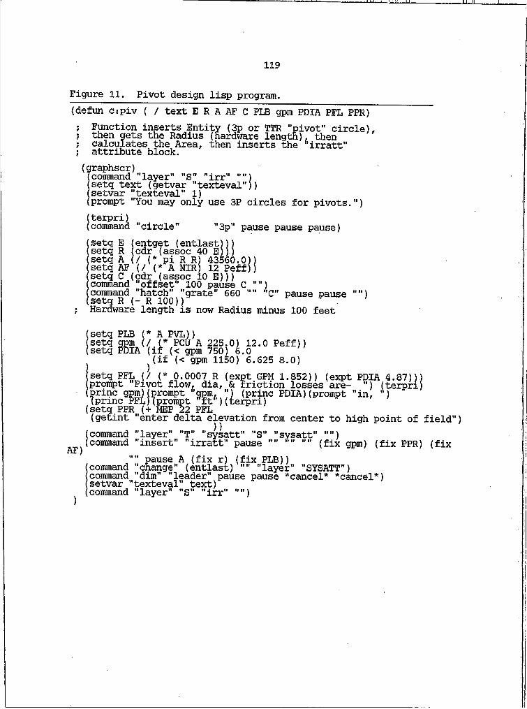
Figure 11. Pivot design lisp program.(defun cspiv ( / text E R A AF C PLB gpm PDIA PFL PPR); Function inserts Entity (3p or TTR "pivot" circle), ; then gets the Radius (hardware length), then ; calculates the Area, then inserts the f,irratt"; attribute block.(graphscr)(command "layer" "S” "irr" "")(setq text (getvar "texteval"))(setvar "texteval" I)(prompt "You may only use 3P circles for pivots.") (terpri)(command "circle" "3p" pause pause pause)[setq E (entget (entlast))) setq R (cdr (assoc 40 E))) setq A (/ (* pi R R) 43560.0)) setq AF (/ (* A NIR) 12 Peff)) setq C (cdr (assoc 10 E))) command "offset" 100 pause C "") command "hatch" "grate" 660 "" A (setq R (- R 100))

; Hardware length is now Radius minus 100 feetC" pause pause "")

(setq PLB (* A PVL))setq gpm (/ (* PCU A 225.0) 12.0 Peff)) (setq PDIA (if (< gpm 750) 6.0 (if (< gpm 1150) 6.625 8.0)(setq PFL (/ (* 0.0007 R (expt GPM 1.852)) (prompt "Pivot flow, dia, & friction losse

t h l l e S S f P D m > (PromPt ',in'

(expt PDIA 4.87)))- .nJlosses are- ") (terpri

AF)

(setq PPR (+ MEP 22 PFL (getint "enter delta elevation from center to high point of field")(command "layer" "T" "sysatt" "S" "sysatt'...)(command "insert" "irratt" pause "" "" (fix gpm) (fix PPR) (fix

"" pause A (fix r) (fix PLB))(command "change" (entlast) "" "layer" "SYSATT")(command "dim" "leader" pause pause *cancel* *cancel*)(setvar "texteval" text)(command "layer" "S" "irr" ""))

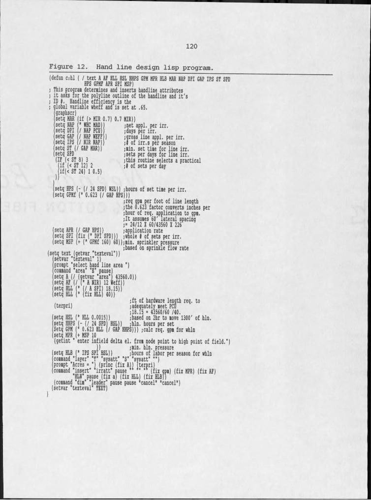
120

Figure 12. Hand line design lisp program.(deftm Cibl ( n e x t p ^ H i L p H S ^ H H P S GPM MPR HLB MAR NAP DPI GAP IPS SI SPDThis program determines and inserts handline attributes t asks for the polyline outline of the handline and it's ID t. Handline efficiency is the (lobal variable wheff and is set at .65. graphscr)setq MAR 'setq NAP setq DPI setq GAP

if (> MIR 0.7) 0.7 MIR))NHC MAD) / NAP PCD) / NAP NKPFsetq IPS / NIR NAP)

! M 1 ' " 1 1

l P A V t i 2if(< ST 24) I 0.5)

;net appl, per irr.;days per irr.;gross line appl. per irr.of irr.s per season ;min. set time for line irr.;sets per days for line irr.;this routine selects a practical ;l of sets per day

setq HPS (- {/ 24 SPD) NSL)) ;hours of set time per irr. setq GPMf (* 0.623 (/ GAP HPS)))

;req gpm per foot of line length ;tbe 0.623 factor converts inches per•hour of req. application to gpm. ;It assumes 60' lateral spacing ;= 24/12 I 60/43560 I 226 / GAP HPSI) ;application ratex (* DPI SPD))] ;whole I of sets per irr.

(* GPMf 160) 60));nin, sprinkler p ; based on sprinkl(setq text (getvar "texteval")) setvar "texteval" I) prompt "select hand line area ") command "area" T pause)

setq APR setq SPI setq MSP - - - pressuresprinkle flow rate

setq A (/ (getvar "area") 43560.0)) setq AP (/ (* A NIR) 12 Neff)) setq HLL [[ (/ A SPI) 18.15))

;ft of hardware length req. !adequately meet PCu ;18.15 = 43560/60 /40.

setq HLL (terpri)

fix HLL) 40))

(based on 2hr to move 1300' of bin.HSL]) ;hln, hours per set I GAP HHPS))) jcalc req. gpm for whin

setq HSL (* HLL 0.0015 ) setq HHPS (- (/ 24 SPD "Setq GPM I1 0.623 HLL setq MPR (+ MSP 10(getint " enter infield delta el. from node point to high point of field.")

)) ;min. bin. pressuresetq HLB (* IPS SPl HSL)) ;hours of labor per season for whin command "layer" "T" "sysatt" "S’ "sysatt" ’") prompt "Acres = "I (prmc (fix A]] terpri]

% % % , m l IfiIW1 |f“ m| "" m(couand "dim" "leader" pause pause ‘cancel* ‘cancel*)(setvar "texteval" TEXT)

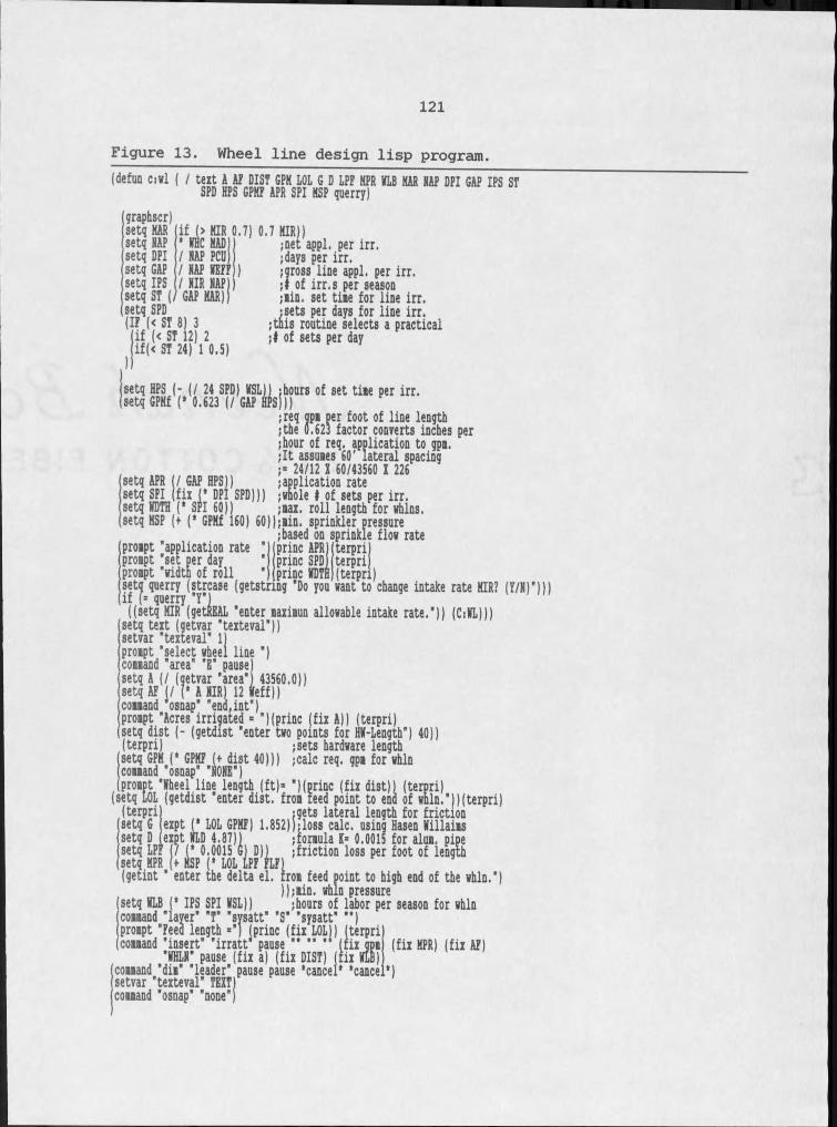
121

Figure 13. Wheel line design lisp program.(defun CiVl ( / text A Af DIST GPH LOL G D LPF MPR VLB KAR NAP DPI GAP IPS ST SPD HPS GPHF APR SPI MSP querry)

graphscr)setq MAR setq NAP setq DPI setq GAP setq IPS setq ST ( setq SPD (IF (< ST 8) 3 (if (< ST 12) 2 (if(< ST 24) I 0.5)

if (> MIR 0.7) 0.7 KIR))* VHC MAD) ;net appl. per irr. I NAP PCD)I NAP VEFFI NIR NAP) GAP MARfj

jdays per irr.;gross line appl. per irr.;# of irr.s per season ;iin. set time for line irr. ;sets per days for line irr. ;tnis routine selects a practical ;t of sets per day

;req qpm per foot of line length ;the 0.623 factor converts inches per jhour of req. application to gpm.;It assumes 60' lateral spacing ;= 24/12 I 60/43560 I 226setq APR (/ GAP HPS)) setq SPI fix (' DPI SPD))) setq VDTH (* SPI 60))

setq MSP (+ (* GPMf 160) 60));nin. sprinkler pressure;based on sprinkle flow rate

!application rate ;whole I of sets per irr. ;max. roll length for whins.

princ APR) princ SPDj princ VDTHterpri)terprij(terpri)

prompt "application rate " prompt "set per day prompt "width of roll ' setj| querry (strcase (getstnng "Do you want to change intake rate MIR? (Y/N)')))((setq KIR^getigAL "enter maxinun allowable intake rate.")) (CiVL))) setq text (getvar "texteval")) setvar "texteval" I)

prompt "select wheel line ") command "area" T pause) setq A (/ (getvar "area") 43560.0)) setq AF I/ (* A NIR) 12 Veff)) command osnap" "end.int")prompt "Acres irrigated = ")(princ (fix A)) (terpri) setq dist (- (getdist "enter two points for HV-Length") 40))(terpri) ;sets hardware lengthsetq GPH (' GPMF (+ dist 40))) ;calc req. gpm for whin command "osnap" "NONE")prompt "Vheel line length (ft)= ")(princ (fix dist)I (terpri)(setq LOL (getdist "enter dist. from reed point to end of whin.")((terpri)(terpri igets lateral length for frictionsetq G expt (* LOL GPMF) 1.852)j;loss calc, using Hasen Villains setq D (expt VLD 4.87)1 ;formula K= 0,0015 for alum, pipesetq LPr (/ (* 0.0015 GJ D)) ;friction loss per foot of lengthSetqiKPRjt MSP (J LQLiLPF FLFj(getint " enter the delta el. setq VLB (* IPS SPI VSL))

end of the whin.")rom feed point to high ));nin. whin pressure ;hours of labor per season for whin(command "layer" "T" "sysatt" "S’ 'sysatt" ") (prompt "Feed length =’) (princ (fix LOL)) (terpri)

(command "insert" "irratv pause . . . . (fix gpminsert irratt pause. . . . (fix gpm"VHLN" pause (fix a) (fix DIST) (fix VLB) command "dim" "leader" pause pause "cancel* ‘cancel* setvar "texteval" TEXT) command "osnap' "none")

(fix HPR) (fix AF)

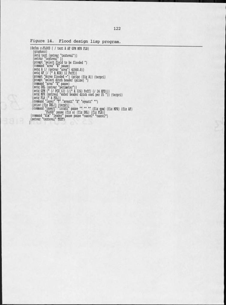
122

Figure 14. Flood design lisp program.(defim CiFLOOD ( I text A AF GPM MPR FLB) graphscr)

couand 'area' "E* pause setq A (/ (getvar 'area* setq AT {/ (‘ A MIR) 12 fe

setq text (getvar "texteval")) setvar "texteval" I) prompt "select field to be floflooded

43560.0))iff))(princ (fix A)) (terpri) er (plme) )

prompt "Acres flooded " prompt "select ditch beat command "area" T pausesetq DHL .. .. . . .setq GPM setq MPRsetq FLB ‘ A FDL))command "layer" T "sysatt" "S" "sysatt'

getvar "perimeter"))r i l ,wi,

command layer T sysatt" "S* "sysatt" ") princ (fix DHL)) [terpri)command "insert1 ‘irratt1 pause . . . . (fix gpm (fix MPR) (fix AF)"FLOOD" pause (fix a) (fix DHL) [fix FLB) couand "dim" "leader" pause pause "cancel* "cancel")setvar "texteval" FEXf)

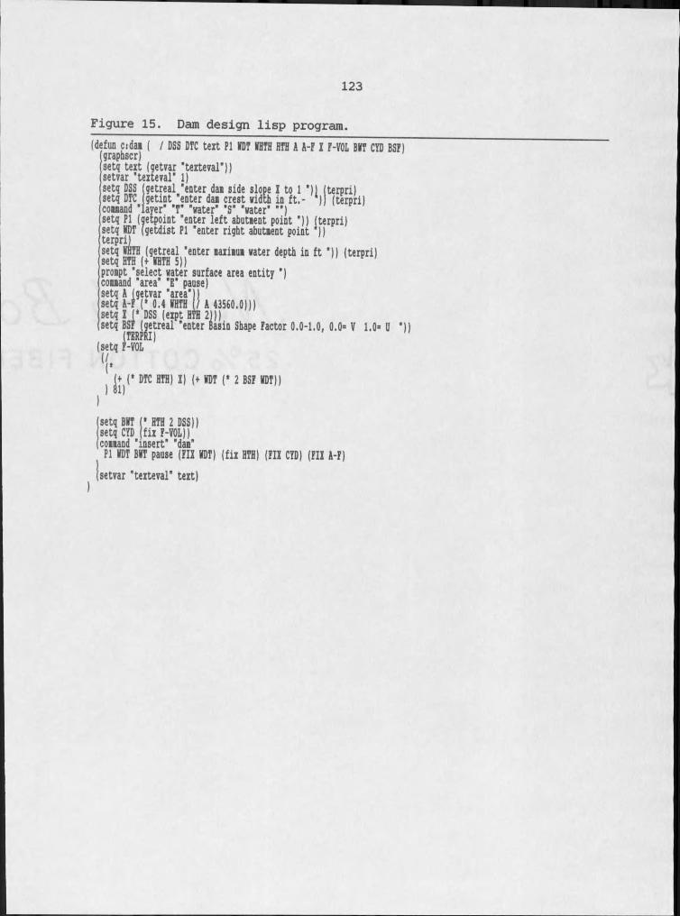
123

Figure 15. Dam design lisp program.(defUD^Cidai ( I DSS D K text Pl KDT MHTH HTH A A-F I F-VOl BMT CVD BSF)

setq text (getvar "texteval’)) setvar "texteval" I)setq DSS (getreal "enter dam side slope I to I 'll (terpri) setq DTC (getint "enter dam crest width in ft.- ‘)j (terpri) command "layer" T "water" "S" "water" ’") setq Pl (getpoint "enter left abutment point ")) (terpri) setq MDT (getdist Pl "enter right abutment point 1J) terpri)setq MHTH (getreal "enter maximum water depth in ft ’)) (terpri) setq HTH (+KHTH 5))prompt "select water surface area entity ")command "area" "E* pause)setq A (getvar "area")setq A-F (‘ 0.4 MHTH I/ A 43560.0)))setq I (‘ DSS (expt HTH 2)))setq BSFJgetreal "enter Basin Shape Factor 0.0-1.0, 0.0= V 1.0= U "))T(TKRPRI)

+|C DTC HTH) X) (+ MDT (* 2 BSF KDT))

setq BMT (' HTH 2 DSS)) setq CYD (fix F-VOL)) command "insert" "dam"Pl MDT BMT pause (FIX MDT) (fix HTH) (FIX CYD) (FIX A-F)

jsetvar "texteval" text)

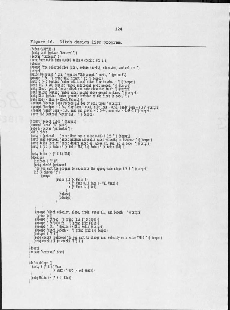
124

Figure 16. Ditch design lisp program.(defun CiDITCH ()(setq text Iqetvar "texteval")) setvar 'texteval' I)setq Siax 0.006 Siin 0.0005 Helin 0 check I VCC 2.2) choose)'proipt "The selected flow (cfs), voluie (ac-ft), elevation, and wel are ')

Hprinc EL)

rpnnc g) (proipt' cfs, 'Hprinc VOL) (proipt" ac-ft, ' proipt ft, 1Hprinc VEL)(proipt ' ft "((terpri) setq Q (+ Q (getmt "enter additional ditch flow in cfs. - ")))(teii setq VOL (+ VOL (qetint "enter additional ac-ft needed. "I)) terpri setq ELout (getint "enter ditch end node elevation in ft ))(terpri, setq Helout (getint "enter water height above ground surface, ')l(terpri) setq ELm (getint "enter ground elevation of the ditch in node. 1I) ietg ELd (- ELin (<• ELout Helouti)) proipt "Seepage Loss factors SLf for by soil types "Hterpri) proipt "hardpan - 0.34, clay Ioai - 0.41. silt Ioai - 0.53, sandy Ioai - 0.66")(terpri) proipt sandy Ioai - 1.0, sand and gravel - 2.0+/-, concrete - 0,05-0.1") terpri) setq SLf (getreal "enter SLf. ") Hterpri)

proipt "select ditch "Hterpri) coiiand "area" "E" pause) setq L (getvar "perueter")) while checksetq n (getreal "enter Hannings n value 0.013-0.025 ")) (terpri) setq Viax (getreal "enter laxiiui allowable water velocity in ft/sec.- ")Hterpri) setq Helin getint "enter desire water el. above gr. sur. at in node ') terpri] setq S if (> Siin (/ (+ Helin ELd) L)) Siin (/ (+ Helin ELd) L)setq Helin (- (' S L) Eld)) ddesign(initget I "Y H")(setq checks (getkword"Do you want the prograi to calculate the appropreate slope Y/H ? ")Hterpri)(if (= checks "Y")(progn

(while (if < Helin I)Viax 0.1) (abs (- Vel Vmax))) Viax 1.1) Vel)

proipt "ditch velocity, slope, grade, water el., and length ")(terpri) (princ Vel)(proipt " ft/sec, ")(princ (fix (‘ S 1000))) prompt ' ft/1000 ft, 'I(princ (fix Helin)) proipt" ft, ") (princ (+ BLin Helin) Hterpri)fix Helin) elin))(ter1Hprinc (fix L)i(terpri)setq'cbeckV (getkword "Do you want to change lax. velocity or n value Y/H ? ')Hterpri) setq check (if (= checkV "Y") I))

proipt "ditch Length initget I "Y H")

dcost)setvar "texteval" text)

(defun dslope ()(setq S It S (/ Viax

(+ Viax (‘ VCC (- Vel Viax)))(setq Helin (I S L) Eld))

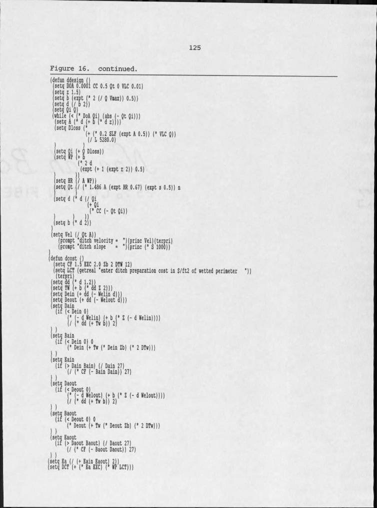
125

Figure 16. continued.(defun ddesign (IsetqDOA 0,0061 CC 0.5 Qt 0 VlC 0.01) setq z 1.5)setq b eipt (‘ 2 (/ Q Viax)) 0.5)) setq ijl b 2))while (< ' DoA Qi) (abs I-QtQi)))(setq A (1 O (+6 Cdz))))(setq Dloss (‘

(+ C 0.2 SLF (expt A 0.5)) (' VLC Q)) (/L 5280.0)setq Qi (+ setq VP (+

setq HR setq Qtsetq d (

(eipt (+ I (expt z 2)) 0.5)I AMP))I C 1.486 A (expt HR 0.67) (expt s 0.5)) n

''ft) C C C I - O t Q i ) ) setq b C d 2))

(setq Vel (/ Qt A))(prompt "ditch velocity = "Hprinc Vel)(terpri) (prompt "ditch slope = "Hprinc (* S 1000))

defun dcost |)setq CF 1.5 BXC 2.0 Zb 2 DTM 12) setq LCT (getreal "enter ditch preparation cost in $/ft2 of wetted perimeter ")) Iter

setq(terpri) etq dd * d 1.2)1 setq TM (+ b C dd setq Dein ' setq Deou setq Dain (it (< Dein 0)

. . caaz2)))setq Dein (+ dd (- Melin d)|j^setq Deout (+dd( in 0)- d Meli , ,* dd (+Twh)) 2

in 0) 0* Dein (+ Tw (* Dein Zb) (' 2 DTw)))

j‘ j- d Melin) j+.bj* Z (- d Melin))))

setq Bain (if (< Dein 0) 0

setq Bain(it (> Dain Bain) (/ Dain 27)(/ C CF (-Bain Dain)) 27)

setq Daout (it (< Deout 0)C - d Melout) C b I ' Z C d Melout))))

I/ C dd (+ Twb)) 2)

l I S fBaout(< Deout 0) 0C Deout (+ Tw C Deout Zb) (* 2 DTw)))

(setq Baout (if (> Dao(/ C CF (- Baout Daout)) 27)

(if (> Daout Baout) (/ Daout 27)I )setq Ba (/ (t Bain Baout) 21) setq DCT (+ C Ba BBC) (‘ MP LCT)))

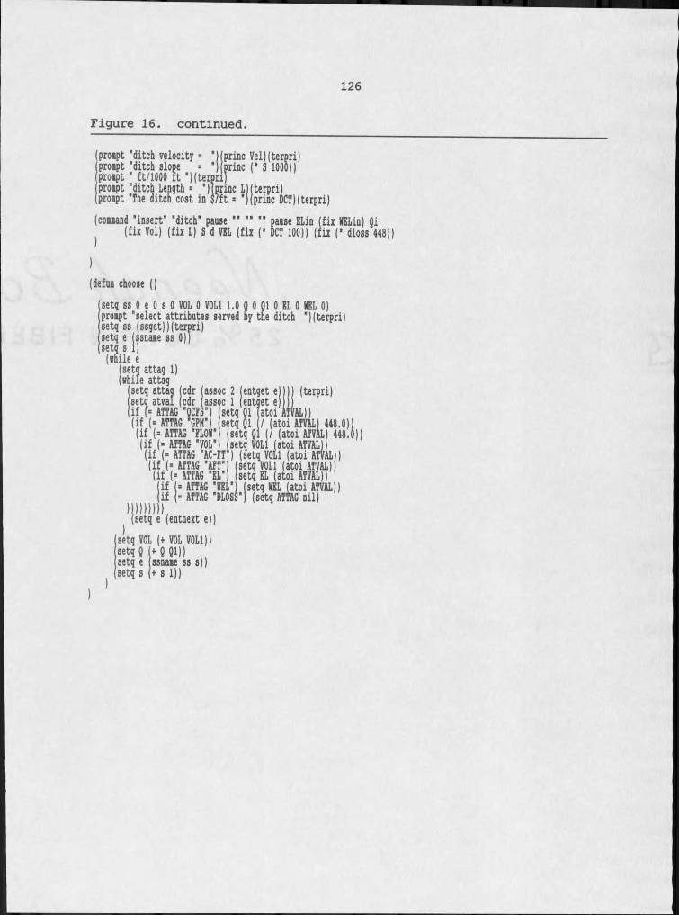
126

Figure 16. continued.prompt 'ditch velocity = prompt 'ditch slope prompt ' ft/1000 ft ")(te prompt "ditch Length = " prompt 'The ditch cost in

'Ifprinc Vel)(terpri) 'I||rinc (* S 1000))

(couand 'insert' 'ditch' pause " " " pause ELin (fix MELin) Oi (fix Vol) (fix L) S d VEL (fix (' DCT 100)) (fix (‘ dloss 448))

(defun choose ()setq ss 0 e 0 s 0 VOL 0 VOLl 1.0 Q 0 Ql 0 EL 0 KEL 0) prompt "select attributes served by the ditch '((terpri) setq ss (ssget))(terpri) setq e (ssname ss 0)) setq s I)(while esetq attag I)

while attag(terpri)

atoi ATVALj 448.0) j / (atoi ATVAL) 448.0))(if (= ATTAG "FLOK'(if (= ATTAG 'VOL' . __ _ _ _ _(if (= ATTAG 'AC-lT ) (setq VOtl (atoi ATVJlL))(setq VOLl (atoi ATVAL)I Isetq VOL I

( i f > ATTAG "EL"| (setq EHatoHTVAL))(if (' ATTAG 'AFT')(if (= ATTAG 'KEL'j (setq KEL (atoi ATVAL)) (if (= ATTAG 'DLOSS') (setq ATTAG nil)

*}setq*e*(entnext e))setq VOL (+ VOL VOLl))setq Q setq e setq s

M QD) u ssname ss s ) <• s I))

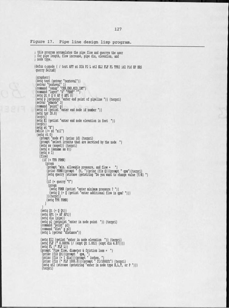
127

Figure 17. Pipe line design lisp program.I this program accumulates the pipe flow and querns the user ; for pipe length, flow increase, pipe dia, elevation, and • node type.(defun cspnode ( I text AfI nt DIA P2 L nt2 KL2 FLf fL IPR2 id2 Pid HP HRS querry DeltaH)graphscr)setq text (getvar "texteval")) setvar "texteval" I) command "osnap' "CEN1KHDfHID1IRI") command "layer" "S' tTEKP" "‘j setq QtO Q O Af O AFtO)setq p (getpoint "enter end point of pipeline *)) (terpri) setvar pdmode" 3) command point" p)setq id (getint enter end node id number ’))setq tpr 20.0)terpri]setq El (getint "enter end node elevation in feet ’)) terpri)whi?eD(/=Eni "nil")(setq ct 0)

(prompt node I") (princ id) (terpri) prompt "select irratts that are serviced by the node ") setq ss (ssget)) (terpri) setq e Issname ss 0)|(setq s I)(flow)(if (< TPR PRHN)(progn(prompt "min. allowable pressure, and flow = ")princ PRKNKprompt ’ ft, ") (princ (fix Q))(prompt' gpm")(terpri)(setq querry (strcase (getstnng "Do you want to change value (T/N) ")|if (« querry*T )(prognsetq PRHN (getint "enter minimum pressure ? ")) setq Q (f Q (getint "enter additional flow in gpm? *)))

^isetqrTPR1PRKN)

(setq Qt (+ Q Qt))(setq Aft (+ Af Aft)) setq dia (pipe))setq p2 (getpoint "enter in node point ")) (terpri)(command point" p2) command "dist" p p2)(setq L (getvar distance"))setq B12 (getint "enter in node elevation ")) (terpri) setq FLf 8 0.00096 (/ (expt Qt 1.852) (expt dia 4.87)))) setq FL (‘ FLF L))prompt "Pipe flow, diameter & friction loss = "I

terpri)

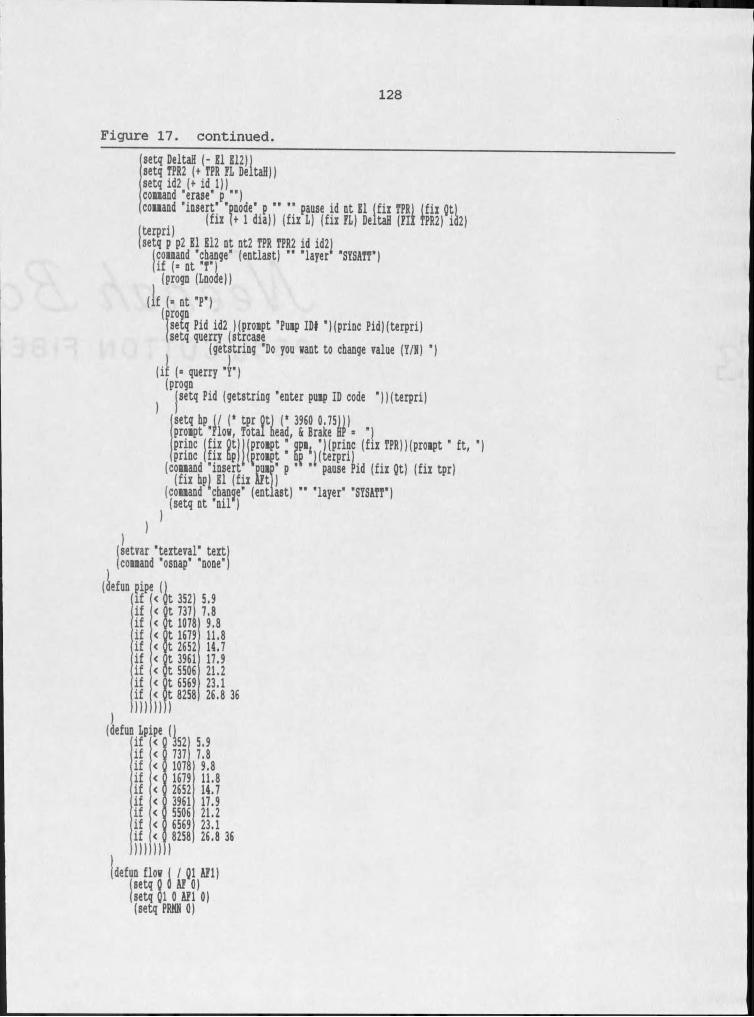
128

Figure 17. continued.setq DeltaH (- El E12)] setq TPR2 (+ TPR PL DeltaH)) setq id2 (+ id I)) command "erase* p ’")court « njfu mj JIj5ijJj2i(setq p p2 El E12 nt nt2 TPR TPR2 id id2]

jcommand^change' (entlast) " "layer "SYSATT")(progn (Lnode))

(!f (- nt T )(prognsetq Pid id2 ((prompt "Pump IDI ")(princ Pid)(terpri)(setq querry (strcase

(getstring "Do you want to change value (Y/H) ")(if (= querry 'Y")(prognI Jsetq Pid (getstring "enter pump ID code "))(terpri|

setq hp I/ (* tpr Ot) (* 3960 0.75)1) prompt "Plow, Total nead, & Brake HP = ")@ I i i i ® I S : r - . I K | t u

(couand "insert pump" p pause Pid (fix Qt) (fix tpr) (fix bp) El (fix APt])(couand change" (entlast) " "layer" "SYSATT")(setq nt "nil1)

ft,

(setvar "texteval" text) (command 'osnap" "none")

(defun pipe ( if if if

< fit 3521 5.9 t 737) 7.8

(di111 111)

I,MLpipe (| if

t 1078 t 1679 t 2652 t 3961 t 5506 t 6569 1 8258

9.811.814.7 17.9 21.2 23.126.8 36

ifI lI Iif ifIII I) I

1527371078167926523961550665698258

5.97.89.811.814.7I!:!23.126.8 36

(defun flow I I gi API) (setq Q O M O ) (setq g i 0 API 0) (setq PRHH 0)

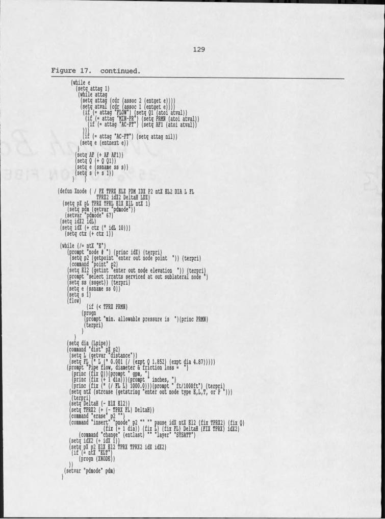
129

Figure 17. continued.(while e (setg attag I)(while attagjsetq attao jcdr (assoc 2 Ientget el)I

(setq atval (cdr (assoc I (entget e jj (if (= attag 1FLoX') (setq Ql (atoi atval))(if (= attag 1KIN-PR1) (setq PRHN (atoi atval)) (if (= attag 1AC-FI1) (setq AFl (atoi atval))III (= attag 1AC-FT1) (setq attag nil))

(setq e (entnext e))setq AF (+ AF AFl))setq Q setq e setq s

+ 0 01)1 ssnaie ss sjj + s i ) )

(defun Xnode ( I PX TPRX RLX PDN IDX P2 ntX EL2 DIA L FL TPRX2 idX2 DeltaH LDX)L TPRX TPRL RlX RlL ntX l) e (getvar "pdiode1))(setvar "pdaode" 67)(setq idX2 idL)

(setq idX (+ ctx (* idL 10)))(setq ctx (+ ctx I))(while (/« ntX 1E1)

(proapt "node t ') (princ idX) (terpri)(setq p2 (getpoint enter out node point ')) (terpri) (coaaand point" o2)setq E12 (aetint enter out node elevation ")) (ternri)proapt "select irratts serviced at out sublateral node ‘)setq ss (ssget)) (terpri)setq e jssnaae ss 0))setq s I)flow) (if (< TPRX PRHN)

(progn(proapt "ain. allowable pressure is ')(princ PRKN) (terpri)

(setq dia (Lpine)) (coaaand 'dist pX p2)(setq L (getvar "distance"))t i A t e . . .

princprincprinc fix

TdialIHproapt inches,r— — , „ 1000.0)))(proapt 1 ft/lOOOft1) (terpri)(setq ntX (strcase (getstring "enter out node type R,L,T, or P )))SetqpDeltaH (- RlX E12)) setq TPRX2 (+ (- TPRX FL) DeltaH)) coaaand "erase p2 "")coaaand "insert" "pnode" p2 11 "" pause idX ntX R12 (fix TPRX2) (fix Q)

(fix (+ I dia)) (fix LI (fix FL) DeltaH (FIX TPRX) idX2)(coaaand "change" (entlast (setq idX2 (f idX I))(setq pX p2 ElX R12 TPRX TPRX2p 2 __'(if'f= ntX 1RLTV (progn (XNODEj)

(setvar "pdaode" pda)

.ayer" "SYSATT") 1PRX TPRX2 idX idX2)

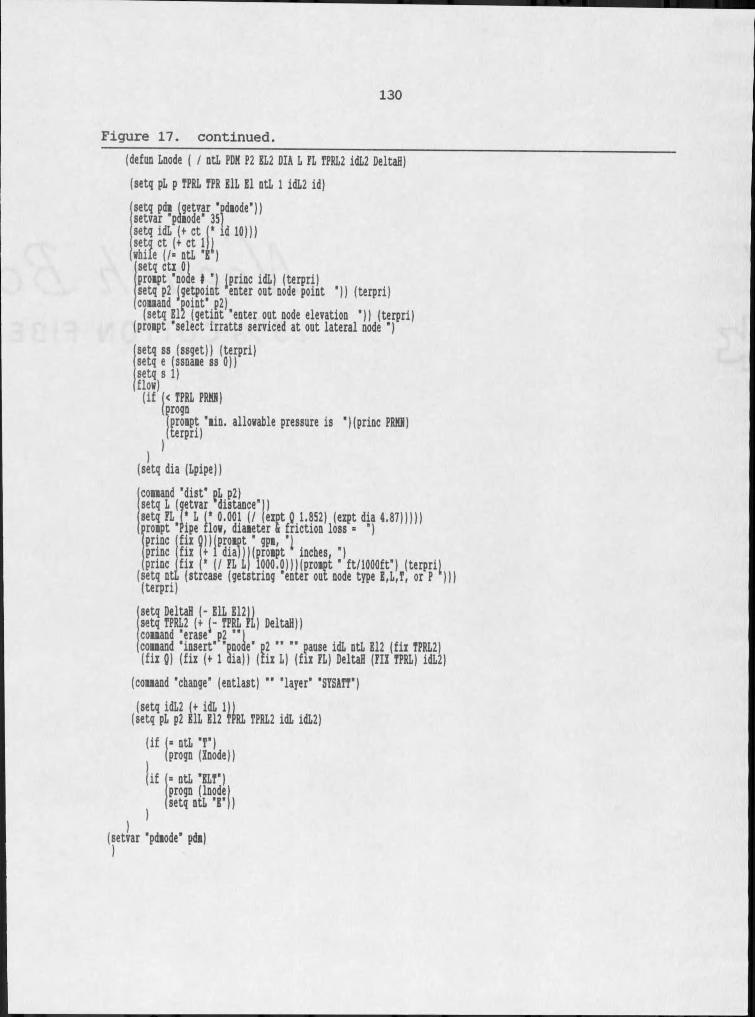
130

Figure 17. continued.(defim Lnode ( / ntL PDK P2 EL2 DIA L PL TPRL2 idL2 DeltaB) (setq pL p TPRL TPR RlL Rl ntL I idL2 id)

setq IdL (+ ct [* id 10))) setq ct (+ ct I)) while (/= ntL 'Rt) setq ctx Olprompt "none I ") Iprinc idL) (terpri)setq p2 Igetpoint enter out node point ')) (terpri)command point' p2)(setq R12 (getint "enter out node elevation ')) (terpri) (prompt "select irratts serviced at out lateral node ")setq ss (ssget)) (terpri) setq e (ssname ss O)) setq s I) flow)(if (< TPRL PRKR)progn

(prompt "min. allowable pressure is ")(princ PRHR) (terpri)

(setq dia (Lpipe))command 'dist" pL p2) setq L (getvar distance’)) setq FL I* L (* 0.001 (/ (exp prompt "Pipe flow, diameter S friction loss princ fix Q))(prompt ' gpm, 'I princ fix I+ I dia))!(prompt inches, , princ fix (‘ (/ FL L) 1000.0))!(prompt ' ft/lOOOft") (terpri) (setq ntL (strcase (getstring "enter out node type R1L1T1 or P ))) (terpri

:pt 0,1.852) (expt dia 4.87))))) & friction I

setq DeltaH (- RlL E12]lsetq TPRL2 (+ (- TPRL Fl) DeltaH))command "erase p2 "Icommand "insert" "pnode" p2 " "" pause idL ntL R12 (fix TPRL2) (fix Q) (fix (+ I dia)) (fix L) (fix FL) Deltafl (FII TPRL) idL2)

(command "change" (entlast) ” "layer" "SYSATT")(setq idL2 (+ idL I))(setq pL p2 ElL R12 TPRL TPRL2 idL idL2)

(if (- ntL "I")(progn (Xnode))

if = ntL 'RLT") progn (Inode) setq ntL 'R'))

(setvar "pdmode" pdm)

APENDIX B Tables

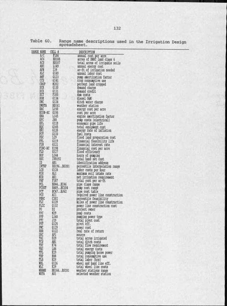
132

Table 60. Range name descriptions used in the Irrigation Designspreadsheet.RANGE NAME CELL I

A/C ?i86AC6 BD108ACS BD107AEC L149AfN 129ALC G149AMf G123CCU G141CROP M202DCH G130DCR G131DCT FIDODOM G134DMC G124DMSTA BD161EAC L150ECON-AC G198ENA L145EPC J88EPL Gl 18EOC G145ERI G120fCT G133PDC L29PfL G119PIN G121PINC-AC K198PLD G127HOP L144HSC IV8192ID ABlINTRP BD196..B0201LCH G128MIR ALlNIR AKlPAP F187PCL BD44..BI46PCOST BA89..BC104PCT BC47..BJ62PCU AllPERC C202PLC G139PLCC G132PO D2PPC H29PPP L148PTC J29PVT G125PMC G129RRR G122SRC APITAI D29TCU ANlTDC K74TEC L88TPL E29THP E88TLB H29MHL G126MLC K29MNAME BR166..BS181MSTA AOl

DESCRIPTIONannual cost per acre acres of DNRC land class 6 total acres of irrigable soils annual energy cost ac-ft of irrigation needed annual labor cost puip amortization factor crop consumptive use percent land cropped demand charge demand credit dam costs diesel O&M ditch water charge weather station energy cost per acre cost per acreengine amortization factor pump costs (electrical) economic pipe life total equipment cost energy rate of inflation fuel costsflood land preparation cost financial feasibility life financial interest rate financial cost per acre flood efficiency hours of pumping total hand set cost identification address percentile interpolation range labor costs per hour maximum soil intake rate net irrigation requirement total cost per ac-ft pipe class range pump cost range pipe cost tablerequired power line constructionpercentile feasibilitymiles of power line constructionpower line construction costproject ownerpump costspumping power typetotal pivot costpivot eff.power costreal rate of returnsourcetotal acres irrigated total ditch costs total flow requirement total energy costs total pumping horse power total consumptive use total labor (hrs) wheel and hand line eff. total wheel line costsweather stations range selected weather station

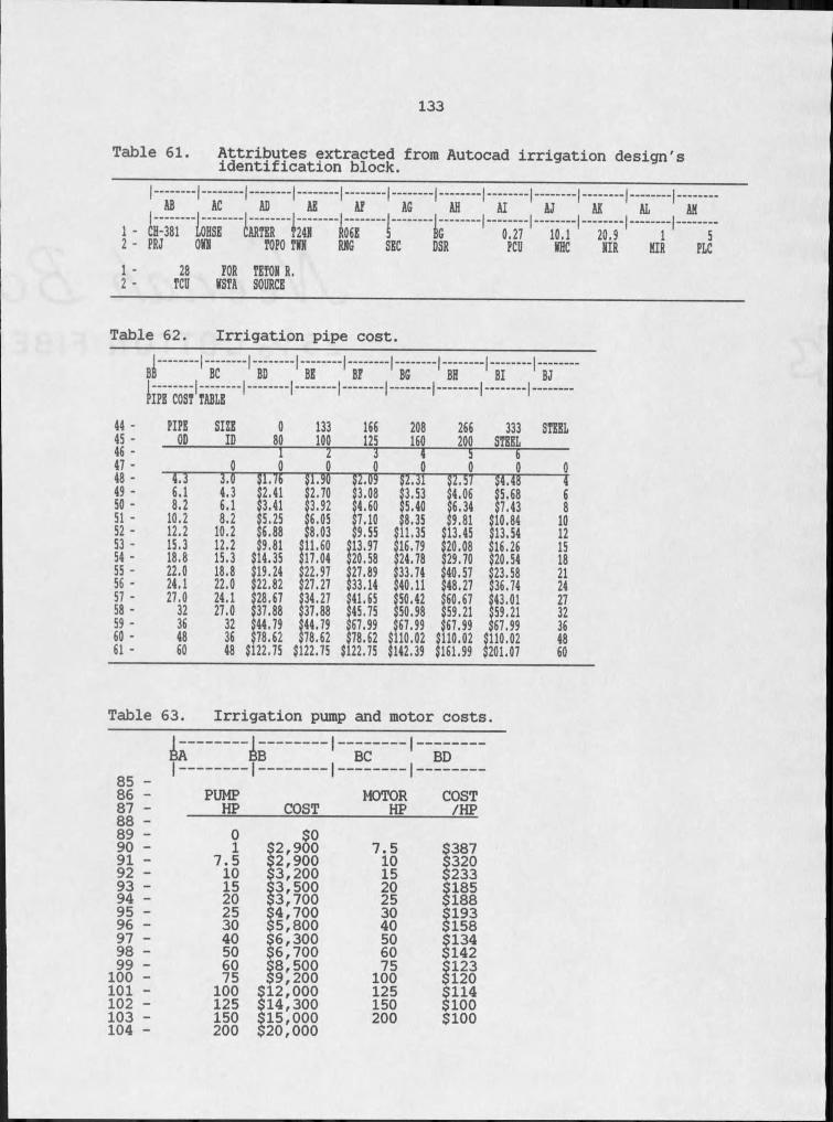
133

Table 61. Attributes extracted from Autocad irrigation design's identification block.

ABI - Ih-381 2- PRJ1 -2 -

28TCU

AC AC AE Af AG iLohse CARTER T24H ks I IgOMH TOPO TMH RHG SEC DSR

POR TETOH R.MSTA SOURCE

0.27 10.1PCU MHC

AK 1 AL20.9 1 I HIR ER 5PLC

Table 62. Irrigation pipe cost.

siI. . . . I BC BD BE Bf r BG BH BI BJPIPE COST TABLE

44 - PIPE SIZE 0 133 166 208 266 333 STEEL45 - OD ID 80 100 125 160 20046 - r r r r . 5 r ~47 - 0 0 0 „„ 0 0 0 0 048 - 4.3 3.0 SI./6 $1.90 $2.09 52.31 $2.57 $4.48 J49 - 6.1 4,3 $2.41 $2.70 3.08 3.53 $4.06 $5.68 650 - 8.2 6.1 $3.41 $3.92 $4.60 $5.40 $6.34 $7.43 851 - 10.2 8.2 5.25 $6.05 $7.10 $8,35 $9.81 $10.84 1052 - 12.2 10.2 $6.88 $8.03 $9.55 $11.35 $13.45 $13.54 1253 - 15.3 12.2 $9.81 $11.60 $13.97 $16.79 $20.08 $16.26 1554 - 18.8 15.3 $14.35 $17.04 $20.58 $24.78 $29.70 $20.54 1855 - 22.0 18.8 $19.24 $22.97 27.89 $33.74 $40,57 $23.58 2155 - 24.1 22.0 $22.82 $27.27 $33.14 $40.11 $48.27 $36.74 2457 - 27.0 24.1 $28.67 $34.27 41.65 $50.42 $60.67 $43.01 27SB - 32 27.0 $37.88 $37.88 $45,75 $50.98 $59.21 $59.21 3259 - 36 32 $44.79 44.79 $67.99 $67.99 $67.99 $67.99 3660 - 48 36 $78.62 $78.62 $78.62 $110.02 $110.02 $110.02 4861 - 60 48 $122.75 $122.75 $122.75 $142.39 $161.99 $201.07 60

Table 63. Irrigation pump and motor costs.

Lr -I _ - - f ,

I I I I

BD85 -86 -

IPUMP

I

MOTOR COST87 - HP COST HP /HP88 -89 - O $090 - I $2,900 7.5 $38791 - 7.5 $2,900 IO $32092 - IO $3,200 15 $23393 - 15 $3,500 20 $18594 - 20 $3,700 25 $18895 - 25 $4,700 30 $19396 - 30 $5,800 40 $15897 - 40 $6,300 50 $13498 - 50 $6,700 60 $14299 — 60 $8,500 75 $123IOO - 75 $9,200 IOO $120IOl - IOO $12,000 125 $114102 - 125 $14,300 150 $100103 - 150 $15,000 200 $100104 - 200 $20,000

134

Table 64. Irrigation equipment range documentation of the IrrigationDesign spreadsheet.

B C- L - I - - L1 - -------2 - Project* i

3 - Owner s4 - Location i5 . . . . . . . . .6 -7 - ------------8 - IRRIGATION ATTRIBUTES9 .........

CH-381LOHSET24N ROSE NI,SN,SE

TOPO: CARTER,ANTEL. LAKE SOURCE: TETON R. 17-Apr-89

10 - TYPE ID* AREA FLON HIN-PR HN-L LABOR NATER USE11 - 12 - (system) (acres) (gpi) (ft) (ft) (hours) (a-f/yr)13 - PIVOT I 103.3 697 87 1096 77 23914 - PIVOT 2 138.2 932 93 1284 103 32015 - PIVOT 3 80 539 67 953 59 18516 - PIVOT 4 57.3 387 60 791 43 13317 - PIVOT 5 76.5 516 66 930 57 17718 - NHLN I 40 479 130 1100 76 10919 - HLN I 89 883 137 1720 395 239

LINECOST

21 - 81 22 - 8123 - 8124 - 8125 - 8126 - 8127 - 8128 -29 -30 -31 - —

22,589II

I

9,8006,880Esosososo

584.3 4433

FLOODCOST

$29,756 SO S'$34,224 SO S'

810 1402 $138,819 $16,680

K13: H f Igis=O,OjiFflJ=-NHLN',32io+6^13,*IF(iR=’HLi',4‘G13,ll)rG13J13: (CO H F G13<100,0,!IF(IR=’PIVOT,,!IF{G13>1280,12.5*(G13-1280).0)+€13*23.5t4000,0))K13: CO HF(G13=0,0,HFIIR=-NHLN",3250+6^13,HF(iR='HLN",4'G13,0 IL13: CO Nil] H F G13=0,0JIF!IR=‘FLOOD’,200{D13+F13*G13,O)(M13: HF(Jl3>0,G13‘0.005,il3/El3‘5420,0)«29: (CO) OSUHfHia..M28)‘PNC

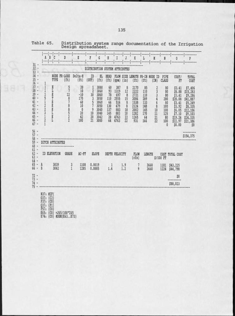
135

Table 65. Distribution system range documentation of the IrrigationDesign spreadsheet.

T1,-1="31323334353637383940414243444546475657 ■5859 ■60 ■ 61 ■

L 1 K 1 S 1 O-

DISTRIBUTION STSTBH ATTRIBUTESNODE FR-LOSS Delta-H ID BL HEAD FLOM SIZE LENGTH PR-IN NODE ID PIPETYPE (ft) (ft) (OUT) (ft) (ft) (qpi) (in) (ft) (ft) (III) CLASSE 5 20 I 3080 60 387 8 2170 85 2 80L 7 10 2 3060 93 1319 12 2222 HO 3 80E 22 -10 30 3060 78 697 8 2721 HO 3 80T 8 170 3 3050 HO 2555 15 2086 289 4 200E 7 60 5 3060 66 516 8 1538 133 6 80E 8 10 7 3050 130 479 8 2124 148 8 100E 8 0 9 3040 137 883 10 2002 145 10 100L 5 20 10 3040 145 883 10 1282 170 11 125E 2 42 20 3042 20 4763 22 1265 64 21 80L 2 100 21 3000 64 4763 22 931 166 22 100

0

COST/ TOTALFT COST

53.41 $6.88 $3.41 $20.083.41 3.92 6.05 7.10

$19.24$22,97$0.00

$3:41 $$3.92 $:

$7,406$15,283$9,286$41,887‘5,2498.335

$12,106 $9,10324.335 21,386$0

$154,375DITCH ATTRIBUTES

62 - ID ELEVATION63 -64 -

GRADE AC-FT SLOPE DEPTH VELOCITY FLOM(cfs) LENGTH

65 - A 3039 3 1108 0.0019 I 1.9 7 366066 - B 3042 I 1285 0.0005 1.4 1.2 9 366072737475

COST TOTAL COST $/100 FT1181 $43,225 1224 $44,798

$0$88,023

N37: !IF037! C2P37s CO037= FlP57, COK65: COK74i CO

fJ65/100*I65iSUH(K63..K73)

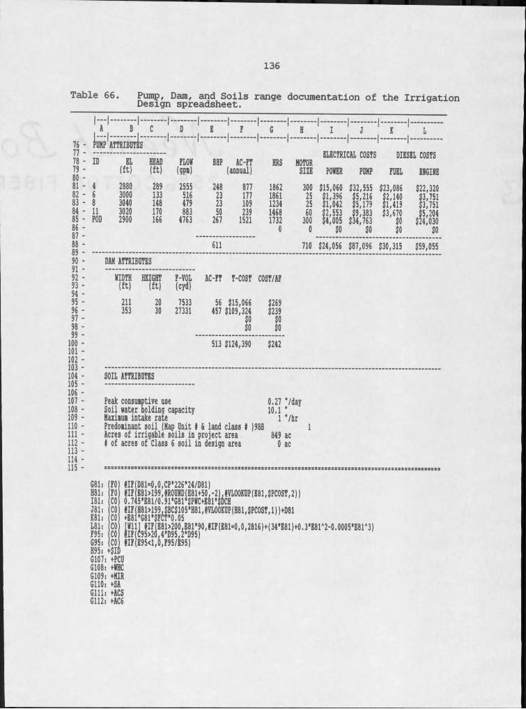
136

Table 66. Pump, Dam, and Soils range documentation of the IrrigationDesign spreadsheet.

76 -77 -78 -79 -80 - 81 - 82 -83 -84 -85 -86 -87 -88 -89 -90 -

PDHP ATTRIBUTES

46811POD

EL(ft)28803000304030202900

C D E 'T"'T-' H

HEAD FLOK BHP AC-FT HRS HOTOR(ft) (gpi) (annual) SIZE289 2555 248 877 1862 300133 516 23 177 1861 25148 479 23 109 1234 25170 883 50 239 1468 60166 4763 267 1521 1732 300

0 0611 710

J K L ----------1---- 1----

ELECTRICAL COSTS DIESEL COSTSSIZE POtfER PDHP PDEL ENGINE

S I ,396 55,216 52,140$1,042 $5,179 51,41952,553 9,383 $3,67084,005 $34,763 $050 $0 $0

522,32053,751$3,75185,204524,030

50710 $24,056 $87,096 $30,315 $59,055

DAH ATTRIBUTES92 - WIDTH HEIGHT P-VOL93 - (ft) (ft) (cyd)94 -95 - 211 20 753396 - 353 30 27331

AC-PT T-COST C0ST/AF

97 -98 -99 -100 - 101 - 102 -103 -104 -105 -106 -107 -108 - 109 -no - 111 - 112 -113 -114 -115 -

56 $15,066 457 $109,324

I !

$269$239

Il

513 $124,390 $242

SOIL ATTRIBUTES

Peak consumptive use 0.27 "/daySoil water holding capacity 10.1 'Haximua intake rate I "/hrPredominant soil (Hap Unit I & land class I )98B IAcres of irrigable soils in project area 849 ac4 of acres of Class 6 soil in design area 0 ac

ssssss:sssssssss:srs:ssssssssss=ssssssssz3sssssssssss=ss:ssss=sr:ssssrssssssssss=:s::::=sss:ssassB:ss

G81i H81:181.J81:K81:L81:F95:G95:H95. +$IA G107: +PCU G108. +MHC G109. +KIR GUO. +SA Gill: +ACS G112. +AC6

@IF(D81=0,0,CP'226"24/D81)H P E81>199,fROUND(E81+50,-2).fVLOOKUP(E81,$PCOST,2)|0.745'E81/0.91'G8r$PNC+EEl'$DCHHP|H81>199j$BC$105*H81,!VLOOKUP(H81,$PCOST,l))+D81

jMlljpHyESlgOO^Sl^O'HPfESl'O'O'lSHl+lSd'ESlI+O.l'EaHl-O.OOOS'ESl'S)

IIp|E95<l,6j95/695)951

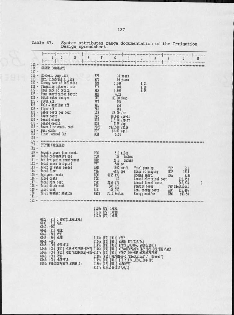
137

Table 67. System attributes range documentation of the IrrigationDesign spreadsheet.

115 -116 -117 -118 -119 -120 - 121 - 122 -

123 -124 -125 -126 -127 -128 -129 -130 -131 -132 -133 -134 -135 -136 -137 -138 -139 -140 -141 -142 -143 -144 -145 -146 -147 -148 -149 -150 -151 -152 -

======================..==========... =================.. ==================...=================SYSTEM COESTAliTSEconomic pump life Max. Financial I. life Energy rate of inflation Financing interest rate Real rate of return Pump amortization factor Ditch water charges Pivot eff.Hhln & handline eff. Flood eff.Labor costs per hour Power costs Demand charge Demand credit Power line const, cost Fuel costs Diesel annual 0&M

EPL 30 yearsFFL 10 yearsERI I. OOt 1.01FIN IOt 1.10RRR 4.60t 1.05AMF 6.2tDEC $0.00 $/acPVT 75tHHL 65tFLD 701LCH $5.00 /hrPHC $0,030 /kw-hrDCH $15.00 /hp-yrDCR $125 /hpPLCC $12,500 /mileFCT $1.00 /galDON 5.51srcsssrssssaasssssssassasssssssssssssssssssssssssssssssasssssaasssssasasssssssssssssssssssssssssssssssssssssssSYSTEM VARIABLESRequire power line const. Total consumptive use Eet irrigation requirement Total acres irrigated Ac-ft of water needed Total flow Equipment costs Flood costs Total pipe cost Total ditch cost Labor costTR-21 weather station

PLC 5.0 milesTCD 28 inchesNIR 20.9 inchesTAI 584 acAFE 1402 ac-ft Total pump hp THP 611TFL 4433 gpm Hours of pumping HOP 1715EOC $155,499 Engine amort. EHA 8.81FDC $0 Annual electrical cost $28,753TPC $154,375 Annual diesel costs $46,374TDC $88,023 Pumping power PPP ElectricalALC $4,050 Ann. energy costs AEC $25,466HSTA Fort Benton Energy cost/ac EAC $43.58ssssassssasssssasssssaassasssssssssaaasssssssaasassassasssssssssassssssssaaaasssssssssssssssssssssssssssssssss

1120,1121:1122:G123: Pl D tPMT(l,RRR1EPL)G139: Fl +AMlG140: HCG141: Fl +EIRG142: FO +TAIG143: FO +AFN L143:G144: +TFL L144:G145: CO +PTC+HLC L145:L146: CO [Hill +I88+EPC'AMF+@PNT( (L146:L147: CO Hll +TEC(DOH+ENA)+K88+L147:G148: CO +TDC L148:G149: CO +LCH1TLB L149:GlSOi fVLOOKOP(HSTA,HEAME1I) L150:

F2F2F2

1+ERI1+FIH1+RRR

M147, H F L146<L147,0,1)

+THPtAFH/ITFL/226/241 PPMTfl,0.046,128000/HOP)) +I88+EPC'AMF4PLC'PLCC-DCR'THP)'AMf +TEHDOMfEHA +K88+EPC'AMF

M147=0,'Electrical'.' Diesel') HF(M147=1,K88,I88)+PPC +AEC/TAI

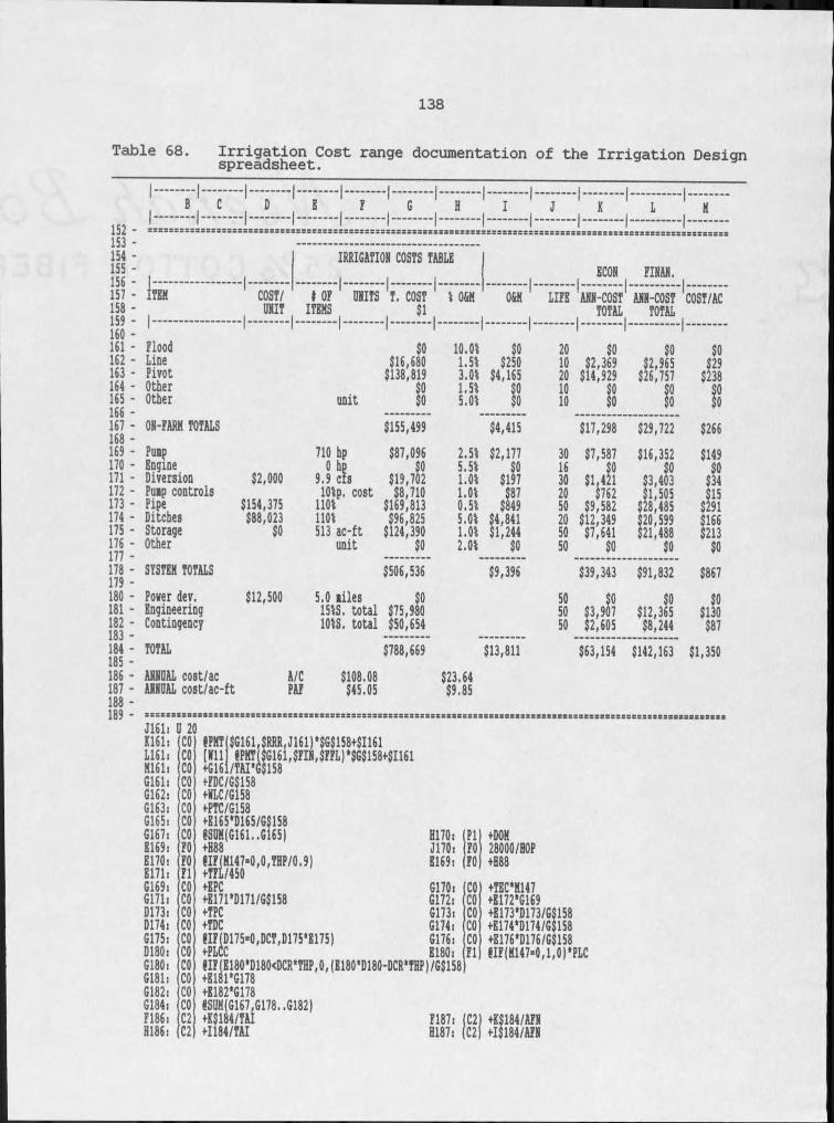
138

Table 68. Irrigation Cost range documentation of the Irrigation Design spreadsheet.

---------sasssrsrsssssssssssssrrsssssrssssssssssssssscsssssssssssssasssssssscssrssssasssssssssssssssssrssassss152 -153 -154 -155 -156 -157 -158 -159 -160 - 161 - 162 -163 -164 -165 -166 -167 -168 -169 -170 -171 -172 -173 -174 -175 -176 -177 -178 -179 -180 - 181 - 182 -183 -184 -185 -186 -187 -188 - 189 -

EC08 F mITEMI--------------------

COST/ OHIT I OF * OHITS ITEMS 't . COST

>....... ! L 1% 0&M O&M ' LIFE 1AHH-COSt 1TOTAL AHH-COST

TOTAL 1COSTZAcIFlood $0 10.0t $0 20 $0 $0 $0Line $16,680 I.St $250 10 $2,369 $2,965 $29Pivot $138,819 3,Ot $4,165 20 $14,929 $26,757 $238Other $0 I. Si $0 10 $0 $0 $0Other unit $0 5.Ot $0 10 $0 $0 $0OH-FARM TOTALS $155,499 $4,415 $17,298 $29,722 $266Puip 710 hp $87,096 2.Si $2,177 30 $7,587 $16,352 $149Engine 0 hp $0 5.Si $0 16 $0 $0 $0Diversion $2,000 9.9 crs $19,702 not $197 30 $1,421 $3,403 $34Puip controls IOtp, cost $8,710 not $87 20 $762 $1,505 $15Pipe $154,375 not $169,813 0.5t $849 50 $9,582 $28,485 $291Ditches $88,023 not $96,825 5.Ot $4,841 20 $12,349 $20,599 $166Storage $0 513 ac-ft $124,390 not $1,244 50 $7,641 $21,488 $213Other unit $0 2.Ot $0 50 $0 $0 $0SYSTEM TOTALS $506,536 $9,396 $39,343 $91,832 $867Power dev. $12,500 5.0 iiles $0 50 $0 $0 $0Engineering 15tS, total $75,980 50 $3,907 $12,365 $130Contingency IOtS. total $50,654 50 $2,605 $8,244 $87TOTAL $788,669 $13,811 $63,154 $142,163 $1,350AHHOAL cost/ac AHHOAL cost/ac-ft A/CPAF $108.08$45.05 $23.64$9.85aaaaaaaaaaaaaaBaaaaaaaaaaacaaaaaaaaaaaaazaaacaaaazaaaaaaaaaaaaaaaaaaacaazaaacaaaaaaaaaaaaaaaaaaaaaaaaaaaaaaaazJ161, 20Kisn COLisn COMisn COGlen COG162: COG163: COG165: COG167i COE169: FOE170: FOE171: FlG169i COG171: COD173: COD174: COG175: COD180: COG180: COGisn C OG182: COG184: C OF186: C2R186: C2

fPHT $G161,$RRR,J161)*$G$158+$I161 [Jfll 8PKT|$G161,$FIH,$FFL)'$GS158+$I161+FDC/G$158+HLC/G158+PTC/G158+E165‘D165/G$158fS0H(G161..G165)+H88jIFJH147-0(0,THP/0.9)+EPC+E171*D171/G$158+TPC+TDC(IFjD175*0,DCT,D175‘E175)

+E182*G178eS0H(G167,G178..G182)+KS184/TAI+I184/TAI

H170s Pl +DOMJ170: FO 28000/HOPE169: FO +588G170: CO +TEC*M147G172i CO +E172*G169G173: CO +E173‘D173/G$158G174i CO +E174*D174/G$158G176: CO +E176*D176/G$158E180: Fl HF(M147«0,1,0)*PLC

F187iH187: +KS184/AFH+I$184/AFH

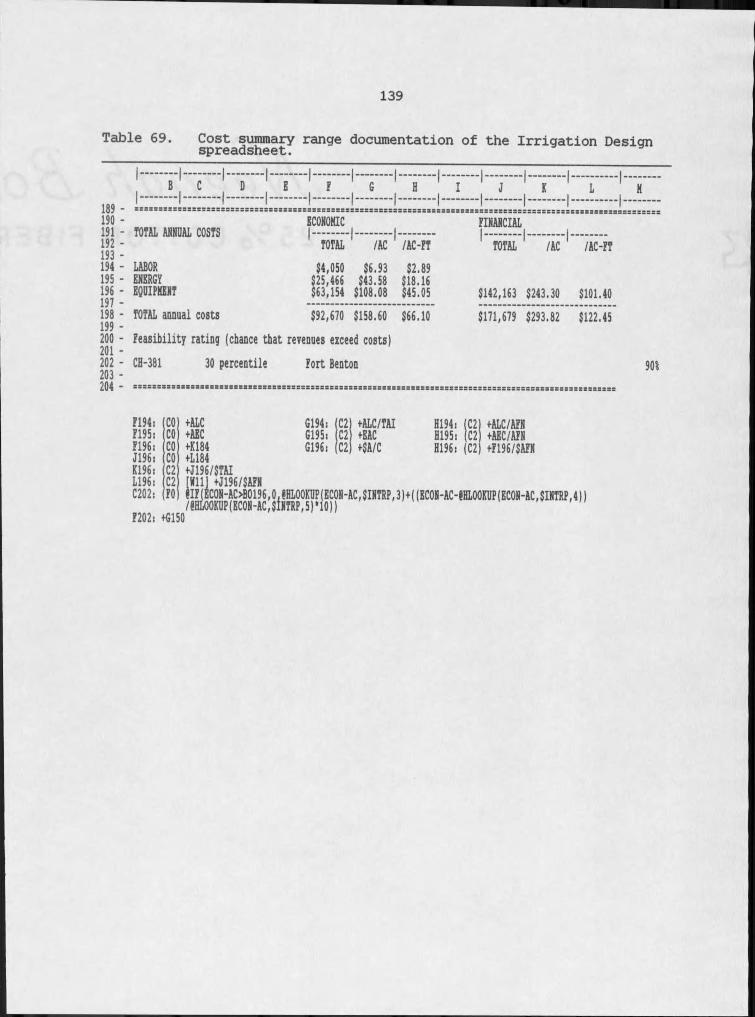
139

Table 69. Cost summary range documentation of the Irrigation Designspreadsheet.

189 - ================================190 -191 - TOTAL A8KUAL COSTS192 -

ECONOMIC7 . . . . 1. . . . 1 FINANCIAL

I . i I

' TOTAL ' /AC ' /AC-FT ' TOTAL /AC /AC-FT193 -194 - LABOR $4,050 $6.93 $2.89195 - ENERGY $25,466 $43.58 $18.16196 - EQUIPMENT197 -

$63,154 $108.08 $45.05 $142,163 $243.30 $101.40198 - TOTAL annual costs199 -

$92,670 $158.60 $66.10 $171,679 $293.82 $122.45200 - feasibility rating (chance that revenues exceed costs)201 -

202 - CH-381 30 percentile203 -I A i I __________________________________________ _________

fort Benton 90%204 " =z=rs====5====sss======sc=s=c=3========c=========ss=r=======zE=e============z===============;s=======

F194: COF195: COF196: COJ196: COK196: C2L196: C2C202: FOF202: +G150

+ALC G194: C2 +ALC/TAI H194i C2| +ALC/AFN+AEC G195: C2 +EAC H195: C2) +AEC/AEN+K184 G196i C2 +SA/C 8196: C2) +F196/SAE8+L184+J196/$rAI [811] +J196/5AE8

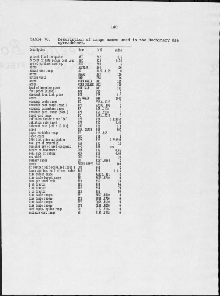
140

Table 70. Description of range names used in the Machinery Use spreadsheet.Description Name Cell Valuepercent flood irrigation IEI F62 0.5percent of ASAE repair cost used IRC F28 0.75age of purchase used eg. AGE F60 5acres ALFALFA B44 100annual user range AU A122..N169 0acres BEANS B43 100bottom width BND F58 16acres CORN GRAIN B41 100acres CORN SILAGE B42 100head of breeding stock CON-CALF B47 100fuel price (diesel) DFP F29 Idiscount from list price DIS F25 0.8acres DL GRAIN B46 1000economic costs range SC T183..AC23 0economic cost range (cont.) ECS AF183..A02 0economic parameters range EP A65..J108 0economic para, range (cont.) EPP K60..T108 0fixed cost range FC A183..J227 0inflation factor since "84" IFF F24 1.124864inflation rate (awe) IFR F22 0.04interest rate (.01 = 10.001) INR F21 0.1acres IRR. GRAIN B45 100input variables range labor costs IV

LBC A15..K65F31 0I1984 list price multiplier max. yrs of ownership LPM

MAI F26 0.899891F30 10purchase new or used equipment N-U F59 newreturn on investment RET F32 0.05real rate of return RRR F23 0.06row width RND F57 20summary range SO A227..G263 0acres SUGAR BEETS B40 100if swather self-propelled input I SNT F61 0taxes and ins. as I of ave. value TSI F27 0.015time budget range time table budget range TB

TM AA122..AL1EG69..EP10 00tons per truck axle TPA F56 10I st tractor TRl F53 902 nd tractor TR2 F54 703 rd tractor TR3 F55 50time table ranges TT AN67..BU10 0time table ranges TTS BU68..CP10 0time table ranges TTT CQ68..DL10 0time table ranges TTU DL68..EG10 0used equip, option range

variable cost rangeUO 0122..V166 0VC K183..S238 0

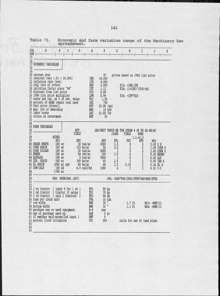
141

Table 71. Economic and farm variables range of the Machinery Use spreadsheet.COL A B CR o n I . . . . . . . . . I . . . I - - -1617 ECOXOKIC VARIABLES181920 current year21 interest rate (.01 = 10.OOi)22 inflation rate (ave)23 real rate of return24 inflation factor since "84"25 discount from list price26 1984 list price multiplier27 taxes and ins. as I of ave. value28 percent of ASAE repair cost used29 fuel price (diesel)30 max. yrs of ownership31 labor costs32 return on investment333435 FARK VARIABLES

E F H I J

87 prices based on 1984 list price IXR 10.OOiIFR 4.00iRRR 6.00iIFF 1.12DIS 0.80LPK 0.90F&I I. Si IRC 751DFP $1.00 /galKAE 10 yrsLBC $1.00 /hrRE! 51

F23i +INR-IFR F24, (l+IFR)A(F20-84)F26; +IFF1DIS

363738 ACRES

ES!.YIELD LBS/UXIT IRDCE-HR TON STRAW I OF IR AE-HR/AC /LOAD YIELD USED 1.2,or,339 ACS ESY IPU TPL TSY ITU APA40 SUGAR BEETS 100 ac 20 ton/ac 2000 2.5 0 3 5.00 S B41 CORN GRAIN 100 ac 125 bu/ac 56 2.5 2 2 1.08 CORN G42 CORK SILAGE 100 ac 20 ton/ac 2000 I 0 3 2.00 CORN S43 BEANS 100 ac 24 cwt/ac 100 2.5 0 I 0.30 BEANS44 ALFALFA 100 ac 5 ton/ac 2000 I 0 I 0.50 ALF45 IRR. GRAIN 100 ac 100 bu/ac 60 2.5 2 2 0.95 IRR G46 DL GRAIN 1000 ac cpd 45 bu/ac 60 2.5 0.25 2 0.36 DL G47 COW-CALF48 100 hd

1700 ac 0.9 calf/hd 1500 6 I 2 0.51 C-C49

B48: tSUK(B40..B47)


505 1 --5253 I st tractor54 2 nd tractor55 3 rd tractor56 tons per truck axle57 row widty58 bottom width59 purchase new or used equipment60 age of purchase used eg.61 if swather self-propelled input I62 percent flood irrigation6465

J40: +D401F40/2000/$!PA1G40+H40/$TPA

TRl 90 hpTR2 70 hpTR3 50 hpTPA 10 tonRWD 20 "BWD 16 "N-U newAGE 5 yrSWT 0)FI 501

1.7 ft H63: +RKD/121.3 ft H64: +8KD/12

calls for use of land plane

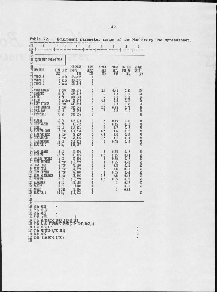
142

Table 72. Equipment parameter range of the Machinery Use spreadsheet.COL K B C D E F G H II. . . . . . . .'65 ' - ' ' 1 1 16667 EQUIPMENT PARAMETERS6869 PURCHASE USER SPEED FIELD HR USE POWER70 MACHINE SIZE UNIT PRICE INPUT MPH EFF. PER AC UNIT71 SIZ PUP INP SPD FEF HUA PWU72 TRUCK 3 2 axle $38,695 073 TRUCK 2 2 axle $38,695 074 TRUCK I75 2 axle $38,695 076 CORN HEADER 6 row $10,799 0 2.5 0.65 0.51 12077 COMBINE 24 ft $85,715 0 3 0.7 0.16 12078 DISK 14 ft $10,664 0 4 0.8 0.18 9079 PLOW 4 bottom $8,579 0 4.5 0.8 0.43 9080 BEET DIGGER 4 row $47,994 0 3 0.7 0.59 9081 CORN CHOPPER 4 row $35,546 0 2.5 0.65 0.76 9082 TOOL BAR 20 ft $8,099 0 5 0.8 0.10 9083 TRACTOR I8485 HARROW

90 bp $32,396 0 9030 ft $19,123 0 5 0.85 0.06 7086 CULTIVATOR 15 ft $3,672 0 5 0.85 0.13 7087 DRILL 20 ft $14,511 0 4 0.7 0.15 7088 PLANTER CORN 8 row $14,218

$8,5190 4.5 0.6 0.23 7089 PLANTER BEET 8 row 0 4.5 0.6 0.23 7090 DEFOLIATOR 4 row $6,916 0 2.5 0.7 0.71 7091 BALER(ROUND)92 TRACTOR 2

9312 ft 70 bp $16,333$25,197 00 5 0.75 0.18 7070

94 LAND PLANE 12 ft $4,054 0 6 0.85 0.13 5095 SPRAYER 48 ft 3,825 0 6.5 0.65 0.04 5096 ROLLER PACKER 12 ft $4,054 0 6 0.85 0.13 5097 BEST THINNER 4 row $10,799 0 4 0.75 0.41 5098 CORN CULT. 8 row $5,190 0 5 0.8 0.15 5099 BEET CULT. 8 row $4,799 0 5 0.8 0.15 50100 BEAN CUTTER 4 row $2,040 0 4 0.75 0.41 50101 BEAN WINDROWER 4 row $5,246 0 3.5 0.8 0.44 50102 SWATHER 12 ft $10,259 0 4.5 0.75 0.20 50103 FARMHAND 6 ft%

0 I 0.27 50104 SCROPF 6 ft 0 I 0.76 50105 AUGER 8 Z41 $2,814 0 I 0.05106 TRACTOR 3 50 bp $16,873 0 50107108 109H O B83: +TRl111 891: +8102112 892: +TR2113 BIOS: +TR3 - I114 D72: H F ($872=1,28000,43000)‘L h115 H76: 8.25/(F76*B76*G76*HF(C76=’ROr,H$63,l))117 178:' HFITRi=O,TR2,TR1)118 185: +TR2119 1102: HF(SMT=1,0,TR3)120

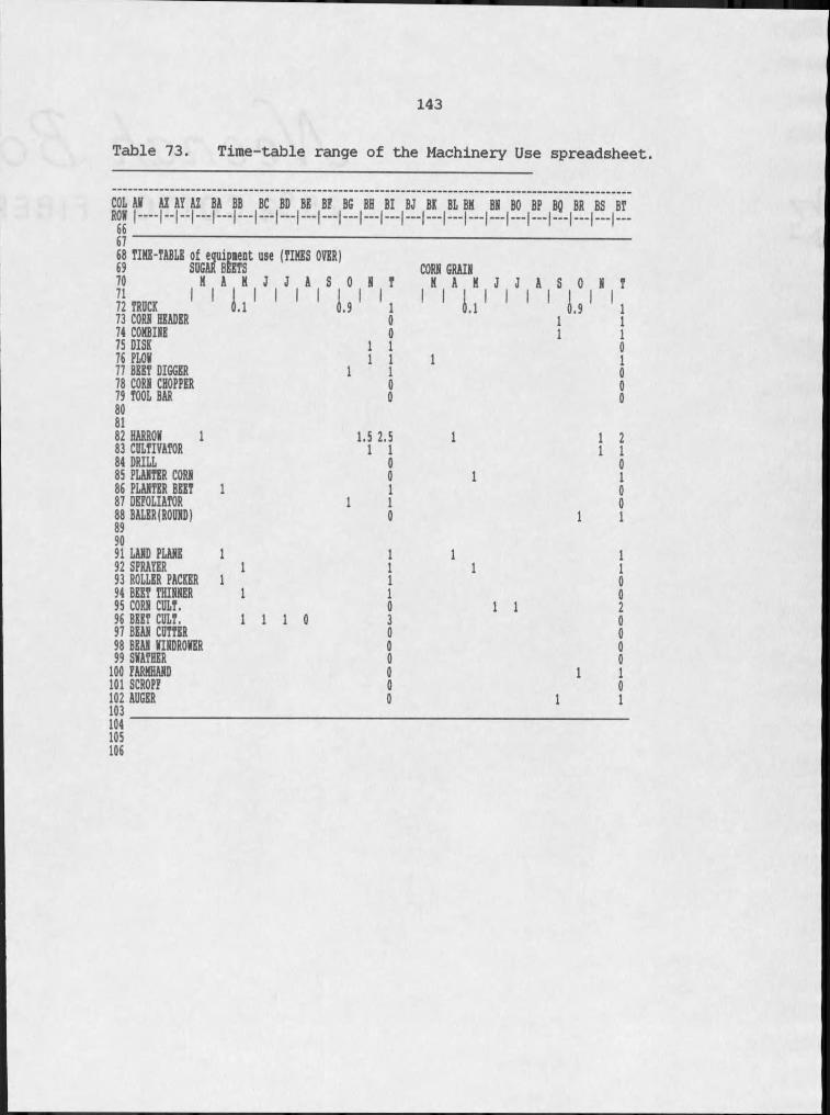
143

Table 73. Time-table range of the Machinery Use spreadsheet.

COL AU Al AY AZ BA BB BC BD BE BE BG BH BI BJ BK BL BK BH BO BP BQ BR BS BTr o i i - h - H H H H H — I H H H H H H H H H H H H H H H - - -b b _ _ _ _ _ _ _ _ _ _6768 TIKE-TABLE of equipment use (TIKES OVER)69 SUGAR BEETS CORN GRAIN70 K A71 I " ) ' ! ' ) " ! 8 ! 0 I * ! 1 I k I a I k I j I j I A | S O N72 TRUCK 1.1 1.9 ' 'l 1 1 L 1 11 I I 1.9 I 1 I73 CORH HEADER 0 I I74 COKBIHE 0 I I75 DISK I I 076 PLOV I I I I77 BEET DIGGER I I 078 CORH CHOPPER 0 079 TOOL BAR80 81

0 0

82 HARROV I 1.5 2.5 I I 283 CULTIVATOR I I I I84 DRILL 0 085 PLAHTER CORH 0 I I86 PLAHTER BEET I I 087 DEFOLIATOR I I 088 BALER (ROUHD)8990

0 I I

91 LAHD PLAHE I I I I92 SPRAYER I I I I93 ROLLER PACKER I I 094 BEST THINNER I I 095 CORN CULT. 0 I I 296 BEET CULT. 1 1 1 0 3 097 BEAN CUTTER 0 098 BEAH VINDROVER 0 099 SVATHER 0 0100 FARMHAND 0 I I101 SCROPF 0 0102 AUGER103 0 I I104105106

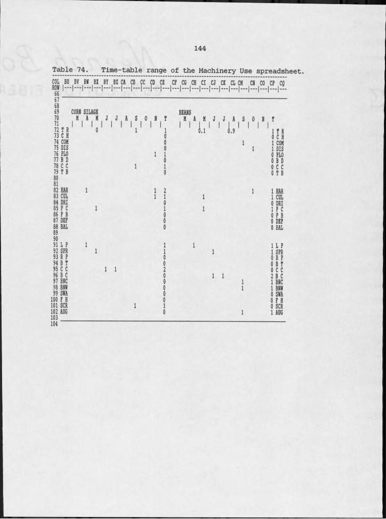
144

Table 74. Time-table range of the Machinery Use spreadsheet.COL BII onv I_ BV BI BY BZ CA CB CC CD CE ,CF ,CG ,CH Cl CJ CE CL CK CR co cp eg

676869 CORR SILAGE BEARS7071 I* | A l" j A S O R / ,Y lV | 0 1 H | T72 T R I I 0 I I I I i I I I I I 1.1 I I 1.9 I T R73 C H 0 0 C H74 COK 0 I I COH75 DIS 0 I I DIS76 PLO I I 0 PLO77 B D 0 0 B D78 C C I I 0 C C79 I B80 81

0 0 T B

82 HAS I I 2 I I HAR83 CllL I I I I CDL84 DRI 0 0 DRI85 P C I I I I P C86 P B 0 0 P B87 DEP 0 0 DEF88 BAL8990

0 0 BAL

91 L P I I I I L P92 SPR I I I I SPR93 R P 0 0 R P94 B T 0 0 B F95 C C I I 2 0 C C96 B C 0 I I 2 B C97 BRC 0 I I BRC98 BRW 0 I I BRI99 SWA 0 0 SWA100 F H 0 0 F H101 SCR I I 0 SCR102 ADG103 0 I I AOG104

145

COL eg CR CS Cr CU CV CM cx ct CZ DA DB DC DO DK DK DG DH DI DJ DK DL ROM I I I I I I I , I , I I I , I I I I I— I— I— I—6 7 - - - - - - - - - - - - - - - - - - - - - - - - - - - - - - - - - - - - - - - - - - - - - - - -

Table 75. Time-table range of the Machinery Use spreadsheet.

6869 ALFALFA70 M A H J J A S 0 K T! In 1 1 1 1,1,1,' ' I , 1,73 C H 074 COM 075 DIS 076 PLO 0 0.277 B D 078 C C 079 T B 0808182 HAR 083 CDL 084 DRI 085 P C 086 P B 087 DBF 088 BAL 1 1 I 3899091 L P 0.2 0.292 SPR I I93 R P 094 B T 095 C C 096 B C 097 BHC 098 BHM 099 SKA 1 1 1 3100 F H 1 1 I 3101 SCR 0102 ADG 0103

104105106

IRR. GRiIHM A H J J i S O H TM , 1 1 I , 1 1 1

0 C HI I COM1 DIS I PLO 0 B D 0 C C 0 T B

I HAR0 CDL1 DRI 0 P C 0 P B 0 DKF

I I BAL

I L PI I SPR0 R P0 B T0 C C0 B C0 BHC0 BHMI I SMAI IFH0 SCR

I I ADG

146

Table 76. Time-table range of the Machinery Use spreadsheet.COLDL DM DM DO DP DQ DR DS DI DD DV DM DZ DI DZ EA EB EC ED EE EE00676869 DL GRAIN COM-CALF70 N A71 i l l H

I , Y 1Y 1Y 1Y , Y l Y i 8 I72 I R I1 ' ' I1 . 5 1 . 5 I 1 . 3 i i i i I . , 1 ,73 C H 0 074 COM I I 075 DIS i I 076 PLO 0 077 B D 0 078 C C 0 079 I B I 2 I 0 4 08081

82 BAR 0 083 CDL 0 084 DRI I I 085 P C 0 086 P B 0 087 DBF 0 088 BAL 0 0899091 L P 0 092 SPR i I 093 R P 0 094 B I 0 095 C C 0 096 B C 0 097 BMC 0 098 BMV 0 099 SMA 0 0100 F B 0 6.6 6.6101 SCR 0 0102 ADG I I 0103

104105106

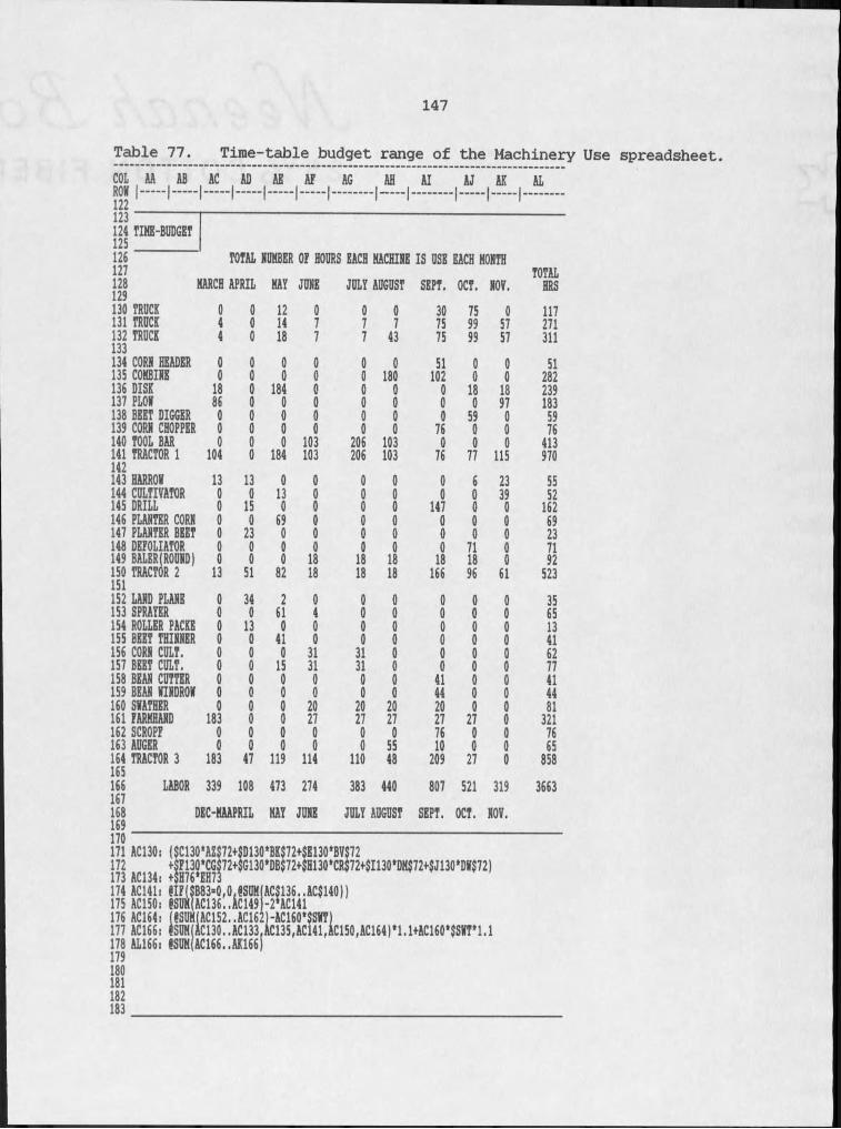
147

Table 77. Time-table budget range of the Machinery Use spreadsheet.COL AA ABDAW I. . . I___ AC AD AE AF AG AH Al AJ AK AL

I . . . . . . . . . . . . . I I I i i— I. . . . . .123124 TINE-BODGHT125126 TOTAL NUMBER OF HOURS EACH MACHINE IS USE EACH MONTH127 TOTAL128 MARCH APRILIlQ MAY JUNE JULY AUGUST SEPT. OCT. NOV. HRS130 TRUCK 0 0 12 0 0 0 30 75 0 117131 TRUCK 4 0 14 7 7 7 75 99 57 271132 TRUCK133 4 0 18 7 7 43 75 99 57 311134 CORN HEADER 0 0 0 0 0 0 51 0 0 51135 COHBINE 0 0 0 0 0 180 102 0 0 282136 DISK 18 0 184 0 0 0 0 18 18 239137 PLON 86 0 0 0 0 0 0 0 97 183138 BEET DIGGER 0 0 0 0 0 0 0 59 0 59139 CORN CHOPPER 0 0 0 0 0 0 76 0 0 76140 TOOL BAR 0 0 0 103 206 103 0 0 0 413141 TRACTOR I142 104 0 184 103 206 103 76 77 115 970143 HARROW 13 13 0 0 0 0 0 6 23 55144 CULTIVATOR 0 0 13 0 0 0 0 0 39 52145 DRILL 0 15 0 0 0 0 147 0 0 162146 PLANTER CORN 0 0 69 0 0 0 0 0 0 69147 PLANTER BEET 0 23 0 0 0 0 0 0 0 23148 DEFOLIATOR 0 0 0 0 0 0 0 71 0 71149 BALER(ROUND) 0 0 0 18 18 18 18 18 0 92150 TRACTOR 2151 13 51 82 18 18 18 166 96 61 523152 LAND PLANE 0 34 2 0 0 0 0 0 0 35153 SPRAYER 0 0 61 4 0 0 0 0 0 65154 ROLLER PACKS 0 13 0 0 0 0 0 0 0 13155 BEET THINNER 0 0 41 0 0 0 0 0 0 41156 CORN CULT. 0 0 0 31 31 0 0 0 0 62157 BEET CULT. 0 0 15 31 31 0 0 0 0 77158 BEAN CUTTER 0 0 0 0 0 0 41 0 0 41159 BEAN WINDROW 0 0 0 0 0 0 44 0 0 44160 SWATHER 0 0 0 20 20 20 20 0 0 81161 FARMHAND 183 0 0 27 27 27 27 27 0 321162 SCROPF 0 0 0 0 0 0 76 0 0 76163 AUGER 0 0 0 0 0 55 10 0 0 65164 TRACTOR 3165 183 47 119 114 n o 48 209 27 0 858166 LABOR167 339 108 473 274 383 440 807 521 319 3663168 DEC-NAAPRIL MAY JUNE JULY AUGUST SEPT. OCT. NOV.169171 AC130: ($C130‘AZ$72t$D130‘BK$72tSE130*BV$72173 AC134: +$H76'EH7:174 AC141, HF(SB83-fl,O.ISIlM(ACS136..AC$140))175 AC150: BSDK(AC136..AC149)-2*AC141176 AC164:177 AC166:178 AL166: BSDM(AC166..AK166179180 181 182 183

+SF130'CGj72+$G130*DB$72+$H130*CR$72+$I130*DK$72+$J130*D1f$72) +JH

IFSUH(AC152..AC162)-AC160‘$SlfTI fSUH(AC130..AC133)AC135,AC141,AC150,AC164)*l, !+AciOOtJSlfTtL l

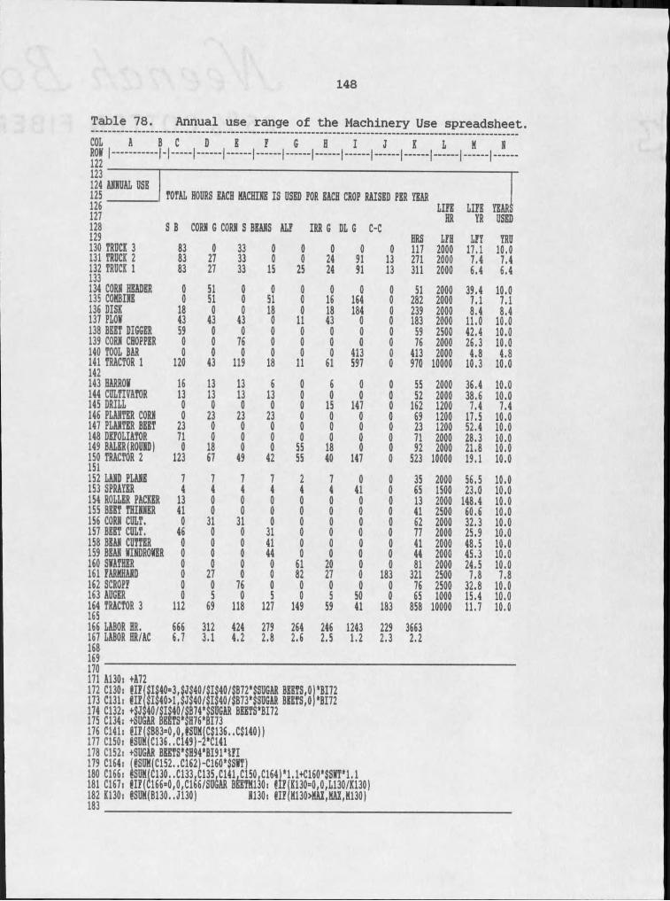
148

Table 78. Annual use range of the Machinery Use spreadsheet.COL A B C

I .................... l . i ___D E F G H I J K L M H

123124 ARHUAL USE125 TOTAL HOURS EACH MACHIKE IS USED FOR EACH CROP RAISED PER YEAR126 LIFE LIFE YEARS127 HR YR USED128 S B CORK G CORK S BEARS ALF IRR G DL G C-C129 HRS LFH LFY YRU130 TRUCK 3 83 0 33 0 0 0 0 0 117 2000 17.1 10.0131 TRUCK 2 83 27 33 0 0 24 91 13 271 2000 7.4 7.4132 TRUCK I133 83 27 33 15 25 24 91 13 311 2000 6.4 6.4134 CORH HEADER 0 51 0 0 0 0 0 0 51 2000 39.4 10.0135 COHBIHE 0 51 0 51 0 16 164 0 282 2000 7,1 7.1136 DISK 18 0 0 18 0 18 184 0 239 2000 8.4 8.4137 PLOi 43 43 43 0 11 43 0 0 183 2000 11.0 10.0138 BEET DIGGER 59 0 0 0 0 0 0 0 59 2500 42.4 10.0139 CORH CHOPPER 0 0 76 0 0 0 0 0 76 2000 26.3 10.0140 TOOL BAR 0 0 0 0 0 0 413 0 413 2000 4.8 4.8141 TRACTOR I 120 43 119 18 11 61 597 0 970 10000 10.3 10.0142143 HARROi 16 13 13 6 0 6 0 0 55 2000 36.4 10.0144 CULTIVATOR 13 13 13 13 0 0 0 0 52 2000 38.6 10.0145 DRILL 0 0 0 0 0 15 147 0 162 1200 7.4 7.4146 PLAHTER CORN 0 23 23 23 0 0 0 0 69 1200 17.5 10.0147 PLAHTER BEET 23 0 0 0 0 0 0 0 23 1200 52.4 10.0148 DEFOLIATOR 71 0 0 0 0 0 0 0 71 2000 28.3 10.0149 BALER(ROUHD) 0 18 0 0 55 18 0 0 92 2000 21.8 10.0150 TRACTOR 2151 123 67 49 42 55 40 147 0 523 10000 19.1 10.0152 LAHD PLAHE 7 7 7 7 2 7 0 0 35 2000 56.5 10.0153 SPRAYER 4 4 4 4 4 4 41 0 65 1500 23.0 10.0154 ROLLER PACKER 13 0 0 0 0 0 0 0 13 2000 148.4 10.0155 BEET THIHHER 41 0 0 0 0 0 0 0 41 2500 60.6 10.0156 CORH CULT. 0 31 31 0 0 0 0 0 62 2000 32.3 10.0157 BEET CULT. 46 0 0 31 0 0 0 0 77 2000 25.9 10.0158 BEAH CUTTER 0 0 0 41 0 0 0 0 41 2000 48.5 10.0159 BEAH iIHDROiER 0 0 0 44 0 0 0 0 44 2000 45.3 10.0160 SiATHER 0 0 0 0 61 20 0 0 81 2000 24.5 10.0161 FARMHAHD 0 27 0 0 82 27 0 183 321 2500 7.8 7.8162 SCROPF 0 0 76 0 0 0 0 0 76 2500 32.8 10.0163 AUGER 0 5 0 5 0 5 50 0 65 1000 15.4 10.0164 TRACTOR 3 112 69 118 127 149 59 41 183 858 10000 11.7 10.0165166 LABOR HR. 666 312 424 279 264 246 1243 229 3663167 LABOR HR/AC 6.7 3.1 4.2 2.8 2.6 2.5 1.2 2.3 2.2168169170171 A130. +A72172 C130s iIF(SIS40-3,SJi40/SIS40/SB72‘SSDGlR BiiISfOltB m173 C131: « ? $I$40>1.$J$40/SI$40/$B73‘$S0GAR BEEISfO ‘BI72174 C132: +SJS40/SIS40/SB74tSSDGAR BEEIS‘BI72175 C134: +SUGAR BEETS‘$H76tBI73176 C141: m(SB83-0,0,tSUM(C$136..C$140))177 ClSOi ESUH(C136..C149)-2‘C141178 C152i +SUGAR BEETStSHSAtBISltIEI179 C164i (EsuM(ClSI--Cm)-ClSOtSSiT)180 C166; iSUM(C130..C133.C135.C141.C150.C164]tl.l+C160t$SiTtl.l181 C167: eiE(Cl66=0,0,C166/SU6AR BEETMUOi fIE(K130=0,0,L130/K130)182 K130: ESUM(B130.,J130) N130i EIE(M130>MAXfMAI,M130)183 _ _ _ _ __ _ _ _ _ _ _ _ _ _ _ _ _ _ _ _ _ _ _ _ _ _ _ _

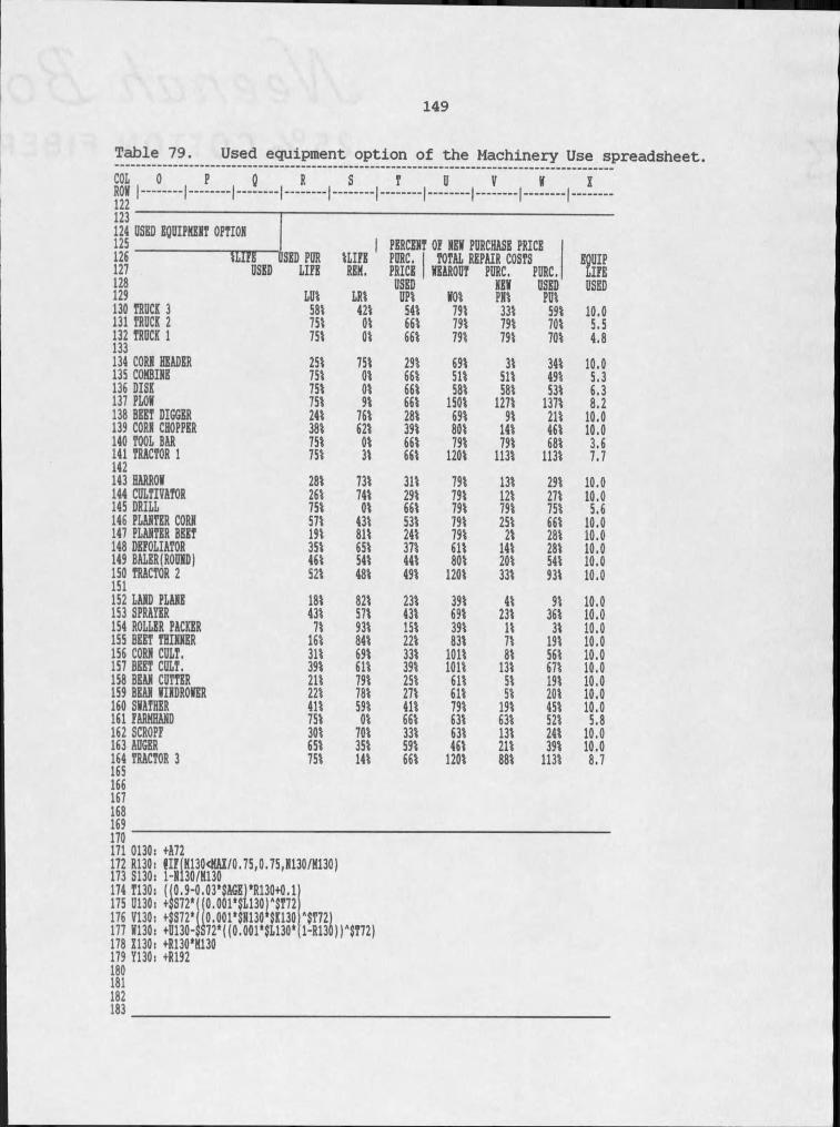
149

Table 79. Used equipment option of the Machinery Use spreadsheet.COL 0 P 9cne I- - - - 1. . . . i_ :_ _ ...» i. S T U V W I1 22 . . . . . . . . . . . . . . . . . . . . . . . . . ' '- - - - '. . . .123124 USED EQDIPKHIir OPTION125 PERCEN ' OF NEW PURCHASE PRICE126 UIPE ISED PUR !LIFE PURC. TOTAL REPAIR COSTS EQUIP127 USED LIFE REM. PRICE WEAROUT PURC. PURC. LIFE128 USED NEW USED USED129 LUl LRl UPl WOl PNl PUl130 TRUCK 3 581 421 541 791 331 591 10.0131 TRUCK 2 751 01 661 791 791 701 5.5132 TRUCK I 751 01 661 791 791 701 4.8133134 CORE HEADER 251 751 291 691 31 341 10.0135 COMBINE 751 01 661 511 511 491 5.3136 DISK 751 01 661 581 581 531 6.3137 PLOW 751 91 661 1501 1271 1371 8.2138 BEET DIGGER 241 761 281 691 91 211 10.0139 CORN CHOPPER 381 621 391 801 141 461 10.0140 TOOL BAR 751 01 661 791 791 681 3.6141 TRACTOR I142 751 31 661 1201 1131 1131 7.7143 HARROW 281 731 311 791 131 291 10.0144 CULTIVATOR 261 741 291 791 121 271 10.0145 DRILL 751 01 661 791 791 751 5.6146 PLANTER CORN 571 431 531 791 251 661 10.0147 PLANTER BEET 191 811 241 791 21 281 10.0148 DEFOLIATOR 351 651 371 611 141 281 10.0149 BALER(ROUND) 461 541 441 801 201 541 10.0150 TRACTOR 2151 521 481 491 1201 331 931 10.0152 LAND PLANE 181 821 231 391 41 91 10.0153 SPRAYER 431 571 431 691 231 361 10.0154 ROLLER PACKER 71 931 151 391 11 31 10.0155 BEET THINNER 161 841 221 831 71 191 10.0156 CORN CULT. 311 691 331 1011 81 561 10.0157 BEET CULT. 391 611 391 1011 131 671 10.0158 BEAN CUTTER 211 791 251 611 51 191 10.0159 BEAN WINDROWER 221 781 271 611 51 201 10.0160 SWATHER 411 591 411 791 191 451 10.0161 FARMHAND 751 01 661 631 631 521 5.8162 SCROPF 301 701 331 631 131 241 10.0163 AUGER 651 351 591 461 211 391 10.0164 TRACTOR 3 751 141 661 1201 881 1131 8.7165166167168169H O171 0130: +A72172 R130: fIFjH130<HU/0.75,0.75,lil30/M130)174 1130i ((0.9-0.03*$AGK)*R130+0.1175 U130: +5S72*((0.001*$L130I*$172176 V130: t$S72‘ (0.001‘$H130‘$!130 ,$T72|177 «130: +D130-}S72*((0.M1*$L130* 1-R130))A$T72)178 1130: +R130'M130179 Y130: +R192180 181 182 183

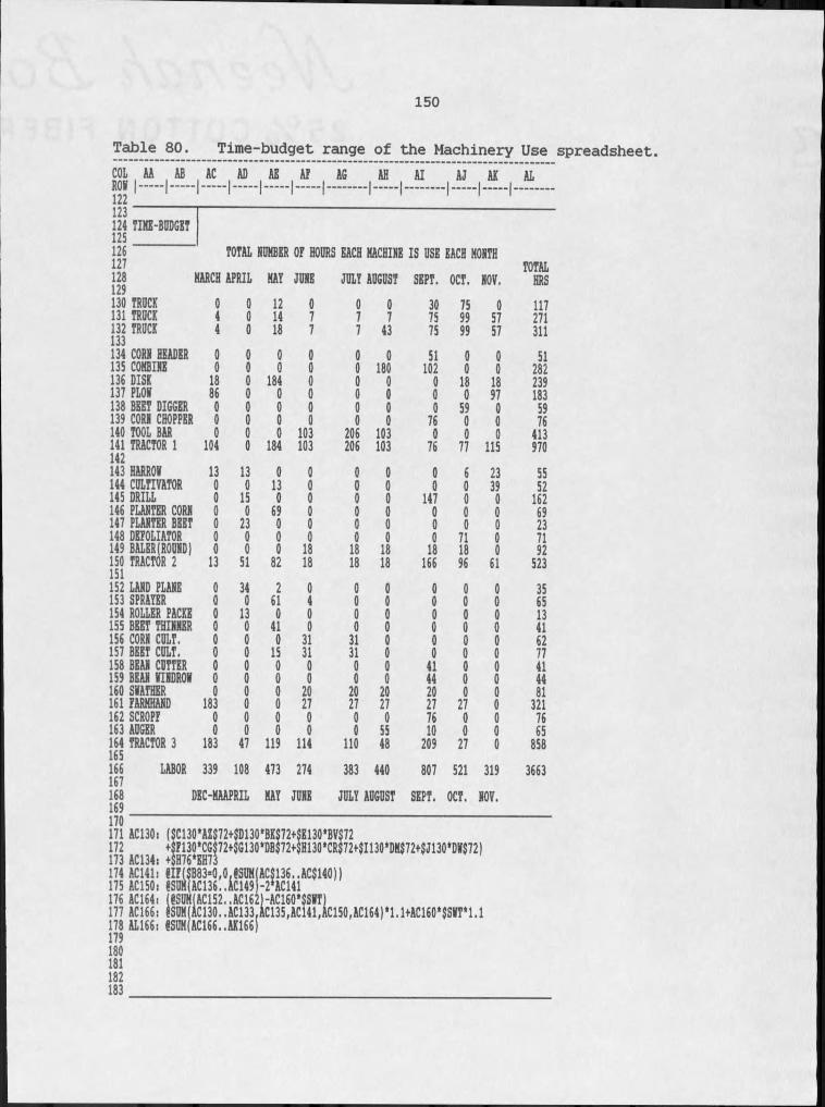
150

Table 80. Time-budget range of the Machinery Use spreadsheet.COL AA AB AC AU AE AF AGP n if I ............. I .............. I .............. I .............. I _______ I ...............I ....................

, AH Al AJ AK AL1 2 2123124 TIKE-BUDGET125 __126 TOTAL NUMBER OF HOURS EACH MACHINE IS USE EACH MONTH127128 I129 MARCH APRIL MAY JUNE JULY AUGUST SEPT. OCT. NOV. TOTAL

HRS130 TRUCK 0 0 12 0 0 0 30 75 0 117131 TRUCK 4 0 14 7 7 7 75 99 57 271132 TRUCK 4 0 18 7 7 43 75 99 57 311133134 CORN HEADER 0 0 0 0 0 0 51 0 0 51135 COMBINE 0 0 0 0 0 180 102 0 0 282136 DISK 18 0 184 0 0 0 0 18 18 239137 PLOW 86 0 0 0 0 0 0 O 97 183138 BEET DIGGER 0 0 0 0 0 0 0 59 0 59139 CORN CHOPPER 0 0 0 0 0 0 76 0 0 76140 TOOL BAR 0 0 0 103 206 103 0 0 0 413141 TRACTOR I 104 0 184 103 206 103 76 77 115 970142143 HARROW 13 13 0 0 0 0 0 6 23 55144 CULTIVATOR 0 0 13 0 0 0 0 0 39 52145 DRILL 0 15 0 0 0 0 147 0 0 162146 PLANTER CORN 0 0 69 0 0 0 0 0 0 69147 PLANTER BEET 0 23 0 0 0 0 0 0 0 23148 DEFOLIATOR 0 0 0 0 0 0 0 71 0 71149 BALER(ROUND) 0 0 0 18 18 18 18 18 0 92150 TRACTOR 2151 13 51 82 18 18 18 166 96 61 523152 LAND PLANE 0 34 2 0 0 0 0 0 0 35153 SPRAYER 0 0 61 4 0 0 0 0 0 65154 ROLLER PACKE 0 13 0 0 0 0 0 0 0 13155 BEET THINNER 0 0 41 0 0 0 0 0 0 41156 CORN CULT. 0 0 0 31 31 0 0 0 0 62157 BEET CULT. 0 0 15 31 31 0 0 0 0 77158 BEAN CUTTER 0 0 0 0 0 0 41 0 0 41159 BEAN WINDROW 0 0 0 0 0 0 44 0 0 44160 SWATHER 0 0 0 20 20 20 20 0 0 81161 FARMHAND 183 0 0 27 27 27 27 27 0 321162 SCROPF 0 0 0 0 0 0 76 0 0 76163 AUGER 0 0 0 0 0 55 10 0 0 65164 TRACTOR 3 183 47 119 114 HO 48 209 27 0 858165166 LABOR 339 108 473 274 383 440 807 521 319 3663167168 DSC-MAAPRIL MAY JUNE JULY AUGUST SEPT. OCT. NOV.169170171 AC130: ($C130*AZ$72+$D130*BK$72+$E130*BVS72172 +SF130‘CG$72+$G130‘DB$72+ H130,CR$72t$I130‘DM$72t$J130*DI$72)173 AC134: +$H76‘EH73174 AC141: HF(SB83=0,0.4SUM(ACS136..AC$140))175 ACISO1 eSUH(AC136..AC149)-2$AC141176 AC164: NSGM(AC152..AC162)-AC160,$SNT)177 AC166: iSUM(AC130..AC133,AC135,AC141,AC150,AC164)'l.l+AC160%SMT*l.l178 AL166: 4SUM(AC166..AK166179180 181 182 183

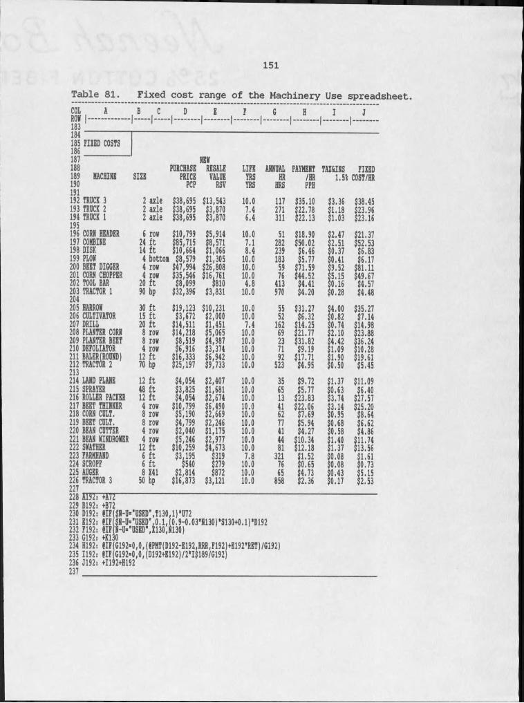
151

Table 81. Fixed cost range of the Machinery Use spreadsheet.COL A ROV I. . . . . .183184185 HIED COSTS186187188189 NACHHE190191192 TRUCK 3193 TRUCK 2194 TRUCK I195196 CORH HEADER197 COKBHE198 DISK199 PLOW200 BEET DIGGER201 CORN CHOPPER202 TOOL BAR203 TRACTOR I204205 HARROW206 CULTIVATOR207 DRILL208 PLANTER CORN209 PLANTER BEET210 DEFOLIATOR

B C H

NEW

212 TRACTOR 2213214 LAND PLANE215 SPRAYER216 ROLLER PACKER217 BEET THINNER218 CORN CULT.219 BEET CULT.220 BEAN CUTTER221 BEAN WINDROWER222 SWATHER223 FARMHAND224 SCROPF225 AUGER226 TRACTOR 3227228 A192: +A72229 B192; +872230 D192: H F231 E192: H F232 F192= H F233 G192: +Kl30234 H192, H F235 1192, HF236 J192, +I192+H192237

PURCHASE RESALE LIFE ANNUAL PAYMENT TAXSINS FIXEDSIZE PRICE VALUE H S HR /HR 1.51 COST/HRPCP RSV YRS HRS PPH2 axle $38,695 $13,543 10.0 117 $35.10 $3.36 $38.452 axle $38,695 $3,870 7.4 271 $22.78 $1.18 $23.962 axle $38,695 $3,870 6.4 311 $22.13 $1.03 $23.166 row $10,799 $5,914 10.0 51 $18.90 $2.47 $21.3724 ft 85,715 8,571 7.1 282 $50.02 $2.51 $52.5314 ft $10,664 $1,066 8.4 239 $6.46 $0.37 $6.834 bottoi $8,579 $1,305 10.0 183 $5.77 $0.41 $6.174 row $47,994 $26,808 10.0 59 $71.59 $9.52 $81.114 row $35,546 $16,761 10.0 76 $44.52 $5,15 $49.6720 ft $8,099 $810 4.8 413 $4.41 $0.16 $4.5790 hp $32,396 $3,831 10.0 970 $4.20 $0.28 $4.4830 ft $19,123 $10,231 10.0 55 $31.27 $4.00 $35.2715 ft $3,672 $2,000 10.0 52 $6.32 $0.82 $7.1420 ft $14,511 $1,451 7.4 162 $14.25 $0.74 $14.988 row $14,218 $5,065 10.0 69 $21.77 $2.10 $23.888 row 8,519 $4,987 10.0 23 $31.82 $4.42 $36.244 row $6,916 3,374 10.0 71 $9.19 $1.09 $10.2812 ft $16,333 $6,942 10.0 92 $17.71 $1.90 $19.6170 hp $25,197 $9,733 10.0 523 $4.95 $0.50 $5.4512 ft $4,054 $2,407 10.0 35 $9.72 $1.37 $11.0948 ft $3,825 $1,681 10.0 65 $5.77 $0.63 $6.4012 ft $4,054 $2,674 10.0 13 $23.83 $3.74 $27.574 row $10,799 6,490 10.0 41 $22.06 3.14 $25.208 row $5,190 $2,669 10.0 62 $7.69 $0.95 $8.648 row $4,799 $2,246 10.0 77 $5.94 $0.68 $6.624 row $2,040 $1,175 10.0 41 $4.27 $0.58 $4.864 row $5,246 $2,977 10.0 44 $10.34 $1.40 $11.7412 ft $10,259 $4,673 10.0 81 $12.18 $1.37 $13.566 ft $3,195 319 7.8 321 $1.52 $0.08 $1.616 ft $540 $279 10.0 76 $0.65 $0.08 $0.738 K41 $2,814 $872 10,0 65 $4,73 $0.43 $5.1550 bp $16,873 $3,121 10.0 858 $2.36 $0.17 $2.53

I-U=1USED',T130,1)‘U72iV'USED1 "il30' Inoj0 *8130+0.1) *D1926192=0,0,(fPHT(D192-E192,RRR,F192)+E192,RET)/G192) G192=0,0,(D192+E192)/2,I$189/G192)

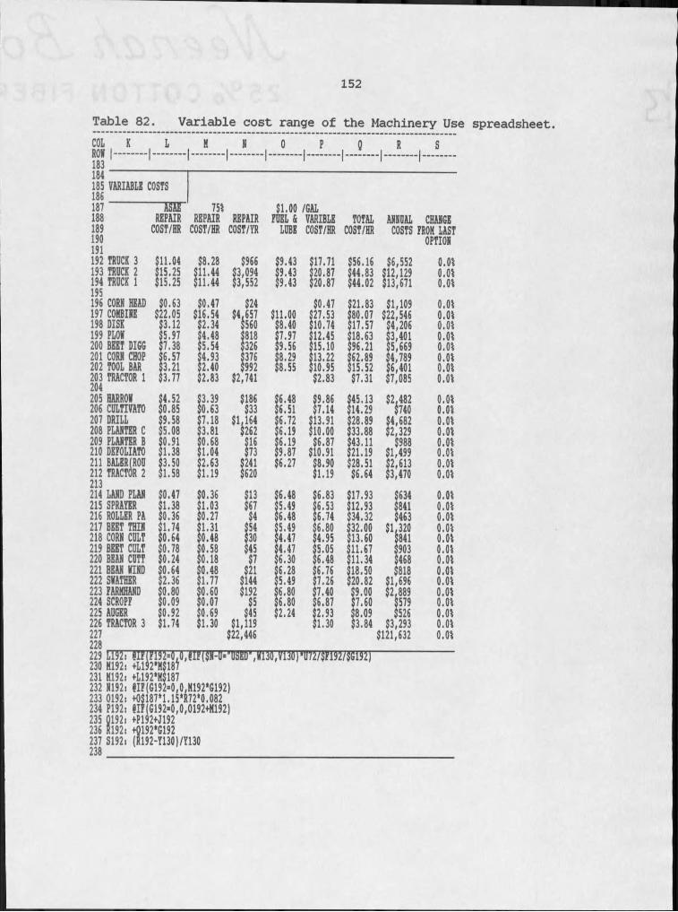
152

Table 82. Variable cost range of the Machinery Use spreadsheet.COL KDMT I_ _ _ _ _ A M N 0 P 6 R Sm . . . . . . . . . . . . . . . . . . . . . . . . . . . . . . 1 — '. . . .184185 VARIABLE COSTS186187 ASAE 751 $1.00 /GAL188 REPAIR REPAIR REPAIR FUEL & VARIBLE TOTAL ANNUAL CHANGE189 COST/HR COST/HR COST/YR LUBE COST/HR COST/HR COSTS FROM LAST190191 OPTION192 TRUCK 3 $11.04 $8.28 $966 $9.43 $17.71 $56.16 $6,552 0.01193 TRUCK 2 $15.25 $11.44 $3,094 $9.43 $20.87 $44.83 $12,129 0.01194 TRUCK II Q C

$15.25 $11.44 $3,552 $9.43 $20.87 $44.02 $13,671 0.01ItfJ196 CORK HEAD $0.63 $0.47 $24 $0.47 $21.83 $1,109 0.01197 COMBINE $22.05 $16.54 $4,657$560 $11.00 $27.53 $80.07 $22,546 0.01198 DISK $3.12 $2.34 $8.40 $10.74 $17,57 $4,206 0.01199 PLON 5.97 $4.48 818 7.97 12.45 $18.63 $3,401 0.01200 BEET DIGG $7.38 $5.54 $326 $9.56 $15.10 $96.21 $5,669 0.01201 CORN CHOP $6.57 4.93 $376 $8.29 13.22 $62.89 $4,789 0.01202 TOOL BAR $3.21 $2.40 $992 $8.55 $10.95 $15.52 $6,401 0.01203 TRACTOR I204 $3.77 $2.83 $2,741 $2.83 $7.31 $7,085 0.01205 HARROW $4.52 $3.39 $186 $6.48 $9.86 $45.13 $2,482 0.01206 CULTIVATO $0.85 $0.63 $33 $6.51 $7.14 $14.29 $740 0.01207 DRILL $9.58 $7.18 ilSlii $6.72 $13.91 $28,89 $4,682 0.01208 PLANTER C $5.08 $3.81 $6.19 $10.00 $33.88 $2,329 0,01209 PLANTER B $0.91 $0.68 $16 6.19 $6.87 $43.11 $988 0.01210 DEFOLIATO $1.38 $1.04 $73 $9.87 $10.91 $21.19 $1,499 0.01211 BALER)ROU $3.50 $2.63 $241 $6.27 $8.90 $28.51 $2,613 0.01212 TRACTOR 2213 $1.58 $1.19 $620 $1.19 $6.64 $3,470 0.01214 LAND PLAN $0.47 $0.36 $13 $6.48 $6.83 $17.93 $634 0.01215 SPRAYER $1.38 1.03 $67 $5.49 $6.53 $12.93 $841 0.01216 ROLLER PA $0.36 $0.27 $4 $6.48 $6.74 $34.32 $463 0.01217 BEET THIN 1.74 $1.31 $54 $5.49 $6.80 $32.00 $1,320 0.01218 CORN CULT $0.64 $0.48 $30 $4.47 $4.95 $13.60 $841 0.01219 BEET CULT $0.78 $0.58 $45 $4.47 $5.05 $11.67 $903 0.01220 BEAN CUTT $0.24 $0.18 $7 $6.30 $6.48 $11.34 $468 0.01221 BEAN WIND $0.64 $0.48 $ 2 1 $6.28 $6.76 $18.50 $818 0.01222 SNATHER $2.36 $1.77 $144 $5.49 $7.26 $20.82 $1,696 0.01223 FARMHAND $0.80 $0,60 $192 $6.80 $7.40 $9.00 $2,889 0.01224 SCROPF $0.09 $0.07 $5 $6.80 $6.87 $7.60 $579 0.01225 AUGER $0.92 $0.69 $45 $2,24 $2.93 $8.09 $526 0.01226 TRACTOR 3 $1.74 $1.30 $1,119 $1.30 $3.84 $3,293 0.01227228 $22,446 $121,632 0.01229 L192: eiF|F192=^0,MF(SN-U=’USED',N130,V130)'U72/SF192/SG192)231 M192, tL192*M$187232 N192: HF(G192'O,0.H192*G192)233 0192: +08187*1.15'R72'0.082234 P192: fIF(G192=0,0,0192+M192)235 0192: +P192+J192236 K192: +0192*6192237 S192: (R192-Y130I/Y130238

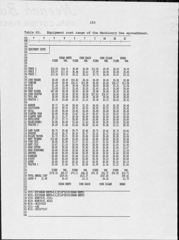
153

Table 83. Equipment cost range of the Machinery Use spreadsheet.col r oDAtf I- - - - 1- - - - J.... * X Y Z AA Afi AC1 83 . . . . . . . . . . . . . . . . . . . . . . . . . . . . . . 1 '- - - - '- - - -184185 BQUIPKEET COSTS186187188 SUGAR BEETS CORN GRAIN CORN SILAGE BEANS189190 FIXED VAR. FIXED VAR. FIXED VAR. FIXED VAR.191192 TRUCK 3 $32.05 $14.76 $0.00 $0.00 $12.82 $5.90 $0.00 $0.00193 TRUCK 2 $19.97 $17.39 $6.44 $5.61 $7.99 $6.96 $0.00 $0.00194 TRUCK I195 $19,30 $17.39 $6.22 $5,61 $7.72 $6.96 $3.47 $3.13196 CORH HEADER $0.00 $0.00 $10.85 $0.24 $0.00 $0.00 $0.00 $0.00197 COMBINE $0.00 $0.00 $26.67 $13.98 $0.00 $0.00 $26.67 $13.98198 DISK $1.26 $1.98 $0.00 $0.00 $0.00 $0.00 $1.26 $1.98199 PLOE $2.65 5.35 $2.65 $5.35 $2.65 $5.35 $0.00 0.00200 BEET DIGGER $47.80 $8.90 $0.00 $0.00 $0.00 $0.00 $0.00 $0.00201 CORN CHOPPER $ 0 . 0 0 $0.00 $0.00 $0.00 $37.83 $10.07 $0.00 $ 0 . 0 0202 TOOL BAR $0.00 $0,00 $0.00 $0.00 $0.00 $0.00 $0.00 $0.00203 TRACTOR I204 $5.39 $3.40 $1.93 $1.21 $5.34 $3,37 $0.83 $0.52205 HARRO* $5.71 $1.60 $4.56 $1.28 $4.56 $1.28 $2.28 $0.64206 CULTIVATOR $0.92 $0.92 $0.92 $0.92 $0.92 $0.92 $0.92 $0.92207 DRILL $0.00 $0.00 $0.00 $0.00 $0.00 $0.00 $0.00 $0.00208 PLANTER CORN $0.00 $0.00 $5.47 $2.29 $5.47 $2.29 $5.47 $2.29209 PLANTER BEET 8.31 $1.57 $0.00 $0.00 $0.00 $0.00 $0.00 $0.00210 DEFOLIATOR $7.27 $7.72 $0.00 $0.00 $0.00 $0.00 $0.00 $0.00211 BALER(ROUND)212 TRACTOR 2213

$0.00$6.69 $0.00$1.46 $3.60$3.66 $1.63$0.80 $0.00$2.66 $0.00$0.58 $0.00$2.31 $0.00$0.50

214 LAND PLANE $0.75 $0.46 $0.75 $0.46 $0.75 $0.46 $0.75 $0.46215 SPRAYER $0.26 $0.27 $0.26 $0.27 $0.26 $0.27 $0.26 0.27216 ROLLER PACKER $3.72 $0.91 $0.00 $0.00 $0.00 $0.00 $0.00 $0.00217 BEET THINNER $10.40 $2.80 $0.00 $0.00 $0.00 $0.00 $0.00 $ 0 . 0 0218 CORN CULT. $0.00 $0.00 $2.67 $1.53 $2.67 $1.53 $0,00 $0.00219 BEET CULT. $3.07 $2.35 $0.00 $0.00 $0.00 $0.00 $2.05 $1,56220 BEAN CUTTER $0.00 $0.00 $0.00 $0.00 $0.00 $0.00 $2.00 $2.67221 BEAN NINDR0VER $0.00 $0.00 0.00 $0.00 $0.00 $0.00 $5.19 $2.99222 SVATHER $0.00 $0.00 $0.00 $0.00 $0.00 $0.00 $0.00 $0.00223 FARMHAND $0.00 $0.00 $0.44 $2.03 $0.00 $0.00 $0.00 0.00224 SCROPF $0.00 $0.00 $0.00 $0.00 $0.56 $5.23 $0.00 $0.00225 AUGER $0.00 $0.00 0.26 $0.15 $0.00 $0.00 $0.26 $0.15226 TRACTOR 3 $2.84 $1.46 $1.75 $0.90 $2.99 $1.54 $3.22 $1.66L L l

228 FIXED VAR. FIXED VAR. FIXED VAR. FIXED VAR.229 $178.34 $90.67 $79.11 $44.26 $95.18 $52.70 $56.94 $33.72230 TOTAL ANNUAL COST $269.01 $123.37 $147,88 $90.66231 LABOR @ $1.00 $6.66 $3.12 $4.24 $2.79233234235

SUGAR BEETS CORN GRAIN CORN SILAGE BEANS

236 mi-. eirisuGAK B6KTS=o,o ,5cII3I) jiD2/su(;ak bkki'S) H F SUGAR BRETS=O,0,SC130‘$P192/SUGAR BEETS) fSUR(V192..V22«)

237 *192:238 V229:239 *229: iSUMj*192..*226240 *230: +W229+V229241 U231: +LBC242 *231: +$U231‘C167243244

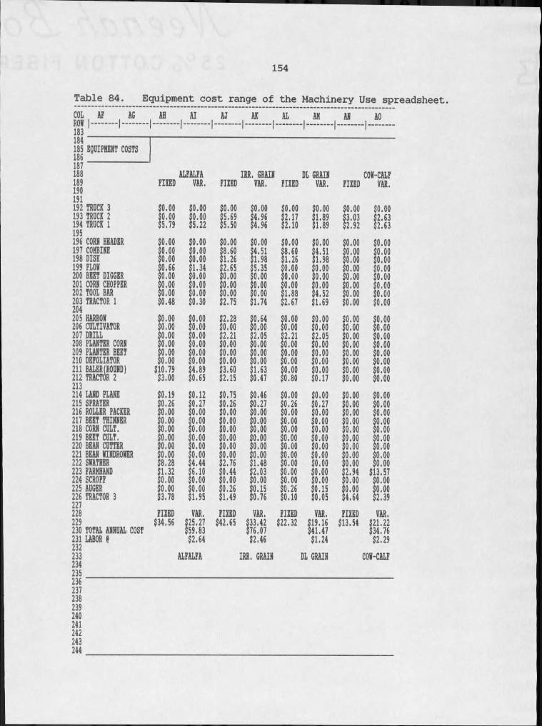
154

Table 84. Equipment cost range of the Machinery Use spreadsheet.COL AJ AGDnv I. . . . . I. . . . . . Al AJ AK AL AK AN AO1 83 . . . . . . . . . . . . . . . . . . . . . . . . . . . . . . . . . . . . '- - - - '- - - -184185 EQOIPfflllT COSTS186187188 ALPALPA IRR. GRAIN DL GRAIN COH-CALP189190 PIKED VAR. PIKED VAR. PIKED VAR. PIKED VAR.191192 TROCK 3 $0.00 $0.00 $0.00 $0.00 $0.00 $0.00 $0.00 $0.00193 TROCK 2 $0.00 $0.00 5.69 $4.96 $2.17 $1.89 $3.03 $2.63194 TROCK I195 $5.79 $5.22 $5.50 $4.96 $2.10 $1.89 $2.92 $2.63196 CORK HEADER $0.00 $0.00 $0.00 $0.00 $0.00 $0.00 $0.00 $0.00197 COKBIHE $0.00 $0.00 $8.60 $4.51 $8.60 $4.51 $0.00 $0.00198 DISK $0.00 $0.00 $1.26 $1.98 $1.26 $1.98 $0.00 $0.00199 PLOH $0.66 $1.34 2.65 $5.35 $0.00 $0.00 $0.00 $0.00200 BEET DIGGER $0.00 $0.00 $0.00 $0.00 $0.00 $0.00 $0.00 $0.00201 CORN CHOPPER $0.00 $0.00 0.00 0.00 $0,00 $0.00 $0.00 0.00202 TOOL BAR $0.00 $0.00 $0.00 $0.00 $1.88 $4.52 $0.00 $0.00203 TRACTOR I204 $0.48 $0.30 $2.75 $1.74 $2.67 $1.69 $0.00 $0.00205 HARROW $0.00 $0.00 $2.28 $0.64 $0.00 $0.00 $0.00 $0.00206 CULTIVATOR $0.00 $0.00 $0.00 $0.00 $0.00 $0.00 $0.00 $0.00207 DRILL $0.00 $0.00 $2.21 $2.05 2.21 $2.05 $0.00 $0.00208 PLANTER CORN $0.00 $0.00 $0.00 $0.00 $0.00 $0.00 $0.00 $0.00209 PLANTER BEET $0.00 $0.00 $0.00 0.00 $0.00 $0.00 $0.00 $0.00210 DEPOLIATOR $0.00 $0.00 $0.00 $0.00 $0.00 $0.00 $0.00 $0.00211 BALER(ROOND)212 TRACTOR 2 $10.79 $4.89 $3.60 $1.63 $0.00 $0.00 $0.00 $0.00$3.00 $0.65 $2.15 $0.47 $0.80 $0.17 $0.00 $0.00213214 LAND PLANE $0.19 $0.12 $0.75 $0.46 $0.00 $0.00 $0.00 $0.00215 SPRAYER $0.26 $0.27 $0.26 $0.27 $0,26 $0.27 $0.00 $0.00216 ROLLER PACKER $0.00 $0.00 $0.00 $0.00 $0.00 $0.00 $0.00 $0.00217 BEET THINNER $0.00 $0.00 $0.00 $0.00 $0.00 $0.00 $0.00 $0.00218 CORN COLT. $0.00 $0.00 $0.00 $0.00 $0.00 $0.00 $0,00 $0.00219 BEET CULT. $0.00 $0.00 $0.00 $0.00 $0.00 $0.00 $0.00 $0.00220 BEAN CUTTER $0.00 $0.00 $0.00 $0.00 $0.00 $0.00 $0.00 $0.00221 BEAN HINDROHER $0.00 $0.00 $0.00 $0.00 $0.00 $0.00 $0.00 $0.00222 SHATHER $8.28 $4.44 $2.76 $1.48 $0.00 $0.00 $0.00 $0.00223 PARKHAND 1.32 6.10 $0.44 $2.03 $0.00 $0.00 $2.94 $13.57224 SCROPP $0.00 $0.00 $0.00 $0.00 $0.00 $0.00 $0.00 $0.00225 AUGER $0.00 $0.00 0.26 $0.15 $0.26 0.15 $0.00 $0.00226 TRACTOR 3 $3.78 $1.95 $1.49 $0.76 $0.10 $0.05 $4.64 $2.39LU228 PIKED VAR. PIKED VAR. PIKED VAR. PIKED VAR.229 $34.56 $25.27 $42.65 $33.42 $22.32 $19.16 $13.54 $21.22230 TOTAL ANNUAL COST $59,83 $76,07 $41.47 $34.76231 LABOR @232

$2.64 $2.46 $1.24 $2.29233 ALPALPA IRR. GRAIN DL GRAIN COH-CALP234235236237238239240241242243244

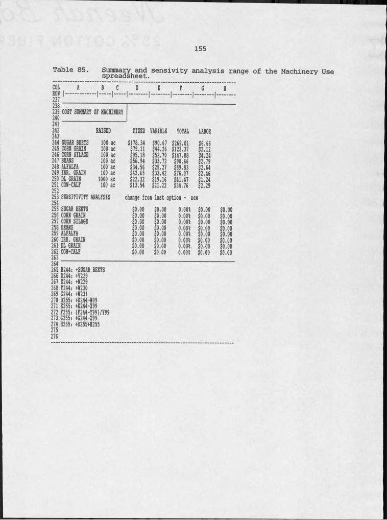
155

Table 85. Summary and sensivity analysis range of the Machinery Use spreadsheet.COL A B CBMf I- - - - - - - - - 1___ I___ D E F G H237 ' i l l I i i i238239 COST SOHMARY Oi MACHINERY240241 '242 RAISED243 FIXED VARIBLE TOTAL LABOR244 SUGAR BEETS 100 ac $178.34 $90.67 $269.01 $6.66245 CORN GRAIN 100 ac $79.11 $44.26 $123.37 $3.12246 CORN SILAGE 100 ac $95.18 $52.70 $147.88 $4.24247 BEANS 100 ac $56.94 $33.72 $90.66 $2.79248 ALFALFA 100 ac $34.56 $25.27 $59.83 $2.64249 IRR. GRAIN 100 ac $42.65 $33.42 $76.07 $2.46250 DL GRAIN 1000 ac $22.32 $19,16 $41.47 $1.24251 CON-CALF 100 ac252 $13.54 $21.22 $34.76 $2.29253 SENSITIVITY ANALYSIS change from last option - new255 SUGAR BEETS $0.00 $0.00 0.00% $0.00 $0.00256 CORN GRAIN $0.00 $0.00 0.00% $0.00 $0.00257 CORN SILAGE $0.00 $0.00 0.00% $0.00 $0.00258 BEANS $0.00 $0.00 0.00% $0.00 $0.00259 ALFALFA $0.00 $0.00 0.00% $0.00 $0.00260 IRR. GRAIN $0.00 $0.00 0.00% $0.00 $0.00261 DL GRAIN $0.00 $0.00 0.00% $0.00 $0.00262 CON-CALF263 $0.00 $0.00 0.00% $0.00 $0.00264265 B244: +SUGAR BEETS266 D244: +V229267 E244: +N229268 F244: +N230269 G244: +N231270 D255: +D244-N99271 E255i +E244-I99272 F255, (F244-Y99)/Y99273 G255: +G244-Z99274 H255: +D255+E255275276

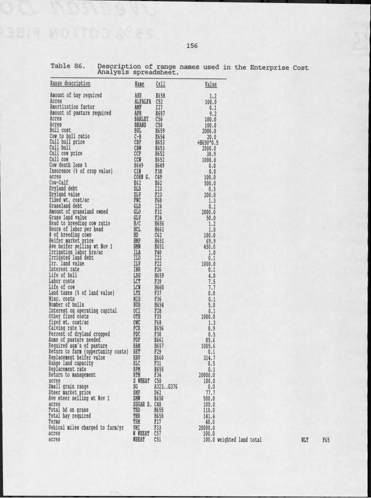
156

Table 86. Description of range names used in the Enterprise CostAnalysis spreadsheet.Range description Name CellAmount of hay required AflR B658Acres ALFALFA C52Amortization factor AHF 127Amount of pasture required APR E657Acres BARLEY C56Acres BEANS C50Bull cost BUL E659Cow to bull ratio C-B E654Cull bull price CBP H653Cull bull CBN E653Cull cow price CCP H652Cull cow CCH E652Cow death loss I H649 H649Insurance (I of crop value) CIN F38acres CORN G. C49Cow-Calf E62 E62Dryland debt DLD 123Dryland value DLV F23fixed wt. cost/ac FHC F68Grassland debt GLD 124Amount of grassland owned GLO F32Grass land value GLV F24Head to breeding cow ratio H/C H656Hours of labor per bead HCL H661♦ of breeding cows HD C62Heifer market price Ave heifer selling wt Hov I HHP H651HHH E651Irrigation labor brs/ac ILA F40Irrigated land debt ILD 122Irr. land value ILV F22Interest rate INR F26Life of bull LBU H659Labor costs LCT F39Life of cow LCH H660Land taxes (% of land value) LTZ F37Hisc. costs HIS F36Number of bulls NUB H654Interest on operating capital OCI F28Other fixed costs OTH F35fixed wt. cost/ac OHC F68Calving rate % PCR E656Percent of dryland cropped PDC P30Aums of pasture needed PDF E661Required aus's of pasture RAH H657Return to farm (opportunity costs) Replacement heifer value

RETRHV

F29E660Range land capacity RLC F31Replacement rate Return to management RPKRTK E655F34acres S HHEAT C58Small grain range SG A323..G376Steer market price Ave steer selling wt Nov I SKP D62SHH E650acres SUGAR B. C48Total hd on grass THD H655Total hay required THR H658Terms TRH F27Vehical miles charged to farm/yr VKI F33acres H HHEAT C57acres KHEAT C51

Value1.2100.00.19.2

100.0100.02000.020.0+H650*0.52000.038.91000.00.00.0

100.0500.0 0.5200.01.30.12000,050.0 1.21.0

100.069.9450.01.0 0.11000.0 0.14.0 7.5 7.7 0.0 0.15.0 0.11000.01.3 0.9 0.585.6

1085.6 0.1

314.7 0.5 0.120000.0100.00.077.7500.0100.0118.0141.640.020000.0100.0100.0 weighted land total m i F65

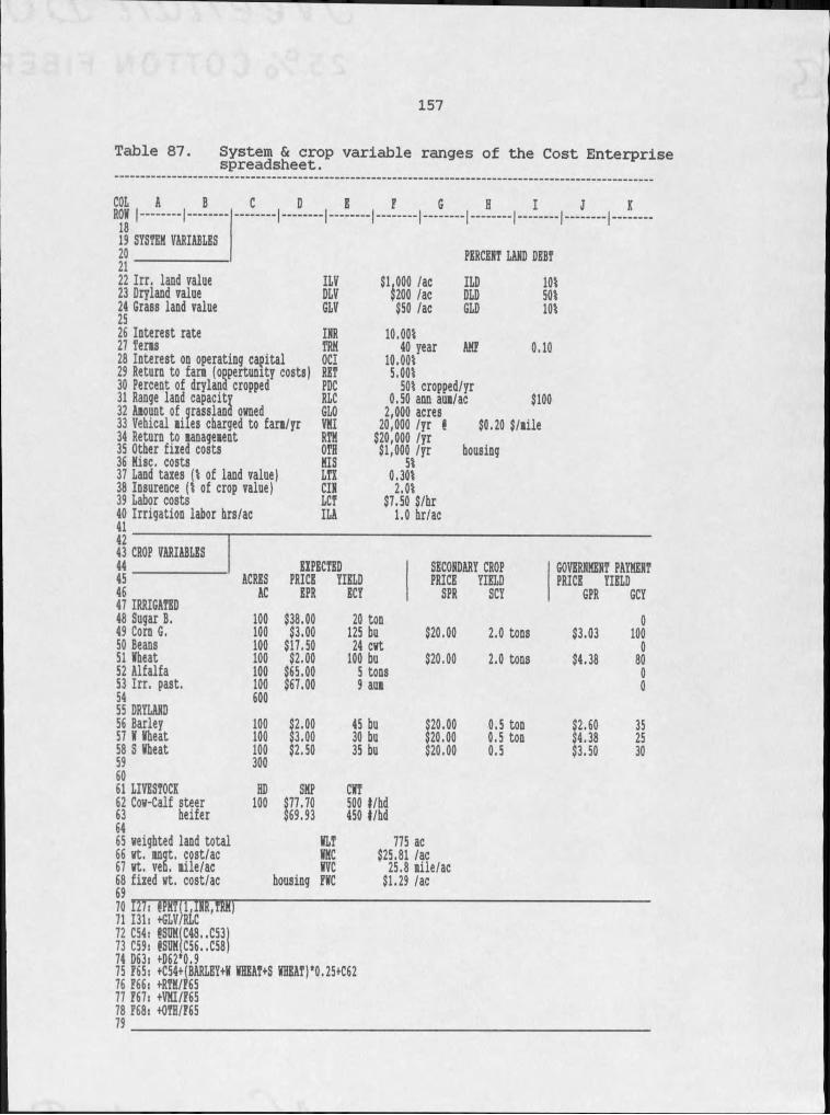
157

Table 87. System & crop variable ranges of the Cost Enterprise spreadsheet.

- I -BCOLROM I -

1819 SYSTEM VARIABLES20 21 PERCEHT land debt22 Irr. land value ILV $1,000 /ac ILD 10%23 Dryland value DLV $200 /ac DLD 50%24 Grass land value25 GLV $50 /ac GLD 10%26 Interest rate IHR27 Tens TRM28 Interest on operating capital OCI29 Return to fan (opportunity costs) RET30 Percent of dryland cropped PDC31 Range land capacity RLC32 Aiount of grassland owned GLO33 Vehical miles charged to fan/yr VMI34 Return to management RTM35 Other fixed costs OTH36 Misc. costs MIS37 Land taxes (I of land value) LTX38 Insurence (I of crop value) CIH39 Labor costs LCT40 Irrigation labor hrs/ac ILA4142

AMF10.00%40 year10.00%5.00%

50% cropped/yr 0.50 ann aua/ac 2,000 acres

0.10

$10020.000 /yr520.000 /yr51.000 /yr

0.30%2.0%57.50 S/hr 1.0 hr/ac

t $0.20 S/milehousing

43 CROP VARIABLES44 EXPECTED SECONDARY CROP GOVERNMENT PAYMENT45 ACRES PRICE YIELD PRICE YIELD PRICE YIELD4647 IRRIGATED AC EPR ECY SPR SCY GPR GCY48 Sugar B. 100 $38.00 20 ton 049 Corn G, 100 $3.00 125 bu $20.00 2.0 tons $3.03 10050 Beans 100 $17.50 24 cwt 051 Mheat 100 $2.00 100 bu $20.00 2.0 tons $4.38 8052 Alfalfa 100 $65.00 5 tons 053 Irr. past. 100 $67.00 9 aum 05455 DRYLAND 60056 Barley 100 $2.00 45 bu $20.00 0.5 ton $2.60 3557 M Mheat 100 $3.00 30 bu $20.00 0.5 ton $4.38 2558 S Mheat 100 $2.50 35 bu $20.00 0.5 $3.50 30596061 LIVESTOCK

300HD SMP CMT62 Cow-Calf steer 100 $77.70 500 t/hd63 heifer

6465 weighted land total$69.93 450 t/hd

MLT 77! ac66 wt. nngt. cost/ac MMC $25.81 /ac67 wt. veh, mile/ac MVC 25.8 mile/ac68 fixed wt. cost/ac69 housing FMC $1.29 /ac70 127: JPMT I,IHR1TRM)71 131: +GLV/RLC72 C54: @S0M(C48..C53)73 C59: @SUN(C56..C58)74 D63: +062*0.975 F65: +C54+(BARLEY+W MHEAT+S NHEAT)*0.25+C6276 F66: +RTM/F6577 F67: +VMI/F6578 F68: +OTH/F657 9 _ _ _ _ _ _ _

158

Table 88. Equipment and user entered variables ranges of the Enterprise Cost spreadsheet.COL A BRON I- - - - 1- - - - C D E F G H I J K81 1 '82 EQUIPMENT VARIABLES838485 MACHINERY COSTS IRRIGATION COSTS86 FIXED VAR. TOTAL LABOR FIXED VAR. ENERGY TOTAL87

$178.34 (hr/ac)88 Sugar B. $90.67 $269.01 6.66 $0.00 $10.00 $5.00 $15.0089 Corn G. $79.11 $44.26 $123.37 3.12 $0.00 $10.00 $5.00 $15.0090 Beans $56.94 $33.72 $90.66 2.79 $0.00 $10.00 $5.00 $15.0091 Nheat $42.65 $33.42 $76.07 2.46 $0.00 $10.00 $5.00 $15.0092 Alfalfa 34.56 $25.27 $59.83 2.64 $0.00 $10.00 $5.00 $15.0093 Irr. past,9495 Barley

$19.42 $16.40 $35.82 3.00 $0.00 $10.00 $5.00 $15.00$22.32 $19.16 $41.48 1.2496 N Nheat $22.32 $19.16 $41.48 1.24 $0.00 $0.00 $0.00 $0,0097 S Nheat9899 Cow-Calf$22.32 $19.16 $41.48 1.24 $0.00 $0.00 $0.00 $0.00$13.54 $21.22 $34.76 2.29

101102 USER ENTERED ENTERPRISE COSTS103 _104105 INPUT106107 - Sugar B.108 SB-I109 SB-2 HO SB-3111 V112 Hoe Beets113 P114 - - - - Com G.115 Furdan116 Laso117 Banvil118 Drying119 TNlNE120 storage121 - - - - Beans122 Benlate123 Treflan124 Eptae125 V126 V127 F128 . . . . Nbeat129 V130 2,4-D131 V132 Twine133 V134 storage135 . . . . Alfalfa136 soil nitrogen137 Furdan138 V139 V140 TNINE141 F142 - - - - - -

PRICE /UNIT CROP INPUT PRICE /UNIT RATE/UNIT

$47.15$0.98$0.45$25.00

0.610.016.01.01.01.0

V -Irr. pastVet. supplies Fencing o&e Cattle labor VF

$1.00 oz 10.0 V$0.18 oz 22.0 2,4 - D$0.42 oz 2.0 V$0.05 bu 125.0 V$2.00 ton 2.0 V$0.08 bu 125.0 storage$15.15 lb 2.0 V$46.80 gal 0.3 2,4 - D$23.65 oz 0.5 Vac Vac Vac storage

ac 2,4 - D$7.55 gal 0.3 Vac V$2.00 tons 2.0 Vac V$0.08 bu 100.0 F

-Barley

-N Nheat

-S Nheat

$0.25 lb $1.00 oz ac ac

$1.50 ton ac

-25.08.0-Cow-Calf

Hay StrawSalt & minerals Protien sup,VF

$0,00 ac 0.0$3.00 bd 3.2$2.00 ac 1.0$5,00 hr 1.0$4.00 acac$0.00 ac 0.0$7.00 gal 0.2$0.00 ac$0.00 ac$0.00 ac$0.08 bu 45.0$0.00 ac 0.0$7.00 gal 0.2$0,00 ac$0.00 ac$0.00 ac$0.08 bu 30.0$7.00 gal 0.2$0.00 gal 0.0$0.00 ac$0.00 ac$0.00 ac$0.08 bu 35.0$65.00 ton 1.4$20.00 ton 0.6$25.00 cwt 0.2$8.00 cwt 2.9$1.00 ac$1.00 ac

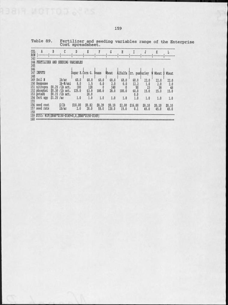
159

Table 89. Fertilizer and seeding variables range of the EnterpriseCost spreadsheet.

-I-COL A B C D

144 BERTILIZKR AXD SEEDING VARIABLES145

-I------1-

146147 INPUTS148

Ilugar B.iorn G. leans ILeat II

llfalfa lrr. paslarley I[ Vbeat iI Vheat149 Soil N Ib/ac 60.0 60.0 60,0 60.0 60.0 60.0 22.0 22.0 22.0150 Response Ib-N/uni 8.0 1.5 0.0 2.0 0.0 12.2 1.0 2.0 2.0151 nitrogen $0.25 /lb act. 100 128 0 140 0 50 23 38 48152 phospnat $0.30 /lb act. 125.0 63.0 100.0 28.0 100.0 60.0 15.0 15.0 15.0153 potash $0.15 /lb act. 20.0 0.0154 tert app155 $1.25 /ac 1.0 1.0 1.0 1.0 1.0 1.0 1.0 1.0 1.0156 seed cost S/lb $10.00 $0,82 $0.39 $0.10 $2.00 $16.00 $0.10 $0.10 $0.10157 seed rate Ib/ac 2.0 20.0 55.0 120.0 15.0 0.1 45.0 45.0 45.0159 DlSl: ?IF(SE48JDl50-D149<0,0,5E48’D150-D149)160 SS = 3 ,S * S3 = = = SSBSBSSSSSSS3S3SSSSSSSS = > = SEEB*BS3SS3 = 3S = S = BESSS = XSEXSSESSBSS3S3 = &XSB = SXSS = S5SS3X = S&

160

Iou = = = = = = = = = = = = = = = = = = = = = = = = = = = = = = = = = = = = = = = = = z = = = = = = = = = = = = = = 3 = = z = = = = = z = z = = = = = = = = = = = = z = = = = = = = = = = = = = =

161

Table 90. Enterprise cost analysis of sugar beets.

162 Sugar B.163 COST OP PRODDCTIOH 100.0 ACRES P162i +SUGAR B.164 PRICE /UNIT QUANT. COST165 VASIABLi COSTS166 F167: +D151'C167167 Hitrogen $0.25 lbs 100.0 $25.00 C167:+B151 E167: +D151168 Phosphate $0.30 lbs 125.0 $37.50 C168:+B152 E168: +D152169 Other Pert. $0.15 lbs 0.0 $0.00 C169i+B153 E169: +D153170 Pert. AppL $1.25 ac 1.0 1.25 C170i+B154 E170: +D154171 Seed $10.00 lbs 2.0 $20.00 C17L+D156 E171i +D157172 SB-I $47.15 oz 0.6 $27.82 C172i+C109 E172: +E109173 SB-2 $0.98 OZ 10.0 $9.80 C173.'+C110174 SB-3 $0.45 oz 16.0 $7.20 CMi+Clll175 V $0.00 ac 1.0 $0.00 C175i+C112176 Hoe Beets $25,00 ac 1.0 $25.00 C176:+C113177 Vehicle $0.20 miles 26 $5.16 C177s+H33 E177: +F$67178 Machinery $90.67 ac 1.0 $90.67 C178:+D$88179 Parting Labor $7.50 hr 6.66 $49.95 C179i+LCT E179: +F$88180 Irr. Labor $7.50 hr 1.0 $7.50 C180i+LCT E180: +ILA181 Irr Sys Op Costs $10.00 ac 1.0 $10.00 C181i+I$88 E183: (P2) +OCI182 Irr Energy Cost $5.00 ac 1.0 $5.00 C182i+J$88183 Int. On Op. Costs $321.85 $ 10.001 $32.18 C183:jSUK(F167..F182)184 Kics. Costs $321.85 $ 51 $16.09 E184: +MIS185 TOTAL VARIBLE COSTS

I O C$370.13 G185, eSUM(F167..F184)

187 PIIED COSTS188189 Machinery $178.34 ac 1.0 $178.34 C189i +C$88190 Management $25.81 S 1.0 $25.81 C190, +F$66191 housing $1.29 $ 1.0 $1.29 C191, +OHC192 Taxes (land & imp $1,000 ac 0.31 $3.00 C192: +ILV E192: +LTX193 Insurance $760 ac 2.01 $15.20 C193: +D48*E48 E193i +CIH194 Irr Sys Costs $0.00 ac 1.0 $0.00 C194: +H$88195 P $0.00 ac 1.0 $0.00 C195: +C114 E195: +E114196 Land $100 ac 0.10 $10.23 C196: +ILVILD E196: +AMP197 TOTAL PIPED COSTS198 $233.86 G197: PSUM(P189..P196)199 TOTAL COSTS ISugar B. $603.99 G199: +G197+G185200201 PRICE YIELD202 Return/acres P $38.00 20.0 ton $760.00 G202i +C202*D202+G48*H48203 Break EvenI A A

$30.20 15.9 ton C203: +G199/D202205 /ACRE /PARK B/C206 ROVC $389.87 C206: +G202-G185207 Profit(Ioss) $156.01 $15,601 1.26 C207: +G202-G199208 Labor Cost $57.45 $5,745 C208: +P180+P179209 Gov pmnt $0.00 $0 C209s (J48-D48)*K48210 D209: J48-D48 ‘K48*C48211 TOTAL EIPENCESo n

$60,399 D211: +P162*G199213 S = S S S S r S S S S S X S S S S S Z Z B S S S S S Z S S S S Z r Z S Z Z S S B S S S S S Z Z Z S Z S Z S Z Z S S S Z S S S Z B S Z Z S Z Z S S S B S Z Z S Z Z Z Z Z Z Z Z Z S S S S S S S S S S S

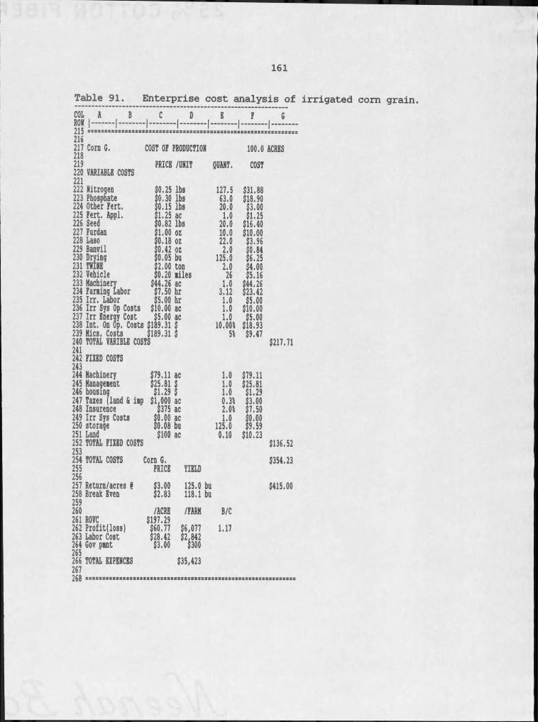
161

Table 91. Enterprise cost analysis of irrigated c o m grain.COL A ROV I- - -215 ========216217 Corn G.218 COST OF PRODUCTION219220 VARIABLE COSTS221

PRICE /UNIT QUANT.

222 Nitrogen $0.25 lbs 127.5223 Phosphate 0.30 lbs 63.0224 Other Pert. $0.15 lbs 20.0225 Fert. Appl. $1.25 ac 1.0226 Seed $0.82 lbs 20.0227 Furdan $1.00 Oi 10.0228 Laso $0.18 oz 22.0229 Banvil $0.42 oz 2.0230 Drying231 TWINE $0.05 bu

$2.00 ton125.02.0232 Vehicle $0.20 miles 26233 Machinery234 Farming Labor $44.26 ac 1.0$7.50 hr 3.12235 Irr. Labor $5.00 hr 1.0236 Irr Sys Op Costs $10.00 ac 1.0237 Irr Energy Cost $5.00 ac238 Int. On Op. Costs $189.31 $ 1.010.00%239 Hies. Costs $189.31 $ 5%240 TOTAL VARIBLE COSTS241242 FIXED COSTS243244 Hachinery

245 Hanageient246 housing247 Taxes (land & iip248 Insurence249 Irr Sys Costs250 storage251 Land252 TOTAL FIXED COSTS253254 TOTAL COSTS255256257 Return/acres t258 Break Even259260261 ROVC262 Profit(Ioss)263 Labor Cost264 Gov pint265266 TOTAL EXPEHCES267268 . . . . =====

$79.11 ac $25.81 $1.29 $1,000 ac $375 ac $0.00 ac $0.08 bu $100 ac

100.0 ACRES COST

$31.88 $18.90 $3.00 $1.25 $16.40

$10.00 $3.96 0.84 6.25 $4.00 $5.16 $44.26 $23.42 $5.00 $10.00 $5.00 $18.93 $9.47 $217.71

1.01,01.00.3%2.0%1.0125.0

0.10

$79.11$25.81$1.293.007.50

$0.00$9.59$10.23I

Corn G. PRICE YIELD

$136.52$354.23

$3.00$2.83 125.0 bu118.1 bu $415.00

/ACRE$197.29

/FARH B/C$60.77$28.42$3.00

$6,077$2,842§300$35,423

1.17

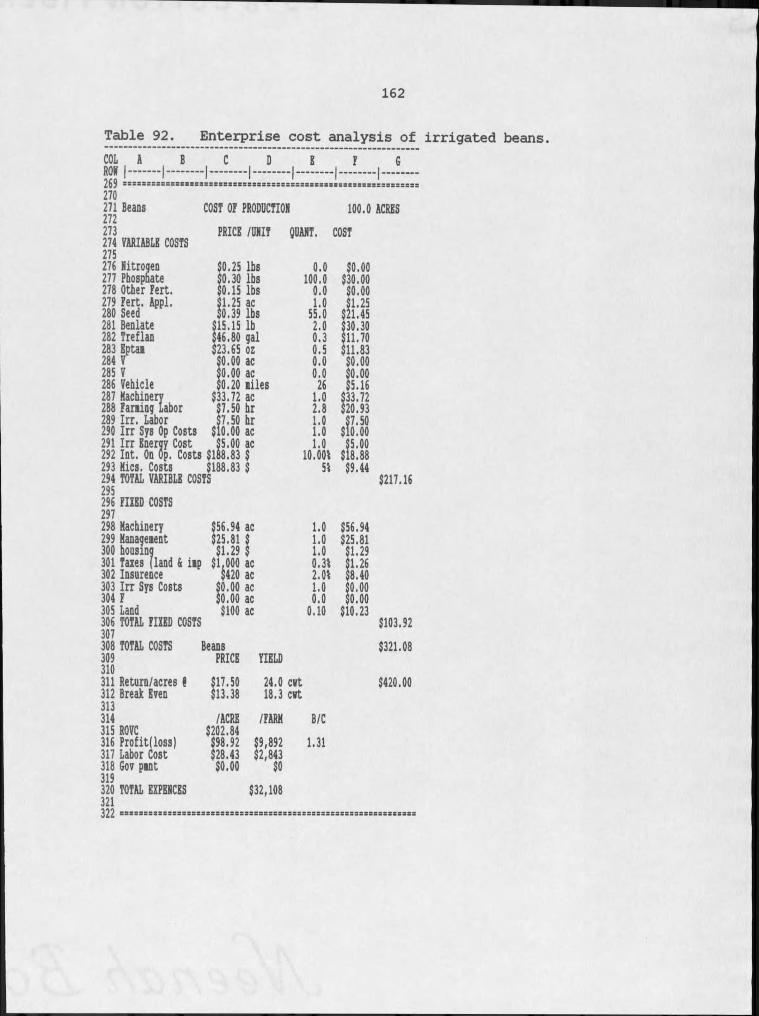
162

Table 92. Enterprise cost analysis of irrigated beans.B C I ICOL A,0,1----1---- 1---- 1---- 1.... 1---- 1-

Z b " = = = = = = = = = = = = = = = = = = = = = = := r = = z c 2 = = = = = = = = c = z = = = = = 3 z = = r = = = = = = = z = = =

270271 Beans COST OT PRODUCTION273 PRICE /UNIT OUANT.274 VARIABLE COSTS275276 Nitrogen $0.25 lbs 0.0277 Phospnate $0.30 lbs 100.0278 Other Pert. $0.15 lbs 0.0279 Pert. AppL $1.25 ac 1.0280 Seed $0.39 lbs 55.0281 Benlate $15.15 lb 2.0282 Treflan $46.80 gal 0.3283 Eptai $23.65 oz 0.5284 V $0.00 ac 0.0285 V $0.00 ac 0.0286 Vehicle $0.20 miles 26287 Machinery288 Paning Labor $33.72 ac 1.0$7.50 hr 2.8289 Irr. Labor 7.50 hr 1.0290 Irr Sys Op Costs $10.00 ac 1.0291 Irr Energy Cost $5.00 ac292 Int. On Op. Costs $188.83 $ 1.010.00%293 Mies. Costs $188.83 $ 5%294 TOTAL VARIBLE COSTS295296 FIZKD COSTS297

100.0 ACRES COST

SO. 00 $30.00 SO. 00 $1.25 $21.45 $30.30 $11.70 $11.83 $0.00 $0.00 $5.16 $33.72 $20.93 $7.50

$10.00 $5.00 $18.88 $9.44

$217.16

298 Machinery $56.94 ac 1.0 $56.94299 Management $25.81 $ 1.0 $25.81300 housing $1.29 $ 1.0 $1.29301 Taxes (land & imp $1,000 ac 0,3% $1.26302 Insurence $420 ac 2.0% $8.40303 Irr Sys Costs $0.00 ac 1.0 $0.00304 F $0.00 ac 0.0 $0.00305 Land $100 ac 0.10 $10.23306 TOTAL PIPED COSTS $103.92307308 TOTAL COSTS Ileans $321.08309 PRICE YIELD310311 Return/acres i $17.50 24.0 evt $420.00312 Break Even $13.38 18.3 evt313314 /ACRE /FARM B/C315 ROVC $202.84316 Profit(Ioss) $98.92 $9,892 1.31317 Labor Cost $28.43 $2,843318 Gov pmnt $0.00 $0319320 TOTAL EZPENCES $32,108321322

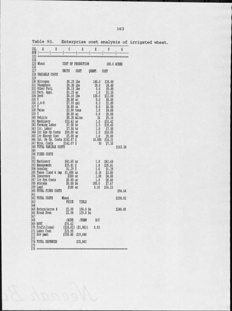
163

Table 93. Enterprise cost analysis of irrigated wheat.COL A BDnir I. . . . I.... . C ( D B P G» _ _ _ _ _ _ _ _ _ _ I_ _ _ _ _ _ _ _ _ _ _ :32«325 Mheat326 COST OP PRODUCTION 100.0 ACRES327 UNITS COST OUANT. COST328 VARIABLE COSTS329330 Nitrogen $0.25 lbs 140.0 $35,00331 PLospnate $0.30 lbs 28.0 $8.40332 Other Pert. $0.15 lbs 0.0 $0.00333 Pert. AppL $1.25 ac 1.0 $1.25334 Seed $0.10 lbs 120.0 $12.00335 V $0.00 ac 0.0 $0.00336 2,4-D $7.55 gal 0.3 $1.89337 V $0.00 ac 0.0 0.00338 Twine $2.00 tons 2.0 $4.00339 V $0.00 ac 0.0 $0.00340 Vehicle $0.20 miles 26 $5.16341 Machinery $33,42 ac 1.0 $33.42342 Parting Labor $7.50 hr 2.5 $18.45343 Irr. Labor $7.50 hr 1.0 $7.50344 Irr Sys Op Costs $10.00 ac 1.0 $10.00345 Irr Energy Cost $5.00 ac346 Int. On Op. Costs $142.07 $ 1.010.004 $5.00$14.21347 Kies. Costs $142.07 $ 54 $7.10348 TOTAL VARIBLE COSTS $163.38349350 PIPED COSTS351352 Machinery $42.65 ac 1.0 $42.65353 Management $25.81 S 1.0 $25.81354 housing $1.29 $ 1.0 $1.29355 Taxes (land & imp $1,000 ac 0.34 $3.00356 Insurance $200 ac 2.04 $4.00357 Irr Sys Costs $0.00 ac 1.0 0.00358 storage $0.08 bu 100.0 $7.67359 Land $100 ac 0.10 $10.23360 TOTAL PIPED COSTS $94.64361362 TOTAL COSTS Wheat $258.02363 PRICE YIELD364365 Return/acres @ $2.00 100.0 bu $240.00366 Break Even $2.58 129.0 bu367368 /ACRE /FARM B/C369 ROVC $76.62370 Profit(Ioss) ($18.02) ($1,802) 0.93371 Labor Cost $25.95372 Gov pint373 $190.40 $19,040374 TOTAL EPPENCES $25,802375376 . . . . . . . . .

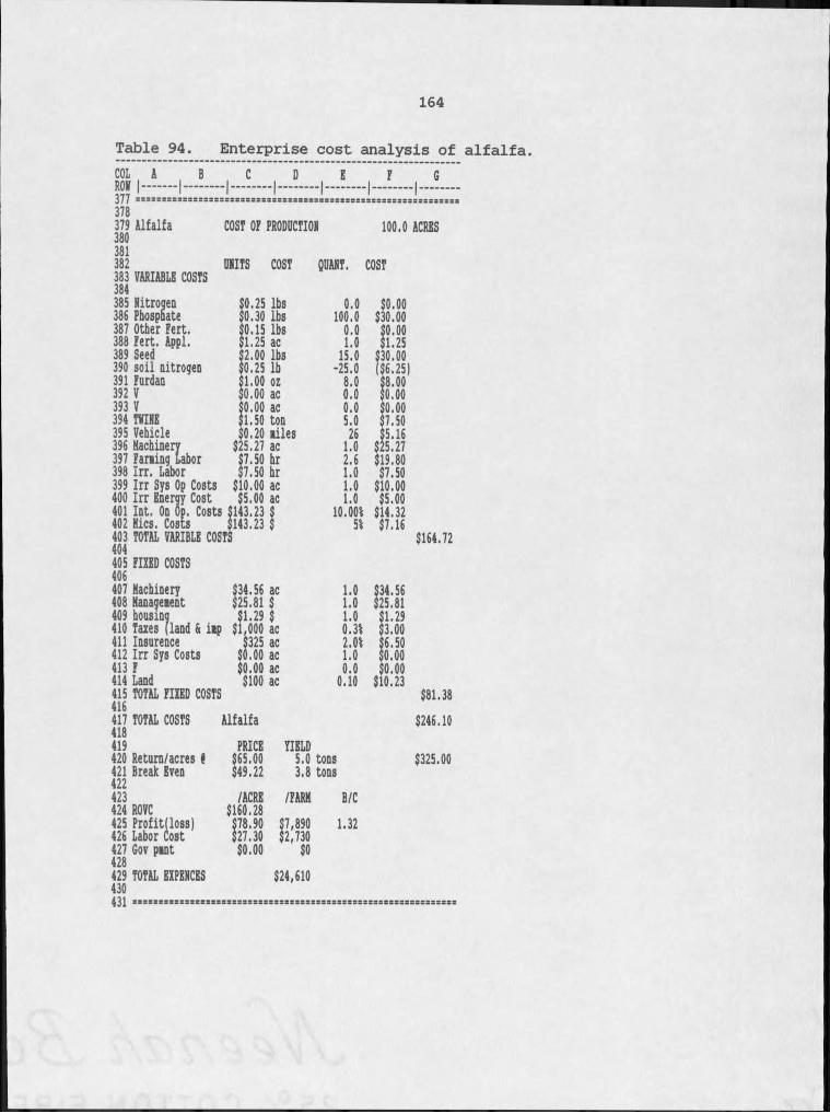
164

Table 94. Enterprise cost analysis of alfalfa.

Sll sssssssssrssssssssssssssssssssssssssssssrsrssssrsrxsssssssssss378379 Alfalfa COST OF PRODOCTIOX 100.0 ACRES380381

COST382 DHITS COST QUART.383 VARIABLE COSTS384385 nitrogen $0.25 lbs 0.0386 Phosphate $0.30 lbs 100.0387 Other Pert. $0.15 lbs 0.0388 Fert. AppL $1.25 ac 1.0389 Seed $2.00 lbs 15.0390 soil nitrogen $0.25 lb -25.0391 Furdan $1.00 oz 8.0392 V $0.00 ac 0,0393 V $0.00 ac 0.0394 TWIHE $1.50 ton 5.0395 Vehicle $0.20 miles 26396 Machinery $25.27 ac 1.0397 Farming Labor $7.50 hr 2.6398 Irr, Labor $7.50 hr 1.0399 Irr Sys Op Costs $10.00 ac 1.0400 Irr Energy Cost $5.00 ac 1.0401 Int. On Op. Costs $143.23 $ 10.00%402 Hies. Costs $143.23 $ 5%403 TOTAL VARIBLE COSTS404405 FIXED COSTS406407 Machinery408 Management409 housing410 Taxes (land & imp411 Insurance412 Irr Sys Costs413 F414 Land415 TOTAL FIXED COSTS416417 TOTAL COSTS418419420 Return/acres (421 Break Even422423424 ROVC

AlfalfaPRICE$65.00$49.22

425 Profit(Ioss)426 Labor Cost427 Gor pant428429 TOTAL EXPEHCBS430431

/ACRE$160.2878.9027.30$0.00

YIELD 5.0 tons 3.8 tons

/FARM7,8902,730$0

$24,610

B/C1.32

$0.00$30.00$0.00$1.25$30.00($6.25)$8.00$0.00$0.00$7.50$5.16$25.27

$19.80$7.50$10.00$5.00$14.32$7.16

$164.72

$34.56 ac 1.0 $34.56$25.81 $ 1.0 $25.81$1.29 $ 1.0 $1.29$1,000 ac 0.3% $3.00$325 ac 2.0% $6.50$0.00 ac 1.0 $0.00$0.00 ac 0.0 $0.00$100 ac 0.10 $10.23$81.38$246.10

$325.00

S S S S S S S S S S S S S S S S S S S S S S S S S S S S S S S S S S S S S S S S S S S S S S S S C B S S S S S S S X Z S S S

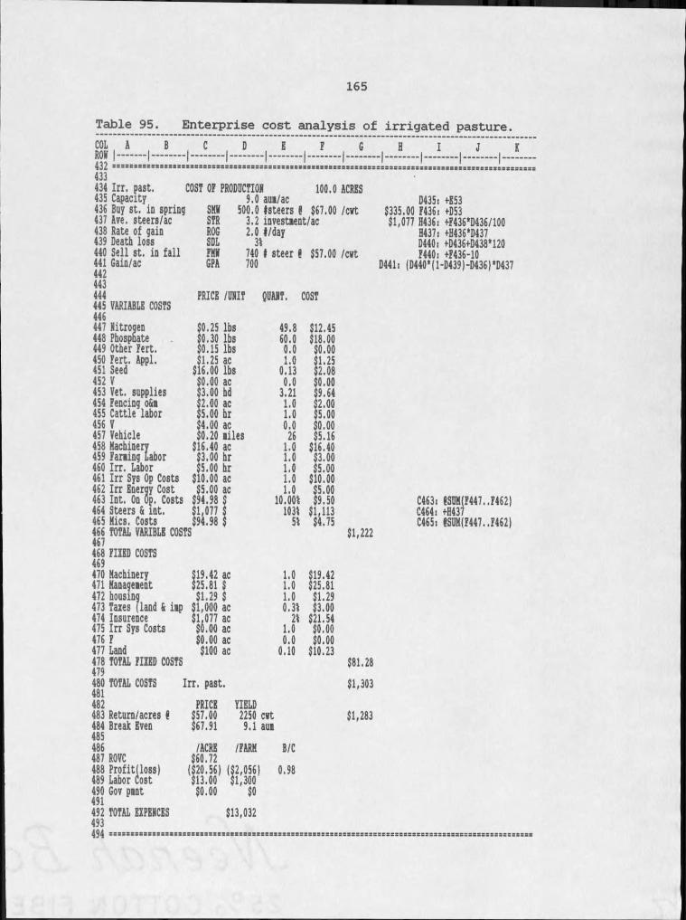
165

Table 95. Enterprise cost analysis of irrigated pasture.COL A BBfisr I. . . . I. . . . . F ( G H i I i J i K;;; i_ _ _ _ i_ _ _ _ _ i_ _ _ _ _ i_ _ _ _ _ i_ _ _ _ _ i_ _ _ _ _ a ' '- - - - '- - - -433 .434 Irr. past. ICOST OF PRODUCTION 100.0 ACRES435 Capacity 9.0 aum/ac D435: fE53436 Buy st. in spring SMW 500.0 Fsteers i $67.00 /cwt $335.00 F436: +053437 Ave. steers/ac STR 3.2 investment/ac $1,077 H436: +F436‘D436/100438 Rate of gain ROG 2.0 4/day H437: +H436‘D437439 Death loss SDL 31 D440: +0436+0438*120440 Sell st. in fall FMW 740 4 steer 8 $57.00 /evt F440: +F436-10441 Gain/ac442 GPA 700 D441: (D440*(1-D439)-D436)*D437443444 PRICE /UNIT QUANT. COST445 VARIABLE COSTS446447 Nitrogen $0.25 lbs 49.8 $12,45448 Phosphate $0.30 lbs 60.0 $18.00449 Other Fert. $0.15 lbs 0.0 $0.00450 Fert. Appl. $1.25 ac 1.0 $1.25451 Seed $16.00 lbs 0.13 $2.08452 V $0.00 ac 0.0 $0.00453 Vet. supplies $3.00 bd 3.21 $9.64454 Fencing oSi $2.00 ac 1.0 $2.00455 Cattle labor $5.00 hr 1.0 $5.00456 V $4.00 ac 0.0 $0.00457 Vehicle $0.20 miles 26 $5.16458 Machinery $16.40 ac 1.0 $16.40459 Farming Labor $3.00 hr 1.0 $3.00460 Irr. Labor $5.00 hr 1.0 $5.00461 Irr Sys Op Costs $10.00 ac 1.0 $10.00462 Irr Energy Cost $5.00 ac 1.0 $5.00463 Int. On Op. Costs $94.98 $ 10.001 $9.50 C463r 8SUM(F447..F462)464 Steers & int. $1,077 $ 1031 $1,113 C464: +H437465 Hies. Costs $94.98 $ 51 $4.75 C465: eSUM(F447..F462)466 TOTAL VARIBLE COSTS $1,222467468 FIXED COSTS469470 Machinery471 Hanacfeient472 housing473 Taxes [land & imp474 Insurance475 Irr Sys Costs476 I477 Land478 TOTAL FIXED COSTS479

$19.42 ac 1.0 $19.42$25.81 $ 1.0 $25.81$1.29 $ 1.0 $1.29$1,000 ac 0.31 $3.00$1,077 ac $0.00 ac 21 $21.541.0 $0.00$0.00 ac 0.0 $0.00$100 ac 0.10 $10.23

480 TOTAL COSTS Irr. past.481482 PRICE YIELD483 Return/acres 8 $57.00 2250 c»t484 Break Even $67.91 9.1 aum485486 /ACRE /FARM B/C487 ROVC $60.72488 Profitlloss)489 Labor Cost ($20.56) ($2,056) 0.98$13.00 $1,300490 Gov pmnt491 $0.00 $0492 TOTAL EXPENCES $13,032

$81.28$1,303

$1,283

r s s s s s s & s s s r s s s s = s : s s s s s s r s s B s s s = s s s s s s s s s s s s s s 3 S S S 3 s s s r x s s s 3 S 3 s r r : s s = s s s r = s s : s s s s = s s s s : r s s s s r r s s s

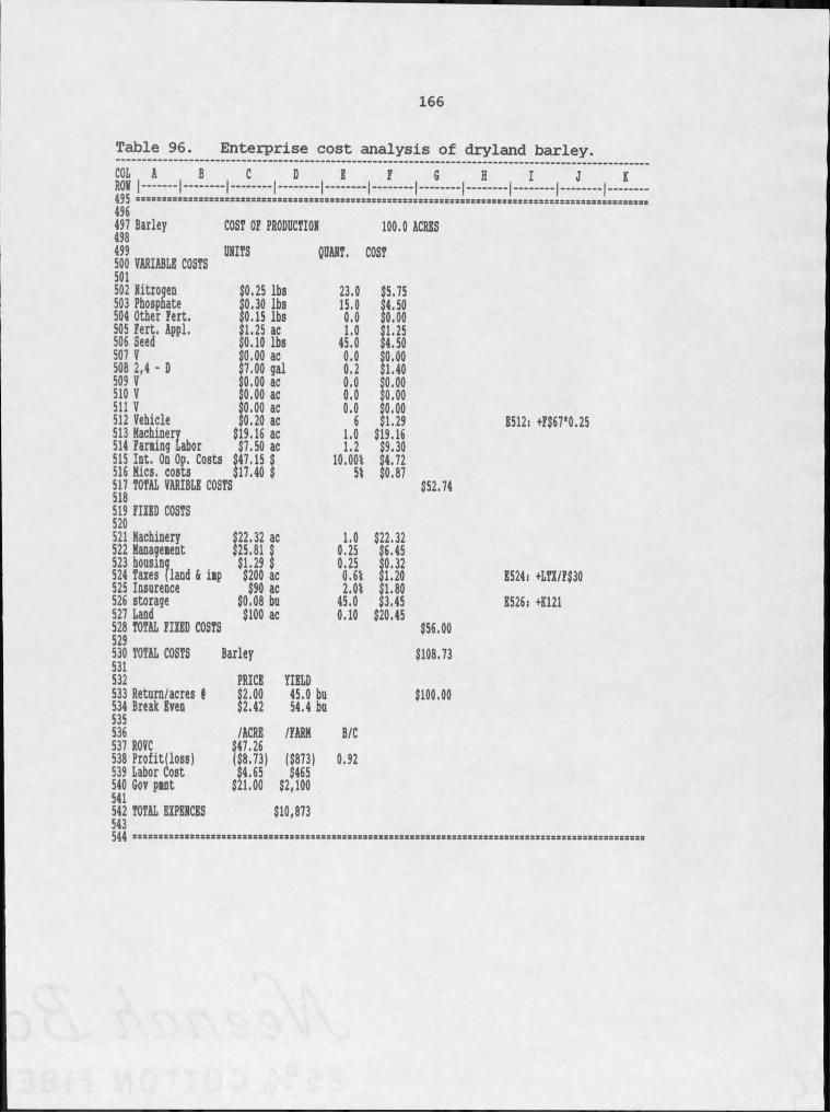
166

Table 96. Enterprise cost analysis of dryland barley.COl A Bone I--------- 1............. K F 1 G 1 H I J K

_ __ :_ _ _ _ i _ _ _ i— __ _ _ _ _ _ _ _ _ _ _ I,,:::: I i i- - - - 1- - - -496497 Barley498 COST OF PRODDCTIOR 100.0 ACRES499 URITS QUART. COST500 VARIABLE COSTS501502 nitrogen $0.25 lbs 23.0 $5.75503 Phosphate $0.30 lbs 15.0 $4.50504 Other Pert. $0.15 lbs 0.0 $0.00505 Fert. AppL $1.25 ac 1.0 $1.25506 Seed $0.10 lbs 45.0 $4.50507 V $0.00 ac 0.0 $0.00508 2,4 - D $7,00 gal 0.2 $1.40509 V $0.00 ac 0.0 $0,00510 V $0.00 ac 0.0 $0.00511 V $0.00 ac 0.0 $0.00512 Vehicle $0.20 ac 6 $1.29 E512: +F$67*0.25513 Machinery $19.16 ac 1.0 $19.16514 Farming Labor $7.50 ac 1.2 $9.30515 Int. On Op. Costs $47.15 $ 10.00% $4.72516 Hies, costs 17.40 $ 5% $0.87517 TOTAL VARIBLK COSTS $52.74518519 FIXED COSTS520521 Machinery $22.32 ac 1.0 $22.32522 Management $25.81 $ 0.25 $6.45523 housing $1.29 $ 0.25 $0.32524 Taxes [land & imp $200 ac 0.6% $1.20 E524: +LTX/P$30525 Insurance $90 ac 2.0% $1.80526 storage $0.08 bu 45.0 $3.45 E526: +K121527 Land $100 ac 0.10 $20.45528 TOTAL FIXED COSTS529 $56.00530 TOTAL COSTS ICQl

Barley $108.73532 PRICE YIELD533 Return/acres 8 $2.00 45.0 bu $100.00534 Break Even $2.42 54.4 bu535536 /ACRE /FARM B/C537 ROVC $47.26538 Profit(Ioss) ($8.73) ($873) 0.92539 Labor Cost $4.65 $465540 Gov pmnt $21.00 $2,100541542 TOTAL EXPERCES $10,873543544

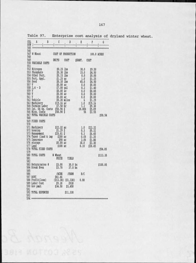
167

Table 97. Enterprise cost analysis of dryland winter wheat.COL A BDrttf I. . . . . I_ _ _ _ _ C | D K P , G* _ __ ........_ _ _ _ _ _ _ _ _ _ _ _ _ :546547 V Kheat548 COST OP PRODUCTION 100.0 ACRES549 UNITS COST QUANT. COST550 VARIABLE COSTS551552 nitrogen $0.25 lbs 38.0 $9.50553 Phosphate $0.30 lbs 15.0 $4.50554 Other Pert. $0.15 lbs 0.0 $0.00555 Pert. AppL $1.25 ac 1.0 $1.25556 Seed $0.10 lbs 45.0 $4.50557 V $0,00 ac 0.0 $0.00558 2,4 - D $7.00 gal 0.2 $1.40559 V $0.00 ac 0.0 $0.00560 V $0.00 ac 0,0 $0.00561 V $0.00 ac 0.0 $0.00562 Vehicle $0.20 miles 6 $1.29563 Machinery $19.16 ac 1.0 $19.16564 Paning Labor $7.50 hr 1.2 $9.30565 Int. On Op. Costs $50.90 S 10.001 $5.09566 Hies. Costs $50.90 $ 51 $2.55567 TOTAL VARIBLK COSTS $58.54568569 PIIKD COSTS570571 Machinery $22.32 ac 1.0 $22.32572 housing $1.29 $ 0.3 $0.32573 Management $25.81 $ 0.3 $6.45574 Taxes (land & imp $200 ac 0.61 $1.20575 Insurence $90 ac 2.01 $1.80576 storage $0.08 ac 30.0 $2.30577 Land578 TOTAL PIIKD COSTS579

$100 ac 0.10 $20.45 $54.85580 TOTAL COSTS N Wheat $113.38581 PRICE YIELD582583 Return/acres 8 $3.00 30.0 bu $100.00584 Break Even585 $3.78 37.8 bu586 /ACRE /PARK B/C587 ROVC $41.46588 Profit(Ioss) ($13.38) ($1,338) 0.88589 Labor Cost $9.30 $930590 Gov pint591 $34.50 $3,450592 TOTAL KIPKNCKS m $11,338

! S S S S S S S S S S S S S S S S S S B S S S S S S S S S

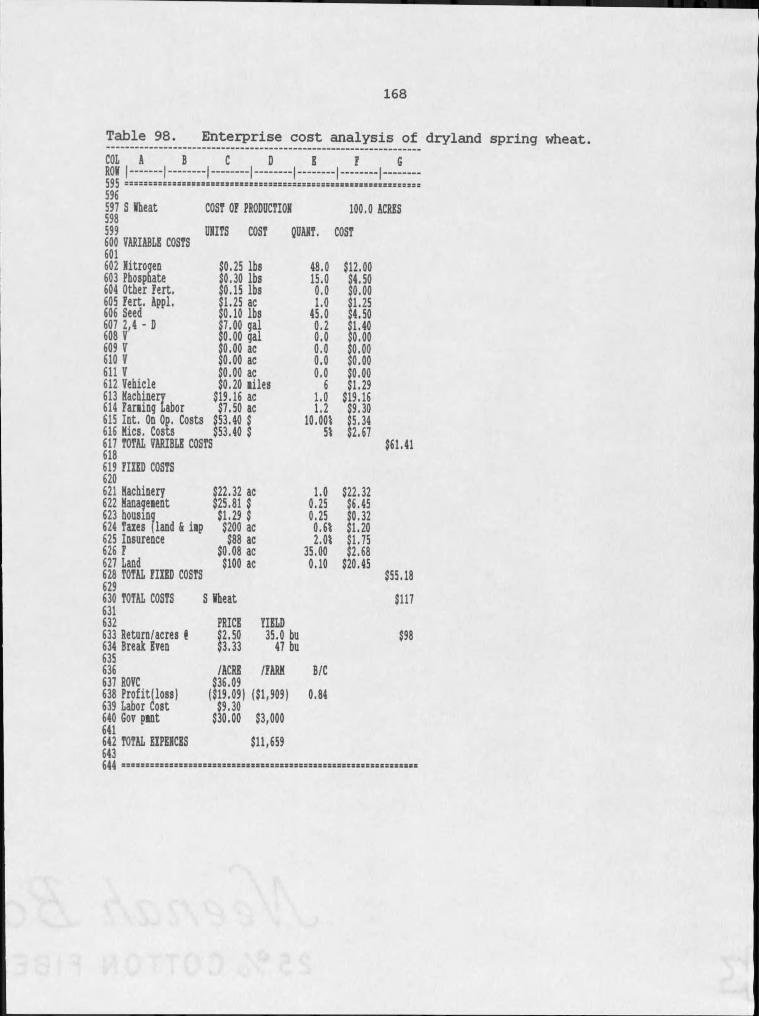
168

Table 98. Enterprise cost analysis of dryland spring wheat.COL A B™ L - : : : : : : ! : : : : : : : : I " " '— I--"— I'

E- - - 1 FI- - - - GI- - - -

596597 S Ifheat598 COST OF PRODUCTION 100.0 ACRES599 UNITS COST QUANT. COST600 VARIABLE COSTS601602 Nitroqen $0.25 lbs 48.0 $12.00603 Phospnate $0.30 lbs 15.0 $4.50604 Other Fert $0.15 lbs 0.0 $0.00605 Fert AppL $1.25 ac 1.0 $1.25606 Seed $0.10 lbs 45.0 $4.50607 2,4 - D $7.00 gal 0.2 $1.40608 V $0.00 gal 0.0 $0.00609 V $0.00 ac 0.0 $0.00610 V $0.00 ac 0.0 $0.00611 V $0.00 ac 0.0 $0.00612 Vehicle $0.20 miles 6 $1.29613 Machinery $19.16 ac 1.0 $19.16614 Farming Labor $7.50 ac 1.2 $9.30615 Int. On Op. Costs $53.40 $ 10.001 5.34616 Hies. Costs 53.40 $ 51 $2.67617 TOTAL VARIBLE COSTS $61.41618619 FIFED COSTS620621 Machinery $22.32 ac 1.0 $22.32622 Management $25.81 $ 0,25 $6.45623 housing $1.29 $ 0.25 $0.32624 Taies (land & imp $200 ac 0.61 $1.20625 Insurance $88 ac 2.01 $1.75626 F $0.08 ac 35.00 $2.68627 Land $100 ac 0.10 $20.45628 TOTAL FIFED COSTS $55.18629630 TOTAL COSTS I3 Wheat $117631632 PRICE YIELD633 Return/acres 8 $2.50 35.0 bu $98634 Break Even $3.33 47 bu635636 /ACRE /FARM B/C637 ROVC $36.09638 Profit(Ioss) ($19.09) ($1,909) 0.84639 Labor Cost $9.30640 Gov pmnt641 $30.00 $3,000642 TOTAL EFPENCES $11,659643644 =================!

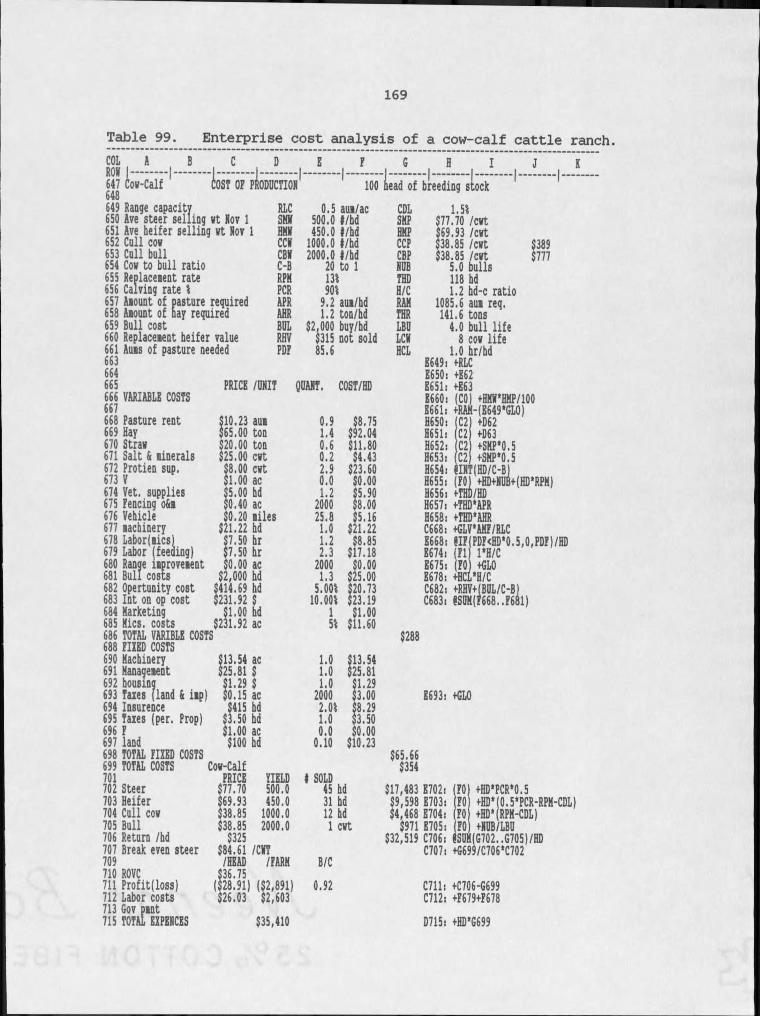
169

Table 99. Enterprise cost analysis of a cow-calf cattle ranch.B C

L i o? pIoCOL A HO* I- --647 Cow-Calf648649 Range capacity650 Ave steer selling vt Nov I651 Ave heifer selling wt Nov I652 Cull cos653 Cull bull654 Cow to bull ratio655 Replacement rate656 Calving rate I657 Amount of pasture required658 Amount of nay required659 Bull cost660 Replacement heifer value661 Aums of pasture needed663664665666 VARIABLE COSTS667668 Pasture rent669 Hay670 Straw671 Salt & minerals672 Protien sup.673 V674 Vet. supplies675 fencing o&m676 Vehicle677 machinery678 Labor(mics)679 Labor (feeding)680 Range improvement681 Bull costs682 Opertunity cost683 Int on op cost684 Karketing685 Hies, costs688 FIIKD COSTS690 Machinery691 Management692 housing693 Taxes (land & imp)694 Insurance695 Taxes (per. Prop)696 P697 land698 TOTAL FIIED COSTS699 TOTAL COSTS701702 Steer703 Heifer704 Cull cow705 Bull706 Return /hd707 Break even steer709710 ROVC711 Profit(Ioss)712 Labor costs713 Gov pmnt715 TOTAL EIPENCES

D E F G H I J KICTION ' 100 Iiead of breeding stockRLC 0,5 aum/ac CDL 1.51SHW 500.0 l/hd SHP $77.70 /cutHMW 450.0 l/hd HKP $69.93 /cutCCW 1000.0 l/hd CCP $38.85 /evt $389CBW 2000.0 l/hd CBP $38.85 /cut $777C-B 20 to I NOB 5.0 bullsRPK 131 THD 118 hdPCR 901 H/C 1.2 hd-c ratioAPR 9.2 aum/hd RAM 1085.6 aum req.AHR 1.2 ton/hd THR 141.6 tonsBDL $2,000 buy/hd LBD 4.0 bull lifeRflV $315 not sold LCW 8 cow lifePDF 85.6 HCL 1.0 hr/hdE649: fRLC

E650: +E62PRICE /ONIT ODANT. COST/HD K651: +E63

$10.23 aum $8.75E660: (CO) +HMW'HHP/100 E661: +RAH-(B649*GL0)0.9 H650: (C2 +D62$65.00 ton 1.4 $92.04 H651: C2 +063$20.00 ton 0.6 $11.80 H652: C2 +SKP1O.5$25.00 cwt 0.2 $4.43 H653: (C2 +SHP1O.5$8.00 cwt $1.00 ac 2.90.0 $23.60$0.00 H654:H655: IIN

iaF(HDZC-B)+HDtNDBt(HD1RPM)$5.00 hd 1.2 $5.90 H656i )/HD$0.40 ac 2000 $8.00 H657, +THD1APR$0.20 miles 25.8 $5.16 H658: +THD1AHR$21.22 hd 1.0 $21.22 C668; +GLV'AMF/RLC$7.50 hr 1.2 $8.85 E668: HF(PDF<HD‘0.5,0,PDF)/HD$7.50 hr 2.3 $17.18 E674: Fl I1HZC$0.00 ac 2000 $0.00 E675: (F0 +GLO$2,000 hd 1.3 $25.00 E678: +HCL1HZC$414.69 hd 5.001 $20.73 C682: +RHV+IB0L/C-B]$231.92 $ 10.001 $23.19 C683: ISDH(F668..F6ul)$1.00 hd I $1.00$231.92 acrs 51 $11.60

$288$13.54 ac 1.0 $13.54$25.81 $ 1.0 $25.81$1.29 $ 1.0 $1.29$0.15 ac 2000 $3.00 K693: +GLO$415 hd 2.01 $8.29$3.50 hd 1.0 $3.50$1.00 ac 0.0 $0.00$100 hd 0.10 $10.23

$65.66Cow-Calf $354PRICE YIELD I SOLD$77.70 500.0 45 hd $17,483 E702: FO +HD1PCR1O1S$69.93 450.0$38.85 1000.0 31 hd 12 hd $9,598 E703: $4,468 K704: FO

FO +HD1(0.SiPCR-RPM-CDL) +HD1(RPK-CDL)$38.85 2000.0 I cwt $971 K705: FO +NDBZLBD

$84.61 /CKT /HEAD /FARM $36.75($28.91) ($2,891) $26.03 $2,603

$35,410

0.92

$32,519 C706: 4SUM(G702..G705)/HD C707: +G699/C706*C702

C711: +C706-G699 C712: +F679+F678D715: +HD*G699

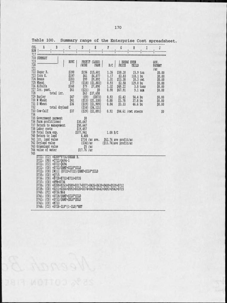
170

Table 100. Summary range of the Enterprise Cost spreadsheet.

717 s s s s s s s s s z s s s s s s s s r s s s s s s a s s s s s s s s s s s a s s s s s s s s s x s c s s s s s s s r s s s s s s s s s s s s s s s s s r s s s s s s s s s s s s s s

718 SUMMARY I719 _ _ _ _ _ _ _ I ROVC I PROFIT (LOSS)720 /ACRE FARM721

$156 $15,601$390197203$77$160$61

722 Sugar B.723 Corn G.724 Beans725 Wheat726 Alfalfa727 Irr. past.728 total irr.729 Barley $47730 W Wheat $41731 S Wheat $36732 total dryland733 Cow-Calf $37734

$61 $6,077 $99 $9,892l I i S 1 ' S S 2 1

$37,6^8" a1,909 4,121

$2,891

Si

B/C I I BREAK EVEW PRICE YEILD GOV.PAYMWT1.26 $30.20 15.9 ton /ac

$0.001.17 $2.83 118.1 bu $0.001.31 $13.38 18.3 cwt $0.000.93 $2.58 129.0 bu $0.001.32 $49.22 3.8 tons $0.000.98 $67.91 9.1 aum $0.000,92 $2.42 54.4 bu $0.000.88 $3.78 37.8 bu $0.000.84 $3.33 46.6 bu $0.000.92 $84,61 /cwt steers $0

735 Government payment736 Farm profit(loss)737 Return to management738 Labor costs739 Total farm exp.740 Return to land741 Irr. land value742 Dryland value743 Grassland value744 value of water745

$0$30,647$50,647$19,457

$377,941 1.08 B/C4.484$714 /ac ave. $62.76 ave profit/ac ($34)/ac ($13.74)ave profit/ac$5 /ac $17.76 /ac

U/22: (!2D722: POD722: C2D722: COD722: COD735: COD736: COD737, COD738: COD739: COD740: P2D741: COD742: COD743: COD744: C2

+D209'P716/SUGAR B.+C722/0694-1+0722-0694+D722/$AHF+$ILV’$ILD[Will (D722+J722)/$AMF+$ILV*$ILD$728+E732+E733+D735+RTH+D736+D208+D263+D589+D317+D371+D426»D639+D489+D539+D712+D211+D266+D592+D320+D374+D429+D642+D492+D542+D715+D736/R64+D728/$AMF>$ILV‘$ILD+D732/$AMF+$DLV*$DLDfM733+D728-ILV* ( H L D ) tRET

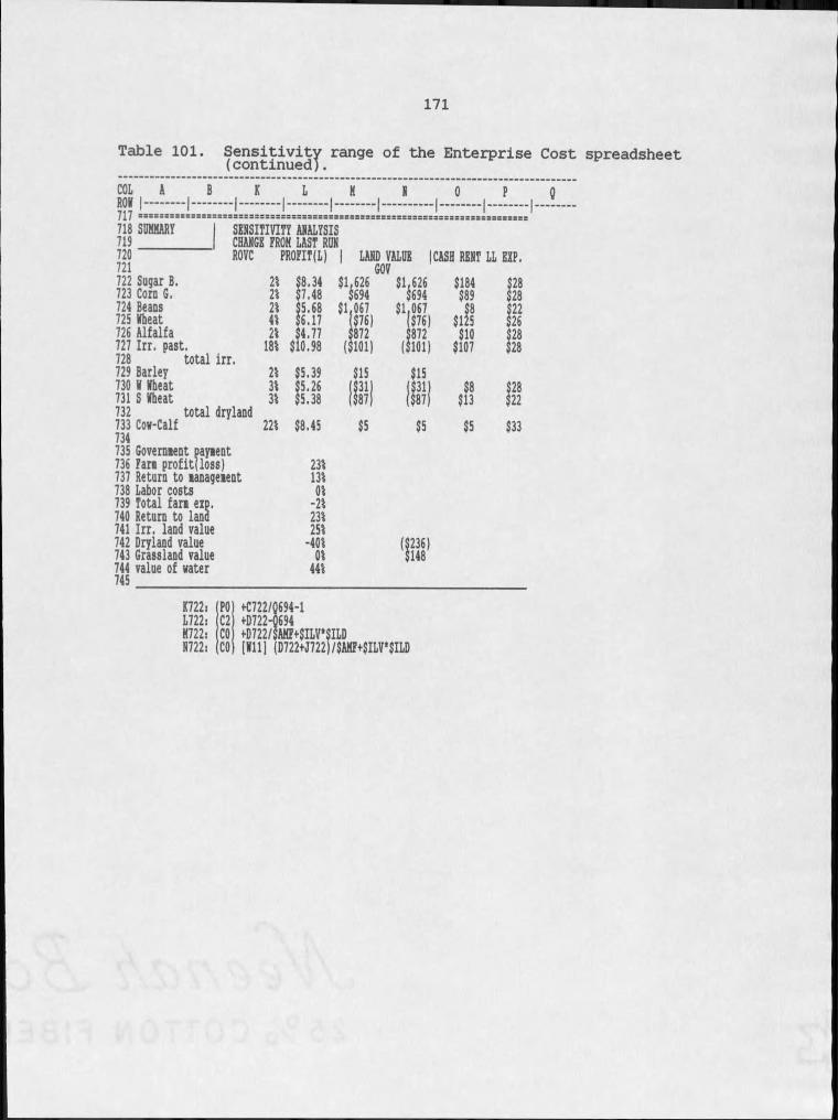
171

Table 101. Sensitivity range of the Enterprise Cost spreadsheet (continued).

-I-PCOL A B K L K A

KM I-------- 1...........1---------1...........1...........1-------111 = = = = = = = = = = = = = = = = = = = = = = = = = = = = = = = Z 3 Z = = = = = = = = = = = = = = = = = Z

718 SUMMARY I SENSITIVITY ANALYSIS719 _ _ _ _ _ _ _ I CHANGE FROM LAST RUN720 ROVC PROFIT(L) | LAND VALUE |CASH RENT LL EXP.721 GOV

======================

722 Sugar B.723 Corn G.724 Beans725 Vheat726 Alfalfa727 Irr. past.728 total irr.729 Barley730 V Vheat731 S Vheat732 total dryland733 Cow-Calf734

2% $8.34 $1,626$694 $1,626$694 $184 $282% $7.48 $89$8 $282% $5.68 $1,067 $1,067 $224% $6.17 $76) ($76) $125 $262% $4.77 $872 $872 $10 $2818% $10.98 ($101) ($101) $107 $28

2% $5.39 $15 $153% $5.26 (311 ($31) $8 $283% $5.38 ($87) ($87) $13 $2222% $8.45 $5 $5 $5 $33

735 Government payment736 Farm profit)loss) 231737 Return to management 13%738 Labor costs 0%739 Total farm exp. -2%740 Return to land 23%741 Irr. land value 25%742 Dryland value -40%743 Grassland value 0%744 value of water 44%745 _ _ _ _ _ _ _ _ _ _ _ _ _ _ _ _ _ _ _ _

0

K722:L722:H722:N722s

POC2COCO

+C722/Q694-1<•0722-0694+D722/SAMFt$ILV‘$ILD(Vll) (D722+J722)I$AMF<-$ILV*$ILD

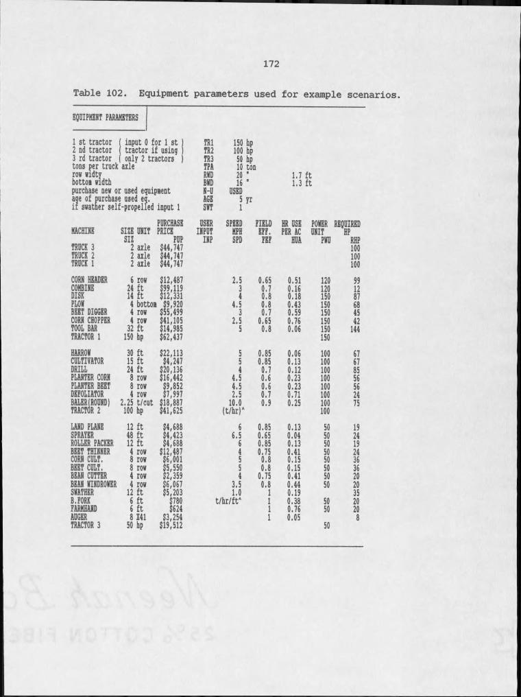
172

Table 102. Equipment parameters used for example scenarios.


I st tractor input O for I st TRl 150 hp2 nd tractor tractor if using TR2 100 hp3 rd tractor only 2 tractors TR3 50 hptons per truck axle TPA 10 tonrov vidty RWD 20 ' 1.7 ftbottom vidth BWD 16 ’ 1.3 ftpurchase nev or used equipment N-U USEDage of purchase used eg. if svatner self-propelled AGE 5 yrinput I SWT I

PURCHASE USER SPEED FIELD HR USE POWER REQUIREDMACHINE SIZE UNIT PRICE INPUT MPH SFF. PER AC UNIT HPSIZ PUP INP SPD FEF HUA PWU RHPTRUCK 3 2 axle $44,747 100TRUCK 2 2 axle $44,747 100TRUCK I 2 axle $44,747 tooCORN HEADER 6 rov $12,487 2.5 0.65 0.51 120 99COMBINE 24 ft $99,119 3 0.7 0.16 120 12DISK 14 ft $12,331 4 0.8 0.18 150 87PLOW 4 botton $9,920 4.5 0.8 0.43 150 68BEET DIGGER 4 rov $55,499 3 0.7 0.59 150 45CORN CHOPPER 4 rov $41,105 2.5 0.65 0.76 150 42TOOL BAR 32 ft $14,985

$62,437 5 0.8 0.06 150 144TRACTOR I ISO hp 150HARROW 30 ft $22,113 5 0.85 0.06 100 67CULTIVATOR 15 ft $4,247 5 0.85 0.13 100 67DRILL 24 ft $20,136 4 0.7 0.12 100 85PLANTER CORN 8 rov $16,442 4.5 0.6 0.23 100 56PLANTER BEET 8 rov $9,852 4.5 0.6 0.23 100 56DEFOLIATOR 4 rov $7,997 2.5 0.7 0.71 100 24BALERjROUND) TRACTOR 2 2.25 t/cut 100 hp $18,887$41,625 10.0(t/hrr 0.9 0.25 100100 75

LAND PLANE 12 ft $4,688 6 0.85 0.13 50 19SPRAYER 48 ft $4,423 6.5 0.65 0.04 50 24ROLLER PACKER 12 ft $4,688 6 0.85 0.13 50 19BEET THINNER 4 rov $12,487 4 0.75 0.41 50 24CORN CULT. 8 rov $6,001 5 0.8 0.15 50 36BEET CULT. 8 rov 5,550 5 0.8 0.15 50 36BEAN CUTTER 4 rov $2,359 4 0.75 0.41 50 20BEAN WINDROWER 4 rov $6,067 3.5 0.8 0.44 50 20SWATHER 12 ft $5,203 1.0 I 0.19 35B.FORK 6 ft $780 t/hr/ft* I 0.38 50 20FARMHAND 6 ft $624 I 0.76 50 20AUGER 8 141 $3,254 I 0.05 8TRACTOR 3 50 hp $19,512 50

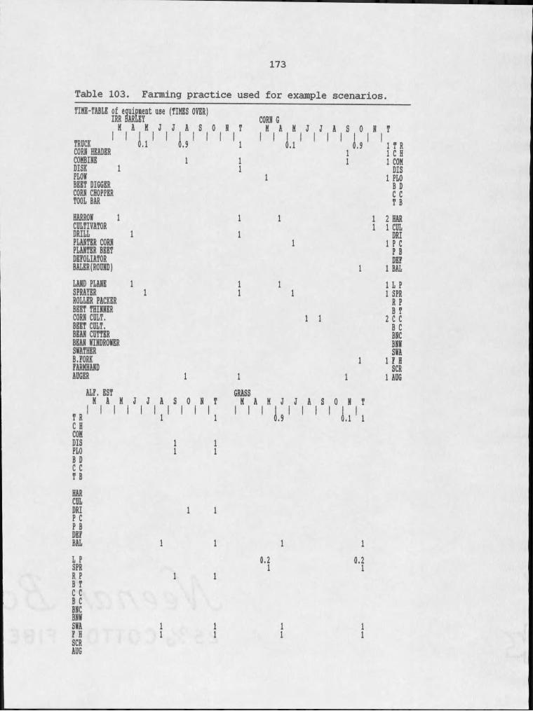
173

T a b l e 1 0 3 . F a n n i n g p r a c t i c e u s e d f o r e x a m p l e s c e n a r i o s . TIHE-TABLE of equipment use (TIMES OVER)

M AI | K | J | V 1Y 1Y , Y I 11I j I j , Y O N TTRDCK ' IL i 1 L 1 1 1 'i 1 1 (1.1 1 '

i I1.9

I I T RCORN HEADER i I C HCOMBINE I I i I COMDISK I I DISPLOW i I PLOBEET DIGGER B DCORN CHOPPER C CTOOL BAR T BHARROW I I i I 2 HARCDLTIVATOR I I CULDRILL I I DRIPLANTER CORN I I P CPLANTER BEET P BDEFOLIATOR DEFBALER(ROUND) I I BALLAND PLANE I I i I L PSPRAYER i I I I SPRROLLER PACKER R PBEET THINNER B TCORN CDLT. I I 2 C CBEET CDLT. B CBEAN CUTTER BNCBEAN WINDROWER BNWSWATHER SWAB.FORK I I F HFARMHAND SCRAUGER I I i I AUG

ALE. EST GRASSK A H J J A S O N T H A M J J A S O N T„ M 11 1 1 1 1 1 1 L 1 1 1 1 L 1 1C H COHDIS I IPLO I IB D C CT BHARCDLDRI I IP C P B DBFBAL I I I IL P 0.2 0.2SPR I IR P I IB TC CB CBNCBNWSWA I I I IF H I I I ISCRADG

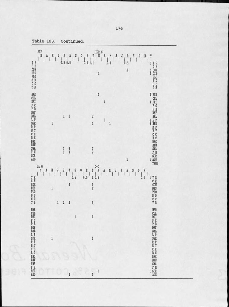
174

Table 103. Continued.

A UN A K J J A S O

T R C H COK DIS PLO B D C C T BHAR COL DRI P C P B DEP BAL L P SPR R P B I C C B C BRC BR* SKA P H SCR AOG

I I I I

IRR GR P K AL I , 1 1 L I , 1 1 I,

K J J A S OL 1 1 I I

T R C H COK DIS PLO B D C C P BHAR COL DRI P C P B DEP BAL L P SPR R P B P C C B C BRC BR* SKA P H SCR AOG

I I

DL GH A K J JI I I

A S O RL 1

C-CP H A K

L L I , ' 1J J

IA S O R

I,

I 2 I

I P R C H I COK I DIS PLO B D C C P B

I HAR COL I DRI P C P B DEP BAL

I L P I SPR R P B P C C B C BRC BH* SKA F H SCR I AOG PIKE

I P R C H COK DIS PLO B D C C P BHAR COL DRI P C P B DEP BAL L P SPR R P B P C C B C BRC BR* SKA P H

I SCR AOG

175

Table 104. Farm budget variables used in the example scenarios.

SYSTEM VARIABLES

Irr. land value Dryland value Grass land valueInterest rate TermsInterest on operating capital Return to fan (opportunity costs) Percent of dryland cropped Range land capacity Amount of grassland owned Vehical miles charged to fan/yr Return to management Other fixed costs Kisc. costsLand taxes (I of land value) Insurence (% of crop value)Labor costsIrrigation labor hrs/ac

PERCENT LAND DEBTILV $650 /ac ILD 164DLV $200 /ac DLD 164GLV $75 /ac GLD 164INR 5.004TRH 40 year AKF 0.06 127: @PMT(1,INR,TRH)OCI 10.004RET 5.004PDC 504 cropped/yrRLC 0,50 ann aum/ac $150 131, GLV/RLCGLO 5,120 acresVKIRTMOTH

10,000 /yr is J S /'is $0.20 $/milehousingKIS 54LTF 0.304CIN 1.04LCT $5.00 $/hr

ILA 0.7 hr/ac

USER ENTERED ENTERPRISE COSTSI M T PRICE /UNIT I CROP INPUT PRICE /UNIT RATE/UNIT

V2,4-DVTwineVstorageVVVVTWINEP

■Irr. barl

-Grass hay

Alf estFurdanVVV FV2,4-DTwineV

-Grain

storage. . . . . Alfalfasoil nitrogen FurdanVVTWINEF

ac$7.55 gal ac$2.00 tons ac

-Irr. pastVet. supplies Fencing o&m Cattle labor V$0.00 bu 70.0 F

$0.00 oz 0.0 V$0,00 oz 0.0 2,4 - D$0.00 oz 0.0 V$0.00 bu 0.0 V$2.00 ton 1.0 V$0.00 bu 0.0 storage

V$1.00 oz 8.0 2,4 - Dac Vac V

$1.50 ton 1.4 Vac storageac 2,4 - D$7.55 gal 0.3 Vac V

$2.00 tons 2.0 Vac V

$0.04 bu 70.0 F$0.25 lb -12.5 Hay$1.00 oz 8.0 Straw

ac Salt & miac Protien s$0.00 ton 4.4 Vac F

Barley

W Wheat

S Wheat

Cow-Calf

$0.00 ac $3.00 hd $2.00 ac $5.00 hr $4.00 ac ac

0.03.21.01.0

$0.00 ac 0.0$7.00 gal $0.00 ac $0.00 ac $0.00 ac

0.2

$0.04 bu 33.6$0.00 ac 0.0$7.00 gal $0.00 ac $0.00 ac $0.00 ac

0.2

$0,04 bu 29.4$7.00 gal 0.2$0.00 gal $0.00 ac $0.00 ac $0.00 ac

0.0

$0.04 bu 22.6$60.88 ton 1.4$0.00 ton 0.6$25.00 cwt 0.2$8.00 cwt $1.00 ac $1.00 ac

2.9

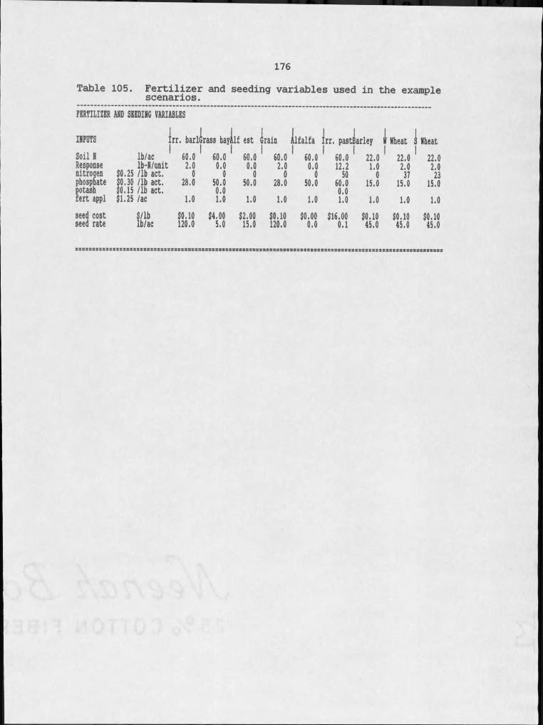
176Table 105. Fertilizer and seeding variables used in the examplescenarios.FERTILIZER ARD SEEDIRG VARIABLES

IRPDTS lrr. barlirass hayilf est drain llfalfa Ir:. pastlarley I Mheat I MheatSoil R Ib/ac 60.0 60.0 60.0Response Ib-R/unit 2.0 0.0 0.0nitrogen $0.25 /lb act. 0 0 0phosphate $0.30 /lb act. 28.0 50.0 50.0potash $0.15 /lb act. 0.0fert appl $1.25 /ac 1.0 1.0 1.0seed cost S/lb $0.10 $4,00 $2.00seed rate Ib/ac 120.0 5.0 15.0

60.0 60.0 60.0 22.0 22.0 22.02.0 0.0 12.2 1.0 2.0 2.00 0 50 0 37 2328.0 50.0 60.0 15.0 15.0 15.00.01.0 1.0 1.0 1.0 1.0 1.0$0.10 $0.00 $16.00 $0.10 $0.10 $0.10120.0 0.0 0.1 45.0 45.0 45.0

s s s s s s s s s x s s r s s s s s s s a s s s s s s s s s s s s s s s s s s s s s a s s s s s s s s s s s s s s s s s s s s s s r s s s s s s a s s s s s s s s s s s s s s s s s s a s s s a s s s s s s s s s s s s

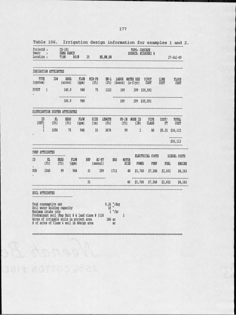
177

Table 106. Irrigation design information for examples I and 2.Project! , CS-IOl TOPO: CASCADEOwner , DANA RANCH SOURCE: MISSOURI RLocation i T18N ROlW 25 NElNWfSW 27-Jul-89

IRRIGATION ATTRIBUTESTYPE(system) ID! AREA(acres) PLOW

(gp«)MIN-PR

(ft)HW-L(ft)

LABOR WATER USE (hours) (a-f/yr) PIVOTCOST LINECOST FLOODCOSTPIVOT I 145.9 948 75 1322 109 299 $35,592

145.9 948 109 299 $35,592

DISTRIBUTION SYSTEM ATTRIBUTESID

(OUTjEL

(ft)HEAD(ft)

FLOW(gp i)

SIZE( in )

LENGTH(ft)

PR-IN(ft)

NODE ID (IN)

PIPECLASS COST/

PTTOTALCOST

I 3350 75 948 10 3070 99 2 80 $5.25 $16,112

$16,112

PUMP ATTRIBUTESELECTRICAL COSTS DIESEL COSTSEL

(ft)HEAD(ft)

FLOW(gpi)

BHP AC-FT (annual) HRS MOTORSIZE POWER PUMP FUEL ENGINE3340 99 948 31 299 1711 40 $1,768 $7,248 $2,652 $4,143

31 40 $1,768 $7,248 $2,652 $4,143

SOIL ATTRIBUTES

Peak consimptive use 0.26 "/daySoil water Bolding capacity 10 ’Kaxieui intake rate I '/hrPredominant soil (Map Unit ! & land class ! )118 3Acres of irrigable soils in project area 246 ac! of acres of Class 6 soil in design area ac

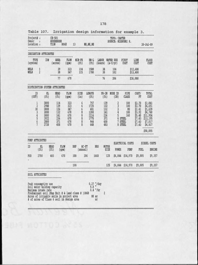
178Table 107. Irrigation design information for example 3.Project! i Owner i Location i

CH-50I ROUDEBUSHT23N ROfiE 13 NE,NE,NE

TOPOi CARTER SOURCE; MISSOURI R.

20-M-89

IRRIGATION ATTRIBUTESTYPE ID! AREA ELON MIN-PR HN-L LABOR NATSR USE PIVOT LINE FLOOD(systea) (acres) (gpi) (ft) (ft) (hours) (a-f/yr) COST COST COST

NHLN I 39 323 114 1580 38 104 $12,680NHLN 2 38 347 115 1700 38 102 $13,40077 670 76 206 $26,080

DISTRIBUTION SYSTEM ATTRIBUTESID EL HEAD FLON SIZE LENGTH PR-IN NODE ID PIPE COST/ TOTAL

(OUT) ( f t ) ( f t ) (g p i) ( in ) ( f t ) ( f t ) (IN ) CLASS FT COST

I 3000 114 323 6 757 139 2 100 $2.70 $2,0412 2980 139 323 6 1725 132 3 100 $2.70 $4,651

30 3000 126 347 6 681 132 3 80 2.41 $1,6393 3000 132 670 8 1208 141 4 100 $3.92 $4,7404 3000 141 670 8 2214 236 5 160 $5.40 $11,9545 2922 236 670 8 1775 371 6 STEEL $7.43 $13,1956 2800 371 670 8 944 458 7 STEEL $7.43 $7,0177 2720 458 670 8 648 483 8 STEEL $7.43 $4,817

$50,055

PUMP ATTRIBUTESID EL

(ft)HEAD(ft)

FLON(g p i)

BHP AC-FT (annual) HRS MOTORSIZEELECTRICAL COSTS PONER PUMP

DIESEL COSTS FUEL ENGINE

POD 2700 483 670 108 206 1668 125 $6,044 $14,970 $9,005 $9,357

108 125 $6,044 $14,970 $9,005 $9,357

SOIL ATTRIBUTES

Peak consuaptive use 0.27 "/daySoil water holding capacity 9.8 "Maxiaua intake rate 0.4 "/hrPredoainant soil (Map Unit I & land class I )386B 2Acres of irrigable soils in project area 80 acI of acres of Class 6 soil in design area ac

s s s s r s s s s s s s s r r s r s B s s s s B S S S B s r s s s s s s s s s s s s s s s s B s s s s s s s s s a s s s s s s s s s s s s s s s s x s s s s s s s s s s s s s s s s s s s s s s s s s & s

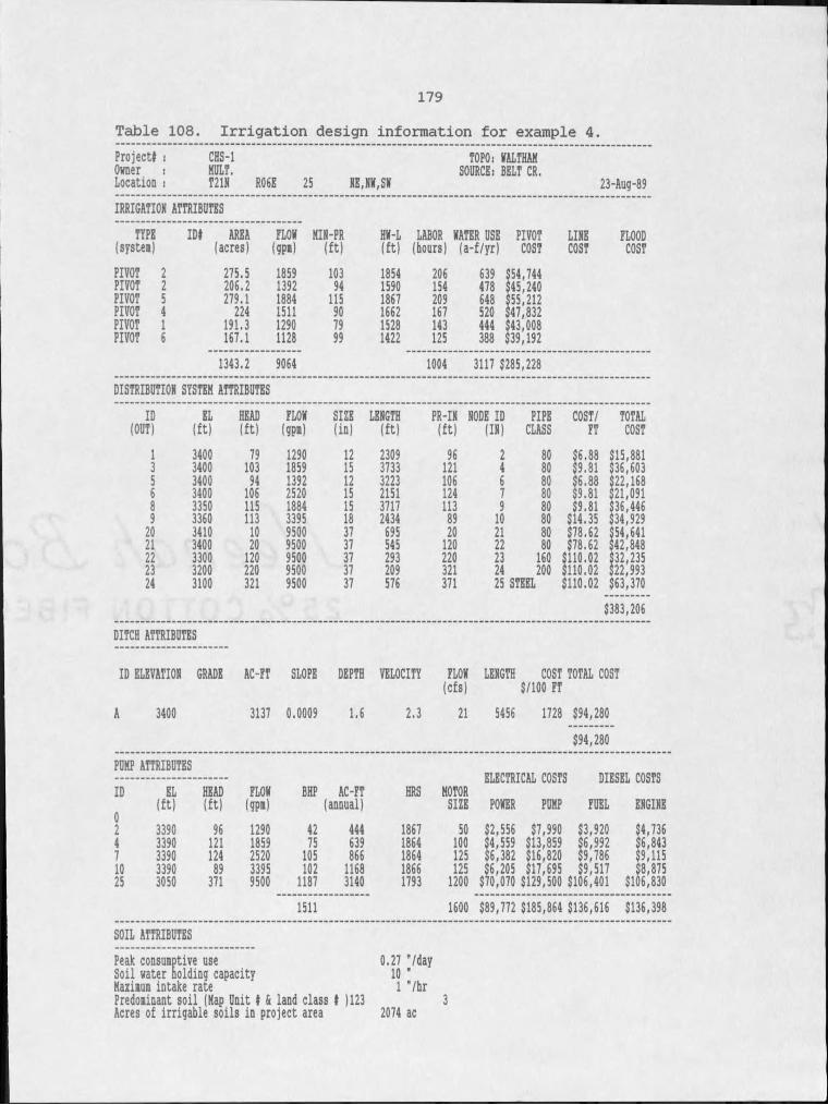
179Table 108. Irrigation design information for example 4.Project# i Owner s Location :

CHS-IMULT.T21N R06E 25 NE,NW,SWTOPOi WALTHAM SOURCE: BELT CR. 23-Aug-89

IRRIGATION ATTRIBUTESTYPE ID# AREA FLOW MIN-PR HW-L LABOR WATER USE PIVOT LINE FLOOD(system) (acres) I(gpi) (ft) (ft) (hours) (a-f/yr) COST COST COST

PIVOT 2 275.5 1859 103 1854 206 639 $54,744PIVOT 2 206.2 1392 94 1590 154 478 $45,240PIVOT 5 279.1 1884 115 1867 209 648 $55,212PIVOT 4 224 1511 90 1662 167 520 $47,832PIVOT I 191.3 1290 79 1528 143 444 $43,008PIVOT 6 167.1 1128 99 1422 125 388 $39,1921343.2 9064 1004 3117 $285,228

DISTRIBUTION SYSTEM ATTRIBUTESID EL HEAD FLOW SIZE LENGTH PR-IN NODE ID PIPE COST/ TOTAL(OUT) (ft) (ft) (gpi) (in) (ft) (ft) (IN) CLASS FT COSTI 3400 79 1290 12 2309 96 2 80 $6.88 I>15,8813 3400 103 1859 15 3733 121 4 80 $9.81 (!36,6035 3400 94 1392 12 3223 106 6 80 $6.88 !!22,1686 3400 106 2520 15 2151 124 7 80 $9.81 !>21,0918 3350 115 1884 15 3717 113 9 80 $9.81 |!36,4469 3360 113 3395 18 2434 89 10 80 $14.35 <!34,92920 3410 10 9500 37 695 20 21 80 $78.62 I>54,64121 3400 20 9500 37 545 120 22 80 $78.62 (>42,84822 3300 120 9500 37 293 220 23 160 <1110.02 S132,23523 3200 220 9500 37 209 321 24 200 $1110.02 122,993

24 3100 321 9500 37 576 371 25 STEEL $110.02 $63,370$383,206

DITCH ATTRIBUTES

ID ELEVATION GRADE AC-FT SLOPE DEPTH VELOCITY FLOW LENGTH COST TOTAL COST(cfs) $/100 FT

A 3400 3137 0.0009 1.6 2.3 21 5456 1728 $94,280$94,280

PUMP ATTRIBUTES ELECTRICAL COSTS DIESEL COSTSID SL HEAD FLOW BHP AC-FT HRS MOTOR

(ft) (ft) lgp*) (annual) SIZE POWER PUMP FUEL ENGINE2 3390 96 1290 42 444 1867 50 $2,556 $7,990 $3,920 $4,7364 3390 121 1859 75 639 1864 100 $4,559 $13,859 $6,992 $6,8437 3390 124 2520 105 866 1864 125 $6,382 $16,820 $9,786 $9,11510 3390 89 3395 102 1168 1866 125 $6,205 $17,695 $9,517 $8,87525 3050 371 9500 1187 3140 1793 1200 $70,070 $129,500 $106,401 $106,830

1511 1600 $89,772 $185,864 $136,616 $136,398SOIL ATTRIBUTESPeak consumptive use 0.27 "/daySoil water holding capacity 10 "Maximum intake rate I "/hrPredominant soil (Hap Unit t & land class f 1123 Acres of irrigable soils in project area 2074 ac 3

MONTANA STATE UNIVERSITY LIBRARIES

3 762 101 4392

Computer aided evaluation of the value of water for irrigation ...

Documents

Transcript of Computer aided evaluation of the value of water for irrigation ...