Computational Analysis of Single Molecule Force ... - SISSA
111
Scuola Internazionale Superiore di Studi Avanzati Physics Area Doctoral Program in Physics and Chemistry of Biological Systems Computational Analysis of Single Molecule Force Spectroscopy Experiments on Native Membranes PhD candidate: Nina Ilieva Supervisor: Prof. Alessandro Laio September 30, 2018
-
Upload
khangminh22 -
Category
Documents
-
view
3 -
download
0
Transcript of Computational Analysis of Single Molecule Force ... - SISSA
Scuola Internazionale Superiore di Studi Avanzati
Physics Area
Doctoral Program in Physics and Chemistry of Biological Systems
Computational Analysis of Single
Molecule Force Spectroscopy Experiments
on Native Membranes
PhD candidate:
Nina Ilieva
Supervisor:
Prof. Alessandro Laio
September 30, 2018
Contents
1 Introduction 3
2 AFM-SMFS of membrane proteins: an overview 12
2.0.1 Cell Membranes . . . . . . . . . . . . . . . . . . . . . . . . . . . . . . . . . . 12
2.0.2 Integral Membrane Proteins. . . . . . . . . . . . . . . . . . . . . . . . . . . . 14
2.0.3 Probing the Structure of Membrane Proteins by Atomic Force Microscopy
(AFM). . . . . . . . . . . . . . . . . . . . . . . . . . . . . . . . . . . . . . . . 19
2.0.4 AFM based Single Molecule Force Spectroscopy (SMFS). . . . . . . . . . . . 21
2.0.5 Molecular modeling. . . . . . . . . . . . . . . . . . . . . . . . . . . . . . . . . 27
2.0.6 Analysis tools for AFM-SMFS experiments. . . . . . . . . . . . . . . . . . . . 33
3 Molecular modeling of rhodopsin. 44
3.1 Experimental results. . . . . . . . . . . . . . . . . . . . . . . . . . . . . . . . . . . . . 45
3.1.1 AFM imaging. . . . . . . . . . . . . . . . . . . . . . . . . . . . . . . . . . . . 45
3.1.2 SMFS experiments. . . . . . . . . . . . . . . . . . . . . . . . . . . . . . . . . . 46
3.2 Theoretical approach. . . . . . . . . . . . . . . . . . . . . . . . . . . . . . . . . . . . 47
3.2.1 The molecular model of the rhodopsin-membrane system. . . . . . . . . . . . 48
3.2.2 Coarse-grained MD simulations setup. . . . . . . . . . . . . . . . . . . . . . . 50
3.2.3 Validation of the membrane potential. . . . . . . . . . . . . . . . . . . . . . . 53
3.2.4 All-atom MD simulations. . . . . . . . . . . . . . . . . . . . . . . . . . . . . . 54
3.2.5 Estimating the effect of membrane hydrophobicity on rhodopsin flexibility. . 55
3.3 Results. . . . . . . . . . . . . . . . . . . . . . . . . . . . . . . . . . . . . . . . . . . . 57
3.3.1 Coarse grained MD simulations of the unfolding experiments. . . . . . . . . . 57
3.3.2 Rhodopsin’s activation is affected by the membrane hydrophobicity. . . . . . 60
3.4 Conclusions. . . . . . . . . . . . . . . . . . . . . . . . . . . . . . . . . . . . . . . . . . 63
4 Automatic classification of SMFS data from membranes. 65
4.1 High throughput AFM in native membranes. . . . . . . . . . . . . . . . . . . . . . . 66
4.2 The algorithm. . . . . . . . . . . . . . . . . . . . . . . . . . . . . . . . . . . . . . . . 68
1
CONTENTS 2
4.2.1 Cutting and filtering the traces. . . . . . . . . . . . . . . . . . . . . . . . . . . 70
4.2.2 Computing the consistency score. . . . . . . . . . . . . . . . . . . . . . . . . . 72
4.2.3 The distance between two traces. . . . . . . . . . . . . . . . . . . . . . . . . . 76
4.2.4 Proxy distance for speeding up the calculation. . . . . . . . . . . . . . . . . . 79
4.2.5 Clustering. . . . . . . . . . . . . . . . . . . . . . . . . . . . . . . . . . . . . . 80
4.3 Relation with previous works. . . . . . . . . . . . . . . . . . . . . . . . . . . . . . . . 81
4.4 Benchmark AFM-SMFS traces. . . . . . . . . . . . . . . . . . . . . . . . . . . . . . . 82
4.5 Results. . . . . . . . . . . . . . . . . . . . . . . . . . . . . . . . . . . . . . . . . . . . 84
4.5.1 Results in data set I. . . . . . . . . . . . . . . . . . . . . . . . . . . . . . . . . 84
4.5.2 Validation of the main parameters. . . . . . . . . . . . . . . . . . . . . . . . . 87
4.5.3 Results in data set II: Rhodopsin + Unknown 1 + Unknown 2 + CNGA1. . . 91
4.5.4 Results in data set III. . . . . . . . . . . . . . . . . . . . . . . . . . . . . . . . 91
4.6 Conclusions . . . . . . . . . . . . . . . . . . . . . . . . . . . . . . . . . . . . . . . . . 99
Bibliography 102
Chapter 1
Introduction
Every living cell is surrounded by a biological membrane that separates the cell’s inner content
from the outside world. The basic structural unit of every membrane is the lipid bilayer, which is
built from phospholipids, sphingolipids and sterols. Phospholipids and sphingolipids are amphiphatic
molecules, which means that their molecules have hydrophilic (water-loving) head-groups and hy-
drophobic (water-fearing) tails. The specific chemical properties of these lipid molecules determine
the characteristic structure of the lipid bilayer: the polar head-groups face the outer environment of
the cell on both sides, while the hydrophobic tails form the interior of the bilayer (see Figure 2.1).
The main functional components of the cell membrane are the membrane proteins, which are
embedded in the lipid bilayer. Membrane proteins are active participants in the most important
biological processes in the cell membrane, like active transport of ions and molecules across the mem-
brane, signal transduction and cell-cell communication. Nearly 30 % of all proteins in eukaryotic
cells are membrane proteins. They are the targets of more than 50 % of modern medicinal drugs
and many diseases are found to be related to membrane proteins misfolding [1]. Despite their sig-
nificance, the number of three-dimensional membrane protein structures remains small. Currently,
there are 827 unique structures of membrane proteins available [2]. The reason is that the standard
experimental techniques used for studying the structure of soluble proteins (X-ray crystallography,
NMR spectroscopy and cryo-electron microscopy (cryo-EM)) experience difficulties when it comes
to membrane proteins. The main problems are associated with membrane proteins extraction, solu-
bilization, and purification. For example, the solubilization and purification of a specific membrane
protein require the selection of a suitable detergent and that step is critical [3].
Atomic force microscopy (AFM) turned out to be a promising alternative to the conventional
experimental methods used for studying proteins. Developed initially to image surfaces with atomic
resolution, the AFM method went far beyond the expectations. The atomic force microscope is a
scanning probe microscope, namely a device that uses a physical probe to scan the sample surface
producing a topographical image of the surface. The probe in this case is the tip, which is the most
3
CHAPTER 1. INTRODUCTION 4
important component of the microscope because it is the only component which physically touches
the sample. The AFM tip is mounted on the end of a flexible cantilever (see Figure 2.8a). Once
brought in contact with the sample, the tip raster scans the surface and experiences the attraction
forces acting between its sharp edge and the sample surface. Accordingly, the spring-like cantilever
bends. A laser beam pointed to the cantilever bounces off its back onto a position-sensitive photo
detector and the deflection of the light is measured with high precision. The roughness of the
sample surface induces changes in the cantilever deflection and its measurement and processing
shapes the final topographical image. In addition to this, the interaction forces between the tip and
the sample can be estimated from the deflections through Hooke’s law. AFM is used in a wide range
of disciplines, from solid state physics to medicine, from the study of quantum dots to the imaging of
living cells. What makes this method extremely suitable for biological samples is the fact that AFM
can operate in water solution, in physiological conditions and at body temperature. This allowed
using AFM for imaging of native cell membranes [4].
Apart from the imaging mode, AFM quickly became one of the most common techniques used
for single molecule force spectroscopy (SMFS) experiments. In this kind of experiments a single
molecule, like the double-helix of DNA, a protein or a polysaccharide, is directly manipulated with
a probe, usually of microscopic size [5], obtaining information about its structural and dynamical
properties in real time and at the single molecule level. In AFM-based SMFS, the microscope is
used as a pico-Newton force measuring device [6]. The protein molecule is on one side bound to the
surface, while on the other side it gets picked by the AFM tip and stretched as the tip retracts from
the surface (see Figure 2.9a). The molecular force response versus the distance between the tip and
the sample surface is recorded and presented in the form of a force-extension (F-x) curve (see Figure
2.9b). F-x curves, known also as traces, are direct probes of the protein’s unfolding pathways. These
curves store the information about the unfolding of the protein domains, their mechanical stability,
the order in which they unfold, etc. This information has been used to understand better protein
folding[7]. These studies highlighted a very important fact: that the force pattern contained in these
curves is a fingerprint of the protein under examination. For example, the mechanical unfolding of
the multidomain protein titin [8], responsible for the passive elasticity of muscle cells, results in F-x
curves bearing a characteristic sawtooth pattern in which the number of force peaks is equal to the
number of immunoglobulin domains (see Figure 2.10). The order in which the individual domains
unfold is governed by the strength of the interactions which hold them, thus the weakest domains
unfold first. This example is a clear demonstration of the enormous potentialities of this technique.
These potentialities are exploited at best for studying membrane proteins, where, as we have
seen, other methods often fail. AFM allows both imaging of the cell membrane and manipulating
single membrane proteins embedded in it. All of this is accomplished under physiological conditions.
The number of membrane proteins unfolded in AFM-SMFS experiments is rapidly growing. The
list includes the light-sensitive receptor proteins bacteriorhodopsin and rhodopsin [9, 10, 11, 12], the
CHAPTER 1. INTRODUCTION 5
CNGA1 channel [13, 12], the Na+/K+ antiporter [14], the leucine-binding protein [15] and many
others. The first membrane protein studied with AFM-SMFS was bacteriorhodopsin (bR). This was
done in a work by Muller et al. [9] dealing with the unfolding pathways of bR. In this study, the
AFM was used at the same time for imaging the membrane and unfolding of the bR present in it (see
Figure 2.11). The obtained F-x patterns revealed pairwise unfolding of the transmembrane helices of
bR. However, rather surprisingly, in this experiment not all the F-x curves looked similar. In some
of them, two of the helices were unfolding one after the other, which indicates different unfolding
pathways. This illustrates that AFM can also be used to detect different unfolding pathways of the
same protein.
This technique has not yet shown all its potentialities, and new avenues are opened almost every
year. Recent advances in AFM-SMFS enabled the acquisition of a huge amount of data in reasonable
time [16, 17]. Moreover, this has been achieved with experiments performed directly in native cell
membranes under physiological conditions [18]. The obtained data are highly heterogeneous, the
amount of high-quality traces is very low and they come from the unfolding of different proteins with
different size. Between 1,000 and 10,000 F-x curves are usually generated in a single experiment.
The availability of this huge amount of experimental data encouraged the development of novel
automatic tools promoting its processing with the least possible manual intervention. Several tools
aimed at this scope have already been proposed [19, 20, 21, 22]. These approaches work very well for
membrane proteins of the same type or for samples with well-known protein composition. However,
the same approaches have some serious limitations when it comes to data sets with unknown protein
composition like those collected in native membranes. The main issue with AFM-SMFS data is that
in < 1% of the cases membrane proteins are completely unfolded [21]. This means that in the large
bulk of data, only a tiny portion of traces is worth looking at. Not only this, but the majority of the
traces do not contain any unfolding events. This makes the careful preprocessing of the raw data a
crucially important step. All the available methods are based on knowing the approximate length of
the fully-stretched protein under investigation. This information allows the selection of F-x curves
having their last force peak at extension values comparable with the protein length. A solution
of this kind is useful in AFM experiments performed in controlled environments where a certain
protein of interest is unfolded. However, if we want to analyze data coming from experiments in
native cell membranes, this approach is incapable of spanning all the possibilities simply because the
membrane for sure contains proteins unidentified so far. Ideally, an appropriate method for analysis
AFM-SMFS data coming from native cell membranes should be able to select in an unsupervised
manner all traces which contain successful unfolding events and to group those that are similar to
each other in separate clusters. In this way, all the meaningful data will be extracted and presented
in a human-readable manner, easier to interpret.
This thesis was motivated by developing tools for interpreting AFM-SMFS experiments on mem-
brane proteins performed in native cell membranes. In particular, we address two problems. The
CHAPTER 1. INTRODUCTION 6
first one deals with the effects of lipid composition of different membranes on the mechanical sta-
bility and and unfolding pathway of membrane proteins. The second one deals with the analysis of
the huge amount of data generated by AFM-SMFS experiments in native cell membranes.
In Chapter 2 we provide a general overview on cell membranes and a brief description of the
main components they contain. Our focus is on membrane proteins embedded in the cell membrane,
known also as integral membrane proteins, since they are the molecular objects of this study. We
describe the two basic secondary motifs by which they are built: the α-helix and the β-barrel. We
discuss two classifications of membrane proteins: topology-based and function-based. In subsection
2.0.3 we shortly explain how the AFM imaging mode works, while in subsection 2.0.4 we comment
its performance in the SMFS mode, providing a descriptions of the experiments. After that, we
discuss molecular models used to describe these experiments. Finally, we make an overview of some
of the currently available procedures for analysis of AFM-SMFS data.
The work presented in Chapter 3 was motivated by AFM-SMFS experiments performed in the
discs and the plasma membrane of the rod OS, where rhodopsin is the dominant protein. The
obtained F-x curves from pulling rhodopsin from the discs and from the plasma membrane re-
vealed two strikingly different unfolding patterns [12]. Moreover, rhodopsin in the discs initiates the
phototransuction cascade, while rhodopsin in the plasma membrane does not. The discs and the
plasma membrane have different lipid composition [23]. The plasma membrane has higher choles-
terol concentration. This suggests that the different lipid environment affects both the rhodopsin
mechanical properties and its function. In order to test this hypothesis we used a simple topology-
based coarse-grained model of the protein-membrane system. The protein molecule was described
with a coarse-grained Go-like model initially developed by Cieplak et al. [24] to study the mechanical
unfolding of soluble proteins [25, 26, 27]. This model successfully reproduced the experimental F-x
curves and provided an important insight in the interpretation of these spectra. A modified version
of this model was applied also to membrane proteins, to bacteriorhodopsin in particular [28]. When
it comes to the unfolding of membrane proteins, the proper modeling of the system becomes much
more demanding in comparison to soluble proteins. Membrane proteins do not only get stretched
but they also get extracted out of the membrane. This necessarily requires taking the membrane
into account in the model. Cieplak et al. [28] did this explicitly representing the membrane with a
lipid bilayer, modeled in a coarse-grained manner. When the protein is pulled the membrane is kept
frozen: as a portion of the polypeptide chain gets extracted, the space it was occupying remains
empty, leaving a hole in the membrane. In simple terms, the lipid bilayer does not adjust to the
new configuration of the system. This approximation is in our opinion unrealistic. To model more
accurately the unfolding of a membrane protein we developed a new approach in which we model
the effect of the membrane by adding to the original Go model of Cieplak et al. [24] an extra poten-
tial energy term VMEMBR. The potential operates in a different manner on the different residues
depending on their hydrophobicity and the contact they form with the membrane in the native
CHAPTER 1. INTRODUCTION 7
configuration. When a hydrophobic residue forms a native contact with the membrane and it is
positioned inside the membrane, VMEMBR is 0. If that same residue is in a region corresponding
to the region occupied by the polar head-groups of the lipids, it gets moderately unfavored. If the
residue is outside the membrane and is water-exposed, it gets a full penalty, which is defined by the
only important parameter of the model, εMEMBR. This parameter determines the strength of the
membrane potential. Furthermore, by varying εMEMBR one can model different lipid compositions
of the membrane. For example, larger values of εMEMBR specify a more hydrophobic membrane
like a cholesterol-rich membrane.
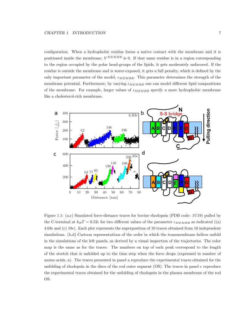
Figure 1.1: (a,c) Simulated force-distance traces for bovine rhodopsin (PDB code: 1U19) pulled by
the C-terminal at kBT = 0.52ε for two different values of the parameter εMEMBR as indicated ((a)
4.03ε and (c) 10ε). Each plot represents the superposition of 10 traces obtained from 10 independent
simulations. (b,d) Cartoon representations of the order in which the transmembrane helices unfold
in the simulations of the left panels, as derived by a visual inspection of the trajectories. The color
map is the same as for the traces. The numbers on top of each peak correspond to the length
of the stretch that is unfolded up to the time step when the force drops (expressed in number of
amino acids, n). The traces presented in panel a reproduce the experimental traces obtained for the
unfolding of rhodopsin in the discs of the rod outer segment (OS). The traces in panel c reproduce
the experimental traces obtained for the unfolding of rhodopsin in the plasma membrane of the rod
OS.
CHAPTER 1. INTRODUCTION 8
Changing the values of εMEMBR in our model is like changing the hydrophobicity of the mem-
brane arising from its different lipid composition. We performed stretching MD simulations with
four different values of εMEMBR. With our simple model, we were able to qualitatively reproduce
the difference in the experimental curves obtained from unfolding of rhodopsin in the discs and in
the plasma membrane. In Figure 1.1 we show F-x curves predicted by our model together with car-
toon representations of rhodopsin colored in correspondence with the order of unfolding of the single
units. The superimposition of simulated traces depicted in Figure 1.1a is in good agreement with
the experimental curves from unfolding of rhodopsin from the discs, while the superimposition of
simulated traces in Figure 1.1c corresponds to the experimental curves from unfolding of rhodopsin
from the plasma membrane. These results support the hypothesis that the reason we observe differ-
ent unfolding patterns of rhodopsin from the discs and from the plasma membrane is in the different
lipid composition implying different membrane hydrophobicity captured in our model by the value
of εMEMBR.
In Chapter 3 we also attempt to model and understand the inactivation of rhodopsin in the
plasma membrane. Since the main difference between the plasma membrane and the discs is the
higher cholesterol concentration of the former, we decided to check if the conformation with a
larger membrane-exposed hydrophobic area would be favored in a more hydrophobic membrane.
Our coarse-grained model is a Go-model, and therefore cannot be used to describe conformational
changes. Therefore, it is not appropriate for addressing this problem. Instead, we used all-atom MD
simulation of rhodopsin embedded in a DPPC bilayer in two different conformations relevant to the
light-harvesting cycle. To evaluate the effect of cholesterol on rhodopsin’s flexibility we used free
energy perturbation theory. The final results suggest that the higher cholesterol concentration of
the plasma membrane favors the inactive rhodopsin conformation hence preventing rhodopsin from
activation. These results confirm the utmost influence of membrane composition on the mechanical
properties of membrane proteins.
Chapter 4 describes the main contribution of this Thesis. We there describe a fully-automatic
procedure for the analysis of F-x curves coming from experiments performed in native cellular
membranes. This work is motivated from the recent development of techniques for performing AFM-
SMFS experiments on native membrane patches [18]. The obtained data is highly heterogeneous
and presents some serious challenges to data analysis. In the available methods [19, 20, 21, 22] the
analysis is guided by knowledge on the protein sample composition. In native membrane patches
this information is simply not available. Another issue is determined by the extremely small amount
of high-quality traces in these data sets. Here by high-quality traces, we mean F-x curves associated
with meaningful unfolding events.
To address these issues, we developed an automatic procedure that does not require knowledge
on the protein sample composition and is able to extract high-quality traces from the data bulk
in an unsupervised manner. The idea is to be able to distinguish different proteins based on the
CHAPTER 1. INTRODUCTION 9
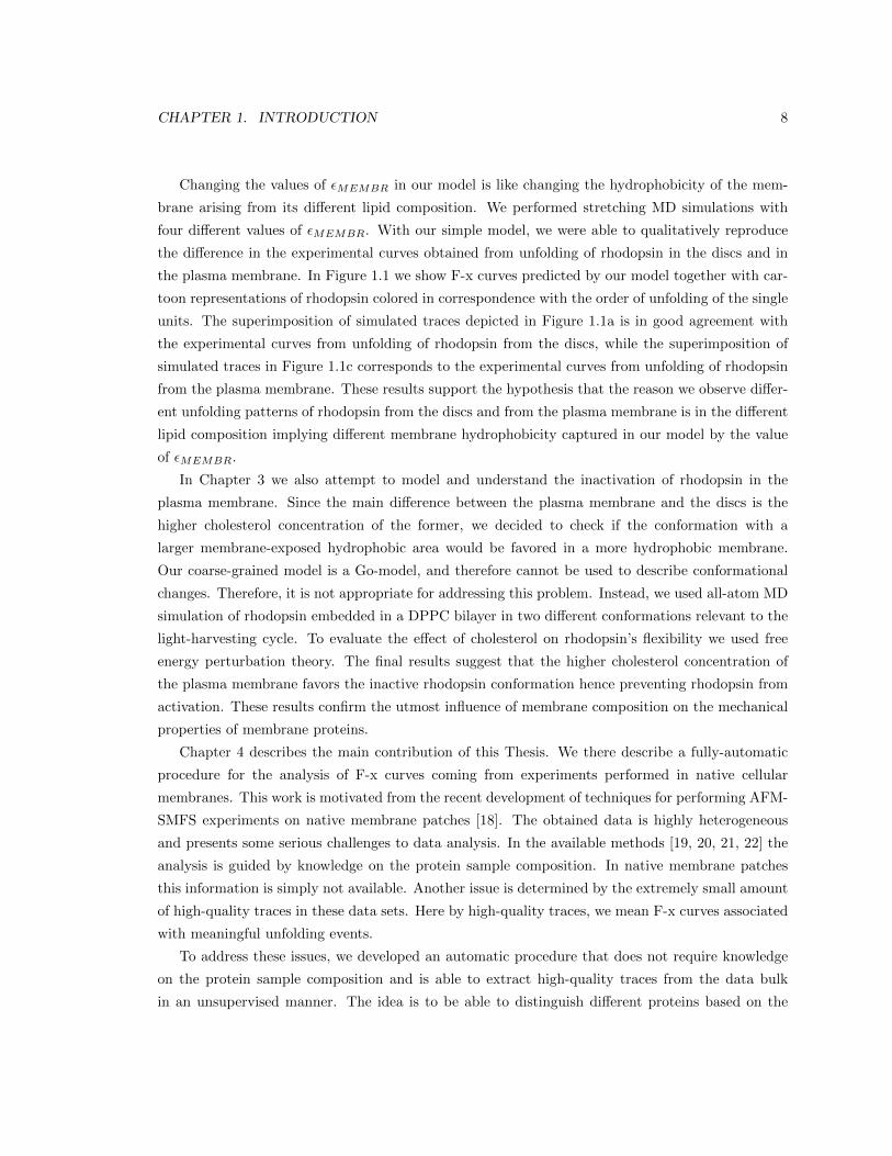
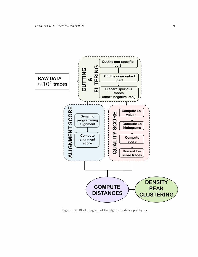
Figure 1.2: Block diagram of the algorithm developed by us.
CHAPTER 1. INTRODUCTION 10
characteristic unfolding patterns observed in their F-x curves without knowing who these proteins
are. In Figure 1.2 we show a block diagram representing the procedure. Initially, we process all
traces removing the noisy parts of the signal, aiming at obtaining only this part of the F-x curve
that contains the unfolding pattern. This step corresponds to the ”Cutting & Filtering” block in
Figure 1.2. The nature of the data requires alignment of the F-x curves to overcome horizontal shifts
due to the different tip-protein attachment positions. For this scope, we use dynamic programming
alignment, which gives an alignment score that provides a measure of the similarity between two
traces. A pair of similar traces is characterized by a high alignment score. This alignment approach
has been already applied to SMFS data and described in the literature by Marsico et al. [20]. In
order to extract high-quality traces from the large data set, we assigned a quality score to each trace
and used that for selecting the meaningful traces. The quality score measures the consistency of
each trace with a polymer physics model called the worm-like chain (WLC) model (see subsection
2.0.4). The WLC model has proved to provide a reliable interpretation of the experimental F-x
curves and moreover, a quantitative one. The WLC consistency score evaluates the quality of a
trace. If the score is high, the trace is good; if the score is low, the trace is bad. Once we have
selected good traces, based on their quality score we would like to group them into clusters based
on the unfolding patterns they contain. In order to do this, we use density-peak clustering [29], a
clustering approach which robustly recognizes groups of data points belonging to separate peaks in
the probability distribution. The crucial ingredient of this approach is the distance between two data
points, in our case two AFM-SMFS traces. We defined a distance which combines the alignment
score and the quality score. According to this distance, high-quality traces similar to each other have
a small distance. Instead, low-quality traces, even if they are similar to each other, have a larger
distance. This guarantees that the clusters we obtain contain traces which are not only similar to
each other (which is the case in the work of Marsico et al. [20]) but which are also both of a high
quality, in terms of consistency with the WLC model. We will show how important it is using a
distance with these properties.
We tested our method on a data set containing ∼ 100 manually selected traces corresponding
to the unfolding of the CNGA1 channel and ∼ 4,000 traces of unidentified origin and quality. Our
method was able to detect the CNG traces and to put them in a separate cluster. Remarkably, the
method was also able to find other CNG traces that escaped the manual selection and to assign
them to the CNG cluster. In addition, we obtained other clusters whose molecular origin we are
currently unable to identify.
We also applied our procedure on a data set containing ∼ 400,000 traces from pulling experiments
in the plasma membrane of the rod outer segment (OS). This large data set presents a challenge for
every currently available tool for SMFS data analysis, including our method. The time it took to
our program to analyze this huge amount of traces on a workstation with 16 CPUs is ∼ 90 minutes.
Not surprisingly, only ∼ 5 % of all traces passed the selection procedure. The plasma membrane
CHAPTER 1. INTRODUCTION 11
of the rod OS hosts primarily rhodopsin and CNG channels, thus we expect to obtain clusters
corresponding to the unfolding these two proteins. Two of the clusters contain decent candidates for
the unfolding of rhodopsin, but we couldn’t find a cluster corresponding to the CNG channel. We
assume that the reason for this is that the number of good CNG traces that are similar to each other
is insufficient to form a cluster. To test this hypothesis we added the manually selected CNG traces
from the previous data set to this data set and applied our procedure. As a final result we obtained
an additional cluster containing the manually selected CNG traces supporting our hypothesis. We
looked also at the other clusters and indeed, the number of cluster members very similar to the
cluster center is very small suggesting that not only the CNG traces similar to each other are very
little but the number of high-quality traces similar to each other is very low. This seriously troubles
the clusters identification. We need more data sets from native membranes in order to further
validate this hypothesis.
Chapter 2
AFM-SMFS of membrane proteins:
an overview
2.0.1 Cell Membranes
Every living cell is surrounded by a biological membrane that separates the cell’s inner con-
tent from the outside world. This biological membrane is not an inactive barrier but a protection
sheath through which transport of nutrients and waste products is accomplished. The cell mem-
brane is composed of lipids, proteins and carbohydrates. Lipids are represented by phospholipids,
sphingolipids and sterols. Phospholipids and sphingolipids are amphipathic molecules: they have a
hydrophilic (water-loving) group attached to a hydrophobic (water-fearing) chain. The hydrophilic
heads of the lipid molecules face the outer environment on each side of the membrane, while the
hydrophobic tails point to each other in the membrane interior escaping the water environment.
This molecular orientation provides the formation of the lipid bilayer - the basic structure of the
cell membrane (Figure 2.1). The lipid bilayer is fluid with viscosity similar to that of olive oil [30].
The most common sterol molecule in animal cell membranes is cholesterol. Cholesterol is randomly
distributed in the bilayer and the fluidity of the membrane depends on its presence. Cholesterol
helps the phospholipid molecules to stay together, not moving too far from each other or packing too
tightly. This is important because if the phospholipids are separated at a great distance, unwanted
toxic substances might easily enter the cell; if the phospholipids are too close, the passive transport
of ions and small molecules through the membrane might be hindered.
12
CHAPTER 2. AFM-SMFS OF MEMBRANE PROTEINS: AN OVERVIEW 13
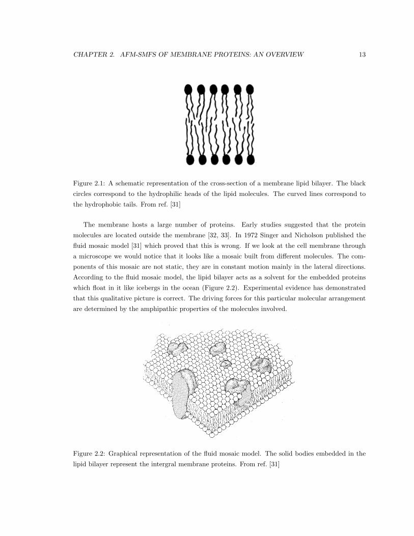
Figure 2.1: A schematic representation of the cross-section of a membrane lipid bilayer. The black
circles correspond to the hydrophilic heads of the lipid molecules. The curved lines correspond to
the hydrophobic tails. From ref. [31]
The membrane hosts a large number of proteins. Early studies suggested that the protein
molecules are located outside the membrane [32, 33]. In 1972 Singer and Nicholson published the
fluid mosaic model [31] which proved that this is wrong. If we look at the cell membrane through
a microscope we would notice that it looks like a mosaic built from different molecules. The com-
ponents of this mosaic are not static, they are in constant motion mainly in the lateral directions.
According to the fluid mosaic model, the lipid bilayer acts as a solvent for the embedded proteins
which float in it like icebergs in the ocean (Figure 2.2). Experimental evidence has demonstrated
that this qualitative picture is correct. The driving forces for this particular molecular arrangement
are determined by the amphipathic properties of the molecules involved.
Figure 2.2: Graphical representation of the fluid mosaic model. The solid bodies embedded in the
lipid bilayer represent the intergral membrane proteins. From ref. [31]
CHAPTER 2. AFM-SMFS OF MEMBRANE PROTEINS: AN OVERVIEW 14
The protein molecules in the membrane can be divided in two groups: integral and peripheral
proteins. The integral membrane proteins are embedded in the membrane and their extraction
requires usage of detergents, non-polar solvents and denaturing agents. Transmembrane proteins
play an active role in transport, in signal transduction, in cell-cell communication, among the most
crucial biological processes in the cell. The peripheral proteins are located on the membrane surface,
bounded through electrostatic or hydrogen bonds with the polar groups of the lipid molecules or
the integral proteins. They can be easily extracted through changes in the external conditions, for
example the pH of the environment.
Now that we briefly introduced the composition and the structure of the cell membrane we focus
on the object of this study: integral membrane proteins. Later on when we use ’membrane proteins’
in the text we refer to integral membrane proteins.
2.0.2 Integral Membrane Proteins.
Most of the protein structures we know, have been determined by X-ray crystallography. Mem-
brane proteins turned out to be harder to crystallize compared to soluble proteins and in the very
beginning only few structures were available. Recent advances in crystallography brought high-
resolution X-ray structures for a larger number of membrane proteins. Protein structures can be
determined also with NMR spectroscopy and electron microscopy or through a combination of the
mentioned techniques. This has led to an increase in the number of solved three-dimensional struc-
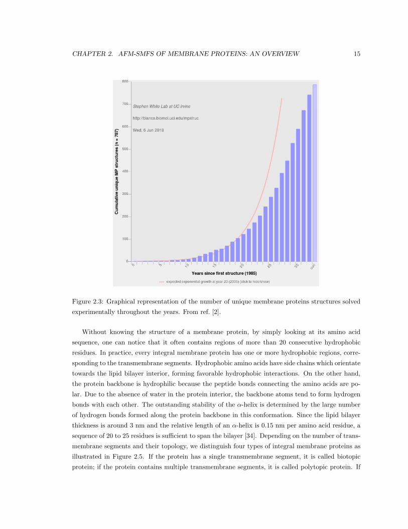
tures of membrane proteins as depicted in Figure 2.3. Anyway, compared to soluble proteins, the
number of available three-dimensional structures of membrane proteins remains small.
The folded state of a membrane protein does not depend only on the protein itself, like in the case
of soluble proteins. The folded state strongly depends on the presence of the lipid bilayer. A simple
comparison between the properties of the plasma membrane and the cytosol reveals more differences
regarding membrane proteins and soluble proteins. Unlike cytosol, the plasma membrane is a het-
erogeneous and anisotropic environment with a very low dielectric constant. In most membranes
gradients of pH, electric field, pressure, dielectric constant, and redox potential are present [30]. As
a consequence, the lipid bilayer restricts the conformational space of membrane proteins.
Integral membrane proteins can be divided in two groups depending on their structural charac-
teristics: α-helical and β-barrel proteins. α-helical membrane proteins are far more common. They
are present in all types of biological membranes. It has been estimated that 27 % of all proteins
in humans are α-helical membrane proteins. This can be explained by the underlying physics and
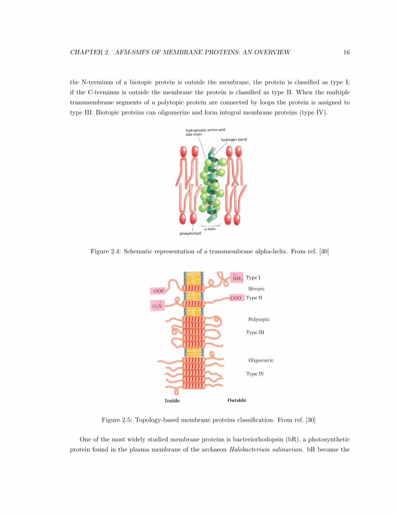
chemistry of the interactions which stabilize α-helices in membranes (Figure 2.4).
CHAPTER 2. AFM-SMFS OF MEMBRANE PROTEINS: AN OVERVIEW 15
Figure 2.3: Graphical representation of the number of unique membrane proteins structures solved
experimentally throughout the years. From ref. [2].
Without knowing the structure of a membrane protein, by simply looking at its amino acid
sequence, one can notice that it often contains regions of more than 20 consecutive hydrophobic
residues. In practice, every integral membrane protein has one or more hydrophobic regions, corre-
sponding to the transmembrane segments. Hydrophobic amino acids have side chains which orientate
towards the lipid bilayer interior, forming favorable hydrophobic interactions. On the other hand,
the protein backbone is hydrophilic because the peptide bonds connecting the amino acids are po-
lar. Due to the absence of water in the protein interior, the backbone atoms tend to form hydrogen
bonds with each other. The outstanding stability of the α-helix is determined by the large number
of hydrogen bonds formed along the protein backbone in this conformation. Since the lipid bilayer
thickness is around 3 nm and the relative length of an α-helix is 0.15 nm per amino acid residue, a
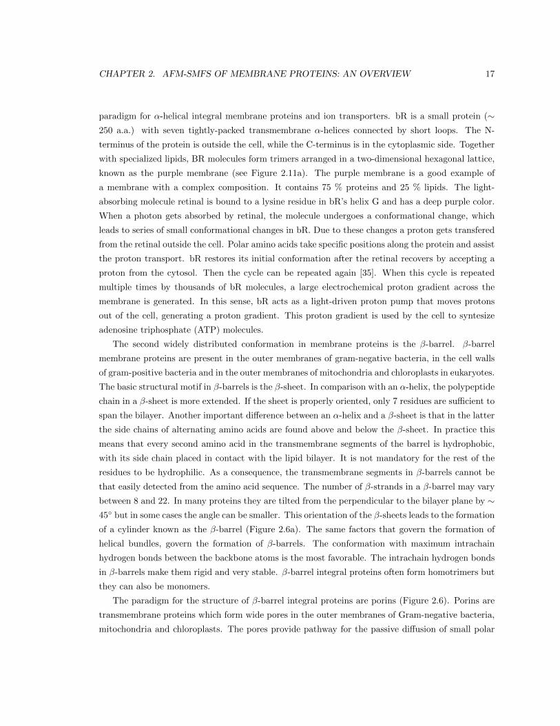
sequence of 20 to 25 residues is sufficient to span the bilayer [34]. Depending on the number of trans-
membrane segments and their topology, we distinguish four types of integral membrane proteins as
illustrated in Figure 2.5. If the protein has a single transmembrane segment, it is called biotopic
protein; if the protein contains multiple transmembrane segments, it is called polytopic protein. If
CHAPTER 2. AFM-SMFS OF MEMBRANE PROTEINS: AN OVERVIEW 16
the N-terminus of a biotopic protein is outside the membrane, the protein is classified as type I;
if the C-terminus is outside the membrane the protein is classified as type II. When the multiple
transmembrane segments of a polytopic protein are connected by loops the protein is assigned to
type III. Biotopic proteins can oligomerize and form integral membrane proteins (type IV).
Figure 2.4: Schematic representation of a transmembrane alpha-helix. From ref. [30]
Figure 2.5: Topology-based membrane proteins classification. From ref. [30]
One of the most widely studied membrane proteins is bacteriorhodopsin (bR), a photosynthetic
protein found in the plasma membrane of the archaeon Halobacterium salinarium. bR became the
CHAPTER 2. AFM-SMFS OF MEMBRANE PROTEINS: AN OVERVIEW 17
paradigm for α-helical integral membrane proteins and ion transporters. bR is a small protein (∼250 a.a.) with seven tightly-packed transmembrane α-helices connected by short loops. The N-
terminus of the protein is outside the cell, while the C-terminus is in the cytoplasmic side. Together
with specialized lipids, BR molecules form trimers arranged in a two-dimensional hexagonal lattice,
known as the purple membrane (see Figure 2.11a). The purple membrane is a good example of
a membrane with a complex composition. It contains 75 % proteins and 25 % lipids. The light-
absorbing molecule retinal is bound to a lysine residue in bR’s helix G and has a deep purple color.
When a photon gets absorbed by retinal, the molecule undergoes a conformational change, which
leads to series of small conformational changes in bR. Due to these changes a proton gets transfered
from the retinal outside the cell. Polar amino acids take specific positions along the protein and assist
the proton transport. bR restores its initial conformation after the retinal recovers by accepting a
proton from the cytosol. Then the cycle can be repeated again [35]. When this cycle is repeated
multiple times by thousands of bR molecules, a large electrochemical proton gradient across the
membrane is generated. In this sense, bR acts as a light-driven proton pump that moves protons
out of the cell, generating a proton gradient. This proton gradient is used by the cell to syntesize
adenosine triphosphate (ATP) molecules.
The second widely distributed conformation in membrane proteins is the β-barrel. β-barrel
membrane proteins are present in the outer membranes of gram-negative bacteria, in the cell walls
of gram-positive bacteria and in the outer membranes of mitochondria and chloroplasts in eukaryotes.
The basic structural motif in β-barrels is the β-sheet. In comparison with an α-helix, the polypeptide
chain in a β-sheet is more extended. If the sheet is properly oriented, only 7 residues are sufficient to
span the bilayer. Another important difference between an α-helix and a β-sheet is that in the latter
the side chains of alternating amino acids are found above and below the β-sheet. In practice this
means that every second amino acid in the transmembrane segments of the barrel is hydrophobic,
with its side chain placed in contact with the lipid bilayer. It is not mandatory for the rest of the
residues to be hydrophilic. As a consequence, the transmembrane segments in β-barrels cannot be
that easily detected from the amino acid sequence. The number of β-strands in a β-barrel may vary
between 8 and 22. In many proteins they are tilted from the perpendicular to the bilayer plane by ∼45◦ but in some cases the angle can be smaller. This orientation of the β-sheets leads to the formation
of a cylinder known as the β-barrel (Figure 2.6a). The same factors that govern the formation of
helical bundles, govern the formation of β-barrels. The conformation with maximum intrachain
hydrogen bonds between the backbone atoms is the most favorable. The intrachain hydrogen bonds
in β-barrels make them rigid and very stable. β-barrel integral proteins often form homotrimers but
they can also be monomers.
The paradigm for the structure of β-barrel integral proteins are porins (Figure 2.6). Porins are
transmembrane proteins which form wide pores in the outer membranes of Gram-negative bacteria,
mitochondria and chloroplasts. The pores provide pathway for the passive diffusion of small polar

CHAPTER 2. AFM-SMFS OF MEMBRANE PROTEINS: AN OVERVIEW 18
molecules across the outer membrane. Each β-barrel is composed from 16 to 18 β-strands with
antiparallel orientation between each other (Figure 2.6a). The strands are connected by short loops
on the periplasmic side, and long irregular loops on the extracellular side. There is an internal
loop that faces the barrel interior and keeps the structure more compact. These architectures are
remarkably stable and denaturation is the only way to disassemble them [36].
Figure 2.6: A schematic representation of the transmembrane β-barrel protein OmpF porin from E.
coli. In panel a: side view; in panel b: top view. From ref. [36]
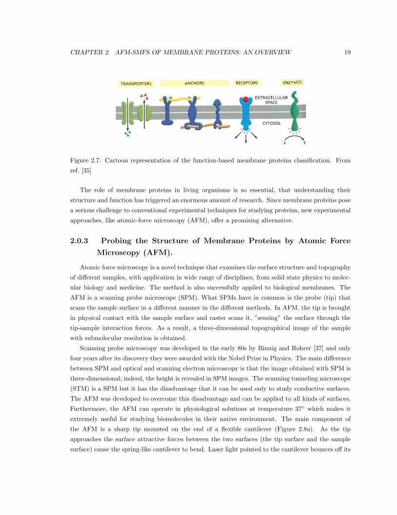
Most of the functions of the cell membrane are performed by certain types of membrane proteins.
Based on their functions they can be divided into transporters, anchors, receptors and enzymes
(Figure 2.7). Transporters carry nutrients, metabolites and ions across the membrane. The solutes
can be distinguished by their size and charge (in ion channels) or according to their ability of
fitting into the binding site of the protein. Anchors bind macromolecules on both sides of the
membrane. For example, integrins bind fibronectin outside the membrane and they are linked
to the cytoskeleton inside the membrane. Integrins facilitate the cell-extracellular matrix (ECM)
adhesion. Receptors generate intracellular signals through binding specific extracellular molecules.
In this manner communication between the outside environment and the cell is accomplished and
in response a particular action is performed by the cell. Platelet-derived growth factor (PDGF)
receptor binds PDGF and causes the cell to grow and divide. Membrane proteins which act as
enzymes catalyze different reactions. For example, adenylyl cyclase catalyzes the production of
cyclic AMP inside the cell.
CHAPTER 2. AFM-SMFS OF MEMBRANE PROTEINS: AN OVERVIEW 19
Figure 2.7: Cartoon representation of the function-based membrane proteins classification. From
ref. [35]
The role of membrane proteins in living organisms is so essential, that understanding their
structure and function has triggered an enormous amount of research. Since membrane proteins pose
a serious challenge to conventional experimental techniques for studying proteins, new experimental
approaches, like atomic-force microscopy (AFM), offer a promising alternative.
2.0.3 Probing the Structure of Membrane Proteins by Atomic Force
Microscopy (AFM).
Atomic force microscopy is a novel technique that examines the surface structure and topography
of different samples, with application in wide range of disciplines, from solid state physics to molec-
ular biology and medicine. The method is also successfully applied to biological membranes. The
AFM is a scanning probe microscope (SPM). What SPMs have in common is the probe (tip) that
scans the sample surface in a different manner in the different methods. In AFM, the tip is brought
in physical contact with the sample surface and raster scans it, ”sensing” the surface through the
tip-sample interaction forces. As a result, a three-dimensional topographical image of the sample
with submolecular resolution is obtained.
Scanning probe microscopy was developed in the early 80s by Binnig and Rohrer [37] and only
four years after its discovery they were awarded with the Nobel Prize in Physics. The main difference
between SPM and optical and scanning electron microscopy is that the image obtained with SPM is
three-dimensional; indeed, the height is revealed in SPM images. The scanning tunneling microscope
(STM) is a SPM but it has the disadvantage that it can be used only to study conductive surfaces.
The AFM was developed to overcome this disadvantage and can be applied to all kinds of surfaces.
Furthermore, the AFM can operate in physiological solutions at temperature 37◦ which makes it
extremely useful for studying biomolecules in their native environment. The main component of
the AFM is a sharp tip mounted on the end of a flexible cantilever (Figure 2.8a). As the tip
approaches the surface attractive forces between the two surfaces (the tip surface and the sample
surface) cause the spring-like cantilever to bend. Laser light pointed to the cantilever bounces off its

CHAPTER 2. AFM-SMFS OF MEMBRANE PROTEINS: AN OVERVIEW 20
back onto a position-sensitive photo detector. As the cantilever bends, the position of the reflected
laser beam on the photo diode shifts and the deflection of the light is measured with high precision.
Since protrusions and indentations in the sample surface lead to changes in the cantilever deflection,
measuring and processing this deflection leads to the topographical image of the examined surface.
Furthermore, Hooke’s law can be applied to the cantilever and knowing the cantilever’s spring
constant, the deflections can be transformed into forces. In this manner, the interaction forces
acting between the AFM tip and the sample are measured.
Figure 2.8: Schematic represetation of an atomic-force microscope (AFM). a. The AFM cantilever.
b. The basic components in a standard AFM setup. From ref. [38, 39]
The basic components of an AFM are: the tip and the cantilever, the laser, the photodiode
detector, the piezoelectric scanner and the feedback electronics (Figure 2.8b). The tip is the most
important component since it is the part of the microscope that physically touches the sample. The
AFM tip comes in different sizes and shapes, but the typical tip radius is between 5 and 20 nm.
The resolution of the image depends strongly on the sharpness of the tip. The sharper the tip,
the higher the resolution. But we should keep in mind that due to the physical interactions with
the sample, the tip changes during the experiment and the operator should take account for these
changes. Working with the sharpest tip does not guarantee the optimal experiment outcome. The
AFM cantilever is 100-200 µm long and what really matters is its spring constant. The smaller
the spring constant, the smaller the forces ”sensed” by the cantilever. The photo detector used in
commercial AFMs is usually a quadrant photo diode (QPD). Once a photo diode gets hit by light,
a voltage is generated. In a QPD the voltage magnitude is position-dependent. For example, if the
CHAPTER 2. AFM-SMFS OF MEMBRANE PROTEINS: AN OVERVIEW 21
light beam falls in the centre of the diode, the voltage is zero; in any other place, a finite voltage
is generated. In many instruments, a piezoelectric scanner governs the motion of the sample stage.
Piezo is a material that changes its dimensions due to applied voltage. For example, if a positive
voltage is applied, the material elongates; if a negative voltage is applied, the material becomes
shorter and thicker. These properties of the piezo allow control on the distance between the AFM
tip and the sample. In other AFMs, the piezoelectric scanner is implemented in the cantilever holder
and controls the cantilever motion. In the most frequently used AFM operational modes constant
contact force between the tip and the sample during scanning is maintained through a feedback
electronics loop. The feedback electronics maintains constant contact force by adjusting the tip-
sample distance with the piezoelectric scanner. In practice, the cantilever deflection is monitored
and kept at a user-predefined value.
2.0.4 AFM based Single Molecule Force Spectroscopy (SMFS).
Single molecule force spectroscopy techniques enable the manipulation of single molecules one
at a time as opposed to bulk experimental approaches. Studying the properties of single molecules
becomes extremely important at the cellular level where the concentrations of biopolymers, such
as DNA and proteins, can be on the nanomolar scale. Single molecule force spectroscopy (SMFS)
techniques allow to study the mechanical properties of single biomolecules through measurement of
the inter- and intramolecular forces acting in these molecules. The AFM is one of the most commonly
used techniques for SMFS. The physical contact between the tip and the sample allows direct
manipulation. The forces acting between the tip and the sample can be measured straightforward
and in addition, external forces can be exerted on the sample. These operations can be performed
under native conditions, which is without any doubt the major advantage of the method.
AFM-based SMFS has been used to study protein unfolding [8, 9], antigen-antibody binding [40],
protein-ligand interactions [41], polysaccharides elasticity [42] etc. Here we will focus on the appli-
cation of AFM-SMFS in protein unfolding, membrane proteins unfolding in particular. In these
experiments, referred to as pulling experiments, the protein molecule is on one side bound to the
surface in solution. For example, if the surface is made of gold, the sulfhydryl group of a cysteine
residue added to one of the protein ends, can bind covalently to the surface. On the other side,
the molecule gets picked by the AFM tip and stretched as the tip retracts from the surface. The
molecular force response versus the distance between the tip and the sample surface is recorded and
presented in the form of a force-extension (F-x) curve (Figure 2.9). The red line in Figure 2.9b
represents the approach of the tip towards the surface, while the black line represents the retraction
cycle.
CHAPTER 2. AFM-SMFS OF MEMBRANE PROTEINS: AN OVERVIEW 22
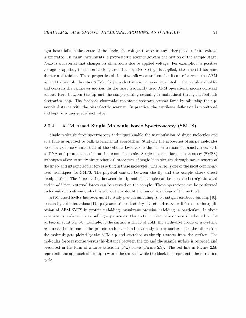
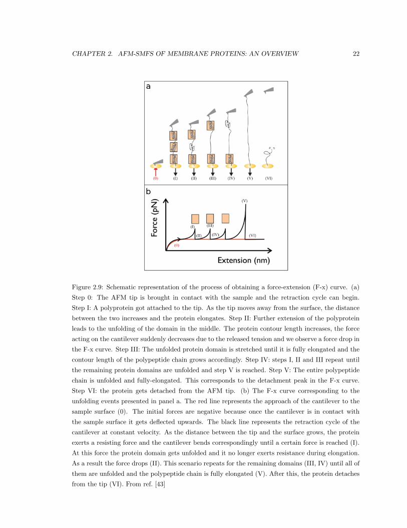
Figure 2.9: Schematic representation of the process of obtaining a force-extension (F-x) curve. (a)
Step 0: The AFM tip is brought in contact with the sample and the retraction cycle can begin.
Step I: A polyprotein got attached to the tip. As the tip moves away from the surface, the distance
between the two increases and the protein elongates. Step II: Further extension of the polyprotein
leads to the unfolding of the domain in the middle. The protein contour length increases, the force
acting on the cantilever suddenly decreases due to the released tension and we observe a force drop in
the F-x curve. Step III: The unfolded protein domain is stretched until it is fully elongated and the
contour length of the polypeptide chain grows accordingly. Step IV: steps I, II and III repeat until
the remaining protein domains are unfolded and step V is reached. Step V: The entire polypeptide
chain is unfolded and fully-elongated. This corresponds to the detachment peak in the F-x curve.
Step VI: the protein gets detached from the AFM tip. (b) The F-x curve corresponding to the
unfolding events presented in panel a. The red line represents the approach of the cantilever to the
sample surface (0). The initial forces are negative because once the cantilever is in contact with
the sample surface it gets deflected upwards. The black line represents the retraction cycle of the
cantilever at constant velocity. As the distance between the tip and the surface grows, the protein
exerts a resisting force and the cantilever bends correspondingly until a certain force is reached (I).
At this force the protein domain gets unfolded and it no longer exerts resistance during elongation.
As a result the force drops (II). This scenario repeats for the remaining domains (III, IV) until all of
them are unfolded and the polypeptide chain is fully elongated (V). After this, the protein detaches
from the tip (VI). From ref. [43]
CHAPTER 2. AFM-SMFS OF MEMBRANE PROTEINS: AN OVERVIEW 23
What happens in pulling experiments is the following. When the AFM tip is brought in contact
with the sample surface a single protein can attach to the tip. The physics behind this interaction
is still unclear. A possible explanation includes non-specific physioadsorption and electrostatic in-
teractions [43]. The results show that the adsorption is increased when a large force (∼ 800-3,000
pN) is applied to the surface once the tip is in contact [43]. The AFM tip is then retracted from the
surface. During retraction, the protein chain, tethered between the tip and the surface, elongates.
The polypeptide chain resists to this elongation. The resistance forces are entropy-driven. The
fully-stretched conformation is unfavorable. The preferred conformation of an unfolded protein is a
random coil, which maximizes the entropy. As the tip moves away from the surface, it experiences
the resistance force of the protein and the cantilever bends. The cantilever deflection is proportional
to the force acting on the cantilever. Once the protein is unfolded and fully-stretched the tension is
released and the force drops. In the case of a multi-domain protein, like the one in Figure 2.9a, the
scenario repeats until all protein domains are unfolded. The resulting force-extension curve (Figure
2.9b) typically bears a sawtooth pattern. Each force peak in the curve corresponds to the unfolding
of a single protein domain. The last peak is known as the detachment peak and is assumed to
correspond to a point in which the polypeptide chain is fully stretched and detaches from the tip.
Polymer elasticity models can be used to describe the mechanical behavior of proteins during
unfolding. Some of these models turned out to be very useful in the analysis of force-extension
curves. The standard model used for the analysis of F-x curves is the worm-like chain (WLC)
model. Bustamante et al. were the first to derive an interpolation formula for F-x curve and to
apply it to their DNA unfolding experiments [44]. The resulting formula, now known as the WLC
equation, is:
F (x) =kBT
lp
(1
4
(1− x
Lc
)−2
+x
Lc− 1
4
)(2.1)
where F is force, x is extension, kB is Boltzmann’s constant, T is temperature, lp is persistence
length and Lc is contour length. Eq. 2.1 enables computation of the entropic restoring force F
exerted by the polymer at different extension values. This computation requires two parameters:
the persistence length, lp, and the contour length, Lc. The persistence length is a measure of the
stiffness of the polymer; at length above lp the polymer behaves like an elastic rod. The contour
length, Lc, is defined as the length of a polymer chain at maximum physically possible extension [45].
Fitting the experimental data with the WLC model at fixed persistence length, gives the portion of
unfolded protein in terms of Lc. When the fit is performed for each peak in the spectra, we obtain
information about the length of the unfolded segments. Failure of the model at large forces due to
overstretching of the bonds has been reported [46]. In a first approximation, the persistence length
is assumed to be the same for the folded and unfolded states and to be independent of the extension.
In the literature, different lp values for proteins have been reported [47, 8, 9], 0.4 nm is accepted to
be the standard for membrane proteins [9].
CHAPTER 2. AFM-SMFS OF MEMBRANE PROTEINS: AN OVERVIEW 24
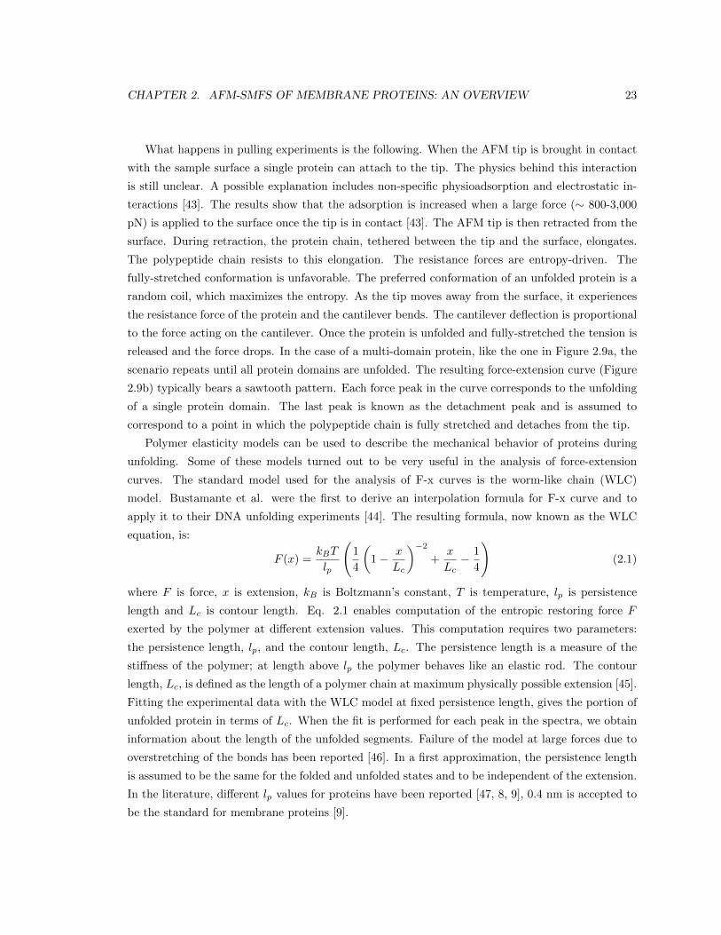
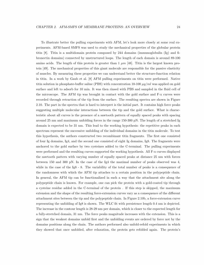
To illustrate better the pulling experiments with AFM, let’s look more closely at some real ex-
periments. AFM-based SMFS was used to study the mechanical properties of the globular protein
titin [8]. Titin is a multidomain protein composed by 244 domains (immunoglobulin (Ig) and fi-
bronectin domains) connected by unstructured loops. The length of each domain is around 89-100
amino acids. The length of this protein is greater than 1 µm [48]. Titin is the largest known pro-
tein [49]. The mechanical properties of this giant molecule are responsible for the passive elasticity
of muscles. By measuring these properties we can understand better the structure-function relation
in titin. In a work by Gaub et al. [8] AFM pulling experiments on titin were performed. Native
titin solution in phosphate-buffer saline (PBS) with concentration 10-100 µg/ml was applied on gold
surface and left to adsorb for 10 min. It was then rinsed with PBS and sampled in the fluid cell of
the microscope. The AFM tip was brought in contact with the gold surface and F-x curves were
recorded through retraction of the tip from the surface. The resulting spectra are shown in Figure
2.10. The part in the spectra that is hard to interpret is the initial part. It contains high force peaks
suggesting multiple molecular interactions between the tip and the gold surface. What is charac-
teristic about all curves is the presence of a sawtooth pattern of equally spaced peaks with spacing
around 25 nm and maximum unfolding forces in the range 150-300 pN. The length of a stretched Ig
domain is expected to be 31 nm. This lead to the working hypothesis: the repetitive peaks in each
spectrum represent the successive unfolding of the individual domains in the titin molecule. To test
this hypothesis, the authors constructed two recombinant titin fragments. The first one consisted
of four Ig domains, Ig4, and the second one consisted of eight Ig domains, Ig8. The fragments were
anchored to the gold surface by two cysteines added to the C-terminal. The pulling experiments
were performed and the resulting curves supported the working hypothesis. All F-x curves displayed
the sawtooth pattern with varying number of equally spaced peaks at distance 25 nm with forces
between 150 and 300 pN. In the case of the Ig4 the maximal number of peaks observed was 4,
while in the case of the Ig8 - 8. The variability of the total number of peaks is a consequence of
the randomness with which the AFM tip attaches to a certain position in the polypeptide chain.
In general, the AFM tip can be functionalized in such a way that the attachment site along the
polypeptide chain is known. For example, one can pick the protein with a gold-coated tip through
a cysteine residue added in the C-terminal of the protein . If this step is skipped, the maximum
extension and the shape of the resulting force-extension curves vary as a consequence of the different
attachment sites between the tip and the polypeptide chain. In Figure 2.10b, a force-extension curve
representing the unfolding of Ig8 is shown. The WLC fit with persistence length 0.4 nm is depicted.
The increase in the contour length is 28-29 nm per domain, which is closer to the expected length for
a fully-stretched domain, 31 nm. The force peaks magnitude increases with the extension. This is a
sign that the weakest domains unfold first and the unfolding events are ordered by force not by the
domains positions along the chain. The authors performed also unfold-refold experiments in which
they showed that once unfolded, after relaxation, the protein gets refolded again. The protein’s
CHAPTER 2. AFM-SMFS OF MEMBRANE PROTEINS: AN OVERVIEW 25
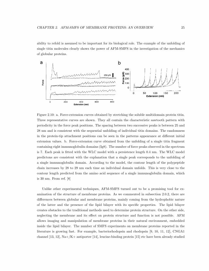
ability to refold is assumed to be important for its biological role. The example of the unfolding of
single titin molecules clearly shows the power of AFM-SMFS in the investigation of the mechanics
of globular proteins.
Figure 2.10: a. Force-extension curves obtained by stretching the soluble multidomain protein titin.
Three representative curves are shown. They all contain the characteristic sawtooth pattern with
periodicity in the force peak positions. The spacing between two successive peaks is between 25 and
28 nm and is consistent with the sequential unfolding of individual titin domains. The randomness
in the protein-tip attachment positions can be seen in the patterns appearance at different initial
extension values. b. Force-extension curve obtained from the unfolding of a single titin fragment
containing eight immunoglobulin domains (Ig8). The number of force peaks observed in the spectrum
is 7. Each peak is fitted with the WLC model with a persistence length 0.4 nm. The WLC model
predictons are consistent with the explanation that a single peak corresponds to the unfolding of
a single immunoglobulin domain. According to the model, the contour length of the polypeptide
chain increases by 28 to 29 nm each time an individual domain unfolds. This is very close to the
contour length predicted from the amino acid sequence of a single immunoglobulin domain, which
is 30 nm. From ref. [8]
Unlike other experimental techniques, AFM-SMFS turned out to be a promising tool for ex-
amination of the structure of membrane proteins. As we commented in subsection 2.0.2, there are
differences between globular and membrane proteins, mainly coming from the hydrophobic nature
of the latter and the presence of the lipid bilayer with its specific properties. The lipid bilayer
creates obstacles to the traditional methods used to determine protein structure. On the other side,
neglecting the membrane and its effect on protein structure and function is not possible. AFM
allows imaging and manipulation of membrane proteins in their natural environment, embedded
inside the lipid bilayer. The number of SMFS experiments on membrane proteins reported in the
literature is growing fast. For example, bacteriorhodopsin and rhodopsin [9, 10, 11, 12], CNGA1
channel [13, 12], Na+/K+ antiporter [14], leucine-binding protein [15] etc have been already studied
CHAPTER 2. AFM-SMFS OF MEMBRANE PROTEINS: AN OVERVIEW 26
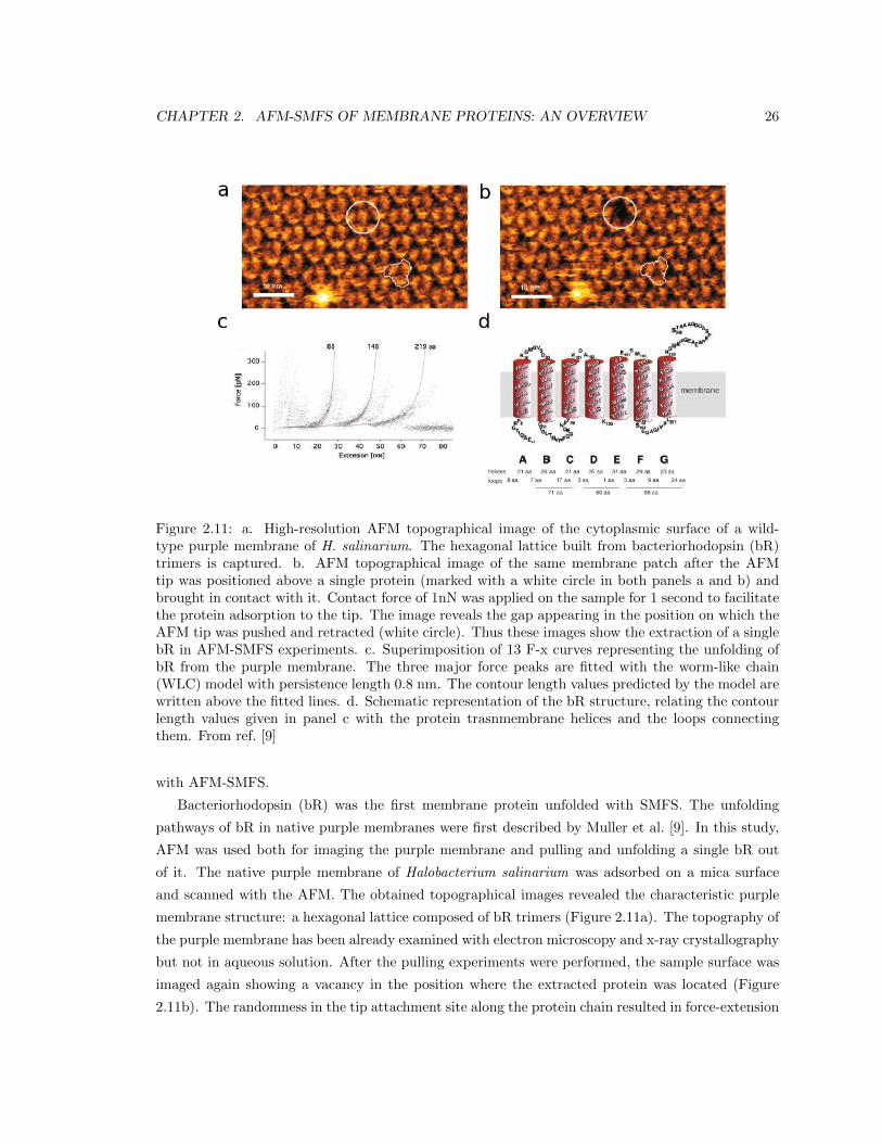
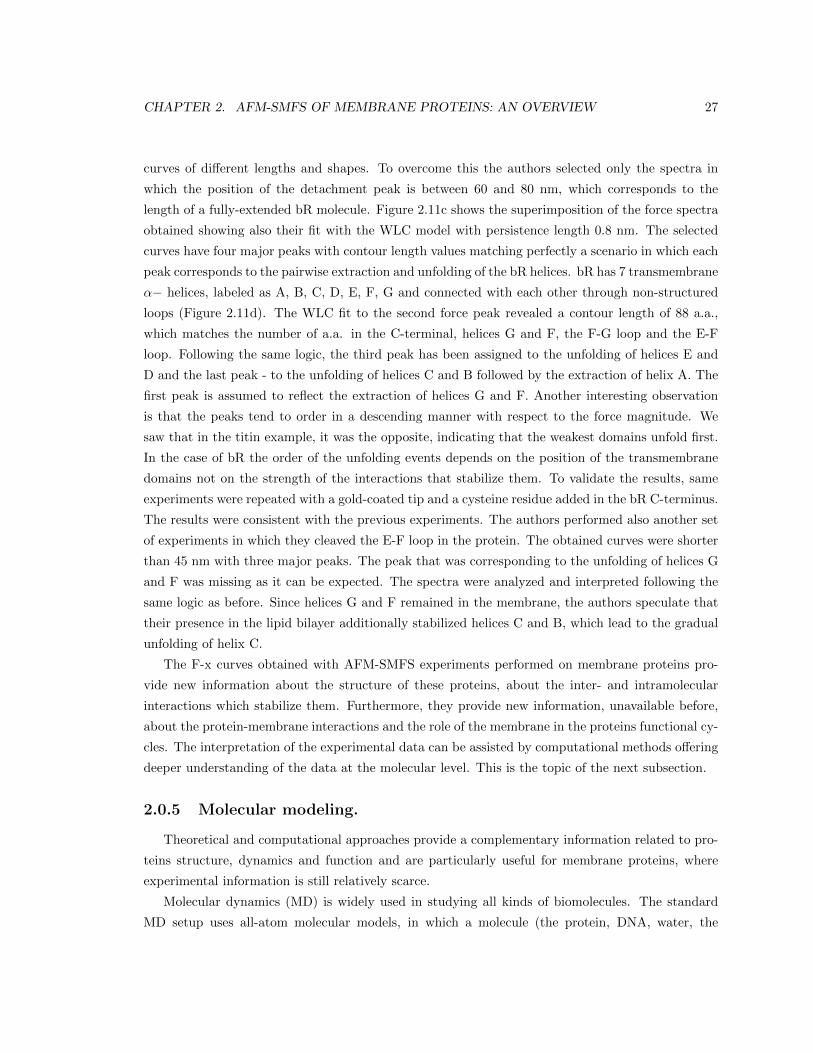
Figure 2.11: a. High-resolution AFM topographical image of the cytoplasmic surface of a wild-type purple membrane of H. salinarium. The hexagonal lattice built from bacteriorhodopsin (bR)trimers is captured. b. AFM topographical image of the same membrane patch after the AFMtip was positioned above a single protein (marked with a white circle in both panels a and b) andbrought in contact with it. Contact force of 1nN was applied on the sample for 1 second to facilitatethe protein adsorption to the tip. The image reveals the gap appearing in the position on which theAFM tip was pushed and retracted (white circle). Thus these images show the extraction of a singlebR in AFM-SMFS experiments. c. Superimposition of 13 F-x curves representing the unfolding ofbR from the purple membrane. The three major force peaks are fitted with the worm-like chain(WLC) model with persistence length 0.8 nm. The contour length values predicted by the model arewritten above the fitted lines. d. Schematic representation of the bR structure, relating the contourlength values given in panel c with the protein trasnmembrane helices and the loops connectingthem. From ref. [9]
with AFM-SMFS.
Bacteriorhodopsin (bR) was the first membrane protein unfolded with SMFS. The unfolding
pathways of bR in native purple membranes were first described by Muller et al. [9]. In this study,
AFM was used both for imaging the purple membrane and pulling and unfolding a single bR out
of it. The native purple membrane of Halobacterium salinarium was adsorbed on a mica surface
and scanned with the AFM. The obtained topographical images revealed the characteristic purple
membrane structure: a hexagonal lattice composed of bR trimers (Figure 2.11a). The topography of
the purple membrane has been already examined with electron microscopy and x-ray crystallography
but not in aqueous solution. After the pulling experiments were performed, the sample surface was
imaged again showing a vacancy in the position where the extracted protein was located (Figure
2.11b). The randomness in the tip attachment site along the protein chain resulted in force-extension
CHAPTER 2. AFM-SMFS OF MEMBRANE PROTEINS: AN OVERVIEW 27
curves of different lengths and shapes. To overcome this the authors selected only the spectra in
which the position of the detachment peak is between 60 and 80 nm, which corresponds to the
length of a fully-extended bR molecule. Figure 2.11c shows the superimposition of the force spectra
obtained showing also their fit with the WLC model with persistence length 0.8 nm. The selected
curves have four major peaks with contour length values matching perfectly a scenario in which each
peak corresponds to the pairwise extraction and unfolding of the bR helices. bR has 7 transmembrane
α− helices, labeled as A, B, C, D, E, F, G and connected with each other through non-structured
loops (Figure 2.11d). The WLC fit to the second force peak revealed a contour length of 88 a.a.,
which matches the number of a.a. in the C-terminal, helices G and F, the F-G loop and the E-F
loop. Following the same logic, the third peak has been assigned to the unfolding of helices E and
D and the last peak - to the unfolding of helices C and B followed by the extraction of helix A. The
first peak is assumed to reflect the extraction of helices G and F. Another interesting observation
is that the peaks tend to order in a descending manner with respect to the force magnitude. We
saw that in the titin example, it was the opposite, indicating that the weakest domains unfold first.
In the case of bR the order of the unfolding events depends on the position of the transmembrane
domains not on the strength of the interactions that stabilize them. To validate the results, same
experiments were repeated with a gold-coated tip and a cysteine residue added in the bR C-terminus.
The results were consistent with the previous experiments. The authors performed also another set
of experiments in which they cleaved the E-F loop in the protein. The obtained curves were shorter
than 45 nm with three major peaks. The peak that was corresponding to the unfolding of helices G
and F was missing as it can be expected. The spectra were analyzed and interpreted following the
same logic as before. Since helices G and F remained in the membrane, the authors speculate that
their presence in the lipid bilayer additionally stabilized helices C and B, which lead to the gradual
unfolding of helix C.
The F-x curves obtained with AFM-SMFS experiments performed on membrane proteins pro-
vide new information about the structure of these proteins, about the inter- and intramolecular
interactions which stabilize them. Furthermore, they provide new information, unavailable before,
about the protein-membrane interactions and the role of the membrane in the proteins functional cy-
cles. The interpretation of the experimental data can be assisted by computational methods offering
deeper understanding of the data at the molecular level. This is the topic of the next subsection.
2.0.5 Molecular modeling.
Theoretical and computational approaches provide a complementary information related to pro-
teins structure, dynamics and function and are particularly useful for membrane proteins, where
experimental information is still relatively scarce.
Molecular dynamics (MD) is widely used in studying all kinds of biomolecules. The standard
MD setup uses all-atom molecular models, in which a molecule (the protein, DNA, water, the
CHAPTER 2. AFM-SMFS OF MEMBRANE PROTEINS: AN OVERVIEW 28
phospholipids of the membrane, etc.) is represented explicitly by all of its atoms. This approach is
accurate and realistic from both the physical and the chemical point of view but it is computationally
expensive. Atomistic MD simulations have been successfully used to investigate the conformational
changes of membrane proteins in lipid environments [50, 51]. Even though advances have been
made, still there are limitations regarding the time scales accessible to these simulations. It is
known that the transition time between the functional states of membrane proteins is much longer
than the time accessible with conventional MD simulations [52]. The time it takes to perform AFM
pulling experiments is of the order of magnitude of 0.1 s, 105 times more that the time that can be
simulated on systems of this complexity with ordinary resources. Indeed, a MD simulation of an
AFM experiment requires simulating a system containing thousands of solvent molecules, hundreds
of lipid molecules and the membrane protein itself. Given that the number of calculations per
molecule scales linearly with the number of particles in the molecule, the larger the system, the
bigger the simulations length.
Despite the limitations of conventional MD, Kappel et al. [53] investigated the mechanical un-
folding of bacteriorhodopsin (bR) using all-atom MD simulations. The membrane was included ex-
plicitly in the model, represented with a POPC (1-palmitoyl-2-oleoyl-sn-glycero-3-phosphocholine)
lipid bilayer. Four bR trimers were embedded in the bilayer reproducing the characteristic purple
membrane structure, in which bR trimers are organized into two-dimensional hexagonal lattice (see
subsection 2.0.2). Therefore, the simulation box contained 12 bR monomers. When a protein is
pulled, it elongates accordingly. This demands the simulation box to provide enough space to host
the extracted polypeptide chain. A water layer with thickness 10 nm was added to the simulation
box in order to provide such space. With this, the total number of atoms in the simulation box
became 236,124. The mechanical stretching of the protein was achieved by applying a harmonic
potential to the Cα atom at the terminus, which was pulled in the z-direction at a constant velocity
moving away from the membrane. Anyway, the size of the simulation box still did not provide enough
space to comprise the fully elongated polypeptide chain of the bR monomer. The z-dimension of
the box was 15.32 nm, while the approximate length of a single bR monomer is ∼ 92.4 nm. A novel
computational protocol was introduced to deal with this issue. The unfolded parts of the protein
at a certain distance from the upper wall of the simulation box and from the lipid bilayer border,
were repeatedly removed. The holes left by the missing residues were filled with water, the energy
of the system was minimized and the system was equilibrated. A new terminal Cα atom was defined
and subjected to the pulling potential. These steps were iterated until complete protein unfolding
occurred. The authors performed MD simulations using different pulling velocities. The smallest
was 1 m/s, which is ∼ 107 times larger than the typical values used in real experiments. In this field,
the gap between simulation conditions and experimental conditions is so large that the improvement
of computer hardware is not likely to fill it in the near future.
To overcome the main limitations of all-atom MD simulations two main approaches can be
CHAPTER 2. AFM-SMFS OF MEMBRANE PROTEINS: AN OVERVIEW 29
used: one is to simplify the molecular model of the protein-membrane system, and the second is
to use enhanced sampling techniques. A combination of the two can also be attempted. Here we
are going to describe only the first approach. We will describe the different coarse-grained (CG)
techniques specifically developed for membrane proteins and we are going to see how the method of
MD combined with CG models has been used to reproduce the characteristic F-x curves obtained
with AFM-SMFS.
Implicit solvation models.
In these schemes, the protein is modeled explicitly in an atomistic manner, while the solvent and
the membrane are included implicitly with a mean-field model, for example the generalized Born
(GB) model [54]. Water is modeled as a continuous environment with dielectric constant ε = 80. A
solvation energy term is added to the molecular mechanics potential energy function to account for
the solvent-solute interactions. The conventional lipid bilayer is replaced by a low-dielectric slab of
a certain thickness, placed in the high-dielectric environment induced by the water molecules and
the lipids polar head-groups. The dielectric constant in the protein interior is typically set to 1.
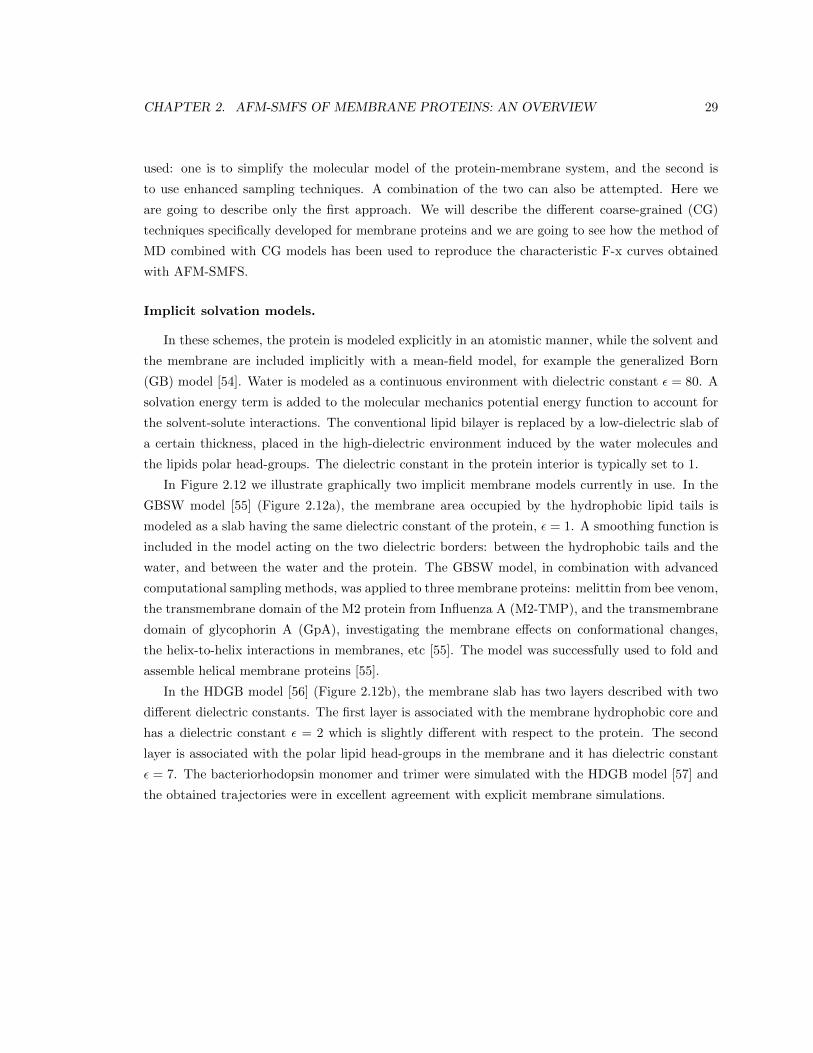
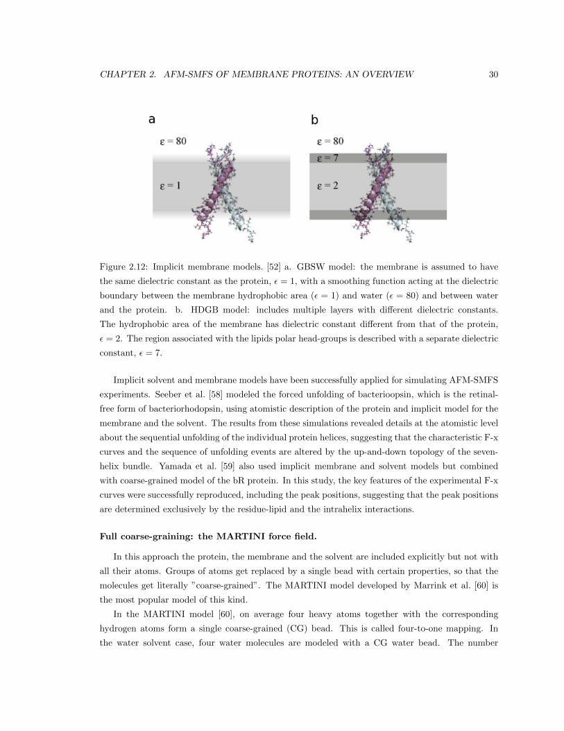
In Figure 2.12 we illustrate graphically two implicit membrane models currently in use. In the
GBSW model [55] (Figure 2.12a), the membrane area occupied by the hydrophobic lipid tails is
modeled as a slab having the same dielectric constant of the protein, ε = 1. A smoothing function is
included in the model acting on the two dielectric borders: between the hydrophobic tails and the
water, and between the water and the protein. The GBSW model, in combination with advanced
computational sampling methods, was applied to three membrane proteins: melittin from bee venom,
the transmembrane domain of the M2 protein from Influenza A (M2-TMP), and the transmembrane
domain of glycophorin A (GpA), investigating the membrane effects on conformational changes,
the helix-to-helix interactions in membranes, etc [55]. The model was successfully used to fold and
assemble helical membrane proteins [55].
In the HDGB model [56] (Figure 2.12b), the membrane slab has two layers described with two
different dielectric constants. The first layer is associated with the membrane hydrophobic core and
has a dielectric constant ε = 2 which is slightly different with respect to the protein. The second
layer is associated with the polar lipid head-groups in the membrane and it has dielectric constant
ε = 7. The bacteriorhodopsin monomer and trimer were simulated with the HDGB model [57] and
the obtained trajectories were in excellent agreement with explicit membrane simulations.
CHAPTER 2. AFM-SMFS OF MEMBRANE PROTEINS: AN OVERVIEW 30
Figure 2.12: Implicit membrane models. [52] a. GBSW model: the membrane is assumed to have
the same dielectric constant as the protein, ε = 1, with a smoothing function acting at the dielectric
boundary between the membrane hydrophobic area (ε = 1) and water (ε = 80) and between water
and the protein. b. HDGB model: includes multiple layers with different dielectric constants.
The hydrophobic area of the membrane has dielectric constant different from that of the protein,
ε = 2. The region associated with the lipids polar head-groups is described with a separate dielectric
constant, ε = 7.
Implicit solvent and membrane models have been successfully applied for simulating AFM-SMFS
experiments. Seeber et al. [58] modeled the forced unfolding of bacterioopsin, which is the retinal-
free form of bacteriorhodopsin, using atomistic description of the protein and implicit model for the
membrane and the solvent. The results from these simulations revealed details at the atomistic level
about the sequential unfolding of the individual protein helices, suggesting that the characteristic F-x
curves and the sequence of unfolding events are altered by the up-and-down topology of the seven-
helix bundle. Yamada et al. [59] also used implicit membrane and solvent models but combined
with coarse-grained model of the bR protein. In this study, the key features of the experimental F-x
curves were successfully reproduced, including the peak positions, suggesting that the peak positions
are determined exclusively by the residue-lipid and the intrahelix interactions.
Full coarse-graining: the MARTINI force field.
In this approach the protein, the membrane and the solvent are included explicitly but not with
all their atoms. Groups of atoms get replaced by a single bead with certain properties, so that the
molecules get literally ”coarse-grained”. The MARTINI model developed by Marrink et al. [60] is
the most popular model of this kind.
In the MARTINI model [60], on average four heavy atoms together with the corresponding
hydrogen atoms form a single coarse-grained (CG) bead. This is called four-to-one mapping. In
the water solvent case, four water molecules are modeled with a CG water bead. The number
CHAPTER 2. AFM-SMFS OF MEMBRANE PROTEINS: AN OVERVIEW 31
four was chosen to reach a compromise between the computational efficiency and the realism of the
chemical description. For certain types of molecular fragments, like aromatic rings, a single CG
particle contains only two heavy atoms for a more proper characterization. Practically, the initial
all-atom molecular structure is mapped onto CG particles connected to each other in such a way
that the overall topology of the molecules is preserved. The MARTINI particles are divided into
types and subtypes based on polarity and hydrogen-bonding capacity. In this manner, 18 particle
types are obtained, which are called ’building blocks’. The main assumption in MARTINI is that
the parametrization of the building blocks is transferable to different molecules and the model does
not need to be reparametrized in each case. The parametrization is performed using an extensive
calibration of chemical building blocks towards thermodynamic data, mainly oil/water partition
coefficients. The MARTINI force field currently contains parameters for lipids, sterols, proteins,
sugars etc.
The MARTINI CG model has been successfully applied to MD studies of the self-aggregation of
rhodopsin monomers in different explicit CG lipid membrane environments [61]. In a study by Xu
et al. [62] the effect of different cholesterol content in the membrane on the aggregation of the toxic
peptide amylin was investigated. They performed simulations in a mixed dipalmitoylphosphatidyl-
choline (DPPC) and dipalmitoylphosphatidylserine (DPPS) bilayers with different cholesterol con-
centrations and without cholesterol. It was shown that in the absence of cholesterol, the amylin
aggregates are located inside the bilayer, while in the presence of cholesterol, the amylin aggregates
are positioned outside the bilayer, on the bilayer-water interface. These results are consistent with
cholesterol hindering formation of the toxic amylin oligomers inside the cell membrane. To the best
of our knowledge the MARTINI force field has never been used to simulate AFM-SMFS experiments.
Go-like models.
An even simpler approach for simulating AFM-SMFS experiments was developed by Cieplak et
al [25]. Since in our work we use the Cieplak model as a starting point for the investigation of the
mechanical unfolding of rhodopsin (see Chapter 3), we are going to describe it in more details.
The model introduced by Cieplak et al. [24] is a Go-type model in which the native protein
conformation is determined by the experimental structure at room temperature. The protein is
represented as a chain of beads centered at the Cα atoms in the protein backbone. A harmonic
backbone potential acts between consecutive beads, tethering them at the peptide bond length,
r0=3.8 A:
V BB =
N−1∑i=1
1
2kBB(ri,i+1 − r0)2 (2.2)
where ri,i+1 = ri−ri+1 is the distance between two adjacent beads and kBB = 100ε/A2
is the spring
constant.
In order to preserve the native chirality, a potential V CHIR was introduced in the model. The

CHAPTER 2. AFM-SMFS OF MEMBRANE PROTEINS: AN OVERVIEW 32
chirality potential has the form:
V CHIR =
N−2∑i=2
kCHIRC2i Θ(−CiCNATi ) (2.3)
where the chirality of the residue i is given by
Ci =( (vi−1 × vi) · vi+1
r30
)(2.4)
with vi = ri+1 − ri and r0 the peptide bond length. Ci can take values between -1 and 1. The
positive values of Ci correspond to a right-handed helix, the negative values - to a left-handed helix.
CNATi is the chirality of residue i in the native conformation. Θ is a step function that returns 1
for positive arguments and 0 otherwise. In practice, if the chirality sign for a given residue matches
the native chirality sign for the same residue, V CHIR is 0. If there is a mismatch in the two signs,
that conformation is punished with the square of Ci. kCHIR is set to be equal to ε.
The non-bonded interactions are divided into native and non-native interactions. This is done
following the procedure developed by Tsai et al. [63]. The distances between all heavy atoms in the
native conformation are computed and if a distance is smaller than the sum of the vdw radii of the
two atoms multiplied by a factor of 1.244, the contact between these two atoms is considered native;
otherwise the contact between the two atoms is considered non-native.
The interaction between residues that form a native contact is described by the Lennard-Jones
potential:
V NAT =
NAT∑i<j
4ε[(σijrij
)12
−(σijrij
)6](2.5)
Here, rij is the distance between the Cα atoms of residues i and j. The σij values are computed by
multiplying the experimental distances by 2−16 , which adjusts the potential minima to the native
state. The parameter, ε, when divided by kB , has value 900 K, which proved to be appropriate
in previous simulations of folding and unfolding, yielding the correct force peak magnitudes for
titin [25] and ubiquitin [27] at room temperature.
The non-native interactions are assumed to be purely repulsive for distances shorter than the
equilibrium distance corresponding to σ0 = 5A, rcut = 5.61A:
V NON =
NON∑i<j
Vij (2.6)
V NONij =
∑NONi<j 4ε
[(σ0
rij
)12
−(σ0
rij
)6]+ ε, if rij < rcut
0, otherwise(2.7)

CHAPTER 2. AFM-SMFS OF MEMBRANE PROTEINS: AN OVERVIEW 33
The model described so far was successfully applied to soluble proteins like titin [25], calmod-
ulin [26] and ubiquitin [27]. The simulated F-x curves preserved the characteristic features of the
experimental curves. Moreover, the simplicity and the computational efficiency of this model enabled
the evaluation of the effects of varying temperature and pulling velocity.
Afterwards, Cieplak et al. extended the model to simulate the unfolding of membrane proteins,
in particular bacteriorhodopsin (bR) [28], where the membrane effects are essential for the final
outcome from the simulations. They approached the problem in the following way: the membrane
was included in the model explicitly with a coarse-grained representation similar to the one used
for the protein. In order to arrive to an adequate initial configuration of the protein-membrane
system, all-atom MD simulation of bR embedded in a POPC lipid bilayer with water solvent was
performed with computational protocol described in ref. [28]. The resulting conformation was used
as a starting point for the stretching simulations. In the coarse-grained model of the membrane, the
lipids were represented by merely all of their C atoms. The contacts of these carbon atoms with
the protein were determined using the same procedure by Tsai et al. [63] used to derive the native
contacts in the protein. The protein-membrane interactions were modeled with the Lennard-Jones
potential applying the same strength used for the native protein interactions, namely ε. The main
limitation of this approach is that during the stretching simulations, the membrane was held frozen.
Therefore, when an unfolded part of the protein is extracted from the membrane it leaves a hole in
it. Clearly, such description is not very realistic, since in a real membrane the lipid molecules fill the
voids left by the extracted protein. In Chapter 3 we describe a model capable of overcoming this
limitation.
2.0.6 Analysis tools for AFM-SMFS experiments.
SMFS experiments need to be performed multiple times on the same molecule in order to obtain
statistically relevant information. Recent improvements allow the collection of large amount of
data [16] but careful preprocessing is required because not every F-x curve contains meaningful
unfolding events. Most of the traces result from non-specific interactions, or contain partial unfolding
events, or simply noise. Typically membrane proteins are completely unfolded in < 1% of the
cases [21]. Furthermore, there is a certain variability in the peak patterns of F-x curves of the same
protein reflecting different unfolding pathways. What experimentalists often do is manual notation
by visual inspection of the traces. If the data set contains thousands of traces, handling the problem
manually is far from optimal, not only because it is time consuming but also because the result
depends on the user’s expertise. Recording thousands of force-extension curves in a reasonable time
is now possible. This huge amount of data calls for an automatic procedure for classification and
statistical data analysis. Many attempts of developing such a procedure have been made. Next, we
will describe some of these methods in a chronological order.
CHAPTER 2. AFM-SMFS OF MEMBRANE PROTEINS: AN OVERVIEW 34
The analysis approach by Kuhn et al. (2005)
One of the earliest attempts for the development of an automatic SMFS data analysis tool
was published in 2005 by Kuhn et al. [19]. The software they developed allows classification and
statistical analysis of large amount of force spectra. The procedure performs fit with the WLC
model, automatic alignment of F-x curves and peak patterns classification for detection of different
unfolding pathways. The data they analyzed comes from unfolding of two membrane proteins:
bacteriorhodopsin (bR) from Halobacterium salinarium [9, 64] and the sodium-proton antiporter
NhaA from Escherichia coli [65]. The algorithm is based on two steps: first, individual processing
and analysis of each trace; and second, pairwise alignment of all traces, followed by hierarchical
clustering and peak classification.
As a first step, each F-x curve undergoes determination of a zero-force baseline and contact point
detection. The zero-force baseline was defined using a linear fit to the non-contact part. The contact
point was recognized as the first point in which the zero-force baseline intersects the F-x curve. The
contact point corresponds to the point at which the undeflected cantilever is in contact with the
sample surface [19]. Next, the detachment peak is identified in the following way: the standard
deviation from a linear fit to the last 5 nm of the trace was estimated and the first point, moving
in the direction of the trace origin, in which the standard deviation increased by a factor of 1.5 was
the detachment peak. Next, the peaks in each F-x curve were detected. In order to ease the peak
detection step, each F-x curve was smoothed. The force peaks were detected based on the differences
between local minima and local maxima. If a peak with height above 30 pN is surrounded by force
minima with force difference of at least twice the standard deviation of the baseline to the maximum,
it is recognized as a force peak by the program. All peaks were fitted with the WLC model except
the ones in the first 15 nm which are assumed to come from non-specific interactions.
In general, the analysis of F-x curves requires an alignment step. The reason is that different
attachment sites between the AFM tip and the protein might introduce horizontal shifts in the
curves [21]. The authors tested three different approaches for alignment. First, they tried to align
the force spectra using the contour length values of each peak. This attempt was unsuccessful
because the variability in the tip-sample attachment sites leads to high variability in the absolute
and relative contour length values. The second trial was based on alignment of pixel images of the F-
x curves represented as two-dimensional histograms. In this procedure, two pixel images are shifted
with respect to each other and an alignment score is computed. The results were encouraging but
the alignment quality was affected by variations of the data points density, for example in the base
of the peaks. In the third approach, each F-x curve was represented as a sequence of equally-spaced
normal distributions of the force. The alignment problem was reduced to shifting two vectors with
respect to each other and estimating their alignment score.
The last step of the procedure is a hierarchical clustering classification. The distance measure
used for clustering is the negative of the alignment score. Small distances correspond to similar
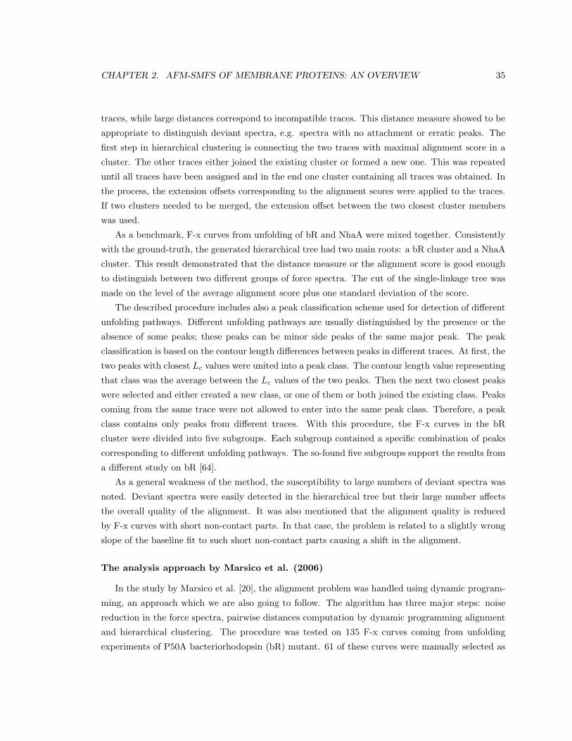
CHAPTER 2. AFM-SMFS OF MEMBRANE PROTEINS: AN OVERVIEW 35
traces, while large distances correspond to incompatible traces. This distance measure showed to be
appropriate to distinguish deviant spectra, e.g. spectra with no attachment or erratic peaks. The
first step in hierarchical clustering is connecting the two traces with maximal alignment score in a
cluster. The other traces either joined the existing cluster or formed a new one. This was repeated
until all traces have been assigned and in the end one cluster containing all traces was obtained. In
the process, the extension offsets corresponding to the alignment scores were applied to the traces.
If two clusters needed to be merged, the extension offset between the two closest cluster members
was used.
As a benchmark, F-x curves from unfolding of bR and NhaA were mixed together. Consistently
with the ground-truth, the generated hierarchical tree had two main roots: a bR cluster and a NhaA
cluster. This result demonstrated that the distance measure or the alignment score is good enough
to distinguish between two different groups of force spectra. The cut of the single-linkage tree was
made on the level of the average alignment score plus one standard deviation of the score.
The described procedure includes also a peak classification scheme used for detection of different
unfolding pathways. Different unfolding pathways are usually distinguished by the presence or the
absence of some peaks; these peaks can be minor side peaks of the same major peak. The peak
classification is based on the contour length differences between peaks in different traces. At first, the
two peaks with closest Lc values were united into a peak class. The contour length value representing
that class was the average between the Lc values of the two peaks. Then the next two closest peaks
were selected and either created a new class, or one of them or both joined the existing class. Peaks
coming from the same trace were not allowed to enter into the same peak class. Therefore, a peak
class contains only peaks from different traces. With this procedure, the F-x curves in the bR
cluster were divided into five subgroups. Each subgroup contained a specific combination of peaks
corresponding to different unfolding pathways. The so-found five subgroups support the results from
a different study on bR [64].
As a general weakness of the method, the susceptibility to large numbers of deviant spectra was
noted. Deviant spectra were easily detected in the hierarchical tree but their large number affects
the overall quality of the alignment. It was also mentioned that the alignment quality is reduced
by F-x curves with short non-contact parts. In that case, the problem is related to a slightly wrong
slope of the baseline fit to such short non-contact parts causing a shift in the alignment.
The analysis approach by Marsico et al. (2006)
In the study by Marsico et al. [20], the alignment problem was handled using dynamic program-
ming, an approach which we are also going to follow. The algorithm has three major steps: noise
reduction in the force spectra, pairwise distances computation by dynamic programming alignment
and hierarchical clustering. The procedure was tested on 135 F-x curves coming from unfolding
experiments of P50A bacteriorhodopsin (bR) mutant. 61 of these curves were manually selected as
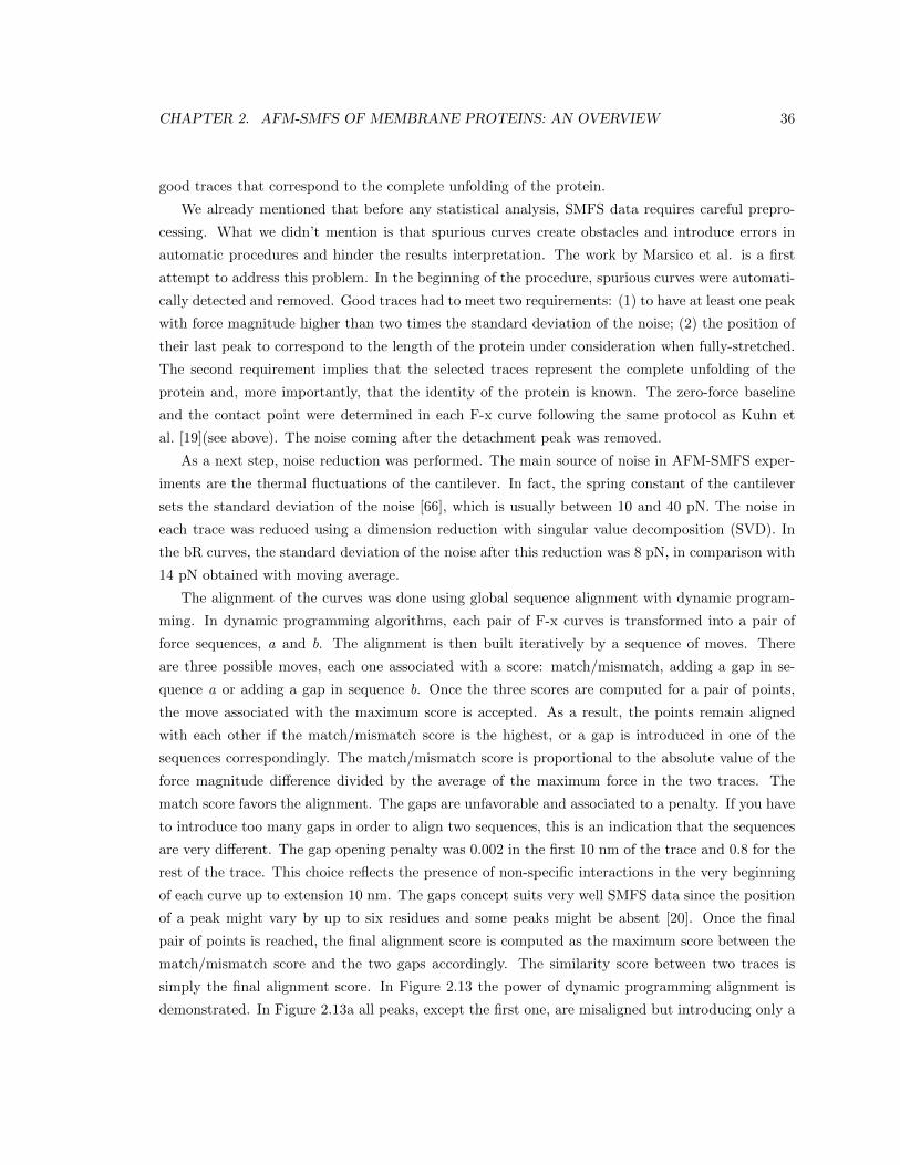
CHAPTER 2. AFM-SMFS OF MEMBRANE PROTEINS: AN OVERVIEW 36
good traces that correspond to the complete unfolding of the protein.
We already mentioned that before any statistical analysis, SMFS data requires careful prepro-
cessing. What we didn’t mention is that spurious curves create obstacles and introduce errors in
automatic procedures and hinder the results interpretation. The work by Marsico et al. is a first
attempt to address this problem. In the beginning of the procedure, spurious curves were automati-
cally detected and removed. Good traces had to meet two requirements: (1) to have at least one peak
with force magnitude higher than two times the standard deviation of the noise; (2) the position of
their last peak to correspond to the length of the protein under consideration when fully-stretched.
The second requirement implies that the selected traces represent the complete unfolding of the
protein and, more importantly, that the identity of the protein is known. The zero-force baseline
and the contact point were determined in each F-x curve following the same protocol as Kuhn et
al. [19](see above). The noise coming after the detachment peak was removed.
As a next step, noise reduction was performed. The main source of noise in AFM-SMFS exper-
iments are the thermal fluctuations of the cantilever. In fact, the spring constant of the cantilever
sets the standard deviation of the noise [66], which is usually between 10 and 40 pN. The noise in
each trace was reduced using a dimension reduction with singular value decomposition (SVD). In
the bR curves, the standard deviation of the noise after this reduction was 8 pN, in comparison with
14 pN obtained with moving average.
The alignment of the curves was done using global sequence alignment with dynamic program-
ming. In dynamic programming algorithms, each pair of F-x curves is transformed into a pair of
force sequences, a and b. The alignment is then built iteratively by a sequence of moves. There
are three possible moves, each one associated with a score: match/mismatch, adding a gap in se-
quence a or adding a gap in sequence b. Once the three scores are computed for a pair of points,
the move associated with the maximum score is accepted. As a result, the points remain aligned
with each other if the match/mismatch score is the highest, or a gap is introduced in one of the
sequences correspondingly. The match/mismatch score is proportional to the absolute value of the
force magnitude difference divided by the average of the maximum force in the two traces. The
match score favors the alignment. The gaps are unfavorable and associated to a penalty. If you have
to introduce too many gaps in order to align two sequences, this is an indication that the sequences
are very different. The gap opening penalty was 0.002 in the first 10 nm of the trace and 0.8 for the
rest of the trace. This choice reflects the presence of non-specific interactions in the very beginning
of each curve up to extension 10 nm. The gaps concept suits very well SMFS data since the position
of a peak might vary by up to six residues and some peaks might be absent [20]. Once the final
pair of points is reached, the final alignment score is computed as the maximum score between the
match/mismatch score and the two gaps accordingly. The similarity score between two traces is
simply the final alignment score. In Figure 2.13 the power of dynamic programming alignment is
demonstrated. In Figure 2.13a all peaks, except the first one, are misaligned but introducing only a
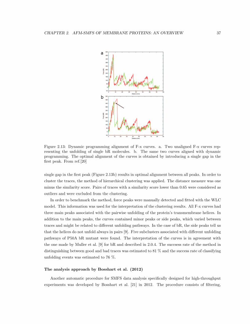
CHAPTER 2. AFM-SMFS OF MEMBRANE PROTEINS: AN OVERVIEW 37
Figure 2.13: Dynamic programming alignment of F-x curves. a. Two unaligned F-x curves rep-resenting the unfolding of single bR molecules. b. The same two curves aligned with dynamicprogramming. The optimal alignment of the curves is obtained by introducing a single gap in thefirst peak. From ref.[20]
single gap in the first peak (Figure 2.13b) results in optimal alignment between all peaks. In order to
cluster the traces, the method of hierarchical clustering was applied. The distance measure was one
minus the similarity score. Pairs of traces with a similarity score lower than 0.65 were considered as
outliers and were excluded from the clustering.
In order to benchmark the method, force peaks were manually detected and fitted with the WLC
model. This information was used for the interpretation of the clustering results. All F-x curves had
three main peaks associated with the pairwise unfolding of the protein’s transmembrane helices. In
addition to the main peaks, the curves contained minor peaks or side peaks, which varied between
traces and might be related to different unfolding pathways. In the case of bR, the side peaks tell us
that the helices do not unfold always in pairs [9]. Five subclusters associated with different unfolding
pathways of P50A bR mutant were found. The interpretation of the curves is in agreement with
the one made by Muller et al. [9] for bR and described in 2.0.4. The succsess rate of the method in
distinguishing between good and bad traces was estimated to 81 % and the success rate of classifying
unfolding events was estimated to 76 %.
The analysis approach by Bosshart et al. (2012)
Another automatic procedure for SMFS data analysis specifically designed for high-throughput
experiments was developed by Bosshart et al. [21] in 2012. The procedure consists of filtering,
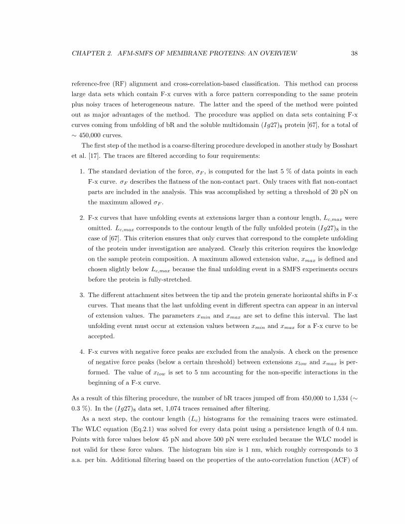
CHAPTER 2. AFM-SMFS OF MEMBRANE PROTEINS: AN OVERVIEW 38
reference-free (RF) alignment and cross-correlation-based classification. This method can process
large data sets which contain F-x curves with a force pattern corresponding to the same protein
plus noisy traces of heterogeneous nature. The latter and the speed of the method were pointed
out as major advantages of the method. The procedure was applied on data sets containing F-x
curves coming from unfolding of bR and the soluble multidomain (Ig27)8 protein [67], for a total of
∼ 450,000 curves.
The first step of the method is a coarse-filtering procedure developed in another study by Bosshart
et al. [17]. The traces are filtered according to four requirements:
1. The standard deviation of the force, σF , is computed for the last 5 % of data points in each
F-x curve. σF describes the flatness of the non-contact part. Only traces with flat non-contact
parts are included in the analysis. This was accomplished by setting a threshold of 20 pN on
the maximum allowed σF .
2. F-x curves that have unfolding events at extensions larger than a contour length, Lc,max were
omitted. Lc,max corresponds to the contour length of the fully unfolded protein (Ig27)8 in the
case of [67]. This criterion ensures that only curves that correspond to the complete unfolding
of the protein under investigation are analyzed. Clearly this criterion requires the knowledge
on the sample protein composition. A maximum allowed extension value, xmax is defined and
chosen slightly below Lc,max because the final unfolding event in a SMFS experiments occurs
before the protein is fully-stretched.
3. The different attachment sites between the tip and the protein generate horizontal shifts in F-x
curves. That means that the last unfolding event in different spectra can appear in an interval
of extension values. The parameters xmin and xmax are set to define this interval. The last
unfolding event must occur at extension values between xmin and xmax for a F-x curve to be
accepted.
4. F-x curves with negative force peaks are excluded from the analysis. A check on the presence
of negative force peaks (below a certain threshold) between extensions xlow and xmax is per-
formed. The value of xlow is set to 5 nm accounting for the non-specific interactions in the
beginning of a F-x curve.
As a result of this filtering procedure, the number of bR traces jumped off from 450,000 to 1,534 (∼0.3 %). In the (Ig27)8 data set, 1,074 traces remained after filtering.
As a next step, the contour length (Lc) histograms for the remaining traces were estimated.
The WLC equation (Eq.2.1) was solved for every data point using a persistence length of 0.4 nm.
Points with force values below 45 pN and above 500 pN were excluded because the WLC model is
not valid for these force values. The histogram bin size is 1 nm, which roughly corresponds to 3
a.a. per bin. Additional filtering based on the properties of the auto-correlation function (ACF) of

CHAPTER 2. AFM-SMFS OF MEMBRANE PROTEINS: AN OVERVIEW 39
the Lc histograms was applied. The position and the amplitude of the first side peak in the ACF
were used as a filter for detection of characteristic unfolding events in the F-x curves. Their values
were obtained form the ACF of the average Lc histogram for an entire data set. For example, the
position of the first side peak reflects the periodicity of the pattern. In the case of the multidomain
protein (Ig27)8, the first side peak is positioned at 27.6 nm, which is an agreement with the interpeak
distances published in the literature [67, 8]. We remark that also this procedure requires the previous
knowledge of the identity of the protein that is analyzed. Next, the peaks in each Lc histogram were
automatically detected and their positions were stored in a matrix. To avoid overestimation of the
number of peaks, the Lc histograms were smoothed. The traces were divided into peak-number
groups depending on the number of peaks found in their Lc histograms. In general, the larger the
number of peaks in the Lc histograms, the more the details and the side peaks that could be found
in the F-x curves.
The reference-free alignment algorithm [68] was then performed separately in each peak-number
group. The algorithm can be divided in four blocks.
1. Two randomly selected Lc histograms are cross-correlated and aligned based on the corre-
lation maximum. An arithmetic average of the two histograms is then computed. A third
Lc histogram is randomly chosen, aligned and then added to the arithmetic average. This is
repeated until all histograms belonging to that peak-number group are included in the arith-
metic average. A Lc histogram is counted only once. The final arithmetic average is the global
average representing that particular group.
2. Each Lc histogram in the group gets aligned to the global average on the basis of their corre-
lation maximum.
3. Each Lc histogram is subtracted from the global average and a temporary average is computed.
The histogram is then aligned to that temporary average and a new arithmetic average is
computed. This is repeated for all histograms.
4. The global averages of all peak-number groups get aligned to each other. This makes the
comparison between different peak-number groups easier and overcomes the different offsets
which might turn out to be problematic. In the end, all histograms in a peak-number group
get aligned to the final global average.
The goal of this procedure is determining the unfolding fingerprint of a given protein. The power
of alignment in solving this problem is illustrated in Figure 2.14 for the (Ig27)8. It becomes clear
that the characteristic unfolding pattern of the protein is hardly seen in the superimposition of the
unaligned spectra, while obvious in the aligned superimposition.
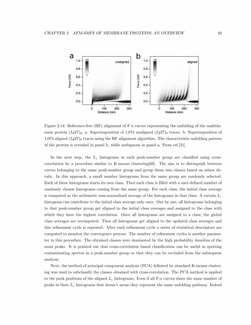
CHAPTER 2. AFM-SMFS OF MEMBRANE PROTEINS: AN OVERVIEW 40
Figure 2.14: Reference-free (RF) alignment of F-x curves representing the unfolding of the multido-
main protein (Ig27)8. a. Superimposition of 1,074 unaligned (Ig27)8 traces. b. Superimposition of
1,074 aligned (Ig27)8 traces using the RF alignment algorithm. The characteristic unfolding pattern
of the protein is revealed in panel b, while ambiguous in panel a. From ref.[21]
In the next step, the Lc histograms in each peak-number group are classified using cross-
correlation by a procedure similar to K-means clustering[69]. The aim is to distinguish between
curves belonging to the same peak-number group and group them into classes based on minor de-
tails. In this approach, a small number histograms from the same group are randomly selected.
Each of these histograms starts its own class. Then each class is filled with a user-defined number of
randomly chosen histograms coming from the same group. For each class, the initial class average
is computed as the arithmetic sum-normalized average of the histograms in that class. A certain Lc
histogram can contribute to the initial class average only once. One by one, all histograms belonging
to that peak-number group get aligned to the initial class averages and assigned to the class with
which they have the highest correlation. Once all histograms are assigned to a class, the global
class averages are recomputed. Then all histograms get aligned to the updated class averages and
this refinement cycle is repeated. After each refinement cycle a series of statistical descriptors are
computed to monitor the convergence process. The number of refinement cycles is another parame-
ter in this procedure. The obtained classes were dominated by the high probability densities of the
main peaks. It is pointed out that cross-correlation based classification can be useful in spotting
contaminating spectra in a peak-number group so that they can be excluded from the subsequent
analysis.
Next, the method of principal component analysis (PCA) followed by standard K-means cluster-
ing was used to subclassify the classes obtained with cross-correlation. The PCA method is applied
to the peak positions of the aligned Lc histograms. Even if all F-x curves share the same number of
peaks in their Lc histograms that doesn’t mean they represent the same unfolding pathway. Indeed
CHAPTER 2. AFM-SMFS OF MEMBRANE PROTEINS: AN OVERVIEW 41
the peaks might have different positions. This is the reason why the PCA was applied to the peak
positions within a class. K-means clustering is then applied in the space of the principal compo-
nents; the number of clusters, ncl is a user-defined parameter. It is normally set to a value slightly
higher than the number of expected clusters. The number of expected clusters in this approach
is roughly estimated from the PCA factor map. The number of estimated clusters in the largest
class in the bR peak-number group with six peaks, was 3. In all of them, four main peaks were
present, while the differences between the clusters arose from the densities of the side peaks. The
combination of PCA and K-means clustering did not work in all cases. For example, in the largest
class of the peak-number group with seven peaks, it was not possible to identify any clusters in the
PCA factor map and the K-means clustering was not executed. In addition, the described method
was successfully used to localize the unfolding barriers in the bR structure. All peaks in the average
Lc histogram were related to a position in the bR helices.
The analysis approach by Galvanetto et al. (2018)
Recently, Galvanetto et al. developed an open-source software for analysis of F-x curves, named
Fodis (for Force-distance software) [22]. The software operates in MATLAB and offers a variety of
tools for the manipulation and statistical analysis of F-x curves. It was tested on SMFS data from
unfolding of the cyclic nucleotide-gated CNGA1 channel overexpressed in oocytes membranes [13].
Fodis implement a filtering procedure, also based on the prior knowledge of the protein that is
analyzed. Before filtering the Lc histograms of all traces need to be estimated. The persistence
length used for the Lc transformation was 0.4 nm. Only Lc values corresponding to forces larger
than 30 pN were included in the histograms. The filtering criterion in the first step is based on
the length of the F-x curves and adopts the fully-stretched condition. The fully-stretched condition
implies that F-x curves longer or shorter than the Lc value corresponding to the fully-stretched
protein can be discarded. The trace length is determined by the position of the last peak in the Lc
histogram. The authors noted that the computed contour length strongly depends on the persistence
length value, which can vary between 0.3 and 0.8 nm [9]. For this reason, instead of fixing a Lc
threshold, a window of values centered around the expected length was defined. The size of the
window is recommended to be at least 30 % of the protein expected length. In the CNGA1 example,
the window was between 210 and 360 nm. We remark that this procedure is robust and accurate,
but requires the knowledge of the identity of the protein.
In the second filtering step, traces with high non-specific adhesion (F>150 pN) in the very
beginning of the force spectra (up to 70 nm) were discarded.
The third filtering step is based on cross-correlation and finds similar F-x curves. The similarity
between two traces is given by the cross-correlation computed for their Lc histograms. A similarity
matrix containing the correlation values for all pairs of traces is generated. The symmetric approx-
imate minimum permutation algorithm [11] is applied to the matrix in order to detect clusters of
CHAPTER 2. AFM-SMFS OF MEMBRANE PROTEINS: AN OVERVIEW 42
similar traces. The obtained clusters can be further inspected and analyzed.
The reference-free alignment algorithm [21] described above was implemented in Fodis with
some modifications. The first modification is related to the alignment of the force spectra, which is
performed by adding a Gaussian curve centered at zero extension to the cross-correlation function
for each pair of histograms. In this manner, the alignment in which the zero points of the two curves
match each other is favored. The second modification is related to the division of force spectra in
peak-number groups. The global histogram generated from all Lc histogram is manually divided
into peak intervals for the purposes of the analysis. As an alternative to manual intervention, the
software offers an option in which the peak intervals are automatically determined and extracted
from the global histogram of maxima. This plot shows the Lc peaks with highest probability, or the
most abundant Lc peaks in the entire data set. The global histogram of maxima reveals the main
unfolding pattern in the particular group of force spectra. Each trace is then transformed into a
binary string of size equal to the total number of peak intervals. A value of 0 is assigned if no peak
is present in the corresponding interval; a value of 1 is assigned if there is a peak in that interval.
From the binary representation, two sequences are generated: N and Pn The sequence N contains
information for the interval position occupied by the peak; if the peak is in the fourth interval, the
value of this peak in N will be 4. The sequence Pn keeps track on the order in which the peak
appears along the trace; if it is the third peak in the trace but is positioned in the fourth peak
interval, the value it gets will be 3 not 4. The plot sequence N versus sequence Pn for all traces of
interest is quite informative. It enables the identification of different unfolding pathways and offers
a graphical summary of the number and the position of occurrence of unfolding events. In Figure
2.15 the power of this algorithm is illustrated for 106 CNGA1 curves. The thickness of the lines
reflects the abundance of traces following that path.
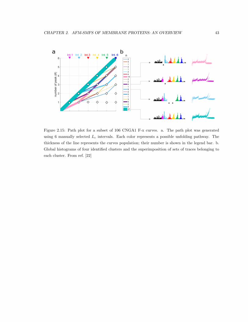
CHAPTER 2. AFM-SMFS OF MEMBRANE PROTEINS: AN OVERVIEW 43
Figure 2.15: Path plot for a subset of 106 CNGA1 F-x curves. a. The path plot was generated
using 6 manually selected Lc intervals. Each color represents a possible unfolding pathway. The
thickness of the line represents the curves population; their number is shown in the legend bar. b.
Global histograms of four identified clusters and the superimposition of sets of traces belonging to
each cluster. From ref. [22]

Chapter 3
Molecular modeling of single
molecule force spectroscopy.
The phototransduction process, in which light undergoes a biochemical transformation to electric
signals, takes place in the rod outer segment (rod OS) of photoreceptor cells. The rod OS is a
cylindrical biological structure of highly ordered membranes. It hosts discrete membranous discs
enclosed by the plasma membrane of the cell [70]. The disc membranes and the plasma membrane
are two membranes with a different lipid and protein composition and independent functions. The
plasma membrane is enriched in cholesterol and saturated fatty acids compared to the discs [23].
Rhodopsin is the only membrane protein present both in the discs and in the plasma membrane [23].
Moreover, rhodopsin is the dominant protein by mass in both membranes [23]. Strikingly, rhodopsin
is active (i.e. initiates the phototransduction cascade) only in the discs.
The starting point of our investigations were experiments in which rhodopsin was unfolded using
AFM-SMFS from the discs and from the plasma membrane of Xenopus laevis retinas [12]. Surpris-
ingly, the obtained unfolding patterns were quite different from each other. Normally, the unfolding
pattern of a protein in F-x curves is considered an unique fingerprint of that protein. However,
in AFM-SMFS experiments on membrane proteins, the protein is not only stretched but it is also
extracted out of the membrane. Therefore, the obtained unfolding pattern may depend on the com-
position of the membrane in which the protein is embedded and with which it interacts. Following
this line of reasoning, we formulated the hypothesis that the different cholesterol concentration of
the discs and the plasma membrane introduces changes in the mechanical stability of rhodopsin
embedded in the two lipid environments.
To test this hypothesis, we designed a coarse-grained model of the rhodopsin-membrane system
in which the membrane is modeled implicitly with an additional potential energy term, VMEMBR,
44
CHAPTER 3. MOLECULAR MODELING OF RHODOPSIN. 45
which favors the native contacts between the transmembrane hydrophobic residues and the mem-
brane. Then, we performed molecular dynamics (MD) simulations of the pulling AFM experiments
to evaluate the mechanical stability of rhodopsin. The only free parameter in the model is εMEMBR
which defines the strength of the membrane potential, thus reflecting the different membrane com-
positions.
The activation of rhodopsin in the phototransduction cascade is associated with a series of
conformational changes. Rhodopsin (PDB: 1U19) is known to be the inactive conformation and
metarhodopsin II (PDB: 3PXO) is known to be the active conformation. We also investigated the
effect of the higher cholesterol concentration in the plasma membrane on the flexibility of rhodopsin.
The assumption we made is that a cholesterol-rich membrane, like the plasma membrane, might
stabilize the inactive conformation of rhodopsin, hindering its transition to the active metarhodopsin
II. We used all-atom MD simulations in a combination with free energy perturbation theory to
address this issue.
3.1 Experimental results.
Our work is motivated by the experiments performed by Maity et al. [12] in the rod OS of
Xenopus laevis retinas. They used the AFM both as an imaging technique and as a SMFS tool.
The experiments were made in the discs and in the plasma membrane of the rod OS. The obtained
F-x curves revealed two strikingly different patterns describing the unfolding of rhodopsin in the
disks and in the plasma membrane. These observations together with the fact that rhodopsin is
active only in the discs were calling for a molecular explanation.
3.1.1 AFM imaging.
Rod OSs from dark-adapted Xenopus laevis retinas were isolated and purified plasma membrane
and discs were extracted as described in ref. [12]. The AFM (JPK NanoWizard 3) was used in
tapping mode to image 500 x 500 nm2 patches of the cytoplasmic side of the discs and the rod
OS plasma membrane. The cantilever spring constant was ∼ 0.08 N/m. The topography images
revealed two types of protrusions in the plasma membrane: one with relative height 1.5 ± 0.7 nm
and another with height 4.9 ± 0.9 nm (Figure 3.1a). In the discs only the low protrusions with
height around 1.5 nm were present. Subsequently, SMFS experiments were performed to identify
the molecular origin of the protrusions.

CHAPTER 3. MOLECULAR MODELING OF RHODOPSIN. 46
Figure 3.1: (a) AFM topography image of the rod outer segment (OS) plasma membrane. The
numbered circles point to protrusions in the lipid bilayer with different height: 1,2,3 point out high
protrusions with 4.9 ± 0.9 nm height; 4, 5 point out low protrusions with 1.5 ± 0.7 nm height. (b)
F-x curves obtained after pulling the selected protrusions 1,2,3,4,5. Protrusions 1,2,3 were identified
as native CNG channels. Protrusions 4,5 were identified as rhodopsin. From ref. [12]
3.1.2 SMFS experiments.
The same AFM tip used for imaging was also used for the SMFS experiments. The cantilever
was calibrated before each experiment. The AFM tip was pushed to the surface with a contact
force of 1 nN for 0.5 s and then retracted at a constant speed 500 nm/s. The high and the low
protrusions in the plasma membrane were localized and pulled out of the membrane, obtaining
longer and shorter F-x curves respectively (Figure 3.1). The proteins in the high protrusions in the
plasma membrane were identified as native CNG channels after validation towards the F-x curves
obtained from unfolding of the CNGA1 channel [13]. The curves obtained from the unfolding of the
proteins in the lower protrusions were analyzed as described in ref. [13] and assigned to the unfolding
of rhodopsin.
In Figure 3.2, F-x curves resulting from the unfolding of rhodopsin in the discs and in the plasma
membrane are plotted. The unfolding of rhodopsin from the discs is characterized by 5 major force
peaks, while the unfolding from the plasma membrane - by 7 major force peaks. Furthermore, the
forces, required to unfold rhodopsin from the plasma membrane are larger compared to the discs.
The average force to unfold rhodopsin from the plasma membrane is 136 ± 135 pN, compared to 74
± 140 pN from the discs.
One can notice that the Lc of the last peak in both membranes corresponds to roughly 240 a.a..
At the same time, rhodopsin from the rod OS of Xenopus laevis retinas contains 354 a.a.. This is
explained by the fact that the functional form of rhodopsin is known to contain a disulfide bridge
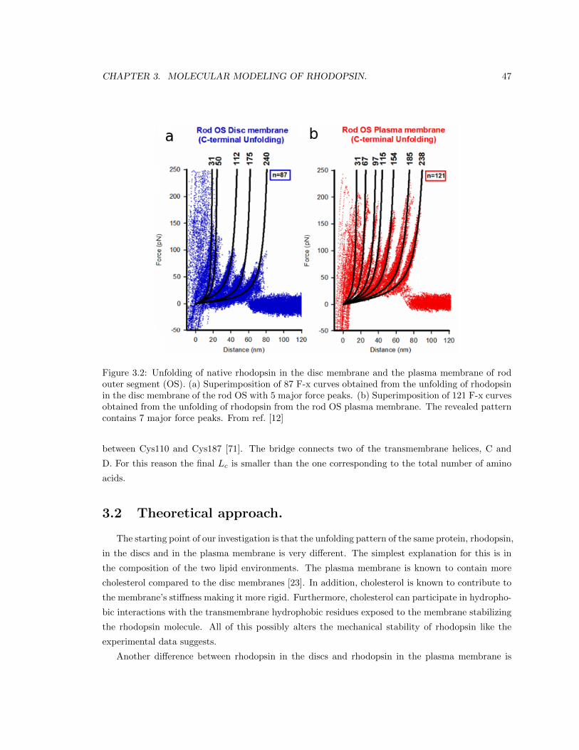
CHAPTER 3. MOLECULAR MODELING OF RHODOPSIN. 47
Figure 3.2: Unfolding of native rhodopsin in the disc membrane and the plasma membrane of rodouter segment (OS). (a) Superimposition of 87 F-x curves obtained from the unfolding of rhodopsinin the disc membrane of the rod OS with 5 major force peaks. (b) Superimposition of 121 F-x curvesobtained from the unfolding of rhodopsin from the rod OS plasma membrane. The revealed patterncontains 7 major force peaks. From ref. [12]
between Cys110 and Cys187 [71]. The bridge connects two of the transmembrane helices, C and
D. For this reason the final Lc is smaller than the one corresponding to the total number of amino
acids.
3.2 Theoretical approach.
The starting point of our investigation is that the unfolding pattern of the same protein, rhodopsin,
in the discs and in the plasma membrane is very different. The simplest explanation for this is in
the composition of the two lipid environments. The plasma membrane is known to contain more
cholesterol compared to the disc membranes [23]. In addition, cholesterol is known to contribute to
the membrane’s stiffness making it more rigid. Furthermore, cholesterol can participate in hydropho-
bic interactions with the transmembrane hydrophobic residues exposed to the membrane stabilizing
the rhodopsin molecule. All of this possibly alters the mechanical stability of rhodopsin like the
experimental data suggests.
Another difference between rhodopsin in the discs and rhodopsin in the plasma membrane is
CHAPTER 3. MOLECULAR MODELING OF RHODOPSIN. 48
related to the protein activation. It is well known that the transition of rhodopsin to its active form,
metarhodopsin II, is accompanied by a series of conformational changes. Rhodopsin is functional
only in the discs. A possible explanation for this is that the higher cholesterol concentration in
the plasma membrane favors the inactive rhodopsin conformation impeding the phototransduction
process.
In order to address these issues, we first developed a coarse-grained model of the rhodopsin-
membrane system. We started from a Go-like model inroduced by Cieplak et al. [24] (see subsection
2.0.5). We modeled the presence of the membrane with an additional potential energy term account-
ing for the protein-membrane interactions. As far as we know, this way of modeling the membrane
hasn’t been reported before in the literature. Our model has one free parameter, εMEMBR, which
determines the strength of the rhodopsin-membrane interactions. The main goal of this model is to
reproduce the characteristic F-x curves obtained experimentally when rhodopsin was unfolded from
the discs and from the plasma membrane.
In the second part, we examined the effect of the higher cholesterol content in the plasma mem-
brane on the rhodopsin flexibility with all-atom MD simulations in a lipid bilayer. We used a
statistical mechanics approach to extract qualitative description of the rhodopsin behavior in a
cholesterol-rich membrane from the atomistic simulations performed in a cholesterol-free lipid bi-
layer.
3.2.1 The molecular model of the rhodopsin-membrane system.
We represented the rhodopsin polypeptide chain in a simplified manner as a chain of beads.
We implemented this using the coarse-grained Go-like model developed by Cieplak et al. [24]. The
detailed description of the model is provided in subsection 2.0.5. Briefly, the amino acids are rep-
resented as beads centered around the Cα atoms. The beads are tethered together at the typical
peptide bond length, 3.8A, by a harmonic potential. The native chirality of the protein is conserved
by a chirality potential. The non-covalent interactions are divided into native and non-native de-
pending on the contact type in the native state. The contact type is determined from the distances
between all heavy atoms in the atomistic representation of the native state using the procedure of
Tsai et al. [63]. According to this procedure, if the distance between two atoms is larger than the
sum of their van der Waals radii multiplied by 1.244, the contact is non-native. If the distance
is smaller - the contact is native. The potential used to describe the interactions between native
contacts is the Lennard-Jones potential with a minimum corresponding to the distance between the
Cα atoms in the native state. The potential used to describe the interactions between non-native
contacts is purely repulsive. It has the form of the repulsive part of the Lennard-Jones potential
corresponding to a minimum at σ = 5A. This potential is shifted upward with zero energy at σ = 5A
and vanishes at larger equilibrium distances. The protein system evolves in time according to the
Langevin equation (see below, Eq. 3.2). Stretching is implemented in the following manner: one of
CHAPTER 3. MOLECULAR MODELING OF RHODOPSIN. 49
the two protein ends is kept fixed, while the other, attached to a harmonic spring, is being pulled
in the z-direction. The separation of the moving end from its origin corresponds to the cantilever
displacement in the AFM experiment. This model has been successfully used to describe the elastic
properties of globular proteins like titin [25], calmodulin [26] and ubiquitin [27].
Cieplak et al. used the same model in combination with all-atom MD simulations to describe the
unfolding of the membrane protein bacteriorhodopsin [28]. The atomistic simulations were necessary
to determine the initial state of the rhodopsin-membrane system. The membrane was modeled by a
POPC lipid bilayer. Rhodopsin was embedded in the lipid bilayer and the system was equilibrated.
Afterwards, the equilibrated rhodopsin-membrane system was coarse-grained as follows: rhodopsin
was modeled in the way we just described and the POPC lipids were represented by their carbon
atoms (see subsection 2.0.5). Native and non-native contacts between the protein and the lipids were
determined again following the Tsai et al. [63] protocol. The potentials describing the native and
non-native interactions were of the same functional forms. During the stretching, the coarse-grained
lipid bilayer was kept rigid and not allowed to adjust to the new configuration of the system. In this
manner, when the protein is pulled out, the space it was filling in the membrane remains empty,
leaving a sort of a hole. This is unrealistic, since in a real membrane the phospholipids are able to
fill the space left empty by the protein.
In order to circumvent this approximation, we model the effect of the membrane with an extra
potential energy term, VMEMBR, applied only along the z-axis and which acts in a different manner
on the different residues based on their chemical nature and on their native contact with the mem-
brane. Initially, all amino acids are divided into hydrophobic, hydrophilic and unspecified according
to the Kyte and Doolittle hydrophobicity scale [72]. We used the program GetArea [73] to compute
the solvent accessible surface area (SASA) and to determine which amino acids in the experimental
structure are exposed to the solvent, with the membrane being the solvent in our case. If a residue
i is membrane exposed and hydrophobic, it contributes to VMEMBR as follows:
VMEMBR(zi) =
0, if |zi| < l
2
εMEMBR, if |zi| < l2 + 3A
εMEMBR
(|zi|− l
2
3
), otherwise
(3.1)
where zi is the z-coordinate of residue i and l is the membrane thickness in A. Here we take
l = 33A. εMEMBR is the most important parameter in our model. It is a measure of the strength of
the membrane potential: a larger value of εMEMBR defines a highly hydrophobic membrane such as
a cholesterol-rich membrane. The same potential multiplied by -1 acts on the hydrophilic residues
exposed to the membrane.
A scheme representation of the membrane potential is presented in Figure 3.3. When a hy-
drophobic residue in native contact with the membrane has a z-coordinate corresponding to the
hydrophobic core of the membrane formed by the lipid tails, VMEMBR = 0. If the z-coordinate
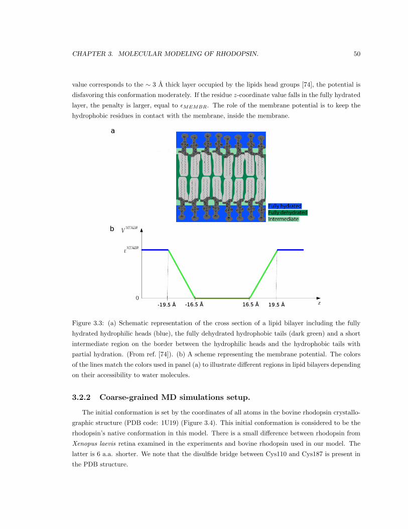
CHAPTER 3. MOLECULAR MODELING OF RHODOPSIN. 50
value corresponds to the ∼ 3 A thick layer occupied by the lipids head groups [74], the potential is
disfavoring this conformation moderately. If the residue z-coordinate value falls in the fully hydrated
layer, the penalty is larger, equal to εMEMBR. The role of the membrane potential is to keep the
hydrophobic residues in contact with the membrane, inside the membrane.
Figure 3.3: (a) Schematic representation of the cross section of a lipid bilayer including the fully
hydrated hydrophilic heads (blue), the fully dehydrated hydrophobic tails (dark green) and a short
intermediate region on the border between the hydrophilic heads and the hydrophobic tails with
partial hydration. (From ref. [74]). (b) A scheme representing the membrane potential. The colors
of the lines match the colors used in panel (a) to illustrate different regions in lipid bilayers depending
on their accessibility to water molecules.
3.2.2 Coarse-grained MD simulations setup.
The initial conformation is set by the coordinates of all atoms in the bovine rhodopsin crystallo-
graphic structure (PDB code: 1U19) (Figure 3.4). This initial conformation is considered to be the
rhodopsin’s native conformation in this model. There is a small difference between rhodopsin from
Xenopus laevis retina examined in the experiments and bovine rhodopsin used in our model. The
latter is 6 a.a. shorter. We note that the disulfide bridge between Cys110 and Cys187 is present in
the PDB structure.

CHAPTER 3. MOLECULAR MODELING OF RHODOPSIN. 51
Figure 3.4: (a) Rhodopsin (PDB: 1U19) all-atom graphical representation colored by the aminoacids names. (b) Graphical representation of coarse-grained rhodopsin. Each bead corresponds tothe Cα atom of the residue.
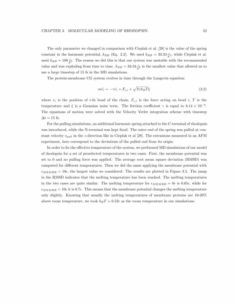
CHAPTER 3. MOLECULAR MODELING OF RHODOPSIN. 52
The only parameter we changed in comparison with Cieplak et al. [28] is the value of the spring
constant in the harmonic potential, kBB (Eq. 2.2). We used kBB = 33.34 ε
A2 , while Cieplak et al.
used kBB = 100 ε
A2 . The reason we did this is that our system was unstable with the recommended
value and was exploding from time to time. kBB = 33.34 ε
A2 is the smallest value that allowed us to
use a large timestep of 15 fs in the MD simulations.
The protein-membrane CG system evolves in time through the Langevin equation:
mri = −γri + Fc,i +√
2γkBTξ (3.2)
where ri is the position of i-th bead of the chain, Fc,i is the force acting on bead i, T is the
temperature and ξ is a Gaussian noise term. The friction coefficient γ is equal to 8.14 × 10⁻⁴.
The equations of motion were solved with the Velocity Verlet integration scheme with timestep
∆t = 15 fs.
For the pulling simulations, an additional harmonic spring attached to the C-terminal of rhodopsin
was introduced, while the N-terminal was kept fixed. The outer end of the spring was pulled at con-
stant velocity vpull in the z-direction like in Cieplak et al [28]. The extensions measured in an AFM
experiment, here correspond to the deviations of the pulled end from its origin.
In order to fix the effective temperature of the system, we performed MD simulations of our model
of rhodopsin for a set of preselected temperatures in two cases. First, the membrane potential was
set to 0 and no pulling force was applied. The average root mean square deviation (RMSD) was
computed for different temperatures. Then we did the same applying the membrane potential with
εMEMBR = 10ε, the largest value we considered. The results are plotted in Figure 3.5. The jump
in the RMSD indicates that the melting temperature has been reached. The melting temperatures
in the two cases are quite similar. The melting temperature for εMEMBR = 0ε is 0.65ε, while for
εMEMBR = 10ε it is 0.7ε. This means that the membrane potential changes the melting temperature
only slightly. Knowing that usually the melting temperatures of membrane proteins are 10-20%
above room temperature, we took kBT = 0.52ε as the room temperature in our simulations.
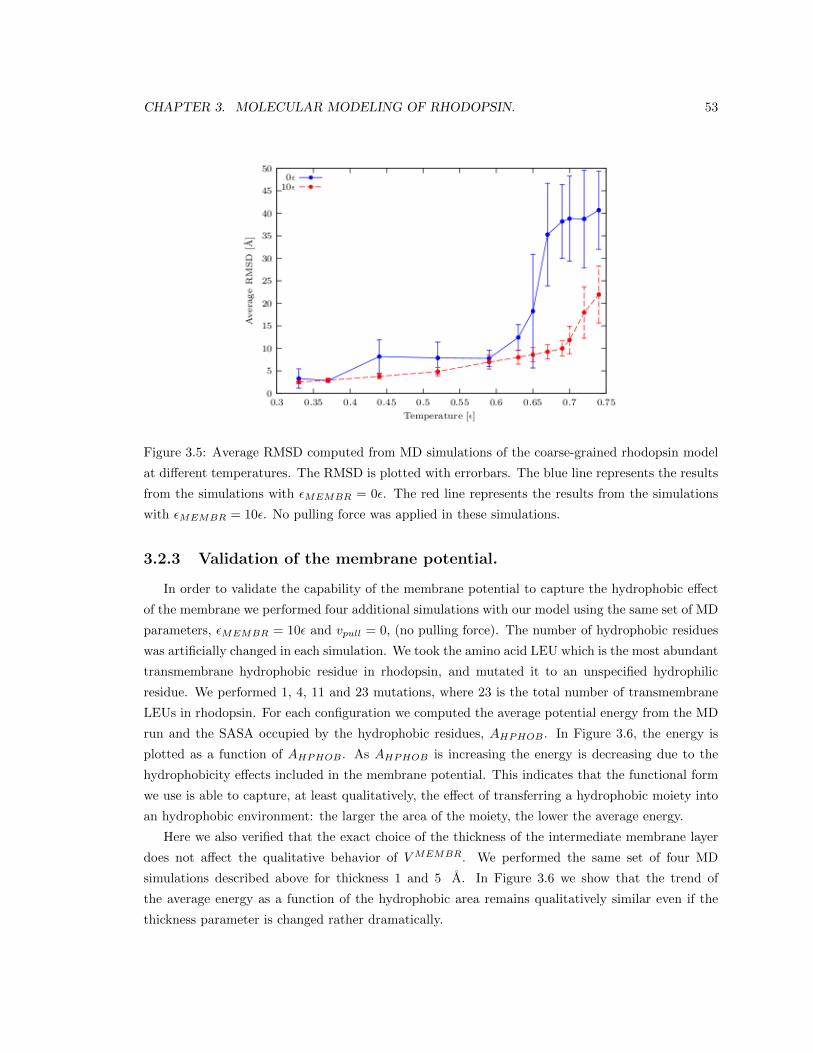
CHAPTER 3. MOLECULAR MODELING OF RHODOPSIN. 53
Figure 3.5: Average RMSD computed from MD simulations of the coarse-grained rhodopsin model
at different temperatures. The RMSD is plotted with errorbars. The blue line represents the results
from the simulations with εMEMBR = 0ε. The red line represents the results from the simulations
with εMEMBR = 10ε. No pulling force was applied in these simulations.
3.2.3 Validation of the membrane potential.
In order to validate the capability of the membrane potential to capture the hydrophobic effect
of the membrane we performed four additional simulations with our model using the same set of MD
parameters, εMEMBR = 10ε and vpull = 0, (no pulling force). The number of hydrophobic residues
was artificially changed in each simulation. We took the amino acid LEU which is the most abundant
transmembrane hydrophobic residue in rhodopsin, and mutated it to an unspecified hydrophilic
residue. We performed 1, 4, 11 and 23 mutations, where 23 is the total number of transmembrane
LEUs in rhodopsin. For each configuration we computed the average potential energy from the MD
run and the SASA occupied by the hydrophobic residues, AHPHOB . In Figure 3.6, the energy is
plotted as a function of AHPHOB . As AHPHOB is increasing the energy is decreasing due to the
hydrophobicity effects included in the membrane potential. This indicates that the functional form
we use is able to capture, at least qualitatively, the effect of transferring a hydrophobic moiety into
an hydrophobic environment: the larger the area of the moiety, the lower the average energy.
Here we also verified that the exact choice of the thickness of the intermediate membrane layer
does not affect the qualitative behavior of VMEMBR. We performed the same set of four MD
simulations described above for thickness 1 and 5 A. In Figure 3.6 we show that the trend of
the average energy as a function of the hydrophobic area remains qualitatively similar even if the
thickness parameter is changed rather dramatically.
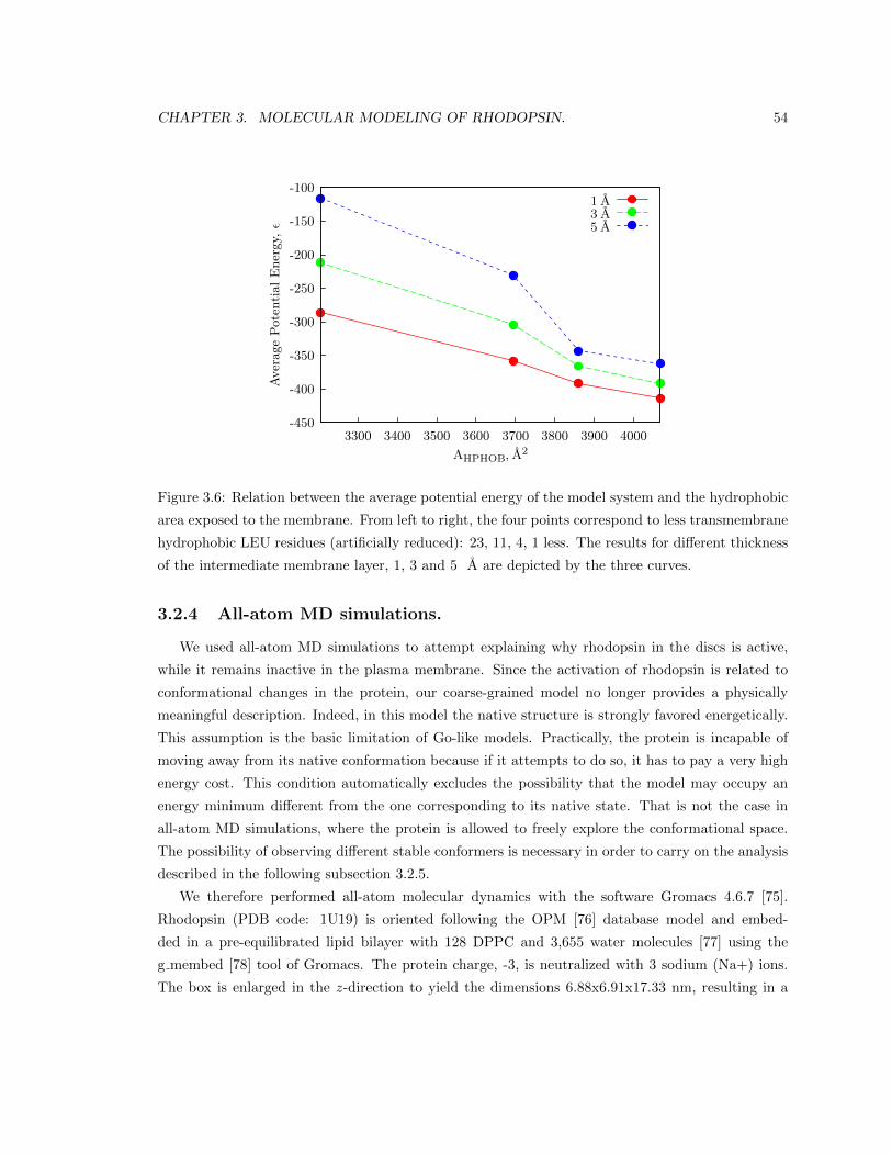
CHAPTER 3. MOLECULAR MODELING OF RHODOPSIN. 54
-450
-400
-350
-300
-250
-200
-150
-100
3300 3400 3500 3600 3700 3800 3900 4000
Aver
age
Pote
ntia
lEne
rgy,
ϵ
AHPHOB, Å2
1 Å3 Å5 Å
Figure 3.6: Relation between the average potential energy of the model system and the hydrophobic
area exposed to the membrane. From left to right, the four points correspond to less transmembrane
hydrophobic LEU residues (artificially reduced): 23, 11, 4, 1 less. The results for different thickness
of the intermediate membrane layer, 1, 3 and 5 A are depicted by the three curves.
3.2.4 All-atom MD simulations.
We used all-atom MD simulations to attempt explaining why rhodopsin in the discs is active,
while it remains inactive in the plasma membrane. Since the activation of rhodopsin is related to
conformational changes in the protein, our coarse-grained model no longer provides a physically
meaningful description. Indeed, in this model the native structure is strongly favored energetically.
This assumption is the basic limitation of Go-like models. Practically, the protein is incapable of
moving away from its native conformation because if it attempts to do so, it has to pay a very high
energy cost. This condition automatically excludes the possibility that the model may occupy an
energy minimum different from the one corresponding to its native state. That is not the case in
all-atom MD simulations, where the protein is allowed to freely explore the conformational space.
The possibility of observing different stable conformers is necessary in order to carry on the analysis
described in the following subsection 3.2.5.
We therefore performed all-atom molecular dynamics with the software Gromacs 4.6.7 [75].
Rhodopsin (PDB code: 1U19) is oriented following the OPM [76] database model and embed-
ded in a pre-equilibrated lipid bilayer with 128 DPPC and 3,655 water molecules [77] using the
g membed [78] tool of Gromacs. The protein charge, -3, is neutralized with 3 sodium (Na+) ions.
The box is enlarged in the z-direction to yield the dimensions 6.88x6.91x17.33 nm, resulting in a
CHAPTER 3. MOLECULAR MODELING OF RHODOPSIN. 55
system of 1 protein, 118 DPPC and 20,826 water molecules and 3 Na+. Periodic boundary condi-
tions are applied. The force field GROMOS96 53a6 [79] with included Berger lipids parameters [80]
for the DPPC molecules is used. All bonds are constrained to their equilibrium lengths with the
LINCS algorithm [81]. The non-bonded interactions are described by Lennard-Jones potential with
a cutoff at 1.2 nm. The electrostatic interactions are estimated by the particle mesh Ewald (PME)
method [82] with cutoff of 1.2 nm. The equations of motion are integrated with the leap-frog algo-
rithm, using a time step of 2 fs. The equilibration is performed in three steps: (1) The system was
first heated to a temperature of 323 K in 1 ns keeping the protein backbone fixed; (2) then a 7 ns
run in a NPT ensemble is performed, with a surface tension equal to 28 mN/m (corresponding to
a -55.56 bar pressure) in the x and y directions and 1 bar in the z direction with a semi isotropic
Parrinello-Rahman barostat [83]; temperature is kept fixed at 323 K with Berendsen thermostat [84];
(3) Finally, a 70 ns production run is performed.
3.2.5 Estimating the effect of membrane hydrophobicity on rhodopsin
flexibility.
Here we derive a set of equations which will allow us to evaluate the effect of the membrane
hydrophobicity on rhodopsin flexibility from the atomistic MD simulation of rhodopsin in the
cholesterol-free DPPC bilayer.
The partition coefficient per unit area of a hydrophobic molecule between a cholesterol-free
membrane and a membrane with a given cholesterol content can be used to measure the effect of
a change in the cholesterol content in the membrane. This quantity can be in principle measured
experimentally, and it has been estimated for a few compounds by atomistic simulations. We denote
this partition coefficient by γ. We model the effect of the change in the membrane hydrophobicity
by adding to the ordinary potential energy function, an extra term of the form:
Vγ(x) = −γA(x) (3.3)
where A(x) is the transmembrane hydrophobic SASA in configuration x. This term favors con-
figurations with large A and vanishes if γ = 0. The functional form of Vγ is consistent with the
mesoscopic definition of the hydration free energy, which should be proportional to the surface of
the molecule. It is also consistent with the apolar contribution to the free energy of solvation used
in several implicit solvation models [85, 86].
The probability distribution function, Pγ(x), is given by:
Pγ(x) = ce−V0(x)kBT e
γA(x)kBT = c ′e
γA(x)kBT P0(x) (3.4)
where c and c ′ are normalization constants, V0(x) is the potential energy function and P0(x) is the
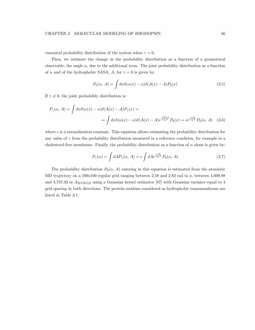
CHAPTER 3. MOLECULAR MODELING OF RHODOPSIN. 56
canonical probability distribution of the system when γ = 0.
Then, we estimate the change in the probability distribution as a function of a geometrical
observable, the angle α, due to the additional term. The joint probability distribution as a function
of α and of the hydrophobic SASA, A, for γ = 0 is given by:
P0(α, A) =
∫dxδ(α(x)− α)δ(A(x)−A)P0(x) (3.5)
If γ 6= 0, the joint probability distribution is:
Pγ(α, A) =
∫dxδ(α(x)− α)δ(A(x)−A)Pγ(x) =
=
∫dxδ(α(x)− α)δ(A(x)−A)e
γA(x)kBT P0(x) = ce
γAkBT P0(α, A) (3.6)
where c is a normalization constant. This equation allows estimating the probability distribution for
any value of γ from the probability distribution measured in a reference condition, for example in a
cholesterol-free membrane. Finally, the probability distribution as a function of α alone is given by:
Pγ(α) =
∫dAPγ(α, A) = c
∫dAe
γAkBT P0(α, A) (3.7)
The probability distribution P0(α, A) entering in this equation is estimated from the atomistic
MD trajectory on a 100x100 regular grid ranging between 2.58 and 2.83 rad in α, between 4,009.88
and 4,737.92 in AHPHOB using a Gaussian kernel estimator [87] with Gaussian variance equal to 4
grid spacing in both directions. The protein residues considered as hydrophobic transmembrane are
listed in Table 3.1.
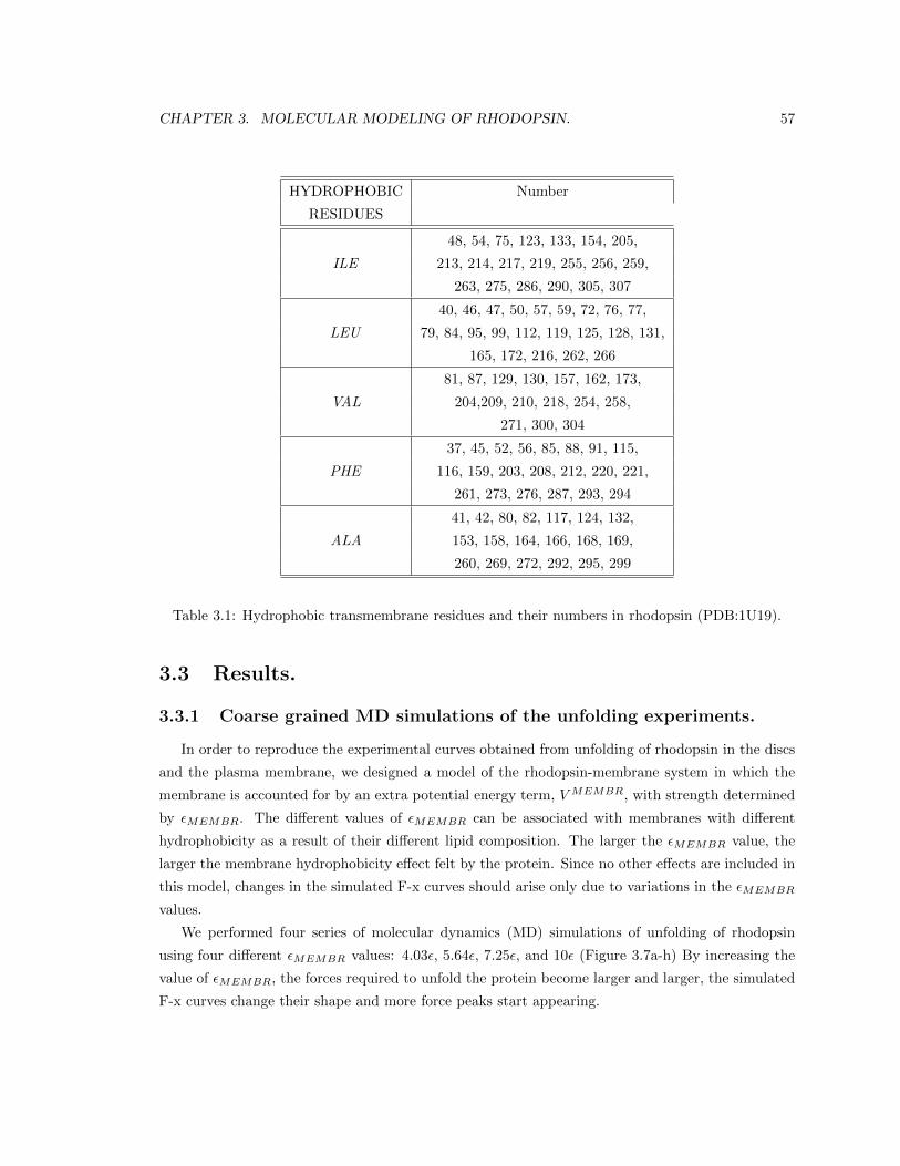
CHAPTER 3. MOLECULAR MODELING OF RHODOPSIN. 57
HYDROPHOBIC Number
RESIDUES
48, 54, 75, 123, 133, 154, 205,
ILE 213, 214, 217, 219, 255, 256, 259,
263, 275, 286, 290, 305, 307
40, 46, 47, 50, 57, 59, 72, 76, 77,
LEU 79, 84, 95, 99, 112, 119, 125, 128, 131,
165, 172, 216, 262, 266
81, 87, 129, 130, 157, 162, 173,
VAL 204,209, 210, 218, 254, 258,
271, 300, 304
37, 45, 52, 56, 85, 88, 91, 115,
PHE 116, 159, 203, 208, 212, 220, 221,
261, 273, 276, 287, 293, 294
41, 42, 80, 82, 117, 124, 132,
ALA 153, 158, 164, 166, 168, 169,
260, 269, 272, 292, 295, 299
Table 3.1: Hydrophobic transmembrane residues and their numbers in rhodopsin (PDB:1U19).
3.3 Results.
3.3.1 Coarse grained MD simulations of the unfolding experiments.
In order to reproduce the experimental curves obtained from unfolding of rhodopsin in the discs
and the plasma membrane, we designed a model of the rhodopsin-membrane system in which the
membrane is accounted for by an extra potential energy term, VMEMBR, with strength determined
by εMEMBR. The different values of εMEMBR can be associated with membranes with different
hydrophobicity as a result of their different lipid composition. The larger the εMEMBR value, the
larger the membrane hydrophobicity effect felt by the protein. Since no other effects are included in
this model, changes in the simulated F-x curves should arise only due to variations in the εMEMBR
values.
We performed four series of molecular dynamics (MD) simulations of unfolding of rhodopsin
using four different εMEMBR values: 4.03ε, 5.64ε, 7.25ε, and 10ε (Figure 3.7a-h) By increasing the
value of εMEMBR, the forces required to unfold the protein become larger and larger, the simulated
F-x curves change their shape and more force peaks start appearing.
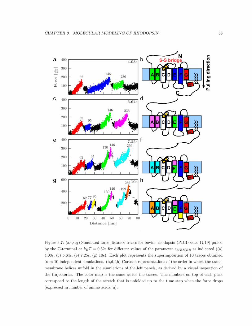
CHAPTER 3. MOLECULAR MODELING OF RHODOPSIN. 58
Figure 3.7: (a,c,e,g) Simulated force-distance traces for bovine rhodopsin (PDB code: 1U19) pulled
by the C-terminal at kBT = 0.52ε for different values of the parameter εMEMBR as indicated ((a)
4.03ε, (c) 5.64ε, (e) 7.25ε, (g) 10ε). Each plot represents the superimposition of 10 traces obtained
from 10 independent simulations. (b,d,f,h) Cartoon representations of the order in which the trans-
membrane helices unfold in the simulations of the left panels, as derived by a visual inspection of
the trajectories. The color map is the same as for the traces. The numbers on top of each peak
correspond to the length of the stretch that is unfolded up to the time step when the force drops
(expressed in number of amino acids, n).
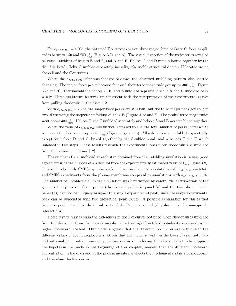
CHAPTER 3. MOLECULAR MODELING OF RHODOPSIN. 59
For εMEMBR = 4.03ε, the obtained F-x curves contain three major force peaks with force ampli-
tudes between 150 and 200 εnm (Figure 3.7a and b). The visual inspection of the trajectories revealed
pairwise unfolding of helices E and F, and A and B. Helices C and D remain bound together by the
disulfide bond. Helix G unfolds separately including the stable structural domain H located inside
the cell and the C-terminus.
When the εMEMBR value was changed to 5.64ε, the observed unfolding pattern also started
changing. The major force peaks became four and their force magnitude got up to 300 εnm (Figure
3.7c and d). Transmembrane helices G, F, and E unfolded separately, while A and B unfolded pair-
wisely. These qualitative features are consistent with the interpretation of the experimental curves
from pulling rhodopsin in the discs [12].
With εMEMBR = 7.25ε, the major force peaks are still four, but the third major peak got split in
two, illustrating the stepwise unfolding of helix E (Figure 3.7e and f). The peaks’ force magnitudes
went above 300 εnm . Helices G and F unfolded separately and helices A and B were unfolded together.
When the value of εMEMBR was further increased to 10ε, the total number of peaks increased to
seven and the forces went up to 500 εnm (Figure 3.7g and h). All α-helices were unfolded sequentially,
except for helices D and C, linked together by the disulfide bond, and α-helices F and E which
unfolded in two steps. These results resemble the experimental ones when rhodopsin was unfolded
from the plasma membrane [12].
The number of a.a. unfolded at each step obtained from the unfolding simulation is in very good
agreement with the number of a.a derived from the experimentally estimated value of Lc (Figure 3.8).
This applies for both, SMFS experiments from discs compared to simulations with εMEMBR = 5.64ε,
and SMFS experiments from the plasma membrane compared to simulations with εMEMBR = 10ε.
The number of unfolded a.a. in the simulation was determined by careful visual inspection of the
generated trajectories. Some points (the two red points in panel (a) and the two blue points in
panel (b)) can not be uniquely assigned to a single experimental peak, since the single experimental
peak can be associated with two theoretical peak values. A possible explanation for this is that
in real experimental data the initial parts of the F-x curves are highly dominated by non-specific
interactions.
These results may explain the differences in the F-x curves obtained when rhodopsin is unfolded
from the discs and from the plasma membrane, whose significant hydrophobicity is caused by its
higher cholesterol content. Our model suggests that the different F-x curves are only due to the
different values of the hydrophobicity. Given that the model is built on the basis of essential inter-
and intramolecular interactions only, its success in reproducing the experimental data supports
the hypothesis we made in the beginning of this chapter, namely that the different cholesterol
concentration in the discs and in the plasma membrane affects the mechanical stability of rhodopsin,
and therefore the F-x curves.
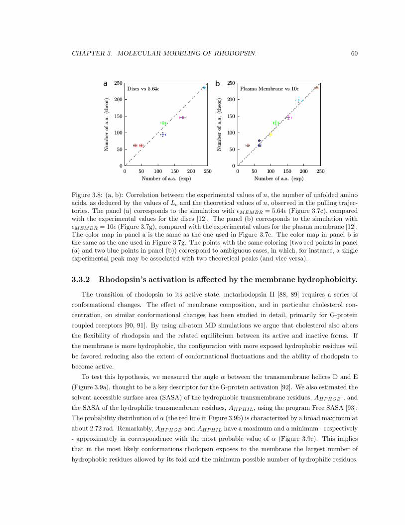
CHAPTER 3. MOLECULAR MODELING OF RHODOPSIN. 60
Figure 3.8: (a, b): Correlation between the experimental values of n, the number of unfolded aminoacids, as deduced by the values of Lc and the theoretical values of n, observed in the pulling trajec-tories. The panel (a) corresponds to the simulation with εMEMBR = 5.64ε (Figure 3.7c), comparedwith the experimental values for the discs [12]. The panel (b) corresponds to the simulation withεMEMBR = 10ε (Figure 3.7g), compared with the experimental values for the plasma membrane [12].The color map in panel a is the same as the one used in Figure 3.7c. The color map in panel b isthe same as the one used in Figure 3.7g. The points with the same coloring (two red points in panel(a) and two blue points in panel (b)) correspond to ambiguous cases, in which, for instance, a singleexperimental peak may be associated with two theoretical peaks (and vice versa).
3.3.2 Rhodopsin’s activation is affected by the membrane hydrophobicity.
The transition of rhodopsin to its active state, metarhodopsin II [88, 89] requires a series of
conformational changes. The effect of membrane composition, and in particular cholesterol con-
centration, on similar conformational changes has been studied in detail, primarily for G-protein
coupled receptors [90, 91]. By using all-atom MD simulations we argue that cholesterol also alters
the flexibility of rhodopsin and the related equilibrium between its active and inactive forms. If
the membrane is more hydrophobic, the configuration with more exposed hydrophobic residues will
be favored reducing also the extent of conformational fluctuations and the ability of rhodopsin to
become active.
To test this hypothesis, we measured the angle α between the transmembrane helices D and E
(Figure 3.9a), thought to be a key descriptor for the G-protein activation [92]. We also estimated the
solvent accessible surface area (SASA) of the hydrophobic transmembrane residues, AHPHOB , and
the SASA of the hydrophilic transmembrane residues, AHPHIL, using the program Free SASA [93].
The probability distribution of α (the red line in Figure 3.9b) is characterized by a broad maximum at
about 2.72 rad. Remarkably, AHPHOB and AHPHIL have a maximum and a minimum - respectively
- approximately in correspondence with the most probable value of α (Figure 3.9c). This implies
that in the most likely conformations rhodopsin exposes to the membrane the largest number of
hydrophobic residues allowed by its fold and the minimum possible number of hydrophilic residues.
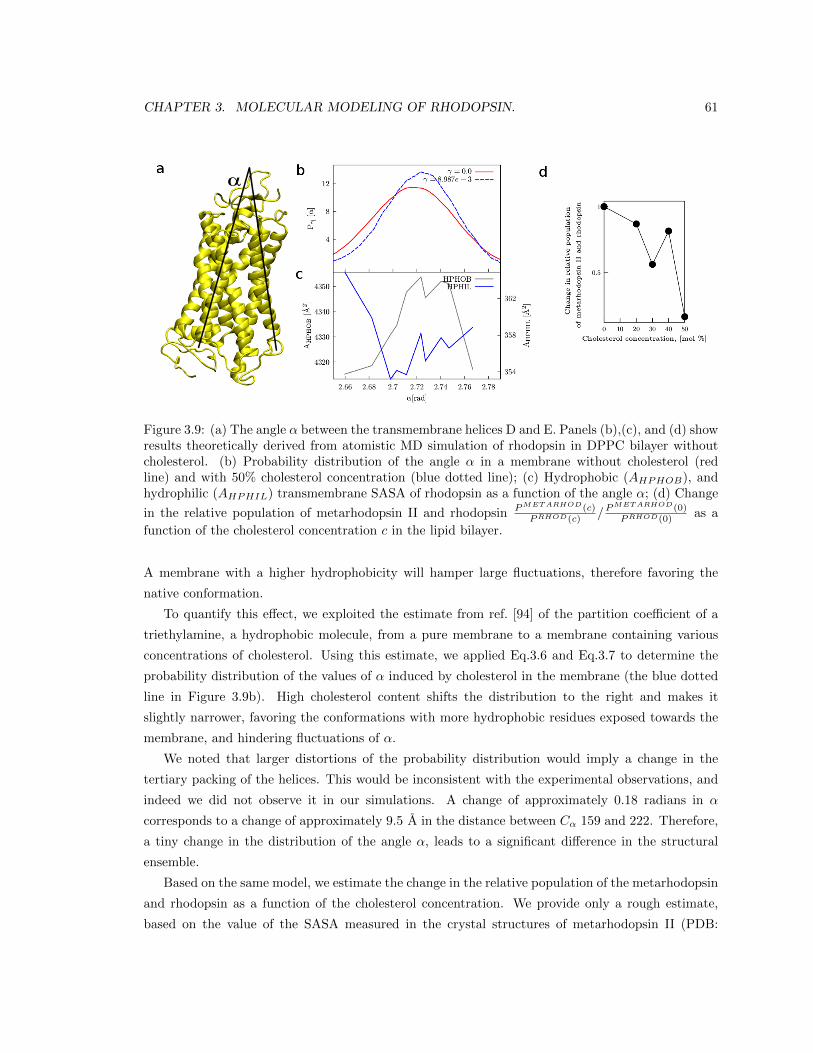
CHAPTER 3. MOLECULAR MODELING OF RHODOPSIN. 61
Figure 3.9: (a) The angle α between the transmembrane helices D and E. Panels (b),(c), and (d) showresults theoretically derived from atomistic MD simulation of rhodopsin in DPPC bilayer withoutcholesterol. (b) Probability distribution of the angle α in a membrane without cholesterol (redline) and with 50% cholesterol concentration (blue dotted line); (c) Hydrophobic (AHPHOB), andhydrophilic (AHPHIL) transmembrane SASA of rhodopsin as a function of the angle α; (d) Change
in the relative population of metarhodopsin II and rhodopsin PMETARHOD(c)PRHOD(c)
/PMETARHOD(0)PRHOD(0)
as a
function of the cholesterol concentration c in the lipid bilayer.
A membrane with a higher hydrophobicity will hamper large fluctuations, therefore favoring the
native conformation.
To quantify this effect, we exploited the estimate from ref. [94] of the partition coefficient of a
triethylamine, a hydrophobic molecule, from a pure membrane to a membrane containing various
concentrations of cholesterol. Using this estimate, we applied Eq.3.6 and Eq.3.7 to determine the
probability distribution of the values of α induced by cholesterol in the membrane (the blue dotted
line in Figure 3.9b). High cholesterol content shifts the distribution to the right and makes it
slightly narrower, favoring the conformations with more hydrophobic residues exposed towards the
membrane, and hindering fluctuations of α.
We noted that larger distortions of the probability distribution would imply a change in the
tertiary packing of the helices. This would be inconsistent with the experimental observations, and
indeed we did not observe it in our simulations. A change of approximately 0.18 radians in α
corresponds to a change of approximately 9.5 A in the distance between Cα 159 and 222. Therefore,
a tiny change in the distribution of the angle α, leads to a significant difference in the structural
ensemble.
Based on the same model, we estimate the change in the relative population of the metarhodopsin
and rhodopsin as a function of the cholesterol concentration. We provide only a rough estimate,
based on the value of the SASA measured in the crystal structures of metarhodopsin II (PDB:
CHAPTER 3. MOLECULAR MODELING OF RHODOPSIN. 62
3PXO) and rhodopsin (PDB: 1U19). The probability distribution as a function of the cholesterol
concentration is:
P (c) = e− V0kBT e
γ(c)AkBT = e
γ(c)AkBT P (0) (3.8)
where P (0) corresponds to the probability distribution in a cholesterol-free membrane.
Denoting by PMETARHOD(c)PRHOD(c)
the ratio between the population of metarhodopsin and rhodopsin
in a membrane characterized by a concentration c of cholesterol and applying Eq.3.8, we obtain
PMETARHOD(c)
PRHOD(c)= exp
[ γ(c)
kBT(AMETARHOD
HPHOB −ARHODHPHOB)]PMETARHOD(0)
PRHOD(0)(3.9)
where AMETARHODHPHOB and ARHODHPHOB are the SASA of the hydrophobic residues in the two confor-
mations and γ(c) is the partition coefficient per unit area of a hydrophobic molecule between a
cholesterol-free membrane and a membrane characterized by a cholesterol concentration c. γ(c) is
estimated from a work by Zocher et al, [94] using the value of triethylamine (TEA) in membranes
composed of DOPC with cholesterol concentrations 0, 20, 30, 40 and 50 mol %. To compute the
values of the partition coefficient we used the relations:
PTEA(c) = exp[ATEAkBT
γ(c)]PTEA(0) (3.10)
γ(c) =(lnPTEA(c)− lnPTEA(0))
ATEAkBT (3.11)
where PTEA(c) corresponds to the probability distribution of TEA as a function of the cholesterol
concentration, c (values extracted from Figure 4B in ref. [94]), γ(c) is the partition coefficient between
the two lipid environments and ATEA the SASA of a single triethylamine molecule. The values for
γ are presented in Table 3.2. In this definition γ estimates the surface tension per unit area of a
hydrophobic moiety. The results are largely insensitive to the choice of the molecule used to compute
the surface tension per unit area, if this is hydrophobic. For example, for pyridine in membranes
composed of DOPC with cholesterol concentration 40 mol % we have γPYR
APYR= 0.0018, a value similar
to the one observed for TEA, γTEA
ATEA= 0.0014 (values extracted from Figure 6C and D in ref. [94]).
Due to the hydrophobicity effect, the cholesterol concentration changes the relative ratio between
metarhodopsin II and rhodopsin (Figure 3.9d) and therefore the rate of rhodopsin activation. At
a concentration of 50% the ratio between metarhodopsin II and rhodopsin is approximately 0.17 of
the ratio observed in the absence of cholesterol, but even at a lower concentration the ratio of the
two populations is affected.
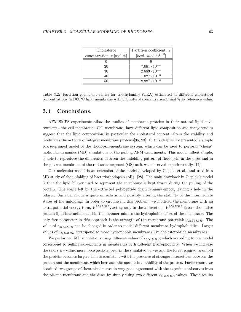
CHAPTER 3. MOLECULAR MODELING OF RHODOPSIN. 63
Cholesterol Partition coefficient, γ
concentration, c [mol %] [kcal ·mol−1A−2
]
0 020 7.061 · 10−4
30 2.889 · 10−4
40 1.027 · 10−3
50 8.987 · 10−3
Table 3.2: Partition coefficient values for triethylamine (TEA) estimated at different cholesterolconcentrations in DOPC lipid membrane with cholesterol concentration 0 mol % as reference value.
3.4 Conclusions.
AFM-SMFS experiments allow the studies of membrane proteins in their natural lipid envi-
ronment - the cell membrane. Cell membranes have different lipid composition and many studies
suggest that the lipid composition, in particular the cholesterol content, alters the stability and
modulates the activity of integral membrane proteins[95, 23]. In this chapter we presented a simple
coarse-grained model of the rhodopsin-membrane system, which can be used to perform ”cheap”
molecular dynamics (MD) simulations of the pulling AFM experiments. This model, albeit simple,
is able to reproduce the differences between the unfolding pattern of rhodopsin in the discs and in
the plasma membrane of the rod outer segment (OS) as it was observed experimentally [12].
Our molecular model is an extension of the model developed by Cieplak et al. and used in a
MD study of the unfolding of bacteriorhodopsin (bR) [28]. The main drawback in Cieplak’s model
is that the lipid bilayer used to represent the membrane is kept frozen during the pulling of the
protein. The space left by the extracted polypeptide chain remains empty, leaving a hole in the
bilayer. Such behaviour is quite unrealistic and possibly altering the stability of the intermediate
states of the unfolding. In order to circumvent this problem, we modeled the membrane with an
extra potential energy term, VMEMBR, acting only in the z-direction. VMEMBR favors the native
protein-lipid interactions and in this manner mimics the hydrophobic effect of the membrane. The
only free parameter in this approach is the strength of the membrane potential: εMEMBR. The
value of εMEMBR can be changed in order to model different membrane hydrophobicities. Larger
values of εMEMBR correspond to more hydrophobic membranes like cholesterol-rich membranes.
We performed MD simulations using different values of εMEMBR, which according to our model
correspond to pulling experiments in membranes with different hydrophobicity. When we increase
the εMEMBR value, more force peaks appear in the simulated curves and the force required to unfold
the protein becomes larger. This is consistent with the presence of stronger interactions between the
protein and the membrane, which increases the mechanical stability of the protein. Furthermore, we
obtained two groups of theoretical curves in very good agreement with the experimental curves from
the plasma membrane and the discs by simply using two different εMEMBR values. These results
CHAPTER 3. MOLECULAR MODELING OF RHODOPSIN. 64
suggest that the differences in the F-x curves of rhodopsin in the discs and in the plasma membrane
are due to the higher hydrophobicity of the plasma membrane, induced by its higher cholesterol
concentration.
Our findings were supported by additional experiments performed in the plasma membrane of
the rod OS treated with cyclodextrin [12]. Cyclodextrin is an agent that binds cholesterol and lowers
its concentration. As a result, in many traces the number of force peaks decreased from 7 to 5, which
is the number of force peaks present in the traces from the discs.
In this chapter, we addressed also another problem concerned with the inactivation of rhodopsin
in the plasma membrane. We argue that the cholesterol-rich plasma membrane reduces the flex-
ibility of rhodopsin and alters its ability to change conformation. This is in agreement with the
larger mechanical stability of rhodopsin observed experimentally in the plasma membrane and sup-
ported by our CG simulations. If this is true, rhodopsin can not switch to its active conformation
metarhodopsin II and the phototransduction cascade can not be initialized. In order to test this hy-
pothesis, we performed all-atom MD simulations of the inactive conformation of rhodopsin embedded
in a DPPC bilayer without cholesterol. We used a statistical mechanics apparatus in combination
with theoretical data on partition coefficients in membranes with different cholesterol concentra-
tions, to evaluate the cholesterol effects on rhodopsin’s flexibility. Our results suggest that the
higher cholesterol content might shift the equilibrium ratio between rhodopsin and metarhodopsin
towards the inactive state, which may explain the inactivation of rhodopsin in the plasma membrane.
The coarse-grained MD approach described in this chapter is not restricted to rhodopsin. It can
be applied to any other membrane protein of known structure. However, our results indicate that the
F-x curves of membrane proteins depend on many factors, including not only the lipid composition
of the membrane but possibly its protein composition too. We saw that by simply changing a single
parameter in the model, εMEMBR, the features of the F-x curves change tremendously. This makes
the identification of membrane proteins based on the unfolding pattern observed in their F-x curves
difficult, because clearly this pattern is not uniquely defined like for soluble proteins. Therefore,
even more than for soluble proteins, for membrane proteins experimental data need to be provided
in order to verify the results coming from the model.
In the next chapter, we describe an automatic tool we developed for the analysis of AFM-SMFS
data coming from experiments in native cell membranes. With this procedure we are able to find
clusters of traces sharing the same features, possibly describing the unfolding of same membrane
protein. A key missing ingredient, which should be addressed in the future, is that these clusters
should be assigned to a specific membrane proteins. A possible manner of achieving this goal is
using our MD tool to simulate the F-x curves for many proteins of known structure with different
εMEMBR values and look for a match with the experimental curves included in the cluster.

Chapter 4
Automatic classification of AFM
traces from native membranes.
Membrane proteins perform a variety of functions in the cell. They are key mediators in the
processes of signaling, cell-cell recognition and transport of ions and molecules across the membrane.
Nearly 30 % of all proteins in eukaryotic cells are membrane proteins. They are the targets of more
than 50 % of modern medicinal drugs and many diseases are found to be related to membrane
proteins misfolding [1]. However, studying membrane proteins is non-trivial, mainly because they
are difficult to purify and crystallize. Studying membrane proteins in their native environment is
even more difficult due to the heterogeneity of the membrane and its specific chemical properties.
Moreover, most of the modern experimental techniques have been designed to study soluble proteins.
A way out, as we will show in this chapter, seems to be offered by AFM-based SMFS. This method
allows localizing and quantifying key inter- and intramolecular interactions, estimating the effect of
environmental factors on the unfolding process, probing structural and conformational properties of
membrane proteins. The interpretation of the obtained experimental data reveals important insights
in the membrane proteins structure-function relations in the presence of the membrane. Recent
developments in the AFM-SMFS experimental approach enabled the accumulation of hundreds of
thousands of traces in a reasonable time [16, 17]. Strikingly, these experiments can nowadays be
performed in native cell membranes under physiological conditions: in section 1.1 we will describe
an experimental technique which allows reaching this goal.
The availability of this huge amount of data calls for the development of specific theoretical tools
allowing analysis and interpretation. However, these data require careful preprocessing since most
of the F-x curves do not contain meaningful unfolding events. It has been estimated that membrane
proteins get completely unfolded by SMFS in < 1% of the cases [21].
To the best of our knowledge, there is no automatic procedure which allows the classification of
65
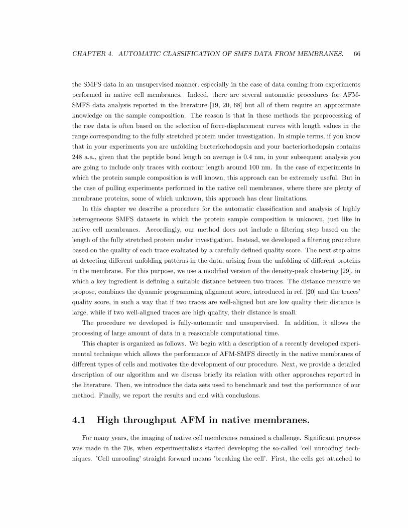
CHAPTER 4. AUTOMATIC CLASSIFICATION OF SMFS DATA FROM MEMBRANES. 66
the SMFS data in an unsupervised manner, especially in the case of data coming from experiments
performed in native cell membranes. Indeed, there are several automatic procedures for AFM-
SMFS data analysis reported in the literature [19, 20, 68] but all of them require an approximate
knowledge on the sample composition. The reason is that in these methods the preprocessing of
the raw data is often based on the selection of force-displacement curves with length values in the
range corresponding to the fully stretched protein under investigation. In simple terms, if you know
that in your experiments you are unfolding bacteriorhodopsin and your bacteriorhodopsin contains
248 a.a., given that the peptide bond length on average is 0.4 nm, in your subsequent analysis you
are going to include only traces with contour length around 100 nm. In the case of experiments in
which the protein sample composition is well known, this approach can be extremely useful. But in
the case of pulling experiments performed in the native cell membranes, where there are plenty of
membrane proteins, some of which unknown, this approach has clear limitations.
In this chapter we describe a procedure for the automatic classification and analysis of highly
heterogeneous SMFS datasets in which the protein sample composition is unknown, just like in
native cell membranes. Accordingly, our method does not include a filtering step based on the
length of the fully stretched protein under investigation. Instead, we developed a filtering procedure
based on the quality of each trace evaluated by a carefully defined quality score. The next step aims
at detecting different unfolding patterns in the data, arising from the unfolding of different proteins
in the membrane. For this purpose, we use a modified version of the density-peak clustering [29], in
which a key ingredient is defining a suitable distance between two traces. The distance measure we
propose, combines the dynamic programming alignment score, introduced in ref. [20] and the traces’
quality score, in such a way that if two traces are well-aligned but are low quality their distance is
large, while if two well-aligned traces are high quality, their distance is small.
The procedure we developed is fully-automatic and unsupervised. In addition, it allows the
processing of large amount of data in a reasonable computational time.
This chapter is organized as follows. We begin with a description of a recently developed experi-
mental technique which allows the performance of AFM-SMFS directly in the native membranes of
different types of cells and motivates the development of our procedure. Next, we provide a detailed
description of our algorithm and we discuss briefly its relation with other approaches reported in
the literature. Then, we introduce the data sets used to benchmark and test the performance of our
method. Finally, we report the results and end with conclusions.
4.1 High throughput AFM in native membranes.
For many years, the imaging of native cell membranes remained a challenge. Significant progress
was made in the 70s, when experimentalists started developing the so-called ’cell unroofing’ tech-
niques. ’Cell unroofing’ straight forward means ’breaking the cell’. First, the cells get attached to

CHAPTER 4. AUTOMATIC CLASSIFICATION OF SMFS DATA FROM MEMBRANES. 67
a surface through a gluing substance (polylysine or Alcian blue). Then, they have to be broken so
that pieces of the membrane are extracted. There are three main strategies to accomplish this: (1)
break the cells with a strong lateral flux of medium, leaving pieces of membrane attached to the
substrate [96]; (2) squash the cells between two coverslips, freeze them and fracture them by separa-
tion of the coverslips [97]; (3) use sonic waves to break the cells leaving pieces of the membrane on
the substrate [98]. The scanning electron microscope is then used to image the membrane patches.
These strategies are difficult to implement. The sonic waves, for example, affect the entire cell
culture in an unconstrained manner. Moreover, the AFM might be more appropriate for direct
imaging of cell membranes since it can operate in buffer solutions under physiological conditions.
Recently, a new methodology designed by Galvanetto et al. [18] made possible the investigation
of the native membranes of a variety of single cells in a simplified and handy manner. In this work
a new ’cell unroofing’ strategy is developed in which a single cell is ruptured with a sharp triangular
piece of glass, called the arrow. A piece of the membrane remains on the arrow and gets imaged
with the AFM. A characteristic feature of this approach is that the AFM is used also in the sample
preparation.
The sample preparation requires three main ingredients: the cell culture coverslip, the cell culture
holder and the arrow. The cell culture coverslip is simply a glass round coverslip (12 mm in diameter,
200 µm thick), plasma cleaned and coated with poly-D-lysine. The coating step enhances the
adhesion of the cells and the substrate, which is necessary because otherwise the entire cells might
get adsorbed on the arrow. The cell culture holder acts as a motor with micrometer precision used
to bring in contact the cell culture coverslip and the arrow. The motor role is performed by the
AFM. The arrow was prepared by breaking a round coverslip (24 mm in diameter, 200 µm thick)
in four with hands. It was also immersed in poly-D-lysine but for a shorter time period.
The AFM was mounted on an inverted optical microscope. The cell culture coverslip was attached
to the AFM holder. The coverslip was moved down with the AFM, towards the arrow. A single cell
was brought in contact with the apex of the arrow and squeezed for ∼ 3 minutes. Afterwards, the
cell culture coverslip was rapidly moved away from the arrow. As a result, a piece of the membrane
remained on the arrow as shown in Figure 4.1. The AFM images were obtained with a NanoWizard
3 JPK system in the intermittent contact mode. The cantilever spring constant was 0.08 N/m.
The method was tested on five different cell types, among which human brain cancer cells and
primary hippocampal neurons of rats. The success of the experiment depends on the adhesion of
the cell types to the substrate. If this effect is not strong enough, the entire cell gets adsorbed on
the arrow.
Once the membrane patches were isolated, their topology and mechanics were examined. Fur-
thermore, using the same technique, SMFS experiments were performed and a huge amount of F-x
curves obtained.
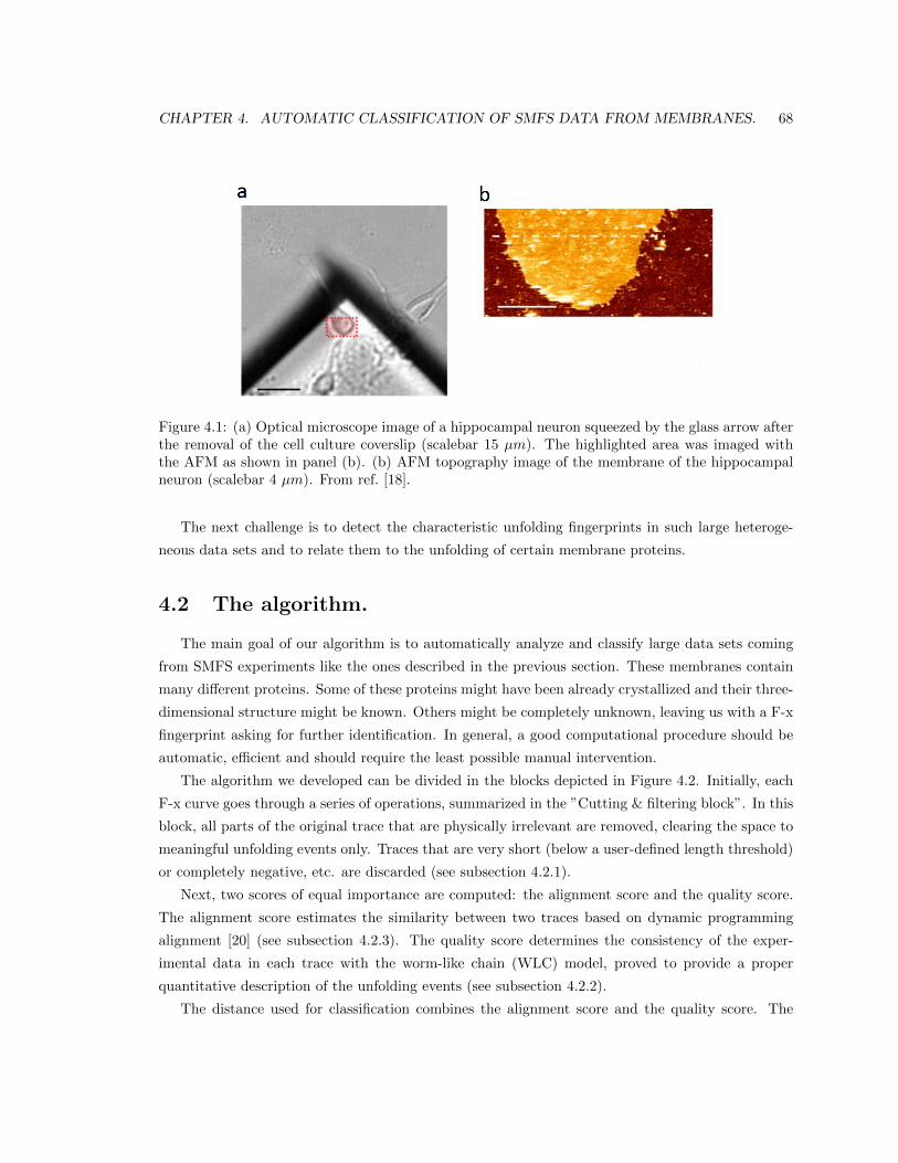
CHAPTER 4. AUTOMATIC CLASSIFICATION OF SMFS DATA FROM MEMBRANES. 68
Figure 4.1: (a) Optical microscope image of a hippocampal neuron squeezed by the glass arrow afterthe removal of the cell culture coverslip (scalebar 15 µm). The highlighted area was imaged withthe AFM as shown in panel (b). (b) AFM topography image of the membrane of the hippocampalneuron (scalebar 4 µm). From ref. [18].
The next challenge is to detect the characteristic unfolding fingerprints in such large heteroge-
neous data sets and to relate them to the unfolding of certain membrane proteins.
4.2 The algorithm.
The main goal of our algorithm is to automatically analyze and classify large data sets coming
from SMFS experiments like the ones described in the previous section. These membranes contain
many different proteins. Some of these proteins might have been already crystallized and their three-
dimensional structure might be known. Others might be completely unknown, leaving us with a F-x
fingerprint asking for further identification. In general, a good computational procedure should be
automatic, efficient and should require the least possible manual intervention.
The algorithm we developed can be divided in the blocks depicted in Figure 4.2. Initially, each
F-x curve goes through a series of operations, summarized in the ”Cutting & filtering block”. In this
block, all parts of the original trace that are physically irrelevant are removed, clearing the space to
meaningful unfolding events only. Traces that are very short (below a user-defined length threshold)
or completely negative, etc. are discarded (see subsection 4.2.1).
Next, two scores of equal importance are computed: the alignment score and the quality score.
The alignment score estimates the similarity between two traces based on dynamic programming
alignment [20] (see subsection 4.2.3). The quality score determines the consistency of the exper-
imental data in each trace with the worm-like chain (WLC) model, proved to provide a proper
quantitative description of the unfolding events (see subsection 4.2.2).
The distance used for classification combines the alignment score and the quality score. The
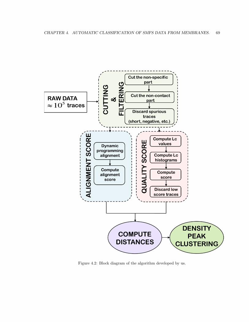
CHAPTER 4. AUTOMATIC CLASSIFICATION OF SMFS DATA FROM MEMBRANES. 69
Figure 4.2: Block diagram of the algorithm developed by us.
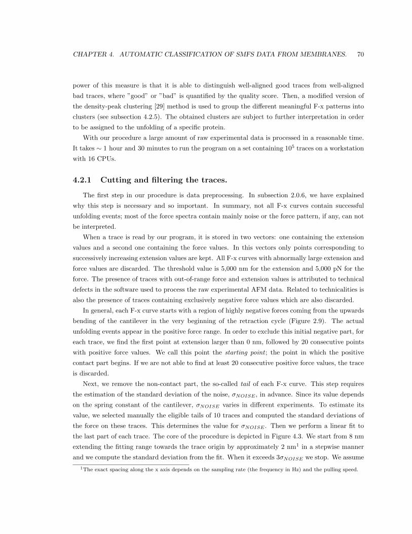
CHAPTER 4. AUTOMATIC CLASSIFICATION OF SMFS DATA FROM MEMBRANES. 70
power of this measure is that it is able to distinguish well-aligned good traces from well-aligned
bad traces, where ”good” or ”bad” is quantified by the quality score. Then, a modified version of
the density-peak clustering [29] method is used to group the different meaningful F-x patterns into
clusters (see subsection 4.2.5). The obtained clusters are subject to further interpretation in order
to be assigned to the unfolding of a specific protein.
With our procedure a large amount of raw experimental data is processed in a reasonable time.
It takes ∼ 1 hour and 30 minutes to run the program on a set containing 105 traces on a workstation
with 16 CPUs.
4.2.1 Cutting and filtering the traces.
The first step in our procedure is data preprocessing. In subsection 2.0.6, we have explained
why this step is necessary and so important. In summary, not all F-x curves contain successful
unfolding events; most of the force spectra contain mainly noise or the force pattern, if any, can not
be interpreted.
When a trace is read by our program, it is stored in two vectors: one containing the extension
values and a second one containing the force values. In this vectors only points corresponding to
successively increasing extension values are kept. All F-x curves with abnormally large extension and
force values are discarded. The threshold value is 5,000 nm for the extension and 5,000 pN for the
force. The presence of traces with out-of-range force and extension values is attributed to technical
defects in the software used to process the raw experimental AFM data. Related to technicalities is
also the presence of traces containing exclusively negative force values which are also discarded.
In general, each F-x curve starts with a region of highly negative forces coming from the upwards
bending of the cantilever in the very beginning of the retraction cycle (Figure 2.9). The actual
unfolding events appear in the positive force range. In order to exclude this initial negative part, for
each trace, we find the first point at extension larger than 0 nm, followed by 20 consecutive points
with positive force values. We call this point the starting point ; the point in which the positive
contact part begins. If we are not able to find at least 20 consecutive positive force values, the trace
is discarded.
Next, we remove the non-contact part, the so-called tail of each F-x curve. This step requires
the estimation of the standard deviation of the noise, σNOISE , in advance. Since its value depends
on the spring constant of the cantilever, σNOISE varies in different experiments. To estimate its
value, we selected manually the eligible tails of 10 traces and computed the standard deviations of
the force on these traces. This determines the value for σNOISE . Then we perform a linear fit to
the last part of each trace. The core of the procedure is depicted in Figure 4.3. We start from 8 nm
extending the fitting range towards the trace origin by approximately 2 nm1 in a stepwise manner
and we compute the standard deviation from the fit. When it exceeds 3σNOISE we stop. We assume
1The exact spacing along the x axis depends on the sampling rate (the frequency in Hz) and the pulling speed.
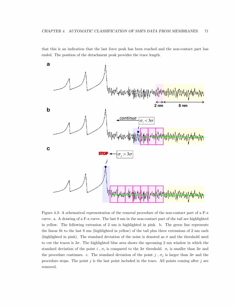
CHAPTER 4. AUTOMATIC CLASSIFICATION OF SMFS DATA FROM MEMBRANES. 71
that this is an indication that the last force peak has been reached and the non-contact part has
ended. The position of the detachment peak provides the trace length.
Figure 4.3: A schematical representation of the removal procedure of the non-contact part of a F-x
curve. a. A drawing of a F-x curve. The last 8 nm in the non-contact part of the tail are highlighted
in yellow. The following extension of 2 nm is highlighted in pink. b. The green line represents
the linear fit to the last 8 nm (highlighted in yellow) of the tail plus three extensions of 2 nm each
(highlighted in pink). The standard deviation of the noise is denoted as σ and the threshold used
to cut the traces is 3σ. The highlighted blue area shows the upcoming 2 nm window in which the
standard deviation of the point i , σi is compared to the 3σ threshold. σi is smaller than 3σ and
the procedure continues. c. The standard deviation of the point j , σj is larger than 3σ and the
procedure stops. The point j is the last point included in the trace. All points coming after j are
removed.
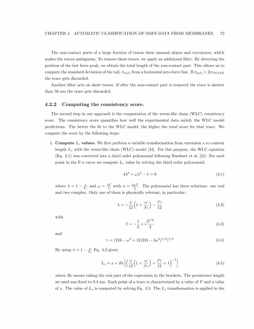
CHAPTER 4. AUTOMATIC CLASSIFICATION OF SMFS DATA FROM MEMBRANES. 72
The non-contact parts of a large fraction of traces show unusual slopes and curvatures, which
makes the traces ambiguous. To remove these traces, we apply an additional filter. By detecting the
position of the last force peak, we obtain the total length of the non-contact part. This allows us to
compute the standard deviation of the tail, σtail, from a horizontal zero-force line. If σtail > 2σNOISE
the trace gets discarded.
Another filter acts on short traces. If after the non-contact part is removed the trace is shorter
than 50 nm the trace gets discarded.
4.2.2 Computing the consistency score.
The second step in our approach is the computation of the worm-like chain (WLC) consistency
score. The consistency score quantifies how well the experimental data satisfy the WLC model
predictions. The better the fit to the WLC model, the higher the total score for that trace. We
compute the score by the following steps:
1. Compute Lc values. We first perform a variable transformation from extension x to contour
length Lc with the worm-like chain (WLC) model [44]. For this purpose, the WLC equation
(Eq. 2.1) was converted into a third order polynomial following Bosshart et al. [21]. For each
point in the F-x curve we compute Lc value by solving the third order polynomial:
4λ3 + ωλ2 − 1 = 0 (4.1)
where λ = 1 − xLc
and ω = 4Fα with α = kBT
lp. The polynomial has three solutions: one real
and two complex. Only one of them is physically relevant, in particular:
λ = − ω
12
(1 +
ω
βγ
)− βγ
12(4.2)
with
β = −1
2+ i
31/2
2(4.3)
and
γ = (216− ω3 + 12(324− 3ω3)1/2)1/3 (4.4)
By using λ = 1− xLc
Eq. 4.2 gives:
Lc = x×Re[( ω
12
(1 +
ω
βγ
)+βγ
12+ 1)−1]
(4.5)
where Re means taking the real part of the expression in the brackets. The persistence length
we used was fixed to 0.4 nm. Each point of a trace is characterized by a value of F and a value
of x. The value of Lc is computed by solving Eq. 4.5. The Lc transformation is applied in the
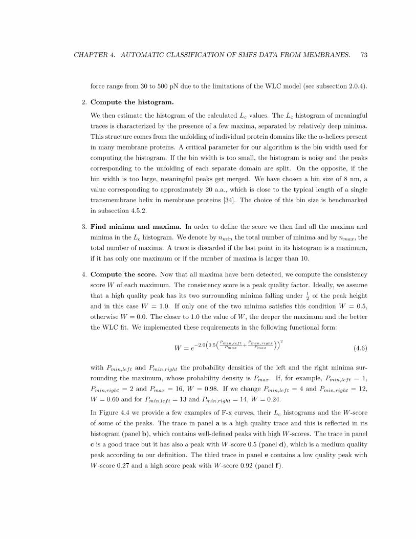
CHAPTER 4. AUTOMATIC CLASSIFICATION OF SMFS DATA FROM MEMBRANES. 73
force range from 30 to 500 pN due to the limitations of the WLC model (see subsection 2.0.4).
2. Compute the histogram.
We then estimate the histogram of the calculated Lc values. The Lc histogram of meaningful
traces is characterized by the presence of a few maxima, separated by relatively deep minima.
This structure comes from the unfolding of individual protein domains like the α-helices present
in many membrane proteins. A critical parameter for our algorithm is the bin width used for
computing the histogram. If the bin width is too small, the histogram is noisy and the peaks
corresponding to the unfolding of each separate domain are split. On the opposite, if the
bin width is too large, meaningful peaks get merged. We have chosen a bin size of 8 nm, a
value corresponding to approximately 20 a.a., which is close to the typical length of a single
transmembrane helix in membrane proteins [34]. The choice of this bin size is benchmarked
in subsection 4.5.2.
3. Find minima and maxima. In order to define the score we then find all the maxima and
minima in the Lc histogram. We denote by nmin the total number of minima and by nmax, the
total number of maxima. A trace is discarded if the last point in its histogram is a maximum,
if it has only one maximum or if the number of maxima is larger than 10.
4. Compute the score. Now that all maxima have been detected, we compute the consistency
score W of each maximum. The consistency score is a peak quality factor. Ideally, we assume
that a high quality peak has its two surrounding minima falling under 12 of the peak height
and in this case W = 1.0. If only one of the two minima satisfies this condition W = 0.5,
otherwise W = 0.0. The closer to 1.0 the value of W , the deeper the maximum and the better
the WLC fit. We implemented these requirements in the following functional form:
W = e−2.0
(0.5
(Pmin,leftPmax
+Pmin,rightPmax
))2
(4.6)
with Pmin,left and Pmin,right the probability densities of the left and the right minima sur-
rounding the maximum, whose probability density is Pmax. If, for example, Pmin,left = 1,
Pmin,right = 2 and Pmax = 16, W = 0.98. If we change Pmin,left = 4 and Pmin,right = 12,
W = 0.60 and for Pmin,left = 13 and Pmin,right = 14, W = 0.24.
In Figure 4.4 we provide a few examples of F-x curves, their Lc histograms and the W -score
of some of the peaks. The trace in panel a is a high quality trace and this is reflected in its
histogram (panel b), which contains well-defined peaks with high W -scores. The trace in panel
c is a good trace but it has also a peak with W -score 0.5 (panel d), which is a medium quality
peak according to our definition. The third trace in panel e contains a low quality peak with
W -score 0.27 and a high score peak with W -score 0.92 (panel f).
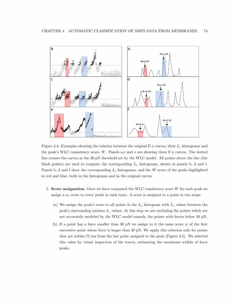
CHAPTER 4. AUTOMATIC CLASSIFICATION OF SMFS DATA FROM MEMBRANES. 74
Figure 4.4: Examples showing the relation between the original F-x curves, their Lc histograms and
the peak’s WLC consistency score, W . Panels a,c and e are showing three F-x curves. The dotted
line crosses the curves at the 30 pN threshold set by the WLC model. All points above the line (the
black points) are used to compute the corresponding Lc histograms, shown in panels b, d and f.
Panels b, d and f show the corresponding Lc histograms, and the W -score of the peaks highlighted
in red and blue, both in the histograms and in the original curves.
5. Score assignation. Once we have computed the WLC consistency score W for each peak we
assign a wi score to every point in each trace. A score is assigned to a point in two steps:
(a) We assign the peak’s score to all points in the Lc histogram with Lc values between the
peak’s surrounding minima Lc values. In this step we are excluding the points which are
not accurately modeled by the WLC model namely, the points with forces below 30 pN.
(b) If a point has a force smaller than 30 pN we assign to it the same score w of the first
successive point whose force is larger than 30 pN. We apply this criterion only for points
that are within 75 nm from the last point assigned to the peak (Figure 4.5). We selected
this value by visual inspection of the traces, estimating the maximum widths of force
peaks.

CHAPTER 4. AUTOMATIC CLASSIFICATION OF SMFS DATA FROM MEMBRANES. 75
Figure 4.5: A scheme representing the second step in the score assignation process. At this step the
peak score, depicted in pink is assigned also to points belonging to the peak but with forces below
30 pN and at distance 75 nm from the last peak point (the yellow area). The 30 pN threshold is
set by the WLC model limitations. The 75 nm range was chosen based on visual inspection of the
traces, looking at the maximum extension of relevant force peaks.
The threshold distance of 75 nm is introduced in order to avoid assigning too many points to
a peak. For example, if there is a high score peak preceded by a long flat region, the points
belonging to that part of the trace will be wrongly assigned to the peak’s score. When we
apply the threshold they get zero score. Zero score is assigned also to points that do not satisfy
the criteria pointed in (a) and (b), to points belonging to a peak with probability less than 1
% or to the points belonging to a peak corresponding to Lc = 0.
6. Compute the global score. The global WLC consistency score is computed as the sum of
the wi scores for each trace,
Sw =
N∑i=1
wi (4.7)
where N is the total number of points in the F-x curve. The global score Sw is a measure of
the quality of that trace.
7. Discard the traces with low global score.
We use the ratio between the global score and the trace length to select high quality traces for
subsequent analysis. If this ratio is smaller than 0.5, the trace is discarded. This is the same
as saying: if more than half of the trace is inconsistent with the WLC model, it is a bad trace
CHAPTER 4. AUTOMATIC CLASSIFICATION OF SMFS DATA FROM MEMBRANES. 76
and we are not interested in analyzing it. On the contrary, if more than half of the trace is
consistent with the WLC model, it is possibly a meaningful trace.
In Figure 4.6 we demonstrate this idea with an example. The data used in the figure is from a
data set which contains a portion of manually selected traces describing the unfolding of the
membrane protein, CNGA1 channel, and a larger portion of unknown traces which might be
good or bad. A detailed description of the data set is given in section 4.4.
In Figure 4.6a we show the relation between the trace length and the global WLC consistency
score. The traces with score-length ratio higher than 0.5 are shown as gray points and the
selected CNGA1 traces are among them, depicted in black. The traces with score-length ratio
lower than 0.5 are shown as red points. One can notice that for most of the CNG traces, the
score is more or less equal to their length, which means that most of them satisfy well the
WLC model and these traces are good according to our model (black points).
Figure 4.6a also shows that the dataset contains traces both much shorter and much longer
than the CNG traces with high global scores with respect to their lengths (depicted with blue
symbols). In Figure 4.6b, we plotted two of the shorter ones and two of the longer ones to
illustrate that the combination of trace length and score can be used to detect meaningful
traces.
The red points in Figure 4.6a have global scores much smaller than their length indicating
poor agreement of the data with the WLC model.
4.2.3 The distance between two traces.
The final goal of our procedure is finding in an automatic and unsupervised manner meaningful
F-x curves bearing a specific unfolding pattern and to group them into clusters based on their
similarity to each other. To reach this goal a key ingredient is the distance between traces. The
distance used in this work is based on a combination of the trace distance obtained by dynamic
programming as in ref. [20] and of the quality score defined in the previous paragraph.
Dynamic programming finds the best match between the traces by allowing insertions and dele-
tions. Given two traces, a and b, denote by SD(i, j) the score between trace a up to position i and
trace b up to position j. In dynamic programming SD(i, j) is defined recursively starting from the
beginning of the traces,
SD(i, j) = max(SD(i− 1, j)− µ, SD(i, j − 1)− µ, SD(i− 1, j − 1) +M(i, j)) (4.8)
where µ is the gap penalty and M(i, j) is the match/mismatch score.
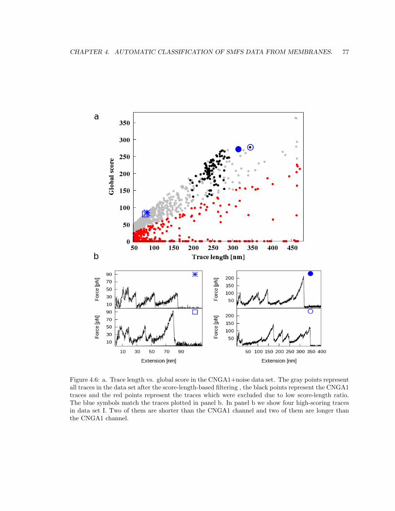
CHAPTER 4. AUTOMATIC CLASSIFICATION OF SMFS DATA FROM MEMBRANES. 77
Figure 4.6: a. Trace length vs. global score in the CNGA1+noise data set. The gray points representall traces in the data set after the score-length-based filtering , the black points represent the CNGA1traces and the red points represent the traces which were excluded due to low score-length ratio.The blue symbols match the traces plotted in panel b. In panel b we show four high-scoring tracesin data set I. Two of them are shorter than the CNGA1 channel and two of them are longer thanthe CNGA1 channel.
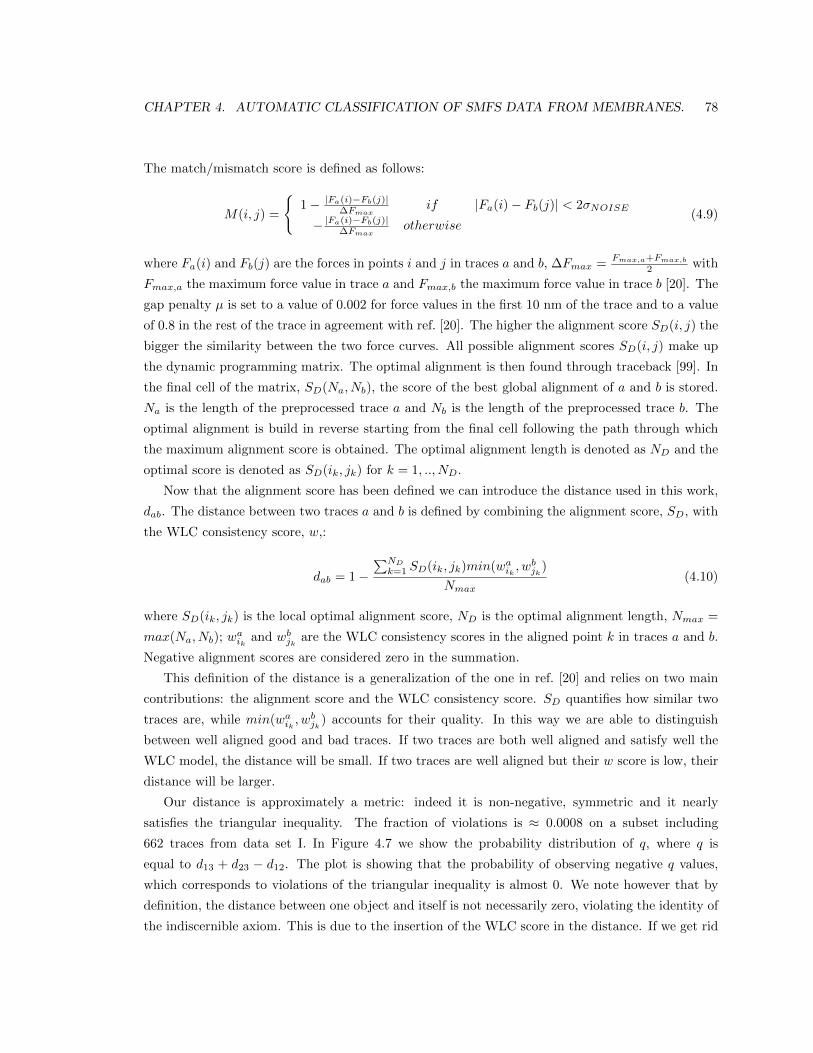
CHAPTER 4. AUTOMATIC CLASSIFICATION OF SMFS DATA FROM MEMBRANES. 78
The match/mismatch score is defined as follows:
M(i, j) =
{1− |Fa(i)−Fb(j)|
∆Fmaxif |Fa(i)− Fb(j)| < 2σNOISE
− |Fa(i)−Fb(j)|∆Fmax
otherwise(4.9)
where Fa(i) and Fb(j) are the forces in points i and j in traces a and b, ∆Fmax =Fmax,a+Fmax,b
2 with
Fmax,a the maximum force value in trace a and Fmax,b the maximum force value in trace b [20]. The
gap penalty µ is set to a value of 0.002 for force values in the first 10 nm of the trace and to a value
of 0.8 in the rest of the trace in agreement with ref. [20]. The higher the alignment score SD(i, j) the
bigger the similarity between the two force curves. All possible alignment scores SD(i, j) make up
the dynamic programming matrix. The optimal alignment is then found through traceback [99]. In
the final cell of the matrix, SD(Na, Nb), the score of the best global alignment of a and b is stored.
Na is the length of the preprocessed trace a and Nb is the length of the preprocessed trace b. The
optimal alignment is build in reverse starting from the final cell following the path through which
the maximum alignment score is obtained. The optimal alignment length is denoted as ND and the
optimal score is denoted as SD(ik, jk) for k = 1, .., ND.
Now that the alignment score has been defined we can introduce the distance used in this work,
dab. The distance between two traces a and b is defined by combining the alignment score, SD, with
the WLC consistency score, w,:
dab = 1−∑NDk=1 SD(ik, jk)min(waik , w
bjk
)
Nmax(4.10)
where SD(ik, jk) is the local optimal alignment score, ND is the optimal alignment length, Nmax =
max(Na, Nb); waik
and wbjk are the WLC consistency scores in the aligned point k in traces a and b.
Negative alignment scores are considered zero in the summation.
This definition of the distance is a generalization of the one in ref. [20] and relies on two main
contributions: the alignment score and the WLC consistency score. SD quantifies how similar two
traces are, while min(waik , wbjk
) accounts for their quality. In this way we are able to distinguish
between well aligned good and bad traces. If two traces are both well aligned and satisfy well the
WLC model, the distance will be small. If two traces are well aligned but their w score is low, their
distance will be larger.
Our distance is approximately a metric: indeed it is non-negative, symmetric and it nearly
satisfies the triangular inequality. The fraction of violations is ≈ 0.0008 on a subset including
662 traces from data set I. In Figure 4.7 we show the probability distribution of q, where q is
equal to d13 + d23 − d12. The plot is showing that the probability of observing negative q values,
which corresponds to violations of the triangular inequality is almost 0. We note however that by
definition, the distance between one object and itself is not necessarily zero, violating the identity of
the indiscernible axiom. This is due to the insertion of the WLC score in the distance. If we get rid
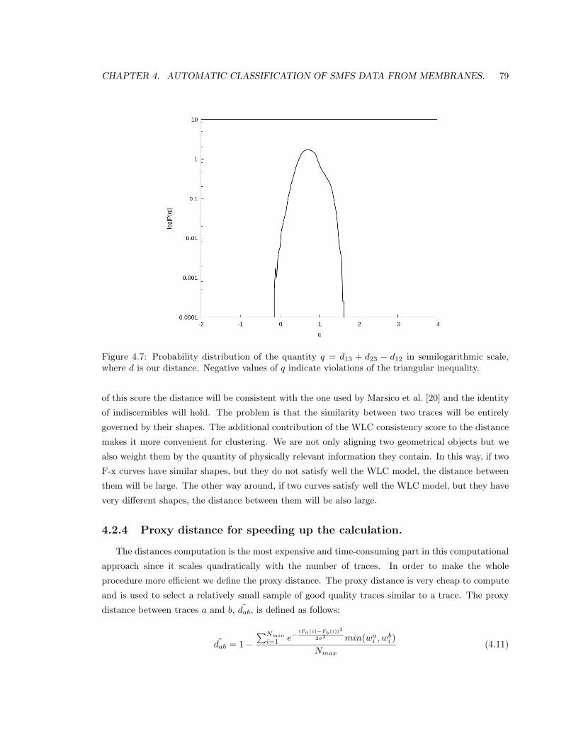
CHAPTER 4. AUTOMATIC CLASSIFICATION OF SMFS DATA FROM MEMBRANES. 79
Figure 4.7: Probability distribution of the quantity q = d13 + d23 − d12 in semilogarithmic scale,where d is our distance. Negative values of q indicate violations of the triangular inequality.
of this score the distance will be consistent with the one used by Marsico et al. [20] and the identity
of indiscernibles will hold. The problem is that the similarity between two traces will be entirely
governed by their shapes. The additional contribution of the WLC consistency score to the distance
makes it more convenient for clustering. We are not only aligning two geometrical objects but we
also weight them by the quantity of physically relevant information they contain. In this way, if two
F-x curves have similar shapes, but they do not satisfy well the WLC model, the distance between
them will be large. The other way around, if two curves satisfy well the WLC model, but they have
very different shapes, the distance between them will be also large.
4.2.4 Proxy distance for speeding up the calculation.
The distances computation is the most expensive and time-consuming part in this computational
approach since it scales quadratically with the number of traces. In order to make the whole
procedure more efficient we define the proxy distance. The proxy distance is very cheap to compute
and is used to select a relatively small sample of good quality traces similar to a trace. The proxy
distance between traces a and b, dab, is defined as follows:
dab = 1−∑Nmini=1 e−
(Fa(i)−Fb(i))2
2σ2 min(wai , wbi )
Nmax(4.11)
CHAPTER 4. AUTOMATIC CLASSIFICATION OF SMFS DATA FROM MEMBRANES. 80
where Nmin is the minimum length between the length of the preprocessed trace a, Na, and the
length of the preprocessed trace b, Nb, or Nmin = min(Na, Nb); Fa(i) and Fb(i) are the force values
in point i in traces a and b; min(wai , wbi ) is the minimum WLC consistency score in point i between
traces a and b; σ = 25; and Nmax is simply the maximum length, Nmax = max(Na, Nb).
The similarity of a pair of traces is accounted for by the similarities in the forces and the
consistency of the data with the WLC model. The similarity of the forces is taken into account
by the exponential function while the consistency with the model is expressed by min(wai , wbi ). If
two traces are very similar in terms of their force values and they satisfy well the WLC model, their
proxy distance will be small indicating their similarity. If the traces differ a lot in the forces and
they do not satisfy well the WLC model, their proxy distance will be large. Last but not least, if two
traces have similar force values but they do not satisfy well the WLC model, their proxy distance
will be shifted towards larger values.
For each trace we sort the computed proxy distances,dab, in ascending order and then we compute
the true similarity distance measure,dab, for the first ntrue traces only. ntrue is a user-defined
parameter with default value 5,000. If the total number of traces remaining after filtering is smaller
than 5,000, the ntrue value is adjusted to the total number of traces. This is equivalent to computing
the similarity distances for all pairs.
The true similarity distance and the proxy distance are well correlated with Pearson correlation
coefficient ∼ 0.84.
4.2.5 Clustering.
Once we have computed all distances, we use a modified version of the density peak clustering
algorithm [29] with the k-nearest neighbor (k-NN) density estimator. An advantage of the method
is that it doesn’t require the preselection of the number of clusters. The main idea behind density
peak clustering is that the highest density points are located at relatively large distances from each
other. The algorithm is the following:
1. The first step is computing the densities. In the k-NN method the density around a point is
estimated as the ratio between k nearest neighbors and the occupied volume; therefore,
ρi =k
ωdrdk,i(4.12)
where d is the intrinsic dimensionality (ID) of the dataset [100], ωd is the volume of the d-
sphere with unitary radius and rk,i is the distance of point i to its k-th nearest neighbor. We
then compute the logarithm of the density, log ρi = −Fi, identified as the free energy at point
i [101]. Notice that using a k-NN estimator, the rank of Fi is not influenced by the value of d,
which therefore we do not compute. Eq. 4.12 reduces to:
CHAPTER 4. AUTOMATIC CLASSIFICATION OF SMFS DATA FROM MEMBRANES. 81
log ρi = c1 + c2 log1
rk,i(4.13)
where c1 and c2 are constants, whose exact values do not influence the results.
2. We find the cluster centers, according to two conditions: (1) they should have highest density
among their k nearest neighbors, and (2) they should not be among the k nearest neighbors
of other points with higher density [101].
3. Subsequently, all points that are not centers are assigned to the same cluster as the nearest
point with higher density.
4.3 Relation with previous works.
The first step in our procedure is quite similar to the one used by Kuhn et al. and Marsico et
al. [19, 20]. We detect the detachment peak in each F-x curve and then remove the non-contact part.
We remove also the initial negative contact part of each trace. Afterwards this part is not a subject
of any physically relevant interpretation. In other approaches [20, 21, 22] the filtering of traces is
done based on the expected contour length of the fully-stretched protein under investigation, which
requires knowledge of the sample composition and the protein structure. This is a key assumption
which reduces the number of analyzed traces tremendously. In fact, using such strong filtering
condition can be useful in analyzing data coming from SMFS experiments with the scope of analyzing
the structure of a specific protein. On the other hand, the analysis of SMFS data from experiments
in native biological membranes, hosting a variety of membrane proteins, some of them unknown or
with unknown structure, calls for a procedure which is able to automatically and simultaneously
detect the characteristic unfolding fingerprints of several different proteins. In simple terms, the
proper filtering procedure should be able to distinguish between good and bad traces based on their
quality not on their length. For this purpose we developed the global WLC consistency score, which
is a measure for the quality of each trace with respect to the WLC model. The WLC model describes
the expected behavior of biopolymer molecules in AFM-SMFS experiments. If the peaks in a trace
fit well with the model they should correspond to meaningful unfolding events, which is exactly what
we are interested in, independently of the number of peaks, their positions and the trace length.
Instead of filtering traces based on their length, we filter traces based on their quality. We
compute the ratio between the global WLC consistency score of the trace and its length, and if it
is larger than 0.5, the trace is included in the subsequent analysis. This allows the analysis of large
heterogeneous data sets without previous knowledge on the protein composition.
The alignment procedure we are using is the one reported by Marsico et al. [20]. The dynamic
programming alignment gives as output the alignment score, which measures how similar two traces
are. The larger the alignment score, the higher the similarity between the traces. The distance
CHAPTER 4. AUTOMATIC CLASSIFICATION OF SMFS DATA FROM MEMBRANES. 82
metric used by Marsico et al. [20] is simply one minus the final alignment score. This is pretty much
consistent with the metric used by Kuhn et al. [19] which is defined in the same way but with an
alignment score not obtained using dynamic programming. With this metric two traces similar to
each other have small distance, while two traces very different from each other have large distance.
A problem arises if two traces are similar to each other but they are both of low quality. As long
as they match each other they will have small distances. In order for the procedure to be successful
only good traces should be included.
We address this issue by introducing the WLC consistency score in the distance metric. In this
way, two traces can have small similarity distance only if they match each other and they satisfy
the WLC model. If two traces have high alignment score but they do not fit well the model, which
indicates that their quality is low, their distance will be large, and they will not form a cluster .
Finally, we are using a different clustering procedure with respect to other approaches. The
major advantages of using density-peak clustering [29] is its simplicity and the fact that it doesn’t
require knowing the number of clusters in advance.
The methods described in the literature [19, 20, 21, 22] include procedures for distinguishing
different unfolding pathways of the same protein. We haven’t tackled this problem. A possible
manner of tackling it would be using the path plot algorithm implemented in Fodis [22] within a
cluster obtained with our program and see if different unfolding pathways are included. If yes, they
can be divided in groups and further investigated.
4.4 Benchmark AFM-SMFS traces.
We tested our procedure on three data sets.
• Data set I.
The first data set contains 101 manually selected traces ascribed to the unfolding of the CNGA1
channel and 4,027 traces from the same experiments containing traces of other proteins or noise.
CNGA1 channels were expressed in Xenopus laevis oocytes with sample preparation and ex-
perimental procedure described in [13]. SMFS experiments were performed in the oocytes
membrane with the AFM (NanoWizard 3, JPK). The cantilever was calibrated before the
start of each experiment; its spring constant was ∼ 0.08 N/m. The AFM tip was pushed into
the surface and a force of 1 nN was applied for 0.5 s to enhance the proteins adsorption. The
tip was retracted from the surface at pulling speed 500 nm/s.
The manual selection of the CNG traces was based on two criteria: the contour length of
the curves and their force pattern. According to the interpretation of the experimental data
made in ref. [13], the last peak in the CNG traces has a Lc value larger than 220 nm and
all CNG traces share a common unfolding fingerprint. The unfolding fingerprint consists of
CHAPTER 4. AUTOMATIC CLASSIFICATION OF SMFS DATA FROM MEMBRANES. 83
a peak at Lc around 100 nm corresponding to the unfolding of the cyclic nucleotide-binding
(CNB) domain attached to the C-terminus; 3 or 4 force peaks between Lc 120 nm and 250 nm
corresponding to the unfolding of the six transmembrane helices and the detachment peak.
The 101 CNG traces include traces that satisfy these criteria and some other traces that miss
a peak in the middle or the last peak assuming different unfolding pathways as suggested in
ref. [13]. Overall, the selected CNG traces can be divided in two groups based on the number
of force peaks: traces with 5 to 6 major force peaks and traces with 4 major force peaks.
• Data set II.
The second data set contains a mixture of four manually selected groups of F-x curves corre-
sponding to the unfolding of different proteins.
1. Group number 1 contains 35 F-x curves representing one of the possible unfolding path-
ways of rhodopsin in the plasma membrane of the rod outer segment (ROS) of Xenopus
laevis as described in ref. [12]. The traces contain 4 to 5 major force peaks. The de-
tachment peak has a Lc value around 100 nm. The experiments were performed with
the AFM (NanoWizard 3, JPK). The cantilever spring constant was ∼ 0.08 N/m. The
cantilever was calibrated before each experiment. A contact force of 1 nN was applied by
the tip into the surface for 0.5 s. Subsequently, the tip was retracted at pulling speed 500
nm/s.
2. Group number 2 contains 61 F-x curves with a characteristic unfolding pattern that hasn’t
been assigned to any protein yet. They come from SMFS experiments in the plasma
membrane of primary hippocampal neurons using the cell unroofing technique described
in section 4.1. The pulling experiments were performed on the membrane patch adsorbed
on the glass arrow at pulling speed 500 nm/s. The cantilever spring constant was ∼ 0.08
N/m. The cantilever was calibrated before each experiment. The contact force was 1 nN,
applied for 1 s before retraction.
The 61 F-x curves belonging to this group contain 5 to 6 major peaks. The detachment
peak is with Lc value between 220 and 320 nm.
3. Group number 3 contains 46 F-x curves representing the unfolding of another unknown
protein coming from the same experiments like group 2. The traces contain 3 to 4 main
peaks. The last peak has a Lc value between 150 and 220 nm.
4. Group number 4 is built from the manually selected 101 CNGA1 traces included in data
set I.
• Data set III.
The third data set comes from unfolding experiments in the plasma membrane of the rod outer
segment (ROS) of Xenopus laevis with experimental protocol described in subsection 3.1.2.
CHAPTER 4. AUTOMATIC CLASSIFICATION OF SMFS DATA FROM MEMBRANES. 84
The plasma membrane hosts a variety of membrane proteins among which the CNG channels
and rhodopsin are the most common [12].
The entire data set contains 386,756 traces.
4.5 Results.
4.5.1 Results in data set I.
Data set I contains 4,128 traces, 101 of which were manually selected by visual inspection and
attributed to the unfolding of the membrane protein CNGA1 (for details see section 4.4). After
filtering the traces, their number was reduced to 662. 91 % of the manually selected CNG traces
passed the filters.
By applying our procedure, we obtained six clusters. In Figure 4.8 the clusters are represented
by the superimposition of their nine highest density members aligned to the cluster center depicted
in orange. The alignment used for this graphical representation was accomplished in an automatic
manner using the software Fodis [22]. All manually selected CNG traces were found in cluster
number 1 except for two that were assigned to cluster number 6. Therefore, cluster 1 is the CNG
cluster. The CNG unfolding pattern consists of a double peak around 100 nm, three major peaks
between 120 nm and 200 nm and the detachment peak corresponding to Lc value ∼ 290 nm. The
peak at 100 nm is associated with the unfolding of the CNB domain, while the force peaks in the
middle are associated with the pairwise unfolding of the six transmembrane helices in the CNGA1
channel.
The remaining five clusters contain traces much shorter than the CNG traces. The traces in
cluster 2 have Lc values of the last peak between 70 and 80 nm and 2 major peaks. The cluster
center has Lc value of the last peak ∼ 70 nm and 2 major peaks at relatively low forces. The traces
in cluster 3 have Lc between 90 and 120 nm and 1 or 2 major peaks. The last force peak is the only
peak in the cluster center of cluster 3 and it has an Lc value of ∼ 100 nm. Also the cluster center
of cluster 4 has one peak but with a smaller Lc value of ∼ 80 nm. The members of cluster 4 are
characterized by Lc values between 80 and 90 nm and only 1 major peak. In cluster 5 the Lc is
between 120 and 150 nm and 1 or 2 major peaks are present. The cluster center of cluster 5 has two
force peaks, the first one is in the very beginning up to extension 20 nm. The Lc value of the last
peak is ∼ 130 nm. In cluster 6 the Lc values are longer, from 140 to 180 nm and 2 or 3 major peaks
are present. The cluster center has two clean force peaks with Lc values ∼ 95 and 145 nm. With the
data that are available, we cannot aim at relating these clusters to proteins or further investigate
their molecular origin.
Approximately 54 % of the population of cluster 1 is made by the CNG traces. The overall
content of the cluster is visualized in Figure 4.9 where we plot the cluster members ranked by their
density in a descending order. The highest density traces are the CNG traces with 5 to 6 peaks (the
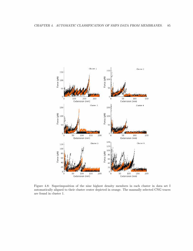
CHAPTER 4. AUTOMATIC CLASSIFICATION OF SMFS DATA FROM MEMBRANES. 85
Figure 4.8: Superimposition of the nine highest density members in each cluster in data set Iautomatically aligned to their cluster center depicted in orange. The manually selected CNG tracesare found in cluster 1.
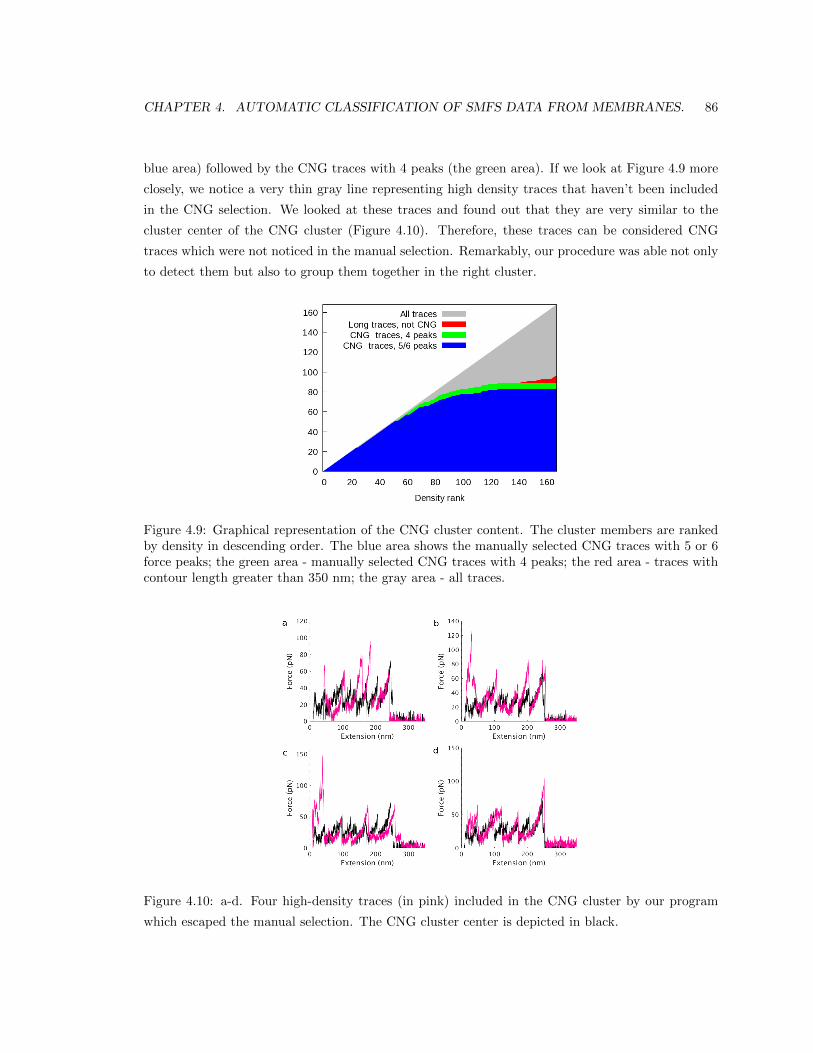
CHAPTER 4. AUTOMATIC CLASSIFICATION OF SMFS DATA FROM MEMBRANES. 86
blue area) followed by the CNG traces with 4 peaks (the green area). If we look at Figure 4.9 more
closely, we notice a very thin gray line representing high density traces that haven’t been included
in the CNG selection. We looked at these traces and found out that they are very similar to the
cluster center of the CNG cluster (Figure 4.10). Therefore, these traces can be considered CNG
traces which were not noticed in the manual selection. Remarkably, our procedure was able not only
to detect them but also to group them together in the right cluster.
Figure 4.9: Graphical representation of the CNG cluster content. The cluster members are rankedby density in descending order. The blue area shows the manually selected CNG traces with 5 or 6force peaks; the green area - manually selected CNG traces with 4 peaks; the red area - traces withcontour length greater than 350 nm; the gray area - all traces.
Figure 4.10: a-d. Four high-density traces (in pink) included in the CNG cluster by our program
which escaped the manual selection. The CNG cluster center is depicted in black.
CHAPTER 4. AUTOMATIC CLASSIFICATION OF SMFS DATA FROM MEMBRANES. 87
The long traces (length > 350 nm) in the cluster have significantly smaller densities. The shape
of these traces varies a lot and a common unfolding pattern can not be easily found. Moreover, these
traces are not similar enough to each other to form a separate cluster. For this reason we consider
them as outliers in the periphery of the cluster. Consistently with this interpretation, their density
is very low.
4.5.2 Validation of the main parameters.
Bin width of the Lc histogram.
An important parameter in our procedure is the size of the bin width of the Lc histogram. We
chose it to be 8 nm, which corresponds to the typical Lc of a transmembrane α-helix. In order to
validate this choice, we applied our method on the CNG data set using different bin sizes, 1, 3, 7,
9 and 12 nm respectively. With bin width 1 nm, we obtained 2 clusters and with bin width 3 nm
- 4 clusters. With bin widths 7, 9 and 12 nm we obtained 5 clusters, opposed to 6 clusters at bin
width 8 nm. The CNG cluster was not found with bin widths 1 and 3 nm. In fact, only 2 of the
manually selected CNG traces passed the filtering criteria defined in section 4.2 at bin width 1 nm,
and 50 at bin width 3 nm. These results exclude the possibility of using such small bin sizes in our
procedure. The 50 CNG traces remaining in the 3 nm case were assigned to cluster 4 but they do
not form the core of the cluster. The first CNG trace has a density rank 119. With bin widths 7, 9
and 12 nm the CNG cluster remains well-defined. We will compare the results for these bin widths
to the results for bin width 8 nm used as a reference.
With bin width 7, 9 and 12 nm, two of the reference clusters were merged but these two clusters
were different at each bin width. Cluster 2 at bin width 7 nm is made from the merging of reference
clusters 3 and 4, and cluster 5 at bin widths 9 and 12 nm is made from the merging of reference
clusters 5 and 6. The change in the bin width leads also to a tiny difference in the number of
traces remaining after applying the score-length ratio filter. In the reference setup, the number of
remaining traces is 662. With bin width 7 nm, it is 657; with bin width 9 nm - 675 and with bin
width 12 nm - 664.
More quantitatively, we use three descriptors to compare the results with the reference setup.
The first descriptor measures how many among the ten highest density members in the reference
cluster are found in the current cluster. It can take values between 0 and 10. The second descriptor
counts how many of the ten highest density members in the reference cluster are among the ten
highest density members in the current cluster. It can also take values between 0 and 10. The third
descriptor gives the lowest density rank among the ten highest density members in the reference
cluster. It can have values between 1 and M , where M is the cluster size. For example, if we
compare a reference cluster with itself, the corresponding sequence of descriptors will be 10-10-10.
We summarized the results in Table 4.1. If a given field of the table contains two sequences of
descriptors this means that the corresponding cluster is made from the merging of two reference
CHAPTER 4. AUTOMATIC CLASSIFICATION OF SMFS DATA FROM MEMBRANES. 88
clusters. The CNG cluster is present both at the three bin widths with very similar descriptor
values. For bin width equal to 7 nm, its descriptors are 10-6-55. This means that all ten highest
density members in the reference are assigned to the analogous CNG cluster, 6 of them are among
the ten highest density members in the cluster and the reference member farthest away from the
cluster center has density rank 55. In the example with bin width 9 nm this sequence almost didn’t
change, it is 10-7-57. We do not compare the remaining 4 clusters at different bin widths with each
other because they correspond to different reference clusters. A proper comparison is the one with
the corresponding clusters at bin width 8 nm. For example, cluster 3 at bin width 7 nm corresponds
to cluster 5 at bin width 8 nm, cluster 3 at bin width 9 nm corresponds to cluster 3 at bin width 8
nm and cluster 3 at bin width 12 nm corresponds to cluster 2 at bin width 8 nm.
We performed an additional check to see if the ten highest density members in the four non-CNG
clusters obtained with bin sizes 7, 9 and 12 nm were found in the corresponding reference clusters
and we confirm it for bin sizes 7 and 9 nm. With bin width 12 nm, this is valid for the first two
clusters only, including the CNG cluster. The ten highest density members of the remaining three
clusters at bin width 12 nm are split among the reference clusters. This suggests that the clustering
results are robust with respect to small changes in the bin width.
There might be changes in the density rank between the different setups but the clusters content
is not seriously affected, especially if the data set contains a significant number of high-quality traces
corresponding to the same protein. Indeed, the CNG cluster is extremely robust with respect to
changes of the bin width in the range 7-12 nm. Instead, reducing the bin width to 5 nm or less is
for sure detrimental.
Different k values in the k-NN density estimator.
We performed tests with different values of the parameter k used in the k−nearest neighbors
density estimator used in the clustering (Eq.4.13). The default value of k is 3 and we use these
results as reference. We applied our procedure to data set I using k-values 2, 4, 5 and 10. We
obtained different number of clusters for the different k-values. We present the results in Table 4.2.
As k-increases, the total number of clusters decreases. The number of clusters we obtain changes
significantly for small values of k, for k=2 to k=3, from 12 to 6 clusters. If we increase k from
5 to 10, the number of clusters changes from 4 to 2, which is a small change with respect to the
difference between the two k values. From Table 4.2, we also learn that in all setups the CNG cluster
is found independently of the exact k-value. This shows that the CNG cluster detection is robust
with respect to the value of k.
We used the same three descriptors like in the bin width comparison to quantify the clustering
results with different k values. The descriptors values are given in Table 4.2. The CNG cluster is
found in all setups with relatively similar values of the descriptors. We tried ot match the non-CNG
clusters to the reference clusters and we were able to do it only for the remaining three clusters at

CHAPTER 4. AUTOMATIC CLASSIFICATION OF SMFS DATA FROM MEMBRANES. 89
k = 4. We matched them successfully to the reference clusters at k = 3 and they remain quite robust.
The only difference is that reference clusters 5 and 6 got merged into cluster 3. The large number
of clusters obtained with k = 2 makes results hard to interpret. It was difficult to match the results
for the remaining three clusters also at k = 5. The reason is that among the ten highest density
members of these clusters, members from different reference clusters were found. For example, the
highest density members of cluster 3 belong to reference clusters 2,3,4 and 5. Anyway, none of them
contains members of the CNG cluster.
We relate the fact that the CNG cluster is identified at all k values to the high density of high-
quality CNG traces very similar to each other in this cluster. When the core of the cluster is made
from a smaller portion of similar traces, the results become sensitive to the precise value of k. We
observe this in the given examples with the non-CNG clusters. Different clusters get merged in
the different setups. Moreover, the total number of clusters changes significantly for the different k
values. This can be explained as follows. When k increases, the distances might become too large
to detect separate clusters. The density estimation becomes inaccurate and clusters get wrongly
merged. As we will see, most of the data sets we are working on are highly heterogeneous and the
amount of high-quality traces similar to each other is very small (see subsection 4.5.4). This makes
the k value important for the final outcome of this procedure. We use as default a k value of 3,
which according to us is neither too small, neither too large for the adequate description of the data
sets under consideration.
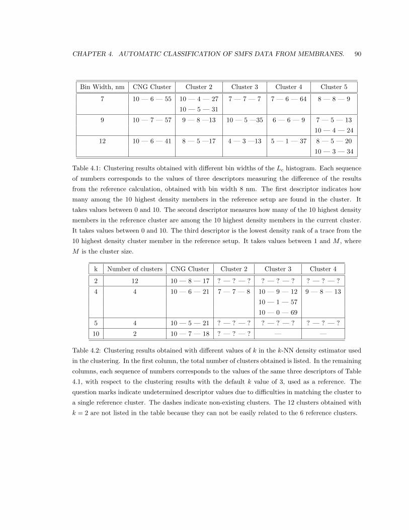
CHAPTER 4. AUTOMATIC CLASSIFICATION OF SMFS DATA FROM MEMBRANES. 90
Bin Width, nm CNG Cluster Cluster 2 Cluster 3 Cluster 4 Cluster 5
7 10 — 6 — 55 10 — 4 — 27 7 — 7 — 7 7 — 6 — 64 8 — 8 — 9
10 — 5 — 31
9 10 — 7 — 57 9 — 8 —13 10 — 5 —35 6 — 6 — 9 7 — 5 — 13
10 — 4 — 24
12 10 — 6 — 41 8 — 5 —17 4 — 3 —13 5 — 1 — 37 8 — 5 — 20
10 — 3 — 34
Table 4.1: Clustering results obtained with different bin widths of the Lc histogram. Each sequence
of numbers corresponds to the values of three descriptors measuring the difference of the results
from the reference calculation, obtained with bin width 8 nm. The first descriptor indicates how
many among the 10 highest density members in the reference setup are found in the cluster. It
takes values between 0 and 10. The second descriptor measures how many of the 10 highest density
members in the reference cluster are among the 10 highest density members in the current cluster.
It takes values between 0 and 10. The third descriptor is the lowest density rank of a trace from the
10 highest density cluster member in the reference setup. It takes values between 1 and M , where
M is the cluster size.
k Number of clusters CNG Cluster Cluster 2 Cluster 3 Cluster 4
2 12 10 — 8 — 17 ? — ? — ? ? — ? — ? ? — ? — ?
4 4 10 — 6 — 21 7 — 7 — 8 10 — 9 — 12 9 — 8 — 13
10 — 1 — 57
10 — 0 — 69
5 4 10 — 5 — 21 ? — ? — ? ? — ? — ? ? — ? — ?
10 2 10 — 7 — 18 ? — ? — ? — —
Table 4.2: Clustering results obtained with different values of k in the k-NN density estimator used
in the clustering. In the first column, the total number of clusters obtained is listed. In the remaining
columns, each sequence of numbers corresponds to the values of the same three descriptors of Table
4.1, with respect to the clustering results with the default k value of 3, used as a reference. The
question marks indicate undetermined descriptor values due to difficulties in matching the cluster to
a single reference cluster. The dashes indicate non-existing clusters. The 12 clusters obtained with
k = 2 are not listed in the table because they can not be easily related to the 6 reference clusters.

CHAPTER 4. AUTOMATIC CLASSIFICATION OF SMFS DATA FROM MEMBRANES. 91
4.5.3 Results in data set II: Rhodopsin + Unknown 1 + Unknown 2 +
CNGA1.
Data set II contains four different groups of manually selected traces and as a final result we would
like to obtain four clusters. The first group of traces in data set II consists of 35 traces representing
the unfolding of rhodopsin in the plasma membrane of the rod OS. The second group contains 61
traces associated with the unfolding of an unknown protein in the hippocampus, which we label
as unknown protein 1. The third selected group contains 46 traces representing the unfolding of
a different unknown protein in the hippocampus, labeled as unknown protein 2. The last group
contains the 101 traces coming from the unfolding of the CNGA1 channel. The total number of
traces in data set II is 243. After filtering, 194 traces, ∼ 80%, remained and were clustered together.
We obtained the three clusters depicted in Figure 4.11. The traces representing the unfolding of
unknown protein 1 and the CNGA1 channel were properly identified and grouped into two separate
clusters: clusters 2 and 3 (Figure 4.11b and c). The traces representing the unfolding of rhodopsin
and unknown protein 2 were grouped together in a common cluster, cluster 1 (Figure 4.11a). The
five highest density members in cluster 1 are rhodopsin traces, followed by five traces from the
unfolding of unknown protein 2.
In order to better understand the reasons for this error we performed additional tests changing
some of the parameters in our procedure. Given that data set II contains only good traces which
were manually selected, we decided to change the program setup by using a slightly milder criterion
for cutting the non-contact parts, considering as meaningful the last peak exceeding a 3σNOISE
threshold instead of the default 2σNOISE threshold (see subsection 4.2.1). In this way, a larger por-
tion of traces was kept after filtering - 216 traces, ∼ 89% of the initial number of traces. As a result,
we obtained four clusters corresponding to the four selected groups. The clusters superimpositions
are shown in Figure 4.12. The members of the manual group selection for rhodopsin and CNGA1,
were exclusively included in clusters 1 and 4 respectively. The majority of curves related to the
unfolding of the two unknown proteins were found in clusters 2 and 3 respectively, but some of their
manually selected members were spread between the other clusters.
These results indicate that a cluster is identified robustly and reliably if ∼ 100 high quality traces
corresponding to the same protein are present in the data set. If this number is smaller, or the traces
are not so similar (like in the case of rhodopsin), the clustering partition becomes less robust, and
can change (for better or worse) if an important parameter is modified.
4.5.4 Results in data set III.
We now describe the results for the data set which motivates our work and presents a true chal-
lenge for a traditional method for AFM-SMFS data analysis. The data is coming from experiments
performed in the plasma membrane of the rod OS under native conditions without overexpression
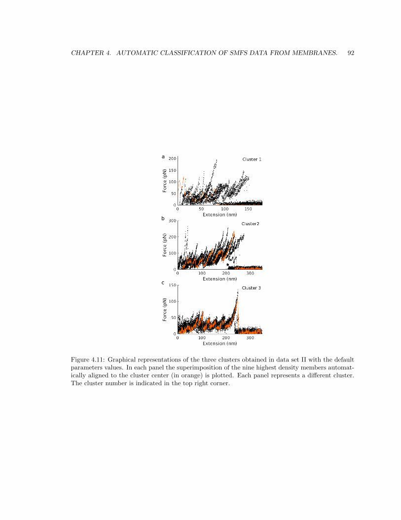
CHAPTER 4. AUTOMATIC CLASSIFICATION OF SMFS DATA FROM MEMBRANES. 92
Figure 4.11: Graphical representations of the three clusters obtained in data set II with the defaultparameters values. In each panel the superimposition of the nine highest density members automat-ically aligned to the cluster center (in orange) is plotted. Each panel represents a different cluster.The cluster number is indicated in the top right corner.
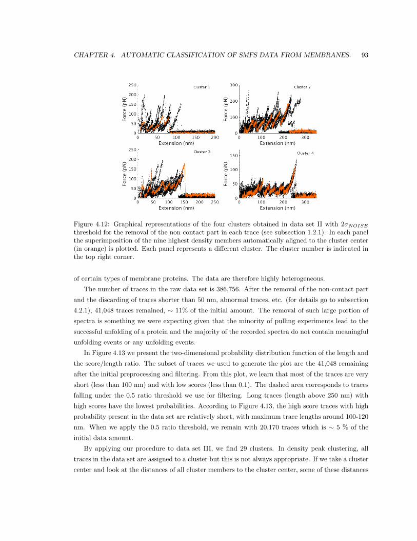
CHAPTER 4. AUTOMATIC CLASSIFICATION OF SMFS DATA FROM MEMBRANES. 93
Figure 4.12: Graphical representations of the four clusters obtained in data set II with 2σNOISEthreshold for the removal of the non-contact part in each trace (see subsection 1.2.1). In each panelthe superimposition of the nine highest density members automatically aligned to the cluster center(in orange) is plotted. Each panel represents a different cluster. The cluster number is indicated inthe top right corner.
of certain types of membrane proteins. The data are therefore highly heterogeneous.
The number of traces in the raw data set is 386,756. After the removal of the non-contact part
and the discarding of traces shorter than 50 nm, abnormal traces, etc. (for details go to subsection
4.2.1), 41,048 traces remained, ∼ 11% of the initial amount. The removal of such large portion of
spectra is something we were expecting given that the minority of pulling experiments lead to the
successful unfolding of a protein and the majority of the recorded spectra do not contain meaningful
unfolding events or any unfolding events.
In Figure 4.13 we present the two-dimensional probability distribution function of the length and
the score/length ratio. The subset of traces we used to generate the plot are the 41,048 remaining
after the initial preprocessing and filtering. From this plot, we learn that most of the traces are very
short (less than 100 nm) and with low scores (less than 0.1). The dashed area corresponds to traces
falling under the 0.5 ratio threshold we use for filtering. Long traces (length above 250 nm) with
high scores have the lowest probabilities. According to Figure 4.13, the high score traces with high
probability present in the data set are relatively short, with maximum trace lengths around 100-120
nm. When we apply the 0.5 ratio threshold, we remain with 20,170 traces which is ∼ 5 % of the
initial data amount.
By applying our procedure to data set III, we find 29 clusters. In density peak clustering, all
traces in the data set are assigned to a cluster but this is not always appropriate. If we take a cluster
center and look at the distances of all cluster members to the cluster center, some of these distances
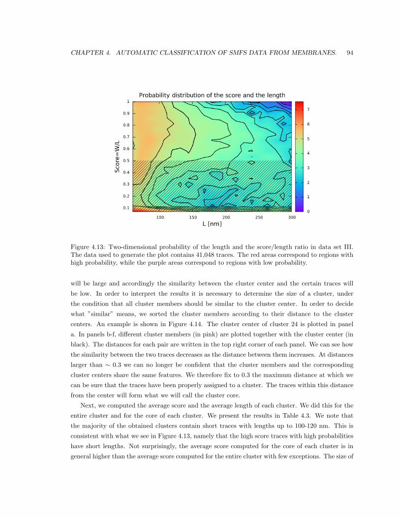
CHAPTER 4. AUTOMATIC CLASSIFICATION OF SMFS DATA FROM MEMBRANES. 94
Figure 4.13: Two-dimensional probability of the length and the score/length ratio in data set III.The data used to generate the plot contains 41,048 traces. The red areas correspond to regions withhigh probability, while the purple areas correspond to regions with low probability.
will be large and accordingly the similarity between the cluster center and the certain traces will
be low. In order to interpret the results it is necessary to determine the size of a cluster, under
the condition that all cluster members should be similar to the cluster center. In order to decide
what ”similar” means, we sorted the cluster members according to their distance to the cluster
centers. An example is shown in Figure 4.14. The cluster center of cluster 24 is plotted in panel
a. In panels b-f, different cluster members (in pink) are plotted together with the cluster center (in
black). The distances for each pair are written in the top right corner of each panel. We can see how
the similarity between the two traces decreases as the distance between them increases. At distances
larger than ∼ 0.3 we can no longer be confident that the cluster members and the corresponding
cluster centers share the same features. We therefore fix to 0.3 the maximum distance at which we
can be sure that the traces have been properly assigned to a cluster. The traces within this distance
from the center will form what we will call the cluster core.
Next, we computed the average score and the average length of each cluster. We did this for the
entire cluster and for the core of each cluster. We present the results in Table 4.3. We note that
the majority of the obtained clusters contain short traces with lengths up to 100-120 nm. This is
consistent with what we see in Figure 4.13, namely that the high score traces with high probabilities
have short lengths. Not surprisingly, the average score computed for the core of each cluster is in
general higher than the average score computed for the entire cluster with few exceptions. The size of
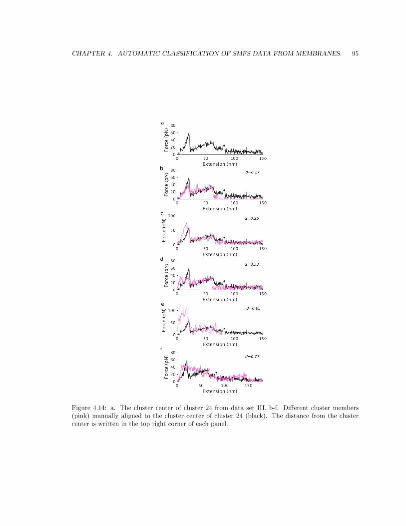
CHAPTER 4. AUTOMATIC CLASSIFICATION OF SMFS DATA FROM MEMBRANES. 95
Figure 4.14: a. The cluster center of cluster 24 from data set III. b-f. Different cluster members(pink) manually aligned to the cluster center of cluster 24 (black). The distance from the clustercenter is written in the top right corner of each panel.
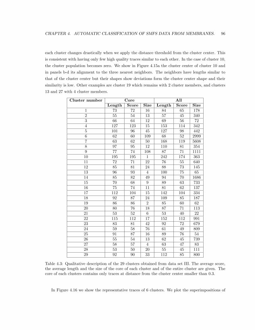
CHAPTER 4. AUTOMATIC CLASSIFICATION OF SMFS DATA FROM MEMBRANES. 96
each cluster changes drastically when we apply the distance threshold from the cluster center. This
is consistent with having only few high quality traces similar to each other. In the case of cluster 10,
the cluster population becomes zero. We show in Figure 4.15a the cluster center of cluster 10 and
in panels b-d its alignment to the three nearest neighbors. The neighbors have lengths similar to
that of the cluster center but their shapes show deviations form the cluster center shape and their
similarity is low. Other examples are cluster 19 which remains with 2 cluster members, and clusters
13 and 27 with 4 cluster members.
Cluster number Core AllLength Score Size Length Score Size
1 73 72 16 84 65 1782 55 54 13 57 45 3403 66 64 12 69 56 724 127 123 15 153 114 3425 101 96 45 127 98 4426 62 60 109 68 52 29997 63 62 50 168 119 56088 97 95 12 110 81 3549 77 74 108 87 71 111110 195 195 1 242 174 36311 72 71 22 76 55 64012 85 81 24 88 73 14513 96 93 4 100 75 6514 85 82 49 94 70 168615 70 68 9 89 63 73316 75 74 11 81 62 13717 112 104 15 142 104 33418 92 87 24 109 85 18719 86 86 2 85 60 6220 80 76 18 87 71 11321 53 52 6 53 40 2222 115 112 17 152 112 99123 83 81 42 92 72 67924 59 58 76 61 49 80925 91 87 16 89 76 5426 55 54 13 62 45 73927 58 57 4 63 47 8328 53 50 20 55 45 11129 92 90 33 112 85 800
Table 4.3: Qualitative description of the 29 clusters obtained from data set III. The average score,the average length and the size of the core of each cluster and of the entire cluster are given. Thecore of each clusters contains only traces at distance from the cluster center smaller than 0.3.
In Figure 4.16 we show the representative traces of 6 clusters. We plot the superimpositions of
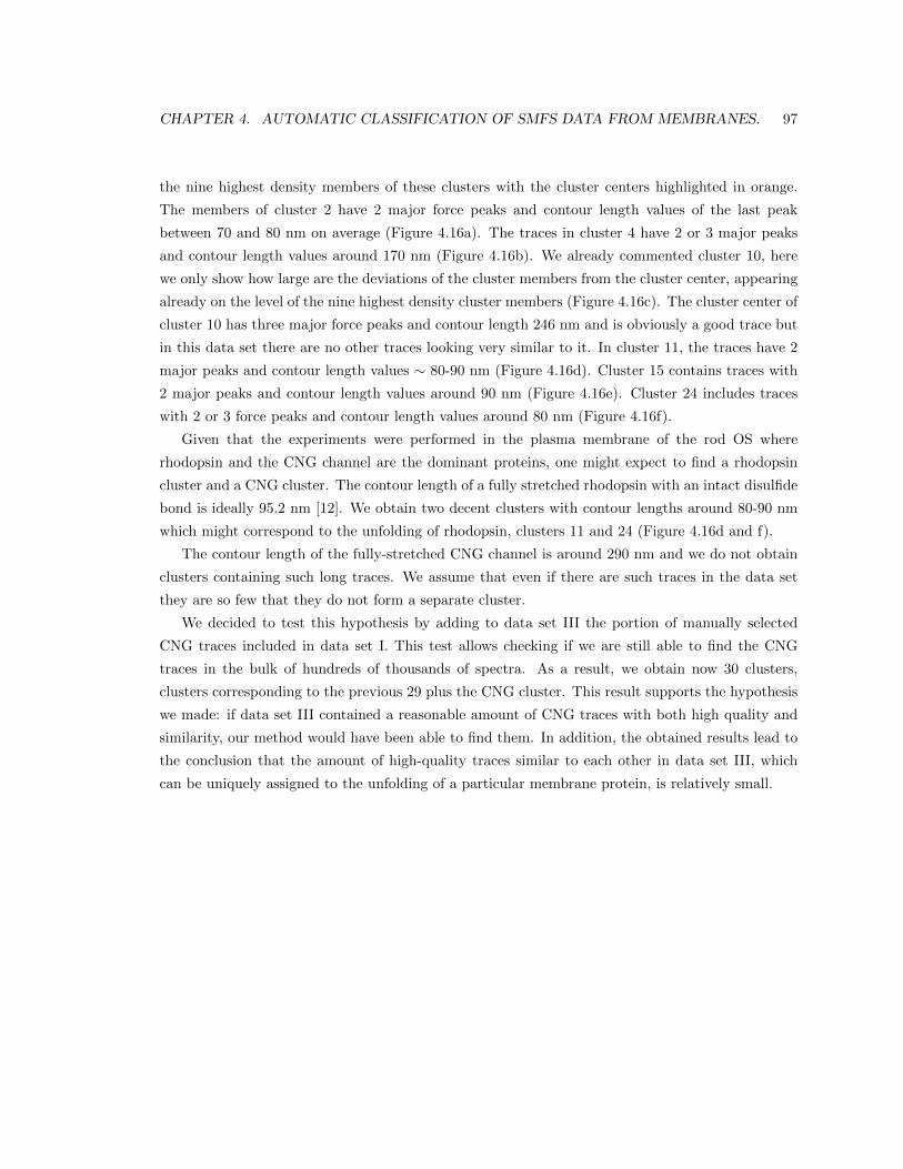
CHAPTER 4. AUTOMATIC CLASSIFICATION OF SMFS DATA FROM MEMBRANES. 97
the nine highest density members of these clusters with the cluster centers highlighted in orange.
The members of cluster 2 have 2 major force peaks and contour length values of the last peak
between 70 and 80 nm on average (Figure 4.16a). The traces in cluster 4 have 2 or 3 major peaks
and contour length values around 170 nm (Figure 4.16b). We already commented cluster 10, here
we only show how large are the deviations of the cluster members from the cluster center, appearing
already on the level of the nine highest density cluster members (Figure 4.16c). The cluster center of
cluster 10 has three major force peaks and contour length 246 nm and is obviously a good trace but
in this data set there are no other traces looking very similar to it. In cluster 11, the traces have 2
major peaks and contour length values ∼ 80-90 nm (Figure 4.16d). Cluster 15 contains traces with
2 major peaks and contour length values around 90 nm (Figure 4.16e). Cluster 24 includes traces
with 2 or 3 force peaks and contour length values around 80 nm (Figure 4.16f).
Given that the experiments were performed in the plasma membrane of the rod OS where
rhodopsin and the CNG channel are the dominant proteins, one might expect to find a rhodopsin
cluster and a CNG cluster. The contour length of a fully stretched rhodopsin with an intact disulfide
bond is ideally 95.2 nm [12]. We obtain two decent clusters with contour lengths around 80-90 nm
which might correspond to the unfolding of rhodopsin, clusters 11 and 24 (Figure 4.16d and f).
The contour length of the fully-stretched CNG channel is around 290 nm and we do not obtain
clusters containing such long traces. We assume that even if there are such traces in the data set
they are so few that they do not form a separate cluster.
We decided to test this hypothesis by adding to data set III the portion of manually selected
CNG traces included in data set I. This test allows checking if we are still able to find the CNG
traces in the bulk of hundreds of thousands of spectra. As a result, we obtain now 30 clusters,
clusters corresponding to the previous 29 plus the CNG cluster. This result supports the hypothesis
we made: if data set III contained a reasonable amount of CNG traces with both high quality and
similarity, our method would have been able to find them. In addition, the obtained results lead to
the conclusion that the amount of high-quality traces similar to each other in data set III, which
can be uniquely assigned to the unfolding of a particular membrane protein, is relatively small.

CHAPTER 4. AUTOMATIC CLASSIFICATION OF SMFS DATA FROM MEMBRANES. 98
Figure 4.15: a. The cluster center of cluster 10 from data set III. b-d. The three nearest neighbors
(pink) of the cluster center (black) are plotted together with it. The corresponding distances are
written in the top right corner of each panel.
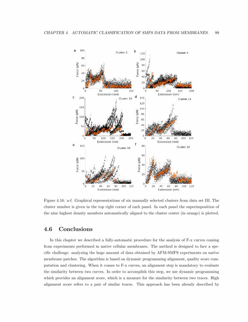
CHAPTER 4. AUTOMATIC CLASSIFICATION OF SMFS DATA FROM MEMBRANES. 99
Figure 4.16: a-f. Graphical representations of six manually selected clusters from data set III. The
cluster number is given in the top right corner of each panel. In each panel the superimposition of
the nine highest density members automatically aligned to the cluster center (in orange) is plotted.
4.6 Conclusions
In this chapter we described a fully-automatic procedure for the analysis of F-x curves coming
from experiments performed in native cellular membranes. The method is designed to face a spe-
cific challenge: analyzing the huge amount of data obtained by AFM-SMFS experiments on native
membrane patches. The algorithm is based on dynamic programming alignment, quality score com-
putation and clustering. When it comes to F-x curves, an alignment step is mandatory to evaluate
the similarity between two curves. In order to accomplish this step, we use dynamic programming
which provides an alignment score, which is a measure for the similarity between two traces. High
alignment score refers to a pair of similar traces. This approach has been already described by
CHAPTER 4. AUTOMATIC CLASSIFICATION OF SMFS DATA FROM MEMBRANES. 100
Marsico et al. and applied to a hand-curated data set containing 135 traces from AFM-SMFS ex-
periment on bacteriorhodopsin mutant P50A [20]. In addition, we defined a quality score measuring
the consistency of each trace with the WLC model. It is well known that when a protein is stretched
in an AFM experiment it behaves like a polymer chain described by the WLC model [44]. The
WLC consistency score provides a quantitative measure for the quality of a trace. If the score is
high, the trace is good and if the score is low, the trace is bad. One of the key components in our
procedure is the distance which combines the alignment score and the quality score in such a way
that high-quality traces similar to each other are characterized by a small distance, while low-quality
traces, even if they are similar to each other, are characterized by a larger distance. This property of
the distance is of crucial importance for the efficient analysis of non-curated data sets and membrane
proteins data sets in general, because of the low amount of high-quality traces generated during the
AFM-SMFS experiments [21]. The clustering method we use is a modified version of the density-
peak clustering [29] with k-NN density estimator. The major advantages of this clustering approach
are its simplicity, the fact that it is unsupervised and doesn’t require knowing the number of clusters.
Compared to other procedures [19, 20, 68, 22], our method provides filtering of spurious traces
and selection of high-quality traces in a non-demanding manner. Mainly, it doesn’t require any
previous knowledge on the sample composition and the proteins contour length. We achieve this by
combining the WLC quality score with the trace length to measure the amount of experimental data
consistent with the WLC model. In this manner we are able to reduce the amount of bad traces and
to increase the method’s computational efficiency at the same time by filtering the traces based on
their score/length ratio. We remark that our procedure is not appropriate for distinguishing different
unfolding pathways, which is something that other methods in the literature can do [19, 20, 68, 22].
We benchmarked our method on a data set containing a manually-selected sample of CNG traces
distributed among a larger portion of traces of unidentified quality. Our method successfully detected
the CNG traces and grouped them in a separate cluster. Remarkably, it was also able to find CNG
traces which escaped the manual selection and to properly assign them to the CNG cluster. This
result demonstrates the ability of our method to detect high-quality traces similar to each other and
to group them in the same cluster.
We obtained also other clusters whose molecular origin we are currently unable to identify. As we
commented in Chapter 3, this issue might be managed through a combination of new experimental
data with molecular modeling tools like the one we developed and described in the same chapter.
With our procedure, we were able to analyze a data set consisting of ∼ 400,000 traces of uniden-
tified molecular origin sampled from the plasma membrane of the rod outer segment (OS). The
main motivation for the work presented in this chapter comes from data sets like this one. Our
program turned out to be quite efficient taking only ∼ 90 minutes to analyze the entire data set.
The general observation we made from the obtained clusters is that the data set contains overall
very few high-quality traces that are very similar to each other. Given that the protein composition
CHAPTER 4. AUTOMATIC CLASSIFICATION OF SMFS DATA FROM MEMBRANES. 101
of the rod OS plasma membrane is dominated by rhodopsin and the CNG channel, one can expect
to find clusters depicting the unfolding of these two membrane proteins. Indeed, two of the clusters
we obtained are decent rhodopsin candidates, but we were unable to find a cluster describing the
unfolding of the CNG channel. We decided to perform a test by adding the manually selected CNG
traces from the previous data set to the large plasma membrane data set. The algorithm proved
to be able to detect the selected CNG traces in the bulk of data and to group them in a separate
cluster. This result support the observation we made, namely that high-quality traces, coming from
the unfolding of the CNG channel, that are similar to each other are very rare. This makes the
clustering of these traces extremely difficult and hinders the identification of characteristic unfolding
patterns related to specific membrane proteins. In order to further validate this hypothesis we will
have to analyze more data from native cell membranes.

Bibliography
[1] Charles R Sanders and Joanna K Nagy. Misfolding of membrane proteins in health and disease:
the lady or the tiger? Current Opinion in Structural Biology, 10(4):438 – 442, 2000.
[2] Stephen White lab at UC Irvine, 2018.
[3] Sue-Hwa Lin and Guido Guidotti. Chapter 35 Purification of Membrane Proteins, volume 463
of Methods in Enzymology. Academic Press, 2009.
[4] P.L.T.M. Frederix, P.D. Bosshart, and A. Engel. Atomic force microscopy of biological mem-
branes. Biophysical Journal, 96(2):329–338, 2009.
[5] C. Bustamante, J.C. Macosko, and G.J.L. Wuite. Grabbing the cat by the tail: manipulating
molecules one by one. Nature Reviews Molecular Cell Biology, 1(2):130–136, 2000.
[6] M. Rief and H. Grubmller. Force spectroscopy of single biomolecules. ChemPhysChem,
3(3):255–261, 2002.
[7] Hao Yu, Matthew G. W. Siewny, Devin T. Edwards, Aric W. Sanders, and Thomas T.
Perkins. Hidden dynamics in the unfolding of individual bacteriorhodopsin proteins. Science,
355(6328):945–950, 2017.
[8] Matthias Rief, Mathias Gautel, Filipp Oesterhelt, Julio M. Fernandez, and Hermann E.
Gaub. Reversible unfolding of individual titin immunoglobulin domains by afm. Science,
276(5315):1109–1112, 1997.
[9] F. Oesterhelt, D. Oesterhelt, M. Pfeiffer, A. Engel, H. E. Gaub, and D. J. Muller. Unfolding
pathways of individual bacteriorhodopsins. Science, 288(5463):143–146, 2000.
[10] K. Tanuj Sapra, Hseyin Besir, Dieter Oesterhelt, and Daniel J. Muller. Characterizing molecu-
lar interactions in different bacteriorhodopsin assemblies by single-molecule force spectroscopy.
Journal of Molecular Biology, 355(4):640 – 650, 2006.
[11] Colozo AT et al. Kawamura S, Gerstung M. Kinetic, energetic, and mechanical differences
between dark-state rhodopsin and opsin. Structure, 21(3):426 – 437, 2013.
102

BIBLIOGRAPHY 103
[12] Ilieva N. Laio A. Torre V. Mazzolini M. Maity, S. New views on phototransduction from atomic
force microscopy and single molecule force spectroscopy on native rods. Scientific Reports, 7,
2017.
[13] Arcangeletti M. Valbuena A. Fabris P. Lazzarino M. Torre V. Maity, S. Conformational
rearrangements in the transmembrane domain of cnga1 channels revealed by single-molecule
force spectroscopy. Nature Communications, 6, 2015.
[14] Kedrov Alexej, Krieg Michael, Ziegler Christine, Kuhlbrandt Werner, and Muller Daniel J.
Locating ligand binding and activation of a single antiporter. EMBO reports, 6(7):668–674.
[15] Hema Chandra Kotamarthi, Riddhi Sharma, Satya Narayan, Sayoni Ray, and Sri Rama Koti
Ainavarapu. Multiple unfolding pathways of leucine binding protein (lbp) probed by single-
molecule force spectroscopy (smfs). Journal of the American Chemical Society, 135(39):14768–
14774, 2013.
[16] Ott W. Jobst A. M. Milles F. L. Verdorfer T. Pippig A. D. Nash M. Gaub E. H. Otten, M.
From genes to protein mechanics on a chip. Nature Methods, 11:1127, 2014.
[17] Casagrande F. Frederix P. Ratera M. Bippes C. Muller D. Palacin M. Engel A. Fotiadis D.
Bosshart, P. High-throughput single-molecule force spectroscopy for membrane proteins. Nan-
otechnology, 19, 2008.
[18] Nicola Galvanetto. Single-cell unroofing: probing topology and nanomechanics of nativemem-
branes. Biochimica et Biophysica Acta - Biomembranes, 2018. Accepted.
[19] Kuhn M., Janovjak H., Hubain M., and Muller D. J. Automated alignment and pattern
recognition of single-molecule force spectroscopy data. Journal of Microscopy, 218(2):125–
132.
[20] Annalisa Marsico, Dirk Labudde, Tanuj Sapra, Daniel J. Muller, and Michael Schroeder. A
novel pattern recognition algorithm to classify membrane protein unfolding pathways with
high-throughput single-molecule force spectroscopy. Bioinformatics, 23(2):e231–e236, 2007.
[21] P. et al. Bosshart. Reference-free alignment and sorting of single-molecule force spectroscopy
data. Biophysical Journal, 102:2202 – 2211, 2012.
[22] Perissinotto A. Pedroni A. Torre V. Galvanetto, N. Fodis: Software for protein unfolding
analysis. Biophysical Journal, 114:1264 – 1266, 2018.
[23] Arlene D. Albert and Kathleen Boesze-Battaglia. The role of cholesterol in rod outer segment
membranes. Progress in Lipid Research, 44(2):99 – 124, 2005.
BIBLIOGRAPHY 104
[24] Hoang TX Cieplak M. Universality classes in folding times of proteins. Biophysical Journal,
84(1):475–488, 2003.
[25] Marek Cieplak, Trinh Xuan Hoang, and Mark O. Robbins. Thermal effects in stretching of
go-like models of titin and secondary structures. Proteins: Structure, Function, and Bioinfor-
matics, 56(2):285–297.
[26] Marek Cieplak. Mechanical stretching of proteins: Calmodulin and titin. 352, 12 2004.
[27] Marek Cieplak and Piotr E. Marszalek. Mechanical unfolding of ubiquitin molecules. The
Journal of Chemical Physics, 123(19):194903, 2005.
[28] Marek Cieplak, Sawomir Filipek, Harald Janovjak, and Krystiana A. Krzyko. Pulling single
bacteriorhodopsin out of a membrane: Comparison of simulation and experiment. Biochimica
et Biophysica Acta (BBA) - Biomembranes, 1758(4):537 – 544, 2006.
[29] Alex Rodriguez and Alessandro Laio. Clustering by fast search and find of density peaks.
Science, 344(6191):1492–1496, 2014.
[30] Mary Luckey. Membrane Structural Biology: With Biochemical and Biophysical Foundations.
Cambridge University Press, 2008.
[31] S. J. Singer and Garth L. Nicolson. The fluid mosaic model of the structure of cell membranes.
175(4023):720–731, 1972.
[32] Danielli James Frederic and Davson Hugh. A contribution to the theory of permeability of
thin films. Journal of Cellular and Comparative Physiology, 5(4):495–508, 1935.
[33] Robertson J.D. Origin of the unit membrane concept. Symposium on Biophysics and Physi-
ology of Biological Transport, 1967.
[34] Albert L. Lehninger. Lehninger principles of biochemistry. Worth Publishers: New York, 2000.
[35] Bray D. Hopkin K. Alberts, B. Essential cell biology. New York : Garland Science, 2010.
[36] Tilman Schirmer. General and specific porins from bacterial outer membranes. Journal of
Structural Biology, 121(2):101 – 109, 1998.
[37] G Binnig and H Rohrer. Scanning tunneling microscopy. IBM J. Res. Dev., 30(4):355–369,
1986.
[38] Alexej Kedrov, Harald Janovjak, K. Tanuj Sapra, and Daniel J. Mller. Deciphering molecular
interactions of native membrane proteins by single-molecule force spectroscopy. Annual Review
of Biophysics and Biomolecular Structure, 36(1):233–260, 2007.
BIBLIOGRAPHY 105
[39] Allison M. Whited and Paul S.-H. Park. Atomic force microscopy: A multifaceted tool to
study membrane proteins and their interactions with ligands. Biochimica et Biophysica Acta
(BBA) - Biomembranes, 1838(1, Part A):56 – 68, 2014.
[40] Anselmetti D et al. Dammer U, Hegner M. Specific antigen/antibody interactions measured
by force microscopy. Biophysical Journal, 70(5):2437–2441, 1996.
[41] Schoeler C. Malinowska K. Nash M. A. Jobst, M. A. Investigating receptor-ligand systems of
the cellulosome with afm-based single-molecule force spectroscopy. J. Vis. Exp., 82, 2013.
[42] Matthias Rief, Filipp Oesterhelt, Berthold Heymann, and Hermann E. Gaub. Single molecule
force spectroscopy on polysaccharides by atomic force microscopy. Science, 275(5304):1295–
1297, 1997.
[43] Megan L Hughes and Lorna Dougan. The physics of pulling polyproteins: a review of single
molecule force spectroscopy using the afm to study protein unfolding. Reports on Progress in
Physics, 79(7):076601, 2016.
[44] C Bustamante, JF Marko, ED Siggia, and S Smith. Entropic elasticity of lambda-phage dna.
Science, 265(5178):1599–1600, 1994.
[45] Wikipedia. Contour length — Wikipedia, the free encyclopedia, 2004.
[46] Allemand J Strick T Block SM Croquette V. Bouchiat C, Wang MD. Estimating the persistence
length of a worm-like chain molecule from force-extension measurements. Biophysical Journal,
76(1 Pt 1):409–413, 1999.
[47] Kirstin A. Walther, Frauke Grater, Lorna Dougan, Carmen L. Badilla, Bruce J. Berne, and
Julio M. Fernandez. Signatures of hydrophobic collapse in extended proteins captured with
force spectroscopy. Proceedings of the National Academy of Sciences, 104(19):7916–7921, 2007.
[48] Eric H Lee, Jen Hsin, Olga Mayans, and Klaus Schulten. Secondary and tertiary structure
elasticity of titin z1z2 and a titin chain model. Biophysical journal, 93(5):1719–1735, 2007.
[49] Christiane A. Opitz, Michael Kulke, Mark C. Leake, Ciprian Neagoe, Horst Hinssen, Roger J.
Hajjar, and Wolfgang A. Linke. Damped elastic recoil of the titin spring in myofibrils of human
myocardium. Proceedings of the National Academy of Sciences, 100(22):12688–12693, 2003.
[50] D.P. Tieleman and H.J.C. Berendsen. A molecular dynamics study of the pores formed by
escherichia coli ompf porin in a fully hydrated palmitoyloleoylphosphatidylcholine bilayer.
Biophysical Journal, 74(6):2786 – 2801, 1998.
BIBLIOGRAPHY 106
[51] Jamie Parkin and Syma Khalid. Atomistic molecular-dynamics simulations enable predic-
tion of the arginine permeation pathway through occd1/oprd from pseudomonasaeruginosa.
Biophysical Journal, 107(8):1853 – 1861, 2014.
[52] Takaharu Mori, Naoyuki Miyashita, Wonpil Im, Michael Feig, and Yuji Sugita. Molecular
dynamics simulations of biological membranes and membrane proteins using enhanced confor-
mational sampling algorithms. Biochimica et Biophysica Acta (BBA) - Biomembranes, 1858(7,
Part B):1635 – 1651, 2016.
[53] Christian Kappel and Helmut Grubmller. Velocity-dependent mechanical unfolding of bacte-
riorhodopsin is governed by a dynamic interaction network. Biophysical Journal, 100(4):1109
– 1119, 2011.
[54] D. Bashford and D.A. Case. Generalized born models of macromolecular solvation effects.
Annual Review of Physical Chemistry, 51:129–152, 2000.
[55] Wonpil Im, Michael Feig, and Charles L. Brooks. An implicit membrane generalized born
theory for the study of structure, stability, and interactions of membrane proteins. Biophysical
Journal, 85(5):2900 – 2918, 2003.
[56] S. Tanizaki and M. Feig. A generalized born formalism for heterogeneous dielectric environ-
ments: Application to the implicit modeling of biological membranes. Journal of Chemical
Physics, 122(12), 2005.
[57] S. Tanizaki and M. Feig. Molecular dynamics simulations of large integral membrane proteins
with an implicit membrane model. Journal of Physical Chemistry B, 110(1):548–556, 2006.
[58] Michele Seeber, Francesca Fanelli, Emanuele Paci, and Amedeo Caflisch. Sequential unfolding
of individual helices of bacterioopsin observed in molecular dynamics simulations of extraction
from the purple membrane. Biophysical Journal, 91(9):3276 – 3284, 2006.
[59] Tatsuya Yamada, Takahisa Yamato, and Shigeki Mitaku. Forced unfolding mechanism of
bacteriorhodopsin as revealed by coarse-grained molecular dynamics. Biophysical Journal,
111(10):2086 – 2098, 2016.
[60] S.J. Marrink, H.J. Risselada, S. Yefimov, D.P. Tieleman, and A.H. De Vries. The martini force
field: Coarse grained model for biomolecular simulations. Journal of Physical Chemistry B,
111(27):7812–7824, 2007.
[61] X. Periole, T. Huber, S.-J. Marrink, and T.P. Sakmar. G protein-coupled receptors self-
assemble in dynamics simulations of model bilayers. Journal of the American Chemical Society,
129(33):10126–10132, 2007.
BIBLIOGRAPHY 107
[62] W. Xu, G. Wei, H. Su, L. Nordenskild, and Y. Mu. Effects of cholesterol on pore formation
in lipid bilayers induced by human islet amyloid polypeptide fragments: A coarse-grained
molecular dynamics study. Physical Review E - Statistical, Nonlinear, and Soft Matter Physics,
84(5), 2011.
[63] Jerry Tsai, Robin Taylor, Cyrus Chothia, and Mark Gerstein. The packing density in proteins:
standard radii and volumes. Journal of Molecular Biology, 290(1):253 – 266, 1999.
[64] Daniel J. Muller, Max Kessler, Filipp Oesterhelt, Clemens Mller, Dieter Oesterhelt, and Her-
mann Gaub. Stability of bacteriorhodopsin -helices and loops analyzed by single-molecule
force spectroscopy. Biophysical Journal, 83(6):3578 – 3588, 2002.
[65] Alexej Kedrov, Christine Ziegler, Harald Janovjak, Werner Khlbrandt, and Daniel J Mller.
Controlled unfolding and refolding of a single sodium-proton antiporter using atomic force
microscopy. Journal of Molecular Biology, 340(5):1143 – 1152, 2004.
[66] Harald Janovjak. Exploring the Mechanical Stability and Visco-elasticity of Membrane Pro-
teins by Single-Molecule Force Measurements. PhD thesis, Fakultt Mathematik und Natur-
wissenschaften der Technischen Universitt Dresden, 2005.
[67] Nunes JooM., Hensen Ulf, Ge Lin, Lipinsky Manuela, Helenius Jonne, Grubmller Helmut,
and Muller DanielJ. A force buffer protecting immunoglobulin titin. Angewandte Chemie
International Edition, 49(20):3528–3531, 2010.
[68] Pawel Penczek, Michael Radermacher, and Joachim Frank. Three-dimensional reconstruction
of single particles embedded in ice. Ultramicroscopy, 40(1):33 – 53, 1992.
[69] J. B. MacQueen. Some methods for classification and analysis of multivariate observations. In
L. M. Le Cam and J. Neyman, editors, Proc. of the fifth Berkeley Symposium on Mathematical
Statistics and Probability, volume 1, pages 281–297, 1967.
[70] Frans J.M. Daemen. Vertebrate rod outer segment membranes. Biochimica et Biophysica Acta
(BBA) - Reviews on Biomembranes, 300(3):255 – 288, 1973.
[71] S S Karnik and H G Khorana. Assembly of functional rhodopsin requires a disulfide bond
between cysteine residues 110 and 187. Journal of Biological Chemistry, 265(29):17520–4,
1990.
[72] Jack Kyte and Russell F. Doolittle. A simple method for displaying the hydropathic character
of a protein. Journal of Molecular Biology, 157(1):105 – 132, 1982.
[73] Robert Fraczkiewicz and Werner Braun. Exact and efficient analytical calculation of the
accessible surface areas and their gradients for macromolecules. Journal of Computational
Chemistry, 19(3):319–333.

BIBLIOGRAPHY 108
[74] Wikipedia. Lipid bilayer — Wikipedia, the free encyclopedia, 2018.
[75] Hess B van der Spoel D, Lindahl E and the GROMACS development team. Gromacs user
manual version 4.6.7, 2014.
[76] Mikhail A. Lomize, Irina D. Pogozheva, Hyeon Joo, Henry I. Mosberg, and Andrei L. Lomize.
Opm database and ppm web server: resources for positioning of proteins in membranes. Nucleic
Acids Research, 40(D1):D370–D376, 2012.
[77] D. P. Tieleman and H. J. C. Berendsen. Molecular dynamics simulations of a fully hydrated
dipalmitoylphosphatidylcholine bilayer with different macroscopic boundary conditions and
parameters. The Journal of Chemical Physics, 105(11):4871–4880, 1996.
[78] Maarten G. Wolf, Martin Hoefling, Camilo Aponte-Santamara, Helmut Grubmller, and Gerrit
Groenhof. g membed: Efficient insertion of a membrane protein into an equilibrated lipid
bilayer with minimal perturbation. Journal of Computational Chemistry, 31(11):2169–2174.
[79] Chris Oostenbrink, Alessandra Villa, Alan E. Mark, and Wilfred F. Van Gunsteren. A
biomolecular force field based on the free enthalpy of hydration and solvation: The gromos
force-field parameter sets 53a5 and 53a6. Journal of Computational Chemistry, 25(13):1656–
1676.
[80] O. Berger, O. Edholm, and F. Jhnig. Molecular dynamics simulations of a fluid bilayer of
dipalmitoylphosphatidylcholine at full hydration, constant pressure, and constant temperature.
Biophysical Journal, 72(5):2002 – 2013, 1997.
[81] Berk Hess, Henk Bekker, Herman J. C. Berendsen, and Johannes G. E. M. Fraaije. Lincs:
A linear constraint solver for molecular simulations. Journal of Computational Chemistry,
18(12):1463–1472.
[82] T. Darden, D. York, and L. Pedersen. Particle mesh Ewald: An Nslog(N) method for Ewald
sums in large systems. Journal of Chemical Physics, 98:10089–10092, June 1993.
[83] M. Parrinello and A. Rahman. Polymorphic transitions in single crystals: A new molecular
dynamics method. Journal of Applied Physics, 52:7182–7190, 1981.
[84] H. J. C. Berendsen, J. P. M. Postma, W. F. van Gunsteren, A. DiNola, and J. R. Haak.
Molecular dynamics with coupling to an external bath. The Journal of Chemical Physics,
81(8):3684–3690, 1984.
[85] Benot Roux and Thomas Simonson. Implicit solvent models. Biophysical Chemistry, 78(1):1
– 20, 1999.
BIBLIOGRAPHY 109
[86] Wonpil et al. Im. An implicit membrane generalized born theory for the study of structure,
stability, and interactions of membrane proteins. Biophysical Journal, 85(5):2900 – 2918, 2003.
[87] Emanuel Parzen. On estimation of a probability density function and mode. Ann. Math.
Statist., 33(3):1065–1076, 09 1962.
[88] T.D. Lamb and E.N. Pugh. Dark adaptation and the retinoid cycle of vision. Progress in
Retinal and Eye Research, 23(3):307 – 380, 2004.
[89] Klaus Peter Hofmann, Patrick Scheerer, Peter W. Hildebrand, Hui-Woog Choe, Jung Hee
Park, Martin Heck, and Oliver P. Ernst. A g protein-coupled receptor at work: the rhodopsin
model. Trends in Biochemical Sciences, 34(11):540 – 552, 2009.
[90] Thomas J Pucadyil and Amitabha Chattopadhyay. Cholesterol modulates ligand binding
and g-protein coupling to serotonin1a receptors from bovine hippocampus. Biochimica et
Biophysica Acta (BBA) - Biomembranes, 1663(1):188 – 200, 2004.
[91] K. Burger, G. Gimpl, and F. Fahrenholz. Regulation of receptor function by cholesterol.
Cellular and Molecular Life Sciences CMLS, 57(11):1577–1592, 2000.
[92] Viktor Hornak, Shivani Ahuja, Markus Eilers, Joseph A. Goncalves, Mordechai Sheves,
Philip J. Reeves, and Steven O. Smith. Light activation of rhodopsin: Insights from molecu-
lar dynamics simulations guided by solid-state nmr distance restraints. Journal of Molecular
Biology, 396(3):510 – 527, 2010.
[93] Simon Mitternacht. Freesasa: An open source c library for solvent accessible surface area
calculation. F1000Research, 5(189), 2016.
[94] Florian Zocher, David van der Spoel, Peter Pohl, and Jochen S. Hub. Local partition coef-
ficients govern solute permeability of cholesterol-containing membranes. Biophysical journal,
105 12:2760–70, 2013.
[95] Samuel Genheden, Jonathan W. Essex, and Anthony G. Lee. G protein coupled receptor
interactions with cholesterol deep in the membrane. Biochimica et Biophysica Acta (BBA) -
Biomembranes, 1859(2):268 – 281, 2017.
[96] Schatten G. Mazia D. Spudich J. A. Clarke, M. Visualization of actin fibers associated with the
cell membrane in amoebae of dictyostelium discoideum. Proceedings of the National Academy
of Sciences of the United States of America, 72(5):17581762, 1975.
[97] J E Heuser, T S Reese, M J Dennis, Y Jan, L Jan, and L Evans. Synaptic vesicle exocytosis
captured by quick freezing and correlated with quantal transmitter release. The Journal of
Cell Biology, 81(2):275–300, 1979.
BIBLIOGRAPHY 110
[98] John Heuser. The production of cell cortices for light and electron microscopy. Traffic,
1(7):545–552.
[99] Richard Durbin. Biological sequence analysis probabilistic models of proteins and nucleic acids.
Cambridge Univ. Press, 2013.
[100] d’Errico Maria Rodriguez Alex Facco, Elena and Alessandro Laio. Estimating the intrinsic
dimension of datasets by a minimal neighborhood information, 2018.
[101] Maria d’Errico, Elena Facco, Alessandro Laio, and Alex Rodriguez. Automatic topogra-
phy of high-dimensional data sets by non-parametric density peak clustering. arXiv preprint
arXiv:1802.10549, 2018.