Complex Region Spatial Smoother (CReSS)1

L.A.S. Scott-Hayward ∗

M.L. Mackenzie,C.R. Donovan,

CREEM, University of St. AndrewsC.G. Walker,

Department of Operations Research, University of Aucklandand

E. Ashe,SMRU, University of St. Andrews

2

August 24, 20113

Abstract4

Conventional smoothing over complicated coastal and island regions may result in errors across5

boundaries, due to the use of Euclidean distances to represent inter-point similarity. The new Complex6

Region Spatial Smoother (CReSS) method presented here, uses estimated geodesic distances, model7

averaging and a local radial basis function to provide improved smoothing over complex domains.8

CReSS is compared, via simulation, to recent related smoothing techniques, Thin Plate Splines (TPS,9

Harder and Desmarais, 1972), geodesic low rank TPS [Wang and Ranalli, 2007] and the Soap film10

smoother [Wood et al., 2008]. The GLTPS method cannot be used in areas with islands and SOAP11

can be hard to parameterize. CReSS is comparable with, if not better than, all considered methods12

on a range of simulations. Supplementary materials for this article are available online.13

Geodesic Distance, Local Radial Basis, Thin Plate Splines, Model Averaging14

1 Introduction15

Every year hundreds of surveys are carried out to monitor spatial and temporal trends in abundance and16

distribution of animals and, in particular, develop management frameworks for individual species. As an17

example, here we consider the 2006 survey of inshore waters around San Juan Island, Washington State18

∗The authors gratefully acknowledge NERC for funding and John Harwood for advice

1

(USA) and adjacent Canadian waters with a view to designing Marine Protected Areas (MPA’s) for killer19

whales. For this survey (and similar land or water-based surveys) to be an effective tool for conservation,20

accurate maps of animal densities are required.21

Conventional smoothers such as Thin Plate Splines (TPS; Harder and Desmarais, 1972) are currently22

employed to construct many density surfaces. However, these smoothing methods can struggle to produce23

good estimates for highly variable animal densities over complex topographies. For example the West coast24

of Canada/USA (Figure 1(a)) or the man-made palm developments off the coast of Dubai (Figure 1(b)),25

where the topography includes coastline and island regions. These represent unique ecosystems where26

long-term monitoring is underway, and where accurate mapping of animal densities and environmental27

data is of great scientific interest.28

−123.4 −123.2 −123.0 −122.8

48.4

48.6

48.8

49.0

Longitude

Latit

ude

●

●

●

●

●

●

●

●

●

●

●

●

●

●●

● ●

●●

●●●

●●

●

●

●

●

●●

●●

●

●

●

●

●

●●

●●

●

●

●

●

●

●

●

●

●

●

●

●

●

●

●

●

●●

●

●

●

●

●

●

●

●

●

●

●

●

●●●●●

●●●

●●●●

●●●●●

●●●

●●

●

●

●●

●

●

●●

●

●

●

●

●

●

●

●

●

●

●

●

●

●

●

●

●

●

●

●

●

●

●

●

●

●

●

●

●

●

●

●

●

●

●

●

●

●

●

●

●

●

●

●

●

●

●

●

●

●

●

●

●

●

●

●

●

●●

●

●●

●

●

●

●

●●

●

●

●

●

●

●

●

●

●

●

●●

●●

●●●●●

●

●

●

●

●

●

●

●

●

●

●

●

●●

●●

●●

● ●

●

●

●

●

●

●

●

●

●

●

●●

●

●

●

●

●●

●

●

●

●

●

●

●

●

●●

●

●

●

●

●

●●

●

●

●

●

●●

●

●

●

●

●

●

●

●

●

●

●

●●

●●

●

●

●

●●

●● ● ● ● ●

● ●●●

●

●

●

●

●

●

●

●

●

●

●

●

●

●

●

●

●

●

●●

●

●

●

●

●

●

●●

●

●

●

●●

●

●●

●

●●

●

●

●

●● ●

●

●●●●●●

●●

●

●

●

●

●

●

●

●

●

●

●

●

●

●

●

●●●●●●●●●●●●

●●●●●●●

●●

●

●

●

●

●

●

●

●

●

●

●

●

●

●

●

●

●

● ●

●●●

●●

●●

●

●

●

●

●

●

●

●●●

● ●

●●●●●●●●●●●

●●●●●●●●●

●●●●●

●●●●●●●

●●●

●

●

●

●

●●

●

●●

●

●

●

●

●

●

●●

●

●●

●

●●

●

●

●

●

●

●●

●● ●

●●

●

●

●●

●

●

●

●

●

●

●

●●

●●● ●● ●●

●

●

●

●

●●

●

●●

●

●●●

●

●

●

●

●

●

●

●●

●

●

●

●

●●

●

●●

●

●

●● ● ●●●●●●●●●●●●●●●

●

●

●

●

●

●

●●

●

●

●

●●●

●

●

●

●

●

●

●

●

●

●

●

●

●

●

●

●

●

●●

●

●

●

●

●

●

●

●

●

●

●

●

●

●

●

●

●

●

●

●● ● ●●

●●

●●

●

●●

●

●

●

●

●

●

●

●

●

●

●

●

●

●

●

●

●

●

●

●

●

●●

●

●

●●●

●

●

●

●

●

●

●

●

●

●●

●

●

●

●

●

●

●

●

●

●

●

● ●

●

●

●

●

●

●

●

●

●

●

●●

●

●

●

●

●

●

●

●

●

●

●●

● ●

●

●

●

●

●

●

●●

●

●

●

●

●

●

●

●

●

●

●

●

●

●

●

●●

●

●

●

●

●

●

●

●●

●

●

●

●

●

●●

●

●

●

●

●

●

●●

●

●

●

●●

●

●

●

●

●●●

●

●

●

●

●

●

●

●

●

●

●

●

USA

Canada

(a) (b)

Figure 1: Killer whale group size off the West coast of the USA/Canada (a) and Palm Jumeirah in thePersian Gulf off the coast of Dubai [McMorrow, 2004] (b). Red dots are killer whale group size, with thesize of the dots representing relative group size. The range of the group sizes is 1 to 50 individuals.

TPS are often the default method for modelling spatial data and tend to use the Euclidean (straight29

line) distance between two points to define the basis functions. This is not always a realistic representation30

of distance, as a straight path between points may cross an exclusion zone. For example, in measuring31

the distance between abundance observations of a marine species, a straight line may cross a coastline.32

This can result in ‘leakage’ in the model predictions, where high or low densities in one body of water can33

have undue influence across boundaries into another. This results in over- or under-prediction in certain34

2

regions which is purely an artefact of the distance measure.35

There are recent alternatives to the TPS method which are designed to respect complex boundaries.36

Finite Element L-Splines (FELS, Ramsay, 2002) utilise a mesh that is constrained to the domain and the37

observed points within it. The FELS approach has been shown to be a marked improvement over TPS38

Ramsay [2002].39

A more recent alternative, the Geodesic Low rank Thin Plate Spline method (GLTPS; Wang and40

Ranalli, 2007), involves a mixed model representation of the TPS basis and uses local neighbourhoods41

around points to estimate geodesic inter-point distances (see Section 2.3 for more details). The amount42

of leakage that is permitted by GLTPS can be small if the size of the neighbourhood chosen is also small,43

but there is no inherent constraint to prevent leakage across boundaries. This method also requires that44

a grid is chosen prior to modelling, to which the solution is sensitive. Additionally, GLTPS uses global45

basis functions, meaning individual points can be influential over the entire surface.46

The most recent alternative to conventional TPS is SOAP film smoothing (SOAP; Wood et al., 2008)47

which uses a specific basis function to model the domain interior, alongside a cyclic penalised cubic48

regression spline to model each boundary. This method respects boundaries and has been shown to49

perform well compared with TPS and FELS but has not yet been compared with the GLTPS method.50

This method respects boundaries but employs at least two tuning parameters: one global parameter for51

the interior, which may struggle to approximate surfaces with spatially varying complexity, and one for52

each boundary.53

In this paper we provide a review of current methods along with a new smoothing method, the54

Complex Region Spatial Smoother (CReSS), which respects boundaries and employs both global and55

local smoothers. This method uses a more accurate estimate of the geodesic distance than Wang and56

Ranalli [2007] and allows the choice of a local or global radial basis function. In contrast to the TPS57

and GLTPS methods, we explicitly use points on the domain boundary in the function construction.58

This explicitly constrains connections between points to be within the domain, allowing more accurate59

distances to be determined, even for sparse data sets.60

This article is organised as follows. Section 2 first gives a brief explanation of TPS as a precursor to61

SOAP and GLTPS (Sections 2.1, 2.2 and 2.3, respectively). Section 2.4 introduces the CReSS method.62

Two simulation studies are used to compare the performance of the TPS, GLTPS, SOAP and CReSS63

methods. The first study (Section 3.1) uses the, now-standard, horseshoe region [Ramsay, 2002] while64

the second study (Section 3.2) is loosely based on a newly constructed palm development off the coast of65

3

Dubai. Section 4 describes the application of CReSS and other methods to killer whale data around the66

West coast of Canada/USA, followed by a discussion of the relative merits of CReSS and the TPS, GLTPS67

and SOAP methods for this application (Section 5). A FELS comparison has not been explicitly included68

in this paper as our simulation conclusions were very similar to those of Wang and Ranalli [2007] & Wood69

et al. [2008]. Specifically, GLTPS and SOAP both clearly outperform the FELS method. However, there70

has been no comparison of GLTPS and SOAP to date, so this is undertaken.71

2 Methods72

We consider here a regression problem, where a functional relationship is sought between a single response73

variable and a set of covariates. The observed data are n observations consisting of the covariate vector74

xi (i = 1, ..., n) and the corresponding scalar response yi. The general model assumed is yi = s(xi) + ei,75

and the problem consists of approximating the underlying function s from the data in the presence of76

noise. The surface approximation, s, can then be used for prediction or to explain the systematic process77

generating the observations.78

The assumed function can be defined exactly, however it is often desirable to let the data dictate the79

functional form of the relationship between the response and the covariates. The Generalized Additive80

Model [GAM, Hastie and Tibshirani, 1990] has popularised this approach, where splines are usually used81

to capture non-linear additive components of the regression function. The methods described here are82

useful components in GAM problems, particularly when a response is functionally related to interactions83

of several covariates, but where little can be assumed about the functional form.84

2.1 Thin Plate Splines (TPS)85

TPS are a well studied generalisation of a smoothing spline, providing a flexible smooth function in86

multiple dimensions [Green and Silverman, 1994, Harder and Desmarais, 1972]. Only two-dimensional87

penalised low rank thin plate regression splines are considered here, where the number of underlying basis88

functions is less than the set of n observations. A low rank TPS requires some decision for the number and89

location of basis functions - referenced spatially by points called knots, κt (t = 1, .., T ). TPS used in this90

paper are of the form in Hastie [1993] and implemented using the mgcv package in R [R Development Core91

Team, 2009, Wood, 2003]. TPS can be used to estimate the smooth surface, s, by finding the function g92

that minimises93

4

‖y − g‖2 + λJ(g)

where y is the vector of yi response data, g = (g(x1), g(x2), ..., g(xn)), J is a functional measuring94

the wiggliness and ‖ · ‖ is the euclidean norm. The smoothing parameter, λ, which controls the trade-95

off between fitting the response data and function smoothness, is typically estimated, for example, by96

Generalised Cross Validation (GCV).97

TPS use a radial basis function:98

η(di,t) = d2i,t log di,t = ‖κt − xi‖2 log(‖κt − xi‖) (1)

where xi = [x1,i, x2,i]T and κt = [κ1,t, κ2,t]

T are coordinates in R2. Variable di,t represents the distance,99

in this case Euclidean, between the tth knot (κt) and ith datum (xi) [Green and Silverman, 1994, Harder100

and Desmarais, 1972].101

Therefore, given κ, the equation for the smooth surface s at a point xi using this low rank radial basis102

is103

s(xi) = β0 + β1x1,i + β2x2,i +T∑t=1

δtη(di,t) (2)

where the β’s and δ’s are estimated coefficients.104

2.2 Soap Film Smoothing105

SOAP uses the same GAM framework for fitting as the TPS but specifies a SOAP basis rather than a106

TPS basis [Wood, 2010, Wood et al., 2008]. SOAP smoothing is actually constructed using two sets of107

basis functions; one for the interior region of interest and one for finding values on each boundary. These108

are then summed to form109

s(x1, x2) =J∑

j=1

αjaj(x1, x2) +K∑k=1

γkgk(x1, x2) (3)

where the γk and αj are the parameters to be estimated. The boundary basis is the first part in110

Equation 3, where aj are known cyclic cubic spline basis functions for J knots.111

For the internal part of the smooth, a set of functions ρ(x1, x2) are found such that they are each112

5

solutions to the Laplace’s equation in two dimensions113

∂2ρ

∂x12+

∂2ρ

∂x22= 0

except at one of the knots. Then Poisson’s equation is solved in 2-dimensions114

∂2gk∂x12

+∂2gk∂x22

= ρk(x1, x2)

for K knots. When the boundary condition ρk(x1, x2) = 0 is applied, the set of basis functions for the115

soap film smoother, gk(x1, x2) is found.116

Therefore, knots must be chosen for the internal basis and for every boundary basis constructed. For117

further details of this method refer to Wood et al. [2008].118

2.3 Geodesic Low-Rank Thin Plate Splines (GLTPS)119

The geodesic distance between two points xi and xj in a region A, in R2, is the length of the shortest path120

between xi and xj that lies within A. Wang and Ranalli [2007] describe GLTPS within a mixed model121

framework using a modified version of low rank thin plate splines, where an estimated geodesic distance122

is used to determine the similarity between all observations and knot locations.123

They estimate the geodesic distance by viewing the data set of n points as a set of vertices in a graph.124

Edges are included between every data point and its k closest data points (using Euclidean distance to125

measure closeness). This permits calculation of a matrix of distances between the (i, j)th pair of points,126

restricted to paths involving this set of edges. The resulting restricted inter-point distances are equal to127

the Euclidean distance if there is an edge between them, and infinity otherwise.128

Floyds algorithm [Floyd, 1962] is then used to establish the shortest path between points based upon129

this restricted distance matrix. Wang and Ranalli [2007] recommend using the smallest k for which there130

are no infinite values in the shortest path distance matrix (all points can be reached from every other131

point).132

The mixed model representation of low rank TPS with geodesic distances is133

y = Xβ + Z∗u + ε (4)

6

where matrix Z∗ is defined:134

Z∗ = [C(|xi, κt|G)] 1 ≤ i ≤ n

1 ≤ t ≤ T

[C(|κt, κt′ |G)]−1/2

1 ≤ t, t′ ≤ T(5)

κt are the knot locations and | · |G denotes Geodesic distance. The function C is the same as Equation135

1 but with geodesic distance (dG) between the tth knot (κt) and ith datum (xi) or between two knots (κt,136

κt′), replacing di,t.137

While the GLTPS technique has been shown to perform better than TPS and FELS it does not138

preclude the shortest distance between two points crossing a boundary. The choice of k is fixed for the139

entire surface and represents a trade-off between accuracy and computational feasibility. Ideally, k is small140

so that in areas where the exclusion area between boundaries is small, the possibility and extent of leakage141

is also small. However, if k is too small, the points in the network may be poorly connected. Furthermore,142

if k is too big then points are connected directly by Euclidean distance and boundaries will be breached.143

To alleviate problems associated with relatively small k, Wang and Ranalli [2007] use a pre-defined grid144

over the region. The finer the grid, the greater the likelihood of the distances between points converging on145

the true geodesic distance. While this provides a lower likelihood of leakage, grid resolution is constrained146

by computational resources in practice. Notably, Wang and Ranalli [2007] do not explicitly include the147

boundary points in the grid.148

Owing to leakage and plotting artefacts created using distances calculated by Wang and Ranalli [2007],149

we use an alternative method of calculation of geodesic distance (Section 2.4). Thus, the modelling150

framework of GLTPS is assessed without being compromised by geodesic distance calculations.151

2.4 Complex Region Spatial Smoother (CReSS)152

CReSS is able to utilise a locally or globally acting basis, uses a model averaging framework and yields153

a more accurate estimate of the geodesic distance than the GLTPS method. An overview of the CReSS154

method can be seen in Figure 2.155

Firstly for the CReSS method we must calculate geodesic distances between points. In GLTPS the156

data points are viewed as a set of vertices in a graph. However for CReSS, edges are only included between157

pairs of points where the straight line distance between these pairs does not cross the boundary polygon(s).158

In cases where the straight line between two observations is not contained within the region of interest,159

A, a value of infinity is entered in the corresponding position of the restricted distance matrix. Floyds160

7

CReSS:Inputs

spatial coordinates,geodesic distance matrix,T knot sets containing different numbers of knots,and basis size parameter (1:R)

Model Fittingfor t in 1:T

for r in 1:RCalculate locally radial basis functions for each r and tFit GLM models for each t and rRetrieve AICc score (fit statistic)

T * R models calculatedModel Selection

Calculate model weights for ∆AICc < 10 (F models)Model Prediction

Calculate weighted sums of predictions from F models

Figure 2: Pseudocode outlining the structure of CReSS.

algorithm is then run on the restricted matrix containing the distances between data, knot points, and161

the boundary points (which GLTPS does not explicitly include). The boundary is defined by one or more162

polygons, the vertices of which are included in the distance network to accommodate the calculation of163

the geodesic distance between the pairs of data points. All edges between the data points and the polygon164

vertices that are contained within A are also included in the distance network. In the case when the edge165

between two data points is not included in A, the geodesic distance is calculated using these additional166

edges (see example in Figure 3).167

A local radial basis can accommodate spatially varying complexity which is more difficult under a168

globally defined radial TPS basis (Equation 1). A test region (Web Figure 1), which shows a triangular169

exclusion region, is used to show the global nature of TPS, using one of the usual TPS basis functions170

(Web Figure 2(a)). For instance, when choosing a new basis, the behaviour of many radial basis functions171

near the boundaries is cause for concern [Fornberg et al., 2002]. The values of the TPS basis increase with172

distance from each knot location often leading to errors at the edges of the plot [Fornberg et al., 2002],173

which give rise to pronounced edge-effects. These effects are exaggerated when non-Euclidean distances174

are used, since the furthest distance from a knot point is no longer at the edge of the plot and the radial175

pattern may no longer be guaranteed if distances are modified to accommodate boundaries. In some176

cases, the basis is distorted, leading to areas of reinforcement (Web Figure 2(b)) where large distances177

8

a b c

Figure 3: An example of graph construction using the CReSS method, where the grey areas representexclusion zones, filled circles represent the polygon vertices and lines represent edges. (a) is the Euclideandistance between two points (open circles). (b) is the distance network created by CReSS for these twopoints and (c) is the geodesic distance between the two points using only the edges shown in b.

compound. This could make some surfaces difficult to approximate and prediction errors are typically178

greatest where reinforcement occurs (Web Figure 2(d)). A local basis restricts the distance from each179

knot over which the basis is effective and reduces the likelihood of reinforcement occurring (Web Figure180

2(c)).181

Thus, CReSS replaces global radial basis function η(d), (Equation 1) with η(G, r) = exp(−G/r2), where182

r determines the radius of this Exponential [Rathbun, 1998], and thus its local nature, and G is a more183

realistic distance matrix with elements gi,t. Parameter r takes a range of values that results in local to184

global basis functions. These values are dependent upon the range and units of the spatial covariates. A185

range of knot numbers is also selected and the best model set chosen using AICc model weights [Burnham186

and Anderson, 2002, Hurvich and Tsai, 1989]. AICc is a small sample AIC and Burnham and Anderson187

[2002] recommend it be used when the ratio n/k < 40, where n is the sample size and k is the total188

number of estimated regression parameters (including the intercept and σ2). For values of this ratio > 40189

AIC and AICc converge. Other information criteria may be substituted for AICc. We have also removed190

the planar parts of Equation 2 since a linear trend in x1 or x2 could be based on unrealistic Euclidean191

9

distance. Thus the equation for the smooth surface s at point xi, knot set T and parameter r using the192

CReSS method is193

sT,r(xi) = β0 +T∑t=1

δtη(gi,t, rT )

The candidate model set is all possible combinations of knot numbers and r’s. A model set, F , of194

models with a ∆AICc < 10 have weights calculated using195

wi =exp(−1

2∆i)

F∑f=1

exp(−12∆f )

Predictions are made for model set F and a weighted sum of these is calculated to get an overall model196

prediction. Burnham and Anderson [2002] suggest that a model, i, with a ∆i > 10 shows no empirical197

support for that model.198

Knot placement in this paper follows Wang and Ranalli [2007] by using a space filling design, such as199

that of John et al. [1995] from the FIELDS package [Furrer et al., 2010]. The knots for all methods were200

generated from the observed data so as to minimise a geometric space-filling criterion. Therefore, for a201

given simulation run each method has the same knot choices.202

3 Simulation Studies203

We consider CReSS’s performance using two simulation studies and compare with TPS, GLTPS and204

SOAP. The first simulation employs the horseshoe [Ramsay, 2002, Wang and Ranalli, 2007] (Figure 4,205

Section 3.1) and the second is inspired by a land reclamation project in the Persian Gulf near the coast206

of the United Arab Emirates (Figure 9, Section 3.2). Both are examples of areas with irregular shaped207

boundaries and sharp changes in the response across these boundaries, though the latter shows more208

complexity.209

3.1 Horseshoe Simulation210

The horseshoe (Figure 4) varies smoothly from approximately 4 to -4 from the right hand end of the211

top arm to the right hand end of the lower arm [Ramsay, 2002]. Three test cases were generated, for212

evaluation of the different methods, by randomly choosing n = 600 points from the surface and adding213

10

Figure 4: The underlying function on the horseshoe region.

a normal errors noise term with standard deviation 0.05, 1 and 5 to the function values (low, medium214

and high noise respectively). Predictions were obtained on a grid of N = 3584 points. For the GLTPS215

method, the geodesic distances calculated using code by Wang and Ranalli [2007] were poor and led to216

artefacts. Therefore, the same geodesic distances were used for both GLTPS and CReSS and calculated217

using the method in Section 2.4. SOAP is constructed using a cyclic penalised cubic regression spline (40218

knots) to estimate the unknown boundary values [Wood et al., 2008]. There is no guidance for boundary219

knot allocation, so the authors use the same as Wood et al. [2008]. Additionally, for CReSS, parameter220

r took values between 2 and 10,000 for basis calculation. All methods use a choice of 10 to 100 knots221

(by 5) generated using the space-filling algorithm. As per author’s recommendations, model selection was222

performed using GCV for TPS and SOAP, AIC for GLTPS and AICc for weights calculation for CReSS.223

Three measures were employed to determine the performance of each of the methods: The estimation224

bias, b (Equation 6), Mean Squared Error (MSE; Equation 7), and k -fold Cross Validation (CV; Equation225

8). The estimation bias, b, is a vector of bias evaluations bj at each of N points, tj (j = 1, ..., N):226

bj = 100−1

100∑p=1

zp(tj)− z∗(tj) for j = 1, ..., N, (6)

where zp(tj) is the method’s estimate of the true value, z∗(tj), at replicate p (random data realisations227

11

from a surface with noise) for p = 1, ..., 100. MSE considers differences in predictions to the underlying228

function and is calculated for out-of-set prediction locations (locations unseen by the fitting process,229

Equation 7). Both MSE and CV are calculated for each replicate, p:230

MSEp = N−1

N∑j=1

{zp(tj)− z∗(tj)}2. (7)

where z(tj) are the observed response values i.e. z∗(t)j+ error.231

10-fold CV was calculated where for each iteration, 10% of the data is removed prior to fitting and232

then used for assessing prediction.233

CV = 10−1

10∑g=1

∑q

(zq − zq)2 (8)

with q being an index providing a random sample of 90% of the data, without replacement.234

(a) (b) (c)

●

●

●●

TPS GLTPS SOAP CReSS

0.00

0.05

0.10

0.15

0.20

0.25

0.30

CV

Sco

re

(d) (e) (f)

Figure 5: Boxplots of MSE (top) and CV scores (bottom) for 100 simulations on the horseshoe (a, d) Lownoise (σ = 0.05), (b, e) Medium noise (σ = 1) and (c, f) High noise (σ = 5)

12

CReSS, SOAP and GLTPS all perform substantially better than TPS for this function at all noise235

levels (Table 1 and Figure 5). Consistent with other analyses [Ramsay, 2002, Wang and Ranalli, 2007,236

Wood et al., 2008] the main error for TPS is along the inner edges of the two arms and while GLTPS,237

SOAP and CReSS show their greatest error in the elbow region (Figure 6-8). The range of the estimation238

bias, b, is comparable for complex region methods, but slightly lower for CReSS at high noise (Figure239

6-8). CReSS also has the best mean MSE score (and smallest σ) at high noise. At other noise levels the240

methods are very similar with soap marginally better at low noise and GLTPS medium noise. A single241

model tended to be chosen at low noise using CReSS, but for high noise many more were chosen and242

averaged. CReSS also describes the increasing function along the arms better than SOAP or GLTPS243

(Figure 8).244

Table 1: Mean MSE scores and standard deviation for all methods at all noise levels on the horseshoesimulation.

Method Low Medium Highµ σ µ σ µ σ

TPS 0.24608 1.69x10−2 0.2925 0.0224 1.163 0.285GLTPS 0.00062 1.54x10−4 0.0261 0.0064 0.365 1.198SOAP 0.00055 7.68x10−5 0.0294 0.0114 0.458 0.358CReSS 0.00073 2.23x10−4 0.0286 0.0100 0.327 0.258

13

(a) (b)

(c) (d)

Figure 6: Bias for low noise, (a) TPS, (b) GLTPS, (c) SOAP and (d) CReSS

14

(a) (b)

(c) (d)

Figure 7: Bias for medium noise, (a) TPS, (b) GLTPS, (c) SOAP and (d) CReSS

3.2 Palm Simulation245

The simulated palm region is inspired by the palm structures in the Persian Gulf off the coast of Dubai246

(Figure 9 & 1(b)). The upper-hat shaped island and edge pieces represent the outer breakwater with two247

channels, whilst the inner segment represents a palm leaf with three fronds on each side. The surface is248

constructed using the definitions in Web Table 2 and the zones in Figure 9, and was created to test the249

performance of the method when the function changes greatly across small exclusion areas.250

The function varies smoothly from approximately -40 to 110 and contains an island, which can give251

rise to the reinforcement issue outlined in Section 2.4. Three test cases were generated, for evaluation252

of the different methods, by randomly choosing n = 500 points from the surface and adding a normal253

errors noise term with standard deviation 0.5, 9 and 50 to the function values. The noise was added such254

that the signal-to-noise ratio is similar to that of the horseshoe simulation. Predictions were obtained on255

N = 2518 points. SOAP is constructed with unknown boundary values and, after some trial and error,256

15

(a) (b)

(c) (d)

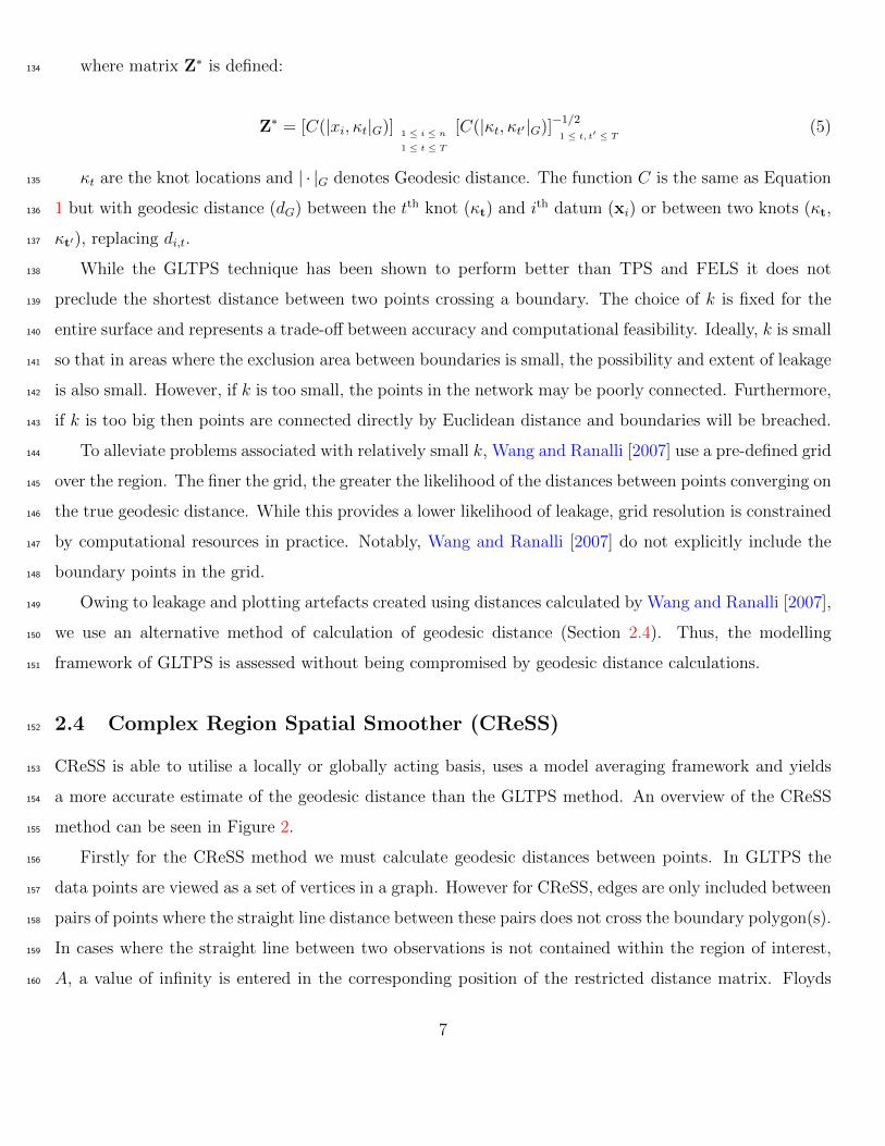
Figure 8: Bias for high noise, (a) TPS, (b) GLTPS, (c) SOAP and (d) CReSS

50 knots for the outer boundary and 40 for the island. There is no guidance for boundary knot selection257

and the default (10 knots) is too small in many situations, so these knot numbers were found to be the258

best after an extensive non-exhuastive search. As for the simulation study in Section 3.1, parameter r,259

for the CReSS method, took values between 2 and 10,000. For all methods a choice of 10 to 100 knots260

was allowed and finalised using GCV (TPS and SOAP), AIC (GLTPS) and AICc (CReSS). In the case of261

SOAP these knots are for the interior soap basis.262

Of the methods trialled, the CReSS method exhibited the lowest MSE scores at low and medium noise263

for this region and, unsurprisingly, TPS has the worst fit to the data and underlying function across all264

noise levels (Table 2 and Figure 10). CV distinguishes TPS from the other methods at low and medium265

noise but at high noise, no clear distinction can be made between model fits (Figure 10). The lack of fit266

of TPS becomes more pronounced as noise increases and is mainly due to leakage across the island where267

the difference in underlying function values is greatest (Figures 11(a), 13(a), 13(a)). At high noise there268

16

(a)

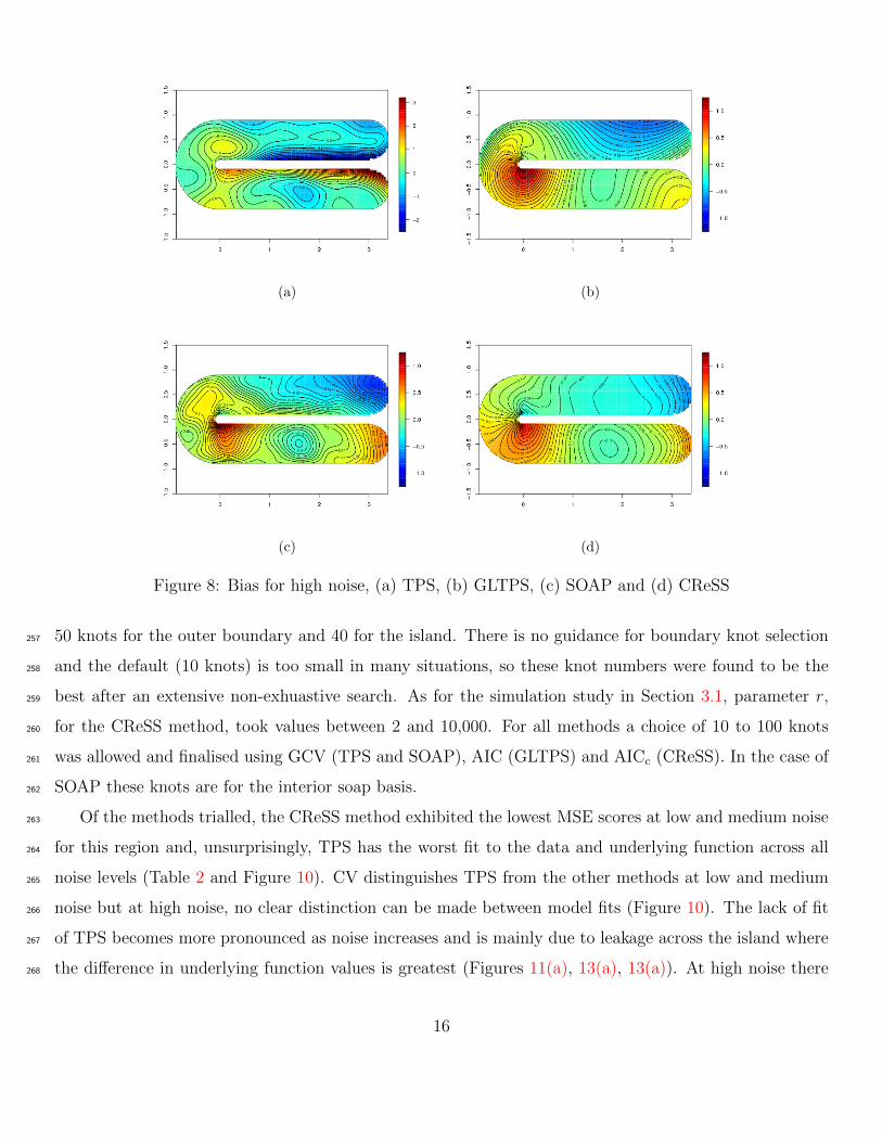
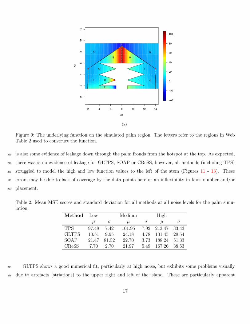
Figure 9: The underlying function on the simulated palm region. The letters refer to the regions in WebTable 2 used to construct the function.

is also some evidence of leakage down through the palm fronds from the hotspot at the top. As expected,269

there was is no evidence of leakage for GLTPS, SOAP or CReSS, however, all methods (including TPS)270

struggled to model the high and low function values to the left of the stem (Figures 11 - 13). These271

errors may be due to lack of coverage by the data points here or an inflexibility in knot number and/or272

placement.273

Table 2: Mean MSE scores and standard deviation for all methods at all noise levels for the palm simu-lation.

Method Low Medium Highµ σ µ σ µ σ

TPS 97.48 7.42 101.95 7.92 213.47 33.43GLTPS 10.51 9.95 24.18 4.78 131.45 29.54SOAP 21.47 81.52 22.70 3.73 188.24 51.33CReSS 7.70 2.70 21.97 5.49 167.26 38.53

GLTPS shows a good numerical fit, particularly at high noise, but exhibits some problems visually274

due to artefacts (striations) to the upper right and left of the island. These are particularly apparent275

17

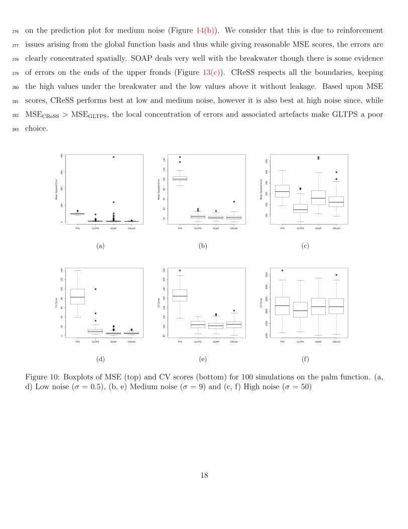
on the prediction plot for medium noise (Figure 14(b)). We consider that this is due to reinforcement276

issues arising from the global function basis and thus while giving reasonable MSE scores, the errors are277

clearly concentrated spatially. SOAP deals very well with the breakwater though there is some evidence278

of errors on the ends of the upper fronds (Figure 13(c)). CReSS respects all the boundaries, keeping279

the high values under the breakwater and the low values above it without leakage. Based upon MSE280

scores, CReSS performs best at low and medium noise, however it is also best at high noise since, while281

MSECReSS > MSEGLTPS, the local concentration of errors and associated artefacts make GLTPS a poor282

choice.283

●●

●●

●

●●●

●●●

●

●

●●

●●

●●

●

●●

TPS GLTPS SOAP CReSS

020

040

060

080

0

Mea

n S

quar

ed E

rror

(a)

●

●

●

● ●

●

TPS GLTPS SOAP CReSS

2040

6080

100

120

140

Mea

n S

quar

ed E

rror

(b)

●●

●●

●

●

TPS GLTPS SOAP CReSS

100

150

200

250

300

350

Mea

n S

quar

ed E

rror

(c)

●

●

●

●●●●

●

●

●

●●

TPS GLTPS SOAP CReSS

020

4060

8010

012

014

0

CV

Sco

re

(d)

●

●●

●

TPS GLTPS SOAP CReSS

8010

012

014

016

018

020

022

0

CV

Sco

re

(e)

●

●

TPS GLTPS SOAP CReSS

2200

2400

2600

2800

3000

3200

CV

Sco

re

(f)

Figure 10: Boxplots of MSE (top) and CV scores (bottom) for 100 simulations on the palm function. (a,d) Low noise (σ = 0.5), (b, e) Medium noise (σ = 9) and (c, f) High noise (σ = 50)

18

2 4 6 8 10 12 14

24

68

10

−80

−60

−40

−20

0

20

40

(a)

2 4 6 8 10 12 14

24

68

10

−30

−20

−10

0

10

20

30

(b)

2 4 6 8 10 12 14

24

68

10

−30

−20

−10

0

10

20

30

(c)

2 4 6 8 10 12 14

24

68

10−30

−20

−10

0

10

20

30

(d)

Figure 11: Bias for low noise a) TPS, (b) GLTPS, (c) SOAP and (d) CReSS

19

2 4 6 8 10 12 14

24

68

10

−80

−60

−40

−20

0

20

40

(a)

2 4 6 8 10 12 14

24

68

10

−40

−20

0

20

40

(b)

2 4 6 8 10 12 14

24

68

10

−40

−20

0

20

40

(c)

2 4 6 8 10 12 14

24

68

10

−40

−20

0

20

40

(d)

Figure 12: Bias for medium noise (a) TPS, (b) GLTPS, (c) SOAP and (d) CReSS

4 Killer whale analysis: Mapping killer whale group size off284

the West coast of the Canadian/USA border285

The region of this study contains a complex area of coastline with 15 islands (Figure 1). The data consist286

of n = 763 group size estimates from 1 to 50. A choice of 10 to 60 knots were chosen randomly from a287

sample of 200 space-filled knots. This prevented over-populating the ‘arms’ of the data and thus having288

too many knots where there is no data support. The data is over-dispersed and therefore modelled using289

a quasipoisson error distribution with a log link. A more realistic surface could be produced by including290

other covariates, such as depth or chlorophyll, however the two-dimensional smooth serves as a good291

exemplar. Predictions were made on a grid of N = 4799 points, with GCV used to choose knots for TPS292

and SOAP, QAICc [Lebreton et al., 1992] for CReSS and Residual Sums of Squares (RSS) for GLTPS.293

All of the methods showed a decent fit to the data using RSS scores, with SOAP having the best fit294

20

2 4 6 8 10 12 14

24

68

10

−80

−60

−40

−20

0

20

40

60

(a)

2 4 6 8 10 12 14

24

68

10

−60

−40

−20

0

20

40

60

(b)

2 4 6 8 10 12 14

24

68

10

−60

−40

−20

0

20

40

60

(c)

2 4 6 8 10 12 14

24

68

10

−60

−40

−20

0

20

40

60

(d)

Figure 13: Bias for high noise, (a) TPS, (b) GLTPS, (c) SOAP and (d) CReSS

to the data, and CReSS having the best QAICc score (Table 3). However, even very minor extrapolation295

presented some interesting problems. TPS and GLTPS both show edge effects from the use of a global296

basis function, but the range of group size predictions for TPS is much closer to the data (Figure 15).297

GLTPS also shows some effect of reinforcement errors in the very centre of the plot. SOAP was particularly298

difficult to parameterise with knot choices needed for all 16 boundaries (1 outer box and 15 islands). There299

is no guidance for selection so, after various combinations tried, the authors chose 40 knots for the outer300

box and 5 for all remaining polygons. SOAP is notably poor for extrapolation in this region, with values301

of infinity predicted in the centre of the plot (Figure 15). To see if SOAP could extrapolate a small302

distance from the data the prediction area was restricted to a non-convex bounding polygon close-fitting303

to the data. No values of infinity were predicted but 6 points had predictions > 103, which is well outside304

the data range (Web Figure 5). CReSS fits the data better than TPS and GLTPS and predicts a surface305

which would seem more realistic. Hotspots are produced in areas where there are large group sizes in the306

21

2 4 6 8 10 12 14

24

68

10

0

50

100

(a)

2 4 6 8 10 12 14

24

68

10

0

50

100

(b)

2 4 6 8 10 12 14

24

68

10

0

50

100

(c)

2 4 6 8 10 12 14

24

68

10

0

50

100

(d)

Figure 14: Example predictions for medium noise, (a) TPS, (b) GLTPS, (c) SOAP, (d) CReSS (iteration80)

data and the surface declines to approximately zero elsewhere.307

5 Conclusions308

CReSS has been developed by extending an existing method in two ways to deal with issues arising from309

biologically meaningless distances in complex regions. Firstly, an accurate estimate of geodesic distance310

between points (that which an animal may travel) is used as a measure of inter point similarity. Secondly, a311

locally varying basis function is employed to accommodate local smoothing requirements while alleviating312

problems with reinforcement. Further, since these modifications are made prior to or at the basis function313

stage, it allows the basis to be used in a wide variety of statistical models. The use of model averaging314

eliminates the need for choice of radius.315

22

Table 3: Knots chosen, RSS and QAICc scores for the killer whale data

Method Knot Number RSS QAICc

TPS 60 46169 788GLTPS 40 46911 -SOAP 60 34487 844CReSS 45 41833 95

−123.4 −123.2 −123.0 −122.8 −122.6

48.3

48.4

48.5

48.6

48.7

48.8

48.9

49.0

Longitude

Latit

ude

0

10

20

30

40

50

60

5

5

5 5

5

5

5

10

10

10

10

10 15

15

15

15

20

20

20

25

25

25

30

30

30

35

35

35

35

40

40

45

50

50

55

(a)

−123.4 −123.2 −123.0 −122.8 −122.6

48.3

48.4

48.5

48.6

48.7

48.8

48.9

49.0

LongitudeLa

titud

e

0

20

40

60

80

100

5

5

5

5

5

5

5

10

10

10

10

10

15

15

15

15

15

15

20

20

20

20 25

25

25

30

30

30

35

35

35 40

40

45

45 50

50

65 75

75

(b)

−123.4 −123.2 −123.0 −122.8 −122.6

48.3

48.4

48.5

48.6

48.7

48.8

48.9

49.0

Longitude

Latit

ude

0

20

40

60

80

100

5

5

5 5

5 5 5

5

5

5

5

5

5

10

10

10

10

10

10

10

10

10

10

10

15

15

15

15

15

15

15

20

20

20

20

20

25

25

25

30

30

35

40

40

45

45 55

55

60

65

70 75

● ●

● ●

● ● ● ● ●

● ● ● ● ● ●

● ● ● ● ● ●

● ● ● ● ● ● ●

● ● ● ● ● ● ● ● ●

● ● ● ● ● ● ● ●

● ● ● ● ●

● ● ● ● ● ● ● ●

● ● ● ● ● ● ● ● ● ● ●

● ● ● ● ● ● ● ● ●

● ● ● ● ● ● ● ● ● ● ●

● ● ● ● ● ● ● ● ● ● ● ● ●

● ● ● ● ● ● ● ● ● ● ● ● ●

● ● ● ● ● ● ● ● ● ● ● ● ● ● ● ●

● ● ● ● ● ● ● ● ● ● ● ●

● ● ● ● ● ● ● ● ●

● ● ● ● ● ● ●

● ● ● ●

● ● ●

● ● ● ● ●

● ● ● ● ● ●

● ● ● ● ●

●

● ●

● ● ●

● ● ●

● ● ● ● ● ●

● ● ● ● ● ●

● ● ● ● ● ● ●

● ● ● ● ● ●

● ● ●

● ●

● ● ● ●

● ● ● ●

● ● ● ●

● ● ● ● ●

● ● ● ● ● ●

● ● ● ● ● ● ● ●

● ● ● ● ● ●

● ● ● ● ● ● ●

● ● ● ● ● ●

● ● ● ● ● ●

● ● ● ● ● ●

● ● ● ●

● ●

(c)

−123.4 −123.2 −123.0 −122.8 −122.6

48.3

48.4

48.5

48.6

48.7

48.8

48.9

49.0

Longitude

Latit

ude

0

10

20

30

40

50 5

5

5

5

5

5

5

5

5

5

10

10

10

10

10

10

10 10

10

15

15

15

15

15 20

20

20

25

30

35

(d)

Figure 15: Plots of predictions for the killer whale data using (a) TPS, (b) GLTPS (c) SOAP and (d)CReSS. The density scale is wider for GLTPS and SOAP to accommodate higher predictions. Grey dotsrepresent points with counts >100 and black dots represent points where a value of infinity was predicted.Colour plots may be found in Web Figure 5.

After reviewing the methods in this paper, the GLTPS method cannot be used in areas with islands316

and SOAP is hard to parameterise, particularly with increasing boundary loops. We have attempted to317

provide the best results from all methods for comparison, frequently trialling many parameterisations -318

23

many more than would be reasonably expected for general use. CReSS is very simple to implement and319

is comparable with, if not better than, other methods in all examples shown.320

The issue of knot selection is common to all the methods seen in this paper. Here, the knots are chosen321

using a space filling algorithm which does not necessarily allow surface flexibility in the areas it is most322

required, particularly for the sparse killer whale test data set. In the one dimensional case, a new Spatially323

Adaptive Local Smoothing Algorithm (SALSA, Walker et al., 2010) has proved to be very effective for324

knot placement and is currently being incorporated into the CReSS method.325

SUPPLEMENTAL MATERIALS326

Supplementary Material327

Web Tables and Figures referenced in Sections 2 and 4 are available at the web link given.328

329

References330

K. P. Burnham and D. R. Anderson. Model Selection and Multimodel Inference: A practical information-331

theoretic approach. Springer, 2 edition, 2002.332

R. W. Floyd. Algorithm 97: Shortest path. Communications of the ACM, 5:345, 1962.333

B. Fornberg, T. Driscoll, G. Wright, and R. Charles. Observations on the behavior of radial basis function334

approximations near boundaries. Computers & Mathematics with Applications, 43(3-5):473–490, 2002.335

R. Furrer, D. Nychka, and S. Sain. fields: Tools for spatial data, 2010. URL http://CRAN.R-project.336

org/package=fields. R package version 6.3.337

P. J. Green and B. W. Silverman. Nonparametric Regression and Generalised Linear Models (A roughness338

penalty approach). Chapman and Hall, England, 1994.339

R. L. Harder and R. N. Desmarais. Interpolation using surface splines. Journal of Aircraft, 9:189–191,340

1972.341

T. Hastie. Statistical models in S. Chapman and Hall, 1993.342

24

T. J. Hastie and R. J. Tibshirani. Generalized Additive Models. Chapman & Hall, 1990.343

C. M. Hurvich and C.-L. Tsai. Regression and time series model selection in small samples. Biometrika,344

76(2):297–307, 1989. doi: 10.1093/biomet/76.2.297. URL http://biomet.oxfordjournals.org/345

content/76/2/297.abstract.346

P. W. M. John, M. E. Johnson, L. M. Moore, and D. Ylvisaker. Minimax distance designs in two-level347

factorial experiments. Journal of Statistical Planning and Inference, 44:249–263, 1995.348

J.-D. Lebreton, K. P. Burnham, J. Clobert, and D. R. Anderson. Modeling survival and testing biological349

hypotheses using marked animals: A unified approach with case studies. Ecological Monographs, 62(1):350

pp. 67–118, 1992. ISSN 00129615. URL http://www.jstor.org/stable/2937171.351

B. McMorrow. Palm jumeirah photograph. World Wide Web, 2004. URL http://www.pbase.com/352

bmcmorrow.353

R Development Core Team. R: A Language and Environment for Statistical Computing. R Foundation for354

Statistical Computing, Vienna, Austria, 2009. URL http://www.R-project.org. ISBN 3-900051-07-0.355

T. O. Ramsay. Spline smoothing over difficult regions. Journal of the Royal Statistical Society: Series B356

(Statistical Methodology), 64(1):307–319, 2002.357

S. L. Rathbun. Spatial modelling in iregularly shaped regions: Kriging estuaries. Environmetrics, 9:358

109–129, 1998.359

C. Walker, M. Mackenzie, C. Donovan, and M. O’Sullivan. Salsa - a spatially adaptive local smoothing360

algorithm. Journal of Statistical Computation and Simulation, 81(2):179–191, 2010.361

H. Wang and M. G. Ranalli. Low-rank smoothing splines on complicated domains. Biometrics, 63(1):362

209–217, 2007.363

S. N. Wood. Thin plate regression splines. J. R. Statist. Soc. B, 65(1):95–114, 2003.364

S. N. Wood. soap: Soap film smoothing, 2010. R package version 0.1-5.365

S. N. Wood, M. V. Bravington, and S. L. Hedley. Soap film smoothing. J. R. Statist. Soc. B, 70(5), 2008.366

25

Web-based Supplementary Materials forComplex Region Spatial Smoother

August 24, 2011

1

0.0 0.2 0.4 0.6 0.8 1.0

0.0

0.2

0.4

0.6

0.8

1.0

0.0

0.5

1.0

1.5

2.0

Web Figure 1: Underlying function used to show the problems of reinforcement

2

0.0 0.2 0.4 0.6 0.8 1.0

0.0

0.2

0.4

0.6

0.8

1.0

−0.15

−0.10

−0.05

0.00

0.05

0.10

(a)

0.0 0.2 0.4 0.6 0.8 1.0

0.0

0.2

0.4

0.6

0.8

1.0

−0.1

0.0

0.1

0.2

0.3

(b)

0.0 0.2 0.4 0.6 0.8 1.0

0.0

0.2

0.4

0.6

0.8

1.0

0.2

0.4

0.6

0.8

(c)

0.0 0.2 0.4 0.6 0.8 1.0

0.0

0.2

0.4

0.6

0.8

1.0

−0.2

0.0

0.2

0.4

0.6

(d)

Web Figure 2: Graphical representations of one basis (out of a possible 30 knots)for TPS (a) a global basis function (b) and a local basis function (c). The globalbasis shows reinforcement at the top of the triangle and this is also shown by thearea of greatest prediction error (d) for the surface in Figure 1

3

Web Table 1: The benchmark function, F , is defined by region as shown. Wedenote the geodesic distance between two points X and Y as d(X, Y ). The left-most red dot at co-ordinate (2,5) we denote by L. The rightmost dot at co-ordinate(14,5) we denote by R.

Region F(X) = F(X1,X2)

A d(X,L)− (X1 − 2)2

B d(X,L) + (X1 − 2)2 + (X1 − 4)3

C d(X,L) + (X1 − 2)2

D d(X,L) + (X1 − 2)2 + (4−X2)3 + (X1 − 4)4

E d(X,L) + (X1 − 2)2 + (4−X2)3 − (X1 − 4)4

F d(X,L) + (X1 − 2)2 + (4−X2)3

G d(X,R)− (14−X1)2

H d(X,R)− (14−X1)2 − (12−X1)

3

I d(X,R) + (14−X1)2

J d(X,R) + (14−X1)2 + (4−X2)

K d(X,R) + (14−X1)2 + (4−X2)− (12−X1)

2

L d(X,R) + (14−X1)2 + (4−X2)− (12−X1)

2 4 6 8 10 12 14

02

46

81

01

2

X1

X2

−40

−20

0

20

40

60

80

100

A

B

C

D

E

F

G

H

I

JK

L

Web Figure 3: The underlying function on the simulated palm region. The lettersrefer to the regions in Web Table 2 used to construct the function

4

−123.4 −123.2 −123.0 −122.8

48.4

48.6

48.8

49.0

Longitude

Latit

ude

0

10

20

30

40

50

60

70

(a)

−123.4 −123.2 −123.0 −122.8

48.4

48.6

48.8

49.0

Longitude

Latit

ude

0

50

100

150

200

● ● ●

● ● ● ●

● ● ● ●

● ● ● ●

● ● ● ● ●

● ● ● ● ●

● ● ● ● ●

● ● ● ● ● ●

(b)

−123.4 −123.2 −123.0 −122.8

48.4

48.6

48.8

49.0

Longitude

Latit

ude

0

50

100

150

200

●

● ●

● ● ● ● ●

● ● ● ● ● ●

● ● ● ● ● ●

● ● ● ● ● ● ●

● ● ● ● ● ● ● ●

● ● ● ● ● ● ● ●

● ● ● ● ●

● ● ● ● ● ● ● ●

● ● ● ● ● ● ● ● ● ● ●

● ● ● ● ● ● ● ● ●

● ● ● ● ● ● ● ● ● ● ●

● ● ● ● ● ● ● ● ● ● ● ● ●

● ● ● ● ● ● ● ● ● ● ● ● ●

● ● ● ● ● ● ● ● ● ● ● ● ● ● ● ●

● ● ● ● ● ● ● ● ● ● ● ●

● ● ● ● ● ● ● ● ●

● ● ● ● ● ● ●

● ● ●

● ● ●

● ● ●

● ●

●

● ●

● ●

● ● ● ●

● ● ● ●

● ● ●

● ●

●

● ●

● ● ● ●

● ● ● ●

● ● ● ●

● ● ● ● ●

● ● ● ● ● ●

● ● ● ● ● ● ● ●

● ● ● ● ● ●

● ● ● ● ● ● ●

● ● ● ● ● ●

● ● ● ● ● ●

● ● ● ● ● ●

● ● ● ●

● ●

(c)

−123.4 −123.2 −123.0 −122.8

48.4

48.6

48.8

49.0

Longitude

Latit

ude

0

10

20

30

40

50

(d)

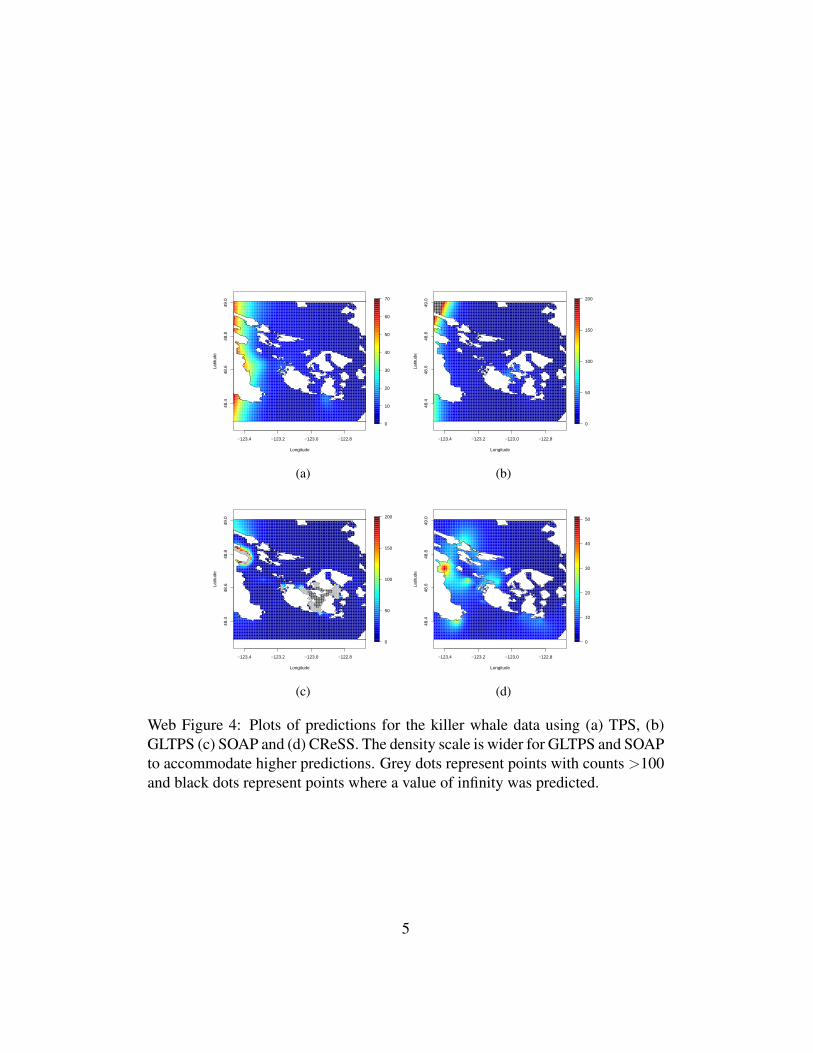
Web Figure 4: Plots of predictions for the killer whale data using (a) TPS, (b)GLTPS (c) SOAP and (d) CReSS. The density scale is wider for GLTPS and SOAPto accommodate higher predictions. Grey dots represent points with counts >100and black dots represent points where a value of infinity was predicted.

5

−123.4 −123.2 −123.0 −122.8

48.4

48.6

48.8

49.0

Longitude

Latit

ude

0

50

100

150

200

xx

x

x xx

Web Figure 5: Reduced extrapolation for killer whale region, red crosses representpoints with group size >200

6