lable at ScienceDirect

Atmospheric Environment 44 (2010) 4510e4520

Contents lists avai

Atmospheric Environment

journal homepage: www.elsevier .com/locate/atmosenv

Comparison of summer and winter California central valley aerosoldistributions from lidar and MODIS measurements

Jasper Lewis a,*, Russell De Young b, Richard Ferrare b, D. Allen Chu c

aCenter for Atmospheric Science, Hampton University, Hampton, VA 23668, USAb Science Directorate, NASA Langley Research Center, Hampton, VA 23681, USAcGoddard Earth Science and Technology Center, University of Maryland Baltimore County, Greenbelt, MD 20771, USA

a r t i c l e i n f o

Article history:Received 8 September 2009Received in revised form19 April 2010Accepted 5 July 2010

Keywords:MODISAerosolCaliforniaSan Joaquin ValleyLidar

* Corresponding author.E-mail address: jasper.r.lewis@nasa.gov (J. Lewis).

1352-2310/$ e see front matter � 2010 Elsevier Ltd.doi:10.1016/j.atmosenv.2010.07.006

a b s t r a c t

Aerosol distributions from two aircraft lidar campaigns conducted in the California Central Valley arecompared in order to identify seasonal variations. Aircraft lidar flights were conducted in June 2003 andFebruary 2007. While the ground PM2.5 (particulate matter with diameter� 2.5 mm) concentration washighest in the winter, the aerosol optical depth (AOD) measured from the MODIS and lidar instrumentswas highest in the summer. A multiyear seasonal comparison shows that PM2.5 in the winter can exceedsummer PM2.5 by 68%, while summer AOD from MODIS exceeds winter AOD by 29%. Warmer temper-atures and wildfires in the summer produce elevated aerosol layers that are detected by satellitemeasurements, but not necessarily by surface particulate matter monitors. Temperature inversions,especially during the winter, contribute to higher PM2.5 measurements at the surface. Measurements ofthe mixing layer height from lidar instruments provide valuable information needed to understand thecorrelation between satellite measurements of AOD and in situ measurements of PM2.5. Lidarmeasurements also reflect the ammonium nitrate chemistry observed in the San Joaquin Valley, whichmay explain the discrepancy between the MODIS AOD and PM2.5 measurements.

� 2010 Elsevier Ltd. All rights reserved.

1. Introduction

The California Central Valley is a major agricultural areastretching some 600 km from north to south and is one of the mostproductive agricultural regions in the world (Andrews et al., 2002).The southern half of the valley is known as the San Joaquin Valleyencompassing nearly 64,000 km2. The valley has cool wet wintersand hot dry summers. On the western edge of the valley is theCoastal Mountain range with peaks reaching 1530 m. On the eastside is the Sierra Nevada range (max 4418 m) and the TehachapiMountains (max 2432 m) form the southern boundary of theValley, which contain mountain passes to the Los Angeles basin andthe Mojave Desert. The surrounding mountains prevent ventilationof air masses, causing pollutants and their precursors to be retainedin the valley. The valley topography and climate create idealconditions for trapping and holding pollutants within the valley.The particle and gaseous emissions can recirculatewithin the valleyand accumulate to unhealthy levels (Smith et al., 1981a,b, 1984).

All rights reserved.

The valley is currently a nonattainment area with the PM2.5(particulate matter with diameter� 2.5 mm) National Ambient AirQuality Standard (NAAQS) because measurements of severalmonitoring sites exceed the daily and annual PM2.5 standards,especially in the lower part of the valley where air quality isa significant health issue (San Joaquin Valley APCD, 2008a).Significant progress has been made in reducing the PM10 (partic-ulate matter with diameter� 10 mm) and PM2.5 emissions anda plan is in place to meet the NAAQS and state standards for airquality in 2014 (San Joaquin Valley APCD, 2008a).

It should be noted however that valley emissions are notdominated by a single source. The observed PM2.5 levels representaggregated urban emissions with contributions from the region.The local climate produces seasonal variations in particulate levelsthrough the changes in atmospheric conditions that affect the typesof emissions, emission rates, and atmospheric formation of parti-cles from precursor emissions.

During fall and winter, meteorological conditions contribute tolow wind speeds, low-lying inversion layers and increasedsecondary particle formation, all establishing a situation conduciveto the formation and accumulation of PM2.5. Colder, frequentlystagnant conditions occurring in December and January favorformation of ammonium nitrate, and thus experience the highest

J. Lewis et al. / Atmospheric Environment 44 (2010) 4510e4520 4511

levels of ground PM2.5. The cold weather also induces the public toincrease residential wood burning that further adds emissions tothe atmosphere. During the winter, wind direction varies from thesouth-southeasterly directions to north-northwesterly directions.Temperature inversions trap aerosols below the mixing layerheight (MLH), where they can remain more concentrated thanwhen they can mix more freely with cleaner air at higher altitudes.This contributes to higher PM2.5 concentrations as inversions areformed more persistently (stable) during the winter months, wheninversions occur from 15 to 1200 m (Chow et al., 1999).

In the summer, long periods of little or no rainfall result inextreme dryness of soils along roadways, increasing emissions fromtraffic movement. Limited rainfall during the summer monthsreduces the frequency of events that clear emissions from the localarea. At night, cooler drainage winds from the surroundingmountains prevent exit of the air at the southern end of the Valley,causing recirculation of pollutants in a counterclockwise patternand returning polluted air to urban areas. Throughout the valley,some of the pollutants transported to higher altitudes fromdaytime heating return to the surface at night by drainage windsfrom the mountains. In the spring and summer PM2.5 tends to belower with mostly motor vehicle emissions, secondary sulfate, andprimary geological material from the fine particle fraction ofairborne soil. Daytime temperature inversions during the summerare usually not encountered until 610e760 m above the surface(San Joaquin Valley APCD, 2008b).

Fig.1 summarizes the seasonal trends and chemical componentsof PM2.5 near Bakersfield, California in the lower valley. Winter andspring months are heavily dominated by secondary ammoniumnitrate with moderate contributions of secondary sulfate, motorvehicle emissions, primary geological material and direct emissionof organic aerosols identified as biomass burning from woodcombustion, wild fires or agricultural burning. In the summer,organic carbon dominates the composition of PM2.5.

The primary transport route into the Valley is from the north-west in the vicinity of Stockton where transport is directed fromStockton to Bakersfield for all the months except January andFebruary. During the summer the air into the valley is directed fromthe northwest at all hours of the day. The primary transport routeout of the valley is over the TehachapiMountains at the southeast ofBakersfield. This outflow pattern contributes significantly to thepollution in the Mojave Desert. The flow over the TehachapiMountains is most effective during the summer and nearly absentduring winter periods because of stagnation. Upslope flow occur-ring during the afternoon throughout the year is effective inremoving pollutants from foothills of the valley. A portion of thepollutants; however, is returned to the valley by the nocturnal

Fig. 1. Seasonal pattern and composition of PM2.5 near Bakersfield, CA from SanJoaquin Valley Air Pollution Control District, 2008 PM2.5 Plan e Final Adopted(2008b). Note that the ammonium nitrate concentration decreases significantlybetween February and June.

drainage winds. Ventilation of the valley during the summer leadsto a typical pollution residence time of 1e2 days, dependent uponlocation (Smith et al., 1981a). During the winter, because of stag-nation, typical residence times of 2e8 days may be experienced(Smith et al., 1981a). In general, the air at ground level is warmed bysunlight causing it to rise and carry emissions aloft. This rising airpattern mixes the fresh emissions with air at higher elevations,dispersing the emissions and reducing the concentration of directlyemitted PM2.5 and precursors. However, temperature inversionlayers frequently block the rising air recirculating it down to thesurface (Smith et al., 1981a).

This paper will compare the results of two airborne aerosol lidarcampaigns over the San Joaquin Valley. The first campaign occurredin June 2003 (De Young et al., 2005) and the second in February2007 (Al-Saadi et al., 2008). These two lidar campaigns providecontrasted aerosol conditions in summer and winter. The lidarreturns will be used to derive aerosol optical depth (AOD) andcompared with the MODIS (Moderate Resolution Imaging Spec-troradiometer) AOD from the Terra and Aqua satellites. Theadvantage of aerosol lidar is that it provides the high-resolutionvertical distribution of aerosols. Though it does not provide directmeasurements of the number density of aerosols, it does measurethe MLH accurately (Boers et al., 1984), which is important sincemost of the PM2.5 aerosols observed during these lidar campaignswere confined within the mixing layer. Lidar can also be used todetermine the height of aerosol plumes above the mixing layer;these plumes can be transported from great distances. Lidar withmultiple wavelengths and depolarization can be used to classifyaerosol types (Sasano and Browell, 1989).

While lidar gives high vertical resolution, but low spatialcoverage, satellite AOD measurements give a very broad coverage,but columnar measurement at moderate resolutions. Correlationsbetween MODIS AOD and PM2.5 are poor in the western UnitedStates due to high surface reflectances, variations in aerosol type,and higher occurrences of smoke and elevated aerosol plumes(Engel-Cox et al., 2004; Hoff and Christopher, 2009). The synthe-sized lidar and satellite measurements can result in a betterunderstanding of aerosols with ground PM2.5 concentrations forhealth and regulatory needs over a large area. This paper willexamine lidar and MODIS AOD measurements in comparison withground PM2.5 concentrations to give a clearer picture of thedistribution of aerosols within the valley.

Publications describing aircraft lidar flights in the valley are rare.The first such campaign occurred in September 1994 when a 1064-nm lidar was flown along the California coast as validation for theLidar In-Space Technology Experiment (LITE) (Strawbridge andHoff, 1996). Pronounced aerosol structures were seen towards thesouthern end of the San Joaquin Valley, near Bakersfield.

2. Method

Two different aircraft lidar systems were used in this study. The2003 lidar measurements were made using the Compact AerosolLidar (CAL) deployed on the NASA DC-8 during the DC-8 Inlet/Instrument Characterization Experiment (DICE), while the 2007lidar measurements were made using the Airborne High SpectralResolution Lidar (HSRL) deployed on the NASA King Air B-200.A summary of the two lidar systems is shown in Table 1.

2.1. Compact Aerosol Lidar (CAL)

The CAL used in the 2003 San Joaquin Valley campaignwas built inthe Science Directorate of NASA Langley Research Center (De Younget al., 2005; Gili and De Young, 2006; Lewis et al., 2010). The standardbackscatter lidar system has dimensions of 108-cm� 64-cm� 53-cm

Table 2Summary of summer 2003 San Joaquin Valley campaign.

Date Takeoff(UTC/PDT)

MODIS Overpass(UTC)

Altitude(km)

Angstromexponent

1064-lidarratio (sr)

June 3, 2003 23:40/16:40 Aqua 21:05 6 1.451 40June 5, 2003 22:39/15:39 Aqua 20:55 11 1.436 30June 5, 2003 27:16/20:16 Aqua 20:55 12 1.436 30June 11, 2003 27:16/20:16 Aqua 20:15, 20:20 12 1.060 35June 12, 2003 23:33/16:33 Aqua 21:00 12 1.151 30June 17, 2003 19:55/12:55 Aqua 21:20 6 1.377 30

Table 1Summary of lidar properties for CAL and airborne HSRL lidars.

CAL HSRL

LaserManufacturer Big Sky (Quantel) FibertekRepetition rate 20-Hz 200-HzBeam divergence 1.5-mrad 0.8-mrad1064-nm energy 60-mJ 1.1-mJ532-nm energy 80-mJ 2.5-mJ

TelescopeDiameter 0.30-m 0.40-mFOV 1.6-mrad 1.0-mrad

Filters1064-nm 1-nm, FWHM 0.4-nm, FWHM532-nm 0.5-nm, FWHM 60-pm (etalon),

FWHM

Detectors1064-nm channel APD (analog) APD (analog)532-nm channel PMT (analog & photon

counting)PMT (analog)

J. Lewis et al. / Atmospheric Environment 44 (2010) 4510e45204512

and a mass of 115-kg and was flown on the NASA DC-8. The laser isa frequency doubled Nd:YAG (Big Sky Laser e Quantel) with a 20-Hzrepetition rate. The 1064-nmand532-nmenergies are typically 60-mJand 80-mJ, respectively. A steerable 45� turningmirror is used to alignthe transmitted beam to the telescope. The atmospheric return passesto the receiver box by a 1-mm diameter optical fiber coupled to thefocal point of a 0.30-m diameter telescope.

The received light is collimated and split into 1064-nm and 532-nm channels, with a further split of the 532-nm wavelength intoanalog (90%) and photon counting (10%) channels. The 1064-nmreturnpasses through a 1-nm full-width-at-half-maximum (FWHM)filter before being focused onto an avalanche photodiode (APD)detector. The 532-nm return passes through a 0.5-nm FWHM filterbefore being split between analog and photon-counting photo-multiplier detectors. Data are averaged over a 2-s (40 shots) timeinterval before being stored by the computer.

The 532-nm wavelength was unavailable during the 2003campaign; therefore, the lidar derived AOD was obtained by con-verting the 1064-nm AOD to a 532-nm AOD using the Angstromexponent. In this calculation, it was assumed that the Angstromexponent for the 500-nm and 1020-nm AERONET (Holben et al.,2001) wavelengths measured from Fresno, CA could be used forthe 532-nm and 1064-nm lidar wavelengths. The power returnedto the lidar receiver, P(z), is given by the lidar equation as:

PðzÞ ¼ Cz2½bmðzÞ þ baðzÞ�T2ðzÞ (1)

where C is the calibration constant, bm(z) is the molecular back-scattering coefficient, ba(z) is the aerosol backscattering coefficient,and T(z) is the one-way transmittance from the lidar to the height z.The lidar data is inverted using the Fernald method (Fernald et al.,1972; Fernald, 1984) to determine the aerosol backscatter coeffi-cient, ba. The lidar AOD, s, is calculated as:

s ¼ Sa

ZZ*

0

baðzÞdz (2)

where Sa is the lidar ratio and Z* is an altitude where it is assumedonly molecular scattering occurs (i.e. ba (Z*)¼ 0). In practice, Z* waschosen at an altitude a few hundred meters below the aircraftaltitude, shown in Table 2.

For two different wavelengths l1064 and l532 the Angstromexponent, g, relates the AOD s1064 and s532 such that:

s532 ¼ s1064l532l1064

(3)

� ��g

AODs calculated using Equation (3) are referred to as the con-verted 532-nm AOD in the sections that follow. A similar calcu-lation was performed to determine the converted 532-nm aerosolextinction for the 2003 lidar campaign. The 1064-nm lidar ratioused to invert the lidar signal was selected by matching the con-verted 532-nm AOD to the MODIS AOD along a small segment ofthe lidar flight path (usually averaged over 2e3 MODIS pixels nearBakersfield).

2.2. Airborne High Spectral Resolution Lidar (HSRL)

The Airborne HSRL used in the 2007 San Joaquin Valleycampaign was also developed in the Science Directorate of NASALangley Research Center (Hair et al., 2008) and deployed on theNASA King Air B-200. The HSRL takes advantage of Dopplerbroadening to independently resolve the molecular and aerosolatmospheric lidar returns. Backscattered radiation from air mole-cules is Doppler broadened on the order of GHz due to the high-velocity random thermal motion of the molecules. By contrast,slower-velocity aerosol particles are only Doppler broadened onthe order of MHz due to their much larger mass. An extremelynarrow-band iodine vapor (I2) absorption filter is used to separatethe molecular return from the aerosol return at the 532-nmwavelength. The HSRL instrument also functions as a standardbackscatter lidar at the 1064-nm wavelength.

The HSRL system uses a 200-Hz pulsed Nd:YAG laser (Fibertek).The 1064-nm and 532-nm energies are 1.1-mJ and 2.5-mJ, respec-tively. The receiver employs a 40-cm telescope with a 1-mrad fieldof view. The transmitter and receiver occupy a volume withdimensions of 83-cm� 56-cm� 76-cm, while the data acquisitionand control system occupies an additional 0.37-m3.

The 1064-nm lidar return passes through a 0.4-nm FWHMinterference filter before being separated into parallel andperpendicular polarization channels, which distinguishes betweenspherical and nonspherical particles. The 532-nm lidar returnpasses through a temperature tuned, 60-pm etalon, (Coronado),and then splits between the boresight detector (4%) which main-tains alignment between the transmitter and receiver, the paralleland perpendicular polarization channels (10%), and the I2 filter andmolecular return channel (86%). Data are typically averaged overa 0.5-s (100 shots) time interval before being stored by thecomputer.

A more complete description of the HSRL system and themethods used to retrieve aerosol parameters from this system isdescribed by Hair et al. (2008). Rogers et al. (2009) compared theHSRL layer AOD values to AOD derived from the airborne Sunphotometer with the results showing HSRL lower by a bias differ-ence of �0.0032 (�6.5%) and an rms difference of 0.0079 (15.6%).They also compared the HSRL AOD values with coincident AODmeasured by AERONET ground-based sun photometers and foundthe HSRL AOD lower by a bias difference of �0.015 or �6%.

J. Lewis et al. / Atmospheric Environment 44 (2010) 4510e4520 4513

2.3. Calculation of mixing layer heights

The MLHs were calculated using the Haar wavelet transform asdescribed by Davis et al. (2000). The Haar wavelet transform isa convolution of the Haar function (or step function) and the lidarbackscatter signal. The mixing layer height is identified by themaximum in the Haar wavelet transform, which corresponds toa step-like decrease in aerosol scattering in the lidar signal. Thismethod works best when there is a sharp gradient produced at thetop of the mixing layer, strong convective mixing, and no aerosol orcloud layers aloft. There were no PTU radio soundings availableduring either aircraft lidar campaign to validate the lidarmeasurements of the MLH.

2.4. Moderate Resolution Imaging Spectroradiometer (MODIS)

MODIS is a 36-channel spectroradiometer onboard both Terraand Aqua satellites of the Earth Observing Systems (EOS). The

Fig. 2. Summer 2003 comparison of MODIS (550-nm) 5� 5-km2 AOD and flight t

MODIS spectral channels used in retrieving AOD over land andocean include two 250-m (660 and 860-nm channels), and five500-m (470, 550, 1240, 1640, and 2130-nm) channels. The 250-mresolution 660 nm and 860 nm channels are used to detect waterbodies such as lakes or rivers. Then the aggregated 500-m resolu-tion 660-nm and 860-nm reflectances together with other 500-mchannels are used to derive AOD. The detailed methodology of theMODIS aerosol algorithm for the procedures of screening cloudsand surface snow/ice was described by Remer et al. (2006). TheAERONET instruments have been used to validate the MODIS AODproducts over land and ocean (Remer et al., 2005; Chu et al., 2002).The global results show that over land, at worst 68% of theMODIS retrievals at 0.55 nm fall within the predicted errorof Ds¼�0.05� 0.15s (Chu et al., 1998; King et al., 1999). Overvegetated and semi-arid surfaces where AOD values are shown asthe majority of MODIS retrievals, the AOD products have beenwidely used in routine air quality monitoring, such as Infusingsatellite Data into Environmental Applications (IDEA) (http://idea.

racks for CAL (converted 532-nm) AOD in the San Joaquin Valley, California.

J. Lewis et al. / Atmospheric Environment 44 (2010) 4510e45204514

umbc.edu) (Al-Saadi et al., 2005) and in correlating with surfacePM2.5 concentrations for public health related studies (Kumar et al.,2007, 2008; Tsai et al., in press).

MODIS 5� 5-km2 AOD products are derived based upon theoperational 10�10-km2 algorithm (Level 2, Collection 005) with100 available pixels. Thus the degree of freedom in selecting thebest pixels is largely reduced. To maintain the quality of retrieval atthe same level as the operational 10�10-km2 retrievals, we chooseto use the same requirement of minimum number of pixels e 12pixels for the 5� 5-km2 retrievals. Though the number of availablepixels is significantly reduced (by a factor of 4 from 10 km to 5 km),the quality of the retrieval, however, is retained, which is importantfor the case studies with variable clouds above the CaliforniaCentral Valley. Note that the 5� 5-km2 AOD retrievals are derivedonly over land for comparisons with 10�10-km2 AOD values incorrelating with PM2.5 ground measurements.

Fig. 3. AOD of CAL flight track (converted 532-nm) with back trajectories (markers represemass concentrations at the time of the nearest MODIS overpass, and AERONET AOD (500-nmPM2.5* denotes FRM 24-h averages.

2.5. Ground in situ PM2.5 measurements

Remote measurements of aerosols from lidar and MODIS arecompared with pointesource, in situ measurements of PM2.5 massconcentrationmade at the surface. There are several PM2.5monitorslocated within the San Joaquin Valley, operated by the San JoaquinValley Unified Air Pollution Control District and the California AirResources Board. Data from both continuous mass monitors (beta-attenuation monitors) and Federal Reference Method (FRM) gravi-metric filter-based samplers are utilized in this study.

PM2.5 data used in the multiyear MODIS AOD comparison wereobtained from the California Air Resources Boards’s Air Quality andMeteorological Information System (AQMIS2, www.arb.ca.gov/aqmis2/aqmis2.php) database. Vertical humidity profile measure-ments were not made during either aircraft lidar campaign; there-fore, hygroscopic growth of aerosols has not been accounted for.

nt 1-h time intervals) at different altitudes (shown in different colors), PM10 and PM2.5

) measured at Fresno, CA during the summer 2003 San Joaquin Valley campaign. The

J. Lewis et al. / Atmospheric Environment 44 (2010) 4510e4520 4515

3. Results

The data used for comparison between the summer and winterSan Joaquin Valley campaigns were collected on the dates of June 3,5, 11, 12, and 17 of 2003 using the CAL, and the dates of February 15,16, and 17 of 2007 using the Airborne HSRL. For each campaign,comparisons of the lidar derived AOD (532-nm) to MODIS AOD(550-nm), AERONET AOD (500-nm), PM2.5 and PM10 massconcentrations, and lidar extinction profiles (1064-nm) will bepresented.

While the winter 2007 lidar flights were designed to fly overPM2.5 stations stretching from the northern to the southern end of

Fig. 4. Curtain plots of the converted 532-nm lidar extinction during the summer

the San Joaquin Valley, the summer 2003 lidar flights were mainlyfocused on the southern part of the valley. Since both campaignsconducted flights over Bakersfield, special attentionwill be given tothe Bakersfield area data.

3.1. Summer 2003 campaign

Fig. 2 shows the summer 2003 comparison of Aqua satelliteMODIS AOD at 550-nm with 5� 5-km2 resolution to the lidarderived AOD from CAL for each flight date. High AODs (s> 0.3) aremeasured by MODIS throughout the San Joaquin Valley, as well asnear San Francisco and Los Angeles. Moving south from Stockton to

2003 San Joaquin Valley campaign. Bakersfield, CA is indicated in each plot.

J. Lewis et al. / Atmospheric Environment 44 (2010) 4510e45204516

Bakersfield, there appears to be an increase in aerosol loading. Table2 provides a summary of each individual flight. The Angstromexponentswere calculated using Equation (3) and the 1020-nm and500-nm AODs from the AERONET site in Fresno, CA. The lidar ratiosand Angstrom exponents are in the range of what is expected forurban/industrial aerosols (Ackermann, 1998; Mattis et al., 2004).

Fig. 3 shows the ground particulate matter concentrationsthroughout the San Joaquin Valley at the time of the MODIS over-pass. Despite the high values of MODIS AOD, the PM2.5 groundconcentrations are relatively low for the region. Using the valuesfrom the Stockton, CA ground monitor, PM2.5 makes up 20e25% ofthe PM10 mass concentration.

Fig. 4 shows curtain plots of the converted 532-nm aerosolextinction for each of the flight dates. The highest extinction valuesare measured near Bakersfield and the Tehachapi Mountains,as shown in the figures. The MLH for the region is between 1.5 and2-km. In the majority of the curtain plots, the peak in aerosolextinction is well above the surface, which may explain why the

Fig. 5. Winter 2007 comparison of MODIS (550-nm) 5� 5-km2 AOD and flig

ground PM2.5 mass concentrations do not measure the high level ofaerosol loading that is measured by the MODIS instrument.

3.2. Winter 2007 campaign

The Airborne HSRL AOD was obtained directly via the HSRLtechnique from the 532-nmwavelength lidar channel as describedby Hair et al. (2008). Fig. 5 shows the comparison between the lidarderived AOD andMODIS during the winter 2007 San Joaquin Valleycampaign. Because both Aqua and Terra satellite overpassesoccurred during the February 15 lidar flight, the lidar flight path isshown compared to both satellite MODIS AOD values. Similar to thesummer 2003 campaign, the highest AOD are located in the centralpart of the Valley and near San Francisco and Los Angeles; however,the AOD values are lower than those measured during the 2003summer. Table 3 provides a summary of each of the aircraft lidarflights. The standard deviations shown for the Angstrom exponentand 532-nm lidar ratio relate to the variability in the vertical profile

ht tracks for HSRL (532-nm) AOD in the San Joaquin Valley, California.

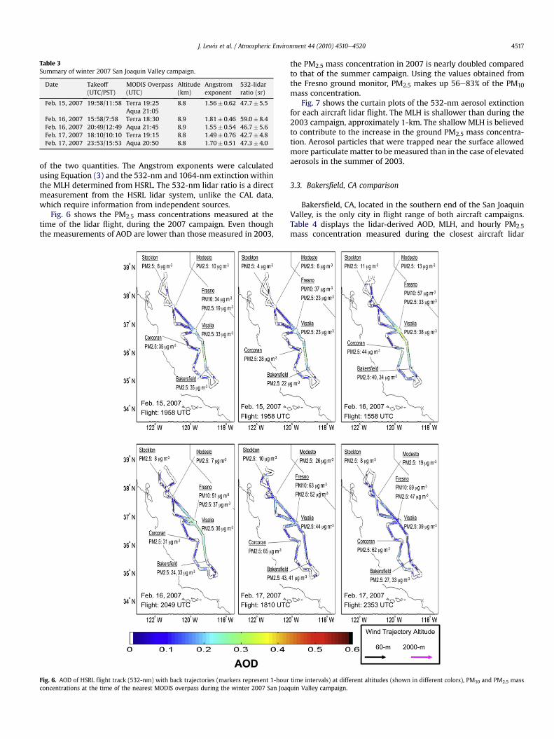
Table 3Summary of winter 2007 San Joaquin Valley campaign.

Date Takeoff(UTC/PST)

MODIS Overpass(UTC)

Altitude(km)

Angstromexponent

532-lidarratio (sr)

Feb. 15, 2007 19:58/11:58 Terra 19:25 8.8 1.56� 0.62 47.7� 5.5Aqua 21:05

Feb. 16, 2007 15:58/7:58 Terra 18:30 8.9 1.81� 0.46 59.0� 8.4Feb. 16, 2007 20:49/12:49 Aqua 21:45 8.9 1.55� 0.54 46.7� 5.6Feb. 17, 2007 18:10/10:10 Terra 19:15 8.8 1.49� 0.76 42.7� 4.8Feb. 17, 2007 23:53/15:53 Aqua 20:50 8.8 1.70� 0.51 47.3� 4.0

J. Lewis et al. / Atmospheric Environment 44 (2010) 4510e4520 4517

of the two quantities. The Angstrom exponents were calculatedusing Equation (3) and the 532-nm and 1064-nm extinction withinthe MLH determined from HSRL. The 532-nm lidar ratio is a directmeasurement from the HSRL lidar system, unlike the CAL data,which require information from independent sources.

Fig. 6 shows the PM2.5 mass concentrations measured at thetime of the lidar flight, during the 2007 campaign. Even thoughthe measurements of AOD are lower than those measured in 2003,

Fig. 6. AOD of HSRL flight track (532-nm) with back trajectories (markers represent 1-hourconcentrations at the time of the nearest MODIS overpass during the winter 2007 San Joaq

the PM2.5 mass concentration in 2007 is nearly doubled comparedto that of the summer campaign. Using the values obtained fromthe Fresno ground monitor, PM2.5 makes up 56e83% of the PM10mass concentration.

Fig. 7 shows the curtain plots of the 532-nm aerosol extinctionfor each aircraft lidar flight. The MLH is shallower than during the2003 campaign, approximately 1-km. The shallow MLH is believedto contribute to the increase in the ground PM2.5 mass concentra-tion. Aerosol particles that were trapped near the surface allowedmore particulatematter to bemeasured than in the case of elevatedaerosols in the summer of 2003.

3.3. Bakersfield, CA comparison

Bakersfield, CA, located in the southern end of the San JoaquinValley, is the only city in flight range of both aircraft campaigns.Table 4 displays the lidar-derived AOD, MLH, and hourly PM2.5mass concentration measured during the closest aircraft lidar

time intervals) at different altitudes (shown in different colors), PM10 and PM2.5 massuin Valley campaign.

Fig. 7. Curtain plots of the 532-nm lidar extinction during the winter 2007 San Joaquin Valley campaign. Bakersfield, CA is indicated in each plot.

J. Lewis et al. / Atmospheric Environment 44 (2010) 4510e45204518

overpass for each campaign day. The ratio of the mean AOD to themean MLH is nearly the same for both the winter (0.140� 0.057)and summer (0.136� 0.037) campaigns. Similarly, the product ofthe mean PM2.5 mass concentration and mean MLH is nearly thesame for both the winter (29.2� 9.1) and summer (25.6� 9.1)campaigns, which may suggest an inverse relationship betweenthe two.

Fig. 8 shows the mean 532-nm aerosol extinction profile nearBakersfield for the entire 2003 summer campaign compared witha similar mean profile from the 2007 winter campaign. The profilesterminate at ground level in both cases. As previously mentioned,the MLH is higher in the summer than in the winter. Also note the

elevated peak in aerosol extinction during the summer campaign;whereas, aerosol extinction peaks near the surface during thewinter.

It is interesting to note that in Fig. 1, the major species differencebetween February and June is ammonium nitrate. It is hypothesizedthat the differences in the summer and winter aerosol extinctionprofiles in Fig. 8 can be explained in terms of ammonium nitratechemistry. Ammonium nitrate (NH4NO3) is formed in a reversiblereaction of ammonia (NH3; animal waste) and nitric acid (HNO3;oxidation of combustion sources).

NH3 þHNO3#NH4NO3 (4)

Table 5Yearly comparison of MODIS AOD within the San Joaquin Valley (SJV)

Year Mean AOD within SJV % Difference

Winter (February) Summer (June)

2003 0.0758� 0.0368 0.1620� 0.0607 722004 0.0969� 0.0521 0.1146� 0.0491 172005 0.1237� 0.0706 0.1438� 0.0398 152006 0.1035� 0.0565 0.2130� 0.2289 692007 0.1392� 0.0829 0.1147� 0.0411 �195-year 0.1117� 0.0688 0.1500� 0.1179 29

The percent difference was calculated using the difference between the summer andwinter AOD divided by the mean.

Table 4Comparison of summer and winter lidar and PM2.5 data near Bakersfield, CA.

2003 summer campaign (CAL) 2007 winter campaign (HSRL)

Date AOD MLH(km)

Hourly PM2.5

(mgm�3)Date AOD MLH

(km)Hourly PM2.5

(mgm�3)

June 3 0.2472 1.63 19.5 Feb. 15 0.1855 1.32 18.9June 5 0.2423 1.57 21.9 Feb. 16 0.2020 1.11 35.8June 5 0.2579 1.81 17.0 Feb. 16 0.2371 1.17 29.7June 11 0.2244 1.24 9.0 Feb. 17 0.0604 0.51 32.1June 12 0.1696 1.54 18.5 Feb. 17 0.0504 0.87 30.0June 17 0.1145 1.47 13.5Mean 0.2093 1.54 16.6 Mean 0.1471 1.00 29.3St. Dev. 0.056 0.19 4.6 St. Dev. 0.086 0.32 6.3

J. Lewis et al. / Atmospheric Environment 44 (2010) 4510e4520 4519

The reaction favors the formation of ammonium nitrate underconditions of high relative humidity and low temperature, as seenin the winter in the San Joaquin Valley (Chow and Egami, 1997;Stockwell et al., 2000). In the winter profile of Fig. 8, ammoniumnitrate is formed close to the ground due to generally humidconditions that enhance gas to particle conversion resulting in highPM2.5 concentrations. Conversely, during the summer which is lesshumid at the ground, less gas-to-particle conversion takes place atthe surface and the PM2.5 concentration is lower than in thewinter.Within the boundary layer the gas phase ammoniumnitraterises and converts to the particle phase as the humidity increasesresulting in the increased aerosol extinction at 500 m in thesummer profile of Fig. 8. This is partially confirmed by the results ofNeuman et al. (2003) where they made in situ aircraft measure-ments of particle concentration in May 2002 and measured a verysimilar profile to that shown in the summer lidar profile in Fig. 8.

3.4. Seasonal AOD-PM2.5 comparisons

The 10�10-km2 operationalMODISAOD (Level 2, Collection 005)from Aqua was used to determine the mean AOD in the San JoaquinValley for themonths of February (winter) and June (summer) during

Fig. 8. Comparison of mean 532-nm aerosol extinction profiles near Bakersfield, CA forsummer 2003 campaign (dashed line) and 2007 winter campaign (solid line). Eachaerosol profile terminates at the ground level.

theyears between 2003and2007. Dateswhen cloud cover preventedAODretrievalswere removed fromthe comparison resulting ina totalof 103 retrievals in winter and 174 retrievals in summer. Table 5shows the comparison of the mean AOD within the San JoaquinValley for each year. The summer AOD is generally higher than thewinter AODwith the exception of 2007, whichmight be explained bywildfire activity. The lowest number of wildfire incidents (3610)occurred in 2007, which was 33% lower than the 5-year average (CALFIRE, 2007). Table 6 shows the comparison of mean FRM PM2.5measured in Bakersfield (5558 California Avenue site) in the monthsof February and June for the years between 2003 and 2008. In allcases, PM2.5 concentration is highest in the winter.

The seasonal trends of AOD and PM2.5 found from the satelliteand surface data generally agree with the findings of the 2003 and2007 aircraft lidar campaigns. While the PM2.5 mass concentrationis always higher in the winter, the MODIS AOD is higher in thesummer (with the exception of 2007). Over the five-year timeperiod, the PM2.5 in winter is 68% higher than the summer PM2.5;however, the summer AOD is 29% higher than the winter AOD.

A likely explanation for the difference is in the summer elevatedaerosols due to higher MLH and aloft layers from wildfires add tothe MODIS AOD, but are not completely measured by PM2.5monitors on the surface. By contrast, in the winter, low inversionlayers combined with wood burning result in high PM2.5measurements, even at low AODs.

4. Discussion

Aerosol distributions in the San Joaquin Valley, as measured bytwo different aircraft lidar systems and MODIS sensors onboardTerra and Aqua satellites, are compared for summer (June 2003)and winter (February 2007). MODIS AOD data are being explored asan indicator of ground air quality (Hoff and Christopher, 2009), andin the San Joaquin Valley this is important as the Valley hassignificant air quality concerns. While satellite data give a broadarea picture of the AOD, they do not give the vertical distribution ofthe aerosols, which is why lidar measurements are needed. Thesedata must then be correlated with ground-based PM2.5 measure-ments to understand the air quality throughout the Valley.

Table 6Yearly comparison of PM2.5 mass concentration within the San Joaquin Valley.

Year Mean PM2.5 within SJV (mg/m3) % Difference

Winter (February) Summer (June)

2003 37.1� 13.6 17.8� 4.5 702004 30.7� 11.5 18.2� 4.7 742005 33.2� 17.1 13.0� 4.7 872006 36.4� 17.8 17.0� 6.4 732007 37.0� 27.2 19.4� 3.4 625-year 34.9� 18.1 17.1� 5.2 68

The percent difference was calculated using the difference between the winter andsummer PM2.5 divided by the mean.

J. Lewis et al. / Atmospheric Environment 44 (2010) 4510e45204520

MODIS AOD tended to be higher in the summer than in thewinter campaign and highly non-uniform throughout the Valley. Acomparison of summer and winter MODIS AOD from 2003 to 2007showed the AOD in the summer exceeded the winter AOD by 29%.However, during the same time period, the winter PM2.5 massconcentration exceeded the summer PM2.5 mass concentration byan average of 68%. Generally AOD increased toward the southernend of the Valley. The two lidar campaigns had different flighttracks, but they did overlap in the Bakersfield, CA area where thesummer lidar campaign had an average AOD of 0.21 with a groundPM2.5 of 16.6 mgm�3 and the winter lidar campaign had an averageAOD of 0.15 with a ground PM2.5 of 29.3 mgm�3. The correspondingaverage MLHs were 1.54 km (summer) and 1.0 km (winter),showing a correlation between the reduced MLH and increase inPM2.5 concentration during the winter.

While the PM2.5 sources are different in the summer and winterseasons, the MLH does seem to play a significant role in the PM2.5 asmeasured on the ground. If the MLH and the associated PM2.5 massconcentration are multiplied together the summer value is25.6 mgm�3 km and the winter value is 29.2 mgm�3 km, nearly thesame for the Bakersfield area. It would be interesting to determine ifthis value remains fairly constant throughout the year resulting in analternate way to approximate the PM2.5 concentration using theMLH. Themean lidarprofiles near Bakersfield shown in Fig. 8 seemtoreflect the ammonium nitrate chemistry in the San Joaquin Valley. Itis hypothesized that ammoniumnitrate, which is the largest varyingparticulatematter constituent in the San Joaquin Valley, is connectedto the variations in the MLH. The summer lidar profiles consistentlyshowedan increase in extinction above the groundmaking the useofMODIS AOD as an indicator of ground PM2.5 problematic.

The increased use of ground-based aerosol lidars in the SanJoaquin Valley could, along with the broader area MODIS AOD data,substantially improve the understanding of air quality. A networkof lidar systems collocated with the current ground PM2.5 monitorsshould be implemented in the San Joaquin Valley in order to assessthe role the MLH plays in the seasonal variation in PM2.5measurements.

Acknowledgements

The authors thank James J. Szykman, Jassim A. Al-Saadi, Chris A.Hostetler, JohnathanW. Hair, Anthony L. Cook, and David B. Harper,for the planning, collection, and use of the 2007 San Joaquin ValleyHSRL data. This research is supported by the US EPA AdvancedMonitoring Initiative and NASA Applied Sciences Program.

References

Ackermann, J., 1998. The extinction-to-backscatter ratio of tropospheric aerosol:a numerical study. J. Atmos. Oceanic Technol. 15, 1043e1050.

Al-Saadi, J.A., et al., 2005. Improving national air quality forecasts with satelliteaerosol observations. Bull. Amer. Meteor. Soc. 86, 1249e1261.

Al-Saadi, J.A., et al., 2008. Application of satellite aerosol optical depth and airbornelidar data for monitoring fine particulate formation and transport in San Joa-quin Valley, California. In: Preprints, 10th Conference on Atmospheric Chem-istry. Amer. Meteor. Soc., New Orleans, LA.

Andrews, S.S., et al., 2002. On-farm assessment of soil quality in California’s CentralValley. Agron. J. 94, 12e23.

Boers, R., Eloranta, E.W., Coulter, R.L., 1984. Lidar observation of mixed layerdynamics: test of parameterized entrainment models of mixed layer growthrate. J. Appl Meteor. Climat. 23, 247e266.

California Department of Forestry and Fire Protection (CAL FIRE), 2007. Wildfireactivity statistics. Available from: <http://www.fire.ca.gov/fire_protection/fire_protection_fire_info_redbooks.php>.

Chow, J.C., Egami, R.T., 1997. San Joaquin Valley Integrated Monitoring Study: Docu-mentation, Evaluation, andDescriptive Analysis of PM10 and PM2.5, and PrecursorGas Measurements. Technical Support Studies No. 4 and No. 8, Final Report forCalifornia Regional Particulate Air Quality Study. Technical Report. California AirResources Board/Desert Research Institute, Sacramento, CA/Reno, NV.

Chow, J.C., Watson, J.G., Lowenthal, D.H., Hackney, R., Magliano, K., Lehrman, D.,Smith, T., 1999. Temporal variations of PM2.5, PM10, and gaseous precursorsduring the 1995 integrated monitoring study in Central California. J. Air WasteManage. Assoc. 49, PM16ePM24.

Chu, D.A., Kaufman, Y.J., Remer, L.A., Holben, B.N., 1998. Remote sensing of smokefrom MODIS airborne simulator during the SCAR-B experiment. J. Geophys. Res.103, 31979e31988.

Chu, D.A., Kaufman, Y.J., Ichoku, C., Remer, L.A., Tanré, D., Holben, B.N., 2002. Vali-dation of MODIS aerosol optical depth retrieval over land. Geophys. Res. Lett.29, 8007. doi:10.1029/2001GL013205.

Davis, K.J., Gamage, N., Hagelberg, C.R., Kiemle, C., Lenschow, D.H., Sullivan, P.P.,2000. An objective method for deriving atmospheric structure from airbornelidar observations. Amer. Meteor. Soc. 17, 1455e1468.

De Young, R.J., Grant, W.B., Severance, K., 2005. Aerosol transport in the CaliforniaCentral Valley observed by airborne lidar. Environ. Sci. Technol. 39, 8351e8357.

Engel-Cox, J.A., Holloman, C.H., Coutant, B.W., Hoff, R.M., 2004. Qualitative andquantitative evaluation of MODIS satellite sensor data for regional and urbanscale air quality. Atmos. Environ. 38, 2495e2509.

Fernald, F.G., Herman, B.M., Reagan, J.A., 1972. Determination of aerosol heightdistributions by lidar. Appl. Meteorol. 11, 482e489.

Fernald, F.G., 1984. Analysis of atmospheric lidar observations: some comments.Appl. Opt. 23, 652e653.

Gili, C., De Young, R., 2006. A Compact Efficient Lidar Receiver For MeasuringAtmospheric Aerosols. NASA Tech. Rep. NASA/TP-2006-213950.

Hair, J.W., et al., 2008. Airborne high spectral resolution lidar for profiling aerosoloptical properties. Appl. Opt. 47, 6734e6753.

Hoff, R.M., Christopher, S.A., 2009. Critical review: remote sensing of particulatepollution from space: have we reached the promised land? J. Air & WasteManage. Assoc. 59, 645e675. doi:10.3155/1047-3289.59.6.645.

Holben, B.N., et al., 2001. An emerging ground-based aerosol climatology: aerosoloptical depth from AERONET. J. Geophys. Res. 106, 12067e12097.

King, M.D., Kaufman, Y.J., Tanré, D., Nakajima, T., 1999. Remote sensing of tropo-spheric aerosols from space: Past, present, and future. Bull. Amer. Meteor. Soc.80, 2229e2259.

Kumar, N., Chu, A., Foster, A., 2007. An empirical relationship between PM2.5 andaerosol optical depth in Delhi metropolitan. Atmos. Environ. 41, 4492e4503.

Kumar, N., Chu, A., Foster, A., 2008. Remote sensing of ambient particles inDelhi and itsenvirons: estimation and validation. Int. J. Remote Sens. 29 (12), 3383e3405.

Lewis, J., De Young, R., Chu, D.A., 2010. A study of air quality in the southeasternHampton-Norfolk-Virginia Beach region with airborne lidar and MODIS aerosoloptical depth retrievals. J. Appl. Meteor. Climat 49, 3e19.

Mattis, I., Ansmann, A., Müller, D., Wandinger, U., Althausen, V., 2004. Multiyearaerosol observations with dual-wavelength Raman lidar in the framework ofEARLINET. J. Geophys. Res. 109, D13203. doi:10.1029/2004JD004600.

Neuman, J.A., et al., 2003. Variability in ammonium nitrate formation and nitric aciddepletionwith altitude and locationover California. J. Geophys. Res.108, 6-1e6-12.

Remer, L.A., et al., 2005. The MODIS aerosol algorithm, products, and validation. J.Atmos. Sci. 62, 947e973. doi:10.1175/JAS3385.1.

Remer, L.A., et al., 2006. Algorithm For Remote Sensing of Tropospheric AerosolFrom Land: Collection 5. Available from:. ATBD-MOD-96, NASA Goddard SpaceFlight Center <http://modis-atmos.gsfc.nasa.gov/reference_atbd>.

Rogers, R., et al., 2009. NASA LaRC airborne high spectral resolution lidar aerosolmeasurements during MILAGRO: observations and validation. Atmos. Chem.Phys. 9, 4811e4826.

San Joaquin Valley Air Pollution Control District, 2008a. Annual report to thecommunity. Available from: <http://www.valleyair.org/General_info/pubdocs/2008AnnualReportfinal-web.pdf>.

San Joaquin Valley Air Pollution Control District, 2008b. 2008 PM2.5 plan e finaladopted. Available from: <http://www.valleyair.org/air_quality_plans/AQ_Final_Adopted_PM25_2008.htm>.

Sasano, Y., Browell, E.V., 1989. Light scattering characteristics of various aerosoltypes derived from multiple wavelength lidar observations. Appl. Opt. 28 (9),1670e1679.

Smith, T.B., Lehrman, D.E., Reible, D.D., Shair, F.H., 1981a. The origin and fate ofairborne pollutants within the San Joaquin Valley. In: Extended Summary andSpecial Analysis Topics, vol. 1. Prepared for California Air Resources Board/Meteorology Research Inc./California Institute of Technology, Sacramento, CA/Altadena, CA/Pasadena, CA.

Smith, T.B., Lehrman, D.E., Reible, D.D., Shair, F.H., 1981b. The origin and fate ofairborne pollutants within the San Joaquin valley. In: Extended Summary andSpecial Analysis Topics, Vol. 2. Prepared for California Air Resources Board/Meteorology Research Inc./California Institute of Technology, Sacramento, CA/Altadena, CA/Pasadena, CA.

Smith, T.B., Saunders, W.D., Takeuchi, D.M., 1984. Application of ClimatologicalAnalyses to Minimize Air Pollution Impacts in California. Prepared undercontract AZ-119-32 for California Air Resources Board/Meteorology ResearchInc., Sacramento, CA/Altadena, CA.

Stockwell, W.R., Watson, J.G., Robinson, N.F., Steiner, W., Sylte, W.W., 2000. Theammonium nitrate particle equivalent of NOx emissions for wintertime condi-tions in Central California’s San Joaquin Valley. Atmos. Environ. 34, 4711e4717.

Strawbridge, K.B., Hoff, R.M., 1996. LITE validation experiments along California’scoast: preliminary results. Geo. Res. Lett. 23, 73e76.

Tsai, T.-C., et al. Analysis of the relationship between MODIS aerosol optical depthand particulate matter from 2006 to 2008, Atmos. Environ., in press, doi:10.1016/j.atmosenv.2009.10.006.