Creating Reprojected True Color MODIS Images: A Tutorial

Creating Reprojected True Color MODIS Images: A Tutorial

Liam Gumley Space Science and Engineering Center, University of Wisconsin-‐‑Madison

Jacques Descloitres and Jeffrey Schmaltz

MODIS Rapid Response Team, NASA Goddard Space Flight Center

Version 1.0.1, August 16, 2007 (updated web links)

2

Corresponding author address: Liam Gumley Space Science and Engineering Center University of Wisconsin-‐‑Madison 1225 W. Dayton St. Madison, WI 53706 USA (608) 265-‐‑5358 [email protected]

3

1.0 Introduction The Moderate Resolution Imaging Spectroradiometer (MODIS) instruments onboard the Terra and Aqua spacecraft are providing a wealth of spectral and spatial information about the planet Earth. One of the most aesthetically pleasing products from MODIS is the true color images (also known as natural color images) of the Earth at 250 meter spatial resolution. MODIS is the first imaging sensor in Earth orbit to provide such images at relatively high spatial resolution over a wide swath (2330 kilometers). Examples of MODIS true color images may be found at the following sites: MODIS home page: http://modis.gsfc.nasa.gov/ MODIS Rapid Response System: http://rapidfire.sci.gsfc.nasa.gov/ University of Wisconsin-‐‑Madison: http://cimss.ssec.wisc.edu/ The purpose of this document is to explain how MODIS true color images may be created from MODIS Level 1B image and geolocation data. Detailed examples, including source code, are presented. Several freely available software packages are used, as well as one commercial package (IDL). 1.1 FTP Site All of the source code, scripts, and sample data files described in this document, as well as the latest version of this document, are available at the following FTP site: ftp://ftp.ssec.wisc.edu/pub/IMAPP/MODIS/TrueColor/ 1.2 Required Software This tutorial requires you to install a variety of freely available software. All of the software is designed to run on the UNIX operating system (sorry, no Windows), and the examples shown were created on Red Hat Intel Linux. However, other UNIX systems may be used if you wish.

4

In order to run the examples shown in this tutorial, the following software packages are required: MODIS Corrected Reflectance (look for “NDVI” at the following site): http://directreadout.gsfc.nasa.gov/index.cfm?section=downloads&page=technology The corrected reflectance program is named crefl.c. MODIS Swath to Grid Toolbox (MS2GT): http://nsidc.org/data/modis/ms2gt/ ImageMagick: http://www.imagemagick.org/ Interactive Data Language (IDL): http://www.ittvis.com/idl/index.asp http://www.ittvis.com/download/download.asp If you do not have a license for IDL, you can still run the IDL Virtual Machine (VM) to run pre-‐‑compiled versions of the IDL software described in this document. The IDL VM is included in the IDL 6.0 distribution package available for download at the website mentioned above. Simply install the IDL 6.0 package on your system according to the instructions at the site above, and you will be able to run the example code via IDL VM. Note: The software described in this document has been tested with IDL versions 6.0 and 5.5 on Red Hat Intel Linux. It is your responsibility to download and install these packages. Please direct any questions about installation to the respective software providers. 1.3 Acknowledgements Terry Haran and Ken Knowles at NSIDC created the MODIS Swath to Grid Toolbox (MS2GT), the best freely available package for reprojecting MODIS images known to the authors. John Cristy and the co-‐‑authors of ImageMagick are recognized for developing an excellent set of tools for adjust ing and converting digital images.

5

2.0 MODIS Fundamentals The Terra and Aqua spacecraft both have MODIS instruments onboard. Terra was launched in December 1999, and has a 10:30 am local descending orbit. Aqua was launched in May 2002, and has a 1:30 pm local time ascending orbit. Data from MODIS are transmitted in real-‐‑time by direct broadcast on both Terra and Aqua, and are also recorded onboard for subsequent playback to specialized ground stations. MODIS scans a swath of 2330 km across track by 10 km along track. The double sided scan mirror allows a scan rate of 40.6 scans per minute (1.477 seconds per scan). The orbital period is roughly 100 minutes; inclination is approximately 98 degrees, and altitude is around 705 km.

MODIS has 36 spectral bands in the range 0.4 to 14.4 microns. Bands 1 and 2 are sampled at 250 meter nadir spatial resolution; Bands 3-‐‑7 at 500 meter resolution; and Bands 8-‐‑36 at 1000 meter resolution. For the purpose of this document, the primary spectral bands of interest are bands 1 (red), 4 (green), and 3 (blue). The characteristics of these bands are shown in Table 1.

Table 1: MODIS True Color Bands Band Bandwidth (microns) Spatial resolution (meters) 1 0.62 – 0.67 250 4 0.54 – 0.57 500 3 0.46 – 0.48 500

2.1 MODIS Level 1 Data Products The following data products are required for creating MODIS true color images: Level 1B Radiance at 1000, 500, and 250 meter resolution: (MOD021KM, MOD02HKM, MOD02QKM for Terra), (MYD021KM, MYD02HKM, MYD02QKM for Aqua). AND Level 1A Geolocation at 1000 meter resolution: (MOD03 for Terra), (MYD03 for Aqua).

6

Note that MODIS data from the GSFC Level 1 and Atmosphere Archive and Distribution System (LAADS), or data produced by the International MODIS/AIRS Processing Package (IMAPP) may be used. To search and order global MODIS data, visit the GSFC LAADS at: http://ladsweb.nascom.nasa.gov/data/search.html It is your responsibility to select the appropriate Level 1B data files to cover the scene of interest. However, some useful tools for selecting granules are SSEC Terra and Aqua Orbit Tracks: http://www.ssec.wisc.edu/datacenter/terra/ MODIS Rapid Response Near Real Time Browser: http://rapidfire.sci.gsfc.nasa.gov/realtime/ Note that you may need more than one granule to cover the scene of interest.

7

3.0 Corrected Reflectance The MODIS Corrected Reflectance algorithm (crefl.c) was developed by Jacques Descloitres at NASA/GSFC. The purpose of this algorithm is to provide natural-‐‑looking images by removing gross atmospheric effects, such as Rayleigh scattering, from MODIS visible bands 1-‐‑7. In particular, the algorithm produces quasi-‐‑true-‐‑color images from MODIS bands 1, 3, 4. In contrast, the MODIS land surface reflectance product (MOD09) is a more complete atmospheric correction algorithm that includes aerosol correction, and is designed to derive land surface properties. In clear atmospheric conditions the corrected reflectance product is very similar to the MOD09 product, but they depart from each other in presence of aerosols. If you wish to perform a complete atmospheric correction, please do not use the corrected reflectance algorithm. 3.1 Required Input Files The MODIS Level 1B radiance files at 1000, 500, and 250 meter resolution (MOD021KM, MOD02HKM, and MOD02QKM) and the geolocation file at 1000 meter resolution (MOD03) are required1. All spatial resolutions are required because we want the option of using any of the MODIS spatial resolutions to create reprojected images. The corrected reflectance algorithm (crefl.c) obtains low resolution geolocation information from the MOD021KM file. However, the MOD03 geolocation is required later when reprojected images are created. Note that either DAAC or IMAPP format Level 1B files may be used. The sample files used in this tutorial are from Terra MODIS and were acquired on 21 January 2003 at 16:00 UTC: MOD021KM.A2003021.1600.004.2003022113345.hdf MOD02HKM.A2003021.1600.004.2003022113345.hdf MOD02QKM.A2003021.1600.004.2003022113345.hdf MOD03.A2003021.1600.004.2003022060031.hdf These are the only MODIS files required to make true color images using the method described in this tutorial. 3.2 Running the Corrected Reflectance Algorithm 1 Aqua MODIS files from the DAAC have the prefix MYD.

8

The corrected reflectance algorithm is implemented in a C program named crefl.c, written by Jacques Descloitres. This program opens the input HDF files, reads the MODIS radiances, and computes the corrected reflectance for each MODIS pixel. The output is written to a HDF file as scaled integers. By default , MODIS bands 1, 3, and 4 are processed, however you can select any combination of MODIS bands 1-‐‑7. The example script for running the algorithm is shown below: #!/bin/csh # Script to create MODIS corrected reflectance files # Check the input arguments if ($#argv != 4) then echo "Usage" Crefl.csh MOD01KM MOD02HKM MOD02QK M MOD03" exit(1) endif ln -f -s $1 MOD021KM.hdf ln -f -s $2 MOD02HKM.hdf ln -f -s $3 MOD02QKM.hdf ln -f -s $4 MOD03.hdf setenv ANCPATH $HOME/NDVI/run $HOME/NDVI/NDVI.src/crefl -f -v -1km \ MOD02HKM.hdf MOD02QKM.hdf MOD021KM.hdf -of=crefl.1km.hdf $HOME/NDVI/NDVI.src/crefl -f -v -500m \ MOD02HKM.hdf MOD02QKM.hdf MOD021KM.hdf -of=crefl.hkm.hdf $HOME/NDVI/NDVI.src/crefl -f -v -250m \ MOD02HKM.hdf MOD02QKM.hdf MOD021KM.hdf -of=crefl.qkm.hdf

For input arguments, the script expects the full path and name of the MOD021KM, MOD02HKM, MOD02QKM, and MOD03 files. In case the input file names do not correspond to the DAAC file name conventions, the script creates a soft link to file names in the DAAC format which is expected by the program. Then the environment variable ANCPATH is set to the path where the ancillary terrain information file tbase.hdf is located (this file is distributed with crefl.c). Finally the corrected reflectance program is run three times; once for each MODIS spatial resolution (selected with the –1km, -‐‑500m, and –250m flags). The output file is named via the –of parameter. In this example, the output corrected reflectance files are named crefl.1km.hdf (1000 meter resolution) crefl.hkm.hdf (500 meter resolution) crefl.qkm.hdf (250 meter resolution) For more information on the input parameters accepted by crefl.c, run the program with no input arguments.

9

3.3 Corrected Reflectance File Format Each output file created by crefl.c contains one SDS array for each MODIS band. For example, the 1000 meter resolution file contains the following arrays2: $ ncdump -h crefl.1km.hdf netcdf crefl.1km { dimensions: fakeDim0 = 2030 ; fakeDim1 = 1354 ; fakeDim2 = 2030 ; fakeDim3 = 1354 ; fakeDim4 = 2030 ; fakeDim5 = 1354 ; variables: short CorrRefl_01(fakeDim0, fakeDim1) ; CorrRefl_01:_FillValue = 32767s ;

short CorrRefl_03(fakeDim2, fakeDim3) ; CorrRefl_03:_FillValue = 32767s ; short CorrRefl_04(fakeDim4, fakeDim5) ; CorrRefl_04:_FillValue = 32767s ; }

The arrays named CorrRefl_01, CorrRefl_02, and Corr_refl_03 contain the corrected reflectance values for MODIS bands 1, 3, and 4, respectively. The values are stored as 16-‐‑bit signed integers with a scale factor of 0.0001. To retrieve the unscaled value, the following equation is used unscaled = scaled * 0.0001 IDL routines: get_corr_refl.pro, hdf_sd_varread.pro, hdf_sd_varinfo.pro

2 ncdump is available as part of the HDF4 toolkit at http://hdf.ncsa.uiuc.edu

10

4.0 Resolution Sharpening MODIS has only two bands at 250 meter resolution: bands 1 and 2. If you want to create true color images at 250 meter resolution, you must sharpen the MODIS green and blue bands (4 and 3) from 500 meter to 250 meter resolution. The resolution sharpening algorithm can be described as follows: First, compute the spatial resolution ratio from MODIS band 1 R = B1* / B1 where R spatial resolution ratio, B1* band 1 at 500 m resolution, interpolated to 250 m resolution, B1 band 1 at 250 m resolution. Then the sharpened MODIS bands 3 and 4 are computed by B3 = B3* / R

B4 = B4* / R where B3*, B4* bands 3 and 4 at 500 m resolution, interpolated to 250 m resolution, B3, B4 bands 3 and 4 at 250 m resolution. The spatial resolution ratio encodes the difference in image resolution for band 1. If you make the assumption that the same resolution difference exists for bands 3 and 4, you can use the spatial resolution ratio to sharpen the green and blue bands. While this method works well for creating true color images, this tutorial does not try to make a case for the scientific integrity of the sharpening algorithm. 4.1 Image Interpolation for Resolution Sharpening The algorithm described in the previous section requires that bands 1, 3, and 4 at 500 meter resolution be interpolated to the equivalent of 250 meter resolution. To

11

be more precise, it requires that each band be bilinearly interpolated, earth scan by earth scan, to 250 meter resolution. You must also take account of the fact that the centers of the first 1000, 500, and 250 meter pixels across track on each earth scan are co-‐‑registered. It is crucial that each earth scan be interpolated separately. Do not use a general purpose interpolation routine (like CONGRID or REBIN in IDL) which assumes you simply want to “blow up” the image to 250 meter resolution, as artifacts will be introduced at the edge of the MODIS swath. Note that one earth scan includes 10 along-‐‑track MODIS 1000 meter pixels. IDL routines: modis_level1b_hkm2qkm.pro

12

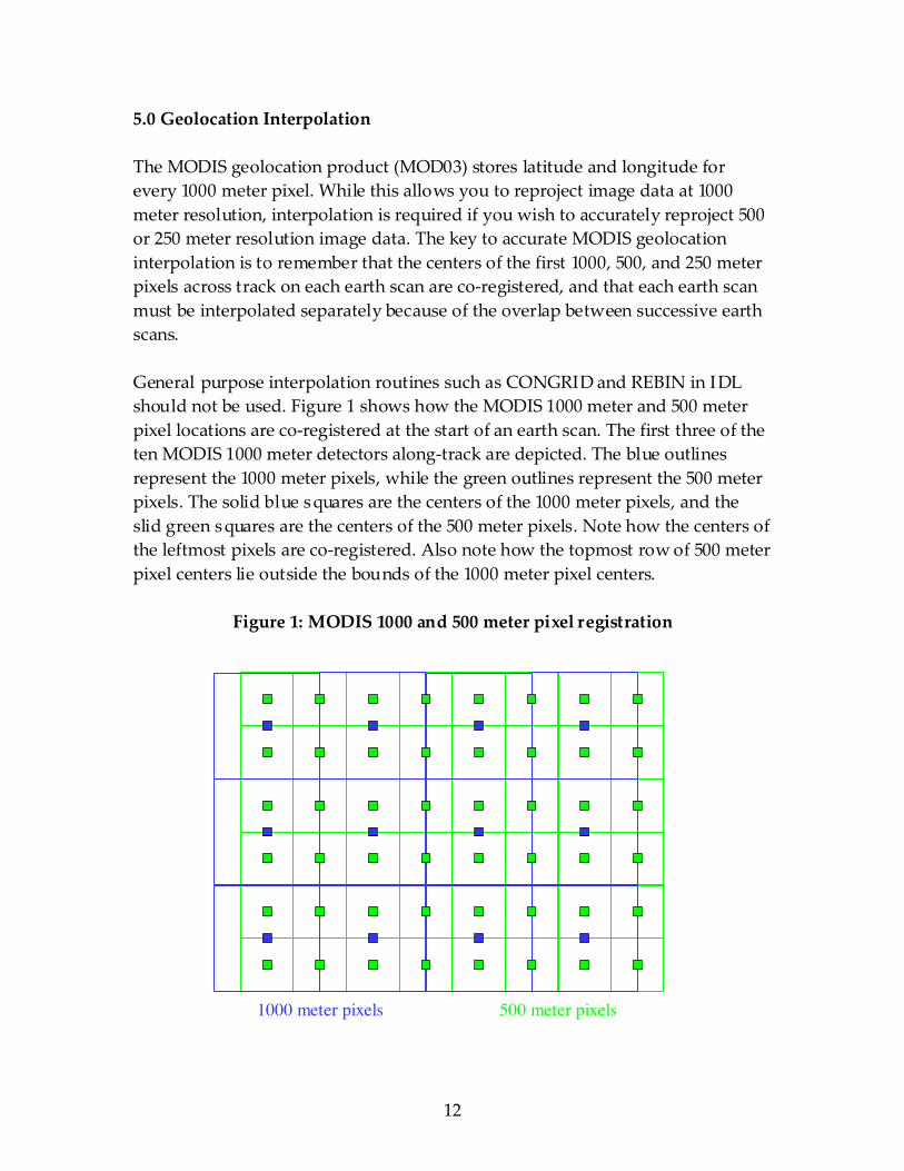
5.0 Geolocation Interpolation The MODIS geolocation product (MOD03) stores latitude and longitude for every 1000 meter pixel. While this allows you to reproject image data at 1000 meter resolution, interpolation is required if you wish to accurately reproject 500 or 250 meter resolution image data. The key to accurate MODIS geolocation interpolation is to remember that the centers of the first 1000, 500, and 250 meter pixels across track on each earth scan are co-‐‑registered, and that each earth scan must be interpolated separately because of the overlap between successive earth scans. General purpose interpolation routines such as CONGRID and REBIN in IDL should not be used. Figure 1 shows how the MODIS 1000 meter and 500 meter pixel locations are co-‐‑registered at the start of an earth scan. The first three of the ten MODIS 1000 meter detectors along-‐‑track are depicted. The blue outlines represent the 1000 meter pixels, while the green outlines represent the 500 meter pixels. The solid blue squares are the centers of the 1000 meter pixels, and the slid green squares are the centers of the 500 meter pixels. Note how the centers of the leftmost pixels are co-‐‑registered. Also note how the topmost row of 500 meter pixel centers lie outside the bounds of the 1000 meter pixel centers.

Figure 1: MODIS 1000 and 500 meter pixel registration

1000 meter pixels 500 meter pixels

13

To interpolate the 1000 meter geolocation data to 500 meter resolution, a bilinear interpolation algorithm is applied to each earth scan. For the first and last row of 500 meter pixels, bilinear extrapolation is used. A similar method is used to interpolate the geolocation data to 250 meter resolution. IDL routines: get_geodata.pro, modis_geo_interp_500.pro, modis_geo_interp_250.pro

14

6.0 Reprojecting to a Map Grid with MS2GT The MODIS Swath-‐‑to-‐‑Grid Toolbox (MS2GT), developed by Terry Haran and Ken Knowles, allows MODIS image data to be reprojected to a map grid easily and efficiently. While the standard MS2GT distribution package provides a collection of Perl scripts, IDL routines, and C code, in this tutorial you will use just two of the low-‐‑level reprojection routines, named ll2cr.c and fornav.c. While MS2GT supports a variety of map projections, we’ll use the Lambert Azimuthal Equal Area Projection for the example presented here. The basic decisions you need to make when using MS2GT are: (1) What will be the center latitude and longitude of your reprojected image? (2) What will be the grid resolution of the projected image? (3) Which spatial resolution of MODIS do you want to use as input? Note that it does not have to equal the grid resolution. For example, you could use 500 meter resolution MODIS data to create a reprojected image at 1000 meter grid resolution. (4) What will be the dimensions of the reprojected image (number of columns and rows)? The center latitude and longitude is usually chosen to coincide with a certain feature of interest on the Earth’s surface. It is easy and relatively fast to generate low resolution reprojected images (say 2000 meter grid resolution), so you can always experiment with different center lat/lons and image dimensions until you get the right coverage area. To demonstrate, the Table 2 shows the dimensions of an image with a landscape aspect ratio at different grid resolutions:

Table 2: Landscape image dimensions vs. grid resolution Width (columns) Height (rows) Grid Resolution (m) Map Scale3 (x10-‐‑6)

550 425 2000 8.0 1100 850 1000 4.0 2200 1700 500 2.0 4400 3400 250 1.0

3 Assuming there are 40 pixels per centimeter (the default in IDL)

15

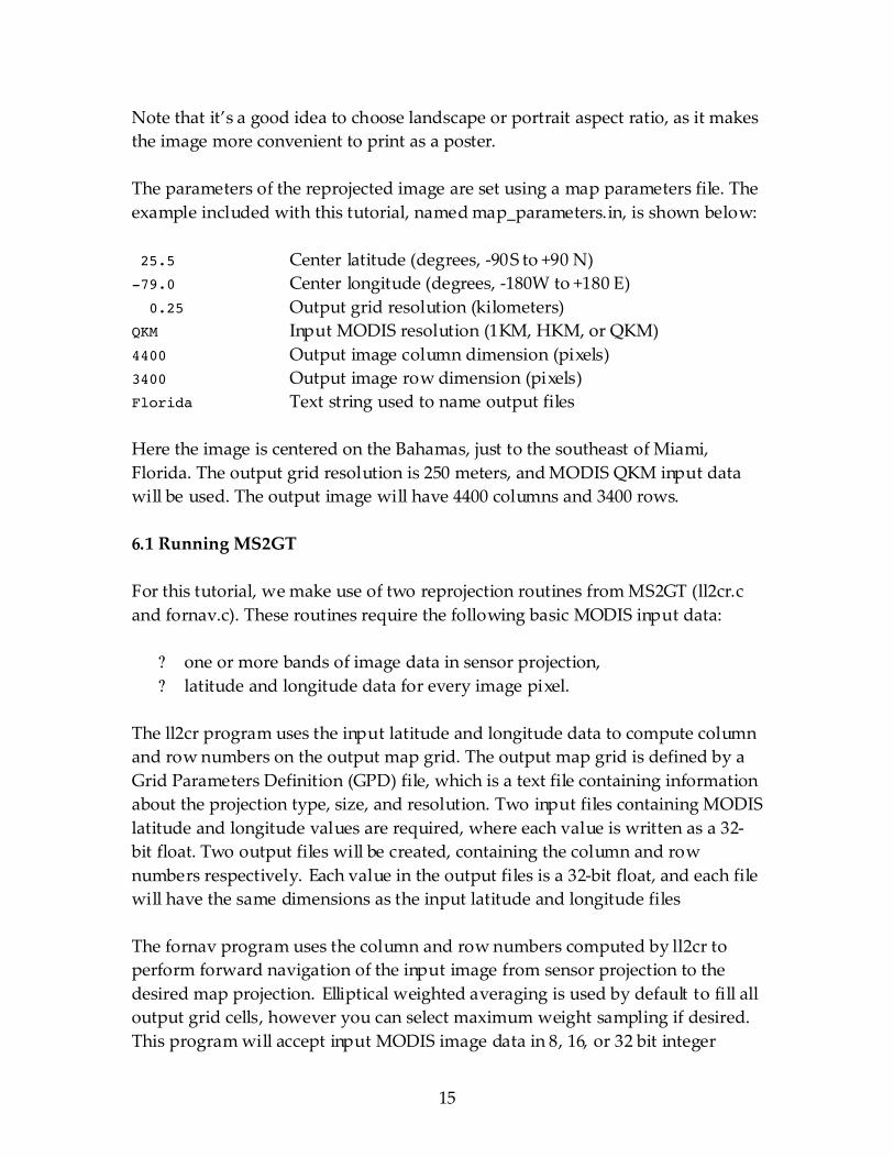
Note that it’s a good idea to choose landscape or portrait aspect ratio, as it makes the image more convenient to print as a poster. The parameters of the reprojected image are set using a map parameters file. The example included with this tutorial, named map_parameters.in, is shown below: 25.5 Center latitude (degrees, -‐‑90S to +90 N) -79.0 Center longitude (degrees, -‐‑180W to +180 E) 0.25 Output grid resolution (kilometers) QKM Input MODIS resolution (1KM, HKM, or QKM) 4400 Output image column dimension (pixels) 3400 Output image row dimension (pixels) Florida Text string used to name output files Here the image is centered on the Bahamas, just to the southeast of Miami, Florida. The output grid resolution is 250 meters, and MODIS QKM input data will be used. The output image will have 4400 columns and 3400 rows. 6.1 Running MS2GT For this tutorial, we make use of two reprojection routines from MS2GT (ll2cr.c and fornav.c). These routines require the following basic MODIS input data:

? one or more bands of image data in sensor projection, ? latitude and longitude data for every image pixel.

The ll2cr program uses the input latitude and longitude data to compute column and row numbers on the output map grid. The output map grid is defined by a Grid Parameters Definition (GPD) file, which is a text file containing information about the projection type, size, and resolution. Two input files containing MODIS latitude and longitude values are required, where each value is written as a 32-‐‑bit float. Two output files will be created, containing the column and row numbers respectively. Each value in the output files is a 32-‐‑bit float, and each file will have the same dimensions as the input latitude and longitude files The fornav program uses the column and row numbers computed by ll2cr to perform forward navigation of the input image from sensor projection to the desired map projection. Elliptical weighted averaging is used by default to fill all output grid cells, however you can select maximum weight sampling if desired. This program will accept input MODIS image data in 8, 16, or 32 bit integer

16

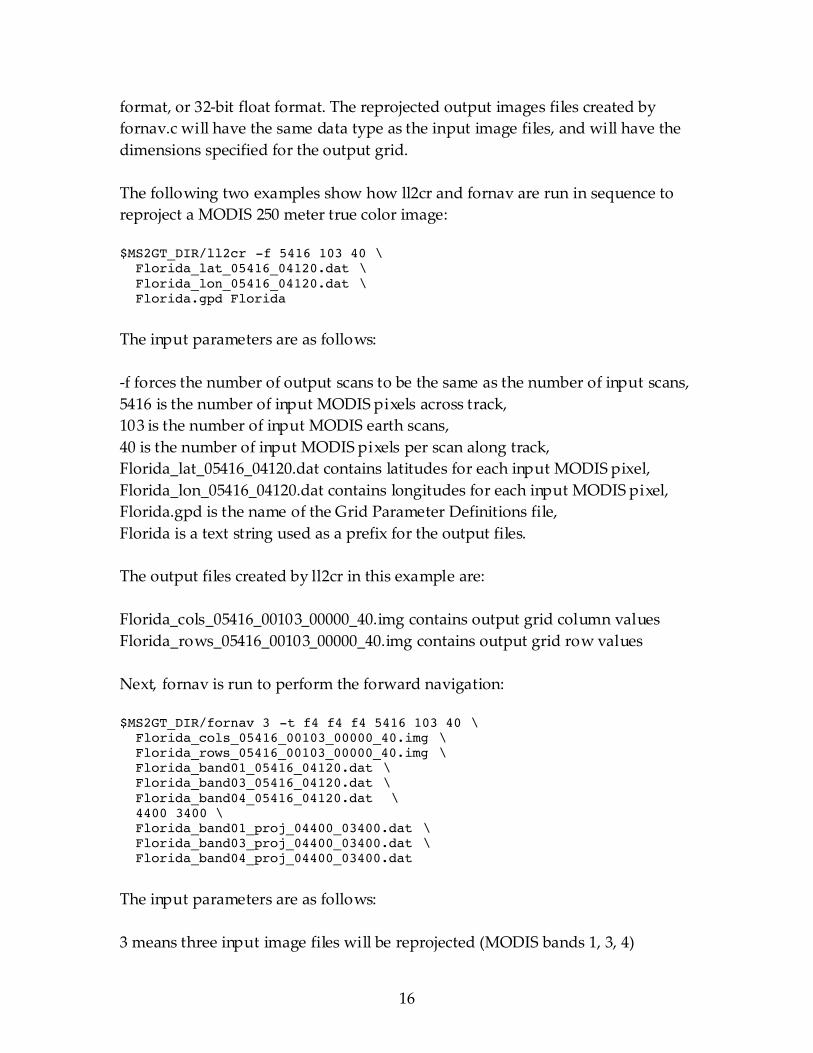
format, or 32-‐‑bit float format. The reprojected output images files created by fornav.c will have the same data type as the input image files, and will have the dimensions specified for the output grid. The following two examples show how ll2cr and fornav are run in sequence to reproject a MODIS 250 meter true color image: $MS2GT_DIR/ll2cr -f 5416 103 40 \ Florida_lat_05416_04120.dat \ Florida_lon_05416_04120.dat \ Florida.gpd Florida

The input parameters are as follows: -‐‑f forces the number of output scans to be the same as the number of input scans, 5416 is the number of input MODIS pixels across track, 103 is the number of input MODIS earth scans, 40 is the number of input MODIS pixels per scan along track, Florida_lat_05416_04120.dat contains latitudes for each input MODIS pixel, Florida_lon_05416_04120.dat contains longitudes for each input MODIS pixel, Florida.gpd is the name of the Grid Parameter Definitions file, Florida is a text string used as a prefix for the output files. The output files created by ll2cr in this example are: Florida_cols_05416_00103_00000_40.img contains output grid column values Florida_rows_05416_00103_00000_40.img contains output grid row values Next, fornav is run to perform the forward navigation: $MS2GT_DIR/fornav 3 -t f4 f4 f4 5416 103 40 \ Florida_cols_05416_00103_00000_40.img \ Florida_rows_05416_00103_00000_40.img \ Florida_band01_05416_04120.dat \ Florida_band03_05416_04120.dat \ Florida_band04_05416_04120.dat \ 4400 3400 \ Florida_band01_proj_04400_03400.dat \ Florida_band03_proj_04400_03400.dat \ Florida_band04_proj_04400_03400.dat

The input parameters are as follows: 3 means three input image files will be reprojected (MODIS bands 1, 3, 4)

17

-‐‑t f4 f4 f4 means the type of each input image file is 32-‐‑bit float 5416 is the number of input MODIS pixels across track, 103 is the number of input MODIS earth scans, 40 is the number of input MODIS pixels per scan along track, Florida_cols_05416_00103_00000_40.img contains output grid column values Florida_rows_05416_00103_00000_40.img contains output grid row values Florida_band01_05416_04120.dat contains MODIS band 1 data Florida_band03_05416_04120.dat contains MODIS band 3 data Florida_band04_05416_04120.dat contains MODIS band 4 data 4400 is the number of columns in the output grid 3400 is the number of rows in the output grid The output files created by fornav in this example are Florida_band01_proj_04400_03400.dat contains reprojected MODIS band 1 data Florida_band03_proj_04400_03400.dat contains reprojected MODIS band 3 data Florida_band04_proj_04400_03400.dat contains reprojected MODIS band 4 data The reprojected output files are stored as 32-‐‑bit floats, and the dimensions are the number of columns and rows in the output grid. IDL routines: create_gpd.pro, create_scr.pro, image_bounds.pro, map_limits.pro, get_limits.pro, remap_corr_refl.pro

18

7.0 Enhancing the Image and Creating TIFF Output Now that you have created reprojected MODIS corrected reflectances for bands 1, 3, and 4, it is necessary to convert the floating point values to RGB brightness. A non-‐‑linear enhancement is used to increase the brightness of darker portions of the scene, such as land or water. The enhancement table used in this tutorial was developed by Jacques Descloitres at NASA/GSFC. Table 3 lists the set points for the enhancement. Note that this enhancement table was designed for scenes which do not contain bright clouds.

Table 3: Non-‐‑linear Brightness Enhancement Table (non cloud) Input Brightness Output Brightness

0 0 30 110 60 160 120 210 190 240 255 255

To apply the enhancement curve, you first convert the floating point reflectances to 8-‐‑bit brightness using a linear mapping. For example, a typical conversion would linearly scale reflectances in the range 0.0 to 1.1 to brightness in the range 0 to 255. For scenes containing no clouds, you may wish to use a reflectance rage of 0.0 to 0.8. Once you have linearly scaled brightness values, the non-‐‑linear enhancement described in Table 3 can be applied to create the final scaled image. Note that the same enhancement is used on each of the MODIS bands (1, 3, 4). 7.1 Creating TIFF Output TIFF 24-‐‑bit format is used for the output image, where each channel is represented by an 8-‐‑bit byte value. The mapping of MODIS bands to RGB channels is as follows: Band 1 ? Red channel; Band 4 ? Green channel; Band 3 ? Blue channel The output image is written as a band-‐‑interleaved uncompressed TIFF. IDL routines: enhance.pro, modis_true.pro

19

8.0 Image adjustments The final touches to the MODIS true color image can be made with the ImageMagick toolkit. First, the image appearance can usually be improved by enhancing the lightness and saturation of the image, and by applying a sharpening algorithm. Second, the image must be converted to a Web-‐‑friendly format such as JPEG for display on a web page. Third, reduced resolution versions of a 250 meter resolution reprojected image can be created for a smaller file sizes and for thumbnail display. The following script (Convert.csh) shows how this is done using the ImageMagick convert program: #!/bin/csh # Script to convert a MODIS true color 250 meter reprojected image # to JPEG format at 250 meter, 1000 meter, and thumbnail resolution # using the ImageMagick 'convert' utility convert -quality 85 -modulate 105,125 -sharpen 3 true.tif true_250m.jpg convert -modulate 105,125 -geometry 25% true.tif true_1000m.jpg convert -geometry 150x150 true_1000m.jpg true_thumb.jpg

The first call to the convert utility creates a JPEG version of the 250 meter resolution image, with JPEG quality set to 85%; lightness and saturation enhanced 5% and 25%, respectively; and a Laplacian sharpening operator with a radius of 3 pixels applied. The second call creates a JPEG image at 1000 meter resolution with the same lightness and saturation enhancement. The final call creates a thumbnail version of the image.

Creating Reprojected True Color MODIS Images: A Tutorial

Documents

Transcript of Creating Reprojected True Color MODIS Images: A Tutorial