Comparison of Group Testing Algorithms for Case Identification in the Presence of Test Error

Biometrics 63, 1152–1163December 2007

DOI: 10.1111/j.1541-0420.2007.00817.x

Comparison of Group Testing Algorithms for Case Identificationin the Presence of Test Error

Hae-Young Kim,1 Michael G. Hudgens,1,∗ Jonathan M. Dreyfuss,2

Daniel J. Westreich,3 and Christopher D. Pilcher4

Department of Biostatistics, School of Public Health, University of North Carolina at Chapel Hill,3107-E McGavran-Greenberg Hall, Chapel Hill, North Carolina 27599, U.S.A.

Department of Statistics and Operations Research, University of North Carolina at Chapel Hill,North Carolina 27599, U.S.A.

Department of Epidemiology, University of North Carolina at Chapel Hill,North Carolina 27599, U.S.A.

HIV/AIDS Division, University of California-San Francisco, San Francisco,California 94110, U.S.A.

∗email: [email protected]

Summary. We derive and compare the operating characteristics of hierarchical and square array-basedtesting algorithms for case identification in the presence of testing error. The operating characteristicsinvestigated include efficiency (i.e., expected number of tests per specimen) and error rates (i.e., sensitivity,specificity, positive and negative predictive values, per-family error rate, and per-comparison error rate).The methodology is illustrated by comparing different pooling algorithms for the detection of individualsrecently infected with HIV in North Carolina and Malawi.

Key words: Array; Group testing; Hierarchical; HIV; Per-comparison error rate; Per-family error rate;Predictive value; Sensitivity; Specificity.

1. IntroductionPooling of specimens to increase efficiency of screening in-dividuals for rare diseases has a long history, dating backto screening for syphilis in military inductees in the 1940s(Dorfman, 1943). Subsequently, specimen pooling or grouptesting has been applied to screening for many other in-fectious diseases (Kacena et al., 1998; Quinn et al., 2000;Centers for Disease Control and Prevention, 2003) andhas also found broader application in entomology (Venette,Moon, and Hutchinson, 2002), screening for genetic mutations(Gastwirth, 2000), the blood bank and pharmaceutical indus-tries (Jones and Zhigljavsky, 2001), and many other areas. Inthe context of infectious diseases, group testing is typicallyused for (i) case identification, i.e., detecting all individualshaving the disease of interest and (ii) prevalence estimation,i.e., estimating the proportion of individuals in the populationhaving a particular disease.

This article is motivated by examples of the former. Forinstance, currently the North Carolina Department of Pub-lic Health and investigators from the University of NorthCarolina (UNC) at Chapel Hill employ specimen poolingas part of the Screening and Tracing Active Transmission(STAT) program to detect individuals recently infected withHIV (Pilcher et al., 2002, 2005). Likewise, the newly createdCenter for HIV/AIDS Vaccine Immunology plans to employ

similar testing procedures as part of a global attempt to iden-tify acute infections (NIAID Office of Communications andPublic Liaison, 2005). This specimen pooling strategy hasalso been used to identify recent HIV infections in antibodynegative males attending STD clinics in Malawi. In these ap-plications, the problem is how to detect very rare cases ofHIV infection that elude detection by routine, standard anti-body testing assays (Pilcher et al., 2005) because they are inthe pre-antibody “acute” phase of infection. The PCR-basednucleic acid amplification tests (NAATs) that detect thesepersons are highly sensitive but (compared to antibody tests)are expensive, time consuming, and have inadequate speci-ficity (Daar et al., 2001; Hecht et al., 2002). In this case, grouptesting is used to enhance testing efficiency and accuracy ofhigh throughput screening for rare cases of acute HIV.

Case identification (or classification) was the original mo-tivation behind group testing, as proposed by Dorfman(1943). Dorfman’s algorithm entailed pooling together bio-logical specimens from several individuals and testing thesepools of specimens rather than testing each individual speci-men. If a pool tested negative, all specimens in that pool weredeclared negative. Otherwise, further testing was required toidentify positive specimens. Dorfman’s original algorithm re-quired simply testing all individual specimens within positivepools. This pooling procedure is appealing in that, for diseases

1152 C© 2007, The International Biometric Society

Comparison of Group Testing Algorithms 1153

with prevalence less than approximately 30% (Samuels, 1978;Turner, Tidmore, and Young, 1988), fewer numbers of testsare required on average to identify all cases compared toindividual testing. Numerous generalizations of Dorfman’spooling protocol have been proposed and analyzed exten-sively (Johnson, Kotz, and Wu, 1991; Du and Hwang, 1993;Lancaster and Keller-McNulty, 1998; Venette et al., 2002).The overarching result from this body of work is that grouptesting can be both more efficient and more accurate (in termsof specificity and predictive values) than individual testing.

A simple extension of Dorfman’s original procedure en-tails repeatedly dividing positive pools into smaller, non-overlapping subpools until eventually all positive specimensare individually tested. We refer to this approach as a hierar-chical group testing algorithm (Finucan, 1964; Johnson et al.,1991; Litvak, Tu, and Pagano, 1994). For example, the NCSTAT program (Pilcher et al., 2002) employs a hierarchicaltesting algorithm as follows. First, disjoint master pools of90 specimens are tested. Second, positive master pools are di-vided into 9 subpools of 10 specimens each and these subpoolsare tested. Third, specimens from positive subpools are indi-vidually tested. Similar hierarchical pooling algorithms havebeen used for the detection of recent HIV infections in Malawi(Pilcher et al., 2004) and India (Quinn et al., 2000). Whilesome methodological investigation of hierarchical group test-ing in the presence of test error exists (Johnson et al., 1991),many of these results have gone unrecognized owing to thevast and diverse group testing literature. For example, sev-eral results from Johnson et al. (1991) on hierarchical testinghave been rederived subsequently (Litvak et al., 1994; Amos,Fazier, and Wang, 2000; Gastwirth, 2000).

Array-based specimen pooling is an alternative to hierar-chical group testing that uses overlapping pools. While thecorresponding pooling algorithms are more complex, array-based group testing can be very efficient. This approach isfrequently employed in genetics (Barillot, Lacroix, and Cohen,1991; Amemiya et al., 1992; Bruno et al., 1995), but remainsunderutilized in the infectious disease setting. In its simplestform, n2 specimens are placed on an n × n matrix. Poolsof size n are made from all samples in the same row or inthe same column. These 2n pools are then tested and, as-suming no false negative tests, all positive specimens willlie at the intersection of a positive row pool and a posi-tive column pool. Any ambiguities are resolved by individ-ually testing all specimens at these intersections. Phatarfodand Sudbury (1994) derived the expected number of tests fortwo-dimensional array (i.e., matrix) group testing procedures.Berger, Mandell, and Subrahmanya (2000) extended this workto higher-dimensional arrays.

Unfortunately, there are limitations in directly applying thearray-based procedures proposed in the literature to the in-fectious disease setting. First, several proposed array poolingalgorithms do not guarantee that all cases will be unambigu-ously identified in the absence of test error (Bruno et al.,1995; Woodbury, Fitzloff, and Vincent, 1995). For example,Woodbury et al. (1995) noted that testing row and columnpools, without further testing, results in ambiguities in iden-tifying positive specimen locations. In order to resolve theseambiguities, they proposed pooling samples along diagonalsof the array. However, such an approach will not resolve all

ambiguities if all specimens in the first row and first col-umn are positive. Second, the optimal procedures proposedby Berger et al. (2000) are not necessarily clinically feasibledue to both an overly complex pooling algorithm and therequirement of extremely large numbers of specimens. Third,and perhaps most importantly, with the exception of Section 5of Phatarfod and Sudbury (1994), the array-based group test-ing literature does not consider test error, i.e., the diagnostictest is unrealistically assumed to be a gold-standard test with100% sensitivity and 100% specificity.

In this work, we study the efficiency and error rates of hier-archical and array-based pooling algorithms in the presence oftest error. Given the operational constraints of clinical labo-ratory practice, we consider only two- and three-stage testingalgorithms whereby stage refers to the number of sequentialsteps required by a particular algorithm. In Section 2, wedefine operating characteristics of testing algorithms and theassumptions of our models. We review results on the efficiencyand error rates of hierarchical algorithms in Section 3. In Sec-tions 4 and 5, we derive the efficiencies and error rates oftwo-dimensional square array pooling algorithms without andwith master pool testing. An approach to assessing variabilityassociated with the various operating characteristics is pre-sented in Section 6. The application of our results in the con-text of the detection of acute HIV is considered in Section 7.We conclude with a short discussion in Section 8. Several ofthe mathematical details are given in the Web Appendix.

2. Preliminaries2.1 AssumptionsIn order to derive operating characteristics of the various pool-ing algorithms considered, we make the assumptions enumer-ated below. These assumptions are general enough to applyto both the hierarchical and square array algorithms.

Assumption 1. All specimens are independent and identi-cally distributed with probability p of being positive.

We refer to p as the prevalence and let q = 1 − p.

Assumption 2. Given a pool P containing at least one pos-itive specimen is tested, the probability P tests positive equalsSe.

We refer to Se as the test sensitivity. Assumption 2 im-plies that the test sensitivity is independent of the numberof specimens within a pool and the number of positive spec-imens therein. It follows that Se is also the sensitivity for atest of an individual specimen, i.e., a pool of size 1. We donot consider here more elaborate models where test sensitiv-ity depends on the number of specimens within a pool, i.e.,dilution effects (Hwang, 1976; Wein and Zenios, 1996). Thepractical implication of Assumption 2 is that the results inthis article are applicable only to settings where the largestpool size is not believed to suffer appreciable dilution effects.Determination of the maximum allowable pool size will be ap-plication specific. For example, Litvak et al. (1994) considerpool sizes up to 15 specimens when using an ELISA test todetect individuals with HIV antibodies. Another example isgiven by detection of acute HIV in antibody negative popu-lations where NAATs are thought to be sufficiently sensitive

1154 Biometrics, December 2007

such that pools of size 90 or 100 are often used in practice(Quinn et al., 2000; Pilcher et al., 2002, 2005).

Assumption 3. Given a pool P containing no positive spec-imens is tested, the probability P tests positive equals 1 − Sp.

We refer to Sp as the test specificity. Assumption 3 impliestest specificity is independent of pool size.

2.2 Operating CharacteristicsIn this section, we define various operating characteristics (initalics) of testing algorithms for case identification in the pres-ence of test error.

Define efficiency of a particular pooling algorithm to be theexpected number of tests per specimen required to identify allpositive specimens. For a group testing algorithm A, denotethe efficiency by E(A).

Define pooling specificity to be the probability an individualis categorized as negative by a particular pooling proceduregiven that individual is truly negative (Johnson et al., 1991;Litvak et al., 1994). Similarly, define the pooling sensitivity tobe the probability an individual is categorized as positive by aparticular pooling procedure given that an individual is trulypositive. Denote the pooling specificity and sensitivity for A

by Sp(A) and Se(A). For example, if I denotes individualtesting, then Sp(I) = Sp and Se(I) = Se.

Define the pooling positive predictive value of A to be theprobability an individual is truly positive given they are cate-gorized as positive by A. Likewise, define the pooling negativepredictive value of A to be the probability an individual istruly negative given they are categorized as negative by A.Denote the pooling positive and negative predictive values ofA by PPV (A) and NPV (A). The predictive values are simplefunctions of Se(A) and Sp(A):

PPV (A) =pSe(A)

q[1 − Sp(A)] + pSe(A),

and

NPV (A) =qSp(A)

p[1 − Se(A)] + qSp(A).

Additionally, we consider other error rates that have beenproposed in the multiple comparisons literature (Cook andDunnett, 1998), but to our knowledge have not been consid-ered in the context of group testing. These quantities providealternative metrics for quantifying the degree of misclassifica-tion of negative individuals as positive and positive individu-als as negative.

Define the per-family error rate (PFER) to be the expectednumber of false positive classifications and the per-comparisonerror rate (PCER) to be the expected number of false pos-itive classifications divided by the total number of speci-mens (Hochberg and Tamhane, 1987). In Web Appendix A,we show that PFER(A) = nq{1 − Sp(A)} for any poolingalgorithm A, which immediately gives PCER(A) becausePFER(A) = nPCER(A), where n is the number of speci-mens to be tested.

Define the type II per-family error rate (PFER2) to be theexpected number of false negative classifications and the typeII per-comparison error rate (PCER2) to be the expected num-

ber of false negative classifications divided by the total num-ber of specimens. In Web Appendix A, we also show thatPFER2(A) = np{1 − Se(A)} for any pooling algorithm A,which gives PCER2(A) since PFER2(A) = nPCER2(A).

3. Hierarchical AlgorithmIn this section, we present the efficiency and error rates of ahierarchical group testing algorithm with S stages under As-sumptions 1–3. These results first appeared in Johnson et al.(1991), but often go unrecognized in the literature and thusare restated here.

Consider a hierarchical algorithm where a master poolof size n1 = k1k2 · · · kS−1 is tested at first stage wherek1,k2, . . . , kS−1 are positive integers. If the master pooltests positive, then k1 pools of size n2 = k2 · · · kS−1 aretested, and so forth. Denote this algorithm by A = DS(n1 :n2 : n3 : . . . : nS−1 : nS), where n1 = k1,k2 · · · kS−1, n2 =k2 · · · kS−1, . . . ,nS−1 = kS−1, nS = 1. Let Xsi be random vari-ables that equal 1 if the ith pool in sth stage tests positive,and 0 otherwise for s = 1, . . . ,S and i = 1, . . . ,n1/ns.

3.1 EfficiencyLet the number of tests be T = T 1 + T 2 + T 3 + · · ·+ TS

where T s is the number of tests at the sth stage for s =1, 2, 3, . . . ,S. Then the expected number of tests given n1

specimens equals

E(T ) = 1 + k1E(X1i) + k1k2E(X2i) + · · · + n1E(XS−1,i).

From equation (6.18) of Johnson et al. (1991),

E(Xsi) = qn1(1 − Sp)s +

s−1∑j=1

(qnj+1 − qnj )Sje(1 − Sp)

s−j

+(1 − qns)Sse , (1)

for s = 1, 2, . . . ,S − 1.From equation (1), it follows that for a two-stage hierarchi-

cal algorithm, i.e., S = 2, the expected number of tests perspecimen for D2 is

E(D2) ≡ E(T

n1

)=

1

n1+ f(n1), (2)

where f(n) ≡ (1 − Sp)qn + Se(1 − qn), is the probability

a pool of size n tests positive without any knowledge of thetrue status of the pool. For notational simplicity, we suppressthe dependence of f on the parameters p, Se, and Sp. Forgiven values of p, Se, and Sp, the optimally efficient two-stageprocedure is determined by the value of n that minimizes (2).Special cases of (2) were also derived by Litvak et al. (1994)and Gastwirth (2000). In particular, for n1 = 15, (2) reducesto the first equation in Section 2.4 of Litvak et al. (1994).Similarly, if Se = 1, (2) reduces to equation (2) of Gastwirth(2000).

For a three-stage hierarchical algorithm, i.e., S = 3, it fol-lows from equation (1) that the expected number of tests perspecimen for D3 is

E(D3) ≡ E(T

n1

)=

1

n1+f(n1)

k2

+S2e(1 − qk2) + (1 − Sp)f(n1 − k2)q

k2 . (3)


Finucan (1964) showed that, in the absence of test error,n2 =

√n1 is approximately optimal with regards to minimiz-

ing the expected number of tests per specimen. Thus in theApplication below (Section 7) we primarily consider configu-rations of D3 where n2 =

√n1.

3.2 Error RatesFrom equations (6.15) and (6.16) of Johnson et al. (1991), thepooling sensitivity and specificity of DS are

Se(DS) = SSe , (4)

and

Sp(DS) = 1 −S∑

s=1

(qns−1 − qns−1−1)Ss−1e (1 − Sp)

S−(s−1), (5)

where qn0−1 ≡ 0. It follows that the pooling sensitivity andspecificity of the Dorfman procedure (i.e., S = 2) are

Se(D2) = S2e, (6)

and

Sp(D2) = 1 − (1 − Sp)f(n1 − 1). (7)

For n1 = 15, (6) and (7) reduce to equations (1) and (4) ofLitvak et al. (1994). For S = 3, the pooling sensitivity andspecificity are Se(D3) = S3

e, and Sp(D3) = 1 − [(1 − Sp){(1 −Sp)f(n1 − k2)q

k2−1 + S2e(1 − qk2−1)}]. Note that because S3

e ≤S2

e ≤ Se, neither D2 nor D3 will ever improve over individualtesting in terms of sensitivity.

4. Square Array without Master Pool TestingIn this section, we derive the operating characteristics of atwo-stage square array testing algorithm in the presence oftesting error, denoted by A2(n : 1). In particular, considerthe n × n square array set-up of Phatarfod and Sudbury(1994), where n2 specimens are placed on an n × n matrix.Pools are then made from all samples in the same row or inthe same column. These 2n pools (n row pools and n columnpools) are then tested and, assuming no test error, all pos-itive specimens will lie at the intersection of a positive rowpool and a positive column pool. Therefore, all specimens atthe intersection of a positive row and a positive column aresubsequently tested. However, when there is testing error, onemust allow for the possibility of positive row pools and no pos-itive column pools (or vice versa). Thus we assume that the(i, j)th sample is tested individually if either both the ithrow and the jth column test positive, the ith row tests pos-itive but all columns test negative, or the jth column testspositive but all rows test negative. Let Ri represent the testoutcome of the ith row, and Cj represent the test outcomeof the jth column. Similarly, denote the true values by RT

iand CT

j . Let Xij denote the test outcome of individual (i, j)and Y ij denote the true status of individual (i, j) such thatRT

i = I[∑

jYij > 0] and CT

j = I[∑

iYij > 0]. We will make

the following additional assumption to derive efficiencies anderror rates for array pooling algorithms:

Assumption 4. Given the true status of ith row and jthcolumn, the ith row and jth column tests are conditionally in-dependent of each other.

4.1 EfficiencyLet the number of tests be T = T 1 + T 2, where T 1 = 2n corre-sponds to the row and column testing and T2 =

∑i,jT2ij cor-

responds to the possible subsequent individual testing where

T2ij =

1 if Ri = 1 and Cj = 1

1 if Ri = 1 and∑

Cj = 0

1 if∑

Ri = 0 and Cj = 1

0 otherwise.

(8)

To derive the expected number of tests, by symmetry wewrite

E(T2ij) = Pr[Ri = 1, Cj = 1] + 2Pr

[Ri = 1,

∑j

Cj = 0

].

(9)

The first component of the right-hand side of (9) equals

Pr[Ri = 1, Cj = 1] =

1∑r,c=0

Pr[Ri = 1, Cj = 1

∣∣RTi = r, CT

j = c]

× Pr[RT

i = r, CTj = c

].

Under Assumptions 1–4, direct substitution and some algebrayields

Pr[Ri =1, Cj =1] = (1 − Sp)2q2n−1 + 2Se(1 − Sp)(1 − qn−1)qn

+S2e(1 − 2qn + q2n−1)

= Sef(n)+ (1−Sp −Se)qnf(n− 1) ≡ g(n).

The second component of the right-hand side of (9) can bewritten as

1∑r=0

n∑c=0

Pr

[Ri = 1,

∑j

Cj = 0∣∣RT

i = r,∑j

CTj = c

]

× Pr

[RT

i = r,∑j

CTj = c

]. (10)

For c ∈ {0, . . . ,n}, let

β0(c) ≡ Pr

[RT

i = 0,∑j

CTj = c

]

=

(n

c

)(qn

2−cn+c)(1 − qn−1)c, (11)

β1(c) ≡ Pr

[RT

i = 1,∑j

CTj = c

]

=

(n

c

)qn

2−cn(1 − qn)c − β0(c), (12)

γ0(c) ≡ Pr

[Ri = 1,

∑j

Cj = 0∣∣RT

i = 0,∑j

CTj = c

]

= (1 − Sp)(1 − Se)cSn−c

p ,


and

γ1(c) ≡ Pr

[Ri = 1,

∑j

Cj = 0∣∣RT

i = 1,∑j

CTj = c

]

= SeSn−cp (1 − Se)

c,

where we define γ1(0) ≡ 0. Then it follows that

Pr

[Ri = 1,

∑j

Cj = 0

]

=

n∑c=0

{γ0(c)β0(c) + γ1(c)β1(c)} ≡ h(n),

such that the expected number of tests per specimen for A2is

E(A2) ≡ E(T

n2

)=

2

n+ g(n) + 2h(n). (13)

Note that if Se = Sp = 1, then h(n) = 0, g(n) = f(n) −qnf (n − 1) and f(n)= 1 − qn such that E(A2) = 2/n +1 − 2qn + q2n−1, which equals equation (2) of Phatarfod andSudbury (1994).

4.2 Error RatesFor i ∈ {1, . . . ,n} and j ∈ {1, . . . ,n},

1 − Sp(A2) = Pr[Xij = 1 |Yij = 0]

= Pr[Ri = 1, Cj = 1,Xij = 1 |Yij = 0]

+2Pr

[Ri = 1,

∑k

Ck = 0,Xij = 1 |Yij = 0

]

= Pr[Xij = 1 |Yij = 0, Ri = 1, Cj = 1]

× Pr[Ri = 1 |Yij = 0]Pr[Cj = 1 |Yij = 0]

+2Pr

[Xij = 1 |Yij = 0, Ri = 1,

∑k

Ck = 0

]

× Pr

[Ri = 1,

∑k

Ck = 0 |Yij = 0

]

= (1 − Sp)f(n− 1)2 + 2(1 − Sp)

× Pr

[Ri = 1,

∑k

Ck = 0 |Yij = 0

], (14)

where the second equality is from the definition of algorithmA2 given by (8) and the third equality holds by Assumption 4.

Note that Pr[Ri = 1 |Yij = 0] = Pr[Cj = 1 |Yij = 0] = f(n−1). Next let

h(n | y) ≡ Pr

[Ri = 1,

∑k

Ck = 0 |Yij = 0

]

=

1∑r=0

n∑c=0

Pr

[Ri = 1,

∑k

Ck = 0∣∣RT

i = r,

∑k

CTk = c, Yij = 0

]

× Pr

[RT

i = r,∑k

CTk = c

∣∣Yij = 0

],

β0(c | y) ≡ Pr

[RT

i = 0,∑k

CTk = c

∣∣Yij = 0

]=

β0(c)

q,

and

β1(c | y) ≡ Pr

[RT

i = 1,∑k

CTk = c

∣∣Yij = 0

]

= Pr

[∑k

CTk = c

∣∣Yij = 0

]− β0(c | y)

=

(n− 1

c

)(1 − qn)cqn

2−nc−1

+

(n− 1

c− 1

)(1 − qn)c−1qn

2−nc(1 − qn−1) − β0(c | y),

for c ∈ {0, . . . ,n} where β1(0 | y) ≡ 0. Then

h(n | y) =

1∑r=0

n∑c=0

βr(c | y)γr(c), (15)

since γr(c) ≡ Pr[Ri = 1,∑

kCk = 0 |RT

i = r,∑

kCT

k = c,Yij = 0]. Thus, (14) is equivalent to

Sp(A2) = 1 − {(1 − Sp)f(n− 1)2 + 2(1 − Sp)h(n | y)}. (16)

We can derive pooling sensitivity using several applicationsof Assumptions 1 and 2:

Se(A2) = Pr[Xij = 1 |Yij = 1]

= Pr[Ri = 1, Cj = 1,Xij = 1 |Yij = 1]

+2Pr

[Ri = 1,

∑k

Ck = 0,Xij = 1 |Yij = 1

]

= S3e + 2S2

e Pr[Cj = 0 |Yij = 1]∏k =j

Pr[Ck = 0]

= S3e + 2S2

e(1 − Se) Pr[Ck = 0]n−1

= S3e + 2S2

e(1 − Se){1 − f(n)}n−1. (17)

5. Square Array with Master Pool TestingWe also consider a three-stage square array testing algorithmwhere we first test a master pool of size n2. If the master pool


tests negative, the procedure stops. Otherwise, the procedurecontinues as in A2. Denote this square array testing procedurewith master pool testing by A2M(n2 : n : 1).

5.1 EfficiencyLet the number of tests be T = T 0 + T 1 + T 2 where T 0 =1 corresponds to testing the master pool, T1 corresponds topossible row and column testing, and T2 corresponds to pos-sible individual testing. To compute the efficiency of A2M, letX0 be a random variable that equals 1 if the master pool testspositive and 0 otherwise such that T 1 = 2nX 0 and E(T 1) =2nf (n2). Next write T2 =

∑i,jT2ij , where

T2ij =

1 if X0 = 1, Ri = 1 and Cj = 1

1 if X0 = 1, Ri = 1 and∑

Cj = 0

1 if X0 = 1,∑

Ri = 0 and Cj = 1

0 otherwise,

such that the expected number of tests per specimen for A2Mis E(A2M) ≡ 1

n2 + 2nf(n2) +E(T2ij), where

E(T2ij) = Pr[X0 = 1, Ri = 1, Cj = 1]

+2Pr

[X0 = 1, Ri = 1,

∑j

Cj = 0

]. (18)

It is straightforward to show the first part of the right-handside of (18) equals

Pr[X0 = 1, Ri = 1, Cj = 1]

= (1 − Sp)2qn

2(1 − Sp − Se) + Seg(n). (19)

Likewise, the second part of the right-hand side of (18), i.e.,Pr[X0 = 1, Ri = 1,

∑jCj = 0], can be written as

1∑r=0

n∑c=0

{Pr

[Ri = 1,

∑j

Cj = 0 |X0 = 1, RTi = r,

∑j

CTj = c

]

× Pr

[X0 = 1

∣∣RTi = r,

∑j

CTj = c

]

× Pr

[RT

i = r,∑j

CTj = c

]},

which implies

Pr

[X0 = 1, Ri = 1,

∑j

Cj = 0

]

= (1 − Sp)γ0(0)β0(0) + Se

n∑c=1

{γ0(c)β0(c) + γ1(c)β1(c)}

= (1 − Sp − Se)γ0(0)β0(0) + Seh(n).

Therefore the expected number of tests per specimen forA2M is

E(A2M) =1

n2 + (1 − Sp − Se)qn2

×{

2

n+ (1 − Sp)

2 + 2(1 − Sp)Snp

}+ SeE(A2).

5.2 Error RatesTo derive the pooling specificity of A2M, write

1 − Sp(A2M) = Pr[Xij = 1 |Yij = 0]

= (1 − Sp)µ(n | y) + 2(1 − Sp)ν(n | y), (20)

where

µ(n | y) = Pr[X0 = 1, Ri = 1, Cj = 1 |Yij = 0]

= f(n2 − 2n+ 1){(1 − Sp)q

n−1}2

+S2e(1 − qn−1)

{(1 − Sp)q

n−1 + f(n− 1)},

and

ν(n | y) = Pr

[X0 = 1, Ri = 1,

∑k

Ck = 0 |Yij = 0

]

= (1 − Sp)β0(0 | y)γ0(0) + Se

1∑r=0

n∑c=1

βr(c | y)γr(c),

since γr(c) = Pr[Ri = 1,∑

kCk = 0 |RT

i = r,∑

kCT

k = c,Yij = 0,X0 = 1].

Applying Assumptions 1 and 2 several times, pooling sen-sitivity equals

Se(A2M) = Pr[Xij = 1, Ri = 1, Cj = 1,X0 = 1 |Yij = 1]

+2Pr

[Xij = 1, Ri = 1,

∑k

Ck = 0,X0 = 1 |Yij = 1

]

= S4e + 2S3

e(1 − Se){1 − f(n)}n−1. (21)

6. Assessing VariabilityThus far we have presented expressions for different grouptesting algorithm parameters such as the expected number oftests, pooling sensitivity, and pooling specificity. The formu-lae for PPV and NPV and the other error rates described inSection 2.2 follow immediately. However, for a particular setof specimens, the observed number of tests may differ from theexpected number of tests due to sampling variability. Whilethe error rates for a particular set of specimens are not directlyobservable in the absence of a gold-standard test, clearly theselatent “observed” error rates may also differ from the corre-sponding parameter values due to sampling variability. Quan-tifying this uncertainty associated with the different operatingcharacteristics can be helpful in comparing different poolingstrategies. For example, if two group testing procedures havecomparable expected number of tests, the one with smallervariance may be preferable operationally.

Explicit expressions for the variance associated with thenumber of tests per specimen for D2, D3, A2, and A2M arederived in the Web Appendix B. In turn, large sample prob-ability intervals (PIs) for the observed number of tests perspecimen can be computed by appealing to the central limittheorem. For instance, suppose N samples are to be testedusing D3(n :

√n : 1) with N sufficiently larger than n. Then

there is an approximate (1 − α) probability that the observed


�

�

�

�

��

0.00

50.

020

0.10

00.

500

n

Exp

ecte

d nu

mbe

r of

test

s pe

r sp

ecim

en

4 9 16 25 36 49 64 81 100

�

�

�

�

�

�

��

�

�

�

Individual testA2 ( n:1)D2 (n:1)A2M (n: n:1)D3 (n: n:1)

��

�

�

�

�

�

�

�

0.99

970

0.99

980

0.99

990

1.00

000

n

Poo

ling

Spe

cific

ity

4 9 16 25 36 49 64 81 100

� � � � � � � � �

� � � � � � � � �

0.70

0.75

0.80

0.85

0.90

0.95

1.00

n

Poo

ling

Sen

sitiv

ity

4 9 16 25 36 49 64 81 100

� � � � � � � � �

��

��

��

��

�

0.0

0.2

0.4

0.6

0.8

1.0

n

Poo

ling

PP

V

4 9 16 25 36 49 64 81 100

� � � � � � � � �

��

�

�

�

�

�

�

�

0.00

00.

005

0.01

00.

015

0.02

00.

025

n

Poo

ling

PF

ER

4 9 16 25 36 49 64 81 100

� � � � � � � ��

��

�

�

�

�

�

�

�

0.00

00.

002

0.00

40.

006

n

Poo

ling

PF

ER

2

4 9 16 25 36 49 64 81 100

�

�

�

�

�

�

�

�

�

�

�

�

�

��

0.00

50.

020

0.10

00.

500

n

Exp

ecte

d nu

mbe

r of

test

s pe

r sp

ecim

en

4 9 16 25 36 49 64 81 100

�

�

�

�

�

�

��

�

�

�


a.

��

�

�

�

�

�

�

�

0.99

970

0.99

980

0.99

990

1.00

000

n

Poo

ling

Spe

cific

ity

4 9 16 25 36 49 64 81 100

� � � � � � � � �

b.

� � � � � � � � �

0.70

0.75

0.80

0.85

0.90

0.95

1.00

n

Poo

ling

Sen

sitiv

ity

4 9 16 25 36 49 64 81 100

� � � � � � � � �

c.

��

��

��

��

�

0.0

0.2

0.4

0.6

0.8

1.0

n

Poo

ling

PP

V

4 9 16 25 36 49 64 81 100

� � � � � � � � �

d.

��

�

�

�

�

�

�

�

0.00

00.

005

0.01

00.

015

0.02

00.

025

n

Poo

ling

PF

ER

4 9 16 25 36 49 64 81 100

� � � � � � � ��

e.

��

�

�

�

�

�

�

�

0.00

00.

002

0.00

40.

006

n

Poo

ling

PF

ER

2

4 9 16 25 36 49 64 81 100

�

�

�

�

�

�

�

�

�

f.

Figure 1. (a) Expected number of tests per specimen, (b) pooling specificity, (c) pooling sensitivity, (d) pooling PPV,(e) pooling PFER, and (f) pooling PFER2 for different algorithms assuming test sensitivity Se = 0.9, test specificity Sp =0.99, and prevalence p = 0.0002. The � denotes the three-stage hierarchical pooling algorithm employed in the NC STATProgram. Note that pooling specificity for individual testing equals Sp = 0.99 and is not shown in panel (b).

number of tests per specimen required to identify all N indi-viduals as positive or negative will be in the PI

E(D3) ± z1−α/2

√Var(D3)

N/n,

where z1−α/2 is the 1 − α/2 quantile of the standard nor-mal distribution, E(D3) is given by equation (3) and Var(D3)

follows from equation (2) in Web Appendix Section B.2. Sim-ilar reasoning can be employed to obtain PIs for the observednumber of tests using D2, A2, and A2M.

The cumulative distribution functions (CDFs) for the ob-served pooling sensitivity, specificity, and predictive values arederived in Web Appendix C. Using these CDFs, correspond-ing PIs can easily be determined. For instance, we show that


��

�

�

�

�

��

0.3

0.4

0.5

0.6

0.7

0.8

1.0

n

Exp

ecte

d nu

mbe

r of

test

s pe

r sp

ecim

en

4 9 16 25 36 49 64 81 100

�

� ��

��

��

�

a.

�

�


�

�

�

�

�

�

��

0.99

00.

992

0.99

40.

996

0.99

81.

000

n

Poo

ling

Spe

cific

ity

4 9 16 25 36 49 64 81 100

��

��

��

��

�

b.

� � � � � � � � �

0.6

0.7

0.8

0.9

1.0

n

Poo

ling

Sen

sitiv

ity

4 9 16 25 36 49 64 81 100

� � � � � � � � �

c.

�

�

�

�

�

�

��

0.80

0.85

0.90

0.95

1.00

n

Poo

ling

PP

V

4 9 16 25 36 49 64 81 100

�

�

�

�

��

��

�

d.

��

�

�

�

�

�

�

�

0.0

0.2

0.4

0.6

0.8

n

Poo

ling

PF

ER

4 9 16 25 36 49 64 81 100

� � ��

�

�

�

�

�

e.

��

�

�

�

�

�

�

�

0.0

0.5

1.0

1.5

n

Poo

ling

PF

ER

2

4 9 16 25 36 49 64 81 100

�

�

�

�

�

�

�

�

�

f.

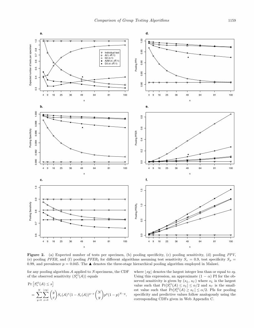
Figure 2. (a) Expected number of tests per specimen, (b) pooling specificity, (c) pooling sensitivity, (d) pooling PPV,(e) pooling PFER, and (f) pooling PFER2 for different algorithms assuming test sensitivity Se = 0.9, test specificity Sp =0.99, and prevalence p = 0.045. The � denotes the three-stage hierarchical pooling algorithm employed in Malawi.

for any pooling algorithm A applied to N specimens, the CDFof the observed sensitivity (SO

e (A)) equals

Pr[SOe (A) ≤ s

]=

N∑y=0

�sy�∑x=0

(y

x

)Se(A)x(1 − Se(A))y−x

(N

y

)py(1 − p)N−y,

where �sy� denotes the largest integer less than or equal to sy.Using this expression, an approximate (1 − α) PI for the ob-served sensitivity is given by (sL, sU ) where sL is the largestvalue such that Pr[SO

e (A) ≤ sL] ≤ α/2 and sU is the small-est value such that Pr[SO

e (A) ≥ sU ] ≤ α/2. PIs for poolingspecificity and predictive values follow analogously using thecorresponding CDFs given in Web Appendix C.


7. ApplicationUsing the results derived above, in this section we explore theoperating characteristics of individual testing, D2, D3, A2,and A2M for identification of acute HIV using NAATs. Forour first example, we consider a setting similar to the NCSTAT program. First, we assume prevalence of acute HIV isp = 0.0002 (Pilcher et al., 2005) and NAAT has a 99% testspecificity (Hecht et al., 2002) and 90% test sensitivity. Sup-pose further we are limited to a master pool size of 100 dueto dilution effects (Quinn et al., 2000). Under these assump-tions, Figure 1 depicts the efficiency, pooling sensitivity, speci-ficity, PPV and PFERs of individual testing, D2(n : 1),D3(n :√n : 1) (here k2 =

√n), A2M(n :

√n : 1), and A2(

√n : 1) as

a function of the number of specimens n. (Recall that D2(n :1) denotes two-stage hierarchical testing with pools of size nin the first stage; D3(n :

√n : 1) denotes three-stage hierar-

chical testing with pools of size n at the first stage and poolsof size

√n at the second stage; A2(

√n : 1) denotes two-stage√

n×√n array testing; and A2M(n :

√n : 1) denotes three-

stage√n×√

n array testing wherein the first stage entailstesting a master pool of size n.) The panel (a) of Figure 1indicates the two most efficient algorithms are D3 and A2Mwhen n = 100. The expected number of tests per specimenfor D3(90 : 10 : 1), the algorithm currently employed by theNC STAT program, is 0.016. For N = 8,505 total specimens(Pilcher et al., 2002), the 95% PI for efficiency of D3(90 : 10 :1) is (0.010, 0.021), which contains the observed rate of 0.018reported by Pilcher et al. (2002). Under these same condi-tions, the expected number of tests per specimen is also 0.016(95% PI: 0.008 to 0.024) for A2M(100 : 10 : 1). Panels (b) and(d) of Figure 1 indicate D3 and A2M are also preferable withregards to pooling specificity and, especially, PPV. However,these two algorithms are also the least sensitive as depicted inpanel (c) of Figure 1. Panel (e) of Figure 1 indicates D3 andA2M are preferable with regards to pooling PFER. We also seethat other algorithms are better than individual testing withregards to the efficiency, pooling specificity, PPV and PFER.Overall, these results suggest by moving from D3(90 : 10 : 1)to A2M(100 : 10 : 1), could improve pooling specificity, sensi-tivity, PPV, PCERs, and PFERs without sacrificing efficiency.In particular, given the NC STAT program processes 120,000specimens per year, this change in pooling algorithm wouldresult in a decrease in PFER2 from 6.5 to 5.1. In other words,on average one to two additional acute HIV cases would bedetected each year, representing a 5–10% increase over thecurrent detection rate (Pilcher et al., 2005).

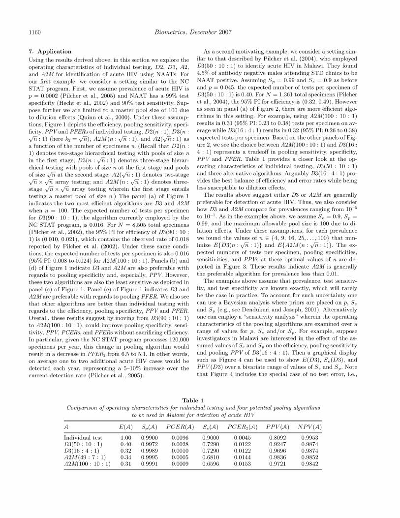
Table 1Comparison of operating characteristics for individual testing and four potential pooling algorithms

to be used in Malawi for detection of acute HIV

A E(A) Sp(A) PCER(A) Se(A) PCER2(A) PPV (A) NPV (A)

Individual test 1.00 0.9900 0.0096 0.9000 0.0045 0.8092 0.9953D3(50 : 10 : 1) 0.40 0.9972 0.0028 0.7290 0.0122 0.9247 0.9874D3(16 : 4 : 1) 0.32 0.9989 0.0010 0.7290 0.0122 0.9696 0.9874A2M(49 : 7 : 1) 0.34 0.9995 0.0005 0.6810 0.0144 0.9836 0.9852A2M(100 : 10 : 1) 0.31 0.9991 0.0009 0.6596 0.0153 0.9721 0.9842

As a second motivating example, we consider a setting sim-ilar to that described by Pilcher et al. (2004), who employedD3(50 : 10 : 1) to identify acute HIV in Malawi. They found4.5% of antibody negative males attending STD clinics to beNAAT positive. Assuming Sp = 0.99 and Se = 0.9 as beforeand p = 0.045, the expected number of tests per specimen ofD3(50 : 10 : 1) is 0.40. For N = 1,361 total specimens (Pilcheret al., 2004), the 95% PI for efficiency is (0.32, 0.49). Howeveras seen in panel (a) of Figure 2, there are more efficient algo-rithms in this setting. For example, using A2M(100 : 10 : 1)results in 0.31 (95% PI: 0.23 to 0.38) tests per specimen on av-erage while D3(16 : 4 : 1) results in 0.32 (95% PI: 0.26 to 0.38)expected tests per specimen. Based on the other panels of Fig-ure 2, we see the choice between A2M(100 : 10 : 1) and D3(16 :4 : 1) represents a tradeoff in pooling sensitivity, specificity,PPV and PFER. Table 1 provides a closer look at the op-erating characteristics of individual testing, D3(50 : 10 : 1)and three alternative algorithms. Arguably D3(16 : 4 : 1) pro-vides the best balance of efficiency and error rates while beingless susceptible to dilution effects.

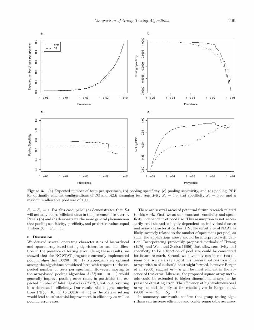
The results above suggest either D3 or A2M are generallypreferable for detection of acute HIV. Thus, we also considerhow D3 and A2M compare for prevalences ranging from 10−5

to 10−1. As in the examples above, we assume Se = 0.9, Sp =0.99, and the maximum allowable pool size is 100 due to di-lution effects. Under these assumptions, for each prevalencewe found the values of n ∈ {4, 9, 16, 25, . . . , 100} that min-imize E{D3(n :

√n : 1)} and E{A2M(n :

√n : 1)}. The ex-

pected numbers of tests per specimen, pooling specificities,sensitivities, and PPVs at these optimal values of n are de-picted in Figure 3. These results indicate A2M is generallythe preferable algorithm for prevalence less than 0.01.

The examples above assume that prevalence, test sensitiv-ity, and test specificity are known exactly, which will rarelybe the case in practice. To account for such uncertainty onecan use a Bayesian analysis where priors are placed on p, Se

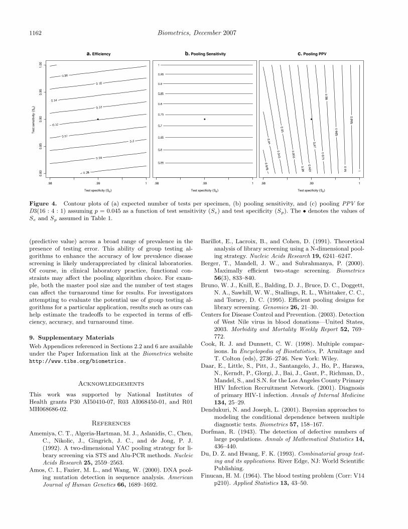
and Sp (e.g., see Dendukuri and Joseph, 2001). Alternativelyone can employ a “sensitivity analysis” wherein the operatingcharacteristics of the pooling algorithms are examined over arange of values for p, Se and/or Sp. For example, supposeinvestigators in Malawi are interested in the effect of the as-sumed values of Se and Sp on the efficiency, pooling sensitivityand pooling PPV of D3(16 : 4 : 1). Then a graphical displaysuch as Figure 4 can be used to show E(D3), Se(D3), andPPV (D3) over a bivariate range of values of Se and Sp. Notethat Figure 4 includes the special case of no test error, i.e.,


1 e-05 1 e-04 1 e-03 1 e-02 1 e-01

0.0

0.1

0.2

0.3

0.4

0.5

Prevalence

Exp

ecte

d nu

mbe

r of

test

s pe

r sp

ecim

en

a.

A2MD3

1 e-05 1 e-04 1 e-03 1 e-02 1 e-01

0.5

0.6

0.7

0.8

0.9

1.0

Prevalence

Poo

ling

Sen

sitiv

ity

c.

1 e-05 1 e-04 1 e-03 1 e-02 1 e-01

0.99

800.

9985

0.99

900.

9995

1.00

00

Prevalence

Poo

ling

Spe

cific

ity

b.

1 e-05 1 e-04 1 e-03 1 e-02 1 e-01

0.80

0.85

0.90

0.95

1.00

Prevalence

Poo

ling

PP

V

d.

Figure 3. (a) Expected number of tests per specimen, (b) pooling specificity, (c) pooling sensitivity, and (d) pooling PPVfor optimally efficient configurations of D3 and A2M assuming test sensitivity Se = 0.9, test specificity Sp = 0.99, and amaximum allowable pool size of 100.

Se = Sp = 1. For this case, panel (a) demonstrates that D3will actually be less efficient than in the presence of test error.Panels (b) and (c) demonstrate the more general phenomenonthat pooling sensitivity, specificity, and predictive values equal1 when Se = Sp = 1.

8. DiscussionWe derived several operating characteristics of hierarchicaland square array-based testing algorithms for case identifica-tion in the presence of testing error. Using these results, weshowed that the NC STAT program’s currently implementedpooling algorithm D3(90 : 10 : 1) is approximately optimalamong the algorithms considered here with respect to the ex-pected number of tests per specimen. However, moving tothe array-based pooling algorithm A2M(100 : 10 : 1) wouldgenerally improve pooling error rates, in particular the ex-pected number of false negatives (PFER2), without resultingin a decrease in efficiency. Our results also suggest movingfrom D3(50 : 10 : 1) to D3(16 : 4 : 1) in the Malawi settingwould lead to substantial improvement in efficiency as well aspooling error rates.

There are several areas of potential future research relatedto this work. First, we assume constant sensitivity and speci-ficity independent of pool size. This assumption is not neces-sarily realistic and is highly dependent on individual diseaseand assay characteristics. For HIV, the sensitivity of NAAT islikely inversely related to the number of specimens per pool; assuch, the applications above should be interpreted with cau-tion. Incorporating previously proposed methods of Hwang(1976) and Wein and Zenios (1996) that allow sensitivity andspecificity to be a function of pool size could be consideredfor future research. Second, we have only considered two di-mensional square array algorithms. Generalizations to n × marrays with m = n should be straightforward, however Bergeret al. (2000) suggest m = n will be most efficient in the ab-sence of test error. Likewise, the proposed square array meth-ods could be extended to higher-dimensional arrays in thepresence of testing error. The efficiency of higher-dimensionalarrays should simplify to the results given in Berger et al.(2000) when Se = Sp = 1.

In summary, our results confirm that group testing algo-rithms can increase efficiency and confer remarkable accuracy

1162 Biometrics, December 20070.

800.

850.

900.

951.

00

Test specificity (Sp)

(Se)

Tes

t sen

sitiv

ity

.98 .99 1

�

a. Efficiency


.98 .99 1

�

b. Pooling Sensitivity


.98 .99 1

�

c. Pooling PPV

Figure 4. Contour plots of (a) expected number of tests per specimen, (b) pooling sensitivity, and (c) pooling PPV forD3(16 : 4 : 1) assuming p = 0.045 as a function of test sensitivity (Se) and test specificity (Sp). The • denotes the values ofSe and Sp assumed in Table 1.

(predictive value) across a broad range of prevalence in thepresence of testing error. This ability of group testing al-gorithms to enhance the accuracy of low prevalence diseasescreening is likely underappreciated by clinical laboratories.Of course, in clinical laboratory practice, functional con-straints may affect the pooling algorithm choice. For exam-ple, both the master pool size and the number of test stagescan affect the turnaround time for results. For investigatorsattempting to evaluate the potential use of group testing al-gorithms for a particular application, results such as ours canhelp estimate the tradeoffs to be expected in terms of effi-ciency, accuracy, and turnaround time.

9. Supplementary MaterialsWeb Appendices referenced in Sections 2.2 and 6 are availableunder the Paper Information link at the Biometrics websitehttp://www.tibs.org/biometrics.

Acknowledgements

This work was supported by National Institutes ofHealth grants P30 AI50410-07, R03 AI068450-01, and R01MH068686-02.

References

Amemiya, C. T., Algeria-Hartman, M. J., Aslanidis, C., Chen,C., Nikolic, J., Gingrich, J. C., and de Jong, P. J.(1992). A two-dimensional YAC pooling strategy for li-brary screening via STS and Alu-PCR methods. NucleicAcids Research 25, 2559–2563.

Amos, C. I., Fazier, M. L., and Wang, W. (2000). DNA pool-ing mutation detection in sequence analysis. AmericanJournal of Human Genetics 66, 1689–1692.

Barillot, E., Lacroix, B., and Cohen, D. (1991). Theoreticalanalysis of library screening using a N-dimensional pool-ing strategy. Nucleic Acids Research 19, 6241–6247.

Berger, T., Mandell, J. W., and Subrahmanya, P. (2000).Maximally efficient two-stage screening. Biometrics56(3), 833–840.

Bruno, W. J., Knill, E., Balding, D. J., Bruce, D. C., Doggett,N. A., Sawhill, W. W., Stallings, R. L., Whittaker, C. C.,and Torney, D. C. (1995). Efficient pooling designs forlibrary screening. Genomics 26, 21–30.

Centers for Disease Control and Prevention. (2003). Detectionof West Nile virus in blood donations—United States,2003. Morbidity and Mortality Weekly Report 52, 769–772.

Cook, R. J. and Dunnett, C. W. (1998). Multiple compar-isons. In Encyclopedia of Biostatistics, P. Armitage andT. Colton (eds), 2736–2746. New York: Wiley.

Daar, E., Little, S., Pitt, J., Santangelo, J., Ho, P., Harawa,N., Kerndt, P., Glorgi, J., Bai, J., Gaut, P., Richman, D.,Mandel, S., and S.N. for the Los Angeles County PrimaryHIV Infection Recruitment Network. (2001). Diagnosisof primary HIV-1 infection. Annals of Internal Medicine134, 25–29.

Dendukuri, N. and Joseph, L. (2001). Bayesian approaches tomodeling the conditional dependence between multiplediagnostic tests. Biometrics 57, 158–167.

Dorfman, R. (1943). The detection of defective numbers oflarge populations. Annals of Mathematical Statistics 14,436–440.

Du, D. Z. and Hwang, F. K. (1993). Combinatorial group test-ing and its applications. River Edge, NJ: World ScientificPublishing.

Finucan, H. M. (1964). The blood testing problem (Corr: V14p210). Applied Statistics 13, 43–50.


Gastwirth, J. L. (2000). The efficiency of pooling in the de-tection of rare mutations. American Journal of HumanGenetics 67, 1036–1039.

Hecht, F., Busch, M., Rawal, B., Webb, M., Rosenberg, E.,Swanson, M., Chesney, M., Anderson, J., Levy, J., andKahn, J. (2002). Use of laboratory tests and clinicalsymptoms for identification of primary HIV infection.AIDS 16(8), 1119–1129.

Hochberg, Y. and Tamhane, A. C. (1987). Multiple Compari-son Procedures. New York: Wiley.

Hwang, F. K. (1976). Group testing with a dilution effect.Biometrika 63, 671–673.

Johnson, N. L., Kotz, S., and Wu, X. (1991). Inspection Errorsfor Attributes in Quality Control. New York: Chapmanand Hall Ltd.

Jones, C. M. and Zhigljavsky, A. A. (2001). Comparison ofcosts for multistage group testing methods in the phar-maceutical industry. Communications in Statistics, PartA—Theory and Methods 30(10), 2189–2209.

Kacena, K. A., Quinn, S. B., Hartman, S. C., Quinn, T. C.,and Gaydos, C. A. (1998). Pooling of urine samples forscreening for Neisseria gonorrhea by ligase chain reac-tion: Accuracy and application. Journal of Clinical Mi-crobiology 36, 3624–3628.

Lancaster, V. A. and Keller-McNulty, S. (1998). A review ofcomposite sampling methods. Journal of the AmericanStatistical Association 93, 1216–1230.

Litvak, E., Tu, X. M., and Pagano, M. (1994). Screening forthe presence of a disease by pooling sera samples. Journalof the American Statistical Association 89, 424–434.

NIAID Office of Communications and Public Liaison. (2005).NIAID Funds Center for HIV/AIDS Vaccine Immunol-ogy (CHAVI). NIAID News. Bethesda, MD.

Phatarfod, R. M. and Sudbury, A. (1994). The use of a squarearray scheme in blood testing. Statistics in Medicine 13,2337–2343.

Pilcher, C. D., McPherson, J. T., Leone, P. A., Smurzyn-ski, M., Owen-O’Dowd, J., Peace-Brewer, A. L., Harris,

J., Hicks, C. B., Eron, J. J., and Fiscus, S. A. (2002).Real-time, universal screening for acute HIV infectionin a routine HIV counseling and testing population.Journal of the American Medical Association 288, 216–221.

Pilcher, C. D., Price, M. A., Hoffman, I. F., Galvin, S., Mar-tinson, F. E., Kazembe, P. N., Eron, J. J., Miller, W. C.,Fiscus, S. A., and Cohen, M. S. (2004). Frequent detec-tion of acute primary HIV infection in men in Malawi.AIDS 18, 517–524.

Pilcher, C. D., Fiscus, S. A., Nguyen, T. Q., et al. (2005).Detection of acute infections during HIV testing in NorthCarolina. New England Journal of Medicine 352, 1873–1883.

Quinn, T. C., Brookmeyer, R., Kline, R., Shepherd, M.,Paranjape, R., Mehendale, S., Gadkari, D. A., andBollinger, R. (2000). Feasibility of pooling sera for HIV-1 viral RNA to diagnose acute primary HIV-1 infectionand estimate HIV incidence. AIDS 14, 2751–2757.

Samuels, S. M. (1978). The exact solution to the two-stagegroup-testing problem. Technometrics 20, 497–500.

Turner, D., Tidmore, F., and Young, D. (1988). A calculusbased approach to the blood testing problem. SIAM Re-view 30, 119–122.

Venette, R. C., Moon, R. D., and Hutchinson, W. D. (2002).Strategies and statistics of sampling for rare individuals.Annual Review of Entomology 47, 143–174.

Wein, L. M. and Zenios, S. A. (1996). Pooled testing for HIVscreening: Capturing the dilution effect. Operations Re-search 44, 543–569.

Woodbury, C. P., Fitzloff, J. F., and Vincent, S. S. (1995).Sample multiplexing for greater throughput in HPLCand related methods. Analytical Chemistry 67, 885–890.

Received December 2005. Revised January 2007.Accepted January 2007.

Comparison of Group Testing Algorithms for Case Identification in the Presence of Test Error

Documents

Transcript of Comparison of Group Testing Algorithms for Case Identification in the Presence of Test Error