Comparison of ensemble forecasts with the measurements from the meteorological mast at Risø...
46
PSO (FU 2101) Ensemble-forecasts for wind power Comparison of ensemble forecasts with the measurements from the meteorological mast at Risø National Laboratory Henrik Aalborg Nielsen 1 , Henrik Madsen 1 , Torben Skov Nielsen 1 , Jake Badger 2 , Gregor Giebel 2 , Lars Landberg 2 Kai Sattler 3 , Henrik Feddersen 3 1 Technical University of Denmark, Informatics and Mathematical Modelling, DK-2800 Lyngby 2 Risø National Laboratory, Wind Energy Department, DK-4000 Roskilde 3 Danish Meteorological Institute, Research and Development, DK-2100 København Ø 23rd March 2004
-
Upload
independent -
Category
Documents
-
view
3 -
download
0
Transcript of Comparison of ensemble forecasts with the measurements from the meteorological mast at Risø...

PSO (FU 2101)Ensemble-forecasts for wind power
Comparison of ensemble forecasts with the
measurements from the meteorological mast
at Risø National Laboratory
Henrik Aalborg Nielsen1, Henrik Madsen1, Torben Skov Nielsen1,
Jake Badger2, Gregor Giebel2, Lars Landberg2
Kai Sattler3, Henrik Feddersen3
1 Technical University of Denmark, Informatics and Mathematical Modelling, DK-2800 Lyngby2 Risø National Laboratory, Wind Energy Department, DK-4000 Roskilde
3 Danish Meteorological Institute, Research and Development, DK-2100 København Ø
23rd March 2004

Contents
1 Summary 4
2 Introduction 4
3 Ensemble forecasts 5
3.1 NCEP ensemble forecasts . . . . . . . . . . . . . . . . . . . . . . . . . . . 5
3.2 ECMWF medium range ensemble forecasts . . . . . . . . . . . . . . . . . . 6
3.3 HIRLAM short range ensemble forecasts . . . . . . . . . . . . . . . . . . . 6
4 Wind data and ensemble forecast data 7
5 Some properties of the ensemble forecasts 8
6 Comparison of ensemble forecasts with measurements 10
6.1 Reliability . . . . . . . . . . . . . . . . . . . . . . . . . . . . . . . . . . . . 11
6.1.1 Unadjusted ensemble forecasts . . . . . . . . . . . . . . . . . . . . . 11
6.1.2 MOS adjusted ensemble forecasts . . . . . . . . . . . . . . . . . . . 15
6.2 Resolution . . . . . . . . . . . . . . . . . . . . . . . . . . . . . . . . . . . . 23
7 Conclusion and Discussion 29
References 34
Appendices 35
A Plots of MOS adjusted ensemble forecasts 35
A.1 ECMWF corrected using the unperturbed forecast as the dependent variable. 35
1

A.2 HIRLAM corrected using the unperturbed forecast as the dependent variable. 42
2

Preface
This report is mainly based on investigations carried out in the autumn of 2003. Thereport describes the first attempt of comparing measurements (here of wind speed) withensemble forecasts. Three types of ensemble forecasts are considered. For one of these(NCEP) is was discovered after completion of the work that the unperturbed forecastwith initialization time 12:00 (UTC) is actually a modified version of the other models inthis ensemble. This may explain some of the observations reported.
3

1 Summary
Three types of ensemble forecasts of wind speed are compared with measurements 76ma.g.l. Specifically, the comparisons are performed in terms of reliability (average cor-rectness in a probabilistic sense) and resolution (sharpness of the conditional densityfunction). Ensembles from the experimental HIRLAM ensemble forecast system seem tobe reliable w.r.t. the upper quantiles (≥ 80%), but the number of cases is only 86 andon average only 17.2 should exceed the 80% quantile. The resolution of the 80% quantileis good; it varies from 1.7 to 25.7 m/s. The NCEP and ECMWF ensemble forecasts arenot reliable for the point measurement.
Since the forecasts should be interpreted as spatial averages the forecasts are adjustedusing MOS (Model Output Statistics) and then compared with the point measurements.It is argued that the usual approach to MOS adjustment possess properties which aresomewhat in conflict with ensemble forecasting. These problems are demonstrated andalternatives are suggested. However, for the short horizons (< 36 hours), all methodsyields adjusted ensemble forecasts for which the spread is too small. The spread ofthe adjusted NCEP ensembles are in general too small. For ECMWF and HIRLAMand horizons approximately in the range 36–60 hours some of the alternative methodssuggested yields reliable ensemble forecasts. For longer horizons the spread of the adjustedensemble forecasts are too wide.
Unfortunately, the methods which yields reliable ensemble forecasts have problems w.r.t.numerical instabilities, whereby only horizons up to approximately 48 hours have good res-olution. The report discuss ways to circumvent the numerical instabilities, which mainlyare caused by uncertainty on the unperturbed forecast and inefficient use of the measure-ments.
2 Introduction
This report documents investigations carried out as part of the PSO-funded projectEnsemble-forecasts for wind power (FU 2101).
In meteorological ensemble forecasting several forecasts are produced and it is hopedthat these are informative w.r.t. the predictability of the actual weather situation. Forwind power applications it is not sufficient to obtain forecasts of the near-extremes; itis necessary to be able to interpret the ensemble forecasts in a probabilistic sense. Inorder to investigate the extend to which this is possible three types of ensemble forecastsare compared with actual measurements of wind speed 76m a.g.l. from a mast at RisøNational Laboratory.
4

The wind data and ensembles are briefly described in Section 4 and some backgroundinformation on the ensemble forecast systems are given in Section 3. Section 5 describessome properties of the ensemble forecasts which can be observed in the forecast-data.In Section 6 the forecasts and MOS adjusted versions of these are compared with themeasurements w.r.t. reliability (Section 6.1) and resolution (Section 6.2). Finally, inSection 7, we conclude and discuss on the findings.
3 Ensemble forecasts
The investigations in this report make use of ensemble forecast data from numericalweather prediction (NWP) models of three meteorological centres. Two of the NWPmodels are global, and the third one is a limited-area model. The global ensemble pre-diction systems have been in operation since about a decade, within which they werecontinuously further developed. They are especially designed for the medium forecastrange with lead times beyond 3 days. The third ensemble is experimental and is designedfor the short range below 3 days lead time.
The ensemble prediction systems address the sensitivity of the weather development to theinitial condition by making use of perturbed initial conditions in order to account for theuncertainty in the analysis of the atmospheric state, from which the NWP simulations forthe forecast are to be started. Common for all three ensemble prediction systems is thatthey include the “unperturbed” forecast, which takes the original “best-guess” analysisas initial condition. It is referred to as the control forecast.
In addition to the initial condition perturbation the ensemble prediction systems make useof either different components of the NWP model or try to perturb tendencies of modelparameters in order to address uncertainties that arise during the model integration anddue to the model formulation.
Some major aspects of the ensemble prediction systems are outlined in the followingsub-sections.
3.1 NCEP ensemble forecasts
The National Center for Environmental Prediction (NCEP) and the National WeatherService of NOAA (National Oceanic and Atmospheric Administration) in the USA haveoperated an ensemble prediction system since many years [11]. It includes a global aswell as regional NWP models. The set of ensemble members consists of one unperturbedforecast and 5 pairs of perturbed forecasts. For each pair the initial condition is perturbedin the positive and negative direction of bred vectors [12], which are determined within
5

the analysis/forecasting cycle and which are regarded to reflect the largest state changesof the model atmosphere within the cycle time.
The ensemble system comprises model simulations in different horizontal resolutions andwith different lead times of up to 16 days. In this study, the interpolated medium rangeensemble data on a 1◦ horizontal grid are utilized with lead times up to 3.5 days.
3.2 ECMWF medium range ensemble forecasts
The European Centre for Medium-Range Weather Forecasts (ECMWF) has operatedtheir Ensemble prediction system1 (ECMWF-EPS) since the early 1990s [9, 6]. The setof ensemble members consists of one unperturbed forecast and 25 pairs of forecasts, forwhich the initial conditions are perturbed in the positive and negative direction of theanalysis error on basis of singular vectors [2]. The singular vectors used in the ECMWF-EPS describe the largest growth of initial state differences in accordance with the analysiserror covariances within a time of 48 hours, in which uncertainties are assumed to growlinearly. The initial perturbations are calculated as linear combinations of the singularvectors such that they cover most of the global area. They are scaled such that theiramplitude is comparable to the root-mean-square analysis error of the data assimilationsystem.
Furthermore, for each model run attempts are made to account for uncertainties in thedescription and calculation of sub-grid processes by use of stochastic physics [1]. Theseaffect the model dynamics by adding a stochastic component to the tendencies from thesub-grid parameterizations of the model. As a result two runs with the same set of initialconditions will not result in exactly the same output.
The NWP model of the ECMWF-EPS is a global spectral model with truncation atwave number 255 and with 40 vertical levels (TL255L40). The horizontal resolution iscomparable to that of a grid with about 80km mesh size. The ensemble simulations arecarried out operationally up to a lead time of 10 days.
3.3 HIRLAM short range ensemble forecasts
High resolution short range ensemble forecasts using the High Resolution Limited-AreaModel HIRLAM have been provided by the Danish Meteorological Institute (DMI). Theseare experimental ensembles and they are based on the ECMWF-EPS. They adopt a nestedmodel system from a HIRLAM model setup of a previous study with HIRLAM ensembles[10]. The forecast simulations have been performed on a grid with approximately 20kmin mesh size on a domain, which includes Danmark and the North Sea.
1http://www.ecmwf.int/products/forecasts/guide/The Ensemble Prediction System EPS.html
6
In a limited-area model, the boundary conditions need to be prescribed in addition tothe initial condition. As a simple solution, the members from the ECMWF-EPS havetherefore been chosen as host model. They can supply initial perturbations with consistentboundary data during the limited-area model simulation. Uncertainties in the initial andin the boundary conditions are addressed this way to some extent. The frequency ofavailability of the boundary data has been 6 hours. The size of this HIRLAM ensembleis the same as that of the ECMWF-EPS, namely 50 plus the control forecast.
In addition to the ECMWF-EPS members, four further model permutations have beenintegrated, too. These consist of the control simulation being integrated with differentparameterization schemes for convection and condensation in order to address modeluncertainties related to these processes. The data from these simulations were, however,not utilized in this study.
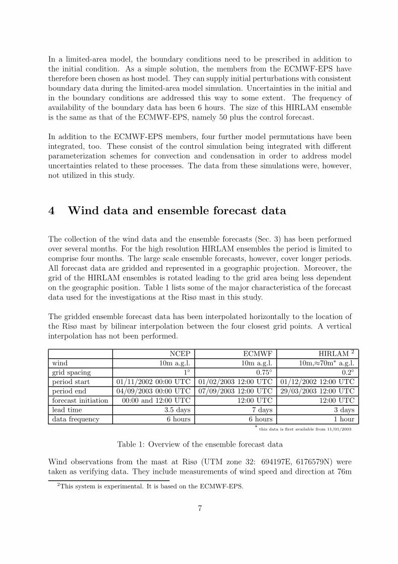
4 Wind data and ensemble forecast data
The collection of the wind data and the ensemble forecasts (Sec. 3) has been performedover several months. For the high resolution HIRLAM ensembles the period is limited tocomprise four months. The large scale ensemble forecasts, however, cover longer periods.All forecast data are gridded and represented in a geographic projection. Moreover, thegrid of the HIRLAM ensembles is rotated leading to the grid area being less dependenton the geographic position. Table 1 lists some of the major characteristica of the forecastdata used for the investigations at the Risø mast in this study.
The gridded ensemble forecast data has been interpolated horizontally to the location ofthe Risø mast by bilinear interpolation between the four closest grid points. A verticalinterpolation has not been performed.
NCEP ECMWF HIRLAM 2
wind 10m a.g.l. 10m a.g.l. 10m,≈70m∗ a.g.l.
grid spacing 1◦ 0.75◦ 0.2◦
period start 01/11/2002 00:00 UTC 01/02/2003 12:00 UTC 01/12/2002 12:00 UTC
period end 04/09/2003 00:00 UTC 07/09/2003 12:00 UTC 29/03/2003 12:00 UTC
forecast initiation 00:00 and 12:00 UTC 12:00 UTC 12:00 UTC
lead time 3.5 days 7 days 3 days
data frequency 6 hours 6 hours 1 hour∗
this data is first available from 11/01/2003
Table 1: Overview of the ensemble forecast data
Wind observations from the mast at Risø (UTM zone 32: 694197E, 6176579N) weretaken as verifying data. They include measurements of wind speed and direction at 76m
2This system is experimental. It is based on the ECMWF-EPS.
7

a.g.l., and they cover the period from 31/01/2002 23:06 to 01/09/2003 10:59 (UTC).The measurements are averages over the 10 minutes up to the time stamp, and theensemble forecast data are interpreted the same way. In the case of the data from theNCEP ensembles and for the ECMWF-EPS the time step of the model simulations islarger than the measurement interval. In the case of the HIRLAM ensembles the timestep of the model simulations is smaller than the measurement interval. The data wastherefore averaged over several time steps to represent an interval of 10 minutes. However,some uncertainty in representation remains for all models, because the ensemble forecastscorrespond to spatial averages over the grid size of the respective model. This blurs thepicture of temporal representation, even though spatial interpolation as mentioned aboveis used to obtain ensemble forecasts for the Risø mast.
5 Some properties of the ensemble forecasts
Figure 1 shows the mean and quantiles of each of the ensemble forecasts for each horizon.Interestingly the mean and median of the NCEP analysis, i.e. forecast horizon 0 hours,is approximately 2 m/s lower than the remaining mean values.
For ECMWF the mean and median has a cyclic behavior with peaks occurring at horizons0, 12, 24, 36, . . . hours. For the median the distance between the top and bottom isapproximately 0.5 m/s and slightly less for the mean. Since ECMWF is only initiatedonce daily this may just be a consequence of the diurnal variation. Actually, if NCEPforecasts are split in two groups according to the initialization of calculations (00:00 and12:00 UTC) the same kind of behavior is observed, but to a somewhat less extend (plotsnot shown).
For HIRLAM within the first 12 hours, which corresponds to the time interval 12:00 –24:00 UTC, the mean value drops from 9.5 m/s at 0 hours (12:00) to 7.2 m/s at 3 hours(15:00). Hereafter, the mean increase to 8.0 m/s at 8 hours (19:00). Note also thatfor HIRLAM the 25% and 75% quantiles seems to be in opposite phase, whereas thesequantiles seems to be in phase for ECMWF.
8

0
5
10
15
20
25
0 2 4 6
NCEP
0 2 4 6
ECMWF
0 2 4 6
HIRLAM @ 70m
Horizon (days)
Win
d sp
eed
(m/s
)
4
6
8
10
0 2 4 6
NCEP
0 2 4 6
ECMWF
0 2 4 6
HIRLAM @ 70m
Horizon (days)
Win
d sp
eed
(m/s
)
Figure 1: Mean (black) and quantiles (red) of ensemble forecasts for each horizon. Thequantiles 0, 0.05, 0.25, 0.50, 0.75, 0.95, and 1 are depicted. The top row displays part ofthe data in the bottom row (approx. 3-10 m/s).
9

6 Comparison of ensemble forecasts with measure-
ments
For wind power production applications we are interested in interpreting the ensembleforecast in a probabilistic sense. For example if 10 out of 50 ensemble members show windspeeds above 10 m/s at a particular point in the future then we would like to interpret thisas a 20% chance of wind speeds above 10 m/s at that particular point in the future. If thisproperty holds on average for all thresholds then the ensemble forecasts are called reliable.If an ensemble forecast system is reliable as compared to a particular measurement thenthe rank of the measurement, when compared with the ensemble members, is uniformlydistributed. This can be investigated by plotting a histogram of the ranks which should befairly flat [13] or by Quantile-Quantile-plots (QQ-plots) [3] where the observed quantilesare plotted against the theoretical (uniform) distribution.
However, if climatological information is available reliable (but uninformative for practicaluse) ensemble forecasts can easily be produced by random sampling from the observeddistribution. Figure 2 exemplifies this by using measurements before the first NCEPforecast as climatological information3. The obtained rank histogram is fairly flat exceptthat there is a slight over-representation of observations with low ranks; indicating thatthe observed wind speeds after 1/11/2002 is somewhat lower than before 1/11/2002.This is probably due to a relatively windy period in February and March, 2002. Note alsothat using the empirical cumulative distribution in the left panel of Figure 2 results in ahistogram of essentially the same shape; i.e. the main features of the right panel of thefigure is not due to random variation.
The problem with the ensemble forecasts generated using climatology is that the uncer-tainty indicated by the ensemble is high. For instance the 10% and 90% quantiles in theleft panel of Figure 2 is 3.0 and 11.3 m/s, respectively. This feature of “sharpness” of thedensity indicated by the ensemble of forecasts is called resolution. The ultimate goal isto have reliable ensemble forecasts with high resolution.
When comparing ensemble forecasts with a point measurement it should be noted thatthe forecasts are forecasts of a spatial average corresponding to the horizontal resolutionof the model. The measurements at a particular point may well deviate systematicallyfrom the spatial average.
Remark:
Here the terms reliability and resolution are for continuous variables as described above.It seems that in the meteorological literature (e.g. [13]) these words is often used for themore restricted case of binary variables.
3This definition of climatology is used throughout this report, it covers the period 31/01/2002 23:06– 31/10/2002 23:57 (UTC).
10

0 5 10 15 20 25
0.0
0.04
0.08
0.12
Wind speed (m/s)
Pro
babi
lity
0.0
0.2
0.4
0.6
0.8
1.0
Cum
ulat
ive
prob
abili
ty
2 4 6 8 10 12
0.0
0.04
0.08
Rank
Pro
babi
lity
1 2 3 4 5 6 7 8 9 11
Figure 2: Left: Histogram and empirical cumulative distribution for the measurementsfrom the Risø mast before the first NCEP forecast (1/11/2002). Right: Rank histogramobtained for a climatological ensemble forecast obtained by randomly picking 11 samplesin the empirical distribution at the left.
6.1 Reliability
In this section the reliability of the ensemble forecasts or ensemble forecasts adjustedusing MOS (Model Output Statistics) are investigated. In all cases only forecasts withall members present will be considered, i.e. 11 members for NCEP and 51 members forECMWF and HIRLAM. The model permutations included in the HIRLAM ensemblesare not included in the investigation.
6.1.1 Unadjusted ensemble forecasts
Figures 3 and 4 show rank histograms when comparing the three ensemble forecasts to themeasurements at the Risø mast. In case of mismatch between time points observationsare generated for the forecast time points by linear interpolation between actual timepoints. To account for unequal number of ensembles between ensemble types the rank isnormalized as indicated in the figures. The number of bins are selected as the default forthe function histogram in S-PLUS.
Generally, for all horizons ECMWF ensembles seem to have an over-representation of highranks indicating some downward bias of the forecasts as compared to the measurements.For HIRLAM the forecasts for the low horizons are generally too high as compared to themeasurements, whereas the rank histograms are fairly flat for the longer horizons. ForNCEP, generally, there is an tendency for U-shaped rank histograms, indicating that thespread of the ensemble forecasts are too low as compared to the measurements. However,for the longer horizons the rank histograms corresponding to the NCEP ensembles arefairly flat.
11

0
20
40
60
80
0.0 0.2 0.4 0.6 0.8 1.0
NCEP (10m) 0d 0h
ECMWF (10m) 0d 0h
0.0 0.2 0.4 0.6 0.8 1.0
HIRLAM (70m) 0d 0h
NCEP (10m) 0d 6h
0.0 0.2 0.4 0.6 0.8 1.0
ECMWF (10m) 0d 6h
HIRLAM (70m) 0d 6h
NCEP (10m)0d 12h
ECMWF (10m)0d 12h
HIRLAM (70m)0d 12h
NCEP (10m)0d 18h
ECMWF (10m)0d 18h
0
20
40
60
80
HIRLAM (70m)0d 18h
0
20
40
60
80
NCEP (10m) 1d 0h
ECMWF (10m) 1d 0h
HIRLAM (70m) 1d 0h
NCEP (10m) 1d 6h
ECMWF (10m) 1d 6h
HIRLAM (70m) 1d 6h
NCEP (10m)1d 12h
ECMWF (10m)1d 12h
HIRLAM (70m)1d 12h
NCEP (10m)1d 18h
ECMWF (10m)1d 18h
0
20
40
60
80HIRLAM (70m)
1d 18h0
20
40
60
80NCEP (10m)
2d 0hECMWF (10m)
2d 0hHIRLAM (70m)
2d 0hNCEP (10m)
2d 6hECMWF (10m)
2d 6hHIRLAM (70m)
2d 6h
NCEP (10m)2d 12h
ECMWF (10m)2d 12h
HIRLAM (70m)2d 12h
NCEP (10m)2d 18h
ECMWF (10m)2d 18h
0
20
40
60
80HIRLAM (70m)
2d 18h0
20
40
60
80NCEP (10m)
3d 0hECMWF (10m)
3d 0hHIRLAM (70m)
3d 0hNCEP (10m)
3d 6hECMWF (10m)
3d 6hHIRLAM (70m)
3d 6h
NCEP (10m)3d 12h
0.0 0.2 0.4 0.6 0.8 1.0
ECMWF (10m)3d 12h
0
20
40
60
80HIRLAM (70m)
3d 12h
(rank − 1)/N
Per
cent
of T
otal
Figure 3: Rank histograms for horizons up to 84 hours. Note that HIRLAM forecasts arenot available after 72 hours.
12

0
10
20
30
0.0 0.4 0.8
ECMWF (10m)3d 18h
ECMWF (10m) 4d 0h
0.0 0.4 0.8
ECMWF (10m) 4d 6h
ECMWF (10m)4d 12h
0.0 0.4 0.8
ECMWF (10m)4d 18h
ECMWF (10m) 5d 0h
0.0 0.4 0.8
ECMWF (10m) 5d 6h
ECMWF (10m)5d 12h
0.0 0.4 0.8
ECMWF (10m)5d 18h
ECMWF (10m) 6d 0h
0.0 0.4 0.8
ECMWF (10m) 6d 6h
ECMWF (10m)6d 12h
0.0 0.4 0.8
ECMWF (10m)6d 18h
0
10
20
30
ECMWF (10m) 7d 0h
(rank − 1)/N
Per
cent
of T
otal
Figure 4: ECMWF rank histograms for horizons longer than 84 hours.
Although, rank histograms give some indication of the overall reliability of the ensembleforecasts it is unclear when the rank histograms are “sufficiently uniform”. For thispurpose we propose to use QQ-plots where the normalized rank is plotted against thetheoretical quantiles of the uniform distribution on [0, 1] (U(0, 1)). Since the cumulativedistribution function of U(0, 1) is a line connecting (0,0) and (1,1) the plots are particularsimple to interpret in this case.
Figure 5 shows QQ-plots for selected horizons. Consider e.g. the 12h NCEP ensembleforecast; the maximum of this forecast (2nd axis at 1.0) is exceeded in approximately40% of the cases (1.0 − 0.6 on the 1st axis). Likewise, when the 60h HIRLAM ensembleforecast indicates that there is a 40% chance that a certain threshold will be exceeded(1− 0.6 on the 2nd axis) then the data suggests that this threshold will only be exceededin approximately 20% (1 − 0.8 on the 1st axis) of the cases. Of cause, such observationsare to be regarded as estimates and as such influenced by random variation.
Besides the information gained from the rank histograms the QQ-plots adds the insightthat the HIRLAM ensembles seems to represent the upper quantiles (approximately 80%and above) fairly well, i.e. the curves are close to the line of identity. None of theensemble forecast systems represent the lower quantiles well, except maybe for the 72hour HIRLAM forecast.
Table 2 summarizes the results when comparing the 80% ensemble quantile to the actualobservations and likewise with the 80% quantile based on climatology (as defined onpage 10). It is seen that the actual number of cases is rather small. Furthermore, itis seen that the relative frequencies of observations above the 80% ensemble quantile isconsequently lower than 20%, i.e. the 80% ensemble quantile seems seems to be too high.
13

0.0
0.2
0.4
0.6
0.8
1.0
0.0 0.2 0.4 0.6 0.8 1.0
NCEP (10m)0d 12h
ECMWF (10m)0d 12h
0.0 0.2 0.4 0.6 0.8 1.0
HIRLAM (70m)0d 12h
NCEP (10m) 1d 0h
ECMWF (10m) 1d 0h
0.0
0.2
0.4
0.6
0.8
1.0HIRLAM (70m)
1d 0h0.0
0.2
0.4
0.6
0.8
1.0NCEP (10m)
1d 12hECMWF (10m)
1d 12hHIRLAM (70m)
1d 12h
NCEP (10m) 2d 0h
ECMWF (10m) 2d 0h
0.0
0.2
0.4
0.6
0.8
1.0HIRLAM (70m)
2d 0h0.0
0.2
0.4
0.6
0.8
1.0NCEP (10m)
2d 12hECMWF (10m)
2d 12hHIRLAM (70m)
2d 12h
NCEP (10m) 3d 0h
0.0 0.2 0.4 0.6 0.8 1.0
ECMWF (10m) 3d 0h
0.0
0.2
0.4
0.6
0.8
1.0HIRLAM (70m)
3d 0h
Quantile of uniform distribution on [0,1]
(ran
k −
1)/
N
Figure 5: QQ-plots of ranks when comparing measurements with ensemble forecasts
14
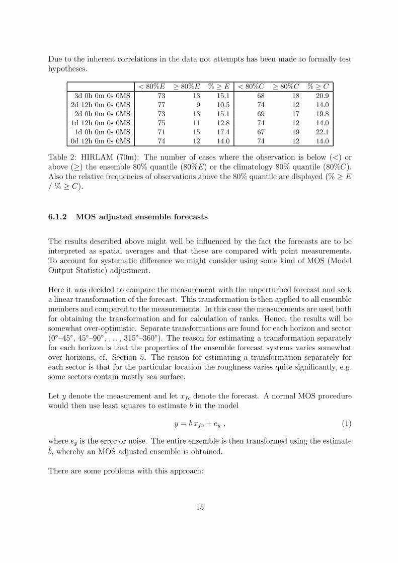
Due to the inherent correlations in the data not attempts has been made to formally testhypotheses.
< 80%E ≥ 80%E % ≥ E < 80%C ≥ 80%C % ≥ C
3d 0h 0m 0s 0MS 73 13 15.1 68 18 20.92d 12h 0m 0s 0MS 77 9 10.5 74 12 14.02d 0h 0m 0s 0MS 73 13 15.1 69 17 19.8
1d 12h 0m 0s 0MS 75 11 12.8 74 12 14.01d 0h 0m 0s 0MS 71 15 17.4 67 19 22.1
0d 12h 0m 0s 0MS 74 12 14.0 74 12 14.0
Table 2: HIRLAM (70m): The number of cases where the observation is below (<) orabove (≥) the ensemble 80% quantile (80%E) or the climatology 80% quantile (80%C).Also the relative frequencies of observations above the 80% quantile are displayed (% ≥ E/ % ≥ C).
6.1.2 MOS adjusted ensemble forecasts
The results described above might well be influenced by the fact the forecasts are to beinterpreted as spatial averages and that these are compared with point measurements.To account for systematic difference we might consider using some kind of MOS (ModelOutput Statistic) adjustment.
Here it was decided to compare the measurement with the unperturbed forecast and seeka linear transformation of the forecast. This transformation is then applied to all ensemblemembers and compared to the measurements. In this case the measurements are used bothfor obtaining the transformation and for calculation of ranks. Hence, the results will besomewhat over-optimistic. Separate transformations are found for each horizon and sector(0◦–45◦, 45◦–90◦, . . . , 315◦–360◦). The reason for estimating a transformation separatelyfor each horizon is that the properties of the ensemble forecast systems varies somewhatover horizons, cf. Section 5. The reason for estimating a transformation separately foreach sector is that for the particular location the roughness varies quite significantly, e.g.some sectors contain mostly sea surface.
Let y denote the measurement and let xfc denote the forecast. A normal MOS procedurewould then use least squares to estimate b in the model
y = b xfc + ey , (1)
where ey is the error or noise. The entire ensemble is then transformed using the estimate
b, whereby an MOS adjusted ensemble is obtained.
There are some problems with this approach:
15

• The ranks of the point measurements as compared to the adjusted ensemble willhave a tendency of non-uniformity (too few low ranks) due to the fact that ey isneglected.
• The forecast can be considered a noisy estimate of the spatial average x. If themodel y = b x + ey is the model in which we want to estimate b then using (1) willresult in an estimate of b biased towards zero. This will also produce a tendency oftoo few low ranks.
To account for the uncertainty of the forecast we might want to add an intercept a to thelinear model (1), i.e.:
y = a + b xfc + ey . (2)
An other solution is obtained by considering the point measurement to be noise free, i.e.only systematic deviations from the spatial average is present in the data. This leads toa model with the forecast as the response:
xfc = α + β y + ex , (3)
where ex is the forecast error and α and β are coefficients which are estimated using leastsquares. Estimates of intercept a and slope b by which to transform the ensemble forecastsare then obtained as:
a = −α/β and b = 1/β . (4)
However, in reality there may both be uncertainty on the forecast and random deviationbetween the spatial average and the point measurement. Technically, model (2) shouldthen be treated as an errors-in-variables problem, but this requires knowledge about theratio between the standard deviation of the forecast error (when comparing the forecastto the spatial average) and the standard deviation of the point measurement (the randomdeviation from E(y|x) = a + b x). However, this ratio is not known and therefore we justuse orthogonal regression, which corresponds to assuming the ratio to be one.
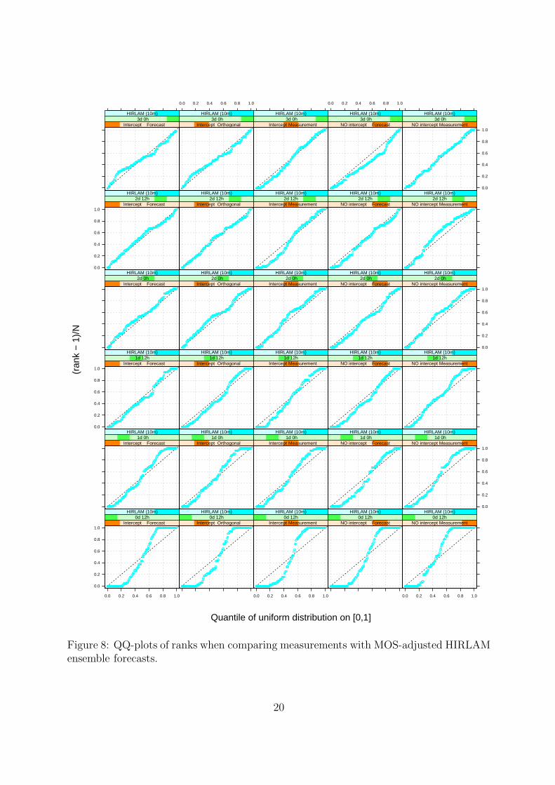
QQ-plots of the ranks obtained when using these different possibilities are shown in Fig-ures 6, 7, and 8. The labels used in the plots are:
“Intercept Forecast”: Linear regression including intercept and with the forecast asthe response, i.e. xfc = a + b y + ex fitted by least squares.
“Intercept Orthogonal”: Linear relation found by minimizing the sums of squares ofthe (orthogonal) distances between the line (including intercept) and the data points.
“Intercept Measurement”: Linear regression including intercept and with the measure-ment as the response, i.e. y = a + b xfc + ey fitted by least squares.
“NO intercept Forecast”: Linear regression excluding intercept and with the forecastas the response, i.e. xfc = b y + ex fitted by least square.
16

“NO intercept Measurement”: Linear regression excluding intercept and with the mea-surement as the response, i.e. y = b xfc + ey fitted by least squares.
From the QQ-plots it is concluded that, with respect to reliability :
• None of the QQ-plots obtained for NCEP ensembles are close to the line of identity.
• For ECMWF and HIRLAM the methods labeled “Intercept Forecast” and“Intercept Orthogonal” perform well whereas the remaining methods results inQQ-plots deviating from the line of identity. There is a tendency of “InterceptForecast” performing better than “Intercept Orthogonal”.
• For the low horizons the ensemble spread is too small (S-shaped curves).
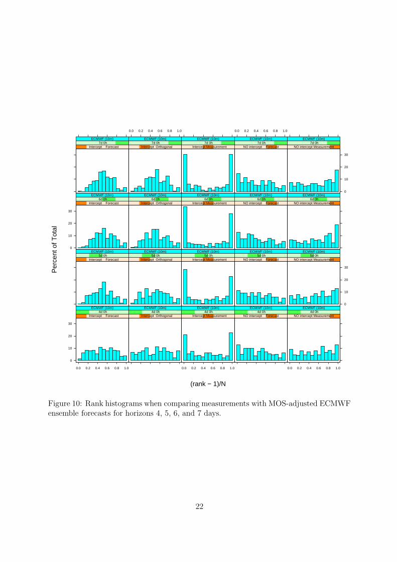
Figure 9 shows the QQ-plots for ECMWF forecasts for horizons longer than the onescovered in the plots mentioned above. The corresponding rank histograms are displayedin Figure 10. It is seen that the conclusions listed above are valid for the 4 day horizonalso. However, for horizons of 5 days or longer especially “Intercept Forecast” theadjusted ensemble forecasts are too wide, i.e. there are too many ranks near the center.Since the standard deviation of the point measurement can not depend on the forecasthorizon the results indicate that the underlying spread of the ECMWF ensemble forecastare too wide for horizons 5 days and above.
Overall for all horizons up to 7 days the method “Intercept Orthogonal” perform well,but for horizons up to approximately 3 days the method “Intercept Forecast” is betterin terms of reliability. The possibility exists that averaging of point measurements canreduce the random variation and thereby improving the estimates. .
17

0.0
0.2
0.4
0.6
0.8
1.0
0.0 0.2 0.4 0.6 0.8 1.0
Intercept Forecast0d 12h
NCEP (10m)
Intercept Orthogonal0d 12h
NCEP (10m)
0.0 0.2 0.4 0.6 0.8 1.0
Intercept Measurement0d 12h
NCEP (10m)
NO intercept Forecast0d 12h
NCEP (10m)
0.0 0.2 0.4 0.6 0.8 1.0
NO intercept Measurement0d 12h
NCEP (10m)
Intercept Forecast 1d 0h
NCEP (10m)
Intercept Orthogonal 1d 0h
NCEP (10m)
Intercept Measurement 1d 0h
NCEP (10m)
NO intercept Forecast 1d 0h
NCEP (10m)
0.0
0.2
0.4
0.6
0.8
1.0NO intercept Measurement
1d 0hNCEP (10m)
0.0
0.2
0.4
0.6
0.8
1.0 Intercept Forecast
1d 12hNCEP (10m)
Intercept Orthogonal1d 12h
NCEP (10m)
Intercept Measurement1d 12h
NCEP (10m)
NO intercept Forecast1d 12h
NCEP (10m)
NO intercept Measurement1d 12h
NCEP (10m)
Intercept Forecast 2d 0h
NCEP (10m)
Intercept Orthogonal 2d 0h
NCEP (10m)
Intercept Measurement 2d 0h
NCEP (10m)
NO intercept Forecast 2d 0h
NCEP (10m)
0.0
0.2
0.4
0.6
0.8
1.0NO intercept Measurement
2d 0hNCEP (10m)
0.0
0.2
0.4
0.6
0.8
1.0 Intercept Forecast
2d 12hNCEP (10m)
Intercept Orthogonal2d 12h
NCEP (10m)
Intercept Measurement2d 12h
NCEP (10m)
NO intercept Forecast2d 12h
NCEP (10m)
NO intercept Measurement2d 12h
NCEP (10m)
Intercept Forecast 3d 0h
NCEP (10m)
0.0 0.2 0.4 0.6 0.8 1.0
Intercept Orthogonal 3d 0h
NCEP (10m)
Intercept Measurement 3d 0h
NCEP (10m)
0.0 0.2 0.4 0.6 0.8 1.0
NO intercept Forecast 3d 0h
NCEP (10m)
0.0
0.2
0.4
0.6
0.8
1.0NO intercept Measurement
3d 0hNCEP (10m)
Quantile of uniform distribution on [0,1]
(ran
k −
1)/
N
Figure 6: QQ-plots of ranks when comparing measurements with MOS-adjusted NCEPensemble forecasts.
18

0.0
0.2
0.4
0.6
0.8
1.0
0.0 0.2 0.4 0.6 0.8 1.0
Intercept Forecast0d 12h
ECMWF (10m)
Intercept Orthogonal0d 12h
ECMWF (10m)
0.0 0.2 0.4 0.6 0.8 1.0
Intercept Measurement0d 12h
ECMWF (10m)
NO intercept Forecast0d 12h
ECMWF (10m)
0.0 0.2 0.4 0.6 0.8 1.0
NO intercept Measurement0d 12h
ECMWF (10m)
Intercept Forecast 1d 0h
ECMWF (10m)
Intercept Orthogonal 1d 0h
ECMWF (10m)
Intercept Measurement 1d 0h
ECMWF (10m)
NO intercept Forecast 1d 0h
ECMWF (10m)
0.0
0.2
0.4
0.6
0.8
1.0NO intercept Measurement
1d 0hECMWF (10m)
0.0
0.2
0.4
0.6
0.8
1.0 Intercept Forecast
1d 12hECMWF (10m)
Intercept Orthogonal1d 12h
ECMWF (10m)
Intercept Measurement1d 12h
ECMWF (10m)
NO intercept Forecast1d 12h
ECMWF (10m)
NO intercept Measurement1d 12h
ECMWF (10m)
Intercept Forecast 2d 0h
ECMWF (10m)
Intercept Orthogonal 2d 0h
ECMWF (10m)
Intercept Measurement 2d 0h
ECMWF (10m)
NO intercept Forecast 2d 0h
ECMWF (10m)
0.0
0.2
0.4
0.6
0.8
1.0NO intercept Measurement
2d 0hECMWF (10m)
0.0
0.2
0.4
0.6
0.8
1.0 Intercept Forecast
2d 12hECMWF (10m)
Intercept Orthogonal2d 12h
ECMWF (10m)
Intercept Measurement2d 12h
ECMWF (10m)
NO intercept Forecast2d 12h
ECMWF (10m)
NO intercept Measurement2d 12h
ECMWF (10m)
Intercept Forecast 3d 0h
ECMWF (10m)
0.0 0.2 0.4 0.6 0.8 1.0
Intercept Orthogonal 3d 0h
ECMWF (10m)
Intercept Measurement 3d 0h
ECMWF (10m)
0.0 0.2 0.4 0.6 0.8 1.0
NO intercept Forecast 3d 0h
ECMWF (10m)
0.0
0.2
0.4
0.6
0.8
1.0NO intercept Measurement
3d 0hECMWF (10m)
Quantile of uniform distribution on [0,1]
(ran
k −
1)/
N
Figure 7: QQ-plots of ranks when comparing measurements with MOS-adjusted ECMWFensemble forecasts.
19
0.0
0.2
0.4
0.6
0.8
1.0
0.0 0.2 0.4 0.6 0.8 1.0
Intercept Forecast0d 12h
HIRLAM (10m)
Intercept Orthogonal0d 12h
HIRLAM (10m)
0.0 0.2 0.4 0.6 0.8 1.0
Intercept Measurement0d 12h
HIRLAM (10m)
NO intercept Forecast0d 12h
HIRLAM (10m)
0.0 0.2 0.4 0.6 0.8 1.0
NO intercept Measurement0d 12h
HIRLAM (10m)
Intercept Forecast 1d 0h
HIRLAM (10m)
Intercept Orthogonal 1d 0h
HIRLAM (10m)
Intercept Measurement 1d 0h
HIRLAM (10m)
NO intercept Forecast 1d 0h
HIRLAM (10m)
0.0
0.2
0.4
0.6
0.8
1.0NO intercept Measurement
1d 0hHIRLAM (10m)
0.0
0.2
0.4
0.6
0.8
1.0 Intercept Forecast
1d 12hHIRLAM (10m)
Intercept Orthogonal1d 12h
HIRLAM (10m)
Intercept Measurement1d 12h
HIRLAM (10m)
NO intercept Forecast1d 12h
HIRLAM (10m)
NO intercept Measurement1d 12h
HIRLAM (10m)
Intercept Forecast 2d 0h
HIRLAM (10m)
Intercept Orthogonal 2d 0h
HIRLAM (10m)
Intercept Measurement 2d 0h
HIRLAM (10m)
NO intercept Forecast 2d 0h
HIRLAM (10m)
0.0
0.2
0.4
0.6
0.8
1.0NO intercept Measurement
2d 0hHIRLAM (10m)
0.0
0.2
0.4
0.6
0.8
1.0 Intercept Forecast
2d 12hHIRLAM (10m)
Intercept Orthogonal2d 12h
HIRLAM (10m)
Intercept Measurement2d 12h
HIRLAM (10m)
NO intercept Forecast2d 12h
HIRLAM (10m)
NO intercept Measurement2d 12h
HIRLAM (10m)
Intercept Forecast 3d 0h
HIRLAM (10m)
0.0 0.2 0.4 0.6 0.8 1.0
Intercept Orthogonal 3d 0h
HIRLAM (10m)
Intercept Measurement 3d 0h
HIRLAM (10m)
0.0 0.2 0.4 0.6 0.8 1.0
NO intercept Forecast 3d 0h
HIRLAM (10m)
0.0
0.2
0.4
0.6
0.8
1.0NO intercept Measurement
3d 0hHIRLAM (10m)
Quantile of uniform distribution on [0,1]
(ran
k −
1)/
N
Figure 8: QQ-plots of ranks when comparing measurements with MOS-adjusted HIRLAMensemble forecasts.
20

0.0
0.2
0.4
0.6
0.8
1.0
0.0 0.2 0.4 0.6 0.8 1.0
Intercept Forecast 4d 0h
ECMWF (10m)
Intercept Orthogonal 4d 0h
ECMWF (10m)
0.0 0.2 0.4 0.6 0.8 1.0
Intercept Measurement 4d 0h
ECMWF (10m)
NO intercept Forecast 4d 0h
ECMWF (10m)
0.0 0.2 0.4 0.6 0.8 1.0
NO intercept Measurement 4d 0h
ECMWF (10m)
Intercept Forecast 5d 0h
ECMWF (10m)
Intercept Orthogonal 5d 0h
ECMWF (10m)
Intercept Measurement 5d 0h
ECMWF (10m)
NO intercept Forecast 5d 0h
ECMWF (10m)
0.0
0.2
0.4
0.6
0.8
1.0NO intercept Measurement
5d 0hECMWF (10m)
0.0
0.2
0.4
0.6
0.8
1.0 Intercept Forecast
6d 0hECMWF (10m)
Intercept Orthogonal 6d 0h
ECMWF (10m)
Intercept Measurement 6d 0h
ECMWF (10m)
NO intercept Forecast 6d 0h
ECMWF (10m)
NO intercept Measurement 6d 0h
ECMWF (10m)
Intercept Forecast 7d 0h
ECMWF (10m)
0.0 0.2 0.4 0.6 0.8 1.0
Intercept Orthogonal 7d 0h
ECMWF (10m)
Intercept Measurement 7d 0h
ECMWF (10m)
0.0 0.2 0.4 0.6 0.8 1.0
NO intercept Forecast 7d 0h
ECMWF (10m)
0.0
0.2
0.4
0.6
0.8
1.0NO intercept Measurement
7d 0hECMWF (10m)
Quantile of uniform distribution on [0,1]
(ran
k −
1)/
N
Figure 9: QQ-plots of ranks when comparing measurements with MOS-adjusted ECMWFensemble forecasts for horizons 4, 5, 6, and 7 days.
21
0
10
20
30
0.0 0.2 0.4 0.6 0.8 1.0
Intercept Forecast 4d 0h
ECMWF (10m)
Intercept Orthogonal 4d 0h
ECMWF (10m)
0.0 0.2 0.4 0.6 0.8 1.0
Intercept Measurement 4d 0h
ECMWF (10m)
NO intercept Forecast 4d 0h
ECMWF (10m)
0.0 0.2 0.4 0.6 0.8 1.0
NO intercept Measurement 4d 0h
ECMWF (10m)
Intercept Forecast 5d 0h
ECMWF (10m)
Intercept Orthogonal 5d 0h
ECMWF (10m)
Intercept Measurement 5d 0h
ECMWF (10m)
NO intercept Forecast 5d 0h
ECMWF (10m)
0
10
20
30
NO intercept Measurement 5d 0h
ECMWF (10m)0
10
20
30
Intercept Forecast 6d 0h
ECMWF (10m)
Intercept Orthogonal 6d 0h
ECMWF (10m)
Intercept Measurement 6d 0h
ECMWF (10m)
NO intercept Forecast 6d 0h
ECMWF (10m)
NO intercept Measurement 6d 0h
ECMWF (10m)
Intercept Forecast 7d 0h
ECMWF (10m)
0.0 0.2 0.4 0.6 0.8 1.0
Intercept Orthogonal 7d 0h
ECMWF (10m)
Intercept Measurement 7d 0h
ECMWF (10m)
0.0 0.2 0.4 0.6 0.8 1.0
NO intercept Forecast 7d 0h
ECMWF (10m)
0
10
20
30
NO intercept Measurement 7d 0h
ECMWF (10m)
(rank − 1)/N
Per
cent
of T
otal
Figure 10: Rank histograms when comparing measurements with MOS-adjusted ECMWFensemble forecasts for horizons 4, 5, 6, and 7 days.
22

6.2 Resolution
As noted on page 13, the unadjusted HIRLAM ensemble forecast at 70m seems to repre-sent the upper quantiles (80% and above) fairly well. The quantiles and the observationsare depicted in Figure 11. The climatological (page 3) 80% quantile is 9.5 m/s, whereasthe ensemble quantile ranges from 1.7 m/s to 25.7 m/s. This indicates good resolution ofthe 80% HIRLAM ensemble quantile, see also Figure 12 where histograms of the quantilesare displayed.
510
1520
Jan Feb Mar Apr2003
0d 12h
510
1520
1d 0h
510
1520
1d 12h
510
1520
2d 0h
510
1520
2d 12h
510
1520
3d 0h
Figure 11: Observations the wind speed in 76m (black) and 80% quantiles of HIRLAM(70m) ensembles (red) for the horizons indicated on the plots. Only time points whereall members are present are included in the plots. In case of mismatch between timepoints for observations and time points for forecasts linear interpolation is used to obtainappropriate observations.
The resolution of the MOS adjusted ECMWF ensembles is considered in the following.Also, the HIRLAM ensembles are briefly discussed. In Section 6.1 it was concluded that
23

0
5
10
15
20
25
30
5 10 15 20
0d 12h 1d 0h
5 10 15 20
1d 12h
2d 0h
5 10 15 20
2d 12h
0
5
10
15
20
25
30
3d 0h
80% ensemble quantile (m/s)
Per
cent
of T
otal
Figure 12: Histograms of the 80% HIRLAM ensemble quantile for the 70m wind speed.The 80% climatology quantile is indicated as a dotted line and the forecast horizon isdisplayed on top of each plot.
using the unperturbed forecast as the dependent variable and the point measurementas the independent variable and including an intercept in the model (i.e. Intercept
Forecast on page 16) yielded good results w.r.t. reliability. More, specifically:
1. For horizons of 24 hours or lower the MOS adjusted ECMWF ensembles are toonarrow.
2. For horizons between 36 and 60 hours the MOS adjusted ECMWF ensembles arereliable.
3. For horizons of 3 days or longer the MOS adjusted ECMWF ensembles are too wide.
Note that all coefficients (intercept and slope) used in the correction are found using thesame data as the data for which ranks etc. are calculated.
Since the ensembles are too narrow it does not make sense to consider the resolution ofitem 1. For item 3 the resolution may still be better than for climatology and hence itmay be beneficial to consider these as reliable. The plots in Appendix A.1 shows theMOS adjusted ensembles considered above. And in Appendix A.2 corresponding plots forHIRLAM are included.
24

It is seen that negative forecasts occur, which indicates that the linear approximation isinappropriate at low wind speeds. However, as shown in Section 6.1 fixing the interceptat zero does not yield reliable ensemble forecasts. Since only non-negative measurementsof wind speed are possible the reliability plots, i.e. rank histograms and QQ-plots, willnot be affected by setting negative forecasts to zero. This approach will be used below.
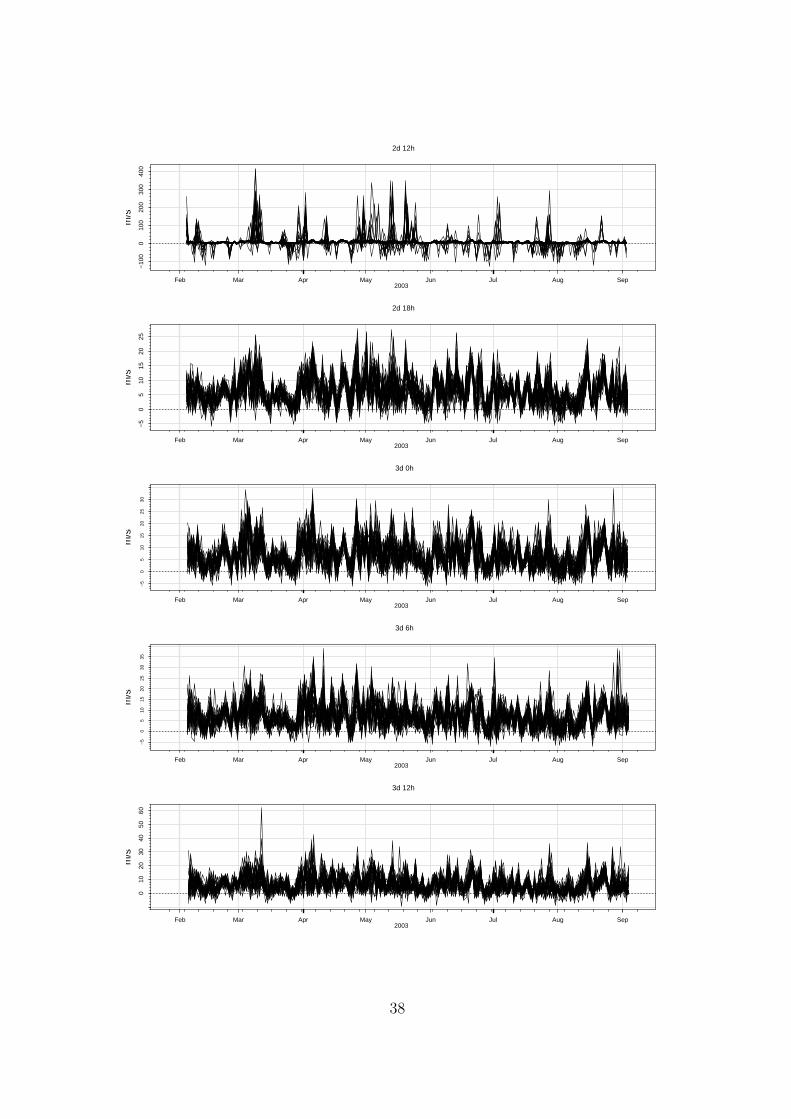
Also, the plots show that for some horizons numerical instability seems to occur. Closerinvestigations reveal that these instabilities occur for certain sectors where the sector 180◦
– 225◦ is the one most frequently occurring. The reason for the instabilities is that β in (3)(page 16) is estimated as being close to zero whereby the absolute values of (4), which areused for transforming the ensembles, increase dramatically. These results indicate thatin practice more advanced methods of MOS transformation is required. One possibilitywould be to estimate the coefficients in (3) as smooth functions of the wind directionand the forecast horizon. Furthermore, all observations of the wind speed should be used.One way to do this is to define the forecasts as continuous curves by use of e.g. linearinterpolation.
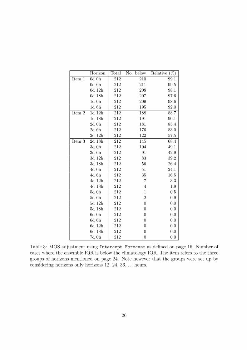
Table 3 shows the number of cases where the ensemble IQR (Inter Quantile Range)4 isbelow the IQR of climatology. For the horizons mentioned in item 2 above the MOSadjusted ensemble forecasts are reliable. It is seen that although the 60 hour (2d 12h)forecast has numerical instable values the ensemble IQR is below the climatology IQRin nearly 60% of the cases. For the horizons mentioned under item 3 some of the lowerhorizons have near 50% cases where the ensemble IQR is lower than the climatology IQR.
For horizons 36 and 48 hours Figure 13 shows histograms of the IQR of the MOS adjustedECMWF ensemble compared to the IQR of the climatological distribution. The figure alsocontains plots based on the MOS adjusted HIRLAM ensembles, but these are availablefor a shorter period. Considering this the adjusted HIRLAM ensembles do not seem todiffer much in resolution as compared to the ECMWF ensembles.
For ECMWF it is seen that the majority of the ensemble IQR values are well below theclimatology value. This indicates a clear benefit from using the ensemble forecasts. Forthe 36 hour forecast it turns out that in approximately 50% of the cases the IQR is below2 m/s. A IQR of 2 m/s indicates that in 50% of these cases the forecast is within 1 m/s.
As mentioned in Section 6.1 the MOS adjustment of the ECMWF forecasts obtained usingorthogonal regression perform also fairly well in terms of reliability. For MOS performedusing orthogonal regression Table 4 show the number of cases where the ensemble IQR isbelow the climatology IQR. Comparing with Table 3 it is clearly seen that the resolutionof the MOS-adjusted ensemble forecasts obtained using orthogonal regression is higherthan the resolution obtained using the unperturbed forecast as the dependent variable.However, as discussed above the method primarily discussed in this section may possiblybe improved. This may be preferable due to it’s simplicity.
4The inter quantile range is the difference between the 75% and the 25% quantiles and hence is ameasure of how wide the distribution is.
25
Horizon Total No. below Relative (%)
Item 1 0d 0h 212 210 99.10d 6h 212 211 99.50d 12h 212 208 98.10d 18h 212 207 97.61d 0h 212 209 98.61d 6h 212 195 92.0
Item 2 1d 12h 212 188 88.71d 18h 212 191 90.12d 0h 212 181 85.42d 6h 212 176 83.02d 12h 212 122 57.5
Item 3 2d 18h 212 145 68.43d 0h 212 104 49.13d 6h 212 91 42.93d 12h 212 83 39.23d 18h 212 56 26.44d 0h 212 51 24.14d 6h 212 35 16.54d 12h 212 7 3.34d 18h 212 4 1.95d 0h 212 1 0.55d 6h 212 2 0.95d 12h 212 0 0.05d 18h 212 0 0.06d 0h 212 0 0.06d 6h 212 0 0.06d 12h 212 0 0.06d 18h 212 0 0.07d 0h 212 0 0.0
Table 3: MOS adjustment using Intercept Forecast as defined on page 16: Number ofcases where the ensemble IQR is below the climatology IQR. The item refers to the threegroups of horizons mentioned on page 24. Note however that the groups were set up byconsidering horizons only horizons 12, 24, 36, . . . hours.
26

0
20
40
60
80
0 2 4 6 8 10 12
1d 12hECMWF
1d 18hECMWF
0 2 4 6 8 10 12
2d 0hECMWF
2d 6hECMWF
1d 12hHIRLAM
0 2 4 6 8 10 12
1d 18hHIRLAM
2d 0hHIRLAM
0
20
40
60
80
0 2 4 6 8 10 12
2d 6hHIRLAM
IQR (m/s)
Cou
nt
Figure 13: Histograms (counts) of ensemble IQR (MOS adjusted ECMWF/HIRLAMwith the unperturbed forecast as the dependent variable). The IQR corresponding toclimatology, as defined on page 3, is shown as a vertical line on the plot.
27

Horizon Total No. below Relative (%)
Item 1 0d 0h 212 210 99.10d 6h 212 211 99.50d 12h 212 207 97.60d 18h 212 209 98.61d 0h 212 211 99.51d 6h 212 201 94.8
Item 2 1d 12h 212 199 93.91d 18h 212 198 93.42d 0h 212 190 89.62d 6h 212 193 91.02d 12h 212 175 82.5
Item 3 2d 18h 212 176 83.03d 0h 212 148 69.83d 6h 212 154 72.63d 12h 212 147 69.33d 18h 212 121 57.14d 0h 212 127 59.94d 6h 212 125 59.04d 12h 212 58 27.44d 18h 212 52 24.55d 0h 212 39 18.45d 6h 212 74 34.95d 12h 212 31 14.65d 18h 212 1 0.56d 0h 212 2 0.96d 6h 212 0 0.06d 12h 212 7 3.36d 18h 212 0 0.07d 0h 212 0 0.0
Table 4: MOS adjustment using orthogonal regression: Number of cases where the en-semble IQR is below the climatology IQR. The item refers to the three groups of horizonsmentioned on page 24. Note however that the groups were set up by considering horizonsonly horizons 12, 24, 36, . . . hours.
28

7 Conclusion and Discussion
This report compares three types of ensemble forecasts of wind speed to a wind speed mea-surement 76m a.g.l. from a mast at Risø National Laboratory, Denmark. The ensembleforecasts considered are
• NCEP (National Centers for Environmental Prediction) ensemble forecasts from theNational Weather Service of NOAA (National Oceanic and Atmospheric Adminis-tration) in U.S. This set of ensembles consists of one unperturbed forecast and 5pairs of forecasts for which the initial conditions are perturbed in the positive andnegative direction of bred vectors. Horizontal resolution: 1◦.
• ECMWF (European Centre for Medium-Range Weather Forecasts) ensemble fore-casts from the Ensemble Prediction System5. This set of ensembles consists of oneunperturbed forecast and 25 pairs of forecasts for which the initial conditions areperturbed in the positive and negative direction of singular vectors. Furthermore,for each model run attempts are made to account for sub-grid processes by useof stochastic physics [1]. As a result two runs with the same set of initial condi-tions will not result in exactly the same output. Horizontal resolution: 75km. Theunperturbed forecast is not influenced by stochastic physics.
• HIRLAM ensembles from DMI (Danish Meteorological Institute). These are experi-mental ensembles based on the ECMWF ensembles. Also a few model permutationsare included, but these are not used in this report. Horizontal resolution: 20km.
For NCEP and ECMWF the 10m a.g.l. wind speed and direction are used and forHIRLAM the 70m a.g.l. wind speed and direction are used. For the analysis of the MOSadjusted forecasts (see below) the 10m a.g.l. HIRLAM wind speed is used since moredata are available for this level. Bilinear interpolation is used to obtain forecasts valid forthe location of the mast. The period for which measurements and forecasts are availableare listed in Section 4.
In Section 5 the ensemble forecasts are investigated without comparing them to the mea-surements. It is shown that the NCEP analysis (0 hour forecast) averaged over all en-semble members and time points is approximately 2 m/s lower than the remaining meanvalues. For ECMWF the average and quantiles over all ensemble members and time pointsvaries with a period of 24 hours, but since the calculations are only initiated once a day,this may just be a consequence of the diurnal variation forecasted by the model. In fact ifthe NCEP forecasts are split by initialization time the same kind of behavior is observed,but to a lesser extent. For the HIRLAM ensembles the average drops by more than 2 m/swithin the first three hours, i.e. comparing the analysis and the 3 hour forecast. Thistime interval corresponds to 12:00 to 15:00 UTC and hence the drop can not be attributed
5http://www.ecmwf.int/products/forecasts/guide/The Ensemble Prediction System EPS.html
29

to diurnal variation (Denmark is one hour ahead of UTC). Consequently, there is someindication that the bias of the forecasts depends on the horizon.
The ensemble forecasts are compared w.r.t. reliability (average correctness of the fore-casted distributions) and resolution (sharpness of the forecasted distributions), cf. [13]or the beginning of Section 6. When interpreting ensemble forecasts in a probabilisticsense reliability is a requirement and resolution is an indicator of performance. In thisreport reliability is addressed by use of rank histograms and QQ-plots. Rank histograms,also called Talagrand diagrams, are useful in order to obtain an overview, but QQ-plots(quantile-quantile-plots) are generally preferable in that they contain additional informa-tion. As an example QQ-plots may indicate that overall a particular ensemble forecastsystem is not reliable, but the upper quantiles are reliable. Only the overall conclusioncan be reached by use of rank histograms. Resolution is addressed by comparing the IQR(Inter Quantile Range), the difference between the 75% and the 25% quantiles, with theIQR obtained using climatological information. Here the climatological information isobtained by simply using the available measurements with time stamps before any of theensemble forecasts, i.e. 9 months of measurements. See also Section 4.
When comparing the forecasts to the point measurement differences in temporal andspatial resolution should be taken into account. Both measurements and forecasts are 10minute averages (over the interval up to the time stamp), however the spatial resolutionsof the measurements and forecasts are very different. This may have the consequencethat (i) the point measurement may differ systematically from the (unobservable) spatialaverages although the forecasts may agree well with the spatial averages, and (ii) the pointmeasurement may differ non-systematically or stochastically from the spatial averages.Using MOS (Model Output Statistics) it should be possible to correct for (i). However,(ii) will influence the reported reliability of the ensemble forecasts, even when these arecorrected by MOS.
As expected without MOS correction none of the ensemble forecast systems are reliablew.r.t. the measurement. Nevertheless, the upper quantiles (from 80%) of the HIRLAMensembles seems to be reliable, but the actual number of times in which the 80% quantileis exceeded is very small, cf. Table 2 page 15. The 80% ensemble quantile range from 1.7to 25.7 m/s, indicating good resolution.
If (ii) above can be neglected then some kind of MOS correction should be able to correctfor systematic differences. If further, the ensemble forecast system produce forecasts whichare reliable w.r.t. the spatial averages then the MOS adjusted ensembles should also bereliable and this can be investigated using rank histograms or QQ-plots. In the reportdifferent ways of performing the MOS adjustment are considered. Due to the limiteddata the coefficients used for correction are determined on the same set of data as theone for which the correction is performed. To account for a bias which may depend onthe horizon and on the sector (0◦–45◦, 45◦–90◦, . . . , 315◦–360◦) the MOS correction isdetermined separately for each combination of sector and horizon.
30

Usually, a linear regression through the origin with the unperturbed forecast as the in-dependent variable and the measurement as the dependent variable is used for MOSadjustment. However, due to the uncertainty of the forecast the estimate will be biased,but the point predictions of the wind speed at the mast will be good in e.g. mean squaresense [5, 7, 8]. The point predictions can probably be further improved by not forcingthe linear regression through the origin. At least two reasons exists why this approachto MOS adjustment must be expected to result in unreliable ensemble forecasts; (a) evenif the estimates are unbiased the error-term of the linear regression is not included inthe MOS adjustment, and (b) the uncertainty of the unperturbed forecast result in adownward bias on the slope and an upward bias on the intercept. The consequence ofboth (a) and (b) are that the spread of the MOS adjusted ensemble forecasts will be toosmall. This is demonstrated in Section 6.1, see e.g. Figure 7 on page 19. Actually, w.r.t.reliability it seems to be best to force the linear regression through the origin.
If there is no non-systematic difference between the point measurement (10 minute av-erage) and the spatial average, then only the unperturbed forecast is associated withuncertainty. Consequently, using the unperturbed forecast as the dependent variable andthe measurement as the independent variable will yield unbiased estimates.
Horizons 12, 24, 36 , ... of the MOS adjusted ensembles are checked w.r.t. reliability andresolution. The spread of the NCEP ensembles adjusted in this way is still too small.For ECMWF and HIRLAM the adjusted ensembles seems to be reliable for horizons 36–60 hours, whereas the spread is too small for shorter horizons and too large for longerhorizons.
For horizons 36–48 hours the resolution is good in that the ensemble IQR, in most cases,is smaller than the IQR corresponding to climatology. For 60 hours numerical instabilitiesresults in unrealistic MOS adjusted ensemble forecasts. For horizons of 60 hours or longerQQ-plots indicate that the spread of the MOS adjusted ensemble forecasts is too large,also for some of these horizons numerical instabilities are observed.
The cause of the numerical instabilities seems to be a rather large uncertainty of theestimates associated with the MOS correction, cf. Section 6.2, caused by the low numberof observations in each sector and the fact that the ensemble calculations are only initiatedat 12:00 UTC. When the unperturbed forecast is rather uncertain the estimate of slopemay occasionally be close to zero, possibly just due to random variation6 and this resultsin a very large slope for in the linear transformation which is used to adjust the ensembleforecasts, cf. (4) on page 16.
To avoid the numerical instabilities the following issues should be considered:
• More effective use of the observations. One way to accomplish this is to obtain
6By swapping x and y in the regression we have replaced bias by variance. This is required since wecan not accept bias in this case.
31

forecasts for all observations, e.g. by linear interpolation, and then let the coefficientsbe smooth functions of the horizon.
• More effective use of the information contained in the wind direction by modelingthe coefficients as smooth functions of the wind directions.
• Derive the MOS transformation based on a short forecast horizon and use this forall horizons. However this is difficult, at least for HIRLAM (cf. Section 5).
If both uncertainty on the forecast and stochastic variations between the point measure-ment and the unobservable spatial average is to be taken into account the problem mustbe treated as an errors-in-variables problem [4]. This require knowledge about the ratio ofthe two variances involved. The ratio is not known in this case, but orthogonal regressionhas been applied which corresponds to a ratio of one. The method results in adjustedensemble forecasts with similar reliability as when the unperturbed forecast is used as thedependent variable. Furthermore, the numerical instabilities of the method is somewhatsmaller.
In [13, p. 141] it is stated that for statistically stationary forecast and observation systemsand given a large enough sample, perfect reliability can be achieved by a simple statis-tical calibration. The corresponding transformation can be obtained by fitting a smoothfunction to the data on a QQ-plot, with the observed quantile/probability ((rank−1)/N)as the explanatory variable. This transformation is then used to transform the ensemblequantiles to agree with the observed quantiles.
Note that this transformation is solely focusing on reliability; as an extreme example, ifthe ensemble forecasts are not related to the observations then the quantiles obtained aresimply quantiles in the climatological distribution. Also, in practice the transformationcan not repair any QQ-plot. As an example consider the 12h NCEP ensemble forecast forwhich the QQ-plot is displayed in the lower left corner of Figure 5 on page 14. It is seenthat in approximately 20% / 40% of the cases the observation is below / above the lowest/ highest ensemble member. There is no way to distinguish between these quantiles; thebest we can hope for is values near the center of the two extreme intervals. Consequently,in the example, we should not expect to gain information about quantiles below 10% orabove 80%. The same kind of problems occur when many of the observations are in thehigh end of the ensemble members as e.g. for ECMWF on the figure just mentioned.
Because of the above and because the transformation is not directly based on any phys-ical aspects (e.g. spatial averages versus point measurements) we suggest that a MOStransformation based on the unperturbed forecast is applied before the transformationbased on the QQ-plot is applied. In this setting it may not be a requirement that theMOS adjustment is based on unbiased estimates. Hence, one solution might be to use astandard MOS adjustment derived on basis of a low forecast horizon and then apply thetransformation based on the QQ-plots, for each horizon separately. By substituting theMOS adjustment by the estimation of a power curve for wind farms, this points towardsa way of producing reliable wind power ensembles.
32

Finally, we note that the observations mentioned in Section 5 do have consequence forhow to estimate and use a power curve model for producing ensembles of wind power.Since we, for some setups, want an estimate without bias we might want to select themost precise forecast for building the power curve model. If e.g. for NCEP the analysis isselected for this purpose then using other horizons result in a large upward shift in powerproduction.
33
References
[1] R. Buizza, M. Miller, and T.N. Palmer. Stochastic representation of model uncer-tainties in the ECMWF Ensemble Prediction System. Quarterly Journal of the Royal
Meteorological Society, 125(560):2887–2908, 1999.
[2] R. Buizza and T.N. Palmer. The singular vector structure of the atmosphere globalcirculation. Atmos. Sci., 52:1434–1456, 1995.
[3] J.M. Chambers, W.S. Cleveland, B. Kleiner, and P.A. Tukey. Graphical methods for
data analysis. Wadsworth Publishing Co Inc, 1983.
[4] Wayne A. Fuller. Measurement error models. John Wiley & Sons, 1987.
[5] Bo Jonsson. Prediction with a linear regression model and errors in a regressor.International Journal of Forecasting, 10(4):549–555, 1994.
[6] F. Molteni, R. Buizza, T.N. Palmer, and T. Petroliagis. The ecmwf ensemble predic-tion system: methodology and validation. Quart. J. Roy. Meteor. Soc., 122:73–119,1996.
[7] Henrik Aalborg Nielsen, Torben Skov Nielsen, and Henrik Madsen. On on-line sys-tems for short-term forecasting for energy systems. In Proceedings of the OR 2002
conference, pages 265–271, Klagenfurt, Austria, 2002. Springer.
[8] Henrik Aalborg Nielsen, Torben Skov Nielsen, and Henrik Madsen. Using meteoro-logical forecasts for short term wind power forecasting. In Proceedings of the IEA
R&D Wind Annex XI Joint Action Symposium on Wind Forecasting Techniques,pages 49–58, Norrkoping, Sweden, December 3–4 2002.
[9] T.N. Palmer, F. Molteni, R. Mureau, R. Buizza, P. Chapelet, and J. Tribbia. En-semble prediction. In Proceedings of the ECMWF Seminar on Validation of models
over Europe, volume 1, Shinfield Park, Reading RG2 9AX, UK, 1993. ECMWF.
[10] K. Sattler and H. Feddersen. Treatment of uncertainties in the prediction of heavyrainfall using different ensemble approaches with dmi-hirlam. DMI Sci. Rep., 03-07,62pp, 2003. Available at www.dmi.dk.
[11] Z. Toth and E. Kalnay. Ensemble forecasting at nmc: Thegeneration of perturbations.Bull. Amer. Meteor. Soc., 74:1485–1490, 1993.
[12] Z. Toth and E. Kalnay. Ensemble forecasting and the breeding method. Mon. Wea.
Rev., 12:3297–3319, 1997.
[13] Zoltan Toth, Oliver Talagrand, Guillem Candille, and Yuejian Zhu. Forecast ver-
ification – a practitioner’s guide in atmospheric science, chapter Probability andensemble forecasts. Wiley, 2003.
34

Appendices
A Plots of MOS adjusted ensemble forecasts
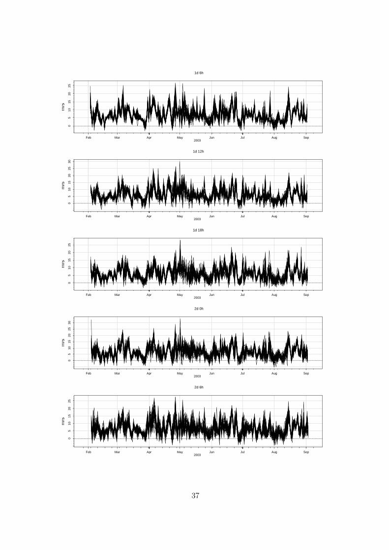
A.1 ECMWF corrected using the unperturbed forecast as the
dependent variable.
35

Feb Mar Apr May Jun Jul Aug Sep2003
05
1015
20 0d 0h
m/s
Feb Mar Apr May Jun Jul Aug Sep2003
05
1015
20
0d 6h
m/s
Feb Mar Apr May Jun Jul Aug Sep2003
05
1015
20
0d 12h
m/s
Feb Mar Apr May Jun Jul Aug Sep2003
−5
05
1015
20
0d 18h
m/s
Feb Mar Apr May Jun Jul Aug Sep2003
05
1015
2025
1d 0h
m/s
36
Feb Mar Apr May Jun Jul Aug Sep2003
05
1015
2025
1d 6h
m/s
Feb Mar Apr May Jun Jul Aug Sep2003
05
1015
2025
30
1d 12h
m/s
Feb Mar Apr May Jun Jul Aug Sep2003
05
1015
2025
1d 18h
m/s
Feb Mar Apr May Jun Jul Aug Sep2003
05
1015
2025
30
2d 0h
m/s
Feb Mar Apr May Jun Jul Aug Sep2003
05
1015
2025
2d 6h
m/s
37
Feb Mar Apr May Jun Jul Aug Sep2003
−10
00
100
200
300
400
2d 12h
m/s
Feb Mar Apr May Jun Jul Aug Sep2003
−5
05
1015
2025
2d 18h
m/s
Feb Mar Apr May Jun Jul Aug Sep2003
−5
05
1015
2025
30
3d 0h
m/s
Feb Mar Apr May Jun Jul Aug Sep2003
−5
05
1015
2025
3035
3d 6h
m/s
Feb Mar Apr May Jun Jul Aug Sep2003
010
2030
4050
60
3d 12h
m/s
38
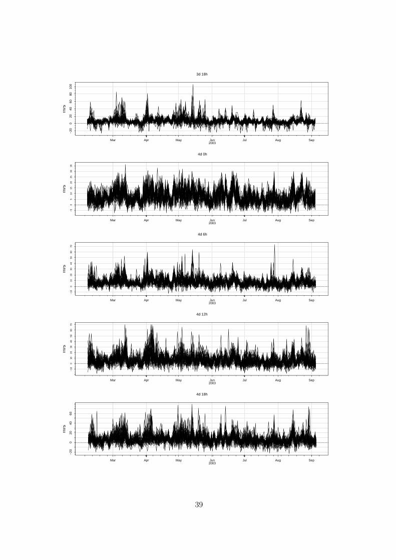
Mar Apr May Jun Jul Aug Sep2003
−20
020
4060
8010
03d 18h
m/s
Mar Apr May Jun Jul Aug Sep2003
−5
05
1015
2025
3035
4d 0h
m/s
Mar Apr May Jun Jul Aug Sep2003
−10
010
2030
4050
6070
4d 6h
m/s
Mar Apr May Jun Jul Aug Sep2003
−10
010
2030
4050
6070
4d 12h
m/s
Mar Apr May Jun Jul Aug Sep2003
−20
020
4060
4d 18h
m/s
39
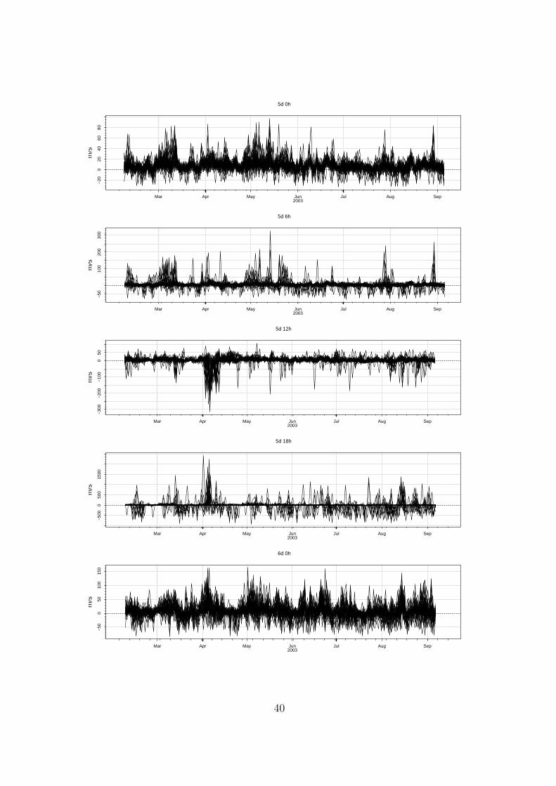
Mar Apr May Jun Jul Aug Sep2003
−20
020
4060
80 5d 0h
m/s
Mar Apr May Jun Jul Aug Sep2003
−50
100
200
300
5d 6h
m/s
Mar Apr May Jun Jul Aug Sep2003
−30
0−
200
−10
00
50
5d 12h
m/s
Mar Apr May Jun Jul Aug Sep2003
−50
00
500
1500
5d 18h
m/s
Mar Apr May Jun Jul Aug Sep2003
−50
050
100
150
6d 0h
m/s
40
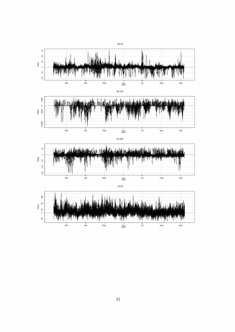
Mar Apr May Jun Jul Aug Sep2003
−20
0−
100
010
020
030
0
6d 6h
m/s
Mar Apr May Jun Jul Aug Sep2003
−12
000
−40
000
4000
6d 12h
m/s
Mar Apr May Jun Jul Aug Sep2003
−15
00−
1000
−50
00
500
6d 18h
m/s
Mar Apr May Jun Jul Aug Sep2003
−40
020
6010
0
7d 0h
m/s
41

A.2 HIRLAM corrected using the unperturbed forecast as the
dependent variable.
42

Dec Jan Feb Mar Apr2002 2003
−5
05
1015
20 0d 0h
m/s
Dec Jan Feb Mar Apr2002 2003
−2
02
46
810
1214
16
0d 6h
m/s
Dec Jan Feb Mar Apr2002 2003
−2
24
610
1418
0d 12h
m/s
Dec Jan Feb Mar Apr2002 2003
−2
02
46
810
1214
1618
0d 18h
m/s
Dec Jan Feb Mar Apr2002 2003
05
1015
20
1d 0h
m/s
43

Dec Jan Feb Mar Apr2002 2003
05
1015
20 1d 6h
m/s
Dec Jan Feb Mar Apr2002 2003
02
46
812
1620
1d 12h
m/s
Dec Jan Feb Mar Apr2002 2003
05
1015
20
1d 18h
m/s
Dec Jan Feb Mar Apr2002 2003
05
1015
20
2d 0h
m/s
Dec Jan Feb Mar Apr2002 2003
−5
05
1015
20
2d 6h
m/s
44

Dec Jan Feb Mar Apr2002 2003
−60
−20
2060
100
140
2d 12h
m/s
Dec Jan Feb Mar Apr2002 2003
05
1015
2025
2d 18h
m/s
Dec Jan Feb Mar Apr2002 2003
−5
05
1015
2025
3d 0h
m/s
45