Comparison of DES, RANS and LES for the separated around a plate at high incidence

INTERNATIONAL JOURNAL FOR NUMERICAL METHODS IN FLUIDSInt. J. Numer. Meth. Fluids 2003; 41:357–388 (DOI: 10.1002/�d.445)

Comparison of DES, RANS and LES for the separated �owaround a �at plate at high incidence

M. Breuer1;∗;†, N. Jovi�ci�c1 and K. Mazaev2

1Lehrstuhl f�ur Str�omungsmechanik, Universit�at Erlangen-N�urnberg, Cauerstr. 4; D-91058 Erlangen; Germany2Saint Petersburg State Marine Technical University; Lotsmanskaja Street 3; 190008 Saint Petersburg; Russia

SUMMARY

The separated turbulent �ow past an inclined �at plate with sharp leading and trailing edges wascomputed based on three di�erent simulation approaches for a Reynolds number Rec=20 000 and ahigh angle of attack �=18◦. The simulation techniques applied were the Reynolds-averaged Navier–Stokes (RANS) equations combined with a one-equation Spalart–Allmaras turbulence model, the large-eddy simulation (LES) based on an algebraic eddy-viscosity model, and a hybrid approach knownas detached-eddy simulation (DES) applying a slightly modi�ed Spalart–Allmaras model in the entireintegration domain. DES is a non-zonal coupling technique of RANS and LES developed in the hopeof reducing the large computational resources required for LES computations of turbulent �ows withpractical relevance. However, the objective of the present study was not to compare the resources(CPU time, memory) required for all three techniques but to investigate and evaluate the quality ofthe predicted results for RANS, DES and LES. For this purpose, a test case which is favourable tothe basic concept of DES and which places special emphasis on the LES part of the DES concept waschosen. This last issue was important since the modi�ed Spalart–Allmaras model applied as a subgridscale model in the LES part is not as well validated as other models usually applied in LES. For thispurpose, an LES prediction on a very �ne grid served as a reference case for the evaluation. For all threetechniques, predictions with di�erent grid resolutions were carried out and compared with each otherbased on important integral parameters (e.g. Strouhal number, mean drag and lift coe�cients and theirstandard deviations), the instantaneous and time-averaged �ow structures, and higher-order statistics.As expected, the pure RANS calculation, although applied as unsteady RANS, failed to predict theunsteady characteristics of the separated �ow. In contrast, the DES approach yielded reasonably theshedding phenomenon and some integral parameters. However, analysing the results in more detail ledto remarkable deviations between the DES and LES predictions also when the same grid resolutionwas applied. Especially the free shear layer originating from the leading edge of the plate was not wellreproduced by DES, showing strong de�ciencies of the model applied as a subgrid scale model. Thereasons for this behaviour of the model were analysed in detail. Two basic causes were identi�ed; the�rst is given by some near-wall corrections in the �nite Reynolds number version of the model whichare not working properly in the LES mode of DES. The second is a modi�ed de�nition of the �lterwidth typically applied for DES, leading to strongly increased values of the eddy viscosity. A revised

∗ Correspondence to: M. Breuer, LSTM, Universit�at Erlangen–N�urnberg, Cauerstr. 4, D–91058 Erlangen, Germany.† E-mail: [email protected]

Contract=grant sponsor: German Academic Exchange Programme (DAAD)Contract=grant sponsor: Deutsche Forschungsgemeinschaft; contract=grant number: BR 1847=2

Received 10 June 2002Copyright ? 2003 John Wiley & Sons, Ltd. Revised 16 September 2002

358 M. BREUER, N. JOVI �CI �C AND K. MAZAEV

version of the S–A model taking both issues seriously into account was used as a subgrid scale modelin the LES mode. As a direct consequence, much better agreement with the reference LES solution wasfound for the DES prediction on the coarse grid, eliminating the de�ciencies of the original formulation.Copyright ? 2003 John Wiley & Sons, Ltd.

KEY WORDS: large-eddy simulation; detached-eddy simulation; separation; high-lift con�guration

1. INTRODUCTION

It is well known that the prediction of complex separated unsteady �ows based on Reynolds-averaged Navier–Stokes (RANS) is not completely successful for many cases. Unfortunately,even the use of the most modern turbulence models could not essentially improve the situ-ation. Therefore, during the last decade many researchers have paid more attention towardslarge-eddy simulation (LES) and direct numerical simulation (DNS) as alternative predictionmethods. However, these alternatives are actually too expensive in the sense of the requiredcomputer performance; this thesis is clear for DNS, but the situation with LES, if the de-velopment of supercomputers is taken into account, seems to be not so drastic. Nevertheless,the analysis carried out by Spalart et al. [1] shows that for Reynolds numbers of about 107,i.e. normal aerodynamic values, a computational grid consisting of a minimum of 1011 cellshas to be used. Such huge computations will be out of reach for the next couple of decades.This circumstance, namely very high computational costs, was the main reason for develop-ing new kinds of hybrid methods, which combine the main features of both LES and RANSsimulations (see, e.g. References [2–6]). In the present work, the detached-eddy simulation(DES) hybrid approach is used, whose basic principles are described in Reference [1] and�rst results are presented in Reference [7]. The results of DES are compared with both RANSand LES data, all obtained by the same computer code. The main di�erence between otherattempts at coupling RANS and LES is that the �ow is not explicitly subdivided into twozones. As a consequence, there is no problem of explicit boundary conditions between RANSand LES zones. The main features of DES and the di�erences between LES, DES and RANSsimulations are discussed below.In spite of the widespread application of RANS predictions for turbulent �ows, the main

disadvantage of the method is clear: RANS describes �ows in a statistical sense typicallyleading to time-averaged pressure and velocity �elds. Generally, this approach is not ableto distinguish between quasi-periodic large-scale and turbulent chaotic small-scale featuresof the �ow �eld. This leads to huge problems when the �ow �eld is governed by bothphenomena. A typical representative is a blu�-body �ow. Generally, the RANS approach isnot able to reproduce the unsteady characteristics of the �ow �eld reasonably, resulting inan inadequate description of unsteady phenomena, such as vortex formation and sheddingbehind blu� or inclined bodies. Even with help of complex turbulence models which areusually semi-empirical and contain about 6–9 empirical constants, it is not possible to modelthese large-scale phenomena adequately. LES, on the other hand, operates with unsteady �eldsof physical values; the governing equations are the Navier–Stokes equations but, unlike theRANS approach, spatial �ltering is applied instead of averaging in time, and turbulent stressesare divided into resolved and modelled stresses. The latter can be found from very simple(in comparison with the normal turbulence models) subgrid scale models, often based on an

Copyright ? 2003 John Wiley & Sons, Ltd. Int. J. Numer. Meth. Fluids 2003; 41:357–388

DES, RANS AND LES FOR FLOW PAST AN INCLINED PLATE 359

algebraic eddy-viscosity concept such as Smagorinsky’s hypothesis [8]. As mentioned above,the main disadvantage of LES is the high computational costs resulting from extremely �negrids used for the direct prediction of the non-modelled vortical structures. Additionally very�ne time steps are required for resolving the turbulent time scales.DES could be represented as a natural hybrid method combining RANS and LES (see

Section 3). This means, that near solid boundaries the governing equations work in the RANSmode, i.e. all turbulent stresses should be modelled with the help of a statistical turbulencemodel such as the Spalart–Allmaras (S–A) model [9]. Furthermore, pressure and velocity �eldsare time averaged and unsteady attached vortical structures should not be resolved directly. Farfrom solid boundaries, the method switches to the LES mode. From the physical point of view,it means resolving all large-scale vortical structures and modelling of small eddies based on asubgrid scale model, which can be similar to a statistical turbulence model. From the numericalpoint of view, one has to deal with unsteady �elds of pressure and velocity in this mode.However, the computational domain contains no explicit boundaries or interfaces between thetwo modes of operation. It is natural that RANS works within the attached boundary layerregion, where statistical turbulence models in general perform properly. Moreover, LES isapplied far from the boundaries in the detached �ow region, where large unsteady vortices,which should be resolved directly, are present. Exactly this kind of division allows us touse a coarse, highly stretched grid near the walls for the RANS simulation unlike in LESwhich requires a �ne resolution in all three spatial directions. Furthermore, the spanwise andstreamwise resolution do not have to be very high for RANS [10]. Both factors raise thehope that DES can be used with acceptable e�ort even for high Reynolds numbers, typicallyencountered in technical applications.Therefore, the main application area of DES should be in accordance with the DES concept

itself: unsteady turbulent �ows with large separation regions for which RANS predictions donot work properly. DES modelling of non-separated �ow typically leads to severe problems, asdemonstrated by Nikitin et al. [10]. For a plane channel �ow the predicted results were stableup to very high Reynolds numbers, and can be obtained even on very coarse grids. However,both constants in the logarithmic law of the wall were strongly overpredicted compared withclassical values; the authors explained this as being due to both insu�cient grid resolution anda non-adjusted Spalart–Allmaras model [9] (because the S–A model was originally developedfor RANS only). It should be mentioned that usually DES works purely in RANS mode ifthe �ow does not separate [7]; otherwise, some kind of initial velocity perturbations shouldbe used in order to induce the unsteady mode as shown for the channel test case [10]. On theother hand, all DES applications of separated �ows brie�y summarized below were successful.Hence DES applications to such turbulent �ows seem to be reasonable and reliable whosedynamics are de�ned by large-scale separated vortices playing a dominant role in the energybalance.For a brief review of published papers dedicated to DES, both the steps of its development

and some basic advantages of this new approach are considered. Spalart et al. [1] formulatedthe principles of DES and derived the DES constant CDES based on the simulation of homoge-neous turbulence, which controls the switching process between RANS and LES. Thus, DESwas adjusted; furthermore, the �rst true (three-dimensional) simulation was applied to the �owaround an NACA wing pro�le [7] for a very wide range of angle of attacks (0◦6�690◦).For the high (from the point of view of DNS=LES) Reynolds number of about 105 resultswere obtained which were in very good agreement with experimental investigations and much



better than those obtained by pure RANS. Forsythe et al. [11] made the �rst attempt to useDES on an unstructured grid; it was shown that the CDES value has to be adapted becauseof the special shape of the grid cells. The DES solution was found to be much more reliablethan the RANS result for each of the two turbulence models used.A classical test case for LES, namely the �at channel �ow, was investigated by Nikitin

et al. [10]. In spite of some problems with the constants in the predicted logarithmic meanvelocity pro�le already mentioned above, the simulations were at least partially successful:the solution was stable over a very wide range of Re and almost does not depend on the gridresolution, which was much coarser than typically needed for LES. Here some demands onthe grid are given:

• the �rst grid layer near the boundary should correspond to a non-dimensional valuey+∼1 (thus, no wall-functions are required);

• a stretching ratio of about 1.15 could be used (the authors [10] deduced that only 17additional grid layers would be necessary if the Reynolds number were to be increasedby one order of magnitude);

• the non-dimensional size of the grid cells in both the longitudinal and spanwise directions(x+ and z+) is several orders of magnitude larger than the normal size.

An investigation of another classical test case, the �ow around a circular cylinder, byTravin et al. [12] shows some possible problems: although the values of the base pressure,the friction coe�cient, the total drag and the vortex shedding frequency were very close to theexperimental values, at the same time the estimated error for the length of the recirculationzone and for the turbulent stresses was very large. Nevertheless, generally the results seemto be better than in RANS simulations. It should be mentioned that no grid convergencewas achieved similar to comparable LES investigations [13]; the authors [12] explained thisas the result of ‘running a complex numerical-physical system with numerous sources oferror : : :; the reduction of one error does not drive the solution towards perfection’. Finally,in two recent publications concerned with the DES approach, by Strelets [14] and Squireset al. [15], some new results predicted for more complex geometries, namely the �ow aroundan airplane carriage and around a forebody cross-section, are presented. However, these aredi�cult to evaluate.In spite of a wide range of DES applications which are available in the literature, in

most of these investigations the results determined by the DES approach were comparedwith RANS simulations only. A detailed comparison with LES could also be very useful inorder to see which of the advantages of LES could be reached in the framework of DES.Furthermore, it is worthwhile to determine more sharply its main disadvantages, as a price forthe lower computational resources required. A direct comparison would be favourable if bothDES and LES simulations would be carried out based on the same code and, probably, usingthe same spatial and temporal discretization. This procedure guarantees that numerical andimplementation issues play no role in the comparison of the results. Therefore, the evaluationcan be restricted to the modelling aspects. Of special importance in this context is how themodi�ed S–A model performs as a subgrid model in the LES mode of the DES prediction. Ofcourse, such an investigation is still not possible for very high Reynolds numbers. Therefore,a small Re was chosen for the present study, which allows the application of LES. Thegoal of the work was an attempt to locate some error sources of the DES technique and tocompare and evaluate all three kinds of simulation techniques (DES, LES and RANS) for the



same—or as similar as possible—conditions. The subject of the investigation, namely aninclined �at plate, has a very simple geometry and is a representative of high-lift aerodynamic�ows with a massive separation region. This con�guration was chosen as a preliminary testcase for the �ow past an airfoil at the same conditions. It has proven to be a good choice,since we found very similar �ow features as well as comparable results for both cases [16, 17].Furthermore, the �ow con�guration studied allows a detailed investigation especially of theLES mode of the DES predictions. Owing to the �xed separation at the sharp leading edge,the RANS region is restricted to a narrow gap near the wall. Hence the DES approach has towork nearly completely in the LES mode, which allows one to evaluate the performance ofthe S–A model as a subgrid scale model and additionally the coupling with the RANS region.Based on the results obtained, which include pressure and velocity distributions, total lift anddrag coe�cients, vortex shedding frequency, Reynolds stresses, unsteady vorticity, etc., themain advantages and disadvantages of the applied methods (DES, LES, RANS) are comparedwith each other.The paper is organized as follows. First, the governing equations are given for the LES

and the RANS simulations. Second, in Section 3, the modelling approaches are described indetail for DES and RANS, whereas this issue is only brie�y addressed for LES. Section 4gives an overview of the numerical solution method applied. In the subsequent section thegeometry and the details of the �ow con�guration are de�ned, including details on the gridsand boundary conditions used. Finally, in Section 6, the results are presented and analysed,leading to an improved DES formulation.

2. GOVERNING EQUATIONS

An incompressible �uid with constant �uid properties is considered. The governing equationsare the Navier–Stokes equations describing the conservation of mass and momentum. In thecase of LES, these equations are �ltered in space with the �lter width � in order to separatelarge- and small-scale motions, which leads to the so-called �ltered Navier–Stokes equations.In the RANS approach, the same equations are time averaged (or ensemble averaged), leadingto the well-known RANS equations. Both kinds of equations can be written in a common(dimensionless) form:

@ uj@xj

=0 (1)

@ ui@t+@( ui uj)@xj

=−@ p@xi

− 1Re@�molij

@xj− @�turbij

@xj(2)

�molij =−2� Sij where Sij=12

(@ ui@xj

+@ uj@xi

)(3)

where ui, p and �=� (�=1) are the velocity component, the pressure and the viscosity,respectively. In LES the overbar (·) de�nes the resolved scales, whereas in RANS it denotesthe time-averaged components. Re is the characteristic Reynolds number de�ned below. Theterm �molij describes the momentum transport due to molecular motion, which for a Newtonian�uid is given by Equation (3). Owing to �ltering (LES) or time-averaging (RANS) of the



non-linear convective term in the momentum equation (2), the additional term �turbij ariseswhich has to mimic the momentum transport due to turbulence motion. In the case of LES,�turbij is denoted as the subgrid scale (SGS) stress tensor and restricted to the in�uence ofthe non-resolved small-scale structures on the resolved large eddies. However, in RANS �turbijsigni�es the Reynolds stress tensor describing the in�uence of the entire spectrum of alllength scales on the averaged �ow �eld. In both cases this unknown has to be modelled. Themodelling approaches are described in detail for DES and RANS in the next section. For LESonly a brief description is given. More details on this topic can be found elsewhere [18, 19].

3. MODELLING APPROACHES

3.1. DES and RANS

As already mentioned above, the DES approach is based on a non-explicit splitting of thecomputational domain into two zones. In the �rst region near solid walls, the conventionalRANS equations have to be solved. Within the second region, the governing equations arethe �ltered Navier–Stokes equations of the LES approach. In principle, the DES conceptallows one to apply totally di�erent models for the two regions, which would be a naturalchoice since the models have clearly distinguishable tasks. However, following the conceptof Spalart et al. [1, 2, 7, 12], in both cases the S–A turbulence model [9] is used either as anormal turbulence model or as an SGS model, respectively. The model and the mechanism,which allows it to be applied in both the RANS and LES modes are described brie�y.The S–A model is based on Boussinesq’s approximation, which describes the stress tensor

�turbij as the product of the strain rate tensor Sij (see Equation (3)) and an eddy viscosity �T :

�turb; aij =�turbij − �ij�turbkk =3=−2�T Sij (4)

where �turb; aij is the anisotropic (traceless) part of the stress tensor �turbij and �ij is the Kroneckerdelta. The trace of the stress tensor is added to the pressure, resulting in the new pressureP= p+ �turbkk =3.The determination of the eddy viscosity �T is based on the solution of an additional transport

equation. It was derived by Spalart and Allmaras [9] by taking the empiricism and argumentsof dimensional analysis, the Galilean invariance and the selective dependence of the molecularviscosity into account. The governing equation for the new eddy viscosity variable �̃ formingthe one-equation S–A model (low-Re variant) is

@�̃@t︸︷︷︸

local change

+ ui@�̃@xi︸︷︷︸

convection

= cb1S̃��̃︸︷︷︸production

+1�{∇ · [(�+ �̃)∇�̃] + cb2(∇�̃)2}︸︷︷︸

di�usion

− cw1fw[�̃d

]2︸︷︷︸destruction

(5)

The left-hand side of Equation (5) represents local and convective changes of the transportvariable �̃; the right-hand side includes the production term, the di�usion term and �nally thedestruction term for the reduction of the stresses in the vicinity of solid walls. It represents thedissipation of the turbulent kinetic energy in the near-wall region. Owing to its physical nature,in the RANS mode the destruction term is directly related to the reciprocal of the minimalwall distance d. Consequently, the boundary condition for the intermediate variable �̃ at solid



walls is �̃=0. The production term includes the scalar quantity S̃� which is expressed bythe quantity S� plus a near-wall correction (see Equation (6)). The term S� can be modelleddi�erently (e.g. by |Sij |); however, as in the original model [9], S� is chosen here as themagnitude of the vorticity |�|. The derivation of the missing relations

�T= �̃fv1; S̃�≡ S� + �̃�2d2

fv2; S�= |�|; ≡ �̃�

(6)

fv1=3

3 + c3v1; fv2=1−

1 + fv1; fw=g

[1 + c6w3g6 + c6w3

]1=6(7)

g=r + cw2(r6 − r); r≡ �̃S̃��2d2

(8)

can be found in Reference [9]. The corresponding constants are �=0:41, �=2=3, cb1=0:1355,cb2=0:622, cv1=7:1, cw1=cb1=�2 + (1 + cb2)=�, cw2=0:3 and cw3=2.This is the standard RANS formulation of the S–A model. The modi�cation of this model

for the DES approach is based on the following idea [1, 2, 7, 12]. Under the condition oflocal equilibrium, the production term (∼S̃��̃) in Equation (5) is balanced by the destructionterm (∼(�̃=d)2). This local balance leads to the relation �̃∼ S̃�d2, which is very similar to therelation given by the Smagorinsky subgrid scale model [8] used for LES (see Section 3.2) ifthe wall distance d is replaced by the �lter width �. This analogy allows one in principle toapply the S–A model as a subgrid scale model if the wall distance d in Equations (5), (6)and (8) is substituted by a characteristic length scale proportional to �. Replacing d by thenew variable d̃

d̃≡ min(d;CDES ·�) with �≡ max(�x;�y;�z) (9)

leads to a uniform model for the RANS and the LES mode of the DES approach. Therecommended value for the adjustable parameter on structured grids is CDES=0:65. If thegrid is �ne enough to resolve vortex structures far away from the wall or within separated�ow regions and is almost isotropic such as for a conventional LES, the relation d¿� willguarantee that Equation (5) is used as an SGS model. Otherwise, because of the extremely�ne grids required for LES computations of the near-wall �ow (especially at high Re), itis not desirable to use this technique in this speci�c region. Therefore, the RANS approachshould be applied for d¡� and d̃ should be de�ned in the original manner (d̃=d). Withinthin boundary layers near walls, the RANS approach also requires �ne grids. However, incontrast to LES, for RANS a �ne resolution of the wall normal direction (e.g. �y) is oftensu�cient. This leads to highly stretched grids in the vicinity of walls, where only the �yvalues are small in comparison with the wall distance d, and �x and=or �z are much larger.Thus, it should be mentioned that the de�nition of the �lter size � in the LES mode [Equation(9)] di�ers from that of conventional subgrid scale models, which typically scale the �lterwidth with the size of the control volume, i.e. �=(�x ·�y ·�z)1=3. However, relation (9)guarantees the desired behaviour of the model including the switch-over between the twomodes (RANS=LES). The region corresponding to d∼� is called grey area by the authorsof DES [1, 2, 7, 12]. This notation is chosen because it is not clear what exactly happens inthis region and how signi�cant the role of modelled and resolved vortical structures existingbetween the RANS and LES zones is. The non-explicit character of the splitting of the �ow



zones means that a prede�ned distribution of grid cells can be used for an implicit de�nitionof an RANS region. For example, for two similar grids with only di�erent resolutions in thespanwise direction, the RANS regions will not be the same.Concerning the resolved vortical structures, the following should be mentioned. Unlike in

LES, not only will the small-scale eddies smaller than the grid cells be �ltered out, but alsothe eddies scaled with the grid cells in a boundary layer will not be resolved, because theyare in the region which is modelled by RANS. Owing to this, it is assumed that the DESapproach should be most e�ective for �ows consisting of regions with thin attached boundarylayers (I) and separated regions which are controlled by large, unsteady vortical structures(II). Flow regions of type (I) can be predicted reliably and e�ciently by the RANS approach,whereas LES is also appropriate but extremely expensive. On the other hand, �ow phenomenaof type (II) cannot be computed reliably by RANS. For this purpose, LES is the superior tool.Furthermore, such �ows with attached and separated regions are the most natural choice forDES in order to guarantee the coupling of the RANS and the LES region in the grey area.In conclusion, the DES concept is expected to work most e�ciently for this special class of�ows. The main expectations are:

• saving computational resources compared with pure LES and• predicting separated �ows more reliably than pure RANS.

3.2. LES

In principle, the LES concept leads to a closure problem similar to that obtained by theRANS approach. Therefore, a similar classi�cation of turbulence models starting with zero-equation models and ending up with full stress models is possible. However, the non-resolvablesmall scale in an LES is much less problem dependent than the large-scale turbulence sothat the subgrid scale turbulence can be represented by relatively simple models, e.g. zero-equation eddy-viscosity models. Like the S–A model for DES and RANS, the well knownand most often used Smagorinsky model [8] is based on Boussinesq’s approximation givenby Equation (4). The eddy viscosity �T itself is a function of the strain rate tensor Sij andthe subgrid length l:

�T = l2 | Sij | with l=Cs�

[1− exp

(−y+A+

)3]0:5

�= (�x ·�y ·�z)1=3; y+=yu��; u�=

√�w�

and A+=25 (10)

Cs is the well-known Smagorinsky constant, which has to be prescribed as a �xed valuein the entire integration domain or can be determined as a function of time and space by thedynamic procedure originally proposed by Germano et al. [20] and later improved by severalauthors, e.g. Reference [21]. In the �rst case, a Van Driest damping function is required [seeEquation (10)] in order to take the reduction of the subgrid length l near solid walls intoaccount. In the present investigation, the �xed parameter version of the Smagorinsky modelwith a standard constant Cs=0:1 was applied. Even though it is well known that the dynamicmodel is superior for free shear layer �ows, it is not considered in this study. The reason



for that lies in the SGS type of model within the LES mode of the DES formulation. Theway the modi�ed S–A model is used as an SGS model in the LES mode strongly resemblesthe Smagorinsky model with a corresponding constant CDES. Further investigations could dealwith a comparison of both methods using a dynamic type of model for either the Smagorinskymodel in LES and the S–A model in DES. Additionally, the in�uence of the SGS model isexpected to be small owing to the low Reynolds number of this investigation as this was thecase for similar con�gurations (see, e.g. Reference [19]).

4. NUMERICAL METHODOLOGY

The same computer code LESOCC [18, 19] is used for all three approaches to reduce thein�uence on the �nal results of di�erent spatial and time discretizations, various solvers forthe system of linear equations and other numerical and implementation details. The code isbased on a 3D �nite-volume method for arbitrary non-orthogonal and block-structured grids.All viscous �uxes are approximated by central di�erences of second-order accuracy, which�ts the elliptic nature of the viscous e�ects. As shown in Reference [19] and by other authors,e.g. [22], the quality of LES predictions is strongly dependent on low-di�usive discretizationschemes for the non-linear convective �uxes in the momentum equation (2). Although severalschemes are implemented in the code applied, the central scheme of second-order accuracy(CDS-2) is preferred for the LES and the DES predictions in the present work. In the pureRANS case, this issue is much less critical than for the other approaches. Therefore, in additionto the CDS-2 scheme, the HLPA scheme (Hybrid linear=parabolic approximation) proposed byZhu [23] was used. It combines a second-order upstream-weighted approximation with �rst-order upwind di�erencing under the control of a convection boundedness criterion. The mainadvantage of this scheme for the RANS case is that it leads to faster convergence towards asteady state compared with CDS-2. Furthermore, any numerical oscillations that might occurin predictions based on CDS-2 if the local value of the Peclet number Pe=u�x=� is ¿2 aresuppressed by the HLPA scheme. However, as was proved in the present study, the di�erencein the RANS results when using CDS-2 and HLPA are only marginal. Therefore, this speci�cfeature of the RANS predictions does not in�uence the �nal results.Time advancement is performed by a predictor–corrector scheme. A low-storage multi-stage

Runge–Kutta method (three sub-steps, second-order accuracy) is applied for integrating themomentum equations in the predictor step. Within the corrector step the Poisson equation forthe pressure correction is solved implicitly by the incomplete LU decomposition method ofStone [24]. Explicit time marching works well for LES=DES with small time steps which arenecessary to resolve turbulence motion in time. For the RANS predictions an implicit methodmight be more e�cient, but this was not the topic of the present investigation. The pressureand velocity �elds on a non-staggered grid are coupled by the momentum interpolation tech-nique of Rhie and Chow [25] which is uncritical for LES if design rules for appropriate gridsare taken into account [26]. The S–A model for the RANS and DES computations requires thesolution of the additional scalar transport equation (5), which is discretized in the same wayas the momentum equations (2). The code is highly vectorized and additionally parallelizedby domain decomposition with explicit message passing based on MPI, allowing e�cientcomputations especially on vector-parallel machines and SMP clusters. The simulations werepartially carried out on a Fujitsu VPP 300=700 applying four processors and partially on a



Hitachi SR 8000-F1 applying eight nodes (8×8 processors). A variety of di�erent test cases(see, e.g. References [13,16–19]) served for the purpose of code validation.

5. DESCRIPTION OF THE CONFIGURATION

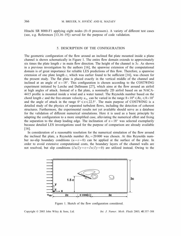
The geometric con�guration of the �ow around an inclined �at plate mounted inside a planechannel is shown schematically in Figure 1. The entire �ow domain extends to approximatelysix times the plate length c in main �ow direction. The height of the channel is 3c. As shownin a previous investigation by the authors [16], the spanwise extension of the computationaldomain is of great importance for reliable LES predictions of this �ow. Therefore, a spanwiseextension of one plate length c, which was earlier found to be su�cient [16], was chosen forthe present study. The �at plate is placed exactly in the vertical middle of the channel andinclined at an angle of �=18◦. This con�guration is chosen according to the COSTWINGexperiment initiated by Lerche and Dallmann [27], which aims at the �ow around an airfoilat high angles of attack. Instead of a �at plate, a nominally 2D airfoil based on an NACA-4415 pro�le is mounted inside a wind and a water tunnel. The Reynolds number based on thechord length c and the free-stream velocity u∞ can be varied in the range 8×1046Rec68×105and the angle of attack in the range 0◦6�622:5◦. The main purpose of COSTWING is adetailed study of the physics of separated turbulent �ows, including the detection of coherentstructures. Furthermore, the experimental results not yet available should serve as a databasefor the validation of di�erent numerical simulations. Here it is used as a basic principle byadapting the con�guration to a more simpli�ed case, alleviating the numerical e�ort and �xingthe separation to the sharp leading edge. The inclination of �=18◦ was selected exemplarilybecause detailed LES investigations used for the purpose of comparison are already available[16].In consideration of a reasonable resolution for the numerical simulation of the �ow around

the inclined �at plate, a Reynolds number Rec=20000 was chosen. At this Reynolds num-ber no-slip boundary conditions (u=v=0) can be applied at the surface of the plate. Inorder to avoid extensive computational costs, the boundary layers of the channel walls arenot resolved, but slip conditions (@u=@y=v=@w=@y=0) are utilized instead. Owing to the

Figure 1. Sketch of the �ow con�guration considered.



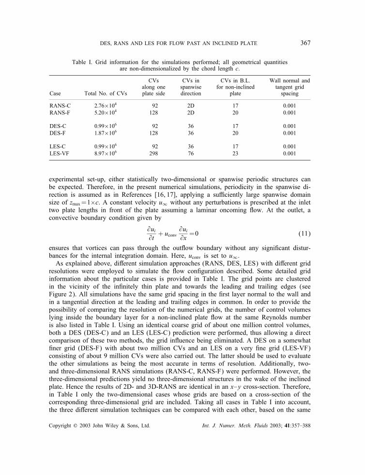
Table I. Grid information for the simulations performed; all geometrical quantitiesare non-dimensionalized by the chord length c.

CVs CVs in CVs in B.L. Wall normal andalong one spanwise for non-inclined tangent grid

Case Total No. of CVs plate side direction plate spacing

RANS-C 2:76×104 92 2D 17 0.001RANS-F 5:20×104 128 2D 20 0.001

DES-C 0:99×106 92 36 17 0.001DES-F 1:87×106 128 36 20 0.001

LES-C 0:99×106 92 36 17 0.001LES-VF 8:97×106 298 76 23 0.001

experimental set-up, either statistically two-dimensional or spanwise periodic structures canbe expected. Therefore, in the present numerical simulations, periodicity in the spanwise di-rection is assumed as in References [16, 17], applying a su�ciently large spanwise domainsize of zmax=1×c. A constant velocity u∞ without any perturbations is prescribed at the inlettwo plate lengths in front of the plate assuming a laminar oncoming �ow. At the outlet, aconvective boundary condition given by

@ui@t+ uconv

@ui@x=0 (11)

ensures that vortices can pass through the out�ow boundary without any signi�cant distur-bances for the internal integration domain. Here, uconv is set to u∞.As explained above, di�erent simulation approaches (RANS, DES, LES) with di�erent grid

resolutions were employed to simulate the �ow con�guration described. Some detailed gridinformation about the particular cases is provided in Table I. The grid points are clusteredin the vicinity of the in�nitely thin plate and towards the leading and trailing edges (seeFigure 2). All simulations have the same grid spacing in the �rst layer normal to the wall andin a tangential direction at the leading and trailing edges in common. In order to provide thepossibility of comparing the resolution of the numerical grids, the number of control volumeslying inside the boundary layer for a non-inclined plate �ow at the same Reynolds numberis also listed in Table I. Using an identical coarse grid of about one million control volumes,both a DES (DES-C) and an LES (LES-C) prediction were performed, thus allowing a directcomparison of these two methods, the grid in�uence being eliminated. A DES on a somewhat�ner grid (DES-F) with about two million CVs and an LES on a very �ne grid (LES-VF)consisting of about 9 million CVs were also carried out. The latter should be used to evaluatethe other simulations as being the most accurate in terms of resolution. Additionally, two-and three-dimensional RANS simulations (RANS-C, RANS-F) were performed. However, thethree-dimensional predictions yield no three-dimensional structures in the wake of the inclinedplate. Hence the results of 2D- and 3D-RANS are identical in an x–y cross-section. Therefore,in Table I only the two-dimensional cases whose grids are based on a cross-section of thecorresponding three-dimensional grid are included. Taking all cases in Table I into account,the three di�erent simulation techniques can be compared with each other, based on the same



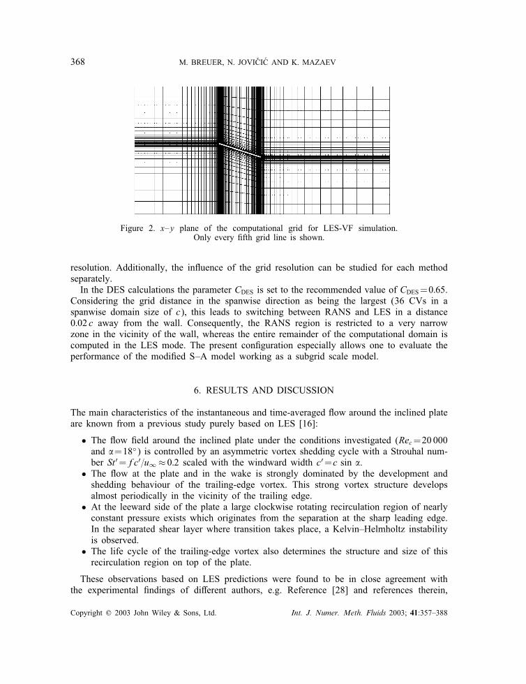
Figure 2. x–y plane of the computational grid for LES-VF simulation.Only every �fth grid line is shown.

resolution. Additionally, the in�uence of the grid resolution can be studied for each methodseparately.In the DES calculations the parameter CDES is set to the recommended value of CDES=0:65.

Considering the grid distance in the spanwise direction as being the largest (36 CVs in aspanwise domain size of c), this leads to switching between RANS and LES in a distance0:02 c away from the wall. Consequently, the RANS region is restricted to a very narrowzone in the vicinity of the wall, whereas the entire remainder of the computational domain iscomputed in the LES mode. The present con�guration especially allows one to evaluate theperformance of the modi�ed S–A model working as a subgrid scale model.

6. RESULTS AND DISCUSSION

The main characteristics of the instantaneous and time-averaged �ow around the inclined plateare known from a previous study purely based on LES [16]:

• The �ow �eld around the inclined plate under the conditions investigated (Rec=20000and �=18◦) is controlled by an asymmetric vortex shedding cycle with a Strouhal num-ber St′=fc′=u∞ ≈ 0:2 scaled with the windward width c′=c sin �.

• The �ow at the plate and in the wake is strongly dominated by the development andshedding behaviour of the trailing-edge vortex. This strong vortex structure developsalmost periodically in the vicinity of the trailing edge.

• At the leeward side of the plate a large clockwise rotating recirculation region of nearlyconstant pressure exists which originates from the separation at the sharp leading edge.In the separated shear layer where transition takes place, a Kelvin–Helmholtz instabilityis observed.

• The life cycle of the trailing-edge vortex also determines the structure and size of thisrecirculation region on top of the plate.

These observations based on LES predictions were found to be in close agreement withthe experimental �ndings of di�erent authors, e.g. Reference [28] and references therein,



[29, 30]. The objectives of the present investigation were to prove the applicability of DES(and RANS) for this �ow and to compare the quality of the predicted results for all threeapproaches (RANS, DES and LES) with each other. The LES calculation on the �nest grid(LES-VF, see Table I) will serve as a reference case.Some remarks on the calculations are required prior to the analysis. Although RANS pre-

dictions on di�erent grids were carried out, in the following only the case of the �ne grid(RANS-F) is considered and discussed in detail. Because the di�erences between the resultson both grids were marginal, the RANS prediction on the �ne grid is grid independent and itis therefore not necessary to discuss results obtained with di�erent resolutions. Furthermore,it is important to mention that all computations based on RANS, although applied in an un-steady mode known as URANS, do not show the unsteady shedding motion discussed above.Instead, the RANS simulations converge to steady-state results. Hence they are not capableof describing the unsteady nature of the �ow �eld around the inclined plate. In contrast, theDES and LES predictions yield the main characteristics of the unsteady �ow �eld. In orderto compare all results including RANS, the DES and LES computations are averaged bothin time and in space (spanwise). For all simulations performed an averaging in time of atleast 50 dimensionless time units was made. The additional averaging in the spanwise direc-tion is done in order to obtain a well-averaged �ow �eld more rapidly and therefore to savecomputing time. The analysis will start with the averaged �ow �eld (Section 6.1). In the sec-ond and third parts, also the unsteady �ow �eld (Section 6.2) and the higher-order statistics(Section 6.3) of the DES and LES predictions are discussed. Finally, the results are analysedwith respect to the performance of the SGS models applied in pure LES and the LES modeof the hybrid DES predictions (Section 6.4). Based on this analysis, some modi�cations ofthe S–A model are proposed for the use as an SGS model within the DES approach stronglyenhancing the quality of the predictions.

6.1. Averaged �ow �eld

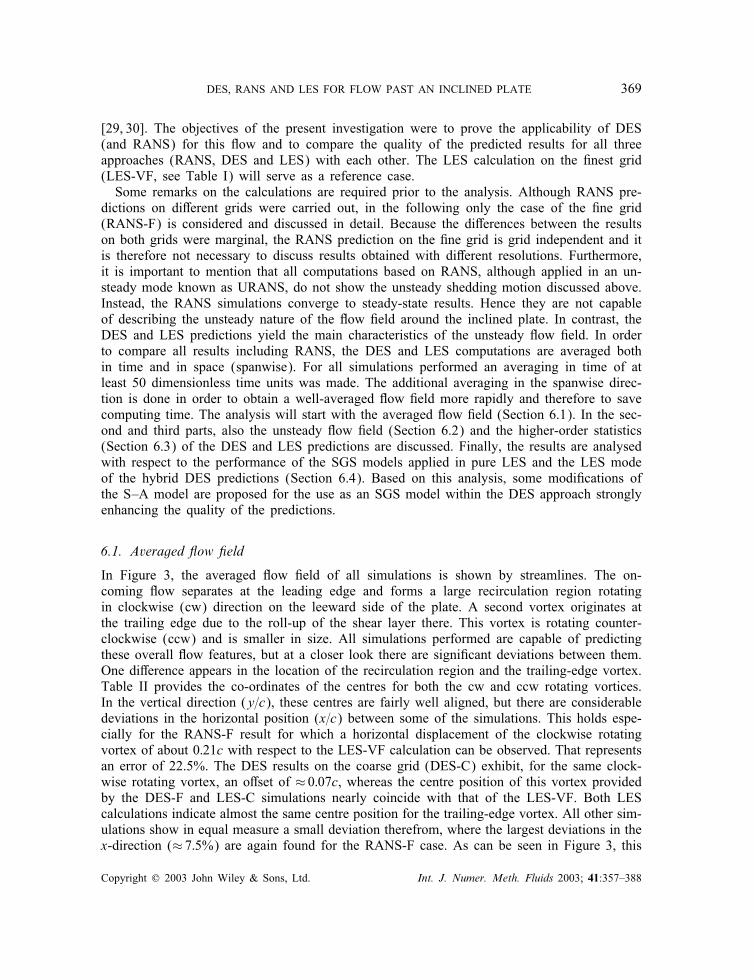
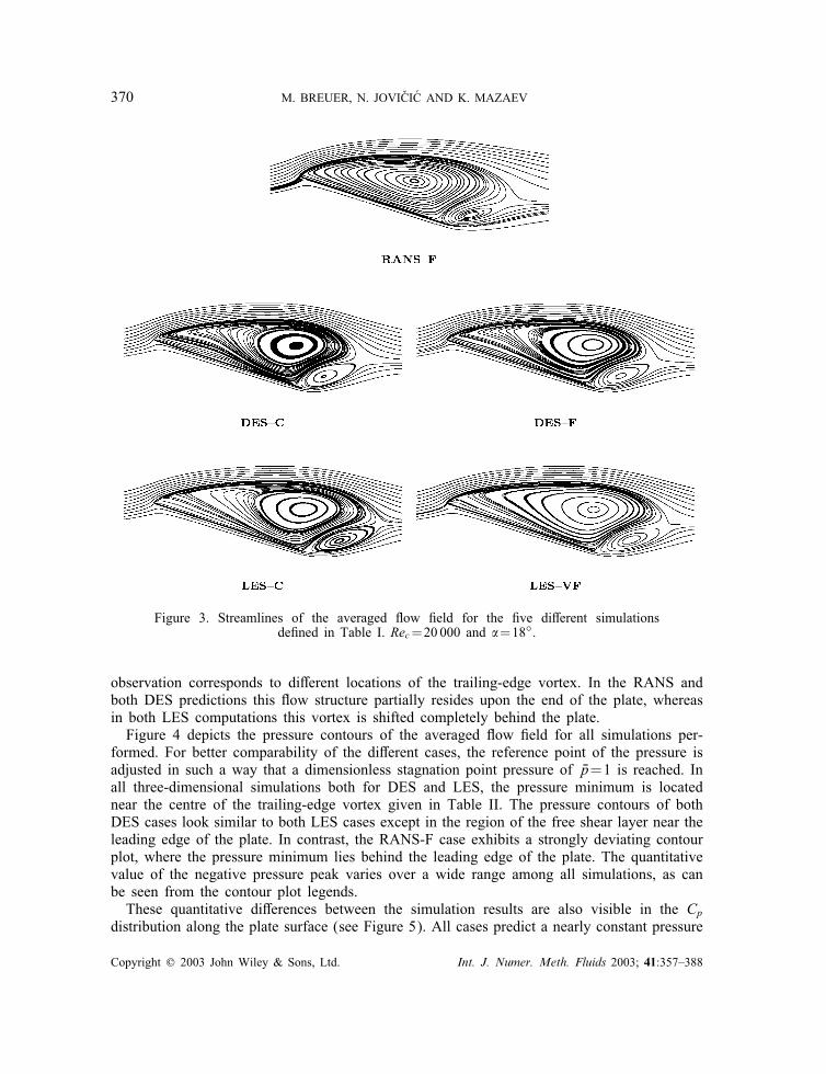
In Figure 3, the averaged �ow �eld of all simulations is shown by streamlines. The on-coming �ow separates at the leading edge and forms a large recirculation region rotatingin clockwise (cw) direction on the leeward side of the plate. A second vortex originates atthe trailing edge due to the roll-up of the shear layer there. This vortex is rotating counter-clockwise (ccw) and is smaller in size. All simulations performed are capable of predictingthese overall �ow features, but at a closer look there are signi�cant deviations between them.One di�erence appears in the location of the recirculation region and the trailing-edge vortex.Table II provides the co-ordinates of the centres for both the cw and ccw rotating vortices.In the vertical direction (y=c), these centres are fairly well aligned, but there are considerabledeviations in the horizontal position (x=c) between some of the simulations. This holds espe-cially for the RANS-F result for which a horizontal displacement of the clockwise rotatingvortex of about 0:21c with respect to the LES-VF calculation can be observed. That representsan error of 22.5%. The DES results on the coarse grid (DES-C) exhibit, for the same clock-wise rotating vortex, an o�set of ≈ 0:07c, whereas the centre position of this vortex providedby the DES-F and LES-C simulations nearly coincide with that of the LES-VF. Both LEScalculations indicate almost the same centre position for the trailing-edge vortex. All other sim-ulations show in equal measure a small deviation therefrom, where the largest deviations in thex-direction (≈ 7:5%) are again found for the RANS-F case. As can be seen in Figure 3, this



Figure 3. Streamlines of the averaged �ow �eld for the �ve di�erent simulationsde�ned in Table I. Rec=20 000 and �=18◦.

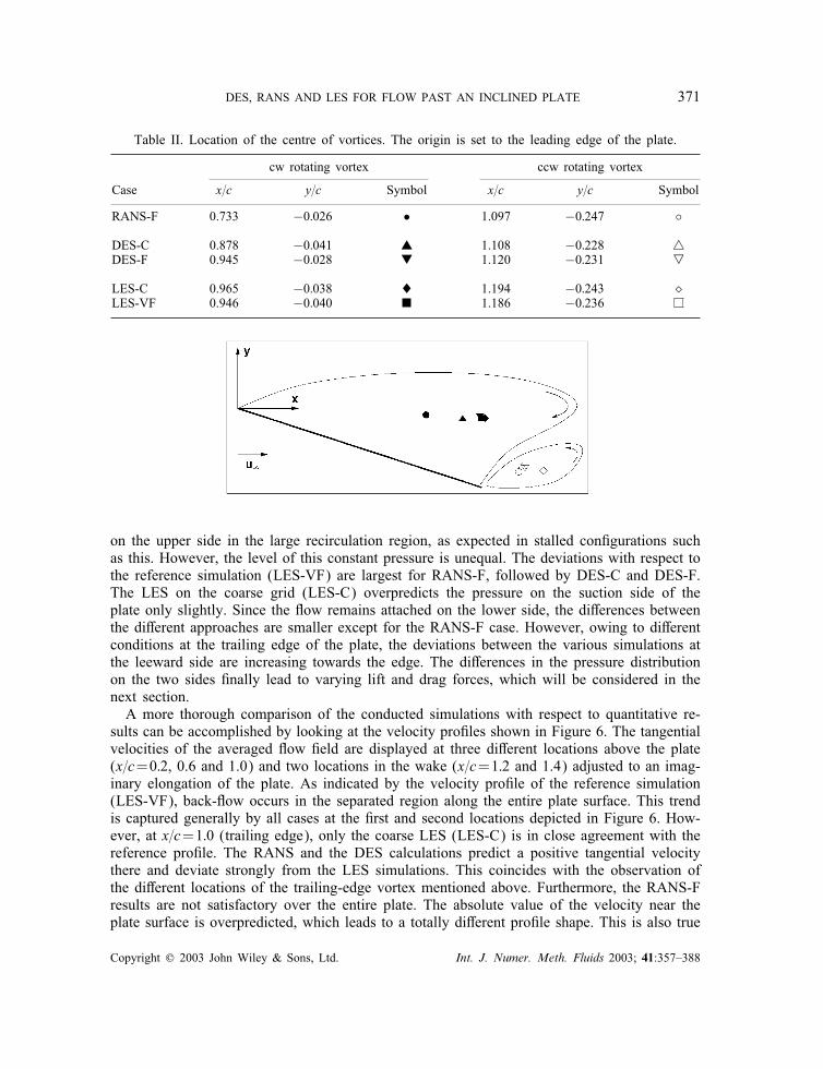
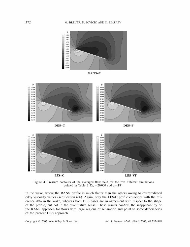
observation corresponds to di�erent locations of the trailing-edge vortex. In the RANS andboth DES predictions this �ow structure partially resides upon the end of the plate, whereasin both LES computations this vortex is shifted completely behind the plate.Figure 4 depicts the pressure contours of the averaged �ow �eld for all simulations per-

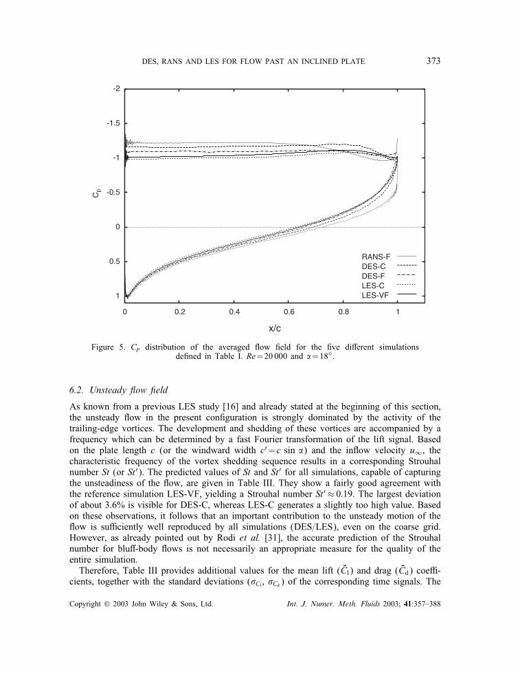
formed. For better comparability of the di�erent cases, the reference point of the pressure isadjusted in such a way that a dimensionless stagnation point pressure of p=1 is reached. Inall three-dimensional simulations both for DES and LES, the pressure minimum is locatednear the centre of the trailing-edge vortex given in Table II. The pressure contours of bothDES cases look similar to both LES cases except in the region of the free shear layer near theleading edge of the plate. In contrast, the RANS-F case exhibits a strongly deviating contourplot, where the pressure minimum lies behind the leading edge of the plate. The quantitativevalue of the negative pressure peak varies over a wide range among all simulations, as canbe seen from the contour plot legends.These quantitative di�erences between the simulation results are also visible in the Cp

distribution along the plate surface (see Figure 5). All cases predict a nearly constant pressure



Table II. Location of the centre of vortices. The origin is set to the leading edge of the plate.

cw rotating vortex ccw rotating vortex

Case x=c y=c Symbol x=c y=c Symbol

RANS-F 0.733 −0:026 • 1.097 −0:247 ◦

DES-C 0.878 −0:041 N 1.108 −0:228 �DES-F 0.945 −0:028 H 1.120 −0:231 O

LES-C 0.965 −0:038 � 1.194 −0:243 �LES-VF 0.946 −0:040 1.186 −0:236

on the upper side in the large recirculation region, as expected in stalled con�gurations suchas this. However, the level of this constant pressure is unequal. The deviations with respect tothe reference simulation (LES-VF) are largest for RANS-F, followed by DES-C and DES-F.The LES on the coarse grid (LES-C) overpredicts the pressure on the suction side of theplate only slightly. Since the �ow remains attached on the lower side, the di�erences betweenthe di�erent approaches are smaller except for the RANS-F case. However, owing to di�erentconditions at the trailing edge of the plate, the deviations between the various simulations atthe leeward side are increasing towards the edge. The di�erences in the pressure distributionon the two sides �nally lead to varying lift and drag forces, which will be considered in thenext section.A more thorough comparison of the conducted simulations with respect to quantitative re-

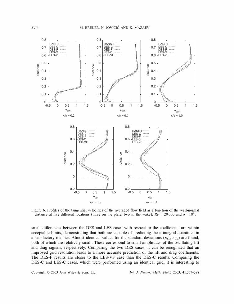
sults can be accomplished by looking at the velocity pro�les shown in Figure 6. The tangentialvelocities of the averaged �ow �eld are displayed at three di�erent locations above the plate(x=c=0:2, 0.6 and 1.0) and two locations in the wake (x=c=1:2 and 1.4) adjusted to an imag-inary elongation of the plate. As indicated by the velocity pro�le of the reference simulation(LES-VF), back-�ow occurs in the separated region along the entire plate surface. This trendis captured generally by all cases at the �rst and second locations depicted in Figure 6. How-ever, at x=c=1:0 (trailing edge), only the coarse LES (LES-C) is in close agreement with thereference pro�le. The RANS and the DES calculations predict a positive tangential velocitythere and deviate strongly from the LES simulations. This coincides with the observation ofthe di�erent locations of the trailing-edge vortex mentioned above. Furthermore, the RANS-Fresults are not satisfactory over the entire plate. The absolute value of the velocity near theplate surface is overpredicted, which leads to a totally di�erent pro�le shape. This is also true



Figure 4. Pressure contours of the averaged �ow �eld for the �ve di�erent simulationsde�ned in Table I. Rec=20 000 and �=18◦.

in the wake, where the RANS pro�le is much �atter than the others owing to overpredictededdy viscosity values (see Section 6.4). Again, only the LES-C pro�le coincides with the ref-erence data in the wake, whereas both DES cases are in agreement with respect to the shapeof the pro�le, but not in the quantitative sense. These results con�rm the inapplicability ofthe RANS approach for �ows with large regions of separation and point to some de�cienciesof the present DES approach.



-2

-1.5

-1

-0.5

0

0.5

1

0 0.2 0.4 0.6 0.8 1

Cp

x/c

RANS-FDES-CDES-FLES-CLES-VF

Figure 5. Cp distribution of the averaged �ow �eld for the �ve di�erent simulationsde�ned in Table I. Re=20 000 and �=18◦.

6.2. Unsteady �ow �eld

As known from a previous LES study [16] and already stated at the beginning of this section,the unsteady �ow in the present con�guration is strongly dominated by the activity of thetrailing-edge vortices. The development and shedding of these vortices are accompanied by afrequency which can be determined by a fast Fourier transformation of the lift signal. Basedon the plate length c (or the windward width c′=c sin �) and the in�ow velocity u∞, thecharacteristic frequency of the vortex shedding sequence results in a corresponding Strouhalnumber St (or St′). The predicted values of St and St′ for all simulations, capable of capturingthe unsteadiness of the �ow, are given in Table III. They show a fairly good agreement withthe reference simulation LES-VF, yielding a Strouhal number St′ ≈ 0:19. The largest deviationof about 3.6% is visible for DES-C, whereas LES-C generates a slightly too high value. Basedon these observations, it follows that an important contribution to the unsteady motion of the�ow is su�ciently well reproduced by all simulations (DES=LES), even on the coarse grid.However, as already pointed out by Rodi et al. [31], the accurate prediction of the Strouhalnumber for blu�-body �ows is not necessarily an appropriate measure for the quality of theentire simulation.Therefore, Table III provides additional values for the mean lift ( Cl) and drag ( Cd) coe�-

cients, together with the standard deviations (�Cl , �Cd ) of the corresponding time signals. The



0

0.1

0.2

0.3

0.4

0.5

0.6

0.7

0.8

-0.5 0 0.5 1 1.5

dist

ance

vtan


0

0.1

0.2

0.3

0.4

0.5

0.6

0.7

0.8

-0.5 0 0.5 1 1.5

dist

ance

vtan


0

0.1

0.2

0.3

0.4

0.5

0.6

0.7

0.8

-0.5 0 0.5 1 1.5

dist

ance

vtan


-0.2

0

0.2

0.4

0.6

0.8

-0.5 0 0.5 1 1.5

dist

ance

vtan


-0.2

0

0.2

0.4

0.6

0.8

-0.5 0 0.5 1 1.5

dist

ance

vtan


x/c = 0.2

x/c = 1.2 x/c = 1.4

x/c = 0.6 x/c = 1.0

Figure 6. Pro�les of the tangential velocities of the averaged �ow �eld as a function of the wall-normaldistance at �ve di�erent locations (three on the plate, two in the wake). Rec=20 000 and �=18◦.

small di�erences between the DES and LES cases with respect to the coe�cients are withinacceptable limits, demonstrating that both are capable of predicting these integral quantities ina satisfactory manner. Almost identical values for the standard deviations (�Cl , �Cd ) are found,both of which are relatively small. These correspond to small amplitudes of the oscillating liftand drag signals, respectively. Comparing the two DES cases, it can be recognized that animproved grid resolution leads to a more accurate prediction of the lift and drag coe�cients.The DES-F results are closer to the LES-VF case than the DES-C results. Comparing theDES-C and LES-C cases, which were performed using an identical grid, it is interesting to



Table III. Comparison of integral quantities for the �at plate at Rec=20 000 and �=18◦.

Case Cl Cd �Cl �Cd St St′

RANS-C 1.314 0.438 — — — —RANS-F 1.318 0.439 — — — —

DES-C 1.182 0.399 8:0 · 10−2 2:5 · 10−2 0.60 0.185DES-F 1.153 0.389 8:1 · 10−2 2:5 · 10−2 0.61 0.189

LES-C 1.078 0.365 7:9 · 10−2 2:5 · 10−2 0.63 0.195LES-VF 1.128 0.380 7:0 · 10−2 2:2 · 10−2 0.62 0.192

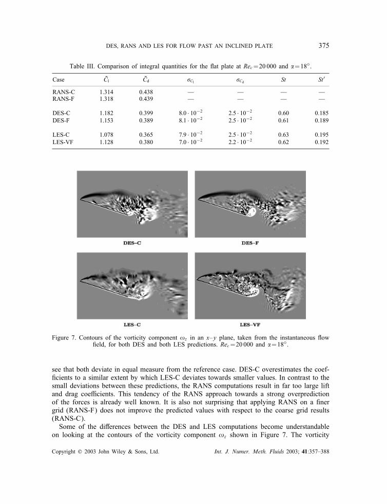
Figure 7. Contours of the vorticity component !z in an x–y plane, taken from the instantaneous �ow�eld, for both DES and both LES predictions. Rec=20 000 and �=18◦.

see that both deviate in equal measure from the reference case. DES-C overestimates the coef-�cients to a similar extent by which LES-C deviates towards smaller values. In contrast to thesmall deviations between these predictions, the RANS computations result in far too large liftand drag coe�cients. This tendency of the RANS approach towards a strong overpredictionof the forces is already well known. It is also not surprising that applying RANS on a �nergrid (RANS-F) does not improve the predicted values with respect to the coarse grid results(RANS-C).Some of the di�erences between the DES and LES computations become understandable

on looking at the contours of the vorticity component !z shown in Figure 7. The vorticity



is taken from the instantaneous �ow �eld at an arbitrary time instant. The four parts ofFigure 7 were not meant to represent a synchronous instant of the vortex shedding cycle,since this was not relevant for the purpose of showing them here. Anyhow, it seems that thesnap shots of the DES-F and LES-VF vorticity contours do represent almost the same instantby chance. Compared with the LES on the very �ne grid (LES-VF), the contours obtainedby the other simulations are visibly smoother and do not show a large variety of resolvedsmall-scale structures. This is particularly noticeable in the region of the leading-edge shearlayer. In contrast, the LES-VF prediction reproduces this �ow feature sharply, thus allowingthe motion of single eddies in this region to be resolved in detail. Consequently, for the LES-VF case and at least allusively also for LES-C, it is possible to detect a Kelvin–Helmholtzinstability occurring in the shear layer and leading to transition. Such detailed �ow structuresare not resolved by either DES calculation. Therefore, they fail to re�ect the �ow in thisregion properly. This will also become evident on looking at the higher-order statistics in thefollowing section. Although the same grid is applied in the DES-C and the LES-C cases,the latter tends more clearly to the reference case. Hence the grid resolution is not solelyresponsible for the quality of the results. In contrast the modelling aspect plays the dominantrole in this behaviour, which will be analysed in detail in Section 6.4.

6.3. Higher-order statistics

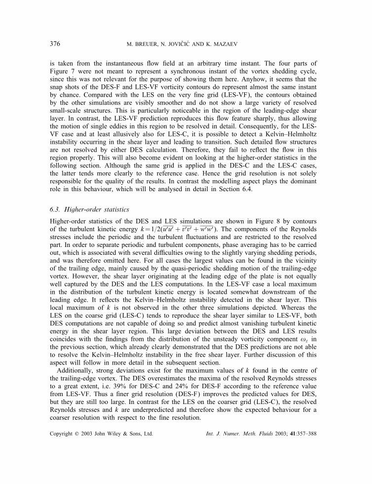
Higher-order statistics of the DES and LES simulations are shown in Figure 8 by contoursof the turbulent kinetic energy k=1=2(u′u′ + v′v′ + w′w′). The components of the Reynoldsstresses include the periodic and the turbulent �uctuations and are restricted to the resolvedpart. In order to separate periodic and turbulent components, phase averaging has to be carriedout, which is associated with several di�culties owing to the slightly varying shedding periods,and was therefore omitted here. For all cases the largest values can be found in the vicinityof the trailing edge, mainly caused by the quasi-periodic shedding motion of the trailing-edgevortex. However, the shear layer originating at the leading edge of the plate is not equallywell captured by the DES and the LES computations. In the LES-VF case a local maximumin the distribution of the turbulent kinetic energy is located somewhat downstream of theleading edge. It re�ects the Kelvin–Helmholtz instability detected in the shear layer. Thislocal maximum of k is not observed in the other three simulations depicted. Whereas theLES on the coarse grid (LES-C) tends to reproduce the shear layer similar to LES-VF, bothDES computations are not capable of doing so and predict almost vanishing turbulent kineticenergy in the shear layer region. This large deviation between the DES and LES resultscoincides with the �ndings from the distribution of the unsteady vorticity component !z inthe previous section, which already clearly demonstrated that the DES predictions are not ableto resolve the Kelvin–Helmholtz instability in the free shear layer. Further discussion of thisaspect will follow in more detail in the subsequent section.Additionally, strong deviations exist for the maximum values of k found in the centre of

the trailing-edge vortex. The DES overestimates the maxima of the resolved Reynolds stressesto a great extent, i.e. 39% for DES-C and 24% for DES-F according to the reference valuefrom LES-VF. Thus a �ner grid resolution (DES-F) improves the predicted values for DES,but they are still too large. In contrast for the LES on the coarser grid (LES-C), the resolvedReynolds stresses and k are underpredicted and therefore show the expected behaviour for acoarser resolution with respect to the �ne resolution.



Figure 8. Resolved Reynolds stresses in terms of the turbulent kinetic energy k=1=2(u′u′+v′v′+w′w′)for the DES and LES cases. Rec=20 000 and �=18◦.

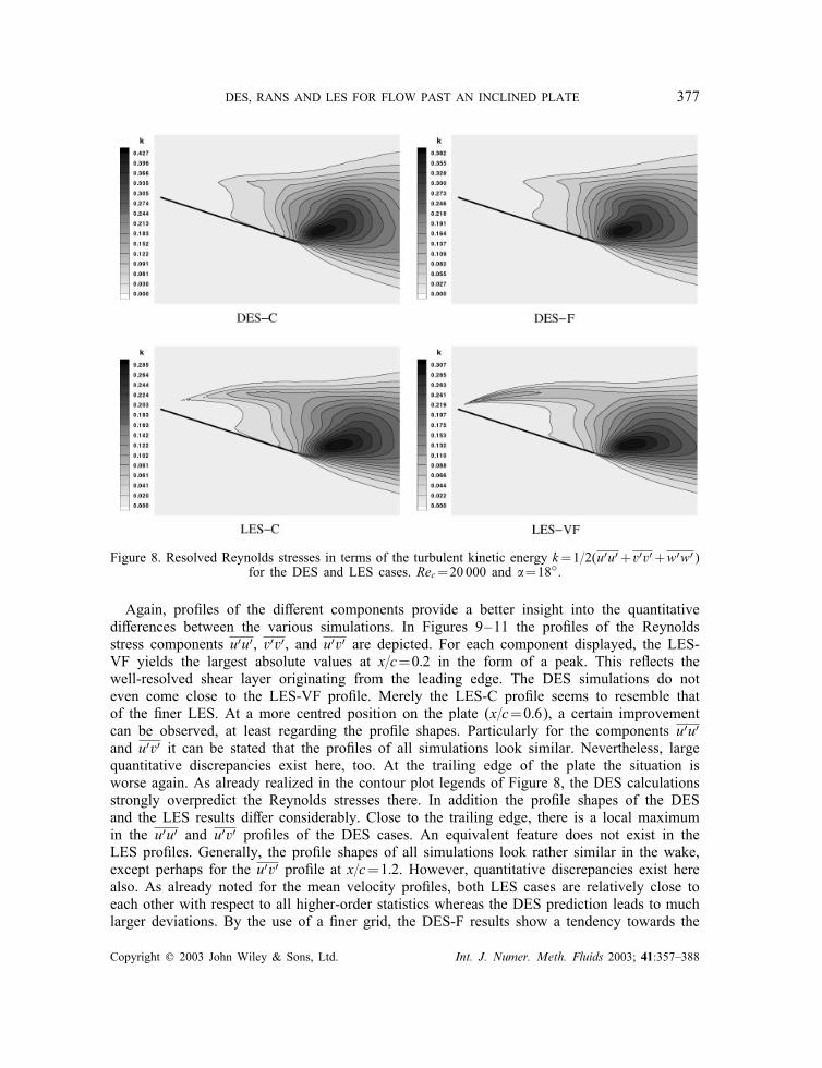
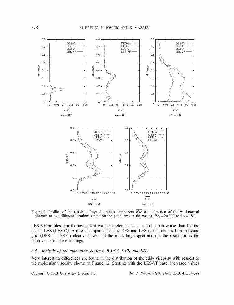
Again, pro�les of the di�erent components provide a better insight into the quantitativedi�erences between the various simulations. In Figures 9–11 the pro�les of the Reynoldsstress components u′u′, v′v′, and u′v′ are depicted. For each component displayed, the LES-VF yields the largest absolute values at x=c=0:2 in the form of a peak. This re�ects thewell-resolved shear layer originating from the leading edge. The DES simulations do noteven come close to the LES-VF pro�le. Merely the LES-C pro�le seems to resemble thatof the �ner LES. At a more centred position on the plate (x=c=0:6), a certain improvementcan be observed, at least regarding the pro�le shapes. Particularly for the components u′u′and u′v′ it can be stated that the pro�les of all simulations look similar. Nevertheless, largequantitative discrepancies exist here, too. At the trailing edge of the plate the situation isworse again. As already realized in the contour plot legends of Figure 8, the DES calculationsstrongly overpredict the Reynolds stresses there. In addition the pro�le shapes of the DESand the LES results di�er considerably. Close to the trailing edge, there is a local maximumin the u′u′ and u′v′ pro�les of the DES cases. An equivalent feature does not exist in theLES pro�les. Generally, the pro�le shapes of all simulations look rather similar in the wake,except perhaps for the u′v′ pro�le at x=c=1:2. However, quantitative discrepancies exist herealso. As already noted for the mean velocity pro�les, both LES cases are relatively close toeach other with respect to all higher-order statistics whereas the DES prediction leads to muchlarger deviations. By the use of a �ner grid, the DES-F results show a tendency towards the



0

0.1

0.2

0.3

0.4

0.5

0.6

0.7

0.8

0 0.05 0.1 0.15 0.2 0.25

dist

ance

u’ u’

DES-CDES-FLES-CLES-VF

0

0.1

0.2

0.3

0.4

0.5

0.6

0.7

0.8

0 0.05 0.1 0.15 0.2 0.25

dist

ance

u’ u’


0

0.1

0.2

0.3

0.4

0.5

0.6

0.7

0.8

0 0.05 0.1 0.15 0.2 0.25

dist

ance

u’ u’


-0.2

0

0.2

0.4

0.6

0.8

0 0.05 0.1 0.15 0.2 0.25 0.3 0.35

dist

ance

u’ u’


-0.2

0

0.2

0.4

0.6

0.8

0 0.05 0.1 0.15 0.2 0.25 0.3 0.35

dist

ance

u’ u’


x/c = 0.2

x/c = 1.2 x/c = 1.4

x/c = 0.6 x/c = 1.0

Figure 9. Pro�les of the resolved Reynolds stress component u′u′ as a function of the wall-normaldistance at �ve di�erent locations (three on the plate, two in the wake). Rec=20 000 and �=18◦.

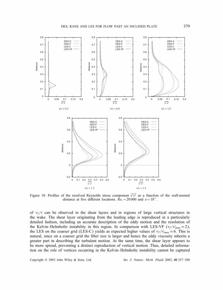
LES-VF pro�les, but the agreement with the reference data is still much worse than for thecoarse LES (LES-C). A direct comparison of the DES and LES results obtained on the samegrid (DES-C, LES-C) clearly shows that the modelling aspect and not the resolution is themain cause of these �ndings.

6.4. Analysis of the di�erences between RANS, DES and LES

Very interesting di�erences are found in the distribution of the eddy viscosity with respect tothe molecular viscosity shown in Figure 12. Starting with the LES-VF case, increased values



0

0.1

0.2

0.3

0.4

0.5

0.6

0.7

0.8

0 0.05 0.1 0.15 0.2

dist

ance

v’ v’


0

0.1

0.2

0.3

0.4

0.5

0.6

0.7

0.8

0 0.05 0.1 0.15 0.2

dist

ance

v’ v’


0

0.1

0.2

0.3

0.4

0.5

0.6

0.7

0.8

0 0.05 0.1 0.15 0.2

dist

ance

v’ v’


-0.2

0

0.2

0.4

0.6

0.8

0 0.1 0.2 0.3 0.4 0.5 0.6

dist

ance

v’ v’


-0.2

0

0.2

0.4

0.6

0.8

0 0.1 0.2 0.3 0.4 0.5 0.6

dist

ance

v’ v’


x/c = 0.2 x/c = 0.6 x/c = 1.0

x/c = 1.4x/c = 1.2

Figure 10. Pro�les of the resolved Reynolds stress component v′v′ as a function of the wall-normaldistance at �ve di�erent locations. Rec=20 000 and �=18◦.

of �T =� can be observed in the shear layers and in regions of large vortical structures inthe wake. The shear layer originating from the leading edge is reproduced in a particularlydetailed fashion, including an accurate description of the eddy motion and the resolution ofthe Kelvin–Helmholtz instability in this region. In comparison with LES-VF (�T =�|max≈ 2),the LES on the coarser grid (LES-C) yields as expected higher values of �T =�|max≈ 6. This isnatural, since on a coarser grid the �lter size is larger and hence the eddy viscosity inherits agreater part in describing the turbulent motion. At the same time, the shear layer appears tobe more spread, preventing a distinct reproduction of vortical motion. Thus, detailed informa-tion on the role of vortices occurring in the Kelvin–Helmholtz instability cannot be captured



0

0.1

0.2

0.3

0.4

0.5

0.6

0.7

0.8

-0.03 -0.02 -0.01 0 0.01

dist

ance

u’ v’


0

0.1

0.2

0.3

0.4

0.5

0.6

0.7

0.8

-0.03 -0.02 -0.01 0 0.01

dist

ance

u’ v’


0

0.1

0.2

0.3

0.4

0.5

0.6

0.7

0.8

-0.06 -0.05 -0.04 -0.03 -0.02 -0.01 0 0.01

dist

ance

u’ v’


-0.2

0

0.2

0.4

0.6

0.8

-0.1 -0.05 0 0.05 0.1 0.15

dist

ance

u’ v’


-0.2

0

0.2

0.4

0.6

0.8

-0.1 -0.05 0 0.05 0.1 0.15

dist

ance

u’ v’


x/c = 0.2

x/c = 1.2 x/c = 1.4

x/c = 0.6 x/c = 1.0

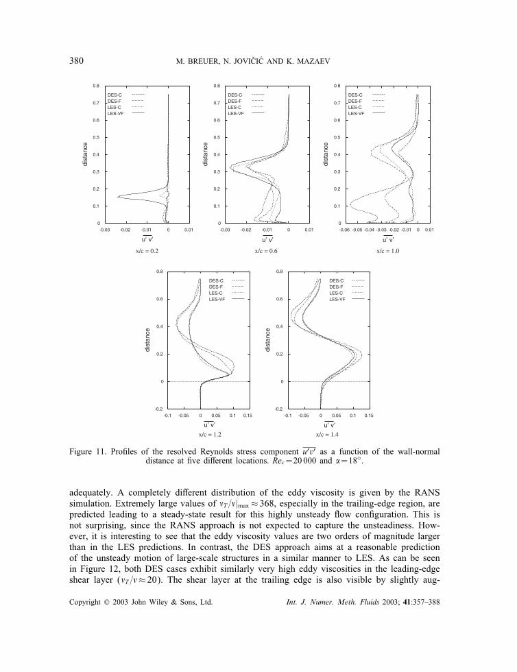
Figure 11. Pro�les of the resolved Reynolds stress component u′v′ as a function of the wall-normaldistance at �ve di�erent locations. Rec=20 000 and �=18◦.

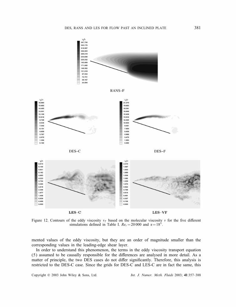
adequately. A completely di�erent distribution of the eddy viscosity is given by the RANSsimulation. Extremely large values of �T =�|max≈ 368, especially in the trailing-edge region, arepredicted leading to a steady-state result for this highly unsteady �ow con�guration. This isnot surprising, since the RANS approach is not expected to capture the unsteadiness. How-ever, it is interesting to see that the eddy viscosity values are two orders of magnitude largerthan in the LES predictions. In contrast, the DES approach aims at a reasonable predictionof the unsteady motion of large-scale structures in a similar manner to LES. As can be seenin Figure 12, both DES cases exhibit similarly very high eddy viscosities in the leading-edgeshear layer (�T =�≈ 20). The shear layer at the trailing edge is also visible by slightly aug-



Figure 12. Contours of the eddy viscosity �T based on the molecular viscosity � for the �ve di�erentsimulations de�ned in Table I. Rec=20 000 and �=18◦.

mented values of the eddy viscosity, but they are an order of magnitude smaller than thecorresponding values in the leading-edge shear layer.In order to understand this phenomenon, the terms in the eddy viscosity transport equation

(5) assumed to be causally responsible for the di�erences are analysed in more detail. As amatter of principle, the two DES cases do not di�er signi�cantly. Therefore, this analysis isrestricted to the DES-C case. Since the grids for DES-C and LES-C are in fact the same, this



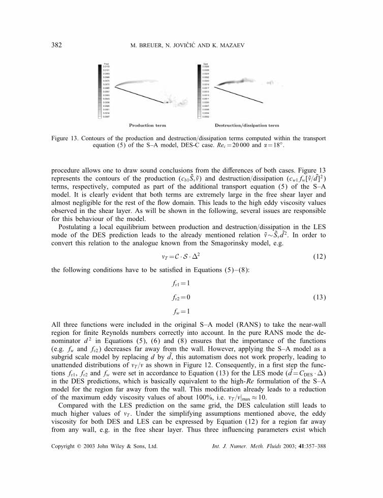
Figure 13. Contours of the production and destruction=dissipation terms computed within the transportequation (5) of the S–A model, DES-C case. Rec=20 000 and �=18◦.

procedure allows one to draw sound conclusions from the di�erences of both cases. Figure 13represents the contours of the production (cb1S̃��̃) and destruction=dissipation (cw1fw[�̃=d̃]2)terms, respectively, computed as part of the additional transport equation (5) of the S–Amodel. It is clearly evident that both terms are extremely large in the free shear layer andalmost negligible for the rest of the �ow domain. This leads to the high eddy viscosity valuesobserved in the shear layer. As will be shown in the following, several issues are responsiblefor this behaviour of the model.Postulating a local equilibrium between production and destruction=dissipation in the LES

mode of the DES prediction leads to the already mentioned relation �̃∼ S̃� d̃2. In order toconvert this relation to the analogue known from the Smagorinsky model, e.g.

�T=C · S ·�2 (12)

the following conditions have to be satis�ed in Equations (5)–(8):

fv1=1

fv2=0

fw=1

(13)

All three functions were included in the original S–A model (RANS) to take the near-wallregion for �nite Reynolds numbers correctly into account. In the pure RANS mode the de-nominator d2 in Equations (5), (6) and (8) ensures that the importance of the functions(e.g. fw and fv2) decreases far away from the wall. However, applying the S–A model as asubgrid scale model by replacing d by d̃, this automatism does not work properly, leading tounattended distributions of �T =� as shown in Figure 12. Consequently, in a �rst step the func-tions fv1, fv2 and fw were set in accordance to Equation (13) for the LES mode (d̃=CDES ·�)in the DES predictions, which is basically equivalent to the high-Re formulation of the S–Amodel for the region far away from the wall. This modi�cation already leads to a reductionof the maximum eddy viscosity values of about 100%, i.e. �T =�|max≈ 10.Compared with the LES prediction on the same grid, the DES calculation still leads to

much higher values of �T . Under the simplifying assumptions mentioned above, the eddyviscosity for both DES and LES can be expressed by Equation (12) for a region far awayfrom any wall, e.g. in the free shear layer. Thus three in�uencing parameters exist which



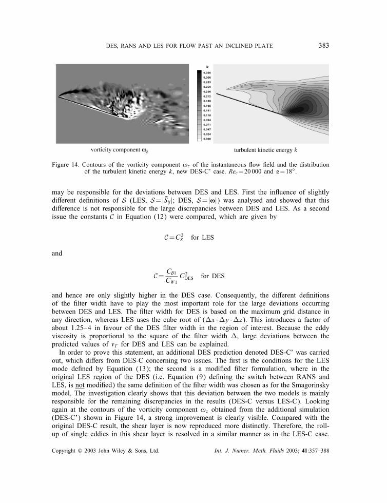
Figure 14. Contours of the vorticity component !z of the instantaneous �ow �eld and the distributionof the turbulent kinetic energy k, new DES-C’ case. Rec=20 000 and �=18◦.

may be responsible for the deviations between DES and LES. First the in�uence of slightlydi�erent de�nitions of S (LES, S= | Sij |; DES, S= |�|) was analysed and showed that thisdi�erence is not responsible for the large discrepancies between DES and LES. As a secondissue the constants C in Equation (12) were compared, which are given by

C=C 2S for LES

and

C= CB1CW1

C 2DES for DES

and hence are only slightly higher in the DES case. Consequently, the di�erent de�nitionsof the �lter width have to play the most important role for the large deviations occurringbetween DES and LES. The �lter width for DES is based on the maximum grid distance inany direction, whereas LES uses the cube root of (�x ·�y ·�z). This introduces a factor ofabout 1.25–4 in favour of the DES �lter width in the region of interest. Because the eddyviscosity is proportional to the square of the �lter width �, large deviations between thepredicted values of �T for DES and LES can be explained.In order to prove this statement, an additional DES prediction denoted DES-C’ was carried

out, which di�ers from DES-C concerning two issues. The �rst is the conditions for the LESmode de�ned by Equation (13); the second is a modi�ed �lter formulation, where in theoriginal LES region of the DES (i.e. Equation (9) de�ning the switch between RANS andLES, is not modi�ed) the same de�nition of the �lter width was chosen as for the Smagorinskymodel. The investigation clearly shows that this deviation between the two models is mainlyresponsible for the remaining discrepancies in the results (DES-C versus LES-C). Lookingagain at the contours of the vorticity component !z obtained from the additional simulation(DES-C’) shown in Figure 14, a strong improvement is clearly visible. Compared with theoriginal DES-C result, the shear layer is now reproduced more distinctly. Therefore, the roll-up of single eddies in this shear layer is resolved in a similar manner as in the LES-C case.



0

0.1

0.2

0.3

0.4

0.5

0.6

0.7

0.8

-0.5 0 0.5 1 1.5

dist

ance

vtan

DES-CDES-FLES-CLES-VFDES-C’

-0.2

0

0.2

0.4

0.6

0.8

-0.5 0 0.5 1 1.5

dist

ance

vtan


x/c = 1.0 x/c = 1.2

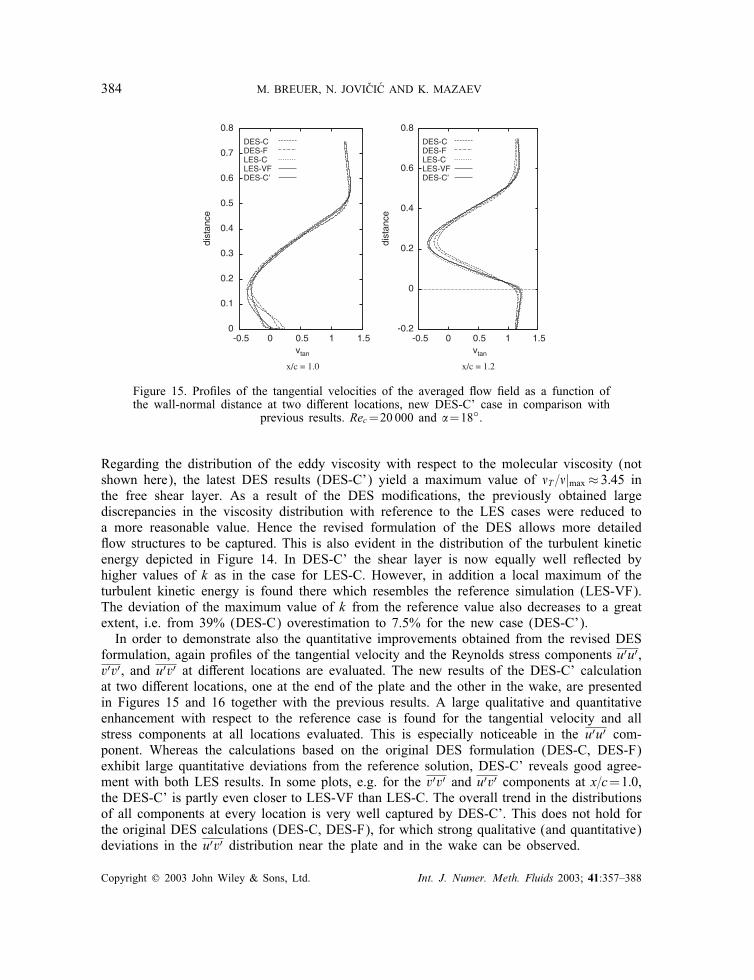
Figure 15. Pro�les of the tangential velocities of the averaged �ow �eld as a function ofthe wall-normal distance at two di�erent locations, new DES-C’ case in comparison with

previous results. Rec=20 000 and �=18◦.

Regarding the distribution of the eddy viscosity with respect to the molecular viscosity (notshown here), the latest DES results (DES-C’) yield a maximum value of �T =�|max≈ 3:45 inthe free shear layer. As a result of the DES modi�cations, the previously obtained largediscrepancies in the viscosity distribution with reference to the LES cases were reduced toa more reasonable value. Hence the revised formulation of the DES allows more detailed�ow structures to be captured. This is also evident in the distribution of the turbulent kineticenergy depicted in Figure 14. In DES-C’ the shear layer is now equally well re�ected byhigher values of k as in the case for LES-C. However, in addition a local maximum of theturbulent kinetic energy is found there which resembles the reference simulation (LES-VF).The deviation of the maximum value of k from the reference value also decreases to a greatextent, i.e. from 39% (DES-C) overestimation to 7.5% for the new case (DES-C’).In order to demonstrate also the quantitative improvements obtained from the revised DES

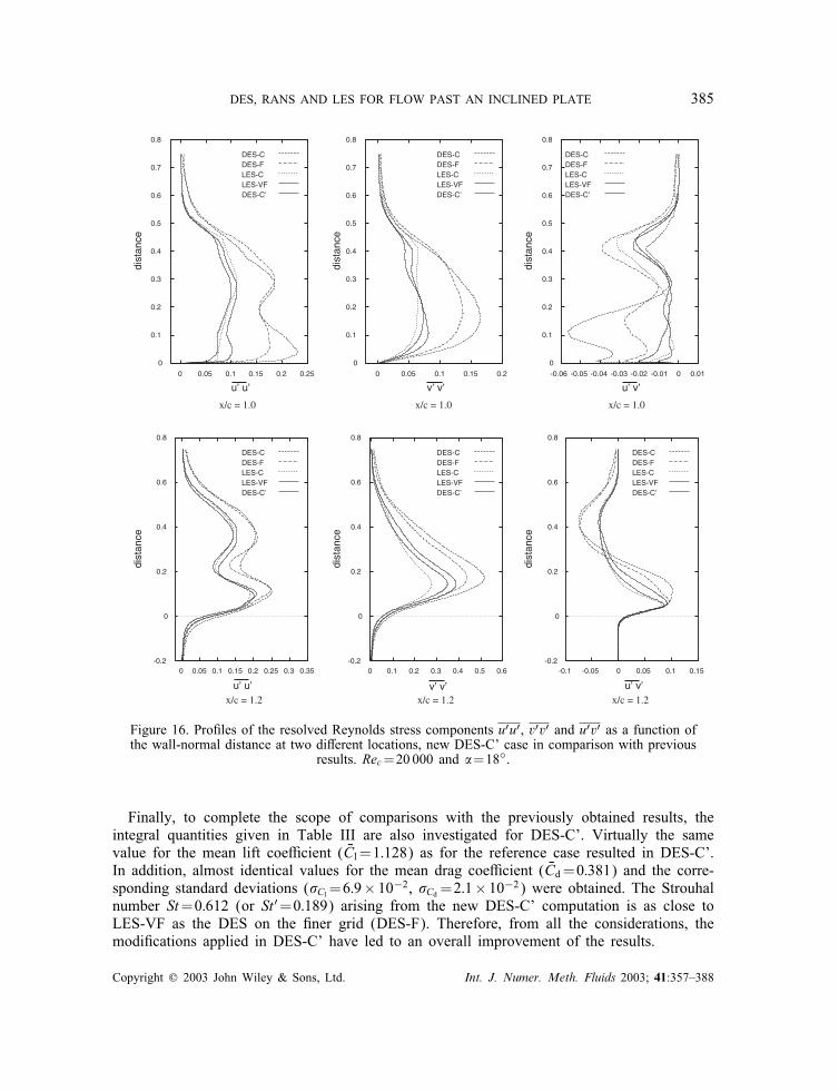
formulation, again pro�les of the tangential velocity and the Reynolds stress components u′u′,v′v′, and u′v′ at di�erent locations are evaluated. The new results of the DES-C’ calculationat two di�erent locations, one at the end of the plate and the other in the wake, are presentedin Figures 15 and 16 together with the previous results. A large qualitative and quantitativeenhancement with respect to the reference case is found for the tangential velocity and allstress components at all locations evaluated. This is especially noticeable in the u′u′ com-ponent. Whereas the calculations based on the original DES formulation (DES-C, DES-F)exhibit large quantitative deviations from the reference solution, DES-C’ reveals good agree-ment with both LES results. In some plots, e.g. for the v′v′ and u′v′ components at x=c=1:0,the DES-C’ is partly even closer to LES-VF than LES-C. The overall trend in the distributionsof all components at every location is very well captured by DES-C’. This does not hold forthe original DES calculations (DES-C, DES-F), for which strong qualitative (and quantitative)deviations in the u′v′ distribution near the plate and in the wake can be observed.



0

0.1

0.2

0.3

0.4

0.5

0.6

0.7

0.8

0 0.05 0.1 0.15 0.2 0.25

dist

ance

u’ u’


0

0.1

0.2

0.3

0.4

0.5

0.6

0.7

0.8

0 0.05 0.1 0.15 0.2

dist

ance

v’ v’


0

0.1

0.2

0.3

0.4

0.5

0.6

0.7

0.8

-0.06 -0.05 -0.04 -0.03 -0.02 -0.01 0 0.01

dist

ance

u’ v’


-0.2

0

0.2

0.4

0.6

0.8

0 0.05 0.1 0.15 0.2 0.25 0.3 0.35

dist

ance

u’ u’


-0.2

0

0.2

0.4

0.6

0.8

0 0.1 0.2 0.3 0.4 0.5 0.6

dist

ance

v’ v’


-0.2

0

0.2

0.4

0.6

0.8

-0.1 -0.05 0 0.05 0.1 0.15

dist

ance

u’ v’


x/c = 1.0

x/c = 1.2 x/c = 1.2 x/c = 1.2

x/c = 1.0 x/c = 1.0

Figure 16. Pro�les of the resolved Reynolds stress components u′u′, v′v′ and u′v′ as a function ofthe wall-normal distance at two di�erent locations, new DES-C’ case in comparison with previous

results. Rec=20 000 and �=18◦.

Finally, to complete the scope of comparisons with the previously obtained results, theintegral quantities given in Table III are also investigated for DES-C’. Virtually the samevalue for the mean lift coe�cient ( Cl =1:128) as for the reference case resulted in DES-C’.In addition, almost identical values for the mean drag coe�cient ( Cd=0:381) and the corre-sponding standard deviations (�Cl =6:9× 10−2, �Cd =2:1× 10−2) were obtained. The Strouhalnumber St=0:612 (or St′=0:189) arising from the new DES-C’ computation is as close toLES-VF as the DES on the �ner grid (DES-F). Therefore, from all the considerations, themodi�cations applied in DES-C’ have led to an overall improvement of the results.



7. CONCLUSIONS

In this investigation, the separated �ow past an inclined �at plate (Rec=20000 and �=18◦)was computed based on RANS, DES and LES in order to evaluate the quality of the predictedresults and especially to reveal the di�erences between DES and LES. In order to excludein�uences from di�erent numerical schemes and di�erent resolutions, all computations werebased on the same code and the same grid. In addition, predictions with increased resolutionwere carried out for all three techniques which allow one to investigate the in�uence of thisaspect. In contrast, no attempt was made to compare the computational resources required foreach technique.As expected, the RANS computations were not able to capture the unsteady vortex shedding

behaviour of this blu�-body �ow. Both two- and three-dimensional RANS predictions led tothe same steady-state results, where no three-dimensional structures were observed in thelatter case. In contrast, the asymmetric vortex shedding motion was well reproduced by DESand LES based on di�erent grid resolutions. Concerning the integral parameters, the �owstructures and the pressure distribution, the RANS predictions consequently led to the largestdeviations with respect to the reference LES solution on a very �ne grid (LES-VF). However,comparison of DES and LES predictions carried out on the same grid (i.e. DES-C versusLES-C) yielded considerable di�erences especially in the representation of the free shear layerand the higher-order statistics. The DES computation (even on the �ne grid) was found not tobe capable of reproducing the Kelvin–Helmholtz instability adequately. Concerning all relevant�ow features, the deviations of both DES computations were always much larger comparedwith LES-VF than the corresponding LES result on the coarse grid (LES-C). Therefore, thisobservation was not an e�ect of the grid resolution but on the modelling of the non-resolvedsubgrid scales. This is based on the modi�ed S–A model for DES and on the Smagorinskymodel for LES. Because the speci�c test case chosen is favourable to the DES concept andoptimal to investigate especially the LES mode of the DES predictions in comparison withpure LES, the determination of the eddy viscosity distribution was analysed in detail. It wasshown that two main reasons are responsible for the observed deviations between LES andDES. On the one hand, it was found that special functions included in the S–A model toaccount for the correct near-wall behaviour of the model do not work properly in the LESmode and have to be excluded from the formulation of the corresponding SGS model. On theother hand, the varying de�nition of the �lter width was identi�ed as being responsible forthe remaining large deviations observed in the eddy viscosity levels between the DES and theLES predictions. A revised version of the model for the LES mode taking both issues intoaccount clearly led to strongly improved results (DES-C’). The investigation exhibits that theS–A model can be applied as an SGS model in DES provided that it is properly adapted tothis purpose.

ACKNOWLEDGEMENTS

This work was supported by a fellowship from the German Academic Exchange Programme (DAAD)to K. Mazaev, which is gratefully acknowledged. Additionally, the LES contributions were supportedby the Deutsche Forschungsgemeinschaft under contract number BR 1847=2. The computations werecarried out on a variety of high-performance computers. Computing time on the Fujitsu VPP 300at the RRZE, Erlangen, the Fujitsu VPP 700 at the Leibniz Computing Centre, Munich and the



German Federal Top-Level Compute Server Hitachi SR 8000-F1 at HLRB, Munich are also gratefullyacknowledged.

REFERENCES

1. Spalart PR, Jou W-H, Strelets M, Allmaras SR. Comments on the feasibility of LES for wings, and on a hybridRANS=LES approach, First AFOSR International Conference on DNS=LES, Ruston, LA, 4–8 August 1997. InAdvances in DNS=LES, Liu C, Liu Z (eds). Greyden Press: Columbus, OH, 1997.

2. Spalart PR. Trends in turbulence treatments. AIAA Paper 2000-2306, FLUIDS 2000, Computational FluidDynamics Symposium: Denver, Colorado, USA, 19–22 June 2000.

3. Spalart PR. Strategies for turbulence modelling and simulations. International Journal of Heat and Fluid Flow2000; 21:252–263.

4. Speziale CG. Turbulence modeling for time-dependent RANS and VLES: a review. AIAA Journal 1996;36(2):173–184.

5. Speziale CG. A combined large-eddy simulation and time-dependent RANS capability for high-speedcompressible �ows. Journal of Scienti�c Computation 1998; 13:253–274.

6. Germano M. From RANS to DNS: towards a bridging model. In Direct and Large-Eddy Simulation III,Proceedings of the Isaac Newton Institute Symposium=ERCOFTAC Workshop on Direct and Large-EddySimulation, Cambridge, U.K., 12–14 May 1999, ERCOFTAC Series, vol. 7, Voke PR, Sandham ND, Kleiser L(eds). Kluwer Academic Publishers: Dordrecht, 1999; 225–236.

7. Shur M, Spalart PR, Strelets M, Travin A. Detached-eddy simulation of an airfoil at high angle of attack,Fourth International Symposium on Engineering Turbulence Modelling and Measurements, Corsica, France, 24–26 May 1999. Engineering Turbulence Modelling and Experiments, vol. 4, Rodi W, Laurence D (eds). Elsevier:Amsterdam, 1999; 669–678.

8. Smagorinsky J. General circulation experiments with the primitive equations, I, the basic experiment. MonthlyWeather Review 1963; 91:99–165.

9. Spalart PR, Allmaras SR. A one-equation turbulence model for aerodynamic �ows. La Recherche A�erospatiale1994; 1:5–21.

10. Nikitin NV, Nicoud F, Wasistho B, Squires KD, Spalart PR. An approach to wall modeling in large-eddysimulations. Physics of Fluids 2000; 12(7):1629–1632.

11. Forsythe JR, Ho�mann KA, Dietiker JF. Detached-eddy simulation of a supersonic axisymmetric base �ow withan unstructured solver. AIAA Paper 2000-2410, FLUIDS 2000, Computational Fluid Dynamics Symposium:Denver, Colorado, USA, 19–22 June 2000.

12. Travin A, Shur M, Strelets M, Spalart PR. Detached-eddy simulations past a circular cylinder. Journal of Flow,Turbulence and Combustion 2000; 63(1=4):293–313.

13. Breuer M. A challenging test case for large-eddy simulation: high Reynolds number circular cylinder �ow.International Journal of Heat and Fluid Flow 2000; 21(5):648–654.

14. Strelets M. Detached-eddy simulation of massively separated �ows. AIAA Paper 2001-0879, 2000.15. Squires KD, Forsythe JR, Spalart PR. Detached-eddy simulation of the separated �ow around a forebody cross-

section, 4th Workshop on Direct and Large-Eddy Simulation, Enschede, The Netherlands, 18–20 July 2001,ERCOFTAC Series, vol. 8, Direct and Large-Eddy Simulation IV, Geurts BJ, Friedrich R, M�etais O (eds).Kluwer Academic Publishers: Dordrecht, 2001; 484–500.

16. Breuer M, Jovi�ci�c N. Separated �ow around a �at plate at high incidence: an LES investigation. Journal ofTurbulence (http://iop.jot.org) 2001; 2:1–15.

17. Breuer M, Jovi�ci�c N. An LES investigation of the separated �ow past an airfoil at high angle of attack. 4thWorkshop on Direct and Large-Eddy Simulation, Enschede, The Netherlands, 18–20 July 2001, ERCOFTACSeries, Direct and Large-Eddy Simulation IV, vol. 8. Geurts BJ, Friedrich R, M�etais O (eds). Kluwer AcademicPublishers, Dordrecht, 2001; 165–172.

18. Breuer M, Rodi W. Large-eddy simulation of complex turbulent �ows of practical interest. In Flow Simulationwith High-Performance Computers II, vol. 52. Hirschel EH (ed.), Notes on Numerical Fluid Mechanics,Vieweg: Braunschweig, 1996; 258–274.

19. Breuer M. Large-eddy simulation of the sub-critical �ow past a circular cylinder: numerical and modelingaspects. International Journal for Numerical Methods in Fluids 1998; 28:1281–1302.

20. Germano M, Piomelli U, Moin P, Cabot WH. A dynamic subgrid scale eddy viscosity model. Physics of FluidsA 1991; 3(7):1760–1765.

21. Lilly DK. A proposed modi�cation of the Germano subgrid scale closure method. Physics of Fluids A 1992;4(3):633–635.

22. Kravchenko AG, Moin P. On the e�ect of numerical errors in large-eddy simulation of turbulent �ows. Journalof Computational Physics 1997; 131:310–322.

23. Zhu J. A low-di�usive and oscillation-free convection scheme. Communications in Applied Numerical Methods1991; 7:225–232.



24. Stone HL. Iterative solution of implicit approximations of multidimensional partial di�erential equations. SIAMJournal of Numerical Analysis 1968; 5:530–558.

25. Rhie CM, Chow WL. A numerical study of the turbulent �ow past an isolated airfoil with trailing edgeseparation. AIAA Journal 1983; 21:1525–1532.

26. Wille M. Large-eddy simulation of jets in cross �ows. Ph.D. Thesis, Department of Chemical Engineering,Imperial College of Science, Technology and Medicine: London, U.K., 1997.

27. Lerche Th, Dallmann UCh. Das Prinzipexperiment COSTWING I: Dokumentation der Aufbauphase. Inst. f.Str�omungsmechanik, DLR G�ottingen, IB 223-99 A04, 1999.

28. Knisely CW. Strouhal numbers of rectangular cylinders at incidence: a review and new data. Journal of Fluidsand Structures 1990; 4:371–393.

29. Lam KM. Phase-locked education of vortex shedding in �ow past an inclined �at plate. Physics of Fluids A1996; 8(5):1159–1168.

30. Perry AE, Steiner TR. Large-scale vortex structures in turbulent wakes behind blu� bodies, part 1: vortexformation process. Journal of Fluid Mechanics 1987; 174:233–270.

31. Rodi W, Ferziger JH, Breuer M, Pourqui�e M. Status of large-eddy simulation: results of a workshop. Workshopon LES of Flows Past Blu� Bodies, Rottach-Egern, Tegernsee, Germany, 26–28 June 1995. Journal of FluidsEngineering 1997; 119(2):248–262.


Comparison of DES, RANS and LES for the separated around a plate at high incidence

Documents

Transcript of Comparison of DES, RANS and LES for the separated around a plate at high incidence