Journal of Computational Physics 230 (2011) 3719–3726

Contents lists available at ScienceDirect

Journal of Computational Physics

journal homepage: www.elsevier .com/locate / jcp

Comparison between fixed and Gaussian steplength in Monte Carlosimulations for diffusion processes

V. Ruiz Barlett, M. Hoyuelos ⇑, H.O. MártinInstituto de Investigaciones Físicas de Mar del Plata (CONICET-UNMdP), Departamento de Física, Facultad de Ciencias Exactas y Naturales, UniversidadNacional de Mar del Plata, Funes 3350, 7600 Mar del Plata, Argentina

a r t i c l e i n f o a b s t r a c t

Article history:Received 29 November 2010Accepted 27 January 2011Available online 3 February 2011

Keywords:DiffusionMonte CarloSimulation

0021-9991/$ - see front matter � 2011 Elsevier Incdoi:10.1016/j.jcp.2011.01.041

⇑ Corresponding author.E-mail address: hoyuelos@mdp.edu.ar (M. Hoyue

We analyze the different degrees of accuracy of two Monte Carlo methods for the simula-tion of one-dimensional diffusion processes with homogeneous or spatial dependent diffu-sion coefficient that we assume correctly described by a differential equation. The methodsanalyzed correspond to fixed and Gaussian steplengths. For a homogeneous diffusion coef-ficient it is known that the Gaussian steplength generates exact results at fixed time stepsDt. For spatial dependent diffusion coefficients the symmetric character of the Gaussiandistribution introduces an error that increases with time. As an example, we consider a dif-fusion coefficient with constant gradient and show that the error is not present for fixedsteplength with appropriate asymmetric jump probabilities.

� 2011 Elsevier Inc. All rights reserved.

1. Introduction

Diffusion is a fundamental and ubiquitous process in physics, chemistry or biology. The necessity of describing systemswith properties that change point to point is not uncommon in those disciplines. In such cases, the diffusion coefficient canbe spatial-dependent. For example, diffusion of Ca2+ in the neuromuscular junction of the crayfish has a large variation withposition along the junction. The tortuosity represents the degree of turns or detours that has a curve. The tortuosity of theparticle path delays the diffusion process. It was found that, in order to account for certain experimental results, it was nec-essary to assume that the tortuosity decreases as one moves away from the release site and in fact that there is a fivefoldincrease in the diffusion coefficient in a distance of the order of 100 nm [1,2]. In [3] there is an example that comes fromcommunication technology. The connectivity of a mobile wireless network is described using a diffusion model with spatialdependent diffusion coefficient.

In some systems the variability of the diffusion coefficient is due to a position-dependent random force such as the onestudied in [4], or due to a variation of the concentration [5]. It is possible to generate a drift current in the absence of anyexternal force or concentration gradient using a spatial dependent diffusion coefficient, as shown in [6].

Numerical simulation with Monte Carlo (MC) method is a basic tool for the analysis of diffusion processes. The methodsimulates the dynamics of each particle; in each MC step time is increased by a time interval Dt, a particle is randomly cho-sen and it jumps a distance Dx. Assuming that the process is correctly described by a partial differential equation, the numer-ical simulation should reproduce a solution of the equation when the limits Dt ? 0 and Dx ? 0 are taken. In Ref. [7] it wasshown that, for non interacting particles, a fixed time step Dt introduces errors in the dispersion and correlations of particleswith biased diffusion, and that an exponential distribution of the time steps (kinetic MC) eliminates these errors.

. All rights reserved.

los).

3720 V. Ruiz Barlett et al. / Journal of Computational Physics 230 (2011) 3719–3726

On the other hand, an appropriate choice of the steplength distribution is also important to obtain correct results. A com-mon choice is a Gaussian distribution (see [4,8,9] for a few examples). The Gaussian distribution is a natural choice because itis the solution of the Fokker Planck equation (with constant diffusion coefficient) when starting from a Dirac delta distribu-tion representing the known initial position of a pointlike particle. Another common choice is the fixed steplength distribu-tion, in which particles jump to fixed nearest neighbor positions; it is appropriate for simulation of diffusion over a lattice. Aninteresting question is to determine which of these two common choices performs better when trying to simulate a diffusionprocess that is described by a partial differential equation. As mentioned before, we will assume that the description given bythe equation is exact, and that the results of the simulations are approximations (of course, this is not always the case, since adiffusion equation is obtained in many cases as an approximation of a discrete process).

For a constant diffusion coefficient, it can be shown that the Gaussian steplength generates exact results at fixed timesteps Dt. There is an important difference when the diffusion coefficient depends on position. It was shown that a Gaussiandistribution of steplengths produces errors in a one dimensional system with spatial dependent diffusion coefficient [1]. Thiserror is intrinsic to the steplength choice and can not be avoided taking the limit Dt ? 0. The solution proposed by theauthors of [1] (when the diffusion coefficient D(x) is a differentiable function) is a modified Gaussian distribution that isasymmetric. Here, we want to emphasize, firstly, that the main ingredient of the solution is the asymmetry of the distribu-tion, since it is necessary to reproduce the drift current that is generated by the spatial dependence of the diffusion coeffi-cient, and, secondly, that a fixed steplength distribution, with different probabilities for right or left jumps, is enough toproduce correct results.

In [10] the problem of a nonhomogeneous diffusion coefficient is analyzed considering a MC simulation with fixed step-length, in the sense that it is not stochastic, defined as

ffiffiffiffiffiffiffiffiffiffiffiffi2DDtp

, where D is the diffusion coefficient and Dt the time step of thesimulation. According to this definition, the steplength depends on position through the dependence on D. It was shown thatthis choice also generates errors and a correction that involves modification of the steplength and of the transition proba-bilities was proposed [10]. We introduce an alternative approach and will show that when the steplength is completely fixed,i.e., when it is equal to a constant Dx independent of position, the error is not present and no corrections are needed whenthe appropriate asymmetric jumping probabilities are used.

Results of numerical simulations using Gaussian and fixed steplengths are presented and compared to the exact analyticalresult for a diffusion coefficient that has a constant gradient. Nevertheless, the method can be applied to a general casewhere the diffusion coefficient D(x) has a smooth spatial dependence with respect to the steplength Dx.

2. Relation between jump probability and diffusion coefficient

In this section we review some calculations for determining the relation between jump probabilities in the simulationsand diffusion coefficient in the differential equation.

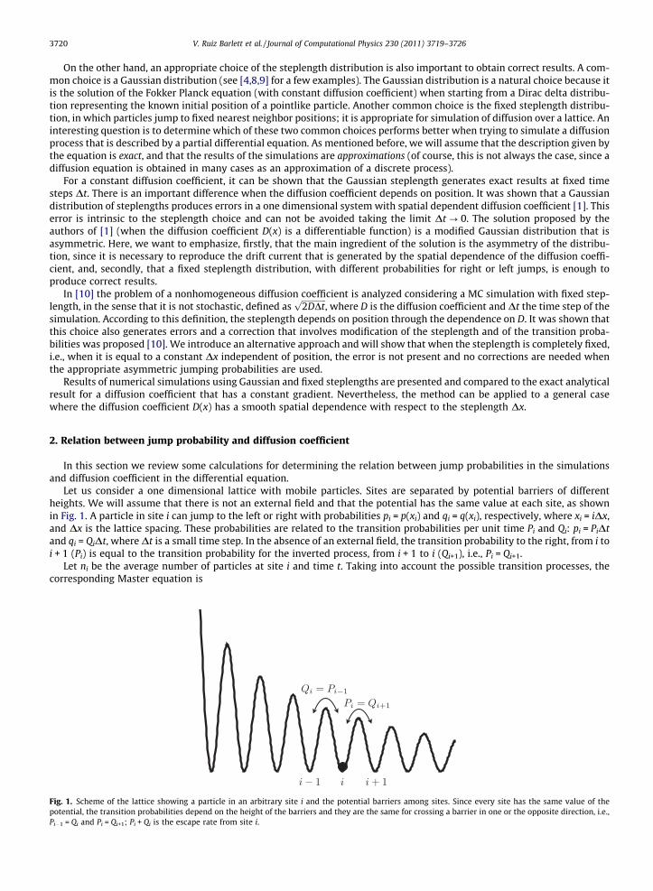
Let us consider a one dimensional lattice with mobile particles. Sites are separated by potential barriers of differentheights. We will assume that there is not an external field and that the potential has the same value at each site, as shownin Fig. 1. A particle in site i can jump to the left or right with probabilities pi = p(xi) and qi = q(xi), respectively, where xi = iDx,and Dx is the lattice spacing. These probabilities are related to the transition probabilities per unit time Pi and Qi: pi = PiDtand qi = QiDt, where Dt is a small time step. In the absence of an external field, the transition probability to the right, from i toi + 1 (Pi) is equal to the transition probability for the inverted process, from i + 1 to i (Qi+1), i.e., Pi = Qi+1.

Let ni be the average number of particles at site i and time t. Taking into account the possible transition processes, thecorresponding Master equation is

Fig. 1. Scheme of the lattice showing a particle in an arbitrary site i and the potential barriers among sites. Since every site has the same value of thepotential, the transition probabilities depend on the height of the barriers and they are the same for crossing a barrier in one or the opposite direction, i.e.,Pi�1 = Qi and Pi = Qi+1; Pi + Qi is the escape rate from site i.

V. Ruiz Barlett et al. / Journal of Computational Physics 230 (2011) 3719–3726 3721

@ni

@t¼ Pi�1ni�1 þ Q iþ1niþ1 � ðPi þ QiÞni: ð1Þ

Using the previous relation between Pi and Qi+1, the equation can be rewritten as

@ni

@t¼ Pi þ Pi�1

2ðni�1 � 2ni þ niþ1Þ þ

Pi � Pi�1

2ðniþ1 � ni�1Þ: ð2Þ

We now consider a system with continuous spatial dependence and take the differences in the right hand side of the pre-vious equation as approximate derivatives,

@nðx; tÞ@t

¼ ðPi þ Pi�1ÞDx2

2@2n@x2 þ ðPi � Pi�1ÞDx

@n@x; ð3Þ

where n(x, t) represents the concentration of particles. Before we interpret the meaning of the terms of this equation, it isuseful to analyze the relation between the Fokker Planck and diffusion equations. The one dimensional Fokker Planck equa-tion is

@n@t¼ � @

@xðAnÞ þ @2

@x2 ðDnÞ ¼ � @

@xA� @D

@x

� �n

� �þ @

@xD@n@x

� �; ð4Þ

where A is the drift coefficient or drift velocity and D is the diffusion coefficient, and both are, in general, functions of positionx. Detailed balance imposes a relation among A, D and the stationary equilibrium solution ns(x), see [11, Sect. 5.3.5]:

AðxÞnsðxÞ ¼@

@xðDðxÞnsðxÞÞ: ð5Þ

We are considering that, in the discretized version of the system, each site of the lattice has the same value of the potential,this means that the equilibrium solution ns(x) must be homogeneous. Then, A ¼ @D

@x and Eq. (4) is reduced to the diffusionequation:

@n@t¼ @

@xD@n@x

� �¼ D

@2n@x2 þ

@D@x

@n@x: ð6Þ

Comparing Eqs. (3) and (6), we obtain the relations between diffusion and drift coefficients and transition probabilities:

D ¼ ðPi þ Pi�1ÞDx2

2¼ ðPi þ Q iÞDx2

2; ð7Þ

@D@x¼ ðPi � Pi�1ÞDx ¼ ðPi � Q iÞDx: ð8Þ

Let us note that, for one particle, the average velocity can be directly obtained from the jump probabilities as v = (Pi � Qi)Dx,which implies a drift current Jd = vn. This result is in agreement with Eqs. (4) and (8) (using v = A = @D/@ x and Jd = An).

In summary, in order to solve Eq. (6) for a given diffusion coefficient D(x), our approach is to simulate the diffusion of non-interacting particles using a discrete model with a set of jumping rates {Pi} that fulfill Eq. (7). This approach will be comparedwith the simulation of diffusion using a continuous model with a Gaussian probability distribution for jump lengths.

The authors of [6] not only measured a diffusion coefficient that depends on position, but also reported and explained adrift of the particles’ individual positions in the direction of the diffusion coefficient gradient, in the absence of any externalforce or concentration gradient. We will show that this drift can not be reproduced by a symmetric steplength distributionlike the Gaussian distribution.

3. Comparison between fixed and Gaussian steplength for homogeneous diffusion

The diffusion equation in one dimension for a homogeneous diffusion coefficient D0 is @n@t ¼ D0

@2n@x2 . For an initial condition

given by n(x,0) = d(x � x0), the solution is

neðx; tÞ ¼e�ðx�x0Þ2=ð4D0tÞffiffiffiffiffiffiffiffiffiffiffiffiffiffi

4pD0tp : ð9Þ

Subindex e is used to identify this as an exact solution. The aim is to approximately reproduce this result using MC simula-tions. The average concentration obtained from MC simulations will not coincide exactly with this result and the errors willdepend on the details of the method. In each MC step time is increased by Dt. At time t = 0 a particle is found at position x0. Attime t = Dt, using Eq. (9), we have a Gaussian distribution of width

ffiffiffiffiffiffiffiffiffiffiffiffiffiffi2D0Dtp

and mean x0. In accordance with this result, it isnatural to use a Gaussian steplength distribution of width

ffiffiffiffiffiffiffiffiffiffiffiffiffiffi2D0Dtp

for each MC step. In other words, if a Gaussian steplengthdistribution is chosen, then it must have a width

ffiffiffiffiffiffiffiffiffiffiffiffiffiffi2D0Dtp

in order to reproduce the second moment of the exact result. Thischoice gives as a result a continuous and smooth distribution in contrast with the discrete distribution that is obtained with afixed steplength. In the last case, the density n takes values different from 0 only in discrete positions xi = iDx, i = 0,±1,±2,. . .

We will consider a smoothed version of this distribution by filtering modes with wavelengths smaller than 2Dx.

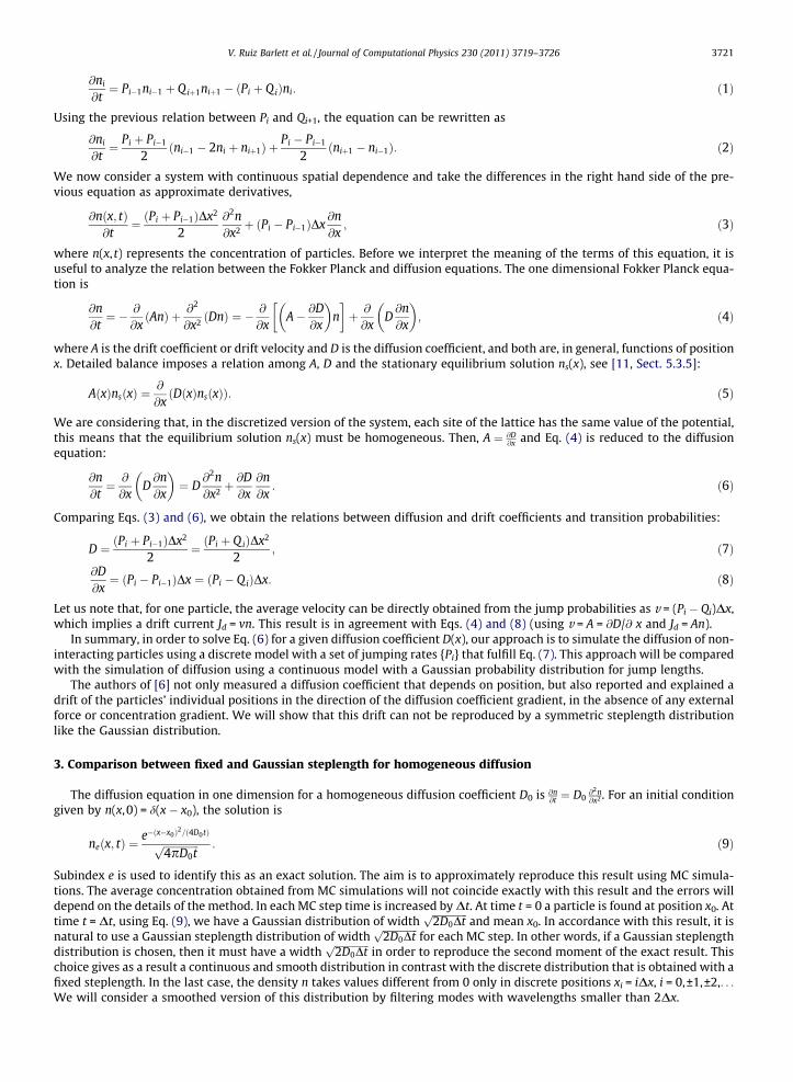
Fig. 2. Exact concentration ne (continuous curve) and the approximation given by MC method with fixed steplength (nf, dashed curve) as a function ofposition x/Dx, for Rt = 10. The inset shows the absolute error nf � ne as a function of x/Dx.

3722 V. Ruiz Barlett et al. / Journal of Computational Physics 230 (2011) 3719–3726

In the simple case of homogeneous diffusion coefficient, it is possible to exactly calculate the result that a MC simulationwith fixed steplength would provide (see Appendix 1). We call nf the concentration obtained with fixed steplength.

Fig. 2 shows the exact concentration ne and the approximation given by nf, for Rt = 10, where R = 2P = 2D0/Dx is the escaperate. The difference is better appreciated in the inset, where the absolute error nf � ne is plotted for Rt = 10. The relative errorfor the maximum absolute error (at x = 0) is 1.3%; although the absolute error tends to 0 as t ?1, the relative error increasessince ne also tends to 0.

For completeness, we show in Appendix 2 that, when a Gaussian steplength distribution is used, the exact probabilitydensity is obtained at discrete time steps.

In summary, for homogeneous diffusion coefficients, MC simulations with fixed steplength have a small error in the par-ticle probability density while a Gaussian steplength distribution produces exact results. Despite this difference, the fixedsteplength choice has some good features that is convenient to consider. It is easier to implement. More importantly, it pro-duces exact results in the evaluation of first and second order moments. The moment errors can be evaluated with

hxpif � hxpie ¼@p

@kp ~nf ðkÞ����

k¼0� @p

@kp ~neðkÞ����k¼0; ð10Þ

where p is the moment order, subindices f and e correspond to fixed steplength and exact results, and ~nf and ~ne are the Fou-rier transform of nf and ne (see Eqs. (14) and (18) in Appendix 1). It can be found that hxpif � hxpie = 0 not only for p = 1 and 2but also for all odd values of p because the concentration is symmetric. For p P 4, the scaled errors, h(x/r)pif � h(x/r)pie,where r ¼

ffiffiffiffiffiffiffiffiffiffiffi2D0tp

¼ffiffiffiffiffiffiffiffiffiffiffiffiffiRDx2tp

, behave as t�1 to leading order.

4. Spatial dependent diffusion coefficient

In this section we study differences between numerical methods for a system with spatial dependent diffusion coefficient.The model consists in one mobile particle that diffuses in a discrete one-dimensional lattice of L + 1 sites with a diffusioncoefficient that depends on position xi = iDx, with i = 0,1, . . .,L. Initially the particle is found in xL/2 = (L/2)Dx (for simplicity,we assume that L is an even number). In the simulations we use the two steplength distributions mentioned in the previoussections: Gaussian steplength and fixed steplength. In both cases we used a fixed time step Dt since it was not possible toappreciate differences with the results obtained with kinetic MC (i.e. with an exponential distribution of time steps).

We consider a system in which the jump probabilities, and the diffusion coefficient, increase linearly with position.For fixed steplength, a particle in position xi jumps to the right a distance Dx with probability p(xi) = PiDt = a(xi + Dx) or

the same distance to the left with probability q(xi) = QiDt = axi, where a = 1/[Dx(2L + 1)]; the value of the slope a is obtainedfrom the condition p(LDx) + q(LDx) = 1. Particles can not reach the negative part of the x axis since when a particle reachessite x0 = 0 the probability of a left jump is equal to 0. On the other hand, we consider the evolution during times small enoughso that no particle reaches position xL = LDx. From Eq. (7), the corresponding diffusion coefficient is

DðxÞ ¼ aðxþ Dx=2ÞDx2=Dt; ð11Þ

where we are using x instead of xi for position in the discrete model to lighten the notation. This model is an approximationof a continuous one dimensional substrate where D(x) is given by Eq. (11) for all x.

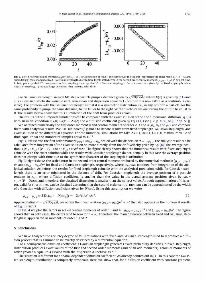
Fig. 3. Left: first order scaled moment lf/g/r = (hxif/g � xL/2)/r as function of time t; the curve (over the squares) represents the exact result le = (P � Q)Dxt.Subindex f(g) corresponds to fixed (Gaussian) steplength distribution. Right: scaled error in the second order central moment (l2,f/g � l2,e)/r2 against time.In both plots, symbol ‘h’ corresponds to fixed steplength and symbol ‘�’ to Gaussian steplength. Correct results are given by the fixed steplength, whileGaussian steplength produces large deviations that increase with time.

V. Ruiz Barlett et al. / Journal of Computational Physics 230 (2011) 3719–3726 3723

For Gaussian steplength, in each MC step a particle jumps a distance given byffiffiffiffiffiffiffiffiffiffiffiffiffiffiffiffiffiffi2DðxÞDt

pn, where D(x) is given by (11) and

n is a Gaussian stochastic variable with zero mean and dispersion equal to 1 (position x is now taken as a continuous var-iable). The problem with the Gaussian steplength is that it is a symmetric distribution, i.e., in any position a particle has thesame probability to jump (the same distance) to the left or to the right. With this choice we are forcing the drift to be equal to0. The results below show that this elimination of the drift term produces errors.

The results of the numerical simulations can be compared with the exact solution of the one dimensional diffusion Eq. (6)with an initial condition n(x,0) = d(x � LDx/2) and a diffusion coefficient given by Eq. (11) (see [12, p. 495], or [1, App. A1]).

We obtained numerically the first order moment l and central moments of order 2, 3 and 4 (l2, l3 and l4), and comparethem with analytical results. We use subindices f, g and e to denote results from fixed steplength, Gaussian steplength, andexact solution of the differential equation. For the numerical simulations we take Dx = 1, Dt = 1, L = 100, maximum value oftime equal to 50 and number of samples equal to 1010.

Fig. 3 (left) shows the first order moment lf/g = hxif/g � xL/2 scaled with the dispersion r ¼ ffiffiffiffiffiffiffiffil2;ep

. The analytic result can becalculated from integration of the exact solution or, more directly, from the drift velocity given by Eq. (8). The average posi-tion is hxie = xL/2 + (Pi � Pi�1)Dx t = xL/2 + aDx2 t/Dt. The figure clearly shows that the numerical results with fixed steplengthcoincide with the exact solution while the results with Gaussian steplength do not, actually in this case the average positiondoes not change with time due to the symmetric character of the steplength distribution.

Fig. 3 (right) shows the scaled error in the second order central moment produced by the numerical methods: (l2,f � l2,e)/r2 and (l2,g � l2,e)/r2 for fixed and Gaussian steplength, respectively, where l2,e was obtained from integration of the ana-lytical solution. As before, the results for fixed steplength coincide with the analytical prediction, while for Gaussian step-length there is an error originated in the absence of drift. For Gaussian steplength the average position of a particleremains in xL/2, where diffusion coefficient is smaller than the value in the actual average position given by hxie =xL/2 + (P � Q)Dxt, and, therefore, the obtained dispersion is smaller than the correct value. A rough approximation of this er-ror, valid for short times, can be obtained assuming that the second order central moment can be approximated by the widthof a Gaussian with diffusion coefficient given by D(hxie). Using this assumption we write

l2;g � l2;e ’ 2½DðxL=2Þ � DðhxieÞ�t ¼ �2a2t2Dx4=Dt2: ð12Þ

Approximating r ’ffiffiffiffiffiffiffiffiffiffiffiffiffiffiffiffiffiffiffiffi2DðxL=2Þt

p, we obtain the linear relation (l2,g � l2,e)/r2 / �t that also appears in the numerical results

of Fig. 3 (right).In Fig. 4 we plot the errors in scaled central moments of order 3 and 4: (l3,f/g � l3,e)/r3 and (l4,f/g � l4,e)/r4. The figure

shows that, in both cases, the errors tend to zero for t ?1. Therefore, the main difference between fixed and Gaussian step-length is appreciated in moments of order 1 and 2.

5. Conclusions

We have analyzed the accuracy degree of MC simulations with fixed and Gaussian steplength used to reproduce a diffu-sion process that is assumed to be exactly described by a differential equation.

For a homogeneous diffusion coefficient, a Gaussian steplength generates exact probability densities. A fixed steplengthdistribution produces exact values of the first and second order moments (and of all odd moments). Errors of moments oforder greater o equal to 4 (scaled with the dispersion r) behave as t�1.

The situation is different for a spatial dependent diffusion coefficient. As already pointed out in [1], in this case the Gauss-ian steplength distribution is completely erroneous. Here, we show that, for a diffusion coefficient with constant gradient,

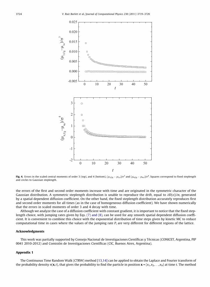
Fig. 4. Errors in the scaled central moments of order 3 (top), and 4 (bottom), (l3,f/g � l3,e)/r3 and (l4,f/g � l4,e)/r4. Squares correspond to fixed steplengthand circles to Gaussian steplength.

3724 V. Ruiz Barlett et al. / Journal of Computational Physics 230 (2011) 3719–3726

the errors of the first and second order moments increase with time and are originated in the symmetric character of theGaussian distribution. A symmetric steplength distribution is unable to reproduce the drift, equal to @D(x)/@x, generatedby a spatial dependent diffusion coefficient. On the other hand, the fixed steplength distribution accurately reproduces firstand second order moments for all times (as in the case of homogeneous diffusion coefficient). We have shown numericallythat the errors in scaled moments of order 3 and 4 decay with time.

Although we analyze the case of a diffusion coefficient with constant gradient, it is important to notice that the fixed step-length choice, with jumping rates given by Eqs. (7) and (8), can be used for any smooth spatial dependent diffusion coeffi-cient. It is convenient to combine this choice with the exponential distribution of time steps given by kinetic MC to reducecomputational time in cases where the values of the jumping rate Pi are very different for different regions of the lattice.

Acknowledgments

This work was partially supported by Consejo Nacional de Investigaciones Científicas y Técnicas (CONICET, Argentina, PIP0041 2010-2012) and Comisión de Investigaciones Científicas (CIC, Buenos Aires, Argentina).

Appendix 1

The Continuous Time Random Walk (CTRW) method [13,14] can be applied to obtain the Laplace and Fourier transform ofthe probability density n(x, t), that gives the probability to find the particle in position x = (x1,x2, . . .,xN) at time t. The method

V. Ruiz Barlett et al. / Journal of Computational Physics 230 (2011) 3719–3726 3725

is a generalization of the random walk, in which time appears as a continuous variable. It can be applied to fixed time stepMC or kinetic MC (in which time is a stochastic variable). The complete solution of the CTRW problem is given by theMontroll–Weiss equation [15] for the characteristic function, i.e. the Fourier and Laplace transform of n(x, t):

~nðk; sÞ ¼ 1� wðsÞs

1

1� wðsÞ~f ðkÞ; ð13Þ

where wðsÞ is the Laplace transform of the waiting time distribution w(t) (the probability density of a time increment of dura-tion t between two successive steps); and ~f ðkÞ, called the structure function of the random walk, is the Fourier transform off(x), the probability density of a jump of size x.

Let us consider a particle that diffuses in a system in one dimension with a homogeneous diffusion coefficient D0. Theexact solution of the diffusion equation for this problem, Eq. (9), in Fourier space is

~neðk; tÞ ¼ exp �RDx2k2t2

!; ð14Þ

where, using Eq. (7), we have replaced D0 = RDx2/2, with R being the escape rate R = P + Q = 2P (subindex i was removed fromthe transition probabilities since them do not depend on position in this case). Eq. (14) will be useful to compare with theresults that MC simulations provide.

In the simulations, we take a fixed time step Dt, so that the waiting time distribution is

wðtÞ ¼ dðt � DtÞ; wðsÞ ¼ e�sDt : ð15Þ

The probability density of a jump of size x, and its Fourier transform, for fixed steplength is

ff ðxÞ ¼ ðdðx� DxÞ þ dðxþ DxÞÞRDt=2þ ð1� RDtÞdðxÞ;~f f ðkÞ ¼ RDt cosðkDxÞ þ 1� RDt; ð16Þ

where we are considering the general situation in which there is a probability 1 � RDt that the particle remains in its site.Introducing Eqs. (15) and (16) in Eq. (13), we obtain the Fourier and Laplace transform of the distributions provided by the

fixed steplength,

~nf ðk; sÞ ¼1

sþ Rð1� cos kDxÞ sDtexpðsDtÞ�1

!Dt!0

1sþ Rð1� cos kDxÞ : ð17Þ

We also included the limit Dt ? 0. This limit is numerically not unfeasible. It can be shown that it is possible to obtain di-rectly the result in the limit Dt ? 0 when a stochastic time step with exponential distribution, corresponding to kinetic MC,is used [7] [i.e., a waiting time distribution given by w(t) = Rexp(�Rt), wðsÞ ¼ R=ðsþ RÞ]. We consider that the fixed steplengthdistribution is used with kinetic MC in order to eliminate the source of error related to Dt and to consider only the error thatcomes from the finite value of Dx.

The Laplace antitransform (for Dt ? 0) is

~nf ðk; tÞ ¼ exp½�Rð1� cos kDxÞt�: ð18Þ

This result correctly approximates the exact solution when the escape rate R, used in the simulations, is related with the dif-fusion coefficient D0, of the differential equation, by D0 = RDx2/2. This relation was already used in Eq. (14). In the limit ofsmall values of kDx, Eq. (18) approaches the exact result (14). As mentioned in Sect. 3, we consider a smoothed versionof nf(x, t) by Fourier antitransforming Eq. (18) in the range (�p/Dx,p/Dx).

Appendix 2

For a Gaussian steplength distribution, the probability density of having the particle at position x after one time step Dt,and starting from position x0 = 0, is

f1ðxÞ ¼1ffiffiffiffiffiffiffiffiffiffiffiffiffiffiffiffiffi

4pD0Dtp e�x2=ð4D0DtÞ; ð19Þ

and its Fourier transform is ~f 1ðkÞ ¼ e�D0Dtk2. After two steps, the probability density is

f2ðxÞ ¼Z 1

�1dx0f1ðx0Þf1ðx� x0Þ: ð20Þ

The Fourier transform of this convolution product is ~f 2ðkÞ ¼ ½~f 1ðkÞ�2. In general, for m time steps, we have

~f mðkÞ ¼ ½~f 1ðkÞ�m ¼ e�D0k2mDt : ð21Þ

This result coincides with the exact solution (14) (where D0 was replaced by RDx2/2) for discrete times t = mDt.

3726 V. Ruiz Barlett et al. / Journal of Computational Physics 230 (2011) 3719–3726

References

[1] L. Farnell, W.G. Gibson, Monte Carlo simulation of diffusion in a spatially nonhomogeneous medium: correction to the Gaussian steplength, J. Comput.Phys. 198 (2004) 65–79.

[2] V. Matveev, A. Sherman, R.S. Sucker, New and corrected simulations of synaptic facilitation, Biophys. J. 83 (2002) 1368–1373.[3] M. Piórkowski, N. Sarafijanovic-Djukic, M. Grossglauser, A parsimonious model of mobile partitioned network with clustering, in: First International

Conference on Communication Systems and Networks and Workshops, COMSNETS, 2009.[4] David S. Sholla, Michael K. Fenwick, Brownian dynamics simulation of the motion of a rigid sphere in a viscous fluid very near a wall, J. Chem. Phys. 113

(2000) 9268–9278.[5] Kemal Yükseka, Yeliz Kocab, Hasan Sadikoglu, Solution of counter diffusion problem with position dependent diffusion coefficient by using variational

methods, J. Comput. Appl. Math. 232 (2009) 285–294.[6] P. Lançon, G. Batrouni, L. Lobry, N. Ostrowsky, Drift without flux: Brownian walker with a space-dependent diffusion coefficient, Europhys. Lett. 54 (1)

(2001) 2834;P. Lançon, G. Batrouni, L. Lobry, N. Ostrowsky, Brownian walker in a confined geometry leading to a space-dependent diffusion coefficient, Physica A304 (2002) 65–76.

[7] V. Ruiz Barlett, J.J. Bigeon, M. Hoyuelos, H.O. Martin, Differences between fixed time step and kinetic Monte Carlo methods for biased diffusion, J.Comput. Phys. 228 (2009) 5740–5748.

[8] Christoph Eisenmann, Chanjoong Kim, Johan Mattsson, David A.Weitz, Shear Melting of a Colloidal Glass, Unpublished, 2009.[9] J. Gavnholt, J. Juul Rasmussen, O.E. Garcia, V. Naulin, A.H. Nielsen, Up-gradient transport in a probabilistic transport model, Phys. Plasmas 12 (2005)

084501–084504.[10] L. Farnell, W.G. Gibson, Monte Carlo simulation of diffusion in a spatially nonhomogeneous medium: a biased random walk on an asymmetrical lattice,

J. Comput. Phys. 208 (2005) 253265.[11] C.W. Gardiner, Handbook of Stochastic Methods, Springer, Berlin, 1985.[12] H.S. Carslaw, J.C. Jaeger, Conduction of Heat in Solids, second ed., Oxford University Press, London, 1959.[13] R. Balescu, Statistical Dynamics, Matter Out of Equilibrium, Imperial College Press, London, 1997.[14] G.H. Weiss, Aspects and Applications of Random Walks, North Holland, Amsterdam, 1994.[15] E.W. Montroll, G.H. Weiss, J. Math. Phys. 6 (1965) 167;

E.W. Montroll, M.F. Shlesinger, in: J.L. Lebowitz, E.W. Montroll (Eds.), Studies of Statistical Mechanics, vol. 11, North Holland, Amsterdam, 1984, p. 5.