A Comparative Evaluation of Anomaly Detection Techniques for Sequence Data

Technical Report

Department of Computer Science

and Engineering

University of Minnesota

4-192 EECS Building

200 Union Street SE

Minneapolis, MN 55455-0159 USA

TR 08-021

A Comparative Evaluation of Anomaly Detection Techniques for

Sequence Data

Varun Chandola, Varun Mithal, and Vipin Kumar

July 07, 2008

Comparing Anomaly Detection Techniques for Sequence Data

Submitted for Blind Review

Abstract

Anomaly detection has traditionally dealt with record or

transaction type data sets. But in many real domains, data

naturally occurs as sequences, and therefore the desire of

studying anomaly detection techniques in sequential data

sets. The problem of detecting anomalies in sequence data

sets is related to but different from the traditional anomaly

detection problem, because the nature of data and anoma-

lies are different than those found in record data sets. While

there are many surveys and comparative evaluations for

traditional anomaly detection, similar studies are not done

for sequence anomaly detection. We investigate a broad

spectrum of anomaly detection techniques for symbolic se-

quences, proposed in diverse application domains. Our hy-

pothesis is that symbolic sequences from different domains

have distinct characteristics in terms of the nature of se-

quences as well as the nature of anomalies which makes

it important to investigate how different techniques behave

for different types of sequence data. Such a study is criti-

cal to understand the relative strengths and weaknesses of

different techniques. Our paper is one such attempt where

we have comparatively evaluated 7 anomaly detection tech-

niques on 10 public data sets, collected from three diverse

application domains. To gain further understanding in the

performance of the techniques, we present a novel way to

generate sequence data with desired characteristics. The

results on the artificially generated data sets help us in

experimentally verifying our hypothesis regarding different

techniques.

1 Introduction

Anomaly detection has traditionally dealt with record or

transaction type data sets [5]. But in many real domains,

data naturally occurs as sequences, and therefore the desire

of studying anomaly detection techniques in sequential data

sets. The problem of detecting anomalies in sequence data

sets is related to but different from the traditional anomaly

detection problem, because the nature of data and anomalies

are different than those found in record data sets.

Several anomaly detection techniques for symbolic se-

quences have been proposed [10, 14, 29, 4, 22, 19, 18,

12, 11], their applicability demonstrated in diverse appli-

cation domains such as intrusion detection [10], proteomics

[29], and aircraft safety [4] as shown in Table 1. One of

the earliest technique [9] used lookahead pairs to deter-

mine anomalous sequence of system calls. In a later paper

[14], the same authors propose a window based technique

(STIDE) and show that STIDE outperforms the lookahead

pairs based technique on operating system call data. Since

then several other techniques have been proposed to de-

tect anomalies in system call data, using Hidden Markov

Models (HMM) [24], Finite State Automata (FSA) [22],

and classification models such as RIPPER [19, 18]. All of

these papers demonstrated the applicability of their respec-

tive techniques only on system call intrusion detection data,

while some compared their techniques with STIDE.

While there are many surveys and comparative evalua-

tions for traditional anomaly detection, for e.g., [5, 13, 17],

similar studies are not done for sequence anomaly detec-

tion. We found only one work [10] comparing the evalu-

ation of four techniques on system call intrusion detection

data sets.that compared the performance of four anomaly

detection techniques; namely STIDE, t-STIDE (a threshold

based variant of STIDE), HMM based, and RIPPER based;

on 6 different data sets from system call intrusion detection

domain. However, this comparison limits the evaluation to

just four techniques, using only system call intrusion detec-

tion data sets.

Herein lies the motivation for our work: Though several

techniques have been proposed in different domains; their

applicability is shown, exclusively, in their respective do-

main, as is evident in Table 1. There has been a lack of a

comprehensive and comparative evaluation of anomaly de-

tection techniques across diverse data sets that facilitates

in understanding their relative strengths and weaknesses

when applied across varied domains. The insights gathered

through such analysis equips us to know which techniques

would give better performance for which specific data sets;

and, thus, given the data sets, which technique to apply

when.

In this paper we investigate a variety of anomaly detec-

tion techniques that have been proposed to detect anoma-

lies in symbolic sequences. We classify such techniques as:

kernel based, window based, and Markovian techniques.

Kernel based techniques use a similarity measure to com-

pute similarity between sequences. Window based tech-

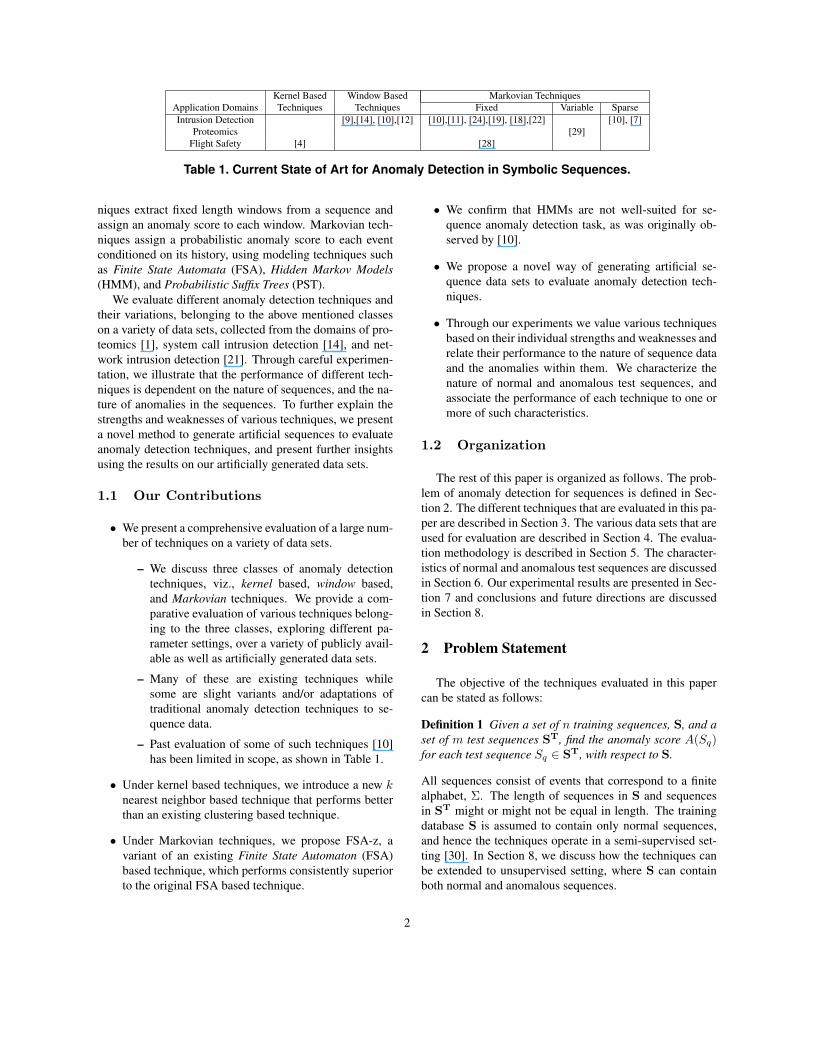
Kernel Based Window Based Markovian Techniques

Application Domains Techniques Techniques Fixed Variable Sparse

Intrusion Detection [9],[14], [10],[12] [10],[11], [24],[19], [18],[22] [10], [7]

Proteomics [29]

Flight Safety [4] [28]

Table 1. Current State of Art for Anomaly Detection in Symbolic Sequences.

niques extract fixed length windows from a sequence and

assign an anomaly score to each window. Markovian tech-

niques assign a probabilistic anomaly score to each event

conditioned on its history, using modeling techniques such

as Finite State Automata (FSA), Hidden Markov Models

(HMM), and Probabilistic Suffix Trees (PST).

We evaluate different anomaly detection techniques and

their variations, belonging to the above mentioned classes

on a variety of data sets, collected from the domains of pro-

teomics [1], system call intrusion detection [14], and net-

work intrusion detection [21]. Through careful experimen-

tation, we illustrate that the performance of different tech-

niques is dependent on the nature of sequences, and the na-

ture of anomalies in the sequences. To further explain the

strengths and weaknesses of various techniques, we present

a novel method to generate artificial sequences to evaluate

anomaly detection techniques, and present further insights

using the results on our artificially generated data sets.

1.1 Our Contributions

• We present a comprehensive evaluation of a large num-

ber of techniques on a variety of data sets.

– We discuss three classes of anomaly detection

techniques, viz., kernel based, window based,

and Markovian techniques. We provide a com-

parative evaluation of various techniques belong-

ing to the three classes, exploring different pa-

rameter settings, over a variety of publicly avail-

able as well as artificially generated data sets.

– Many of these are existing techniques while

some are slight variants and/or adaptations of

traditional anomaly detection techniques to se-

quence data.

– Past evaluation of some of such techniques [10]

has been limited in scope, as shown in Table 1.

• Under kernel based techniques, we introduce a new k

nearest neighbor based technique that performs better

than an existing clustering based technique.

• Under Markovian techniques, we propose FSA-z, a

variant of an existing Finite State Automaton (FSA)

based technique, which performs consistently superior

to the original FSA based technique.

• We confirm that HMMs are not well-suited for se-

quence anomaly detection task, as was originally ob-

served by [10].

• We propose a novel way of generating artificial se-

quence data sets to evaluate anomaly detection tech-

niques.

• Through our experiments we value various techniques

based on their individual strengths and weaknesses and

relate their performance to the nature of sequence data

and the anomalies within them. We characterize the

nature of normal and anomalous test sequences, and

associate the performance of each technique to one or

more of such characteristics.

1.2 Organization

The rest of this paper is organized as follows. The prob-

lem of anomaly detection for sequences is defined in Sec-

tion 2. The different techniques that are evaluated in this pa-

per are described in Section 3. The various data sets that are

used for evaluation are described in Section 4. The evalua-

tion methodology is described in Section 5. The character-

istics of normal and anomalous test sequences are discussed

in Section 6. Our experimental results are presented in Sec-

tion 7 and conclusions and future directions are discussed

in Section 8.

2 Problem Statement

The objective of the techniques evaluated in this paper

can be stated as follows:

Definition 1 Given a set of n training sequences, S, and a

set of m test sequences ST, find the anomaly score A(Sq)for each test sequence Sq ∈ ST, with respect to S.

All sequences consist of events that correspond to a finite

alphabet, Σ. The length of sequences in S and sequences

in ST might or might not be equal in length. The training

database S is assumed to contain only normal sequences,

and hence the techniques operate in a semi-supervised set-

ting [30]. In Section 8, we discuss how the techniques can

be extended to unsupervised setting, where S can contain

both normal and anomalous sequences.

2

3 Anomaly Detection Techniques for Se-

quences

Most of the existing techniques can be grouped into three

categories:

1. Kernel based techniques compute similarity between

sequences and then apply a similarity based traditional

anomaly detection technique [5, 30].

2. Window based techniques analyze a short window

of events within the test sequence at a time. Thus

such techniques treat a subsequence within the test se-

quence as a unit element for analysis. Such techniques

require an additional step in which the anomalous na-

ture of the entire test sequence is determined, based on

the scores of each subsequence.

3. Markovian techniques assign a probability to each

event of the test sequence based on the previous obser-

vations in the sequence. Such techniques exploit the

Markovian dependencies in the sequence.

In the following subsections we describe several tech-

niques that are instantiations of the above three category of

anomaly detection techniques.

3.1 Kernel Based Techniques

Kernel based techniques make use of pairwise similar-

ity between sequences. In the problem formulation stated

in Definition 1 the sequences can be of different lengths,

hence simple measures such as Hamming Distance cannot

be used. One possible measure is the normalized length of

longest common subsequence between a pair of sequences.

This similarity between two sequences Si and Sj , is com-

puted as:

nLCS(Si, Sj) =|LCS(Si, Sj)|

√

|Si||Sj |(1)

Since the value computed above is between 0 and 1,

nLCS(Si, Sj) can be used to represent distance between

Si and Sj [30]. Other similarity measures can be used as

well, for e.g., the spectrum kernel [20]. We use nLCS in

our experimental study, since it was used in [4] in detecting

anomalies in sequences and appears promising.

3.1.1 Nearest Neighbors Based (kNN)

In the nearest neighbor scheme (kNN), for each test se-

quence Sq ∈ ST, the distance to its kth nearest neighbor

in the training set S is computed. This distance becomes

the anomaly score A(Sq) [30, 26].

A key parameter in the algorithm is k. In our experi-

ments we observe that the performance of kNN technique

does not change much for 1 ≤ k ≤ 8, but the performance

degrades gradually for larger values of k.

3.1.2 Clustering Based (CLUSTER)

This technique clusters the sequences in S into a fixed num-

ber of clusters, c, using CLARA [16] k-medoids algorithm.

The test phase involves measuring the distance of every test

sequence, Sq ∈ ST, with the medoid of each cluster. The

distance to the medoid of the closest cluster becomes the

anomaly score A(Sq).The number of clusters, c, is a parameter for this tech-

nique. In our experiments we observed that the performance

of CLUSTER improved when c was increased, but stabi-

lized after a certain value. As c is increased, the number of

sequences per cluster become fewer and fewer, thus making

the CLUSTER technique closer to kNN technique.

3.2 Window Based Technique (t-STIDE)

Researchers have argued that often, the cause of anomaly

can be localized to one or more shorter subsequences within

the actual sequence [9]. If the entire sequence is ana-

lyzed as a whole, the anomaly signal might not be distin-

guishable from the inherent variation that exists across se-

quences. Window based techniques try to localize the cause

of anomaly in a test sequence, within one or more windows,

where a window is a fixed length subsequence of the test se-

quence.

One such technique called Threshold Sequence Time-

Delay Embedding (t-STIDE) [10] uses a sliding window of

fixed size k to extract k-length windows from the training

sequences in S. The count of each window occurring in S is

maintained. During testing, k-length windows are extracted

from a test sequence Sq . Each such window ωi is assigned

a likelihood score P (ωi) as:

P (ωi) =f(ωi)

f(∗)(2)

where f(ωi) is the frequency of occurrence of window ωi

in S, and f(∗) is the total number of k length windows ex-

tracted from S.

For the test sequence Sq , |Sq| − k + 1 windows are

extracted, and hence a likelihood score vector of length

|Sq|−k +1 is obtained. This score vector can be combined

in multiple ways to obtain A(Sq), as discussed in Section

3.4.

3.3 Markovian Techniques

Such techniques estimate the conditional probability for

each symbol in a test sequence Sq conditioned on the sym-

3

bols preceding it. Most of the techniques utilize the short

memory property of sequences, which is manifested across

domains [27]. This property is essentially a higher-order

Markov condition which states that for a given sequence

S = 〈s1, s2, . . . s|S|〉, the conditional probability of occur-

rence of a symbol si given the sequence observed so far can

be written as:

P (si|s1s2 . . . si−1) ≈ P (si|sksk+1 . . . si−1)∀k ≥ 1 (3)

Like window based techniques, Markovian techniques

also determine a score vector for the test sequence Sq . This

score vector is combined to obtain A(Sq).We investigate the following four Markovian techniques:

3.3.1 Finite State Automata Based Techniques (FSA

and FSA-z)

A fixed length Markovian technique (FSA) [22] estimates

the probability P (sqi) of a symbol sqi, conditioned on a

fixed number of previous symbols.

The approach employed by FSA is to learn the probabil-

ities P (sqi) for every symbol occurring in the training data

S, using a Finite State Automaton. During testing, this au-

tomaton is used to determine the probability for each sym-

bol in the test sequence.

FSA extracts n+1 sized subsequences from the training

data S using a sliding window1. Each node in the automaton

constructed by FSA corresponds to the first n symbols of

such n + 1 length subsequences. Thus n becomes a key pa-

rameter for this technique. The maximum number of nodes

in the FSA will be equal to n|Σ|, though usually the number

of unique subsequences in training data sets are much less.

An edge exists between a pair of nodes, Ni and Nj , in the

FSA, if Ni

FSA-z We propose a variant of FSA technique, in which

if the node corresponding to the first n symbols of a n + l

subsequence does not exist, we assign a score of 0 to that

subsequence, instead of ignoring it. We experimented with

assigning lower scores such as -1, -10, and −∞, but the per-

formance did not change significantly. The intuition behind

assigning a 0 score to non-existent nodes is that anomalous

test sequences are more likely to contain such nodes, than

normal test sequences. This characteristic, is therefore, key

to distinguish between anomalous and normal sequences.

While FSA ignored this information, we utilize it in FSA-z.

For both FSA and FSA-z techniques, we experimented

with different values of l and found that the performance

does not vary significantly for either technique, and hence

we report results for l = 1 only. The value of n is a critical

1A more general formulation that determines probability of l symbols

conditioned on preceding n symbols is discussed in [22]. The results for

the extended n + l FSA are presented in our extended work [?].

parameter for both techniques. Setting n to be very low (

≤ 3) or very high (≥ 10), results in poor performance. The

best results were obtained for n = 6.

3.3.2 Variable Markovian Technique (PST)

Such techniques estimate the probability, P (sqi), of an

event sqi, in the test sequence, Sq , conditioned on a vari-

able number of previous events. In other words, for each

event, the technique conditions its probability on variable

history (variable markov models). We evaluate one such

technique (PST), proposed by [29] using Probabilistic Suf-

fix Trees [27]. A PST is a tree representation of a variable-

order markov chain and has been used to model biological

sequences [3]. In the training phase, a PST is constructed

from the sequences in S. The depth of a fully constructed

PST is equal to the length of longest sequence in S. For

anomaly detection, it has been shown that the PST can

be pruned significantly without affecting their performance

[29]. The pruning can be done by limiting the maximum

depth of the tree to a threshold, L, or by applying thresholds

to the empirical probability of a node label, MinCount, or

to the conditional probability of a symbol emanating from a

given node, PMin.

It should be noted that if the thresholds MinCount and

PMin are not applied, the PST based technique is equiv-

alent to FSA technique with n = L and l = 1. When the

two thresholds are applied, the events are conditioned on

the maximum length suffix, with maximum length L, that

exists in the PST.

For testing, the PST assigns a likelihood score to each

event sqi of the test sequence Sq as equal to the proba-

bility of observing symbol sqi after the longest suffix of

sq1sq2 . . . sqi−1 that occurs in the PST. The score vector

thus obtained can be then combined to obtain A(Sq) using

combination techniques discussed in Section 3.4.

3.3.3 Sparse Markovian Technique (RIPPER)

The variable Markovian techniques described above allow

an event sqi of a test sequence Sq to be analyzed with re-

spect to a history that could be of different lengths for dif-

ferent events; but they still choose contagious and imme-

diately preceding events to sqi in Sq . Sparse Markovian

techniques are more flexible in the sense that they estimate

the conditional probability of sqi based on events within the

previous k events, which are not necessarily contagious or

immediately preceding to sqi. In other words the events are

conditioned on a sparse history.

We evaluate an interesting technique in this category,

that uses a classification algorithm (RIPPER) to build sparse

models [19]. In this approach, a sliding window is applied

to the training data S to obtain k length windows. The first

4

k − 1 positions of these windows are treated as k − 1 cate-

gorical attributes, and the kth position is treated as a target

class. The authors use a well-known algorithm RIPPER [6]

to learn rules that can predict the kth event given the first

k − 1 events. To ensure that there is no symbol that oc-

curs very rarely as the target class, the authors replicate all

training sequences 12 times.

It should be noted that if RIPPER is forced to learn rules

that contain all k − 1 attributes, the RIPPER technique is

equivalent to FSA with n = k − 1 and l = 1. For testing,

k length windows are extracted from each test sequence Sq

using a sliding window. For the ith window, the first k − 1events are classified using the classifier learnt in the train-

ing phase and the prediction is compared to the kth sym-

bol sqi. RIPPER also assigns a confidence score associated

with the classification. Let this confidence score be denoted

as p(sqi). The likelihood score of event sqi is assigned as

follows. For a correct classification, A(sqi) = 0, while for

a misclassification, A(sqi) = 100P (ωi).

Thus the testing phase generates a score vector for the

test sequence Sq . The score vector thus obtained can be then

combined to obtain A(Sq) using combination techniques

discussed in Section 3.4.

3.3.4 Hidden Markov Models Based Technique

(HMM)

Hidden Markov Models (HMM) are powerful finite state

machines that are widely used for sequence modeling [25].

HMMs have also been applied to sequence anomaly detec-

tion [10, 24, 31]. Techniques that apply HMMs for model-

ing the sequences, transform the input sequences from the

symbol space to the hidden state space. The underlying as-

sumption for such techniques is that the nature of the se-

quences is captured effectively by the hidden space.

The training phase involves learning an HMM with σ

hidden states, from the normal sequences in S using the

Baum Welch algorithm [2]. In the testing phase, the tech-

nique investigated in [10] determines the optimal hidden

state sequence for the given input test sequence Sq, us-

ing the Viterbi algorithm [8]. For every pair of contiguous

states, sHqis

Hqi + 1, in the optimal hidden state sequence,

the state transition matrix provides a probability score for

transitioning from hidden state sHqi to hidden state sH

qi+1.

Thus a likelihood score vector of length |Sq|−1 is obtained

for a test sequence Sq . As for other Markovian techniques, a

combination method is required to obtain the anomaly score

A(Sq) from this score vector.

Note that the number of hidden states σ is a critical pa-

rameter for HMM. We experimented with values ranging

from |Σ| (number of alphabets) to 2. Our experiments re-

veal that σ = 4 gives the best performance for most of the

data sets.

3.4 Combining Scores

The window based and Markovian techniques discussed

in the previous sections generate a likelihood score vector

for a test sequence, Sq . A combination function is then ap-

plied to obtain a single anomaly score A(Sq). Techniques

discussed in previous sections originally have used different

combination functions to obtain A(Sq). Let the score vec-

tor be denoted as P = P1P2 . . . P|P|. To obtain an overall

anomaly score A(Sq) for the sequence Sq from the likeli-

hood score vector P, any one of the following techniques

can be used:

1. Average score

A(Sq) =1

|P|

|P|∑

i=1

Pi

2. Minimum transition probability

A(Sq) = min∀i

Pi

3. Maximum transition probability

A(Sq) = max∀i

Pi

4. Log sum

A(S, q) =1

|P|

|P|∑

i=1

log Pi

If Pi = 0, we replace it with 10−6.

Alternatively, a threshold parameter δ can used to de-

termine if any likelihood score is unlikely. This results

in a |P| length binary sequence, B1B2 . . . B|P|−1,

where 0 indicates a normal transition and 1 indicates

an unlikely transition. This sequence can be combined

in different ways to estimate an overall anomaly score

for the test sequence, Sq:

5. Any unlikely transition

A(Sq) = 1 if

|P|∑

i=1

Bi ≥ 1

= 0 otherwise

6. Average unlikely transitions

A(Sq) =

|P|∑

i=1

Bi

|P|

5

We experimented with all of the above combination func-

tions for different techniques, and conclude that the log sum

function has the best performance across all data sets. In

this paper we report our results only for the log-sum func-

tion. It should be noted that originally the techniques inves-

tigated in this paper used the following combination func-

tions:

• t-STIDE - Average unlikely transitions.

• FSA - Average unlikely transitions.

• PST - Log sum.

• RIPPER - Average score.

• HMM - Average unlikely transitions.

4 Data Sets Used

In this section we describe three various publicly avail-

able as well as the artificially generated data sets that we

used to evaluate the different anomaly detection techniques.

To highlight the strengths and weaknesses of different tech-

niques, we also generated artificial data sets using HMMs.

For every data set, we first constructed a set of normal se-

quences, and a set of anomalous sequences. A sample of

the normal sequences was used as training data for different

techniques. A different sample of normal sequences and

a sample of anomalous sequences were added together to

form the test data. The relative proportion of normal and

anomalous sequences in the test data determined the “diffi-

culty level” for that data set. We experimented with differ-

ent ratios such as 1:1, 10:1 and 20:1 of normal and anoma-

lous sequences and encountered similar trends. In this paper

we report results when normal and anomalous sequences

were in 20:1 ratio in test data.

Source Data Set |Σ| l̂ |SN| |SA| |S| |ST|

PFAM

HCV 44 87 2423 50 1423 1050

NAD 42 160 2685 50 1685 1050

TET 42 52 1952 50 952 1050

RUB 42 182 1059 50 559 525

RVP 46 95 1935 50 935 1050

UNMsnd-cert 56 803 1811 172 811 1050

snd-unm 53 839 2030 130 1030 1050

DARPA

bsmweek1 67 149 1000 800 10 210

bsmweek2 73 141 2000 1000 113 1050

bsmweek3 78 143 2000 1000 67 1050

Table 2. Public data sets used for experi-mental evaluation. l̂ – Average Length of

Sequences, SN – Normal Data Set, SA –Anomaly Data Set, S – Training Data Set, ST

– Test Data Set.

0 5 10 15 20 25 30 35 40 45 500

0.02

0.04

0.06

0.08

0.1

0.12

rvp Normal

Symbols

(a) Normal Sequences

0 5 10 15 20 25 30 35 40 45 500

0.02

0.04

0.06

0.08

0.1

0.12

rvp Anomaly

Symbols

(b) Anomalous Sequences

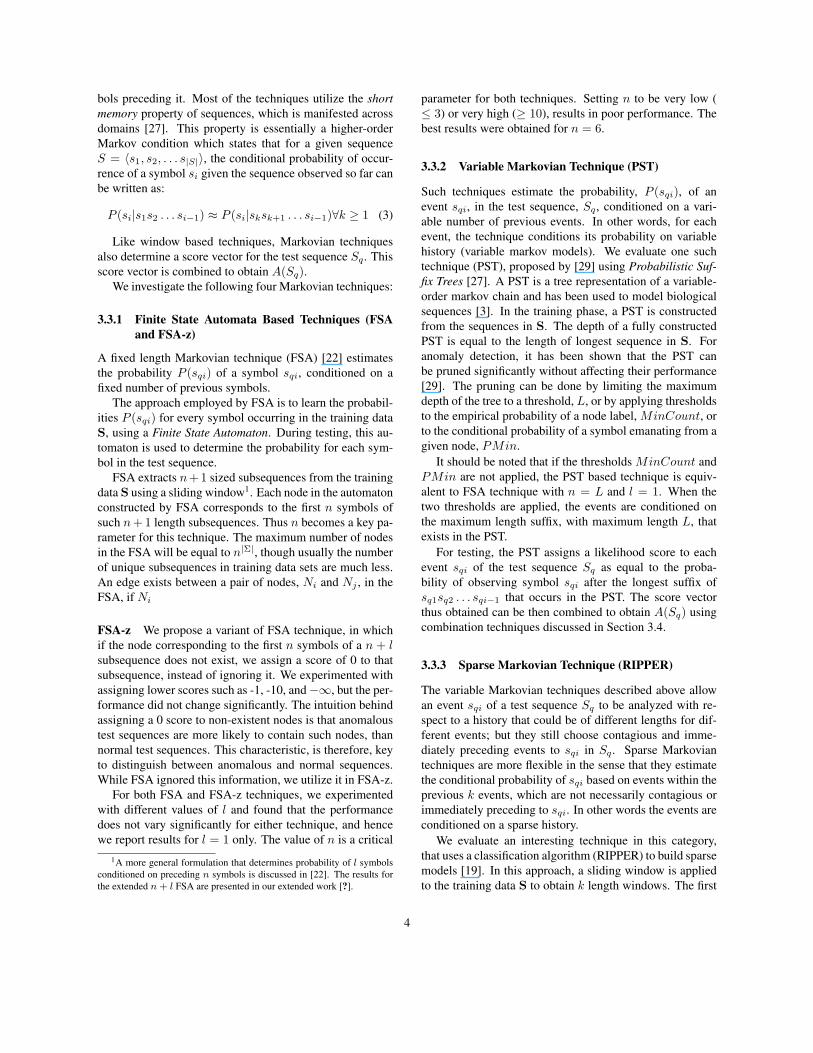
Figure 1. Distribution of symbols in RVP.

0 10 20 30 40 50 600

0.05

0.1

0.15

0.2

0.25

0.3

snd−unm Normal

Symbols

(a) Normal Sequences

0 10 20 30 40 50 600

0.05

0.1

0.15

0.2

0.25

0.3

snd−unm Anomaly

Symbols

(b) Anomalous Sequences

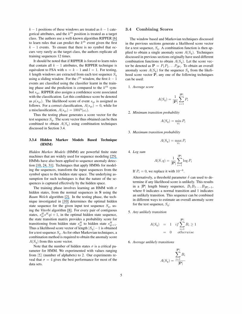
Figure 2. Distribution of symbols in snd-unm.

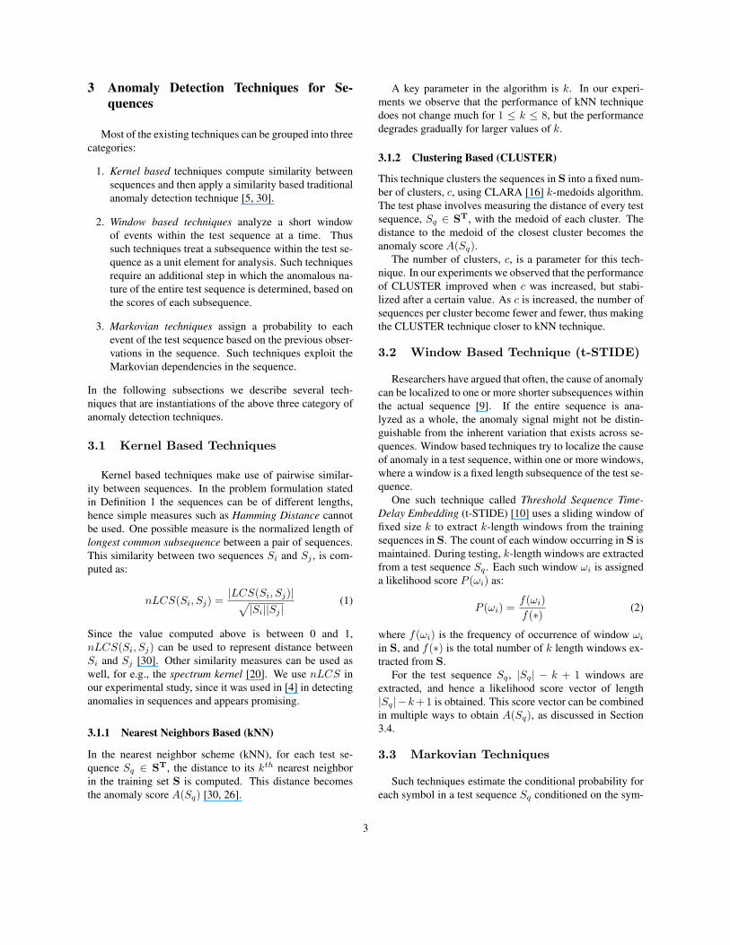
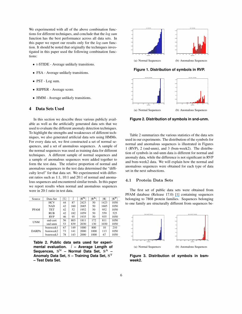
Table 2 summarizes the various statistics of the data sets

used in our experiments. The distribution of the symbols for

normal and anomalous sequences is illustrated in Figures

1 (RVP), 2 (snd-unm), and 3 (bsm-week2). The distribu-

tion of symbols in snd-unm data is different for normal and

anomaly data, while the difference is not significant in RVP

and bsm-week2 data. We will explain how the normal and

anomalous sequences were obtained for each type of data

set in the next subsections.

4.1 Protein Data Sets

The first set of public data sets were obtained from

PFAM database (Release 17.0) [1] containing sequences

belonging to 7868 protein families. Sequences belonging

to one family are structurally different from sequences be-

0 10 20 30 40 50 60 70 800

0.05

0.1

0.15

0.2

0.25

0.3

bsm−week2 Normal

Symbols

(a) Normal Sequences

0 10 20 30 40 50 60 70 800

0.05

0.1

0.15

0.2

0.25

0.3

bsm−week2 Anomaly

Symbols

(b) Anomalous Sequences

Figure 3. Distribution of symbols in bsm-week2.

6

longing to another family. We choose five families, viz.,

HCV, NAD, TET, RVP, RUB. For each family we construct

a normal data set by choosing a sample from the set of se-

quences belonging to that family. We then sample 50 se-

quences from other four families to construct an anomaly

data set. Similar data was used to evaluate the PST tech-

nique [29]. The difference was that the authors used se-

quences from HCV family to construct the normal data set,

and sampled sequences from only one other family to con-

struct the anomaly data set.

4.2 Intrusion Detection Data Sets

The second set of public data sets were collected from

two repositories of benchmark data generated for evalua-

tion of intrusion detection algorithms. One repository was

generated at University of New Mexico2. The normal se-

quences consisted of sequence of system calls generated in

an operating system during the normal operation of a com-

puter program, such as sendmail, ftp, lpr etc. The anoma-

lous sequences consisted of sequence of system calls gener-

ated when the program is run in an abnormal mode, corre-

sponding to the operation of a hacked computer. We exper-

imented with a number of data sets available in the reposi-

tory but are reporting results on two data sets, viz, snd-unm

and snd-cert. For each of the two data sets, the original

size of the normal as well as anomaly data was small, so

we extracted sliding windows of length 100, with a sliding

step of 50 from every sequence to increase the size of the

data sets. The duplicates from the anomaly data set as well

as sequences that also existed in the normal data set were

removed.

The other intrusion detection data repository was the Ba-

sic Security Module (BSM) audit data, collected from a vic-

tim Solaris machine, in the DARPA Lincoln Labs 1998 net-

work simulation data sets [21]. The repository contains la-

beled training and testing DARPA data for multiple weeks

collected on a single machine. For each week we con-

structed the normal data set using the sequences labeled as

normal from all days of the week. The anomaly data set

was constructed in a similar fashion. The data is similar to

the system call data described above with similar (though

larger) alphabet.

The protein data sets and intrusion detection data sets

are quite distinct in terms of the nature of anomalies. The

anomalous sequences in a protein data set belong to a dif-

ferent family than the normal sequences, and hence can be

thought of as being generated by a very different genera-

tive mechanism. This is also supported by the difference in

the distributions of symbols for normal and anomalous se-

quences for RVP data as shown in Figure 1. The anomalous

sequences in the intrusion detection data sets correspond to

2http://www.cs.unm.edu/∼immsec/systemcalls.htm

S1

S2

S3

S4

S5

S6

S11

S10

S9

S8

S7

S12

a1

a2

a3

a4

a1

a2a6

a5 a3

a4

a6

a5

λ

1 − λ

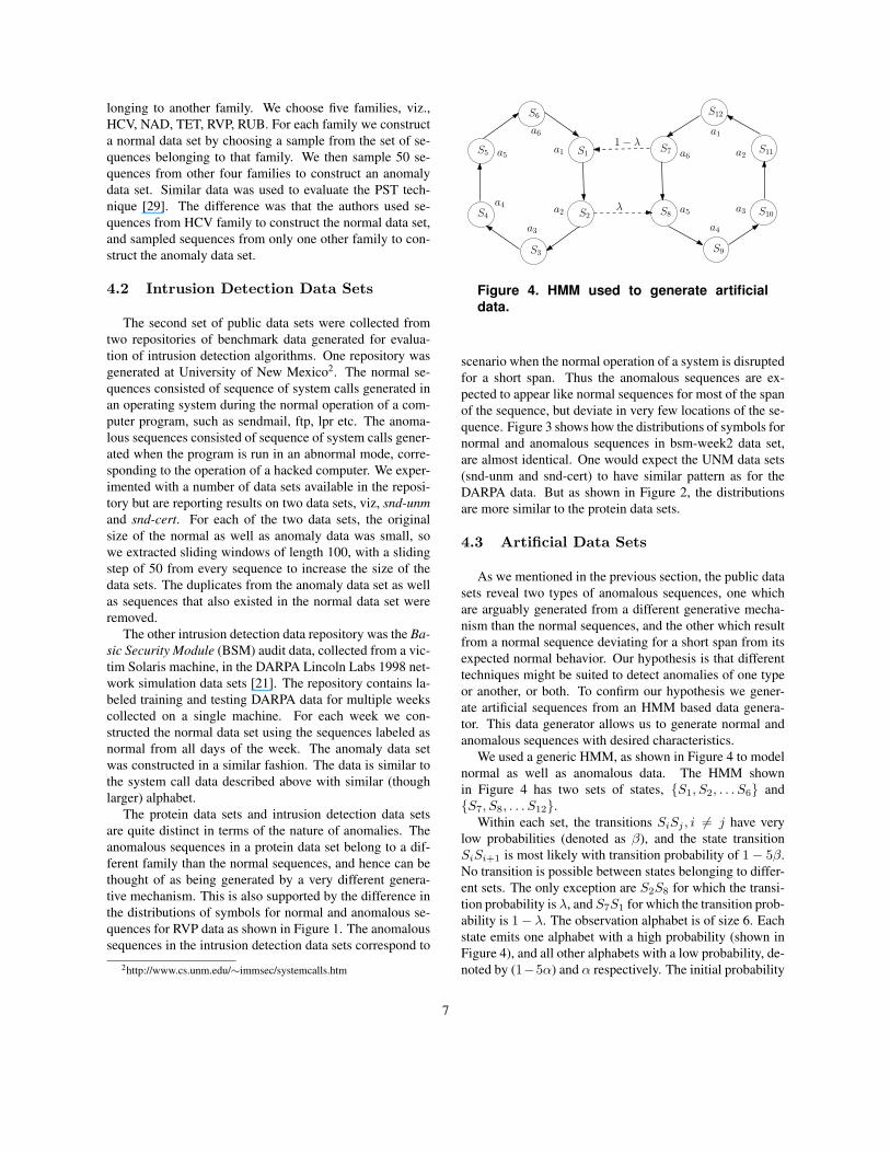
Figure 4. HMM used to generate artificialdata.

scenario when the normal operation of a system is disrupted

for a short span. Thus the anomalous sequences are ex-

pected to appear like normal sequences for most of the span

of the sequence, but deviate in very few locations of the se-

quence. Figure 3 shows how the distributions of symbols for

normal and anomalous sequences in bsm-week2 data set,

are almost identical. One would expect the UNM data sets

(snd-unm and snd-cert) to have similar pattern as for the

DARPA data. But as shown in Figure 2, the distributions

are more similar to the protein data sets.

4.3 Artificial Data Sets

As we mentioned in the previous section, the public data

sets reveal two types of anomalous sequences, one which

are arguably generated from a different generative mecha-

nism than the normal sequences, and the other which result

from a normal sequence deviating for a short span from its

expected normal behavior. Our hypothesis is that different

techniques might be suited to detect anomalies of one type

or another, or both. To confirm our hypothesis we gener-

ate artificial sequences from an HMM based data genera-

tor. This data generator allows us to generate normal and

anomalous sequences with desired characteristics.

We used a generic HMM, as shown in Figure 4 to model

normal as well as anomalous data. The HMM shown

in Figure 4 has two sets of states, {S1, S2, . . . S6} and

{S7, S8, . . . S12}.

Within each set, the transitions SiSj , i 6= j have very

low probabilities (denoted as β), and the state transition

SiSi+1 is most likely with transition probability of 1 − 5β.

No transition is possible between states belonging to differ-

ent sets. The only exception are S2S8 for which the transi-

tion probability is λ, and S7S1 for which the transition prob-

ability is 1− λ. The observation alphabet is of size 6. Each

state emits one alphabet with a high probability (shown in

Figure 4), and all other alphabets with a low probability, de-

noted by (1−5α) and α respectively. The initial probability

7

vector π is set such that either the first 6 states have initial

probability set to 1

6and rest 0, or vice versa.

Normal sequences are generated by setting λ to a low

value and π to be such that the first 6 states have initial prob-

ability set to 1

6and rest 0. If λ = β = α = 0, the normal

sequences will consist of the subsequence a1a2a3a4a5a6

getting repeated multiple times. By increasing λ or β or α,

noise can be induced in the normal sequences.

The generic HMM can also be tuned to generate two type

of anomalous sequences. For the first type of anomalous se-

quences, λ is set to a high value and π to be such that the last

6 states have initial probability set to 1

6and rest 0. The re-

sulting HMM is directly opposite to the HMM constructed

for generating normal sequences. Hence the anomalous se-

quences generated by this HMM are completely different

from the normal sequences and will consist of the subse-

quence a6a5a4a3a2a1 getting repeated multiple times.

To generate second type of anomalous sequences, the

HMM used to generate the normal sequence is used, with

the only difference that λ is increased to a higher value.

Thus the anomalous sequences generated by this HMM will

be similar to the normal sequences except that there will be

short spans when the symbols are generated by the second

set of states.

By varying λ, β, and α, we generated several evaluation

data sets (with two different type of anomalous sequences).

We will present the results of our experiments on these arti-

ficial data sets in next section.

5 Evaluation Methodology

The techniques investigated in this paper assign an

anomaly score to each test sequence Sq ∈ ST. To com-

pare the performance of different techniques we adopt the

following evaluation strategy:

1. Rank the test sequences in decreasing order based on

the anomaly scores.

2. Count the number of true anomalies in the top p por-

tion of the sorted test sequences, where p = δq,

0 ≤ δ ≤ 1, and q is the number of true anomalies

in ST. Let there be t true anomalous sequences in top

p ranked sequences.

3. Accuracy of the technique = tq

= tδp

.

We experimented with different values of δ and reported

consistent findings. We present results for δ = 1.0 in this

paper.

6 Nature of Normal and Anomalous Se-

quences

To understand the performance of different anomaly de-

tection techniques on a given test data set, we first need to

understand what differentiates normal and anomalous se-

quences in the test data set.

If we treat sequences as instances, one distinction be-

tween normal and anomalous sequences is that normal test

sequences are more similar (using a certain similarity mea-

sure) to training sequences, than anomalous test sequences.

If the difference in similarity is not large, this characteristic

will not be able to accurately distinguish between normal

and anomalous sequences. This characteristic is utilized by

kernel based techniques to distinguish between normal and

anomalous sequences.

Another characteristic of a test sequence is the relative

frequency of short patterns (subsequences) in that test se-

quence with respect to the training sequences. Let us clas-

sify a short pattern occurring in a test sequence as seen if

it occurs in training sequences and unseen if it does not oc-

cur in training sequences. The seen patterns can be further

classified as seen-frequent, if they occur frequently in the

training sequences, and seen-rare, if they occur rarely in

the training sequences. A given test sequence can contain

all three type of patterns, in varying proportions. The per-

formance of a window based or a Markovian technique will

depend on following factors:

1. What is the proportion of seen-frequent, seen-rare, and

unseen patterns for normal sequences, and for anoma-

lous sequences?

2. What is the relative score assigned by the technique to

the three type of patterns?

We will refer back to this characteristic when analyzing the

performance of different techniques in Section 7.4.

7 Experimental Results

The experiments were conducted on a variety of data sets

discussed in Section 4. The various parameter settings asso-

ciated with each technique were explored. The results pre-

sented here are for the parameter setting which gave best re-

sults across all data sets, for each technique. The parameter

settings for the reported results are : CLUSTER (c = 32),

kNN (k = 4), FSA,FSA-z(n = 5, l = 1), tSTIDE(k = 6),

PST(L = 6, Pmin = 0.01), RIPPER(k = 6). For public

data sets, HMM was run with σ = 4, while for artificial

data sets, HMM was run with σ = 12. For window based

and Markovian techniques, the techniques were evaluated

using different combination methods discussed in Section

8

Kernel Markovian

cls knn tstd fsa fsaz pst rip hmm Avg

PFAM

hcv 0.54 0.88 0.90 0.88 0.92 0.74 0.22 0.10 0.65

nad 0.46 0.64 0.74 0.66 0.72 0.10 0.20 0.06 0.48

tet 0.84 0.86 0.50 0.48 0.50 0.66 0.36 0.20 0.55

rvp 0.86 0.90 0.90 0.90 0.90 0.50 0.52 0.10 0.70

rub 0.76 0.72 0.88 0.80 0.88 0.28 0.56 0.00 0.61

UNMsndu 0.76 0.84 0.58 0.82 0.80 0.28 0.76 0.00 0.61

sndc 0.94 0.94 0.64 0.88 0.88 0.10 0.74 0.00 0.64

DRPA

bw1 0.20 0.20 0.20 0.40 0.50 0.00 0.30 0.00 0.22

bw2 0.36 0.52 0.36 0.52 0.56 0.10 0.34 0.02 0.35

bw3 0.52 0.48 0.60 0.64 0.66 0.34 0.58 0.20 0.50

Avg 0.62 0.70 0.63 0.70 0.73 0.31 0.46 0.07

Table 3. Results on public data sets.

Kernel Markovian

cls knn tstd fsa fsaz pst rip hmm Avg

d1 1.00 1.00 1.00 1.00 1.00 1.00 1.00 1.00 1.00

d2 0.80 0.88 0.82 0.88 0.92 0.84 0.78 0.50 0.80

d3 0.74 0.76 0.64 0.50 0.60 0.82 0.64 0.34 0.63

d4 0.74 0.76 0.64 0.52 0.52 0.76 0.66 0.42 0.63

d5 0.58 0.60 0.48 0.24 0.32 0.68 0.52 0.16 0.48

d6 0.64 0.68 0.50 0.28 0.38 0.68 0.44 0.66 0.53

Avg 0.75 0.78 0.68 0.57 0.62 0.80 0.67 0.51

Table 4. Results on artificial data sets.

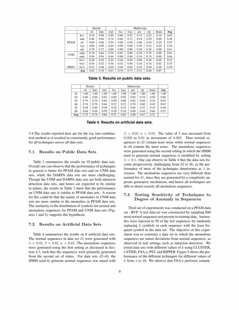
3.4.The results reported here are for the log sum combina-

tion method as it resulted in consistently good performance

for all techniques across all data sets.

7.1 Results on Public Data Sets

Table 3 summarizes the results on 10 public data sets.

Overall one can observe that the performance of techniques

in general is better for PFAM data sets and on UNM data

sets, while the DARPA data sets are more challenging.

Though the UNM and DARPA data sets are both intrusion

detection data sets, and hence are expected to be similar

in nature, the results in Table 3 show that the performance

on UNM data sets is similar to PFAM data sets. A reason

for this could be that the nature of anomalies in UNM data

sets are more similar to the anomalies in PFAM data sets.

The similarity in the distribution of symbols for normal and

anomalous sequences for PFAM and UNM data sets (Fig-

ures 1 and 2), supports this hypothesis.

7.2 Results on Artificial Data Sets

Table 4 summarizes the results on 6 artificial data sets.

The normal sequences in data set d1 were generated with

λ = 0.01, β = 0.01, α = 0.01. The anomalous sequences

were generated using the first setting as discussed in Sec-

tion 4.3, such that the sequences were primarily generated

from the second set of states. For data sets d2–d6, the

HMM used to generate normal sequences was tuned with

β = 0.01, α = 0.01. The value of λ was increased from

0.002 to 0.01 in increments of 0.002. Thus normal se-

quences in d2 contain least noise while normal sequences

in d6 contain the most noise. The anomalous sequences

were generated using the second setting in which the HMM

used to generate normal sequences is modified by setting

λ = 0.1. One can observe in Table 4 that the data sets be-

come progressively challenging from d2 to d6, as the per-

formance of most of the techniques deteriorates as λ in-

creases. The anomalous sequences are very different than

normal for d1, since they are generated by a completely op-

posite generative mechanism, and hence all techniques are

able to detect exactly all anomalous sequences.

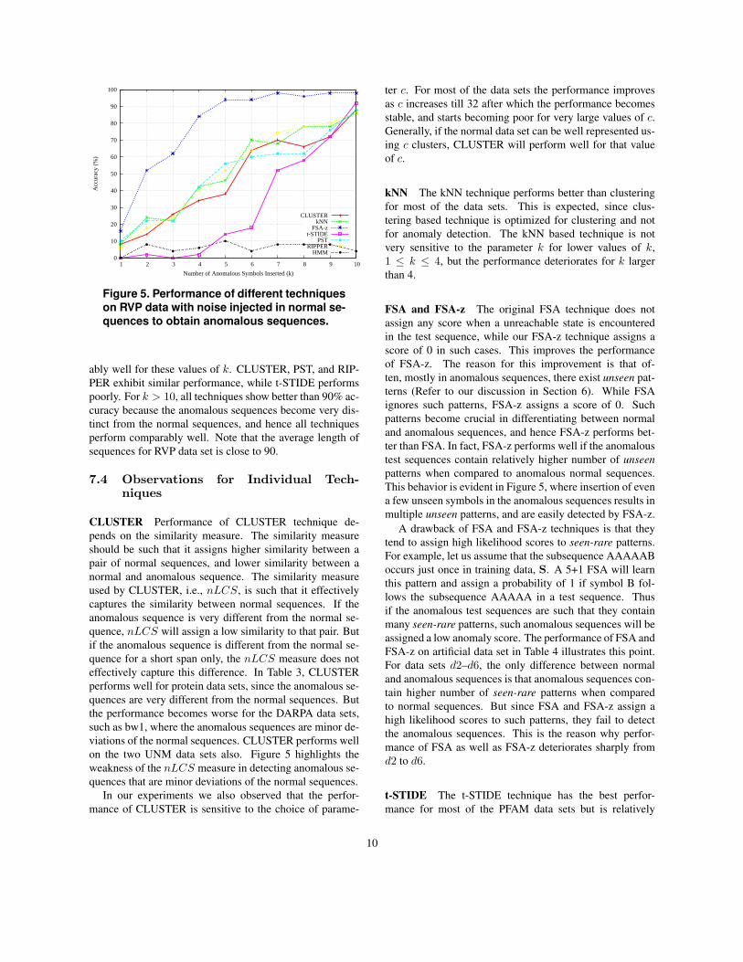
7.3 Testing Sensitivity of Techniques toDegree of Anomaly in Sequences

Third set of experiments was conducted on a PFAM data

set - RVP. A test data set was constructed by sampling 800

most normal sequences not present in training data. Anoma-

lies were injected in 50 of the test sequences by randomly

replacing k symbols in each sequence with the least fre-

quent symbol in the data set. The objective of this exper-

iment was to construct a data set in which the anomalous

sequences are minor deviations from normal sequences, as

observed in real settings such as intrusion detection. We

tested data sets with different values of k using CLUSTER,

t-STIDE, FSA-z, PST, and RIPPER. Figure 5 shows the per-

formance of the different techniques for different values of

k from 1 to 10. We observe that FSA-z performs remark-

9

0

10

20

30

40

50

60

70

80

90

100

1 2 3 4 5 6 7 8 9 10

Acc

urac

y (%

)

Number of Anomalous Symbols Inserted (k)

CLUSTERkNN

FSA-zt-STIDE

PSTRIPPER

HMM

Figure 5. Performance of different techniques

on RVP data with noise injected in normal se-quences to obtain anomalous sequences.

ably well for these values of k. CLUSTER, PST, and RIP-

PER exhibit similar performance, while t-STIDE performs

poorly. For k > 10, all techniques show better than 90% ac-

curacy because the anomalous sequences become very dis-

tinct from the normal sequences, and hence all techniques

perform comparably well. Note that the average length of

sequences for RVP data set is close to 90.

7.4 Observations for Individual Tech-niques

CLUSTER Performance of CLUSTER technique de-

pends on the similarity measure. The similarity measure

should be such that it assigns higher similarity between a

pair of normal sequences, and lower similarity between a

normal and anomalous sequence. The similarity measure

used by CLUSTER, i.e., nLCS, is such that it effectively

captures the similarity between normal sequences. If the

anomalous sequence is very different from the normal se-

quence, nLCS will assign a low similarity to that pair. But

if the anomalous sequence is different from the normal se-

quence for a short span only, the nLCS measure does not

effectively capture this difference. In Table 3, CLUSTER

performs well for protein data sets, since the anomalous se-

quences are very different from the normal sequences. But

the performance becomes worse for the DARPA data sets,

such as bw1, where the anomalous sequences are minor de-

viations of the normal sequences. CLUSTER performs well

on the two UNM data sets also. Figure 5 highlights the

weakness of the nLCS measure in detecting anomalous se-

quences that are minor deviations of the normal sequences.

In our experiments we also observed that the perfor-

mance of CLUSTER is sensitive to the choice of parame-

ter c. For most of the data sets the performance improves

as c increases till 32 after which the performance becomes

stable, and starts becoming poor for very large values of c.

Generally, if the normal data set can be well represented us-

ing c clusters, CLUSTER will perform well for that value

of c.

kNN The kNN technique performs better than clustering

for most of the data sets. This is expected, since clus-

tering based technique is optimized for clustering and not

for anomaly detection. The kNN based technique is not

very sensitive to the parameter k for lower values of k,

1 ≤ k ≤ 4, but the performance deteriorates for k larger

than 4.

FSA and FSA-z The original FSA technique does not

assign any score when a unreachable state is encountered

in the test sequence, while our FSA-z technique assigns a

score of 0 in such cases. This improves the performance

of FSA-z. The reason for this improvement is that of-

ten, mostly in anomalous sequences, there exist unseen pat-

terns (Refer to our discussion in Section 6). While FSA

ignores such patterns, FSA-z assigns a score of 0. Such

patterns become crucial in differentiating between normal

and anomalous sequences, and hence FSA-z performs bet-

ter than FSA. In fact, FSA-z performs well if the anomalous

test sequences contain relatively higher number of unseen

patterns when compared to anomalous normal sequences.

This behavior is evident in Figure 5, where insertion of even

a few unseen symbols in the anomalous sequences results in

multiple unseen patterns, and are easily detected by FSA-z.

A drawback of FSA and FSA-z techniques is that they

tend to assign high likelihood scores to seen-rare patterns.

For example, let us assume that the subsequence AAAAAB

occurs just once in training data, S. A 5+1 FSA will learn

this pattern and assign a probability of 1 if symbol B fol-

lows the subsequence AAAAA in a test sequence. Thus

if the anomalous test sequences are such that they contain

many seen-rare patterns, such anomalous sequences will be

assigned a low anomaly score. The performance of FSA and

FSA-z on artificial data set in Table 4 illustrates this point.

For data sets d2–d6, the only difference between normal

and anomalous sequences is that anomalous sequences con-

tain higher number of seen-rare patterns when compared

to normal sequences. But since FSA and FSA-z assign a

high likelihood scores to such patterns, they fail to detect

the anomalous sequences. This is the reason why perfor-

mance of FSA as well as FSA-z deteriorates sharply from

d2 to d6.

t-STIDE The t-STIDE technique has the best perfor-

mance for most of the PFAM data sets but is relatively

10

worse for the intrusion detection data sets. A strength of t-

STIDE is that unlike FSA and FSA-z, t-STIDE does not get

affected by the presence of seen-rare windows in anoma-

lous test sequences. This can be observed in the artificial

data sets, where the performance of t-STIDE does not dete-

riorate as sharply as for FSA-z as λ is increased (from d2 –

d6).

The above mentioned strength of t-STIDE can also have

a negative impact on its performance. t-STIDE learns only

frequently occurring patterns in the training data, and ig-

nores rarely occurring ones. Thus if a normal sequence is

tested against t-STIDE, and it contains a seen-rare pattern,

it will be assigned a low likelihood score by t-STIDE, while

FSA and FSA-z will assign a higher score in such a sce-

nario. This weakness of t-STIDE is illustrated in Figure 5.

The reason for the poor performance of t-STIDE in these

set of experiments is that many normal test sequences in

RVP data contain multiple seen-rare patterns. The anoma-

lous sequences contain multiple unseen windows induced

by adding anomalous symbols. But the difference between

the scores assigned by t-STIDEfor seen-rare windows in

normal sequences and unseen windows in anomalous se-

quences is not enough to distinguish between normal and

anomalous sequences.

In the previous evaluation of t-STIDE [10] with other

techniques, t-STIDE was found to be performing the best

on UNM data sets. We report consistent results. t-STIDE

performs better than HMM, as well as the RIPPER tech-

nique (refer to Section 3.3.3).

In the original t-STIDE technique [10] the authors use a

threshold based combination function, in which the number

of windows in the test sequence whose scores are equal to

or below a threshold, are counted. Our experiments show

that using the average log values of the scores performs

equally well without relying on the choice of a threshold.

The STIDE technique [14] is a simpler variant of t-STIDE

in which the threshold is set to 0. In [10] the authors have

shown that t-STIDE is better than STIDE, hence we evalu-

ate the technique used in t-STIDE.

PST We observe that PST performs very poorly on most

of the public data sets. It should be noted that in the paper

that used PST for anomaly detection, the evaluation done

on protein data sets was different than our evaluation. We

provide a more unbiased evaluation which reveals that PST

does not perform that well on similar protein data sets.

PST assigns moderately high likelihood scores to seen-

rare patterns observed in a test sequence, since it computes

the probability of the last event in the pattern conditioned

on a suffix of the preceding symbols in the pattern. Thus

the score assigned to seen-rare patterns by PST are lower

than the score assigned by FSA-z, but higher than the score

assigned by t-STIDE. Similarly, PST assigns a moderately

high score for unseen patterns occurring in test sequences.

The latter characteristic of PST can become the weakness

of PST in a way that the anomaly signal due to the unseen

as well as seen-rare patterns is smoothed by the PST. If in a

data set the normal sequences contain a significant number

of seen-rare patterns, and the anomalous sequences contain

bad patterns, they might still not be distinguishable. This

behavior is observed for many public data sets in Table 3,

well as on the modified RVP data set in Figure 5.

The fact that the scores assigned to seen-rare patterns by

PST are lower than the score assigned by FSA-z, can also

become strength of PST because it does not get affected by

the presence of seen-rare patterns in normal test sequences,

unlike FSA-z. This characteristic is observed with the arti-

ficial data sets in Table 4. As λ increases, the performance

of PST remains more stable than any other technique.

RIPPER Both RIPPER and PST techniques are more

flexible than FSA-z in conditioning the probability of an

event based on its preceding symbols. Thus RIPPER tech-

nique also smoothens the likelihood scores of unseen as well

as seen-rare patterns in test sequences. Therefore, we ob-

serve that for public data sets, RIPPER exhibits relatively

poor performance, in comparison to FSA and FSA-z.

RIPPER performs better than PST on 8 out of 10 data

sets. Thus choosing a sparse history is more effective than

choosing a variable length suffix. The reason for this is

that the smoothing done by RIPPER is less than smooth-

ing done by PST (since the RIPPER classifier applies more

specific and longer rules first, and is hence biased towards

using more symbols of the history), and hence RIPPER is

more similar to FSA and FSA-z than PST. The results on

artificial data sets in Table 4 also show that the deterioration

of RIPPER’s performance from d1 – d7 is less pronounced

than for FSA-z while more pronounced than PST.

In [10] the RIPPER technique was found to be perform-

ing better than t-STIDE on UNM data sets. Our results on

UNM data sets are consistent with the previous findings. On

the DARPA data sets RIPPER performs comparably with

t-STIDE, but on PFAM data sets its performance is poor

when compared to t-STIDE.

HMM The HMM technique performs very poorly on all

public data sets. The reasons for the poor performance of

HMM are twofold. The first reason is that HMM tech-

nique makes an assumption that the normal sequences can

be represented with σ hidden states. Often, this assumption

does not hold true, and hence the HMM model learnt from

the training sequences cannot emit the normal sequences

with high confidence. Thus all test sequences (normal and

anomalous) are assigned a low probability score. The sec-

ond reason for the poor performance is the manner in which

a score is assigned to a test sequence. The test sequence is

11

first converted to a hidden state sequence, and then a 1 + 1FSA is applied to the transformed sequence. A 1 + 1 FSA

does not perform well. A better technique would be to ap-

ply a higher order FSA technique as presented in [24]. The

second reason is more prominent in the results on artificial

data sets. Since the training data was actually generated by

a 12 state HMM and the HMM technique was trained with

σ = 12, the HMM model effectively captures the normal

sequences. The results of HMM for artificial data sets are

therefore better than for public data sets, but still worse than

other techniques.

8 Conclusions and Future Work

Our experimental evaluation has not only provided us in-

sights into strengths and weaknesses of the techniques, but

have also allowed us to proposed a variant of FSA tech-

nique, which is shown to perform better than the original

technique.

We investigated kernel based techniques and found that

they perform well for real data sets, and for artificial data

sets with large number of anomalies, but they perform

poorly when the sequences have very few anomalies. This

can be attributed to the similarity measure. As a future work

we would like to investigate other similarity measures that

would be able to capture the difference between sequences

which are minor deviations of each other.

We characterize normal as well as anomalous test se-

quences in terms of the type of patterns (seen-frequent,

seen-rare, and unseen) contained in them. We argue that the

different window based and Markovian techniques handle

the three patterns differently. Since different data sets have

different composition of normal and anomalous sequences,

the performance of different techniques varies for different

data set. Through our experiments we have identified rela-

tive strengths and weaknesses of window based as well as

Markovian techniques. We have shown that while t-STIDE,

FSA, and FSA-z, perform consistently well for most of the

data sets, they all have weaknesses in handling certain type

of data and anomalies. The PST technique, which was not

compared earlier with other techniques, is shown to per-

form relatively worse than the previous three techniques.

We have also shown that our variant of RIPPER technique

is also an average performer on most of the data sets, though

it is better than t-STIDE on UNM data sets, which is an im-

provement on the original RIPPER technique. The HMM

technique performs poorly when the assumption that the se-

quences were generated using an HMM does not hold true.

When the assumption is true, the performance improves sig-

nificantly. The hidden state sequences, obtained as a in-

termediate transformation of data, can actually be used as

input data to any other technique discussed here. The per-

formance of such an approach has not been studied and will

be a future direction of research.

The original FSA technique [23] proposed estimating

likelihoods of more than one event at a time. Using such

higher-order Markovian models might change the perfor-

mance of the Markovian techniques and will be investigated

in future.

While the problem addressed by techniques discussed in

this paper is of semi-supervised nature, many of these tech-

niques can also be applied in an unsupervised setting, i.e.,

the training data contains both normal as well as anomalous

sequences, under the assumption that anomalous sequences

are very rare. The anomaly detection task will be to assign

an anomaly score to each sequence in the training data it-

self. While techniques such as CLUSTER, kNN, PST, and

RIPPER seem to be applicable, it remains to be seen how

FSA, FSA-z, and HMM will perform in the unsupervised

setting.

References

[1] A. Bateman, E. Birney, R. Durbin, S. R. Eddy, K. L. Howe,

and E. L. Sonnhammer. The pfam protein families database.

Nucleic Acids Res., 28:263–266, 2000.

[2] L. E. Baum, T. Petrie, G. Soules, and N. Weiss. A maximiza-

tion technique occuring in the statistical analysis of proba-

bilistic functions of markov chains. In Annals of Mathemat-

ical Statistics, volume 41(1), pages 164–171, 1970.

[3] G. Bejerano and G. Yona. Variations on probabilistic suffix

trees: statistical modeling and prediction of protein families

. Bioinformatics, 17(1):23–43, 2001.

[4] S. Budalakoti, A. Srivastava, R. Akella, and E. Turkov.

Anomaly detection in large sets of high-dimensional sym-

bol sequences. Technical Report NASA TM-2006-214553,

NASA Ames Research Center, 2006.

[5] V. Chandola, A. Banerjee, and V. Kumar. Anomaly detection

– a survey. ACM Computing Surveys (To Appear), 2008.

[6] W. W. Cohen. Fast effective rule induction. In A. Priedi-

tis and S. Russell, editors, Proceedings of the 12th Inter-

national Conference on Machine Learning, pages 115–123,

Tahoe City, CA, jul 1995. Morgan Kaufmann.

[7] W. L. E. Eskin and S. Stolfo. Modeling system call for intru-

sion detection using dynamic window sizes. In Proceedings

of DARPA Information Survivability Conference and Expo-

sition, 2001.

[8] J. Forney, G.D. The viterbi algorithm. Proceedings of the

IEEE, 61(3):268–278, March 1973.

[9] S. Forrest, S. A. Hofmeyr, A. Somayaji, and T. A. Longstaff.

A sense of self for unix processes. In Proceedinges of the

1996 IEEE Symposium on Research in Security and Privacy,

pages 120–128. IEEE Computer Society Press, 1996.

[10] S. Forrest, C. Warrender, and B. Pearlmutter. Detecting in-

trusions using system calls: Alternate data models. In Pro-

ceedings of the 1999 IEEE Symposium on Security and Pri-

vacy, pages 133–145, Washington, DC, USA, 1999. IEEE

Computer Society.

12

[11] B. Gao, H.-Y. Ma, and Y.-H. Yang. Hmms (hidden markov

models) based on anomaly intrusion detection method. In

Proceedings of International Conference on Machine Learn-

ing and Cybernetics, pages 381–385. IEEE Computer Soci-

ety, 2002.

[12] F. A. Gonzalez and D. Dasgupta. Anomaly detection using

real-valued negative selection. Genetic Programming and

Evolvable Machines, 4(4):383–403, 2003.

[13] V. Hodge and J. Austin. A survey of outlier detection

methodologies. Artificial Intelligence Review, 22(2):85–

126, 2004.

[14] S. A. Hofmeyr, S. Forrest, and A. Somayaji. Intrusion detec-

tion using sequences of system calls. Journal of Computer

Security, 6(3):151–180, 1998.

[15] J. W. Hunt and T. G. Szymanski. A fast algorithm for

computing longest common subsequences. Commun. ACM,

20(5):350–353, 1977.

[16] A. K. Jain and R. C. Dubes. Algorithms for Clustering Data.

Prentice-Hall, Inc., 1988.

[17] A. Lazarevic, L. Ertoz, V. Kumar, A. Ozgur, and J. Srivas-

tava. A comparative study of anomaly detection schemes in

network intrusion detection. In Proceedings of the Third

SIAM International Conference on Data Mining. SIAM,

May 2003.

[18] W. Lee and S. Stolfo. Data mining approaches for intrusion

detection. In Proceedings of the 7th USENIX Security Sym-

posium, San Antonio, TX, 1998.

[19] W. Lee, S. Stolfo, and P. Chan. Learning patterns from unix

process execution traces for intrusion detection. In Proceed-

ings of the AAAI 97 workshop on AI methods in Fraud and

risk management, 1997.

[20] C. S. Leslie, E. Eskin, and W. S. Noble. The spectrum ker-

nel: A string kernel for svm protein classification. In Pacific

Symposium on Biocomputing, pages 566–575, 2002.

[21] R. P. Lippmann, D. J. Fried, I. Graf, J. W. Haines,

K. P. Kendall, D. McClung, D. Weber, S. E. Webster,

D. Wyschogrod, R. K. Cunningham, and M. A. Zissman.

Evaluating intrusion detection systems - the 1998 darpa off-

line intrusion detection evaluation. In DARPA Information

Survivability Conference and Exposition (DISCEX) 2000,

volume 2, pages 12–26. IEEE Computer Society Press, Los

Alamitos, CA, 2000.

[22] C. C. Michael and A. Ghosh. Two state-based approaches to

program-based anomaly detection. In Proceedings of the

16th Annual Computer Security Applications Conference,

page 21. IEEE Computer Society, 2000.

[23] L. Portnoy, E. Eskin, and S. Stolfo. Intrusion detection with

unlabeled data using clustering. In Proceedings of ACM

Workshop on Data Mining Applied to Security, 2001.

[24] Y. Qiao, X. W. Xin, Y. Bin, and S. Ge. Anomaly intru-

sion detection method based on hmm. Electronics Letters,

38(13):663–664, 2002.

[25] L. R. Rabiner and B. H. Juang. An introduction to hidden

markov models. IEEE ASSP Magazine, 3(1):4–16, 1986.

[26] S. Ramaswamy, R. Rastogi, and K. Shim. Efficient algo-

rithms for mining outliers from large data sets. In Proceed-

ings of the 2000 ACM SIGMOD international conference on

Management of data, pages 427–438. ACM Press, 2000.

[27] D. Ron, Y. Singer, and N. Tishby. The power of amne-

sia: learning probabilistic automata with variable memory

length. Machine Learning, 25(2-3):117–149, 1996.

[28] A. N. Srivastava. Discovering system health anomalies using

data mining techniques. In Proceedings of 2005 Joint Army

Navy NASA Airforce Conference on Propulsion, 2005.

[29] P. Sun, S. Chawla, and B. Arunasalam. Mining for outliers

in sequential databases. In Proceedings of SIAM Conference

on Data Mining, 2006.

[30] P.-N. Tan, M. Steinbach, and V. Kumar. Introduction to Data

Mining. Addison-Wesley, 2005.

[31] X. Zhang, P. Fan, and Z. Zhu. A new anomaly detection

method based on hierarchical hmm. In Proceedings of the

4th International Conference on Parallel and Distributed

Computing, Applications and Technologies, pages 249–252,

2003.

13