Comparative Analysis of Mobile Robot Localization Methods Based on Proprioceptive and Exteroceptive...

11

Comparative Analysis of Mobile Robot Localization Methods Based On Proprioceptive

and Exteroceptive Sensors

Gianluca Ippoliti, Leopoldo Jetto, Sauro Longhi, Andrea Monteriù Dipartimento di Ingegneria Informatica Gestionale e dell’Automazione

Università Politecnica delle Marche Via Brecce Bianche – 60131 Ancona

Italy

1. Introduction Two different approaches to the mobile robot localization problem exist: relative and absolute. The first one is based on the data provided by sensors measuring the dynamics of variables internal to the vehicle; absolute localization requires sensors measuring some parameters of the environment in which the robot is operating. If the environment is only partially known, the construction of appropriate ambient maps is also required. The actual trend is to exploit the complementary nature of these two kinds of sensorial information to improve the precision of the localization procedure (see e.g. (Bemporad et al., 2000; Bonci et al., 2004; Borenstein et al., 1997; Durrant-Whyte, 1988; Gu et al., 2002; Ippoliti et al., 2004)) at expense of an increased cost and computational complexity. The aim is to improve the mobile robot autonomy by enhancing its capability of localization with respect to the surrounding environment. In this framework the research interests have been focused on multi-sensor systems because of the limitations inherent any single sensory device that can only supply partial information on the environment, thus limiting the ability of the robot to localize itself. The methods and algorithms proposed in the literature for an efficient integration of multiple-sensor information differ according to the a priori information on the environment, which may be almost known and static, or almost unknown and dynamic. In this chapter both relative and absolute approaches of mobile robot localization are

investigated and compared. With reference to relative localization, the purpose of this chapter is to propose and to compare three different algorithms for the mobile robot localization only using internal sensors like odometers and gyroscopes. The measurement systems for mobile robot localization only based on relative or dead-reckoning methods, such as encoders and gyroscopes, have the considerable advantage of being totally self-contained inside the robot, relatively simple to use and able to guarantee a high data rate. A drawback of these systems is that they integrate the relative increments and the localization errors may considerably grow over time if appropriate sensor-fusion algorithms are not used (De Cecco, 2003). Here, different methods are analysed and tested. The best performance has been obtained in the stochastic framework where the localization problem has been formulated as a state estimation problem and the Extended Kalman Filtering (EKF)

216 Mobile Robots, Perception & Navigation

is used. The EKF fuses together odometric and gyroscopic data. A difference with respect to other EKF based techniques is that the approach followed here derives the dynamical equation of the state-space form from the kinematic model of the robot, while the measure equation is derived from the numerical integration equations of the encoder increments. This allows to fuse together all the available informative content which is carried both by the robot dynamics and by the acquired measures. As previously mentioned, any relative localization algorithm is affected by a continuous growth in the integrated measurement error. This inconvenience can be reduced by periodically correcting the internal measures with the data provided by absolute sensors like sonar, laser, GPS, vision systems (Jarvis, 1992; Talluri & Aggarwal, 1992; Zhuang & Tranquilla, 1995; Mar & Leu, 1996; Arras et al., 2000; Yi et al., 2000; Panzieri et al., 2002). To this purpose, a localization algorithm based on a measure apparatus composed of a set of proprioceptive and exteroceptive sensors, is here proposed and evaluated. The fusion of internal and external sensor data is again realized through a suitably defined EKF driven by encoder, gyroscope and laser measures. The developed algorithms provide efficient solutions to the localization problem, where

their appealing features are: • The possibility of collecting all the available information and uncertainties of a

different kind into a meaningful state-space representation, • The recursive structure of the solution, • The modest computational effort.

Significant experimental results of all proposed algorithms are presented here, and their comparison concludes this chapter.

2. The sensors equipment In this section the considered sensor devices are introduced and characterized.

2.1 Odometric measures Consider a unicycle-like mobile robot with two driving wheels, mounted on the left and right sides of the robot, with their common axis passing through the center of the robot (see Fig. 1).

Fig. 1. The scheme of the unicycle robot.

Comparative Analysis of Mobile Robot Localization Methods Based On Proprioceptive and Exteroceptive Sensors 217

Localization of this mobile robot in a two-dimensional space requires the knowledge of coordinates x and y of the midpoint between the two driving wheels and of the angle θ between the main axis of the robot and the X -direction. The kinematic model of the unicycle robot is described by the following equations: ( ) ( ) ( )cosx t t tν θ=& (1)

( ) ( ) ( )siny t t tν θ=& (2)

( ) ( )t tθ ω=& (3)

where ( )tν and ( )tω are, respectively, the displacement velocity and the angular velocity

of the robot and are expressed by: ( ) ( ) ( )

2r lt t

t rω ω

ν+

= (4)

( ) ( ) ( )r lt tt r

dω ω

ω−

= (5)

where ( )r tω and ( )l tω are the angular velocities of the right and left wheels, respectively,

r is the wheel radius and d s the distance between the wheels. Assuming constant ( )r tω and ( )l tω over a sufficiently small sampling period

1:k k kt t t+Δ = − ,

the position and orientation of the robot at time instant 1kt + can be expressed as:

( ) ( ) ( )( )

( ) ( ) ( )1

sin2 cos

22

k k

k kk k k k k

k k

t tt t

x t x t t t tt t

ωων θ

ω+

ΔΔ⎛ ⎞

= + Δ +⎜ ⎟Δ ⎝ ⎠

(6)

( ) ( ) ( )( )

( ) ( ) ( )1

sin2 sin

22

k k

k kk k k k k

k k

t tt t

y t y t t t tt t

ωων θ

ω+

ΔΔ⎛ ⎞

= + Δ +⎜ ⎟Δ ⎝ ⎠

(7)

( ) ( ) ( )1k k k kt t t tθ θ ω+ = + Δ (8)

where ( )k kt tν Δ and ( )k kt tω Δ are:

( ) ( ) ( )2

r k l kk k

q t q tt t rν

Δ + ΔΔ = (9)

( ) ( ) ( ) .r k l kk k

q t q tt t r

dω

Δ − ΔΔ = (10)

The terms ( )r kq tΔ and ( )l kq tΔ are the incremental distances covered on the interval ktΔ by

the right and left wheels of the robot respectively. Denote by ( )r ky t and ( )l ky t the measures

of ( )r kq tΔ and ( )l kq tΔ respectively, provided by the encoders attached to wheels, one has

( ) ( ) ( )r k r k r ky t q t s t= Δ + (11)

( ) ( ) ( )l k l k l ky t q t s t= Δ + (12)

where ( )rs ⋅ and ( )ls ⋅ are the measurement errors, which are modelled as independent,


zero mean, gaussian white sequences (Wang, 1988). It follows that the really available values ( )ky tν

and ( )ky tω of ( )k kt tν Δ and ( )k kt tω Δ

respectively are given by: ( ) ( ) ( ) ( ) ( )

2r k l k

k k k k

y t y ty t r t t tν νν η

+= = Δ + (13)

( ) ( ) ( ) ( ) ( )2

r k l kk k k k

y t y ty t r t t tω ωω η

−= = Δ + (14)

where ( )νη ⋅ and ( )ωη ⋅ are independent, zero mean, gaussian white sequences

, where, by (9) and (10), ( )2 2 2 2 4r l rνσ σ σ= + and

( )2 2 2 2 2r l r dωσ σ σ= + .

2.2 The Fiber optic gyroscope measures The operative principle of a Fiber Optic Gyroscope (FOG) is based on the Sagnac effect. The FOG is made of a fiber optic loop, fiber optic components, a photo-detector and a semiconductor laser. The phase difference of the two light beams traveling in opposite directions around the fiber optic loop is proportional to the rate of rotation of the fiber optic loop. The rate information is internally integrated to provide the absolute measurements of orientation. A FOG does not require frequent maintenance and have a longer lifetime of the conventional mechanical gyroscopes. In a FOG the drift is also low. A complete analysis of the accuracy and performances of this internal sensor has been developed in (Killian, 1994; Borenstein & Feng, 1996; Zhu et al., 2000; Chung et al., 2001). This internal sensor represents a simple low cost solution for producing accurate pose estimation of a mobile robot. The FOG readings are denoted by ( ) ( ) ( )gyθ θθ η⋅ = ⋅ + ⋅ , where ( )gθ ⋅ is the true value and ( )θη ⋅ is

an independent, zero mean, gaussian white sequence .

2.3 Laser scanner measures The distance readings by the Laser Measurement System (LMS) are related to the in-door environment model and to the configuration of the mobile robot. Denote with l the distance between the center of the laser scanner and the origin O′ of the coordinate system ( ), ,O X Y′ ′ ′ fixed to the mobile robot, as reported in Fig. 2.

Fig. 2. Laser scanner displacement.


At the sampling time kt , the position

sx , sy and orientation

sθ of the center of the laser scanner, referred to the inertial coordinate system ( ), ,O X Y , have the following form:

( ) ( ) ( )coss k k kx t x t l tθ= + (15)

( ) ( ) ( )sins k k ky t y t l tθ= + (16)

( ) ( )s k kt tθ θ= (17)

The walls and the obstacles in an in-door environment are represented by a proper set of planes orthogonal to the plane XY of the inertial coordinate system. Each plane jP ,

{ }1,2, , pj n∈ K (where pn is the number of planes which describe the indoor environment),

is represented by the triplet jrP , j

nP and jPν, where j

rP is the normal distance of the plane from the origin O , j

nP is the angle between the normal line to the plane and the X -direction and jPν

is a binary variable, { }1,1jPν ∈ − , which defines the face of the plane reflecting the

laser beam. In such a notation, the expectation of the i -th ( )1,2, , si n= K laser reading

( )ji kd t , relative to the present distance of the center of the laser scanner from the plane jP ,

has the following expression (see Fig. 3):

( )( ) ( )( )cos sin

cos

j j j jr s k n s k nj

i k ji

P P x t P y t Pd t ν

θ− −

= (18)

where j j

i n iPθ θ ∗= − (19) with [ ]0 1,iθ θ θ∗ ∈ given by (see Fig. 4):

.2i s iπθ θ θ∗ = + − (20)

The vector composed of geometric parameters jrP , j

nP and jPν, { }1,2, , pj n∈ K , is denoted by ∏ .

Fig. 3. Laser scanner measure.


Fig. 4. Laser scanner field of view for plane jP .

The laser readings ( )ji

kdy t are denoted by ( ) ( ) ( )j

i

ji id

y d η⋅ = ⋅ + ⋅ , where ( )jid ⋅ is the true value

expressed by (18) and ( )iη ⋅ is an independent, zero mean, gaussian white sequence

.

3. Relative approaches for mobile robot localization The purpose of this section is to propose and to compare three different algorithms for the mobile robot localization only using internal sensors like odometers and gyroscopes. The first method (Algorithm 1) is the simplest one and is merely based on a numerical integration of the raw encoder data; the second method (Algorithm 2) replaces the gyroscopic data into the equations providing the numerical integration of the increments provided by the encoders. The third method (Algorithm 3) operates in a stochastic framework where the uncertainty originates by the measurement noise and by the robot model inaccuracies. In this context the right approach is to formulate the localization problem as a state estimation problem and the appropriate tool is the EKF (see e.g. (Barshan & Durrant-Whyte, 1995; Garcia et al., 1995; Kobayashi et al., 1995; Jetto et al., 1999; Sukkarieh et al., 1999; Roumeliotis & Bekey, 2000; Antoniali & Oriolo, 2001; Dissanayake et al., 2001)). Hence, Algorithm 3 is a suitably defined EKF fusing together odometric and gyroscopic data. In the developed solution, the dynamical equation of the state-space form of the robot kinematic model, has been considered. The numerical integration equations of the encoder increments have been considered for deriving the measure equation. This allows to fuse together all the available informative content which is carried both by the robot dynamics and by the acquired measures.

3.1 Algorithm 1 Equations (6)-(8) have been used to estimate the position and orientation of the mobile robot at time

1kt + replacing the true values of ( )k kt tν Δ and ( )k kt tω Δ with their measures ( )ky tν

and ( )ky tω respectively, provided by the encoders. An analysis of the accuracy of this


estimation procedure has been developed in (Wang, 1988; Martinelli, 2002), where it is shown that the incremental errors on the encoder readings especially affect the estimate of the orientation ( )ktθ and reduce its applicability to short trajectories.

3.2 Algorithm 2 This algorithm is based on the ascertainment that the angular measure ( )ky tθ

provided by

the FOG is much more reliable than the orientation estimate obtainable with Algorithm 1. Hence, at each time instant, Algorithm 2 provides an estimate of the robot position and orientation ( ) ( ) ( )1 1 1, ,k k kx t y t y tθ+ + +⎡ ⎤⎣ ⎦ , where ( )1ky tθ +

is the FOG reading, ( )1kx t + and ( )1ky t +

are computed through equations (6), (7), replacing ( )k kt tν Δ with its measure ( )ky tν, ( )ktθ

with ( )ky tθ and ( )k kt tω Δ with ( ) ( )1k ky t y tθ θ+ − .

3.3 Algorithm 3 This algorithm operates in a stochastic framework exploiting the same measures of Algorithm 2. A state-space approach is adopted with the purpose of defining a more general method merging the information carried by the kinematic model with that provided by the sensor equipment. The estimation algorithm is an EKF defined on the basis of a state equation derived from (1)-(3) and of a measure equation inglobing the incremental measures of the encoders ( )ky tν

and the angular measure of the gyroscope

( )ky tθ. This is a difference with respect to other existing EKF based approaches,

(Barshan & Durrant-Whyte, 1995; Kobayashi et al., 1995; Sukkarieh et al., 1999; Roumeliotis & Bekey, 2000; Antoniali & Oriolo, 2001; Dissanayake et al., 2001b), where equations (1)-(3) are not exploited and the dynamical equation of the state-space model is derived from the numerical integration of the encoder measures. Denote with ( ) ( ) ( ) ( ): , ,

TX t x t y t tθ= ⎡ ⎤⎣ ⎦ the true robot state and with ( ) ( ) ( ): ,

TU t t tν ω= ⎡ ⎤⎣ ⎦ the

robot control input. For future manipulations it is convenient to partition ( )X t as

( ) ( ) ( )1: ,T

X t X t tθ= ⎡ ⎤⎣ ⎦ , with ( ) ( ) ( )1 : ,T

X t x t y t= ⎡ ⎤⎣ ⎦ . The kinematic model of the robot can be

written in the compact form of the following stochastic differential equation

( ) ( ) ( )( ) ( ),dX t F X t U t dt d tη= + (21)

where ( ) ( )( ),F X t U t represents the set of equations (1)-(3) and ( )tη is a Wiener process

such that ( ) ( )( )TE d t d t Qdtη η = . Its weak mean square derivative ( )d t dtη is a white noise

process representing the model inaccuracies (parameter uncertainties, slippage, dragging). It is assumed that 2

3Q Iησ= , where nI denote the n n× identity matrix. The

diagonal form of Q understands the hypothesis that model (21) describes the true dynamics of the three state variables with nearly the same degree of approximation and with independent errors. Let

kt TΔ = be the constant sampling period and denote kt by kT , assume


( ) ( ) ( ):U t U kT U k= = , for ( ), 1t kT k T∈ +⎡ ⎤⎣ ⎦ and denote by ( )X k and by ( )ˆ ,X k k the current state and its filtered estimate respectively at time instant

kt kT= . Linearization of (15) about ( )1U k − and ( )ˆ ,X k k and subsequent discretization with period T results in the following equation ( ) ( ) ( ) ( ) ( ) ( ) ( )1 dX k A k X k L k U k D k W k+ = + + + (22)

Partitioning vectors and matrices on the right hand side of equation (22) according to the partition of the state vector one has

( ) ( )( ) ( ) ( )( ) ( ) ( ) ( )

( ) ( ) ( )( )

1,1 1,2 1 1

2 22,1 2,2

exp , ,d d

d d

d

A k A k L k D kA k A k T L k D k

L k D kA k A k

⎡ ⎤ ⎡ ⎤ ⎡ ⎤= = = =⎢ ⎥ ⎢ ⎥ ⎢ ⎥

⎢ ⎥ ⎣ ⎦ ⎣ ⎦⎣ ⎦

(23)

( ) ( ) ( )( )

( ) ( ) ( )( ) ( )

( ) ( )( ) ( )

ˆ ,1

ˆ0 0 1 sin ,, ˆ: 0 0 1 cos ,

0 0 0X t X k kU t U k

k k kF X t U t

A k k k kX t

ν θ

ν θ== −

⎡ ⎤− −⎢ ⎥⎡ ⎤∂

= = −⎢ ⎥⎢ ⎥∂⎢ ⎥ ⎢ ⎥⎣ ⎦⎢ ⎥⎣ ⎦

(24)

( ) ( ) ( ) ( )( ) ( )1,1 2 1,2

ˆ1 sin ,1 0: , ˆ0 1 1 cos ,d d

k k k TA k I A k

k k k T

ν θ

ν θ

⎡ ⎤− −⎡ ⎤= = = ⎢ ⎥⎢ ⎥ −⎣ ⎦ ⎢ ⎥⎣ ⎦

(25)

( ) [ ] ( )2,1 2,20 0 , 1d d

A k A k= = (26)

( ) ( ) ( ) ( )( ) ( ) ( )

( ) [ ]2

1 22

ˆ ˆcos , 0.5 1 sin ,, 0ˆ ˆsin , 0.5 1 cos ,

T k k k T k kL k L k T

T k k k T k k

θ ν θ

θ ν θ

⎡ ⎤− −= =⎢ ⎥

−⎢ ⎥⎣ ⎦

(27)

( ) ( ) ( ) ( )( ) ( ) ( )

( )1 2

ˆ ˆ1 , sin ,, 0ˆ ˆ1 , cos ,

T k k k k kD k D k

T k k k k k

ν θ θν θ θ

⎡ ⎤−= =⎢ ⎥

− −⎢ ⎥⎣ ⎦

(28)

( ) ( ) ( )( ) ( ) ( )( )

( )11

2

: exp 1k T

kT

W kW k A k k zT d

W kτ η τ τ

+ ⎡ ⎤= + − =⎡ ⎤ ⎢ ⎥⎣ ⎦

⎣ ⎦∫ (29)

with ( ) 21W k ∈ℜ , ( ) 1

2W k ∈ℜ , 0,1,2,...k = .

The integral term ( )W k given (29) has to be intended as a stochastic Wiener integral, its

covariance matrix is ( ) ( ) ( ) ( ) ( )2:TdE W k W k Q k k Q kησ⎡ ⎤ = =⎣ ⎦

, where

( ) ( ) ( )( ) ( )

1,1 1,2

2,1 2,2

Q k Q kQ k

Q k Q k⎡ ⎤

= ⎢ ⎥⎣ ⎦

(30)

( )

( ) ( ) ( ) ( ) ( )

( ) ( ) ( ) ( ) ( )

3 32 2 2

1,1 3 32 2 2

ˆ ˆ ˆ1 sin , 1 cos , sin ,3 3

ˆ ˆ ˆ1 cos , sin , 1 cos ,3 3

T TT k k k k k k k kQ k

T Tk k k k k T k k k

ν θ ν θ θ

ν θ θ ν θ

⎡ ⎤+ − − −⎢ ⎥

= ⎢ ⎥⎢ ⎥− − + −⎢ ⎥⎣ ⎦

(31)


( )

( ) ( )

( ) ( )( ) ( ) ( )

2

1,2 2,1 1,2 2,22

ˆ1 sin ,2 , , .

ˆ1 cos ,2

T

Tk k kQ k Q k Q k Q k T

Tk k k

ν θ

ν θ

⎡ ⎤− −⎢ ⎥= = =⎢ ⎥⎢ ⎥− −⎢ ⎥⎣ ⎦

(32)

Denote by ( ) ( ) ( )1 2,T

Z k z k z k= ⎡ ⎤⎣ ⎦ the measurement vector at time instant kT , the elements of

( )Z k are: ( ) ( )1 kz k y tν≡ , ( ) ( )2 kz k y tθ≡ , where ( )ky tν is the measure related to the

increments provided by the encoders through equations (9) and (13), ( )ky tθ is the angular

measure provided by the FOG. The observation noise ( ) ( ) ( ),T

V k k kν θη η= ⎡ ⎤⎣ ⎦ is a white

sequence where 2 2diag ,R ν θσ σ⎡ ⎤= ⎣ ⎦ . The diagonal form of R follows by the

independence of the encoder and FOG measures. As previously mentioned, the measure

( )2z k provided by the FOG is much more reliable than ( )1z k , so that . This gives

rise to a nearly singular filtering problem, where singularity of R arises due to the very high accuracy of a measure. In this case a lower order non singular EKF can be derived assuming that the original R is actually singular (Anderson & Moore, 1979). In the present problem, assuming 2 0θσ = , the nullity of R is 1m = and the original singular EKF of order

3n = can be reduced to a non singular problem of order 2n m− = , considering the third component ( )kθ of the state vector ( )X k coinciding with the known deterministic signal

( ) ( )2 gz k kθ= . Under this assumption, only ( )1X k needs be estimated as a function of ( )1z ⋅ .

As the measures ( )1z ⋅ provided by the encoders are in terms of increments, it is convenient to

define the following extended state ( ) ( ) ( )1 1: , 1TT TX k X k X k⎡ ⎤= −⎣ ⎦

in order to define a measure

equation where the additive gaussian noise is white. The dynamic state-space equation for ( )X k

is directly derived from (22), taking into account that, by the assumption on ( )2z ⋅ , in all vectors

and matrices defined in (25)–(32), the term ( )ˆ ,k kθ must be replaced by ( )g kθ .

The following equation is obtained ( ) ( ) ( ) ( ) ( ) ( ) ( ) ( ) ( )1 gX k A k X k L k U k B k k D k W kθ+ = + + + + (33)

where

( ) ( ) ( ) ( )( )1,22 2,2 1

2 2,2 2,2 2,1

0, ,

0 0 0d

A kI L kA k L K B k

I⎡ ⎤⎡ ⎤⎡ ⎤

= = = ⎢ ⎥⎢ ⎥⎢ ⎥⎢ ⎥⎣ ⎦ ⎣ ⎦ ⎣ ⎦

(34)

( ) ( ) ( ) ( )1 1

2,1 2,1

,0 0D k W k

D k W k⎡ ⎤ ⎡ ⎤

= =⎢ ⎥ ⎢ ⎥⎣ ⎦ ⎣ ⎦

(35)

,0i j being the ( )i j× null matrix.

Equations (6), (7) and (13) and the way the state vector ( )X k is defined imply that the

( ) ( )1 kz k y tν≡ can be indifferently expressed as


( ) ( ) ( ) ( ) ( )1 11 ,0, ,0z k k k X k kνα α η− −⎡ ⎤= − +⎣ ⎦

(36)

or

( ) ( ) ( ) ( ) ( )1 11 0, ,0,z k k k X k kνβ β η− −⎡ ⎤= +⎣ ⎦

(37)

where

( )( )

( ) ( ) ( )sin2: cos

22

k k

k kk

k k

t tt t

kT tt t

ωω

α θω

ΔΔ⎛ ⎞

= +⎜ ⎟Δ ⎝ ⎠

(38)

( )( )

( ) ( ) ( )sin2: sin

22

k k

k kk

k k

t tt t

kT tt t

ωωβ θ

ω

ΔΔ⎛ ⎞

= +⎜ ⎟Δ ⎝ ⎠

(39)

with ( ) ( ) ( )1k k g k g kt t t tω θ θ+Δ = − and ( ) ( )k g kt tθ θ= . The measure equations (36) and (37) can

be combined to obtain a unique equation where ( )1z k is expressed as a function both of

( ) ( )1x k x k+ − and of ( ) ( )1y k y k+ − . As the amount of observation noise is the same,

equations (36) and (37) are averaged, obtaining ( ) ( ) ( ) ( )1 1 1z k C k X k v k= + (40)

where ( ) ( ) ( ) ( ) ( )1 1 1 11 2, 2, 2, 2C k k k k kα β α β− − − −⎡ ⎤= − −⎣ ⎦

and ( ) ( )1 :v k kνη= . Equations (33)

and (40) represent the linearized, discretized state-space form to which the classical EKF algorithm has been applied.

3.4 Experimental results The experimental tests have been performed on the TGR Explorer powered wheelchair (TGR Bologna, 2000) in an indoor environment. This mobile base has two driving wheels and a steering wheel. The odometric system is composed by two optical encoders connected to independent passive wheels aligned with the axes of the driving wheels, as shown in Fig. 5. A sampling time of 0.4 s has been used.

Fig. 5. TGR Explorer with data acquisition system for FOG sensor and incremental encoders.


The odometric data are the incremental measures that at each sampling interval are provided by the encoders attached to the right and left passive wheels. The incremental optical encoders SICOD mod. F3-1200-824-BZ-K-CV-01 have been used to collect the odometric data. Each encoder has 1200 pulses/rev. and a resolution of 0.0013 rad. These measures are directly acquired by the low level controller of the mobile base. The gyroscopic measures on the absolute orientation have been acquired in a digital form by a serial port on the on-board computer. The fiber optic gyroscope HITACHI mod. HOFG-1 was used for measuring the angle θ of the mobile robot. The main characteristics of this FOG are reported in the Table 1. While the used FOG measures the rotational rates with a very high accuracy, the internal integration of angular rates to derive the heading angle can suffer from drift (Barshan & Durrant-Whyte, 1995; Komoriya & Oyama, 1994). Because of the low rate integration drift of the used FOG (see Table 1), the drift is not accounted for in the proposed experiments where the robot task duration is on the order of several minutes. For longer task duration the rate integration drift can be compensated as proposed in (Ojeda et al., 2000) or can be periodically reset by a proper docking system or an absolute sensing mechanism (Barshan & Durrant-Whyte, 1995).

Rotation Rate -1.0472 to +1.0472 rad/s Angle Measurement Range -6.2832 to +6.2832 rad Random Walk 0.0018 rad h≤ Zero Drift (Rate Integration) 0.00175rad h≤ Non-linearity of Scale Factor within ± 1.0% Time Constant Typ. 20 ms Response Time Typ. 20 ms Data Output Interval Min. 10 ms Warm-up Time Typ. 6.0 s

Table 1. Characteristics of the HITACHI gyroscope mod. HFOG - 1.

The navigation module developed for the considered mobile base interacts with the user in order to involve her/him in the guidance of the vehicle without limiting the functionality and the security of the system. The user sends commands to the navigation module through the user interface and the module translates the user commands in the low level command for the driving wheels. Two autonomy levels are developed to perform a simple filtering or to introduce some local corrections of the user commands on the basis of the environment information acquired by a set of sonar sensors (for more details see (Fioretti et al., 2000)). The navigation system is connected directly with the low level controller and with the Fiber Optic Gyroscope by analog and digital converters and serial port RS232, respectively. All the experiments have been performed making the mobile base track relatively long trajectories. In the indoor environment of our Department a closed trajectory of 108 m length, characterized by a lot of orientation changes has been considered. The trajectory has been imposed by the user interface with the end configuration coincident with the start configuration. In order to quantify the accuracy of the proposed localization algorithms, six markers have been introduced along the trajectory. The covariance matrix R of the observation noise ( )V ⋅ has been determined by an analysis of the sensor characteristics. The detected estimate errors in correspondence of the marker


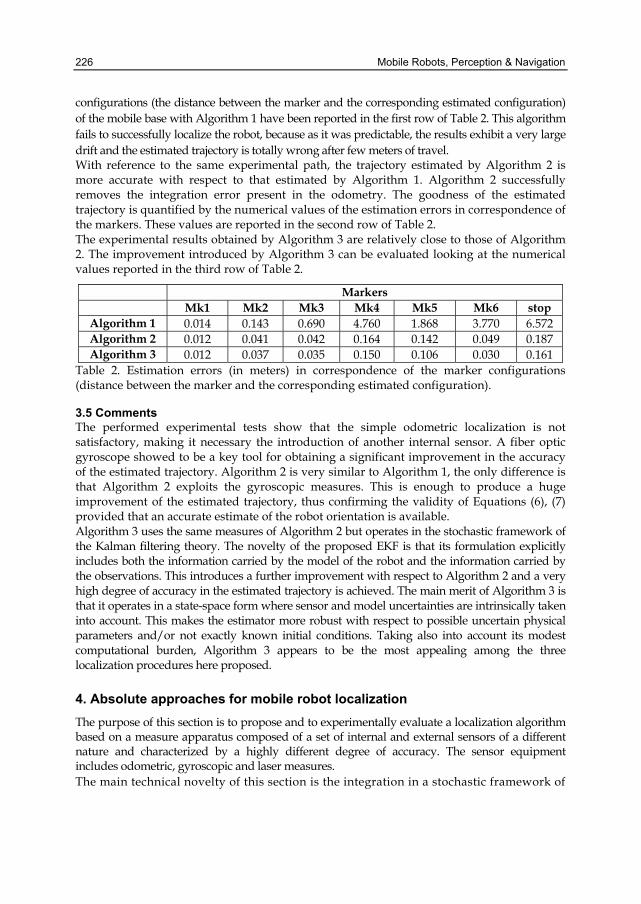
configurations (the distance between the marker and the corresponding estimated configuration) of the mobile base with Algorithm 1 have been reported in the first row of Table 2. This algorithm fails to successfully localize the robot, because as it was predictable, the results exhibit a very large drift and the estimated trajectory is totally wrong after few meters of travel. With reference to the same experimental path, the trajectory estimated by Algorithm 2 is more accurate with respect to that estimated by Algorithm 1. Algorithm 2 successfully removes the integration error present in the odometry. The goodness of the estimated trajectory is quantified by the numerical values of the estimation errors in correspondence of the markers. These values are reported in the second row of Table 2. The experimental results obtained by Algorithm 3 are relatively close to those of Algorithm 2. The improvement introduced by Algorithm 3 can be evaluated looking at the numerical values reported in the third row of Table 2.

Markers Mk1 Mk2 Mk3 Mk4 Mk5 Mk6 stop

Algorithm 1 0.014 0.143 0.690 4.760 1.868 3.770 6.572 Algorithm 2 0.012 0.041 0.042 0.164 0.142 0.049 0.187 Algorithm 3 0.012 0.037 0.035 0.150 0.106 0.030 0.161

Table 2. Estimation errors (in meters) in correspondence of the marker configurations (distance between the marker and the corresponding estimated configuration).

3.5 Comments The performed experimental tests show that the simple odometric localization is not satisfactory, making it necessary the introduction of another internal sensor. A fiber optic gyroscope showed to be a key tool for obtaining a significant improvement in the accuracy of the estimated trajectory. Algorithm 2 is very similar to Algorithm 1, the only difference is that Algorithm 2 exploits the gyroscopic measures. This is enough to produce a huge improvement of the estimated trajectory, thus confirming the validity of Equations (6), (7) provided that an accurate estimate of the robot orientation is available. Algorithm 3 uses the same measures of Algorithm 2 but operates in the stochastic framework of the Kalman filtering theory. The novelty of the proposed EKF is that its formulation explicitly includes both the information carried by the model of the robot and the information carried by the observations. This introduces a further improvement with respect to Algorithm 2 and a very high degree of accuracy in the estimated trajectory is achieved. The main merit of Algorithm 3 is that it operates in a state-space form where sensor and model uncertainties are intrinsically taken into account. This makes the estimator more robust with respect to possible uncertain physical parameters and/or not exactly known initial conditions. Taking also into account its modest computational burden, Algorithm 3 appears to be the most appealing among the three localization procedures here proposed.

4. Absolute approaches for mobile robot localization The purpose of this section is to propose and to experimentally evaluate a localization algorithm based on a measure apparatus composed of a set of internal and external sensors of a different nature and characterized by a highly different degree of accuracy. The sensor equipment includes odometric, gyroscopic and laser measures. The main technical novelty of this section is the integration in a stochastic framework of


the new set of measures. Both the information carried by the kinematic model of the robot and that carried by the dynamic equations of the odometry are exploited. The nearly singular filtering problem arising from the very high accuracy of angular measure has been explicitly taken into account. An exteroceptive laser sensor is integrated for reducing the continuous growth in the integrated error affecting any relative localization algorithm, such as the Algorithm 3.

4.1 Algorithm 4 The algorithm operates in a stochastic framework as Algorithm 3, and is based on the ascertainment that the angular measure ( )ky tθ

provided by the FOG is much accurate than

the other measures. This gives rise to a nearly singular filtering problem which can be solved by a lower order non singular Extended Kalman Filter, as described in subsection 3.3. The EKF is defined on the basis of a state equation derived from (1)–(3) and of a measure equation containing the incremental measures of the encoders ( )ky tν

and the distance

measures ( )ji

kdy t , 1,2, , si n= K , provided by the laser scanner from the jP plane,

{ }1,2, , pj n∈ K . The angular measure of the gyroscope ( )ky tθ is assumed coincident to the

third component ( )kθ of the state vector ( )X k .

Let ( )Z k be the measurement vector at time instant kT . Its dimension is not constant,

depending on the number of sensory measures that are actually used at each time instant. The measure vector ( )Z k is composed by two subvectors ( ) ( ) ( )1 1 2,

TZ k z k z k= ⎡ ⎤⎣ ⎦ and

( ) ( ) ( ) ( )2 3 4 2, , ,s

T

nZ k z k z k z k+⎡ ⎤= ⎣ ⎦L , where the elements of ( )1Z k are: ( ) ( )1z k y kν≡ ,

( ) ( )2z k y kθ≡ , where ( )y kν is the measure related to the increments provided by the

encoders through equations (9) and (13), ( )y kθ is the angular measure provided by the

FOG. The elements of ( )2Z k are: ( ) ( ) ( )2j

i i iz k d k kη+ = + , 1,2, , si n= K , { }1,2, , pj n∈ K , with

( )jid k given by (18) and . The environment map provides the information needed

to detect which is the plane jP in front of the laser. The observation noise ( ) ( ) ( ) ( ) ( )1, , , ,

s

T

nV k k k k kν θη η η η⎡ ⎤= ⎣ ⎦K , is a white sequence

where [ ]1 2: blockdiag ,R R R= , with 2 21 : diag ,R ν θσ σ⎡ ⎤= ⎣ ⎦

and 2 2 22 1 2: diag , , ,

snR σ σ σ⎡ ⎤= ⎣ ⎦L .

The diagonal form of R follows by the independence of the encoder, FOG and laser scanner measures. The components of the extended state vector ( )X k and the last sn components of vector

( )Z k are related by a non linear measure equation which depends on the environment

geometric parameter vector ∏ . The dimension ( )sn k is not constant, depending on the

number of laser scanner measures that are actually used at each time, this number depends on enviroment and robot configuration. Linearization of the measure equation relating ( )2Z k and ( )X k about the current estimate


of ( )X k results in:

( ) ( ) ( ) ( )2 2 2Z k C k X k V k= + (41)

where ( ) ( ) ( ) ( )2 1 2, , ,sn

V k k k kη η η⎡ ⎤= ⎣ ⎦K is a white noise sequence and

( ) ( ) ( ) ( ) ( )2 1 2: , , ,s

TT T Tn kC k c k c k c k⎡ ⎤= ⎣ ⎦L (42)

with

( ) ( ) { }cos , sin ,0,0 , 1,2, , , 1,2, ,cos

jj j

i n n s pji

Pc k P P i n k j nν

θ⎡ ⎤= − − = ∈⎣ ⎦ K K (43)

and

2

j ji n g iP πθ θ θ= − − + (44)

Equations (33), (40) and (41) represent the linearized, discretized state-space form to which the classical EKF algorithm has been applied.

4.2 Laser scanner readings selection To reduce the probability of an inadequate interpretation of erroneous sensor data, a method is introduced to deal with the undesired interferences produced by the presence of unknown obstacles on the environment or by incertitude on the sensor readings. Notice that for the problem handled here both the above events are equally distributed. A simple and efficient way to perform this preliminary measure selection is to compare the actual sensor readings with their expected values. Measures are discharged if the difference exceeds a time-varying threshold. This is here done in the following way: at each step, for each measure ( )2 iz k+

of the laser scanner, the residual ( ) ( ) ( )2j

i i ik z k d kγ += − represents the

difference between the actual sensor measure ( )2 iz k+ and its expected value j

id ,

( )1,2, , si n k= K , 1,2, , pj n= K , which is computed by (18) on the basis of the current estimate

of the vector state ( )X k . As , the current value ( )2 iz k+ is accepted if

( ) ( )2i ik s kγ ≤ (Jetto et al., 1999). Namely, the variable threshold is chosen as two times the

standard deviation of the innovation process.

4.3 Experimental results The experimental tests have been performed in an indoor environment using the same TGR Explorer powered wheelchair (TGR Bologna, 2000), described in Section 3.4. The laser scanner measures have been acquired by the SICK LMS mod. 200 installed on the vehicle. The main characteristics of the LMS are reported in Table 3.

Aperture Angle 3.14 rad Angular Resolution 0.0175/ 0.0088/ 0.0044 rad Response Time 0.013/ 0.026/ 0.053 s Resolution 0.010 m


Systematic Error ± 0.015 m Statistic Error (1 Sigma) 0.005 m Laser Class 1 Max. Distance 80 m Transfer Rate 9.6/ 19.2/ 38.4/ 500 kBaud

Table 3. Laser.

A characterization study of the Sick LMS 200 laser scanner has been performed as proposed in (Ye & Borenstein, 2002). Different experiments have been carried out to analyze the effects of data transfer rate, drift, optical properties of the target surfaces and incidence angle of the laser beam. Based on empirical data a mathematical model of the scanner errors has been obtained. This model has been used as a calibration function to reduce measurement errors. The TGR Explorer powered wheelchair with data acquisition system for FOG sensor, incremental encoders, sonar sensors and laser scanner is shown in Fig. 5.

Fig. 6. Sample of the estimated trajectory. The dots are the actually used laser scanner measures.


A significative reduction of the wrong readings produced by the presence of unknown obstacles has been realized by the selection of the laser scanner measures using the procedure described in the previous subsection . Different experiments have been performed making the mobile base track short and relatively long and closed trajectories. Fig. 6 illustrates a sample of the obtained results; the dots in the figure, are the actually used laser scanner measures. In the indoor environment of our Department, represented by a suitable set of planes orthogonal to the plane XY of the inertial system, a trajectory of 118 m length, characterized by orientation changes, has been imposed by the user interface. The starting and final positions have been measured, while six markers specify different middle positions; this permits to compute the distance and angle errors between the marker and the corresponding estimated configuration. In these tests, the performances of Algorithm 4 have been compared with those ones of the Algorithm 3, which is the most appealing among the three relative procedures here analyzed. Table 4 summarizes the distance and angle errors between the marker and the corresponding configurations estimated by the two algorithms.

Markers Mk1 Mk2 Mk3 Mk4 Mk5 Mk6 stop

Error 0.1392 0.095 0.2553 0.1226 0.2004 0.0301 0.3595

Alg

3

θΔ 0.49 0.11 0.85 0.58 1.39 0.84 2.66

Error 0.0156 0.0899 0.0659 0.1788 0.0261 0.0601 0.0951

Alg

4

θΔ 0.59 0.05 0.45 0.07 0.72 0.12 1.55

Table 4. Estimation errors (in meters) in correspondence of the marker configurations (distance between the marker and the corresponding estimated configuration) and corresponding angular errors (in degrees).

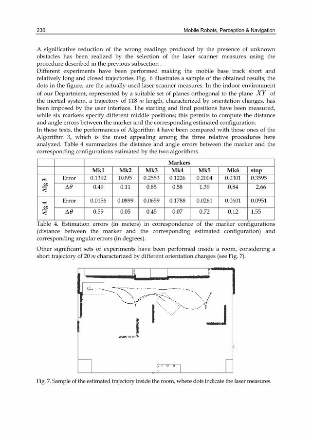
Other significant sets of experiments have been performed inside a room, considering a short trajectory of 20 m characterized by different orientation changes (see Fig. 7).

Fig. 7. Sample of the estimated trajectory inside the room, where dots indicate the laser measures.


The room has been modelled very carefully, permitting a precise evaluation of the distance and angle errors between the final position and the corresponding configuration estimated by the Algorithm 4; Table 5 resumes these results.

final position error 0.0061

Alg

4

θΔ 0.27

Table 5. Estimation distance errors (in meters) and corresponding angular errors (in degrees).

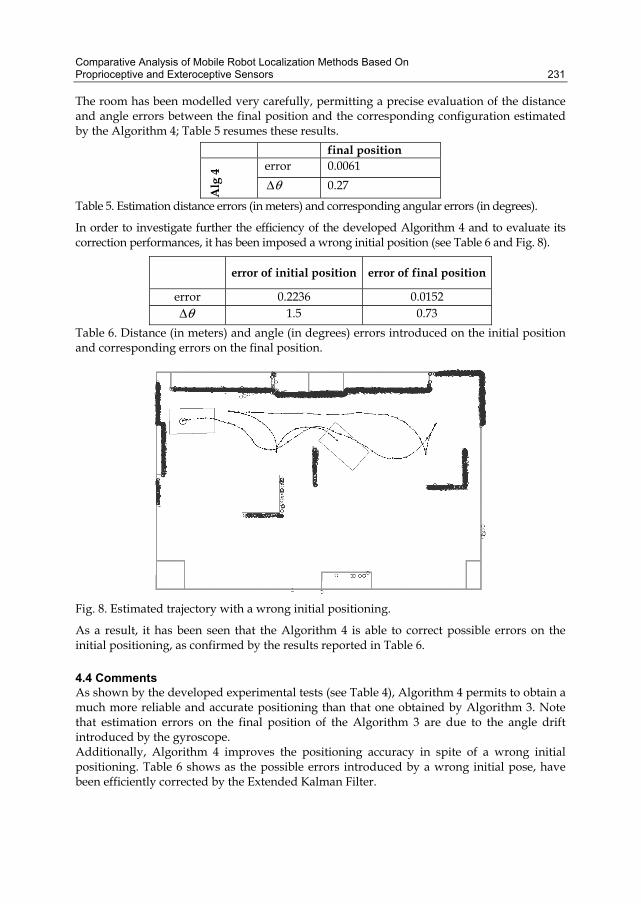
In order to investigate further the efficiency of the developed Algorithm 4 and to evaluate its correction performances, it has been imposed a wrong initial position (see Table 6 and Fig. 8).

error of initial position error of final position

error 0.2236 0.0152 θΔ 1.5 0.73

Table 6. Distance (in meters) and angle (in degrees) errors introduced on the initial position and corresponding errors on the final position.

Fig. 8. Estimated trajectory with a wrong initial positioning.

As a result, it has been seen that the Algorithm 4 is able to correct possible errors on the initial positioning, as confirmed by the results reported in Table 6.

4.4 Comments As shown by the developed experimental tests (see Table 4), Algorithm 4 permits to obtain a much more reliable and accurate positioning than that one obtained by Algorithm 3. Note that estimation errors on the final position of the Algorithm 3 are due to the angle drift introduced by the gyroscope. Additionally, Algorithm 4 improves the positioning accuracy in spite of a wrong initial positioning. Table 6 shows as the possible errors introduced by a wrong initial pose, have been efficiently corrected by the Extended Kalman Filter.


5. Concluding remarks This chapter has presented a concise look at the problems and methods relative to the mobile robot localization. Both the relative and absolute approaches have been discussed. Relative localization has the main advantage of using a sensor equipment which is totally self-contained in the robot. It is relatively simple to be used and guarantees a high data rate. The main drawback is that the localization errors may considerably grow over time. The three corresponding algorithms which have been proposed only use odometric and gyroscopic measures. The experimental tests relative to Algorithm 1 show that the incremental errors of the encoder readings heavily affect the orientation estimate, thus reducing the applicability of the algorithm to short trajectories. A significant improvement is introduced by Algorithm 2 where the odometric measures are integrated with the angular measures provided by a gyroscope. Algorithm 3 uses the same measures of Algorithm 2 but operates in a stochastic framework. The localization problem is formulated as a state estimation problem and a very accurate estimate of the robot localization is obtained through a suitably defined EKF. A further notable improvement is provided by the fusion of the internal measures with absolute laser measures. This is clearly evidenced by Algorithm 4 where an EKF is again used. A novelty of the EKF algorithms used here is that the relative state-space forms include all the available information, namely both the information carried by the vehicle dynamics and by the sensor readings. The appealing features of this approach are:

• The possibility of collecting all the available information and uncertainties of a different kind in the compact form of a meaningful state-space representation,

• The recursive structure of the solution, • The modest computational effort.

Other previous, significant experimental tests have been performed at our Department using sonar measures instead of laser readings (Bonci et al., 2004; Ippoliti et al., 2004). Table 7 reports a comparison of the results obtained with Algorithm 3, Algorithm 4, and the algorithm (Algorithm 4(S)) based on an EKF fusing together odometric, gyroscopic and sonar measures. The comparative evaluation refers to the same relatively long trajectory used for Algorithm 4.

Alg 3 Alg 4 Alg 4(S) error 0.8079 0.0971 0.1408

θΔ 2. 4637 0.7449 1. 4324 Table 7. Estimation errors (in meters) in correspondence of the final vehicle configuration (distance between the actual and the corresponding estimated configuration) and corresponding angular errors (in degrees).

Table 7 evidences that in spite of a higher cost with respect to the sonar system, the localization procedure based on odometric, inertial and laser measures does really seem to be an effective tool to deal with the mobile robot localization problem. A very interesting and still open research field is the Simultaneous Localization and Map Building (SLAM) problem. It consists in defining a map of the unknown environment and simultaneously using this map to estimate the absolute location of the vehicle. An efficient solution of this problem appears to be of a dominant importance because it would definitely confer autonomy to the vehicle. The SLAM problem has been deeply investigated in (Leonard et al., 1990; Levitt & Lawton, 1990; Cox, 1991; Barshan & Durrant-Whyte, 1995; Kobayashi et al., 1995; Thrun et al., 1998; Sukkarieh et al., 1999; Roumeliotis & Bekey, 2000;


Antoniali & Orialo, 2001; Castellanos et al., 2001; Dissanayake et al., 2001a; Dissanayake et al., 2001b; Zunino & Christensen, 2001; Guivant et al., 2002; Williams et al., 2002; Zalama et al., 2002; Rekleitis et al., 2003)). The algorithms described in this chapter, represent a solid basis of theoretical background and practical experience from which the numerous questions raised by SLAM problem can be solved, as confirmed by the preliminary results in (Ippoliti et al., 2004; Ippoliti et al., 2005).

6. References Anderson, B.D.O. & Moore, J.B. (1979). Optimal Filtering. Prentice-Hall, Inc, Englewood

Cliffs Antoniali, F.M. & Oriolo, G. (2001). Robot localization in nonsmooth environments:

experiments with a new filtering technique, Proceedings of the IEEE International Conference on Robotics and Automation (2001 ICRA), Vol. 2, pp. 1591–1596

Arras, K.O.; Tomatis, N. & Siegwart, R. (2000). Multisensor on-the-fly localization using laser and vision, Proceedings of the 2000 IEEE/RSJ International Conference onIntelligent Robots and Systems, (IROS 2000), Vol. 1, pp. 462–467

Barshan, B. & Durrant-Whyte, H.F. (1995). Inertial navigation systems for mobile robots. IEEE Transactions on Robotics and Automation, Vol. 11, No. 3, pp. 328–342

Bemporad, A.; Di Marco, M. & Tesi, A. (2000). Sonar-based wall-following control of mobile robots. Journal of dynamic systems, measurement, and control, Vol. 122, pp. 226–230

Bonci, A.; Ippoliti, G.; Jetto, L.; Leo, T. & Longhi, S. (2004). Methods and algorithms for sensor data fusion aimed at improving the autonomy of a mobile robot. In: Advances in Control of Articulated and Mobile Robots, B. Siciliano, A. De Luca , C. Melchiorri, and G. Casalino, Eds. Berlin, Heidelberg, Germany: STAR (Springer Tracts in Advanced Robotics ), Springer-Verlag, Vol. 10, pp. 191–222.

Borenstein, J. & Feng, L. (1996). Measurement and correction of systematic odometry errors in mobile robots. IEEE Transaction on Robotics and Automation, Vol. 12, No. 6, pp. 869–880

Borenstein, J.; Everett, H. R.; Feng, L. & Wehe, D. (1997). Mobile robot positioning: Sensors and techniques. Journal of Robotic Systems, Vol. 14, No. 4, pp. 231–249

Castellanos, J.A.; Neira, J. & Tardós, J.D. (2001). Multisensor fusion for simultaneous localization and map building. IEEE Transactions on Robotics and Automation, Vol. 17, No. 6, pp. 908–914

Chung, H.; Ojeda, L. & Borenstein, J. (2001). Accurate mobile robot dead-reckoning with a precision-calibrated fiber-optic gyroscope. IEEE Transactions on Robotics and Automation, Vol. 17, No. 1, pp. 80–84

Cox, I. (1991). Blanche – an experiment in guidance and navigation of an autonomous robot vehicle. IEEE Transactions on Robotics and Automation, Vol. 7, No. 2, pp. 193–204

De Cecco, M. (2003). Sensor fusion of inertial-odometric navigation as a function of the actual manoeuvres of autonomous guided vehicles. Measurement Science and Tecnology, Vol. 14, pp. 643–653

Dissanayake, M.; Newman, P.; Clark, S.; Durrant-Whyte, H.F. & Csorba, M. (2001a). A solution to the simultaneous localization and map building (slam) problem. IEEE Transactions on Robotics and Automation, Vol. 17, No. 3, pp. 229–241


Dissanayake, G.; Sukkarieh, S.; Nebot, E. & Durrant-Whyte, H.F. (2001b). The aiding of a low-cost strapdown inertial measurement unit using vehicle model constraints for land vehicle applications. IEEE Transactions on Robotics and Automation, Vol. 17, pp. 731–747

Durrant-Whyte, H.F. (1988). Sensor models and multisensor integration. International Journal of Robotics Research, Vol. 7, No. 9, pp. 97–113

Fioretti, S.; Leo, T. & Longhi, S. (2000). A navigation system for increasing the autonomy and the security of powered wheelchairs. IEEE Transactions on Rehabilitation Engineering, Vol. 8, No. 4, pp. 490–498

Garcia, G.; Bonnifait, Ph. & Le Corre, J.-F. (1995). A multisensor fusion localization algorithm with self-calibration of error-corrupted mobile robot parameters, Proceedings of the International Conference in Advanced Robotics, ICAR’95, pp. 391–397, Barcelona, Spain

Gu, J.; Meng, M.; Cook, A. & Liu, P.X. (2002). Sensor fusion in mobile robot: some perspectives, Proceedings of the 4th World Congress on Intelligent Control and Automation, Vol. 2, pp. 1194–1199

Guivant, J.E.; Masson, F.R. & Nebot, E.M. (2002). Simultaneous localization and map building using natural features and absolute information. In: Robotics and Autonomous Systems, pp. 79–90

Ippoliti, G.; Jetto, L.; La Manna, A. & Longhi, S. (2004). Consistent on line estimation of environment features aimed at enhancing the efficiency of the localization procedure for a powered wheelchair, Proceedings of the Tenth International Symposium on Robotics with Applications - World Automation Congress (ISORA-WAC 2004), Seville, Spain

Ippoliti, G.; Jetto, L.; La Manna, A. & Longhi, S. (2005). Improving the robustness properties of robot localization procedures with respect to environment features uncertainties, Proceedings of the IEEE International Conference on Robotics and Automation (ICRA 2005), Barcelona, Spain

Jarvis, R.A. (1992). Autonomous robot localisation by sensor fusion, Proceedings of the IEEE International Workshop on Emerging Technologies and Factory Automation, pp. 446–450

Jetto, L.; Longhi, S. & Venturini, G. (1999). Development and experimental validation of an adaptive extended Kalman filter for the localization of mobile robots. IEEE Transactions on Robotics and Automation, Vol. 15, pp. 219–229

Killian, K. (1994). Pointing grade fiber optic gyroscope, Proceedings of the IEEE Symposium on Position Location and Navigation, pp. 165–169, Las Vegas, NV,USA

Kobayashi, K.; Cheok, K.C.; Watanabe, K. & Munekata, F. (1995). Accurate global positioning via fuzzy logic Kalman filter-based sensor fusion technique, Proceedings of the 1995 IEEE IECON 21st International Conference on Industrial Electronics, Control, and Instrumentation, Vol. 2, pp. 1136–1141, Orlando, FL ,USA

Komoriya, K. & Oyama, E. (1994). Position estimation of a mobile robot using optical fiber gyroscope (ofg), Proceedings of the 1994 International Conference on Intelligent Robots and Systems (IROS’94), pp. 143–149, Munich, Germany

Leonard, J.; Durrant-Whyte, H.F. & Cox, I. (1990). Dynamic map building for autonomous mobile robot, Proceedings of the IEEE International Workshop on Intelligent Robots and Systems (IROS ’90), Vol. 1, pp. 89–96, Ibaraki, Japan


Levitt, T.S. & Lawton, D.T. (1990). Qualitative navigation for mobile robots. Artificial Intelligence Journal, Vol. 44, No. 3, pp. 305–360

Mar, J. & Leu, J.-H. (1996). Simulations of the positioning accuracy of integrated vehicular navigation systems. IEE Proceedings - Radar, Sonar and Navigation, Vol. 2, No. 143, pp. 121–128

Martinelli, A. (2002). The odometry error of a mobile robot with a synchronous drive system. IEEE Transactions on Robotics and Automation, Vol. 18, No. 3, pp. 399–405

Ojeda, L.; Chung, H. & Borenstein, J. (2000). Precision-calibration of fiber-optics gyroscopes for mobile robot navigation, Proceedings of the 2000 IEEE International Conference on Robotics and Automation, pp. 2064–2069, San Francisco, CA, USA

Panzieri, S.; Pascucci, F. & Ulivi, G. (2002). An outdoor navigation system using GPS and inertial platform. IEEE/ASME Transactions on Mechatronics, Vol. 7, No. 2, pp. 134–142

Rekleitis, I.; Dudek, G. & Milios, E. (2003). Probabilistic cooperative localization and mapping in practice, Proceedings of the IEEE International Conference on Robotics and Automation (ICRA ’03), Vol. 2, pp. 1907 – 1912

Roumeliotis, S.I. & Bekey, G.A. (2000). Bayesian estimation and Kalman filtering: a unified framework for mobile robot localization, Proceedings of the IEEE International Conference on Robotics and Automation (ICRA ’00), Vol. 3, pp. 2985–2992, San Francisco, CA, USA

Sukkarieh, S.; Nebot, E.M. & Durrant-Whyte, H.F. (1999). A high integrity IMU GPS navigation loop for autonomous land vehicle applications. IEEE Transactions on Robotics and Automation, Vol. 15, pp. 572–578

Talluri, R. & Aggarwal, J.K. (1992). Position estimation for an autonomous mobile robot in an outdoor environment. IEEE Transactions on Robotics and Automation, Vol. 8, No. 5, pp. 573–584

TGR Bologna (2000). TGR Explorer. Italy [Online]. Available on-line: http://www.tgr.it. Thrun, S.; Fox, D. & Burgard, W. (1998). A probabilistic approach to concurrent mapping

and localization for mobile robots. Machine Learning Autonom. Robots, Vol. 31, pp. 29–53. Kluwer Academic Publisher, Boston

Wang, C.M. (1988). Localization estimation and uncertainty analysis for mobile robots, Proceedings of the Int. Conf. on Robotics and Automation, pp. 1230–1235

Williams, S.B.; Dissanayake, G. & Durrant-Whyte, H.F. (2002). An efficient approach to the simultaneous localization and mapping problem, Proceedings of the 2002 IEEE International Conference on Robotics and Automation, pp. 406–411, Washington DC, USA

Ye, C. & Borenstein, J. (2002). Characterization of a 2d laser scanner for mobile robot obstacle negotiation, Proceedings of the IEEE International Conference on Robotics and Automation (ICRA ’02), Vol. 3, pp. 2512 – 2518, Washington DC, USA

Yi, Z.; Khing, H. Y.; Seng, C.C. & Wei, Z.X. (2000). Multi-ultrasonic sensor fusion for mobile robots, Proceedings of the IEEE Intelligent Vehicles Symposium, Vol. 1, pp. 387–391, Dearborn, MI, USA

Zalama, E.; Candela, G.; Gómez, J. & Thrun, S. (2002). Concurrent mapping and localization for mobile robots with segmented local maps, Proceedings of the 2002 IEEE/RSJ Conference on Intelligent Robots and Systems, pp. 546–551, Lausanne, Switzerland


Zhu, R.; Zhang, Y. & Bao, Q. (2000). A novel intelligent strategy for improving measurement precision of FOG. IEEE Transactions on Instrumentation and Measurement, Vol. 49, No. 6, pp. 1183–1188

Zhuang, W. & Tranquilla, J. (1995). Modeling and analysis for the GPS pseudo-range observable. IEEE Transactions on Aerospace and Electronic Systems, Vol. 31, No. 2, pp. 739–751

Zunino, G. & Christensen, H.I. (2001). Simultaneous localization and mapping in domestic environments, Proceedings of the International Conference on Multisensor Fusion and Integration for Intelligent Systems (MFI 2001), pp. 67–72

Comparative Analysis of Mobile Robot Localization Methods Based on Proprioceptive and Exteroceptive...

Documents

Transcript of Comparative Analysis of Mobile Robot Localization Methods Based on Proprioceptive and Exteroceptive...