Communications in Computer and Information

Science:

A Weight Least square Algorithm for Hyperbolic

Localization with Linear Sensor Array in 3-D scenario

H. Kabir1, K. Jeevan

1, A. W. Reza

1, and H. Ramiah

1

1Faculty of Engineering, Department of Electrical Engineering

University of Malaya, 50603 Kuala Lumpur, Malaysia

Abstract. In modern communication technology, source localization is a key

research in application of navigation, tracking, radar, and sonar. A low-complex

and non-iterative is proposed to estimate the source position based on Time

difference of arrival at linear array sensor network (LSAN) in three dimensional

scenario. We simulated our proposed method for (1) close and disjoint source

from LSAN and (2) different baseline of LSAN where all sensors are on the x-

axis under the Gaussian noise. The proposed method has approximated the

CRLB at low to moderate noise level and contributed the better localization

accuracy than Taylor’s series. Only using three sensors in LSAN, the source

position is estimated by the proposed method in the 3-D scenario.

Keywords: TDOA, Localization, LSAN and 3-D.

1 Introduction

In radar, sonar, acoustic tracking and navigation application, signal source

localization is a key challenge [1, 2]. A number of sensors which are arranged

arbitrary or linear fashion, receive the signal from the emitter is used for source

position estimation [3]. Time difference of arrival (TDOA) is one of the common

techniques to estimate the source position, because it is appropriate for passive

localization, does not have necessary time-stamping and easy to implement in the

practical localization set up [4]. In arbitrary sensor fashion, Maximum likelihood

estimation (MLE)[5], least square (LS)[6], Weight least square (WLS)[7], Taylor’s

series [8], Genetic algorithm [9], etc. are applied to estimate the source location in the

two or three dimensional scenario. However, in linear array sensor network (LASN)

in Figs.1 and 2, the same method cannot be applied to singularity problem. For

avoiding the singularity problem, Yiu-tong [5] , Zhengyan Xu [10], and K.C ho [11]

developed an approximate maximum likelihood estimation based on time of arrival,

hyperbolic geometrical solution, and analytical solution based on TDOA for 2-D

scenario respectively. In our best knowledge, nobody has worked with a linear sensor

array in 3-D scenario for estimating the position of the source. Therefore, we

proposed an algebraic solution to locate the stationary source based on TDOA on

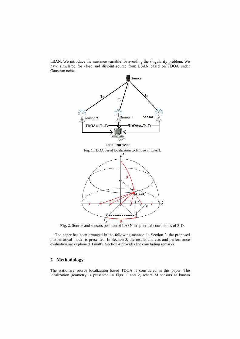
LSAN. We introduce the nuisance variable for avoiding the singularity problem. We

have simulated for close and disjoint source from LSAN based on TDOA under

Gaussian noise.

Fig. 1.TDOA based localization technique in LSAN.

Fig. 2. Source and sensors position of LASN in spherical coordinates of 3-D.

The paper has been arranged in the following manner. In Section 2, the proposed

mathematical model is presented. In Section 3, the results analysis and performance

evaluation are explained. Finally, Section 4 provides the concluding remarks.

2 Methodology

The stationary source localization based TDOA is considered in this paper. The

localization geometry is presented in Figs. 1 and 2, where M sensors at known

locations t

iiiizyxs ] [ are used to estimate the emitting electromagnetic source at

an unknown location Tzyx ] [ . The range between thethi sensor and emitter is

2220 )()()(||iiiii

zzyyxxsr where, i 1,2, 3,….N (1)

The true range difference between the thi sensor and the reference which is assumed

sensor 1is

0

1

0

1

0

1 rrctr iii (2)

where c and 1i

t are the velocity of signal propagation and the time difference of signal

arrival in thi sensor and reference. Equation (2) is rearranged as 00

1

0

11 iirrr and

squared both sides. Substituting the 0

1r and 0

ir form equation (1), we obtained

zzzyyyxxxzyxzyxrrriiiiiiii

)(2)(2)(22111

2

1

2

1

2

1

2220

1

0

1

20

1 (3)

where i 2,3,…, N. The nonlinear equations set with and 0

1r produced M-1

hyperbolic curves which are intersected a single point. This point is the estimated

position of the source. Adding the measurement noise with true TDOA, we obtained,

1

0

11 iiinrr (4)

where 1i

n is the Gaussian noise. The vector of noisy TDOA , ] ... [13121 N

rrrR and has a

covariance matrix and variance σ2 [7]

1

0.5

.

.

.

.

. .

. . . . .

. . 0.5 1 5.0

. . 0.5 0.5 1

}{ 2TRREQ

(5)

Substituting the 1i

r in equation (3), nonlinear equation sets are

20

1

2

1

2

1

2

1

2220

1

0

11112)(2)(2)(2

iiiiiiiirzyxzyxrrzzzyyyxxx (6)

All sensors are situated on a straight line in LSAN. We considered all sensors are on

the x-axis where 0i

y and 0i

z . Singularity problem is introduced in equation (6)

because of 01 yy

i and 0

1 zz

i. For avoiding the singularity problem, an

equation (6) can be rewritten when the reference sensor is at the origin as

22

1

0

111 2)(2 iiii xrrrxxx (7)

where x and 0

1r are unknown and y-axis and z-axis position parameters of source are

absent. The error vector of equation (7) is obtained as

gh (8)

where is the error vector of TODAs equation

22

1

2

3

2

31

2

2

2

21

.

NN xr

xr

xr

h ,

1

31

21

3

2

.

.

2

NM r

r

r

x

x

x

g and Trx ] [ 0

1

Minimizing the error vector, equation (8) can be written as

)(minarg1

gh (9)

Weight least squared method is used for minimizing the error vector. We get the

unknown vector as

WhgWgg TT 1

1)( (10)

where 1 QW . From the above equation, only x-axis unknown position x and one

nuisance variable 0

1r are estimated. Determining the y-axis and z-axis position

parameters, x and 0

1r values are substituted in equation (1)

20

1

222 rzyx (11)

Estimating the y-axis and z-axis coordinates of source, a function is introduced

as20

1

222),( rzyxzyf solving ),( zyf where y-axis and z-axis

coordinates are estimated as

),(minarg,

1zyf

zy

(12)

Finally, we estimate the source position Tx ] [

1 from equations (9) and (12).

3 Result and discussion

The stationary source localization simulation based on TDOA on LSAN in the 3-D

scenario are presented and discussed in this section. The sensors position are

( ixi , 0

iy , and 0

iz ) and ( )1( ix

i0

iy and 0

iz ) when i are even and

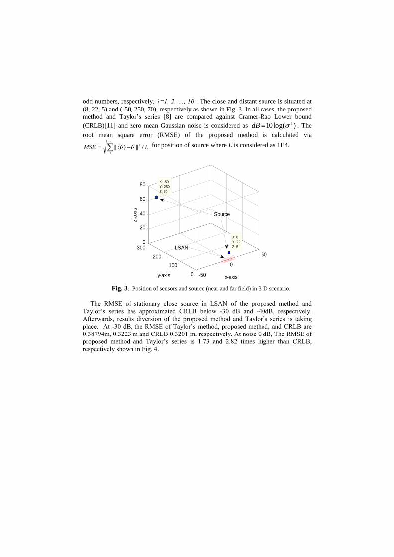
odd numbers, respectively, i =1, 2, …, 10 . The close and distant source is situated at

(8, 22, 5) and (-50, 250, 70), respectively as shown in Fig. 3. In all cases, the proposed

method and Taylor’s series [8] are compared against Cramer-Rao Lower bound

(CRLB)[11] and zero mean Gaussian noise is considered as )log(10 2dB . The

root mean square error (RMSE) of the proposed method is calculated via

LMSEL

/||||1

2 for position of source where L is considered as 1E4.

-50

0

50

0

100

200

3000

20

40

60

80

X: 8

Y: 22

Z: 5

x-axisy-axis

X: -50

Y: 250

Z: 70

z-a

xis

LSAN

Source

Fig. 3. Position of sensors and source (near and far field) in 3-D scenario.

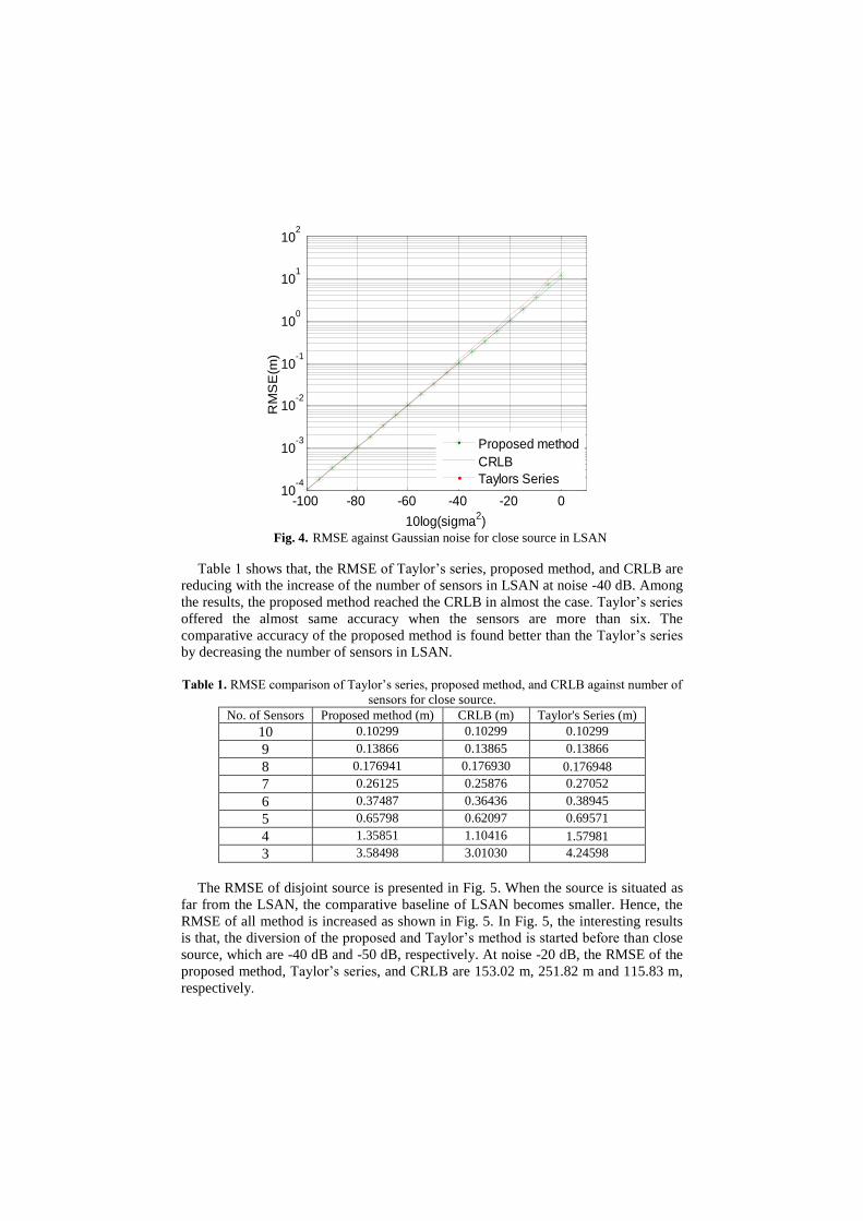
The RMSE of stationary close source in LSAN of the proposed method and

Taylor’s series has approximated CRLB below -30 dB and -40dB, respectively.

Afterwards, results diversion of the proposed method and Taylor’s series is taking

place. At -30 dB, the RMSE of Taylor’s method, proposed method, and CRLB are

0.38794m, 0.3223 m and CRLB 0.3201 m, respectively. At noise 0 dB, The RMSE of

proposed method and Taylor’s series is 1.73 and 2.82 times higher than CRLB,

respectively shown in Fig. 4.

-100 -80 -60 -40 -20 010

-4

10-3

10-2

10-1

100

101

102

10log(sigma2)

RM

SE

(m)

Proposed method

CRLB

Taylors Series

Fig. 4. RMSE against Gaussian noise for close source in LSAN

Table 1 shows that, the RMSE of Taylor’s series, proposed method, and CRLB are

reducing with the increase of the number of sensors in LSAN at noise -40 dB. Among

the results, the proposed method reached the CRLB in almost the case. Taylor’s series

offered the almost same accuracy when the sensors are more than six. The

comparative accuracy of the proposed method is found better than the Taylor’s series

by decreasing the number of sensors in LSAN.

Table 1. RMSE comparison of Taylor’s series, proposed method, and CRLB against number of

sensors for close source.

No. of Sensors Proposed method (m) CRLB (m) Taylor's Series (m)

10 0.10299 0.10299 0.10299

9 0.13866 0.13865 0.13866

8 0.176941 0.176930 0.176948

7 0.26125 0.25876 0.27052

6 0.37487 0.36436 0.38945

5 0.65798 0.62097 0.69571

4 1.35851 1.10416 1.57981

3 3.58498 3.01030 4.24598

The RMSE of disjoint source is presented in Fig. 5. When the source is situated as

far from the LSAN, the comparative baseline of LSAN becomes smaller. Hence, the

RMSE of all method is increased as shown in Fig. 5. In Fig. 5, the interesting results

is that, the diversion of the proposed and Taylor’s method is started before than close

source, which are -40 dB and -50 dB, respectively. At noise -20 dB, the RMSE of the

proposed method, Taylor’s series, and CRLB are 153.02 m, 251.82 m and 115.83 m,

respectively.

-100 -80 -60 -40 -2010

-2

10-1

100

101

102

10log(sigma2)

RM

SE

(m)

Proposed method

CRLB

Taylors Series

Fig. 5. RMSE against Gaussian noise from disjoint source in LSAN

Linearization error is introduced when the baseline reduces in LSAN. For the

linearization problem, the RMSE of simulated methods is so large when the sensors

are three in LSAN. The proposed method gives the better accuracy as also represented

in Table 2.

Table 2: RMSE comparison of Taylor’s series, proposed and CRLB against a number of

sensors for disjoint source

No. of Sensors Proposed method (m) CRLB (m) Taylor's Series (m)

10 11.38253 11.38253 11.38254

9 14.7832 14.7636 14.7912

8 20.1489 20.0963 20.3458

7 28.84897 28.12984 29.0474

6 43.47981 42.5743 44.5456

5 72.9879 71.735 75.798

4 385.94 371.13 402.52

The most significant observation is that the proposed method can be located the

source position by using only three sensors in LSAN, though it is the 3-D scenario. X-

axis location parameter and nuisance variable are unknown in equation (7). To

determine the two unknown parameters, only )22( g and )21( h matrix is needed in

equation (10). Hence, the source position can be estimated by using three sensors.

From all the figures and tables, we have summarized that, RMSE depends on the

distance between the source and network and baseline of the network. Increase of the

distance and decrease of the baseline of network has contributed to increasing the

RMSE of the source position and velocity. In all cases, the performance of the

proposed method is better than the Taylor’s series, and achieved the CRLB at low to

moderated noise.

4 Conclusions

A low complex and non-iterative linear algorithm to estimate the position of

stationary source on the 3-D plane based on hyperbolic technique where all sensors

are positioned on x-axis is presented in this paper. In LSA network, singularity

problem is the key challenge. For avoiding this challenge, nuisance variable is

introduced for simulation. Our proposed method yields better accuracy than iterative

Taylor’s method and reached the CRLB under the Gaussian noise where close and

disjoint source are considered. By only using the three sensors in LSAN, the source

position is located by the proposed method in the 3-D scenario.

References

1. Arslan, G. and F.A. Sakarya, A unified neural-network-based speaker localization

technique. Neural Networks, IEEE Transactions on, 2000. vol. 11, no. 4, p. 997-1002.

2. Asono, F., H. Asoh, and T. Matsui. Sound source localization and signal separation for

office robot “Jijo-2”. in Multisensor Fusion and Integration for Intelligent Systems, 1999.

MFI'99. Proceedings. 1999 IEEE/SICE/RSJ International Conference on. 1999. IEEE.

3. Kozick, R.J. and B.M. Sadler, Source localization with distributed sensor arrays and partial

spatial coherence. Signal Processing, IEEE Transactions on, 2004. vol. 52, no. 3, p. 601-

616.

4. Ho, K., Bias reduction for an explicit solution of source localization using TDOA. Signal

Processing, IEEE Transactions on, 2012. vol. 60, no. 5, p. 2101-2114.

5. Chan, Y.-T., H. Yau Chin Hang, and P.-c. Ching, Exact and approximate maximum

likelihood localization algorithms. Vehicular Technology, IEEE Transactions on, 2006. vol.

55, no. 1, p. 10-16.

6. Ho, K., X. Lu, and L.-o. Kovavisaruch, Source localization using TDOA and FDOA

measurements in the presence of receiver location errors: analysis and solution. Signal

Processing, IEEE Transactions on, 2007. vol. 55, no. 2, p. 684-696.

7. Ho, K. and W. Xu, An accurate algebraic solution for moving source location using TDOA

and FDOA measurements. Signal Processing, IEEE Transactions on, 2004. vol. 52, no 9, p.

2453-2463.

8. Foy, W.H., Position-location solutions by Taylor-series estimation. Aerospace and

Electronic Systems, IEEE Transactions on, 1976 vol. 2, p. 187-194.

9. Duckett, T. A genetic algorithm for simultaneous localization and mapping. in IEEE

International Conference on Robotics and Automation. 2003. Citeseer.

10. Liu, N., Z. Xu, and B.M. Sadler, Low-complexity hyperbolic source localization with a

linear sensor array. Signal Processing Letters, IEEE, 2008. vol. 15: p. 865-868.

11. Chan, Y. and K. Ho, A simple and efficient estimator for hyperbolic location. Signal

Processing, IEEE Transactions on, 1994. vol. 42, no 8, p. 1905-1915.