Computer Graphics - PTU (Punjab Technical University)

Self Learning Material

Computer Graphics (MSIT-301)

Course: Masters of Science [IT]

Semester-III

Distance Education Programme

I. K. Gujral Punjab Technical University

Jalandhar

2

Syllabus

I. K. Gujral Punjab Technical University

SECTION- A

MSIT301- Computer Graphics

Introduction to Active and Passive Graphics, Applications of Computer Graphics. Input devices: light pens, Graphic tablets, Joysticks, Trackball, Data Glove, Digitizers, Image scanner, Graphs and Types of Graphs. Video Display Devices-- Refresh Cathode Ray Tube, Raster Scan displays, Random Scan displays, Architecture of Raster and Random Scan Monitors, Color CRT-monitors and Color generating techniques (Shadow Mask, Beam Penetration) , Direct View Storage Tube, Flat-Panel Displays; 3-D Viewing Devices, Raster Scan Systems, Random Scan Systems, Graphics monitors and workstations, Color Models (RGB and CMY), Lookup Table. SECTION-B Process and need of Scan Conversion, Scan conversion algorithms for Line, Circle and Ellipse, effect of scan conversion, Bresenham's algorithms for line and circle along with their derivations, Midpoint Circle Algorithm, Area filling techniques, flood fill techniques, character generation. SECTION-C 2-Dimensional Graphics: Cartesian and need of Homogeneous co-ordinate system, Geometric transformations (Translation, Scaling, Rotation, Reflection, Shearing), Two- dimensional viewing transformation and clipping (line, polygon and text), Cohen Sutherland, Sutherland Hodgeman and Liang Barsky algorithm for clipping. Introduction to 3-dimensional Graphics: Geometric Transformations (Translation, Scaling, Rotation, Reflection, Shearing), Mathematics of Projections (parallel & perspective). Introduction to 3-D viewing transformations and clipping. SECTION-D Hidden line and surface elimination algorithms: Z-buffer, Painters algorithm, scan-line, subdivision, Shading and Reflection: Diffuse reflection, Specular reflection, refracted light, Halftoning, Dithering techniques. Surface Rendering Methods: Constant Intensity method, Gouraud Shading, Phong Shading (Mash Band effect). Morphing of objects. Note: Graphics Programming using C/C++ with introduction to Open GL. References: 1. D. Hearn and M.P. Baker, ―Computer Graphicsǁ, PHI New Delhi; Third Edition.

2. J.D. Foley, A.V. Dam, S.K. Feiner, J.F. Hughes,. R.L Phillips, ǁComputer Graphics Principles & Practices, Second Editionǁ, Pearson Education, 2007. 3. R.A. Plastock and G. Kalley, ―Computer Graphicsǁ, McGraw Hill, 1986. 4. F.S. Hill: Computer Graphics using Open GL- Second Edition, Pearson Education- 2003

Table of Contents

ChapterNo. Title Written By Page No.

1 Introduction to computer graphics Ms. Kamaljeet Kaur, AP,

Deptt. Of Computer Science,

DAV College Jalandhar

1

2

OUTPUT DEVICES Ms. Kamaljeet Kaur, AP,



33

3

Scan Conversion and its techniques

for Line drawing

Ms. Kamaldeep Kaur, AP,



60

4

Scan converting techniques for circle

Ms. Kamaldeep Kaur, AP, Deptt. Of Computer Science, DAV College Jalandhar

88

5

Scan converting techniques for ellipse


115

6 Area filling and character

generation techniques


135

7

2D Transformations

Ms. Richa, AP, Deptt. Of Computer Science, DAV College Jalandhar

155

8

2D Viewing Transformations

Ms. Richa, AP, Deptt. Of

Computer Science, DAV

College Jalandhar

180

9

3-Dimensional Graphics

Ms. Richa, AP, Deptt. Of Computer Science, DAV College Jalandhar

201

10 Hidden line and Surfaces

elimination algorithm

Ms. Monika Chopra, AP, Deptt. Of Computer Science, DAV College Jalandhar

220

11

Shading and Reflection

Ms. Monika Chopra, AP, Deptt. Of Computer Science, DAV College Jalandhar

241

12 Surface rendering and its methods

Ms. Monika Chopra, AP,



261

3

4

Reviewed By: Dr. Dalveer Kaur

IKGPTU, Jalandhar, Punjab, 144603

©IK Gujral Punjab Technical University Jalandhar All rights reserved with I K Gujral Punjab Technical University Jalandhar

1

Lesson 1

Introduction to computer graphics

Structure of the Chapter

1.0 Objectives

1.1 Introduction to computer graphics and input devices 1.2 Difference between active and passive Graphics 1.3 Applications of Computer Graphics 1.4 Graphs and Types of Graphs 1.5 Input Devices

1.5.1 Light pen 1.5.2 Graphic tablet 1.5.3 Joystick 1.5.4 Trackball 1.5.5 Data gloves 1.5.6 Digitizers 1.5.7 Image scanner

1.6 Summary 1.7 Glossary 1.8 Answer to check your progress/self assessment questions 1.9 References and suggested readings 1.10 Model Questions

1.0 Objective After studying this chapter students will be able to:

Differentiate raster and vector images Identify the importance of graphics in day to day life Identify the kind of graph to be used to graphically represent the data Identify the input device to be used for certain application.

1.1 Introduction to Computer graphics includes“almost anything on computer that is not

text or sound”. It incorporates image data created with the help of specialized graphical

hardware and software. It is an important sub field of computer science. The phrase was

coined in 1960 by pioneer researchers Verne Hudson and William Fetter of Boeing. The

process of computer graphics depends on underlying sciences of geometry, optics and

physics. It is greatly helpful in the display of art and image data in an effective and efficient

way. It is found to be of great use in understanding of computers and interpretation of data. In

general they are making their contribution in animation, movies, advertisement, video games

2

and graphic design and many more. It includes the display of the image, its manipulation and

storage by using a computer.

Resolution

It is the amount of pixel data that is used to make an image. 300 dpi (dots per inch) is the

resolution of standard and commercial printing. It means the total number of pixels in an

image, along with its length and height. It determines the quality of image. If an image

without enough pixel information is used to fill the output area, and if the image is enlarged

to fill up the area, the image will get distorted. It is called pixilation. Fig 1.1 shows letter A

without and with pixilation.

Type of Images

Fig. 1.1: Pixilation

Computer graphics deals with images in digital form. Mainly two types images are dealt in

Computer graphics namely

Raster Images Vector Images

Raster Images

A raster image is displayed by the arrangement of pixels having different colours. The quality of image is calculated in ppi. A 300 ppi image has 300 pixels in every one inch. Higher the ppi, higher is the quality of the resultant image. Since, bitmap image stores the colour information for each pixel that forms the image so it is larger in size.

In order to determine the size of a raster image for a high quality outlook and printing, multiply the resolution required by the area to be printed.

To print an image in a 5 inch area on a printer of minimum 300 ppi, the image must be at least 300 * 5= 1500 pixels wide. JPEG, GIF, BMP are types of vector images. These are well supported on the web. These are best for images having a wide range of colour gradations

Vector Images

3

It is another kind of images dealt in Computer Graphics. These are comprised of paths defined by start and end point. These are made up of paths defined by a mathematical formula defining the path, its colour and other information. Since, such images are not made of dots, so they could be easily scaled to a larger size without losing quality of the image. If a vector image is enlarged, the edges of the object within the graphic stay smooth and clean. It is the reason; vector images are used to deal with logos which could be used on ID card as well as a banner. They take less space than a raster image. This is because; vector image stores the mathematical formulas to make up the image. Vector images are useful for images that consist of a few areas of solid colour. EPS, SVG, DRW are types of vector images.

Differences between Raster and Vector Image

Raster Image Vector Image A raster image is made up pixels having different colours.

Raster images are not scalable. With increase in size of image, the quality of raster image decreases.

These are made up of paths defined by a mathematical formula defining the path, its colour and other information Vector images are scalable. These images retain appearance even when zoomed. This is because, their render is dictated by mathematical formulas

They can display natural quality of image Natural quality of image is sacrificed. Raster images are often large in size Size of a vector images is comparatively

lesser. Web images are raster images Vector images are converted to raster image

before publishing on web. Text is rendered using vector format.

Raster image could not be displayed at highest resolution of output device.

These are generally used with photos. Photoshop is an example of raster image editing program

Vectors image could be displayed at the highest resolution allowed by the output device Adobe Illustrator is an example of vector editing program. It automatically creates vector formulas for the images drawn.

Photographs are handled as raster images Logos are handled as vector images.

1.2 Difference between Active vs Passive Graphics

Differences between Active and Passive Graphics Active/Interactive Graphics Passive Graphics

These are interactive graphics in which the

user can interact with the graphics as well as

the programs used to generate that graphic.

The user can make any change in image

show on the screen including colour change

or adding animation in the graphic as per

In case of Passive graphics, the user has no

control over the image. The user is unable to

make any change in image show on the

screen

4

requirement.

In case of web page interactive graphics, it

leads to increase in the size of the associated

web page. In case of slow internet

connectivity, the problem multiplies.

For slow internet connectivity, passive

graphics are recommended.

The output of the interactive graphic used

through internet depends on the client’s

computer. The computer on client site may

not support the scripting language used or it

may has an older version.

The image formats used in passive graphics

to be used online are very common. Most of

the browsers support these image formats.

These are quite entertaining but are difficult

to deal with.

These are quite easy to handle but are found

to be monotonous.

The quality of image produced with

interactive graphics is quite high.

The quality of passive images are lesser than

that produced with active graphics

Example: video games is a kind of active

graphics in which the user decides the next

scene to appear on the basis of interaction

through the mouse, keyboard, joystick etc.

Example: Watching a TV channel, in which

the user can switch off the TV or change the

channel but have to watch whatever is

broadcasted by that particular channel.

Let us discuss the working of Interactive Graphics Display

It consists of three main components:

Frame Buffer or Digital Memory: The image to be displayed is stored in this digital memory or frame buffer in the form of binary numbers representing individual pixel making up the image. For a black and white image, the information is in the form of 1’s and 0’s.

Display Controller: It reads the information about the image form the digital memory or frame buffer in the form of binary number and converts them into video signals.

Monitor: Display controller displays the image picked from digital memory onto the monitor to produce the image.

In order to make modifications in the image, suitable changes could be made in the

information stored in the digital memory.

5

1.3 Applications of Computer Graphics Computer graphics is the field of computer science which is observing wide variety of

applications. Computer graphics is emerging as a powerful tool for the rapid and economical

production of pictures. Advances in this field have made the availability of interactive

computer graphics a practical tool. It has found applications in areas ranging from science,

engineering, medicine, business, government, art, entertainment, advertising, education etc.

Some of the important applications are listed below

Graphic User Interface (GUI) It is the most important application of computer graphics that has been widely used. It is an

interface between the user and the graphics application program. It helps the user to interact

with the graphic application program for input as well as output.

Some of the most common and typical components used in GUI are

Menus Icons Cursors Dialog boxes Scrollbars Buttons Grids

Let us discuss these components as typical GUI.

Let us take an example of a graphic user interface of Ms-Word. Fig. 1.2 shows a snapshot of

this interface.

Fig. 1.2: Microsoft Word GUI

It uses various components o f GUI.

Clicking on Office button displays a pull down menu to select options to open, save the document.

Different icons are visible in the figure that acts as a GUI.

6

Cursor is used to click and make selections. The dialog box is an important component of GUI that is used by a computer graphic

system for interaction with the user. The scroll bar is another example of GUI. It is used to scroll up and down the

application program. It is helpful to view previous and next data in the document.

Computer-Aided Design Computer-aided design (CAD) is an important application of Computer graphics in which the

computer technology is used for the design of real or virtual objects. Another application

includes the design of geometric models for object shapes called computer-aided geometric

design (CAGD).

It is one of the major uses of computer graphics and is used by the engineers and architects in

the design processes. It makes their job comparatively easier as for some design applications

the objects could be displayed in a wireframe outline form to describe the internal features of

objects prior to its make. Some of the uses of CAD technology are listed below.

The designers can watch multiple views of the object which leads to see enlarged sections or different views of objects at the same time.

Animations are often used in CAD applications which are used in entertainment and movie industry.

Real-time animations are also possible which could be used to display wire frame of the objects that could be used by the engineering for testing performance of a vehicle.

The designers can see the interior behaviour of vehicle during motion which is otherwise not easily feasible.

These are very much helpful for finalising the layouts of the buildings. Interior-designers use them for deciding the interior layouts and lightening with the

help of realistic inbuilt lightening models. In this way, a designer using CAD is enabled to lay out the design and save it for

future editing, which ultimately leads to saving time on their drawings. These are useful is in the design of tools and machinery. It is found to be very much helpful in drafting and design of all types of buildings,

hospitals, shopping malls and factories. It could be used for detailed engineering of 3D models as well as 2D drawings. It has found applications throughout the engineering process ranging from conceptual

design, layout, strength and dynamic analysis of assemblies and so on. CAD packages are now included with virtual-reality systems. With the help of this

utility, the designers can plan a simulated walk inside the building. This technique is based on virtual reality environments and is dominated primarily by visual experiences. Monitors or sometimes special display devices are used as output. Additional sensory information, such as sound through speakers etc is also used. Users can interact with a virtual environment either through the use of standard input devices such as a keyboard and mouse. Sometimes advanced multimodal devices such as a wired glove and omni-directional treadmill etc are also used. The simulated environment is quite similar in appearance to the real world. The simulators used for the training of pilots are very much using the concept of virtual reality.

7

Fig. 1.3 shows an example design developed in CAD.

Fig. 1.3: Design developed in CAD

In this way they have made the working of people using them easy, efficient and effective.

Entertainment

It is one of the most widely used applications of computer graphics. IT is an important and

huge market for graphic software. Computer Graphics system are used in the designing of

movie, TV advertisements, video games etc. In fact a majority of the market economy of

computer graphics are generated by the entertainment industry including creation of

animation and carton movies, real time movies with the real time characters (Hindi movie

RAVON is an example where Computer graphics have been widely used), TV

advertisements made impressive with the involvement of both real characters as well as

cartoon characters and other animations to make them more impressive.

Video game is an entertainment industry which is very much in boom these days. So is the

use of computer graphics. A video game is defined as an electronic game which is played by

the interaction of the use through GUI to generate visual feedback on a output device usually

a raster display device. The electronic system that is generally used to play video games

includes personal computers to small handheld devices like smartphones. The user can use a

keyboard, mouse, joystick etc as a game controller input device for manipulating the video

games. Fig 1.4 shows some of the game controller input devices.

8

Fig. 1.4: Game controller input devices

making very much use of computer graphics an

nown real system. Computer simulations have

ematical modelling in the field of computationa

s, psychology, and social science etc. Fig 1.5 sh

Computer Simulation

It is a technique that is d is used to simulate

an abstract model of a k become a powerful

tool to be used in math l physics, chemistry

and biology, economic ows a view of pilot

simulator.

Fig 1.5. A view of pilot simulator.

Visualization

Information Graphics: Information graphics or infographics deals with the visual

representations of information, data or knowledge. A picture is worth more than thousand

words. It well justifies the use of computer graphics for visualization. These graphics are very

much helpful to display complex information quickly and clearly. For example maps,

technical writings etc. They are highly used by scientists, mathematicians, and statisticians

for communicating conceptual information easily and effectively. It is being used these days

as visual shorthand for everyday concepts such as stop and go.

Scientific Visualization: It is the branch of computer graphics which deals with the

visualization of complex data which is otherwise difficult to interpret. Data from the field of

9

meteorology, medicine, biology could be easily interpreted and visualized using computer

graphics. Scientific visualization deals with the use of computer graphics to create visual

representation for understanding of complex, massive numerical representation off of

concepts and results. Fig. 1.6 shows example of scientific visualization.

Fig. 1.6: Example of scientific visualization

Business Visualization is an application of computer graphics for visualization of complex

data sets from the field of commerce, industry and other non-scientific areas.

Image processing

Computer graphic deals with the creation, storage and manipulation of digital images. Image

Processing include the techniques that are applied to modify or interpret existing pictures

such as photographs and TV scans. It could be used in for ultrasound and nuclear medicine

scanners; to improving the quality of the picture (by enhancing color separation, quality of

shading), for machine perception of visual information to be used in robotics. One of the

recent medical applications of image processing is in computer-aided surgery in which used

to plan and practice surgery, artificial limbs designing etc. Fig 1.7 shows an improvement in

an image with image processing techniques.

10

Fig 1.7: Improvement in quality of an image using image processing techniques.

Digital Art

Digital art is another application of computer graphics. It is related to the art that has been

created on a computer in digital form. The advancements in the field of computer graphics

have made the practice of traditional art such as painting, drawing and sculpture. These

traditional art activities are transformed into net art, digital installation art, and (VR) virtual

reality. The artists making use of digital practices are called Digital artists. They are using

computer graphics software along with other advanced technologies such as digital

photography and computer assisted painting for the creation of art. Fig 1.8 shows example

digital art.

Fig 1.8: Example digital art.

Education and Training

With advancements in technology, children are getting exposed to new techniques in schools,

home everywhere. For the people with special needs, technology is found to be very much

helpful in education and training. Using advanced computer graphic software, people with

special needs could be taught about colours, shapes, basic techniques and concepts etc.

In order to make students under concepts from the core, computer generated models of

physics, finance and economics are quite popular.

Numbers of specialized systems are available for training purpose. Computer aided graphical

training systems for training of

ship captains pilots heavy equipment operators air traffic-control personnel

11

Fig 1.9: Model of solar system built using computer graphics7

Web Design Web designing is the technique that is used to present the contents in the form of hypertext or

hypermedia that presented to the end-user through the World Wide Web on the client side

Web browser. The designing of web pages incorporate the technique of computer graphics

for effective and efficient convey of information to the users.

Presentation Graphics In order to present the information in a meeting, conference, symposium etc., presentations

are used these days. The main reason of using presentation is the ease and effectiveness in

convey of information to the mass by the use of computer graphics in these presentations.

Graphics in the form of bar charts, line graphs, surface graphs etc display relationship

between parameters in an efficient manner. 3-D graphics are a step ahead in this case.

Fig. 1.10 shows a graph to be used in a business presentation.

Fig. 1.10: Graph to be used in a business presentation.

12

Check your progress

1. Differentiate vector and raster graphics.

2. What is the significance of resolution of an image?

3. How is Computer graphics helpful in CAD?

4. What is aspect ratio?

Exercise

1. In a black and white image, the intensity of the pixel could be between 0 (black)

and (white) 2. Video game is a kind of (Active/Passive) graphics.

1.4 Graphs

Graphs are the pictures that help to understand data. A well structured and properly

constructed graph can present complex statistics that could be easily interpreted. It leads to

well understanding of the data otherwise difficult to interpret in text. These are quite helpful

to illustrate data in research papers, reports, thesis and other presentations etc. It helps to

understand large quantity of data and relationship between variables.

Graphs are used in abundance in business and economics to create financial charts to represent important textual at that would be otherwise ignores.

Advantages of Graphs

These are useful to grasp attention of viewers and readers to a particular numerical data.

13

Helps in understanding of concepts and makes it more understandable. 1.4.1 Principles in construction of graphs

Distortion of data should be avoided while construction a graph. Proportion and scale should be maintained. Generally have greater length than breadth. Most commonly the height (y-axis) and length

(x-axis) of the graph should have 3:4 ratios. This is because horizontal axis displays the causal variable in more detail.

Abbreviations are spelled in a note for better understanding Colours could be used to clarify the groupings

Different kinds of graphs are used to convey different type of information sometimes

depending on type of variable namely nominal, ordinal or interval.

1.4.2 Bar Charts

It is a specialised kind of graph which is used to display information that fall into categories.

It is used to shoe how nominal data changes over time. It could be used to display

information about one or more variables. The simplest bar chart is the one-variable bar chart.

Each category of the variable is represented by a bar.

Some of the important points to be taken care while construction bar graphs are listed below:

The categories of the bar are arranged in some order that might be an alphabetical order. The bars constructed in the bar graph could be horizontal or vertical. The bars may be positioned vertically or horizontally. The width of the bars should be equal for excellent look of the graph. Space should be left between subsequent group of bars and not among bars in the same

group. Different variables are given codes in terms of different colours or shades or patterns for

distinction. Legends should be included for interpretation of codes.

Advantages of Bar graphs

They are very much useful in displaying nominal or ordinal data in frequency distribution.

They are very efficient in summarizing large data in visual form.

14

Trends could be better visualized as compared to tables. Makes the interpretation and understanding of the data easy.

Disadvantages of Bar graphs

These could be easily manipulated and may yield to false impressions They are unable to disclose assumptions, cause-effect relationship precisely.

Types of bar graphs Single variable bar graph:

These are used to display information about a single variable. Fig. 1.11 shows the amount of

ice-cream sold in the months from May-September. In one glance, it is easily interpreted that

sales are maximum in the month of July.

Fig. 1.11: Single variable bar chart

Grouped bar graph: These are used to display information about two or three variables. Bar graph in Fig. 1.12

shows the cases of diseases such as Measles, Mumps and Chicken pox in thousands in

months 1-12. It is seen that in first 7 months, cases of Measles are more than Chicken pox

which is more than Mumps.

15

Fig. 1.12: Grouped bar graph

Stacked bar graph: Each data category is stacked over one another to form a single bar.

They are very difficult to interpret. Only bottom category rest on a flat baseline. When one category of the variable ends, the next begins. They are quite deceptive and are generally used to hide information.

Fig 1.13 displays sales in each quarter in North, South, East, and West.

16

Fig. 1.13: Stacked bar graph

1.4.3 Histogram These are used for graphing grouped interval data.

Advantages of Histogram These are useful to depict the central tendency and dispersion of a data set

It is used to show trends better than do tables or arrays.

They are easy to understand and interpret the data.

Disadvantages of Histogram They could be very easily manipulated to yield false impressions.

It is very difficult to display data of all kinds on a single scale.

It is difficult to read and extract exact values as data is grouped into categories.

It is difficult to compare two data sets.

The Fig 1.14 shows the birth weight of 32 lambs. X-axis shows the weight of lambs and y-

axis shows the number of lambs with that weight.

17

1.14: Example Histogram

Difference between histogram and bar graph

Bar graph Histogram

It is used to display data that has categories It is used to display frequency distribution of

in it. variables.

The variables involved are discrete The variable involved is continuous.

The bars do not touch each other The bars touch each other. There is no space

in between.

1.4.4 Pie Chart

A pie chart is a kind of graph which could be easily understood. In a pie chart, total

contribution from the entire variable should be 360. This is because the total degree in a

circle is 360. The contribution from each variable is depicted by the proportional

contribution to the complete pie. To calculate the contribution from each variable determines

the proportion of the pie to be represented by variable by first multiplying the proportion by

360.

18

It displays variable as percentage of whole.

Advantages of Pie Chart

It can display multiple variables in the form of relative proportion. It is able to summarize a large data in an effective manner. It is visually simpler as compared to other types of graphs. It has the capability to check the accuracy of calculations. As compared to other types of graphs, pie charts need minimal additional

explanation. These are widely used in business and research presentations.

Disadvantages of Pie Chart

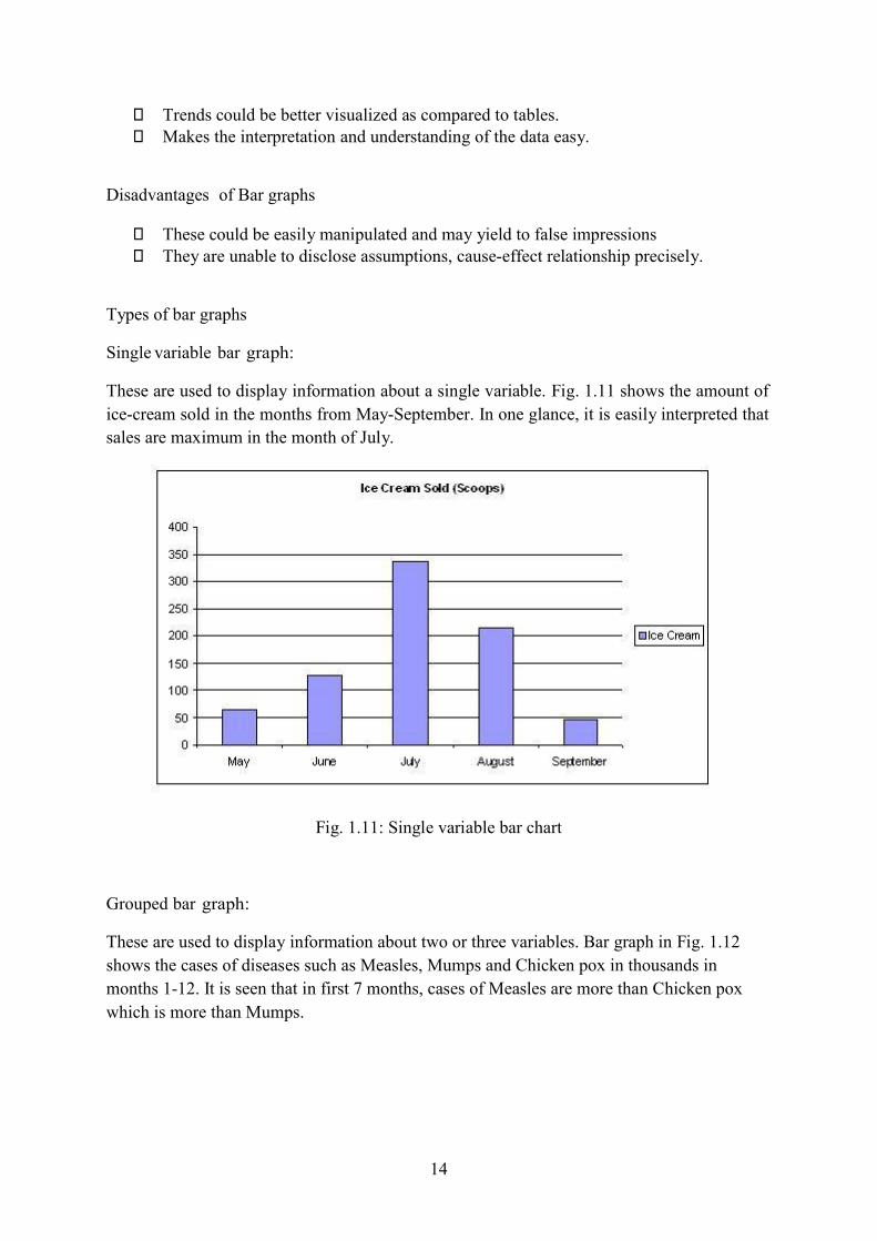
It is difficult to understand and extract exact values. It is unable to reveal key assumptions, causes and effect etc. It is difficult to compare variables. It could be used only with discrete.

The Fig 1.15 shows population of European countries in percentage.

1.15: Example Pie chart

1.4.5 Frequency Polygon / Line Graphs A frequency polygon is an alternative to the histogram. In order to construct a frequency

polygon, the midpoints at the top of each bar in the histogram are joined.

X-axis: scale of variable Y-axis: Frequency of observation

Frequency values are plotted at the midpoint of each class interval.

19

Advantages of Frequency Polygon Frequency polygons can be plotted on the same graph for comparison purposes.

Frequency polygons also are easy to interpret.

It is very easy to interpret the skewness of the data involved.

It helps in quick analysis of data

It can clarify patterns better than counterparts It has a capability to show minimum and maximum values easily.

Clusters and outliers are easily identifiable.

Exact and original values are retained as such.

Need minimum additional information.

Disadvantages of Frequency Polygon It is not possible to identify the exact values of the distribution.

It is also difficult to compare different data sets.

It is not visually appealing It can work with small range of data only.

Large data values are difficult to interpret

IT has minimal ability to reveal statistics, skew, kurtosis about the data plotted Accuracy of the data could not be checked.

The Fig 1.16 shows the frequency polygon between marks and number of students scoring

those marks.

20

1.16: Example Frequency Polygon

1.4.6 Scatter Diagram Scatter plot is a graphic technique that is used to display the relationship between two

continuous variables. One variable is plotted on x-axis and other on y-axis. In order to

analyse the relationship between variables, put a point on the graph corresponding to the

values of both the variables.

Scatter diagram helps to analyse the overall pattern (Correlation and regression) among the

variables. Fig 1.17 shows the scatter diagrams showing relationship between variables

involved.

Advantages of Scatter Diagram The relationship between variables could be linear if the points fall in a straight line

Highly scattered points indicate no relationship among variables.

It helps in quick analysis of data.

Clusters among the data could be identified at a glance.

Outliers could be easily identified at a glance.

Disadvantages of Scatter Diagram

It is hard to visualize large datasets.

Flat trends are difficult to analyse.

They need data on both axes to be continuous. .

21

No correlation Weak positive correlation

Strong positive correlation Strong negative correlation

Fig. 1.17:Exmaple Scatter graphs

1.5 Input Devices

An input device is a peripheral hardware device is used to supply data and control

information to the information processing system that may include a computer or information

appliance.

Some of the most common input devices are keyboard, mice, scanner, digital camera and

joystick etc. Some of the input device that are commonly used while delaing with computer

graphics are

Light pen Graphic tablet Joystick Trackball Data gloves Digitizers Image scanner

1.5.1 Light pen A light pen is an input device similar in appearance to a light sensitive wand which is used along with a computer (Cathode Ray Tube) CRT display. It provides the user a facility to

22

point to the displayed objects or draw on the screen very much similar to a touch screen but with much more positional accuracy. It is particularly a pointing device that detects the presence of light. Fig. 1.18 shows a light pen.

The light pen works on the technology in which it detects a change in brightness of screen pixels near its placement. CRT scans the entire screen pixel by pixel and the computer infers the pen’s position from the latest timestamp.

Light pens are very popular among health care professionals like doctors and dentists and design work. CAD users use them as input device.

Let us discuss some of the advantages and disadvantages of light pen.

Advantages of light pen

It is more direct and precise as compared to a mouse.

It is found to be convenient for applications having limited desktop space.

For simple input, use of light pen is faster than mouse.

It works very efficiently in keeping track of moving objects.

It is observed to be very efficient for subsequent multiple selection

No need to scan for the cursor on the screen for its usage.

Disadvantages of light pens

The use of light pen normally needs a specially designed monitor.

Use of light pen is not as natural as use of a normal pen.

Sometimes the contact with the computer may be lost unintentionally

Simultaneous pressing of button may lead to inaccuracy.

It is required to be attached to the terminal which is sometimes inconvenient.

Pen is required to be held perpendicular to the usage point which could be tiring.

Tilted pen leads to glare and inaccuracy.

While usage, hand may act as an obstacle for a portion of screen.

Adequate “activate” area is required to be provided around choice point.

It cannot be used on gas plasma panel.

Accuracy and precision might be reduced because of the aperture distance from the CRT screen

23

1.18: Light Pen

1.5.2 Digitizer / Graphic tablet

Digitizer is a common input device that is used for drawing, painting and sometimes selecting

co-ordinate positions on an object interactively. Such devices could be used to input co-

ordinate values in either a two-dimensional or a three dimensional space.

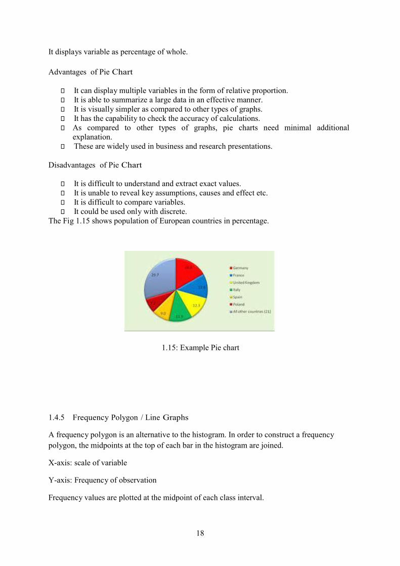
Graphicstablet is a kind of digitizer. Fig. 1.19 shows a digitizer graphic table. A graphics tablet is an input device that enables a user to draw images, animations and graphics. It is used in a way similar to a pencil and paper. It could be used for capturing data or signatures. The process of capturing data by tracing and entering corners of the shape is called digitization.

It consists of a flat surface on which image could be drawn using a pen type drawing apparatus called stylus and an optional screen to display the output.

Advantages of graphic tablet

It is of much use for graphic artists.

It is an effective input device as compared to mouse.

It is available in variable sizes

It is familiar to use for anyone who can use pen

It can read levels of pressure for input which is not possible in other input device.

Disadvantages of Graphic tablets

It is slower to draw than paper drawing

It is sometimes difficult to access menus and make selections using tablets.

It is comparatively an expensive device.

24

Fig. 1.19: Digitizer 1.5.3 Joystick

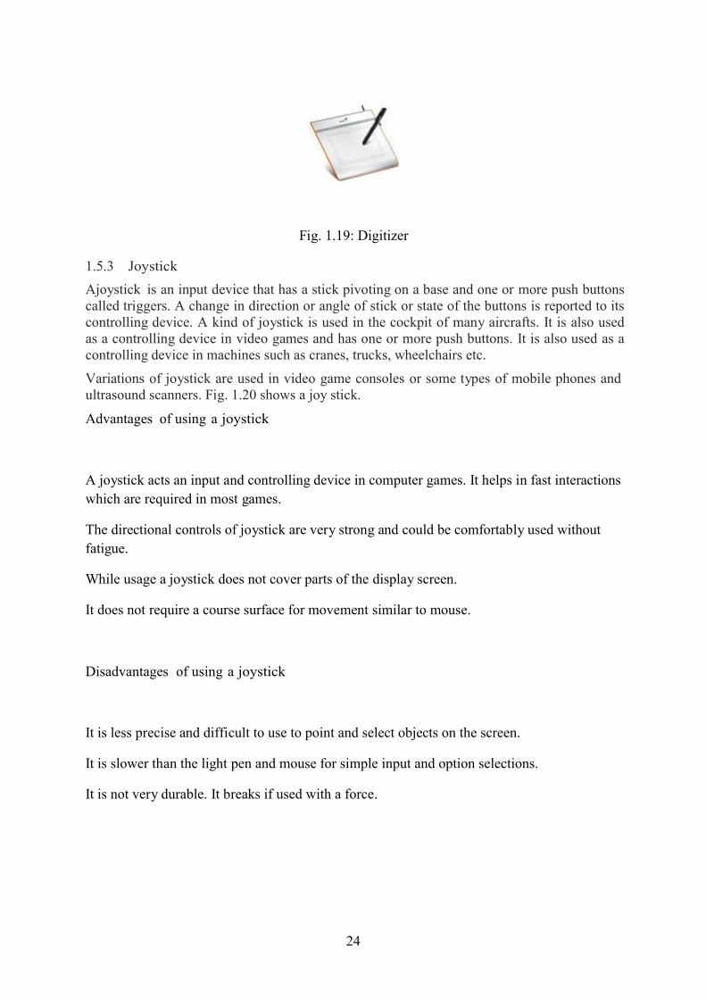
Ajoystick is an input device that has a stick pivoting on a base and one or more push buttons called triggers. A change in direction or angle of stick or state of the buttons is reported to its controlling device. A kind of joystick is used in the cockpit of many aircrafts. It is also used as a controlling device in video games and has one or more push buttons. It is also used as a controlling device in machines such as cranes, trucks, wheelchairs etc.

Variations of joystick are used in video game consoles or some types of mobile phones and ultrasound scanners. Fig. 1.20 shows a joy stick.

Advantages of using a joystick

A joystick acts an input and controlling device in computer games. It helps in fast interactions

which are required in most games.

The directional controls of joystick are very strong and could be comfortably used without

fatigue.

While usage a joystick does not cover parts of the display screen. It does not require a course surface for movement similar to mouse.

Disadvantages of using a joystick

It is less precise and difficult to use to point and select objects on the screen. It is slower than the light pen and mouse for simple input and option selections.

It is not very durable. It breaks if used with a force.

25

Fig. 1.20: Joy Stick

1.5.4 Track Ball

A trackball is a pointing input device whose working is based on a ball mechanism on its top.

It consists of a ball held by a socket which detects the rotation and movement of ball (through

sensors) about two axes. The user may give input by rolling the ball with the thumb, figure or

palm etc. As compared to mouse there is no limit on working area. A mouse may reach edge

of working area while rolling but there is no such limit in trackball. Fig. 1.21 shows a track

ball.

Uses

CAD users are very fond of using track ball due to its efficient working style. They are appreciated in computer game industry as a successful input device.

Advantages of a trackball

A trackball is highly appreciated as input device where desk space is limited. The user needs t

move the ball the entire device being stationary.

It can successfully work on any kind of surface even your lap.

Disadvantages of trackball

It is not as accurate and precise as mouse. The structure of device needs more frequent cleaning as compared to mouse

26

Fig. 1.20: Track Ball

e input device similar in appearance to

es physical sensing and accurate and pr

eality. Data gloves are the devices whic

pplications possible. Haptics means co

ve that can be used as an input device t

eries of sensors that can detect hand an g

and receiving antennas that can be u

information about the position and ori

1.21 shows a data glove.

1.5.5 Data Gloves

A data glove is an interactiv a glove worn on the

hand. It is used in which facilitat ecise motion control

in robotics and (VR) virtual r h makes the

development of computer based haptics a

mmunication by touch.

Fig. 1.21 shows a data glo o grasp a “virtual” object. A

data glove is built with a s d finger motions to capture

input. It has transmittin sed for electromagnetic

coupling to provide input entation of the hand. Fig.

Fig. 1.21: Data Gloves

Advantages of Data Gloves

Same glove could be used in left and right hand

27

Palm and rear side of the hand works in a similar manner It does not have an impact of size of any hand

It works very precisely for two dimensional hand positioning

It is available with both close and open finger tips as per the user’s convenience.

Disadvantages of Data Gloves

The performance of the input device depends on the illumination condition For precise input palm should be kept perpendicular to the camera

Bends in the fingers are not recognizable

1.5.6 Image scanner

It is an electronic device that captures a printed text, object or image and converts it into

digital format for manipulation and storage. These are available in various forms including:

Flatbed scanners: The input to be scanned is placed on top of scanner. A light is placed on the

image by the scanner and sensor scans the document automatically.

Handheld scanners: The user has to be push manually and sensor senses the image. It is

generally of small size. Fig. 1.22 shows scanners of both kinds.

Fig. 1.22: Scanner

A scanner acts as an input device but needs computer software program to import data to the

computer from the scanner. Another application of scanner is OCR (Optical character

recognition) systems that can convert scanned text document into digital text that can be

manipulated in word processing software.

28

Advantages of scanner

A document or image could be converted into digital form very easily and quickly. Even if

original document has taken days to be produced, the scanner can reproduce it without

damaging in seconds.

The document could be altered and can be easily transmitted via email or pen drive.

Disadvantages of scanner

3-D scanning is not possible yet. It is not as good in quality as original document due to hardware limitations

Maintenance could be an issue sometimes. A scanner may need new drivers, LED bulbs may

dim with time.

Cleaning scan bed is required frequently for quality scan.

Flatbed scanners are not portable as they need host computers.

Image may take a lot of space in memory.

29

Check your progress

5. What are the principals to be followed in the construction of graph?

6. What are the kinds of bar graphs?

7 Ppi means 8 Vector image takes (less/more) space than raster image. 9 Graphic tablet is a input/output devices.

Exercise

1. Track ball is a kind of (input/output) device. 2. Image scanner is helpful in .

1.6 Summary Computer graphics deals with the display of the image, its manipulation and storage by using

a computer.

Two types of graphic images namely raster and vector are mainly used in computer graphics A raster image is displayed by the arrangement of pixels having different colours. Vector

image comprises of paths defined by start and end point.

Two kinds of graphics are available. Active graphics in which the user can interact with the

graphics as well as the programs used to generate that graphic. In passive graphics the user is

unable to make any change in image show on the screen.

They are used in wide variety of applications including GUI, CAD, entertainment, computer

simulation, entertainment, image processing, digital art, education and training, presentations

etc.

Various kinds of graphs could be used to present data in an effective manner. It includes bar

charts, histogram, pie chart, frequency polygon, scatter diagram.

Various kinds of input devices such as light pen, Graphic tablet, Joystick, Trackball, Data

gloves, Digitizers, Image scanner are used to input information about graphics. Each has its

own advantages and disadvantages and application

30

1.7 Glossary Pixel

Pixel is also called picture element. In a digital image, a pixel is a smallest element to be

displayed. In a raster image, it is a single point. On a two-dimensional representation, pixels

are generally represented using dots or squares. Each individual pixel acts as a sample of

original image. It means more samples provide more accuracy in the resultant picture. The

intensity of the pixel is a variable. In a black and white image, the intensity of the pixel could

be between 0 (black) and 255(white). For coloured image the intensity could be represented

as a RGB (Red, Green, Blue) colour or CYMK (Cyan, Magenta, Yellow, Black).

DPI (Dots per Inch)

It is being set by the printer device and measures the amount of ink dots the printer will use

on each pixel of the image.

Rendering It deals with the generation of a 2D image from a 3D model by means of computer programs

often called rendering programs. A 3-D model is always associated with a scene file which

contains objects in a strictly defines data structures. The scene contains information about

geometry, texture, lightening and shading information about the scene to be described. The

data stored in the scene file is passed as an input to a rendering program to be processed and

digital image is obtained as an output. The rendering program is often available as a built in

the computer graphics software. Sometimes their plug-ins is available as entirely separate

programs. It is also useful to describe the process of calculating effects in a video editing file

to produce final video output

3D projection

It deals with the projection of three dimensional graphic to two-dimensional plane. It is a

widely used in computer graphics especially related to engineering and medicines. This is

because most of the present methods for displaying graphical data are associated with planar

two dimensional media.

Aspect Ratio It is the ratio of vertical points of an image to that of the horizontal points. It is a projection

attribute which is often necessary while resizing the graphics. It helps to avoid resizing it out

of proportion. It is generally expressed as x:y as a relation between width and height. For

example, aspect ratio of 2:1 means the width is twice of the height.

31

1.8 Answer to check your progress/self assessment questions

1 Raster image is made up of pixels of different colours and hence are not scalable where as vector image is made up of paths defined by mathematical formulae and hence are scalale.

2 Resolution determines the quality of image. It indicates the total number of pixels in an image, along with its length and height.

3 Computer graphics are helpful in CAD as The designers can watch multiple views of the object which leads to see

enlarged sections or different views of objects at the same time. Animations are often used in CAD applications which are used in

entertainment and movie industry. Real-time animations are also possible which could be used to display

wire frame of the objects that could be used by the engineering for testing performance of a vehicle.

The designers can see the interior behaviour of vehicle during motion which is otherwise not easily feasible.

These are very much helpful for finalising the layouts of the buildings. 4 It is the ratio of vertical points of an image to that of the horizontal points. 5 Following are the major principles to be followed while constructing graphs

Distortion of data should be avoided while construction a graph. Proportion and scale should be maintained. Generally have greater length than breadth. Most commonly the height (y-

axis) and length (x-axis) of the graph should have 3:4 ratios. This is because horizontal axis displays the causal variable in more detail.

Abbreviations are spelled in a note for better understanding Colours could be used to clarify the groupings

6 Single variable, Grouped, stacked bar graph 7 Pixel per inch 8 More 9 Input 10 Track ball is based on a ball mechanism on its top rather than at bottom in mouse.

1.9 References and suggested readings 1 Computer Graphics, Donald Hearn and M.Pauline Baker, Prentice Hall of India,

New Delhi. 2 Introduction to computer graphics, A. Van Dam, S. K. Feiner, J. F. Hughes,, R. L.

Phillips,Reading: Addison-Wesley.

1.10 Model Questions 1 What does pixilation means? 2 How is computer graphics helpful in education? 3 How does visualization and presentation improve with computer graphics? 4 Discuss the scenario where pie chart is advantageous to other data presentation

graphs.

33

Structure of the Chapter

2.0 Objectives

Lesson 2

OUTPUT DEVICES

2.1 Output devices and Video display devices

2.2 Colour Models (RGB, CMYK)

2.3 Cathode ray tube

2.4 Direct view storage tube

2.5 Raster scan displays

2.6 Random scan displays

2.7 Architecture of raster and random scan monitors

2.8 Colour CRT monitors.

2.9 Flat panel displays

2.9.1 3-D viewing devices

2.9.2 Raster scan systems

2.9.3 Ransom scan systems

2.9.4 Graphics monitors and workstations 2.9.5 Lookup tables

2.10 Summary 2.11 Glossary 2.12 Answer to check your progress/self assessment questions 2.13 References and suggested readings 2.14 Model Questions

2.0 Objective After studying this chapter students will be able to:

Differentiate colour models to be used in graphics Identify the technology behind graphic based output devices Identify the technology behind recent advancements in technology used in grahic

display devices including television.

Anoutput device is a computer hardware which is used to communicate the electronically

obtained information resulted by processing performed by an information processing system

such as computer into human readable form.

34

2.1 Video display devices It is an electronic device which is used as an output device to represent information in visual

form. For example CRT, LCD monitors, Television screen etc.

2.2 Colour Models

Colour is the way a human brain interprets combination of band of wavelengths of light. A

colour model refers to an abstract mathematical model by which human brain’s colour vision

is modelled. It includes the way by which colours are represented as combination of numbers

called colour components

Two colour models very much famous in computer graphics are

RGB

CMYK RGB Colour Model

The RGB colour model was introduced by two scientists named Thomas Young and Herman

Helmholtz in their research work called ‘Theory of Trichromatic Colour vision’ in early 19th

Century.

35

In this model, a colour is specified by three components for intensity level of

primary colours – Red, Green and Blue. They are based on the theory that every

possible colour is made of these three primary colours. Each colour is specified by

a binary number with 32 bits. 32 bits are decomposed into 4 bytes of 8 bits each.

Each byte can hold 0-255 values. The fourth byte is used to specify the opacity of

the colour. It means if the colour in the topmost layer has value in fourth byte less

than 255, the colour from underlying layer is seen through.

This model is used for display in Televisions and Computer monitors. Fig 2.1

shows RGB colour wheel.

As an example

Red Green Blue Colour

255 0 0 Red

0 255 0 Green

0 0 255 Blue

0 255 255 Magenta

255 0 255 Cyan

255 128 0 Orange

255 255 0 Yellow

255 255 255 White

0 0 0 Black

Fig. 2.1: RGB Colour Wheel

RGB is an additive colour model. It means new colours could be created by adding these

primary red, green and blue colours. White colour is created by combination of all primary

colours and black is created by absence of these colours. New colours are created by making

changes in these three values along with changes in shades, tints and tones. The equations

and examples are discussed below.

Change in shades of the colour

The shades (new intensity) of a colour could be created by using following equation

new intensity = current intensity * (1 – shade factor)

36

Shade factor of 0 means no change in colour and 1 means colour completely powered by

black colour.

For example if in orange colour (255, 128, 0), the shades are as shown below.

0

.25

.5

.75

1.0

(255, 128, 0)

(192, 96, 0)

(128, 64, 0)

(64, 32, 0)

(0, 0, 0)

Change in tints of the colour

The tints (new intensity) of a colour could be created by using following equation

new intensity = current intensity + (255 – current intensity) * tint factor

A tint factor of 0 means no change in colour and 1 produces white:

For example if in orange colour (255, 128, 0), the tints are as shown below.

0

.25

.5

.75

1.0

(255, 128, 0)

(255, 160, 64)

(255, 192, 128)

(255, 224, 192)

(255, 255, 255)

The value of shade factor and tint factor must be between 0 and 1.

Change in tones of the colour

The tones (new intensity) of a colour could be created by using both shade and tint. On the

application of tint operation and then shade, the intensity of the dominant colour is used in

place of 255.

For example if in orange colour (255, 128, 0), the tones are as shown below.

0

.25

.5

.75

1.0

0

(255, 128, 0)

(192, 96, 0)

(128, 64, 0)

(64, 32, 0)

(0, 0, 0)

.25

(255, 160, 64)

(192, 144, 96)

(128, 80, 32)

(64, 40, 16)

(0, 0, 0)

.5

(255, 192, 128)

(192, 144, 96)

(128, 96, 64)

(64, 48, 32)

(0, 0, 0)

37

.75

(255, 240, 192)

(192, 168, 144)

(128, 112, 96)

(64, 56, 48)

(0, 0, 0)

1.0

(255, 255, 255)

(192, 192, 192)

(128, 128, 128)

(64, 64, 64)

(0, 0, 0)

CMYK Colour Model

It is a subtractive colour model which is based on four colours namely CYAN, MAGENTA,

YELLOW and key BLACK. Cyan, magenta and yellow are secondary colours as shown in

Fig 2.1. The model is based on subtractive colour combinations which means new colours are

created by partially or entirely masking base colours on a lighter, usually white, background.

Ink is used to reduce the light that would be reflected to produce white colour. Since ink

subtracts brightness of white colour to produce new colours the model is called subtractive.

In this model, white is created by absence of these colours and black by combination of all

the colours. The primary advantage of using black colour as key colours long with three

secondary colours include

Rather than mixing cyan, magenta and yellow colours to make black ink, use of black

ink is cheaper. Printing text with black ink results in quality better than if printed with using three

different colours. Black shade obtained by missing cyan, magenta and yellow is not perfect black. Using three colours to create blank colour takes time to dry up.

CMYK uses dithering to display colours. Dithering is a technique in which a computer

program approximates a colour cyan; magenta, yellow and black if the colour to be displayed

is not available. For example, when a web page contains a colour that the client browser does

not support. Fig 2.2 shows CMYK colour wheel.

Fig 2.2: CMYK model

Difference between RGB and CMYK colour models

RGB CMYK

RGB is based on projecting. CMYK is based on ink

38

White colour is created using red, green, blue

colours altogether and black by absence of

these colours.

white is created by absence of cyan, magenta,

yellow and black whereas black is by

combination of all the colours

Colour space is more than CMYK Colour space is lesser than RGB RGB displays bright colours If a colour is converted from RGB to CMYK,

the bright colours in RGB will be duller in

CMYK

It is an additive colour model It is subtractive colour model Most of the screens are based on RGB model Most printers are based on CMYK model

It is an additive colour mode. The

background of screen is taken as black.

Varying intensities are developed adding

light to black colour.

It is a subjective colour mode. The

background of paper is taken as white. The

ink subtracts brightness of the white paper to

develop new colours.

RGB uses primary colours that are much

brighter than CMYK

CMYK uses secondary colours that are much

lighter than those used in RGB. In order to

produce darker colours more ink needs to be

added

RGB is based on three primary colours. CMYK uses four colours rather than three in

RGB. This additional black colour is used

instead of reproducing black by combining the

three colours. 2.3 Cathode ray tube

A Cathode Ray Tube CRT is an output display device in which there is an evacuated glass

tube with a heating element called filament on one end and a phosphor coated screen on the

other.

The operation of CRT can be summarized as below.

Current flows through the filament leading high temperature and hence reduction in

conductivity of this metal filament. Electrons start piling up on the filament and some of them start boiling off from the

filament. Outer surface of the anode focusing cylinder called electrostatic lens attracts these free

electrons with a strong positive charge. The inside of the cylinder has a weaker negative charge. This opposite charge forces the

electrons with repulsion into a beam.

39

As a result the electrons shoot at a very fast pace. The electrons pass through two sets of weakly charged focussing deflection plates having

opposite charges. The charge on these plates influences the path of the electron beam. The first set of deflection plates displaces the beam up and down. Further, the second set of plates displaces them left and right. The electrons shoot out of neck of the tube and smash into the screen with phosphor

coating placed on the other end of the bottle. As a result of this smash on phosphor some of the electrons are made to jump into another

band.

The picture is redrawn by directing the electron beam to the same screen points quickly

over and over again.

Fig 2.3 displays the complete operation including the electron gun with accelerating mode

and working of deflection plates

40

Fig. 2.3: CRT operations

2.4 Direct-view storage tube

Direct View Storage Tube (DVST) has concepts very much similar to a CRT and is

accompanied with highly persistent phosphor. The main advantage of DVST is that the

graphic drawn will persist for several minutes (40-50 minutes) before getting fade. The

working of DVST is described below.

It consists of electronic gun and phosphor-coated screen similar to CRT.

A fine-mesh wire grid is used to display graphic on phosphor coated screen rather than the

electron beam.

This grid is made up of high quality wire.

It is located with a dielectric and is mounted just before the screen.

It is mounted on the path of the electron beam from the gun.

The graphic to be displayed is deposited on this wire grid as a pattern of positive charges.

The pattern is transferred to phosphor coated CRT with the help of continuous flood of

electrons.

Flood gun separate frame the electron gun is used to generate flood of electrons.

Another grid called collector is placed behind the mesh.

The flow of flood of electrons is managed and smoothened with the help of collector

mesh.

The high velocity flood of electrons is slowed down by the negative charge of the collector

grid.

The low velocity negatively charged flood of electrons pass through the collector and

attracted to the positively charged storage mesh

This pattern of positive charges which are residing on the storage mesh leads to display of

the picture.

Electrons have been slowed down by the collector. As a result, the image might not be

sharp and bright as required.

To make the image bright, the screen is applied high voltage to provide a high positive

potential.

Voltage is applied to a thin aluminium coating that has been added between the tube face

and the phosphor screen.

41

The phosphor on the CRT screen has a very high persistence quality, the image and

graphics created on the screen will persist for several minutes without the need for being

refreshed.

To remove the picture, a positive charge is applied to the negatively charged mesh for its

neutralization. As a result all charges are removed and screens clears up.

It may produce an unpleasant momentary flash.

A gradual degradation in the quality of image produced occurs due to the accumulation of

the background glow.

Selected part of the graphic cannot be erased.

Fig 2.4 shows the architecture of DVST. It contains two guns called Flood gun and primary

gun.

Fig 2.4: Direct view storage tube DVST is accompanied by several advantages as well as disadvantages.

Advantages of DVST

Refreshing of graphics is not required for a longer period of time.

It can display very complex pictures at very high resolution without flicker

Disadvantages of DVST

Generally they don’t display colours.

Some part of the graphics can’t be erased.

The erasing and redrawing of a new and complex graphics may take some time.

42

Animation is not possible with DVST. Difference between DVST and CRT

Although DVST is similar to CRT but some of the differences are listed below.

DVST CRT

It has flat screen It may or may not have a flat screen

It has poor contrast Contrast is better than DVST

Refreshing is not required Frequent refreshing is required

Selective erasing of the graphics is not

allowed

Selective erasing of the graphics is possible

Performance is inferior as compared to CRT Performs very well as compared to DVST

Complex pictures could be displayed at a

high resolution

Performance to generate flicker free complex

graphics is poor as compared to DVST

Check your progress

1. RGB is additive/subtractive colour model.

2 CMYK is additive/subtractive colour model.

3 CMYK stands for , , and

.

2.5 Raster scan Araster scan is a technique that has been most commonly used to display images in CRT. It

is used to capture rectangular pattern of an image as well as for reconstruction in television.

The term has been derived from raster graphics which is a kind of image storage and

transmission technique used in most computer bitmap images.

It is based on the line-by-line scanning technique to be used for covering the display area

progressively, one line at a time. It resembles the way a reader’s gaze travels while reading

lines of text.

Image Scan Process

43

Image is divided into a sequence of horizontal strips called "scan lines". The scanned lines

could be transmitted as analog signals (in Television systems) or discrete pixels (computer

systems) as read from video source.

For image scan, the beam is swept horizontally from left to right at a steady pace. For next

line scan, the vertical position for the scan increases steadily and slowly and for horizontal

scan, the beam moves back rapidly to the left.

The beam is off while moving back from right to left.

For horizontal scan, the backward sweep is faster than forward one.

The display screen is taken as matrix of pixels and each point is addressable in memory as

well as display screen.

On reaching the bottom of the screen, beam is made off. It is brought rapidly at the beginning

of screen at top left to start again.

There happens one vertical sweep per image frame and one horizontal per line of resolution.

In this way, it is observed that or vertical the scanning process there occurs a downhill slope

towards lower right and the slope is almost 1/horizontal resolution.

This resulting slope is compensated mostly by the tilt and parallelogram adjustments. As a

result of adjustments this tilt cancels the downward slope of the scanned lines.

The scanning is done by using the technique of magnetic deflection which is imposed by the

change in current in the coils of the deflection yoke.

Printers are example where images are created using raster scanning.

Fig 2.5 displays how this horizontal and vertical sweep takes place.

Get rid of flicker

Fig 2.5: Raster scan

44

The phosphor used in the display screen has persistence impact which means that even if

pixels are drawn one at a time, by the time whole pixels on the screen are drawn, the initial

pixels are still illuminating. Flicker impact is created due to drop in brightness of the pixels.

Interlacing technique has been used to get rid of flickers in raster scan.. In this technique,

Odd-numbered scan lines are displayed for the first vertical scan followed by the even-

numbered lines. As every other line is drawn in a single broadcast, the newly-drawn lines will

be brighter and when interlaced with the earlier drawn somewhat dimmed the overall

illumination happens to be more even. Most appropriate refreshing rate on raster-scan is 60 to

80 frames per second.

2.6 Random-scan display

Random scan monitors draw an image line by line and so are called vector displays (or

stroke-writing or calligraphic displays). The individual line could be displayed and refreshed

in any specified order.

Only desired lines are traced on CRT. As an example, in order to connect a point A and B on

the vector graphics display, drive the beam deflection circuitry to move it directly from Point

A to B. To move the beam from point A to point B without showing a line between points

blank the beam while moving. Both magnitude and direction information are required for

effective display. Vector graphics generator is used to perform these operations. Fig 2.6

displays one such vector.

Fig 2.6: Vector component

On a random scan system, in order to get rid of flicker, refresh rates selected depending on

the number of lines to be displayed. Refresh display file is used to store image definition as

vectors in the form of set of line-drawing commands. Refresh display file is also called

display list, display program, or simply the refresh buffer.

In order to display an image in random scan, the set of line commands stored in refresh file

are executed resulting in display of each component line in turn.

After processing all line drawing commands, the random scan system gets back to the first

line command in the list. All the component lines of an image are processed 30 to 60times

each second in most of the cases.

45

2.7 Architecture of Raster Scan Raster scan consists of a

Display controller Central Processing Unit (CPU) Video Controller Refresh buffer Keyboard Mouse CRT

A special area of memory called frame buffer is dedicated to graphics only. The set of

intensity values are stored for all the screen pixels. The image displayed is stored in the form

of 1s and 0s in the refresh buffer.

Actual image is displayed by reading stored intensity values from the refresh buffer and

display one scan line at a time.

Pixel position is specified by a row and column number.

Intensity range for pixel positions can be a simple black and white system or colour system.

Simple black and white system is simple as you need to store one bit per pixel as either on or

off. The frame buffer is called bitmap. For colour system, additional bits are required to store information about colour and intensity.

A high quality display of image by using 24 bits per pixel and it may require several

megabytes of buffer storage space. The buffer is called a pixmap.

Fig. 2.7 displays the raster scan system architecture

46

Fig 2.7: Raster scan system architecture

A separate display controller called display processor is used to access the display

information from refresh buffer and process it in every refresh cycle. In this way, the CPU

gets free from graphic display processes. Along with this, the display processor digitises a

picture definition given in an application program into a set of pixel-intensity values that

could be stored in refresh buffer. This process is called scan conversion.

Video Controller:

The purpose of video controller is to receive the intensity information of each pixel from

frame buffer to display graphics on the screen. It is made of following components

Raster-scan generator: It is used to produce deflection signal that generates the raster

scan. It also controls the x and y address registers.

x and y address registers: These are used to define the location in the memory to be

accessed next.

Pixel value registers: Defines the screen positions referenced as Cartesian

coordinates. The architecture of Random scan

Fig 2.8 displays the typical vector display architecture. It consists of following components.

47

Display controller Central processing unit (CPU) Display buffer memory CRT

The image to be displayed is stored in the display buffer memory in the form of display

commands.

Display controller is connected to the CPU as I/O peripheral. The commands stored in display buffer are drawn by sending commands in the form of point

coordinates to a vector generator.

The digital coordinate values obtained are converted to analog voltages by vector generator

so that information could be sent to beam deflection circuits of CRT to displace electron

beam displaying image on phosphor coated CRT screen.

Fig 2.8 displays the Random scan system architecture.

Fig 2.8: Random scan system architecture

Difference between Raster scan and random scan

Raster scan Random scan

The beam is moved one scan line at a The beam is moved between the end points

48

Time first from top to bottom and then back to top.

of the primitive vectors of the graphic to be

displayed.

Refresh rate is independent of complexity of

the image

With increase in primitive vectors in the

image, the complexity and hence refresh rate

needs to be increased

Primitive are required to be scan converted

into their corresponding pixels

in the frame buffer.

No scan conversion is required

Raster display can display continuous and

smooth lines by approximating them with

pixels on the raster grid.

Vector display is made to work on draws

continuous and smooth lines.

Cost is less It costs more

Raster scan has the capability to display has

images filled with solid colours or patterns.

Random scan has cannot display images

filled with solid colours or patterns They can

only draws line characters.

Electron beam is directed across whole

screen for display of image

Electron beam is directed only to the part

where graphics is to be displayed

Resolution is poor Resolution is good

Graphics is stored as set of intensity values

for all screen pixels in the refresh buffer

Graphics is stored as set of lines in display

file

As intensity value of pixels are stored as such

so it is well suited to display realistic scenes

containing even shadows

It is based on line drawing capability, so it is

not well suited for realistic scene display.

Pixels are the base of display Mathematical functions are base of display Editing is difficult Editing is easy

It uses interlacing It doesn’t use interlacing

It uses shadow penetration It is based on beam penetration

2.8 CRT colour monitors

In order to display a graphic on coloured CRT monitor, the pixel values are read to control

the intensity of the CRT beam to be displayed on the screen during each refresh cycle.. In

order to display coloured graphics on CRT, different phosphors having the ability to emit

different coloured lights. Two main methods to perform this operation are

49

Shadow mask method.

Beam penetration method Shadow Mask Method: This method of displaying coloured images is used in Raster scan displays (colour TV). The screen is made of phosphor of three different coloured dots that can emit red, green and blue colours in a single pixel position. Three guns emitting electrons are used to emit these three colours namely red, green and blue. Fig 2.9 shows the technique of shadow masking. The steps followed are listed below.

Three guns emit three electrons simultaneously

These electrons when go through a shadow mask a phosphor dot triangle red, green and

blue colours are formed on CRT screen. It is actual pixel on screen.

In order to generate different colours on the pixel the intensity of the electron beams are

controlled. It can generate colours from combination of colours red, green and blue.

Fig 2.9: Shadow masking

Beam penetration method: It is used to display coloured images in random or vector scan

systems. It is cheaper than shadow masking. In this method, an outer red layer and inner

green layer phosphors are coated in the inside section of CRT.

By adjusting the speed of electrons, the amount of their penetrations is adjusted. In order to

generate red colour, the electrons are emitted slow so that they penetrate only the outer layer.

In order to get green colour the electrons are emitted fast so that they can penetrate the outer

layer and the inner layer. In this way adjusting speed of electrons may generate red, green,

orange and yellow colours. The main limitation of this method is that it can display only four

colours on the screen and hence quality of image thus obtained is diminished.

Beam Penetration Shadow Penetration It is used in random or vector scan system to display coloured graphics Only four colours namely red, green, orange and yellow could be displayed

It is used in raster scan system to display coloured graphics Million of colours could be displayed

50

Since the colours to be displayed depends on the speed of colours, few colours are possible

Since the colours depend on kind of ray, millions of colours are possible

It is less expensive It is costly Quality of graphic thus obtained is poor. Quality of graphic thus obtained is high. It has high resolution It has low resolution

2.9 Flat panel displays

Flat panel displays are a class of video display devices with reduced volume, weight, and

power requirements as compared to a CRT. They are thinner than CRT and it could be hung

on walls. Flat-panel displays are categorised as

Emissive displays

Non-emissive displays

The emissive displays also called emitters convert electrical energy into light to display. For

example light-emitting diodes (LED).

In this technique, matrix of diodes is arranged on the basis of information stored in refresh

buffer to form the pixel positions in the display. Picture definition is read from the refresh

buffer and on the basis of information; voltage levels are generated that are applied to the

diodes to produce the light patterns in the display.

Non-emissive displays also called non-emitters use optical effects to convert sunlight or light

from some other source into graphics patterns. For example liquid- crystal device (LCD).

Plasma panel is a type of flat panel display. It is also called gas discharge displays. It

contains two glass plates. The region between glass plates is filled with a mixture of gases

usually neon. One glass panel is encompassed with a series of vertical conducting ribbons

and the other with horizontal. Application of voltages to these horizontal and vertical

conductors breaks down the gas at the intersection of two conductors into glowing plasma of

electrons and ions. Information about the picture is stored in refresh buffer and the voltage is

used to refresh picture pixels usually 60 times per second.

Liquid- crystal displays

Liquid- crystal displays (LCDs) are kind of flat panel display devices that are commonly used

in calculators and laptop computers. These are non-emissive devices in which a picture is

displayed by passing polarized light through a liquid- crystal material. This crystal material is

adjusted to either block or transmit the light. It consists of two glass plates having liquid

crystal material containing a light polarizer at right angles to the other palate. One glass plate

has horizontal conductors and other has vertical. Both types of plates intersect at a pixel

position. Voltage has been applied to two intersecting plates to turn the pixel on. It leads to

alignment of molecules in the liquid so that the light is not twisted. It is also called passive

51

matrix LCD. Similar to emission devices, Information about the picture is stored in refresh

buffer and the voltage is used to refresh picture pixels usually 60 times per second.

In order to display colours, different kind of materials has been placed at colour pixels at each

screen location. Sometime, transistors are placed at each pixel location to display colours

using thin-film transistor technology. The transistors also help to retain charge in liquid

crystal cells by controlling voltage at pixel locations. These devices are called active-matrix

display.

Flat panel displays

Difference between CRT and Flat Panel Display devices CRT Flat Panel Display

Advantages of Flat Panel Display over CRT

CRT is bulky the back size is proportionate

to the size of the monitor

Slim as compared to Flat panel display

leading to portability and space saving.

Viewable area is smaller due to the frame

around the glass screen of the monitor.

Viewable area is slightly bigger than CRT

Screen is not flat leading to distraction

especially while working on light

background.

Screen is 90 degree true flat

CRTs emit electromagnetic radiation which

are sometimes uncomfortable

These emit a very small amount of radiation

These are heavy Flat panel displays are lighter Higher power consumption Low power consumption

Glass screen causes glare Glass screen is not used leading to no glare.

Displays slightly less sharp images Displays sharp images

Quality of image is not very good Good quality display

Automatic resize facility is does not work

well and may require micro adjustments to

fill the screen

Automatic resize is possible by hitting Auto

button. Every pixel within its viewable area

will be auto adjusted.

If same image is displayed for a longer

period of time it is possible that it would be

Burn-in does not happen in Flat panel

displays

52

embedded in the display permanently.

In order to generate a flicker free image

minimum of 75hz is required

They generate flicker free image every time

Gets noticeably warm Does not get too warm Advantages of CRT over Flat Panel Displays

Dead pixels are not there on CRT There could be dead pixels due to

manufacturing defects

Cheaper Expensive

It could be used at any resolution up to the

maximum supported.

It should be used at a native resolution

It has wide viewing angle It has narrow viewing angle

2.9.1 3-D Viewing Devices

Modern monitors have the ability to provide a stereoscopic perception of 3D depth of the graphic involved.

The main operation of 3-D view is made by displaying the views for left and right eye separately. These are called 2D offset. These image offsets are then combined in the brain which gives the perception of 3D view. 3D is overestimation of capability of such display systems. This is because these are considering two 2D images as being 3D. More accurate term that could be used for such monitors is "stereoscopic".

Stereoscopic technology deals with the different image captured by left and right eye of the viewer. For example anaglyph images and polarized glasses. It means Stereoscopic technologies generally deal with special kind of spectacles.

Due to the issues such as price and basic infrastructure the growth in this market is lacking a bit. But they have potential of tremendous growth. Some of the existing applications of this technique include TV, film, and game industry.

The main versions of "3D" (stereoscopic) technology are:

Active Stereo 3D – It is most widely used technology for 3-D views. In this

technology, images captured by left and right eyes are separated by active shutter glasses which lead to 3D effect to the user.

Passive Stereo 3D – In this technology, left and right images are separated by using polarized glasses. Screen is activated by special films. It is becoming very popular these days.

Autostereoscopic 3D – In this technology, there is no use of glasses. The technology is quite expensive and needs special stereoscopic screens.

53

Stages of Stereo 3D Presentation

Stereo 3-D presentation includes stages shown in Fig 2.10.

Source: Stereo 3D content to be displayed are created for view Preparation and Transmission: Left and right images to be viewed for creation of

3D are prepared. These images are transmitted to the display device Presentation: With the help of stereo glasses, left image and right images are

relayed to the eyes.

Fig 2.10: Stages of 3D stereo presentation

Active Shutter Technology (SG)

In order to reach the desktop LCD monitors active shutter technology using shutter glasses (SG) or liquid crystal glasses has been a boon. The active use of these shutter glasses for presenting 3-D affect is the reason for addition of word active in its name. It is also called time division switching.

The hardware required for this technology involves:

Special shutter glasses 3D enabled display Graphics card Software package

The glass on each eye contains a liquid crystal layer having the ability to become dark when voltage is applied. A special transmitter is connected to the glasses is controlled by PC with the help of timing signal to make glasses dark in synchronization on the basis of refresh rate of the screen. The glasses open and close at a very fast speed (60 times per second) to view the image by one eye at a time.

Polarized or passive 3D technology

This technology creates 3D effect by the screen and not by the glasses. Some of the modern 3D films like Avatar or Harry Potter are built with this technology.

Each image is polarized in a different direction Glasses wear have lenses that are polarized in opposite directions Each lens polarizes according to corresponding image. The polarized lens on the left eye polarizes and blocks the right image In this way, left eye will be able to see left image and right eye only right image. Images with different polarizations can’t be displayed as such on flat screen.

54

Special film polarizes left and right image and resultant 3D graphics could be seen with polarized glasses which filter light so that correct eye sees the correct image.

2.9.2 Raster scan systems

In a raster- scan system the graphics is created by sweeping electron beam row by row across the display screen. While sweeping, the intensity of the beam is turned on and off for displaying illumination on the display screen. Frame or refresh buffer stores the information about the graphic to be displayed. The screens are refreshed at 60 to 80 frames per second. After scanning all the rows, the electron beam returns to the beginning of the next line. It is called the horizontal retrace of the electron beam. After scanning all the rows the electron beam returns to the beginning of top left corner of the screen called vertical retrace

2.9.3 Random-scan Systems

Random scan monitors draw graphics line by line. The vectors are refreshed at a rate which depends on the number of lines to be displayed. The vectors could be refreshed in any order. Information about the graphics is stored in an area of memory called the refresh display file. In order to display a specified graphic, the system cycles through the set of commands in the display file to draw vectors one by one. After displaying all the vectors, the system cycles back to the first line command in the display file.

7 Raster scan is used to display in monitors.

8 Resolution of raster scan is than random scan. 9 Raster scan uses (Beam penetration/shadow

masking) for image display.

10 LCD is a kind of (CRT/Flat panel) monitor.

2.9.4 Graphic monitors and workstations

Graphic monitor is the monitor which has the ability to display graphics along with text.

Most of the modern monitors are graphic monitors. They are output device.

In other words, monitors that support the following graphic applications are called graphic

monitors.

Animation CAD Drawing programs Paint Applications Presentation Graphics Software’s such as Excel capable of managing pie and bar

charts

55

Desktop publishing such as MS Office, Share points, Document managements Graphic workstation refers to the specially configured computer for graphic works such as image manipulation. For management of complex graphics, workstations need good operating power and graphic capabilities.

The general specification of such computers include

Minimum of 64 Megabytes of RAM Very good Resolution Graphics screen GUI Graphical User Interface High capacity storage device Built-in Network Support

The computing capabilities of workstations lie between Personal computer and minicomputers They can work as standalone station or local area network LAN. The most common operating systems used in workstations are Unix and Windows NT.

2.9.5 Look up tables

A look up table (LUT) also called colour map is a table which is used to display a graphic

image in the computer. It contains information about the association of a numeric pixel value

and its colour to be displayed on the output device. Similar to a painter, this colour palette is

the basis of coloured images. This colour is managed in the computer as a combination of

Red, Green, and Blue colours. Corresponding to each pixel, colour map thus contains three

components. Generally speaking, a colour map has 256 rows corresponding to 0-255 pixels

that could be stored in an 8-bit field. GIF images are an example of image file type that uses

LUT to store colour information. It is called pseudo-colour because they are unable to display

photo-realistic images. A true-colour system can display 16 million colours developed by all

possible mixtures of 256 levels for each primary colour.

Characteristics of LUT

The number of entries in the palette: This is a base to identify the maximum number of

colours that can appear on screen simultaneously. It is actually a subset of the full RGB

colour palette.

The width of each entry in the palette: It is the base to identify the number of colours that

could be represented by the wider full palette.

As an example, a palette of 256 colours which needs 8 bits to store information. It is called

colour depth or bits per pixel (bpp). The width of each entry is formed by 8 bits for each

colour making a total of 24 bits.

56

Further, 8 bits per channel makes 256 levels for each possible red, green, and blue sub-

components making total of 256 × 256 × 256 = 16,777,216 colours.

So, we can say each colour could be chosen from a full palette of RGB with a total of 16.7

million colours.

If changes are made in the palette, the whole screen is affected at once. This technique could

be used to produce special effects.

Advantages of Look up tables

In this way, we can have large number of simultaneous colours without large frame buffers.

Entries in the colour table could be easily manipulated for experimentation with different

colour combinations without changing the attribute settings. In image processing applications, LUT could be used for setting a threshold value such that

pixels having value above or below this threshold are set to same colour.

Fig. 2.11 displays a look up table with 24 bit entries with 8 bits per colour. A value of 200

stored at a pixel accesses information from the table as 2083. Each 8 bit component of this

entry is used to control the intensity of each of electron guns for Red, green and blue colours.

0

200

2083

200

255

00000000 00001000 00100011

RED GREEN BLUE

Fig 2.11 :A colour lookup table with 24 bits.

2.10 Summary Video display device is an electronic device which is used as an output device to represent

information in visual form. RGB and CMYK are two most popular colour models popular for

video display. RGB is an additive colour model in which new colours could be created by

adding these primary red, green and blue colours. CMYK is a subtractive colour model which

is based on four colours namely CYAN, MAGENTA, YELLOW and key BLACK.

Various display devices are used in computer graphics. A Cathode Ray Tube CRT is an output display device in which there is an evacuated glass

tube with a heating element called filament on one end and a phosphor coated screen on the

other.

57

Direct View Storage Tube (DVST) is an output device which has concepts very much similar

to a CRT and is accompanied with highly persistent phosphor. The main advantage of DVST

is that the graphic drawn will persist for several minutes.

Araster scan is a based on the line-by-line scanning technique to be used for covering the

display area progressively, one line at a time.


stroke-writing or calligraphic displays). The individual line could be displayed and refreshed

in any specified order

Flat panel displays are a class of video display devices with reduced volume, weight, and

power requirements as compared to a CRT.

A look up table (LUT) also called colour map is a table which is used to display a graphic

image in the computer. It contains information about the association of a numeric pixel value

and its colour to be displayed on the output device. Similar to a painter, this colour palette is

the basis of coloured images. This colour is managed in the computer as a combination of

Red, Green, and Blue colours.

2.11 Glossary Let us discuss some key concepts to be used for better understanding of video display device

Phosphor: It is a key substance use to display in video display devices. This substance emits

light when exposed to electron beam.

Persistence: There are different kinds of phosphors which differ in their persistence.

Persistence means the time taken by the emitted light from the screen of phosphors to decay

to one-tenth of its original intensity. Lower persistence phosphors means the phosphors takes

lesser time for its emitted light to decay and hence needs higher refreshing rates for the

maintenance of the picture on the screen without flicker.

Look up table: A look up table (LUT) also called colour map is a table which is used to

display a graphic image in the computer. It contains information about the association of a

numeric pixel value and its colour to be displayed on the output device

Liquid- crystal displays (LCDs): It kind of flat panel display devices that are commonly

used in calculators and laptop computers.

58

Raster scan monitors: It is based on the line-by-line scanning technique to be used for

covering the display area progressively, one line at a time.


stroke-writing or calligraphic displays).

2.12 Answer to check your progress/self assessment questions 1. Additive 2. Subtractive 3. Cyan, Magenta, Yellow, Black 4. highly persistent phosphor 5. In RGB, white colour is created using red, green, blue where as in CMYK it is

created by the absence of cyan, magenta, yellow and black. 6. The phosphor used on the display screen has a very high persistence quality.

So, the image and graphics created on the screen will persist for several minutes without the need for being refreshed.

7. CRT 8. poor 9. shadow masking 10. flat panel 11. For image scan, the beam is swept horizontally from left to right at a steady

pace. For next line scan, the vertical position for the scan increases steadily and slowly and for horizontal scan, the beam moves back rapidly to the left.

12. Flickering is removed in raster scan by interlacing. Odd-numbered scan lines are displayed for the first vertical scan followed by the even-numbered lines.

13. In order to get rid of flicker in random scan, refresh rates are selected depending on the number of lines to be displayed.

2.13 References and suggested readings 1. Computer Graphics, Donald Hearn and M.Pauline Baker, Prentice Hall of India, New

Delhi. 2. Computer graphics: Principals and practice, J. F. Hughes, A. Van Dam, James D Foley,

S.K. Feiner, Pearson ‘education, India, New Delhi. 3. Introduction to computer graphics, A. Van Dam, S. K. Feiner, J. F. Hughes,, R. L.

Phillips, Reading: Addison-Wesley.

2.14 Model Questions 1 Discuss the operation of CRT monitor. 2 Differentiate RGB and CMYK colour model. 3 How is DVST different from CRT? 4 Discuss the image scan process used in Raster scan. 5 How to you get rid of flicker in Raster image architecture? 6 Discuss the role of raster buffer in raster scan display architecture. 7 How is beam penetration technique of image display different from shadow masking? 8 How is flat panel display better than CRT monitors?

9 What is purpose of Look up tables in display of coloured graphics?

59

60

Lesson -03

Scan Conversion and its techniques for Line drawing Structure of the chapter

3.0. Objective

3.1. Process and need of Scan Conversion

3.1.1. Scan Converting a Point

3.2. Scan Converting a straight line

3.3. Algorithms for scan converting a line

3.3.1. Direct method of line drawing

3.3.2. Simple DDA method of line drawing

3.3.3. Incremental DDA method of line drawing

3.3.4. Integer DDA method of line drawing

3.4. Bresenham’s line drawing algorithm and its derivation

3.4.1. Derivation

3.4.2. Algorithm

3.4.3. Program to scan convert a line using Bresenham line drawing algorithm

3.5. Summary

3.6. Glossary

61

3.7. Answers to check your progress / self assessment questions 3.8. Model Questions

3.0. Objective After studying this chapter, the student will be able to:

Explain what scan conversion is and how it is done. Explain scan conversion of a straight line. Explain various methods of scan converting a line. Explain Bresenham line drawing algorithm. Solve various numerical based on scan conversion.

3.1. Process and need of Scan Conversion

62

Scan conversion is a fundamental operation in computer graphics and visualization. We know

that our display screen is made up of large number of pixels and any image can be displayed

by illuminating the pixels at suitable locations. For this, the image information is stored in the

refresh buffer of the display device. This information is used by the video controller circuitry

of the computer and voltages are applied to the control grid and the deflection plates are

moved to ‘on’ the required pixel.

A pixel (short form of ‘picture element’) is the smallest dot that makes up the complete image

in a computer memory. Pixel in our display screen looks like the one shown in figure 3.1.

Scan conversion refers to the process of plotting the objects on the screen. If we talk about

raster devices, this process is referred as Rasterization. We can think of image as being made

up of graphics primitives such as point, straight line, circle, ellipse and other conic sections or

quadratic surfaces. In any raster scan device, the screen pixels are located at integer positions.

Hence for displaying an image, the pixels closest to the actual points are illuminated. An

image usually appears on any raster screen like the one shown in Figure 3.2 where a triangle

is drawn using three vertices.

Scan conversion is needed in many applications such as video projectors, LCD monitors, TV,

cinema equipments and other aspects of image processing.

3.1.1. Scan Converting a Point

We know that our display screen is made up of 2-dimensional array of pixel positions in

which the origin lies at the upper left corner and each pixel position is referred as (x,y)

coordinate pair where x-value signifies the column position and the y-value signifies the

corresponding row position. But in mathematic coordinate system, the origin lies at bottom

left corner from where x axis runs to the right and y axis runs upward.

In order to scan-convert a mathematical point expressed as (x,y), where x and y are real

numbers to a pixel position (x’,y’), where x’ and y’ are integers, we need to extract only

63

integral part of x and y and store the result into x’ and y’ respectively. This can be done with

the help of floor function as shown below

x’=floor(x)

y’=floor(y) where floor will return the largest integer which is less than or equal to the parameters

specified.

For example, a point P1(1.7, 0.8) will be represented at pixel position (1,0) because

Here x=1.7 and y=0.8, then

x’=floor(x)=floor(1.7)=1

y’=floor(y)=floor(0.8)=0

One thing that is important to note here is that with the above approach, all the points that

satisfy the conditions:

x’< x < x’+1 and y’< y< y’+1 are scan converted to same pixel position (x’,y’).

For example, let us take two points P2 (2.2, 1.3) and P3 (2.7, 1.9) are both mapped to same

pixel position (2,1). Now, if we want to have round-off values then we need to modify the

above function as :

x’= floor(x+0.5)

y’= floor(y+0.5) By doing this, we will get two different pixel values of points P2 and P3.

For point P2(2.2, 1.3), x’= floor(2.2+0.5)= floor(2.7)=2 and y’= floor(1.3+0.5)=floor(1.8)=

1 i.e. the corresponding pixel position is (2,1). Similarly for point P3(2.7, 1.9),

x’=floor(2.7+0.5)= floor(3.2)=3 and y’=floor(1.9+0.5)=floor(2.4)= 2 i.e. the corresponding

pixel value is (3,2) as shown in figure 3.3.

64

In order to plot any point on the screen, we will use a function PlotPixel(x,y). Check your progress / Self assessment questions

Q1. Points are scan converted to integer values so that they can be plotted on the screen. State

whether true or false.

Q2. Why do we need to scan convert a point? ----------------------------------------------------------------------------------------------------------------

----------------------------------------------------------------------------------------------------------------

----------------------------------------------------------------------------------------------------------------

------------------------------------------ 3.2 . Scan Converting a straight line

A straight line can be drawn if we are given two end points of the line. All the discrete points

between these two end points are illuminated to make a line visible on the screen. We find

these discrete points using the equation of line. As we already know that our screen is

composed of pixels which have integral values. So every point (x,y) on the line must be

converted into integer values because the end points and the intermediate points can be real

numbers. This means that the plotted line will be an approximation of the actual line. This

approximation basically refers to aliasing effect that shows distortion between the plotted and

the actual object.

We do not get this aliasing effect when we are dealing with horizontal and vertical lines but

this problem is clearly visible while scan converting diagonal lines. The approximation

results in staircase effect which gives a jaggy look.

In order to scan convert a straight line, we need to calculate all the intermediate points

between the two end points which will be given. Then they will be converted into integer

values and finally are plotted with the help of PlotPixel function on raster screen.

Let us go through the equations of a straight line which are going to be used further: Slope-Intercept form : y = mx+b

65

where m is slope of the line, m=(y2-y1)/(x2-x1)

and b is y-intercept, b=y1-m*x1

One-Point form: (y-y1) = m(x-x1)

where m= (y2-y1)/(x2-x1)

3.3 . Algorithms for scan converting a line There are various methods available for scan converting a straight line. These are discussed

as follows:

3.3.1. Direct method of line drawing:

We will use the slope-intercept form of the straight line i.e. y= mx+b. Let us given two end

points of the line i.e. (x1,y1) and (x2,y2). The slope and y-intercept can be calculated as

m= (y2-y1)/(x2-x1) and b=y1-mx1 In order to draw any line, we first need to find the orientation of line which will be decided

from the slope. There are two major cases:

Case 1: If |m|<=1, then the line is more inclined towards x-axis. So in this case we will

increment x-value by unit intervals and then find the corresponding y- values from the

equation:

y=mx+b This calculated value may be a floating point value which must be rounded off to its nearest

integer which will provide the pixel position and is then plotted.

Case 2: If |m|>1, then the line is more inclined towards y-axis. So in this case we will keep

on incrementing y-value by unit intervals and then find the corresponding x-values from the

equation:

66

x= (y-b)/m This will also give us a floating point value which should be converted into integer value in

order to illuminate the corresponding pixel position.

Algorithm: Step 1: Enter two end points of the line: (x1,y1) and (x2, y2)

Step 2: Calculate the slope of the line: m=(y2-y1)/(x2-x1)

Step 3: Calculate the y-intercept as: b=y1-m.x1

Step 4: Initialize the values of x and y as : x=x1 and y=y1 Step 5: Plot the first end point as PlotPixel(x,y)

Step 6: If |m|<=1 then

While(x<=x2)

x= x+1

y= mx+b

Round off y value and PlotPixel(x, y)

EndWhile

EndIf

Else

While(y<=y2)

y= y+1

x= (y-b)/m

Round off x value and PlotPixel(x, y)

EndWhile

EndIf Step 7: End

Example : Trace all the intermediate points between the two end points (12,10) and (20,20)

using direct method of line drawing. Solution: (x1,y1)=(12,10) and (x2,y2)=(20,20)

Slope of the line, m=(y2-y1)/(x2-x1)= (20-10)/(20-12) = 10/8=1.25 > 1

67

Y-intercept, b= y1-m.x1= 10-1.25*12= -5 Since the value of m>1, this means our line is more inclined towards y-axis so we will

increment y by 1 and will find the corresponding x- value as shown in table below:

x=(y-b)/m y=y+1 PlotPixel(x,y)

12 10 (12,10)

12.8 11 (13,11)

13.6 12 (14,12)

14.4 13 (14,13)

15.2 14 (15,14)

16 15 (16,15)

16.8 16 (17,16)

17.6 17 (18,17)

18.4 18 (18,18)

19.2 19 (19,19)

20 20 (20,20) The first and last points to be plotted will always be the end points of the line.

3.3.2. Simple DDA method of line drawing:

DDA stands for Digital Differential Analyzer. This method is better than the direct method.

In this method, previous x and y coordinate values are used to find their new values and

hence pixel positions determined by this method are closer to the actual points. Here less

aliasing is achieved. In this approach, we increment both x and y values at each step to find

the plotted points. We use dx and dy as change in x-coordinate and change in y-coordinate

respectively which are determined as:

dx=(x2-x1) and dy=(y2-y1)

So, slope can be found by m= dy/dx.

Equation of line which will be used here is: y-y1= m(x-x1), where (x1,y1) is the first end

point.

Before finding the intermediate points, we need to check the orientation of the line which is

determined by the value of slope. There are two cases:

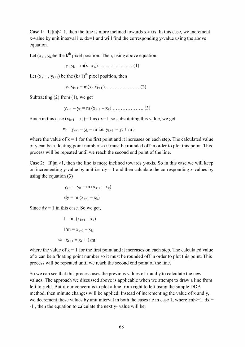
68

Case 1: If |m|<=1, then the line is more inclined towards x-axis. In this case, we increment

x-value by unit interval i.e. dx=1 and will find the corresponding y-value using the above

equation.

Let (xk , yk)be the kth pixel position. Then, using above equation,

y- yk = m(x- xk,)………………….(1)

Let (xk+1 , yk+1) be the (k+1)th pixel position, then

y- yk+1 = m(x- xk+1,)………………….(2)

Subtracting (2) from (1), we get

yk+1 – yk = m (xk+1 – xk) ………………..(3) Since in this case (xk+1 – xk)= 1 as dx=1, so substituting this value, we get

yk+1 – yk = m i.e. yk+1 = yk + m ,

where the value of k = 1 for the first point and it increases on each step. The calculated value

of y can be a floating point number so it must be rounded off in order to plot this point. This

process will be repeated until we reach the second end point of the line.


on incrementing y-value by unit i.e. dy = 1 and then calculate the corresponding x-values by

using the equation (3)

yk+1 – yk = m (xk+1 – xk)

dy = m (xk+1 – xk)

Since dy = 1 in this case. So we get,

1 = m (xk+1 – xk)

1/m = xk+1 – xk

xk+1 = xk + 1/m

where the value of k = 1 for the first point and it increases on each step. The calculated value

of x can be a floating point number so it must be rounded off in order to plot this point. This

process will be repeated until we reach the second end point of the line.

So we can see that this process uses the previous values of x and y to calculate the new

values. The approach we discussed above is applicable when we attempt to draw a line from

left to right. But if our concern is to plot a line from right to left using the simple DDA

method, then minute changes will be applied. Instead of incrementing the value of x and y,

we decrement these values by unit interval in both the cases i.e in case 1, where |m|<=1, dx =

-1 , then the equation to calculate the next y- value will be,

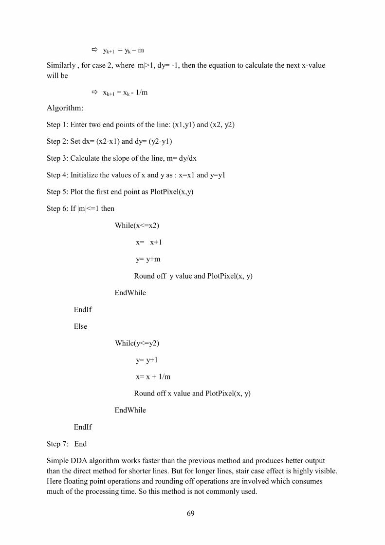
69

yk+1 = yk – m

Similarly , for case 2, where |m|>1, dy= -1, then the equation to calculate the next x-value

will be

Algorithm:

xk+1 = xk - 1/m

Step 1: Enter two end points of the line: (x1,y1) and (x2, y2)

Step 2: Set dx= (x2-x1) and dy= (y2-y1)

Step 3: Calculate the slope of the line, m= dy/dx Step 4: Initialize the values of x and y as : x=x1 and y=y1

Step 5: Plot the first end point as PlotPixel(x,y)

Step 6: If |m|<=1 then

While(x<=x2)

x= x+1

y= y+m

Round off y value and PlotPixel(x, y)

EndWhile

EndIf

Else

While(y<=y2)

y= y+1

x= x + 1/m

Round off x value and PlotPixel(x, y)

EndWhile

EndIf Step 7: End

Simple DDA algorithm works faster than the previous method and produces better output

than the direct method for shorter lines. But for longer lines, stair case effect is highly visible.

Here floating point operations and rounding off operations are involved which consumes

much of the processing time. So this method is not commonly used.

70

Example : Calculate all the intermediate points between the two end points (13,10) and

(21,20) using Simple DDA method of line drawing. Solution: (x1,y1)=(13,10) and (x2,y2)=(21,20)

dx= (x2- x1) = (21-13)= 8 and dy = (y2- y1) = (20 – 10) = 10

Slope of the line, m = dy/dx = 10/8= 5/4= 1.25 > 1

Since the value of m>1, this means our line is more inclined towards y-axis so we will

increment y by 1 and will find the corresponding x- value. We need 1/m here.

1/m= 4/5= 0.8 The following table will give all the points of the line.

x= x+1/m y=y+1 PlotPixel(x,y)

13

10

(13,10)

13+0.8= 13.8

11

(14,11)

13.8 + 0.8 = 14.6

12

(15,12)

14.6 + 0.8 = 15.4

13

(15,13)

15.4 + 0.8 = 16.2

14

(16,14)

16.2 + 0.8 = 17

15

(17,15)

17+ 0.8 = 17.8

16

(18,16)

17.8 + 0.8 = 18.6

17

(19,17)

18.6 + 0.8= 19.4

18

(19,18)

19.4 + 0.8 =20.2

19

(20,19)

20.2 + 0.8 = 21

20

(21,20)

3.3.3. Incremental DDA method of line drawing:

In this method, we increment both x and y coordinates at each step. We will use Δx and Δy as

x-extent and y-extent respectively which denotes change in x coordinate and change in y

coordinate. We include a variable called step and two more variable x-inc and y-inc that show

increment towards x-axis and y-axis respectively. There are again two cases that will

determine the orientation of the line.

Case 1: If |m|<=1, then the line is more inclined towards x-axis. Variable step= Δx .

71

Case 2: If |m|>1, then the line is more inclined towards y-axis. Variable step= Δy. In both the above cases, after finding the step value, we need to calculate x-increment and y-

increment which be added to x and y respectively at each step to computer new (x,y) values

from their previous values. They are calculated as:

x-inc = Δx / step

y-inc = Δy / step

This method is quite simpler and easier to understand but is also not used commonly because

of the time consuming rounding off and floating point arithmetic involved.


Step 2: Set Δx = (x2-x1) and Δy = (y2-y1)

Step 3: Calculate the slope of the line, m= Δy / Δx Step 4: If |m|<=1 then

step = Δx

else

step = Δy

EndIf Step 5: Calculate x-inc = Δx / step and y-inc = Δy / step

Step 6: Initialize the values of x and y as : x=x1 and y=y1


Step 8: For i= 1 to steps do

x= x + x-inc

y= y + y-inc

Round off x and y value and PlotPixel(x,y)

EndFor

Step 9: End Example: Scan convert a line by using incremental DDA method whose end points are (3,4)

and (9, 5).

72

Solution: (x1, y1)=( 3,4) and (x2,y2)= (9,5)

Δx = x2-x1 = 9 – 3 = 6 and Δy = y2-y1 = 5 – 4 = 1 Slope of the line, m = Δy /Δx = 1/6= 0.166 < 1

Since the value of m < 1, this means our line is more inclined towards x-axis so we will

increment x by 1 and will find the corresponding y- value.

step = Δx = 6

So, x-inc = Δx / step = 6 / 6 = 1

y-inc = Δy / step = 1 / 6 = 0.166 The following table will provide us all the points of the given line.

x= x+1 y= y+ y-inc PlotPixel(x,y)

3

4

(3,4)

3+1=4

4+0.166= 4.166

(4,4)

4+1=5

4.166+0.166= 4.332

(5,4)

5+1=6

4.332+0.166=4.498

(6,4)

6+1=7

4.498+0.166=4.664

(7,5)

7+1=8

4.664+0.166=4.83

(8,5)

8+1=9

4.83+0.166=4.996

(9,5)

3.3.4. Integer DDA method of line drawing:

Although simple DDA and incremental DDA are better than direct method but a lot of time is

wasted in rounding off and floating point operations. This makes these methods

comparatively slow. Integer Digital Differential Analyzer (DDA) method overcome these

drawbacks because in this method, floating point operation is eliminated and real values are

replaced with their integer parts. This method is faster than the previous methods discussed

so far.

We know that the plotted pixels are different from the actual points. We use this deviation

between the plotted pixels and the actual points of the line. Here a variable called dev will be

used that will check this deviation at each step. Since the first end point is plotted as such , so

initial deviation is set to zero. Let us discuss the two cases that decide the orientation of the

line.

73

Case 1: If |m|<=1, then the line is more inclined towards x-axis. We will increment x-

coordinate by unit interval and will calculate the y value at each step. Here two sub cases

arise.

i. If deviation is negative (i.e. dev < 0), this means that the plotted point lies below the actual point. So in order to make it aligned, we increment y coordinate by unit interval and will add (Δx – Δy) to deviation.

ii. If the deviation is positive (i.e. dev > 0), this means the plotted point is above the actual point, so in order to make it aligned, we do not increment y coordinate but will subtract Δy from the deviation.


on incrementing y-value by unit intervals and then find the corresponding x-values.

i. If deviation is negative (i.e. dev < 0), this means that the plotted point lies below the actual point. So in order to make it aligned, we increment x coordinate by unit interval and will add (Δy – Δx) to deviation.

ii. If the deviation is positive (i.e. dev > 0), this means the plotted point is above the actual point, so in order to make it aligned, we do not increment x coordinate but will subtract Δx from the deviation.

At the end, the deviation will again turn to zero value. This means that we have reached the

second end point of the line.



Step 3: Initialize deviation, dev = 0 Step 4: Calculate the slope of the line, m= Δy / Δx

Step 5: Initialize the values of x and y as : x=x1 and y=y1


Step 7: If |m| <= 1 then

While (x <= x2)

If dev < 0 then

x= x + 1

y= y + 1

dev= dev + (Δx – Δy )

Else

74

x= x + 1

dev= dev – Δy

EndIf

PlotPixel (x, y)

EndWhile

Else

While (y <= y2)

If dev < 0 then

y= y + 1

x= x + 1

dev= dev + (Δy – Δx )

Else

y= y + 1

dev= dev – Δx

EndIf

PlotPixel (x, y)

EndWhile

EndIf Step 8: End

Example: Find the points of the that can be plotted using Integer DDA method whose end

points are (3,4) and (9,8).

Solution: (x1, y1)=( 3,4) and (x2,y2)= (9,8)



increment x by 1 and will find the corresponding y- value. As the first point plotted will be

same as the first end point of the line, dev = 0 initially.

Δx – Δy = 6 – 4 = 2

75

The following table will give all the points of the line.

x = x+1 y dev PlotPixel(x,y)

3

4

0

(3,4)

4

4

0-4= -4

(4,4)

5

5

-4 +2 = -2

(5,5)

6

6

-2 + 2= 0

(6,6)

7

6

0-4 = -4

(7,6)

8

7

-4 + 2= -2

(8,7)

9

8

-2 + 2 = 0

(9,8)

As it can be seen from the above table that when the deviation is positive (i.e. >=0) then the

previous value of y is remained unchanged and Δy is subtracted from dev. When deviation

becomes negative, y is incremented by 1 and (Δx – Δy ) is added to dev. Check your progress / Self assessment questions

Q3. What is the difference between Direct method and DDA method of line drawing? ----------------------------------------------------------------------------------------------------------------

----------------------------------------------------------------------------------------------------------------

----------------------------------------------------------------------------------------------------------------

------------------------------------------ Q4. What are various DDA methods available to scan convert a line and how they differ from

each other?

----------------------------------------------------------------------------------------------------------------

----------------------------------------------------------------------------------------------------------------

----------------------------------------------------------------------------------------------------------------

------------------------------------------ 3.4. Bresenham line drawing algorithm and its derivation

Bresenham’s line drawing algorithm is widely used line drawing algorithm in computer

graphics. Earlier it was used to plot lines on digital plotter but now it is commonly used in

computer graphics. It was developed by Jack Bresenham of IBM and was later rectified by

various other researchers. It is the efficient algorithm because it makes use of only integer

arithmetic i.e. integer addition, subtraction and multiplication by 2. This method is faster than

the previously discussed methods as it eliminates the complex floating point and rounding off

operations that consumes most of the processing time.

76

First we have to calculate the slope of the line. As in other methods, there arises two cases.

The first one, when |m| <= 1, then the line is more inclined towards x-axis. Here we will

increment x-coordinate by unit interval and will calculate the corresponding y value. The

second case, when |m|>1, then the line is more inclined towards y-axis. So in this case we

will keep on incrementing y-value by unit intervals and then find the corresponding x-values.

3.4.1. Derivation:

Here we will derive the Bresenham’s line drawing algorithm for the case where slope of the

line is less than or equal to 1 (i.e. |m| <= 1). In this case, we are more inclined towards x axis

and we start from the first end point and increment x coordinate by unit interval. At each

point, we have two options of the pixel position that are candidates for plotting as shown in

the figure 3.5.

Let at the ith position, we have plotted the point (xi, yi). Then at the (i+1)th position, we will

increment xi by 1 i.e. xi+1 = xi + 1 and there will be two options for y-coordinate. These are yi

or yi+1. This means two candidate pixel positions are (xi + 1, yi ) and (xi + 1, yi+1 ).

We know slope intercept form of line: y= mx + b

where m is slope of the line and b is the y-intercept.

Using above equation, y = m xi + b at ith

position and similarly at (i+1)th position,

value of y coordinate will be

y = m (xi + 1) + b

…………………………………….. (1)

Let ‘s’ and ‘t’ be the distance between the

lower and the upper pixel positions from

the actual point on the line. On the basis

of this distance, we are going to decide

which pixel position is going to be

illuminated.

77

As it can be seen from the figure 3.6,

s = y - yi

t = yi+1 – y Here, y is the y value of the actual pixel position, yi is the y value of the previous plotted

pixel which is below the actual point and will remain unchanged for (i+1)th position and yi+1

is the y value which is above the actual point which is 1 more than the previous y value. This means y will take either of two values- yi or yi+1 . If s is smaller, then point yi will be chosen

and if t is smaller, then point yi+1 will be taken. This we see later on.

s – t = (y - yi ) – (yi+1 – y )

= y - yi - yi+1 + y

= 2y - yi - yi+1

As yi+1 = yi + 1, so substituting this value, we get

s – t = 2y - yi – (yi + 1)

= 2y - 2 yi - 1

Put y from (1), we get

s – t = 2 (m (xi + 1) + b ) - 2 yi - 1

s – t = 2 m (xi + 1) + 2b - 2 yi - 1

For the selection of next pixel position, we will include a decision parameter (di) at the ith

position that will take this decision. This parameter will examine which of the two candidate

pixels is more closer to the line. As we are moving on x axis by unit interval, so di has value:

78

di = Δx (s – t)

= Δx { 2 m (xi + 1) + 2b - 2 yi – 1}…………………………...... (2)

As m = Δy / Δx => Δx = Δy / m

di = Δx { 2 (Δy / Δx) (xi + 1) + 2b - 2 yi – 1}

= 2Δy (xi + 1) + 2bΔx - 2 yi Δx – Δx

= 2Δy xi + 2Δy + 2bΔx - 2 yi Δx – Δx

= 2 xi Δy – 2 yi Δx + 2Δy + 2bΔx – Δx

= 2 xi Δy – 2 yi Δx + k ………………………………………. (3)

where k = 2Δy + 2bΔx – Δx

Similarly at (i+1)th position,

di+1 = 2 xi+1 Δy – 2 yi+1 Δx + k ………………………………….. (4)

For the intermediate point, subtract (3) from (4)

di+1 - di = 2 xi+1 Δy – 2 yi+1 Δx + k – { 2 xi Δy – 2 yi Δx+ k }

= 2 xi+1 Δy – 2 yi+1 Δx + k – 2 xi Δy + 2 yi Δx- k

= 2Δy (xi+1 - xi) - 2Δx(yi+1 - yi) Because we are increasing x coordinate by unit interval, so xi+1 = xi + 1

di+1 - di = 2Δy (xi + 1- xi) - 2Δx(yi+1 - yi)

di+1 = di + 2Δy - 2Δx(yi+1 - yi) ………………………………………(5)

Now if we choose T point whose coordinates are (xi+1, yi+1), that means yi+1 = yi +1

Put this value in equation (5), we get

di+1 = di + 2Δy - 2Δx(yi +1- yi)

di+1 = di + 2Δy - 2Δx(1)

di+1 = di + 2Δy - 2Δx But if we choose S point whose coordinates are (xi+1, yi), that means yi+1 = yi

Substituting this value, we get

di+1 = di + 2Δy - 2Δx(yi - yi)

di+1 = di + 2Δy - 2Δx(0)

79

+ – ; ≥ . . + ; < 0 . .

di+1 = di + 2Δy

+ =

To find the initial decision parameter, put i =1 in equation (2)

d1 = Δx { 2 m (x1 + 1) + 2b - 2 y1 – 1}

= Δx { 2 m x1 + 2 m + 2b - 2 y1 – 1}

= Δx { 2 (m x1 + b - y1) + 2 m – 1}…………………………………. (6)

According to equation y = m x + b , y1 = m x1 + b => m x1 + b - y1 = 0

Put this value in equation (6), so we get

d1 = Δx { 2 (0) + 2 m – 1}

d1 = Δx {2 m – 1}

Substituting m = Δy / Δx,

d1 = Δx {2Δy / Δx – 1} d1 = 2Δy - Δx

Similarly we can derive Bresenham’s line drawing algorithm for slope |m| > 1. This is left as

an exercise.

3.4.2. Algorithm:

Step 1: Enter two end points of the line: (x1,y1) and (x2, y2)


Step 3: Calculate the slope of the line, m= Δy /Δx Step 4: Initialize the values of x and y as : x=x1 and y=y1


Step 6: Calculate decision parameter, d = 2 * Δy – Δx

Step 7: If |m| <= 1 then

While (x <= x2)

If d < 0 then

x= x + 1

d= d + 2*Δy

80

Else

x= x + 1

y= y + 1

d= d + 2*Δy – 2*Δx

EndIf

PlotPixel (x, y)

EndWhile

Else

While (y <= y2)

If d < 0 then

y= y + 1

d= d + 2*Δx

Else

y= y + 1

x= x + 1

d= d + 2*Δx – 2*Δy

EndIf

PlotPixel (x, y)

EndWhile

EndIf Step 8: End

Example 1: Scan Convert a line whose end points are (2,3) and (8,6) using Bresenham line

drawing algorithm.

Solution: (x1, y1)=( 2, 3) and (x2, y2)= (8, 6)




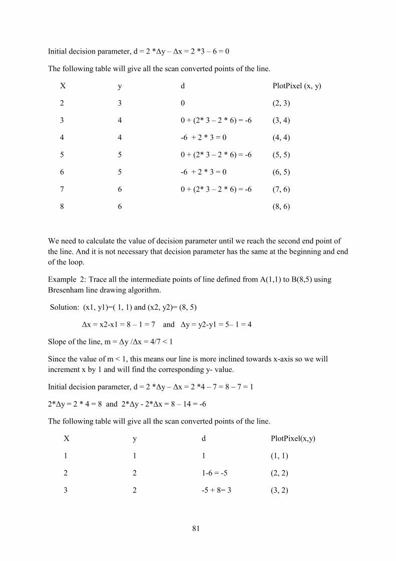
81

Initial decision parameter, d = 2 *Δy – Δx = 2 *3 – 6 = 0 The following table will give all the scan converted points of the line.

X y d PlotPixel (x, y)

2

3

0

(2, 3)

3

4

0 + (2* 3 – 2 * 6) = -6

(3, 4)

4

4

-6 + 2 * 3 = 0

(4, 4)

5

5

0 + (2* 3 – 2 * 6) = -6

(5, 5)

6

5

-6 + 2 * 3 = 0

(6, 5)

7

6

0 + (2* 3 – 2 * 6) = -6

(7, 6)

8

6

(8, 6)

We need to calculate the value of decision parameter until we reach the second end point of

the line. And it is not necessary that decision parameter has the same at the beginning and end

of the loop.

Example 2: Trace all the intermediate points of line defined from A(1,1) to B(8,5) using

Bresenham line drawing algorithm.


Δx = x2-x1 = 8 – 1 = 7 and Δy = y2-y1 = 5– 1 = 4 Slope of the line, m = Δy /Δx = 4/7 < 1



Initial decision parameter, d = 2 *Δy – Δx = 2 *4 – 7 = 8 – 7 = 1 2*Δy = 2 * 4 = 8 and 2*Δy - 2*Δx = 8 – 14 = -6

The following table will give all the scan converted points of the line.

X y d PlotPixel(x,y)

1 1 1 (1, 1)

2 2 1-6 = -5 (2, 2)

3 2 -5 + 8= 3 (3, 2)

82

4 3 3 - 6 = -3 (4, 3)

5

3

-3 + 8 = 5

(5, 3)

6

4

5 – 6 = -1

(6, 4)

7

4

-1 + 8 = 7

(7, 4)

8

5

(8, 5)

Let us give some examples where the slope of the line is negative. All the signs in calculating

decision parameter at each step will be reversed.

Example 3: Scan convert a line using Bresenham line drawing algorithm where end points of

the line are A(0, 6) and B(4, 0).


Δx = x2-x1 = 4 – 0 = 4 and Δy = y2-y1 = 0 – 6 = -6 Slope of the line, m = Δy /Δx = -6/4= - 1.5

|m| = |-1.5|= 1.5 > 1 i.e. our line is more inclined towards y-axis. As we can see that initial y

coordinate is higher than second end point so we will decrement y value by 1 at each step and

will increment x value according to the algorithm.

Initial decision parameter, d = - 2 *Δx + Δy = -2 *4 + 6 = -8 + 7 = -2 2*Δx = 2 * 4 =8 and 2*Δx + 2*Δy = 8 – 12= -4

If d>0, d = d - 2*Δx else d = d – (2*Δx + 2*Δy)

If d is negative, x will be incremented else it will remain the same.

The following table will give all the scan converted points of the line.

X y d PlotPixel(x, y)

0 6 -2 (0, 6)

1 5 -2 – (-4)= 2 (1, 5)

1 4 2 – (8)= -6 (1, 4)

2 3 -6 – (-4)= -2 (2, 3)

3 2 -2 – (-4)= 2 (3, 2)

3 1 2 – (8)= -6 (3, 1)

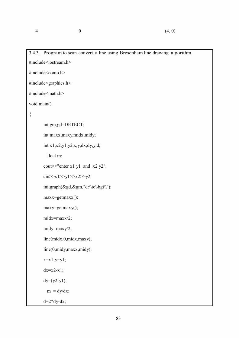
83

4 0 (4, 0)

3.4.3. Program to scan convert a line using Bresenham line drawing algorithm.

#include<iostream.h> #include<conio.h>

#include<graphics.h>

#include<math.h>

void main()

{

int gm,gd=DETECT;

int maxx,maxy,midx,midy;

int x1,x2,y1,y2,x,y,dx,dy,y,d;

float m;

cout<<"enter x1 y1 and x2 y2";

cin>>x1>>y1>>x2>>y2;

initgraph(&gd,&gm,"d:\\tc\\bgi\\");

maxx=getmaxx();

maxy=getmaxy();

midx=maxx/2;

midy=maxy/2;

line(midx,0,midx,maxy);

line(0,midy,maxx,midy);

x=x1;y=y1;

dx=x2-x1;

dy=(y2-y1);

m = dy/dx;

d=2*dy-dx;

84

if(fabs(m)<=1)

{

while(x<=x2)

{

putpixel(midx+x,midy-y,15);

if(d>=0)

{

d+=(2*dy – 2*dx);

y=y+1;

}

else

{

d+=2*dy;

}

x=x+1;

}

}

else

{

while(y<=y2)

{

putpixel(midx+x,midy-y,15);

if(d>=0)

{

d+=(2*dx – 2*dy);

x=x+1;

}

85

else

{

d+=2*dx;

}

y=y+1;

}

}

getch();

closegraph();}

3.4.4. Differences between DDA and Bresenham line drawing algorithm

S.no. Criteria DDA algorithm Bresenham algorithm

1. Arithmetic

operation

This algorithm uses real i.e.

floating point arithmetic. It uses

multiplication and division in its

operation.

This algorithm uses only fixed point

i.e. integer arithmetic operations.

Only addition and subtraction is

involved.

2. Speed This algorithm is slower than

Bresenham algorithm because it

works with real numbers.

It runs faster as compared to other

methods.

3. Accuracy Results provided by DDA are not

as accurate as provided by

Bresenham’s algorithm.

This is the most accurate and

efficient line drawing algorithm.

4. Round off operation It makes use of round off operation

because of the floating point

arithmetic.

There is no need of any rounding off

operation.

5. Expensive It is expensive because it

consumes much of the processing

time since there are complex

floating point and round off

operations being involved.

It is less expensive since it runs

faster because it deals only with

integers.

Check your progress / Self assessment questions

86

Q5. Why is Bresenham line drawing algorithm the most efficient among various scan

converting methods of line?

----------------------------------------------------------------------------------------------------------------

----------------------------------------------------------------------------------------------------------------

----------------------------------------------------------------------------------------------------------------

------------------------------------------ 3.5. Summary

Scan conversion is an important operation in computer graphics. It illuminates the pixel

positions that will make the complete picture. We have discussed about various line drawing

methods. Line is a primitive that is used in almost every image so it is important to learn how

we can scan convert an image. Direct method is the simplest among all the methods but is

very inefficient because every time, x and y values are calculated without using any previous

values. DDA methods are better than the direct method since it reduces the computation time

and hence provides better throughput. Both Direct and DDA methods except integer DDA

involve large number of rounding off and floating point operations that make these methods

time consuming. Bresenham line drawing method is the most accurate method and provides

faster results because it involves only integer arithmetic.

3.6. Glossary Pixel – A pixel (short form of ‘picture element’) is the smallest dot that makes up the

complete image in a computer memory.

Scan conversion – The process that involves plotting the objects on a display screen by

illuminating discrete pixel positions is called scan conversion.

3.7. Answers to check your progress / self assessment questions 1. True.

2. We need to scan convert a point because point is a basic element that makes up a complete

image. We use the function PlotPixel(x, y) in the process of scan conversion of any graphics

primitive which is function that plots a single point. All the calculated values of the point

should be converted into their integer counterpart so that this point can be plotted.

3. Direct method is the simplest method with less efficiency. In this method, x and y-values

are calculated from scratch at each step without using the previous values. DDA (Digital

Differential Analyzer) method is faster as compared to direct method. It uses the previous

values of x and y to calculate their next values.

4. There are various DDA methods such as Simple DDA, Incremental DDA and Integer

DDA. Simple DDA uses the previous values of x and y to calculate the new values by using

the formula. In Incremental DDA, both x and y coordinates are incremented by a fixed

amount at each step. In Integer DDA method, floating point operation is eliminated and real

87

values are replaced with their integer parts. This method is faster than the other DDA

methods. 5. Bresenham line drawing algorithm is the most efficient among various scan converting

methods of line because there is no floating point and rounding off operation involved in this

method. It works faster and provides more accurate results. Aliasing effect is less visible in

Bresenham method.

3.8. Model Questions

1. What is scan conversion in computer graphics?

2. What are various line drawing algorithms? Explain in brief.

3. Explain Bresenham line drawing algorithm with example.

4. Differentiate between DDA and Bresenham line algorithm. Which is the accurate line

drawing algorithm? Explain in brief.

5. Indicate the raster positions that will be illuminated by Bresenham line algorithm,

when scan converting a line from A(3,7) to B(6,1).

6. Scan convert a line using Bresenham’s line algorithm whose end points are P (-2, -1)

and Q (4, 5).

7. Trace all the points of the line whose end points are (-6, 4) and (-2, -5) using

Bresenham line algorithm.

88

Lesson-04

Scan converting techniques for circle Structure of the chapter

4.0. Objective

4.1. Scan converting a circle

4.2. Algorithms for scan converting a circle

4.2.1. Direct method of Circle Drawing

89

4.2.2. Trigonometric method of Circle Drawing 4.3. Bresenham’s Circle drawing algorithm and its derivation

4.3.1. Derivation

4.3.2. Algorithm to scan convert a circle using Bresenham’s circle drawing

4.3.3. Program to scan convert a circle using Bresenham circle drawing

algorithm

4.4. MidPoint Circle drawing algorithm and its derivation

4.4.1. Derivation

4.4.2. Algorithm to scan convert a circle using MidPoint circle drawing

4.4.3. Program to scan convert a circle using MidPoint circle drawing algorithm 4.5. Summary

4.6. Glossary

4.7. Answers to check your progress / self assessment questions



Explain scan conversion of a circle. Explain various methods of scan converting a circle. Explain Bresenham circle drawing algorithm. Explain MidPoint Circle drawing algorithm. Solve some problems based on scan conversion of a circle.

4.1. Scan converting a circle Circle is one of the most widely used shape in drawing pictures and graphs and in computer

graphics, various procedures are developed to draw complete circles or any portion of it such

as arcs and sectors.

A circle is such a geometric shape that is defined by a center position and a fixed distance

from the center which is called radius. It is drawn by combining all the points that are at a

fixed distance from the center. Scan converting a circle requires each point on the

circumference of the circle to be illuminated. Various algorithms and techniques are

employed in computer graphics to scan convert a circle that uses equation of circle. The

90

Polynomial equation of the circle in Cartesian coordinates whose center is C ( h, k) and

radius is r units is given as

(x – h)2 + (y – k)2 = r2

Let us see how this equation has been derived. Pythagoras theorem is being used to derive

this standard equation of a circle.

As it can be seen from above figure that in a right angled triangle ΔPCQ,

CP = r , PQ = y – k , CQ = x – h

Using Pythagoras theorem,

CQ2 + PQ2 = CP2

(x – h)2 + (y – k)2 = r2

Another widely used equation of circle is by using polar coordinates. The equations to

calculate any arbitrary position on circle P(x,y) are given as:

x = h + r cosθ

y = k + r sinθ

Now let us see how these equations are derived. Using figure 4.1, in right angled triangle

ΔPCQ,

cosθ = i.e cosθ =

x – h = r cosθ

91

x = h + r cosθ Similarly, sinθ = i.e sinθ =

y – k = r sinθ

y = k + r sinθ

Check your progress/ Self assessment questions

Q1. Write the equation of circle in Cartesian coordinates and in polar coordinates. ----------------------------------------------------------------------------------------------------------------

----------------------------------------------------------------------------------------------------------------

---------------------------- 4.2. Algorithms for scan converting a circle

Circle is a symmetrical geometric shape. It can be drawn by using two way, four way or eight

way symmetry. There are various algorithms available that helps in scan converting a circle

and each of them employ some symmetry. Here is a brief description about symmetry of the

circle:

Two-way symmetry:In this symmetry, we calculate points for only half of the circle (i.e.

semicircle). Since it is symmetrical about its diameter, we just

copy those points to other semicircle to make it a complete circle.

For example, if we are scan converting a circle about x- axis,

then each x-value will have two corresponding y-value ( whose

magnitude is same but one is above x- axis and other is below x-

axis). So here we need to find single pixel position and other will

be foung by inverting the sign of its y-value. Two way symmetry

is shown in figure 4.2.

Four-way symmetry: A circle deals with greater symmetry. In

four way symmetry, instead of computing values for semicircle,

we just need to find the values for quadrant of the circle. We

know that there are four quadrants in a circle and each value in

first quadrant has three corresponding values in other three

quadrants. For example, there is value (x, y) in first quadrant, other three values will be (-x,

y) in second quadrant, (-x, -y) in third quadrant and (x, -y) in fourth quadrant. It is shown in

figure 4.3.

92

hod is also called Polynomial

his method uses polynomial

Eight-way symmetry:We can save computation time by using 8 – way symmetry of the

circle in which we compute pixel positions only for one octant and rest of the pixel

positions for other octants can be computed from that value. For example, if we have

computed (x, y) in 1st octant, then seven other corresponding values will be (x, -y), (-

x,y), (-x,-y), (y,x), (y,-x), (-y,x),(-y,-x). hence, we are dealing with only 1/8th part of the

circle and from that we can generate the complete circle. It is shown in figure 4.4. Various circle drawing algorithms are discussed in the following sub sections:

4.2.1. Direct method of Circle drawing:

Direct met

method. T

equation

of the

circle. It

is the

simplest

among

all the

algorith

ms. Let

us

discuss

it with

two way

93

symmetry, we are supposed to draw a circle about x – axis. As it can be seen from figure 4.5,

we will start from (h - r) and end at (h + r) where (h , k) are the center coordinates and r is

radius of the circle.

(x – h)2 + (y – k)2 = r2

Here we will increment x- axis by unit interval and will calculate the corresponding y- value

using the formula,

= ± − ( − ℎ)

As we know that pixel positions are discrete integer values, so we need to round off y- value

every time we want to plot a point (x, y).

Algorithm to scan convert a circle using two-way symmetry: Step 1: Enter center of circle C (h, k) and radius = r units

Step 2: Initialize x = h – r and y = k

Step 3: Plotpixel(x, y)

Step 4: While ( x <= (h+r) )

y = ± − ( − ℎ)

Round off y-coordinate and PlotPixel (x, y)

x = x + 1

EndWhile Step 5: End

This algorithm is slower since it takes a lot of processing time. So this algorithm is not so

good. Hence we move towards 4-way symmetry. In this case, we start x from h instead of (h

– r) and will end at (h+r) i.e. 1st quadrant. The formula to calculate y value corresponding to

the values of x in 1st quadrant is given as:

= + − ( − ℎ)

We have taken only positive sign because in first quadrant, both x and y coordinates are

positive. For one (x, y) value, other three values will be (- x, y), (- x, -y) and (x, -y) as it can

be seen from figure 4.6.

94

Algorithm to scan convert a circle using four-way symmetry: Step 1: Enter center of circle C (h, k) and radius = r units

Step 2: Initialize x = h and y = r

Step 3: While ( x <= (h+r) )

y = + − ( − ℎ)

Round off y-coordinate

PlotPixel (x, y) , PlotPixel (-x, y)

PlotPixel (x, - y) , PlotPixel (- x,- y)

x = x + 1


Although this algorithm works faster as compared to previous algorithm but we can better

utilize the symmetry by using 8-way symmetry. 8-way symmetry works faster among all and

consumes less processing time. Here we start from x = h and will end at √ 2. Let us see how

this value comes. From figure 4.7, in ΔPOQ which is right angled at Q,

cosθ =

95

here θ = 45° i.e.

cos 45° =

= √

x = √ 2 At Q.

For one pixel position (x, y) in one octant, we have other seven values as (x, -y), (-x,y), (-x,- y), (y,x), (y,-x), (-y,x),(-y,-x) .

Algorithm to scan convert a circle using eight-way symmetry:

Step 1: Enter center of circle C (h, k) and radius = r units

Step 2: Initialize x = h and y = r

Step 3: While ( x <= √ 2 )

y = + − ( − ℎ)

Round off y-coordinate

PlotPixel (x, y) ,

PlotPixel (y, x)

PlotPixel (-x, y) ,

PlotPixel (-y, x)

PlotPixel (x,- y) ,

PlotPixel (y, -x)

PlotPixel (- x,- y) ,

PlotPixel (- y,- x)

x = x + 1


Program to scan convert a circle using Polynomial method (by using eight way

symmetry).

#include<iostream.h> #include<conio.h>


96

#include<math.h> int h,k,midx,midy;

void plot8points(int x,int y);

void main()

{

int gm,gd=DETECT;

int x;

float r,y;

cout<<"enter h & k:";

cin>>h>>k;

cout<<"enter radius:";

cin>>r;

initgraph(&gd,&gm,"d:\\tc\\bgi");

int maxx,maxy;

maxx=getmaxx();

maxy=getmaxy();

midx=maxx/2;

midy=maxy/2;



x=0;

y=r;

while(x<=y)

{

plot8points(x,(int)(y+0.5));

x=x+1;

y=sqrt(r*r-x*x);

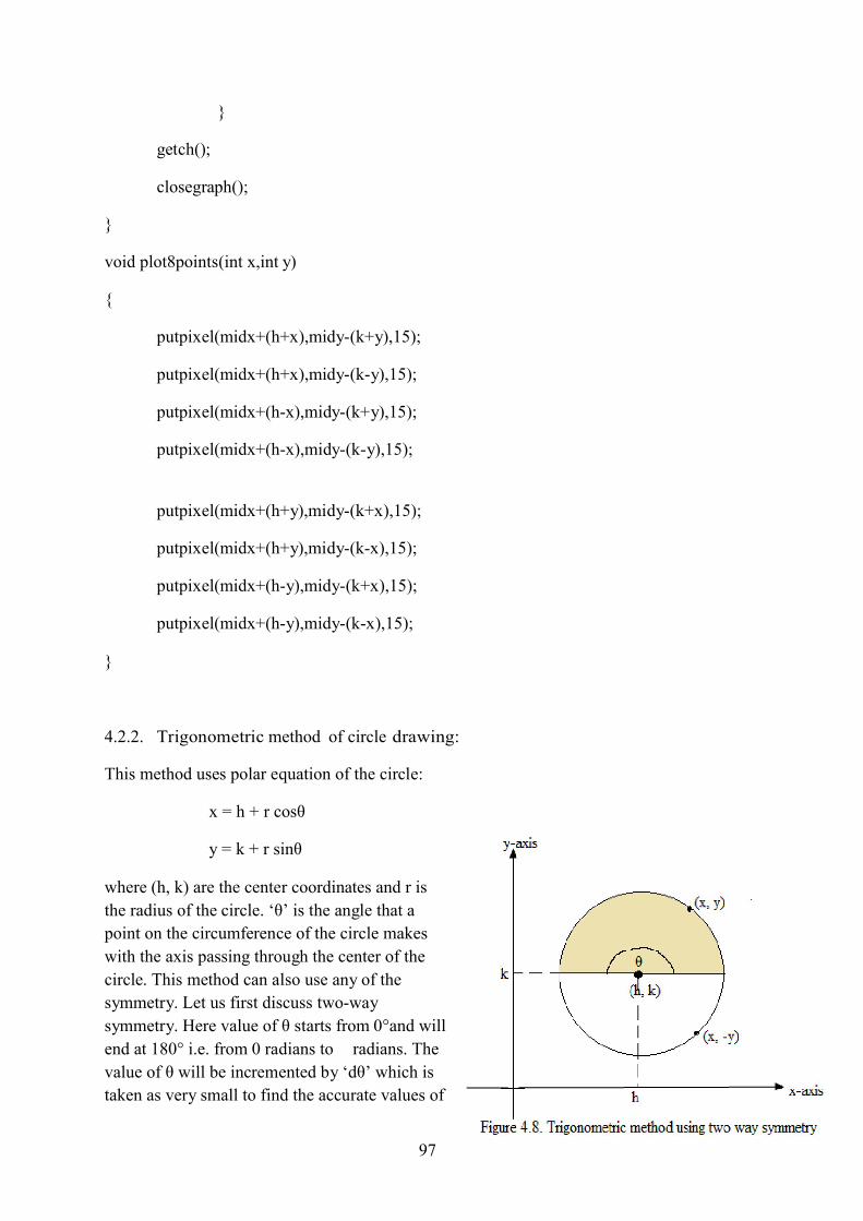
97

}

getch();

closegraph();

} void plot8points(int x,int y)

{

putpixel(midx+(h+x),midy-(k+y),15);

putpixel(midx+(h+x),midy-(k-y),15);

putpixel(midx+(h-x),midy-(k+y),15);

putpixel(midx+(h-x),midy-(k-y),15);

putpixel(midx+(h+y),midy-(k+x),15);

putpixel(midx+(h+y),midy-(k-x),15);

putpixel(midx+(h-y),midy-(k+x),15);

putpixel(midx+(h-y),midy-(k-x),15);

}

4.2.2. Trigonometric method of circle drawing: This method uses polar equation of the circle:

x = h + r cosθ

y = k + r sinθ

where (h, k) are the center coordinates and r is

the radius of the circle. ‘θ’ is the angle that a

point on the circumference of the circle makes

with the axis passing through the center of the

circle. This method can also use any of the

symmetry. Let us first discuss two-way

symmetry. Here value of θ starts from 0°and will

end at 180° i.e. from 0 radians to radians. The

value of θ will be incremented by ‘dθ’ which is

taken as very small to find the accurate values of

98

(x, y) at each step. Although we can take any value of dθ, but just to keep it small, we take it

as 1/r. After finding values for semi-circle, we invert the sign for y-value to calculate values

for other semi-circle.

Algorithm to draw a circle using two-way symmetry:

Step1: Enter center of circle C (h, k) and radius = r units

Step 2: Initialize theta to 0 and dtheta = 1/ r

Step 3: While (theta < = )

x = h + r cos(theta)

y = k + r sin(theta)

Round off both x and y values

PlotPixel(x, y)

PlotPixel(x, - y)

theta = theta + dtheta


As discussed in previous algorithm, we can use

four-way symmetry to reduce the processing time

and increase the efficiency. Here we start with θ =

0°and will end at 90° i.e. from 0 radians to /2

radians. So by finding value in one quadrant, we can calculate corresponding values in rest of the quadrants. For each value (x, y) we have three values (x, -y), (-x, y) and (-x, -y). We can

use dθ as 1/r but for the sake of simplicity we have increased θ by unit interval in this case.

Algorithm to draw a circle using four-way symmetry:


Step 2: Initialize theta to 0

Step 3: While (theta < = /2)




PlotPixel(x, y) PlotPixel(-x, y)

99

PlotPixel(x, - y) PlotPixel(-x, - y)

theta = theta + 1


In order to further reduce the processing time,

we can take the advantage of eight way

symmetry in which we start θ from 0° and will

continue upto θ = 45° i.e from 0 radians to /4

radians. By doing so we are traversing only the octant of the circle but we are able to draw the

complete circle by using the points in one

octant. One pixel position (x, y) has seven

values in other octants which are (x, -y), (-x,y),

(-x,-y), (y,x), (y,-x), (-y,x), (-y,-x) .

Algorithm to draw a circle using eight-way symmetry:



Step 3: While (theta < = /4)




PlotPixel(x, y) PlotPixel(y, x)

PlotPixel(x, - y) PlotPixel(y, - x)

PlotPixel(-x, y) PlotPixel(-y, x)

PlotPixel(-x, - y) PlotPixel(-y, - x)

theta = theta + 1


Program to scan convert a circle using Trigonometric method (by using eight way

symmetry).

#include<iostream.h>

100

#include<conio.h> #include<math.h>


#define Pi 3.142

void plot8points(int,int);

int midx,midy;

float h,k,x,y;

void main()

{

int gm,gd=DETECT;

int maxx,maxy;

float r;

cout<<"enter h,k and r";

cin>>h>>k>>r;


maxx=getmaxx();

maxy=getmaxy();

midx=maxx/2;

midy=maxy/2;



int i;

for(i=0;i<=45;i++)

{

x=r*cos(i*Pi/180); y=r*sin(i*Pi/180);

plot8points((int)(x+0.5),(int)(y+0.5));

101

}

getch();

closegraph();


{








putpixel(midx+(h-y),midy-(k-x),15); }

Two important and efficient circle drawing algorithms are explained in the following

sections. Check your progress/ Self assessment questions

Q2. Among the different types of symmetry, which symmetry is more efficient and why? ----------------------------------------------------------------------------------------------------------------

----------------------------------------------------------------------------------------------------------------

----------------------------------------------------------------------------------------------------------------

------------------------------------------ 4.3. Bresenham’s Circle drawing algorithm and its derivation

This algorithm is better than previously discussed methods. Processing time is sufficiently

reduced because complex square root and multiplication operations are removed in this

method. It just includes integer addition and subtraction. This method uses eight-way

symmetry of the circle. At every plotted point, we have two options to plot next point. So a

102

decision parameter (d) is used here that will decide which of the two locations is closer to the

circumference of the circle. In this algorithm we will move towards x-axis and will find the

corresponding closest y-coordinate. It is an incremental approach of circle drawing.

4.3.1. Derivation:

In this method, we just find the points in the first octant of the first quadrant i.e. we will start

at x = 0 and will continue till x< = y. Suppose at ith position, plotted pixel is (xi , yi ). At

position (i + 1)th , we have two candidate y-coordinates for xi+1 = xi + 1 as shown in figure

4.11. These candidate locations are marked as S(xi + 1 , yi -1) and T(xi + 1 , yi ).

From the above figure, it can be seen that if we generating points from 90° to 45°(i.e. from x=

0 to x= y), each new pixel position closest to the actual circumference of the circle can be

found by taking either of the two actions:

i. moving in the x-direction by unit interval and not changing the y-coordinate. ii. moving in the x-direction by unit interval and moving in the negative y-direction by

unit interval (i.e. decrementing y-coordinate by unit interval).

Distance of the pixel T from the origin is calculated by using distance formula i.e.

CT = (x + 1) + y

Similarly Distance of the pixel S from the origin is given as

CS = (x + 1) + (y − 1)

103

Here we are using a function D( ) that provides a relative measurement of the distance from

the center of the pixel from the actual circle. Let D(T) be the square of the distance from the

origin to the pixel T minus square of the distance to the actual circle ( i.e. r (radius)).

D(T) = CT2 – r2

D(T) = (x + 1) + y - r2

Let D(S) be the square of the distance from the origin to the pixel S minus square of the distance to the actual circle.

D(S) = CS2 – r2

D(S) = (x + 1) + (y − 1) - r2

Since T point lies outside the actual circle so D(T) is always positive but D(S) is negative because point S lies inside the circle. The decision parameter is defined as the sum of D(S)

and D(T) and is given as:

di = D(S) + D(T)

di = (x + 1) + (y − 1) - r2 + (x + 1) + y - r2

di = 2(x + 1) + y + (y − 1) - 2r2

…………………………………………(1)

If di< 0 (i.e. D(S) > D(T)), then in this case, point T is closer to the circle and will be plotted

otherwise point S is closer and will be illuminated.

Decision parameter at (i+1)th position is given as

di+1 = 2(x + 1) + y + (y − 1) - 2r2

………………………………..(2) Subtracting (1) from (2), we get

di+1 - di = 2(x + 1) + y + (y − 1) - 2r2 – {2(x + 1) + y + (y − 1) - 2r2}

As x = x + 1, so

104

di+1 = di + 4 xi +2 (y - y ) – 2 (yi+1 - yi ) + 6

……………………………....................(3) If we choose point T, then put yi+1 = yi, in (3)

di+1 = di + 4 xi +2 (y - y ) – 2 (yi - yi ) + 6

di+1 = di + 4 xi + 6 If we choose point S, then put yi+1 = yi – 1 in (3)

di+1 = di + 4 xi +2 {(y − 1) - y } – 2 {(yi -1) - yi } + 6

di+1 = di + 4( xi - yi ) + 10

+ + ; < . . =

+ ( − ) + ; ≥ 0 . .

To find the starting decision parameter, we need to put the starting point i.e. (0, r) in

equation(1)

d1 = 2(x + 1) + y + (y − 1) - 2r2

d1 = 2(0 + 1) + r + (r− 1) - 2r2

d1 = 2 + r + r + 1 - 2r - 2r2

d1 = - 2r

4.3.2. Algorithm to scan convert a circle using Bresenham’s circle drawing


Step 2: Initialize x to 0 and y to r

Step 3: Calculate decision parameter d= 3 - 2r

Step 4: While (x <= y)

If(d < 0) then

x = x + 1

d = d + 4x + 6

else

105

x = x + 1

y = y – 1

d = d + 4(x – y) + 10

EndIf

PlotPixel (x + h, y + k) PlotPixel (y + h, x + k)

PlotPixel (-x + h, y + k) PlotPixel (-y + h, x + k)

PlotPixel (x + h, -y + k) PlotPixel (y + h, -x + k)

PlotPixel (-x + h, -y + k) PlotPixel (-y + h, -x + k)


4.3.3. Program to scan convert a circle using Bresenham circle drawing method


#include<conio.h>


#include<math.h>

float h,k;

int midx,midy;


void main()

{

int gm,gd=DETECT;

int x;

float r,y,d;


cin>>h>>k;


cin>>r;

106


int maxx,maxy;

maxx=getmaxx();

maxy=getmaxy();

midx=maxx/2;

midy=maxy/2;



x=0;

y=r;

d=3-2*r;

while(x<=y)

{


if(d<0)

{

d=d+4*x+6;

}

else

{

d=d+4*(x-y)+10;

y=y-1;

}

x=x+1;

}

107

getch();

closegraph();


{









}

Example 1: Scan Convert a circle whose center is (50, 60 ) and radius is 8 units using

Bresenham Circle drawing algorithm. Solution: (h , k) =(50 , 60) and r = 8

Initial decision parameter , d = 3 – 2r = 3 – 2 * 8 = 3 – 16 = -13

We will increment x coordinate by unit interval at each step and will find the corresponding y

coordinate. The following table gives all the points in the first octant of the circle.

x y d (x, y) PlotPixel(x+h, y+k) 0 8 -13 (0, 8) (50, 68)

1 8 -13 + 4(1) + 6 = -3 (1, 8) (51, 68)

2 8 -3 + 4(2) + 6 = 11 (2, 8) (52, 68)

3 7 11 + 4(3 - 7) + 10 = 5 (3, 7) (53, 67)

4 6 5 + 4(4 – 6) + 10 = 7 (4, 6) (54, 66)

108

5 5 (5, 5) (55, 65)

We will stop when the value of both x and y are same. So there is no need to calculate

decision parameter at this step. Check your progress/ Self assessment questions

Q3. What is the value of initial decision parameter in Bresenham Circle Drawing Algorithm? ----------------------------------------------------------------------------------------------------------------

----------------------------------------------------------------------------------------------------------------

---------------------------- 4.4. Mid-Point circle drawing algorithm and its derivation

This algorithm is like Bresenham’s algorithm. Here also we start from x=0 and will continue

till x< = y. It is also an incremental approach of circle drawing. In this algorithm, we will

consider the point that will lie in the middle of two candidate pixel points to determine which

among the two candidate pixel positions will be plotted.

4.4.1. Derivation: As shown in figure 4.12, the point in the middle of points S(xi + 1 , yi -1) and T(xi + 1 , yi ) is

calculated by using mid-point formula i.e.

M = ( , ) = ( , ) = (x + 1, − )

We know that equation of circle whose center is (0, 0) and radius = r units is given as :

x2 + y2 = r2 i.e. x2 + y2 - r2 = 0

To define this equation, we choose a function f(x, y) that will define any point on the circle

i.e.

f(x, y) = x2 + y2 - r2 = 0 This function always gives 0 for all the points that lie on the circle. Its value will be negative

(i.e. < 0) if the points are inside and will be positive (i.e. > 0) if the points lie outside the

circle.

The decision parameter (d) for this algorithm at position ‘i’ is defined as

di = f (x + 1, y − )

di = (x + 1)2 + ( y − )2 - r2

………………………………………………………(1)

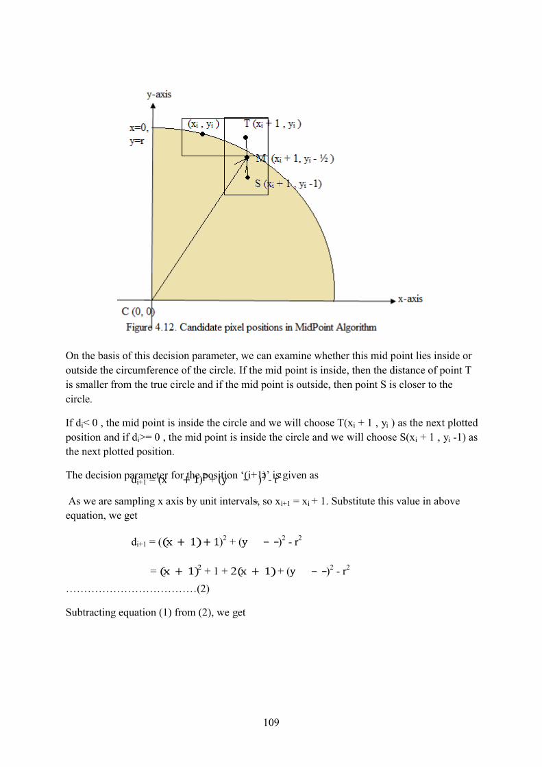
109

On the basis of this decision parameter, we can examine whether this mid point lies inside or

outside the circumference of the circle. If the mid point is inside, then the distance of point T

is smaller from the true circle and if the mid point is outside, then point S is closer to the

circle.

If di< 0 , the mid point is inside the circle and we will choose T(xi + 1 , yi ) as the next plotted

position and if di>= 0 , the mid point is inside the circle and we will choose S(xi + 1 , yi -1) as

the next plotted position. The decision parameter for the position ‘(i+1)’ is given as di+1 = (x + 1)2 + (y − )2 - r2

As we are sampling x axis by unit intervals, so xi+1 = xi + 1. Substitute this value in above

equation, we get

di+1 = ((x + 1)+ 1)2 + (y − )2 - r2

= (x + 1)2 + 1 + 2(x + 1) + (y − )2 - r2

………………………………(2)

Subtracting equation (1) from (2), we get

110

= 2(x + 1) + 1 + y + − y − y − + y

= 2(x + 1) + 1 + y − y − y + y

= 2(x + 1) + 1 + (y − y ) − (y − y )

di+1 = di + 2(x + 1) + 1 + (y − y ) − (y − y )

……………………………………...(3)

If we choose T point, then y = y so

di+1 = di + 2(x + 1) + 1 + (y − y ) − (y − y )

di+1 = di + 2x + 2 + 1 + 0 − 0

di+1 = di + +

If we choose S point, then y = y − 1 so

di+1 = di + 2(x + 1) + 1 + ((y − 1) − y ) − (y − 1 − y )

di+1 = di + 2(x + 1) + 1 + y + 1 − 2 − y + 1

di+1 = di + 2x + 2 + 1 − 2 + 1 + 1

di+1 = di + ( − ) +

+ + ; < . .

= + ( − ) + ; ≥ 0 . .

For finding initial decision parameter, put (0, r) in equation (1),

d1 = (0+1)2 + (r – ½)2 – r2

d1 = 1 + r2 + ¼ -r - r2

d1 = 5/4 – r

Now integer value of 5/4 can be used as 1 just to keep our decision parameter an integer

value,

d1 = 1 – r 4.4.2. Algorithm to scan convert a circle using MidPoint circle drawing algorithm


111

Step 2: Initialize x to 0 and y to r Step 3: Calculate decision parameter d= 1 - r

Step 4: While (x <= y)

If(d < 0) then

x = x + 1

d = d + 2x + 3

else

x = x + 1

y = y – 1

d = d + 2(x – y) + 5

EndIf

PlotPixel (x + h, y + k) PlotPixel (y + h, x + k)

PlotPixel (-x + h, y + k) PlotPixel (-y + h, x + k)

PlotPixel (x + h, -y + k) PlotPixel (y + h, -x + k)

PlotPixel (-x + h, -y + k) PlotPixel (-y + h, -x + k)


4.4.3. Program to scan convert a circle using MidPoint circle drawing method


#include<conio.h>


#include<math.h>

float h,k;

int midx,midy;


void main()

{

112

int gm,gd=DETECT;

int x;

float r,y,p;


cin>>h>>k;


cin>>r;


int maxx,maxy;

maxx=getmaxx();

maxy=getmaxy();

midx=maxx/2;

midy=maxy/2;



x=0;

y=r; p=1- r;

while(x<=y)

{


if(p<0)

{

p=p+2*x+3;

}

else

{

113

p=p+2*(x-y)+5;

y=y-1;

}

x=x+1;

}

getch();

closegraph();


{









}

Example: Using MidPoint Circle generating algorithm, trace all the points which center (0,

0) and radius is 10 units. Solution: (h , k) =(0 , 0) and r = 10

Initial decision parameter , d = 1 – r = 1 – 10 = - 9

We will increment x coordinate by unit interval at each step and will find the corresponding y

coordinate. The following table gives all the points in the first octant of the circle.

x y d (x, y) PlotPixel(x+h, y+k) 0 10 -9 (0, 10) (0, 10)

114

1 10 -9+ 2(1) +3 = -4 (1, 10) (1, 10)

2

10

-4 + 2(2) + 3 = 3

(2, 10)

(2, 10)

3

9

3 +2(3 - 9) + 5 = -4

(3, 9)

(3, 9)

4

9

-4 + 2(4) + 3 = 7

(4, 9)

(4, 9)

5

8

7 + 2(5 - 8) + 5 = 6

(5, 8)

(5, 8)

6

7

6 + 2( 6 – 7) + 5 = 9

(6, 7)

(6, 7)

7

6

Stop here

- -


Q4. What is the value of initial decision parameter in MidPoint Circle Drawing Algorithm?

----------------------------------------------------------------------------------------------------------------

----------------------------------------------------------------------------------------------------------------

----------------------------

4.5. Summary

Circle is one of the most commonly used graphics primitive and hence it is necessary to know

about its scan conversion in computer graphics. We have discussed here the two widely used

equations of circle that provides the basis for various algorithms. Many algorithms are there

those attempts to scan convert a circle but two most important algorithms are Bresenham’s

Circle Drawing and MidPoint Circle Drawing. These methods are highly efficient and less

time is consumed in their processing.

4.6. Glossary

Circle - A circle is such a geometric shape that is defined by a center position and a fixed

distance from the center which is called radius.


1. The equation of circle in Cartesian coordinates is (x – h)2 + (y – k)2 = r2 and the equation

of circle in polar coordinates is x = h + r cosθ and y = k + r sinθ

2. Among the different types of symmetry, eight-way symmetry is the most efficient because

it reduces the processing time as we are supposed to find the points in the first octant and then

replicate the same in other octants. For example, if we have calculated a point (x, y) in first

octant, the values in other octants will be (x, -y), (-x, y), (-x, -y), (y, x), (y, -x), (-y, x) and (-y,

-x).

115

3. The value of initial decision parameter in Bresenham Circle Drawing algorithm is d1 = 3 -

2r.

4. The value of initial decision parameter in MidPoint Circle Drawing algorithm is d1 = 1 - r.


1. How scan conversion of a circle is carried out?

2. What are various methods to scan convert a circle?

3. Explain Bresenham circle drawing algorithm.

4. Explain MidPoint circle drawing algorithm.

5. Scan convert a circle whose center is (20, 20) and radius is 10 units using Bresenham

circle drawing algorithm.

6. Scan convert a circle whose center is (50, 60) and radius is 8 units using MidPoint

circle drawing algorithm.

Lesson-05

Scan converting techniques for ellipse

116

Structure of the chapter 5.0. Objective

5.1. Scan converting an ellipse

5.2. Algorithms for scan converting an ellipse

5.2.1. Direct method of ellipse drawing

5.2.2. Trigonometric method of ellipse drawing

5.2.3. MidPoint method of ellipse drawing

5.3. Effects of scan conversion

5.4. Summary

5.5. Glossary



5.0. Objective

After studying this chapter, the student will be able to:

Explain scan conversion of ellipse. Explain various methods of ellipse scan conversion. Explain various effects of scan conversion.

5.1. Scan converting an ellipse An ellipse is a graphic primitive that is similar to circle but is elliptical in shape and is one of

the widely used shapes in computer graphics. It can be thought of made up of set of points

such that sum of distance of any point on the circumference of the ellipse from two fixed

positions called foci (or focus) is always same. This is true for all the points on the ellipse

boundary. Let two focus points of the ellipse be F1 (x1 ,y1 ) and F2 (x2 ,y2 ) and P (x, y) be

any point on the ellipse, then

d1 + d2 = constant value

…………………………………………………… (1) where d1 is the distance of the point P(x, y) from the focus point F1 and d2 is the distance of

the point P from the second focus point F2. It is shown in figure 5.1.

117

Using distance formula,

d1 = (x − x ) + (y − y ) and

d2 = (x − x ) + (y − y )

Substituting these values in equation (1), we get

(x − x ) + (y − y ) + (x − x ) + (y − y ) = constant …………………………(2)

Scan converting an ellipse means illuminating those pixel positions that are quite near to the

boundary of the ellipse. Ellipse is comparatively difficult to plot as compared to other graphic

primitives that we have discussed in previous chapters. If we try to scan convert an ellipse

using equation (2), then it will be very difficult since it will take considerable amount of time

to perform computations to calculate the value of constant for every point.

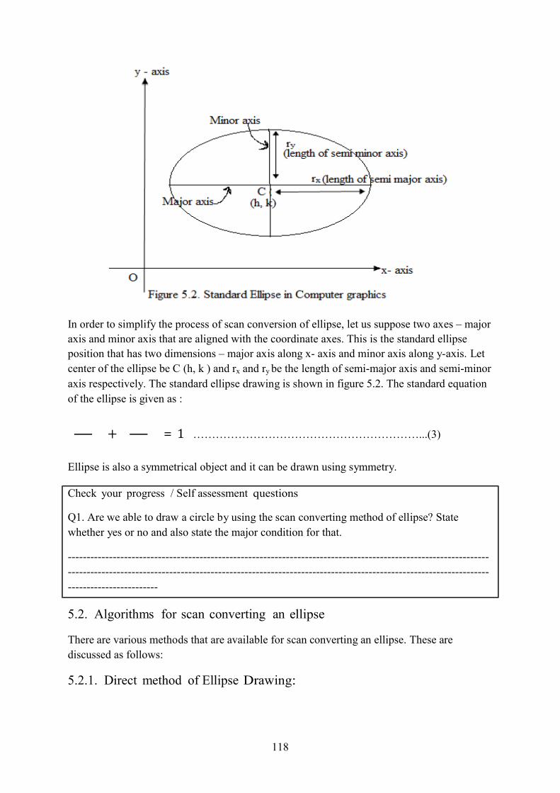
118

In order to simplify the process of scan conversion of ellipse, let us suppose two axes – major

axis and minor axis that are aligned with the coordinate axes. This is the standard ellipse

position that has two dimensions – major axis along x- axis and minor axis along y-axis. Let

center of the ellipse be C (h, k ) and rx and ry be the length of semi-major axis and semi-minor

axis respectively. The standard ellipse drawing is shown in figure 5.2. The standard equation

of the ellipse is given as :

+ = 1 ……………………………………………………...(3)

Ellipse is also a symmetrical object and it can be drawn using symmetry.


Q1. Are we able to draw a circle by using the scan converting method of ellipse? State

whether yes or no and also state the major condition for that.

----------------------------------------------------------------------------------------------------------------

----------------------------------------------------------------------------------------------------------------

------------------------

5.2. Algorithms for scan converting an ellipse There are various methods that are available for scan converting an ellipse. These are

discussed as follows:

5.2.1. Direct method of Ellipse Drawing:

119

This method is also known as polynomial method. In this method, we will use the standard

ellipse equation. Here we will increment x- coordinate by unit interval and will find the

corresponding y value for each x value using equation (3).

From equation (3),

x − h

r

y − k + = 1 r

= 1 −

= ± 1 −

y-k = ± r 1 −

y = k± r 1 −

Using Two – way symmetry:

Here we will start from x = (h – rx ) and will

end at (h + rx). We will increment x value by 1

and will calculate the y value from above

equation at each step. This calculated value

can be a floating point value so we need to

round off the y value to get integral pixel

position. In this case, we are supposed to find

the values for half of the ellipse and will invert

the y value for all the points to find the other half of the ellipse i.e. corresponding to (x, y )

value we have (x, -y) value. Algorithm:

Step 1: Enter Center of Ellipse i.e. C(h, k)

Step 2: Enter length of semi major and semi minor axis i.e. rx and ry

Step 3: Initialize x = (h – rx ) and y = k

Step 4: While (x < = (h + rx))

x = x + 1

Calculate y = k +r 1 −

120

Round off y-value PlotPixel (x, y) and PlotPixel (x, -y)

EndWhile

Step 5: End We have discussed two-way symmetry of ellipse about its major axis in which we are

increasing x coordinate by 1 and finding y coordinate. Similar approach can be followed if

are supposed to scan convert an ellipse about minor axis in which we will increment y

coordinate by 1 and we will find the x value by using the equation (3).

From equation (3),

x − h

r

y − k + = 1 r

= 1-

± r 1 −

= ± 1 −

x – h =

x = h ± r 1 −

Four-way symmetry:

We can use four-way symmetry to draw

an ellipse with direct method. It is less

time consuming than previous one

because we will find points in 1st quadrant and rest of the points in other quadrants can be

found by using symmetry. If we plot a point (x, y) in 1st quadrant, rest of the three points will

be (x, -y), (-x, y) and (-x, -y). Here we will start from x = h and will continue till x <= (h +

rx). X-coordinate is incremented by unit interval and we will find the corresponding y value at

each step. Here we are using symmetry about major axis but same can be done about minor

axis also in which y coordinate will be incremented by 1 and corresponding x value can be

found at each step and in this case, y will be started at k and will end at (k + ry ).

Algorithm:

121

Step 1: Enter Center of Ellipse i.e. C(h, k) Step 2: Enter length of semi major and semi minor axis i.e. rx and ry

Step 3: Initialize x = h

Step 4: While (x < = (h + rx))

Calculate y = k +r 1 −

Round off y-value

PlotPixel (x, y) PlotPixel (x, -y)

PlotPixel (-x, y) PlotPixel (-x, -y)

x = x + 1


5.2.2. Trigonometric method of Ellipse Drawing: The equation of an ellipse in polar coordinates with center C(h, k) and rx and ry , the lengths

of semi-major and semi-minor axis is:

x = h + rx cosθ and

y = k + ry sinθ

where θ is an angle made by any point (x, y) on

the ellipse with the major axis of the ellipse as

shown in figure 5.5. θ can have values ranging

from 0 to 2π radians. At each step, we find both

x and y value and will increment θ by small

amount which is dθ and it is usually taken very

small. We can take dθ as or . In this

method also, we take advantage of symmetry.

Two-way symmetry:

Here θ is initialized to 0 and loop will be continued upto π radians. In this method, just for

simplicity, we will increment θ by 1.

Algorithm:


122



Step 4: While (theta < = 180)

x = h + rx cos(theta)

y = k + ry sin(theta)

PlotPixel(x, y) PlotPixel(x, -y)

theta = theta + 1

EndWhile

Step 5: End

Four-way symmetry: In this case, we start θ from 0 and will end at radians. We deal with only the first quadrant

of the ellipse and rest of the points can be found from the points in first quadrant. For

example, if we have calculated a point (x, y) in the first quadrant, then rest of the points will

be (x, -y), (-x, -y ) and (x, -y) in rest of the three quadrants.

Algorithm:



123

Step 3: Initialize theta to 0 Step 4: While (theta < = 90)

x = h + rx cos(theta)

y = k + ry sin(theta)

PlotPixel(x, y) PlotPixel(x, -y)

PlotPixel(-x, y) PlotPixel(-x, -y)

theta = theta + 1


5.2.3. Midpoint ellipse drawing method: Midpoint ellipse drawing method is very similar to midpoint circle drawing algorithm. The

basic difference is that in circle drawing, we just draw the circle in first octant and then copy

it to other octants using eight-way symmetry. But in midpoint ellipse method, we have to

draw the ellipse in both the octants of the first quadrant and further copy it rest of the

quadrants using four-way symmetry. This method is the most efficient among all the methods

of the ellipse drawing. It is faster and accurate one.

Derivation:

Let us suppose an ellipse whose center is C(h, k) and whose length of semi-major and semi-

minor axis is rx and ry respectively. We will draw the ellipse with center at the origin and then

translate it to the given center C by just adding h and k to the x and y coordinate respectively

of the calculated points.

Scan converting the ellipse in the first quadrant requires further two parts because of its

elliptical shape. We have shown an ellipse whose rx < ry in figure 5.7.

124

As shown in above figure, we have divided the first quadrant into two parts- octant 1 with

slope < -1 and octant 2 with slope > -1 and the line that separates these octants has |slope| = 1.

So in octant 1, we will move towards x-axis by unit intervals and find the corresponding y-

coordinate at each step and when we move in octant 2, we will increment y-coordinate by 1

and will find the corresponding x-value at each step.

From equation (3), we get

x − h

r +

y − k

r = 1

If the center of the ellipse is at the origin, i.e. (h , k) = (0 , 0), then

+ = 1

r x + r y = r r

r x + r y - r r = 0………………………………………………………….(4)

We can define an ellipse function as:

f (x, y) = r x + r y - r r

This function returns 0 for all the points that lie on the boundary of the ellipse and f (x, y) < 0 for any point that is inside the ellipse and f (x, y) > 0 for any point that is outside the ellipse.

125

So it can be decided from the sign of this function that whether a point is inside or outside the

ellipse. Hence this function can be taken as the decision parameter of this method.

The procedure of ellipse drawing is started at (0, r ) which will be the first point to be

plotted. In octant 1, we will increment x value by 1 until we reach a point where slope = -1 i.e. at the joining of octant 1 and octant 2. In order to find the slope, we need to differentiate

equation (4) w.r.t x.

2r x + 2r y = 0

∴ = -

The boundary of octant 1 and octant 2 has slope = -1, so

=1

- = -1

2r x = 2r y i.e. r x = r y

This is the condition that decides when we will move from octant 1 to octant 2. We will continue in octant 2 until we reach the final point (rx , 0). Once we find points in first

quadrant, we will copy these points to rest of the quadrants.

Octant 1:

At ith position, let us suppose that we have plotted a point (xi , yi ). At position (i+1)th, we

have two candidate pixels that can be plotted. They are points T (xi + 1, yi ) and S (xi + 1, yi –

1) as shown in figure 5.8. Mid-point of these two pixel values is M (xi + 1, yi – ½ ).

The decision parameter di will take into account the ellipse function.

di = f (xi + 1, yi – ½ )

di = r (xi + 1) + r (yi

– ½ ) - r r

……………………………………………..(5)

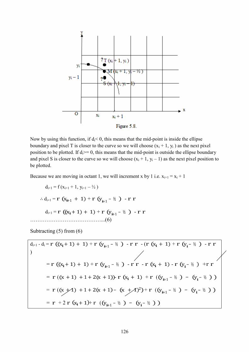
126

2

Now by using this function, if di< 0, this means that the mid-point is inside the ellipse

boundary and pixel T is closer to the curve so we will choose (xi + 1, yi ) as the next pixel

position to be plotted. If di>= 0, this means that the mid-point is outside the ellipse boundary

and pixel S is closer to the curve so we will choose (xi + 1, yi – 1) as the next pixel position to

be plotted.

Because we are moving in octant 1, we will increment x by 1 i.e. xi+1 = xi + 1

di+1 = f (xi+1 + 1, yi+1 – ½ )

∴ di+1 = r (xi+1 + 1) + r (yi+1

– ½ ) - r r

((x + 1) + 1) + r (y

– ½ ) - r r

di+1 = r i i+1

…………………………………...(6)

Subtracting (5) from (6)

di+1 - di = r ((xi + 1) + 1) + r (yi+1

– ½ ) - r r - (r (xi + 1) + r (yi

– ½ ) - r r

)

= r ((xi + 1) + 1) + r (yi+1

– ½ ) - r r - r (xi + 1) - r (yi

– ½ ) +r r

= r ((x + 1) + 1 + 2(x + 1))- r (xi + 1) + r ((y

i+1 – ½ ) − (y

i – ½ ) )

= r ((x + 1) + 1 + 2(x + 1) − (x + 1) ) + r ((y

i+1 – ½ ) − (y

i – ½ ) )

= r + 2 r (xi + 1)+ r ((y

i+1 – ½ ) − (y

i – ½ ) )

127

r + 2 r ( i )+ r (( i

) − ( i

)1

di+1 = di + r + 2 r (xi + 1)+ r ((yi+1

– ½ ) − (yi

– ½ ) )

…………………………(7) if di< 0 , then yi+1 = yi. Put this value in (7), we get,

di+1 = di + r + 2 r (xi + 1)+ r ((yi

– ½ ) − (yi

– ½ ) )

di+1 = di + r + 2 r (xi + 1)+ r (0)

di+1 = di + r + 2 r (xi + 1)

Since x + 1 = xi+1

So, di+1 = di + + 2 xi+1

If di>= 0 , then yi+1 = yi - 1. Put this value in (7), we get,

di+1 = di + r + 2 r (xi + 1)+ r ((yi

− 1 – ½ ) − (yi

– ½ ) )

3 di+1 = di + x + 1 y − 2

y – ) 2

di+1 = di + r + 2 r (xi + 1)+ r (y + − 3y − (y + − y ))

di+1 = di + r + 2 r (xi + 1)+ r (y + − 3y − y − + y )

di+1 = di + r + 2 r (xi + 1)+ r ( − 2y )

di+1 = di + r + 2 r (xi + 1)+ r (2 − 2y )

di+1 = di + r + 2 r (xi + 1)- 2 r (y − 1)

In this case also, x + 1 = x and y − 1 =y

So, di+1 = di + + 2 + - 2

+

In order to find the initial decision parameter, we need to put (0, ry) in equation (5) and is denoted as d0.

d0 = r (0 + 1) + r (ry – ½ ) - r r

= r + r (r + − r ) - r r

= r + r r + r − r r - r r

d0 = − +

128

i

2

Octant 2: In this octant, we keep on incrementing y coordinate by unit interval along the negative y-

axis. Let us suppose that at position i, we have (xi , yi ). At position (i+1)th, we have two

candidate pixels that can be plotted. They are points P (xi , yi - 1 ) and Q (xi + 1, yi – 1) as

shown in figure 5.9. Mid-point of these two pixel values is M’ (xi + ½ , yi – 1). In this case, at

each step yi+1 = yi – 1.

The decision parameter di’in this case will be The decision parameter di will take into account the ellipse function.

di’ = f (xi + ½ , yi – 1 )

1

di’ = r (xi + ) + r (y – 1 ) - r r 2

……………………………………………..(8) Now by using this function, if di’< 0, this means that the mid-point is inside or on the ellipse

boundary and pixel Q is closer to the curve so we will choose (xi +1, yi-1) as the next pixel

position to be plotted. If di>= 0, this means that the mid-point is outside the ellipse boundary

and pixel P is closer to the curve so we will choose (xi, yi – 1) as the next pixel position to be

plotted.

Because we are moving in octant 2, so yi+1 = yi – 1

di+1’ = f (xi+1 + ½ , yi+1 – 1 )

1

∴ di+1’ = r (xi+1 +

) + r (yi+1

– 1 ) - r r

129

+ r ( i

) - r r

+ r ( i

) - r r - r ( i -r ( i

) +r r

− ( i

− ( i ) + r - 2r i

)+ r ( i

+ 1 − 2 i

( i

) )

1

1

3

1i

1

1i

1i

di+1’ = r (xi+1 + 1 ) (y − 1) – 1 2

…………………………………...(9) Subtracting (8) from (9)

di+1’ - di’ = r (xi+1 + 1 ) (y − 1) – 1 x + 2

1 ) y – 1 2

= r ((xi+1 +

= r ((xi+1 +

1 ) x + 2

1 ) x + 2

1 ) (y − 1) (y − 1) − y – 1 2

1 ) (y − 1) 2

di+1’ = di’ + r - 2r (yi

− 1)+r [ xi+1 + 2

………………………………(10)

− x + ] 2

If di+1’ > 0, put xi+1 = xi in equation (10), we get

1

− x + ]

di+1’ = di’ + r - 2r (yi

− 1)+r [ xi + 2 i 2

di+1’ = di’ + r - 2r (yi

− 1)+r (0)

di+1’ = di’ + r - 2r (y

i − 1)

Since y − 1 = yi+1, so

di+1’ = di’ + - 2

+

If di+1’ <= 0, put xi+1 = xi + 1in equation (10), we get

di+1’ = di’ + r - 2r (yi

− 1)+r [ xi + 1 + 2 − x + ]

2

di+1’ = di’ + r - 2r (yi

− 1)+r [ xi + 2 − x + ]

2

di+1’ = di’ + r - 2r (yi

− 1)+r [x + + 3x − x − − x ]

di+1’ = di’ + r - 2r (y

i − 1)+r (2x + )

di+1’ = di’ + r - 2r (y

i − 1)+r (2x + 2)

di+1’ = di’ + r - 2r (y

i − 1)+2r (x + 1)

Since in this case, y − 1 = y and (x + 1) = x , so

130

0

di+1’ = di’ + - 2 +

+

In order to find the initial decision parameter in octant 2, we have to put the last position in octant 1 i.e. the position which will be the start of octant 2. Let it be (x0, y0) and by putting

this value in equation (8) d0’ will be:

1

d0’ = r (x0 + ) + r (y – 1 ) - r r 2

If we want to simplify the calculation, we can start second octant from ( rx , 0) and will move

along the positive y axis i.e. incrementing y value by 1. Algorithm:



Step 3: Calculate the initial decision parameter, d = r − r r + r

Step 4: Initialize the x and y values as x =0 and y = ry Step 5: Plot the initial point, PlotEllipsePoint (x + h , y + k ) Step 6: While (r x<= r y )

If (d < 0)

x = x + 1

d = d + r + 2 r x

Else

x = x + 1

y = y – 1

d = d + r + 2 r x - 2 r y

EndIf

PlotEllipsePoint( x+ h, y + k)

EndWhile

Step 7: Calculate initial decision parameter taking the last values of x and y,

d = r (x + ) + r (y – 1 ) - r r Step 8: While((x < rx) and (y > 0))

131

If (d <= 0)

y = y – 1

x = x + 1

d = d+ r – 2r y+2r x

Else

y = y - 1

d = d + r - 2r y

EndIf

PlotEllipsePoint( x+ h, y + k)

EndWhile

Step 9: End Check your progress / Self assessment questions

Q2. Write the value of initial decision parameter in octant 1 in midpoint ellipse drawing

method.

----------------------------------------------------------------------------------------------------------------

----------------------------------------------------------------------------------------------------------------

------------------------ Q3. State the condition that is necessary for switching from octant 1 to octant 2.

----------------------------------------------------------------------------------------------------------------

----------------------------------------------------------------------------------------------------------------

------------------------

5.3. Effects of Scan conversion

There are many side effects of scan conversion which is observed in scan converting any of

the computer graphics primitives. Some of the commonly visible effects of scan conversion

are discussed as follows:

1. Aliasing: We know that pixel positions on a raster screen are integer values. Aliasing refers to the problem of plotting a point at a location which is different from its actual location on a display screen. For example, if we are drawing a line, the calculated coordinates of a point is (4, 5.6). But in order to plot this point using PlotPixel() function, we have to round off the value and we get (4, 6) which is different from the true position. The plotted position is called as alias position. The figure 5.10. shows this effect. The aliasing effect is more visible at lower resolutions of the screen. In case of a straight line, this effect is also known as jaggy or stair-case effect. If we

132

want to minimize this aliasing effect, we can increase the resolution i.e. number of pixels of the screen so that the visibility of the staircase effect is reduced.

2. Unequal Intensity:Our raster screen consists of an array of pixels which are arranged

in rows and columns. Let us suppose that the spacing in the horizontal and vertical

direction is 1 unit. Then the spacing in the diagonal opposite pixels will be √ 2 as shown in figure 5.11. This means that the arrangement of pixels in the horizontal and vertical direction is denser than the pixels that lie on the diagonals. Therefore if the resolution of the screen is low, then the diagonal lines will appear dimmer than the horizontal and vertical lines. The reason being vision of a human eye depend not only the intensity of light but it is dependent on the density of light sources as well.

The problem discussed above is called as unequal intensity and to resolve this

problem, the number of pixels should be increased. And other solution can be to

increase the intensity of pixels plotted on the diagonal line.

133

3. Over Strike: During scan conversion, if the same pixel is illuminated more than once, then there is a problem of overstrike. Although its effect is not visible on the display screen, but the output speed is affected by it. The reason is time is consumed in scan converting the same pixel but the intensity of the pixel is not enhanced by plotting it two or more times. If instead of taking output on a raster screen, we take the output on a photographic medium, then overstrike effect can be clearly visible because of more exposure of the same portion of the medium to ink. This effect can be reduced if we make a check on the pixel position that whether the same position has been plotted or not.

4. Picket Fence Problem: There is another problem being faced by the graphics designer while working with the scan conversion. This problem occurs when either the object cannot be aligned with the pixel array or when the object itself cannot fit into it. If the distance between the two consecutive boundary edges of an object called its pickets is not equal to the unit distance between the pixels or any multiple of it, then scan converting will result into uneven distances between the pickets as we have to map the picket coordinates to the discrete pixel positions. It is shown in figure 5.12.(a). Figure 5.12.(b) shows that overall length of the pickets fence will be correct approximately through the spacing between the pickets is distorted. It is called global aliasing. Another solution to this problem is to reduce the distance between the pickets. The distance should be tried to make as close to their relative distances as possible. Again the overall length of the picket fence will get distorted. This case is shown in figure 5.12.(c). This is known as local aliasing. It is the decision of the computer graphics designer either to use global aliasing or to use local aliasing.

134


Q4. We can decrease the effects of scan conversion by increasing the number of pixels. State

whether True or False.

135

----------------------------------------------------------------------------------------------------------------

----------------------------------------------------------------------------------------------------------------

------------------------

5.4. Summary In this chapter we have discussed how to scan convert an ellipse and various methods that are

used in its scan conversion. Most important among these methods is MidPoint ellipse

drawing method because of its accuracy and efficiency. We have gone through many side

effects of scan conversion and along with some solutions to these problems are also provided.

We cannot eliminate these effects but we can reduce their visibility.

5.5. Glossary Aliasing - Aliasing refers to the problem of plotting a point at a location which is different

from its actual location on a display screen.

5.6. Answers to check your progress / self assessment questions 1. Yes, we are able to draw a circle using scan converting methods of an ellipse with a single

condition that rx = ry i.e. length of semi-major and semi-minor axis should be same.

2. The value of initial decision parameter is d = r − r r + r , where rx and ry are the

lengths of semi-major and semi-minor axis respectively.

3. We will switch from octant 1 to octant 2 when r x>r y .

4. True.


1. What do you mean by scan converting an ellipse? 2. What are the various methods of ellipse drawing? Explain briefly. 3. Derive MidPoint Ellipse drawing method. 4. State various effects of scan conversion.

136

Lesson-06

Area filling and character generation techniques Structure of the chapter

6.0. Objectives

6.1. Introduction to area filling

6.1.1. Types of polygons

6.1.2. Representing polygons

6.2. Area filling techniques

6.2.1. Seed fill

6.2.1.1. Boundary fill / Edge fill algorithm

6.2.2. Scan line algorithm

6.3. Flood fill technique

6.4. Character generation

6.5. Strategies of character generation

6.5.1. Stroke Method

6.5.2. Starbust Method

6.5.3. Bitmap Method

6.6. Advantages of character generation

6.7. Summary

6.8. Glossary


6.10. Modal questions

6.0. Objectives


137

Explain what area filling is. Explain what the various methods to fill areas in graphics are. Explain flood fill technique. Explain character generation strategies.

6.1. Introduction to area filling In the previous chapters, we have learnt scan conversion of basic primitives like lines, circles

and ellipses. This chapter aims to provide a basic overview of different kinds of polygons,

how to represent them and area filling techniques. In computer graphics, one of the standard

output primitives is a solid-color or patterned polygon area. Although a number of area

primitives are available but polygons are quite easier to process because they have linear

boundaries.

A polygon is basically a series of interconnected line segments. It can be specified by vertices

(or node) like P0, P1, P2, P3, and so on. The first node is called starting or initial vertex and the

last one is referred as final or terminal vertex. A simple polyline is shown in figure 6.1. When

the initial and the final vertex of a polyline is same, then it becomes a polygon as shown in

figure 6.2. We can say that a closed polyline is a polygon.

6.1.1. Types of polygons The types of polygons depend on the position of the line segment that joins any two points.

There are two basic types:

Concave Polygons

Convex Polygons

A concave polygon is the one in which the line segment that joins any two points may not lie

completely inside the polygon boundary. Examples are shown in figure 6.3.

138

A convex polygon, on the other hand, is the one in which the line segment that joins any two

points lie completely within the polygon. Figure 6.4. shows some examples.

6.1.2. Representing polygons As we know that a polygon is a closed polyline. Every polygon has its sides and edges. The

end points are known as nodes or vertices. There are three basic methods to represent

polygons according to the graphics system:

Polygon drawing primitive method

Trapezoid primitive method

Line and point method

The polygon primitive approach can draw the polygon shapes directly on the graphic devices.

Polygons are stored as a unit on such devices. In those graphic devices that support trapezoid

primitive method, the trapezoids are obtained from two scan lines and two line segments as

figure 6.5. depicts. The trapezoids are drawn by stepping down the line segments using two

vector generators and for every polygon, fill in all the pixels that lie between them. So every

polygon is divided into trapezoids and it is represented as a chain of trapezoids.

139

Many graphics devices are not having any polygon support at all. In these cases, we represent

polygons using lines and points. A polygon is stored in a display file. In the display file,

polygons are not stored just with a series of line commands since they do not identify how

many of the following line commands are the element of the polygon. So, a new command is

used in the display file to represent the polygons. The opcode (i.e. operation code) for new

command itself identify the number of line segments in the polygon. The figure 6.6.

represents the polygons and its depiction using display file.

Entering polygons: We can use the following algorithm to enter the polygon command and

data into the display file. In such a file, we need to enter the number of sides and coordinates

of each vertex.

Algorithm:

1. Read arrays Ax and Ay of length n. These arrays contain the vertices of the polygon

and length of the array specifies the number of sides of the polygon.

2. Initialize i to 0

140

DF_OP[i] <- n

DF_x[i] <- Ax[i]

DF_y[i] <- Ay[i]

i <- i +1 // loading polygon command

3. Do

{

DF_OP[i] <- 2

DF_x[i] <- Ax [i]

DF-y[i] <- Ay [i]

i <- i + 1

} while ( i < n) // entering line commands

4. DF_OP[i] <- 2

DF_x[i] <- Ax[0]

DF_y[i] <- Ay[0] // entering last line command

5. Stop.

Polygon test: When a polygon is being entered into a display file, we can draw the boundary

of the polygon. To draw the polygon as a solid object, we just need to illuminate the pixels

inside the polygons and the pixels that are on the pixel boundary. But how we can decide

whether a point is inside the polygon or not.

One method is even-odd method that determines the points inside the polygon. In this,

we draw a line segment between the given point and the point that is already known to

be outside. Then we count the number of intersections of this line segment with the

polygon boundary. If the number of intersections is odd, then the given point is inside

the polygon otherwise it is outside. This method is shown in figure 6.7.

141

Another method is winding-number method. In this method, we will take a given

point and a point that is known to be on the boundary of the polygon. Abstractly, we

will stretch a piece of elastic between these two points and slide the end point on the

boundary for a complete revolution. We will count the number of times the elastic

has wound around the given point. If there is at least one winding, the point lies inside

and if there is no winding, the point is outside. Similar to the previous method, we

will draw a line segment from the outside to the given point and we will consider the

polygon sides that it crosses. But instead of counting the number of intersections, we

will provide a direction number to every line that is crossed and will find the sum of

these direction numbers. This number indicates the direction in which the polygon

side was drawn relative to the line segment for our test. This test is shown in figure

6.8.

As it can be seen from the above figure that (xa, ya ) is a test point and y = ya is a horizontal

line that is running from the outside to the point (xa, ya ). We can draw the edges of the

polygon that are being crossed by this line in two ways. Firstly, the edge can be constructed

by initiating from below the line, crossing it and ending above the line or starting from above,

crossing and ending below the line. In the first one, we will give the direction number of -1

and in the second one, the direction number will be given as 1. After the direction number is

allocated, we will calculate the sum of them. This sum is referred as winding number. If this

number is nonzero, the point is said to be inside the polygon otherwise it is outside.


Q1. What are the different methods of representing polygons? ----------------------------------------------------------------------------------------------------------------

----------------------------------------------------------------------------------------------------------------

----------------------------------------------------------------------------------------------------------------

--------------------------------- Q2. State the difference between convex and concave polygon.

142

----------------------------------------------------------------------------------------------------------------

----------------------------------------------------------------------------------------------------------------

----------------------------------------------------------------------------------------------------------------

---------------------------------

6.2. Area filling techniques Area filling means highlighting all the pixels that lie inside the polygon with some color

which is different from the background color. Polygons’ filling is easy because they have

linear boundaries.

There are two common methodologies for filling areas on the raster systems. The first way to

fill an area is by determining the overlapped intervals for scan lines that are crossing the area.

The second method for area filling is to initiate from a given internal position and paint

outward from this position till the point we encounter the specified boundary conditions. The

scan-line method is commonly used to fill the areas primitives like polygons, circles, ellipse

and other simple curves. The other method i.e. fill methods that start from an internal point

are used for more complex boundaries and responsive painting systems.

The two basic method of area filling is discussed below:

6.2.1. Seed Fill In this method, we will fill a polygon by starting from a given ‘seed’ point (i.e. a point which

is known to be inside the polygon) and we will be highlighting outwards from this seed pixel

which means neighbouring pixels will be highlighted until we reach the boundary. It is

similar to water flooding on the surface of a container. There are two algorithms based on this

approach: flood fill algorithm and the boundary fill algorithm or edge filled algorithm. The

flood fill algorithms fill the interior defined regions while the second one aims to fill the

boundary defined regions. In this section, we will discuss boundary fill algorithm and flood

fill algorithm will be discussed in the next section in detail.

6.2.1.1. Boundary fill / Edge Fill algorithm In this algorithm, polygon edges are constructed. Then, we will start from a seed (i.e. any

point inside the polygon) and we will examine the neighboring pixels to check if we have

reached the boundary pixel. If we have not reached the boundary pixels, the pixels are

highlighted and this process continues till we reach the boundary pixels.

The boundary defined areas can be either 4-connected or 8-connected as depicted in figure

6.9. If an area or a polygon region is 4-connected, then each pixel within the region can be

reached with a combination of moves in just four directions: left, right, up and down but for

an 8-connected polygon region, each pixel can be reached with a combination of moves in

two horizontal directions, two vertical directions and four diagonal directions.

143

In some cases, 8-connected regions are more preferred than 4-connected one. This is because

sometimes, 4-connected results in partial fill as shown in figure 6.10.

The following function provides the recursive method of filling a 4-connected polygon region

with the color specified in the parameter fill color (denoted as f_color) upto a boundary color

being specified with parameter boundary color (denoted as b_color). Boundary_Fill (x, y, f_color, b_color)

{

If (GetPixel(x, y) != b_color && GetPixel(x, y) != f_color)

{

PutPixel(x, y, f_color);

Boundary_Fill(x+1, y, f_color, b_color);

Boundary_Fill(x, y+1, f_color, b_color);

Boundary_Fill(x-1, y, f_color, b_color);

Boundary_Fill(x, y-1, f_color, b_color);

144

}

} The GetPixel() function being used here will return the color of the pixel being specified as

an argument and the PutPixel() functions plots the pixel with the color being specified as an

argument. We can use the same procedure for 8-connected regions also with some

modifications like we need to include four extra statements that test the diagonal positions

like (x+1, y+1).

6.2.2. Scan line algorithm

The recursive algorithms discussed in seed fill methods are facing two major difficulties. The

first difficulty is that if there are some pixels inside the polygon that are already colored, then

our recursive loop terminates and some of the internal pixels are remained uncolored. To

overcome this difficulty, we first need to change the color of some internal pixels which were

initially set to the fill color before seed fill algorithms are applied. The second difficulty is

that these methods are unsuitable for large polygons. It is so because it requires storage of the

neighboring pixels and for large polygons, the stack space for storing the pixels can be

insufficient. To overcome this problem, we need more efficient algorithms. Such methods fill

the horizontal pixels that spans across the scan lines instead of going to 4-connected or 8-

connected neighboring points. This can be done by recognizing the rightmost and the leftmost

pixels of the seed pixel and then draw a horizontal scan line between these two extreme

pixels. This process is repeated by changing the seed pixel above and below the scan line just

drawn till whole polygon is filled. With this method, we need to store the starting pixel for

every horizontal pixel span.

The scan line method for polygon filling is shown in figure 6.11. For every scan line that

crosses a polygon, this method locates the points of intersection of the scan line with the

edges of the polygon. These points are then sorted from left to right, and the corresponding

points between these intersection points are set to the desired fill color.

145

From the above figure, we can observe that there are two stretches of internal points from

x=6 to x=9 and x=12 to x= 15. The scan line method first finds the biggest and the smallest y

coordinates of the polygon. It then begins with the biggest y-value and works its way down,

scans from left to right just the way raster display do.

An important job in the scan line method is to locate the points of intersection of the scan line

with the boundary of the polygon. If the intersection points are even, they are arranged from

left to right in a sorted manner, are paired and the pixels between the paired points are set to

the fill color. But there are some cases in which the intersection point is a node (or vertex).

When the scan line intersects a polygon vertex, a special handling is needed to find the actual

intersection points. To handle these cases, we have to look at the other end points of the two

line segments of the polygons that meet at this vertex point. If these points are on the same

side ( up or down) of the scan line, then the given point will be counted as an even number of

the intersections and if they are opposite sides of the line, the point will be counted as a single

intersection. This is depicted by figure 6.12.

As we can see from the above figure that every scan line intersects the vertex of the polygon.

For scan line 1, the rest of the end points B and D of the two line segments are lying

on the same side of the scan line, so there are two intersections that result in two pairs:

1-2 and 3-4 where the intersection points 2 and 3 are actually the same points.

146

For scan line 2, the end points D and F of the two line segments of the polygon are

lying on the opposite sides of the scan line, so there is a single intersection that results

in two pairs: 1-2 and 3-4.

For scan line 3, there are two vertices that are the intersection points. For vertex F, the

other end points E and G of the two line segments of the polygon are on the same side

of the scan line while for vertex H, the end point G and I of the line segments are on

the opposite side of the scan line. So at vertex F, we have two intersections and for

Vertex H, we have a single intersection. The result is two pairs: 1-2 and 3-4 and the

points 2 and 3 are same.

It is required to calculate the x-intersection points for the scan line with each polygon edge.

We can use coherence properties to simplify the computations. A coherence property of a

picture is the one in which one part can be related to the other parts of the picture. We will

slope of an edge as a coherence property. Making use of this property, we can calculate the x-

intersection point on the lower scan line if we know the x-intersection value for the current

scan line. It is given as:

xi+1 = xi – 1/m

where m is the slope of the side.

Since we scan from top to bottom, the y-value changes by 1 and is given as:

yi+1 = yi – 1 Most of the times, it is not always required to calculate the x-interection value for scan line

with each polygon edge. We will just consider those polyon sides whose end points are

spanning the current scan as shown in figure 6.13.

If we sort the edges in order of their maximum y-coordinate, then it becomes easy to test for

x-intersection. When the sides are sorted, we scan the lines from top to bottom resulting in a

list of active edges for every scan line that crosses the polygon boundary. The list contains all

147

the edges crossed by the scan line. The figure 6.14. shows sorted order of the polygon along

with active edges.


Q3. Why 8-connected regions are more preferred over 4-connected regions? ----------------------------------------------------------------------------------------------------------------

----------------------------------------------------------------------------------------------------------------

----------------------------------------------------------------------------------------------------------------

--------------------------------- Q4. What are the major difficulties being faced by seed fill methods?

----------------------------------------------------------------------------------------------------------------

----------------------------------------------------------------------------------------------------------------

----------------------------------------------------------------------------------------------------------------

---------------------------------

6.3. Flood fill technique Sometimes there is a requirement of filling an area which is not defined with a single color

boundary. For these cases, we can fill the areas by replacing a defined interior color rather

than searching for a boundary color. This method of filling areas is called flood fill. Like

boundary fill method, in this method also we will start from a seed point and then examine

the neighboring pixels. But in this case, we will check the neighboring pixels for a specified

interior color and not for a boundary color and after checking, they are replaced with a new

color. We can use 4-connected or 8-connected approach and can step through the pixels until

all the internal points have been filled. The following procedure depicts the recursive method

of filling an 8-connected area by using flood-fill algorithm.

148

Flood_Fill (x, y, old_color, new_color)

{

if ( getpixel (x, y) = old_color)

{

putpixel (x, y, new_colour);

Flood_Fill (x + 1, y, old_color, new_color);

Flood_Fill (x - 1, y, old_color, new_color);

Flood_Fill (x, y + 1, old_color, new_color);

Flood_Fill (x, y - 1, old_color, new_color);

Flood_Fill (x + 1, y + 1, old_color, new_color);

Flood_Fill (x - 1, y - 1, old_color, new_color);

Flood_Fill (x + 1, y - 1, old_color, new_color);

Flood_Fill (x - 1, y + 1, old_color, new_color);

}

} Check your progress / Self assessment questions

Q5. What is the role of GetPixel() and PutPixel() in area filling? ----------------------------------------------------------------------------------------------------------------

----------------------------------------------------------------------------------------------------------------

----------------------------------------------------------------------------------------------------------------

---------------------------------

6.4. Character Generation

149

When we draw anything or any design, it should be labeled that requires letters, numbers and

special characters. This design and style is usually referred as typeface or fonts. We are

having hundreds of fonts available. On the basis of styles, commonly used are Times New

Roman, Arial, Calibri, etc and on the basis of language, it can be any regional language like

Korean, Japanese, Hindi, etc. Special characters like ®, ©, ™, E, $, etc are stored in a font

table. Each of these can be made bold, italic or underlined. Character creation is a fast

process in graphics. It refers to the process of generating characters in various applications.

There are two basic techniques to represent different fonts: bitmap font and outline font.

In bitmap font, a character or a letter is written on a rectangular grid. The on grid pixel

represents digital value 1 and the off pixels represent digital value 0. It makes use of font

table. In any font table, there are group of fonts that range from 0 to 255 (i.e. there are total

256 fonts) and each font is represented by 16 values and each row of a particular font is

represented by an 8-bit number i.e. 1 byte. So a single font is of 16 bytes. In order to store

256 fonts, we need 256 × 16 = 4096 bytes. This is the simplest method of representing and

storing different fonts. Another method is known as outline font. Straight lines and curved segments are used to

represent fonts like in PDF (portable data format). It consumes less storage as compared to

bitmap font. It is easy to produce variations in fonts by changing the curves for the outlines.

Clipping of these fonts is easier since we can consider a character as a simple polygon. More

processing is required because every font needs to be scan converted into a frame buffer. Check your progress / Self assessment questions

Q6. Write two ways to represent the characters in graphics? ----------------------------------------------------------------------------------------------------------------

----------------------------------------------------------------------------------------------------------------

----------------------------------------------------------------------------------------------------------------

---------------------------------

6.5. Strategies of character generation In computer graphics, we display letters, numbers and characters usually as labels that

provide information and instructions to the users. These characters are built into the display

devices mostly as hardware but sometimes this can be done via software also. There are three

basic strategies of generating characters:

Stroke Method

Starbust Method

Bitmap Method

Let us discuss these strategies in detail.

6.5.1. Stroke Method

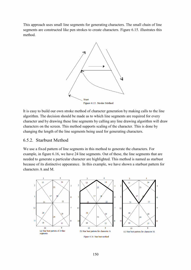
150

This approach uses small line segments for generating characters. The small chain of line

segments are constructed like pen strokes to create characters. Figure 6.15. illustrates this

method.

It is easy to build our own stroke method of character generation by making calls to the line

algorithm. The decision should be made as to which line segments are required for every

character and by drawing these line segments by calling any line drawing algorithm will draw

characters on the screen. This method supports scaling of the character. This is done by

changing the length of the line segments being used for generating characters.

6.5.2. Starbust Method We use a fixed pattern of line segments in this method to generate the characters. For

example, in figure 6.16, we have 24 line segments. Out of these, the line segments that are

needed to generate a particular character are highlighted. This method is named as starbust

because of its distinctive appearance. In this example, we have shown a starbust pattern for

characters A and M.

151

The pattern of line segments is stored as a 24-bit code where each bit represents one line

segment. If the line segment is highlighted, the corresponding bit is set to 1 otherwise it will

be set to 0. The 24-bit code for character A and M is given below:

Code for ‘A’: 0011 0000 0011 1100 1110 0001 Code for ‘M’: 0000 0011 0000 1100 1111 0011

This method is not so popular because of the following reasons:

Every character is being represented by 24-bits so more memory is required.

24-bits code needs to be converted to display a character that requires some code

conversion software.

The quality of the character is poor. This method is not suitable for curve-shaped

characters.

6.5.3. Bitmap Method The third strategy of character generation is bitmap method which is also called as dot-matrix

method because in this approach, characters are represented by an array of dots in the matrix

form. A two-dimensional array is used having rows and columns. Figure 6.17 shows a 5×7

array which is most commonly used for character representation. 7×9 and 9×13 arrays are

also popular. The devices having high resolution like inkjet printers or laser printers can use

arrays of size 100×100.

Every dot in the matrix represents a pixel. The character is shown on the display screen by

copying the pixel values from the matrix into a portion of the frame buffer. The pixel value

controls the pixel’s intensity.

A hardware device called a ‘character generationchip’ is used to store all the dot patterns for

each character. This device accepts an address for the character and provides the bit pattern

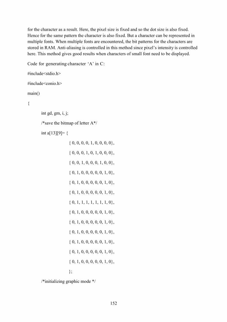
152

for the character as a result. Here, the pixel size is fixed and so the dot size is also fixed.

Hence for the same pattern the character is also fixed. But a character can be represented in

multiple fonts. When multiple fonts are encountered, the bit patterns for the characters are

stored in RAM. Anti-aliasing is controlled in this method since pixel’s intensity is controlled

here. This method gives good results when characters of small font need to be displayed.

Code for generating character ‘A’ in C: #include<stdio.h>

#include<conio.h>

main()

{

int gd, gm, i, j;

/*save the bitmap of letter A*/

int a[13][9]= {

{ 0, 0, 0, 0, 1, 0, 0, 0, 0},

{ 0, 0, 0, 1, 0, 1, 0, 0, 0},

{ 0, 0, 1, 0, 0, 0, 1, 0, 0},

{ 0, 1, 0, 0, 0, 0, 0, 1, 0},

{ 0, 1, 0, 0, 0, 0, 0, 1, 0},

{ 0, 1, 0, 0, 0, 0, 0, 1, 0},

{ 0, 1, 1, 1, 1, 1, 1, 1, 0},

{ 0, 1, 0, 0, 0, 0, 0, 1, 0},

{ 0, 1, 0, 0, 0, 0, 0, 1, 0},

{ 0, 1, 0, 0, 0, 0, 0, 1, 0},

{ 0, 1, 0, 0, 0, 0, 0, 1, 0},

{ 0, 1, 0, 0, 0, 0, 0, 1, 0},

{ 0, 1, 0, 0, 0, 0, 0, 1, 0},

};

/*initializing graphic mode */

153

detectgraph( &gd, &gm);

initgraph (&gd, &gm, “ ”);

for(i=0; i<13; i++)

{

for( j=0; j<9; j++)

{

PutPixel(200 + j, 200 + i, 15* a[i][j]);

}

}

getch();

closegraph();

} Check your progress / Self assessment questions

Q7. What are the limitations of Starbust method of character generation? ----------------------------------------------------------------------------------------------------------------

----------------------------------------------------------------------------------------------------------------

----------------------------------------------------------------------------------------------------------------

---------------------------------

6.6. Advantages of character generation Character generation will provide a way to the programmers to know about the generation of

characters in various ways that is useful for them in many ways. The various character

generation strategies involve the use of line drawing algorithms to generate different styles of

characters. It helps us to know about storage of character information in dot matrix form.

Different fonts that we normally use are also made up of various lines and curves and this we

will know with character generation methods.

6.7. Summary This chapter focuses on area filling in computer graphics. There are many methods to fill the

polygons. Area filling is an important task and requires complex algorithms. Character

generation is required in almost every scan conversion of popular graphic primitives like

lines and curves. Three important strategies are there for character generations are discussed

along with their examples.

154

6.8. Glossary Polygon - A polygon is basically a series of interconnected line segments. It can be specified

by vertices (or node) like P0, P1, P2, P3, and so on.

Concave polygon - A concave polygon is the one in which the line segment that joins any

two points may not lie completely inside the polygon boundary.

Convex polygon - A convex polygonis the one in which the line segment that joins any two

points lie completely within the polygon.


1. There are three basic methods to represent polygons:

Polygon drawing primitive method

Trapezoid primitive method

Line and point method

2. The major difference between concave and convex polygon is that in former, the line

segment joining any two points of the polygon may not lie completely inside the

polygon while in latter, the line segment that joins any two internal points always lie

within the polygon.

3. 8-connected regions are more preferred over 4-connected regions because 4-

connected regions result in partial filling because every pixel cannot be reached from

only four directions. In 8-connected region, there is no problem of partial filling.

4. Seed fill method is facing two major difficulties.

If there are some pixels inside the polygon that are already colored, then our

recursive loop terminates and some of the internal pixels are remained uncolored.

These methods are unsuitable for large polygons. It is so because it requires

storage of the neighboring pixels and for large polygons, the stack space for

storing the pixels can be insufficient.

5. The GetPixel() function being used here will return the color of the pixel being

specified as an argument and the PutPixel() functions plots the pixel with the color

being specified as an argument.

6. Two ways to represent the characters in graphics are Bitmap font representation and

Outline font representation.

155

7. Starbust method has the following limitations:

Every character is being represented by 24-bits so more memory is required.

24-bits code needs to be converted to display a character that requires some

code conversion software.

The quality of the character is poor. This method is not suitable for curve-

shaped characters.

6.10. Modal Questions

1. Why do we need area filling techniques in computer graphics?

2. Explain flood fill algorithm.

3. What do you mean by character generation?

4. Explain various strategies of character generation.

156

Lesson- 7

2D Transformations

Structure

7.0 Objective 7.1 Introduction

7.2 Cartesian coordinate system

7.3 Geometric Transformations

7.4 Homogeneous Coordinates

7.5 Inverse geometric Transformations

7.6 Coordinate Transformations

7.7 Composite Transformations

7.8 Summary

7.9 Glossary

7.10 Answers of Self-Assessment Questions

7.11 References

7.12 Model Questions

7.0 Objective

What are transformations and its types.

How objects move, rotate or change their shape.

Cartesian and Homogeneous Coordinate systems.

Learn to combine transformation matrices from simple transformation.

7.1 Introduction

With the passage of time, output devices change their attributes. We can create a variety of

animations, pictures, objects and graphics. In some cases we need to modify the existing

pictures. If we have only two coordinates say x and y axis, then it is called two dimensional

graphics and if we have three coordinates say x, y and z-axis then it is called three

157

dimensional graphics. A Transformation is the concept of repositioning any geometric objects

using some particular rules. Transformations in computer graphics can be used to change the

position, size and orientation of the objects.

Types of Transformations: There are two types of transformations depending upon the

object whether the object is moved relative to fixed coordinate

system or background, described by geometric transformation or

object is held stationary while the co-ordinate system is moving

relative to the object. This effect is described through coordinate

transformation.

Geometric Transformations

In this type of transformation, the object is moving relative to a fixed coordinate axis,

e.g. a car is moving, backdrop scenery is fixed. Following are the geometric transformation:

The basic geometric transformations are:

Translation

Scaling

Rotation Other transformations are:

Reflection

Shearing Coordinate Transformations Fig. 7.1

Here the object is fixed relative to a moving coordinate axis e.g. a car is fixed while backdrop

scenery is moving.

7.2Cartesian coordinate system

The Cartesian coordinate system is a two dimensional plane having two axes i.e. a horizontal

axis called as x-axis and a vertical axis called as y-axis. A Cartesian coordinate system

specifies each point in the x, y in plane with numerical coordinates, which are the signed

distances from the point to the x and y-axis. The point where both the axes intersect each

other is known as the origin. Here values of both x-axis and y-axis are zero. The intersection

of these two axes divides the two dimensional plane into four quadrants as shown in Fig. 7.1.

Cartesian coordinates are used in algebra and geometry in mathematics for solving

equations. Using the Cartesian coordinate system different geometric shapes can be

described. This is used in computer graphics, computer-aided design etc. But in computer

graphics, when we use these shapes and theorems, we need to calculate lengths, angles etc.

158

Homogeneous coordinate systems provide a method for doing calculations, when it is

used in practical applications. Homogeneous coordinate is used to represent the Cartesian

equations. People in computer field and graphics often deal with homogeneous coordinates.

Homogeneous coordinates are used to simplify various transformations. A Cartesian

pair(x, y) can be converted to a homogeneous coordinate (xh,yh, h) containing three

parameters xh, yh and h. We will discuss the concept of homogeneous coordinates after

transformations.

7.3Geometric Transformation

In this section, we will discuss about transformations of two dimensional objects and how

their matrix representation can be expressed.

7.3.1 Translation

Translation is the method to change the position of an object from one position to another

along a straight line path. We translate two dimensional objects by adding translation

distances and to the original co-ordinates(x, y) to move an object to a new position

x’ and y’ as:

’= + … (1)

’= + … (2)

Here ( , ) is known as translation vector or shift vector.

Suppose we have a point P at co-ordinate , and we want to

shift that point P to a new position P’ having co-ordinates ’

and ’see Fig. 7.2.

Matrix representation of the above equations is as follows:

′ = +

’ = +

where P = , P’ = ′

and T =

Fig. 7.2

159

Translation moves the objects without changing the object in size and shape. Each point on the object moves by same value. Suppose we want to translate a triangle with its three

vertices P(x1, y1), Q(x2, y2) and R(x3, y3) by tx along x-axis and ty along y-axis as shown in Fig 7.3

Fig. 7.3

In case of straight lines, triangles, polygons etc., we translate the objects by adding only translation vectors to the current set of vertices of the objects and redraw the objects using new set of vertices. In case of curved objects like circle or ellipse, we shift or translate the centre co-ordinates of the object and redraw the object at the new location.

7.3.2 Scaling with respect to the origin

Scaling transformation is used to change the size of the object. The scaling transformation is

carried out by multiplying the co-ordinates(x, y) of each vertex by scaling factors sx and syfor

transformed co-ordinates (x’, y’).

x’ = x. sx … (3)

y’ = y. sy ... (4)

The scaling factors sx and sy, scale the object along x and y-axis. The above set of

equations can be expressed in matrix form as:

0

′ = 0

P’ = P. S

where P = , P’ = ′

The values of :

and S =

160

1 2 2 1 3 0 3 6 6 3

1 1 2 2 0

1

1

Any positive real value can be assigned to scaling factors.

a) If the value of < 1, size of the object will be reduced.

b) If the value of > 1,size of the object will be increased.

c) If = , size of the object will remain same. This type of scaling is called

UniformScaling.

d) If ≠ ,this type of scaling is called Differential Scaling. This type of

scaling is often used in design applications, where pictures are constructed from a few fundamental shapes that can be adjusted by scaling and positioning

transformations.

With scaling transformation objects are scaled and repositioned. Scaling factors

having values less than 1 move objects closer to the co-ordinate origin (0, 0). The values

greater than 1 move objects farther from the co-ordinate origin. For example: The value of

is i.e. less than 1 moves the line closer to the

origin, see Fig. 7.4

Let us suppose we have a square having vertices:

P (1,1), Q(2,1), R(2,2) and S(1,2)

We scale it by scaling factors = 3 =

. After

scaling, square will transform in rectangle (see Fig. 7.5) as we

multiply scaling factors with original vertices and the value

becomes:

P’ (3, ), Q’ (7, ), R’(7,1) and S’ (3,1).

Matrix representation of above vertices is as follows: Fig. 7.4

P Q R Ssx sy P’ Q’ R’ S’

=

161

Before Scaling Fig. 7 5 After

We can take another example to scale a triangle. As a triangle has thre

(30, 0) and C (50, 100) and scaling factors = 2 = 2.Usin

scaling of triangle is as shown in Fig.7.6

. Scaling

e vertices A (20, 0), B

g equations of scaling,

Before Scaling Fig. 7.6 After Scaling

7.3.3 Rotation about the origin

In rotation, the object is rotated along a two dimensional plane. The rotation is done through

some angle θ ° about the origin, either in clockwise or in anti-clockwise direction.

If θ is the positive angle, the direction of rotation is anti-clockwise and if θ is the negative

angle, the direction of rotation is clock wise.

First we find the rotation transformation equations for a point P(x, y) which is rotated anti-

clockwise by an angel θ to the point P’(x’, y’) as shown in Fig. 7.7. This transformation can

also be specified as a rotation about a rotation axis that is perpendicular to the xy plane and

passes through the pivot point.

162

Fig. 7.7

The angular and coordinate relationship of the original and new transformed point is shown

in Fig. 7.8. In this Fig, r is the constant distance from the origin, is the original angular

position and θ is the rotation angel.

Now, we determine relationship between (x, y) and (x’, y’).

x = r cos … (5)

y = r sin … (6)

Similarly,

x’ = r cos (θ+ ) … (7)

y’ = r sin (θ+ ) … (8)

From eq. (7)

x’ = r cos (θ+ )

= r (cos θ cos - sin θ sin )

[∴ cos( + ) = cos cos − sin sin ]

= r cos cos θ – r sin sin θ

= (r cos ) cos θ – (r sin ) sin θ

= x cos θ - y sin θ

∴ x’ = x cos θ – y sin θ … (9) Fig. 7.8

Similarly, from eq. (8), we get

y’ = x sin θ+ y cos θ … (10)

Eq. (9) and (10) can be written in the matrix form as:

cos − sin

′ =

sin cos

163

P’ = Rθ.P

where Rθ = cos − sin sin cos

= Rotation matrix

If rotation of a point is in clockwise direction, then values of rotation matrix will not

change, only its sine components change signs i.e.

Rθ = cos sin

− sin cos

7.3.4 Reflection

A reflection is the transformation that produces the mirror image of the graphics objects. The

mirror image for two dimensional reflections is generated relative to axis of reflection by

rotating the object 180° about the reflection axis. The distances and image of the objects are

same from the reflection axis. We can choose an axis for reflection in the plane.

Reflection may be of horizontal type (about x-axis) or vertical type (about y-axis).

Following are the equations for mirror reflection: Reflection about x-axis:

The transformation matrix for getting the reflection image about the horizontal axis can be

expressed as:

x’ = x …(11)

y’ = -y …(12)


Reflection about x-axis

1 0

′ =

0 − 1

P’ = Mx. P Fig. 7.9

where Mx = Reflection matrix about x-axis.

Reflection about y-axis:

164

Similarly, the transformation matrix for getting the reflection

image about the vertical axis can be expressed as:

x’= -x …(13)

y’=y …(14) Eq. (13) and (14) can be written in matrix form as:

= − 1 0

′ 0 1

P’=My.P

Where My= Reflection matrix about y-axis.

Fig. 7.10Reflection about y-axis Reflection about both axes:

In the same way, we can get the transformation matrix for the

reflection across the horizontal and vertical axis as:

x’’= -x’, y’’ =y’

And x’= x, y’= -y

∴x’’= -x …(15)

y’’= -y …(16)


= − 1 0

′′ 0 − 1

P’’=M.P

M= Reflection matrix Fig. 7.11

165

axes

7.3.5 Shear

Reflection about both

This transformation distorts the shape of the image in such a way that it seems some layers of

the image have been sheared off from the original image. Two common shearing

transformations are used: towards x-axis and towards y-axis. The x-axis maintains the y-

coordinates but changes the x values. The y-axis shift y-coordinates but maintains x-

coordinate values.

Following are the equations of shearing: Shearing towards x-axis:

The transformation matrix for shearing in the x- axis direction can be given as:

x’ = x + ℎ . …(17)

y’ = y …(18) where ℎ is shearing constant towards x-axis. Any real value can be assigned to this constant. A coordinate position ( , ) is shifted horizontally from x-axis. Giving values of ℎ to 2 changes the square in parallelogram as in Fig. 7.12. Negative values for ℎ shift

coordinate positions to the left.

The matrix representation is as follows:

1 ℎ

′ =

0 1

Where ℎ = shearing matrix towards x-axis.

Any real value can be assigned to shearing matrix.

If value of ℎ is positive, shearing will be on right side.

If value of ℎ is negative, shearing will be on left side.

If value of ℎ is zero, there will be no shearing.

166

Fig. 7.12

Shearing

towards y-

axis:

The transformation matrix for shearing towards y-axis is as follows:

’ = … (19)

’ = + ℎ . … (20)

Above eq. can be written in matrix form as:

1 0

′ = ℎ 1

shy= shearing matrix towards y-axis. Like shx, shy can also take any real value.

If the value of shy is positive, the shearing will be towards upper side i.e. towards

positive y-axis.

If the value of shy is negative, the shearing will be towards lower side i.e. towards

negative y-axis.

If value of shy is zero, there will be no shearing.

Fig. 7.13 illustrates the conversion of a square into parallelogram with shy=1/2

167

Fig. 7.13 Shearing towards both axes:

The equation for both x-axis and y-axis is as follows:

x’ = x + shx . y …(21)

y’ = y + shy . x …(22)

The matrix representations of these equations are as follows:

1 ℎ

′ = ℎ 1

shx.shy = shearing matrix towards both directions.

7.4 Homogeneous Coordinates

Homogeneous coordinates are used for matrix representation of all these transformations.

Here two dimensional transformation matrix of 2×2 can be written in 3×3 matrix with the

Self Assessment-Questions:

Q1. What is the difference between geometric transformation and coordinate transformation?

Q2. When value of ℎ is positive towards x axis, shearing will be on left side?

a) TRUE b) FALSE

168

homogeneous coordinate triple (xh, yh, h)

where , x = xh/h and y = yh/h

h is called homogeneous parameter, it can have any non-zero value. Corresponding to each

value of h, we have different homogeneous representation of coordinate point (x, y). Most of

the time h will be taken as unity i.e. h=1.Homogeneous coordinates help us to represent all

transformation equations as matrix multiplication.

Every point (x, y) in two dimensional is represented with homogeneous coordinate (x, y, 1).

7.4.1 Advantages of Homogeneous Coordinates

a) Two dimensional transformations can be represented by 3×3 matrices. This will

make operations easier to perform.

b) For transformations of floating point calculations to integer calculations, the

operations will be performed in better way.

7.4.2Representation of Transformations in Homogeneous Coordinates

i. Translation

1 0

= 0 1 .

1 0 0 1 1

ii. Scaling

0 0

= 0 0 .

1 0 0 1 1

iii. Rotation

cos − sin 0

= sin cos 0 . 1 0 0 1 1

iv. Reflection

About x-axis =

1 0 0 0 − 1 0

0 0 1

169

M yx

About y-axis = − 1 0 0 0 1 0

0 0 1

v. Shearing

Relative to x-axis =

Relative to y-axis =

1 ℎ 0 0 1 0

0 0 1

1 0 0

ℎ 1 0

0 0 1

Relative to both the axes = 1 ℎ 0

ℎ 1 0

0 0 1

7.5 Inverse Geometric Transformations:

When geometric transformations are performed in opposite order, then they are called inverse

geometric transformations. Each transformation has its inverse. Inverse geometric

transformations are as follows:

a) Translation: Translation in the opposite direction. -1

Tv = T-v, where v is the translation vector.

b) Rotation: Rotation in the opposite direction.

Rθ-1 = R-θ, where θ is angle of rotation.

c) Scaling: Scaling in the opposite direction.

S-1 s , s

= S1/s ,1/s , where sx, sy are called scaling factors in x, y direction.

x y x y

d) Reflection: Reflection in the opposite direction. -1 = Mx , M -1

=My

7.6 Coordinate Transformation:

In this type of transformation, the body is fixed and coordinate system is moving. Here we

suppose that we have two coordinate systems in the plane. The first system is located at

origin O and has coordinates (x, y). The second coordinate system is located at origin O’ and

has coordinates (x’, y’) and v is the displacement vector as in Fig. 7.14.

170

Here we also have all these five transformations namely Translation, Rotation, Scaling,

Reflection and Shearing.

7.6.1 TranslationFig. 7.14

If the x, y plane or coordinate system is displaced to a new position, where the direction and

distance of the displacement is given by vector ⃗ = tx⃗+ ty ,⃗ where tx and ty are translation

towards x and y axes respectively.

The relationship between old coordinates (x, y) and new coordinates (x’, y’) is as follows:

x’ = x - tx

y’ = y - ty

Matrix representation is as follows:

1 0 −

= 0 1 − 1 0 0 1

1

P’ = . P

Where =

1 0 − 0 1 −

0 0 1

= Coordinate Translation matrix

7.6.2 Rotation about origin

The coordinate system xy is rotated by θ° about the origin then the coordinates of a point on

both systems are related by the rotational transformation . The equation of rotation is as

follows:

x’ = x cos θ + y sin θ

y’ = - x sin θ + y cos θ

Above equations can be written in matrix form as follows:

171

P’ = . P

= 1

cos sin 0

cos sin 0 − sin cos 0

0 0 1 1

Where = − sin cos 0 = Coordinate Rotational matrix

0 0 1

7.6.3 Scaling with respect to the origin

In this case, new coordinate system is formed by taking different measurement units along x

and y axis, here origin and coordinate axes remain unchanged. The relationship between new

coordinates (x’, y’) and old coordinates (x, y) is as follows:

x’ = . x

y’ = . y

where sx and sy are scaling factors along x and y axis respectively.

The matrix representation of the above equations is as follows:

⎡ 0 0⎤

= ⎢ ⎥

1 ⎢0 0⎥ 1

⎣0 0 1⎦

P’ = Ssx.sy

. P

⎡ 0 0⎤

⎢ ⎥

Where ̅Ssx.sy =

⎢0 0⎥ ⎣0 0 1⎦

= Coordinate Scaling matrix

7.6.3 Mirror Reflection about an axis

In this case, new coordinate system is reflecting the old coordinate system about either x or y

axes. Relationship between new coordinates (x’, y’) and old coordinates (x, y) is given by:

About x-axis

x’ = x

y’ = - y


172

1 0 0 = 0 − 1 0

1 0 0 1 1

P’ = Mx . P

Where ̅Mx =

1 0 0 0 − 1 0

0 0 1

= Coordinate Reflection matrix

About y-axis

x’ = - x

y’ = y


− 1 0 0

= 0 1 0 1 0 0 1 1

P’ = My . P

− 1 0 0

Where ̅My = 0 1 0 = Coordinate Reflection matrix 0 0 1

7.7 Composite transformations:

More complex geometric transformations can be built from basic transformations described

above. For composite transformation, we combine basic transformation and multiply

matrices. This process is known as concentration of matrices and the resultant matrix is called

composite transformation matrix. For example, rotation about a point other than the origin.

7.7.1 Translations

If two successive translation vectors (tx1, ty1) and (tx2, ty2) are applied to a coordinate

position P, P’ can be calculated as:

P’ = T (tx2, ty2). {T (tx1, ty1).P}

= {T (tx2, ty2).T (tx1, ty1)}.P

Now the product of these two translation vectors can be as follows:

173

cos − sin 0 cos − sin 0 sin cos 0 . sin cos 0

0 0 1 0 0 1

1 0 1 0 1 0 + 0 1 . 0 1 = 0 1 + 0 0 1 0 0 1 0 0 1

T (tx2, ty2). T (tx1, ty1) = T (tx1 + tx2, ty1 + ty2)

This expression indicates that the effects of successive translations are always additive in

nature.

7.7.2 Rotation

Using the same principal, we can write the general expression of the transformations if two

successive rotations are provided at point P, rotations of angle θ1 and θ2. The equation can be

expressed as:

P’ = R(θ2). {R(θ1).P}

= {R(θ2).R(θ1)}.P

= R(θ).P

∴ R(θ) = R(θ1).R(θ2)

=

cos .cos − sin .sin + 0 cos sin − sin .cos + 0 0 = sin .cos − cos .sin + 0 sin .sin − cos .cos + 0 0

0 0 1

R(θ) =

cos( + ) − sin( + ) 0 sin( + ) cos( + ) 0 0 0 1

In simple terms it can be written as:

R(θ1).R(θ2) = R(θ1+θ2)

This expression indicates that two successive rotations are additive. The result of composite

matrix is as follows:

P’ = R(θ1+θ2) . P

7.7.3 Scaling

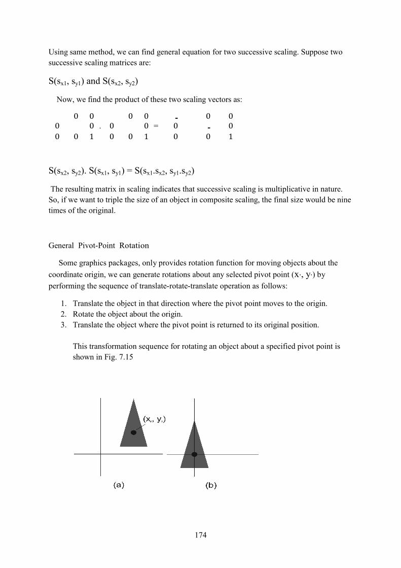
174

Using same method, we can find general equation for two successive scaling. Suppose two

successive scaling matrices are:

S(sx1, sy1) and S(sx2, sy2)

Now, we find the product of these two scaling vectors as:

0 0 0 0 . 0 0 0 0 . 0 0 = 0 . 0 0 0 1 0 0 1 0 0 1

S(sx2, sy2). S(sx1, sy1) = S(sx1.sx2, sy1.sy2)

The resulting matrix in scaling indicates that successive scaling is multiplicative in nature.

So, if we want to triple the size of an object in composite scaling, the final size would be nine

times of the original.

General Pivot-Point Rotation

Some graphics packages, only provides rotation function for moving objects about the

coordinate origin, we can generate rotations about any selected pivot point (x’, y’) by

performing the sequence of translate-rotate-translate operation as follows:

1. Translate the object in that direction where the pivot point moves to the origin.

2. Rotate the object about the origin.

3. Translate the object where the pivot point is returned to its original position.

This transformation sequence for rotating an object about a specified pivot point is

shown in Fig. 7.15

175

Fig. 7.15

For first translation: T(x’,y’) =

1 0 0 1

0 0 1

For rotation: R(θ) =

cos − sin 0 sin cos 0 0 0 1

For last transformation: T(-x’, -y’) = 1 0 − 0 1 −

0 0 1

The concatenated matrix is:

1 0 cos − sin 0 1 0 − 0 1 . sin cos 0 . 0 1 − 0 0 1 0 0 1 0 0 1

cosθ − sinθ (1 − cos ) + sin = sinθ cos (1 − cos ) − sin

0 0 1

In simple form:

T(x’,y’). R(θ). T(-x’,-y’)= R(x’,y’,θ)

where T(-x’,-y’) = T-1(x’,y’)

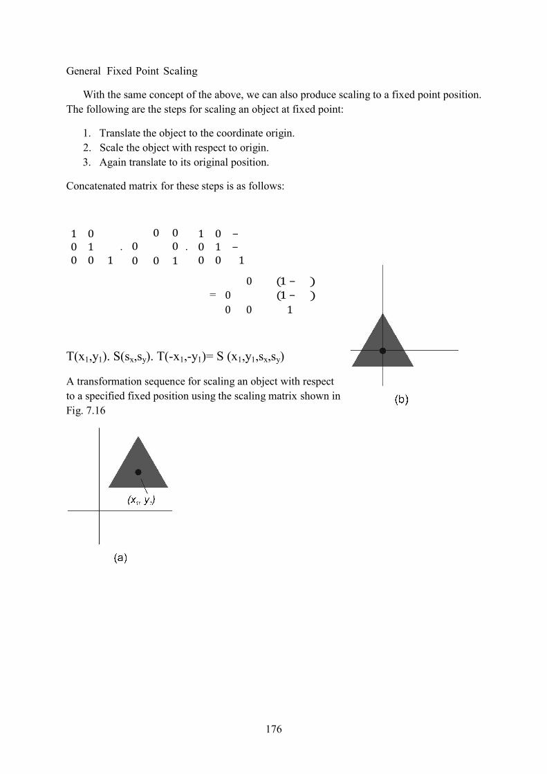
176

0 (1 − ) = 0 (1 − )

0 0 1

T(x1,y1). S(sx,sy). T(-x1,-y1)= S (x1,y1,sx,sy) A transformation sequence for scaling an object with respect

to a specified fixed position using the scaling matrix shown in

Fig. 7.16

1 0 0 0 1 0 − 0 1 . 0 0 . 0 1 − 0 0 1 0 0 1 0 0 1

General Fixed Point Scaling

With the same concept of the above, we can also produce scaling to a fixed point position.

The following are the steps for scaling an object at fixed point:

1. Translate the object to the coordinate origin.

2. Scale the object with respect to origin.

3. Again translate to its original position.

Concatenated matrix for these steps is as follows:

177

Fig. 7.16

Self Assessment Questions:

Q3. What is the general form of scaling with respect to a fixed point P (h, k)?

7.8 Summary Transformation is the process of repositioning any geometric

object to new location either by translation, rotation, scaling

or by other transformations (reflection, shearing) technique.

In translation, the object is moved to new location by adding

translation distance tx and ty. Scaling alters the size of the

objects i.e. the object can be compressed or expanded. This

transformation alters the size by multiplying with scaling

factors sx and sy to the coordinate values. In case of rotation,

an object is rotated about the origin at a certain angle θ. If θ is

the positive angle then the direction of rotation is anti clockwise and clockwise if θ is the

negative angle. Reflection produces the mirror image of graphics object. The reflection is

done by rotating the object 180° about the reflection axis. Shear transformation distorts the

shape of the image in such a way that it seems some layers of the image have been sheared

off from the original image. When geometric transformations are performed in opposite

order, they are known as inverse geometric transformations. Two dimensional

transformations can be represented by 3×3 matrix. In this each coordinate point (x, y) can be

represented with homogeneous coordinate (xh, yh, h). By combining elementary

transformations, we can generate composite transformation. Here we combine basic

178

transformations and multiply matrices, the resultant is called composite transformation

matrix.

7.9 Glossary

Coordinate system- A way to assign numerical coordinates to geometric points. Each point

is in the form of pair (x, y) and is called x-axis and y-axis respectively. The geometric points

is known as a plane.

Geometric transformation- The object is moved relative to a fixed or stationary coordinate

system.

Homogeneous coordinates- a way to represent transformations in matrix form. Two

dimensional transformation can be represented by 3×3 matrix by including homogeneous

parameter h. the value of h can be taken as unity i.e. h=1.

Inverse transformation- When geometric transformations are performed in opposite order,

they are known as inverse geometric transformations. Every transformation has its inverse.

Matrix- Collection of numbers arranged in rows and columns represented by rectangular

array of numbers.

7.10 Answers of Self Assessment Questions

1. In Geometric transformation, the object is moved relative to a fixed coordinate axis.

Example, a car is moving while backdrop scenery is fixed. In Coordinate

transformation, the object is fixed relative to moving coordinate axis. Example, a car

is fixed while backdrop scenery is moving.

2. FALSE

3. Following is the sequence of steps for fixed point scaling:

a. Translate point P (h, k) to the origin.

b. Scale about origin by scaling factors sx and sy along x-axis and y-axis

respectively.

c. Again translate to its original position.

Solutions of EXERCISES

EXERCISE 1

Sol. Rotation matrix is given by cos − sin

Rθ = sin cos

now, θ=45°(given)

179

R45° =

cos45° − sin45° sin45° cos45°

− √ √ 1

= ∵ sin45° = cos45° = √ 2

√ √

7.11 References

1. Computer Graphics, Donald Hearn, M. Pauline Baker, Second Edition

2. Computer Graphics, Shefali Aggarwal


Q1. What do you mean by Transformations? Explain geometric transformations with suitable

examples.

Q2. Explain composite transformation with example.

Q3. Discuss about the homogeneous coordinate system.

181

Lesson- 8

2D Viewing Transformations

Structure 8.0 Objective

8.1 Introduction

8.2 Window-to-Viewport Mapping

8.3 Clipping

8.4 Point Clipping

8.5 Line Clipping

8.6 Cohen-Sutherland Algorithm

8.7 Liang Barsky Algorithm

8.8 Polygon Clipping

8.9 Sutherland-Hodgeman algorithm

8.10 Text Clipping

8.11 Summary

8.12 Glossary


8.14 References


8.0 Objective

After studying this chapter, students will be able to:

Introduction of windowing concepts.

Understand Viewing Transformations.

Describe clipping and its algorithms.

182

8.1 Introduction

The two dimensional viewing is the concept to view an image from different positions. The

computer graphics images can be drawn either on two dimensional or three dimensional

planes. The two dimensional graphics normally use device coordinates. Any graphics object

that lies partially or completely outside the window then that part will not be viewed. Many

graphics packages allow a user to specify which part of specific picture is to be displayed. A

rectangular area with its edges parallel to coordinate axes where the picture is to be displayed

is called window and the viewing area is known as the viewport. The window describes what

is to be displayed and viewport describe where to display. A window and viewport are

rectangular in standard shape. They can be of any shape like general polygon shapes and

circles. But analysis of these shapes is complex than rectangular shape.

World co-ordinate system:A Cartesian co-ordinate system can be referred to as word

coordinate system (WCS) to display the picture.

Device co-ordinate system:The devices where picture is to be displayed. Normalized device co-ordinate system: The sizes of display devices like monitors differ

from one system to another, a device independent tool introduced to describe the display area

known as normalized co-ordinate system (NDCS). In this system, unit square (1×1) whose

lower left corner is at origin of co-ordinate system.

Viewing Transformation: Viewing transformation can be defined as the mapping of picture

co-ordinates of world co-ordinate system to device co-ordinate system or normalized device

co-ordinate system (NDCS). It can also be referred as windowing transformation or window

to viewport transformation or Normalized Transformation.

Fig. 8.1Viewing Transformation

8.2 Window-to-Viewport Mapping

183

A window is specified by four world co-ordinates: xwmin, xwmax, ywmin and ywmax. Similarly,

a viewport has four normalized device co-ordinates: xvmin, xvmax, yvmin and yvmax (see Fig.

8.2). The main purpose of window-to-viewport mapping is to convert the world co-ordinates

( , ) to its corresponding normalized device co-ordinates( , ). For maintaining the

relative placement of the point in the viewport as in the window, we need:

=

= … (2)

… (1)

Now calculate as:

=

=

− −

( − ) +

−

− ( − ) +

Fig. 8.2 Window-to-viewport mapping

There are total eight co-ordinate values that define window and viewport which are constants.

The normalized transformation N is as follows:

0 (− . + )

N= 0 (− . + )

Where

0 0 1

− − = = − −

184

, are co-ordinates of viewport and

, are co-ordinates of window.

Example1. Derive the normalization transformation N that maps a rectangular window

with x-extent xwmin to xwmax in the x direction and y-extent ywmin to ywmax in the y

direction onto a rectangular viewpoint with x-extent xvminto xvmaxand y-extent yvminto

yvmax

Sol. Scaling transformations

xw = =

yw = =

Normal Transformation

0 (− − + ) 1 0 ( − ) N = 0 (− . + ) 0 1 ( − )

0 0 1 0 0 1

0 (− . = 0 (− .

+

+

)

)

0 0 1

Examle2. Find the normalization transformation that maps a window whose lower left

corner is at (2, 2) and upper right corner is at (3, 4) onto

(a) A viewport that is the entire normalized device screen and

(b) A viewpoint that has lower left corner at (0, 0) and upper right corner (3/2, 3/2).

Sol. The windows parameters are:

xwmin = 2, xwmax = 3, ywmin = 2 and ywmax= 4

The viewport parameters are:

xvmin = 0, xvmax = 1, yvmin = 0 and yvmax= 1

xw = = = 1 yw = = =

185

0 (− . + ) (a) N = 0 (− . + ) 0 0 1

1 0 (− 1 ∗ 2 + 0)

= 0 1 2

− 1

∗ 2 + 0 2

0 0 1 1 0 − 2

= 0 1

− 1 2

0 0 1

(b) xvmin = 0, xvmax = , yvmin = 0, yvmax =

xw = =

3− 0 2 = , 3− 2

yw = =

3− 0 2 = 4− 2

3 0 − 3

2 N = 3 3

0 2

− 2

0 0 1


Q1: To change the size and amount of the object, the dimensions of the viewport must be

changed.

(a) TRUE

(b) False

Q2. The rectangular area where a selected object is viewed is known as window.

(a) TRUE

(b) FALSE

8.3 Clipping

Clipping is the procedure that identifies the portions of the picture that are either inside or

outside of a specified region of space. It is also called clipping algorithm. The region or space

which is used to see the object is called as clip window.

186

In the viewing transformation, only

that part of picture is to be displayed which in

inside the clipping window. Everything outside

the window is discarded.

There are four types of clipping:

(1) Point Clipping

(2) Line Clipping

(3) Polygon Clipping or Area Clipping

(4) Text Clipping

8.4 Point Clipping

For point clipping, we assume that the clip window is rectangle in shape. We consider a point

P (x, y) for display if the following conditions are satisfied:

£ £

£ £

The edges of the clip window ( , ) and ( , ) can be either world co-

ordinate window boundaries or viewport boundaries. If any one of the above conditions is not

satisfied, the point is clipped but not saved for display. Point clipping is less required in real

life applications.

8.5 Line Clipping

A line clipping method is used to check whether a line is completely inside or outside a

window and if it is not,we perform intersection calculation with one or more clipping

boundaries. We start by checking the endpoints of the lines and test which points of the lines

comes inside or outside the clip window. A line with both the endpoints inside the clipping

boundary is saved as P1 and P2(see Fig. 8.3). A line with both the endpoints outside the

clipping boundaries is outside the window like P3and P4, P9and P10 (see Fig. 8.3). The P5 and

P6 line, the P5 is outside to the clipping window but P6 is inside the window. So that part of

the line will be visible that comes in clipping window.

187

Before Clipping Fig. 8.3After Clipping

There are two line clipping algorithms:

1) Cohen-Sutherland Algorithm

2) Liang Barsky Algorithm

8.6 Cohen-Sutherland Algorithm

This is one of the oldest and popular lines clipping algorithm. In this we divide the clipping

process into two steps:

1) Determine the lines for clipping which intersect the window.

2) Apply clipping process. The following are the line clipping categories:

a) Visible-In this category, both the endpoints of a line are inside the clipping window.

b) Not Visible- Here, the line segment is completely outside the clipping window. This

will happen when the line segment from (x, y) to (x’, y’) satisfies any one of the four

inequalities.

c) Clipping Candidate- when the line segment condition is neither in category (a) nor

(b). Cohen Sutherland algorithm for line clipping performs following procedure:

1. find the visibility of the line by assigning 4-bit region code to every endpoint of the line.

Each bit in the region code is used to indicate four relative co-ordinate positions of the point

with respect to the clip window (see Fig. 8.4). Bit 1 (left bit) of this code and all other bits are

set to 1 depending upon following conditions:

Bit 1- set to 1 if the endpoint is above the window.

Bit 2- set to 1 if the endpoint is below the window.

Bit 3- set to 1 if the endpoint is to the right of the window.

Bit 4- set to 1 if the endpoint is to the left of the window.

188

Fig. 8.4 A 4 bit region code 2. If both region codes are 0000, the line is visible and the line is inside the window. The line

is not visible, if the logical AND of the region codes is not 0000. If logical AND of the region

codes is 0000 the line is candidate for clipping.

3. Find the intersection points of the line which is candidate clipping with boundaries of

window.

The intersection point of the line is easy to calculate using slope intercept form of the line

equation. Let we have co-ordinates of line (x1, y1) and (x2, y2) and the minimum and

maximum co-ordinates of the boundary lines are (xmin, ymin) and (xmax, ymax).

To find intersection points with vertical boundary i.e. left or right, following equations used:

− 1 = ( − 1)

= ( ℎ )

= ( )

189

To find intersection points with horizontal boundary i.e. top or bottom, following equations

used:

− = +

= ( )

= ( )

After finding intersection points, the new points are generated. Hence, the line is clipped. Example:

Fig. 8.5

The region codes for all points are:

A 0000 D 1010

B 0000 E 1001

C 0000 F 1000 As we can see, the line AB is inside the clip window, so save this line. Perform AND

operation on C and D and E and F

190

C 0000 E 1001

D 1010 F 1000

——

0000 candidate for clipping

——

1000 discard the line

CD line is candidate for clipping. Clipping of CD is performed with top boundary

−

= + … (1)

Ymax = 6, (3, 8) i.e. x1= -1, y1= 5

− = −

8 − 5 3 = = 3 + 1 4

Put values of x1,y1, ymax and m in eq. (1)

6 − 5 = + (− 1)

1 = − 1 =

4 − 1 = 3

4 − 3 1 = 3 3

1 = 3

∴ = = 6

∴ C= (-1, 5) and D= ( , 6)

After Clipping (see Fig. 8.6)

191

Fig. 8.6

8.7 Liang Barsky Algorithm

Liang Barsky line clipping algorithm is faster than Cohen Sutherland algorithm. This

algorithm has been developed using the parametric equation of line. This algorithm reduces

the intersection calculations. The parametric equation of the can be written as:

= + D

= + D

Where u is an independent variable and range of u is from 0 to 1 (see Fig.8.7) and Dx=x2-x1

and Dy=y2-y1.

If value of u is 0 then x will be equal to xmin and y will be equal to ymin. Similarly, if value of

u is 1 then x will be xmax and y will be ymax. Consider point clipping condition in parametric

form as:

£ + D £

£ + D £

The above four inequalities can be written as:

£ , k=1, 2, 3, 4

Where parameters p and q are defined as:

= − D , = 1 − (left)

= D , = − (right)

= − D , = 1 − (bottom)

192

= D , = − (top)

8.7

Fig.

Check the following situations:

if = 0, the line is parallel to the corresponding boundary. If k=1, it will parallel to left boundary. For k=2, it will be parallel to the right boundary. Similarly, for k=3 and k=4, the line will parallel to bottom and top of the boundary and

if < 0 , the line is completely outside the boundary and no clipping is

required. if ³ 0 , the line is inside the parallel clipping boundary.

if < 0 , the line will be proceeded from outside to the inside of the viewport and

the clipping will be required.

if > 0 , the line proceeds from the inside to the outside of the viewport and needs

to be clipped. if ≠ 0 , calculate the value of u where the line intersects the boundary k as:

=

Using above relation we can calculate values of parameters u1 and u2. The value of u1 can be

calculated by the line proceeds from outside to the inside ( < 0). For this we calculate =

/ . The value of u1 is taken as maximum of the set consisting of 0 and values of r. the

value of u2is calculated by from inside to the outside ( > 0) and value of u2 is minimum of

the set consisting of 1 and values of r. if u1>u2, the line is completely outside the clipping window and can be rejected. Otherwise, endpoints of the clipped line are calculated from u1

and u2.

8.8 Polygon Clipping

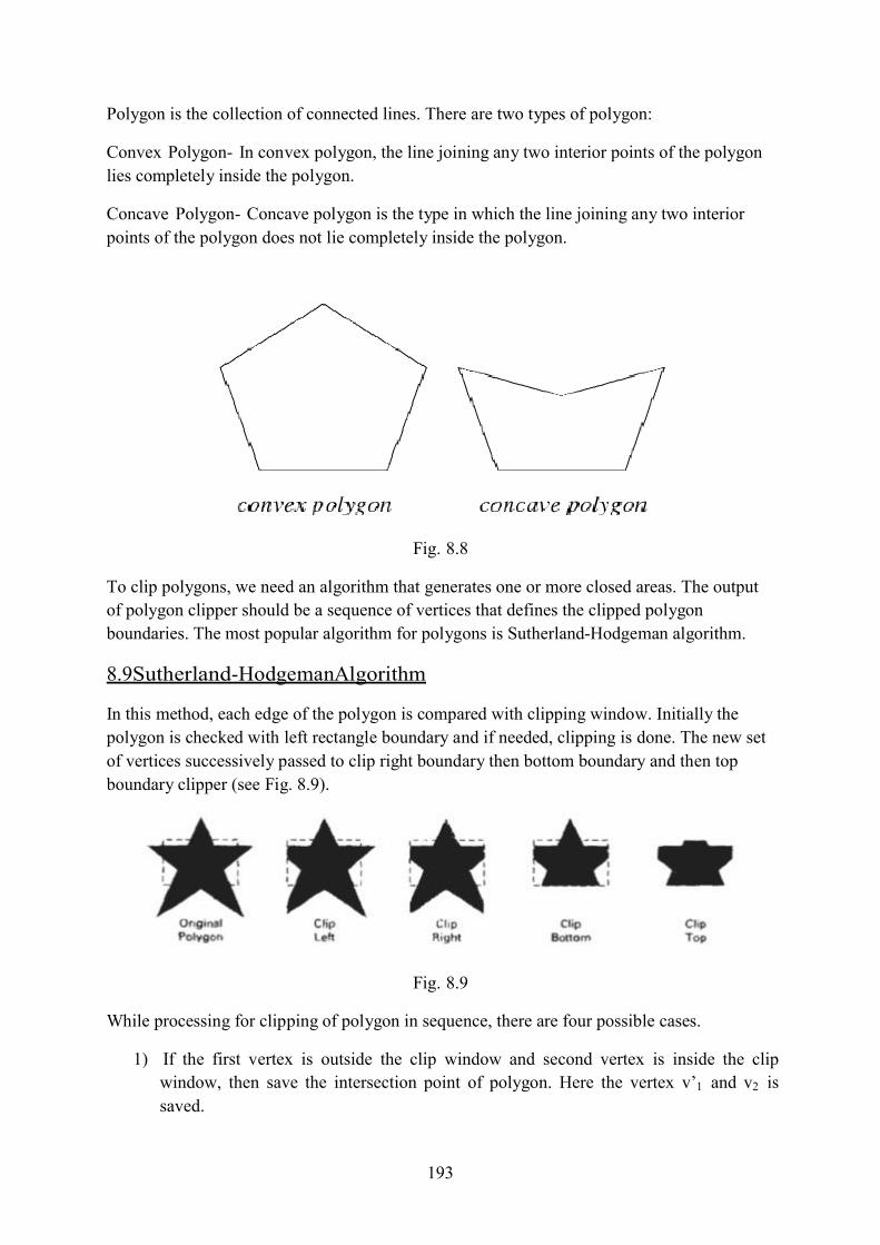
193

Polygon is the collection of connected lines. There are two types of polygon: Convex Polygon- In convex polygon, the line joining any two interior points of the polygon

lies completely inside the polygon.

Concave Polygon- Concave polygon is the type in which the line joining any two interior

points of the polygon does not lie completely inside the polygon.

Fig. 8.8

To clip polygons, we need an algorithm that generates one or more closed areas. The output

of polygon clipper should be a sequence of vertices that defines the clipped polygon

boundaries. The most popular algorithm for polygons is Sutherland-Hodgeman algorithm.

8.9 Sutherland-Hodgeman Algorithm

In this method, each edge of the polygon is compared with clipping window. Initially the

polygon is checked with left rectangle boundary and if needed, clipping is done. The new set

of vertices successively passed to clip right boundary then bottom boundary and then top

boundary clipper (see Fig. 8.9).

Fig. 8.9

While processing for clipping of polygon in sequence, there are four possible cases.

1) If the first vertex is outside the clip window and second vertex is inside the clip

window, then save the intersection point of polygon. Here the vertex v’1 and v2 is

saved.

194

Fig. 8.10

2) If both the vertices are inside the clip window, then save the second vertex only. In

this case, v1 and v2 both are inside the clip window so v2 is saved.

Fig. 8.11

3) If the first vertex is inside the clip window and second vertex is outside the clip

window, then save the intersection point of polygon edge and window boundary i.e.

v’1 and v1.

Fig. 8.12

4) If both input vertices are outside the clip window, then nothing is saved. Both vertices

v1 and v2 are outside of clip window.

195

Fig. 8.13 ple: Clip the polygon P1, P2, P3,…….., P8 against the window LMNO.

Exam

Fig. 8.14

(i) Clip against an edge LM of the clip window.

The vertex output list = I1, I2, P2, P3, P4, P5, P6, P7, P8,

where I1and I2 are intersection points of P1P2, LM, and P1P8, LM respectively.

196

Fig. 8.15. Clipping against bottom edge

(ii) Clip against an edge MN

The vertex output list = I1, I2, P2, I3, I4, P4, P5, P6, P7, P8,

where I3and I4 are intersection points of P2P3, MN, and P3P4, MN respectively.

Fig. 8.16. Clipping against right edge

(iii) Clip against an edge ON

The vertex output list = I1, I2, P2, I3, I4, P4,I5, I6,P6, P7, P8,

where I5and I6 are intersection points of P4P5, ON, and P5P6, ON respectively.

197

Fig. 8.17. Clipping against top edge

(iv) Clip against an edge OL

The vertex output list = I1, I2, P2, I3, I4, P4,I5, I6,P6, I7, I8, P8,

where I7 and I8 are intersection points of P6P7, OL, and P7P8, OL respectively.

Fig. 8.18. Clipping against left edge

So, polygon P1,P2……P8 after applying Sutherland-Hodgeman clipping algorithm will be

transformed to I1, I2, P2, I3, I4, P4,I5, I6,P6, I7, I8, P8.

8.10 Text Clipping

Sometimes it is required to clip text in the clipping window. There are different techniques to

clip the text. The methods are as follows:

All or none string clipping-If the string is completely inside the clip window, then we save

it. Otherwise the string is not saved and discarded (see Fig. 8.19). This is implemented by

considering a bounded rectangle around the string. The boundary positions of the rectangle

are compared to the clip window. If there is an overlap, the string is rejected.

198

Fig. 8.19

or none character clipping-In this method, we discard only these characters that are

pletely inside the clip window (see Fig. 8.20) and not the complete text. Here the

undary limits of each individual character are compared to the window. Any character t

utside the clip window is discarded.

All not

com

bo hat

is o

Fig. 8.20 Individual character clipping-This method checks character by character of the text

whether it is inside or outside the clip window. If the text is present inside the clip window, it

will be displayed. Otherwise it is discarded. If some part of the character is inside and some

part is outside of the clip window then clipping is done so that the part of the text which is

inside the clip window is saved (see Fig. 8.21).

199

Fig. 8.21


Q3. In point clipping, the boundary of the clip window can be either world co-ordinate

boundary or viewport boundary.

a. TRUE

b. FALSE

Q4. If the line is either completely inside or not visible, then line is candidate for clipping.

a. TRUE

b. FALSE

8.11 Summary

A rectangular area with its edges parallel to coordinate axes where the picture is to be

displayed is called window and the viewing area is known as the viewport.A window and

viewport are rectangular in standard shape.Viewing transformation can be defined as the

mapping of picture co-ordinates of world co-ordinate system to device co-ordinate system or

normalized device co-ordinate system (NDCS).Window-to-viewport mapping is to convert

the world co-ordinates ( , ) to its corresponding normalized device co-

ordinates( , ). Clipping is the procedure that identifies the portions of the picture that are

either inside or outside of a specified region of space.Only that part of picture is to be displayed which in inside the clipping window. Everything outside the window is

discarded.A line clipping method is used to check whether a line is completely inside or

outside a window and if it is not,we perform intersection calculation with one or more

clipping boundaries. We start by checking the endpoints of the lines and test which points of

the lines comes inside or outside the clip window. Polygon is the collection of connected

lines.There are two types of polygon: Convex Polygon- In convex polygon, the line joining

any two interior points of the polygon lies completely inside the polygon. Concave Polygon-

200

Concave polygon is the type in which the line joining any two interior points of the polygon

does not lie completely inside the polygon. In Sutherland-Hodgeman Algorithm, each edge

of the polygon is compared with clipping window. Initially the polygon is checked with left

rectangle boundary and if needed, clipping is done. The new set of vertices successively

passed to clip right boundary then bottom boundary and then top boundary clipper. Text

Clippingis required to clip text in the clipping window. There are different techniques to clip

the text. All or none string clipping, all or none character clipping and Individual character

clipping.

8.12 Glossary

Clipping-The method that identifies the portions of the picture that is either inside or outside

of a specified region of space.

Device co-ordinate system:The devices where picture is to be displayed. Normalized device co-ordinate system: A device independent tool introduced to describe

the display area known as normalized co-ordinate system (NDCS). In this system, unit square

(1×1) whose lower left corner is at origin of co-ordinate system.

Viewing Transformation: The mapping of picture co-ordinates of world co-ordinate system

to device co-ordinate system or normalized device co-ordinate system (NDCS).

Viewport- Describe where the picture is to be displayed. Window-The window describes what is to be displayed.

World co-ordinate system:A Cartesian co-ordinate system can be referred to as word

coordinate system (WCS) to display the picture.


1. TRUE 2. TRUE

3. TRUE

4. False

8.14 References


4. Computer Graphics, Shefali Aggarwal

5. Introduction to Computer Graphics, Ravi Khurana, Amit Dawar.


201

Q1. What is line clipping? Explain Cohen-Sutherland line clipping.

Q2. Explain Sutherland-Hodgeman algorithm for polygons.

Q3. Distinguish between window and viewport. Q4. What is clipping? What are different types of clipping?

202

Chapter- 9

3-Dimensional Graphics

Structure 9.0 Objective

9.1 Introduction

9.2 Geometric Transformations

9.2.1 Translation

9.2.2 Scaling

9.2.3 Rotation

9.2.4 Reflection

9.2.5 Shearing

9.3 Projection

9.3.1 Parallel Projection

9.3.2 Perspective Projection

9.4 3-D Viewing

9.4.1 View Plane Coordinate System

9.4.2 World to View Plane Coordinates Transformation

9.4.3 View Volume

9.5 Clipping

9.5.1 3D Line Clipping Algorithm

9.5.2 3D Polygon Clipping Algorithm

9.6 Summary

9.7 Glossary


9.9 References


203

9.0 Objective

After studying this chapter, students will be able to:

3D Geometric Transformation Representation Explain Projections 3D Viewing and Clipping

9.1 Introduction

The three dimensional graphics include three axes x, y and z. x and y axes are used as two

dimensional plane. The z-axes can be shown in two directions. There are two methods of

placing z-axis. These are right handed system and left handed system. In right handed system

the z-axis is in positive direction and in left handed system the z-axis is in negative direction

as shown in Fig. 9.1. For representing any coordinate in the 3 dimensional we should have all

the values of x, y and z axes.

Fig. 9.1

9.2 Geometric Transformation

Like 2 dimensional systems, three dimensional systems also have geometric transformations.

The basic geometric transformations are translation, scaling and rotation and other

transformations are reflection and shearing.

9.2.1 Translation

Translation is the method to change the position of an object from one position to another

along a straight line path. We translate three dimensional objects by adding translation

distances tx , tyand tz to the original co-ordinates(x, y, z) to move object to a new position x’,

y’ and z’ as:

204

0 0 0

.

0 0 0 0 0 0

1 0 0 0 1 1

’= +

’= +

’= +

where , are the translation distances

along x, y and z directions respectively.

In three dimensional homogeneous system, a point P

having co-ordinates (x, y, z) is translated to new position the co-ordinates changes to (x’, y’,

z’). In two dimensional homogeneous systems we represent co-ordinates in 3×3 matrix.

In three dimensional homogenous systems it is converted in 4×4 matrix as follows:

1 0 0 0 1 0

= . 0 0 0

1 0 0 0 1 1

’= .

If we apply negative values of translation distances, the object will moves towards origin.

This is called inverse translation.

Fig. 9.2

9.2.2 Scaling

Scaling transformation is used to change or alter the size of the object. The scaling

transformation is carried out by multiplying the co-ordinates(x, y, z) of each vertex by scaling

factors sx, syand sz for transformed co-ordinates (x’, y’, z’) as:

’ = .

’ = .

’ = .


=

’= .

205

e

e

y

s

ed

′ 0 0 1 0

1 0 0 0 1 1

where , , are scaling factors.

The values of , , are:

Any positive real value can be assigned to scaling factors.

e) If the value of , , <1, size of the object will b reduced and moves towards origin.

f) If the value of , , >1, size of the object will b

increased and moves away from origin. g) If = = , size of the object will reduced b

same size in all directions. This type of scaling i called UniformScaling.

h) If factors are different,this type of scaling is call

Differential Scaling. The inverse scaling matrix can be generated by taking

reciprocal of scaling factors.

9.2.3 Rotation To rotate an object we must select an axis for rotation, about

which the object is to be rotated and the rotation angle θ. If θ

is positive angle, the direction of rotation is anti-clockwise

about the coordinate axes and if θ is negative angle, the

direction of rotation is clock wise. The two dimensional

equations are easily extended to three dimensions in

rotation. Rotation about z-axis

Here the z coordinate remains same in the new position.

’ = cos – sin

’ = +

’= Fig. 9.3


cos − sin 0 0 sin cos 0 0

= .

’= , .

Where , is the rotation matrix about z-axis by an angle θ. Fig. 9.4

206

1 0 0 0 0 cos − sin 0

Rotation about x-axis Rotation about other axes is same as rotation about z-axis and can be obtained with a cyclic

permutation of the coordinate parameters x, y and z. So x is replaced with y, y with z and z

with x.

Equations for rotation about x- axis are:

’ =

’ = cos – sin

’= +


′ =

0 sin cos 0 .

1 0 0 0 1 1

’= , .

Where , is the rotation matrix about x-axis by an angle θ.

Rotation about y-axis Rotation about y-axis can be obtained from rotation about x-

axis using cyclic permutation.

Equations for rotation about y- axis are:

’ = +

’ = y

’= cos – sin


cos 0 sin 0 0 1 0 0

′ =

− sin 0 cos 0 .

1 0 0 0 1 1

’= , .

Fig. 9.5

207

1 0 0 0 0 1 0 0 0 0 − 1 0 0 0 0 1

1 0 0 0 1 0 0 0 1 0 0 0 0 1

Where , is the rotation matrix about y-axis by an angle θ.

9.2.4 Reflection

A reflection is the transformation that produces the mirror image of graphics object. The

mirror image for three dimensional reflections is generated relative to axis of reflection by

rotating the object 180° about the reflection axis. Reflection of any object can be obtained in

any of the xy plane, xz plane or in yz plane. For example, a reflection from right handed

system to left handed system. This transformation changes the z coordinate and other

coordinates remains same.

’ =

’ = y

’= −

The matrix representation relative to plane is as follows:

=

Similarly, reflections relative to yz and xz plane can also be done in same manner.

9.2.5 Shearing

This transformation distorts the shape of the image in such a way that it seems some layers of

the image have been sheared off from the original image. A shear along a coordinate axis will

change the values of the other two coordinates by an amount to its distance from the third

axis. Like two dimensional shearing along x and y axes distorts the shapes of the object we can

also use it in three dimensional along z axis. The following transformation matrix produces a

z axis shear.

SHz =

Any real values can be assigned to theparameters a, b. The values of x and y coordinates

changes and z coordinate remains same.


208

Q1. In three dimensional transformations, the representation of homogeneous coordinates is

in 3×3 matrix.

(a) TRUE

(b) FALSE

9.3 Projections

Projections can be defined as mapping of a point P (x, y, z) onto its image P’ (x’, y’, z’) in the

projection plane or view plane. The mapping is determined by a projection line called the

projector which passes through P and intersects the view plane. Based on the spatial

relationship between the projection lines and view plane projection methods can be divided

into two types:

1) Parallel Projections

2) Perspective Projections

9.3.1 Parallel Projections

In parallel projection, the viewing coordinate positions are transformed to the view plane

along parallel lines. The point at which projection lines meet the view plane forms the

projected image of the object point. All these projection lines are parallel to each other, so

this type of projection is called parallel projections. A parallel projection preserves the

relative dimensions of the object. Parallel projection is used by architects and drafters to

create scale drawings.

Parallel Projection is of two types:

(i) Orthographic parallel projection

(ii) Oblique parallel projection When the projection is perpendicular to the view plane, it is called orthographic parallel

projection. When the projection is not perpendicular to the view plane, it is called oblique

parallel projection.

9.3.1.1 Orthographic Parallel Projections

In orthographic projections the direction of the projection lines are parallel to each other and

perpendicular to the view plane. Orthographic parallel projection is of two types: Multiview

orthographic parallel projection and axonometric orthographic parallel projection.

209

(a) Multiview Orthographic Parallel Projection

When the direction of projection lines is parallel to any of the principal axis this is called

multiview

orthographic parallel projections. This projection is used to create front, side and top views of

the objects. Front, side and rear orthographic projections are called elevation views. The top

orthographic projection is called plan view.

Fig. 9.6

(b) Axonometric Orthographic Parallel Projection

210

When the direction of projection lines is not parallel to any of the principal axes, then it is

called axonometric orthographic parallel projection. This projection is not perpendicular to

any principal axis. The axonometric projections are of three types:

(i) Isometric Projection: The direction of projection lines makes equal angles with

all the three axes. The view plane intersects each principal axes at the same

distance from origin.

(ii) Diametric Projection: The direction of projection lines makes equal angles with

exactly two of the principal axes.

(iii) Trimetric Projection: The direction of projection lines makes unequal angles

with all the three principal axes. In this case, the view plane intersects the

principal axes at different distances from origin.

Fig. 9.7

Transformation equations for parallel equations are easy to find. If P (x, y, z) is any point

then transformation of this point on the view plane is as follows:

’=

’=

’= 0

Where z coordinate is preserved for depth information and used in depth sorting as hidden surface removal purposes.

9.3.1.2 ObliqueParallel Projections

211

In this

projection, the parallel projection lines those are not perpendicular to the view plane but

specified by some angle to it. The direction of oblique parallel projection is specified by two

angles θ and . The point P (x, y, z) is projected to position P’ (x’, y’) on the view plane. The

Q (x, y) is the orthographic projected point on the view plane. Then length of the line joining the oblique projected point P’ (x’, y’) and the orthographic projected point is Q (x, y) is L. θ

is the angle with projection line makes with L. and is the angle that L makes with horizontal

direction of the view plane.

Fig. 9.8

From P’QA,

212

’= + ’= +

’= + ′

’= + ′

− cos =

And

− =

The projection coordinates as:

…(1)

Length L depends not only on an angle θ but also on z coordinate where the point is

projected. Closer the point is to the view plane smaller will be angle θ and line L.

From PP’Q,

tan =

=

= ’

’=

The above eq. (1) can be written as:

…(2)

Also z’=0 on the view plane. The above transformation eq. can be expressed as:

1 0 cos 0

0 1 sin 0

= . ′ 0 0 0 0

1 0 0 0 1 1

’= .

Where is called oblique parallel projection matrix.

The oblique parallel projection is of two types:

(a) Cavalier Projections

213

The common type of oblique projections is cavalier projection. Here tan θ=1 i.e. θ=45°. This

means the projection lines make an angle of 45° with the view plane. All lines perpendicular

to the view plane are projected with no change in length.

Fig. 9.9

(b) Cabinet Projections

Here the value of tan θ=2 i.e. 63.4°. this means the direction of projection makes an

angle of 63.4° with the view plane. All line perpendicular to the view plane are projected

one-half their angles.

9.3.2 Perspective Projections

For perspective projections the viewing coordinate positions are transformed to the view

plane along lines that meet at the projection reference point. The perspective projections are

commonly used by artists and designers to draw 3 dimensional objects and scenes.

Perspective projection gives realistic views of 3 d objects. Perspective foreshortening is an

illusion of the objects appear smaller as their distance from projection reference point

increases.

For perspective projections the transformations equations are placed on the view plane at -

distance zvpfrom the origin along the negative viewing zv axis. let P (x, y, z) is any object -

point then we draw projection line from P towards view plane that meets zv axis. at the

projection reference point C. the parametric equation for perspective projection can be as

follows:

’= −

214

’= −

’= − ( + )

Where varies from 0 to 1.

When = 0,then above eq. is as follows:

’=

’=

’=

But when u=1 then,

’= 0

’= 0

’=

And its projection reference point (0,0,− )

On the view plane, ’= − . Using this value of ’in above eq. we get

’= − ( + )

− = − ( + )

+ = ( + )

+ = +

Putting this value of u in parametric equations of x’ and y’, we get

+ ’= −

+

+ = (1 − ) +

+ − = .( ) +

− ’= .( ) +

Similarly

215

1

− ’= .( ) +

Also ’= −


1 0 0 0 ⎡0 1 0 0 ⎤ ⎢

′ = ⎢0 0

⎢ 0 0 ⎣

. ⎥ ⎥.

⎥ 1

⎦

Vanishing Points

The point at which the set of projected lines appear to converge is called a vanishing point.

Each such set of projected parallel lines will have a separate vanishing point. The vanishing

point for any set of lines that are parallel to one of the principal axes of an object is said to be

as a principal vanishing point. We can control the number of principal vanishing points (one,

two or three) with the orientation of the projection plane and perspective projections are

classified as one-point, two-point or three point projections. The number of principal

vanishing points in a projection is determined by the number of principal axes intersecting the

view plane.

(a) One Point Perspective Projection When the view plane intersects one of the principal axes hence one principal vanishing point

is generated. This is called one-point perspective projection.

(b) Two Point Perspective Projection When the view plane intersects two of the principal axes then two principal vanishing points

are generated. This is called two-point perspective projection.

(c) Three Point Perspective Projection When the view plane intersects all the three principal axes then three principal vanishing

points are generated. This is called three-point perspective projection.

216

Fig. 9.10

9.4 3 D Viewing

Three dimensional viewing is much complex than two dimensional viewing. In three

dimensional viewing, the objects for view needs the projection plane or view plane and a

centre of projection known as viewpoint or the direction of projection and a view volume in

world coordinates.

9.4.1 View Plane coordinate system

To represent 3D objects onto a view plane, the object descriptions in world coordinates need

to be transformed to the coordinates of the view plane called viewing coordinates. First we

need to create a View Coordinate Reference Frame that needs the specification of the view

plane and its orientation. As discussed earlier, the view plane is perpendicular the viewing z-

axis.

For establishing, the view plane coordinate system or the Viewing Coordinate Reference

Frame, first we choose a point close to the object. This point in world coordinate system is

called View Reference Point (VRP). It is the origin of the View Coordinate Reference Frame

to be established. The view reference in world coordinate can be taken as ( , , ).

9.4.2 World To View Plane Coordinates Transformation

The general world coordinate system to view plane coordinate systems transformation is a

series of following transformation:

1. Translate the view plane reference point ( , , ) to the origin of world

coordinate system.

217

2. Rotate the view plane about axis with axis of the view plane for transformation matrix , . After this transformation we also get axis of the view plane. 3. Convert the right handed system to left handed system by applying the transformation

matrix. 9.4.3 View Volume

In 3D viewing, how much of the scene is to be projected on the view plane? In 2D viewing

we had view-window that bounded the region to be displayed on a device screen. Similarly,

we have a 3D viewing to bound the region of the scene in world coordinates to be projected

on the view plane and display on the screen. The portion of the scene which lies outside the

view volume is clipped or discarded.

9.5 Clipping

Three dimensional clipping finds and saves all portions of the image which is inside the

boundaries of the view volume for projection onto the view plane. The portions of image

which is outside the view plane are clipped or discarded and will not be projected onto the

view plane.

In two-dimensional viewing, tosimplify calculations;direct clipping is performed against the

boundary edges of a clip window which is aligned with x and y axes.But in these dimensional

viewing,clipping is performed against a view volume whose boundary planes can have any

position depending on the type of projection, the view window and the position of projection

referencepoint. The front and back clipping planes are kept parallel to the view plane,and so

they have constant z-coordinates values ,but the other four planes can have any position

.Finding the intersection points of edges of the objects in the scene with equations of the

boundary planes demands a great deal of calculations.

Two strategies are used for three dimensional clipping:

1) Direct Clipping: In this method, the clipping is done directly against the view

volume.

2) Canonical Clipping: Here, normalizing transformations are applied which transform

the view volume into canonical view volume. Then clipping is performed against the

canonical view volume.

Canonical view volume for parallel projection is unit cube defined by planes

= 0, = 1, = 0, = 1, = 0, = 1

Canonical view volume for perspective projection is unit cube defined by planes

= , = − , = , = − , = , = 1

Where is to be calculated.

9.5.1 3D Line Clipping Algorithm

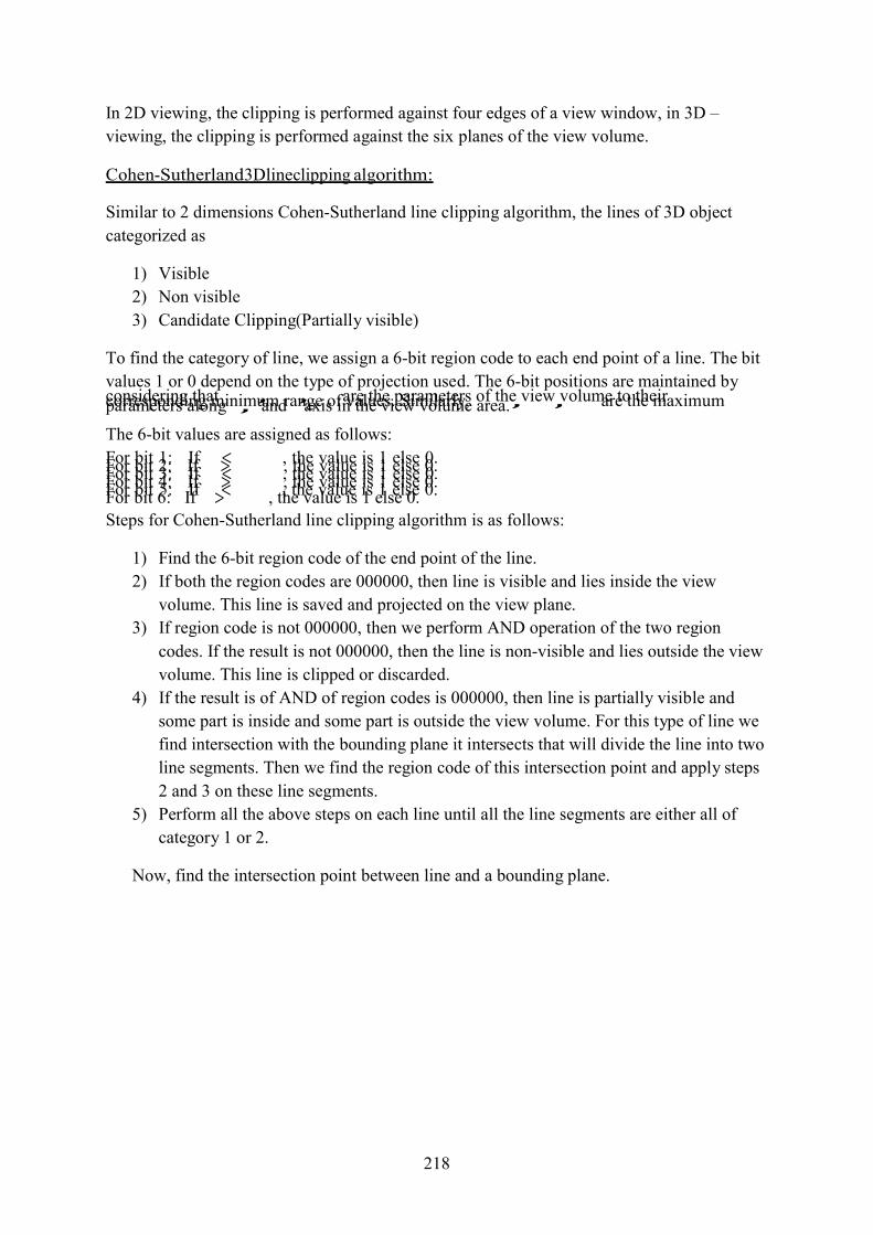
218

In 2D viewing, the clipping is performed against four edges of a view window, in 3D –

viewing, the clipping is performed against the six planes of the view volume. Cohen-Sutherland 3D line clipping algorithm:

Similar to 2 dimensions Cohen-Sutherland line clipping algorithm, the lines of 3D object

categorized as

1) Visible

2) Non visible

3) Candidate Clipping(Partially visible) To find the category of line, we assign a 6-bit region code to each end point of a line. The bit

values 1 or 0 depend on the type of projection used. The 6-bit positions are maintained by considering that , , are the parameters of the view volume to their corresponding minimum range of values. Similarly, , , are the maximum parameters along , and axis in the view volume area.

The 6-bit values are assigned as follows: For bit 1: If < , the value is 1 else 0. For bit 2: If > , the value is 1 else 0. For bit 3: If < , the value is 1 else 0. For bit 4: If > , the value is 1 else 0. For bit 5: If < , the value is 1 else 0. For bit 6: If > , the value is 1 else 0.

Steps for Cohen-Sutherland line clipping algorithm is as follows:

1) Find the 6-bit region code of the end point of the line.

2) If both the region codes are 000000, then line is visible and lies inside the view

volume. This line is saved and projected on the view plane.

3) If region code is not 000000, then we perform AND operation of the two region

codes. If the result is not 000000, then the line is non-visible and lies outside the view

volume. This line is clipped or discarded.

4) If the result is of AND of region codes is 000000, then line is partially visible and

some part is inside and some part is outside the view volume. For this type of line we

find intersection with the bounding plane it intersects that will divide the line into two

line segments. Then we find the region code of this intersection point and apply steps

2 and 3 on these line segments.

5) Perform all the above steps on each line until all the line segments are either all of

category 1 or 2.

Now, find the intersection point between line and a bounding plane.

219

Let a line present between two points ( , , ) and ( , , ). The

parametric equation of line is as follows:

= + ( − )

= + ( − )

= + ( − )

To find the intersection point of the line, consider an edge from the view volume. By considering, the view from the front plane of the viewing area, we take z-axis.

Here, =

Putting the value of z in above equation:

=

( − ) ( − )

Put values of u in x and y

= + ( − )

( − ) ( − )

( − )

= + ( − ) ( − )

The coordinate ( , ) will represent the coordinate of the intersection point.

9.5.2 3D Polygon Clipping Algorithm

3D-polygon clipping algorithms are also an extension of their 2D-counter parts.Where as in

2D viewing,a polygon is clipped against a view window;in 3D the polygon is clipped by

processing the polygon boundary formed by its vertices against each boundary plane of the

view volume.

3D Sutherland-Hodgeman Polygon Clipping Algorithm

The 3D Sutherland-Hodgeman polygon clipping algorithm is similar to 2D Sutherland –

Hodgeman Polygon clipping algorithm. The only difference is that instead of processing the

polygon edges against each view window boundary, we process the polygon edges against

the view volume as a whole. Four possible cases can be as follows:

(1) If first vertex is outside the view volume and second is inside, then we save both the

intersection point of polygon edge with the boundary plane it intersects and the

second vertex.

(2) If both the first and second vertices are inside the view volume, then we save the

second vertex.

220

(3) If the first vertex is inside and second vertex is outside the view volume,then we save

the intersection point of polygon edge with boundary plane it intersects.

(4) If both the first and second vertices are outside the view plane, then we save none.


Q2. The polygon edges are clipped that lie outside the window boundary.

(a) TRUE

(b) FALSE

Q3. Parallel projections are the two dimensional objects that are placed on a three

dimensional projection plane.

(a) TRUE

(b) FALSE

9.6 Summary

Viewing procedures for three dimensional scenes follow the two dimensional viewing. We

started a viewing coordinate reference frame and transfer objects from world coordinates to

viewing coordinates. Unlike two dimensional viewing, three dimensional viewing requires a

projection to transform object to a viewing plane before the transformation to device

coordinates.

Parallel projections are either orthographic or oblique. Orthographic parallel projections that

display more than one face of an object are called axonometric projections. Commonly used

oblique projections are the cavalier and cabinet projection. Objects in three dimensional

scenes are clipped against a view volume. The top, bottom, and sides of the view volume are

formed with planes that are parallel to projection lines.

9.7 Glossary

Viewing transformation- That converts 3D world coordinates to 3D viewing. Viewport- Rectangular area where picture is to be displayed.

Projections-Mapping of a point P in the projection plane or view plane.

Clipping-The method that identifies the portions of the picture that is either inside or outside

of a specified region of space.

221


1. FALSE 2. TRUE

3. FALSE

9.9 References


7. Introduction to Computer Graphics, Ravi Khurana, Amit Dawar.


Q1. What do you mean by projection? What are its various types.

Q2. What is the difference between perspective and parallel projection.

Q3. Explain 3D geometric transformations.

Q4. What is clipping? How 2D and 3D line clipping algorithms.

222

Chapter – 10

Hidden line and Surfaces elimination algorithm Structure of the chapter

10.0. Objective

10.1. Need for hidden line and surface elimination algorithms

10.2. Z-buffer algorithm

10.3. Painters algorithm

10.4. Scan line coherence

10.5. Area subdivision algorithm

10.6. Summary

10.7. Glossary



10.0. Objective


Explain what is hidden line and surface elimination.

Answer what is the need of hidden line and surface removal algorithms in computer

graphics.

Explain some most commonly used algorithms for removing hidden objects.

Explain Z-buffer algorithm, Painters algorithm, Scan line coherence and Area

subdivision algorithm in detail.

10.1. Need for hidden line and surface elimination algorithms When we attempt to view a picture that contains some non-transparent things or surfaces,

then those objects or surfaces are hidden from us i.e. we cannot view those parts that are

behind the objects that we can see. We should remove such hidden surfaces to get a realistic

223

view of an image. Hidden surface problem is a process in which we identify and remove the

hidden surfaces of a picture as shown in figure 10.1.

Objects in computer graphics are generally represented in the three-dimensional system.

Usually most of the objects are not transparent, so we deal with the outer surfaces of the

objects. The properties such as shape, color and texture affect the graphical representation of

any object. In three dimensional, it is difficult to implement a wire-frame drawing of a solid

object as it includes those parts of the object which are hidden and thus there is a need for

some kind of hidden-line or hidden-surface removal. Although many algorithms for hidden

surface removal exist but not a single one can work well that can consider all the cases.

Many algorithms are there in computer graphics which are used to remove hidden lines and

surfaces. They are classified as follows:

(i) Object-Space Algorithms: These algorithms directly deal with the object

definition and their visibility is decided by line or surface. They include:

Back-Face Removal Algorithm

Depth Sorting ( or Painter’s Algorithm)

Area Subdivision Algorithm

Binary Space Partition Trees

(ii) Image-Space Algorithms: These algorithms deal with the projected image and

their visibility is checked point by point. They include:

Depth Buffer ( or Z-buffer Algorithm)

Scan-Line Algorithm

Depth Sorting (or Painter’s Algorithm) Both categories use sorting and coherence techniques since sorting methods are used to

compare the depth values and coherence is required to make use of the regularities in the

scene.


Q1. Which algorithms deal directly with the object definition?

224

----------------------------------------------------------------------------------------------------------------

----------------------------------------------------------------------------------------------------------------

----------------

10.2. Z-buffer algorithm

Depth comparisons:

We use hidden surface elimination algorithms to determine the edges and surfaces that are

visible either alongside the direction of projection in case of parallel projection or from the

center of the projection in case of perspective projection. If there are two points to view – A(

x1 , y1 , z1 ) and B (x2 , y2 , z2 ) in three dimensional coordinate system, then we use the

following steps to find out which point is hidden from the other:

(i) If A and B are not lying on the same line of projection, then neither point is hiding

the other point i.e. both points are visible.

(ii) If A and B lie on the same line of projection, then we use depth buffer algorithm (

or Z-buffer algorithm) to find the point that is hiding the other point.

In the case of parallel projection onto xy-plane, A and B will be in the same plane if x1 = x2

and y1 = y2. Now if z1< z2 then point A is in front of point B i.e. B is the hidden point as

shown in figure 10.2.

In the case of perspective projection, same is done viewing objects from the center of the

projection as shown in figure 10.3.

Z-buffer algorithm

Z-buffer Algorithm is modern and the most commonly used image-space method to detect

visible surfaces. It compares the surface depths at each pixel location on the projection plane.

It is also known as Depth Buffer Algorithm and it is the simplest one. It was introduced by

Edwin Catmull in 1974.

225

As its name imply, we need a z-buffer, which stores the depth values for every (x,y) position

when we process the surfaces. Initially, all the values in the depth z-buffer are set to the

farthest z value. We process each surface mentioned in the polygon tables and the z-value is

calculated for each position taking one scan line at one time. If the new calculated depth

value is small than the stored value in our z-buffer, then we store this new value.

This z-buffer is generally set as a two-dimensional array (x-y) with one value for each screen

pixel. If there is another object that should be rendered in the same pixel value, then 3-D

graphics card will compare the two depth value and it will choose the one which is closer to

the observer. The chosen depth value is then added to the z-buffer, replacing the old value.

The granularity of the z-buffer plays an important role in the scene quality: a 16-bit z-buffer

usually results in artifacts (called "z-fighting") when two objects are too close to each other.

A 24-bit or 32-bit z-buffer behaves comparatively better, although additional algorithms are

required to completely eliminate the problem. An 8-bit z-buffer is never used because of its

little precision.

In this algorithm, we use some coherence. Commonly used is point-by-point coherence

because the z-value of adjacent horizontal positions across the scan line is easily calculated

by adding some constant value to the previous z-value. Also, on every scan line, we can

simply calculate z-value at the starting point using the previous starting point of the previous

scan line.

So, this method is quite easy to implement and no sorting of the surface is required in a scene.

But there is a requirement of the availability of a second z buffer in addition to the frame

buffer.

In this algorithm, we will use two arrays : intensity and depth. Each array is indexed by pixel

value (x, y).

226

(i) For all the pixel values on the screen, set depth[x, y] = 1.0 (in the z-buffer) and set

intensity[x, y] to a background value.

(ii) For each polygon, find all the pixel positions that are within the boundaries of the

polygon when they are projected on the screen for each pixel.

Calculate the depth value Z of the polygon at the position (x, y).

If Z < depth[x, y], this means this pixel value is closer to the observer than

already recorded value for this pixel, so it will replace the previous value.

If Z > depth[x,y], this means the closest value of this pixel has already

been recorded in the depth buffer and no change is done to the buffer.

Pseudo code of this algorithm is given as follows:

For each polygon P

For each pixel (x, y) in P

Calculate z_depth at x, y

if z_depth < z_buffer (x, y) then

set_pixel (x, y, color)

z_buffer (x, y) = z_depth

If the points A( x1 , y1 , z1 ) and B (x2 , y2 , z2 ) are to be scan converted at a pixel P (x, y) and

if z1< z2 , A is hiding B and depth of A will be z1 = z value.

Advantages of z-buffer algorithm:

It is quite simple to implement.

It projects wire frame models onto the screen.

227

Disadvantages:

It may paint the same pixel numerous times and hence computing the color of a pixel

may be costly.

The Z-buffer algorithm is not always practical because of the erroneous size of the

depth array and the intensity array.

It consumes much of the CPU time.

It requires large amount of memory.

Example: Let us consider a z buffer with range of 0 (at the screen) to 10 (at the far clipping

plane), and having a 6x6 pixel image. We are taking four polygons here and will explain how

some parts of these polygons are hidden and are not shown on the display screen. Let us see

how it works:

Initialization:

All the z values are set to maximum.

Rendering polygons:

Polygon 1: Given :

Depth=4; vertex1=(1,1); vertex2=(1,3); vertex3=(3,3); vertex4=(3,1)

228

etely rendered because there is nothing to

0); vertex1=(3,2); vertex1=(5,2); vertex1

This polygon is compl obscure it.

Polygon 2: Given:

Depth=2; vertex1=(3, =(5,0)

This polygon is closer to the viewer than the red one, so it is drawn entirely.

Polygon 3: Given:

Depth=8; vertex1=(2,2); vertex2=(2,5); vertex3=(4,5); vertex4=(4,2)

229

his polygon has a higher depth value tha

fer does not allow some part of it to be dr

0); vertex2=(2,3); vertex3=(5,3); vertex4=

As it can be seen that t n the

previous polygons, so the z buf awn.

Polygon 4: Given:

Depth=4; vertex1=(2, (5,0)

This polygon is drawn hiding some portion of the red and purple polygons, but is

itself obscured by the yellow polygon.


Q2. Which type of coherence is used in z-buffer algorithm? ----------------------------------------------------------------------------------------------------------------

----------------------------------------------------------------------------------------------------------------

----------------

230

Q3. Why Z-buffer algorithm is time consuming?

----------------------------------------------------------------------------------------------------------------

----------------------------------------------------------------------------------------------------------------

----------------

10.3. Painter’s Algorithm

Painter’s algorithm is also called as depth sorting algorithm in which first the surfaces are

sorted according to their depth values in the decreasing order and then we start the scan

conversion with the surface having greater depth. Just like a painter paints the most far-off

objects first and then paints the closer objects and foreground objects are painted over the

background objects on the drawing canvas and rest of the objects which are of least interest

are painted separately, similar approach is used in this algorithm. Figure 10.5 illustrates this

approach of painter’s algorithm.

To describe Painter’s Algorithm, we use the following pseudo-code:

sort polygons by z;

for all polygon p do

for all pixel(x, y) ϵp do

paint polygon.colour;

end for

end for

Algorithm:

1. Arrangethe surfaces according totheir z-value. 2. Select the surface having thegreatest depth. 3. Select the next greatest-depthsurface. 4. If there is no depth overlap, then paint the surfaces.

231

5. If there is depth overlap, then we will carry out a number of tests to find whether surface projections (X and Y)overlap or not. These cases are shown in figure 10.6.

Being an object space algorithm, it considers all the objects in the scene. Therefore, some

sorting algorithms are used to sort all the polygons in the scene are by depth. There are

number of ways that define a polygon's depth that range from calculating the z-value in the

middle of the polygon, to the z-value farthest from the given view point. After all the

polygons are sorted depending on their z-values, they are painted from back to front. Pixels

of each polygon are painted until the final and closest object is painted.

We take k as the number of polygons in a picture, and n as the number of pixels in the

resolution of the screen. It is clear that Painter's algorithm which is painting from backto

front, going through each pixel of every object, has a complexity of O(kn). This is ignoring

the sorting algorithm which is used to sort each object according to it's z-value.The efficiency

232

of Painter's algorithm actually depends on the method of sorting, and using a simple sorting

algorithm, a worst case complexity of O(n2) is achieved, with an average complexity of O(nlog(n)).

Example: The above algorithm can be understood with the help of following example. Here we are

taking a set of triangle as shown in figure 10.7.

First we will create a depth order table as shown below:

Triangle Behind Counter List of triangle in front

1

2

of it

5

2

0

4,3,1

3

2

1,5

233

4 1 3

5

2

-

6

0

-

The Behind Counter tells the number of triangles that are behind the given triangle.

Step 1: We will paint those triangles first which are not in front of any triangle. From the

above table, we will see that triangle number 2 and 6 are not in the front list which means

they will be painted first. New behind counter is calculated in this step.

Triangle Front list Behind Counter Output New behind

counter

1

5

2

1

2

4,3,1

0 6

-1

3 4

1,5

3

2

1

2 1

0

5

-

2

2

6

-

0

-1

Because the triangles 2 and 6 have been painted now, so their new behind counter is set to -1

as their initial behind counter value was 0. Remaining values are also modified by

eliminating the count of 2 and 6 numbered triangle from them.

Step 2: As we can see from Step 1 table that the only triangle whose new behind counter is 0

is 4 so it will be painted next.

Triangle Front list Behind Counter Output New behind

counter

1

5

1

1

2

4,3,1

-1

-1

3

1,5

1

0

4

3

0

-1

5

-

2

2

6

-

-1

-1

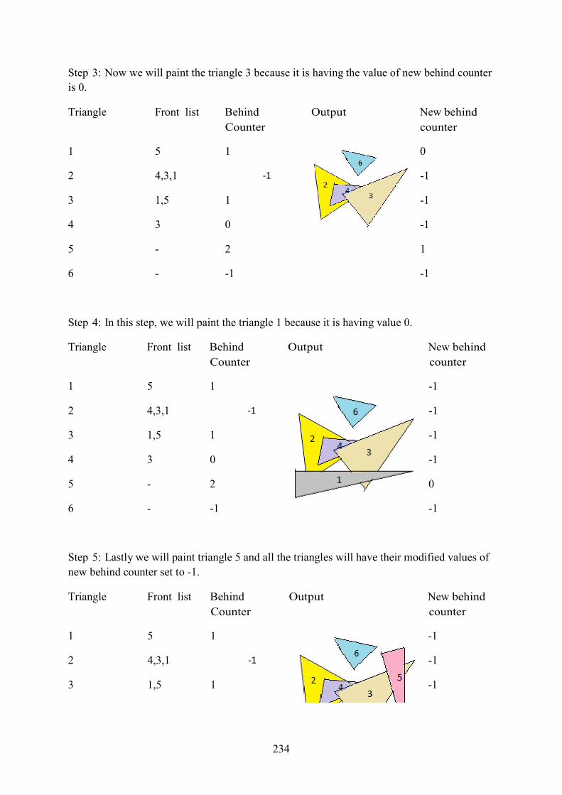
234

Step 3: Now we will paint the triangle 3 because it is having the value of new behind counter

is 0.

Triangle Front list Behind

Counter

Output New behind

counter

1 5 1 0 2 4,3,1 -1 -1

3 1,5 1 -1

4 3 0 -1

5 - 2 1

6 - -1 -1

Step 4: In this step, we will paint the triangle 1 because it is having value 0.


Counter

Output New behind

counter

1 5 1 -1 2 4,3,1 -1 -1

3 1,5 1 -1

4 3 0 -1

5 - 2 0

6 - -1 -1

Step 5: Lastly we will paint triangle 5 and all the triangles will have their modified values of

new behind counter set to -1.


Counter

Output New behind

counter

1 5 1 -1 2 4,3,1 -1 -1

3 1,5 1 -1

235

4 3 0 -1

5

-

2

0

6

-

-1

-1

Hence by using this step by step approach, we are able to paint the complete scene.

This method is well applicable to those triangles which do not overlap cyclically. One such

case is shown in figure 10.8. because in such a case, there is no depth order. But this

algorithm can be applied to such a case if we divide the intersecting polygons into smaller

triangles from the point of intersection and then we are able to prepare a depth order table.

But by doing so, complexity will be increased a lot.


Q4. Why painter’s algorithm is also known as depth sort algorithm?

----------------------------------------------------------------------------------------------------------------

----------------------------------------------------------------------------------------------------------------

----------------

236

10.4. Scan line coherence The scan line coherence method solves the problem of hidden surfaces one scan line at one

time. It processes the scan lines from top to the bottom of the screen. It successively

examines a series of windows on the display screen, where each window is one scan line high

and as wide as the screen. The simplest among the scan line algorithms is one dimensional

description of the depth buffer. We need two 1-D arrays: Intensity[x] and Depth[x] that hold

the values for a single scan line.

Algorithm:

Perform the following steps for each scan line:

1. For all the pixels on a scan line, set the value of Depth[x] to 1.0 and

Intensity[x] to a background value.

2. For every polygon in the scene, find all pixels on the currently scan line y that

lie within the polygon. This step uses the y-x scan conversion algorithm for

every x-value.

a) Compute the Depth z of the polygon at position (x, y).

b) If z > Depth[x], then set Depth[x] = z and Intensity[x] to 1.0 i.e. the

intensity value corresponding to the polygon shading and that surfaces will

be visible which are having depth values greater than the depth value of

this surface.

3. When all the polygons have been considered, the values which are contained

in the Intensity[x] array provide the solution and it will be copied into a frame

buffer.

This algorithm is a simple extension of the y-x scan conversion algorithm that requires

computation of the depth values and comparison with the value which is already stored in the

depth buffer.

Example:

Let us take two surfaces S1 and S2 in the view-plane as shown in figure 10.9.

237

The scan lines are checked starting from left to right for first scan line. When we move from

left to right, we get ab and bc edges where the surface S1 is visible and between the edges eh

and ef, S2 surface is visible. This means for scan line 1, we do not need to calculate the depth

value but we calculate the value of intensity of both the surfaces which are intersected by

scan line 1 and for the positions which are not intersected by scan line 1, the intensity values

are set to background intensity. For scan line 2, between the edges ad and eh, only surface S1

is present. But between the edges eh and bc, both the surfaces S1 and S2 are present. Hence

between the edges eh and bc, we need to calculate the depth values of both the surfaces S1

and S2. If the depth value of surface S1 is less than the depth value of S2, then surface S1 is

visible and we will calculate the intensity values of surface S1 from the edge ch until the edge

bc comes. After this only surface S2 is present between the edges bc and fg, so again there is

no need to compute the depth values. We will have to calculate the intensity values from edge

bc until fg is encountered.

In the above example, we have taken only two scan lines but we can draw any number of

scan lines and accordingly we can find which surfaces are hidden and which surfaces are

visible.

Advantages:

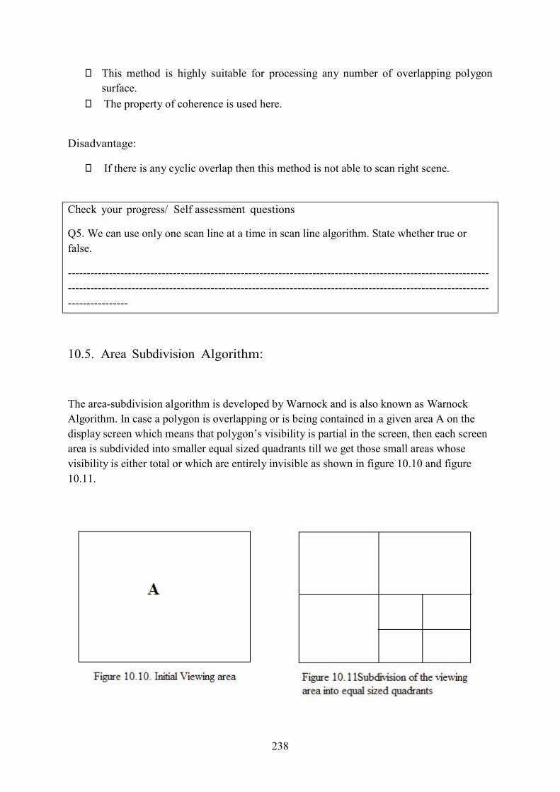
238

This method is highly suitable for processing any number of overlapping polygon

surface.

The property of coherence is used here.

Disadvantage:

If there is any cyclic overlap then this method is not able to scan right scene.


Q5. We can use only one scan line at a time in scan line algorithm. State whether true or

false.

----------------------------------------------------------------------------------------------------------------

----------------------------------------------------------------------------------------------------------------

----------------

10.5. Area Subdivision Algorithm:

The area-subdivision algorithm is developed by Warnock and is also known as Warnock

Algorithm. In case a polygon is overlapping or is being contained in a given area A on the

display screen which means that polygon’s visibility is partial in the screen, then each screen

area is subdivided into smaller equal sized quadrants till we get those small areas whose

visibility is either total or which are entirely invisible as shown in figure 10.10 and figure

10.11.

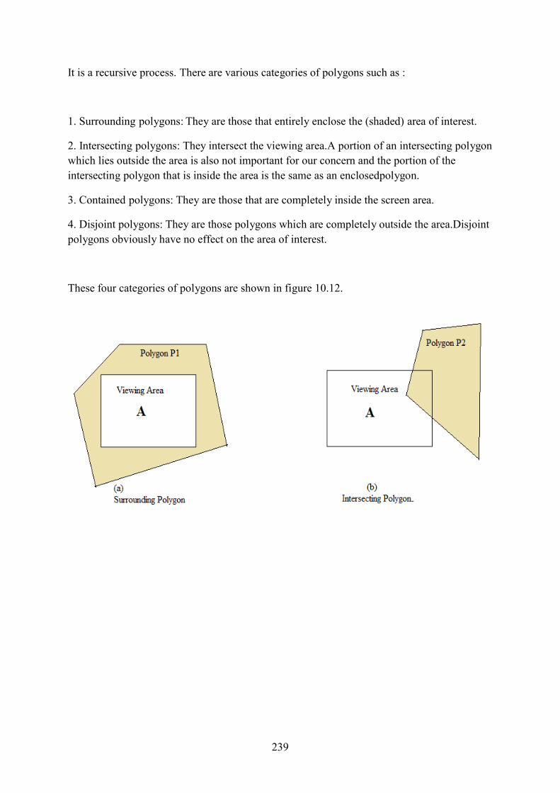
239

It is a recursive process. There are various categories of polygons such as :

1. Surrounding polygons: They are those that entirely enclose the (shaded) area of interest. 2. Intersecting polygons: They intersect the viewing area.A portion of an intersecting polygon

which lies outside the area is also not important for our concern and the portion of the

intersecting polygon that is inside the area is the same as an enclosedpolygon.

3. Contained polygons: They are those that are completely inside the screen area. 4. Disjoint polygons: They are those polygons which are completely outside the area.Disjoint

polygons obviously have no effect on the area of interest.

These four categories of polygons are shown in figure 10.12.

240

Algorithm:

The various steps involved in this algorithm are discussed as follows:

4. Firstly we need to define the viewing area of the screen.

5. We create a list of polygons that contains minimum zmin- coordinate value of

polygon’s vertex that is visible in a sorted order.

6. Divide the polygons into suitable categories. We will remove those polygons

that are disjointed i.e. which lie outside the viewing area and those polygons

will also be removed which are completely hidden by surrounding polygons.

7. For rest of the polygons, we will test their visibility taking into account the

following points:

a) If all the polygons appear under the category of the outside (disjoint)

polygon, then we will color all the pixels of the viewing area as

background color because these polygons are invisible.

b) If any polygon comes under the category of the surrounding polygon,

then color the viewing area as the color of the polygon since it should

be entirely visible.

c) If any polygon lies inside the viewing area, then we have to scan

convert the area and the remaining area of the screen should be colored

with the background color.

d) If there are polygons that are behind the surrounding polygons, then

the surrounding polygons which are closer to the viewport are visible

241

and other polygons are hidden. So the area of the screen will be

colored as the color of the visible polygon.

e) If there is a pixel (x, y) for which neither of the above points hold, then

we need to calculate the depth value of this pixel position and then it

will be compared with the z-value (depth value) in the polygon’s list

nor that pixel will be displayed which is having minimum depth value.

8. If neither of the steps 1 to 4 is applied to any of the polygons, then we have to

split the screen into equal quadrants and for each small area, we will go to step

(2).


Q6. State the category of the polygons that are not having any influence on area of interest in

area subdivision algorithm.

----------------------------------------------------------------------------------------------------------------

----------------------------------------------------------------------------------------------------------------

----------------

10.6. Summary In this chapter we focused on the removal of those surfaces which are hidden behind the other

surfaces. For this purpose, there arises a need of hidden surface removal algorithms. Various

methods are available each with some pros and cons. Most popular hidden line and surface

elimination algorithms are discussed here such as z-buffer, painter’s algorithm, scan line

algorithm and area subdivision methods.

10.7. Glossary Hidden surface problem - Hidden surface problem is a process in which we identify and

remove the hidden surfaces of a picture.

10.8. Answers to check your progress/ self assessment questions

1. Object space algorithms deal direct with the object definition. These algorithms

include Back-Face Removal Algorithm, Depth Sorting (or Painter’s Algorithm), Area

Subdivision Algorithm and Binary Space Partition Trees.

2. Point-to-point coherence is used in z-buffer algorithm.

3. Z-buffer algorithm is time consuming because it calculates the depth value of every

pixel of the image which consumes much of the processing time.

242

4. Painter’s algorithm is also known as depth sort algorithm because the surfaces are

first sorted according to their depth values in the decreasing order and then we start

the scan conversion with the surface having greater depth.

5. True.

6. Disjoint Polygons.

10.9. Modal Questions

1. Why do we need hidden surface removal algorithms in computer graphics?

2. Explain briefly the various methods that help in eliminating hidden lines and surfaces.

3. Explain Z-buffer algorithm.

4. Explain depth-sort algorithm.

5. Explain scan-line coherence.

6. Explain area subdivision algorithm.

243

Chapter-11

Shading and Reflection

Structure of the chapter

11.0. Objective

11.1. Introduction

11.1.1. Light sources

11.2. Diffuse Reflection

11.3. Specular Reflection

11.4. Refracted Light

11.5. Halftoning

11.6. Dithering Techniques

11.7. Summary

11.8. Glossary



244

11.0. Objective


Explain the concept of illumination in computer graphics.

Explain Diffuse and specular reflections.

Explain refraction of light.

Explain need of halftoning.

Explain various methods of halftoning the images.

Explain dithering techniques. 11.1. Introduction

We can obtain realistic views of a scene by creating perspective projections of objects and by

using natural lighting effects to the visible areas. An illumination model which is also called a

lighting model or shading model is used to measure the intensity of light on the surface of an

object. There is a surface-rendering algorithm that uses the intensity calculations from an

illumination model to find out the light intensity for all projected pixel positions for the

various surfaces in a scene. Obtaining realism in computer graphics needs two elements:

precise graphical representations of objects and fine physical descriptions of the lighting

effects in a scene. The Lighting effects include light reflections, transparency, surface texture,

and shadows. Color modification and effects of lighting effects is a complex process that

involves principles of both physics and psychology. We describe lighting effects with models

that takes electromagnetic energy of the object surfaces into account. When light reaches our

eyes, it generates a perception of the scene. Number of factors is included in physical

illumination models like type of object, position of object with respect to light sources and

other objects, and the light-source conditions. Objects can be opaque, more or less

transparent, can have shiny or dull surfaces as well as can have distinctive texture patterns. In

order to give illumination effects to a scene, light sources of different shapes, color or

position can be used. The illumination models in graphics are frequently freely derived from

the physical laws that illustrate surface light intensities.

11.1.1. Light sources We see light reflected from the surface of an object whenever we view an opaque, non-

luminous object. Reflection refers to the phenomenon of bouncing back of light from an

object. The total light being reflected is basically the sum of the contributions from all light

sources and other reflecting surfaces in the scene as shown in figure 11.1.So, a surface that is

not directly exposed to a light source may still be visible if its nearby objects are illuminated.

245

object can be both a light source and a light reflector. For example, a pl

ght bulb inside it emits as well as reflects light from the surface of the gl ht

from the globe may then illuminate other objects in the surrounding a orm

for a light emitter is a point source. Rays from the light source then f

erging paths from the source position, as shown in figure 11.2.This light

mall as compared to the size of objects in the scene. Light sources like th

ufficiently far away from the scene, can be correctly taken as point sour

urce like the long fluorescent light as shown in figure 11.3, is referred as

light source. In this case, the illumination effects cannot be approximate

with a point source, because the area of source is not small compared t

the scene. An accurate model for the distributed source is the one which

ulated illumination effects of the points over the surface of the source.

Sometimes, the light sources are also referred to as light-emittingsources and the reflecting

surfaces like the walls of a room, are termed light-reflecting sources. The term light source is

used to refer to an object that will emit radiant energy. Example of light source can be light

bulb or the sun.

Aluminous astic globe

having a li obe.

Emitted lig reas. The

simplest f ollow

radially div -source

model is s e sun,

which are s ces. A

nearby so a

distributed d

realistically o the other

surfaces in considers

the accum When light is incident on an opaque surface, some part of light is reflected and some is

absorbed. The amount of incident light being reflected by any surface depends on the kindof

material. Glossy materials reflect most part of light incident on it, and dull surfaces absorb

246

most part of the incident light while for an illuminated transparent surface, some portion of

light will be reflected and some will be transmitted through the material. Surfaces which are

rough usually scatter the reflected light in all directions.

This light which is scattered is called diffuse reflection. A very rough surface produces

primarily diffuse reflections, so that the surface looks equally dazzling from all viewing

directions. Figure 11.4. depicts diffuse light scattering from a surface. The color of an object

is the color of the diffuse reflection of the light incident on it. A red object illuminated by a

light source, for example, reflects the red component of the white light and completely

absorbs all the other components of light. If the red object is viewed under a blue light, it

looks black because the entire incident light is absorbed. Along with diffuse reflection, light

sources can also create highlights, or bright spots, called specular reflection. The highlighting

effect is more pronounced on shiny surfaces than on dull surfaces. Specular reflection is

shown in figure 11.5.

The empirical models give a simple and quick method for calculating the surface intensity at

a given point, and they give good results for most scenes. Optical characteristics, background

light conditions and specifications of the light source are the basis of lighting calculations.

Optical parameters are used for setting the surface properties like glossy, rough, opaque, and

transparent. It controls the amount of reflection and absorption of the incident light. All light

sources will be considered as point sources which are specified with a coordinate position

value and an intensity value (i.e. color).

Ambient Light

A surface which is not uncovered directly to a light source is still visible if the objects closer

to it are illuminated. In our basic lighting model, we may set a general level of intensity for a

scene. This is an easy way to model the combination of reflections from different surfaces to

create a uniform illumination which is called the ambient light or background light. Ambient

247

light is not having any spatial or directional characteristics which mean the amount of

ambient light incident on every object is a constant for all the surfaces and over all directions.

The level for the ambient light in a picture can be set with parameter Iaand every surface will

be illuminated with this fixed value. The resulting reflected light is a constant for every

surface and this reflected light neither depend on the direction of viewer nor on the

orientation of the surface in space. But the amount of the reflected light for every surface

depends on the optical properties of the surface i.e. how much incident energy is to be

reflected and how much is absorbed.


Q1. Give an example of point light source and distributed light source. ----------------------------------------------------------------------------------------------------------------

----------------------------------------------------------------------------------------------------------------

----------------------

11.2. Diffuse Reflection

Diffuse reflection is consistent light reflection in which there is no directional dependence for

the viewer, e.g., a dull surface like a cardboard. Diffuse reflection has its origin from a

mixture of internal dispersion of light, i.e. first the light is absorbed and then re-emitted, and

external dispersion from the irregular surface of the object. There are two types of diffuse

reflections and an illumination model should hold both.

Direct diffuse reflection is one in which light is coming directly from a source of light

to a surface and is then reflected to the viewer.

Indirect diffuse reflection also called as diffuse interreflections, is the second type in

which light is coming from a source, it is being reflected to a surface, then is reflected

to another surface, so on, and is finally reflected to the viewer.

A number of local illumination models like those which are normally applied in many scan-

line depiction and ray tracing systems, hold the indirect diffuse reflection contribution by just

assuming that it has constant intensity in all the directions. This fixed term is referred as the

ambient involvement and it is considered as a non-directional background light. Radiosity

helps to compute this term for diffuse interreflections.

248

Diffuse reflection of ambient light

Let us assume a constant intensity of ambient light denoted by Ia, then at any point on the

object surface, the intensity of the diffuse reflection is given as:

I = ka × Ia,

where ka = coefficient of reflection for the ambient diffuse light and 0.0 <= ka<= 1.0.

There are three kavalues for the colored surfaces, one value for red, one for green, and one for

blue. Let us approximate the ambient diffuse part of the light reflection intensity function

referred as R(j,q,l) by this constant ka. For a matte and non-reflecting surface, value of kais

taken close to 0.0 while for a polished and highly reflective surface, eg, a mirror, ka is taken

close to 1.0.

Diffuse reflection in case of point light sources

Let us consider a point light source and assume that the source of light is quite far from the

object’s surface so that we can assume the incident light rays to be parallel. As figure 11.6.

shows that light rays coming from a nearby light source are not parallel. So we take the

source at some distance from the object.

For a point light source far away from the object’s surface, we will use Lambert's cosine law.

The intensity of light being reflected is f . Let us see two cases which is shown in figure 11.7.

We will use N which is the unit normal to the object’s surface and L which is the unit vector

i.e. the direction to the light source.

249

The Lambert's cosine law states that the light being reflected is proportional to cos q (where q

<= 90 otherwise the light is behind the surface). Let Ip be the intensity of a point light source, then the brightness is f (which is 1/d2 where

d=distance between the light source and the surface). Various models use a ‘d’ distance

instead of d2, and this mostly works because many light sources are not actually point sources.

Therefore, I = [( kd × Ip) / (D)] × (N . L)

where D = distance function. Its value is less than or equal to 1 for far away light sources and

its value is equal to d or d2 for other cases.

kd = the diffuse reflection coefficient and 0.0 <= kd<= 1.0.

There are some models that also add a constant term do in order to avoid the value of d to

become zero. Normally ka is set same askd. The vectors N and L are always taken in

normalized form.

We will get a two-term illumination model if we also include ambient light.

I = ka × Ia + [( kd × Ip) / (D)] × (N . L)

If we are considering color also then we need to have explicit wavelength reliance. But we

normally sample the color space at only three colors i.e. red, green and blue. Then there will

be 3 equations like the above: one each for Red, Green, and Blue color.


Q2. Discuss two types of diffuse reflection. ----------------------------------------------------------------------------------------------------------------

----------------------------------------------------------------------------------------------------------------

---------------------- Q3. Diffuse reflections occur on a smooth surface. State whether true or false.

250

----------------------------------------------------------------------------------------------------------------

----------------------------------------------------------------------------------------------------------------

---------------------- 11.3. Specular Reflection

When we keep a polished surface under the effect of light, we can find a bright spot at a

definite viewing direction. This event is called specular reflection. This effect is shown in

figure 11.9.

Law of reflection given by Fresnel gives the intensity of specular reflection as:

Ispec = W(θ) I1 cosnØ

where W(θ) gives the coefficient of specular reflection. At θ= 90ᵒ, W(θ) = 1and all the light

which is incident is reflected back.

The value of n depends on the object’s surface. It is taken large for glossy and shining

surfaces and it is quite small for dull and matte surfaces. This judgement can be made by

examining the range of available intensities and the plane to be considered.

Ø = viewing angle relative to the direction of specular reflection.

Figure 11.10. shows the model of specular reflection.

251

gress Self assessment questions

uation to calculate the intensity of specular reflection as give ------------------------------------------------------------------------

------------------------------------------------------------------------

--

ight

an interface between two mediums that are havin

all direction (shortly, isotropic mediums) and a homo

indices are n1 and n2 respectively. Assume a ray of ligh

index is n1 that hits the interface at a point P. We draw a no

he angle of incidence is the angle between the incident ra

int of intersection. This incident ray will get deviated into s

2 because of the concept of refraction. The angle of refra

acted ray of light and the normal to the interface.

Check your pro Q4. Give the eq

/

n by Fresnel.

--------------------

--------------------

--------------------

--------------------

--------------------

11.4. Refracted L

Let us consider

g same optical

characteristics in

geneous medium

whose refractive

t in the medium

whose refractive

rmal at this point

normal to the po

econd medium of

refractive index n

between the refr

ction is the angle

of intersection. T y of light and the

252

The laws of refraction judge the direction of refracted ray. The laws of refraction (also known

as Snell’s law) are given as follows:

1. The first law is called the plane of incidence and this law states that the incident light

ray, normal at the point of incident and the refracted light ray must lie in the same

plane.

2. The second law gives the following relation:

n1 sin i = n2 sin r

where n1 = refractive index of medium 1

n2 = refractive index of medium 2

i = angle of incidence, and

r = angle of refraction

We can also obtain the law of reflectionby substituting n2= -n1in the above law of refraction.

Two cases are there which are discussed as follows:

Case 1: When n1 < n2

In this case, the angle of refraction (r) is less than the angle of incidence (i) always. Hence

this case will always result in refraction when the angle of incidence is increased until 90o.

Case 2: When n1 > n2

in this case, the angle of refraction (r) is always more than the angle of incidence (i). When

the angle of incidence increases, the angle of refraction also increases a bit faster. There is a

value of angle of incidence when angle of refraction will become 90o and this angle of

incidence is known as critical angle (ic). For the angles of incidence which are greater than

the critical angle, there will be no refraction. Instead of refraction, the ray gets totally

reflected. This phenomenon is called total internal reflection and it plays a very important

role in the light guidance.

253


Q5. State the laws of refraction. ----------------------------------------------------------------------------------------------------------------

----------------------------------------------------------------------------------------------------------------

----------------------

Halftoning

Halftoning or analog halftoning refers to a process that simulates shades of gray by changing

the size of minute black dots arranged in a regular pattern. This practice is used in printers

and the publishing industry. When we examine a snap in a newspaper, we notice that the snap

is made up of black dots although it appears to be comprised of grays. It is possible because

of the spatial mixing performed by our eyes. Our eyes combine fine details and trace the

overall intensity. Digital halftoning is analogous to halftoning in which an image is divided

into a grid of cells of halftone. Units of an image are simulated by filling the suitable halftone

cells. More the number of black dots in a halftone cell, darker the cell will appear. For

example, in Figure 11.13., a tiny dot situated at the middle is simulated in digital halftoning

by filling the middle halftone cell. Similarly, a medium sized dot situated at the top-left

corner is examined by filling the four cells at the top-left corner. The big dot covering most of

the area in the third image is examined by filling all halftone cells.

254

on methods for producing digital halftoning ima

st two methods here and the last method will be nd easiest method among other techniques for pr

ates an image which is of superior spatial resol ge

has same number of halftone cells as that of t ery

halftone cell is further divided into a 4x4 gri aried

number of filled squares in the halftone cel ecause

a 4x4 grid is capable of representing onl

nd figure 11.15. depicts an example for this.

There are three comm ges. These are

1. Patterning

2. Error Diffusion

3. Dithering

We will explain the fir explained in the next

section.

Patterning

Patterning is simple a oducing digital

halftoned images. It cre ution than the original

image. The output ima he number of pixels in

the original image. Ev d. Every input pixel

value is formed by a v l. The original image

needs to be quantized b y 17 different

intensity levels. Figure 11.14. a

255

The patterning technique uses a pattern function that produces a digital halftoned image. This

function reads an image as input, then quantize the pixel values and each pixel is mapped to

its equivalent pattern. The result is 16 times bigger than the source image. The resulted image

is written to an output file in the form of a TIFF file. This technique needs a huge number of

computations. So generally those images are halftoned with this method whose size is less

than 100 x100.

Syntax of pattern is :

Pattern (input_filename, output_filename)

The example shown in figure 11.16. produces a digital haltoned image from an image named

painter using this method. The pattern function will be:

Pattern('Painter.TIF', 'new_painter.tif')

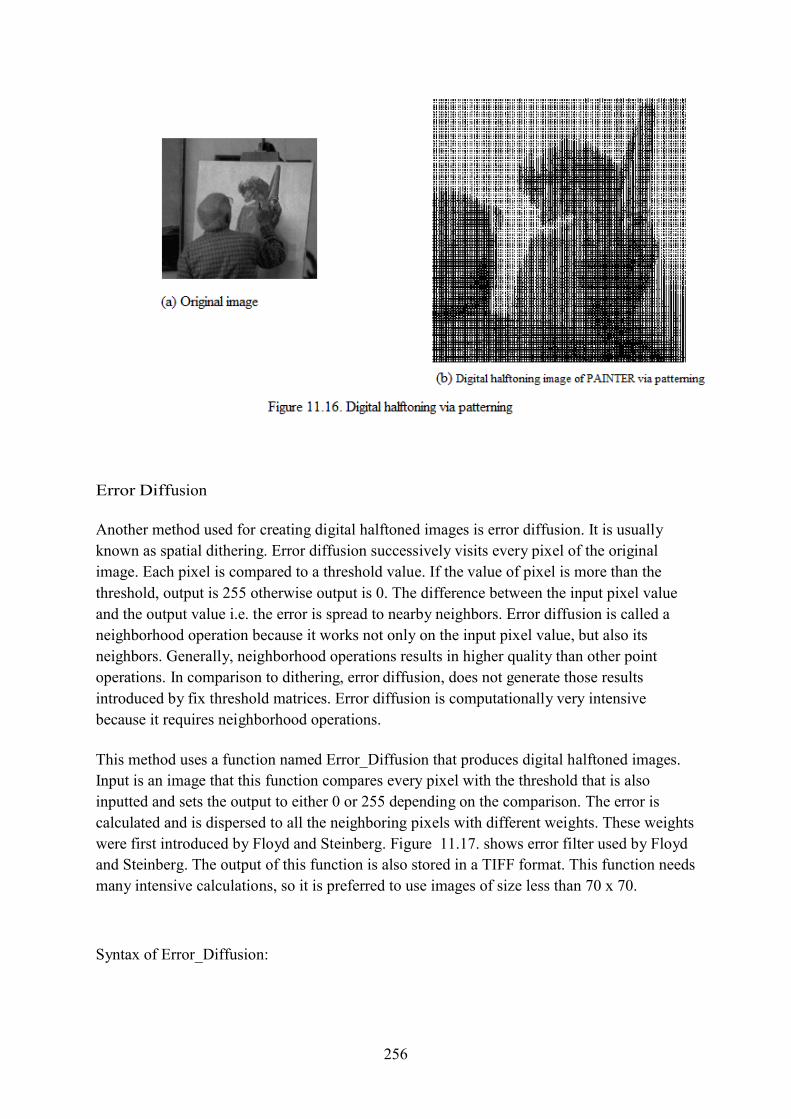
256

Error Diffusion

Another method used for creating digital halftoned images is error diffusion. It is usually

known as spatial dithering. Error diffusion successively visits every pixel of the original

image. Each pixel is compared to a threshold value. If the value of pixel is more than the

threshold, output is 255 otherwise output is 0. The difference between the input pixel value

and the output value i.e. the error is spread to nearby neighbors. Error diffusion is called a

neighborhood operation because it works not only on the input pixel value, but also its

neighbors. Generally, neighborhood operations results in higher quality than other point

operations. In comparison to dithering, error diffusion, does not generate those results

introduced by fix threshold matrices. Error diffusion is computationally very intensive

because it requires neighborhood operations.

This method uses a function named Error_Diffusion that produces digital halftoned images.

Input is an image that this function compares every pixel with the threshold that is also

inputted and sets the output to either 0 or 255 depending on the comparison. The error is

calculated and is dispersed to all the neighboring pixels with different weights. These weights

were first introduced by Floyd and Steinberg. Figure 11.17. shows error filter used by Floyd

and Steinberg. The output of this function is also stored in a TIFF format. This function needs

many intensive calculations, so it is preferred to use images of size less than 70 x 70.

Syntax of Error_Diffusion:

257

Error_Diffusion(input_filename, output_filename, threshold_value)

In this case, the threshold value determines whether the output will be set to 0 or 255 and it is

generally set to 128.

For example, figure 11.18. shows an error diffusion technique applied to Painter’s image and

threshold value is set to 128.

Error_Diffusion('Painter.TIF', 'new_err_diff_painter.tif', 128)


Q6. Write the file format in which output halftoned images are stored. ----------------------------------------------------------------------------------------------------------------

----------------------------------------------------------------------------------------------------------------

----------------------

11.6. Dithering Techniques

258

Dithering is a method which is used in quantization processes like graphics and audio to

decrease or remove the correspondence between noise and signal. Dithering is used in

computergraphics to form additional colors and shades from an existing pattern. It doesn't

decrease resolution. There are three types of dithering:

Regular dithering that uses a very regular predefined pattern

Random dithering is one in which the pattern is a random noise

Pseudo Random dithering that uses a very large, very regular, predefined pattern.

Dithering is used to make patterns that can be used as backgrounds, fills and shading, and for

making halftones for printing. When it is used for printing, it is very sensitive to properties

of paper. We can combine with rasterising but is not connected to anti-aliasing.

Dithering in digital graphics

All the digital photos are an estimation of the source as computers are not able to display an

infinite amount of colors. As an alternative, the colors are approximated, or rounded to the

closest color value available. For example, an 8-bit GIF image can comprise of 256 (i.e. 28)

colors. This is sufficient for a logo or computer graphic, but may not for a digital image. This

is the reason that most of the digital photos are stored as 16 or 24-bit JPEG images because

they bear thousands or millions of colors.

When a digital photo contains only a few hundred colors, they normally look blemished, as

big areas are represented by single colors. Dithering is used to decrease this spotted

appearance by adding some digital noise to smooth out the transitions between the colors.

This added noise makes the photo appear grainier, but it provides a more precise

representation as the colors mix together more smoothly. In reality, if we see a dithered 256-

colored image from far away, it looks similar to the same image which is represented by

thousands or millions of colors. Hence dithering helps to improve the appearance of digital

images.

Dithering in digital audio

Digital audio recordings are estimation of the original analog source just like digital images.

Hence if the sampling rate or bit depth rate of an audio is very low, it may sound choppy or

rough. We can apply dithering to the audio file to plain the roughness. Similar to dithering in

digital images, audio dithering also adds a digital noise to the audio to plain out the sound. If

we see a dithered waveform in an audio editor, it will look less blocky and if we listen to a

dithered audio track, it sound smoother and almost like the original analog sound.

Dithering in halftoning

http://encyclopedia2.thefreedictionary.com/rasterising

http://encyclopedia2.thefreedictionary.com/anti-aliasing

http://techterms.com/definition/analog

259

The first syntax uses a default dither matrix to threshold the input image. The default dit

given as

Dithering is also used for creating digital halftoning images. Unlike patterning, dithering

generates an output image which is having same number of dots as the number of pixels in

the original image. Dithering uses a dither matrix for thresholding the source image. This

matrix is used frequently over the original image. When the pixel value of the image is

greater than the value in the dither matrix, a dot on the output image is filled at that point.

Dithering has a problem that it produces patterns specified by fixed thresholding matrices.

Figure 11.19. shows an example of the dithering operation.

The dithering operation uses a Dither function that generates a halftone image. It uses two

syntax given below:

Dither(input_filename, output_filename) // for default dither matrix

Dither(input_filename, output_filename, Dmatrix) // uses a dither matrix specified by

Dmatrix

her is

This matrix is a rectangular dither matrix taken from a 450 dither matrix.

The second syntax uses a dither matrix being defined by the user. Dither reads in an input

image, then compares every pixel with the corresponding part in the dither matrix, produces

260

the output image, and finally writes it to the output file in TIFF format. As Dither requires a

sufficient number of calculations, images whose size is less than 100x100 are preferred.

For example, figure shows dithering applied on an image named Lena using default dither

matrix and its syntax is given as follows:

Dither('Lena.TIF', 'Di_le.tif')

The figure 11.20. shows dithering applied on Painter image with a given dither matrix.

Dither(‘Painter.TIF', 'Di_spa.tif', [105,135,30;90,67.5,120;45,15,45;])

Various types of dithering techniques are used by several image and audio editors, although

random dithering is the most common one. Though dithering is usually used to enhance the

appearance and sound of low class graphics and audio, it is also applicable to high quality

images and recordings. In such situations, dithering is able to provide extra smoothness to an

image or sound.


Q7. What are the various types of dithering? ----------------------------------------------------------------------------------------------------------------

----------------------------------------------------------------------------------------------------------------

---------------------- 11.7. Summary

In this chapter, we have studied about various light sources and two major types of reflection-

diffuse and specular. Diffuse reflections take place on a rough, irregular and matte surface

while specular reflection occurs on a glossy and shining surface. Refraction of light is

discussed. Halftoning in computer graphics is an important process and three important

methods- patterning, error diffusion and dithering that aims at halftoning are discussed in

detail.

261

11.8. Glossary

Diffuse reflection - Diffuse reflection is consistent light reflection in which there is no

directional dependence for the viewer, e.g., a dull surface like a cardboard.

Angle of incidence -The angle of incidence is the angle between the incident ray of light and

the normal to the point of intersection.

Angle of refraction -The angle of refraction is the angle between the refracted ray of light

and the normal to the interface.

Halftoning - Halftoning or analog halftoning refers to a process that simulates shades of gray

by changing the size of minute black dots arranged in a regular pattern.

Dithering -Dithering is a method which is used in quantization processes like graphics and

audio to decrease or remove the correspondence between noise and signal.


1. An example of point light source is Sun and example of distributed light source is

long fluorescent light.

2. There are two types of diffuse reflection:

Direct diffuse reflection is one in which light is coming directly from a source

of light to a surface and is then reflected to the viewer.

Indirect diffuse reflection also called as diffuse interreflections, is the second

type in which light is coming from a source, it is being reflected to a surface,

then is reflected to another surface, so on, and is finally reflected to the

viewer.

3. False.

262

4. Ispec = W(θ) I1 cosnØ

5. There are two laws of reflection:

The incident light ray, normal at the point of incident and the refracted light

ray must lie in the same plane.

n1 sin i = n2 sin r

6. TIFF format.

7. There are three types of dithering:

Regular dithering that uses a very regular predefined pattern

Random dithering is one in which the pattern is a random noise

Pseudo Random dithering that uses a very large, very regular, predefined

pattern.


1. What is meant by light sources? What are the different types of reflections in

graphics?

2. Explain Diffuse and specular reflection.

3. Differentiate between Diffuse and specular reflection by giving suitable example.

4. What do you mean by the phenomenon of refraction of light?

5. How is halftoning of images achieved in computer graphics? Explain various

halftoning techniques.

6. What is Dithering? How is it done?

263

Lesson- 12

Surface rendering and its methods

Structure of the chapter 12.0. Objective

12.1. Introduction to shading models

12.2. Flat and smooth shading

12.3. Adding texture to faces

12.4. Rendering texture

12.5. Drawing shadows

12.6. Constant intensity method

12.7. Gourad shading

12.8. Phong shading (Mash Band effect)

12.9. Morphing of objects

12.10. Summary

12.11. Glossary




Explain need of shading models in computer graphics Explain methods of shading the objects. Explain rendering and texture mapping. Compare various shading models. Explain the concept of shadows. Explain the morphing of objects.

12.1. Introduction to Shading models Images which are having visual realism are an effective means of sharing ideas and designs

for the designers. Shading is one of the major tools which are used to create the images that

264

are quite realistic. Shaded images with quite high degree of realism are able to create the

impression that these images are realistic objects and are not just artifacts or geometric

models. The shaded images with raised level of quality give an easy, more interactive and

less costly way of reviewing various design alternatives than designing actual models or

prototypes. Virtual graphics provides multidimensional views and is very effective. When the

geometric model of an object is prepared and is transformed according to the viewing

conditions, the image surfaces are shaded and are then analyzed from an artistic point of view

to estimate how good a model will be when it is finally released from any manufacturing

process. For example, a sofa set image is developed with various effects of creative computer

graphics modeling along with the shading effects under the given lighting. This model of sofa

set is then placed in a living room with certain color to examine whether the setting

arrangements are fine or there is some need of manipulation before manufacturing the actual

sofa set.

The shading models are also sometimes referred as illumination models. They can be used to

check the intensity of light at any given point on the surface of an object. But the surface

shading models are quite different. Surface shading refers to a process that determine the

light intensity calculations from a given illumination model. So surface shading models are

also known as surface rendering models. These methods are popular to interpolate across the

surfaces from a small set of illumination models at every pixel position and to transform the

computer models into the raster images that involve projecting a 3D model onto the 2D plane

screen that takes into account the lighting properties as well as the object properties. Check your progress / Self assessment questions

Q1. Why shading models are also called illumination models? ----------------------------------------------------------------------------------------------------------------

----------------------------------------------------------------------------------------------------------------

---------------------- 12.1. Flat and Smooth Shading

Polygon Shading Methods

Any surface of an object can be shaded pixel to pixel by calculating the surface normal vector

at every pixel and obtaining the dot product with the light vector and then calculating the

intensity of that pixel. This process becomes slow when producing each frame if we consider

the effect of different rendering algorithms. This can be improved by dividing the surface into

a polygon mesh. The intensity of calculation is applied to each vertex of the polygon and

thereafter the intermediate points are interpolated.

There are two major methods of polygon shading – Flat shading and smooth shading. Flat Shading

A. Z-Flat Shading:

265

It is an uneven looking shading method which can be implemented by providing a polygon

the color intensity value depending on the z coordinate average value of the polygon’s

vertices:

I = Imax – (vertex1.z + vertex2.z + vertex3.z)/a, Where a is some appropriate number, dividing by a one get average value of z that ranges

from 0 to maximum intensity. There is an assumption that z is directing inside the plane of

the screen. Therefore, the intensity reduces as the point moves farther away from the screen.

Drawbacks: Some of the drawbacks of this method are:

1. When we are calculating the color of the polygons, such as KLGH and OPKL in

which the point K is common for both the polygons, the color value for the points that

are nearer to K will be different if all the points of each polygon do not have the same

average depth value.

2. The color changes suddenly. But still this method is commonly used because it is quite faster and is easy to understand.

B. Lambert Flat:

This technique attempts to make an object as real as possible because it uses a real light

source. This method uses a surface normal vector for calculating intensity. Surface normal

vector is defined as the vector which is perpendicular to the plane of the surface and is given

as:

N= a ı̂+ bȷ̂+ c k

This normal vector can be directed into or out of the plane of the surface. But we will use harmonized surface normals that consider that all the surfaces of a closed volume have their

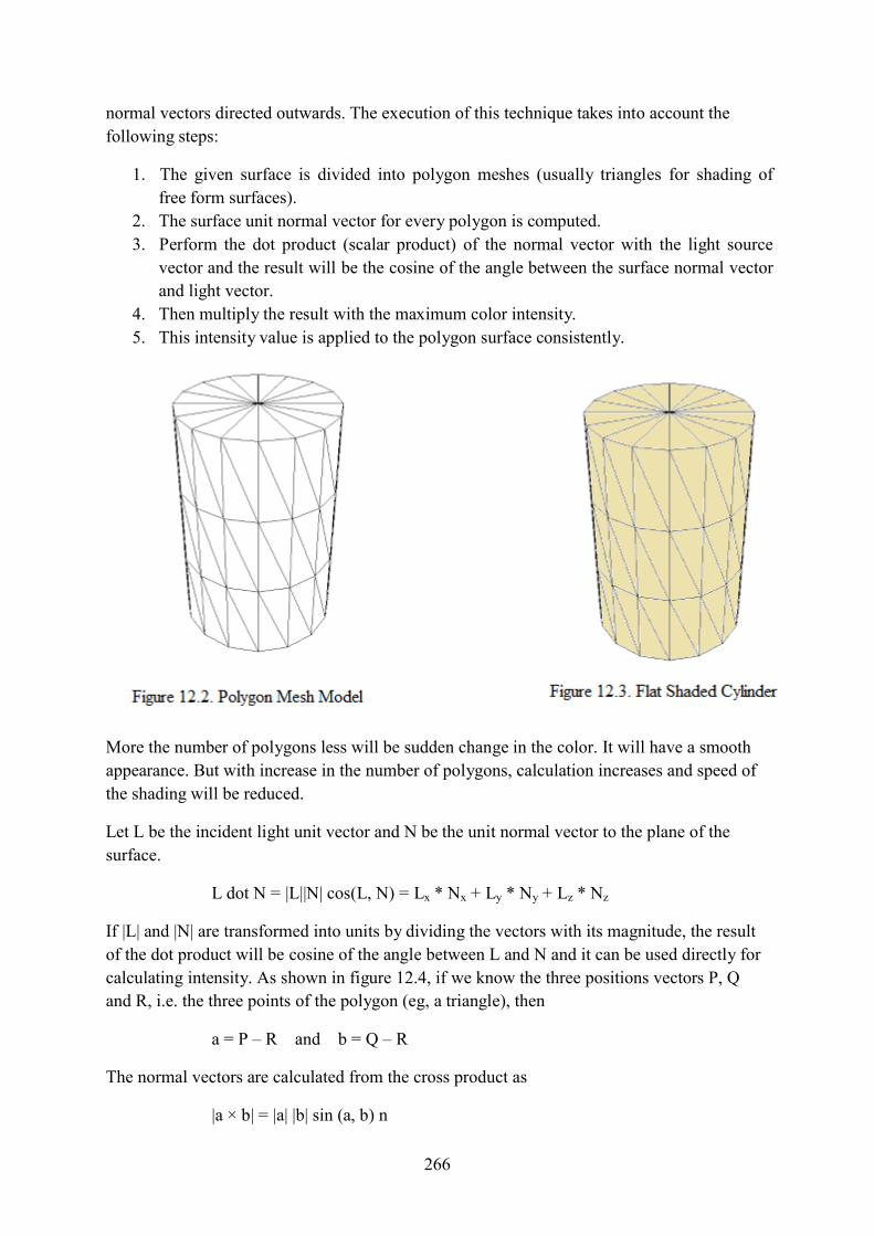
266

normal vectors directed outwards. The execution of this technique takes into account the

following steps:

1. The given surface is divided into polygon meshes (usually triangles for shading of

free form surfaces).

2. The surface unit normal vector for every polygon is computed.

3. Perform the dot product (scalar product) of the normal vector with the light source

vector and the result will be the cosine of the angle between the surface normal vector

and light vector.

4. Then multiply the result with the maximum color intensity.

5. This intensity value is applied to the polygon surface consistently.

More the number of polygons less will be sudden change in the color. It will have a smooth

appearance. But with increase in the number of polygons, calculation increases and speed of

the shading will be reduced.

Let L be the incident light unit vector and N be the unit normal vector to the plane of the

surface.

L dot N = |L||N| cos(L, N) = Lx * Nx + Ly * Ny + Lz * Nz

If |L| and |N| are transformed into units by dividing the vectors with its magnitude, the result

of the dot product will be cosine of the angle between L and N and it can be used directly for

calculating intensity. As shown in figure 12.4, if we know the three positions vectors P, Q

and R, i.e. the three points of the polygon (eg, a triangle), then

a = P – R and b = Q – R The normal vectors are calculated from the cross product as

|a × b| = |a| |b| sin (a, b) n

267

= ( Ay* Bz - By*Az , Az*Bx – Bz*Ax , Ax*By – Bx*Ay ) It gives the components of normal vector N. On dividing this vector with its magnitude, we

will get the unit normal vector n. The function that calculates the unit surface normal of a

triangle having the end points (x1, y1, z1), (x2, y2, z2 ) and (x3 , y3, z3 ) will provide the unit

normal vector.

Intensity will be calculated as

I = Imax * cos (L, N).

The second polygon shading method – smooth shading consists of two techniques: Gouraud

Shading and Phong Shading which will be discussed later. Check your progress / Self assessment questions

Q2. What are the two methods of polygon shading in computer graphics? ----------------------------------------------------------------------------------------------------------------

----------------------------------------------------------------------------------------------------------------

---------------------- 12.3. Adding texture to faces

In computer graphics, the finer details of an object are produced using textures. The addition

of separately specified pattern gets converted into a smooth surface as texture. After the

pattern is added, the surface is still smooth. This is based on two types of internal mapping-:

In the first one, we map the texture image onto a simple three dimensional surface

such as a plane, cylinder, a sphere or a box. This is called S-mapping.

268

Secondly, map the result of S-mapping onto the final 3-D surface. This is called O-

mapping.

As the details become more complex, explicit modeling of polygons becomes impractical. So

we need to map a digital image onto a surface and this technique is called texture or pattern

mapping. The image is referred as texture map and the individual units or elements are called

texels. The rectangular texture map has its own (u, v) texture space. One image pixel is often

mapped into number of texels. In order to avoid the aliasing problems, all the relevant texels

are considered. When a texture is mapped to a polygon, it is common to assign the texture

map coordinates directly into its vertices.

In texture mapping methods, software and hardware are designed to display complex scenes

at real times frame rates (60 Hz or more). So there is need of high capacity data channel.

Texture hardware consists of a local memory for storing texture data. The size of its local

memory is 16MB or more. The download rate at which the texture maps are loaded from

texture memory into the frame buffer is as high as 240MB/second.


Q3. Discuss the two internal mappings in texture mapping.

269

----------------------------------------------------------------------------------------------------------------

----------------------------------------------------------------------------------------------------------------

---------------------- 12.4. Rendering Texture

Rendering takes a series of objects as input and use them to form new image from different

camera locations. The images resulted by rendering systems are usually more realistic as

compared to the classical rendering models. The basic objective is to take some subset of the

required viewpoints and from these, make the picture that we want to see from a new

viewpoint. It involves making choices among factors that affect the quality of the images, the

speed of producing the rendered images or both. Rendering refers to the process of

converting of a 3-D scene into a 2-D image using computer programs.

The 3-D scene is composed of models in three spaces. Models are entered by hand or are

created by a program. For many purposes, the models are already generated. The image is

drawn on the display screen, printed on a laser printer, or is stored in memory or file.

Basically the models are converted into device coordinate space where they are converted

into pixels for illumination. There are many coordinate systems that are being used such as :

MCS (Modelling Coordinate System)

WCS (World Coordinate system)

VCS (Viewer Coordinate System)

NDCS (Normalized Device Coordinate System)

DCS (Device Coordinate System) or SCS (Screen Coordinate System) Techniques for rendering:

The three major techniques that are being used for rendering in computer graphics are – Ray

casting, Ray tracing and Rasterization. These techniques are briefly discussed below:

270

1. Ray Casting: It is a method which is used to render high-quality images of solid

objects. The basic idea is to make best use of the given 3-D data without imposing

any geometric structure on it. It uses ray-surface intersection tests to resolve various

problems in graphics. It is being the first solution to the earlier problems when

computers were not able to run real 3-D engines.

2. Ray Tracing: It is a technique taken from optics that models that path taken by light

by following the rays of light as they intersect the optical surfaces. This technique is

used in designing the optical systems like camera lenses, microscope, telescope and

binoculars, etc. it facilitates advanced optical effects like correct simulations of

refraction and reflection and is quite efficient also.

3. Rasterization: This is a process that transforms the geometric primitives such as

lines, circles, ellipse, etc into a raster image i.e. finding appropriate pixel locations to

illuminate the image being formed. The basic raster process is described in the

following flow chart:

Check your progress / Self assessment

questions

Q4. Name the rendering technique which

is used in the design of optical systems.

-------------------------------------------------

-------------------------------------------------

-------------------------------------------------

-------------------------------------------------

-------------------------------------------------

- 12.5. Drawing shadows

Shadows are taken as an important sign

in computer graphics when we deal with

depth observation, allocation of light

sources, day time, weather conditions and reality, etc. Generally, shadows consist of a

271

penumbra and an umbra as shown in Figure 12.-, because there is a finite distance between

the finite sized light source and the object. We usually make an assumption that position of a

point-light source is at infinity, which will throw out rays that appear in parallel at any object

thus creating a perfect sharp shadow. For this we will ignore the diffraction effects. Shadow

generation becomes a complex problem when there multiple light-sources and reflective

surfaces. In such cases, the shadow generation problem becomes a part of the global

illumination problem and solutions are provided by special ray-tracing algorithm.

Because of the computational complexity of the shadow generation procedure, they are used

comparatively less. They are considered as quality add-on and are applied only to some parts

of the scene (e.g. main characters). Light sources are usually taken as point light sources.

We will discuss some methods of shadow generation and they depend on polygon mesh

models for their working.

1. Simple shadows on a ground plane

This quite simple and restrictive technique suggested by Blinn. It is an effective one. The idea

is to draw the projection of an object on a flat ground surface. The basic restriction is that the

scene is either limited to only one object, or if there are many objects, they should not be too

close to each other that result in shadow casting over one another. Another restriction is that

the ground plane should be flat. The advantage of this technique is its simplicity and it is a

modification of Z-buffer initialization.

2. Projecting polygons-scan line

This technique was developed by Appel as well as Bouknight and Kelley. Like a

preprocessing stage to the scan-line coherence, a secondary data structure is used that holds

information about all polygons that may throw shadows on a given polygon. The shadow

pairs (one the polygon and other polygon shadow) are detected by projecting all polygons

onto the surface of a sphere centered at the light source. Those polygon-pairs are discarded

which cannot possibly interact. If there are n polygons, the possible number of projected

shadows is n(n-1).

3. Shadow volumes

The shadow volume approach was developed by Crow and was further extended by others

including Brotman and Badler , which used Crow's method for soft-shadow generation. A

shadow volume is the junction between the view-frustum and the semi-infinite shadow

volume which was created by a polygon as shown in Figure 12.--. The polygons consisting of

the shadow volume are prepared with a front- and-back facing property and a point on an

object is said to be in shadow if it lies behind a front-facing shadow polygon and in the front

of a back-facing polygon.

272

This algorithm can be implemented most easily with a depth-priority method of hidden- surface-removal.


Q5. Which method of hidden surface removal is used in shadow volume? ----------------------------------------------------------------------------------------------------------------

----------------------------------------------------------------------------------------------------------------

---------------------- 12.6. Constant Intensity method:

This is fast and simple method of polygon rendering techniques. It is also called as flat

shading. In this technique as its name suggests, single intensity value is calculated for every

polygon. All the points on the polygon surface are displayed with the same intensity value.

This type of shading is useful for displaying the general emergence of a curved surface in a

quick manner as shown in figure 12.10.

273

Generally, this type of shading technique provides accurate results for an object if the

following assumptions are valid:

1. The object should be a polyhedron and it should not be an approximation of an object

which is having a curved surface.

2. All the light sources providing light to the object should be sufficiently far from the

object’s surface so that N.L and the noise functions are constant over that surface.

3. The viewing position should also be far from the surface so that V.R is constant over

the object surface. If all the above listed assumptions are not satisfied, we are still able to approximate the

surface-lighting effects using small polygons with this method and calculate intensity for

each of the small polygon facet, assume, at the center of the polygon. Check your progress / Self assessment questions

Q6. Constant intensity method suffers from the mach band effect. State whether true or false. ----------------------------------------------------------------------------------------------------------------

----------------------------------------------------------------------------------------------------------------

---------------------- 12.7. Gouraud shading

This technique is an intensity interpolation method which was developed by Gouraud and it is

quite similar to Lambert Flat model. Here we will use a vertex normal (Nv) which is average

vector of the adjoining set of surface normals i.e.

N = ∑ a ı̂+ ∑ b ȷ̂+ ∑ c k

where n is the number of adjoining surfaces. Now we consider the angle with the vertex normal instead of surface normal. The intensity will be calculated at the vertex by taking the

dot product with the light vector and multiply it with the maximum intensity. The following

steps explain this technique more easily:

1. The surface is divided into polygon meshes.

2. The surface normal vector for each polygon surface is calculated.

3. All vertex normal is set to zero.

4. For every face, face normal is calculated and then added to the vertex normal for each

vertex which touches it. Alternatively, we can traverse the vertices and keep on

adding the face normal to it for each face that it touches.

5. Find the average value of the vertex normal (i.e. dividing the vertex normal with the

number of adjoining faces).

6. Normalize each vertex normal.

7. Illumination model is applied to calculate the color intensity at each vertex.

8. Then interpolate linearly the vertex intensity over each polygon surface.

274

This model is useful in providing a continuous appearance of the rendered model. Interpolation Technique for calculating intensity:

When the intensity value at the vertex of a polygon (e.g. a triangle) is computed, we assume

that intensity varies linearly across the vertices along the edge of a triangle. Firstly the

minimum and the maximum value of y of every vertex are detected. For all lines ranging

from minimum y-value to the maximum y-value, the edges of the triangle are detected.

For example, using figure 12.5, we can calculate the left edge and the right edge using the

following formulae

Left edge (x4 ) = min [ x1 + (y-y1)/slope(1-3), x2 + (y-y2)/slope(2-3) ]

Right edge (x5) = max [x1 + (y-y1)/slope(1-3), x2 + (y-y2)/slope(2-3) ]

For a given scan line below y1, the left edge is changed to the edges of line 1- 2 as

I4 = I + I

and I5 = I + I

Now when we know the color intensities of the end points of the scan line, then linear interpolation along the line 4-5 is done. Intensity at any point P can be calculated as

Ip = I + I

Similarly, we can calculate the intensity for every pixel within the triangle.

275

Example: By using Gouraud Interpolation technique, calculate the pixel color value at the

centroid P of the triangle shown in the figure 12.6. The coordinates and the color values of

the vertices of the triangle is given in the figure.

Solution: The centroid of the triangle ABC is P= ( , , )

P= (226.67, 143.33, 8) The parallel projected pixels can be obtained by assigning value z = 0 to all the points and

consider only the plane (x, y).

By using Gouraud method, for the scan line 143.33

I4 = I + I = .

0 + .

34

So, I4 = 7.3661

I5 = I + I = .

63 + .

34

So, I5 = 36.556 + 14.2711 = 50.8271 Left edge of the scan line (x4) = min [ x1 + (y-y1)/slope(1-3), x2 + (y-y2)/slope(2-3) ]

Slope(1-3) = (300-100)/(200-100) = 2

So, x4 = 100 + (143.33 – 100)/2 = 121.665 Right edge of the scan line (x5) = max [x1 + (y-y1)/slope(1-3), x2 + (y-y2)/slope(2-3) ]

Slope(2-3) = (300 – 30)/(200 – 380) = -1.5

276

. . . . . . . .

So, x5 = 380 – (143.33 – 30)/1.5 = 304.446

Ip = I + I

Ip = 7.3661 + 50.8271 = 32.33 Mach band effect:

Mach band is an optical illusion that consists of an image with two wide bands- one light and

other dark. These bands are separated by a narrow strip with a light-to-dark gradient. The

human eye receives two narrow bands of varying brightness on either side of the gradient

which are not present in the actual image. This effect is shown in figure 12.8. Another

example of this illusion is shown in figure 12.9. from which we can see that each grey band is

not constantly denser. The left band appears darker than the right one.


Q7. Write the equations to calculate the left and right edge in Gouraud interpolation method. ----------------------------------------------------------------------------------------------------------------

----------------------------------------------------------------------------------------------------------------

---------------------- 12.8. Phong Shading

This shading technique is similar to Gouraud shading. The basic difference is that this

method computes the average unit normal vector at each vertex of the polygons and then

interpolates the vertex normal over the polygon’s surface. After the surface normal vector is

calculated, the illumination model is applied to get the color intensity for each pixel of the

polygons.

The interpolation of the intermediate polygon surface normal is similar to the one that we

have done in Gouraud technique. Figure 12.7 illustrates the vector interpolation method being

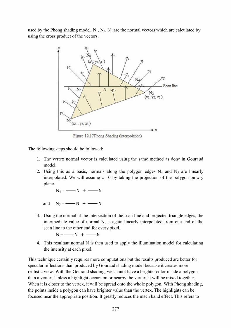
277

used by the Phong shading model. N1, N2, N3 are the normal vectors which are calculated by

using the cross product of the vectors.

The following steps should be followed:

1. The vertex normal vector is calculated using the same method as done in Gouraud

model.

2. Using this as a basis, normals along the polygon edges N4 and N5 are linearly

interpolated. We will assume z =0 by taking the projection of the polygon on x-y

plane.

N4 = N + N

and N5 = N + N

3. Using the normal at the intersection of the scan line and projected triangle edges, the

intermediate value of normal N, is again linearly interpolated from one end of the

scan line to the other end for every pixel.

N = N + N

4. This resultant normal N is then used to apply the illumination model for calculating the intensity at each pixel.

This technique certainly requires more computations but the results produced are better for

specular reflections than produced by Gouraud shading model because it creates more

realistic view. With the Gouraud shading, we cannot have a brighter color inside a polygon

than a vertex. Unless a highlight occurs on or nearby the vertex, it will be mixed together.

When it is closer to the vertex, it will be spread onto the whole polygon. With Phong shading,

the points inside a polygon can have brighter value than the vertex. The highlights can be

focused near the appropriate position. It greatly reduces the mach band effect. This refers to

278

an effect where the contrast between the two areas of different shading is enhanced and it

appears as the border between the shades.


Q8. Which method is suitable for specular reflections?

----------------------------------------------------------------------------------------------------------------

----------------------------------------------------------------------------------------------------------------

----------------------

Comparison among various shading models:

S.no 1

Flat Shading

It is simplest and the fastest

Gouraud Shading

It is more realistic than flat

Phong Shading

It provides the highest

method. shading. quality and is expensive

in nature.

2

There is no mach band

effect.

It suffers from mach band

effect.

It also does not suffer

from mach band effect.

3

This technique finds the

vertex normal vector.

This method finds the

average normal at each

vertex.

This method also finds

the vertex normal.

4

There is no interpolation of

the normals across the

polygons.

This technique interpolates

vertex shades among each

polygon.

This method

interpolates normals

across the polygons.

5

It is unrealistic in nature.

It is realistic in nature.

It is also realistic in

nature.

6

It is not at all expensive.

It is costly approach.

It is most expensive

among all.

7

This is one of the oldest

method in computer

graphics.

It is slightly new method.

It is the latest technique

being used in graphics.

8

Specular effects are visible.

Specular effects are not

seen.

The problem of secular

effects has been

overcome.

12.9. Morphing of objects

279

Morphing refers to a process of transforming an image into another image. This process

makes use of the image processing techniques that includes warping and cross dissolving.

Morphing sequences produced by using cross-dissolving only (e.g. linear interpolation to

lighten from one image to another) of the original and the target images are very poor. These

results are of low quality because of the misalignment among the features of source and

destination images. When we are simply using cross dissolve technique, there will be the

double exposure effect in the misaligned regions. In order to reduce this problem, warping is

used that aligns the two images first before proceeding for cross dissolving. Warping

provides the way in which the pixels of one image should be transformed to the pixels in the

other image. For warping to execute, the mapping of few important pixels needs to be

specified. The movement of the other pixels is produced by extrapolating the information

specified for the control pixels. As cross dissolving is very effortless, warping becomes the

prime problem of morphing techniques. Morphing can be thought of a cross-dissolve method

which is applied to warped image. There are different warping techniques that differ in the

way the control pixels are to be specified and the interpolating technique that they use for the

other pixels. The prominent features of an image are specified by the set of these control

pixels.

Morphing= (warping)2 + blending As we can see from the above equation that morphing is basically a two-stage process that

involves coupling image warping with color interpolation. Check your progress / Self assessment questions

Q9. Why is warping important before cross dissolving? ----------------------------------------------------------------------------------------------------------------

----------------------------------------------------------------------------------------------------------------

---------------------- 12.10. Summary

Shading creates a realistic view. We have discussed various shading models that describe

how light reflects a surface. Lambert shading is simplest method that takes source of light and

illumination models into consideration. In this method, objects appearance is not smooth.

Phong shading is a method that renders the surface of displayed objects providing them a

smooth appearance. Gouraud shading technique is also used for smooth shading but is

comparatively less efficient as compared to phong shading. Some techniques of rendering is

provided. Methods to cast shadows are discussed.

12.11. Glossary Rendering - Rendering refers to the process of converting of a 3-D scene into a 2-D image

using computer programs.

Ray Casting – It is a method which is used to render high-quality images of solid objects.

280

Ray Tracing - It is a technique taken from optics that models that path taken by light by

following the rays of light as they intersect the optical surfaces.

Rasterization - This is a process that transforms the geometric primitives such as lines,

circles, ellipse, etc into a raster image i.e. finding appropriate pixel locations to illuminate the

image being formed.

Mach band effect - Mach band is an optical illusion that consists of an image with two wide

bands- one light and other dark.

Morphing - Morphing refers to a process of transforming an image into another. This

process involves the image processing techniques of warping and cross dissolving.

12.12. Answers to check your progress / self assessment questions 1. The shading models are also called illumination models because they can be used to check

the intensity of light at any given point on the surface of an object.

2. The two methods are: Flat shading and Smooth shading. 3. The two types of internal mapping are:

S-mapping: In this, the texture image is mapped onto a simple three dimensional

surface such as a plane, cylinder, a sphere or a box.

O-mapping : In this, the result of S-mapping is mapped onto the final 3-D surface. 4. Ray tracing.

5. Depth-Sort (or Priority Algorithm).

6. False.

7. Left edge (x4 ) = min [ x1 + (y-y1)/slope(1-3), x2 + (y-y2)/slope(2-3) ]

Right edge (x5) = max [x1 + (y-y1)/slope(1-3), x2 + (y-y2)/slope(2-3) ]

8. Phong Shading method.

9. Warping is important before cross dissolving because it reduces the double exposure effect in the misaligned regions. Warping is used that aligns the two images first before proceeding for cross dissolving. It provides the way in which the pixels of one image should be transformed to the pixels in the other image.


1. Explain various polygon shading models in graphics.

2. Why do we need shading models in computer graphic?

3. Explain Gouraud Shading Model in detail.

4. Explain Phong Shading Model in detail.

5. Compare and contrast various shading models.

281

6. How can we add textures to objects?

7. How is morphing of objects done?

Computer Graphics - PTU (Punjab Technical University)

Documents

Transcript of Computer Graphics - PTU (Punjab Technical University)