Common Components - Springer LINK
53
333 APPENDIX A Common Components This brief primer appendix offers a look at the basic components that you will need to know something about if you plan to do many electronic or MCU projects. Here we look at a selection of simple components that crop up time and again and form the basic building blocks of all electronic circuitry. Resistors A resistor, as its name implies, is a component that, to varying degrees, resists the flow of electrical current. When I was new to electronics, it always seemed a little odd to me that resistors were needed. After all, I reasoned, the purpose of most electronic devices is to originate or amplify electrical signals, why would you want a component to reduce them down again? I soon learned that not all electronic components operate at the same signal levels and so resistors are needed to match signal levels between devices of different capabilities and types. Resistors are also used to regulate the flow of current to levels that components can handle. For example, we use resistors to ensure that a device such as an LED (which we’ll look at later) does not demand more current than it can handle, thus endangering itself, and whatever electronics it is connected to. Resistance is measured in ohms, since it was Georg Ohm who, in 1827, first accurately described the relationships between voltage, resistance, and current. The “ohms” rating of a resistor determines how much resistance it will offer to the flow of electricity through it. Ohm’s law gives us multiple mathematical methods to calculate the characteristics of a circuit. The main method of interest in the context of this discussion states that the current (in amps) flowing through a circuit is found by dividing the voltage by the number of ohms of the resistance in that circuit (where I is the current, V is the voltage, and R is the resistance). I = V/R For example, suppose we have a simple circuit comprised of a +12V battery with a 10 ohm resistor connected across it. 12 ÷ 10 = 1.2 + - 10 Ohms 12VDC
-
Upload
khangminh22 -
Category
Documents
-
view
3 -
download
0
Transcript of Common Components - Springer LINK
333
APPENDIX A
Common Components
This brief primer appendix offers a look at the basic components that you will need to know something about if you plan to do many electronic or MCU projects. Here we look at a selection of simple components that crop up time and again and form the basic building blocks of all electronic circuitry.
Resistors A resistor, as its name implies, is a component that, to varying degrees, resists the flow of electrical current .
When I was new to electronics, it always seemed a little odd to me that resistors were needed. After all, I reasoned, the purpose of most electronic devices is to originate or amplify electrical signals, why would you want a component to reduce them down again? I soon learned that not all electronic components operate at the same signal levels and so resistors are needed to match signal levels between devices of different capabilities and types. Resistors are also used to regulate the flow of current to levels that components can handle. For example, we use resistors to ensure that a device such as an LED (which we’ll look at later) does not demand more current than it can handle, thus endangering itself, and whatever electronics it is connected to.
Resistance is measured in ohms, since it was Georg Ohm who, in 1827, first accurately described the relationships between voltage, resistance, and current. The “ohms” rating of a resistor determines how much resistance it will offer to the flow of electricity through it.
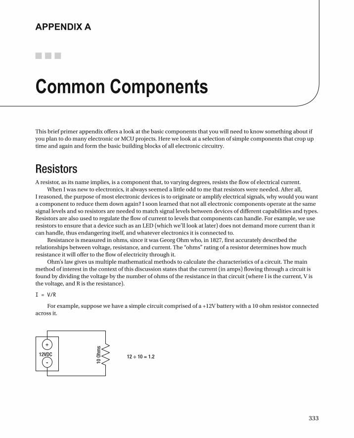
Ohm’s law gives us multiple mathematical methods to calculate the characteristics of a circuit. The main method of interest in the context of this discussion states that the current (in amps) flowing through a circuit is found by dividing the voltage by the number of ohms of the resistance in that circuit (where I is the current, V is the voltage, and R is the resistance).
I = V/R
For example, suppose we have a simple circuit comprised of a +12V battery with a 10 ohm resistor connected across it.
12 ÷ 10 = 1.2
+
- 10 O
hms
12VDC
APPENDIX A ■ COMMON COMPONENTS
334
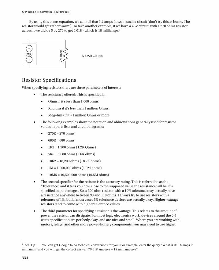
By using this ohms equation , we can tell that 1.2 amps flows in such a circuit (don’t try this at home. The resistor would get rather warm!). To take another example, if we have a +5V circuit, with a 270 ohms resistor across it we divide 5 by 270 to get 0.018 - which is 18 milliamps. 1
5 ÷ 270 = 0.018
+
- 270
Ohm
s
5VDC
Resistor Specifications When specifying resistors there are three parameters of interest:
The resistance offered: This is specified in •
Ohms if it’s less than 1,000 ohms. •
Kilohms if it’s less than 1 million Ohms. •
Megohms if it’s 1 million Ohms or more. •
The following examples show the notation and abbreviations generally used for resistor • values in parts lists and circuit diagrams:
270R = 270 ohms •
680R = 680 ohms •
1K2 = 1,200 ohms (1.2K Ohms) •
5K6 = 5,600 ohms (5.6K ohms) •
18K2 = 18,200 ohms (18.2K ohms) •
1M = 1,000,000 ohms (1.0M ohms) •
10M5 = 10,500,000 ohms (10.5M ohms) •
The second specifier for the resistor is the accuracy rating. This is referred to as the • “Tolerance” and it tells you how close to the supposed value the resistance will be; it’s specified in percentages. So, a 100 ohm resistor with a 10% tolerance may actually have a resistance anywhere between 90 and 110 ohms. I always try to use resistors with a tolerance of 1%, but in most cases 5% tolerance devices are actually okay. Higher-wattage resistors tend to come with higher tolerance values.
The third parameter for specifying a resistor is the wattage. This relates to the amount of • power the resistor can dissipate. For most logic electronics work, devices around the 0.5 watts specification are perfectly okay, and are nice and small. Where you are working with motors, relays, and other more power-hungry components, you may need to use higher
1 Tech Tip You can get Google to do technical conversions for you. For example, enter the query “What is 0.018 amps in milliamps” and you will get the correct answer: “0.018 amperes = 18 milliamperes”.

APPENDIX A ■ COMMON COMPONENTS
335
wattages, up to 10 watts or even more. These are physically much larger devices. Project parts lists often specify the wattage required for each resistor.
To calculate the wattage (Power) required for any particular situation you should use the • formula P = (V times I): This means power = voltage times amperage. To reuse an earlier example: We know that our 270 ohms resistor, connected across a 5-volt power source, consumes 0.018 amps (18 milliamps): so, we can calculate how many watts the resistor will dissipate using P = (V times I), thus: 5 x 0.018 = 0.09 - which is 90 milliwatts. So, in this case, a 0.5W (500 milliwatts) resistor or even a 0.25 (250 milliwatts) resistor would easily cope.
A very few larger resistors have their values printed on them in words (“27K 10 Watts,” for example). However, most use a system of color-coded rings to show their values. This is because of the difficulty of printing text on something so small. There seems little point in reproducing a chart of color codes in black and white here. However, there are many such charts online you can look at in full color. For example, see
• http://en.wikipedia.org/wiki/Resistor_colour_codes.
• www.digikey.com/web%20export/mkt/general/mkt/resistor-color-chart.jpg.
Resistor Types and Packagings For the purposes of this book we will be using conventional resistors, but there are also even smaller resistors available as surface mount devices (SMDs). However, these can’t be used on breadboards and are difficult (though not impossible) for the hobbyist to use — thus we avoid them in this book.
There are various kinds of other resistors. One prime example is the variable resistor, which is called the potentiometer (usually shortened to “pot”). On analog audio and visual gear the volume control or the brightness control was a potentiometer. A potentiometer is a variable resistor and it has a resistance value in ohms, just the same as a normal resistor. It has three terminals, and Figure A-1 shows the circuit symbol:
100K Ohms
Wiper
End 1
End 2
Figure A-1 . Potentiometer connections
If you only connect the terminals marked “End 1” and “End 2” into your circuit, the pot behaves exactly like a normal resistor — that is, this 100KOhm pot could be used to replace a 100K resistor.
The third terminal, however ( “the wiper”), slides up and down the resistance as the pot knob is turned: when it is exactly centered (as shown in the diagram) the resistance between the wiper and each end will be exactly half of the rated resistance. If the setup is as depicted in the diagram, you would see 50K ohms between the wiper and End 1, and the same between the wiper and End 2.
APPENDIX A ■ COMMON COMPONENTS
336
If the pot is physically turned as far as it can go in on direction, then the resistance between the wiper and one of the ends will be zero ohms and between the wiper and the other end will be 100K ohms (which end will depend on which way it is turned). Thus, the potentiometer gives you the possibility of setting any resistance value you like between zero and whatever the pot value is (in this case we can get anything between 0 and 100K ohms).
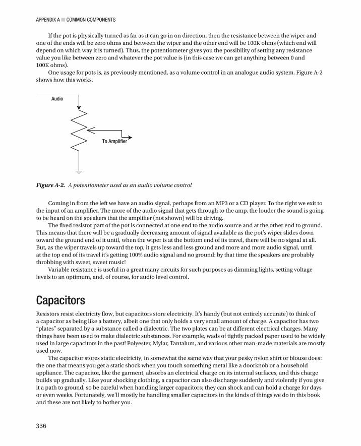
One usage for pots is, as previously mentioned, as a volume control in an analogue audio system. Figure A-2 shows how this works.
To Amplifier
Audio
Figure A-2 . A potentiometer used as an audio volume control
Coming in from the left we have an audio signal, perhaps from an MP3 or a CD player. To the right we exit to the input of an amplifier. The more of the audio signal that gets through to the amp, the louder the sound is going to be heard on the speakers that the amplifier (not shown) will be driving.
The fixed resistor part of the pot is connected at one end to the audio source and at the other end to ground. This means that there will be a gradually decreasing amount of signal available as the pot’s wiper slides down toward the ground end of it until, when the wiper is at the bottom end of its travel, there will be no signal at all. But, as the wiper travels up toward the top, it gets less and less ground and more and more audio signal, until at the top end of its travel it’s getting 100% audio signal and no ground: by that time the speakers are probably throbbing with sweet, sweet music!
Variable resistance is useful in a great many circuits for such purposes as dimming lights, setting voltage levels to an optimum, and, of course, for audio level control.
Capacitors Resistors resist electricity flow, but capacitors store electricity. It’s handy (but not entirely accurate) to think of a capacitor as being like a battery, albeit one that only holds a very small amount of charge. A capacitor has two “plates” separated by a substance called a dialectric . The two plates can be at different electrical charges. Many things have been used to make dialectric substances. For example, wads of tightly packed paper used to be widely used in large capacitors in the past! Polyester, Mylar, Tantalum, and various other man-made materials are mostly used now.
The capacitor stores static electricity , in somewhat the same way that your pesky nylon shirt or blouse does: the one that means you get a static shock when you touch something metal like a doorknob or a household appliance. The capacitor, like the garment, absorbs an electrical charge on its internal surfaces, and this charge builds up gradually. Like your shocking clothing, a capacitor can also discharge suddenly and violently if you give it a path to ground, so be careful when handling larger capacitors; they can shock and can hold a charge for days or even weeks. Fortunately, we’ll mostly be handling smaller capacitors in the kinds of things we do in this book and these are not likely to bother you.
APPENDIX A ■ COMMON COMPONENTS
337
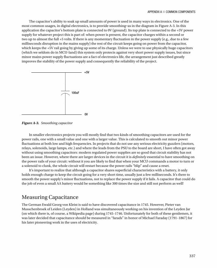
The capacitor’s ability to soak up small amounts of power is used in many ways in electronics. One of the most common usages, in digital electronics, is to provide smoothing — as in the diagram in Figure A-3 . In this application the capacitor’s bottom plate is connected to 0V (ground). Its top plate is connected to the +5V power supply for whatever project this is part of: when power is present, the capacitor charges within a second or two up to almost the full +5 volts. If there is any momentary fluctuation in the power supply (e.g., due to a few milliseconds disruption in the mains supply) the rest of the circuit keeps going on power from the capacitor, which keeps the +5V rail going by giving up some of its charge. Unless we were to use physically huge capacitors (which we seldom do in MCU-land) this system only protects against very short power supply issues, but since minor mains power supply fluctuations are a fact of electronics life, the arrangement just described greatly improves the stability of the power supply and consequently the reliability of the project.
0V
+5V
100uF
Figure A-3 . Smoothing capacitor
In smaller electronics projects you will mostly find that two kinds of smoothing capacitors are used for the power rails, one with a small value and one with a larger value. This is calculated to smooth out minor power fluctuations at both low and high frequencies. In projects that do not use any serious electricity guzzlers (motors, relays, solenoids, large lamps, etc.) and where the leads from the PSU to the board are short, I have often got away without using smoothing capacitors: modern regulated power supplies are so good that circuit stability has not been an issue. However, where there are larger devices in the circuit it is definitely essential to have smoothing on the power rails of your circuit: without it you are likely to find that when your MCU commands a motor to turn or a solenoid to clunk, the whole circuit will restart because the power rails “blip” and cause a reset.
It’s important to realize that although a capacitor shares superficial characteristics with a battery, it only holds enough charge to keep the circuit going for a very short time, usually just a few milliseconds. It’s there to smooth the power supply’s minor fluctuations, not to replace the power supply if it fails. A capacitor that could do the job of even a small AA battery would be something like 300 times the size and still not perform as well!
Measuring Capacitance The German Ewald Georg von Kleist is said to have discovered capacitance in 1745. However, Pieter van Musschenbroek of Leiden (Leyden) in Holland was simultaneously working on his invention of the Leyden Jar (on which there is, of course, a Wikipedia page) during 1745–1746. Unfortunately for both of these gentlemen, it was later decided that capacitance should be measured in “farads” in honor of Michael Faraday (1791–1867) for his later pioneering work in the uses of electricity.
APPENDIX A ■ COMMON COMPONENTS
338
In fact, one farad is an awful lot of capacitance and a capacitor offering that much capacity is very large, far bigger than a battery. Fortunately, in electronics we rarely need capacitances anything like as large as one farad, so, we mostly use capacitors that are measured in millionths of farads, the name for which is “microfarads.” This is formally written using a symbol called “mu” or “micro” and it looks like this “ μ ”. However, the mu symbol is not found on general-purpose computer keyboards 2 and so very often the lower case “u” symbol is used instead. Thus, the following all mean the same thing:
100 uf (using the lower case “u”) •
100 μ f (using mu) •
100 microfarads •
But, often we need even less capacitance than one microfarad. In such cases we have to go down to nanofarads and picofarads. These quantities break down as follows:
One farad—the basic unit of capacitance. •
1,000 millifarads = one farad (millifarads are never used in electronics). •
1,000 microfarads = one millifarad (with 1,000,000 microfarads to the farad). •
1,000 nanofarads = One microfarad (with 1,000,000,000 nanofarads to the farad). •
1,000 picofarads = One nanofarad (with 1,000,000,000,000 picofarads to the farad). •
Unfortunately, different capacitor manufacturers have chosen to label their products in different ways, and there are many competing labeling standards used. For example, you will find that some manufacturers sell a “0.1 μ F” capacitor, while others sell a “100 nF” capacitor—both products would have the same value, just expressed in a different way; it’s the same idea as $1.2 being the same amount of money as 1,200 cents. We’ll look in more detail at capacitor labeling a bit later on in this section.
Time for a Capacitance The other way that we often use capacitors is as timing components. It takes a finite amount of time for a capacitor to charge up to its full potential, and we can slow it down even more if we use a resistor and capacitor in series combination: we can then use this time delay in various ways. This kind of circuit is called an RC network , as in Figure A-4 .
2 In MS Word you can get a mu symbol by holding down the ALT key and typing 230 on the number pad then releasing ALT. On a Mac, hold down the Option key and press m to get a μ character. Option and Z will get the Ω character.

APPENDIX A ■ COMMON COMPONENTS
339
In this circuit, a resistor stops the capacitor from charging up as quickly as it wants to, and the sense wire goes off into some electronics (not shown) for some purpose—see below. When the +5V supply first starts up, the capacitor’s bottom plate of course remains at 0V because it is grounded to 0V. However, the capacitor’s top plate gradually charges towards something close to +5Volts, through the resistor.
The “rise time” of the voltage at the “sense” point will be a lot slower than the power supply rise time. This means that any electronic devices connected to it will be “on power” before the capacitor is fully charged. If the “sense” lead shown in the diagram is connected to the active-low reset input of the MCU chip, you now have what is known as a “power on Reset” circuit. The MCU powers up, but for a brief time, until the capacitor charges up, its reset input will be held LOW, thus ensuring it is properly reset before operation begins and whilst the power supply stabilizes. This being electronics, all of this happens very quickly—within a few milliseconds at most. You may notice that we use an RC network on the AVR test bed that we built in Chapter 2 . This is to ensure that the MCU there is properly reset at power on.
Without a “power on reset” circuit like the one just described, “intelligent” devices such as MCUs, microprocessors, complex graphics processor chips, and many others would not initialize properly and would start doing all kinds of random things because different parts of the chip begin in unsynchronized ways. Thus, holding the reset pin active for a short while after power-up gets all the pieces at the “Start line” at the same moment, ready to start working together as they should. So, although the RC network is a simple thing, it’s an essential part of even the most complex circuits.
RC networks are used in all kinds of ways in electronics: for example, the venerable, but still very popular, 555 timer chip uses an RC network to provide its time delays. Many kinds of RC networks can be built: there is, of course, a Wikipedia page on this subject with lots of examples and information about calculating rise times and the shape of rise time curves. In the case of our preceding example, the exact point at which the “sense” line turns from logic LOW to logic HIGH depends equally as much on the characteristics of the device to which it is attached as to the RC rise time.
Another way that RC networks are used is in audio. The same basic idea of a resistor and capacitor in series is used, but if the resistor is made variable (like a tone control or volume control) the charge/discharge time of
+5V
100uF
R1 10K
0V
Sense
Figure A-4 . An RC network
APPENDIX A ■ COMMON COMPONENTS
340
the capacitor can be varied, which means that the circuit will nullify audio signals at or above a certain frequency. One or many RC networks will be found at the heart of all predigital tone controls and graphic equalizers in audio gear. So as you can see, RC networks have a huge number of applications—our use for them in power-on-reset is just one of many.
All capacitors have a maximum working voltage. You can’t put a capacitor rated for use at 16 volts DC into a circuit that operates at 30 volts; if you do, bad and probably smoky things will happen! On the other hand, you can put a 30 volt capacitor into a 16 volt circuit with no problem. Although it may be physically bigger than you would wish, it will still work properly. Since capacitor specs and limits usually drift as they age, it’s best to allow some voltage leeway when selecting them. As a rule of thumb, allow something around 40% or so: in other words, if your circuit operates at 12 volts, select a 16V capacitor. If your circuit operates at 5 volts, use a capacitor rated for 7 volts or more.
WARNING! SAFETY NOTE: CAPACITOR FAILURE MODES
An overstressed capacitor will not fail gracefully! Generally, when a capacitor is used at too high a voltage or if you connect a polarized capacitor the wrong way around, it will burst like a popped balloon soon after power is applied to the circuit it’s in. When it pops, it will likely shoot out very hot and acidic dialectric substance and bits of capacitor body in all directions. This can be very harmful and can cause injury to skin or eyes.
If you always use the right capacitor for the job, and always double-check that capacitors are connected the right way round, you should never experience this problem.
But, please, be very careful if you think there is even the slightest possibility of this happening; wear safety gloves and glasses and keep as far away from the circuit in question as you can when you power it on.
This also applies if you are trying to rescue old equipment (such as power supplies) that contains large, old capacitors. Such devices can—especially if they have been stored in a damp place—get seriously out of spec and pop when you apply power to them for the first time in many years. You should always, as a first step before power on, replace any large capacitors in an old device. I have seen an old capacitor from a pinball machine PSU explode and I can tell you from first-hand experience that it’s not nice!
Capacitor Shapes and Sizes So far, we have looked at capacitors with a positive and a negative plate. These are called electrolytic capacitors . However, capacitors in the smaller range of values (usually this means less than one microfarad) are not “polarized”—you can connect them either way around and they will work just fine.
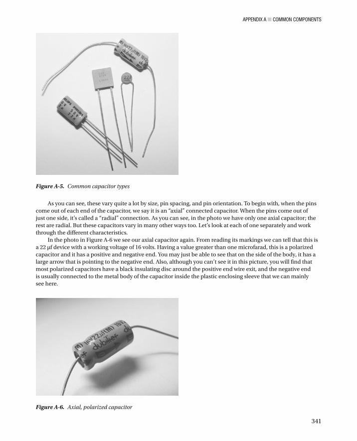
Capacitors come in an embarrassingly large range of styles and with a confusing array of markings. We can only look at the major kinds in a short introduction like this. Wikipedia has a fuller survey of the less common types. The photo in Figure A-5 shows a handful of capacitors.
APPENDIX A ■ COMMON COMPONENTS
341
As you can see, these vary quite a lot by size, pin spacing, and pin orientation. To begin with, when the pins come out of each end of the capacitor, we say it is an “axial” connected capacitor. When the pins come out of just one side, it’s called a “radial” connection. As you can see, in the photo we have only one axial capacitor; the rest are radial. But these capacitors vary in many other ways too. Let’s look at each of one separately and work through the different characteristics.
In the photo in Figure A-6 we see our axial capacitor again. From reading its markings we can tell that this is a 22 μ f device with a working voltage of 16 volts. Having a value greater than one microfarad, this is a polarized capacitor and it has a positive and negative end. You may just be able to see that on the side of the body, it has a large arrow that is pointing to the negative end. Also, although you can’t see it in this picture, you will find that most polarized capacitors have a black insulating disc around the positive end wire exit, and the negative end is usually connected to the metal body of the capacitor inside the plastic enclosing sleeve that we can mainly see here.
Figure A-5 . Common capacitor types
Figure A-6 . Axial, polarized capacitor
APPENDIX A ■ COMMON COMPONENTS
342
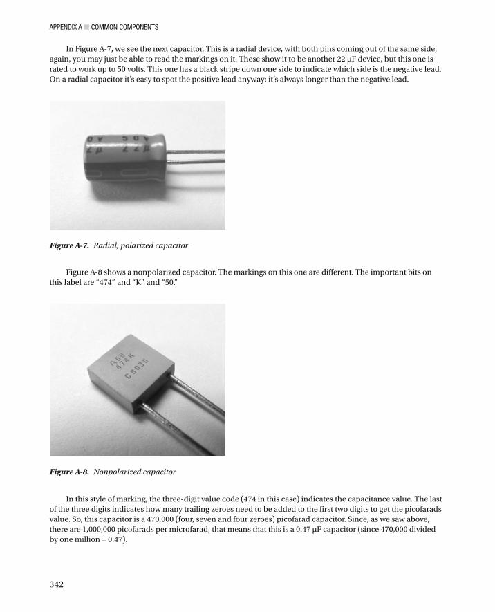
Figure A-8 shows a nonpolarized capacitor . The markings on this one are different. The important bits on this label are “474” and “K” and “50.”
In Figure A-7 , we see the next capacitor. This is a radial device, with both pins coming out of the same side; again, you may just be able to read the markings on it. These show it to be another 22 μ F device, but this one is rated to work up to 50 volts. This one has a black stripe down one side to indicate which side is the negative lead. On a radial capacitor it’s easy to spot the positive lead anyway; it’s always longer than the negative lead.
Figure A-7 . Radial, polarized capacitor
Figure A-8 . Nonpolarized capacitor
In this style of marking, the three-digit value code (474 in this case) indicates the capacitance value. The last of the three digits indicates how many trailing zeroes need to be added to the first two digits to get the picofarads value. So, this capacitor is a 470,000 (four, seven and four zeroes) picofarad capacitor. Since, as we saw above, there are 1,000,000 picofarads per microfarad, that means that this is a 0.47 μ F capacitor (since 470,000 divided by one million = 0.47).
APPENDIX A ■ COMMON COMPONENTS
343
The “K” is a tolerance code: like a resistor, this specifies how close to the marked value the capacitor is likely to be. Tolerance codes may indicate percentages or absolute pF values. For example a tolerance code indicating 20% means that the capacitance may be 20% more or 20% less than the marked value. Tolerance codes are as follows:
Code Letter Percentage or Amount of Tolerance
B ± 0.1 pF
C ± 0.25 pF
D ± 0.5 pF
F ± 1%
G ± 2%
J ± 5%
K ± 10%
M ± 20%
Z +80%, –20%
Finally, the “50” on this capacitor indicates that it operates at a maximum 50 volts. These markings vary a little from manufacturer to manufacturer. If you are in doubt about the exact value of
a capacitor, try to contact its maker. If (as is often the case) you can’t find out who made it, it’s better not to use the device; buy a new one whose value you are sure of. It’s cheaper to buy a new device than to cause damage to whatever you are building and to have to replace more expensive parts.
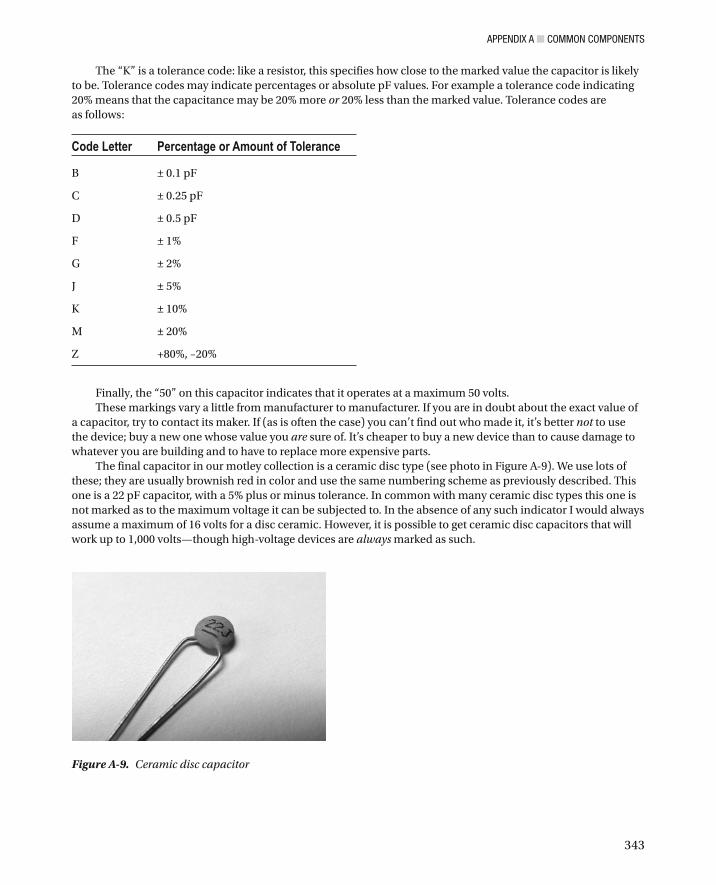
The final capacitor in our motley collection is a ceramic disc type (see photo in Figure A-9 ). We use lots of these; they are usually brownish red in color and use the same numbering scheme as previously described. This one is a 22 pF capacitor, with a 5% plus or minus tolerance. In common with many ceramic disc types this one is not marked as to the maximum voltage it can be subjected to. In the absence of any such indicator I would always assume a maximum of 16 volts for a disc ceramic. However, it is possible to get ceramic disc capacitors that will work up to 1,000 volts—though high-voltage devices are always marked as such.
Figure A-9 . Ceramic disc capacitor
APPENDIX A ■ COMMON COMPONENTS
344
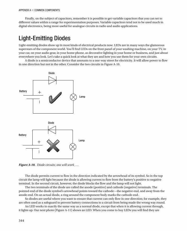
The diode permits current to flow in the direction indicated by the arrowhead of its symbol. So in the top circuit the lamp will light because the diode is allowing current to flow from the battery’s positive to negative terminal. In the second circuit, however, the diode blocks the flow and the lamp will not light.
The two terminals of the diode are called the anode (positive) and cathode (negative) terminals. The pointed end of the diode symbol’s arrowhead points toward the cathode—the negative end, and away from the anode end. On an actual diode, a ring around the component body marks the cathode end.
So diodes are useful where you want to ensure that current can only flow in one direction; for example, they are often used as a safeguard to prevent battery connections to a circuit from being made the wrong way round.
An LED works in exactly the same way as a normal diode, except that when it is allowing current through, it lights up. Our next photo (Figure A-11 ) shows an LED. When you come to buy LEDs you will find they are
Diode
Lamp
Battery
Diode
Lamp
Battery
Figure A-10 . Diode circuits ; one will work . . .
Finally, on the subject of capacitors, remember it is possible to get variable capacitors that you can set to different values within a range for experimentation purposes. Variable capacitors tend not to be used much in digital electronics, being more useful for analogue circuits in radio and audio applications.
Light-Emitting Diodes Light-emitting diodes show up in most kinds of electrical products now. LEDs are in many ways the glamorous superstars of the component world. You’ll find LEDs on the front panel of your washing machine, on your TV, in your car, on your audio gear, in your home phone, as decorative lighting in your home or business, and just about everywhere you look. Let’s take a quick look at what they are and how you use them for your own circuits.
A diode is a semiconductor device that amounts to a one-way street for electricity. It will allow power to flow in one direction but not in the other. Consider the two circuits in Figure A-10 .
APPENDIX A ■ COMMON COMPONENTS
345
available in many different colors and in quite a few different sizes. Sizes, which refer to the lens part of the component (shown at the left in this photo), are usually expressed in millimeters. Common sizes are 3 mm, 5mm, and 10 mm. As a very general rule (to which there are many exceptions) the larger the lens the brighter the light.
Figure A-11 . A single LED
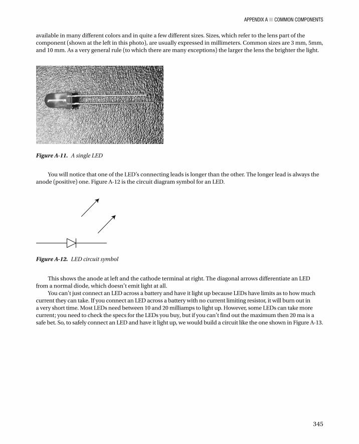
You will notice that one of the LED’s connecting leads is longer than the other. The longer lead is always the anode (positive) one. Figure A-12 is the circuit diagram symbol for an LED.
Figure A-12 . LED circuit symbol
This shows the anode at left and the cathode terminal at right. The diagonal arrows differentiate an LED from a normal diode, which doesn’t emit light at all.
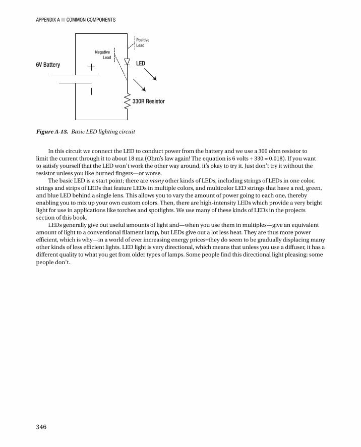
You can’t just connect an LED across a battery and have it light up because LEDs have limits as to how much current they can take. If you connect an LED across a battery with no current limiting resistor, it will burn out in a very short time. Most LEDs need between 10 and 20 milliamps to light up. However, some LEDs can take more current; you need to check the specs for the LEDs you buy, but if you can’t find out the maximum then 20 ma is a safe bet. So, to safely connect an LED and have it light up, we would build a circuit like the one shown in Figure A-13 .
APPENDIX A ■ COMMON COMPONENTS
346
In this circuit we connect the LED to conduct power from the battery and we use a 300 ohm resistor to limit the current through it to about 18 ma (Ohm’s law again! The equation is 6 volts ÷ 330 = 0.018). If you want to satisfy yourself that the LED won’t work the other way around, it’s okay to try it. Just don’t try it without the resistor unless you like burned fingers—or worse.
The basic LED is a start point; there are many other kinds of LEDs, including strings of LEDs in one color, strings and strips of LEDs that feature LEDs in multiple colors, and multicolor LED strings that have a red, green, and blue LED behind a single lens. This allows you to vary the amount of power going to each one, thereby enabling you to mix up your own custom colors. Then, there are high-intensity LEDs which provide a very bright light for use in applications like torches and spotlights . We use many of these kinds of LEDs in the projects section of this book.
LEDs generally give out useful amounts of light and—when you use them in multiples—give an equivalent amount of light to a conventional filament lamp, but LEDs give out a lot less heat. They are thus more power efficient, which is why—in a world of ever increasing energy prices — they do seem to be gradually displacing many other kinds of less efficient lights. LED light is very directional, which means that unless you use a diffuser, it has a different quality to what you get from older types of lamps. Some people find this directional light pleasing; some people don’t.
LED6V Battery
330R Resistor
Positive Lead
Negative Lead
Figure A-13 . Basic LED lighting circuit
347
APPENDIX B
A Digital Electronics Primer
Microcontroller units (MCUs) are great big blocks of digital electronic circuitry, but they still obey the basics of digital electronics. I’d like for us to take a short walk through these basics in this appendix. As we go through this, we’ll also be using a “breadboard”—which I explain in Appendix C.
This appendix aims to provide a basic introduction to digital electronics. It doesn’t cover the whole subject (which is vast), and it won’t make you into an instant expert on the subject. However, it should cover enough of the groundwork for you to understand the material presented throughout this book.
The Highs and the Lows Like all circuits, digital devices have inputs, via which signals enter the circuit, and outputs, via which signals leave the circuit. In an analog circuit, the signal coming into the circuit can vary right across the allowed voltage range, and the output from it can also be at any allowable level. In other words, the inputs and outputs from an analog circuit can vary continuously; they can be at any voltage allowed for that circuit.
For example, if the inputs to an analog circuit (such as an audio amplifier) are designed to accept inputs of between zero and 2 volts, then the input signal can be at any level (0.1 volts, 1.1 volts 1.8 volts, 1.99 volts, etc.) between those two voltages. Each tiny change of input voltage results in a slightly different output from the circuit. Digital circuitry is very different.
Digital circuits are designed to accept only two levels of input. These are “LOW” and “HIGH.” Many, but by no means all, digital circuits use a power supply voltage of 5 volts DC. In such circuits anything above about 3 volts is interpreted by the circuit as HIGH, and anything below about 1.8 volts is interpreted as LOW. Similarly, the outputs from digital circuits are designed to put out a HIGH or a LOW level and never anything in between. This is why digital circuits are incredibly reliable; they don’t have to be designed with the finesse that it takes to respond to very small changes of signal, the signals they process are always very definite, HIGHs or LOWs (also known as ones and zeroes).
Because it works in this somewhat brutal fashion, digital circuitry is comparatively simple, meaning you can get lots of it on a single chip. It also means that it fails in different ways. If you think back to predigital TV, if you were getting interference it would just distort or cloud the picture. On a bad digital TV signal, you lose chunks of the picture, or a few seconds of picture disappears, completely. Similarly, if you think about copying your files to a CD or a floppy disc, it either works or it doesn’t. If you can remember trying to copy tapes, it would usually work, but the copy would be degraded to some degree. These are the kind of differences you get between digital and analog circuitry and processes.
I Count—In Denary? Now, the behavior of digital electronics is, of course, ideal for use in circuits that use binary data . Binary numbers consist of only ones and zeroes and so can be stored, manipulated, and transmitted via digital circuits very easily. Let’s briefly review how binary works.
APPENDIX B ■ A DIGITAL ELECTRONICS PRIMER
348
It comes as a shock, perhaps, to realize that the number system you have used all through your life is only one of many possible systems. The denary system is the one we use to represent values in everyday life, and it deals in powers of ten. By adding zeroes to the right of a number (e.g., by turning 10 into 100), we multiply it by ten.
In the denary number system we use ten different symbols (0 to 9) and we arrange them in columns to show their “weight” in the represented value. The leftmost digit has the greatest weight, and the rightmost digit has the least. For example, the number 2390 in denary means (reading from right to left):
0 times 1 + 9 times 10 + 3 times 100 + 2 times 1000
So each column has a “weight” in our denary system, and each column’s weight is ten times that of the column to the right of it.
When representing values in the binary system, we use only two symbols (0 and 1) and the “weight” of a column is twice the value of the column to the right of it. So, in binary the column weights, reading from right to left are 1, 2, 4, 8, 16, 32, 64, and so on. For example, the binary number 1110 means (reading from right to left again):
0 times 1 + 1 times 2 + 1 times 4 + 1 times 8
If you work that one out, it means that the binary number 1110 is actually representing the value 14. With only 0 and 1 to represent, binary and digital electronic circuits are a match made in heaven! Of course,
this was no accident: digital circuits were specifically designed to handle binary data and to do arithmetic operations in binary.
The problem is that we humans don’t find it easy to deal in just ones and zeroes or HIGHs and LOWs. We like and demand subtlety and nuance; our preferred world is analog. Imagine a picture of a rich red sunset featuring a thousand subtle shades of color. Now, imagine that same scene rendered into just pure black and pure white: Yuk! So, to interface the binary world of computers with our real analog world, we need some special interfaces.
Hybrid circuits called A/D convertors and their mirror image, D/A convertors, allow the interchange of signals between digital and analog.
An A/D (analog to digital) convertor can continuously sample the voltage of an analog signal and represent it—moment to moment — to digital circuitry as a continuous stream of binary values that can be stored in the memory of a computer (e.g., your AVR microcontroller), so that it can be manipulated in some way.
Similarly, a D/A (digital to analog) convertor can be used to convert a succession of binary values (e.g., a file containing digitally sampled music) back into an analog signal suitable for feeding into an amplifier. Very fast A-to-D and D-to-A convertors are the whole basis for digital audio and video recording and playback. Without them there would be no digital TV or MP3 players. Your iPod or iRiver MP3 player has at least two such convertors in it—probably more.
However complex the information you are providing, whatever the source of the information (a camera, a DVD, a microphone, a scanner, a GPS system . . .) to the basic levels of your computer, it’s all just ones and zeroes; there may be trillions of them, but they’re all just binary data.
In this book you’ll see how binary data are acquired (via A/D circuits which are built in to the AVR chip we’re using) and you’ll see how binary data are sent back out into the outside world as analog data (again, using built-in AVR chip features).
APPENDIX B ■ A DIGITAL ELECTRONICS PRIMER
349
Deciding, Logically I’ve done some explaining about specific digital electronics within the main part of this book. However, it’s probably a good idea to look at one very specific digital electronic concept here, so that you hit the ground running when you encounter it later. That concept is “gates” (no, nothing to do with Bill at Microsoft, before you ask).
A great deal of digital electronics is composed of a structure called gates. A gate—as its name implies—is really just a device for letting through (open) or blocking (closed) a digital signal, based on certain conditions.
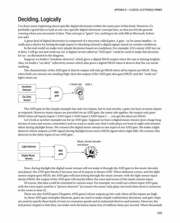
In the real world we make very simple decisions based on conditions. For example, if it’s sunny AND my car is dirty, I will go out and wash my car. A digital circuit called an “AND gate” could be used to make this decision for us—as illustrated in the diagram.
Suppose we build a “sunshine detector,” which gives a digital HIGH output when the sun is shining brightly. Also, we build a “car dirty” reflectivity sensor which also gives a digital HIGH when it detects that the car needs washing.
The characteristic of the AND gate is that its output will only go HIGH when all its inputs are HIGH. Thus, when both our sensors are sending High, then the output of the AND gate also goes HIGH, and the “wash car” light comes on.
AND gate
Sunshine Detector
Car Dirty Sensor
!! WASH CAR NOW !!
The AND gate in this simple example has only two inputs, but in real circuits, a gate can have as many inputs as required. However many inputs are provided on an AND gate, the same rule applies: the output only goes HIGH when all inputs (input 1 AND input 2 AND input 3 AND input 4 . . . you get the idea) are HIGH.
Let’s look at another example use for an AND gate. Suppose we have a digital music stream (just a huge long stream of ones and zeroes, remember) and we want to make sure that it only plays out loud at night and remains silent during daylight hours. We connect the digital music stream to one input of our AND gate. We make a light detector which outputs a LOW signal during daylight hours and a HIGH signal when night falls. We connect this detector to the other input of our AND gate.
AND gate
Light Detector
Digital Music Stream
Music stream decoder and player
Now, during daylight the digital music stream will not make it through the AND gate to the music decoder and player; the AND gate blocks it because one of its inputs is always LOW. When darkness comes, and the light sensor output goes HIGH, the AND gate will start letting through the music stream: with the light sensor input always HIGH, the output of the AND gate will exactly follow the ones and zeroes of the music stream input.
Of course, this idea could be extended in various ways. For example, we could use a three input AND gate, with the extra input used for a “person detector ” (to ensure the music only plays out loud when there is someone in the room to hear it).
There are also NAND gates (Negative AND gates) whose outputs go low only when all the inputs are high. As these AND gate examples illustrate, gates are used to make simple rudimentary decisions, and gate chips
are used in exactly these kinds of ways in consumer goods and in industrial devices and systems. However, the real power of gates is that they can make such decisions many tens of millions times per second. When thousands
APPENDIX B ■ A DIGITAL ELECTRONICS PRIMER
350
of gates are interconnected in complex ways, the result can be the processor in your desktop machine, or the processor core of your AVR microcontroller chip.
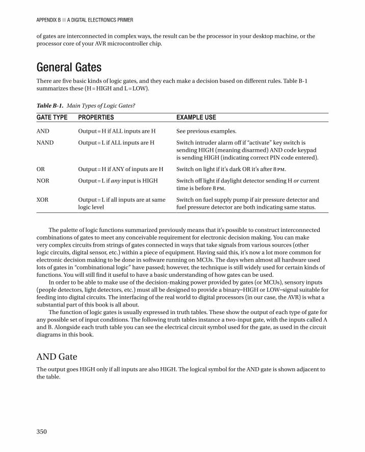
General Gates There are five basic kinds of logic gates, and they each make a decision based on different rules. Table B-1 summarizes these (H = HIGH and L = LOW).
The palette of logic functions summarized previously means that it’s possible to construct interconnected combinations of gates to meet any conceivable requirement for electronic decision making. You can make very complex circuits from strings of gates connected in ways that take signals from various sources (other logic circuits, digital sensor, etc.) within a piece of equipment. Having said this, it’s now a lot more common for electronic decision making to be done in software running on MCUs. The days when almost all hardware used lots of gates in “combinational logic” have passed; however, the technique is still widely used for certain kinds of functions. You will still find it useful to have a basic understanding of how gates can be used.
In order to be able to make use of the decision-making power provided by gates (or MCUs), sensory inputs (people detectors, light detectors, etc.) must all be designed to provide a binary — HIGH or LOW — signal suitable for feeding into digital circuits. The interfacing of the real world to digital processors (in our case, the AVR) is what a substantial part of this book is all about.
The function of logic gates is usually expressed in truth tables. These show the output of each type of gate for any possible set of input conditions. The following truth tables instance a two-input gate, with the inputs called A and B. Alongside each truth table you can see the electrical circuit symbol used for the gate, as used in the circuit diagrams in this book.
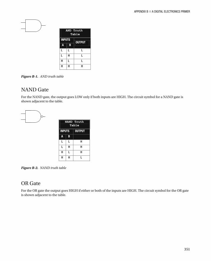
AND Gate The output goes HIGH only if all inputs are also HIGH. The logical symbol for the AND gate is shown adjacent to the table.
Table B-1. Main Types of Logic Gates?
GATE TYPE PROPERTIES EXAMPLE USE
AND Output = H if ALL inputs are H See previous examples.
NAND Output = L if ALL inputs are H Switch intruder alarm off if “activate” key switch is sending HIGH (meaning disarmed) AND code keypad is sending HIGH (indicating correct PIN code entered).
OR Output = H if ANY of inputs are H Switch on light if it’s dark OR it’s after 8 pm .
NOR Output = L if any input is HIGH Switch off light if daylight detector sending H or current time is before 8 pm.
XOR Output = L if all inputs are at same logic level
Switch on fuel supply pump if air pressure detector and fuel pressure detector are both indicating same status.
APPENDIX B ■ A DIGITAL ELECTRONICS PRIMER
351
NAND Gate For the NAND gate , the output goes LOW only if both inputs are HIGH. The circuit symbol for a NAND gate is shown adjacent to the table.
OR Gate For the OR gate the output goes HIGH if either or both of the inputs are HIGH. The circuit symbol for the OR gate is shown adjacent to the table.
INPUTSOUTPUT
A B
L L L
L H L
H L L
H H H
AND Truth Table
Figure B-1 . AND truth table
Figure B-2 . NAND truth table
NAND Truth Table
INPUTS OUTPUT
A B
L L H
L H H
H L H
H H L

APPENDIX B ■ A DIGITAL ELECTRONICS PRIMER
352
NOR Gate For the NOR gate, the output goes HIGH only if both inputs are LOW. The circuit symbol for a NOR gate is shown adjacent to the table.
XOR Gate For the XOR gate , the output goes HIGH if the inputs differ and LOW when inputs are the same. The circuit symbol for an XOR gate is shown adjacent to the table.
Figure B-3 . OR truth table
OR Truth Table
INPUTSOUTPUT
A B
L L L
L H H
H L H
H H H
Figure B-4 . NOR truth table
NOR Truth Table
INPUTSOUTPUT
A B
L L H
L H L
H L L
H H L
Figure B-5 . XOR truth table
INPUTSOUTPUT
A B
L L L
L H H
H L H
H H L
XOR Truth Table
APPENDIX B ■ A DIGITAL ELECTRONICS PRIMER
353
Understanding the Specifications of Gates Following are some general points about gates:
Although, so far, we have used the terms “HIGH” and “LOW” to indicate voltage levels, • they are equally often indicated by “1” and “0” (indicating HIGH and LOW, respectively). Both methods indicate the same thing in a different way. You may also occasionally hear logical levels referred to as true and false.
Although the truth tables in the preceding sections show only two inputs, bear in mind • that real gate devices can have many inputs. No matter how many inputs a gate has, the same rules apply.
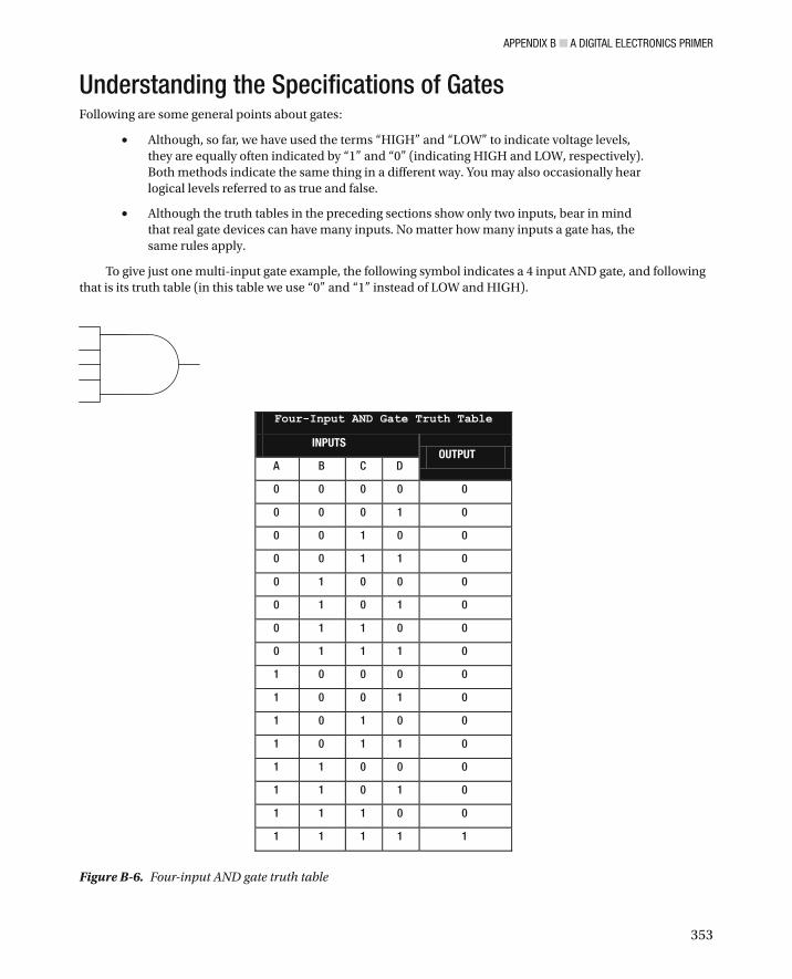
To give just one multi-input gate example, the following symbol indicates a 4 input AND gate, and following that is its truth table (in this table we use “0” and “1” instead of LOW and HIGH).
Figure B-6 . Four-input AND gate truth table
Four-Input AND Gate Truth Table
INPUTSOUTPUT
A B C D
0 0 0 0 0
0 0 0 1 0
0 0 1 0 0
0 0 1 1 0
0 1 0 0 0
0 1 0 1 0
0 1 1 0 0
0 1 1 1 0
1 0 0 0 0
1 0 0 1 0
1 0 1 0 0
1 0 1 1 0
1 1 0 0 0
1 1 0 1 0
1 1 1 0 0
1 1 1 1 1
APPENDIX B ■ A DIGITAL ELECTRONICS PRIMER
354
This multi-input gate obeys the same AND gate rule as the smaller two input gates: its output only goes HIGH (“1”) when all its inputs are HIGH.
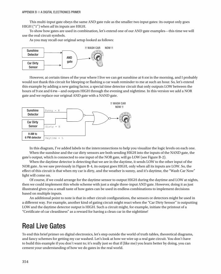
To show how gates are used in combination, let’s extend one of our AND gate examples—this time we will use the real circuit symbols.
As you may recall our original setup looked as follows:
AND gate
Sunshine Detector
Car Dirty Sensor
!! WASH CAR NOW !!
However, at certain times of the year where I live we can get sunshine at 6 am in the morning, and I probably would not thank this circuit for bleeping or flashing a car wash reminder to me at such an hour. So, let’s extend this example by adding a new gating factor, a special time detector circuit that only outputs LOW between the hours of 9 am and 6 pm —and outputs HIGH through the evening and nighttime. In this version we add a NOR gate and we replace our original AND gate with a NAND gate.
Sunshine Detector
Car Dirty Sensor
9 AM to 6 PM detector
Sunny = H
Dirty = H
Daytime = L
!! WASH CARNOW !!
In this diagram, I’ve added labels to the interconnections to help you visualize the logic levels on each one. When the sunshine and the car dirty sensors are both sending HIGH into the inputs of the NAND gate, the
gate’s output, which is connected to one input of the NOR gate, will go LOW (see Figure B-2 ). When the daytime detector is detecting that we are in the daytime, it sends LOW to the other input of the
NOR gate. As we saw previously in Figure B-4 , its output goes HIGH, only when all its inputs are LOW. So, the effect of this circuit is that when my car is dirty, and the weather is sunny, and it’s daytime, the “Wash Car Now” light will come on.
Of course, if we could arrange for the daytime sensor to output HIGH during the daytime and LOW at nights, then we could implement this whole scheme with just a single three-input AND gate. However, doing it as just illustrated gives you a small taste of how gates can be used in endless combinations to implement decisions based on multiple inputs.
An additional point to note is that in other circuit configurations, the sensors or detectors might be used in a different way. For example, another kind of gating circuit might react when the “Car Dirty Sensor” is outputting LOW and the daytime detector output is HIGH. Such a circuit might, for example, initiate the printout of a “Certificate of car cleanliness” as a reward for having a clean car in the nighttime!
Real Live Gates To end this brief primer on digital electronics, let’s step outside the world of truth tables, theoretical diagrams, and fancy schemes for getting my car washed. Let’s look at how we wire up a real gate circuit. You don’t have to build this example if you don’t want to; it’s really just so that if (like me) you learn better by doing, you can cement your understanding of how we do gates in the real world.
APPENDIX B ■ A DIGITAL ELECTRONICS PRIMER
355
The 7400 range of integrated circuits (commonly called TTL chips, for Transistor-Transistor-Logic ) were originally designed in the 1960s. They provided basic logic functions (gates, counters, registers) that proved so useful that they are still being sold and designed into commercial equipment today.
Today’s versions of the 7400 series use much less power than the originals, but they still offer the same functions and connections as their predecessors. We will use just one of these chips, the 74LS08, in this visual example of using gates. We could also have used the 74HC08, the 74 AC08, the 74 F08, or one of the other many variants of the 7408.
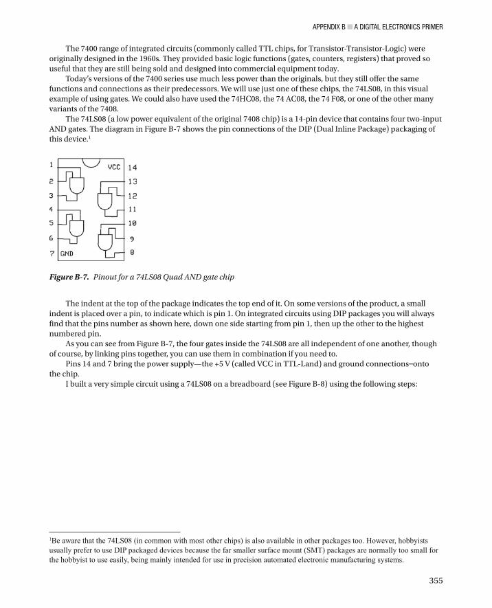
The 74LS08 (a low power equivalent of the original 7408 chip) is a 14-pin device that contains four two-input AND gates. The diagram in Figure B-7 shows the pin connections of the DIP (Dual Inline Package) packaging of this device. 1
The indent at the top of the package indicates the top end of it. On some versions of the product, a small indent is placed over a pin, to indicate which is pin 1. On integrated circuits using DIP packages you will always find that the pins number as shown here, down one side starting from pin 1, then up the other to the highest numbered pin.
As you can see from Figure B-7 , the four gates inside the 74LS08 are all independent of one another, though of course, by linking pins together, you can use them in combination if you need to.
Pins 14 and 7 bring the power supply—the +5 V (called VCC in TTL-Land) and ground connections — onto the chip.
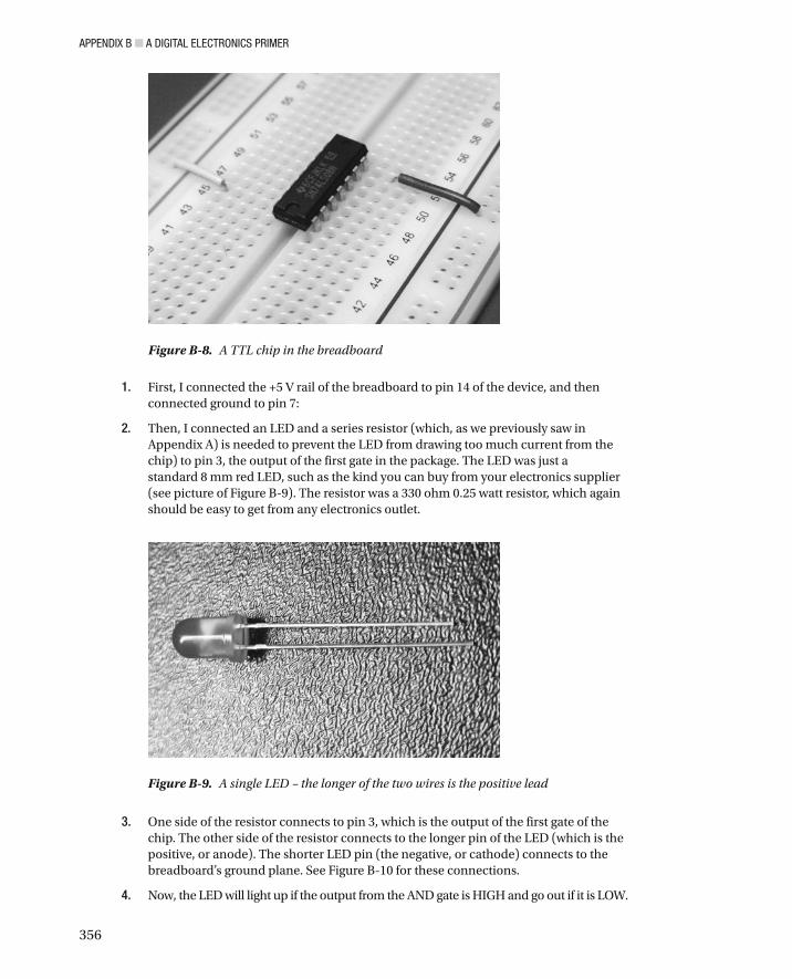
I built a very simple circuit using a 74LS08 on a breadboard (see Figure B-8 ) using the following steps:
Figure B-7 . Pinout for a 74LS08 Quad AND gate chip
1Be aware that the 74LS08 (in common with most other chips) is also available in other packages too. However, hobbyists usually prefer to use DIP packaged devices because the far smaller surface mount (SMT) packages are normally too small for the hobbyist to use easily, being mainly intended for use in precision automated electronic manufacturing systems.
APPENDIX B ■ A DIGITAL ELECTRONICS PRIMER
356
1. First, I connected the +5 V rail of the breadboard to pin 14 of the device, and then connected ground to pin 7:
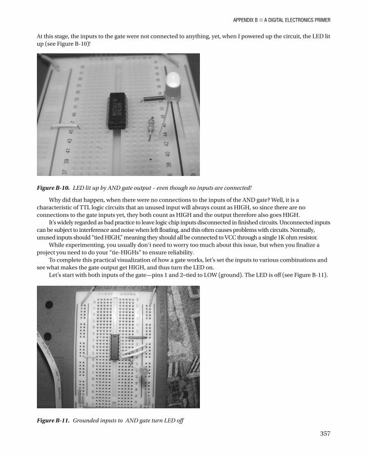
2. Then, I connected an LED and a series resistor (which, as we previously saw in Appendix A) is needed to prevent the LED from drawing too much current from the chip) to pin 3, the output of the first gate in the package. The LED was just a standard 8 mm red LED, such as the kind you can buy from your electronics supplier (see picture of Figure B-9 ). The resistor was a 330 ohm 0.25 watt resistor, which again should be easy to get from any electronics outlet.
3. One side of the resistor connects to pin 3, which is the output of the first gate of the chip. The other side of the resistor connects to the longer pin of the LED (which is the positive, or anode). The shorter LED pin (the negative, or cathode) connects to the breadboard’s ground plane. See Figure B-10 for these connections.
4. Now, the LED will light up if the output from the AND gate is HIGH and go out if it is LOW.
Figure B-8 . A TTL chip in the breadboard
Figure B-9 . A single LED – the longer of the two wires is the positive lead
APPENDIX B ■ A DIGITAL ELECTRONICS PRIMER
357
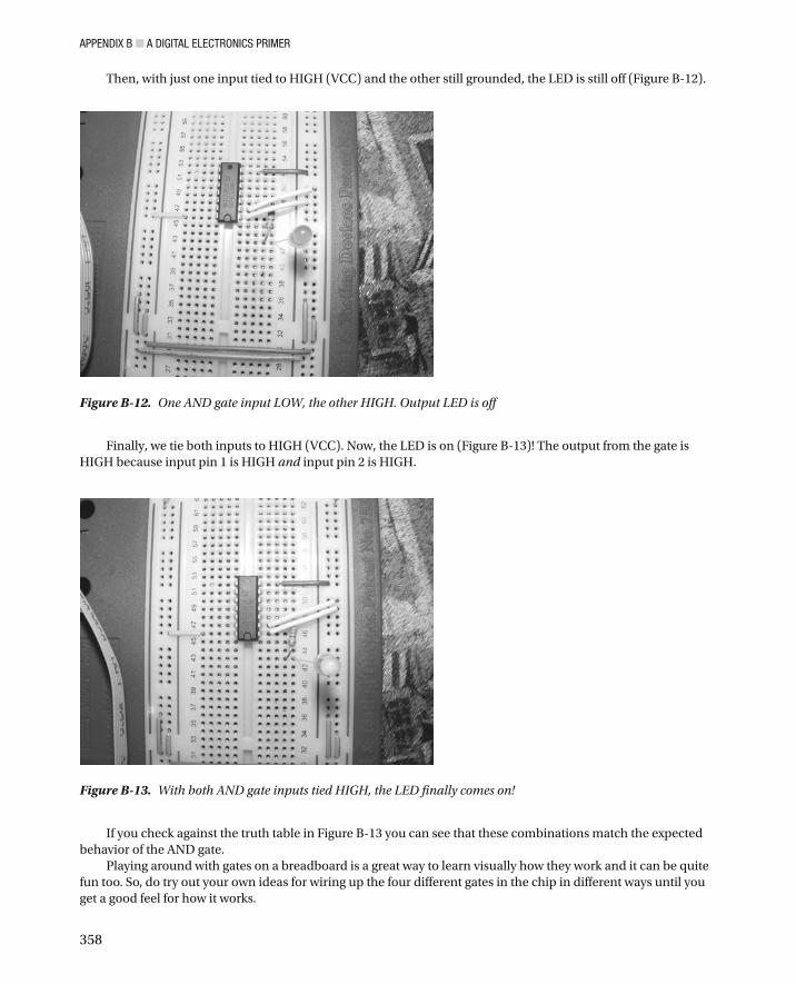
At this stage, the inputs to the gate were not connected to anything, yet, when I powered up the circuit, the LED lit up (see Figure B-10 )!
Figure B-10 . LED lit up by AND gate output – even though no inputs are connected!
Figure B-11 . Grounded inputs to AND gate turn LED off
Why did that happen, when there were no connections to the inputs of the AND gate? Well, it is a characteristic of TTL logic circuits that an unused input will always count as HIGH, so since there are no connections to the gate inputs yet, they both count as HIGH and the output therefore also goes HIGH.
It’s widely regarded as bad practice to leave logic chip inputs disconnected in finished circuits. Unconnected inputs can be subject to interference and noise when left floating, and this often causes problems with circuits. Normally, unused inputs should “tied HIGH ,” meaning they should all be connected to VCC through a single 1K ohm resistor.
While experimenting, you usually don’t need to worry too much about this issue, but when you finalize a project you need to do your “tie-HIGHs” to ensure reliability.
To complete this practical visualization of how a gate works, let’s set the inputs to various combinations and see what makes the gate output get HIGH, and thus turn the LED on.
Let’s start with both inputs of the gate—pins 1 and 2 — tied to LOW (ground). The LED is off (see Figure B-11).
APPENDIX B ■ A DIGITAL ELECTRONICS PRIMER
358
Then, with just one input tied to HIGH (VCC) and the other still grounded, the LED is still off (Figure B-12 ).
Finally, we tie both inputs to HIGH (VCC). Now, the LED is on (Figure B-13 )! The output from the gate is HIGH because input pin 1 is HIGH and input pin 2 is HIGH.
If you check against the truth table in Figure B-13 you can see that these combinations match the expected behavior of the AND gate.
Playing around with gates on a breadboard is a great way to learn visually how they work and it can be quite fun too. So, do try out your own ideas for wiring up the four different gates in the chip in different ways until you get a good feel for how it works.
Figure B-12 . One AND gate input LOW, the other HIGH. Output LED is off
Figure B-13 . With both AND gate inputs tied HIGH, the LED finally comes on!
359
APPENDIX C
Breadboards
There are lots of reasons to build electronic and computer circuits ; but only some of them involve building a circuit to keep forever. In many cases (such as building as a learning exercise, or just seeing if an idea works without any real application for it) you may just want to get it working and then tear it down and reuse the pieces for something new.
If you build your circuits by soldering all the components together, you expose the components concerned to quite a lot of heat and you will have to cut the component leads to size. Electronic components are not meant to stand up to repeated soldering; if you solder them more than a couple of times, it’s quite likely that they will be heat damaged and could stop working properly. The second problem with the soldering approach is that if (or more likely, when) you want to make even minor changes to the circuit you may find that it’s a difficult thing to do.
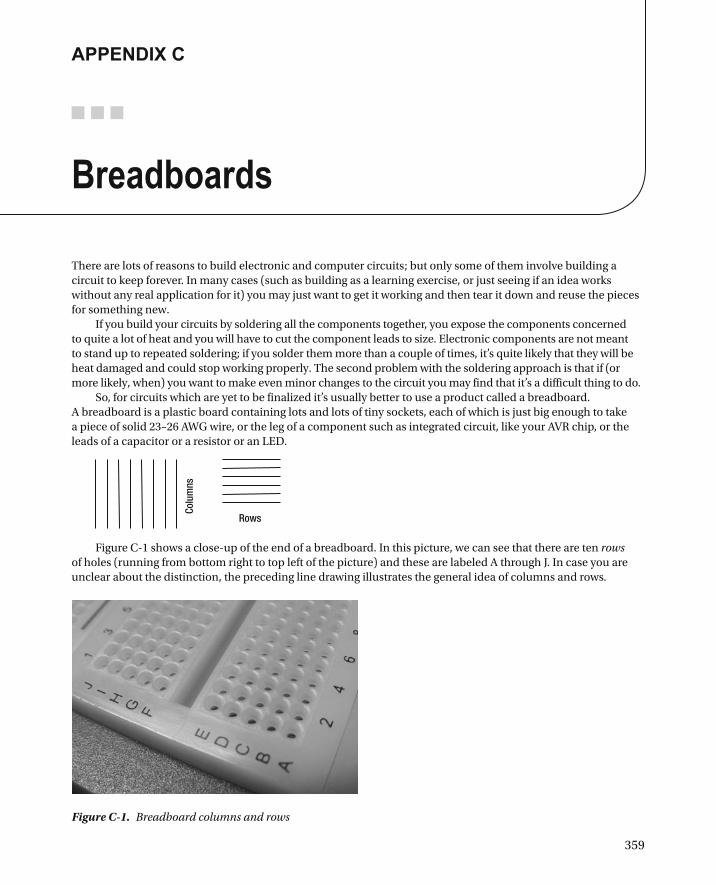
So, for circuits which are yet to be finalized it’s usually better to use a product called a breadboard . A breadboard is a plastic board containing lots and lots of tiny sockets, each of which is just big enough to take a piece of solid 23–26 AWG wire, or the leg of a component such as integrated circuit, like your AVR chip, or the leads of a capacitor or a resistor or an LED.
Colu
mns
Rows
Figure C-1 shows a close-up of the end of a breadboard. In this picture, we can see that there are ten rows of holes (running from bottom right to top left of the picture) and these are labeled A through J. In case you are unclear about the distinction, the preceding line drawing illustrates the general idea of columns and rows.
Figure C-1 . Breadboard columns and rows
APPENDIX C ■ BREADBOARDS
360
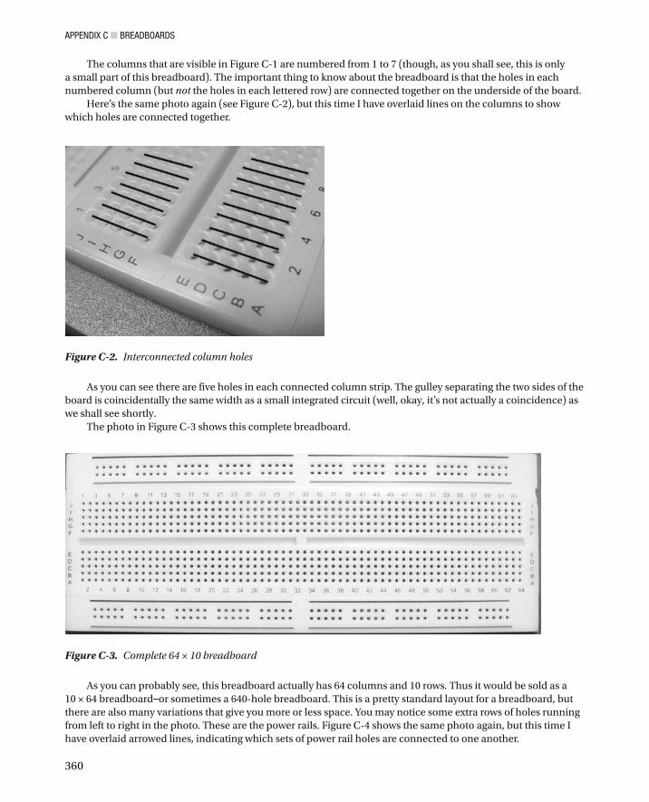
The columns that are visible in Figure C-1 are numbered from 1 to 7 (though, as you shall see, this is only a small part of this breadboard). The important thing to know about the breadboard is that the holes in each numbered column (but not the holes in each lettered row) are connected together on the underside of the board.
Here’s the same photo again (see Figure C-2 ), but this time I have overlaid lines on the columns to show which holes are connected together.
Figure C-2 . Interconnected column holes
As you can see there are five holes in each connected column strip. The gulley separating the two sides of the board is coincidentally the same width as a small integrated circuit (well, okay, it’s not actually a coincidence) as we shall see shortly.
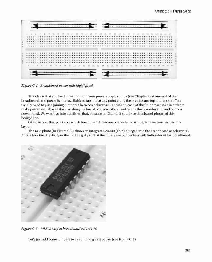
The photo in Figure C-3 shows this complete breadboard.
Figure C-3 . Complete 64 × 10 breadboard
As you can probably see, this breadboard actually has 64 columns and 10 rows. Thus it would be sold as a 10 × 64 breadboard — or sometimes a 640-hole breadboard. This is a pretty standard layout for a breadboard, but there are also many variations that give you more or less space. You may notice some extra rows of holes running from left to right in the photo. These are the power rails. Figure C-4 shows the same photo again, but this time I have overlaid arrowed lines, indicating which sets of power rail holes are connected to one another.
APPENDIX C ■ BREADBOARDS
361
Let’s just add some jumpers to this chip to give it power (see Figure C-6 ).
The idea is that you feed power on from your power supply source (see Chapter 2) at one end of the breadboard, and power is then available to tap into at any point along the breadboard top and bottom. You usually need to put a joining jumper in between columns 31 and 34 on each of the four power rails in order to make power available all the way along the board. You also often need to link the two sides (top and bottom power rails). We won’t go into details on that, because in Chapter 2 you’ll see details and photos of this being done.
Okay, so now that you know which breadboard holes are connected to which, let’s see how we use this layout.
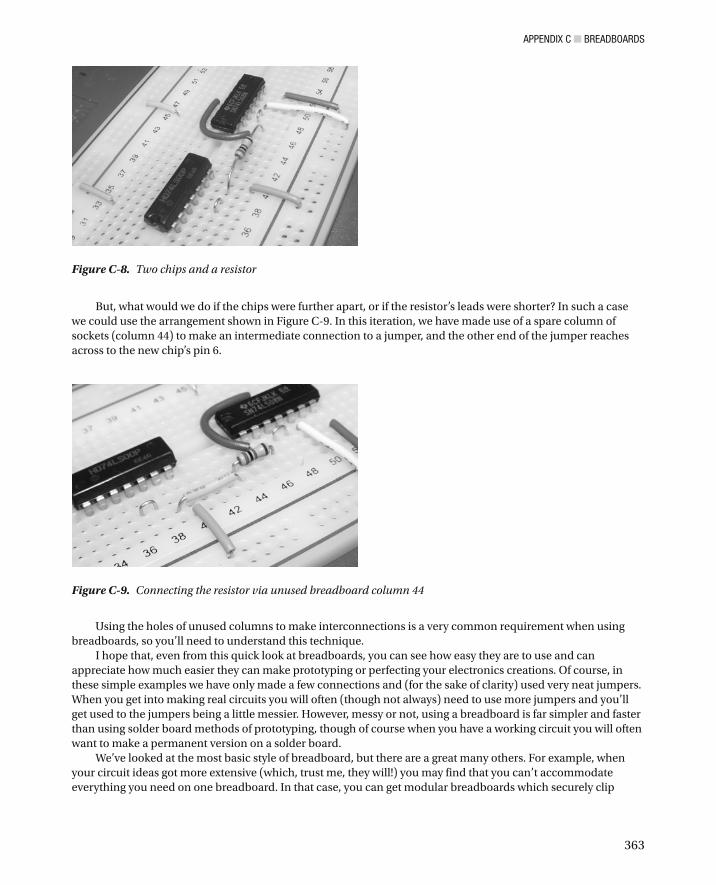
The next photo (in Figure C-5 ) shows an integrated circuit (chip) plugged into the breadboard at column 46. Notice how the chip bridges the middle gully so that the pins make connection with both sides of the breadboard.
Figure C-4 . Breadboard power rails highlighted
Figure C-5 . 74LS08 chip at breadboard column 46

APPENDIX C ■ BREADBOARDS
362
This chip needs a ground connection to pin 7 and a +5V connection to pin 14. If you’re unsure how the pins number, refer to Appendix B where I describe the pinout for this chip. As you can see in Figure C-6 , the chip is now connected (at top right) to the ground rail and at the top left to the +5 volts rail. This is done using some jumper wires. You can get jumper wire sets from your favorite electronics supplies outlet — Chapter 2 mentions some example products. You can also make your own jumpers if you want to; you should use 23AWG solid (not stranded) insulated wire.
Now, refer to the next photo in Figure C-7 . In this picture, we have the power jumpers installed, but you can also see that there are now some additional jumpers installed. A jumper has been used to link together two of the pins (pins 3 and 4) and another jumper is used to link together two pins, one on either side of the chip (pins 1 and 11, since you ask!) and yet another jumper ties pin 5 to the positive power rail (this is a tie-high, since we are permanently connecting the pin to a logic HIGH level).
Figure C-6 . Chip with power jumpers in place
Figure C-7 . Chip with power and signal jumpers installed
At this stage you don’t need to worry about what these pins do, or why they are being linked together: the only thing to you need to understand is how putting these jumper wires onto the breadboard makes connections between pins of the chip, and from the pins of the chip to the power rails.
Now, suppose we want to bring more components into the picture? Suppose we wanted to add another chip and connect a resistor between a pin on our existing chip and the new one: How would we do that? Figure C-8 shows one way to do it. The newly added chip has its power connections, as the first one did. It has a link jumper between its pin 4 and pin 5. The resistor (which luckily has quite long leads at each end) easily reaches from the original chip’s pin 2 to the new chip’s pin 6.
APPENDIX C ■ BREADBOARDS
363
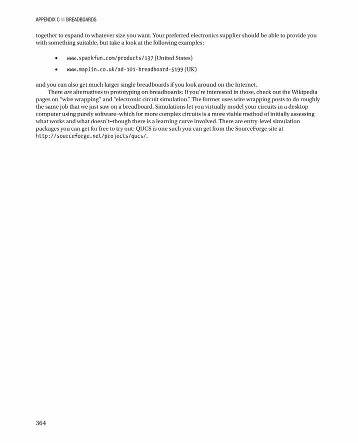
But, what would we do if the chips were further apart, or if the resistor’s leads were shorter? In such a case we could use the arrangement shown in Figure C-9 . In this iteration, we have made use of a spare column of sockets (column 44) to make an intermediate connection to a jumper, and the other end of the jumper reaches across to the new chip’s pin 6.
Figure C-8 . Two chips and a resistor
Figure C-9 . Connecting the resistor via unused breadboard column 44
Using the holes of unused columns to make interconnections is a very common requirement when using breadboards, so you’ll need to understand this technique.
I hope that, even from this quick look at breadboards, you can see how easy they are to use and can appreciate how much easier they can make prototyping or perfecting your electronics creations. Of course, in these simple examples we have only made a few connections and (for the sake of clarity) used very neat jumpers. When you get into making real circuits you will often (though not always) need to use more jumpers and you’ll get used to the jumpers being a little messier. However, messy or not, using a breadboard is far simpler and faster than using solder board methods of prototyping, though of course when you have a working circuit you will often want to make a permanent version on a solder board.
We’ve looked at the most basic style of breadboard, but there are a great many others. For example, when your circuit ideas got more extensive (which, trust me, they will!) you may find that you can’t accommodate everything you need on one breadboard. In that case, you can get modular breadboards which securely clip
APPENDIX C ■ BREADBOARDS
364
together to expand to whatever size you want. Your preferred electronics supplier should be able to provide you with something suitable, but take a look at the following examples:
• www.sparkfun.com/products/137 (United States)
• www.maplin.co.uk/ad-101-breadboard-5199 (UK)
and you can also get much larger single breadboards if you look around on the Internet. There are alternatives to prototyping on breadboards: If you’re interested in those, check out the Wikipedia
pages on “wire wrapping” and “electronic circuit simulation .” The former uses wire wrapping posts to do roughly the same job that we just saw on a breadboard. Simulations let you virtually model your circuits in a desktop computer using purely software — which for more complex circuits is a more viable method of initially assessing what works and what doesn’t — though there is a learning curve involved. There are entry-level simulation packages you can get for free to try out: QUCS is one such you can get from the SourceForge site at http://sourceforge.net/projects/qucs/ .
365
APPENDIX D
Serial Communications
This appendix provides an overview of the serial data transmission techniques you may need to understand when creating an in-depth design and implementing your AVR projects. This is by no means an exhaustive survey of the subject, which is huge, but it should give you the information that you need in understanding the serial data communication methods used in this book’s projects.
Data communication over long distances has always had to be a serial process, but at one time it looked like serial transmission would be consigned to history for very short distance transfer purposes. However, as machines got faster and faster and the amount of data to be moved around got ever bigger, some physical limits came into play which could not be overcome in any practical way, other than by reembracing (and to some extent, reinventing) serial data transfer. But, before we unpack those statements, let’s look at some basics.
Data Transfer Basics In this section we begin by reviewing the binary number system and the basics of how information is stored inside a computer. About now, the question may pop into your mind as to why it’s necessary to review all this material in a section that’s supposed to be about serial data transmission.
I believe that, as you can infer from the name, serial transmission involves taking bytes of data apart, serially sending them down some kind of communications medium, and then correctly putting them back together at the receiving end of the transaction. That being the case, knowing a little about bits and bytes is a great help in gaining a clear understanding of this subject and, of course, of digital electronics in general. Feel free to skip the next section if you’re already okay with binary, bytes, and bits.
Binary Me! It might come as a shock to realize that the number system you have spent your whole life (up to now) using is only one of many possible number systems! In our “real world” we use the “denary” number system . Like denary, binary is simply a system of counting.
Denary uses the symbols “0” to “9” (ten symbols, thus the name) to form representations of numbers. The position of each symbol in any given number indicates whether the symbol represents thousands, hundreds, tens, or units. For example, in denary, the sequence of symbols “900” means no units, no tens and nine hundreds. So, in denary, each column is worth ten times as much as the one to the right of it, and the rightmost column is worth exactly what it says (i.e., “008” represents eight).
Binary works in the same way, except that it only uses the symbols “1” and “0,” and each column represents a power of two. The rightmost column is worth one, and each successive column going left is worth two times as much. So, in a binary number, reading from right to left, columns are worth 1, 2, 4, 8, 16, 32, and so on, rather than a power of ten. So, for example, in binary — which, remember, only uses the symbols “0” and “1” — the symbol sequence “110” reading from right to left means no 1 s, one 2, and one 4 — the denary equivalent of which is six (2 + 4).
APPENDIX D ■ SERIAL COMMUNICATIONS
366
Digital electronic circuits were developed specifically to handle binary. In a digital circuit a signal is said to be in only one of the two following states:
One: (also called “logic HIGH,” or True). •
Zero: (also called “logic LOW,” or False). •
And in reality, these are the only signals that the digital circuits inside your digital devices really understand how to process and store: they appear to understand numbers and letters and colors and images and music and sound and video only because mountains of software (itself composed of binary codes) does endlessly clever interpretations of the binary data that the electronics are really dealing in. However, these digital circuits process binary data really, really fast!
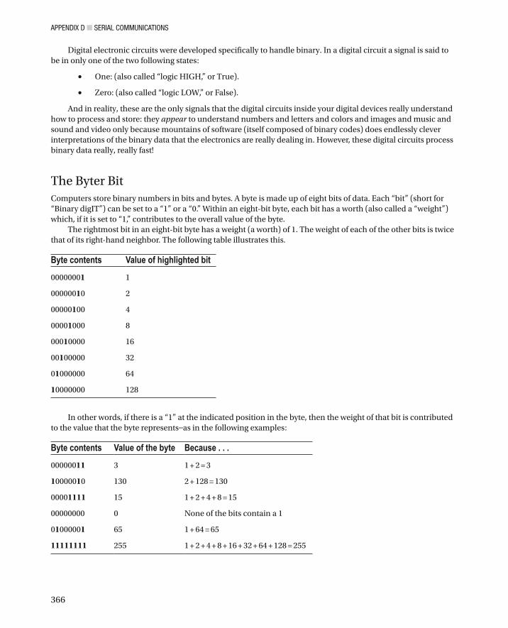
The Byter Bit Computers store binary numbers in bits and bytes. A byte is made up of eight bits of data. Each “bit” (short for “Binary digIT”) can be set to a “1” or a “0.” Within an eight-bit byte, each bit has a worth (also called a “weight”) which, if it is set to “1,” contributes to the overall value of the byte.
The rightmost bit in an eight-bit byte has a weight (a worth) of 1. The weight of each of the other bits is twice that of its right-hand neighbor. The following table illustrates this.
Byte contents Value of highlighted bit
0000000 1 1
000000 1 0 2
00000 1 00 4
0000 1 000 8
000 1 0000 16
00 1 00000 32
0 1 000000 64
1 0000000 128
In other words, if there is a “1” at the indicated position in the byte, then the weight of that bit is contributed to the value that the byte represents — as in the following examples:
Byte contents Value of the byte Because . . .
000000 11 3 1 + 2 = 3
1 00000 1 0 130 2 + 128 = 130
0000 1111 15 1 + 2 + 4 + 8 = 15
00000000 0 None of the bits contain a 1
0 1 00000 1 65 1 + 64 = 65
11111111 255 1 + 2 + 4 + 8 + 16 + 32 + 64 + 128 = 255
APPENDIX D ■ SERIAL COMMUNICATIONS
367
To be able to identify bits within a byte, the bits are given numbers, starting from the right, as in the following example which represents the value 64, because bit 6 is “set” but all the others are “clear”:
Binary Value 0 1 0 0 0 0 0 0
Bit Numbers
Bit
7
Bit
6
Bit
5
Bit
4
Bit
3
Bit
2
Bit
1
Bit
0
Because it has the lowest weight, the rightmost bit (bit 0) in the byte is referred to as the “least significant” bit, and the leftmost bit (bit 7) as the “most significant” bit.
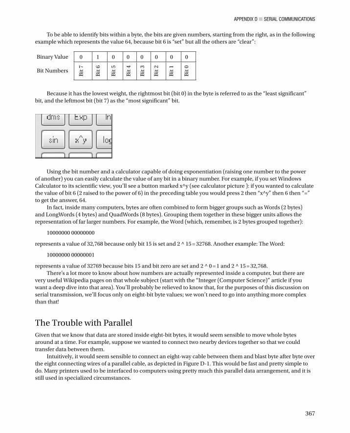
Using the bit number and a calculator capable of doing exponentiation (raising one number to the power of another) you can easily calculate the value of any bit in a binary number. For example, if you set Windows Calculator to its scientific view, you’ll see a button marked x^y (see calculator picture ): if you wanted to calculate the value of bit 6 (2 raised to the power of 6) in the preceding table you would press 2 then “x^y” then 6 then “=” to get the answer, 64.
In fact, inside many computers, bytes are often combined to form bigger groups such as Words (2 bytes) and LongWords (4 bytes) and QuadWords (8 bytes). Grouping them together in these bigger units allows the representation of far larger numbers. For example, the Word (which, remember, is 2 bytes grouped together):
10000000 00000000
represents a value of 32,768 because only bit 15 is set and 2 ^ 15 = 32768. Another example: The Word:
10000000 00000001
represents a value of 32769 because bits 15 and bit zero are set and 2 ^ 0 = 1 and 2 ^ 15 = 32,768. There’s a lot more to know about how numbers are actually represented inside a computer, but there are
very useful Wikipedia pages on that whole subject (start with the “Integer (Computer Science)” article if you want a deep dive into that area). You’ll probably be relieved to know that, for the purposes of this discussion on serial transmission, we’ll focus only on eight-bit byte values; we won’t need to go into anything more complex than that!
The Trouble with Parallel Given that we know that data are stored inside eight-bit bytes, it would seem sensible to move whole bytes around at a time. For example, suppose we wanted to connect two nearby devices together so that we could transfer data between them.
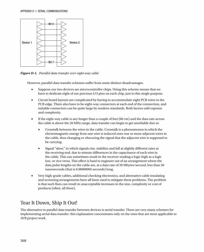
Intuitively, it would seem sensible to connect an eight-way cable between them and blast byte after byte over the eight connecting wires of a parallel cable, as depicted in Figure D-1 . This would be fast and pretty simple to do. Many printers used to be interfaced to computers using pretty much this parallel data arrangement, and it is still used in specialized circumstances.
APPENDIX D ■ SERIAL COMMUNICATIONS
368
However, parallel data transfer schemes suffer from some distinct disadvantages.
Suppose our two devices are microcontroller chips. Using this scheme means that we • have to dedicate eight of our precious I/O pins on each chip, just to this single purpose.
Circuit board layouts are complicated by having to accommodate eight PCB wires to the • PCB edge. There also have to be eight-way connectors at each end of the connection, and suitable connectors can be quite large by modern standards. Both factors add expense and complexity.
If the eight-way cable is any longer than a couple of feet (60 cm) and the data rate across • the cable is above the 20 MHz range, data transfer can begin to get unreliable due to:
Crosstalk between the wires in the cable. Crosstalk is a phenomenon in which the • electromagnetic energy from one wire is induced onto one or more adjacent wires in the cable, thus changing or obscuring the signal that the adjacent wire is supposed to be carrying.
Signal “skew,” in which signals rise, stabilize and fall at slightly different rates at • the receiving end, due to minute differences in the capacitance of each wire in the cable. This can sometimes result in the receiver reading a logic high as a logic low, or vice versa. This effect is hard to engineer out of an arrangement where the data pulse lengths on the cable are, at a data rate of 20 Mbytes/second, less than 50 nanoseconds (that is 0.00000005 seconds) long.
Very high-grade cables, additional checking electronics, and alternative cable insulating • and screening arrangements have all been used to mitigate these problems. The problem is that such fixes can result in unacceptable increases in the size, complexity or cost of products (often, all three).
Tear It Down, Ship It Out! The alternative to parallel data transfer between devices is serial transfer. There are very many schemes for implementing serial data transfer: this explanation concentrates only on the ones that are most applicable to AVR project work.
Device 2Device 1
Bit 0
Bit 7
Figure D-1 . Parallel data transfer over eight-way cable
APPENDIX D ■ SERIAL COMMUNICATIONS
369
The first method is asynchronous serial transfer . In this method, there is only one wire required to send data because, to send one byte of data, the sender places each bit of the byte on the wire, in a prearranged order, for a predetermined amount of time after transmission begins. The most commonly known asynchronous serial device is the serial port on your desktop machine (if it has one; they are becoming rare now), but most AVR microcontroller chips have a serial port, and some have more than one (or can be configured to provide more than one).
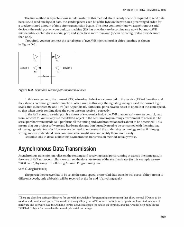
If required, you can connect the serial ports of two AVR microcontroller chips together, as shown in Figure D-2 .
Device 2Device 1
Tx
Rx
Rx
Tx
Ground
Figure D-2 . Send and receive paths between devices
In this arrangement, the transmit (TX) wire of each device is connected to the receive (RX) of the other and they share a common ground connection. When used in this way, the signaling voltages used are normal logic levels , that is, between 0V and +5V (see Appendix B). Both serial ports have to be set to operate at the same speed, so that when one is sending data, the other one can receive it correctly.
In the AVR context, a serial port is a chunk of electronics inside the AVR that our software can control, read from, or write to. We usually use the SERIAL object in the Arduino Programming environment to access it. The serial port hardware inside AVR performs all the timing and synchronization tasks about to be described. 1 This means that our project software and hardware designs don’t usually need to be concerned with the minutiae of managing serial transfer. However, we do need to understand the underlying technology so that if things go wrong, we can understand error conditions that might arise and rectify them more easily.
Let’s now look in detail at how this asynchronous transmission method actually works.
Asynchronous Data Transmission Asynchronous transmission relies on the sending and receiving serial ports running at exactly the same rate. In the case of AVR microcontrollers, we can set the data rate to one of the standard rates (in this example we use “9600 baud”) by using the following Arduino Programming line :
Serial.Begin(9600);
The port at the receiver has to be set to the same speed, or no valid data transfer will occur; if they are set to different speeds, only gibberish will be received at the far end (if anything at all).
1There are also free software libraries for use with the Arduino Programming environment that allow normal I/O pins to be used as additional serial ports. This would in theory allow your AVR to have multiple serial ports implemented in a mix of hardware and software. See the Arduino library downloads page for details on libraries, and the Arduino help page on the “SERIAL” object for more details on multiple serial port usage.
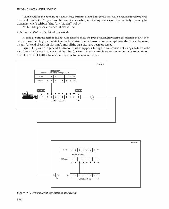
APPENDIX D ■ SERIAL COMMUNICATIONS
370
What exactly is the baud rate? It defines the number of bits per second that will be sent and received over the serial connection. To put it another way, it allows the participating devices to know precisely how long the transmission of each bit of data (the “bit-slot”) will be.
At 9600 bits per second, each bit-slot will be:
1 Second ÷ 9600 = 104.16 microseconds
As long as both the sender and receiver devices know the precise moment when transmission begins, they can both use their highly accurate internal timers to advance transmission or reception of the data at the same instant (the end of each bit-slot time), until all the data bits have been processed.
Figure D-3 provides a general illustration of what happens during the transmission of a single byte from the TX of one AVR (device 1) to the RX of the other (device 2). In this example we will be sending a byte containing the value 70 (0100 0110 in binary) between the two microcontrollers.
Device 2
Device 1
Tx
Rx
7 6 5 4 3 2 1 0
0 1 0 0 0 1 1 0
Bit Num
Bit Values
BYTE TO BE SENT: CONTAINS BINARY VERSION OF 70 (64 + 4 + 2)
0 1 0 0 0 1 1 01 01
Stop Bits Start Bit
Shift Direction:
7 6 5 4 3 2 1 0
- - - - - - - -
Bit Num
Bit Values
Receiver Byte Buffer
- - - - - - - -
Shift Direction:
Figure D-3 . Asynch serial transmission illustration
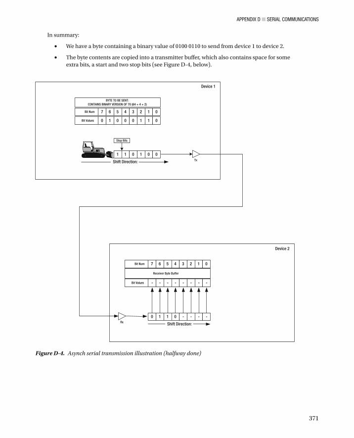
APPENDIX D ■ SERIAL COMMUNICATIONS
371
In summary:
We have a byte containing a binary value of 0100 0110 to send from device 1 to device 2. •
The byte contents are copied into a transmitter buffer, which also contains space for some • extra bits, a start and two stop bits (see Figure D-4 , below).
Device 2
Device 1
Tx
Rx
7 6 5 4 3 2 1 0
0 1 0 0 0 1 1 0
Bit Num
Bit Values
BYTE TO BE SENT: CONTAINS BINARY VERSION OF 70 (64 + 4 + 2)
1 1 0 1 0 0
Stop Bits
Shift Direction:
7 6 5 4 3 2 1 0
- - - - - - - -
Bit Num
Bit Values
Receiver Byte Buffer
0 1 1 0 - - - -
Shift Direction:
Figure D-4 . Asynch serial transmission illustration (halfway done)
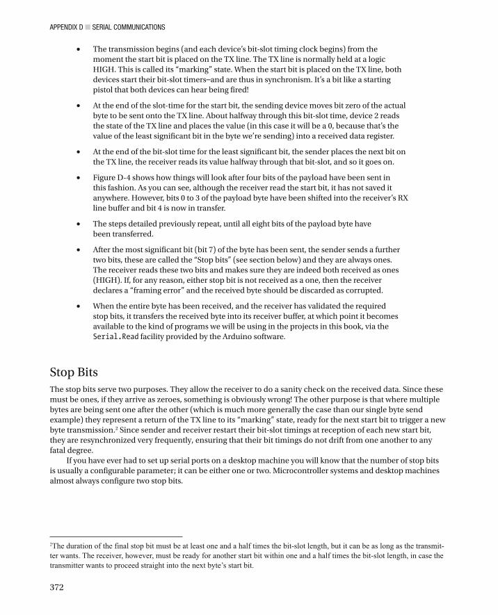
APPENDIX D ■ SERIAL COMMUNICATIONS
372
The transmission begins (and each device’s bit-slot timing clock begins) from the • moment the start bit is placed on the TX line. The TX line is normally held at a logic HIGH. This is called its “marking” state. When the start bit is placed on the TX line, both devices start their bit-slot timers — and are thus in synchronism. It’s a bit like a starting pistol that both devices can hear being fired!
At the end of the slot-time for the start bit, the sending device moves bit zero of the actual • byte to be sent onto the TX line. About halfway through this bit-slot time, device 2 reads the state of the TX line and places the value (in this case it will be a 0, because that’s the value of the least significant bit in the byte we’re sending) into a received data register.
At the end of the bit-slot time for the least significant bit, the sender places the next bit on • the TX line, the receiver reads its value halfway through that bit-slot, and so it goes on.
Figure D-4 shows how things will look after four bits of the payload have been sent in • this fashion. As you can see, although the receiver read the start bit, it has not saved it anywhere. However, bits 0 to 3 of the payload byte have been shifted into the receiver’s RX line buffer and bit 4 is now in transfer.
The steps detailed previously repeat, until all eight bits of the payload byte have • been transferred.
After the most significant bit (bit 7) of the byte has been sent, the sender sends a further • two bits, these are called the “Stop bits” (see section below) and they are always ones. The receiver reads these two bits and makes sure they are indeed both received as ones (HIGH). If, for any reason, either stop bit is not received as a one, then the receiver declares a “framing error” and the received byte should be discarded as corrupted.
When the entire byte has been received, and the receiver has validated the required • stop bits, it transfers the received byte into its receiver buffer, at which point it becomes available to the kind of programs we will be using in the projects in this book, via the Serial.Read facility provided by the Arduino software.
Stop Bits The stop bits serve two purposes. They allow the receiver to do a sanity check on the received data. Since these must be ones, if they arrive as zeroes, something is obviously wrong! The other purpose is that where multiple bytes are being sent one after the other (which is much more generally the case than our single byte send example) they represent a return of the TX line to its “marking” state, ready for the next start bit to trigger a new byte transmission. 2 Since sender and receiver restart their bit-slot timings at reception of each new start bit, they are resynchronized very frequently, ensuring that their bit timings do not drift from one another to any fatal degree.
If you have ever had to set up serial ports on a desktop machine you will know that the number of stop bits is usually a configurable parameter; it can be either one or two. Microcontroller systems and desktop machines almost always configure two stop bits.
2The duration of the final stop bit must be at least one and a half times the bit-slot length, but it can be as long as the transmit-ter wants. The receiver, however, must be ready for another start bit within one and a half times the bit-slot length, in case the transmitter wants to proceed straight into the next byte’s start bit.
APPENDIX D ■ SERIAL COMMUNICATIONS
373
Word Length In our example, we showed the transfer of an eight-bit byte. It is possible to configure serial channels to transfer only seven-bit values. This is still useful if all you want to do is send or receive the letters and characters in American Standard Code for Information Interchange (ASCII ), which is a seven-bit character set (just put “ASCII” into a search engine to see a list of character codes it supports).
Parity Checking and Error Detection When only seven-bit values are being sent over a serial link, the eighth bit can be used for an additional error checking mechanism called parity checking. Parity checking comes in two flavors: even and odd parity. For even parity, the parity bit is set to a 1 if the number of 1 s in the transmitted byte (which does not include the parity bit) is odd. This is called even parity because if there are an odd number of bits set to 1 in the data byte, the parity bit being set brings the tally of 1 s to an even number.
If you use odd parity, the opposite happens. The parity bit is set only if there is an even number of 1 s in the sent byte — and, of course, setting the parity bit to a 1 makes the total number of 1 s odd. The idea is that if any one of the bits arrives at the receiver in error, the parity bit setting is unlikely to match the parity flag value and the receiver can know that the received data is likely to be wrong.
Parity checking is only a very basic method of error checking; it only takes the inversion of any two bits in the sent byte to make everything seem okay at the receiving end. Furthermore, by using the eighth bit of the byte for a parity flag, you lose one-eighth of the potential throughput of your serial channel.
In MCU-land, seven-bit usage of serial ports is almost unheard of because we need our serial channels to transfer full eight-bit bytes, so we set our serial channels to eight bits, with no parity. Error checking, if it’s done at all, is usually done at a higher level, using checksums within packets of data. See Chapter 6 for more details in these general areas.
Protocol Overhead It’s worth noting that — in our example — we transferred 8 bits of actual payload data, but with the start bit and the two stop bits, what actually went over the wire was 11 bits. The collective name for the necessary extra bits is protocol overhead.
In the case where we are sending one start bit, 8 data bits, and two stop bits, the protocol overhead is 3 bits out of every 11 — or about 27 %. This means that at a baud rate of 9600 you cannot, in fact, send 9600 bits of actual per second. 3 If you need to use a serial port for transferring significant amounts of data, it’s worth remembering to factor in the protocol overhead to any throughput predictions or assumptions you may make — or else you may end up scratching your head about the perceived under-performance of your serial link!
Important Note ■ Don’t ever connect your AVR chip’s serial port pins directly to your desktop computer’s serial port. You will very likely fry your AVR chip and it’s likely that you will damage your desktop machine.
Okay, So Tell Me About RS-232 and RS-485 The serial ports we have looked at, so far, have been dealing only in the voltage levels that logic chips such as AVRs use. In such circuits a HIGH (or a “1”) is represented by about +5V, and a LOW by anything under
3Due to various factors, such as interrupt latency, buffering delays, and many other issues, it’s never possible to attain the full data transfer rate that the baud rate might seem to indicate. I always derate by at least 40% to be realistic. That is, at 9600 I would expect a microcontroller serial port carrying out continuous activity to shift, perhaps, 5KB/second.
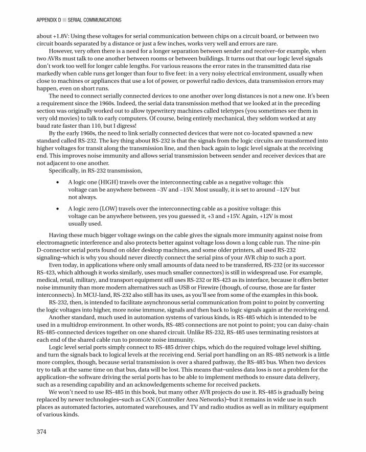
APPENDIX D ■ SERIAL COMMUNICATIONS
374
about +1.8V: Using these voltages for serial communication between chips on a circuit board, or between two circuit boards separated by a distance or just a few inches, works very well and errors are rare.
However, very often there is a need for a longer separation between sender and receiver — for example, when two AVRs must talk to one another between rooms or between buildings. It turns out that our logic level signals don’t work too well for longer cable lengths. For various reasons the error rates in the transmitted data rise markedly when cable runs get longer than four to five feet: in a very noisy electrical environment, usually when close to machines or appliances that use a lot of power, or powerful radio devices, data transmission errors may happen, even on short runs.
The need to connect serially connected devices to one another over long distances is not a new one. It’s been a requirement since the 1960s. Indeed, the serial data transmission method that we looked at in the preceding section was originally worked out to allow typewritery machines called teletypes (you sometimes see them in very old movies) to talk to early computers. Of course, being entirely mechanical, they seldom worked at any baud rate faster than 110, but I digress!
By the early 1960s, the need to link serially connected devices that were not co-located spawned a new standard called RS-232. The key thing about RS-232 is that the signals from the logic circuits are transformed into higher voltages for transit along the transmission line, and then back again to logic level signals at the receiving end. This improves noise immunity and allows serial transmission between sender and receiver devices that are not adjacent to one another.
Specifically, in RS-232 transmission,
A logic one (HIGH) travels over the interconnecting cable as a negative voltage: this • voltage can be anywhere between −3V and −15V. Most usually, it is set to around −12V but not always.
A logic zero (LOW) travels over the interconnecting cable as a positive voltage: this • voltage can be anywhere between, yes you guessed it, +3 and +15V. Again, +12V is most usually used.
Having these much bigger voltage swings on the cable gives the signals more immunity against noise from electromagnetic interference and also protects better against voltage loss down a long cable run. The nine-pin D-connector serial ports found on older desktop machines, and some older printers, all used RS-232 signaling — which is why you should never directly connect the serial pins of your AVR chip to such a port.
Even today, in applications where only small amounts of data need to be transferred, RS-232 (or its successor RS-423, which although it works similarly, uses much smaller connectors) is still in widespread use. For example, medical, retail, military, and transport equipment still uses RS-232 or RS-423 as its interface, because it offers better noise immunity than more modern alternatives such as USB or Firewire (though, of course, those are far faster interconnects). In MCU-land, RS-232 also still has its uses, as you’ll see from some of the examples in this book.
RS-232, then, is intended to facilitate asynchronous serial communication from point to point by converting the logic voltages into higher, more noise immune, signals and then back to logic signals again at the receiving end.
Another standard, much used in automation systems of various kinds, is RS-485 which is intended to be used in a multidrop environment. In other words, RS-485 connections are not point to point; you can daisy-chain RS-485-connected devices together on one shared circuit. Unlike RS-232, RS-485 uses terminating resistors at each end of the shared cable run to promote noise immunity.
Logic level serial ports simply connect to RS-485 driver chips, which do the required voltage level shifting, and turn the signals back to logical levels at the receiving end. Serial port handling on an RS-485 network is a little more complex, though, because serial transmission is over a shared pathway, the RS-485 bus. When two devices try to talk at the same time on that bus, data will be lost. This means that — unless data loss is not a problem for the application — the software driving the serial ports has to be able to implement methods to ensure data delivery, such as a resending capability and an acknowledgements scheme for received packets.
We won’t need to use RS-485 in this book, but many other AVR projects do use it. RS-485 is gradually being replaced by newer technologies — such as CAN (Controller Area Networks) — but it remains in wide use in such places as automated factories, automated warehouses, and TV and radio studios as well as in military equipment of various kinds.

APPENDIX D ■ SERIAL COMMUNICATIONS
375
Are There Other Types of Serial Data Interface ? There are many other serial data interconnects and interfaces. USB, for example, carries serial data (though it uses a different protocol from the one we examined earlier), as does Firewire. Then there’s SATA . . .
If you look inside a computer made before about 2002, you will find that the hard drives and optical drives are connected to the motherboard via flat, wide, ribbon cables. These will be ATA (which stands for AT Attachment), though it’s now often called PATA — for Parallel ATA) cables. ATA used a 16-bit parallel data transfer method, similar to the one we discussed previously in this appendix, with all the attendant problems that brings.
When it became apparent that the storage devices in commodity IT kit needed faster interconnects, it proved problematic to make faster versions of ATA at a price point that the industry and consumers were willing to bear; enter SATA.
SATA (Serial ATA) is based on ATA, but uses serial data transmission to move data between storage devices (mainly hard drives, but also DVD-ROMS or Blu-Ray drives) and computer motherboards. SATA is intended only for short-haul serial connections: it imposes a one meter (39 inches) maximum cable length.
Although SATA is a serial interface standard, it operates completely differently to the serial interfaces we looked at previously. Being primarily intended as a storage interconnect, SATA is a lot faster too. As of this writing there have been three SATA standards, SATA 1.0 through SATA 3.0. These are all backward compatible and all use the same physical connectors: in other words, a SATA 3.0 port will still recognize and connect to a SATA 1.0 hard drive.
These three levels of SATA connections offer raw data transfer rates as follows (notice these are Bytes, not Bits, per second, multiply by ten to see the bit rates):
SATA 1.0: 150MB per second. •
SATA 2.0: 300MB per second. •
SATA 3.0: 600MB per second. •
As with all raw transfer rates, these are absolute maximum figures that can never be truly attained in a real system. However, SATA is far faster than the older IDE, ATA, and PATA standards that it replaced because it overcame the problems of parallel data interfaces by reinventing serial data transmission for the modern era.
SATA, USB, and Firewire together rescued the idea of serial data transfer, a technique which, at one point, seemed to have had its day. Sadly, since we do not use spinning storage devices in this book, we do not use SATA for any of the projects.

377
� A ADD command , 239 addToDictionary() function , 243 American Standard Code for Information Interchange
(ASCII) , 12 Application layer , 168 Arduino and AVR
Arduino IDE , 56 AVRDude , 57 ( see also AVRDude) avr-gcc compiler , 57 C compilers , 56 555 chip , 51–52 chip facts , 60–61 confi guration fi les
Arduino Duemilanove , 58 avrisp2 , 59 boards.txt , 57, 59 clock speed , 59 communications and command
protocol , 58 core software , 59 delay function , 59 f_cpu specifi cation , 59 memory size , 59 Pololu AVRISP programmer , 59 program code memory , 58 programmers.txt , 59 Shiney McFloopy board , 59 upload speed , 14
core computing function , 49 debugging , 79, 82 delay() function , 81 dual LED fl asher circuit , 52 errors , 56 external crystal , 61–62 fuses , 58
ATmega328 , 62 AVRDude program , 62 extended , 65–66
FLB , 63–64 hFuse , 64–65
hex fi le , 56 ID problem , 76–77 infrastructure software , 56 loop() function , 81 MCU , 49, 55 minimal LED fl asher circuit, AVR , 50 packaged system , 49 pin name translations
Analog Reference input , 79 Arduino port connector , 77, 78 ATmega328 , 78 crystal pins , 79 digital I/O lines , 79 PWM pins , 79 Serial.Begin() function , 79 supply voltage , 79
program execution , 81 programmer , 57 push-pull version , 53 quadruple LED fl asher circuit , 53–55 serial connection scheme , 80 Serial_Example_01 program , 81 Serial.println() , 81 Serial.print() statements , 79, 80 setup() function , 81 SoftwareSerial Library , 82 terminal emulators , 82–83 theCounter , 80, 81 TTL level serial channel , 79, 81
Arduino code , 224 Arduino pins , 251 ASCII code , 241 Asynchronous data transmission
Arduino Programming line , 369 asynchronous serial transfer , 369 asynch serial transmission , 370–372 parity checking and error detection , 373 protocol overhead , 373
Index

■ INDEX
378
sender and receiver devices , 370 stop bits , 372 word length , 373
Asynchronous serial transfer , 369 ATmega328 , 219, 251 ATMEGA328 AVR , 61 ATTINY13 device , 50 AVRDude
AVRProg , 66 confi guration fi le
ATmega328pu , 76–77 avrdude.conf , 69 avrdudeRC fi le , 71 double-checking , 71 editing , 69 $HOMEPATH , 71 lower-power consumption version , 69, 70 modifi cations , 71 multiple instances , 71 save as plain text fi le , 69 signature , 71
examples ATmega328p port , 72 clock speed , 73 /dev/ttyACM0 port , 72 EEPROM memory , 74–75 fuse calculator , 72 program memory , 73
external crystal clock , 75–76 Linux system , 67 Mac OS X , 66 name , 67 part number code , 68 serial port , 67 Terminal Mode , 67 time-out error , 69 Windows system , 66 WordDune , 237
AVRISP programmer , 67 AVR microcontroller
CISC , 8 desktop computer , 5, 7 KISS principle , 8 R2000 , 9 RISC , 9 serial ports connection , 369 timeline , 4–5 value of , 5 wraps off , 10
AVR test bed Arduino software
installation kit , 15 selection , 39–42 suite , 13
Atmel’s AVRStudio software , 39–42
basic test bed , 15 conventional serial port , 13 desktop computer , 14–15 ISP ( see In-system programming) piece parts , 16
ATmega328 , 23–24 breadboard , 19 bridging and linking, power supply rails , 23 device , 21 fuse holders , 20 lab-grade power supply , 19 power supply leads , 21–22 PSU attach points , 22 repurposed 5 volt supply , 20–21 wall-wart AC to DC power , 20
Pololu programmer , 30 power supply , 13 programming adaptor
header pins addition , 35 pin position , 36–38 unstriped jumper wires , 38 +5V connection , 39
prototyping breadboard , 13 semipermanent , 13 software–installation , 39 system-testing development , 13 testing
Arduino interface , 43 Arduino software , 42 breadboard power bus , 44 check power connections , 45 code upload , 45 double-check , 45 power off , 44 power on , 44 TTL level serial port , 45–46
Tmega328 , 15 Toolkit
bits box , 17 component grab bags , 18 DVM , 17 helping hands , 18 logic probe , 18 mini HSS drill sets , 17 needle-nosed , 16 retractable blade , 17 small screwdriver , 17 soldering iron, interchangeable tip , 16 wire cutters , 17
awaitKeypress() function , 247
� B BasicDoorbells object , 187 Breadboards
23AWG solid , 362
Asynchronous data transmission (cont.)

■ INDEX
379
build electronic and computer circuits , 359 chip with power and signal jumpers , 361–362 columns and rows , 359, 360 complete 64 × 10 breadboards , 360 defi nition , 359 electronic circuit simulation , 364 electronics supplier , 364 interconnected column holes , 360 74LS08 chip , 361 power rails highlighted , 360–361 power supply source , 361 prototyping , 364 resistor connection via unused
column 44 , 369 solder board methods , 363 soldering approach , 359 two chips and resistor , 363 wire wrapping , 364
� C Capacitors
capacitance measurement , 337–338 dielectric , 336 overstressed , 340 “power on reset,” 339 RC network , 338–339 shapes and sizes
axial polarized , 341 ceramic disc , 343 common capacitor types , 340–341 electrolytic capacitors , 340 nonpolarized , 342 radial, polarized capacitor , 342 tolerance codes , 343
smoothing capacitor , 337 static electricity , 336
CatBuilder , 240, 241 ChangeLoopDelay() , 227 Checksums
calculator , 170 defi nition , 169 failure , 170 packet , 170 simple , 169
chooseRandomWordIndexIndex() function , 246 Color and light sensors , 165 Crazy Beams
assembly laser modules on servo motors , 218 overall view , 219, 220 servo motor reset program , 217–218 vertical motor to horizontal assembly
linkage , 219 electronics
AVR pins , 222
circuit diagram , 221 motor and laser wiring , 223 power arrangement , 222
horizontal motors frame , 215–216 laser source , 214 project description , 213–214 software
code walk , 224–227 values and constants , 223–224 version 214 , 223
vertical motor frame , 216–217 CurrentAngle , 224
� D DB9 connector , 173 DELETE command , 239 DEPROM command , 239 Device-to-device communication , 168 DICTIONARY command , 239 Digital electronics
binary data , 347 circuit inputs and outputs , 347 denary system , 348 digital circuits , 347 gates ( see Gates) HIGHs/LOWs levels , 347 hybrid circuits , 348
Digital voltmeter (DVM) , 17 doBeep() function , 257 doDeleteWord() function , 246 doInputBuff erParser() function ,
244, 257 doLevelEnd() function , 246 doLevelIntroducer() function , 246 DoorbellEntryPhone object , 185 Doorbells object , 185 doPowerDownSound() function , 258 doPowerUpSound() function , 258 doSerialInput() function , 247, 258 doSplashScreen() function , 242, 247 Duck shooter game
bar graph LED , 284 circuit diagram , 278–280 ISP plug , 282 protoboards , 280 rules , 277 serial port add-on wire socket , 282 software , 285–287 solder boards , 280 soldering tips , 283–284 tripad board , 280
ISP plug , 282 size , 281 topside , 282 underside , 283

■ INDEX
380
dumpDictToSerialChannel() function , 243 dumpEEPROMToSerialChannel() function , 243
� E EEPROM memory , 73–75, 187, 237 Eight-pin DIP device , 50 Embedded intelligence. See Intelligent devices EndAngle , 224 Engine control unit (ECU) , 155 ExitPaperworkPackage contents , 181
� F fi llScreenWithRandomCharacters() function , 247 fi ndNumberInWordArray() function , 246 format_EEPROM() function , 243 Fuse low byte (FLB) , 63–64
� G Gates
breadboard 74LS08 , 355 TTL chip , 356
decision-making power , 350 defi nition , 349 AND gate
characteristic , 349 digital music stream , 349 LED off , 357–358 LED on , 358 light detector , 349 output , 357 person detector , 349 property , 350 truth table , 351
integrated circuits , 355 LED , 356 74LS08 Quad AND gate chip , 355 NAND gate , 350, 351 NOR gate , 350, 352 OR gate , 350, 351 specifi cations , 353–354 tied HIGH , 357 XOR gate , 350, 352
Gem Light Arduino pin 4 , 107 Arduino sketch , 104–106 Assembling , 102, 103 black electrical tape masking tape , 101 cardboard tube center , 101 circuit diagram , 106 features , 107 header pins , 107
heat-resistant food wrap fi lm , 101 holder , 102, 108 LED/motor assembly , 104 nuts and bolt sets , 101 powerful LED light , 101 servo motor , 101 stick wood , 101 strain relief tie-on , 103 support cradle , 104 Swarovski crystals , 101
getDictWord() function , 244 Globally Unique IDs (GUID) , 185
� H HELP command , 239 High fuse byte , 64–65 HomeHelp protocol
door sensor circuit diagram , 319–320 receiver software , 321 sender software , 321 summary , 322
functions , 315 low-cost Smart Home wireless node ,
317–319 packet layout , 316–317 socket cracking , 307–308
Home lighting controlled and varied lighting , 249 LED worklight , 250 Mark II electronics
Arduino installation , 271 circuit diagram , 271, 272 dual TLC5940 basic circuit , 274, 275 fuse byte value , 274 M5450 chip , 270 resistor value , 273 softPWM library , 269 system clock , 273 TLC5940 chip , 270, 271
passageway light ( see Passageway light) people sensors , 249
HorizontalMotorRandom() , 226 HRFormsCreator object , 181 HundredthSec() function , 257
� I, J initiatePaymentToEmployee method , 181 In-system programming (ISP) , 15
adaptor and pin headers , 34–35 Arduino boards , 25 Atmel programmer , 26 AVRISP MKII programmer , 25

■ INDEX
381
AVR microcontrollers , 25 box
external measurements , 28 Hammond 1593JTBU , 28 mini-USB plug , 30 plastic project box , 28 Polulu programmer , 29 ribbon cable cutout , 31 screw terminal , 32
parallel programming , 24 Pololu programmer , 26–28 signals , 24 upload software , 24
Intelligent devices adaptive behavior , 157–158 advantages , 164 alarm clock , 167 communications channel types
application layer , 168 message packetization , 168 network layer , 168 OSI model , 169 physical layer , 168 sequence , 169 transport layer , 168
communications protocol , 167 digital scale , 155 disadvantages , 164 ECU , 155 effi ciency , 158 electronic scale , 155 error checking
ATmega168 , 171 ATmega328 AVR microcontroller , 171 checksums ( see Checksums) error consequence , 171 networking protocols , 169 ready-made communications libraries , 171
Greener products , 164 increased functionality , 156–157 interdevice communications , 167 microcontroller KISS communications
AVR programmer , 171–172 direct logic level intelligent devices , 174 libraries , 171 RS-232 connection , 171–173 time-getter protocol ( see Time-getter
protocol) mother ship support , 164 outside light
controller enhancements , 163 with intelligent controller , 162–163 without intelligence , 159–161
problem management , 159 strain gauge , 156
� K Keep It Simple Stupid (KISS) principle , 8–9
� L LasersOff () , 226 LasersOn() , 226 LED. See Light-emitting diodes (LED) LEVEL command , 239 Light-dependent resistor (LDR) , 150 Light-emitting diodes (LED)
anode and cathode , 344 circuit symbol , 345 color, strings and strips , 346 diode circuits , 344 electrical products , 344 fl asher circuit, 555 chip , 51, 52 lighting circuit , 346 semiconductor device , 344 single , 345 torches and spotlights , 346
LongPress() function , 258 LOOP_DELAY_MAX , 224 LOOP_DELAY_MIN , 223 loop() function , 223, 225, 242, 256
� M MakeFinalPayments method , 181 Mark II electronics
Arduino installation , 271 circuit diagram , 272 dual TLC5940 basic circuit , 275 fuse byte value , 274 M5450 chip , 270 resistor value , 273 softPWM library , 269 system clock , 273 TLC5940 chip , 270, 271
MAX232 and MAX233 chips , 173 MaxAngle , 224 Measuring capacitors , 337–338 Metal Oxide Semiconductor Field Eff ect Transistor
(MOSFET) , 114–115 Microcontroller KISS communications
AVR programmer , 171–172 direct logic level connection , 174 libraries , 171 RS-232 connection , 171–173
Microcontroller project circuit diagrams , 192 code walk , 192 description , 192 design discussion , 192

■ INDEX
382
Eagle , 191 Fritzing , 191 maker section , 192 project software , 192 safety , 193 solder board , 191 test rig , 191, 192
Microcontroller Unit (MCU) , 49 active sensors
accelerometer , 150, 151 Arduino sketch , 148 code , 149 connector block , 146 degree of embedded intelligence , 144 GP2D12 distance sensor , 147–148 helper-call systems , 146 LDR , 150 MMA7260Q chip , 151 MM7260 chip , 153 MMS7260Q chip , 152 pins , 147 PIR sensor , 144–146 power savings schemes , 146 refl ective sensor , 149 Sparkfun product , 151 tamper switch , 145 test program , 153 uses , 149
Gem Light ( see Gem Light) MOSFET , 114–115 non-servo motor ( see Non-servo motor) relays ( see Relays) sensor switches
actuator arms , 138 advantages , 143 contact bounce , 140 debouncing, software solution , 140 direction switches , 144 door switches , 138 fl oat switches , 144 Hall-eff ect switch , 143 4K7 pull-up resistor , 143 mercury switches , 143 opto-isolator , 142–143 pressure switches , 144 reed switch , 142 relay coil , 143 switch handling, fl owchart , 140, 141 thermostats , 144 wear and tear , 140 wind-operated switches , 144
servo motor ( see Servo motor) solenoids , 121–124 stepper motor
coils , 134 control electronics , 135 H switch , 136, 137 L293D chip , 136, 137 logic lines , 135 74LS04 , 137 roundabout , 134 SN754410NE chip , 136 software , 138 specifi cation , 138 stepper library , 138 two-coil wiring , 135
transistor array chip , 111 back-EMF , 110–111 clamping diode , 111 Darlington confi guration , 111 driver circuit , 108, 109 electronically controlled switch , 108 high-powered LEDs , 109 iCMax parameter , 109 load current calculation , 109 motors , 109 relays , 109, 113 snubber diodes , 110, 111 solenoids , 109 ULN2803A chip , 112–114
MKII approach , 252 Moiré wheel
arrangement , 298, 299 clear plastic , 298 draw facility , 297 DVD/CD recordable cake box
packs , 298 graphics package , 297 hatched pattern , 297 horns , 301 inkjet/laser decal waterslide paper , 298 mesh pattern , 296 prototype rig , 301–303 semirigid transparent plastic
boxes/trays , 298 servo motor , 298 software , 303–304 spray-on acrylic varnish , 298 thin bolt , 298 transparent discs , 298 underlight , 301 waterslide decals , 299–300
MotorsHome() , 226 MotorsRest() , 226 MotorsToEnd() , 226 MotorsToMax() , 226 MotorsToStart() , 226 MyLfuse.txt fi le , 72
Microcontroller project (cont.)

■ INDEX
383
� N Network layer , 168 NoneSuch , 68 Non-servo motor
Arduino’s analogWrite() function , 128 circuit diagram , 124 code , 129–133 doRampDown() function , 133, 134 doRampUp() function , 134 incPwmEnabled value , 128 loop() function , 129 lower and upper section , 124 main loop() , 129 mechanical advantage , 124 Motor PWM Tester V2 , 129 mounting bracket , 125 PWM control , 124, 125 PWM Tester V1 program , 129 s and r commands , 133 setup() function , 129 test program , 126–128
� O Object-oriented programming,179–181 Opto-isolator , 142–143 Outside light
controller enhancements , 163 with intelligent controller , 162–163 without intelligence
ambient light sensor , 160 darkness and proximity sensor , 161 darkness detector , 160, 161 motion-triggered light , 161 switch and/or timer switch , 160
� P, Q Paradox PA-461 PIR sensors , 252 Passageway light
ATmega328 , 251 fl exible single color LED strip , 251 function-by-function code
doBeep() , 257 doInputBuff erParser() , 257 doPowerDownSound() , 258 doPowerUpSound() , 258 doSerialInput() , 258 global header , 255 hundredthSec() , 257 longPress() , 258 loop() , 256 processKeyboardChar() , 258 sensorEvent() , 257 setFadeCycleMode() , 257
setup() , 255 shortPress() , 258 showPwmParameters() , 257 showSystemTime() , 258 turnAllOff () , 258 turnAllOn() , 258
installation circuit diagram , 263 control box connection , 261,
266, 268 DC power jacks , 262 disassembled plug and socket , 261 far sensor , 266 fi nished eff ect , 269 ISP connector , 265 light exit , 268 light holder assembly , 260 physical system layout , 264 piezo mount , 267 plastic cable trunking , 259 ribbon cable conductors , 265 seven-way DIN connector , 261 12V DC power supply , 266
Mark II , 269 MKII approach , 252 Paradox PA-461 PIR sensors , 252 processKeyboardChar() function , 258 proving circuit
controller modes , 253 jumper , 254 piezo speaker , 254 software commands , 254 waterfall lights , 253
sensorEvent() function , 257 setFadeCycleMode() function , 257 setup() function , 255 shortPress() function , 258 showPwmParameters() function , 257 showSystemTime() function , 258 TLC5940 chip , 270, 271 turnAllOff () function , 258 turnAllOn() function , 258 Waterfall light ( see Passageway light)
Passive infrared (PIR) sensor , 144 paychecksPrinter method , 181 Payroll object , 181 PerticalMotorRandom() , 226 PestAngle , 224 PetMotorAngles() , 223, 226 Petup()function , 224 Physical layer , 168 Pololu AVR programmer , 15, 67 Presence detectors , 165 printCheck method , 181 printJob method , 181 ProcessKbInput() , 227

■ INDEX
384
processKeyboardChar() function , 245 ProgressHorizMotion() , 226 ProgressVerticalMotion() , 226 PtartAngle , 224 Pulse width modulation (PWM) pins , 79 PurnOff Lasers() , 226 PurnOnLasers() , 226
� R Reduced instruction set computer (RISC) , 9 Relays
armature , 117 changeover contacts , 117 earthing problems , 117 isolation , 117 open relay , 118 SSR , 118–120 stray voltages , 117
Remotely commandable light stand cable attached , 324–325 cut points , 322 electronics , 325–326 fi nished product , 329–331 LED strip channel , 324 RGB LED strip , 322 RGB values sender , 326–328 software, receiver , 328
Resistors electrical current fl ows , 333 LED , 333 ohms equation , 333–334 specifi cations , 334–335 types and packagings , 335–336
returnDictionaryBase() function , 246 returnDictWordCount() function , 244 returnFreeEEPROMSpace() function , 245 returnTotalTryCount() function , 246 returnWordLocation() function , 246 Ride tokens , 179
� S sayMessage() function , 245 sayTh is() function , 247 Secret panel
acme threaded rods , 198 circuit diagram , 205 clock version , 202 concealer , 199, 209 drive assembly with motor , 201 drive assembly without motor , 201 fi nal installation , 209–212 fi reline , 196–197 frame , 200
gearboxes and motor assemblies , 199 helical spring , 197 hidden keypad , 201 metric M6 thread , 198 motor/gearbox assembly , 198 position sensors , 203 rack-and-pinion system , 198 rack parts , 199 requirements , 195–196 secret compartment , 203–204 sliding panel , 198
electronics troubleshooting , 207 frame , 203
software commentary , 208–209 steel-threaded rod , 197 sticking point , 199
selectFourWords() function , 246 Serial data communication
asynchronous data transmission ( see Asynchronous data transmission)
data transfer basics binary , 365 byter bit , 366–367 denary number system , 365 digital electronic circuits , 366
normal logic levels , 369 parallel data transfer , 368 RS-232 and RS-485 transmission , 373–374 serial data interface , 375 serial port , 369
Servo motor , 88 actuation mechanism , 91 analog elements , 91 Arduino digital pin 4 , 94 ball guide gate positioning , 91 built-in electronics , 86 connections , 85 continuous motors , 86 control part , 86 diff erence voltage , 87 driver part , 86 frames , 86–88, 94 fullCW constants , 95 Gem Light , 101 horns package , 91 internal control board , 85 library code
Arduino program , 98–99 Arduino sketch , 97 inChar variable , 99 motor calibration program , 100 myMotor , 97 myMotor.writeMicroseconds(uSecs) , 97 read() method , 99 Serial channel , 100

■ INDEX
385
standard pulse lengths , 97 theAngle variable , 99 write method , 97
main program loop , 95 margin testing , 96 mechanical adjuster , 88 mechanical limiters , 92 min and max pulse length values , 96 mounting brackets , 90 positioner motors , 86 potentiometer , 87 self-tapping cheesehead screws , 89, 90 standard mounting arrangements , 89 test program , 126–128
setup() function , 242 Shadow puppets
building assembly , 290 fi nal picture , 292 LED , 291 motor end linkage , 289 plastic strip , 289 rubber band and end anchor hook , 289 servo motor , 288 silhouettes , 290, 291 transparent tape , 290
circuit diagram , 293–294 high-intensity LED light , 288 motorized movement mechanism , 288 software , 294–296
SHOM. See Smart Home Object Model (SHOM) showDuneWords() function , 247 Smart device
color and light sensors , 165 digital memory , 165 I/O subsystem , 165 microcontrollers , 166 presence detectors , 165 specialist sensors , 165 speed and distance sensors , 165 temperature and pressure sensors , 165 user interface sensors , 165
Smart Home enablers alternatives to running wires , 308 components , 305–306 HomeHelp protocol
door sensor circuit diagram , 319–320 door sensor receiver software , 321 door sensor sender software , 321 door sensor summary , 322 functions , 315 low-cost Smart Home wireless
node , 317–319 packet layout , 316–317
remotely commandable light stand
cable attached , 324–325 cut points , 322 electronics , 325–326 fi nished product , 329–331 LED strip channel , 324 RGB LED strip , 322 RGB values sender , 326–328 software, receiver , 328
un-wired home basics , 311–312 low-cost wireless communication , 312–313 mixed network , 313–315 radial or wiring needs , 309–311
Smart home object model (SHOM) addressed version , 186 “HeaterOn” event message , 182 hierarchy , 182, 183 hypothetical doorbell object , 184–186 object defi nitions , 182 object information , 182 setOnTime and setOff Time , 182 setState method , 182 SpaceHeater object , 182 UML , 181
Smoothing capacitor , 337 Socket cracking, Smart Home enablers , 307–308 Solenoids , 121–124 Solid state relay (SSR) , 118–120 Specialist sensors , 165 Speed and distance sensors , 165 SWC command , 239
� T Temperature and pressure sensors , 165 Terminal emulators , 82–83 Th readed insert , 198 Time-getter protocol
application-specifi c communications protocol , 175
AVR side fl owchart , 175, 176 AVR software , 176–177 communications medium , 174 laptop/desktop side fl owchart , 177–178 object models
implementation, AVR , 187–188 object-oriented approach , 179–181 SHOM ( see Smart home object model (SHOM)) tokenizing , 185–187
specifi cation , 175 talking tokens , 1178–179
555 Timer chip , 51–53 Tokenization , 185–188 Transistor-transistor-logic (TTL) , 355 Transport layer , 168

■ INDEX
386
� U, V Unifi ed Modeling Language (UML) , 181 Un-wired home
basics , 311–312 low-cost wireless communication ,
312–313 mixed network , 313–315 radial/wiring needs
central control , 309–310 daisy chain wiring , 310 mixed topology , 310–311
User interface sensors , 165
� W, X, Y, Z WordDune game
commands , 239 game end , 236 hardware
capacitors , 232 circuit diagram , 231 header pin and socket strips , 230 ISP jack , 231 power supply , 231 serial port , 232 4x20 LCD display , 229
installation button holder , 235 coff ee jar lid button mount , 234 fl ying jumpers , 233 LCD display , 232 push button , 233, 234
level 0 , 235 level 2 and 3 , 236 level 1 introducer screen , 236 sketch code walk
addToDictionary() , 243 awaitKeypress() , 247 chooseRandomWordIndexIndex() , 246 declarations , 242 doDeleteWord() , 246 doInputBuff erParser() , 244 doLevelEnd() , 246 doLevelIntroducer() , 246 doSerialInput() , 247 doSplashScreen() , 247 dumpDictToSerialChannel() , 243, 244 dumpEEPROMToSerialChannel() , 243 fi llScreenWithRandomCharacters() , 247 fi ndNumberInWordArray() , 246 format_EEPROM() , 243 getDictWord() , 244 main loop , 242 processKeyboardChar() , 245 returnDictionaryBase() , 246 returnDictWordCount() , 244 returnFreeEEPROMSpace() , 245 returnTotalTryCount() , 246 returnWordLocation() , 246 sayMessage() , 245 sayTh is() , 247 selectFourWords() , 246 setup function , 242 showDuneWords() , 247
software setup , 237–238 software structure
ASCII code , 241 CatBuilder , 240, 241 help text , 240 main body , 239 messages and prompts , 239, 240 word list , 240
start prompt , 235