Combining linear programming and geographical information systems as tools for land evaluation. ...

KATHOLIEKE UNIVERSITEIT LEUVEN CENTER FOR IRRIGATION ENGINEERING

Facufty of Agricultural Sciences Faculty of Engineering

Combining

LINEAR PROGRAMMING

and

GEOGRAPHICAL INFORMATION SYSTEMS

as tools for

LAND EVALUATION

Supervisor: Master's dissertation submitted Prof. J. DECKERS in partial fulfillment of the

requirements for the Degree of

Master ¡n Irrigation Engineering by:

DONDEYNE Stéphane

Leuven 1993 BELG I UM

Dissertation nr. 109

KATHOL! EKE U N IVERSITEIT LEUVENCENTER FOR IRRIGATION ENGINEERING

Faculty of Agricultural SciencesFaculty of Engineering

Combining

LINEAR PROGRAMMING

and

GEOGRAPHICAL INFORMATION SYSTEMS

as tools forLAND EVALUATION

Superuisor:

Prof. J. DECKERS

Master's disseftation submitted

in partial fulfillment of the

requirements for the Degree of

Master in lrrigation Engineeringby:

DONDEYNE St6phane

Leuven 1993BELGIUM

Disseftation nr. 109

PDF compression, OCR, web optimization using a watermarked evaluation copy of CVISION PDFCompressor

http://www.cvisiontech.com

Met de computer werken, is altUd een beet] e z 'n zeif verstopre paaseieren terugvinden...

Met de computer werl<en, is altijd een beetjez'n zelf verstopte paaseieren terugvinden...



PREFACE

Looking differently at familiar phenomena, may be the most satisfying outcome of a learning

process. This dissertation, at the conclusion of one year of 'supplementary studies' should be

seen as a reflection of such a process.

I am grateftil to all who helped me finding my way. Land evaluation by its nature, is

essentially a multi- or better, interdisciplinary, enterprise. How limited this study may be, I

had to combine knowledge from such different fields as soil physics, soil classification and

geography, cartography, agricultural economics and operation research. This was only

possible thanks to the kind assistance and guidance of, first of all, Professor Dr Ir Jozef Deckers, the promoter of this work. I consider it as a great privilege that I could take

advantage of his expertise on soils and land evaluation. His enthusiasm and support in the

course of this work, as well as on many other issues which have been on my mind, were very

stimulating and of great comfort. Professor Dr Ir Dirk Cattrysse, and the research assistants

Dr Ir Jos Van Orshoven and Ir Kristine Smets played a key role in the process of carving out

and elaborating the study topics.

Thanks also to Professor Dr Ir Rudi Dudal who kindly provided me with soil maps and

literature on Spain, and to Ir Erik Bomans who assisted in the digitizing work of the soil map

of Madrid. I very much appreciated the kindness of Ir Annick Grillet, Ir Sigi Rampe/berg,

Dr Ir Jos Van Orshoven and Ms Kanne Casteels whom I have always find ready for helping

me to solve my 'Arc/Info problems'.

ii-i

PREFACE

Looking differentty at familiar phenomena, may be the most satisffing outcome of a learning

process. This dissertation, at the conclusion of one year of 'supplementary studies' should be

seen as a reflection of such a process.

I am grateful to all who helped me finding my way. Land evaluation by its nature, is

essentially a multi- or better, interdisciplinary, enterprise. How limited this study may be, Ihad to combine knowledge from such different fields as soil physics, soil classification and

geography, cartography, agricultural economics and operation research. This was only

possible thanks to the kind assistance and guidance of, first of all, Professor Dr h lozefDeckcrs, the promoter of this work. I consider it as a great privilege that I could take

advantage of his expertise on soils and land evaluation. His enthusiasm and support in the

course of this work, as well as on many other issues which have been on my mind, were very

stimulating and of great comfort. Professor Dr h Dirk Cattrysse, and the research assistants

Dr Ir "Ios Van Orshoven and h Kristine Smets played a key role in the process of carving out

and elaborating the study topics.

Thanks also to Professor Dr h Rudi Dudal who kindly provided me with soil maps and

literature on Spain, and to b Erik Bomans who assisted in the digitizing work of the soil map

of Madrid. I very much appreciated the kindness of Ir Annick Grillet, Ir Sigi Rampelberg,

Dr k ,Ios Van Orshoven and Ms Karine Casteels whom I have always find ready for helping

me to solve my 'Arc/Info problems'.

ll-1



Table of Contents

i Problem definition and objectives i

2 Methods and tools for Land Evaluation 3

2.1 The procese and principles of land evaluation 3

2.2 Decision Support Systems as tools for Land Evaluation 5

2.2.1 Geographical Information Systems G

2.2.2 Simulation and optimization models 7

2.2.3 Applying Linear Programming for Land Evaluation 7

3 Combining LP and GIS for land evaluation on a local scale: the commune of Lubbeek (Belgium) as a case study 14

3.1 Introduction and objectives 14

3.2 Materials and Methods 16

3.2.1 LP models for Land Evaluation 17

3.2.2 Used soil map and selected crops 20

3.2.3 Soil sensitivity for leaching of Nitrates and Phosphates 22

3.2.4 Economic parameters 23

3.2,5 Maximum allowable quantities for Nitrogen and Phosphorus 25

3.2.6 Computation tools 25

3.3 Results and Discussion 26

3.3.1 Optimal allocation of the land utilisation types 26

3.3.2 Interpretation of the LP output 31

3.4 Concluding remarks 37

3.4.1 Concerning the methodology 37

3.4.2 Concerning the output 38

iv

Table of Conteuts

Problem definition and objectives

2 Metbods aud tools for Land Evaluatioa

2.L ?he procesg and principles of land evaluation

2.2 Decieion Support Systema ae tools for Land Evaluation

2.2.1 Geographical Information Systems

2.2.2 Simulation and optimization models

2.2.3 Applying Linear Programming for Land Evaluation

3

3

5

6

7

7

3 Conbiuiug LP and CIS for land evaluatioa on a local scalet thecommuae of Lubbeek (Belgiun) aE a case study L4



3.2.L LP modele for Land Evaluation l7

3.2.2 Ueed soil map and selected crops 20

3.2.3 Soil sensitivity for leaching of Nitrates and Phosphates 22


3.2.5 Maximum allowable guantities for Nitrogen and Phosphorus 25

3.2.6 Computation tooLs 25


3.3.1 Optimal allocation of the land utilisation types 26

3.3.2 Interpretation of the LP output 31

3.4 Concluding remarks 37

3.4.1 Concerning the methodology 37

3.4.2 Concerning the output 38

lv



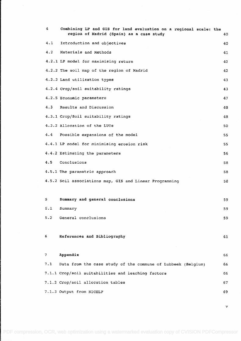
4 Combining LP and GIS for land evaluation on a regional scale: the region of Madrid (Spain) as a case study 40



4.2.1 LP model for maximising return 42

4.2.2 The soil map of the region of Madrid 42

4.2.3 Land utilization types 43

4.2.4 crop/soil suitability ratings 43



4.3.1 Crop/Soil suitability ratings 48

4.3.2 Allocation of the LUTs 50

4.4 Possible expansions of the model 55

4.4.1 LP model for minimising erosion risk 55

4.4.2 Estimating the parameters 56

4.5 Conclusions 58

4.5.1 The parametric approach 58

4.5.2 Soil associations map, GIS and Linear Programming 58

5 Summary and general conclusions

5.1 Summary

5.2 General conclusions

59

59

59

6 References and Bibliography 61

7 Appendix 66

7.1 Data from the case study of the commune of Lubbeek (Belgium) 66

7.1.1 Crop/soil suitabilities and leaching factors 66

7.1.2 Crop/soil allocation tables 67

7.1.3 Output from NICELP 69

V

4 Conbiaing LP and GIS for land evaluation oa a regional scale: tberegion of l,{adrid (Spain) aa a caae study 40

4.7 Introduction and objectives 4O

4.2 Materials and Methods 4L

4.2.1 LP model for maximieing return 42

4.2.2 The soil map of the region of Madrid 42

4.2.3 Land utilization types 43

4.2.4 Crop/soil suitability ratings 43


4.3 Resulte and Discussion 48


4.3.2 Allocation of the LUTg 50

4.4 Possible expansions of the model 55

4.4.1 LP model for minimising eroeion risk 55

4.4.2 Estimating the parameters 55

4.5 Conclusions 58

4.5.1 The parametric approach 58

4.5.2 Soil associations map, cIS and Linear Programming 58

5

5.1

5.2

Summary and general conclusions

Summary

General conclusions

59

59

59

56

66

66

67

59

v

References and Bibliography

7 Appeadix

7.1 Data from the case study of

7.L.1 Crop/soil suitabilities and

7.1.2 Crop/soil allocation tables

7.1.3 Output from NICELP

the commune of Lubbeek (Belgium)

leaching factors

51



7.2 Data from the case study of the region of Madrid (Spain) 85

7.2.1 Soil physical and chemical data (Source: Rodríguez, 1990a) 86

7.2.2 Crop/Soil physical suitability ranges 91

7.2.3 Crop/Soil chemical suitability ranges 92


7.2.5 Opportunity cost for assigning a particular crop to a particular soil unit 94

7.2.6 Output from NICELP for Madrid 95

List of Figures

Figure 1 Steps in the process of Land Evaluation 3

Figure 2 Conceptual representation of a decision support system for land evaluation 6

Figure 3 Suitability ratings and classes for maize as a function of percentage CaCO3 9

Figure 4 Graphical representation of an LP problem with two decision variables 12

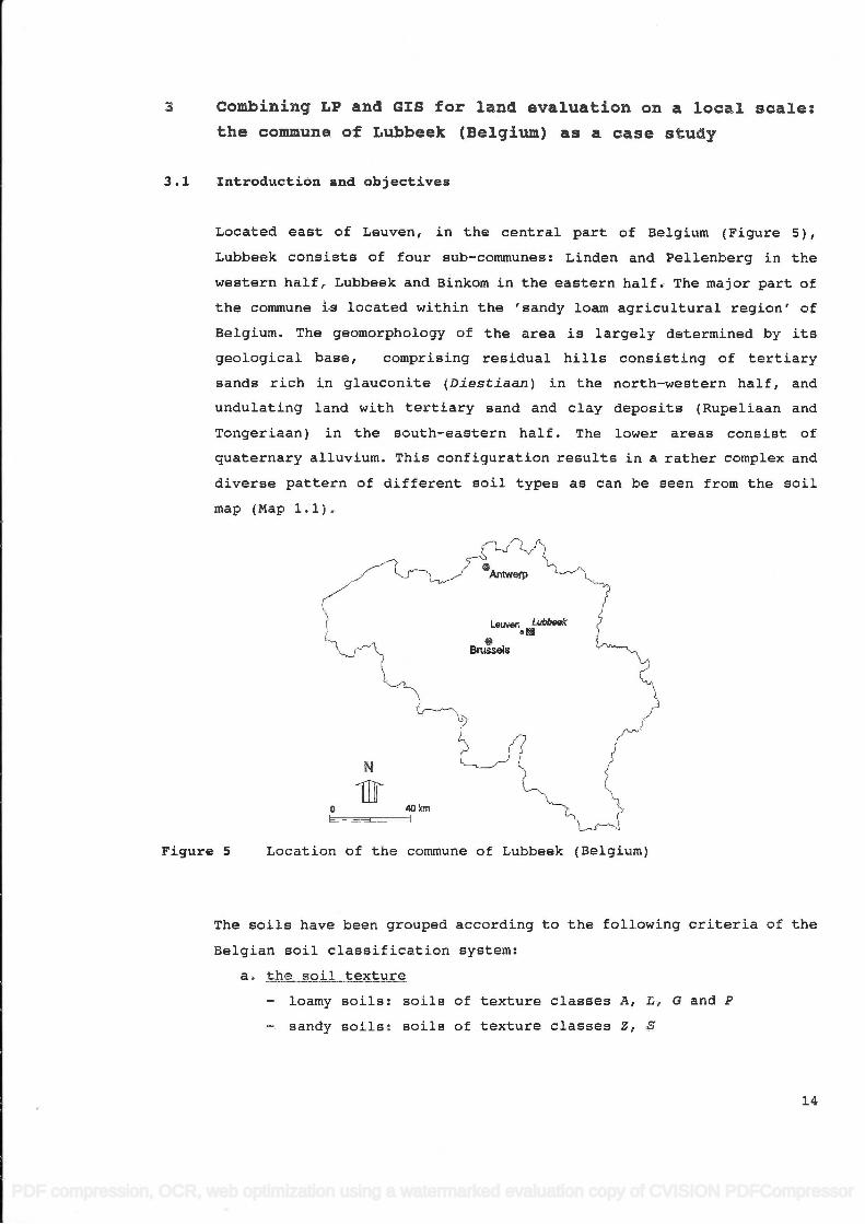
Figure 5 Location of the commune of Lubbeek (Belgium) 14

Figure 6 Location of the region of Madrid (Spain) 4].

List of Tables

Table 1 Area used in the LP model for the different crops 21

Table 2 Class limits for the water storing capacity and phosphate fixing capacity 22

Table 3 Standard Gross Margin of crops in Belgium 24

Table 4 Net Present Value and annuity for two varieties of poplar 25

Table 5 Shifts over the allocated area for the major soil series without (A) and with (B) environmental constraint 28

vi

7.2 Data from the caee atudy of the region of Madrid (spain) 85

7.2.L soil physical and chemical data (Source: Rodriguez, 1990a) 86

7.2.2 crop/Soil phyeical suitability rangeE 91

7.2.3 Crop/Soil chemical suitability ranges 92

7.2.4 crop/Soil guitability ratinge 93

7.2.5 opportunity cost for assigning a particular crop to a particularsoil unit

7.2.6 Output from NICELP for t-{adrid

List of I'igures

94

95

Figure

Figure

Figure 3

Figure 4

Figure

Figure

Table 1

Table 2

Table 3

Tab1e 4

Table 5

1

2

72

L4

4L

5

6

Steps in the process of Land Evaluation

conceptual representation of a decision eupport eystem forIand evaluation

Suitability ratingE and claeeee for maize ag a function ofpercentage CaCO3

Graphical representation of an LP problem with two decisionvariables

Location of the commune of Lubbeek (Belgium)

Location of the region of Madrid (Spain)

List of Tables

Area used in the LP model for the different cropE

Class limits for the water storing capacity and phosphatefixing capacity

Standard Gross Margin of crops in Belgium

Net PreEent Value and annuity for two varietieE of poplar

Shifts over the allocated area for the major soil serieewithout (A) and with (B) environmental constraint

27

22

24

25

28

vt



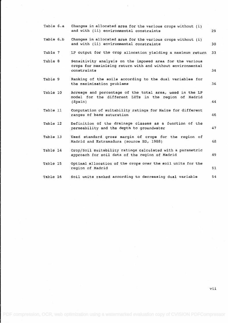
Table 6.a Changes in allocated area for the various crops without (i)

and with (ii) environmental constraints 29

Table 6.b Changes in allocated area for the various crops without (i)

and with (ii) environmental constraints 30

Table 7 LP output for the crop allocation yielding a maximum return 33

Table 8 sensitivity analysis on the imposed area for the various crops for maximising return with and without environmental constraints 34

Table 9 Ranking of the soils according to the dual variables for the maximisation problems 36

Table 10 Acreage and percentage of the total area, used in the LP model for the different LUTs in the region of Madrid (Spain) 44

Table 11 Computation of suitability ratings for Maize for different ranges of base saturation 46

Table 12 Definition of the drainage classes as a function of the permeability and the depth to groundwater 47

Table 13 Used standard gross margin of crops for the region of

Madrid and Extramadura (source EG, 1988) 48

Table 14 Crop/Soil suitability ratings calculated with a parametric approach for soil data of the region of Madrid 49

Table 15 Optimal allocation of the crops over the soil units for the region of Madrid 51

Table 16 Soil units ranked according to decreasing dual variable 54

vii

Tab1e 5.a Changree in allocated area for the various crops without (i)and with (ii) environmental constrainte

Tab1e 5.b Changes in allocated area for the varioue crops without (i)and with (ii) environmental conetraintE 30

Table 7 LP output for the erop allocation yielding a maximum return 33

Table 8 Sensitivity analysie on the impoeed area for the variouecropE for maximisingr return with and without environmentalconstraints

Tab1e 9 Ranking of the soils according to the dual variables forthe maximisation problems

Table 10 Acreage and percentage of the total area, used in the LPmodel for the different LUTE in the region of Madrid( Spain)

Table 11 Computation of suitability ratings for Maize for differentranges of base gaturation

Table 12 Definition of the drainage classeE aa a function of thepermeability and the depth to groundwater

Table 13 UEed etandard grosa margin of crops for the region ofltadrid and Extramadura (source Ec, 1988)

Table 14 Crop/Soil suitability ratings calculated with a parametricapproach for soil data of the region of Madrid

Table 15 Optimal allocation of the crops over the soil unitg for theregion of Madrid 51

Table 16 Soil units ranked aceording to decreasing dual variable 54

29

34

35

44

46

47

48

49

vrt



List of used abbreviations and acronyms

BAGRAB Beoordeling AGRArisch Bodemgebruik

BEF Belgian Franc

CORINE EC-experimental progranmie on COoRdination of INformation on

the Environment

DSS Decision Support Systems

EC European Community

ECU European Currency Unit

EG Europese Gemeenschap

FAO Food and Agricultural Organisation

GIS Geographical Information Systems

LE Land Evaluation

LEI Landbouw Economisch Instituut

LP Linear Programming

LUT Land Utilisation Type

NIS Nationaal Instituut voor de Statistiek

PFC Phosphate Fixing Capacity

SGM Standard Gross Margin

USLE Universal Soil Loss Equation

WSC Water Storage Capacity

viii

List of used abbreviations and acronfms

BAGRAB Beoordeling AGRArisch Bodemgebruik

BEF Belgian Franc

CORfNE EC-experimental progranme on COoRdination of INformation on

the Environment

DSS Decision Support Systems

AC European Community

ECU European Currency UnitEG Europese Gemeenschap

FAO Food and Agricultural OrganieationcIS Geographical Information Syetems

LE Land EvaluationLEf Landbouw Economisch InstituutLP Linear Programming

LUT Land Utilisation Type

NfS Nationaal- Instituut voor de StatistiekPFC Phosphate Fixingr CapacitySG}[ Standard Gross I'larginUSLE Universal Soil Loss EquationWSC Water StoraEe Capacity

v].ll



List of symbols used in the mathematical models

zp* the optimal production level

a production reduction factor for crop i on soil type j

R. the expected return of crop i

the (decision variable) area of crop i on soil type j

i a crop index

i a soil index

AJX the maximum area available of soil type j 1req the required area with crop i

ZN the minimum quantity of nitrogen which may leach out

-'i a factor for the sensitivity of soil type j for leaching of

nitrates

N1X the maximal admissible quantity of nitrogen which may be

applied per hectare for crop i

zF the minimum quantity of phosphates which may leach out

f a leaching factor for phosphates on soil type j

F1X the maximal admissible quantity of phosphates which may be


cp the maximal desired deviation from the optimal production Z

aN and OEF the maximal desired deviation from the optimal level Z and

ZF

ix

List of slmbols used in the mathematical morlels

Zr* the optimal production leveltij a production reduction factor for erop i on soil type JRi the expected return of crop iAij the (decieion variable) area of crop i on soil type -Z

i a erop indexj a soil index

^j*' the maximum area available of soil type -Z

Ait{ the required area with crop i

Zr* the minimum quantity of nitrogen which may leach out7j a factor for the sensitivity of soil type j for leaching of

nitrateetri** the maximal admiseible guantity of nitrogen which may be


,r* the minimum guantity of phosphates which may leach outtj a leaching factor for phoephateE on soil type Jfi*' the maximal admissible quantity of phosphates which may be


up the maximal deEired deviation from the optimal production Zr*

c* and c, the maximal desired deviation from the optimal level Z** and*z-

f

IX



2. Problem definition and objectives

Land evaluation aims at assessing the performance of land for specific

land utilization types (LUT) of a given area, taking into account bio-

physical and socio-economic constraints. Most commonly used methods of

land evaluation enable to determine the unconditional suitability of a

given area for specific land uses (FAO 1989; FAO 1990). These methods

provide little clues on how to allocate appropriately different LUTs in

a certain area for given goals and constraints. This step is simply

left over to policy makers. However, to ensure a rational management

of land resources, it is required to identify the optimal allocation of

different land-uses for various land units. This should be determined

as a function of productivity as well as of potential risk of

environmental degradation. The objective of the study is to work out

a procedure enabling the identification and evaluation of 'optimal

land-use allocations' by combining linear programming and geographical

information systems.

Linear Programming (LP) is a computation technique of which 'the most

common type of application involves the general problem of allocating

limited resources among competing activities' (Hillier, 1990).

Allocation of land utilisation types - land being a limited resource

for which different LUT compete - seems thus to be a standard problem

which can be solved with LP. Typically, an LP model seeks to optimize

one objective function e.g. maximising return. With the technique of

Multiple Goal Programming (de Wit et al., 1988), a mix of different

dependent objective functions can be optimized e.g. minimising erosion

risk for a given economic return. Geographical Information Systems

(GIS) enable to compile, store, retrieve and present geographical

information, Combining both LP and GIS will allow to identify the

location and the geographical extent of various land units with their

optimal use.

In view of testing the elaborated procedure at local scale as well as

at regional scale, two case study areas have been selected: (i) the

commune of Lubbeek located east of Leuven in Belgium, and (ii) the

region of Madrid in Spain. For the commune of Lubbeek the optimal

allocation of agricultural land is determined for an optimal crop

production capacity, whilst minimising the risk of leaching of nitrates

i

Problem definition and objectives

Land evaluation aims at assessing the performance of land for specificIand utilization types (LUT) of a given area, taking into account bio-physical and eocio-economic constrainte. Moat commonly used methods ofland evaluation enable to determine the unconditional suitability of a

given area for specific land usee (FAO 1989; FAO 1990). These methode

provide litt1e cluee on how to allocate appropriately different LUTe ina certain area for given goal-e and constrainte. ?hie atep is simplyleft over to policy makers. However, to ensure a rational management

of land reeourceE, it is reguired to identify the optimal allocation ofdifferent land-ueeg for varioue land units. This ghould be determinedas a function of productivity aa well as of potential risk ofenvironmental degradation. The objective of the study is to work outa procedure enabling the identification and evaluation of 'optimalland-use allocations' by combining linear programming and geographical

information systems.

Linear Programming (LP) is a computation technique of which 'the most

cornmon type of application involves the general problem of allocatinglimited resources, among competing activities' (Hi1lier, 1990).

Allocation of land utilisation types - land being a }imited resourcefor which different LUT compete - Eeema thus to be a standard problem

which can be eolved with LP. Typical-Iy, an LP model seekg to optimizeone objective function e.g. maximising return. With the technigue ofMultiple GoaJ- Programming (de llit et a1., 1988), a mix of differentdependent objective functions can be optimized e.g. minimising erosionrisk for a given economic return. Geographical Information Systems

(cIS) enable to compiJ.e, store, retrieve and present geographicalinformati-on. Combining both LP and GfS will allow to identify thelocation and the geographical extent of various land units with theiroptimal use.

In view of testing the elaborated procedure at local scale as well as

at regional scale, two caee study areaE have been seleeted: (i) thecommune of Lubbeek located east of Leuven in Belgium, and (ii) theregion of Madrid in Spain. For the commune of Lubbeek the optimalallocation of agricultural land is determined for an optimal cropproduction capacity, whilst minimising the risk of leaehing of nitrates



and phosphates to the groundwater. A detailed soil map (1:20,000) is

used as the main source of information. For the region of Madrid the

applicability of the proposed procedures when using a soil association

map is investigated.

The aspiration of this work is to demonstrate that available data from

land evaluation and soil suitability studies can have more dynamic

applications, and as such be of better use for decision support, so as

to come to a rational management of land resources.

2

and phosphatee to the groundwater. A detailed eoil map (1:20,000) isused as the main Eource of information. For the region of Madrid theapplicability of the proposed procedures when using a soil associationmap is investigated.

?he aspiration of this work ig to demonstrate that available data from

land evaluation and soil suitability studieg ean have more dynamic

applicatione, and as guch be of better uEe for deciEion support, Eo aB

to come to a rational management of land resourceE,.



2 Methods and tools for Land Evaluation

2.1 The process and principles of land evaluation

Land evaluation is the term used to describe the process of collecting

and interpreting basic inventories of soil, vegetation, climate and

other aspects of land in order to identify and compare land-use

alternatives. The process of land evaluation according to the FAO

methodology is summarized in Figure 1.

3 identifying land uses

112 5 6 7 8

I I

identifying defining LJ

Identifying planning _- suUability k-1 erwironm. the most land use

andsoclo- suitable I I

omic land use j ____________I

I

issues

I identing

Application

i° land j

evaluation

Figure 1 Steps in the process of Land Evaluation (Source: FAO, 1990)

The focus of the present study mainly relates to steps 5, 6 and 7 in

this process, as the work is based on maps prepared by other authors.

Therefore some major concepts, especially with regards to assessing

suitability, are defined below.

The principles of land evaluation according to FAO (1976) are

summarized here:

- Land suitability is assessed and classified with respect to

specified kinds of use.

- Evaluation requires a comparison of the benefits obtained and the

inputs needed on different types of land.

- A multidisciplinary approach is required.

2

2.L

Irlethods and tools for tand Evaluation

Ehe process aad principleg of laad evaluatiou

Land evaluation is the term used to describe the procesB of collectingand interpreting baeic inventorieg of soil, vegetation, climate and

other aepects of land Ln order to identify and compare land-uge

alternativeE. The procese of land evaluation according to the FAo

methodology iE gummarized in Figrure 1.

6idenffylnggllronm.and socloeconomlclssuee

Figure 1 Steps in the procesE of Land Evaluation (Source: FAo, 1990)

The focus of the preeent study mainly relates to steps 5, 6 and 7 inthis proeees, as the work is based on mape prepared by other authore.

Therefore some major concepts, especially with regards to assessing

suitability, are defined below.

The principles of land evaluation according to FAO (L976) are

surnmarized herel

- Land euitability is assessed and classified with respect tospecified kindg of use.

- Evaluation requires a comparison of the benefite obtained and theinputs needed on different types of land.

- A multidisciplinary apProach is reguired.



- Evaluation is made in terms relevant to the physical, economic

and social context of the area concerned.

- Suitability refers to use on a sustained basis.

- Evaluation involves comparison of more than a single kind of use.

Assessing suitability of land units for a specific land-use is clearly

a key step in the process of land evaluation. This essentially is a

process whereby relative ratings are assigned to land utilisation types

(e.g. specific crops) for the different identified land units (e.g.

soil series). This can be done based on field experiments, eventually

complemented with farmers experience and expert knowledge as has been

done during the survey resulting in the soil map of Belgium. The FAO

system classifies land units according to specific limitations in

hierarchical system comprising suitability order, classes, subclasses

and units:

Suitability order

kind of suitability S suitable

N not suitable

Suitability class

degree of suitability i highly

2 moderately

3 marginally

Suitability subclass

kind of limitation c climatic

w wetness

t topographic

Suitability units

determined by the degree of limitation and other minor

differences in production characteristics and management

requirements. There are no strict conventions for this

classification.

An alternative procedure consists of assigning ratings to various

relevant land characteristics from which a suitability rating can be

calculated using a multiplicative model, as is done in the parametric

approach by Sys (1991) or in the soil productivity rating of the FAO

system (ILACO, 1985).

4

Evaluation is made in terms relevant to the physical, economic

and social eontext of the area concerned.Suitability refers to use on a EuEtained basiE.Evaluation involves comparj-son of more than a single kind of use.

Assessing euitabllity of land unite for a specific land-use ie clearlya key step in the proceeg of land evaluation. Thie eseentially ie a

process whereby relative ratinge are aseigned to land utiliEation types(e.9. specific crops) for the different identified land units (e.9.eoil seriee). This can be done based on field experimente, eventuallycomplemented with farmerE experience and expert knowledge aE has been

done during the survey resulting in the eoil map of Belgium. The FAO

system claseifiee land units according to specific limitatione inhierarehical system comprising suitability order, classes, Eubclaeeee

and units:

Suitabilitv orderkind of suitability S suitable

I{ not suitableSuitability clase

degree of suitability t highly2 moderately

3 marginallySuitabilitv subclass

kind of limitation c climaticr lrretneEs

t t,opographic

Suitabilitv unitsdetermined by the degree of Iimitation and other minor

differences in production charaeterieticE and management

requiremente. There are no gtrict conventione for thiEclaesificatLon.

An alternative procedure coneiste of assigning ratinge to variousrelevant land characterietics from which a euitability rating ean be

calculated using a multiplicative model, as ie done in the parametricapproach by Sye (1991) or in the soil productivity rating of the FAo

syetem (ILACO, 1985).



The final outcome invariably is a table indicating the suitability of

specific LUTs for the different land units which in turn can be

represented as a map. This undeniably forms an important base for

further land-use planning, but as such it does not indicate which will

be the most appropriate land utilisation type, neither thus it indicate

which land unit has an (economic) comparative advantages for the

various LUTs.

2.2 Decision Support Systems as tools for Land Evaluation

Decision support systems (DSS) imply effective computer-based tools to

help planners and managers to determine the most appropriate sequence

of actions for solving complex problems, often involving multiple and

conflicting objectives. Land evaluation, and ultimately land-use

planning, typically implies evaluating decisions dealing with multiple

and often conflicting goals. A synthetic overview is given here of the

elements constituting decision support systems for land evaluation.

Sprague (cited by Labadie, 1989a) claims that decision support systems

should have the following attributes:

- attempt to combine the use of models or analytical techniques

with traditional data access and retrieval functions;

- focus on features which make them easy to use by non-computer

people in an interactive mode;

- emphasize flexibility and adaptability to accommodate changes in

the environment and the decision making approach of the user.

An integrated DSS for land evaluation can be conceptualised as in

Figure 2. The main sub-systems are Geographical Information Systems and

related database management systems, simulation models and optimization

(search) algorithms. As notified by Labadie (1989b), historically there

has existed a dichotomy in the relation to the use of descriptive

models (i.e. simulation) and prescriptive models (i.e. optimization).

This is unfortunate as their joint usage offers unique advantages.

Moreover, it seems that optimization models have not yet as commonly

been applied for land evaluation as simulation models. The main

features of these sub-systems are outlined in the following paragraphs.

5

2.2

The final outcome invariably is a table indicating the suitability ofspecific LUTE for the different land units which in turn can be

represented as a map. This undeniably forme an important base forfurther land-use planning, but ae euch it does not indicate which willbe the moet appropriate land utilieation type, neither thue it indicatewhich land unit has an (economic) comparative advantages for thevarious LUTg.

Decision Support Systems as toole for Laud Evaluatiou

Decieion support systems (DSS) imply effeetive computer-based toole tohelp planners and managers to determine the most appropriate sequence

of aetions for solving complex problems, often involving multiple and

conflicting objectives. Land evaluation, and ultimately land-use

planning, typically implies evaluating decisions dealing with multipleand often conflicting goa1s. A synthetic overview is given here of the

elements congtituting decision aupport eystems for land evaluation.

Sprague (eited by Labadie, 1989a) claims that decision support systems

should have the following attributes:- attempt to combine the use of modela or analytical technigues

with traditional data access and retrieval functions;

- foeus on features which make them easy to use by non-computer

people in an interactive mode;

- emphasize flexibility and adaptability to accommodate changes inthe environment and the decision making approach of the user.

An integrated DsS for land evaluation can be eonceptualised as inFigure 2. The main sub-syetems are eeographical fnformation Systems and

related database management systems, simulation modele and optimization(search) algorithms. As notified by Labadie (1989b), historically therehas existed a dichotomy in the relation to the use of descriptivemodels (i.e. simulation) and prescriptive models (i.e. optimization).Thie is unfortunate aE their joint usage offers unique advantages.

ltoreover, it seems that optimization models have not yet as commonJ-y

been applied for land evaluation as simulation models. The main

features of these sub-systems are outlined in the following paragraphs.



Non-spatia Spatial Data Data

U flu

GIS and Data Base management system

U Simulation model

o E C o

____________________ E

Search algorithm

Figure 2 Conceptual representation of a decision support system for land evaluation

2.2.1 Geographical Information Systems

Geographical Information Systems (GIS) are essentially computer

programmes designed to compile, store, retrieve and present

geographical information. One of the important features of GIS is the

capability to make overlay analysis of different spatial data and from

there to generate new maps. Besides, the geographical data in a GIS can

be linked to non-spatial data, known as attribute tables. This makes it

possible to automate analysis, e.g. performing queries in order to

filter out a subset of the data base. Through these attribute tables,

spatial information can also be linked to newly acquired information,

e.g. from surveys or from modelling. This eventually enables to

generate new maps. With a GIS it is thus quite convenient to generate

'land suitability' maps from soil maps linked to suitability tables.

More powerful applications can be thought of when these data are

further linked to simulation and optimization models.

6

GIS and Data Basemanag€ment system

$

Figure 2 Conceptual repreeentation of adecigion support system forland evaluation

2.2.L Geographical Information systems

Geographical Information Systeme (GIS) are essentially computer

progJrarmes designed to compile, store, retrieve and presentgeographical information. One of the important features of GIS is thecapability to make overlay anaLysis of different spatial data and from

there to generate new mapE. Besides, the geographical data in a cIS can

be linked to non-spatial data, known ae attribute tables. This makes itpossible to automate analysis, e.g. performing gueries in order tofilter out a eubset of the data base. Throuqh theee attribute tablee,spatial information can aleo be linked to newly acquired information,e.g. from aurveya or from modelling. This eventually enables togenerate new maps. Vlith a cIS it is thus quite convenient to generate

'land suitability' maps from soil maps linked to suitability tables"More powerful applications can be thought of when these data are

further linked to eimulation and optimization models.

E@ol Iet I

e, Atlolt I6 il{}N.ETE i searcn argor

,



2.2.2 Simulation and optimization models

Simulation models are primarily developed to mimic complex processes so

that they can be studied in a convenient way. They are essentially

descriptive in nature, and can either be stochastic or deterministic.

They allow accurate modelling of complex systems, but cannot find a

'best" solution, which represents the primary advantage of prescriptive

model structures (Labadie, 1989b).

Prescriptive models (optimizing) offer the possibility to

systematically select optimum solutions, or families of solutions,

under agreed objectives and constraints. They however, often require

simplifying assumptions on the model structure, and are usually less

suited to simulate a process. Combining simulation and optimization

models seems thus to be the best approach. Optimizing models can be

used for generating operational policies which can then be tested and

refined with a more detailed simulation model (Labadie, 1989b), while

parameters generated by simulation models can be used in the

optimization model.


(i) Features and limitations of Linear Programming

Linear Programming (LP) is just one type out of a family of search

algorithms. Some other related algorithms are Integer Programming,

Transportation Models and Dynamic Programming. In general terms, LP is

used to optimize production in cases of scarce resource availability.

It should hence be typically suited for determining optimal land-use.

It makes use of linear equations to express an objective function and

constraint functions. Linear equations imply multiplicativity and

additionality. An LP model in its standard form can be expressed as

z* _ max (or mm) Z r1 . X [i]

which represents the objective function, and subject to the constraints

7

2.2.2 Simulation and optimization modelg

Simulation models are primarily developed to mimLc complex procesEea Eo

that they can be studied in a convenient way. They are easentiallydescriptive in nature, and can elther be Etochastic or deterministic.They allow accurate modelling of complex systems, but cannot find a

"beEt" solution, which repreaents the primary advantage of prescriptivemodel structures (Labadie, 1989b).

Preecriptive modele (optimizing) offer the possibility tosyatematically Belect optimum eolutione, or familiee of eolutione,under agreed objectives and conetraints. They however, often reguiresimplifying assumptions on the model atructure, and are usually lesssuited to simulate a proceas. Combining simulation and optimizationmodele Eeeme thue to be the beEt approach. Optimizing modele can be

used for generating operational policies which can then be tested and

refined with a more detailed simulation model (LabadJ-e, 1989b), whileparameters generated by eimulation models can be used in theoptimization model.


(i) Eeatures and Tinitations of Linear Prograntning

Linear Programming (LP) is just one type out of a family of search

algorithms. Some other related algorithma are fnteger Programming,

Transportation Models and Dynamic Programming. fn general terms, LP iE

used to optimize production in cases of gcarce re€,ource availability.It ehould hence be typically auited for determining optimal land-use.It makes use of linear equations to expresa an o.bjective tuncxion and

constraint tunctions. Linear eguatione imply multiplicativity and

additionality. An LP model in its standard form can be expreseed ae

nZr - rndx (or min) Z - Ert. Xt

i-1t11

which represents the objective function, and subject to the constrainte



c1.X1(or)B [2)

where Z the optimal value of the objective function

xi the decision variables (e.g. area to be planted)

r1 benefit or return (in case of maximisation)

ci a unit "cost'

B a "budget" constraint (e.g. available area), and

i an index and totalling to n, the number of decision

variables (e.g. number of crops)

The advantage of using LP for land evaluation lies in the ease of use

and that available soil and land evaluation parameters can directly be

applied. The apparent disadvantages can be itemised as: equations have

to be linear, the LP algorithm can only optimize one objective

function, and it might be difficult to identify and formulate all

relevant constraints. In well understood and controllable technical

processes the latter is usually quite straightforward, but identifying

explicitly all relevant constraints relating to land evaluation and

land-use might be more difficult. This is probably a major reason why

applications of LP for land evaluation have been limited so far.

(ii) How to overcome these limitations?

Non-linear equations can often be transformed into linear equations by

applying classical arithmetic techniques such as log transformations,

substituting quadratic terms, etc., or by partitioning the function

into appropriate linear segments. Crop production functions are basic

components for assessing crop/soil suitabilities in the process of land

evaluation. They are evidently non-linear but can easily be partioned

into linear parts. Essentially, this is done when suitability ratings

are assigned to ranges of specific soil characteristics for a

particular crop. An example of this principle is shown for maize in

Figure 3.

8

xrs (or>) B 121

the optimal value of the objective functionthe decision variables (e.9. area to be planted)benefit or return (in case of maximisation)

a unit "cogt"a "budget" conEtraint (e.9. available area), and

an index and totalling to n, the number of decisionvariables (e.9. number of cropsl

E*where z*

xirisi

B

i

The advantage of using LP for land evaluation lies in the ease of use

and that available soil and land evaluation parameters can directly be

applied. The apparent disadvantages can be itemiEed as: equatlons have

to be linear, the LP algorithm can only optimize one objectivefunction, and it might be difficuLt to identify and formulate allrelevant constraints. fn well understood and controllable technicalproceE,ses the latter is ugually quite straightforward, but identifyingexplicitly all relevant constraintg relating to land evaluation and

land-use might be more difficult. ThiE is probably a major reason why

applications of LP for land evaluation have been limited so far.

(ii) Hov to overcome these Timitations?

Non-linear eguationE can often be transformed into linear eguations by

applying classical arithmetic technigueg such ae log transformations,substituting guadratic terms, etc., or by partitioning the functioninto appropriate linear segments. crop production functions are basiccomponents for assessing crop/soil suitabilities in the process of land

evaluation. They are evidently non-linear but can eaeily be partioned

into linear parts. Essentially, thig is done when suitability ratingsare assigned to rangea of specific Eoil characteristicE for a

particular crop. An example of this principle is shown for maize inFigure 3.



w H a L)

a

o H

a

Suitability classes

100

SI 90

80

70

60

50

40

30

20

10

o

52

53

N

o io 20 30

CaCO3 ()

Figure 3 Suitability ratings and classes for maize as a function of percentage CaCO3 (adapted from Sys, 199Th)

Besides the limitation emanating from the requirement of linear

equations, LP models can only handle one objective function. In real

life situations usually several objectives should be optimized, or

compromises should be made between them, e.g. maximising profit, and

minimising environmental impact. Some techniques exist to deal with

this problem. One way to overcome this limitation is, when the

different objectives can be ranked, to optimize the first ranked

objective one, and subsequently adding it, within a determined range

from its optimal solution, as an additional constraint to the following

objective function. This technique of using LP models is referred to as

Multiple Goal Programming (e.g. de Wit et al., 1988).

Problems with regard to defining and formulating all constraints

relevant to land evaluation can be overcome by identifying constraints

which implicitly cover a large proportion of them as will be shown in

the subsequent case studies.

9

0JdIJm

UI

.t

d

?o

60

50

30

4A

Suitability classes

caco3 (9d )

Suitability ratings and claseespercentage CaCO3 (adapted from Sys,

Figure 3

30

for maize as a function of1991b )

Besides the limitation emanating from the requirement of linearequations, LP models can only handle one objective function. In reallife situations usually several objectiveg should be optimized, orcompromiseE shouLd be made between them, e.g. maximising profit, and

minimising environmental impact. Some techniqueE exist to deal withthie problem. One way to overcome thie limitation ie, when thedifferent objectiveE can be ranked, to optimize the firet ranked

objective one, and subsequently adding it, within a determined range

from itg optimal solution, as an additional constraint to the followingobjective function. This technigue of ueing LP models ig referred to as

Multiple eoal Programming (e.9. de Wit et aI., 1988).

Problems with regard to defining and formulating all constraintErelevant to land evaluation can be overcome by identifying constraintewhich implicitly cover a large proportion of them aE will be shown inthe EubEeguent case studies.



An objective function, maximising the return

max Z = max {60,000 * XsugarBeet + 40,000 * Xwheat}

and subject to the constraints

1) of production

XsugarBeet 40 ha ..................... (1)

Xuheat 30 ha ....................... (2)

2) of labour

2x XSugarBeet + lx Xwheat 85 ................ (3)

3) inputs (fertilizers)

lx XsugarBeet + 2x Xwheat 70 ................ (4)

and with XsugarBeet and XWheat the area planted with sugar-beet and wheat

respectively.

Graphically this problem can be depicted as in Figure 4. Line 1, 2, 3,

and 4 represent the respective constraints, and the shaded area the

resulting solution space. Line 5, the dashed line, is a projection of

the objective function into the solution space. All points on that line

represent equivalent combinations of the decision variables with

respect to the objective function. It can be seen that 20 ha of sugar-

beet and none of wheat will have a return of 120 thousand (20 x

60,000), equivalent to 30 ha of wheat (30 x 40,000) and none of sugar-

beet. Hence, line 5 and 6 represent equipotential lines. It can be

seen from the figure that the highest possible value will be reached

when line 5 is translated towards line 6 where the ultimate optimal

solution is reached in point A.

How the input and output of this problem looks like when solving it

with the computer programme NICELP (Labadie, 1993) is illustrated in

Box 1. The programme computes the value of the decision variables, and

its corresponding reduced costs. The reduced cost, or opportunity cost,

gives a measure of how much the objective function will deviate from

the optimal solution for a unit change in the decision variable. This

can be expressed as

Reduced Cost - $! [31

The reduced cost of decision variables which are part of the optimal

solution are by definition zero, while the others are negative for a

maximisation problem, and positive for a minimisation problem.

11

An objective function, maximiaing the returnmax Z = max {601000 * Xsus""Beet + 401000 * XHh""t}

and subject to the congtraints1) of production

xsusarBeet s 4o ha (1)

X!,heat < 30 ha Ql2l of labour

2x xsrg""B"et * 1x \h""t t 85 (3)

3) inputs (fertilizers)1x xsugarBe", + 2x xHh".t = 7o (4)

and with XsugarBeet and X,heat, the area planted with sugar-beet and wheat

respectively.

Graphically this problem can be depicted ae in Figure 4. Line 1, 2, 3,

and 4 repreeent the respective conetrainte, and the ghaded area theresulting solution 6pace. Line 5, the dashed line, is a projection ofthe objective function into the solution space. AII points on that linerepresent equivalent eombinatione of the deciEion variableg withrespect to the objective function. It can be seen that 20 ha of Eugar-

beet and none of wheat will have a return of t2O thousand l2O x60,000), eguivalent to 30 ha of wheat (30 x 40,000) and none of sugar-

beet. Hence, line 5 and 5 represent equipotential lines. It can be

Eeen from the figure that the higheet possible value will be reached

when line 5 is translated towardE line 5 where the ultimate optimaleolution is reached in point A.

How the input and output of this problem looks like when solving itwith the computer programme NICELP (Labadie, 1993) is illustrated inBox 1. The prograrnme computee the value of the decision variables, and

l-tg corresponding reduced cogts. The redused cost, or opportunity cost,givee a meaEure of how much the obJective function will- deviate from

the optimal eolution for a unit change in the decision variable. Thiscan be expreesed as

Reduced cost - 626Xi t3I

of the optimalnegative for a

problem.

The reduced cost of deciEion variables which are partgolution are by definition zero, while the others are

maximiEation problem, and positive for a minimisation

11



(iii) Mathematical principles of LP

From a mathematical point of view, Linear Programming enables to solve

problems with n equations (the constraints) and m unknowns (the

decision variables), the number of equations n not necessarily equal to

the number of unknowns m. The constraint equations can either be

equalities (=) or inequalities ( or ). In general this set of

equations will not have a unique solution (one point) but will define

a solution space. Iteratively the algorithm searches for a point of

that space corresponding to a maximum (or a minimum) of a given

objective function. Several algorithms exist to solve this problem of

which the simplex method is a basic one.

In order to illustrate some fundamental concepts of LP, as well as the

formulation of LP problems, a simple example is worked out here. The

example covers some of the basic features of the latter used more

practical models. Only two 'decision variables' are considered in the

example enabling a graphical representation. For a comprehensive

account on LP, reference is made to literature (Hillier et al., 1990;

Cattrysse, 1993).

A simple example

Consider a farmer having 60 ha of land, for which he has to decide, the

proportion of land which he will plant with wheat and sugar-beet. Due

to production limitations, (e.g. resulting from EC agriculture

policies), he may have as a maximum 30 ha of wheat and 40 ha of sugar

beet. He expects a return of 60,000 BEF/ha for sugar-beet and 40,000

BEF/ha for wheat and his objective is to maximise the return. The

labour required for one hectare of sugar-beet is twice of wheat, and

his maximum available labour is 85 working days. Besides, the cost for

fertilizers needed for one hectare of wheat is twice as much as for one

hectare of sugar-beet. Buying more than 70 units of it is thought not

to be economical. The foregoing can mathematically be formulated as:

10

(iii) Uathematical pri-rtciples ot Lp

From a mathematical point of view, Linear Programming enablee to solveproblems with n eguatione (the constraints) and m unknowng (thedecision variables), the number of eguations n not necessarily egual tothe number of unknowns m. The constraint equations can either be

equalities (=) or inequalities (s or >). fn general this set ofeguations will not have a unigue golution (one point) but will definea eolution space. Iteratively the algorithm searches for a point ofthat Bpace corresponding to a maximum (or a minimum) of a givenobjective function. Several algorithms exist to eolve this problem ofwhich the eimp)-ex method ie a basic one.

fn order to illustrate some fundamental concepts of LP, as well as theformulation of LP problems, a simple example is worked out here. The

example covere aome of the baEic featureg of the latter used more

practical models. Only two 'decision variablee' are considered in theexample enabling a graphical representation. For a comprehensive

aceount on LP, reference is made to literature (Hillier et aI., 1990;

Cattrysse, 1993).

A sinple example

Consider a farmer having 50 ha of land, for which he hae to decide, theproportion of land which he will plant with wheat and eugar-beet. Due

to production limitations, (e.9. resulting from EC agriculturepolicies), he may have ae a maximum 30 ha of wheat and 40 ha of sugar-beet. He expects a return of 6O1000 BEF/ha for sugar-beet and 401000

BEF/ha for wheat and his objective ie to maximise the return. The

labour reguired for one hectare of sugar-beet is twice of wheat, and

his maximum available labour ie 85 workj-ng days. Besides, the cost forfertilizers needed for one hectare of wheat is twice as much ag for one

hectare of augar-beet. Buying more than 70 units of it is thought notto be economical. The foregoing can mathematicalty be formulated as:

10



40

0 20 40 60 80

area with sugar-beet (ha)

Figure 4 Graphical representation of an LP problem with two decision variables

The slack value (Box 1) is the remaining amount of the limited

resource. This is zero for binding constraints, while it will be

greater or smaller than zero for non-binding constraints. The

corresponding dual variable indicates how much the optimal solution

will be altered by a unit change of the right hand side of the

constraint equation, which obviously is zero for non-binding

constraints. This can be expressed as

Dual Variable [4]

Furthermore the programme gives the value of the objective function,

and determines the range of the constraints wherein the decision

variables will be kept in the solution (in the basis).

Note that in case the objective function would have been parallel to

line 4 in Figure 4, all points of the line between A and B would have

yielded alternative optimal solutions. It would have been possible to

12

@

\B\/

1

2

(9

SOtuti QI TPSPE:

50

&

30

2A

6E.Eos,i.C

i(E

eC,

10

20&area with sugar-beet (ha)

8060

Figure 4 Graphical representation of an LP problem with two decigionvariables

The slack value (Box 1) is the remaining amount of the limitedreEource. This is zero for binding constraints, while it will be

greater or smaller than zero for non-binding constraints. The

corresponding dual variable indicateg how much the optimal Eolutionwill be altered by a unit change of the right hand side of theconstraint equation, which obviously is zeto for non-bindingconetraints. This can be expressed ae

DuaT VariabTe - 62q t41

Furthermore the programme givee the value of the objective function,and determinee the range of the conatraints wherein the decisionvariables will be kept in the solution (in the basisl.

Note that in case the objective function would have been parallel toline 4 in Figure 4, all points of the line between A and B would have

yielded alternative optimal solutionE. It would have been possible to

L2



discern this from the output as a decision variable to which no land is

allocated (non-basic variable) will have a reduced cost of zero.

Box i Example of the input and output of a

Programming problem in NICELP simple Linear :

Input OBJECTIVE FUNCTION:

MAX 6 XSgBeet[l]+ 4 XWheat[2]

SUBJECT TO CONSTRAINTS: 1. 1 XSgBeetfl]+ O XWheat[2] < 40

2. 0 XSgBeet[l]+ 1 Xwheat[2] < 30

3. 2 XSgBeet[l]+ i XWheat(2) < 85

4. 3. XSgBeet[lJ+ 2 XWheat[2] < 70

Ou tp u t DECISION VARIABLES: VARIABLE NAME VALUE REDUCED COST

J_ XSgBeet[l] 33.33334 0

2 Xwheat[2J 18.33333 0

SLACK/SURPLUS/DUAL VARIABLES: CONSTRAINT TYPE VALUE DUAL VARIABLE

i SLACK 6.666667 0

2 SLACK 11.66667 0

3 SLACK O 2.666667

4 SLACK O .6666667

MAXIMUM OBJECTIVE VALUE= 273.3333

RANGE OF CONSTRAINING VALUES LOWER PRESENT UPPER

CONSTRAINT i 33.33333 40

OBJECTIVE VALUE 273.3333 273.3333 273.3333

CONSTRAINT 2 18.33333 30 co

OBJECTIVE VALUE 273.3333 273.3333 273.3333

CONSTRAINT 3 50 85 95

OBJECTIVE VALUE 180 273.3333 300

CONSTRAINT 4 50 70 87.5

OBJECTIVE VALUE 260 273.3333 285

13

discern this from the output aa a decision variable to which no land iEallocated (non-basic variable) will have a reduced cost of zero.

i:r:enil:ir:rtbutpUt.

ilri:,,'N:[CBlPr:,: :'::

s,f{nele illoe5f

;'IiPut ,,, ,:,:,::::,::::,:: ,, ,,, ,',,,.." ',

.i.........-68''8 ct.IYEi.i.i.fl'NcI IoN,i,,...,...,...............

.:.:.:.:.t.:.t.:.t.:.:.:l{$lt:.:.:.:.:.:.:6:.:::::XfSEBeCt'[ 1 1'+]:ttt:4

SIIB{EET.., ,,::::I:: ,

:: :: :: :: :: :: :::: ::::::::::::|::::::|:.: ::: :::

i....iii..ii.i.....2.lil.l.'i..ii.i..i.:::::,::::,,:? ,,,,:lll,l,l 9 ! ,,,::::,

: ,

: ,

: ,

: ,

: ,

] ,

: , :, : :

. :': : : :. : :

: ' : ' : ' : ,

: ,

: '

,:,:,:,:,:,:'.,.,:'lttii i,:,:,:,:,:,:,

rlr,tO::111:l1l:::1::1

l:i:::::::::::i::

:iiliiiiii:i::i::

CONSiISAINTS I'i,.,,,,,,,,,

1,.....ix .Etseert [..1. I .#0J......X:SEBEet,(.1.'1..+

,2...,.x;s,sBeet [,.1I 1,.+

f ,i...'X:!S.gtsEet-.t,'1. I+

::::::l:::l:1:::::lll

,,0,:,,,,X

,..t.rrrr:x

ii.r.i..i.x::2::::::x

,i,.,.,.,i

',iVAtUEi,.,.,.,i,.,.,i,.,i i i,

::::::::::::::i:::::,:18:;::3 33i3 3

REDUCED::;r,jCQsr

.,,.' O.,.,...i.l.,,:.:,:,:,.,,,:.t.:.:.:.:.:..................t'.

':,:,,,O,,:,,,,,,,,,,,,,,,,,i :,,:,,:,,,,,:,:t]',':,],,,,,,,',,,,,,

,,,,,,,,r,, lllll[GE. ...OFI,,,..CONSf,RA.INING

LOWER ' PRESEMI:''

3,3..t.3,3.s..3.3

,2,,n.3i',,3,03,3t3

lrg.:;i3'33-3:3

i273.i.3i33i3

50,,,...,.ii.....i.i...i ....,.,i.l

,1.80:,.,,.,. .,.,.,...,.,.,.,.,.,

:.:.::::.::::,:::. .l.ll. ::.l.:.l.:'::::l.:':50::::::::,,,': ::::::::::::::::::::::

,2,'6A:,',, "'.,:

",:,,,,:,:,:,,,,,,1

:i:i:lt,:':......,......4'O..i.tltlt.:li.:..l.l:.i.:l:.:i:.........

............'...',...l.,.2.',.t..t..u.'.".,.

,]:it.:ii]ii,l,iiiii:l:.i3,O::]::1lt::::::i1l]l]]iiil]]li|::,iii.t't

tl,..l,l.. llt.,.,.:....2'7,3 ,;,.3 3 3'3 I'

ltl::::::::::::::::,:::::,:::,,:]:,:::::,:i:]]]:]::: i,ilt:Ilt: lt::li:::

iti:::.:.:....i:,:l:.::..8.51:ltl::ll:l:lil:ltltl:ii:: l: :i..:...'.

:i::::::::lt:i::::::l:::12l?i3,,t:,3.3,33:::

:ll:.::.:.::l:;:.l:::::l:r,o:::::::::::l:ll:.::l:.:ll:::::::.,1l,:,, 273.3333:

i i,ii.ii.'..

'..it:i.... . ..,...i

I i,.iiiiiii.i.iiiii.i'...i....

,:,;,,,,,,;2.,;,,,':,;:,,.,,

vi49rrE

, :],:ii:i:i:::i:::i:i:i:::,::

.. ttttt:3:...:,:.:.:.:

VAAUE

CONST,RAINl :4,'J:,,'

.,.,.,., oBJE Gil EVE,,.,,,V4IiUE

i,...' . -

. i .,i.:,'

'....'.,.,.,8.;7',',

5,,,r.,,,r,,,:;t;2,8,.,5i,;,',i,

,,,,,',,i,,,,i,i :,.,..:.,.,,.,i.

13



3 Combining LP and GIS for land evaluation on a local scale:

the commune of Lubbeek (Belgium) as a case study

3.1 Introduction and objectives

Located east of Leuven, in the central part of Belgium (Figure 5),

Lubbeek consists of four sub-communes: Linden and Pellenberg in the

western half, Lubbeek and Binkom in the eastern half. The major part of

the commune is located within the 'sandy loam agricultural region' of

Belgium. The geomorphology of the area is largely determined by its

geological base, comprising residual hills consisting of tertiary

sands rich in glauconite (Diestiaan) in the north-western half, and

undulating land with tertiary sand and clay deposits (Rupeliaan and

Tongeriaan) in the south-eastern half. The lower areas consist of

quaternary alluvium. This configuration results in a rather complex and

diverse pattern of different soil types as can be seen from the soil

map (Map 1.1).

Figure 5 Location of the commune of Lubbeek (Belgium)

The soils have been grouped according to the following criteria of the

Belgian soil classification system:

a. the soil texture

- ioamy soils: soils of texture classes A, L, G and P

- sandy soils: soils of texture classes Z, S

14

Conbining LP and GIS for land evaluation on a local seale:tbe commune of L,ubbeek (Belgium) as a ease study


Located east of Leuven, in the central part of Belgium (Figure 5),Lubbeek consists of four sub-communes: Linden and Pellenberg in thewestern half, Lubbeek and Binkom in the eaetern haIf. The major part ofthe commune iE located within the 'sandy loam agricultural region' ofBelgium. The geomorphology of the area is largely determined by itegeological base, comprising residual hills consisting of tertiarysandg rich in glauconite (Diestiaanl in the north-western half, and

undulating land with tertiary sand and clay deposits (Rupeliaan and

Tongeriaan) in the south-eastern haIf. The lower area€r consist ofquaternary alluvium. This configuration results in a rather complex and

diverse pattern of different eoil types aE can be seen from the soilmap (uap 1.1) .

Figure 5 Location of the eommune of Lubbeek (Belgium)

lhe soile have been grouped

Belgian soil classificationa. the soil texture

- loamy soils: soilg- sandy soils: soils

according to the following eriteria of the

system:

of textureof texture

classesclasseg

L,GalndPs

A,

z,

L4



- clay soils: soils of texture classes E, U, and including the

complexes ELZ, ULS

- peat soils: soils indicate as V

b. the drainage class

- well drained: soils of drainage class a, b and c

- poorly drained: soils of drainage class d or wetter

In the study area, the soil texture of the upper 30cm is predominantly

'sandy loam' (zandleem L). A large proportion of the loamy soils

formed on Distiaan have a clayey sand substratum (32% of the soils of

Linden and 19% of Pellenberg) at a depth ranging from 40 to 80 cm.

Soils formed on Rupeliaan and Tongeriaan have commonly a clay or sand

substratum at a depth of 40 to 80 cm.

Lubbeek preserved rather well its agrarian character. This is reflected

in its master plan where 66% of the area has been set aside for

agricultural use. Out of a total area of 4527 hectares, the current

agricultural land is estimated to be 2964 ha, of which 2405 ha with

arable crops. According to census data of 1987 of the National

Institute for Statistics (NIS), the most common arable crops are wheat

(430 ha), barley (346 ha), and sugar-beet (342 ha), while pasture land

is covering 489 ha (Lenders and Heyleri, 1989). According to a satellite

imagery analysis done by Lenders and Heylen (1989) about 570 ha are

covered with forests or tree plantations.

The specific objective of this case study is to determine by means of

LP and GIS an optimal land-use allocation enabling a reasonable return

while providing a minimal risk for pollution of the groundwater by

agrochemicals. More specifically, nitrates and phosphates are

considered, the former as an example of mobile and water soluble

anions, the latter as an example of relative immobile elements.

One of the reasons for selecting the commune of Lubbeek as a case study

area was its great diversity in soil types. Besides, data and maps were

available from a study on the land-use and crop/soil suitability by

Lenders and Heylen (1989).

15

- clay goils: soile of texture clasees E,

complexes ELZ, ALs

- peat soils: eoile indicate as Y

b. the drainaqe class

- well drained: goils of drainage class a,

- poorly drained: soilE of drainage class

A, and including the

bandcd or wetter

In the etudy area, the goil texture of the upper 3ocm is predominantly

'sandy loam' (zandleem Ll. A large proportion of the loamy soileformed oo Distiaan have a clayey sand eubstratum (32* of the soils ofLinden and 19t of Pellenbergl at a depth ranging from 4O to 8O cm.

Soilg formed on RupeJ.iaaa and Tongeriaan have commonly a clay or sand

gubgtratum at a depth of 40 to 8O cm.

Lubbeek preserved rather well ite agrarian character. This is reflectedin its master plan where 55t of the area has been set aside foragrieultural use. out of a total area of 4527 hectares, the currentagricultural land is estimated to be 2964 }:.a, of which 2405 ha witharable crops. According to cenaus data of t9A7 of the NationalInstitute for Statistics (NIS), the most common arable crops are wheat

(43O ha), barley (345 ha), and sugar-beet (342 ha), while pasture land

is covering 489 ha (Lenders and Heylen, 1989). According to a satelliteimagery analyeis done by Lenders and Heylen (1989) about 570 ha are

covered with foreats or tree plantatione.

The specific objective of this case etudy is to determine by means ofLP and GIS an optimal land-use allocation enabling a reasonable returnwhile providing a minimal risk for pollution of the groundwater by

agrochemicals. Uore epecificall-y, nitrates and phosphatest are

considered, the former as an example of mobile and water solubleaniong, the latter aE, an example of relative immobile elements.

One of the reasons for selecting the commune of Lubbeek aE a case study

area $ras its great diversity in soil types. Besides, data and maps were

available from a study on the land-uEe and crop/aoil suitability by

Lenders and Heylen (1989).

15



3.2 Materials and Methods

A digitized soil map was used. For each of the soil series, crop/soil

suitability ratings are known for the most common crops. The

sensitivity of the various soil series for leaching of nitrates and

phosphates is estimated based on available soil parameters and some

pedo-transfer functions. The standard gross margin of the agricultural

land, and the annuity for poplar plantations, are used as economic

parameters.

On the basis of these selected parameters, the optimal allocation for

five selected crops (wheat, sugar-beet, potato, pasture, and poplar)

was determined using an LP model. In a first step the crop allocation

yielding a maximum return is determined. In subsequent steps the crop

allocation is calculated by taking into account the risk of leaching

nitrates and phosphates, while maintaining a production level of at

least 75% of the maximum return as obtained in the first step. Using a

GIS package, the geographical extent of the various land allocations is

presented on maps.

The procedure is further elaborated in the following paragraphs and

summarized in Box 2. Firstly, the mathematical formulation of the LP

models is presented. Subsequently, the procedure followed to estimate

and use the parameters is explained.

16

3,2 Materiet s and Methods

A digitized soil map hraE used. E.or each of the aoil Eeriee, crop/eoilsuitability ratings are known for the moet common crops. The

eensitivity of the varioue eoil geries for leaching of nitrates and

phosphates is estimated based on available goil parameters and some

pedo-trangfer functions. The standard gro6e margin of the agriculturalIand, and the annuity for poplar plantations, are used aB economic

ParErmeters.

On the basig of these selected parameterE, the optimal allocation forfive selected crops (wheat, sugar-beet, potato, pasture, and poplar)was determined using an LP model. In a firEt step the crop allocationyielding a maximum return is determined. In subseguent Etepa the crop

allocation ie calculated by taking into account the risk of leachingnitrateE and phoaphates, while maintaining a production level of atleast 75t of the maximum return as obtained in the first step. Using aGIS package, the geographical extent of the various land allocations iepresented on maps.

The procedure is further elaborated in the following paragraphs and

summarized in Box 2. Firetly, the mathematical formulation of the LP

models is preeented. Subeequently, the procedure followed to estimateand use the parameterg ie explained.

15



The optimal allocation of five crops is determined

for a given area of each soil type in three inter-liriced steps

Step one - maximising the return (Zp)

Step two - minimizing risk of leaching

(a) of nitrates (Zn)

(b) of phosphates (Zf)

for a return of at least 75% of Zp .

Step three - maximising the return (Zp)

for risk of leaching

smaller or equal to Zn, and

smaller or' ecp.iai to Zp

3.2.1 LP models for Land Evaluation

(i) Maximising return

The proposed Linear Programming (LP) model seeks, as a first step, an

optimal allocation of specific crops on the different soil types

yielding a maximum return. This is determined considering yield

reduction factors - derived from the crop/soil suitability ratings -

and economic parameters. The maximum available acreage of each soil

unit within the area is a first set of constraints. As a second set of

constraints a required area for each crop is defined.

If the maximum area of each soil unit is the only given set of

constraints, an almost trivial solution is obtained, whereby the crop

for which the highest return is obtained, will be put on almost all

soils. This would lead to an impractical solution as limiting factors

such as labour availability, machinery, production limitations, etc.

are totaly neglected. However, by stating that the cropped area should

17

Step one - maximising the return (Zp)

Step two - mhimizing risk of leaching

(a) of nltrates (Zn)

(b) of phosphates (Zf)

for a return of at least 75% ot

Step three - maximising the return (Zp)

for risk of leaching

smaller or equalto Zn, and

smaler or eqralto Zp

3.2.7 LP models for Land Evaluation

( i) tlaximising return

The proposed Linear Programming (LP) model seeks, as a first step, an

optimal allocation of specific cropa on the different soil typesyielding a maximum return. This is determined considering yieldreduction factors - derived from the crop/soil suitability ratinga -and economic parameters. The maximum available acreage of each soilunit within the area is a first set of constraints. As a second set ofconstraints a required area for each crop ie defined.

If the maximum area of each soil unit is the only given set ofconstraints, an almost trivial solution is obtained, whereby the crop

for which the highest return is obtained, wil,l- be put on almost allsoils. This would lead to an impractical solution as limiting factorssuch as labour availability, machinery, produetion limitations, etc.are totaly neglected. However, by stating that the cropped area should

L7



be equal to the current acreage of each crop, all these factors are

implicitly covered. The sensitivity analysie of the LP output allows

to assess how these constraints affect the final solution. Figures for

the actual cropped data can either be obtained from a national census

(e.g. from NIS in Belgium) or from remotely sensed data, as was done in

this study.

The LP model(1) can mathematically be expressed as, the objective

function in equation [5)

z - max Z,-> r . R1 . A [5]

with ZF, the maximum return a production reduction factor for crop i on soil type j

R1 the expected return of crop i

the (decision variable) area of crop i on soil type j

i a crop index, and n the total number of crops

j a soil index, and m the total number of soil types

and subject to the constraints as stated in equation [6] and [7)

n A [6]

1-1

: A1 Afe [7] j-1

with AJX the maximum area available of soil type j

Are the required area with crop i

The decision variables A1 are defined by the combination of a crop with

a soil unit: cropisoill, croplsoil2, etc. There are thus n times m

decision variables to be considered.

i The model as defined by the equations [5], [6] and [7] can also be handled as a transportation model, whereby the crops are regarded as "sources" and the soils as "demand nodes".

18

be equal to the current acreage of each crop, all these factors are

implicitly covered. The sensitivity analysie of the LP output aLlows

to assess how these constraints affect the final eolution. Figuree forthe actual cropped data can either be obtained from a national cenEua

(e.9. from NIS in Belgium) or from remotely seneed data, aE eraE done inthie study.

The LP model1l1 can mathematically be expressed ES, the objectivefunction in equation [5]

z| - max ,r-i i , r, . Ri.Aij tslt-t J-t

with ,r*tijRi

Aijij

1 lh" model as defined byhandled ag a transportation model,and the soils ag "demand nodeE".

and subjeet to the constraints as stated in equation [5] and [7]

<Ar

1Il

E zr, - Ai'*J-7

with oj*^ the maximum area available of soil type JAit{ the required area with crop i

the maximum returna production reduction factor for crop i on soil type Jthe expected return of crop ithe (deeieion variable) area of erop i on eoil type -Z

a erop index, and n the total number of crops

a soil index, and ra the total number of goil types

t71

t5lh",,

The decision variables A, are defined by the combination of a crop witha soil unit: cropl_soil1, cropl_soi1-2, etc. There are thus n times ra

decision variables to be considered.

the eguations [5], t6l and 171 can also bewhereby the erope are regarded as "gources"

18



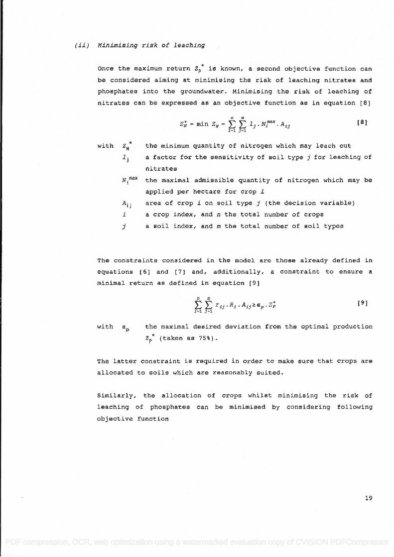
(ii) Minimi.sing risk of leaching

Once the maximum return Z is known, a second objective function can

be considered aiming at minimising the risk of leaching nitrates and

phosphates into the groundwater. Minimising the risk of leaching of

nitrates can be expressed as an objective function as in equation [8]

a in

Z, - min ZN l.N?'.A1 [81

with ZN* the minimum quantity of nitrogen which may leach out

li a factor for the sensitivity of soil type j for leaching of

nitrates

the maximal admissible quantity of nitrogen which may be


A1 area of crop i on soil type j (the decision variable)


j a soil index, and m the total number of soil types

The constraints considered in the model are those already defined in

equations [6) and [7] and, additionally, a constraint to ensure a

minimal return as defined in equation [9]

r1.R1.Aa9.Z [9]

with a the maximal desired deviation from the optimal production

zP* (taken as 75%).

The latter constraint is required in order to make sure that crops are

allocated to soils which are reasonably suited.

Similarly, the allocation of crops whilst minimising the risk of

leaching of phosphates can be minimised by considering following

obj ective function

19

(ii) ltininising risk ot Teaching

Once the maximum return Zr* Ls known, a second obJective function can

be considered aiming at minimising the riek of leaching nitrates and

phosphates into the groundwater. Minimieing the riEk of leaching ofnltratee can be expressed aE an objective function as in equation [8]

zi-minzn- .Au t81AD

E E 7t.Nfl-L J-L

with Zr*

7i

the minimum quantity of nitrogen whlch may leach out

a faetor for the sensitivity of soil type j for leachingnitrategthe maximal admisEible guantity of nitrogen which may

applied per hectare for crop iarea of crop i on soil type -Z (the decision variable)a crop index, and n the total number of crops

a soil index, and ra the total number of soil types

of

betri*'

Aijij

The constraints considered in the model are thoEe already defined lneguatione t6] and l7l and, additionally, a constraint to ensture a

minimal return as defined in eguation [9]

rtj.Ri.Aij>dn.Zi teI

optimal productionthe maximal desired deviation from thezr* {taken as 75t).

The latter constraint is regulred in order to make sure that crops are

allocated to soils which are reasonably euited.

Similarly, the allocation of crops whilst minimising the risk ofleaching of phosphates can be minimieed by considering followingobjective function

iil-t J-7

with op

19



n m

- min ZF - F. A. [10]

.1-1 3-1

with ZF the minimal quantity of phosphates which may leach out

fi a leaching factor for phosphates on soil type j

F1X the maximal admissible quantity of phosphates which may


(iii) Naximising return for given risk

The above described models enable to determine the minimal value (Zw and

ZF) for the risk of leaching nitrates and phosphates. In a third step

the optimal allocation of the crops is determined once more, using

equations [5J as objective function, and the equations [6] and [7] as

constraints, in addition to the constraints as defined by the equations

[11) and [12] to impose a maximal admissible risk for leaching.

n m

: Elj.Ni .Aii«N.z; [11] max

1-1 31

n m

: i t . F;ax.AIJF. z [12]

f-i j-i

with a and UF the maximal desired deviation from the optimal level

z; and ZF*.

In this exercise «i and OEF have been taken equal to one, but it is

conceivable to impose these equations as more stringent.

3.2.2 Used soil map and selected crops

A digitized soil map, prepared by Lenders and Heylen (1989) from the

1:20,000 map sheets 89E (Leuven), 90W (Lubbeek) and 90E (Glabbeek-

Zuurbemde) of the Belgian soil map, was used. The digital map

encompasses 67 different soil series according to the Belgian soil

classification system. The total area of each soil series can directly

be determined from this map, and subsequently used to set A' in the

LP models.

z| - mirl z, .Au T lOI

with Zr* the minimal guantity of phosphatee which may leach outt j a leaching factor for phosphateE on soiltype -Z

fi*' the maximal admissible quantity of phosphates which may


(iii) Ilaximising return for given risk

The above deecribed modele enable to determine the minimal value (Zn and

zrl for the risk of leaching nitrates and phosphates. In a third stepthe optimal allocation of the cropa is determined once more, ueingeguations [5J as objective function, and the equations t6] and [7] aE

constrainte, in addition to the conetraints ae defined by the eguatione

t1ll and [12] to impose a maximal admissible riek for leaching.

. Arr<u*. Zi1 t 111

' Arr<ay z| 112l

with ail and cF the maximal deeired deviation from the optimal levelz** and zr* .

In this exercise dil and at have been taken egual to one, but it isconceivable to impose these equations as more stringent.

3.2.2 Used soil map and selected cropE

A digitized soil map, prepared by Lenders and Heylen (1989) from the1:20rOOO map sheete 898 (Leuven), 90W (Lubbeek) and 908 (Glabbeek-

Zuurbemde) of the Belgian soil map, was used. The digital map

encompasEes 67 different soil Eeries according to the Belgian soilclaesification system. The total area of each soil seriee can directlybe determined from this map, and subseguently used to set Armx in theLP models.

- EE tt'4*

ii jt.N*,*t-t l-7

P E rt'F{n*

20



Lenders and Heylen (1989) established a crop/soil suitability table for

eight arable crops (wheat, barley, summer barley, oat, potatoes, sugar-

beet, fodder crops and fodder-beet), pasture land, orchards, Populus

sp. (poplar) and Pinus sp. This table io based on the data published

in the explanatory text of the Belgian soil map prepared by G. Scheys

and L. Bayens in 1957, 1959 and complemented with expert knowledge by

L. Bayens in 1989.

To limit the total number of decision variables (A1 in the LP model)

to a number lower than 300 (which is the maximum which can be handled

by the used LP software), soil series with an area smaller than one

hectare were disregarded as well as the units for urbanised and

disturbed areas. The study has been limited to five crops: wheat,

potato, sugar-beet, pasture and poplar plantations (Populus sp.),

resulting in 285 (5 x 57) decision variables to be considered in the LP

model. The crops were selected among those actually grown in the study

area and such that a wide range of agricultural characteristics are

covered in terms of farming practice and crop/soil requirements.

Crop/soil suitability ratings were related to the production reduction

factor as

lo-si- r- -

10 [13]

with s the given crop/soil suitability, a figure ranging from i

for the most suited, to 5 for the less suited soils

(Appendix 7.1.1, 7.2.2).

The area for each of the crops used in the LP model (Are), was taken

from Lenders and Heylen (1989) based on satellite imagery of 1987. The

retained areas for each crop are presented in Table 1, totalling to

1985 ha or 44% of the commune area.

21

Lenders and Heylen (1989) eetablished a crop/soil suitability table foreight arable crops (wheat, barley, summer barley, oat, potatoes, augar-beet, fodder cropE and fodder-beet), pasture land, orcharda, popuTus

Ep. lpoplar) and Pinus sp. This table iE based on the data publiehedin the explanatory text of the BeJ-gian soil map prepared by G. ScheyE

and L. BayenE in 1957, 1959 and complemented with expert knowledge by

L. Bayens in 1989.

To limit the total number of decision variables (A, In the LP model)

to a number lower than 300 (which iE the maximum which can be handled

by the used LP aoftware), soil seriee with an area gmaLler than one

hectare were disregarded as well aE the units for urbanieed and

disturbed areas. ?he etudy hag been limited to five erops! wheat,

potato, eugar-beet, paeture and poplar plantations (Populus Bp. ),resulting in 285 (5 x 57) decieion variablea to be coneidered in the LP

model. The crops were Eelected among those actually grolrn in the studyarea and euch that a wide range of agricultural characteristicE are

covered in terms of farming practice and erop/soil reguirements.Crop/soiJ- suitability ratingE were related to the production reductionfactor rij aE

with "i j

10-s;;-rr -16-

the given crop/Eoil suitability.for the moEt auited, to 5 for(Appendix 7.L.1, 7.2.21.

t 13l

a figure ranging from 1

the lees suited soils

The area for each of the cropsr used in the LP model (Aitq), was taken

from LenderE and Heylen (1989) based on satellite imagery of 1987. The

retained areaE for each crop are presented in Table 1, totalling to1985 ha or 44t of the commune area.

2t



Table i Area used in the LP model for the different crops

Crop Area (ha) I

Percentage

Wheat 476 24

Potato 439 22

sugar-beet 296 15

Pasture 560 28

Poplar 214 11

TOTAL 1985 100

3.2.3 Soil sensitivity for leaching of Nitrates and Phosphates

For the geographical information system BAGRAB, developed by Van

Orshoven et al. (1992a), parameters have been calculated to estimate

the water storage and phosphate fixing capacity. These have been

calculated for 5599 soil profiles - for which complete profile

descriptions and analytical data are available - and stored in a data

base. The values are grouped into four classes as shown in Table 2.

These class values were further used as leaching factors 1 for nitrates

and f for phosphates. A value of one corresponds with the highest

capacity, hence the lowest risk of leaching, reciprocally a value of

four corresponds to the lowest capacity, thus with the highest risk of

leaching (see Appendix 7.1.1, 7.2.2).

Table 2 Class limits for the water storing capacity and phosphate fixing capacity (adapted from Van Orshoven, et al. 1992a)

Nitrates

The sensitivity of the soils for leaching of nitrates - nitrate being

highly soluble in water and very mobile in the soil profile - is taken

as a function of the 'water storage capacity' of the soil. The water

22

Eable 1 Area used in the LP model for the different crops

Crop Area (ba) Percentage

WheatPotato

Sugar-beetPasturePoplar

476439296550214

2422152811

TOTAL 198s 100

3.2.3 SoiI geneitivity for leaching of Nitrateg and Phoephatee

For the qeographical information system BAGRAB, developed by Van

Orehoven et al. (1992a), parameters have been calculated to estimate

the water storage and phosphate fixing capacity. These have been

calculated for 5599 soil profiles - for which complete profiledescriptions and analytical data are available - and stored in a data

base. The valueE are grouped into four classes as shown in Table 2.

lhese class values were further used as leaching factors 1, for nitratesand f, for phosphates. A value of one corresponds with the highestcapacity, henee the lowest risk of leaching, reciprocally a value offour corresponds to the lowest capacity, thus with the highest risk of

leaching (see Appendix 7.1.1, 7.2.2r.

table 2 Clase limite for the water etoring capacity and phosphatefixing capacity (adapted from van orshoven, et al. 1992a)

NitratesThe eensitivity of the soils for leaching of nitrates - nitrate being

highty soluble in water and very mobile in the soil profile - is taken

as a funetion of the 'water storage capacity' of the soil. The water

CIass Water storage Capacity(nn)

Pbosphate Fixing Capacitylnol n/n2;

12

34

> ]-26.785.4 - 126.7s8.1 - 8s.4

< 58.1

> L17.773.5 - 1L7.746.8 - 73.6

< 46.8

22



storage capacity is defined as the amount of water which can be hold in

the soil profile above the groundwater table. It is calculated as the

difference in moisture content between field capacity and wilting point

of the layers above the groundwater according to Vereecken et al.

(1989). The average depth of the groundwater table is assessed from

the drainage class of the particular soil series.

Phosphates

The phosphate fixing capacity (PFC) of the unsaturated zone is

calculated as a function of the oxalate extractable iron and aluminium

content by equation as proposed by Breeuwsma et al. (1986).

PFC - O 4 * [Fe0 + Al 1 [141

As for the soils of Flanders figures for Fo0 and Al0 are only

fragmentarily available, these were estimated using regression

equations as proposed by Blume et al. (1969) for Fe0, and by Ross et

al. (1985) for Al0 as a function of the limonite (Fe203) content and for

the different horizons.

3.2.4 Economic parameters

In order to evaluate the performance of different crops on various

land-units, it is necessary to be able to compare them on a common

ground. Therefore, an economic parameter is introduced so as to

transform the production potential of the crops into a comparable unit,

in casti BEF/ha.

As an estimate of the economical return of the agricultural land (R

in the LP model), the three years average of the standard gross margin

for winter wheat, potato, sugar-beet and permanent pasture land were

used, as presented in Table 3. The Standard Gross Margin (SGM) of an

agricultural product is defined as the difference between the

standardized monetary value of gross production and the standardized

monetary value of certain special costs; at regional level, this

difference is determined for each type of production either per hectare

of utilized agricultural area for crops, or per head of livestock for

23

Btorage capacity is defined as the amount of water which can be hold inthe eoil profile above the groundwater table. It iE calculated ae thedifference in moisture content between field capacity and wilting pointof the layers above the groundwater according to Vereecken et al.(1989). The average depth of the groundwater table is assessed from

the drainage class of the particular eoil eeries.

Phosphates

The phosphate fixing capacity (Pf'C) of the unsaturatedcaleulated ae a function of the oxalate extractable iron and

content by equation aE propoaed by Breeuwsma et aI. (1985).

PFCeoc - 0.4*lrer*+ Alo*l

zone iealuminium

t 141

AE for the goils of Flanders figuree for F.o" and Afor. are onlyfnagmentarily availabler these vrere estimated using regresEion

equations as proposed by Blume et al. (1959) for .Feo*r and by Ross etal. (1985) for Aio, as a function of the limonite (Fe2o3) content and forthe different horizonE.


In order to evaluate the performance of different cropa on varioueland-units, it is neceesary to be able to compare them on a common

ground. Thereforer Erl economic parameter iE introduced so aE totranEform the production potential of the crope into a comparable unit,in casu BEF/ha.

AE an estimate of the economical return of the agricultural land (Rlj

in the LP model), the three years average of the etandard gross margin

for winter wheat, potato, eugar-beet and permanent pasture land were

ueed, aE presented in Table 3. The Standard eroEE Margin (SGl4) of an

agricultural product is defined a€r the difference between thestandardized monetary value of grosa production and the standardized

monetary value of certain special costs; at regional level, thisdifference is determined for each tlpe of production either per hectare

of utilized agricultural area for crops,, or per head of livestock for

23



animals (Van Hecke, 1993). SGM figures are based on farm account

analyses and are computed and published for all the regions of the

European Community. They are used for analyzing the farm structures in

the EC by enabling a typology of the farms.

Table 3 Standard Gross Margin of crops in Belgium (Source: LEI, 1989)

Standard Gross Margin (BEF/ha/year) _________

1985/86 1986/87 1987/88 Average Crop

Wheat (winter) 49500 55030 39640 48350

(summer) 34020 35850 35620 34970

Barley (winter) 41820 41340 33770 38910 (summer) 29410 28200 27950 28120

Oat 31060 31730 31120 31310

Maize (grain) 47940 36800 34740 40860 (fodder*) 40050 37300 36150 37850

Potato 46500 85750 42000 57900

Sugar beet 70730 76400 66810 69440

Fodder beet** 58600 60650 34750 47890

Pasture land(permanent) 36550 35350 32450 34800

(temporary) 45200 41600 41700 42900

Orchards 287400 281150 316900 295200 * "melk- of deegrijpe maïs" ** "voederhakvrucht"

Standard gross margin figures are not readily available for poplar

plantations. Moreover, the economy of forestry and tree plantations, is

not directly comparable to regular agricultural crops as it takes much

longer before the product can be harvested (e.g. at least 20 years for

poplar). As an estimate of the return (R1 in the LP model), an average

of the annuity was used, which is taken from an economical analysis of

two poplar varieties on five parcels (Table 4) done by Lambrechts

(1988). This author took a discount rate of six percent.

24

animals (Van Hecke, 1993). SGU figures are based on farm account

analyses and are computed and published for all the regions of theEuropean Community. They are ueed for analyzing the farm structures inthe Ec by enabling a typology of the farme.

fable 3 Standard croaa Margin of erops in Belgium(Source: LEIr 1989)

** "voederhakvrucht"

Standard gross margin figures are not readily available for poplarpl-antationa. l,toreover, the economy of foreetry and tree plantations, isnot directly eomparable to regular agricultural crops as it takes much

longer before the product ean be harvested (e.9. at least 20 years forpoplar). As an estimate of the return (R, in the LP model) r an average

of the annuity was used, which is taken from an economical analysis oftwo poplar varietieg on five parcela (Table 4) done by LambrechtB

(1988). This author took a discount rate of six percent.

Crop

Staadard Gross Margin(BEF/ba/year)

LeBsl86 L986187 LeeT 188 Average

Wheat (winter)( summer)

4950034020

ss0303s850

396403s520

483s034970

BarJ-ey (winter)( summer)

4L420294LO

4L34028200

3377027950

3891028L20

oat 31060 31730 31120 3 1310

Maize (grain)1 fodder* 1

47940400s0

3580037300

34740351sO

40850378s0

Potato 45sOO 85750 42000 57900

Sugar beet 70730 7 6400 66810 69440

Fodder beet** s8500 506s0 347 50 47890

Pasture land (permanent)(temporary)

3 6sso4s200

3s3s041500

3245041700

3480042900

Orchards 287400 2811s0 3 16900 29s200* me o eegrJ-lpe mals

24



Table 4 Net Present Value and annuity for two varieties of poplar (Populus sp.) (Source: Lambrechts, 1988)

Cultivar Parcel Net Present Value (BEF)

Annuity (BEF)

Beaupré S 52 223,674 20,373 S 56 304,336 26,533 S 60 374,998 32,694

Ghoy 140 206,388 17,993

170 259,869 22,657

AVERAGE II

24,050

3.2.5 Maximum allowable quantities for Nitrogen and Phosphorus

A decree (known as "het mestdecreet') published in the "Belgische

Staatsblad" in 1991 determines the admissible quantities of manure

which can be applied on the fields; it is defined in terms of maximum

quantities of nitrogen and phosphorous which may be applied:

N = 400 kg/ha/year

and P205 = 200 kg/ha/year for fodder maize or pasture land

or P205 = 150 kg/ha/year for other crops.

The decree further specifies that it is forbidden to apply any animal

manure on non-agricultural land. Therefore N and 2max for forest land,

in casu poplar plantations, have been taken zero.

3.2.6 Computation tools

All operations have been done on IBM compatible personal computers. The

linear programming software NICELP (Labadie, 1993) was utilized, which

makes use of the inverse revised simplex method. The GIS software

pcArc/Info 3.4D (ESRI, 1990) was used for treating the geographical

information towards maps. Calculations of parameters were done with a

spreadsheet programmes.

25

Cultivar Parcel Net Present Va1ue(BEr)

Annuity(BEB)

Beaupr6 S 52s56s60

223,574304, 335374,998

20,37325,53332,694

Ghoy 14O1_70

206, 388259,869

L7,99322,557

AVERAGE 24,O5O

fab].e 4

and PZOS

or PZOS

Net Present Value and(PopuJus sp. ) (Souree:

annuity for two varieties of poplarLambrechta, 1988 )

3.2.5 Maximum allowable quantities for Nitrogen and Phosphorus

A deeree (known aE "het mestdecreet"t published in the "BelgischeStaatsblad" in 1991 determines the admissible quantities of manure

which can be applied on the fields; it is defined in terms of maximum

guantitiee of nitrogen and phosphorous which may be applied:N = 400 kg/ha/year

= 2OO kg/ha/year for fodder maize or pasture land

= 150 kg/ha/year for other crops.

The decree further epecifies that it ie forbidden to apply any animal

manure on non-agricultural land. Therefore ilmx and Pmx for forest land,

in casu poplar plantatione, have been taketl zero.

3.2.6 Computation toolg

AIl operations have been done on IBU compatible personal eomputers. The

linear programming software NICELP (Labadie, 1993) was utilized, which

makes use of the inverse revised simplex method. The GIS software

pcArc/Info 3.4D (EsRI, 1990) was used for treating the geographical

information towardE mapa. Calculations of parameterg were done with a

spreadsheet programmes.

25



3.3 Results and Discussion

3.3.1 Optimal allocation of the land utilisation types

(i) Maximising return (Map 1.2)

The proposed optimal allocation for the five crops generating a maximal

return is illustrated in Map 1.2. This allocation represents a maximum

return level equal to 79,555 units(2). All crops are assigned to soils

for which they have a soil suitability ratings of 1 or 2 (Table 7). For

the arable crops this corresponds to the better drained loamy soils

(texture A, L and P, with drainage class b, c and d), while pasture

land and even more poplar plantations are assigned to the poorly

drained soils (drainage class c to h) . No crops are allocated to any of

the soil series with clay textures (E, U), nor to peat soils (V). Only

to a limited extend (18 ha) poplar has been allocated to soils with a

substratum (uLhc, gLca, sLhc and wLhc). Of the sandy soils, only one

small polygon (S.txd) is allocated to poplar. The crop allocation is

distributed over 19 soil units (see table i in Appendix 7.1.2, 7.2.3).

(ii) Minimizing risk of leaching of nitrates and phosphates

(Maps 1.3 and 1.4)

The LP output for the allocation of crops, while objective functions

are the minimisation of the risk of leaching of nitrates and

phosphates, contains the largest number of alternative solutions (see

±::.:__C Appendix ,7 ,Ï2, which makes it difficult to give a useful

interpretation to it in terms of land allocation. This results from the

fact that, the coefficients for the risk of leaching for nitrates and

phosphates (l arid f1 in the LP models) were only determined as a

function of the soil characteristics. The specific influence each crop

will likely have on the risk of leaching has been neglected. The only

divergence results from the values attributed to and F: 400 for the agricultural crops and zero for poplar as

jD1X, while for F1X 200

2 Although the figure is related to financial return, the obtained

value should not be expressed in monetary units as relative values (the

suitability ratings) were used in the computation.

26

t-l.3.hpc


3.3.1 Optimal allocation of the land utilisation types

(i) tlaximising return (Uap 1.2)

The proposed optimal allocation for the five cropa generating a maximal

return is illuetrated in Map 1.2. This allocation represente a maximum

return level egual to 79r555 units(2). A11 crope are aseigned to soilsfor which they have a soil suitability ratings of 1 or 2 (Table 7). For

the arable crops this corresponds to the better drained loamy soils(texture A, tr and P, with drainage claee b, c and d), while pasture

land and even more poplar plantations are asaigned to the poorlydrained soils (drainage class c to A). No crops are allocated to any ofthe soil series with clay texturea (8, Ul, nor to peat soils (v). only

to a limited extend (18 ha) poplar has been allocated to soils with a

substratum (uLhc, gLca, stric and wlhcl. Of the sandy soils, only one

gma1l polygon (sfxd) is allocated to poplar. The crop allocation isdistributed over 19 soil unite (see table j in Appendix 7.1.2, 7.2.31.

(ii) I{ininising risk of Teaching of nitrates and phosphates

(l.tapE 1.3 and 1.4 )

The LP output for the allocation of crops, while objective functionsare the minimisation of the risk of leaching of nitrates and

phosphates, containe the largest number of alternative solutions (Bee

Appendix }*{2, Z*Z*37 which makes it dif f icult to give a usefulinterpretation to it in terms of land allocation. Thie results from the

fact that, the coefficiente for the risk of leaching for nitrates and

phosphater {lj and f i in the LP models) r^rere only determined as a

function of the soil characteriEtics. The specific influence each crop

will likely have on the riek of leaching hag been neglected. The only

divergence resulte from the values attributed to llrmx and .Frmx: 40O forthe agricultural cropa and zero for poplar as rtmx, while for Fimx 2OO

2 atthoughvalue should not besuitability ratings)

the figure is related to financial return,expressed in monetary units as relative

were used in the computation.

the obtainedvalues (the

26



for pasture land, 150 for the arable crops and zero for poplar. The

minimum leaching values Z and Z are respectively 7084 and 5101. As,

according to the model, no nitrogen nor phosphates can be put on the

poplar plantations the reduced cost of allocating poplar is always

zero. Assigning a small, but non-zero, number to it might have yielded

a more useful solution.

(iii) Maximising return while minimising risk of groundwater pollution

(Map 1.5)

The optimal production level attained, while incorporating the

restrictions concerning leaching of nitrates and phosphates, is 66,948

units, which is about 80% of the initially computed maximal production

level. The crops are now distributed over 32 soil series. Compared to

the first solution there is thus a wider spread of the crops over the

various soil types.

Crops have to be allocated to soils which can be regarded as less

favourable from an agronomic point of view (e.g. with clay textures, or

with substratum in the upper part) to meet the imposed requirements. In

other words, from a crop/soil suitability point of view, crops could

not as ideally be assigned to each of the soils. The suitability

ratings are mostly ranging between i to 3, and pasture land has even

been assigned to soils for which it has suitability ratings of 4 and 5.

The latter is to soils with a higher nitrate storage and phosphate

fixing capacity. As farmers are allowed to apply more fertilizers and

manure on pasture land, the model indicates a trade-off between

suitability and minimising risk of pollution. The fact that more soils

with clay texture or clay sand substratum are to be used, is due to

their higher water retention capacity, hence to lower risks of leaching

of nitrates. How this shift takes place for some major soils series,

irrespectively of the crop, is represented in Table 5.

The changes in allocated area per soil series and for the various crops

is presented in Table 6.a and Table 6.b. The figures above the line

correspond to the allocated area without considering the constraints

for leaching, the figures below were obtained while considering the

risk of pollution.

27

for pasture land, 150 for the arable cropE and zero for poplar. ?he

minimum leaching varueg z* and zp are respectively 7o84 and 51o1. As,

according to the model, no nitrogen nor phoephateE can be put on thepoplar plantations the reduced coet of allocating poplar is alwaye

zero. Assigning a small, but non-zero, number to it might have yieldeda more useful solution.

(iii) llaximising return whiTe minimising risk of groundvater poTTution

(uap 1. 5 )

The optimal produetion level attained, while incorporating therestrictionE concerning leaching of nitratee and phosphates, is 66,948

units, which is about 80t of the initially computed maximal productionIevel. The crops are nov, diEtributed over 32 soil series. Compared tothe first solution there is thus a wider epread of the crops over thevarious soil types.

crops have to be allocated to soils which can be regarded as lessfavourable from an agronomic point of view (e.9. with clay texturee, orwith substratum in the upper part) to meet the imposed requirementE. fnother words, from a crop/soil suitability point of view, crops couldnot as ideally be aseigned to each of the soile. The suitabilityratings are mostly ranging between 1 to 3, and paeture land has even

been ageigned to soils for which it hag suitability ratinge of 4 and 5.

The latter is to soils with a higher nitrate storage and phosphate

fixing capacity. As farmers are allowed to apply more fertilizere and

manure on paeture Iand, the model indicates a trade-off between

Euitability and minimisinq risk of pollution. The fact that more eoilEwith clay texture or clay sand substratum are to be used, is due totheir higher water retention capacity, hence to lower rieks of leachingof nitrates. How this shift takes place for some major soils series,irrespectively of the crop, is represented in Table 5.

The changeE in allocated area per soil Eeries and for the various cropB

is presented in Tab1e 5.a and Table 5.b. The figureg above the linecorespond to the alloeated area without considering the constraintEfor leaching, the figures below were obtained while eonsidering therisk of pollution.

27



Table 5 Shifts over the allocated area for the major soil series without (A) and with (B) environmental constraint

Soil series A (ha) B (ha)

EDX - 92.3 Lbp 276 135

Lca 675 19

Lda 474 112

uLda - 118

wLca - 397 wLda - 141

A particular case is picked out illustrating the shift in soil types

for pasture land. In the solution without the environmental constraints

(i) most of the pasture land was assigned to soil series Lda (474.6 ha)

besides 83.7 ha to Ldp. In the final solution, with the environmental

constraints (ii), only 112.4 ha of pasture land is allocated to Lda

while 299 ha to Ldp. This can be attributed to the higher estimated

phosphate fixing capacity of the Ldp soil series (WSC = I and PFC = 1,

against 1 and 3 for Lda).

The remaining soils to which no crops are allocated to, are very poorly

drained loamy soils (e.g. Ala, Alp, Lfa), peat soils (V), soil

complexes with clays, barns and sands (ELZ and ULS) or less fertile

sandy soils as ZAfe, wZAfe. These areas are clearly the least

interesting for the considered agricultural uses.

28

Soil series A (ha) B (ha)

EDxLbpLcaLda

uLdasrLcawLda

276675

92.313s191t2118397141

fable 5 Shifte over thewithout (A) and

allocated area for the major Eoil serieswith (B) environmental conetraint

A particular case ie picked out illustrating the shift in soil typee

for pasture land. In the golution without the environmental constrainte(i) most of the pasture land was assigned to soil eeries Lda (474.5 ha)

besides 83.7 ha to Ldp. In the final solution, with the environmentalconstraints (ii), only 112.4 ha of pasture land is allocated to Lda

while 299 ha to Ldp. Thie can be attributed to the higher estimatedphosphate fixing capacity of the ldp eoil series (!{SC = 1 and PFC = 1,

againet 1 and 3 for Ldal.

The remaining soilE to which no crops are allocated to, are very poorlydrained loamy soils (e.9. Afa, Mp, Lfal , peat soils (Vl , soilcomplexes with clays, loams and sands (ELZ arrd ALSI or less fertilesandy soils as ZAfe, wZAfe. These areas are cLearly the leastinteresting for the considered agricultural uses.

28



Il

p,

I-

p,

o.

p,

p-

g

p,

i-.. a

Cf

p,

i...

:

Ql,.

CD

p,p,

I_.m Q

}-..

rl.

p'

:

p,

Q.

p,

-opi'-»

I-0

Il

00

rl-o

rf

::r:j

'-t

'IP'

p-"

I-..

'p

ww

mrn_0

o

.

o

Q.p,

*:

I-..

t-.

'...

û

'-.1-s-

p,0.

-roo

I-.-

rl- O -

s-.

p,

fable 5.a Changee in alLocated area for the varioug cropEr without (i)and with (ii) environrnental constraints (- no alloeation;0 posaible alternative; other figures indicate thealLocated area in ha)

29



SOIL

Ldp

Ldp

Ldp

LdpJ

j Lh

c Ji

P

ApT

S

fxdj

L6a

sLhc

uL

c.

ULh

G&

w

Ab8

w

Lba

wLc

c w

Lda

wLh

o

CR

OP

W

heat

S

gB P

otat

oPas

tur Pop

Popi. Pop.

none

S

gB

Pop

i. no

n.

Pop

i. no

n.

none

Ñ P

opLflS

none

j no

ne.

none

na

ne P

opi.

215.

3 0

0 83

.7

..:.... .

.

Ldp

Pas

ture

29

9 -

-

-

1.4

;;.;.

:

. ....

.

L.

Pas

ture

14

1 17

59

Lhc

Pop

i. 17

5.9

[ 12.5

.

..

.

Pas

ture

.

.

.

::.:...

12.51

-

.

PA

p P

otat

o .

24.5

..

..

.

PA

p P

astu

re

O . .

PA

p W

heat

O

11

.8

L::

:

flOflC

...

...::...

..

1

1.2

Slxd

Popi.

1.21

-

sIb

Potato

:

.

.

:

I

:

(i) a

lloca

ted

area

(ha

)

s

Wheat

.

01

..

with

out

envi

ronm

enta

l con

stra

ints

aLb

Pas

ture

.

OL _ -

sI.Ii

c P

opi.

6.71

UDx

..

Wheat

44.2

u

SgB

eet

.

O

UD

x P

aatu

re

.

.

o

-

uLca

P

astu

re

13.8

j -

uLda

Pas

ture

..

.

.

fl.:.

.

.

.

.

.

.

....

1184

1.

5

uLhc

P

opi.

i

.

i, uU

Dx

Pas

ture

.

.........

.

.

.

...

.

.

...

:

.

.

:

:

. .::

i

-

wA

bB

Pot

ato

4

wA

bB

Whe

at

O

wA

bB

SgB

eet

O

-

wt.Ax

Pas

ture

:

:

.:

.

.

.

.

..

.

.

...

.

.

1.81

-

wLb

a P

otat

o 69.8

wLb

a W

heat

O

wLb

a S

gBee

t (j':) al

loca

ted

area

(ha)

O

wLb

a P

astu

re

with

env

ironm

enta

l con

stra

ints

o

wLcs

Pot

ato

286.

wL.oe

SgB

eet

92.5

wI.ca

Whe

at

18.5

wLca

Pas

ture

..

O

wLc

c P

otat

o O

wLc

c W

heat

O

wLc

c P

astu

re

O

wLc

c S

gBee

t 3.

9 -

wLda

Whe

at

141.Lj7

wLh

c Popi.

1.7

'.3

t»

a'

p, O) û

'.-

I-.

Qpi

Orj

:i

n o

Q

p'

(D

ç'.W

t»

,-..

Qtr

-

p-. -.

,

(D

':

pl

'1-

w Wp

I-

,-.

l-s.

fl,<

I-..

(D

. Q,

p, O

- r

I

p,

.

,1

.-

(D

(D

: cl-

p-JO

I__O

I1

n o

rl.

(D

Q.

»(D

t

pl,

I-..

l.a.

Q tO

h

ra

wI o

-

o

O.w

*:

I..-

i.-.

i...

n

(trt

I-.-

(-to.-

:-

(D -.

Iable 6.b Changes in allocated area for the varioue crops without (i)and wi-th (ii) environrnentaL constraints (- no allocation;0 possible alternative; other figurea indicate theallocated area in ha) [continued]

EJi

iiB

f;ii?o(,Ji

ao0-Iit':EipiE

otroc

N

:iXXIirX*fir**tXIt

iiiliiiiiilr.j.filliiiliiiil(oo o oo(o

i:E*ii:iaitii

iii#iiiliiilii#i::i:iiii::::

iiiiiiiiiiiiiiiiiiiiii

&.\e

l,:i::i,i:::i.,i.i.,::.::::.,. :: .:..:.,::::.: -

iil:Iii.liiii!::i!:i,.i:rt.i,.,:ir ,i::.,,..:,,.::..':..:::i...i::::::::,::::::::::: A ":1:i.':..

RI

a"clii|i!i!:!!:i:i:::!!;:1::::::::::.,..,:

r;::!:::::ii:iri!:ji!riri:iiiiiiii,jjii;iir;iiiiiriii:.,::,,.- ...:.::.:i +i t: ':. B O il;ii:.:r.r,:lili.iii...i:ii:iiliiiii:ii:iiiii:ilir;ii:'':';:::''r,:..:::i:':l; .:i.. ,:.j, E .rt' i!::::::.'

!d6s:i::i:::::::jj:::::::|:|::::::::|l::||:||:,|::|-] w A |:,iiliiiiiliiil+iIii;IiI;iii':i::i:iiii.,"' 1-:::r::::;':::,i:..,:,i;i:::;:i (I :l :+:: : :

iti:i:ri:ir:ruiliiiiii::r,r::r,, :, ,i ! ,:,i::,,,;i:i.i::i,;ii;iii O =:.::i.::;

iiil::,i,;ii:;jr,;,;:i , ' :: ,, .;i :ii.i::'iii::i,:iili:i:::i::::i:i: E 'S:llillllii

u?lu?

-tF

.lt-t-I

I

'ln? o o,,,,,,ItltN ,:::I

l:,1:,,:l:,,,.. : .,. t{t,:irrrr;;r,rr;rN,t 6*;

ollol ,,.:,,,i,to1t.,!,,i!!!!!!NIN!!!!!!!i!:-l-:"::

,i,r...::+liC:r,;i,iii.:;ili!!!!i,-l-: :!:!:::i::

l-l '::;:r,::,;, .:.,,

dl .,,,',,i,, :: ,r

lol ',,,, ,,,:,:,r

I I !ii!:!ii!: i

lol ' '. ,,:::::,.:

'lqiii:;i;'lgl r,:,

lor:b b,: ,,,..,,,..

l!+.:!::::::::!:!ii:i ::ii;i:..l.t!!!!!!!!l!:ri:::il rll::::!i

iiiiiiiiiii*tiiixi" i::i:ri: : : : : : : : : : : : : : : :::: i:: : ! :

j::: j: : : i ; i | : i i

j

:i::llii:*-l- lliiiii;

iii:iiiiiiiii:iiiiii:iiiiiii:iiiiiii:::i:

l;1::,i;;,:ii:i::::i:::;!i:ii iXiiiiiii

iiiiiixiiXi'-::i:ir :i:iii:ii::::i!:riulu::i::::::::iliiiiiii: illiliiiri:iiiiiiii i I i :i::::::l:

:i:i:xi::iii::riii:::::iii ii:i:i::ii

lrir;lirtilii:r,ii;iriiiiii t:,1'tttt:t:t'::

::u:,::::ta::t:::ii::t::iiiii iiiii::ii:

i:i;iiiiii::::::i::::iiiii::i ;:ri!:ir:;

rii:'ii:i:::ii:f:i:i:;:iii.i

*ii:iiil

::il' -:;::r iiiiiiiliii.xffi ffi

:li:;*::ifi:?i==:: i:i;Xiiii

:::i::::::ij:il:iiii:i]::ii ii;:i::ii|

:;i:iiii:ii:i:i::il:il::::i:l :::: i: ii i:

iriirii!:;i:::!!!!;:i:!:ii;il iliii\ta::a

****i iiii-

!S

i::iiiirliiiiiilii:iii;;:;i:iiili

iiiiiiilxiii:ixiiiiiir*iiiiiliii:i---" rJ'\l(oI

I'ur::'o-o.l:;rG':::'::':! i,::,!I |tl,::!,rli:,,;!i:!iiiii:

i:i::::iiiixiiiixiiiiiiiii:iiiil

::;i:;;:ri;;;i;:iii:ii:Iiiiiii:::]i:::i:::iiiiiiiiiiiiiiiiii:iiXi

iiiiiiiiititii:;ii::i:ii:iitiit:::a

,i:::r:iri;;::i:::iiiiii::i:i1

:iii::iiiiil!!!;!!iiiiii!;::llli::

i::];;::i i11iii:iiir;iiiiiiiii

;:.-i-iliiillii:xi:iiiiiii:ii::iiiiiii:iiiiriiiiii

ii::iiiiiliii::riiliii.il

l.i:ii..ri**'.:!::::i::!:::::i::;i::it:::ii:i::ia

riii:iillr::i::r:ii::iiiiiixil

*tr.r.,...,;i,i

*#ffi

]ilii:ii:

:i:::::i:::

iEa;:'iiiii &.ll!ii.i: .\lllll:.. tr!:::! \

!iir!!!i! gl\iririiiiii O:;i!:!i!!!. $

.:.iiii.:,: G.E:,,i..i S C::t::::.!!,:,,;' B triiliii::i: O

=\\..,,,,, u.Siiiiiii::ii O

=illliillll G 0)ii!;:,,:., q)

-,:.:;:,,::: o t::li;iriiii E S,,., s:tat:i::a

iiitiiilii

i:i:ii:iiii;iIiii;i:

1t:tltlitl

ii:li:::::

iiiilili

::':.*

t::talil:t:

:,,r,,tt

;iii;i::i::

::iiii::::i

;,:,::t;:tt

------;G:;:;

rlool cJt6ilc

Dl r

EIE

53

e5I

E!a

o(0.

a€

Eoo.

Eoo-

oor-

up

oeoc

ocoE

ac EoD.

ol:5lE

losl€Jlt

loo.l !t!l c

'luol!cl;-llli

E,$F$,8;i Ed'll{&r E& 3 =,,,I,, itl:*ii, i!:i:ir illii: :il

,,,:E E ;,...F,':,.6,..,i.. g':'o = =:1o:o: I. :,fEd*@.,IElllE,,o:l r+"r.(*:f,,Li:=iiii::iii:E: ::!i::iiii+:itniii

:';,g g 6 5.,,r=':6oo::r

ioEef'#;:: :}1;i :i

!€T E S.:

iEf tsEii:ii i:

I5:8,,,,99E E6,Ez

ia,$g$gEpS_'P

o<d

EBTBi<<<!. o- o- o-

iI,,rl:ta.l.i!iril.:C- (,:i;trl:l:E:;,I... !,Iii:1€*r;# 4jGl,oii O., qI'::ir+!:i { lii::5:':5: JD,:;l-:;!t e !IEii+i!l!!:!!-! J

iili!::r::i:rii:i*::i:i

I O,::i

t5If 5t?

@@61.(l -O !:i<<<;] M:i

o o 0 e::-o -o , !:iJJ J J:1i i 3 iii

ai:.!ltJ+JilxrirF

i.. s.: Iii:J!l

I O O C, (,.r:O (, (, O,I.:J J J J':i, . . 3 .,1



3.3.2 Interpretation of the LP output

(i) Allocation of the crops

The LP models determine an optimal allocation of the crops over the

different soil units. However, in most cases the proposed solutions do

not lead to a uniquely defined allocation.

This is firstly a consequence of the fact that the total area of each

soil series has been designed as a "demand node" in the LP model,

rather than individual polygons. This is inevitable as the digital soil

map contains 1140 polygons, representing 67 soil series. Using each

polygon as a decision variable would have resulted in a prohibitive

large number of decision variables and constraints, put aside whether

it would be feasible to define relevant constraints to each polygon.

How to distribute a specific crop over the different polygons of one

soil series, in the case where only a fraction of the total area of

that series is required, remains undetermined. Additional constraints

have to be defined if more precise allocation is desired (e.g. minimal

distance to farm, or to a type of road,...).

Secondly, the LP model offers a large number of alternative solutions

between soil series - besides some degenerated solutions. These two

points are illustrated with part of the output determining the crop

allocation for a maximal return (Table 7). All decision variables with

a reduced cost equal to zero are presented in the table. It can be seen

that the solution does not allocate any crop to e.g. soil series Lba,

however the reduced cost for wheat, potato and sugar-beet is zero.

Assigning any of these crops to that soil unit will yield the same

solution and thus offers a perfect alternative. Similarly, the reduced

cost (opportunity cost) for allocating wheat, potato, and sugar-beet to

soil series Lda is also zero. However, all the available area of Lda

has to be allocated to pasture land if the requirement of covering 560

ha of pasture land has to be met. This solution is therefore

degenerated. Related to the first mentioned problem, it can be seen

from the table that the LP model proposes to allocate 28.1 ha of potato

and 248.5 ha of sugar-beets to the Lbp soil series, of which 427.9 ha

is available.

31

3.3.2 Interpretation of the LP output

(i) ATTocation ot the crops

The LP modeLs determine an optimal allocation of the crope over thedifferent soil units. However, in moet cagee the proposed solutione do

not lead to a uniguely defined al-location.

thie is firstly a coneequence of the fact that the total area of each

soil gerieg hag been designed as a "demand node" in the LP model,

rather than individual polygons. Thie ie inevitable as the digital soilmap containe 114O polygJons, representing 57 eoil series. Using each

polygon as a decision variable would have resulted in a prohibitivelarge number of decision variables and constraints, put aside whether

it would be feasible to define relevant conetrainte to each polygon.

How to dietribute a specific crop over the different polygons of one

soil Eeries, in the case where only a fraction of the total area ofthat series is reguired, remainE undetermined. Additional constraintshave to be defined if more precise allocation is desired (e.9. minimal

distance to farm, or to a type of roadr... ).

Secondly, the LP model offers a large number of alternative Eolutionsbetween soil series - besidee Eome degenerated solutions. These two

pointe are illuEtrated with part of the output determining the crop

allocation for a maximal return (table 7). A11 decieion variableg witha reduced cost equal to zero are presented in the table. rt can be seen

that the eolution does not allocate any crop to e.g. soil seriea Lba,

however the reduced cost for wheat, potato and sugar-beet is zeto.Assigning any of these cropE to that eoil unit will yield the same

solution and thus offers a perfect alternative. Similarly, the reduced

coet (opportunity cost) for allocating wheat, potato, and sugar-beet tosoil series Lda is also zero. However, all the available area of .Eda

hae to be allocated to pasture land if the reguirement of covering 550

ha of pasture land hae to be met. This solution is thereforedegenerated. Related to the first mentioned problem, it can be seen

from the table that the LP model propoEes to allocate 28.1 ha of potatoand 248.5 ha of sugar-beets to the.&bp soil eeries, of which 427.9 ha

is avaiLable.

31



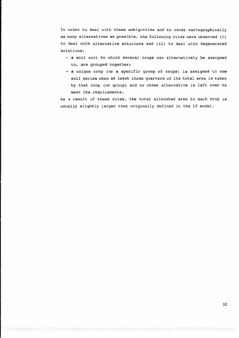
In order to deal with these ambiguities and to cover cartographically

a8 many alternatives as possible, the following rules were observed (i)

to deal with alternative solutions and (ii) to deal with degenerated

solutions:

- a soil unit to which several crops can alternatively be assigned

to, are grouped together;

- a unique crop (or a specific group of crops) is assigned to one

soil series when at least three quarters of its total area is taken

by that crop (or group) and no other alternative is left over to

meet the requirements.

As a result of these rules, the total allocated area to each crop is

usually slightly larger then originally defined in the LP model.

32

In order to deal with these ambiguities and to cover cartographicallyaa many alternatives aE possible, the following ru1eE were observed (i)to deal with alternative solutions and (ii) to deal with degenerated

Eolutiona 3

- a soil unit to which geveral crops can alternatively be assigned

to, are grouped together;- a unique crop (or a epecific group of erops) is aseigned to one

soil series when at least three guartere of ite total area ig takenby that crop (or group) and no other alternative is left over tomeet the requirements.

As a result of these rules, the total allocated area to each crop isusually slightly larger then originally defined in the LP model.

32



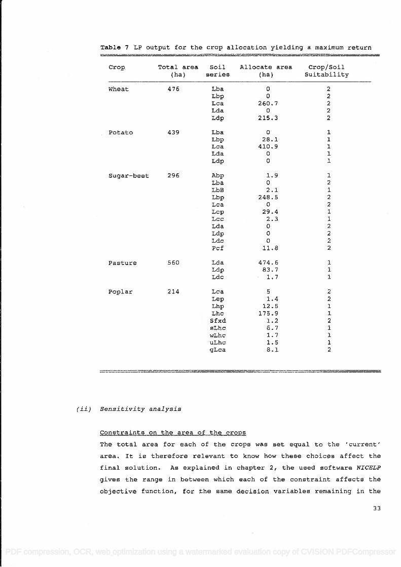
Table 7 LP output for the crop allocation yielding a maximum return

Crop Total area Soil Allocate area Crop/Soil (ha) series (ha) Suitability

Wheat 476 Lba 0 2

Lbp 0 2

Lca 260.7 2

Lda 0 2

Ldp 215.3 2

Potato 439 Lba 0 1

Lbp 28.1 1

Lca 410.9 1

Lda O i

Ldp 0 1

Sugar-beet 296 Abp 1.9 1

Lba 0 2

LbB 2.1 1

Lbp 248.5 2

Lca 0 2

Lcp 29.4 1

Lcc 2.3 1

Lda 0 2

Ldp 0 2

Ldc 0 2

Pcf 11.8 2

Pasture 560 Lda 474.6 1

Ldp 83.7 1

Ldc 1.7 1

Poplar 214 Lca 5 2

Lep 1.4 2

Lhp 12.5 1

Lhc 175.9 1

Sfxd 1.2 2

sLhc 6.7 1

wLhc 1.7 1

uLhc 1.5 1

gLca 8.1 2

(ii) Sensitivity analysis

Constraints on the area of the crops

The total area for each of the crops was set equal to the 'current'

area. It is therefore relevant to know how these choices affect the

final solution. As explained in chapter 2, the used software NICELP

gives the range in between which each of the constraint affects the

objective function, for the same decision variables remaining in the

33

fable 7 LP output for the crop allocation yielding a maximum return

Crop ?otal area Soil(ha) eeriee

Allocate area Crop/Soil(ha) Suitability

Wheat 475

Potato 439

Sugar-beet 296

Pasture s60

Poplar 214

LbaLbpLcaLdaLdP

LbaLbpLcaLdaLdp

AbpLbaLbBLbpLcaLcPLccLdaLdpLdcPcf

LdaLdpLdc

LcaLepLhpLhcSfxdsLhcwLhcul,hcgLca

00

260 "70

21s.3

028.1

410.900

1.9o2.L

248.50

29.42.3000

11. 8

47 4.583. 71.7

5L.4

12.s175.9

t.z6.71.71.58.1

22222

11111

12122112222

(ii) Sensitivity analysis

Constraints on the area of the crops

The total area for each of the crope was set equal to the 'current'area. It ie therefore relevant to know how these choices affect thefinal solution. As explained in chapter 2, the used software NICELP

gives the range in between which each of the constraint affects theobjective funetion, for the same decision variables remaining in the

33



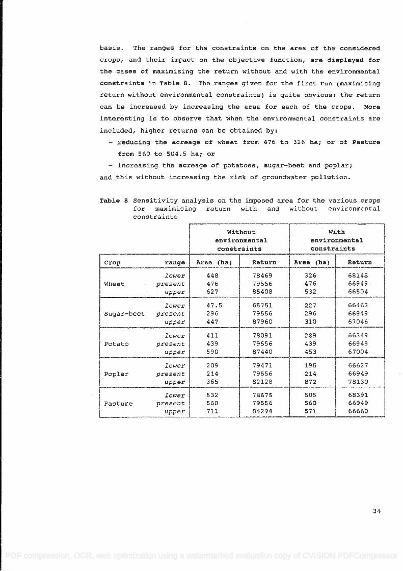
basis. The ranges for the constraints on the area of the considered

crops, and their impact on the objective function, are displayed for

the cases of maximising the return without and with the environmental

constraints in Table 8. The ranges given for the first run (maximising

return without environmental constraints) is quite obvious: the return

can be increased by increasing the area for each of the crops. More

interesting is to observe that when the environmental constraints are

included, higher returns can be obtained by:

- reducing the acreage of wheat from 476 to 326 ha; or of Pasture

from 560 to 504.5 ha; or

- increasing the acreage of potatoes, sugar-beet and poplar;

and this without increasing the risk of groundwater pollution.

Table 8 Sensitivity analysis on the imposed area for the various crops for maximising return with and without environmental c on st rams

Without With environmental environmental constraints constraints

Crop range Area (ha) Return Area (ha) Return

lower 448 78469 326 68148

Wheat present 476 79556 476 66949

upper 627 85408 532 66504

lower 47.5 65751 227 66463

Sugar-beet present 296 79556 296 66949

upper 447 87960 310 67046

lower 411 78091 289 66349

Potato present 439 79556 439 66949

upper 590 87440 453 67004

lower 209 79471 195 66627

Poplar present 214 79556 214 66949

upper 365 82128 872 78130

lower 532 78675 505 68391

Pasture present 560 79556 560 66949

upper 711 84294 571 66660

34

basis. The ranges for the constraints on the area of the eonsidered

cropa, and their impact on the objective function, are displayed forthe caeeg of maximising the return without and with the environmentaleonstraints in Table 8. The ranges given for the first run (maxi.rnieing

return without environmental constrainte) ia quite obvious: the returncan be increased by increasing the area for each of the crops. More

interesting is to observe that when the environmental constraints are

included, higher returns can be obtained by:

- reducing the acreage of wheat from 476 to 326 ha; or of Pasture

from 55O to 504.5 hai or

- increasing the acreage of potatoes, sugar-beet and poplar;and this without increasing the risk of groundwater pollution.

fable 8 Sensitivity analyeie on the imposed area for the various cropsfor maximising return with and without environmentalconstraints

Withoutenvironmentalconstraints

witheavironmentalconstraints

Crop rattge Area (ha) Retura Area (ha) Retura

TowerWheat present

upper

448476627

7846979is68s408

326476532

681486694966sO4

lowerSugar-beet present

upper

47 .5296447

557517955687960

227296310

664636694967046

lowerPotato present

upper

4Lt439s90

78091795568?444

2894394s3

663496694967004

TowerPoplar present

upper

2092L435s

794777955682L28

19s2t4872

665276594978130

TowerPasture present

upper

532560711

786757955584294

50556057L

583916694966660

34



Constraints on minimal return

Further, the sensitivity analysie for the model seeking to minimise the

risk of leaching indicates a positive slack value (a surplus) for the

production constraint equal to 8398 in the case of minimising the risk

of leaching of nitrates, and 1032 in the case of minimising the risk

phosphates leaching (see Appendix 7.1.3.B and 7.1.3.C). This means

that, all other constraints remaining constant (i.e. the requirements

for area) a higher return than the minimal imposed level of 75% can be

obtained, in other words the constraint for the return is not binding.

Hence, the risk of leaching can only be reduced by reducing the acreage

of the crops. From the foregoing it is not surprising that when

maximising the return with the environmental constraints, a higher

value is obtained than the 75% imposed in the two previous runs.

Constraint on the area of the soils

As the area of a particular soil type within the commune cannot be

increased, the sensitivity analysis of these constraints seems only

meaningful when looking how reducing the area of a particular soil type

will affect the solution. Evidently, whenever any change in the

availability of land (soil series) is introduced - e.g. by developing

a retention reservoir - this information can be useful to assess the

possible impact on the final outcome. Particularly for the soils which

are used to their available extend, it is worth to know which of them

are the most valuable.

This information can be deduced from the dual variables3 of the

constraints determining the area of each soil series. The larger the

dual variable, the larger the impact will be on the objective function.

E In Table 9,Tb1e-6the soil series are sorted with decreasing dual variable. It is thus possible to rank the soils in terms of 'quality'

for the imposed problem: for the considered crops and environmental

limitations. It should be kept in mind that soils which are in surplus

are not included (increasing their acreage will obviously not have any

effect on the objective function). This is for instance the case for

soils series Lba which provide an alternative solution for the

3 see p.12 for the definition of the dual variable

35

x

Constraints on minimal returnFurther, the sensitivity analysis for the model seeking to minimiee therisk of leaching indicateE a positive elack value (a surplus) for theproduction constraint egual to 8398 in the case of minimising the riekof leaching of nitrates, and 1O32 in the case of minimiging the riskphosphates leaching (see Appendix 7.1.3.8 and 7.1.3.C). This means

that, all other constrainte remaining constant (i.e. the reguirementg

for area) a higher return than the minimal imposed leve1 of 75t can be

obtained, in other words the constraint for the return is not binding.Hence, the risk of leaching can only be reduced by redueing the aereage

of the crops. From the foregoing it is not surprieing that when

maximieing the return with the environmental constrainte, a highervalue is obtained than the 758 imposed in the two previouE runE.

Constraint on the area of the soilsAB the area of a partieular eoil- type within the cornmune cannot be

increased, the sensitivity analyeis of theee constraints seems onlymeaningful when looking how reducing the area of a partieular eoil type

will affect the solution. Evidently, whenever any change in theavailability of J.and (soil eeriee) is introduced - e.g. by developing

a retention reservoir - thie information can be useful to assesg theposeibJ-e impact on the final outcome. Particularly for the soils which

are uEed to their available extend, it is worth to know which of them

are the most valuable.

This information can be deduced from the dual variables3 of theconstraints determining the area of each soil series. The larger thedual variable, the larger the impaet will be on the objective function.In Table 9, -\lfuvl€ the soil series are sorted with decreasing dual

variable. It ig thus poesible to rank the soils in terms of 'guality'for the imposed problem: for the considered crops and environmental

Iimitations. It should be kept in mind that soils which are in surplue

are not included (increasing their acreage will obviously not have any

effect on the objective function). This is for inetance the case forsoilg series Lba which provide an alternative solution for the

aee p. L2 for the definition of the dual variable

35



allocation of wheat, sugar-beet and/or potato, but which are not

required to meet the demanded acreage of the crops.

Table 9 Ranking of the soils according to the dual variables for the maximisation problems

Without environmental constraints

With environmental constraints

Soil series Dual Variable Soil series Dual Variable

Abp 6.95 Lcp 34

LbB 6.95 Ldp 32

Lcp 6.95 uLca 25

Lcc 6.95 uLda 22

Lep 2 Abp 22

Lhp 2 LbB 22

sLhc 2 Lcc 20 wLhc 2 Lep 16

uLhc 2 Lba 9

sLba 9

wAbB 9

wLba 9

wLca 9

wLcc 9

wLda 9

gLba 9

gLbc 9

uUDx 6

Lhp 4

sLhc 2

wLhc 2

wLAx 2

uLhc 2

allocation of wheat, sugar-beet and/or potato, but which are notreguired to meet the demanded acreage of the crops.

Table 9 Ranking of the eoilg according to the dual variableg for themaximisation problems

llitbout euviroameotalcoastraiutE

?fith environmeatal constraints

Soil series DuaI Variable Soil series Dual Variable

AbpLbBLcpLceLepLhpeLhcwLhcuLhc

6.9s6.955.955.95222

2

2

LcPLdpul,cauLdaAbpLbBLccLepLbasLbawAbBwl,bawLcaI^tLCC

wLdagl.bagLbcuUDxLhpsLhcwLhcwLAxuLhc

343225222222201699999999954222

2

35



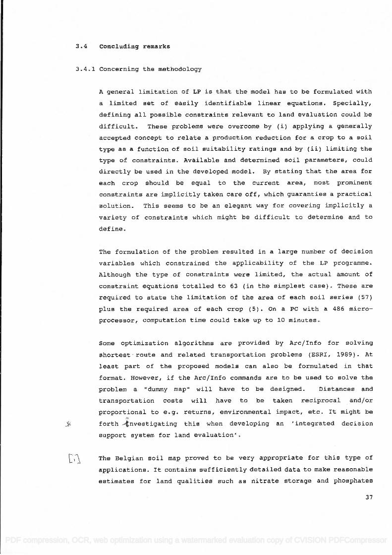
3.4 Concluding remarks

3.4.1 Concerning the methodology

A general limitation of LP is that the model has to be formulated with

a limited set of easily identifiable linear equations. Specially,

defining all possible constraints relevant to land evaluation could be

difficult. These problems were overcome by (i) applying a generally

accepted concept to relate a production reduction for a crop to a soil

type as a function of soil suitability ratings and by (ii) limiting the

type of constraints. Available and determined soil parameters, could

directly be used in the developed model. By stating that the area for

each crop should be equal to the current area, most prominent

constraints are implicitly taken care off, which guaranties a practical

solution. This seems to be an elegant way for covering implicitly a

variety of constraints which might be difficult to determine and to

define.

The formulation of the problem resulted in a large number of decision

variables which constrained the applicability of the LP programme.

Although the type of constraints were limited, the actual amount of

constraint equations totalled to 63 (in the simplest case). These are

required to state the limitation of the area of each soil series (57)

plus the required area of each crop (5). On a PC with a 486 micro-

processor, computation time could take up to lO minutes.

Some optimization algorithms are provided by Arc/Info for solving

shortest route and related transportation problems (ESRI, 1989). At

least part of the proposed models can also be formulated in that

format. However, if the Arc/Info commands are to be used to solve the

problem a "dummy map" will have to be designed. Distances and

transportation costs will have to be taken reciprocal and/or

proportional to e.g. returns, environmental impact, etc. It might be

forth -nvestigating this when developing an 'integrated decision

support system for land evaluation'.

The Belgian soil map proved to be very appropriate for this type of

applications. It contains sufficiently detailed data to make reasonable

estimates for land qualities such as nitrate storage and phosphates

37

3.4

3.4. 1

Coacluding reuarks

Concerning the methodology

A general lirnitation of LP is that the model hae to be formulated witha limited Bet of eaeily identifiable linear equations. Specially,defining aII possible conetraints relevant to land evaluation could be

difficult. TheEe problems were overcome by (i) applying a generallyaccepted concept to relate a production reduction for a crop to a soiltype ae a function of Eoil Euitability ratinge and by (ii) limiting thetype of conetraints. AvaiLable and determined soil parameters, could

directly be uged in the developed model. By etating that the area foreach crop should be equal to the current area, most prominent

constrainte are implicitly taken care off, which guaranties a practicalEoLution. ThiE seems to be an elegant way for covering implicitly a

variety of constraintE whieh might be difficult to determine and todefine.

The formulation of the problem resulted in a large number of decision

variables which constrained the applicability of the LP programme.

Although the type of constraints were limited, the actual amount ofconstraint eguations totalled to 63 (in the simplest case). These are

required to state the limitation of the area of each soil series (57)

plus the required area of each crop (5). On a PC with a 486 micro-processor, computation time could take up to 1O minutes.

Some optimization algorithmE, are provided by Arc/Info for solvingshortest route and related transportation problems (ESRI, 1989). At

least part of the propoaed modelE can also be formulated in thatformat. Ilowever, if the Arc/Info commande are to be used to solve theproblem a "dummy map" will have to be deeigned. Distances and

transportation cogts will have to be taken reciprocal and/or

proportional to e.g. returns, environmental impact, etc. It might betu

forth -finvestigating this when developing an 'integrated deeision

support system for land evaluation'.

The Belgian soil map proved to be very appropriate for this type ofapplications. ft contains sufficiently detailed data to make reasonable

estimateE for land qualities Euch aE nitrate storage and phosphatee

*

t,l

37



fixing capacities (although specially for the latter, methods can still

be improved) and it has the advantage that crop/soil suitability

ratings are known for the major crops on most of the soil series.

3.4.2 Concerning the output

It should be noted that the proposed land allocation maps do not cover

all possible alternative optima, though it was attempted to cover them

as widely as possible. This is particularly the case for Map 1.3 and

Map 1.4, where the LP solution offered the largest number of

alternatives. It should also be kept in mind that in the cases where

only part of a particular soil type had to be assigned to a particular

land utilization type, the whole area has been tagged. Therefore Map

1.2 and Map 1.5 rather indicate where a particular crop has a

comparative advantage over other crops.

A large number of alternative solutions were obtained. By considering

the problem on an individual farm scale, it would have been feasible to

identify additional constraints to determine more precise allocations.

By doing the exercise ori the scale of a commune, a general evaluation

of potential optimal land use allocations was possible. The obtained

solutions can be useful for further land-use planning, by allowing the

identification of areas where particular crops have a comparative

advantage over others. This could be useful in land consolidation

projects. From the sensitivity analysis, the impact of taking land out

of use can be assessed. This can be relevant when e.g. land has to be

taken out of production for building roads, retention reservoirs, etc.

The strategy suggested by the LP models, to minimise the risk of

leaching of nitrates and phosphates, seems to spread the different

crops over a wider range of soil types to maintain a minimum production

level while minimising risk of leaching. Henceforth, part of the crops

are allocated to less favourable soils but with lower risks of nitrate

and phosphate leaching.

The maximum level for phosphates which may be applied is, especially

for livestock farmers, usually more a limiting factor then the maximum

level for nitrates. This is a consequence of the rather high levels

38

fixing capacitiesbe improved) and

ratings are known

(although specially for the latter, methodE can stillit hag the advantage that crop/soil suitability

for the major crops on most of the soil seriee.

3.4.2 Concerning the output

It should be noted that the proposed land allocation maps do not cover

all possible alternative optima, though it wag attempted to cover them

as wideLy as possible. This is particularly the case for Map 1.3 and

Uap t.4, vrhere the LP solution offered the largest number ofalternatives. It should also be kept in mind that in the caaes where

only part of a particular eoil type had to be aseigned to a partieularland utilization type, the whole area hae been tagged. Therefore Map

L.2 and uap 1.5 rather indicate where a particuJ-ar crop has a

eomparative advantage over other cropE.

A large number of alternative eolutions were obtained. By consideringthe problem on an individual farm sca1e, it would have been feasible toidentify additional conetraints to determine more precise allocations.By doing the exercige on the Eeale of a commune, a general evaluationof potential optimal land use allocations was possible. The obtainedsolutions can be useful for further land-use plannin9, by allowing theidentification of areas where particular crops have a comparativeadvantage over others. This could be useful- in land consolidationprojects. From the sensitivity analysis, the impact of taklng land outof use can be asgeeEed. This can be relevant when e.g. Iand has to be

taken out of production for building roads, retention reservoirs, etc.

The strategy suggested by the LP models, to minimise the risk ofleaching of nitratee and phosphates, seemE to spread the differentcrops over a wider range of soiL types to maintain a minimum productionlevel while minimiging risk of leaching. llenceforth, part of the crops

are allocated to lesg favourable goils but with lower risks of nitrateand phosphate leaching.

The maximum level for phoephates which may be applied is, especiallyfor livestock farmera, uEually more a limiting factor then the maximum

level for nitratee. This is a conseguence of the rather high levelE

38



which are legally tolerated for nitrates and, is of course, also a

function of the nitrate and phosphate ratio of the manures. In the LP

model however, nitrate and phosphate leaching were both binding constraints.

39

which are legally tolerated for nitrates and, is of course, also a

function of the nitrate and phoaphate ratio of the manurea. In the LP

model however, nitrate and phosphate leaching r^rere both bindingconetraints.

39



4 Combining LP and GIS for land evaluation on a regional

scale: the region of Madrid (Spain) as a case study


In the preceding chapter, the application of LP and GIS as tools for

land evaluation on a local scale (commune) was investigated for which

detailed soil maps are available providing information up to soil

series level. Moreover, for each of the soil series, and thus for each

of the map units, crop/soil suitabilities are known and leaching

parameters could be estimated, and directly introduced in the LP

models. Combining the results of the LP model with a geographical

information system enabled to identify and present the location of the

potential optimal land use allocation.

However, when soil maps are prepared on a smaller scale - e.g. on a

regional or national scale - it is usually cartographically not

feasible to indicate the location of each soil series. The information

is therefore summarized by grouping soil units into soil associations.

Each map unit is defined by a dominant soil series, besides a specific

set of minor soil series. The objective of this part of the study is

to explore to which extend soil association maps can be used for land

evaluation when using LP. Particularly in view of the planned soil

association map of the European Community at a 1:250,000 scale, it is

worth to examine to which extend information contained in such maps can

be used in combination with linear programming for evaluating land

allocation options and possibly assessing their environmental impact.

The region of Madrid in Spain (Figure 6) was chosen as a case study

area, for which a soil association map at a 1:200,000 scale prepared by

Rodríguez et al. (1990a) was used. To limit the digitalizing work, the

final analysis has been restricted to the eastern half of the region

(see Maps 2.1 and 2.2), chosen such that most of the soil association

units are found in the study area.

40

4.1

Conbining LP and cfg for land evaluation on a regionalscale: the region of tiladrid (Spain) as a case study

Introductiou aod objectives

In the preceding chapter, the application of LP and eIS as toole forland evaluation on a local scale (commune) wae inveetigated for which

detailed soil maps are available providing information up to soilgeries level. Moreover, fot each of the goil eerLes, and thue for each

of the map units, crop/soil suitabilitiee are known and leachingparameters could be estimated, and direetly introduced in the LP

modelg. Combining the results of the LP model with a geographicalinformation system enabled to identify and present the location of thepotential optimal land uEe allocation.

However, when soil mapE are prepared on a smaller ecale - e.g. on a

regional or national scale - it is usually cartographically notfeasible to indicate the location of each soil series. The informationis therefore BurnmarLzed by grouping eoil units into soil associations.Each map unit is defined by a dominant Eoil series, besides a specificset of minor soil series. the objective of thie part of the study isto explore to which extend eoil aEeociation mapa can be ueed for landevaluation when using LP. Particularly in view of the planned soilassociation map of the European Community at a 1z25OrOO0 scale, it isworth to examine to which extend information contained in such mape can

be used in combination with linear programming for evaluating landallocation options and poesibly assessing their environmental impact.

The region of Madrid in Spain (Figure 6) was chosen as a ease studyarea, for which a soil aEsociation map at a 1t2OOr0OO scale prepared by

Rodri.guez et aI. (1990a) wag used. To limit the digitalizing work, thefinal analysis has been restricted to the eastern half of the region(see Mape 2.1 and 2.21, chosen such that most of the soil associationunits are found in the study area.

40



Spain

regIon of

Madrid

N

t o

Figure 6 Location of the region of Madrid (Spain)

In the northern and north-western part of the region of Madrid, a

mountain range is found (the Sierra de Guadarrama) where associations

with Cambisols and Leptosols are predominant. In the lower parts,

associations with Cambisols and Regosols are the most common.

Associations with Luvisols are found on the plateaus east and west of

the city of Madrid. Associations with Fluvisols are found along the

major rivers. The hydrography is dominated by the Jarama river and its

main tributaries: the Henares, Manzanares and Tajufla river. Coming

from the north, the Jarama river joins the Tajo river which is edging

the south-eastern border of the region. Associations with Calcisols

and Gypsisols are prominent in the south-eastern part between the

Tajuna and Tajo river (Map 2.1).

4.2 Materials and Methods

The soil association map at a scale of 1:200,000 prepared by Rodríguez

et al. (1990a), was used as a base to determine the optimal allocation

of eight land utilisation types by means of an LP model maximising the

return. Crop/soil suitability ratings of each crop for each soil unit,

were calculated using a parametric approach. The standard gross

margins of the crops were used as economic parameter.

41

Figrure 6 Location of the region of Madrid (spain)

In the northern and north-western part of the region of Madrid, a

mountain range ig found (the Sierra de Guadarramal where associationgwith CamDiso-Is and treptosoJ,s are predominant. In the lower parts,aegociations with Cambisols and RegosoJs are the most common.

Associations with LuvisoJs are found on the plateaus east and weet ofthe city of l.Iadrid. AsgociationE with ffuvjso-Ls are found along themajor rivers. The hydrography is dominated by the Jarama river and itsmain tributaries: the HenareE, llanzanares and Tajuf,a river. Coming

from the north, the Jarama river joins the Tajo river which is edging

the south-eastern border of the region. Associations with Calcisolsand Gypsisols are prominent in the south-eastern part between theTajuna and Tajo river (Map 2.1).

4.2 Uaterials and Metbods

The goil association map at a scale of 1:2OO,000 prepared by Rodriguez

et aI. (1990a), was used as a base to determine the optimal allocationof eight land util-isation types by means of an LP model maximising thereturn. Crop/soil euitability ratings of each crop for each soil unit,were calculated using a parametric approach. The standard gross

margins of the crops were ueed aE economic parameter.

4L



4.2.1 LP model for maximising return

The optimal allocation of eight land utilisation types was determined

using the LP model presented in the previous chapter. For convenience

the formulation its formulation is recapitulated. Mathematically the

model is expressed as, the objective function in equation (15]

n m

- max Z-E . R1. [15]

i-1 j-1

with Z the maximum return rjj a production reduction factor for crop i on soil type j,

taken equal to a calculated suitability rating ranging

between 0.5 and 1

R the expected return of crop i

A1 the area of crop i on soil type j (decision variable)


i a soil index, and m the total number of soil types

and subject to the constraints as stated in equation [16) and [17)

1

A1 [16]

m

E A1 - [17]

J-1

with Amax the maximum area available of soil type j

Are the required area with crop i

4.2.2 The soil map of the region of Madrid

The legend of the soil association map of the community of Madrid,

prepared by Rodríguez et al. (l990a) covers 93 different soil

associations, including 32 soil units according to the FAO'88 soil

classification system. A soil association is defined by one dominant

soil group and may include one, two or three minor soil units, given in

decreasing order of importance in terms of area. Of the 93 map

42

4.2.1 LP model for maximising return

The optimal allocation of eight land utiLieation types was deteminedueing the LP model presented in the previoue chapter. For convenience

the formulation its formulation is recapitulated. Mathematically themodel is expressed as, the objective function in eguation [15]

z| 'nax [lslzp-PEr".Rt.Au

with Zr*

tij

Ri

Aijij

and subject

with ^j*^

theAit4 the

the maximum returna production reduction factor for crop i on soil type J,taken egual to a calculated suitability rating ranging

between 0.5 and 1

the expected return of crop ithe area of erop z on goil type -Z (decision variable)a crop index, and n the total number of crops

a soil index, and ra the total number of soil types

to the constraints as etated in equation [16J and [17]

<Ar [ 16I

- z leql [ 171

maximum area available of soil type

required area with crop i

Do"

m

E e,,J-t

4.2.2 The soil map of the region of Madrid

The legend of the soil association map of the community of Madrid,

prepared by Rodrlguez et al. (1990a) covers 93 different soilassociations, including 32 soil units according to the FAo'88 soilclassification Eystem. A Eoil association is defined by one dominant

soil group and may include one, two or three minor soil units, given indecreasing order of importance in terme of area. of the 93 map

42



(association) units, 17 represent only one soil unit, 35 embrace two

units, 33 encompass three units and 8 cover four units.

The cartography of the soils (by Rodríguez et al., 1990a) of the region

of Madrid was first done on a 1:100,000 scale and based on the

interpretation of areal photographs. The preliminary map was latter

reduced to a scale of 1:200,000. The map is drawn according to a U.T.M.

projection and covers an area of 782,400 ha.

In the accompanying explanatory text, Rodríguez et al. (1990a) report

average values of physical and chemical properties. These analytical

data were used for calculating crop/soil suitability ratings. Besides,

the total area covered by each soil unit is given, which was used as

the maximum available area of each soil type in the LP model

4.2.3 Land utilization types

The required area for the considered LUT was arbitrarily determined

according to the following ratios:

- 40% with arable land of which about half was reserved to perennial

crops (grapes, citrus and olives) and half to cereals (rice, wheat

and maize);

- 30% with pasture land; and

- 30% with forests.

The used acreage in the LP model as for the various crops, and the

corresponding percentage of the total area, is presented in Table 10.

4.2.4 Crop/soil suitability ratings

As no data on the crop suitability of the soils of the region was

provided with the soil map, suitability ratings were estimated using a

parametric approach.

Suitability scores, ranging from 0.95 to 0.1, were attributed for three

soil physical characteristics (texture, soil depth, drainage) and four

soil chemical characteristics (pH, base saturation, CaCO3 and salinity).

43

(association) units, 17 represent only one goil unit, 35 embrace two

units, 33 encompasE three units and 8 cover four unlts.

The cartography of the soilE (by Rodriguez et al., 1990a) of the regionof lladrid was firet done on a 1:1OOrOO0 eeale and based on theinterpretation of areal photographe. The preliminary map was latterreduced to a gcale of 122OO1000. The map is drawn according to a U.T.M.

projection and covera an area of 782r40O ha.

In the accompanying explanatory text, Rodriguez et al. (199Oa) reportaverage valuee of physical and chemical propertiee. These analyticaldata were used for calculating crop/eoil guitability ratings. Beeidee,

the total area covered by each soil unit ig given, which wag ueed ae

the maximum available area of each soil type in the LP model (aj*').

4.2.3 Land utilization types

The required area for the considered LUT waE arbitrarily determined

according to the following ratios:- 40t with arable land of which about half wag regerved to perennial

cropa (grapes, citrus and olives) and half to cereals (rice, wheat

and maize);

- 30t with pasture landi and

- 30t with foreste.The used acreage in the LP model as A.rtrl for the various crope, and thecorreEponding percentage of the total area, is presented in Table 10.

4.2.4 Crop/soil suitability ratinge

Ag no data on the crop suitability ofprovided with the eoil map, suitabilityparametric approach.

the Eoile of the region was

ratings were eetimated ueing a

Suitability seores, ranging from O.95 to 0.1, were attributed for threesoil physical characteristics (texture, soil depth, drainage) and foursoil chemical characteristics (pH, base saturation, CaCo3 and salinity).

43



Table 10 Acreage and percentage of the total area, used in the LP model for the different LUTs in the region of Madrid (Spain)

Crop Area (ha) Percentage of total area

Grapes 50,000 6.4

Citrus 55,000 7.0

Olive 50,400 6.5

Rice 10,000 1.3

Wheat 70,000 8.9

Maize 72,000 9.2

Pasture 235,000 30.0 Forest 240,000 30.7

TOTAL 782,000 100.0

These scores were based on crop/soil suitability data reported in

literature (FAO 1980; Jensen, 1983; ILACO, 1985; Sys, 1985; Deckers,

1993a). Where values were not available, figures were estimated based

on the properties of similar crops.

The analytical data of the 32 soil units reported in the explanatory

text was assumed to be representative for each soil unit. Based on

these data(4), corresponding scores (sckjj) were assigned to soil

characteristic for each crop (Appendix 7.2.4). Suitability ratings

(s) were calculated by multiplying these scores as presented in

equation [18]. To attenuate the influence of the concentration of CaCO3

in the fine earth, which is believed to be of less importance (Sys,

1991a), the square root of the corresponding score was taken.

Finally, in order to work with values which are not too small, the

suitability ratings were adjusted applying a linear transformation such

that the lowest computed value corresponds to 0.5 and the highest value

to 1, as presented in equation [19]. This was calculated using the data

for all the given layers. The ratings finally used, were only those

calculated for the upper horizons.

4 Accidentally, one soil type (the Luvic Calcisols) was not taken

into account, the total number of considered soil units was thus 31.

44

4 A"cidenta1ly, one aoil type (theinto account, the total number of considered

the total area, ueed in the LPLUTs in the region of lladrid

Luvic CaTcisols) vras not takensoil units wag thus 31.

tabl.o 10 Acreage and percentage ofmodel for the different(spain)

Crop Area (ha) Perceutage of totalarea

GrapeECitrueolive

RicetlheatMaize

PastureForeet

50, o0o55,00050, 4O0

10, ooo70, ooo72,OOO

235,0OO24O,OOO

6.47.O6.5

1.38.99.2

30. o30 -7

TOTAT 782,OOO 100. o

TheEe Ecorea were baEed on crop/soil suitability data reported inliterature (FAO 1980; ,rensen, 1983; ILAco, 1985; SyE, 1985; Deckers,

1993a). Where vaLuee were not available, figures were eEtimated based

on the properties of similar crops.

The analytical data of the 32 eoil units reported in the explanatorytext wag assumed to be representative for each soil unit. Based on

these data141 , coreEponding scores (sck,i j ) were assigned to soilcharacteristic for each crop (Appendix '1.2.41. Suitabilit-y ratings(sij) were calculated by multiplying these Ecores as presented ineguation t181. To attenuate the influence of the concentration of CaCO3

in the fine earth, which is believed to be of lese importance (Sys,

1991a), the sguare root of the correeponding acore was taken.

Finally, in order to work with valuee which are not too small, thesuitability ratingsr were adjusted applying a linear transformation euch

that the loweEt computed value correEponds to 0.5 and the highest value

to 1, aE presented in equation t19]. lhis was calculated using the data

for all the given layers. The ratings finally used, were only those

calculated for the upper horizons.

44



p [18]

k

with

suitability rating of crop i on soil unit j

SCkIJ suitability score of crop i on soil unit j for soil

property k

SCCaCO3 suitability score of crop i on soil unit j for soil

CaCO3 content in the fine earth

with

Sjj adj a + b.s1 [19]

11j - 5ij,adj

adj an adjusted suitability rating of crop i on soil

unit j such that min(s1) = 0.5 and max(s1) = 1,

and a and b corresponding transformation parameters

(which were 0.494 and 1.117 respectively)

production reduction factor.

The soil properties, on which the calculations are based are presented

in Appendix 7.2,1. The crop/soil physical and chemical suitabilities

from which the scores were derived, are presented in Appendix 7.2.2 and

7.2.3. The procedure followed when assigning suitability scores is

illustrated in Table 11 for maize as a function of base saturation

ranges. The highest score (0.95) was assigned to the ranges falling

within (or closest to) the optimal range. The further the range

deviates from the optimal, gradually lower scores were given (0.9, 0.8,

0.7, 0.5, 0.3, 0.2, 0.1). In order to have the calculation done

automatically in a spreadsheet, fixed ranges were used for each soil

property independently of the crop.

With regard to the drainage, only figures for the permeability were

reported in the explanatory text by Rodríguez et al. (1990a). The

drainage status is however also function of the depth of the

45

"r, - S scx.u.,Fa",*"u

suitability rating of cropsuitability score of crop iproperty .k

T 18I

with

"ij""k, i j

scc"co3

j. on eoil uniton soil unit j

Jfor soil

for soilEuitability score of crop i on soil unit 7

CaCOS content in the fine earth

su,"a,-a+b.sfiTtJ - stl,raj

t1el

withsi j,"dj an adjusted suitability rating of crop j on soil

uni.t 7 guch that min(s,r) = 0.5 and max(sr,) = L,

and a and.b corresponding transformation parameters

(which were 0.494 and 1.117 respectively)production reduction factor.

The soil properties, on which the calculations are based are presentedin AppendLx 7.2.7. The crop/soil phyeical and chemical suitabilitiesfrom which the scoreE were derived, are presented in AppendLx 7.2.2 and

7.2.3. The procedure followed when assigning suitability EcoreE isillugtrated in Table 11 for maize as a function of base saturationranges. fhe higheet score (0.95) was assigned to the ranges fallingwithin (or closeet to) the optimal range. The further the range

deviates from the optimal, gradually lower scores, were given (0.9, O.8,

O.'1 , O.5, 0.3, 4.2, 0.1). In order to have the calculation done

automatically in a spreadsheet, fixed ranges were used for each soilproperty independently of the crop.

With regard to the drainage, only figures for the permeability were

reported in the explanatory text by Rodriguez et al. (1990a). The

drainage status ie however aleo function of the depth of the

'ij

45



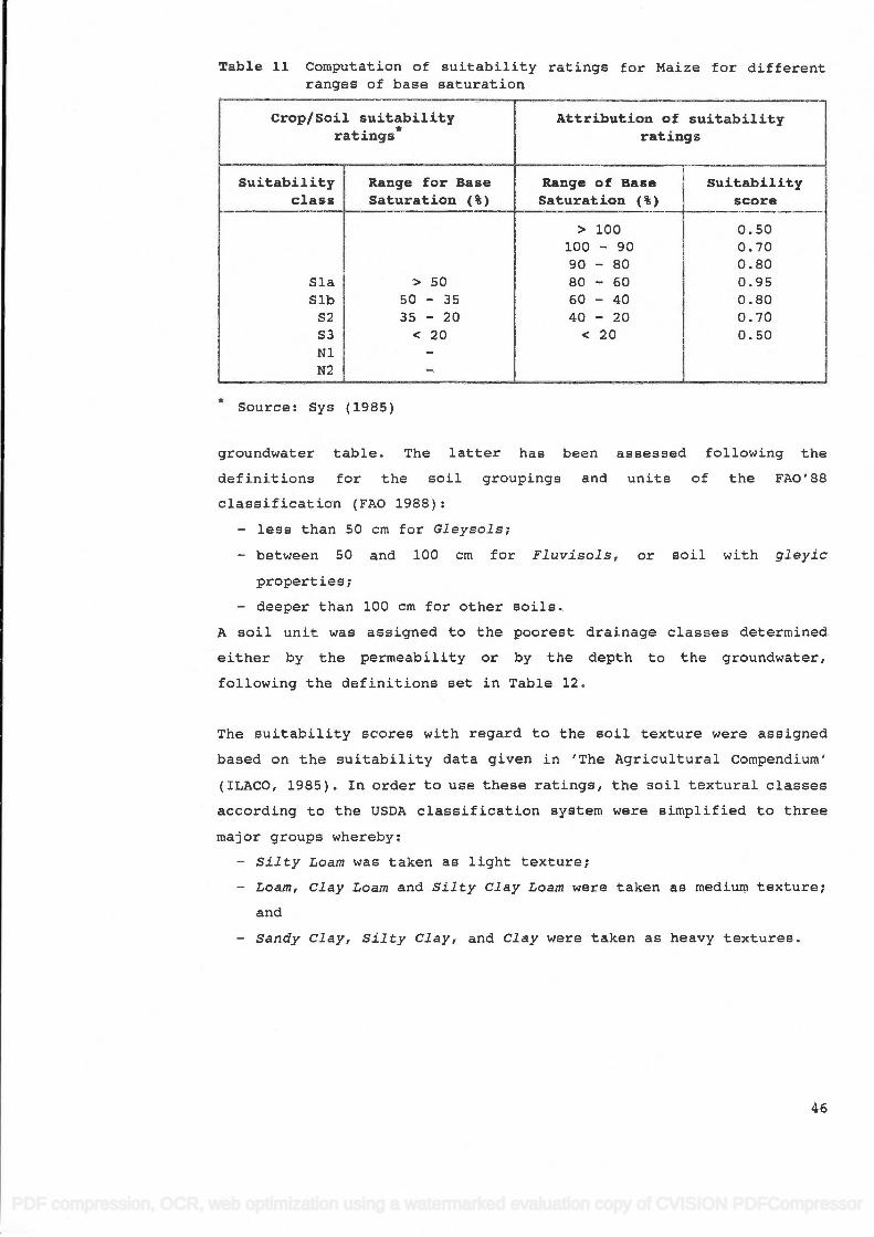
Table 11 Computation of suitability ratings for Maize for different ranges of base saturation

Crop/Soil suitability ratings*

Attribution of suitability ratings

Suitability Range for Base Range of Base Suitability class Saturation (%) Saturation (%) score

> loo 0.50 100 - 90 0.70 90 - 80 0.80

Sia > 50 80 - 60 0.95

Sib 50 - 35 60 - 40 0.80 52 35 - 20 40 - 20 0.70 S3 <20 <20 0.50 Nl -

N2 -

* Source: Sys (1985)

groundwater table. The latter has been assessed following the

definitions for the soil groupings and units of the FAO'88

classification (FAO 1988):

- less than 50 cm for Gleysols;

- between 50 and 100 cm for Fluvisols, or soil with gleyic

properties;

- deeper than 100 cm for other soils.

A soil unit was assigned to the poorest drainage classes determined

either by the permeability or by the depth to the groundwater,

following the definitions set in Table 12.

The suitability scores with regard to the soil texture were assigned

based on the suitability data given in 'The Agricultural Compendium'

(ILACO, 1985). In order to use these ratings, the soil textural classes

according to the USDA classification system were simplified to three

major groups whereby:

- Silty Loam was taken as light texture;

- Loam, Clay Loam and Silty Clay Loam were taken as medium texture;

and

- Sandy Clay, Silty Clay, and Clay were taken as heavy textures.

46

fable 11 Computation of suitability ratingE for llaize for differentranges of base eaturation

Crop/Soil suitabilityratings*

Attribution of suitabilityratiags

suitabilityclass

Range for BaseSaturatioa (t)

Raage of BaseSaturation (t)

suitabilityacore

S1as1b

s2s3N1N2

>50so-3535-20'j'

> 100100 - 9090-8080-6060-4040-20<20

0. 500. 700.800.9s0.800. 700. 50

* sorrrce: sys ( 1985 )

groundwater table. The latter hae been aseesged following thedefinitions for the soil groupinge and unite of the fAo'88

classification (rAO 1988) :

- Iees than 5O cm for GleysoTsi

- between 50 and 100 cm for Fluvisolsr ot soil with gleyicproperties;

- deeper than 10O cm for other Eoils.A soil unit was assigned to the poorest drainage claaaea determined

either by the permeability or by the depth to the groundwater,

following the definitions set in Table 12.

The suitability Ecore€r with regard to the soil texture were assigned

based on the suitability data given in 'The Agricultural Compendium'

(ILACO, 1985). In order to use these ratings, the soil textural classes

according to the USDA classification system were eimplified to threemajor groups whereby:

- SiTty Loam was taken as light texturel- Loam, clay rJoam and SiJty CJay Loam were taken as medium texture;

and

- Sandy Clay, Silty Clay, and Clay were taken as heavy textures.

46



Table 12 Definition of the drainage classes as a function of the permeability and the depth to groundwater

Drainage class Permeability (mm/h)

Depth to groundwater (cm)

E-SE (excessive - sLightly exc.) > 150 > 100 W (well) 150 - 100 -

MW (moderateLy well) loo - 75 -

I (inerfect) 75 - 50 100 - 50

P (poorly) 50 - 25 -

VP (very poorly) < 25 < 50


The standard gross margin (SGM) of the agricultural land for the region

of Madrid, published by the European community (EG, 1988), was used.

For citrus orchards and rice, data was completed with figures of the

nearby located region of Extramadura. Only specific costs are

discounted for in the SGM(5), investment costs such as irrigation

infrastructure are not taken into account. Consequently, the SGM of

irrigated land is skewed to higher values compared to non-irrigated

land. The SGM of irrigated land was taken as this data was most

complete. For forest land, a return was estimated by taking it equal

to 90% of the lowest SGM considered (Table 13).

5see p.23 for the definition of SGM

47

4.2 .5

Table 12 Definition of the drainage classee aE a function of thepermeability and the depth to groundwater

Drainage clasa PerueabiLity(nn/h)

Depth togroundwater (cD)

E-SE (excessive - stightty exc.)W (rett )

UW (moderatety xett)I ( irperfect)P (poorty)VP (very poorty)

> 1501s0 - 100100 - 7575- 50so- 25

25

> 100

100 - so

.uo

Economic parametere

The standard grosa margin (ScM) of the agricultural land for the regionof Madrid, published by the European community (EG, 1988), was uEed.

For citrus orchards and rice, data wae completed with figures of thenearby located region of Extramadura. OnIy specifie costa are

discounted for in the sGM(5), investment coEts sueh as irrigationinfrastructure are not taken into account. Conseguent1y, the SGM ofirrigated land is skewed to higher valuee compared to non-irrigatedland. The scl'{ of irrigated land waa taken aE this data wag mogt

complete. For forest land, a return waE eEtimated by taking it equal

to 90t of the loweet SGM conEidered (Table 13).

Seee p.23 for the definition of SGM

47



Table 13 Used standard gross margin of crops for the region of Madrid and

Extramadura (source EG, 1988)

Average Standard Gross Iargin

for 1983, p84, 85

(ECU/ha/year)

Extramadara Hadrid Used

figures

Crop non-irrigated irrigated non-irrigated irrigated

Wheat (durn) 227 438 196 470 470

Maize (grain) 243 916 164 932 932

Rice - 1072 - - 1072

Pasture (high) 78 720 117 438 438

land (tow yielding) 47 - 31 -

Citrus orchards - 2192 - - 2192

Olive orchard 321 697 219 438 438

Vineyard quality wine - - 196 360 360

other wine 407 157 344 __________

Forest - - - -

* 324

* calculated as 90% of the lowest used SGM


4.3.1 crop/Soil suitability ratings

The calculated crop/soil suitability ratings (r1 in the LP model) are

presented in Table 14, Table 16. The results are not fully satisfying.

The Calcaric Fluvisols (FLc) seem to be rather underestimated,

specially for the cereals and pasture land. Similarly the Dystric

Cambisols (CMd) seem to be overestimated compared to the Eutric

Cainbisols (CMe). Rice gets quite high ratings for the Leptosols (LP)

which may look odd, but is due to the fact that the slopes were not

taken into account in the evaluation, and that rice do not require deep

soils. Quite surprisingly equal ratings were obtained for the Calcic

(LVk) and the Chromic Luvisols (LVx), the properties of their surface

horizons did not vary sufficiently to yield different suitability

ratings.

48

Crop

Avrrage Stardard Gross Iarginfor l9&1, rg(, rEE

(EcU^a/yrar)

t sedfigrres

Extrmdra lladrid

non- i rrigated i rrigated non-irrigated i rr i gated

lJheat (durm) 227 438 196 470 470

llaize (srain) 213 916 164 932 93?

Rice 1072 1072

Pasture (high)Land (tox yietdinq)

7847

724 11731

01, 438

Citrus orchards 2192 2192

0tive orchard 321 697 219 138 138

Vi neyardquatity rine

other rine r,it196157

360344

360

Forest*

324

fable 13 Used atandard gross margin of crops for the region of Madrid andExtramadura (source EG, 1988)

*catcutated as 90% of the lorest used SGH

4.3 Results aad Discussion

4.3.1 crop/Soil suitability ratings

The calculated crop/soil suitability ratings (rtj, in the LP model) are

presented in Table 14, Table 15. The resulte are not fully satiefying.The Calcaric Eluvisols (FLcl Eeem to be rather underestimated,

specially for the cerealE and pasture land. Similarly the DystricCambisols (Cl,ldl seem to be overestimated compared to the EutricCambisols (Cttel. Rice gets guite high ratings for the LeptosoTs lLPlwhich may look odd, but is due to the fact that the slopes were not

taken into account in the evaluation, and that rice do not require deep

soils. Quite surprisingly equal ratings were obtained for t}:'e Calcic(LVkl and the Chromic Luvisols (LVxl, the properties of their surface

horizons did not vary sufficiently to yield different suitabilityratings.

48



Table 14 crop/soil suitability ratings calculated with a parametric approach for soil data of the region of Madrid

Sail Unit Grape Citrus Olive Rice Wheat Maize Pasture Forest

FLe 0.57 0.72 0.7 0.81 0,72 0.76 O76 0.84 FLc 0.53 0.53 0.55 0.53 0.63 0.57 0.58 0.54

GLm 0.52 0.54 0.54 0,59 0.6 0.56 0.59 0.53

GLk 0.52 0.53 0.55 0.53 0.59 0.56 0.56 0.53

RGe 0.62 0.6 0.74 0.52 0.7]. 0.67 0.65 0.59

RGc 0.64 0.56 0.6]. 0.53 0.74 0.62 0.64 0.57

RGy 0.61 0.51 0.59 0.54 0.7]. 0.58 0.67 0.57

RGd 0.51 0.81 0.71 0.85 0.77 0.8 0.8 0.95

LPe 0.67 0.53 0.53 0.55 0.61 0.55 0.58 0.53

LPd 0.54 0.58 0.53 0.72 0.56 0.58 0.58 0.62

LPk 0.59 0.51 0.51 0.51 0.53 0.52 0.51 0.51

LPm 0.52 0.52 0.54 0.53 0.58 0.55 0.56 0.53

LPu 0.54 0.58 0.53 0.72 0.56 0.58 0.58 0.62

LPq 0.6 0.57 0.55 0.66 0.59 0.6 0.61 0.62

cMe 0.63 0.58 0.55 0.66 0.58 0.59 0.59 0.62

CMd 0.52 0.73 0.6]. 0.92 0.66 0.72 0.72 0.83

cMu 0.53 0.63 0.54 0.72 0.6 0.63 0.63 0.7

cMc 0.53 0.5 0.66 0.52 0.64 0.6 0.6 0.59

CMV 0.59 0.53 0.53 0.55 0.61 0.55 0.58 0.53

CMg 0.5 0.61 0.56 0.81 0.58 0.61 0.61 0.66

CLh 0.57 0.55 0.54 0.58 0.6 0.58 0.59 0.56

CLp 0.51 0.5 0.53 0.52 0.57 0.54 0.54 0.52

GYk 0.65 0.51 0.55 0.5 0.6 0.56 0.55 0.53

LVx 0.91 0.62 0.59 0.62 QJ 0.64 0.64 0.62

LVk 0,91 0.62 0.59 0.62 0.7 0.64 0.64 0.62

LVg 0.52 0.7 0.58 0.81 0.64 0.66 0.66 0.64

LVh 0.55 0.64 0.56 0.72 0.64 0.67 0.67 0.64

ALh 0.52 0.66 0.56 0.85 0.62 0.63 0.63 0.74

ALg 0.52 0.64 0.54 0.81 0.6 0.62 0.62 0.64

PHi 0.51 0.61 0.61 0.73 0.61 0.63 0.63 0.67

(Note: trie uncterLinea values correspona to tne optimai aijocation uiscusseu

in the following paragraph)

49

Table 14 Crop/Soil suitability ratings calculated with a parametric approachfor soil data of the region of Madrid

Soilunit Grape Citrus Olive Rice Wheat Irlgize Pasture Forest

FLeFLc

GLm

GLK

RGeRGC

RGyRGd

LPeLPdLPKLPmLPULPq

CUecttdCUU

CMC

CMvcltg

cLhCLP

GYK

LVxLVkLvgLVh

ALhALg

PH1

0. 57o. s3

o.s2o.52

o.620. 54o.610. 51

o.67o. s40. 59o.s2o. 54o.5

0. 63o.s20. s30. 530. s9o.5

o. 57o. s1

o. 65

o.91o.91o. 520. s5

0. s2a.s2

o.51

o.720. s3

0. s40. 53

0.50. s60.510.81

0. s30. s80.51o.s20.580. 57

0. s80. 730. 630.s

0. s3o. 51

0. 5so.5

0. s1

o.620.624.7

0. 64

0. 650. 64

0.61

o.70. 55

o. s40. 55

o.740. 61o. 590. 71

0. s3o. s30.51o. 540. 53o. 55

0. 550. 610. s40. 55o. 530.56

0. 540. s3

0. 55

0. 590. s9o. s8o. s5

o. 55o. 54

o.51

0.810. s3

0. s90. 53

o.52o. s30. s40.8s

o.55o.720. s10. 53o.720. 56

0. 55o.92o.720. 52o.55o.81

0. 58o.52

0.5

o.62o.620.81o.72

0. 850.81

0. 73

o.720.63

0.5o. s9

o.71o.74o. 71o.77

0.610. s50. s3o. s80. s50.59

0. s80. 650.6

0. 640. 61o. s8

0.5o.57

0.6

o.7o.7

0.640. 64

o.620.5

o. 61

o.760. 57

o. 560. s5

o.67o.620. s80.8

0. 550. s8o.s20. 550. s8o.6

0. s9o.720. 630.5

o. 55o. 61

0. 580. s4

0. s6

4.644.64o.65o .67

0. 63o.62

0. 53

0.76o. s8

0. s9o.55

o. 6so.64o.670.8

o. 58o. s8o. s1o. 56o. 580. 61

0. s9o.720. 530.6

o. s8o. 61

0. s9o. 54

o. 55

0. 540. 540. 65a .67

0. 63o.62

o. 63

o. 84o. 54

o. 530. s3

0. 590. 57o.570.95

0. s3o.620. s1o. s3o.62o.62

o.620.83o.7

o.590. 530. 56

0. 56o.52

o. 53

o.62o.62o. 64o.64

4.740. 64

o .67Note t valueE, corres oru lma a usat on

in the foJ-lowing paragraph)

49



4.3.2 Allocation of the LUTs

(i) Allocation of the crops to the soil units

The allocatioriof the different crops over the soil units as determined

by the Linear Programming (LP) is presented in Table 15. As can be

seen from Table 15 only three alternative solutions (with values of

zero) came out, of which two (for grapes and pasture) concern the

Calcic and Chromic' Luvisols for which equal suitability ratings were

found. To most of the soil units one single crop was allocated to (24

out of 30). Nevertheless, two crops are only allocated to soil types

where other crops should also be assigned to: grapes to the Luvisols

together with wheat and pasture, and rice to Dystric Cambisols together

with maize, citrus and forest.

Despite the not so satisfying crop/soil suitabilities, the proposed

allocation seems quite acceptable from an agronomic point of view.

Maize and pasture land should be assigned to the Fluvisols (Ele and FLc

respectively). Only pasture seems to give the best use of the poorly

drained soils Gleysols (GLm and GLk). Citrus should be grown on the

weakly developed and more acid soils (Dystric Regosols and Cambisols).

Besides, rice, maize and forest should also be allocated to the Dystric

Cambisols. Grapes (actually vineyards) and wheat, besides pasture,

should be allocated to the Luvisols (LVx and LVk). Olives, it seems,

should be placed on the weakly developed soils and/or shallow soils,

relatively rich in bases, as the Eutric Regosols (RGe), Rendzic

Leptosols (LPk), Calcaric Cambisols (CMc). The 400 hectares of olives

which should be allocated to the Haplic Alisols (ALh) are somewhat a

discordance in that line. Pasture and forest, to which the largest

portion of the land was to be assigned, also get the widest variety of

soils. Generally they get the less favourable soils.

The considerable lower number of alternative solutions obtained in this

case study compared to the study of Lubbeek, is due to the more precise

(therefore not more accurate) suitability ratings used, as well as to

the greater divergence in the used SGM. For instance, the suitability

rating calculated for olives on the Calcaric Cambisol (CMC) was 0.66

while the suitability rating for wheat on the same soil was 0.64. In

the LP this small divergence will have an influence while the actually

suitability might not be significantly different.

50

4.3.2 Alloeation of the LUTg

(i) AlTocaxion of the crops to the soiT units

The allocation. of the different crops over the soil units as determLned

by the Linear Programming (LP) ie preeented in Table 15. AE can be

seen from Table 15 only three alternative solutione (with values ofzero) cErme out, of which two (for grapes and pasture) concern theCalcic an'd Chromic LuvisoJ,s for which equal suitability ratingE were

found. To most of the soLl units one single crop waE allocated Eo (24

out of 30). Nevertheleee, two crope are on1-y allocated to soil typeswhere other crops should also be aseigned to: grapes to the I'uvisolstogether with wheat and paeture, and rice to Dystric Cambisols togetherwith maize, citrug and foreet.

Despite the not Eo satiefying crop/eoil euitabilitiee, the proposed

allocation EeemE guite acceptable from an agronomic point of view.

Maize and paeture land should be aseigned to the fJ,uvisols (Ele and -FEc

respectively). Only pasture Eeems to give the beEt use of the poorlydrained soils Gleysols (GEm and cLkl. Citrus ehould be grown on theweakly developed and more acid soila (Dystric Regosols and canbisolsl.Besides, rice, maize and forest should also be allocated to the DystricCanbisols. crapes (actually vineyards) and wheat, besides pasture,should be allocated to the .tuvisols (lYx and LVkl. Olives, it seems,

should be placed on the weakly developed soile and,/or shallow soils,relatively rich in bases, as, the Eutric RegosoJ.s (RGe), Rendzic

LeptosoTs (LPkl , Calcaric Cambisols (CI,Icl. The 400 hectares of oliveswhich Ehould be allocated to t}l.e HapLic Alisols (A.Ell) are somewhat a

discordance in that line. Pasture and forest, to which the largestportion of the land was to be assigned, also get the widest variety ofsoils. Generally they get the lese favourable EoilE.

The considerable lower number of alternative solutions obtained in thiscase study compared to the etudy of Lubbeek, is due to the more precise(therefore not more accurate) suitability ratinge used, as well as tothe greater divergence in the uged SGl.[. I'or instance, the suitabilityrating calculated for olivee on the Calcaric Cambisol (cl,Ict wae 0.65

while the suitability rating for wheat on the eame soil wag 0.64. fnthe LP this small divergence will have an influenee while the actuallysuitability might not be eignificantly different.

50



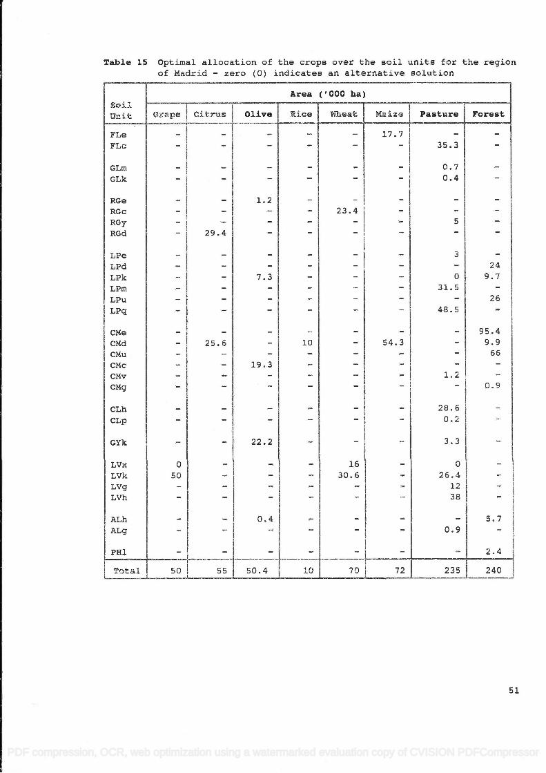
Table 15 Optimal allocation of the crops over the soil units for the region of Madrid - zero (0) indicates an alternative solution

Area ('000 ha)

Soil Unit Grape Citrus Olive Rice Wheat Maize Pasture Forest

FLe - - - - - 17.7 - -

FLc - - - - - - 35.3 -

GLm - - - - - - 0.7 -

GLk - - - - - - 0.4 -

RGe - - 1.2 - - - - -

RGc - - - - 23.4 - - -

RGy - - - - - - 5 -

RGd - 29.4 - - - - - -

LPe - - - - - - 3 -

LPd - - - - - - - 24

LPk - - 7.3 - - - O 9.7

LPm - - - - - - 31.5 -

LPu - - - - - - - 26

LPq - - - - - - 48.5 -

CMe - - - - - - - 95.4

CMd - 25.6 - 10 - 54.3 - 9.9

CMu - - - - - - - 66

CMc - - 19.3 - - - - -

CMv - - - - - - 1.2 -

CMg - - - - - - - 0.9

CLh - - - - - - 28.6 -

CLp - - - - - - 0.2 -

GYk - - 22.2 - - - 3.3 -

LVx O - - - 16 - O -

LVk 50 - - - 30.6 - 26.4 -

LVg - - - - - - 12 -

LVh - - - - - - 38 -

ALh - - 0.4 - - - - 5.7

ALg - - - - - - 0.9 -

PHi - - - - - - - 2.4

Total 50 55 50.4 10 70 72 235 240

51

fable 15 optimal aLlocation of the crops over the soil units for the regionof Madrid - zero (0) indicates an alternative solution

SoiIUnit

Area ('OOO ha)

Grape Citrus Olive Riee Wheat Maize Paature Forest

E.LetrLc

GLmGLK

RGeRGC

RGyRGd

LPeLPdLPKLPmLPuLPq

cUecMdCMU

CMcCMvcMg

cLhCLP

GYK

LVxLVkLVgLVh

ALhALg

PHI

050

29.4

25.6

1.2

7.3

19. 3

22.2

o.4

10

23.4

1630. 6

L7.7

54.3

35.;

o.7o.4

:

3

o31. s

48. s

-

7.2

28.5o.2

3.3

026.4

7238

0.9

2;9.7

26

95.49.9

,r_

o.9

5.7

2.4

Total 50 55 s0.4 10 70 72 23s 240

51



(ii) Allocation of the crops to the soil associations (Map 2.2)

The distribution of the land utilization types over the soil

associations, based on the dominating soil unit as determined by the LP

model, is presented in Map 2.2. Noteworthy is the group of crops with

maize, rice, citrus and forest found in the northern region of the

study area, this is right in the mountains. Apart from forest, this

solution should be regard as inappropriate, and is due to the

suitability ratings which have been computed based on soil physical and

chemical properties only, without taking into account e.g. slope or

water availability for irrigation. The other proposed solutions seem to

be feasible.

Inherent to a soil association map, there are within each map unit,

soil types present which may substantially differ from the major soil

unit. It is therefore important to evaluate to which extend these

inclusions may influence the proposed allocation. This information is

provided by the reduced cost, or opportunity cost, provided by the LP

model.

The information provided by the opportunity costs can be assessed from

two entries: (i) to which extend is assigning a particular crop to a

soil unit present within the association unfavourable, or (ii) which

crop should actually be assigned to a particular soil association with

regard to the soils present in at the second or lower level. To

illustrate this point, a particular case is looked at. The optimal

allocation determined by the LP model suggests to grow grapes on either

the Chromic or Calcic Luvisols (LVx or LVk) . These are found in the

soil associations LV1 through EV9 of the soil map. However, in soil

association LV4, for instance, the second most common soil units are

Dystric Regosols (RGd) for which grapes have an opportunity cost of

-3.7. This means that allocating one hectare of grapes to RGd, will

result in a reduction of the return by 3.7 units, all other constraints

remaining constant. The opportunity cost of citrus for Dystric

Regosols is however zero, and the LP actually suggests to allocate

citrus to these soils. The same analysis can be carried on for the

included soils on the third and eventually on the fourth level of the

soil associations.

52

(ii) ATlocation ot the crops to the soj'J, associations (Map 2.2)

The distribution of the land utilization typee over the soilassociations, based on the dominating soil unit ag determined by the LP

model, ie preeented in l(ap 2.2. Noteworthy ie the group of crops withmaize, rice, citrue and forest found in the northern region of thestudy area, thig is right in the mountains. Apart from forest, thissolution should be regard as inappropriate, and is due to thesuitability ratingg which have been computed baged on Eoil physical and

chemical properties only, without taking into aceount e.g. slope orwater availability for irrigation. The other proposed solutions seem tobe feasible.

Inherent to a soil association map, there are within each map unit,soil types present which may substantially differ from the major soilunit. It is therefore important to evaluate to which extend these

inclusions may influence the proposed allocation. This information isprovided by the reduced cost, or opportunity cost, provided by the LP

model.

Ihe information provided by the opportunity costs can be assessed from

two entries: (i) to whieh extend ie aesigning a particular crop to a

soil unit preeent within the association unfavourable, or (ii) which

crop should actually be assigned to a particular soil association withregard to the soils present in at the second or lower leveI. To

illustrate this point, a particular case is looked at. The optimalallocation determined by the LP model suggests to grow grapes on eitherLhe Chromic or CaTcic Luvisols (LVx or LVkl. These are found in thesoil associationg Ey1 through LV, of the soil map. However, in soilaseoeiatioo LV4r for inetanee, the second most common soil unit€t are

Dystric Regosols (Rcd) for which grapes have an opportunity cost of-3.7. This means that alloeating one hectare of grapes to RGd, willreeult in a reduction of the return by 3.7 units, all other constraintsremaining constant. The opportunity cost of citrue for DystricRegosols is however zerot and the LP actually suggests to allocatecitrus to these soils. The eame analysis can be carried on for theincluded soils on the third and eventually on the fourth level of the

Eoil asgociations.

52



In the table on Map 2.2, the opportunity costs for allocating crops to

the second most important soil type present in a soil association (to

which the crops are assigned to based on the dominant soil type) are

presented. For convenience, the values have been re-scaled linearly

and rounded such that the highest value corresponds to 20. In the

table (Map 2,2) the 24 soil associations with the highest opportunity

cost are represented. This excludes 14 associations which have as

highest, an opportunity cost of minus one and the 55 others which had

reduced costs of zero. The latter means that the second most important

soil units do not negatively influence the production. A plus sign was

put to indicate crops which were not originally assigned to a

particular soil association (based on the dominating soil unit), but

which should be allocated to the second most common soil unit. From

the table it is possible to identify to which extend the second most

important soil type limits the allocation of a crop to a particular

association, as well as which crop should actually be assigned to that

soil type. It is also known that the allocation of the crops to the

soil associations not presented in the table is not or only slightly

limited. The originally computed opportunity costs for the eight crops

to the various soil units are presented in Appendix 7.2.5.

(iii) Which are actually the best soils?

Considering the eight land utilization types - and the required area

which had to be allocated to each of them - which are the most valuable

soils? This question is relevant when decisions have to be taken for

selecting land to be taken out of production, e.g. because of expansion

of urban areas, construction of reservoirs, etc. As in this case study

the available land was set equal to the total area of the region, all

soils are in relative shortage or, to put it in LP terms, the slack

values are zero. Consequently, the dual variables of all soils are

greater than zero. The larger this value, the larger the increase of

the objective function will be for one unit increase of available area.

The LP solution of this problem enables thus to rank the soils in terms

of 'quality'. The soil units are presented in decreasing order of the

; corresponding dual variable (ab1 Table 16). The Dystric Regosols

(RGd) come out as the best soils. Citrus has been allocated to these

soils, for which a high suitability rate (0.81) was found and which had

53

In the table on Map 2.2, ttre opportunity costs for allocating cropE tothe second most important soil type present in a soil aseociation (towhich the erops are assigned to based on the dominant soil type) are

presented. For convenience, the values have been re-scaled linearlyand rounded such that the highest value corresponds to 2O. In the

table (Map 2.2) the 24 soLL associations with the highest opportunitycost are represented. This excludes 14 associationg which have aE

highest, an opportunity cost of minus one and the 55 others which had

reduced coste of zero. The latter means that the gecond most important

soil units do not negatively influence the production. A plue eign wae

put to indicate crops which erere not originally aseigned to a

particular soil asgociation (baeed on the dominating eoil unit), but

which should be allocated to the eecond mogt cornmon goil unit. From

the table it is poseibte to identify to which extend the second most

important soil type limits the allocation of a crop to a Particularassociation, aE well as whieh crop should actually be assigned to thatsoil type. It is also known that the allocation of the croPs to the

eoil associatione not preeented in the table is not or only elightlylimited. ?he originally computed opportunity costa for the eight croPel

to the various soil units are preeented in AppendLx 7.2.5.

(iii) Which are actuaTTy the best soiTs?

Considering the eight land utilization types - and the reguired area

whieh had to be alloeated to each of them - whieh are the most valuablegoils? This guestion ie relevant when decisions have to be taken forselecting Land to be taken out of production, e.g. because of expansion

of urban areae, construction of reservoirs, etc. AE in this case etudy

the available land !,raE set egual to the totalarea of the region, allsoils are in relative shortage or, to put it in LP terms, the slack

values are zero. Conseguently, the dual variables of all soils are

greater than zero. The larger this vaLue, the larger the increase ofthe objective function will be for one unit increase of available area.

The LP solution of thie problem enablee thue to rank the soils in terms

of 'guality'. The goil unite are presented in decreasing order of the

sorresponding dual variable $ffi Table 16). T,ine Dystric Regosols

(Rcd) eome out ae the best eoils. Citrus has been aLlocated to these

eoils, for which a high euitability rate (0.81) was found and which had

53



the highest SGM. Just as for irrigated fields compared to non-

irrigated crops, the SGM of perennial crops may be an overestimated of

the actual return when compared to annual crops, because of different

types of specific cost (none or lower planting coste, etc). The

proposed ranking of the soil units should thus be considered bearing in

mind the limitation of the calculated suitabilities and the

representativeness of the standard gross margin.

Table 16 Soil units ranked according

to decreasing dual variable

Soil Unit

(according to FAO 1988)

Dual Variable

Dystric Regosols (RGd) 4.5

Eutric Fluvisols (FLe) 3.11

Dystric Cambisols (CMd) 2.74

Eutric Regosols (RGe) 2.68

Haplic Alisols (ALh) 2.45

Calcaric Regosols (RGc) 2.43

Haplic Luvisols (LVh) 2.37

Gypsiric Regosols (RGy) 2.37

Calcaric Cambisols (CMc) 2.33

Gleyic Luvisols (LVg) 2.33

Humic Cambisols (CMu) 2.32

Calcic Luvisols (LVk) 2.24

Chromic Luvisols (LVx) 2.24

Luvic Phaeozems (PHi) 2.22

Gleyic Cambisols (CMg) 2.19

Gleyic Cambisols (ALg) 2.16

Lithic Leptosols (LPq) 2.11

Dystric Leptosols (LPd) 2.06

Eutric Cambisols (CMe) 2.06

Umbric Leptosols (LPu) 2.06

Haplic Calcisols (CLh) 2.02

Mollic Gleysols (GLm) 2.02

Calcaric Fluvisols (FLc) 1.98

Eutric Leptosols (LPe) 1.98

Vertic Cambisols (CMv) 1.98

Mollic Leptosols (LPm) 1.89

Calcic Gleysols (GLk) 1.89

Calcic Gypsisols (GYk) 1.85

Petric Calcisols (CLp) 1.81

Rendzic Leptosols (LPk) 1.67

54

the highest sGM. Juet aa for irrigated fields compared to non-

irrigated cropE, the SGU of perennial crops may be an overeBtimated of

the actual return when compared to annual croPE, becauee Of different

types of specific coet (none or lower planting coete' etc) ' The

proposed ranking of the Eoil unite should thus be considered bearing in

mind the limitation of the calculated suitabilitiee and the

representativeness of the etandard grosE margin'

lfable 16 SoiI unitE ranked accordingto decreasing dual variable

Soil Uuit(accordiug to FAo 1988)

DualVariable

Dystric Regosols (RGd)Eutric FluvisolE (fl,e)Dyetric Cambieole (CMd)

Eutric Regosols (RGe)Haplic Alisols (ALh)Calcaric RegoEoIE (RGc)

Haplic LuviEols (LVh)Gypsiric Regoeols (RGY)

Calcaric CambieolE (CMc)

Gleyic Luvisols (LVq)Humic Cambisole (CMu)Calcic Luvisols (LVk)Chromic Luvisols (LVx)Luvic Phaeozems (PHI)Gleyic Cambigole (CMS)

Gleyic CambiEols (ALS)Lithic Leptoso1E (LPe)Dystric LePtoaoJ.s (LPd)Eutric Cambisols (CMe)

Umbric LePtosole (LPu)Haplic calcisols (cLh)Mollic GleYsols (GLm)

Calcaric Fluvieole (FLc)Eutric LePtosols (LPe)Vertic Cambisols (CMv)Motlic LePtoeole (LPm)Calcic GleYsols (GLk)Calcic GyPsisola (GYk)Petric Calcieole (CLP)Rendzic LePtosols (LPk)

4.s3. 112.742.682.452.432.372.372.332.332.322.242.242.222.192.162.LL2.062.062.062.O22.421.981.981. 981.891.891.851.811.67

54



4,4 Possible expansions of the model

The foregoing model has been limited to maximising return given certain

crop and soil properties and an economic parameter, but without taking

into account any environmental limitations. An LP model is presented

here which may be useful to determine an optimal allocation of crops

whilst minimising the risk for erosion, similarly as was done in the

case study of Lubbeek for minimising the risk of leaching.

4.4.1 LP model for minimising erosion risk

The universal soil loss equation (USLE) is a model developed in the USA

by Wischmeir and colleagues as a means for assessing soil loss by

rainfall on field-scale (CEC, 1992b). Its mathematical formulation is

presented in equation [20]

E- 2.24.R.(K.LS.C.P) [20]

with

E loss of soil in (ton/ha]

R index for the climatic erosivity which is calculated as a

function of the global precipitation energy and the

precipitation intensity

K a soil erodibility index

LS an index for the slope, and determined as

LS - -- (0.76+0.535+0.07652) [21] 100

and L the length of the slope and S the slope in percent

C a crop cover index, and

p an index for soil conservation measures

55

4.4 Possible expansioas of the model

The foregoing model has been limited to maximising return given certaincrop and soil properties and an economic parameter, but without takinginto account any environmental limitations. An LP model is presented

here whieh may be useful to determine an optimal allocation of crops

whilst minimiEing the risk for erosion, si-milar1y aE wasr done in thecase study of Lubbeek for minimising the risk of leaching.

4.4.1 LP model for minimieing erosion risk

The universal soil loss equation (USLE) isby Wischmeir and coLleagues as a means

rainfall on field-scale (CEC, 1992b). ItEpresented in eguation [20]

a model developed in the USA

for aseessing soil loss by

mathematical formulation is

t 201

calculated as a

energy and the

E-2.24.R.(K.LS.C.P)

withE loes of soil in [ton/ha]R index for the climatic erosivity which ie

function of the global precipitationprecipitation intensity

x a soil erodibility index

Ls an index for the slope, and determined as

Ls - g (o.ze +0.53 s+o.o76sz) t21l1-0 0

and .L the length of the slope and .5 the slope in percentC a crop cover index, and

P an index for soil conservation measures

55



The following objective function is proposed for allocating crops with

a minimimal erosion risk based on the USLE

z: - minzE- : R1. Sk. I(. C . [22] 1,k,Lj

with

ZE* minimum erosion risk

RL a class factor for climatic erosivity

a class factor for soil erodibility and j = (l,..,m) with m the

number of soil units

Sk a class factor for the slope; as there is a quadratic

relationship between the soil loss and the slope (equation [20)

and [21)), the function can be linearized by partitioning it

e.g. as follows:

Si = 0.01 for flat to almost flat (S 5%)

S2 = 0.02 for moderate slopes (5 < S 15%)

S3 = 0.04 for steep slopes (15 < S 25%)

S4 = 0.16 for very steep slope (S > 25%)

a crop cover factor similar or equal to the C index of the USLE

This objective function should be subjected to constraints of area for

the soils and the crops, and to a constraint ensuring a minimal

production level, similarly as in the model for minimising the risk of

leaching of nitrates and phosphates in chapter 3.

It should be noticed that, to simplify equation [22] compared to the

USLE, the length of the slope (L) and the index for soil conservation

measures (P), are not explicitly in the equation. A disadvantage of

the proposed model will be that the number of decision variables will

proportional increase with the classes for the climatic erosivity and

for the slope.

4.4.2 Estimating the parameters

In general works related to agriculture or soil conservation as e.g.

"Mémento de l'Agronome", (MCD, 1989) or in "Conservation des sols au

sud du Sahara" (MC, 1979), crop cover indices and soil erodibility

56

The following objective function is proposed for allocating crope witha minimimal erosion risk based on the USLE

z! ' minzr- ,,D.rRr

. s* . Kr - ci. Aij t22l

with*

zE

Rt

x.j

sk

This objective function Ehould be subjected to constraintsthe soils and the EropE, and to a eongtraint ensuringproduction leve1, aimilarly as in the model for minimieingleaching of nitrates and phosphates in chapter 3.

minimum eroEion riska claEe factor for climatic erosivitya class factor for soil erodibility and j = (L,..,m| with rn thenumber of soil unitsa class factor for the elope; aE there is a guadratic

relationship between the soil loss and the slope (eguation [20]and 1211), the function can be linearized by partitioning ite.g. as followe:

S1 = 0.01 for flat to almost flat (S < 5t)52 = 0.O2 for moderate alopee (5 < s < 158)

53 = 0.O4 for steep elopes (15 < S s 25t)54 = O.15 for very steep slope (S > 25t)

Ci a crop cover factor similar or equal to the C index of the USLE

of

a

the

area forminimal

risk of

It should be noticed that, to simplify equation 1221 compared to theUSLE, the length of the elope (E) and the index for soil conservationmeasures (Pl, are not explicitly in the equation. A disadvantage ofthe proposed model will be that the number of decision variables willproportional increase with the classes for the climatic erosivity and

for the slope.

4.4.2 Estimating the parameters

In general works related to agriculture or soil conservation as e.g.

"M6mento de I'Agronome", (MCD, 1989) or in "Conservation des sols au

sud du sahara" (MC, 1979), crop cover indices and soil erodibility

56



values can be found from which the required ratings for the proposed LP

model can be deduced.

Complementarily, in the particular case of the region of Madrid, a map

like the land capability map prepared by Rodríguez et al. (1990b) could

be used. This map contains five classes according to different degrees

of limitations; soils of class A have no important limitations, the

other units are classified according to increasing importance of

limitation from Class B to E. Each class is further divided in sub-

classes depending on the nature of the most limiting factor. The

considered limiting factors are:

- risk for erosion

- risk for salinisation

- limitation due to physical characteristics as liquid limit,

plasticity, density, bulk density

- hydromorphic conditions, depending on the permeability and the

water retention

- soil depth

- slope

- stoniness

By doing an overlay analysis of the soil map and land capability map -

which can typically be done with a GIS system - new land units can be

defined for which it should be possible to determine more accurate

production ratings and limitation factors.

The work done, and methodology followed, by the CORINE project on soil

erosion risk (CEC, 1992b), could in particular by fitted for estimating

appropriate weighing factors for the climatic erosivity, the soil

erodibility and the slope (RL, and Sk respectively in the proposed

LP model).

57

valuea can be found from which the reguired ratings for the propoeed LP

model can be deduced.

Complementarily, in the partieular case of the region of Madrid, a map

Iike the land capability map prepared by Rodriguez et al. (1990b) could

be used. Thie map contains five clagses according to different degreee

of limitations; soils of elaee A have no important limitations, the

other units are claEsified according to increasingr importance oflimitation from Class B to E. Each clasg ig further divided in sub-

classes depending on the nature of the most limiting factor. The

considered Iimiting factors are:

- risk for erosion

- risk for salinisation- limitation due to physica). characterietice as liguid limit,

plasticity, density, bulk density

- hydromorphic conditions, depending on the permeability and the

water retention- soil depth

- slope

- stoniness

By doing an overlay analyeie of the soil map and land capability map -which can typically be done with a GIS eystem - nev, land units can be

defined for which it should be possible to determine more accurateproduetion ratings and limitation factore.

The work done, and methodology followed, by the coRINE project on soilerosion risk (CEc, 1992b), could in particular by fitted for estimatingappropriate weighing factors for the climatic erosivity, the soilerodibility and the slope (Rt, I(j, and .sk respectively in the proposed

LP model).

57



4.5 Conclusions

4.5.1 The parametric approach

With the parametric approach, suitability coefficients were obtained

which could directly be used in an LP model for maximising the return.

The parametric approach enabled to generate a reasonable first estimate

on the suitability of the soils. Finding appropriate ratings for the

various soil characteristics was not obvious. Data based on local

experiments are probably necessary to ensure more accurate estimations

of the suitability ratings. However, the question may than be raised

whether it would not be more practical to establish relative

suitability ratings of the various crops for the various soils from

knowledgable persons (local practitioners with expert knowledge and

farmers) during the soil survey work.

4.5.2 Soil associations map, GIS and Linear Programming

Inherent to soil association maps is that part of the information on

the location and extend of minor soil types is lost. Representative

data on the physical and chemical properties of each soil type are

obviously indispensable to enable any land evaluation. The acreage of

each soil unit also proved to be relevant, specially when using the

proposed LP models. By introducing the soil map into a GIS system, a

new map could be deduced visualising the proposed allocation as

determined by the LP model.

Linear Programming proved to be a very handy tool for land evaluation

when using a soil association map. The data provided by the sensitivity

analysis (the reduced cost and dual variables in particular) helped to

assess limitations and impact of allocating specific land utilisation

types to the soil associations.

58

4.5 Coaclusions

4.5.1 The parametric approach

With the parametric approach, suitability coefficientE were obtainedwhich could directly be ueed in an LP model for maximising the return.The parametric approach enabled to generate a reasonable firet egtimateon the euitability of the EoilE. Finding appropriate ratings for thevarioue eoil characterigtics was not obvioue. Data baeed on localexperiments are probably necessary to engure more accurate estimationsof the suitability ratinge. However, the gueation may than be raieedwhether it would not be more practical to eetablish relativeguitability ratinge of the various cropE for the various eoile from

knowledgable persons (l-oeal practitionere with expert knowledge and

farmers) during the eoil Eurvey work.

4.5.2 Soil associationE map, GfS and Linear Programming

Inherent to soil association maps is that part of the information on

the location and extend of minor soil types is lost. Representativedata on the physical and chemical properties of each soil type are

obviouely indispensable to enable any land evaluation. The acreage ofeach EoiI unit aIEo proved to be relevant, specially when using theproposed LP models. By introducing the soil map into a GfS system, a

new map could be deduced vieualising the proposed allocation aE

determined by the LP model

Linear Programming proved to be a very handy tool for land evaluationwhen using a soil association map. The data provided by the sensitivityanalysis (the reduced cost and dua-L variables in particular) helped toaE sess limitations and impact of allocating speciflc land utilisationtypes to the soil associatione.

58



5 Summary and general conclusions

5.1 Summary

A framework is set for an integrated decision support system for land

evaluation, the main constituents being Geographical Information

Systems (GIS) and Data Management, linked to simulation and

optimisation models. The main features of these elements are outlined.

In two case studies, Linear Prograniming and Geographical Information

Systems are combined as tools for land evaluation. In a first case

study, digitized and detailed soils maps (original scale 1:20,000) are

used as a base for the geographical information. Linear Programming

models are developed to identify and evaluate the optimal allocation of

five crops taking into account a minimal risk of leaching of pollutants

(nitrates and phosphates) into the groundwater. In a second case

study, a soil association map (at a 1:200,000) scale is used to explore

to which extend information contained in this type of maps, can still

usefully be combined with an LP determining the optimal allocation of

land utilisation types yielding a maximum the return. Finally, an LP

model for identifying optimal land allocation whilst minimising the

risk of erosion is suggested.


Linear Programming is generally seen as a tool for planning. It is

commonly used for helping to solve management problems dealing with

rather technical and more predictable processes as e.g. in water supply

and irrigation. Difficulties to identify all constraints relevant to

land-use planning and translating them into meaningful linear equations

may have impeded its application in the fields of land evaluation and

land-use planning. In this study, it was shown that LP can be applied

for evaluating several land utilisation options conjunctively.

Generally accepted parameters of land evaluation, such as crop/soil

suitabilities, factors for sensitivity for leaching of pollutants, and

eventually parameters for estimating risk of erosion, can readily be

introduced in the proposed LP models. A major advantage of LP is that

relative values (classes), can also be used meaningfully.

59

5

5.1

Sunnary and general conclusions

SuDmary

A framework iE eet for an integrated decision support system for landevaluation, the main eonEtituentE being Geographical InformationSyEtemE (cIS) and Data Uanagement, Iinked to eimulation and

optJ.misation modele. The main featuree of theee elemente are outlined.

In two case etudies, Linear Programming and Geographical InformationSysteme are combined as tools for land evaluation. fn a first case

study, digitized and detailed soils maps (original Ecale 1220,000) are

ueed as a baEe for the geographical information. Linear Programming

models are developed to identify and evaluate the optimal allocation offive crops taklng into account a minimal risk of leaching of pollutants(nitrates and phosphatee) into the groundwater. In a second caEe

study, a soil agsociation map (at a Lt2OOTOOO) scale is used to exploreto which extend information contained in this type of mapa, can stillueefully be combined with an LP determining the optimal allocation ofland utilisation typee yi-elding a maximum the return. Finally, an LP

model for identifying optimal land allocation whilst minimising therisk of eroeion is suggested.


Linear Programming is generally Eeen as a tool for planning. ft iscommonly used for helping to solve management problems dealing withrather technical and more predictable processes as e.g. in water supply

and irrigation. Difficulties to identify aII constraints relevant toland-use planning and translating them into meaningful linear equations

may have impeded its application in the fields of land evaluation and

Iand-use planning. In thiE study, it was shown that LP can be appliedfor evaluating several land utilisation options conjunctively.Generally accepted parameters of land evaluation, sueh aE crop/soilsuitabilities, factors for sensitivity for leaching of pollutants, and

eventually parameters for estimating risk of erosion, can readily be

introduced in the proposed LP modele. A major advantage of LP is thatrelative values (elasses), can algo be used meaningfully.

s9



By linking several objective functions, optimal allocations can be

determined considering competing goals (e.g. maximising return whilst

minimising risk of leaching). Furthermore, the sensitivity analysis

offered by Linear Programming enables to assess the impact of the

allocation of several land utilisation types. This especially proved to

be a handy tool when using soil association maps for land evaluation.

60

By linking several objective functions, optimal allocations can be

determined considering competing goals (e.9. maximising return whiletminimising riak of leaching). Furthermore, the eengitivity analyeisoffered by Linear Programming enables to aE €resEr the impaet of the

allocation of several land utilieation types. Thie eepecially proved tobe a handy tool when ueing eoil association maps for land evaluation.

50



6 References and Bibliography

BELGISCH STAATSBLAD (1991)

Decreet inzake de beschermimg van het leefmilieu te gen de

verontreininging door meststoff en, 28.02.1991, p No 3834. (in Dutch)

Blume, H.P. and U. Schwertmann (1969)

Genetic evaluation of profile dístributíon of aluminium, iron and

manganese oxides. Soil Sci. 2xner. Proc., Vol. 33: 438-444.

Breeuwsma, A., J.H.M. Wösten, J.J. Vleeshouwer, A.M. van Slobbe and J.

Bouma (1991) Derivation of land qualities to assess environmental

problems from soil surveys. Soil Sci. Am. J., Vol 50: 186-190.

Cattrysse, D. (1993)

Mathematical Planning in Irrigation, lecture notes, Center for

Irrigation Engineering, KU Leuven.

CEC (1991)

Agricultural markets, Prices, European Communities - Commission,

document nr 5, 138pp.

CEC (1992a)

The agricultural situation in the community, 1991 report, published

in conjunction with the XXVth General report on the activities of

the European Communities, European Communities - Commission, 294pp.

CEC (1992b)

CORINE - Soil erosion risk and important land resources in the

southern regions of the European Community, 97pp + maps.

Chuvieco, Emilio (1993)

Integration of linear programming and GIS for land-use modelling

mt. j Geographical Information Systems, vol. 7, No. 1, p 71-83.

Deckers, J.A. (l993a)

Land evaluation and land use, lecture notes, Center for Irrigation

Engineering, KU Leuven.

61

5 Ref€reaces and Bibliography

BELGISCH STAATSBLAD (1991)

Deeteet inzake de beschermimg van het TeefniTieu tegen de

verontreininging door meststoffen, 25.O2.t99L, p No 3834. (in Dutch)

Blume, H.P. and U. Schwertmann (1969)

Genetic evaluation of profiTe distribution of aTuminium, iron and

manganese oxides. Soil Sci. Amer. Proc., Vol. 33: 438-444.

Breeuwsma, A., J.H.M. 9l6sten, .r..r. VleeEhouwer, A.l,[. van Slobbe and J.Bouma (19911 Derivation of Tand qualities to assess envitonmentalproblems trom soil sutveys. Soil Sci. Am. .r., Vol 50: 186-190.

Cattrysse, D. (1993)

Mathematical PTanning in lrrigation, Iecture notes, Center forIrrigation Engineering, KU Leuven.

cEc (1e91)

Agricultural markets, Prices, European Communities - Commiesion,

document nr 5, 138pp.

cEc (L992al

?he agricultural sixuation in the eomnunixy, 7997 report, publiehedin conjunction with the xxvth General report on the activities ofthe European Communitiee, European Communitiee - Commission, 294pp.

cEc (1992b)

CORINE - soi-l erosion risk and imporxanx Tand resources in thesouthern regions of the European Conmunity, 97pp + maps.

Chuvieco, Emilio (1993)

Integration of Tinear progranming and GIS tor Tand-use nodelTingInt. J. Geographical Information Systems, vol. 7, No. 1, p 71-83.

Deckers, J.A. (1993a)

Land evaTuation and Tand use, lecture notes, Center for frrigationEngineering, KU Leuven.

61



Deckers, J.A. (1993b)

Bodemgeschiktheid, cursus nota's, Faculteit Landbouwwetenschappen,

KU Leuven (in Dutch).

de Wit, C.T., H. van Keulen, N.G. Seligman and I. Sharim (1988)

Application of interactive multiple goal programming techniques for

analysis and planning of regional agricultural development,

Agricultural Systems, p 211-230.

Doorenbos, J. and A.H. Kaasan (1979)

Yield response to water, FAO Irrigation and drainage paper nr 33,

193pp.

Driessen, P.M. and R. Dudal (1991)

The major soils of the world - lecture notes on their geography,

formation, properties and use, Agricultural University Wageningen

& Katholieke Universiteit Leuven, 3O9pp.

EG (1988)

Mededelingen van de Commissie: De Bruto standaardsaldi "1984",

Publikatieblad van de Europese Gemeenschappen Nr C 133/1: p 52-61

(in Dutch).

ESRI (1989)

PC Network Users Guide, Environmental Systems Research Institute

Inc., Redlands, CA, USA.

ESRI (1990)

pcARC/Info, Environmental Systems Research Institute Inc. , Redlands,

CA, USA.

FAO (1988)

FAO-Unesco Soil map of the World. Revised Legend. Soils Bulletin 60.

FAO, Rome, 119 pp.

FAO (1989)

Guidelines for Land Use Planning, "Interdepartmental Working Group

on Land Use Planning", 7Opp.

Deekere, iI.A. ( 1993b)

Bodemgeschiktheid, cursus nota's, Faculteit Landbouwwetenschappen,

KU Leuven (in Dutch).

de Wit, C.T., H. van Keulen, N.G. Seligrman and I. Sharim (1988)

Application of interactive multiple goal programning techniques foranaLysis and planning of regionaT agricuTtural deveTopment,

AgrJ.cultural Systemsr p 2Ll-23O.

Doorenboe, J. and A.H. KaBBam (1979)

Yield tesponse to watett FAO Irrigation and drainage paper nr 33,

193pp.

Driesaen, P.ll. and R. Dudal (1991)

The major soiTs of the vorld - lecture noXes on their geography,

formation, properties and use, Agricultural University Wageningen

& Katholieke Univereiteit Leuven, 309pp.

Ee (1988)

Ilededelingen van de Commissies De Bruto standaardsaldi '7984u1Publikatieblad van de Europeee Gemeenschappen Nr c 133/1: p 52-6L

(in Dutch).

ESRr (1989)

PC Network Users Guide, Environmental Systems Research Inetitutefnc., RedlandE, CA, USA.

EsRr (1990)

pcARC/Znto, Environmental Systems Research Institute Inc., Redlands,

cA, usA.

FAo (1988)

EAO-Anesco SoiT map of the Wotld. Rerzjsed Legend. Soils Bulletin 6O.

l.AO, Rome, 119 pp.

FAo (1989)

Guidelines fot Land ase PTanning, "Interdepartmental working croup

on Land Use P1anning", 70pp.

62



FAO (1990)

Land Evaluation, The process, "Land Evaluation for development",

33pp.

Hillier, F.S. and G.J. Lieberman (1990)

Introduction to Operations Research, fifth edition, McGraw-Hill

publishing company, 954pp.

ILACO (1985)

Agricultural compendium for rural development in the tropics and

subtropics, Elsevier, The Netherlands, 738pp.

Konijn, N.T. (1990)

Multiple Goal Planning, PHLO-cursus 'Geografische

Informatiesytemen', Stichting Post-Hoger Landbouwonderwijs, LU

Vakgroep Bodemkunde en Geologie, iOpp.

Labadie, JW. (1989a)

Decision support systems in water resources, NATO Advanced Study

Institute, stochastic hydrology in water resources, Systems:

Simulation and optimization, September 18-29, 1989, Pefliscola,

Spain, 23pp.

Labadie, J.W. (1989b)

Combining simulation and optimization in river basin management


Simulation and optimization, September 18-29, 1989, Peñiscola,

Spain, 27pp.

Labadie, J.W. (1993)

Program NICELP, Linear Programming for PCs, explicit inverse revised

simplex with upper bounding, Department of Civil Engineering,

Colorado State University, USA.

Lambrechts, Ann (1988)

Bedrijfseconomische rendabiliteítsstudie van de populierenteelt in

8 x 8 m plantverband cv. Ghoy en cv. Beaupré, eindwerk Faculteit

Landbouwwetenschappen, KU Leuven, llSpp (in Dutch).

63

FAo (1990)

Land Evaluation, The process, "Land Evaluation for development,,33pp.

Hillier, F.S. and G.J. Lieberman (1990)

Inttoduetion to opetations Researci, fifth edition, McGraw-Hillpubliehing company, 954pp.

rLACO (198s)

Agricultural compendium for rural deveTopment in the tropics and

subtropics, Elsevier, The Netherlands, 738pp.

Konijn, N.T. (1990)

Ilultiple Goal PTanning, PHLO-curE,us 'Geograf iecheInformatieeytemen', Stichting Post-lloger Landbouwonderwijs, Lu

Vakgroep Bodemkunde en Geologie, 10pp.

Labadie, J.W. (1989a1

Decision support systems in water resoutces, NATO Advanced Study


Simulation and optimization, September 18-29, 1989, Pefliscola,Spain, 23pp.

Labadie, J.W. (1989b)

Combining simulation and optimization in river basin management

Institute, stochastic hydrology in water resources, Syetems:

Simulation and optimization, September L8-29, 1989, PefliEcola,

Spain, 27pp.

Labadie, J.W. (1993)

Program NLCELP, Linear Programming for PCs, explicit inverse revisedeimplex with upper bounding, Department of CiviI Engineering,

Col-orado State Univergity, USA.

Lambrechts, Ann (1988)

Bedtijfseconomische tendabiTiteitsstudie van de populierenteelt in8 x 8 m plantverband cv. Ghoy en ev. Beaupr6, eindwerk FaculteitLandbouwwetenschappen, KU Leuven, 115pp (in Dutch).

63



LEI (1989)

Bruto standaardsaldi voor de gewassen en de veehouderij (periode

1985/86 - 1987/88), Ministerie van Landbouw, Landbouw Economisch

Instituut (LEI), Brussels, 49pp (in Dutch).

Lenders, S. and C. Heylen (1989)

Bodemgeschiictheídsonderzoek in Lubbeek: toepassing van een

geografisch informatie systeem en teledetectie, eindwerk Faculteit

Landbouwwetenschappen, KU Leuven, 147pp + bijiagen (in Dutch).

MC (1979)

Conservation dea sols au sud du Sahara, 2e édition, Centre Technique

Forestier Tropical, Ministère de la Coopération, 296pp (in French).

MCD (1989)

Mémento du forestier, "Techniques rurales en Afrique", 3e édition,

Centre Technique Forestier Tropical, Ministère de la Coopération et

du Développement, 1266pp (in French).

Sys, C. (1985)

International Training Centre for Post-

Graduate soil scientists, State University of Ghent, Belgium, ?pp.

Rodríguez, Francisico M. and Luís Alcalá del Olmo Bodadilla (1990a)

Mapa de asociaciones de suelos de la comunidad de Madrid, escala

1:200.000, 1a edición - Instituto de Edafología y Biología Vegetal

(CSIC) + memoria, 7lpp (in Spanish).

Rodríguez, Francisico M., and Luís Alcalá del Olmo Bodadilla (1990b)

Mapa de capacidad potencial de uso agricola de la comunidad de

Madrid, escala 1:200.000, 1a edición - Instituto de Edafología y

Biología Vegetal (CSIC) + memoria, 3lpp (in Spanish).

Ross, G.J., C. Wang and P.A. Schuppi (1985)

Hydroxylamine and ammonium oxalate soultions as extractants for iron

and aluminium from soils. Soil Sci. Soc. Am. J. 49: 783-785.

64

LEr (1989)

Bruto standaardsaldi voot de gewassen en de veehoudetij (periode1985/86 - 1987/88), Ministerie van Landbouw, Landbouw Economisch

Instituut (LEI), Brueeels, 49pp (in Dutch).

Lenders, S. and c. HeyLen (1989)

Bodemgeschikxheidsonderzoek ingeogratisch informatie systeem en

Landbouwwetenschappen, KU Leuven,

Lubbeek: toepassing van een

teledetectie, eindwerk Facultelt147pp + bijJ.agen (in Dutch).

Mc (1979)

Conservation des soJs au sud du Sahara, 2e 6dition, Centre Technique

Foreetier Tropical, MinistEre de la Coop6ration, 296pp (in French).

McD (1989)

ttdmento du toresxiet, "techniques rurales en Afrielu€", 3e 6dition,Centre Technigue Forestier Tropical, MinistEre de Ia Coop6ration etdu D6veloppement, 1256pp (in French).

Sys, C. (1985)

Land Evaluaxion, part flf, International Training Centre for Post-Graduate soil scientists, state University of Ghent, Belgium, ?Pp.

Rodriguez, !'rancisico M. and Luis Alcala del olmo Bodadilla (1990a)

llapa de asociaciones de suelos de 7a comunidad de l{adrid, escala

7:200.000, 1a ediei6n - rnstituto de Edafologia y Biologia vegetal(csfc) + memoria, 71pp (in SpaniBh).

Rodriguez, Francisico M., and Luis Alcald del olmo Bodadilla (1990b)

Itapa de capacidad potencial de uso agricola de 7a comunidad de

t{adrid, escala 1:200.000, 1a edici6n - Instituto de Edafologia y

Biologia Vegetal (CSIC) + memoria, 31pp (in Spanish).

Ross, G.J., C. Wang and P.A. Schuppi (1985)

Hydroxylamine and anwnonium oxalate soultions as extractants for ironand aluminium trom soifs. Soil Sci. soc. Am. J. 49: 783-785.

64



Van Hecke (1993)

Farm structure 1985 survey: analysis of results. Regional structure

of Agricultural Production.

Van Orshoven, J. (1993)

Assessing hydrodynamic land qualities from soil survey data, PhD

thesis, Katholieke Universiteit Leuven, Belgium, 264pp.

Van Orshoven, J., P. Verbeke, B. Meylemans, L. Faes, J.A. Deckers and

J. Feyen (1992a) BAGRAB, Beoordeling AGRArisch Bodemgebruik - Een

geografisch informatiesysteem betreffende agrarische

bodemgeschiktheid in Vlaanderen, Vlaams gewest - AMINAL, besturr

landinrichting en - beheer, KU Leuven Instituut voor Land- en

Waterbeheer, 47pp. (in Dutch).

Van Orshoven, J., J.A. Deckers and D. Vandenbroucke (1992b)

From low to high intensity land evaluation: the need for a powerful

RDBMS. In: Proceedings of the 3rd European Conference on

Geographical Information Systems (eds. J. Harts, H.F.L. Otteris and

H.J. Scholten), Munich, Germany, March 23-26, 1992: 408-416.

Vereecken, H., J. Maes and J. Feyeri and P. Darius (1989)

Estimating the moisture retention characteristic from texture, bulk

density and carbon content. Soil Sci. 148: 389-403.

Vereecken, H., J. Maes and J. Feyen (1990)

Estimating the unsaturated hydraulic conductivity from easy to

measure soil properties. Soil Science 149: 1-12.

65

van Hecke (1993)

Earm structure 1985 survey: anaTysis of resulte. Regional structureof AgriculturaL Production.

Van Orshoven, J. (1993)

Assessing hydrodynamic Tand quaTities from soiT sutvey data, PhD

thesie, Katholieke Universiteit Leuven, Belgium, 264pp.

Van Orshoven, J., P. Verbeke, B. Meylemans, L. Faes, J.A. Deckers and

J. Eeyen (1992a) BAGRAB, Beoordeling AGRArisch Bodemgebruik - Een

geogtafisch informatiesysteem betreffende agtatischebodemgeschiktheid in Vlaanderen, Vlaams ge$reEt - AI.iINAL, besturrlandinrichting en - beheer, KU Leuven InEtituut voor Land- en

Waterbeheer, 47pp. (in Dutch).

Van OrEhoven, J., J.A. Deckers and D. Vandenbroucke (1992b1

Erom low to high intensity Tand evaluationt the need for a powerful

RDBI,IS. In: Proceedings of the 3rd European Conference on

Geographical fnformation Systems (ede. J. Harta, H.F.L. Ottens and

H.J. Scholten), Munich, cermany, March 23-26, L9922 408-416.

Vereecken, H., J. Maeg and J. Feyen and P. Darius (1989)

Estimating the moisture retention characteristic from texturet buTk

density and carbon content. SoiI Sci. 148: 389-403.

Vereecken, H., J. Maes and J. Feyen (1990)

Estimating the unsaturated hydraulic conductivity from easy tomeasute soiT ptopertiee. SoiI Scj-ence 149: 1-12.

55



Combining linear programming and geographical information systems as tools for land evaluation. ...

Documents

Transcript of Combining linear programming and geographical information systems as tools for land evaluation. ...