Durham Research Online

Deposited in DRO:

16 August 2010

Version of attached file:

Published Version

Peer-review status of attached file:

Peer-reviewed

Citation for published item:

Hardy, R. J. and Best, J. L. and Lane, S. N. and Carbonneau, P. E. (2009) ’Coherent flow structures in adepth-limited flow over a gravel surface : the role of near-bed turbulance and influence of Reynoldsnumber.’, Journal of geophysical research : earth surface., 114 . F01003.

Further information on publisher’s website:

http://dx.doi.org/10.1029/2007JF000970

Publisher’s copyright statement:

Hardy, R. J. and Best, J. L. and Lane, S. N. and Carbonneau, P. E. (2009) ’Coherent flow structures in adepth-limited flow over a gravel surface : the role of near-bed turbulance and influence of Reynolds number.’,Journal of geophysical research : earth surface., 114, F01003, 10.1029/2007JF000970. To view the published openabstract, go to http://dx.doi.org and enter the DOI.

Use policy

The full-text may be used and/or reproduced, and given to third parties in any format or medium, without prior permission orcharge, for personal research or study, educational, or not-for-profit purposes provided that:

• a full bibliographic reference is made to the original source

• a link is made to the metadata record in DRO

• the full-text is not changed in any way

The full-text must not be sold in any format or medium without the formal permission of the copyright holders.

Please consult the full DRO policy for further details.

Durham University Library, Stockton Road, Durham DH1 3LY, United KingdomTel : +44 (0)191 334 3042 — Fax : +44 (0)191 334 2971

http://dro.dur.ac.uk

Coherent flow structures in a depth-limited flow over a gravel surface:

The role of near-bed turbulence and influence of Reynolds number

Richard J. Hardy,1 James L. Best,2 Stuart N. Lane,1 and Patrice E. Carbonneau1

Received 18 December 2007; revised 18 August 2008; accepted 1 October 2008; published 10 January 2009.

[1] In gravel bed rivers, the microtopography of the bed exerts a significant effect on thegeneration of turbulent flow structures. Although field and laboratory measurementshave indicated that flows over gravel beds contain coherent macroturbulent flowstructures, the origin of these phenomena, and their relationship to the ensemble ofindividual roughness elements forming the bed, is not quantitatively well understood. Herewe report upon a flume experiment in which flow over a gravel surface is quantifiedthrough the application of digital particle imaging velocimetry, which allows study of thedownstream and vertical components of velocity over the entire flow field. The resultsindicate that as the Reynolds number increases (1) the visual distinctiveness of thecoherent flow structures becomes more defined, (2) the upstream slope of the structuresincreases, and (3) the turbulence intensity of the structures increases. Analysis of the meanvelocity components, the turbulence intensity, and the flow structure using quadrantanalysis demonstrates that these large-scale turbulent structures originate from flowinteractions with the bed topography. Detection of the dominant temporal length scalesthrough wavelet analysis enables calculation of mean separation zone lengths associatedwith the gravel roughness through standard scaling laws. The calculated separationzone lengths demonstrate that wake flapping is a dominant mechanism in the productionof large-scale coherent flow structures in gravel bed rivers. Thus, we show that coherentflow structures over gravels owe their origin to bed-generated turbulence and thatlarge-scale outer layer structures are the result of flow-topography interactions in thenear-bed region associated with wake flapping.

Citation: Hardy, R. J., J. L. Best, S. N. Lane, and P. E. Carbonneau (2009), Coherent flow structures in a depth-limited flow over a

gravel surface: The role of near-bed turbulence and influence of Reynolds number, J. Geophys. Res., 114, F01003,

doi:10.1029/2007JF000970.

1. Introduction

[2] Gravel bed rivers have complex, porous and irregularsurfaces [Robert et al., 1992;Kirchner et al., 1990;Clifford etal., 1992; Butler et al., 2002; Lane et al., 2004] characterizedby a range of morphological forms. These forms scale fromindividual gravel grains through microtopographic particleclusters to large-scale bed forms [Brayshaw et al., 1983;Robert et al., 1993]. Flow in gravel bed rivers is typicallyshallow, and the relative submergence of clasts (ratio of meanflow depth to typical roughness height) seldom exceeds10–20 in floods and can be less than 5 during base flowconditions. In such shallow flows, the microtopography ofthe bed exerts a significant influence on the generation ofcoherent flow structures [Wiberg and Smith, 1991; Dinehart,1992]. Such structures are related to the wakes of individualobstacle clasts, and jetting of higher-velocity flow between

such clasts, and may not penetrate vertically within the flowto much above the tops of the obstacles. Yet, field measure-ments and laboratory visualization also indicate that shallowflows over gravel beds contain coherent macroturbulent flowstructures [e.g., Kirkbride, 1993; Best et al., 2001; Roy et al.,2004], whose origin and relationship to the ensemble ofindividual roughness elements forming the bed is not quan-titatively well understood. Much of the uncertainty in ourunderstanding of these flow structures stems from the factthat most previous studies have used point time series,sometimes with many points, but not time series of the wholeflow field. Here we investigate the nature of coherent flowstructures formed over heterogeneous gravel surfaces andhow these are influenced by flow Reynolds number, asdictated by changing the mean flow velocity while keepingthe flow depth constant. These aims are addressed by use ofdigital particle imaging velocimetry (DPIV), which enablesthe whole, time-dependent flow field to be examined.

2. Background

[3] Coherent turbulent flow structures, defined hereinas repetitive quasi-cyclic large-scale turbulent motions[Shvidchenko and Pender, 2001], are prevalent in depth-

JOURNAL OF GEOPHYSICAL RESEARCH, VOL. 114, F01003, doi:10.1029/2007JF000970, 2009ClickHere

for

FullArticle

1Department of Geography, Durham University, Durham, UK.2Department of Geology and Department of Geography, and Ven Te

Chow Hydrosystems Laboratory, University of Illinois at Urbana-Champaign,Urbana, Illinois, USA.

Copyright 2009 by the American Geophysical Union.0148-0227/09/2007JF000970$09.00

F01003 1 of 18

limited open channel flows. Shvidchenko and Pender [2001]report that Velikanov [1949] was the first to propose atheoretical model of turbulence in open channels that con-sisted of depth-scale rolling vortices that were both structuredand quasiperiodic. Since then, several experimental studieshave combined flow visualization techniques with flowmeasurements [e.g., Fidman, 1953, 1991; Klaven, 1966;Klaven and Kopaliani, 1973; Imamoto and Ishigaki, 1986a,1986b; Best et al., 2001; Shvidchenko and Pender, 2001; Royet al., 2004] to gain an understanding of the generation,evolution and dissipation of these large-scale structures, overboth smooth and homogenous rough surfaces. These studieshave identified large-scale eddies that scale closely with theflow depth (h) in the vertical and approximately 2h in thelateral spanwise direction [Zaitsev, 1984]. The downstreamscale of these structures appears to be dependent upon bothbed roughness and hydraulic conditions: the greater the flowdepth and velocity, the more pronounced the development ofthe coherent flow structure [Shvidchenko and Pender, 2001].The downstream scale of these structures has been proposedto be between 4h and 7h, with this scale increasing as bedroughness decreases [Klaven, 1966; Klaven and Kopaliani,1973; Shvidchenko and Pender, 2001]. It has also beensuggested that the origin of these flow structures is closelylinked to the bursting phenomena in turbulent boundarylayers [Grishanin, 1990; Yalin, 1992; Smith, 1996; Grass andMansour-Tehrani, 1996] where (1) ejected, low-momentumfluid travels across the entire flow depth irrespective of thebed roughness [Grass, 1971; Talmon et al., 1986; Shenand Lemmin, 1999] and (2) high-momentum fluid movesfrom near the water surface toward the bed [Rashidi andBanerjee, 1988; Grass et al., 1991]. However, in mostphysical modeling studies, the rough boundaries have beenrestricted to well-sorted beds composed of homogenousparticles where skimming flow develops [Grass, 1971;Grasset al., 1991; Krogstad et al., 1992]. Therein, the mechanismof momentum exchange shows strong similarities to burstingprocesses over smooth surfaces [Smith, 1996; Grass andMansour-Tehrani, 1996], although the origin of such struc-tures may be radically different [Kirkbride, 1993; Smith,1996; Best, 1996]. Studies of turbulent flow structures ingravel bed rivers in the field are limited because of thechallenges of instrumentation [Roy et al., 1996], althoughstudies over natural gravel beds suggest that coherent flowstructures in the near-bed region scale with respect to both thesize and sorting of the bed material [Clifford et al., 1992;Clifford and French, 1993]. As with flow over smooth beds,the larger structures may be created by the coalescence andamalgamation of numerous smaller-scale structures [Headand Bandyopadhyay, 1981; Smith et al., 1991]. Microtopo-graphic features, such as particle clusters, are prevalent inmost gravel bed rivers [Brayshaw et al., 1983; Biggs et al.,1997] and localized topographic forcing of flow may providea dominant mechanism for momentum exchange. This iscommonly thought to be in the form of a horseshoe vortexformed upstream of clasts, and shedding of vortices in the leeof the cluster [Robert et al., 1992, 1993; Kirkbride, 1993],with the upstream horseshoe vortex being analogous to asimple juncture vortex [Brayshaw et al., 1983; Best, 1996;Buffin-Belanger and Roy, 1998; Lawless and Robert, 2001].Here, a region of weak recirculation is caused by flowstagnation and separation immediately upstream of the

object, which leads to the generation of vorticity that can,in turn, trigger the formation of large-scale coherent flowstructures [Lawless, 2004].[4] Given the above, it is clear that a full understanding of

the causes and regularity of macroturbulent fluctuations inshallow flows over gravel beds does not exist. Indeed,process information derived from data collected from pre-vious studies provides contradictory evidence. Some studieshave been interpreted as showing low-frequency velocityfluctuations corresponding to a spatial scale of the order ofthe flow depth [Komori et al., 1982; Grinvald and Nikora,1988; Clifford et al., 1992; Lapointe, 1992; Nezu andNakagawa, 1993; Robert et al., 1993; Roy et al., 1996;Cellino and Graf, 1999; Shen and Lemmin, 1999]. However,other authors do not detect any regular periodicity in theturbulent fluctuations of flow [Grinvald, 1974; Nikora andSmart, 1997], which suggests the coherent flow structuresare randomly distributed in time and space [Nychas et al.,1973; Smith, 1996; Nikora and Goring, 1999]. In order todetermine quantitatively the generation, evolution and typ-ical spatial and temporal persistence of such turbulent flowstructures over heterogeneous gravel surfaces, it is neces-sary both to visualize and quantify the whole flow fieldcontinuously. The present paper reports on a study of depth-limited flow at three different flow Reynolds numbers overa water-worked gravel surface. The influence of the Reynoldsnumber was investigated by increasing the mean flowvelocity while keeping flow depth constant. Flow velocitieswere quantified by application of two-dimensional digitalparticle imaging velocimetry (2-D DPIV) which enablescontinuous measurement of the whole flow field. TheseDPIV measurements were linked to high-resolution quanti-fication of the bed surface topography obtained using digitalphotogrammetry. This experimental setup enabled study ofthe generation and evolution of coherent flow structuresover a known bed topography that allowed identification of(1) the topographic characteristics required for generation ofmacroscale turbulent flow structures, (2) the geometricshape of the flow structures, (3) the temporal length scalesof the flow structures, and (4) how these characteristicschange with flow Reynolds number.

3. Experimental Methodology

[5] All experiments were conducted in a hydraulic flume,10 m in length (lc) and 0.3 m in width (w). A series of four‘‘honeycomb’’ baffle plates were fastened to the channelinlet in order to dampen incoming turbulence and to helpestablish a uniform, subcritical, depth-limited boundarylayer upstream of the gravel surface. The slope of the flumewas adjusted to achieve constant flow depth within the testsection, which was located 5.5 m downstream from thechannel inlet.

3.1. Digital Elevation Model Generation UsingDigital Photogrammetry

[6] A bulk sample of sediment from the River Wharfe,northern England, was placed in the flume and waterworked until a stable bed (no sediment transport) wasobtained. The surface morphology was then measured usingclose range terrestrial digital photogrammetry. Using themethods established by Butler et al. [1998] and Carbonneau

F01003 HARDY ET AL.: FLOW STRUCTURES OVER A GRAVEL SURFACE

2 of 18

F01003

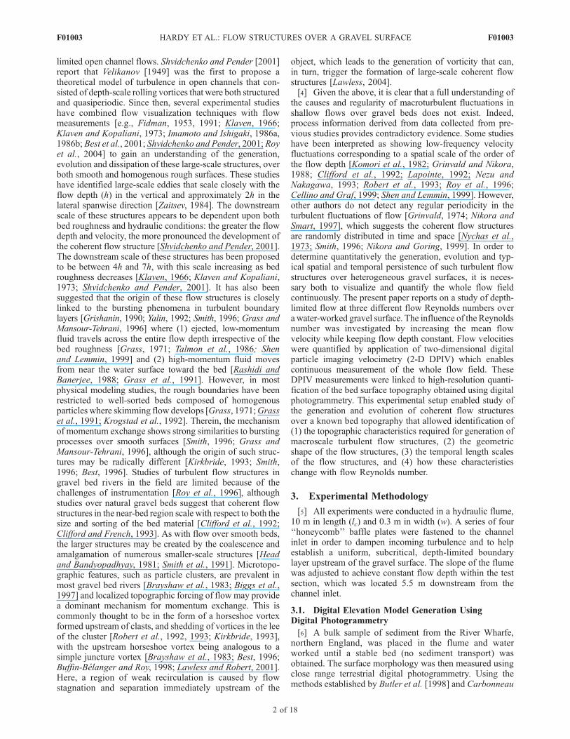
et al. [2003], a photogrammetric survey was designed inorder to produce digital elevation models (DEMs) with aspatial resolution of 1 mm2. This survey employed a KodakDCS 460 digital camera with an imaging resolution of3060 � 2036 pixels in standard red, green and blue bands.High-precision DEMs are regularly produced with suchcameras provided that additional surveyed ground calibra-tion points are added on the target surface [Carbonneau etal., 2003]. Accordingly, 84 ground control targets wereglued to stable large clasts in the bed. These targets werethen surveyed with a Geodimeter 608S total station toobtain x, y, z coordinates of points with a known positionin the imagery. To generate a DEM of the investigationregion, nine consecutive images with 60% overlap betweenconsecutive images were required. The resulting DEM wasnot smoothed. However, the edges were cropped to elimi-nate errors that typically occur on the periphery of the DEM,as a result of greater geometric distortion with distanceaway from the image centre. The size of the final DEM was0.923 by 0.26 m (Figure 1) with a vertical precision of±0.001 m. The topographic statistics of the DEM are givenin Table 1, and represent the topographic elevation of each0.001 m grid cell rather than that of individual gravelparticles.

3.2. Hydraulic Conditions

[7] In these experiments, the water depth was maintainedat a constant value of 0.2 m, with three different experi-ments being undertaken at mean downstream velocities at

0.4 z/h of 0.155 m s�1, 0.3 m s�1, and 0.435 m s�1 (where zand h are height above the bed and flow depth, respectively).The constant flow depth of 0.2 m was adopted for boththeoretical and practical reasons. The present study aimed tounderstand the nature of coherent flow structures formingover a heterogeneous gravel surface and the influence of anincrease in flow Reynolds number (through changes in flowvelocity) upon the generation of these flow structures.Consequently, depth was held constant and mean flowvelocity was used to increase the flow Reynolds number.Additionally, in practical terms, it was not possible toilluminate the whole flow depth with the laser configurationused herein. If greater flow depths were used it would nothave been possible to track the flow structures to the watersurface. Table 2 summarizes the hydraulic conditions usedin the study and the experiments are subsequently referredto according to their flow Reynolds numbers (Re).[8] Velocity measurements were obtained using a

DANTEC two-dimensional digital particle imaging veloc-imetry system (2-D DPIV), which is a nonintrusive, wholeflow field technique for velocity measurement. A majoradvantage of DPIV is that it is multipoint, and can be usedto study the entire flow field instantaneously to allowquantitative flow visualization (by analysis of consecutiveresolved velocity images) where flow structures can beobserved moving over the bed. The DPIV methodologyand postprocessing applied herein is identical to that previ-ously used by Hardy et al. [2005] and only a brief synopsis

Figure 1. The digital elevation model measured by digital photogrammetry on a 1 mm � 1 mmresolution. The boxes represent the interrogation regions of the digital particle imaging velocimetry withan area of 0.25 m � 0.252 m. The bold box on the left-hand side of the image demonstrates the flow fieldregion investigated herein.

Table 1. Topographic Statistics of the Digital Elevation Model

Particle Size (m) Roughness Height

Mean 0.0236 0.1179s 0.0086 . . .D16 0.0150 0.0748D50 0.0226 0.1130D84 0.0329 0.1646

Table 2. Hydraulic Conditions Used in This Analysis

Experiment 1 Experiment 2 Experiment 3

Flow velocity (m s�1) 0.155 0.300 0.435Flow depth (m) 0.200 0.200 0.200Qs (m

3 s�1) 9.3 � 10�3 1.8 � 10�2 2.6 � 10�2

Froude number �0.11 �0.21 �0.31Reynolds number �13,000 �25,000 �37,000

F01003 HARDY ET AL.: FLOW STRUCTURES OVER A GRAVEL SURFACE

3 of 18

F01003

is provided below. Measurement is based upon seeding theflowwith neutrally buoyant tracer particles (hollow reflectiveglass spheres with a mean diameter of 10 mm) and illumi-nating the flow field with a double-pulsed 50 mJ Nd-YAGlaser light sheet, with the time gap between flashes being setto 0.067 s. When the laser sheet illuminated the flow, lightwas scattered by the seeding material and detected by acharge-coupled device (CCD) camera positioned perpendic-ular to the light sheet. In order to derive a velocity vector map,a digital mesh of small interrogation regions (16� 16 pixels,where 1 pixel � 2.5 � 10�4 m) was draped over the images.For each interrogation region, in each pair of images, thedisplacement of groups of particles between the first andsecond image was measured using a fast Fourier transform–based spatial cross-correlation technique and a velocityvector was determined [see Westerweel, 1997]. The entireprocess was repeated at 15 Hz until the flow was sampledfor 1 min. This sample length provided a sufficient timeperiod to obtain a stationary time series, which was testedby systematic convergence of the cumulative variance forboth velocity components to a constant value (for a fullexplanation see Sukhodolov and Rhoads [2001]) andfollows the recommended sampling period suggested byBuffin-Belanger and Roy [2005].[9] In the present study, the DPIV camera was located

perpendicular to the bed, so that slices of flow could beinterrogated for the downstream u and vertical w componentsof velocity. With a 16 � 16 pixel interrogation region andthe setup described above, each instantaneous velocity mapconsisted of 15,750 individual vectors enabling data collec-tion at a spatial resolution of 2 � 10�3 m. In order tomaximize the signal-to-noise ratio of the particle crosscorrelations, a sequence of six quality checks [see Hardyet al., 2005] was undertaken. With this methodology, theestimated precision of the derived velocities is greater thanone tenth of a pixel [Wilbert and Gharib, 1991; Huang etal., 1997; DANTEC Dynamics, 2000]. Thus, the uncertaintyin the velocity measurement is better than ±0.08 mm s�1.[10] The area illuminated by the light sheet over the gravel

surfaces was aligned along the centerline of the flume. Forthis transect, three sections, each ’0.25 m in downstreamlength, were collected to enable a time-averaged map of0.75 m length to be quantified (see location of DPIV area inFigure 1). Because of the illumination requirements, tworegions needed to be illuminated and DPIV data collected inthe vertical dimension: (1) the near-bed region and (2) theregion extending to the free surface (see Figure 1). Thus, sixinterrogation regions were collected to cover the 0.75 mdownstream length for each of the three different flowconditions, with the map for each Reynolds number con-sisting of �90,000 points.

3.3. Analysis Methodology

[11] The DPIV data was collected on a regular grid (125�126, covering a spatial area of 0.25 by 0.252 m) with eachpoint providing a time series for 1 min at a temporalresolution of 15 Hz. The whole flow field can then be analyzedby either time-averaged or time-dependent techniques. In thisstudy, we explore the flow characteristics through (1) thetime-averaged flow fields, (2) instantaneous flow visualiza-tion, which is achieved by the analysis of consecutive imagesof the calculated u component velocity minus 0.85 of the

mean value at each point following the recommendation ofAdrian et al. [2000], (3) the time-averaged and instantaneousuw vorticity (w), (4) the root-mean-square (RMS) valuesof the deviatoric components of velocity, (5) analysis ofturbulent structures through classical quadrant analysis, and(6) identification of temporal length scales through waveletanalysis.3.3.1. Quadrant Analysis[12] Quadrant analysis has previously been used to dis-

criminate boundary layer turbulent events by examining theinstantaneous deviations of velocity from the mean values[e.g., Lu and Willmarth, 1973; Bogard and Tiederman,1986; Bennett and Best, 1995; Hardy et al., 2007]. Byapplying the standard definition of Lu and Willmarth [1973],four quadrants can be defined around a zero mean: quadrant 1events or outward interactions (positive u component, pos-itive w component), quadrant 2 events or ejections (bursts)(negative u component, positive w component), quadrant 3events or inward interactions (negative u component, neg-ative w component), and quadrant 4 events or inrushes(sweeps) (positive u component, negative w component).In the present analysis, each velocity pair was studiedusing a ‘‘hole’’ size [Lu and Willmarth, 1973; Bogard andTiederman, 1986; Bennett and Best, 1995] of one standarddeviation, in which the signal was examined only if thevalues exceeded this threshold.3.3.2. Wavelet Analysis[13] Wavelet analysis was identified as the most beneficial

method of analysis because visual inspection of the timeseries suggested that (1) the scales of variability were onlyintermittently present and (2) the scales of variability evolvedtemporally and spatially as a function of time (or space). Asthe evolution of scales of variability is continuous withindiscrete subseries, one option was to use a windowedFourier transform. However, this is both inaccurate (as itcan result in the aliasing of high- and low-frequencycomponents that do not fall within the frequency range ofthe window) and inefficient (as a result of the number offrequencies which must be analyzed at each time stepregardless of the window size or dominant frequenciespresent) [Torrence and Compo, 1998]. Here, we use waveletanalysis with scale-dependent time frequency localization[e.g., Labat et al., 2000; Torrence and Compo, 1998], whichis achieved by breaking the data series into a set of scaledand translated versions of a wavelet function, with the scaleof the wavelet varying with frequency. Thus, whereas aFourier transform yields a power value for each frequencydetermined, wavelet analysis produces power values for aset of locations in time and for a range of frequencies, thelatter being related to the scales of the wavelet functionconsidered. Wavelet analysis has also been previouslyapplied in studies of turbulence [e.g., Farge, 1992].[14] A full review of wavelet analysis is provided by

Torrence and Compo [1998], and the details below arerestricted to the application of wavelet analysis in thepresent study. Herein, we use a simple, real and nonorthog-onal wavelet, the Morlet wavelet, to estimate the powerpresent in the time series for a set of s (time) scales ofvariability and at a set of t time periods. The result is awavelet power spectrum with power mapped onto each (s, t)location. Choosing the right type of wavelet for a given dataseries is important, although if the prime goal of the study is

F01003 HARDY ET AL.: FLOW STRUCTURES OVER A GRAVEL SURFACE

4 of 18

F01003

determination of the wavelet power spectra, the precisechoice of the wavelet should not matter as different waveletswill give the same qualitative results [Torrence and Compo,1998]. Indeed, in a global sense, having to choose aparticular waveform is no different to the type of assump-tion made in conventional spectral analysis about the fit ofparticular waveforms to the data. Nonetheless, some justi-fication of the choice adopted herein is required. First, theprime aim of this analysis was a continuous transformationof the time series into a time-dependent, period frequencyseries in order to identify the intermittent presence offeatures at a range of time scales, as well as possibleevolution of the scale of features as a function of time.This suggested that the continuous wavelet transform wasmost appropriate. Second, we should expect a quasi-continuous variation in velocity fluctuations in this timeseries, and thus a simple wavelet form was most appropri-ate. Third, we needed to use a wavelet with a goodfrequency resolution: the data were collected at 15 Hz,leading to the probability of some redundancy at smallertime steps in relation to understanding the characteristics ofmacroturbulence. Thus, time resolution was less important.As a result of these deliberations, the present analysisutilized a Morlet wavelet, primarily because, of all thesimple wavelets considered, it has one of the best resolu-tions in frequency space. Furthermore, if the schematicdiagram of the elementary decomposition of turbulent energyfrom a characteristic eddy (as proposed by Tennekes andLumley [1972]) is studied, its morphology is very similar tothe Morlet wavelet. Consequently, it has been suggested thatthe Morlet wavelet is the most appropriate for studying thedynamics of turbulence [Liandrat and Moret-Bailly, 1990].[15] Four additional issues need specific mention: (1) the

reduction in the reliability of the analysis at the edges of thedata series, (2) the scales that will be analyzed, (3) conver-sion from wavelet scale to Fourier period, and (4) statisticalsignificance testing in relation to the difference between theobserved wavelet fits and the theoretical wavelet fits asso-ciated with a background spectrum. First, as the edges of atime series are reached, the length (in seconds) of thewavelet that can be resolved will be reduced, and a coneof influence (or detectable scales) needs to be set. The

Morlet wavelet has an e-folding time offfiffiffi

2p

s, which wasused to set the cone of influence. Second, with hundreds ofdata at a 15 Hz resolution, there are 999 possible scales ofanalysis. It is inefficient to analyze all of these scales as thisleads to redundancy in power determination at long scales(where the resolved scale has a much lower frequency than15 Hz) and poor resolution at short scales (where theresolved scale has a frequency approaching the Nyquistfrequency of 7.5 Hz). Thus, we initially used a dyadic seriesand analyzed over the range 29 scales, which corresponds toscales of up to 51.2 s, but constrained by the cone ofinfluence at the edges. In order to obtain a reasonableresolution in frequency space between dyadic numbers,tests suggested an increment of 0.1 was appropriate. Thus,we analyzed scales from 21 through 2n to 29 where n wasincremented in units of 0.1. Third, the wavelet scale is notnecessarily equivalent to the Fourier period, which is theequivalent scale measure that is of interest. Thus, we trans-formed the wavelet scale into the equivalent Fourier period,and hence frequency, prior to visualization of results[Torrence and Compo, 1998]. Finally, we determinedwhether or not the particular fit of a wavelet for a given nand s was statistically significant. Torrence and Compo[1998] show that the most appropriate method for doingthis is based upon choice of an appropriate backgroundspectrum that is associated with noise: if a point (at t, s) inthe wavelet power spectrum is statistically distinguishablefrom the associated point in the background spectrum, thenit can be assumed to be a significant fit at the confidencelevel chosen for the analysis. As is commonly observed invelocity time series, we assumed that white noise would bepresent [Biron et al., 1998].

4. Results

4.1. Time-Averaged Flow Fields

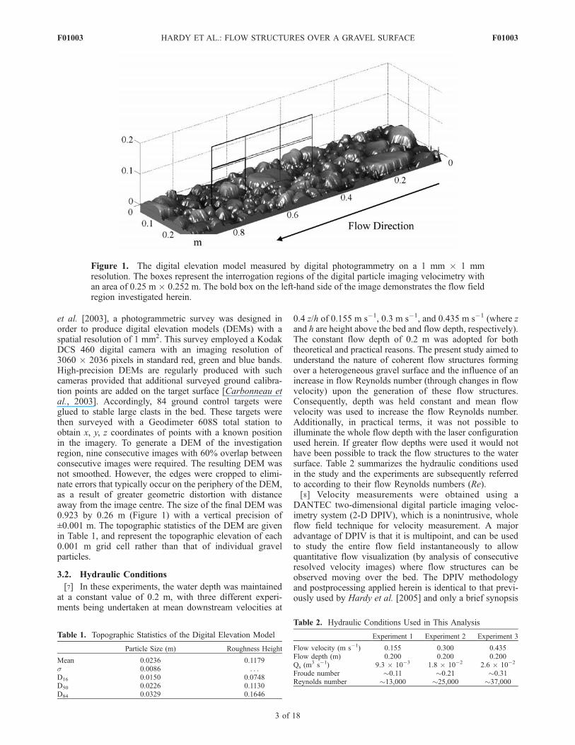
[16] The time-averaged flow fields for the downstream uand vertical w velocity components (Figure 2) show theinfluence of the bed topography on the near-bed flow.Analysis of the time-averaged downstream u componentfor the three different Reynolds numbers (Figures 2a–2c)shows areas of recirculation in the wakes of protruding

Figure 2. Time-averaged velocity for (a, b, c) the downstream u component and (d, e, f) the vertical wcomponent and for three Reynolds numbers: 13,000 (Figures 2a and 2d), 25,000 (Figures 2b and 2e), and37,000 (Figures 2c and 2f). Flow direction is from right to left; z/h is equal to 0.12 m, and x/l is equal to0.25 m. Regions A, B, and C represent areas of local recirculation. All scales are in m s�1.

F01003 HARDY ET AL.: FLOW STRUCTURES OVER A GRAVEL SURFACE

5 of 18

F01003

clasts, above which there in an increase in average flowvelocity with depth. The local recirculation identified in theu component appears over a short distance (�0.03 m; regionA in Figure 2a). The vertical w component more clearlyidentifies regions of both separation and reattachment offlow over individual particles which are not necessarilydefined in the u component (region B in Figure 2e). Theseregions have a downstream length of �0.04 m that appearsconsistent for all Reynolds numbers. In addition, the w com-ponent identifies a larger region of reattachment, whichexists for all three Re numbers, that is generated from alarger clast upstream (region C in Figure 2f), and whichextends over a downstream distance of �0.1 m. Althoughthese images are of the mean values, and individual coher-ent flow structures are thus not identified, the effect of thetopographic protrusion of bed forms is clearly seen toinfluence the whole flow field.

4.2. Instantaneous Flow Visualization

[17] Analysis of the instantaneous downstream u velocitycomponent of flow for the three different Reynolds numbers,through a series of consecutive images, provides a visual-

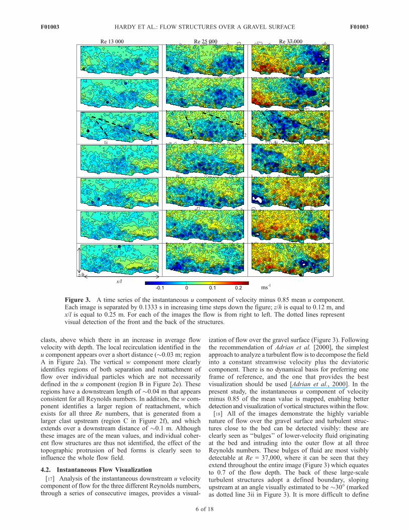
ization of flow over the gravel surface (Figure 3). Followingthe recommendation of Adrian et al. [2000], the simplestapproach to analyze a turbulent flow is to decompose the fieldinto a constant streamwise velocity plus the deviatoriccomponent. There is no dynamical basis for preferring oneframe of reference, and the one that provides the bestvisualization should be used [Adrian et al., 2000]. In thepresent study, the instantaneous u component of velocityminus 0.85 of the mean value is mapped, enabling betterdetection and visualization of vortical structureswithin the flow.[18] All of the images demonstrate the highly variable

nature of flow over the gravel surface and turbulent struc-tures close to the bed can be detected visibly: these areclearly seen as ‘‘bulges’’ of lower-velocity fluid originatingat the bed and intruding into the outer flow at all threeReynolds numbers. These bulges of fluid are most visiblydetectable at Re = 37,000, where it can be seen that theyextend throughout the entire image (Figure 3) which equatesto 0.7 of the flow depth. The back of these large-scaleturbulent structures adopt a defined boundary, slopingupstream at an angle visually estimated to be �30� (markedas dotted line 3ii in Figure 3). It is more difficult to define

Figure 3. A time series of the instantaneous u component of velocity minus 0.85 mean u component.Each image is separated by 0.1333 s in increasing time steps down the figure; z/h is equal to 0.12 m, andx/l is equal to 0.25 m. For each of the images the flow is from right to left. The dotted lines representvisual detection of the front and the back of the structures.

F01003 HARDY ET AL.: FLOW STRUCTURES OVER A GRAVEL SURFACE

6 of 18

F01003

the front of the structure visually, although the downstreamlead angle appears to be steeper at �45� (marked as dottedline 3i in Figure 3) than the rear, upstream back of thestructure. There is also an apparent decrease in the stream-wise velocity toward the back of the flow structure, with aclearly defined region of higher-velocity flow between eachof these low-velocity structures (Figure 3). These featuresdecrease in their distinctiveness at lower Reynolds numbers;the rear, upstream angle of the structures decreases and theyare not visible as far from the bed (lines 1 and 2 in Figure 3).However, these features do show similar geometric charac-teristics to those formed at Re = 37,000, with the lowerstreamwise velocity flow being located closer to the back ofthe structure, and the downstream lead angle appearingsteeper but harder to define clearly (lines 1i and 2i inFigure 3). Furthermore, the distance between these struc-tures appears to increase at higher Reynolds number. Insummary, as the Reynolds number increases, then the visualdistinctiveness of these structures becomes more apparent as(1) they become visible through the whole image, whichequates to �0.7 of the flow depth, (2) the downstream slopeof the coherent structure increases, (3) the decrease instreamwise flow velocity toward the back of the structurebecomes greater, and (4) the spacing between these coherentflow structures increases. These observations agree withprevious work which showed that at higher flow velocitiesthe development of coherent flow structures became morepronounced [Shvidchenko and Pender, 2001]. Furthermore,our results appear to visualize structures similar to theclassical bursting phenomenon in which low-momentumfluid is ejected from the bed [Grass, 1971; Talmon et al.,1986; Shen and Lemmin, 1999; Roy et al., 2004; Lacey etal., 2007], although here this is clearly seen to be develop-ing over the large anchor clasts in the bed. Studies in theturbulent boundary layer over a flat surface have alsosuggested a change in the form and angle of hairpin vorticesthat is dependent on the flow Reynolds number [Head andBandyopadhyay, 1981]. Head and Bandyopadhyay [1981]illustrate that at higher Reynolds numbers, the number ofhairpins traversing the boundary layer decreases, but thevortices still penetrate through the entire boundary layer, asalso revealed in the present study over rough gravel surfaces.

4.3. Time-Averaged and Instantaneous uw Vorticity

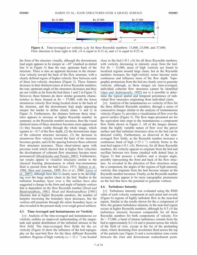
[19] Analysis of the time-averaged and instantaneous uwvorticity enables an improved understanding of the magni-tude and spatial distribution of the turbulent stresses in theflow field. The time-averaged flow fields for the uwvorticity (Figure 4) show the influence of the bed topogra-phy on the near-bed flow for the three different Reynoldsnumbers. Regions of high vorticity (w > 12 s�1) are located

close to the bed (<0.1 z/h) for all three Reynolds numbers,with vorticity decreasing in intensity away from the bed.For Re = 13,000, areas of high vorticity are found inlocalized regions around large clasts, but as the Reynoldsnumbers increases the high-vorticity zones become morecontinuous and influence more of the flow depth. Topo-graphic protrusions from the bed are clearly seen to generatevorticity, although, as these images are time-averaged,individual coherent flow structures cannot be identified[Agui and Andreopoulis, 1992] nor is it possible to deter-mine the typical spatial and temporal persistence of indi-vidual flow structures originating from individual clasts.[20] Analysis of the instantaneous uw vorticity of flow for

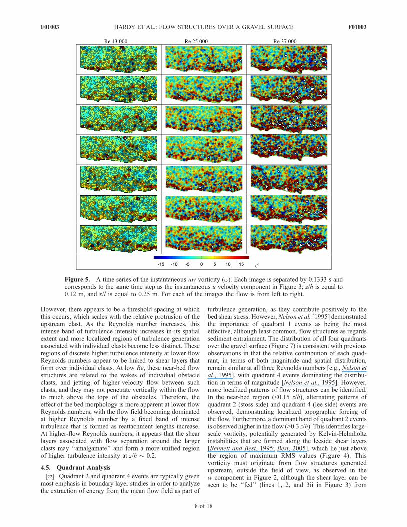
the three different Reynolds numbers, through a series ofconsecutive images similar to the analysis of instantaneousvelocity (Figure 3), provides a visualization of flow over thegravel surface (Figure 5). The flow maps presented are forthe equivalent time steps to the instantaneous u componentflow fields shown in Figure 3. All of the images demon-strate the highly variable nature of flow over the gravelsurface and that turbulent structures close to the bed can bedetected visibly. Furthermore, as observed in the time-averaged flow fields, as the Reynolds number increases acontinuous band of high (>15 s�1) vorticity forms in thenear-bed region (<0.1 z/h). However, for all three Reynoldsnumbers, the vorticity appears to originate from the bed andoscillate between two forms (marked with dotted lines inFigure 5) that possess a shallow and a steeper angle,possibly representing the front and back of the flow struc-ture. As revealed in the detection of flow structures usingthe u component, the angles of the regions of high-intensityvorticity that originate from the bed become steeper as theReynolds number increases. Finally, as the Reynolds numberincreases there appear to be more topographic protrusionson the bed that have the potential to generate vortices.

4.4. Turbulence Intensity

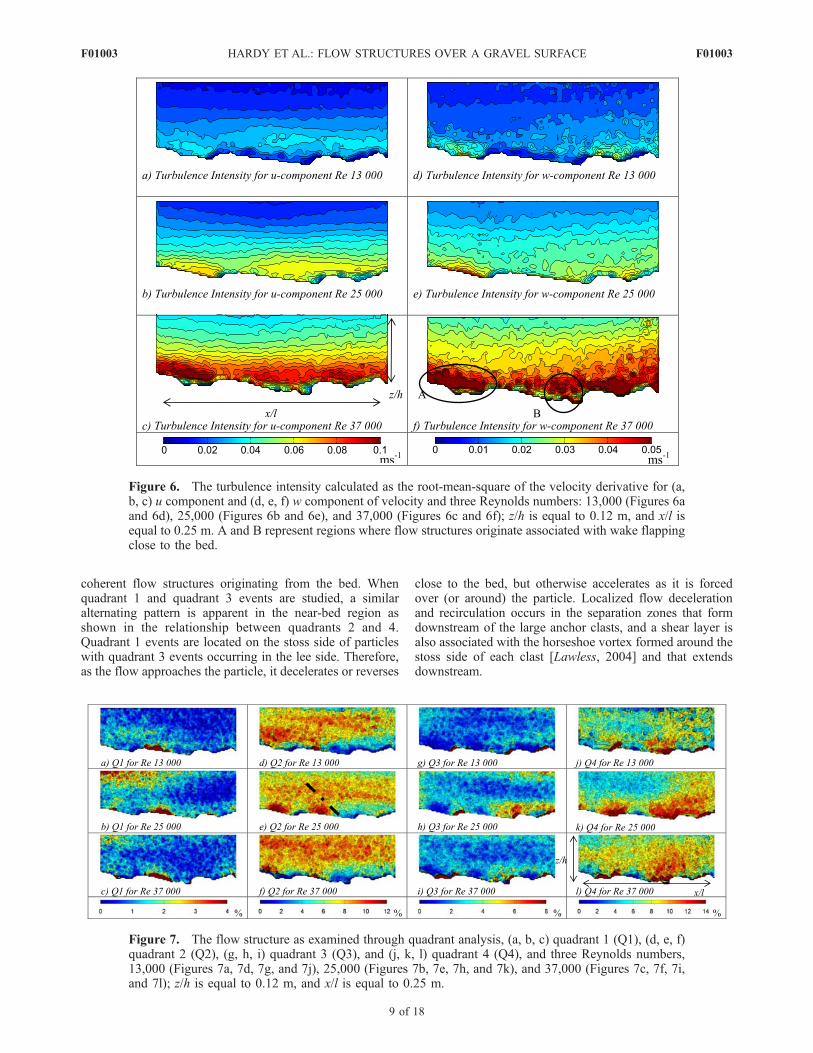
[21] Turbulence intensity was evaluated using the RMSvalue of each velocity component at each point and reveals(Figure 6) regions of highly turbulent flow in the near-bedregion. Similar to the results shown for the u component offlow, the greatest turbulence intensity in the near-bed regionoccurs at higher Reynolds numbers, although by 0.5 z/h theturbulence intensity becomes comparable for all threeReynolds numbers for both components of velocity. ForRe = 37,000, a band of intense turbulence extends from thebed to approximately 0.2 z/h and is present across the wholeof the field of view, except in the lee of the protrudingclasts, where skimming flow accelerates fluid across the topof the particle (see Figure 2) and a recirculation zone existsbetween the clast and downstream reattachment point.

Figure 4. Time-averaged uw vorticity (w)y for three Reynolds numbers: 13,000, 25,000, and 37,000.Flow direction is from right to left; z/h is equal to 0.12 m, and x/l is equal to 0.25 m.

F01003 HARDY ET AL.: FLOW STRUCTURES OVER A GRAVEL SURFACE

7 of 18

F01003

However, there appears to be a threshold spacing at whichthis occurs, which scales with the relative protrusion of theupstream clast. As the Reynolds number increases, thisintense band of turbulence intensity increases in its spatialextent and more localized regions of turbulence generationassociated with individual clasts become less distinct. Theseregions of discrete higher turbulence intensity at lower flowReynolds numbers appear to be linked to shear layers thatform over individual clasts. At low Re, these near-bed flowstructures are related to the wakes of individual obstacleclasts, and jetting of higher-velocity flow between suchclasts, and they may not penetrate vertically within the flowto much above the tops of the obstacles. Therefore, theeffect of the bed morphology is more apparent at lower flowReynolds numbers, with the flow field becoming dominatedat higher Reynolds number by a fixed band of intenseturbulence that is formed as reattachment lengths increase.At higher-flow Reynolds numbers, it appears that the shearlayers associated with flow separation around the largerclasts may ‘‘amalgamate’’ and form a more unified regionof higher turbulence intensity at z/h � 0.2.

4.5. Quadrant Analysis

[22] Quadrant 2 and quadrant 4 events are typically givenmost emphasis in boundary layer studies in order to analyzethe extraction of energy from the mean flow field as part of

turbulence generation, as they contribute positively to thebed shear stress. However, Nelson et al. [1995] demonstratedthe importance of quadrant 1 events as being the mosteffective, although least common, flow structures as regardssediment entrainment. The distribution of all four quadrantsover the gravel surface (Figure 7) is consistent with previousobservations in that the relative contribution of each quad-rant, in terms of both magnitude and spatial distribution,remain similar at all three Reynolds numbers [e.g., Nelson etal., 1995], with quadrant 4 events dominating the distribu-tion in terms of magnitude [Nelson et al., 1995]. However,more localized patterns of flow structures can be identified.In the near-bed region (<0.15 z/h), alternating patterns ofquadrant 2 (stoss side) and quadrant 4 (lee side) events areobserved, demonstrating localized topographic forcing ofthe flow. Furthermore, a dominant band of quadrant 2 eventsis observed higher in the flow (>0.3 z/h). This identifies large-scale vorticity, potentially generated by Kelvin-Helmholtzinstabilities that are formed along the leeside shear layers[Bennett and Best, 1995; Best, 2005], which lie just abovethe region of maximum RMS values (Figure 4). Thisvorticity must originate from flow structures generatedupstream, outside the field of view, as observed in thew component in Figure 2, although the shear layer can beseen to be ‘‘fed’’ (lines 1, 2, and 3ii in Figure 3) from

Figure 5. A time series of the instantaneous uw vorticity (w). Each image is separated by 0.1333 s andcorresponds to the same time step as the instantaneous u velocity component in Figure 3; z/h is equal to0.12 m, and x/l is equal to 0.25 m. For each of the images the flow is from left to right.

F01003 HARDY ET AL.: FLOW STRUCTURES OVER A GRAVEL SURFACE

8 of 18

F01003

coherent flow structures originating from the bed. Whenquadrant 1 and quadrant 3 events are studied, a similaralternating pattern is apparent in the near-bed region asshown in the relationship between quadrants 2 and 4.Quadrant 1 events are located on the stoss side of particleswith quadrant 3 events occurring in the lee side. Therefore,as the flow approaches the particle, it decelerates or reverses

close to the bed, but otherwise accelerates as it is forcedover (or around) the particle. Localized flow decelerationand recirculation occurs in the separation zones that formdownstream of the large anchor clasts, and a shear layer isalso associated with the horseshoe vortex formed around thestoss side of each clast [Lawless, 2004] and that extendsdownstream.

Figure 6. The turbulence intensity calculated as the root-mean-square of the velocity derivative for (a,b, c) u component and (d, e, f) w component of velocity and three Reynolds numbers: 13,000 (Figures 6aand 6d), 25,000 (Figures 6b and 6e), and 37,000 (Figures 6c and 6f); z/h is equal to 0.12 m, and x/l isequal to 0.25 m. A and B represent regions where flow structures originate associated with wake flappingclose to the bed.

Figure 7. The flow structure as examined through quadrant analysis, (a, b, c) quadrant 1 (Q1), (d, e, f)quadrant 2 (Q2), (g, h, i) quadrant 3 (Q3), and (j, k, l) quadrant 4 (Q4), and three Reynolds numbers,13,000 (Figures 7a, 7d, 7g, and 7j), 25,000 (Figures 7b, 7e, 7h, and 7k), and 37,000 (Figures 7c, 7f, 7i,and 7l); z/h is equal to 0.12 m, and x/l is equal to 0.25 m.

F01003 HARDY ET AL.: FLOW STRUCTURES OVER A GRAVEL SURFACE

9 of 18

F01003

4.6. Wavelet Analysis

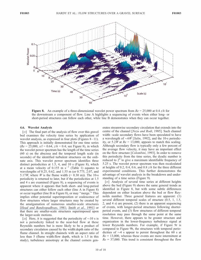
[23] The final part of the analysis of flow over this gravelbed examines the velocity time series by application ofwavelet analysis, as expressed in four plots (Figures 8–11).This approach is initially demonstrated for one time series(Re = 25,000, x/l = 0.64, z/h = 0.4; see Figure 8), in whichthe wavelet power spectrum has the length of the time series(60 s) on the abscissa and the temporal length scale (inseconds) of the identified turbulent structures on the ordi-nate axis. This wavelet power spectrum identifies threedistinct periodicities at 1.5, 4, and 10 s (Figure 8), whichat a mean velocity of 0.155 m s�1 (Table 1) equates towavelengths of 0.25, 0.62, and 1.55 m (or 0.775, 2.07, and5.17W, where W is the flume width (= 0.30 m)). The 10-speriodicity is returned to later, but if the periodicities at 1.5and 4 s are examined (Figure 8), a sequencing of events isapparent where it appears that both short- and long-periodstructures can either follow each other (line A in Figure 8)or occur together (line B in Figure 8), or may ‘‘merge.’’ Thisimplies either potential superimposition or coalescence offlow structures where larger structures may be created bythe amalgamation of numerous smaller-scale structures[Head and Bandyopadhyay, 1981; Smith et al., 1991] orthat there are smaller-scale structures superimposed uponthe larger-scale motions.[24] Here, it is suggested that the periodicity of �10 s is

not a periodicity linked to the near-bed flow at theseReynolds numbers but is more likely to be a product ofsecondary circulation caused by the width:depth ratio of theflume channel. In straight channels with an aspect ratio ofless than 5 (flume width:flow depth, which is 1.5 in thisstudy), turbulence anisotropy at the channel corners gen-

erates streamwise secondary circulation that extends into thecentre of the channel [Nezu and Rodi, 1985]. Such channelwidth–scale secondary flows have been speculated to havea wavelength of �6W [Yalin, 1992], and the 10-s periodic-ity, or 5.2W at Re = 13,000, appears to match this scaling.Although secondary flow is typically only a few percent ofthe average flow velocity, it may have an important effecton the flow structure [Colombini, 1993]. In order to removethis periodicity from the time series, the dyadic number isreduced to 26 to give a maximum identifiable frequency of5.25 s. The wavelet power spectrum was then recalculatedat heights of 0.2, 0.4, 0.6, and 0.8 z/h for the three differentexperimental conditions. This further demonstrates theadvantage of wavelet analysis in the breakdown and under-standing of a time series (Figure 9).[25] Analysis of several time series at different heights

above the bed (Figure 9) shows the same general trends asidentified in Figure 8, but with some subtle differencesdependent on either location above the bed or flow Rey-nolds number. Three general features are apparent: (1)several different temporal scales of structure (0.5, 1, 1.5,2, and 4 s) are present, (2) there is an apparent sequencingof events, with longer-period structures following shorter-period events, and (3) flow structures of different temporalresolution may pass through the same point at the sametime. However, there appears to be greater structure andorganization in the lower-frequency turbulence signal atlower Reynolds numbers. For example, if Figure 9r iscompared to Figure 9b, the structures with temporal perio-dicities of �4 s appear to persist throughout the 60 s atRe = 13,000, whereas these events are more intermittent atRe = 37,000. This trend is consistent throughout the flow

Figure 8. An example of a three-dimensional wavelet power spectrum from Re = 25,000 at 0.4 z/h forthe downstream u component of flow. Line A highlights a sequencing of events when either long- orshort-period structures can follow each other, while line B demonstrates when they can occur together.

F01003 HARDY ET AL.: FLOW STRUCTURES OVER A GRAVEL SURFACE

10 of 18

F01003

Figure

9.

Thewaveletpower

spectraforboth

(a,b,c,d,i,j,k,l,q,r,s,t)theuvelocity

componentand(e,f,g,h,m,n,o,

p,u,v,w,x)thewvelocity

componentforthreeReynoldsnumbers:37,000(Figures9a–9h),25,000(Figures9i–9p),and

13,000(Figures9q–9x).Thewavelet

power

spectrahavethelength

ofthetimeseries

(60s)

ontheabscissa

andthe

temporallength

scale(inseconds)oftheidentified

turbulentstructuresontheordinateaxes.Thelines

onFigure

9cidentify

anincrease

intemporallength

scaleofstructurespassingthroughthepoint.

F01003 HARDY ET AL.: FLOW STRUCTURES OVER A GRAVEL SURFACE

11 of 18

F01003

depth. For Re = 37,000, the frequencies <1 s are dominant,especially at 0.2 z/h, while their detection is minimal forRe = 13,000. This suggests that the higher-frequency scalesbecome more important, and the lower frequency lessimportant, as the Reynolds number increases.[26] For Re = 37,000, there visually appears to be more

sequencing of flow structures, especially at heights of 0.4 to0.8 z/h, with frequencies from 1 to 3 s. On Figure 9c, twoconsecutive dotted diagonal lines illustrate an increase in thetemporal length scales of structures passing through thepoint, implying that larger temporal scale structures areforming at a location downstream. Finally, as the Reynoldsnumber increases, especially at Re = 37,000, the 5-speriodicity ceases to exist.[27] Although yielding a unique insight into the temporal

dynamics of coherent flow structures over this gravel bed,this form of Eulerian analysis does not enable the detectionof changes in the entire flow field as Reynolds numberincreases. Primarily, it is difficult to detect major changesthrough the profile (from 0.2 to 0.8 z/h) as these flowstructures appear to influence the whole flow depth. Second,it is difficult to distinguish any major differences betweenthe u and w components, and the flow structures appear to betwo-dimensional. Consequently, the analysis was expanded

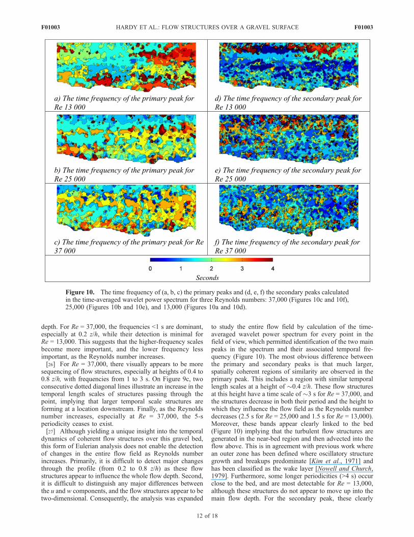
to study the entire flow field by calculation of the time-averaged wavelet power spectrum for every point in thefield of view, which permitted identification of the two mainpeaks in the spectrum and their associated temporal fre-quency (Figure 10). The most obvious difference betweenthe primary and secondary peaks is that much larger,spatially coherent regions of similarity are observed in theprimary peak. This includes a region with similar temporallength scales at a height of �0.4 z/h. These flow structuresat this height have a time scale of �3 s for Re = 37,000, andthe structures decrease in both their period and the height towhich they influence the flow field as the Reynolds numberdecreases (2.5 s for Re = 25,000 and 1.5 s for Re = 13,000).Moreover, these bands appear clearly linked to the bed(Figure 10) implying that the turbulent flow structures aregenerated in the near-bed region and then advected into theflow above. This is in agreement with previous work wherean outer zone has been defined where oscillatory structuregrowth and breakups predominate [Kim et al., 1971] andhas been classified as the wake layer [Nowell and Church,1979]. Furthermore, some longer periodicities (>4 s) occurclose to the bed, and are most detectable for Re = 13,000,although these structures do not appear to move up into themain flow depth. For the secondary peak, these clearly

Figure 10. The time frequency of (a, b, c) the primary peaks and (d, e, f) the secondary peaks calculatedin the time-averaged wavelet power spectrum for three Reynolds numbers: 37,000 (Figures 10c and 10f),25,000 (Figures 10b and 10e), and 13,000 (Figures 10a and 10d).

F01003 HARDY ET AL.: FLOW STRUCTURES OVER A GRAVEL SURFACE

12 of 18

F01003

defined regions are not as visible as the primary peak,especially for Re = 25,000 and Re = 37,000 (Figure 8).However, a similar band to that observed in the primarypeak is identified for Re = 13,000 at a similar height abovethe bed (z/h = 0.3), with a periodicity of 1.25 s. Thegeometric similarity with the primary peak for Re =37,000 may suggest it is the same physical processes whichgenerates these flow structures, although the influence ofthis period on the flow field decreases at lower Reynoldsnumbers, where it is absent at Re = 13,000. The same‘‘streaky’’ patterns of structures, originating from the bedand moving up into the flow, are observed, with thetemporal scale of these structures depending greatly onthe local bed structure.

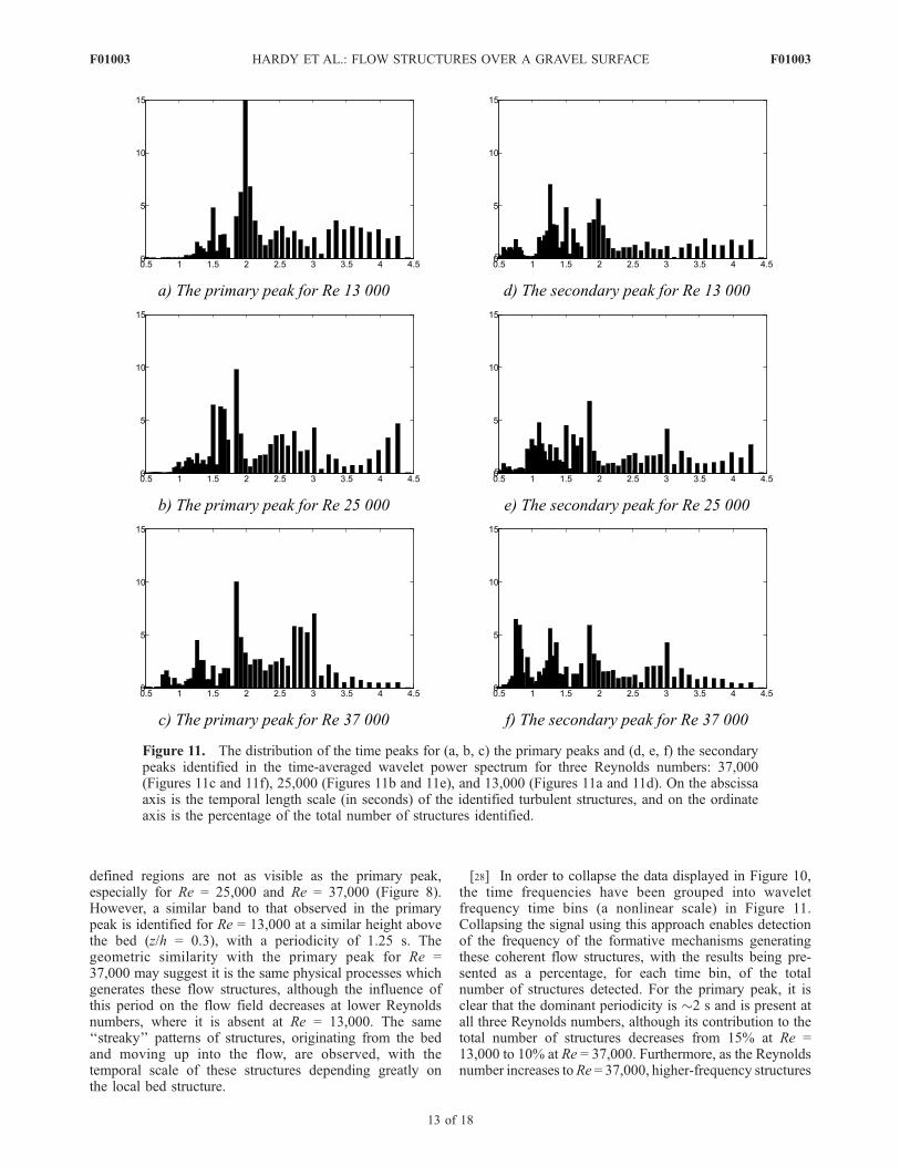
[28] In order to collapse the data displayed in Figure 10,the time frequencies have been grouped into waveletfrequency time bins (a nonlinear scale) in Figure 11.Collapsing the signal using this approach enables detectionof the frequency of the formative mechanisms generatingthese coherent flow structures, with the results being pre-sented as a percentage, for each time bin, of the totalnumber of structures detected. For the primary peak, it isclear that the dominant periodicity is �2 s and is present atall three Reynolds numbers, although its contribution to thetotal number of structures decreases from 15% at Re =13,000 to 10% at Re = 37,000. Furthermore, as the Reynoldsnumber increases toRe = 37,000, higher-frequency structures

Figure 11. The distribution of the time peaks for (a, b, c) the primary peaks and (d, e, f) the secondarypeaks identified in the time-averaged wavelet power spectrum for three Reynolds numbers: 37,000(Figures 11c and 11f), 25,000 (Figures 11b and 11e), and 13,000 (Figures 11a and 11d). On the abscissaaxis is the temporal length scale (in seconds) of the identified turbulent structures, and on the ordinateaxis is the percentage of the total number of structures identified.

F01003 HARDY ET AL.: FLOW STRUCTURES OVER A GRAVEL SURFACE

13 of 18

F01003

become more apparent at �1.25 and �0.75 s. However, themost dominant change as Reynolds number increases is theappearance of a period at �3 s that makes the distributionbimodal. More subtle trends can be observed in the sec-ondary peak data in Figures 9d–9f, similar to that revealedin the analysis of secondary peaks shown in Figure 10.Structures with a frequency of �2 s are detected for all threeReynolds numbers (Figures 11d–11f) with shorter-frequencystructures, again at �1.25 s, also being present. Theapparent contribution of the �1.25-s structures in thesecondary peaks appears to decrease as the Reynoldsnumber increases, again with the appearance of a �0.75-sfrequency at Re = 37,000. Thus, although the magnitudeof the contribution from these structures changes withReynolds number, the �2-s periodicity is detected at allReynolds numbers, and suggests that the same formativemechanism is generating the coherent flow structures.Furthermore, it appears that as the Reynolds numberexceeds a critical threshold, additional processes influencethe generation of the flow field and these periodicities are

examined below through the application of existing scalinglaws.[29] Several different generalized relationships have been

proposed to calculate dimensionless numbers that define theperiod of large-scale turbulence and aid understanding ofthe overall turbulence signature, such as the boil periodicitysuggested by Jackson [1976], the Strouhal relationship[Levi, 1983, 1991] or vortex and wake flapping frequenciesproposed by Simpson [1989]. The underlying problem withall of these relationships is that the flow reattachment pointis extremely difficult to determine [Nelson and Smith, 1989;Kostaschuk, 2000; Best and Kostaschuk, 2002], and this ismade even more problematic over a gravel bed because ofvortices merging into a continuous shear layer. However,Simpson [1989] proposed two scaling relations: for vortexshedding

fv ¼ 0:6U=Xr; ð1Þ

where fv is vortex frequency, U is the mean velocity, and Xr

is the mean length of the separation zone, and for wakeflapping

fw < 0:1U=Xr: ð2Þ

Figure 11 provides an approximation of the frequency(s) forthe identifiable peaks (0.75, 1.5, 2, and 3 s, which equates to1.3, 0.8, 0.5, and 0.3 Hz). Furthermore, analysis of the DEM(Figure 1) shows that the maximum particle length in thegravel matrix is 0.14 m and the maximum height is 0.062 m.If equations (1) and (2) are rearranged to calculate thereattachment length by using the hydraulic conditions givenin Table 2, a second-order approximation of processesgenerating the turbulent flow field can be deduced (Table 3).[30] By applying the scaling laws to the four identified

frequencies and three hydraulic conditions, the calculatedmean lengths of flow separation from wake flapping arebetween 0.01 and 0.13 m. It is suggested that these are

Table 3. Estimation of Reattachment Lengths From Frequencies

Identified in Collapsing the Entire Flow Field Flow Frequenciesa

Frequency (Hz)

1.33 0.80 0.50 0.33

Vortex Shedding fv = 0.6U/XrRe = 13,000 �0.07 �0.12 �0.19 �0.31Re = 25,000 �0.13 �0.26 �0.36 �0.54Re = 37,000 �0.19 �0.32 �0.52 �0.79

Wake Flapping fw < 0.1U/Xr

Re = 13,000 �0.011 �0.014 �0.031 �0.047Re = 25,000 �0.023 �0.038 �0.06 �0.091Re = 37,000 �0.033 �0.054 �0.087 �0.132

aReattachment lengths are measured in meters.

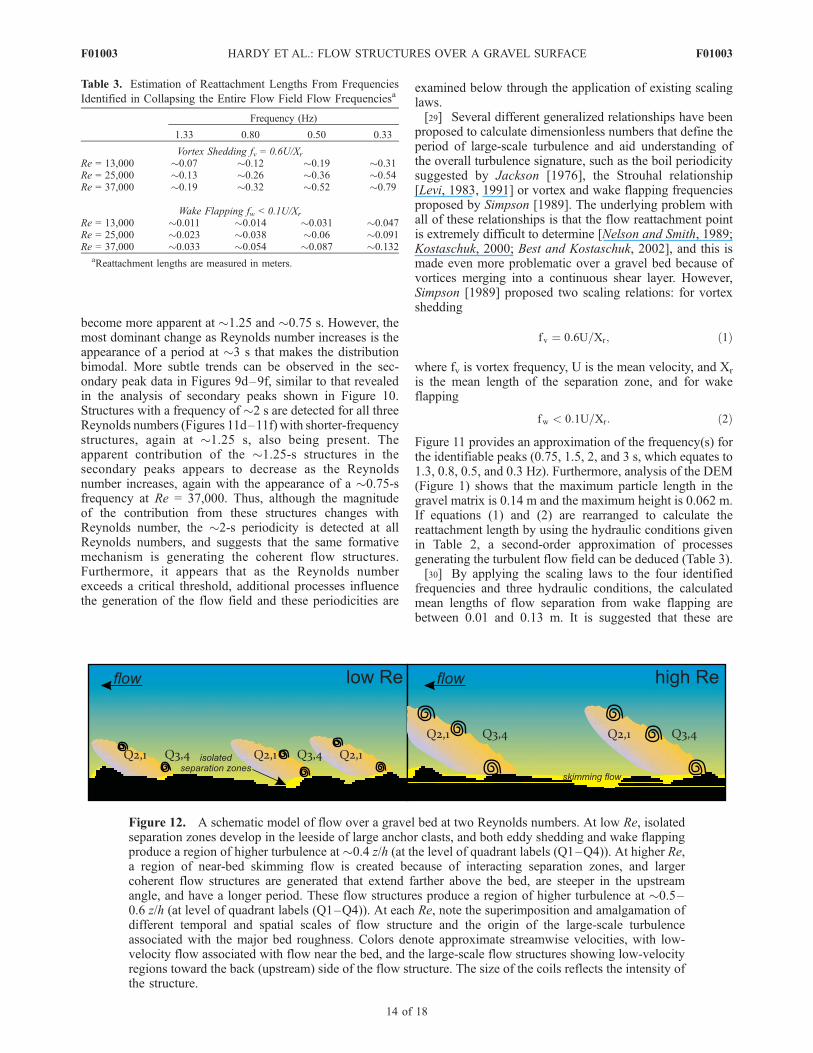
Figure 12. A schematic model of flow over a gravel bed at two Reynolds numbers. At low Re, isolatedseparation zones develop in the leeside of large anchor clasts, and both eddy shedding and wake flappingproduce a region of higher turbulence at �0.4 z/h (at the level of quadrant labels (Q1–Q4)). At higher Re,a region of near-bed skimming flow is created because of interacting separation zones, and largercoherent flow structures are generated that extend farther above the bed, are steeper in the upstreamangle, and have a longer period. These flow structures produce a region of higher turbulence at �0.5–0.6 z/h (at level of quadrant labels (Q1–Q4)). At each Re, note the superimposition and amalgamation ofdifferent temporal and spatial scales of flow structure and the origin of the large-scale turbulenceassociated with the major bed roughness. Colors denote approximate streamwise velocities, with low-velocity flow associated with flow near the bed, and the large-scale flow structures showing low-velocityregions toward the back (upstream) side of the flow structure. The size of the coils reflects the intensity ofthe structure.

F01003 HARDY ET AL.: FLOW STRUCTURES OVER A GRAVEL SURFACE

14 of 18

F01003

reasonable length scales for flows over such complexheterogeneous topography with a median particle heightof 0.02 m and maximum particle length of 0.14 m. Becauseof the several (temporal) scales of turbulence that have beenidentified (Figures 10 and 11) and the apparent amalgam-ation of flow structures into an intense band of turbulence(Figure 6), it may not be possible to separate individualprocesses of coherent flow structure generation. This is dueto the complex bed topography, where each topographicprotrusion generates its own flow field and the considerablepositive feedback between bed form topography and thegeneration of flow structures.[31] However, as demonstrated in Figure 11, the 2-s

structure is prevalent for all three Reynolds numbers. Themean lengths of flow separation calculated for wake flap-ping range from 0.03 to 0.09 m as the Reynolds numberincreases. Furthermore, when the w component of meanflow (Figure 2) and turbulence intensity (Figure 6) arestudied, flow structures with length scales of the same orderof magnitude are identified. As discussed previously, flowstructures with a length scale of �0.04 m are clearlydetected in the time-averaged images. These flow structuresare intermittent and therefore the whole structure will notnecessarily be detectable in a time-averaged analysis, sincethe patterns of structure motion would not be regular.However, the point from where these structures are initiatedand generated will be consistent. The same observations canbe made in the plots of turbulence intensity (regions A andB in Figure 6) where regions of �0.07 m length with highturbulence intensity are detected behind protruding clasts.Thus, these structures may be associated with wake flappingclose to the bed and its interaction with the protrudingtopography. This follows classical hydraulic theory thatwould suggest that as flow approaches an obstacle, alocalized area of low flow velocity develops in front ofthe topographic protrusion and a suppressed saddle pointvortex forms [Hunt et al., 1978]. This flow thus movesaround such topographic protrusions in the form of tertiaryvortices [Hunt et al., 1978] and it is reasoned that these,together with wake flapping associated with the leeside flowseparation zone shear layer, may form the coherent flowstructures documented herein. This mechanism is possiblefor all four identified frequencies, with wake flappingreattachment lengths ranging from 0.01 to 0.13 m. Finally,at Re = 37,000, shorter periodicities are identified, whichprovides an average vortex shedding reattachment length of0.19 m, similar to that identified at this Reynolds number inFigure 2.

5. Discussion

[32] This analysis has examined the characteristics ofturbulent flow generated over known gravel bed topographyat three different flow Reynolds numbers. The analysis hasdetected coherent flow structures with defined spatial andtemporal characteristics that scale with the flow Reynoldsnumber. As the Reynolds number increases (Figure 12)(1) the visual distinctiveness of the flow structures becomesmore defined through the flow depth, (2) the upstream slopeof the coherent flow structure increases in angle, (3) thereduction in streamwise flow velocity, and turbulence

intensity, toward the upstream side of the structureincreases, and (4) the spacing between these coherent flowstructures increases. The source of these structures isidentified through examination of the mean and turbulentintensity values, as well as by quadrant analysis. Analysis ofthe mean u and w components identifies flow recirculationover short distances (�0.03 m) that is generated by flowseparation associated with individual clasts. In addition, asecondary ‘‘reattachment structure’’ is identified in thew component with a length scale of �0.1 m. This localizedseparation and reattachment is further identified in theturbulence intensity plots where the greatest turbulenceintensity is detected in the near-bed region. At higherReynolds numbers, a continuous band of high turbulenceintensity is formed that appears linked to the amalgamationof shear layers associated with flow separation around thelarger clasts, thus forming a more unified region of higherturbulence intensity at �0.2 z/h. By 0.5 z/h, the turbulenceintensity becomes comparable for all three Reynolds numb-ers. Finally, in the near-bed region, quadrant analysisidentifies alternating patterns of quadrant 2 (stoss side)and quadrant 4 (lee side) events, again demonstratinglocalized bed/topographic forcing of the flow. Furthermore,a band of quadrant 2 events are detected higher in the flow,most likely formed by large-scale Kelvin-Helmholtz insta-bilities along a shear layer [e.g., Bennett and Best, 1995;Best, 2005]. A similar pattern is observed in quadrant 1(stoss side) and quadrant 3 (lee side) events in the near-bedregion, which suggests that as the flow approaches theparticle, it decelerates or reverses close to the bed, butotherwise accelerates as it is forced over (or around) theparticle. Localized flow deceleration occurs in the separa-tion zones that form downstream of the large anchor clasts:flow within these separation zones recirculates, forming abody-fitted vortex, and a shear layer that extends down-stream is associated with each of the clast lee sides.[33] Wavelet analysis has enabled the temporal length

scales of the turbulent signatures to be identified. Decom-posing the selected time series in the temporal domainidentified general trends which included (1) several differ-ent dominant temporal scales of flow structure (0.5, 1, 1.5,2, and 4 s), (2) an apparent sequencing of events, withlonger-period structures following shorter-period events,and (3) flow structures of different temporal resolutionpassing through the same point at the same time. Whenthe signal is decomposed and analyzed, for the wholeimage, by detecting the primary and secondary peaks inthe wavelet power spectrum, the time scales of the dominantflow structures can be identified. The most obvious differ-ence between the primary and secondary peaks is that muchlarger, spatially coherent regions of similarity are observedin the primary peak, and includes a region with similartemporal length scales at a height of �0.4 z/h. The flowstructures at this height have a time scale of �3 s for Re =37,000 but, as the Reynolds number decreases, are seen todecrease in both their temporal scale (2.5 s for Re = 25,000and 1.5 s for Re = 13,000) and the height above the bed atwhich they influence the flow field. These bands appearlinked to the bed (lines A and B in Figure 8), suggesting thatturbulent flow structures are generated in the near-bedregion and then entrained into the flow above. If this

F01003 HARDY ET AL.: FLOW STRUCTURES OVER A GRAVEL SURFACE

15 of 18

F01003

analysis is extended, the distribution of turbulent lengthscales identifies a 2-s flow structure that is prevalent at allthree Reynolds numbers. By applying standard scalinglaws, the mean lengths of flow separation calculated forwake flapping range from 0.03 to 0.09 m and increase athigher Reynolds numbers.[34] The results obtained in this analysis agree with

previous work in which the development of the flowstructure has been found to be proportional to the flowvelocity (i.e., Reynolds number if flow depth is keptconstant [Shvidchenko and Pender, 2001]), and identifiesstructures similar to the classical bursting phenomenon inwhich low-momentum fluid is ejected from the bed [Grass,1971; Talmon et al., 1986; Shen and Lemmin, 1999].However, the present study shows that these flow structuresdevelop over the large anchor clasts in the bed, potentiallyby wake flapping. Studies of turbulent boundary layers overflat surfaces have also suggested a change in the form andangle of hairpin vortices dependent on the flow Reynoldsnumber [Head and Bandyopadhyay, 1981], with the hairpinvortices becoming stretched and narrower at higher Re. Athigher Reynolds numbers, the number of hairpins traversingthe boundary layer was found to decrease, although thevortices still penetrated through the entire boundary layer,and can merge to form ‘‘packets’’ of hairpin vortices [e.g.,Christensen and Adrian, 2001]. Over rough surfaces, theseflow structures appear to merge into a single layer, whichimplies that skimming flow [Grass, 1971; Grass et al.,1991; Krogstad et al., 1992] generated over the largestroughness elements tends to dominate as the Reynoldsnumber increases, and may form large-scale vorticity. Thepresent study illustrates that the origin of these larger-scalemotions are Kelvin-Helmholtz instabilities generated alongthe separation zone shear layer [e.g., Muller and Gyr, 1982,1986; Rood and Hickin, 1989; Bennett and Best, 1995; Best,2005], thus forming a region defined as where oscillatorystructure growth and breakups predominate [Kim et al.,1971] and which has previously been classified as the wakelayer (wake flapping) [Nowell and Church, 1979]. Thisimplies the creation of larger-scale flow structures by eitherpotential superimposition, or coalescence, of numeroussmaller-scale structures [Head and Bandyopadhyay, 1981;Smith et al., 1991], or where smaller-scale structures existupon larger-scale structures. Thus, our present analysissuggests that coherent flow structures over gravels owetheir origin to bed-generated turbulence and that large-scaleouter layer structures are the result of flow-topographyinteractions in the near-bed region associated with wakeflapping.

6. Conclusions

[35] Turbulent flows moving over a gravel bed developlarge-scale, macroturbulent flow structures that are initiatedat the bed, and grow and dissipate as they move upwardthrough the flow depth. These large-scale flow structureschange their form and magnitude at higher Reynoldsnumbers, becoming more distinct, with a clearer velocitysignature and steeper upstream-dipping slopes. This studyshows that the near-bed flow controls the flow structure fedinto the outer flow and that macroturbulence over gravelbeds is sourced from these flow-bed interactions. These

large-scale coherent flow structures are separated by regionsof higher than average streamwise velocity, and defineregions that are dominated by quadrant 2 and quadrant 1events, which are interspersed with regions dominated byquadrant 4 and quadrant 3 events. At low Reynolds numb-ers, flow over the gravel surface is found to possess distinctregions of flow separation in the leeside of individual clasts,but as Reynolds number increases and the length of the flowrecirculation zones grows, then these amalgamate to form alayer of skimming flow near the bed. Turbulence associatedwith both eddy shedding and wake flapping in the leeside ofthese clasts creates the larger-scale coherent turbulentmotions, which may amalgamate to form a region of higherturbulence intensity at a dimensionless height away fromthe bed, z/h, of �0.5 at higher Reynolds numbers. Super-imposition of such motions appears to create the conditionsnecessary for the formation of large-scale coherent flowstructures that can advect through the entire flow depth.Wavelet analysis has been shown to be a powerful tool indeciphering the complex signatures of such large-scalemotions, and shows that these organized motions havelonger periods at higher Reynolds numbers and penetratefurther into the outer flow. The occurrence of severaltemporal scales of structure, and their presence at the sametime, suggest the superimposition and amalgamation ofsmaller-scale flow structures to create this large-scaleturbulence.[36] Future work clearly needs to investigate further the

exact nature of such superimposition, amalgamation andvortex evolution, and investigate the links between thegrowth and dissipation of these structures, and both sedi-ment suspension and bed load transport. The interactionsbetween such flow structures and sediment entrainmentholds the key for understanding and predicting the transportand fate of a range of different size and compositionparticles both above, at, and within the bed of gravelsubstrates.

[37] Acknowledgments. The authors are grateful to Mark Franklinfor assistance with the flume experiments and operation of the DPIV and toJ. H. Chandler, University of Loughborough, for the loan of the KodakDCS 460 digital camera and discussion regarding errors in camerageometry. R.J.H. was funded through NERC fellowship NER/J/S/2002/00663 while the DANTEC DPIV system was funded by NERC JREI grantGR3/JE140 to J.L.B. We are grateful to the Associate Editor and twoanonymous referees for providing helpful comments that have led tosignificant improvements in this manuscript.

ReferencesAdrian, R. J., C. D. Meinhart, and C. D. Tomkins (2000), Vortex organiza-tion in the outer region of the turbulent boundary layer, J. Fluid Mech.,422, 1–54, doi:10.1017/S0022112000001580.

Agui, J. H., and J. Andreopoulis (1992), Experimental investigation of athree-dimensional boundary layer flow in the vicinity of an upright wallmounted cylinder, J. Fluids Eng., 114, 566–576, doi:10.1115/1.2910069.

Bennett, S. J., and J. L. Best (1995), Mean flow and turbulence structureover fixed, two-dimensional dunes: Implications for sediment transportand dune stability, Sedimentology, 42, 491–513, doi:10.1111/j.1365-3091.1995.tb00386.x.

Best, J. L. (1996), The fluid dynamics of small-scale alluvial bedforms, inAdvances in Fluvial Dynamics and Stratigraphy, edited by P. A. Carlingand M. Dawson, pp. 67–125, John Wiley, New York.

Best, J. L. (2005), The fluid dynamics of river dunes: A review and somefuture research directions, J. Geophys. Res., 110, F04S02, doi:10.1029/2004JF000218.

Best, J. L., and R. A. Kostaschuk (2002), An experimental study of turbulentflow over a low-angle dune, J. Geophys. Res., 107(C9), 3135, doi:10.1029/2000JC000294.

F01003 HARDY ET AL.: FLOW STRUCTURES OVER A GRAVEL SURFACE

16 of 18

F01003

Best, J. L., T. Buffin-Belanger, A. Kirkbride, and I. Reid (2001), Visualisa-tion of coherent flow structures associated with particle clusters: Temporaland spatial characterisation revealed using ultrasonic Doppler velocityprofiling, paper presented at Gravel-Bed Rivers 2000, N. Z. Hydrol.Soc., Christchurch, New Zealand.

Biggs, B., M. Duncan, S. Francoeur, and W. Meyer (1997), Physical char-acteristics of microform bed cluster refugia in 12 headwater streams, NewZealand, N. Z. J. Mar. Freshwater Res., 31, 413–422.

Biron, P. M., S. N. Lane, A. G. Roy, K. F. Bradbrook, and K. S. Richards(1998), Sensitivity of bed shear stress estimated from vertical velocityprofiles: The problem of sampling resolution, Earth Surf. ProcessesLandforms, 23, 133–139, doi:10.1002/(SICI)1096-9837(199802)23:2<133::AID-ESP824>3.0.CO;2-N.

Bogard, D. G., and W. G. Tiederman (1986), Burst detection with single-point velocity measurement, J. Fluid Mech., 162, 389–413, doi:10.1017/S0022112086002094.

Brayshaw, A. C., L. E. Frostick, and I. Reid (1983), The hydrodynamics ofparticle clusters and sediment entrainment in coarse alluvial channels,Sedimentology, 30, 137–143, doi:10.1111/j.1365-3091.1983.tb00656.x.

Buffin-Belanger, T., and A. G. Roy (1998), Effects of a pebble cluster onthe turbulent structure of a depth-limited flow in a gravel-bed river,Geomorphology, 25, 249–267, doi:10.1016/S0169-555X(98)00062-2.

Buffin-Belanger, T., and A. G. Roy (2005), 1 min in the life of a river:Selecting the optimal record length for the measurement of turbulence influvial boundary layers,Geomorphology,68, 77–94, doi:10.1016/j.geomorph.2004.09.032.

Butler, J. B., S. N. Lane, and J. H. Chandler (1998), Assessment of DEMquality for characterizing surface roughness using close range digitalphotogrammetry, Photogramm. Rec., 16(92), 271–291.

Butler, J. B., S. N. Lane, J. H. Chandler, and K. Porfiri (2002), Through-water close-range digital photogrammetry in flume and field environ-ments, Photogramm. Rec., 17, 419–439, doi:10.1111/0031-868X.00196.

Carbonneau, P. E., S. N. Lane, and N. E. Bergeron (2003), Cost-effectivenon-metric close-range digital photogrammetry and its application to astudy of coarse gravel river beds, Int. J. Remote Sens., 24, 2837–2854,doi:10.1080/01431160110108364.

Cellino, M., and W. H. Graf (1999), Sediment-laden flow in open-channelsunder noncapacity and capacity conditions, J. Hydraul. Eng., 125, 455–462,doi:10.1061/(ASCE)0733-9429(1999)125:5(455).

Christensen, K. T., and R. J. Adrian (2001), Statistical evidence of hairpinvortex packets in wall turbulence, J. FluidMech., 431, 433–443, doi:10.1017/S0022112001003512.

Clifford, N. J., and J. R. French (1993), Monitoring and analysis of turbu-lence in geophysical boundaries: Some analytical and conceptual issues,in Turbulence: Perspectives on Flow and Sediment Transport, edited byN. J. Clifford, J. R. French, and J. Hardisty, pp. 93–120, John Wiley,New York.

Clifford, N. J., A. Robert, and K. S. Richards (1992), Estimation of flowresistance in gravel-bedded rivers: A physical explanation of the multiplierof roughness length, Earth Surf. Processes Landforms, 17, 111–126,doi:10.1002/esp.3290170202.

Colombini, M. (1993), Turbulence driven secondary flows and the for-mation of sand ridges, J. Fluid Mech., 254, 701–719, doi:10.1017/S0022112093002319.

DANTEC Dynamics (2000), FlowMap: Particle image velocimetry instru-mentation, Publ. 9040U3625, Skovlunde, Denmark.

Dinehart, R. L. (1992), Evolution of coarse gravel bed forms: Field measure-ments at flood stage, Water Resour. Res., 28, 2667–2689, doi:10.1029/92WR01357.

Farge, M. (1992), Wavelet transforms and their application to turbulence,Annu. Rev. Fluid Mech., 24, 395–457, doi:10.1146/annurev.fl.24.010192.002143.

Fidman, B. A. (1953), Principal results of experimental study of the structureof turbulent flows, inProblem of Channel Processes (in Russian), edited byN. E. Kondrat’ev and N. N. Fedorov, pp. 138–150, Gidrometeoizdat,Leningrad, Russia.

Fidman, B. A. (1991), Turbulence in Water Flows (in Russian), Gidrome-teoizdat, Leningrad, Russia.

Grass, A. J. (1971), Structural features of turbulent flow over smooth and roughboundaries, J. Fluid Mech., 50, 233–255, doi:10.1017/S0022112071002556.

Grass, A. J., and M. Mansour-Tehrani (1996), Generalized scaling ofcoherent bursting structures in the near-wall region of turbulent flowover smooth and rough boundaries, in Coherent Flow Structures inOpen Channels, edited by P. J. Ashworth et al., pp. 41–62, John Wiley,New York.

Grass, A. J., R. J. Stuart, and M. Mansour-Tehrani (1991), Vortical struc-tures and coherent motion in turbulent flow over smooth and roughboundaries, Philos. Trans. R. Soc., Ser. A, 336, 35–65, doi:10.1098/rsta.1991.0065.

Grinvald, D. I. (1974), Turbulence of Open-Channel Flows (in Russian),Gidrometeoizdat, Leningrad, Russia.

Grinvald, D. I., and V. I. Nikora (1988), River Turbulence (in Russian),Gidrometeoizdat, Leningrad, Russia.

Grishanin, K. V. (1990), Fundamentals of the Dynamics of Alluvial Flows(in Russian), Transport, Moscow.

Hardy, R. J., S. N. Lane, M. R. Lawless, J. L. Best, L. Elliott, and D. B.Ingham (2005), Development and testing of a numerical code for treat-ment of complex river channel topography in three-dimensional CFDmodels with structured grids, J. Hydraul. Res., 43, 468–480.

Hardy, R. J., S. N. Lane, R. I. Ferguson, andD. R. Parsons (2007), Emergenceof coherent flow structures over a gravel surface: A numerical experiment,Water Resour. Res., 43, W03422, doi:10.1029/2006WR004936.

Head, M. R., and P. Bandyopadhyay (1981), New aspects of turbulentboundary layer structure, J. Fluid Mech., 107, 297–338, doi:10.1017/S0022112081001791.

Huang, H., D. Dabiri, and M. Gharib (1997), On errors of digital particleimage velocimetry, Meas. Sci. Technol., 8, 1427–1440, doi:10.1088/0957-0233/8/12/007.

Hunt, J. C. R., C. J. Abell, J. A. Peterka, and H. Woo (1978), Kinematicstudies of the flow around free or surface mounted obstacles: Applyingtopology to flow visualization, J. Fluid Mech., 86, 179–200, doi:10.1017/S0022112078001068.

Imamoto, H., and T. Ishigaki (1986a), The three dimensional structure ofturbulent shear flow in an open channel, paper presented at Fifth Con-gress of the Asian and Pacific Regional Division of the InternationalAssociation for Hydraulic Research, Seoul.

Imamoto, H., and T. Ishigaki (1986b), Visualization of longitudinal eddiesin an open channel flow, in Flow Visualization IV: Proceedings of theFourth International Symposium on FlowVisualization, edited by C. Veret,pp. 333–337, Hemisphere, Washington, D.C.

Jackson, R. G. (1976), Sedimentological and fluid-dynamic implications ofthe turbulent bursting phenomenon in geophysical flows, J. Fluid Mech.,77, 531–560.

Kim, K. T., S. J. Kline, and W. C. Reynolds (1971), The production ofturbulence near a smooth wall in a turbulent boundary layer, J. FluidMech., 50, 133–147, doi:10.1017/S0022112071002490.

Kirchner, J. W., W. E. Dietrich, F. Iseya, and H. Ikeda (1990), The variabilityof critical shear stress, friction angle, and grain protrusion in water-workedsediments, Sedimentology, 37, 647–672, doi:10.1111/j.1365-3091.1990.tb00627.x.

Kirkbride, A. D. (1993), Observations of the influence of bed roughness onturbulence structure in depth-limited flows over gravel beds, in Turbu-lence: Perspectives on Flow and Sediment Transport, edited by N. J.Clifford, J. R. French, and J. Hardisty, pp. 185–196, John Wiley,Chichester, U. K.

Klaven, A. B. (1966), Investigation of the flow turbulent structure (inRussian), Trans. State Hydrol. Inst., 136, 65–76.

Klaven, A. B., and Z. D. Kopaliani (1973), Laboratory investigations of thekinematic structure of turbulent flow over a rough bed (in Russian),Trans. State Hydrol. Inst., 209, 67–90.

Komori, S., H. Ueda, F. Ogino, and T. Mizushina (1982), Turbulencestructure and transport mechanism at the free surface in an open channelflow, Int. J. Heat Mass Transfer, 25, 513–521, doi:10.1016/0017-9310(82)90054-0.

Kostaschuk, R. A. (2000), A field study of turbulence and sedimentdynamics over subaqueous dunes with flow separation, Sedimentology,47, 519–531, doi:10.1046/j.1365-3091.2000.00303.x.

Krogstad, P. A., R. A. Antonia, and W. B. Browne (1992), Comparisonbetween rough and smooth-wall turbulent boundary layers, J. FluidMech., 245, 599–617, doi:10.1017/S0022112092000594.

Labat, D., R. Ababou, and A. Mangin (2000), Rainfall-runoff relations forkarstic springs. Part II: Continuous wavelet and discrete orthogonal mul-tiresolution analyses, J. Hydrol., 238, 149–178, doi:10.1016/S0022-1694(00)00322-X.

Lacey, R. W. J., P. Legendre, and A. G. Roy (2007), Spatial scale partition-ing of in situ turbulent flow data over a pebble cluster in a gravel-bedriver, Water Resour. Res., 43, W03416, doi:10.1029/2006WR005044.

Lane, S. N., R. J. Hardy, L. Elliott, and D. B. Ingham (2004), Numericalmodeling of flow processes over gravelly surfaces using structured gridsand a numerical porosity treatment, Water Resour. Res., 40, W01302,doi:10.1029/2002WR001934.

Lapointe, M. (1992), Burst-like sediment suspension events in a sand bedriver, Earth Surf. Processes Landforms, 17, 253 –270, doi:10.1002/esp.3290170305.

Lawless, M. R. (2004), Junction flow systems: Mechanics and implicationsfor natural flows, Ph.D. thesis, Univ. of Leeds, Leeds, U. K.

Lawless, M. R., and A. Robert (2001), Scales of boundary resistance incoarse-grained channels: Turbulent velocity profiles and implications,Geomorphology, 39, 221–238, doi:10.1016/S0169-555X(01)00029-0.

F01003 HARDY ET AL.: FLOW STRUCTURES OVER A GRAVEL SURFACE

17 of 18

F01003

Levi, E. (1983), A universal Strouhal law, J. Eng. Mech., 109, 718–727.Levi, E. (1991), Vortices in hydraulics, J. Hydraul. Eng., 117, 399–413,doi:10.1061/(ASCE)0733-9429(1991)117:4(399).

Liandrat, J., and F. Moret-Bailly (1990), The wavelet transform: Someapplications to fluid dynamics and turbulence, Eur. J. Mech. BFluids,9, 1–19.

Lu, S. S., and W. W. Willmarth (1973), Measurements of structure ofReynolds stress in a turbulent boundary layer, J. Fluid Mech., 60,481–511, doi:10.1017/S0022112073000315.

Muller, A., and A. Gyr (1982), Visualisation of the mixing layer behinddunes, in Mechanics of Sediment Transport, edited by B. M. Summer andA. Muller, pp. 41–45, A. A. Balkema, Rotterdam, Netherlands.

Muller, A., and A. Gyr (1986), On the vortex formation in the mixing layerbehind dunes, J. Hydraul. Res., 24, 359–375.

Nelson, J. M., and J. D. Smith (1989), Mechanics of flow over ripples anddunes, J. Geophys. Res., 94, 8146–8162, doi:10.1029/JC094iC06p08146.

Nelson, J. M., R. L. Shreve, S. R. McLean, and T. G. Drake (1995), Role ofnear-bed turbulence structure in bed load transport and bed formmechanics, Water Resour. Res., 31, 2071–2086, doi:10.1029/95WR00976.

Nezu, I., and H. Nakagawa (1993), Turbulence in Open Channel Flows, A.A. Balkema, Rotterdam, Netherlands.

Nezu, I., and W. Rodi (1985), Experimental study of secondary currents inopen channel flow, paper presented at 21st IAHR Congress, Int. Assoc. ofHydraul. Res., Melbourne, Victoria, Australia.

Nikora, V. I., and D. G. Goring (1999), Are weakly mobile-bed flowsa special class of wall-bounded flows?, paper presented at the 28thCongress of the International Association for Hydraulic Research, Graz,Austria, 22–27 Aug.

Nikora, V. I., and G. M. Smart (1997), Turbulence characteristics of NewZealand gravel-bed rivers, J. Hydraul. Eng., 123, 764–773, doi:10.1061/(ASCE)0733-9429(1997)123:9(764).

Nowell, A. R. M., and M. Church (1979), Turbulent flow in a depth limitedboundary layer, J. Geophys. Res., 84, 4816 – 4824, doi:10.1029/JC084iC08p04816.

Nychas, S. G., H. C. Hershey, and R. S. Brodkey (1973), A visual study ofturbulent shear flow, J. Fluid Mech., 61, 513 – 540, doi:10.1017/S0022112073000844.

Rashidi, M., and S. Banerjee (1988), Turbulence structure in free-surfacechannel flow, Phys. Fluids, 31, 2491–2503, doi:10.1063/1.866603.

Robert, A., A. G. Roy, and B. De Serres (1992), Changes in velocityprofiles at roughness transitions in coarse grained channels, Sedimentol-ogy, 39, 725–735, doi:10.1111/j.1365-3091.1992.tb02149.x.

Robert, A., A. G. Roy, and B. De Serres (1993), Space-time correlations ofvelocity measurements at a roughness transition in a gravel-bed river, inTurbulence: Perspectives on Flow and Sediment Transport, edited byN. J. Clifford et al., pp. 165–184, John Wiley, Chichester, U. K.

Rood, K. M., and E. J. Hickin (1989), Suspended sediment concentration inrelation to surface-flow structure in Squamish River estuary, southwes-tern British Columbia, Can. J. Earth Sci., 26, 2172–2176.

Roy, A. G., T. Buffin-Belanger, and S. Deland (1996), Scales of turbulentcoherent flow structures in a gravel bed river, in Coherent Flow Structure

in Open Channels, edited by P. J. Ashworth et al., pp. 147–164, JohnWiley, Hoboken, N. J.

Roy, A. G., T. Buffin-Belanger, H. Lamarre, and A. D. Kirkbride (2004),Size, shape and dynamics of large-scale turbulent flow structures in agravel-bed river, J. Fluid Mech. , 500 , 1 – 27, doi:10.1017/S0022112003006396.

Shen, C., and U. Lemmin (1999), Application of an acoustic particle fluxprofiler in particle-laden open-channel flow, J. Hydraul. Res., 37, 407–419.

Shvidchenko, A., and G. Pender (2001), Macroturbulent structure of open-channel flow over gravely beds, Water Resour. Res., 37, 709–719,doi:10.1029/2000WR900280.

Simpson, R. L. (1989), Turbulent boundary layer separation, Annu. Rev.Fluid Mech., 21, 205–234, doi:10.1146/annurev.fl.21.010189.001225.

Smith, C. R. (1996), Coherent flow structures in smooth-wall turbulentboundary layers: Facts, mechanisms and speculation, in Coherent FlowStructures in Open Channels, edited by P. J. Ashworth et al., pp. 1–40,John Wiley, Hoboken, N. J.

Smith, C. R., J. D. A. Walker, A. H. Haidari, and U. Sobrun (1991), On thedynamics of near-wall turbulence, Philos. Trans. R. Soc. London, Ser. A,336(1641), 131–175.

Sukhodolov, A. N., and B. L. Rhoads (2001), Field investigation of threedimensional flow structure at stream confluences, Water Resour. Res., 37,2411–2424, doi:10.1029/2001WR000317.

Talmon, A. M., J. M. G. Kunen, and G. Oooms (1986), Simultaneous flowvisualization and Reynolds stress measurement in a turbulent boundarylayer, J. Fluid Mech., 163, 459–478, doi:10.1017/S0022112086002380.

Tennekes, H., and J. L. Lumley (1972), A First Course in Turbulence, MITPress, Cambridge, Mass.

Torrence, C., and G. P. Compo (1998), A practical guide to wavelet ana-lysis, Bull. Am. Meteorol. Soc., 79, 61 – 78, doi:10.1175/1520-0477(1998)079<0061:APGTWA>2.0.CO;2.

Velikanov, M. A. (1949), Dynamics of Alluvial Flows (in Russian), Gidro-meteoizdat, Leningrad, Russia.

Westerweel, J. (1997), Fundamental of digital particle image velocimetry,Meas. Sci. Technol., 8, 1379–1392, doi:10.1088/0957-0233/8/12/002.

Wiberg, P. L., and J. D. Smith (1991), Velocity distribution and bed rough-ness in high-gradient streams, Water Resour. Res., 27, 825 – 838,doi:10.1029/90WR02770.

Wilbert, C., and M. Gharib (1991), Digital particle image velocimetry, Exp.Fluids, 10, 181–193.

Yalin, M. S. (1992), River Mechanics, 219 pp., Pergamon Press, Oxford,U. K.

Zaitsev, N. I. (1984), Large-scale structure of turbulent flow in a rectangularflume (in Russian), Trans. State Hydrol. Inst., 318, 3–17.

�����������������������J. L. Best, Department of Geology, University of Illinois at Urbana-

Champaign, 1301 West Green Street, Urbana, IL 61801, USA.P. E. Carbonneau, R. J. Hardy, and S. N. Lane, Department of Geography,

Durham University, Science Site, South Road, Durham DH1 3LE, UK.(r.j.hardy@durham.ac.uk)

F01003 HARDY ET AL.: FLOW STRUCTURES OVER A GRAVEL SURFACE

18 of 18

F01003