I

Faculty of Science and Technology

MASTER’S THESIS

Study program/ Specialization:

MSc Petroleum Technology

Production Technology

Spring semester, 2010

Open / Restricted access

Writer:

Barbro Ramstad

………………………………………… (Writer’s signature)

Faculty supervisor: Rune Wiggo Time

Laboratory supervisor: Hermonja Andrianifaliana Rabenjafimanantsoa

External supervisor(s): Vidar Alstad, Atle Gyllensten

Title of thesis:

Effect of Water Flow in Gravel Pack with Regards to Heavy Oil Production

Credits (ECTS): 30

Key words:

- 1D flow in gravel pack

- Physical and experimental modelling

of gravel pack

- Fluid and gravel pack properties

Pages: …………………

+ enclosure: …………

Stavanger, June 15, 2010

II

Effect of Water Flow in Gravel Pack

with Regards to

Heavy Oil Production

Master Thesis

By

Barbro Ramstad

Production Technology

Faculty of Science and Technology

Department of Petroleum Engineering

2010

III

Acknowledgements

I would like to give thanks to Prof. Rune Wiggo Time for providing me with an interesting and

challenging master thesis and for his experimental and theoretical guidance.

I would also like to thank Hermonja Andrianifaliana Rabenjafimanantsoa for his excellent

guidance through laboratory experiments and providing tools for experiments.

A great thank you to Statoil ASA for help and useful information throughout this study.. Thank

you to Ruben Schulkes, Vidar Alstad and Atle Gyllensten from Statoil ASA.

I would also like to say thank you to the Senior Engineers and professors at Departement of

Petroleum Engineering, Inger Johanne Munthe-Kaas Olsen for help with different fluids and

HSSE data sheets for the different fluids and Svein Myhren for his help with data

installations.

Also a great thank you to the other master students in production and reservoir, both at the

University of Stavanger and Techniche Universität (TU) Clausthal, Germany, for cooperation

during this semester.

I really appreciate the work done by Cristma Plastic, Forus, have done when helping me with

building the gravel pack-model.

And last but not the least, I want to say thank you to the great students at multiphase

laboratories for excellent team spirit.

Barbro Ramstad,

Master Student Petroleum Technology,

Production Technology

University of Stavanger,

22nd

of June, 2010

IV

ABSTRACT

The objective of the thesis is to see how the effect of water is displacing the oil through gravel

pack. Experimental solutions have been developed for displacement performance of two

vertical displacements and one horizontal. The two vertical displacements were done to

calculate the absolute permeability, relative permeabilities and saturations. Production

performance and displacement efficiency was also determined to find out the recovery of the

vertical displacement. The horizontal displacement was performed to see the occurrence of

viscous fingering. It was assumed that after a certain time, water started to cone upwards

towards the well and entered the gravel pack. Then the experimental part was to see on how

the water was fingering through the gravel pack.

Viscous fingering appeared in both horizontal and vertical displacement. The vertical

displacement was also affected by gravity segregation. This was because the displacing water

is denser than the displaced oil and the displacing direction is vertical upwards.

Two models have been designed for modeling the gravel pack. The original model was based

on experimental setup of the formation and the gravel pack, to see water coning effect in

gravel pack. The revised model is the horizontal model used for experimental visualization of

the water flow through gravel pack.

Both of the displacements had viscous fingering. The breakthrough of water occurred earlier

than anticipated. For the vertical displacement 99% of the oil was displaced while, for the

horizontal

V

INTRODUCTION

Petroleum is the most economical source of energy at the present time. The reservoir is the

source of fluids for the productions system. It is the porous, permeable media in which the

reservoir fluids are stored and through which the fluids will flow to the wellbore through the

gravel pack (1).

Two phase flow in porous media are related to many important industrial and geological

applications, such as recovery, ground water flow modelling and effect of water coning. For

immiscible flow, a wide range of behaviours are observed depending on the wetting

properties of the two fluids, their viscosity ratio, their resepective density and their flowing

rate.

In this thesis, the reader will be introduced to the different displacement mechanisms that can

occur when water has coned upwards and entered the gravel pack.

This thesis is based on the assumption that somewhere in the production a water cone has

started to grow. In a certain time, the water will start to be produced and the production of oil

will decline. The behaviour of water is incremental and after a while it will take over the

production, and no oil will be produced.

In this study, its adressed which effects a water cone has in a porous medium, where the

porous medium is given as a gravel pack. At a certain time, the water cone has occured and

production of water will start. The effect of water coning consists of immiscible displacement

of less viscous water by a highly viscous oil. There are several effects happening during the

displacement.

The gravel pack consists of large grained sand that prevents sand production from the

formation. Even if it prevents sand from the formation, it nevertheless allows fluids to flow

through. The design of the gravel pack is important and the beads used are sized to be 5 to 6

times larger than the formation sand. The gravel pack will also maintain its permeability

under a broad range of producing conditions.

VI

DEFINITIONS AND ABBREVIATIONS

Table 1-1 Definitions

Heterogeneities Degree of uniformity in porous media

Wettability The tendency of one fluid to spread on, or adhere to the solid’s surface in

the presence of another immiscible fluid

Permeability A medium’s fluid-transmission capacity

Relative Permeability Relative permeability relates the absolute permeability of the porous

system with the effective permeability of a particular fluid in the system.

Porosity Fluid-storage capacity, the void part of the rock’s total volume

Saturation Fraction of pore space that is occupied by a phase

Connate water saturation Saturation of water when water is displaced by oil

Roundness of porous

medium Degree of angularity of the particle

Sphericity of porous

medium Degree of which the particles approaches a spherical shape

Darcy

The permeability of a porous medium is 1 Darcy if a fluid with viscosity

of 1 cP and a pressure difference of 1atm/cm is flowing through the

medium’s cross-section of 1cm2 at a rate of 1cm3/s

Interstitial water

saturation

Saturation at which the water is immobile which means that the

permeability to water, krw is zero

Mesh Number of openings per inch, counting from the center of any wire in the

sieve to a point exactly 1-in. distant

Cohesion The molecules of a fluid are attracted to each other by an electrostatic

force

Adhesion The molecules to a fluid are to some degree attracted to the molecules of

an adjoining solid, an electrostatic force

Capillary pressure The molecular pressure difference across the interface of two fluids

Table 1-2 Abbreviations

α

Interfacial tension

ΔP Pressure drop

ρo Oil density

ρw Water density

θ

Wetting contact angle

μ Viscosity of oil or water

Φ Effective porosity

|Φ| Absolute porosity

DSD Mobility of the displacing phase measured at the average displacing phase saturation at

breakthrough

dSd Mobility of the displaced phase measured at the average saturation ahead of the

displacement front, just before breakthrough

w Mobility water

o Mobility oil

v Average velocity of fluid in the pores of the medium

σos Surface tension between the oil and the fluid

σow Interfacial tension between water and oil

σow Interfacial Tension between oil and water

σws Surface tension between the water and solid

b ???

VII

A

Interface area

Ad Surface area of the water-oil contact

Aglass Cross sectional area of glass plate

As Surface area of the water-solid contact

Bt Breakthrough

d Diameter

D Darcy

dPD Darcy Pressure Drop

dPf Frictional Pressure Drop

dPh

Hydrostatic Pressure Drop

dPtot Total Pressure Drop

dX Delta length

EA Area Efficiency

ED Displacement Efficiency

EI Vertical Efficiency

EV Volumetric Displacement Efficiency

fw Fractional Flow of Water

G

Gibbs free energy

g Gravity

H Height

h1 Fluid height

Hglass Height of glass plate

k Absolute permeability

ke Effective permeability

kj Permeability in layer j

ko

Permeability oil

kro

Relative permeability oil

krw

Relative Permeability water

kw

Permeability water

L Length

M Mass

M Mobility ratio

Maverage Average momentum on glass plate

n Total number of layers

nj Number of flooded layers

NpBt Cumulative oil production

P

Pressure

PA Pressure at point A

patm Atmospheric pressure, 1.0 bara

PB Pressure at point B

Pc Pressure difference between the wetting and the non-wetting fluid

Pcow Capillary pressure

Po Pressure oil

po Oil-phase pressure at a point just above the oil/water interface

Pw Pressure water

pw Water-phase pressure just below the interface

q Flow rate

qo Flow rate oil

qreal Actual flow rate

qt Total flow rate

qw Flow rate water

VIII

r Radius

R Pore throat dimension

R Regression factor

Re Reynolds number

RF Recovery efficiency

Siw Interstitial water saturation

Sor

Reducable oil saturation after displacement by water

Soi Initial oil saturation

Sowr

Critical oil saturation in oil/water system

Sw

Saturation water

Swc

Saturation water connate

Swi Saturation water irreducible

T

Temperature

t Time

tglass Thickness of glass plate

u Fluid velocity

Vb Bulk volume

Vg Volume gas

Vo Volume oil

Voi

Initial oil volume

Vp Total volume of interconnected voids (pore volume)

Vpa Total void volume

Vt

Total volume produced

Vw Volume water

Xsw Location of water saturation

IX

LIST OF FIGURES

Figure 2-1 Capillary pressure resulting from interfacial forces in a capillary tube. .................. 9

Figure 2-2 Pore throat between two glass beads ...................................................................... 10

Figure 2-3 Microscopic visualization of a well rounded glass bead ........................................ 12

Figure 2-4 Microscopic view of glass beads with a size of approximately 300µm ................. 13

Figure 2-5 Well sorted glass beads of approximately 200µm .................................................. 14

Figure 2-6 Viscous fingering .................................................................................................... 17

Figure 2-7 Water saturation distribution profile [28] ............................................................... 27

Figure 2-8 Water saturation distribution, ................................................................................. 27

Figure 2-9 Viscous fingering due to capillary and gravity forces[28] ..................................... 28

Figure 3-1 Schematic setup of Test Cell .................................................................................. 30

Figure 3-2 Cylindrical test cell ................................................................................................. 31

Figure 3-3 Illustration of original model .................................................................................. 32

Figure 3-4 Uniformly distributed load on the glass, ................................................................ 33

Figure 3-5 Momentum caused by the load ............................................................................... 33

Figure 3-6 Gravel Pack divided into different blocks. ............................................................. 36

Figure 3-7 Number of blocks can be increased to reduce the numerical dispersion. ............... 36

Figure 3-8 Water is injected and “underride” the oil. .............................................................. 36

Figure 3-9 Design of spacer ..................................................................................................... 38

Figure 3-10 Side Profiles with bolts, length specification between bolts. ............................... 39

Figure 3-11 Model seen from above ........................................................................................ 40

Figure 3-12 End Profile with spacer in the middle with two side profiles ............................... 40

Figure 3-13 New revised model. One injection inlet for water and four injection inlets for oil.

.................................................................................................................................................. 41

Figure 4-1 Physica -Viscosimeter ............................................................................................ 47

Figure 4-2 Autopycnometer ..................................................................................................... 49

Figure 4-3 Haver EML 200 digital T Test Sieve Shaker used for separation of glass beads .. 54

Figure 4-4 Le Chatelier Method ............................................................................................... 55

Figure 5-1 Air pocket at water injection tube........................................................................... 82

Figure 5-2 Air pocket at water injection tube........................................................................... 82

X

LIST OF PLOTS

Plot 2-1 Ideal Displacement of Oil ........................................................................................... 16

Plot 4-1 The plot gives the flow rate, Qinn for pump, vs. pressure drop, dp/dx ...................... 57

Plot 4-2 The plot gives flow rate, Qreal, vs. Pressure Drop, for measured flow rate .............. 57

Plot 5-1 Production rate vs time ............................................................................................... 75

Plot 5-2 Relative permeability curves with values of kro, krw ................................................ 76

Plot 5-3 Normalizing relative permeability .............................................................................. 76

Plot 5-4 Velocity and front of the viscous finger before breakthrough ................................... 85

Plot 5-5 The viscous front during displacement over a time t. ................................................ 86

Plot 5-6 Production of oil and water through gravel pack ....................................................... 87

Plot 5-7 dP and total flow befor breakthrough ......................................................................... 87

Plot 5-8 Flow and dP throgh gravel pack after breaktrough .................................................... 88

Plot 5-9 Dp and production of water ........................................................................................ 88

XI

LIST OF TABLES

Table 1-1 Definitions ............................................................................................................... VI

Table 1-2 Abbreviations ........................................................................................................... VI

Table 3-1 Dimensions of tubes and distance between equipment ........................................... 30

Table 3-2 Cylindrical test cell model ....................................................................................... 31

Table 3-3 Design specifications ............................................................................................... 38

Table 3-4 Side Profile specification for two units .................................................................... 39

Table 3-5 Specification of End Profile ..................................................................................... 40

Table 4-1 Technical Data ......................................................................................................... 48

Table 4-2 Environment and physical specifications ................................................................ 49

Table 4-3 Typical properties [36] [37] ..................................................................................... 51

Table 4-4 Typical properties [43] ............................................................................................. 52

Table 4-5 Physical and Chemical Properties ............................................................................ 52

Table 4-6 Specifications of oil and water used for displacing fluid ......................................... 53

Table 5-1 Time, position and velocity and average velocity for the viscous finger ................ 85

Table 5-2Time and position of the front before and at breakthrough ...................................... 85

XII

TABLE OF CONTENTS

ACKNOWLEDGEMENTS ..................................................................................................... III

ABSTRACT ............................................................................................................................. IV

INTRODUCTION ..................................................................................................................... V

DEFINITIONS AND ABBREVIATIONS .............................................................................. VI

LIST OF FIGURES .................................................................................................................. IX

LIST OF PLOTS ....................................................................................................................... X

LIST OF TABLES ................................................................................................................... XI

1 OBJECTIVES .................................................................................................................... 1

1.1 Objectives of the project .............................................................................................. 1

1.2 Laboratory Study ......................................................................................................... 1

1.3 Share of Work .............................................................................................................. 2

2 GRAVEL PACK CONDITIONS ....................................................................................... 3

2.1 Properties of gravel pack ............................................................................................. 3

2.1.1 Porosity ................................................................................................................. 3

2.1.2 Permeability ......................................................................................................... 3

2.1.3 Saturation ............................................................................................................. 5

2.1.4 Interfacial tension ................................................................................................. 7

2.1.5 Capillary Forces ................................................................................................... 7

2.1.6 Wettability ............................................................................................................ 8

2.1.7 Capillary Pressure ................................................................................................ 8

2.2 Relationship between permeability and porosity ....................................................... 10

2.3 Petro-physical Controls ............................................................................................. 11

2.3.1 Relationship between Porosity, Permeability and Grain shape .......................... 11

2.3.2 Relationship between Porosity, Permeability and Grain Size ............................ 12

2.3.3 Relationship between Porosity, Permeability and Grain Sorting ....................... 13

2.3.4 Relationship between Porosity, Permeability and Grain Packing ...................... 14

2.4 Vertical permeability variation .................................................................................. 14

2.5 Effects of Water Coning ............................................................................................ 15

2.6 1D displacement through a porous medium .............................................................. 15

2.6.1 Piston-like displacement .................................................................................... 16

2.6.2 Viscous fingering ............................................................................................... 16

2.7 Darcy’s law ................................................................................................................ 18

2.7.1 Background ........................................................................................................ 18

2.7.2 Definition ........................................................................................................... 18

2.7.3 Units ................................................................................................................... 18

2.7.4 Limitations ......................................................................................................... 19

2.7.5 Applications ....................................................................................................... 19

2.7.6 True fluid velocity .............................................................................................. 19

2.8 Displacement Efficiency ............................................................................................ 20

2.8.1 Mobility Ratio .................................................................................................... 20

2.8.2 Volumetric Displacement Efficiency ................................................................. 21

2.8.3 Areal Displacement Efficiency .......................................................................... 21

2.8.4 Vertical Displacement Efficiency ...................................................................... 22

2.9 Frontal Advance Equations ....................................................................................... 24

2.10 Buckley Lewerett-Theory ...................................................................................... 27

2.11 Viscous Forces ....................................................................................................... 28

2.12 Immiscible Displacement ....................................................................................... 28

3 GRAVEL PACK DESIGN .............................................................................................. 29

XIII

3.1 Introduction ............................................................................................................... 29

3.2 Test Cell Setup ........................................................................................................... 29

3.3 Test Cell Specifications ............................................................................................. 31

3.4 Original Model .......................................................................................................... 32

3.4.1 Description of Original Model ........................................................................... 32

3.4.2 Glass Strength Calculation ................................................................................. 33

3.4.3 Conclusion .......................................................................................................... 34

3.5 Revised Model ........................................................................................................... 34

3.5.1 Design of Model ................................................................................................. 34

3.5.2 The Model’s Input Data ..................................................................................... 34

3.5.3 Properties and Dimensions ................................................................................. 37

3.5.4 Mathematical model ........................................................................................... 41

4 DETERMINATION OF TEST INPUT PROPERTIES ................................................... 46

4.1 Equipment .................................................................................................................. 46

4.1.1 Gilson Pump 305 Piston Pump ........................................................................... 46

4.1.2 Physica – Viscosity meter .................................................................................. 47

4.1.3 Anton Paar - DMA 4500/5000 Density/Specific Gravity/Concentration Meter 48

4.1.4 Rosemount dP logger ......................................................................................... 48

4.1.5 AccuPyc 1340 Pycnometer ................................................................................ 48

4.1.6 Du Noüy Ring Method ....................................................................................... 49

4.1.7 Pressure testing of revised model ....................................................................... 49

4.2 Determination of Permeability .................................................................................. 50

4.2.1 Permeability of Test Cell .................................................................................... 50

4.2.2 Conditions for Permeability Measurements ....................................................... 50

4.3 Determination of fluid properties .............................................................................. 51

4.3.1 Chemicals ........................................................................................................... 51

4.3.2 Density measurements ........................................................................................ 52

4.3.3 Viscosity ............................................................................................................. 52

4.3.4 Surface and Interfacial Tension .......................................................................... 53

4.4 Preparation of Porous Medium .................................................................................. 53

4.4.1 Glass beads drying ............................................................................................. 53

4.4.2 Glass Beads Separation ...................................................................................... 53

4.5 Density of Silica Glass Beads .................................................................................... 54

4.5.1 Density of Glass Beads with Le Chatelier method ............................................ 55

4.6 Porosity Measurement of Silica glass beads .............................................................. 55

4.7 Saturation of Porous Medium .................................................................................... 55

4.8 Packing of Porous Medium in Test Cell .................................................................... 55

4.9 Packing of Porous Medium in Gravel Pack model .................................................... 56

4.10 Measurement of Absolute Permeability with specified size of particles ............... 56

5 DISPLACEMENT OF OIL IN POROUS MEDIUM ...................................................... 58

5.1 Experiments Performed ............................................................................................. 58

5.2 1D displacement of Oil in Porous Vertical Medium ................................................. 58

5.2.1 Visualization of Displacement ........................................................................... 58

5.3 1D displacement of Water in Porous Vertical Medium ............................................ 64

5.4 1D Displacement of Oil in Porous Horizontal Gravel Pack Model .......................... 64

5.4.1 Visualization of displacement ............................................................................ 64

5.5 Results and discussion ............................................................................................... 72

5.5.1 1D displacement of Oil in porous vertical medium ........................................... 72

5.5.2 1D displacement of Water in porous vertical medium ....................................... 75

5.5.3 1D displacement of oil in horizontal Gravel Pack model .................................. 81

XIV

5.6 Recommendations ..................................................................................................... 90

REFERENCES ......................................................................................................................... 91

APPENDIX A .......................................................................................................................... 93

APPENDIX B - VISCOSITY MEASUREMENTS ................................................................. 94

APPENDIX C - 1D DISPLACEMENT OF OIL IN POROUS MEDIUM ........................... 100

APPENDIX D - CALCULATION OF PRODUCED OIL AND WATER BEFORE AND

AFTER BREAKTHROUGH ................................................................................................. 110

APPENDIX E - PRODUCTION DECLINE CURVE .......................................................... 111

APPENDIX F - GOAL SEEK ............................................................................................... 114

APPENDIX G - VISUALIZATION OF DISPLACEMENT IN HORIZONTAL GRAVEL

PACK ..................................................................................................................................... 116

APPENDIX H - DATA FOR DISPLACEMENT IN GRAVEL PACK ............................... 133

APPENDIX I - PRODUCTION OF OIL BEFORE AND AFTER BREAKTHROUGH ..... 135

APPENDIX J – ROSEMOUNT DATA LOGGING TOOL SETUP .................................... 136

1

1 OBJECTIVES

1.1 Objectives of the project

The objective of this project is to find out how flow is behaving in gravel pack with 1D

displacement of oil. This thesis is given by the Production Technology, TNE RD RCP, Statoil

ASA, department Porsgrunn.

The assignment is prepared to give an understanding of fluid flow through gravel pack. The

reader will be introduced to some of the different reservoir conditions like porosity,

permeability, saturation and other important reservoir conditions needed for a proper

modelling of gravel pack. Water coning in horizontal wells will be introduced to some extent,

since the main problem from the beginning of was to see the effect of flow in gravel pack

with influence from water coning in oil reservoir.

Further on the reader will be introduced to modelling of gravel pack and horizontal

displacement of oil in a porous medium.

The different parts discussed in this thesis are, as mentioned before, reservoir conditions, 1D

displacement of oil through a porous medium, Modelling of gravel pack, properties of test cell

and gravel pack model, horizontal displacement efficiency, displacement mechanisms,

production of oil, and determination of fluid properties.

Tools and software used will be mentioned in one chapter, but among them are tools for

determining viscosity, density and porosity. The software used, Lab View, was together with

Rosemount dP logger, measuring the pressure difference for the flow rate in the gravel pack.

The different results have been reviewed and discussed in the discussion part.

1.2 Laboratory Study

The thesis Effect of Water Flow in Gravel Pack with Regards to Heavy Oil Production is a

laboratory study where there have been performed laboratory experiments and analysis of

actual measured data. Many different literature sources to obtain the information needed have

been used. Society of Petroleum Engineers (SPE) has many of the articles and research done

by different companies and professors. International Journal of Multiphase flow, Science

Direct, Springer Link and the Petroleum Engineering Handbooks have been effectively used

together with different reservoir literature. In these different books and web pages it is

possible to find papers, definitions, abbreviations and documents needed for this thesis. Other

books, assignments and documents related to this thesis have been used.

The author of this thesis had the chance to talk with the representatives from Statoil where

they presented high understanding of the field of this thesis, everything from the design to

simulation of the gravel pack. The information provided gave the author a satisfactory

understanding of the thesis.

The laboratory experiments were performed at the multiphase laboratory, University of

Stavanger (UiS). The tools and software used have been presented further in this thesis.

2

Several experiments have been done to get the overall result. The modelled gravel pack is for

a horizontal well and the flow is modelled in 1 dimension.

1.3 Share of Work

This assignment is done by one master thesis in Production Technology with specialization in

Production Technology. The writer built and modelled her own gravel pack model, did

several experiments on displacement and made a discussion out of the obtained results.

3

2 GRAVEL PACK CONDITIONS

2.1 Properties of gravel pack

2.1.1 Porosity

The rock’s porosity, or fluid-storage capacity, is the void part of the rock’s total volume,

unoccupied by the rock grains and mineral cement. Absolute porosity,|Φ|, is defined as the

ratio of the total void volume, Vpa, to the bulk volume, Vb, of a rock sample, irrespective of

whether the voids are interconnected or not(2).

b

pa

V

V (2-1)

Effective porosity,Φ, means the ratio of the total volume of interconnected voids, Vp, to the

bulk volume, Vb, of the sample (2).

b

p

V

V (2-2)

Effective porosity depends on several factors, such as the rock type, grain size range, packing

and orientation, content and hydration of clay minerals. Porosity is a static parameter,

comparing to permeability which defines the rock’s fluid-transmission capability and relates

to the condition where the fluid is moving through a porous medium (3).

2.1.2 Permeability

The permeability of a medium is an expression of the medium’s fluid-transmission capacity

and can be considered as a reverse of the medium’s resistivity to an internal flow of fluids (2)

Permeability in a reservoir rock is associated with its capacity to transport fluids through a

system of interconnected pores (4). Only single phase permeability is considered in this

thesis.

In order to calculate the absolute permeability the medium must be 100% saturated with oil

and neither the fluid nor the medium should react chemically, or by adsorption or absorption.

In general terms the permeability is a tensor, since the resistance towards fluid flow will vary,

depending on the flow direction (3).

Relative permeability together with capillary pressure relationships is used to measure the

amount of oil and for predicting the capacity for flow of oil and water (5). The relative

permeability and the capillary pressure can vary from place to place in the gravel pack. The

relative permeability have not been considered for the modelling of gravel pack because of its

complexity, but have been calculated for finding the fractional flow in the reservoir and for

the front velocity of the displacement. Capillary pressure has been neglected in this thesis, but

will be mentioned because of its importance in measuring interfacial tension in the gravel

pack.

The relative permeability represents the flow through a porous medium. Relative permeability

relates the absolute permeability of the porous system with the effective permeability of a

4

particular fluid in the system. In this case the absolute permeability is measured with oil and

the displacing fluid is water. For 100% saturation, the effective permeability is equal to the

absolute permeability, ke = k. When measuring the flow rate, q, of a fluid versus the pressure

difference, it is possible to obtain, for single phase flow (2);

Darcy Equation L

PAkq e

(2-3)

Maximum effective permeability is found from:

Oil ko(Sw=Swc) = k×kro’

(2-4)

Water kw(Sw=Swc) = k×krw’

(2-5)

Relative permeability of water and oil

It is important to consider that permeability only can be regarded as a constant property of a

porous medium if there is a single fluid flowing through it. This is an absolute permeability,

which is constant for a particular medium, and independent of the fluid type (2). When

several phases or mixtures of fluids are passing through a rock simultaneously, each fluid

phase will counteract the free flow of the other phases and reduced the effective permeability

(3). The effective permeability of each fluid strongly depends upon the relative saturation and

may be much lower than the absolute permeability of the medium. The relative permeability

to a fluid is the ratio of the rock’s effective permeability to a particular fluid over its absolute

permeability (2).

To have an increased capacity of flow, the permeability needs to be high. The following

relative permeabilities are defined below, where they are specifically written for water and oil

flow in horizontal direction. Gravitational effects have been neglected (5).

Oil x

pAkkq o

o

roo

(2-6)

Water x

pAkkq w

w

rww

(2-7)

The relative permeabilities can also be found from the effective and absolute permeability (6):

Oil k

kk o

ro (2-8)

Water k

kk w

rw

(2-9)

The difference in pressure between the two phases is called capillary pressure:

wocow ppP

(2-10)

The relationship between the two pressures can range from large negative values to large

positive. Normally the relative permeabilities and the capillary pressures are functions of

saturations of phases in the porous media and this will be for oil and water flow, kro(Sw),

krw(Sw):

5

k

SkSk ww

wrw

(2-11)

k

SkSk wo

wro

(2-12)

The model considered in this thesis will be capable of simulating the flow in two phases, oil

and water. At a reservoir location where several phases are flowing simultaneously, the

effective permeability ke of the phases will normally be smaller than the absolute permeability

k. The relative permeability for both water and oil are calculated in the result part, and the

equations are shown above (6). The value of relative permeability lies normally in between 0

and 1 (6).

10 , wrok

(2-13)

Where kro,w are the relative permeability for oil and water. Since the system in this model is a

water/oil system the relative permeability of water, krw, and oil, krow, are measured as

functions of water saturation Sw. The number of water saturation will influence the amount of

water initially. The , Sowr, is 0.2, referred to as the largest oil saturation for which oil

relative permeability is zero. The maximal water saturation is 1.00, which means that there is

only water below the water/oil contact (6).

2.1.3 Saturation

Saturation is defined as the “fraction of pore space that is occupied by a phase” (7). For oil

and water flow the saturation will be:

wocow ppP

(2-14)

1 wo SS

(2-15)

A representative elementary volume of particles is considered. The pores are filled with oil.

The pore’s contents can be written as follows (2):

wgop VVVV

(2-16)

Let’s take two fluids, oil and water. The fluids are distributed unevenly in the pore space due

to the wettability preferences. The adhesive forces of one fluid against the pore walls and on

the surface of the grains are always stronger than those of the other fluid (2).

The fluid saturation, So and Sw, in the reservoir will vary in space. This is most notably from

the water-oil contact to the reservoir top. During production the fluid saturation will also vary

(2).

Residual Saturation

Not all of the oil present in the reservoir rock’s pores can be removed from the reservoir

during production. The oil recovery factor can be as low as 5-10% and high as 99.99%.

6

Higher than 70% is rarely, and it depends on the reservoir quality and the oil-recovery method

(2).

The remaining oil in the reservoir is a residue, and can be called residual oil. The fluid

saturation and the oil-recovery factor needs to be estimated (2). When the pore volume, Vp, is

estimated, then it is possible to calculate the residual oil (2):

p

ooior

V

VVS

(2-17)

Irreducible Water Saturation

Irreducible water saturation, Swi, is the lowest saturation water can have when it is displaced

by oil in the test model. The state is achieved when oil is displacing water in a water wet

medium (8). The relative permeabilities can also be termed as the effective permeability. The

effective permeability of oil at irreducible water saturation, ko(Swi) is used to normalize

relative permeabilities (7).

p

wwiwi

V

VVS

(2-18)

Endpoint Saturations

The most encountered saturation endpoints are residual oil saturation and irreducible water

saturation. The residual oil and the irreducible water refers to the remaining saturation after

first displacing oil by water and then by oil again, which means displacing one phase with

another phase (7).

Residual oil relationships

Residual oil saturation refers to the remaining oil saturation after displacing by water, where

the displacement starts near the maximum initial oil saturation: = 1 – Swi (7).

Residual irreducible water saturation

The residual or irreducible water saturation is the lowest water saturation that can be achieved

by displacement of oil. The water saturation also depends on the extent of displacement and

its displacement efficiency, and also by how many pore volumes of the displacing fluid that is

injected. Swi also varies with increasing breadth of grain size distribution. Swi should occur

when small clusters of consolidated media of one grain size are surrounded by media of

another grain size. If the grains of the clusters are larger than those of the surrounding media,

Swi decreases, if it is smaller Swi increases (7).

Connate water saturation, Swc, is the saturation of water when water is displaced by oil. Swc

differentiate from Swi, because if the processes that produced connate water can be replicated,

then Swi should be the same as Swc. It is also significant to its connection with initial oil or gas

saturation in a saturated model. For an oil saturated model:

So = 1 – Swc

(2-19)

The connate water saturation will also affect the relative permeability, in that way that gravel

pack with a low permeability compare to one with high permeability, the relative permeability

7

to oil are higher for the gravel pack with a low permeability than it is for the one with high

permeability (7).

2.1.4 Interfacial tension

Interfacial tension is the tension between two interfaces of two fluids. Depending on the

magnitude of the intra- and interfluid cohesive forces, the interfacial tension might be either

positive or negative. When the molecules of each fluid are strongly attracted to the molecules

of their own kind and the fluids are immiscible, the interfacial tension is positive, σ > 0.

The reservoir fluids used belong to the immiscible category, but even water and oil can be

miscible and developed to a certain extent by use of chemical techniques. The interface

between two immiscible fluids can be considered as a membrane- like equilibrium surface

separating phases with relatively strong intermolecular cohesion and little or no molecular

exchange. The cohesive force is stronger on the denser’ fluid side and this means that there is

a sharper change in molecular pressure across the boundary surface. The boundary surface is

in a state of tangential tension called the interfacial tension, σ.

At the interface of water and oil, the molecules of each fluid are attracted symmetrically to

one side of the boundary and are therefore less free to move and accelerate. On the average

they have less kinetic energy than the molecules on either side of the boundary . Since the

energy of molecules is a function of temperature, and since the temperature is uniform, the

potential energy of the molecules in the boundary zone is greater than that of the bulk-fluid

molecules on either side.

A molecule at surface of the fluid has a higher potential energy than the bulk of the phase’s

molecules, because of the anisotropy of intermolecular attractions and dynamic interactions

(collisions). The energy or work that is required to move a molecule from interior of the

liquids phase to the surface and to increase the surface area.

The surface area is proportional to the potential energy of the fluids phases’ energy, the

surface area of the fluid phase is always minimized.

The interfacial tension can be formulated as follows:

(2-20)

The stronger the intermolecular attractions in the fluid phase, the greater the work needed to

bring its molecules to the surface and the greater the interfacial tension, σ. The interfacial

tension between a liquid and its vapour phase, the liquids surface tension, is in the range of

10-80 mN/m.

2.1.5 Capillary Forces

A petroleum reservoir, saturated with more than one fluid is a complex system of mutual

static interaction of water, oil, gas and the rock mineral solids. A combined effect of these

phenomena controls the saturation distribution and contacts of fluids in a reservoir. The effect

of these phenomena controls the saturation distribution and contacts of fluids in a reservoir.

The molecules of a fluid are attracted to each other by an electrostatic force, called cohesion.

All the fluids have intrafluid molecular attraction, and if this attraction is stronger than the

interfluid attraction, the two fluids are immiscible (2). The intrafluid molecular attraction is

8

the inner forces between molecules in the fluid, and the interfluid attraction means the force

between the fluids. This gives a respectable understanding that the two fluids will be

immiscible, like water and oil. The molecules to a fluid are to some degree attracted to the

molecules of an adjoining solid, an electrostatic force called adhesion. If one or more fluid is

present in the reservoir the most adhesive one sticks to the solid’s surface and is called the

wetting fluid.

The interfacial tension between two immiscible fluids in contact with each other depends on

the chemical composition of the fluids and is very sensitive to chemical changes at the fluid

contact (2).

2.1.6 Wettability

Wettability can be defined as “the tendency of one fluid to spread on, or adhere to the solid’s

surface in the presence of another immiscible fluid”. The wettability can be measured by

finding the contact angle between the liquid-liquid interface and the solids surface. The

wetting angle, θ, is reflecting the equilibrium between the interfacial tension of the two fluid

phases, and individual adhesive attraction to the solid. The angle is measured on the denser

fluids side of the interface. If the angle is less than 90º, the denser fluid is the wetting phase.

If the angle is above 90º, the lighter fluid is considered to be the wetting phase. The

wettability of a solid’s pore walls depends upon the chemical composition of the solid and

fluid and the solids mineral composition (2).

Wetting Angle

For oil and water as two immiscible fluids, there are three types of interfacial tension to

consider, σos, σws, σwo, but they are not independent of each other (2).

2.1.7 Capillary Pressure

The consideration of the wettability of pores leads us to the concept of wettability. This is the

phenomenon whereby liquid is drawn up a capillary tube (9). When two immiscible fluids are

in contact with each other in a narrow capillary tube, glass pipe, or a glass basin, the stronger

adhesive force of the wetting fluid causes their interface to curve. There will be an

axisymmetric meniscus developed, convex towards the wetting fluid, and the angle of the

meniscus contact with the pipe’s wall is the wetting angle, θ (9).

The capillary pressure is the difference between the ambient pressure and the pressure exerted

by the column of liquid. It is possible to say that the capillary pressure can be defined as “the

molecular pressure difference across the interface of two fluids” (9). The pressure difference

can be calculated from the external (adhesive) and internal (cohesive) electrostatic forces that

is acting on the two fluids (9). Capillary pressure increases with decreasing tube diameter, or

with a decreasing pore size (9).

Capillary pressure is also related to the surface tension generated by the two adjacent fluids.

In this case it is water and oil.

Capillary pressure can be tested by which samples of 100% of one fluid are injected with

another (oil, gas, water). The injected fluid begins to invade the reservoir and we have the

displacement pressure. As the pressure increase, the proportions of the two fluids gradually

reverse until the irreducible saturation point is reached, and no further invasion by the second

fluid is possible at any pressure (9).

9

The capillary pressure in tubes is little bit different. If the pipe is vertical and the fluids are

water and oil, the greater pressure of the water will displace the oil in the pipe to some height,

until equilibrium is reached between the pressure difference and the fluid gravity. Pc is the

pressure difference between the wetting and the non-wetting fluid (9).

Figure 2-1 Capillary pressure resulting from interfacial forces in a capillary tube.

This is an oil wet system, where the meniscus is concave.

Figure 2-1 shows water rise in a glass capillary. The fluid being displaced is oil, and the water

saturate the glass and there is a capillary rise. The two pressures of oil and water, po and pw

are identified.

Force balance:

Oil 1ghpp oatmo (2-21)

Water ghhhgpp wwatmw 1 (2-22)

cowwo Pghpp (2-23)

From the equation it is possible to see that there exists a pressure difference across the

interface, which is the capillary pressure Pc.

Interfacial tension between oil and water:

cos2

ow

ow

rgh (2-24)

Equation (2-23) and equation (2-24) gives:

cos2

cow

rP (2-25)

r

P owc

cos2 (2-26)

The capillary pressure is then related to the interfacial tension of the fluid and the relative

wettability of the fluids θ, and the radius of the channel, r.

10

2.2 Relationship between permeability and porosity

Permeability is directly related to porosity, and the factors controlling the permeability will

also affect the porosity. If a sample or rock is without any connections between pores it will

be considered impermeable (2). It is therefore natural to assume that there exist certain

correlations between permeability and effective porosity. As rock permeability is difficult to

measure in a reservoir, porosity correlated permeabilities are often used in extrapolating

reservoir permeability between wells (3).

The texture of sediment is closely correlated to its porosity and permeability (9).

The permeability can be considered to be a property of pore space geometry. It can be found

to be proportional to (RΦ2) (4).

2~ Rk

(2-27)

R is a pore throat dimension and Φ is porosity (4). For an intergranular medium, the small

pore space at the point where two grains meet and connects two larger pore volumes is

defined as the pore throat (10) (Figure 2-2). The volume of a pore throat is very small relative

to volumes of pore bodies. So an eventually movement of the interface through a pore throat

is assumed to occur instantaneously. The flow in the pore throat is laminar and is given by

Poiseuille’s law:

4

8

r

LQP

(2-28)

Figure 2-2 Pore throat between two glass beads

The pore throats can be assumed to be cylindrical and then the interface movement is

instantaneous, and only the fluid can occupy a given pore throat at a given time (11).

The pores and the pore throat size together control the initial and residual flow distribution

and fluid flow through the reservoir (12).

A measure of the pore throat dimension R is not possible unless capillary pressure have been

made (4).

11

2.3 Petro-physical Controls

The most important textural parameters of unconsolidated sediment that may affect porosity

and permeability are (13):

Grain shape – roundness and sphericity

Grain size

Sorting

Packing

Of the parameters listed above, grain size and sorting are most importantant. With respect to

porosity and permeability is the grain shape and roundness of less importance. Packing is

difficult to measure with respect to its influence on porosity and permeability (13). The

permeability can also depend on the size ratio of particles as well as particles size, and

porosity depend on size ratio of particles and also particle size.

2.3.1 Relationship between Porosity, Permeability and Grain shape

Roundness and sphericity are two aspects to consider. These two properties are quite distinct.

Roundness describes the degree of angularity of the particle, and sphericity describes the

degree to which the particle approaches a spherical shape (9). It is easy to distinguish between

them. Sharpness to edges and corners of a grain refers to roundness. It is difficult to separate

angularity from sphericity. Porosity and permeability can be higher as the angularity

increases. This may also be due to brigding of pores by other angular grains and then looser

packing. Sphericity might be defined as the “ratio of the surface area of a sphere of the same

volume to the surface area of the object in question” (13). Sand grains of high sphericity can

pack with a minimum of pore space, and from that porosity and permeability increases

depending on orientation of grains. This is due to bridging of pores of lowest sphericity and

looser original packing. The effect of low sphericity and high angularity (grain shape and

roundness) is to increase porosity and permeability of unconsolidated sand (13).

Porosity might decrease with sphericity because spherical grains may be more tightly packed

than subspherical (9).

It is difficult to separate the effects of grain shape and roundness for natural sand. It is then

difficult to obtain irregular shaped grains of the same grain size (13). But for laboratory

purposes this is simpler, because the size can be measured with sieves and the sphericity can

be obtained from microscope.

12

Figure 2-3 Microscopic visualization of a well rounded glass bead

2.3.2 Relationship between Porosity, Permeability and Grain Size

The permeability, k, will have a large value for coarse grain size, where Φ will decrease. Very

fine grains, like for silt, can produce low k at high porosity. Theoretically, porosity is

independent on grain size for uniformly packed and graded sands. Coarser sands sometimes

have higher porosities than the finer sands or vice versa. This disparity may be due to

separate, but correlative factors such as sorting and cementation. Permeability declines with

decreasing grain size because pore diameter decreases and the capillary pressure increases.

A common and accepted method for determining grain size is a combination of sieving and

by the use of electron microscope. The sieves give an average size of the grain sizes, where a

more exact determination of sizes can be given with the electron microscope. Sieving is most

accurate for finding the size interval, and the electron microscope can measure sphericity,

roundness, angularity and size. The sieving is time consuming and with the electron

microscope it is only a small part of the sample that will be measured.

13

Figure 2-4 Microscopic view of glass beads with a size of approximately 300µm

2.3.3 Relationship between Porosity, Permeability and Grain Sorting

Consider that better sorting increases both Φ and k. This means that porosity increases with

improved sorting (4). If there is a bad sorting the small particles will fill in the larger,

framework-forming grains. For the same reason, the permeability will decrease (9). As

mentioned earlier, sorting sometimes varies with the grain size of particular reservoir sand,

thus indicating possible correlation between porosity and grain size. Sand with grain diameter

between 250-500µm can be classed as medium grained sand, because grain size correlates

with pore size and is a control on permeability (4). The size classes can be labeled to phiD 2

, where it will be in mm. The glass beads used, the range in diameter is between 250-355 µm,

and the size class can be, 22D for 200µm and 5.12D for 350µm.

For samples that do not have a good sorting, where an increase in coarse grain content can

result in decreased Φ and k increases. Beard and Weyl (13) also stated that permeability is

proportional to the square of grain size and it can be said that their data demonstrate that pore

size is proportional to grain size. Very poorly sorted sand indicates that dry unconsolidated

sand is more difficult to pack uniformly as grain size becomes finer and sorting becomes

poorer (13). Permeability of unconsolidated sand decreases as grain size becomes finer and as

sorting becomes poorer.

14

2.3.4 Relationship between Porosity, Permeability and Grain Packing

Two important characteristics of the fabrics of a sediment are how the grains are packed and

how they are oriented. It is possible that the packing geometries can be divided into six parts.

The geometries are ranging from the loosest cubic style with a porosity, Φ = 48%, down to

the tightest rombohedral style with porosity, Φ = 26%. Porosity of packed sand is for same

sorting independent of grain size, but porosity varies with sorting. When comparing

compaction studies of sandstones, there must always be a comparison between the same

sorting (13). Packing is obviously a major influence on porosity of the glass beads (13).

Figure 2-5 Well sorted glass beads of approximately 200µm

2.4 Vertical permeability variation

Vertical variation in permeability in a gravel pack is relatively common. The vertical variation

in permeability will lead to a reduction of the vertical displacement efficiency at

breakthrough, because of uneven flow in the different layers. This would occur at idealized

conditions of mobility ratio and in the abscense of gravity segregation. (14)

15

2.5 Effects of Water Coning

Oil reservoirs which have a high water drive will exhibit high oil recovery due to

supplementary energy impacted in the aquifer. A large oil production rate may cause water to

be produced by upward flow. This is a phenomena that is known as water coning and refers to

deformation of water-oil interface which was initially horizontal. Several researchers has

investigated several issues as critical rate and/or breakthrough time calculations. The

maximum water-free oil production rate corresponds to the critical rate and the breakthrough

time which represents the period required by bottom water to reach the well’s oil perforation.

If oil production rate is above this critical value, water breakthrough occurs. (15)

After breakthrough the water phase may dominate the total production rate to the extent

thatfurther operation of the well becomes economically not valuable and the well must be shut

down. (15)

There are several ways of keeping the unwanted water from the oil wells;

- Keeping production rate below the critical value

- Have the perforation far away from the initial water-oil contact (WOC)

The use of horizontal wells can also minimize water coning, but they are of course not free for

water influx(15).

Several factors affecting water coning are(15):

- Oil production rate

- Mobility ratio between oil and water (displaced and displacing fluid)

- Porosity

- Density between fluids

There are three forces that may affect fluid flow distribution around the wellbore;

- Capillary forces

- Gravity forces

- Viscous forces

Capillary forces have been neglected, because it does not have so much affection on water

cone. Gravity forces are directed in vertical way and arise from the water and oils’ fluid

density differences. Viscous forces refers to pressure drop associated with fluids flowing

through the porous gravel pack model. At a given time there is a balance between

gravitational forces and viscous forces. When the viscous forces exceed the gravitational

forces, a cone will break into the well. If the pressure is at unsteady state condition a unstable

cone will occur and water will flow through the gravel pack and into the well(15).

2.6 1D displacement through a porous medium

Displacement methods involve the displacement of one fluid by another (16). Displacement

of oil by water from a porous medium is one of the processes of primary importance in

connection with oil production.

Displacement of oil in a porous medium by water depends both on heterogeneities and the

interaction of several forces. The acting forces include gravity forces driven by fluid density

gradients, capillary forces due to interfacial tension between immiscible fluids and viscous

forces driven by adverse viscosity ratios

16

Under a wide variety of circumstances a thin layered porous media can provide a suitable

method of investigate the stability of displacement fronts (17). A porous medium is any solid

phase that is permeable. The flow is going through the connected pores in the porous medium.

The porous medium contains oil, where water will displace the oil. Usually the flow models

are based on direct extensions of one-phase flow equations like Darcy’s law and conservation

of mass. These equations lead to introduction of constitutive relationships like relative

permeabilities (11).

Also discussed is the immiscible displacement when two phases flow simultaneously.

2.6.1 Piston-like displacement

Piston like displacedment is the ideal displacement mechanism. Oil is flowing in the precence

of water, while behind th interface water alone is flowing in the presence of residual oil, kro.

This favourable displacement only occur if the relative mobility ratio, M is less than 1 (18):

1'

'

Mk

k

oro

wrw

(2-29)

When M ≤ 1 the oil is capable of travelling with a velocity equal to, or greater than that of the

water and the water cannot bypass the oil. The injection of water is the same as the production

of oil.

Plot 2-1 Ideal Displacement of Oil

2.6.2 Viscous fingering

In many cases a displacement is governed by what might be called viscous fingering (19).

When the displaced fluid has a higher viscosity than the displacing fluid it can be associated

with displacement processes where there are viscous instabilities (17). When the viscosity of

the oil is higher it might happen that smaller fingers are formed (20). In immiscible

displacement, will the behaviour of displacement be strongly dependent on capillary forces.

Occurrence of perturbations which is fingering through the system is obtained when the less

viscous displacing fluid flows more easily than the more viscous displaced fluid. The balance

between the heterogeneity and the capillary forces of the porous medium affects the initiation

of viscous fingers. When there is a balance, the viscous fingering can increase with the

viscosity ratio, between the displaced and the displacing fluid. Unstable displacement process

17

is also together with viscous fingering also associated with early breakthrough of the

displacing fluid (21). Figure 2-6 shows the behaviour of viscous fingering.

Figure 2-6 Viscous fingering

The breakthrough will of water might come before then expected, when there is viscous

fingering. The porous medium is initially filled with oil. Longitudinal dispersion is assumed

negligible in this case. Another consideration is if there are heterogeneities, because if

heterogeneities are absent the displacement front should remain a plane surface during the

displacement. And if there is a small region of higher permeability, the front entering this part

of the region will travel much faster than the rest of the front (22). Differences in permeability

heterogeneities can be the reason for the viscous fingers, and small scale permeability

heterogeneities can also cause finger initiation (23). A place where the finger initiation occurs

is at a mobility ratio greater than one.

Fingers can occur for the presence of permeability heterogeneities. For the porous media is

the finger initiation easily visualized as a microscopically random pore structure and even for

a pack of glass beads that appear macroscopically homogeneous.

According to Hill(14), the finger will remain stable if just across the interface of the finger the

pressure in the displaced phase (oil) is greater than the displacing phase (water), i e(14):

0 ow PP (2-30)

The pressures can be obtained from(14):

Oil o

po

ook

LuLgpP

sin0 (2-31)

Water w

pw

wwk

LuLgpP

sin0

(2-32)

Onset of viscous fingering and the position of the front can be found by equation (2-33)(14).

18

))1(( fs

f

xMML

Pk

dt

dx

(2-33)

2.7 Darcy’s law

2.7.1 Background

The first important experiments of fluid flow through porous media were reported by Dupuit

in 1854, using water-filters. The results he gained showed that the pressure drop across a filter

is proportional to the water filtration velocity.

2.7.2 Definition

Henry Darcy noted that the flow rate through sand filters obeys the following relationship (2):

l

hAkq

(2-34)

q = fluid flow rate

h = difference in manometer levels (i.e. the hydrostatic pressure gradient across the filter)

A = the cross sectional area of the filter in flow transverse

Δl = the length of the filter medium in flow-parallel direction

k = proportionality coefficient (defined as permeability)

In this equation the viscosity, µ, was not included. The reason was that only water was used

and the effect of its density and viscosity was negligible. The Darcy Law for linear horizontal

flow of an incompressible fluid can be written as:

dx

dPkAq

(2-35)

The negative sign in front of the equation serves mainly to denote a decrease in flow in the

direction of the flow, which means a negative pressure gradient in the x-direction. This

physical formality is most commenly disregarded in order to obtain a non-negative value for

the flow rate.

L

PkAq

(2-36)

2.7.3 Units

When calculating the permeability, the Darcy law shows that the permeability has the

dimension of surface area, L2. This is not a convenient unit in order to express and perceive

the fluid-transmission capacity of a porous medium. Permeability’s unit is called Darcy, and

the definition is as follows (2):

“The permeability of a porous medium is 1 Darcy if a fluid with viscosity of 1 cP and a

pressure difference of 1atm/cm is flowing through the medium’s cross-section of 1cm2 at a

rate of 1cm3/s.”

Below the units are converted to the SI unit system.

19

q = 10-6

m3/s

µ = Pa×s = kg/ms

A = m2

ΔP = Pa =kg/(ms2)

L = m

1 D = 0,987 µm2 = 9,87*10

-13 m

2

Permeability is a tensor, which means that it may have different values in different directions.

Vertical permeability, normal to the bedding, might be lower than the horizontal permeability,

parallel to the bedding (2).

2.7.4 Limitations

The Darcy’s law is only valid for slow, viscous flow.

At high flow rates the Darcy’s law breaks down as the high velocity imposes a pressure drop

which is no longer linear with the flow rate. At low flow velocities the difference between the

actual pressure drop and that calculated by Darcy’s law is negligible.

The Darcy Law only holds for viscous flow and as described in chapter 2.1.2, the medium

must be 100% saturated with the flowing oil when the determination of the absolute

permeability is made.

2.7.5 Applications

Darcy’s law is applicable to the great majority of reservoirs producing oil. Application of

Darcy’s law to reservoir flow requires definition of the inner and outer reservoir boundaries.

Several flow geometries that might be expected are (24):

Cylindrical/radial flow

Converged flow

Linear flow

Elliptical flow

Pseudoradial flow

Spherical flow

Hemispherical flow

Cylindrical/radial flow geometry is probably the most representative for the majority of oil

wells (24).

2.7.6 True fluid velocity

The velocity of a fluid through a porous medium’s across cross-sectional area, A, called

superficial or bulk velocity, can for a linear flow be written as:

dX

dPk

A

qu

(2-37)

The true velocity of the fluid flow through the pores is called interstitial fluid. The interstitial

fluid velocity is higher than the bulk velocity, as the actual cross-sectional area is in average

Φ times smaller than the bulk samples cross sectional area, A (2).

20

2.8 Displacement Efficiency

The displacement efficiency, ED, for oil is defined as the ratio of mobile oil to original oil in

place at reservoir conditions (25). Since an immiscible displacement always will leave behind

some amount of residual oil, ED will always be less than 1 (26).

The displacement efficiency is expressed as:

oi

oroi

oip

orpoip

DS

SS

SV

SVSVE

(2-38)

If oil saturation is calculated to zero, ED can reach 100%. Therefore it is of interest to reduce

the residual oil saturation, thus increasing the displacement efficiency.

Assuming no gas present, Soi and Swi is given by:

wioi SS 1 (2-39)

ED says something about how effective oil can be recovered, or how the behaviour of the

water is during displacement of oil.

It can be assumed that the displacement efficiency is kept constant at the start of the

displacement, and then wS is also set to be constant. When wS starts to increase ED will

continuously increase during the displacement.

The displacement efficiency can also be expressed as a function of the cumulative oil

production, NpBt:

wi

Btp

DS

NE

1 (2-40)

2.8.1 Mobility Ratio

The mobility ratio is a useful concept of the displacing and the displaced fluid phases. M is

dimensionless and important in the displacement profile. It affects both vertical and horizontal

displacement. The displacement decreases when M increases for a given volume of fluid

injected. When M > 1.0 the displacement becomes unstable, and is called viscous fingering.

The larger value is referred to as unfavorable mobility ratio.

Mobility ratio for immiscible piston like displacement:

Siwro

o

Sorw

rw

k

kM

(2-41)

krw and kro are measured at residual oil saturation and interstitial water saturation.

The mobility ratio for two or more flowing phases may change in position and time as the

phase saturation changes:

21

dSd

DSD

dSrd

d

DSD

rD

S k

kM

(2-42)

Viscosity ratio (14)

w

o

(2-43)

2.8.2 Volumetric Displacement Efficiency

The volumetric displacement efficiency is a measure of how effective the displacing fluid is

moving out of the gravel pack. The result from the volumetric displacement indicates how

much oil that will remain in the gravel pack.

As the volumetric efficiency will be <100%, some areas will be untouched by the

displacement. It is therefore reasonable to assume that some of the displaced oil will migrate

to these regions, thus imposing a local increase of oil saturation, Sor.

The residual oil will be located both where oil has been displaced by water and in those areas

not affected by the displacement.

The volumetric displacement efficiency can be considered as the product of the area and

vertical sweep efficiencies. EV can therefore be described as (27):

IAV EEE (2-44)

The area efficiency EA and vertical efficiency EI are defined by (26):

total

swept

AA

AE (2-45)

nessTotalThick

nessSweptThickEI (2-46)

In overall the total hydrocarbon recovery efficiency, RF, in a displacement process can be

expressed as:

VDEERF (2-47)

IAD EEERF (2-48)

2.8.3 Areal Displacement Efficiency

General

Areal displacement efficiency is controlled by the following main factors (14):

Number of injection points to the gravel pack model

Number of production perforations

Reservoir permeability heterogeneity

Mobility ratio

22

Viscous forces

Gravity

Before breakthrough is the areal displacement efficiency directly proportional to the volume

of water injected in the gravel pack(14).

oroi

iA

SSPV

VE

(2-49)

Areal displacement efficiency at breakthrough can be determined from empirical correlations

based on the mobility ratio (28) (29): The displacing phase is completed when multiplying

with M (14).

Prediction Based on Piston-Like Displacement

For piston-like displacement the displacing phase will only flow in the swept region and the

displaced fluid will flow in the unswept region. The production of the displacement phase is

assumed to come entirely from the unswept region of the pattern. Equation (2-50)is only

applicable where the displaced phase is the only phase flowing and if the mobility ratio is

unity. It is applicable when there is a total flow out, but with the displaced phase properties

replaced by the properties of the displacing phase.

Prediction Based on Mobile Displaced Phase behind the Displacement Front

For the displacement of two immiscible fluids such as water –oil displacement, there is

typically two phase flow and a saturation gradient behind the front. For a piston-like

displacement there will only be produced water after the breakthrough. But for water under-

riding and viscous fingering the oil will be produced also after breakthrough of water. Some

of that production will come from the unswept region and some from the swept region (14).

2.8.4 Vertical Displacement Efficiency

General

Vertical displacement efficiency is controlled by four factors:

Gravity segregation caused by differences in density

Mobility ratio

Vertical to horizontal permeability variation

Capillary forces

The Vertical Displacement Efficiency can be described by the following relationship (14)

Effect on Gravity Segregation and Mobility Ratio on Vertical Displacement Efficiency

MeM

EMABt 00509693.0

30222997.003170817.054602036.0 (2-50)

t

btp

IVM

NE

, (2-51)

23

Gravity segregation will happen when density differences between injected and displaced

fluids are large enough to induce a significant component of fluid flow in the vertical

direction when the principal direction of fluid flow is in the horizontal plane. When the

displaced fluid is denser than the displacing fluid, the displacing fluid will under-ride the

displaced fluid. For this, also gravity segregation will happen. Gravity segregation leads to an

early breakthrough of the injected fluid and reduced vertical displacement efficiency.

Gravity Segregation for Horizontal Reservoir and Gravel Pack

An experimentally model has been used to define if gravity forces become important and to

describe its effect on displacement efficiency. The experimentally laboratory model is both

homogeneous and isotropic. Other information might be based on calculations made with

numerical computer simulators. Craig et al. and Spivak (14) indicate the following effects of

various parameters on gravity segregation:

1. Gravity Segregation increases with increasing horizontal and vertical permeability.

2. Gravity segregation increases with increasing density difference between the

displacing and displaced fluids.

3. Gravity segregation increases with increasing mobility ratio.

4. Gravity segregation increases with decreasing rate. This effect can be reduced with

viscous fingering.

5. Gravity segregation decreases with increasing level of viscosity for a fixed viscosity

ratio.

If M > 1, the viscous fingering can occur along with gravity segregation. At conditions where

gravity effects are important and the mobility ratio is unfavourable, vertical displacement can

be affected by both the tendency of the displacing fluid to flow into the gravity tongue (14).

Effect of Vertical Heterogeneity and Mobility Ratio on Vertical Displacement Efficiency

Variation in vertical permeability in reservoirs is relatively common. The vertical variation

might lead to reduction in vertical displacement efficiency at breakthrough in a displacement

process owing to uneven flow in the different layers. This would occur at idealized conditions

of unit mobility and in the absence of gravity segregation (14).

Displacement at Nonunit Mobility Ratio

Assuming piston-like displacement in a layered gravel pack (no crossflow), singelphase flow

exists both ahead and in front of the displacement. If the mobility ratio, M, ≠1 the total

resistance across the system varies as a function of the volume injected, thus the flow varies at

constant pressure drop. An expressions describing the displacement is found below(14):

This is a differential equation that by integration, separation of variables results in;

Drdrf

rDf

SSXMML

pk

dt

dX

11

(2-52)

21

12

f

f

rD

DrdrX

MMLXpk

SSt

(2-53)

24

Dykstra-Parsons Model for Vertical Heterogeneity

The effects of reservoir heterogeneity on vertical displacement efficiency can be estimated

with simple models by assuming that the reservoir is represented by non-communicating

layers and by neglecting gravity segregation. This model was developed by Dykstra-Parsons

for piston like displacement in a linear reservoir flooded at constant pressure drop. The model

is based on dividing the reservoir into n layers of equal thickness that have different

permeabilities. When the displacement is piston-like, the vertical displacement efficiency

given by (14):

n

k

kn

E

n

jk j

j

I

1

(2-54)

The vertical displacement efficiency for a non-unity mobility ratio, M, is given by:

n

Mk

kM

MM

Mnnn

E

n

jk j

j

j

I

1

2/1

22 11

1

1

(2-55)

At piston-like displacement, described in chapter 2.6.1, only displaced fluid is produced

before breakthrough and no displaced fluid is produced at breakthrough in a particular layer.

The ratio of displacing fluid to displaced fluid at the producing well can be determined from

the Dykstra-Parsons-Model and is given by the equations below (14):

n

jk

j

kwo

k

k

F

1

1 (2-56)

For M> or <1

n

jk

j

j

kwo

Mk

kM

k

k

F

12/1

22

1

1

(2-57)

2.9 Frontal Advance Equations

The frontal advanced theory is predicted for water flooding performance in a linear system.

Frontal advanced theory is applied to viscous water flooding. Finally dispersion or mixing

when one fluid displaces the other miscible fluid is described, as are viscous fingering and its

effect on displacement (14). The gravel pack medium is considered homogeneous with

porosity, Φ, permeability, k, length L, and cross-sectional A.

25

Frontal advance:

Buckley Leverett Equation

w

w

SSw

wtS

S

f

A

q

dt

dx

(2-58)

For the Bucley Leverett equation the water in the rock is at interstitial saturation, Siw.

Interstitial water saturation is defined as the “saturation at which the water is immobile which

means that the permeability to water, krw is zero” (14). There is also no gas saturation. When

water is injected into the linear system at a sufficient rate for the frontal advance assumptions

to apply, each water saturation, Sw, travels at a constant velocity through the system given by

Equation (2-58) (14).

The Buckley Leverett theory assumes a so called diffuse flow condition, which means that

fluid saturations at any point in the linear displacement path are uniformly distributed with

respect to the reservori thickness. The main reason for making this assumption is that it

permits the displacement to be described, mathematically, in one dimension and this provides

the most basic possible model of the displacment process (2).

From the given equation above it is possible to calculate the fractional flow of water, when

the system is horizontally and capillary and gravity forces are neglected. The formula is

shown below.

The sum of the flow rate, qt, is defined as the sum of the water and oil rate, if no gas is

present:

owt qqq (2-59)

Darcy’s law for linear, steady state and simultaneous one dimensional, 1D, flow for oil and

water, without influx of the gravity force is defined as:

For water x

pAkq w

w

ww

(2-60)

For oil x

pAkq o

o

oo

(2-61)

The derivative form of capillary pressure is:

x

p

x

p

x

p ooc

(2-62)

The mobility ratio, M, is given by the mobility ratio for oil and water which means the

displacing fluid w divided by the displaced fluid o :

wo

ow

o

o

w

w

o

w

k

k

k

k

M

(2-63)

26

By combining equations (2-60), (2-61), (2-62) and (2-63) the flow rate for oil and water can

be expressed as:

Water

M

x

pkq

q

c

o

ot

w

1

(2-64)

Oil

M

x

pkqM

q

c

w

wt

o

1

(2-65)

Inserting equations (2-64) and (2-65) into equations Error! Reference source not found. and

Error! Reference source not found. respectively gives:

Water

11

1

M

x

S

S

p

q

k

f

w

w

c

ot

o

w

(2-66)

Oil

M

x

S

S

p

q

k

f

w

w

c

wt

w

o

1

1

(2-67)

If neglection of capillary pressure together with water saturation, Sw, the fractional flow can

be simplified:

Water 11

1

M

fw (2-68)

Oil M

fo

1

1

(2-69)

This assumption is valid only if the permeability is high. A large plateau of the capillary

pressure function implies a homogeneous distribution of the pore throats and therefore high

permeability.

If the oil displacement process is performed under isothermal conditions, the viscosity is

constant and the fractional flow is only a function of the water saturation, as related through

the relative permeabilities.

27

2.10 Buckley Lewerett-Theory

Buckley and Leverett made a theory about end effects and immiscible displacement fronts,

with a dimensional analysis of displacement process and on a basis of relative permeability.

They made a number of model experiments on the displacement. The formation they used

consisted of sand layers of different grain sizes and contained both oil and a phase simulating

connate water (19).

The Buckley Leverett Theory is known as a linear and one dimensional “leaking piston”

displacement process. In the theory it is assumed that:

1. The fluids are non-compressible and immiscible

2. Homogeneous and isotropic porous medium

3. One dimensional (1D) and stable displacement

4. The multiphase Darcy Law can describe the filtration theory

The correct water saturation profile will be, with the use of Buckley Leverett technique, and

requirement of a vertical line, will be:

Figure 2-7 Water saturation distribution profile (29)

By integrating the saturation distribution over the distance from the injection point to the front

will give a more accurate result (29).

Figure 2-8 Water saturation distribution,

a function of distance prior to breakthrough(29)

Figure 2-8 shows the water distribution profile. Swf is the saturation at the shock front. A is

the displaced area and B is the area left behind, both with the same volume. Swc is the water

connate saturation.Figure 2-8 shows the water saturation distribution during a displacement.

This can be seen as a function of distance prior to breakthrough.

28

2.11 Viscous Forces

When a fluid is flowing through a porous medium a pressure drop occur. The viscous forces

are a reflection of the pressure drop that occurs when the fluid is flowing through the medium.

A simple approximation used is to consider that the porous medium is flowing through a

horizontally or a vertically tube. With this assumption it is possible to calculate the pressure

drop with help terms of Darcy’s equation:

k

Lvp

)158.0(

(2-70)

The typical values for the bulk of the reservoir volume 0.1 to > 1.0 psi/ft, 2280.1 to > 22801

Pa/m.

Figure 2-9 Viscous fingering due to capillary and gravity forces(29)

2.12 Immiscible Displacement

For an immiscible displacement the capillary pressure and interfacial tension have an effect

on the displacement efficiency. Some residual fluid will be left after an immiscible

displacement. For unstable immiscible flow the interfacial tension may have a dampening and

promoting effect on viscous fingers. The interfacial tension will prevent the development of

small perturbations on the finger surface. This results in all the fluid flowing into the already

developed finger, promoting its growth. Large capillary numbers will result in a chaotic

system where the finger dynamics is very complex. Few or single fingers is dominated by low

capillary numbers. These fingers can be described by shielding, spreading and splitting (23).

A finger lying ahead runs faster than the one lying behind. This is due to instability processes.

The finger will then spread until it reaches its dominant width. If they still grew after finding

its width, the finger will spread at the tip of the finger. The interfacial force should be as large

as the finger tip starts to be unstable and low enough to cause spreading.

29

3 GRAVEL PACK DESIGN

3.1 Introduction

A physical model of a gravel pack can describe the process which is taking place when a fluid

is flowing through it and give an understanding of the different flow behaviors described in

chapter HOLD. From laboratory experiments and measurements a small part of the reservoir

or the well as the gravel pack can be performed.

Two different experiments where performed:

1. A vertical test cell, described in chapter 3.2.

The following data was obtained from this experiment; the permeably of the porous

medium, the relative permeability of oil and water, the residual and interstitual

saturation of oil and water. These results was used as input values in the main

experiment.

2. Main experiment with horisontal gravel pack

A horizontal model was designed in order to study the flow behavior of oil and water

through a gravel pack

3.2 Test Cell Setup

In Figure 3-1 the schematic figure is shown. Oil is injected from bottom of test cell. Then the

oil is flowing from bottom to top. The actual flow rate, qreal, and production of oil, is

measured from the burette. The logging tool gives differential pressure between two end

points. Table 3-1 shows the dimensions and distance between the different equipment. The

flow here is in the y-direction.

30

Figure 3-1 Schematic setup of Test Cell

Table 3-1 Dimensions of tubes and distance between equipment

Volume of burette [ml] 50

Height of burette [cm] 70

Height from pump to inlet valve manifold [cm] 45

Height from pump to outlet valve manifold [cm] 15

Height outlet to burette [cm] 14

Height outlet to manifold [cm] 6

Length of tube between outlet and burette [cm] 79

Length of tube from outlet to dP logger [cm] 119

Length from valve manifold to inlet [cm] 5,5

Length of tube from pump to valve manifold [cm] 100

31

3.3 Test Cell Specifications

When displacing flow in the vertical direction a cylindrical test cell is used.

Design of test cell is described in Table 3-2 below.

Table 3-2 Cylindrical test cell model

Length, L [m] 0.500

Inner Length, L [m] 0.468

Inner Diameter, ID [m] 0.0238

Area, A [m2] 4.4488*10

-4

Volume, Vb [cm3] 208.2646

Figure 3-2 Cylindrical test cell

32

3.4 Original Model

3.4.1 Description of Original Model

The overall purpose of the thesis was injecting water into the oil column in order to find out

which effect water coning, from the reservoir, gave in a gravel pack.

In order to study the effect of water coning a relative large model, capable of withstanding a

relative large pressure has to be built. Proposed dimensions are shown below.

Figure 3-3 Illustration of original model

Height: 0.3m

Thickness of glass: 0.03m

Length: 1m

Width of formation and gravel pack: 2cm

Height of formation: 49cm

Height of gravel pack: 1cm

33

3.4.2 Glass Strength Calculation

Measurement of required glass strength needed to be calculated, for thickness, t = 3cm, The

cross sectional area was calculated, where h=30cm. The cross sectional area (Aglass) of the

glass is then calculated(30): At the top and bottom of the model it was planned to have

aluminum u-profile to withstand the pressure from the porous medium and the flow through

it. The internal pressure was approximated to be 5bar.

2

glassglassglass m009.0m3.0m03.0htA

(3-1)

Figure 3-4 Uniformly distributed load on the glass,

with aluminum u-profile in the upper and lower ends.

Figure 3-5 Momentum caused by the load

It is assumed that the internal pressure yields a uniformly distributed load across the glass

plate. The load (q - force per length) can therefore be expressed as the internal pressure (P)

multiplied with the height (Hglass) of the model.(30)

m/N150000MPa5.0m3.0hPq glass

(3-2)

Further on, the momentum (Maverage) caused by the load is calculated according to equation

(3-3) below.(31)(32)

8

Lq

4

Lq

4

L

2

Lq

2

L

2

LqM

22

average

(3-3)

Moment balance, Maverage

NmmmNmmN

M average 187508

1/150000

4

1/15000022

(3-4)

3

22

0045.06

3.003.0

6m

mmht glassglass

b

(3-5)

34

The required yield strength of the glass plate can then be calculated according to equation

(3-6) (31)(32)

MPam

NmM

b

average

b 6.4100045.0

187503

(3-6)

3.4.3 Conclusion

The required yield strength calculated above, is above the capacity of the glass plates

available. And the internal pressure of 5bar was high for the glass plates. It was therefore

decided to build a revised model of the test cell with a lower utilization of the material.

The revised model will not be able to demonstrate the effect from water coning in a gravel

pack.

3.5 Revised Model

3.5.1 Design of Model

One model with transparent plates has been designed, with an injected porous medium (glass

beads). The dimension of the model is discussed in the below. The model has been made of

acrylic glass.

The glass beads used were carefully sieved for obtaining the proper size for gravel pack.

Before experiment started they were properly saturated with silicon oil.

Oil of density ρo and viscosity µo fills the pores completely. Water is forced in from one side

at an average pressure and flow rate (m3/sec). The density and viscosity of water are ρw and

µw. The interfacial tension and wetting is noted with α and with contact angle θ of the system

oil-water-solid material.

3.5.2 The Model’s Input Data

For building a model a huge amount of data is needed. Petro-physical data like permeability

and porosity is one of the most important ones and usually exhibits strong heterogeneities.

Different grids of the gravel pack are also needed for the numerical calculations.

Permeability

The data for absolute permeability is critical for the modelling of most reservoir processes,

and also the gravel pack. The absolute permeability exhibits strong heterogeneities. Absolute

permeability is normally considered to be time independent so there is not supposed to vary

with pressure, but if there is a strong influence on flow performance, the pressure drop will

vary and also the permeability.

The absolute permeability has been obtained from analysis from test cell, with different flow

rates and variation in pressure drop. This analysis is performed in chapter 4.10.

Porosity

35

Between the particles in the gravel pack there is space for fluid. The fluid occupies some part

of the fraction of the reservoir volume. The occupied part of the volume is called porosity and

is denoted with the sign, Φ.

The porosity is also strongly heterogeneous, like the permeability. The porosity of the

medium (glass beads) used in the experiment is calculated in chapter 5.5.1.

Fluid Data Assumptions

Basic assumptions for the model are:

Two phases; water and oil

Two components; water and oil

The water component only exists in water phase

The oil component only exists in oil phase

No phase transfer between water and hydrocarbons. This means that there is no

dissolved oil in water and vice versa. And the water is still in water phase and consists

of water component only.

Saturation Conditions

The model that is considered consist of two phases, water and oil, which are flowing

simultaneously. The saturation of phase l, Sl, which is the fraction of the pore volume,

occupied by a phase, and l can be both water and oil. If both oil and water phase are flowing

simultaneously, the effective permeability of each phase depends on the saturation

distribution. So if the saturations vary, the effective permeability also changes.

Another set of saturation dependent parameters is the capillary pressures. As described in

chapter 2.1.7. This parameter can influence all different parts of the simulations, like initial

fluid distribution, flow characteristics and the ultimate recovery.

The permeability in the model is assumed to be constant, thus capillary pressures and changes

in saturation are neglected.

Finite differences and dimensions

Figure 3-6 shows the different blocks where the different boundaries have been placed in the

middle of the inlet tubes.

The horizontal x-axis is divided into smaller segments, where the boundaries are with the

horizontal perforations, and injection “holes” for water and oil.

The pressure drop was calculated between one grid block to the other one. The total pressure

drop was found, when multiplying the darcy pressure drop (in x-direction) with the vertical

friction pressure drop from inlet tubes (y-direction). An also important factor is the flow rate

given from the inlet tubes. Calculation of flow rate was done in comparison with the pressure

drop. Total flow rate was calculated and measured.

36

Figure 3-6 Gravel Pack divided into different blocks.

Water is injected from rightmost block toward leftmost block. Outlet is placed at the outlet block. Oil is

injected from the other inlet, towards the outlet. Pressure drop is calculated for both vertical pipes and

horizontal gravel pack. The arrows shows the flow direction of oil and water, injected in to the gravel pack.

There are supposed to be two perforations here, but since one of them are decided to be closed, only one with

the flow direction is drawn.

The flow from one block to another is determined with the pressure drop and the composition

of the fluids in the upstream tanks (if it is water or oil). The fluid properties do not vary within

the blocks. The total number of blocks does have an influence on the calculation when it

comes to precision of describing the gravel pack model numerically.

To reduce the numerical error, the number of grid blocks can be increased, Figure 3-7 and

Figure 3-8. Then the flow rate and the pressure drop calculations can be more accurate. But

the time of modelling will frequently impose the limits on the size of the model.

Figure 3-7 Number of blocks can be increased to reduce the numerical dispersion.

This picure is based on piston like displacement

Figure 3-8 Water is injected and “underride” the oil.

37

3.5.3 Properties and Dimensions

The model visualized under in different drawings is the drawing of the new revised model.

This model has been used for the laboratory experiment for displacement of oil in gravel

pack.

Spacer

The first drawing is visualizing the model from profile. In the middle of the whole block is an

open space where the gravel is displaced into correct placing for optimum flow through gravel

pack. This block is transparent, which means that it is possible to see how the flow is

displacing from every possible angle. As seen there are some red and blue dots riddled. The

leftmost and rightmost red hole is one of two perforations, perforated from gravel pack to

well. The rightmost blue dotted riddle is the water inlet. Inlet for oil tubes are the four other

blue dotted riddles. Gravel was displaced into the open space, from an open hole at the right

side (purple dots). Flow direction was set to be from left to right. The spacer is shown in

Figure 3-9 below. A design specification is given below.

Side Profiles

In Figure 3-10 the side profiles are drawn. The side profiles have been placed on the right side

and the left side of the spacer, also ment as behind the spacer and in front of the spacer. The

black dashed line is a milled area where there should be room for an o-ring, used to keep the

model stiff, and to prevent leakage of oil. Specifications of the side profiles are given in Table

3-4.

End Profile

The end profile shown is from the right side of the model,Figure 3-12. In-between two Side

Profiles is the spacer. Dotted black lines visualize placing of gravel pack. The purple circle is

the injection of gravel pack.

Top

Figure 3-11 visualize the model seen from above. The spacer is placed in the middle with two

longitudinal plates on both sides. The perforations, water and oil injections and opening to

inject gravel is pointed out in the figure.

38

Figure 3-9 Design of spacer

Table 3-3 Design specifications

Total length of model [mm] 1060

Inside length L, [mm] 1000

Thickness bottom and top (above and under gravel pack) [mm] 32.5

Total height of model [mm] 80

Thickness of side walls [mm] 30

Thickness of end walls [mm] 30

Height of gravel pack, hgp [mm] 15

Depth of gravel pack , Dgp [mm] 15

Length of gravel pack , Lgp [mm] 1000

Area of gravel pack, A [cm2] 150

Cross sectional area, A [cm2] 2.25

Volume of gravel pack, Vgp [cm2] 225

Diameter of perforations (red dots) [mm] approx 10

Diameter of inlet of water and oil tubes (blue dots) [mm] approx 10

Diameter of packing hole (purple dots) [mm] 10

Number of bolts 14

Diameter of bolts [mm] 8

39

Figure 3-10 Side Profiles with bolts, length specification between bolts.

The dotted line is a milled trace for o-ring used to put the model stiff and to prevent leakage

Table 3-4 Side Profile specification for two units

Thickness of plates [mm] 30

Depth of plates [mm] 30

Length of plates [mm] 1060

Diameter of bolts [mm] 8

Number of bolts [units] 14

Distance from bottom edge to centre of bolt holes [mm] 14

Distance from upper edge to centre of bolt holes [mm] 14

Distance from end edge (left + right) to centre of bolt holes [mm] 19

Length between bolt holes parallel upper holes and bottom holes [mm] 140,195, 200, 170, 180, 145

40

Figure 3-11 Model seen from above

Figure 3-12 End Profile with spacer in the middle with two side profiles

Table 3-5 Specification of End Profile

Width of spacer [mm] 15

Thickness of side profiles [mm] 30

Radius of hole [mm] 5

Height of model [mm] 80

41

3.5.4 Mathematical model

A mathematical model of the gravel pack descibes the process which is taking place when a

fluid is flowing through it. For the mathematical modelling of flow through a gravel pack, the

physical system modelling is expressed in terms of equations. The model of flow is often

called numerical models, using numerical terms. The following model used in this thesis is

made for single phase, 1D flow, with the two components oil and water.

The accuracy of the performance predictions will depend on the characteristics of the model

and the accuracy and completeness of the input description:

The numerical equations will give only an approximated description of the physical

process

For the modelling of reservoir fluid in the gravel pack, approximations for the different

units are used. So when using approximations the values from calculated data will be

different from experimental data.

The values of all variables, like porosity, permeability, viscosity of the medium and fluid,

and the values for length of gravel pack, depth and height of gravel pack, need to be

determined and clarified.

As described in chapter 3.5.3 the gravel pack model consist of one water filled tube and four

tubes filled with oil, all connected to a rectangular model packed with glass beads. The glass

beads are saturated with oil prior to the initiation of the experiment. A schematic illustration

of the model is depicted below. Each inlet tube is assigned a letter, from A to E, while the

outlet perforation is marked P. These letters corresponds to the subscripts used in the

equations below. The flow direction is from inlet A to P and the pressure drop is measured

between the high side, inlet A and the low side, perforation P.

Figure 3-13 New revised model. One injection inlet for water and four injection inlets for oil.

42

Calculation basis

An analytic approach is used to estimate a value for the flow rate through the model. The flow

rate is dependent of the available pressure provided by the pumps and limited by the

hydrostatic head difference, the friction induced pressure drop through the tubes and by the

pressure drop through the porous medium.

As the pressure at each inlet is known, as well as the ambient pressure at the perforation, P, it

is possible to calculate the flow rate which corresponds to the known differential pressure.

Key assumptions

In order to simplify the calculation some assumptions are performed.

It is assumed that the permeability of the porous medium is constant.

It is assumed that the flow through each tube is independent of each other.

Calculations

As described above, the flow through the model is dependent on the available pressure

difference between the pumps (Pa – pressure at tube A) and the pressure at the perforation

(Patm). The differential pressure (dPtot) can therefore be expressed as:

atmatot PPdPpa

(3-7)

The differential pressure can also be described by the pressure drop through the model. The

pressure drop consists of three elements; the hydrostatic head (dPh), the friction induced

pressure drop (dPf) and the pressure drop through the porous medium (dPD).

paaapa Dfhtot dPdPdPdP

(3-8)

As described by Bernoulli (33) the hydrostatic head is a function of the fluid density (ρ), the

gravity (g), and the height difference (h) from pump discharge to the perforation.

awaterh hgdPa

(3-9)

The pressure drop through the porous medium is described by Darcy’s law (14)which consists

of the following elements; the flow rate (q), the length of the model (L), the viscosity of the

flowing medium (µ), the permeability of the porous medium (к) and the cross sectional area

of the model (Agravel).

Note that the oil viscosity is used to calculate the pressure drop through the porous medium

(including the pressure drop originating from A) as the model is saturated with oil and water

will not flow until the oil is displaced.

gravel

oilapa

DA

LqdP

pa

(3-10)

43

The frictional pressure drop can be expressed using a function for single phase pressure drop

for laminar flow. (34) Laminar flow is valid for Reynolds number below 2300. The function

consists of the following elements; diameter of the tube (D), the Fanning friction factor (f)

(34) the density of the medium (ρ) and the velocity (U).

2

awatera

a

f U2

1f

D

4dP

a (3-11)

The velocity U can be expressed using the flow rate (q) and the area of the tube (A):

a

aa

A

qU (3-12)

The Fanning friction factor is a function of the Reynolds number:

Re

16fa (3-13)

The Reynolds number is a function of the density of the flowing medium (ρ), the velocity (U), the diameter of the tube (D) and the viscosity of the medium (µ).

water

aawater DURe

(3-14)

Combining equations (3-13)and (3-14):

water

aawatera DU

16f

(3-15)

The frictional pressure drop can therefore be expressed as:

aa

awater

a

a

water

water

a

a

a

watera

awater

water

aawatera

f

AD

q

A

q

DA

qD

UDUD

dPa

2

2

2

32

2

1164

2

1164

(3-16)

Combining equations (3-9),(3-10),(3-11)and (3-13):

44

atm

w

a

gravel

oilapa

a

2

a

awaterawatertot PP

A

Lq

AD

q32hgdP

pa

(3-17)

Solving for flow rate:

gravel

oilap

a

2

a

water

awateratm

w

aa

A

L

AD

32

hgPPq

(3-18)

Assuming that the flow through each tube is independent of each other, the total flow rate can

be expressed as:

edcbatotal qqqqqq (3-19)

Combining equation (3-18)and (3-19), using the notations indicated in Figure 3-13 the total

flow rate can be expressed as:

...

A

L

AD

32

hgPP

A

L

AD

32

hgPP

A

L

AD

32

hgPPq

gravel

oilcp

c

2

c

oil

coilatm

oil

c

gravel

oilbp

b

2

b

oil

boilatm

oil

b

gravel

oilap

a

2

a

water

awateratm

w

atotal

gravel

oilep

e

2

e

oil

eoilatm

oil

e

gravel

oildp

d

2

d

oil

doilatm

oil

d

A

L

AD

32

hgPP

A

L

AD

32

hgPP...

(3-20)

Calculation of flow rate and pressure drop using Goal Seek

First the input data was decided. The length from the different inlet holes to the

perforation was decided. The height of the water and oil pipe was also set, the same with

the inner diameter. The width and depth of the gravel pack was decided and calculated in

advance. Permeability was set to be constant. The absolute inlet pressure was set to be

constant. The density and viscosity of water was assumed, and the same for the density of

oil.

After deciding the input data, area of pipe and gravel pack was calculated, with using

some of the input data.

For the flow rate an initial calculation was assumed.

For finding the frictional pressure drop,friction

dy

dP

, calculation of Reynolds number, Re,

friction drop, f, for both oil and water is needed, ref equation (3-15)

The hydrostatic pressure drop,cchydrostati

dy

dP

ref equation (3-9)

45

The Darcy Equation was used to calculate the pressure drop in the gravel pack with use of

permeability and Darcy flow. From the hydrostatic pressure drop, frictional pressure drop

and Darcy pressure drop, the calculation of total pressure drop, dPcalculated, have been

performed.

If Pcalculated ≠ dPreal, then the initial assumed flow rate is incorrect. To find the correct flow

rate Excel function “Goal Seek” is used. This function increases/decreases the flow rate

until the dPcalculated = dPreal.

The Goal Seek function is found on the Data tab in Excel, in the Data Tools, under the

What-If Analysis, and then click on Goal Seek. In the Set Cell box, enter the reference for

the cell that contains the formula that is supposed to be solved. To the value box, the

wanted value has to be typed. In the By Changing cell box, the reference for the cell that

contains the value that wanted to be adjusted. The Goal Seek changes must be referenced

by the formula in the cell that is specified in the Set Cell box. When Run is clicked, the

Goal Seek runs and produces a result. (35)

46

4 DETERMINATION OF TEST INPUT PROPERTIES

4.1 Equipment

4.1.1 Gilson Pump 305 Piston Pump

The 305 Master pump is designed as a system controller. It can operate as a stand-alone pump

or as a system controller. The pump controls, as a system controller, a complete pumping

system, elution pumps and injection pump. The pump can operate in three different modes

(36):

1. Flow

The pump provides a constant flow rate. It starts and stops with the Run and Stop key.

The flow mode is for isocratic use only

2. Dispense

The pump dispenses a specified volume. The pump starts when the start button is pressed

and stops when the specified volume has been dispensed. The dispense mode is for

isocratic use only.

3. Program

The pump controls a multi pump system with up to two slave elution mumps and 1 slave

injection pump. In this mode the pump can create gradients of flow rate and composition,

open and close outputs to control other instruments and wait for signals from other

instruments.

In flow mode, the pump provides a constant flow rate. Input is activated from the run key and

stopped when pushing the stop key. The flow rate can be set between 0.01% and 100% of the

pump head size. A flow rate will not be accepted if it is larger than the pump head size. The

flow rate can be modified at any time during a run by keying a new value. It is possible to

review and change the pump and I/O setup parameters except the pump head size during the

run (36).

In the dispense mode the pump can be used to deliver a specified volume beginning when the

run button or start input is activated, and finishing when the specified volume of liquid has

been delivered. The parameters to be delivered are dispense volume and dispense flow rate or

time of dispense. The maximum dispense flow rate depends on the refill time and

compressibility. If the dispense flow rate or volume is not compatible with the head size, the

software will not accept the value and a new value must be keyed in (36).

In the program mode the pump can create both flow rate and composition gradients, program

timed events, and control an injection pump. The program can also simulate the flow and

dispense modes, with the advantage of safety error files and the ability to program timed

events (36).

47

4.1.2 Physica – Viscosity meter

Physica was used to measure viscosity of the different oils and water used. It was done to

have a precise value of viscosity. The measuring system used was MK24 cone plate. (37)

Specifications of Physica:

Accurate readings

Shear rate factor [s-1

] 6.05

Shear rate range [s-1

] 0-4.840

Shear stress range [Pa] 0-453

Viscosity range [Pa*s] 0.001-748

Figure 4-1 Physica -Viscosimeter

48

4.1.3 Anton Paar - DMA 4500/5000 Density/Specific Gravity/Concentration Meter

The DMA 4500/5000 is an oscillation U-tube density meter measuring with high accuracy in

wide viscosity and temperature ranges. It provides stability and makes adjustments at

temperatures other than 20ºC. (38)

To perform measurements, one out of 10 individual measurement methods is selected. And

the sample is filled to the measuring cell. An acoustic signal informs when the measurement

is finished, and results are automatically converted (including temperature compensation

where necessary) into concentration, specific gravity or other density-related units using the

built-in conversion tables and functions. The accuracy of the DMA 4500 is 5x10-5

g/cm3. (38)

Measurements

There are different measurement methods and among them is density measurement.

Measurement of density and specific gravity including viscosity correction for liquids of

viscosity below 700mPa*s. This method is suitable for highly accurate measurements of the

true density of liquids.

The sample used has to be homogeneous and free of gas bubbles. Suspensions or emulsions

may tend to separate in the measuring cell, giving incorrect results. And a sample temperature

similar to the measuring temperature of 20ºC reduces the measuring time. A waste bottle is

placed at the outlet of the measuring cell and the samples need to be used together with the

nozzles. This is in order to avoid glass breakage of the measuring cell. The syringe is attached

slowly and continuously until a drop emerges from the other nozzle. The syringe is left in the

filling position to prevent leakage.

Table 4-1 Technical Data

Measuring range 0-3 g/cm3

Repeatability

Density 1 x 10-5

Temperature 0.01 ºC

Measuring temperature 0ºC-90ºC

Pressure range 0-10 bars

Amount of sample in the measuring cell Approx. 1ml

Measuring time per sample Approx. 30 sec.

4.1.4 Rosemount dP logger

The differential pressure is measued with a standard Rosemount dP logger. The differential

pressure is measured between the two perforations on the horizonthal gravel pack model as

described in chapter 3.5.3.

4.1.5 AccuPyc 1340 Pycnometer

The AccuPyc 1340 Pycnometer is a fully automatic gas displacement pycnometer. Analyses

are started, data collected, calculations performed and results displayed without further

operatior intervention. Autopyknometer is used for laboratory work to find the density of a

substance with an unknown volume. The technique for the instrument is to compress

identically two quantities of dry gas at the same temperature and pressure, but initially of

equal volume because of the space occupied by a sample. Even at the same temperature the

compression of unequal volume results in unequal pressure. Then an adjustment has to be

made in the volume of the lower gas while under-compression to bring it to the higher. The

compression of two gasses has then been removed and the gas pressures are equalized.

49

Compression of gases is applied with unequal pressure testing. The pressures must be more

equal than before, because of the volume adjustment. In the following, further volume

adjustments have been made and the decompression, equalization and recompression repeated

until pressure equality is established. The sum of the volume adjustments is equal to the

sample volume. This volume is then electronically divided by the sample weight to give the

sample volume (39).

Table 4-2 Environment and physical specifications

Height [cm] 17.9

Width [cm] 27.3

Depth [cm] 36.2

Weight [kg] 9.3

Figure 4-2 Autopycnometer

4.1.6 Du Noüy Ring Method

Du Noüy ring method is used to measure surface tension of fluids. The method involves

lifting a platinum ring on the surface of a fluid or at the interface between two immiscible

fluids. The force that is required to lift the ring from the liquid’s surface is measured and is

called the interfacial or surface tension (40). The interfacial tension is measured between

Bayol35 and ionized water, and Marcol82 and ionized water.

4.1.7 Pressure testing of revised model

After compiling the three plates together, the model was pressure tested. Unfortunately it was

discovered that the model started to leak severly at a pressure of 2.0barg. Therefore, the

experiments had to be performed with a lower dP than anticipated.

50

4.2 Determination of Permeability

4.2.1 Permeability of Test Cell

The absolute permeability has been measured in a vertical circular test cell. The porous

medium was a cell composed of unconsolidated glass beads saturated with oil. The oil fills the

sample pores completely and shows little or no connection between interactions with the glass

beads. The oil’s molecules are able to penetrate even the smallest pore throats. This means

that the pore channels will be involved in the fluid transmission and hence the permeability

measured will be a good estimation of the pore network’s bulk transmissibility (2).

4.2.2 Conditions for Permeability Measurements

The permeability of the oil saturated glass beads is measured for a horizontal flow and the

basic conditions have to be satisfied (2):

Incompressible fluid

100% fluid saturation in the sample

Stationary flow (constant transverse cross-section)

Laminar fluid flow

No chemical reactions or ion exchange between the fluid and the glass beads

The permeability is measured by Equation (2-35):

PL

Akq

Where q and ΔP and the other remaining data are measured and calculated. Value of k is

determined by plotting the measured the measured data in a two-axial diagram and finding a

trend line for the projected points. The permeability, k, is then calculated from the line slope’s

equation, y = ax + b. By plotting the data in a graph it is also possible to determine the quality

of the measurements. A non linear trend of the projection points or if the data points are

relatively wide spread will indicate a bad correlation between the measured variables, or that

some of the measurements conditions have not been satisfied (2).

PaPL

Akq

(4-1)

L

Aka

(4-2)

PA

Lqk

(4-3)

R2 in the graph is the regression and it says something about the linearity of the plot. The

closer to 1.000 the value of R2, the more linear is the plot, and the more confidence of the

measurements.

51

4.3 Determination of fluid properties

4.3.1 Chemicals

Bayol 35

Bayol is a highly refined white mineral oil and lubricant (41).

Benefits for this oil are;

- Whater white colour

- Non-staining

- Odour free

- Non-reactive

- Low aromatic contents

The colour and degree of refining are adequate for certain processing applications (41).

Table 4-3 Typical properties (41) (42)

Bayol 35

Density [kg/m3] 791

Colour, Saybolt + 30

Kinematic Viscosity, [cSt] 2,3 (from manufacturer)

Flash Point, COC,[°C]

Flash Point, TCC Closed Cup, [°C] 96

Appearance and odor Clear colorless oil with a neutral odor

Density, [g/ml] 0,79

Boiling point N/A

Viscosity [mm2/S] [40°C] 2

Viscosity [Pa*s] 0,00099088

Vapour Pressure [kPa] [20°C] Very low

Evaporation Rate Very low

Solubility in water [20°C] Insignificant

pH Non-relevant

Flash Point Method >75°C PMCC ASTM D-93

Marcol 82

Marcol is a highly refined white mineral oil and lubricant (43)

Benefits for this oil are;

- Clean colourless

- Non-staining

- Odour free

- Non-reactive

- Low aromatic contents

52

Table 4-4 Typical properties (43)

Density [kg/m3] 850

Colour, No colour

Kinematic Viscosity, [cSt] 2,3 (from manufacturer)

Flash Point, COC,[°C]

Flash Point, TCC Closed Cup, [°C] 96

Appearance and odor Clear colorless oil with a neutral odor

Density, [g/ml] 0,85

Viscosity [mm2/S] [40°C] 14.5

Vapour Pressure [kPa] [20°C] <0.013

Solubility in water [20°C] Insignificant

pH Non-relevant

Lissamine Red 6 B

Lissamine Red 6B is a dye used to colour water.

The following will give the reader an understanding of Lissamine Red 6 B Table 4-5 Physical and Chemical Properties

Molar mass 348.566 cmg

Formula 2921920 SNaONHC

Form Solid

Colour Dark red

Odour Not available (N/A)

pH value N/A

Melting point N/A

Boiling point N/A

Ignition temperature N/A

Flash point N/A

Explosion limits N/A

Density N/A

Solubility in water (20⁰C) N/A

4.3.2 Density measurements

The different fluids used were Bayol35, Marcol82 and ionized water. The densities of the oil

were measured with Anton Paar DMA 4500 density meter. Density of Bayol35 was not used

for calculation, only for visualization purposes and informational uses. The density of ionized

water and Marcol82 was used for calculation of pressure drop and total flow in the modelling

of the horizontal and vertical displacement in the gravel pack. The data used for density of the

different oil is shown in Table 4-6

4.3.3 Viscosity

The viscosity of the different types of oil and ionized water was measured with Paar Physica

US 200 Viscosity meter. The measuring system used was MK 24, with different shear rates.

The viscosity was used in calculation of absolute permeability in Equation (2-34). The

viscosity used for calculation is shown in Table 4-6. The information and procedure for

Physica can be found in chapter 4.1.2.

53

4.3.4 Surface and Interfacial Tension

Surface tension of water and the different oil was measured with Du Noüy ring method. The

interfacial tension between Bayol35 and ionized water and Marcol82 and ionized water has

been measured. Du Noüy ring method is introduced in chapter 4.1.6

Table 4-6 Specifications of oil and water used for displacing fluid

Bayol35 Marcol82

Ionized

Water

Bayol35

+ Ionized

Water

Marcol82

+ Ionized

Water

Density ρ [g/cm3] 0.78955 0.99141

Specific gravity [s.g.] 0.7910 0.9932

Viscosity [Pa*s] 0,00245 27.2 0.00126

Temperature [⁰C] 20 20 20

Surface tension [mN

/m] 26.4 70.4

Interfacial tension between Bayol35 and ionized water is 27.4 mN

/m

Interfacial tension between Ionized water and Marcol82 is 42.1 mN

/m

4.4 Preparation of Porous Medium

4.4.1 Glass beads drying

The gravel pack is made by glass beads of silica in the size of 250 to 355µm, and is assumed

to be homogeneous and isotropic.

In order to get sufficient separation of glass beads they were dried at a sufficient temperature

at 90⁰ C for several hours. After drying process the glass beads were separated in different

convenient sizes.

4.4.2 Glass Beads Separation

For correct gravel sizing the formation grain size and range must be determined accurately. A

representative formation sand sample is extracted, dried, weighted, separated and passed

through sieves of different openings.

The grain size separation was done with Haver EML digital T Test Sieve Shaker to separate

the different particle sizes. The instrument can be seen in Figure 4-3. Different sieves with

different mesh size were used for the separation.

The particles size for the gravel pack was decided to be around 255-355µm. The permeability

for this size was measured to be 52.23 D for the viscosity

The sieves’ mesh sizes for finding the correct reservoir particles was, 100µm, 125µm, 180µm,

250µm, 355µm, 400µm, and 500µm. The majority of particle size was between 250-355µm.

This was done first to find the correct particle size for the gravel pack.

The mesh size is related to the standard openings of sieves and the definition of mesh is:

“Mesh = number of openings per inch, counting from the center of any wire in the sieve to a

point exactly 1-in. distant. Mesh sizes are read as follows; 20/40mesh commercial gravel

passes through a 20mesh sieve and is retained by a 40mesh sieve.”

54

Figure 4-3 Haver EML 200 digital T Test Sieve Shaker used for separation of glass beads

4.5 Density of Silica Glass Beads

The density of glass beads was measured with Autopycknometer and is shown below.

33

3

3

ker

ker

/49,2/2,491746

0101,0.

4635,43

30,108

90,143

60,35

cmgcmgV

m

cmdevStd

cmV

gm

gm

gm

avg

particles

particles

avg

particles

particlesbea

bea

From the equation above it is possible to see that the standard deviation, σ, is relatively high.

The density of the particles is distributed between 2.48g/cm3 and 2,50g/cm

3.

55

4.5.1 Density of Glass Beads with Le Chatelier method

Le Chatelier Method is used to dobble check the density of glass beads.

The Le Chatelier bottle (Figure 4-4) was filled up with water at room temperature. This is

done to provide an accurate result of the density. Then the initial volume, Vi, and weight of

the bottle, mi, are found. A certain amount of the glass beads are carefully added into the

bottle. Care must be taken so that the bottle neck is not sealed.

Thereafter the Le Chatelier bottle is filled with glass beads up to the next reading level, 20ml.

The specific density of the glass beads can then be calculated from the volume, Vt and the

weight of the bottle, mt.

Figure 4-4 Le Chatelier Method

gm watercylinder 6.383

gmtotal 9.432 320cmVp

348.2 cmgV

mm

p

watercylindertotal

glassbeads

4.6 Porosity Measurement of Silica glass beads

Porosity was measured in order to calculate the theoretical fluid flow through the gravel pack.

The porosity is calculated to Φ=0.41, ref chapter 5.5.1

4.7 Saturation of Porous Medium

Glass beads were saturated with oil approximately 24hours before packing started. A large

amount of oil was used to saturate the amount of needed glass beads.

4.8 Packing of Porous Medium in Test Cell

As mentioned in chapter 2.3.4 packing of the porous medium is of high importance. To get

the best condition for a good packing of glass beads, a shake machine used. A shake machine

is used so that the glass beads are placed in the best manner. The cross-section area of the test

cell is narrow and it is easy for particles to adhere to the wall. The test cell was placed on the

top of the shake machine. Shaking from the machine, along with gravity, makes glass beads

56

fall easily into place. In between packing it is important to check the test cell for air. Since the

air can cause erroneous permeability and porosity measurements, it is important to clear the

air as soon as air is seen in the cell. The air was removed by stirring gently so that the air

bubbles ascended to the surface. In some cases it was difficult to remove the air, therefore a

part of the glass beads had to be removed and packed again.

4.9 Packing of Porous Medium in Gravel Pack model

Packing of porous medium into the gravel pack model was challenging. Since the size of the

gavel pack is thin and long care had to be taken during packing. Particles had to be brought

down gently in order to make them sit properly. Oil had to be drained out continuously. The

model was set at an angle such that particles slid down the wall and oil flowed upwards along

the other wall. This procedure was performed until the glass beads were packed to the top. At

this stage great care and accuracy had to be taken in order to avoid that the glass beads got

stuck in the threads where the plug was fixed.

4.10 Measurement of Absolute Permeability with specified size of particles

It has been demonstrated that a good packing has a major influence on the permeability.

Nevertheless, the influx of air had its contribution on the permeability and it was decided to

use another pump for the measurements. Pharmacia pump gives a flow rate from 0-1000ml/h,

which is much lower than the previous pump, but still able to use for flow measurements and

the most important; it did not give any influx of air.

Seave analysis was performed in order to have a specific grain size for the formation in the

cell. This analyisis is described in chapter 2.3. Grain size between 250 and 355µm on the

glass beads was used. The permeability, k, was found by rearranging the Darcy equation as

described in 4.2.2. The flow rate, Qinn, and the pressure drop ΔP was measured. All the

measured data was plotted and the permeability determined where a best fit regression line for

the data points was found.

From the tables in Appendix A the permeability can be calculated for both the measurements.

The permeability value is determined by plotting the measured data in a two axial diagram. A

best fit regression line was found between the plots of flow rate, q vs. pressure drop, ΔP.

Plot 5-2and Plot 5-3 below describes the flow rates and the pressure drop for determination of

absolute permeability. The fluid and cell specifications are given in Table 4-6 and chapter 3.3

respectivly.

57

Plot 4-1 The plot gives the flow rate, Qinn for pump, vs. pressure drop, dp/dx

This is used for finding the permeability value

Plot 4-2 The plot gives flow rate, Qreal, vs. Pressure Drop, for measured flow rate

As can be seen from Plot 4-1 and Plot 4-2, the regression values are close to 1, and the

absolute permeability can be calculated accuratly with equation (4-3).

Absolute permeability: DPA

Lqk 23.52

58

5 DISPLACEMENT OF OIL IN POROUS MEDIUM

5.1 Experiments Performed

Experiments were performed for horizontal, vertical upward and vertical downward flow.

Different flow rates, from 40ml/h to 20ml/min, were used for the experiments. The

displacement was performed both in horizontal and vertical upward flow. The vertical

downward flow was performed, due to have a better packing of the porous medium. Vertical

upward flow was also performed to find the absolute permeability. For comparison purposes,

identical experiments were performed. For the immiscible displacement experiments, water

was used to displace first light oil (Bayol35), for upward flow, and heavy oil (Marcol82), for

horizontal displacement.

5.2 1D displacement of Oil in Porous Vertical Medium

The displacement of oil by water from the porous gravel pack has been studied for the simple

case of packs of unconsolidated material made up of grains of nearly uniform size. The

experiment is related to water-drive processes in oil reservoirs. Bayol35 was the wetting and

flowing oil, with a viscosity of 2.45cP. Bayol35 represented the oil phase. Ionized water dyed

with lissamine red represented the water phase.

Water is injected at the lower. Flow direction was vertical upwards. The pressure drop

between the outlet and the inlet was measured. Water and oil were collected in receivers. One

of them can be seen in picture below.

The ultimate recovery was determined and calculated. And the same with breakthrough

recoveries.

5.2.1 Visualization of Displacement

59

Production point

Start test, 16.03.2010 14:39

16.03.2010 15:28

Injection of water. White area is

probably viscous fingers. The

arrow shows the displacement

distance.

16.03.2010 15:29

Three minutes after injection.

Can see some red water

injected.

60

16.03.2010 15:35 Displaced oil and produced oil after 9 min. Can

see strong red water in the bottom of the model.

16.03.2010 16:20 Low capillary pressure in the tube

16.03.2010 15:32

Six minutes after injection. Oil

displaced 14.2cm in six

minutes.

61

16.03.2010 15:37

11 min.

16.03.2010 15:42

16 min.

16.03.2010 15:44

18 min.

62

16.03.2010 15:45

19 min

16.03.2010 15:47

21 min

16.03.2010 15:48

Breakthrough after 22 min.

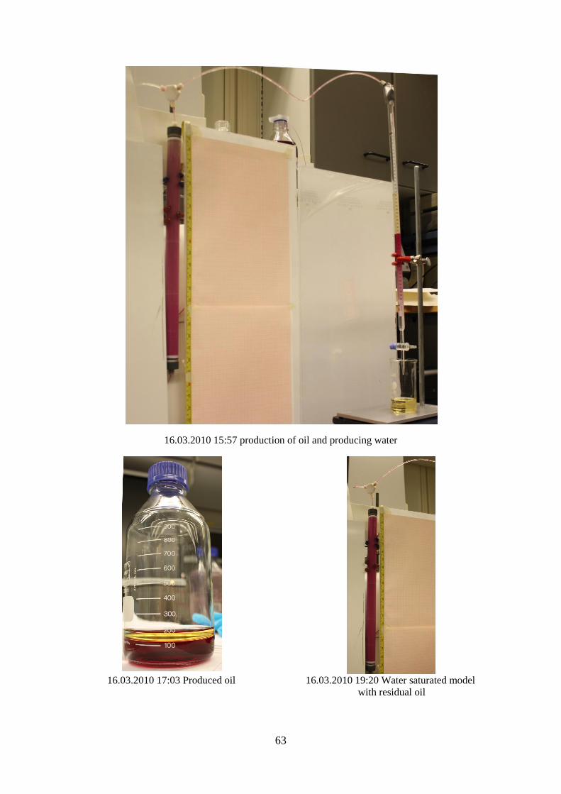
63

16.03.2010 15:57 production of oil and producing water

16.03.2010 17:03 Produced oil 16.03.2010 19:20 Water saturated model

with residual oil

64

5.3 1D displacement of Water in Porous Vertical Medium

The experiment was performed to determinde the relative permeability.

5.4 1D Displacement of Oil in Porous Horizontal Gravel Pack Model

The displacement of oil by water from the porous gravel pack has been studied for the simple

case of packs of unconsolidated material made up of grains of nearly uniform size. The oil

used for gravel pack saturation and flow is Marcol82, with a viscosity of 27.2 cP. The

visualization is shown in Appendix G.

5.4.1 Visualization of displacement

Visualization of displacement in horizontal gravel pack

10. June 2010, 10:47:12 Injection has started to travel through the gravel pack. Already it can be seen that

gravity segregation is affecting the displacement, due to denser water than oil. The water has segregated down in

the first oil injection tube. This injection tube had to be closed.

The injection of water is appearing at a given distance from the gravel pack wall. This makes that the oil in at the

end will not be displaced.

65

10. June 2010, 10:47:16 Ten minutes after water was injected into the porous medium. It was observed that the

water front went up in the closed perforation just after water entering the gravel pack. It went down again and

started to move through the gravel pack. On the left corner (arrows), there is a “dead zone” where the water will

not displace the oil. This is oil entrapment, and the oil will probably not be recovered. When the water is flowing

to the second oil inlet the water curves over an oil section. The reason for the curve is that the inlet is still

injecting oil into the gravel pack. Since the oil is lighter than the water it will move upwards and the water will

create a curve and try to segregate.

10. June 2010, 10:54:58

Water is fingering through the gravel pack and the oil tubes are still injecting. While the water is fingering, the

oil will also still produce and it appears that the oil is making “a layer” under the water finger. This layer also

appears above the water finger. The arrows on the figure visualize the different layers. For this particular

experiment, it is special that the oil is creating a layer under the water. But it is probably due to the continuous

injection of oil from the reservoir. The oil injection rate from the first inlet tube is very low (approximately

1.0ml/min) and the flow in the other injection tubes are increasing in flow rate the closer they are to the

perforation. The water will flow by the part of least resistance. Therefore it is reasonable to assume that the

pressure in the water phases is below the oil pressure. After the water reached the injection inlet the oil is

continuously injecting into the gravel pack and the oil will under ride the water. The water will therefore not be

able to displace this injected oil as it will flow continuously from the reservoir to the production perforation.

66

Two effects can be seen in the figure above. There are three layers in the gravel pack. One with initial oil, the

viscous water finger and the continuous flow of oil. The water and oil is continuously injected with

approximated same velocity. When the water is injected and starts to produce the oil, it tries to under ride the oil

and a viscous finger will occur. But since there is continuous injection of oil and the oil in the gravel pack is

continuously moving, there will not be gravity segregation of water at the bottom of the gravel pack which

indicates that water does not under-ride the injected oil. The other effect is that the water under-ride the oil that is

not injected from the formation. Then there will be water under-riding, and oil will be as a layer over the viscous

water finger. The figure below shows the layering in more detail. The layers seem to be different, where the

viscous finger is the largest one.

The viscous front is difficult to see on these figures. Normally it lies behind the viscous finger.

67

Fig... Layering of oil and viscous finger. The viscous front is lying behind the finger.

10. June 2010, 10:58:14 Breakthrough

The viscous finger reached the perforation and breakthrough occurred after 19min and 20sec. This is close to the

calculated time at 21min 30sec. Here is also possible to see some oil entrapped in the reservoir. The oil in the

right end of the model will probably not be displaced. The viscous finger is directly flowing through the

production perforation and water will be produced together with the initial and injected volume of oil.

68

10. une 2010, 11:26:20 The viscous finger has reached the breakthrough and the water has been started to be produced.

10. une 2010, 11:27:44 This is also at the water injection tube, where the water is injected into the oil column. There are some vertical lines across the

gravel pack. Indicates vertical permeability. The permeability there can be higher than the absolute permeability. Vertical variation in permeability is relative

common. When the permeability is higher, the flow will tend to move faster. It is difficult to predict since no prediction of permeability layering has been

done. As mentioned in chapter…. If there is variation in permeability, it may lead to a reduction of vertical sweep efficiency at breakthrough.

Figures below are from the inlet tubes from water and oil (formation)

69

10. June 2010, 11:41:22 Water inlet tube, showing the entrapped oil and vertical layers.

10. June 2010, 11:41:26 First inlet tube of oil.

10. June 2010, 11:41:28 the middle of the model

70

10. une 2010, 11:41:30 At the third and the fourth oil injectors. And the figure below shows the production outlet.

Saturation and Permeability Differences in different horizontal layers

10. June 2010, 12:27:58 Even if saturation differences have not been included in this thesis it can be seen in the figures above and below. The water saturation

is strong in the beginning with the water injection point. And it reduces after the length of the gravel pack.

71

10. June 2010, 13:24:20

10. June 2010, 13:25:30

The figure visualize that there is water saturation differences. The saturation is stronger where the water is injected and is reducing after the displacement

length.

72

10. June 2010, 13:26:00 Different saturation distribution in the gravel pack. Viscous fingering.

10. June 2010, 13:26:08

10. June 2010, 15:57:44 10. June 2010, 15:58:14

5.5 Results and discussion

The displacement experiments are conducted on one dimensional gravel pack with only one

configuration to investigate the effectiveness of displacing water in a vertical well. Two runs were

conducted, one where displacing oil with water, and the other where displacing water with oil.

Before the displacement by oil, the cell was flooded with oil. The oil flood experiments were conducted

with two different gravel packs. The first one were for calibration of pump. The second experiment was

reused twice, both for determination of absolute permeability.

5.5.1 1D displacement of Oil in porous vertical medium

Porosity

The porosity is the relation between injected oil in the cell, Vp, and the total volume in the cell, which

can be occupied by fluids and porous medium, ref Equation (2-2).

73

41.0204.208

28.86

b

p

V

V

As described in chapter 2.3.4 the porosity for unconsolidated gravel varies between 0.25 and 0.48. The

medium in the test cell is therefore considered to be relatively porous. This can mean that the glass

beads are poorly consolidated to newly deposited (4).

Saturation

Saturation of oil and water after displacement of oil is found from Equation (2-15):

1 wo SS

Residual oil saturation, Sor, is found from Equation (2-17).

mlmlcmmlV

VVS

p

ooior /1048.3/1048.3 333

Initial water saturation, Swi:is derived from Equation (2-15)

1 wior SS

mlmlcmmlSS orwi /997.0/9965.0104789.311 33

Relative permeability and relative permeability curves

Relative permeability relates the absolute permeability of the porous system with the permeability of oil

and water.

In the beginning was the medium 100% oil saturated. Then the permeability of oil is the same as the

absolute permeability as calculated in chapter 4.10.

ko = k = 52.23

Relative permeability, kro, of oil for 100% So is calculated from Equation (2-8)

0.123.52

23.52

k

kk o

ro

Relative water permeability, krw(Sw) after displacement by water is calculated from Equation (2-11).

702.023.52

67.361

D

D

k

SkSSk ww

orwrw

Stable or unstable finger

As described in chapter 2.6.2, it is possible to evaluate the developement of the front displacement by

comparing the oil and water pressure, ref Equation (2-30)

Assuming barp 036.00

Equation (2-31)gives:

)...90sin(0815.0/81.9/5.7893600 23 msmmkgPaPo

barDmD

msmPas123.0

/1310876.923.52

0815.0/1048.200245.0...

3

4

And from Equation (2-32)

74

)...90sin(0815.0/81.9/41.9913600 23 msmmkgPaPw

barDmD

msmPas128.0

/1310876.967.36

0815.0/1048.200126.0...

3

4

Comparing the results:

000209.0 wowo PPbarPP

Based on the above it is shown that the front will be unstable.

Viscous Forces in Vertical Displacement

Average velocity

sm

m

sm

A

qv 4

4

37

1048.210448.4

1011.1

Viscous forces have been found by Darcy’ equation

For the water flood

barPam

msPas

m

k

LvP 0113.02.1131

10876.923.52

399.0468.000126.01048.2

213

4

For the oil flood

barPam

msPas

m

k

LvP 0221.02209

10876.923.52

399.0468.000246.01048.2

213

4

Pressure drop in a pore throat by the use of Poiseuille’s law

For water

Pa

m

smmsPa

r

LqP 9

4

37

410678.1

0238.0

1011.1468.000126.088

For oil

Pa

m

smmsPa

r

LqP 00101.0

0238.0

1011.1468.000246.0884

37

4

It is difficult to predict the pressure drop in a pore throat. The same is with the pressure required to force

the liquid through a pore throat. During the displacement of the oil, the fluid has to flow through many

different throats, and many different paths for the fluid flow exist. For predicting this, trapping forces in

a single capillary needs to be calculated. The wetting angle between all the different pores needs to be

estimated. And then estimate the pore velocity of the displacing fluid water to displace the isolated oil

drop from the pore. The pore channels are also not straight and smooth, but irregularly shaped.

Production rate decline

Data points for the plot can be found in the Appendix E.

75

Plot 5-1 Production rate vs time

5.5.2 1D displacement of Water in porous vertical medium

Porosity

The porosity is equal to the porosity calculated in chapter 5.5.1

41.0

Saturation

Saturation of oil and water after displacement of water is found from Equation (2-15):

1 wo SS

Irreducible water saturation, Swi is calculated from Equation (2-18):

mlmlcmmlV

VVS

p

wwiwi /0916.0/

204.208

20.64276.83 3

Oil saturation at irreducible water saturation is calculated from Equation (2-15).

mlmlcmmlSS iwoi /908.0/9084.00916.011 3

Relative Permeability

Relative permeability of oil with irreducible water saturation is calculated from Equation(2-11)

83.023.52

37.43

D

D

k

SkSk wo

wro

Maximum effective permeability to oil is found from Equation (2-4)

ko(Sw=Swc) = k×kro’

The resulting curves are shown below:

76

Plot 5-2 Relative permeability curves with values of kro, krw

Plot 5-3 Normalizing relative permeability

Fractional Flow of 1D vertical displacement

hmlqw /400 at t = 0 min

hmlqo /0 at t = 0 min

hmlqo /400 at t = 1min

hmlqo /400 at t = 22min

min10*11.1/400 37 mhmlqqq owt

Mobility Ratio

65.183.0

46.2

26.1

702.0

Siwro

o

Sww

rw

o

w

k

kM

The mobility ratio here can also be considered as a end point mobility ratio, since the calculated relative

permeability ratio to water and oil that occur during displacement. The curves of the end point

permeability ratio are shown in Plot 5-2and Plot 5-3

For stabilizing the displacement is the shock front mobility ratio, Ms, shown:

65.246.283.0

26.1702.046.283.0)()('

oro

wwfrwowfro

sk

SkSkM

77

Since no measurements have been done on permeability and saturation of shock front the values will be

the same as the end point mobility ratio. The Buckley-Leverett displacement is not stable and viscous

channelling of water appeared.

The mobility ratio is higher than 1, M ≥ 1, which gives an unsatisfied condition and give the reason for

viscous channelling of water through the oil. Because of gravity segregation and that water has a higher

density than oil does the water underlay and displaces the oil. The channelling is viscous fingering of

water and gave an earlier breakthrough than predicted.

This displacement is unstable due to the high mobility between the displaced and the dity between the

displaced and the displacing fluid. Since the injected water is denser than the displaced oil, gravity

segregation occurred and the displacing water under rides the displaced oil. The gravity can be used to

advantage to improve displacement performance.

Oil/Water Viscosity Ratio

95.126.1

46.2

cP

cP

w

o

The oil/water viscosity ratio is high, together with the mobility ratios, which gives an unstable

displacement.

Fractional flow of water

622.065.11

1

1

111

Mqq

qf

ow

ww

377.065.11

1

1

1

Mqq

qf

ow

oo

These equations are predictable for high permeabilities.

Vertical Displacement Efficiency in application of Darcy’s equation

By using the Darcy equation to find the immiscible displacement, the displacement is considered as

piston like displacement. Even if viscous fingering occurred and gravity segregation, the denser water

will push the oil as a piston-like displacement.

dd

rd

DD

rD

dy

dpkk

dy

dpkk

dDdy

dp

dy

dpM

dD PPP

d

f

D

fdy

dpXL

dy

dpXP

D

ffdy

dpMXLXp

MXLX

p

dy

dp

ffD

From Darcy’s equation:

78

DrdrDD

rDf

DSSdy

dpkk

dt

dXv

1

1

vd = linear velocity of displacing phase front

Sdr = residual saturation of the displaced phase

SDr = residual saturation of the displacing phase

Drdrf

rDf

SSXMML

pk

dt

dX

11

This is a differential equation that by integration, separation of variables results in;

21

12

f

f

rD

DrdrX

MMLXpk

SSt

The location of displacing phase of water;

mX

cmmX

mm

E

sPaEsPamm

M

SS

ptkMMLML

X

f

f

wror

rD

f

96.1

58.414158.0

643481943.065.0

7722.0

65.11

0916.048.31399.0

13203610876.923.5200126.0

702.065.112

468.065.1468.065.1

1

1

12

2

1

2/1

3

13

2

2/1

2

Xf1 will be used since the location of the displacing phase fluid front cannot be negative.

Time, t, when the front reaches the position Xf,

sec22min15

min37.15

2

4158.065.114158.0468.065.1

3610Pa876.923.5200126.0

702.0

0916.048.31399.0

21

1

2

213

3

2

mmm

mEsPa

E

XMMLX

pk

SSt

f

f

rw

iwor

Volume of water injected before breakthrough

mlmmEmXSSAV fwrori 167000167.04158.00916.048.3100044488.01 332

Vi = volume injected

A = cross-sectional area of the medium

Velocity of the displacing phase front

sm

s

m

dt

dXv

f

D

41051.42.922

4158.0

Average Pressure drop

ΔP = 0.0361bar = 3610Pa

79

Time t, when position, Xf = 46.8cm

sec23min17

99.1009

2

468.065.11468.0468.065.1

3610Pa876.923.5200126.0

702.0

0916.01048.31399.0

21

1

2

213

3

2

s

mmm

mEsPa

XMMLX

pk

SSt

f

f

rw

iwor

Time t, when position, Xf = 50cm

sms

m

dt

dXv

f

D

41063.499.1009

468.0

sec41min17

1061

2

50.065.1150.0468.065.1

3610Pa876.923.5200126.0

702.0

0916.048.31399.0

21

1

2

213

3

2

s

mmm

mEsPa

E

XMMLX

pk

SSt

f

f

rw

iwor

sms

m

dt

dXv

f

D

4107.41061

50.0

Volume water injected at Xf = 50cm

mlmmEmXSSAV fwroriw 201000201.050.00916.048.3100044488.01 332

Injection rate after breakthrough;

smm

Pa

sPa

mm

L

pkAki

w

rw

abt

32213

99.0468.0

3610

00126.0

00044488.010876.923.52702.0

Volume injected at any time after breakthrough

3433 10696.1132099.0000167.0 msmmttiVV btabtibtiabt

Displaceable PV after displacement by water and oil

35

324

1054.7

1048.3908.0399.468.0104488.4

m

mlmlmm

SSAhSSVV oroioroippd

Dimensionless injection rate, the injected volume divided by placeable PV,

33

35

34

67.21054.7

1001.2mm

m

m

V

V

pd

wi

Water injection rate at the same point

smmmsmiq abt

3333 64.267.299.0

Viscous Fingering

The idealized piston like behaviour is not followed since the viscosity of water is less than the viscosity

of oil.

95.1w

o

80

The viscous ratio between the oil, bayol35 and water is 1.95. In this event, viscous fingering occurs

during the displacement process. Flow in the fingers is mixed with bypassed oil and it is creating a much

longer mixing zone.

Areal Displacement Efficiency

Areal displacement efficiency before breakthrough is equivalent to the volume of water injected.

%7.88887.0

1043.3908.00002082.0

000167.033

3

m

m

SSPV

VE

oroi

iA

Displacement efficiency at breakthrough

%49.61

6149.0

65.100509693.030222997.0

65.1

03170817.054602036.0

00509693.030222997.003170817.0

54602036.0

65.1

e

MeM

EMAbt

Cumulative Oil Produced

mlmmmESSVN Abtoroipp 1.46000075.06149.01043.3908.0399.468.0104488.4 3324

The gravity force has been neglected here and principally have the other factors mentioned in 2.3 been

focused on during the study. Five injection tubes have been used for flow. For the permeability

heterogeneity it is difficult to develop correct correlations.

Gravity force has been neglected in the model, but densities of oil and water have been adjusted in the

tubes and the inlet to the gravel pack, which means that gravity override, is minimized.

The fronts and interfaces between the displaced and displacing fluids were monitored by use of dyed

water that was photographed.

Vertical Displacement Efficiency

Dykstra Parsons Model

0.11

23.52

23.521

1

n

k

kn

E

n

jk j

kj

I

53.11

65.1123.52

23.5265.1

165.1

111

1

1

2/1

22

1

2/1

22

n

Mk

kM

MM

Mnnn

E

n

jk j

kj

j

I

0.1

65.1123.52

23.5265.1

23.52

23.52

1221

2/1

22

1

n

jk

j

k

k

j

k

k

wo

Mk

kM

k

k

F

Calculation of Vertical Displacement efficiency at breakthrough

From calculated Np:

31.000008672.065.1

000045.03

3,

m

m

VM

NE

t

calcp

I

From measured Np

81

58.000008672.065.1

000083.03

3

m

m

VM

NE

t

p

I

Displacement efficiency

996.0908.0

1048.3908.0 3

oi

oroi

oip

orpoip

DS

SS

SV

SVSVE

Displacement Efficiency Equation

79.10179.0997.01

0000538.0

1

wi

Btp

DS

NE

Volumetric Displacement Efficiency for measured Np based on area efficiency on breakthrough

514.058.0887.0 IAV EEE

Recovery Efficiency:

%51.0514.0996.0 VDEERF

1D displacement of oil by water

The displacement experiments are conducted on one dimensional gravel pack with only one

configuration to investigate the effectiveness of displacing water in a vertical well. After the

displacement was the cumulative oil production at breakthrough and after breakthrough determined. The

volume of oil produced at breakthrough, Vop,bt = 83.28ml over a time of 22min. Volume of oil produced

after breakthrough was 3ml. Vop,t = 86.28ml. The oil and water saturation is different throughout the

displacement. The flood front saturation will differ from some extent to the average saturation. The

residual oil saturation is 3.43*10-3

ml/ml, this gives a water saturation of 0.998ml/ml. This low and high

oil and water saturation means that almost all oil was displaced and produced. The residual oil is most

probably left in the different pores. The recovery factor is 99.44%.

The displacement here is governed by what might be called viscous fingering. The displaced oil has a

viscosity of 2.46 cP where the viscosity of the displacing water is 1.26cP. The viscosity relation will

give a value larger than 1, which means that there are viscous instabilities in the displacement front.

Since the viscosity of oil is higher than the viscosity of water, viscous fingers have been established.

Perturbations, which is the white area on the pictures, has been established when the water is displacing

the oil. The water here is moving faster than the oil, since the water is less viscous than the displaced oil.

The small tiny horizontal lines in the porous medium can be small areas larger permeability and the

front entering could travel much faster than the rest of the front. Probably there are more of them, just

smaller than that are shown on the pictures. This can together with the unfavourable viscosity ratio and

the mobility ratio be the reason for the viscous fingers. When there is difference in gravity between the

displacing fluid and the displaced fluid it will have an effect on the displacement. λo>λw and ρo<ρw,

0.78955g/cm3<0.99141g/cm3. When the gravel pack is vertical there will be vertical upward flow.

When the water is denser than the oil it can be helpful for the displacement in vertical upward direction,

in that way that the gravity will help to stabilize the front. Since the average displacement velocity is

low, it can help to reduce the fingers at the interface.

5.5.3 1D displacement of oil in horizontal Gravel Pack model

Assumptions

- The model used is linear, horizontal and of constant thickness

- The flow is incompressible and obeys Darcy’s law

- After the displacement there is high residual oil saturation

- The flow displacement is by viscous fingering

- There are injection of oil from the formation (4 oil tubes under the gravel pack model)

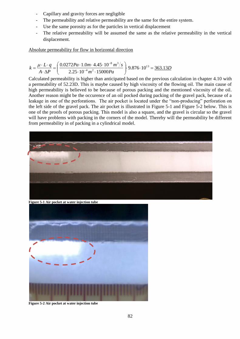
82

- Capillary and gravity forces are negligible

- The permeability and relative permeability are the same for the entire system.

- Use the same porosity as for the particles in vertical displacement

- The relative permeability will be assumed the same as the relative permeability in the vertical

displacement.

Absolute permeability for flow in horizontal direction

DPam

smmPa

PA

qLk 13.36310876.9

150001025.2

1045.40.10272.0 13

24

38

Calculated permeability is higher than anticipated based on the previous calculation in chapter 4.10 with

a permeability of 52.23D. This is maybe caused by high viscosity of the flowing oil. The main cause of

high permeability is believed to be because of porous packing and the mentioned viscosity of the oil.

Another reason might be the occurence of an oil pocked during packing of the gravel pack, because of a

leakage in one of the perforations. The air pocket is located under the “non-producing” perforation on

the left side of the gravel pack. The air pocket is illustrated in Figure 5-1 and Figure 5-2 below. This is

one of the proofs of porous packing. This model is also a square, and the gravel is circular so the gravel

will have problems with packing in the corners of the model. Thereby will the permeability be different

from permeability in of packing in a cylindrical model.

Figure 5-1 Air pocket at water injection tube

Figure 5-2 Air pocket at water injection tube

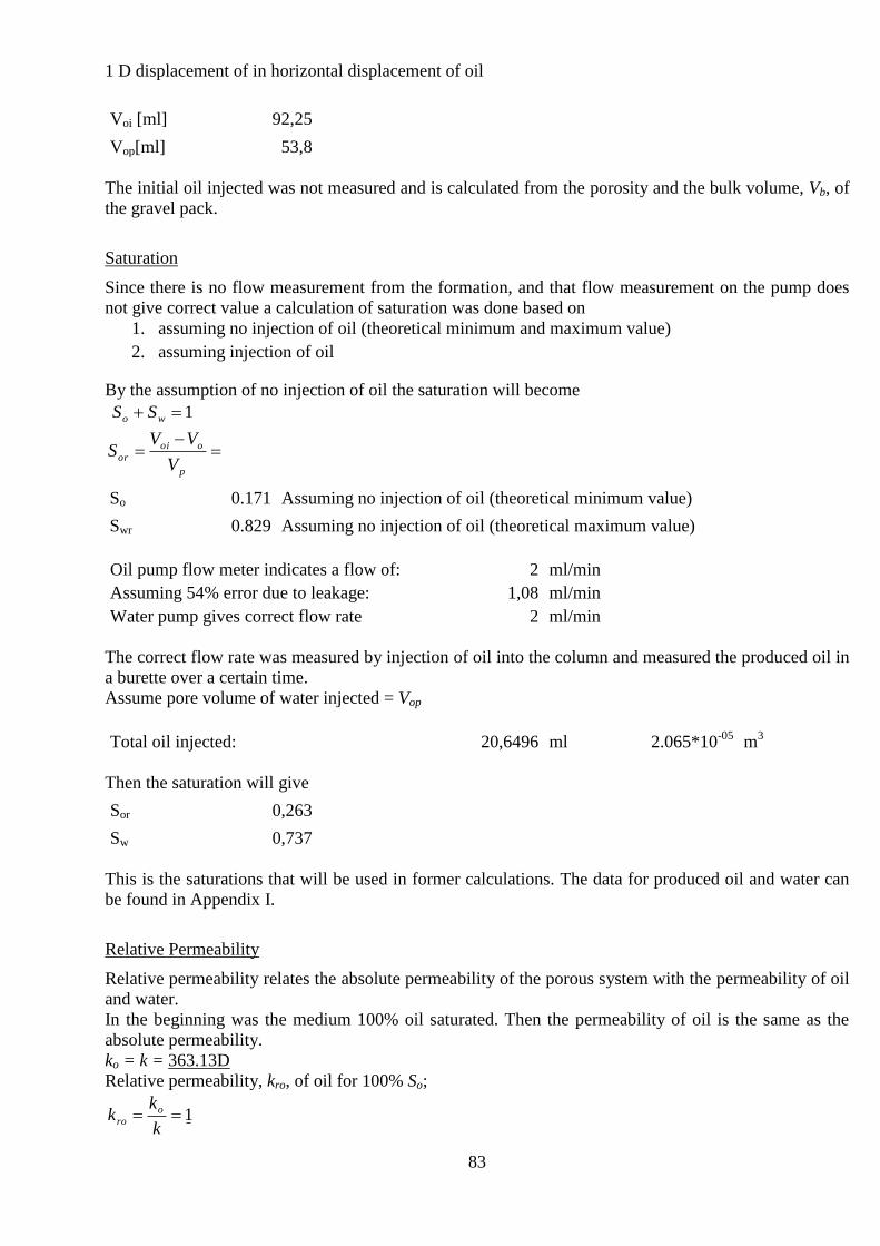
83

1 D displacement of in horizontal displacement of oil

Voi [ml] 92,25

Vop[ml] 53,8

The initial oil injected was not measured and is calculated from the porosity and the bulk volume, Vb, of

the gravel pack.

Saturation

Since there is no flow measurement from the formation, and that flow measurement on the pump does

not give correct value a calculation of saturation was done based on

1. assuming no injection of oil (theoretical minimum and maximum value)

2. assuming injection of oil

By the assumption of no injection of oil the saturation will become

1 wo SS

p

ooior

V

VVS

So 0.171 Assuming no injection of oil (theoretical minimum value)

Swr 0.829 Assuming no injection of oil (theoretical maximum value)

Oil pump flow meter indicates a flow of: 2 ml/min

Assuming 54% error due to leakage: 1,08 ml/min

Water pump gives correct flow rate 2 ml/min

The correct flow rate was measured by injection of oil into the column and measured the produced oil in

a burette over a certain time.

Assume pore volume of water injected = Vop

Total oil injected: 20,6496 ml 2.065*10-05

m3

Then the saturation will give

Sor 0,263

Sw 0,737

This is the saturations that will be used in former calculations. The data for produced oil and water can

be found in Appendix I.

Relative Permeability

Relative permeability relates the absolute permeability of the porous system with the permeability of oil

and water.

In the beginning was the medium 100% oil saturated. Then the permeability of oil is the same as the

absolute permeability.

ko = k = 363.13D

Relative permeability, kro, of oil for 100% So;

1k

kk o

ro

84

The Relative water permeabilities have been assumed to be the same as the one for displacement in

vertical direction

Displacement by water

702.01 k

SkSSk ww

orwrw

Displacement by oil

83.0k

SkSk wo

wro

The irreducible water saturation and oil saturation at irreducible water saturation will also be assumed to

be the same as in vertical displacement by oil,

mlmlV

VVS

p

wwiiw /106.0

Oil saturation at irreducible water saturation

mlmlcmmlSS iwo /894.0/894.0106.011 3

Maximum effective permeability to oil

DSkk wrw 92.254702.013.363)(

DSkk wro 39.30183.013.363)(

Fractional Flow of 1D vertical displacement

/min2mlqw at t = 0min

/min7.0 mlqo at t = 0min

min/7.0 mlqo at t = 19.2min

sm104.50mlmlmlqqq -8

owt /min/7.2min/7.0min/2 3

Mobility Ratio

18,26k

kM

oro

wrw 2.2783.0

26.1702.0'

'

The mobility ratio is high, >> 1, which gives an unfavourable condition and give the reason for viscous

fingering of water. The water will travel faster than the oil and create an early breakthrough of

production of water into the well. The viscous fingering is due to the high viscosity ratio of the

displaced oil and the displacing water.

Oil/Water Viscosity Ratio

21.59cP

cP

w

o 26.1

2.27

The viscosity ratio is >> 1. This implies that together with the mobility ratio, the water will create a

viscous finger.

Viscous fingering

The pictures have been used to calculate the velocity and position of the viscous finger. The points of

the finger in the pictures taken during displacement have been used as a reference note, and the time the

finger reached this point has been used to find the velocity. The table below shows the breakthrough

time for the viscous finger, the position after a certain time and the velocity for the finger.

85

Table 5-1 Time, position and velocity and average velocity for the viscous finger

t [min] 10 16 19,200

t [sec] 600 960 1152,000

xf [m] 0,294 0,594 0,988

uavg [mm/s] 0,49 1,65 5,146

U [mm/s] 0,98 2,32 7,972

The values from the table have been plotted below.

Plot 5-4 Velocity and front of the viscous finger before breakthrough

The plot shows how the viscous finger is moving through the gravel pack. U is the velocity and Xf is the

position of the finger. Displacement is shown over time. The velocity is increasing the more the finger

reaches the oulet perforations. This might be due to the continuous injection of oil from the formation.

Table 5-2Time and position of the front before and at breakthrough

t 100 200 300 400 500 600 700 800 900 1000 1100 1152

xf [m] 0,017 0,034 0,052 0,070 0,090 0,110 0,131 0,154 0,178 0,204 0,232 0,248

The values from the Table 5-2 of time and position before and at breakthrough are plotted below, Plot

5-5 The viscous front. The time is on the x-axis and the position on the y-axis. The distance of the front

have been found by Equation (2-33).

86

Plot 5-5 The viscous front during displacement over a time t.

The plot above shows the viscous front as the viscous finger is moving. This viscous front is moving

very slowly compared to the viscous finger. At breakthrough (1152sec) has the front only moved 0.25m

while the viscous finger has reached the perforation.

Viscous Forces in Horizontal Displacement

Average water rate before breakthrough

smt

Vq

op

w

38-104.68968

Average water velocity

sm

m

sm

A

qv 4-

4

38-

102.08431025.2

104.68968

Viscous forces have been found by Darcy’ equation

For the water flood

0.648bar6481.414Pa10876.913.363

41.00.10272.0100843.2

213

4

mD

msPas

m

k

LvP

Pressure drop in a pore throat by the use of Poiseuille’s law

For water flow

Assumption for this equation:

- Cylindrical pore throat

Pa

m

smmsPa

r

LqP 0,04515

015.0

1033.00.10272.0884

37

4

Difficult to predict this value since the pore channels are not cylindrical, but irregular.

Production

Data points for plots below is found i the Appendix I.

87

Plot 5-6 Production of oil and water through gravel pack

Plot 5-7 dP and total flow befor breakthrough

88

Plot 5-8 Flow and dP throgh gravel pack after breaktrough

Plot 5-9 Dp and production of water

89

Average water rate, qw,avg = 4.246*10-6

m3/s = 4.25ml/min

Volume of water injected before breakthrough

mlmm0.737335mXSSAV fwrori 3.580000583.00.11048.31000224.01 332

Volume injected at any time after breakthrough

33363 1095.41152/10*246.40000583.0 mssmmttiVV btabtibtiabt

Displaceable PV after displacement by water and oil

ml

mlmlmm

SSAhSSVV oroioroippd

42.83

1048.3908.041.0.11025.2 324

Cumulative oil produced before breakthrough, Npd at breakthrough;

Npd,bt = 53.8ml

Cumulative oil produced after breakthrough

Npd,after bt = 678ml -53.8ml = 624.2ml

Measured pore volume injected

PV = 1390ml

Area Displacement Efficiency

Areal displacement efficiency before breakthrough is equivalent to the volume of water injected.

%6.28286.0

1048.3908.0000225.0

0000583.033

3

m

m

SSPV

VE

oroi

iA

Displacement efficiency at breakthrough

%3.45

4529.0

6.1800509693.030222997.0

6.18

03170817.054602036.0

00509693.030222997.003170817.0

54602036.0

6.18

e

MeM

EMAbt

Cumulative Oil Produced Calculated

mlmmmESSVN Abtoroipp 9.370000379.01043.3908.041.0.11025.2 3324

Calculation of Vertical Displacement efficiency at breakthrough

From calculated Np:

%49.30349.00000583.06.18

0000379.03

3

,

,

m

m

VM

NE

btt

calcp

I

From measured Np

%37.50537.00000538.06.18

0000538.03

3

m

m

VM

NE

t

p

I

Displacement Efficiency

90

%79.10179.0997.01

0000538.0

1

wi

Btp

DS

NE

Volumetric Displacement Efficiency for measured Np, based on area efficiency at break through

024.00537.04529.0 IAV EEE

Recovery Efficiency from equation 2.43

%4.4044.0 VD EERF

Breakthrough time

sec30min21min52.21min/71.2

3.58

,

ml

ml

q

Vt

oilwaterinj

inj

Bt

This is high compared to the pressure drop during the displacement. It might be of the high absolute

permeability of 363.13D for this displacement.

The total amount of displaced oil in the horizontal gravel pack was 53.8ml. The total amount of injected

oil is 92.25ml. This value is assumed to be correct, but may differ because of the high permeability. The

total amount of oil injected before breakthrough was found by use of the bulk volume and the porosity.

This assumption will also affect the displacement efficiencies, in areal, vertical and volumetric

efficiencies. The overall recovery is low only 4.4%, the same is it for the displacement efficiency. The

total amount of water injected is almost the same as the oil produced, 58.3 ml injected and 53.8ml

produced. The low recovery efficiency is most probably because of the early breakthrough of water. The

values differensiate from the measured values, can be a reason of the relative permeabilities and the

assumptions made during the calculations.

5.6 Recommendations

T

91

REFERENCES

1. Wiggins, Michael L. Petroleum Engineering Handbook. [ed.] Larry W. Lake. NA. NA : NA, 2007.

Vol. IV. NA.

2. Zolotukhin, A. B. and Ursin, J. R. Introduction to Petroleum Reservoir Engineering. Stavanger :

HøyskoleForlaget AS - Norwegian Academic Press, 2000.

3. Hiort, Aksel. Introduction to Reservoir Technology/Introducksjon til Reservoir Teknikk. Stavanger :

Universitetet i Stavanger, 2009.

4. Nelson, Philip H. and Batzle, Michael L. Single Phase Permeability. [ed.] John R. Fanchi.

Colorado : Society of Petroleum Engineers, 2006. Vol. I.

5. Christiansen, Richard L. Petroleum Engineering Handbook. [ed.] Larry W. Lake and John R.

Fanchi. Colorado : Society of Petroleum Engineers, 2006. Vol. I, Chapter 15. ISBN 978-1-55563-108-6.

6. Kleppe, Hans. Reservoir Simulation. Stavanger : University of Stavanger, Institute of Petroleum

Technology, 2007.

7. Christiansen, Richard L. Relative Permeability and Capillary Pressure. [ed.] Larry W. Lake and

John R. Fanchi. Colorado : Society of Petroleum Engineers, 2006. Vol. I, Chapter 14. ISBN 978-1-

55563-108-6.

8. Schlumberger. Schlumberger Oilfield Glossary. Oilfield Glossary, Irreducible Water. [Online]

Schlumberger. [Cited: 27 May 2010.]

http://www.glossary.oilfield.slb.com/Display.cfm?Term=irreducible%20water.

9. Selley, Richard C. Elements of Petroleum Geology. 2nd Edition. San Diego : Academic Press, An

Imprint of Elsevier, 1998. ISBN-10: 0-12-636370-6.

10. Schlumberger. Schlumberger Oilfield Glossary. [Online] Schlumberger, 25 May 2010.

http://www.glossary.oilfield.slb.com/Display.cfm?Term=pore%20throat.

11. Nordhaug, Hans Fredrik. Modeling of Multi Phase Flow in Porous Media: Operator Splitting,

Front Tracking, Interfacial Area and Network Models. Department of Mathematics, University of

Bergen. Bergen : Department of Mathematics, University of Bergen, Oct. 2001.

12. Porras, Juan Carlos, Barbato, Roberto and Salazar, Diomedes. Upscaling From Core Data to

Production: Closing the Cycle. A Case Study in the Santa Barbara and Pirital Fields, Easten Venezuela

Basin. Various Countries : SPE, June 2-5, 2002.

13. Beard, D. C. and Weyl, P. K. Influence of Texture on Porosity and Permeability of Unconsolidated

Sand. Midland, Texas, Stony Brook, New York : The American Associatwn of Petroleum Geologists

Bultetin, 1973. pp. 349-369. Vols. V.57, nr.2.

14. Green, Don W. and Willhite, G. Paul. Enhanced Oil Recovery. Richardson, Texas : Henry L.

Doherty Memorial Found of AIME, Society of Petroleum Engineers, 1998.

15. Ahmed, Tarek H. Reservoir engineering handbook. s.l. : Elsevier/Gulf Professional, 2006 .

16. Smaoui, Nejib and Gharbi, B. Ridha. Using Karhunen-Loéve decomposition and artificial neural

network to model miscible fluid displacement in porous media. Department of Mathematics and

Computer Science, Department of Petroleum Engineering, Kuwait University. Kuwait : Applied

Mathematical Modelling, Elsevier, 1999. pp. 657-675.

17. Hornof, V. and Morrow, N. R. Flow visualization of the Effects of Interfacial Tension on

Displacement. New Mexico Petroleum Recovery Research Center, University of Ottawa. Ottawa, New

Mexico : SPE, 1988.

18. Dake, L. P. Fundamentals of Reservoir Engineering. Amsterdam, The Netherlands, Oxford, UK :

Elsevier, 1978.

19. Engelberts, W. F. and Klinkenberg, L. J. Laboratory Experiments on the Displacement of Oil by

Water from Packs of Granular Material. The Hague : Society of Petroleum Engineers, 1951. p. 544.

20. Chuoke, R. L., van Meurs, P. and van der Poel, C. The instability of Slow, Immiscible, Viscous

Liquid-Liquid Displacements in Permeable Media. Houston, Texas, Amsterdam, The Netherlands :

SPE, AIME 1959. Petroleum Transactions. T.P. 8073.

21. Araktingi, U. G. and Orr Jr., F. M. Viscous Fingering in Heterogeneous Porous Media. Stanford

University. Stanford : Society of Petroleum Engineers, 1992. p. Vol 1. No. 1.

92

22. Gilje, Eli. Simulation of viscous instabilities in miscible and immiscible displacement. Department

of Chemistry, University of Bergen. Bergen : University of Bergen, 2008. Master Thesis.

23. Homsy, G.M.,. Viscous Fingering in Porous Medium. Stanford, California : Annual Review of

Fluid Mechanics; Department of Chemical Engineering, Stanford University, Stanford, 1987. pp. 271-

311.

24. Golan, Michael and Curtis H, Whitson. Well Performance. Trondheim : Prentice Hall, 1991.

ISBN 0-13-946609-6.

25. Cossé, R. Basics of Resevoir Engineering. [trans.] R. Cossé Le gisement. Paris : Institut francais du

pétrole, 1993. Vol. Éditions Technip. ISBN 2-7108-0630-4.

26. Fanchi, John R. Principles of Applied Reservoir Simulation. 3rd edition. Burlington : Gulf

Professional Publishing, Elsevier, 2006. ISBN 10: 0-7506-7933-6.

27. Martel, Richard, et al. Displacement and sweep efficiencies in a DNAPL recovery test using

micellar and polymer solutions injected in a five-spot pattern. INRS-Eau, Terre et Environnement,

Institut national de la recherche scientifique, Université du Québec. Québec : Journal of Contaminant

Hydrology, ScienceDirect, 2002, revised and accepted 2004. 75 (2004) 1-29.

28. Guliyev, Ruslan. Simulation Study of Areal Sweep Efficiency Versus a Function of Mobility Ratio

and Aspect Ratio for Staggered Line-Drive Waterflood Pattern. Petroleum Engineering, Texas A&M

Univeristy. Texas : Office of Graduate Studies, 2008. Master Thesis.

29. Ebrahimi, Arian. Analysis of Waterflood in the Valendis Horizon of Suderbruch Oil Field.

Clausthal University of Technology, Institute of Petroleum Engineering. Clausthal-Zellerfeld : Clausthal

University of Technology, 2009. Seminar thesis.

30. Mott, Robert L. Machine Elements in Mechanical Design 4th edition in SI units. Uni of Dayton.

s.l. : Pearson Prentice Hall. ISBN 0-13-197-644-3.

31. Irgens, Fridtjof. Fasthetslære, 6th ed. s.l. : Tapir, 1999. ISBN 82-519-1522-1.

32. Irgens, Fritjof. Statikk, 7th ed. s.l. : Tapir, 2005. ISBN 82-519-2067-1.

33. Papatzacos, Paul Georg. ÅMA150 Mathematical Modelling. H-2008. Lecture Notes.

34. Time, Rune. MPE 490 Flerfasestrømning i rør. V-2009. s. Chapter 6, Lecture Notes.

35. Microsoft. Help Tool in Microsoft Excel 2010. 2010. pp. Search for Goal Seek and What-If

Analysis.

36. Electronics, Gibson Medical. Gibson 305 Piston Pump. Villiers le Bel, France : s.n.

37. 200, PAAR PHYSICA Rheometer US. Manual.

38. AS, Dipl Ing Houm. Anton Paar, DMA 4500/5000 Density/Spesific/Gravity/Consentration Meter -

Instruction Handbook. Grefsen, Oslo : s.n.

39. Rabenjafimanantsoa, S Myhren. Laboratory exsercises in Reservoir engineering. s.l. : University

of Stavanger, 2010.

40. du Noüy, Pierre Lecomte. An Interfacial Tensiometer for Universal Use. s.l. : The Journal of

General Physiology, 1925.

41. Oil, Esso Imperial. Product Data Sheet, White Oil, Marcol83, Primol, Bayol35. Esso Imperial Oil.

[Online] Esso, 2009. [Cited: 30 3 2010.] http:www.imperialoil.ca/Canada-

English/Files/Products_Lubes/IOCAENWPOESWhiteoil.pdf.

42. AS, Esso Norge. Helse,-Miljø- og Sikkerhetsdatablad. Oslo : Esso Norge AS, 2002. N-63-L5891.

43. Mobile, Exxson. Sikkerhetsdatablad - Marcol 82. Oslo : Exxson Mobile, 2008.

44. Outmans, H. D. Nonlinear Theory for Frontal Stability and Viscous Fingering in Porous Media.

Union Oil Company of California. Brea, California : Society of Petroleum Engineers, SPE 183, 1962.

Member AIME.

45. Satter, Abdus, Iqbal, Ghulam M. and Buchwalter, James L. Practical Enhanced Reservoir

Engineering. Tulsa : PennWell Corporation, 2007. ISBN-10: 1-59370-056-3.

46. Wiggins, Michael L. Inflow and Outflow Performance. NN. U. of Oklahoma : NN, NN. Vol. IV.

NN.

93

APPENDIX A

Table A- 1 Measured Flow, Qreal, and Pressure Drop, dp/dx,

for absolute permeability calculation

Qinn Qreal Pressure Permeabilitet, k

q [ml/h] q [m3/s] q [m

3/s] dP [bar] dP [Pa] [m

2] [D] [D]

0 0 0 0 0 0 0

60 1,67E-08 1,71E-08 0,011 1100 4,01E-11 40,65 52,23

80 2,22E-08 2,36E-08 0,015 1485 4,10E-11 41,50

100 2,78E-08 2,86E-08 0,017 1700 4,34E-11 43,99

120 3,33E-08 3,32E-08 0,020 2000 4,28E-11 43,37

140 3,89E-08 3,76E-08 0,023 2254 4,30E-11 43,61

160 4,44E-08 4,44E-08 0,025 2546 4,49E-11 45,53

180 5,00E-08 4,99E-08 0,029 2885 4,46E-11 45,17

200 5,56E-08 5,61E-08 0,032 3162 4,57E-11 46,33

400 1,11E-07 1,13E-07 0,062 6162 4,73E-11 47,88

800 2,22E-07 2,24E-07 0,122 12192 4,73E-11 47,95

1000 2,78E-07 2,97E-07 0,154 15408 4,97E-11 50,36

94

APPENDIX B - VISCOSITY MEASUREMENTS

Bayol

The viscosity was measured with Physica viscosity meter. Table B- 1 Measured viscosity of Bayol

d(gamma)/dt Meas. Pts. Time Shear Stress Viscosity Speed Torque

1/s

[s] [Pa] [Pa·s] [1/min] [µNm]

1,5 1 10 0,008 0,00504 0,26 0,3

1,5 2 20 0,013 0,00869 0,26 0,5

3,1 1 30 0,028 0,00897 0,54 1,0

3,1 2 40 0,030 0,00955 0,54 1,1

5,1 1 50 0,024 0,00476 0,89 0,9

5,1 2 60 0,006 0,00126 0,89 0,2

10,2 1 70 -0,016 -0,00157 1,78 -0,6

10,2 2 80 0,030 0,00297 1,78 1,1

51,1 1 90 0,051 0,00101 8,90 1,9

51,1 2 100 0,048 0,00094 8,90 1,8

102 1 110 0,081 0,00079 17,80 3,0

102 2 120 0,077 0,00076 17,80 2,9

153 1 130 0,154 0,00100 26,60 5,8

153 2 140 0,142 0,00093 26,60 5,3

340 1 150 0,328 0,00096 59,20 12,3

340 2 160 0,328 0,00097 59,20 12,3

511 1 170 0,500 0,00098 89,00 18,7

511 2 180 0,527 0,00103 89,00 19,7

1021 1 190 1,050 0,00103 178,00 39,4

1021 2 200 1,050 0,00103 178,00 39,2

95

Plot B- 1 Viscosity measurements

The plot shows the measured viscosity over a time of 200sec. The viscosity is on the y-axis and the time

is on the x-axis. Between the first measurement, µ = 0.00504Pa*s at t = 10sec to µ = 0.00100Pa*s at t=

130 sec, the variation in viscosity is varying.

Probably the reason for the large variation of viscosity is because of low velocities and a large

uncertainty in measurement instruments. The viscosity became more stable for higher shear rates. The

viscosity used for first calculation of permeability, was calculated to be 0.00099088Pa*s. This value is

an average number between the viscosities for the eight last shear rates given in Error! Reference

source not found.. The result of the absolute permeability (21.12D) was lower than the permeability of

oil (31D), which gave a relative permeability larger than one.

The second viscosity measurement was done by using another steering tool.

below shows the most relevant measured viscosities for given shear rates. The viscosity used for

permeability calculation was measured to be, µ = 0.00245. This number is an average viscosity from the

numbers in the tables below.

Table B- 2 gives an overview of viscosities measured with MK24 coned plate

Shear Rate Time Shear Stress Viscosity Speed Torque

[1/s] [s] [Pa] [Pa·s] [1/min] [µNm]

-0,002

-0,001

0,000

0,001

0,002

0,003

0,004

0,005

0,006

0,007

0,008

0,009

0,010

0 50 100 150 200

Viscosity vs. Time

Viscosity

vs. Time

Time [sec]

Viscosity [Pa*s]

96

153 10 0,37 0,00245 26 41

153 20 0,37 0,00244 26 41

153 30 0,37 0,00244 26 41

153 40 0,38 0,00245 26 41

153 50 0,37 0,00245 26 41

340 60 0,83 0,00244 57 92

340 70 0,83 0,00245 57 92

340 80 0,83 0,00244 57 92

340 90 0,83 0,00244 57 92

340 100 0,83 0,00244 57 92

511 110 1,26 0,00246 85 139

511 120 1,26 0,00246 85 139

511 130 1,25 0,00244 85 138

511 140 1,24 0,00243 85 137

511 150 1,25 0,00244 85 138

1020 160 2,51 0,00246 170 277

1020 170 2,53 0,00248 170 279

1020 180 2,52 0,00246 170 278

1020 190 2,51 0,00246 170 277

1020 200 2,53 0,00248 170 279

1020 210 2,51 0,00246 170 277

1020 220 2,52 0,00246 170 278

1020 230 2,53 0,00247 170 279

1020 240 2,51 0,00245 170 277

1020 250 2,52 0,00247 170 278

Average viscosity = 0.0024528Pa*s

Viscosity used for permeability calculation, µoil = 0.00245Pa*s

The viscosity used for permeability calculation is more accurate and will be used for calculation.

Plot B- 2 More accurate viscosity measurements. There are fewer variations in viscosity and the average viscosity can be used in

further applications

Ionized Water

Table B- 3 Ionized water

Shear Rate Shear Stress Viscosity Speed Torque

[1/s] [Pa] [Pa·s] [1/min] [µNm]

0,002

0,0021

0,0022

0,0023

0,0024

0,0025

0,0026

0,0027

0,0028

0,0029

0,003

0 50 100 150 200 250

Viscosity vs. Time for Bayol 35

Viscosity

vs. Time

for Bayol

35

Pa*s

t [sec]

97

1020 1,28 0,00125 170 141

1020 1,30 0,00127 170 143

1020 1,29 0,00126 170 142

1020 1,28 0,00125 170 141

1020 1,30 0,00127 170 143

1020 1,28 0,00125 170 141

1020 1,28 0,00126 170 142

1020 1,30 0,00127 170 143

1020 1,28 0,00125 170 141

1020 1,29 0,00126 170 142

Average viscosity = 0.001259Pa*s

Viscosity used for permeability calculation, µw = 0.00126Pa*s

Plot B- 3 Viscosity measured vs. time for ionized water

Marcol82

Table B- 4 Viscosity, shear stress for Marcol82

Marcol 82

Shear Stress [Pa] Viscosity [cP] Viscosity [Pa·s]

0,1 100 0,1

0,1 100 0,1

0,1 100 0,1

0,1 100 0,1

0,1 100 0,1

0,1 44,4 0,0444

0,1 46,1 0,0461

0,1 46,1 0,0461

0,1 46,4 0,0464

0,1 45,8 0,0458

0,2 40 0,04

0,2 40 0,04

0,2 40 0,04

0,2 40 0,04

0,0011

0,00115

0,0012

0,00125

0,0013

0,00135

0,0014

0 10 20 30 40 50 60 70 80 90 100

Viscosity vs. Time of Ionized water

Viscosity vs.

Time of

Ionized water

Pa*s

t [sec]

98

0,2 40 0,04

0,3 31 0,031

0,3 31,8 0,0318

0,3 32,2 0,0322

0,3 32,3 0,0323

0,3 32,8 0,0328

1,6 31,4 0,0314

1,6 31,4 0,0314

1,6 31,4 0,0314

1,6 31,4 0,0314

1,6 31,4 0,0314

2,8 27,5 0,0275

2,8 27,5 0,0275

2,8 27,5 0,0275

2,8 27,5 0,0275

2,8 27,5 0,0275

4,9 28,8 0,0288

4,9 28,8 0,0288

4,9 28,8 0,0288

4,9 28,8 0,0288

4,9 28,8 0,0288

9,5 27,9 0,0279

9,5 27,9 0,0279

9,5 27,9 0,0279

9,5 27,9 0,0279

9,5 27,9 0,0279

14,1 27,6 0,0276

14,1 27,6 0,0276

14,1 27,6 0,0276

14,1 27,6 0,0276

14,1 27,6 0,0276

27,9 27,4 0,0274

27,9 27,3 0,0273

27,9 27,3 0,0273

27,8 27,2 0,0272

27,8 27,2 0,0272

99

Plot B- 4Viscosity vs. time for Marcol82

0,00

0,02

0,04

0,06

0,08

0,10

0,12

0 50 100 150 200 250 300 350 400 450 500 550

Viscosity vs. Time for Marcol82

Viscosity

vs. Time

for

Marcol82

Pa*s

t [sec]

100

APPENDIX C - 1D DISPLACEMENT OF OIL IN POROUS MEDIUM

Figure C 1 The visualization of 1D displacement in vertical upward flow

Start test, 14:39 Test cell after test start, 14:39 Displacing oil. Just before injection

of water, 14:56

101

Production point

16.03.2010 15:28

Injection of water. White area is

viscous fingering. The arrow shows

the displacement distance.

16.03.2010 15:28

Two minutes after injection

16.03.2010 15:29

Three minutes after injection. Can

see some red water

102

16.03.2010 15:29

Three minutes after injection. Can

see some more red water injected.

16.03.2010 15:29

More red water injected after three

minutes. From the shape of the

displacement it might look like

piston like displacement.

16.03.2010 15:32

Six minutes after injection. Oil

displaced 14.2cm in six minutes.

16.03.2010 15:32

103

16.03.2010 15:35 Displaced oil and produced oil after 9 min. Can see strong red water in the bottom of the model.

104

16.03.2010 15:37

11 min.

16.03.2010 15:42

16 min.

16.03.2010 15:44

18 min.

105

16.03.2010 15:45

19 min

16.03.2010 15:47

21 min

16.03.2010 15:48

Breakthrough after 22 min.

106

16.03.2010 15:51

16.03.2010 15:57 production of oil and producing water

107

16.03.2010 16:13 Produced water

16.03.2010 16:20 Low capillary pressure in the tube

108

16.03.2010 16:21

109

16.03.2010 17:03 Produced oil 16.03.2010 19:20 Water saturated model

with residual oil

110

APPENDIX D - CALCULATION OF PRODUCED OIL AND WATER BEFORE

AND AFTER BREAKTHROUGH

q [ml/h] Time [min] Oil Produced [ml] Water Produced [ml] Oil total [ml]

200 0 40,8 0

200 4 25 0

200 7 14 0

400 22 83,27567 2 Water break through

400 24 10,5 13,3 10,5

400 29 12 28,5 12

400 32,5 10 40 10

400 44,5 13,5 36,5 13,5

400 46 12,5 0

400 55 12,3 2

400 57 12 15

400 60 12,9 11,8

400 65 13,4 28,3 13,4

400 68 10 40

400 75 13,9 15 13,9

400 80 13 37

400 88 13,3 8,4

400 95 14,4 30,3

200 96,5 13 37 14,4

50 102,5 8,7 4,9

50 176,5 8,6 11,2

50 182,5 7,8 15

50 187,5 8 20

50 194 7,7 39 0,9

Produced water after breakthrough [ml] 288

Produced oil after breakthrough [ml] 3,5

Produced oil total Before + after breakthrough 86,77567

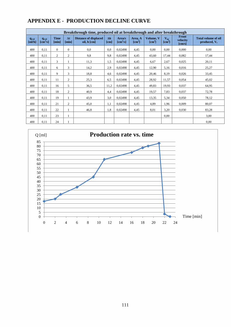
111

APPENDIX E - PRODUCTION DECLINE CURVE

Breakthrough time, produced oil at breakthrough and after breakthrough

qreal

[ml/h]

qreal

[cm3/s]

Time

[min]

Δt

[min]

Distance of displaced

oil, h [cm]

Δh

[cm]

Area/s

[cm2/s]

Area, A

[cm2]

Volume, V

[cm3]

Vop

[cm3]

Front

velocity

[cm/s]

Total volume of oil

produced, Vt

400 0,11 0 0 0,0 0,0 0,02498 4,45 0,00 0,00 0,000 0,00

400 0,11 2 2 9,8 9,8 0,02498 4,45 43,60 17,44 0,082 17,44

400 0,11 3 1 11,3 1,5 0,02498 4,45 6,67 2,67 0,025 20,11

400 0,11 6 3 14,2 2,9 0,02498 4,45 12,90 5,16 0,016 25,27

400 0,11 9 3 18,8 4,6 0,02498 4,45 20,46 8,19 0,026 33,45

400 0,11 11 2 25,3 6,5 0,02498 4,45 28,92 11,57 0,054 45,02

400 0,11 16 5 36,5 11,2 0,02498 4,45 49,83 19,93 0,037 64,95

400 0,11 18 2 40,9 4,4 0,02498 4,45 19,57 7,83 0,037 72,78

400 0,11 19 1 43,9 3,0 0,02498 4,45 13,35 5,34 0,050 78,12

400 0,11 21 2 45,0 1,1 0,02498 4,45 4,89 1,96 0,009 80,07

400 0,11 22 1 46,8 1,8 0,02498 4,45 8,01 3,20 0,030 83,28

400 0,11 23 1 0,00 3,00

400 0,11 24 1 0,00

0

5

10

15

20

25

30

35

40

45

50

55

60

65

70

75

80

85

0 2 4 6 8 10 12 14 16 18 20 22 24

Time [min]

Q [ml] Production rate vs. time

112

Production Rate Decline

Q [ml/min]

t ime[sec]

0

50

100

150

200

250

300

350

400

450

22 42 62 82 102 122 142 162 182 202

Produced Water and Oil after Breakthrough

Produced Water

after

Breakthrough

Produced Oil

after

Breakthrough

time [sec]

Vp [ml]

113

0

50

100

150

200

250

300

350

400

450

0 1 2 3 4 5 6 7 8 9 10 11 12 13 14 15 16 17 18 19 20 21 22 23 24

Oil Production Rate vs. Timeq0(t) [ml/h]

t [sec]

0

50

100

150

200

250

300

350

400

450

22 42 62 82 102 122 142 162 182 202

Water Production Rate vs. Time

t [sec]

114

APPENDIX F - GOAL SEEK

Input data for Goal Seek to calculate pressure drop, flow rates for the different inlet tubes and

total flow rate.

Input data:

Lap, [m]: 0,965 Length from A to Perforation

Lbp, [m]: 0,765 Length from B to Perforation

Lcp, [m]: 0,560 Length from C to Perforation

Ldp, [m]: 0,390 Length from D to Perforation

Lep, [m]: 0,170 Length from E to Perforation

H, [m]: 0,300 Height of pipe

Dpipe, [m]: 0,00635 ID pipe

Wgravel, [m]: 0,0150 Width of gravel pack

Hgravel, [m]: 0,0150 Height of gravel pack

Permeability, [m2]: 5,15E-11 NB! Assumed to be constant

Pinn_vann, [Pa]: 47 000 Inlet pressure (gauge)

Pinn_olje, [Pa]: 47 000 Inlet pressure (gauge)

P_ut, [Pa]: 0 Discharge pressure (gauge)

g, [m/s2]: 9,81 Gravity

ρ_vann, [kg/m3]: 991,41 Density water

ρ_olje, [kg/m3]: 847,38 Density oil

µ_vann, [Pas]: 1,260E-03 Viscosity water

µ_olje, [Pas]: 2,720E-02 Viscosity oil

Calculations:

A_pipe, [m]: 3,17E-05 Area pipe

A_gravel, [m]: 2,25E-04 Area gravel pack

V_water_pipe_a, [m/s]: 0,001 Fluind velocinty in pipe a

V_water_gravel_ap, [m/s]: 0,000 Fluind velocinty in gravel from a-p

V_oil_pipe_b, [m/s]: 0,001 Fluind velocinty in pipe b

V_oil_gravel_bp, [m/s]: 0,000 Fluind velocinty in gravel from b-p

V_oil_pipe_c, [m/s]: 0,001 Fluind velocinty in pipe c

V_oil_gravel_cp, [m/s]: 0,000 Fluind velocinty in gravel from c-p

V_oil_pipe_d, [m/s]: 0,002 Fluind velocinty in pipe d

V_oil_gravel_dp, [m/s]: 0,000 Fluind velocinty in gravel from d-p

V_oil_pipe_e, [m/s]: 0,004 Fluind velocinty in pipe e

V_oil_gravel_ep, [m/s]: 0,000 Fluind velocinty in gravel from e-p

UD

Re

115

Re_water: 3,07E+00 Reynolds number water

Re_oil: 1,71E-02 Reynolds number oil

f_water: 1,92E-01 Friction factor water

f_oil: 1,07E-03 Friction factor oil

DP_h_water, [Pa]: 2 918 Hydrostatic pressure drop - water

DP_h_oil, [Pa]: 2 494 Hydrostatic pressure drop - oil

DP_f_water_a, [Pa]: 0 Friction based pressure drop water

DP_f_oil_b, [Pa]: 0 Friction based pressure drop olje - pipe b

DP_f_oil_c, [Pa]: 0 Friction based pressure drop olje - pipe c

DP_f_oil_d, [Pa]: 0 Friction based pressure drop olje - pipe d

DP_f_oil_e, [Pa]: 0 Friction based pressure drop olje - pipe e

DP_d_water_ap, [Pa]: 44 082 Darcy pressure drop "water" a-p

DP_d_oil_bp, [Pa]: 44 506 Darcy pressure drop oil b-p

DP_d_oil_cp, [Pa]: 44 506 Darcy pressure drop oil c-p

DP_d_oil_dp, [Pa]: 44 506 Darcy pressure drop oil d-p

DP_d_oil_ep, [Pa]: 44 506 Darcy pressure drop oil e-p

Dp_a-p, [Pa]: 47 000 Calculated pressure drop

Dp_b-p, [Pa]: 47 000 Calculated pressure drop

Dp_c-p, [Pa]: 47 000 Calculated pressure drop

Dp_d-p, [Pa]: 47 000 Calculated pressure drop

Dp_e-p, [Pa]: 47 000 Calculated pressure drop

Dp_a-p, [Pa]: 47 000 "Real" pressure drop

Dp_b-p, [Pa]: 47 000 "Real" pressure drop

Dp_c-p, [Pa]: 47 000 "Real" pressure drop

Dp_d-p, [Pa]: 47 000 "Real" pressure drop

Dp_e-p, [Pa]: 47 000 "Real" pressure drop

(assumes that oil will flow through gravel pack

until water break through - oil viscosity is therefore used)

UD

Re

q_"water"_a-p: 1,9E-08 m3/s 1,2E-06 m3/min 1,2 milliliter / min OK - 'Goal Seek ' is used to verify calculation

q_oil_b-p: 2,5E-08 m3/s 1,5E-06 m3/min 1,5 milliliter / min OK - 'Goal Seek ' is used to verify calculation

q_oil_c-p: 3,4E-08 m3/s 2,0E-06 m3/min 2,0 milliliter / min OK - 'Goal Seek ' is used to verify calculation

q_oil_d-p: 4,9E-08 m3/s 2,9E-06 m3/min 2,9 milliliter / min OK - 'Goal Seek ' is used to verify calculation

q_oil_e-p: 1,1E-07 m3/s 6,7E-06 m3/min 6,7 milliliter / min OK - 'Goal Seek ' is used to verify calculation

Result - Qtot: 14,3 milliliter / min

116

APPENDIX G - VISUALIZATION OF DISPLACEMENT IN

HORIZONTAL GRAVEL PACK

Figure G- 1 Visualization of displacement

10. June 2010, 10:47:12 Water has started fingering through the gravel pack.

10. June 2010, 10:47

117

10. June 2010, 10:54:58

10. June 2010, 10:58:14 Breakthrough

118

10. une 2010, 11:00:24

10. June 2010, 11:01:36

10. June 2010, 11:02:14

119

10. June 2010, 11:15:50

10. June 2010, 11:16:20

10. June 2010, 11:17:58

10. June 2010, 11:26:20

120

10. June 2010, 11:27:06

10. June 2010, 11:27:12

10. June 2010, 11:27:44

10. June 2010, 11:27:52

10. June 2010, 11:27:56

10. June 2010, 11:29:30

Inlet tubes from water and oil (formation)

121

10. June 2010, 11:41:22

10. June 2010, 11:41:26

10. June 2010, 11:41:28

10. une 2010, 11:41:30

10.June 2010, 12.09

Saturation and Permeability Differences in different horizontal layers

10. June 2010, 12:27:58

122

10. June 2010, 13:23:38

10. June 2010, 13:24:12

10. June 2010, 13:24:20

10. June 2010, 13:25:30

10. June 2010, 13:25:52

123

10. June 2010, 13:26:00

10. June 2010, 13:26:08

10. June 2010, 13:26:12

10. June 2010, 13:26:18

124

10. June 2010, 13:26:20

10. June 2010, 13:26:52

10. June 2010, 13:26:56

10. June 2010, 13:27:00

10. June 2010, 13:27:04

Small “gravitation segregation” in the production tube.

125

10. June 2010, 16:03:08

10. June 2010, 16:02:46

10. June 2010, 13:30:16

Vertical Permeability and Saturation Layers

10. June 2010, 13:31:38

10. June 2010, 13:32:44

126

10. June 2010, 13:32:46

10. June 2010, 13:32:50

10. June 2010, 13:33:04

10. June 2010, 15:57:44 10. June 2010, 15:58:14

127

10. June 2010, 16:02:16

128

10. June 2010, 19:18:40

11. June 2010, 11:11:12

11. June 2010, 15:28:12

11. June 2010, 15:29:34

12. June 2010, 15:23:48

129

12. June 2010, 15:23:56

10. June 2010, 15:51:56 10. June 2010, 15:53:38

10. June 2010, 16:10:40 10. June 2010, 16:11:10

130

10. June 2010, 16:10:40 10. June 2010, 16:12:52

13. June 2010, 20:35:10 13. June 2010, 20:44:16

11. June 2010, 15:09:54 At the first oil injection tube

131

13. June 2010, 20:38:46 Between second and third

oil injection tube

13. June 2010, 20:40:38 In between third and fourth injection tube

13. June 2010, 20:42:22 At the fourth oil injection

tube

11. June 2010, 15:11:58 Four cm from the first oil injection tube

13. June 2010, 20:43:40 10 cm from outlet 11. June 2010, 15:07:36 8 cm from oulet

132

13. une 2010 20:36:36Between water injection

tube and first oil injection tube

11. June 2010, 15:14:04 Close to water injection tube

Oil Produced at breakthrough of water

133

APPENDIX H - DATA FOR DISPLACEMENT IN GRAVEL PACK

Table H 1

Measured data for horizontal displacement in gravel pack

Date P [bar] T [⁰C] dP [bar] Time [sec]

10:37:06 0,17 22,73 0,19 0,00

10:37:21 0,18 22,74 0,21 0,25

10:37:36 0,23 22,74 0,26 0,50

10:37:51 0,27 22,75 0,30 0,75

10:38:06 0,31 22,74 0,34 1,00

10:38:21 0,34 22,76 0,37 1,25

10:38:36 0,37 22,74 0,40 1,50

10:38:51 0,39 22,75 0,42 1,75

10:39:06 0,41 22,75 0,44 2,00

10:39:21 0,43 22,75 0,46 2,25

10:39:36 0,44 22,75 0,47 2,50

10:39:51 0,45 22,75 0,48 2,75

10:40:06 0,46 22,74 0,48 3,00

10:40:21 0,46 22,74 0,48 3,25

10:40:36 0,46 22,74 0,48 3,50

10:40:51 0,45 22,75 0,48 3,75

10:41:06 0,44 22,74 0,47 4,00

10:41:21 0,43 22,75 0,45 4,25

10:41:36 0,42 22,76 0,44 4,50

10:41:51 0,41 22,76 0,44 4,75

10:42:06 0,41 22,76 0,43 5,00

10:42:21 0,38 22,77 0,41 5,25

10:42:36 0,36 22,75 0,39 5,50

10:42:51 0,34 22,77 0,37 5,75

10:43:06 0,34 22,77 0,36 6,00

10:43:21 0,33 22,78 0,36 6,25

10:43:36 0,32 22,77 0,35 6,50

10:43:51 0,32 22,76 0,35 6,75

10:44:06 0,32 22,77 0,34 7,00

10:44:21 0,31 22,77 0,34 7,25

10:44:36 0,31 22,77 0,34 7,50

10:44:51 0,31 22,78 0,33 7,75

10:45:06 0,30 22,78 0,33 8,00

10:45:21 0,31 22,77 0,34 8,25

10:45:36 0,32 22,77 0,35 8,50

10:45:51 0,33 22,78 0,36 8,75

10:46:06 0,34 22,78 0,37 9,00

10:46:21 0,35 22,77 0,37 9,25

10:46:36 0,35 22,78 0,38 9,50

134

10:46:51 0,36 22,78 0,38 9,75

10:47:06 0,36 22,79 0,39 10,00

10:47:21 0,36 22,79 0,39 10,25

10:47:36 0,36 22,78 0,39 10,50

10:47:53 0,36 22,78 0,39 10,75

10:48:06 0,36 22,78 0,39 11,00

10:48:21 0,36 22,78 0,39 11,25

10:48:36 0,36 22,78 0,38 11,50

10:48:51 0,36 22,79 0,38 11,75

10:49:06 0,35 22,79 0,38 12,00

10:49:21 0,35 22,79 0,38 12,25

10:49:36 0,35 22,79 0,38 12,50

10:49:51 0,35 22,79 0,37 12,75

10:50:06 0,34 22,79 0,37 13,00

10:50:21 0,34 22,79 0,37 13,25

10:50:36 0,34 22,79 0,36 13,50

10:50:51 0,33 22,8 0,36 13,75

10:51:06 0,33 22,8 0,36 14,00

10:51:21 0,33 22,79 0,35 14,25

10:51:36 0,32 22,8 0,35 14,50

10:51:51 0,32 22,79 0,34 14,75

10:52:06 0,31 22,8 0,34 15,00

10:52:21 0,31 22,81 0,34 15,25

10:52:36 0,31 22,81 0,33 15,50

10:52:51 0,30 22,82 0,33 15,75

10:53:06 0,30 22,81 0,33 16,00

10:53:21 0,30 22,81 0,32 16,25

10:53:36 0,29 22,81 0,32 16,50

10:53:51 0,29 22,81 0,32 16,75

10:54:06 0,29 22,82 0,31 17,00

10:54:21 0,28 22,81 0,31 17,25

10:54:36 0,28 22,81 0,31 17,50

10:54:51 0,28 22,82 0,31 17,75

10:55:06 0,28 22,83 0,30 18,00

10:55:21 0,27 22,81 0,30 18,25

10:55:36 0,27 22,82 0,29 18,50

10:55:51 0,26 22,83 0,29 18,75

10:56:06 0,26 22,83 0,28 19,00

10:56:21 0,25 22,82 0,28 19,25

10:56:36 0,25 22,82 0,27 19,50

10:56:51 0,24 22,82 0,26 19,75

10:57:06 0,22 22,82 0,24 20,00

10:57:21 0,20 22,82 0,22 20,25

10:57:36 0,19 22,81 0,21 20,50

10:57:51 0,19 22,83 0,21 20,75

135

APPENDIX I - PRODUCTION OF OIL BEFORE AND AFTER BREAKTHROUGH

Information

time

[min] time [sec] Vop [ml]

qo

[ml/min] qo [m3/s]

time

[min]

time

[sec] Vt

Vwp

[ml] qw [ml/min] qw [m3/s]

qt

[ml/min] qt[m3/s] uw [m/s] uo [m/s]

Start test 0 0 0 0,000 0

0

0,000 0

0

Water into model and

Production starts 0 600 14 0,000 0

14

0,000 0

0

8 480 31 3,850 6,42E-08

31

3,850 6,42E-08

2,85E-04

15,5 930 41 2,632 4,39E-08

41

2,632 4,39E-08

1,95E-04

16,32 979 45 2,776 4,63E-08

45

2,776 4,63E-08

2,06E-04

18,17 1090 51 2,796 4,66E-08

51

2,796 4,66E-08

2,07E-04

Breakthrough, water

production 19,12 1147 54 2,814 4,69E-08 0 0 54 0 0,00 0,000E+00 2,814 4,69E-08 0,00E+00 2,08E-04

21 1260 63 3,014 5,02E-08 2 113 65 2 1,06 3,333E-08 4,078 8,36E-08 1,48E-04 2,23E-04

23 1380 67 2,904 4,84E-08 4 233 71 5 1,16 7,500E-08 4,064 1,23E-07 3,33E-04 2,15E-04

29 1740 77 2,648 4,41E-08 10 593 91 14 1,42 2,333E-07 4,065 2,77E-07 1,04E-03 1,96E-04

31,27 1876 83 2,648 4,41E-08 12 729 104 21 1,73 3,500E-07 4,376 3,94E-07 1,56E-03 1,96E-04

33,24 1994 84 2,536 4,23E-08 14 847 109 25 1,77 4,167E-07 4,307 4,59E-07 1,85E-03 1,88E-04

60 3600 148 2,472 4,12E-08 41 2453 238 90 2,20 1,500E-06 4,673 1,54E-06 6,67E-03 1,83E-04

120 7200 193 1,611 2,68E-08 101 6053 338 145 1,44 2,417E-06 3,048 2,44E-06 1,07E-02 1,19E-04

180 10800 254 1,413 2,35E-08 161 9653 464 210 1,31 3,500E-06 2,718 3,52E-06 1,56E-02 1,05E-04

240 14400 299 1,247 2,08E-08 221 13253 574 275 1,25 4,583E-06 2,492 4,6E-06 2,04E-02 9,24E-05

360 21600 394 1,095 1,83E-08 341 20453 774 380 1,11 6,333E-06 2,210 6,35E-06 2,81E-02 8,11E-05

420 25200 459 1,094 1,82E-08 401 24053 903 444 1,11 7,400E-06 2,201 7,42E-06 3,29E-02 8,10E-05

480 28800 533 1,111 1,85E-08 461 27653 1072 539 1,17 8,983E-06 2,281 9E-06 3,99E-02 8,23E-05

540 32400 578 1,071 1,78E-08 521 31253 1162 584 1,12 9,733E-06 2,192 9,75E-06 4,33E-02 7,93E-05

600 36000 633 1,056 1,76E-08 581 34853 1272 639 1,10 1,065E-05 2,156 1,07E-05 4,73E-02 7,82E-05

Test end 660 39600 678 1,028 1,71E-08 641 38453 1382 704 1,10 1,173E-05 2,126 1,18E-05 5,21E-02 7,61E-05

660 39600 1382

136

APPENDIX J – ROSEMOUNT DATA LOGGING TOOL SETUP