1 23

Natural HazardsJournal of the International Societyfor the Prevention and Mitigation ofNatural Hazards ISSN 0921-030XVolume 71Number 3 Nat Hazards (2014) 71:1795-1819DOI 10.1007/s11069-013-0980-8

Coastal vulnerability to wave storms of Selelittoral plain (southern Italy)

Gianluigi Di Paola, Pietro Patrizio CiroAucelli, Guido Benassai & GermánRodríguez

1 23

Your article is protected by copyright and all

rights are held exclusively by Springer Science

+Business Media Dordrecht. This e-offprint

is for personal use only and shall not be self-

archived in electronic repositories. If you wish

to self-archive your article, please use the

accepted manuscript version for posting on

your own website. You may further deposit

the accepted manuscript version in any

repository, provided it is only made publicly

available 12 months after official publication

or later and provided acknowledgement is

given to the original source of publication

and a link is inserted to the published article

on Springer's website. The link must be

accompanied by the following text: "The final

publication is available at link.springer.com”.

ORI GIN AL PA PER

Coastal vulnerability to wave storms of Sele littoral plain(southern Italy)

Gianluigi Di Paola • Pietro Patrizio Ciro Aucelli • Guido Benassai •

German Rodrıguez

Received: 10 November 2012 / Accepted: 28 November 2013 / Published online: 17 December 2013� Springer Science+Business Media Dordrecht 2013

Abstract This paper presents a new method for coastal vulnerability assessment (CVA),

which relies upon three indicators: run-up distance (as a measurement of coastal inunda-

tion), beach retreat (as a measurement of potential erosion), and beach erosion rate

(obtained through the shoreline positions in different periods). The coastal vulnerability

analysis of Sele Coastal Plain to storm impacts is examined along a number of beach

profiles realized between 2008 and 2009. This particular study area has been selected due

to its low-lying topography and high erosion propensity. Results are given in terms of an

impact index, performed by combining the response due to coastal inundation, storm

erosion, and beach erosion rate. This analysis is implemented on the basis of morphose-

dimentary characteristics of the beach, wave climate evaluation, and examination of

multitemporal aerial photographs and topographic maps. The analysis of the final results

evidences different coastal responses as a function of the beach width and slope, which in

turn depend on the local anthropization level. The comparison of this method with a

Coastal Vulnerability Index method evidences the better attitude of CVA index to take into

account the different beach features to explain the experienced damages in specific

stretches of the coastline considered.

G. Di Paola (&)Dipartimento di Bioscienze e Territorio, Universita degli Studi del Molise, Pesche, IS, Italye-mail: gianluigi.dipaola@unimol.it

P. P. C. AucelliDipartimento di Scienze e Tecnologia, Universita degli Studi ‘‘Parthenope’’, Naples, Italye-mail: pietro.aucelli@uniparthenope.it

G. BenassaiDipartimento d’Ingegneria, Universita degli Studi ‘‘Parthenope’’, Naples, Italye-mail: benassai@uniparthenope.it

G. RodrıguezDepartamento de Fısica, Universidad de Las Palmas de Gran Canaria, Las Palmas de Gran Canaria,Spaine-mail: grodriguez@dfis.ulpgc.es

123

Nat Hazards (2014) 71:1795–1819DOI 10.1007/s11069-013-0980-8

Author's personal copy

Keywords Sele River Coastal Plain � Wave run-up � Beach retreat � Vulnerability

index � CVA index

1 Introduction

Coastal vulnerability, defined as the susceptibility of a coastal area to be affected by either

inundation or erosion, affects the majority of coasts worldwide and is accountable for

destruction of property and infrastructure. Therefore, its evaluation is of major importance;

however, it is a controversial topic, and a vast literature detailing specific system response

to perturbations exists (Bosom and Jimenez 2011; Ozyurt and Ergin 2010; Mendoza and

Jimenez 2008; Cooper and Jay 2002; Cutter 1996; Short 1999; Smith and Jackson 1992).

In fact, due to the large number of different processes involved in coastal zones, their

relative importance, and the relative highly varying space–time dynamic characteristics,

the development of a universal methodology to assess vulnerability of any coastal area is a

difficult task. Up-to-date procedures used to assess coastal vulnerability can be classified

according to different aspects, but the establishment of a concise classification is not easy,

because limits between classes are not strict. Methods have progressively evolved from

single approaches (e.g., Bruun rule, Bruun 1962; UNEP methodology, Carter et al. 1994) to

more consistent ones (i.e., USGS-CVI, Gornitz et al. 1994; SURVAS, Nicholls and de la

Vega-Leinert 2000), which have extended the range of physical and nonphysical factors, in

order to take into account the more significant natural processes.

One of the most commonly used methods worldwide for assessing coastal vulnerability

is the Coastal Vulnerability Index (CVI) (Gornitz et al. 1994, 1997), which combines the

changing susceptibility of the coastal system with its natural capability to adapt to

changing environment. According to this approach, different classes of vulnerability

related to climatic change (i.e., mean elevation, geology, coastal landform, shoreline, wave

height, and tidal range) can be attributed to different coastal sections, defining the relative

susceptibility of a coastline (Arun and Kunte 2012; Gaki-Papanastassiou et al. 2010; Diez

et al. 2007; Lozano et al. 2004). A similar approach, which refers to both time and space

smaller scales, is the Beach (zone) Vulnerability Index (BVI), proposed by Alexandrakis

et al. (2011). The BVI, in essential tideless environment, incorporates longshore and cross-

shore sediment transport, riverine inputs, storm surge, wave run-up, and aeolian sediment

transport. The calculation of the aforementioned variables includes the estimation of other

important parameters, such as sediment statistics, wave conditions (e.g., significant wave

height and period), and geomorphological characteristics of the beach zone (e.g., beach

width and slope).

Another comparative vulnerability assessment, performed by Jimenez et al. (2009),

separately evaluates vulnerability to storm-induced processes (inundation and erosion) and

quantifies the contribution of the forcing (storm properties) and receptor (beach geomor-

phology) to the overall vulnerability. The flood potential is calculated by considering wave

run-up height and storm surge as a measure of the relative dimension of the maximum

water level with respect to the maximum elevation of the beach. Erosion potential is

described by the maximum retreat of a given control line, evaluated through the calculation

of the eroded volume from the inner beach.

A similar approach has been suggested in Benassai et al. (2009, 2012, 2013) and Di

Paola et al. (2011) through the coastal vulnerability assessment (CVA), which takes into

account both the inundation of inshore land and the beach retreat due to storm surge. This

1796 Nat Hazards (2014) 71:1795–1819

123

Author's personal copy

method allows a consistent assessment of coastal vulnerability using a new parameter,

called impact index, which is based on wave climate, bathymetry, geomorphology, and

sediment data. It depends on run-up height, seasonal and multiyear erosion index, and

efficiency of coastal protection structures. This CVA was applied to the Sele Coastal Plain

(Campania, southern Italy), which is a significant test site due to concentration of an

important inhabited area (city of Salerno), archeological sites of UNESCO world heritage

list (ancient town of Poseidonia-Paestum), and complex morphological conditions that are

particularly susceptible to damages. This coastal zone is characterized by spread back-

ridge depressions, with a mean height of about 0.50–1.50 m a.s.l., with a high sensitivity to

future relative sea-level rise (IPCC 2007; Rahmstorf 2007) particularly in the NW sector,

where the back-ridge area, characterized by a lower and flat morphology, could undergo

major flood risks (Pappone et al. 2012).

The paper is structured as follows: Geological features of the study area, as well as its

morphological characteristics and main infrastructures located in different stretches are

introduced in Sect. 2. Data and methodologies used to derive inputs for the coastal vul-

nerability assessment procedure, as well as the theoretical background, are briefly

described in Sect. 3. Experimental results relevant to storm wave numerical simulations

and to coastal vulnerability evaluations are presented and discussed in Sect. 4, together

with the comparison with a CVI method. Conclusions are finally drawn in Sect. 5.

2 Study area

2.1 Geology and beach morphology

Sele Plain is one of the widest alluvial coastal plains of central-southern Italy. It stretches

between the high rocky coasts of Amalfi and Cilento promontory (Campania, southern

Italy) and is limited toward the sea by a narrow sandy beach which extends from NW to SE

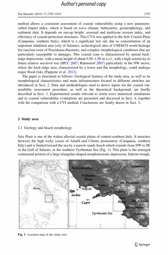
in the Gulf of Salerno, in the southern Tyrrhenian Sea (Fig. 1). This plain is the emerged

continental portion of a large triangular-shaped morphotectonic depression, Salerno trough,

Fig. 1 Location map of the study area

Nat Hazards (2014) 71:1795–1819 1797

123

Author's personal copy

related to the opening and expansion of the Tyrrhenian ocean basin started in the Upper

Miocene (Amato et al. 2013; Casciello et al. 2006; Bartole et al. 1984).

The outer portion of the plain is characterized by the presence of beach-dune ridges

marking the sea level high stands and related paleo-coastlines of Upper Pleistocene, whose

maximum altitude makes it possible to infer a slight uplift of the plain system after their

deposition. Close to the present coastline, a composite sandy ridge occurs, representing the

evolution of a Holocene barrier-lagoon system. At the beginning of Holocene, the prog-

radational trend was interrupted by at least three phases of formation of sandy coastal

ridges. These sandy ridges constitute a discontinuous dune system with a mean height of

about 3 m a.s.l. interrupted by rivers and man-made drainage channels. The back-ridge

depressions, only recently drained, are spread over a large area of the plain, with a mean

height of about 0.50/1.5 m a.s.l. (Amato et al. 2013; Aucelli et al. 2012; Pappone et al.

2011).

This dune system can be considered as a natural barrier to sea ingression. During the last

century, the Sele coastline was affected by prevailing erosion that was very strong around

the main river mouths, due to numerous hydraulic dams that greatly reduced sediment

supply to the rivers (Alberico et al. 2012a, b). Nowadays, the coast is rather stable (Al-

berico et al. 2012a).

The coast is associated with long, narrow, and straight sandy beaches for a total length

of about 40 km. This is a typical open, shallow water coast with beaches of moderate

gradient (6–15 %). Seven-river system that originates in the Picentini and Alburni

Mountains flows into the Gulf of Salerno: Irno, Picentino, Asa, Tusciano, Sele (the major

one), Capodifiume, and Solofrone Rivers (Fig. 2).

Different morphological and anthropic features allow distinguishing the following three

stretches of coastline. The first, which extends from the mouth of Picentino River till the

Asa River (Fig. 2), shows small beaches and strong urbanization, which diminishes

southward. The second, that runs from the mouth of the Tusciano River to the mouth of the

Sele River, is in part still intact with natural beach features enough preserved (with the

exception of the Sele mouth, where there is a strong urbanization). The third, reaching

toward south the ancient town of Paestum and the city of Agropoli, is characterized by

wider beaches with almost preserved dunes.

Beaches of the first section are characterized by a strong anthropic impact, which is also

confirmed by a number of sewage outlets protected by concrete structures and some shore

protection works (small detached longitudinal breakwaters, adherent breakwaters) placed

here and there to protect single infrastructures and sometimes the coastal road (Fig. 2a, b).

In the second coastal section, marked by the river mouths of Tusciano and Sele, beaches

are wider and show a lower anthropogenic load, with some exceptions. In fact, proceeding

from the Tusciano mouth southward, the amplitude of the beach gradually increases with

finer sand sediments, allowing the establishment of numerous beach resorts. On the left

bank of Sele River, a more intense anthropogenic load is experienced, with the presence of

a holiday beach resort which corresponds to a narrower beach and a higher intensity of

wave attack, evidenced by several pines located directly on the beach, due to a retreat of

several tens of meters (Fig. 2e, f).

Fig. 2 Localization of measured profiles on coastal Sele Plain. a profile P1 without dune; b the littoralzone, near P2 profile; c dune on profile P4 with the presence of pioneer vegetation; d emerged and tidalbeach on P6 profile; e demaged house belonging to village Merola, located at the left bank of Sele mouth;f profile P7, with carved dune; g end of physiographic unit near profile P10; h dune and emerged beach ofprofile P8 with the presence of pioneer vegetation on the dune

c

1798 Nat Hazards (2014) 71:1795–1819

123

Author's personal copy

Nat Hazards (2014) 71:1795–1819 1799

123

Author's personal copy

The southward limit of the physiographic unit, marked by the Capodifiume and Sol-

ofrone Rivers, shows wider beaches with fine sand and a lower anthropic load, with also a

protected area for the preservation of the natural dune habitat (Fig. 2g, h).

3 Data and methods

3.1 Beach profile analysis

According to Krause and Soares (2004), van Rijn et al. (2003), and Masselink and Short

(1993), the beach is defined as the area stretching from the dune crest to the closure depth.

Thus, in order to define a detailed mapping of the emerged and submerged beach, a total of

ten topographic and bathymetric profiles were performed, reported in Fig. 3. Emerged

beach profiles were measured using a Differential Global Position System (DGPS) survey,

for a minimum length of 100 m, starting from the crest of dune (Fig. 2a, b) or from the

base of man-made scarps (Fig. 2c, f, h) until a maximum depth of 1.30 m b.s.l. The

submerged beach profiles were recorded by means of a single beam during a survey

developed in 2008 by IAMC-CNR of Naples up to the closure depth (Di Paola 2011).

The closure depth hd was calculated by applying the following Hallermaier (1977)

formula:

hd ¼ 2:28 � He � 68:5 � H2e

g � T2e

� �ð1Þ

where He is the significant wave height associated with a frequency of 12 h/year, Te the

period associated with that significant wave height, and g the acceleration of gravity. A

value of hd = 7.71 m was obtained.

Fig. 3 Topographical profiles carried out in the Sele Plain

1800 Nat Hazards (2014) 71:1795–1819

123

Author's personal copy

These data were included in a geographic information system (GIS) framework which

was used to draw the topographic profiles and compare the main morphometric features of

the beaches.

In order to determine the sediment mean size (l), statistical parameters were determined

on 40 sediment samples (Di Paola 2011).

3.2 Offshore wave climate

Offshore wave climate was obtained through statistical analysis of the data provided by the

Italian Sea Wave Measurement Network (Rete Ondametrica Nazionale; RON 2012) from

the Ponza buoy (40�52000.1000N, 12�56060.0000E), which can be considered representative

of the offshore wave conditions in the study area, according to the wind and wave atlas of

the Mediterranean Sea (Medatlas Group 2004). The period covered by the wave data is

July 1989–March 2008, including a total of 115,651 wave records, or sea states, each one

characterized by a value of significant wave height, Hs, mean wave period, Tm, and mean

wave direction, Dm. After a quality control procedure, 99,376 records were accepted for

further analysis. The bivariate probabilistic structure of significant wave height and mean

wave direction reveals that SW–WNW is the dominant directional sector, as observed in

Fig. 4a. This fact becomes more evident if only sea states with Hs exceeding a threshold

level of 4.0 m are considered, as observed in Fig. 4b. These results agree with previous

studies by Piscopia et al. (2002).

The general wave climate derived from the database analysis shows that the study area

is frequently affected by moderate wave conditions associated with significant wave

heights lower than 3 m, coming mainly from SSW to NNW sector. However, in some

situations, stormy conditions are generated, mainly associated with wave fields travelling

from subsector WSW to WNW, especially during winter (Fig. 4). With regard to astro-

nomical sea-level variation, the study area experiences a typical semi-diurnal tide with a

mean tidal range of 0.45 m. However, main sea-level variations due to meteorological

surges can reach values up to 1 m (IIM 2002).

Fig. 4 Wave rose (Hs–Dm) for the whole data set (a), for sea states with Hs [ 4 m (b)

Nat Hazards (2014) 71:1795–1819 1801

123

Author's personal copy

Wave conditions considered for the numerical simulation approach used to evaluate

coastal vulnerability of beach profiles were referred to a number of wave storms recorded

at Ponza buoy during winter 2010, which parameters are given in Table 1. The first wave

storm occurred during November 8–10, 2010, with a maximum Hs = 4.23 m and a long

time duration (TD = 55 h). The second storm was recorded on December 17–18, 2010, and

exhibited a maximum significant wave height of Hs = 5.01 m and a minimum time

duration (TD = 24 h). The third storm took place on December 23–25, 2010, presenting a

maximum Hs value of 4.29 m and a duration of 48 h.

3.3 Wave model

The wave model used to perform numerical simulations is the SWAN model, a third-

generation numerical wave model that describes temporal and spatial variation of wind-

induced surface elevation, white-capping effects, and friction with the sea bottom layer

(Benassai 2006). In SWAN waves are described with the two-dimensional wave action

density spectrum N = F/r, even when nonlinear phenomena dominate (e.g., in the surf

zone). The action density spectrum N is considered rather than the energy density spectrum

E (r, h), since in the presence of ambient currents only the action density is conserved

(Whitam 1974). The evolution of the wave spectrum is described by the spectral action

balance equation (Hasselmann et al. 1973):

o

dtN þ o

dxcxN þ o

dycyN þ o

drcrN þ o

dhchN ¼ S

rð2Þ

where r is the intrinsic frequency. First term on the left-hand side of Eq. 2 represents the

timely change rate of the local action density spectrum. Second and third terms on left-

hand side represent the propagation of the action density spectrum in the Cartesian

coordinates space, with propagation velocities cx and cy. Fourth term on the left-hand side

represents the shifting of the relative frequency in the action density spectrum due to

variations in depths and currents, with a propagation velocity cr. Fifth term on left-hand

side represents both depth- and current-induced refraction of local action density spectrum,

with propagation velocity ch. The term at the right-hand side of the action balance Eq. 2 is

the source term of the energy density, representing the effects of generation, dissipation,

and nonlinear wave–wave interactions.

The model is typically forced using wind field forcing at 1-h intervals provided through

the Advanced Research Weather Research and Forecast (WRF–ARW) wind field ECMWF

model data outputs from SWAN model, which include significant wave height (Hs) on

gridded fields, associated wave directions (Dm), and mean periods (Tm), as well as wave

energy spectral information at different wavelengths (Benassai 2006; Benassai and Asci-

one 2006; Booij et al. 1999; Holthuijsen et al. 1993).

Table 1 Recorded wave storms of winter 2010

Storm no. Duration Hs max (m) Tp max (s) Dm max (�N) TD (h)

1 09/11/10–10/11/10 4.23 9.5 218 55

2 17/12/10–18/12/10 5.01 9.5 231 24

3 23/12/10–25/12/10 4.29 10.0 255 48

1802 Nat Hazards (2014) 71:1795–1819

123

Author's personal copy

3.4 Coastal vulnerability assessment (CVA) model

The model proposed in this paper for the assessment of coastal vulnerability is based on the

methodology suggested by Benassai et al. (2009) and further developed by Di Paola et al.

(2011), where a new key parameter known as impact CVA index is properly used for

coastal vulnerability evaluation.

The new parameter accounts for wave climate, bathymetry, and sediment data and

depends on the wave run-up height, the seasonal and long-term erosion index, and the

efficiency of coastal protection structures. It can be calculated according to the following

equation:

CVA ¼ IRu þ IR þ ID þ E þ T ð3Þ

where IRu is an index associated with wave run-up distance, IR is the short-term erosion

index for the shoreline, ID is the backshore coastal protection structures stability index, E is

the beach erosion rate index (equivalent to the shoreline indicator used in the CVI-USGS

method in Gornitz et al. 1997), and T is the tidal range.

Here, the CVA is carried out by evaluating Eq. 3 without considering ID and T index

contributions. In fact, the test area (i.e., the southern Tyrrhenian Coastal Sea basin) is a

microtidal coastal environment with a maximum tidal excursion of 0.45 m (IIM 2002)

(hence T = 0) where no coastal protection is present (hence ID = 0). Therefore, only IRu,

IR, and E contributions will be taken into account for the evaluation of CVA.

For each index, the variable values have been applied to ranks 1, 2, 3, and 4 from ‘‘very

low’’ to ‘‘high’’. The resulting CVA index is obtained by the simple addition of the single

indexes, according to EUROSION project (Directorate General Environment European

Commission 2004).

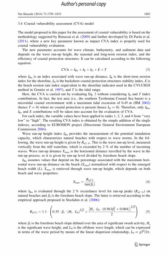
Wave run-up height index IRu provides the measurement of the potential inundation

capacity, which characterizes natural beaches with respect to wave storms. In the fol-

lowing, the wave run-up height is given by Ru2 %. This is the wave run-up level, measured

vertically from the still waterline, which is exceeded by 2 % of the number of incoming

waves. Wave run-up distance Xmax is the horizontal distance travelled by the wave in the

run-up process, so it is given by run-up level divided by foreshore beach slope.

IRu assumes values that depend on the percentage associated with the maximum hori-

zontal wave run-up distance on the beach (Xmax) normalized with respect to the emerged

beach width (L). Xmax is retrieved through wave run-up height, which depends on both

beach and wave properties:

Xmax ¼Ru2 %

tanðbfÞð4Þ

where IRu is evaluated through the 2 % exceedance level for run-up peaks (Ru2 %) on

natural beaches and bf is the foreshore beach slope. The latter is retrieved according to the

empirical approach proposed in Stockdon et al. (2006):

Ru2 % ¼ 1:1 � 0:35 � bf � ðHs � L0Þ1=2 þHs � L0 � ð0:563b2

f þ 0:004Þ� �1=2

2

0@

1A ð5Þ

where bf is the foreshore beach slope defined over the area of significant swash activity, Hs

is the significant wave height, and L0 is the offshore wave length, which can be expressed

in terms of the wave period by means of the linear dispersion relationship, L0 = gT2/2p.

Nat Hazards (2014) 71:1795–1819 1803

123

Author's personal copy

Equation 5 takes into account also the increase in water level due to wave setup, which

constitutes the main part of the increase in mean sea level, so the other terms of wind setup

and inverter barometer are properly neglected.

Based on Eqs. 4 and 5 and according to both Xmax and the beach width L estimates, IRu

values can be customarily clustered into four discrete levels:

IRu¼

1 if Xmax

L%\40

2 if 40� Xmax

L%\60

3 if 60� Xmax

L%\80

4 if Xmax

L%� 80

8>><>>:

9>>=>>;

ð6Þ

where IRu values are ranked into four categories of the short-term vulnerability according to

the classification rule defined in Di Paola et al., (2011), i.e. stable (IRu = 1), low (IRu = 2),

moderate (IRu = 3), and high (IRu = 4) inundation rate of the natural beach (Table 2).

Short-term erosion index IR provides a measurement of potential beach retreat and is

used for the dynamical calculation of the shoreline retreat based on the convolution method

of Kriebel and Dean (1993). IR values depend on the percentage associated with the

maximum beach retreat (Rmax) normalized with the beach width L. Rmax is evaluated as the

maximum value of general solutions associated with the Kriebel and Dean (1993) con-

volution method:

RðtÞR1¼ 1

21� c2

1þ c2exp �2rt=cð Þ � 1

1þ c2cos 2rtð Þ þ csen 2rtð Þ½ �

� �ð7Þ

R1 ¼ SWb � db=m0

Bþ db � S=2ð8Þ

where c ¼ 2p Ts=TD, that is the ratio between the time scale of beach erosion Ts and the

storm duration TD.

In Eqs. 7 and 8 the symbols have the following meaning: S = sea-level increase due to

wave storm, B = berm height, m0 = slope of the seabed in the foreshore, db = breaking

depth and Wb = offshore breaking depth distance.

Based on Eqs. 7 and 8 and according to both Rmax and L estimates, IR values can be

customarily clustered into four discrete levels:

IR ¼

1 if Rmax

L%\40

2 if 40� Rmax

L%\60

3 if 60� Rmax

L%\80

4 if Rmax

L%� 80

8>><>>:

9>>=>>;

ð9Þ

where IR values are properly ranked into four categories of the short-term vulnerability

according to the classification rule defined in Di Paola et al. (2011), i.e., stable (IR = 1),

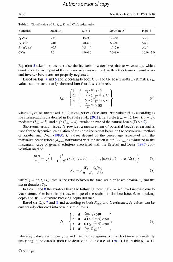
Table 2 Classification of IR, IRu, E, and CVA index value

Variables Stability 1 Low 2 Moderate 3 High 4

IR (%) \15 15–30 30–50 [50

IRu (%) \40 40–60 60–80 [80

E (m/year) \0.5 0.5–1.0 1.0–2.0 [2.0

CVA 3.0 4.0–6.0 7.0–9.0 10.0–12.0

1804 Nat Hazards (2014) 71:1795–1819

123

Author's personal copy

low (IR = 2), moderate (IR = 3), and high (IR = 4) short-term erosion of natural beach

(Table 2).

Finally, in order to evaluate the beach erosion rate index (E), which provides the

evaluation of potential beach retreat, topographic maps, aerial photographs, and multi-

spectral satellite images have been utilized to demarcate shoreline positions of different

periods.

The first comparison, regarding the period 1954–1998, was realized using topographic

maps (1954 IGMI topographic map—scale 1:25,000; 1975 CASMEZ topographic map—

scale 1:5,000) and aerial photography (1954—scale 1:39,000; 1984—scale 1:26,000;

1998—scale 1:10,000). The second comparison, made in the present study, regarded more

recent shoreline positions (2003–2009) detected by SPOT3 and SPOT5 satellite images, in

order to update and confirm the previous trend. Comparisons were made using ArcGIS

release 9.3 and its extension digital shoreline analysis system (DSAS, Thieler et al. 2005).

Beach erosion rate index assumes values that depend on the erosion rate velocity VE (m/

year):

E ¼1 if VEðm year�1Þ\0:52 if 0:5�VEðm year�1Þ\1:03 if 1:0�VEðm year�1Þ\2:04 if VEðm year�1Þ� 2:0

8>><>>:

9>>=>>;

ð10Þ

where E values are properly ranked into four categories according to the classification rule

defined in Di Paola et al. (2011), i.e., stable (E = 1), low (E = 2), moderate (E = 3), and

high (E = 4) beach erosion rate (Table 2).

The impact index CVA is evaluated according to Eq. 3. Based on the customary ranking

of IRu, IR, and E parameters, CVA values are mapped into four categories, according to the

classification rule defined in Di Paola et al. (2011), coming up to the final ranking: stable

(CVA = 3), low (3 \ CVA B6), moderate (6 B CVA B 9), and high (9 B CVA B 12)

coastal vulnerability (Table 2).

4 Experimental results

In this part of the study, numerical sea wave simulations and CVA model are implemented

in the test site.

Firstly, SWAN numerical simulations are carried out with respect to the relevant wave

storms reported in Table 1 using wind field forcing provided by European Centre for

Medium-Range Weather Forecast (ECMWF) model winds, validated with field wave data.

The output of SWAN simulations is then used for CVA model purposes to evaluate the

impact index of the test site, evaluating separately the index associated with each com-

ponent of the physical beach response. Finally, ranks relative to each index have been

summed in the CVA index to come up with a final classification.

Experimental results relevant to the evaluation of run-up height and distance, and

potential beach erosion are described, and then they are transformed in the corresponding

vulnerability indexes and properly ranked according to the scheme shown in Table 2.

4.1 Beach profile and sediment analysis

Firstly, some meaningful coastal morphodynamic features of the coastal test site have been

analyzed in order to explain the results of the beach response. In Fig. 2, the elevation map

Nat Hazards (2014) 71:1795–1819 1805

123

Author's personal copy

of the test area is shown in gray tones together with the position of ten specific elevation

transects (from P1 to P10), each of which encompasses intertidal and emerged beach

elevation as shown in Fig. 3. Longitudinal extensions of the beach are given in Table 3

together with both their relative percentage value and their longitudinal extensions

(Table 4).

Results of the topographic and bathymetric survey on the coastal plain can be sum-

marized as follows.

The topographic profiles P1 and P2 highlighted the absence of the dune system that was

partially replaced by a retaining wall about 5 m high (Fig. 2a, b). Beach morphological

characteristics (Tables 3, 4) show that the emerged beach width is always lower than 50 m;

consequently, the beach was classified of medium width for 48 % of its extension and of

restricted width for 52 %. The emerged and submerged beach, between the dune and the

closure depth, has a mean width of 566 m and a mean slope of 2.1 %.

The stretch of coastline close to Tusciano River mouth is characterized by the presence

of a discontinuous dune system and by some natural areas (Fig. 2c). Topographic profiles

P3 and P4 show a stable dune system with an elevation ridge of about 3.4 m. The emerged

beach is of medium width (20 m \ L \ 50 m) for 68 % and wide (L [ 50 m) for 32 %

(Table 3). In this zone the emerged and submerged beach till the closure depth is 488 m

length on average and its main slope is 2.3 % (Table 4). Topographic profiles from P5 to

P7 evidence that the dune system has eroded and deteriorated particularly in the coastal

area close to Sele River mouth, where the present foredune is cut back to the ancient dune

system. This condition is also testified by several pine trees, previously pertaining to the

retro-dune pinewood, now growing on the beach and some houses destroyed by wave

energy (Fig. 2f, e). The emerged beach width is medium for 82 %, restricted for 14 %, and

defended by structures for 4 %. The emerged and submerged beach till the closure depth is

663 m length on average and has a mean gradient of 1.4 %.

Topographic profiles P8, P9, and P10, which describe the main morphological features

of coastal zone between Sele River mouth and Agropoli headland, show a well-preserved

dune system evidenced by two dune alignments reaching 3.5 m and 3 m height, respec-

tively (Fig. 2h). The emerged beach width is wide for 40 % of its extension and medium

for 60 %; the emerged and submerged beach till the closure depth is 703 m length on

average and has a mean slope of about 1.65 %, the widest beach in the study area. These

features evidence a progradational phase supported by the proximity of the Cilento

promontory (Fig. 2g), which gives a partial shelter to kinetic energy of waves, as shown

later.

4.2 Numerical simulations of wave storms

SWAN model has been typically coupled with WRF–ARW model data (Michalakes et al.

2005), which give wind forcing at 1-h intervals, and has been implemented using a four-

nested grid configuration covering the Mediterranean Sea until the Gulf of Naples (Be-

nassai 2006; Benassai and Ascione 2006), where the inner mesh has the highest resolution

(1.1 9 1.1 km). Outputs from SWAN and WRF–ARW models coupling include signifi-

cant wind–wave interaction parameters, such as Hs, Dm, and Tm.

Numerical simulations of wave storms recorded in winter 2010 by the offshore buoy of

Ponza (Table 1) have been implemented with the coupled SWAN/WRF model. An

example of the spatial distribution of significant wave height Hs in the inner domain is

given in Fig. 5, with reference to the wave storm no. 2 of December 17/18, 2010, which

exhibits the highest Hs among the three storms considered. Time history of Hs for this

1806 Nat Hazards (2014) 71:1795–1819

123

Author's personal copy

Ta

ble

3B

each

esw

idth

on

coas

tal

Sel

eP

lain

.L

egen

d:

L\

20

m=

rest

rict

ed,

20\

L\

50

m=

med

ium

,L

[5

0m

=w

ide

Bea

chw

idth

L(2

01

0)

Mo

uth

of

Pic

enti

no

(m,

%)

Mo

uth

of

Tu

scia

no

(m,

%)

Mo

uth

of

Sel

e(m

,%

)M

ou

tho

fS

olo

fro

ne

(m,

%)

Wid

e(L

[5

0m

)–

–8

00

32

––

1,2

00

60

Med

ium

(20\

L\

50

m1

,200

48

1,7

00

68

2,0

50

82

80

04

0

Res

tric

ted

(L\

20

m)

1,3

00

52

––

35

01

4–

–

Def

ense

wo

rks

––

––

10

04

––

Nat Hazards (2014) 71:1795–1819 1807

123

Author's personal copy

Ta

ble

4S

um

mar

yo

fm

ain

mo

rph

ose

dim

enta

rych

arac

teri

stic

so

fb

each

pro

file

s

Pro

file

sD

un

eri

dg

eh

eigh

t(m

)B

each

emer

ged

wid

thL

(m)

Em

erg

edan

dsu

bm

erg

edb

each

wid

th(m

)B

erm

(m)

Em

erg

edan

dsu

bm

erg

edb

each

slo

pe

mo

(%)

Bea

chfo

resh

ore

slo

pe

bf

(%)

l(m

m)

P1

–2

0.4

57

6.9

1.1

01

.91

1.2

5.0

37

P2

–2

7.3

55

4.7

1.1

92

.31

0.1

0.9

71

P3

3.4

20

.44

54

.11

.38

2.4

9.6

0.7

53

P4

–2

6.2

59

6.2

1.0

02

.21

3.7

0.6

87

P5

2.6

26

.37

02

.31

.13

1.5

5.7

4.4

87

P6

2.4

25

.56

63

.11

.08

1.5

14

.70

.44

4

P7

3.6

15

.86

69

.21

.16

1.7

11

.90

.49

3

P8

3.1

41

.66

68

.91

.18

1.6

6.8

0.3

41

P9

3.6

57

.76

17

.81

.05

1.8

5.9

0.3

96

P1

02

.84

7.1

83

1.5

1.1

81

.61

5.0

0.3

46

1808 Nat Hazards (2014) 71:1795–1819

123

Author's personal copy

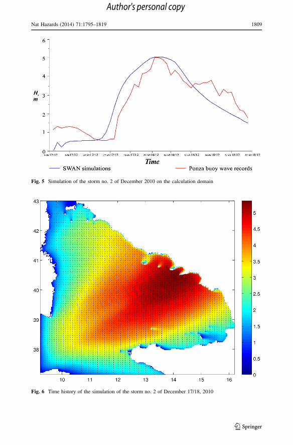
Fig. 5 Simulation of the storm no. 2 of December 2010 on the calculation domain

Fig. 6 Time history of the simulation of the storm no. 2 of December 17/18, 2010

Nat Hazards (2014) 71:1795–1819 1809

123

Author's personal copy

storm is given in Fig. 6, together with the comparison with the offshore wave data of

Ponza. The comparison with the recorded data shows that wave model run with the

ECMWF wind field is capable of reproducing the changing storm characteristics, and also

the peak significant wave height of the storm. In fact, ECMWF model winds retrieve the

peak value of Hs, which numbers 5.01 m. Similar results have been obtained for the

simulation of the other storms in Table 1.

More generally, numerical simulations demonstrate that SWAN model provides sig-

nificant and accurate sea wave estimations and ECMWF model data represent a consistent

wind forcing for SWAN model and the storm wave description parameters. Therefore,

CVA method was applied with reference to the simulated and recorded data.

4.3 Coastal vulnerability assessment

Based on the description and classification of the morphology features of the test area, IRu,

IR, E, and CVA results have been evaluated over the ten considered transects and shown in

Figs. 7 and 8, according to the CVA approach, as described in Sect. 3.4.

The calculation of run-up height and distance on the available profiles was computed on

the foreshore beach slope with the Stockdon et al. (2006) formula (Eq. 5), on the basis of

the morphological beach features reported in Table 3. The run-up distance Xmax associated

with the run-up height Ru2 % was reported in Fig. 7a for each storm of winter 2010, and

then results were made nondimensional through the beach width L (Fig. 7b). This result

highlights the stronger impact of L with respect to bf for the evaluation of Xmax/L and Xmax.

In fact, on the one hand, Xmax/L is inversely proportional to L; therefore, it is minimum for

Fig. 7 Beach retreat (a) and nondimensional beach retreat (b) for storms no. 1, no. 2, and no. 3 of winter2010

1810 Nat Hazards (2014) 71:1795–1819

123

Author's personal copy

the maximum L values, which correspond to P8, P9, and P10 transects (Table 4). On the

other hand, Xmax is inversely proportional to bf; therefore, it is minimum for the maximum

bf values, which correspond to P4, P6, and P10 transects (Table 4). In addition to this, it

can be noted that Xmax/L is greater from P1 to P7 transects with the maximum value

reached at P7 profile, which exhibits the lowest L value and then represents the most

critical case in terms of inundation vulnerability (Table 4).

Based on the classification rule defined for IRu (see sector 2.4) and according to the

Xmax/L values obtained, it is possible to define the inundation vulnerability associated with

IRu for each transect of the considered test area. In detail, with respect to the first and third

wave storms, a very low (IRu = 1), low (IRu = 2), medium (IRu = 3), and high (IRu = 4)

inundation vulnerability is experienced for P10, P8–P9, P2–P4–P6, and P1–P3–P5–P7

transects, respectively. With respect to the second wave storm, a low (IRu = 2), medium

(IRu = 3), and high (IRu = 4) inundation value is experienced for P9–P10, P8, and P1–P2–

P3–P4–P5–P6–P7 transects, respectively. All results demonstrate that P7 is the most

critical case among the ten considered transects, since it exhibits the highest Xmax/L value

and then is the most exposed profile in terms of inundation vulnerability.

Calculation of beach retreat on the available profiles was based on the Kriebel and Dean

(1993) formula, the maximum value of R(t)/R? (indicated as Rmax/R?) was reported in

Fig. 8a, and then it was made nondimensional through the beach width (Rmax/L) (Fig. 8b).

It can be noted that the lowest values of Rmax/L calculated for transects P8–P10 are due to

the fact that the local beach is very wide. In fact, vulnerability to beach retreat has been

calculated as Rmax (Fig. 8a) where it is possible to see that profiles P6 and P10 have similar

Rmax values. If overall width values along the coastal plain are used, the relative retreat

Fig. 8 Run-up distance (a) and nondimensional run-up distance (b) for storms no. 1, no. 2, and no. 3 ofwinter 2010

Nat Hazards (2014) 71:1795–1819 1811

123

Author's personal copy

vulnerability decreases because the beach width in the southern part (transects P8–P10)

increases at least two times. As a matter of fact, the value of Rmax/L on profile P10 is half

the value on profile P6, due to higher beach width. As clearly shown by Fig. 8, the lowest

values of Rmax/L are experienced for P1 and P5 transects that correspond to areas where the

beach sediments show the greatest l values (Table 4). This result can be explained by

considering that Rmax is inversely proportional to l, which plays a key role for the eval-

uation of both Ts and Wb within Eq. 7. Moreover, it can be noted that Rmax/L profile is the

same for all three reference wave storms. The most pronounced results are obtained for the

second wave storm, which exhibits both the greatest Hs and the lowest TD values (Fig. 4).

This result takes into account that Rmax is directly proportional to Hs and inversely pro-

portional to TD (see Eqs. 7 and 8). In fact, on the one hand, high Hs values provide high S,

db, and then Rmax values. On the other hand, low TD values provide the reduction in c,

which in turn provides high Rmax values. This means that for a given Hs value, wave storms

with lower TD value exhibit higher Rmax/L profiles. In addition to this, it is shown that for

the three reference wave storms, the maximum Rmax/L value is experienced at P7 transect,

which exhibits the lowest L value among the ten beach profiles and then is the most critical

case in terms of beach retreat vulnerability (Table 4). This result highlights the impact of

L for the evaluation of Rmax/L.

Based on the classification rule defined for IR and according to Rmax/L values experi-

enced for the three reference wave storms, it is possible to define the beach retreat vul-

nerability associated with IR for each transect of the considered test area. With respect to

the first and third wave storms, a very low (IR = 1), low (IR = 2), medium (IR = 3), and

high (IR = 4) beach retreat vulnerability is experienced for P1–P5–P9, P2–P8, P3–P4–P10,

and P6–P7 transects, respectively. With respect to the second wave storm, a very low

(IR = 1), low (IR = 2), medium (IR = 3), and high (IR = 4) beach retreat vulnerability is

experienced for P1–P5, P9, P2–P8, and P3–P4–P6–P7–P10 transects, respectively.

Examination of Fig. 8 shows that the main values of nondimensional beach retreat

increase from P1 to P7 and then decrease for profiles P8, P9, and P10. All the results

clearly show that P7 is the most critical case among the ten considered transects, since it

exhibits the highest Rmax/L value. This result takes into account the high anthropization

level near Sele River mouth, and the higher beach width of the southern stretch of

coastline, as already noticed. An exception is represented by P5 profile, which is indicative

of a local erosion on the right bank of the Sele mouth, in which finer sediment load

transported by the river is washed out by the current and only the gross fraction is left on-

site.

Finally, beach erosion rate analysis has been performed, taking into account beach

variations prior to 1998 (1954–1975, 1975–1984, and 1984–1998) reported in Fig. 9 and

the more recent data (2003–2009) reported in Table 5.

Comparison of shoreline positions for profiles P1 and P2 shows that in the periods

1954–1975 and 1975–1984 the coastline was characterized by a relative stability, which

was confirmed in the period 1984–1998 (Fig. 9). However, most recent data (2003–2009)

show a moderate erosional trend of 0.7 m/year beach decrease (Table 5).

Profiles P3 and P4 have shown alternate periods of erosion and stability. Comparison of

the shoreline positions shows a relative stability in the period 1954–1975, followed by a

severe erosion in the period 1975–1984 (-3 m/year beach decrease), which was followed

again by a relative stability during 1984–1998 (Fig. 9). However, the most recent com-

parison (2003–2009) shows again an erosional trend of 1.2 m/year of beach decrease

(Table 5).

1812 Nat Hazards (2014) 71:1795–1819

123

Author's personal copy

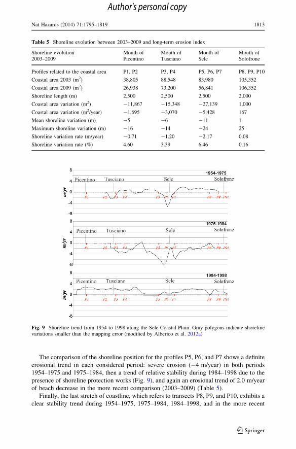
The comparison of the shoreline position for the profiles P5, P6, and P7 shows a definite

erosional trend in each considered period: severe erosion (-4 m/year) in both periods

1954–1975 and 1975–1984, then a trend of relative stability during 1984–1998 due to the

presence of shoreline protection works (Fig. 9), and again an erosional trend of 2.0 m/year

of beach decrease in the more recent comparison (2003–2009) (Table 5).

Finally, the last stretch of coastline, which refers to transects P8, P9, and P10, exhibits a

clear stability trend during 1954–1975, 1975–1984, 1984–1998, and in the more recent

Fig. 9 Shoreline trend from 1954 to 1998 along the Sele Coastal Plain. Gray polygons indicate shorelinevariations smaller than the mapping error (modified by Alberico et al. 2012a)

Table 5 Shoreline evolution between 2003–2009 and long-term erosion index

Shoreline evolution2003–2009

Mouth ofPicentino

Mouth ofTusciano

Mouth ofSele

Mouth ofSolofrone

Profiles related to the coastal area P1, P2 P3, P4 P5, P6, P7 P8, P9, P10

Coastal area 2003 (m2) 38,805 88,548 83,980 105,352

Coastal area 2009 (m2) 26,938 73,200 56,841 106,352

Shoreline length (m) 2,500 2,500 2,500 2,000

Coastal area variation (m2) -11,867 -15,348 -27,139 1,000

Coastal area variation (m2/year) -1,695 -3,070 -5,428 167

Mean shoreline variation (m) -5 -6 -11 1

Maximum shoreline variation (m) -16 -14 -24 25

Shoreline variation rate (m/year) -0.71 -1.20 -2.17 0.08

Shoreline variation rate (%) 4.60 3.39 6.46 0.16

Nat Hazards (2014) 71:1795–1819 1813

123

Author's personal copy

period (2003–2009) with a mean accretion of 1 m in 6 years (Table 5). This information,

added to the significant beach width (Table 3), leads to a lower vulnerability.

Assuming that the last trend (2003–2009) will be confirmed in the future, the more

recent estimations can be considered as reliable to evaluate the erosion rate. In Table 4, the

VE values, obtained through photogrammetric, topographic map and satellite image

comparisons, are shown together with E values for each transect of the considered test area.

Experimental results obtained for a very low (E = 1), low (E = 2), medium (E = 3), and

high (E = 4) beach erosion rate in the more updated comparison are assigned to P8–P9–

P10, P1–P2, P3–P4, and P5–P6–P7 transects, respectively.

In order to perform coastal vulnerability assessment, regardless of the individual storms,

an average index was calculated for the three storms occurred during winter 2010. The

index was referred to the mean values of the indicators Xmax/l and Rmax/l related to each

storm, and results are given in Fig. 10.

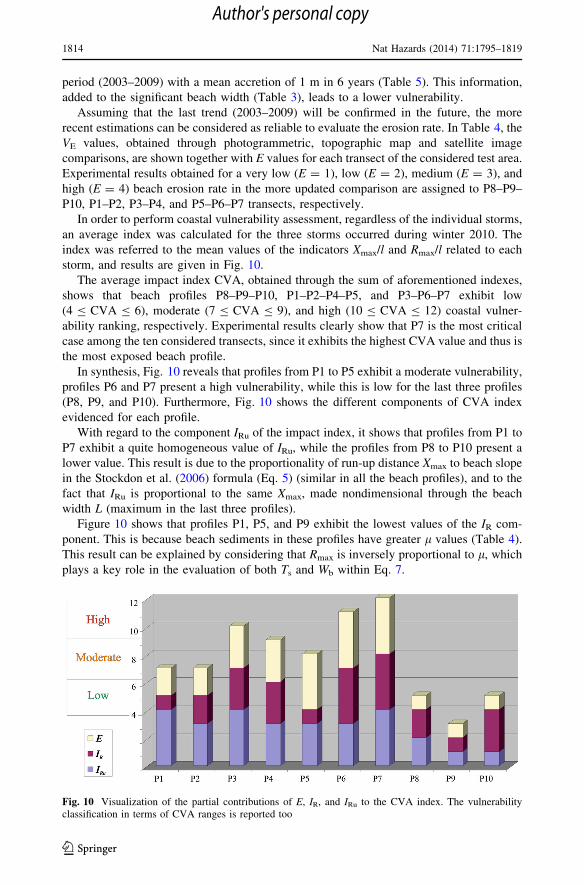
The average impact index CVA, obtained through the sum of aforementioned indexes,

shows that beach profiles P8–P9–P10, P1–P2–P4–P5, and P3–P6–P7 exhibit low

(4 B CVA B 6), moderate (7 B CVA B 9), and high (10 B CVA B 12) coastal vulner-

ability ranking, respectively. Experimental results clearly show that P7 is the most critical

case among the ten considered transects, since it exhibits the highest CVA value and thus is

the most exposed beach profile.

In synthesis, Fig. 10 reveals that profiles from P1 to P5 exhibit a moderate vulnerability,

profiles P6 and P7 present a high vulnerability, while this is low for the last three profiles

(P8, P9, and P10). Furthermore, Fig. 10 shows the different components of CVA index

evidenced for each profile.

With regard to the component IRu of the impact index, it shows that profiles from P1 to

P7 exhibit a quite homogeneous value of IRu, while the profiles from P8 to P10 present a

lower value. This result is due to the proportionality of run-up distance Xmax to beach slope

in the Stockdon et al. (2006) formula (Eq. 5) (similar in all the beach profiles), and to the

fact that IRu is proportional to the same Xmax, made nondimensional through the beach

width L (maximum in the last three profiles).

Figure 10 shows that profiles P1, P5, and P9 exhibit the lowest values of the IR com-

ponent. This is because beach sediments in these profiles have greater l values (Table 4).

This result can be explained by considering that Rmax is inversely proportional to l, which

plays a key role in the evaluation of both Ts and Wb within Eq. 7.

Fig. 10 Visualization of the partial contributions of E, IR, and IRu to the CVA index. The vulnerabilityclassification in terms of CVA ranges is reported too

1814 Nat Hazards (2014) 71:1795–1819

123

Author's personal copy

With regard to the component E of the impact index, its values closely follow the annual

shoreline erosion rate, which is maximum for profiles from P3 to P7, intermediate for P1

and P2, and minimum for profiles from P8 to P10.

4.4 Validation of the CVA method

In order to validate the proposed method, we did a comparison between CVA and CVI

(Gornitz et al. 1994) modified by Thieler and Hammar-Klose (1999). First, the CVI was

calculated on the basis of the geomorphology, wave climate, and beach erosion rate

parameters (Table 6) already available on the different profiles.

The aforementioned variables are ranked on a linear scale from 1 to 5 in order of increasing

vulnerability. Following Gornitz et al. (1997), square root of the product mean of the six

chosen variables is used to calculate the CVI of the coastal region studied. That is,

CVI ¼ffiffiffiffiffiffiffiffiffiffiffiffiffiffiffiffiffiffiffiffiffiffiffiffiffiffiffiffiffiffiffiffiffiffiffiffiffiffiffiffiða � b � c � d � e � f Þ=6

pð11Þ

A synthesis of results is reported in Fig. 11. Furthermore, results from both methods,

CVI and CVA, were normalized with their maximum value and are reported together in

Fig. 12.

Table 6 Ranking of Coastal Vulnerability Index (CVI) variable

Variable 1 2 3 4 5

(a) Geomorphology Rocky,cliffed,coasts

Medium cliffs,intendedcoasts

Low cliffs,alluvialplains

Cobblebeaches,lagoons

Barrier beaches,sand beaches,deltas

(b) Shoreline erosion (-)/accretion (?) (m/year)

[(?2) (?1)–(?2) (-1)–(?1) (-2)–(-1) \(-2)

(c) Coastal slope (%) [12 12–9 9–6 6–3 \3

(d) Relative sea-levelchange (mm/year)

\1.8 1.8–2.5 2.5–3.0 3.0–3.4 [3.4

(e) Main wave height (m) \0.55 0.55–0.85 0.85–1.05 1.05–1.25 [1.25

(f) Main tide range (m) [6.0 4.0–6.0 2.0–4.0 1–2 \1.0

CVI Very low Low Moderate High Very high

Fig. 11 Visualization, for CVA calibration, of CVI results for the profiles considered

Nat Hazards (2014) 71:1795–1819 1815

123

Author's personal copy

The trend exhibited by CVI is quite similar to CVA, except for the last three profiles, in

which the CVI gives a higher value of coastal vulnerability. This difference is due to the

circumstance that the CVI method adapted from Gornitz et al. (1994) by Thieler and

Hammar-Klose (1999) is not based on beach response to inundation and storm retreat, but

it takes into account large-scale coastal features and general wave climate which are

homogeneous in the whole physiographic unit, with the only exception of beach erosion

rate and beach sediment, different for each profile.

On the other hand, the comparison between the two methods for P1 and P5 profiles

shows that CVI method is more cautious for coastal vulnerability of gravel profiles,

because it gives a warning meaning to the gravel sediment size, associating it with higher

energy impact. On the contrary, CVA gives lower values of retreat to the same beach

profiles, because the Kriebel and Dean (1993) retreat equation is inversely proportional to

l.

However, CVI seems to be less suitable, due to its high level of generality, to give

proper stress to different vulnerability conditions of coastline stretches belonging to the

same physiographic unit, in comparison with CVA method, which through a better com-

putation of the specific geomorphological and hydraulic parameters gives a more precise

vulnerability assessment (i.e., closer to the degree of damage experienced on different

stretches of coastline).

5 Conclusions

A new method for coastal vulnerability assessment (CVA) has been used for the response

of Sele Coastal Plain to storm impacts. This method is accomplished with respect to three

wave storms occurred in 2010 along ten beach profiles of Sele Coastal Plain. The main

characteristics of the wave storms recorded in winter 2010 have been evaluated through

SWAN based wind–wave interaction parameters that have been retrieved using ECMWF

model winds, validated with respect to buoy-derived information. Coastal vulnerability has

been calculated on the beach profiles for different wave storms, through some meaningful

vulnerability indexes (i.e., IRu, IR, and E). The impact index CVA, obtained by summing up

the aforementioned indexes, was ranked into four classes. Examination of the results

evidenced different coastal vulnerability rankings for each transect as a function of beach

width and slope, which in turn depended on local anthropization level.

Run-up index IRu evidenced the lowest values for profiles with a wider beach, in

agreement with the experimental evidence. Beach retreat index IR evidenced an increase

Fig. 12 Comparison of normalized CVA results with the normalized CVI results for the profiles considered

1816 Nat Hazards (2014) 71:1795–1819

123

Author's personal copy

for the central profiles, showing a more critical situation at the mouth of Sele River due to

shortage of sediments and high erosive focus. Beach erosion rate index E evidenced the

highest values for northern profiles and lowest for southern ones, except for local condi-

tions at Sele River mouth. This trend is in agreement with the beach erosion retreat

measured by numerous authors in different years. Consequently, coastal vulnerability

index CVA is maximum for Sele River mouth, in which all indexes have a high ranking,

and minimum for the southern part of Sele Coastal Plain (characterized by the lowest beach

erosion rate), while for the first and second stretches of coastline, the index seems to be

more controversial. Nevertheless, CVA index seems to give reliable results on the response

of the stretches of coastline of the same physiographic unit, in agreement with the damage

level experienced along the coastline.

CVA results have been compared with a CVI method, which seems to be less reliable

for vulnerability assessment on different stretches of the same physiographic unit; nev-

ertheless, it seems to be more cautious in case of gravel beaches, which are a signal of

higher energy impact.

Acknowledgments The authors wish to thank G. Mastronuzzi and the anonymous reviewer, whosesuggestions greatly improved the manuscript.

References

Alberico I, Amato V, Aucelli PPC, D’Argenio B, Di Paola G, Pappone G (2012a) Historical shorelineevolution and recent shoreline trends of Sele Plain coastline (Southern Italy). The 1870–2009 timewindow. J Coast Res 28:1638–1647. doi:10.2112/JCOASTRES-D-10-00197.1

Alberico I, Amato V, Aucelli PPC, Di Paola G, Pappone G, Rosskopf CM (2012b) Historical and recentchanges of the Sele River coastal plain (Southern Italy): natural variations and human pressures. RendLincei 23:3–12. doi:10.1007/s12210-011-0156-y

Alexandrakis G, Poulos S, Petrakis S, Collins M (2011) The development of a Beach Vulnerability Index(BVI) for the assessment of erosion in the case of the North Cretan Coast (Aegean Sea). Hell J Geosci45:11–21

Amato V, Aucelli PPC, Ciampo G, Cinque A, Di Donato V, Pappone G, Petrosino P, Romano P, RosskopfCM, Russo Ermolli E (2013) Relative sea level changes and paleogeographical evolution of thesouthern Sele plain (Italy) during the Holocene. Quatern Int 288:112–128. doi:10.1016/j.quaint.2012.02.003

Arun Kumar A, Kunte PD (2012) Coastal vulnerability assessment for Chennai, east coast of India usinggeospatial techniques. Nat Hazards 64:853–872. doi:10.1007/s11069-012-0276-4

Aucelli PPC, Amato V, Budillon F, Senatore MR, Amodio S, D’Amico C, Da Prato S, Ferraro L, PapponeG, Russo Ermolli E (2012) Evolution of the Sele River coastal plain (southern Italy) during the latequaternary by inland and offshore stratigraphical analyses. Rend Lincei 23:81–102. doi:10.1007/s12210-012-0165-5

Bartole R, Savelli D, Tramontana M, Wezel FC (1984) Structural and sedimentary features in the Tyr-rhenian margin off Campania, Southern Italy. Mar Geol 55:163–180

Benassai G (2006) Introduction to coastal dynamics and shoreline protection. Wit Press, SouthamptonBenassai G, Ascione I, (2006) Implementation and validation of wave watch III model offshore the

coastlines of Southern Italy. OMAE 2006 92555:1–8Benassai G, Chirico F, Corsini S (2009) Una metodologia per la definizione del rischio da inondazione

costiera. Studi Costieri 16:51–72Benassai G, Di Paola G, Aucelli PPC, Maffucci A (2012) The response of Sele coastal plain to storm

impacts. Rend Online Soc Geol Italy 21:474–476Benassai G, Montuori A, Migliaccio M, Nunziata F (2013) Sea wave modeling with X-band COSMO-

SkyMed� SAR-derived wind field forcing. Ocean Sci 9:325–341. doi:10.5194/os-9-325-2013Booij N, Ris RC, Holthuijsen LH (1999) A third-generation wave model for coastal regions 1: model

description and validation. J Geophys Res 104:7649–7666. doi:10.1029/98JC02622

Nat Hazards (2014) 71:1795–1819 1817

123

Author's personal copy

Bosom E, Jimenez JA (2011) Probabilistic coastal vulnerability assessment to storms at regional scale—application to Catalan beaches (NW Mediterranean). Nat Hazards Earth Syst Sci 11:475–484

Bruun P (1962) Sea-level rise as a cause of shore erosion. J Waterw Harbours Div 88(1–3):117–130Carter TR, Parry ML, Nishioka S, Harasawa H (1994) Technical guidelines for assessing climate change

impacts and adaptation. University College London, London, and Centre for Global EnvironmentalResearch, Tskuba, J

Casciello E, Cesarano M, Pappone G (2006) Extensional detachment faulting on the Tyrrhenian margin ofthe southern Apennines contractional belt (Italy). J Geol Soc 163:617–629

Cooper NJ, Jay H (2002) Predictions of large-scale coastal tendency: development and application of aqualitative behavior-based methodology. J Coast Res SI36:173–181

Cutter SL (1996) Vulnerability to environmental hazards. Prog Hum Geogr 20(4):529–539Di Paola G (2011) Geological and geo-morphological characterization of coastal Sele Plain (Campania,

Italy) and considerations about its vulnerability. PhD Thesis, Universita degli Studi del Molise, Italy.http://hdl.handle.net/2192/141

Di Paola G, Iglesias J, Rodrıguez G, Benassai G, Aucelli PPC, Pappone G (2011) Estimating coastalvulnerability in a meso-tidal beach by means of quantitative and semi-quantitative methodologies.J Coast Res SI61:303–308. doi:10.2112/SI61-001.30

Diez PG, Perillo GME, Piccolo C (2007) Vulnerability to sea-level rise on the coast of the Buenos AiresProvince. J Coast Res 23(1):119–126

Directorate General Environment European Commission (2004) Living with coastal erosion in Europe:sediment and space for sustainability. Part I: major findings and policy recommendations of theEUROSION project

Gaki-Papanastassiou K, Karymbalis E, Poulos SE, Seni A, Zouva C (2010) Coastal vulnerability assessmentto sea-level rise based on geomorphological and oceanographical parameters: the case of ArgolikosGulf, Peloponnese, Greece. Hell J Geosci 45:109–122

Gornitz VM, Daniels RC, White TW, Birdwell KR (1994) The development of a coastal risk assessmentdatabase: vulnerability to sea-level rise in the U.S. Southeast. J Coast Res SI12:327–338

Gornitz VM, Beaty TW, Daniels RC (1997) A coastal hazards data base for the U.S. West Coast. ORNL/CDIAC-81, NDP-043C, Oak ridge national laboratory, Oak ridge, Tennessee, USA

Hallermaier RJ (1977) Use for a calculated limit depth to beach erosion. In: Proceedings of the XVI coastalengineering conference, pp 1493–1512

Hasselmann K, Barnett TP, Bouws E, Carlson H, Cartwright DE, Enke K, Ewing JA, Gienapp H, Has-selmann DE, Kruseman P, Meerburg A, Mller P, Olbers DJ, Richter K, Sell W, Walden H (1973)Measurements of wind-wave growth and swell decay during the Joint North Sea Wave Project(JONSWAP). Deutsches Hydrographisches Institute, Hamburg, D

Holthuijsen LH, Booij N, Ris RC (1993) A spectral wave model for the coastal zone. In: Proceedings of the2nd international symposium on ocean wave measurement and analysis, pp 630–641

IIM (2002) Tidal data base, Istituto Idrografico della Marina, Genova, IIPCC (2007) Fourth assessment report—climate change 2007. Intergovernmental panel on climate change.

Cambridge University Press, CambridgeJimenez JA, Ciavola P, Balouin Y, Armaroli C, Bosom E, Gervais M (2009) Geomorphic coastal vulner-

ability to storms in microtidal fetch-limited environments: application to NW Mediterranean and NAdriatic Seas. J Coastal Res SI56:1641–1645

Krause G, Soares C (2004) Analysis of beach morphodynamics on the Bragantinian mangrove peninsula(Para, North Brazil) as prerequisite for coastal zone management recommendations. Geomorphology60:225–239. doi:10.1016/j.geomorph.2003.08.006

Kriebel DL, Dean RG (1993) Convolution method for time-dependent beach-profile response. J Waterw PortCoast Ocean Eng 119(2):204–207

Lozano I, Devoy RJN, May W, Andersen U (2004) Storminess and vulnerability along the Atlanticcoastlines of Europe: analysis of storm records and of a greenhouse gases induced climate scenario.Mar Geol 210:205–225

Masselink G, Short AD (1993) The effect of tidal range on beach morphodynamics and morphology: aconceptual beach model. J Coast Res 9:785–800

Medatlas Group (2004) Wind and wave atlas of the Mediterranean Sea, pp 419Mendoza ET, Jimenez JA (2008) Storm induced beach erosion potential on the Catalonian coast. J Coast Res

48:81–88Michalakes J, Dudhia J, Gill D, Henderson T, Klemp J, Skamarock W, Wang W (2005) The weather

research and forecasting model: software architecture and performance. In: Zwiefhofer W, MozdzynskiG (eds) Proceedings of the eleventh ECMWF workshop on the use of high performance computing inmeteorology. World Scientific, pp 156–168

1818 Nat Hazards (2014) 71:1795–1819

123

Author's personal copy

Nicholls RJ, de la Vega-Leinert AC (2000) Synthesis and upscaling of sea-level rise vulnerability assess-ment studies (SURVAS): SURVAS methodology. Flood Hazard Research Centre, Middlesex Uni-versity, USA

Ozyurt G, Ergin A (2010) Improving coastal vulnerability assessments to sea-level rise: a new indicatorbased methodology for decision makers. J Coast Res 26(2):265–273

Pappone G, Alberico I, Amato V, Aucelli PPC, Di Paola G (2011) Recent evolution and the present-dayconditions of the Campanian Coastal plains (South Italy): the case history of the Sele River Coastalplain. WIT Trans Ecol Environ 149:15–27. doi:10.2495/CP110021

Pappone G, Aucelli PPC, Alberico I, Amato V, Antonioli F, Cesarano M, Di Paola G, Pelosi N (2012)Relative sea-level rise and marine erosion and inundation in the Sele River coastal plain (SouthernItaly): scenarios for the next century. Rend Lincei 23:121–129. doi:10.1007/s12210-012-0166-4

Piscopia R, Inghilesi R, Panizzo A, Corsini S, Franco L (2002) Analysis of 12-year wave measurements bythe Italian Wave Network. In: Proceedings of the 28th ICCE conference, Cardiff, pp 121–133

Rahmstorf S (2007) A semi-empirical approach to projecting future sea-level rise. Science 315:368–370RON (2012) Rete ondametrica nazionale. http://www.idromare.it/analisi_dati.php. Accessed 17 May 2012Short AD (1999) Beach and Shoreface morphodynamics. Wiley, ChichesterSmith AWS, Jackson LA (1992) The variability in width of the visible beach. Shore Beach 60(2):7–14Stockdon HF, Holman RA, Howd PA, Sallenger AH (2006) Empirical parameterization of setup, swash, and

run-up. Coast Eng 53(7):573–588Thieler ER, Hammar-Klose ES (1999) National assessment of coastal vulnerability to sea-level rise, U.S.

Atlantic Coast. U.S. Geological Survey, Open-File Report, pp 99–593Thieler ER, Himmelstoss EA, Zichichi JL, Miller TL (2005) Digital shoreline analysis system (DSAS)

version 3.0: an ArcGIS� extension for calculating shoreline change. U.S. Geological Survey Open FileReport 1304

van Rijn LC, Walstra DJR, Grasmeijer B, Sutherland J, Pan S, Sierra JP (2003) The predictability of cross-shore bed evolution of sandy beaches at the time scale of storms and seasons using process-basedProfile models. Coast Eng 47:295–327

Whitam GB (1974) Linear and nonlinear waves. Wiley, New York

Nat Hazards (2014) 71:1795–1819 1819

123

Author's personal copy