
Migratory routes, domesticated birds and cercarial dermatitis
Upload
khangminh22Category
view
3download
0
Clustering community science data to infer migratory connectivity patterns for migratory
songbirds in the Western Hemisphere
by
Jaimie Vincent
A thesis submitted to the Faculty of Graduate and Postdoctoral Affaires in partial
fulfillment of the requirements for the degree of
Master of Science
in
Biology
Carleton University
Ottawa, Ontario
© 2020, Jaimie Vincent
ii
Abstract
Migratory connectivity describes the spatial linkage between individuals through time
and is necessary for full annual cycle conservation. However, conventional methods used
to study migratory connectivity can be expensive and expertise intensive. In Chapter 2,
we infer migratory connectivity patterns for songbirds using relative abundance models
created from eBird, a global community science program, and an underlying broad-scale
parallel migration assumption. We compare migratory connectivity inferences for two
species with previously described connectivity estimates from the literature. We find that
our method is a fast and inexpensive way to infer broad patterns on connectivity for these
two species, though it cannot predict leapfrog migration or extreme deviations from
parallel migration. In Chapter 3, a literature review of migration patterns shows that
broad-scale parallel migration is commonly observed for songbirds in the Western
hemisphere, and thus the methodology presented in Chapter 2 should be widely
applicable to other species.

iii
Acknowledgments
This thesis would not have been possible without the guidance of Joseph Bennet, Richard
Schuster, and Scott Wilson. I would like to thank my supervisor Joe Bennett for
accepting me as a Master’s student; I never thought that a graduate student experience
could be so positive. I credit this in large part to the supportive and kind working
environment that he fosters daily. Thank you for being such a responsive and motivating
mentor. Thank you to Richard Schuster for his invaluable help with creating R code, and
for troubleshooting any problems that I had. My coding skills have greatly improved
since the begining of my Master’s because of this guidance. Thank you to Scott Wilson
for sharing his expert knowledge on migratory bird ecology and insightful perspectives
for both my thesis and the directed studies course. Because of this knowledge, I was able
to understand the significance of my thesis in a more holistic way.
Thank you to all the folks working on the eBird project at the Cornell Lab of
Ornithology, especially Amanda Rodewald and Daniel Fink, and to Peter Arcese for early
discussions and contributions to my thesis. I would also like to thank the innumerable
eBird participants who have provided the data to make this project possible.
Thank you to the students, post-docs, professors, staff and friends of the Geomatics and
Landscape Ecology Lab. The comradery and and peer support made every day at the
office brighter and helped to get through more challenging times. Friday discussions
taught me much about how to write a good paper and helped me gain confidence as a
scientist.

iv
I would also like to thank family who is the foundation of my success in my graduate
studies and beyond. Thank you to my partner Philippe-Israël Morin for his unwavering
support and encouragement and for assiting me with learning new techniques to code
more efficiently. Thank you to my mom Susan Forrest who has always been my biggest
supporter and who has shown me what never-ending love and patience look like. To
Barbara Dumont-Hill for always reminding me to live my life in a good way, chi-
miigwech.

v
Author contributions
Chapter Two: Inferring migratory connectivity for songbirds in the Western
Hemisphere
Jaimie Vincent, Richard Schuster, Scott Wilson, Peter Arcese, Amanda Rodewald,
Joseph Bennett
I am the primary author of this master’s thesis. The original project concept was
conceived by Drs. Peter Arcese, Amanda Rodewald, Joseph Bennett, Richard Schuster,
and myself. I was responsible for writing, analysing and interpreting the data. The R code
used to analyse the data was created by me, with help from Dr. Richard Schuster and Dr.
Joseph Bennett. All co-authors provided comments and critical feedback on the study
design, analysis and interpretation of the data.

vi
Table of contents
Abstract .............................................................................................................................. ii
Acknowledgments ............................................................................................................ iii
Author contributions ........................................................................................................ v
Table of contents .............................................................................................................. vi
List of Tables .................................................................................................................... ix
List of Figures ................................................................................................................... xi
List of Appendices .......................................................................................................... xiii
Chapter 1: General introduction ..................................................................................... 1
1.1 Migratory connectivity must be included in avian conservation planning. ...... 1
1.2 Commonly used strategies for researching migratory connectivity. .................. 2
1.2.1 Banding .............................................................................................................. 3
1.2.2 Stable isotopes ................................................................................................... 4
1.2.3 Genetic markers ................................................................................................. 4
1.2.4 Biologgers .......................................................................................................... 5
1.3 eBird offers new opportunities to monitor avian biodiversity ............................ 6
Chapter 2: Inferring migratory connectivity for songbirds in the Western
Hemisphere ........................................................................................................................ 9
2.1 Abstract .................................................................................................................... 9
2.2 Introduction ............................................................................................................. 9
2.3 Methods .................................................................................................................. 13

vii
2.3.1 Study species .................................................................................................... 13
2.3.2 eBird STEMs ................................................................................................... 14
2.3.3 Delineating regions .......................................................................................... 14
2.3.4 Migratory connectivity analysis using Bayes’ rule .......................................... 16
2.4 Results .................................................................................................................... 18
2.4.1 Wood thrush ..................................................................................................... 18
2.4.2 Wilson’s warbler .............................................................................................. 24
2.5 Discussion............................................................................................................... 29
2.5.1 Wood thrush ..................................................................................................... 29
2.5.2 Wilson’s warbler .............................................................................................. 32
2.5.3 Possible applications ........................................................................................ 35
2.5.4 Caveats ............................................................................................................. 36
2.6 Conclusion ............................................................................................................. 38
Chapter 3: Songbird migration patterns in the Western hemisphere ....................... 39
3.1 Abstract .................................................................................................................. 39
3.2 Introduction ........................................................................................................... 39
3.3 Methods .................................................................................................................. 42
3.4 Results .................................................................................................................... 44
3.5 Discussion............................................................................................................... 50
3.5.1 Crosswise migrants .......................................................................................... 50
3.5.2 Mostly crosswise migrants ............................................................................... 50
3.5.3 Resolving power changes categorization from “mostly crosswise” to “mostly
parallel” ..................................................................................................................... 51

viii
3.5.4 “Mostly parallel” and “parallel” migrants ....................................................... 53
3.6 Conclusion ............................................................................................................. 55
References ........................................................................................................................ 56
Appendices ....................................................................................................................... 72
ix
List of Tables
Table 1.1 Strengths and limitations of different methods used to study migratory
connectivity in passerines.
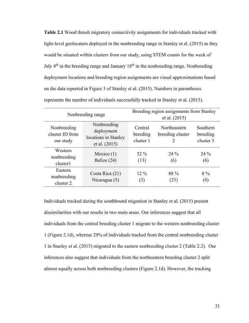
Table 2.1 Wood thrush migratory connectivity assignments for individuals tracked with
light-level geolocators deployed in the nonbreeding range in Stanley et al. (2015) as they
would be situated within clusters from our study, using STEM counts for the week of
July 4th in the breeding range and January 18th in the nonbreeding range. Nonbreeding
deployment locations and breeding region assignments are visual approximations based
on the data reported in Figure 3 of Stanley et al. (2015). Numbers in parentheses
represents the number of individuals successfully tracked in Stanley et al. (2015).
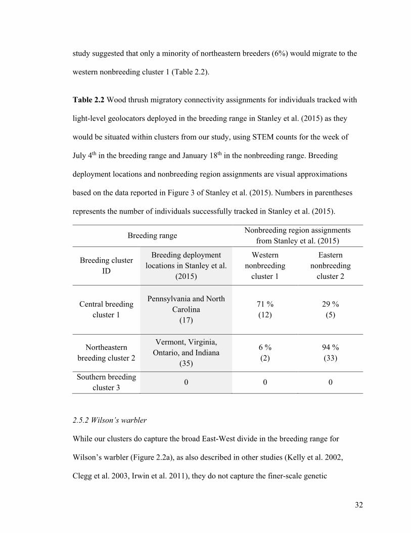
Table 2.2 Wood thrush migratory connectivity assignments for individuals tracked with
light-level geolocators deployed in the breeding range in Stanley et al. (2015) as they
would be situated within clusters from our study, using STEM counts for the week of
July 4th in the breeding range and January 18th in the nonbreeding range. Breeding
deployment locations and nonbreeding region assignments are visual approximations
based on the data reported in Figure 3 of Stanley et al. (2015). Numbers in parentheses
represents the number of individuals successfully tracked in Stanley et al. (2015).
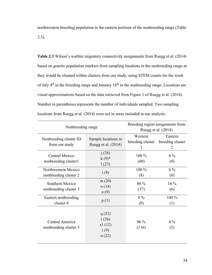
Table 2.3 Wilson’s warbler migratory connectivity assignments from Ruegg et al. (2014)
based on genetic population markers from sampling locations in the nonbreeding range as
they would be situated within clusters from our study, using STEM counts for the week

x
of July 4th in the breeding range and January 18th in the nonbreeding range. Locations are
visual approximations based on the data retrieved from Figure 1 of Ruegg et al. (2014).
Number in parentheses represents the number of individuals sampled. Two sampling
locations from Ruegg et al. (2014) were not in areas included in our analysis.
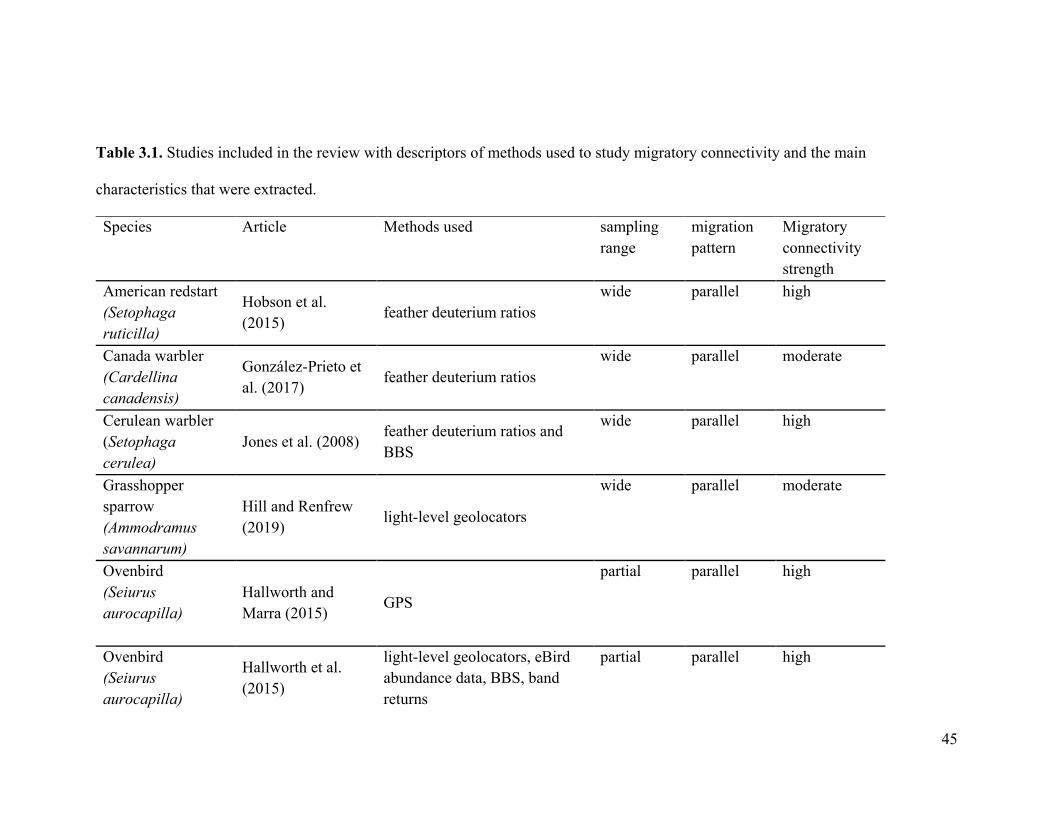
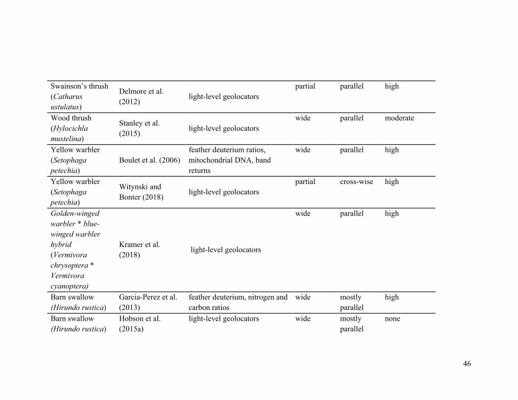
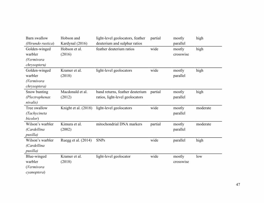
Table 3.1. Studies included in the review with descriptors of methods used to study
migratory connectivity and the main characteristics that were extracted.
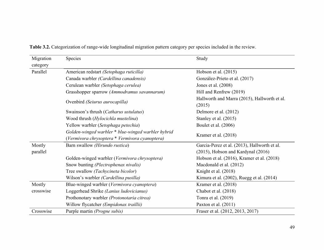
Table 3.2. Categorization of range-wide longitudinal migration pattern category per
species included in the review.
.
xi
List of Figures
Figure 2.1a Clusters for wood thrush breeding range resulting from clustering eBird’s
STEM counts for the week of July 4th. Dark grey pixels represent the excluded pixels
from the home range (95%) analysis. Bottom panel heatmap shows the relative
abundance values at an 8.4 km2 resolution produced by the STEM for the week of July
4th.
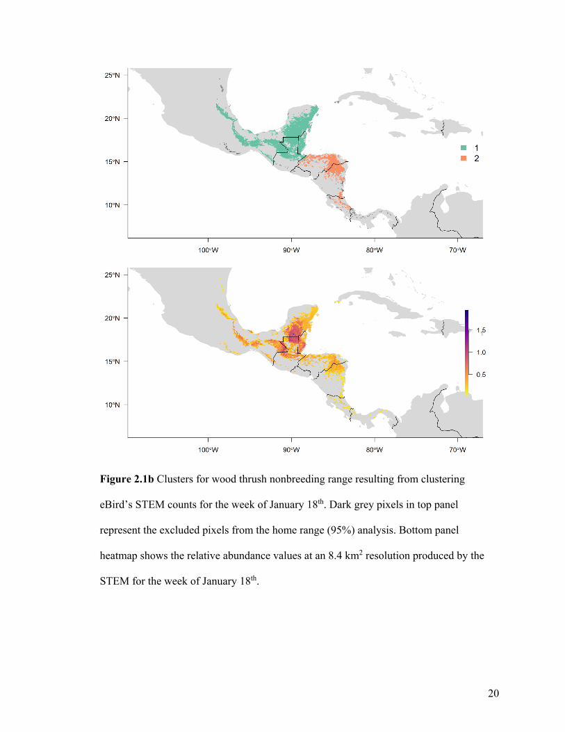
Figure 2.1b Clusters for wood thrush nonbreeding range resulting from clustering
eBird’s STEM counts for the week of January 18th. Dark grey pixels in top panel
represent the excluded pixels from the home range (95%) analysis. Bottom panel
heatmap shows the relative abundance values at an 8.4 km2 resolution produced by the
STEM for the week of January 18th.
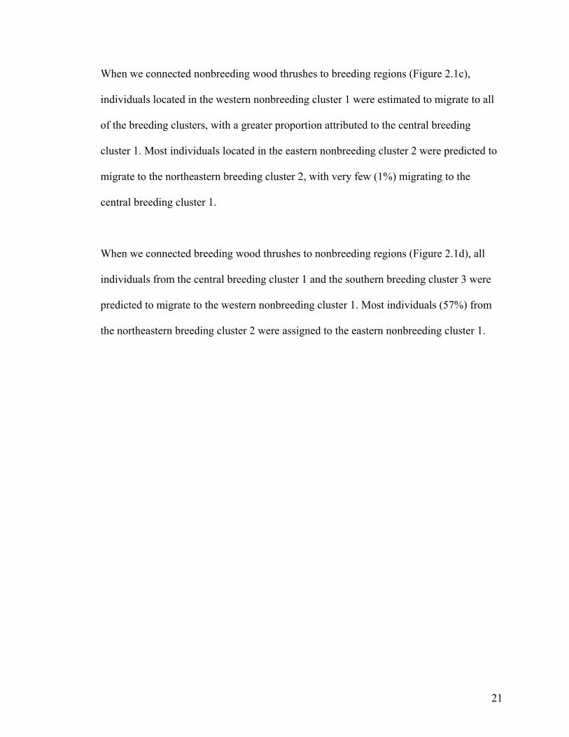
Figure 2.1c Proportion of counts from wood thrush nonbreeding range assigned to the
breeding regions.
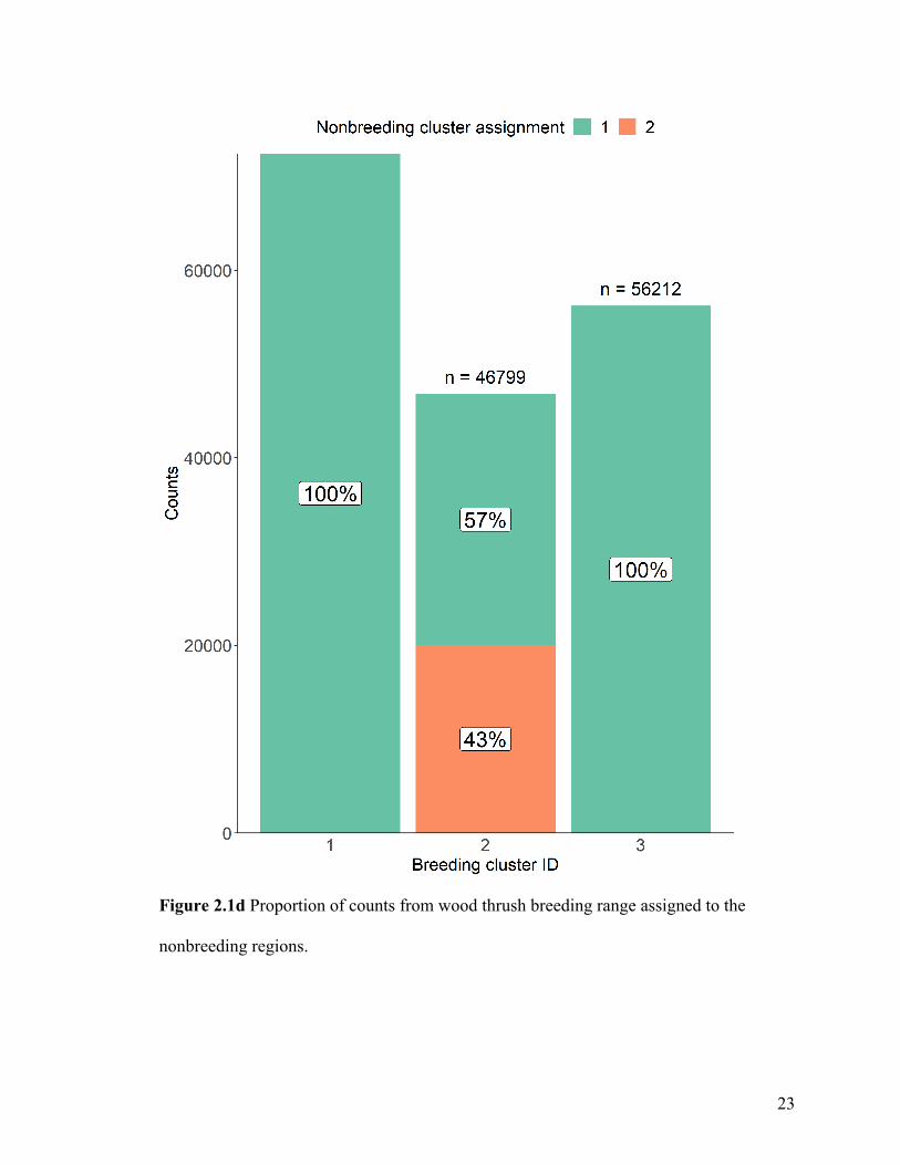
Figure 2.1d Proportion of counts from wood thrush breeding range assigned to the
nonbreeding regions.
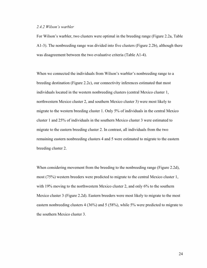
Figure 2.2a Clusters for Wilson’s warbler breeding range resulting from clustering
eBird’s STEM counts for the week of July 4th. Dark grey pixels in top panel represent the
excluded pixels from the home range (95%) analysis. Bottom panel heatmap shows the
xii
relative abundance values at an 8.4 km2 resolution produced by the STEM for the week
of July 4th.
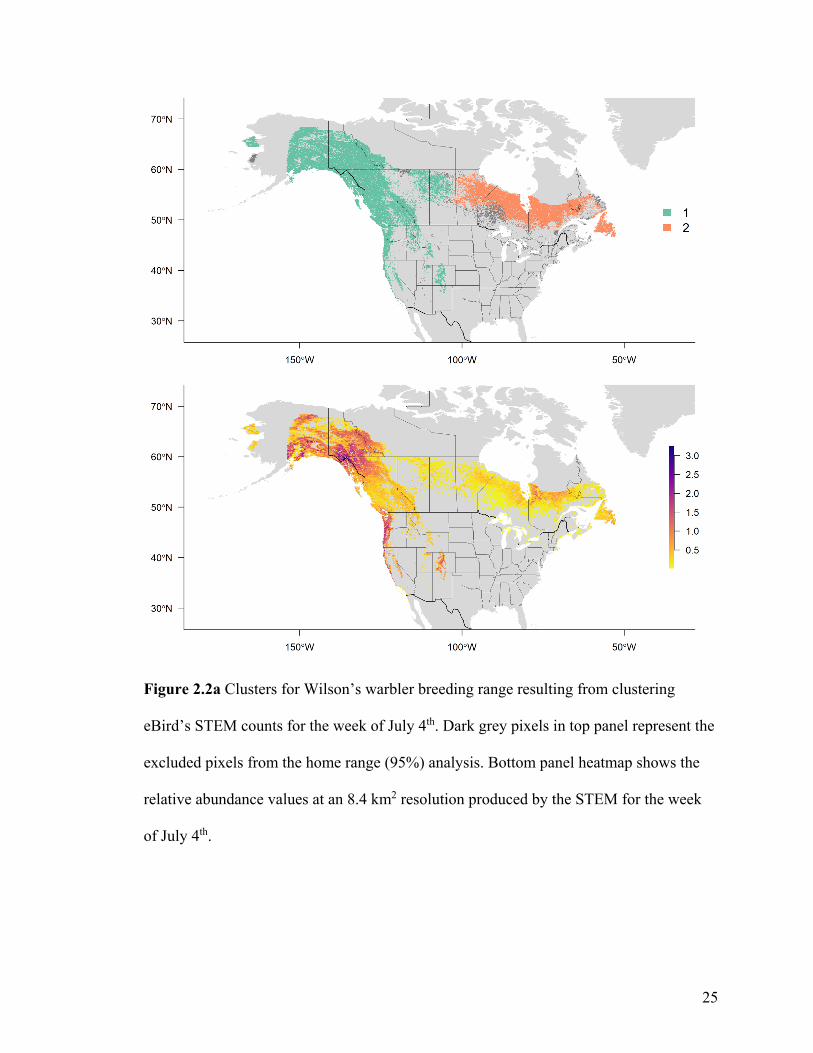
Figure 2.2b Clusters for Wilson’s warbler nonbreeding range resulting from clustering
eBird’s STEM counts for the week of January 18th. Dark grey pixels in top panel
represent the excluded pixels from the home range (95%) analysis. Bottom panel
heatmap shows the relative abundance values at an 8.4 km2 resolution produced by the
STEM for the week of January 18th.
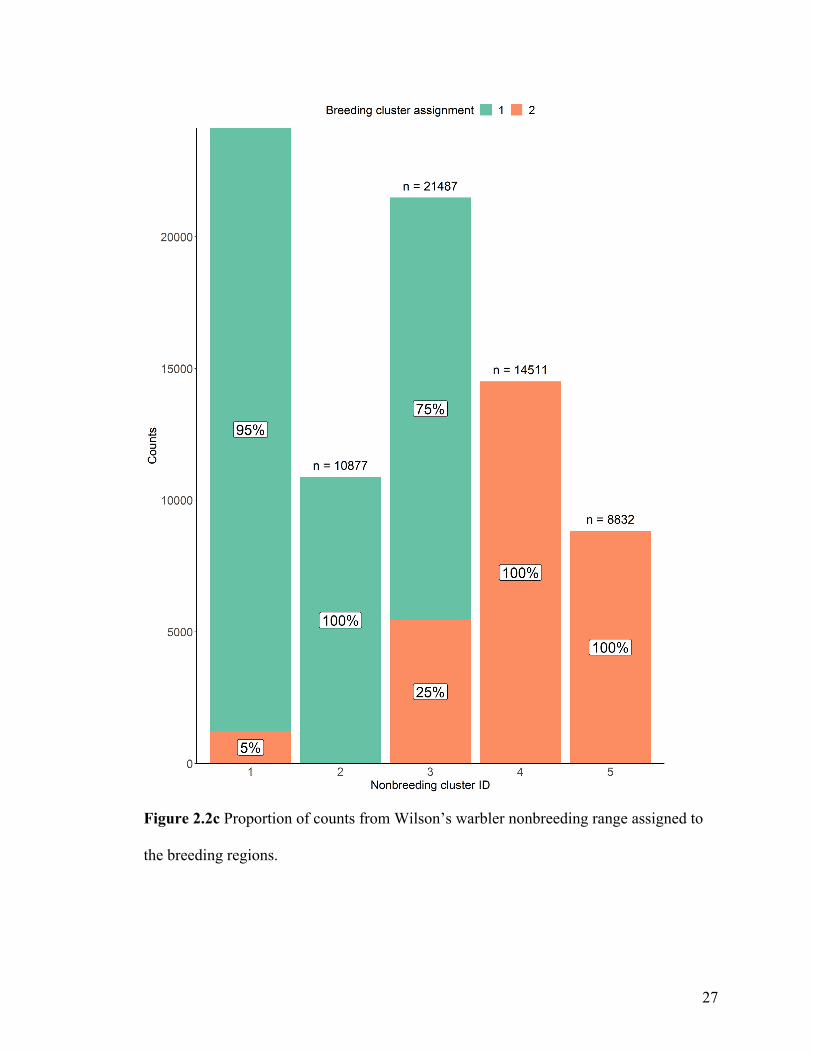
Figure 2.2c Proportion of counts from Wilson’s warbler nonbreeding range assigned to
the breeding regions.
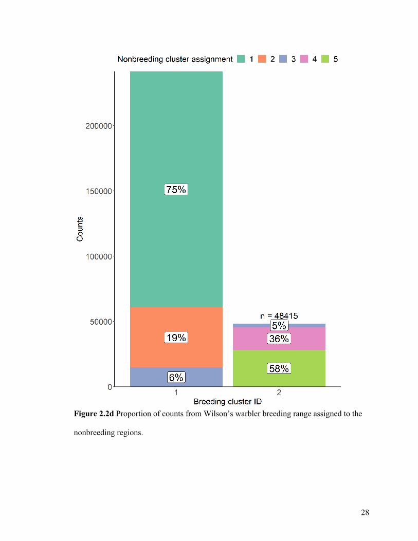
Figure 2.2d Proportion of counts from Wilson’s warbler breeding range assigned to the
nonbreeding regions.
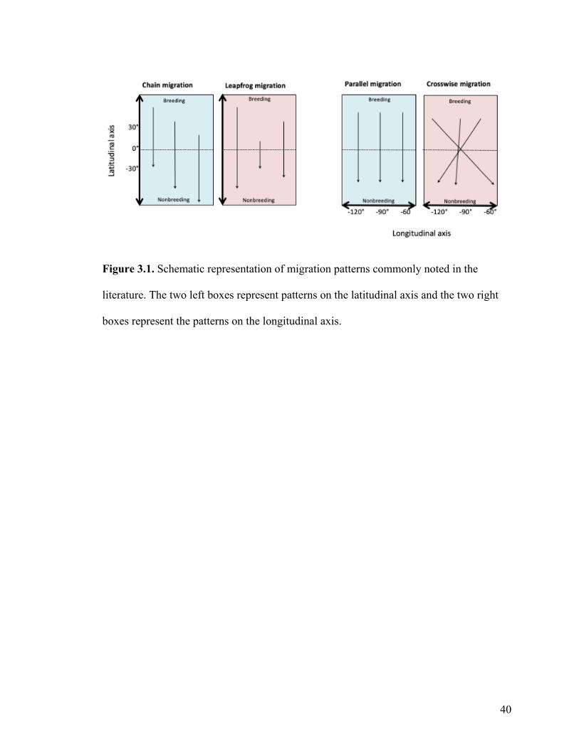
Figure 3.1. Schematic representation of migration patterns commonly noted in the
literature. The two left boxes represent patterns on the latitudinal axis and the two right
boxes represent the patterns on the longitudinal axis

xiii
List of Appendices
Appendix 1. Evaluative criteria results used to determine the optimal number of clusters
per range.
Appendix 2. Distribution of standardized longitude by cluster per range.

1
Chapter 1: General introduction
1.1 Migratory connectivity must be included in avian conservation planning.
For migratory species, knowledge of the full annual cycle is required to understand
population trends observed in any given period of the cycle (Runge et al. 2014, Marra et
al. 2015). In North America, avian population trends are described in large part with the
Breeding Bird Survey (BBS), which has run every breeding season since 1970. This
community science project serves as baseline data and reveals spatially heterogeneous
trends throughout the landscape (Sauer et al. 2017). Trends observed via the BBS are the
result of many different factors that take place throughout different periods of the annual
cycle (Marra et al. 1998). Therefore, identifying where and when the limiting factors
occur and how they carry over throughout the annual cycle is crucial for conservation
purposes (Webster et al. 2002). However, uncovering the full annual cycle is no simple
task because vast distances separate the breeding and nonbreeding ranges, and the
connection between these two regions is masked by migration.
Migratory connectivity describes the geographic linkage of individuals at different
periods of the annual cycle and is crucial to identify priority conservation areas (Webster
et al. 2002). Migratory connectivity can be expressed on a scale from "weak" to "strong."
The former describes individuals that scatter from one period to another, and the latter
describes individuals that remain close to each other from one period to another (Webster
et al. 2002, Cohen et al. 2018). Notably, knowledge of migratory connectivity of a
species allows for spatially and temporally targeted conservation action. For example,

2
neighbouring purple martins (Progne subis) in the South American nonbreeding range
are from very different breeding populations, which demonstrates weak migratory
connectivity (Fraser et al. 2017). Presumably, conservation action in South America
would, therefore, have a diffuse effect across every breeding population of purple
martins. Conversely, ovenbirds (Seiurus aurocapilla) display strong migratory
connectivity throughout the annual cycle (Hallworth and Marra 2015). Therefore,
spatially targeted conservation action could potentially address declines in select
vulnerable ovenbird populations.
1.2 Commonly used strategies for researching migratory connectivity.
Many research methods and technologies have emerged to study the full annual cycle and
migratory connectivity (Marra et al. 2010). Four of the most frequently used connectivity
research methods are bird banding, stable isotope ratios, genetic markers, and biologgers.
Here, I review their advantages and challenges as they pertain to songbird migratory
connectivity research (Table 1.1).
3
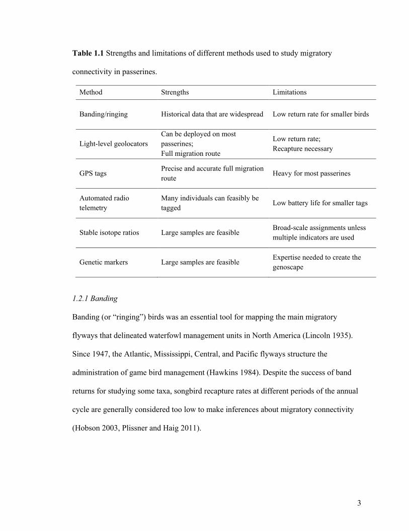
Table 1.1 Strengths and limitations of different methods used to study migratory
connectivity in passerines.
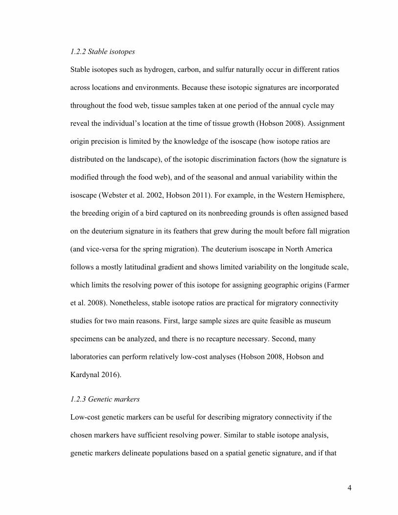
1.2.1 Banding
Banding (or “ringing”) birds was an essential tool for mapping the main migratory
flyways that delineated waterfowl management units in North America (Lincoln 1935).
Since 1947, the Atlantic, Mississippi, Central, and Pacific flyways structure the
administration of game bird management (Hawkins 1984). Despite the success of band
returns for studying some taxa, songbird recapture rates at different periods of the annual
cycle are generally considered too low to make inferences about migratory connectivity
(Hobson 2003, Plissner and Haig 2011).
Method Strengths Limitations
Banding/ringing Historical data that are widespread Low return rate for smaller birds
Light-level geolocators Can be deployed on most passerines; Full migration route
Low return rate; Recapture necessary
GPS tags Precise and accurate full migration route
Heavy for most passerines
Automated radio telemetry
Many individuals can feasibly be tagged Low battery life for smaller tags
Stable isotope ratios Large samples are feasible Broad-scale assignments unless multiple indicators are used
Genetic markers Large samples are feasible Expertise needed to create the genoscape
4
1.2.2 Stable isotopes
Stable isotopes such as hydrogen, carbon, and sulfur naturally occur in different ratios
across locations and environments. Because these isotopic signatures are incorporated
throughout the food web, tissue samples taken at one period of the annual cycle may
reveal the individual’s location at the time of tissue growth (Hobson 2008). Assignment
origin precision is limited by the knowledge of the isoscape (how isotope ratios are
distributed on the landscape), of the isotopic discrimination factors (how the signature is
modified through the food web), and of the seasonal and annual variability within the
isoscape (Webster et al. 2002, Hobson 2011). For example, in the Western Hemisphere,
the breeding origin of a bird captured on its nonbreeding grounds is often assigned based
on the deuterium signature in its feathers that grew during the moult before fall migration
(and vice-versa for the spring migration). The deuterium isoscape in North America
follows a mostly latitudinal gradient and shows limited variability on the longitude scale,
which limits the resolving power of this isotope for assigning geographic origins (Farmer
et al. 2008). Nonetheless, stable isotope ratios are practical for migratory connectivity
studies for two main reasons. First, large sample sizes are quite feasible as museum
specimens can be analyzed, and there is no recapture necessary. Second, many
laboratories can perform relatively low-cost analyses (Hobson 2008, Hobson and
Kardynal 2016).
1.2.3 Genetic markers
Low-cost genetic markers can be useful for describing migratory connectivity if the
chosen markers have sufficient resolving power. Similar to stable isotope analysis,
genetic markers delineate populations based on a spatial genetic signature, and if that
5
genetic marker is detected in an individual on the wintering grounds, a spatial connection
with breeding grounds can be established (Marra et al. 2010). Likewise, large sample
sizes are also feasible because museum specimens can also be sampled, and recapture is
not necessary. Most markers used in the early 2000s such as mitochondrial DNA,
microsatellites and amplified fragment length polymorphisms can only identify broad-
scale differentiation and lack the power to assign individuals to populations at fine scales
(Gibbs et al. 2000, Lovette et al. 2004, Bensch et al. 2008). However, the analysis of
SNPs to create species-specific “genoscapes” provided a breakthrough methodology for
delineating populations at a finer scale (Ruegg et al. 2014, Contina et al. 2019). The most
expensive and expertise-intensive aspect of using genetic markers is mapping the
“genoscape” for each new study species (Ruegg et al. 2017). The subsequent genetic
analysis is relatively inexpensive, and as genomic technological advances become more
widespread and more laboratories can undertake genoscape mapping, this methodology
will surely be a more accessible method for studying different species (Marra et al. 2010).
1.2.4 Biologgers
Light-level geolocators, GPS tags, and radio tags are relatively new technological
advances that allow unprecedented tracking precision. Light-level geolocators can reveal
the entire migratory route completed by individuals and are small enough to be deployed
on most songbirds (McKinnon and Love 2018). They record the time of sunrise and
sunset to predict the location of an individual relative to the angle of the sun. Therefore,
the measure of latitude loses precision around the equator. The cost of light-level
geolocators is at the moment lower than satellite or GPS tags (Lisovski et al. 2019) but
higher than isotopic analyses (Hobson and Kardynal 2016), with great variability in
6
return rates because of low recapture rates, battery failure, and harness failure (Bridge et
al. 2013). Few studies manage to retrieve data for a large number of individuals (but see
Fraser et al. 2012; Knight et al. 2018). Further, the need for recapturing individuals can
create a bias towards the deployment location for territorial species (Hobson and
Kardynal 2016). Archival GPS tags face the same retrieval challenges as light-level
geolocators, but they record the location with more precision (Hobson and Kardynal
2016). However, they remain too heavy for most songbirds. Radio tags do not require
retrieval as the radio towers receive and record the data. At present, the infrastructure
required to track radio-tagged birds throughout the entire annual cycle is insufficient. If a
complete network of receiver towers were put into place, radio tags would offer an
excellent opportunity to track birds across both migrations without needing to recapture
individuals.
1.3 eBird offers new opportunities to monitor avian biodiversity
An increasing number of community science projects have emerged in the past few
decades (Silvertown 2009; Theobald et al. 2015). Community science (also known as
“citizen science”) can be defined as projects that engage the lay public to provide useable
scientific information (McKinley et al. 2017). Even though the inclusion of “non-
scientists” in ecological monitoring schemes has taken place since at least the early
twentieth century (Lincoln 1935), it is only in the twenty-first century that the term
“community science” (or “citizen science”) seems to be more readily used to describe
such projects (Silvertown 2009). Across the globe, volunteers are estimated to have
collectively contributed between $667 million and $2.5 billion in-kind to community

7
science projects annually since the beginning of the 20th century, with a significant
increase in the past 30 years (Theobald et al. 2015). Of these projects, none are more
data-rich than eBird (Chandler et al. 2017).
Launched in 2002, eBird offers unprecedented opportunity to monitor avian biodiversity
(Sullivan et al. 2009, 2014) and is the largest community science project in terms of the
number of observations recorded (Chandler et al. 2017). By capitalizing both on
birdwatchers' record-keeping fondness and the ubiquitous ownership of smartphones,
eBird enables participants to create bird checklists at any time, anywhere in the world.
Community science projects have an exceptional capability to cover large spatial and
temporal scales that are otherwise unachievable using more "conventional" sampling
protocols (Dickinson et al. 2010, Wilson et al. 2013). Not only are raw eBird data useful
for research and monitoring, conservation planning, and conservation action (Sullivan et
al. 2017), they support novel weekly relative abundance models and trend estimates in
the Western Hemisphere (Fink et al. 2010, 2014, 2020). These relative abundance
models, called Spatio-Temporal Exploratory Models (STEM), are currently available for
over 610 species in the Western Hemisphere and can be expected to be available in other
regions as more observations are recorded worldwide. Notwithstanding costs for data
storage and processing to the creators (the Cornell Lab of Ornithology), eBird data
products are free of cost to anyone who wishes to use them.
Considering that many migratory species are rapidly declining and full annual cycle
tracking poses considerable challenges, eBird is an exciting and unexplored avenue for

8
studying migratory connectivity. Drawing on known migration patterns displayed by
songbirds and relative abundance models derived from eBird observations, my thesis will
aim to describe plausible migratory connections between the breeding range and
nonbreeding range for songbirds in the Western Hemisphere.

9
Chapter 2: Inferring migratory connectivity for songbirds in
the Western Hemisphere
2.1 Abstract
Migratory connectivity describes the spatial linkage between individuals through time
and is necessary for full annual cycle conservation planning to avoid uneven protection
and regional population declines. However, conventional methods used to study
migratory connectivity can be expensive and expertise intensive. We present a
methodology that infers migratory connectivity for songbirds using relative abundance
models created from eBird, a global community science program, and an underlying
broad-scale parallel migration assumption. We compare wood thrush and Wilson's
warbler migratory connectivity inferences with previously described patterns of
migratory connectivity found in the literature. We find that this method is a fast and
inexpensive way to infer broad patterns on connectivity for these two species, though it
cannot predict leapfrog migration or extreme deviations from parallel migration.
2.2 Introduction
Conservation plans must consider the full annual cycle to adequately conserve migratory
birds (Webster et al. 2002, Runge et al. 2014, Marra et al. 2015). However, creating such
plans comes with many challenges. Mainly, migrants cover vast distances and spend the
majority of the year outside of the breeding range, in areas where there has historically
been less monitoring (Runge et al. 2014). Knowledge gaps in time and space that ensue
throughout migration and the nonbreeding period limit our ability to understand the full
annual cycle ecology of migrants and hinder targeted conservation planning.

10
Migratory connectivity describes the spatial linkage between individuals through time
(Marra et al. 2010) and is necessary for full annual cycle conservation planning.
Specifically, it lays the groundwork for pinpointing where limiting factors occur in time
and space and understanding carry-over effects (Rushing et al. 2016a), thereby allowing
targeted conservation planning. Conservation plans that ignore migratory connectivity
can lead to uneven protection, which can eventually result in regional population declines
(Martin et al. 2007).
Even though increasingly precise methodologies and technologies have increased our
ability to track songbird migration in the last few decades (Faaborg et al. 2010), they are
not without their respective limitations (Table 1.1). All methods require extensive
sampling across the entire range in order to be effective (Knight et al. 2018); tracking
devices can be expensive and generally have low return rates (McKinnon and Love
2018); and intrinsic population markers provide broad-scale assignments that are
dependent on expert-intensive or resource-intensive methods for population delineation
(Hobson 2011, Ruegg et al. 2014).
A general way of describing songbird migration is by categorizing population movements
on the longitudinal and latitudinal axes. Chain migration or leapfrog migration can occur
on the latitudinal axis. Chain migration occurs when northern breeding individuals
migrate to the northern region of the nonbreeding range. In contrast, leapfrog migration is
used to describe when northern breeding individuals migrate to the southern region of the
11
nonbreeding range, effectively "leapfrogging" over the southern breeders that migrate to
the northern region of the nonbreeding range. Parallel or crosswise migration can occur
on the longitudinal axis. Parallel migration refers to a migratory system where individuals
that breed in the western part of the species' range will also overwinter in the western part
of the nonbreeding range, and, similarly, individuals that breed in the eastern part of the
breeding range will overwinter in the eastern part of the nonbreeding range. Parallel
migration is commonly observed in songbirds, and there is strong evidence in the
literature that supports the preservation of broad East-West divides for many species
throughout the annual cycle, as discussed further in Chapter 3 (Clegg et al. 2003, Kelly
and Hutto 2005, Boulet et al. 2006, Norris et al. 2006, Jones et al. 2008, Delmore et al.
2012, Fraser et al. 2012, Drake et al. 2013, Hallworth and Marra 2015, Stanley et al.
2015, Hallworth et al. 2015, González-Prieto et al. 2017, Kramer et al. 2018, Hill and
Renfrew 2019).
Apart from the technical limitations presented in Table 1.1, another problem arises across
migratory connectivity studies in the literature. There is no standard approach to spatially
delineate migrating populations, except for waterfowl, which have been managed by
continental flyways for the past century (Lincoln 1935). For other species such as
songbirds, the boundaries that delineate migrating populations seem to be drawn either ad
hoc or post hoc, occasionally based on data with various degrees of ecological support.
Delineations between migrating populations have been created by clustering
demographic data (Rushing et al. 2016b) and genetic data (Ruegg et al. 2014), by using
political borders or recognized conservation areas such as Bird Conservation Regions

12
(Kramer et al. 2018) or flyways (Lincoln 1935, Buhnerkempe et al. 2016), or by
intuitively dividing regions on a map. Subjective delineations of migratory regions or
delineating regions post hoc can influence the final interpretation of migratory
connectivity studies and should be used with caution (Cohen et al. 2018).
In this paper, we will develop a new approach to infer songbird migratory connectivity
between the breeding and nonbreeding ranges based on relative abundance models
created from eBird observations (Fink et al. 2014, 2020). To delineate migratory regions,
we use a partition-based clustering method that mirrors the methodology used by Rushing
et al. (2016b) that delineates natural populations based on demographic data. In doing so,
we provide a reproducible and objective way of delineating migratory regions in both the
breeding and nonbreeding ranges. Then, we infer migratory connectivity using Bayes’
rule, incorporating the total abundance of a region as a prior and assuming parallel
migration to calculate the likelihood of individuals migrating to a given breeding region.
To evaluate the performance of our methods, we apply our methodology to two species
for which there has been extensive migratory connectivity research: wood thrush (Stanley
et al. 2014) and Wilson’s warbler (Ruegg et al. 2014). This novel, low-cost approach to
inferring migratory connectivity with community science data and common migration
patterns can hopefully be applied to understudied species that require urgent conservation
action for which it is not practical to collect more data, thereby and allowing managers to
plan for full annual cycle conservation.
13
2.3 Methods
2.3.1 Study species
The wood thrush is a forest songbird listed as threatened in Canada that breeds through
the eastern United States and south-eastern Canada and winters in Central America. The
strength of migratory connectivity during wood thrush migration is uncertain, although
there is some evidence that spatial cohesion diminishes en route (Cohen et al. 2019).
Nevertheless, light-level geolocator tracking evidence suggests strong connectivity
between the breeding and nonbreeding periods and parallel migration patterns (Stanley et
al. 2014).
Wilson’s warbler is a shrub songbird that breeds mostly in northern forests of Canada and
the northwestern United States and winters in Central America and along the Gulf of
Mexico. A broad East-West divide in the breeding range is well documented for this
species (Kelly et al. 2002, Clegg et al. 2003, Irwin et al. 2011), with further genetic
differentiation within the western group more recently recognized (Ruegg et al. 2014).
Continent-wide, there is evidence of moderate parallel migration, where eastern breeders
migrate to the east of the Yucatan, and individuals from the northwestern group tend to
spread throughout the nonbreeding range (Irwin et al. 2011, Ruegg et al. 2014). Isotopic
and genetic analyses have shown that individuals from the western group demonstrate
leapfrog and parallel migration (Kelly et al. 2002, Clegg et al. 2003, Ruegg et al. 2014).
14
2.3.2 eBird STEMs
eBird is a global community science project that records birdwatcher’s observations
(Sullivan et al. 2009). We used relative abundance models created from eBird
observations called Spatiotemporal Exploratory Models, hereafter referred to as STEMs
(Fink et al. 2010, 2014, 2020). STEMs use only "complete" checklists (i.e., observations
of presence and absence data in a given time and place) from traveling counts of less than
3 km that occur during daylight hours (Fink et al. 2010). STEMs predict the average
number of individuals of a species an observer is likely to encounter between 7 a.m. and
8 a.m. while traveling 1 km at a pixel resolution of 8 km2 for every week of the year.
To infer migratory connectivity between the breeding and nonbreeding seasons, we
selected STEMs that were representative of each season. We selected the July 4th STEM
for the breeding season and the January 18th STEM for the nonbreeding season for both
species. We included pixels located within the 95% home range estimate using a kernel
utilization distribution function assuming a bivariate probability density function using
the adehabitat R package (Calenge 2006).
2.3.3 Delineating regions
To delineate the seasonal populations into regions based on proximity between
individuals, we clustered pseudo-counts using the CLARA algorithm, a partition-based
clustering method suitable for large datasets that separates the data points into a user-
defined number of clusters (Kaufman and Rousseeuw 1990). CLARA builds off another
algorithm called PAM, which clusters data objects in an iterative process that minimizes
the dissimilarity (i.e., distance) of objects within clusters. PAM requires considerable

15
computing power, which is why it is unsuitable for large datasets. CLARA randomly
subsamples a large dataset multiple times and computes PAM on each sample. It is up to
the user to define how many times CLARA should draw a sample. CLARA retains the set
of clusters that minimizes the dissimilarity of all objects to their respective central object
(Kaufman and Rousseeuw 1990).
To delineate regions based on the proximity between individuals, CLARA requires the
distance between individuals. Therefore, for each representative week, we transformed
the relative abundance values into pseudo-counts, hereafter referred to as “counts” by
multiplying the relative abundance value of an 8.4 km2 STEM pixel by ten. This we
considered to be the approximate number of individuals located at the center of that pixel.
We used two evaluative criteria to determine the optimal number of clusters (k): the
average silhouette method and the gap statistic. The former measures an object's
similarity (proximity) to other objects of its cluster compared to its similarity to data
objects of other clusters (Kaufman and Rousseeuw 1990). The latter compares the
distribution of the data objects within a cluster to the expected distribution under a null
reference set (Tibshirani et al. 2001).
We used the NbClust function from the NbClust R package to compute the average
silhouette and gap statistic for solutions between two and eight clusters. We chose to test
between two and eight clusters because of computing constraints and because we
presumed that broad-scale migratory connectivity inferences with fewer large regions

16
would produce more conservative inferences than inferences created with a larger
number of smaller regions.
We computed both evaluative criteria 100 times by randomly sampling 1000 individuals
each time. The mode of all the optimal k solutions from the 100 samples derived from the
average silhouette index was compared to that of the Gap statistic. If there was
disagreement between the two criteria, we considered the mode of the average silhouette
index to be the optimal k (Long et al. 2010).
We applied the CLARA algorithm to the counts with the cluster R package (Maechler et
al. 2018). CLARA requires the user to define the size of the samples (i.e., the number of
individuals to input into the PAM algorithm) and the number of samples that it will draw
from the dataset to find the optimal clustering solution (i.e., the number of times that it
will compute the PAM algorithm). We defined the sample size to be 15% of the total
number of counts because of computing constraints. We parameterized the algorithm to
draw 100 samples to determine the optimal clustering solution. We used Euclidean
distance to compute the distance between individuals. Resulting clusters delineated the
regions for each seasonal range.
2.3.4 Migratory connectivity analysis using Bayes’ rule
To infer connections between breeding and nonbreeding regions, we applied Bayes’ rule
to calculate the probabilities of migrating to every breeding region for birds located
within a nonbreeding pixel. Considering that differences in total relative abundance
17
between breeding regions could influence the probability of belonging to one region
(Royle and Rubenstein 2004; Norris et al. 2006; Wilgenburg and Hobson 2011; Gómez et
al. 2019), we included a breeding region’s total relative abundance as a prior while
applying Bayes’ rule:
𝑓𝑓(𝑏𝑏|𝑦𝑦) = 𝑓𝑓(𝑦𝑦|𝑏𝑏)𝑓𝑓(𝑏𝑏)
𝑓𝑓(𝑦𝑦)
The prior probability of migrating to a breeding location b is dependent on the total
relative abundance in that region, noted as f(b), calculated by summing of the counts of
the region. We standardized the prior probabilities for each breeding region to sum to 1.
The likelihood of individuals migrating to a given target breeding region b from a given
nonbreeding pixel y*, denoted as f(y*|b), is calculated with the underlying assumption
that the study species demonstrates parallel migration. That is, individuals that breed in
the most westerly area of the range will migrate to the most westerly area of the
nonbreeding range, and birds that breed in the most easterly area of the breeding range
will migrate to the most easterly area of the nonbreeding range (see Chapter 3 for details
on this assumption). To represent this, we first standardized all of the individuals’
longitudinal values across each range and assumed that the distribution of standardized
values within each cluster was normal (in some cases, the distribution deviated from
normal, see Appendix 2). We then calculated the likelihood of individuals migrating to a
target breeding region from a given nonbreeding pixel, f(y*|b), with a normal density
function:
18
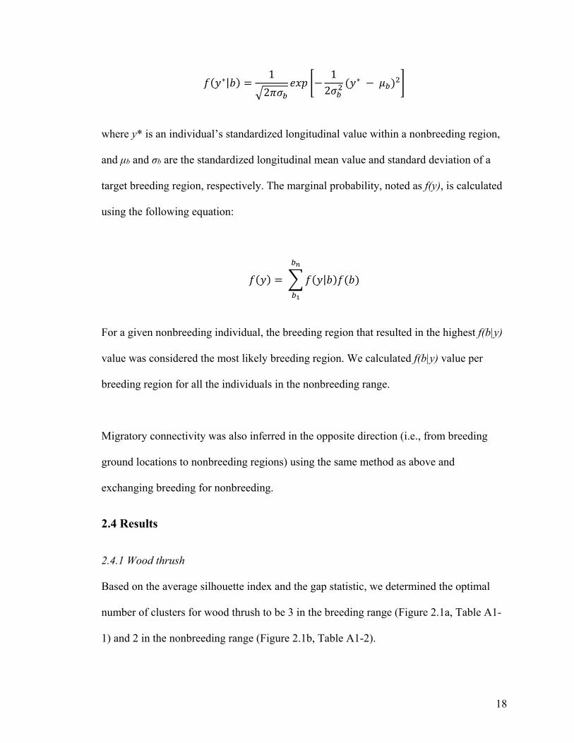
𝑓𝑓(𝑦𝑦∗|𝑏𝑏) =1
�2𝜋𝜋𝜎𝜎𝑏𝑏𝑒𝑒𝑒𝑒𝑒𝑒 �−
12𝜎𝜎𝑏𝑏2
(𝑦𝑦∗ − 𝜇𝜇𝑏𝑏)2�
where y* is an individual’s standardized longitudinal value within a nonbreeding region,
and μb and σb are the standardized longitudinal mean value and standard deviation of a
target breeding region, respectively. The marginal probability, noted as f(y), is calculated
using the following equation:
𝑓𝑓(𝑦𝑦) = �𝑓𝑓(𝑦𝑦|𝑏𝑏)𝑓𝑓(𝑏𝑏)𝑏𝑏𝑛𝑛
𝑏𝑏1
For a given nonbreeding individual, the breeding region that resulted in the highest f(b|y)
value was considered the most likely breeding region. We calculated f(b|y) value per
breeding region for all the individuals in the nonbreeding range.
Migratory connectivity was also inferred in the opposite direction (i.e., from breeding
ground locations to nonbreeding regions) using the same method as above and
exchanging breeding for nonbreeding.
2.4 Results
2.4.1 Wood thrush
Based on the average silhouette index and the gap statistic, we determined the optimal
number of clusters for wood thrush to be 3 in the breeding range (Figure 2.1a, Table A1-
1) and 2 in the nonbreeding range (Figure 2.1b, Table A1-2).

19
Figure 2.1a Clusters for wood thrush breeding range resulting from clustering eBird’s
STEM counts for the week of July 4th. Dark grey pixels represent the excluded pixels
from the home range (95%) analysis. Bottom panel heatmap shows the relative
abundance values at an 8.4 km2 resolution produced by the STEM for the week of July
4th.
20
Figure 2.1b Clusters for wood thrush nonbreeding range resulting from clustering
eBird’s STEM counts for the week of January 18th. Dark grey pixels in top panel
represent the excluded pixels from the home range (95%) analysis. Bottom panel
heatmap shows the relative abundance values at an 8.4 km2 resolution produced by the
STEM for the week of January 18th.
21
When we connected nonbreeding wood thrushes to breeding regions (Figure 2.1c),
individuals located in the western nonbreeding cluster 1 were estimated to migrate to all
of the breeding clusters, with a greater proportion attributed to the central breeding
cluster 1. Most individuals located in the eastern nonbreeding cluster 2 were predicted to
migrate to the northeastern breeding cluster 2, with very few (1%) migrating to the
central breeding cluster 1.
When we connected breeding wood thrushes to nonbreeding regions (Figure 2.1d), all
individuals from the central breeding cluster 1 and the southern breeding cluster 3 were
predicted to migrate to the western nonbreeding cluster 1. Most individuals (57%) from
the northeastern breeding cluster 2 were assigned to the eastern nonbreeding cluster 1.
22
Figure 2.1c Proportion of counts from wood thrush nonbreeding range assigned to the
breeding regions.
23
Figure 2.1d Proportion of counts from wood thrush breeding range assigned to the
nonbreeding regions.
24
2.4.2 Wilson’s warbler
For Wilson’s warbler, two clusters were optimal in the breeding range (Figure 2.2a, Table
A1-3). The nonbreeding range was divided into five clusters (Figure 2.2b), although there
was disagreement between the two evaluative criteria (Table A1-4).
When we connected the individuals from Wilson’s warbler’s nonbreeding range to a
breeding destination (Figure 2.2c), our connectivity inferences estimated that most
individuals located in the western nonbreeding clusters (central Mexico cluster 1,
northwestern Mexico cluster 2, and southern Mexico cluster 3) were most likely to
migrate to the western breeding cluster 1. Only 5% of individuals in the central Mexico
cluster 1 and 25% of individuals in the southern Mexico cluster 3 were estimated to
migrate to the eastern breeding cluster 2. In contrast, all individuals from the two
remaining eastern nonbreeding clusters 4 and 5 were estimated to migrate to the eastern
breeding cluster 2.
When considering movement from the breeding to the nonbreeding range (Figure 2.2d),
most (75%) western breeders were predicted to migrate to the central Mexico cluster 1,
with 19% moving to the northwestern Mexico cluster 2, and only 6% to the southern
Mexico cluster 3 (Figure 2.2d). Eastern breeders were most likely to migrate to the most
eastern nonbreeding clusters 4 (36%) and 5 (58%), while 5% were predicted to migrate to
the southern Mexico cluster 3.
25
Figure 2.2a Clusters for Wilson’s warbler breeding range resulting from clustering
eBird’s STEM counts for the week of July 4th. Dark grey pixels in top panel represent the
excluded pixels from the home range (95%) analysis. Bottom panel heatmap shows the
relative abundance values at an 8.4 km2 resolution produced by the STEM for the week
of July 4th.
26
Figure 2.2b Clusters for Wilson’s warbler nonbreeding range resulting from clustering
eBird’s STEM counts for the week of January 18th. Dark grey pixels in top panel
represent the excluded pixels from the home range (95%) analysis. Bottom panel
heatmap shows the relative abundance values at an 8.4 km2 resolution produced by the
STEM for the week of January 18th.
27
Figure 2.2c Proportion of counts from Wilson’s warbler nonbreeding range assigned to
the breeding regions.
28
Figure 2.2d Proportion of counts from Wilson’s warbler breeding range assigned to the
nonbreeding regions.

29
2.5 Discussion
Migratory connectivity is notoriously challenging to study for migratory birds, especially
for songbirds because of their smaller size and low recapture rates (McKinnon and Love
2018). Conventional methods tend to have a high cost associated with tracking devices or
intensive field sampling requirements and often result in low sample sizes (although
exceptions exist, see Fraser et al. (2012), Ruegg et al. (2014) and Knight et al. (2018)).
To our knowledge, this study is the first to exclusively use community science to infer
migratory connectivity.
Our migratory connectivity inferences for wood thrush suggest that there is strong
connectivity between the southern and central breeding regions and the western
nonbreeding region. Northeastern breeders are predicted to have weaker connectivity and
migrate to both nonbreeding regions. For Wilson’s warbler, our migratory connectivity
inferences suggest that western and eastern breeders are most likely to mix in the
southern Mexico nonbreeding cluster, and somewhat in the central Mexico nonbreeding
cluster. These migratory connectivity inferences are similar to known migratory
connectivity patterns for wood thrush, and less so for Wilson’s warbler.
2.5.1 Wood thrush
Our wood thrush migratory connectivity inferences are in agreement with previous
studies that conclude broad-scale connectivity occurs on an East-West axis (Rushing et
al. 2014, Stanley et al. 2015). In one study, stronger connectivity was found between
individuals in the northwestern quadrant of the breeding range and the western region of

30
the nonbreeding range through feather deuterium ratios and morphological characteristics
(Rushing et al. 2014). Considering that most of northwestern quadrant from Rushing et
al. (2014) overlaps with our central breeding cluster 1 and some of the southern breeding
cluster 3, our migratory connectivity inferences also point to a strong connectivity
between the northwest breeding region and the western nonbreeding region (Figures 2.1c,
2.1d).
Further, we find that our inferences are congruent with the results from a study using
light-level geolocator tracking (Stanley et al. 2015), with some differences. We predict
that a higher proportion of individuals from the western nonbreeding cluster 1 are
assigned to the central breeding cluster 1 (72%, Figure 2.1c) than was shown in Stanley
et al. (2015) (52%, Table 2.1). Similarly, we predict that a higher proportion of
individuals from the eastern nonbreeding cluster 2 are assigned to the northeastern
breeding cluster 2 (99%, Figure 2.1c) than was shown in Stanley et al. (2015) (88%,
Table 2.1)
31
Table 2.1 Wood thrush migratory connectivity assignments for individuals tracked with
light-level geolocators deployed in the nonbreeding range in Stanley et al. (2015) as they
would be situated within clusters from our study, using STEM counts for the week of
July 4th in the breeding range and January 18th in the nonbreeding range. Nonbreeding
deployment locations and breeding region assignments are visual approximations based
on the data reported in Figure 3 of Stanley et al. (2015). Numbers in parentheses
represents the number of individuals successfully tracked in Stanley et al. (2015).
Nonbreeding range Breeding region assignments from Stanley et al. (2015)
Nonbreeding cluster ID from
our study
Nonbreeding deployment
locations in Stanley et al. (2015)
Central breeding cluster 1
Northeastern breeding cluster
2
Southern breeding cluster 3
Western nonbreeding
cluster1
Mexico (1) Belize (24)
52 % (13)
24 % (6)
24 % (6)
Eastern nonbreeding
cluster 2
Costa Rica (21) Nicaragua (5)
12 % (3)
88 % (23)
0 % (0)
Individuals tracked during the southbound migration in Stanley et al. (2015) present
dissimilarities with our results in two main areas. Our inferences suggest that all
individuals from the central breeding cluster 1 migrate to the western nonbreeding cluster
1 (Figure 2.1d), whereas 29% of individuals tracked from the central nonbreeding cluster
1 in Stanley et al. (2015) migrated to the eastern nonbreeding cluster 2 (Table 2.2). Our
inferences also suggest that individuals from the northeastern breeding cluster 2 split
almost equally across both nonbreeding clusters (Figure 2.1d). However, the tracking
32
study suggested that only a minority of northeastern breeders (6%) would migrate to the
western nonbreeding cluster 1 (Table 2.2).
Table 2.2 Wood thrush migratory connectivity assignments for individuals tracked with
light-level geolocators deployed in the breeding range in Stanley et al. (2015) as they
would be situated within clusters from our study, using STEM counts for the week of
July 4th in the breeding range and January 18th in the nonbreeding range. Breeding
deployment locations and nonbreeding region assignments are visual approximations
based on the data reported in Figure 3 of Stanley et al. (2015). Numbers in parentheses
represents the number of individuals successfully tracked in Stanley et al. (2015).
Breeding range Nonbreeding region assignments from Stanley et al. (2015)
Breeding cluster ID
Breeding deployment locations in Stanley et al.
(2015)
Western nonbreeding
cluster 1
Eastern nonbreeding
cluster 2
Central breeding cluster 1
Pennsylvania and North Carolina
(17)
71 % (12)
29 % (5)
Northeastern breeding cluster 2
Vermont, Virginia, Ontario, and Indiana
(35)
6 % (2)
94 % (33)
Southern breeding cluster 3
0 0 0
2.5.2 Wilson’s warbler
While our clusters do capture the broad East-West divide in the breeding range for
Wilson’s warbler (Figure 2.2a), as also described in other studies (Kelly et al. 2002,
Clegg et al. 2003, Irwin et al. 2011), they do not capture the finer-scale genetic

33
populations along the western coast of the United States (Ruegg et al. 2014). To our
knowledge, population delineations in the nonbreeding range have not yet been described
in the literature.
Our connectivity inferences suggest that the broad East-West divide is mostly preserved
throughout the annual cycle, which differs somewhat from fine-scale migratory
connectivity estimates based on high-resolution genetic markers (Ruegg et al. 2014)
(Table 2.3). Our migratory connectivity inferences agree with the patterns estimated from
genetic markers (Ruegg et al. 2014) for the northwestern Mexico nonbreeding cluster 2,
the southern Mexico nonbreeding cluster 3, and the eastern nonbreeding cluster 4.
Disagreements with migratory connectivity patterns estimated from genetic markers
(Ruegg et al. 2014) occur in our central Mexico nonbreeding cluster 1 and in our Central
America nonbreeding cluster 5. While our estimates predict 5% of individuals in the
central Mexico nonbreeding cluster 1 will migrate to the eastern breeding cluster 2
(Figure 2.2c), Ruegg et al. (2014) did not sample any individuals within that area that
were assigned to the eastern breeding region. However, it is important to note that the
northwestern shore of the Gulf of Mexico was not sampled during the nonbreeding
season in Ruegg et al. (2014), whereas individuals are present in that location in our
central Mexico nonbreeding cluster 1. In the Central America nonbreeding cluster 5,
where we do not predict any connectivity with the western breeding cluster 1 (Figures
2.2c, 2.2d), genetic data clearly demonstrated the presence of western breeders in that
area (Ruegg et al. 2014). Our inferences therefore underestimate the spread of the
34
northwestern breeding population to the eastern portions of the nonbreeding range (Table
2.3).
Table 2.3 Wilson’s warbler migratory connectivity assignments from Ruegg et al. (2014)
based on genetic population markers from sampling locations in the nonbreeding range as
they would be situated within clusters from our study, using STEM counts for the week
of July 4th in the breeding range and January 18th in the nonbreeding range. Locations are
visual approximations based on the data retrieved from Figure 1 of Ruegg et al. (2014).
Number in parentheses represents the number of individuals sampled. Two sampling
locations from Ruegg et al. (2014) were not in areas included in our analysis.
Nonbreeding range Breeding region assignments from Ruegg et al. (2014)
Nonbreeding cluster ID from our study
Sample locations in Ruegg et al. (2014)
Western breeding cluster
1
Eastern breeding cluster
2
Central Mexico nonbreeding cluster1
j (28) k (9)* l (23)
100 % (60)
0 % (0)
Northwestern Mexico nonbreeding cluster 2 i (8) 100 %
(8) 0 % (0)
Southern Mexico nonbreeding cluster 3
m (20) n (14) o (9)
86 % (37)
14 % (6)
Eastern nonbreeding cluster 4 p (1) 0 %
(0) 100 %
(1)
Central America nonbreeding cluster 5
q (52) r (26)
s1 (12) t (9)
u (22)
96 % (116)
4 % (5)
35
Our differences in migratory connectivity inferences for Wilson’s warbler are most likely
due to the larger population size of the western breeding group compared to the eastern
breeding group. Eastern Wilson’s warblers have been notoriously difficult to sample in
the nonbreeding range (Irwin et al. 2011), and their abundance is considerably lower than
their western counterparts (e.g. see Figure 2.2a). Accordingly, there were only 12 eastern-
breeding individuals sampled in the nonbreeding range for genetic analysis, as opposed to
221 from the western breeding group (Ruegg et al. 2014). This disparate sampling
between western and eastern breeders could have an overall effect on how the migratory
network is described in the literature for this species. The differences we observed could
also be a limitation in our methodology. Further work to improve our methodology could
incorporate dispersal probabilities relative to the proportion of individuals from each
breeding range and the total area occupied during the nonbreeding season.
Further, the leapfrog migration that is observed across the western groups was not
captured by our method for two reasons. First, the CLARA clustering did not divide the
western population into smaller regions, and second, our methodology does not account
for leapfrog migration possibilities. Currently, eBird data cannot detect leapfrog or chain
migration because individual movement is not tracked.
2.5.3 Possible applications
Our methods are useful to estimate plausible migratory connectivity patterns for species
in need of conservation planning for which it is not feasible to collect more data. Our
methods are particularly useful for species for which urgent interventions are required

36
and cannot afford to wait for more data. We caution that connectivity inferences should
be taken as coarse estimates and that the methods presented in this study might not be
appropriate for all songbird species. In any case, conservation plans should be robust
enough to account for different connectivity scenarios in case migratory connectivity is
not confirmed, poorly understood, or subject to change under different environmental
conditions (Runge et al. 2014).
For species that are subject to field studies, our methods can also be used to generate
hypotheses to improve the sampling design for future fieldwork in both stationary periods
of the annual cycle. Migratory connectivity field studies should indeed aim to sample
individuals across the entire extent of their range with an equal effort at each sampling
site (Cohen et al. 2018, Knight et al. 2018). A sound sampling strategy would be to
ensure at least one sampling location in each hypothesized cluster, with equal sampling
effort among clusters in each period.
2.5.4 Caveats
We note several important caveats. First, our exploratory methodology infers migratory
connectivity between the breeding and the nonbreeding ranges; it does not attempt to
describe connectivity during migration. This is because parallel migration is not always
maintained during migration, even if the final destinations of individuals often follow
parallel patterns (e.g. Delmore, Fox, and Irwin (2012)). However, because eBird STEMs
are available on a weekly basis, important common stopover areas could be identified in
future studies if assumptions can be made about migratory routes. For example,
37
geographically separate migration corridors such as waterfowl migration flyways could
provide baseline assumptions for additional migratory connectivity analysis for certain
species.
Second, we assumed that individuals’ longitude values were normally distributed in each
region to simplify calculations. An improved methodology would consider the unique
distribution of longitudes of individuals in each region and apply different probability
density functions accordingly.
Third, the shape of the clustered regions is limited to the nature of the CLARA algorithm,
which seeks to minimize the objective function based on the Euclidean distance of each
cluster object to the centroid of each cluster. Therefore, CLARA clusters tend to be
spherical, and oblong clusters are not recognized (Kaufman and Rousseeuw 1990).
Ultimately, when applying our method to a species, the resulting clusters should be
tempered with expert opinion and, if available, integrated with other data relevant to
population delineation such as genetic markers, stable isotope ratios, or band returns.
Some density-based clustering techniques such as DBSCAN can better recognize oblong
clusters, but require careful consideration of user-defined parameters (Zerhari et al.
2015). To implement CLARA, the user must only define the number of clusters and
sample sizes. For large datasets (such as ours), the latter is limited by computational
constraints.

38
Finally, community science data can be biased towards charismatic species and areas
with higher human density (Theobald et al. 2015, Chandler et al. 2017, Lloyd et al.
2020). Nevertheless, when properly accounting for species and spatial bias, community
science is a valuable tool for conservation science (McKinley et al. 2017). Indeed,
STEMs account for areas where a greater number of checklists are submitted and only
use higher quality checklists (Fink et al. 2010, 2013, 2020). Continent-wide weekly
models such as STEMs present new opportunities for full annual cycle research (Schuster
et al. 2019).
2.6 Conclusion
To summarize, the full annual cycle must be taken into account when studying migratory
birds and planning for their conservation. However, conventional methods for tracking
migratory connectivity can be challenging and expensive. To our knowledge, this is the
first time that community science has been uniquely used to explore migratory
connectivity. Our work provides a low-cost opportunity to enhance our understanding of
migration and can be applied to understudied species in need of conservation action.
Future work would include stopover connectivity and would integrate all other available
data (such as genetic markers and stable isotopes) on a species-by-species basis to refine
the clustering process and the inferred migratory connectivity.

39
Chapter 3: Songbird migration patterns in the Western
hemisphere
3.1 Abstract
Crosswise and parallel migration are common descriptors for characterizing avian
migration patterns on the longitudinal axis. To determine the prevalence of crosswise,
parallel, and intermediate migration patterns, I reviewed 26 studies that examined
migratory connectivity of 19 songbird species (Passeriformes) in the Western
Hemisphere. I also reviewed the quality of the study design on migratory connectivity
conclusions. I found that most species exhibit broad-scale parallel migration. Studies that
used high-resolution assignment methods and sampled evenly across the entire range of a
species usually provided clear and robust results. Considering the prevalence of parallel
migration, the methods described in Chapter 2 should be widely applicable to songbirds
in the Western Hemisphere.
3.2 Introduction
Four main migration patterns are commonly found in the literature: chain, leapfrog,
parallel, and crosswise migrants (Figure 3.1).
40
Figure 3.1. Schematic representation of migration patterns commonly noted in the
literature. The two left boxes represent patterns on the latitudinal axis and the two right
boxes represent the patterns on the longitudinal axis.

41
Chain migration and leapfrog migration describe the patterns observed on the latitudinal
axis (Figure 3.1). Chain migration refers to a migratory system where individuals that
breed in the northern part of species’ range will also breed in the most northern part of
the nonbreeding range, and, similarly, individuals that breed in the southern part of the
breeding range will winter in the southern part of the nonbreeding range. Leapfrog
migration systems occur when the northern breeding individuals migrate to the southern
part of the nonbreeding range and individuals that breed in the southern part of the
breeding range winter in the most northerly part of the nonbreeding range.
Parallel migration and crosswise migration describe the patterns observed on the
longitudinal axis (Figure 3.1). Parallel migration refers to a migratory system where
individuals that breed in the western part of the species’ range will also breed in the most
western part of the nonbreeding range, and, similarly, individuals that breed in the eastern
part of the breeding range will winter in the eastern part of the nonbreeding range.
Crosswise migration systems occur when the western breeding individuals migrate to the
eastern part of the nonbreeding range and individuals that breed in the eastern part of the
breeding range winter in the most western part of the nonbreeding range.
While all four of these migration patterns are relevant to describe migratory connectivity,
I chose to focus on the frequency at which parallel and crosswise migration occurred in
peer-reviewed literature.
42
3.3 Methods
To conduct a structured review of published studies that examine migratory connectivity
and more specifically, to find those that characterize species as parallel or crosswise
migrants, I searched the Web of Science Core Database on September 2nd, 2019 using a
search string created from the litsearchR R package (Grames et al. 2019). This package
creates Boolean search strings based on a naïve search and benchmark paper keywords
(Marra et al. 1998, Kimura et al. 2002, Clegg et al. 2003, Norris et al. 2004, Lovette et al.
2004, Clark et al. 2006, Jones et al. 2008, Stutchbury et al. 2009, Ryder et al. 2011,
Chabot et al. 2012, Evans et al. 2012, Munafo and Gibbs 2012, Delmore et al. 2012,
Hallworth et al. 2013, Rundel et al. 2013, Garcia-Perez et al. 2013, Cormier et al. 2013,
Ruegg et al. 2014, Hallworth and Marra 2015, Stanley et al. 2015, Hallworth et al. 2015,
Hobson et al. 2015a, 2015ab Reudink et al. 2015, Hobson and Kardynal 2016, Morris et
al. 2016, Fournier et al. 2017a, Fournier et al. 2017b, Fraser et al. 2017, Larkin et al.
2017, Ruegg et al. 2017, Kramer et al. 2018, Knight et al. 2018, Hill and Renfrew 2019,
Cohen et al. 2019). The final search string used was: (("long-dist* migrant*" OR
"migrator* bird*" OR "neotrop* migrant*" OR "migrant* bird*" OR "waterfowl* spec*"
OR migrat*) AND ("long-dist* migrant*" OR "neotrop* migrant*" OR "waterfowl*
spec*" OR bird*) AND ("annual* cycl*" OR "geograph* origin*" OR "migrator*
connect*" OR "popul* connect*" OR "season* interact*" OR "site* fidel*" OR "direct*
track*" OR "geograph* assign*" OR "geograph* structur*" OR "geograph* variat*" OR
"likelihood-bas* assign*" OR "season* distribut*" OR "spatial* connect*" OR "migrat*
connect*" OR "season* connect*") AND ("north* america*" OR "south* america*" OR
"central* america*" OR "north* american*" OR "western* hemispher*" OR nearctic-

43
neotrop*)). Originally, the search string was meant to capture all bird families in the
Western Hemisphere, but the scope was narrowed to only include songbirds
(Passeriformes) during the first screening of the search hits. Based on title and abstract, I
excluded studies that studied species other than songbirds, that were not conducted in the
Western Hemisphere, or were clearly irrelevant and not pertaining to migratory
connectivity.
I applied additional exclusion criteria during the full-text screening to obtain studies with
minimal quality standards for the review. Criteria were based on the recommendations of
minimal study design quality outlined in (Knight et al. 2018). Studies were excluded if
they did not have more than one sampling site or if they did not cover the full migration
from breeding grounds to non-breeding grounds (i.e., if a study only sampled individuals
once at a single stopover site, the paper was excluded). Furthermore, if the authors
determined that they lacked the data to support a conclusion on migratory connectivity,
the study was excluded.
I evaluated the strength of migratory connectivity of each study based on authors’
conclusion as either “none, “low”, “moderate” or “high” and if the study sampled range-
wide or only partially.
I evaluated the migration pattern on the longitudinal axis (crosswise or parallel migration)
of each study from the results or discussion section from text or from figures, because not
every study explicitly mentions if their study species shows crosswise or parallel
44
migration. I classified the preservation of longitudinal structure in one of four categories:
“crosswise”, “mostly crosswise” (although some individuals show parallel migration,
there is substantial crossing of individuals), “mostly parallel” (overall, parallel migration
is observed but some individuals do overlap), and “parallel.”
From each paper, I also extracted the following baseline information: the study species,
the age and sex of the captured individuals, the method used to infer connectivity
(geolocators, genetics, stable isotopes, GPS tags), the sample size, the year(s) of study,
the number of breeding sampling sites and/or nonbreeding sampling sites, whether the
study included the species entire range or not, and the author’s conclusion on the species’
migratory connectivity. I evaluated how the authors delineated the breeding and/or
nonbreeding populations: if it was based on data (for example, genetically-distinct data,
spatially-distinct trends, etc.) or if it was based on their opinion (“we drew lines where
we thought they should go”), or if they used somewhat relevant data to draw subjective
lines (for example, they find high-density areas and determine that they should each be a
population).
3.4 Results
The search string yielded 396 hits (sensitivity 97%, precision 8.1% when considering the
benchmark papers), of which 26 papers were included in the review based on the
screening criteria. The included papers covered a total of 19 species and represent 26
distinct studies (Table 3.1). Most species were classified as parallel migrants (Table 3.2).
45
Table 3.1. Studies included in the review with descriptors of methods used to study migratory connectivity and the main
characteristics that were extracted.
Species Article Methods used sampling range
migration pattern
Migratory connectivity strength
American redstart (Setophaga ruticilla)
Hobson et al. (2015) feather deuterium ratios
wide parallel high
Canada warbler (Cardellina canadensis)
González-Prieto et al. (2017) feather deuterium ratios
wide parallel moderate
Cerulean warbler (Setophaga cerulea)
Jones et al. (2008) feather deuterium ratios and BBS
wide parallel high
Grasshopper sparrow (Ammodramus savannarum)
Hill and Renfrew (2019)
light-level geolocators
wide parallel moderate
Ovenbird (Seiurus aurocapilla)
Hallworth and Marra (2015) GPS
partial parallel high
Ovenbird (Seiurus aurocapilla)
Hallworth et al. (2015)
light-level geolocators, eBird abundance data, BBS, band returns
partial parallel high
46
Swainson’s thrush (Catharus ustulatus)
Delmore et al. (2012) light-level geolocators
partial parallel high
Wood thrush (Hylocichla mustelina)
Stanley et al. (2015) light-level geolocators
wide parallel moderate
Yellow warbler (Setophaga petechia)
Boulet et al. (2006) feather deuterium ratios, mitochondrial DNA, band returns
wide parallel high
Yellow warbler (Setophaga petechia)
Witynski and Bonter (2018) light-level geolocators
partial cross-wise high
Golden-winged warbler * blue-winged warbler hybrid (Vermivora chrysoptera * Vermivora cyanoptera)
Kramer et al. (2018) light-level geolocators
wide parallel high
Barn swallow (Hirundo rustica)
Garcia-Perez et al. (2013)
feather deuterium, nitrogen and carbon ratios
wide mostly parallel
high
Barn swallow (Hirundo rustica)
Hobson et al. (2015a)
light-level geolocators wide mostly parallel
none
47
Barn swallow (Hirundo rustica)
Hobson and Kardynal (2016)
light-level geolocators, feather deuterium and sulphur ratios
partial mostly parallel
high
Golden-winged warbler (Vermivora chrysoptera)
Hobson et al. (2016)
feather deuterium ratios wide mostly crosswise
high
Golden-winged warbler (Vermivora chrysoptera)
Kramer et al. (2018)
light-level geolocators wide mostly parallel
high
Snow bunting (Plectrophenax nivalis)
Macdonald et al. (2012)
band returns, feather deuterium ratios, light-level geolocators
partial mostly parallel
high
Tree swallow (Tachycineta bicolor)
Knight et al. (2018) light-level geolocators wide mostly parallel
moderate
Wilson’s warbler (Cardellina pusilla)
Kimura et al. (2002)
mitochondrial DNA markers partial mostly parallel
moderate
Wilson’s warbler (Cardellina pusilla)
Ruegg et al. (2014) SNPs wide parallel high
Blue-winged warbler (Vermivora cyanoptera)
Kramer et al. (2018)
light-level geolocator wide mostly crosswise
low
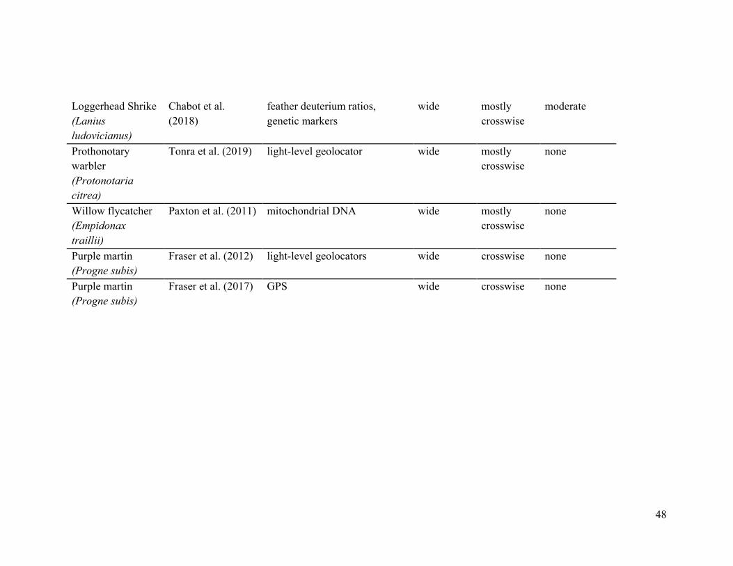
48
Loggerhead Shrike (Lanius ludovicianus)
Chabot et al. (2018)
feather deuterium ratios, genetic markers
wide mostly crosswise
moderate
Prothonotary warbler (Protonotaria citrea)
Tonra et al. (2019) light-level geolocator wide mostly crosswise
none
Willow flycatcher (Empidonax traillii)
Paxton et al. (2011) mitochondrial DNA wide mostly crosswise
none
Purple martin (Progne subis)
Fraser et al. (2012) light-level geolocators wide crosswise none
Purple martin (Progne subis)
Fraser et al. (2017) GPS wide crosswise none
49
Table 3.2. Categorization of range-wide longitudinal migration pattern category per species included in the review.
Migration category
Species Study
Parallel American redstart (Setophaga ruticilla) Hobson et al. (2015) Canada warbler (Cardellina canadensis) González-Prieto et al. (2017) Cerulean warbler (Setophaga cerulea) Jones et al. (2008) Grasshopper sparrow (Ammodramus savannarum) Hill and Renfrew (2019)
Ovenbird (Seiurus aurocapilla) Hallworth and Marra (2015), Hallworth et al. (2015)
Swainson’s thrush (Catharus ustulatus) Delmore et al. (2012) Wood thrush (Hylocichla mustelina) Stanley et al. (2015) Yellow warbler (Setophaga petechia) Boulet et al. (2006) Golden-winged warbler * blue-winged warbler hybrid (Vermivora chrysoptera * Vermivora cyanoptera) Kramer et al. (2018)
Mostly parallel
Barn swallow (Hirundo rustica) Garcia-Perez et al. (2013), Hallworth et al. (2015), Hobson and Kardynal (2016)
Golden-winged warbler (Vermivora chrysoptera) Hobson et al. (2016), Kramer et al. (2018) Snow bunting (Plectrophenax nivalis) Macdonald et al. (2012) Tree swallow (Tachycineta bicolor) Knight et al. (2018) Wilson’s warbler (Cardellina pusilla) Kimura et al. (2002), Ruegg et al. (2014)
Mostly crosswise
Blue-winged warbler (Vermivora cyanoptera) Kramer et al. (2018) Loggerhead Shrike (Lanius ludovicianus) Chabot et al. (2018) Prothonotary warbler (Protonotaria citrea) Tonra et al. (2019) Willow flycatcher (Empidonax traillii) Paxton et al. (2011)
Crosswise Purple martin (Progne subis) Fraser et al. (2012, 2013, 2017)
50
3.5 Discussion
3.5.1 Crosswise migrants
Of the reviewed species, only two clearly displayed crosswise migration: purple martin
and yellow warbler. Three publications discuss the migratory connectivity of purple
martin, which emerged from common data from light-level geolocators (Fraser et al.
2012, 2013, 2017). Since purple martin has particularly weak migratory connectivity,
crosswise migration is unsurprising. On the other hand, the yellow warbler case is
particularly interesting because studies conducted at different scales yielded scale-
dependent patterns, underscoring the importance of scale when describing migration
patterns. Witynski and Bonter (2018) examined the eastern haplotype of yellow warbler
and uncovered the crosswise migration that occurs within the Eastern flyway and the lack
of strong migratory connectivity at the flyway-scale as well. A review by Boulet et al.
(2006) suggests, however, that at the continental scale, parallel migration and strong
migratory connectivity are appropriate characterizations for northern yellow warbler.
3.5.2 Mostly crosswise migrants
Four species classified as preserving only “mostly crosswise” (i.e., preserving only some
of their longitudinal structure between migrations): blue-winged warbler, willow
flycatcher, prothonotary warbler, and loggerhead shrike. These four species were studied
in only one paper each and have weak evidence supporting complete parallel migration
(Table 3.1). Although complete separation of blue-winged warbler breeding populations
was not maintained during the nonbreeding period, there was a weak tendency for
easterly breeding populations to overwinter in the more easterly regions for individuals

51
overwintering in Central America (Kramer et al. 2018). Similarly, even though
prothonotary warbler shows a very large-scale East-West divide in migratory routes,
significant mixing of individuals from different breeding populations on the nonbreeding
grounds shows a lack of complete parallel migration (Tonra et al. 2019). Willow
flycatcher was deemed to have “distinct but overlapping” nonbreeding ranges, based on
mitochondrial DNA analyses (Paxton et al. 2011). Chabot et al. (2018) found evidence
for chain migration and moderate migratory connectivity for loggerhead shrike, but
inferences about the longitudinal structure were unclear and not addressed by the authors
(Figure 1 in Chabot et al. (2018)). As methodologies continue to improve and higher-
resolution location assignments are made possible, it will be interesting to see if these
four species could be categorized more definitely as either crosswise or parallel migrants,
especially for species that have been studied with coarse resolution methods, such as the
prothonotary warbler (Tonra et al. 2019).
3.5.3 Resolving power changes categorization from “mostly crosswise” to “mostly
parallel”
Two species, golden-winged warbler and Wilson’s warbler, were found in multiple
studies with differing conclusions about longitudinal patterns that did not seem scale-
dependent, but rather a result of the resolving power of different assignment
methodologies.
In all golden-winged warbler studies, authors deemed the strength of migratory
connectivity to be high, whereas patterns of longitudinal structure diverged (Table 3.1).
52
Hobson and Kardynal (2016) used deuterium isotope ratios to assign a breeding location
to individuals and found that longitude was the best predictor for breeding moult location.
However, due to the nature of the deuterium isoscape that varies more strongly with
latitude than longitude in North America, deuterium isotopes alone provide insufficient
resolving power on the longitudinal axis to confirm parallel migration, which situated
that study in the “mostly crosswise” category (Table 3.1). Kramer et al. (2018) tracked
golden-winged warblers from different Bird Conservation Regions (BCRs) with light-
level geolocators and found that population segregation on the longitudinal axis was
maintained in the non-breeding range. Nonetheless, because BCR ranges overlapped
somewhat in longitude, a few individuals from different BCRs located at a similar
longitudinal value displayed some crosswise migration, thereby categorizing this species
as displaying “mostly” parallel migration. I classified golden-winged warbler as a
“mostly” parallel migrant (Table 3.2) because light-level geolocators (Kramer et al. 2018)
were able to pinpoint exact locations of individuals as opposed to the deuterium isoscape
method (Hobson and Kardynal 2016). Interestingly, Kramer et al. (2018) found that
golden-winged warbler and blue-winged warbler hybrids clearly show parallel migration.
However, this evidence of parallel migration should be used cautiously as only four
hybrids were tracked.
To describe Wilson’s warbler migratory patterns, genetic markers of varying resolving
power were used in two studies. Mitochondrial DNA markers were only able to separate
western and eastern populations (Kimura et al. 2002), which suggests that crosswise
migration and parallel migration were equally likely possibilities. Using higher resolution
53
genetic markers (SNPs) Ruegg et al. (2014) delineated populations at a finer scale in
breeding and nonbreeding ranges. In doing so, it becomes noticeable that most of the
longitudinal structure is preserved between seasons (Ruegg et al. 2014). The Western
breeding region’s larger population size is probably the cause of the spread of western
breeders to some Eastern portions of the nonbreeding range (see Chapter 2). For that
reason, I consider that Wilson’s warbler is more appropriately classified as a parallel
migrant than as a crosswise migrant.
3.5.4 “Mostly parallel” and “parallel” migrants
Other than golden-winged warbler and Wilson’s warbler described in section 3.5.3, five
other studies representing three species (snow bunting, tree swallow, and barn swallow)
were classified as “mostly parallel” migrants. For snow bunting, the band recovery
records are the only dataset with samples in more than one seasonal location (Macdonald
et al. 2012). These records suggest mostly parallel migration, but more widespread
sampling would be necessary to confirm that categorization. Knight et al. (2018)
deployed 133 light-level geolocators on tree swallows that revealed moderate migratory
connectivity and mostly parallel migration. Three separate studies on barn swallow, a
widespread species, show evidence for mostly parallel migration. Garcia-Perez et al.
(2013) found that longitudinal structure is typically preserved between seasons,
postulating that this gradient is maintained by the use of the main flyways (Cooke 1905).
Hobson et al. (2015) observed the same great East-West divide. Eastern barn swallows,
specifically, could also be categorized as “mostly” parallel migrant, as shown in Hobson
and Kardynal (2016).

54
Seven species in eight studies were categorized as parallel migrants: American redstart
(Norris et al. 2006), cerulean warbler (Jones et al. 2008), Swainson’s thrush, Rocky
Mountains population (Delmore et al. 2012), wood thrush (Stanley et al. 2015), Canada
warbler (González-Prieto et al. 2017) and grasshopper sparrow (Hill and Renfrew 2019).
Parallel migration patterns persisted from range-wide to finer-scale for ovenbirds
(Hallworth and Marra 2015, Hallworth et al. 2015).
The majority of the studies included in my review revealed that range-wide parallel
migration seems to be more common for songbirds (Table 3.2). Nonetheless, parallel
migration cannot be assumed for all songbird species, as clearly demonstrated by the
crosswise migration of purple martins. It is also noteworthy that another study, not
captured in my search string, also demonstrated crosswise migration for black-throated
blue warbler (Royle and Rubenstein 2004).
On another note, I suggest that authors clearly state the scale at which their migratory
connectivity description can be applied. Indeed, it is misleading when migratory
connectivity patterns obtained from only a handful of sampling locations are applied
range-wide when discussing the conservation and management implications. Authors
should also clarify if their sampling locations are based on randomized, stratified, or
block design or if they were selected more opportunistically. A greater spread of
sampling locations across the species range, along with an increased sample size, would
provide a more honest portrait of range-wide migratory connectivity, as shown in Cohen
et al. (2018) and Knight et al. (2018).

55
3.6 Conclusion
Broad-scale parallel migration is a common strategy adopted by songbirds in the Western
Hemisphere, although it should not be assumed without a minimum of supporting
evidence such as band returns or preliminary studies. This chapter supports the
applicability of the methodology presented in Chapter 2, which assumes broad-scale
parallel migration patterns, to additional songbird species in the Western Hemisphere.
56
References
Bensch, S., S. Åkesson, and D. E. Irwin. 2008. The use of AFLP to find an informative
SNP: genetic differences across a migratory divide in willow warblers. Molecular
Ecology 11:2359–2366.
Boulet, M., H. L. Gibbs, and K. A. Hobson. 2006. Integrated Analysis of Genetic, Stable
Isotope, and Banding Data Reveal Migratory Connectivity and Flyways in the
Northern Yellow Warbler (Dendroica petechia; Aestiva group). Ornithological
Monographs 61:28–78.
Bridge, E. S., J. F. Kelly, A. Contina, R. M. Gabrielson, R. B. MacCurdy, and D. W.
Winkler. 2013. Advances in tracking small migratory birds: a technical review of
light-level geolocation. Journal of Field Ornithology 84:121–137.
Buhnerkempe, M. G., C. T. Webb, A. A. Merton, J. E. Buhnerkempe, G. H. Givens, R. S.
Miller, and J. A. Hoeting. 2016. Identification of migratory bird flyways in North
America using community detection on biological networks. Ecological
Applications 26:740–751.
Calenge, C. 2006. The package “adehabitat” for the R software: A tool for the analysis of
space and habitat use by animals. Ecological Modelling 197:516–519.
Chabot, A. A., K. A. Hobson, S. L. Van Wilgenburg, G. J. McQuat, and S. C. Lougheed.
2012. Advances in linking wintering migrant birds to their breeding-ground
origins using combined analyses of genetic and stable isotope markers. PloS ONE
7:e43627.
57
Chabot, A. A., K. A. Hobson, S. L. Van Wilgenburg, G. E. Pérez, and S. C. Lougheed.
2018. Migratory connectivity in the Loggerhead Shrike (Lanius ludovicianus).
Ecology and Evolution 8:10662–10672.
Chandler, M., L. See, K. Copas, A. M. Z. Bonde, B. C. López, F. Danielsen, J. K. Legind,
S. Masinde, A. J. Miller-Rushing, G. Newman, A. Rosemartin, and E. Turak.
2017. Contribution of citizen science towards international biodiversity
monitoring. Biological Conservation 213:280–294.
Clark, R. G., K. A. Hobson, and L. I. Wassenaar. 2006. Geographic variation in the
isotopic (δD, δC-13, δN-15, δS-34) composition of feathers and claws from lesser
scaup and northern pintail: implications for studies of migratory connectivity.
Canadian Journal of Zoology 84:1395–1401.
Clegg, S. M., J. F. Kelly, M. Kimura, and T. B. Smith. 2003. Combining genetic markers
and stable isotopes to reveal population connectivity and migration patterns in a
Neotropical migrant, Wilson’s warbler (Wilsonia pusilla). Molecular Ecology
12:819–830.
Cohen, E. B., J. A. Hostetler, M. T. Hallworth, C. S. Rushing, T. S. Sillett, and P. P.
Marra. 2018. Quantifying the strength of migratory connectivity. Methods in
Ecology and Evolution 9:513–524.
Cohen, E. B., C. R. Rushing, F. R. Moore, M. T. Hallworth, J. A. Hostetler, M. G.
Ramirez, and P. P. Marra. 2019. The strength of migratory connectivity for birds
en route to breeding through the Gulf of Mexico. Ecography 42:658–669.
58
Contina, A., J. L. Alcantara, E. S. Bridge, J. D. Ross, W. F. Oakley, J. F. Kelly, and K. C.
Ruegg. 2019. Genetic structure of the Painted Bunting and its implications for
conservation of migratory populations. Ibis 161:372–386.
Cooke, W. W. 1905. Routes of Bird Migration. The Auk 22:1–11.
Cormier, R. L., D. L. Humple, T. Gardali, and N. E. Seavy. 2013. Light-level geolocators
reveal strong migratory connectivity and within-winter movements for a coastal
California Swainson’s Thrush (Catharus ustulatus) population. The Auk 130:283–
290.
Delmore, K. E., J. W. Fox, and D. E. Irwin. 2012. Dramatic intraspecific differences in
migratory routes, stopover sites and wintering areas, revealed using light-level
geolocators. Proceedings. Biological sciences 279:4582–4589.
Dickinson, J. L., B. Zuckerberg, and D. N. Bonter. 2010. Citizen Science as an
Ecological Research Tool: Challenges and Benefits. Annual Review of Ecology,
Evolution, and Systematics 41:149–172.
Drake, A., C. Rock, S. P. Quinlan, and D. J. Green. 2013. Carry-over effects of winter
habitat vary with age and sex in yellow warblers Setophaga petechia. Journal of
Avian Biology 44:321–330.
Evans, K. L., J. Newton, J. W. Mallord, and S. Markman. 2012. Stable isotope analysis
provides new information on winter habitat use of declining avian migrants that is
relevant to their conservation. PloS ONE 7:e34542.
Faaborg, J., R. T. Holmes, A. D. Anders, K. L. Bildstein, K. M. Dugger, S. A.
Gauthreaux, P. Heglund, K. A. Hobson, A. E. Jahn, D. H. Johnson, S. C. Latta, D.
J. Levey, P. P. Marra, C. L. Merkord, E. Nol, S. I. Rothstein, T. W. Sherry, T. S.
59
Sillett, F. R. Thompson, and N. Warnock. 2010. Recent advances in
understanding migration systems of New World land birds. Ecological
Monographs 80:3–48.
Farmer, A., B. S. Cade, and J. Torres-Dowdall. 2008. Fundamental limits to the accuracy
of deuterium isotopes for identifying the spatial origin of migratory animals.
Oecologia 158:183–192.
Fink, D., T. Auer, A. Johnston, V. Ruiz-Gutierrez, W. M. Hochachka, and S. Kelling.
2020. Modeling avian full annual cycle distribution and population trends with
citizen science data. Ecological Applications 30:e02056.
Fink, D., T. Damoulas, N. E. Bruns, F. A. L. Sorte, W. M. Hochachka, C. P. Gomes, and
S. Kelling. 2014. Crowdsourcing Meets Ecology: Hemisphere-Wide
Spatiotemporal Species Distribution Models. AI Magazine 35:19-30.
Fink, D., T. Damoulas, and J. Dave. 2013. Adaptive Spatio-Temporal Exploratory
Models: Hemisphere-wide species distributions from massively crowdsourced
eBird data. Twenty-Seventh AAAI Conference on Artificial Intelligence.
Bellevue, Washington USA.
Fink, D., W. M. Hochachka, B. Zuckerberg, D. W. Winkler, B. Shaby, M. A. Munson, G.
Hooker, M. Riedewald, D. Sheldon, and S. Kelling. 2010. Spatiotemporal
exploratory models for broad-scale survey data. Ecological Applications
20:2131–2147.
Fournier, A. M. V., K. L. Drake, and D. C. Tozer. 2017a. Using citizen science
monitoring data in species distribution models to inform isotopic assignment of
migratory connectivity in wetland birds. Journal of Avian Biology 48:1556–1562.
60
Fournier, A. M. V., A. R. Sullivan, J. K. Bump, M. Perkins, M. C. Shieldcastle, and S. L.
King. 2017b. Combining citizen science species distribution models and stable
isotopes reveals migratory connectivity in the secretive Virginia rail. Journal of
Applied Ecology 54:618-627.
Fraser, K. C., A. Shave, A. Savage, A. Ritchie, K. Bell, J. Siegrist, J. D. Ray, K.
Applegate, and M. Pearman. 2017. Determining fine-scale migratory connectivity
and habitat selection for a migratory songbird by using new GPS technology.
Journal of Avian Biology 48:339–345.
Fraser, K. C., C. Silverio, P. Kramer, N. Mickle, R. Aeppli, and B. J. M. Stutchbury.
2013. A Trans-Hemispheric Migratory Songbird Does Not Advance Spring
Schedules or Increase Migration Rate in Response to Record-Setting
Temperatures at Breeding Sites. PLoS ONE 8:e64587.
Fraser, K. C., B. J. M. Stutchbury, C. Silverio, P. M. Kramer, J. Barrow, D. Newstead, N.
Mickle, B. F. Cousens, J. C. Lee, D. M. Morrison, T. Shaheen, P. Mammenga, K.
Applegate, and J. Tautin. 2012. Continent-wide tracking to determine migratory
connectivity and tropical habitat associations of a declining aerial insectivore.
Proceedings of the Royal Society B: Biological Sciences 279:4901–4906.
Garcia-Perez, B., K. A. Hobson, R. L. Powell, C. J. Still, and G. H. Huber. 2013.
Switching Hemispheres: A New Migration Strategy for the Disjunct Argentinean
Breeding Population of Barn Swallow (Hirundo rustica). PLoS ONE 8:e55654.
Gibbs, H. L., R. J. G. Dawson, and K. A. Hobson. 2000. Limited differentiation in
microsatellite DNA variation among northern populations of the yellow warbler:
evidence for male-biased gene flow? Molecular Ecology 9:2137–2147.
61
Gómez, C., S. L. Guerrero, A. M. FitzGerald, N. J. Bayly, K. A. Hobson, and C. D.
Cadena. 2019. Range-wide populations of a long-distance migratory songbird
converge during stopover in the tropics. Ecological Monographs 89:e01349.
González-Prieto, A. M., N. J. Bayly, G. J. Colorado, and K. A. Hobson. 2017.
Topography of the Andes Mountains shapes the wintering distribution of a
migratory bird. Diversity and Distributions 23:118–129.
Grames, E. M., A. N. Stillman, M. W. Tingley, and C. S. Elphick. 2019. An automated
approach to identifying search terms for systematic reviews using keyword co-
occurrence networks. Methods in Ecology and Evolution 10:1645–1654.
Hallworth, M. T., and P. P. Marra. 2015. Miniaturized GPS Tags Identify Non-breeding
Territories of a Small Breeding Migratory Songbird. Scientific Reports 5:11069.
Hallworth, M. T., T. S. Sillett, S. L. Van Wilgenburg, K. A. Hobson, and P. P. Marra.
2015. Migratory connectivity of a Neotropical migratory songbird revealed by
archival light-level geolocators. Ecological Applications 25:336–347.
Hallworth, M. T., C. E. Studds, T. S. Sillett, and P. P. Marra. 2013. Do archival light-
level geolocators and stable hydrogen isotopes provide comparable estimates of
breeding-ground origin? The Auk 130:273–282.
Hawkins, A. S. 1984. Flyways : pioneering waterfowl management in North America.
U.S. Dept. of the Interior, Fish and Wildlife Service, Washington, D.C.
Hill, J. M., and R. B. Renfrew. 2019. Migratory patterns and connectivity of two North
American grassland bird species. Ecology and Evolution 9:680–692.

62
Hobson, K. A. 2003. Making migratory connections with stable isotopes. Pages 367-377
in: P. Berthold, E. Gwinner, E. Sonnenschein (eds) Avian Migration. Springer,
Berlin, Heidelberg, Germany.
Hobson, K. A. 2008. Using endogenous and exogenous markers in bird conservation.
Bird Conservation International 18:S174–S199.
Hobson, K. A. 2011. Isotopic ornithology: a perspective. Journal of Ornithology 152:49–
66.
Hobson, K. A., and K. J. Kardynal. 2016. An isotope (δ34S) filter and geolocator results
constrain a dual feather isoscape (δ2H, δ13C) to identify the wintering grounds of
North American Barn Swallows. The Auk 133:86–98.
Hobson, K. A., K. J. Kardynal, S. L. Van Wilgenburg, G. Albrecht, A. Salvadori, M. D.
Cadman, F. Liechti, and J. W. Fox. 2015a. A Continent-Wide Migratory Divide in
North American Breeding Barn Swallows (Hirundo rustica). PLoS ONE
10:e0129340.
Hobson, K. A., S. L. Van Wilgenburg, E. H. Dunn, D. J. T. Hussell, P. D. Taylor, and D.
M. Collister. 2015b. Predicting origins of passerines migrating through Canadian
migration monitoring stations using stable-hydrogen isotope analyses of feathers:
a new tool for bird conservation. Avian Conservation and Ecology 10:3.
Hobson, K. A., S. L. V. Wilgenburg, A. M. Roth, N. J. Bayly, L. Chavarría-Duriaux, and
G. J. Colorado. 2016. Golden-winged warbler migratory connectivity derived
from stable isotopes. Pages 193-203 in H.M. Streby, D.E. Andersen, and D.A.
Buehler (eds) Golden-winged Warbler Ecology, Conservation, and Habitat
63
Management. Studies in Avian Biology (no. 49). CRC Press, Boca Raton, Florida,
USA.
Irwin, D. E., J. H. Irwin, and T. B. Smith. 2011. Genetic variation and seasonal migratory
connectivity in Wilson’s warblers (Wilsonia pusilla): Species-level differences in
nuclear DNA between western and eastern populations. Molecular Ecology
20:3102–15.
Jones, J., D. R. Norris, M. K. Girvan, J. J. Barg, T. K. Kyser, and R. J. Robertson. 2008.
Migratory Connectivity and Rate of Population Decline in a Vulnerable Songbird.
The Condor 110:538–544.
Kaufman, L., and P. J. Rousseeuw. 1990. Finding Groups in Data: An Introduction to
Cluster Analysis. Wiley, New York, New York, USA.
Kelly, J. F., V. Atudorei, Z. D. Sharp, and D. M. Finch. 2002. Insights into Wilson’s
Warbler migration from analyses of hydrogen stable-isotope ratios. Oecologia
130:216–221.
Kelly, J. F., and R. L. Hutto. 2005. An East-West Comparison of Migration in North
American Wood Warblers. The Condor 107:197–211.
Kimura, M., S. M. Clegg, I. J. Lovette, K. R. Holder, D. J. Girman, B. Mila, P. Wade,
and T. B. Smith. 2002. Phylogeographical approaches to assessing demographic
connectivity between breeding and overwintering regions in a Nearctic-
Neotropical warbler (Wilsonia pusilla). Molecular Ecology 11:1605–1616.
Knight, S. M., D. W. Bradley, R. G. Clark, E. A. Gow, M. Bélisle, L. L. Berzins, T.
Blake, E. S. Bridge, L. Burke, R. D. Dawson, P. O. Dunn, D. Garant, G. L.
Holroyd, D. J. T. Hussell, O. Lansdorp, A. J. Laughlin, M. L. Leonard, F.
64
Pelletier, D. Shutler, L. Siefferman, C. M. Taylor, H. E. Trefry, C. M. Vleck, D.
Vleck, D. W. Winkler, L. A. Whittingham, and D. R. Norris. 2018. Constructing
and evaluating a continent-wide migratory songbird network across the annual
cycle. Ecological Monographs 88:445–460.
Kramer, G. R., D. E. Andersen, D. A. Buehler, P. B. Wood, S. M. Peterson, J. A.
Lehman, K. R. Aldinger, L. P. Bulluck, S. Harding, J. A. Jones, J. P. Loegering,
C. Smalling, R. Vallender, and H. M. Streby. 2018. Population trends in
Vermivora warblers are linked to strong migratory connectivity. PNAS
115:E3192–E3200.
Larkin, J. L., D. Raybuck, A. Roth, L. Chavarría-Duriaux, G. Duriaux, M. Siles, and C.
Smalling. 2017. Geolocators reveal migratory connectivity between wintering and
breeding areas of Golden-winged Warblers. Journal of Field Ornithology 88:288–
298.
Lincoln, F. C. 1935. The Waterfowl Flyways of North America. Circular, United States
Dept. of Agriculture, no 342. Washington, D.C., USA.
Lisovski, S., S. Bauer, M. Briedis, S. Davidson, K. Dhanjal-Adams, M. Hallworth, J.
Karagicheva, C. Meier, B. Merkel, J. Ouwehand, L. Pedersen, E. Rakhimberdiev,
A. Roberto-Charron, N. Seavy, M. Sumner, C. Taylor, S. Wotherspoon, and E.
Bridge. 2019. Light‐Level Geolocator Analyses: A user’s guide. Journal of
Animal Ecology 89:221-236.
Lloyd, T. J., R. A. Fuller, J. L. Oliver, A. I. Tulloch, M. Barnes, and R. Steven. 2020.
Estimating the spatial coverage of citizen science for monitoring threatened
species. Global Ecology and Conservation 23:e01048.

65
Long, J., T. Nelson, and M. Wulder. 2010. Regionalization of landscape pattern indices
using multivariate cluster analysis. Environmental Management 46:134–142.
Lovette, I. J., S. M. Clegg, and T. B. Smith. 2004. Limited Utility of mtDNA Markers for
Determining Connectivity among Breeding and Overwintering Locations in Three
Neotropical Migrant Birds. Conservation Biology 18:156–166.
Macdonald, C. A., K. C. Fraser, H. G. Gilchrist, T. K. Kyser, J. W. Fox, and O. P. Love.
2012. Strong Migratory Connectivity in a Declining Arctic Passerine. Animal
Migration 1:23-30.
Maechler, M., P. Rousseeuw, A. Struyf, M. Hubert, and K. Hornik. 2018. cluster: Cluster
Analysis Basics and Extensions. R package version 2.1.0.
Marra, P., E. B. Cohen, S. R. Loss, J. E. Rutter, and C. M. Tonra. 2015. A call for full
annual cycle research in animal ecology. Biology Letters 11:20150552.
Marra, P. P., K. A. Hobson, and R. T. Holmes. 1998. Linking winter and summer events
in a migratory bird by using stable-carbon isotopes. Science 282:1884–1886.
Marra, P. P., C. Studds, and M. Webster. 2010. Migratory Connectivity. Pages 455–461
in M. D. Breed and J. Moore (eds) Encyclopedia of Animal Behavior. Academic
Press, Cambridge, Massachusetts, USA.
Martin, T. G., I. Chadès, P. Arcese, P. P. Marra, H. P. Possingham, and D. R. Norris.
2007. Optimal conservation of migratory species. PLoS ONE 2:e751.
McKinley, D. C., A. J. Miller-Rushing, H. L. Ballard, R. Bonney, H. Brown, S. C. Cook-
Patton, D. M. Evans, R. A. French, J. K. Parrish, T. B. Phillips, S. F. Ryan, L. A.
Shanley, J. L. Shirk, K. F. Stepenuck, J. F. Weltzin, A. Wiggins, O. D. Boyle, R.
D. Briggs, S. F. Chapin, D. A. Hewitt, P. W. Preuss, and M. A. Soukup. 2017.
66
Citizen science can improve conservation science, natural resource management,
and environmental protection. Biological Conservation 208:15–28.
McKinnon, E. A., and O. P. Love. 2018. Ten years tracking the migrations of small
landbirds: Lessons learned in the golden age of bio-logging. The Auk 135:834–
856.
Morris, S. R., K. M. Covino, J. D. Jacobs, and P. D. Taylor. 2016. Fall migratory patterns
of the Blackpoll Warbler at a continental scale. The Auk 133:41–51.
Munafo, K. M., and L. Gibbs. 2012. Lack of Stable-Isotope Differences between Canada
Goose Populations Nesting in the Subarctic and Temperate Zones. The Condor
114:491–499.
Norris, D. R., P. P. Marra, G. J. Bowen, L. M. Ratcliffe, J. A. Royle, and T. K. Kyser.
2006. Migratory Connectivity of a Widely Distributed Songbird, the American
Redstart (Setophaga ruticilla). Ornithological Monographs 61:14–28.
Norris, D. R., P. P. Marra, T. K. Kyser, T. W. Sherry, and L. M. Ratcliffe. 2004. Tropical
winter habitat limits reproductive success on the temperate breeding grounds in a
migratory bird. Proceedings of the Royal Society B: Biological Sciences 271:59-
64.
Paxton, E. H., P. Unitt, M. K. Sogge, M. Whitfield, and P. Keim. 2011. Winter
Distribution of Willow Flycatcher Subspecies. The Condor 113:608–618.
Plissner, J. H., and S. M. Haig. 2011. Status of a broadly distributed endangered species:
results and implications of the second International Piping Plover Census.
Canadian Journal of Zoology 78:128-139.
67
Reudink, M. W., S. L. Van Wilgenburg, L. S. Steele, A. G. Pillar, P. P. Marra, and A. E.
McKellar. 2015. Patterns of migratory connectivity in Vaux’s Swifts at a northern
migratory roost: A multi-isotope approach. The Condor 117:670–682.
Royle, J. A., and D. R. Rubenstein. 2004. The Role of Species Abundance in
Determining Breeding Origins of Migratory Birds with Stable Isotopes.
Ecological Applications 14:1780–1788.
Ruegg, K. C., E. C. Anderson, R. J. Harrigan, K. L. Paxton, J. F. Kelly, F. Moore, and T.
B. Smith. 2017. Genetic assignment with isotopes and habitat suitability
(GAIAH), a migratory bird case study. Methods in Ecology and Evolution
8:1241–1252.
Ruegg, K. C., E. C. Anderson, K. L. Paxton, V. Apkenas, S. Lao, R. B. Siegel, D. F.
DeSante, F. Moore, and T. B. Smith. 2014. Mapping migration in a songbird
using high-resolution genetic markers. Molecular Ecology 23:5726–5739.
Rundel, C. W., M. B. Wunder, A. H. Alvarado, K. C. Ruegg, R. Harrigan, A. Schuh, J. F.
Kelly, R. B. Siegel, D. F. Desante, T. B. Smith, and J. Novembre. 2013. Novel
statistical methods for integrating genetic and stable isotope data to infer
individual-level migratory connectivity. Molecular Ecology 22:4163-4176.
Runge, C. A., T. G. Martin, H. P. Possingham, S. G. Willis, and R. A. Fuller. 2014.
Conserving mobile species. Frontiers in Ecology and the environment 12:395-
402.
Rushing, C. S., T. B. Ryder, and P. P. Marra. 2016a. Quantifying drivers of population
dynamics for a migratory bird throughout the annual cycle. Proceedings of the
Royal Society B: Biological Sciences 283:20152846.
68
Rushing, C. S., T. B. Ryder, J. F. Saracco, and P. P. Marra. 2014. Assessing migratory
connectivity for a long-distance migratory bird using multiple intrinsic markers.
Ecological Applications 24:445-56.
Rushing, C. S., T. B. Ryder, A. L. Scarpignato, J. F. Saracco, and P. P. Marra. 2016b.
Using demographic attributes from long-term monitoring data to delineate natural
population structure. Journal of Applied Ecology 53:491-500.
Ryder, T. B., J. W. Fox, and P. P. Marra. 2011. Estimating Migratory Connectivity of
Gray Catbirds (Dumetella carolinensis) using Geolocator and Mark–recapture
Data. The Auk 128:448–453.
Sauer, J. R., D. K. Niven, J. E. Hines, K. L. Pardieck, J. E. Fallon, W. A. Link, and D. J.
Jr. Ziolkowski. 2017. The North American Breeding Bird Survey, Results and
Analysis 1966 - 2015. Version 12.23.2015. USGS Patuxent Wildlife Research
Center, Laurel, Maryland, USA.
Schuster, R., S. Wilson, A. D. Rodewald, P. Arcese, D. Fink, T. Auer, and Joseph. R.
Bennett. 2019. Optimizing the conservation of migratory species over their full
annual cycle. Nature Communications 10:1754.
Silvertown, J. 2009. A new dawn for citizen science. Trends in Ecology and Evolution
24:467-471.
Stanley, C. Q., E. A. McKinnon, K. C. Fraser, M. P. Macpherson, G. Casbourn, L.
Friesen, P. P. Marra, C. Studds, T. B. Ryder, N. E. Diggs, and B. J. M.
Stutchbury. 2015. Connectivity of wood thrush breeding, wintering, and
migration sites based on range-wide tracking. Conservation Biology 29:164–174.

69
Stutchbury, B. J. M., S. A. Tarof, T. Done, E. Gow, P. M. Kramer, J. Tautin, J. W. Fox,
and V. Afanasyev. 2009. Tracking long-distance songbird migration by using
geolocators. Science 323:896.
Sullivan, B. L., J. L. Aycrigg, J. H. Barry, R. E. Bonney, N. Bruns, C. B. Cooper, T.
Damoulas, A. A. Dhondt, T. Dietterich, A. Farnsworth, D. Fink, J. W. Fitzpatrick,
T. Fredericks, J. Gerbracht, C. Gomes, W. M. Hochachka, M. J. Iliff, C. Lagoze,
F. A. [La Sorte, M. Merrifield, W. Morris, T. B. Phillips, M. Reynolds, A. D.
Rodewald, K. V. Rosenberg, N. M. Trautmann, A. Wiggins, D. W. Winkler, W.-
K. Wong, C. L. Wood, J. Yu, and S. Kelling. 2014. The eBird enterprise: An
integrated approach to development and application of citizen science. Biological
Conservation 169:31–40.
Sullivan, B. L., T. Phillips, A. A. Dayer, C. L. Wood, A. Farnsworth, M. J. Iliff, I. J.
Davies, A. Wiggins, D. Fink, W. M. Hochachka, A. D. Rodewald, K. V.
Rosenberg, R. Bonney, and S. Kelling. 2017. Using open access observational
data for conservation action: A case study for birds. Biological Conservation
208:5-14.
Sullivan, B. L., C. L. Wood, M. J. Iliff, R. E. Bonney, D. Fink, and S. Kelling. 2009.
eBird: A citizen-based bird observation network in the biological sciences.
Biological Conservation 142:2282-2292.
Theobald, E. J., A. K. Ettinger, H. K. Burgess, L. B. DeBey, N. R. Schmidt, H. E.
Froehlich, C. Wagner, J. HilleRisLambers, J. Tewksbury, M. A. Harsch, and J. K.
Parrish. 2015. Global change and local solutions: Tapping the unrealized potential
70
of citizen science for biodiversity research. Biological Conservation 181:236–
244.
Tibshirani, R., G. Walther, and T. Hastie. 2001. Estimating the number of clusters in a
data set via the gap statistic. Journal of the Royal Statistical Society: Series B
(Statistical Methodology) 63:411–423.
Tonra, C. M., M. T. Hallworth, T. J. Boves, J. Reese, L. P. Bulluck, M. Johnson, C.
Viverette, K. Percy, E. M. Ames, A. Matthews, M. C. Slevin, R. R. Wilson, and
E. I. Johnson. 2019. Concentration of a widespread breeding population in a few
critically important nonbreeding areas: Migratory connectivity in the Prothonotary
Warbler. The Condor 121:duz019.
Webster, M. S., P. P. Marra, S. M. Haig, S. Bensch, and R. T. Holmes. 2002. Links
between worlds: unraveling migratory connectivity. Trends in Ecology &
Evolution 17:76–83.
Wilgenburg, S. L. V., and K. A. Hobson. 2011. Combining stable-isotope (𝛿𝛿D) and band
recovery data to improve probabilistic assignment of migratory birds to origin.
Ecological Applications 21:1340–1351.
Wilson, S., E. M. Anderson, A. S. G. Wilson, D. F. Bertram, and P. Arcese. 2013. Citizen
Science Reveals an Extensive Shift in the Winter Distribution of Migratory
Western Grebes. PLoS ONE 8:1–8.
Witynski, M. L., and D. N. Bonter. 2018. Crosswise migration by Yellow Warblers,
Nearctic-Neotropical passerine migrants. Journal of Field Ornithology 89:37–46.

71
Zerhari, B., A. A. Lahcen, and S. Mouline. 2015. Big Data Clustering: Algorithms and
Challenges. International Conference on Big Data, Cloud and Applications.
Tetuan, Morocco.
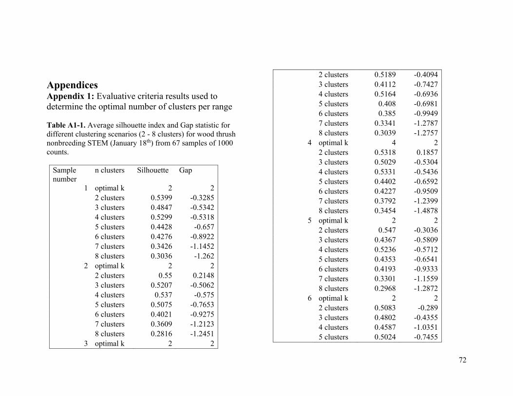
72
Appendices Appendix 1: Evaluative criteria results used to determine the optimal number of clusters per range Table A1-1. Average silhouette index and Gap statistic for different clustering scenarios (2 - 8 clusters) for wood thrush nonbreeding STEM (January 18th) from 67 samples of 1000 counts.
Sample number
n clusters Silhouette Gap
1 optimal k 2 2 2 clusters 0.5399 -0.3285 3 clusters 0.4847 -0.5342 4 clusters 0.5299 -0.5318 5 clusters 0.4428 -0.657 6 clusters 0.4276 -0.8922 7 clusters 0.3426 -1.1452 8 clusters 0.3036 -1.262
2 optimal k 2 2 2 clusters 0.55 0.2148 3 clusters 0.5207 -0.5062 4 clusters 0.537 -0.575 5 clusters 0.5075 -0.7653 6 clusters 0.4021 -0.9275 7 clusters 0.3609 -1.2123 8 clusters 0.2816 -1.2451
3 optimal k 2 2
2 clusters 0.5189 -0.4094 3 clusters 0.4112 -0.7427 4 clusters 0.5164 -0.6936 5 clusters 0.408 -0.6981 6 clusters 0.385 -0.9949 7 clusters 0.3341 -1.2787 8 clusters 0.3039 -1.2757
4 optimal k 4 2 2 clusters 0.5318 0.1857 3 clusters 0.5029 -0.5304 4 clusters 0.5331 -0.5436 5 clusters 0.4402 -0.6592 6 clusters 0.4227 -0.9509 7 clusters 0.3792 -1.2399 8 clusters 0.3454 -1.4878
5 optimal k 2 2 2 clusters 0.547 -0.3036 3 clusters 0.4367 -0.5809 4 clusters 0.5236 -0.5712 5 clusters 0.4353 -0.6541 6 clusters 0.4193 -0.9333 7 clusters 0.3301 -1.1559 8 clusters 0.2968 -1.2872
6 optimal k 2 2 2 clusters 0.5083 -0.289 3 clusters 0.4802 -0.4355 4 clusters 0.4587 -1.0351 5 clusters 0.5024 -0.7455
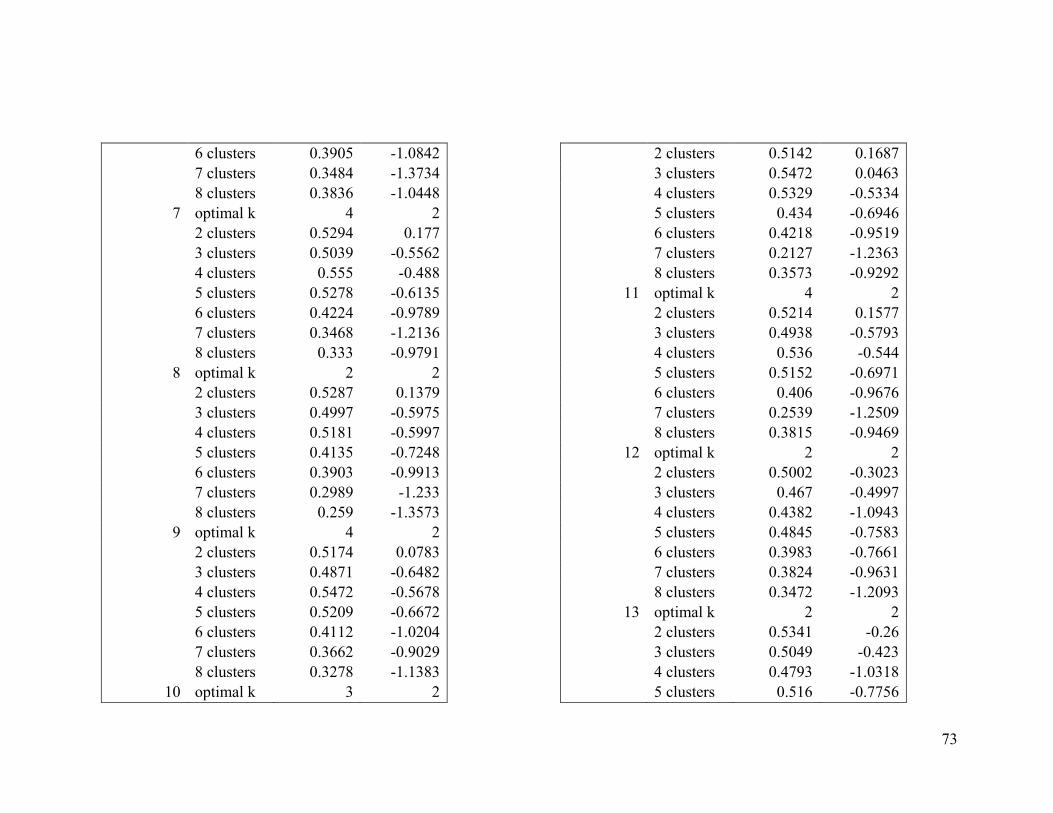
73
6 clusters 0.3905 -1.0842 7 clusters 0.3484 -1.3734 8 clusters 0.3836 -1.0448
7 optimal k 4 2 2 clusters 0.5294 0.177 3 clusters 0.5039 -0.5562 4 clusters 0.555 -0.488 5 clusters 0.5278 -0.6135 6 clusters 0.4224 -0.9789 7 clusters 0.3468 -1.2136 8 clusters 0.333 -0.9791
8 optimal k 2 2 2 clusters 0.5287 0.1379 3 clusters 0.4997 -0.5975 4 clusters 0.5181 -0.5997 5 clusters 0.4135 -0.7248 6 clusters 0.3903 -0.9913 7 clusters 0.2989 -1.233 8 clusters 0.259 -1.3573
9 optimal k 4 2 2 clusters 0.5174 0.0783 3 clusters 0.4871 -0.6482 4 clusters 0.5472 -0.5678 5 clusters 0.5209 -0.6672 6 clusters 0.4112 -1.0204 7 clusters 0.3662 -0.9029 8 clusters 0.3278 -1.1383
10 optimal k 3 2
2 clusters 0.5142 0.1687 3 clusters 0.5472 0.0463 4 clusters 0.5329 -0.5334 5 clusters 0.434 -0.6946 6 clusters 0.4218 -0.9519 7 clusters 0.2127 -1.2363 8 clusters 0.3573 -0.9292
11 optimal k 4 2 2 clusters 0.5214 0.1577 3 clusters 0.4938 -0.5793 4 clusters 0.536 -0.544 5 clusters 0.5152 -0.6971 6 clusters 0.406 -0.9676 7 clusters 0.2539 -1.2509 8 clusters 0.3815 -0.9469
12 optimal k 2 2 2 clusters 0.5002 -0.3023 3 clusters 0.467 -0.4997 4 clusters 0.4382 -1.0943 5 clusters 0.4845 -0.7583 6 clusters 0.3983 -0.7661 7 clusters 0.3824 -0.9631 8 clusters 0.3472 -1.2093
13 optimal k 2 2 2 clusters 0.5341 -0.26 3 clusters 0.5049 -0.423 4 clusters 0.4793 -1.0318 5 clusters 0.516 -0.7756
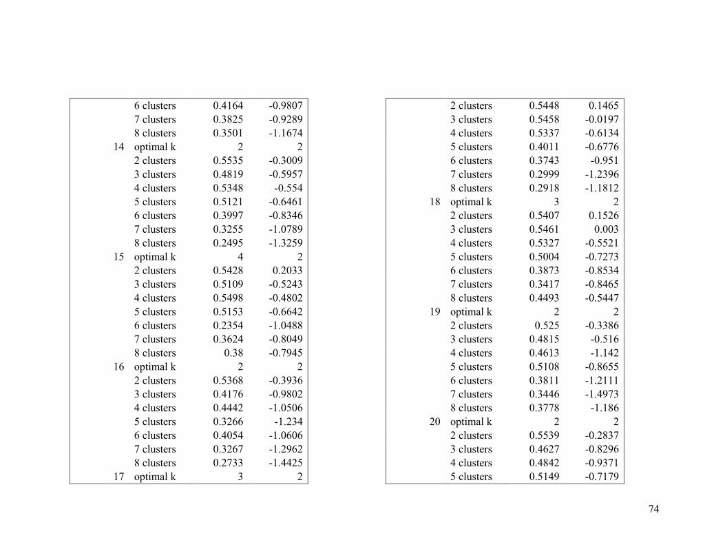
74
6 clusters 0.4164 -0.9807 7 clusters 0.3825 -0.9289 8 clusters 0.3501 -1.1674
14 optimal k 2 2 2 clusters 0.5535 -0.3009 3 clusters 0.4819 -0.5957 4 clusters 0.5348 -0.554 5 clusters 0.5121 -0.6461 6 clusters 0.3997 -0.8346 7 clusters 0.3255 -1.0789 8 clusters 0.2495 -1.3259
15 optimal k 4 2 2 clusters 0.5428 0.2033 3 clusters 0.5109 -0.5243 4 clusters 0.5498 -0.4802 5 clusters 0.5153 -0.6642 6 clusters 0.2354 -1.0488 7 clusters 0.3624 -0.8049 8 clusters 0.38 -0.7945
16 optimal k 2 2 2 clusters 0.5368 -0.3936 3 clusters 0.4176 -0.9802 4 clusters 0.4442 -1.0506 5 clusters 0.3266 -1.234 6 clusters 0.4054 -1.0606 7 clusters 0.3267 -1.2962 8 clusters 0.2733 -1.4425
17 optimal k 3 2
2 clusters 0.5448 0.1465 3 clusters 0.5458 -0.0197 4 clusters 0.5337 -0.6134 5 clusters 0.4011 -0.6776 6 clusters 0.3743 -0.951 7 clusters 0.2999 -1.2396 8 clusters 0.2918 -1.1812
18 optimal k 3 2 2 clusters 0.5407 0.1526 3 clusters 0.5461 0.003 4 clusters 0.5327 -0.5521 5 clusters 0.5004 -0.7273 6 clusters 0.3873 -0.8534 7 clusters 0.3417 -0.8465 8 clusters 0.4493 -0.5447
19 optimal k 2 2 2 clusters 0.525 -0.3386 3 clusters 0.4815 -0.516 4 clusters 0.4613 -1.142 5 clusters 0.5108 -0.8655 6 clusters 0.3811 -1.2111 7 clusters 0.3446 -1.4973 8 clusters 0.3778 -1.186
20 optimal k 2 2 2 clusters 0.5539 -0.2837 3 clusters 0.4627 -0.8296 4 clusters 0.4842 -0.9371 5 clusters 0.5149 -0.7179
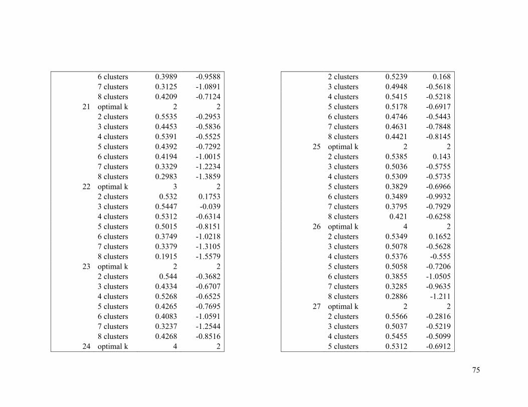
75
6 clusters 0.3989 -0.9588 7 clusters 0.3125 -1.0891 8 clusters 0.4209 -0.7124
21 optimal k 2 2 2 clusters 0.5535 -0.2953 3 clusters 0.4453 -0.5836 4 clusters 0.5391 -0.5525 5 clusters 0.4392 -0.7292 6 clusters 0.4194 -1.0015 7 clusters 0.3329 -1.2234 8 clusters 0.2983 -1.3859
22 optimal k 3 2 2 clusters 0.532 0.1753 3 clusters 0.5447 -0.039 4 clusters 0.5312 -0.6314 5 clusters 0.5015 -0.8151 6 clusters 0.3749 -1.0218 7 clusters 0.3379 -1.3105 8 clusters 0.1915 -1.5579
23 optimal k 2 2 2 clusters 0.544 -0.3682 3 clusters 0.4334 -0.6707 4 clusters 0.5268 -0.6525 5 clusters 0.4265 -0.7695 6 clusters 0.4083 -1.0591 7 clusters 0.3237 -1.2544 8 clusters 0.4268 -0.8516
24 optimal k 4 2
2 clusters 0.5239 0.168 3 clusters 0.4948 -0.5618 4 clusters 0.5415 -0.5218 5 clusters 0.5178 -0.6917 6 clusters 0.4746 -0.5443 7 clusters 0.4631 -0.7848 8 clusters 0.4421 -0.8145
25 optimal k 2 2 2 clusters 0.5385 0.143 3 clusters 0.5036 -0.5755 4 clusters 0.5309 -0.5735 5 clusters 0.3829 -0.6966 6 clusters 0.3489 -0.9932 7 clusters 0.3795 -0.7929 8 clusters 0.421 -0.6258
26 optimal k 4 2 2 clusters 0.5349 0.1652 3 clusters 0.5078 -0.5628 4 clusters 0.5376 -0.555 5 clusters 0.5058 -0.7206 6 clusters 0.3855 -1.0505 7 clusters 0.3285 -0.9635 8 clusters 0.2886 -1.211
27 optimal k 2 2 2 clusters 0.5566 -0.2816 3 clusters 0.5037 -0.5219 4 clusters 0.5455 -0.5099 5 clusters 0.5312 -0.6912
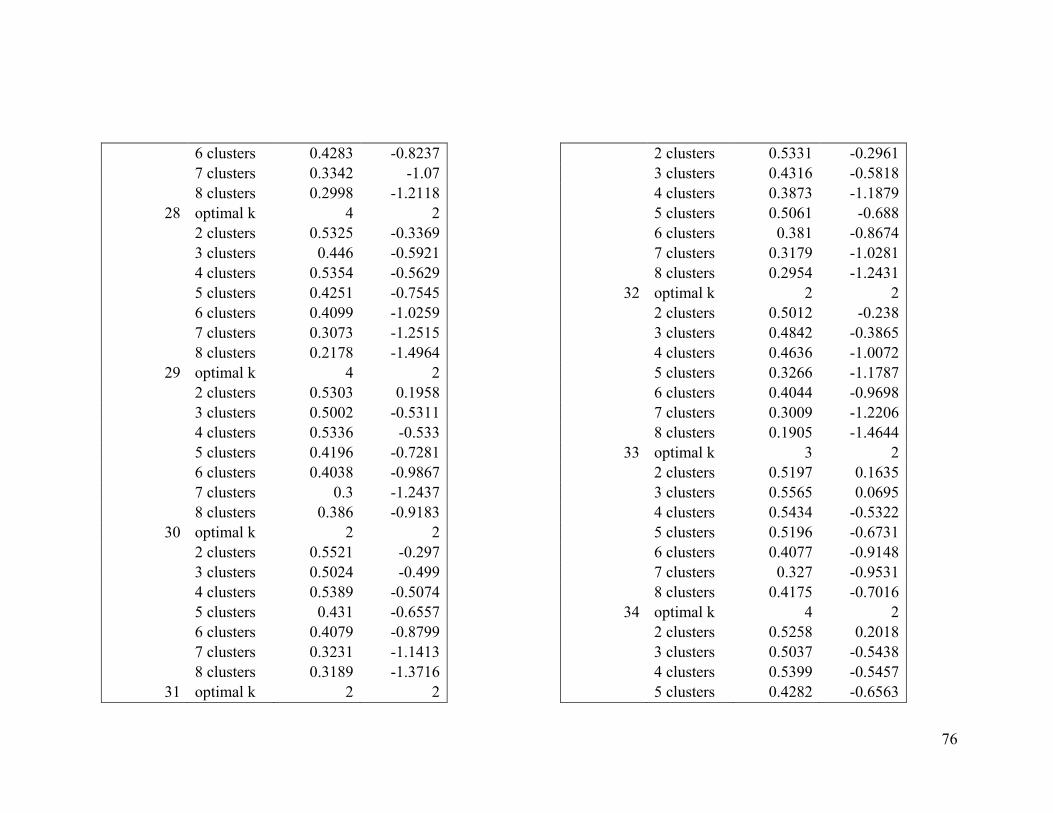
76
6 clusters 0.4283 -0.8237 7 clusters 0.3342 -1.07 8 clusters 0.2998 -1.2118
28 optimal k 4 2 2 clusters 0.5325 -0.3369 3 clusters 0.446 -0.5921 4 clusters 0.5354 -0.5629 5 clusters 0.4251 -0.7545 6 clusters 0.4099 -1.0259 7 clusters 0.3073 -1.2515 8 clusters 0.2178 -1.4964
29 optimal k 4 2 2 clusters 0.5303 0.1958 3 clusters 0.5002 -0.5311 4 clusters 0.5336 -0.533 5 clusters 0.4196 -0.7281 6 clusters 0.4038 -0.9867 7 clusters 0.3 -1.2437 8 clusters 0.386 -0.9183
30 optimal k 2 2 2 clusters 0.5521 -0.297 3 clusters 0.5024 -0.499 4 clusters 0.5389 -0.5074 5 clusters 0.431 -0.6557 6 clusters 0.4079 -0.8799 7 clusters 0.3231 -1.1413 8 clusters 0.3189 -1.3716
31 optimal k 2 2
2 clusters 0.5331 -0.2961 3 clusters 0.4316 -0.5818 4 clusters 0.3873 -1.1879 5 clusters 0.5061 -0.688 6 clusters 0.381 -0.8674 7 clusters 0.3179 -1.0281 8 clusters 0.2954 -1.2431
32 optimal k 2 2 2 clusters 0.5012 -0.238 3 clusters 0.4842 -0.3865 4 clusters 0.4636 -1.0072 5 clusters 0.3266 -1.1787 6 clusters 0.4044 -0.9698 7 clusters 0.3009 -1.2206 8 clusters 0.1905 -1.4644
33 optimal k 3 2 2 clusters 0.5197 0.1635 3 clusters 0.5565 0.0695 4 clusters 0.5434 -0.5322 5 clusters 0.5196 -0.6731 6 clusters 0.4077 -0.9148 7 clusters 0.327 -0.9531 8 clusters 0.4175 -0.7016
34 optimal k 4 2 2 clusters 0.5258 0.2018 3 clusters 0.5037 -0.5438 4 clusters 0.5399 -0.5457 5 clusters 0.4282 -0.6563
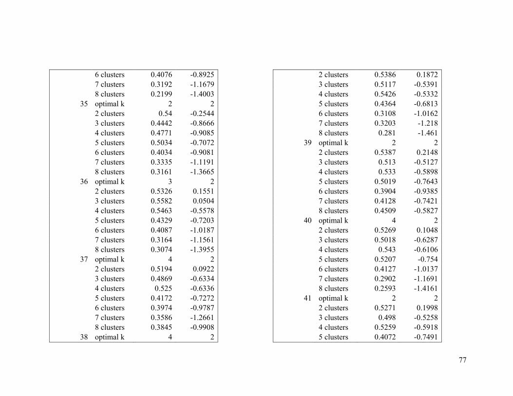
77
6 clusters 0.4076 -0.8925 7 clusters 0.3192 -1.1679 8 clusters 0.2199 -1.4003
35 optimal k 2 2 2 clusters 0.54 -0.2544 3 clusters 0.4442 -0.8666 4 clusters 0.4771 -0.9085 5 clusters 0.5034 -0.7072 6 clusters 0.4034 -0.9081 7 clusters 0.3335 -1.1191 8 clusters 0.3161 -1.3665
36 optimal k 3 2 2 clusters 0.5326 0.1551 3 clusters 0.5582 0.0504 4 clusters 0.5463 -0.5578 5 clusters 0.4329 -0.7203 6 clusters 0.4087 -1.0187 7 clusters 0.3164 -1.1561 8 clusters 0.3074 -1.3955
37 optimal k 4 2 2 clusters 0.5194 0.0922 3 clusters 0.4869 -0.6334 4 clusters 0.525 -0.6336 5 clusters 0.4172 -0.7272 6 clusters 0.3974 -0.9787 7 clusters 0.3586 -1.2661 8 clusters 0.3845 -0.9908
38 optimal k 4 2
2 clusters 0.5386 0.1872 3 clusters 0.5117 -0.5391 4 clusters 0.5426 -0.5332 5 clusters 0.4364 -0.6813 6 clusters 0.3108 -1.0162 7 clusters 0.3203 -1.218 8 clusters 0.281 -1.461
39 optimal k 2 2 2 clusters 0.5387 0.2148 3 clusters 0.513 -0.5127 4 clusters 0.533 -0.5898 5 clusters 0.5019 -0.7643 6 clusters 0.3904 -0.9385 7 clusters 0.4128 -0.7421 8 clusters 0.4509 -0.5827
40 optimal k 4 2 2 clusters 0.5269 0.1048 3 clusters 0.5018 -0.6287 4 clusters 0.543 -0.6106 5 clusters 0.5207 -0.754 6 clusters 0.4127 -1.0137 7 clusters 0.2902 -1.1691 8 clusters 0.2593 -1.4161
41 optimal k 2 2 2 clusters 0.5271 0.1998 3 clusters 0.498 -0.5258 4 clusters 0.5259 -0.5918 5 clusters 0.4072 -0.7491
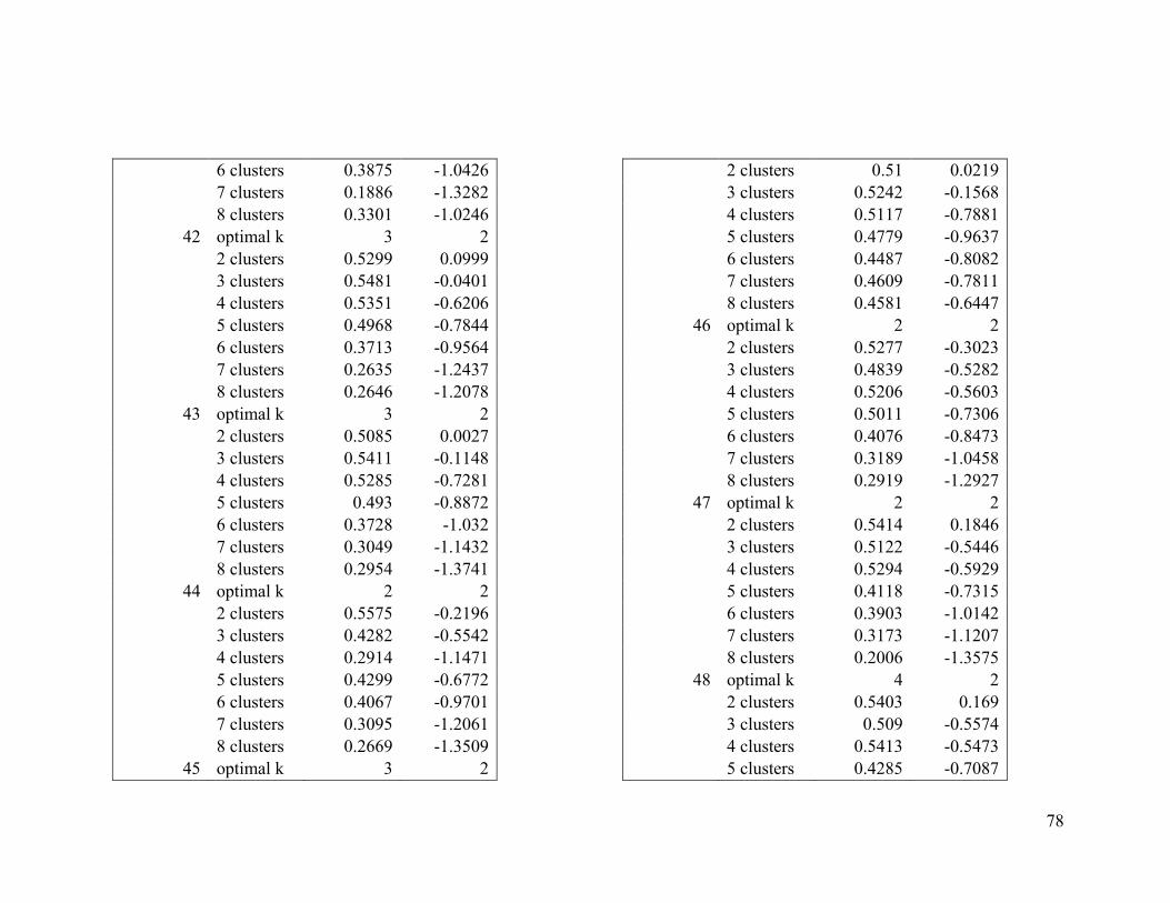
78
6 clusters 0.3875 -1.0426 7 clusters 0.1886 -1.3282 8 clusters 0.3301 -1.0246
42 optimal k 3 2 2 clusters 0.5299 0.0999 3 clusters 0.5481 -0.0401 4 clusters 0.5351 -0.6206 5 clusters 0.4968 -0.7844 6 clusters 0.3713 -0.9564 7 clusters 0.2635 -1.2437 8 clusters 0.2646 -1.2078
43 optimal k 3 2 2 clusters 0.5085 0.0027 3 clusters 0.5411 -0.1148 4 clusters 0.5285 -0.7281 5 clusters 0.493 -0.8872 6 clusters 0.3728 -1.032 7 clusters 0.3049 -1.1432 8 clusters 0.2954 -1.3741
44 optimal k 2 2 2 clusters 0.5575 -0.2196 3 clusters 0.4282 -0.5542 4 clusters 0.2914 -1.1471 5 clusters 0.4299 -0.6772 6 clusters 0.4067 -0.9701 7 clusters 0.3095 -1.2061 8 clusters 0.2669 -1.3509
45 optimal k 3 2
2 clusters 0.51 0.0219 3 clusters 0.5242 -0.1568 4 clusters 0.5117 -0.7881 5 clusters 0.4779 -0.9637 6 clusters 0.4487 -0.8082 7 clusters 0.4609 -0.7811 8 clusters 0.4581 -0.6447
46 optimal k 2 2 2 clusters 0.5277 -0.3023 3 clusters 0.4839 -0.5282 4 clusters 0.5206 -0.5603 5 clusters 0.5011 -0.7306 6 clusters 0.4076 -0.8473 7 clusters 0.3189 -1.0458 8 clusters 0.2919 -1.2927
47 optimal k 2 2 2 clusters 0.5414 0.1846 3 clusters 0.5122 -0.5446 4 clusters 0.5294 -0.5929 5 clusters 0.4118 -0.7315 6 clusters 0.3903 -1.0142 7 clusters 0.3173 -1.1207 8 clusters 0.2006 -1.3575
48 optimal k 4 2 2 clusters 0.5403 0.169 3 clusters 0.509 -0.5574 4 clusters 0.5413 -0.5473 5 clusters 0.4285 -0.7087
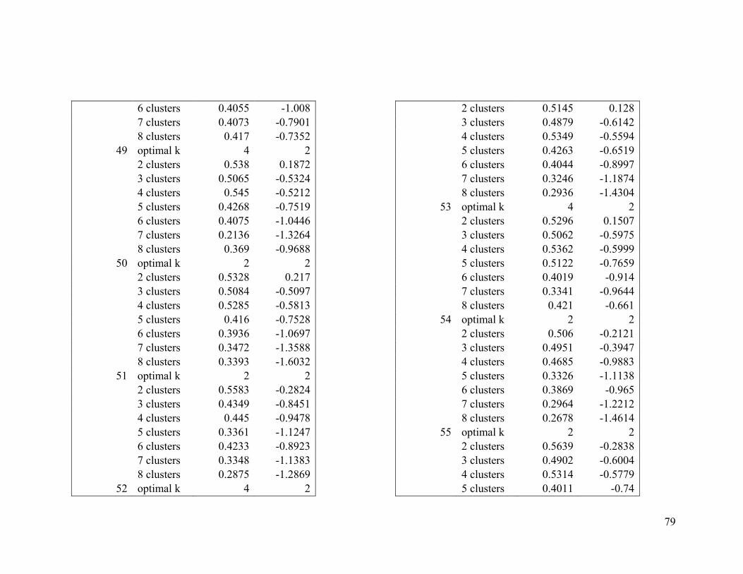
79
6 clusters 0.4055 -1.008 7 clusters 0.4073 -0.7901 8 clusters 0.417 -0.7352
49 optimal k 4 2 2 clusters 0.538 0.1872 3 clusters 0.5065 -0.5324 4 clusters 0.545 -0.5212 5 clusters 0.4268 -0.7519 6 clusters 0.4075 -1.0446 7 clusters 0.2136 -1.3264 8 clusters 0.369 -0.9688
50 optimal k 2 2 2 clusters 0.5328 0.217 3 clusters 0.5084 -0.5097 4 clusters 0.5285 -0.5813 5 clusters 0.416 -0.7528 6 clusters 0.3936 -1.0697 7 clusters 0.3472 -1.3588 8 clusters 0.3393 -1.6032
51 optimal k 2 2 2 clusters 0.5583 -0.2824 3 clusters 0.4349 -0.8451 4 clusters 0.445 -0.9478 5 clusters 0.3361 -1.1247 6 clusters 0.4233 -0.8923 7 clusters 0.3348 -1.1383 8 clusters 0.2875 -1.2869
52 optimal k 4 2
2 clusters 0.5145 0.128 3 clusters 0.4879 -0.6142 4 clusters 0.5349 -0.5594 5 clusters 0.4263 -0.6519 6 clusters 0.4044 -0.8997 7 clusters 0.3246 -1.1874 8 clusters 0.2936 -1.4304
53 optimal k 4 2 2 clusters 0.5296 0.1507 3 clusters 0.5062 -0.5975 4 clusters 0.5362 -0.5999 5 clusters 0.5122 -0.7659 6 clusters 0.4019 -0.914 7 clusters 0.3341 -0.9644 8 clusters 0.421 -0.661
54 optimal k 2 2 2 clusters 0.506 -0.2121 3 clusters 0.4951 -0.3947 4 clusters 0.4685 -0.9883 5 clusters 0.3326 -1.1138 6 clusters 0.3869 -0.965 7 clusters 0.2964 -1.2212 8 clusters 0.2678 -1.4614
55 optimal k 2 2 2 clusters 0.5639 -0.2838 3 clusters 0.4902 -0.6004 4 clusters 0.5314 -0.5779 5 clusters 0.4011 -0.74
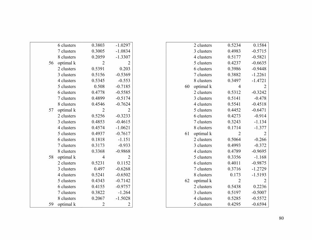
80
6 clusters 0.3803 -1.0297 7 clusters 0.3005 -1.0834 8 clusters 0.2059 -1.3307
56 optimal k 2 2 2 clusters 0.5391 0.203 3 clusters 0.5156 -0.5369 4 clusters 0.5345 -0.553 5 clusters 0.508 -0.7185 6 clusters 0.4778 -0.5585 7 clusters 0.4899 -0.5174 8 clusters 0.4546 -0.7624
57 optimal k 2 2 2 clusters 0.5256 -0.3233 3 clusters 0.4853 -0.4615 4 clusters 0.4574 -1.0621 5 clusters 0.4937 -0.7617 6 clusters 0.1818 -1.151 7 clusters 0.3173 -0.933 8 clusters 0.3368 -0.9868
58 optimal k 4 2 2 clusters 0.5231 0.1152 3 clusters 0.497 -0.6268 4 clusters 0.5241 -0.6502 5 clusters 0.4343 -0.7142 6 clusters 0.4155 -0.9757 7 clusters 0.3822 -1.264 8 clusters 0.2067 -1.5028
59 optimal k 2 2
2 clusters 0.5234 0.1584 3 clusters 0.4983 -0.5715 4 clusters 0.5177 -0.5821 5 clusters 0.4237 -0.6635 6 clusters 0.3986 -0.9448 7 clusters 0.3882 -1.2261 8 clusters 0.3497 -1.4721
60 optimal k 4 2 2 clusters 0.5312 -0.3242 3 clusters 0.5141 -0.478 4 clusters 0.5541 -0.4518 5 clusters 0.4452 -0.6471 6 clusters 0.4273 -0.914 7 clusters 0.3243 -1.134 8 clusters 0.1714 -1.377
61 optimal k 2 2 2 clusters 0.5064 -0.266 3 clusters 0.4993 -0.372 4 clusters 0.4789 -0.9695 5 clusters 0.3356 -1.168 6 clusters 0.4011 -0.9875 7 clusters 0.3716 -1.2729 8 clusters 0.173 -1.5193
62 optimal k 2 2 2 clusters 0.5438 0.2236 3 clusters 0.5197 -0.5007 4 clusters 0.5285 -0.5572 5 clusters 0.4295 -0.6594
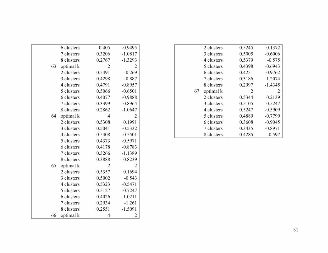
81
6 clusters 0.405 -0.9495 7 clusters 0.3206 -1.0817 8 clusters 0.2767 -1.3293
63 optimal k 2 2 2 clusters 0.5491 -0.269 3 clusters 0.4298 -0.887 4 clusters 0.4791 -0.8957 5 clusters 0.5066 -0.6501 6 clusters 0.4077 -0.9888 7 clusters 0.3399 -0.8964 8 clusters 0.2862 -1.0647
64 optimal k 4 2 2 clusters 0.5308 0.1991 3 clusters 0.5041 -0.5332 4 clusters 0.5408 -0.5501 5 clusters 0.4373 -0.5971 6 clusters 0.4178 -0.8783 7 clusters 0.3266 -1.1389 8 clusters 0.3888 -0.8239
65 optimal k 2 2 2 clusters 0.5357 0.1694 3 clusters 0.5002 -0.543 4 clusters 0.5323 -0.5471 5 clusters 0.5127 -0.7247 6 clusters 0.4026 -1.0211 7 clusters 0.2934 -1.261 8 clusters 0.2551 -1.5091
66 optimal k 4 2
2 clusters 0.5245 0.1372 3 clusters 0.5005 -0.6006 4 clusters 0.5379 -0.575 5 clusters 0.4398 -0.6943 6 clusters 0.4251 -0.9762 7 clusters 0.3186 -1.2074 8 clusters 0.2997 -1.4345
67 optimal k 2 2 2 clusters 0.5344 0.2139 3 clusters 0.5105 -0.5247 4 clusters 0.5247 -0.5909 5 clusters 0.4889 -0.7799 6 clusters 0.3608 -0.9045 7 clusters 0.3435 -0.8971 8 clusters 0.4285 -0.597
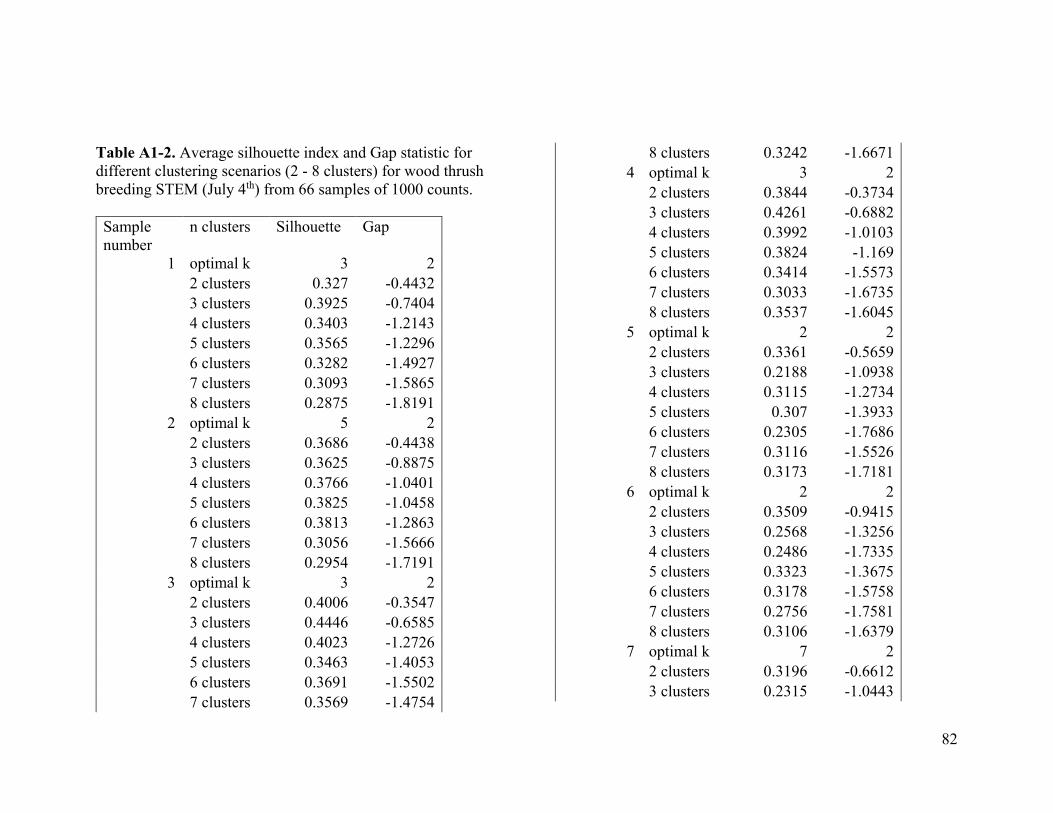
82
Table A1-2. Average silhouette index and Gap statistic for different clustering scenarios (2 - 8 clusters) for wood thrush breeding STEM (July 4th) from 66 samples of 1000 counts. Sample number
n clusters Silhouette Gap
1 optimal k 3 2 2 clusters 0.327 -0.4432 3 clusters 0.3925 -0.7404 4 clusters 0.3403 -1.2143 5 clusters 0.3565 -1.2296 6 clusters 0.3282 -1.4927 7 clusters 0.3093 -1.5865 8 clusters 0.2875 -1.8191
2 optimal k 5 2 2 clusters 0.3686 -0.4438 3 clusters 0.3625 -0.8875 4 clusters 0.3766 -1.0401 5 clusters 0.3825 -1.0458 6 clusters 0.3813 -1.2863 7 clusters 0.3056 -1.5666 8 clusters 0.2954 -1.7191
3 optimal k 3 2 2 clusters 0.4006 -0.3547 3 clusters 0.4446 -0.6585 4 clusters 0.4023 -1.2726 5 clusters 0.3463 -1.4053 6 clusters 0.3691 -1.5502 7 clusters 0.3569 -1.4754
8 clusters 0.3242 -1.6671 4 optimal k 3 2 2 clusters 0.3844 -0.3734 3 clusters 0.4261 -0.6882 4 clusters 0.3992 -1.0103 5 clusters 0.3824 -1.169 6 clusters 0.3414 -1.5573 7 clusters 0.3033 -1.6735 8 clusters 0.3537 -1.6045
5 optimal k 2 2 2 clusters 0.3361 -0.5659 3 clusters 0.2188 -1.0938 4 clusters 0.3115 -1.2734 5 clusters 0.307 -1.3933 6 clusters 0.2305 -1.7686 7 clusters 0.3116 -1.5526 8 clusters 0.3173 -1.7181
6 optimal k 2 2 2 clusters 0.3509 -0.9415 3 clusters 0.2568 -1.3256 4 clusters 0.2486 -1.7335 5 clusters 0.3323 -1.3675 6 clusters 0.3178 -1.5758 7 clusters 0.2756 -1.7581 8 clusters 0.3106 -1.6379
7 optimal k 7 2 2 clusters 0.3196 -0.6612 3 clusters 0.2315 -1.0443
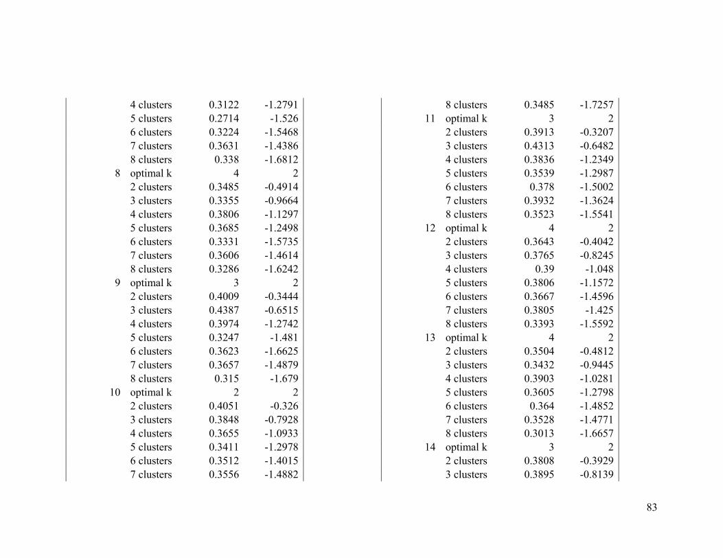
83
4 clusters 0.3122 -1.2791 5 clusters 0.2714 -1.526 6 clusters 0.3224 -1.5468 7 clusters 0.3631 -1.4386 8 clusters 0.338 -1.6812
8 optimal k 4 2 2 clusters 0.3485 -0.4914 3 clusters 0.3355 -0.9664 4 clusters 0.3806 -1.1297 5 clusters 0.3685 -1.2498 6 clusters 0.3331 -1.5735 7 clusters 0.3606 -1.4614 8 clusters 0.3286 -1.6242
9 optimal k 3 2 2 clusters 0.4009 -0.3444 3 clusters 0.4387 -0.6515 4 clusters 0.3974 -1.2742 5 clusters 0.3247 -1.481 6 clusters 0.3623 -1.6625 7 clusters 0.3657 -1.4879 8 clusters 0.315 -1.679
10 optimal k 2 2 2 clusters 0.4051 -0.326 3 clusters 0.3848 -0.7928 4 clusters 0.3655 -1.0933 5 clusters 0.3411 -1.2978 6 clusters 0.3512 -1.4015 7 clusters 0.3556 -1.4882
8 clusters 0.3485 -1.7257 11 optimal k 3 2
2 clusters 0.3913 -0.3207 3 clusters 0.4313 -0.6482 4 clusters 0.3836 -1.2349 5 clusters 0.3539 -1.2987 6 clusters 0.378 -1.5002 7 clusters 0.3932 -1.3624 8 clusters 0.3523 -1.5541
12 optimal k 4 2 2 clusters 0.3643 -0.4042 3 clusters 0.3765 -0.8245 4 clusters 0.39 -1.048 5 clusters 0.3806 -1.1572 6 clusters 0.3667 -1.4596 7 clusters 0.3805 -1.425 8 clusters 0.3393 -1.5592
13 optimal k 4 2 2 clusters 0.3504 -0.4812 3 clusters 0.3432 -0.9445 4 clusters 0.3903 -1.0281 5 clusters 0.3605 -1.2798 6 clusters 0.364 -1.4852 7 clusters 0.3528 -1.4771 8 clusters 0.3013 -1.6657
14 optimal k 3 2 2 clusters 0.3808 -0.3929 3 clusters 0.3895 -0.8139
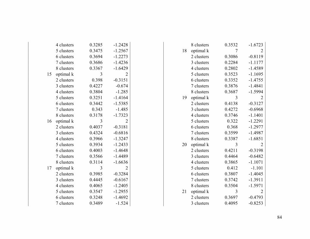
84
4 clusters 0.3285 -1.2428 5 clusters 0.3475 -1.2567 6 clusters 0.3694 -1.2273 7 clusters 0.3686 -1.4236 8 clusters 0.3367 -1.6429
15 optimal k 3 2 2 clusters 0.398 -0.3151 3 clusters 0.4227 -0.674 4 clusters 0.3804 -1.285 5 clusters 0.3251 -1.4164 6 clusters 0.3442 -1.5385 7 clusters 0.343 -1.485 8 clusters 0.3178 -1.7323
16 optimal k 3 2 2 clusters 0.4037 -0.3181 3 clusters 0.4324 -0.6816 4 clusters 0.3966 -1.3247 5 clusters 0.3934 -1.2433 6 clusters 0.4003 -1.4648 7 clusters 0.3566 -1.4489 8 clusters 0.3114 -1.6636
17 optimal k 3 2 2 clusters 0.3985 -0.3284 3 clusters 0.4445 -0.6167 4 clusters 0.4065 -1.2405 5 clusters 0.3547 -1.2955 6 clusters 0.3248 -1.4692 7 clusters 0.3489 -1.524
8 clusters 0.3532 -1.6723 18 optimal k 7 2
2 clusters 0.3086 -0.8119 3 clusters 0.2284 -1.1177 4 clusters 0.2802 -1.4589 5 clusters 0.3523 -1.1695 6 clusters 0.3352 -1.4755 7 clusters 0.3876 -1.4841 8 clusters 0.3687 -1.5994
19 optimal k 3 2 2 clusters 0.4138 -0.3127 3 clusters 0.4272 -0.6968 4 clusters 0.3746 -1.1401 5 clusters 0.322 -1.2291 6 clusters 0.368 -1.2977 7 clusters 0.3599 -1.4987 8 clusters 0.3387 -1.6851
20 optimal k 3 2 2 clusters 0.4211 -0.3198 3 clusters 0.4464 -0.6482 4 clusters 0.3865 -1.1071 5 clusters 0.412 -1.101 6 clusters 0.3807 -1.4045 7 clusters 0.3742 -1.3911 8 clusters 0.3504 -1.5971
21 optimal k 3 2 2 clusters 0.3697 -0.4793 3 clusters 0.4095 -0.8253
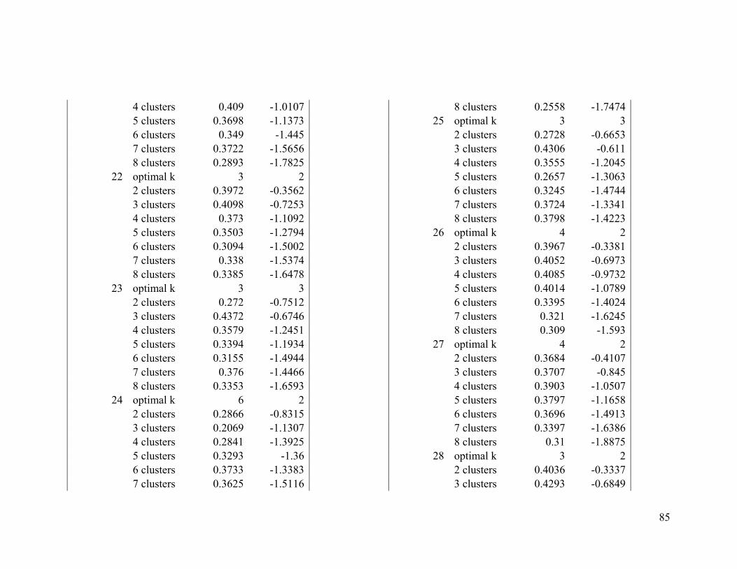
85
4 clusters 0.409 -1.0107 5 clusters 0.3698 -1.1373 6 clusters 0.349 -1.445 7 clusters 0.3722 -1.5656 8 clusters 0.2893 -1.7825
22 optimal k 3 2 2 clusters 0.3972 -0.3562 3 clusters 0.4098 -0.7253 4 clusters 0.373 -1.1092 5 clusters 0.3503 -1.2794 6 clusters 0.3094 -1.5002 7 clusters 0.338 -1.5374 8 clusters 0.3385 -1.6478
23 optimal k 3 3 2 clusters 0.272 -0.7512 3 clusters 0.4372 -0.6746 4 clusters 0.3579 -1.2451 5 clusters 0.3394 -1.1934 6 clusters 0.3155 -1.4944 7 clusters 0.376 -1.4466 8 clusters 0.3353 -1.6593
24 optimal k 6 2 2 clusters 0.2866 -0.8315 3 clusters 0.2069 -1.1307 4 clusters 0.2841 -1.3925 5 clusters 0.3293 -1.36 6 clusters 0.3733 -1.3383 7 clusters 0.3625 -1.5116
8 clusters 0.2558 -1.7474 25 optimal k 3 3
2 clusters 0.2728 -0.6653 3 clusters 0.4306 -0.611 4 clusters 0.3555 -1.2045 5 clusters 0.2657 -1.3063 6 clusters 0.3245 -1.4744 7 clusters 0.3724 -1.3341 8 clusters 0.3798 -1.4223
26 optimal k 4 2 2 clusters 0.3967 -0.3381 3 clusters 0.4052 -0.6973 4 clusters 0.4085 -0.9732 5 clusters 0.4014 -1.0789 6 clusters 0.3395 -1.4024 7 clusters 0.321 -1.6245 8 clusters 0.309 -1.593
27 optimal k 4 2 2 clusters 0.3684 -0.4107 3 clusters 0.3707 -0.845 4 clusters 0.3903 -1.0507 5 clusters 0.3797 -1.1658 6 clusters 0.3696 -1.4913 7 clusters 0.3397 -1.6386 8 clusters 0.31 -1.8875
28 optimal k 3 2 2 clusters 0.4036 -0.3337 3 clusters 0.4293 -0.6849
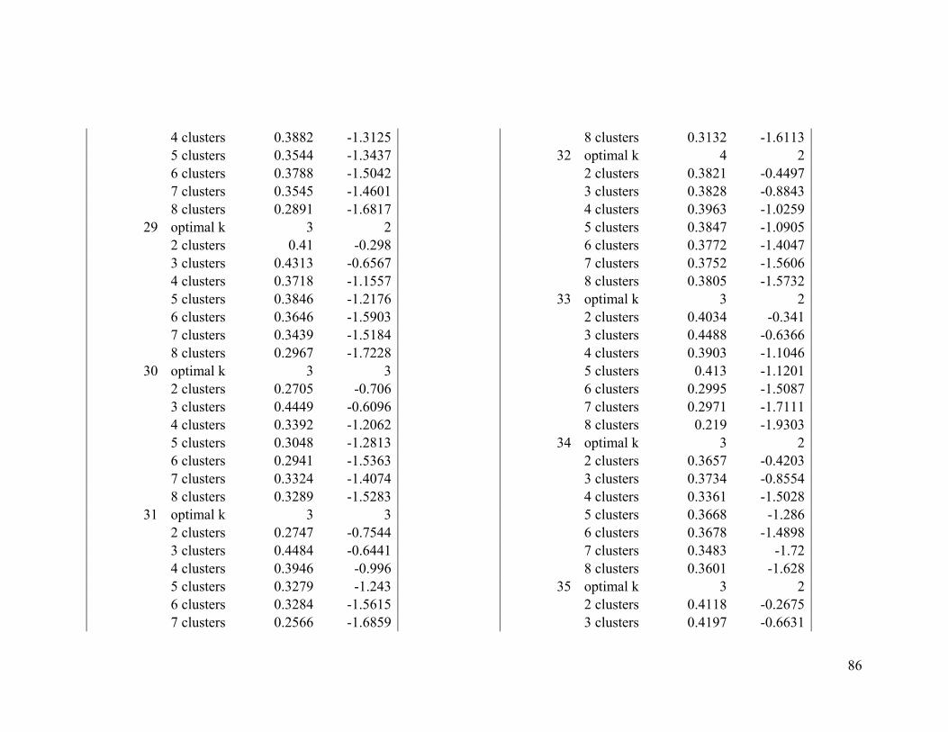
86
4 clusters 0.3882 -1.3125 5 clusters 0.3544 -1.3437 6 clusters 0.3788 -1.5042 7 clusters 0.3545 -1.4601 8 clusters 0.2891 -1.6817
29 optimal k 3 2 2 clusters 0.41 -0.298 3 clusters 0.4313 -0.6567 4 clusters 0.3718 -1.1557 5 clusters 0.3846 -1.2176 6 clusters 0.3646 -1.5903 7 clusters 0.3439 -1.5184 8 clusters 0.2967 -1.7228
30 optimal k 3 3 2 clusters 0.2705 -0.706 3 clusters 0.4449 -0.6096 4 clusters 0.3392 -1.2062 5 clusters 0.3048 -1.2813 6 clusters 0.2941 -1.5363 7 clusters 0.3324 -1.4074 8 clusters 0.3289 -1.5283
31 optimal k 3 3 2 clusters 0.2747 -0.7544 3 clusters 0.4484 -0.6441 4 clusters 0.3946 -0.996 5 clusters 0.3279 -1.243 6 clusters 0.3284 -1.5615 7 clusters 0.2566 -1.6859
8 clusters 0.3132 -1.6113 32 optimal k 4 2
2 clusters 0.3821 -0.4497 3 clusters 0.3828 -0.8843 4 clusters 0.3963 -1.0259 5 clusters 0.3847 -1.0905 6 clusters 0.3772 -1.4047 7 clusters 0.3752 -1.5606 8 clusters 0.3805 -1.5732
33 optimal k 3 2 2 clusters 0.4034 -0.341 3 clusters 0.4488 -0.6366 4 clusters 0.3903 -1.1046 5 clusters 0.413 -1.1201 6 clusters 0.2995 -1.5087 7 clusters 0.2971 -1.7111 8 clusters 0.219 -1.9303
34 optimal k 3 2 2 clusters 0.3657 -0.4203 3 clusters 0.3734 -0.8554 4 clusters 0.3361 -1.5028 5 clusters 0.3668 -1.286 6 clusters 0.3678 -1.4898 7 clusters 0.3483 -1.72 8 clusters 0.3601 -1.628
35 optimal k 3 2 2 clusters 0.4118 -0.2675 3 clusters 0.4197 -0.6631
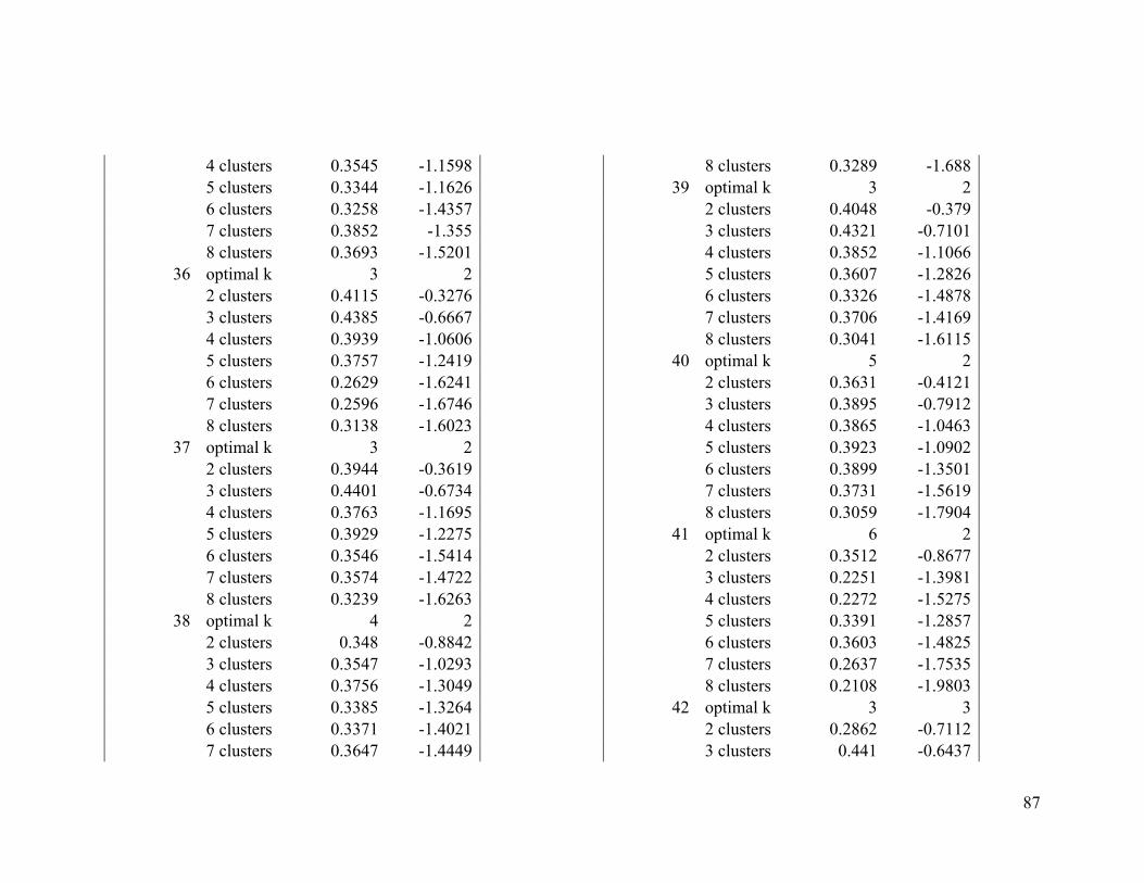
87
4 clusters 0.3545 -1.1598 5 clusters 0.3344 -1.1626 6 clusters 0.3258 -1.4357 7 clusters 0.3852 -1.355 8 clusters 0.3693 -1.5201
36 optimal k 3 2 2 clusters 0.4115 -0.3276 3 clusters 0.4385 -0.6667 4 clusters 0.3939 -1.0606 5 clusters 0.3757 -1.2419 6 clusters 0.2629 -1.6241 7 clusters 0.2596 -1.6746 8 clusters 0.3138 -1.6023
37 optimal k 3 2 2 clusters 0.3944 -0.3619 3 clusters 0.4401 -0.6734 4 clusters 0.3763 -1.1695 5 clusters 0.3929 -1.2275 6 clusters 0.3546 -1.5414 7 clusters 0.3574 -1.4722 8 clusters 0.3239 -1.6263
38 optimal k 4 2 2 clusters 0.348 -0.8842 3 clusters 0.3547 -1.0293 4 clusters 0.3756 -1.3049 5 clusters 0.3385 -1.3264 6 clusters 0.3371 -1.4021 7 clusters 0.3647 -1.4449
8 clusters 0.3289 -1.688 39 optimal k 3 2
2 clusters 0.4048 -0.379 3 clusters 0.4321 -0.7101 4 clusters 0.3852 -1.1066 5 clusters 0.3607 -1.2826 6 clusters 0.3326 -1.4878 7 clusters 0.3706 -1.4169 8 clusters 0.3041 -1.6115
40 optimal k 5 2 2 clusters 0.3631 -0.4121 3 clusters 0.3895 -0.7912 4 clusters 0.3865 -1.0463 5 clusters 0.3923 -1.0902 6 clusters 0.3899 -1.3501 7 clusters 0.3731 -1.5619 8 clusters 0.3059 -1.7904
41 optimal k 6 2 2 clusters 0.3512 -0.8677 3 clusters 0.2251 -1.3981 4 clusters 0.2272 -1.5275 5 clusters 0.3391 -1.2857 6 clusters 0.3603 -1.4825 7 clusters 0.2637 -1.7535 8 clusters 0.2108 -1.9803
42 optimal k 3 3 2 clusters 0.2862 -0.7112 3 clusters 0.441 -0.6437
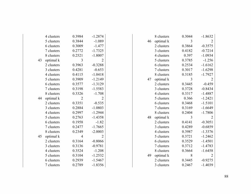
88
4 clusters 0.3984 -1.2874 5 clusters 0.3844 -1.089 6 clusters 0.3009 -1.477 7 clusters 0.2772 -1.7325 8 clusters 0.2521 -1.8007
43 optimal k 3 2 2 clusters 0.3963 -0.3288 3 clusters 0.4281 -0.653 4 clusters 0.4115 -1.0418 5 clusters 0.3909 -1.2149 6 clusters 0.3577 -1.3129 7 clusters 0.3198 -1.5583 8 clusters 0.3326 -1.708
44 optimal k 2 2 2 clusters 0.3351 -0.535 3 clusters 0.2884 -1.0803 4 clusters 0.2997 -1.2944 5 clusters 0.2763 -1.4358 6 clusters 0.1958 -1.82 7 clusters 0.2477 -1.7665 8 clusters 0.2349 -2.0003
45 optimal k 4 2 2 clusters 0.3164 -0.8066 3 clusters 0.3136 -0.9781 4 clusters 0.3524 -1.208 5 clusters 0.3104 -1.2532 6 clusters 0.2939 -1.5467 7 clusters 0.2789 -1.8356
8 clusters 0.3044 -1.8632 46 optimal k 3 2
2 clusters 0.3864 -0.3575 3 clusters 0.4182 -0.7214 4 clusters 0.397 -1.0934 5 clusters 0.3785 -1.256 6 clusters 0.2534 -1.6162 7 clusters 0.3017 -1.6298 8 clusters 0.3185 -1.7927
47 optimal k 3 2 2 clusters 0.3445 -0.459 3 clusters 0.3728 -0.8434 4 clusters 0.3317 -1.4887 5 clusters 0.366 -1.2421 6 clusters 0.3468 -1.5101 7 clusters 0.3169 -1.6649 8 clusters 0.2404 -1.7806
48 optimal k 3 2 2 clusters 0.4141 -0.3051 3 clusters 0.4289 -0.6859 4 clusters 0.3987 -1.3376 5 clusters 0.3721 -1.2462 6 clusters 0.3529 -1.4501 7 clusters 0.3712 -1.4783 8 clusters 0.3664 -1.6458
49 optimal k 8 2 2 clusters 0.3445 -0.9275 3 clusters 0.2467 -1.4039
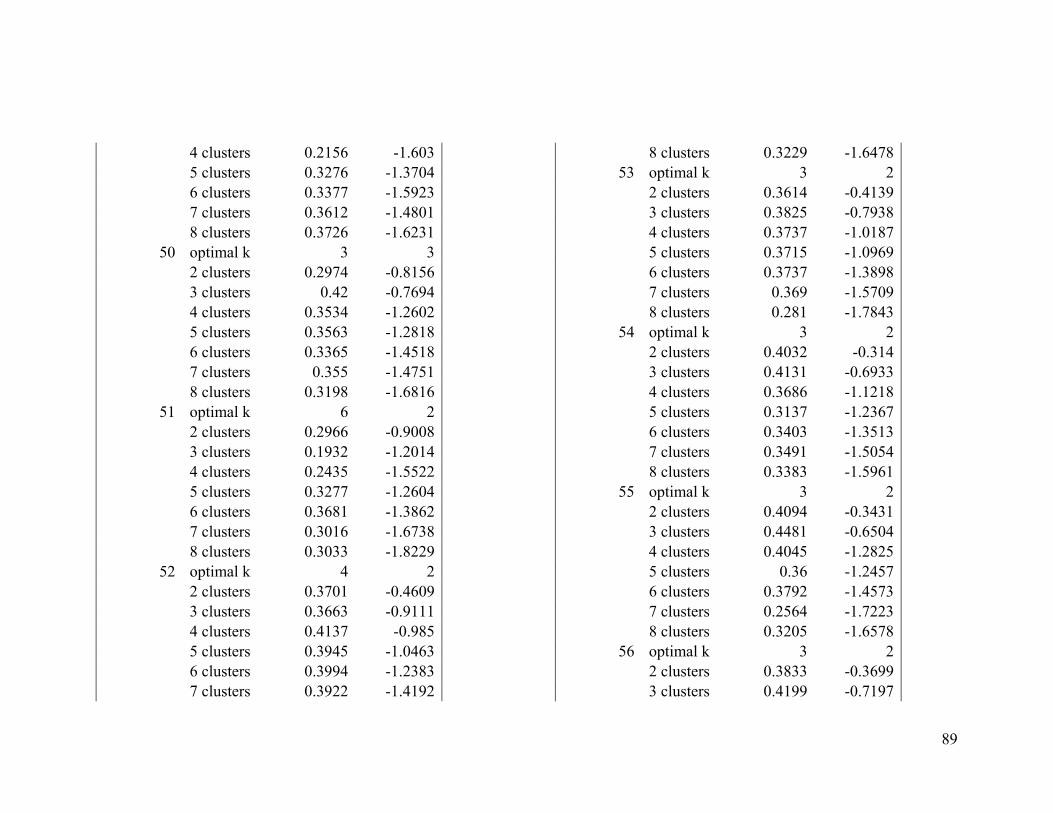
89
4 clusters 0.2156 -1.603 5 clusters 0.3276 -1.3704 6 clusters 0.3377 -1.5923 7 clusters 0.3612 -1.4801 8 clusters 0.3726 -1.6231
50 optimal k 3 3 2 clusters 0.2974 -0.8156 3 clusters 0.42 -0.7694 4 clusters 0.3534 -1.2602 5 clusters 0.3563 -1.2818 6 clusters 0.3365 -1.4518 7 clusters 0.355 -1.4751 8 clusters 0.3198 -1.6816
51 optimal k 6 2 2 clusters 0.2966 -0.9008 3 clusters 0.1932 -1.2014 4 clusters 0.2435 -1.5522 5 clusters 0.3277 -1.2604 6 clusters 0.3681 -1.3862 7 clusters 0.3016 -1.6738 8 clusters 0.3033 -1.8229
52 optimal k 4 2 2 clusters 0.3701 -0.4609 3 clusters 0.3663 -0.9111 4 clusters 0.4137 -0.985 5 clusters 0.3945 -1.0463 6 clusters 0.3994 -1.2383 7 clusters 0.3922 -1.4192
8 clusters 0.3229 -1.6478 53 optimal k 3 2
2 clusters 0.3614 -0.4139 3 clusters 0.3825 -0.7938 4 clusters 0.3737 -1.0187 5 clusters 0.3715 -1.0969 6 clusters 0.3737 -1.3898 7 clusters 0.369 -1.5709 8 clusters 0.281 -1.7843
54 optimal k 3 2 2 clusters 0.4032 -0.314 3 clusters 0.4131 -0.6933 4 clusters 0.3686 -1.1218 5 clusters 0.3137 -1.2367 6 clusters 0.3403 -1.3513 7 clusters 0.3491 -1.5054 8 clusters 0.3383 -1.5961
55 optimal k 3 2 2 clusters 0.4094 -0.3431 3 clusters 0.4481 -0.6504 4 clusters 0.4045 -1.2825 5 clusters 0.36 -1.2457 6 clusters 0.3792 -1.4573 7 clusters 0.2564 -1.7223 8 clusters 0.3205 -1.6578
56 optimal k 3 2 2 clusters 0.3833 -0.3699 3 clusters 0.4199 -0.7197
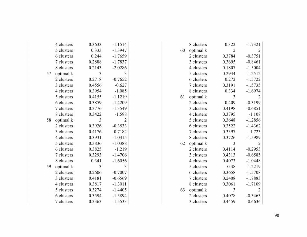
90
4 clusters 0.3633 -1.1514 5 clusters 0.333 -1.3947 6 clusters 0.244 -1.7659 7 clusters 0.2888 -1.7837 8 clusters 0.2143 -2.0286
57 optimal k 3 3 2 clusters 0.2718 -0.7652 3 clusters 0.4556 -0.627 4 clusters 0.3954 -1.085 5 clusters 0.4155 -1.1219 6 clusters 0.3859 -1.4209 7 clusters 0.3776 -1.3549 8 clusters 0.3422 -1.598
58 optimal k 3 2 2 clusters 0.3926 -0.3533 3 clusters 0.4176 -0.7182 4 clusters 0.3931 -1.0315 5 clusters 0.3836 -1.0388 6 clusters 0.3825 -1.219 7 clusters 0.3293 -1.4706 8 clusters 0.341 -1.6056
59 optimal k 3 3 2 clusters 0.2606 -0.7007 3 clusters 0.4181 -0.6569 4 clusters 0.3817 -1.3011 5 clusters 0.3274 -1.4405 6 clusters 0.3594 -1.5894 7 clusters 0.3363 -1.5533
8 clusters 0.322 -1.7321 60 optimal k 2 2
2 clusters 0.3784 -0.3751 3 clusters 0.3695 -0.8461 4 clusters 0.1807 -1.5004 5 clusters 0.2944 -1.2512 6 clusters 0.272 -1.5722 7 clusters 0.3191 -1.5735 8 clusters 0.334 -1.6974
61 optimal k 3 2 2 clusters 0.409 -0.3199 3 clusters 0.4198 -0.6851 4 clusters 0.3795 -1.108 5 clusters 0.3648 -1.2856 6 clusters 0.3522 -1.4362 7 clusters 0.3397 -1.723 8 clusters 0.3726 -1.5989
62 optimal k 3 2 2 clusters 0.4114 -0.2953 3 clusters 0.4313 -0.6585 4 clusters 0.4073 -1.0448 5 clusters 0.38 -1.2219 6 clusters 0.3658 -1.5708 7 clusters 0.2408 -1.7883 8 clusters 0.3061 -1.7109
63 optimal k 3 2 2 clusters 0.4078 -0.3463 3 clusters 0.4459 -0.6636
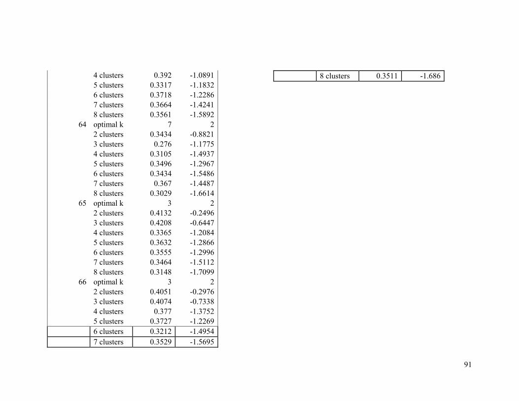
91
4 clusters 0.392 -1.0891 5 clusters 0.3317 -1.1832 6 clusters 0.3718 -1.2286 7 clusters 0.3664 -1.4241 8 clusters 0.3561 -1.5892
64 optimal k 7 2 2 clusters 0.3434 -0.8821 3 clusters 0.276 -1.1775 4 clusters 0.3105 -1.4937 5 clusters 0.3496 -1.2967 6 clusters 0.3434 -1.5486 7 clusters 0.367 -1.4487 8 clusters 0.3029 -1.6614
65 optimal k 3 2 2 clusters 0.4132 -0.2496 3 clusters 0.4208 -0.6447 4 clusters 0.3365 -1.2084 5 clusters 0.3632 -1.2866 6 clusters 0.3555 -1.2996 7 clusters 0.3464 -1.5112 8 clusters 0.3148 -1.7099
66 optimal k 3 2 2 clusters 0.4051 -0.2976 3 clusters 0.4074 -0.7338 4 clusters 0.377 -1.3752 5 clusters 0.3727 -1.2269 6 clusters 0.3212 -1.4954 7 clusters 0.3529 -1.5695
8 clusters 0.3511 -1.686

92
Table A1-3. Average silhouette index and Gap statistic for different clustering scenarios (2 - 8 clusters) for Wilson’s warbler nonbreeding STEM (January 18th) from 83 samples of 1000 counts.
Sample number
n clusters Silhouette Gap
1 optimal k 5 2 2 clusters 0.4595 -0.6211 3 clusters 0.2958 -1.3577 4 clusters 0.402 -1.3619 5 clusters 0.5335 -0.5901 6 clusters 0.4305 -0.9551 7 clusters 0.4324 -1.2412 8 clusters 0.4039 -1.2929
2 optimal k 5 2 2 clusters 0.5143 -0.4676 3 clusters 0.3662 -1.2012 4 clusters 0.4542 -1.1959 5 clusters 0.5337 -0.5138 6 clusters 0.5303 -0.898 7 clusters 0.4819 -1.0679 8 clusters 0.4518 -0.8501
3 optimal k 5 2 2 clusters 0.4724 -0.5833 3 clusters 0.3439 -1.3136 4 clusters 0.4246 -1.2067 5 clusters 0.5287 -0.5685 6 clusters 0.4778 -0.7229 7 clusters 0.4559 -0.8583
8 clusters 0.4569 -1.1014 4 optimal k 5 2 2 clusters 0.4979 -0.4945 3 clusters 0.352 -1.2223 4 clusters 0.4422 -1.1969 5 clusters 0.5247 -0.542 6 clusters 0.4357 -0.7799 7 clusters 0.4369 -1.065 8 clusters 0.4095 -1.1484
5 optimal k 5 2 2 clusters 0.485 -0.4717 3 clusters 0.3451 -1.2053 4 clusters 0.4188 -1.2801 5 clusters 0.5149 -0.5453 6 clusters 0.5108 -0.9309 7 clusters 0.4021 -1.0779 8 clusters 0.3686 -1.0549
6 optimal k 5 2 2 clusters 0.4695 -0.5715 3 clusters 0.3248 -1.2783 4 clusters 0.4199 -1.2304 5 clusters 0.5382 -0.5089 6 clusters 0.5336 -0.8881 7 clusters 0.4544 -1.012 8 clusters 0.44 -1.1272
7 optimal k 5 2 2 clusters 0.5155 -0.4815 3 clusters 0.3671 -1.2025
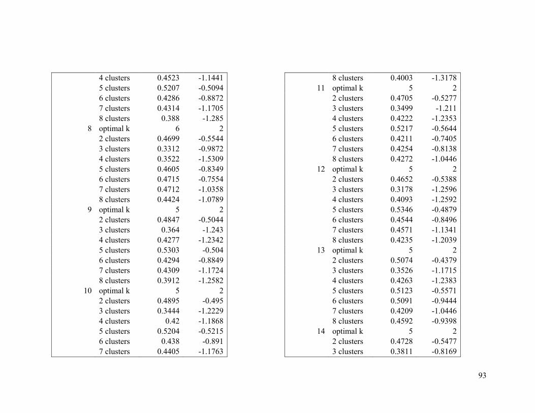
93
4 clusters 0.4523 -1.1441 5 clusters 0.5207 -0.5094 6 clusters 0.4286 -0.8872 7 clusters 0.4314 -1.1705 8 clusters 0.388 -1.285
8 optimal k 6 2 2 clusters 0.4699 -0.5544 3 clusters 0.3312 -0.9872 4 clusters 0.3522 -1.5309 5 clusters 0.4605 -0.8349 6 clusters 0.4715 -0.7554 7 clusters 0.4712 -1.0358 8 clusters 0.4424 -1.0789
9 optimal k 5 2 2 clusters 0.4847 -0.5044 3 clusters 0.364 -1.243 4 clusters 0.4277 -1.2342 5 clusters 0.5303 -0.504 6 clusters 0.4294 -0.8849 7 clusters 0.4309 -1.1724 8 clusters 0.3912 -1.2582
10 optimal k 5 2 2 clusters 0.4895 -0.495 3 clusters 0.3444 -1.2229 4 clusters 0.42 -1.1868 5 clusters 0.5204 -0.5215 6 clusters 0.438 -0.891 7 clusters 0.4405 -1.1763
8 clusters 0.4003 -1.3178 11 optimal k 5 2
2 clusters 0.4705 -0.5277 3 clusters 0.3499 -1.211 4 clusters 0.4222 -1.2353 5 clusters 0.5217 -0.5644 6 clusters 0.4211 -0.7405 7 clusters 0.4254 -0.8138 8 clusters 0.4272 -1.0446
12 optimal k 5 2 2 clusters 0.4652 -0.5388 3 clusters 0.3178 -1.2596 4 clusters 0.4093 -1.2592 5 clusters 0.5346 -0.4879 6 clusters 0.4544 -0.8496 7 clusters 0.4571 -1.1341 8 clusters 0.4235 -1.2039
13 optimal k 5 2 2 clusters 0.5074 -0.4379 3 clusters 0.3526 -1.1715 4 clusters 0.4263 -1.2383 5 clusters 0.5123 -0.5571 6 clusters 0.5091 -0.9444 7 clusters 0.4209 -1.0446 8 clusters 0.4592 -0.9398
14 optimal k 5 2 2 clusters 0.4728 -0.5477 3 clusters 0.3811 -0.8169
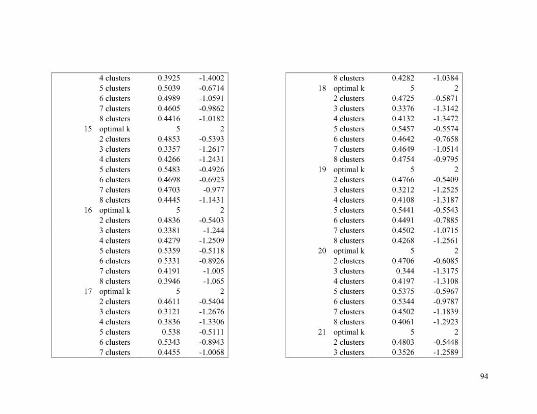
94
4 clusters 0.3925 -1.4002 5 clusters 0.5039 -0.6714 6 clusters 0.4989 -1.0591 7 clusters 0.4605 -0.9862 8 clusters 0.4416 -1.0182
15 optimal k 5 2 2 clusters 0.4853 -0.5393 3 clusters 0.3357 -1.2617 4 clusters 0.4266 -1.2431 5 clusters 0.5483 -0.4926 6 clusters 0.4698 -0.6923 7 clusters 0.4703 -0.977 8 clusters 0.4445 -1.1431
16 optimal k 5 2 2 clusters 0.4836 -0.5403 3 clusters 0.3381 -1.244 4 clusters 0.4279 -1.2509 5 clusters 0.5359 -0.5118 6 clusters 0.5331 -0.8926 7 clusters 0.4191 -1.005 8 clusters 0.3946 -1.065
17 optimal k 5 2 2 clusters 0.4611 -0.5404 3 clusters 0.3121 -1.2676 4 clusters 0.3836 -1.3306 5 clusters 0.538 -0.5111 6 clusters 0.5343 -0.8943 7 clusters 0.4455 -1.0068
8 clusters 0.4282 -1.0384 18 optimal k 5 2
2 clusters 0.4725 -0.5871 3 clusters 0.3376 -1.3142 4 clusters 0.4132 -1.3472 5 clusters 0.5457 -0.5574 6 clusters 0.4642 -0.7658 7 clusters 0.4649 -1.0514 8 clusters 0.4754 -0.9795
19 optimal k 5 2 2 clusters 0.4766 -0.5409 3 clusters 0.3212 -1.2525 4 clusters 0.4108 -1.3187 5 clusters 0.5441 -0.5543 6 clusters 0.4491 -0.7885 7 clusters 0.4502 -1.0715 8 clusters 0.4268 -1.2561
20 optimal k 5 2 2 clusters 0.4706 -0.6085 3 clusters 0.344 -1.3175 4 clusters 0.4197 -1.3108 5 clusters 0.5375 -0.5967 6 clusters 0.5344 -0.9787 7 clusters 0.4502 -1.1839 8 clusters 0.4061 -1.2923
21 optimal k 5 2 2 clusters 0.4803 -0.5448 3 clusters 0.3526 -1.2589
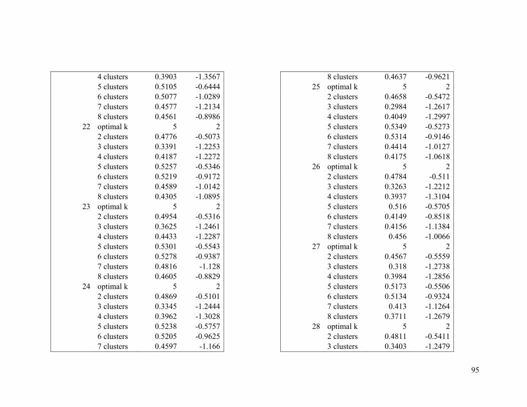
95
4 clusters 0.3903 -1.3567 5 clusters 0.5105 -0.6444 6 clusters 0.5077 -1.0289 7 clusters 0.4577 -1.2134 8 clusters 0.4561 -0.8986
22 optimal k 5 2 2 clusters 0.4776 -0.5073 3 clusters 0.3391 -1.2253 4 clusters 0.4187 -1.2272 5 clusters 0.5257 -0.5346 6 clusters 0.5219 -0.9172 7 clusters 0.4589 -1.0142 8 clusters 0.4305 -1.0895
23 optimal k 5 2 2 clusters 0.4954 -0.5316 3 clusters 0.3625 -1.2461 4 clusters 0.4433 -1.2287 5 clusters 0.5301 -0.5543 6 clusters 0.5278 -0.9387 7 clusters 0.4816 -1.128 8 clusters 0.4605 -0.8829
24 optimal k 5 2 2 clusters 0.4869 -0.5101 3 clusters 0.3345 -1.2444 4 clusters 0.3962 -1.3028 5 clusters 0.5238 -0.5757 6 clusters 0.5205 -0.9625 7 clusters 0.4597 -1.166
8 clusters 0.4637 -0.9621 25 optimal k 5 2
2 clusters 0.4658 -0.5472 3 clusters 0.2984 -1.2617 4 clusters 0.4049 -1.2997 5 clusters 0.5349 -0.5273 6 clusters 0.5314 -0.9146 7 clusters 0.4414 -1.0127 8 clusters 0.4175 -1.0618
26 optimal k 5 2 2 clusters 0.4784 -0.511 3 clusters 0.3263 -1.2212 4 clusters 0.3937 -1.3104 5 clusters 0.516 -0.5705 6 clusters 0.4149 -0.8518 7 clusters 0.4156 -1.1384 8 clusters 0.456 -1.0066
27 optimal k 5 2 2 clusters 0.4567 -0.5559 3 clusters 0.318 -1.2738 4 clusters 0.3984 -1.2856 5 clusters 0.5173 -0.5506 6 clusters 0.5134 -0.9324 7 clusters 0.413 -1.1264 8 clusters 0.3711 -1.2679
28 optimal k 5 2 2 clusters 0.4811 -0.5411 3 clusters 0.3403 -1.2479
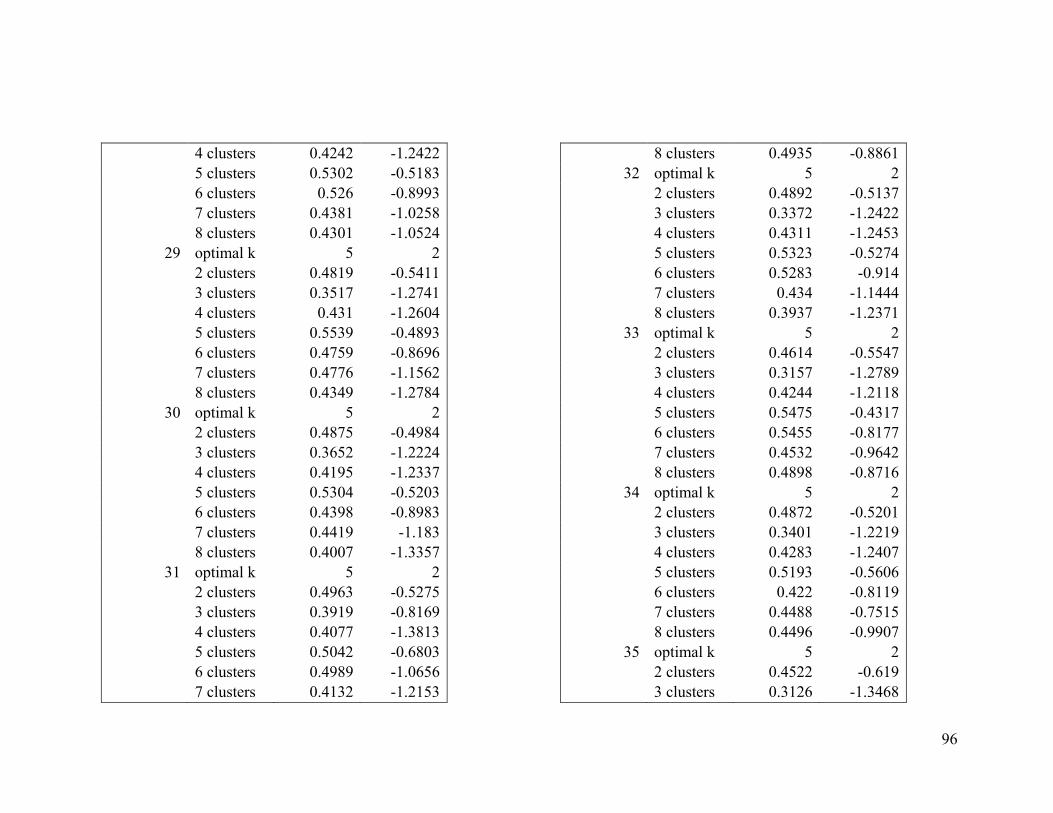
96
4 clusters 0.4242 -1.2422 5 clusters 0.5302 -0.5183 6 clusters 0.526 -0.8993 7 clusters 0.4381 -1.0258 8 clusters 0.4301 -1.0524
29 optimal k 5 2 2 clusters 0.4819 -0.5411 3 clusters 0.3517 -1.2741 4 clusters 0.431 -1.2604 5 clusters 0.5539 -0.4893 6 clusters 0.4759 -0.8696 7 clusters 0.4776 -1.1562 8 clusters 0.4349 -1.2784
30 optimal k 5 2 2 clusters 0.4875 -0.4984 3 clusters 0.3652 -1.2224 4 clusters 0.4195 -1.2337 5 clusters 0.5304 -0.5203 6 clusters 0.4398 -0.8983 7 clusters 0.4419 -1.183 8 clusters 0.4007 -1.3357
31 optimal k 5 2 2 clusters 0.4963 -0.5275 3 clusters 0.3919 -0.8169 4 clusters 0.4077 -1.3813 5 clusters 0.5042 -0.6803 6 clusters 0.4989 -1.0656 7 clusters 0.4132 -1.2153
8 clusters 0.4935 -0.8861 32 optimal k 5 2
2 clusters 0.4892 -0.5137 3 clusters 0.3372 -1.2422 4 clusters 0.4311 -1.2453 5 clusters 0.5323 -0.5274 6 clusters 0.5283 -0.914 7 clusters 0.434 -1.1444 8 clusters 0.3937 -1.2371
33 optimal k 5 2 2 clusters 0.4614 -0.5547 3 clusters 0.3157 -1.2789 4 clusters 0.4244 -1.2118 5 clusters 0.5475 -0.4317 6 clusters 0.5455 -0.8177 7 clusters 0.4532 -0.9642 8 clusters 0.4898 -0.8716
34 optimal k 5 2 2 clusters 0.4872 -0.5201 3 clusters 0.3401 -1.2219 4 clusters 0.4283 -1.2407 5 clusters 0.5193 -0.5606 6 clusters 0.422 -0.8119 7 clusters 0.4488 -0.7515 8 clusters 0.4496 -0.9907
35 optimal k 5 2 2 clusters 0.4522 -0.619 3 clusters 0.3126 -1.3468
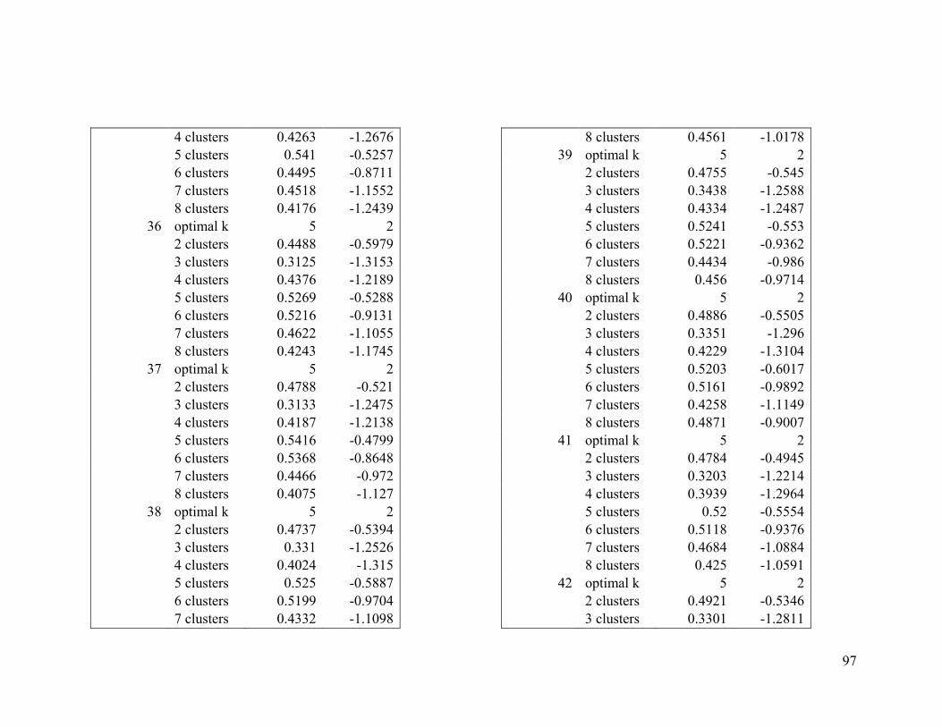
97
4 clusters 0.4263 -1.2676 5 clusters 0.541 -0.5257 6 clusters 0.4495 -0.8711 7 clusters 0.4518 -1.1552 8 clusters 0.4176 -1.2439
36 optimal k 5 2 2 clusters 0.4488 -0.5979 3 clusters 0.3125 -1.3153 4 clusters 0.4376 -1.2189 5 clusters 0.5269 -0.5288 6 clusters 0.5216 -0.9131 7 clusters 0.4622 -1.1055 8 clusters 0.4243 -1.1745
37 optimal k 5 2 2 clusters 0.4788 -0.521 3 clusters 0.3133 -1.2475 4 clusters 0.4187 -1.2138 5 clusters 0.5416 -0.4799 6 clusters 0.5368 -0.8648 7 clusters 0.4466 -0.972 8 clusters 0.4075 -1.127
38 optimal k 5 2 2 clusters 0.4737 -0.5394 3 clusters 0.331 -1.2526 4 clusters 0.4024 -1.315 5 clusters 0.525 -0.5887 6 clusters 0.5199 -0.9704 7 clusters 0.4332 -1.1098
8 clusters 0.4561 -1.0178 39 optimal k 5 2
2 clusters 0.4755 -0.545 3 clusters 0.3438 -1.2588 4 clusters 0.4334 -1.2487 5 clusters 0.5241 -0.553 6 clusters 0.5221 -0.9362 7 clusters 0.4434 -0.986 8 clusters 0.456 -0.9714
40 optimal k 5 2 2 clusters 0.4886 -0.5505 3 clusters 0.3351 -1.296 4 clusters 0.4229 -1.3104 5 clusters 0.5203 -0.6017 6 clusters 0.5161 -0.9892 7 clusters 0.4258 -1.1149 8 clusters 0.4871 -0.9007
41 optimal k 5 2 2 clusters 0.4784 -0.4945 3 clusters 0.3203 -1.2214 4 clusters 0.3939 -1.2964 5 clusters 0.52 -0.5554 6 clusters 0.5118 -0.9376 7 clusters 0.4684 -1.0884 8 clusters 0.425 -1.0591
42 optimal k 5 2 2 clusters 0.4921 -0.5346 3 clusters 0.3301 -1.2811
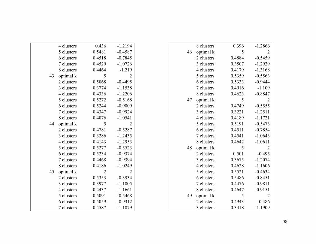
98
4 clusters 0.436 -1.2194 5 clusters 0.5481 -0.4587 6 clusters 0.4518 -0.7845 7 clusters 0.4529 -1.0726 8 clusters 0.4464 -1.219
43 optimal k 5 2 2 clusters 0.5068 -0.4495 3 clusters 0.3774 -1.1538 4 clusters 0.4336 -1.2206 5 clusters 0.5272 -0.5168 6 clusters 0.5244 -0.9009 7 clusters 0.4347 -0.9924 8 clusters 0.4076 -1.0541
44 optimal k 5 2 2 clusters 0.4781 -0.5287 3 clusters 0.3286 -1.2435 4 clusters 0.4143 -1.2953 5 clusters 0.5277 -0.5523 6 clusters 0.5234 -0.9374 7 clusters 0.4468 -0.9394 8 clusters 0.4186 -1.0249
45 optimal k 2 2 2 clusters 0.5353 -0.3934 3 clusters 0.3977 -1.1005 4 clusters 0.4437 -1.1661 5 clusters 0.5091 -0.5468 6 clusters 0.5059 -0.9312 7 clusters 0.4587 -1.1079
8 clusters 0.396 -1.2866 46 optimal k 5 2
2 clusters 0.4884 -0.5459 3 clusters 0.3507 -1.2929 4 clusters 0.4179 -1.3168 5 clusters 0.5359 -0.5563 6 clusters 0.5333 -0.9444 7 clusters 0.4916 -1.109 8 clusters 0.4623 -0.8847
47 optimal k 5 2 2 clusters 0.4749 -0.5555 3 clusters 0.3221 -1.2511 4 clusters 0.4189 -1.1721 5 clusters 0.5191 -0.5473 6 clusters 0.4511 -0.7854 7 clusters 0.4541 -1.0643 8 clusters 0.4642 -1.0611
48 optimal k 5 2 2 clusters 0.501 -0.495 3 clusters 0.3675 -1.2074 4 clusters 0.4628 -1.1606 5 clusters 0.5521 -0.4634 6 clusters 0.5486 -0.8451 7 clusters 0.4476 -0.9811 8 clusters 0.4647 -0.9151
49 optimal k 5 2 2 clusters 0.4943 -0.486 3 clusters 0.3418 -1.1909
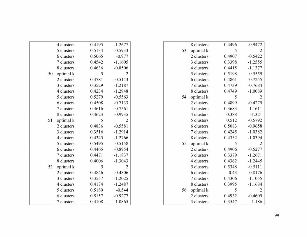
99
4 clusters 0.4195 -1.2677 5 clusters 0.5134 -0.5933 6 clusters 0.5065 -0.977 7 clusters 0.4542 -1.1605 8 clusters 0.4636 -0.8506
50 optimal k 5 2 2 clusters 0.4781 -0.5143 3 clusters 0.3529 -1.2187 4 clusters 0.4234 -1.2948 5 clusters 0.5279 -0.5563 6 clusters 0.4508 -0.7133 7 clusters 0.4616 -0.7561 8 clusters 0.4623 -0.9935
51 optimal k 5 2 2 clusters 0.4836 -0.5581 3 clusters 0.3516 -1.2914 4 clusters 0.4345 -1.2766 5 clusters 0.5495 -0.5158 6 clusters 0.4465 -0.8954 7 clusters 0.4471 -1.1837 8 clusters 0.4006 -1.3043
52 optimal k 5 2 2 clusters 0.4846 -0.4806 3 clusters 0.3557 -1.2025 4 clusters 0.4174 -1.2487 5 clusters 0.5189 -0.544 6 clusters 0.5157 -0.9277 7 clusters 0.4108 -1.0865
8 clusters 0.4496 -0.9472 53 optimal k 5 2
2 clusters 0.4907 -0.5422 3 clusters 0.3398 -1.2555 4 clusters 0.4415 -1.1377 5 clusters 0.5198 -0.5559 6 clusters 0.4861 -0.7255 7 clusters 0.4739 -0.7684 8 clusters 0.4749 -1.0089
54 optimal k 5 2 2 clusters 0.4899 -0.4279 3 clusters 0.3683 -1.1611 4 clusters 0.388 -1.321 5 clusters 0.512 -0.5792 6 clusters 0.5083 -0.9658 7 clusters 0.4245 -1.0382 8 clusters 0.4352 -1.0394
55 optimal k 5 2 2 clusters 0.4906 -0.5277 3 clusters 0.3379 -1.2671 4 clusters 0.4362 -1.2445 5 clusters 0.5348 -0.5111 6 clusters 0.43 -0.8176 7 clusters 0.4306 -1.1055 8 clusters 0.3995 -1.1684
56 optimal k 5 2 2 clusters 0.4932 -0.4609 3 clusters 0.3547 -1.186
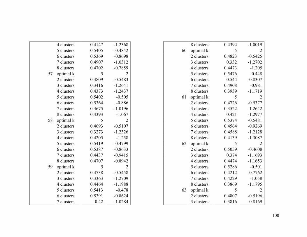
100
4 clusters 0.4147 -1.2368 5 clusters 0.5405 -0.4842 6 clusters 0.5369 -0.8698 7 clusters 0.4907 -1.0312 8 clusters 0.4702 -0.7859
57 optimal k 5 2 2 clusters 0.4809 -0.5483 3 clusters 0.3416 -1.2641 4 clusters 0.4373 -1.2437 5 clusters 0.5402 -0.505 6 clusters 0.5364 -0.886 7 clusters 0.4675 -1.0196 8 clusters 0.4393 -1.067
58 optimal k 5 2 2 clusters 0.4693 -0.5107 3 clusters 0.3273 -1.2326 4 clusters 0.4205 -1.258 5 clusters 0.5419 -0.4799 6 clusters 0.5387 -0.8633 7 clusters 0.4437 -0.9415 8 clusters 0.4707 -0.8942
59 optimal k 5 2 2 clusters 0.4738 -0.5458 3 clusters 0.3363 -1.2709 4 clusters 0.4464 -1.1988 5 clusters 0.5413 -0.478 6 clusters 0.5391 -0.8624 7 clusters 0.42 -1.0284
8 clusters 0.4394 -1.0019 60 optimal k 5 2
2 clusters 0.4823 -0.5425 3 clusters 0.332 -1.2702 4 clusters 0.4473 -1.205 5 clusters 0.5476 -0.448 6 clusters 0.544 -0.8307 7 clusters 0.4908 -0.981 8 clusters 0.3939 -1.1719
61 optimal k 5 2 2 clusters 0.4726 -0.5377 3 clusters 0.3522 -1.2642 4 clusters 0.421 -1.2977 5 clusters 0.5374 -0.5481 6 clusters 0.4564 -0.9269 7 clusters 0.4588 -1.2128 8 clusters 0.4139 -1.3087
62 optimal k 5 2 2 clusters 0.5059 -0.4608 3 clusters 0.374 -1.1693 4 clusters 0.4474 -1.1653 5 clusters 0.5286 -0.501 6 clusters 0.4212 -0.7762 7 clusters 0.4229 -1.058 8 clusters 0.3869 -1.1795
63 optimal k 5 2 2 clusters 0.4807 -0.5196 3 clusters 0.3816 -0.8169
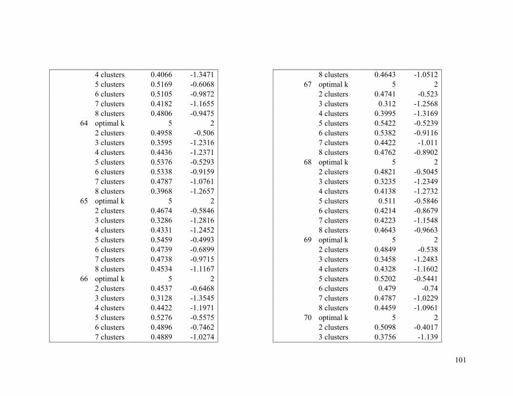
101
4 clusters 0.4066 -1.3471 5 clusters 0.5169 -0.6068 6 clusters 0.5105 -0.9872 7 clusters 0.4182 -1.1655 8 clusters 0.4806 -0.9475
64 optimal k 5 2 2 clusters 0.4958 -0.506 3 clusters 0.3595 -1.2316 4 clusters 0.4436 -1.2371 5 clusters 0.5376 -0.5293 6 clusters 0.5338 -0.9159 7 clusters 0.4787 -1.0761 8 clusters 0.3968 -1.2657
65 optimal k 5 2 2 clusters 0.4674 -0.5846 3 clusters 0.3286 -1.2816 4 clusters 0.4331 -1.2452 5 clusters 0.5459 -0.4993 6 clusters 0.4739 -0.6899 7 clusters 0.4738 -0.9715 8 clusters 0.4534 -1.1167
66 optimal k 5 2 2 clusters 0.4537 -0.6468 3 clusters 0.3128 -1.3545 4 clusters 0.4422 -1.1971 5 clusters 0.5276 -0.5575 6 clusters 0.4896 -0.7462 7 clusters 0.4889 -1.0274
8 clusters 0.4643 -1.0512 67 optimal k 5 2
2 clusters 0.4741 -0.523 3 clusters 0.312 -1.2568 4 clusters 0.3995 -1.3169 5 clusters 0.5422 -0.5239 6 clusters 0.5382 -0.9116 7 clusters 0.4422 -1.011 8 clusters 0.4762 -0.8902
68 optimal k 5 2 2 clusters 0.4821 -0.5045 3 clusters 0.3235 -1.2349 4 clusters 0.4138 -1.2732 5 clusters 0.511 -0.5846 6 clusters 0.4214 -0.8679 7 clusters 0.4223 -1.1548 8 clusters 0.4643 -0.9663
69 optimal k 5 2 2 clusters 0.4849 -0.538 3 clusters 0.3458 -1.2483 4 clusters 0.4328 -1.1602 5 clusters 0.5202 -0.5441 6 clusters 0.479 -0.74 7 clusters 0.4787 -1.0229 8 clusters 0.4459 -1.0961
70 optimal k 5 2 2 clusters 0.5098 -0.4017 3 clusters 0.3756 -1.139
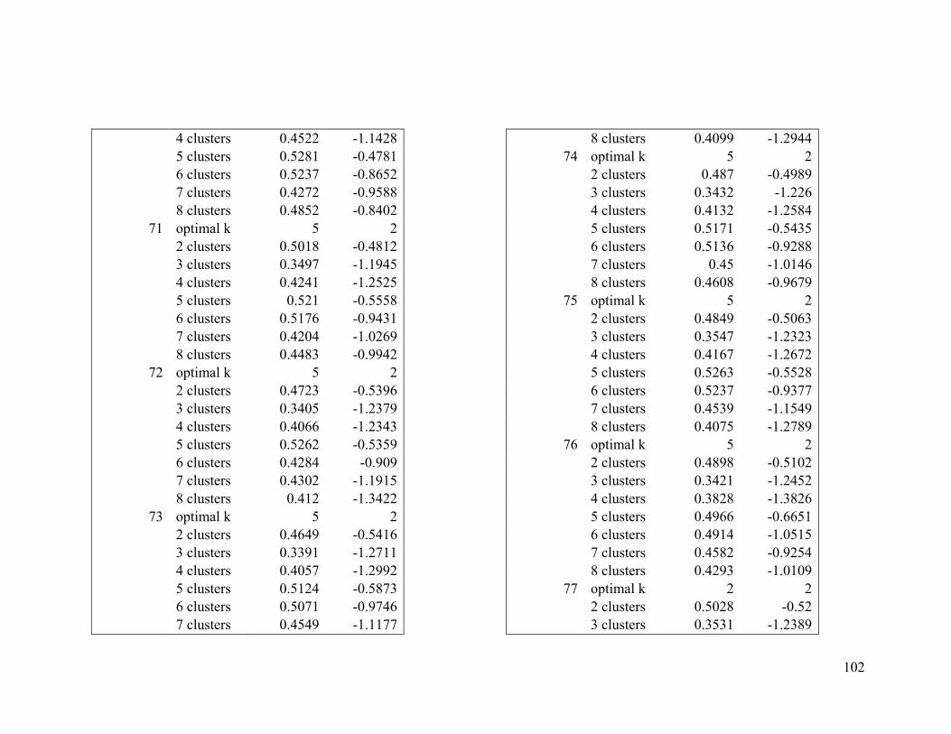
102
4 clusters 0.4522 -1.1428 5 clusters 0.5281 -0.4781 6 clusters 0.5237 -0.8652 7 clusters 0.4272 -0.9588 8 clusters 0.4852 -0.8402
71 optimal k 5 2 2 clusters 0.5018 -0.4812 3 clusters 0.3497 -1.1945 4 clusters 0.4241 -1.2525 5 clusters 0.521 -0.5558 6 clusters 0.5176 -0.9431 7 clusters 0.4204 -1.0269 8 clusters 0.4483 -0.9942
72 optimal k 5 2 2 clusters 0.4723 -0.5396 3 clusters 0.3405 -1.2379 4 clusters 0.4066 -1.2343 5 clusters 0.5262 -0.5359 6 clusters 0.4284 -0.909 7 clusters 0.4302 -1.1915 8 clusters 0.412 -1.3422
73 optimal k 5 2 2 clusters 0.4649 -0.5416 3 clusters 0.3391 -1.2711 4 clusters 0.4057 -1.2992 5 clusters 0.5124 -0.5873 6 clusters 0.5071 -0.9746 7 clusters 0.4549 -1.1177
8 clusters 0.4099 -1.2944 74 optimal k 5 2
2 clusters 0.487 -0.4989 3 clusters 0.3432 -1.226 4 clusters 0.4132 -1.2584 5 clusters 0.5171 -0.5435 6 clusters 0.5136 -0.9288 7 clusters 0.45 -1.0146 8 clusters 0.4608 -0.9679
75 optimal k 5 2 2 clusters 0.4849 -0.5063 3 clusters 0.3547 -1.2323 4 clusters 0.4167 -1.2672 5 clusters 0.5263 -0.5528 6 clusters 0.5237 -0.9377 7 clusters 0.4539 -1.1549 8 clusters 0.4075 -1.2789
76 optimal k 5 2 2 clusters 0.4898 -0.5102 3 clusters 0.3421 -1.2452 4 clusters 0.3828 -1.3826 5 clusters 0.4966 -0.6651 6 clusters 0.4914 -1.0515 7 clusters 0.4582 -0.9254 8 clusters 0.4293 -1.0109
77 optimal k 2 2 2 clusters 0.5028 -0.52 3 clusters 0.3531 -1.2389
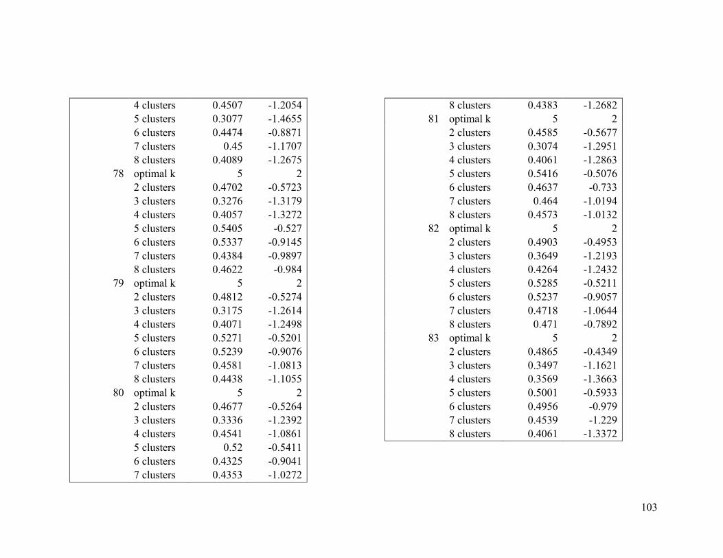
103
4 clusters 0.4507 -1.2054 5 clusters 0.3077 -1.4655 6 clusters 0.4474 -0.8871 7 clusters 0.45 -1.1707 8 clusters 0.4089 -1.2675
78 optimal k 5 2 2 clusters 0.4702 -0.5723 3 clusters 0.3276 -1.3179 4 clusters 0.4057 -1.3272 5 clusters 0.5405 -0.527 6 clusters 0.5337 -0.9145 7 clusters 0.4384 -0.9897 8 clusters 0.4622 -0.984
79 optimal k 5 2 2 clusters 0.4812 -0.5274 3 clusters 0.3175 -1.2614 4 clusters 0.4071 -1.2498 5 clusters 0.5271 -0.5201 6 clusters 0.5239 -0.9076 7 clusters 0.4581 -1.0813 8 clusters 0.4438 -1.1055
80 optimal k 5 2 2 clusters 0.4677 -0.5264 3 clusters 0.3336 -1.2392 4 clusters 0.4541 -1.0861 5 clusters 0.52 -0.5411 6 clusters 0.4325 -0.9041 7 clusters 0.4353 -1.0272
8 clusters 0.4383 -1.2682 81 optimal k 5 2
2 clusters 0.4585 -0.5677 3 clusters 0.3074 -1.2951 4 clusters 0.4061 -1.2863 5 clusters 0.5416 -0.5076 6 clusters 0.4637 -0.733 7 clusters 0.464 -1.0194 8 clusters 0.4573 -1.0132
82 optimal k 5 2 2 clusters 0.4903 -0.4953 3 clusters 0.3649 -1.2193 4 clusters 0.4264 -1.2432 5 clusters 0.5285 -0.5211 6 clusters 0.5237 -0.9057 7 clusters 0.4718 -1.0644 8 clusters 0.471 -0.7892
83 optimal k 5 2 2 clusters 0.4865 -0.4349 3 clusters 0.3497 -1.1621 4 clusters 0.3569 -1.3663 5 clusters 0.5001 -0.5933 6 clusters 0.4956 -0.979 7 clusters 0.4539 -1.229 8 clusters 0.4061 -1.3372
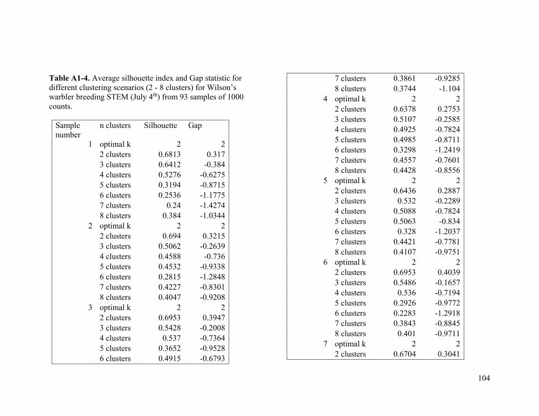
104
Table A1-4. Average silhouette index and Gap statistic for different clustering scenarios (2 - 8 clusters) for Wilson’s warbler breeding STEM (July 4th) from 93 samples of 1000 counts.
Sample number
n clusters Silhouette Gap
1 optimal k 2 2 2 clusters 0.6813 0.317 3 clusters 0.6412 -0.384 4 clusters 0.5276 -0.6275 5 clusters 0.3194 -0.8715 6 clusters 0.2536 -1.1775 7 clusters 0.24 -1.4274 8 clusters 0.384 -1.0344
2 optimal k 2 2 2 clusters 0.694 0.3215 3 clusters 0.5062 -0.2639 4 clusters 0.4588 -0.736 5 clusters 0.4532 -0.9338 6 clusters 0.2815 -1.2848 7 clusters 0.4227 -0.8301 8 clusters 0.4047 -0.9208
3 optimal k 2 2 2 clusters 0.6953 0.3947 3 clusters 0.5428 -0.2008 4 clusters 0.537 -0.7364 5 clusters 0.3652 -0.9528 6 clusters 0.4915 -0.6793
7 clusters 0.3861 -0.9285 8 clusters 0.3744 -1.104
4 optimal k 2 2 2 clusters 0.6378 0.2753 3 clusters 0.5107 -0.2585 4 clusters 0.4925 -0.7824 5 clusters 0.4985 -0.8711 6 clusters 0.3298 -1.2419 7 clusters 0.4557 -0.7601 8 clusters 0.4428 -0.8556
5 optimal k 2 2 2 clusters 0.6436 0.2887 3 clusters 0.532 -0.2289 4 clusters 0.5088 -0.7824 5 clusters 0.5063 -0.834 6 clusters 0.328 -1.2037 7 clusters 0.4421 -0.7781 8 clusters 0.4107 -0.9751
6 optimal k 2 2 2 clusters 0.6953 0.4039 3 clusters 0.5486 -0.1657 4 clusters 0.536 -0.7194 5 clusters 0.2926 -0.9772 6 clusters 0.2283 -1.2918 7 clusters 0.3843 -0.8845 8 clusters 0.401 -0.9711
7 optimal k 2 2 2 clusters 0.6704 0.3041
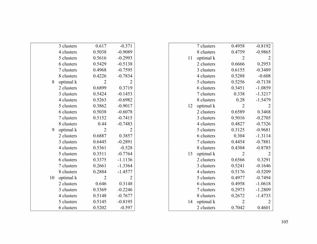
105
3 clusters 0.617 -0.371 4 clusters 0.5038 -0.9089 5 clusters 0.5616 -0.2993 6 clusters 0.5429 -0.5138 7 clusters 0.4968 -0.7595 8 clusters 0.4226 -0.7834
8 optimal k 2 2 2 clusters 0.6899 0.3719 3 clusters 0.5424 -0.1453 4 clusters 0.5263 -0.6982 5 clusters 0.3862 -0.9017 6 clusters 0.5038 -0.6078 7 clusters 0.5152 -0.7415 8 clusters 0.44 -0.7483
9 optimal k 2 2 2 clusters 0.6887 0.3857 3 clusters 0.6445 -0.2891 4 clusters 0.5361 -0.528 5 clusters 0.3511 -0.7764 6 clusters 0.3375 -1.1136 7 clusters 0.2661 -1.3364 8 clusters 0.2884 -1.4577
10 optimal k 2 2 2 clusters 0.646 0.3148 3 clusters 0.5369 -0.2246 4 clusters 0.5148 -0.7677 5 clusters 0.5145 -0.8195 6 clusters 0.5202 -0.597
7 clusters 0.4958 -0.8192 8 clusters 0.4759 -0.9865
11 optimal k 2 2 2 clusters 0.6666 0.2953 3 clusters 0.6155 -0.3489 4 clusters 0.5288 -0.608 5 clusters 0.5256 -0.7138 6 clusters 0.3451 -1.0859 7 clusters 0.338 -1.3217 8 clusters 0.28 -1.5479
12 optimal k 2 2 2 clusters 0.6589 0.3468 3 clusters 0.5016 -0.2705 4 clusters 0.4827 -0.7326 5 clusters 0.3125 -0.9681 6 clusters 0.304 -1.3114 7 clusters 0.4454 -0.7881 8 clusters 0.4304 -0.8785
13 optimal k 2 2 2 clusters 0.6566 0.3291 3 clusters 0.5241 -0.1646 4 clusters 0.5176 -0.5209 5 clusters 0.4977 -0.7494 6 clusters 0.4958 -1.0618 7 clusters 0.2973 -1.2809 8 clusters 0.2672 -1.4733
14 optimal k 2 2 2 clusters 0.7042 0.4601
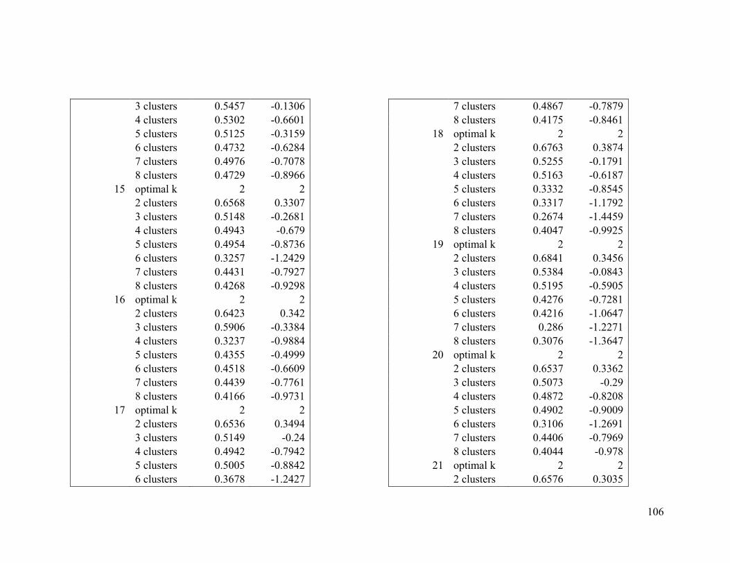
106
3 clusters 0.5457 -0.1306 4 clusters 0.5302 -0.6601 5 clusters 0.5125 -0.3159 6 clusters 0.4732 -0.6284 7 clusters 0.4976 -0.7078 8 clusters 0.4729 -0.8966
15 optimal k 2 2 2 clusters 0.6568 0.3307 3 clusters 0.5148 -0.2681 4 clusters 0.4943 -0.679 5 clusters 0.4954 -0.8736 6 clusters 0.3257 -1.2429 7 clusters 0.4431 -0.7927 8 clusters 0.4268 -0.9298
16 optimal k 2 2 2 clusters 0.6423 0.342 3 clusters 0.5906 -0.3384 4 clusters 0.3237 -0.9884 5 clusters 0.4355 -0.4999 6 clusters 0.4518 -0.6609 7 clusters 0.4439 -0.7761 8 clusters 0.4166 -0.9731
17 optimal k 2 2 2 clusters 0.6536 0.3494 3 clusters 0.5149 -0.24 4 clusters 0.4942 -0.7942 5 clusters 0.5005 -0.8842 6 clusters 0.3678 -1.2427
7 clusters 0.4867 -0.7879 8 clusters 0.4175 -0.8461
18 optimal k 2 2 2 clusters 0.6763 0.3874 3 clusters 0.5255 -0.1791 4 clusters 0.5163 -0.6187 5 clusters 0.3332 -0.8545 6 clusters 0.3317 -1.1792 7 clusters 0.2674 -1.4459 8 clusters 0.4047 -0.9925
19 optimal k 2 2 2 clusters 0.6841 0.3456 3 clusters 0.5384 -0.0843 4 clusters 0.5195 -0.5905 5 clusters 0.4276 -0.7281 6 clusters 0.4216 -1.0647 7 clusters 0.286 -1.2271 8 clusters 0.3076 -1.3647
20 optimal k 2 2 2 clusters 0.6537 0.3362 3 clusters 0.5073 -0.29 4 clusters 0.4872 -0.8208 5 clusters 0.4902 -0.9009 6 clusters 0.3106 -1.2691 7 clusters 0.4406 -0.7969 8 clusters 0.4044 -0.978
21 optimal k 2 2 2 clusters 0.6576 0.3035
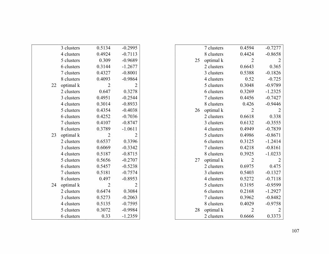
107
3 clusters 0.5134 -0.2995 4 clusters 0.4924 -0.7113 5 clusters 0.309 -0.9689 6 clusters 0.3144 -1.2677 7 clusters 0.4327 -0.8001 8 clusters 0.4093 -0.9864
22 optimal k 2 2 2 clusters 0.647 0.3278 3 clusters 0.4951 -0.2544 4 clusters 0.3014 -0.8933 5 clusters 0.4354 -0.4038 6 clusters 0.4252 -0.7036 7 clusters 0.4107 -0.8747 8 clusters 0.3789 -1.0611
23 optimal k 2 2 2 clusters 0.6537 0.3396 3 clusters 0.6069 -0.3342 4 clusters 0.5187 -0.8715 5 clusters 0.5656 -0.2707 6 clusters 0.5457 -0.5238 7 clusters 0.5181 -0.7574 8 clusters 0.497 -0.8953
24 optimal k 2 2 2 clusters 0.6474 0.3084 3 clusters 0.5273 -0.2063 4 clusters 0.5135 -0.7595 5 clusters 0.3072 -0.9984 6 clusters 0.33 -1.2359
7 clusters 0.4594 -0.7277 8 clusters 0.4424 -0.8658
25 optimal k 2 2 2 clusters 0.6643 0.365 3 clusters 0.5388 -0.1826 4 clusters 0.52 -0.725 5 clusters 0.3048 -0.9789 6 clusters 0.3269 -1.2325 7 clusters 0.4456 -0.7427 8 clusters 0.426 -0.9446
26 optimal k 2 2 2 clusters 0.6618 0.338 3 clusters 0.6132 -0.3555 4 clusters 0.4949 -0.7839 5 clusters 0.4986 -0.8671 6 clusters 0.3125 -1.2414 7 clusters 0.4218 -0.8161 8 clusters 0.3925 -1.0233
27 optimal k 2 2 2 clusters 0.6975 0.475 3 clusters 0.5403 -0.1327 4 clusters 0.5272 -0.7118 5 clusters 0.3195 -0.9599 6 clusters 0.2168 -1.2927 7 clusters 0.3962 -0.8482 8 clusters 0.4029 -0.9758
28 optimal k 2 2 2 clusters 0.6666 0.3373
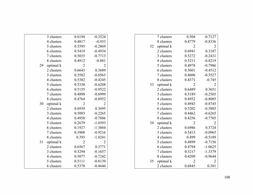
108
3 clusters 0.6194 -0.3524 4 clusters 0.4817 -0.933 5 clusters 0.5595 -0.2869 6 clusters 0.5419 -0.4934 7 clusters 0.5035 -0.7713 8 clusters 0.4912 -0.881
29 optimal k 2 2 2 clusters 0.6643 0.3689 3 clusters 0.5582 -0.0563 4 clusters 0.5382 -0.4245 5 clusters 0.5338 -0.6208 6 clusters 0.5155 -0.9522 7 clusters 0.4898 -0.6999 8 clusters 0.4764 -0.8952
30 optimal k 2 2 2 clusters 0.6939 0.3695 3 clusters 0.5093 -0.2265 4 clusters 0.4958 -0.7886 5 clusters 0.2679 -1.0393 6 clusters 0.1927 -1.3884 7 clusters 0.3908 -0.9216 8 clusters 0.393 -1.0241
31 optimal k 2 2 2 clusters 0.6567 0.3771 3 clusters 0.5294 -0.1657 4 clusters 0.5077 -0.7242 5 clusters 0.5111 -0.8139 6 clusters 0.5378 -0.4646
7 clusters 0.504 -0.7127 8 clusters 0.4779 -0.8336
32 optimal k 2 2 2 clusters 0.6941 0.3187 3 clusters 0.5272 -0.2431 4 clusters 0.5211 -0.8219 5 clusters 0.4978 -0.7986 6 clusters 0.5601 -0.4512 7 clusters 0.4606 -0.5527 8 clusters 0.4371 -0.745
33 optimal k 2 2 2 clusters 0.6489 0.3651 3 clusters 0.5189 -0.2565 4 clusters 0.4952 -0.8085 5 clusters 0.4943 -0.8745 6 clusters 0.5202 -0.5885 7 clusters 0.4462 -0.6265 8 clusters 0.4256 -0.7705
34 optimal k 2 2 2 clusters 0.6986 0.3724 3 clusters 0.5413 -0.0965 4 clusters 0.499 -0.5189 5 clusters 0.4899 -0.7156 6 clusters 0.4794 -1.0625 7 clusters 0.3217 -1.3379 8 clusters 0.4209 -0.9644
35 optimal k 2 2 2 clusters 0.6845 0.381
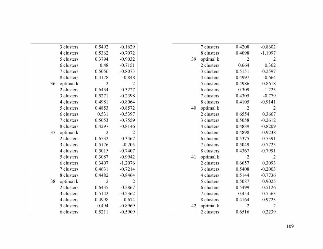
109
3 clusters 0.5492 -0.1629 4 clusters 0.5362 -0.7072 5 clusters 0.3794 -0.9032 6 clusters 0.48 -0.7151 7 clusters 0.5056 -0.8073 8 clusters 0.4178 -0.848
36 optimal k 2 2 2 clusters 0.6434 0.3227 3 clusters 0.5271 -0.2398 4 clusters 0.4981 -0.8064 5 clusters 0.4853 -0.8572 6 clusters 0.531 -0.5397 7 clusters 0.5053 -0.7559 8 clusters 0.4297 -0.8146
37 optimal k 2 2 2 clusters 0.6532 0.3467 3 clusters 0.5176 -0.205 4 clusters 0.5015 -0.7407 5 clusters 0.3087 -0.9942 6 clusters 0.3407 -1.2076 7 clusters 0.4631 -0.7214 8 clusters 0.4482 -0.8464
38 optimal k 2 2 2 clusters 0.6435 0.2867 3 clusters 0.5142 -0.2362 4 clusters 0.4998 -0.674 5 clusters 0.494 -0.8969 6 clusters 0.5211 -0.5909
7 clusters 0.4208 -0.8602 8 clusters 0.4098 -1.1097
39 optimal k 2 2 2 clusters 0.664 0.362 3 clusters 0.5151 -0.2597 4 clusters 0.4997 -0.664 5 clusters 0.4986 -0.8618 6 clusters 0.309 -1.223 7 clusters 0.4305 -0.779 8 clusters 0.4105 -0.9141
40 optimal k 2 2 2 clusters 0.6554 0.3667 3 clusters 0.5058 -0.2612 4 clusters 0.4889 -0.8209 5 clusters 0.4898 -0.9238 6 clusters 0.5375 -0.5391 7 clusters 0.5049 -0.7723 8 clusters 0.4367 -0.7991
41 optimal k 2 2 2 clusters 0.6657 0.3093 3 clusters 0.5408 -0.2003 4 clusters 0.5144 -0.7736 5 clusters 0.5087 -0.9025 6 clusters 0.5499 -0.5126 7 clusters 0.454 -0.7563 8 clusters 0.4164 -0.9723
42 optimal k 2 2 2 clusters 0.6516 0.2239
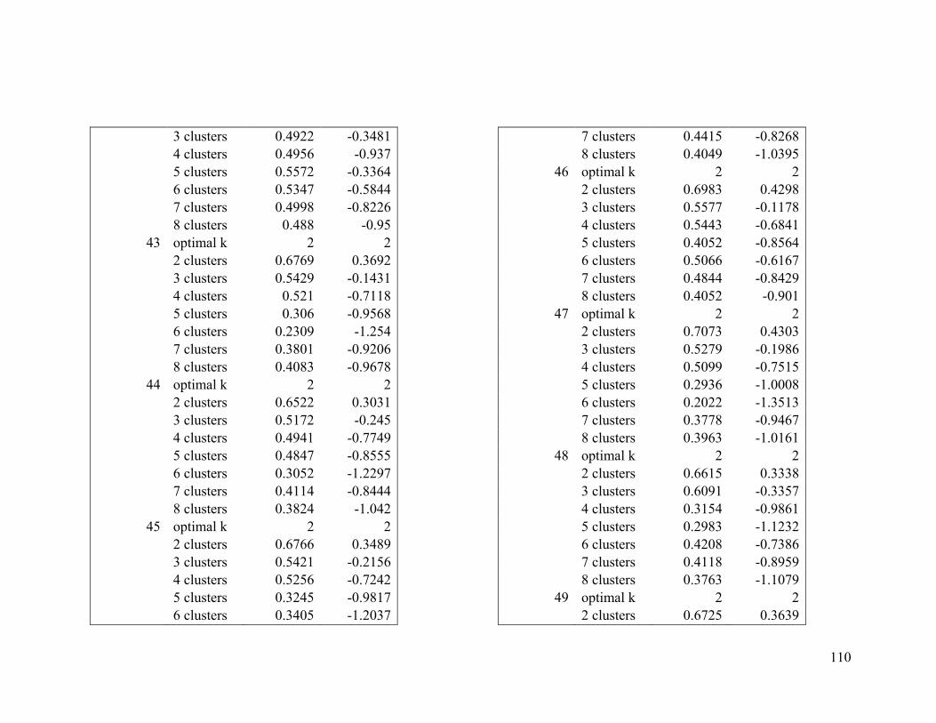
110
3 clusters 0.4922 -0.3481 4 clusters 0.4956 -0.937 5 clusters 0.5572 -0.3364 6 clusters 0.5347 -0.5844 7 clusters 0.4998 -0.8226 8 clusters 0.488 -0.95
43 optimal k 2 2 2 clusters 0.6769 0.3692 3 clusters 0.5429 -0.1431 4 clusters 0.521 -0.7118 5 clusters 0.306 -0.9568 6 clusters 0.2309 -1.254 7 clusters 0.3801 -0.9206 8 clusters 0.4083 -0.9678
44 optimal k 2 2 2 clusters 0.6522 0.3031 3 clusters 0.5172 -0.245 4 clusters 0.4941 -0.7749 5 clusters 0.4847 -0.8555 6 clusters 0.3052 -1.2297 7 clusters 0.4114 -0.8444 8 clusters 0.3824 -1.042
45 optimal k 2 2 2 clusters 0.6766 0.3489 3 clusters 0.5421 -0.2156 4 clusters 0.5256 -0.7242 5 clusters 0.3245 -0.9817 6 clusters 0.3405 -1.2037
7 clusters 0.4415 -0.8268 8 clusters 0.4049 -1.0395
46 optimal k 2 2 2 clusters 0.6983 0.4298 3 clusters 0.5577 -0.1178 4 clusters 0.5443 -0.6841 5 clusters 0.4052 -0.8564 6 clusters 0.5066 -0.6167 7 clusters 0.4844 -0.8429 8 clusters 0.4052 -0.901
47 optimal k 2 2 2 clusters 0.7073 0.4303 3 clusters 0.5279 -0.1986 4 clusters 0.5099 -0.7515 5 clusters 0.2936 -1.0008 6 clusters 0.2022 -1.3513 7 clusters 0.3778 -0.9467 8 clusters 0.3963 -1.0161
48 optimal k 2 2 2 clusters 0.6615 0.3338 3 clusters 0.6091 -0.3357 4 clusters 0.3154 -0.9861 5 clusters 0.2983 -1.1232 6 clusters 0.4208 -0.7386 7 clusters 0.4118 -0.8959 8 clusters 0.3763 -1.1079
49 optimal k 2 2 2 clusters 0.6725 0.3639
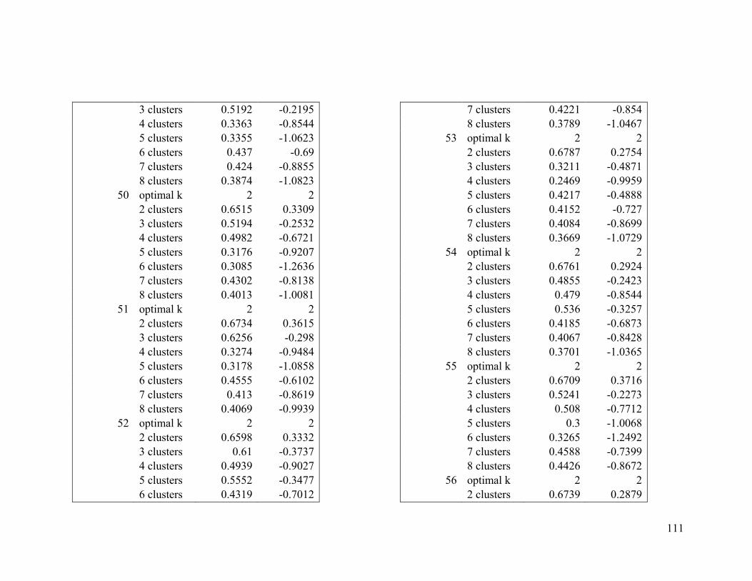
111
3 clusters 0.5192 -0.2195 4 clusters 0.3363 -0.8544 5 clusters 0.3355 -1.0623 6 clusters 0.437 -0.69 7 clusters 0.424 -0.8855 8 clusters 0.3874 -1.0823
50 optimal k 2 2 2 clusters 0.6515 0.3309 3 clusters 0.5194 -0.2532 4 clusters 0.4982 -0.6721 5 clusters 0.3176 -0.9207 6 clusters 0.3085 -1.2636 7 clusters 0.4302 -0.8138 8 clusters 0.4013 -1.0081
51 optimal k 2 2 2 clusters 0.6734 0.3615 3 clusters 0.6256 -0.298 4 clusters 0.3274 -0.9484 5 clusters 0.3178 -1.0858 6 clusters 0.4555 -0.6102 7 clusters 0.413 -0.8619 8 clusters 0.4069 -0.9939
52 optimal k 2 2 2 clusters 0.6598 0.3332 3 clusters 0.61 -0.3737 4 clusters 0.4939 -0.9027 5 clusters 0.5552 -0.3477 6 clusters 0.4319 -0.7012
7 clusters 0.4221 -0.854 8 clusters 0.3789 -1.0467
53 optimal k 2 2 2 clusters 0.6787 0.2754 3 clusters 0.3211 -0.4871 4 clusters 0.2469 -0.9959 5 clusters 0.4217 -0.4888 6 clusters 0.4152 -0.727 7 clusters 0.4084 -0.8699 8 clusters 0.3669 -1.0729
54 optimal k 2 2 2 clusters 0.6761 0.2924 3 clusters 0.4855 -0.2423 4 clusters 0.479 -0.8544 5 clusters 0.536 -0.3257 6 clusters 0.4185 -0.6873 7 clusters 0.4067 -0.8428 8 clusters 0.3701 -1.0365
55 optimal k 2 2 2 clusters 0.6709 0.3716 3 clusters 0.5241 -0.2273 4 clusters 0.508 -0.7712 5 clusters 0.3 -1.0068 6 clusters 0.3265 -1.2492 7 clusters 0.4588 -0.7399 8 clusters 0.4426 -0.8672
56 optimal k 2 2 2 clusters 0.6739 0.2879
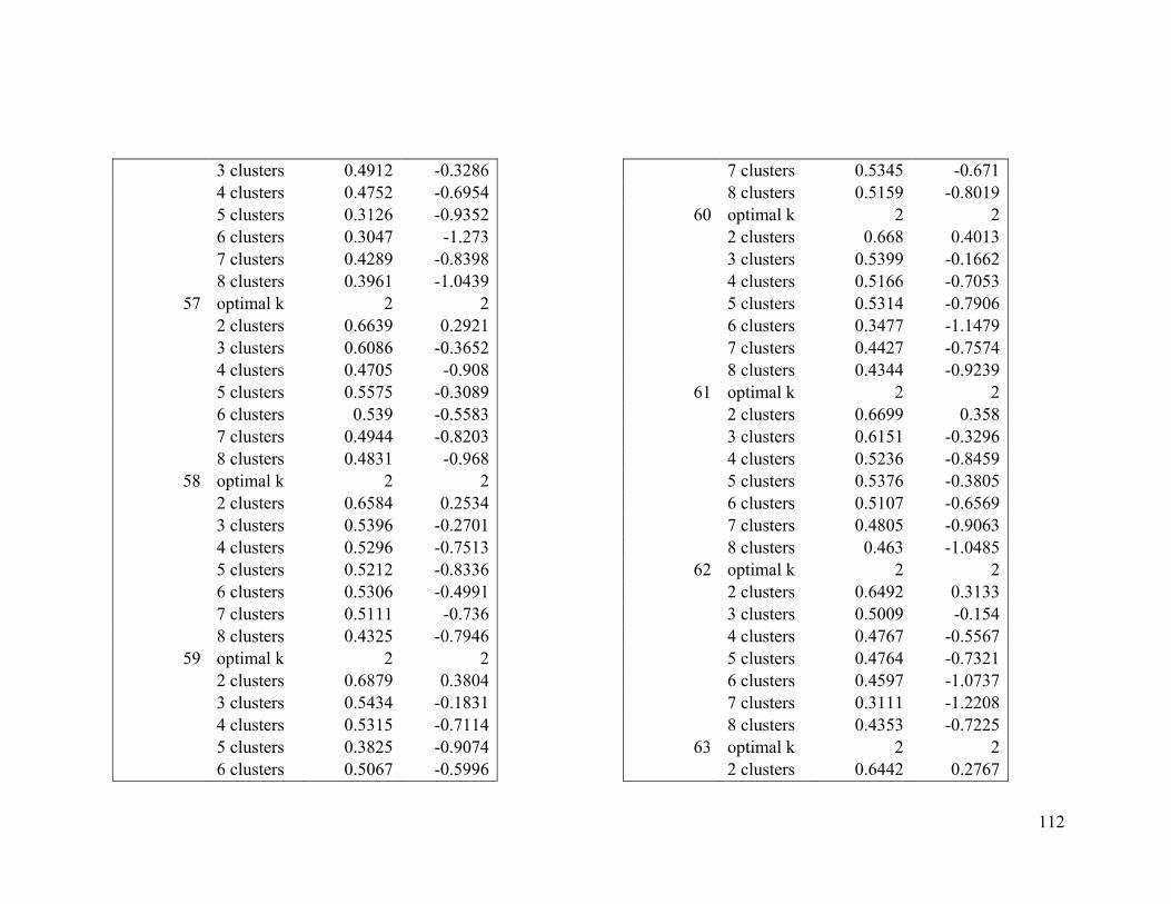
112
3 clusters 0.4912 -0.3286 4 clusters 0.4752 -0.6954 5 clusters 0.3126 -0.9352 6 clusters 0.3047 -1.273 7 clusters 0.4289 -0.8398 8 clusters 0.3961 -1.0439
57 optimal k 2 2 2 clusters 0.6639 0.2921 3 clusters 0.6086 -0.3652 4 clusters 0.4705 -0.908 5 clusters 0.5575 -0.3089 6 clusters 0.539 -0.5583 7 clusters 0.4944 -0.8203 8 clusters 0.4831 -0.968
58 optimal k 2 2 2 clusters 0.6584 0.2534 3 clusters 0.5396 -0.2701 4 clusters 0.5296 -0.7513 5 clusters 0.5212 -0.8336 6 clusters 0.5306 -0.4991 7 clusters 0.5111 -0.736 8 clusters 0.4325 -0.7946
59 optimal k 2 2 2 clusters 0.6879 0.3804 3 clusters 0.5434 -0.1831 4 clusters 0.5315 -0.7114 5 clusters 0.3825 -0.9074 6 clusters 0.5067 -0.5996
7 clusters 0.5345 -0.671 8 clusters 0.5159 -0.8019
60 optimal k 2 2 2 clusters 0.668 0.4013 3 clusters 0.5399 -0.1662 4 clusters 0.5166 -0.7053 5 clusters 0.5314 -0.7906 6 clusters 0.3477 -1.1479 7 clusters 0.4427 -0.7574 8 clusters 0.4344 -0.9239
61 optimal k 2 2 2 clusters 0.6699 0.358 3 clusters 0.6151 -0.3296 4 clusters 0.5236 -0.8459 5 clusters 0.5376 -0.3805 6 clusters 0.5107 -0.6569 7 clusters 0.4805 -0.9063 8 clusters 0.463 -1.0485
62 optimal k 2 2 2 clusters 0.6492 0.3133 3 clusters 0.5009 -0.154 4 clusters 0.4767 -0.5567 5 clusters 0.4764 -0.7321 6 clusters 0.4597 -1.0737 7 clusters 0.3111 -1.2208 8 clusters 0.4353 -0.7225
63 optimal k 2 2 2 clusters 0.6442 0.2767
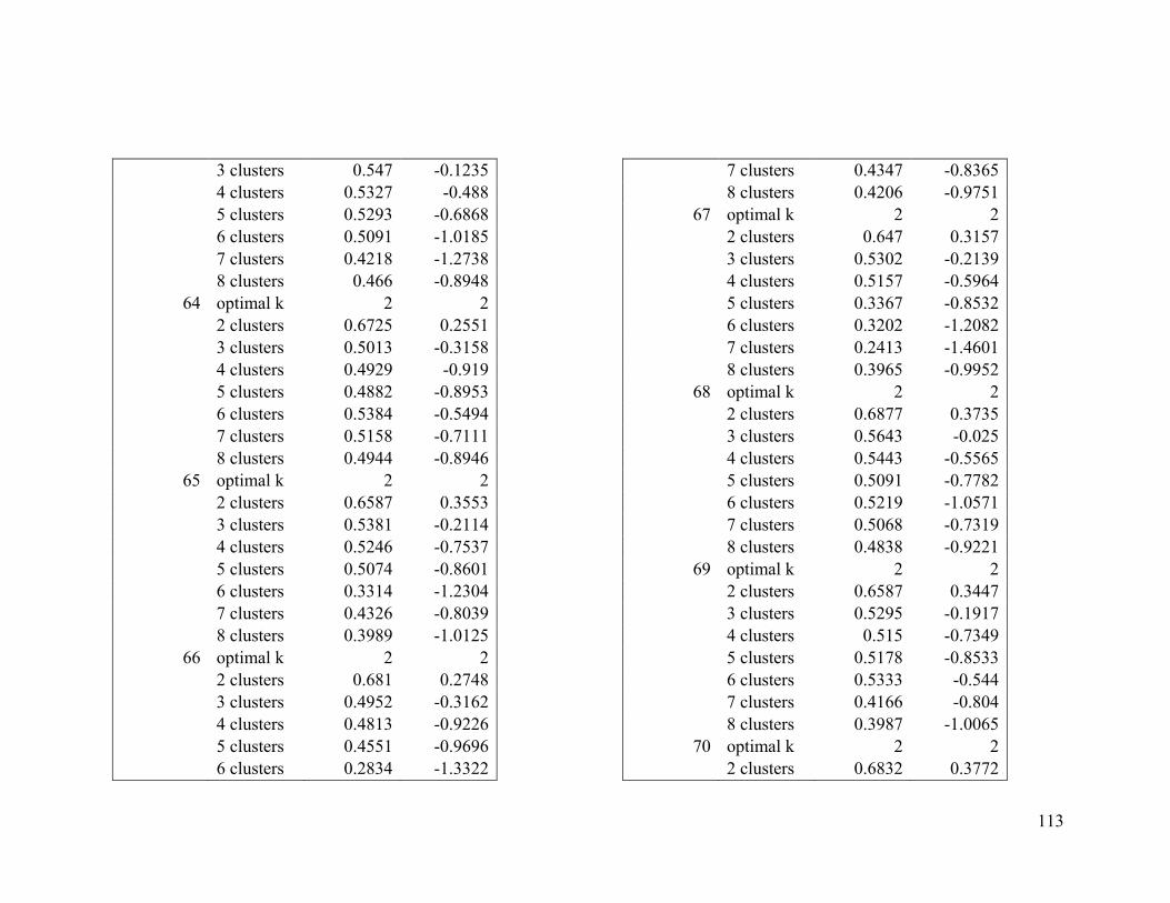
113
3 clusters 0.547 -0.1235 4 clusters 0.5327 -0.488 5 clusters 0.5293 -0.6868 6 clusters 0.5091 -1.0185 7 clusters 0.4218 -1.2738 8 clusters 0.466 -0.8948
64 optimal k 2 2 2 clusters 0.6725 0.2551 3 clusters 0.5013 -0.3158 4 clusters 0.4929 -0.919 5 clusters 0.4882 -0.8953 6 clusters 0.5384 -0.5494 7 clusters 0.5158 -0.7111 8 clusters 0.4944 -0.8946
65 optimal k 2 2 2 clusters 0.6587 0.3553 3 clusters 0.5381 -0.2114 4 clusters 0.5246 -0.7537 5 clusters 0.5074 -0.8601 6 clusters 0.3314 -1.2304 7 clusters 0.4326 -0.8039 8 clusters 0.3989 -1.0125
66 optimal k 2 2 2 clusters 0.681 0.2748 3 clusters 0.4952 -0.3162 4 clusters 0.4813 -0.9226 5 clusters 0.4551 -0.9696 6 clusters 0.2834 -1.3322
7 clusters 0.4347 -0.8365 8 clusters 0.4206 -0.9751
67 optimal k 2 2 2 clusters 0.647 0.3157 3 clusters 0.5302 -0.2139 4 clusters 0.5157 -0.5964 5 clusters 0.3367 -0.8532 6 clusters 0.3202 -1.2082 7 clusters 0.2413 -1.4601 8 clusters 0.3965 -0.9952
68 optimal k 2 2 2 clusters 0.6877 0.3735 3 clusters 0.5643 -0.025 4 clusters 0.5443 -0.5565 5 clusters 0.5091 -0.7782 6 clusters 0.5219 -1.0571 7 clusters 0.5068 -0.7319 8 clusters 0.4838 -0.9221
69 optimal k 2 2 2 clusters 0.6587 0.3447 3 clusters 0.5295 -0.1917 4 clusters 0.515 -0.7349 5 clusters 0.5178 -0.8533 6 clusters 0.5333 -0.544 7 clusters 0.4166 -0.804 8 clusters 0.3987 -1.0065
70 optimal k 2 2 2 clusters 0.6832 0.3772
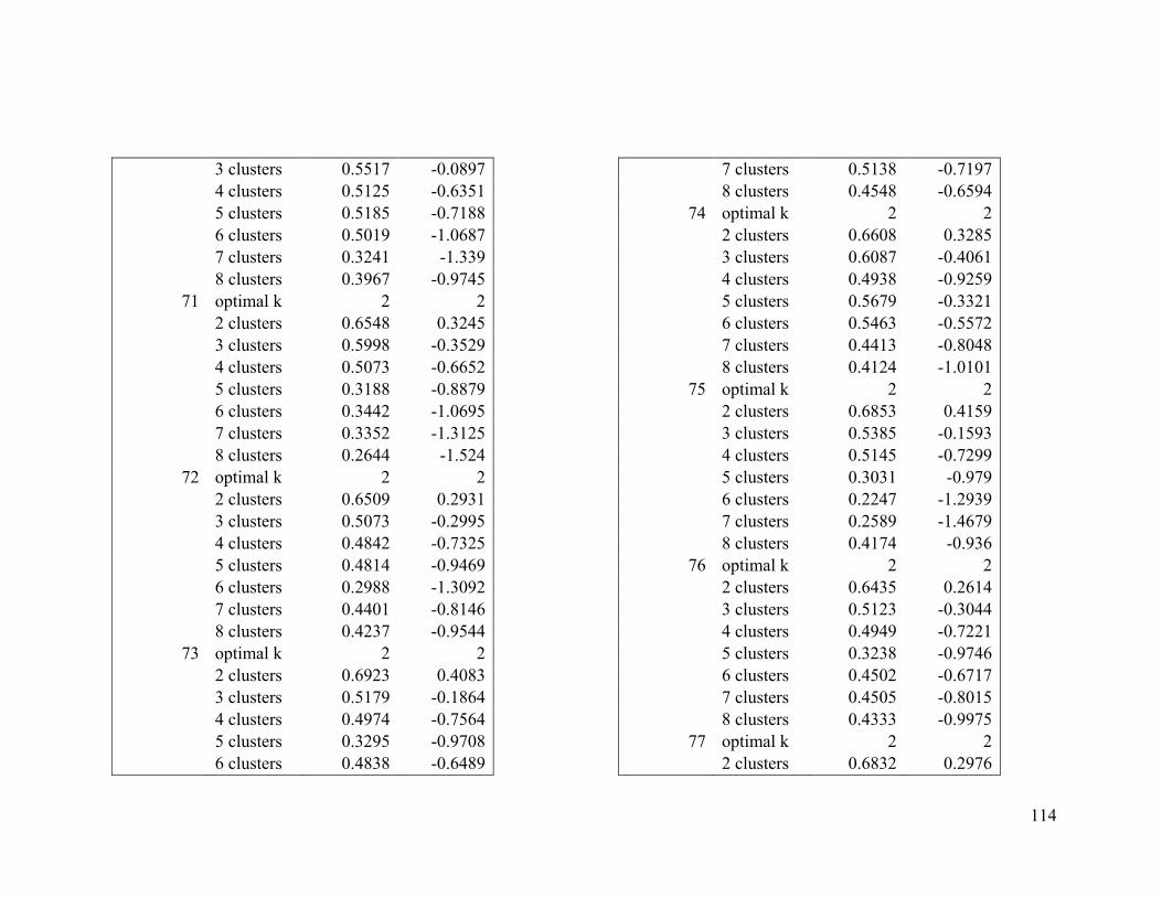
114
3 clusters 0.5517 -0.0897 4 clusters 0.5125 -0.6351 5 clusters 0.5185 -0.7188 6 clusters 0.5019 -1.0687 7 clusters 0.3241 -1.339 8 clusters 0.3967 -0.9745
71 optimal k 2 2 2 clusters 0.6548 0.3245 3 clusters 0.5998 -0.3529 4 clusters 0.5073 -0.6652 5 clusters 0.3188 -0.8879 6 clusters 0.3442 -1.0695 7 clusters 0.3352 -1.3125 8 clusters 0.2644 -1.524
72 optimal k 2 2 2 clusters 0.6509 0.2931 3 clusters 0.5073 -0.2995 4 clusters 0.4842 -0.7325 5 clusters 0.4814 -0.9469 6 clusters 0.2988 -1.3092 7 clusters 0.4401 -0.8146 8 clusters 0.4237 -0.9544
73 optimal k 2 2 2 clusters 0.6923 0.4083 3 clusters 0.5179 -0.1864 4 clusters 0.4974 -0.7564 5 clusters 0.3295 -0.9708 6 clusters 0.4838 -0.6489
7 clusters 0.5138 -0.7197 8 clusters 0.4548 -0.6594
74 optimal k 2 2 2 clusters 0.6608 0.3285 3 clusters 0.6087 -0.4061 4 clusters 0.4938 -0.9259 5 clusters 0.5679 -0.3321 6 clusters 0.5463 -0.5572 7 clusters 0.4413 -0.8048 8 clusters 0.4124 -1.0101
75 optimal k 2 2 2 clusters 0.6853 0.4159 3 clusters 0.5385 -0.1593 4 clusters 0.5145 -0.7299 5 clusters 0.3031 -0.979 6 clusters 0.2247 -1.2939 7 clusters 0.2589 -1.4679 8 clusters 0.4174 -0.936
76 optimal k 2 2 2 clusters 0.6435 0.2614 3 clusters 0.5123 -0.3044 4 clusters 0.4949 -0.7221 5 clusters 0.3238 -0.9746 6 clusters 0.4502 -0.6717 7 clusters 0.4505 -0.8015 8 clusters 0.4333 -0.9975
77 optimal k 2 2 2 clusters 0.6832 0.2976
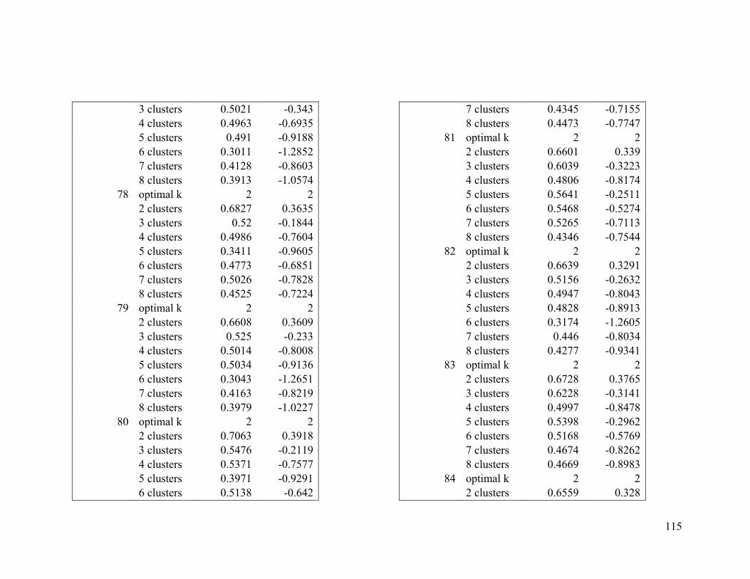
115
3 clusters 0.5021 -0.343 4 clusters 0.4963 -0.6935 5 clusters 0.491 -0.9188 6 clusters 0.3011 -1.2852 7 clusters 0.4128 -0.8603 8 clusters 0.3913 -1.0574
78 optimal k 2 2 2 clusters 0.6827 0.3635 3 clusters 0.52 -0.1844 4 clusters 0.4986 -0.7604 5 clusters 0.3411 -0.9605 6 clusters 0.4773 -0.6851 7 clusters 0.5026 -0.7828 8 clusters 0.4525 -0.7224
79 optimal k 2 2 2 clusters 0.6608 0.3609 3 clusters 0.525 -0.233 4 clusters 0.5014 -0.8008 5 clusters 0.5034 -0.9136 6 clusters 0.3043 -1.2651 7 clusters 0.4163 -0.8219 8 clusters 0.3979 -1.0227
80 optimal k 2 2 2 clusters 0.7063 0.3918 3 clusters 0.5476 -0.2119 4 clusters 0.5371 -0.7577 5 clusters 0.3971 -0.9291 6 clusters 0.5138 -0.642
7 clusters 0.4345 -0.7155 8 clusters 0.4473 -0.7747
81 optimal k 2 2 2 clusters 0.6601 0.339 3 clusters 0.6039 -0.3223 4 clusters 0.4806 -0.8174 5 clusters 0.5641 -0.2511 6 clusters 0.5468 -0.5274 7 clusters 0.5265 -0.7113 8 clusters 0.4346 -0.7544
82 optimal k 2 2 2 clusters 0.6639 0.3291 3 clusters 0.5156 -0.2632 4 clusters 0.4947 -0.8043 5 clusters 0.4828 -0.8913 6 clusters 0.3174 -1.2605 7 clusters 0.446 -0.8034 8 clusters 0.4277 -0.9341
83 optimal k 2 2 2 clusters 0.6728 0.3765 3 clusters 0.6228 -0.3141 4 clusters 0.4997 -0.8478 5 clusters 0.5398 -0.2962 6 clusters 0.5168 -0.5769 7 clusters 0.4674 -0.8262 8 clusters 0.4669 -0.8983
84 optimal k 2 2 2 clusters 0.6559 0.328
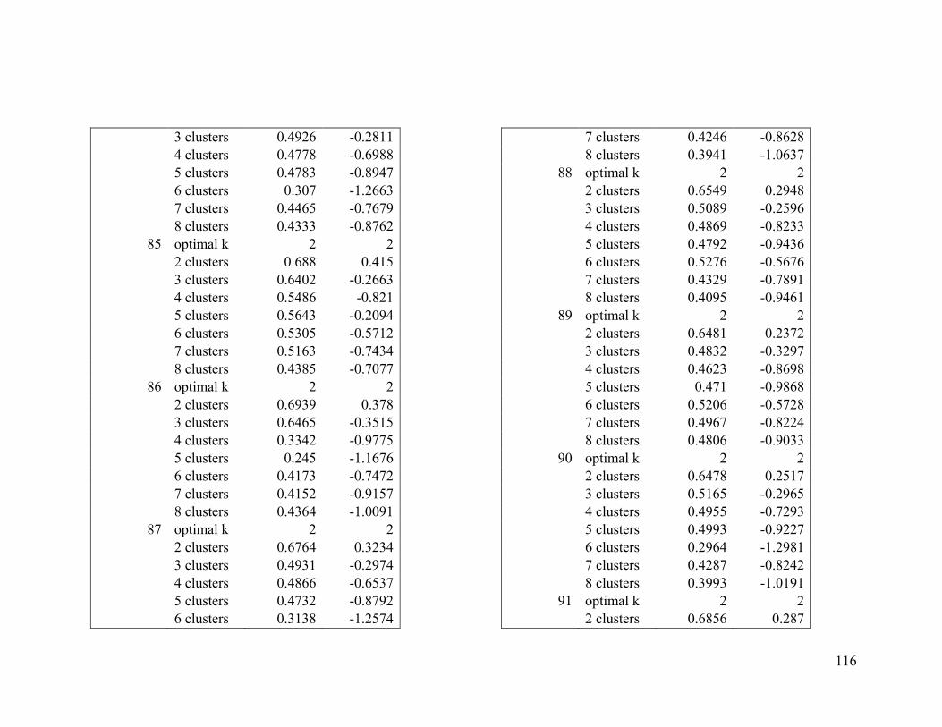
116
3 clusters 0.4926 -0.2811 4 clusters 0.4778 -0.6988 5 clusters 0.4783 -0.8947 6 clusters 0.307 -1.2663 7 clusters 0.4465 -0.7679 8 clusters 0.4333 -0.8762
85 optimal k 2 2 2 clusters 0.688 0.415 3 clusters 0.6402 -0.2663 4 clusters 0.5486 -0.821 5 clusters 0.5643 -0.2094 6 clusters 0.5305 -0.5712 7 clusters 0.5163 -0.7434 8 clusters 0.4385 -0.7077
86 optimal k 2 2 2 clusters 0.6939 0.378 3 clusters 0.6465 -0.3515 4 clusters 0.3342 -0.9775 5 clusters 0.245 -1.1676 6 clusters 0.4173 -0.7472 7 clusters 0.4152 -0.9157 8 clusters 0.4364 -1.0091
87 optimal k 2 2 2 clusters 0.6764 0.3234 3 clusters 0.4931 -0.2974 4 clusters 0.4866 -0.6537 5 clusters 0.4732 -0.8792 6 clusters 0.3138 -1.2574
7 clusters 0.4246 -0.8628 8 clusters 0.3941 -1.0637
88 optimal k 2 2 2 clusters 0.6549 0.2948 3 clusters 0.5089 -0.2596 4 clusters 0.4869 -0.8233 5 clusters 0.4792 -0.9436 6 clusters 0.5276 -0.5676 7 clusters 0.4329 -0.7891 8 clusters 0.4095 -0.9461
89 optimal k 2 2 2 clusters 0.6481 0.2372 3 clusters 0.4832 -0.3297 4 clusters 0.4623 -0.8698 5 clusters 0.471 -0.9868 6 clusters 0.5206 -0.5728 7 clusters 0.4967 -0.8224 8 clusters 0.4806 -0.9033
90 optimal k 2 2 2 clusters 0.6478 0.2517 3 clusters 0.5165 -0.2965 4 clusters 0.4955 -0.7293 5 clusters 0.4993 -0.9227 6 clusters 0.2964 -1.2981 7 clusters 0.4287 -0.8242 8 clusters 0.3993 -1.0191
91 optimal k 2 2 2 clusters 0.6856 0.287
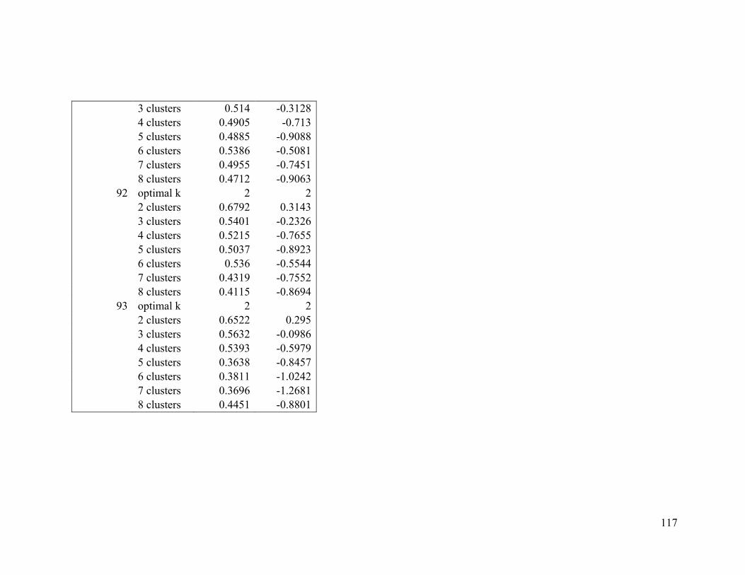
117
3 clusters 0.514 -0.3128 4 clusters 0.4905 -0.713 5 clusters 0.4885 -0.9088 6 clusters 0.5386 -0.5081 7 clusters 0.4955 -0.7451 8 clusters 0.4712 -0.9063
92 optimal k 2 2 2 clusters 0.6792 0.3143 3 clusters 0.5401 -0.2326 4 clusters 0.5215 -0.7655 5 clusters 0.5037 -0.8923 6 clusters 0.536 -0.5544 7 clusters 0.4319 -0.7552 8 clusters 0.4115 -0.8694
93 optimal k 2 2 2 clusters 0.6522 0.295 3 clusters 0.5632 -0.0986 4 clusters 0.5393 -0.5979 5 clusters 0.3638 -0.8457 6 clusters 0.3811 -1.0242 7 clusters 0.3696 -1.2681 8 clusters 0.4451 -0.8801
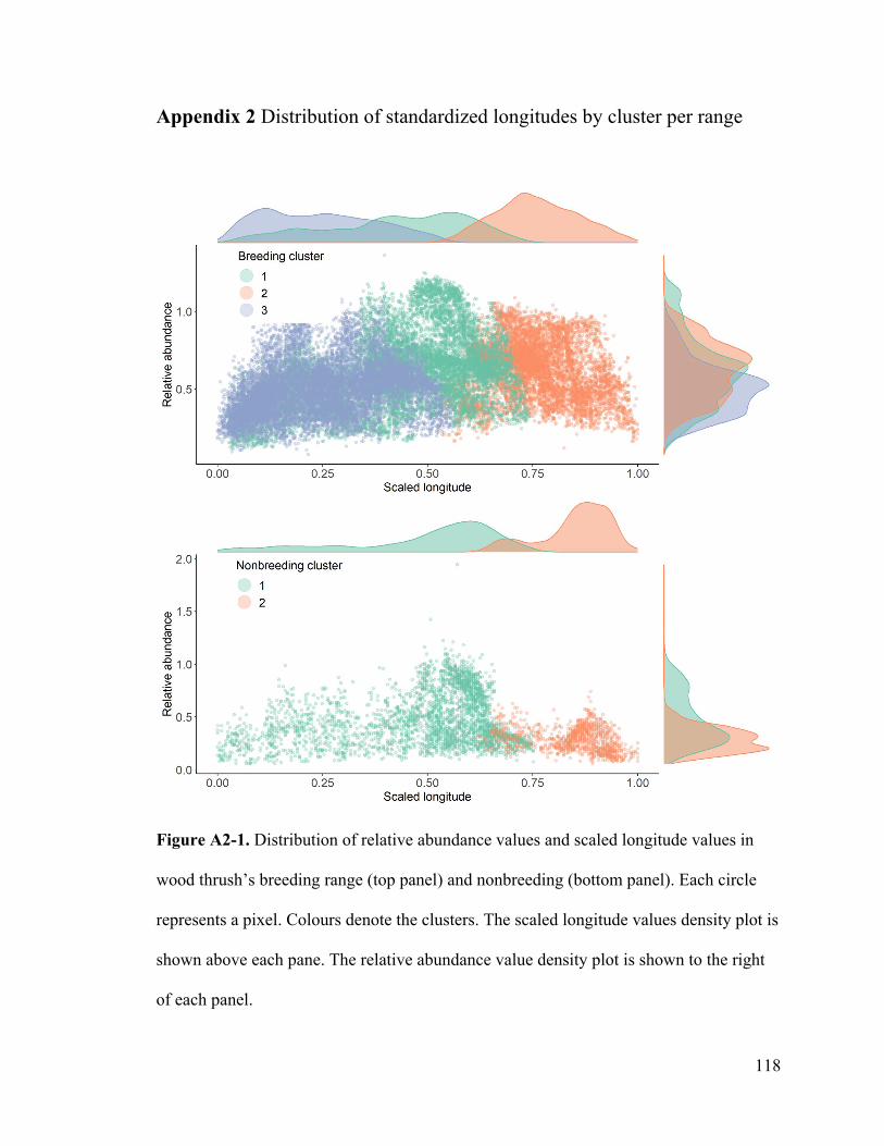
118
Appendix 2 Distribution of standardized longitudes by cluster per range
Figure A2-1. Distribution of relative abundance values and scaled longitude values in
wood thrush’s breeding range (top panel) and nonbreeding (bottom panel). Each circle
represents a pixel. Colours denote the clusters. The scaled longitude values density plot is
shown above each pane. The relative abundance value density plot is shown to the right
of each panel.
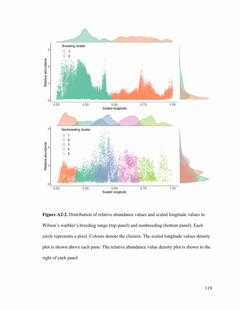
119
Figure A2-2. Distribution of relative abundance values and scaled longitude values in
Wilson’s warbler’s breeding range (top panel) and nonbreeding (bottom panel). Each
circle represents a pixel. Colours denote the clusters. The scaled longitude values density
plot is shown above each pane. The relative abundance value density plot is shown to the
right of each panel.
Copyright © 2022 FDOKUMEN