Math GeosciDOI 10.1007/s11004-008-9189-x

Integrated Interpretation of Interwell ConnectivityUsing Injection and Production Fluctuations

Ali A. Yousef · Jerry L. Jensen · Larry W. Lake

Received: 18 January 2008 / Accepted: 27 August 2008© International Association for Mathematical Geosciences 2008

Abstract A method to characterize reservoirs, based on matching temporal fluctu-ations in injection and production rates, has recently been developed. The methodproduces two coefficients for each injector–producer pair; one parameter, λ, quanti-fies the connectivity and the other, τ , quantifies the fluid storage in the vicinity of thepair. Previous analyses used λ and τ separately to infer the presence of transmissibil-ity barriers and conduits in the reservoir, but several common conditions could not beeasily distinguished. This paper describes how λ and τ can be jointly interpreted toenhance inference about preferential transmissibility trends and barriers. Two differ-ent combinations are useful: one is a plot of log(λ) versus log(τ ) for a producer andnearby injectors, and the second is a Lorenz-style flow capacity (F ) versus storativity(C) plot. These techniques were tested against the results of a numerical simulatorand applied to data from the North Buck Draw field. Using the simulated data, wefind that the F–C plots and the λ–τ plots are capable of identifying whether the con-nectivity of an injector–producer well pair is through fractures, a high-permeabilitylayer, multiple-layers or through partially completed wells. Analysis of data from theNorth Buck Draw field shows a reasonable correspondence between τ and the tracerbreakthrough times. Of two possible geological models for Buck Draw, the F–C andλ–τ plots support the model that has less connectivity in the field. The wells in fluvial

A.A. Yousef · L.W. LakeDepartment of Petroleum and Geosystems Engineering, The University of Texas at Austin, Austin,TX 78712, USA

A.A. YousefSaudi Aramco, Dhahran, Saudi Arabia

J.L. Jensen (�)Department of Chemical and Petroleum Engineering, The University of Calgary, 2500 UniversityDrive NW, Calgary, AB T2N 1N4, Canadae-mail: jjensen@ucalgary.ca

Math Geosci

deposits show better communication than those wells in more estuarine-dominatedregions.

Keywords Lorenz plot · North Buck Draw field · Reservoir characterization ·Capacitance model

1 Introduction

Most waterfloods in hydrocarbon-bearing reservoirs show some surprising behavior.Production wells near injection wells may be among the last to respond to the injec-tion while distant producers respond quickly. This disparity, caused by the geologicaldistribution of the reservoir properties, leads to an uneven sweep of hydrocarbons,giving poor and/or prolonged periods of low recovery, and unnecessary water pro-duction which requires energy for treatment and disposal. A full understanding ofthe degree of communication between injection and production wells is critical toachieve high hydrocarbon recoveries with minimal environmental impact. To quan-titatively determine reservoir connectivity, Yousef et al. (2006) proposed a “capac-itance model” or CM, which includes capacitance (compressibility) and resistance(transmissibility) effects. For each injector–producer pair, two coefficients are deter-mined. One parameter (the weight λ) quantifies the connectivity, and another (thetime constant τ ) quantifies the amount of fluid storage between the wells. Both aredefined below.

The CM also accounts for primary production, multiple injectors, and bottom holepressure (BHP) changes for multiple producers. Based on a total material balance ofa region between injector i and producer j , the predicted total fluid production rate(oil+water+gas in reservoir volumes/time) is given by

q̂j (n) = λpjq(n0j )e

−(n−n0j )

τpj +i=I∑

i=1

λijw′ij (n)

+k=K∑

k=1

νkj

[pwf kj (n0j )e

−(n−n0j )

τkj − pwf kj (n) + p′wf kj (n)

], (1)

where

w′ij (n) =

m=n∑

m=n0j

�n

τij

e(m−n)

τij wij (m),

p′wf kj (n) =

m=n∑

m=n0j

�n

τkj

e(m−n)

τkj pwf kj (m),

and λpj and τpj are the weighting factor and time constant for the primary produc-tion contribution to the estimated rate q̂j of producer j , with production beginning at

Math Geosci

time n0j . λij is the weight between injector i and producer j that indicates the con-nectivity between the (ij) well pair. τij is the corresponding time constant definedas

τij =(

ctVp

J

)

ij

= ctijVpij

Jij

, (2)

where ctij is the total compressibility of the fluids and rock in the pore volume Vpij

between injector i and producer j . Vpij may be considered as the volume of in-vestigation for the ij wellpair injection-production response. The volume size andgeometry vary with time and the reservoir heterogeneity.

Jij is the partial productivity index, defined by

qj =i=I∑

i=1

qij =i=I∑

i=1

Jij

(p̄ij − pwfj

). (3)

Jij is similar to the well-known concept of the productivity index (Kimmel and Dalati1987, pp. 32–2 to 32–4), except that the reference pressure—the average pressure inthe drainage area—is replaced with the average pressure in the region between theith injector and jth producing wells, p̄ij . w′

ij (n) is the convolved or filtered injectionrate at time step n and p′

wf kj (n) is the convolved bottom-hole pressure (BHP) forproducer k. νkj is a coefficient that determines the effect of changing the BHP ofproducer k on the production rate of producer j . The entire last term disappears if allK of the producer BHP’s are constant, as in the cases here.

Yousef et al. (2006) used an iterative, non-linear least-squares procedure to fit therates given by (1) to the actual rates. Fitting was achieved by adjusting the λ’s, τ ’s,and ν’s. They also proposed two versions of the capacitance model: the balanced(BCM) and the unbalanced capacitance model (UCM). A waterflood is balancedwhen the field-wide average injection rate is approximately equal to field-wide av-erage production rate. When this is true, the BCM (1) should be used. However, if thewaterflood is unbalanced, a constant (qoj ) is added to (1) to form the UCM. Yousefet al. (2006) analyzed the model λ’s in homogeneous cases to show that the CM gavebetter performance than an earlier model, proposed by Albertoni and Lake (2003).For example, the CM estimates of λ are more stable in high-compressibility casesand the CM can better tolerate periods when injection wells are shut in. However,Yousef et al. (2006) did not analyze both λ’s and τ ’s together and in heterogeneoussystems. Combining both sets of parameters in certain representations has the poten-tial to enhance inference about the geological features.

Two different interpretative plots for joint analysis of the CM parameters are de-scribed. One is a log–log plot of the λ’s vs. the τ ’s for a producer and nearby injec-tors, and another is the F –C plot where the λ’s and the τ ’s are combined using thesame concept as Lorenz plots. The synthetic and field applications show that the rela-tion between λ’s and corresponding τ ’s are consistent with the known heterogeneity,the distance between wells, and their relative positions. The F –C plots and the log–log plots are capable of identifying whether the connectivity of an injector–producerwell pair is through fractures, a high-permeability layer, multiple layers or through

Math Geosci

partially completed wells. Application of the plots to the North Buck Draw field sug-gests that, of the two geological models proposed in the literature, the one with lesscommunication is more appropriate.

2 Analysis Methods

We describe two different representations to enhance the inference about reservoirheterogeneity, using the estimated parameters from the CM: the F –C plot, and alog–log plot of λ’s vs. the τ ’s.

2.1 The Flow Capacity Plot

The idea of flow versus storage was developed initially to estimate injection sweepefficiency in a layered reservoir. This method relates the relative flow in a cross sec-tion to its associated pore volume, usually in a flow-storage diagram (also known asLorenz or F –C plots). These plots can be used quantitatively to describe reservoirgeology. For example, if 50% of flow comes from only 10% of the pore volume of areservoir, then there are fast flow paths in the reservoir. The F –C plots estimated fromthe CM parameters are different from the conventional Lorenz plots described bySchmalz and Rahme (1950) and Lake and Jensen (1991). Conventional Lorenz plotsare based on static permeability and porosity data obtained from measured samplestaken from the reservoir, where the spatial relationships of the samples are ignored.The F –C plots here are based on parameters λ and τ obtained from dynamic data inwhich these parameters account for all variations in reservoir properties in the vicin-ity of a producer. Shook (2003) also developed these plots (flow-storage diagrams)using tracer test results. Because the F –C plots are based on injection and produc-tion data, it is likely they will better reflect the flow paths and geological features ina reservoir than Lorenz plots.

The Lorenz curve (Fig. 1) is a plot of cumulative flow capacity, Fm, versus cumu-lative thickness, Hm, where

Fm =∑i=m

i=1 kihi∑i=ni=1 kihi

, (4)

Hm =∑i=m

i=1 hi∑i=ni=1 hi

, (5)

for a reservoir of n layers. The layers are arranged in order of decreasing permeabil-ity so that m = 1 is the layer with thickness h1 and the largest permeability k1 whilem = n is the layer with thickness hn and the smallest permeability kn. By defini-tion, 0 ≤ Fm ≤ 1 and 0 ≤ Hm ≤ 1 for 1 ≤ m ≤ n. The Lorenz curve, constructed byletting m vary from 1 to n, has a monotonically decreasing slope. If the medium ishomogeneous, all the permeabilities are identical and the Lorenz curve is a straightline with unit slope. Increasing levels of heterogeneity are indicated by movement ofthe Lorenz curve away from the straight line. Twice the area between the diagonal

Math Geosci

Fig. 1 Conventional Lorenz(F –C) plot. The dashed 45° lineis the Lorenz curve for ahomogenous reservoir

line and the Lorenz curve is an indicator of the heterogeneity, known as the Lorenzcoefficient, Lc (Schmalz and Rahme 1950).

The Lorenz procedure can be modified by including porosity (Craig 1971, p. 64;Lake 1989, p. 195). In place of Hm, the cumulative storage capacity, Cm, is

Cm =∑i=m

i=1 φihi∑i=ni=1 φihi

. (6)

In this plot, a fraction of Fm is provided by a fraction Cm of the reservoir pore volume(for a layered reservoir). If porosity is constant, the original Lorenz curve results. Thedata must now be arranged according to decreasing k/φ. By analogy to the Lorenzplot, the F –C plot is formed using the λ’s and τ ’s for a producer and nearby injectors.This requires reinterpreting the λ’s appearing in (1) as

λij = Jij∑i=Ii=1 Jij

. (7)

The λij is equivalent to kijhij between the (ij) well pair or, in other words, λij quan-tifies the F –C between the (ij) well pair. Based on the definitions in (2) and (7),the λ and its corresponding τ are not independent because λ is directly proportionalto J and τ is inversely proportional to the same J . The product of λ and the corre-sponding τ provides a parameter that contains only the storage capacity between theinjector–producer pair

λij τij = ctijVpij∑i=Ii=1 Jij

. (8)

Similar to (4) and (5), the F –C curve is a plot of cumulative F –C (Fm) againstcumulative storage capacity (Cm), where

Fmj =∑i=m

i=1 λij∑i=Ii=1 λij

(9)

Math Geosci

and

Cmj =∑i=m

i=1 λij τij∑i=Ii=1 λij τij

, (10)

for producer j with I injectors; λpj and τpj are not included in the calculations. Thedata are arranged in order of decreasing 1/τij so that i = 1 is the injector–producerwell pair with the smallest τ while i = I is the injector–producer well pair with thelargest τ . Because of the data ordering, the F –C curve monotonically increases fromi = 1 to i = I with a monotonically decreasing slope as does a Lorenz plot. The F –C

plots can indicate specific geological features in the vicinity of an injector. In thiscase, sets of λ’s and τ ’s for one injector and all producers are used to form the F –C

plot. The procedure can make use of the extensive literature already available on theinterpretation of these plots (Gunter et al. 1997; Cortez and Corbett 2005).

2.2 The log–log Plot

As discussed above, the λ and the corresponding τ are inversely related through thepartial productivity index Jij ((2) and (7)). For homogeneous reservoirs, where eachproducer communicates with all injectors, a log–log plot of λ’s against τ ’s for eachproducer with all injectors should give a straight line of slope −1. This behavior wasconfirmed for homogeneous reservoirs (Yousef et al. 2006). For non-homogeneousreservoirs, the deviations of the estimated λ’s and the τ ’s from a line with slope −1will indicate specific geological conditions in these reservoirs.

3 Results

The techniques described above were tested through applications to two well arrange-ments in simulated reservoir systems (Synfields) and to data from the North BuckDraw field (NBD). For the synthetic cases, the emphasis will be on the consistencyof the estimated model parameters (λ’s and τ ’s) with the imposed geology, and thecapability of the F –C plots to indicate the geological conditions imposed in eachcase. Application of the methods to the field case will show what can be achieved inpractice.

3.1 Application to Synthetic Fields

Numerical simulation was done with a commercial finite difference simulator. Weapplied the BCM approach to the numerically simulated Synfields: one of 5 injectorsand 4 producers, the 5 × 4 Synfield, and a second of 25 injectors and 16 producers,the 25 × 16 Synfield (Fig. 2). The 5 × 4 Synfield consists of five continuous layerswhile the 25 × 16 Synfield consists of three layers. All layers were of equal thicknessand the Synfields were flowing undersaturated oil initially. The injector–producerdistance was 800 ft for the 5 × 4 Synfield and 890 ft for the 25 × 16 Synfield. Theoil, water, and rock compressibility are 5 × 10−6, 1 × 10−6, and 1 × 10−6 psi−1,respectively. The oil–water mobility ratio is unity. All wells are vertical with no skin

Math Geosci

Fig. 2 Well locations for the 5 × 4 (left) and 25 × 16 (right) synthetic cases (Synfields). Producing wellsare denoted by P and injection wells by I

and the producer BHP’s are constant and equal. Because the simulations cover alimited time period for a system with few wells in a bounded domain, the resultingλ’s and τ ’s will show some scatter about their ideal values. The characteristics of thesynfields are similar to those of the real case to which the CM will be applied later.

3.1.1 5 × 4 Synfield

Several different geological conditions were analyzed for this field. Injection rateswere randomly selected from different wells in a real field and proportionally mod-ified to be in agreement with the Synfield injectivity. The numerical simulation ex-tends to n = 100 months, with �n = 1 month.

3.1.1.1 Homogeneous Reservoir The base case is a homogenous reservoir with anisotropic permeability of 40 md. A log–log plot of the λ’s against the τ ’s estimatedfrom the 5 × 4 homogenous Synfield gives an approximate straight line of slope −1(Fig. 3), which indicates that all injectors communicate with the producers throughlayers that have equal properties. All F –C plots are nearly straight lines, indicatingthat the reservoir model is indeed homogeneous (Fig. 4).

3.1.1.2 High Permeability Layer For this case, injectors I04 and I05 are completedin a large permeability (500 md) layer, while injectors I01–I03 are completed in asmall permeability (10 md) layer (Fig. 5). The vertical permeability is 0.1 md and theporosity is constant throughout. All other parameters are similar to the base case. TheBCM match to the total production rate yields a coefficient of determination of R2 =0.997, where the predicted rate (1) is the explanatory variable and the actual rate isthe response variable. This suggests that the CM is well able to model the productionusing the given injection rates. The estimated λ’s (Fig. 6, left) are very similar tothose from the base case (Fig. 7), indicating that the λ’s reflect little or no informationabout the high permeability layer (L5) or about the well completions; they are onlyfunctions of the distance between wells and their relative locations. However, the

Math Geosci

Fig. 3 Log–log plot of λ’sversus τ ’s for a 5 × 4homogeneous Synfield has theexpected slope of −1

Fig. 4 The F –C plots for all producers for the 5 × 4 Synfield. A homogeneous reservoir shows anear-homogeneous F –C plot

estimated τ ’s of I04 and I05 are smaller than those of I01–I03 (Fig. 6, right). This isconsistent with I04 and I05 being completed only in the high permeability layer (L5),“seeing” a smaller pore volume than the other injectors.

Unlike the base case (Fig. 3), the log–log plot of λ vs. τ in this case reveals twodifferent groups, each with an approximate straight line of slope −1 (Fig. 8). Thegroups have τ ’s that differ by a factor of 5, in agreement with the smaller reservoirvolume swept by fluid injected at wells I04 and I05. The combination of both para-

Math Geosci

Fig. 5 Well completions for the5 × 4 Synfieldhigh-permeability layer case

Fig. 6 Calculated parameters λij (left) and τij (right) for the 5×4 Synfield, high-permeability layer case.The λij and τij are represented by arrows or cones that start from injector i and point to producer j . Thelonger the arrow, the larger is τ or λ

Fig. 7 Comparison of the λ’sestimated from the highpermeability layer case and theλ’s estimated from the base case

Math Geosci

Fig. 8 Log–log plot of λ versusτ for the high-permeability layercase. The two groups each havean approximate straight line ofslope −1

Fig. 9 F –C plots for all producers for the high-permeability layer case. Each plot shows two differentgeological layers that are approximated by two straight lines. The dashed line presents the 45◦ line. Thestatic F –C curves are also shown in each plot. The F –C curves from the CM show less heterogeneity thanthe static curves

meters, λ and τ , and the expectation that points will lie on lines of slope −1 helps toidentify wells I04 and I05 as accessing different parts of the reservoir from the otherthree injection wells.

The F –C curves are not straight lines (Fig. 9) and indicate that the Synfield isnot homogeneous. For each producer, the F –C plot has two distinct segments. The

Math Geosci

Fig. 10 Representation of the parameters λij (left) and τij (right) for the fractures case. Fractures areplaced between well pairs I01–P01 and I03–P04

left straight line segment with a large slope is for I04 and I05, while the small slopestraight line is for I01, I02, and I03. Similar to the dynamic F –C curves, the staticLorenz curves indicate two distinct layers (Fig. 9); however, the deviation of theLorenz curves from homogeneous behavior is larger than that for the dynamic F –C curves. This suggests that the dynamic heterogeneity of the reservoir, as reflectedthrough several factors including the layer-to-layer variations, the well completions,and the flow patterns, is less than the apparent heterogeneity, based on the staticporosity and permeability values alone.

3.1.1.3 Fractures This case has two vertical “fractures”, both with one grid-sizewidth. One fracture is between I01 and P01 with a permeability of 1 000 md, and asecond is between I03 and P04 with a smaller permeability (500 md). The permeabil-ity of the rest of the Synfield is 5 md. The two fractures, which extend to all layers andinjectors and producers, are completed in all layers. All other parameters are the sameas the base case. The BCM match to the total production rate yields R2 = 0.997. Theλ’s between I01–P01 and I03–P04 are large, while the corresponding τ ’s are verysmall (Fig. 10). This is consistent with the two fractures existing in this case. Theinjectors nearest to P04, I04, and I05, also have large λ’s but the corresponding τ ’sare larger than those for the I01–P01 and I03–P04 well pairs. Both sets of parametersreflect the heterogeneity of the field.

The log–log plot of the λ’s against the τ ’s indicates that there are three differentgroups (Fig. 11). Group 1, which includes the data for I01–P01 and I03–P04, reflectsthe two fractures existing in the field. Group 2 represents well pairs near the fractureswith large λ’s and large τ ’s, and Group 3 shows the distant well pairs with small λ’sand large τ ’s. The data is very scattered, indicating a heterogeneous system. Noneof the points within a group fall on a line of −1 slope. The F –C plots of P01 andP04 show a very heterogeneous reservoir while the F –C plots of P02 and P03 shownear-homogeneity (Fig. 12). These plots reflect the apparent levels of heterogeneityin the drainage areas surrounding the respective producers. A large fracture or other

Math Geosci

Fig. 11 Log–log plot of λ’sversus τ ’s shows points in threegroups for the fractures case

Fig. 12 The F –C plots for all producers show a mixture of homogeneous and heterogeneous responsesfor the case with fractures

high-permeability conduit will substantially increase the heterogeneity in a regionwhere significant amounts of fluid may flow.

The F –C plots for P01 and P04 indicate two distinct conditions in the vicinity ofthese producers. Similar to the previous case, two straight lines can be fitted to theF –C curves. The steep straight line suggests that a large fraction of the total flowcapacity is provided by a small fraction of the total pore volume. This is usually anindication of fractures existing in the vicinity of the corresponding producer. Because

Math Geosci

Fig. 13 Representation of the parameters λij (left) and τij (right) obtained using the BCM for the caseof P04 completed only in layer 5

P01 and P04 are supported by I01 and I03 through fractures, their F –C plots deci-sively indicate these fractures by the steep straight line segment. Furthermore, thefirst straight line in the F –C plot of P01 is much steeper than that of P04, whichis consistent with the difference in the permeabilities of the fractures. The secondstraight line in both plots suggests that a small fraction of total F –C is provided by alarge fraction of the total volume; this flow is from injectors communicating throughthe matrix of the reservoir. Once again, the static-measured heterogeneity is largerthan that depicted by the dynamic F –C of all producers (Fig. 12). The F –C plotsappear to be capable of identifying whether the connectivity of an injector–producerwell pair is through a fracture or a high-permeability layer.

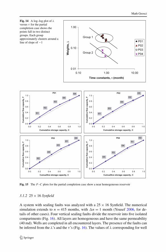
3.1.1.4 Producer with Partial Completion In this case, P04 is completed only inlayer L5, while the other producers and injectors are completed in all layers (L1–L5).The vertical permeability is 0.4 md and all other parameters are similar to those in thebase case. The small λ’s for P04 are consistent with the small productivity becauseof its limited completion (Fig. 13). However, the estimated τ ’s are the same as thebase case results; evidently, the τ ’s carry no information about the partial comple-tion of P04. Because Vp and J in the definition of τ (6) are both functions of thepay thickness of the corresponding producer, τ does not depend on the pay thickness(Larsen 2001; Ibragimov et al. 2005). The log–log plot of λ vs τ reflects the partialcompletion of P04, represented by Group 2 (Fig. 14). Group 1 represents the parame-ter values associated with other producers and shows the expected linear arrangementwith slope of −1. None of the F –C plots, however, shows the partial completion ofP04 (Fig. 15). Evidently, the vertical permeability of this case is large enough so thatthe entire reservoir is available for flow.

Math Geosci

Fig. 14 A log–log plot of λ

versus τ for the partialcompletion case shows thepoints fall in two distinctgroups. Each groupapproximately clusters around aline of slope of −1

Fig. 15 The F –C plots for the partial completion case show a near homogeneous reservoir

3.1.2 25 × 16 Synfield

A system with sealing faults was analyzed with a 25 × 16 Synfield. The numericalsimulation extends to n = 415 months, with �n = 1 month (Yousef 2006, for de-tails of other cases). Four vertical sealing faults divide the reservoir into five isolatedcompartments (Fig. 16). All layers are homogeneous and have the same permeability(40 md). Wells are completed in all encountered layers. The presence of the faults canbe inferred from the λ’s and the τ ’s (Fig. 16). The values of λ corresponding for well

Math Geosci

Fig. 16 Representation of the parameters λij (left) and τij (right) obtained using the BCM for the caseof vertical sealing faults

Fig. 17 Log–log plot for thesealing faults case shows theparameter values form twodistinct groups. Only the pointsin Group 1 fall close to a linewith slope −1

pairs located in different compartments are close to zero, while the correspondingvalues of τ for the same well pairs are large. This shows no communication betweenthese wells, which is consistent with the presence of the sealing faults. The log–logplot of λ’s versus τ ’s indicates two different groups (Fig. 17). Group 1, characterizedby relatively large λ’s and small τ ’s reflects the values of λ and τ for well pairs lo-cated in the same compartment. Group 2, characterized by small λ’s (λ < 0.03) andlarge τ ’s, are for well pairs in different compartments. All F –C plots (not shown)indicate a near-homogeneous reservoir, with producers away from the faults showingsomewhat more heterogeneity than those near to the faults.

3.2 Application to Field Data

The technique was applied to data from a portion of the North Buck Draw field,Wyoming. Yousef (2006, pp. 451–468) reports on several other field studies. Unlike

Math Geosci

Fig. 18 Results of the UCMapplied to a portion of the NBDfield. Only λ’s > 0.05 areshown. Dashed lines representthe approximate east–west limitsof the channel facies asdescribed by Sellars andHawkins (1992). Anderson andHarrison (1997) place thewestern edge to the west of Well33-12. Flow is from the south

the Synfield applications, there are no concrete standards or agreement with the im-posed geology against which to compare results. Our truth test will be comparisonagainst the geological features that are, as much as possible, independently known.The NBD study consists of data from 8 injectors and 12 producers (Fig. 18). Thereservoir average porosity is 9.5%, and the average permeability is 10.7 md. Thereservoir fluid is near-volatile oil and the fluid properties fall between those of blackand volatile oils. The fluid meets the majority of volatile-oil criteria, including largeoil formation volume factors and solution gas-oil ratios. The bubble point pressureis 4680 psi, and the reservoir fluid is a single-phase, low-viscosity fluid above thispressure (Sellars and Hawkins 1992).

Commercial production began in June 1983. In 1988 a pressure maintenanceproject was initiated by injecting gas. Since the field is undergoing gas injection,the reservoir total compressibility is large, which could violate the assumption ofslightly compressible fluids used in the derivation of (1). However, if the productof ct�p � 1, the assumption of slightly compressible fluids will be approximatelycorrect (Dake 1978, pp. 243–244). In this case, reservoir pressure has varied, but

Math Geosci

is approximately 5 000 psi and pressure variations are 300 psi (Fulco 1999). Thus,ct�p ≈ �p/p = 0.06, indicating that the CM is being used appropriately. The timeperiod selected for the analysis was determined by a procedure described in Yousef(2006, pp. 466). The analysis is carried out using monthly flow rates starting in month35, and covering 56 monthly flow rates. Because the reservoir total compressibilityis large, the inference procedure most likely will not be able to indicate the connec-tivity between distant injector–producer pairs. Therefore, we applied the UCM onlyto producers and nearby injectors. The fits to the production data are relatively good;for example, the R2 for producers 13-7 and 33-12 are 0.94 and 0.97, respectively.

Two geological models of NBD have been proposed (Fig. 18). Sellars andHawkins (1992) describe a system of predominantly fluvial channels and point bardeposits, while Gardner et al. (1994) propose a more mixed system of fluvial andestuarine deposits and marine shales. While the field boundaries suggest a simplepoint-bar deposit with good connectivity, Gardner et al. (1994) propose that the con-tinuity is more restricted by the incision of finer-grained, lower-quality estuarine de-posits and marine shales as in well 14-18. The λ’s suggest poor interwell connectivityin some areas of NBD, in better agreement with Gardner et al.’s model. For exam-ple, well 14-18 has only a small proportion of fluvial channels and small λ’s; nearbywells 33-13 and 33-18 have significantly more fluvial material and larger λ’s. Well33-7 also has more fluvial material but small λ’s, which may be caused by somecompartmentalization of the deposits around this well.

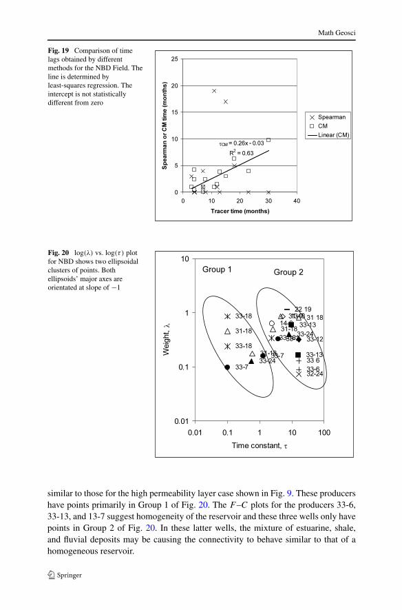
Radioactive tracers were injected into NBD, and their occurrence was monitoredat the producing wells from February 1989 to March 1993. Refunjol and Lake (1998)applied Spearman analysis to determine preferential flow trends in the NBD fieldand compared the results with injected tracer response; they related injection flowrates with those of adjacent producers and used time lags to find a maximum Spear-man correlation coefficient (rs ). Because rs can be interpreted as another measure ofinjector–producer communication, a comparison between the rs ’s and the λ’s shouldprovide a consistency check with the interwell connectivity between well pairs fromUCM. We found that rs tends to be larger and less variable than the corresponding λ.Thus, the estimated λ’s are broadly consistent with the rs ’s. Because the tracer re-sponse breakthrough times are considered real field measurements, we use them as abasis for assessing the τ ’s and the Spearman time lags (Fig. 19). The correlation ofτ with the tracer breakthrough times is substantially better than the correlation withthe Spearman time lags. The slope of the least-squares regression line is less than 1,which is consistent with the tracer taking longer to arrive at the producer than thepressure disturbances from the injection fluctuations.

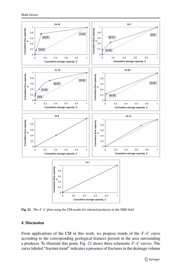
The log(λ) vs. log(τ ) plot reveals that there are two different behaviors for inter-well connectivity in NBD (Fig. 20). Group 1 contains wells having and surroundedby significant amounts of fluvial deposits (e.g., wells 33-18, 31-18, and 33-7) whileGroup 2 wells tend to have greater amounts of estuarine deposits (e.g., wells 33-12 and 14-18). The response of points is similar to the high permeability layer case(Fig. 8), where good communication may exist through fluvial deposits but pathwayscan still be interrupted by poorer-quality, incising estuarine and shale deposits. TheF –C plots also indicate two distinctly different behaviors, in which certain injectorscommunicate with the corresponding producer well and the other injectors commu-nicate poorly (Fig. 21). The F –C plots for producers 33-18, 33-7, and 31-18 plots are

Math Geosci

Fig. 19 Comparison of timelags obtained by differentmethods for the NBD Field. Theline is determined byleast-squares regression. Theintercept is not statisticallydifferent from zero

Fig. 20 log(λ) vs. log(τ ) plotfor NBD shows two ellipsoidalclusters of points. Bothellipsoids’ major axes areorientated at slope of −1

similar to those for the high permeability layer case shown in Fig. 9. These producershave points primarily in Group 1 of Fig. 20. The F –C plots for the producers 33-6,33-13, and 13-7 suggest homogeneity of the reservoir and these three wells only havepoints in Group 2 of Fig. 20. In these latter wells, the mixture of estuarine, shale,and fluvial deposits may be causing the connectivity to behave similar to that of ahomogeneous reservoir.

Math Geosci

Fig. 21 The F –C plots using the CM results for selected producers in the NBD field

4 Discussion

From applications of the CM in this work, we propose trends of the F –C curveaccording to the corresponding geological features present in the area surroundinga producer. To illustrate this point, Fig. 22 shows three schematic F –C curves. Thecurve labeled “fracture trend” indicates a presence of fractures in the drainage volume

Math Geosci

Fig. 22 Schematic of differenttrends of the F –C curveestimated from the CMparameters according to thecorresponding geologicalfeature present in the vicinity ofa producer

of a producer; the second “high permeability layer trend” indicates that some injec-tors communicate with the producer through high permeability layers and the otherinjectors communicate through low permeability layers. For the last curve labeled the“reservoir seal trend”, a fraction of the total storage capacity or the total pore volumeswept by injectors provides a negligible fraction of the total F –C. This is a typicalcharacteristic of nonpay zones or a reservoir seal. However, there are cases wherethe F –C plots are not able to reflect the conditions in the vicinity of the producer.As discussed earlier, the F –C plot cannot identify a partial completion of a producereven though this can be easily inferred from the model parameters (λ’s and τ ’s).

The log–log plot of λ’s versus τ ’s gives patterns consistent with the imposed ge-ology in the application to synthetic fields, where distinct groups can be easily iden-tified. For some real field cases, however, the scatter in the data can be so large thatdistinct groups of data are not apparent. Nonetheless, we could identify two differentcommunication responses for NBD which are consistent with the geological modelof Gardner et al. (1994). These patterns were not so clear when examining either theλ’s or τ ’s separately. Because both the F –C and λ–τ plots are based on inferred pa-rameters (λ’s and τ ’s) from dynamic, injection and production data, different sourcesof error can obscure inferences about the geological conditions. Example sources in-clude deviations from the assumptions on which the CM is based, correlation betweeninjection rates, using too short an assessment interval, and the quality of injection andproduction rate measurements. Our experience with various datasets suggests, for ex-ample, that results with λ < 0.05 may not be significant.

5 Conclusions

This paper describes the development of the capacitance model into a diagnostic toolto enhance inferences about preferential transmissibility trends and the presence offlow barriers. Complex geological conditions are often not easily identified using theλ and τ values individually. However, combining both parameters in specific repre-sentations enhances inferences about the geological features. Two different represen-tations are used. One representation is a log–log plot of the λ’s versus the τ ’s for a

Math Geosci

producer and nearby injectors; another representation is the F –C plot where the λ’sand τ ’s are combined using the idea of Lorenz plots. The synthetic field applicationsshow that the relation between the λ’s and the corresponding τ ’s are consistent withknown heterogeneity, the distance between wells, and their relative positions. TheF –C plots and the log–log plots are capable of identifying whether the connectivityof an injector–producer well pair is through fractures, a high-permeability layer, orthrough partially completed wells.

The technique was applied to the North Buck Draw field. The capacitance modelresults agree with the tracer analysis better than that of the Spearman analysis. Theestimated λ’s and τ ’s are consistent with the geological interpretation of Gardner et al.(1994) and suggest that some compartmentalization is present. The log(λ) vs. log(τ )

plot appears to separate the wells situated predominantly in fluvial sediments fromthose in more mixed, fluvial and estuarine deposits. F –C plots similarly indicate thatsome nearby injectors communicate with some producers through the better qualityfluvial deposits.

Acknowledgements The authors wish to thank Steven Hubbard and Brian Willis for their geologicalassistance. A.A.Y. would like to thank Saudi Aramco for his graduate fellowship. Larry W. Lake holds theW.A. (Monty) Moncrief Chair at The University of Texas and Jerry L. Jensen holds the Schulich Chair inGeostatistics at The University of Calgary. This work was supported in part by US Department of EnergyContract DE PS26021215375.

References

Albertoni A, Lake LW (2003) Inferring connectivity only from well-rate fluctuations in waterfloods. SPEReserv Evalu Eng 6(1):6–16

Anderson GP, Harrison WJ (1997) Depositional and diagenetic controls on porosity distribution at BuckDraw Field, Campbell and Converse Counties, Wyoming. Wyoming geological association 48th an-nual field conference guidebook, pp 99–107

Cortez OD, Corbett PM (2005) Time-lapse production logging and the concept of flowing units. In: SPEpaper 94436, SPE Europec/EAGE annual conference held in Madrid, Spain, 13–16 June, 12 p

Craig FF (1971) The reservoir engineering aspects of waterflooding. Society of Petroleum Engineers,Dallas, 134 p

Dake LP (1978) Fundamentals of reservoir engineering. Elsevier, New York, 443 pFulco GJ (1999) Case history of miscible gas flooding in the Powder River Basin North Buck Draw Unit.

In: SPE paper 55634, SPE Rocky Mountain regional meeting held in Gillette, WY, 15–18 May, 19 pGardner MH, Dharmasamadhi W, Willis BJ, Dutton SP, Fang Q, Kattah S, Yeh J, Wang W (1994) Reservoir

characterization of Buck Draw Field. Bureau of economic geology deltas industrial associates fieldtrip, Rapid City, SD, 8–14 October, 30 p

Gunter GW, Finneran JM, Hartmann DJ, Miller JD (1997) Early determination of reservoir flow unitsusing an integrated petrophysical method. In: SPE paper 38679, SPE annual technical conferenceand exhibition held in San Antonio, TX, 5–8 October, 5 p

Ibragimov A, Khalmanova D, Valko P, Walton J (2005) On a mathematical model of the productivity indexof a well from reservoir engineering. SIAM J Appl Math 65(6):1952–1980

Kimmel JD, Dalati RN (1987) Potential tests of oil wells. In: Bradley HB (ed) Petroleum engineeringhandbook. Society of Petroleum Engineers, Richardson

Lake LW (1989) Enhanced oil recovery. Prentice Hall, Englewood Cliffs, 550 pLake LW, Jensen JL (1991) A review of heterogeneity measures used in reservoir characterization. In Situ

15(4):409–439Larsen L (2001) General productivity models for wells in homogeneous and layered reservoirs. In: SPE

paper 71613, SPE annual technical conference and exhibition held in New Orleans, LA, 30 Septemberto 3 October, 14 p

Math Geosci

Refunjol BT, Lake LW (1998) Reservoir characterization based on tracer response and rank analysis ofproduction and injection rates. In: Schatzinger R, Jordan JF (eds) Reservoir characterization—recentadvances. AAPG Memoir, vol 71, pp 209–218

Schmalz JP, Rahme HS (1950) The variation in water flood performance with variation in permeabilityprofile. Prod Mon 14(9):9–12

Sellars R, Hawkins C (1992) Geology and stratigraphic aspects of the Buck Draw Field, Powder RiverBasin, Wyoming. Wyoming geological association 43rd annual field conference guidebook, pp 97–110

Shook GM (2003) A simple, fast method of estimating fractured reservoir geometry from tracer tests.Trans Geotherm Resour Counc 27:407–411

Yousef AA (2006) Investigating statistical techniques to infer interwell connectivity from production andinjection rate fluctuations. PhD Dissertation, The University of Texas at Austin, 540 p

Yousef AA, Gentil P, Jensen JL, Lake LW (2006) A capacitance model to infer interwell connectivity fromproduction and injection rate fluctuations. SPE Reserv Evalu Eng 9(6):630–646