JOURNAL OF GEOPHYSICAL RESEARCH, VOL. 106, NO. D21, PAGES 27,449-27,464, NOVEMBER 16, 2001

Cloud effective particle size and water content profile retrievals using combined lidar and radar observations 2. Comparison with IR radiometer and in situ measurements of ice clouds

D. P. Donovan, 1 A. C. A. P. van Lammeren, 1 R. J. Hogan, 2 H. W. J. Russchenberg, 3 A. Apituley, 4 p. Francis, • J. Testud, • J. Pelon, 7 M. Quante, 8 and J. Goddard •

Abstract. A new combined iidar/'radar inversion procedure has been de -' .... _, cA__ cloud effective radius and water content retrievals. The algorithm treats the lidar extinction, derived effective particle size, and multiple-scattering effects together in a consistent fashion. This procedure has been applied to data taken during the Netherlands Cloud and Radiation (CLARA) campaign and the Cloud Lidar and Radar Experiment (CLARE'98) multisensor cloud measurement campaign. The results of the algorithm compare well with simultaneous IR radiometer cloud measurements as well as with measurements made by using aircraft-mounted two-dimensional probe particle-sizing instruments.

1. Introduction

Recently, a new methodology for extracting cloud physical and optical properties from combined lidar and radar soundings was introduced. In our companion paper Donovan and van Lammeren, this issue, (here- inafter referred to as paper 1) it was shown that a com- bined lidar/radar equation may be formulated by pa- rameterizing the lidar backscatter and extinction using the radar reflectivity together with the radar/lidar ef- fective radius (R'efr). This equation can then be solved to yield lidar extinction and R•efr profiles. In paper 1, it was also shown how water content and effective radius (Reft) profiles could be estimated if assumptions about the size distribution and (in the case of ice clouds) shape distribution of the cloud particles were made.

In paper I some sample applications of the pro- cedure to radar and lidar data obtained during the

1Royal Netherlands Meteorological Institute, De Bilt, The Netherlands. 2Department of Meteorology, University of Reading, Reading, UK. 3Department of Electrical Engineering, Technical University of

Delft, Delft, The Netherlands. 4RIVM, Bilthoven, The Netherlands. 5UK Meteorological Office, Met. Research Flights, Famborough, UK. 6IPSL Centre d'•tude des Environnements Terrestre et Planetaires,

V61izy, France. 7CNRS-IPSL-Service d'A•ronomie, Paris, France. SGKSS, Institute for Atmospheric Physics, Geesthacht, Germany. 9Rutherford Appleton Laboratory, Didcot, UK.

Copyright 2001 by the American Geophysical Union.

Paper number 2001JD900241. 0148-0227/01/2001JD9002 41 $09.00

Dutch Clouds and Radiation (CLARA) campaign [Van Lammeren et al., 1998] were presented. In this pa- per the strengths and weaknesses of the algorithm will be further illustrated by examining the application of the lidar/radar inversion procedure to data obtained during both CLARA and the Cloud Lidar and Radar Experiment (CLARE'98) [Wursteisen and Illingworth, 1999] multisensor cloud measurement campaigns. Dur- ing both CLARA and CLARE'98, infared (IR) radiome- ters were often operated alongside the lidars and radars. As an indirect check on the validity of the lidar/radar inversion procedure, for a number of suitable cases, the lidar-derived optical cloud properties are used as a ba- sis for determining the downwelling 10.5-/•m irradiance using a radiative transfer model. The model results are then compared with observations made by using collo- cated 10.5-/•m radiometers.

In addition to the comparison with the IR radiometer observations, more direct comparisons with the results of in situ two-dimensional (2-D) particle sizing probes are made for some cases during CLARE'98. In partic- ular, for a couple of overpasses, results derived using ground-based lidar (Vaisala CT-75K celiometer) and radar data (GKSS Miracle Radar) are compared with 2-D aircraft-mounted probe results. In addition, On

October 20 a-near coincident flight path was flown by the French ARAT aircraft and the UK Meteorological Office (UKMO) C-130. The ARAT carried the LEAN- DRE 532-nm lidar along with the KESTREL 94-GHz radar. A comparison between the in situ and remotely derived lidar/radar results was conducted by using this data set.

In this paper, we will first briefly review the lidar/radar inversion procedure presented in paper 1. Following

27,449

27,450 DONOVAN ET AL.: LIDAR/RADAR CLOUD OBSERVATIONS,2

that, the application of the lidar/radar procedure to some illustrative examples taken from CLARA and CLARE'98 will be presented together with compar- isons with the IR radiometer results. Next, comparisons between remotely derived cloud properties and in-situ measurements will be presented.

2. Lidar/Radar Inversion procedure 2.1. Lidar/Radar ratios

The lidar radar inversion procedure employed here has been extensively described in paper 1; so only a brief overview is given here. In brief, the procedure relies on using the radar reflectivity together with the lidar/radar effective radius (R•eff) to parameterize the lidar extinction. Considering solid spherical scatterers for the time being, we have

- (</'6>) 1/4 •'eff <--•> , (1) where r is the particle radius and the braces indicate averaging over the cloud particle size distribution. If the cloud particles are large enough to be considered optical scatterers with respect to the lidar wavelength and at the same time can still be considered Rayleigh scatterers with respect to the radar wavelength then

Oqid (X (r2), (2)

where Oqid is the extinction coefficient at the lidar wave- length and

Ze- •r4ad r•w - 47r•rad O• (r6>, (3) •r • n• + 2

where Ze is the radar reflectivity, ]•rad is the backscatter coefficient at the radar wavelength (Ara•), and by con- vention, n• is the complex index of refraction of water at 20øC. This implies that

Ze '4 0½ Res (4)

C•lid

regardless of the details of the size distribution. This will hold true whenever the particles are not so large they cannot be considered Rayleigh scatterers with re- spect to the radar wavelength nor so small that they cannot be treated as optical scatterers with respect to the lidar wavelength.

An exact treatment of ice crystals is not attempted here. Instead, the previous considerations may be ap- proximately extended to the case of randomly orien- tated ice crystals. Since the lidar extinction will mainly depend on the cross-sectional area of the particles and the radar reflectivity will mainly depend on the square of the mass of the particles, we model ice clouds using distributions of equivalent R•e• spheres. However, the

definition of R•eg must be interpreted in terms of the mass and cross-sectional area of the particles such that

9 ((M(D)/Ps,i) 2)) R•efr - 16• <Ac(D)> 1/4

(s)

where D is the maximum ice crystal dimension, M(D) is the ice crystal mass, ps,i is the density of solid ice, and Ac(D) is the cross-sectional area of the particles. For the case of solid spherical particles where r has an obvious definition, then we have M(D)/ps,i = 4/3•rr a and Ac = 7rr 2, and thus equation (5) reduces to equa- tion (1). The idea of using equivalent R•eg spheres is similar in concept to the idea of using equivalent Reg spheres for modeling the absorption and scattering of ice crystals in the visible and IR [Grenfell and Warren, 1999]. However, the concept of using equivalent R•eg spheres is different from the traditional approaches to modeling the radar wavelength scattering of nonspher- ical ice-crystals. The difference between using R•g and other equivalent sphere formulations (e.g., equivalent Ac or equivalent D spheres) will be discussed further in section 4 and Appendix A.

In order to interpret a measurement of R•eg in an ice cloud and to estimate its ice water content (IWC), it is necessary to know or assume both the form of the ice crystal particle size distribution and the relationship be- tween the particles cross-sectional area and mass. Suit- able relationships between D, mass, and Ac have been compiled by Mitchell et al. [1996] and others.

2.2. Inversion Algorithm

Referring to Figures 4 and 5 of paper 1, it can be seen that there is a well- defined power law relationship (in terms of R•eg) between alid, •lid and Ze. Thus if the lidar extinction profile and the radar reflectivity profile are known, then R•eg can be estimated. However, the lidar extinction must first be extracted from the lidar

signal. The lidar signal is a function of both the lidar backscatter and extinction and can be written, assum- ing single scattering, as

[/z z ] P**(z) - ClidZ--2•lid exp --2 alid(z•)dz • , (6) o

where z is the altitude, P**(z) is the returned single scattering power, •lid is the backscattering coefficient at the lidar wavelength, and alid is the corresponding extinction coefficient. Here CUd is the effective calibra- tion constant which takes into account fixed instrument

parameters as well as the two-way attenuation loss suf- fered by the lidar signal between the lidar and Zo.

Let us neglect the contribution to the backscatter and extinction from molecular scattering. As discussed in paper 1, to reasonable approximation it can be as-

•A sumed that alid -- BaZeReg • and •lid -- BZZe ffAs Equation (6) then becomes

DONOVAN ET AL' LIDAR/RADAR CLOUD OBSERVATIONS,2 27,451

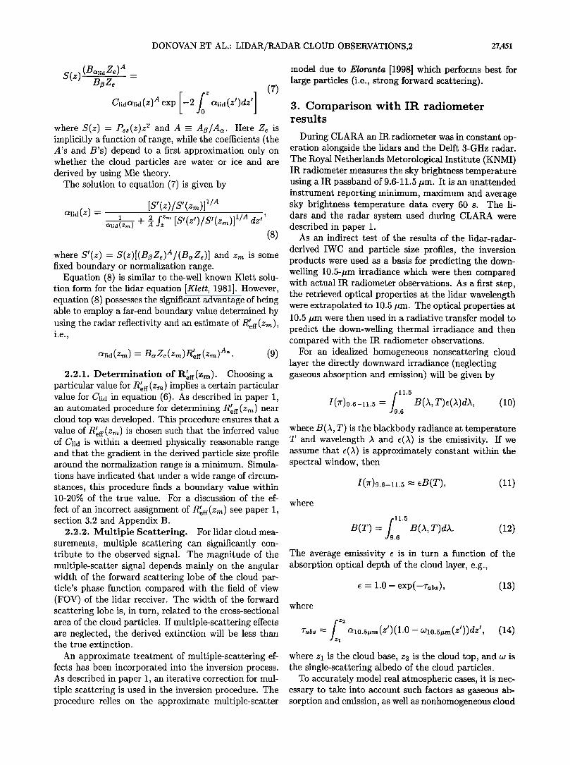
(Boqid Ze) A =

B•Ze (7)

•lidOqid(z)Aexp[--2•oZOqid(zt)dz t] where S(z) - P•(z)z 2 and A - A•/A•. Here Z• is implicitly a function of range, while the coefficients (the A's and B's) depend to a first approximation only on whether the cloud particles are water or ice and are derived by using Mie theory.

The solution to equation (7) is given by

Oqid (g) -- 1 z,• 1/A ' + fz (8)

where S'(z) - S(z)[(B•Z•)•/(B•Z•)] and z,• is some fixed boundary or normalization range.

Equation (8) is similar to the-well known Klett solu- tion form for the lidar equation [Klett, 1981]. However, equation (8) possesses the significant advantage of being able to employ a far-end boundary value determined by using the radar reflectivity and an estimate of R'e•(z,•), i.e.,

Oqid(Zm)- Bc•Ze(zm)t•;ff(Zm) Aø' . (9)

2.2.1. Determination of R•eff(Zm). Choosing a particular value for R•e• (Zm) implies a certain particular value for Cnd in equation (6). As described in paper 1, an automated procedure for determining R•e•(Zm) near cloud top was developed. This procedure ensures that a value of Rteff(Zm) is chosen such that the inferred value of C•id is within a deemed physically reasonable range and that the gradient in the derived particle size profile around the normalization range is a minimum. Simula- tions have indicated that under a wide range of circum- stances, this procedure finds a boundary value within 10-20% of the true value. For a discussion of the ef-

fect of an incorrect assignment of R•e•(zm) see paper 1, section 3.2 and Appendix B.

2.2.2. Multiple Scattering. For lidar cloud mea- surements, multiple scattering can significantly con- tribute to the observed signal. The magnitude of the multiple-scatter signal depends mainly on the angular width of the forward scattering lobe of the cloud par- ticle's phase function compared with the field of view (FOV) of the lidar receiver. The width of the forward scattering lobe is, in turn, related to the cross-sectional area of the cloud particles. If multiple-scattering effects are neglected, the derived extinction will be less than the true extinction.

An approximate treatment of multiple-scattering ef- fects has been incorporated into the inversion process. As described in paper 1, an iterative correction for mul- tiple scattering is used in the inversion procedure. The procedure relies on the approximate multiple-scatter

model due to Eloranta [1998] which performs best for large particles (i.e., strong forward scattering).

3. Comparison with IR radiometer results

During CLARA an IR radiometer was in constant op- eration alongside the lidars and the Delft 3-GHz radar. The Royal Netherlands Metorological Institute (KNMI) IR radiometer measures the sky brightness temperature using a IR passband of 9.6-11.5 pm. It is an unattended instrument reporting minimum, maximum and average sky brightness temperature data every 60 s. The li- dars and the radar system used during CLARA were described in paper 1.

As an indirect test of the results of the lidar-radar-

derived IWC and particle size profiles, the inversion products were used as a basis for predicting the down- welling 10.5-pm irradiance which were then compared with actual IR radiometer observations. As a first step, the retrieved optical properties at the lidar wavelength were extrapolated to 10.5 pm. The optical properties at 10.5 pm were then used in a radiative transfer model to predict the down-welling thermal irradiance and then compared with the IR radiometer observations.

For an idealized homogeneous nonscattering cloud layer the directly downward irradiance (neglecting gaseous absorption and emission) will be given by

11.5 I(Tr)o.•_•.s = B(A, T)e(X)dX, .6

(10)

where B(A, T) is the blackbody radiance at temperature T and wavelength A and e(X) is the emissivity. If we assume that e(X) is approximately constant within the spectral window, then

I(•r)9.6-•.5 m eB(T), (11)

where

11.5 B(T) - B(A,T)aA. (12) .6

The average emissivity e is in turn a function of the absorption optical depth of the cloud layer, e.g.,

e - 1.0 - exp(--Tabs), (13)

where

Tabs -- OZlO.5•m (Zt)(1.O -- 6olO.5•m(Zt))dz t, (14) 1

where 2:1 is the cloud base, z2 is the cloud top, and w is the single-scattering albedo of the cloud particles.

To accurately model real atmospheric cases, it is nec- essary to take into account such factors as gaseous ab- sorption and emission, as well as nonhomogeneous cloud

27,452 DONOVAN ET AL.' LIDAR/RADAR CLOUD OBSERVATIONS,2

'• 1,4

• •.2

o 1.0

•'• 0.8 .,•

• 0.6

0.4

o 0.2

Ice

No. 1/No. ( 10

• R d.eff. 1 -- 5 micron,

10 100

R'•.[microns]

Complex Polycrystals Ice

1.4 +• 1.4

1.2 1.2

1.0 1.0

0.8 0.8

0.6 0.6

0.4 0.4

0.2 d,eff:l = 1, 5, ,ml, c,1øns t 0.2 0.0 0.0

10 100

R'err[microns ]

Ice

No 1/No2 = 10

l(f

d,eff, 1 ----

, 11,1 , , , , , 1,11

lO lOO

R'.rf[microns ]

Brown and Francis, D m Binned Ice Ice Ice

1.4 N o /No2=10 1.4 No•/No2=10 1.4 '• ' '

1.2 1.• 1.2[ '"' X'"• 1•1 ] 1.0 1.0 1.0

0.8 0.8 0.8

0.6 0.6 0.6

0.4 0.4 0.4

0.0 0.0 0.0 too •o •oo lo loo

microns ] R'.,[mic ton s ] R'.,r [ microns ]

Figure 1. Ratio of 10.5-/•m extinction to 905-nm extinction for a number of different families of bimodal gamma type cloud particle size distributions (see equation (23) in paper 1) for two different ice crystal habits.

optical properties and temperature variations within the cloud. However, the dominant factor is the cor- rect specification of the cloud 10.5-/•m absorption op- tical depth. This quantity may be inferred by using the lidar/radar inversion results as a starting point. If the particles are sufficiently large, then they may be re- garded as optical scatterers/absorbers at both 10.5/•m and 905 nm. The ratio of the extinction at both wave-

lengths will then be close to unity. For sufficiently large absorbing particles the single-scattering albedo will also approach 0.5. Thus if the cloud particles are large enough, then there will be no difficulty in extrapolat- ing the 905-nm extinction to the extinction at 10.5/•m. For ice cloud particle size distribution which contains sufficient fraction of particles whose maximum dimen- sion is less that 10.5 /•m the relationship between the 10.5-/•m absorption and the 905-nm extinction will be more complicated.

The relationship between the 10.5-/•m extinction 905- nm extinction is explored in a quantative sense in Fig- ure I in which the ratio of the 10.5-/•m extinction to 905-nm extinction is shown for a number of cases. Here

we have assumed bimodal gamma type size distribu- tions of the type described by equation (23) in paper 1. In each case, the values of No,2/No,1, ]Z•d,e//,1, 0/1 ---- 10, and 72 = 4 were fixed while Rm,2 was varied. Re- sults are shown for three values of Rd,e//,1 (5,15, and 30 /•m) for four values of No,2/No,1 (106, 10 -1, 10 -2, and 10-3). The No,2/No,1 = 106 case represents the case of a virtually unimodal size distribution. The results shown are the product of Mie calculations applied to equivalent Reft spheres for two different crystal habits (complex polycrystal Mitchell et al. [1996] and Brown and Francis [1995] Dmbinned (see paper 1)). That is, each nonspherical particle in the size distribution is re- placed by an appropriate number of solid ice spheres whose radius is such that both the crystal mass (M(ra)) and cross-sectional area (Ac(ra)) are preserved. It was demonstrated by Grenfell, and Warren [1999] who found that equal volume-to-area ratio spheres (equivalent Reft spheres) can usefully model the infrared scattering and absorption properties of nonspherical ice particles.

Consistent with our aim of using the lidar-radar de- rived 905-nm extinction profile together with the lidar-

DONOVAN ET AL.' LIDAR/RADAR CLOUD OBSERVATIONS,2 27,453

radar effective particle size measurements, the results are shown as functions of Rtef (and not as functions of Reft). It can be seen that, as expected, the ratios converge for large values of Rtef. However, how rapid the convergence is depends on the value of No,2/No,2, R•,e//,1, and the crystal habit. It can be seen, gener- ally speaking, that for values of R•ef• greater than 40/•m and values of No,2/No,1 greater than 10 -2 the ratios are in the range of 0.9-1.1. For smaller values of Rtef•, the ratios are quite variable in the cases where Ra,e/y,1 is relatively small. Corresponding to Figure 1, the 10.5- ym single-scattering albedo (w) is shown as a function of R•ef• in Figure 2. The size distributions and crystal habits used here are the same as those used in the pre- vious figure and the calculations were performed in a similar fashion. Here it can be seen that w generally varies between 0.4 and 0.5 for R•ef• greater than 40/•m and No,2/No,2 greater than 10 -2. Putting the extinc- tion ratio and single-scattering albedo results together implies that the conversion between 905-nm extinction and 10.5-/•m absorption can be reasonably carried out if Rtef• is greater than about 40 /•m. Below this value the exact form of the ice cloud particle size distribution becomes increasingly important.

A model based on a one-dimensional plane-parallel discrete ordinate radiative transfer equation solver (DIS- ORT $tamnes et al., [1988]) was constructed which cal- culates the 9.6-11.5-/•m sky zenith radiance based on the lidar/radar inversion results and a specified atmo- spheric gaseous composition and temperature profile. DISORT itself is a well-known radiative transfer equa- tion solver for multiple-scattering and emitting layered media and is used as the core solver in packages sfich as MODTRAN [Berk et al., 1989] and STREAMER [Key and Schweiger, 1998]. Once the relevant parameters are specified at each model level (in our case, layer op- tical depth, single-scattering albedo, scattering phase function, and temperature), then DISORT is used to solve the discrete ordinate form of the radiative transfer

equation in order to obtain the downwelling vertical ir- radiance profiles. Thus factors such as the atmospheric transmission of the layer between the ground and the cloud, the emission of this layer, and the scattering of the infrared radiation by the cloud particles are all im- plicitly accounted for.

In this work, 16 streams were specified in the discrete ordinate calculations. A model level was specified ev- ery 100 m for altitudes below the cloud top along with

¸

• 10 ,o ß

.• 0.a

o 0.6

• 0.4 .,•

o k 0.2

.,•

¸

© 10 .o ß

• 0.8

o 0.6

I

• {).4 o,.•

•o 0.z ,,•

Ice

R d,eff, 1 = 5 microns

N02/N0.1= 10

, ,•,1 i • i

10 100

R'eff[microns ]

Complex Polycrystals Ice

R a,•m• =15microns

-2

, •,1 I I

10 100

R'eff[microns]

R d,at,• = 30 microns

No,2/NoA = 10 10

10 100

R'•ff[microns]

Brown and Francis, D m-Binned lee Ice lee

R d,•r• = 15 microns 0.8

0.6

0ø4

0.•

13.0 ..............

10 100 10 100

R'•u[mierons ] R'•u[mierons ]

Figure 2. Single-scattering albedos corresponding to Figure 1.

R d,eff, l = 5 microns

-2

I .... • N0.2/No, i= 10 t

-1

No.2/No. 1 = 10

R d,eff, 1 : 30 microns

-1

No.2/No, 1 = 10

10 100

R'•u[microns ]

27,454 DONOVAN ET AL- LIDAR/RADAR CLOUD OBSERVATIONS,2

Backscatter Signal [Sr Km]" 18/4/1796 8 -'-'" ...... ' ................... ' .... , ....................... 0.!

6

0 1o --• 20 21 22 23 24 25

Time Hrs. [UTC]

R.. [microns] 18/4/1996 8 i ........................................ , ........................ •40.00

55.00

6 30.00

* 25.00 i • • 15.00

I

•o.oo

5.00

Reflectivity [Dez] 18/4/1996 8f .......... ' .......... ''""'"" ........ ' ...... ' .......... , ......... ,

20 21 22 23 24 25 Time Hrs. [UTC]

Water content [g/m'] 18/4/1996 8( ............ ' ........................................ , 0.1

6

%7.,

2

,,, 10 -za

j I i

0 .... • ..... 0.00 0 10 '*• 20 21 22 25 24 25 20 21 22 25 24 25

Time Hrs. [UTC] Time Hrs. [UTC]

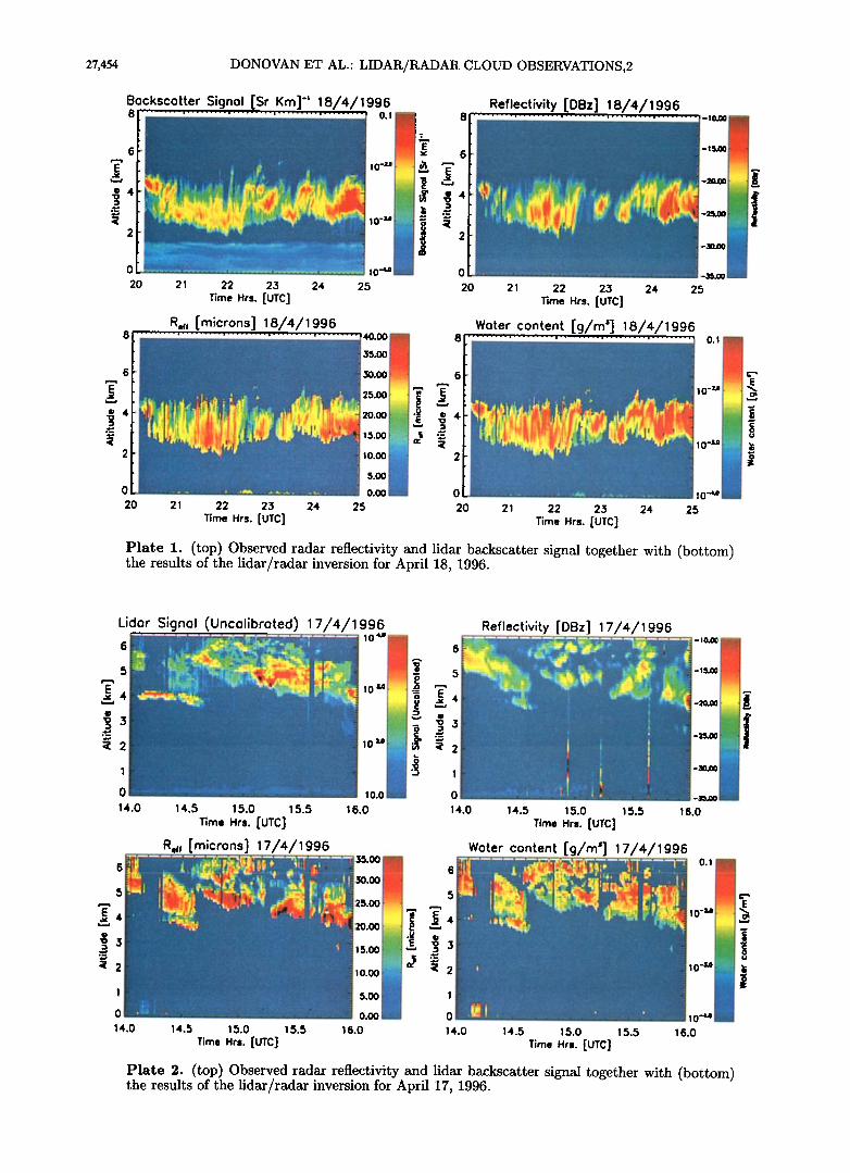
Plate 1. (top) Observed radar reflectivity and lidar backscatter signal together with (bottom) the results of the lidar/radar inversion for April 18, 1996.

Lidor Signal (Uncolibroted) 17/4/1996 ............... 10 ,•.D

6

5

1

0

14.0

5

14.5 15.0 15.5

Time Hrs. [UTC]

10.0

16.0

R.,, [microns] 17/4/1996

I

1

o

140

20.00

6

< 2

;3 1

Reflectivity [DBz] 17/4/1996

5

• ;• 2

14.0 14.5 15.0 15.5 16 0 Time Hrs. [UTC]

_ Water...content ' [g/m'] 17/4/1996 •'J•' ........ • ...................... 0.1 6 .... ' .•1

• 10-za

' 0.00 0 ' ' 10 '•'• •4.5 • 5.o • 5.5 • •.o • 4.0 • 4.5 • 5.o • 5.5 • 6.0

Time Hrs. [UTC] Time Hrs. [UTC]

Plate 2. (top) Observed radar reflectivity and lidar backscatter signal together with (bottom) the results of the lidar/radar inversion for April 17, 1996.

DONOVAN ET AL.: LIDAR/RADAR CLOUD OBSERVATIONS,2 27,455

100 logarithmically spaced levels between the cloud top and 50 km. The model includes gaseous absorption and emission by water vapor, 03, and CO2. To find the gaseous optical depth for each layer, a Malkmus band model together with the two-parameter van de Hulst, Curtis, and Godson (H-C-G) approximation was used to account for the line absorption for 03 and CO2 [Goody and Yung 1989; Lenoble, 19931. A Goody band model was used to treat the water vapor lines, while the water vapor continuum was handled by using the em- pirical formulas of Roberts et al. [1976]. The spectro- scopic data used were taken from the tables compiled by Lenobie [1993]. The atmospheric temperature and hu- midity profiles used in the calculations for a particular instance of time were obtained by interpolating between profiles measured by locally launched radiosondes. The ozone mixing ratio profiles were taken from the clima- tology of Fortuin and Kelder [1998]. Emission from the ground was also accounted for. Consistent with a mix- ture of vegetation and damp ground, the ground emis- sivity was fixed at 0.95. For a discussion regarding the expected relative contribution of various processes (i.e., the importance of photons emitted by the ground and reflected by the clouds, etc.,) the reader is referred to Platt [1973,1979], and Young [1995].

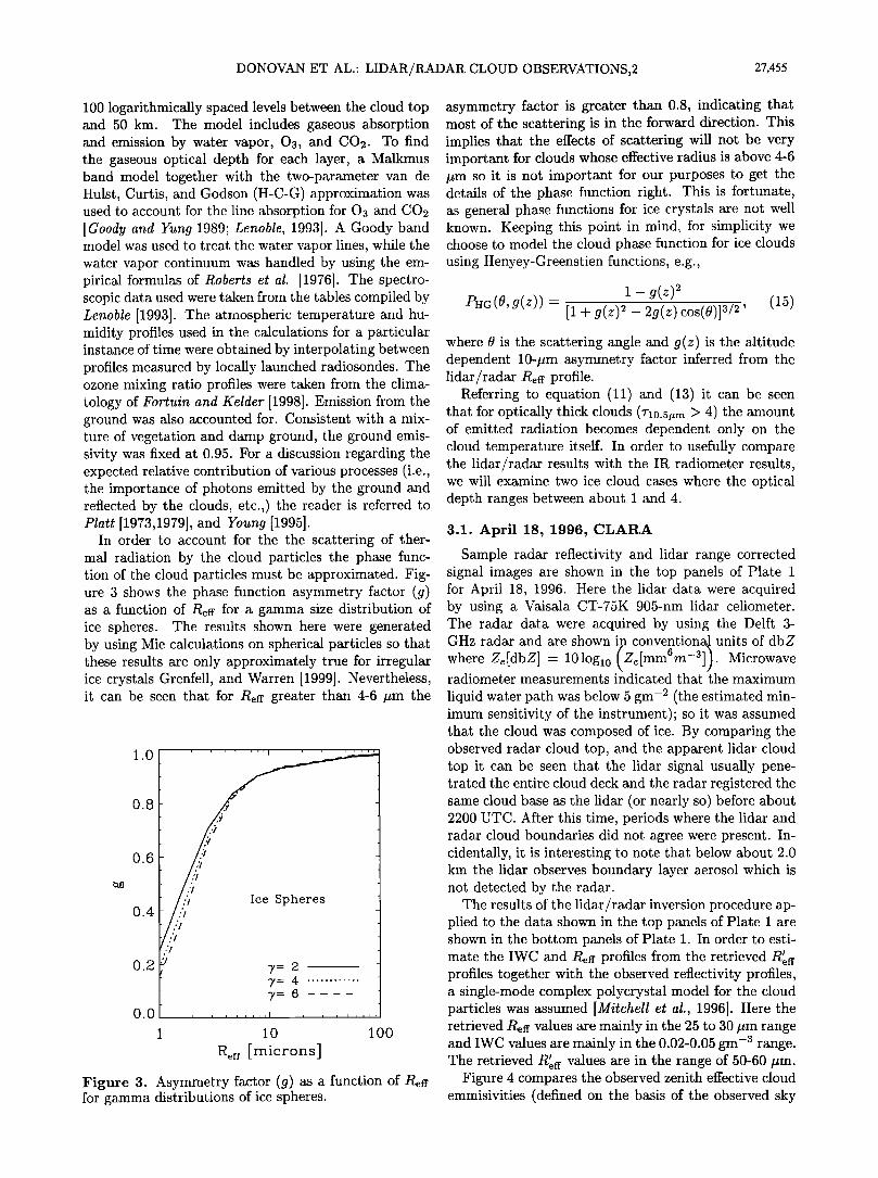
In order to account for the the scattering of ther- mal radiation by the cloud particles the phase func- tion of the cloud particles must be approximated. Fig- ure 3 shows the phase function asymmetry factor (g) as a function of Ref for a gamma size distribution of ice spheres. The results shown here were generated by using Mie calculations on spherical particles so that these results are only approximately true for irregular ice crystals Grenfell, and Warren [1999]. Nevertheless, it can be seen that for Ref greater than 4-6 •um the

1.0

0.8

0.6

0.4

0.2

0.0

I

/..:/ Ice Spheres

./

7 = 2 7- 4 7=6

1 10 100

R•ff [microns]

Figure 3. Asymmetry factor (g) as a function of Reft for gamma distributions of ice spheres.

asymmetry factor is greater than 0.8, indicating that most of the scattering is in the forward direction. This implies that the effects of scattering will not be very important for clouds whose effective radius is above 4-6 •um so it is not important for our purposes to get the details of the phase function right. This is fortunate, as general phase functions for ice crystals are not well known. Keeping this point in mind• for simplicity we choose to model the cloud phase function for ice clouds using Henyey-Greenstien functions, eog.,

- - + o,(.),_ 2a(.)

where 0 is the scattering angle and g(z) is the altitude dependent 10-•um asymmetry factor inferred from the lidar/radar Ref profile.

Referring to equation (11) and (13) it can be seen that for optically thick clouds (r•0.5,m > 4) the amount of emitted radiation becomes dependent only on the cloud temperature itself. In order to usefully compare the lidar/radar results with the IR radiometer results, we will examine two ice cloud cases where the optical depth ranges between about I and 4.

3.1. April 18, 1996, CLARA

Sample radar reflectivity and lidar range corrected signal images are shown in the top panels of Plate 1 for April 18, 1996. Here the lidar data were acquired by using a Vaisala CT-75K 905-nm lidar celiometer. The radar data were acquired by using the Delft 3- GHz radar and are shown in conventional units of dbZ

where Zc[dbZ]- 101og•0 (Zc[mm6m-3]). Microwave radiometer measurements indicated that the maximum

liquid water path was below 5 gm -2 (the estimated min- imum sensitivity of the instrument); so it was assumed that the cloud was composed of ice. By comparing the observed radar cloud top, and the apparent lidar cloud top it can be seen that the lidar signal usually pene- trated the entire cloud deck and the radar registered the same cloud base as the lidar (or nearly so) before about 2200 UTC. After this time, periods where the lidar and radar cloud boundaries did not agree were present. In- cidentally, it is interesting to note that below about 2.0 km the lidar observes boundary layer aerosol which is not detected by the radar.

The results of the lidar/radar inversion procedure ap- plied to the data shown in the top panels of Plate I are shown in the bottom panels of Plate 1. In order to esti- mate the IWC and Ref profiles from the retrieved R'ef profiles together with the observed reflectivity profiles, a single-mode complex polycrystal model for the cloud particles was assumed [Mitchell et al., 1996]. Here the retrieved Ref values are mainly in the 25 to 30 •um range and IWC values are mainly in the 0.02-0.05 gm -3 range. The retrieved R'ef values are in the range of 50-60 •um.

Figure 4 compares the observed zenith effective cloud emmisivities (defined on the basis of the observed sky

27,456 DONOVAN ET AL.' LIDAR/RADAR CLOUD OBSERVATIONS,2

1.0

E L• 0.6

o

.2 0.4

¸

• 0.2

0.0

2O

......... I ......... I

21 22 23 24

Time (Hrs. UTC)

Figure 4. Observed and calculated effective cloud 10.5- pm emissivities for April 18, 1996. The triple lines show the maximum. average, and minimum IR radiometer observation within a 60-s time interval, while the dark line marked with squares shows results from the radia- tive transfer model using the lidar/radar inversion re- sults. The solid line segments mark time periods where the lidar or radar cloud boundaries differed by 200 m or more.

radiances and the temperature at the observed cloud base) for April 18 with the results from the radiative transfer model using the lidar/radar inversion results. From 2000 to around 2200 UTC. the observed and cal-

culated values agree within about 0.05. Using equa- tions (11)-(14), this implies that the lidar-derived op- tical depth appears to be correct within about 15%. Later in the day the disagreement between the IR ra- diometer and the lidar/radar results grows to over 0.2. This is due mainly to parts of the cloud being below the radar's sensitivity (about -35 dbZ). As previously men- tioned, before 2200 the lidar observed cloud boundaries are close to the observed radar cloud boundaries. After

2200 differences of up to 500 m are seen between the lidar- and radar-observed cloud boundaries. This high- lights a weakness in the lidar/radar method, namely, that signals from both instruments must be present for the inversion to yield reliable results.

For this case the values of R•ef• were between 50 and 60 pm so that according to our earlier discussion (see Figures I and 2) the ratio between the 10.5-pm absorp- tion and the 905-nm extinction is not very dependent on the particle size for monomodal distributions and for bimodal distributions if No,2/No,1 is greater than about 10 -2 . Thus the agreement of our model calcu- lations based on the lidar/radar retrieval results really only indicates that the derived 10.5-pm optical depth is correct. This implies that the 905-nm optical depth de- rived by the lidar/radar procedure is correct to within 10-15%. In terms of particle size, though, the results only indicate that the particles were not smaller than R•ef• =20-25 pm (otherwise the conversion between the 905-nm and 10.5-pm extinction would have been no-

ticeably off). In short, the IR radiometer observations are consistent with the particle sizes inferred by the lidar/radar inversion, but not a rigorous test of the de- rived particle sizes.

3.2. April 17, 1996, CLARA

In contrast to the relatively homogeneous April 18 ice cloud example, a more structured mixed-cloud example is presented in Plate 2 (April 17, 1400-1530 UTC). The lidar data shown here were acquired by the Dutch Na- tional Institute of Public Health and the Environment

(RIVM) Fight Temperol Resolution (HTRL) lidar at a wavelength of 1064 nm. Here there are several fea- tures present in the lidar image which are not present in the corresponding radar image. In particular, a layer present at 4.0 km between 1400 and 1430 UTC is clearly detected by the RIVM lidar but not by the radar. It is believed that the particles in this layer are too small to give rise to a usable radar signal; this implies that the layer had an effective radius below a few microns. Particles with radii this small may suggest the presence of supercooled water droplets. The temperature at 4.0 km was around-15øC; supercooled water layers may be observed down to temperatures of around -40øC. Note also that this layer completely attenuates the lidar sig- nals implying that its minimum optical depth is of the order of 4 at 1064 nm. Another area where the lidar

detects cloud and the radar does not is present between 4.5 and 5.0 km at around 1510-1518 UTC.

The results of the inversion applied to the lidar and radar data are shown in the bottom panels of Plate 2. This example highlights the fact •hat retrievals are only possible when both the lidar and radar signals are above the noise floor. Here the retrievals are only representa- tive of the entire cloud

columns between about 1430-1512 and 1518-1548 UTC.

During other times the presence of noise, attenuation of

'- With MS .__ Observed

Ld 0.6 .-- 0.4

o

cr 0.2 [- NoMS O.Of, , , , , • , , , , , , , , , , , , , , , , , , , , , , , 14.6 14.8 15.0 15.2 15.4 15.6 15.8

Time (Hrs. UTC)

Figure 15, Observed and calculated effective cloud emissivities for April 17, 1996. The area labeled "No MS" shows the computed emissivities when multiple scattering in the lidar signal is neglected.

DONOVAN ET AL.: LIDAR/RADAR CLOUD OBSERVATIONS,2 27,457

the lidar signal, or the absence of a strong enough radar return made a representative retrieval impossible.

A comparison between the observed zenith sky radi- ance with the results from the radiative transfer model

using the lidar/radar inversion results for April 17 is shown in Figure 5. As was discussed earlier, the re- trievals are only representative of the entire cloud col- umns between about 1430 Hrs and 1548 UTC. Here it

can be seen that good agreement is obtained for data taken past 1430 UTC. Note, that for this plot at around 1515 UTC, where the lidar has detected much more cloud in the column than the radar (see Plate 2) the lidar/radar data have not been plotted.

For the Vaisala lidar which has a small field of view

(less than 0.5 mrad) there is generally only a small difference in the final results if multiple scattering is taken into account or not. However, the RIVM lidar has a large FOV (10 mrad); so multiple-scattering ef- fects must be accounted for in the inversions. The lower

line in Figure 5 shows the cases where the lidar/radar results derived by ignoring multiple scattering effects have been used to calculate the IR radiances. It can be

seen that the agreement between the IR radiometer ob- servations and the inversion results is notably degraded. The difference in the results stems mainly from the dif- ferent cloud optical depths inferred when the inversion procedure accounts for multiple-scattering or not. If multiple scattering is ignored then the effective extinc- tion is smaller than the real extinction (by up to a factor of 2 for large particles and large lidar fields of view). In addition, here the algorithm also tends to chose a dif- ferent boundary value which results in an even lower re- trieved extinction profile. The results shown in Figure 5 demonstrate the need to account for multiple-scatter ef- fects in the retrievals and further support the manner in which we are accounting for multiple-scatter effects. More detail on the effects of multiple scattering on the inversion procedure can be found in paper 1.

4. Comparison With In-situ Measurements

In this section, comparisons between the C-130 2- D probe measurements and the results of both ground and aircraft based lidar/radar cloud soundings are pre- sented for two days during the CLARE'98 campaign. CLARE'98 was conducted during October 5-23, 1998, at the Chilbolton Observatory, Hampshire, UK [Wur- steisen and Illingworth, 1999]. For two overflights of the UK Meteorological Office (UKMO) C-130 on Oc- tober 21, results are shown which use the combination of the ground-based GKSS 94-GHz radar [Danne and Quante, 1999] and the Vaisala CT-75K 905-nm lidar celiometer [Goddard, 1999]. For October 20, compar- isons between the lidar/radar inversion results using the airborne KESTREL 94-GHz radar together with the LEANDRE 532-nm lidar (both mounted on the

ARAT aircraft) and in situ measurements made dur- ing a near-coincident C-130 flight are presented. De- tails of the LEANDRE radar and the KESTRAL li- dar instruments can be found in the work of Pelon et

al. [1999] and Guyot et al. [1999] respectively. For the 94-GHz CLARE data that are presented in this work, the gaseous attenuation was calculated from the UKMO Unified Model output and using the model of Liebe [1985], while the temperature dependence Kw was calculated by using the approach of Liebe at al. [1989].

During CLARE'98, several flights of the UK meteo- rological office C-130 aircraft were conducted [Francis, 1999]. The C-130 mounted several in situ particle siz- ing instruments including 2-D Cloud (2D-C) and 2-D Precipitation (2D-P) probes. The probes are based on the instrument described by Knollenburg [1970] and ba- sically consist of a laser which illuminates a linear ar- ray of 32 photodiodes; as hydrometeors pass through the sample volume, they cast a shadow on one or more of the diodes and enable a two-dimensional image to be compiled from which size and shape can be deter- mined. The 2D-C probe detects particles in the size range 25-800 pm, and the 2D-P probe detects particles in the range 200-6400 pm. From each crystal image both the area (Ac) and the mean of the maximum crys- tal dimensions measured parallel and perpendicular to the photodiode array (Din) are calculated. Crystal size spectra are then computed as functions of both Ac and Dm for each 5 s segment of data.

Two different methos for estimating the crytsal masses from the 2-D results have been used. One method pa- rameterizes the crystal mass according to its value of Dm; the other parameterizes the crystal mass according to its value of Ac. These two methods agree for small crystal sizes but diverge for crystals with Dm greater than about 100 pm. The two different relationships give a different mass versus area relationship and thus imply different R•ef versus Ref relationships. For the purpose of interpreting the radar reflectivity the rela- tionship between R•ef and Ref is important, since, as was shown in paper 1, the IWC is proportional to the

t

reflectivity and Reft/Reft, i.e.,

IWC - ps,i• IKI where ps,i is the density of solid ice. A comparison of the Rtef to Ref ratio as a function of Rtef for several ice crystal habits was shown in paper 1, Figure 10. There the relationships implied by the two different methods of interpreting the 2-D spectra are compared with those implied by the various models used by Mitchell et al. [1996].

4.1. October 21, 1998, CLARE'98

On this day the UKMO C-130 passed over the Chilbolton site four times. Two of the over passes

27,458 DONOVAN ET AL' LIDAR/RADAR CLOUD OBSERVATIONS,2

21/10/1998- 10.3304 Hrs

Lidor S(r)[km sr]-' WC g/m 3 10 -4 10 -3 10 -2 10 -1 10 -2

TøC

10 -• -40 -50 -20 -10

........ i ........ i ............. "'"i '1 ......... i ......... t ........

-30-20-10 0 10-310-210 -• 1.0 10 •

Reflectivity [dgz] Extinction [1/km] 4O 60 80 100

Reff[,/-zm ]

Figure 6. (left) Lidar (light solid line) and radar (heavy solid line) signal profiles for October 21, 1996, at 1020 UTC. (middle) Retrieved 905-rim extinction pro- file (heavy solid line) and estimated IWC profile (light solid line). (right) Retrieved Reft profile and the UKMO temperature profile (dotted line, upper axis). Solid cir- cles denote values inferred from the C-130 mounted 2-

D probes using the mass-versus-area relationship, while the shaded circles show the respective estimate made by using the mass-versus-maximum average dimension relationship.

occurred around 1020 UTC and two occurred around

1050 UTC. Throughout the campaign a ground-based Vaisala CT-75K 905-nm lidar was in continuous oper- ation. During the aircraft flight times, the GKSS 94- GHz radar and the Rablies 35-GHz radar were mainly operating in a scanning mode, but they also obtained vertically pointing "snapshots" around the direct over- pass times. Here the GKSS radar data were chosen for comparison with the lidar due to the higher spatial res- olution of the data.

The Vaisala CT-75K lidar signal and the equivalent reflectivity observed by the GKSS radar are shown in Figure 6. The radar signal here is a snapshot of around 10 s, while the lidar signal is an average of about 1.5 min. The raw CT-75K measurements have a tem-

poral resolution of 30 s, and averaging beyond this was found to be necessary. This was due to the relatively low signal-to-noise ratio of the lidar signal and the spo- radic detection of the cloud layer between 5.5 and 7 km by the lidar celiometer. Figure 6 also shows the ice wa- ter content and R'ef r profiles derived for the lidar and radar signals together with the values estimated for the IWC and effective radius from the 2-D probe data at around 5.8 km during the overpass.

The lidar-radar derived IWCs and Res values were estimated from the reflectivity profiles along with the derived R'ef r profile assuming the Dm binned model rela- tionship between particle mass and cross-sectional area of Francis et al. [19981, while the 2-D probe estimates shown were made by using both the Dm binned and Ac

binned relationships. These two methods tend to agree for smaller particles but diverge for larger particle sizes. It can be seen that the values for the ice water content

estimated using the lidar-radar inversion are consistent with the 2-D probe estimates. In this figure it can be seen that the effective radii estimates at 5.8 km seem

consistent within their respective uncertainties. The results for a later overpass are shown in Figure 7.

Here it appears that the aircraft sampled near the top of the cloud. The agreement here is seen tp be not as good as that for the earlier overpass. In particular, the aircraft appeared to fly just over the top of the observed cloud; also in this case there is a 30-s delay between the lidar/radar data and the actual overpass time. Either of these two effects may account for the apparent mis- match between the 2-D probe and lidar/radar IWC val- ues. However, the agreement between the particle sizes appears to be quite good. Here it can be seen that the observed particle sizes are smaller than those measured for the previous overpass for the higher cloud layer.

4.2. October 20, 1998

On October 20 a near-coincident flight path was flown by the French ARAT aircraft and the UKMO C-130. The ARAT carried the LEANDRE 532-nm lidar along with the KESTREL 94-GHz radar. The observed re-

flectivities and backscatter signals for this flight are shown in the top panels of Plate 3. A large cloud is visible in the top right portion of both panels, while the lidar image shows several strong backscattering layers not prominent in the radar reflectivities. These layers attenuate the lidar returns so that no useful lidar signal is present below about 2.0 km.

The bottom panels of Plate 3 show the estimated li- dar/radar effective particle size and the estimated water contents. The C-130 flights on this day show that lay- ers of liquid water were often present over and around Chilbolton. However, little water was encountered dur- ing the coincident C-130 flight at 4.6 km. The inversion

21/10/1998- 10.8222 Hrs

Lidor $(r) [km sr]-' WC g/m 3 10 -4 10 -3 10 -2 10 -• 10 -3 10 -2

TøC

-40 -50 -20 -10 0 ........ I ........ I ........ ......... i .......... I ......... I .........

'\

,,

¸o

-50-20-10 0 1 10 -1 1.0

Reflectivity [dBz] Extinction [1/km] 40 60 80 100

R•.[/zm]

Figure 7. Same as Figure (6) except for 1049 UTC.

DaNaVAN ET AL.: LIDAR/RADAR CLOUD OBSERVATIONS,2 27,459

Backscotter [Sr Km]" 20/10/1998 s• ....... ' ...... ' ........... •i •0.0 •

4

0:

14.70

4

O=

14.70

1.0

0.1

14.72 14.74 14.76 14.78 14.80

Time Hrs [UTC]

R,,, [microns] 20/10/1998

,

Reflectivity [DBz] 20/10/1998 ............. , ............... , ....... , ............ , .........

4

2

,

,,

ß

O'

14.70 14.72 14.74 14.76 14.78

Time Hrs [UTC]

20.00

!

27.5O

14.80

Water content [g/re'] 20/10/1998

-

' ' 10.0

I 1,0 14.72 14.74 14.76 14.78 14.80 14.72 14.74 14.76 14,78

Time Hrs. [UTC] Time Hrs. [UTC]

4

O:

14.70

1.0

10.• c o

I 0

14.80

Plate 3. (top) Observed radar reflectivity and lidar backscatter signal together with (bottom) the results of the lidar/radar inversions for the ARAT flight path.

results shown here were conducted by assuming that the strong backscattering layers below about 3.25 km (T - -4øC) were composed mainly of liquid water, while else- where it was assumed that the clouds were ice. If an

inversion is conducted by assuming ice everywhere, then the inferred particle sizes in these layers are still quite small (less than 2-4 pm). Since the far-end boundary values used in the inversions were set at the altitudes

of these layers, assuming they are mainly ice instead of water alters the particle sizes and IWCs inferred for al- titudes closer to the aircraft by not more than 10-20%.

The separation in space and time as a function of latitude between the ARAT and the UKMO C-130 are

shown in Figure 8. It can be seen that within about

10 km of Chilbolton the horizontal separation of the two aircraft was within 300 meters and the time dif-

ference within half a minute. Such separations are not ideal, but given the large extent and high apparent sta- bility of the large ice cloud sampled here together with the horizontal resolution of the aircraft measurements

(about 500-600 m for the C-130 measurements), they may be considered adequate for useful comparison in this case.

A comparison between various cloud properties in- ferred from the 2-D probe measurements and the li- dar/radar inversion results is shown in Figure 9. The lidar/radar results shown are for an altitude of 4.55 kin, which was the maximum height at which reliable data

• 1.5 ,_

½• 1.0

"' 0.,5

c 0.0' o

._• -2.4

CLARE98, 20 October, ARAT/C- 150 CLARE98, 20 October, ARAT/C- 150

2.0

1.5

1.0

0.5

o.o

-2.4 -2.2 -2.0 - 1.8 - 1.6 - 1.4 -2.2 -2.0 -1.8 - 1.6

Longitude (Deg) Longitude (Deg) -1.4

Figure 8. Separation in space and time between the ARAT and the UKMO C-130 as a function of longitude.

27,460 DONOVAN ET AL.' LIDAR/RADAR CLOUD OBSERVATIONS,2

•,10

120

T 100 o 80

b 60 T:

40

o

300

,• 250

• 200 ._u 150

• 100

• 50 0

0.50

0.40

• 0.30

ro 0.20

O. lO

oooo

CLARE98, 20 October, ARAT/C-130 (Altitude 4.55 Kin)

2.4 -2.2 -2.0 -1.8 -1.6 -1.4 Longitude (Deg)

Figure 9. Comparison of lidar/radar results and 2-D probe results for the ARAT/C-130 flight path. Heavy solid lines show the respective results from the li- dar/radar inversions at 4.55 km. Light solid lines show the respective results for the 2-D probe data using the mass-versus-area relationship, while the dot-dashed lines show results of the mass-versus-maximum average dimension relationship.

the set of assumed mass to Dm and area to Dm relation- ships. However, it can be seen for both the Ac binned and the Dm binned methods of determining the particle masses that reasonable agreement could be achieved by using a monomodal size distribution with q• - 2.

Referring back to Figure 9 it can be seen that the comparisons between the lidar-radar-derived quantities and the 2-D probe measurements are consistent within the uncertainty between the two methods for determin- ing particle mass from the 2-D probe measurements. In particular, the lidar/radar results for IWC appear to agree somewhat better for most of the flight path with the Dm derived 2-D probe estimates. The sig- nificance of this result is unclear at this point. The li- dar/radar estimate of R/err and extinction are the funda- mental products of the inversion and are not dependent on the assumed crystal habit. However, the 2-D probe estimates of R/eft are dependent on the assumed crystal- habit. It is quite encouraging that the lidar/radar R/elf time series agrees well with one of the methods for inter- preting the 2-D probe data, but it remains to be seen whether such agreement is to be commonly expected or is limited to certain special circumstances. Further flight data, in connection with an independent measure of the IWC, are needed to truly verify the accuracy of the lidar/radar method as well as to better interpret the 2-D probe measurements themselves.

5. Summary and Conclusions

In this paper we have presented evidence that the li- dar/radar inversion algorithm described in detail in pa- per 1 generates results which compare well with ground-

were obtained. The ARAT flew at an altitude of about

4.85 km, while the C-130 flew at an altitude of around 4.6 km, which is just slightly higher than the maximum height of reliable lidar/radar data but is within one range bin (the resolution of the lidar data was 60 m) of the top of the lidar/radar data. As was the case for the ground-based October 21 results, results for the two different ways of interpreting the 2-D probe data are presented except for the case of the inferred extinc- tion. Since the optical extinction inferred from the 2-D probes is just twice the cross-sectional area of the par- ticles, the area-binned 2-D probe results for extinction are considered to be more accurate than those that may be inferred from the average dimension spectra. The lidar/radar IWC and Reft estimates shown here were generated by using the Dm binned model and assum- ing that the particle size distribution could be described by a gamma-type function with q• - 2. A comparison

/

between the values of/•eff/Reff inferred from the 2-D probe data and theoretical values based on gamma size distributions is shown in Figure 10. Both the "observed" values of the ratio and the theoretical values depend on

] ,

I ........................... Brown and Francis + Francis et al. (D binned.) Brown and Francis + Francis et al. (A?binn%d:)

'"';' . . ";"" ../.•:.-..

;. ......... :.:. _

1 -

0

100

R'•ff[microns]

Figure 10. R•eg/Reg inferred from the 2-D probe data using both the Ac binned and the Dm methods. The lines show results that would be expected using gamma- type size distributions (in Dm) with the width param- eter 7 equal to 2.

DONOVAN ET AL.' LIDAR/RADAR CLOUD OBSERVATIONS,2 27,461

based passive remote sensing observations as well as mogeneous mixture of ice and air. Using equations (31) with in situ aircraft-mounted particle probes. The and (32) of paper 1, implies that in both cases, crystals agreement obtained between the lidar/radar results and smaller than around 0.1 mm are composed of solid ice, independent IR radiometer observations and in-situ mea- while at larger sizes inclusions of air result in a lower surements presented here is very encouraging. In par- ticular, the demonstration that the lidar/radar method results can be used to predict the 10.0-•um surface irra- diance demonstrates that the method yields the proper extinction within about 10%. This is supported by com- parison with the area measurements of 2-D probe data. However, it is difficult to determine how accurate the IWC estimations are, owing to the fact that it is nec- essary to assume a crystal habit to interpret both the lidar/radar measurements and the 2-D probe measure- ments of mass. The agreement between the in-situ mea- surements and the lidar/radar measurements is encour- aging. However, further comparisons with in situ mea- surements must be made under different cloudy condi- tions before firm conclusions concerning the accuracy of this method may be drawn. In particular, an inde- pendent measure of the IWC would be extremely use- ful. The possibility of conducting such measurements in the near future seems bright. The UKMO C-130 now mounts a Nevzorov hotwire probe [Korolev et al., 1998] which provides a bulk measure of liquid water content and total condensed water content, from which ice water content can be derived. It is considerably more accurate than the bulk measure provided by Brown's [1993] total water probe, which measures the total water content in- cluding vapor and then subtracts the components that are not ice using other bulk measurements.

Despite these reservations it should be noted that the lidar,/radar method developed in paper and demon- strated in this paper represents a significant advance- ment with regard to active remote sensing of clouds. By using the radar and lidar signals together the pro- cedure, to a large degree, overcomes the problem of ac- curately extracting the extinction from the lidar signal, while at the same time it accounts for multiple scat- tering. With respect to cloud remote sensing this pro- cedure demonstrates the power of combining the lidar and radar measurements together within a consistent framework. However, further work will be necessary to quantify the accuracy and the range of validity of the assumptions inherent in the method.

Appendix A' Calculation of

The problem of relating the radar reflectivity to the lidar extinction is very similar to the problem of predict- ing Ze from 2-D images of particle area (extinction). Thus we have used the 2-D probe data alone to ex- plore the consequences of using equivalent R'eff spheres to model the cloud scattering properties. This method of modeling the particle scattering differs from previous approaches. Traditional approaches to calculating Ze from 2-D particle size probe measurements assume that each single ice crystal can be modeled as a spherical ho-

effective density. The reflectivity of a collection of these homogeneous spheres is then given by

0.9-•r•iD•?(Di), (A1) i

where Di is the diameter of the equivalent sphere in cor- responding to the ith size bin, ni is the corresponding number density, -/(D) is the Mie/Rayleigh backscatter ratio, and [K(f)[ 2 is the "dielectric parameter" for a ho- mogeneous ice-air mixture with an ice fraction f and is calculated by using the formulae of Meneghini and Liao [1996] and Liebe et al. [1989]. To a good approxima- tion, [K[ is proportional to f. For spectra binned by D,• we assume that the equivalent spherical diameter (D) is equal to Dm, and for spectra binned by area we assume that D = DA• = 2(Ac/7r) ø'5. The value of f for crystals in each size bin can then be calculated from equations (31) and (32) of paper 1. The factor of 0.93 is present in equation (A1) to make Z relative to liq- uid water at centimeter wavelengths. Both Brown et al. [1995] and Hogan and Illingworth [1999] have used this approach to calculate Z at 94 GHz from Dm binned aircraft size spectra.

An important point to note is that if a particular crys- tal is nonspherical, then in virtually every case, that will be larger than DAc. This is because Din, by its def- inition, represents in some sense an "envelope" that en- closes the two-dimensional crystal image. As discussed in more detail later, both Dm and DAc will be tend to be larger than the corresponding values of their equivalent

Ice Spheres (94 GHz)

lO ø -5

lO -lO

-15

•0-20 10

10 •

1.0

10-'

10 -z

10 -a

100 lOOO

10 100 1000

Radius[microns]

Figure 11. (top) Relative backscattering coefficient for solid ice spheres computed by using Mie theory (thin solid line) and the Rayleigh scattering approximation (solid thick line). (bottom) Ratio of Mie backscatter to that computed by using the Rayleigh scattering ap- proximation.

27,462 DONOVAN ET AL.: LIDAR/RADAR CLOUD OBSERVATIONS,2

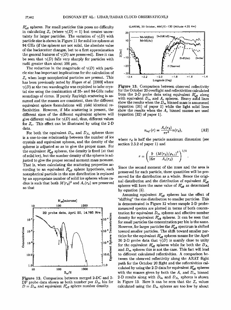
R•eff spheres. For small particles this poses no difficulty in calculating Ze (where ?(D) = 1) but creates uncer- tainty for larger particles. The variation of ?(D) with particle size is shown in Figure 11 for solid ice spheres at 94 GHz (if the spheres are not solid, the absolute value of the backscatter changes, but to a first approximation the general features of ?(D) are preserved). Here it can be seen that ?(D) falls very sharply for particles with radii greater than about 500 ttm.

The reduction in the magnitude of ?(D) with parti- cle size has important implications for the calculation of Ze when large nonspherical particles are present. This has been previously noted by Hogan et al. [2000] where ?(D) at the two wavelengths was exploited to infer crys- tal size using the combination of 35- and 94-GHz radar soundings of cirrus. If purely Rayleigh scattering is as- sumed and the masses are consistent, then the different equivalent sphere formulations will yield identical re- fiectivities. However, if Mie scattering is present, the different sizes of the different equivalent spheres will give different values for ?(D) and, thus, different values for Ze. This effect can be illustrated by using the 2-D data.

For both the equivalent Dm and DAc spheres there is a one-to-one relationship between the number of ice crystals and equivalent spheres, and the density of the spheres is adjusted so as to give the proper mass. For the equivalent R•eff spheres, the density is fixed (at that of solid ice), but the number density of the spheres is ad- justed to give the proper second moment mass moment. That is, when calculating the scattering properties ac- cording to an equivalent R•ff sphere hypothesis, each nonspherical particle in the size distribution is replaced by an appropriate number of solid ice spheres whose ra- dius is such that both M(rd) 2 and Ac(rd) are preserved so that

R'.•[mierons]

10 4

10

:Z 10 a

• 10 2

10.0

100 1000

probe data, April 20, 14.785 Hrs

1.0 •

10 100

, ,

1000

D•/2

104•

10a•

10 2 I:h

1 o.o.g

1.o

Figure 12. Comparison between merged 2-DC and 2- DP probe data shown as both number per Dm bin for D- Dm and equivalent R•fr sphere number density.

CLARE98, 20 October, ARAT/C-130 (Altitude 4.55 Krn)

20 ß ' ' ' _

D=D(R'eff) . 10

0

N _10 D (Ac) D=Dm'•

- 20 Z Observed

-30 , , , •i . ...... -2 -2.0 -1.8 -1.6 - .4

Longitude (Deg)

Figure 13. Comparison between observed reflectivity for the October 20 overflight and reflectivities calculated from the 2-D probe data using equivalent R'•ff along with equivalent Dm and Ac spheres. Heavy solid lines show the results when the Dm binned mass is assummed (equation (31) of paper 1) while the light solid lines show the results when the Ac binned masses are used (equation (32) of paper 1).

! ß ,

• M=M(Dm) M=M(Ac)

_

' \\ _

! ,

.4 -2.2

Ac(r•) n(r•), (A2) neq, (r) -- 7rr2 where ra is half the particle maximum dimension (see section 2.3.2 of paper 1) and

o ) r- 16•r Ac(r•)

1/4

Since the second moment of the mass and the area is

preserved for each particle, these quantities will be pre- served for the distribution as a whole. Hence the origi- nal distribution and the distribution of equivalent spheres will have the same value of R•eff as determined by equation (5).

Assuming equivalent R•ff spheres has the effect of "shifting" the size distribution to smaller particles. This is demonstrated in Figure 12 where sample 2-D probe- measured spectra are plotted in terms of both concen- tration for equivalent Dm spheres and effective number density for equivalent R•ff spheres. It can be seen that for small particles the concentration per bin is the same. However, for larger particles the R•ff spectrum is shifted toward smaller particles. The shift toward smaller par- ticles for the equivalent R•ff spheres means for the April 20 2-D probe data that ?(D) is mainly close to unity for the equivalent R•eff spheres while for both the and Dm spheres this is not the case. This fact will lead to different calculated refiectivities. A comparison be- tween the observed reflectivity along the ARAT flight path for the October 20 flight and the refiectivities cal- culated by using the 2-D data for equivalent R'•ff spheres with the masses given by both the Ac and Dm binned 2-D results along with Dm and DA• spheres is shown in Figure 13. Here it can be seen that the Z• values calculated using the Dm spheres are too low by about

DONOVAN ET AL.: LIDAR/RADAR CLOUD OBSERVATIONS,2 27,463

8 dbZ while the equivalent R•efr spheres using the area- binned masses give reflectivities which are about 5 dbZ too high. However, both the R•eg spheres using the Dm binned masses and the D = DAc spheres match the observed reflectivities within 1-2 dbZ.

Both matching methods here assume different masses for the ice crystals. Thus if an independent measure of the ice mass were available it would be possible to show whether the R•efr spheres or the equivalent Ac spheres are most useful to model the reflectivity. Unfortunately, no such measurement was available. As was the case

with the comparison between the 2-D results and the li- dar/radar results, the results are very encouraging but not conclusive. The results, however, do support the consistency of the effective lidar/radar radius (Rtef•) ap- proach, which is an important concept in the the li- dar/radar inversion procedure (see paper 1).

Acknowledgments. The authors wish to gratefully ac- knowledge the financial support of of the Netherlands Re- search Program on Climate Change and Environmental Pro- tection who partly funded the CLARA project. The finan- cial and technical support of ESA/ESTEC is also greatfully acknowledged. Part of this work was funded by ESA/ESTEC contract 12953/98/NL/6D. The CLARE'98 campaign was carried out as part of ESA's Earth Observation Preparatory Program (EOPP).

References

Berk, A., L. S. Bernstein, and D.C. Robertson, MOD- TRAN: A moderate resolution model for LOWTRAN 7, Tech. Rep. GL-TR-89-0122, Air Force Geophys. Lab., Hanscorn Air Force Base, Mass., 1989.

Brown, P. R •A, Measurements of the ice water content of cirrus using an evaporative technique, J. Atmos. Oceanic Technol., 10, 579-590, 1993.

Brown, P. Ro A., and P. N. Francis, Improved measurements of the ice water content in cirrus using a total-water probe, J. Atmos. Oceanic Technol., 12, 410-414, 1995.

Brown, P. R. A., A. J. Illingworth, A. J. Heymsfield, G. M. McFarquhar, K. A. Browning and M. Gosset, The role of spaceborne millimeter-wave radar in the global monitor- ing of ice-cloud, J. Appl. Meteorol., 3•, 2346-2366, 1995.

Danne, O., and M. Quante, The GKSS 95 GHz Cloud radar during CLARE'98: System performance and data prod- ucts, in International Workshop Proceedings: CLARE'98 Cloud Lidar and Radar Experiment, ESA/ESTEC ISSN 1022-6656, pp.51-53, Eur. Space Agency, Paris, 1999.

Donovan, D. P., and A. C. A. P. van Lammeren, Cloud effective particle size and water content retrievals using combined lidar and radar observations, 1, Theory and ex- amples, this issue.

Eloranta, E. W., Practical model for the calculation of mul- tiply scattered lidar returns, Appl. Opt., 37, 2464-2472, 1998.

Fortuin, J.P. F and H. Kelder, An ozone climatology based on ozonesonde and satellite measurements, J. Geophys. Res., 103, 31,709-31,734, 1998.

Francis, P. N., P. Hignett, and A. Macke, The retrieval of cirrus cloud properties from aircraft multi-spectral re- flectance measurements during EUCREX '93. Q. J. R. Meteorol. Soc., 12J, 1273-1291, 1998.

Francis, P. N., A summary of the cloud microphysics data collected during CLARE'98 by the UKMO C-130 Aircraft,

in International Workshop Proceedings: CLARE'98 Cloud Lidar and Radar Experiment, ESA/ESTEC ISSN 1022- 6656, pp.43-46, Eur. Space Agency, Paris, 1999.

Goddard J., Provision of Chilbolton Infrastructure and In- strumentation for CLARE'98, in International Workshop Proceedings: CLARE'98 Cloud Lidar and Radar Experi- ment, ESA/ESTEC ISSN 1022-6656, pp.47-51, Eur. Space Agency, Paris, 1999.

Goody, R. M., and Y. L. Yung, Atmospheric Radiation, The- oretical Basis, 2nd ed., Oxford Univ. Press, New York, 1989.

Grenfell, T. C., and S. G. Warren, Representation of a nonspherical ice particle by an assembly of spheres, in Nonspherical Light Scattering, edited by J. Hovenier, M. Mishchenko, and L. Travis, Academic Press, San Diego, California, 1999.

Guyot, A., J. Testud, O. Danne, M. Quante, Calibration of the University of Wyoming 95 GHz airborne radar during CLARE'98, in "International Workshop Proceed- ings: CLARE'98 Cloud Lidar and Radar Experiment", ESA/ESTEC ISSN 1022-6656, 69-75, 1999.

Hogan, R. J., and A. J. Illingworth, The potential of space- borne dual-wavelength radar to make global measure- ments of cirrus clouds. J. Atmos. Oceanic Technol., 16, 518-531, 1999.

Hogan, R. J., A. J. Illingworth, and H. Sauvageot, Measur- ing crystal size in cirrus using 35- and 94-GHz radars, J. Atmos. Oceanic Technol., 17, 27-37, 2000.

Hu, Y. X., and K. Stamnes, An accurate parameterization of the radiative properties of water clouds suitable for use in climate models, J. Clim., 6, 728-742, 1993.

Key, J., and A. J. Schweiger, Tools for atmospheric radiative transfer: Streamer and FluxNet, Cornput. Geosci., 24, 443-451, 1998.

Klett, J. D., Stable analytical inversion solution for process- ing lidar returns, Appl. Opt., 20, 211-220, 1981.

Knollenberg, R. G., The optical array: An alternative to scattering for airborne particle size determination, J. Appl. Meteorol., 9, 86-103, 1970.

Korolev, A. V., J. W. Strapp, G. A. Isaac, and A. N. Nev- zorov, The Nevzorov airborne hot-wire LWC-TWC probe: Principle of operation and preformance characteristics, J. Atmos. Oceanic Technol., 15, 1495-1510, 1998.

Lammeren, A. C. A. P, H. Russchenberg, A. Apituley, H. T. Brink, and A. Feijt, CLARA: A data set to study sensor synergy, in Synergy of Active Instruments in the Earth Radiation Mission, 12-1J November 97, Geesthacht, ESA EWP-1968- GKSS 98/E/10, edited by M. Quante, J.P. V. Baptista, and E. Raschke, pp.157-160, 1998.

Lenoble, J., Atmospheric Radiative Transfer, A. Deepak, Hampton, Va., 1993.

Liebe, H. J., An updated model for millimeter wave propa- gation in moist air, Radio Sci., 20, 1069-1089, 1985.

Liebe, H. J., T. Manabe and G. A. Hufford, Millimeter-wave attenuation and delay rates due to fog/cloud conditions, IEEE Trans. Antennas Propag., 37, 1617-1623, 1989.

Meneghini, R., and L. Liao, Comparisons of cross-sections for melting hydrometeors as derived from dielectric mixing formulas and a numerical-method, J. Appl. Meteorol., 35, 1658-1670, 1996.

Mitchell, D. L., A. Macke, and Y. Liu, Modeling cirrus clouds, Part II, Treatment of radiative properties, J. At- mos. Sci., 53, 2967-2988, 1996.

Pelon, J., et al., Observations of warm and cold clouds using the airborne backscatter lidar LEANDRE during CLARE'98, part 1, Lidar data analysis, in International Workshop Proceedings: CLARE'98 Cloud Lidar and Radar Experiment, ESA/ESTEC ISSN 1022-6656, pp.33-39, Eur. Space Agency, Paris, 1999.

27,464 DONOVAN ET AL.: LIDAR/RADAR CLOUD OBSERVATIONS,2

Platt, C. M. R., Lidar and radiometric observations of cirrus clouds, J. Atmos. $ci., 30, 1191-1204, 1973.

Platt, C. M. R., Remote sensing of high clouds, part 1, Cal- culation of visable and infared optical properties from li- dar and radiometer measurements, J. App!. Meteorol., 18, 1130-1143, 1979.

Roberts, R. E., J. E. A. Selby, and L. M. Biberman. Infared continuim absorption by atmospheric water vapor in the 8-12 micron window, Appl. Opt., 15, 2085-2090, 1976.

Stamnes, K., S.-C. Tsay, W. Wiscombe, and K. Jayaweera, A numerically stable algorithm for discrete-ordinate-method radiative transfer in multiple scattering and emitting layered media, Appl. Opt., 27, 2502-2509, 1988.

Wursteisen, P. and A. Illingworth, CLARE'98 Campaign Summary, in International Workshop Proceedings: CLARE '98 Cloud Lida, r and Radar Experiment, ESA/ESTEC ISSN 1022-6656, pp.9-17, Eur Space Agency, Paris, 1999.

Young, S. A., Analysis of lidar backscatter profiles in opti- cally thin clouds, Appl. Opt., oø4{, 7019-7031, 1995.

D. P. Donovan and A. C. A. P. van Lam-

meren, Royal Netherlands Meteorological Institute, P.O. box 201, 3730 AE, De Bilt, Netherlands. (donovan@knmi.nl; lammeren@knmi.nl)

R. J. Hogan, Dept. of meteorology Univ. of Reading, Reading, RG6 6BB, UK. (R.J.Hogan@reading.ac.uk)

H. W. .J. Russchenberg, Delft University of Tech- nology, Faculty of Information Technology and Sys- tems, P.O. box 5031, 2600 GA, Delft, The Netherlands. ( h. w.j .russch enb erg@i tr. tu delft. nl)

A. Apituley, National Institute of Public Health and the Environment, P.O. Box 1,3720 BA Bilthoven, Netherlands. (Arnoud. Apituley@rivm.nl)

P. Francis, UK Meteorological Office, Meteorological Re- search Flight, Y46 Building, DERA Farnborough, GU14 0LX, UK. (pnfrancis@meto.gov.uk)

J. Testud, IPSL-CETP, 10-12, avenue de l'Europe, 78140 Velizy, Fraance. (jacques.testud@cetp.ipsl.fr)

J. Pelon, Univ. Pierre et Marie Curie, CNRS- IPSL Service d'A•ronomie, Tour 15, couloir 15-14, B102, 4, Place Jussieu, 75252 Paris Cedex 05, France. (jacques. pelon @ aero.j ussieu. fr)

M. Quante, GKSS Institue for Atmospheric Physics, 21502 Geesthacht, Germany. (markus.quante@gkss.de)

J. Goddard, Ruther Appleton Lab. Radio Communica- tions Research Unit, Chilbolton, Didcot, Oxon OXll 0QX, UK. (j.w.f. goddard@rl. ac.uk)

(Received June 28, 2000; revised February 8, 2001; accepted May 29, 2001.)