1

Charging of dielectric surfaces in contact with aqueous

electrolyte – the influence of CO2

Peter Vogel*[a], Nadir Möller[a], Pravash Bista[b], Stefan Weber[b], Hans-Jürgen Butt[b], Benno Liebchen[c]

and Thomas Palberg[a]

[a] P. Vogel*, N. Möller, Prof. Dr. T. Palberg

Institut für Physik

Johannes Gutenberg Universität

Staudinger Weg 7, 55128 Mainz (Germany)

E-mail:

[b] P. Bista, Jun. Prof. Dr. Stefan Weber, Prof. Dr. H.-J. Butt

Max Planck Institut für Polymerforschung

Ackermannweg 10, 55128 Mainz (Germany)

[c] Prof. Dr. Benno Liebchen

Institut für Physik kondensierter Materie

Technische Universität Darmstadt

Hochschulstr. 8, 64289 Darmstadt (Germany)

Abstract: The charge state of dielectric surfaces in aqueous environments is of fundamental and technological importance. Here, we

study the influence of dissolved molecular CO2 on the charging of three, chemically different surfaces (SiO2, Polystyrene,

Perfluorooctadecyltrichlorosilane). We determine their charge state from electrokinetic experiments. We compare an ideal, CO2-free

reference state to ambient CO2 conditions. In the reference state, the salt-dependent decrease of the -potentials follows the

expectations for a constant charge scenario. In the presence of CO2, the starting potential is lower by some 50%. The following salt-

dependent decrease is weakened for SiO2 and inverted for the organic surfaces. We show that screening and pH driven charge

regulation alone cannot explain the observed effects. As additional cause, we tentatively suggest dielectric regulation of surface charges

due to a diffusively adsorbed thin layer of molecular CO2.

Introduction

The charge state of dielectric surfaces in contact with aqueous media is important for many contemporary technological challenges.

Examples range from desalination, ice nucleation, and fog harvesting to nervous conduction, chemotaxis and fluid transport. [1–6]

Charging plays a central role for stabilization of colloidal dispersions. [7–10] Charging, however, depends strongly on the environmental

conditions. Interest in the charging process of surfaces in contact with fluids is therefore motivated at the same time by the complexity

of this fundamental process and the prospect of useful application. Knowledge of the charge state under ideal lab conditions is vital to

develop a principle understanding of mechanisms underlying the surface properties. Conversely, the charge state under ambient

conditions is crucial for their performance.[2,9] Here we focus on the influence of dissolved CO2 on the -potential of dielectric surfaces

which has been neglected in most previous studies of this quantity.

In contact with a fluid, practically all dielectric surfaces are charged, either through dissociation of ionogenic surface groups[11] or

by adsorbed ions.[12,13] In nominally neutral polymer spheres dispersed in organic solvents, even individual charging events were

discriminated.[14] The equilibrium charge densities, respectively the corresponding potentials, are conveniently accessed in

electrokinetic experiments. Conductivity yields the effective number of freely moving micro-ions.[15] -potentials of planar or spherical

surfaces are obtained from electrokinetic mobilities µ = v E. (where v is the electrokinetic slip velocity in an applied electric field E),

which are evaluated by established IUPAC protocols based on the standard electrokinetic model.[16–18] For a constant charge density,

2

one expects a decrease of the mobility with increasing electrolyte concentration due to screening effects. This has been confirmed in

numerous experiments at elevated concentrations of added salt, cs 10−3 mol/L.[7] At lower added salt concentration, however, data

appear to be conflicting. Some authors report the expected decrease of mobilities[19–22], some an increase,[23] some find a maximum or

even a minimum followed by a maximum.[24] The underlying reason is not yet resolved.

Closer inspection shows that the qualitatively different behaviour may relate to differences in the salt-free starting point. Salt-free

or deionized water may contain several types of dissolved gases.[10] CO2 can react to carbonic acid. The solubility of CO2 in deionized

water[25–27] at ambient conditions (standard air at 25 °C) is 1.18 × 10−5 molL−1. The carbonate related chemical reactions in CO2 saturated

salt-free aqueous solution are:[25–32]

−

−

−

−

+ −

+ −

− + −

⎯⎯⎯→ +⎯⎯⎯

⎯⎯⎯→ +⎯⎯⎯

⎯⎯⎯→ +⎯⎯⎯

⎯⎯⎯→ +⎯⎯⎯

1

1

2

2

3

3

4

4

2

2 3 2 2

2 3 3

2

3 3

K

K

K

K

K

K

K

K

H O H OH

H CO CO H O

H CO H HCO

HCO H CO

(1)

Ki and K−i (i = 1−4) are the corresponding forward and backward kinetic constants. For the two-step acidic dissociation, pK3 = 3.6

and pK4 = 10.33.[33] At ambient conditions, they contribute 6.3 µmolL−1 of electrolyte. Simultaneously, the pH is shifted to 5.5. A so-

called realistic salt-free aqueous system results.[28–31] Under geologically relevant conditions of high pressures and high salt

concentrations, the solubility of CO2 is decreased due to salting-out.[27,34] Note that by contrast to other gases, like N2 and O2, the CO2

content can be adjusted by ion exchange and transient exposition to ambient air. This renders the present experiments sensitive for

the specific effects of CO2.

The increased salinity alters the double layer structure, the screening parameter , and in turn also the electrokinetic behaviour.[28–

30] The increased acidity alters the dissociation equilibrium of surface groups. Their degree of dissociation is determined by their pK

(e.g. 3R O SO H

apK − −= 1.5, and

−R COOH

apK = 4.5, = 4.0SiOH

apK ) and the amount of protonic counter-ions accumulated close to the surface

upon double layer formation.[31] A decrease in bulk pH enhances the proton accumulation and thus decreases the degree of dissociation

(pH driven charge regulation).

Dissolved gases may further adsorb at surfaces.[10] Neutron reflectivity measurements suggest the presence of a reduced

(deuterated) water density region that depends on the type and concentration of dissolved gases.[35] Molecular dynamics simulations

on a Lennard-Jones system report a significant enrichment of gas density close to hydrophobic surfaces. [36] Also experiments on

colloidal suspensions, conducted at ambient pressure and µmolar salt concentrations suggest, that CO2 can become stored at or on

particle surfaces.[37,38] Gas has even been observed to form films or nano-bubbles at dielectric surfaces.[39,40] Being of immense practical

importance, gas adsorption from solution and the equilibrium structure of gas-containing water near solid surfaces thus remain under

intense investigation.[10,41] However, somewhat surprisingly, a systematic study on the influence of dissolved (and possibly

accumulated) CO2 on the charge state of dielectric surfaces and on its salt concentration dependence is still missing.

The present paper addresses this issue for three different dielectric surfaces. We study standard glass slides (SiO2) as hydrophilic,

inorganic material, slides coated by Perfluorooctadecyltrichlorosilane (PFOTS) as strongly hydrophobic sample, and 40:60 Poly-n-

butylacrylamide-Polystyrene-copolymer (PnBAPS) spheres as mildly hydrophobic organic surface. All three surfaces are negatively

charged: the glass bears terminal OH− groups, the perfluorinated surface is presumably charged by adsorbed OH− [42], and the polymer

spheres carry ionizable carboxyl and sulphate groups. Under ambient conditions, their contact angles decrease with increasing -

potential (Figure S3 of the supplementary materials). Experiments on salt- and CO2-free conditions serve as reference. We compare

the results for the reference case to those at different levels of CO2 and of added NaCl or HCl. By adding NaCl at equilibrium with

airborne CO2, we approach conditions typical for practical applications.

We mount the specimen slides as side walls of a specially designed electrophoretic cell [43] (Figure S4a of the supporting information).

We fill the cell with a preconditioned suspension of PnBAPS tracer spheres, diluted to the desired low concentration. Cell dimensions

and tracer concentrations are chosen such as to prevent double layer overlap. The cell is connected to a gas tight conditioning circuit

comprising an ion exchange column to replace all ions in solution by H+ and OH− (Figure S1 of the supporting information)[44] Electrolyte

content and pH are monitored in-situ.[15,45] Our setup allows complete removal of dissolved and adsorbed CO2. Starting from CO2

3

equilibrated DI water, the pH drops from 5.5 to 7.0 and we obtain a stable conductivity of 55−60nScm−1 within a few minutes. Starting

from pre-conditioned suspensions, the removal of dissolved CO2 takes about one hour for typical tracer volume fractions of 0.0005

+ 0.001. The final conductivity values are larger and with a small offset proportional to the tracer concentration.

Equilibration with airborne CO2 starts from the thoroughly deionized state. The suspensions are cycled in contact with air until after

about an hour, conductivity, pH, and -potential have attained constant values.

The mobilities of spherical and flat surfaces are reliably determined by a recently introduced super-heterodyne version of laser

Doppler velocimetry (SH-LDV).[46] It features a low angle integral measurement across the complete sample cross section. It records

the distribution of tracer particle velocities vp in an applied electric field, E, in terms of their Doppler spectra, CSH(q,). The spectral

shape is given by a Lorentzian of width = q2Deff convoluted with the distribution p(q∙vp), where q is the scattering vector and Deff the

effective tracer diffusion coefficient.[47] Super-heterodyning shifts the signal away from low-frequency noise and homodyne scattering.

Figure 1a shows a field strength dependent series of spectra recorded under reference conditions on PnBAPS tracers in a cell with

PFOTS-coated walls.

Figure 1. a) SH-LDV spectra (symbols) recorded on PnBAPS tracers in a cell with PFOTS-coated walls at salt and CO2-free conditions.

Data are for different field strengths as indicated in the key. Solid lines are least squares fits of Equation S1−S3. b) Moduli of electro-

kinetic velocities plotted versus E. Error bars denote the standard error of the fits in a) at a confidence level of 0.95. Dashed lines are

least squares fits of a linear function to the data.

The SH-frequency of fSH = SH2 = 3kHz corresponds to zero particle velocity. The characteristic spectral shape corresponds to a

parabola like velocity profile.[48] With increasing field strength, the spectra stretch and their centre of mass shifts towards larger Doppler

frequencies. The solid lines are least squares fits of our light scattering model (Equation S1−S4 of the Supplementary Materials). They

return three independent parameters: The tracer velocity against the solvent, vep = µPnBAPS E from the spectral center of mass, the

solvent velocity at the charged walls, veo = µPFOTS E from the field dependent width, and the tracer diffusivity, Deff, from the homogeneous

broadening.

Further details on materials, sample conditioning, experimental set-up and raw-data analysis are given in the supplementary

material.

Results and Discussion

Figure 1b shows the moduli of velocities extracted from the spectra of Figure 1a. They increase linearly with field strength, as

expected in the linear response regime. Least square fits of a linear function (dashed lines) return mobilities of µPnBAPS = − (3.10.2)×10−8

m2V−1s−1 and µPFOTS = − (4.00.1)×10−8 m2V−1s−1, respectively. The quoted uncertainties correspond to the standard errors of the fits at

0 10 20 30 400

50

100

150

200

ele

ctr

okin

etic v

elo

city

v

(µm

s−1)

veo,PFOTS

vep,PnBAPS

b

E (Vcm−1

)

2980 3000 3020 3040 3060 3080

0.0

0.2

0.4

0.6

0.8

1.0 a E (Vcm−1

)

5.42

10.42

15.42

20.42

25.42

30.42

no

rma

lize

d C

SH(q

,)

f = /2 (Hz)

4

a confidence level of 0.95. For SiO2 at deionized and CO2-free conditions, we obtained µeo,SiO2 = − (9.00.1)×10−8 m2V−1s−1 (Figure S6

of the supplementary materials).

For all measurements, the mobilities are converted to reduced mobilities µred = 3µse2rkBT.[16] These are further evaluated for -

potentials using the standard electrokinetic model[17] adapted to treat realistic salt free conditions.[18] The model accounts for the

systematic reduction in mobility at spherical surfaces due to double layer relaxation effects not present for flat surfaces (cf. Figure S4

of the supporting materials). It thereby introduces a dependence of mobilities on the tracer size and the screening parameter . The

latter is calculated from the concentrations of all micro-ionic species present in the system (particle counter ions, ions from water

hydrolysis, ions from CO2 reaction, and added salt ions). For the set of reference experiments under salt and CO2-free conditions

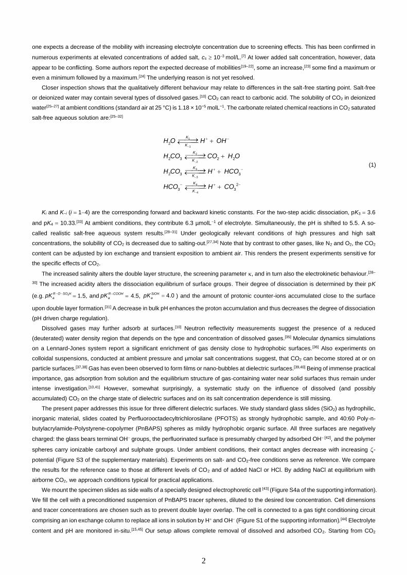
(Figure 1 and S6), we obtain: PnBAPS = −(614) mV, PFOTS = −(491) mV, and SiO2 = −(1121) mV, respectively.

In Figure 2a we compare their salt dependence for the three dielectric surfaces. Data are plotted against the total electroly te

concentration = = / (1000 )s i i Ai i

c c n N . For all three data sets, the mobility decreases monotonically with increasing salt

concentration. The corresponding -potentials are shown in Figure 2c. Note that going from mobilities to potentials, the curves for

PFOTS slides (grey squares) and PnBAPS spheres (open circles) switch place due to relaxation effects.

All three -potentials decrease in magnitude with added salt. At cs = 1000 µmolL−1, we obtain SiO2 = −(831) mV, PnBAPS = −(352)

mV, and PFOTS = −(361) mV. The corresponding slip-plane charge densities are SiO2 = −(0.490.01) µCcm−2, PnBAPS = −(0.140.02)

µCcm−2, and PFOTS = −(0.150.01) µCcm−2 using Grahame´s equation.[49] Further, for all three surfaces in the semi-log plot of Figure

2c, the decrease in -potential is approximately linear. This is theoretically expected for surfaces of constant surface charge subject to

screening by increasing concentrations of added monovalent salt.

Next, we repeated the experiments under ambient conditions. Resulting mobilities are shown in Figure 2b, resulting -potentials in

Figure 2d. In the presence of CO2 but still without salt, all mobilities and -potentials are significantly lower than in the CO2-free state.

In fact, irrespective of material, they drop by about a factor of two. Further, upon the addition of salt, all three -potentials change in

non-linear ways in this semi-log plot indicating a deviation from the constant charge scenario seen without CO2. The salt concentration

dependent decrease is significantly weakened for SiO2, and for both organic surfaces, we even observe an increase in -potential with

increasing salt concentration!

Figure 2. Comparison of mobilities (left) and -potentials (right) observed without and with CO2. Results for SiO2 (blue squares),

PnBAPS (open circles) and PFOTS-coated glass (grey squares) are plotted versus the logarithm of the total salt concentration. Error

bars denote standard errors of the linear least squares fits (see Figure 1b) at a confidence level of 0.95. All three surfaces are negatively

charged. a) Moduli of mobilities obtained for the salt and CO2 free reference state. b) Moduli of mobilities as obtained after CO2

equilibration in contact with ambient air. c) -potentials obtained for the reference state in mV (left scale) and reduced units (right scale).

d) same as c) but for systems equilibrated in contact with ambient air.

1 10 100 1000

30

40

50

60

70

80

90

100

110

120

ci (µM)

ze

ta p

ote

ntia

l

(m

V)

with CO2 d

1.0

1.5

2.0

2.5

3.0

3.5

4.0

4.5

(k

BT

/e)

1 10 100 1000

30

40

50

60

70

80

90

100

110

120

ci (µM)

ze

ta p

ote

ntia

l

(m

V)

cno CO2

1.0

1.5

2.0

2.5

3.0

3.5

4.0

4.5

(kBT

/e)

1 10 100 10000

1

2

3

4

5

6

7

8

9

10

ele

ctr

okin

etic m

ob

ility

µ

(1

0−8m

2V

−1s

−1)

ci (µM)

with CO2 b

1 10 100 10000

1

2

3

4

5

6

7

8

9

10

ci (µM)

e

lectr

okin

etic m

ob

ility

µ

(1

0−8m

2V

−1s

−1)

no CO2 a

5

Figure 2a confirms the theoretical expectation for CO2 free systems, i.e., we find a decrease of mobilities with increasing salt

concentration. Figure 2c shows that it relates to a reduction of the -potentials upon enhanced Double layer compression due to

screening. Comparison to Figures 2b and d, however, unequivocally demonstrates a significant CO2-induced effect for both spheres

and flat surfaces. The strong drop in the absence of salt is present for three rather different dielectrics. The changes in the salt

dependence differ in detail, but all three surfaces are strongly affected. We therefore exclude specific chemical reaction as underlying

reason. Further, due to the employed CO2-specific degassing process, we can exclude N2 or O2 to be responsible for the observed

behaviour.

A decrease of -potentials upon the addition of CO2 can be expected from the corresponding increase in screening and from the

decrease in pH. To discriminate between these two causes, we studied the -potentials of glass and PnBAPS as a function of overall

electrolyte content for three different added chemicals. We started from a salt and CO2 free state. First, we added NaCl, which only

contributes to screening. Next, we added HCl, which increases the electrolyte concentration, but also shifts the pH. Third, we altered

the CO2 content under conductivity and pH monitoring. Both latter quantities gave consistent values for the electrolyte content. The

results for the different additives are displayed as a function of total electrolyte content in Figure 3a for SiO2 and in Figure 3b for

PnBAPS.

Figure 3. -potentials of a) SiO2 and b) PnBAPS in dependence on total electrolyte concentration for three different added chemicals

as indicated in the key.

It is instructive, to compare the results at an electrolyte content of 6.3 µmolL-1, which is the amount provided through carbonic acid

in the absence of other electrolyte. Due to screening (NaCl), the -potential drops from (1123) mV to (1073) mV for glass and from

(614) mV to (572) mV for PnBAPS. The combined effects of screening and pH driven charge regulation (HCl) induce a drop to (942)

mV for glass and (602) mV for PnBAPS. The glass surface with weakly acidic groups becomes even less charged than for NaCl. The

PnBAPS surface bearing dominantly dissociated strongly acidic groups remains practically unchanged due to the small pH shift and

shows only the effects of screening. A similar behaviour would be expected for the carbonic acid provided by dissolved CO2. However,

in the presence of CO2 as only electrolyte we observe a drop to (681) mV for SiO2 and to (352) mV for PnBAPS. At the same time,

the effective conductivity charge of the tracers drops from Z = 2350 to Z = 1300 (Figure S2b in the supplementary materials). For both

our surfaces, the combined effects of increased electrolyte concentration and of pH shift are way too small to explain the observed

factor two reduction upon addition of CO2. We conclude that this additional drop must be due to the presence of molecular CO2.

Neither decreased -potentials upon the controlled addition of CO2 nor their increase upon successive addition of NaCl have been

reported before. Further, neither observation is backed by present theory assuming a simple double layer structure. [18] We therefore

feel free to speculate. We tentatively suggest that the underlying reason might be some kind of restructuring of the innermost part of

0 5 10 15 20 2560

70

80

90

100

110

120

130

a

NaCl

HCl

CO2

zeta

po

tentia

l

(m

V)

ci (µM)

SiO2

0 5 10 15 20 2530

40

50

60

70

PnBAPS

b NaCl

HCl

CO2

zeta

pote

ntia

l

(m

V)

ci (µM)

6

the double layer. We propose a diffusively adsorbed, thin but highly populated layer of molecular CO2, which decreases the surface

charge by dielectric charge regulation.

Weak acids dissociate in solution completely at neutral pH and infinite dilution. Similarly, the dissociation of surface groups is

controlled by the local pH at the surface and the mutual electrostatic interaction between dissociated groups. The former was discussed

in connection with bulk pH changes as well as with results from colloidal probe force microscopy [50] and the observation of charge

reduction in strongly interacting colloidal suspensions. [31] It there was shown to be a double layer overlap-driven charge regulation.

Regarding the latter, we have an average lateral separation of acidic groups of d = 1.7nm from titration. For groups to dissociate, the

electrostatic interaction energy should not exceed the thermal energy. The distance at which Coulomb and thermal energy balance is

known as Bjerrum length, B = e240rkBT. In pure water, B 7Å. B increases with decreasing dielectric constant. Too closely spaced

groups will dissociate less. In the absence of CO2, we can assign a minimum area required for an electric charge as A+min = B

2

0.5nm2. This naturally limits the bare charge number for large group numbers N. This is corroborated by conductivity measurements

under addition of NaCl in the absence of CO2. Evaluated within Hessingers model of independent ion migration, we obtain a bare

charge of Z 1×104.

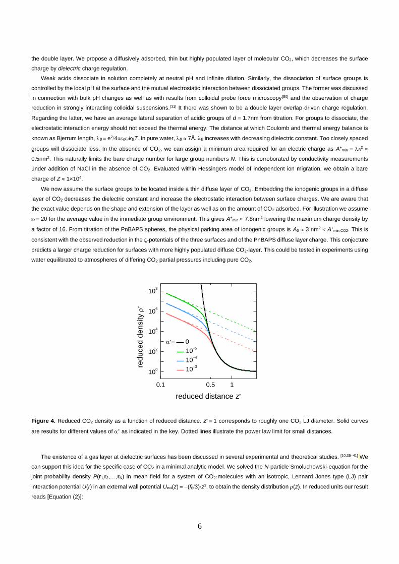
We now assume the surface groups to be located inside a thin diffuse layer of CO2. Embedding the ionogenic groups in a diffuse

layer of CO2 decreases the dielectric constant and increase the electrostatic interaction between surface charges. We are aware that

the exact value depends on the shape and extension of the layer as well as on the amount of CO2 adsorbed. For illustration we assume

r = 20 for the average value in the immediate group environment. This gives A+min 7.8nm2 lowering the maximum charge density by

a factor of 16. From titration of the PnBAPS spheres, the physical parking area of ionogenic groups is A0 3 nm2 A+min,CO2. This is

consistent with the observed reduction in the -potentials of the three surfaces and of the PnBAPS diffuse layer charge. This conjecture

predicts a larger charge reduction for surfaces with more highly populated diffuse CO2-layer. This could be tested in experiments using

water equilibrated to atmospheres of differing CO2 partial pressures including pure CO2.

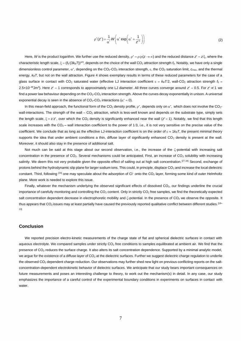
Figure 4. Reduced CO2 density as a function of reduced distance. z = 1 corresponds to roughly one CO2 LJ diameter. Solid curves

are results for different values of as indicated in the key. Dotted lines illustrate the power law limit for small distances.

The existence of a gas layer at dielectric surfaces has been discussed in several experimental and theoretical studies. [10,35–41] We

can support this idea for the specific case of CO2 in a minimal analytic model. We solved the N-particle Smoluchowski-equation for the

joint probability density P(r1,r2,…,rN) in mean field for a system of CO2-molecules with an isotropic, Lennard Jones type (LJ) pair

interaction potential U(r) in an external wall potential Uext(z) = −(f03)z3, to obtain the density distribution (z). In reduced units our result

reads [Equation (2)]:

0.1 0.5 1

100

102

104

106

108

= 0

10−5

10−4

10−3

red

uce

d d

en

sity

reduced distance z

7

3

1 1( ) expz W

z

= +

(2)

Here, W is the product logarithm. We further use the reduced density, = (z → ) and the reduced distance z = z, where the

characteristic length scale, = (f0(3kBT))1/3, depends on the choice of the wall CO2 attraction strength f0. Notably, we have only a single

dimensionless control parameter, , depending on the CO2-CO2 interaction strength, , the CO2 saturation limit, cmax, and the thermal

energy, kBT, but not on the wall attraction. Figure 4 shows exemplary results in terms of these reduced parameters for the case of a

glass surface in contact with CO2 saturated water (effective LJ interaction coefficient = kBT2, wall-CO2 attraction strength f0 =

2.5×10−49Jm3). Here z = 1 corresponds to approximately one LJ diameter. All three curves converge around z = 0.5. For z 1 we

find a power law behaviour depending on the CO2-CO2 interaction strength. Above the curves decay exponentially in unison. A universal

exponential decay is seen in the absence of CO2-CO2 interactions ( = 0).

In this mean-field approach, the functional form of the CO2 density profile, , depends only on which does not involve the CO2-

wall-interactions. The strength of the wall – CO2 attraction, which is less-well known and depends on the substrate type, simply sets

the length scale, = zz, over which the CO2 density is significantly enhanced near the wall (z 1). Notably, we find that this length

scale increases with the CO2 – wall interaction coefficient to the power of 13, i.e., it is not very sensitive on the precise value of the

coefficient. We conclude that as long as the effective LJ-interaction coefficient is on the order of 1kBT, the present minimal theory

supports the idea that under ambient conditions a thin, diffuse layer of significantly enhanced CO2 density is present at the wall.

Moreover, it should also stay in the presence of additional salt.

Not much can be said at this stage about our second observation, i.e., the increase of the -potential with increasing salt

concentration in the presence of CO2. Several mechanisms could be anticipated, First, an increase of CO2 solubility with increasing

salinity. We deem this not very probable given the opposite effect of salting out at high salt concentration. [27,34] Second, exchange of

protons behind the hydrodynamic slip plane for larger sodium ions. This could, in principle, displace CO2 and increase the local dielectric

constant. Third, following [24] one may speculate about the adsorption of Cl− onto the CO2 layer, forming some kind of outer Helmholtz

plane. More work is needed to explore this issue.

Finally, whatever the mechanism underlying the observed significant effects of dissolved CO2, our findings underline the crucial

importance of carefully monitoring and controlling the CO2 content. Only in strictly CO2 free samples, we find the theoretically expected

salt concentration dependent decrease in electrophoretic mobility and -potential. In the presence of CO2 we observe the opposite. It

thus appears that CO2 issues may at least partially have caused the previously reported qualitative conflict between different studies. [19–

23]

Conclusion

We reported precision electro-kinetic measurements of the charge state of flat and spherical dielectric surfaces in contact with

aqueous electrolyte. We compared samples under strictly CO2 free conditions to samples equilibrated at ambient air. We find that the

presence of CO2 reduces the surface charge. It also alters its salt concentration dependence. Supported by a minimal analytic model,

we argue for the existence of a diffuse layer of CO2 at the dielectric surfaces. Further we suggest dielectric charge regulation to underlie

the observed CO2 dependent charge reduction. Our observations may further shed new light on previous conflicting reports on the salt-

concentration-dependent electrokinetic behavior of dielectric surfaces. We anticipate that our study bears important consequences on

future measurements and poses an interesting challenge to theory, to work out the mechanism(s) in detail. In any case, our study

emphasizes the importance of a careful control of the experimental boundary conditions in experiments on surfaces in contact with

water.

8

Acknowledgements

Financial support of the DFG (Grants No. PA-459–15.2 and -19.1.) is gratefully acknowledged. This project has received funding from

the European Research Council (ERC) under the European Union’s Horizon 2020 research and innovation programme (grant

agreement No 883631). N.M. acknowledges financial support by the Max Planck Graduate Center at the JGU, Mainz.

Keywords: charge state • dielectric surfaces • adsorption • zeta potentials • electrophoresis

[1] A. V. Delgado, M. L. Jiménez, G. R. Iglesias, S. Ahualli, Current Opinion in Colloid & Interface Science 2019, 44, 72.

[2] M. Lukas, R. Schwidetzky, A. T. Kunert, U. Pöschl, J. Fröhlich-Nowoisky, M. Bonn, K. Meister, Journal of the American Chemical

Society 2020, 142, 6842.

[3] S. Korkmaz, İ. A. Kariper, Environ Chem Lett 2020, 18, 361.

[4] C. Hammond, Cellular and Molecular Neurophysiology, Academic Press, 2014.

[5] U. B. Kaupp, L. Alvarez, Eur. Phys. J. Spec. Top. 2016, 225, 2119.

[6] Q. Sun, D. Wang, Y. Li, J. Zhang, S. Ye, J. Cui, L. Chen, Z. Wang, H.-J. Butt, D. Vollmer et al., Nature materials 2019, 18, 936.

[7] E. J. W. VERWEY, The Journal of physical and colloid chemistry 1947, 51, 631.

[8] B. Derjaguin, L. Landau, Progress in Surface Science 1993, 43, 30.

[9] C.N. Bensley, R.J. Hunter, Journal of Colloid and Interface Science 1983, 92, 436.

[10] N. Maeda, K. J. Rosenberg, J. N. Israelachvili, R. M. Pashley, Langmuir 2004, 20, 3129.

[11] A. Homola, R.O. James, Journal of Colloid and Interface Science 1977, 59, 123.

[12] K. G. Marinova, R. G. Alargova, N. D. Denkov, O. D. Velev, D. N. Petsev, I. B. Ivanov, R. P. Borwankar, Langmuir 1996, 12, 2045.

[13] G. Seth Roberts, Tiffany A. Wood, William J. Frith, Paul Bartlett, The Journal of Chemical Physics 2007, 126, 194503.

[14] F. Beunis, F. Strubbe, K. Neyts, D. Petrov, Phys. Rev. Lett. 2012, 108.

[15] D. Hessinger, M. Evers, T. Palberg, Phys. Rev. E 2000, 61, 5493.

[16] A. V. Delgado, F. González-Caballero, R. J. Hunter, L. K. Koopal, J. Lyklema, Journal of Colloid and Interface Science 2007, 309,

194.

[17] R. W. O'Brien, L. R. White, J. Chem. Soc., Faraday Trans. 2 1978, 74, 1607.

[18] F. Carrique, E. Ruiz-Reina, R. Roa, F. J. Arroyo, Á. V. Delgado, Journal of Colloid and Interface Science 2015, 455, 46.

[19] J. R. Goff, P. Luner, Journal of Colloid and Interface Science 1984, 99, 468.

[20] M. Deggelmann, T. Palberg, M. Hagenbüchle, E. E. Maier, R. Krause, C. Graf, R. Weber, Journal of Colloid and Interface Science

1991, 143, 318.

[21] V. Lobaskin, B. Dünweg, M. Medebach, T. Palberg, C. Holm, Physical review letters 2007, 98, 176105.

[22] Y. Gu, D. Li, Journal of Colloid and Interface Science 2000, 226, 328.

[23] J. Laven, H. N. Stein, Journal of Colloid and Interface Science 2001, 238, 8.

[24] C.F. Zukoski, D.A. Saville, Journal of Colloid and Interface Science 1986, 114, 45.

[25] F. J. Millero, Geochimica et Cosmochimica Acta 1995, 59, 661.

[26] F. J. Millero, R. Feistel, D. G. Wright, T. J. McDougall, Deep Sea Research Part I: Oceanographic Research Papers 2008, 55, 50.

[27] K. Gilbert, P. C. Bennett, W. Wolfe, T. Zhang, K. D. Romanak, Applied Geochemistry 2016, 67, 59.

[28] E. Ruiz-Reina, F. Carrique, The Journal of Physical Chemistry B 2008, 112, 11960.

[29] F. Carrique, E. Ruiz-Reina, The Journal of Physical Chemistry B 2009, 113, 8613.

[30] A. V. Delgado, S. Ahualli, F. J. Arroyo, M. L. Jiménez, F. Carrique, Advances in Colloid and Interface Science 2021, 102539.

[31] M. Heinen, T. Palberg, H. Löwen, The Journal of Chemical Physics 2014, 140, 124904.

[32] Aqion freeware program, can be found under https://www.aqion.de/.

9

[33] A. F. Holleman, E. Wiberg, N. Wiberg (Eds.) Lehrbuch der anorganischen Chemie, de Gruyter, Berlin, 2007.

[34] A. Hasseine, A.-H. Meniai, M. Korichi, Desalination 2009, 242, 264.

[35] D. A. Doshi, E. B. Watkins, J. N. Israelachvili, J. Majewski, PNAS 2005, 102, 9458.

[36] S. M. Dammer, D. Lohse, Phys. Rev. Lett. 2006, 96, 206101.

[37] E. Villanova-Vidal, T. Palberg, H. J. Schöpe, H. Löwen, Philosophical Magazine 2009, 89, 1695.

[38] D. Botin, F. Carrique, E. Ruiz-Reina, T. Palberg, The Journal of Chemical Physics 2020, 152, 244902.

[39] X. H. Zhang, A. Khan, W. A. Ducker, Phys. Rev. Lett. 2007, 98, 136101.

[40] B. İlhan, C. Annink, D. V. Nguyen, F. Mugele, I. Siretanu, M.H.G. Duits, Colloids and Surfaces A: Physicochemical and Engineering

Aspects 2019, 560, 50.

[41] B. W. Ninham, R. M. Pashley, P. Lo Nostro, Current Opinion in Colloid & Interface Science 2017, 27, 25.

[42] A. Z. Stetten, D. S. Golovko, S. A. L. Weber, H.-J. Butt, Soft Matter 2019, 15, 8667.

[43] D. Botin, J. Wenzl, R. Niu, T. Palberg, Soft Matter 2018, 14, 8191.

[44] P. Wette, H.-J. Schöpe, R. Biehl, T. Palberg, The Journal of Chemical Physics 2001, 114, 7556.

[45] N. Möller, B. Liebchen, T. Palberg, The European physical journal. E, Soft matter 2021, 44, 41.

[46] D. Botin, L. M. Mapa, H. Schweinfurth, B. Sieber, C. Wittenberg, T. Palberg, The Journal of Chemical Physics 2017, 146, 204904.

[47] T. Palberg, T. Köller, B. Sieber, H. Schweinfurth, H. Reiber, G. Nägele, J. Phys.: Condens. Matter 2012, 24, 464109.

[48] T. Palberg, H. Versmold, J. Phys. Chem. 1989, 93, 5296.

[49] S. H. Behrens, D. G. Grier, The Journal of Chemical Physics 2001, 115, 6716.

[50] G. Trefalt, S. H. Behrens, M. Borkovec, Langmuir 2016, 32, 380.

Entry for the Table of Contents

Using Doppler velocimetry with low tracer concentrations, we determined -potentials of surfaces with different hydrophobicity (glass,

standard polymer, perfluorinated polymer (PFOTS)). Without CO2, the potentials drop upon increasing the salt concentration. With

CO2 however, they drop by some 50% in the salt-free state. Moreover, the salt dependence seen for SiO2 is significantly weakened

and inverted for the organic dielectrics.

Tracer, H2O | Salt, CO2

( , )pv x y ( )epv E

( )eov Ei 2(c ,CO )

E

x

y

1 10 100 100030

35

40

45

50

55

ci (µM)

no CO2

with CO2

PFOTS

zeta

pote

ntial

(mV

)

10

Supporting Information

Charging of dielectric surfaces in contact with aqueous

electrolyte – the influence of CO2

Peter Vogel*[a], Nadir Möller[a], Pravash Bista[b], Stefan Weber[b], Hans-Jürgen Butt[b], Benno Liebchen[c]

and Thomas Palberg[a]

Abstract: The charge state of dielectric surfaces in aqueous environments is of fundamental and technological importance. Here, we

study the influence of dissolved molecular CO2 on the charging of three, chemically different surfaces (SiO2, Polystyrene,

Perfluorooctadecyltrichlorosilane). We determine their charge state from electrokinetic experiments. We compare an ideal, CO2-free

reference state to ambient CO2 conditions. In the reference state, the salt-dependent decrease of the -potentials follows the

expectations for a constant charge scenario. In the presence of CO2, the starting potential is lower by some 50%. The following salt-

dependent decrease is weakened for SiO2 and inverted for the organic surfaces. We show that screening and pH driven charge

regulation alone cannot explain the observed effects. As additional cause, we tentatively suggest dielectric regulation of surface charges

due to a diffusively adsorbed thin layer of molecular CO2.

11

Table of contents

1 Experimental section ...................................................................................................... 12

1.1 Materials .................................................................................................................................................................................... 12

1.2 Sample conditioning ................................................................................................................................................................ 12

1.2.1 Tracer pre-conditioning ............................................................................................................................................................ 12

1.2.2 Circuit-conditioning .................................................................................................................................................................. 12

1.3 Tracer and wall characterization ............................................................................................................................................. 14

1.3.1 Tracer concentration ................................................................................................................................................................ 14

1.3.2 Tracer charge .......................................................................................................................................................................... 14

1.3.3 Flat substrate contact angles ................................................................................................................................................... 15

1.4 Custom-made electrokinetic cell ............................................................................................................................................. 15

1.5 Laser Doppler Velocimetry ...................................................................................................................................................... 17

1.6 Mobility evaluation ................................................................................................................................................................... 19

2 Theoretical section .......................................................................................................... 20

2.1 Analytic Theory ......................................................................................................................................................................... 20

2.1.1 Parameters .............................................................................................................................................................................. 21

2.1.2 Asymptotics ............................................................................................................................................................................. 22

2.2 Comment ................................................................................................................................................................................... 22

12

1 Experimental section

1.1 Materials

PnBAPS tracer particles are a 40:60 W/W copolymer of poly-n-butyl acrylamide (PnBA) and polystyrene (PS), kindly provided by

BASF, Ludwigshafen (Lab code PnBAPS359, manufacturer Batch No. 2168/7390). Their diameter of 2a = 359 nm was determined by

the manufacturer utilizing analytical ultracentrifugation.

Standard microscopy glass slides (75 × 25 × 1 mm, soda lime glass of hydrolytic class 3 by VWR International, Germany) served

as charged wall specimen. They were sonicated prior to use for 30 min in 2% alkaline detergent water solution (Hellmanex III, Hellma

Analytics), rinsed with double distilled water several times and dried with pressurized air. Low charge specimens were prepared by

silanisation with perfluorooctadecyltrichlorosilane (PFOTS) in a chemical vapor deposition process. After oxygen plasma cleaning at

300 W for 10 min (Femto low-pressure plasma system, Diener electronic), the slides were placed in a vacuum desiccator containing a

vial filled with 0.5 mL of 1H,1H,2H,2H-perfluorooctadecyltrichlorosilane (97%, Sigma Aldrich). The desiccator was evacuated to less

than 100 mbar and the reaction was allowed to proceed for 30 min.[1]

1.2 Sample conditioning

1.2.1 Tracer pre-conditioning

By dilution with doubly distilled water, we prepared stock suspensions of approximately n = 1×1018m−3, added mixed-bed ion

exchange resin (IEX) (Amberjet, Carl Roth GmbH + Co. KG, Karlsruhe, Germany) and left it to stand under occasional stirring for some

weeks. Then, the suspension was coarsely filtered using Sartorius 5 µm filters to remove dust, ion-exchange debris and coagulate

regularly occurring upon first contact of suspension with IEX. All further conditioning was performed by circuit conditioning.

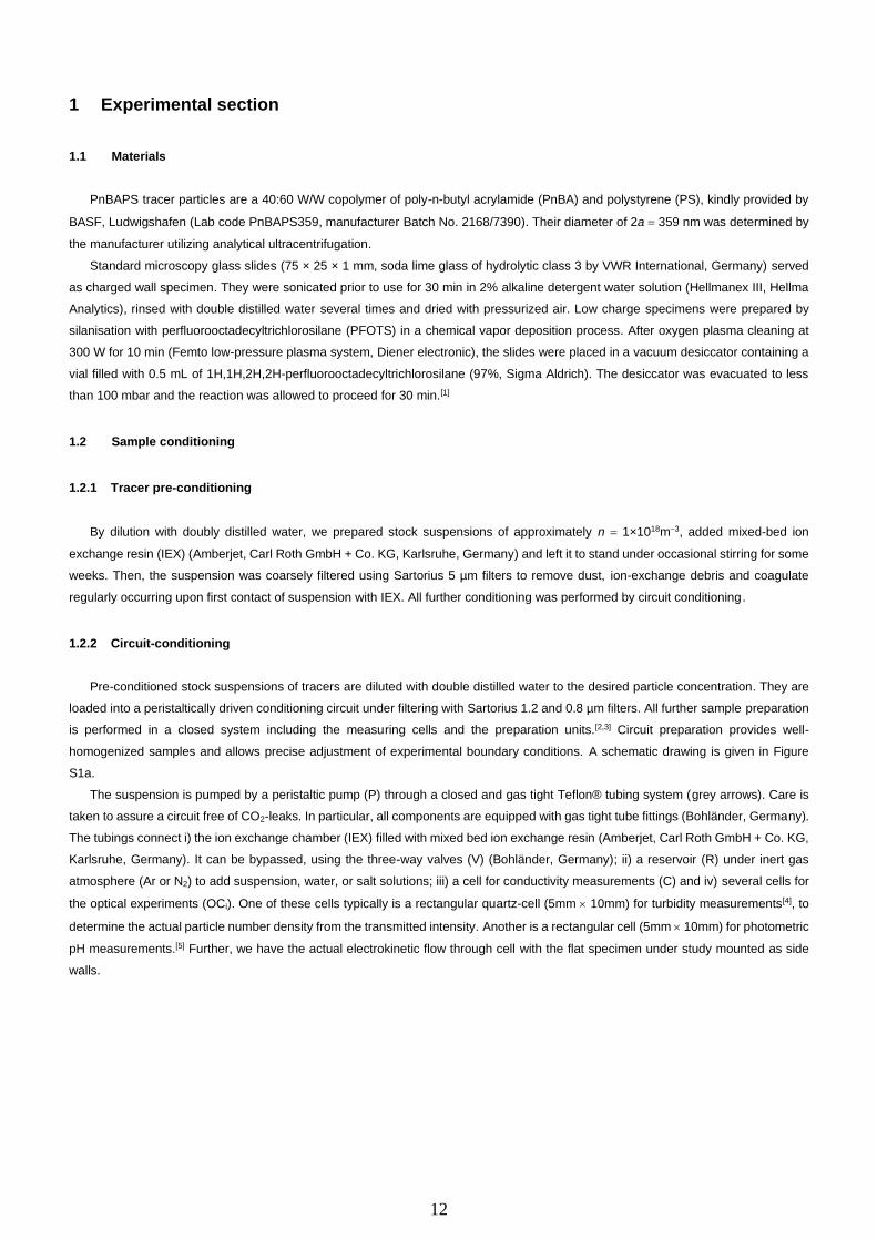
1.2.2 Circuit-conditioning

Pre-conditioned stock suspensions of tracers are diluted with double distilled water to the desired particle concentration. They are

loaded into a peristaltically driven conditioning circuit under filtering with Sartorius 1.2 and 0.8 µm filters. All further sample preparation

is performed in a closed system including the measuring cells and the preparation units.[2,3] Circuit preparation provides well-

homogenized samples and allows precise adjustment of experimental boundary conditions. A schematic drawing is given in Figure

S1a.

The suspension is pumped by a peristaltic pump (P) through a closed and gas tight Teflon® tubing system (grey arrows). Care is

taken to assure a circuit free of CO2-leaks. In particular, all components are equipped with gas tight tube fittings (Bohländer, Germany).

The tubings connect i) the ion exchange chamber (IEX) filled with mixed bed ion exchange resin (Amberjet, Carl Roth GmbH + Co. KG,

Karlsruhe, Germany). It can be bypassed, using the three-way valves (V) (Bohländer, Germany); ii) a reservoir (R) under inert gas

atmosphere (Ar or N2) to add suspension, water, or salt solutions; iii) a cell for conductivity measurements (C) and iv) several cells for

the optical experiments (OCi). One of these cells typically is a rectangular quartz-cell (5mm 10mm) for turbidity measurements[4], to

determine the actual particle number density from the transmitted intensity. Another is a rectangular cell (5mm 10mm) for photometric

pH measurements.[5] Further, we have the actual electrokinetic flow through cell with the flat specimen under study mounted as side

walls.

13

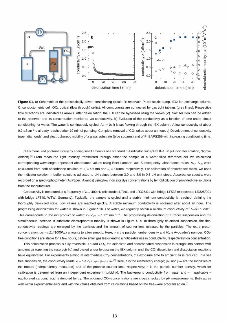
Figure S1. a) Schematic of the peristaltically driven conditioning circuit: R: reservoir, P: peristaltic pump, IEX: ion exchange column,

C: conductometric cell, OCi: optical (flow through) cell(s). All components are connected by gas tight tubings (grey lines). Respective

flow directions are indicated as arrows. After deionization, the IEX can be bypassed using the valves (V). Salt solution can be added

to the reservoir and its concentration monitored via conductivity. b) Evolution of the conductivity as a function of time under circuit

conditioning for water. The water is continuously cycled. At t = 0s it is set flowing through the IEX column. A low conductivity of about

0.2 µScm−1 is already reached after 10 min of pumping. Complete removal of CO2 takes about an hour. c) Development of conductivity

(open diamonds) and electrophoretic mobility of a glass substrate (blue squares) and of PnBAPS359 with increasing conditioning time.

pH is measured photometrically by adding small amounts of a standard pH indicator fluid (pH 3.0−10.0 pH indicator solution, Sigma-

Aldrich).[5] From measured light intensity transmitted through either the sample or a water filled reference cell we calculated

corresponding wavelength dependent absorbance values using Beer-Lambert law. Subsequently, absorbance ratios, A1 A2, were

calculated from both absorbance maxima at 1 = 430nm and 2 = 615nm, respectively. For calibration of absorbance ratios, we used

the indicator solution in buffer solutions adjusted to pH values between 3.0 and 8.0 in 0.5 pH unit steps. Absorbance spectra were

recorded on a spectrophotometer (AvaSpec, Avantis) using low indicator dye concentrations by tenfold dilution of provided dye solutions

from the manufacturer.

Conductivity is measured at a frequency of = 400 Hz (electrodes LTA01 and LR325/01 with bridge LF538 or electrode LR325/001

with bridge LF340, WTW, Germany). Typically, the sample is cycled until a stable minimum conductivity is reached, defining the

thoroughly deionized state. Low values are reached quickly. A stable minimum conductivity is obtained after about an hour. The

progressing deionization for water is shown in Figure S1b. For water, we regularly obtain a minimum conductivity of 55−60 nScm−1.

This corresponds to the ion product of water: cH+ cOH- = 10−14 mol2L−2. The progressing deionization of a tracer suspension and the

simultaneous increase in substrate electrophoretic mobility is shown in Figure S1c. In thoroughly deionized suspension, the final

conductivity readings are enlarged by the particles and the amount of counter-ions released by the particles. The extra proton

concentration, cH+ = nZσ(1000NA) amounts to a few µmolL. Here, n is the particle number density and NA is Avogadro’s number. CO2-

free conditions are stable for a few hours, before small gas leaks lead to a noticeable rise in conductivity, respectively ion concentration.

This deionization process is fully reversible. To add CO2, the deionized and decarbonated suspension is brought into contact with

ambient air (opening the reservoir lid) and cycled under bypassing the IEX column until the CO2 dissolution and dissociation reactions

have equilibrated. For experiments aiming at intermediate CO2 concentrations, the exposure time to ambient air is reduced. In a salt

free suspension, the conductivity reads: = n e Z (µep + µH+) + B.[6] Here, e is the elementary charge; µep and µH+ are the mobilities of

the tracers (independently measured) and of the protonic counter-ions, respectively; n is the particle number density, which for

calibration is determined from an independent experiment (turbidity). The background conductivity from water and – if applicable –

equilibrated carbonic acid is denoted by B. The obtained CO2-concentrations are cross checked by pH measurements. Both agree

well within experimental error and with the values obtained from calculations based on the free-ware program aqion.[7]

0 10 20 30 40

0.0

0.5

1.0

1.5

2.0

2.5

con

du

ctivity

(µ

Scm

−1)

deionization time t (min)

0

1

2

3

4

5

6

7

8

9

10

c

ele

ctr

okin

etic m

obili

ty

µ

(10

−8m

2V

−1s

−1)

aC

VP

IEX

Salt

R

OCi

V0 20 40 60 80

0.0

0.5

1.0

1.5

2.0

2.5

b

co

nd

uctivity

(µ

Scm

−1)

deionization time t (min)

14

Experiments at elevated electrolyte concentration start from either the deionized or the CO2-equilbrated state. Again, the IEX column

is by passed. Then, salt solution (Titrisol 0.1 molL−1 NaCl or HCl, Merck, Germany) is added with a syringe through the septum of the

reservoir in small quantities. The conductivity quickly reaches a constant larger value.

1.3 Tracer and wall characterization

1.3.1 Tracer concentration

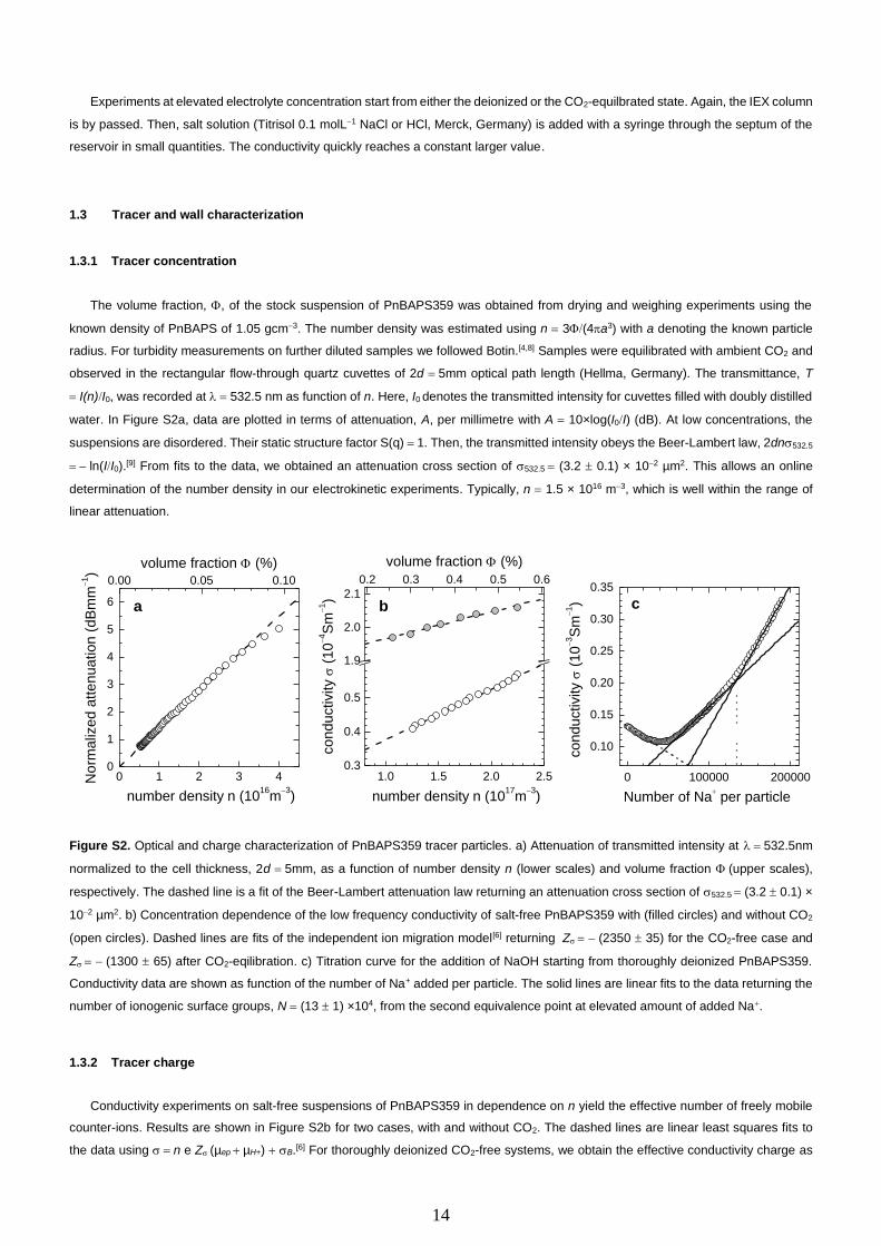
The volume fraction, , of the stock suspension of PnBAPS359 was obtained from drying and weighing experiments using the

known density of PnBAPS of 1.05 gcm−3. The number density was estimated using n = 3(4a3) with a denoting the known particle

radius. For turbidity measurements on further diluted samples we followed Botin.[4,8] Samples were equilibrated with ambient CO2 and

observed in the rectangular flow-through quartz cuvettes of 2d = 5mm optical path length (Hellma, Germany). The transmittance, T

= I(n)I0, was recorded at = 532.5 nm as function of n. Here, I0 denotes the transmitted intensity for cuvettes filled with doubly distilled

water. In Figure S2a, data are plotted in terms of attenuation, A, per millimetre with A = 10×log(I0I) (dB). At low concentrations, the

suspensions are disordered. Their static structure factor S(q) = 1. Then, the transmitted intensity obeys the Beer-Lambert law, 2dn532.5

= − ln(II0).[9] From fits to the data, we obtained an attenuation cross section of 532.5 = (3.2 0.1) × 10−2 µm2. This allows an online

determination of the number density in our electrokinetic experiments. Typically, n = 1.5 × 1016 m−3, which is well within the range of

linear attenuation.

Figure S2. Optical and charge characterization of PnBAPS359 tracer particles. a) Attenuation of transmitted intensity at = 532.5nm

normalized to the cell thickness, 2d = 5mm, as a function of number density n (lower scales) and volume fraction (upper scales),

respectively. The dashed line is a fit of the Beer-Lambert attenuation law returning an attenuation cross section of 532.5 = (3.2 0.1) ×

10−2 µm2. b) Concentration dependence of the low frequency conductivity of salt-free PnBAPS359 with (filled circles) and without CO2

(open circles). Dashed lines are fits of the independent ion migration model[6] returning Z = − (2350 35) for the CO2-free case and

Z = − (1300 65) after CO2-eqilibration. c) Titration curve for the addition of NaOH starting from thoroughly deionized PnBAPS359.

Conductivity data are shown as function of the number of Na+ added per particle. The solid lines are linear fits to the data returning the

number of ionogenic surface groups, N = (13 1) ×104, from the second equivalence point at elevated amount of added Na+.

1.3.2 Tracer charge

Conductivity experiments on salt-free suspensions of PnBAPS359 in dependence on n yield the effective number of freely mobile

counter-ions. Results are shown in Figure S2b for two cases, with and without CO2. The dashed lines are linear least squares fits to

the data using = n e Z (µep + µH+) + B.[6] For thoroughly deionized CO2-free systems, we obtain the effective conductivity charge as

0 100000 200000

0.10

0.15

0.20

0.25

0.30

0.35

c

co

nd

uctivity

(1

0−3S

m−1)

Number of Na+ per particle

0 1 2 3 40

1

2

3

4

5

6 a

No

rma

lize

d a

tte

nu

atio

n (

dB

mm

−1)

number density n (1016

m−3

)

0.00 0.05 0.10

volume fraction (%)

1.0 1.5 2.0 2.50.3

0.4

0.5

1.9

2.0

2.1

0.2 0.3 0.4 0.5 0.6

volume fraction (%)

b

co

nd

uctivity

(1

0−4S

m−1)

number density n (1017

m−3

)

15

Z = − (2350 35). For realistic salt free systems, we find Z = − (1300 65). These numbers have to be compared to the number of

dissociable groups. Figure S2c shows the results of a conductivity titration starting from deionized/decarbonated PnBAPS359. The

titration curve is typical for the simultaneous presence of strong and weak acid groups.[6,10,11] From the crossing points of linear fits

before and past the second equivalence point, we have a titrated group number N = (13 1) ×104. From the initial slope we extract a

charge ratio of ZZ 0.12, and from that a bare charge Z of Z 1.9×104. As expected and in agreement with previous work,[12,13] the

conductivity effective charge is much smaller than the bare charge, which in turn is much smaller than the group number Z Z N.

Moreover, the effective charge is considerable smaller than the bare charge, due to charge renormalization.

Dividing the particle surface area by the group number, N, yields a mean physical parking area per surface group of A0 3 nm2.

The average spacing between ionogenic groups is approximately 1.7 nm 2.5 B. The parking area for dissociated groups under CO2

free conditions is 0.5 nm2. Thus, mutual electrostatic interactions are not expected to interfere with dissociation. However, even without

CO2-induced effects, there is only weak degree of dissociation related to the group pK and the low pH within the innermost part of the

double layer.

1.3.3 Flat substrate contact angles

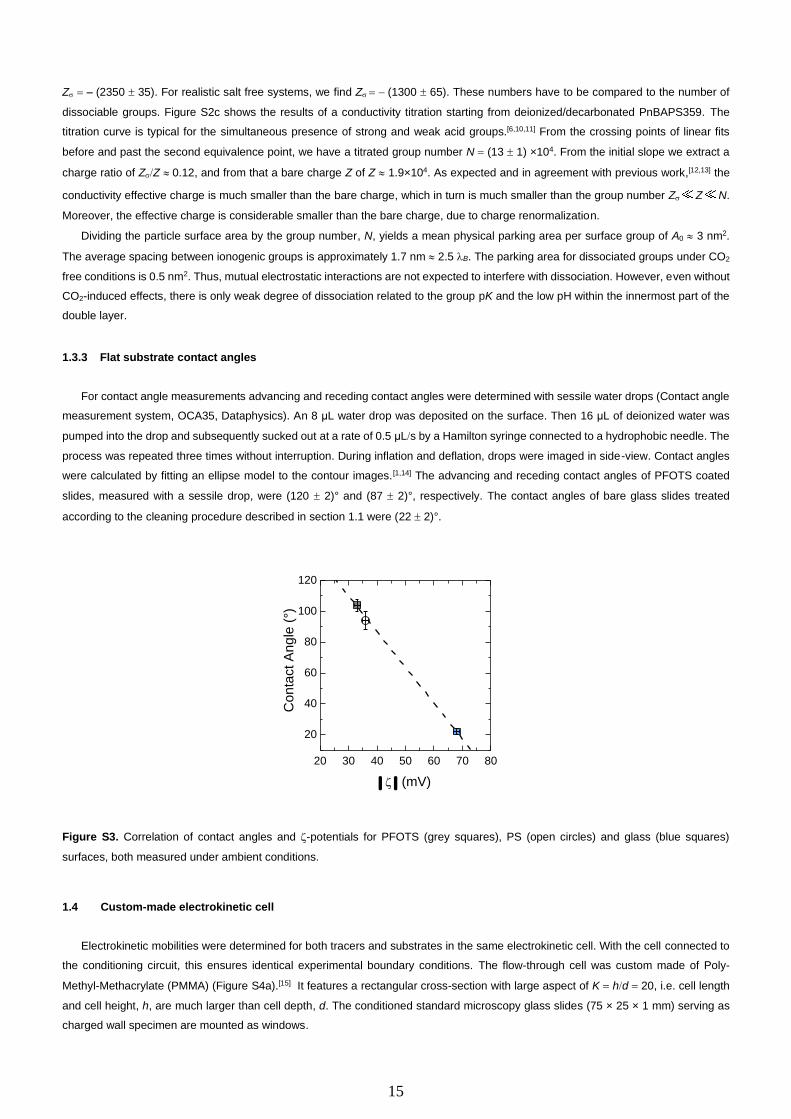
For contact angle measurements advancing and receding contact angles were determined with sessile water drops (Contact angle

measurement system, OCA35, Dataphysics). An 8 μL water drop was deposited on the surface. Then 16 μL of deionized water was

pumped into the drop and subsequently sucked out at a rate of 0.5 μLs by a Hamilton syringe connected to a hydrophobic needle. The

process was repeated three times without interruption. During inflation and deflation, drops were imaged in side-view. Contact angles

were calculated by fitting an ellipse model to the contour images. [1,14] The advancing and receding contact angles of PFOTS coated

slides, measured with a sessile drop, were (120 2)° and (87 2)°, respectively. The contact angles of bare glass slides treated

according to the cleaning procedure described in section 1.1 were (22 2)°.

Figure S3. Correlation of contact angles and -potentials for PFOTS (grey squares), PS (open circles) and glass (blue squares)

surfaces, both measured under ambient conditions.

1.4 Custom-made electrokinetic cell

Electrokinetic mobilities were determined for both tracers and substrates in the same electrokinetic cell. With the cell connected to

the conditioning circuit, this ensures identical experimental boundary conditions. The flow-through cell was custom made of Poly-

Methyl-Methacrylate (PMMA) (Figure S4a).[15] It features a rectangular cross-section with large aspect of K = hd = 20, i.e. cell length

and cell height, h, are much larger than cell depth, d. The conditioned standard microscopy glass slides (75 × 25 × 1 mm) serving as

charged wall specimen are mounted as windows.

20 30 40 50 60 70 80

20

40

60

80

100

120

(mV)

C

on

tact A

ng

le (

°)

16

Platinized platinum electrodes with 14/20 ground glass joints (Rank Bros. Bottisham, UK) are inserted into the electrode chamber

of the cell. The effective electrode distance L = 12 cm was calibrated from conductivity measurements using potassium chloride

electrolyte solutions. Data in electrokinetic measurements are recorded with an electric field applied. Figure S4a shows the field

direction with the anode to the right and the cathode to the left. It also shows the coordinate system used in interpretation.

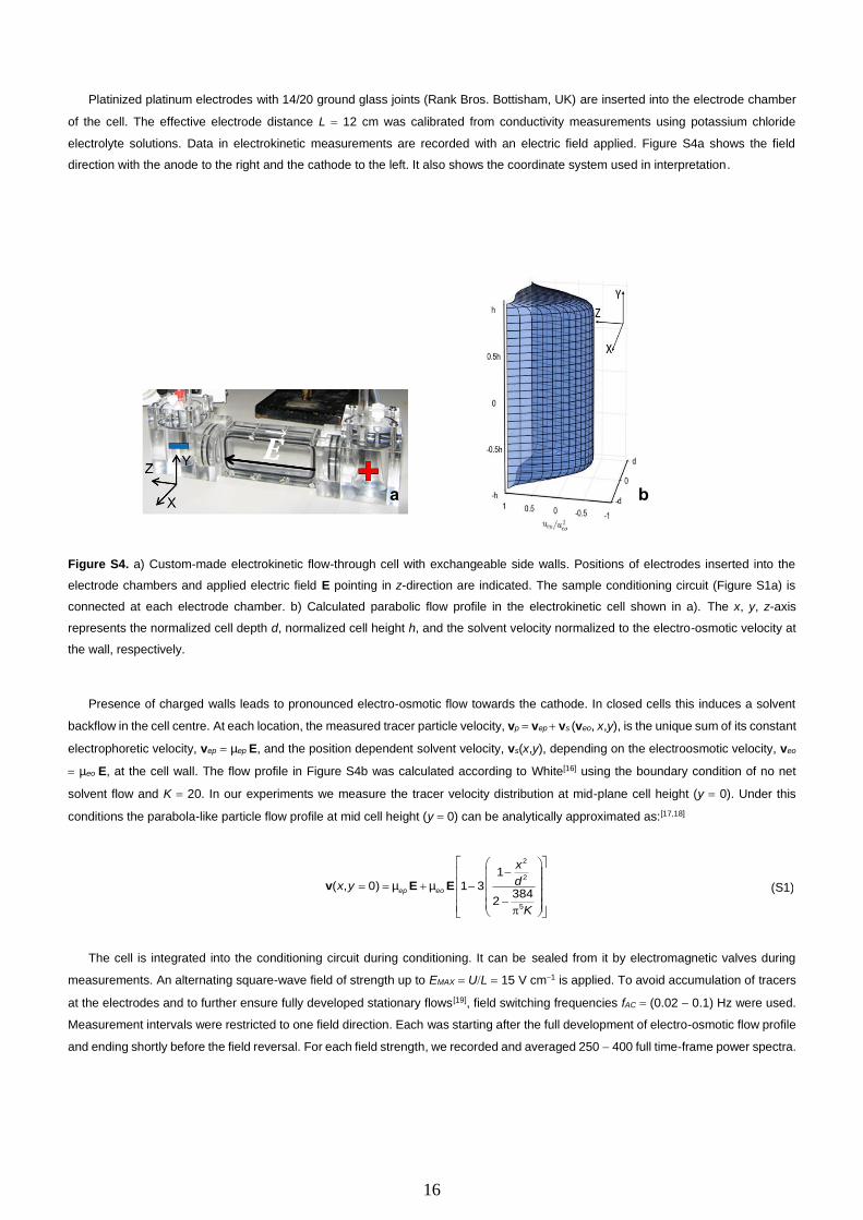
Figure S4. a) Custom-made electrokinetic flow-through cell with exchangeable side walls. Positions of electrodes inserted into the

electrode chambers and applied electric field E pointing in z-direction are indicated. The sample conditioning circuit (Figure S1a) is

connected at each electrode chamber. b) Calculated parabolic flow profile in the electrokinetic cell shown in a). The x, y, z-axis

represents the normalized cell depth d, normalized cell height h, and the solvent velocity normalized to the electro-osmotic velocity at

the wall, respectively.

Presence of charged walls leads to pronounced electro-osmotic flow towards the cathode. In closed cells this induces a solvent

backflow in the cell centre. At each location, the measured tracer particle velocity, vp = vep + vs (veo, x,y), is the unique sum of its constant

electrophoretic velocity, vep = µep E, and the position dependent solvent velocity, vs(x,y), depending on the electroosmotic velocity, veo

= µeo E, at the cell wall. The flow profile in Figure S4b was calculated according to White[16] using the boundary condition of no net

solvent flow and K = 20. In our experiments we measure the tracer velocity distribution at mid-plane cell height (y = 0). Under this

conditions the parabola-like particle flow profile at mid cell height (y = 0) can be analytically approximated as:[17,18]

−

= = + − −

2

2

5

1( , 0) µ µ 1 3

3842

ep eo

x

dx y

K

v E E (S1)

The cell is integrated into the conditioning circuit during conditioning. It can be sealed from it by electromagnetic valves during

measurements. An alternating square-wave field of strength up to EMAX = UL = 15 V cm−1 is applied. To avoid accumulation of tracers

at the electrodes and to further ensure fully developed stationary flows[19], field switching frequencies fAC = (0.02 − 0.1) Hz were used.

Measurement intervals were restricted to one field direction. Each was starting after the full development of electro-osmotic flow profile

and ending shortly before the field reversal. For each field strength, we recorded and averaged 250 − 400 full time-frame power spectra.

a b

17

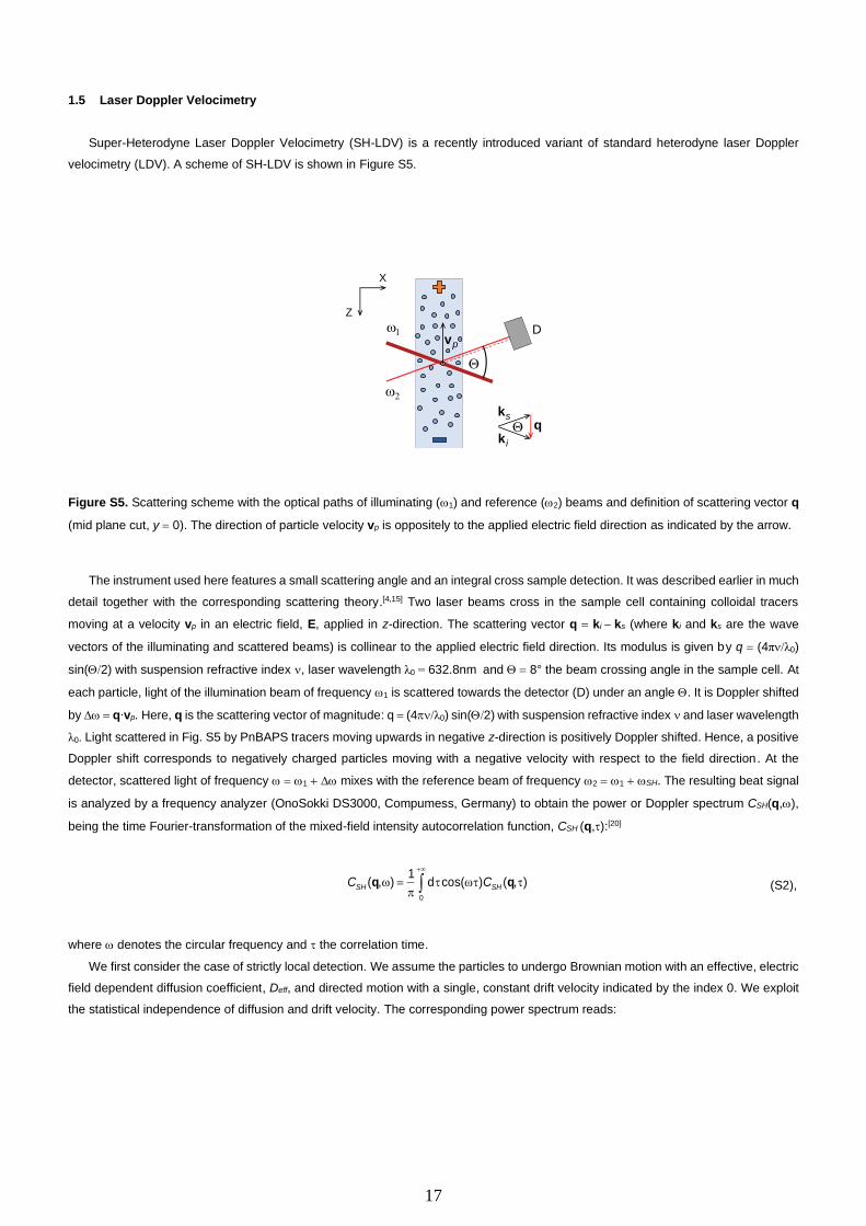
1.5 Laser Doppler Velocimetry

Super-Heterodyne Laser Doppler Velocimetry (SH-LDV) is a recently introduced variant of standard heterodyne laser Doppler

velocimetry (LDV). A scheme of SH-LDV is shown in Figure S5.

Figure S5. Scattering scheme with the optical paths of illuminating (1) and reference (2) beams and definition of scattering vector q

(mid plane cut, y = 0). The direction of particle velocity vp is oppositely to the applied electric field direction as indicated by the arrow.

The instrument used here features a small scattering angle and an integral cross sample detection. It was described earlier in much

detail together with the corresponding scattering theory.[4,15] Two laser beams cross in the sample cell containing colloidal tracers

moving at a velocity vp in an electric field, E, applied in z-direction. The scattering vector q = ki − ks (where ki and ks are the wave

vectors of the illuminating and scattered beams) is collinear to the applied electric field direction. Its modulus is given by q = (4πλ0)

sin(2) with suspension refractive index , laser wavelength λ0 = 632.8nm and = 8° the beam crossing angle in the sample cell. At

each particle, light of the illumination beam of frequency 1 is scattered towards the detector (D) under an angle . It is Doppler shifted

by = q∙vp. Here, q is the scattering vector of magnitude: q = (4λ0) sin(2) with suspension refractive index and laser wavelength

λ0. Light scattered in Fig. S5 by PnBAPS tracers moving upwards in negative z-direction is positively Doppler shifted. Hence, a positive

Doppler shift corresponds to negatively charged particles moving with a negative velocity with respect to the field direction. At the

detector, scattered light of frequency = 1 + mixes with the reference beam of frequency 2 = 1 + SH. The resulting beat signal

is analyzed by a frequency analyzer (OnoSokki DS3000, Compumess, Germany) to obtain the power or Doppler spectrum CSH(q,),

being the time Fourier-transformation of the mixed-field intensity autocorrelation function, CSH (q,):[20]

+

=

0

1( , ) d cos( ) ( , )q qSH SHC C (S2),

where denotes the circular frequency and the correlation time.

We first consider the case of strictly local detection. We assume the particles to undergo Brownian motion with an effective, electric

field dependent diffusion coefficient, Deff, and directed motion with a single, constant drift velocity indicated by the index 0. We exploit

the statistical independence of diffusion and drift velocity. The corresponding power spectrum reads:

1

2

D

sk

ikq

pv

Z

X

18

( ) = + 20 ( , ) ( ) ( )SH r sC I Iq q

+ +

2 2

2 2 2

( ) 2

(2 )

s eff

eff

I D

D

q q

q

2

2 2 2

( )

( [ ]) ( )

r s eff

SH eff

I I D

D

+ +

+ + +

q q

q

− + +

2

2 2 2( [ ]) ( )

eff

SH eff

D

D

q

q

(S3)

where Ir is the reference beam intensity and ( )sI q the time-averaged scattering intensity in dependence on q.

The spectrum contains three contributions. First, a static background term () centred at zero frequency. Second, a homodyne

Lorentzian of width = 2q2Deff, centred at the origin and independent of drift velocity. This term is well known from standard dynamic

light scattering. Third, two super-heterodyne Lorentzians of spectral width = q2Deff shifted symmetrically away from the origin by A,B

= (SH + q∙vp), i.e. both by SH and the Doppler shift frequency = q∙vp. Note that it is this additional super-heterodyning frequency

shift of the reference beam by SH, which allows shifting the SH-term away from any low-frequency noise and separate it from homodyne

scattering of the second term. The desired information regarding electrophoretic and diffusive particle motion is fully contained via

in each of the two super-heterodyne Lorentzians. It is thus sufficient to analyse measured data only for positive frequencies.[4]

In the present set-up, scattered light is collected from an extended detection volume comprising the full x,z-cross section at mid cell

height (y = 0). The observable particle velocity, vp, depends on position (c.f. Equation S1), leading to a distribution of particle velocities

and Doppler frequencies, respectively. The spectral shape of the selectively detected SH-part then results from a convolution of the

distribution p() = p(q∙vp) with a Lorentzian of width = q2Deff.[15,20]

= SH p p SHC p C0( , ) d( ) ( ) ( , )q q v q v q (S4)

The super-heterodyne signal thus averages over all particle velocities and Doppler frequencies, respectively, present in the

scattering volume. We note, that for a given field strength, the shape of CSH(q,) is solely determined by the solvent flow profile whereas

its centre of mass is determined by the particle electrophoretic velocity and its broadening by the effective diffusion coeff icient. Thus,

we have three statistically independent variables for the fitting of the spectra. For fitting and evaluation we follow the procedures outlined

in much detail in previous work.[4,15,20,21]

Figure S6a shows a set of spectra recorded at different field strengths in cells with bare glass side walls at salt- and CO2-free

conditions. The SH-frequency of fSH = SH2 = 3kHz corresponds to zero particle velocity. The characteristic spectral shape

corresponds to a parabola like velocity profile.[17] With increasing field strength, the spectra stretch and their centre of mass shifts

towards larger Doppler frequencies. The solid lines are least square fits of our model (Equation S1 used in Eqns. S2−S4) returning

three independent parameters: vep from the spectral center of mass, veo from the field dependent width, and the tracer diffusivity, Deff,

from the homogeneous broadening. Our particles and walls are negatively charged, resulting in negative velocities and mobilit ies.

Figure S6b shows the moduli of extracted velocities to increase linearly with field strength. Least squares fits of a linear function (dashed

lines) return mobilities of µep = µPnBAPS = − (3.10.2)×10−8 m2V−1s−1 and µeo = µSiO2 = − (9.00.1)×10−8 m2V−1s−1, respectively. The quoted

uncertainties correspond to the standard errors of the linear fits at a confidence level of 0.95. The effective tracer diffusivity is extracted

from the spectral width of the super-heterodyne Lorentzian and increases linearly with increasing field strength (see Figure S6c). As

discussed in Ref.[20], this can be related to Taylor dispersion in the parabolic solvent flow.

19

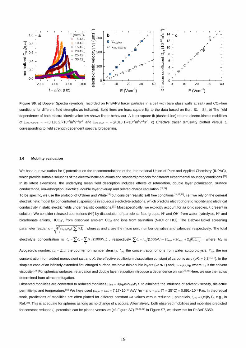
Figure S6. a) Doppler Spectra (symbols) recorded on PnBAPS tracer particles in a cell with bare glass walls at salt- and CO2-free

conditions for different field strengths as indicated. Solid lines are least square fits to the data based on Eqn. S1 − S4. b) The field

dependence of both electro-kinetic velocities shows linear behaviour. A least square fit (dashed line) returns electro-kinetic mobilities

of µep,PnBAPS = − (3.10.2)×10−8m2V−1s−1 and µeo,SiO2 = − (9.00.1)×10−8m2V−1s−1. c) Effective tracer diffusivity plotted versus E

corresponding to field strength dependent spectral broadening.

1.6 Mobility evaluation

We base our evaluation for -potentials on the recommendations of the International Union of Pure and Applied Chemistry (IUPAC),

which provide suitable solutions of the electrokinetic equations and standard protocols for different experimental boundary conditions.[22]

In its latest extensions, the underlying mean field description includes effects of retardation, double layer polarization, surface

conductance, ion-adsorption, electrical double layer overlap and related charge regulation.[23,24]

To be specific, we use the protocol of O’Brien and White[25] but consider realistic salt free conditions[21,23,26], i.e., we rely on the general

electrokinetic model for concentrated suspensions in aqueous electrolyte solutions, which predicts electrophoretic mobility and electrical

conductivity in static electric fields under realistic conditions.[23] Most specifically, we explicitly account for all ionic species, i, present in

solution. We consider released counterions (H+) by dissociation of particle surface groups, H+ and OH− from water hydrolysis, H+ and

bicarbonate anions, HCO3−, from dissolved ambient CO2 and ions from salination (NaCl or HCl). The Debye-Hückel screening

parameter reads: 2

0 r B i ii

e k T n z = , where ni and zi are the micro ionic number densities and valences, respectively. The total

electrolyte concentration is = = / (1000 )s i i Ai i

c c n N , respectively = + + +2 2

(1000 ) 2 2 2i ci A H O NaCl a COi

c n N c c K c , where NA is

Avogadro’s number, nci = Z n the counter ion number density, 2H Oc the concentration of ions from water autoprotolysis, NaClc the ion

concentration from added monovalent salt and Ka the effective equilibrium dissociation constant of carbonic acid (pKa = 6.3 [7,27]). In the

simplest case of an infinitely extended flat, charged surface, we have thin double layers (a 1) and µ = 0rs where s is the solvent

viscosity.[28] For spherical surfaces, retardation and double layer relaxation introduce a dependence on a.[25,29] Here, we use the radius

determined from ultracentrifugation.

Observed mobilities are converted to reduced mobilities µred = 3µse2rkBT, to eliminate the influence of solvent viscosity, dielectric

permittivity, and temperature.[30] We here used water = 0r = 7.17×10−10 AsV−1m−1 and water (T = 25°C) = 0.891×10−3 Pas. In theoretical

work, predictions of mobilities are often plotted for different constant a values versus reduced -potentials, red = e(kBT), e.g., in

Ref.[25]. This is adequate for spheres as long as no change of occurs. Alternatively, both observed mobilities and mobilities predicted

for constant reduced -potentials can be plotted versus a (cf. Figure S7).[26,29,32] In Figure S7, we show this for PnBAPS359.

2950 3000 3050 3100

0.0

0.2

0.4

0.6

0.8

1.0 a

no

rma

lize

d C

SH(q

,)

E (Vcm−1

) 5.42

10.42

15.42

20.42

25.42

30.42

f = /2 (Hz)

0 10 20 30 400

2

4

6

8

10

12

14 c

Diffu

sio

n c

oe

ffic

ien

t D

eff (

10

−1

2m

2s

−1)

E (Vcm−1

)

0 10 20 30 400

100

200

300veo,glass

vep,PnBAPS

b

ele

ctr

okin

etic v

elo

city

v

(µm

s−1)

E (Vcm−1

)

20

Figure S7. Moduli of reduced tracer mobilities µred plotted against reduced screening parameter a obtained for the salt and CO2-free

reference state (open circles) and upon CO2 equilibration in contact with ambient air (grey filled circles). Solid lines represent theoretical

predictions according to standard electrokinetic theory for realistic conditions at respective constant reduced -potential.

2 Theoretical section

2.1 Analytic Theory

For the present system of interacting neutral CO2 molecules at an attractive charged wall in aqueous environment, we consider the

N-particle Smoluchowski-equation for the joint probability density P(r1,r2,...,rN) for particles with an isotropic pair interaction potential

== , 1

(1 2) ( )N

iji jV U r , where ij i jr = −r r , in an external wall potential

1( )

N

ext ext iiV U z

== :[33]

, 1

( )N

i ij j ext ji j

P D V V P P=

= + + (S5)

where Dij are the elements of the microscopic diffusion matrix and 1/ = kBT is the thermal energy. To model the aggregation of

interacting particles at an attractive wall, we are interested in the density distribution under steady state conditions. Thus, we set P =

0 such that the square bracket on the right-hand side has to varnish. We then reduce equation (S5) to an equation for the one-particle

probability density given by 2 3 2( ) ... d d ...d ( , ,..., )N NP P= r r r r r r r .

Applying the mean field approximation, P(r,r’) P(r)P(r’), after performing the truncated Taylor expansion

( ) − −( ') ( ) ( ) 'P P Pr r r r r and using Vext(r) = Vext(z), we obtain the following equation for the (macroscopic) density (r) = N P(r)

(N−1) P(r), where for symmetry reasons (r) = (z):

min

31 d 4 d d dln d ( ) 0

d 3 d d dext

r

r r U r Uz z r z

− + − =

(S6)

Here we have replaced the lower boundary of the integration range by a minimal cutoff distance rmin accounting for the nearest possible

distance between two particles.

0.1 1 10 1000

1

2

3

4

5

6

7

8

9

10no CO2

with CO2

red

uce

d m

ob

ility

µ

red

a

red

6

5

4

3

1

2

21

Now defining

= min

34 dd ( )

3 dr

I r r U rr

, this equation reduces to

− + − =

1 d d d0

d d dextI U

z z z (S7)

Specifying the external wall potential to Uext(z) = −(f03)z3 and choosing the boundary condition as → = ( )z , the solution of

equation (S7) reads

3

1 1( ) expz W

z

= +

(S8)

where W is the product logarithm, and where we have defined the reduced density as

= and the reduced length as z = z.

is the characteristic length scale given by

1/3

0

3 B

f

k T

=

(S9)

We note that the solution (S8) depends on one dimensionless parameter only, which measures the relevance of the interactions

B

I

k T

= − . (S10)

In the absence of pair-interactions, i.e., = 0, the solution (S8) reduces to

=

3

1( ) expz

z (S11)

which translates into ( ) = −( ) exp ( )extz U z when reinstating the dimensional units.

2.1.1 Parameters

For numerical calculations, the saturation concentration of ambient CO2 dissolved in water was assumed to be = 1.18×10−5mol/L

7.1×1021m−3 and the thermal energy was estimated to be kBT 3.6×10−21J. Interpreting the particle pair interaction potential as

Lennard-Jones potential, 12 6( ) ( ) 4 ( ) ( )LJU r U r r r = = − , the distance at which ULJ vanishes was approximated to be 2CO 0.37nm.

If the attractive part of the interactions among CO2-molecules is due to Van der Waals interactions we have UVdW(r) = −Cr6

= −46r6 yielding = C(46), where C is the coefficient of the Van der Waals interactions of two CO2 molecules in water. We assume

kBT2 for the effective LJ-interaction coefficient of the CO2 – CO2 interaction in water.[34] This corresponds to a Van der Waals

interaction coefficient C = 4 1.8×10-77Jm6 which would be a typical particle interaction strength in vacuum. Let's assume that we

have the same for the interaction between wall molecules and CO2 molecules. Now using Uext(z) = − nglassC(6z3) we have f03 =

(6)nglassC 2.5×10-49Jm3 with nglass 2.65×1028m-3.

Next, we estimate values of I. We obtain for the minimal interparticle distance rmin = :

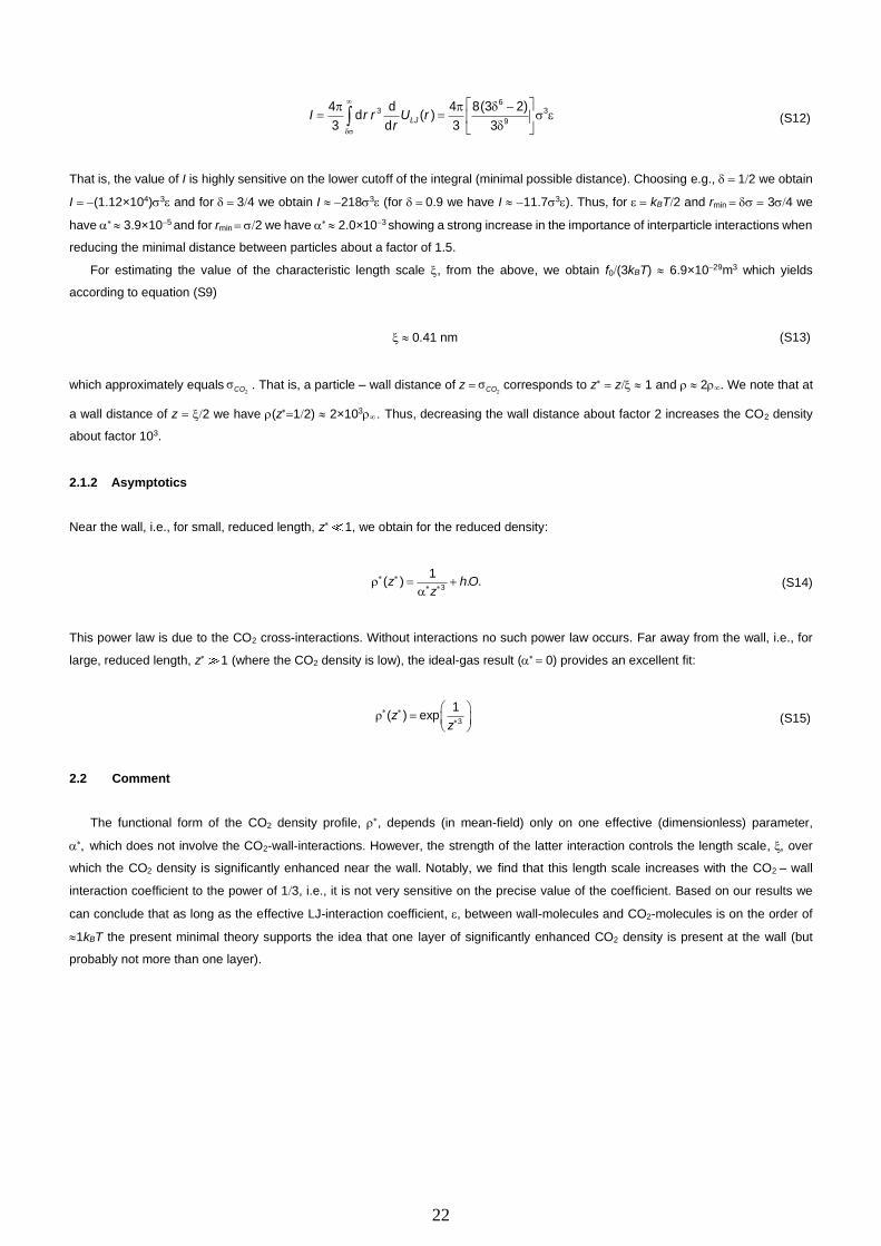
22

−= =

63 3

9

4 d 4 8(3 2)d ( )

3 d 3 3LJI r r U r

r (S12)

That is, the value of I is highly sensitive on the lower cutoff of the integral (minimal possible distance). Choosing e.g., = 12 we obtain

I = −(1.12×104)3 and for = 34 we obtain I −2183 (for = 0.9 we have I −11.73). Thus, for = kBT2 and rmin = = 34 we

have 3.9×10−5 and for rmin = 2 we have 2.0×10−3 showing a strong increase in the importance of interparticle interactions when

reducing the minimal distance between particles about a factor of 1.5.

For estimating the value of the characteristic length scale , from the above, we obtain f0(3kBT) 6.9×10−29m3 which yields

according to equation (S9)

0.41 nm (S13)

which approximately equals 2CO . That is, a particle – wall distance of z =

2CO corresponds to z = z 1 and 2. We note that at

a wall distance of z = 2 we have (z=12) 2×103 Thus, decreasing the wall distance about factor 2 increases the CO2 density

about factor 103.

2.1.2 Asymptotics

Near the wall, i.e., for small, reduced length, z 1, we obtain for the reduced density:

3

1( ) . .z hO

z

= +

(S14)

This power law is due to the CO2 cross-interactions. Without interactions no such power law occurs. Far away from the wall, i.e., for

large, reduced length, z 1 (where the CO2 density is low), the ideal-gas result ( = 0) provides an excellent fit:

=

3

1( ) expz

z (S15)

2.2 Comment

The functional form of the CO2 density profile, , depends (in mean-field) only on one effective (dimensionless) parameter,

which does not involve the CO2-wall-interactions. However, the strength of the latter interaction controls the length scale, over

which the CO2 density is significantly enhanced near the wall. Notably, we find that this length scale increases with the CO2 – wall

interaction coefficient to the power of 13, i.e., it is not very sensitive on the precise value of the coefficient. Based on our results we

can conclude that as long as the effective LJ-interaction coefficient, , between wall-molecules and CO2-molecules is on the order of

1kBT the present minimal theory supports the idea that one layer of significantly enhanced CO2 density is present at the wall (but

probably not more than one layer).

23

REFERENCES

[1] A. Z. Stetten, D. S. Golovko, S. A. L. Weber, H.-J. Butt, Soft Matter 2019, 15, 8667.

[2] T. Palberg, W. Haertl, U. Wittig, H. Versmold, M. Wuerth, E. Simnacher, J. Phys. Chem. 1992, 96, 8180.

[3] P. Wette, H.-J. Schöpe, R. Biehl, T. Palberg, The Journal of Chemical Physics 2001, 114, 7556.

[4] D. Botin, L. M. Mapa, H. Schweinfurth, B. Sieber, C. Wittenberg, T. Palberg, The Journal of Chemical Physics 2017, 146, 204904.

[5] N. Möller, B. Liebchen, T. Palberg, The European physical journal. E, Soft matter 2021, 44, 41.

[6] D. Hessinger, M. Evers, T. Palberg, Phys. Rev. E 2000, 61, 5493.

[7] Aqion freeware program, can be found under https://www.aqion.de/.

[8] D. Botin, F. Carrique, E. Ruiz-Reina, T. Palberg, The Journal of Chemical Physics 2020, 152, 244902.

[9] R. J. Spry, D. J. Kosan, Appl. Spectrosc., AS 1986, 40, 782.

[10] J. Yamanaka, Y. Hayashi, N. Ise, T. Yamaguchi, Phys. Rev. E 1997, 55, 3028.

[11] J. Yamanaka, N. Ise, Journal of Colloid and Interface Science 1996, 179, 324.

[12] P. Wette, H. J. Schöpe, T. Palberg, Colloids and Surfaces A: Physicochemical and Engineering Aspects 2003, 222, 311.

[13] L. Shapran, M. Medebach, P. Wette, T. Palberg, H. J. Schöpe, J. Horbach, T. Kreer, A. Chatterji, Colloids and Surfaces A:

Physicochemical and Engineering Aspects 2005, 270-271, 220.

[14] T. Huhtamäki, X. Tian, J. T. Korhonen, R. H. A. Ras, Nat Protoc 2018, 13, 1521.

[15] D. Botin, J. Wenzl, R. Niu, T. Palberg, Soft Matter 2018, 14, 8191.

[16] P. White, The London, Edinburgh, and Dublin Philosophical Magazine and Journal of Science 1937, 23, 811.

[17] T. Palberg, H. Versmold, J. Phys. Chem. 1989, 93, 5296.

[18] S. Komagata, Researches Electrotech. Lab. Tokyo Comm. 1933, 348.

[19] J. F. Miller, K. Schätzel, B. Vincent, Journal of Colloid and Interface Science 1991, 143, 532.

[20] T. Palberg, T. Köller, B. Sieber, H. Schweinfurth, H. Reiber, G. Nägele, J. Phys.: Condens. Matter 2012, 24, 464109.

[21] H. Reiber, T. Köller, T. Palberg, F. Carrique, E. Ruiz Reina, R. Piazza, Journal of Colloid and Interface Science 2007, 309, 315.

[22] A. V. Delgado, F. González-Caballero, R. J. Hunter, L. K. Koopal, J. Lyklema, Journal of Colloid and Interface Science 2007, 309,

194.

[23] F. Carrique, E. Ruiz-Reina, R. Roa, F. J. Arroyo, Á. V. Delgado, Journal of Colloid and Interface Science 2015, 455, 46.

[24] Á. V. Delgado, F. Carrique, R. Roa, E. Ruiz-Reina, Current Opinion in Colloid & Interface Science 2016, 24, 32.

[25] R. W. O'Brien, L. R. White, J. Chem. Soc., Faraday Trans. 2 1978, 74, 1607.

[26] M. Medebach, L. Shapran, T. Palberg, Colloids and Surfaces B: Biointerfaces 2007, 56, 210.

[27] A. F. Holleman, E. Wiberg, N. Wiberg (Eds.) Lehrbuch der anorganischen Chemie, de Gruyter, Berlin, 2007.

[28] M. von SMOLUCHOWSKI, Bull. Akad. Sci. Cracovie. 1903, 8, 182.

[29] P.H. Wiersema, A.L. Loeb, J.T.G. Overbeek, Journal of Colloid and Interface Science 1966, 22, 78.

[30] J. Lyklema, Fundamentals of Interface and Colloid Science. Vol. II: Solid-Liquid Interfaces, Academic Press, London, 1995.

[31] V. Lobaskin, B. Dünweg, M. Medebach, T. Palberg, C. Holm, Physical review letters 2007, 98, 176105.

[32] T. Palberg, M. Medebach, N. Garbow, M. Evers, A. B. Fontecha, H. Reiber, E. Bartsch, J. Phys.: Condens. Matter 2004, 16,

S4039-S4050.

[33] J.K.G. Dhont, An Introduction to Dynamics of Colloids, Elsevier, 1996.

[34] S. M. Dammer, D. Lohse, Phys. Rev. Lett. 2006, 96, 206101.